Journal of Statistical Planning and Inference 122 (2004) 229 – 252 www.elsevier.com/locate/jspi Robust estimators in semiparametric partly linear regression models Ana Bianco a , Graciela Boente b; ∗ a Universidad de Buenos Aires, Argentina b Universidad de Buenos Aires and CONICET, Argentina Accepted 15 June 2003 Abstract In this paper, under a semiparametric partly linear regression model, a family of robust esti- mates for the regression parameter and the regression function is introduced and discussed. Some of their asymptotic properties are studied. Through a Monte Carlo study the performance of the estimates is compared with the classical ones. c 2003 Elsevier B.V. All rights reserved. MSC: primary 62F35; secondary 62H25 Keywords: Partly linear models; Robust estimation; Smoothing techniques; Rate of convergence; Asymptotic properties 1. Introduction Statistical inference for multidimensional random variables commonly focuses on functionals of its distribution that are either purely parametric or purely nonparametric. A reasonable parametric model produces precise inferences, while a badly misspecied model possibly leads to seriously misleading conclusions. On the other hand, nonpara- metric modeling is associated both with greater stability and less precision. Recently, nonparametric regression models have gained a lot of attention in order to study non- linearity to explore the nature of complex nonlinear phenomena. Let (y i ; x i ;t i ) be This research was partially supported by Grant PICT # 03-00000-006277 from ANPCYT at Buenos Aires, Argentina. The research of Graciela Boente was also partially supported by a Guggenheim fellowship. ∗ Corresponding author. E-mail address: [email protected] (G. Boente). 0378-3758/$ - see front matter c 2003 Elsevier B.V. All rights reserved. doi:10.1016/j.jspi.2003.06.007

Welcome message from author
This document is posted to help you gain knowledge. Please leave a comment to let me know what you think about it! Share it to your friends and learn new things together.
Transcript
Journal of Statistical Planning andInference 122 (2004) 229–252
www.elsevier.com/locate/jspi
Robust estimators in semiparametric partly linearregression models�
Ana Biancoa, Graciela Boenteb;∗aUniversidad de Buenos Aires, Argentina
bUniversidad de Buenos Aires and CONICET, Argentina
Accepted 15 June 2003
Abstract
In this paper, under a semiparametric partly linear regression model, a family of robust esti-mates for the regression parameter and the regression function is introduced and discussed. Someof their asymptotic properties are studied. Through a Monte Carlo study the performance of theestimates is compared with the classical ones.c© 2003 Elsevier B.V. All rights reserved.
MSC: primary 62F35; secondary 62H25
Keywords: Partly linear models; Robust estimation; Smoothing techniques; Rate of convergence;Asymptotic properties
1. Introduction
Statistical inference for multidimensional random variables commonly focuses onfunctionals of its distribution that are either purely parametric or purely nonparametric.A reasonable parametric model produces precise inferences, while a badly misspeci7edmodel possibly leads to seriously misleading conclusions. On the other hand, nonpara-metric modeling is associated both with greater stability and less precision. Recently,nonparametric regression models have gained a lot of attention in order to study non-linearity to explore the nature of complex nonlinear phenomena. Let (yi; x′i ; ti)
′ be
� This research was partially supported by Grant PICT # 03-00000-006277 from ANPCYT at BuenosAires, Argentina. The research of Graciela Boente was also partially supported by a Guggenheim fellowship.
∗ Corresponding author.E-mail address: [email protected] (G. Boente).
0378-3758/$ - see front matter c© 2003 Elsevier B.V. All rights reserved.doi:10.1016/j.jspi.2003.06.007
230 A. Bianco, G. Boente / Journal of Statistical Planning and Inference 122 (2004) 229–252
independent observations such that yi ∈R, ti ∈R, xi ∈Rp and
yi = �(xi ; ti) + �i 16 i6 n; (1)
where the errors �i are independent and independent of (x′i ; ti)′.
Analysis of model (1) requires multivariate smoothing since the function � has amultidimensional domain. Thus, this model often encounters, in applications, the dif-7culty known as the “curse of dimensionality”. In recent years, several authors havedealt with the dimensionality reduction problem in nonparametric regression models. Inorder to solve the problem of empty neighborhoods several approaches have been givento estimate the regression function when covariates lie in a high dimensional space.Hastie and Tibshirani (1990) introduced additive models so as to generalize linear re-gression, with the goal of solving the curse of dimensionality and keeping the easyinterpretability of this model. This approach combines the Iexibility of nonparametricmodels and the simple interpretation of the linear ones.
An intermediate strategy employs a semiparametric form, that combines the ad-vantages of both parametric and nonparametric methods, and in which the regressionfunction is �(x; t) = �′ox + g(t), and so (1) can be written as
yi = �′oxi + g(ti) + �i 16 i6 n: (2)
Partly linear models (2) are more Iexible than standard linear models since they havea parametric and a nonparametric component. They can be a suitable choice when onesuspects that the response y linearly depends on x, but that it is nonlinearly relatedto t. The components of �o may have, for instance, interesting signi7cance. As it iswell known, model (2) is used when the researcher knows more about the dependenceamong y and x than about the relationship between y and the predictor t, whichestablishes an unevenness in prior knowledge.
This model has been studied by several authors: Ansley and Wecker (1983), Greenet al. (1985), Denby (1986), Heckman (1986), Engle et al. (1986), Rice (1986), Chen(1988), Robinson (1988), Speckman (1988), Chen and Chen (1991), Chen and Shiau(1991, 1994), Gao (1992), Gao and Zhao (1993), Gao and Liang (1995), He andShi (1996) and Yee and Wild (1996) who investigated some asymptotic results usingsmoothing splines, kernel or nearest neighbors techniques. Heckman (1986) and Chen(1988) showed that the estimates of the regression parameter �o can achieve a root-nrate of convergence if x and t are independent. Rice (1986) obtained the asymptoticbias of a partial smoothing estimate of �o due to the dependence between x and t.Robinson (1988) explained why estimates of �o based on incorrect parametrizationof the function g are generally inconsistent and proposed a least-squares estimator of�o which will be root-n consistent by inserting nonparametric regression estimators inthe nonlinear orthogonal projection on t. Estimates based on kernel weights were alsoconsidered by Severini and Wong (1992) for the independent setting, in a more generalframework, and by Truong and Stone (1994) for autoregression models. Liang et al.(1999) proposed an unbiased estimate for the case of errors in variables while Heet al. (2001) considered M-type estimates for repeated measurements.
It is well known that, both in linear regression and in nonparametric regression,least-squares estimators can be seriously aMected by anomalous data. The same

A. Bianco, G. Boente / Journal of Statistical Planning and Inference 122 (2004) 229–252 231
statement holds for partly linear models. The aim of this paper is, thus, to proposea class of robust procedures under the partly linear model (2) and to study some oftheir asymptotic properties. In Section 2, we review the classical approach and we intro-duce the robust estimates. Consistency results are stated in Section 3, while asymptoticnormality for the estimates of the regression parameter is studied in Section 4. Allproofs are given in the appendix. Finally, in Section 5, for small samples, the behaviorof the least-squares estimates and of diMerent resistant estimates is compared througha Monte Carlo study under normality and contamination.
2. Estimators
2.1. Model and classical approach
Assume that (Y;X′; T )′ is a random vector with the same distribution as (yi; x′i ; ti)′,
that is
Y = �′oX + g(T ) + �; (3)
where � is independent of (X′; T )′ and we will assume that � has a symmetric dis-tribution. In the classical approach to the problem it is assumed that E(|�|)¡∞ andE(‖X‖2)¡∞.
When E(X) = 0 and X and T are independent, under regularity conditions, theleast-squares procedure of Y on X yields consistent and eNcient estimates of �o. Asnoted by Robinson (1988), the main tool to solve the problem under nonorthogonality isto insert nonparametric shape estimators of the nonparametric component in a standardparametric regression estimate.
Denote �o(t) =E(Y |T = t) and �(t) = (�1(t); : : : ; �p(t))′, where �j(t) =E(Xj|T = t).Then, we have g(t) = �o(t) − �′o�(t) and hence Y − �o(t) = �′o(X − �(t)) + �.
This suggests that estimators of �o(t) and �(t), �o(t) and �(t), can be inserted priorto the estimation of the regression parameter. The classical nonparametric approachestimates the conditional expectations through
�o;LS(t) =n∑
i=1
wi(t)yi �j;LS(t) =n∑
i=1
wi(t)xij;
where, for the kernel approach, the weights are given by
wi(t) =K((ti − t)=h)∑nj=1 K((tj − t)=h)
; (4)
with K a kernel function, i.e., a nonnegative integrable function on R and h the band-width parameter, while the nearest neighbor with kernel approach considers as weightfunction
wi(t) =K((ti − t)=Hn(t))∑nj=1 K((tj − t)=Hn(t))
; (5)
with Hn(t) the distance between t and its kn-nearest neighbor among t1; : : : ; tn.

232 A. Bianco, G. Boente / Journal of Statistical Planning and Inference 122 (2004) 229–252
With either of these initial estimates, the least-squares estimator of �o, �LS, can beobtained minimizing
n∑i=1
[yi − �o;LS(ti) − �′(xi − �LS(ti))]2; (6)
leading to the 7nal least squares estimate of g, gLS(t) = �o;LS(t) − �′LS�LS(t). The
properties of these estimates have been widely studied in the literature, as it wasmentioned in the Introduction.
2.2. Robust estimates
As mentioned by Chen and Shiau (1994), the procedure described above and pro-posed independently by Denby (1986) and Speckman (1988), can be related to thepartial regression procedure in linear regression. More precisely, as in this procedure,in order to obtain the regression estimator, these authors 7rst smoothed the covariatesx and the response y and then, regressed the residuals of the smoothing from y on theresiduals of the smoothing from x. Similarly to the purely parametric and nonparamet-ric models, the least-squares estimators, used at each step, can be seriously aMected bya small fraction of outliers. So, it may be preferable to estimate the conditional loca-tion functional through a robust smoothing and the regression parameter by a robustregression estimator.
Putting these ideas together, the procedure to obtain robust estimators in partly linearmodels can be described as follows:
Step 1: Estimate �o(t) and �j(t) through a robust smoothing, as the local mediansor local M-type estimates. Let �o(t) and �j(t) denote the obtained estimates and �(t)=(�1(t); : : : ; �p(t))′.
Step 2: Estimate the regression parameter by applying a robust regression estimateto the residuals yi − �o(ti) and xi − �(ti). Let � denote the obtained estimator.
Step 3: De7ne the estimate of the regression function g as g(t) = �o(t) − �′�(t).
It is worth noticing that our proposal is a robust version of the partial regressionestimators introduced by Denby (1986), Robinson (1988) and Speckman (1988).
In Step 3, an alternative estimate of the regression function g can be obtained byrobustly smoothing the residual yi − �′xi. However, this procedure would be compu-tationally more expensive than the one described above.
In Step 1, we compute the local medians �o;med(t) and �j;med(t) as the median of theempirical conditional distribution functions Fo(y|T = t) and F j(x|T = t), respectivelywhich are de7ned as
Fo(y|T = t) =n∑
i=1
wi(t)I(−∞;y](yi); (7)
F j(x|T = t) =n∑
i=1
wi(t)I(−∞; x](xij) 16 j6p; (8)
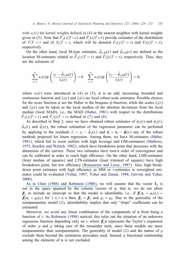
A. Bianco, G. Boente / Journal of Statistical Planning and Inference 122 (2004) 229–252 233
with wi(t) the kernel weights de7ned in (4) or the nearest neighbor with kernel weightsgiven in (5). Note that Fo(y|T =t) and F j(x|T =t) provide estimates of the distributionof Y |T = t and of Xj|T = t, which will be denoted Fo(y|T = t) and Fj(x|T = t),respectively.
On the other hand, local M-type estimates, �o;M(t) and �j;M(t) are de7ned as thelocation M-estimates related to Fo(y|T = t) and F j(x|T = t), respectively. Thus, theyare the solutions of
n∑i=1
wi(t)
(yi − �o;M(t)
so(t)
)= 0
n∑i=1
wi(t)
(xij − �j;M(t)
sj(t)
)= 0;
where wi(t) were introduced in (4) or (5), is an odd, increasing, bounded andcontinuous function and so(t) and sj(t) are local robust scale estimates. Possible choicesfor the score function are the Huber or the bisquare -function, while the scales so(t)and sj(t) can be taken as the local median of the absolute deviations from the localmedian (local MAD), i.e., the MAD (Huber, 1981) with respect to the distributionsFo(y|T = t) and F j(x|T = t) de7ned in (7) and (8).
As described in Step 2, once we have obtained robust estimates of �o(t) and �j(t),�o(t) and �j(t), the robust estimation of the regression parameter can be perfomedby applying to the residuals ri = yi − �o(ti) and zi = xi − �(ti) any of the robustmethods proposed for linear regression. Among them, we have M-estimates (Huber,1981), which fail to resist outliers with high leverage and GM-estimators (Mallows,1975, Krasker and Welsch, 1982), which have breakdown point that decreases with thedimension of the carriers. These two estimates have root-n order of convergence andcan be calibrated in order to reach high eNciency. On the other hand, LMS-estimator(least median of squares) and LTS-estimator (least trimmed of squares) have highbreakdown point, but low eNciency (Rousseeuw and Leroy, 1987). Also, high break-down point estimates with high eNciency as MM or �-estimates or reweighted esti-mates could be evaluated (Yohai, 1987; Yohai and Zamar, 1988; Gervini and Yohai,2000).
As in Chen (1988) and Robinson (1988), we will assume that the vector 1n isnot in the space spanned by the column vectors of x, that is, we do not allow�o to include an intercept so that the model is identi7able, i.e., if �′1xi + g1(ti) =�′2xi + g2(ti) for 16 i6 n then, �1 = �2 and g1 = g2. Due to the generality of thesemiparametric model (2), identi7ability implies that only “slope” coeNcients can beestimated.
Moreover, we avoid any linear combination of the components of x from being afunction of t. As Robinson (1988) noticed, this rules out the situation of an unknownregression function depending only on t, where �′ox represents the Taylor’s expansionof order p and g taking care of the remainder term, since these models are morenonparametric than semiparametric. The generality of model (2) and the nature of gexclude them beyond the estimation procedure used. Instead, a functional relationshipamong the elements of x is not excluded.
234 A. Bianco, G. Boente / Journal of Statistical Planning and Inference 122 (2004) 229–252
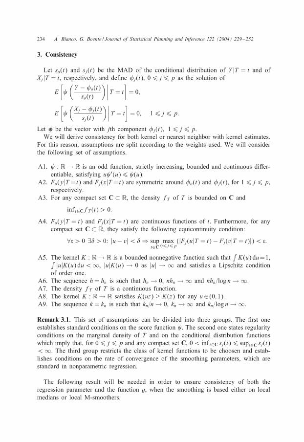
3. Consistency
Let so(t) and sj(t) be the MAD of the conditional distribution of Y |T = t and ofXj|T = t, respectively, and de7ne �j(t), 06 j6p as the solution of
E[ (Y − �o(t)
so(t)
)∣∣∣∣ T = t]
= 0;
E[ (Xj − �j(t)
sj(t)
)∣∣∣∣ T = t]
= 0; 16 j6p:
Let � be the vector with jth component �j(t); 16 j6p.We will derive consistency for both kernel or nearest neighbor with kernel estimates.
For this reason, assumptions are split according to the weights used. We will considerthe following set of assumptions.
A1. : R→ R is an odd function, strictly increasing, bounded and continuous diMer-entiable, satisfying u ′(u)6 (u).
A2. Fo(y|T = t) and Fj(x|T = t) are symmetric around �o(t) and �j(t), for 16 j6p,respectively.
A3. For any compact set C ⊂ R, the density fT of T is bounded on C and
inf t∈CfT (t)¿ 0:
A4. Fo(y|T = t) and Fj(x|T = t) are continuous functions of t. Furthermore, for anycompact set C ⊂ R, they satisfy the following equicontinuity condition:
∀�¿ 0 ∃#¿ 0: |u− v|¡# ⇒ supt∈C
max06j6p
(|Fj(u|T = t) − Fj(v|T = t)|)¡�:
A5. The kernel K : R→ R is a bounded nonnegative function such that∫K(u) du=1,∫ |u|K(u) du¡∞, |u|K(u) → 0 as |u| → ∞ and satis7es a Lipschitz condition
of order one.A6. The sequence h = hn is such that hn → 0, nhn → ∞ and nhn=log n → ∞.A7. The density fT of T is a continuous function.A8. The kernel K : R→ R satis7es K(uz) ≥ K(z) for any u∈ (0; 1).A9. The sequence k = kn is such that kn=n → 0, kn → ∞ and kn=log n → ∞.
Remark 3.1. This set of assumptions can be divided into three groups. The 7rst oneestablishes standard conditions on the score function . The second one states regularityconditions on the marginal density of T and on the conditional distribution functionswhich imply that, for 06 j6p and any compact set C, 0¡ inf t∈C sj(t)6 supt∈C sj(t)¡∞. The third group restricts the class of kernel functions to be choosen and estab-lishes conditions on the rate of convergence of the smoothing parameters, which arestandard in nonparametric regression.
The following result will be needed in order to ensure consistency of both theregression parameter and the function g, when the smoothing is based either on localmedians or local M-smoothers.
A. Bianco, G. Boente / Journal of Statistical Planning and Inference 122 (2004) 229–252 235
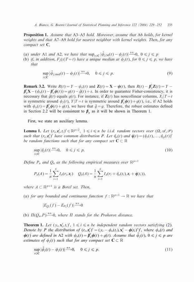
Proposition 1. Assume that A3–A5 hold. Moreover, assume that A6 holds, for kernelweights and that A7–A9 hold for nearest neighbor with kernel weights. Then, for anycompact set C,
(a) under A1 and A2, we have that supt∈C |�j;M(t) − �j(t)| a:s:−→0; 06 j6p(b) if, in addition, Fj(x|T = t) have a unique median at �j(t), for 06 j6p, we have
that
supt∈C
|�j;med(t) − �j(t)| a:s:−→0; 06 j6p: (9)
Remark 3.2. Write R(t) = Y − �o(t) and Z(t) = X − �(t), then R(t) − �′oZ(t) = Y −�′oX− (�o(t)−�′o�(t)) = g(t)− g(t) + �. In order to guarantee Fisher-consistency, it isnecessary that g(t) equals g(t). For instance, if Z(t) has noncollinear columns, Xj|T = tis symmetric around �j(t), Y |T = t is symmetric around �′o�(t)+g(t), i.e., if A2 holdswith �o(t) = �′o�(t) + g(t), we have that g= g. Therefore, the robust estimates de7nedin Section 2.2 will be consistent to �o as it will be shown in Theorem 1.
First, we state an auxiliary lemma.
Lemma 1. Let (ri; z′i ; ti)′ ∈Rp+2; 16 i6 n be i.i.d. random vectors over (';A;P)
such that (ri; z′i)′ have common distribution P. Let (o(t) and �(t) = ((1(t); : : : ; (p(t))′
be random functions such that for any compact set C ⊂ R
supt∈C
|(j(t)| a:s:−→0; 06 j6p: (10)
De8ne Pn and Qn as the following empirical measures over Rp+1
Pn(A) =1n
n∑i=1
IA(ri; zi) Qn(A) =1n
n∑i=1
IA(ri + (o(ti); zi + �(ti));
where A ⊂ Rp+1 is a Borel set. Then,
(a) for any bounded and continuous function f : Rp+1 → R we have that
|EQn(f) − EPn(f)| a:s:−→0
(b) ,(Qn; P) a:s:−→0, where , stands for the Prohorov distance.
Theorem 1. Let (yi; x′i ; ti)′, 16 i6 n be independent random vectors satisfying (2).
Denote by P the distribution of (ri; z′i)′ = (yi − �o(ti); x′i − �(ti)′)′, where �o(t) and
�(t) are de8ned in A2 with �o(t) = �′o�(t) + g(t). Assume that �j(t), 06 j6p areestimates of �j(t) such that for any compact set C ⊂ R
supt∈C
|�j(t) − �j(t)| a:s:−→0; 06 j6p: (11)

236 A. Bianco, G. Boente / Journal of Statistical Planning and Inference 122 (2004) 229–252
Let �(H) be a regression functional, for the model u = �′v + �, where (u′; v)′ ∼ Hand � and v are independent. Assume that �(H) is continuous at P and that it alsoprovides Fisher-consistent estimates.
If Pn(A) = 1n
∑ni=1 IA(ri ; zi) with ri = yi − �o(ti) and zi = xi − �(ti), where �(t) =
(�1(t); : : : ; �p(t))′ and �ROB = �(Pn), we have that
�ROBa:s:−→�o:
Proof. From (11) and Lemma 1, we have that |EPn(f) − EPn(f)| a:s:−→0, where
Pn(A) =1n
n∑i=1
IA(ri; zi)
and so ,(Pn; P) a:s:−→0. The result follows now from the continuity of the functional�(H) and from the fact ri = �′ozi + �i.
Remark 3.3. Note that the continuity condition at P is ful7lled for most robust regres-sion estimates if the components of Z(T ) are not collinear. The implication of thiscondition is that any linear combination of the components of X cannot be a functionof T and therefore, 1n is not in the space spanned by the column vectors of X.
Corollary. Let (yi; x′i ; ti)′, 16 i6 n be independent random vectors satisfying (2) and
assume that �j(t), 06 j6p are estimates of �j(t) such that for any compact setC ⊂ R
supt∈C
|�j(t) − �j(t)| a:s:−→0; 06 j6p:
Under the conditions stated in Theorem 1, the estimates g(t) = �o(t) − �′ROB�(t) ofthe regression function g are uniformly consistent over compact sets.
Remark 3.4. Using Proposition 1 and Theorem 1 we have that the proposed robustestimates, introduced in Section 2.2, are consistent if no linear combination of thecomponents of X is a function of T .
4. Asymptotic distribution
Let 1 and w2 be a score and a weight function, respectively. In this section, wewill derive the asymptotic distribution of the regression parameter estimates de7ned asany solution of
n∑i=1
1
(ri − �′zi
sn
)w2 (‖zi‖) zi = 0; (12)

A. Bianco, G. Boente / Journal of Statistical Planning and Inference 122 (2004) 229–252 237
with ri = yi − �o(ti), zi = xi − �(ti) and sn is an estimate of the residuals scale.Let �o(t) and �(t) denote consistent estimates of �o(t) and �(t), respectively, with�o(t) = �′o�(t) + g(t).
In order to derive the asymptotic distribution of the regression parameter estimates,we will require that the covariates ti lie in a compact set. Thus, without loss of gen-erality, we will assume that ti ∈ [0; 1].
Denote by (R(T );Z(T )′)′ a random vector with the same distribution as (ri; z′i)′ =
(yi − �o(ti); [xi − �(ti)]′)′. Thus, R(T ) − Z(T )′�o ∼ �, with � as in (2).We will need the following set of assumptions.
N1. 1 is an odd, bounded and twice continuously diMerentiable function with boundedderivatives ′
1 and ′′1 , such that ’1(t) = t ′
1(t) and ’2(t) = t ′′1 (t) are bounded.
N2. E(w2(‖Z(T )‖)‖Z(T )‖2)¡∞ and the matrix
A= E( ′
1
(R(T ) − Z(T )′�o
.o
)w2(‖Z(T )‖)Z(T )Z(T )′
)
= E( ′
1
(�.o
))E(w2(‖Z(T )‖)Z(T )Z(T )′)
is nonsingular.N3. w2(u)= 2(u)u−1 ¿ 0 is a bounded function, Lipschitz of order 1. Moreover, 2 is
also a bounded and continuously diMerentiable function with bounded derivative ′
2 such that /2(t) = t ′2(t) is bounded.
N4. E(w2(‖Z(T )‖)Z(T )|T = t) = 0 for almost all t.N5. The functions �j(t), 06 j6p are continuous with 7rst derivative �′
j(t), contin-uous in [0; 1].
As noted by Robinson (1988), condition N2 will prevent any element of X frombeing a.s. perfectly predictable by T . The additional condition implied by N2 is the lackof multicollinearity among the columns X − �(T ), which fails if X itself is collinear.
The smoothness condition N5 is a standard requirement in classical kernel estimationin semiparametric models in order to guarantee asymptotic normality, see for instance,Robinson (1988) and Severini and Wong (1992).
Lemma 2. Let (yi; x′i ; ti)′, 16 i6 n be independent random vectors satisfying (2) with
�i independent of (x′i ; ti)′. Assume that ti are random variables with distribution on
[0; 1]. Denote (R(T );Z(T )′)′ a random vector with the same distribution as (ri; z′i)′ =
(yi − �o(ti); [xi − �(ti)]′)′. Let �j(t), 06 j6p be estimates of �j(t) such that
supt∈[0;1]
|�j(t) − �j(t)| p−→0; 06 j6p
and assume that �p−→�o and sn
p→.o. Then, under N1–N3, Anp→A where A is given
in N2 and
An =1n
n∑i=1
′1
(ri − z′i �
sn
)w2(‖zi‖)zi z′i :

238 A. Bianco, G. Boente / Journal of Statistical Planning and Inference 122 (2004) 229–252
Theorem 2. Let (yi; x′i ; ti)′, 16 i6 n be independent random vectors satisfying (2)
with �i independent of (x′i ; ti)′ with symmetric distribution. Assume that ti are random
variables with distribution on [0; 1]. Denote (R(T );Z(T )′)′ a random vector with thesame distribution as (ri; z′i)
′=(yi−�o(ti); [xi−�(ti)]′)′ where �o(t)=�′o�(t)+g(t). Let�j(t), 06 j6p be estimates of �j(t) such that �j(t) has 8rst continuous derivativeand
n1=4 supt∈[0;1]
|�j(t) − �j(t)| p→0; 06 j6p; (13)
supt∈[0;1]
|�′j(t) − �′
j(t)|p→0; 06 j6p: (14)
Then, if snp→.o, under N1–N5,
n1=2(� − �o) D→N (0;A−1'(A−1)′);
where A is de8ned in N2 and
'= .2oE( 2
1
(R(T ) − Z(T )′�o
.o
)w2
2(‖Z(T )‖)Z(T )Z(T )′)
= .2oE( 2
1
(�.o
))E(w2
2(‖Z(T )‖)Z(T )Z(T )′):
Remark 4.1. Following analogous arguments to those used in Boente and Fraiman(1991) it can be shown that (13) hold under A5 for the optimal bandwidth of ordern−1=5. On the hand, (14) can be derived similarly to Proposition 2.1 in Boente et al.(1997) under regularity conditions on the kernel K .
5. Monte Carlo study
A simulation study was carried when the regression parameter has dimension 2. Thebehavior of the least-squares estimates was compared with the following estimates:
• those obtained by smoothing with a local M-estimate with bisquare score function,with constant 4.685, which gives a 95% eNciency.
• those obtained by smoothing using a local median.
After smoothing the response variables y and the regression covariates x, the fol-lowing regression estimates of �o were computed:
• the M-estimates with Huber function with constant 1.345.• the M-estimates with bisquare (Tukey) function with constant 4.685.• the GM-estimates with Huber functions with constants 1.73 on the regression vari-
ables and 1.6 on the residuals.• the least median of squares.• the least trimmed with 33% trimmed observations.

A. Bianco, G. Boente / Journal of Statistical Planning and Inference 122 (2004) 229–252 239
In all the tables and 7gures LS denotes the least-squares estimate, MH and MT theM-estimates obtained with the Huber and the Tukey function, GM the GM-estimates,while LTS and LMS denote the high breakdown point estimates obtained using theleast trimmed and the least median of squares. When we use the local median assmoother, the estimates are indicated as MH.m, MT.m, GM.m, LTS.m and LMS.m,respectively.
In the smoothing procedure, we have used a bandwidth h = 0:04 and the gaussiankernel with standard deviation 0:25=0:675=0:37 such that the interquartile range is 0.5.
The performance of an estimate g of g is measured using two measures:
MSE(g) =1n
n∑i=1
[g(ti) − g(ti)]2;
MedSE(g) = median([g(ti) − g(ti)]2):
We performed 500 replications generating independent samples of size n = 100 fol-lowing the model
yi = �′oxi + 2 sin(42ti) + �i 16 i6 n;
where �o = (31; 32)′ = (3; 3)′, (x′i ; ti)′ ∼ N (�;') with � = (0; 0; 1
2 )′ and
'=
1 01
6√
3
0 11
6√
31
6√
3
1
6√
3
136
;
and �i ∼ N (0; .2) with .2 = 0:25 in the noncontaminated case.The results for normal data sets will be indicated by C0 in the tables, while C1 and
by C2 will denote the following two contaminations.
• C1: �1; : : : ; �n, are i.i.d. 0:9N (0; .2)+0:1N (0; 25.2). This contamination corresponds toinIating the errors and thus, will only aMect the variance of the regression estimates.
• C2: �1; : : : ; �n, are i.i.d. 0:9N (0; .2)+0:1N (0; 25.2) and arti7cially 10 observations ofthe carriers but not of the response variables, were modi7ed to be equal to (20; 20)′ atequally spaced values of t. This case corresponds to introduce high-leverage points.The aim of this contamination is to study changes in bias in the estimation of theregression parameter.
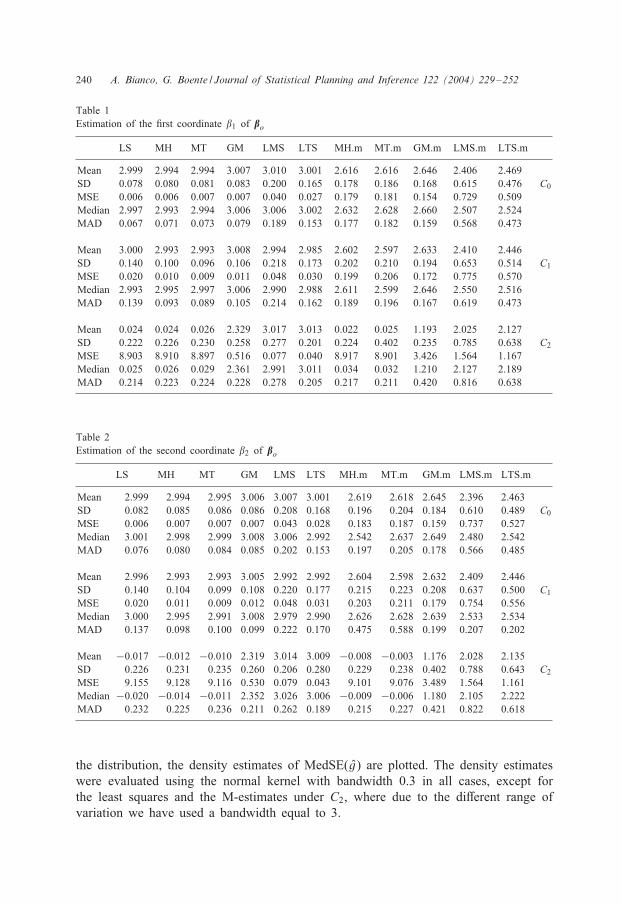
The following tables summarize the results of the simulations. Tables 1 and 2 givemeans, standard deviations and mean square errors for the regression estimates of 31
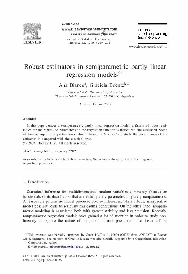
and 32, while Fig. 1 shows the boxplots of the estimates of 31 and 32, respectively.On the other hand, Table 3 gives the mean and median of MSE(g), while Table 4 onlyshows the median of MedSE(g) over the 500 replications since in this case both themean and the median are quite similar. Furthermore, in Fig. 2, due to the skewness of
240 A. Bianco, G. Boente / Journal of Statistical Planning and Inference 122 (2004) 229–252
Table 1Estimation of the 7rst coordinate 31 of �o
LS MH MT GM LMS LTS MH.m MT.m GM.m LMS.m LTS.m
Mean 2.999 2.994 2.994 3.007 3.010 3.001 2.616 2.616 2.646 2.406 2.469SD 0.078 0.080 0.081 0.083 0.200 0.165 0.178 0.186 0.168 0.615 0.476 C0MSE 0.006 0.006 0.007 0.007 0.040 0.027 0.179 0.181 0.154 0.729 0.509Median 2.997 2.993 2.994 3.006 3.006 3.002 2.632 2.628 2.660 2.507 2.524MAD 0.067 0.071 0.073 0.079 0.189 0.153 0.177 0.182 0.159 0.568 0.473
Mean 3.000 2.993 2.993 3.008 2.994 2.985 2.602 2.597 2.633 2.410 2.446SD 0.140 0.100 0.096 0.106 0.218 0.173 0.202 0.210 0.194 0.653 0.514 C1MSE 0.020 0.010 0.009 0.011 0.048 0.030 0.199 0.206 0.172 0.775 0.570Median 2.993 2.995 2.997 3.006 2.990 2.988 2.611 2.599 2.646 2.550 2.516MAD 0.139 0.093 0.089 0.105 0.214 0.162 0.189 0.196 0.167 0.619 0.473
Mean 0.024 0.024 0.026 2.329 3.017 3.013 0.022 0.025 1.193 2.025 2.127SD 0.222 0.226 0.230 0.258 0.277 0.201 0.224 0.402 0.235 0.785 0.638 C2MSE 8.903 8.910 8.897 0.516 0.077 0.040 8.917 8.901 3.426 1.564 1.167Median 0.025 0.026 0.029 2.361 2.991 3.011 0.034 0.032 1.210 2.127 2.189MAD 0.214 0.223 0.224 0.228 0.278 0.205 0.217 0.211 0.420 0.816 0.638
Table 2Estimation of the second coordinate 32 of �o
LS MH MT GM LMS LTS MH.m MT.m GM.m LMS.m LTS.m
Mean 2.999 2.994 2.995 3.006 3.007 3.001 2.619 2.618 2.645 2.396 2.463SD 0.082 0.085 0.086 0.086 0.208 0.168 0.196 0.204 0.184 0.610 0.489 C0MSE 0.006 0.007 0.007 0.007 0.043 0.028 0.183 0.187 0.159 0.737 0.527Median 3.001 2.998 2.999 3.008 3.006 2.992 2.542 2.637 2.649 2.480 2.542MAD 0.076 0.080 0.084 0.085 0.202 0.153 0.197 0.205 0.178 0.566 0.485
Mean 2.996 2.993 2.993 3.005 2.992 2.992 2.604 2.598 2.632 2.409 2.446SD 0.140 0.104 0.099 0.108 0.220 0.177 0.215 0.223 0.208 0.637 0.500 C1MSE 0.020 0.011 0.009 0.012 0.048 0.031 0.203 0.211 0.179 0.754 0.556Median 3.000 2.995 2.991 3.008 2.979 2.990 2.626 2.628 2.639 2.533 2.534MAD 0.137 0.098 0.100 0.099 0.222 0.170 0.475 0.588 0.199 0.207 0.202
Mean −0.017 −0.012 −0.010 2.319 3.014 3.009 −0.008 −0.003 1.176 2.028 2.135SD 0.226 0.231 0.235 0.260 0.206 0.280 0.229 0.238 0.402 0.788 0.643 C2MSE 9.155 9.128 9.116 0.530 0.079 0.043 9.101 9.076 3.489 1.564 1.161Median −0.020 −0.014 −0.011 2.352 3.026 3.006 −0.009 −0.006 1.180 2.105 2.222MAD 0.232 0.225 0.236 0.211 0.262 0.189 0.215 0.227 0.421 0.822 0.618
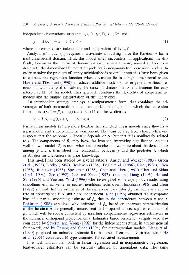
the distribution, the density estimates of MedSE(g) are plotted. The density estimateswere evaluated using the normal kernel with bandwidth 0.3 in all cases, except forthe least squares and the M-estimates under C2, where due to the diMerent range ofvariation we have used a bandwidth equal to 3.
A. Bianco, G. Boente / Journal of Statistical Planning and Inference 122 (2004) 229–252 241
LS MH MT GM LMS LTS LS MH MT GM LMS LTS LS MH MT GM LMS LTS
MH.m MT.m GM.m LMS.mLTS.m MH.m MT.m GM.m LMS.mLTS.m MH.m MT.m GM.m LMS.mLTS.m
LS MH MT GM LMS LTS LS MH MT GM LMS LTS LS MH MT GM LMS LTS
MH.m MT.m GM.m LMS.mLTS.m MH.m MT.m GM.m LMS.mLTS.m MH.m MT.m GM.m LMS.mLTS.m
C0 C1 C2
Regression Estimates of β1 based on Local M-Estimators
Regression Estimates of β1 based on Local Medians
Regression Estimates of β2 based on Local M-Estimators
Regression Estimates of β2 based on Local Medians
-1
1234
-1
1234
-1
1234
-1
1234
-1
1234
-1
1234
-1
1234
-1
1234
-1
1234
-1
1234
-1
1234
-1
1234
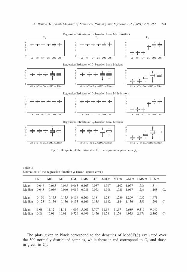
Fig. 1. Boxplots of the estimates for the regression parameter �o.
Table 3Estimation of the regression function g (mean square error)
LS MH MT GM LMS LTS MH.m MT.m GM.m LMS.m LTS.m
Mean 0.048 0.065 0.065 0.065 0.103 0.087 1.097 1.102 1.077 1.786 1.514Median 0.045 0.059 0.060 0.059 0.081 0.073 1.008 1.025 1.017 1.236 1.168 C0
Mean 0.150 0.155 0.155 0.156 0.200 0.181 1.231 1.239 1.209 1.937 1.671Median 0.125 0.136 0.136 0.135 0.169 0.155 1.142 1.144 1.136 1.359 1.291 C1
Mean 11.08 11.12 11.11 4.007 5.603 5.707 11.99 11.97 7.689 9.310 9.040Median 10.86 10.91 10.91 0.729 0.499 0.476 11.76 11.76 4.953 2.476 2.302 C2
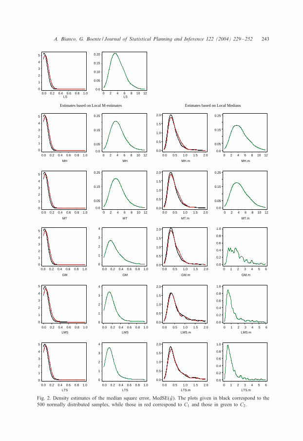
The plots given in black correspond to the densities of MedSE(g) evaluated overthe 500 normally distributed samples, while those in red correspond to C1 and thosein green to C2.

242 A. Bianco, G. Boente / Journal of Statistical Planning and Inference 122 (2004) 229–252
Table 4Estimation of the regression function g (median square error)
LS MH MT GM LMS LTS MH.m MT.m GM.m LMS.m LTS.m
Median 0.016 0.023 0.023 0.022 0.031 0.026 0.388 0.396 0.386 0.459 0.427 C0
Median 0.036 0.042 0.042 0.042 0.052 0.047 0.428 0.432 0.421 0.484 0.447 C1
Median 3.775 3.890 3.914 0.207 0.157 0.142 4.244 4.256 1.592 0.837 0.769 C2
5.1. Conclusions
The simulation con7rms the expected inadequate behavior of the least-squares esti-mates in the presence of outliers.
With respect to the estimation of �o, both bias and an increased standard deviationare observed, specially under C2. Note also that, under C2, the best performance forestimating the regression parameters is obtained by the least median of squares and theleast trimmed estimates, see Tables 1 and 2 and Fig. 1. The M-estimates increase theirmean square error under C1 and C2, in the 7rst case due to an inIated variance andin the second one due to the bias. Recall that M-estimates breakdown when leveragepoints are present. Fig. 1 shows, not only the poor behavior of least squares andM-estimates in the presence of outliers in the carriers, but also the moderate sensitivityof GM-estimates to C2. On the other hand, both least median and least trimmed ofsquares behave robustly, since their boxplots look quite similarly for normal and forcontaminated samples. This resistance to outliers is more evident for least trimmed,mainly due to the numerical instability of least median. In general, the estimates basedon initial M-smoothers show less variability than those based on the local median.
With regard to the estimation of the function g, as it can be seen in Tables 3 and4, under C2, the least squares and M-estimators estimate inadequately the regressionfunction. The estimates based on GM-estimators and specially those based on leastmedian and least trimmed estimates show a better performance. Notice that, even forthese estimates, large values of MSE(g) are present since means are considerably largerthan medians in Table 3. The plots in Fig. 2 show, not only the described poor behaviorof the least-squares estimates and of the M-estimates in the presence of high leverageoutliers, but also the sensitivity of those based on GM-estimates.
On the other hand, least trimmed and least median of squares seem to be the morerobust procedures. Also, all methods, including least squares, appear to be mainly un-aMected by the presence of outliers in the errors (contamination C1), but the proceduresbased on local medians are more stable under this contamination than those based onM-smoothers. However, a bias in the estimation with local medians can be observedsince the mode of the density of MedSE(g) using local medians is near 0.5 whileit is closer to 0 for local M-smoothers. In consequence, the MSE(g) and MedSE(g)obtained from least squares and a M-smoother are on the whole smaller than thoseresulting from local medians under C0 and C1.
A. Bianco, G. Boente / Journal of Statistical Planning and Inference 122 (2004) 229–252 243
LS0.0 0 2 4 6 8 10 120.2 0.4 0.6 0.8 1.0
0.0 0.2 0.4 0.6 0.8 0.0 0.5 1.0 1.5 2.01.0
0.0 0.2 0.4 0.6 0.8 1.0
0.0 0.2 0.4 0.6 0.8 1.0
0.0 0.2 0.4 0.6 0.8 1.0 0.0 0.2 0.4 0.6 0.8 1.0
0.0 0.2 0.4 0.6 0.8 1.0
0 2 4 6 8 10 12
0 2 4 6 8 10 12 0 2 4 6 8 10 12
0 1 2 3 4 5 6
0 2 4 6 8 10 12
LS
0.0
0.05
0.10
0.15
0.20
MH MH MH.m
0.0
0.5
1.0
1.5
2.0
0.0
0.5
1.0
1.5
2.0
0.0
0.5
1.0
1.5
2.0
0.0
0.5
1.0
1.5
2.0
0.0
0.5
1.0
1.5
2.0
MH.m
MT MT
0.0
0.05
0.15
0.25
0.0
0.05
0.15
0.25
0.0
0.05
0.15
0.25
0.0
0.05
0.15
0.25
MT.m MT.m
Estimates based on Local MediansEstimates based on Local M-estimates
GM GM GM.m
0.0 0.5 1.0 1.5 2.0
GM.m
0.0
0.2
0.4
0.6
0.8
1.0
0.0
0.2
0.4
0.6
0.8
1.0
LMS LMS LMS.m
0.0 0.5 1.0 1.5 2.0
LMS.m
LTS LTS LTS.m
0.0 0.5 1.0 1.5 2.0
LTS.m
0
1
2
3
4
5
0
1
2
3
4
5
0
1
2
3
4
5
0
1
2
3
4
5
0
1
2
3
4
0
1
2
3
4
0
1
2
3
4
0
1
2
3
4
5
0
1
2
3
4
5
0.0 0.2 0.4 0.6 0.8 1.0 0.0 0.2 0.4 0.6 0.8 1.0
0.0 0.5 1.0 1.5 2.0
0 1 2 3 4 5 6
0 1 2 3 4 5 6
0.0
0.2
0.4
0.6
0.8
1.0
Fig. 2. Density estimates of the median square error, MedSE(g). The plots given in black correspond to the500 normally distributed samples, while those in red correspond to C1 and those in green to C2.
244 A. Bianco, G. Boente / Journal of Statistical Planning and Inference 122 (2004) 229–252
Acknowledgements
The authors wish to thank an anonymous referee for valuable comments which ledto an improved version of the original paper.
Appendix
Proof of Proposition 1. (a) Follows using Theorem 3.3 from Boente and Fraiman(1991).
(b) The equicontinuity condition required in A4 and the uniqueness of the conditionalmedian imply that �j(t) is a continuous function of t and thus, for any 7xed a∈R thefunction ha(t) = Fj(a + �j(t)|T = t) will also be continuous as a function of t.
Given �¿ 0, let 0¡#¡� be such that
|u− v|¡# ⇒ supt∈C
max06j6p
(|Fj(u|T = t) − Fj(v|T = t)|)¡ �2: (A.1)
Then, from the uniqueness of the conditional median and (A.1) we get that, for06 j6p,
12¡Fj(�j(t) + #|T = t)¡
12
+�2; (A.2)
12− �
2¡Fj(�j(t) − #|T = t)¡
12: (A.3)
Write mj(#) = inf t∈C Fj(�j(t) + #|T = t) and Mj(#) = supt∈C Fj(�j(t) − #|T = t).The continuity of h#(t) and h−#(t) together with (A.2) and (A.3) entail that, for any
06 j6p, Mj(#)¡ 12 ¡mj(#) and thus
( = min06j6p
min(mj(#) − 1
2;12−Mj(#)
)¿ 0:
Using Theorem 3.1 or 3.2 from Boente and Fraiman (1991), we have that
supt∈C
supx∈R
|F j(x|T = t) − Fj(x|T = t)| a:s:−→0; 06 j6p:
Let N be such that P(N) = 0 and for any ! �∈ N,
max06j6p supt∈C supx∈R |F j(x|T = t) − Fj(x|T = t)| → 0:
Thus, for n large enough we have that max06j6p supt∈C supx∈R |F j(x|T=t)−Fj(x|T=t)|¡min( (
2 ;�2 ) = �1. Therefore, for 06 j6p, and t ∈C, we have that
Fj(�j(t) + #|T = t) − �1 ¡Fj(�j(t) + #|T = t)¡Fj(�j(t) + #|T = t) + �1;
Fj(�j(t) − #|T = t) − �1 ¡Fj(�j(t) − #|T = t)¡Fj(�j(t) − #|T = t) + �1;
which entail that 12 ¡Fj(�j(t) + #|T = t)¡ 1
2 + � and 12 − �¡ Fj(�j(t)− #|T = t)¡ 1
2
and so, max06j6p supt∈C|�j;med(t) − �j(t)|6 #¡� which concludes the proof.

A. Bianco, G. Boente / Journal of Statistical Planning and Inference 122 (2004) 229–252 245
Proof of Lemma 1. (a) For any �¿ 0, there exist compact sets C1 ⊂ Rp+1 and C2 ⊂ Rsuch that, if C=C1×C2, P(C)¿ 1−�=(4‖f‖∞). Note that |EQn(f)−EPn(f)|6A1n +A2n, where
A1n =1n
n∑i=1
|f(ri + (o(ti); zi + �(ti)) − f(ri; zi)|IC(ri; zi ; ti);
A2n = 2‖f‖∞ 1n
n∑i=1
ICc(ri; zi ; ti):
From (10) and the Strong Law of Large Numbers, we have that there exists a setN ⊂ ' such that P(N) = 0 and such that for any ! �∈ N we obtain that
supt∈C2
|(o(t)| + supt∈C2
|�(t)| → 0 and1n
n∑i=1
ICc(ri; zi ; ti) → P(Cc): (A.4)
Hence, for n large enough A2n6 �2 for ! �∈ N.
Denote by C1 the closure of a neighborhood of radius 1 of C1. The uniform continu-ity of f on C1 implies that there exists # such that max16j6p+1 |uj−vj|¡#; u; v∈C1
entails |f(u) − f(v)|¡ �2 . Hence, from (A.4) we have that for ! �∈ N and n large
enough max06j6p supt∈C2|(j(t)|¡# and so, for 16 i6 n, we obtain that
|f(ri + (o(ti); zi + �(ti)) − f(ri; zi)|IC(ri; zi ; ti)¡�2;
which entails that A1n ¡ �2 . Therefore, |EQn(f) − EPn(f)|¡� for n large enough and
! �∈ N.(b) Follows immediately.
From now on, C: will denote the Lipschitz constant for a Lipschitz function :.
Proof of Lemma 2. For any matrix B∈Rp×p, let |B|=max16‘; j6p |b‘j|. Denote by =i
intermediate points between ri−z′i � and ri− z′i � and (j(t)=�j(t)−�j(t) for 06 j6p,and �= ((1(t); : : : ; (p(t))′. A Taylor expansion of 7rst order and some algebra lead usto An = A1
n + A2n + A3
n + A4n, where
A1n =
1n
n∑i=1
′1
(ri − z′i �
sn
)w2(‖zi‖)ziz′i ;
A2n = −1
n
n∑i=1
′1
(ri − z′i �
sn
)w2(‖zi‖)[�(ti)z′i + zi �(ti)′];
A3n = −1
n
n∑i=1
′′1
(=i
sn
)((o(ti) − �(ti)′�
sn
)w2(‖zi‖)ziz′i ;
A4n =
1n
n∑i=1
′1
(ri − z′i �
sn
)[w2(‖zi‖) − w2(‖zi‖)]ziz′i :

246 A. Bianco, G. Boente / Journal of Statistical Planning and Inference 122 (2004) 229–252
Analogous arguments to those used in Lemma 1 in Bianco and Boente (2002) allowus to show that A1
np→A. From N3, it is easy to see that
‖zi‖2|w2(‖zi‖) − w2(‖zi‖)|6 ‖�(ti)‖(‖ 2‖∞ + ‖�(ti)‖(‖w2‖∞ + ‖ ′
2‖∞) + ‖/2‖∞):
Now, the result follows from N2, the consistency of sn and �, the Law of LargeNumbers and the fact that max06j6p supt∈[0;1] |(j(t)| p→0, since
|A2n|6 ‖ ′
1‖∞ max06j6p
supt∈[0;1]
|(j(t)|(
2‖ 2‖∞ + ‖w2‖∞ max06j6p
supt∈[0;1]
|(j(t)|)
;
|A3n|6 ‖ ′′
1 ‖∞ max06j6p
supt∈[0;1]
|(j(t)|(
1 + p‖�‖sn
)1n
n∑i=1
w2(‖zi‖)‖zi‖2;
|A4n|6p‖ ′
1‖∞ max16j6p
supt∈[0;1]
|(j(t)|
×(‖ 2‖∞ + p max
16j6psup
t∈[0;1]|(j(t)|(‖w2‖∞ + ‖ ′
2‖∞) + ‖/2‖∞)
:
Proof of Theorem 2. Write
Ln(.; �) =.n
n∑i=1
1
(ri − z′i�
.
)w2(‖zi‖)zi ;
L n(.; �) =.n
n∑i=1
1
(ri − z′i�
.
)w2(‖zi‖)zi :
Using a 7rst order Taylor expansion around �, we get
L n(.; �o) =.n
n∑i=1
1
(ri − z′i �
.
)w2(‖zi‖)zi
+1n
n∑i=1
′1
(ri − z′i �
.
)w2(‖zi‖)zi z′i(� − �o);
with � an intermediate point between � and �o. This implies that
L n(sn; �o) = 0 +1n
n∑i=1
′1
(ri − z′i �
sn
)w2(‖zi‖)zi z′i(� − �o)
A. Bianco, G. Boente / Journal of Statistical Planning and Inference 122 (2004) 229–252 247
and so, we get that (� − �o) = A−1n L n(sn; �o) with
An =1n
n∑i=1
′1
(ri − z′i �
sn
)w2(‖zi‖)zi z′i :
From the consistency of �, Lemma 2 implies that Anp→A and therefore, from N2 it
will be enough to show that
(a) n1=2Ln(.o; �o)D→N (0;').
(b) n1=2[ L n(sn; �o) − Ln(sn; �o)]p→0.
(c) n1=2[Ln(sn; �o) − Ln(.o; �o)]p→0.
(a) Follows immediately from the Central Limit Theorem, since ri − zi�′o = �i.
(b) Denote by =i intermediate points between ri−z′i � and ri− z′i � and (j(t)=�j(t)−�j(t) for 06 j6p, and �=((1(t); : : : ; (p(t))′. Using a second order Taylor expansion,we have that L n(sn; �o) = Ln(sn; �o) + L n;1 + L n;2 + L n;3 + L n;4 + L n;5 + L n;6,where
L n;1 =1n
n∑i=1
′1
(ri − z′i�o
sn
)[�′(ti)�o − (o(ti)]w2(‖zi‖)zi ;
L n;2 =snn
n∑i=1
1
(ri − z′i�o
sn
)[w2(‖zi‖)zi − w2(‖zi‖)zi];
L n;3 =snn
n∑i=1
[ 1
(ri − z′i�o
sn
)− 1
(ri − z′i�o
sn
)]w2(‖zi‖)(zi − zi);
L n;4 =1
2sn
1n
n∑i=1
′′1
(=i
sn
)[�′(ti)�o − (o(ti)]2w2(‖zi‖)zi ;
L n;5 =1n
n∑i=1
′1
(ri − z′i�o
sn
)[�′(ti)�o − (o(ti)][w2(‖zi‖) − w2(‖zi‖)]zi :
Since, N3 entails |w2(‖zi‖) − w2(‖zi‖)|6C ‖�(ti)‖‖zi‖ , where C = ‖w2‖∞ + C 2 , and
n1=2‖ L n;3‖6p‖w2‖∞‖ ′1‖∞n1=2
[max
16j6psup
t∈[0;1]|(j(t)|
]2
(1 + p‖�o‖);
248 A. Bianco, G. Boente / Journal of Statistical Planning and Inference 122 (2004) 229–252
n1=2‖ L n;4‖6 12
1sn‖ ′′
1 ‖∞n1=2
[max
16j6psup
t∈[0;1]|(j(t)|
]2
(1 + p‖�o‖)2
×(‖ 2‖∞ + p ‖w2‖∞ max
16j6psup
t∈[0;1]|(j(t)|
);
n1=2‖ L n;5‖6pC‖ ′1‖∞(1 + p ‖�o‖)n1=2
[max
16j6psup
t∈[0;1]|(j(t)|
]2
;
using (13) and the consistency of sn, we get that for 36 j6 5, n1=2‖ L n; j‖ p→0.It remains to show that n1=2 L n; j
p→0 for j = 1; 2, that is,
n1=2 snn
n∑i=1
′1
(ri − z′i�o
sn
)(‘(ti)w2(‖zi‖)zi
p→0; 06 ‘6p; (A.5)
n1=2 snn
n∑i=1
1
(ri − z′i�o
sn
)[w2(‖zi‖)zi − w2(‖zi‖)zi]
p→0: (A.6)
For this purpose, we will use the maximal inequality for covering numbers, componen-twise, and so, we will need to de7ne suitable classes of functions with 7nite uniformentropy.
Fix the coordinate j, 16 j6p. For any function h, any vector of funtions h(t) =(h1(t); : : : ; hp(t))′ and any .∈ ( .o
2 ; 2.o), if zi; j denotes the jth coordinate of zi, wede7ne
Jn;1(.; h) = n1=2 .n
n∑i=1
′1
(ri − z′i�o
.
)h(ti)w2(‖zi‖)zi; j ;
Jn;2(.; h)
=n1=2 .n
n∑i=1
1
(ri − z′i�o
.
)[w2(‖zi + h(ti)‖)(zi; j + hj(ti)) − w2(‖zi‖)zi; j];
where we have omitted the subscript j for the sake of simplicity.Let I=( .o
2 ; 2.o) and H={h∈C1[0; 1] : ‖h‖∞6 1 ‖h′‖∞6 1}. Note that, for anyprobability measure Q, the bracketing number N[ ](�;H; L2(Q)), and so the coveringnumber N
(�;H; L2(Q)
), satis7es
logN( �
2;H; L2(Q)
)6 logN[ ]
(�;H; L2(Q)
)6K�−1
for 0¡�¡ 2, where the constant K is independent of the probability measure Q (seeCorollary 2.7.2 in van der Vaart and Wellner, 1996).
A. Bianco, G. Boente / Journal of Statistical Planning and Inference 122 (2004) 229–252 249
Consider the classes of functions
F1 ={f1;.;h(r; z; t) = . ′
1
(r − z′�o
.
)w2(‖z‖)zjh(t); .∈I; h∈H
};
F2 ={f2;.;h(r; z; t) = . 1
(r − z′�o
.
)[w2(‖z + h(t)‖)(zj + hj(t)) − w2(‖z‖)zj];
.∈I; h(t) = (h1(t); : : : ; hp(t))′ h‘ ∈H} ;where again we have omitted the subscript j for the sake of simplicity. Note that F1
and F2 have envelope the constants A1 =2.o‖ ′1‖∞‖ 2‖∞ and A2 =4.o‖ 1‖∞‖ 2‖∞,
respectively. On the other hand, the independence between the errors �i = ri − z′i�oand the carriers (x′i ; ti)
′ implies that, for any f∈F1, Ef(ri; zi ; ti) = 0 since N4 holds;while, Ef(ri; zi ; ti) = 0 for any f∈F2, since 1 is odd and the errors have symmetricdistribution.
Write 1; s(t) = s 1( ts ) and ′
1; s(t) = s ′1( t
s ). From N1, we have that ’1 and ’2 arebounded, which entails that
| ′1; s1
(r) − ′1; s2
(r)|6 (‖ ′1‖∞ + ‖’2‖∞)|s1 − s2|; (A.7)
| 1; s1 (r) − 1; s2 (r)|6 (‖ 1‖∞ + ‖’1‖∞)|s1 − s2|: (A.8)
Write ‖f‖Q;2 = (EQ(f2))1=2, B1 = (‖ ′1‖∞(3 + 2.o) + ‖’2‖∞)‖ 2‖∞ and B2 =
2‖ 2‖∞(‖ 1‖∞ + ‖’1‖∞) + 2.op‖ 1‖∞(‖w2‖∞(1 + p) + p ‖ ′2‖∞). It is easy to
see that, given h∈H, .∈I and 0¡�¡ 2, ‖hs − h‖Q;2 ¡� and |.‘ − .|¡�, entail
‖f1;.‘;hs − f1;.;h‖Q;26B1�
and so,
N (�B1;F1; L2(Q))6N (�;H; L2(Q)) · N (�;I; | · |):In an analogous way, given h = (h1; : : : ; hp)′ with hj ∈H, .∈I and 0¡�¡ 2,
hs = (hs;1; : : : ; hs;p)′ with ‖hs;j − hj‖Q;2 ¡� for 06 j6p and |.‘ − .|¡�, it is easyto see that
‖f2;.‘;hs − f2;.;h‖Q;26B2�;
which implies
N (� B2;F2; L2(Q))6N (�;H; L2(Q))p · N (�;I; | · |):Therefore, these classes of functions have 7nite uniform entropy.For any class of functions F, de7ne the integral
J(#;F) = supQ
∫ #
0
√1 + log (N (�||F ||Q;2;F; L2(Q))) d�;
250 A. Bianco, G. Boente / Journal of Statistical Planning and Inference 122 (2004) 229–252
where the supremum is taken over all discrete probability measures Q with ‖F‖Q;2 ¿ 0and F is the envelope of F. The function J is increasing, J(0;F) = 0 and J(1;F)¡∞ and J(#;F) → 0 as # → 0 for classes of functions F which satisfy theuniform-entropy condition. Moreover, if Fo ⊂ F and the envelope F is used for Fo,then J(#;Fo)6J(#;F).
For any 0¡#¡ 1, consider the subclasses
F1; # = {f1;.;h(r; z; t)∈F1 with ‖h‖∞ ¡#} ⊂ F1;
F2; # = {f2;.;h(r; z; t)∈F2 with h(t) = (h1(t); : : : ; hp(t))′ and
‖h‘‖∞ ¡#; 16 ‘6p} ⊂ F2:
For any �¿ 0, let 0¡#¡ 1. Using that snp→.o and since (13) and (14) entail, for
06 j6p
supt∈[0;1]
|(j(t)| = supt∈[0;1]
|�j(t) − �j(t)| p→0; supt∈[0;1]
|(′j(t)| = supt∈[0;1]
|�′j(t) − �′
j(t)|p→0;
we have that, for n large enough, P(sn ∈I)¿ 1− #=2 and P((j ∈H and ‖(j‖∞ ¡#)¿ 1 − #=2, for 06 j6p.
Let A3 = 2.o‖ 1‖∞(‖w2‖∞(1 + p) + p ‖ ′2‖∞). Straighforward calculations lead us
to
supf∈F1;#
1n
n∑i=1
f2(ri; zi ; ti)6A21#;
supf∈F2;#
1n
n∑i=1
f2(ri; zi ; ti)6A23#:
The maximal inequality for covering numbers entails that, for any 06 ‘6p,
P(|Jn;1(sn; (‘)|¿�)6 P(|Jn;1(sn; (‘)|¿�; sn ∈I; (‘ ∈H and ‖(‘‖∞ ¡#) + #
6 P
(sup
f∈F1;#
∣∣∣∣∣n1=2 1n
n∑i=1
f(ri; zi ; ti)
∣∣∣∣∣¿�
)+ #
61�E
(sup
f∈F1;#
∣∣∣∣∣n1=2 1n
n∑i=1
f(ri; zi ; ti)
∣∣∣∣∣)
+ #
61�D1A1J(#;F1) + #;
where D1 is a constant not depending on n. Similarly,
P(|Jn;2(sn; �)|¿�)61�D2A2J
(A2
3
A22#;F2
)+ #:

A. Bianco, G. Boente / Journal of Statistical Planning and Inference 122 (2004) 229–252 251
Now, (A.5) and (A.6) follow from the fact that lim#→0 J(#;F1) = 0 and lim#→0
J(#;F2) = 0, since the classes F1 and F2 satisfy the uniform-entropy condition.(c) Since
n1=2[Ln(sn; �o) − Ln(.o; �o)]
=n−1=2n∑
i=1
[ 1; sn(ri − z′i�o) − 1;.o(ri − z′i�o)]w2(‖zi‖)zi ;
we get the desired result using (A.8), the boundness of 2 and the maximal inequalityfor covering numbers, as in (b).
References
Ansley, C., Wecker, W., 1983. Extension and examples of the signal extraction approach to regression. In:Zeller, A. (Ed.), Applied Time Series Analysis of Economic Data, Bureau of Census, Washington, DC,pp. 181–192.
Bianco, A., Boente, G., 2002. On the asymptotic behavior of one-step estimates in heteroscedastic regressionmodels. Statist. Probab. Lett. 60, 33–47.
Boente, G., Fraiman, R., 1991. Strong uniform convergence rates for some robust equivariant nonparametricregression estimates for mixing processes. Internat. Statist. Rev. 59, 355–372.
Boente, G., Fraiman, R., Meloche, J., 1997. Robust plug-in bandwidth estimators in nonparametric regression.J. Statist. Plann. Inference 57, 109–142.
Chen, H., 1988. Convergence rates for parametric components in a partly linear model. Ann. Statist. 16,136–146.
Chen, H., Chen, K., 1991. Selection of the splined variables and convergence rates in a partial spline model.Canad. J. Statist. 19, 323–339.
Chen, H., Shiau, J., 1991. A two-stage spline smoothing method for partially linear models. J. Statist. Plann.Inference 25, 187–201.
Chen, H., Shiau, J., 1994. Data-driven eNcient estimates for partially linear models. Ann. Statist. 22,211–237.
Denby, L., 1986. Smooth regression functions, Statistical Research Report 26, AT& T Bell Laboratories,Murray Hill.
Engle, R., Granger, C., Rice, J., Weiss, A., 1986. Semiparametric estimates of the relation between weatherand electricity sales. J. Amer. Statist. Assoc. 81, 310–320.
Gao, J., 1992. A large sample Theory in Semiparametric Regression Models. Ph.D. Thesis, University ofScience and Technology of China, Hefei, China.
Gao, J., Liang, H., 1995. Asymptotic normality of pseudo-LS estimator for partly linear autoregressionmodels. Statist. Probab. Lett. 23, 27–34.
Gao, J., Zhao, L., 1993. Adaptive estimation in partly linear regression models. Sci. China Ser. A 1, 14–27.Gervini, D., Yohai, V.J., 2000. A class of robust and fully eNcient regression estimators. Technical report
(December 2000), submitted.Green, P., Jennison, C., Seheult, A., 1985. Analysis of 7eld experiments by least squares smoothing. J. Roy.
Statist. Soc. Ser. B 47, 299–315.Hastie, T.J., Tibshirani, R.J., 1990. Generalized Additive Models. In: Monographs on Statistics and Applied
Probability, Vol. 43. Chapman & Hall, London.He, X., Shi, P., 1996. Bivariate tensor-product B-spline in a partly linear model. J. Multivariate Anal. 58,
162–181.He, X., Zhu, Z., Fung, W., 2001. Estimation in a semiparametric model for longitudinal data with unspeci7ed
dependence structure. Working Paper.Heckman, N., 1986. Spline smoothing in a partly linear model. J. Roy. Statist. Soc., Ser. B 48, 244–248.Huber, P., 1981. Robust Statistics. Wiley, New York.
252 A. Bianco, G. Boente / Journal of Statistical Planning and Inference 122 (2004) 229–252
Krasker, W., Welsch, R., 1982. ENcient bounded-inIuence regression estimation. J. Amer. Statist. Assoc.77, 595–604.
Liang, H., HYardle, W., Carroll, R., 1999. Estimation in a semiparametric partially linear errors-in-variablesmodel. Ann. Statist. 27, 1519–1535.
Mallows, C., 1975. On some topics in robustness. Technical Memorandum, AT& T Bell Laboratories, MurrayHill.
Rice, J., 1986. Convergence rates for partially splined models. Statist. Probab. Lett. 4, 203–208.Robinson, P., 1988. Root-n-consistent semiparametric regression. Econometrica 56, 931–954.Rousseeuw, P., Leroy, A., 1987. Robust Regression and Outlier Detection. Wiley, New York.Severini, T., Wong, W., 1992. Pro7le likelihood and conditionally parametric models. Ann. Statist. 20,
1768–1802.Speckman, P., 1988. Kernel smoothing in partial linear models. J. Roy. Statist. Soc. Ser. B 50, 413–436.Truong, Y., Stone, C., 1994. Semiparametric time series regression. J. Time Ser. Anal. 15, 405–428.van der Vaart, A., Wellner, J., 1996. Weak Convergence and Empirical Processes. With Applications to
Statistics. Springer, New York.Yee, T., Wild, C., 1996. Vector generalized additive models. J. Roy. Statist. Soc., Ser. B 58, 481–493.Yohai, V., 1987. High breakdown point and high eNciency robust estimates for regression. Ann. Statist. 15,
642–656.Yohai, V., Zamar, R., 1988. High breakdown estimates of regression by means of the minimization of an
eNcient scale. J. Amer. Statist. Assoc. 83, 406–413.
Related Documents