Robust bandwidth selection in semiparametric partly linear regression models: Monte Carlo study and influential analysis

Robust bandwidth selection in semiparametric partly linear

regression models: Monte Carlo study and influential analysis

Graciela BoenteDepartamento de Matematicas, Instituto de Calculo

FCEyN, Universidad de Buenos Aires and CONICET, Argentinaand

Daniela RodriguezDepartamento de Matematicas, Instituto de Calculo

FCEyN, Universidad de Buenos Aires and CONICET, Argentina

Abstract

In this paper, under a semiparametric partly linear regression model with fixed de-sign, we introduce a family of robust procedures to select the bandwidth parameter.The robust plug–in proposal is based on nonparametric robust estimates of the ν−thderivatives and under mild conditions, it converges to the optimal bandwidth. A ro-bust cross–validation bandwidth is also considered and the performance of the differentproposals is compared through a Monte Carlo study. We define an empirical influencemeasure for data–driven bandwidth selectors and, through it, we study the sensitivityof the data–driven bandwidth selectors. It appears that the robust selector comparesfavorably to its classical competitor, despite the need to select a pilot bandwidth whenconsidering plug–in bandwidths. Moreover, the plug–in procedure seems to be less sen-sitive than the cross–validation in particular, when introducing several outliers. Whencombined with the three-step procedure proposed by Bianco and Boente (2004), therobust selectors lead to robust data–driven estimates of both the regression functionand the regression parameter.

Corresponding AuthorGraciela BoenteMoldes 1855, 3o ABuenos Aires, C1428CRA, Argentinaemail: gboente a©mate.dm.uba.ar

AMS Subject Classification 2000: Primary 62F35, Secondary 62G05.Key words and phrases: Asymptotic Properties; Bandwidth Selectors; Kernel Weights;Partly Linear Models; Robust Estimation; Smoothing Techniques.

1

1 Introduction

Partly linear models have become an important tool when modelling biometric data, sincethey combine the flexibility of nonparametric models and the simple interpretation of thelinear ones. These models assume that we have a response yi ∈ IR and covariates or designpoints (xt

i , ti)t ∈ IRp+1 satisfying

yi = xti β + g(ti) + εi 1 ≤ i ≤ n , (1)

with the errors εi independent and independent of (xti , ti)

t. The semiparametric natureof model (1) offers more flexibility than the standard linear model, when modelling a com-plicated relationship between the reponse variable with one of the covariates. At the sametime, they keep a simple functional form with the other covariates avoiding the “curse ofdimensionality” existing in nonparametric regression.

In many situations, it seems reasonable to suppose that a relationship between thecovariates x and t exists, so as in Speckman (1988), Linton (1995) and Aneiros–Perez andQuintela del Rıo (2002) we will assume that for 1 ≤ j ≤ p

xij = φj(ti) + ηij 1 ≤ i ≤ n (2)

where the errors ηij are independent. Moreover, the design points ti will be assumed to befixed.

Several authors have considered the semiparametric model (1). See, for instance, Denby(1986), Rice (1986), Robinson (1988), Speckman (1988) and Hardle, Liang and Gao (2000)among others.

All these estimators, as nonparametric estimators, depend on a smoothing parameterthat should be choosen by the practitioner. As it is well known, large bandwidths produceestimators with small variance but high bias, while small values produce more wiggly curves.This trade–off between bias and variance lead to several proposals to select the smoothingparameter, such as cross-validation procedures and plug–in methods. Linton (1995), usinglocal polynomial regression estimators, obtained an asymptotic expression for the optimalbandwidth in the sense that it minimizes a second order approximation of the mean squareerror of the least squares estimate, βls(h), of β. This expression depends on the regressionfunction we are estimating and on parameters which are unknown, such as the standarddeviation of the errors. More precisely, for any c ∈ IRp, let σ2 = σ2

ε ctΣ−1

η c be the

asymptotic variance of U = ctn12 (βls(h)−β), and nMSE(h) = EU2/σ2 its standardized

mean square error. Then, when the smoothing procedure corresponds to local means, undergeneral conditions, that include that the design points are almost uniform design points,i.e., {ti}ni=1 are fixed design points in [0, 1], 0 ≤ t1 ≤ . . . ≤ tn ≤ 1, such that t0 = 0 andtn+1 = 1 and max1≤i≤n+1 |(ti − ti−1) − 1/n| = O(n−δ) for some δ > 1, we have that, forν ≥ 2,

MSE(h) = n−1{1 + (nh)−1A2 + o(n−2µ) + (n12h2νA1 + o(n−µ))2} ,

2

where µ = (4ν − 1)/(2(4ν + 1)), φ(ν)(t) = (φ(ν)1 (t), . . . , φ(ν)

p (t))t, αν(K) =∫uνK(u)du,

K∗(u) = K ∗K(u) − 2K(u) and

A1 = α2ν(K)(ν!)−2 σ−1 ctΣ−1

η

∫ 1

0g(ν)(t)φ(ν)(t)dt A2 =

∫K2

∗ (u)du .

Therefore, the optimal bandwidth in the sense of minimizing the asymptotic MSE(h), isgiven by hopt = A0n

−π, with π = 2/(4ν + 1) and

A0 =(A2/(4νA1

2))π/2

=

{∫K2

∗ (u)du/

[4ν

(σ−1ctΣ−1

η α2ν(K)(ν!)−2

∫ 1

0g(ν)(t)φ(ν)(t)dt

)2]}π/2

.

(3)Linton (1995) considered a plug–in approach to estimate the optimal bandwidth and showedthat it converges to the optimal one, while Aneiros–Perez and Quintela del Rıo (2002)studied the case of dependent errors.

It is well known that, both in linear regression and in nonparametric regression, leastsquares estimators can be seriously affected by anomalous data. The same statement holdsfor partly linear models. To avoid that problem, Bianco and Boente (2004) considered athree–step robust estimate for the regression parameter and the regression function. Besides,for the nonparametric regression setting, i.e., when β = 0, the sensitivity of the classicalbandwidth selectors to anomalous data was discussed by several authors, such as, Leung,Marriott and Wu (1993), Wang and Scott (1994), Boente, Fraiman and Meloche (1997),Cantoni and Ronchetti (2001) and Leung (2005).

In this paper, we consider a robust plug–in selector for the bandwidth, under the partlylinear model (1) which converges to the optimal one and leads to robust data–driven esti-mates of the regression function g and the regression parameter β. We derive an expressionanaloguous to (3) for the optimal bandwidth of the three–step estimator introduced inBianco and Boente (2004). As for its linear relative, this expression will depend on thederivatives of the functions g and φ. In Section 2, we review some of the proposals givento estimate robustly the derivatives of the regression function under a nonparametric re-gression model. The robust bandwidth selector for the partial linear model is introduced inSection 3, where under mild conditions, consistency to the optimal bandwidth is established.In Section 4, for small samples, the behavior of the classical approach and of the resistantselectors is compared through a Monte Carlo study under normality and contamination.Also, a robust cross–validation procedure is introduced and compared with the plug–in one.Finally, in Section 5 an empirical influence measure for the plug–in bandwidth selector isintroduced. We use this measure to study the sensitivity of the plug–in selector on somegenerated examples. All proofs are given in the Appendix.

2 Robust estimation of the derivative of order ν

In this section, we review some of the approaches given to provide robust estimator of theν−th derivative of the regression function under a fully nonparametric regression model.

3

Let zi ∈ IR be independent observations such that

zi = ϕ(ti) + ui 1 ≤ i ≤ n , (4)

where the errors ui are independent and identically distributed with symmetric commondistribution F (·/σu) and 0 ≤ t1 ≤ . . . ≤ tn ≤ 1 are fixed design points.

Robust estimates for the first derivative of the regression function have been introducedby Hardle and Gasser(1985), when the scale is known. Boente and Rodriguez (2006) dis-cussed the estimation of higher derivatives. Their approach is analoguous to that given byBoente, Fraiman and Meloche (1997) when ν = 2. On the other hand, a robust local poly-nomial approach was introduced by Welsh (1996) and extended to the dependent settingby Jiang and Mack (2001).

In order to define both classes of estimates, let us denote by Ψ(j) the j−th derivativesof the score function Ψ while wni(t, h) and w

(ν)ni (t, h) stand for the kernel weights used to

estimate the regression function and its ν−th derivative, respectively. More precisely, letwni(t, h) and w(ν)

ni (t, h) be defined as

wni(t, h) = (nh)−1K0 ((t− ti)/h) , (5)

w(ν)ni (t, h) = (nhν+1)−1K(ν) ((t− ti)/h) , (6)

with h the bandwidth parameter, K0 : IR → IR a continuous integrable function withcompact support and

∫K0(t)dt = 1 and K : IR→ IR is an integrable function differentiable

up to order ν with ν−th derivative K(ν).

2.1 The robust differentiation approach

When scale σu is known, Hardle and Gasser (1985) suggested to use as an estimate ofϕ(ν)(t) the ratio σuBν (t, σu, ϕ) [λ1,n(t, σu, ϕ)]−1, with ϕ(t) a preliminary robust estimate ofthe regression function and

Bν (t, σ, ϕ) =n∑

i=1

w(ν)ni (t, h)Ψ ((zi − ϕ(t))/σ) (7)

λj,n(t, σ, ϕ) =n∑

i=1

wni(t, h)Ψ(j) ((zi − ϕ(t))/σ) . (8)

However, this estimate will be biased if ν > 2, since E[Ψ(j) (ui/σu)

]are not equal to 0

for odd values of j (see Boente and Rodriguez (2006) for a discussion). More precisely, theestimate of ϕ(ν)(t) introduced by Hardle and Gasser (1985) will converge to

ϕ(ν)(t) + (λ1(σu))−1σu∑

3≤j≤ν

j:odd

(σju j!)−1 λj(σu) Hj(ν, t) = ϕ(ν)(t) + (λ1(σu))−1σuCν (t, σu, ϕ)

instead of ϕ(ν)(t), where λj(σ) = EΨ(j) (u1/σ) and Hj(ν, t) = {[ϕ(u) − ϕ(t)]j}(ν)∣∣∣u=t

. Tocorrect the bias, Boente and Rodriguez (2006) introduced an estimator for Cν (t, σu, ϕ) as

4

followsCν (t, σ, ϕ) =

∑

3≤j≤ν

j:odd

(j! σj)−1 λj,n(t, σ, ϕ) Hj(ν, t)

with Hj(ν, t) an estimate of Hj(ν, t). The robust estimator, ϕ(ν)r (t, h), of the derivative of

order ν of the regression function ϕ is, then, defined as

ϕ(ν)r (t, h) = σu [Bν (t, σu, ϕr) − Cν (t, σu, ϕr)]/λ1,n (t, σu, ϕr) . (9)

where σu is a robust estimate of the residuals scale such as the robust Rice–type estimator,i.e., σu = 1

2 median1≤i≤n

|zi − zi−1|, and ϕr(·) = ϕr(·, h0) denotes a kernel–based M−estimate

of the regression function with initial bandwidth h0, i.e., a solution of

n∑

i=1

wni(t, h0)Ψ ((zi − ϕr(t, h0))/σu) = 0 .

As mentioned in Boente and Rodriguez (2006), this procedure depends on the pilotbandwidth h0 used to estimate ϕr and on the preliminary estimates of the derivatives of ϕ(t)up to order ν− 2, which obviously also involve a bandwidth choice, leading to ν− 1 choicesof pilot bandwidths to estimate the ν−th derivative of the regression function, denotedhj , 0 ≤ j ≤ ν − 2. In order to guarantee the convergence of the preliminary estimates,these bandwidths must satisfy hj → 0 and nh2j+1

j /log n → +∞. One possible choice forthem is to define data–driven bandwidths by robustifying and adapting the iterative schemeproposed by Gasser, Kneip and Kohler (1991).

Under mild conditions, in Theorem 3.1 in Boente and Rodriguez (2006), it is shown thatif nhν+2 → ∞ and E(Ψ′(u1/σu)) 6= 0, sup

t∈[h,1−2h]|ϕ(ν)

r (t, h) − ϕ(ν)(t)| a.s.−→ 0. The asymptotic

distribution of the estimates is also derived.

2.2 The robust polynomial approach

To estimate the derivatives of a regression function a different approach was considered byWelsch (1996) who studied local quantile regression and local heteroscedastic M−regressionestimators. On the other hand, under an homoscesdatic regression model as in (4), Jiangand Mack (2001) introduced a family of estimators for the regression function and theirderivatives based on a local M−regression approach that leads to pointwise consistentand asymptotically normally distributed estimates even when the observations satisfy anα−mixing condition. These estimates are defined as follows. Let ρ be an outlier resistantfunction with bounded derivative Ψ and σu a preliminary robust scale estimator. Jiang andMack (2001) propose to find aj to minimize

n∑

i=1

wni(t, h)ρ

(zi −

ν∑

j=0

aj(ti − t)j)/σu

5

Equivalently, the solution a(t) = (a0(t), ..., aν(t)) satisfy the local M−estimation equations:

n∑

i=1

wni(t, h)Ψ

(zi −

ν∑

j=0

aj(t)(ti − t)j)/σu

(ti − t)k = 0 k = 0, . . . , ν . (10)

The local M-type estimator of a(t) = (ϕ(t), ..., ϕ(ν)(t)/ν!) is the solution, a(t), to (10).Therefore, the estimate of ϕ(ν)(t) can be defined as ϕ(ν)(t, h) = ν! aν(t). Under mild condi-tions, if h→ 0 and nh2ν+1 → ∞ the estimates are pointwise consistent and asymptoticallynormally distributed.

3 Resistant choice of the smoothing parameter

As is well known an important issue in any smoothing procedure is the choice of the smooth-ing parameter. As mentioned in the Introduction, under a nonparametric regression model,two commonly used approaches are cross–validation and plug–in. However, these proceduresmay not be robust and their sensitivity to anomalous data was discussed by several authors,including Leung, Marriott and Wu (1993), Wang and Scott (1994), Boente, Fraiman andMeloche (1997), Cantoni and Ronchetti (2001) and Leung (2005). Wang and Scott (1994)note that, in the presence of outliers, the least squares cross–validation function is nearlyconstant on its whole domain and thus, essentially worthless for the purpose of choosinga bandwidth. The robustness issue remains valid for the partly linear considered in thispaper. With a small bandwidth, a small number of outliers with similar values of ti couldeasily drive the estimators of φ and φ0 and so, the final estimator of g, to dangerous levels.

In the following sections we will describe two data–driven bandwidth selectors. In Sec-tion ??, we introduce a robust plug–in bandwidth that relies on an expansion for the meansquare error of the robust estimator of β. Besides, in Section 3.4, a robust bandwidth basedon the cross–validation principles is considered. We begin by reviewing the definition of thethree–step estimator introduced in Bianco and Boente (2004).

3.1 Preliminaries: Estimation of the regression parameter

Let {(yi,xit, ti)t}ni=1 be independent observations satisfying (1). We will assume thatεi ∼ F (·/σε) where F is symmetric and that xi and ti are nonparametrically related through(2), so that the model can be written as

{yi = xitβ + g(ti) + εi 1 ≤ i ≤ n,xij = φj(ti) + ηij 1 ≤ j ≤ p,

(11)

with ηij independent and such that ηij ∼ Gj(·/ση, j) with Gj symmetric. From now on, wewill denote by φ0(t) = φ(t)tβ + g(t) and so, yi = φ0(ti) + ui with ui = ηt

i β + εi.

Without loss of generality, we will assume from now on that the fixed design points ti ∈[0, 1] are such that 0 ≤ t1 ≤ . . . ≤ tn ≤ 1. Moreover, we will assume that assumption B.4 be-low holds, i.e, the fixed design points are “almost”uniform, max1≤i≤n+1 |(ti − ti−1) − 1/n| =O(n−δ) for some δ > 1.

6

It is well known that, both in linear regression and in nonparametric regression, leastsquare estimators can be seriously affected by anomalous data. In partly linear models, theleast squares estimator of β, βls can be obtained by minimizing

n∑

i=1

[yi − φ0,ls(ti) −

(xi − φls(ti)

)tβ

]2

, (12)

with φ0,ls and φj,ls the linear kernel estimators of φ0(t) and φj(t), 1 ≤ j ≤ p, respectively.As expected, these estimators are highly sensitive to outliers. To avoid this problem, Biancoand Boente (2004) proposed a class of estimates based on a three step procedure with amore resistant behavior under the partly linear model which can be described as follows:

Step 1: Estimate φ0(t) and φj(t), 1 ≤ j ≤ p through a robust smoothing, as localM−type estimates. Let φ0,r and φj,r denote the obtained estimates and φr(t) =(φ1,r(t), . . . , φp,r(t))t.

Step 2: Estimate the regression parameter by applying a robust regression estimateto the residuals ri = yi − φ0,r and ηi = xi − φr. Let βr denote an estimate of β.

Step 3: Define the estimate of the regression function g as gr(t) = φ0,r(t)−βtrφr(t).

To make explicit the dependence on the bandwidth h, we will denote these estimates asφ0,r(t, h), φr(t, h), βr(h) and gr(t, h).

Theorem 2 in Bianco and Boente (2004) entails that, under mild conditions, when theestimates of the regression parameter are defined through

n∑

i=1

ψ1

((ri − βr(h)

tηi)/sn

)w2 (‖ηi‖) ηi = 0, (13)

with sn a robust consistent estimate of σε, then√n

(βr(h) − β

) D−→ N(0, σ2εA

−1ΣA−1)with

A = E(ψ′

1 (ε/σε))E

(w2 (‖η‖) η ηt

)= E

(ψ′

1 (ε/σε))Σ1,η

Σ = E(ψ2

1 (ε/σε))E

(w2

2 (‖η‖) η ηt)

= E(ψ2

1 (ε/σε))Σ2,η .

Denote Σr,η = Σ−11,ηΣ2,ηΣ−1

1,η and V (ψ1) = [E (ψ′1 (ε/σε))]

−2E(ψ2

1 (ε/σε)). Thus, for

any c ∈ IRp, the asymptotic variance of Ur = ctn12 (βr(h) − β), is given by σ2

r =σ2ε V (ψ1) ctΣr,η c.

3.2 Robust plug–in bandwidth selector

An important step to define a robust plug–in bandwidth is to obtain an asymptotic expan-sion for MSEr(h) = n−1 EU2

r/σr2. For the sake of simplicity, we will begin by fixing some

7

notation. Let η∗ij = ση, jΨ(ηij/ση, j) /E (Ψ′ (η1j/ση, j)) and u∗i = σ0Ψ(ui/σ0) /EΨ′ (u1/σ0)be the bounded modified residuals. Besides, denote vi = η∗t

i β − u∗i , D = EDψ2 (η) withDψ2 (u), the Jacobian matrix, with (i, j) element ∂

∂ujψ2(u)i and σ0 the scale of u. When

using local M−smoothers with score function Ψ, in the Appendix we derive an expressionfor the MSEr(h) that will allow to obtain the optimal bandwidth for the robust estimatorof β solution of (13). Effectively, therein it is shown that, under mild conditions, for ν ≥ 2,

MSEr(h) = n−1{1 + (nh)−1Ar,2 + o(n−2µ) + (n

12h2νAr,1 + o(n−µ))2

}, (14)

where

Ar,1 = α2ν(K)/(ν!)2 σ−1

r c′Σ−11,ηE (Dψ2(η))

∫ 1

0g(ν)(t)φ(ν)(t)dt

Ar,2 = σ2ε/σ

2r

{κ1

∫K2(u)du + κ2

∫(K ∗K)2(u)du− 2κ3

∫K(u)K ∗K(u)du

},

κ1 = σ−2ε E

(ψ′

1 (ε/σε))2 ctA−1Σ2,ηA−1c E

(v22

)+E (ψ1 (ε/σε))

2 E(ctA−1Dψ2 (η1) η∗

2

)2

+σ−2ε cov

(ψ′

1 (ε1/σε) v2 ctA−1ψ2 (η1) , ψ′1 (ε2/σε) v1 ctA−1ψ2 (η2)

)

+ 2σε−2E(ψ′

1 (ε1/σε)ψ1 (ε2/σε)u∗2 ctA−1ψ2 (η1) ctA−1Dψ2 (η2)η∗1

)

κ2 = σ−2ε

[Eψ′

1 (ε/σε)]2 {

cov(v1 ctA−1Dη∗

2, v2 ctA−1Dη∗1

)+ var

(v1 ctA−1Dη∗

2

)}

κ3 = σ−2ε E

[ψ′

1 (ε/σε)] {

cov(ψ′

1 (ε1/σε) v2 ctA−1ψ2 (η1) , v1 ctA−1Dη∗2

)

+ cov(ψ′

1 (ε1/σε) v2 ctA−1ψ2 (η1) , v2 ctA−1Dη∗1

)

− σε cov(ψ1 (ε1/σε) ctA−1Dψ2 (η1) η∗

2, v2 ctA−1Dη∗2

)}

η∗ij = ση, jΨ(ηij/ση, j) /E(Ψ′ (η1j/ση, j)

)ε∗i = σεΨ(εi/σε) /E

(Ψ′ (ε1/σε)

)

u∗i = σ0Ψ(ui/σ0) /EΨ′ (u1/σ0) ,

with D = EDψ2 (η), vi = βtη∗i − u∗i , σ0 the scale of u, αν(K) defined in the Introduction

and Dψ2 (u), the Jacobian matrix, with (i, j) element ∂∂uj

ψ2(u)i. Therefore, the optimalbandwidth in the sense of minimizing the asymptotic MSEr(h), is given by hr,opt =Ar,0n

−π, with π = 2/4ν + 1 and

Ar,0 =(Ar,2/4νA2

r,1

)π/2. (15)

Note that when using the least squares estimates defined in (12), we recover (3) from theformula above.

Since the optimal bandwidth hr,opt depends on the unknown quantities σ2ε , V (ψ1), Σ1,η,

Σ2,η, κ1 to κ3, g(ν)(t) and φ(ν)(t) robust estimates of them must be considered to definea plug–in selector. To define the robust plug-in bandwidth selection method, we proposeto plug–in robust estimators of the derivative of orden ν, as defined in Section 2, into (15).Therefore, a robust plug–in selector for the regression parameter under the partly linearregression model (11), can be obtained as follows

8

• Let s0 and sj be robust consistent estimates of the scales σ0 of u = ε+βtη and ση, j ,respectively. Denote by φj,r(t) and φ(ν)

j,r(t) preliminary robust consistent estimates of

the regression functions φj(t) and of its derivative φ(ν)j (t), 0 ≤ j ≤ p, computed with

a pilot bandwidth h. As robust estimators of the derivatives φ(ν)j (t), j = 0, . . . , p, one

can use either the robust differentiation or the robust polynomial approach, describedin Section 2.1 and 2.2, respectively.

Moreover, let βr and gr(t) be initial robust consistent estimators of β and g(t),

respectively. For instance, we can define gr(t) = φ0,r(t) − βtrφr(t), as in Step 3.

• Define a robust estimator of g(ν)(t) as

g(ν)r (t) = φ

(ν)0,r(t) − β

trφ

(ν)r (t) , (16)

where φ(ν)r (t) =

(φ

(ν)1,r(t), . . . , φ(ν)

p,r(t))t

.

• Denote by σ2ε , V (ψ1), Σ1,η, Σ2,η, D, κ`, 1 ≤ ` ≤ 3 robust consistent estimates of σ2

ε ,V (ψ1), Σ1,η, Σ2,η, D = EDψ2 (η) and κ`, respectively, obtained using the empirical

distribution of the residuals εi = yi − βtrxi − gr(ti) and ηi = xi − φr(ti). Define an

estimate of σ2r as σ2

r = σ2ε V (ψ1)ctΣr,η c.

• The robust bandwidth selector hr is defined as

hr = Ar,0n−π with Ar,0 =

(Ar,2/4νA2

r,1

)π/2(17)

Ar,1 = α2ν(K)(ν!)−2 σ−1

r ctΣ−11,η D

∫ 1−h

hg(ν)r (t)φ

(ν)

r (t)dt (18)

Ar,2 = κ1

∫K2(u)du+ κ2

∫(K ∗K)2(u)du − 2κ3

∫K(u)(K ∗K)(u)du (19)

In order to avoid numerical integrations, we can consider n−1n∑

i=1

g(ν)r (ti, h)φ

(ν)

r (ti, h)I[h,1−h](ti)

instead of∫ 1−h

hg(ν)r (t, h)φ

(ν)

r (t, h)dt.

As estimates of the scale σ0 of u1 and ση, j of η1j , we can use M-estimates or the robustRice–type estimators defined as

s0 = median1≤i≤n−1

|yi+1 − yi|/(0.6754√

2) sj = median1≤i≤n−1

|xi+1 j − xij |/(0.6754√

2) , (20)

since, under model (11), we are dealing with homoscedastic errors.

As mentioned in Section 2, this procedure depends on the pilot bandwidth h0 used tocompute φj,r(t, h0) and, when using the differentiation approach described in Section 2.1,on the preliminary estimates of the derivatives of φj(t) up to order ν − 2, which obviouslyalso involve a choice for the smoothing parameter. As mentioned by Aneiros–Perez and

9

Quintela del Rıo (2002), whatever method is used to estimate Ar,0 an additional smoothingparameter has to be selected, and in this sense the plug–in method is not fully automatic.A robust version of the iterative scheme proposed by Gasser, Kneip and Kohler (1991) mayalso be considered. Three strategies for choosing the smoothing parameter using the plug–inapproach were discussed in Ruppert, Sheater and Wand (1995). These rules provide ready–to–use plug–in bandwidth selectors for the local linear kernel estimate of the regressionfunction in a fully nonparametric regression model. A robust version of the three iterativeschemes proposed therein can be also adapted to the partly linear model (11) by using therobust version of Mallow’s Cp introduced by Ronchetti and Staudte (1994) and the robustestimates defined in Section 2. However, our simulation study suggests that, for partlylinear models, the final estimates of β may not be too sensitive to the choice of the pilotbandwidth.

3.3 Consistency of the plug–in bandwidth selector

The purpose of this section is to show that under regularity conditions, the adaptive band-width satisfies

hr/hopta.s.−→ 1 as n→ ∞ .

The asymptotic equivalence between the data–driven and the optimal bandwidth impliesthat the robust estimates of the regression parameter β using hr are asymptotically equiva-lent to those obtained using hr,opt. The proof of the asymptotic normality of the data–drivenrobust regression estimates can be derived using similar arguments to those considered inBoente, Fraiman and Meloche (1997) combined with the techniques used in Bianco andBoente (2004).

In order to guarantee the convergence of adaptive bandwidth, we will need of the fol-lowing assumptions:

A.1. The functions g(·), φ1(·), . . . , φp(·) have ν continuous derivatives on [0,1].

A.2. The initial estimators g(t) = gr(t) and β = βr satisfy βa.s.−→ β and sup

t∈[0,1]|g(t) −

g(t)| a.s.−→ 0.

A.3. supt∈[h,1−2h]

|φ(ν)j,r(t) − φ

(ν)j (t)| a.s.−→ 0 for j = 0, 1, . . . , p.

A.4. supt∈[0,1]

|φj,r(t) − φj(t)|a.s.−→ 0 for j = 0, 1, . . . , p.

A.5. s0 and sj are strong consistent estimates of σ0 and ση, j, respectively.

Note that, under mild conditions, Theorem 3.1 in Boente and Rodriguez (2006) showthat A.3 holds when using the estimates defined through the differentiation approach givenby (9).

10

Theorem 3.1. Let ν ≥ 2. Assume that σ2ε , V (ψ1), Σ1,η, Σ2,η, D, κ`, 1 ≤ ` ≤ 3 are

consistent estimates of σ2ε , V (ψ1), Σ1,η, Σ2,η, D and κ` respectively. Under A.1 to A.5,

if in addition E(Ψ′(u1/σ0)) 6= 0 and E(Ψ′(η1j/ση,j)) 6= 0, we have that,

hr/hr,opta.s.−→ 1 as n→ ∞ ,

where hr is defined through (17).

Remark 3.1. A similar result is obtained if we estimate∫ 1−h

hg(ν)(u)φ(ν)

1 (u)du through

n−1n∑

i=1

g(ν)(ti)φ(ν)1 (ti)I(h,1−h)(ti)

which was the procedure used in the simulation study to avoid the calculation of the numericintegral.

The next Proposition provide conditions to obtain strongly consistent estimates of σ2ε

and Σr,η. The following additional assumptions are needed.

B.1. {εi : 1 ≤ i ≤ n} is a sequence of i.i.d. random variables εi ∼ F (./σε). Moreover,u1 = ε1 + βtη1 ∼ G0(./σ0) with G0 a symmetric distribution function.

B.2. For each 1 ≤ j ≤ p, {ηij : 1 ≤ i ≤ n} is a sequence of i.i.d. random variables suchthat η1j ∼ Gj(./ση,j) with Gj a symmetric distribution function.

B.3. {εi} is independent of {ηi}.

B.4. {ti}ni=1 are fixed design points in [0, 1], 0 ≤ t1 ≤ . . . ≤ tn ≤ 1, such that t0 = 0 andtn+1 = 1 and max

1≤i≤n+1|(ti − ti−1) − 1/n| = O(n−δ) for some δ > 1.

B.5. a) ψ1 is an odd, bounded and twice continuously differentiable function with boundedderivatives ψ′

1 and ψ′′1 , such that ϕ1(t) = tψ′

1(t) and ϕ2(t) = tψ′′1 (t) are bounded,

b) E(w2(‖η‖)‖η‖2

)<∞ and Σ1,η is non–singular,

c) w2(u) = ψ2(u) u−1 > 0 is a bounded function, Lipschitz of order 1. Moreover, ψ2

is also a bounded and continuously differentiable function with bounded deriva-tive ψ′

2 such that λ2(t) = tψ′2(t) is bounded.

Proposition 3.1. Let gr(ti) and βr be initial estimators of g(t) and β satisfying A.2.

Denote for 1 ≤ i ≤ n, εi = yi − βtxi − gr(ti). Let Pn be the empirical measure of εi and

P the probability measure related to the distribution of ε1.Let σ2(·) be a continuous scale functional such that σ2(P ) = σ2

ε . Then, under B.1, B.2and B.4, the estimate defined as σ2

ε = σ2(Pn) is a strongly consistent estimate of σ2ε .

11

Moreover, if ηi = xi− φr(ti) with φr satisfying A.4, and B.5 holds then, the estimatesdefined through

V (ψ1) =

[n−1

n∑

i=1

ψ′1 (εi/σε)

]−2

n−1n∑

i=1

ψ21 (εi/σε)

Σ1,η = n−1n∑

i=1

w2 (‖ηi‖) ηi ηti Σ2,η = n−1

n∑

i=1

w22 (‖ηi‖) ηi η

ti

Σr,η = Σ−11,η Σ2,η Σ

−11,η D = n−1

n∑

i=1

Dψ2 (ηi)

are strongly consistent estimates of V (ψ1), Σ1,η, Σ2,η, Σr,η and D, respectively.

As a consequence of Proposition 3.1., we have that the estimate defined through σε =τ1 mad1≤i≤n(yi−β(h0)txi− gr(ti, h0)) is a strongly consistent estimate of σ2

ε . The constantτ1 is a standarizing constant choosen to ensure Fisher–consistency.

Using analogous arguments, it can be seen that A.4 entails that the estimates s0 and sjdefined in (20) satisfy A.5. A similar result can be obtained for the estimates of κ` definedthrough the residuals, in the iterative process.

3.4 Robust cross–validation selector

For spline–based estimators, Cantoni and Ronchetti (2001) introduced a cross-validationcriterion to select the bandwidth parameter while robust cross–validation selectors for kernelM−smoothers were considered by Leung, Marriott and Wu (1993), Wang and Scott (1994)and Leung (2005), under a fully nonparametric regression model.

A robust cross-validation criterion similar to that considered by Bianco and Boente(2007) for partly linear autoregression models can be defined. Let φj,i(t, h) and φ0,i(t, h) bethe smoothers computed with bandwidth h using all the data except (yi,xi, ti). Denote bygi(t, h) = φ0,i(t, h) − φi(t, h)tβr(h), by βr(h) the regression estimator obtained consider-ing the residuals yi− φ0,i(ti, h) and xi− φi(ti, h) and by εi(h) = yi−

(xti βr(h) + gi (ti, h)

).

Then, the classical least squares cross–validation method constructs an asymptotically op-timal data–driven bandwidth and thus, adaptive data–driven estimators, by minimizing

Υ1(h) = n−1n∑

i=1

(yi −

{xti βr(h) + gi (ti, h)

})2w2 (ti) = n−1

n∑

i=1

ε 2i (h)w2 (ti) ,

where the weight function w protects against boundary effects. In the classical setting,linear smoothers and least squares regression estimators are used, while if one tries to obtainresistant procedures, local M−smoothers and robust regression estimators, as described inSection 3.1 should be considered. However, as mentioned above, it is well known that whenthere are outliers in the data, the least squares cross–validation criterion fails, even whenusing robust estimators. Taking into account that the classical cross–validation criterion

12

tries to measure both bias and variance, it would be sensible to introduce a new measurethat establishes a trade–off between robust measures of bias and variance. Let µn andσn denote robust estimators of location and scale, respectively. A robust cross–validationcriterion can be defined by minimizing on h

Υ2(h) = µ2n (εi,w(h)) + σ2

n (εi,w(h)) ,

where εi,w(h) indicates that when computing the robust location and scale estimators eachresidual εi(h) is weighted according to w (ti). As location estimator, µn, one can considerthe median while σn can be taken as the bisquare a–scale estimator or the Huber τ−scaleestimator.

4 Monte Carlo Study

This section contains the results of a simulation study, in dimension p = 1, designed toevaluate the performance, under a partly linear model, of the robust bandwidth selectorsdefined in Section 3. For the plug–in bandwidth, we have used both the differentiation ap-proach and the local polynomial approximation to estimate the derivatives of the regressionfunctions. The aims of this study are

• to compare the behavior of the bandwidth selectors and of the regression estimatorsunder contamination and under normal samples.

• to study the relationship between the bandwidth selection method and the initialsmoothing parameter, when considering plug–in bandwidths.

4.1 General Description

The simulation study was carried out in Splus. The S–code is available athttp://www.ic.fcen.uba.ar/

In the smoothing procedure, we have used the Gaussian kernel with standard deviation0.25/0.675 = 0.37 such that the interquartile range is 0.5.

As mentioned in Section 3, in order to estimate the optimal bandwidth, using a plug–inapproach, we need initial estimators of the regression parameter and the regression function,so that we can estimate the error’s variance and the derivatives of the function g and φ.

Plug–in Bandwidth: Initial estimators of the parameter and the regression function.The behavior of the least squares estimates was compared with that obtained by smooth-ing with a local M−estimate with bisquare score function, with constant 4.685, whichgives a 95% efficiency. As initial estimate in the iterative procedure to compute the localM−estimate, we have considered the local median. Several choices for the initial band-width from 0.25 to 0.45 were considered to study the dependence on the choice of the initialbandwidth.

13

As initial estimate for the regression parameter, we have considered a GM−estimatedefined by (13) with score function on the residuals ψ1(r) = ψh,c1(r) = max(−c1,min(r, c1)),i.e, the Huber function, and weight function w2

w2(η) = W[((η − µη)/ση)

2]

(21)

where W (t) = ψh,c2(t)/t. The tunning constants were chosen as c1 = 1.6 and c2 = χ1,0.975

while µη = median1≤i≤n

(ηi) and ση = mad1≤i≤n

(ηi)/0.6754 with ηi = xi − φr(ti).

Cross–validation selectorThe performance of the plug–in bandwidth selector was also compared with that of thecross-validation criterion described in Section 3.4. We have consider µn as the median andσn as the Huber τ−scale estimator. For this preliminary study, the search for the bandwidthparameter was performed searching, in a first step, over a grid of 16 points on the interval[0.05, 0.8], and then, the search was refined around the minimum with a step of 0.01. So,too small or too large bandwidths are not allowed in this procedure as we do in the plug–inone.

Final estimators of the parameter and the regression functionOnce the data–driven bandwidth was computed, the behavior of the least squares estimatesusing the classical plug–in or the L2 cross–validation selector, was compared with that ofthe three step estimators described in Section 3.1. The local M−estimate was computedusing the robust plug–in or the robust cross–validation bandwidth, respectively.

After smoothing the response variable y and the regression covariates x, the followingrobust regression estimates of β were computed:

• the GM−estimates with Huber function with c1 = 1.6 on the residuals and withweight function (21) on the covariates where c2 = χ1,0.975.

• the least trimmed with 33% trimmed observations, as introduced in Rousseeuw (1984).

We also computed two other estimators: the least median of squares estimator and a one–step estimator based on it. The results are not reported here, since they are quite similarto those obtained with the GM and the least trimmed estimators.

In all the tables and figures ls denotes the least squares estimate, gm and lts denotethe robust alternatives using the GM and the least trimmed estimates, respectively.

The performance of an estimate g of g is measured using two measures:

MSE(g) =1n

n∑

i=1

[g(ti) − g(ti)]2

MedSE(g) = median([g(ti) − g(ti)]

2).

Due to the expensive computing time of the cross–validation criterion, we performed500 replications generating independent samples of size n = 100 according to the following

14

model

yi = xi + 1 + 10t2i + εi 1 ≤ i ≤ n

xi = 1/log(5) exp{log(5)ti} + ηi 1 ≤ i ≤ n ,

where ti = (i− 0.5)/n. Thus, g(t) = 1− 10t2, β = 1 and φ(t) = 1/log(5) exp{log(5)t}. Thismodel was considered by Linton (1995) and corresponds to a ν = 2 degree of smoothness.To isolate the comparison between the competitors from any border effect, data were infact generated at design points outside the interval [0, 1] as well.

The non–contaminated case, indicated by C0, correspond to (εi, ηi) i.i.d normal withmean 0 and standard deviation 1.

C1 and C2 will denote the following two contaminations.

• C1: εi ∼ 0.9N(0, 1) + 0.1 C(0, 1), where C(0, σ) indicates the distribution Cauchycentered in 0 with scale σ. This contamination corresponds to inflating the errorand thus, will affect the variance of the regression estimates. It will also affect theperformance of the plug–in bandwidth.

• C2: εi ∼ 0.9N(0, σ2) + 0.1 C(0, 1) independent and artificially 10 observations of thecarriers but not of the response variables, were modified to be equal to 20 at equallyspaced values of t. This case corresponds to introduce high–leverage points besidesinflating the errors. The aim of this contamination is to study changes in bias in theestimation of the regression parameter and on the bandwidth selector.

The following tables summarize the results of the simulations.

Tables 1 to 3 give means and standard deviations for the estimates h of the optimalbandwidth using the differentiating, polynomial and cross–validation criteria, measuredthrough the summary measures of log

(h/hopt

). Note that for the regression functions

considered hopt equals 0.3581 for the classical least squares estimator while hopt = hr,opt =0.3071 for the robust one. On the other hand, the asymptotically optimal bandwidth relatedto the cross–validation criterion considered, was computed numerically and equals 0.226,since it tries to fit not only the regression parameter but also the nonparametric component.

Table 4 give the mean and standard deviations for the regression estimates of β whileTables 5 and 6 show the mean of MSE(g) and the median of MedSE(g) over the 500replications, when using the differentiating approach. Similar results are obtained by theother two methods and are not reported here. The bias of the regression estimators can beeasily computed as the difference between the mean and 1.

Finally, Figures 1 and 3 gives the boxplots of log(h/hopt

)for the classical and robust

data–driven bandwidths.

4.2 Simulation results

The simulation study confirms the inadequate behavior of the classical plug–in bandwidthselector under contamination and in particular, how it increases the mean square error of

15

the estimates of β.

Table 1 to 3 shows that under contamination the robust estimator of the bandwidth ismuch more stable. Also, under C2, an increasing bias appears for the classical selector asthe pilot bandwidth increases, for both plug–in methods. Moreover, the best performancesunder C0 are obtained for pilot bandwidths in the range of 0.38 to 0.45, both for the classicaland robust estimator.

Figure 1 shows better how the pilot bandwidth influences the bandwidth selector. Itexplains also that the higher variability of the robust selector for normal errors, is not onlydue to some large estimates of the optimal bandwidth but also, when the pilot increases, tosome very small bandwidth estimates, when considering the differentiation approach. It isworth noticing, that when using the robust polynomial method, larger biases are obtained asthe pilot increases, but variability decreases in the same direction. On the other hand, Table3 and Figure 3 show the advantage of the plug–in approach over robust cross–validationsince they provide bandwidths with lower variability under C0 and C1. On the other hand,under C2 plug–in methods show a better performance than cross–validation both in biasand variance while the plug–in bandwidth based on the differentiating approach shows abetter performance than that based on polynomials, particularly, for small bandwidth (seealso, Figure 3). This can be explained by the fact that the local M−regression approachconsidered can have a low local breakdown point (see the discussion given in Chapter 4, inMaronna, Martin and Yohai (2006)).

It is worth noticing that over the 500 replications, we get for the robust cross–validationcriteria 66, 53 and 38 times bandwidths smaller than 0.1, under C0, C1 and C2, respectivelywhile only 2 and 13 times bandwidths larger than 0.7 are obtained under C1 and C2,respectively. On the other hand, for the least squares cross–validation criterion, 70 and 42time bandwidths larger than 0.7 are obtained under C1 and C2, respectively. Besides, in94, 46 and 27 of the 500 replications, we obtain bandwidths smaller than 0.1 under thestudied contamination schemes. This shows that the main problem with cross–validation isits well–known problem of leading to small bandwidths. On the other hand, over the 500replications the plug–in procedure with pilot 0.40 lead to no bandwidth estimates smallerthan 0.1 under C0, C1 and C2, respectively.

Table 4 confirms, as expected, the increased variance of the least squares estimate un-der contamination and the better performance in bias under C2 of the lts estimators.However, the lts estimators have a higher standard deviation under C1 and C2, than theGM−estimator. Finally, it is worth noticing that the final regression estimate is quite stablewith respect to the pilot selection.

With respect to the estimation of the regression function Tables 5 and 6 show the betterperformance of the GM−estimator which lead to almost the half MSE or MedSE thanthe least trimmed estimator, even under contamination. Moreover, these measures seem tobe also quite stable with respect to the initial bandwidth. Moreover, a comparison betweenTable 5 and and 6 allows to conclude that for some design points, ti, the classical estimatordoes a bad job in estimating under contamination. Under normal errors, all estimatorsperform similarly, however the GM−estimator is more efficient than the least trimmed

16

estimator.

5 Empirical Influence of the Bandwidth Selector

One of the aims of a robust procedure is to produce estimates less sensitive to outliers thanthe classical ones. The influence function is a measure of robustness with respect to singleoutliers. Statistical diagnostics and graphical displays for detecting outliers can be builtbased on empirical influence functions. In parametric models this topic is widely developed,however, less attention has been given in the nonparametric literature. A smoothed func-tional approach to nonparametric kernel estimators was introduced by Aıt Sahalia (1995)and used by Tamine (2002) to define a smoothed influence function in nonparametric regres-sion. However, this approach assumes that the bandwidth h is fixed and not data–driven.On the other hand, Manchester (1996) introduced a graphical method to display sensi-tivity of a scatter plot smoother. To measure the influence of outlying observations onthe bandwidth selector, we will follow an approach similar to that given by Manchester(1996) and we will consider the finite–sample version of the influence function introducedby Tukey (1977), called the empirical influence function. Given a data set {(ti,xi, yi)}1≤i≤nwhich satisfies (11), let hn be a bandwidth selector based on this data set. Assume thatz = (t0,x0, y0) represents a contaminating point with t0 ∈ [0, 1] and denote hz the band-width selector based on the augmented data set {(t1,x1, y1), . . . (tn,xn, yn), z}. In order todetect if a contaminating point produces undersmoothing, i.e., bandwidths approaching to0, we can define the empirical influence surface as

EIF(t0,x0, y0) = (n+ 1)∣∣∣log

(hz

)− log

(hn

)∣∣∣ . (22)

Since the range of t is the interval [0, 1] bandwidths approaching to 1 or larger than 1 leadto oversmoothing and so are useless. The measure defined in (22) does not allow us tovisualize easily this type of breakdown, therefore we introduce another empirical influencefunction

EIF1(t0,x0, y0) = (n+ 1)∣∣∣log

(hz/(1 − hz)

)− log

(hn/(1 − hn)

)∣∣∣ . (23)

A surface plot can be constructed for each value of t varying the values of (x, y) to see howoutliers and leverage points (x) affect the bandwidth at different places of the range of t.

As an example, we have generated, as in Section 4, a data set of size n = 100 followingthe model

yi = xi + 1 + 10t2i + εi 1 ≤ i ≤ n

xi = 1/log(5) exp{log(5)ti} + ηi 1 ≤ i ≤ n ,

where ti = (i− 0.5)/n. The data set is shown in Figure 4 together with the nonparametriccomponent g and the regression function γ(t) = g(t) + βφ(t) in dashed and solid lines,respectively. We have considered three values for t0, t0 = 0.10, 0.50 and 0.90. For eachof them we have computed EIF(t0, x, y) and EIF1(t0, x, y) over a grid of 1600 equispaced

17

points in [−40, 40]× [−40, 40]. The resulting plots for t0 = 0.10 are given in Figures 5 and 6.Similar plots are obtained for t0 = 0.50 and t0 = 0.90 are given in Figures 7 to 10. Figure 5reveal the lack of robustness of the classical bandwidth. In particular, EIF1 is not plottedfor values near x = 40, since the bandwidth breaks–down giving values much larger thanone. For other values of t, the same happens if we consider a larger range of values for xand y according to the point t. On the other hand, the empirical functions of the robustbandwidth are bounded and they show that the most influential points correspond to thosehaving x between −3 and −1. Besides, large values of the empirical influence function arealso obtained when y takes values between 5 and 30. However, these points do not yieldto bandwidths in the boundary of the interval [0, 1]. In all cases, the initial bandwidth wastaken equal to 0.45 both for the differentiating approach and for the local polynomial one.Similar results are obtained for other initial bandwidths.

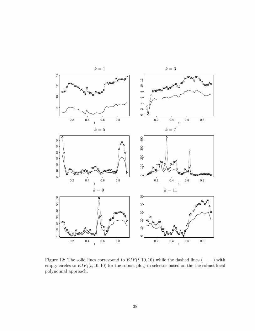
An influential study can be performed by the inclusion of several outliers in the neigh-borhood of the point t. For the robust plug–in bandwidth selectors, Figures 11 to 13 plot,as a function of t, the effect of adding k outliers, z1, . . . , zk, when k = 1, 3, 5, 7, 9 and 11.To be more precise, for a fixed point 0 < t < 1 and a fixed amount of k outliers, we haveadded to the sample the points z` = (t`, 10, 10), 1 ≤ ` ≤ k, with t` = t + (2`− 1)/(2n)if t + (2`− 1)/(2n) < 1 and t` = t − (2`− 1)/(2n), otherwise. This configuration waschoosen so that the outliers were inserted between adjacent pair of design points to increasethe impact on the estimator. The solid lines correspond to EIF(t, 10, 10) while the dashedones with empty circles to EIF1(t, 10, 10). For the cross-validation procedure the searchwas made first in the interval [0.05, 2] with a step of 0.05 and then in the same interval,around the local minimum with a step of 0.01, so that bandwidths smaller than 0.05 werenever choosen not allowing implosion of the bandwidths. However, it should be noted thatwith the inclusion of more than 7 outliers, half of the times the obtained bandwidth was0.05 showing the bad performance of the cross–validation criterion and explaining the largevalues of EIF(t, 10, 10). As we can see, the robust selectors do not explode with this outlierconfiguration, however, the bandwidth selector is sensitive to the inclusion of k = 11 outliersat the boundary. Note that this amount of outliers represents locally more than 10% of con-tamination. An exception is the robust local polynomial selector when including 7 outliersthat explodes at t = 0.255, giving a bandwidth larger than 1, due to the non–convergenceof the algorithm in 20 iterations. Note that, at the boundary, the effect of adding outliersincreases with the number of outliers. Moreover, the robust cross–validation procedure ismuch more sensitive than the robust plug–in selectors, leading as mentioned before, to smallbandwidths when anomalous observations are present. On the other hand, the differentiat-ing approach performs better than the polynomial one as the number of outliers increase.Moreover, as it can be seen from the plots, the dashed lines with empty circles are over thesolid lines, showing that the main problem when introducing several outliers is that largebandwidths can be obtained, leading to oversmoothing. The worst situation arises with therobust plug–in selector based on the polynomial approach. Effectively, as shown in Figure12, where when considering 7 outliers, the maximum of EIF1 equals 419.25 correspondingto a bandwidth hz = 0.9734.

Our influential study shows that the robust procedures seem stable with the inclusion

18

of one isolated outlier. However, even if they do not breakdown, they are quite sensitiveto the inclusion of several outliers in the neighborhood of a fixed point. Moreover, therobust cross–validation criterion seems to perform worst than the robust plug–in proceduresintroduced.

6 Concluding Remarks

Selection of the smoothing parameter is an important step in any nonparametric analysis,even when robust estimates are used. The classical procedures based on least squarescross–validation or on a plug–in rule turn out to be non–robust since they lead to over orundersmoothing as noted for nonparametric regression by Leung, Marriott and Wu (1993),Wang and Scott (1994), Boente, Fraiman and Meloche (1997), Cantoni and Ronchetti (2001)and Leung (2005). The same conclusions hold under a partly linear regression model. Ourproposals tends to overcome the sensitivity of the classical selectors by considering robustestimators of the derivatives of the regression function or a robust cross–validation criteria,under a partly linear regression model.

The problem of defining the influence function of the smoothing parameter is still anoutstanding issue. We introduced an empirical influence measure that allows to evaluateon a given data set the sensitivity of the bandwidth selector to anomalous data. It turnsout that, under a partly linear model, the classical plug–in bandwidth defined in Linton(1995) is not robust, since it leads to unbounded empirical influence functions. On theother hand, our proposals have bounded empirical influence even when introducing severaloutliers. The best performance, in all cases, for the considered model and the studiedcontaminations is attained by the plug–in rules, even they are all influenced by multipleoutliers. In particular, the differentiating approach lead to smaller influence functions thanthat based on polynomials when dealing with more than one outlier.

Acknowledgements

The authors would like to thank the Referee for its valuable comments and suggestions that leadto improve the presentation of the paper. This research was partially supported by Grants X-094from the Universidad de Buenos Aires, pid 5505 from conicet and pav 120 and pict 21407 fromanpcyt, Argentina and by a grant of the Fundacion Antorchas at Buenos Aires, Argentina.

P Appendix: Proofs.

Proof (14). In order to derive (14), we need to assume that A.1, A.5, B.1 to B.5 andthat the score function Ψ defining the local M−smoothers satifies B.5 a).

19

Note that φ0(t) is the solution of

(nh)−1n∑

i=1

K ((ti − t)/h) Ψ((yi − φ0(t))/σ0

)= 0

then, using a Taylor’s expansion, we have that

φ0(t) = (nh)−1n∑

i=1

K ((ti − t)/h) (φ0(ti) + u∗i ) +Op((nh)−1) .

Hence

φ0(t)−φ0(t) = (nh)−1n∑

i=1

K ((ti − t)/h) φ0(ti)−φ0(t)+(nh)−1n∑

i=1

K ((ti − t)/h) u∗i+Op((nh)−1) .

Denote wij = (nh)−1K ((ti − tj)/h), u∗ = (u∗1, . . . , u∗n)

t and φ0 = (φ0(t1), . . . , φ0(tn))t

then φ0 − φ0 = (W − I)φ0 + Wu∗ +Op((nh)−1). In a similar way, we get that φj − φj =(W−I)φj+Wη∗(j)

+Op((nh)−1) with η∗(j)= (η∗1j , . . . , η

∗nj)

t. Denote η∗i = (η∗i1, . . . , η

∗ip)

t,φ = (φ(t1), . . . ,φ(tn))t and φ(ti) = (φ1(ti), . . . , φp(ti))t.

Using the expansion in Bianco and Boente (2004), we get that n1/2(βr(h) − β) =σεA−1Ln(σε,β) + op(n−2µ) with µ = (4ν − 1)/(2(4ν + 1)) and Ln(σε,β) =n−1/2 ∑n

i=1 ψ1

((ri − zti β)/σε

)w2(zi)zi.

Using a Taylor expansion, we have that Ln(σ,β) = Ln(σ,β) +∑3i=1 Sin +Rn where Rn

has higher order than the other terms and

Ln(σε,β) = n−1/2n∑

i=1

ψ1

((ri − zti β)/σε

)ψ2 (ηi)

S1n = n−1/2n∑

i=1

ψ1 (εi/σε)Dψ2 (ηi) (φ(ti) − φ(ti))

S2n = (σε√n)−1

n∑

i=1

ψ′1 (εi/σε)ψ2 (ηi) (g(ti) − g∗(ti))

S3n = (σε√n)−1

n∑

i=1

ψ′1 (εi/σε)Dψ2 (ηi) (φ(ti) − φ(ti))(g(ti) − g∗(ti))

with g∗(t) = φ0(t) − βtφ(t), Dψ2 (u) stands for the matrix with (i, j) element ∂∂uj

ψ2(u)i.

Since the errors have symmetric distribution and ψ1 is odd we get that E(Ln(σε,β)) =0. On the other hand, note that S1n can be written as S1n = n−1/2ΛηΛε where Λε =(ψ1(ε1/σε), . . . , ψ1(εn/σε))t and Λη = (Dψ2 (η1)v1, . . . ,Dψ2 (ηn)vn) with vi the i−th rowof v = (I − W)φ − Wη∗ and η∗ the matrix with j−th column η∗(j)

. Thus, B.1 and B.3entail that E(S1n) = 0.

20

A similar expression is obtained for S2n where ψ2(η) = (ψ2 (η1) , . . . , ψ2 (ηn))t

σε n12S2n =

{ψ2(η)tΛ′(I−W)φ0 − ψ2(η)tΛ′Wu∗ + ψ2(η)tΛ′Wη∗tβ − ψ2(η)tΛ′(I −W)φβ

}

= A1n +A2n +A3n +A4n

with Λ′ = diag(ψ′1(ε1/σε), . . . , ψ

′1(εn/σε)). It is easy to see that E(A1n) = E(A3n) = 0 since

the errors η have symmetric distribution and ψ2 is odd. On the other hand, E(A2n) = 0since both ε and η have a symmetric distribution and ψ1 and ψ2 are odd functions. Finally,it is easy to show that E(A4n) = O((nh2)−1/2).

Analogous arguments to those used in the classical setting allow to derive that

E(S3n) = n1/2h2ν α2ν(K)σ−1

ε (ν!)−2E(ψ′1(ε/σε))E (Dψ2(η))

∫ 1

0g(ν)(t)φ(ν)(t)dt

+ O(n−µ) + o(n(1−4ν)/(2(4ν+1))

)

Then, if c 6= 0 we get that

n1/2E(ct(βr(h) − β)) = σεE(ctA−1Ln(σε,β)) + op(n2ν)

= n1/2h2νctΣ−11,ηE (Dψ2(η))α2

ν(K)(ν!)−2∫ 1

0g(ν)(t)φ(ν)(t)dt + o(n−µ)

To conclude the proof, it is enough to obtain an expression for

var(n1/2ct(βr(h) − β)/σr

)= σ2

ε /σ2rvar

(ctA−1Ln(σε,β)

)+ op(n−2µ) .

Denote W(i) the i−th row of W. Let us consider the following expansion of Ln(σε,β),Ln(σε,β) = Ln(σε,β) + bn + cn +Rn where,

bn = (σε√n)−1

n∑

i=1

ψ′1 (εi/σε)ψ2 (ηi) (g(ti) − g(ti)) + n−1/2

n∑

i=1

ψ1 (εi/σε)Dψ2 (ηi) (φ(ti) − φ(ti))

− (σε√n)−1

n∑

i=1

ψ′1 (ε1/σε) (g(ti) − g(ti))Dψ2 (ηi)W

(i)η∗

+ (σε√n)−1

n∑

i=1

ψ′1 (εi/σε)W(i)(βtη∗ − u∗)Dψ2 (ηi) (φ(ti) − φ(ti))

+ (σε√n)−1

n∑

i=1

ψ′1 (ε1/σε) (g(ti) − g(ti))Dψ2 (ηi) (φ(ti) − φ(ti))

cn = (σε√n)−1

n∑

i=1

ψ′1 (εi/σε)W(i)(βtη∗ − u∗)ψ2 (ηi) − n−1/2

n∑

i=1

ψ1 (εi/σε)Dψ2 (ηi)W(i)η∗

− (σε√n)−1

n∑

i=1

ψ′1 (εi/σε)W(i)(βtη∗ − u∗)Dψ2 (ηi)W

(i)η∗

21

φ = (I−W)φ y g = (I−W)g. With regard to var(ctA−1cn), we have that

V ar(ctA−1cn) = (h2n3)−1

κ1

∑

i

∑

j

K2 ((ti − tj)/h) + κ2

∑

i

∑

j

[(K ∗K) ((ti − tj)/h)]2

− 2κ3

∑

i

∑

j

K ((ti − tj)/h) (K ∗K) ((ti − tj)/h)

Now(n2h

)−1 ∑i

∑jK

2((ti − tj)/h) →∫K2(u)du and arguing in an analogous way, with

the other sums we get that,

V ar(ctA−1cn) = (nh)−1{κ1

∫K2(u)du+ κ2

∫(K ∗K)2(u)du − 2κ3

∫K(u)K ∗K(u)du

}

Similarly we get that E(cn) = 0, var(ctA−1bn) = O(n−µ) and cov(bn, cn) = 0 whichleads to

var(n1/2ct(βr(h) − β)/σr

)= σ2

ε /σ2rvar

(ctA−1Ln(σε,β)

)+ op(n−2µ)

= σ2ε /σ

2r(nh)−1

{κ1

∫K2(u)du+ κ2

∫(K ∗K)2(u)du

−2κ3

∫K(u)K ∗K(u)du

}+ op(n−2µ) ,

concluding the proof.

Proof of Theorem 3.1. A6 entails that supt∈[h,1−2h]

|φ(ν)j,r(t)−φ

(ν)j (t)| a.s.−→ 0, for 0 ≤ j ≤ p.

Then, using (16), A.2 and since∫ h0 g

(ν)(t)φ(ν)1 (t)dt+

∫ 1−hh g(ν)(t)φ(ν)

1 (t)dt converge to 0, weget that, for 1 ≤ j ≤ p

∫ 1−h

hg(ν)r (t, h)φ(ν)

1,r(t, h)dt−∫ 1

0g(ν)(t)φ(ν)

1 (t)dt a.s.−→ 0.

On the other hand, the strong consistency of σ2ε , V (ψ1), Σ1,η Σ2,η, D and κ` entail the

desired result.

Proof of Proposition 3.1. Using the continuity of the functional σ2(·) and since theStrong Law of Large Numbers entails that Π(Pn, P ) a.s.−→ 0, it will be enough to show that

Π(Pn, Pn)a.s.−→ 0 , (P.1)

where Π stands for the Prohorov distance.

To prove (P.1), it will be enough to show that for any bounded and continuous functionf , |E

Pn(f) − EPn(f)| a.s.−→ 0. Let C = C1 × C2 be such that P (C) > 1 − η/(4‖f‖∞) with

C1 = {‖x‖ < C1}, and C2 = {|y| < C2}, then

|EPn

(f) −EPn(f)| ≤ n−1n∑

i=1

|f(εi) − f(εi))|IC(xi, yi) + 2‖f‖∞n−1n∑

i=1

ICc(xi, yi)

≤ S1,n + S2,n .

22

The Strong Law of Large Numbers implies that there exists a set N1 such that P (N1) = 0

and for any w /∈ N1, n−1n∑

i=1

ICc(xi, yi) → P ((x, y) ∈ Cc). Hence, for w /∈ N1 and n ≥ n1,

|S2,n| < η/2.

On the other hand, let U = {u : |u| ≤ C3} where C3 = C2 +C1(‖β‖+1)+‖g‖∞ +1. Theuniformly continuity of f on U entail that there exists δ > 0 such that for any u1, u2 ∈ U ,|u1 − u2| < δ ⇒ |f(u1) − f(u2)| < η/2.

Using A.2 we get that there exists a set N2 such that P (N2) = 0 and for any w /∈ N2

and n ≥ n2 supt∈[0,1]

|g(t) − g(t)| < min(1, δ/2) and |β − β| < min (1, δ/(2C1)).

It is easy to see that yi − βtxi − g(ti) ∈ U and yi −βtxi − g(ti) ∈ U , for n ≥ n2, when

(xi, yi) ∈ C. Then, for n ≥ n2 and i ∈ J = {i : (xi, yi) ∈ C}, we have that εi, εi ∈ T and|εi − εi| < δ implying that |S1,n| < η/2. Thus, |E

Fn(f) − EFn(f)| < η if w /∈ N1 ∪ N2 and

n ≥ N = max(n1, n2), concluding the proof of (P.1).

The proof of the consistency of V (ψ1), Σ1,η, Σ2,η and D follows similar arguments asthose considered in the proof of Lemma 2 in Bianco and Boente (2004).

References

[1] Aıt Sahalia, Y. (1995). The delta method for nonlinear kernel functionals. PhD. dis-sertation, University of Chicago.

[2] Aneiros-Perez, G. and Quintela del Rıo, G. (2002). Plug-in bandwidth choice in partiallinear regression models with autoregressive errors.J. Statist. Plann. Inference, 57, 23-48.

[3] Bianco, A. and Boente, G. (2004). Robust estimators in semiparametric partly linearregression models. J. Statist. Plann. Inference, 122, 229-252.

[4] Bianco, A. and Boente, G. (2007). Robust estimators under a semiparametric partlylinear autoregression model: Asymptotic behavior and bandwidth selection. J. TimeSeries Anal., 28, 274-306.

[5] Boente, G. and Rodriguez, D. (2006). Robust estimators of high order derivatives ofregression functions. Statist. Probab. Lett., 76, 1335-1344.

[6] Boente, G., Fraiman, R. and Meloche, J. (1997). Robust plug-in bandwidth estimatorsin nonparametric regression. J. Statist. Plann. Inference, 57, 109-142.

[7] Cantoni, E. and Ronchetti, E. (2001). Resistant selection of the smoothing parameterfor smoothing splines. Statistics and Computing, 11, 141-146.

[8] Denby, L. (1986). Smooth regression functions. Statistical Research Report 26, AT&TBell Laboratories, Murray Hill.

23

[9] Gasser, Th., Kneip, A., Kohler, W. (1991). A flexible and fast method for automaticsmoothing. J. Amer. Stat. Assoc., 86, 643-652.

[10] Gasser, Th. and Muller, H. (1984). Estimating regression functions and their derivativesby the kernel method. Scand. J. Statist., 11, 171-185.

[11] Gasser, Th., Muller, H., Kohler, W., Molinari, L. and Prader, A. (1984). Nonparametricregression analysis of growth curves. Ann. Statist., 12, 210-229.

[12] Gasser, Th., Muller, H. and Mammitzsch, V. (1985). Kernel for nonparametric curveestimation. J. Royal Statist. Soc., Ser. B, 47, 238-252.

[13] Hardle, W. and Gasser, Th. (1984). Robust non–parametric function fitting. J. RoyalStatist. Soc., 46, 42-51.

[14] Hardle, W. and Gasser, T. (1985). On robust kernel estimation of derivatives of regres-sion functions. Scand. J. Statist., 12, 233-240.

[15] Hardle, W., Liang H. and Gao J. (2000). Partially Linear Models. Physica-Verlag

[16] Hardle, W. and Luckhaus, S. (1988). Uniform consistency of a class of regression func-tion estimator. Ann. Statist., 12, 612-623.

[17] Jiang, J. and Mack, Y. (2001). Robust local polynomial regression for dependent data.Statistica Sinica, 11, 705-722.

[18] Leung, D. (2005). Cross-validation in nonparametric regression with outliers. Ann.Statist., 33, 2291-2310.

[19] Leung, D., Marriott, F. and Wu, E. (1993). Bandwidth selection in robust smoothing.J. Nonparametric Statist., 4, 333–339.

[20] Linton, O. (1995). Second Order Approximation in the partially linear regression model.Econometrica, 63, 1079-112.

[21] Manchester, L. (1996). Empirical Influence for robust smoothing. Austral. J. Statist.,38, 275-296.

[22] Maronna, R., Martin, R. D. and Yohai, V. (2006). Robust Statistics: Theory andPractice. Wiley, New York.

[23] Rice, J. (1986). Convergence rates for partially splined models. Statist. Probab. Lett.,4, 203-208.

[24] Robinson, P. (1988). Root-n-consistent Semiparametric regression. Econometrica, 56,931-954.

[25] Ronchetti, E. and Staudte, R. (1994). A robust version of Mallow’s Cp. J. Amer. Statist.Assoc., 89, 550-559.

24

[26] Rousseeuw, P. J. (1984). Least median of squares regression. J. Amer. Statist. Assoc.,79, 871-881.

[27] Ruppert, D., Sheater, S. and Wand, M. (1995) An effective bandwidth selector for localleast squares regression. J. Amer. Statist. Assoc., 90, 1257-1270.

[28] Speckman, P. (1988). Kernel smoothing in partial linear models. J. Roy. Statist. Soc.,Ser. B, 50, 413-436.

[29] Tamine, J. (2002). Smoothed influence function: another view at robust nonparametricregression. Discussion paper 62, Sonderforschungsbereich 373, Humboldt-Universitatzu Berlin.

[30] Tukey, J. (1977). Exploratory Data Analysis. Reading, MA: Addison–Wesley.

[31] Wang F. and Scott D. (1994). The L1 method for robust nonparametric regression. J.Amer. Stat. Assoc., 89, 65-76.

[32] Welsh, A. (1996). Robust estimation of smooth regression and spread functions andtheir derivatives. Statistics Sinica, 6, 347-366.

25

initial bandwidth0.25 0.30 0.35 0.38 0.40 0.43 0.45

classical estimatorMean -0.2157 -0.1370 -0.1024 -0.0873 -0.0790 -0.0654 -0.0559 C0

SD 0.2578 0.2180 0.1891 0.1451 0.1306 0.1182 0.1129Mean -0.1192 -0.0169 0.0419 0.0712 0.0904 0.0969 0.1126 C1

SD 0.2871 0.2547 0.2486 0.2576 0.2507 0.2305 0.2390Mean 0.0716 0.1588 0.22501 0.2695 0.2993 0.34734 0.3799 C2

SD 0.2416 0.2619 0.2352 0.2437 0.2369 0.2466 0.2459robust estimator

Mean -0.0957 -0.0024 0.0429 0.0719 0.0724 0.0802 0.0831 C0

SD 0.2716 0.2535 0.2394 0.2499 0.2245 0.2271 0.2198Mean -0.0910 -0.0033 0.0435 0.0749 0.0901 0.0855 0.0921 C1

SD 0.2797 0.2561 0.2214 0.2419 0.2332 0.2077 0.2130Mean -0.0269 0.0757 0.1252 0.1446 0.1515 0.1534 0.1509 C2

SD 0.2489 0.2686 0.2389 0.2324 0.2342 0.2200 0.2029

Table 1: Estimation of the optimal bandwidth. Summary measures of log(h/hopt

)using

the differentiation approach.

initial bandwidth0.25 0.30 0.35 0.38 0.40 0.43 0.45

classical estimatorMean -0.0303 0.0274 0.0156 0.0052 0.0007 -0.0030 -0.0049 C0

SD 0.2453 0.2003 0.1316 0.1000 0.0844 0.0731 0.0647Mean 0.0015 0.1529 0.1564 0.1681 0.1602 0.1556 0.1534 C1

SD 0.2479 0.2728 0.2479 0.2639 0.2236 0.2072 0.1983Mean 0.1183 0.2087 0.2898 0.3457 0.3787 0.4385 0.4489 C2

SD 0.2781 0.25501 0.2415 0.2568 0.2493 0.2949 0.2354robust estimator

Mean 0.1169 0.1776 0.1658 0.1553 0.1499 0.1465 0.1441 C0

SD 0.2467 0.2182 0.1414 0.1094 0.0899 0.0815 0.0716Mean 0.0615 0.1792 0.1813 0.1741 0.1605 0.1567 0.1522 C1

SD 0.2793 0.2194 0.1661 0.1226 0.1051 0.1050 0.0756Mean -0.6489 -0.5021 -0.3376 -0.2235 -0.14284 -0.0222 0.0499 C2

SD 0.1517 0.16064 0.2115 0.2323 0.2372 0.2182 0.1946

Table 2: Estimation of the optimal bandwidth. Summary measures of log(h/hopt

)using

local polynomials.

26

log

(h

hopt

)β

LS GM LTS LS GM LTSMean -0.0964 -0.0967 -0.0876 0.9929 0.9973 0.9888 C0

SD 0.4587 0.5297 0.5639 0.1063 0.1927 0.1042Mean 0.2484 0.0044 0.0440 0.932 0.9839 0.9826 C1

SD 0.5381 0.5236 0.5454 1.1457 0.1903 0.1134Mean 0.3881 0.2592 0.3387 0.0565 0.9341 0.8912 C2

SD 0.5615 0.5906 0.5711 0.5007 0.2883 0.1216

Table 3: Estimation of the optimal bandwidth and of the regression parameter β under C0,C1 and C2, using cross–validation.

initial bandwidth0.25 0.30 0.35 0.38 0.40 0.43 0.45

mean 0.9827 0.9823 0.9868 0.9819 0.9816 0.9811 0.9807 LSsd 0.1109 0.1032 0.1005 0.1017 0.1016 0.1015 0.1014

mean 0.9905 0.9922 0.9957 0.9891 0.9901 0.9856 0.9842 LTS C0

sd 0.2171 0.2193 0.2212 0.2241 0.2121 0.2184 0.2138mean 0.9841 0.9825 0.9869 0.9787 0.9804 0.9792 0.9796 GM

sd 0.1059 0.1043 0.1035 0.1053 0.1037 0.1054 0.1044mean 0.8492 0.8507 0.8215 0.8443 0.8617 0.8512 0.8499 LS

sd 1.5911 1.5819 1.9095 1.9312 1.7182 1.7076 1.5221mean 0.9939 0.991 1.0125 1.003 0.9935 0.9877 0.9818 LTS C1

sd 0.2149 0.2176 0.2027 0.2054 0.2063 0.2107 0.2135mean 0.9792 0.9781 0.9921 0.9866 0.9842 0.9809 0.9756 GM

sd 0.1156 0.1134 0.1069 0.1071 0.1108 0.1132 0.1124mean 0.0555 0.0561 0.0562 0.0562 0.0562 0.0562 0.056 LS

sd 0.4103 0.4155 0.4211 0.4243 0.4264 0.4293 0.4311mean 0.9525 0.9395 0.9492 0.9537 0.9472 0.9553 0.9527 LTS C2

sd 0.2726 0.2874 0.2682 0.2618 0.2699 0.2677 0.2693mean 0.8957 0.8894 0.8901 0.8892 0.8883 0.8885 0.8891 GM

sd 0.1181 0.122 0.1183 0.119 0.1194 0.1179 0.1178

Table 4: Estimation of the regression parameter β under C0, C1 and C2 when using thedifferentiating approach.

initial bandwidth0.25 0.30 0.35 0.38 0.40 0.43 0.45

LS 0.0985 0.0979 0.1045 0.0954 0.0951 0.0955 0.0961 C0

LTS 0.206 0.2168 0.2279 0.2389 0.2138 0.217 0.2112GM 0.0963 0.099 0.1044 0.1068 0.1022 0.1055 0.102LS 23.6493 18.6363 22.3226 21.3261 17.7332 18.1118 15.3747 C1

LTS 0.222 0.2257 0.2262 0.2291 0.2332 0.2185 0.2203GM 0.1186 0.1175 0.1209 0.1291 0.129 0.1193 0.1176LS 28.5969 24.3241 21.7866 20.6437 19.9367 18.9953 18.3776 C2

LTS 0.2926 0.3098 0.2841 0.2841 0.2915 0.2955 0.2938GM 0.1163 0.1212 0.1138 0.1128 0.1157 0.1151 0.1124

Table 5: Estimation of the regression function g. Mean of MSE(g) when using the differ-entiating approach

27

initial bandwidth0.25 0.30 0.35 0.38 0.40 0.43 0.45

LS 0.0385 0.0368 0.0371 0.0344 0.0359 0.037 0.0373 C0

LTS 0.0591 0.0598 0.0714 0.0623 0.058 0.062 0.0623GM 0.036 0.0364 0.0413 0.0372 0.0372 0.038 0.0379LS 0.0875 0.0891 0.1271 0.1225 0.1054 0.0973 0.0941 C1

LTS 0.0718 0.0699 0.0881 0.0735 0.073 0.0734 0.0672GM 0.0449 0.0439 0.0471 0.0483 0.0491 0.045 0.0415LS 1.2196 1.164 1.1079 1.0822 1.0454 1.0293 0.9688 C2

LTS 0.0699 0.0697 0.0659 0.0701 0.0691 0.0677 0.0714GM 0.0466 0.044 0.0452 0.0463 0.0455 0.0458 0.0463

Table 6: Estimation of the regression regression function g. Median of MedSE(g) whenusing the differentiating approach.

MSE(g) MedSE(g)LS GM LTS LS GM LTS

C0 0.099 0.1848 0.1005 0.0392 0.0599 0.0405C1 9.698 0.1963 0.1209 0.0863 0.0692 0.0468C2 18.5513 0.3477 0.1203 1.3116 0.0857 0.0493

Table 7: Estimation of the regression regression function g. Mean of MSE(g) and medianof MedSE(g) when using the cross-validation.

Classical selector Robust selector

-0.5

0.5

1.5

0.25 0.30 0.35 0.38 0.40 0.43 0.45

-0.5

0.5

1.5

0.25 0.30 0.35 0.38 0.40 0.43 0.45

-0.5

0.5

1.0

1.5

0.25 0.30 0.35 0.38 0.40 0.43 0.45

-0.5

0.5

1.0

1.5

0.25 0.30 0.35 0.38 0.40 0.43 0.45

-0.5

0.5

1.5

0.25 0.30 0.35 0.38 0.40 0.43 0.45

-0.5

0.5

1.5

0.25 0.30 0.35 0.38 0.40 0.43 0.45

C2

C1

C0

Figure 1: Boxplots of log(h/hopt

)using the differentiating approach.

28

Classical selector Robust selector-0

.50.

51.

01.

5

0.25 0.30 0.35 0.38 0.40 0.43 0.45 -0.5

0.5

1.0

1.5

0.25 0.30 0.35 0.38 0.40 0.43 0.45

-1.0

0.0

1.0

0.25 0.30 0.35 0.38 0.40 0.43 0.45

-1.0

0.0

1.0

0.25 0.30 0.35 0.38 0.40 0.43 0.45

-10

12

0.25 0.30 0.35 0.38 0.40 0.43 0.45

-10

12

0.25 0.30 0.35 0.38 0.40 0.43 0.45

C0

C1

C2

Figure 2: Boxplots of log(h/hopt

)using the robust local polynomials.

(a) (b) (c)

-0.5

0.0

0.5

1.0

C0 C1 C2

-0.5

0.0

0.5

1.0

C0 C1 C2

-1.5

-1.0

-0.5

0.0

0.5

1.0

C0 C1 C2

Figure 3: Boxplots of log(h/hopt

)for the robust data–driven bandwidths (a) and (b) plug–

in bandwidths with initial bandwidth 0.4 (a) using the differentiating approach (b) usingthe local polynomial method and (c) robust cross–validation bandwidths.

29

(a) (b)

t0.0 0.2 0.4 0.6 0.8 1.0

-8-6

-4-2

02

46

g(t)+β φ(t)

g(t)

t0.0 0.2 0.4 0.6 0.8 1.0

02

4

φ(t)

Figure 4: Generated Data Set. The dashed line corresponds to the nonparametric compo-nent g while the solid one to the regression function γ(t) = g(t) + βφ(t) in (a). In (b), thesolid line corresponds to φ(t).

30

(a1) (a2)

-40

-20

0

20

40

x

-40

-20

0

20

40

y

050

100

150

200

250

t=0.10

Classical Plug-in Bandwidth

-40

-20

0

20

40

x

-40

-20

0

20

40

y

010

020

030

040

050

060

0

t=0.10

Classical Plug-in Bandwidth

(b1) (b2)

-40

-20

0

20

40

x

-40

-20

0

20

40

y

050

100

150

200

250 t=0.10

Classical Plug-in Bandwidth: Local Polinomial

-40

-20

0

20

40

x

-40

-20

0

20

40

y

010

020

030

040

050

060

070

0

t=0.10

Classical Plug-in Bandwidth

Figure 5: EIF (0.10, x, y) and EIF1(0.10, x, y) for the classical bandwidth selector, using the differentiating approach, ((a1)and (a2), respectively) and using the local polynomial approach, ((b1) and (b2), respectively).

31

(a1) (a2)

-40

-20

0

20

40

x

-40

-20

0

20

40

y

67

89

1011

t=0.10

Robust Plug-in Bandwidth

t=0.10

Robust Plug-in Bandwidth

-40

-20

0

20

40

x

-40

-20

0

20

40

y

1011

1213

1415

1617

t=0.10

Robust Plug-in Bandwidth

(b1) (b2)

-40

-20

0

20

40

x

-40

-20

0

20

40

y

56

78

910

1112

t=0.10

Robust Plug-in Bandwidth: Local Polinomial

-40

-20

0

20

40

x

-40

-20

0

20

40

y

68

1012

1416

18

t=0.10

Robust Plug-in Bandwidth

Figure 6: EIF (0.10, x, y) and EIF1(0.10, x, y) for the robust bandwidth selector, using the differentiating approach, ((a1) and(a2), respectively) and using the local polynomial approach, ((b1) and (b2), respectively).

32

(a1) (a2)

-40

-20

0

20

40

x

-40

-20

0

20

40

y

1020

3040

5060

70

t=0.50

Classical Plug-in Bandwidth

-40

-20

0

20

40

x

-40

-20

0

20

40

y

020

4060

8010

012

014

0

t=0.50

Classical Plug-in Bandwidth

(b1) (b2)

-40

-20

0

20

40

x

-40

-20

0

20

40

y

010

2030

4050

60

t=0.50

Classical Plug-in Bandwidth: Local Polinomial

-40

-20

0

20

40

x

-40

-20

0

20

40

y

020

4060

8010

012

0

t=0.50

Classical Plug-in Bandwidth: Local Polinomial

Figure 7: EIF (0.50, x, y) and EIF1(0.50, x, y) for the classical bandwidth selector, using the differentiating approach, ((a1)and (a2), respectively) and using the local polynomial approach, ((b1) and (b2), respectively).

33

(a1) (a2)

-40

-20

0

20

40

x

-40

-20

0

20

40

y

56

78

910

1112

t=0.50

Robust Plug-in Bandwidth

-40

-20

0

20

40

x

-40

-20

0

20

40

y

810

1214

1618

t=0.50

Robust Plug-in Bandwidth

(b1) (b2)

-40

-20

0

20

40

x

-40

-20

0

20

40

y

67

89

1011

t=0.50

Robust Plug-in Bandwidth: Local Polinomial

-40

-20

0

20

40

x

-40

-20

0

20

40

y

910

1112

1314

1516

t=0.50

Robust Plug-in Bandwidth: Local Polinomial

Figure 8: EIF (0.50, x, y) and EIF1(0.50, x, y) for the robust bandwidth selector, using the differentiating approach, ((a1) and(a2), respectively) and using the local polynomial approach, ((b1) and (b2), respectively).

34

(a1) (a2)

-40

-20

0

20

40

x

-40

-20

0

20

40

y

1020

3040

5060

7080

t=0.90

Classical Plug-in Bandwidth

-40

-20

0

20

40

x

-40

-20

0

20

40

y

020

4060

8010

012

014

0

t=0.90

Classical Plug-in Bandwidth

(b1) (b2)

-40

-20

0

20

40

x

-40

-20

0

20

40

y

010

2030

4050

6070

t=0.90

Classical Plug-in Bandwidth: Local Polinomial

-40

-20

0

20

40

x

-40

-20

0

20

40

y

020

4060

8010

012

014

0

t=0.90

Classical Plug-in Bandwidth: Local Polinomial

Figure 9: EIF (0.90, x, y) and EIF1(0.90, x, y) for the classical bandwidth selector, using the differentiating approach, ((a1)and (a2), respectively) and using the local polynomial approach, ((b1) and (b2), respectively).

35

(a1) (a2)

-40

-20

0

20

40

x

-40

-20

0

20

40

y

510

15 t=0.90

Robust Plug-in Bandwidth

-40

-20

0

20

40

x

-40

-20

0

20

40

y

05

1015

2025

30

t=0.90

Robust Plug-in Bandwidth

(b1) (b2)

-40

-20

0

20

40

x

-40

-20

0

20

40

y

56

78

910

11

t=0.90

Robust Plug-in Bandwidth: Local Polinomial

-40

-20

0

20

40

x

-40

-20

0

20

40

y

810

1214

16

t=0.90

Robust Plug-in Bandwidth: Local Polinomial

Figure 10: EIF (0.90, x, y) and EIF1(0.90, x, y) for the robust bandwidth selector, using the differentiating approach, ((a1)and (a2), respectively) and using the local polynomial approach, ((b1) and (b2), respectively).

36

k = 1 k = 3

t0.2 0.4 0.6 0.8

1012

1416

1820

t0.2 0.4 0.6 0.8

68

1014

18

k = 5 k = 7

t0.2 0.4 0.6 0.8

510

1520

25

t0.2 0.4 0.6 0.8

510

1520

25

k = 9 k = 11

t0.2 0.4 0.6 0.8

010

2030

40

t0.2 0.4 0.6 0.8

010

2030

4050

Figure 11: The solid lines correspond to EIF (t, 10, 10) while the dashed lines (− · −) withempty circles to EIF1(t, 10, 10) for the robust plug–in selector based on the differentiatingapproach.

37

k = 1 k = 3

t0.2 0.4 0.6 0.8

810

1214

t0.2 0.4 0.6 0.8

02

46

810

12

k = 5 k = 7

t0.2 0.4 0.6 0.8

010

2030

4050

60

t0.2 0.4 0.6 0.8

010

020

030

040

0

k = 9 k = 11

t0.2 0.4 0.6 0.8

010

2030

4050

60

t0.2 0.4 0.6 0.8

010

2030

4050

Figure 12: The solid lines correspond to EIF (t, 10, 10) while the dashed lines (− · −) withempty circles to EIF1(t, 10, 10) for the robust plug–in selector based on the the robust localpolynomial approach.

38

k = 1 k = 3

t0.2 0.4 0.6 0.8

6080

100

140

t0.2 0.4 0.6 0.8

050

100

150

200

k = 5 k = 7

t0.2 0.4 0.6 0.8

5010

015

020

025

0

t0.2 0.4 0.6 0.8

4060

8010

012

014

0

k = 9 k = 11

t0.2 0.4 0.6 0.8

4060

8010

012

014

0

t0.2 0.4 0.6 0.8

020

6010

014

0

Figure 13: The solid lines correspond to EIF (t, 10, 10) while the dashed lines (− · −) withempty circles to EIF1(t, 10, 10) for the robust cross–validation selector.

39