Penalized Quantile Regression with Semiparametric ...harding1/resources/Harding_PQR.pdf · Penalized Quantile Regression with Semiparametric Correlated Effects: ... Erich Battistin,

Penalized Quantile Regression with Semiparametric

Correlated Effects: An Application with

Heterogeneous Preferences∗

Matthew Harding† and Carlos Lamarche‡

January 24, 2015

Abstract

This paper proposes new `1-penalized quantile regression estimators for panel data, which explicitlyallows for individual heterogeneity associated with covariates. Existing fixed effects estimatorscan potentially suffer from three limitations which are overcome by the proposed approach: (i)incidental parameters bias in non-linear models with large N and small T , (ii) lack of efficiency,and (iii) inability to estimate time-invariant effects. We conduct Monte Carlo simulations to assessthe small sample performance of the new estimators and provide comparisons of new and existingpenalized estimators in terms of quadratic loss. We apply the technique to an empirical example ofthe estimation of consumer preferences for nutrients from a demand model using a large transactionlevel dataset of household food purchases. We show that preferences for nutrients vary across theconditional distribution of expenditure and across genders, and emphasize the importance of fullycapturing consumer heterogeneity in demand modeling.

JEL: C21, C23, J22Keywords: Shrinkage, Panel Data, Quantile Regression, Big Data

∗The authors would like to thank Badi Baltagi, Erich Battistin, Zongwu Cai, Cheng Hsiao, Ted Juhl,

Chihwa Kao, Roger Koenker, Roger Moon, Hashem Pesaran, Steve Portnoy, and Jim Ziliak for comments

on a previous draft as well as seminar participants at the University of Southern California, University of

Illinois at Urbana-Champaign, University of Kansas, University of Oklahoma, University of Padova, Syracuse

University, the 17th Midwest Econometric Group conference, and the 25th meeting of the Latin American

Econometric Society. We are also grateful to a Co-Editor and two anonymous referees for their comments

which have improved the paper considerably.†Corresponding author: Sanford School of Public Policy and Duke-UNC USDA Center for Behavioral

Economics and Healthy Food Choice Research, Duke University, 140 Science Drive, Durham, NC 27708;

Phone: (919) 613-1306; Fax: (919) 613-0539; Email: [email protected]‡Department of Economics, University of Kentucky, 335A Gatton College of Business and Economics,

Lexington, KY 40506-0034. Tel.: +1 859-257-3371. Email: [email protected]

2

1. Introduction

The recent availability of Big Data opens up the possibility of devising targeted economic

policies that increase welfare by accounting for the broad individual heterogeneity in both

characteristics and outcomes. At the same time, the large datasets make it possible to

provide increased flexibility in the specification of econometric models. This paper provides

a simple new approach to the estimation of models with heterogeneous marginal effects in

panel data with time-invariant variables by allowing for a flexible specification of correlated

individual effects in a quantile regression setting.

There is a growing theoretical and empirical interest on the estimation of a quantile panel

data model, specially after Koenker (2004). For more recent developments, see Abrevaya

and Dahl (2008), Graham, Hahn, and Powell (2009), Harding and Lamarche (2009, 2014a),

Lamarche (2010), Galvao (2011), Canay (2011), Rosen (2012), Galvao, Lamarche and Lima

(2013), and Chernozhukov, Fernandez-Val, Hahn and Newey (2013). Koenker (2004) pro-

poses to jointly estimate a vector of covariate effects and a vector of individual effects con-

sidering a class of penalized quantile regression estimators. The method uses an `1 penalty

term to control the bias and variance of the estimates of the covariate effects. Lamarche

(2010) obtains the minimum variance estimator in the class of `1-penalized estimators un-

der stochastic independence between individual effects and covariates. While existing fixed

effects approaches might suffer from the incidental parameters problem, recent important de-

velopments in non-separable models estimate the effect of independent variables on quantiles

of the response variable, conditional on time-varying variables. Chernozhukov, Fernandez-

Val, Hahn and Newey (2013) offer identification and estimation results of quantile effects in

nonseparable models.

Flexibility in specification and unobserved heterogeneity has a long history of playing a fun-

damental role in the estimation of economic models (Burtless and Hausman (1978), Haus-

man (1985), Blundell and Meghir (1986), Ziliak and Kniesner (1999), Blundell and MaCurdy

(1999), van Soest, Das, and Gong (2002), Kumar (2012), Dubois, Griffith and Nevo (2014),

among others). Quantile regression for panel data offers a flexible alternative approach to

conditional mean analysis that is efficient under non-Gaussian conditions. However, neither

the estimator of Koenker (2004) nor the penalized quantile regression estimator of Lamarche

(2010) is well suited for estimation of non-linear models with endogenous regressors. For in-

stance, in empirical specifications for food expenditures, the quantity of nutrients purchased

is suspected to be endogenous because unobserved time-invariant preferences for food may be

3

correlated with latent factors associated with product attributes (see, e.g., Dubois, Griffith

and Nevo (2014)).

The penalized quantile regression estimator can be extended to models with endogenous co-

variates. In addition to investigating this extension, this paper proposes a series of Hausman-

type tests to evaluate exogeneity assumptions. We propose penalized estimators that can

be easily applied to a class of semiparametric models (Cai and Xiao (2012)) and paramet-

ric models (Abrevaya and Dahl (2008)). Cai and Xiao (2012) study the estimation of a

partially varying coefficient model in quantile regression which is estimated using semipara-

metric methods. Abrevaya and Dahl (2008) propose a quantile regression approach for a

model that includes correlated random effects. As in Koenker (2004), the individual effects

represent location shift effects on the conditional quantiles of the response, and therefore, we

avoid issues associated with estimating a quantile regression model with additive error terms

(Koenker and Hallock (2000), Rosen (2012)).1 The estimation of these additional parameters

increases the variability of the estimates of the covariate effects, but shrinkage can be used

to control the additional variability. We use an `1 penalty term (Tibshirani (1996), Donoho

et al. (1998)) to shrink a vector of individual effects and a tuning parameter λ to control the

degree of this shrinkage. We present necessary conditions for our method to reduce the vari-

ability of the estimate of the slope parameter without sacrificing bias. The approach allows

estimation of time-invariant effects, while simultaneously addressing issues associated with

incidental parameters and correlation between independent variables and individual effects.

Furthermore, it is not more difficult to implement than other quantile regression panel data

methods.

One of the most significant contributions of this paper is the following aspect. The pe-

nalized estimator proposed in this paper can be seen as a balanced compromise between

misspecification issues arising from the omission of individual heterogeneity and the inci-

dental parameters problem arising from leaving individual heterogeneity unrestricted in a

nonlinear panel model. As first pointed out by Neyman and Scott (1948) and recently elab-

orated by Kato, Galvao and Montes-Rojas (2012), the estimation of individual effects in a

nonlinear panel data model leads to inconsistent estimates of the slope parameters. Kato,

Galvao and Montes-Rojas (2012) employs large T and N asymptotics offering restrictions

on the growth of T which are unusual in micro-econometric panels but serve as important

warning devices to practitioners. Under less general conditions, Graham, Hahn, and Powell

1Koenker and Hallock (2000) recognize the difficulties arising in panel quantile models due to the lack of

a suitable transformation to remove unobserved heterogeneity potentially associated with covariates. Rosen

(2012) points out to the possible lack of identification in models with additive error terms.

4

(2009) show that there is no incidental parameter problem in a non-differentiable panel data

model and Koenker (2004) and Galvao, Lamarche, and Lima (2013) show empirical evidence

that the bias of the fixed effects estimator is small for moderate T . On the other hand, as

in the classical linear panel models described in detail in Hsiao (2014) and Baltagi (2008),

ignoring unobserved heterogeneity generally leads to inconsistent estimates of the slope pa-

rameters. We show that the penalized estimator reduces the noise in the estimation of the

individual effects while controlling for individual heterogeneity, and thus, it reduces the bias

of the fixed effects panel data estimator which might arise from incidental parameters in

small T panels.

This paper seeks to contribute the literature by comparing the new and existing `1-penalized

quantile regression estimators in terms of quadratic loss. We first show that Koenker’s (2004)

estimator is the efficient estimator in the class of panel data quantile regression estimators.

However, the proposed approach has smaller asymptotic mean squared error than the penal-

ized estimator if the correlation between independent variables and latent individual factors

is not negligible. We also show that by choosing λ carefully, we can make the asymptotic

mean squared error of the estimator smaller than the asymptotic mean squared error of a

quantile regression estimator for the correlated effects model. This indicates that shrink-

ing individual effects potentially uncorrelated with independent variables is worthwhile. We

provide conditions under which the strictness of the penalization can be determined by min-

imizing mean squared error.

The next section presents the models and estimators. Section 3 derives the asymptotic

mean squared error of a proposed estimator and Section 4 offers Monte-Carlo evidence.

In Section 5, we provide an empirical example which addresses the problem of estimating

preference heterogeneity in consumer demand models using large transaction level datasets,

where differences between the preference distributions over product attributes vary by socio-

demographics. Section 6 provides conclusions.

2. Models and Estimators

Let the data be observations {(yit, x′it) : i = 1, ...N, t = 1, ...T} from a random coefficient

version of a quantile regression panel data model:

yit = x′itβ(uit) + αi(uit)(2.1)

τ 7→ x′itβ(τ) + αi(τ),(2.2)

5

where yit is the dependent variable, xit = (1, xit,2, ..., xit,p)′ is the vector of independent

variables, the αi’s are unobservable time-invariant effects, uit|xit, αi ∼ U(0, 1) denotes a uni-

form distribution, and τ is the τ -th quantile of the conditional distribution of the response

variable. The right hand side of (2.2) is the conditional quantile function, QYit(τ |xit, αi) =

inf{y : Pr(yit < y|xit, αi) ≥ τ} for all τ in (0, 1). The parameter β(τ) models the covari-

ate effect providing an opportunity for investigating how observable factors influence the

location, scale and shape of the conditional distribution of the response. For simplicity, the

model does not include time-invariant explanatory variables, which can be easily incorpo-

rated as shown in Section 2.2 and Section 5. It is also assumed that the panel is balanced,

with observations (yit, x′it)

′ ∈ R× Rp for each of the N subjects over t = 1, . . . , T .

The model takes a semiparametric form because no parametric assumption is made on the

relationship between the vector of covariates xit and αi and the functional form of the

conditional distribution of the response variable is left unspecified. The unobserved variable

αi could be arbitrarily related to observable variables and unobservable variables:

(2.3) αi(xi, ui1, ai) = αi(xi1, xi2, ..., xiT , ui1, ai) = g(xi1, xi2, ..., xiT , ui1) + ai,

where g(∙) is an unknown function with a certain degree of smoothness, the independent

variable xi = (x′i1, x

′i2, ..., x

′iT )′ and the individual effect ai is, by definition, uncorrelated

with the independent variables. We allow the variables αi and xit to be stochastically

dependent by considering the individual effect to be drawn from a conditional distribution

function with location g(τ, xi1, . . . , xiT ).

It is important to note that (2.3) imposes a time-homogeneity condition similar to Assump-

tion 2 in Chernozhukov, Fernandez-Val, Hahn and Newey (2013). The implication of this is

that the regressors are “strictly exogenous” with respect to ai. At the same time, it requires

that the conditional distribution of uit|xi, ai does not depend on t (e.g., the distribution of

ai, uit|xi is identical to the distribution of ai, ui1|xi).

Under a monotonicity condition assumed in equation (2.2), the model (2.1)-(2.3) represents

a more general version of several specifications recently proposed in the growing literature

on quantile panel data models. Consider for instance the following variations of interest in

the theoretical and empirical literature.

Example 1. If αi(xi, ui1, ai) = g(ui1) for all i and T = 1, then model (2.1) and (2.3)

becomes a semiparametric quantile regression model, yi1 = x′i1β(ui1) + g(ui1), similar to the

cross-sectional models investigated by He and Shi (1996) and Cai and Xiao (2012).

6

Example 2. Semiparametric models for longitudinal data are investigated in Wei and He

(2006) and Wei, Pere, Koenker and He (2006). Under the assumption that repeated mea-

surements are regularly observed over time, a static version of their model arises by replacing

xi by ti in equation (2.3). The conditional quantile function is equal to QYit(τ |ti, xit, ai) =

g(τ, ti) + x′itβ(τ) + ai.

Example 3. If αi(xi, ui1, ai) is a known parametric function, the model can be seen within

the classical framework proposed by Chamberlain (1982) leading to a representation of en-

dogenous individual effects αi(τ, xi, ai) = x′iγ(τ) + ai. Abrevaya and Dahl (2008) study

estimation of a quantile regression model under the assumption that equation (2.3) is equal

to x′iγ(τ), and Koenker (2004), Lamarche (2010) and Canay (2011) study estimation of the

model under the assumption αi(τ) = αi for all i.

2.1. Estimation procedures

Our estimation approaches for model (2.1) and (2.3) serve as an intermediate class of pro-

cedures with good robustness of possible deviations from the classical correlated random

effects model and relatively more precise estimation of the parametric part of the quantile

regression model.

The estimation procedure for the model with flexible correlated effects proceeds in two steps;

see Cai and Xiao (2012), He and Shi (1996) and Tang, Wang, He and Zhu (2012) for a related

discussion. First, we express g(τ, xi) as a linear expansion of B-splines. Although other non-

parametric regression techniques can be used in a first stage, the linear formulation of the

B-splines yields a family of quantile functions that can be easily accommodated to a quantile

regression for panel data problem. We express,

(2.4) g(xi)′γ(τ) ≈ b(xi1)

′γ1(τ) + b(xi2)′γ2(τ) + ... + b(xiT )′γT (τ),

where b(xij) = (b1(xij), . . . , bkn+h+1(xij))′ is a B-spline basis function, kn is the number

of knots, h is the degree of the B-spline basis, and γ is the spline coefficient vector. We

employ cubic B-spline basis functions with k ∝ (NT )1/5 with knots selected as the empirical

quartiles of xij . The model becomes a linear quantile regression model in all coefficients and

can be estimated using the following estimator,

(2.5) minβ,γ,a∈B×G×A

J∑

j=1

T∑

t=1

N∑

i=1

ωjρτj(yit − x′

itβ(τj) − g(xi)′γ(τj) − ai) + λPen(a),

7

where ρτj(u) = u(τj − I(u ≤ 0)) is the quantile loss function, ωj is a relative weight given to

the j-th quantile, J is the number of quantiles {τ1, τ2, ..., τJ} to be estimated, and λ is the

Tikhonov regularization parameter or tuning parameter. The function Pen(a) is a penalty

term that could be defined as ‖a− a∗‖1, where a∗ may be close to the unknown location of

the distribution. In equation (2.3), ai has zero mean by definition, so we made use of this

information defining the penalty term as,

Pen(a) = ‖a‖1,

where ‖a‖1 is the standard `1-norm defined as ‖a‖1 :=∑

i |ai|.

The estimation of the individual effects increases the variability of the estimator of the slope

parameter, but this penalty term that shrinks the fixed effects estimator of the ai’s toward

zero helps to reduce the inflation effect without sacrificing bias. When the a’s are exchange-

able and drawn from a conditional distribution function with location zero, shrinkage that

forces some individual specific effect estimates a’s to be zero does not impose bias and affects

the performance of the estimator of the parameter of interest β(τ ). There is an enormous

amount of work in statistics and lately in econometrics dealing with shrinkage in a wide

spectrum of problems (see, e.g., Horowitz and Lee (2007), Carrasco, Florens and Renault

(2007), Chen (2007), Belloni and Chernozhukov (2011), Belloni, Chen, Chernozhukov and

Hansen (2012); see also Bickel and Li (2006) for a survey in statistics).

Although flexibility in specification is naturally important, the estimation of econometric

models is typically associated with practical choices. We now present a convenient strategy

to estimate a quantile model with endogenous individual effects. A practical formulation for

g(∙) is to use a known parametric function of time-series averages or, alternatively, a vector

of covariates for each of the N subjects. A one-step estimator is obtained by solving the

following problem:

(2.6) minβ,γ,a∈B×G×A

J∑

j=1

T∑

t=1

N∑

i=1

ωjρτj

(

yit − x′itβ(τj) −

T∑

k=1

x′ikγk(τj) − ai

)

+ λ‖a‖1,

where as before ωj is a relative weight given to the j-th quantile. It has been argued that

the choice of the weights, ωj , and the associated quantiles τj , is somewhat analogous to the

choice of discretely weighted L-statistics (Koenker 2004). An alternative less efficient, yet

practical choice, is to ignore the potential gains and estimate models with equal weights

defined as ωj = J−1 for all j.

8

In the case of the one-step estimator, the method considers the following design matrix,[

diag(ω) ⊗ X diag(ω) ⊗ ZD ω ⊗ Z

0 0 λI

]

,

where X is a NT × p matrix, D is a NT × pT matrix, Z is a NT × N matrix and

X =

1 x′11

1 x′12

...

1 x′NT

; D =

x′11 x′

12 ... x′1T

x′21 x′

22 ... x′2T

......

. . ....

x′N1 x′

N2 ... x′NT

; Z =

1 0 ... 0

1 0 ... 0...

.... . .

...

0 0 ... 1

.

In the application considered in Section 5, we show that it is also possible to estimate time-

invariant effects by introducing additional explanatory variables in X. In this case, for

identification when λ is exactly zero, we will need the standard conditions on restricting the

estimation to N − 1 individual specific effects. Note that in a model with time-invariant

variables perfect collinearity arises in the limiting case where λ is equal to zero, which is not

considered in this paper. Our estimator is defined for λ > 0, although λ can be very small.

When λ > 0, there are ai’s that are exactly zero, which is equivalent to a model with m < N

individual effects. This allows identification of time-invariant effects and does not impose

biases under the assumption that ai is independent of the covariates.

2.2. A simple extension

A natural implicit restriction of the framework is that time-invariant variables are assumed

to be exogenous. This section proposes a way out of this problem motivated by several

approaches for correlated random effects models (e.g., Arellano and Bover (1995) and Ziliak

(2003) for an implementation of the estimator). Consider for example a model with time-

varying and time-invariant independent variables:

(2.7) yit = x′itβ + w′

iδ + αi + uit,

where yit is the response variable for subject i at time t, xit = (x1,it, x2,it)′, wi = (w′

1,i, w′2,i)

′,

and uit is the error term. The variable x1,it is a p1-dimensional vector of endogenous variables,

x2,it is a p2-dimensional vector of exogenous independent variables that includes an intercept.

Similarly, the variable w1,i is a k1-dimensional vector of endogenous variables, and w2,i

is a k2-dimensional vector of exogenous independent variables. Following (2.7) and the

representation for αi in equation (2.3), we have that, in the case of a linear model αi =

9

x′iγ + ai, where as before x′

iγ =∑T

t=1 x′itγt. The difference is now that we allow ai to be

correlated with w1i.

This model can be estimated using an extension of the penalized estimator which employs

instrumental variables (see, e.g., Harding and Lamarche (2014b)). For instance, in the case

of the one-step estimator, we consider the following objective function:

(2.8)J∑

j=1

T∑

t=1

N∑

i=1

ωjρτj

(

yit − x′itβ(τj) − w′

iδ(τj) −T∑

k=1

x′ikγk(τj) − ai − φ′

iπ(τj)

)

+ λ‖a‖1,

where τj the quantile of interest and φi is a vector of instruments. Note that we ad-

dress the endogeneity of the time-variant variables by augmenting the design matrix as

before. However, the individual effects ai’s can be correlated with the endogenous time-

invariant variables. Provided that k1 ≤ p2, we can follow Hausman and Taylor (1981) and

construct instruments using transformations of the exogenous variables. For instance, the

time-invariant endogenous variable can be instrumented using a vector of individual specific

variables x2,i = T−1∑T

t=1 x2,it.2

The proposed approach follows two steps. For a given λ, we minimize (2.8) over β, γ, δ2,

a, and π as functions of τ and δ1. Then we estimate the coefficient on the endogenous

time-invariant variable by finding the value of δ1(τ ), which minimizes a weighted distance

function defined on π:

(2.9) δ1(τ ) = argminπ1∈Π1

π(τ , δ1)′Aπ(τ , δ1),

for a given positive definite matrix A. Then, we obtain a two-step instrumental variable

estimator defined as (β(τ , δ1(τ ))′, γ(τ , δ1(τ ))′, δ1(τ )′, δ2(τ , δ1(τ ))′, a(δ1(τ ))′)′. As an al-

ternative to the approach proposed in (2.8) and (2.9), one can accomodate the recent control

variate approach proposed by Chernozhukov, Fernandez-Val and Kowalski (2015) to the case

of endogenous continuous time-invariant variables.

2.3. Inference and selection of the tuning parameter

The solutions of (2.5) and (2.6) are a family of estimates in which each estimate is indexed

by a parameter value of the tuning parameter, λ. As shown in Section 5.2, the family of

estimates associated with the slope coefficients lies on a one-dimensional path of finite length

2It is important to clarify that as in Harding and Lamarche (2009), instruments can be defined outside

the model (e.g., the practitioner does not need to satisfy k1 ≤ p2 as long as valid instrumental variables are

available).

10

in the J(p + 1)-dimensional space of slope coefficients simultaneously estimated. Our goal

however is to reduce the computational burden and find a choice of λ, say λ∗, that is optimal

with respect to a criterion function. The tuning parameter can be selected by a modified

AIC-type approach, λ = arg inf ‖u(τ, λ)‖1 + dfλ/(2NT ), where u(τ, λ) is the residual and

dfλ is the number of nonzero estimated parameters. Alternatively, the tuning parameter

can be selected to minimize a quadratic loss function. Lamarche (2010) shows that the `1

penalty function ‖a‖1 does achieve unbiasedness when the ai’s are drawn from zero-median

distribution function, proposing to find, λ = arg inf {trΣβ}, where Σβ is the covariance

matrix of the slope parameter. The empirical covariance matrix can be easily obtained

given λ and B bootstrap estimates {β∗(τ , λ), γ∗(τ , λ), a∗(λ)}. These bootstrap estimates

are obtained sampling pairs {(yi, xi) : i = 1, ..., N} with replacement.

3. Asymptotic Mean Squared Error

This section investigates the performance of `1 estimators for panel data under large N ,

large T asymptotics. We restrict the analysis to the one-step estimator under the regularity

conditions stated in Koenker (2004) because they facilitate the comparison of the proposed

method with existing `1-penalized methods. We compare the performance of three estima-

tors: the estimator that penalizes uncorrelated individual effects β(τ, λ), the estimator that

penalizes correlated individual effects β(τ, λ), and the quantile regression estimator for the

correlated random effects model β(τ, 0). The estimator β(τ, λ) is similar to the estimator

considered in Koenker (2004) when the location of the distribution of the iid αi’s is different

than zero, and β(τ, 0) is similar to the estimator considered in Abrevaya and Dahl (2008)

replacing the time effects by individual effects.

The appendix presents the assumptions and definitions associated with the main results of

this section. Nevertheless, we briefly introduce notation for convenience. Let H1, Σ1, J0,

J2, J3 be limiting positive definite matrices, L is a weighted orthogonal projection matrix of

independent variables X, and Φ and Υ denote diagonal matrices. Moreover, define A = J3,

C = J2, D = J−12 J0, B = J−1

3 L′ΦL and B = J−13 L′ΥL, and ζa, ζb, ζb, ζc, ζd the

corresponding positive eigenvalues of the matrices. Lastly, define s0,it = (E(sign(αi)xit))it

and S0 = s0s′0. The largest eigenvalue is defined as ζSo = max{ζ1

So, . . . , ζp

So}, and ζa and ζb

are the corresponding eigenvalues.

THEOREM 1. Under the conditions provided in the Appendix, for λ ∈ (0,∞), the penalized

estimator that shrinks endogenous individual effects, β(τ, λ), and the penalized estimator that

11

shrinks exogenous individual effects, β(τ, λ), have covariance matrices,

Avar(√

NT (β(τ, λ)) = (H1 + λJ3)−1(J0 + λ2J2)(H1 + λJ3)

−1,

Avar(√

NT (β(τ, λ)) = (Σ1 + λJ3)−1(J0 + λ2J2)(Σ1 + λJ3)

−1,

and Avar(β(τ, λ)) < Avar(β(τ, λ)). Also,

|Abias(β(τ, λ))| > |Abias(β(τ, λ))| = |Abias(β(τ, 0))| = 0.

The result could be interpreted in terms of asymptotic mean squared error (AMSE). Note

that although β(τ, λ) is asymptotically biased, it may have asymptotically significantly

smaller variance than the unbiased estimators β(τ, λ) and β(τ, 0).

COROLLARY 1. Under the conditions of Theorem 1, for λ ∈ (0,∞), the trace of the

asymptotic mean squared error of the penalized estimator that shrinks endogenous individual

effects β(τ, λ), and the penalized estimator that shrinks exogenous individual effects β(τ, λ)

are:

AMSE(β(τ, λ)) =

p∑

i=1

ζ ic(ζ

id + λ2)

(ζ ia(ζ

ib+ λ))2

+ζSoλ

2

(ζa(ζb + λ))2

AMSE(β(τ, λ)) =

p∑

i=1

ζ ic(ζ

id + λ2)

(ζ ia(ζ

ib+ λ))2

.

It is immediately apparent than for ζSo sufficiently small,

AMSE(β(τ, λ)) ≤ AMSE(β(τ, λ)),

because ζ ib

> ζ ib

for all i by Weyl’s monotonicity principle of eigenvalues (Bhatia 1997),

but the inequality is reversed if the bias and the tuning parameter are large. For λ suffi-

ciently small, we have that AMSE(β(τ, λ)) ≤ AMSE(β(τ, 0)), suggesting that shrinking the

individual effects a’s is worthwhile.

It seems natural to consider choosing λ to minimize AMSE, which for the case of β(τ, λ)

implies choosing λ to minimize asymptotic variance. The primary objective is now to show

that the trace of the asymptotic covariance matrix of β(τ, λ) is convex in λ, therefore a

unique value of λ exists. In contrast, the variance of ai(λ), which is not derived in Theorem

1, is expected to tend monotonically to zero as λ tends to infinity.

The following result demonstrates that it is possible to obtain an optimal tuning parameter

defined as the minimizer of the trace of the asymptotic covariance matrix. Note that the

12

selection of λ∗ is not sensitive to scale effects because we consider normalized asymptotic

variances Avar(βk(τ, λ))/Avar(βk(τ, 0)).

COROLLARY 2. Under the conditions of Theorem 1, there exists a unique variance min-

imizing parameter, λ∗ = arg min{tr(Σ1Σ−10 Σ1)(Σ1 + λΣ3)

−1(Σ0 + λ2Σ2)(Σ1 + λΣ3)−1}.

Standard arguments can be used to construct a “plug-in” estimator λ that consistently es-

timates the optimal degree of shrinkage λ∗. The estimation of the asymptotic covariance

matrix can be accomplished by obtaining estimates of the conditional density f at the con-

ditional quantile ξ(τ) and the density of the individual effects g(0). The estimation of f(ξ(τ))

in iid and non-iid settings requires the use of standard quantile regression methods, consid-

ering the conditional quantile function evaluated at λ equal to zero, ξ(τ, 0). The interested

reader will find in Koenker (2005) detailed explanations on the existing approaches. In the

case of location-scale shift models, the estimation of g(0) can be performed considering a

sample of normalized individual effects estimates {a1(0), a2(0), ..., aN (0)} and classical kernel

methods, (1/(NhN))∑N

i=1 K(ai(0)/hN), where hN is a bandwidth and ai(0) is the “unpun-

ished” estimate of the individual effect ai. More general models can be estimated using the

bootstrap procedure described in Section 2.3.

4. Monte Carlo

This section reports the results of several simulation experiments designed to evaluate the

performance of the method in finite samples. First, we will briefly investigate the bias and

variance of the penalized estimator in models with endogenous individual effects. Finally,

we will contrast the performance of the penalized quantile regression estimator for the cor-

related random effects model with classical least squares estimators and quantile regression

estimators.

4.1. Experiment designs and methods

We generate the dependent variable considering the following version of the model (2.1)-(2.3):

yit = β0 + β1xit + αi + (1 + δxit)uit,

xit = πμi + vit,

αi = g(γ0 + γ1xi1 + ... + γT xiT ) + ai.

13

The first two designs consider the location shift model δ = 0 and the last design assumes a

location-scale shift model with δ = 1:

Design 1: The function g(∙) is assumed to be known and linear and uit is N (0, 1). The

variables μi, vit, and ai are iid Gaussian variables. The parameter of interest β1 is

assumed to be zero, the γ’s are 0.5/T representing the Mundlak-Chamberlain case,

and π is set to be 2.5.

Design 2: The function g(∙) is nonlinear. We assume that g(∙) = sin(∙) and γt = 2π/T

for all t. This implies that αi = sin(2πxi)+ai where xi denotes the individual-specific

average of xit. The variables μi, vit, and ai are iid Gaussian variables.

Design 3: We reproduce the first design used in Canay (2011). The function g(∙) is

assumed to be linear and γt = 2 for all t. The variable uit ∼ N (2, 1), ai ∼ N (0, 1)

and vit ∼ Beta(1, 1). The parameter β0 = −1 and the parameters β1 = π = 0.

In the next section, we employ several sample sizes N = {100, 500} and T = {2, 5, 12} and

compare the performance of the following estimators: (1) the ordinary least squares (OLS);

(2) the generalized least squares (GLS); (3) the pooled quantile regression estimator (QR);

(4) Koenker’s (2004) penalized quantile regression estimator for a model with fixed effects

that uses the optimal tuning parameter proposed in Lamarche (2010) (PFE); (5) Abrevaya

and Dahl’s (2008) quantile regression estimator for the correlated random effects model

(CQR); (6) Canay’s (2011) two-step fixed effects quantile regression estimator (2SQR); (7)

the semiparametric penalized quantile regression estimator (SQR) defined in equation (2.5);

and (8) two penalized quantile regression estimators for the linear parametric correlated

random effects model (PQRd and PQR), defined in equation (2.6). The estimator labelled

PQRd allows γ(τ)’s to vary by quantile, while PQR assumes that γt(τ) = γt for all τ . The

empirical evidence is based on 400 samples.

4.2. Results

We start reporting results on the performance of the penalized quantile regression estimator

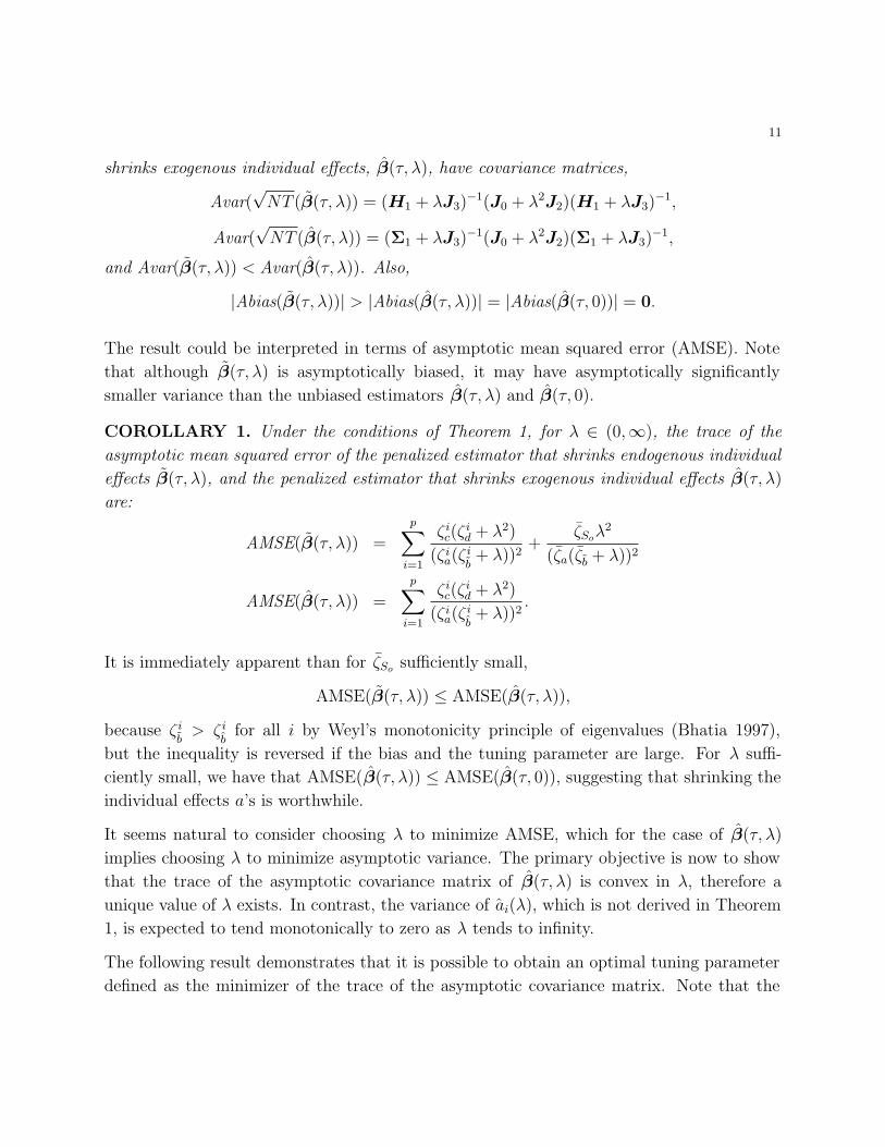
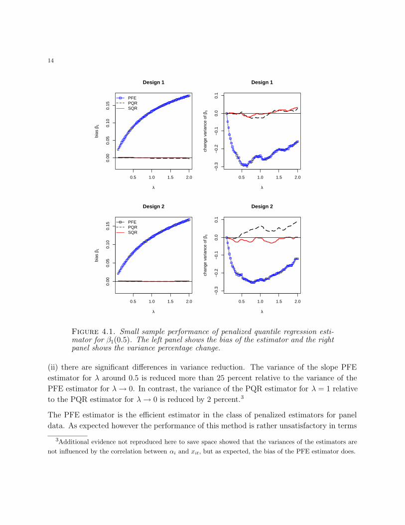
in parametric and semiparametric models. Considering N = 100 and T = 5, Figure 4.1

reports the bias and variance percentage change of PFE, PQR and SQR. The upper panels

present evidence of the performance of these three methods when the data is generated

according to Design 1 and the lower panels present evidence when the data is generated as

in Design 2. We see that the upper left panel shows that the PFE estimator is biased, and

its bias starts to increase as we increase the harshness of the penalization. The right upper

panel reveals that (i) the variance of the estimator decreases first and then increases, and

14

0.5 1.0 1.5 2.0

0.00

0.05

0.10

0.15

Design 1

λ

bias

β1^

PFEPQRSQR

0.5 1.0 1.5 2.0

−0.

3−

0.2

−0.

10.

00.

1

Design 1

λ

chan

ge v

aria

nce

of β

1^

0.5 1.0 1.5 2.0

0.00

0.05

0.10

0.15

Design 2

λ

bias

β1^

PFEPQRSQR

0.5 1.0 1.5 2.0

−0.

3−

0.2

−0.

10.

00.

1

Design 2

λ

chan

ge v

aria

nce

of β

1^

Figure 4.1. Small sample performance of penalized quantile regression esti-mator for β1(0.5). The left panel shows the bias of the estimator and the rightpanel shows the variance percentage change.

(ii) there are significant differences in variance reduction. The variance of the slope PFE

estimator for λ around 0.5 is reduced more than 25 percent relative to the variance of the

PFE estimator for λ → 0. In contrast, the variance of the PQR estimator for λ = 1 relative

to the PQR estimator for λ → 0 is reduced by 2 percent.3

The PFE estimator is the efficient estimator in the class of penalized estimators for panel

data. As expected however the performance of this method is rather unsatisfactory in terms

3Additional evidence not reproduced here to save space showed that the variances of the estimators are

not influenced by the correlation between αi and xit, but as expected, the bias of the PFE estimator does.

15

0 1 2 3 4 5

−0.

050.

000.

05

λ

bias

γγ1

γ2

γ3

γ4

γ5

0 1 2 3 4 5

0.00

80.

010

0.01

20.

014

0.01

60.

018

λ

Var

γ

γ1

γ2

γ3

γ4

γ5

Figure 4.2. Small sample performance of the penalized quantile regressionestimator PQR for γ.

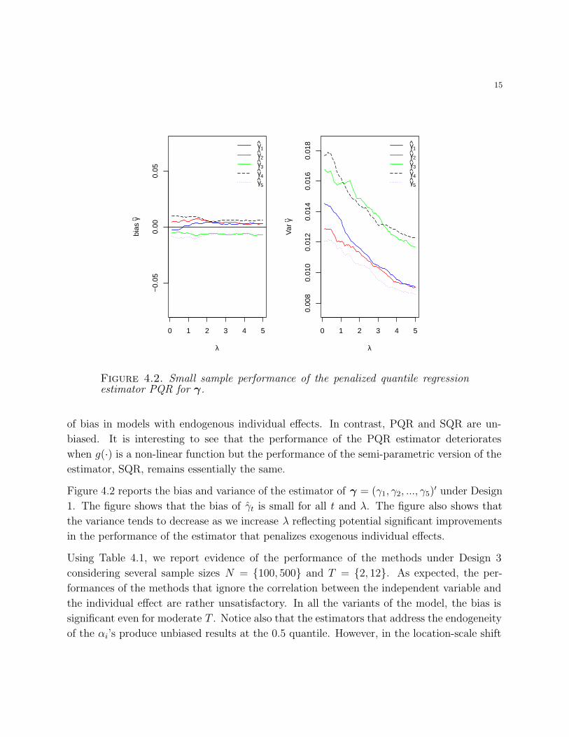
of bias in models with endogenous individual effects. In contrast, PQR and SQR are un-

biased. It is interesting to see that the performance of the PQR estimator deteriorates

when g(∙) is a non-linear function but the performance of the semi-parametric version of the

estimator, SQR, remains essentially the same.

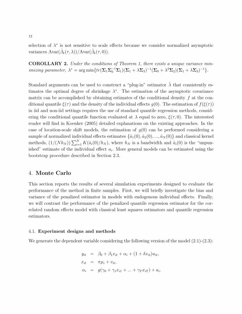
Figure 4.2 reports the bias and variance of the estimator of γ = (γ1, γ2, ..., γ5)′ under Design

1. The figure shows that the bias of γt is small for all t and λ. The figure also shows that

the variance tends to decrease as we increase λ reflecting potential significant improvements

in the performance of the estimator that penalizes exogenous individual effects.

Using Table 4.1, we report evidence of the performance of the methods under Design 3

considering several sample sizes N = {100, 500} and T = {2, 12}. As expected, the per-

formances of the methods that ignore the correlation between the independent variable and

the individual effect are rather unsatisfactory. In all the variants of the model, the bias is

significant even for moderate T . Notice also that the estimators that address the endogeneity

of the αi’s produce unbiased results at the 0.5 quantile. However, in the location-scale shift

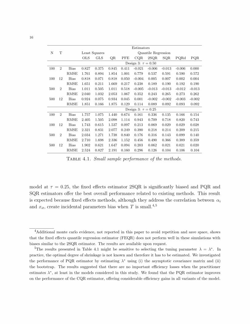
16

Estimators

N T Least Squares Quantile Regression

OLS GLS QR PFE CQR 2SQR SQR PQRd PQR

Design 3: τ = 0.50

100 2 Bias 0.827 0.375 0.845 0.411 -0.021 -0.006 -0.013 -0.006 0.000

RMSE 1.761 0.894 1.854 1.001 0.779 0.537 0.591 0.590 0.572

100 12 Bias 0.818 0.071 0.818 0.050 -0.004 0.005 0.007 0.002 0.004

RMSE 1.651 0.211 1.669 0.217 0.238 0.189 0.190 0.192 0.190

500 2 Bias 1.011 0.505 1.011 0.518 -0.005 -0.013 -0.013 -0.012 -0.013

RMSE 2.040 1.032 2.053 1.067 0.352 0.243 0.265 0.273 0.262

500 12 Bias 0.924 0.075 0.934 0.045 0.001 -0.002 -0.002 -0.003 -0.002

RMSE 1.851 0.166 1.875 0.129 0.114 0.089 0.092 0.093 0.092

Design 3: τ = 0.25

100 2 Bias 1.757 1.075 1.440 0.674 0.161 0.336 0.135 0.166 0.154

RMSE 2.405 1.505 2.098 1.114 0.943 0.709 0.718 0.820 0.743

100 12 Bias 1.743 0.615 1.537 0.097 0.213 0.069 0.029 0.029 0.028

RMSE 2.321 0.831 2.077 0.249 0.390 0.218 0.214 0.209 0.215

500 2 Bias 2.034 1.271 1.738 0.840 0.176 0.316 0.143 0.099 0.140

RMSE 2.710 1.698 2.336 1.152 0.456 0.490 0.366 0.389 0.359

500 12 Bias 1.902 0.621 1.647 0.094 0.203 0.062 0.021 0.021 0.020

RMSE 2.524 0.827 2.191 0.160 0.296 0.126 0.104 0.106 0.104

Table 4.1. Small sample performance of the methods.

model at τ = 0.25, the fixed effects estimator 2SQR is significantly biased and PQR and

SQR estimators offer the best overall performance related to existing methods. This result

is expected because fixed effects methods, although they address the correlation between αi

and xit, create incidental parameters bias when T is small.4,5

4Additional monte carlo evidence, not reported in this paper to avoid repetition and save space, shows

that the fixed effects quantile regression estimator (FEQR) does not perform well in these simulations with

biases similar to the 2SQR estimator. The results are available upon request.5The results presented in Table 4.1 might be sensitive to selecting the tuning parameter λ = λ∗. In

practice, the optimal degree of shrinkage is not known and therefore it has to be estimated. We investigated

the performance of PQR estimator by estimating λ∗ using (i) the asymptotic covariance matrix and (ii)

the bootstrap. The results suggested that there are no important efficiency losses when the practitioner

estimates λ∗, at least in the models considered in this study. We found that the PQR estimator improves

on the performance of the CQR estimator, offering considerable efficiency gains in all variants of the model.

17

5. Heterogeneous nutrition preferences

In the US, obesity rates have increased at alarming rates over the last few decades. Given

the comorbity of obesity with other chronic illnesses, such as diabetes and heart disease,

and the financial strain it imposes on the health care system, obesity is considered to be

one of the main public health concerns of our time. Numerous programs such as the First

Lady’s “Let’s Move” campaign aim to address the challenge of obesity. Designing policies to

address obesity is a complex problem that requires us to tailor interventions to account for

heterogeneous preferences and demographics. In this example, we explore how preferences

for nutrients vary by gender across the conditional food expenditure distribution. 6

A recent report by the Trust for America’s Health and the Robert Wood Johnson Foundation

finds that while obesity rates appear to be stabilizing, the rates nevertheless continue to be

very high.7 More than two thirds of adults are now obese or overweight, and almost 35%

of adults are obese. At the same time, a recent CDC report estimates that while 35.7%

of US adults are now obese, substantial differences exist across race and gender groups. 8

Over the last decade obesity rates for men increased from 27.5% to 35.5%, while obesity

rates for women have not varied significantly in recent years and are currently at 35.8%.

Furthermore, while 56.6% of African American women, and 37.1% of African American men

are obese, only 32.8% of White women and 32.4% of White men are obese. In this section,

we quantify preferences for nutrients by gender across the conditional food expenditure

distribution. Understanding the heterogeneity in preferences is of major policy interest as it

helps us design better policies by accounting for their distributional impact. Distributional

considerations play an important role in the design of US policies. Recently, Berkeley passed

the first per-ounce soda tax on sugar-sweetened beverages in the US. Similar taxes have

already been implemented in a number of other countries including Mexico. Distributional

considerations of these taxes are being vigorously debated by both supporters and opponents

of the taxes.

The consumption model described below allows us to quantify the differences in preferences

for nutrients across sub-populations. Dubois, Griffith, and Nevo (2014) use this modeling

6A previous version of the paper included an application of the new method to the estimation of labor

supply models. We demonstrated how the penalized estimator can be obtained and used to estimate quantile

specific elasticities. The interested reader can find additional details in Harding and Lamarche (2013).7See Levi, Segal, St. Laurent, and Rayburn (2014) for an in-depth analysis based on data from the

2011-2012 Behavioral Risk Factor Surveillance System database.8See Ogden, Carroll, Kit, and Flegal (2012) for more details.

18

approach to show that there are substantial differences across countries. We adapt their

model to explore if differences in preferences between socio-demographic groups exist at

different levels of expenditure. We model a household’s food purchase decision, where each

household can choose among M different food products. Each product k is characterized

by a set of D product attributes. Each product is identified at the UPC level. A typical

American supermarket sells about 50, 000 different products. Thus, while D is large, the

number of product attributes which are salient to the average consumer, C, is typically very

small. We focus on attributes which relate to the underlying nutrients that a consumer

may look for on the product label, such as calories, fat, salt, sugar, cholesterol, protein and

carbohydrates. Each unit of good k contains κk = {κk,1, . . . ,κkC}′ units of the underlying

product attributes.9

We assume that household i with income Ii chooses a bundle of goods Xi and a numeraire

good Xi0 so as to maximize utility conditional on household attributes μi and subject to

a budget constraint. We follow Dubois, Griffith, and Nevo (2014) and assume that the

household derives utility from both the goods purchased and the underlying quantities xi

of the nutrients purchased through the purchase of the goods Xi. We normalize the price

of the numeraire good to 1. Denote by pi the prices faced by household i over the set of

products available for purchase. Thus,

(5.1) maxXi0,Xi

U(Xi0, Xi, xi, μi), s.t. Xi0 + p′iXi = Ii,

where xik = κ′kXi, denotes a home production function which converts products into nutri-

ents (cooking). This model generalizes the Muellbauer (1974) model of household production,

which assumes that household i purchases goods Xi but only derives utility from the product

attributes xi, and which generates a standard hedonic model. By allowing the household to

derive utility from both products and attributes we are relying on insights from the mod-

ern Industrial Organization literature, which shows that households exhibit preferences over

products.

Given the large number of choices D faced by the typical household, it would be impractical

to estimate a disaggregated demand system. It is thus common to aggregate products

into mutually exclusive groups such as milk products, meat products, etc. Harding and

Lovenheim (2014) then estimate a structural Quadratic Almost Ideal Demand System on the

aggregate set of products, which allows for the identification of a detailed substitution matrix.

9Note that we do not require the underlying product attributes to be mutually exclusive. For example

Peanut Butter has 188 total calories per serving; 145 of those calories come from fat. The total amount of

fat in the serving is 16.1 grams.

19

In the context of the current application, we wish to estimate the preference heterogeneity

in the demand for nutrients and follow the more parametric approach of Dubois, Griffith

and Nevo (2014) by choosing a utility which imposes stronger restrictions on the pattern

of substitution between products. While this substantially limits the nature of the price

elasticities, it possesses the attractive feature of weak separability, which leads to a convenient

aggregation over products as shown below.

In particular we let:

(5.2) U(Xi0, Xi, xi, μi) = exp(Xi0)

(D∑

k=1

fik(Xik)

)μi C∏

c=1

hic(xic),

where μi denotes the set of household specific model parameters. We further assume that

fik(Xik) = λikXθiik and hic(xic) = exp(βcxic). After substituting for the budget constraint and

the home production function the household maximizes the following log utility function:

log U(Xi0, Xi, xi, μi, λi, θi, βc) = Ii −D∑

k=1

pikXik + μi log

(D∑

k=1

λikXθiik

)

+C∑

c=1

βc

D∑

k=1

κkcXik,

where κkc are known and observed by both the household and the econometrician. The

parameters βc measure the average contribution of a nutrient to the utility function. The

first order condition for good k is given by:

(5.3) pik = μiθiλikX

θi−1ik∑D

k=1 λikXθiik

+C∑

c=1

βcκkc.

We can express this first order condition in terms of the expenditure for good k to obtain:

(5.4) pikXik = μiθiλikX

θiik∑D

k=1 λikXθiik

+C∑

c=1

βcκkcXik.

Note that we can now aggregate this expression over all (or a subset) of the products to

obtain the relationship between total expenditure Ei and nutrients:

(5.5) Ei = μiθi +C∑

c=1

βcxic.

In practice we observe a household making repeated purchases and we can estimate this

model using the following panel data empirical specification:

(5.6) Eit = αi + w′iδ +

C∑

c=1

βcxitc + uit,

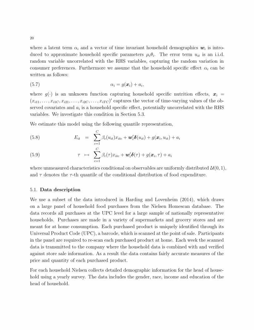
20

where a latent term αi and a vector of time invariant household demographics wi is intro-

duced to approximate household specific parameters μiθi. The error term uit is an i.i.d.

random variable uncorrelated with the RHS variables, capturing the random variation in

consumer preferences. Furthermore we assume that the household specific effect αi can be

written as follows:

(5.7) αi = g(xi) + ai,

where g(∙) is an unknown function capturing household specific nutrition effects, xi =

(xi11, . . . , xi1C , xi21, . . . , xi2C , . . . , xiTC)′ captures the vector of time-varying values of the ob-

served covariates and ai is a household specific effect, potentially uncorrelated with the RHS

variables. We investigate this condition in Section 5.3.

We estimate this model using the following quantile representation,

Eit =C∑

c=1

βc(uit)xitc + w′iδ(uit) + g(xi, uit) + ai(5.8)

τ 7→C∑

c=1

βc(τ)xitc + w′iδ(τ) + g(xi, τ ) + ai(5.9)

where unmeasured characteristics conditional on observables are uniformly distributed U(0, 1),

and τ denotes the τ -th quantile of the conditional distribution of food expenditure.

5.1. Data description

We use a subset of the data introduced in Harding and Lovenheim (2014), which draws

on a large panel of household food purchases from the Nielsen Homescan database. The

data records all purchases at the UPC level for a large sample of nationally representative

households. Purchases are made in a variety of supermarkets and grocery stores and are

meant for at home consumption. Each purchased product is uniquely identified through its

Universal Product Code (UPC), a barcode, which is scanned at the point of sale. Participants

in the panel are required to re-scan each purchased product at home. Each week the scanned

data is transmitted to the company where the household data is combined with and verified

against store sale information. As a result the data contains fairly accurate measures of the

price and quantity of each purchased product.

For each household Nielsen collects detailed demographic information for the head of house-

hold using a yearly survey. The data includes the gender, race, income and education of the

head of household.

21

Variables All consumers Female consumers Male consumers

(1) (2) (3)

Total Expenditure 120.328 119.887 121.311

(77.954) (77.558) (78.821)

Total fat (grams consumed per month) 17.406 17.383 17.456

(14.338) (14.297) (14.429)

Salt (milligrams consumed per month) 818.066 822.313 808.605

(1173.582) (1233.129) (1028.525)

Sugar (grams consumed per month) 30.111 30.200 29.915

(23.609) (23.916) (22.910)

Cholesterol (grams consumed per month) 46.541 46.705 46.176

(42.987) (42.764) (43.479)

Protein (grams consumed per month) 13.852 13.668 14.262

(23.351) (24.363) (20.914)

Carbohydrates (grams consumed per month) 64.023 64.068 63.924

(46.093) (46.989) (44.032)

Black 0.117 0.128 0.093

(0.322) (0.334) (0.291)

Income higher than $70K 0.146 0.123 0.197

(0.353) (0.329) (0.398)

College education 0.475 0.450 0.530

(0.499) (0.497) (0.499)

Number of consumers 9,165 6,326 2,839

Number of observations 109,980 75,912 34,068

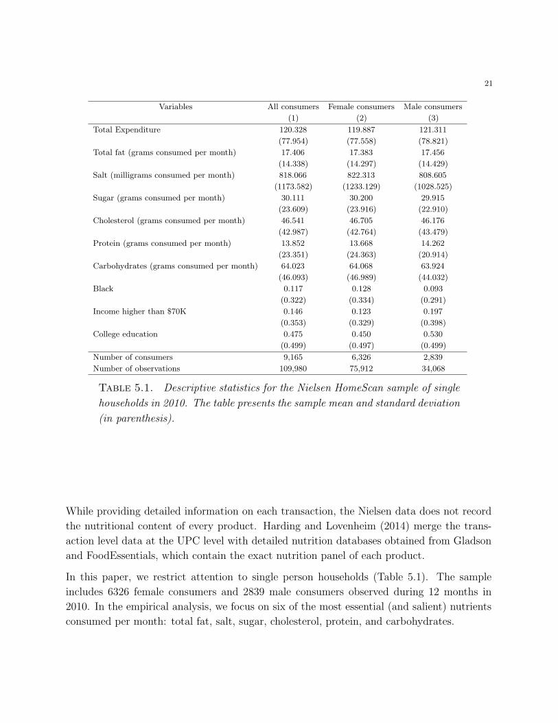
Table 5.1. Descriptive statistics for the Nielsen HomeScan sample of single

households in 2010. The table presents the sample mean and standard deviation

(in parenthesis).

While providing detailed information on each transaction, the Nielsen data does not record

the nutritional content of every product. Harding and Lovenheim (2014) merge the trans-

action level data at the UPC level with detailed nutrition databases obtained from Gladson

and FoodEssentials, which contain the exact nutrition panel of each product.

In this paper, we restrict attention to single person households (Table 5.1). The sample

includes 6326 female consumers and 2839 male consumers observed during 12 months in

2010. In the empirical analysis, we focus on six of the most essential (and salient) nutrients

consumed per month: total fat, salt, sugar, cholesterol, protein, and carbohydrates.

22

Quantiles

0.10 0.50 0.90

QR FEQR SQR QR FEQR SQR QR FEQR SQR

Total fat 1.204 1.175 1.144 1.216 1.170 1.173 1.229 1.273 1.291

(0.038) (0.053) (0.051) (0.028) (0.063) (0.068) (0.058) (0.067) (0.069)

Salt 0.003 0.002 0.002 0.003 0.003 0.003 0.005 0.004 0.004

(0.000) (0.000) (0.000) (0.000) (0.000) (0.000) (0.000) (0.001) (0.001)

Sugar 0.245 0.179 0.165 0.439 0.357 0.362 0.707 0.554 0.551

(0.024) (0.043) (0.043) (0.021) (0.029) (0.030) (0.044) (0.035) (0.039)

Cholesterol 0.091 0.177 0.175 -0.045 0.061 0.064 -0.145 0.008 0.007

(0.011) (0.024) (0.025) (0.010) (0.024) (0.024) (0.016) (0.018) (0.019)

Protein -0.013 -0.120 -0.115 2.761 1.856 1.842 5.134 2.960 3.020

(0.110) (0.245) (0.263) (0.138) (0.346) (0.365) (0.222) (0.283) (0.286)

Carbohydrates 0.414 0.552 0.542 0.356 0.437 0.438 0.331 0.388 0.406

(0.017) (0.029) (0.030) (0.019) (0.035) (0.036) (0.033) (0.030) (0.031)

Black -5.305 -6.135 -6.717 -4.700 -8.570 -3.893

(0.427) (1.128) (0.410) (1.163) (0.884) (1.338)

High income 6.368 7.134 13.990 12.915 22.152 20.305

(0.561) (1.147) (0.539) (1.252) (0.974) (1.646)

College education 3.218 3.979 6.421 5.761 10.707 8.468

(0.319) (0.748) (0.316) (0.880) (0.653) (1.047)

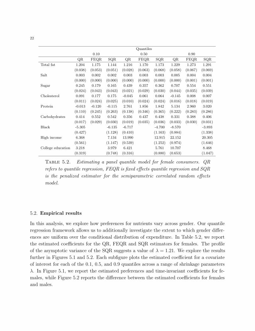
Table 5.2. Estimating a panel quantile model for female consumers. QR

refers to quantile regression, FEQR is fixed effects quantile regression and SQR

is the penalized estimator for the semiparametric correlated random effects

model.

5.2. Empirical results

In this analysis, we explore how preferences for nutrients vary across gender. Our quantile

regression framework allows us to additionally investigate the extent to which gender differ-

ences are uniform over the conditional distribution of expenditure. In Table 5.2, we report

the estimated coefficients for the QR, FEQR and SQR estimators for females. The profile

of the asymptotic variance of the SQR suggests a value of λ = 1.21. We explore the results

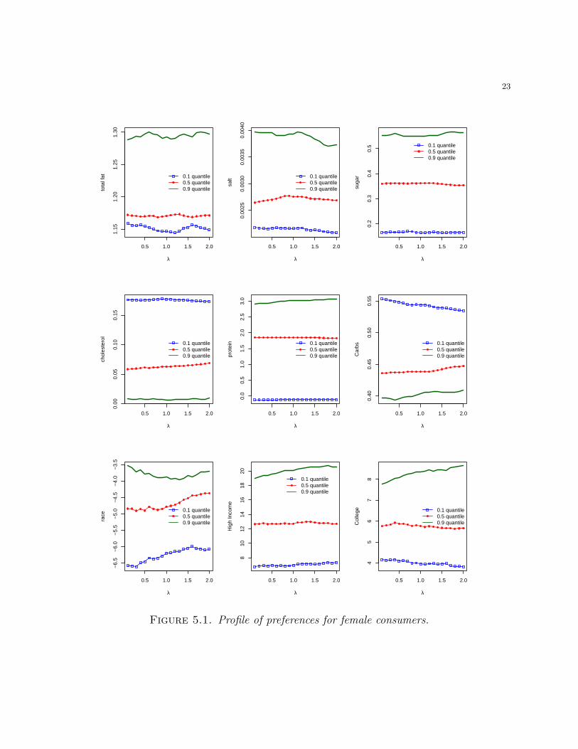
further in Figures 5.1 and 5.2. Each subfigure plots the estimated coefficient for a covariate

of interest for each of the 0.1, 0.5, and 0.9 quantiles across a range of shrinkage parameters

λ. In Figure 5.1, we report the estimated preferences and time-invariant coefficients for fe-

males, while Figure 5.2 reports the difference between the estimated coefficients for females

and males.

23

0.5 1.0 1.5 2.0

1.15

1.20

1.25

1.30

λ

tota

l fat 0.1 quantile

0.5 quantile0.9 quantile

0.5 1.0 1.5 2.00.

0025

0.00

300.

0035

0.00

40

λ

salt 0.1 quantile

0.5 quantile0.9 quantile

0.5 1.0 1.5 2.0

0.2

0.3

0.4

0.5

λ

suga

r

0.1 quantile0.5 quantile0.9 quantile

0.5 1.0 1.5 2.0

0.00

0.05

0.10

0.15

λ

chol

este

rol

0.1 quantile0.5 quantile0.9 quantile

0.5 1.0 1.5 2.0

0.0

0.5

1.0

1.5

2.0

2.5

3.0

λ

prot

ein 0.1 quantile

0.5 quantile0.9 quantile

0.5 1.0 1.5 2.0

0.40

0.45

0.50

0.55

λ

Car

bs 0.1 quantile0.5 quantile0.9 quantile

0.5 1.0 1.5 2.0

−6.

5−

6.0

−5.

5−

5.0

−4.

5−

4.0

−3.

5

λ

race

0.1 quantile0.5 quantile0.9 quantile

0.5 1.0 1.5 2.0

810

1214

1618

20

λ

Hig

h In

com

e

0.1 quantile0.5 quantile0.9 quantile

0.5 1.0 1.5 2.0

45

67

8

λ

Col

lege 0.1 quantile

0.5 quantile0.9 quantile

Figure 5.1. Profile of preferences for female consumers.

24

First, consider the results for female shoppers. We find that higher conditional food expendi-

tures are associated with stronger preferences for fat, salt, sugar, and protein at the 0.5 and

0.9 quantiles. These nutrients are highly correlated with taste and the richer a product is in

these nutrients the more likely it is to be appealing to a consumer. In contrast, cholesterol

and carbohydrates are generally associated with health hazards and have no direct impact

on taste. As a result we see that high expenditure households prefer these nutrients less

than low expenditure households, which may be indicative of avoidance behavior. Popular

culture places a lot of emphasis on diets aimed at avoiding cholesterol and carbohydrates.

At the same time taste matters a lot and drives consumer choices towards products which

have ingredients that make them more appealing to the palate. As a result diets which are

predicated on the idea of reducing the intake of one particular nutrients are not necessarily

healthier overall, since they lead to increased consumption of other nutrients with overall

ambiguous health outcomes.

It is also important to stress that the differences between the estimates for the extreme

quantiles and the median reveal substantial preference heterogeneity across the conditional

expenditure distribution which varies by nutrient. For instance, the effect of protein is

negative and insignificant at the 0.1 quantile, while positive and significant at the 0.9 quantile.

Furthermore, our approach allows us to estimate directly the impact of the demographics

on food expenditure. We find that being African-American is associated with a negative

impact on overall food expenditures, while households with incomes above $70,000 and

with a College education are associated with higher expenditures on food. These effects

become more pronounced across the expenditure distribution. To correctly interpret these

demographic gradients it is important to recall that the data in this sample only captures food

purchased in stores for at-home consumption. Lower expenditures are thus also associated

with a higher propensity to eat outside the home at unhealthy fast-food outlets. Note that

the results of the SQR model are quantitatively similar to those of the FEQR model, but

substantially different than the QR results. This reinforces the importance of controlling for

unobserved heterogeneity. However, our approach also has the advantage of enabling us to

derive the impact of the observable demographics on food expenditures.

From an econometric perspective it is also important to note the role played by the shrink-

age parameter λ. In general we would expect the estimated coefficients on the covariates

of interest to be fairly comparable across different degrees of shrinkage. By construction,

the procedure shrinks the individual effects towards zero and if the model is well specified

we would not expect changes in λ to affect the values of the estimated coefficients at each

quantile. If on the other hand, the distribution of the individual effect ai is not centered at

25

τ SQR estimate at λ equal to SQR: λ = 0.01 with

0.01 0.5 1.0 1.5 2.0 0.5 1.0 1.5 2.0

Total Fat 0.1 1.16 1.15 1.15 1.15 1.15 1.00 0.97 0.99 0.97

0.5 1.17 1.17 1.17 1.17 1.17 1.00 1.00 1.00 1.00

0.9 1.29 1.30 1.29 1.30 1.30 0.99 1.00 1.00 0.99

Salt (× 100) 0.1 0.22 0.22 0.22 0.21 0.21 1.00 1.00 0.98 0.92

0.5 0.26 0.27 0.28 0.27 0.27 0.98 0.93 0.98 0.99

0.9 0.40 0.40 0.39 0.38 0.37 1.00 1.00 0.99 0.89

Sugar 0.1 0.17 0.17 0.16 0.16 0.17 1.00 1.00 1.00 1.00

0.5 0.36 0.36 0.36 0.36 0.35 1.00 1.00 1.00 0.99

0.9 0.55 0.55 0.55 0.56 0.56 1.00 1.00 0.99 0.98

Cholesterol 0.1 0.18 0.18 0.18 0.17 0.17 1.00 1.00 1.00 0.99

0.5 0.06 0.06 0.06 0.06 0.07 0.99 0.99 0.97 0.93

0.9 0.01 0.01 0.01 0.01 0.01 1.00 1.00 1.00 1.00

Protein 0.1 -0.12 -0.12 -0.12 -0.11 -0.11 1.00 1.00 1.00 1.00

0.5 1.86 1.85 1.85 1.84 1.83 1.00 1.00 1.00 1.00

0.9 2.92 2.95 3.02 3.04 3.07 0.99 0.96 0.93 0.91

Carbs 0.1 0.55 0.55 0.54 0.54 0.53 0.98 0.95 0.89 0.79

0.5 0.44 0.44 0.44 0.44 0.45 1.00 1.00 0.99 0.96

0.9 0.40 0.40 0.40 0.41 0.41 1.00 0.99 0.97 0.95

Black 0.1 -6.58 -6.46 -6.21 -6.05 -6.09 0.99 0.93 0.83 0.86

0.5 -4.84 -4.90 -4.78 -4.52 -4.37 1.00 1.00 0.95 0.88

0.9 -3.54 -3.79 -3.89 -3.84 -3.71 0.98 0.96 0.97 0.99

High Income 0.1 6.78 6.96 6.96 7.13 7.38 0.99 1.00 0.96 0.93

0.5 12.65 12.73 12.73 12.88 12.72 1.00 1.00 0.99 1.00

0.9 19.01 19.59 20.06 20.54 20.60 0.95 0.92 0.82 0.84

College Education 0.1 4.16 4.10 3.95 3.96 3.82 1.00 0.97 0.97 0.92

0.5 5.76 5.88 5.77 5.68 5.65 0.99 1.00 0.99 0.99

0.9 7.78 8.08 8.36 8.44 8.64 0.92 0.82 0.81 0.69

Table 5.3. Specification tests in a quantile regression model with semipara-

metric correlated effects. The last columns present the p-values of the tests.

zero, this indicates that the model retains additional unobserved variables which are corre-

lated with the covariates and are not captured by the flexible function g(∙). Our estimates

appear to indicate that while the model appears to fit the data well, there is the possibility

of additional endogeneity not fully captured by the model specification as indicated by the

estimates of the preferences for carbohydrates at the 0.1 quantile, and income and college

education at the 0.9 quantile (Figure 5.1). Next section develops a series of Hausman-type

tests (Hausman 1978) to formally address these questions.

26

τ PQR estimate at λ equal to PQR: λ = 0.01 with

0.01 0.5 1.0 1.5 2.0 0.5 1.0 1.5 2.0

Total Fat 0.1 1.16 1.16 1.15 1.15 1.16 1.00 0.96 0.97 0.98

0.5 1.17 1.16 1.15 1.15 1.14 0.96 0.89 0.78 0.64

0.9 1.29 1.29 1.28 1.27 1.28 1.00 0.95 0.87 1.00

Salt (× 100) 0.1 0.22 0.21 0.21 0.20 0.21 0.99 0.94 0.92 0.95

0.5 0.27 0.27 0.28 0.28 0.27 0.97 0.92 0.94 0.94

0.9 0.40 0.40 0.40 0.39 0.38 1.00 1.00 0.99 0.98

Sugar 0.1 0.17 0.16 0.17 0.17 0.17 1.00 1.00 1.00 0.99

0.5 0.36 0.36 0.37 0.37 0.36 0.99 0.99 0.99 1.00

0.9 0.55 0.56 0.56 0.57 0.58 0.97 0.98 0.94 0.86

Cholesterol 0.1 0.18 0.18 0.18 0.18 0.17 1.00 0.99 0.99 0.78

0.5 0.06 0.06 0.06 0.06 0.06 1.00 1.00 1.00 1.00

0.9 0.01 0.00 0.00 0.00 0.00 0.93 0.82 0.78 0.78

Protein 0.1 -0.12 -0.12 -0.12 -0.12 -0.12 1.00 1.00 1.00 1.00

0.5 1.86 1.90 1.94 1.97 2.00 0.98 0.94 0.85 0.61

0.9 2.93 3.01 3.11 3.18 3.26 0.79 0.52 0.23 0.02

Carbs 0.1 0.55 0.55 0.54 0.54 0.54 0.94 0.68 0.64 0.23

0.5 0.43 0.43 0.43 0.43 0.43 0.98 0.98 0.98 0.98

0.9 0.40 0.39 0.39 0.39 0.39 0.85 0.97 0.95 0.76

Black 0.1 -7.90 -7.85 -7.63 -7.60 -7.67 0.99 0.83 0.82 0.91

0.5 -6.14 -6.12 -6.18 -6.02 -5.95 1.00 1.00 0.97 0.93

0.9 -4.82 -5.06 -5.34 -5.61 -5.47 0.90 0.71 0.51 0.63

High Income 0.1 7.09 7.03 6.89 6.84 7.06 1.00 0.99 0.98 1.00

0.5 12.91 12.79 12.68 12.45 12.23 1.00 0.99 0.94 0.91

0.9 19.27 19.46 20.05 20.15 20.01 0.99 0.90 0.91 0.96

College Education 0.1 4.16 4.10 4.08 4.12 4.17 0.98 0.98 1.00 1.00

0.5 5.77 5.82 5.78 5.83 5.88 0.98 1.00 0.99 0.96

0.9 7.79 8.03 8.46 8.72 9.11 0.78 0.33 0.16 0.03

Table 5.4. Specification tests in a quantile regression model with correlated

effects. The last columns present the p-values of the tests.

5.3. Hypothesis testing

To investigate if the model specification and assumptions are supported by data, we propose

a series of tests. Recall that xit denotes time-variant variables and wi denotes time-invariant

variables as in the model description. If we let αi = g(xi) + ai and αi is correlated with wi,

then ai must be correlated with wi. Therefore, Assumption A2 in Appendix A.2 is violated,

and shrinking ai towards zero leads to biased estimates of time-invariant effects. On the

other hand, the performance of the fixed effects version of the estimator (the limiting case of

the penalized estimator when λ → 0) does not depend on the correlation between ai and wi.

27

It seems natural then to propose a Hausman-type test to evaluate whether the fixed effects

estimator, limλ→0 β(λ) and the penalized estimator β(λ) offer significantly different results.

If ai and wi are independent, we expect that limλ→0 β(λ) and β(λ) be relatively similar for

any value of λ.

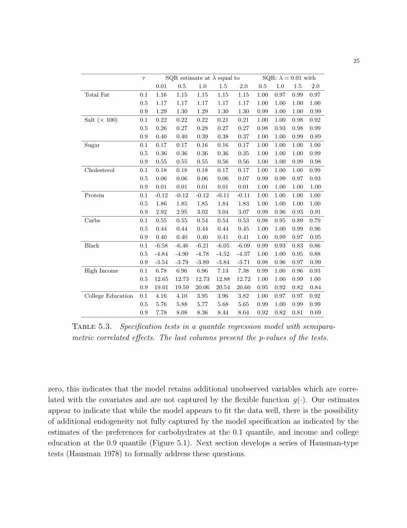
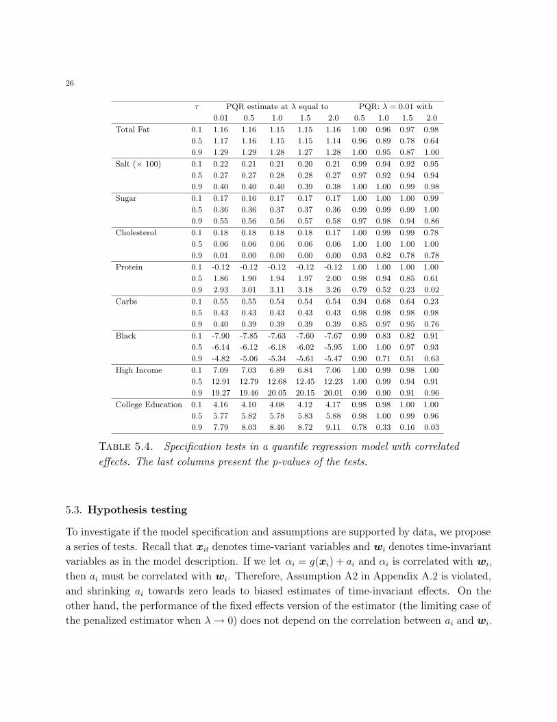
Tables 5.3 and 5.4 show point estimates and p-values of tests associated with the signifi-

cance of difference between fixed effects and penalized quantile regression results. The null

hypothesis is equality of coefficients and we evaluate several null hypotheses considering dif-

ferent values of λ = {0.5, 1, 1.5, 2}. These values are chosen for convenience and represent

points on the profile of the penalized estimator in terms of λ (see, e.g., Figure 5.1). The

specification tests are performed on two models. First, we estimate equation (5.9) using the

semiparametric estimator, SQR. The results are shown in Table 5.3. We also estimate the

model using the one-step estimator, PQR, and compare the results to emphasize the role of

the semiparametric specification of the correlated effects (Table 5.4).

The results in Table 5.3 indicate that preference for nutrients do not significantly change

when the shrinkage parameter changes. This result might seem clear from observing the

point estimates presented in the first columns and the p-values of the tests which naturally

offer more reliable evidence. We interpret these findings as suggesting the empirical findings

are robust to the potential misspecification of equation (5.7). It is interesting to compare

the result with Table 5.4 and observe that the semiparametric specification of the nutrients

helps to correct for potential issues of endogeneity in the one-step estimator. For instance,

the effects of protein at the 0.5 and 0.9 quantiles increase with λ if the one-step estimator is

employed, while they appear to be fairly constant if the two-step semiparametric estimator

is used. The result suggests that the semiparametric specification of the correlated effects

helps address potential endogeneity issues. The results continue to provide support in favor

of a correctly specified model for the time-invariant variables.10 Overall, it is important to

emphasize that the results support the penalized effects specification with semiparametric

correlated effects and this model is not rejected in favor of the fixed effects specification. This

is true specifically among preferences for nutrients among female and male consumers. 11

10The results for college education in a model with parametric correlated effects estimated at the 0.9

quantile reveal some potential endogeneity issues. This naturally suggests that the effect of education at the

upper tail cannot be interpreted as a causal effect. As a referee suggested, the effect might be interpreted

as the sum of the causal effect of education on expenditures at the upper tail of the conditional distribution

plus the effect of college education on time-invariant preferences.11We repeat the exercise of estimating equation (5.9) considering a sample of male consumers. The

results, which are not presented in the paper to economize space, continue to support the semiparametric

28

0.5 1.0 1.5 2.0

−0.

10−

0.05

0.00

0.05

0.10

λ

tota

l fat

0.1 quantile0.5 quantile0.9 quantile

0.5 1.0 1.5 2.0−

0.00

2−

0.00

10.

000

0.00

10.

002

λ

salt

0.1 quantile0.5 quantile0.9 quantile

0.5 1.0 1.5 2.0

−0.

2−

0.1

0.0

0.1

0.2

λ

suga

r

0.1 quantile0.5 quantile0.9 quantile

0.5 1.0 1.5 2.0

−0.

020.

000.

02

λ

chol

este

rol

0.1 quantile0.5 quantile0.9 quantile

0.5 1.0 1.5 2.0

−0.

4−

0.2

0.0

0.2

0.4

λ

prot

ein

0.1 quantile0.5 quantile0.9 quantile

0.5 1.0 1.5 2.0

−0.

06−

0.02

0.00

0.02

0.04

0.06

λ

carb

s

0.1 quantile0.5 quantile0.9 quantile

Figure 5.2. Profile of preferences in terms of λ. The figure shows the differ-ence between the estimated coefficients for female and male shoppers.

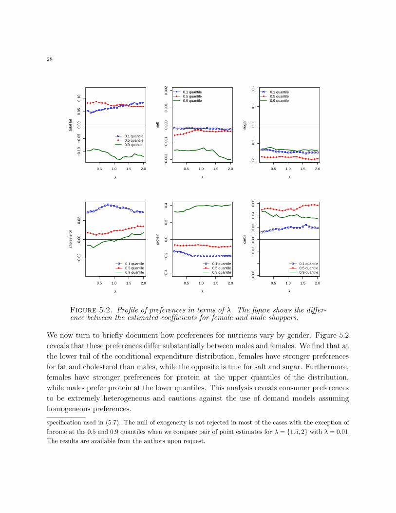
We now turn to briefly document how preferences for nutrients vary by gender. Figure 5.2

reveals that these preferences differ substantially between males and females. We find that at

the lower tail of the conditional expenditure distribution, females have stronger preferences

for fat and cholesterol than males, while the opposite is true for salt and sugar. Furthermore,

females have stronger preferences for protein at the upper quantiles of the distribution,

while males prefer protein at the lower quantiles. This analysis reveals consumer preferences

to be extremely heterogeneous and cautions against the use of demand models assuming

homogeneous preferences.

specification used in (5.7). The null of exogeneity is not rejected in most of the cases with the exception of

Income at the 0.5 and 0.9 quantiles when we compare pair of point estimates for λ = {1.5, 2} with λ = 0.01.

The results are available from the authors upon request.

29

6. Conclusions

This paper investigates simple `1-penalized approaches to the estimation of marginal effects

in panel data models with time-invariant variables by allowing for a flexible specification of

correlated individual effects in a quantile regression setting. The approaches offer a balanced

compromise between misspecification issues arising from the omission of individual hetero-

geneity and the incidental parameters problem arising from leaving individual heterogeneity

unrestricted in a nonlinear panel model. We provide an empirical application illustrating

the practical implementation and use of the proposed methods.

In the application we estimate consumer preferences for nutrients from a semi-structural

demand model using a large scanner dataset of household food purchases. We show that

preferences for nutrients vary across the conditional distribution of expenditure and across

genders and emphasize the importance of fully capturing consumer heterogeneity in demand

modeling and policy evaluation.

References

Abrevaya, J., and C. Dahl (2008): “The Effects of Smoking and Prenatal Care on Birth Outcomes: Evi-

dence from Quantile Regression Estimation on Panel Data,” Journal of Business and Economics Statistics,

26(4), 379–397.

Arellano, M., and O. Bover (1995): “Another look at the instrumental variable estimation of error-

components models,” Journal of Econometrics, 68(1), 29–51.

Baltagi, B. (2008): Econometric Analysis of Panel Data. Wiley, New York, 4 edn.

Belloni, A., D. Chen, V. Chernozhukov, and C. Hansen (2012): “Sparse Models and Methods for

Optimal Instruments With an Application to Eminent Domain,” Econometrica, 80(6), 2369–2429.

Belloni, A., and V. Chernozhukov (2011): “L1-Penalized Quantile Regression in High-Dimensional

Sparse Models,” Annals of Statistics, 39(1), 82–130.

Bhatia, R. (1997): Matrix Analysis. Springer-Verlag, New York.

Bickel, P., and B. Li (2006): “Regularization in Statistics,” Sociedad de Estadistica e Investigacion

Operativa, 15.

Blundell, R., and T. MaCurdy (1999): “Labor Supply: A Review of Alternative Approaches,” in

Handbook of Labor Economics, ed. by O. Ashenfelter, and D. Card, vol. 3, pp. 1560–1618. Elsevier Science.

Blundell, R., and C. Meghir (1986): “Selection Criteria for A Microeconometric Model of Labour

Supply,” Journal of Applied Econometrics, 1, 55–80.

Burtless, G., and J. A. Hausman (1978): “The Effect of Taxation on Labor Supply: Evaluating the

Gary Negative Income Tax Experiment,” Journal of Political Economy, 86(6), pp. 1103–1130.

Cai, Z., and Z. Xiao (2012): “Semiparametric quantile regression estimation in dynamic models with

partially varying coefficients,” Journal of Econometrics, 167(2), 413 – 425.

30

Canay, I. A. (2011): “A simple approach to quantile regression for panel data,” The Econometrics Journal,

14(3), 368–386.

Carrasco, M., J. P. Florens, and E. Renault (2007): “Linear Inverse Problems in Structural Econo-

metrics: Estimation Based on Spectral Decomposition and Regularization,” in Handbook of Econometrics,

ed. by J. Heckman, and E. Leamer, vol. 6B. Elsevier Science.

Chamberlain, G. (1982): “Multivariate Regression Models for Panel Data,” Journal of Econometrics, 18,

5–46.

Chen, X. (2007): “Large Sample Sieve Estimation of Semi-Nonparametric Models,” Handbook of Econo-

metrics, Edited by J. Heckman and E. Leamer, 6B, Elsevier.

Chernozhukov, V., Fernandez-Val, and A. Kowalski (2015): “Quantile Regression with Censoring

and Endogeneity,” Journal of Econometrics, forthcoming.

Chernozhukov, V., I. Fernandez-Val, J. Hahn, and W. Newey (2013): “Average and Quantile

Effects in Nonseparable Panel Models,” Econometrica, 81, 535–580.

Donoho, D., S. Chen, and M. Saunders (1998): “Atomic Decomposition by Basis Pursuit,” SIAM

Journal of Scientific Computing, 20, 33–61.

Dubois, P., R. Griffith, and A. Nevo (2014): “Do Prices and Attributes Explain International Differ-

ences in Food Purchases?,” American Economic Review, 104(3), 832–67.

Galvao, A. F. (2011): “Quantile regression for dynamic panel data with fixed effects,” Journal of Econo-

metrics, 164(1), 142 – 157.

Galvao, A. F., C. Lamarche, and L. R. Lima (2013): “Estimation of Censored Quantile Regression

for Panel Data With Fixed Effects,” Journal of the American Statistical Association, 108(503), 1075–1089.

Graham, B. S., J. Hahn, and J. L. Powell (2009): “The Incidental Parameter Problem in a Non-

differentiable Panel Data Model,” Economics Letters, 105, 181–182.

Harding, M., and C. Lamarche (2009): “A Quantile Regression Approach for Estimating Panel Data

Models Using Instrumental Variables,” Economics Letters, 104, 133–135.

Harding, M., and C. Lamarche (2013): “Penalized Quantile Regression with Semiparametric Correlated

Effects: Applications with Heterogeneous Preferences,” IZA Discussion Paper 7741.

Harding, M., and C. Lamarche (2014a): “Estimating and testing a quantile regression model with

interactive effects,” Journal of Econometrics, 178, Part 1(0), 101 – 113.

(2014b): “A Hausman-Taylor instrumental variable approach to the penalized estimation of quantile

panel models,” Economics Letters, 124(2), 176 – 179.

Harding, M., and M. Lovenheim (2014): “The Effect of Product and Nutrient-Specific Taxes on Shop-

ping Behavior and Nutrition: Evidence from Scanner Data,” working paper.

Hausman, J. A. (1978): “Specification Tests in Econometrics,” Econometrica, 46(6), 1251–1271.

Hausman, J. A. (1985): “Taxes and labor supply,” vol. 1 of Handbook of Public Economics, chap. 4, pp.

213 – 263. Elsevier.

Hausman, J. A., and W. E. Taylor (1981): “Panel Data and Unobservable Individual Effects,” Econo-

metrica, 49 (6), 1377–1398.

He, X., and P. Shi (1996): “Bivariate tensor-product B-splines in a partly linear model,” Journal of

Multivariate Analysis, 58, 162–181.

31

Horowitz, J., and S. Lee (2007): “Nonparametric Instrumental Variables Estimation of a Quantile

Regression Model,” Econometrica, 75(4), 1191–1208.

Hsiao, C. (2014): Analysis of Panel Data. Cambridge University Press, New York, 3rd edn.

Kato, K., A. F. Galvao, and G. Montes-Rojas (2012): “Asymptotics for Panel Quantile Regression

Models with Individual Effects,” Journal of Econometrics, 170, 76–91.

Koenker, R. (2004): “Quantile Regression for Longitudinal Data,” Journal of Multivariate Analysis, 91,

74–89.

(2005): Quantile Regression. Cambridge University Press.

Koenker, R., and K. Hallock (2000): “Quantile Regression: An Introduction,” mimeo, Department of

Economics, University of Illinois at Urbana-Champaign.

Kumar, A. (2012): “Nonparametric estimation of the impact of taxes on female labor supply,” Journal of

Applied Econometrics, 27(3), 415–439.

Lamarche, C. (2010): “Robust Penalized Quantile Regression Estimation for Panel Data,” Journal of

Econometrics, 157, 396–408.

Levi, J., L. Segal, R. St. Laurent, and J. Rayburn (2014): “The State of Obesity,” Discussion paper,

Trust for America’s Health.

Muellbauer, J. (1974): “Household Production Theory, Quality, and the Hedonic Technique,” American

Economic Review, 64(6), 977–994.

Neyman, J., and E. L. Scott (1948): “Consistent Estimates Based on Partially Consistent Observations,”

Econometrica, 16, 1–32.

Ogden, C., M. Carroll, B. Kit, and K. Flegal (2012): “Prevalence of obesity in the United States,”

NCHS data brief, no 82.

Rosen, A. M. (2012): “Set identification via quantile restrictions in short panels,” Journal of Econometrics,

166(1), 127 – 137.

Tang, Y., H. J. Wang, X. He, and Z. Zhu (2012): “An Informative Subset-Based Estimator for Censored

Quantile Regression,” Test, 21, 635–655.

Tibshirani, R. (1996): “Regression Shrinkage and Selection via the Lasso,” Journal of the Royal Statistical

Society B, 58, 267–288.

van Soest, A., M. Das, and X. Gong (2002): “A Structural Labor Supply Model with Flexible Prefer-

ences,” Journal of Econometrics, 107, 345–374.

Wei, Y., and X. He (2006): “Conditional Growth Charts,” Annals of Statistics, 34(5), 2069–2097.

Wei, Y., A. Pere, R. Koenker, and X. He (2006): “Quantile regression methods for reference growth

charts,” Statistics in Medicine, 25, 1369–1382.

Ziliak, J. P. (2003): “Income Transfers and Assets of the Poor,” Review of Economics and Statistics, 85(1),

63–76.

Ziliak, J. P., and T. J. Kniesner (1999): “Estimating Life Cycle Labor Supply Tax Effects,” Journal

of Political Economy, 107(2), pp. 326–359.

32

Appendix A. Technical Appendix

A.1. Some useful lemmas

LEMMA 1. Let a p × p matrix F = (B + λI)−1A−1C(D + λ2I)(B + λI)−1A−1, where A, B,

C, and D are p × p positive definite matrices with eigenvalues ζa, ζb, ζc, and ζd. Then, the trace

of F is equal to,

trF =p∑

i=1

ζic(ζ

id + λ2)

(ζia(ζ

ib + λ))2

.

Proof. We consider a spectral decomposition for the matrices A, B, C, and D. The matrix

A = UaΛaU′a, where U is an orthogonal matrix, and Λ is a diagonal matrix that contains the

characteristic roots of matrix A, with a typical element ζia for i = 1, . . . , p. The trace of F is then,

trF = tr{(B + λI)−1A−1C(D + λ2I)(B + λI)−1A−1}

= tr{(UbΛbU′b + λI)−1(UaΛaU

′a)

−1UcΛcU′c(UdΛdU

′d + λ2I)(UbΛbU

′b + λI)−1(UaΛaU

′a)

−1}

= tr{U ′b(Λb + λI)−1UbU

′aΛ

−1a UaU

′cΛcUcU

′d(Λd + λ2I)UdU

′b(Λb + λI)−1UbU

′aΛ

−1a Ua}

= tr{(Λb + λI)−1Λ−1

a Λc(Λd + λ2I)(Λb + λI)−1Λ−1a

}

=p∑

i=1

ζic(ζ

id + λ2)

(ζia(ζ

ib + λ))2

.

where the fourth equality holds because the trABA = trAAB and U ′U = I. �

LEMMA 2. Let Υ = (I−Λ)Φ and PΥ = (Z ′ΥZ)−1Z ′Υ. Then the weighted projection matrices

PΦ and PΥ achieve the same transformation.

Proof. Write PΥX = (Z ′ΥZ)−1Z ′ΥX. Dividing and multiplying PΥX by T and using the fact

that TI = ZZ ′,

PΥX = (Z ′(I − Λ)ZZ ′ΦZ)−1Z ′(I − Λ)ZZ ′ΦX

= (Z ′ΦZ)−1(Z ′(I − Λ)Z)−1Z ′(I − Λ)ZZ ′ΦX = (Z ′ΦZ)−1Z ′ΦX = PΦX.

�

A.2. Assumptions and sketch of the proofs

This paper employs the following regularity conditions:

ASSUMPTION 1. The variables yit are independent with conditional distribution FYit , and con-

tinuous densities fit uniformly bounded away from 0 and ∞, with bounded derivatives f ′it, at the

points ξit(τj) for j = 1, . . . , J , t = 1, . . . , T and i = 1, . . . , N .

33

ASSUMPTION 2. The random variables ai are identically, and independently distributed with

unconditional distribution function Fa with median zero, and continuous densities fa uniformly

bounded away from 0 and ∞, with bounded derivatives f ′a, for i = 1, . . . , N .

ASSUMPTION 3. There exist positive definite matrices Σ0, Σ1, Σ2, and Σ3 such that

Σ0 = limT→∞N→∞

1TN

Ω11X′W ′

1W1X . . . Ω1JX ′W ′1WJX

.... . .

...

Ω1JX ′W ′JW1X . . . ΩJJX ′W ′

JWJX

Σ1 = limT→∞N→∞

1TN

ω1X′W ′

1Υ1W1X . . . 0...

. . ....

0 . . . ωJX ′W ′JΥJWJX

Σ2 = limT→∞N→∞

Ωm

TN

X ′P ′1P1X . . . X ′P ′

1PJX...

. . ....

X ′P ′JP1X . . . X ′P ′

JPJX

Σ3 = limT→∞N→∞

1NT

X ′P ′1ΨP1X . . . 0...

. . ....

0 . . . X ′P ′JΨPJX

where Ωkl = ωk(τk ∧ τl − τkτl)ωl and Ωm = τm(1 − τm) for the median τm; Wj = I − ZPj, Pj =

(Z ′ΥjZ)−1Z ′Υj, Υj = Φj(I − Λj), Φj = diag(fit(ξit(τj))), Λj = diag(x′i(D

′Z ′ΦjZD)−1Φijxi),

Ψ = diag(fa(0)), and

X =

x′11

x′12...

x′NT

; D =

x′11 x′

12 ... x′1T

x′21 x′

22 ... x′2T

......

. . ....

x′N1 x′

N2 ... x′NT

; Z =

1 0 ... 0

1 0 ... 0...

.... . .

...

0 0 ... 1

.

ASSUMPTION 4. max||xit||/√

TN → 0.

ASSUMPTION 5. There exists a constant c > 0 such that N c/T → 0.

ASSUMPTION 6. The shrinkage parameter λT /√

T → λ ≥ 0.

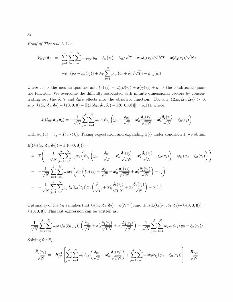
34

Proof of Theorem 1. Let

VNT (δ) =J∑

j=1

T∑

t=1

N∑

i=1

ωjρτj (yit − ξit(τj) − δ0i/√

T − x′itδ1(τj)/

√NT − x′

iδ2(τj)/√

N)

−ρτj (yit − ξit(τj)) + λT

N∑

i=1

ρτm(ai + δ0i/√

T ) − ρτm(ai)

where τm is the median quantile and ξit(τj) = x′itβ(τj) + x′

iγ(τj) + ai is the conditional quan-

tile function. We overcome the difficulty associated with infinite dimensional vectors by concen-

trating out the δ2t’s and δ0i’s effects into the objective function. For any (Δ0i, Δ1, Δ2) > 0,

sup ||k(δ0i, δ1, δ2) − k(0,0,0) − E(k(δ0i, δ1, δ2) − k(0,0,0))|| = op(1), where,

kt(δ0i, δ1, δ2) = −1

√N

J∑

j=1

N∑

i=1

ωjxiψτj

(

yit −δ0i√T

− x′it

δ1(τj)√TN

− x′i

δ2(τj)√N

− ξit(τj)

)

with ψτj (u) = τj − I(u < 0). Taking expectation and expanding k(∙) under condition 1, we obtain

E((kt(δ0i, δ1, δ2)) − kt(0,0,0))) =

= E

(

−1

√N

J∑

j=1

N∑

i=1

ωjxi

(

ψτj

(

yit −δ0i√T

− x′it

δ1(τj)√TN

− x′i

δ2(τj)√N

− ξit(τj)

)

− ψτj (yit − ξit(τj)

))

= −1

√N

J∑

j=1

N∑

i=1

ωjxi

(

Fit

(

ξit(τj) +δ0i√T

+ x′it

δ1(τj)√TN

+ x′i

δ2(τj)√N

)

− τj

)

= −1

√N

J∑

j=1

N∑

i=1

ωjfit(ξit(τj))xi

(δ0i√T

+ x′it

δ1(τj)√TN

+ x′i

δ2(τj)√N

)

+ op(1)

Optimality of the δ2t’s implies that kt(δ0i, δ1, δ2) = o(N−1), and thus E(kt(δ0i, δ1, δ2)−kt(0,0,0)) =

kt(0,0,0). This last expression can be written as,

1√

N

J∑

j=1

N∑

i=1

ωjxifit(ξit(τj))

(δ0i√T

+ x′it

δ1(τj)√TN

+ x′i

δ2(τj)√N

)

=1

√N

J∑

j=1

N∑

i=1

ωjxiψτj (yit − ξit(τj))

Solving for δ2,

δ2(τj)√N

= −h−1jit

J∑

j=1

N∑

i=1

ωjxij

(δ0i√T

+ x′it

δ1(τj)√TN

)

+J∑

j=1

N∑

i=1

ωjxiψτj (yit − ξit(τj))

+RNt√

N

35

where hjit =∑

j

∑i ωjxix

′ij , xij = (fit(ξit(τj))xit)itj and R is the remainder term. Substituting

the δ2t’s, we denote

k(δ0i, δ1) = −1

√T

J∑

j=1

T∑

t=1

ωjψτj

(

yit −δ0i√T

− x′it

δ1(τj)√TN

− x′i

δ2(τj)√N

− ξit(τj)

)

+2λT√T

ψτm

(

ai +δ0i√T

)

Taking expectation and expanding as above, we obtain under conditions 1-2,

E((k(δ0i, δ1)) − k(0,0))) =

= E

(

−1

√T

J∑

j=1

T∑

t=1

ωj(ψτj (yit −δ0i√T

− x′it

δ1(τj)√TN

− x′i

δ2(τj)√N

− ξit(τj)) + 2λT√T

ψτm

(

ai +δ0i√T

)

+1

√T

J∑

j=1

T∑

t=1

ωjψτj (yit − ξit(τj)) − 2λT√T

ψτm(ai)

)

= −1

√T

J∑

j=1

T∑

t=1

ωj

(

Fit

(

ξit(τj) +δ0i√T

+ x′it

δ1(τj)√TN

+ x′i

δ2(τj)√N

)

− τj

)

+ 2λT√T

(

Fa

(

−δ0i√T

)

−12

)

= −1

√T

J∑

j=1

T∑

t=1

ωjfit(ξit(τj))

(δ0i√T

+ x′it

δ1(τj)√TN

+ x′i

δ2(τj)√N

)

− 2λT√T

fa(0)δ0i√T

+ op(1)

= −1

√T

J∑

j=1

T∑

t=1

ωjfit(ξit(τj))

(δ0i√T

+ x′it

δ1(τj)√TN

− x′ih

−1jit

J∑

j=1

N∑

i=1

ωjxij

(δ0i√T

+ x′it

δ1(τj)√TN

)

−x′ih

−1jit

J∑

j=1

N∑

i=1

ωjxiψτj (yit − ξit(τj)) + x′i

RNt√N

)

− 2λT√T

fa(0)δ0i√T

+ op(1)

= −1

√T

J∑

j=1

T∑

t=1

ωjfit(ξit(τj))

((

witjδ0i√T

+ μjitx′it

δ1(τj)√TN

)

− x′ih

−1jitωjxiψτj (yit − ξit(τj)) + x′

i

RNt√N

)

where μjit = 1 − x′ih

−1jit xij , fi = T−1

∑Jj=1

∑Tt=1 ωjfit(ξit(τj)), and witj = μitj + f−1

i λT /√

Tfa(0).

Optimality of the δ0i’s implies that k(δ0i, δ1) = o(T−1), and thus E(k(δ0i, δ1) − k(0,0)) = k(0,0).

Therefore,

1√

T

J∑

j=1

T∑

t=1

ωjfitwitjδ0i√T

+1

√T

J∑

j=1

T∑

t=1

ωjfitμjitx′it

δ1(τj)√TN

=1

√T

J∑

j=1

T∑

t=1

ωjfitμitjψτj (yit − ξit(τj)) + 2λT√T

ψτm(ai) −1

√T

J∑

j=1

T∑

t=1

ωjfitx′i

RNt√N

+RT i√

T

36

The asymptotic (Bahadur) representation of the individual specific effect relates to the slope pa-

rameter in the following way,

δ0i√T

= −f−1ji

1T

J∑

j=1

T∑

t=1

ωjfit(ξit(τj))μitjx′it

δ1(τj)√TN

+ f−1ji

(1T

J∑

j=1

T∑

t=1

ωjfitμitjψτj (yit − ξit(τj))

+2λT√T

ψτm(ai)√T

−1T

J∑

j=1

T∑

t=1

ωjfitx′i

RNt√N

)

+RT i√

T= −

J∑

j=1

xit(τj)′ δ1(τj)√

TN+ rit,

where fji = T−1∑

j

∑t ωjfitwitj and xit =

∑t ωjfitμitjx

′it/Tfi. The term rit includes the last

four terms of the right hand side of the Bahadur presentation of the individual effects. By Lemma

1 in Lamarche (2010), the terms involving rit converge to zero when δ0i/√

T is inserted in the

objective function. This requires T growing faster than N , which is satisfied for some values of c

in Assumption 5 (See Kato, Galvao and Montes-Rojas (2012) for rates of convergence under fairly

general conditions).

We now replace the asymptotic representation of the individual specific effect in the objective

function, and decompose the equation in four terms defined as,

V(1)TN (δ1) = −

J∑

j=1

T∑

t=1

N∑

i=1

ωj(x′it − xi(τj)

′)(δ1(τj)/√

NT )ψτj (yit − ξit(τj))

V(2)TN (δ1) =

J∑

j=1

T∑

t=1

N∑

i=1

ωj

∫ vitj,TN

0(I(yit − ξit(τj) ≤ s) − I(yit − ξit(τj) ≤ 0))ds

V(3)TN (δ1) = −λT

J∑

j=1

N∑

i=1

xi(τj)′(δ1(τj)/

√NT )ψτm(ai)

V(4)TN (δ1) = λT

N∑

i=1

∫ x′iδ1/√

TN

0(I(ai ≤ s) − I(ai ≤ 0))ds

with vitj,TN = (x′it − xi(τj)′)δ1(τj)/

√TN . The first term is asymptotically Gaussian. By the

Lindeberg-Feller Central Limit Theorem, and conditions 3-4,

V(1)TN (δ1) = −

1√

TN

J∑

j=1

T∑

t=1

N∑

i=1

ωj(x′it − xi(τj)

′)δ1(τj)ψτj (yit − ξit(τj)) −δ′1B

The second term converges in probability to a quadratic term in δ1,

EV(2)TN (δ1) =

12TN

J∑

j=1

T∑

t=1

N∑

i=1

ωjfit(ξit(τj))((x′it − xi(τj)

′)δ1(τj))2 + o(1) →

12δ′

1Σ1δ1

37

The variance of V(2)TN (δ1) converges to zero by condition 4. Similarly, by the Lindeberg-Feller

Central Limit Theorem, the Slutsky Theorem, and conditions 3-4, the third term is asymptotically

Gaussian,

V(3)TN (δ1) = −

λT√T

1√

N

J∑

j=1

N∑

i=1

xi(τj)′δ1(τj)ψτm(ai) −λδ′

1C,

where C is a Gaussian vector independent of B with covariance Σ2. The last last term has a

quadratic contribution,

E(V

(4)TN (δ1)

)=

λT

2TN

N∑

i=1

fa(0)(x′iδ1)

2 + o(1) →12λδ′

1Σ3δ1

It follows that VTN (δ1) is convex and V0(δ1) has a unique minimum, and then argmin(VTN (δ1(τ)))

argmin(V0(δ1(τ))). Therefore,

√NT (β(τ, λ) − β(τ)) (Σ1 + λΣ3)

−1(B+ λC).

The penalized estimator converges to a Gaussian random variable with mean zero and covariance

Avar(√

NT (β(τ, λ)) = (Σ1 + λΣ3)−1(Σ0 + λ2Σ2)(Σ1 + λΣ3)−1.

We now derive the distribution of β(τ). Consider the following objective function for the penalized

estimator that shrinks endogenous αi’s as,

VNT (η) =T∑

t=1

N∑

i=1

ρτ

(

yit − κit(τ) −η0i√T

− x′it

η1(τ)√

NT

)

−ρτ (yit−κit(τ))+λT

N∑

i=1

ρτ

(

αi +η0i√T

)

−ρτ (αi)

where τ is the median quantile and κit(τ) = x′itβ(τ) + αi is the conditional quantile function.

Without loss of generality, we consider the location si = x′iγ in a neighborhood of 0. For any

(Δ0i, Δ1) > 0,

sup|η0i|<Δ0, ||η1||<Δ1

||v(η0i, η1) − v(0,0) − E(v(η0i, η1) − v(0,0))|| = op(1)

where,

v(η0i, η1) = −1

√T

T∑

t=1

ψτ

(

yit −η0i√T

− x′it

η1(τ)√

TN− κit(τ)

)

+ 2λT√T

ψτ

(

αi +η0i√T

)

38

Taking expectation and expanding the function v as in Theorem 1, we obtain

E((v(η0i, η1)) − v(0,0))) =

= E

(

−1

√T

T∑

t=1

(ψτ

(

yit −η0i√T

− x′it

η1(τ)√

TN− κit(τ)

)

+ 2λT√T

ψτ

(

αi +η0i√T

)

+1

√T

T∑

t=1

ψτ (yit − κit(τ)) − 2λT√T

ψτ (αi)

)

= −1

√T

T∑

t=1

(

Fit

(

κit(τ) +η0i√T

+ x′it

η1(τ)√

TN

)

− τ

)

+ 2λT√T

(

τ − Fa

(

−η0i√T

))

= −1

√T

T∑

t=1

fit(κit(τ))

(η0i√T

+ x′it

η1(τ)√

TN

)

−λT√T

fa(si)η0i√T

+ o(1)

Optimality of the η0i’s implies that v(η0i, η1) = o(T−1), and thus E(v(η0i, η1) − v(0,0)) = v(0,0).

Letting fi = T−1∑T

t=1 fit(κit(τ)) + λT /√

Tfa(si)/√

T , we find that

η0i√T

= −(Tfi)−1

T∑

t=1

fit(κit(τ))x′it

η1(τ)√

TN+ rit ≈ −x′

i

η1(τ)√

TN

where xi =∑

t fit(κit(τ))xit/Tfi. By Koenker’s (2004) Theorem 1 and Lamarche’s (2010) Lemma

1, the components of r are asymptotically negligible. Therefore, we replace η0i/√

T in the objective

function, and we decompose the function in four parts:

V(1)TN (η1(τ)) = −

T∑

t=1

N∑

i=1

(x′it − x′

i)(η1(τ)/√

NT )ψτ (yit − κit(τ))

V(2)TN (η1(τ)) =

T∑

t=1

N∑

i=1

∫ vit,TN

0(I(yit − κit(τ) ≤ s) − I(yit − κit(τ) ≤ 0))ds

V(3)TN (η1(τ)) = −λT

N∑

i=1

x′i

(η1(τ)/

√NT

)sgn(αi)

V(4)TN (η1(τ)) = λT

N∑

i=1

∫ x′iη1(τ)√

TN

0(I(αi ≤ s) − I(αi ≤ 0))ds

with vit,TN = (x′it − x′

i)η1(τ)/√

TN . The first term is asymptotically Gaussian,

V(1)TN (η1(τ)) = −

1√

TN

T∑

t=1

N∑

i=1

(x′it − x′

i)η1(τ)ψτ (yit − κit(τ)) −η1(τ)′B

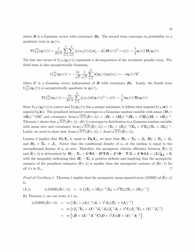
39

where B is a Gaussian vector with covariance H0. The second term converges in probability to a

quadratic term in η1(τ),

EV(2)TN (η1(τ)) =

12TN

T∑

t=1

N∑

i=1

fit(κit(τ))((x′it − x′

i)H1(τ))2 + o(1) →12η1(τ)′H1η1(τ)

The last two terms of VTN (η1(τ)) represents a decomposition of the stochastic penalty term. The

third term is also asymptotically Gaussian,

V(3)TN (η1(τ)) = −

λT√T

1√

N

N∑

i=1

x′iη1(τ)sgn(αi) −λη1(τ)′C

where C is a Gaussian vector independent of B with covariance H2. Lastly, the fourth term

V(4)TN (η1(τ)) is asymptotically quadratic in η1(τ),

EV(4)TN (η1(τ)) =

λT

2TN

N∑

i=1

fa(si)(x′iη1(τ))2 + o(1) →

12λη1(τ)′H3η1(τ)

Since VTN (η1(τ)) is convex and V0(η1(τ)) has a unique minimum, it follows that argmin(VTN (•))

argmin(V0(•)). The penalized estimator converges to a Gaussian random variable with mean (H1+

λH3)−1λEC and covariance Avar(√

NT (β(τ, λ)) = (H1 + λH3)−1(H0 + λ2H2)(H1 + λH3)−1.

Theorem 1 shows that√

NT (β(τ, λ)−β(τ)) converges in distribution to a Gaussian random variable

with mean zero and covariance Avar(√

NT (β(τ, λ)) = (Σ1 + λΣ3)−1(Σ0 + λ2Σ2)(Σ1 + λΣ3)−1.

Lastly, we need to show that Avar(√

NT (β(τ, λ)) < Avar(√

NT (β(τ, λ)).

Lemma 2 implies that PΥXo is equal to PΦXo, we have that H0 = Σ0 = J0, H2 = Σ2 = J2,

and H3 = Σ3 = J3. Notice that the conditional density of αi at the median is equal to the

unconditional density of ai at zero. Therefore, the asymptotic relative efficiency between β(τ, λ)

and β(τ, λ) is determined by H1 −Σ1 = L′ΦL−R′ΥR = L′(Φ−Υ)L = L′ΦΛL = ||L||2ΦΛ > 0,

with the inequality indicating that H1 − Σ1 is positive definite and implying that the asymptotic

variance of the penalized estimator β(τ, λ) is smaller than the asymptotic variance of β(τ, λ) for

all λ’s in R+. �

Proof of Corollary 1. Theorem 1 implies that the asymptotic mean squared error (AMSE) of β(τ, λ)

is,

trAMSE(β(τ, λ)) = tr{(Σ1 + λΣ3)

−1(Σ0 + λ2Σ2)(Σ1 + λΣ3)−1}

.(A.1)

By Theorem 1, we can write A.1 as,

trAMSE(β(τ, λ)) = tr{(Σ1 + λJ3)

−1(J0 + λ2J2)(Σ1 + λJ3)−1}

= tr{(J−1

3 Σ1 + λI)−1J−13 J2(J

−12 J0 + λ2I)(J−1

3 Σ1 + λI)−1J−13

}

= tr{

(B + λI)−1A−1C(D + λ2I)(B + λI)−1A−1}

.

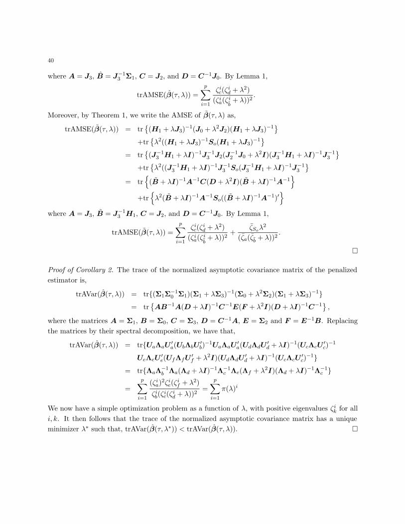
40

where A = J3, B = J−13 Σ1, C = J2, and D = C−1J0. By Lemma 1,

trAMSE(β(τ, λ)) =p∑

i=1

ζic(ζ

id + λ2)

(ζia(ζ

ib+ λ))2

.

Moreover, by Theorem 1, we write the AMSE of β(τ, λ) as,

trAMSE(β(τ, λ)) = tr{(H1 + λJ3)

−1(J0 + λ2J2)(H1 + λJ3)−1}

+tr{λ2((H1 + λJ3)

−1So(H1 + λJ3)−1}

= tr{(J−1

3 H1 + λI)−1J−13 J2(J

−12 J0 + λ2I)(J−1

3 H1 + λI)−1J−13

}

+tr{λ2((J−1

3 H1 + λI)−1J−13 So(J

−13 H1 + λI)−1J−1

3

}

= tr{

(B + λI)−1A−1C(D + λ2I)(B + λI)−1A−1}

+tr{

λ2(B + λI)−1A−1So((B + λI)−1A−1)′}

where A = J3, B = J−13 H1, C = J2, and D = C−1J0. By Lemma 1,

trAMSE(β(τ, λ)) =p∑

i=1

ζic(ζ

id + λ2)

(ζia(ζ

ib+ λ))2

+ζSoλ

2

(ζa(ζb + λ))2.

�

Proof of Corollary 2. The trace of the normalized asymptotic covariance matrix of the penalized

estimator is,

trAVar(β(τ, λ)) = tr{(Σ1Σ−10 Σ1)(Σ1 + λΣ3)

−1(Σ0 + λ2Σ2)(Σ1 + λΣ3)−1}

= tr{AB−1A(D + λI)−1C−1E(F + λ2I)(D + λI)−1C−1

},

where the matrices A = Σ1, B = Σ0, C = Σ3, D = C−1A, E = Σ2 and F = E−1B. Replacing

the matrices by their spectral decomposition, we have that,

trAVar(β(τ, λ)) = tr{UaΛaU′a(UbΛbU

′b)

−1UaΛaU′a(UdΛdU

′d + λI)−1(UcΛcU

′c)

−1

UeΛeU′e(UfΛfU ′

f + λ2I)(UdΛdU′d + λI)−1(UcΛcU

′c)

−1}

= tr{ΛaΛ−1b Λa(Λd + λI)−1Λ−1

c Λe(Λf + λ2I)(Λd + λI)−1Λ−1c }

=p∑

i=1

(ζia)

2ζie(ζ

if + λ2)

ζib(ζ

ic(ζ

id + λ))2

=p∑

i=1

π(λ)i

We now have a simple optimization problem as a function of λ, with positive eigenvalues ζik for all

i, k. It then follows that the trace of the normalized asymptotic covariance matrix has a unique

minimizer λ∗ such that, trAVar(β(τ, λ∗)) < trAVar(β(τ, λ)). �