Robust digital control using pole placement with sensitivity function shaping method

*Correspondence to: I.D. Landau, Laboratoire d’Automatique de Grenoble, ENSIEG, BP. 46, 38402 Saint Martind’Heres, France

CCC 1049-8923/98/020191—20$17.50( 1998 John Wiley & Sons, Ltd.

INTERNATIONAL JOURNAL OF ROBUST AND NONLINEAR CONTROL, VOL. 8, 191—210 (1998)

Int. J. Robust Nonlinear Control, 8, 191—210 (1998)

ROBUST DIGITAL CONTROL USING POLE PLACEMENTWITH SENSITIVITY FUNCTION SHAPING METHOD

I.D. LANDAU* AND A. KARIMI

Laboratoire d’Automatique de Grenoble, ENSIEG, BP. 46, 38402 Saint Martin d’He% res, France

SUMMARY

It is shown in this paper that based on identified discrete-time models a robust digital linear controller canbe designed using the pole placement method combined with sensitivity function shaping in the frequencydomain. Two different design techniques are presented. The first one is based on the shaping of thesensitivity functions using the fixed parts in the controller and the auxiliary poles of the closed loop whilekeeping the dominant poles in the desired places. The main idea of the second one is to determinea weighting filter for the output sensitivity function in an H

=optimization approach which assures partial

pole placement and desired performances. In this technique the weighting filter is interpreted as the inverseof the desired output sensitivity function and is computed using a constrained optimization program. Theapplication of this technique on a flexible transmission system is presented. ( 1998 John Wiley & Sons, Ltd.

Key words: digital control; robust control; pole placement; H=

optimization

1. INTRODUCTION

The controller design methodology considered in this paper is based on pole placement combinedwith the shaping of the sensitivity function. The computation of the controller in the poleplacement technique requires the specification of the desired closed-loop poles (the nominalstability problem) and of some fixed parts of the controller for the rejection of disturbances atvarious frequencies (the nominal performance problem). However, this is not enough to guaranteethe robustness of the design with respect to the plant model uncertainties (the robust stability androbust performance problem). A robust controller design requires also the shaping of the sensitivityfunctions. The sensitivity functions, particularly the output sensitivity function, are key indicatorsfor the nominal and robust performance as well as for the robust stability of the closed-loopsystem. The inverse of the maximum value of the output sensitivity function, i.e., the inverse of itsH

=norm, gives the minimum distance between the Nyquist plot of the open-loop system and the

critical point [!1, j0]. This quantity, called the modulus margin, is a much more significantrobustness indicator than the phase and gain margins. On the other hand, conditions for assuringa certain delay margin which is also a very important robustness indicator, particularly in the highfrequency region, can also be expressed in terms of the shape of the output sensitivity function. Itseems therefore reasonable to combine the pole placement with the shaping of the output

sensitivity function (or eventually with other sensitivity functions) in order to design robust digitalcontrollers for SISO plants.

This paper addresses the robust controller design problem for two cases:

(a) Only one plant model is available. In this case we consider certain robustness marginswhich translate into templates for the sensitivity functions.

(b) Several plant models are given or an estimation of the model uncertainty in the frequencydomain is available. In this case again the uncertainties will translate into templates for thesensitivity functions.

For this purpose two different techniques are given. In the first one an iterative method ispresented for correctly specifying the desired closed-loop poles and the fixed parts of thecontroller in order to assure the nominal performance, the desired robustness margins, as well asthe robust stability of the closed loop for given classes of plant model uncertainties. This methodhas been applied on a large number of real systems.1~4 In the second one a systematic procedureto compute a controller based on partial pole placement with sensitivity function shaping viaH

=optimization is presented. In this technique the weighting filter in the H

=approach is

interpreted as the inverse of the desired output sensitivity function. Therefore, all of the conditionsand the constraints on the output sensitivity function can be considered for the inverse of theweighting filter. One of the properties of the output sensitivity function is that it satisfies theZames—Francis equality.5,6 This equality then is used as a performance index in a constrainedoptimization program in order to find the unknown parameters of the desired sensitivity function.Once the desired sensitivity function is obtained, an H

=approach is used for computing the

controller. The main differences between this technique and the partial pole placement presentedin References 7 and 8 are as follows:

d The weighting filter is interpreted as the inverse of the desired output sensitivity function.d This filter is the result of an optimization problem so it is not necessary to find the

parameters of the filter by trial and error.d The controller design can be carried out using only one weighting filter.d The conditions on the weighting filter in order to obtain a stable controller are intro-

duced.

The paper is organized as follows: Section 2 reviews the R-S-T controller and the notation.Section 3 gives the various sensitivity functions associated with the R-S-T controller. In Section 4a template for the output sensitivity function is defined. The shaping of the sensitivity functionwith pole placement technique is described in Section 5. The shaping of the sensitivity functionwith partial pole placement using H

=optimization is presented in Section 6. The application of

this technique on a flexible transmission system is given in Section 7. Section 8 gives theconcluding remarks.

2. R-S-T CONTROLLER

Figure 1 shows a schematic diagram of an R-S-T controller. The discrete time plant is describedby the following transfer operator:

H (q~1)"q~dB(q~1)

A(q~1)(1)

192 I.D. LANDAU AND A. KARIMI

( 1998 John Wiley & Sons, Ltd.Int. J. Robust Nonlinear Control, 8, 191—210 (1998)

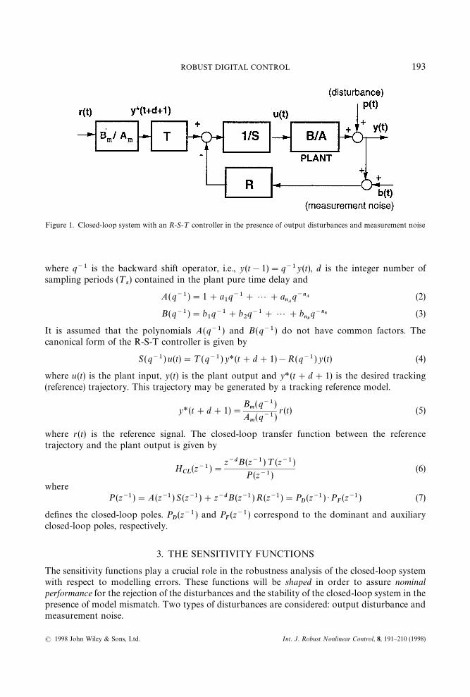
Figure 1. Closed-loop system with an R-S-¹ controller in the presence of output disturbances and measurement noise

where q~1 is the backward shift operator, i.e., y(t!1)"q~1y(t), d is the integer number ofsampling periods (¹

s) contained in the plant pure time delay and

A(q~1)"1#a1q~1#2#a

nAq~nA (2)

B(q~1)"b1q~1#b

2q~1#2#b

nBq~nB (3)

It is assumed that the polynomials A(q~1) and B (q~1) do not have common factors. Thecanonical form of the R-S-T controller is given by

S (q~1) u(t)"¹(q~1) y*(t#d#1)!R(q~1) y (t) (4)

where u (t) is the plant input, y(t) is the plant output and y*(t#d#1) is the desired tracking(reference) trajectory. This trajectory may be generated by a tracking reference model.

y* (t#d#1)"B

m(q~1)

Am(q~1)

r (t) (5)

where r(t) is the reference signal. The closed-loop transfer function between the referencetrajectory and the plant output is given by

HCL

(z~1)"z~dB (z~1)¹(z~1)

P (z~1)(6)

whereP (z~1)"A(z~1 ) S (z~1)#z~dB (z~1 )R(z~1)"P

D(z~1) ·P

F(z~1) (7)

defines the closed-loop poles. PD(z~1) and P

F(z~1) correspond to the dominant and auxiliary

closed-loop poles, respectively.

3. THE SENSITIVITY FUNCTIONS

The sensitivity functions play a crucial role in the robustness analysis of the closed-loop systemwith respect to modelling errors. These functions will be shaped in order to assure nominalperformance for the rejection of the disturbances and the stability of the closed-loop system in thepresence of model mismatch. Two types of disturbances are considered: output disturbance andmeasurement noise.

ROBUST DIGITAL CONTROL 193

( 1998 John Wiley & Sons, Ltd. Int. J. Robust Nonlinear Control, 8, 191—210 (1998)

The various sensitivity functions can be established from Figure 1. The transfer functionbetween the disturbance p(t) and the plant output y (t) (output sensitivity function) is given by

Syp

(z~1)"A(z~1)S(z~1)

A(z~1) S (z~1)#z~dB (z~1) R(z~1)"

A (z~1) S (z~1)

P (z~1)(8)

This function is often called simply the sensitivity function in the literature and is denoted by S.The transfer function between the disturbance p (t) and the plant input u (t) (input sensitivityfunction) is given by

Sup

(z~1)"!A(z~1) R(z~1)

A(z~1)S (z~1)#z~dB(z~1)R (z~1)"

!A(z~1)R(z~1)

P (z~1)(9)

This function is often denoted by º in the literature. The transfer function between themeasurement noise b (t) and the plant output y (t) (noise sensitivity function) is given by

Syb

(z~1)"!z~dB (z~1) R(z~1)

A (z~1) S(z~1)#z~dB (z~1)R(z~1)"

!z~dB (z~1)R(z~1)

P (z~1)(10)

This function with a positive sign is called the complementary sensitivity function denoted by ¹ inthe literature. From equations (8) and (10) it is obvious that

Syp

(z~1)!Syb

(z~1)"1 (11)

4. DEFINITION OF A ‘TEMPLATE’ FOR THE OUTPUT SENSITIVITY FUNCTION

Using the small gain theorem and various representations of the plant uncertainties, the modulusmargin and the delay margin can be converted into robust stability conditions. On the other hand,the robust stability conditions allow the definition of upper templates for the modulus of thevarious sensitivity functions.1,9,10

For a delay margin of one sampling period the robust stability condition is expressed asfollows:11

DSyb

(z~1) D(D (1!z~1) D~1, z"e~ju, 0)u)n (12)

But, from equation (11) we have

1!DSyb

(z~1) D(DSyp

(z~1) D(1#DSyb

(z~1) D (13)

If Syb

(z~1) satisfies the condition (12) then Syp

(z~1) will satisfy the following condition:

1!D1!z~1 D~1(DSyp

(z~1) D(1#D1!z~1 D~1 ; z"e~ju ; 0)u)n (14)

Therefore in order to assure the delay margin *q"¹s, it is required that the modulus of S

yp(z~1)

lies between the bounds defined by a lower template D¼~1 Dinf

"1!D1!z~1 D~1 and an uppertemplate defined by D¼~1 D

sup"1#D1!z~1 D~1 .

The nominal performance requirements and the robust stability conditions lead to the definitionof a desired template for the sensitivity function. We will subsequently consider the definition ofsuch a template for the output sensitivity function. The desired template takes, in general, theform shown in Figure 2. Regarding the robust stability, the chosen modulus margin will define themaximum value of the modulus of the output sensitivity function (upper template) and the chosendelay margin will define an upper and a lower template starting, for example, around 0·15 f

s(for

*q"¹s).



Figure 2. Desired template for the output sensitivity function (the case of low frequencies disturbance rejection)

A template for the input sensitivity function also may be defined in the same way. Additiveuncertainty can be used as an upper template to assure the robust stability of the closed-loopsystem. Another upper bound should be considered for the frequencies where the plant gain isvery low, usually in the high frequencies and at the frequencies of the low damped zeros of theplant model, in order to prevent the unwanted excitation of control input which has no effect inthe output.

5. METHOD A

5.1. Pole placementIn this section the pole placement technique is reviewed; for more details see Reference 12. The

dominant closed-loop poles are chosen to satisfy the desired regulation performance. Theauxiliary poles can be introduced either for filtering effects in certain frequency regions or forreducing the stress on the actuator as well as for improving the robustness of the closed-loopsystem (as will be shown subsequently).

For different reasons, i.e., disturbance rejection, signal blocking, etc. the polynomials R(z~1)and S (z~1) generally contain some fixed parts which are specified before solving equation (7) (forexample the polynomial S(z~1) should contain a factor (1!z~1) for a null steady state error). Inorder to take into account these prespecified parts, the polynomials R(z~1) and S (z~1) arefactored as:

R(z~1)"R@ (z~1) ·HR(z~1) (15)

S(z~1)"S@(z~1) ·HS(z~1) (16)

where HR(z~1) and H

S(z~1) are the prespecified polynomials.The closed-loop poles in equation

(7) become

P(z~1)"A(z~1) ·HS(z~1) ·S@(z~1)#z~dB (z~1) ·H

R(z~1) · R@(z~1) (17)



The design procedure can be summarized as follows:

(a) Choose the desired closed-loop poles P (z~1), the fixed parts of the controller HR(z~1),

HS(z~1) and the desired tracking dynamics B

m(z~1)/A

m(z~1).

(b) Compute S@ (z~1) and R@(z~1) by solving equation (17) and consequently compute S (z~1)and R(z~1) using equations (15) and (16).

(c) Compute the prefilter ¹ (z~1)"P (z~1)/B (1). This choice leads to the following transferfunction between the reference and the plant output:

Hyr

(z~1)"z~dB

m(z~1)

Am(z~1)

·B (z~1)

B(1)(18)

Another method consists of taking ¹ (z~1)"R(1).

Hyr

(z~1)"z~dB

m(z~1)

Am(z~1)

·B (z~1)

P (z~1)·P (1)

B (1)(19)

Of course intermediate solutions between (18)- and (19)- can also be obtained, that is, tochoose ¹(z~1) such that it compensates only a part of the poles of P(z~1).

5.2. Shaping the sensitivity functions

The dominant poles PD(z~1), the auxiliary poles P

F(z~1) and the two filters H

R(z~1) and

HS(z~1) are the tools for shaping the sensitivity functions in order to meet the specifications

defined by the desired templates. Placing a pair of complex zeros in HS(z~1) or in H

R(z~1)

decreases the magnitude of the modulus of the sensitivity functions around the frequencies ofthese zeros. Introducing a pair of pure imaginary zeros at a certain frequency in H

R(z~1) will

make DSyp

D"1 and DSup

D"0 at this frequency. Complex zeros will bring DSyp

D closer to the 0 dBaxis. Putting some asymptotically stable real high frequency poles in P(z~1) will cause anattenuation of DS

ypD in the domain of attenuation of 1/P

F(z~1). Placing a pair of complex poles at

a certain frequency in PF(z~1) will lead to the increase of DS

ypD around this frequency. Introducing

a term of (1#z~1) in HR(z~1) will open the loop in the high frequencies.

The underlying philosophy of the design is to choose the closed-loop poles and the fixed partsof the controller in order to bring the sensitivity functions within the defined templates. Thiscontroller will meet the conditions on modulus and delay margin as well as the attenuation bandand will assure the robust stability of the closed-loop system against the parameter uncertainty.The shaping method which is an iterative procedure (generally converging in few steps) is asfollows:

Step Id Choose the dominant closed-loop poles of P (z~1) and the fixed part of R(z~1) and S (z~1) in

order to meet the nominal performance specifications.d Compute the controller.d Check the shape of the output sensitivity function. If the upper bound of the template is not

satisfied, generally two situations are identified:

(a) the maximum of the output sensitivity function is located in the frequency range next tothe attenuation band. In this case, go to step II;

(b) the maximum of the output sensitivity function is located in the high frequency range(near 0·5 f

s). In this case jump to step III.



Step IId Add a pair of complex zeros to H

S(z~1) :

HS(z~1)"1#a

1z~1#a

2z~2 (20)

The frequency of these zeros is chosen close to the frequency where the maximum of the DSyp

Doccurs (between the maximum frequency of the attenuation band and the frequency whereDS

ypDmax

occurs). The damping factor is chosen such that the introduced attenuation bringsDS

ypDmax

below the admissible value. Typical values are between f"0·3 to 0·8.d Recompute the controller. If DS

ypD is too large in the high frequency range, go to step III.

RemarkThe effects of these additional zeros are in general:(a) a reduction in the modulus of the sensitivity function in the region next to the attenuation

band;(b) an increase in the maximum of the modulus of the sensitivity function in the high frequency

range (in general its maximum is shifted in the high frequency range);(c) an increase in the attenuation band.

Step IIId Add auxiliary high frequency poles of the form:

PF(z~1)"(1!p

1z~1)nF ; 0·05)p

1)0·5 (21)

where

nF)n

P!n

D; n

P"(degP )

max; n

D"degP

D(22)

with increasing values of p1

starting from 0·05 till the specifications on the DSyp

D in the highfrequency range are met. It should be mentioned that high frequency auxiliary poles shift, ingeneral, the maximum of the DS

ypD towards the lower frequency range. If the DS

ypDmax

issatisfactory, stop here, if not go to step IV.

Step IV This step is similar to step IId If the new maximum is close to the one resulting after step I, change accordingly the

frequency and the damping of the zeros introduced in HS.

d If the new maximum is at a significantly different frequency, add a new pair of complex zerosin H

S(z~1) at a frequency close to the maximum of DS

ypD. The damping is chosen in order to

bring DSyp

Dmax

below the maximum acceptable value. If the results are unsatisfactory, go tostep V.

Step Vd The value of the real auxiliary poles (defined in step III) can be increased.d If necessary, the dominant poles may also be slowed down.d End of the procedure for the shaping of the output sensitivity function. Go to step VI.

Step VId Check the input sensitivity function. Add, if necessary, high frequency complex zeros in

HR(z~1) (often at 0·5 f

s).



Figure 3. The flow chart of the iterative procedure of Method A

d Check again the output sensitivity function. Three different situations may occur:

(a) the output sensitivity function is over the template in the high frequencies. Go to step V;(b) the output sensitivity function is over the template in the low frequencies. Go to step IV;(c) the output sensitivity function is inside the template. End of the procedure.

The flowchart of this procedure is illustrated in Figure 3.



6. METHOD B

The problem is to find a controller which guarantees the internal stability of the closed loop,assures desired dominant closed-loop poles and satisfies certain constraints on the outputsensitivity function. To solve this problem, first a desired sensitivity function which satisfies theconstraints on the output sensitivity function is computed. The use of an appropriate fixed partin the desired sensitivity function will assure a partial pole placement to desired values. Then theinverse of the desired sensitivity function will be used as a weighting filter to minimize the infinitynorm of the output sensitivity function. Therefore, the real output sensitivity function willapproximate the desired one. The internal stability of the closed loop will be guaranteed by usingthe Youla parametrization in the H

=optimization.

The demonstration will be carried out in discrete time but it could be done for continuous timeas well.

6.1. Desired sensitivity function

It was shown in Section 3 that the output sensitivity function may be written in the followingform:

Syp

(z~1)"A(z~1)S (z~1)

A(z~1) S (z~1)#z~dB (z~1) R (z~1)"

A(z~1)S (z~1)

PD(z~1) P

F(z~1)

(23)

Where PD

and PFare the dominant and auxiliary poles of the closed loop. Since A and the desired

closed-loop poles PD

are known, we can fix them in the desired sensitivity function. Therefore wecan define

Sd(z~1)"

A(z~1)

PD(z~1)

·X(z~1)

½ (z~1)(24)

where Sd

is the desired sensitivity function and the polynomials X and ½ should be computedusing an optimization method.

It can be proved7 that the denominator of Sdwill appear as a part of the final closed-loop poles

if the inverse of Sdis utilized as a weighting filter in the H

=optimization method. This technique,

known as partial pole placement,7,8 rejustifies the interpretation of the weighting filter as theinverse of the desired sensitivity function. On the other hand, natural choice of the polynomialA in the numerator of S

dwill prevent the presence of the open-loop poles as closed-loop poles.7

In the next step, the polynomials X and ½ will be parametrized. They are parametrizedpreferably as products of real zeros and poles, respectively, in order firstly to prevent theunwanted cancellation of the desired poles P

Dor of the open-loop poles A which may contain low

damped complex poles, and secondly to avoid the oscillatory poles in the polynomial ½ whichwill appear consequently as the closed-loop poles.

Then the polynomials X and ½ are defined as follows:

X(z~1)"(1!x1z~1)(1!x

2z~1)2 (1!x

nXz~1) (25)

½(z~1)"(1!y1z~1) (1!y

2z~1)2 (1!y

nYz~1) (26)

h"[x1, x

2,2 , x

nX, y

1, y

2,2 , y

nY] (27)

where x1

to xnX

are the real zeros of X, y1

to ynY

are the real zeros of ½ and h is the vector of theparameters. It may be considered that S

d(z~1, h) is proper and inversely proper, i.e., the order of

the numerator is equal to the order of denominator. This leads to a proper weighting filter for



H=

optimization. It should be mentioned that the properness of the weighting filter can berelaxed.13

It can be shown that the denominator of the weighting filter will appear as a part of thedenominator of the controller. Then, in this approach, the desired fixed parts in the denominatorof the controller can be put directly in the numerator of the S

d. Thus, for example, to reject the

constant disturbances in the output, an integrator may be used in Sd(z~1, h). This can be easily

done by choosing x1"1.

The minimum order of X and ½ depends on the order of A, PD

and the fixed parts of ½. Wehave

nX*n

A#(n

Y).*/

!nPD

(28)

where nA, n

X, n

PDand (n

Y)min

are the orders of A, X, PD

and the fixed parts of ½, respectively. Forexample, if we choose n

PD"n

Aand an integrator in ½ we will obtain n

X"n

Y"1. In this case we

have only to compute one parameter x1. If with this parameter we do not succeed in minimizing

the criterion (which will be explained subsequently) and in satisfying the constraints, we canincrease the order of X and ½ to have more degrees of freedom in the optimization program.

6.2. Performance index

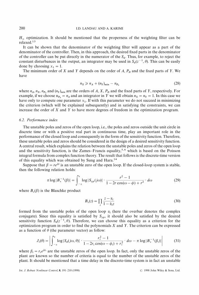
The unstable poles and zeros of the open loop, i.e., the poles and zeros outside the unit circle indiscrete time or with a positive real part in continuous time, play an important role in theperformance of the closed loop and consequently in the form of the sensitivity function. Therefore,these unstable poles and zeros should be considered in the design of a desired sensitivity function.A central result, which explains the relation between the unstable poles and zeros of the open loopand the sensitivity function, is the Zames—Francis equality,5,6 which is based on the Poissonintegral formula from complex function theory. The result that follows is the discrete-time versionof this equality which was obtained by Sung and Hara.14

Suppose that b"rej/ is an unstable zero of the open loop. If the closed-loop system is stable,then the following relation holds:

n log DB~1a (b) D"Pn

~nlog DS

yp( ju) D ·

r2!1

1!2r cos(u!/)#r2· du (29)

where Ba (b) is the Blaschke product

Ba(z)"<i

z!ai

1!a6iz

(30)

formed from the unstable poles of the open loop ai

(here the overbar denotes the complexconjugate). Since this equality is satisfied by S

yp, it should also be satisfied by the desired

sensitivity function Sd(z~1, h ). Therefore, we can choose this equality as a criterion for the

optimization program in order to find the polynomials X and ½. The criterion can be expressedas a function of h (the parameter vector) as follow:

Ji(h)"K P

n

~nlog DS

d( ju, h) D ·

r2i!1

1!2ricos(u!/

i)#r2

i

· du!n log DB~1a (bi) D K (31)

where bi"r

iej/i are the unstable zeros of the open loop. In fact, only the unstable zeros of the

plant are known so the number of criteria is equal to the number of the unstable zeros of theplant. It should be mentioned that a time delay in the discrete-time system is in fact an unstable



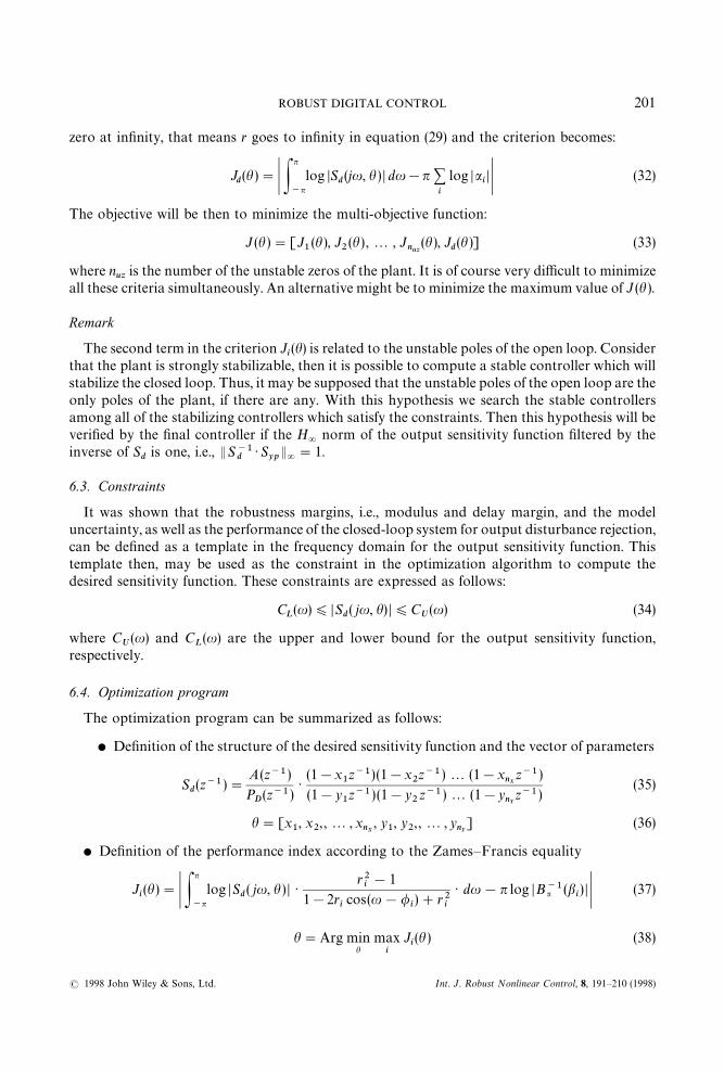
zero at infinity, that means r goes to infinity in equation (29) and the criterion becomes:

Jd(h )"K P

n

~nlog DS

d(ju, h ) D du!n +

i

log DaiD K (32)

The objective will be then to minimize the multi-objective function:

J(h )"[J1(h), J

2(h) ,2 , J

nuz(h), J

d(h )] (33)

where nuz

is the number of the unstable zeros of the plant. It is of course very difficult to minimizeall these criteria simultaneously. An alternative might be to minimize the maximum value of J(h ).

Remark

The second term in the criterion Ji(h) is related to the unstable poles of the open loop. Consider

that the plant is strongly stabilizable, then it is possible to compute a stable controller which willstabilize the closed loop. Thus, it may be supposed that the unstable poles of the open loop are theonly poles of the plant, if there are any. With this hypothesis we search the stable controllersamong all of the stabilizing controllers which satisfy the constraints. Then this hypothesis will beverified by the final controller if the H

=norm of the output sensitivity function filtered by the

inverse of Sd

is one, i.e., ES~1d

· Syp

E="1.

6.3. Constraints

It was shown that the robustness margins, i.e., modulus and delay margin, and the modeluncertainty, as well as the performance of the closed-loop system for output disturbance rejection,can be defined as a template in the frequency domain for the output sensitivity function. Thistemplate then, may be used as the constraint in the optimization algorithm to compute thedesired sensitivity function. These constraints are expressed as follows:

CL(u))DS

d( ju, h) D)C

U(u) (34)

where CU(u) and C

L(u) are the upper and lower bound for the output sensitivity function,

respectively.

6.4. Optimization program

The optimization program can be summarized as follows:

d Definition of the structure of the desired sensitivity function and the vector of parameters

Sd(z~1)"

A(z~1)

PD(z~1)

·(1!x

1z~1)(1!x

2z~1)2 (1!x

nXz~1)

(1!y1z~1) (1!y

2z~1)2 (1!y

nYz~1)

(35)

h"[x1, x

2, ,2, x

nX, y

1, y

2, ,2, y

nY] (36)

d Definition of the performance index according to the Zames—Francis equality

Ji(h)"K P

n

~nlog DS

d( ju, h ) D ·

r2i!1

1!2ricos(u!/

i)#r2

i

· du!n log DB~1a (bi) D K (37)

h"Arg minh

maxi

Ji(h ) (38)



d Definition of the upper and lower bound for the desired sensitivity function

CL(u))DS

d( ju, h ) D)C

U(u) (39)

If the results of the optimization program are not satisfactory in terms of the constraints or theperformance index, we can increase the number of parameters, i.e., the order of X and ½, oreventually we may use a pair of complex poles and zeros in S

d. However, the experimental results

show that even for complex systems it is not necessary to use complex poles and zeros in Sd. This

optimization problem can be solved using the CONSTR instruction in the optimization toolboxof MATLAB.

6.5. H=

optimization

After computing the desired sensitivity function Sd(z~1), the output sensitivity function

Syp

(z~1) filtered by the inverse of Sd(z~1) will be minimized using the H

=optimization method.

This problem, known as the model matching problem, is the simplest problem in the H=

domain.This problem may be solved either iteratively by the standard H

=optimal control problem

using the k-synthesis toolbox in MATLAB or directly by Nevanlinna—Pick’s algorithm.9The second method is more suitable for this technique since in the model matching problemthe optimal solution can be achieved without any iteration. Therefore, a discrete time versionof the Nevanlinna—Pick algorithm has been developed to solve the application problem ofSection 7.

It should be noticed that in this technique only the partial pole placement, i.e., the closed-looppoles defined by P

D, is guaranteed, so it is possible to obtain the other closed-loop poles near to

the unit circle. To avoid this problem we can change the stability domain by choosing a circlewith a radius less than one (or axis shifting in continuous-time domain).

It was mentioned in Section 4 that we need usually to open the loop or to reduce drastically thegain of the polynomial R at certain frequencies where the gain of the system is very low in order toprevent the unwanted excitation in the control input. It means that it is necessary to shape theinput sensitivity function simultaneously with the output sensitivity function, which is called themixed sensitivity problem in the literature.10 An alternative way is to augment the order of theterms of B (the numerator of the plant) by introducing terms of the form (1#az~1) with a'0·7which places zeros at 0·5 f

sand of the form (1#a

1z~1#a

2z~2) which introduce complex zeros at

other desired frequencies. Choosing an appropriate damping factor for the complex zeros willreduce significantly S

upat the corresponding frequencies. These terms correspond to roots which

are very close to the unit circle and will be moved back to the controller (polynomial R ) aftercomputing it. It should be noticed that the stable zeros of the plant will be cancelled by thecontroller in the H

=approach. Then, in order to avoid the cancellation of these zeros, they should

appear as unstable zeros. This is achieved by defining a reduced stability domain, leaving theseroots outside. Using this technique we can shape two sensitivity functions by only one weightingfilter.

7. APPLICATIONS

In this section a flexible transmission system which has been the subject of two benchmarks onadaptive control15 and on robust digital control16 and has been also used as an example byKwakernaak17 is considered. For this system three models of the plant and several specificationsare given.



Figure 4. Schematic diagram of the flexible transmission

7.1. System description

The flexible transmission consists of three horizontal pulleys connected by two elastic belts(Figure 4). The first pulley is driven by a DC motor whose position is controlled by local feedback.The third pulley may be loaded by small disks of different weights. The system input is thereference for the axis position of the first pulley. The system output is the axis position of the thirdpulley measured by a position sensor, sampled and digitized. A PC is used to control the system.The main characteristics of this system are the low damped vibration modes (damping factor lessthan 0·05) and the large variations of their frequencies with the load. The discrete-time identifiedmodels (¹

s"50 ms) of the plant for two extreme situations (no load and full load), as well as for

an intermediate situation are given.Unloaded model:

A0(q~1 )"1!1·41833q~1#1·58939q~2!1·31608q~3#0·88642q~4

B0(q~1 )"0·28261q~1#0·50666q~2 ; d"2

Half load model:

A1(q~1)"1!1·99185q~1#2·20265q~2!1·84083q~3#0·89413q~4

B1(q~1)"0·10276q~1#0·18123q~2 ; d"2

Full load model:

A2(q~1)"1!2·0967q~1#2·3196q~2!1·93353q~3#0·87129q~4

B2(q~1)"0·06408q~1#0·10407q~2 ; d"2

Several time and frequency specifications are considered for this problem which should besatisfied for all loads:

(a) A rise time (0—90% of the final value) of less than 1 s for a step change in the referenceinput.



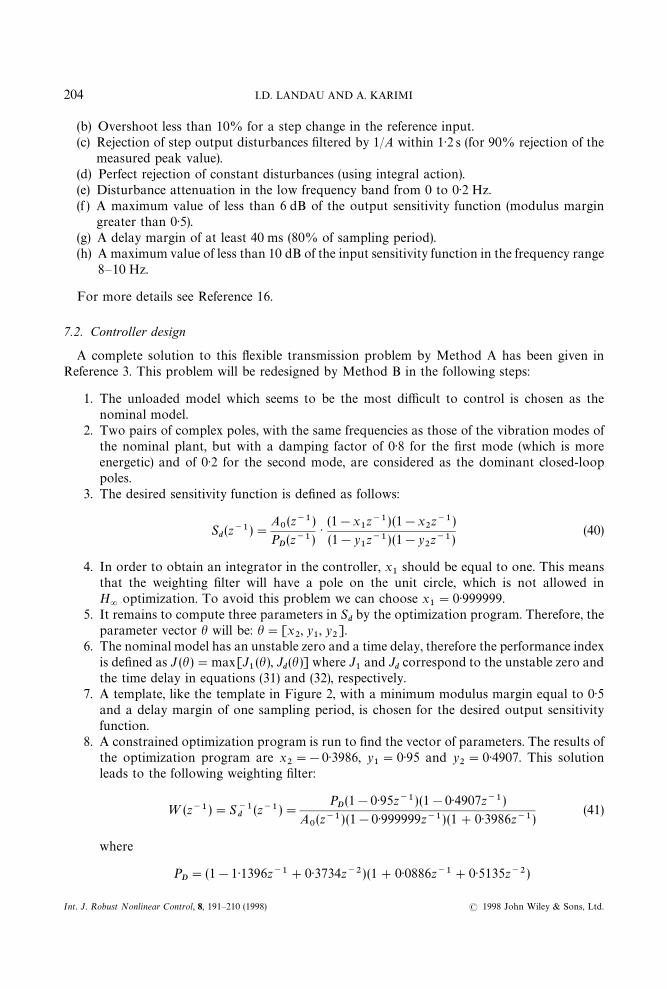
(b) Overshoot less than 10% for a step change in the reference input.(c) Rejection of step output disturbances filtered by 1/A within 1·2 s (for 90% rejection of the

measured peak value).(d) Perfect rejection of constant disturbances (using integral action).(e) Disturbance attenuation in the low frequency band from 0 to 0·2 Hz.(f ) A maximum value of less than 6 dB of the output sensitivity function (modulus margin

greater than 0·5).(g) A delay margin of at least 40 ms (80% of sampling period).(h) A maximum value of less than 10 dB of the input sensitivity function in the frequency range

8—10 Hz.

For more details see Reference 16.

7.2. Controller design

A complete solution to this flexible transmission problem by Method A has been given inReference 3. This problem will be redesigned by Method B in the following steps:

1. The unloaded model which seems to be the most difficult to control is chosen as thenominal model.

2. Two pairs of complex poles, with the same frequencies as those of the vibration modes ofthe nominal plant, but with a damping factor of 0·8 for the first mode (which is moreenergetic) and of 0·2 for the second mode, are considered as the dominant closed-looppoles.

3. The desired sensitivity function is defined as follows:

Sd(z~1)"

A0(z~1)

PD(z~1)

·(1!x

1z~1) (1!x

2z~1)

(1!y1z~1) (1!y

2z~1)

(40)

4. In order to obtain an integrator in the controller, x1

should be equal to one. This meansthat the weighting filter will have a pole on the unit circle, which is not allowed inH

=optimization. To avoid this problem we can choose x

1"0·999999.

5. It remains to compute three parameters in Sdby the optimization program. Therefore, the

parameter vector h will be: h"[x2, y

1, y

2].

6. The nominal model has an unstable zero and a time delay, therefore the performance indexis defined as J (h)"max[J

1(h), J

d(h)] where J

1and J

dcorrespond to the unstable zero and

the time delay in equations (31) and (32), respectively.7. A template, like the template in Figure 2, with a minimum modulus margin equal to 0·5

and a delay margin of one sampling period, is chosen for the desired output sensitivityfunction.

8. A constrained optimization program is run to find the vector of parameters. The results ofthe optimization program are x

2"!0·3986, y

1"0·95 and y

2"0·4907. This solution

leads to the following weighting filter:

¼(z~1)"S~1d

(z~1)"PD(1!0·95z~1)(1!0·4907z~1)

A0(z~1) (1!0·999999z~1) (1#0·3986z~1)

(41)

where

PD"(1!1·1396z~1#0·3734z~2)(1#0·0886z~1#0·5135z~2)



9. The stability domain is reduced to a circle with radius 0·85 centred at a"0·15. Then, theplant model and weighting filter equations are transformed accordingly to this newstability domain (an r is used for the parameter in the new stability domain, for example,¼r(z~1) denotes the weighting filter in the reduced stability domain). It should be noticedthat the reduced stability domain must contain the point [1, 0 j ] in order to keep theintegrator in the weighting filter.

10. The weighting filter in the new system, which may have unstable poles, is factorized into anall-pass function and a stable filter which will be used in H

=optimization.

11. The infinity norm of ¼r(z~1)Sryp

(z~1) should be minimized. First of all, using theQ parametrization Sr

ypis written as follows:

Sryp

(z~1)"1!Br

0(z~1)

Ar0(z~1)

Q(z~1) (42)

then, this problem is converted to the following model matching problem:

min E¹1!¹

2Q E

="c (43)

where ¹1"¼r and ¹

2"¼r ·Br

0/Ar

0. The optimum value of c is computed using the

Nehari’s theorem.18 Next, the parameters of Q are calculated using coprime factorizationand Nevanlinna—Pick’s algorithm in discrete time. Finally, the controller parameters aredetermined using the following relation:

Rr

Sr"

Q

1!QBr0/Ar

0

(44)

where Rr/Sr is the controller in the reduced stability domain.12. The controller is transferred back to the real stability domain and its order is reduced by

zero/pole cancellation techniques.

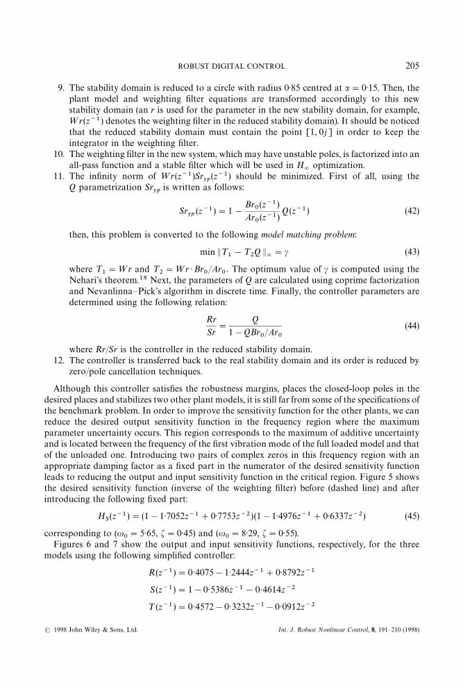
Although this controller satisfies the robustness margins, places the closed-loop poles in thedesired places and stabilizes two other plant models, it is still far from some of the specifications ofthe benchmark problem. In order to improve the sensitivity function for the other plants, we canreduce the desired output sensitivity function in the frequency region where the maximumparameter uncertainty occurs. This region corresponds to the maximum of additive uncertaintyand is located between the frequency of the first vibration mode of the full loaded model and thatof the unloaded one. Introducing two pairs of complex zeros in this frequency region with anappropriate damping factor as a fixed part in the numerator of the desired sensitivity functionleads to reducing the output and input sensitivity function in the critical region. Figure 5 showsthe desired sensitivity function (inverse of the weighting filter) before (dashed line) and afterintroducing the following fixed part:

HS(z~1)"(1!1·7052z~1#0·7753z~2)(1!1·4976z~1#0·6337z~2) (45)

corresponding to (u0"5·65, f"0·45) and (u

0"8·29, f"0·55).

Figures 6 and 7 show the output and input sensitivity functions, respectively, for the threemodels using the following simplified controller:

R(z~1)"0·4075!1·2444z~1#0·8792z~1

S(z~1)"1!0·5386z~1!0·4614z~2

¹(z~1)"0·4572!0·3232z~1!0·0912z~2



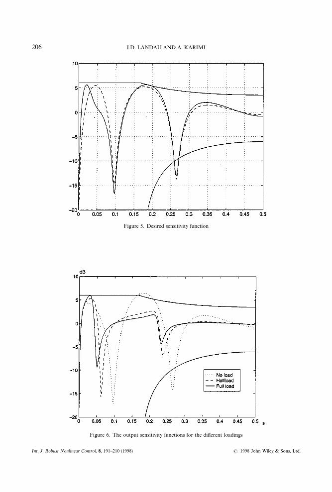
Figure 5. Desired sensitivity function

Figure 6. The output sensitivity functions for the different loadings



Figure 7. The input sensitivity functions for the different loadings

A second order system with u0"6·3 (which corresponds to the first vibration mode of the full

load model) and f"0·8 is chosen for the tracking reference model. The parameters of the prefilter¹(z~1) are computed independently from the controller. In fact the parameters of ¹(z~1) are theresults of an optimization program which minimizes the overshoot and rise time for the threemodels. Figures 8 and 9 show the step and disturbance (filtered by 1/A) responses for the threemodels.

Tables 1 and 2 show the simulation and experimental results of the controller in the differentloadings, respectively.

This controller satisfies 85% of the specifications of the benchmark in simulation. A compari-son, in terms of satisfaction of performances and complexity with the controller designed byMethod A, the H

=controllers in the benchmark designed by Jones and Limebeer19 and

Walker,20 and the controller designed by Kwakernaak,17 is presented in Table 3. For a real timecomparison, only the time characteristics, i.e., rise time, settling time and disturbance rejectiontime, are available. Therefore the normalized sum (with respect to the desired values) of thesecharacteristics for the three cases is used as a performance criterion (smaller criterion meansbetter performance). This criterion is then penalized by the normalized complexity of thecontroller (defined as the sum of the order of the polynomial R, S and ¹ divided by 10) in order toobtain a joint performance/complexity criterion. In Table 4 the controllers are compared withthese criteria. It is observed that the controller designed by Method B has a good result comparedwith the other H

=approaches.

8. CONCLUSIONS

Two different techniques, based on pole placement combined with sensitivity function shaping,have been presented. The first technique combines the main ideas in advanced robust control



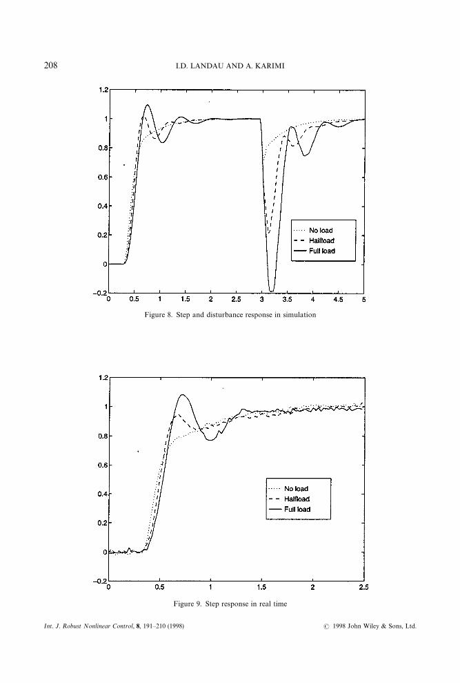
Figure 8. Step and disturbance response in simulation

Figure 9. Step response in real time



Table 1. Simulation results

Rise time Over shoot Rej. of dist. Delay Modulus Atten. band Maximum(s) (%) (s) margin (s) margin (dB) band (Hz) of S

up(dB)

No load 1·135 0% 1·811 50 !6·45 0·118 6·7Half load 0·643 1·6% 1·703 345 !5·29 0·119 7·2Full load 0·717 9·4% 2·105 560 !5·95 0·116 7.3

Table 2. Experimental results

Rise time (s) Overshoot (%) Settling time (s) Rej. of dist. (s)

No load 1·671 0% 2·7 2·55Half load 0·714 0% 3·1 1·55Full load 0·742 8·1% 2·1 1·75

Table 3. Comparison with other approaches in simulation

Controller Performance (%) criterion Complexity (order of R#S#¹ )

Method A 97·12 12Method B 85·09 6Kwakernaak 88·80 18Jones et al. 94·38 35Walker 72·35 15

Table 4. Comparison with other approaches in real-time application

Controller Normalized sum of time Joint performance/complexitycharacteristics criterion

Method A 10·86 12·06Method B 13·64 14·24Kwakernaak 12·71 14·51Jones et al. 11·47 14.97Walker 22·63 24·10

with the classical pole placement for SISO systems without using complex calculations. It adjustsiteratively the sensitivity functions in the frequency domain where it is necessary. Therefore, itseems that this technique is easy to understand for practising control engineers who are notfamiliar with the advanced robust control theories. This technique has already been applied toseveral real and industrial systems.

In the second technique, the idea of pole placement combined with sensitivity function shapinghas been transferred to H

=optimal control via a new interpretation of the weighting filter, as the

inverse of the desired sensitivity function. In this technique, weighting filter selection, which seems



to be the most important step in the H=

design, is carried out automatically by an optimizationprogram. Using this method a solution to a benchmark problem has been given, tested on a realsystem and compared with other H

=type designs.

Research is in progress concerning the proof of the convexity of the optimization procedure forbuilding the desired sensitivity function via a different parametrization.

REFERENCES

1. Landau, I.D., F. Rolland, C. Cyrot and A. Voda, ‘Digital robust control. The combined pole placement/sensitivityshaping method’, Presented at the Summer Control School of Grenoble ‘Robustness Analysis and Design of RobustControllers’. French version published in ¸a Robustesse, A. Oustaloup (Ed), Hermes, Paris, 1993.

2. Landau, I.D., C. Cyrot and D. Rey, ‘Robust control design using the combined pole placement/sensitivity functionshaping method’, European Control Conference, Gronigen, The Netherlands, 1993.

3. Landau, I.D., A. Karimi, A. Voda and D. Rey, ‘Robust digital control of flexible transmission using the combined poleplacement/sensitivity function shaping method’, European Journal of Control, 1(2), (1995).

4. Fenot, C., F. Rolland, G. Vigneron and I.D. Landau, ‘Open loop adaptive feedback control of deposited zinc in hotdip galvanizing, Control Engineering Practice, 5 (1993).

5. Zames, G. and B.A. Francis, ‘Feedback, minimax sensitivity, and optimal robustness’, IEEE ¹rans. Automat. Control,28 (1983).

6. Francis, B.A. and G. Zames, ‘On H=

optimal sensitivity theory for SISO feedback systems’, IEEE ¹rans. Automat.Control, 29 (1984).

7. Kwakernaak, H., ‘A polynomial approach to minimax frequency domain optimization of multivariable systems’, Int.J. Control, 44 (1986).

8. Postlethwaite, I., M.C. Tsai and G.D.W., ‘Weighting function selection in H=

design’, 11-th IFAC World Congress,Tallian, 1990.

9. Doyle, C.J., B.A. Francis and A.R. Tannenbaum, Feedback Control ¹heory, McMillan, NY, 1992.10. Kwakernaak, H., ‘Robust control and H

=optimization’, Automatica, 29 (1993).

11. Landau, I.D., ‘Robust digital control of systems with time delay (the Smith predictor revisited)’, Int. J. Control, 62(2),(1995).

12. Landau, I.D., System Identification and Control Design, Prentice Hall, NJ, 1990.13. Krause, J.M., ‘Comments on Grimble’s comments on Stein’s comments on roll off of H

=optimal controllers’, IEEE

¹rans. Automat. Control, 37 (1992).14. Sung, H.K. and S. Hara, ‘Properties of sensitivity and complementary sensitivity functions in single-input single-

output digital control systems’, Int. J. Control, 48 (1988).15. M’Saad, M., M. Duque and S. Hammad, ‘Flexible mechanical structures adaptive control, in Adaptive Control

Strategies for Industrial ºse, C. Shah and G. Dumont (Ed), Springer Verlag, Berlin, 1989.16. Landau, I.D., D. Rey, A. Karimi, A. Voda and A. Franco, ‘A flexible transmission system as a benchmark for robust

digital control’, European Journal of Control, 1(2), (1995).17. Kwakernaak, H., ‘Symmetries in control system design’, in ¹rends in Control A. Isidori (Ed), Springer Verlag, London,

1995.18. Francis, B.A., ‘A course in H

=control theory’, in ¸ecture Notes in Control and Information Sciences, number 88,

Springer Verlag, Heidelberg, 1987.19. Jones, N.W. and D.J.N. Limebeer, ‘A digital H

=controller for a flexible transmission system’, European Journal of

Control, 1(2), (1995).20. Walker, D.J., ‘Control of a flexible transmission—a discrete time H

=approach’, European Journal of Control, 1(2),

(1995).

.



Robust digital control using pole placement with sensitivity function shaping method

Documents