Regularization using a parameterized trust region subproblem

Regularization Using a

Parameterized Trust Region Subproblem

by

Oleg Grodzevich

A thesis

presented to the University of Waterloo

in fulfillment of the

thesis requirement for the degree of

Master of Mathematics

in

Combinatorics and Optimization

Waterloo, Ontario, Canada, 2004

c©Oleg Grodzevich 2004

I hereby declare that I am the sole author of this thesis. This is a true copy of the thesis,

including any required final revisions, as accepted by my examiners.

I understand that my thesis may be made electronically available to the public.

ii

Abstract

We present a new method for regularization of ill-conditioned problems that extends the

traditional trust-region approach. Ill-conditioned problems arise, for example, in image

restoration or mathematical processing of medical data, and involve matrices that are very

ill-conditioned. The method makes use of the L-curve and L-curve maximum curvature

criterion as a strategy recently proposed to find a good regularization parameter. We

describe the method and show its application to an image restoration problem. We also

provide a MATLAB code for the algorithm. Finally, a comparison to the CGLS approach

is given and analyzed, and future research directions are proposed.

iii

Acknowledgements

I would like to thank my supervisor, Henry Wolkowicz for his support, assistance and

advices during my studies. I would like to thank Arkadii Nemirovskii for his suggestions

and many discussions I have greatly benefited from. I gratefully acknowledge the time

Etienne De Klerk and Edward Vrscay spent on reviewing this work. I am also grateful

to Urs von Matt who provided me with GCV MATLAB code which was helpful while

developing the algorithm.

Finally, I have to thank my parents and my wife for their understanding, patience and

encouragement.

iv

Contents

1 Introduction 1

1.1 What is regularization? . . . . . . . . . . . . . . . . . . . . . . . . . . . . . 1

1.2 Contributions . . . . . . . . . . . . . . . . . . . . . . . . . . . . . . . . . . 2

1.3 Applications . . . . . . . . . . . . . . . . . . . . . . . . . . . . . . . . . . . 3

2 Basic Regularization Theory 4

2.1 Tikhonov Regularization . . . . . . . . . . . . . . . . . . . . . . . . . . . . 4

2.2 Using Singular Values . . . . . . . . . . . . . . . . . . . . . . . . . . . . . . 5

2.3 The L-curve analysis . . . . . . . . . . . . . . . . . . . . . . . . . . . . . . 8

3 Regularization Using TRS 15

3.1 The Optimality Conditions . . . . . . . . . . . . . . . . . . . . . . . . . . . 15

3.2 Perturbations ∆ε for µ . . . . . . . . . . . . . . . . . . . . . . . . . . . . . 16

3.3 Applying TRS in L-curve Analysis . . . . . . . . . . . . . . . . . . . . . . 17

3.4 Regularization as a one-dimensional

parameterized problem . . . . . . . . . . . . . . . . . . . . . . . . . . . . . 20

3.5 Intervals of interest for t, λ and ε . . . . . . . . . . . . . . . . . . . . . . . 22

3.6 Curvature of the L-curve . . . . . . . . . . . . . . . . . . . . . . . . . . . . 23

3.7 Curvature Estimation and Gauss Quadrature . . . . . . . . . . . . . . . . . 24

4 Regularization Algorithm 29

4.1 Initial L-curve point . . . . . . . . . . . . . . . . . . . . . . . . . . . . . . 30

4.2 Outline of the algorithm . . . . . . . . . . . . . . . . . . . . . . . . . . . . 31

v

4.3 Future improvements . . . . . . . . . . . . . . . . . . . . . . . . . . . . . . 37

5 Numerics/Computations 40

5.1 Eigensolver issues . . . . . . . . . . . . . . . . . . . . . . . . . . . . . . . . 40

5.2 Image deblurring example . . . . . . . . . . . . . . . . . . . . . . . . . . . 41

5.3 Open Questions . . . . . . . . . . . . . . . . . . . . . . . . . . . . . . . . . 45

A MATLAB Code 54

A.1 RPTRS Regularization Algorithm . . . . . . . . . . . . . . . . . . . . . . . 54

A.2 Lanczos Bidiagonalization II Algorithm . . . . . . . . . . . . . . . . . . . . 65

A.3 Estimating curvature using Gauss/Gauss-Radau Quadrature . . . . . . . . 67

vi

List of Tables

5.1 Data for points visited by the CGLS algorithm with δ = ‖η‖2 . . . . . . . 49

5.2 Data for points visited by the RPTRS algorithm . . . . . . . . . . . . . . . 50

vii

List of Figures

2.1 Picard plot for a Shaw problem . . . . . . . . . . . . . . . . . . . . . . . . 7

2.2 Picard plot for the unperturbed right-hand side . . . . . . . . . . . . . . . 10

2.3 Picard plot for the noise vector . . . . . . . . . . . . . . . . . . . . . . . . 11

2.4 Picard plot for the perturbed right-hand side . . . . . . . . . . . . . . . . . 12

2.5 The L-curve for the deblurring problem . . . . . . . . . . . . . . . . . . . . 13

2.6 Relative accuracy for different noise vectors . . . . . . . . . . . . . . . . . 14

3.1 Points encountered while solving TRS . . . . . . . . . . . . . . . . . . . . 18

4.1 k(t) and triangle interpolation . . . . . . . . . . . . . . . . . . . . . . . . . 36

5.1 Image deblurring example: original picture . . . . . . . . . . . . . . . . . . 42

5.2 Image deblurring example: observed data, blurred with added noise . . . . 43

5.3 Image deblurring example: corresponding L-curve . . . . . . . . . . . . . . 44

5.4 Image deblurring example: corresponding L-curve with RPTRS points . . . 45

5.5 Image deblurring example: RPTRS solution picture . . . . . . . . . . . . . 46

5.6 Image deblurring example: corresponding L-curve with CGLS points . . . 47

5.7 Image deblurring example: CGLS, RPTRS, xtrue, best Tikhonov solutions . 48

5.8 Image deblurring example: CGLS with δ = 0.6 ‖η‖2, rel.acc. = 52% . . . . 49

5.9 Image deblurring example: point #1, t = 652.166, rel.acc. = 65.39% . . . 50

5.10 Image deblurring example: point #2, t = 994.155, rel.acc. = 49.63% . . . 51

5.11 Image deblurring example: point #3, t = 1271.46, rel.acc. = 38.07% . . . 51

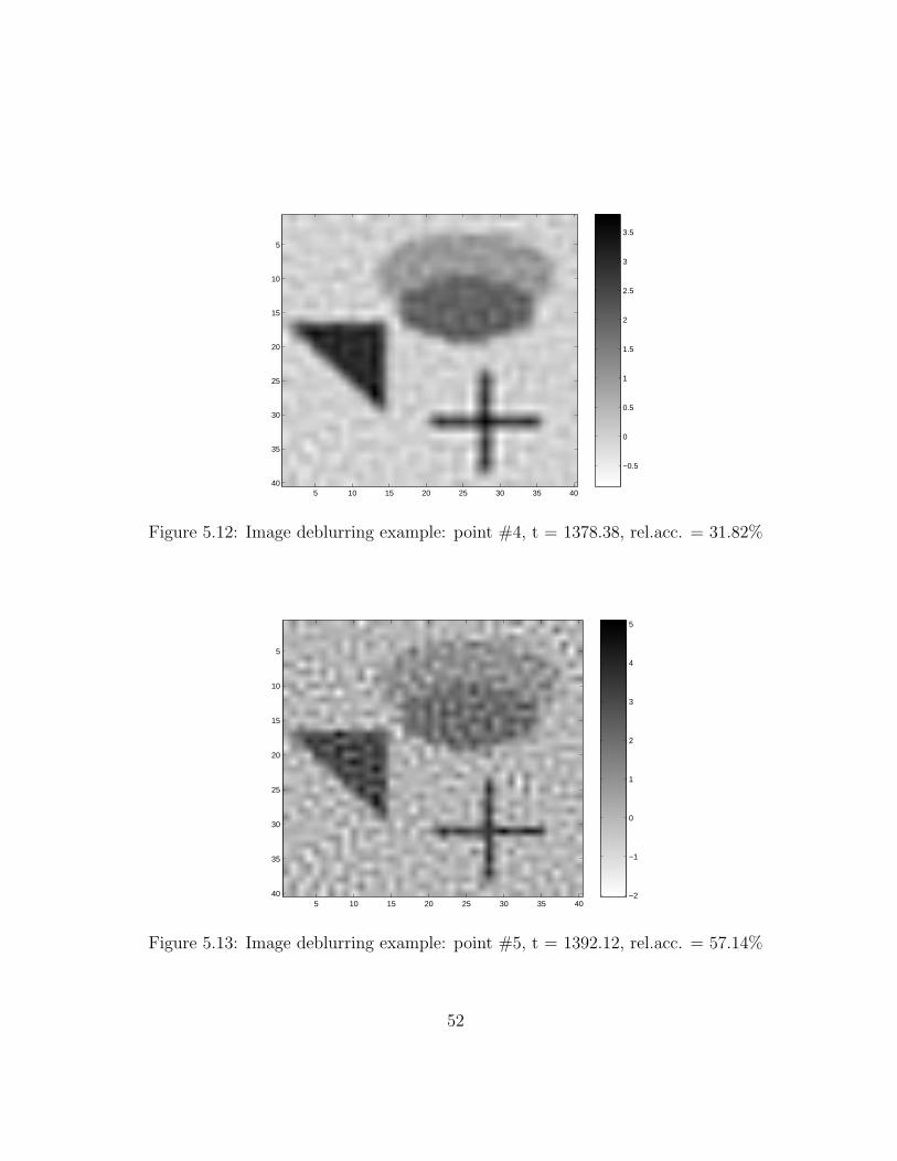
5.12 Image deblurring example: point #4, t = 1378.38, rel.acc. = 31.82% . . . 52

5.13 Image deblurring example: point #5, t = 1392.12, rel.acc. = 57.14% . . . 52

viii

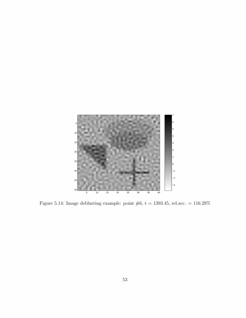
5.14 Image deblurring example: point #6, t = 1393.45, rel.acc. = 116.29% . . . 53

ix

List of Algorithms

3.1 Lanczos Bidiagonalization II . . . . . . . . . . . . . . . . . . . . . . . . . . 26

4.1 Trust-Region Based Regularization [overview] . . . . . . . . . . . . . . . . 31

4.2 Helper Functions . . . . . . . . . . . . . . . . . . . . . . . . . . . . . . . . . 32

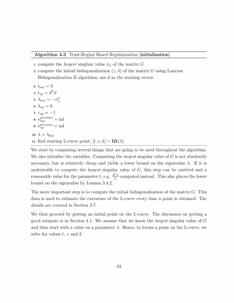
4.3 Trust-Region Based Regularization [initialization] . . . . . . . . . . . . . . 33

4.4 Trust-Region Based Regularization [main loop] . . . . . . . . . . . . . . . 34

4.5 TRS Based Regularization [final solution refinement] . . . . . . . . . . . 37

x

Chapter 1

Introduction

1.1 What is regularization?

Regularization centers on finding approximate solutions for least-squares problems such as

minx‖Gx− d‖2 , (1.1)

where G is a singular or ill-conditioned forward operator and d is a vector of observed data.

This problem arises from mathematical models Gx = d, where the data contains noise η,

Gx = Gxtrue + η = d = dtrue + η.

It is remarkable that, for many applications, a small amount of noise η results in a solution

x that has no relation to xtrue, i.e. we can make the size of the error ‖η‖2 arbitrarily small,

while the size of the error in the solution ‖x− xtrue‖2 is arbitrarily large. Moreover, in the

G singular case, there can be no solution or an infinite number of solutions xtrue. (See e.g.

the survey article [25] or the book [1].) Here we restrict G to being a square n× n matrix.

The least-squares problem (1.1) typically arises from discretizations of linear equations in

infinite dimensional spaces, e.g. Tx = d, where T is typically a compact operator and so

has an unbounded inverse. This means that x is not a continuous function of the data d.

Such problems are called ill-posed [15, 16].

To obtain meaningful solutions to the mathematical model one often uses various methods

of regularization. The aim is to find algorithms for constructing generalized solutions

1

that are stable under small changes in the data d. One method uses the solution of the

constrained least-squares problem:

min ‖Gx− d‖2

subject to ‖x‖2 ≤ ε.(1.2)

The restriction on ‖x‖2 results in a larger residual error ‖Gx− d‖2 but reduces the propa-

gated data error. As ε increases we reduce ‖Gx(ε)− d‖2 and expect x(ε) to approximate

the best least-squares solution xtrue = G†dtrue, where G† denotes the Moore-Penrose gener-

alized inverse of G. However, in practice the error propagation stays small for small ε but

then eventually causes divergence of the iterates from xtrue. (See semiconvergence in [23].)

Regularization depends on controlling/choosing the parameter ε.

By squaring the objective and the constraint, (1.2) can be reformulated as the so-called

trust region subproblem, TRS , e.g. [8]:

(TRS )µ(A, a, ε) := min q(x) := xT Ax− 2aT x

subject to ‖x‖22 ≤ ε2,

where A := GT G is n × n (we assume n ≥ 2) symmetric, a := GT d is an n-vector, ε is a

positive scalar, and x is the n-vector of unknowns. All matrix and vector entries are real.

In this thesis, we apply known results for TRS to efficiently control the parameter ε and find

regularized solutions of (1.1). We also compare our approach to the Conjugate Gradients

method, which is often used for regularization.

1.2 Contributions

This thesis extends the traditional trust-region approach for regularization of ill-conditioned

problems. We show that this is an effective tool that can be used in conjuction with the

L-curve maximum curvature criterion.

Unlike the traditional TRS with a fixed trust region radius, here ε changes at each iteration

to get a new point on the L-curve, thus acting as a regularization parameter. We reveal

the relations between various TRS parameters and employ them to efficiently guide the

2

algorithm along the L-curve. As a result, we require very few iterations to get to the elbow

(to be defined below). Furthermore each iteration is accelerated by using the data from

the previous step.

In comparison to [9] we use a more robust way of choosing/controlling the regularization

parameters. We explicitly compute the curvature and provide a more reliable method to

determine the location of the elbow, and we do not require an apriori knowledge of the

norm of the noise to estimate the initial (starting) point.

1.3 Applications

Many problems in the mathematical sciences have solutions that are unstable with respect

to the initial data. Classical examples include differentiation of functions known only

approximately, solutions of integral equations of the first kind, and solution of singular

or ill-conditioned linear equations. These examples arise in mathematical processing and

interpretation of data in various fields, e.g.

• geophysical: determine an earthquake hypocenter in space and time, vertical seismic

profiling and wave propagation;

• medical: computer-assisted tomography (CAT), magnetic resonance imaging and

magnetoencephalography (MRI, MEG);

• imaging: deconvolution of telescope images and image restoration.

In Section 5.2 we consider an image restoration example: deblurring of an image. This is a

typical problem in astrophotography. Pictures taken by the ground telescopes are subject

to atmospheric blur and require the restoration procedure (see e.g. the forthcoming book

[35]). We observe the difference between the least-squares and regularized solutions, and

illustrate the performance of the algorithm for this type of problem.

3

Chapter 2

Basic Regularization Theory

2.1 Tikhonov Regularization

Regularization dates back to work by Tikhonov [33]. (See also [34].) For the equation

Tx = d, one solves the damped normal equation

(T ∗T + α2I)xα = T ∗d, (2.1)

where d = dtrue +η. In this thesis we restrict our analysis to a finite-dimensional discretiza-

tion of an operator T, represented by a matrix G. We replace (2.1) by

(GT G + α2I)xα = GT d. (2.2)

Regularization involves choosing the correct value for the parameter α > 0, when given

some information on the size of the error η. If α = 0, (2.2) degenerates to the normal

equations for the linear least-squares problem.

The regularization is equivalent to choosing the correct value for ε in (1.2). See Remark

3.1.1.

Moreover, a solution to (2.2) is also a solution to

minx‖Gx− d‖2

2 + α2 ‖x‖22 . (2.3)

4

To see this denote

Gext =

[G

αI

], dext =

[d

0

].

We can now rewrite (2.2) as

GTextGextxα = GT

extdext. (2.4)

Since α > 0, Gext is full-rank then (2.4) are the normal equations for the problem

minx

∥∥∥∥∥[

G

αI

]x−

[d

0

]∥∥∥∥∥2

2

, α > 0,

which is equivalent to (2.3).

2.2 Using Singular Values

The singular value decomposition (SVD) of the matrix G is a tool that helps in under-

standing the L-curve analysis (see Section 2.3). We will write the SVD as

G = USV T ,

where matrix S is a diagonal n×n matrix consisting of singular values σi of G, σ1 ≤ . . . ≤σn, and U , V are orthogonal matrices, i.e.

UT U = I, V T V = I.

We can characterize the Tikhonov regularized solution xα using the SVD in the following

way. Substitute the SVD of the matrix G into (2.2):

(GT G + α2I)xα = GT d

(V SUT USV T + α2I)xα = V SUT d

V (S2 + α2I)V T xα = V SUT d

V T xα = (S2 + α2I)−1SUT d.

Finally using the orthogonality of the matrices U and V we get

xα = V (S2 + α2I)−1SUT d =n∑

i=1

fiUT

:i d

σi

V:i (2.5)

5

and

‖xα‖22 = dT U(S(S2 + α2I))2UT d =

n∑i=1

(fi

UT:i d

σi

)2

, (2.6)

where U:i denotes the ith column of U .

Similarly,

d−Gxα = d− USV T xα = U(I − S(S2 + α2I)−1S)UT d,

‖Gxα − d‖22 =

n∑i=1

((1− fi)U

T:i d

)2

, (2.7)

where the fi are the so called Tikhonov filter factors, defined as

fi =σ2

i

σ2i + α2

. (2.8)

Note that if G is invertible, then setting α = 0 gives the true least-squares solution x0

with the norm of the residual ‖Gx0 − d‖2 = 0, as all filter factors are equal to one. This

means that the solution xα for α > 0 should always have a norm smaller than ‖x0‖, since

the SVD components corresponding to the small singular values are filtered by fi. It also

follows that choosing the value of α2 larger than σ2n is unreasonable, since the factors fi

are small and the corresponding solution xα would have an almost zero norm.

Expressions (2.5), (2.6) and (2.7) can also be used to illustrate what happens to the solution

in the presence of noise. Consider first of all, the least-squares solution x0 for the ”true”

right-hand side dtrue, i.e. without any noise. Then, since dtrue = Gxtrue = USV T xtrue,

we have x0 = V (S2)−1S2V T xtrue. If we further assume that the matrix G, and hence S,

is invertible then x0 = xtrue. However adding uncorrelated noise η would result in extra

contribution to the solution caused by the noise components. Specifically, fi = 1,∀i, and

‖x0‖22 =

n∑i=1

(UT:i dtrue

σi

+UT

:i η

σi

)2

.

It is easy to see that these contributions can be very large in the case of small singular

values whenever the noise vector is not orthogonal to the corresponding singular vectors,

U:i’s. This explains why the naive least-squares solution is not meaningful and a regularized

solution should be sought instead.

6

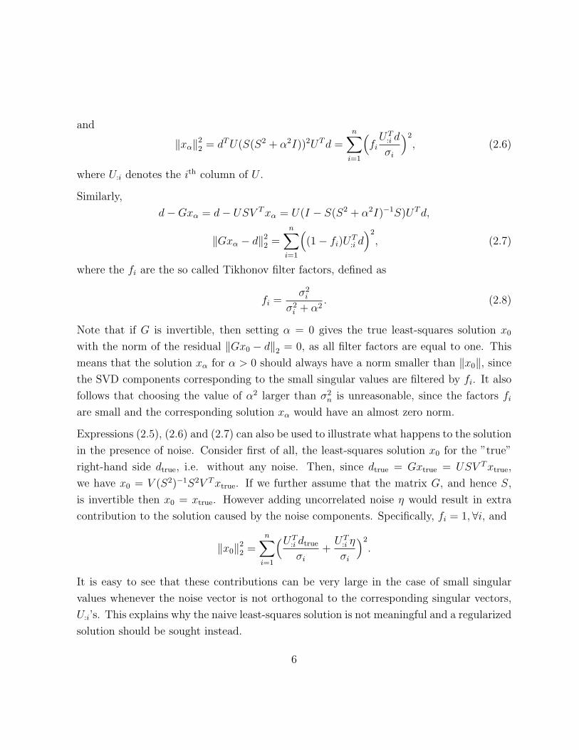
The situation continues to be problematic if the matrix G has very small singular values

in a sense that they are numerically close to 0, even if the noise component is absent. This

can be observed by looking at the ratioUT

:i dtrue

σi. We require that

the Fourier coefficients |UT:i dtrue| decay faster than the σi .

This condition, also known as the Discrete Picard Condition, e.g. see [21], guarantees

that the least-squares solution has a reasonable norm and thus is physically meaningful.

However, if the σi’s become smaller than machine epsilon, i.e. the smallest number we

can numerically operate with, the Picard condition fails. The next example illustrates this

situation.

0 5 10 15 20 25 30 3510

−20

10−15

10−10

10−5

100

105

index, i

σi

U:iT d

true|U

:iT d

true / σ

i|

machine ε

Figure 2.1: Picard plot for a Shaw problem

7

Example 2.2.1. We consider a Shaw problem from the Hansen MATLAB package (see

[19]) with n = 32. This is a one-dimensional image restoration problem which is constructed

via discretization of a Fredholm integral equation of the first kind (see [29]). The MATLAB

shaw command produces the matrix G and the right-hand side vector dtrue, as well as the

true solution vector xtrue.

We then compute the SVD of the matrix G and plot the Fourier coefficients |UT:i dtrue|, the

singular values σi and the ratio|UT

:i dtrue|σi

. The resulting plot is Figure 2.1. It can be seen that

the Picard condition holds until the singular values (x marked line) hit the machine epsilon

level (horizontal dashed line). But for the larger indices, round-off error steps in and the

Picard condition fails. The norm of the least-squares solution computed via SVD, i.e. by

using (2.6), is ∼ 105 while the true solution has norm of ∼ 10. A good approximation of

the true solution is still recoverable via a truncated SVD, i.e. by setting to 0 all the singular

values less than machine epsilon.

2.3 The L-curve analysis

As we have seen in Sections 2.1 and 2.2, finding the regularized solution involves finding

the regularization parameter. In this thesis, we use the approach of studying the corre-

spondence between the norm of the solution and the norm of the residual to obtain the

value of the regularization parameter α. Such a relation can be naturally expressed as a

plot of one of these quantities versus another, i.e. as a log-log curve based on(log(‖Gxα − d‖2), log(‖xα‖2)

).

In the literature (see [21] for example), this plot is often referred to as the L-curve. The

curve usually features a strong L-shaped form with almost linear vertical and horizontal

parts and a well distinguishable elbow or corner. Although for most practical problems its

form is L-shaped, it may vary depending on the structure of the problem. Basing on the

analysis presented in Section 2.2, we give an overview of the L-curve characteristics.

The results presented in this thesis use a nonstandard way of plotting the L-curve, i.e.

the abscissa represents log(‖xα‖2), rather than the traditional orientation which uses the

residual instead. We choose a different view because our analysis centers on changing

8

the trust region radius ε, and it is more convinient to have a parameter of interest as an

abscissa of the plot.

Recall the expressions (2.7) and (2.6) for the norms of the residual and the solution. It is

worthwhile to rewrite the latter as

‖xα‖22 =

n∑i=1

[fi

(UT:i dtrue

σi

+UT

:i η

σi

)]2

.

If we assume uncorrelated noise, then the expected value of the Fourier coefficients of η

should satisfy

E(|UT

:i η|)≈ ‖η‖2 ,∀i.

This means that the noise does not satisfy the Picard condition when there are small

singular values. Furthermore, the Fourier coefficients of perturbed data should eventually

become larger than the corresponding singular values, even if the original data satisfies the

Picard condition. This happens, roughly, once the Fourier coefficients, corresponding to

the true unperturbed data, become dominated by the Fourier coefficients from the noise.

We illustrate our considerations by means of an example - a deblurring of a 20× 20 image.

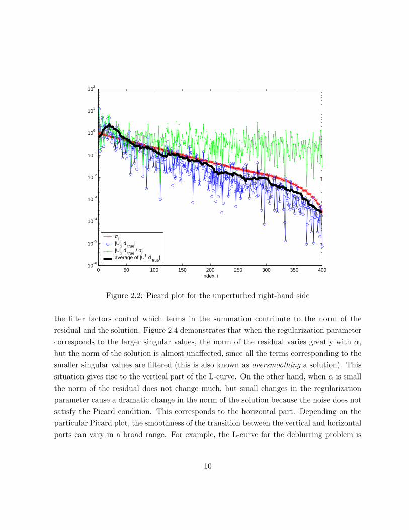
The details of how the problem data is constructed are outlined in Section 5.2. Figure 2.2

shows the Picard plot for the unperturbed right-hand side. It is evident that on average

the Fourier coefficients corresponding to the unperturbed data vector decay faster than the

singular values. Hence, the Picard condition holds and the least-squares solution recovers

the true solution in the absence of the noise.

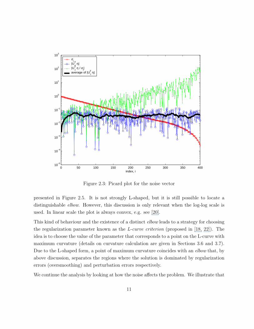
Then we build a random vector η to represent the noise. The Fourier coefficients for η are

plotted in Figure 2.3. We can see that on average they stay on the same level and hence

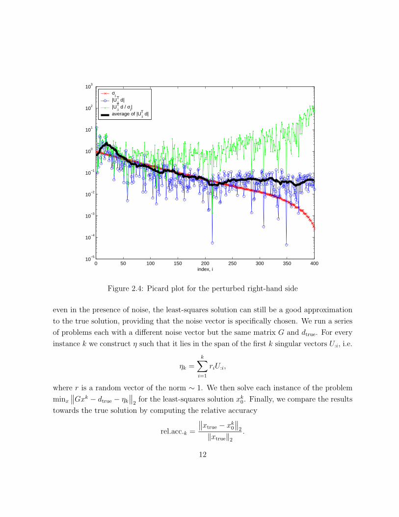
fail to satisfy the Picard condition. As expected, the Picard plot for the perturbed (noisy)

right-hand side levels off at approximately ‖η‖2 as shown in Figure 2.4.

Now we no longer restrict fi = 1 and start looking at solutions xα corresponding to the

different values of the regularization parameter α. Since

fi '

1, σi � ασ2

i

α2, σi � α,

9

0 50 100 150 200 250 300 350 40010

−6

10−5

10−4

10−3

10−2

10−1

100

101

102

index, i

σi

|U:iT d

true|

|U:iT d

true / σ

i|

average of |U:iT d

true|

Figure 2.2: Picard plot for the unperturbed right-hand side

the filter factors control which terms in the summation contribute to the norm of the

residual and the solution. Figure 2.4 demonstrates that when the regularization parameter

corresponds to the larger singular values, the norm of the residual varies greatly with α,

but the norm of the solution is almost unaffected, since all the terms corresponding to the

smaller singular values are filtered (this is also known as oversmoothing a solution). This

situation gives rise to the vertical part of the L-curve. On the other hand, when α is small

the norm of the residual does not change much, but small changes in the regularization

parameter cause a dramatic change in the norm of the solution because the noise does not

satisfy the Picard condition. This corresponds to the horizontal part. Depending on the

particular Picard plot, the smoothness of the transition between the vertical and horizontal

parts can vary in a broad range. For example, the L-curve for the deblurring problem is

10

0 50 100 150 200 250 300 350 40010

−5

10−4

10−3

10−2

10−1

100

101

102

103

index, i

σi

|U:iT η|

|U:iT η / σ

i|

average of |U:iT η|

Figure 2.3: Picard plot for the noise vector

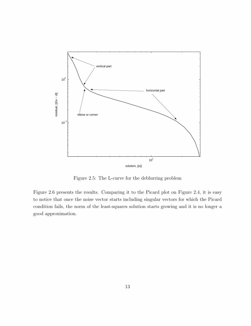
presented in Figure 2.5. It is not strongly L-shaped, but it is still possible to locate a

distinguishable elbow. However, this discussion is only relevant when the log-log scale is

used. In linear scale the plot is always convex, e.g. see [20].

This kind of behaviour and the existence of a distinct elbow leads to a strategy for choosing

the regularization parameter known as the L-curve criterion (proposed in [18, 22]). The

idea is to choose the value of the parameter that corresponds to a point on the L-curve with

maximum curvature (details on curvature calculation are given in Sections 3.6 and 3.7).

Due to the L-shaped form, a point of maximum curvature coincides with an elbow that, by

above discussion, separates the regions where the solution is dominated by regularization

errors (oversmoothing) and perturbation errors respectively.

We continue the analysis by looking at how the noise affects the problem. We illustrate that

11

0 50 100 150 200 250 300 350 40010

−5

10−4

10−3

10−2

10−1

100

101

102

103

index, i

σi

|U:iT d|

|U:iT d / σ

i|

average of |U:iT d|

Figure 2.4: Picard plot for the perturbed right-hand side

even in the presence of noise, the least-squares solution can still be a good approximation

to the true solution, providing that the noise vector is specifically chosen. We run a series

of problems each with a different noise vector but the same matrix G and dtrue. For every

instance k we construct η such that it lies in the span of the first k singular vectors U:i, i.e.

ηk =k∑

i=1

riU:i,

where r is a random vector of the norm ∼ 1. We then solve each instance of the problem

minx

∥∥Gxk − dtrue − ηk

∥∥2

for the least-squares solution xk0. Finally, we compare the results

towards the true solution by computing the relative accuracy

rel.acc.k =

∥∥xtrue − xk0

∥∥2

‖xtrue‖2

.

12

102

10−1

100

solution, ||x||

resi

dual

, ||G

x −

d||

elbow or corner

vertical part

horizontal part

Figure 2.5: The L-curve for the deblurring problem

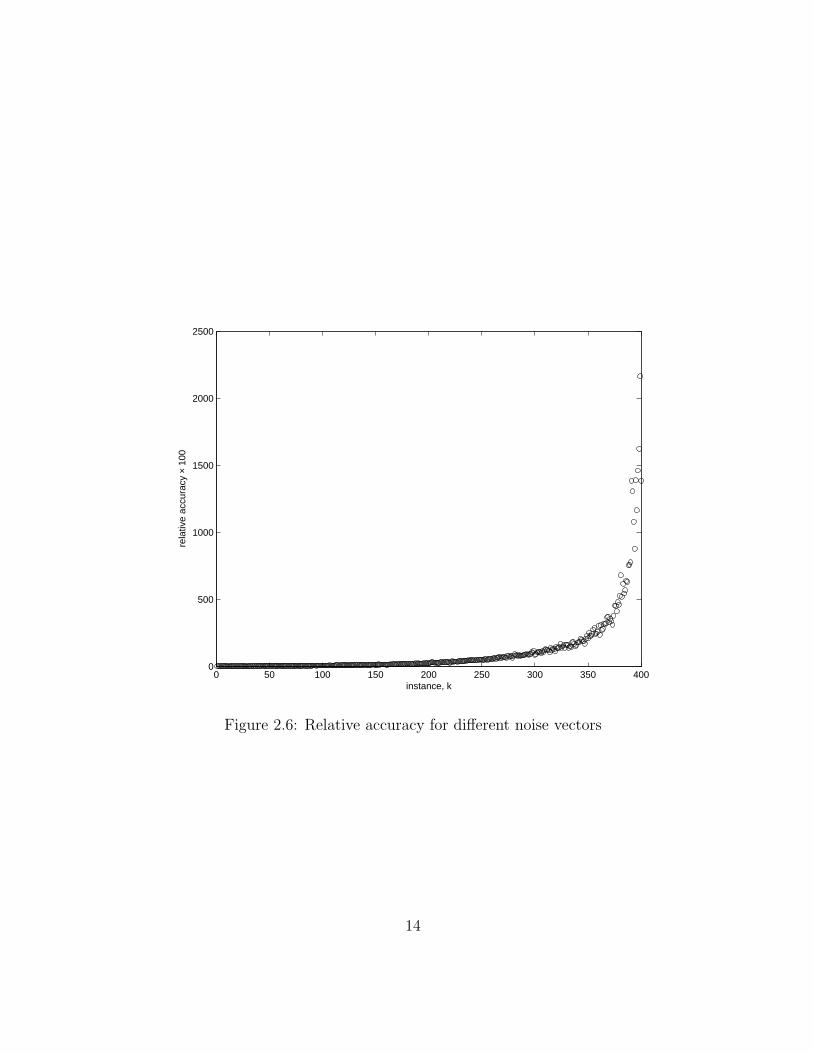
Figure 2.6 presents the results. Comparing it to the Picard plot on Figure 2.4, it is easy

to notice that once the noise vector starts including singular vectors for which the Picard

condition fails, the norm of the least-squares solution starts growing and it is no longer a

good approximation.

13

0 50 100 150 200 250 300 350 4000

500

1000

1500

2000

2500

instance, k

rela

tive

accu

racy

× 1

00

Figure 2.6: Relative accuracy for different noise vectors

14

Chapter 3

Regularization Using TRS

In this chapter, we discuss several results from TRS theory, that help in analyzing the

L-curve behaviour. We consider the optimality conditions for TRS and the behaviour of

the optimal objective value under small changes of the trust region radius. We further

derive the results developed in the Rendl-Wolkowicz TRS algorithm and apply them to

formulate the regularization as a one-dimensional parameterized problem. We show that

the curvature of the L-curve can be efficiently computed for each point visited by the TRS

solver.

3.1 The Optimality Conditions

It is known ([11, 30]) that x∗ is a solution to TRS if and only if:

(A− λ∗I)x∗ = a,

A− λ∗I � 0, λ∗ ≤ 0

}dual feasibility

‖x∗‖2 ≤ ε2 primal feasibility

λ∗(‖x∗‖2 − ε2) = 0 complementary slackness

(3.1)

for some (Lagrange multiplier) λ∗. As shown in Section 2.1, using the above conditions

allows us to relate the regularization in the sense of Tikhonov with TRS . Also note that

in the scope of this thesis, i.e. applied to the regularization, we may restrict λ∗ < 0, which

corresponds to the restriction on the Tikhonov regularization parameter α2 > 0. This leads

15

to two very important consequences. First of all, the optimal solution always lies on the

boundary, i.e. ‖x∗‖2 = ε. Secondly, the so-called easy case holds for TRS . The easy case

corresponds to a 6⊥ N (A − λ1(A)I), where λ1(A) is the smallest eigenvalue of the matrix

A. And this condition is implied by λ∗ < 0 ≤ λ1(A).

Remark 3.1.1. The optimality conditions (3.1) imply that solving (2.2) with a particular

value of the regularization parameter α is equivalent to solving (1.2) with a corresponding

value of ε. This can be seen from a Lagrange multiplier argument. Since A = GT G and

a = GT d, we have (GT G−λI)x = GT d. This, however, is equivalent to (2.2) with λ = −α2.

Fixing λ yields a solution x such that ε = ‖x‖2, due to λ(‖x‖22− ε2) = 0. Hence, for every

choice of α2 > 0 we can find a corresponding value of ε, such that the solutions to both

(2.2) and (1.2) coincide.

3.2 Perturbations ∆ε for µ

We keep the data A, a fixed and consider the optimal value as a function of ε > 0. By

abuse of notation, we write µε = µ(A, a, ε). We now derive the expressions for first- and

second-order derivatives of µε with respect to ε.

We assume (as in Section 3.1) that the easy case holds, and that the optimum point lies

on the boundary of the feasible region, i.e. ‖x∗‖ = ε.

µε = (x∗)T Ax∗ − 2aT x∗

= (x∗)T Ax∗ − 2aT x∗ − λ∗(‖x∗‖2 − ε2)

= (x∗)T (A− λ∗I)x∗ − 2aT x∗ + λ∗ε2

= aT (A− λ∗I)−1a− 2aT (A− λ∗I)−1a + λ∗ε2

= −aT (A− λ∗I)−1a + λ∗ε2.

Then, using aT (A− λ∗I)−2a− ε2 = ‖x∗‖2 − ε2 = 0, we get

∂µε

∂ε= aT (A− λ∗I)−2a

(−∂λ∗

∂ε

)+

(∂λ∗

∂ε

)ε2 + 2λ∗ε

=(−∂λ∗

∂ε

)(aT (A− λ∗I)−2a− ε2) + 2λ∗ε

= 2λ∗ε

(3.2)

16

and∂2µε

∂ε2= 2

(λ∗ + ε

∂λ∗

∂ε

). (3.3)

The derivative ∂λ∗

∂εcan be found using implicit differentiation in

‖(A− λ∗I)−1a‖2−ε2 = 0, which is obtained after substituting x∗ = (A−λ∗I)−1a. Namely:

aT (A− λ∗I)−2a = ε2 ;

2(

∂λ∗

∂ε

)aT (A− λ∗I)−3a = 2ε ;

and∂λ∗

∂ε=

ε

aT (A− λ∗I)−3a. (3.4)

More details on these and other perturbation results can also be found in [32].

3.3 Applying TRS in L-curve Analysis

As Section 2.3 suggests, one can obtain a good regularization parameter α by looking at

the point of the maximum curvature on the L-curve. One way to locate this point is to

sequentially solve a number of trust region subproblems, while gradually changing the trust

region radius. This approach, however, is not very efficient and does not fully exploit the

nature of the problem. To see why this is the case, we need to go into more details here.

As we have seen in Section 2.1, a solution to the regularization problem coincides with the

optimal solution to TRS . The former is identified by the value of the trust region radius

ε, which poses the bound on the norm of the solution. Moreover, as we will see later,

the inequality holds with equality for a certain interval of ε ∈ (0,∥∥GT d

∥∥2). Hence, for

the L-curve analysis, the trust region radius specifies one of the coordinates of an L-curve

point, and another coordinate is given by the objective value of TRS . Thus, every solution

to TRS can be associated with a unique point on the L-curve and vice versa. However, as

we have already noted, this correspondence only holds inside a certain interval of ε.

Solving TRS usually involves going through an iterative procedure which at each step

produces a solution x that is optimal to TRS with different, but close, trust region radius

17

101

102

10−2

10−1

100

solution, ||x||

resi

dual

, ||G

x −

d|| Points visited by the TRS solver

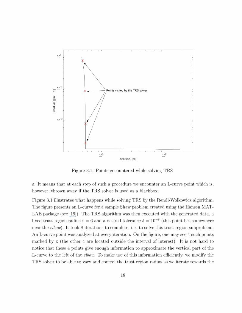
Figure 3.1: Points encountered while solving TRS

ε. It means that at each step of such a procedure we encounter an L-curve point which is,

however, thrown away if the TRS solver is used as a blackbox.

Figure 3.1 illustrates what happens while solving TRS by the Rendl-Wolkowicz algorithm.

The figure presents an L-curve for a sample Shaw problem created using the Hansen MAT-

LAB package (see [19]). The TRS algorithm was then executed with the generated data, a

fixed trust region radius ε = 6 and a desired tolerance δ = 10−8 (this point lies somewhere

near the elbow). It took 8 iterations to complete, i.e. to solve this trust region subproblem.

An L-curve point was analyzed at every iteration. On the figure, one may see 4 such points

marked by x (the other 4 are located outside the interval of interest). It is not hard to

notice that these 4 points give enough information to approximate the vertical part of the

L-curve to the left of the elbow. To make use of this information efficiently, we modify the

TRS solver to be able to vary and control the trust region radius as we iterate towards the

18

solution. We want each point, that we find on the L-curve, to be important in locating the

elbow.

We now present the Rendl-Wolkowicz TRS algorithm along with techniques developed and

discussed in [26].

Exploiting the strong Lagrangian duality of TRS (see [31]), we can show that it (TRS)

can be reformulated as an unconstrained concave maximization problem. As shown in [31]

strong duality holds for TRS with no duality gap, i.e.

µε = minx

maxλL(x, λ) = maxλ

minx

L(x, λ),

where L(x, λ) denotes the Lagrangian of TRS ,

L(x, λ) = xT Ax− 2aT x + λ(‖x‖2 − ε2).

Then

µε = min‖x‖=ε,y20=1 xT Ax− 2y0a

T x

= maxt min‖x‖=ε,y20=1 xT Ax− 2y0a

T x + ty20 − t

≥ maxt min‖x‖2+y20=ε2+1 xT Ax− 2y0a

T x + ty20 − t

≥ maxt,λ minx,y0 xT Ax− 2y0aT x + ty2

0 − t + λ(‖x‖2 + y20 − ε2 − 1)

= maxr=t+λ,λ minx,y0 xT Ax− 2y0aT x + r2

0 − r + λ(‖x‖2 − ε2)

= maxλ

(maxr minx,y0 xT Ax− 2y0a

T x + r20 − r + λ(‖x‖2 − ε2)

)= maxλ minx,y2

0=1 xT Ax− 2y0aT x + λ(‖x‖2 − ε2)

= µε,

where the strong duality and the symmetry of the function are used for the last two

equalities.

We define

k(t) = (ε2 + 1)λ1(D(t))− t, t ∈ R, (3.5)

19

where D(t) is the symmetric (n + 1)× (n + 1) matrix

D(t) =

[t −aT

−a A

], (3.6)

and λ1 denotes the smallest eigenvalue. Then the third expression in the above chain can

be written asmin‖x‖2+y2

0=ε2+1 xT Ax− 2y0aT x + ty2

0 − t =

= min‖x‖2+y20=ε2+1

[y0

x

]T [t −aT

−a A

] [y0

x

]− t =

= (ε2 + 1)λ1(D(t))− t,

where the last equality is obtained by using the Rayleigh quotient for the matrix D(t) and

the vector [y0 x]T .

Finally, this implies

µε = maxt

k(t). (3.7)

Therefore, the Trust Region Subproblem can be transformed to an unconstrained concave

maximization problem. Furthermore, under assumptions of the easy case, λ1(D(t)) is a

singleton eigenvalue, and the derivative of k(t) satisfies

k′(t) = (ε2 + 1)y20 − 1, (3.8)

where(

y0x

)is the normalized eigenvector for λ1(D(t)).

We focus on the function k(t), instead of looking directly at µ. Furthermore, we show that

the regularization problem can be expressed as a one-dimensional parameterized problem

and derive bounds and relations between various controlling parameters.

3.4 Regularization as a one-dimensional

parameterized problem

Consider the following parameters:

20

t – control parameter in k(t), D(t)

ε – trust-region radius, norm of the solution ‖x‖2

α – Tikhonov regularization parameter

λ – optimal Lagrange multiplier for TRS

As was shown in Section 2.1, there is one-to-one correspondence between α and λ providing

λ < 0, namely λ = −α2. However, changing between λ, t and ε is computationally

expensive and the following lemmas describe how to achieve this. The upper bounds

imposed on these parameters correspond to the bound on the Tikhonov regularization

parameter, α2 > 0, and are not crucial for the proofs. The details are discussed in Section

3.5.

Lemma 3.4.1. Given the parameter λ < 0, the corresponding values of t and ε can be

obtained so thatt = λ + dT G(GT G− λI)−1GT d

λ1(D(t)) = λ

ε2 = dT G(GT G− λI)−2GT d

(3.9)

Proof: The formula for t follows from Proposition 3.1 and Corollary 3.4 in [26].

The formula for ε follows from the optimality conditions (3.1). The optimal solution x∗

to TRS , that corresponds to the Lagrange multiplier λ∗ = λ, lies on the boundary, i.e.

ε2 = ‖x∗‖22, and satisfies

x∗ = (A− λ∗I)−1a = (GT G− λI)−1GT d,

since a = GT d, A = GT G � 0 and λ < 0.

Lemma 3.4.2. Given the parameter t < dT d the corresponding values of λ and ε can be

obtained as:λ = λ1(D(t))

ε =

√1− y0(t)2

y0(t)

(3.10)

where y(t) is the eigenvector corresponding to λ1(D(t)) and y0(t) is its first component.

21

Proof: See Theorem 3.7 in [26].

Lemma 3.4.3. Given the parameter ε <∥∥GT d

∥∥2

the corresponding values of t and λ can

be obtained by solving TRS by Rendl-Wolkowicz algorithm and the corresponding optimal

solution stays on a boundary.

Proof: The Rendl-Wolkowicz algorithm solves TRS with a fixed trust region radius ε pro-

ducing the optimal solution x∗, the optimal Lagrange multiplier λ, and the corresponding

parameter t.

Combining the above lemmas we can conlude that every one of t, λ, ε, α can be inter-

changeably used to parameterize the regularization problem.

3.5 Intervals of interest for t, λ and ε

As mentioned in the previous section, the upper bounds on t, λ and ε correspond to the

bound on α2 > 0. We show now, that when the parameters are equal to their corresponding

upper bounds, the optimal solution to TRS is a naive least-squares solution. Consequently,

it is a Tikhonov regularized solution with α2 = 0. This explains the choice for the bounds

and indicates that the true regularized solution should be sought strictly inside the interval.

By [26] the expressions for t and ε in Lemma 3.4.1 also hold for λ = 0 yielding t = dT d

and ε2 = ‖G−1d‖22 respectively. Then

D(t)y = λy

D(dT d)y = 0,

where y = [y0 z]T is the eigenvector corresponding to λ = 0, and, by Theorem 3.7 in [26],

x∗ = zy0

. This gives [dT d −dGT

−GT d GT G

] [y0

z

]= 0.

22

The second row can be written as

GT Gx∗ = GT d.

These are the normal equations for the problem minx ‖Gx− d‖22 and x∗ is indeed a least-

squares solution.

Note that if the largest singular value σn of the matrix G is known, the results of Section

2.2 imply that −σ2n specifies a lower bound on λ.

3.6 Curvature of the L-curve

Following [21], see also [17, 22, 18, 17], let

η := ‖xε‖22 ρ := µε + dT d

and

η := log η ρ := log ρ,

so that the L-curve is a plot of η/2 versus ρ/2. Then the curvature κ of the L-curve, as a

function of ε, is given by

κε = 2ρ′η′′ − ρ′′η′

((ρ′)2 + (η′)2)3/2. (3.11)

Note, that under assumptions made in Section 3.1, η = ε2, and therefore,

η′ =η′

η=

2

εand η′′ = − 2

ε2.

Furthermore,

ρ′ =ρ′

ρ=

µ′εµε

and ρ′′ =µ′′εµε − (µ′ε)

2

µ2ε

.

Substituting these expressions into (3.11) we get

23

κε = 2(−µ′

ε

µε

2ε2 − µ′′

ε µε−(µ′ε)

2

µ2ε

2ε

)((µ′ε

µε

)2+

(2ε

)2)−3/2

= 4εµε

(ε(µ′ε)

2 − µεµ′ε − εµεµ

′′ε

)(ε2(µ′ε)

2 + 4µ2ε

)−3/2

= ε2µε

(2ε2λ∗2 − 2µελ

∗ − εµε

(∂λ∗

∂ε

))(ε4λ∗2 + µ2

ε

)−3/2

.

(3.12)

3.7 Curvature Estimation and Gauss Quadrature

Numerical evaluation of the expression (3.12) requires calculation of (3.4), which becomes

more and more expensive to obtain by direct methods as the dimension of problems in-

creases. This issue, however, is addressed in [12, 13, 2, 14]. A proposed approach lies in

obtaining both upper and lower bounds on the expression of the form

νp(α) = dT G(GT G + αI)pGT d,

where α is a positive scalar and p is a negative integer (p = −3 in (3.4)). These bounds

are obtained using an iterative procedure and become tighter as the number of iterations

increases.

We do not want to reproduce the papers referenced above, but we briefly illustrate the

idea and the notation. Note that we may rewrite νp(α) as a quadratic form

s := gT ϕ(M)g, with ϕ(M) := (M + αI)p , g ∈ Rn.

For the following analysis it is enough to require that ϕ is an analytic function and M is

a symmetric n-by-n matrix. In our case M = GT G and g = GT d. Consider an eigenvalue

decomposition UΛUT of the matrix M with λ1 ≤ · · · ≤ λn as eigenvalues. Then s can be

expressed as a Stieltjes integral with a staircase measure function ω(x) that has steps of

size (UT g)2i at the corresponding eigenvalues λi.

s =

∫ b

a

ϕ(λ) dω(λ)

24

Here the limits of integration are the lower and upper bounds on the spectrum of M , i.e.

a ≤ λ1 ≤ · · · ≤ λn ≤ b. Having s represented as an integral we may further use numerical

integration to approximate it. We use Gauss quadrature for this purpose

s =

∫ b

a

ϕ(λ) dω(λ) ≈k∑

i=1

ϕ(xi)ωi ,

where the quantities xi ≤ · · · ≤ xk denote the abscissas of the quadrature rule, ωi’s are the

corresponding weights and k specifies the degree. The larger the degree is used the more

and more accurate an approximation νp(α) becomes. Prescribing an abscissa x1 = a or

x2 = b will give us a Gauss-Radau quadrature rule.

25

Algorithm 3.1: Lanczos Bidiagonalization II

input : matrix G, starting vector d, optional arguments: γ, δ, p, q, k

output: γ, δ, p, q

] initialization1

if optional arguments are NOT specified then2

kmax =√

minimal of the dimensions of G3

k = 14

p = d/ ‖d‖25

set γ, δ to be zero vectors of size kmax6

else7

kmax = 2k8

expand γ, δ vectors to the size kmax9

end10

] main loop11

while k ≤ kmax do12

if k ≤ 1 then q = GT p13

else q = GT p− δk−1q14

γk = ‖q‖215

q = q/γk16

p = Gq − γkp17

δk = ‖p‖218

p = p/δk19

k = k + 120

end21

26

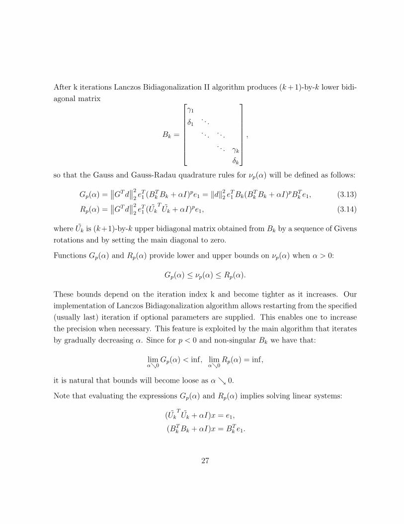
After k iterations Lanczos Bidiagonalization II algorithm produces (k +1)-by-k lower bidi-

agonal matrix

Bk =

γ1

δ1. . .. . . . . .

. . . γk

δk

,

so that the Gauss and Gauss-Radau quadrature rules for νp(α) will be defined as follows:

Gp(α) =∥∥GT d

∥∥2

2eT1 (BT

k Bk + αI)pe1 = ‖d‖22 eT

1 Bk(BTk Bk + αI)pBT

k e1, (3.13)

Rp(α) =∥∥GT d

∥∥2

2eT1 (Uk

TUk + αI)pe1, (3.14)

where Uk is (k+1)-by-k upper bidiagonal matrix obtained from Bk by a sequence of Givens

rotations and by setting the main diagonal to zero.

Functions Gp(α) and Rp(α) provide lower and upper bounds on νp(α) when α > 0:

Gp(α) ≤ νp(α) ≤ Rp(α).

These bounds depend on the iteration index k and become tighter as it increases. Our

implementation of Lanczos Bidiagonalization algorithm allows restarting from the specified

(usually last) iteration if optional parameters are supplied. This enables one to increase

the precision when necessary. This feature is exploited by the main algorithm that iterates

by gradually decreasing α. Since for p < 0 and non-singular Bk we have that:

limα↘0

Gp(α) < inf, limα↘0

Rp(α) = inf,

it is natural that bounds will become loose as α ↘ 0.

Note that evaluating the expressions Gp(α) and Rp(α) implies solving linear systems:

(UkTUk + αI)x = e1,

(BTk Bk + αI)x = BT

k e1.

27

It is easy to see that the above equations are normal equations for the linear least-squares

problem:

min∥∥∥[

Uk√αI

]x−

[0

e1/√

α

]∥∥∥2

min∥∥∥[ Bk√

αI

]x−

[e10

]∥∥∥2.

This means that the solution x for the linear least-squares problem satisfies the original

linear system as well. We may, however, exploit the structure of LLS problems and solve

them efficiently by a sequence of Givens rotations that produces the QR factorization.

This approach is described in [6, 10, 36].

28

Chapter 4

Regularization Algorithm

Before presenting the details of the algorithm we state our assumptions and present some

geometry and relations among the various parameters. The key assumption is that values of

parameters are in a bounded interval, as described in Section 3.5. Making this assumption

does not restrict our ability to locate a good regularized solution, since it is always located

in the interval of interest.

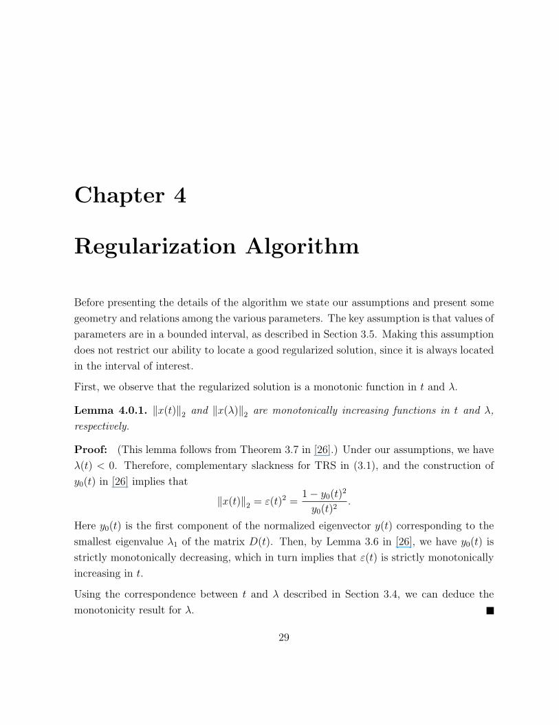
First, we observe that the regularized solution is a monotonic function in t and λ.

Lemma 4.0.1. ‖x(t)‖2 and ‖x(λ)‖2 are monotonically increasing functions in t and λ,

respectively.

Proof: (This lemma follows from Theorem 3.7 in [26].) Under our assumptions, we have

λ(t) < 0. Therefore, complementary slackness for TRS in (3.1), and the construction of

y0(t) in [26] implies that

‖x(t)‖2 = ε(t)2 =1− y0(t)

2

y0(t)2.

Here y0(t) is the first component of the normalized eigenvector y(t) corresponding to the

smallest eigenvalue λ1 of the matrix D(t). Then, by Lemma 3.6 in [26], we have y0(t) is

strictly monotonically decreasing, which in turn implies that ε(t) is strictly monotonically

increasing in t.

Using the correspondence between t and λ described in Section 3.4, we can deduce the

monotonicity result for λ.

29

Throughout the rest of the paper we will interchangeably use parameters ε, t and λ when

describing points on the L-curve. Hence, if a statement is true for smaller or larger values

of ε, it is also true for respectively smaller or larger values of t and λ.

From a given t, we can calculate the corresponding ε and the value of the objective function

µε = k(t), thus obtaining a point on the L-curve. To analyze the location of a given pair

(ε, µε) on the L-curve, we need the derivative of lr := lr(ε) := log(‖Gx(ε)− d‖2) with

respect to lx := lx(ε) := log(‖x(ε)‖2), i.e.

d(lr(ε))/d(ε)

d(lx(ε))/d(ε)=

d(log(‖Gx− d‖2))/d(ε)

d(log(‖x‖2))/d(ε)=

1

2

d(log(µε + dT d))/d(ε)

d(log(ε))/d(ε)

=1

2

µ′εε

µε + dT d

=ε2λε

µε + dT d,

(4.1)

where µ′ε is found using (3.2).

To distinguish whether a point lies before (left) or after (right) the elbow, one can test the

value of the derivative. It should be (negative) close to zero if we are at the plateau after

the elbow. Alternatively, the value tends to a large negative number as we approach the

elbow from the left.

4.1 Initial L-curve point

Our algorithm iterates by steadily increasing the value of parameter t. Then each subse-

quent point is located to the right of the previous one, i.e. corresponds to a larger value

of ε (and t). Hence, locating the elbow of the L-curve is only possible when we start to

the left of the elbow. We need a value of λ or equivalently, by Lemma 3.4.1 or 3.4.2, t, to

locate a point. We can employ different strategies to achieve this task. One way is to start

with the point corresponding to λ = −σn(G)2, see Sections 3.5 and 2.2.

In the case we do not have the largest singular value of the matrix G, we can start with

a point associated with small enough value of t = dT d2

. This value does not have sound

30

theoretical basis, yet empirically, we note that it works in most cases. We will see that

taking this value is good enough to be on the safe side. As we discussed in Section 2.3, a

”well-shaped” L-curve plot can be viewed as a linear plateau to the right of the elbow and

a linear vertical part to the left of the elbow. For well shaped L-curve plots, tiny changes

in t would result in huge changes in ε when we are on the horizontal part. Vice versa, large

changes in t have little affect on ε when we are on the vertical part. This is explained by

the structure of the singular value decomposition of the matrix G (see Section 2.2). The

behaviour remains true for less well-behaved L-shaped plots. This tells us that points that

lie on the plateau region correspond to the values of t that are very close to dT d. Thus,

taking half of this value will put us onto the vertical part to the left of the elbow.

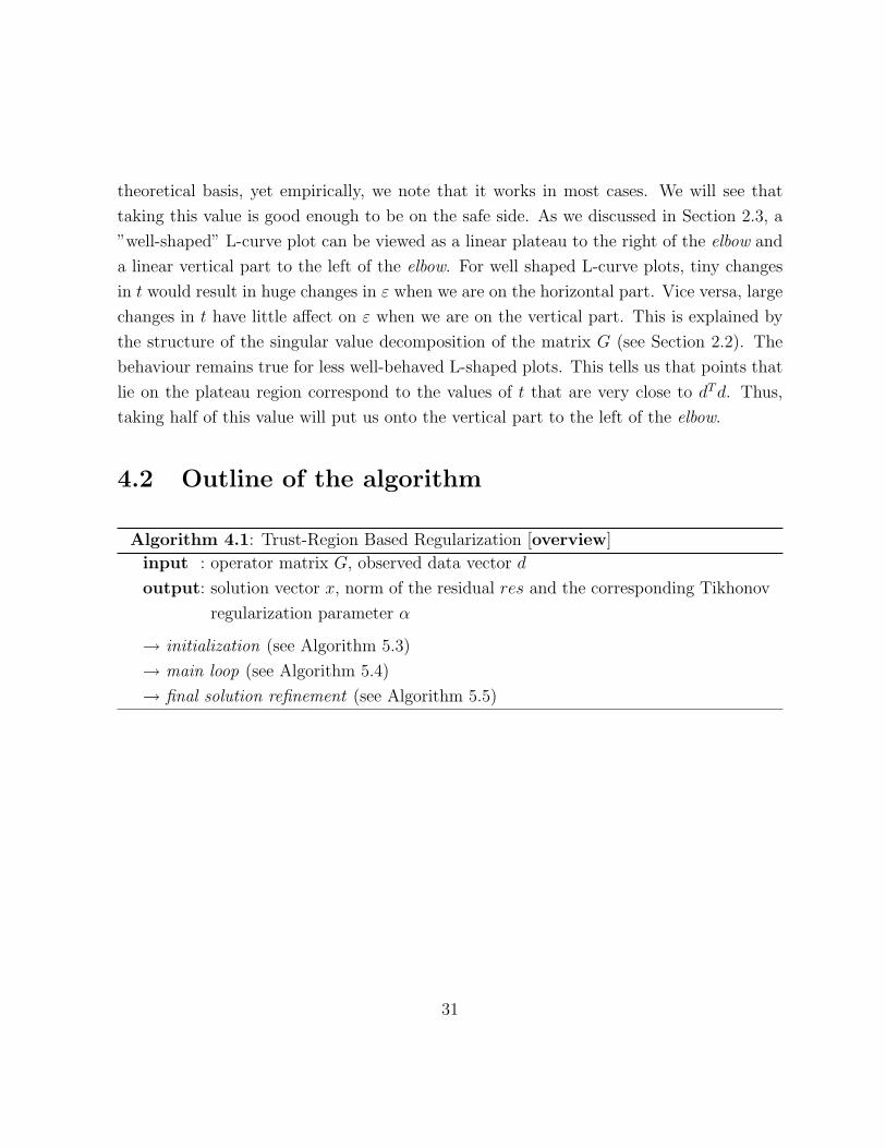
4.2 Outline of the algorithm

Algorithm 4.1: Trust-Region Based Regularization [overview]

input : operator matrix G, observed data vector d

output: solution vector x, norm of the residual res and the corresponding Tikhonov

regularization parameter α

→ initialization (see Algorithm 5.3)

→ main loop (see Algorithm 5.4)

→ final solution refinement (see Algorithm 5.5)

31

Algorithm 4.2: Helper Functions

function [t, x, k] = l2t (λ)

begin

solves for x in (GT G− λI)x = a

t = λ + dT Gx

k = (xT x + 1)λ− t

end

function [λ, x, k] = t2l (t, λ)

beginrun eigs to compute the smallest eigenpair (λ, y) of the matrix D.

use eigenvalue calculated at the previous step as the initial guess, this greatly

improves convergence rate.

change the first component y1 of the eigenvector y to have positive sign.

ε2 = (1− y21)/y

21

x = (ε2 + 1)λ− t

k = y2...n/y1

end

function [κlow, κup] = curvature (ε, res, λ)

begincompute lower and upper bounds on the curvature using current Lanczos

bidiagonalized approximation.end

General idea of the algorithm is presented in the beginning of Section 4. Below we will

describe the details behind the implementation. It can be divided into three large parts:

initialization, main loop and final solution refinement.

32

Algorithm 4.3: Trust-Region Based Regularization [initialization]

compute the largest singluar value σn of the matrix G1

compute the initial bidiagonalization (γ, δ) of the matrix G using Lanczos2

Bidiagonalization II algorithm, use d as the starting vector.

tlow = 03

tup = dT d4

λlow = −σ2n5

λup = 06

εup = −17

κpreviouslow = inf8

κpreviousup = inf9

λ = λlow10

find starting L-curve point, [t, x, k] = l2t(λ)11

We start by computing several things that are going to be used throughout the algorithm.

We also initialize the variables. Computing the largest singular value of G is not absolutely

necessary, but is relatively cheap and yields a lower bound on the eigenvalue λ. If it is

undesirable to compute the largest singular value of G, this step can be omitted and a

reasonable value for the parameter t, e.g. dT d2

computed instead. This also places the lower

bound on the eigenvalue by Lemma 3.4.2.

The more important step is to compute the initial bidiagonalization of the matrix G. This

data is used to estimate the curvature of the L-curve every time a point is obtained. The

details are covered in Section 3.7.

We then proceed by getting an initial point on the L-curve. The discussion on getting a

good estimate is in Section 4.1. We assume that we know the largest singular value of G

and thus start with a value on a parameter λ. Hence, to locate a point on the L-curve, we

solve for values t, x and k.

33

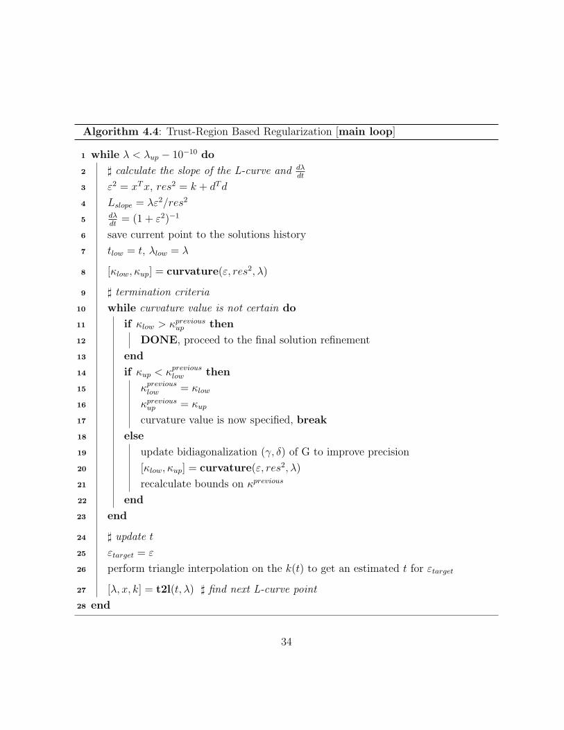
Algorithm 4.4: Trust-Region Based Regularization [main loop]

while λ < λup − 10−10 do1

] calculate the slope of the L-curve and dλdt

2

ε2 = xT x, res2 = k + dT d3

Lslope = λε2/res24

dλdt

= (1 + ε2)−15

save current point to the solutions history6

tlow = t, λlow = λ7

[κlow, κup] = curvature(ε, res2, λ)8

] termination criteria9

while curvature value is not certain do10

if κlow > κpreviousup then11

DONE, proceed to the final solution refinement12

end13

if κup < κpreviouslow then14

κpreviouslow = κlow15

κpreviousup = κup16

curvature value is now specified, break17

else18

update bidiagonalization (γ, δ) of G to improve precision19

[κlow, κup] = curvature(ε, res2, λ)20

recalculate bounds on κprevious21

end22

end23

] update t24

εtarget = ε25

perform triangle interpolation on the k(t) to get an estimated t for εtarget26

[λ, x, k] = t2l(t, λ) ] find next L-curve point27

end28

34

At each iteration the algorithm takes the current point and produces the next one strictly

to the right on the L-curve. There are several possible strategies to achieve this goal.

As Lemma 4.0.1 suggests, increasing either one of the parameters t, λ or ε will move us

further to the right. Hence, we can take a step by changing any one of them. The hard

part, though, is the strategy on choosing the step length. In the current implementation

we do the following.

Suppose we are given the target value for ε. Then we can potentially solve for t and λ (see

Lemma 3.4.3). However, this involves solving TRS that we are trying to avoid. Instead,

we try to estimate the value for t. We do not care if that value does not correspond well

to the target ε. But we require that a new value for t is larger than the previous one, so

that we can take a step.

The key idea behind this estimation lies in observing the properties of the function k(t).

Recall from Section 3.3, that k(t) = (ε2 + 1)λ − t and µε = maxt k(t). The function k(t)

is also concave. Now, let ε0 and t0 represent the optimal pair (ε0, t0) and, hence, a point

on the L-curve. Take also εtgt ≥ ε0. Denote ttgt as the optimal value of t corresponding to

εtgt, so that µ(εtgt) = k(ttgt). Consider the function k(t) with ε = εtgt. Clearly, it attains

the maximum at the point t = ttgt. By monotonicity we have t0 ≤ ttgt. We can also take

the point t1 = dT d. From Section 3.5 we know that k(t1) = −t1 = −dT d. Moreover, the

derivative is k′(t1) = −1. Hence, we get t0 ≤ ttgt ≤ t1.

Now we can take the triangle interpolation at the points t0 and t1 to get an estimate for

ttgt. This technique gives quite good results due to the fact that k(t) can be approximated

by linear models on each of the sides. It is also cheap to compute the tangent at the point

t0, since k′(t) = (ε2 + 1)y20(t)− 1, where y0(t) does not depend on ε. Hence, we can use its

value from the previous step. Figure 4.1 illustrates this approach.

In the algorithm, we use the most simple case of choosing the target value for ε – just

taking the current one. An assumption of the easy case ensures that we have a non-zero

step in t, since k(t) is differentiable everywhere and limt→0 k(t) = −t.

With the new t we can compute both λ and ε as Lemma 3.4.2 suggests. Particular details

on the eigenvalue computation are given in Section 5.1.

The termination condition is based on the L-curve maximum curvature criterion, i.e. we

35

t

k(t)

t0

ttgt

t1

testimated

Figure 4.1: k(t) and triangle interpolation

look for a point on the L-curve that has the maximum negative curvature. To locate such

a point we compute the curvature at each step. This computation uses Gauss Quadrature

approach which is described in Section 3.7. Since we are only getting lower and upper

bounds on the real value of the curvature, it can be a problem to compare between two

values for the consecutive points, e.g. if the corresponding intervals overlap. If such

situation is detected, we improve the bidiagonalization of the matrix G. This increases

the precision in the curvature estimation and, eventually, allows to safely compare the

curvature at these two points. Since L-curve is a convex function near the elbow, we can

determine the area of interest by keeping track of the curvature. Once we get the point

with a smaller curvature than the previous one, we know we have gone too far. The main

loop of the algorithm terminates once we have 3 points, such that the middle one has a

larger curvature value than the other two. From the convexity we deduce that the elbow

36

should lie somewhere between the endpoints. The final refinement is then performed to

estimate the elbow location.

Algorithm 4.5: TRS Based Regularization [final solution refinement]

] observe interval of last three points left, center, right1

while point of maximum curvature still can be improved do2

set λ as bisection of either left or right interval3

find corresponding L-curve point, [t, x, k] = l2t(λ)4

] calculate norm of the residual and ε5

ε2 = xT x6

res2 = k + dT d7

[κlow, κup] = curvature(ε, res2, λ)8

if located point has larger curvature then9

set current point as a solution10

DONE11

end12

shrink interval of intereset13

end14

To estimate the elbow location, we proceed with a simple bisection of the left and right

intervals trying to find a point with the maximum curvature value. We stop once we have

got a point with a curvature value larger than the one we have seen so far.

4.3 Future improvements

The algorithm presented above is not polished enough for commercial use. Rather, it

illustrates the concepts and helps in understanding the regularization process better. It

would be natural to view it as a base for more robust algorithms that can be built upon the

techniques herein. We now outline major improvements and some limitations that apply

to the current implementation.

37

One major limitation is that no proof of convergence to the elbow is provided.

The inability to prove convergence follows from the difficulty of proving correctness of

the optimum. We leave this question open for future research. However, given a proper

L-curve, the method generally finds the solution.

The mathematical reasoning behind the method relies on the L-curve maximum curvature

criterion, a heuristic. Given no apriori information on the error, e.g. either norm or

distribution, there is no way to prove anything definite about the solution. Indeed, it is

proved (see [7]) that, in the absence of the error level information, any method will fail

on a specially constructed input data. It is important to realize that we can only trust

the results if we assume some reasonable constraints on the error level. For example, if

the norm of the error is much larger than the norm of the data or, in a physical sense,

the energy of the noise is larger than that of the signal, the reconstructed solution will be

meaningless. The key difference of our approach to that of the Conjugate Gradient method

is that, though we require some constraints on the error, we never ask for them explicitly.

Using the L-curve criteria we implicity extract the inherent characteristics of the problem.

We believe that many real-world engineering problems possess these characteristics and

can be tackled by our method.

In Section 5.3 we outline some possible directions for future research. These include merg-

ing with Conjugate Gradient type methods. Here we will concentrate on the improvements

that can be done to the presented method.

There are two possible ways to improve the algorithm. One way is to choose a step

length more effectively and another is improvement of the termination criteria. Following

considerations might be helpful for deciding on the step length and elbow location. At

every point on the L-curve we are given the slope of the tangent line. If it is known that

we are sitting either at the vertical or horizontal part, then it is possible to make a larger

step by taking a linear approximation. For instance, we can determine a target value of

ε by taking an intersection of the tangent line with the X-axis. This strategy may help

to climb down the vertical part faster. Same information can help to locate the corner by

taking linear approximations at two points – one on the vertical part and another on the

horizontal.

38

The final refinement step can also be improved by utilizing the data from Lanczos bidi-

agonalization of the matrix G. Once the elbow position is locked, one may construct the

so called L- and Curvature-Ribbons to better approximate the elbow. This approach is

discussed in [2].

39

Chapter 5

Numerics/Computations

5.1 Eigensolver issues

As shown above, obtaining a new L-curve point means solving for the smallest eigenpair of

the matrix D(t). In the case G is large and sparse, the same is true for D(t), so one should

use matrix-free iterative algorithms to compute the eigenpairs, e.g. Lanczos methods. As

t increases, the smallest eigenvalue may become numerically closer to the second one. This

impacts the convergence rate, substantially slowing down the eigensolver.

Under such numerical degeneracy an algorithm may converge to a wrong eigenpair, giving

an incorrect eigenvector and an incorrect regularized solution. One way to control the

eigensolution is to start with an initial eigenvalue smaller than the estimated one and,

at the same time, relatively close to it. For iterative algorithms, it is possible to store

previous eigenvalue results to re-use on the next step as an initial guess. This works only

if the eigenvalue is about to increase at every subsequent iteration.

We have employed this method in our Regularization Algorithm and it proved to be very

efficient. We have used the MATLAB eigs routine which uses a Lanczos-type matrix-free

algorithm. With a good initial eigenvalue guess, this method computes eigenvalues in time

independent of the gap between the first and second eigenvalues.

Another approach that can be used is to apply a spectral transformation to separate the

first and second eigenvalues, i.e. preconditioning. In particular, a Tchebyshev polynomial

40

transformation is discussed in [27] and [28].

A bug in the MATLAB (version 6) eigs routine was also discovered. This routine behaves

incorrectly when called with numeric initial guess for the eigenvalue and a matrix supplied

via an external program file. Under such calling conditions the computed eigenvalue is

completely wrong and differs by several orders from the correct one. The bug was reported

to the MATLAB technical support group. To provide a work around, we force the algorithm

to form the matrix explicitly. This, however, results in larger memory requirements and

should be removed once the bug is fixed.

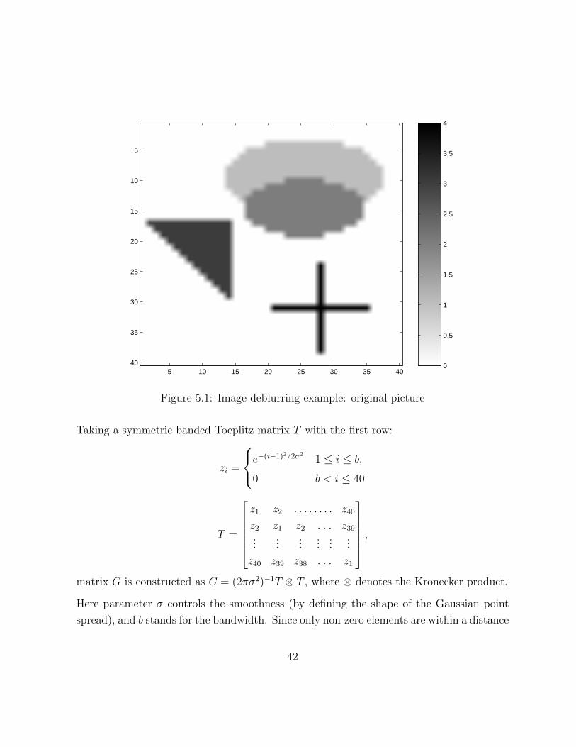
5.2 Image deblurring example

We demonstrate how the algorithm works by considering a sample problem of deblurring

an image. Problems of this nature often occur in the real world. For instance, one might

need to deblur a photo taken by a space telescope or a satellite.

For this particular example we take an image generated by the Hansen MATLAB package

([19]). This package provides an excellent set of regularization tools that can be used

for demonstration purposes. Figure 5.1 shows the image generated by the blur command.

This command also produces the blurring matrix G and the right-hand side d, i.e. observed

data, computed as d = Gxtrue + η. Where η represents the noise. Figure 5.2 shows the

observed image.

The generated image is 40-by-40 grayscale picture, which is stored as a vector xtrue of size

1600. This vector is formed by stretching the image matrix into a single column. Every

component xitrue represents the brightness of the pixel, measured from 0 for the white to

3 for the black (see the colorbar). The matrix G stands for the operator that represents

degradation of the image caused by atmospheric turbulence blur, modelled by a Gaussian

point-spread function,

h(x, y) =1

2πσ2exp

(−x2 + y2

2σ2

).

41

5 10 15 20 25 30 35 40

5

10

15

20

25

30

35

40 0

0.5

1

1.5

2

2.5

3

3.5

4

Figure 5.1: Image deblurring example: original picture

Taking a symmetric banded Toeplitz matrix T with the first row:

zi =

e−(i−1)2/2σ21 ≤ i ≤ b,

0 b < i ≤ 40

T =

z1 z2 . . . . . . . . z40

z2 z1 z2 . . . z39

......

......

......

z40 z39 z38 . . . z1

,

matrix G is constructed as G = (2πσ2)−1T ⊗ T , where ⊗ denotes the Kronecker product.

Here parameter σ controls the smoothness (by defining the shape of the Gaussian point

spread), and b stands for the bandwidth. Since only non-zero elements are within a distance

42

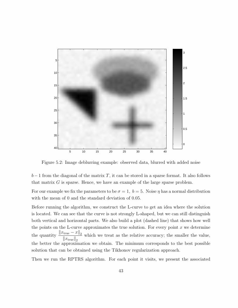
5 10 15 20 25 30 35 40

5

10

15

20

25

30

35

400

0.5

1

1.5

2

2.5

3

Figure 5.2: Image deblurring example: observed data, blurred with added noise

b− 1 from the diagonal of the matrix T , it can be stored in a sparse format. It also follows

that matrix G is sparse. Hence, we have an example of the large sparse problem.

For our example we fix the parameters to be σ = 1, b = 5. Noise η has a normal distribution

with the mean of 0 and the standard deviation of 0.05.

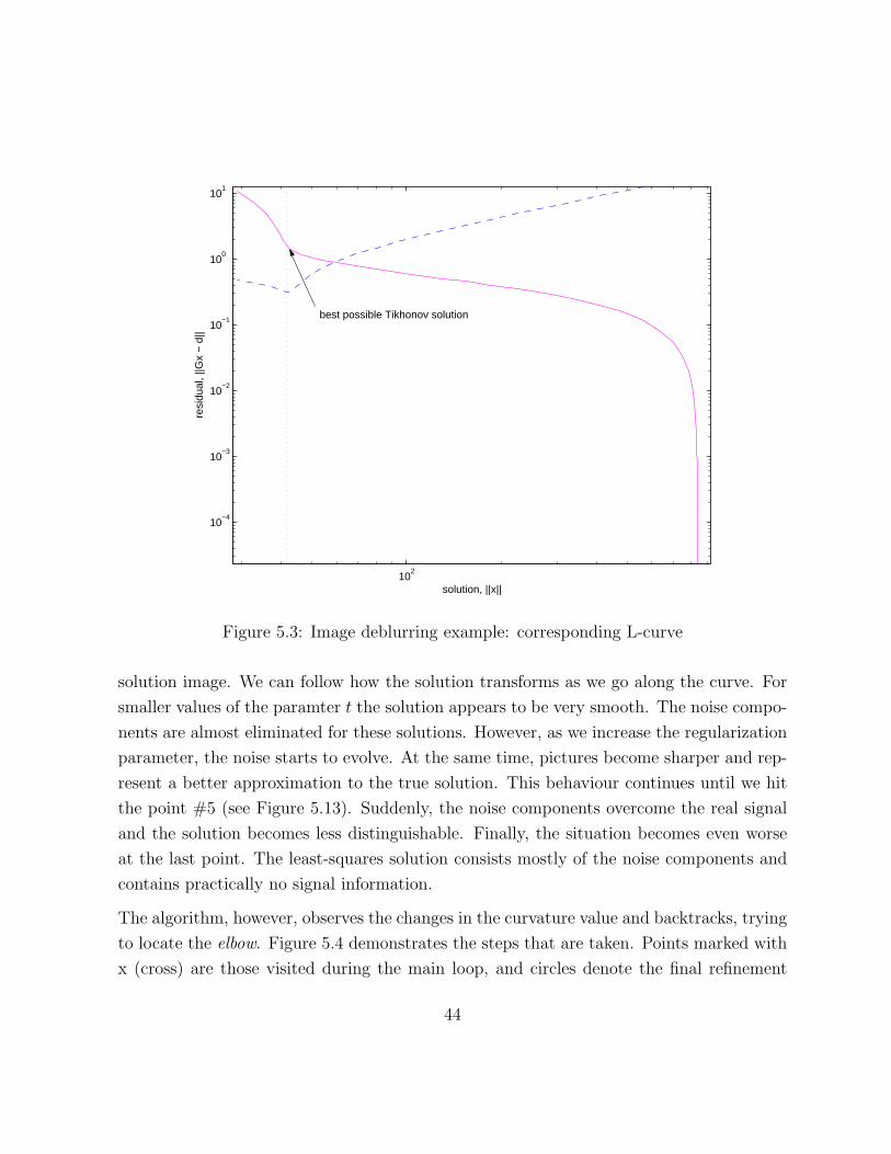
Before running the algorithm, we construct the L-curve to get an idea where the solution

is located. We can see that the curve is not strongly L-shaped, but we can still distinguish

both vertical and horizontal parts. We also build a plot (dashed line) that shows how well

the points on the L-curve approximates the true solution. For every point x we determine

the quantity‖xtrue − x‖2

‖xtrue‖2

which we treat as the relative accuracy; the smaller the value,

the better the approximation we obtain. The minimum corresponds to the best possible

solution that can be obtained using the Tikhonov regularization approach.

Then we run the RPTRS algorithm. For each point it visits, we present the associated

43

102

10−4

10−3

10−2

10−1

100

101

solution, ||x||

resi

dual

, ||G

x −

d||

best possible Tikhonov solution

Figure 5.3: Image deblurring example: corresponding L-curve

solution image. We can follow how the solution transforms as we go along the curve. For

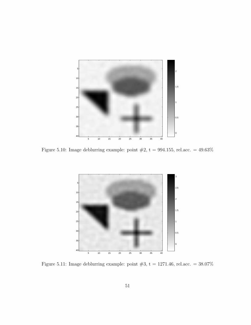
smaller values of the paramter t the solution appears to be very smooth. The noise compo-

nents are almost eliminated for these solutions. However, as we increase the regularization

parameter, the noise starts to evolve. At the same time, pictures become sharper and rep-

resent a better approximation to the true solution. This behaviour continues until we hit

the point #5 (see Figure 5.13). Suddenly, the noise components overcome the real signal

and the solution becomes less distinguishable. Finally, the situation becomes even worse

at the last point. The least-squares solution consists mostly of the noise components and

contains practically no signal information.

The algorithm, however, observes the changes in the curvature value and backtracks, trying

to locate the elbow. Figure 5.4 demonstrates the steps that are taken. Points marked with

x (cross) are those visited during the main loop, and circles denote the final refinement

44

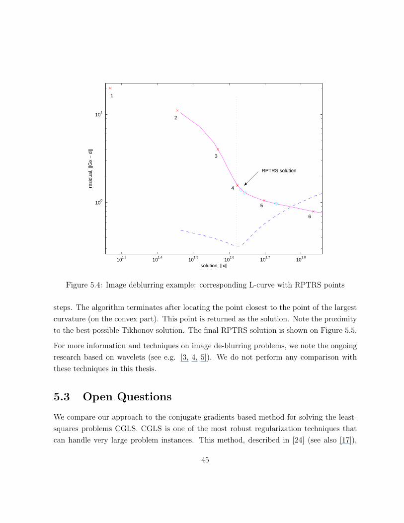
101.3

101.4

101.5

101.6

101.7

101.8

100

101

solution, ||x||

resi

dual

, ||G

x −

d||

1

2

3

4

5

6

RPTRS solution

Figure 5.4: Image deblurring example: corresponding L-curve with RPTRS points

steps. The algorithm terminates after locating the point closest to the point of the largest

curvature (on the convex part). This point is returned as the solution. Note the proximity

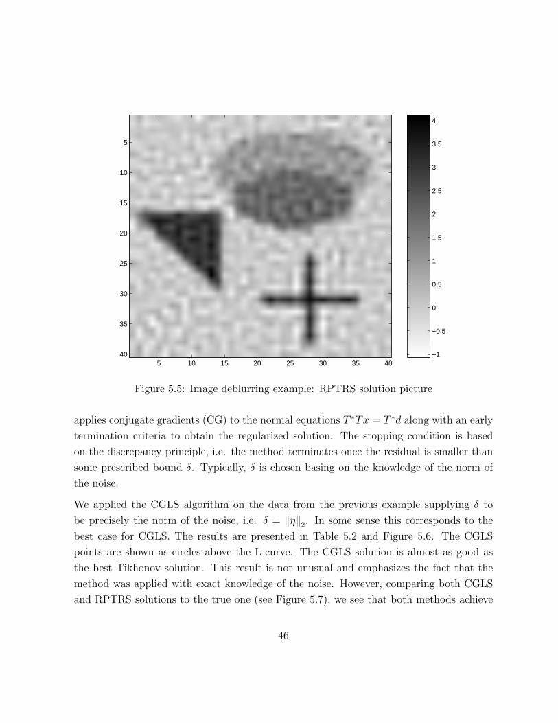
to the best possible Tikhonov solution. The final RPTRS solution is shown on Figure 5.5.

For more information and techniques on image de-blurring problems, we note the ongoing

research based on wavelets (see e.g. [3, 4, 5]). We do not perform any comparison with

these techniques in this thesis.

5.3 Open Questions

We compare our approach to the conjugate gradients based method for solving the least-

squares problems CGLS. CGLS is one of the most robust regularization techniques that

can handle very large problem instances. This method, described in [24] (see also [17]),

45

5 10 15 20 25 30 35 40

5

10

15

20

25

30

35

40 −1

−0.5

0

0.5

1

1.5

2

2.5

3

3.5

4

Figure 5.5: Image deblurring example: RPTRS solution picture

applies conjugate gradients (CG) to the normal equations T ∗Tx = T ∗d along with an early

termination criteria to obtain the regularized solution. The stopping condition is based

on the discrepancy principle, i.e. the method terminates once the residual is smaller than

some prescribed bound δ. Typically, δ is chosen basing on the knowledge of the norm of

the noise.

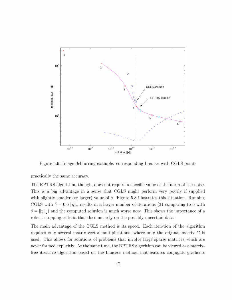
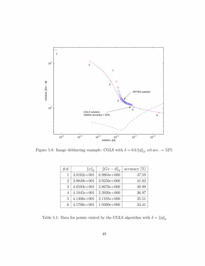
We applied the CGLS algorithm on the data from the previous example supplying δ to

be precisely the norm of the noise, i.e. δ = ‖η‖2. In some sense this corresponds to the

best case for CGLS. The results are presented in Table 5.2 and Figure 5.6. The CGLS

points are shown as circles above the L-curve. The CGLS solution is almost as good as

the best Tikhonov solution. This result is not unusual and emphasizes the fact that the

method was applied with exact knowledge of the noise. However, comparing both CGLS

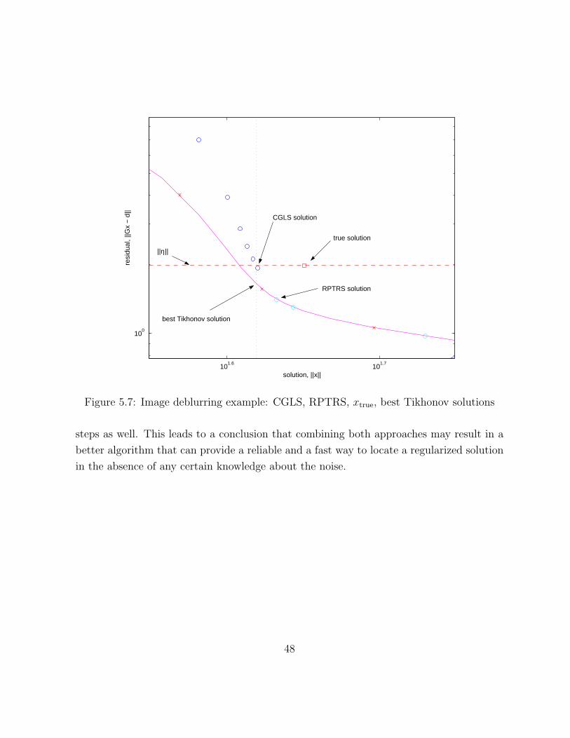
and RPTRS solutions to the true one (see Figure 5.7), we see that both methods achieve

46

101.3

101.4

101.5

101.6

101.7

101.8

100

101

solution, ||x||

resi

dual

, ||G

x −

d||

1

2

3

4

5

6

RPTRS solution

CGLS solution

Figure 5.6: Image deblurring example: corresponding L-curve with CGLS points

practically the same accuracy.

The RPTRS algorithm, though, does not require a specific value of the norm of the noise.

This is a big advantage in a sense that CGLS might perform very poorly if supplied

with slightly smaller (or larger) value of δ. Figure 5.8 illustrates this situation. Running

CGLS with δ = 0.6 ‖η‖2 results in a larger number of iterations (31 comparing to 6 with

δ = ‖η‖2) and the computed solution is much worse now. This shows the importance of a

robust stopping criteria that does not rely on the possibly uncertain data.

The main advantage of the CGLS method is its speed. Each iteration of the algorithm

requires only several matrix-vector multiplications, where only the original matrix G is

used. This allows for solutions of problems that involve large sparse matrices which are

never formed explicitly. At the same time, the RPTRS algorithm can be viewed as a matrix-

free iterative algorithm based on the Lanczos method that features conjugate gradients

47

101.6

101.7

100

solution, ||x||

resi

dual

, ||G

x −

d||

true solution

CGLS solution

RPTRS solution

best Tikhonov solution

||η||

Figure 5.7: Image deblurring example: CGLS, RPTRS, xtrue, best Tikhonov solutions

steps as well. This leads to a conclusion that combining both approaches may result in a

better algorithm that can provide a reliable and a fast way to locate a regularized solution

in the absence of any certain knowledge about the noise.

48

101.3

101.4

101.5

101.6

101.7

101.8

100

101

solution, ||x||

resi

dual

, ||G

x −

d||

1

2

3

4

5

6

RPTRS solution

CGLS solution,relative accuracy = 52%

Figure 5.8: Image deblurring example: CGLS with δ = 0.6 ‖η‖2, rel.acc. = 52%

## ‖x‖2 ‖Gx− d‖2 accuracy [%]

1 3.8162e+001 6.9804e+000 47.59

2 3.9849e+001 3.9256e+000 41.83

3 4.0593e+001 2.8676e+000 38.99

4 4.1045e+001 2.3920e+000 36.97

5 4.1406e+001 2.1105e+000 35.51

6 4.1706e+001 1.9309e+000 34.41

Table 5.1: Data for points visited by the CGLS algorithm with δ = ‖η‖2

49

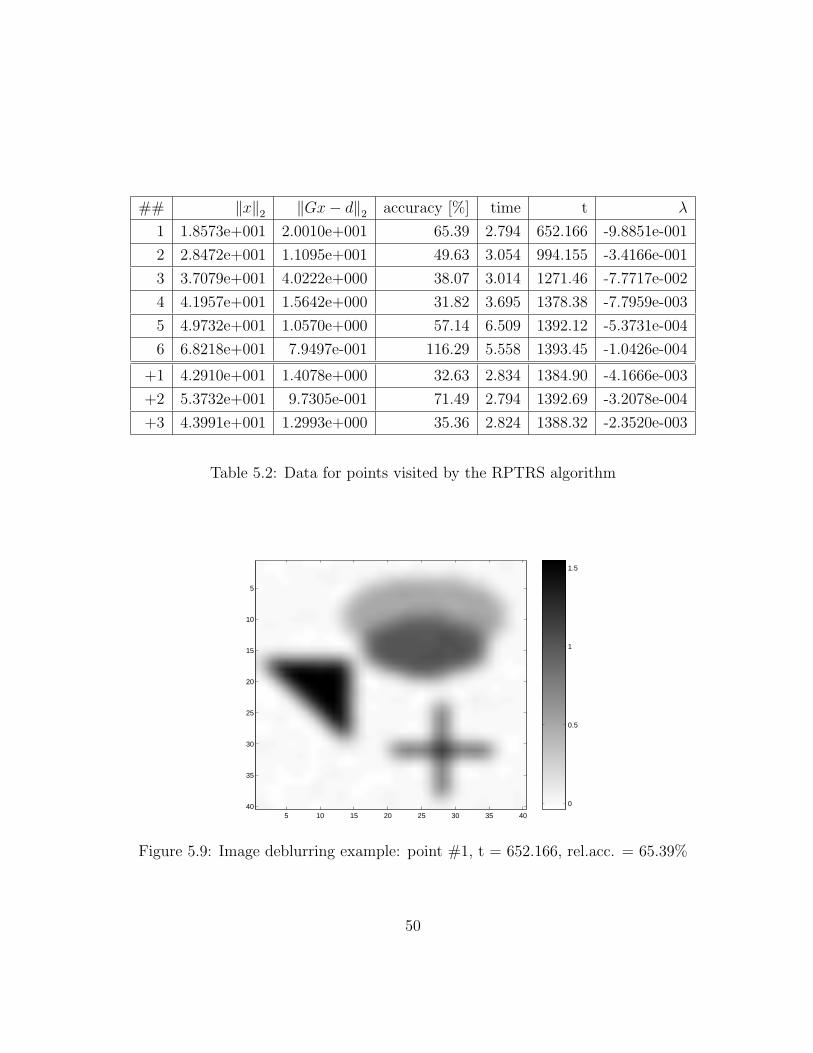
## ‖x‖2 ‖Gx− d‖2 accuracy [%] time t λ

1 1.8573e+001 2.0010e+001 65.39 2.794 652.166 -9.8851e-001

2 2.8472e+001 1.1095e+001 49.63 3.054 994.155 -3.4166e-001

3 3.7079e+001 4.0222e+000 38.07 3.014 1271.46 -7.7717e-002

4 4.1957e+001 1.5642e+000 31.82 3.695 1378.38 -7.7959e-003

5 4.9732e+001 1.0570e+000 57.14 6.509 1392.12 -5.3731e-004

6 6.8218e+001 7.9497e-001 116.29 5.558 1393.45 -1.0426e-004

+1 4.2910e+001 1.4078e+000 32.63 2.834 1384.90 -4.1666e-003

+2 5.3732e+001 9.7305e-001 71.49 2.794 1392.69 -3.2078e-004

+3 4.3991e+001 1.2993e+000 35.36 2.824 1388.32 -2.3520e-003

Table 5.2: Data for points visited by the RPTRS algorithm

5 10 15 20 25 30 35 40

5

10

15

20

25

30

35

40 0

0.5

1

1.5

Figure 5.9: Image deblurring example: point #1, t = 652.166, rel.acc. = 65.39%

50

5 10 15 20 25 30 35 40

5

10

15

20

25

30

35

400

0.5

1

1.5

2

Figure 5.10: Image deblurring example: point #2, t = 994.155, rel.acc. = 49.63%

5 10 15 20 25 30 35 40

5

10

15

20

25

30

35

40

0

0.5

1

1.5

2

2.5

3

Figure 5.11: Image deblurring example: point #3, t = 1271.46, rel.acc. = 38.07%

51

5 10 15 20 25 30 35 40

5

10

15

20

25

30

35

40

−0.5

0

0.5

1

1.5

2

2.5

3

3.5

Figure 5.12: Image deblurring example: point #4, t = 1378.38, rel.acc. = 31.82%

5 10 15 20 25 30 35 40

5

10

15

20

25

30

35

40 −2

−1

0

1

2

3

4

5

Figure 5.13: Image deblurring example: point #5, t = 1392.12, rel.acc. = 57.14%

52

5 10 15 20 25 30 35 40

5

10

15

20

25

30

35

40

−3

−2

−1

0

1

2

3

4

5

6

7

Figure 5.14: Image deblurring example: point #6, t = 1393.45, rel.acc. = 116.29%

53

Appendix A

MATLAB Code

A.1 RPTRS Regularization Algorithm

0001 function [x, res, alpha] = RPTRS (G, d, x bar)

0002

0003 % ------------------------------------------------------------------------

0004 % Parameterized Trust Region Subproblem Regularization Algorithm

0005 %

0006 % solves the problem min ||Gx - d||

0007 %

0008 % INPUT:

0009 % G -- operator matrix

0010 % d -- rhs (observed data)

0011 % x bar -- true solution (optional), this parameter is used for

0012 % accuracy calculations

0013 %

0014 % OUTPUT:

0015 % x -- regularized solution

0016 % res -- norm of the residual

0017 % alpha -- Tikhonov regularization parameter

0018 %

0019 % ------------------------------------------------------------------------

0020 % Developed by Oleg Grodzevich as a part of Master of Mathematics Thesis,

0021 % University of Waterloo, Combinatorics and Optimization department.

54

0022 %

0023 % E-mail: [email protected]

0024 % ------------------------------------------------------------------------

0025

0026 global A a gamma delta bidiag p bidiag q

0027

0028 % ------------------------------------------------------------------------

0029 % Initialization

0030 % ------------------------------------------------------------------------

0031

0032 % x bar is optional

0033 if nargin < 3, x bar = ones(size(d,1),1); end

0034

0035 % in fact we do not need A matrix explicitly, this is only needed to work

0036 % around a bug in the implementation of eigs()

0037 A = G’*G;

0038 a = G’*d;

0039 dd = d’*d;

0040

0041 % configuration options

0042 lslope tol1 = 1;

0043

0044 % compute the largest singular value of G

0045 time = cputime; sigmaLA = svds(G,1); time = cputime - time;

0046

0047 % initial interval [low,up) for t and lambda

0048 t low = 0;

0049 t up = dd;

0050 l low = -sigmaLA^2;

0051 l up = 0;

0052 itcount = 1; % iterations counter

0053 phist = []; % points history

0054 pkappaU = 1e10; % previous curvature

0055 pkappaL = 1e10;

0056 nx bar = norm(x bar);

0057

0058 % largest singular value computation time

0059 disp([’ ’]);

55

0060 disp([’ +----------------------------------------’, ...

0061 ’--------------------------------------------+’]);

0062 disp([sprintf(’ | initial time for sigmaLA = %7g %48c|’, time, ’ ’)]);

0063

0064 % bidiagonalize matrix G

0065 time = cputime;

0066 [gamma, delta, bidiag p, bidiag q] = lbidiag2 (G, d);

0067 time = cputime - time;

0068 disp([sprintf(’ | initial time for bidiagG = %7g %48c|’, time, ’ ’)]);

0069

0070 % solve for the initial point: lambda -> t

0071 lambda = l low;

0072 [t,x,k,time] = l2t(lambda);

0073

0074 % info header

0075 disp([’ +----+--------------+--------------+--------------+’, ...

0076 ’---------+---------+--------------+’]);

0077

0078 disp([’ | ## | norm(x) | norm(Gx-d) | accuracy [%] |’, ...

0079 ’ time | t | lambda |’]);

0080

0081 disp([’ +----+--------------+--------------+--------------+’, ...

0082 ’---------+---------+--------------+’]);

0083

0084 % ------------------------------------------------------------------------

0085 % Loop

0086 % ------------------------------------------------------------------------

0087 l damp = 1e-11;

0088 while lambda < l up - l damp

0089

0090 % calculate the slope of L-curve and d(lambda)/dt = y(1)

0091 eps2 = x’*x; % norm of the solution squared

0092 r2 = k+dd; % norm of the residual squared

0093 lslope = lambda*eps2/r2;

0094 dldt = 1/(1+eps2);

0095

0096 % save current point

0097 pt = [t lambda sqrt(eps2) sqrt(r2) lslope dldt];

56

0098 phist = [pt ; phist];

0099

0100 % update lower bounds on t and lambda

0101 t low = pt(1);

0102 l low = pt(2);

0103

0104 % relative accuracy

0105 acc = norm(x - x bar)/nx bar;

0106

0107 % plot point on the L-curve

0108 hold on; loglog(pt(3),pt(4),’rx’); hold off;

0109

0110 % information

0111 disp([ ...

0112 sprintf(’ | %2d | %12.4e | %12.4e | %12.2f | %7g | %7g | %12.4e |’,...

0113 itcount, pt(3), pt(4), acc*100, time, pt(1), pt(2))]);

0114

0115 disp([’ +----+--------------+--------------+--------------+’, ...

0116 ’---------+---------+--------------+’]);

0117

0118 % calculate curvature

0119 [kappaL, kappaU, time] = curvature(G, d, pt(3), r2, pt(2));

0120

0121 disp([ ...

0122 sprintf(’ | curvature = (%12.4e,%12.4e) time = %7g %26c|’, ...

0123 kappaL, kappaU, time, ’ ’)]);

0124

0125 % --- termination

0126 stop = false;

0127 done = false;

0128 while ~stop

0129 if kappaL > pkappaU

0130 % return previous solution

0131 res = phist(2,4);

0132 alpha = sqrt(-phist(2,2));

0133 done = true;

0134 break;

0135 end

57

0136

0137 if kappaU < pkappaL, pkappaL = kappaL; pkappaU = kappaU; stop = true;

0138 else

0139 time = cputime;

0140 [gamma, delta, bidiag p, bidiag q] = ...

0141 lbidiag2(G, d, gamma, delta, bidiag p, bidiag q, length(gamma)+1);

0142 [kappaL, kappaU, time0] = curvature(G, d, pt(3), r2, pt(2));

0143 time = cputime - time;

0144

0145 disp([ ...

0146 sprintf(’ | curvature = (%12.4e,%12.4e) time = %7g %26c|’, ...

0147 kappaL, kappaU, time, ’ ’)]);

0148

0149 % recalculate previous kappa bounds

0150 [pkappaL, pkappaU, time] = ...

0151 curvature(G, d, phist(2,3), phist(2,4)^2, phist(2,2));

0152

0153 disp([ ...

0154 sprintf(’ | previous = (%12.4e,%12.4e) time = %7g %26c|’, ...

0155 pkappaL, pkappaU, time, ’ ’)]);

0156 end

0157 end

0158

0159 % true solution should sit between two last points

0160 if done, break; end

0161

0162 disp([sprintf(’ | slope = %12.4e %57c|’, pt(5), ’ ’)]);

0163

0164 % possible pause before next iteration

0165 % keyboard

0166

0167 % target epsilon is the current one

0168 tgt eps = pt(3);

0169

0170 % do triangle interpolation on k(t) to obtain the estimate for t

0171 e2p1 = tgt eps^2 + 1;

0172

0173 % we choose the point t=dd,k(t)=-dd for the second pivot, as we

58

0174 % know this point is always there

0175 k1 = e2p1*pt(2)-pt(1);

0176 l1 = e2p1*pt(6)-1;

0177 k2 = -dd;

0178 l2 = -1; % slope ~ -1 there, since y(1)->0

0179 [t,u] = tinterpl (pt(1), dd, k1, k2, l1, l2);

0180

0181 % display target epsilon

0182 disp([sprintf(’ | target eps = %12.4e %57c|’, tgt eps, ’ ’)]);

0183

0184 % information about projected point

0185 disp([sprintf(’ | target t = %12.4e %57c|’, t, ’ ’)]);

0186 disp([’ +----+--------------+--------------+--------------+’, ...

0187 ’---------+---------+--------------+’]);

0188

0189 % now tgt t is the projected point, check bounds, however both

0190 % MUST be good

0191 if t <= t low || t >= t up

0192 disp(’>> PANIC: this should never happen!’);

0193 return;

0194 end

0195

0196 % save previous solution

0197 soln = x;

0198

0199 % need previous lambda as an initial guess

0200 if itcount > 1, [lambda,x,k,time,y] = t2l(t,lambda,y);

0201 else, [lambda,x,k,time,y] = t2l(t,lambda); end

0202

0203 itcount = itcount + 1;

0204 end

0205

0206 % info footer

0207 disp([’ +----------------------------------------’, ...

0208 ’--------------------------------------------+’]);

0209

0210 % ------------------------------------------------------------------------

0211 % Refine between the last two points

59

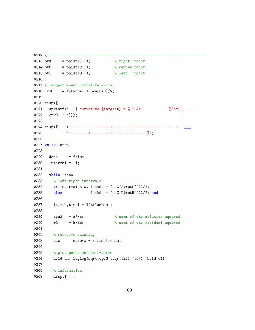
0212 % ------------------------------------------------------------------------

0213 ptR = phist(1,:); % right point

0214 ptC = phist(2,:); % center point

0215 ptL = phist(3,:); % left point

0216

0217 % largest known curvature so far

0218 crvC = (pkappaL + pkappaU)/2;

0219

0220 disp([ ...

0221 sprintf(’ | curvature [largest] = %12.4e %36c|’, ...

0222 crvC, ’ ’)]);

0223

0224 disp([’ +-------------------+--------------+--------------+’, ...

0225 ’---------+---------+--------------+’]);

0226

0227 while ~stop

0228

0229 done = false;

0230 interval = -1;

0231

0232 while ~done

0233 % left/right intervals

0234 if interval < 0, lambda = (ptC(2)+ptL(2))/2;

0235 else lambda = (ptC(2)+ptR(2))/2; end

0236

0237 [t,x,k,time] = l2t(lambda);

0238

0239 eps2 = x’*x; % norm of the solution squared

0240 r2 = k+dd; % norm of the residual squared

0241

0242 % relative accuracy

0243 acc = norm(x - x bar)/nx bar;

0244

0245 % plot point on the L-curve

0246 hold on; loglog(sqrt(eps2),sqrt(r2),’co’); hold off;

0247

0248 % information

0249 disp([ ...

60

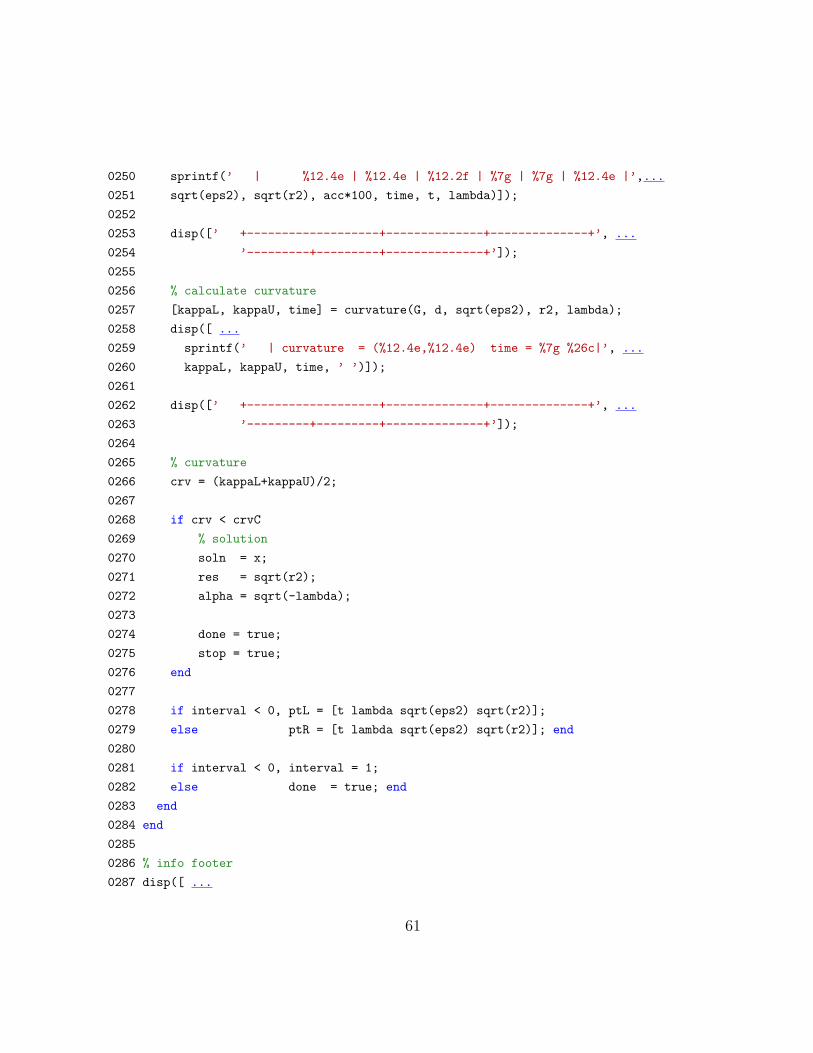
0250 sprintf(’ | %12.4e | %12.4e | %12.2f | %7g | %7g | %12.4e |’,...

0251 sqrt(eps2), sqrt(r2), acc*100, time, t, lambda)]);

0252

0253 disp([’ +-------------------+--------------+--------------+’, ...

0254 ’---------+---------+--------------+’]);

0255

0256 % calculate curvature

0257 [kappaL, kappaU, time] = curvature(G, d, sqrt(eps2), r2, lambda);

0258 disp([ ...

0259 sprintf(’ | curvature = (%12.4e,%12.4e) time = %7g %26c|’, ...

0260 kappaL, kappaU, time, ’ ’)]);

0261

0262 disp([’ +-------------------+--------------+--------------+’, ...

0263 ’---------+---------+--------------+’]);

0264

0265 % curvature

0266 crv = (kappaL+kappaU)/2;

0267

0268 if crv < crvC

0269 % solution

0270 soln = x;

0271 res = sqrt(r2);

0272 alpha = sqrt(-lambda);

0273

0274 done = true;

0275 stop = true;

0276 end

0277

0278 if interval < 0, ptL = [t lambda sqrt(eps2) sqrt(r2)];

0279 else ptR = [t lambda sqrt(eps2) sqrt(r2)]; end

0280

0281 if interval < 0, interval = 1;

0282 else done = true; end

0283 end

0284 end

0285

0286 % info footer

0287 disp([ ...

61

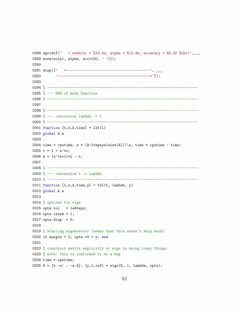
0288 sprintf(’ | norm(x) = %12.4e, alpha = %12.4e, accuracy = %5.2f %20c|’,...

0289 norm(soln), alpha, acc*100, ’ ’)]);

0290

0291 disp([’ +----------------------------------------’, ...

0292 ’--------------------------------------------+’]);

0293

0294 % ------------------------------------------------------------------------

0295 % --- END of main function

0296 % ------------------------------------------------------------------------

0297

0298 % ------------------------------------------------------------------------

0299 % --- conversion lambda -> t

0300 % ------------------------------------------------------------------------

0301 function [t,x,k,time] = l2t(l)

0302 global A a

0303

0304 time = cputime; x = (A-l*speye(size(A)))\a; time = cputime - time;

0305 t = l + a’*x;

0306 k = (x’*x+1)*l - t;

0307

0308 % ------------------------------------------------------------------------

0309 % --- conversion t -> lambda

0310 % ------------------------------------------------------------------------

0311 function [l,x,k,time,y] = t2l(t, lambda, y)

0312 global A a

0313

0314 % options for eigs

0315 opts.tol = 1e6*eps;

0316 opts.issym = 1;

0317 opts.disp = 0;

0318

0319 % starting eigenvector (seems that this doesn’t help much)

0320 if nargin > 2, opts.v0 = y; end

0321

0322 % construct matrix explicitly or eigs is doing crazy things

0323 % note: this is confirmed to be a bug

0324 time = cputime;

0325 D = [t -a’ ; -a A]; [y,l,inf] = eigs(D, 1, lambda, opts);

62

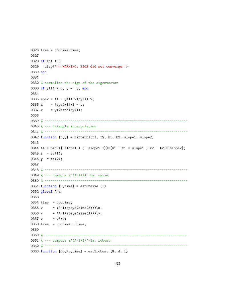
0326 time = cputime-time;

0327

0328 if inf > 0

0329 disp(’>> WARNING: EIGS did not converge!’);

0330 end

0331

0332 % normalize the sign of the eigenvector

0333 if y(1) < 0, y = -y; end

0334

0335 eps2 = (1 - y(1)^2)/y(1)^2;

0336 k = (eps2+1)*l - t;

0337 x = y(2:end)/y(1);

0338

0339 % ------------------------------------------------------------------------

0340 % --- triangle interpolation

0341 % ------------------------------------------------------------------------

0342 function [t,y] = tinterpl(t1, t2, k1, k2, slope1, slope2)

0343

0344 tt = pinv([-slope1 1 ; -slope2 1])*[k1 - t1 * slope1 ; k2 - t2 * slope2];

0345 t = tt(1);

0346 y = tt(2);

0347

0348 % ------------------------------------------------------------------------

0349 % --- compute a’(A-l*I)^-3a: naive

0350 % ------------------------------------------------------------------------

0351 function [v,time] = est3naive (l)

0352 global A a

0353

0354 time = cputime;

0355 v = (A-l*speye(size(A)))\a;0356 w = (A-l*speye(size(A)))\v;0357 v = v’*w;

0358 time = cputime - time;

0359

0360 % ------------------------------------------------------------------------

0361 % --- compute a’(A-l*I)^-3a: robust

0362 % ------------------------------------------------------------------------

0363 function [Gp,Rp,time] = est3robust (G, d, l)

63

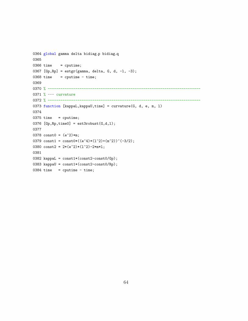
0364 global gamma delta bidiag p bidiag q

0365

0366 time = cputime;

0367 [Gp,Rp] = estgr(gamma, delta, G, d, -l, -3);

0368 time = cputime - time;

0369

0370 % ------------------------------------------------------------------------

0371 % --- curvature

0372 % ------------------------------------------------------------------------

0373 function [kappaL,kappaU,time] = curvature(G, d, e, m, l)

0374

0375 time = cputime;

0376 [Gp,Rp,time0] = est3robust(G,d,l);

0377

0378 const0 = (e^2)*m;

0379 const1 = const0*((e^4)*(l^2)+(m^2))^(-3/2);

0380 const2 = 2*(e^2)*(l^2)-2*m*l;

0381

0382 kappaL = const1*(const2-const0/Gp);

0383 kappaU = const1*(const2-const0/Rp);

0384 time = cputime - time;

64

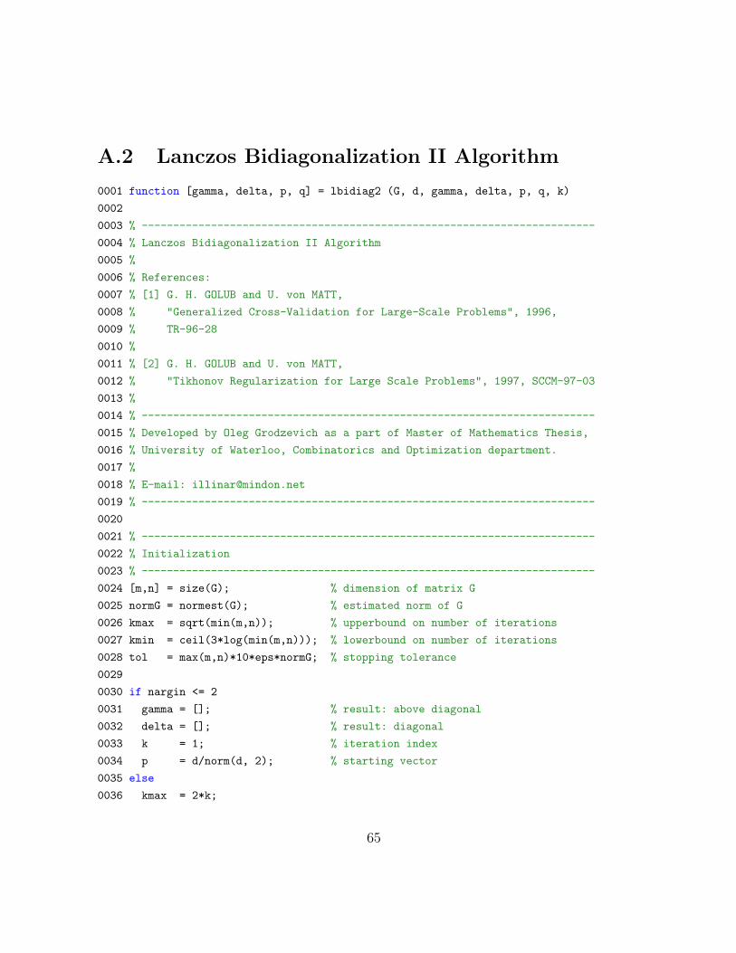
A.2 Lanczos Bidiagonalization II Algorithm

0001 function [gamma, delta, p, q] = lbidiag2 (G, d, gamma, delta, p, q, k)

0002

0003 % ------------------------------------------------------------------------

0004 % Lanczos Bidiagonalization II Algorithm

0005 %

0006 % References:

0007 % [1] G. H. GOLUB and U. von MATT,

0008 % "Generalized Cross-Validation for Large-Scale Problems", 1996,

0009 % TR-96-28

0010 %

0011 % [2] G. H. GOLUB and U. von MATT,

0012 % "Tikhonov Regularization for Large Scale Problems", 1997, SCCM-97-03

0013 %

0014 % ------------------------------------------------------------------------

0015 % Developed by Oleg Grodzevich as a part of Master of Mathematics Thesis,

0016 % University of Waterloo, Combinatorics and Optimization department.

0017 %

0018 % E-mail: [email protected]

0019 % ------------------------------------------------------------------------

0020

0021 % ------------------------------------------------------------------------

0022 % Initialization

0023 % ------------------------------------------------------------------------

0024 [m,n] = size(G); % dimension of matrix G

0025 normG = normest(G); % estimated norm of G

0026 kmax = sqrt(min(m,n)); % upperbound on number of iterations

0027 kmin = ceil(3*log(min(m,n))); % lowerbound on number of iterations

0028 tol = max(m,n)*10*eps*normG; % stopping tolerance

0029

0030 if nargin <= 2

0031 gamma = []; % result: above diagonal

0032 delta = []; % result: diagonal

0033 k = 1; % iteration index

0034 p = d/norm(d, 2); % starting vector

0035 else

0036 kmax = 2*k;

65

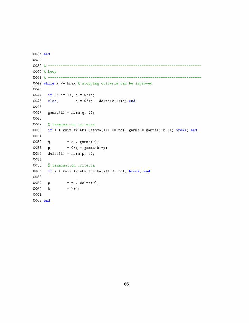
0037 end

0038

0039 % ------------------------------------------------------------------------

0040 % Loop

0041 % ------------------------------------------------------------------------

0042 while k <= kmax % stopping criteria can be improved

0043

0044 if (k <= 1), q = G’*p;

0045 else, q = G’*p - delta(k-1)*q; end

0046

0047 gamma(k) = norm(q, 2);

0048

0049 % termination criteria

0050 if k > kmin && abs (gamma(k)) <= tol, gamma = gamma(1:k-1); break; end

0051

0052 q = q / gamma(k);

0053 p = G*q - gamma(k)*p;

0054 delta(k) = norm(p, 2);

0055

0056 % termination criteria

0057 if k > kmin && abs (delta(k)) <= tol, break; end

0058

0059 p = p / delta(k);

0060 k = k+1;

0061

0062 end

66

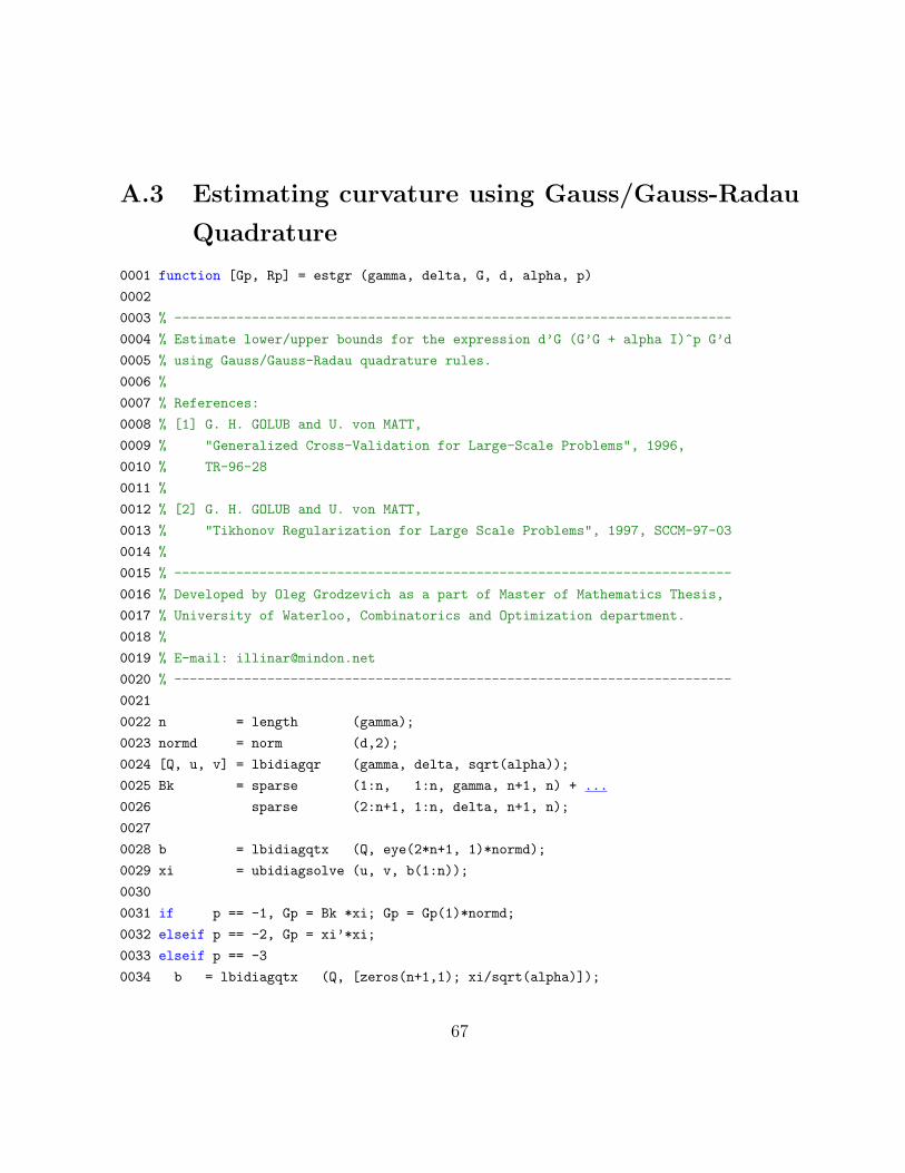
A.3 Estimating curvature using Gauss/Gauss-Radau

Quadrature

0001 function [Gp, Rp] = estgr (gamma, delta, G, d, alpha, p)

0002

0003 % ------------------------------------------------------------------------

0004 % Estimate lower/upper bounds for the expression d’G (G’G + alpha I)^p G’d

0005 % using Gauss/Gauss-Radau quadrature rules.

0006 %

0007 % References:

0008 % [1] G. H. GOLUB and U. von MATT,

0009 % "Generalized Cross-Validation for Large-Scale Problems", 1996,

0010 % TR-96-28

0011 %

0012 % [2] G. H. GOLUB and U. von MATT,

0013 % "Tikhonov Regularization for Large Scale Problems", 1997, SCCM-97-03

0014 %

0015 % ------------------------------------------------------------------------

0016 % Developed by Oleg Grodzevich as a part of Master of Mathematics Thesis,

0017 % University of Waterloo, Combinatorics and Optimization department.

0018 %

0019 % E-mail: [email protected]

0020 % ------------------------------------------------------------------------

0021

0022 n = length (gamma);

0023 normd = norm (d,2);

0024 [Q, u, v] = lbidiagqr (gamma, delta, sqrt(alpha));

0025 Bk = sparse (1:n, 1:n, gamma, n+1, n) + ...

0026 sparse (2:n+1, 1:n, delta, n+1, n);

0027

0028 b = lbidiagqtx (Q, eye(2*n+1, 1)*normd);

0029 xi = ubidiagsolve (u, v, b(1:n));

0030

0031 if p == -1, Gp = Bk *xi; Gp = Gp(1)*normd;

0032 elseif p == -2, Gp = xi’*xi;

0033 elseif p == -3

0034 b = lbidiagqtx (Q, [zeros(n+1,1); xi/sqrt(alpha)]);

67

0035 eta = ubidiagsolve (u, v, b(1:n));

0036 Gp = xi’*eta;

0037 end

0038

0039 % compute \tilde{U} k

0040 [Q, u, v] = lbidiagqr (gamma, delta, 0) ;

0041 u(n) = 0;

0042

0043 [Q, u, v] = ubidiagqr (u, v, sqrt(alpha));

0044 b = ubidiagqtx (Q, [zeros(n,1); eye(n,1)]);

0045 eta = ubidiagsolve (u, v, b(1:n));

0046 zeta = lbidiagsolve (u, v, eta);

0047 Rp = norm(G’*d)^2*norm (zeta, 2)^2/alpha;

Note, functions lbidiagqr, ubidiagqr, lbidiagqtx, ubidiagqtx, ubidiagsolve, lbidi-

agsolve are external C functions that compute and operate with QR-decomposition. They

are available from author upon request.

68

Bibliography

[1] R. ASTER, B. BORCHERS, and C. THURBER. Parameter Estimation and Inverse

Problems. Academic Press, 2004.

[2] D. CALVETTI, P.C. HANSEN, and L. REICHEL. L-curve curvature bounds via

Lanczos bidiagonalization. Electron. Trans. Numer. Anal., 14:135–150 (electronic),

2002. Orthogonal polynomials, approximation theory, and harmonic analysis (Inzel,

2000).

[3] D. L. DONOHO and I. M. JOHNSTONE. Ideal spatial adaptation by wavelet shrink-

age. Biometrika, 81(3):425–455, 1994.

[4] D. L. DONOHO and I. M. JOHNSTONE. Adapting to unknown smoothness via

wavelet shrinkage. Journal of the American Statistical Association, 90(432):1200–

1224, 1995.

[5] D. L. DONOHO, I. M. JOHNSTONE, G. KERKYACHARIAN, and D. PICARD.

Wavelet shrinkage: asymptopia? Journal of the Royal Statistical Society, Ser. B,

57:301–337, 1995.

[6] L. ELDEN. Algorithms for the regularization of ill-conditioned least squares problems.

BIT, 17:134–145, 1977.

[7] H. W. ENGL, M. HANKE, and A. NEUBAUER. Regularization of Inverse Problems.

Kluwer Academic Publishers Group, Dordrecht, 1996.

[8] C. FORTIN and H. WOLKOWICZ. The trust region subproblem and semidefinite

programming. Optimization Methods and Software, 19(1):41–67, 2004. special issue

69

dedicated to Jochem Zowes 60th birthday, Guest Editors: Florian Jarre and Michal

Kocvara.

[9] M. FROH. Trust region subproblems and linear least-squares regularization. Master’s

thesis, University of Waterloo, 2003.

[10] W. GANDER. On the linear least squares problem with a quadratic constraint. Tech-

nical Report STAN-CS-78-697, Department of Computer Science, Stanford University,

Stanford, CA, 1978.

[11] D.M. GAY. Computing optimal locally constrained steps. SIAM J. Sci. Statist.

Comput., 2:186–197, 1981.

[12] G. H. GOLUB and U. von MATT. Generalized cross-validation for large-scale prob-

lems. Journal of Computational and Graphical Statistics, 6(1):1–34, March 1997.

[13] G. H. GOLUB and U. von MATT. Tikhonov regularization for large scale problems.

Technical Report SCCM-97-03, Stanford University, 1997.

[14] G. H. GOLUB and U. von MATT. Tikhonov regularization for large scale problems.

In Scientific computing (Hong Kong, 1997), pages 3–26. Springer, Singapore, 1997.

[15] J. HADAMARD. Sur les problhmes aux dirivies partielles et leur signification

physique. Princeton University Bulletin, pages 49–52, 1902.

[16] J. HADAMARD. Lectures on Cauchy’s problem in linear partial differential equations.

Dover Publications, New York, 1953.

[17] M. HANKE and P.C. HANSEN. Regularization methods for large-scale problems.

Surveys Math. Indust., 3(4):253–315, 1993.

[18] P.C. HANSEN. Analysis of discrete ill-posed problems by means of the L-curve. SIAM

Rev., 34(4):561–580, 1992.

[19] P.C. HANSEN. Regularization tools: a Matlab package for analysis and solution of

discrete ill-posed problems. Numer. Algorithms, 6(1-2):1–35, 1994.

70

[20] P.C. HANSEN. Rank-deficient and discrete ill-posed problems. SIAM Monographs on

Mathematical Modeling and Computation. Society for Industrial and Applied Math-

ematics (SIAM), Philadelphia, PA, 1998. Numerical aspects of linear inversion.

[21] P.C. HANSEN. The l-curve and its use in the numerical treatment of inverse problems.

Technical report, Technical University of Denmark, 1999.

[22] P.C. HANSEN and D.P. O’LEARY. The use of the L-curve in the regularization of

discrete ill-posed problems. SIAM J. Sci. Comput., 14(6):1487–1503, 1993.

[23] F. NATTERER. The Mathematics of Computerized Tomography. Wiley, New York,

1986.

[24] A. NEMIROVSKII. The regularization properties of the adjoint gradient method in

ill-posed problems. USSR Comput. Math. and Math. Phys., 26(2):7–16, 1986.

[25] A. NEUMAIER. Solving ill-conditioned and singular linear systems: a tutorial on

regularization. SIAM Rev., 40(3):636–666 (electronic), 1998.

[26] F. RENDL and H. WOLKOWICZ. A semidefinite framework for trust region sub-

problems with applications to large scale minimization. Math. Programming, 77(2,

Ser. B):273–299, 1997.

[27] M. ROJAS, S.A. SANTOS, and D.C. SORENSEN. A new matrix-free algorithm for

the large-scale trust-region subproblem. Technical Report TR99-19, Rice University,

Houston, TX, 1999.

[28] M. ROJAS and D.C. SORENSEN. A trust-region approach to the regularization of

large-scale discrete forms of ill-posed problems. SIAM J. Sci. Comput., 23(6):1842–

1860 (electronic), 2002.

[29] C.B. SHAW, Jr. Improvement of the resolution of an instrument by numerical solution

of an integral equation. J. Math. Anal. Appl., 37:83–112, 1972.

[30] D.C. SORENSEN. Minimization of a large-scale quadratic function subject to a spher-

ical constraint. SIAM Journal on Optimization, 7(1):141–161, 1997.

71

[31] R. STERN and H. WOLKOWICZ. Indefinite trust region subproblems and nonsym-

metric eigenvalue perturbations. SIAM J. Optim., 5(2):286–313, 1995.

[32] R.J. STERN and J.J. YE. Variational analysis of an extended eigenvalue problem.

Linear Algebra Appl., 220:391–417, 1995.

[33] A. N. TIKHONOV. Regularization of incorrectly posed problems. Soviet Math.,

4:1624–1627, 1963.

[34] A.N. TIKHONOV and V.Y. ARSENIN. Solutions of Ill-Posed Problems. V.H. Win-

ston & Sons, John Wiley & Sons, Washington D.C., 1977. Translation editor Fritz

John.

[35] R.J. VANDERBEI. The Amateur Astrophotographer. Forthcoming.

[36] U. von MATT. Large Constrained Quadratic Problems. Ph. D. thesis, Institute for

Scientific Computing, ETH, Zurich, Switzerland, 1993.

72