Parameterized skeletons in Maude

Parameterized skeletons in Maude∗

Adrian Riesco and Alberto Verdejo

Technical Report 1/07

Departamento de Sistemas Informaticos y Computacion,Universidad Complutense de Madrid

January, 2007

∗Research partially supported by MCyT Spanish projects MIDAS: Metalenguajes para el diseno yanalisis integrado de sistemas moviles y distribuidos (TIC 2003–01000) and DESAFIOS: Desarrollo desoftware de alta calidad, fiable, distribuido y seguro (TIN2006-15660-C02-01).

Abstract

Algorithmic skeletons are a well-known approach for implementing distributed ap-plications. Declarative versions typically use higher-order functions in functional lan-guages. We show here a different approach based on parameterized modules in Maude,that receive the operations needed to solve a concrete problem as a parameter. Ar-chitectures are conceived separately from the skeletons that are executed on top ofthem. The object-oriented methodology followed facilitates nesting of skeletons andthe combination of architectures. Maude analysis tools allow to check properties ofthe applications built by instantiating a skeleton at different abstraction levels.Keywords: Algorithmic skeletons, parameterization, distributed applications, Maude.

Contents

1 Introduction 11.1 Maude . . . . . . . . . . . . . . . . . . . . . . . . . . . . . . . . . . . . . . . . . . . 2

2 Distributable applications 32.1 Ray tracing . . . . . . . . . . . . . . . . . . . . . . . . . . . . . . . . . . . . . . . . 32.2 Euler numbers . . . . . . . . . . . . . . . . . . . . . . . . . . . . . . . . . . . . . . 62.3 Force interactions . . . . . . . . . . . . . . . . . . . . . . . . . . . . . . . . . . . . . 72.4 Mergesort . . . . . . . . . . . . . . . . . . . . . . . . . . . . . . . . . . . . . . . . . 8

3 Different architectures 83.1 Sockets provided by Maude . . . . . . . . . . . . . . . . . . . . . . . . . . . . . . . 9

3.1.1 Client sockets . . . . . . . . . . . . . . . . . . . . . . . . . . . . . . . . . . . 93.1.2 Server sockets . . . . . . . . . . . . . . . . . . . . . . . . . . . . . . . . . . . 103.1.3 Factorial server example . . . . . . . . . . . . . . . . . . . . . . . . . . . . . 11

3.2 Buffered sockets . . . . . . . . . . . . . . . . . . . . . . . . . . . . . . . . . . . . . . 133.3 Common infrastructure . . . . . . . . . . . . . . . . . . . . . . . . . . . . . . . . . 163.4 Star architecture . . . . . . . . . . . . . . . . . . . . . . . . . . . . . . . . . . . . . 193.5 Ring architecture . . . . . . . . . . . . . . . . . . . . . . . . . . . . . . . . . . . . . 223.6 Centralized ring architecture . . . . . . . . . . . . . . . . . . . . . . . . . . . . . . 24

4 Ray tracing case study 26

5 Parameterized skeletons 315.1 Farm skeleton . . . . . . . . . . . . . . . . . . . . . . . . . . . . . . . . . . . . . . . 31

5.1.1 Ray tracing instantiation . . . . . . . . . . . . . . . . . . . . . . . . . . . . 355.1.2 Mandelbrot instantiation . . . . . . . . . . . . . . . . . . . . . . . . . . . . 365.1.3 Euler instantiation . . . . . . . . . . . . . . . . . . . . . . . . . . . . . . . . 38

5.2 Systolic skeleton . . . . . . . . . . . . . . . . . . . . . . . . . . . . . . . . . . . . . 395.2.1 Force interaction instantiation . . . . . . . . . . . . . . . . . . . . . . . . . 43

5.3 Divide and Conquer . . . . . . . . . . . . . . . . . . . . . . . . . . . . . . . . . . . 465.4 Branch and Bound . . . . . . . . . . . . . . . . . . . . . . . . . . . . . . . . . . . . 53

5.4.1 Graph Partitioning Problem . . . . . . . . . . . . . . . . . . . . . . . . . . . 615.5 Pipeline . . . . . . . . . . . . . . . . . . . . . . . . . . . . . . . . . . . . . . . . . . 655.6 Airport instantiation . . . . . . . . . . . . . . . . . . . . . . . . . . . . . . . . . . . 67

6 Formal analysis of distributed applications 706.1 Redefinition of the SOCKET module . . . . . . . . . . . . . . . . . . . . . . . . . . . 726.2 Analyzing the architectures . . . . . . . . . . . . . . . . . . . . . . . . . . . . . . . 72

6.2.1 Using the model checker . . . . . . . . . . . . . . . . . . . . . . . . . . . . . 726.2.2 Using the search command . . . . . . . . . . . . . . . . . . . . . . . . . . . 74

6.3 Verifying skeletons . . . . . . . . . . . . . . . . . . . . . . . . . . . . . . . . . . . . 756.3.1 Euler numbers . . . . . . . . . . . . . . . . . . . . . . . . . . . . . . . . . . 766.3.2 Ray tracing . . . . . . . . . . . . . . . . . . . . . . . . . . . . . . . . . . . . 766.3.3 Atoms interaction . . . . . . . . . . . . . . . . . . . . . . . . . . . . . . . . 766.3.4 Mergesort . . . . . . . . . . . . . . . . . . . . . . . . . . . . . . . . . . . . . 776.3.5 Traveling salesman problem . . . . . . . . . . . . . . . . . . . . . . . . . . . 78

7 Implementation in Mobile Maude 787.1 Euler numbers case study . . . . . . . . . . . . . . . . . . . . . . . . . . . . . . . . 787.2 Mobile Maude skeletons . . . . . . . . . . . . . . . . . . . . . . . . . . . . . . . . . 81

8 Conclusions 84

3

1 Introduction

Most interesting computer systems today, as well as those of the future, are distributedin nature, including the Internet, cellular and PDA communications, biological and bio-tech computations, international trade, multi-national corporate databases, and multi-usergames. The main goal of a distributed computing system is to connect users and resourcesin a transparent, open, and scalable way. Ideally this arrangement is drastically more faulttolerant and more powerful than many combinations of stand-alone computer systems.

Parallel algorithms divide the problem into subproblems, pass them to many proces-sors and put the results back together at one end. An algorithmic skeleton [5, 20] is anabstraction shared by a range of applications which can be executed in a distributed, par-allel way. The aim is to obtain schemes that allow parallel programming where the userdoes not have to handle low level features like communication and synchronization [1].

A skeleton can be executed on different architectures/topologies. However, there isoften a most suitable architecture for each skeleton that takes advantage of the taskdistribution specified by it. In our implementation we have opted to separate the definitionof the architectures from the skeletons, allowing us to combine them in several ways.

Rewriting logic [16, 18] was proposed by Meseguer in the early nineties as a unifiedmodel for concurrency in which several well-known models of concurrent and distributedsystems can be represented in a common framework. Since then, it has proved its valueas a logic of change [13] as well as a logical and semantic framework [14].

Maude [3, 4] is a high level, general purpose language and high performance systemsupporting both equational and rewriting logic computations. It can be used to specifyin a natural way a wide range of software models and systems, and since (most of) thespecifications are directly executable, Maude can also be used to prototype those systems.The recently incorporated support in Maude for communication with external objectsmakes many other application areas (such as internet programming, mobile computing,and distributed agents) ripe for system development in Maude.

We show here how distributed applications can be implemented in Maude by meansof object-oriented parameterized skeletons, that receive the operations needed to solvea concrete problem as a parameter. These operations usually are part of the sequentialversion of the concrete applications, thus encouraging code reusability. The use of Maudeallows us to have the description of the architecture, the definition of the skeleton, andthe implementation of the application solving a problem in the same high level language.Moreover, since Maude has a well-defined semantics, we obtain a good basis for formalreasoning. Tools for doing some kinds of this reasoning in an automatic way and thepossibility to define the properties the applications have to fulfill are also provided byMaude.

Typically, declarative implementations of skeletons are based on functional languages(like Eden [11], GpH [21], or PMLS [19]) that naturally represent skeletons as higher-orderfunctions. Although rewriting logic is not a higher-order framework, the parameterizationfeatures provided by Maude allow to achieve similar results. From a “more practical”world, Java has recently been proposed to implement skeletons in the language JaSkel[9]. It uses object-oriented features like inheritance and abstract classes to present theskeletons in a hierarchical way that allows the user to instantiate them with his concreteapplications. We follow a very similar approach which represents an important advantage.The skeletons implemented, analyzed, and proved correct in Maude can then be translatedto a language as JaSkel with little effort.

Below we briefly describe Maude’s main features, specially the object-oriented notation

1

used in the rest of the paper. In Section 2 we present sequential implementations in Maudeof several applications that will be used in the following. How to implement in Maudedifferent architectures is shown in Section 3, and an example using one of this architecturesis presented in Section 4. Parameterized skeletons are described in Section 5. Finally, wepresent some conclusions and future work.

1.1 Maude

In Maude [4] the state of a system is formally specified as an algebraic data type by meansof an equational specification. In this kind of specifications we can define new types (bymeans of keyword sort(s)); subtype relations between types (subsort); operators (op) forbuilding values of these types, giving the types of their arguments and result, and whichmay have attributes such as being associative (assoc) or commutative (comm), for example;and equations (eq) that identify terms built with these operators. These specifications areintroduced in functional modules, with syntax fmod...endfm.

The dynamic behavior of such a distributed system is then specified by rewrite rulesof the form t −→ t′, that describe the local, concurrent transitions of the system. That is,when a part of a system matches the pattern t, it can be transformed into the correspondinginstance of the pattern t′. Rewrite rules are included in system modules, with syntaxmod...endm.

Regarding object-oriented specifications [17], classes are declared with the syntaxclass C | a1:S1,. . ., an:Sn, where C is the class name, ai is an attribute identifier,and Si is the sort of the values this attribute can have. An object in a given state is rep-resented as a term < O : C | a1 : v1, . . ., an : vn > where O is the object’s name,belonging to a set Oid of object identifiers, and the vi’s are the current values of its at-tributes. Messages are defined by the user for each application (introduced with syntaxmsg). Subclass relations can also be defined, with syntax subclass.

In a concurrent object-oriented system the concurrent state, which is called a config-uration, has the structure of a multiset made up of objects and messages that evolves byconcurrent rewriting using rules that describe the effects of communication events betweensome objects and messages. The rewrite rules in the module specify in a declarative waythe behavior associated with the messages. The general form of such rules is

M1 . . . Mn 〈O1 : F1 | atts1〉 . . . 〈Om : Fm | attsm〉

−→ 〈Oi1 : F ′i1| atts ′

i1〉 . . . 〈Oik

: F ′ik| atts ′

ik〉 〈Q1 : D1 | atts ′′

1〉 . . . 〈Qp : Dp | atts ′′p〉

M ′1 . . . M ′

q if C

where k, p, q ≥ 0, the Ms are message expressions, i1, . . . , ik are different numbers amongthe original 1, . . . ,m, and C is a rule condition. The result of applying a rewrite rule isthat the messages M1, . . . ,Mn disappear; the state and possibly the class of the objectsOi1 , . . . , Oik may change; all the other objects Oj vanish; new objects Q1, . . . , Qp arecreated; and new messages M ′

1, . . . ,M′q are sent.

By convention, the only object attributes made explicit in a rule are those relevantfor that rule. In particular, the attributes mentioned only in the lefthand side of therule are preserved unchanged, the original values of attributes mentioned only in therighthand side of the rule do not matter, and all attributes not explicitly mentioned areleft unchanged. We use here the Full Maude object-oriented notation [4]. However, theactual implementation of the skeletons is in Core Maude because Full Maude does notsupport external objects. The complete Maude code can be found in http://maude.sip.ucm.es/skeletons.

2

Maude modules can be parameterized with one or more parameters, each of which isexpressed by means of one theory that defines the interface of the module, that is, thestructure and properties required of an actual parameter. Views are used to specify howa particular module is claimed to satisfy a theory.

Maude is reflective, that is, it can be represented into itself in such a way that a modulein Maude may be data for another Maude module. This functionality has been efficientlyimplemented in the predefined module META-LEVEL, where concepts such as reduction orrewriting are reified by means of functions.

2 Distributable applications

In this section we present some of the applications we have used to test the implementedskeletons. They are typical well-known case studies used to present parallel distributedcomputing. Here we show the sequential implementation in Maude of the main functionssolving the problems. Some parts of these implementations will be reused in the distributedcounterparts.

2.1 Ray tracing

Given a scene consisting of 3D objects, and given the position of the camera, a ray tracercalculates a 2D image of the scene. For every pixel of the output image, the ray tracershoots a ray into the scene and tests if it impacts with any object of the scene. When animpact is found, the ray is reflected and the color of the intersection point is computedbased on the strength of the ray and on the texture of the object’s material.

Let us see the modules in detail. The FIGURE module includes the modules 3D, thatdefines operations over 3D elements like points and vectors, and COLOR, that defines thecolors for the figures. We define figures by giving them a type, a color and a position (bymeans of absolute coordinates), and we declare the functions filter, that checks whetherthe figures on the list are too far or not; getColor, that extracts the figure color; anddistance, that will be used later to calculate the intersection of the rays with the figures.Although only spheres are considered in this example, other types of figures can be easilyadded just defining their Coordinates and FigureType and the equations dealing withdistance.

fmod FIGURE ispr 3D .pr COLOR .

var FT : FigureType .var C : Color .var CDT : Coordinates .vars F F’ F’’ F’’’ RAD x x’ x’’ y y’ y’’ : Float .vars z z’ z’’ bSq r r2 alpha a2 : Float .vars u v v’ : Vector .var FIG : Figure .vars P1 P2 P3 q : Point .

sort Figure FigureType Coordinates .

op figure : FigureType Color Coordinates -> Figure .

op sphere : -> FigureType .

3

op coord : Point Float -> Coordinates .

op getColor : Figure -> Color .eq getColor(figure(FT, C, CDT)) = C .

op farAway : Figure Float -> Bool .eq farAway(figure(sphere, C, coord(< F, F’, F’’ >, RAD)), F’’’) =

F’’’ < F’’ .

op distance : Point Point Figure -> Distance .ceq distance(P1, P2, FIG) = module(P1 - P3)if P3 := distanceAux(P1, P2, FIG) /\

P3 =/= noIntersection .

eq distance(P1, P2, FIG) = noDistance [owise] .

op distanceAux : Point Point Figure -> Point .ceq distanceAux(< x, y, z >, < x’, y’, z’ >,

figure(sphere, C, coord(< x’’, y’’, z’’ >, r))) =if (bSq > r2) then noIntersectionelse if (alpha >= sqrt(a2)) then (q - (sqrt(a2) * u))

else if ((alpha + sqrt(a2)) > 0.0) then q + (sqrt(a2) * u)else noIntersection fi

fifi

if u := unitVector(< x, y, z >, < x’, y’, z’ >) /\v := < x’’, y’’, z’’ > - < x, y, z > /\alpha := escProd(u, v) /\q := < x, y, z > + (alpha * u) /\v’ := q - < x’’, y’’, z’’ > /\F := module(v’) /\bSq := F * F /\r2 := r * r /\a2 := r2 - bSq .

endfm

We define a module for lists of figures with a function to filter from a list those figuresthat are too far.

view Figure from TRIV to FIGURE issort Elt to Figure .endv

fmod FIGURE-LIST ispr LIST{Figure} * (sort List{Figure} to FigureList,

op nil to mtFigureList) .

var F : Float .var FIG : Figure .var FL : FigureList .

op filter : FigureList Float -> FigureList .eq filter(mtFigureList, F) = mtFigureList .eq filter(FIG FL, F) = if farAway(FIG, F) then mtFigureList

else FIG fi filter(FL, F) .endfm

4

The ROWTRACER module is in charge of coloring each row. The traceRow functiontraverses the row from left to right, and for every pixel in the current line it shoots a rayfrom the camera position, calculates all the collisions with the figures on the list and keepsthe nearest one by using getColor (where d, a constant of sort Color, is the default colorused when the ray does not impact any figure).

fmod ROWTRACER ispr FIGURE-LIST .pr CONVERSION .

vars P P1 P2 : Point .var FL : FigureList .var F : Figure .var C : Color .var D : Distance .vars Xl Xr Near Y : Float .

op getColor : Point Point FigureList -> Color .op getColorAux : Point Point FigureList Color Distance -> Color .

eq getColor(P1, P2, F FL) = getColorAux(P1, P2, F FL, d, noDistance) .eq getColor(P1, P2, mtFigureList) = d .

eq getColorAux(P1, P2, mtFigureList, C, D) = C .eq getColorAux(P1, P2, F FL, C, D) =if less(distance(P1, P2, F), D) thengetColorAux(P1, P2, FL, getColor(FIG), distance(P1, P2, F))

elsegetColorAux(P1, P2, FL, C, D)

fi .

op traceRow : Point Float Float Float Float FigureList -> ColorList .eq traceRow(P, Xr, Xr, Y, Near, FL) = getColor(P, < Xr, Y, Near >, FL) .ceq traceRow(P, Xl, Xr, Y, Near, FL) =

getColor(P, < Xl, Y, Near >, FL) traceRow(P, Xl + 1.0, Xr, Y, Near, FL)if Xl < Xr .

endfm

Finally, the RAYTRACING module below traverses all the rows with the function rayTracingand colors each one with traceRow.

fmod RAYTRACING ispr ROWTRACER .

vars Xlef Xrig Ytop Ybot Near X Y : Float .var FL : FigureList .var P : Point .

--- Xleft Xright Ytop Ybottom Near Far Figuresop rayTracing : Point Float Float Float Float Float FigureList -> ColorRow .

eq rayTracing(P, Xlef, Xrig, Y, Y, Near, FL) =[traceRow(P, Xlef, Xrig, Y, Near, FL)] .

ceq rayTracing(P, Xlef, Xrig, Ytop, Ybot, Near, FL) =[traceRow(P, Xlef, Xrig, Ytop, Near, FL)]rayTracing(P, Xlef, Xrig, Ytop - 1.0, Ymin, Near, FL)

5

if Ytop > Ybot .endfm

This application is highly parallelizable: each row (indeed, each pixel) can be coloredby a different processor in an independent way, and then they can be combined to obtainthe whole screen. We are going to present different ways of parallelizing it in Sections 4and 5.1.1.

2.2 Euler numbers

The Euler number of a given value x, denoted by ϕ(x), is the number of natural numberssmaller than x that are relatively prime to x. We are interested in computing the sum ofthe Euler numbers of the first n numbers, that is

∑ni=1 ϕ(i).

fmod EULER ispr NAT .

vars N N’ Ac : Nat .

op relPrimes : Nat Nat -> Bool .eq relPrimes(N, N’) = gcd(N, N’) == 1 .op euler : Nat -> Nat .op euler* : Nat Nat Nat -> Nat .

eq euler(N) = euler*(N, 1, 0) .eq euler*(N, N, Ac) = Ac .eq euler*(0, N, Ac) = 0 .ceq euler*(N, N’, Ac) =if relPrimes(N, N’) then euler*(N, N’ + 1, Ac + 1)

else euler*(N, N’ + 1, Ac) fiif N’ < N .endfm

The function sumEuler computes the total sum by using successive calls to the eulerfunction.

fmod SUM-EULER ispr EULER .

vars N Ac : Nat .

op sumEuler : Nat -> Nat .op sumEuler* : Nat Nat -> Nat .

eq sumEuler(N) = sumEuler*(N, 0) .eq sumEuler*(0, Ac) = Ac .eq sumEuler*(s(N), Ac) = sumEuler*(N, Ac + euler(s(N))) .endfm

Notice that each ϕ(i) (computed by the function euler above) can be calculatedseparately of the other Euler numbers. This case is slightly different from ray tracing,because in the latter there is some “fixed data” (shared by all the subproblems) that isneeded every time a row is colored (the list of figures, the width of the screen, and thedistance to the viewport) while each Euler number just needs the number to be calculated.

6

2.3 Force interactions

We want to determine the force undergone by each particle in a set of n atoms. Thetotal force fi acting on each atom xi is fi =

∑nj=1 F (xi, xj), where F (xi, xj) denotes

the attraction or repulsion between atoms xi and xj . We are interested in the valueF =

∑ni=1 fi.

We define a function attraction that calculates the value F by using the binary func-tion attraction that computes the force interaction between two particle sets that areinitially the whole set. It uses auxiliary functions attraction*, that calculates the sum-mation of the forces between one particle and all the particles in a set, and attraction**,that calculates the force between two particles. We use the 3D module again for particlepositions and to calculate distances.

fmod PARTICLE ispr 3D .sort Particle .op particle : Point Float -> Particle .endfm

view Particle from TRIV to PARTICLE issort Elt to Particle .endv

fmod PARTICLES ispr LIST{Particle} * (sort List{Particle} to ParticleList,

op nil to mtParticleList) .

op K : -> Float .eq K = 9.0e+9 .

op attraction : ParticleList -> Float .op attraction : ParticleList ParticleList -> Float .op attraction* : Particle ParticleList -> Float .op attraction** : Particle Particle -> Float .

vars P P’ : Particle .vars PL PL’ : ParticleList .vars Pt Pt’ : Point .vars F F’ R : Float .var V : Vector .

eq attraction(PL) = attraction(PL, PL) .eq attraction(mtParticleList, PL) = 0.0 .eq attraction(P PL, PL’) = attraction*(P, PL’) + attraction(PL, PL’) .

eq attraction*(P, mtParticleList) = 0.0 .eq attraction*(P, P’ PL) = attraction**(P, P’) + attraction*(P, PL) .

eq attraction**(P, P) = 0.0 .ceq attraction**(particle(Pt, F), particle(Pt’, F’)) = (K * F * F’) / (R * R)if V := Pt - Pt’ /\

R := module(V) .endfm

We can parallelize this problem dividing the atoms set into smaller subsets S1, . . . , Sk,

7

generating all the pairs (Si, Sj) with i ≤ j, independently calculating the force interactionF (x, y) for every x ∈ Si and y ∈ Sj , and adding all the subresults.

2.4 Mergesort

The well-known sorting algorithm mergesort for lists of natural numbers can be easilyimplemented in Maude as follows, where we have used the predefined module NAT-LISTfor list of natural numbers, renaming the empty list from nil to mtNatList.

fmod SORT ispr NAT-LIST * (op nil to mtNatList) .

vars N N’ N’’ : Nat .vars NL NL’ NL’’ : NatList .var P : Pair .

op mergesort : NatList -> NatList .eq mergesort(mtNatList) = mtNatList .eq mergesort(N) = N .ceq mergesort(N N’ NL) = merge(mergesort(NL’), mergesort(NL’’))if pair(NL’,NL’’) := halfDivide(N N’ NL) .

eq merge(mtNatList, NL) = NL .eq merge(NL, mtNatList) = NL .ceq merge(N NL, N’ NL’) = N merge(NL, N’ NL’)if N <= N’ .ceq merge(N NL, N’ NL’) = N’ merge(N NL, NL’)if N’ < N .

sort Pair .op pair : NatList NatList -> Pair .op halfDivide : NatList -> Pair .op halfDivide* : NatList Pair -> Pair .eq halfDivide(NL) = halfDivide*(NL, pair(mtNatList, mtNatList)) .eq halfDivide*(mtNatList, P) = P .eq halfDivide*(N, pair(NL, NL’)) = pair(NL N, NL’) .eq halfDivide*(N NL N’, pair(NL’, NL’’)) =

halfDivide*(NL, pair(NL’ N, N’ NL’’)) .endfm

The mergesort algorithm uses the well-known divide and conquer approach [10]. Inthis technique problems are divided in smaller problems until they are “simple” enough.These simple problems can be solved in parallel.

3 Different architectures

In this section we show how distributed configurations, made up of located configurations,can be built in Maude, in such a way that the architecture is transparent to the skeletonswe will execute on top of it. Thus, the same skeleton can be run over different architectures.

Each located configuration is executed in a Maude process, and they are connectedthrough sockets. In the following sections we present how we use Maude sockets, and howto define three different architectures, namely, a client/server star network, a ring network,and a centralized ring network.

8

3.1 Sockets provided by Maude

This section explains Maude’s support for rewriting with external objects and an imple-mentation of sockets as the first such external objects. Most of the material in this sectionhas been extracted from [4].

Configurations that want to communicate with external objects must contain at leastone portal, where

sort Portal .subsort Portal < Configuration .op <> : -> Portal [ctor] .

is part of the predefined module CONFIGURATION in the file prelude.maude. Rewriting withexternal objects is started by the external rewrite command erewrite (abbreviated erew),which rewrites a term using a depth-first position-fair strategy that makes it possible forsome rules to be applied that could be starved using the leftmost, outermost rule-fairstrategy of the rewrite command, and allows messages to be exchanged with externalobjects that do not reside in the configuration.

Note that, even if there are no more rewrites possible, erewrite may not terminate;if there are requests made to external objects that have not yet been fulfilled because ofwaiting for external events from the operating system, the Maude interpreter will suspenduntil at least one of those events occurs, at which time rewriting will resume. While theinterpreter is suspended, the command erewrite may be aborted with ^C.

The first example of external objects is sockets, which are declared in the SOCKETmodule, included in the file socket.maude which is part of the Maude distribution.

Currently only IPv4 TCP sockets are supported; other protocol families and sockettypes may be added in the future. The external object named by the socketManagerconstant is a factory for socket objects. Almost everything in the socket implementationis done in a nonblocking way; so, for example, if you try to open a connection to somewebserver and that webserver takes 5 minutes to respond, other rewriting and transactionsmay happen in the meanwhile as part of the same command erewrite. The one exceptionis DNS resolution, which is done as part of the createClientTcpSocket message handlingand which cannot be nonblocking without special tricks.

3.1.1 Client sockets

To create a client socket, you send socketManager a message

createClientTcpSocket(socketManager, ME, ADDRESS, PORT)

where ME is the name of the object the reply should be sent to, ADDRESS is the name of theserver you want to connect to (say “www.google.com”), and PORT is the port you want toconnect to (say 80 for HTTP connections). You may also specify the name of the server asan IPv4 dotted address or as “localhost” for the same machine where the Maude systemis running on.

The reply will be either

createdSocket(ME, socketManager, NEW-SOCKET-NAME)

or

socketError(ME, socketManager, REASON)

9

where NEW-SOCKET-NAME is the name of the newly created socket (an object identifier ofsort Oid) and REASON is the operating system’s terse explanation of what went wrong.

You can then send data to the server with a message

send(SOCKET-NAME, ME, DATA)

which elicits either

sent(ME, SOCKET-NAME)

or

closedSocket(ME, SOCKET-NAME, REASON)

Notice that all errors on a client socket are handled by closing the socket.Similarly, you can receive data from the server with a message

receive(SOCKET-NAME, ME)

which elicits either

received(ME, SOCKET-NAME, DATA)

or

closedSocket(ME, SOCKET-NAME, REASON)

When you are done with the socket, you can close it with a message

closeSocket(SOCKET-NAME, ME)

with reply

closedSocket(ME, SOCKET-NAME, "")

Once a socket has been closed, its name may be reused, so sending messages to a closedsocket can cause confusion and should be avoided.

Notice that TCP does not preserve message boundaries, so sending “one” and “two”might be received as “on” and “etwo”. Delimiting message boundaries is the responsibilityof the next higher-level protocol, such as HTTP. We will present an implementation ofbuffered sockets in Section 3.2 which solves this problem.

In [4] an implementation using sockets of a HTTP/1.0 client that requests one webpage to a HTTP server is shown.

3.1.2 Server sockets

To have communication between two Maude interpreter instances, one of them must takethe server role and offer a service on a given port; generally ports below 1024 are protected.You cannot in general assume that a given port is available for use. To create a serversocket, you send socketManager a message

createServerTcpSocket(socketManager, ME, PORT, BACKLOG)

10

where PORT is the port number and BACKLOG is the number of queue requests for connectionthat you will allow (5 seems to be a good choice). The response is either

createdSocket(ME, socketManager, SERVER-SOCKET-NAME)

or

socketError(ME, socketManager, REASON)

Here SERVER-SOCKET-NAME refers to a server socket. The only thing you can do with aserver socket (other than close it) is to accept clients, by means of the following message:

acceptClient(SERVER-SOCKET-NAME, ME)

which elicits either

acceptedClient(ME, SERVER-SOCKET-NAME, ADDRESS, NEW-SOCKET-NAME)

or

socketError(ME, socketManager, REASON)

Here ADDRESS is the originating address of the client and NEW-SOCKET-NAME is the nameof the socket you use to communicate with that client. This new socket behaves just likea client socket for sending and receiving. Note that an error in accepting a client does notclose the server socket. You can always reuse the server socket to accept new clients untilyou explicitly close it.

3.1.3 Factorial server example

The following modules illustrate a very naive two-way communication between two Maudeinterpreter instances. The issues of port availability and message boundaries are deliber-ately ignored for the sake of illustration (and thus if you are unlucky this example couldfail).

The first module describes the behavior of the server1.

mod FACTORIAL-SERVER isinc SOCKET .pr CONVERSION .

op _! : Nat -> NzNat .eq 0 ! = 1 .eq (s N) ! = (s N) * (N !) .

op Server : -> Cid .op aServer : -> Oid .

vars O O1 O2 : Oid .var A : AttributeSet .var N : Nat .var S : String .

1This module follows the Maude’s object-based notation, explained in [4, Chapter 8].

11

Using the following rules, the server waits for clients. If one client is accepted, theserver waits for messages from it. When the message arrives, the server converts thereceived data to a natural number, computes its factorial, converts it into a string, andfinally sends this string to the client. Once the message is sent, the server closes the socketwith the client.

rl [createdSocket] :< O : Server | A > createdSocket(O, O1, O2)=> < O : Server | A > acceptClient(O2, O) .

rl [acceptedClient] :< O : Server | A > acceptedClient(O, O1, S, O2)=> < O : Server | A > receive(O2, O) acceptClient(O1, O) .

rl [received] :< O : Server | A > received(O, O1, S)=> < O : Server | A > send(O1, O, string(rat(S, 10)!, 10)) .

rl [sent] :< O : Server | A > sent(O, O1)=> < O : Server | A > closeSocket(O1, O) .

rl [closedSocket] :< O : Server | A > closedSocket(O, O1, S)=> < O : Server | A > .

endm

The Maude command that initializes the server is as follows, where the configurationincludes the portal <>.

Maude> erew <> < aServer : Server | none >createServerTcpSocket(socketManager, aServer, 8811, 5) .

The second module describes the behavior of the clients.

mod FACTORIAL-CLIENT isinc SOCKET .op Client : -> Cid .op aClient : -> Oid .

vars O O1 O2 : Oid .var A : AttributeSet .var N : Nat .

Using the following rules, the client connects to the server (clients must be createdafter the server), sends a message representing a number,2 and then waits for the response.When the response arrives, there are no blocking messages and rewriting ends.

rl [createdSocket] :< O : Client | A > createdSocket(O, O1, O2)=> < O : Client | A > send(O2, O, "6") .

rl [sent] :< O : Client | A > sent(O, O1)=> < O : Client | A > receive(O1, O) .

endm2In this quite simple example, it is always the number 6 already represented as the string "6".

12

The initial configuration for the client will be as follows, again with portal <>.

Maude> erew <> < aClient : Client | none >createClientTcpSocket(socketManager,

aClient, "localhost", 8811) .

3.2 Buffered sockets

As we said before, TCP does not preserve message boundaries; to guarantee it we haveimplemented a filter class BufferedSocket, defined in the module BUFFERED-SOCKET.

When a buffered socket is created, in addition to the socket object through whichthe information will be sent, a BufferedSocket object is also created on each side ofthe socket (one in each one of the configurations between which the communication isestablished). All messages sent through a buffered socket are manipulated before they aresent through the socket underneath. When a message is sent through a buffered socket, amark is placed at the end of it; the BufferedSocket object at the other side of the socketstores all messages received on a buffer, in such a way that when a message is requestedthe marks placed indicate which part of the information received must be given as thenext message.

An object of class BufferedSocket has two attributes: read, of sort String, whichstores the concatenation of the strings already received but not handled yet, and complete,that keeps information relative to the fact that a complete message (with the mark) hasalready arrived.3

omod BUFFERED-SOCKET isinc SOCKET .

class BufferedSocket | read : String, complete : FindResult .

The identifiers of the BufferedSocket objects are marked with a b operator, i.e., thebuffers associated with a socket SOCKET have identifier b(SOCKET). Note that there is aBufferedSocket object on each side of the socket, that is, there are two objects with thesame identifier, but in different configurations.

op b : Oid -> Oid [ctor] .

We interact with buffered sockets in the same way we interact with sockets, with theonly difference that all messages in the module SOCKET have been capitalized to avoidconfusion. Thus, to create a client with a buffered socket, you send socketManager amessage

CreateClientTcpSocket(socketManager, ME, ADDRESS, PORT)

instead of a message

createClientTcpSocket(socketManager, ME, ADDRESS, PORT).

All the messages have exactly the same declarations, the only difference being their initialcapitalization:

3In this section and the following ones se use the (more convenient) object-oriented notation providedby Full Maude [4, Chapter 14]. However, since Full Maude does not support external objects yet, thisnotation has to be translated (in a straightforward way) to Core Maude object-based notation in systemmodules. The interested reader can found the final code in http://maude.sip.ucm.es/skeletons.

13

msg CreateClientTcpSocket : Oid Oid String Nat -> Msg .msg CreateServerTcpSocket : Oid Oid Nat Nat -> Msg .msg CreatedSocket : Oid Oid Oid -> Msg .

msg AcceptClient : Oid Oid -> Msg .msg AcceptedClient : Oid Oid String Oid -> Msg .

msg Send : Oid Oid String -> Msg .msg Sent : Oid Oid -> Msg .

msg Receive : Oid Oid -> Msg .msg Received : Oid Oid String -> Msg .

msg CloseSocket : Oid Oid -> Msg .msg ClosedSocket : Oid Oid String -> Msg .

msg SocketError : Oid Oid String -> Msg .

For most of these messages, a buffered socket just converts them into the correspondinguncapitalized message.

vars SOCKET NEW-SOCKET SOCKET-MANAGER O : Oid .vars ADDRESS IP IP’ DATA S S’ REASON : String .var Atts : AttributeSet .vars PORT BACKLOG N : Nat .var FR : FindResult .

rl [CreateServerTcpSocket] :CreateServerTcpSocket(SOCKET-MANAGER, O, PORT, BACKLOG)

=> createServerTcpSocket(SOCKET-MANAGER, O, PORT, BACKLOG) .

rl [AcceptClient] :AcceptClient(SOCKET, O)

=> acceptClient(SOCKET, O) .

rl [CloseSocket] :CloseSocket(b(SOCKET), SOCKET-MANAGER)

=> closeSocket(SOCKET, SOCKET-MANAGER) .

rl [CreateClientTcpSocket] :CreateClientTcpSocket(SOCKET-MANAGER, O, ADDRESS, PORT)

=> createClientTcpSocket(SOCKET-MANAGER, O, ADDRESS, PORT) .

Note that in these cases the buffered socket versions of the messages are just translatedinto the corresponding socket messages.

A BufferedSocket object can also convert an uncapitalized message into the capital-ized one. The rule socketError shows this:

rl [socketError] :socketError(O, SOCKET-MANAGER, REASON)

=> SocketError(O, SOCKET-MANAGER, REASON) .

BufferedSocket objects are created and destroyed when the corresponding socketsare. They start listening as soon as they are created. Thus, we have rules

14

rl [createdSocket] :createdSocket(O, SOCKET-MANAGER, SOCKET)

=> < b(SOCKET) : BufferedSocket | read : "", complete : notFound >CreatedSocket(O, SOCKET-MANAGER, b(SOCKET))receive(SOCKET, b(SOCKET)) .

rl [acceptedclient] :acceptedClient(O, SOCKET, IP’, NEW-SOCKET)

=> AcceptedClient(O, b(SOCKET), IP’, b(NEW-SOCKET))< b(NEW-SOCKET) : BufferedSocket | read : "", complete : notFound >receive(NEW-SOCKET, b(NEW-SOCKET)) .

rl [closedSocket] :closedSocket(SOCKET, SOCKET-MANAGER, DATA)< b(SOCKET) : BufferedSocket | >

=> ClosedSocket(b(SOCKET), SOCKET-MANAGER, DATA) .

Once a connection has been established, and a BufferedSocket object has been cre-ated on each side, messages can be sent and received. When a Send message is receivedby a buffered socket, it converts it in a send message with the same data plus a mark4 toindicate the end of the message.

rl [Send] :Send(b(SOCKET), O, DATA)< b(SOCKET) : BufferedSocket | >

=> < b(SOCKET) : BufferedSocket | >send(SOCKET, O, DATA + "#") .

rl [sent] :sent(O, SOCKET)

=> Sent(O, b(SOCKET)) .

The key is then in the reception of messages. A BufferedSocket object is alwayslistening through the associated socket. A Receive message is then handled if there is acomplete message in the buffer (the number N in the complete attribute is the position ofthe mark), and then the part of the string before the mark is put in a Received message,updating the corresponding attributes.

op getComplete : FindResult String -> FindResult .eq getComplete(N, S) = N .eq getComplete(notFound, S) = find(S, "#", 0) .

rl [received] :received(b(SOCKET), O, DATA)< b(SOCKET) : BufferedSocket | read : S, complete : FR >

=> < b(SOCKET) : BufferedSocket | read : (S + DATA),complete : getComplete(FR, S + DATA) >

receive(SOCKET, b(SOCKET)) .

crl [Receive] :Receive(b(SOCKET), O)< b(SOCKET) : BufferedSocket | read : S, complete : N >

4We use the character ‘#’ as mark; therefore, the user data sent through the sockets should not containsuch a character.

15

=> < b(SOCKET) : BufferedSocket | read : S’, complete : find(S’, "#", 0) >Received(O, b(SOCKET), DATA)

if DATA := substr(S, 0, N) /\S’ := substr(S, N + 1, length(S)) .

endom

3.3 Common infrastructure

In this section we show the elements that are common to all the architectures we definebelow. They basically correspond to the way messages are redirected to reach their ad-dresses. The different parts among the architectures correspond to the way the locationsare connected.

We assume that each located configuration contains one and only one router, plusmessages and possibly objects of other classes. The names of routers range over the sortLoc (subsort of Oid, the sort for objects identifiers declared in the predefined Maudemodule CONFIGURATION), and have the form l(IP, N) with the string IP the IP addressof the machine in which the process is being executed and N a number. We assume globaluniqueness of router names in a distributed configuration. We can communicate the nameof a location when a socket is created by using the message new-socket.

Objects situated in a located configuration L must have as identifier a value o(L, N)of sort Oid, where N is a number not used to name other objects in L. All objects cancommunicate with each other by using the message to_:_, that has as arguments theidentifier of the addressee and a term of sort Contents. Each concrete architecture candefine more messages extending the ARCHITECTURE-MSGS module.

fmod LOC ispr STRING .pr CONFIGURATION .sort Loc .op l : String Nat -> Loc .subsort Loc < Oid .endfm

fmod OID isex CONFIGURATION .pr LOC .op o : Loc Nat -> Oid .endfm

fmod CONTENTS issort Contents .endfm

omod ARCHITECTURE-MSGS ispr OID .pr CONTENTS .

msg new-socket : Loc -> Msg .msg to_:_ : Oid Contents -> Msg .endom

Maude sockets can only transmit strings, so we must translate all the messages intostrings and convert them back once they are received. To do it in a general way (indepen-dently of the concrete application) we use the reflective features of Maude. Concretely, we

16

use a (metarepresented) module with the definition of all the operators used to constructmessages that are going to be transmitted. But, since each application (each skeleton,in our case) needs different messages, we define a parameterized module, that receives asa parameter the syntax of the transferred data in a module MOD required by the SYNTAXtheory.

fth SYNTAX isinc META-MODULE .op MOD : -> Module .endfth

This theory requires a constant MOD of sort Module which in a concrete instantiationwill contain the concrete syntax.

view Loc from TRIV to LOC issort Elt to Loc .endv

view Oid from TRIV to OID issort Elt to Oid .endv

fmod MAYBE{X :: TRIV} issort Maybe{X} .subsort X$Elt < Maybe{X} .op null : -> Maybe{X} .endfm

omod COMMON-INFRASTRUCTURE{M :: SYNTAX} ispr BUFFERED-SOCKET .pr ARCHITECTURE-MSGS .pr MAP{Loc, Oid} .pr MAYBE{Oid} .pr META-LEVEL .

where MAP{Loc, Oid} is a predefined module that defines partial functions from view Locto view Oid (that identifies sockets in this case) and MAYBE{X :: TRIV} is a paremeterizedmodule that adds a default value null to the sort used in the instantiation of the module.

The Router class is defined as follows:

class Router | state : RouterState, port : Nat,neighbors : Map{Loc, Oid}, defNeighbor : Maybe{Oid} .

This class will be specialized in the different architectures.A router may be in states idle, waiting-connection, or active, although other

values can be added in concrete architectures. The attribute state will take one of thesevalues.

sort RouterState .ops idle waiting-connection active : -> RouterState .

The attribute port keeps information about the port through which a server can offerits services or a client can ask for them.

To solve the routing problem we assume a very simple, although quite general, approachconsisting in having a routing table in each router. Such a table gives the socket through

17

which a message must be sent if one wants to reach a particular location. If there is a socketbetween the source and the target of the message then it reaches its destination in a singlestep; otherwise forwarding has to be repeated several times. The neighbors attributemaintains such a routing table as a map associating socket object identifiers to locationidentifiers. That is, the attribute neighbors stores in a partial function Map{Loc, Oid}information about the sockets through which data must be sent to reach a particularlocation. As we will see, each concrete architecture will use the new-socket message toupdate this attribute. The following rule describes how a message is redirected through theappropriate socket. If a message is sent to an object o(L, N) (therefore in location L) andthe message is in a location L’, with L 6= L’, that is directly connected to L (LSPF[L] 6=undefined), then the message is sent through the socket LSPF[L] after converting it to astring with the function msg2string explained below.

vars O O’ SOCKET : Oid .vars L L’ : Loc .vars DATA S S’ S’’ : String .var N : Nat .var MSG : Msg .var C : Contents .var LSPF : Map{Loc,Oid} .var Q : Qid .var QIL : QidList .

crl [redirect] :to o(L, N) : C< L’ : Router | state : active, neighbors : LSPF >

=> < L’ : Router | >Send(LSPF[L], L’, msg2string(to o(L, N) : C))

if L =/= L’ /\ LSPF[L] =/= undefined .

In case there is no socket associated to a particular location in the map neighbors,there can be a default socket stored in the attribute defNeighbor. Nevertheless, thevalue of the defNeighbor attribute may also be unspecified, that is, since defNeighbor isdeclared of sort Maybe{Oid}, it can take as value either an object identifier (representinga socket) or null. The rule redirectDef illustrates this behavior when there exists adefault socket.

crl [redirectDef] :to o(L, N) : C< L’ : Router | state : active, neighbors : LSPF, defNeighbor : O >

=> < L’ : Router | >Send(O, L’, msg2string(to o(L, N) : C))

if L =/= L’ /\ LSPF[L] = undefined .

Notice that defNeighbor cannot be null when this rule is applied because we use thevariable O, of sort Oid (subsort of Maybe{Oid}). If defNeighbor should be used but it isnull, then the data is not delivered.

When a router sees a Received message that is not new-socket, it extracts the string(by means of the function string2msg) and puts a new message in the configuration, andkeeps listening with a new Receive message:

crl [Received] :Received(O, SOCKET, DATA)

18

< O : Router | >=> < O : Router | >

string2msg(DATA)Receive(SOCKET, O)

if not new-socket?(DATA) .

op new-socket? : String -> Bool .ceq new-socket?(DATA) = true if new-socket(L) := string2msg(DATA) .eq new-socket?(DATA) = false [owise] .

The Sent messages are just removed from the configuration:

eq Sent(O, O’) = none .

Finally, we show how the MOD module from the theory SYNTAX is used. This mod-ule must contain the definition (the operator declarations) of all the possible valuesthat the message can take. The function msg2string uses the functions upTerm andmetaPrettyPrint from module META-LEVEL to generate a QidList from a message. Then,the function qidList2String is used to generate a string from the QidList. The func-tion string2msg uses a similar strategy. It uses string2QidList to generate a QidListfrom a string. Then, the function metaParse is used, that needs the same module thanmetaPrettyPrint as first parameter, to generate the message. We handle errors by puttingan error message in the configuration.

msg error : String -> Msg .

op msg2string : Msg -> String .eq msg2string(MSG) = qidList2String(metaPrettyPrint(MOD, upTerm(MSG), none)) .

op string2msg : String -> Msg .eq string2msg(S) =

downTerm(getTerm(metaParse(MOD, string2QidList(S), ’Msg)), error(S)) .

op qidList2String : QidList -> String .op qidList2String* : QidList String -> String .op string2QidList : String -> QidList .op string2QidList* : String QidList -> QidList .

eq qidList2String(QIL) = qidList2String*(QIL, "") .eq qidList2String*(nil, S) = S .eq qidList2String*(Q QIL, S) = qidListString*(QIL, S + string(Q) + " ") .

eq string2QidList(S) = string2QidList*(S, nil) .eq string2QidList*("", QIL) = QIL .ceq string2QidList*(S, QIL) = string2QidList*(S’’, QIL qid(S’) )if N := find(S, " ", 0) /\

S’ := substr(S, 0, N) /\S’’ := substr(S, N + 1, length(S)) .

eq string2QidList*(S, QIL) = QIL qid(S) [owise] .endom

3.4 Star architecture

The architecture we present here consists of a location with a server router, and severallocations with client routers. The server is connected to all clients, and each client is

19

connected only to the server. That is, we have a star network, with a server router in themiddle redirecting all messages.

We distinguish between center of the star and the rest of the nodes by declaring twosubclasses of Router: StarCenter with no additional attributes; and StarNode, with anattribute server, that keeps the server IP address. These classes must define how therouters are connected by filling the neighbor and defNeighbor attributes.

omod STAR-ARCHITECTURE-SERVER{M :: SYNTAX} ispr COMMON-INFRASTRUCTURE{M} .

class StarCenter | .subclass StarCenter < Router .

vars SOCKET NEW-SOCKET SOCKET-MANAGER : Oid .vars L L’ : Loc .vars DATA IP : String .var N : Nat .var LSPF : Map{Loc,Oid} .

The star center plays the server role from the point of view of the sockets so it declaresitself as a serverTcpSocket, and offers its services on the port port.

rl [connect] :< L : StarCenter | state : idle, port : N >

=> < L : StarCenter | state : waiting-connection >CreateServerTcpSocket(socketManager, L, N, 5) .

Note that it goes from state idle to waiting-connection, so this rule is appliedonly once. The response is handled by the rule connected below. Once it receives theCreatedSocket message, it becomes active and sends a message indicating that it isready to accept clients through the server socket.

rl [connected] :CreatedSocket(L, SOCKET-MANAGER, SOCKET)< L : StarCenter | state : waiting-connection >

=> < L : StarCenter | state : active >AcceptClient(SOCKET, L) .

In the rule acceptedClient below, in addition to sending messages AcceptClientand Receive indicating, respectively, that it is ready to accept new clients through theserver socket, and messages through the new socket, the star center sends to the clientthe message new-socket communicating its identifier. These new-socket messages areinterchanged between the center and the nodes in both directions so they can know theirMaude identifiers besides the socket that connects them.

rl [acceptedClient] :AcceptedClient(L, SOCKET, IP, NEW-SOCKET)< L : StarCenter | state : active >

=> < L : StarCenter | >AcceptClient(SOCKET, L)Receive(NEW-SOCKET, L)Send(NEW-SOCKET, L, msg2string(new-socket(L))) .

To avoid loops in the delivering of messages, the star center do not have default neigh-bors. When a new-socket message is received from a client with its name L’, it is storedin the neighbors attribute.

20

crl [Received] :Received(L, SOCKET, DATA)< L : StarCenter | state : active, neighbors : LSPF >

=> < L : StarCenter | neighbors : insert(L’, SOCKET, LSPF) >Receive(SOCKET, L)

if new-socket(L’) := string2msg(DATA) .endom

When a StarNode is created, it first tries to establish a connection with the sever bysending a CreateClientTcpSocket message that uses the IP address and the port of thecenter.

omod STAR-ARCHITECTURE-CLIENT{M :: SYNTAX} ispr COMMON-INFRASTRUCTURE{M} .

vars SOCKET SOCKET-MANAGER : Oid .vars L L’ : Loc .vars DATA IP : String .var N : Nat .

class StarNode | server : String .subclass StarNode < Router .

rl [connect] :< L : StarNode | state : idle, server : IP, port : N >

=> < L : StarNode | state : waiting-connection >CreateClientTcpSocket(socketManager, L, IP, N) .

Clients go to the waiting-connection state as a result of the application of this rule.The response to a star node’s socket connection request is handled by the following ruleconnected, where a client also sends the new-socket message right after the socket iscreated. Notice that the center knows the address of the clients, but not their objectidentities. In this first message the client sends its name to the center, allowing it toestablish the association between the socket and the identity of the client in it. Clientsstart listening with the Receive message.

rl [connected] :CreatedSocket(L, SOCKET-MANAGER, SOCKET)< L : StarNode | state : waiting-connection >

=> < L : StarNode | state : active >Receive(SOCKET, L)Send(SOCKET, L, msg2string(new-socket(L))) .

Finally, star nodes make the first connection (i.e., the connection with the center) thedefault one.

crl [Received] :Received(O, SOCKET, DATA)< L : StarNode | state : active, neighbors : empty,

defNeighbor : null >=> < L : StarNode | neighbors : insert(L’, SOCKET, empty),

defNeighbor : SOCKET >Receive(SOCKET, L)

if new-socket(L’) := string2msg(DATA) .endom

21

28 Chapter 3. Architectures

RingLast RingNode

RingNode RingNode

· · ·

1

2

3n ! 1

n

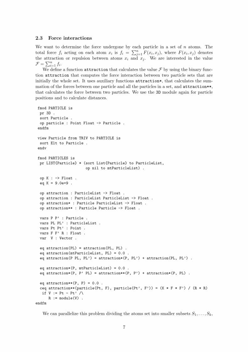
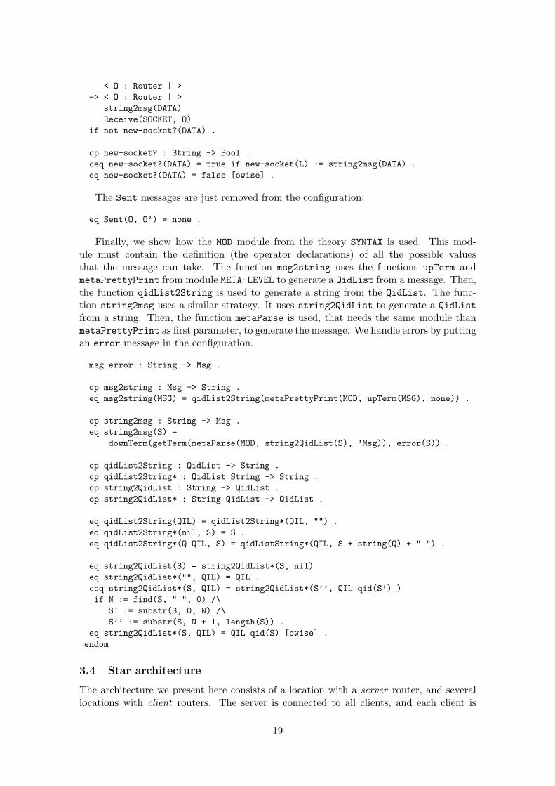
Figure 3.1: Ring architecture.

In this architecture, each node must be declared as a (Maude) server for the previousone and as a (Maude) client of the next one. However, to declare a node as a client itneeds another one working as a server, what it is impossible for the first executed Maudeinstance. We have decided to distinguish between the last Maude instance executed (whichknows that all other instances are already running) and the other ones by declaring twosubclasses of Router:

- RingNode defines the behavior of all the nodes but the last one.1 They first declarethemselves as servers and then wait until someone ask to be their client. Once theyhave accepted a client, they try to be clients themselves of the next node in the ring.

- RingLast defines the behavior of the last node, that asks the next one (that mustexist, because this node is the last one) to be its server, and then waits to be a serveritself.

The order in which the connections are established is illustrated in Figure 3.1.

Both RingNode and RingLast will reach the same states, although in di!erent order(thus they need the same attributes), and will declare themselves as server at start-up, sowe can have a module containing the common behavior. We define a new class RingRouter,a subclass of Router with attributes nextIP and nextPort that keep, respectively, the IPaddress and the port of the next node in the ring.

omod COMMON-RING{A :: ARCH-COMPLEMENT} ispr COMMON-INFRASTRUCTURE{A} .

class RingRouter | nextIP : String, nextPort : Nat .subclass RingRouter < Router .

ops connecting2next waiting4previous : -> RouterState .

The port attribute inherited from class Router is the port used by the ring objects todeclare themselves as servers and accept clients through it.

var L : Loc .var N : Nat .

1Although in a ring there is no “last” node, we refer to the order in which the nodes must be startedto be executed.

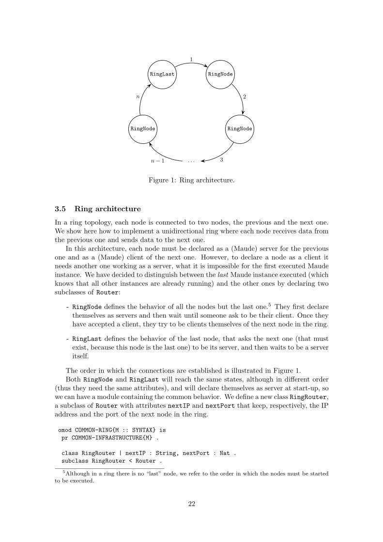
Figure 1: Ring architecture.

3.5 Ring architecture

In a ring topology, each node is connected to two nodes, the previous and the next one.We show here how to implement a unidirectional ring where each node receives data fromthe previous one and sends data to the next one.

In this architecture, each node must be declared as a (Maude) server for the previousone and as a (Maude) client of the next one. However, to declare a node as a client itneeds another one working as a server, what it is impossible for the first executed Maudeinstance. We have decided to distinguish between the last Maude instance executed (whichknows that all other instances are already running) and the other ones by declaring twosubclasses of Router:

- RingNode defines the behavior of all the nodes but the last one.5 They first declarethemselves as servers and then wait until someone ask to be their client. Once theyhave accepted a client, they try to be clients themselves of the next node in the ring.

- RingLast defines the behavior of the last node, that asks the next one (that mustexist, because this node is the last one) to be its server, and then waits to be a serveritself.

The order in which the connections are established is illustrated in Figure 1.Both RingNode and RingLast will reach the same states, although in different order

(thus they need the same attributes), and will declare themselves as server at start-up, sowe can have a module containing the common behavior. We define a new class RingRouter,a subclass of Router with attributes nextIP and nextPort that keep, respectively, the IPaddress and the port of the next node in the ring.

omod COMMON-RING{M :: SYNTAX} ispr COMMON-INFRASTRUCTURE{M} .

class RingRouter | nextIP : String, nextPort : Nat .subclass RingRouter < Router .

5Although in a ring there is no “last” node, we refer to the order in which the nodes must be startedto be executed.

22

ops connecting2next waiting4previous : -> RouterState .

var L : Loc .var N : Nat .

The port attribute inherited from class Router is the port used by the ring objects todeclare themselves as servers and accept clients through it.

rl [connect] :< L : RingRouter | state : idle, port : N >

=> < L : RingRouter | state : waiting-connection >CreateServerTcpSocket(socketManager, L, N, 5) .

endom

As we have said, all the nodes but the last one waits for clients after declares themselvesas servers (by using the rule connect above), reaching the state waiting4previous.

omod RING-NODE{M :: SYNTAX} ispr COMMON-RING{M} .

class RingRouter | .subclass RingNode < RingRouter .

vars SOCKET NEW-SOCKET SOCKET-MANAGER : Oid .var L : Loc .vars IP IP’ : String .var N : Nat .

rl [connected] :CreatedSocket(L, SOCKET-MANAGER, SOCKET)< L : RingNode | state : waiting-connection >

=> < L : RingNode | state : waiting4previous >AcceptClient(SOCKET, L) .

Once a client is accepted, the server tries to be client of the next node in the ring,reaching the state connecting2next.

rl [acceptedClient] :AcceptedClient(L, SOCKET, IP’, NEW-SOCKET)< L : RingNode | state : waiting4previous, nextIP : IP, nextPort : N >

=> < L : RingNode | state : connecting2next >Receive(NEW-SOCKET, L)CreateClientTcpSocket(socketManager, L, IP, N) .

When a node is accepted as client by the next node, it keeps the socket in the attributedefNeighbor, in order to use it to redirect all the messages, and reaches the activestate. Notice that the neighbors attribute remains empty in this architecture and thatno Receive message has been put in the configuration, because a client does not receivedata from the server in this architecture. Neither there is an AcceptClient message onthe righthand side of the rule, because each server has only one client.

rl [connected2next] :CreatedSocket(L, SOCKET-MANAGER, SOCKET)< L : RingNode | state : connecting2next >

=> < L : RingNode | state : active, defNeighbor : SOCKET > .endom

23

The last node traverses the states in different order. When it is accepted as server, ittries to connect to the next node in the ring, reaching the connecting2next state.

omod RING-LAST{M :: SYNTAX} ispr COMMON-RING{M} .

vars SOCKET NEW-SOCKET SOCKET-MANAGER : Oid .var L : Loc .var IP : String .var N : Nat .

class RingLast | .subclass RingLast < RingRouter .

rl [connected] :CreatedSocket(L, SOCKET-MANAGER, SOCKET)< L : RingLast | state : waiting-connection, nextIP : IP, nextPort : N >

=> < L : RingLast | state : connecting2next >AcceptClient(SOCKET, L)CreateClientTcpSocket(socketManager, L, IP, N) .

Once it is accepted as client, it saves the socket identifier in defNeighbor in order toredirect all the messages using it, and reaches the waiting4previous state. Again, noReceive message is needed, because the server does not send data to the clients.

rl [connected2next] :CreatedSocket(L, SOCKET-MANAGER, SOCKET)< L : RingLast | state : connecting2next >

=> < L : RingLast | state : waiting4previous, defNeighbor : SOCKET > .

Finally, when it accepts a client it starts to receive data through the socket and becomesactive.

rl [acceptedClient] :AcceptedClient(L, SOCKET, IP, NEW-SOCKET)< L : RingLast | state : waiting4previous >

=> < L : RingLast | state : active >Receive(NEW-SOCKET, L) .

endom

Notice that in this architecture the neighbors attribute is not used; the ring nodesare just connected by defNeighbor, thus obtaining a unidirectional ring.

3.6 Centralized ring architecture

We show here a special ring architecture, where in addition to the ring we have a centralserver connected to each location, so we have a mixture of the two previous architectures.We have tried to reuse them as much as possible. We use the class StarCenter, from thestar architecture (presented in Section 3.4), for the ring center; and we reuse the classesRingNode and RingLast from the ring architecture (Section 3.5) for the nodes in the ring,although some states must be renamed.

We define a new class CRingRouter in charge of connecting to a central server. Wewill combine the behavior of this new class with the classes RingNode and RingLast fromthe ring architecture in order to obtain the centralized ring. This new class has:

24

- New attributes centerIP and centerPort, with the IP address and port of thecentral server.

- New states connecting2center and waiting4center.

- Rules for connecting to the central node.

omod CENTRALIZED-RING{M :: SYNTAX} ispr COMMON-RING{M} .

vars SOCKET SOCKET-MANAGER : Oid .vars L L’ : Loc .vars DATA IP : String .var N : Nat .var LSPF : Map{Loc,Oid} .

class CRingRouter | centerIP : String, centerPort : Nat .subclass CRingRouter < RingRouter .

ops connecting2center waiting4center : -> RouterState .

When it is in connecting2center state, it tries to connect to the center and reachesthe waiting4center state:

rl [connect2center] :< L : CRingRouter | state : connecting2center, centerIP : IP,

centerPort : N >=> < L : CRingRouter | state : waiting4center >

CreateClientTcpSocket(socketManager, L, IP, N) .

Once the connection has been created, the server and the client interchange new-socketmessages, and the neighbors attribute is updated, getting the active state:

rl [connected] :CreatedSocket(L, SOCKET-MANAGER, SOCKET)< L : CRingRouter | state : waiting4center >

=> < L : CRingRouter | >Receive(SOCKET, L)Send(SOCKET, L, msg2string(new-socket(L))) .

crl [connected2center] :Received(O, SOCKET, DATA)< L : CRingRouter | state : waiting4center, neighbors : LSPF >

=> < L : CRingRouter | state : active, neighbors : insert(L’, SOCKET, LSPF) >Receive(SOCKET, L)

if new-socket(L’) := string2msg(DATA) .endom

Note that we update the neighbors attribute, so the messages to the center will useSOCKET, while all other messages will use defNeighbor from the ring architecture.

Now we look for a class that behaves as a CRingRouter and as a RingNode (or asa RingLast, if it is the last node). To obtaing it, we define a new class CRNode, whichis a subclass of both CRingRouter and RingNode (and a new class CRLast, which is asubclass of CRingRouter and RingLast). These new classes behave as the correspondingnodes in the ring, and once they are connected behave as clients of the center. However,

25

we found the problem that all those classes finish in active state, so some of the rulescould not be applied. We solve it by renaming the state active in the ring nodes toconnecting2center, so the rules in CRingRouter can be applied after the ring connectionshas been established.

omod CENTRALIZED-RING-NODE{M :: SYNTAX} ispr CENTRALIZED-RING{M} .pr RING-NODE{M} * (op active to connecting2center) .

class CRNode | .subclass CRNode < CRingRouter RingNode .endom

omod CENTRALIZED-RING-LAST{M :: SYNTAX} ispr CENTRALIZED-RING{M} .pr RING-LAST{M} * (op active to connecting2center) .

class CRLast | .subclass CRLast < CRingRouter RingLast .endom

In the following sections we will show how these architectures can be used to executeapplications (in our case, skeletons) on top of them.

4 Ray tracing case study

Once we have several locations connected by means of an architecture like those shownabove, we can implement distributed applications. We first illustrate in this section how aconcrete distributed application can be implemented directly in Maude. In the followingsection we will generalize our methodology by implementing generic skeletons that receivethe concrete problem as a parameter.

In order to implement a distributed application, the messages that objects in differ-ent locations will interchange should be declared in a separated module, that then willbe combined with the messages of the architecture and used to instantiate the moduleCOMMON-INFRASTRUCTURE. Then the objects that solve the application have to be imple-mented, in a way as independent of the concrete architecture as possible. Finally, in orderto execute the application, a concrete architecture has to be chosen and the distributionof the application objects through the different locations has to be decided. Let us see anexample.

We use the ray tracing problem as case study. The algorithm shown in Section 2.1can be easily parallelized: we consider each row of the screen as a subproblem that canbe colored in parallel with other subproblems. So we will have a master that deliverssubproblems and combines subresults, and several painters that solve the subproblems,that is, color rows of the screen.

The communication between the master and the workers is through the followingmessages, that must have sort Contents to fit into the to_:_ message.

fmod RT-TRANSMITTED-SYNTAX ispr OID .pr FIGURE-LIST .pr CONTENTS .

26

- world, that sends the data describing the problem, that is, the list of figures in thescene, the position of the camera, and the size of the screen:

op world : FigureList Point Float Float Float -> Contents .

- new-row, that communicates a new task by identifying the height of the row to becolored:

op new-row : Float -> Contents .

- colored-row, that transmits a new result to the server:

op colored-row : Oid Float ColorRow -> Contents .endfm

Once the (contents of the) messages of the application has been defined, we have thesyntax of all transmitted data, and we can define a view from the theory SYNTAX used bythe architecture:

fmod RT-SYNTAX ispr RT-TRANSMITTED-SYNTAX .pr ARCHITECTURE-MSGS .endfm

view RT-Syntax from SYNTAX to META-LEVEL isop MOD to term(upModule(’RT-SYNTAX, false)) .endv

The application only needs the COMMON-INFRASTRUCTURE from the architecture (instan-tiated with RT-Syntax), so it can be executed on different architectures; each utilizationof the application must include the architecture it will use (we will see an example be-low). The module ROWTRACER from Section 2.1 is used; it contains the ingredients of thisproblem, in particular the function traceRow used by the painters.

view ColorRow from TRIV to COLOR issort Elt to ColorRow .endv

omod DISTRIBUTED-RAY-TRACING ispr COMMON-INFRASTRUCTURE{RT-Syntax} .pr RT-TRANSMITTED-SYNTAX .pr ROWTRACER .pr MAP{Float, ColorRow} .pr LIST{Oid} * (sort List{Oid} to OidList, op nil to mtOidList) .pr LIST{Float} * (sort List{Float} to FloatList, op nil to mtFloatList) .

var CM : Map{Float, ColorRow} .var OL : OidList .vars XL XR YT YB ZN ZF R Y : Float .var CR : ColorRow .var FigL : FigureList .var FL : FloatList .var P : Point .vars O O’ : Oid .

27

We define now a class RTMaster in charge of distributing subproblems (rows to becolored) and combining the results (colored rows). This new class has attributes that

- Describe the problem:

– The list of figures.

– The width of the screen (xL and xR).

– The height of the screen (yT and yB).

– The depth where figures can be traced (zN and zF).

- Keep the current row (y).

- Keep the result; the subresults may arrive unordered, so we use a partial functionfrom rows, identified by floats, to colored rows to represent the (parcial) result.

- Store the list with the identifiers of the painters.

class RTMaster | figures : FigureList, xL, xR, yT, yB, zN, zF: Float,y: Float, result : Map{Float, ColorRow},painters : OidList .

First, the master must deliver the information of the world and the first subproblemsto the painters. Initially they receive three tasks6 so they can work in the following onewhile a new one arrives:

rl [new-painter] :< O : RTMaster | xL : XL, xR : XR, y : Y, yT : YT, yB : YB, zN : ZN,

zF : ZF, figures : FigL, painters : O’ OL >=> < O : RTMaster | y : Y - 3.0, painters : OL >

to O’ : world(filter(FigL, ZF),< (XR + XL) / 2.0, (YT + YB) / 2.0, 0.0 >, XL, XR, ZN)

to O’ : new-row(Y)to O’ : new-row(Y - 1.0)to O’ : new-row(Y - 2.0) .

When one result arrives, it is combined with the current partial result (by using theinsert operation from partial functions) and it is checked if the problem has been fullydistributed (in this case Y < YB); if this is not the case, the next subproblem is sent tothe painter:

crl [new-row] :to O : colored-row(O’, R, CR)< O : RTMaster | result : CM, y : Y, yB : YB >

=> < O : RTMaster | result : insert(R, CR, CM), y : Y - 1.0 >to O’ : new-row(Y)

if Y >= YB .

crl [no-more-rows] :to O : colored-row(O’, R, CR)< O : RTMaster | result : CM, y : Y, yB : YB >

=> < O : RTMaster | result : insert(R, CR, CM) >if Y < YB .endom

6We are assuming that the number of works to be dispatched is at least three times the number ofpainters. This will be generalized in the following sections.

28

Now we define the class RTPainter, that will define the painters’ behavior. Its at-tributes will keep the information of the world (the width of the screen, position of thecamera, and the list of figures), the list of undone tasks (row identifiers), and the identifierof the master.

class RTPainter | figures : FigureList, pos : Point, xL, xR, zN : Float,nextWorks : FloatList, master : Oid .

When the world or a new work arrives, the information is stored in the appropriateattributes:

rl [rec-world] :to O : world(FigL, P, XL, XR, ZN)< O : RTPainter | >

=> < O : RTPainter | figures : FigL, pos : P, xL : XL, xR : XR, zN : ZN > .

rl [new-row] :to O : new-row(R)< O : RTPainter | nextWorks : FL >

=> < O : RTPainter | nextWorks : FL R > .

While the list of scheduled tasks is not empty, we can do a new one (trace the row)and send it to the master through the message colored-row. Notice that here we use thefunction traceRow from the sequential version (see Section 2.1):

crl [paint] :< O : RTPainter | figures : FigL, pos : P, xL : XL, xR : XR, zN : ZN,

master : O’, nextWorks : R FL >=> < O : RTPainter | nextWorks : FL >

to O’ : colored-row(O, R, CR)if CR := [traceRow(P, XL, XR, R, ZN, FigL)] .endom

We can now execute an example of distributed ray tracing. To do it we must firstchoose the architecture we are going to use (instantiated with the view RT-Syntax de-fined in the application). In this case the most suitable one is the star topology, placingthe master in the center of the star and the painters in the clients. We define modulesEXAMPLE-MASTER and EXAMPLE-PAINTER where the initial configurations will be executed.The EXAMPLE-MASTER includes too a generator of random spheres that uses the RANDOMmodule provided by Maude.

mod EXAMPLE-MASTER ispr STAR-ARCHITECTURE-SERVER{RT-Syntax} .pr DISTRIBUTED-RAY-TRACING .pr RANDOM .

var L : FigureList .var N : Nat .

op figListN : Nat -> FigureList .op figListN* : Nat FigureList -> FigureList .

eq figListN(N) = figListN*(N, mtFigureList) .eq figListN*(0, L) = L .

29

eq figListN*(s(N), L) = figListN*(N, L figure(sphere, r,coord(< float(random(4 * N)), float(random(4 * N + 1)),

float(random(4 * N + 2)) >, float(random(4 * N + 3))))) .endm

The initial configuration for the center of the star includes a StarCenter and aRTMaster with the whole definition of the problem:

erew <> < l(ip0, 0) : StarCenter |state : idle,neighbors : empty,defNeighbor : null,port : 60039 >

< o(l(ip0, 0), 0) : RTMaster |xL : -35.0,xR : 35.0,y : 30.0,yT : 30.0,yB : -30.0,near : 10.0,far : 1000000000.0,figures : figListN(30),result : empty,painters : o(l(ip1, 1), 0) o(l(ip2, 2), 0)

o(l(ip3, 3), 0) o(l(ip4, 4), 0),counter : 0 > .

where the ipi are IP addresses.All the other locations have in their initial configuration a StarNode and a RTPainter,

and their single difference is its identifier. The configuration for one of them is shownbelow.

mod EXAMPLE-PAINTER ispr STAR-ARCHITECTURE-CLIENT{RT-Syntax} .pr DISTRIBUTED-RAY-TRACING .endm

erew <> < l(ip1, 1) : StarNode |state : idle,neighbors : empty,defNeighbor : null,server : ip0,port : 60039 >

< o(l(ip1, 1), 0) : RTPainter |master : o(l(ip0, 0), 0),counter : 0,nextRows : mtFloatList,figures : mtFigureList,pos : < 0.0, 0.0, 0.0 >,xL : 0.0,xR : 0.0,zN : 0.0 > .

In order to implement a different application we should identify application-dependentparts and modify them. A better approach consists in using parameterized skeletons thatreceive the concrete problem (its data and the operations solving it) as a parameter. Wepresent them in the following section.

30

5 Parameterized skeletons

An important characteristic of skeletons is their generality, that is, the possibility of usingthem in different applications. For this, most skeletons are parameterized by functionsand have a polymorphic type.

We show three kinds of skeletons:

Data-parallel skeletons: The source of parallelism is the distribution of data betweenprocessors and the application of the same operation to all portions of the data. Weapply our methodology to the Farm skeleton.

Systolic skeletons: The systolic skeletons are used in algorithms in which parallel com-putation and global synchronization steps alternate [11]. As example of systolicskeleton we show the Ring skeleton.

Task-parallel skeletons: The source of parallelism is the decomposition of a task intodifferent subtasks which can be done in parallel. These subtasks need not be iden-tical [11]. The task-parallel skeletons shown here are:

- Divide and Conquer skeleton.

- Branch and Bound skeleton.

- Pipeline skeleton.

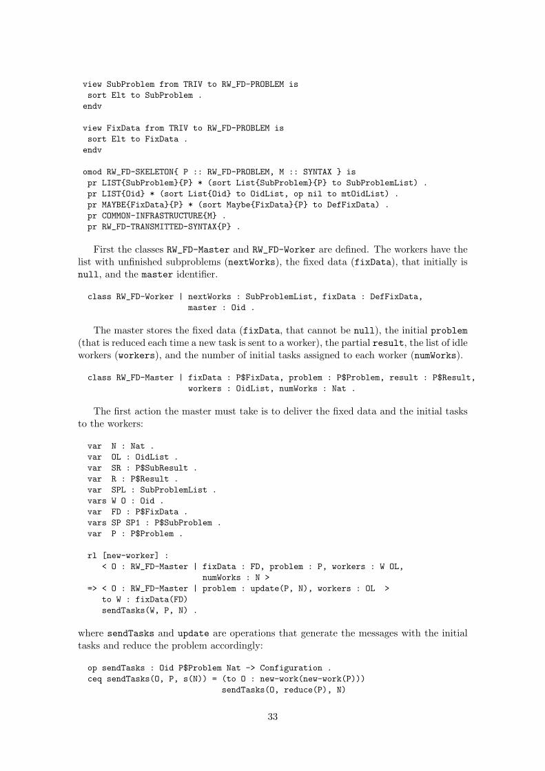
5.1 Farm skeleton

We show here how to implement a skeleton with replicated workers and fixed data [11]. Inthis kind of skeleton, a master initially sends the fixed data and some subproblems to allthe workers. Each time a task is finished by a worker, the subresult is sent to the masterwhere it is combined with the partial result already computed, and a new work is givento that worker, reducing the initial problem. Thus, the tasks are delivered on demand,obtaining an even distribution of the work to be done.

We use a parameterized module to implement the skeleton. Each concrete applicationmust define a module that satisfies the following RW_FD-PROBLEM theory, where

- the sort FixData contains the data shared by all the workers;

- Problem refers to the initial problem;

- SubProblem represents the smaller problems solved by the workers;

- Result is the final result to the original problem; and

- SubResult corresponds to the results obtained by the workers.

fth RW_FD-PROBLEM isinc BOOL .sorts FixData Problem SubProblem Result SubResult .

The operations required by the theory are:

- new-work, that extracts a new subproblem from the current problem:

op new-work : Problem -> SubProblem .

31

- reduce, that updates the current problem making it smaller:

op reduce : Problem -> Problem .

- do-work, that given a subproblem and the fixed data solves the former:

op do-work : SubProblem FixData -> SubResult .

- combine, that merges the current (partial) result with a new subresult, given thesubproblem that was solved. Notice that this operation must be commutative (inthe sense that the final result cannot depend on the order in which the combinationsare performed) because the subresults may arrive unordered:

op combine : Result SubProblem SubResult -> Result .

var R : Result .vars SP SP’ : SubProblem .vars SR SR’ : SubResult .eq combine(combine(R, SP, SR), SP’, SR’) =

combine(combine(R, SP’, SR’), SP, SR) [nonexec] .

- finished?, that checks if the problem has already been solved:

op finished? : Problem -> Bool .endfth

Notice that RW_FD-PROBLEM is a functional theory, that is, the concrete operationsnew-work, reduce, do-work, etc. will be defined equationally and not by means of rules.This is a fact that the implementation of the skeletons assumes.

We need messages for sending the fixed data and new tasks to the workers, and forcommunicating the subresults to the master. We use a parameterized module because weneed the sorts defined in the theory:

fmod RW_FD-TRANSMITTED-SYNTAX{P :: RW_FD-PROBLEM} ispr CONTENTS .pr OID .

op fixData : P$FixData -> Contents .op new-work : P$SubProblem -> Contents .op finished : Oid P$SubProblem P$SubResult -> Contents .endfm

The module defining the skeleton has two parameters: the theory RW_FD-PROBLEMabove, needed by the master and the workers, and the theory SYNTAX, containing the syntaxof the transmitted messages which is used by the architecture as shown in Section 3.3.

We need lists of subproblems (received by workers). We use the predefined parameter-ized module LIST7 which is first instantiated with the view Subproblem from the theoryTRIV to the theory RW_FD-PROBLEM, and then instantiated with the parameter P. The listssorts are renamed. We use LIST with the view Oid too, with one difference: the Oid viewhas no free parameters and it does not need the parameter P. At start-up, the works havenot fixed data, so we use the MAYBE parameterized module. From the architecture, onlythe COMMON-INFRASTRUCTURE module is used.

7As we have said, the order in which the subproblems are solved is irrelevant, so we could use a set.However, it adds matching modulo commutativity, and the skeleton will work slightly slower.

32

view SubProblem from TRIV to RW_FD-PROBLEM issort Elt to SubProblem .endv

view FixData from TRIV to RW_FD-PROBLEM issort Elt to FixData .endv

omod RW_FD-SKELETON{ P :: RW_FD-PROBLEM, M :: SYNTAX } ispr LIST{SubProblem}{P} * (sort List{SubProblem}{P} to SubProblemList) .pr LIST{Oid} * (sort List{Oid} to OidList, op nil to mtOidList) .pr MAYBE{FixData}{P} * (sort Maybe{FixData}{P} to DefFixData) .pr COMMON-INFRASTRUCTURE{M} .pr RW_FD-TRANSMITTED-SYNTAX{P} .

First the classes RW_FD-Master and RW_FD-Worker are defined. The workers have thelist with unfinished subproblems (nextWorks), the fixed data (fixData), that initially isnull, and the master identifier.

class RW_FD-Worker | nextWorks : SubProblemList, fixData : DefFixData,master : Oid .

The master stores the fixed data (fixData, that cannot be null), the initial problem(that is reduced each time a new task is sent to a worker), the partial result, the list of idleworkers (workers), and the number of initial tasks assigned to each worker (numWorks).

class RW_FD-Master | fixData : P$FixData, problem : P$Problem, result : P$Result,workers : OidList, numWorks : Nat .

The first action the master must take is to deliver the fixed data and the initial tasksto the workers:

var N : Nat .var OL : OidList .var SR : P$SubResult .var R : P$Result .var SPL : SubProblemList .vars W O : Oid .var FD : P$FixData .vars SP SP1 : P$SubProblem .var P : P$Problem .

rl [new-worker] :< O : RW_FD-Master | fixData : FD, problem : P, workers : W OL,

numWorks : N >=> < O : RW_FD-Master | problem : update(P, N), workers : OL >

to W : fixData(FD)sendTasks(W, P, N) .

where sendTasks and update are operations that generate the messages with the initialtasks and reduce the problem accordingly:

op sendTasks : Oid P$Problem Nat -> Configuration .ceq sendTasks(O, P, s(N)) = (to O : new-work(new-work(P)))

sendTasks(O, reduce(P), N)

33

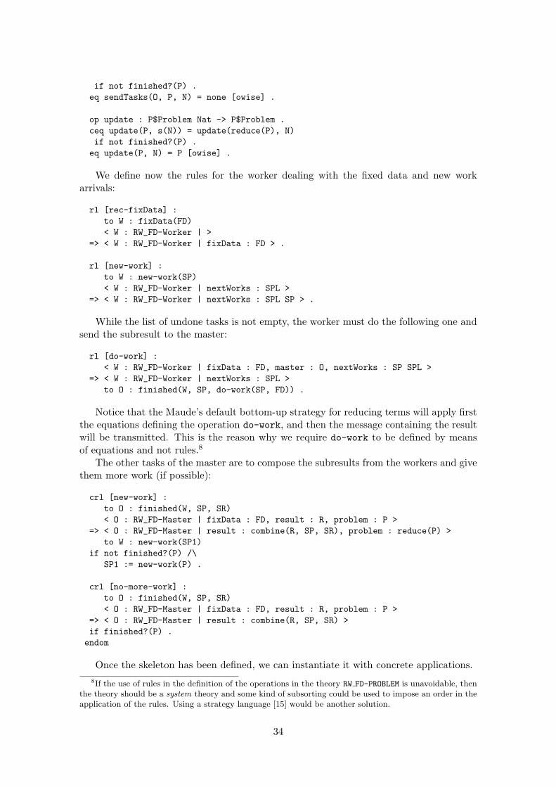
if not finished?(P) .eq sendTasks(O, P, N) = none [owise] .

op update : P$Problem Nat -> P$Problem .ceq update(P, s(N)) = update(reduce(P), N)if not finished?(P) .eq update(P, N) = P [owise] .

We define now the rules for the worker dealing with the fixed data and new workarrivals:

rl [rec-fixData] :to W : fixData(FD)< W : RW_FD-Worker | >

=> < W : RW_FD-Worker | fixData : FD > .

rl [new-work] :to W : new-work(SP)< W : RW_FD-Worker | nextWorks : SPL >

=> < W : RW_FD-Worker | nextWorks : SPL SP > .

While the list of undone tasks is not empty, the worker must do the following one andsend the subresult to the master:

rl [do-work] :< W : RW_FD-Worker | fixData : FD, master : O, nextWorks : SP SPL >

=> < W : RW_FD-Worker | nextWorks : SPL >to O : finished(W, SP, do-work(SP, FD)) .

Notice that the Maude’s default bottom-up strategy for reducing terms will apply firstthe equations defining the operation do-work, and then the message containing the resultwill be transmitted. This is the reason why we require do-work to be defined by meansof equations and not rules.8

The other tasks of the master are to compose the subresults from the workers and givethem more work (if possible):

crl [new-work] :to O : finished(W, SP, SR)< O : RW_FD-Master | fixData : FD, result : R, problem : P >

=> < O : RW_FD-Master | result : combine(R, SP, SR), problem : reduce(P) >to W : new-work(SP1)

if not finished?(P) /\SP1 := new-work(P) .

crl [no-more-work] :to O : finished(W, SP, SR)< O : RW_FD-Master | fixData : FD, result : R, problem : P >

=> < O : RW_FD-Master | result : combine(R, SP, SR) >if finished?(P) .endom

Once the skeleton has been defined, we can instantiate it with concrete applications.8If the use of rules in the definition of the operations in the theory RW FD-PROBLEM is unavoidable, then

the theory should be a system theory and some kind of subsorting could be used to impose an order in theapplication of the rules. Using a strategy language [15] would be another solution.

34

5.1.1 Ray tracing instantiation

In order to obtain a concrete application by using the parameterized skeleton we mustknow the sorts and operators related to those in the theory RW_FD-PROBLEM. We illustratenow how to do it with the ray tracing example. We define the following module, where theincluded module ROWTRACER is shown in Section 2.1. The sort Pair is declared to definethe initial problem (the highest and the lowest y), while World defines the fixed data forthis problem (the width of the screen, the camera, and the list of figures). Partial functions(declared in the predefined module MAP) from Floats (identifying rows) to ColorRows areused to represent the final result.

fmod RAYTRACING-PROBLEM ispr ROWTRACER .pr MAP{Float, ColorRow} .sorts Pair World .

var FL : FigureList .var XL XR Y YT YB N F : Float .var P : Point .

op pair : Float Float -> Pair .op world : FigureList Point Float Float Float -> World .

op traceRow : Float World -> ColorRow .op sub-problem : Pair -> Float .op reduce : Pair -> Pair .op finished? : Pair -> Bool .

eq traceRow(Y, world(FL, P, XL, XR, N)) = [traceRow(P, XL, XR, Y, N, FL)] .eq sub-problem(pair(YT, YB)) = YT .eq reduce(pair(YT, YB)) = pair(YT - 1.0, YB) .eq finished?(pair(YT, YB)) = YT < YB .endfm

To instantiate the module we create a view and define the mapping between sorts andoperators with different name from those in the theory:

view RayTracer from RW_FD-PROBLEM to RAYTRACING-PROBLEM issort Problem to Pair .sort SubProblem to Float .sort Result to Map{Float, ColorRow} .sort SubResult to ColorRow .sort FixData to World .op combine(R:Result, SP:SubProblem, SR:SubResult) to

term insert(SP:Float, SR:ColorRow, R:Map{Float, ColorRow}) .op do-work to traceRow .op new-work to sub-problem .

endv

Finally, we instantiate the module RW_FD-SKELETON, where ray tracing can be executed.As in the application of ray tracing without skeleton shown in Section 4, we use the stararchitecture, placing the master with the server and the workers with the clients:

mod RAYTRACING-SKELETON ispr RW_FD-SKELETON{ RayTracer, RT-Syntax } .

35

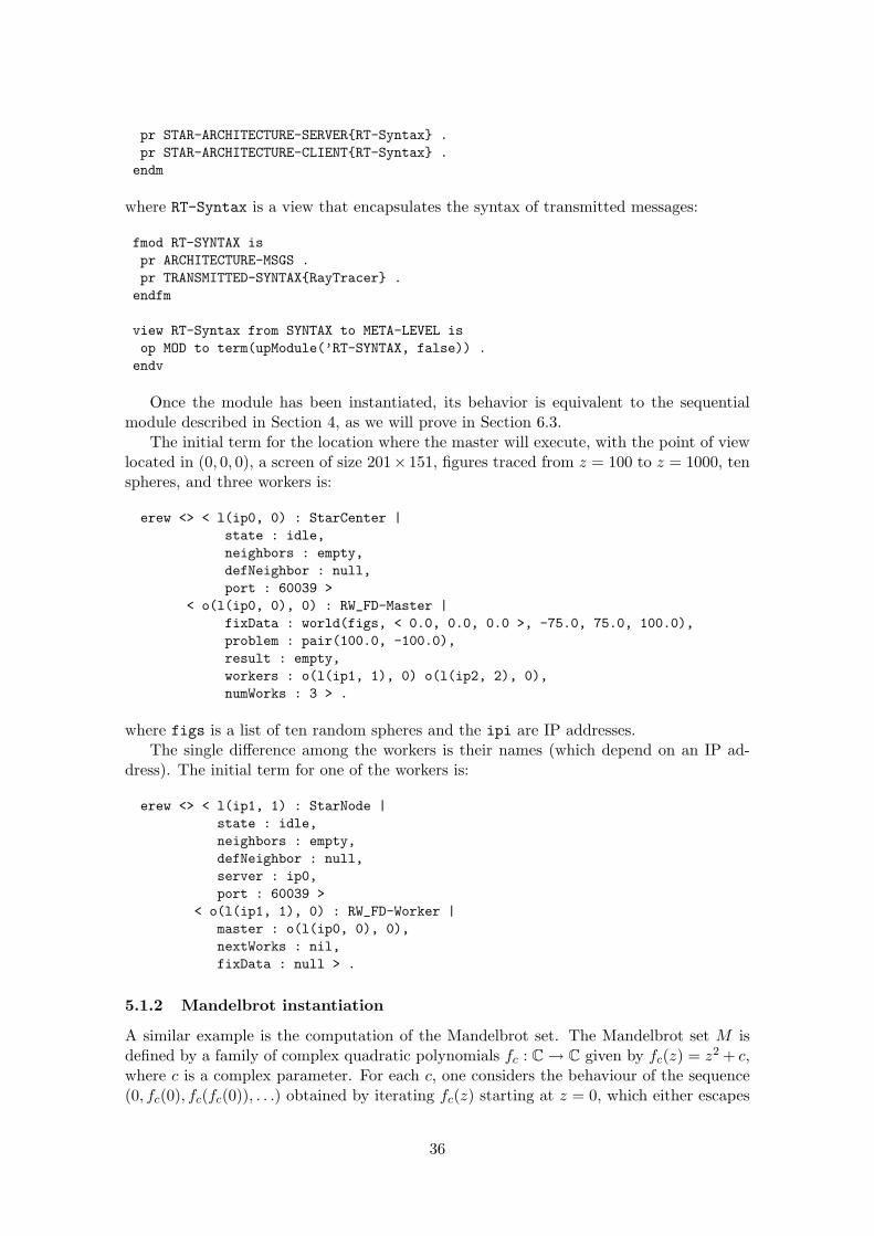
pr STAR-ARCHITECTURE-SERVER{RT-Syntax} .pr STAR-ARCHITECTURE-CLIENT{RT-Syntax} .endm

where RT-Syntax is a view that encapsulates the syntax of transmitted messages:

fmod RT-SYNTAX ispr ARCHITECTURE-MSGS .pr TRANSMITTED-SYNTAX{RayTracer} .endfm

view RT-Syntax from SYNTAX to META-LEVEL isop MOD to term(upModule(’RT-SYNTAX, false)) .endv

Once the module has been instantiated, its behavior is equivalent to the sequentialmodule described in Section 4, as we will prove in Section 6.3.

The initial term for the location where the master will execute, with the point of viewlocated in (0, 0, 0), a screen of size 201× 151, figures traced from z = 100 to z = 1000, tenspheres, and three workers is:

erew <> < l(ip0, 0) : StarCenter |state : idle,neighbors : empty,defNeighbor : null,port : 60039 >

< o(l(ip0, 0), 0) : RW_FD-Master |fixData : world(figs, < 0.0, 0.0, 0.0 >, -75.0, 75.0, 100.0),problem : pair(100.0, -100.0),result : empty,workers : o(l(ip1, 1), 0) o(l(ip2, 2), 0),numWorks : 3 > .

where figs is a list of ten random spheres and the ipi are IP addresses.The single difference among the workers is their names (which depend on an IP ad-

dress). The initial term for one of the workers is:

erew <> < l(ip1, 1) : StarNode |state : idle,neighbors : empty,defNeighbor : null,server : ip0,port : 60039 >

< o(l(ip1, 1), 0) : RW_FD-Worker |master : o(l(ip0, 0), 0),nextWorks : nil,fixData : null > .

5.1.2 Mandelbrot instantiation

A similar example is the computation of the Mandelbrot set. The Mandelbrot set M isdefined by a family of complex quadratic polynomials fc : C→ C given by fc(z) = z2 + c,where c is a complex parameter. For each c, one considers the behaviour of the sequence(0, fc(0), fc(fc(0)), . . .) obtained by iterating fc(z) starting at z = 0, which either escapes

36

to infinity or stays within a disk of some finite radius. The Mandelbrot set is defined asthe set of all points c such that the above sequence does not escape to infinity.

We specify the module MANDELBROT-PROBLEM to implement the skeleton. We defineagain the sorts Pair (that keeps the current row and the lowest row) and World (thatkeeps the width of the screen). We use the function mandelbrot* defined in the moduleMANDELBROT-ROW, that computes the problem for one row.

fmod MANDELBROT-PROBLEM ispr MANDELBROT-ROW .pr MAP{Float, ColorRow} .

sort Pair World .

var Xl Xr Y Ymax Ymin : Float .

op pair : Float Float -> Pair .op world : Float Float -> World .

op mandelbrot : Float World -> ColorRow .op sub-problem : Pair -> Float .op reduce : Pair -> Pair .op finished? : Pair -> Bool .

eq mandelbrot(Y, world(Xl, Xr)) = [ mandelbrot*(Xl, Xr, Y) ] .eq sub-problem(pair(Ymax, Ymin)) = Ymax .eq reduce(pair(Ymax, Ymin)) = pair(Ymax - 1.0, Ymin) .eq finished?(pair(Ymax, Ymin)) = Ymax < Ymin .endfm

Now we can define the view from the theory

view Mandelbrot from RW_FD-PROBLEM to MANDELBROT-PROBLEM issort Problem to Pair .sort SubProblem to Float .sort Result to Map{Float, ColorRow} .sort SubResult to ColorRow .op combine(R:Result, SP:SubProblem, SR:SubResult) to

term insert(SP:Float, SR:ColorRow, R:Map{Float, ColorRow}) .op do-work to mandelbrot .op new-work to sub-problem .endv

and instantiate the skeleton with it. As in the ray tracing example above, the star archi-tecture is the most suitable for this example.

mod MANDELBROT-EXAMPLE ispr RW_FD-SKELETON{Mandelbrot, Mandelbrot-Syntax} .pr STAR-ARCHITECTURE-SERVER{Mandelbrot-Syntax} .pr STAR-ARCHITECTURE-CLIENT{Mandelbrot-Syntax} .endm

The initial configuration for the location that contains the master is

erew <> < l(ip0, 0) : StarCenter |state : idle,

37

neighbors : empty,defNeighbor : null,port : 60039 >

< o(l(ip0, 0), 0) : RW_FD-Master |fixData : world(-1.0, 1.0),problem : pair(1.0, -1.0),result : empty,workers : o(l(ip1, 1), 0) o(l(ip2, 2), 0),numWorks : 3,counter : 0 > .

The initial configurations for the locations that contain workers are the same than theray tracing example.

5.1.3 Euler instantiation

In some problems the fixed data is not needed; we have implemented a slightly modifiedskeleton to deal with this situation. It is very similar to the replicated workers skeletonabove, but all the messages and rules dealing with the fixed data are either not neededor simplified. The complete Maude code can be found in http://maude.sip.ucm.es/skeletons.

We show here a simple example using this new skeleton: the distributed implementa-tion of the Euler function shown in Section 2.2. In this problem we consider as a singlework to calculate each ϕ(i).

The only sort involved in this problem is Nat, so every sort in the skeleton is mappedto it:

view Euler from RW-PROBLEM to EULER issort Problem to Nat .sort SubProblem to Nat .sort Result to Nat .sort SubResult to Nat .

The operations are very simple too: a new work of the problem N is just N; we reducethe problem by subtracting 1; the work that must be done is the function euler frommodule EULER in Section 2.2; combining two results is just adding them; and we havefinished when the number reaches 0:

op new-work(N:Problem) to term N:Nat .op reduce(N:Problem) to term sd(N:Nat, 1) .op do-work to euler .op combine(R:Result, S:SubProblem, SR:SubResult) to term (R:Nat + SR:Nat) .op finished?(N:Problem) to term (N:Nat == 0) .endv

Calculating ϕ(x) may be quite more faster than communication with the master, soit is possible that most of the computation time is used in communication. To avoid thisproblem we can make the granularity of the works coarser by computing more than onenumber in each step. To do this we only need to make small changes in the instantiationmodule, while obviously the skeleton remains unmodified. We show here an example wherewe calculate the sum of 20 Euler numbers in each step:

38

fmod EULER20 ispr EULER .

vars N N’ : Nat .

op euler20 : Nat -> Nat .op euler20* : Nat Nat -> Nat .

eq euler20(N) = euler20*(N, if N > 20 then sd(N, 20) else 0 fi) .eq euler20*(N, N) = 0 .eq euler20*(N, N’) = euler(N) + euler20*(sd(N, 1), N’) [owise] .endfm

Now the view only needs two changes:

view Euler20 from RW-PROBLEM to EULER20 is...

op do-work to euler20 .op reduce(N:Problem) to term (if N:Nat > 20 then sd(N:Nat, 20) else 0 fi) ....

endv

5.2 Systolic skeleton

In this skeleton, a master divides the problem among all the workers, that are organizedin a circular list because they must share some data through it. When the workers haveboth initial and shared data, they do their work, combine the partial result, and give thenew shared data to the next worker. In order to have the first shared data, it must beproduced by the worker itself. When a worker finishes all its tasks, it sends its subresultto the master, that will combine them in order.

We define a theory SYSTOLIC-RING-PROBLEM with the following sorts:

- Problem, that defines the sort of the initial data.

- Result, that describes the sort of the final data.

- ProblemList and ResultList are respectively lists of Problem and Result.9

- SharedData is the sort of the data that is passed by all the workers.

- Pair is a wrapper of Result and SharedData.

fth SYSTOLIC-RING-PROBLEM isinc BOOL .inc NAT .

sorts Problem ProblemList Result ResultList SharedData Pair .subsort Problem < ProblemList .subsort Result < ResultList .

The theory defines the following operators:

- mtRL, mtPL, and __ are the constructors for the lists of Problem and Result:9We cannot use here the predefined module LIST because we would need a parametric theory, that is

not allowed in Core Maude.

39

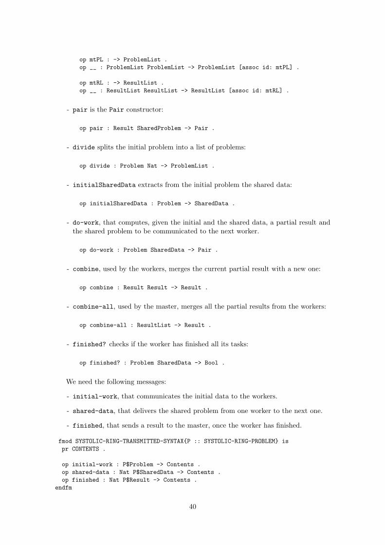
op mtPL : -> ProblemList .op __ : ProblemList ProblemList -> ProblemList [assoc id: mtPL] .

op mtRL : -> ResultList .op __ : ResultList ResultList -> ResultList [assoc id: mtRL] .

- pair is the Pair constructor:

op pair : Result SharedProblem -> Pair .

- divide splits the initial problem into a list of problems:

op divide : Problem Nat -> ProblemList .

- initialSharedData extracts from the initial problem the shared data:

op initialSharedData : Problem -> SharedData .

- do-work, that computes, given the initial and the shared data, a partial result andthe shared problem to be communicated to the next worker.

op do-work : Problem SharedData -> Pair .

- combine, used by the workers, merges the current partial result with a new one:

op combine : Result Result -> Result .

- combine-all, used by the master, merges all the partial results from the workers:

op combine-all : ResultList -> Result .

- finished? checks if the worker has finished all its tasks:

op finished? : Problem SharedData -> Bool .

We need the following messages:

- initial-work, that communicates the initial data to the workers.

- shared-data, that delivers the shared problem from one worker to the next one.

- finished, that sends a result to the master, once the worker has finished.

fmod SYSTOLIC-RING-TRANSMITTED-SYNTAX{P :: SYSTOLIC-RING-PROBLEM} ispr CONTENTS .

op initial-work : P$Problem -> Contents .op shared-data : Nat P$SharedData -> Contents .op finished : Nat P$Result -> Contents .

endfm

40

We define views to Problem, Result, and SharedData, that will be needed by theskeleton:

view Problem from TRIV to SYSTOLIC-RING-PROBLEM issort Elt to Problem .endv

view Result from TRIV to SYSTOLIC-RING-PROBLEM issort Elt to Result .endv

view SharedData from TRIV to SYSTOLIC-RING-PROBLEM issort Elt to SharedData .endv

Again the module defining the skeleton has two parameters: SYSTOLIC-RING-PROBLEMused by the master and the workers, and SYNTAX, used by the architecture:

omod SYSTOLIC-RING-SKELETON{ P :: SYSTOLIC-RING-PROBLEM, M :: SYNTAX } ispr MAYBE{Problem}{P} * (sort Maybe{Problem}{P} to DefProblem,

op null to nullP) .pr MAYBE{Result}{P} * (sort Maybe{Result}{P} to DefResult,

op null to nullR) .pr MAYBE{SharedData}{P} * (sort Maybe{SharedData}{P} to DefSharedData,

op null to nullSD) .pr COMMON-INFRASTRUCTURE{M} .pr SYSTOLIC-RING-TRANSMITTED-SYNTAX{P} .pr LIST{Oid} * (sort List{Oid} to OidList,

op nil to mtOidList) .

The class SWorker has the following attributes:

- problem, that keeps the initial problem, which is initially null.

- shared, that contains the shared data. It is initially null too.

- result, that stores the partial result.

- numWorker, that identifies the worker. This number will be used by the master tosort the received results.

- nextWorker, that saves the identifier of the next worker.

- master, that keeps the master identifier.

- counter, that points out to the next shared data that must be accepted from theprevious worker.

class SWorker | problem : DefProblem, shared : DefSharedData,result : Result, numWorker : Nat, nextWorker : Oid,master : Oid, counter : Nat .

The class SMaster has the following attributes:

- initialProblem, that stores the initial problem. Once the problem has been dividedit takes the default value nullP.

41

- problems, that keeps the list of problems once the initial data has been divided.

- results, that is a list of results where the partial results from the workers are keptin order.

- counter, that points out to the next partial result that must be accepted (appendedin the list results) from the workers.

- result, that contains the final result. We consider that it is initially null.

- workers, that stores the list of workers that have not been assigned a work yet.

- numWorkers, that keeps the number of workers.

class SMaster | initialProblem : DefProblem, problems : ProblemList,results : ResultList, counter : Nat, result : Result,workers : OidList, numWorkers : Nat .

The first thing that must be done by the master is to divide the initial data into a listof problems, that can be delivered to all the workers:

vars N N’ : Nat .vars R R’ : P$Result .var RL : P$ResultList .vars W M O : Oid .vars P P’ : P$Problem .var PL : P$ProblemList .vars SD SD’ : P$SharedData .var OL : OidList .

rl [divide] :< M : SMaster | initialProblem : P, numWorkers : N >

=> < M : SMaster | initialProblem : nullP, problems : divide(P, N) > .

Once the data has been split, the master send it to the workers, that store the dataand extracts the shared data:

rl [new-worker] :< M : SMaster | problems : P PL, workers : O OL >

=> < M : SMaster | problems : PL, workers : OL >to O : initial-work(P) .

rl [initial-data] :to W : initial-work(P)< W : SWorker | problem : nullP, shared : nullSD >

=> < W : SWorker | problem : P, shared : initialSharedData(P),counter : 1 > .

When the shared attribute is not null, the worker can do a new work and send theupdated shared data to the next worker:

crl [working] :< W : SWorker | problem : P, nextWorker : O, shared : SD,

counter : N, result : R >=> < W : SWorker | shared : nullSD, result : combine(R, R’) >

to O : shared-data(N, SD’)if pair(R’, SD’) := do-work(P, SD) .

42

When the next shared data that we must keep arrives, we check whether the work isnot finished, in which case we must keep the shared data, or the work is finished and wecan delete it:

crl [new-work] :to W : shared-data(N, SD)< W : SWorker | counter : N, problem : P, shared : nullSD >

=> < W : SWorker | counter : s(N), shared : SD >if not finished?(P, SD) .

crl [finished] :to W : shared-data(N, SD)< W : SWorker | counter : N, problem : P, master : O, result : R,

numWorker : N’ >=> < W : SWorker | >

to O : finished(N’, R)if finished?(P, SD) .

The master keeps in results the partial results in an ordered way, using the counterattribute:

rl [partial-result] :to M : finished(N, R)< M : SMaster | results : RL, counter : N >

=> < M : SMaster | results : RL R, counter : s(N) > .

When all the results have arrived, the master merges them:

crl [completed] :< M : SMaster | results : RL, result : nullR, counter : N,

numWorkers : N’ >=> < M : SMaster | results : mtRL, result : combine-all(RL) >if N > N’ .

5.2.1 Force interaction instantiation

Using the module PARTICLES from Section 2.3 we can easily implement a distributedversion of the atoms problem. First, we define a wrapper for the particle lists, in order todefine a list of lists. We use a float list to keep the results:

fmod WRAPPER ispr LIST{Particle} * (sort List{Particle} to ParticleList,

op nil to mtParticleList) .

sort WrappedParticles .op w : ParticleList -> WrappedParticles .endfm

view WrappedParticles from TRIV to WRAPPER issort Elt to WrappedParticles .endv

fmod PARTICLES-SKELETON ispr PARTICLES .pr LIST{WrappedParticles} .pr LIST{Float} * (op nil to nilFL) .

43

We define some the functions over ParticleList size, take, and drop, with intuitivemeaning:

op size : ParticleList -> Nat .op take : ParticleList Nat -> ParticleList .op drop : ParticleList Nat -> ParticleList .

var P : Particle .var F : Float .var FL : List{Float} .vars PL PL’ : ParticleList .vars N N’ : Nat .var WPL : WrappedParticles .

eq size(P PL) = s(size(PL)) .eq size(mtParticleList) = 0 .

eq take(P PL, s(N)) = P take(PL, N) .eq take(PL, N) = mtParticleList [owise] .

eq drop(P PL, s(N)) = drop(PL, N) .eq drop(PL, N) = PL [owise] .

The function divide splits the particle list in N lists. The last one may be larger thanthe others, because the number of particles could be not a multiple of N:

op divide : WrappedParticles Nat -> List{WrappedParticles} .op take : WrappedParticles Nat Nat -> List{WrappedParticles} .ceq divide(w(PL), N) = take(w(PL), N, N’)if N’ := size(PL) quo N .eq take(WPL, N, 1) = WPL .eq take(w(PL), N, s(s(N’))) = w(take(PL, N)) take(w(drop(PL, N)), N, s(N’)) .

The combine-all function for float lists is only add them:

op combine-all : List{Float} -> Float .eq combine-all(nilFL) = 0.0 .eq combine-all(F FL) = F + combine-all(FL) .

We redefine the attraction function for wrapped lists. A new sort Pair is used forthe returned value.

sort Pair .op <_,_> : Float WrappedParticles -> Pair .

op attraction : WrappedParticles WrappedParticles -> Pair .eq attraction(w(PL), w(PL’)) = < attraction(PL, PL’), w(PL’) > .

endfm

Notice that in this case the shared data is not modified, although other examples coulddo it.

Now we can create the view from the theory to the module above.

view Particles from SYSTOLIC-RING-PROBLEM to PARTICLES-SKELETON issort Problem to WrappedParticles .

44

sort Result to Float .sort SharedData to WrappedParticles .sort ProblemList to List{WrappedParticles} .sort ResultList to List{Float} .

op mtPL to nil .op mtRL to nilFL .op pair to <_,_> .op initialSharedData(P:Problem) to term(P:WrappedParticles) .op combine(R:Result, R’:Result) to term(R:Float + R’:Float) .op do-work to attraction .op finished? to _==_ .endv

We define too the view for Syntax:

fmod PARTICLES-SYNTAX ispr SYSTOLIC-RING-TRANSMITTED-SYNTAX{Particles} .pr ARCHITECTURE-MSGS .endfm

view Particles-Syntax from SYNTAX to META-LEVEL isop MOD to term(upModule(’PARTICLES-SYNTAX, false)) .endv

The most suitable architecture for this skeleton is the centralized ring (see Section 3.6).The master is located in the center while the workers are placed in the ring.

mod PARTICLES-EXAMPLE ispr SYSTOLIC-RING-SKELETON{Particles, Particles-Syntax} .pr CENTRALIZED-RING-NODE{Particles-Syntax} .pr CENTRALIZED-RING-LAST{Particles-Syntax} .pr STAR-ARCHITECTURE-SERVER{Particles-Syntax} .pr PARTICLES-GENERATOR .endm

The initial configuration for the location with the master is:

erew <> < l(ip0, 0) : StarCenter |state : idle,neighbors : empty,defNeighbor : null,port : 60038 >

< o(l(ip0, 0), 0) : SMaster |workers : o(l(ip1, 1), 0) o(l(ip2, 2), 0) o(l(ip3, 3), 0),numWorkers : 3,result : 0.0,counter : 1,initialProblem : w(atomGenerator(20)),problems : nil,results : nilFL > .

The initial configuration for the locations with workers are very similar, being thesingle difference their IP addresses.

45

erew <> < l(ip1, 1) : CRNode |state : idle,neighbors : empty,defNeighbor : null,port : 60039,nextIP : ip2,nextPort : 60040,centerIP : ip0,centerPort : 60038 >

< o(l(ip1, 1), 0) : SWorker |problem : nullP,master : o(l(ip0, 0), 0),shared : nullSD,result : 0.0,numWorker : 1,nextWorker : o(l(ip2, 2), 0),counter : 0 > .

5.3 Divide and Conquer

Divide and conquer algorithms clearly offers good potential for parallel evaluation. It isnot difficult to see that recursively defined subproblems may be evaluated in parallel ifsufficient processors are available. The whole execution of a divide and conquer algorithmamounts to the evaluation of a dynamically evolving tree of processes, one for each sub-problem generated. However, we show an implementation based on the replicated workersscheme, that allows a balanced distribution of the leaves of the problem tree. This im-plementation is suitable when decomposition of the problems and the composition of theresults are irrelevant compared to the resolution of the subproblems. The master dividesthe initial problem into subproblems, that are delivered to the workers. The structure ofthe subproblems is kept in a tree in order to be able to combine their subresults in theappropriate order and get the final result.

First we define the ID module, that defines the identifiers of the nodes in the tree, thatwill be transmitted by the skeleton. The identifiers are natural numbers lists. We showhow they are applied in the TREE module below.

fmod ID ispr NAT-LIST * (op nil to mtNatList) .

sort Id .op id : NatList -> Id .endfm

The TREE module is defined as follows:

fmod TREE{X :: TRIV} ispr EXT-BOOL .pr ID .pr MAYBE{X} .

We define generic trees, so we need a sort Forest to allow any number of siblings ineach node. As seen above, a node identifier is a list of natural numbers. These numbersspecify the number of sibling we must go through in each level of the tree to reach theidentified node. Notice that the data in the node may be null.

46

sorts Tree Forest .subsort Tree < Forest .

op mtForest : -> Forest .op __ : Forest Forest -> Forest [assoc id: mtForest] .

op empty : -> Tree .op tree : Maybe{X} Forest -> Tree .

We define the following operations over trees: size returns the numbers of trees in aforest; getData returns the value in the root of the tree; and allWithValues checks if allthe trees in a forest have data in their root:

var T : Tree .var F : Forest .var D : Maybe{X} .

op size : Forest -> Nat .eq size(mtForest) = 0 .eq size(T F) = s(size(F)) .

op getData : Tree -> Maybe{X} .eq getData(empty) = null .eq getData(tree(D, F)) = D .

op allWithValues? : Forest -> Bool .eq allWithValues?(mtForest) = true .eq allWithValues?(T F) = getData(T) =/= null and-then allWithValues?(F) .endfm

We define now a theory with operators that allow the skeleton to generate and solvethe problem tree. The sorts Problem and Result define the initial and final data, whileProblemList and ResultList are, respectively, lists of Problem and Result with thecorresponding operators for empty lists and composition. The function divide splits aproblem into a list of subproblems, finishing when the problem isTrivial. Each trivialtask is computed with solve. The function combine merges a list of subresults into a newsubresult.

fth DC-PROBLEM isinc BOOL .

sorts Problem Result ProblemList ResultList .subsort Problem < ProblemList .subsort Result < ResultList .

op mtProblemList : -> ProblemList .op mtResultList : -> ResultList .op __ : ProblemList ProblemList -> ProblemList [assoc id: mtProblemList] .op __ : ResultList ResultList -> ResultList [assoc id: mtResultList] .

op divide : Problem -> ProblemList .op isTrivial : Problem -> Bool .op combine : ResultList -> Result .op solve : Problem -> Result .endfth

47

In the skeleton we will need a tree instantiated with results, so we define now theappropriate view:

view Result from TRIV to DC-PROBLEM issort Elt to Result .endv

Only two messages are used: finished is used to communicate new results to themaster, while new-work transmits new tasks to the workers:

fmod DC-TRANSMITTED-SYNTAX{P :: DC-PROBLEM} ispr ID .pr CONTENTS .pr OID .

op finished : Oid Id P$Result -> Contents .op new-work : Id P$Problem -> Contents .endfm

omod DC-SKELETON{ P :: DC-PROBLEM, M :: SYNTAX } ispr COMMON-INFRASTRUCTURE{M} .pr DC-TRANSMITTED-SYNTAX{P} .pr TREE{Result}{P} .pr LIST{Oid} * (sort List{Oid} to OidList, op nil to mtOidList) .

We keep together each problem and its identifier with the operator <_,_> of sort Task.We define too lists of Tasks with the juxtaposition operator:

sorts Task TaskList .subsort Task < TaskList .op <_,_> : Id P$Problem -> Task .op mtTaskList : -> TaskList .op __ : TaskList TaskList -> TaskList [assoc id: mtTaskList] .

var N : Nat .var OL : OidList .vars R R’ : P$Result .var RL : P$ResultList .var PL : P$ProblemList .vars W O : Oid .var P : P$Problem .var NL : NatList .vars F F’ : Forest .vars T T’ : Tree .vars ID I I’ : Id .vars TL TL’ : TaskList .var Tk : Task .

We define the classes for the master and the workers. A worker keeps informationabout the master identifier and the list of unfinished tasks:

class DCWorker | master : Oid, tasks : TaskList .

The master can be in two states. It is firstly in initial state, once the problem hasbeen divided and it can deliver the subproblems to the workers, it reaches working state:

48

sort DCMasterState .ops initial working : -> DCMasterState .

The master keeps information about the initial problem (initialData); the workersidentifiers; the task list problems; the resultTree; its state (masterState); and thenumber of tasks initially dispatched to each worker (numWorks).

class DCMaster | workers : OidList, problems : TaskList, resultTree : Tree,initialData : P$Problem, masterState : DCMasterState,numWorks : Nat .

First, the master must transform the initial problem in a list of subproblems, andcreate the initial result tree:

crl [start] :< O : DCMaster | problems : mtTaskList, initialData : P,

resultTree : empty, masterState : initial >=> < O : DCMaster | problems : TL, resultTree : T, masterState : working >if p(TL, T) := getInitialData(P) .

where getInitialData uses the operations divide and isTrivial from the theory toobtain a pair with the list of tasks and the result tree (that initially has all its nodeswithout data):

sort Pair .op p : TaskList Forest -> Pair .

op getInitialData : P$Problem -> Pair .op getInitialData : P$Problem Id -> Pair .op getInitialData* : P$ProblemList Id Nat -> Pair .

eq getInitialData(P) = getInitialData(P, id(mtNatList)) .

ceq getInitialData(P, ID) = p(< ID, P >, tree(noData, mtForest))if isTrivial(P) .

ceq getInitialData(P, ID) = p(TL, tree(noData, F))if not isTrivial(P) /\

PL := divide(P) /\p(TL, F) := getInitialData*(PL, ID, 0) .

eq getInitialData*(mtProblemList, ID, N) = p(mtTaskList, mtForest) .ceq getInitialData*(P PL, id(NL), N) = p(TL’ TL, T F)if p(TL’, T) := getInitialData(P, id(NL N)) /\

p(TL, F) := getInitialData*(PL, id(NL), s(N)) .

Once the list of problems has been calculated, the master must transmit the initialtasks to the workers, calculated with sendWorks. The workers will keep them in the tasklist:

rl [new-worker] :< O : DCMaster | problems : TL, workers : O’ OL,

masterState : working, numWorks : N >=> < O : DCMaster | problems : update(TL, N), workers : OL >

sendWorks(O’, TL, N) .

49

rl [new-work] :to W : new-work(I, P)< W : DCWorker | tasks : TL >

=> < W : DCWorker | tasks : TL < I, P > > .

where sendWorks and update just extract tasks from the list:

op sendWorks : Oid TaskList Nat -> Configuration .eq sendWorks(O, < I, P > TL, s(N)) = to O : new-work(I, P)

sendWorks(O, TL, N) .eq sendWorks(O, TL, N) = none [owise] .

op update : TaskList Nat -> TaskList .eq update(Tk TL, s(N)) = update(TL, N) .eq update(TL, N) = TL [owise] .

Eventually, a task is finished and sent to the server, that inserts it in the result tree.While the whole problem is not solved, new subproblems are sent:

rl [do-work] :< W : DCWorker | master : O, tasks : < I, P > TL >

=> < W : DCWorker | tasks : TL >to O : finished(W, I, solve(P)) .

rl [new-work] :to O : finished(W, I, R)< O : DCMaster | resultTree : T, problems : < I’, P > TL,

masterState : working >=> < O : DCMaster | resultTree : insert*(I, R, T), problems : TL >

to W : new-work(I’, P) .

rl [no-more-work] :to O : finished(W, I, R)< O : DCMaster | resultTree : T, problems : mtTaskList,

masterState : working >=> < O : DCMaster | resultTree : insert*(I, R, T) > .

Notice the use of insert*, an operator that inserts a new element in the tree and thentries to recursively combine the leaves, checking if all the siblings of a node have alreadya value:

---- Merging insertop insert* : Id P$Result Tree -> Tree .eq insert*(id(mtNatList), R, tree(null, F)) = tree(R, F) .ceq insert*(id(N NL), R, tree(null, F)) =

if allWithValues?(F’) thentree(combine(getResults(F’)), mtForest)else tree(null, F’)fi

if F’ := insertF*(id(N NL), R, F) .

op insertF* : Id P$Result Forest -> Forest .eq insertF*(ID, R, mtForest) = mtForest .eq insertF*(id(s(N) NL), R, T F) = T insertF*(id(N NL), R, F) .eq insertF*(id(0 NL), R, T F) = insert*(id(NL), R, T) F .endom

50

Mergesort instantiation

We show how to instantiate the skeleton with the mergesort algorithm. We define the sortList, that encapsulates the lists of natural numbers with the operator l, and we definelists of lists of natural numbers in the sort ListList. We use the module SORT shown inSection 2.4.

fmod MERGESORT-SKELETON ispr SORT .

sort List ListList .subsort List < ListList .op l : NatList -> List .

op mtListList : -> ListList .op __ : ListList ListList -> ListList [assoc id: mtListList] .

In the instantiation, List will represent Problem and Result, while ListList the corre-sponding lists.

We define now the operations needed by the theory. The operator divide splits a listsin two sublists, we consider a trivial list a list with at most 50 elements. These trivialcases are solved using the sequential version of mergesort shown in Section 2.4. Finally,we use merge to combine the elements from the subresults:

op divide : List -> ListList .op divide : List ListList -> ListList .

eq divide(L) = divide(L, l(mtNatList) l(mtNatList)) .

eq divide(l(mtNatList), PL) = PL .eq divide(l(N), l(NL) l(NL’)) = l(NL N) l(NL’) .eq divide(l(N NL N’), l(NL’) l(NL’’)) = divide(l(NL), l(NL’ N) l(N’ NL’’)) .

op trivial : List -> Bool .eq trivial(l(NL)) = size(NL) <= 50 .

op merge : ListList -> List .eq merge(l(NL) l(NL’)) = l(merge(NL, NL’)) .

op mergesort : List -> List .eq mergesort(l(NL)) = l(mergesort(NL)) .

We can now declare a view from the skeleton to the module with the operators above:

view Mergesort from DC-PROBLEM to MERGESORT-SKELETON issort Problem to List .sort Result to List .sort ProblemList to ListList .sort ResultList to ListList .

op mtProblemList to mtListList .op mtResultList to mtListList .

op isTrivial to trivial .op solve to mergesort .op combine to merge .

endv

51

Note that although we use mergesort to instantiate solve, we could use any other sortmethod.

We can now instantiate the skeleton with that view and execute some examples. Weuse again the star architecture, with the master placed with the server and the workerswith the clients. A possible initial configuration for the master with two workers and alist of 1000 elements (generated with the gen function below) is:

fmod MERGESORT-SYNTAX ispr DC-TRANSMITTED-SYNTAX{Mergesort} .pr ARCHITECTURE-MSGS .endfm

view Mergesort-Syntax from SYNTAX to META-LEVEL isop MOD to term(upModule(’MERGESORT-SYNTAX, true)) .endv

mod MERGESORT-EXAMPLE ispr RANDOM .pr DC-SKELETON{ Mergesort, Mergesort-Syntax } .pr STAR-ARCHITECTURE-SERVER{Mergesort-Syntax} .pr STAR-ARCHITECTURE-CLIENT{Mergesort-Syntax} .op gen : Nat -> List .op gen* : Nat -> NatList .

var N : Nat .eq gen(N) = l(gen*(N)) .eq gen*(0) = random(0) .eq gen*(s(N)) = random(s(N)) gen*(N) .endm

erew <> < l(ip0, 0) : StarCenter |state : idle,neighbors : empty,defNeighbor : null,port : 60039 >

< o(l(ip0, 0), 0) : DCMaster |masterState : initial,initialData : l(gen(1000)),workers : o(l(ip1, 1), 0) o(l(ip2, 2), 0),numWorks : 3,resultTree : empty,problem : mtTaskList > .

where the ipi are IP adresses. The initial configuration for one worker is:

erew <> < l(ip1, 1) : StarNode |state : idle,neighbors : empty,defNeighbor : null,server : ip0,port : 60039 >

< o(l(ip1, 1), 0) : DCWorker |master : o(l(ip0, 0), 0),tasks : mtTaskList > .

52

5.4 Branch and Bound

In branch and bound algorithms we need to orient the traversal of the state space (con-ceptually, a search tree of possible solutions) in order to expand first the most promisingnodes. We define the theory BB-PROBLEM with the sorts and the operations involved inthe skeleton:

- We consider each node of the search tree as a partial result of sort PartialResult.

- The lists of partial results are represented with the sort PRList, and is constructedwith mtPRList and __.

- The sort FixData is used to represent the data describing the problem that is com-mon to all nodes.

- The sort Value is the renaming of Elt from the predefined theory STRICT-TOTAL-ORDER,so these values must have defined a _<_ relation.

- The function expand expands a node of the tree a number of levels defined by theuser, and returns a list of partial results.

- The function isResult? checks if a partial result is a final result.

- The function getBound extracts the upper bound of a node, that must be a Value.

fth BB-PROBLEM isinc STRICT-TOTAL-ORDER * (sort Elt to Value) .

sort PartialResult PRList FixData .subsort PartialResult < PRList .

op mtPRList : -> PRList .op __ : PRList PRList -> PRList [assoc id: mtPRList] .

op expand : FixData PartialResult Value -> PRList .op isResult? : PartialResult FixData -> Bool .

op getBound : PartialResult FixData -> Value .endfth

The skeleton needs messages for:

- Communicating the fixed data and the new tasks:

fmod BB-TRANSMITTED-SYNTAX{P :: BB-PROBLEM} ispr OID .pr CONTENTS .

op fixData : P$FixData -> Contents .op new-task : P$PartialResult P$Value -> Contents .

- Reporting the identifier of the worker and the work it has just finished:

op finished : Oid P$PRList -> Contents .

53

- Asking for new work:

op work-needed : Oid -> Contents .endfm

The skeleton uses a priority queue to save the nodes and their precedence. We define asort Pair that puts together those values, and an operation insert that inserts a problemlist in the queue.

fmod PQUEUE{ P :: BB-PROBLEM } issort PQueue Pair .subsort Pair < PQueue .

op pair : P$PartialResult P$Value -> Pair .

op mtPQueue : -> PQueue .op _._ : PQueue PQueue -> PQueue [assoc id: mtPQueue] .

op insert : P$PRList PQueue P$FixData -> PQueue .op insert* : Pair PQueue -> PQueue .

vars PQ : PQueue .vars V V’ : P$Value .var PL : P$PRList .vars PR PR1 PR2 : P$PartialResult .var FD : P$FixData .var P : Pair .

eq insert(mtPRList, PQ, FD) = PQ .

We use the getBound function to obtain the value used to sort the queue:

eq insert(PR PL, PQ, FD) =insert*(pair(PR, getBound(PR, FD)), insert(PL, PQ, FD)) .

eq insert*(P, mtPQueue) = P .eq insert*(pair(PR1, V), pair(PR2, V’) . PQ) =if (V < V’) then pair(PR1, V) . pair(PR2, V’) . PQ

else pair(PR2, V’) . insert*(pair(PR1, V), PQ)fi .

endfm

view FixData from TRIV to BB-PROBLEM issort Elt to FixData .

endv

omod BB-SKELETON{ P :: BB-PROBLEM, M :: SYNTAX } ispr COMMON-INFRASTRUCTURE{M} .pr TRANSMITTED-SYNTAX{P} .pr PQUEUE{P} .pr MAYBE{FixData}{P} * (sort Maybe{FixData}{P} to DefFixData ) .pr LIST{Oid} * (sort List{Oid} to OidList, op nil to mtOidList) .

First, we define the class BBMaster. It saves information about:

• The initial problem.

54

• The current result, that is, the best solution found so far.

• The current upper bound (bestResult).

• The workers that have not been assigned tasks yet.

• The state, that can be initial or working.

sort BBMasterState .ops initial working : -> BBMasterState .

• The priority queue where tasks are kept.

class BBMaster | initial : P$Problem, result : P$Result, bestResult : P$Value,workers : OidList, st : MasterState, queue : PQueue .

The BBWorker has the following attributes:

• The identifier of the master.

• The list of unfinished tasks (nextWorks).

• The current upperBound.

• The fixed data (fixData).

class BBWorker | master : Oid, nextWorks : P$ProblemList,upperBound : P$Value, fixData : P$FixData .

Given the initial problem, the master expands it and keeps the nodes in the priorityqueue, changing its state from initial to working. Note that the master uses the functionexpand, that has been defined to be used by the workers. We chose to use it here in orderto obtain enough nodes to deliver them to the workers quickly (the other option is todeliver the initial data to one worker, that expands it, and wait for the results).

vars PQ PQ’ : PQueue .vars N N’ : Nat .vars V V’ : P$Value .var OL : OidList .vars PL PL’ : P$PRList .vars W O O’ : Oid .vars PR PR’ PR’’ : P$PartialResult .var FD : P$FixData .var P : Pair .

crl [start] :< O : BBMaster | initial : PR, fixData : FD, st : initial,

bestResult : V, queue : mtPQueue, result : PR’ >=> < O : BBMaster | st : working, bestResult : V’, queue : PQ,

result : PR’’ >if PL := expand(FD, PR, V) /\

tern(PR’’, PQ, V’) := traverse(PL, FD, tern(PR’, mtPQueue, V)) .

where traverse is a function that traverses a list of partial results, checking for each oneif its upper bound is lower than the best current result, and then examines whether it isa final result, updating the current best result, or a promising node, inserting it in thequeue:

55

sort Tern .op tern : P$PartialResult PQueue P$Value -> Tern .

op traverse : P$PRList P$FixData Tern -> Tern .eq traverse(mtPRList, FD, T) = T .ceq traverse(PR PL, FD, tern(PR’, PQ, V)) =if V’ < V thenif isResult?(PR, FD) then traverse(PL, FD, tern(PR, prune(PQ, V’), V’))else traverse(PL, FD, tern(PR’, insert(PR, PQ, FD), V))fielse traverse(PL, FD, tern(PR’, PQ, V))fi

if V’ := getBound(PR, FD) .

op prune : PQueue P$Value -> PQueue .eq prune(mtPQueue, V) = mtPQueue .eq prune(PQ . pair(PR, V), V’) = if not (V’ < V) then PQ . pair(PR, V)

else prune(PQ, V’) fi .

While the list is not empty, the master delivers the initial tasks and the fixed data tothe workers, that keep them in the corresponding attributes:

crl [new-worker] :< O : BBMaster | workers : O’ OL, bestResult : V, st : working,

queue : PQ, fixData : FD, numWorks : N >=> < O : BBMaster | workers : OL, queue : update(PQ, N) >

sendInitialTasks(O’, PQ, N, V)to O’ : fixData(FD)

if PQ =/= mtPQueue .

where sendInitialTasks and update extract tasks from the queue:

op sendInitialTasks : Oid PQueue Nat P$Value -> Configuration .eq sendInitialTasks(O, pair(PR, V’) . PQ, s(N), V) = to O : new-task(PR, V)

sendInitialTasks(O, PQ, N, V) .eq sendInitialTasks(O, PQ, N, V) = none [owise] .

op update : PQueue Nat -> PQueue .eq update(pair(PR, V’) . PQ, s(N)) = update(PQ, N) .eq update(PQ, N) = PQ [owise] .

rl [fixData] :to W : fixData(FD)< W : BBWorker | >

=> < W : BBWorker | fixData : FD > .

rl [new-task] :to W : new-task(PR, V)< W : BBWorker | nextWorks : PL, upperBound : V’ >

=> < W : BBWorker | nextWorks : PL PR, upperBound : minimum(V, V’) > .

op minimum : P$Value P$Value -> P$Value .eq minimum(V,V’) = if V < V’ then V else V’ fi .

When the priority queue is not empty and a worker needs a new task, the masterdelivers it:

56

rl [work-needed] :to O : work-needed(W)< O : BBMaster | queue : pair(PR, V’) . PQ, st : working, bestResult : V >

=> < O : BBMaster | queue : PQ >to W : new-task(PR, V) .

While the list of unfinished tasks is not empty, the worker expands the node and sendsthe result to the master, or asks for more tasks if the result from expand is mtPRList.If the node upper bound was higher than the best current one, the worker asks for morework without expanding:

crl [do-work] :< W : BBWorker | nextWorks : PR PL, upperBound : V, fixData : FD,

master : O >=> < W : BBWorker | nextWorks : PL >

if (PL’ == mtPRList) then to O : work-needed(W)else to O : finished(W, PL’) fi

if getBound(PR, FD) < V /\PL’ := expand(FD, PR, V) .

crl [do-work] :< W : BBWorker | nextWorks : PR PL, upperBound : V, fixData : FD,

master : O >=> < W : BBWorker | nextWorks : PL >

to O : work-needed(W)if not (getBound(PR, FD) < V) .

When new nodes arrives, the master traverses the list and puts a work-needed messagein the configuration in order to assign a new task to the worker:

crl [partial-results] :to O : finished(W, PL)< O : BBMaster | result : PR, bestResult : V, st : working, queue : PQ,

fixData : FD >=> < O : BBMaster | result : PR’, bestResult : V’, queue : PQ’>

to O : work-needed(W)if tern(PR’, PQ’, V’) := traverse(PL, FD, tern(PR, PQ, V)) .

Traveling salesman instantiation

So far, we have used the sequential implementations of the problems to do instantiaton.First we show a greedy algorithm that will be used to compute the initial upper bound. TheAUXILIARY-SORTS module defines the sorts City, Path (a sequence of cities), CityPair(for pairs of cities), and Graph (a partial function from pairs of cities to natural numbers).

fmod GREEDY-TRAVELER ispr AUXILIARY-SORTS .

vars C C’ C’’ : City .var G : Graph .vars N N’ N’’ : Nat .var NI NI’ NI’’ : NatInf .vars P P’ : Path .var PCN : Pair .

57

---- Initial city, Number of cities, Graphop greedyTravel : City Nat Graph -> TravelResult .

---- Initial city, Number of cities, Graph, Path, Costop greedyTravel : City Nat Graph Path Nat -> TravelResult .

--- The initial Path is the initial city, with cost 0eq greedyTravel(C, N, G) = greedyTravel(C, N, G, C, 0) .

--- The Path contains all the cities (i.e., its size is N), we--- add the edge from the last city in the path to the initial one.ceq greedyTravel(C, N, G, P C’, N’) =

result(P C’ C, N’ + (G [ pair(C’, C) ]))if size(P) = N .

--- The Path does not contain all the cities, so we expand it.ceq greedyTravel(C, N, G, P C’, N’) =

greedyTravel(C, N, G, P C’ C’’, N’ + N’’)if size(P) < N /\

PCN := cheapest(C’, N, P C’, G) /\C’’ := getCity(PCN) /\N’’ := getCost(PCN) .

where cheapest looks for the cheapest edge from the last city in the path (C’) to other citynot used yet, returning a pair with the city and the cost, that are extracted with getCityand getCost. To calculate the cheapest we use a special minimum function minInf, thatdeals with natural numbers and with infinite, a special value obtained when there is noroad between two cities or when the city has been already used:

sort Pair NatInf .subsort Nat < NatInf .

op pair : City NatInf -> Pair .op inf : -> NatInf .

op getCity : Pair -> City .op getCost : Pair -> NatInf .

eq getCity(pair(C, NI)) = C .eq getCost(pair(C, NI)) = NI .

op minInf : Pair Pair -> Pair [comm] .

eq minInf(pair(C, inf), pair(C’, NI)) = pair(C’, NI) .ceq minInf(pair(C, N), pair(C’, N’)) = pair(C, N)if N <= N’ .

op cheapest : City Nat Path Graph -> Pair .op cheapest : City Nat Path Graph Nat -> Pair .

eq cheapest(C, N, P, G) = cheapest(C, N, P, G, 0) .

ceq cheapest(C, N, P, G, N’) = minInf(PCN, cheapest(C, N, P, G, s(N’)))if N’ < N /\

PCN := pair(city(N’), getCost(C, city(N’), P, MC)) .eq cheapest(C, N, P, G, N) = pair(city(N), getCost(C, city(N), P, G)) .

58

--- Cost between two cities, inf if there is no road between them--- or the second city has been used in the path. A natural--- with the weight of the pair in the Graph in other case.op getCost : City City Path Graph -> NatInf .ceq getCost(C, C’, P, G) = infif in(C’, P) .ceq getCost(C, C’, P, G) = infif G [ pair(C, C’) ] == undefined .eq getCost(C, C’, P, G) = G [pair(C, C’)] [owise] .endfm

We define now the module needed to instantiate the skeleton. The fixed data keepsthe cost map, the number of cities, and the cheapest edge, that will be used to estimatethe lower bound of the nodes:

fmod TRAVELER-INSTANTIATION ispr GREEDY-TRAVELER .sort FixData .

---- Cost, Number of cities, Cheapest edgeop fixData : Map{CityPair, Nat} Nat Nat -> FixData .

sorts Node NodeList .subsort Node < NodeList .

---- Path, Current costop node : Path Nat -> Node .

op mtNodeList : -> NodeList .op __ : NodeList NodeList -> NodeList [assoc id: mtNodeList] .

vars P P’ P’’ : Path .vars N N’ N’’ C UB : Nat .var G : Graph .vars ND ND’ : Node .var FD : FixData .var NL : NodeList .var CT : City .

We define now the operator getBound. We estimate a lower bound supposing that theedges to all the cities not visited yet have minimum cost:

---- Unfinished taskop getBound : Node FixData -> Nat .eq getBound(node(P, N), fixData(MC, N’, N’’)) = N + sd(N’, size(P)) * N’’ .

To expand a node, we must check if it is admissible. We consider admissible a node ifthe cities are not repeated in the path (unless all cities are visited, and we return to theinitial one) and the bound of the node is lower than the current upper bound:

---- FixData, Node, UpperBoundop expand : FixData Node Nat -> NodeList .---- FixData, Node, UpperBound, CurrentCityop expand : FixData Node Nat Nat -> NodeList .

59

eq expand(FD, ND, N) = expand(FD, ND, N, 0) .

ceq expand(fixData(G, N, N’), ND, UB, N’’) = mtNodeListif N’’ > N .

ceq expand(fixData(G, N, N’), node(P CT, C), UB, N’’) =ND’ expand(fixData(G, N, N’), node(P CT, C), UB, s(N’’))

if N’’ <= N /\admissible(P CT, city(N’’), N) /\ND’ := node(P CT city(N’’), C + (G [pair(CT, city(N’’))])) /\getBound(ND’, fixData(G, N, N’)) < UB .

eq expand(FD, ND, UB, N) = expand(FD, ND, UB, s(N)) [owise] .

---- We can add the new city (i.e., is admissible) if the city is not---- in the path or the path is complete and we are coming back home.op admissible : Path City Nat -> Bool .eq admissible(P, CT, N) = not in(CT, P) or

(size(P) == s(N) and CT == city(0)) .

Finally, we define the operation result?, that checks if a node is a final result:

op result? : Node FixData -> Bool .eq result?(node(P, N), fixData(G, N’, N’’)) = result?(P, N’) .

op result? : Path Nat -> Bool .eq result?(P, N) = size(P) == s(s(N)) .endfm

We can now define the Traveler view:

view Traveler from BB-PROBLEM to TRAVELER-INSTANTIATION issort Value to Nat .sort PartialResult to Node .sort PRList to NodeList .

op isResult? to result? .op mtPRList to mtNodeList .endv

We show too the view from Syntax:

fmod TRAVELER-SYNTAX ispr BB-TRANSMITTED-SYNTAX{Traveler} .pr ARCHITECTURE-MSGS .endfm

view Traveler-Syntax from SYNTAX to META-LEVEL isop MOD to term(upModule(’TRAVELER-SYNTAX, true)) .endv

We use the star architecture again. The master is located with the server, while theworkers are with the clients:

60

mod TRAVELER-EXAMPLE ispr BB-SKELETON{ Traveler, Traveler-Syntax } .pr STAR-ARCHITECTURE-SERVER{Traveler-Syntax} .pr STAR-ARCHITECTURE-CLIENT{Traveler-Syntax} .endm

We use the greedy algorithm from Section 6.3.5 in the initial configuration to calculatethe first upper bound. The initial term for the master in an example with two workersand seven cities (from 0 to 6) is:

erew <> < l(ip0, 0) : StarCenter |state : idle,neighbors : empty,defNeighbor : null,port : 60039 >

< o(l(ip0, 0), 0) : BBMaster |result : node(getCity(R), getCost(R)),bestResult : getCost(R),fixData : fixData(G, 6, cheapestEdge(G)),initial : node(city(0), 0),workers : o(l(ip1, 1), 0) o(l(ip2, 2), 0),st : initial,queue : mtPQueue,numWorks : 3 > .

where R stands for greedyTravel(city(0), 6, generateCostMatrix(6)) and G standsfor generateCostMatrix(6), a random cost matrix for seven cities. The initial term forone of the workers is:

erew <> < l(ip1, 1) : StarNode |state : idle,neighbors : empty,defNeighbor : null,server : ip0,port : 60039 >

< o(l(ip1, 1), 0) : BBWorker |master : o(l(ip0, 0), 0),nextWorks : mtNodeList,upperBound : 100000,fixData : null > .

5.4.1 Graph Partitioning Problem

Given a graph G = (N, E), where N are nodes (or vertices) and E are edges, the graphpartitioning problem consists in choosing a partition N = N1 ∪ N2 ∪ . . . ∪ NP such thatthe number of edges connecting all different pairs Nj and Nk is minimized. We show herethe special case where p = 2, so we must decide just two partitions.

First we implement a module with the problem (approximately) solved by a greedyalgorithm. This module includes VERTEX, that defines the sorts Vertex, VertexPair (forpairs of vertices), and VertexSet (for sets of vertices, with functions size and delete).We define a graph as (partial) function from pairs of vertices to natural numbers. Asolution consists in the two set of vertices and the number of edges between them:

fmod GRAPH-PARTITIONING is

61

pr VERTEX .pr MAP{VertexPair, Nat} * (sort Map{VertexPair, Nat} to Graph) .

sort Solution .op sol : VertexSet VertexSet Nat -> Solution .

In the algorithm, we first choose randomly one vertex for each set

op greedy-gpp : VertexSet Graph -> Solution .---- Remaining Vertices, Costop greedy-gpp : VertexSet Graph Solution -> Solution .

eq greedy-gpp((V, V’, VS), G) =greedy-gpp(VS, G, sol(V, V’, if (G [pair(V, V’)]) > 0 then 1 else 0 fi)) .

Then, we take the vertices not selected yet with minimum number of edges with verticesin the second set. Of them we take the vertex with more edges with vertices in the firstset, and we add that vertex to the set. Finally, we interchange the sets. The algorithmfinishes when the set of remaining sets is empty:

eq greedy-gpp(mtVertexSet, G, S) = S .ceq greedy-gpp(VS, G, sol(VS’, VS’’, N)) =

greedy-gpp(NVS, G, sol(VS’’, (V, VS’), N + MinEdges))if size(VS) > 0 /\

MinEdges := getMinIntersection(VS, VS’’, G) /\Candidates := getVerticesWith(VS, VS’’, G, MinEdges) /\MaxEdges := getMaxIntersection(Candidates, VS’, G) /\(V, VS’’’) := getVerticesWith(Candidates, VS’, G, MaxEdges) /\NVS := delete(V, VS) .

The function getMinIntersection just traverses all the vertices not used yet, gets thenumber of vertices connected with them and keeps the minimum (the functiongetMaxIntersectionis symmetrical):

op getMinIntersection : VertexSet VertexSet Graph -> Nat .op getMinIntersection : VertexSet VertexSet Graph Nat -> Nat .

ceq getMinIntersection((V, VS), VS’, G) =getMinIntersection(VS, VS’, G, N)

if VS’’ := getConnectedVertices(V, VS’, G) /\N := size(VS’’) .

eq getMinIntersection(mtVertexSet, VS, G, N) = N .ceq getMinIntersection((V, VS), VS’, G, N) =

if (N <= N’) thengetMinIntersection(VS, VS’, G, N)

elsegetMinIntersection(VS, VS’, G, N’)

fiif VS’’ := getConnectedVertices(V, VS’, G) /\

N’ := size(VS’’) .

op getConnectedVertices : Vertex VertexSet Graph -> VertexSet .eq getConnectedVertices(V, (V’, VS), G) = if ((G [pair(V, V’)]) > 0) then V’

else mtVertexSetfi, getConnectedVertices(V, VS, G) .

eq getConnectedVertices(V, mtVertexSet, G) = mtVertexSet .

62

Finally, the function getVerticesWith obtains the set of vertices with the indicatednumber of edges in the other set:

op getVerticesWith : VertexSet VertexSet Graph Nat -> VertexSet .eq getVerticesWith(mtVertexSet, VS, G, N) = mtVertexSet .ceq getVerticesWith((V, VS), VS’, G, N) =if N == N’ then V

else mtVertexSet fi, getVerticesWith(VS, VS’, G, N)if VS’’ := getConnectedVertices(V, VS’, G) /\

N’ := size(VS’’) .endfm

We can now instantiate the skeleton. We define a module indicating the sorts relatedwith the sorts and operators of the theory:

fmod GPP-INSTANTIATION ispr GRAPH-PARTITIONING .

vars VS VS’ VS’’ VS’’’ RN RN’ : VertexSet .vars N N’ N’’ N’’’ : Nat .var G : Graph .vars V V’ V’’ : Vertex .

sorts Node NodeList BBPossibleResult .subsort Node < NodeList .

op result : Node -> BBPossibleResult .op more-tasks : NodeList -> BBPossibleResult .

op mtNodeList : -> NodeList .op __ : NodeList NodeList -> NodeList [assoc id: mtNodeList] .

The nodes contain the set of remaining nodes, the two sets we are creating, and thenumber of edges between them. We obtain the bound for both unfinished tasks and resultsby getting the current cost:

---- Remaining nodes, Set 1, Set 2, Costop node : VertexSet VertexSet VertexSet Nat -> Node .

---- Resultop getBound : Node -> Nat .eq getBound(node(VS, VS’, VS’’, N)) = N .

---- Unfinished taskop getBound : Node Graph -> Nat .eq getBound(node(VS, VS’, VS’’, N), G) = N .

The expand function generates two new nodes, one where the current vertex has beenadded to the first set and another with the vertex added to the second. The nodes arechecked then, we do not admit results with one of the sets empty neither nodes worst thanthe current solution:

op expand : Graph Node Nat -> BBPossibleResult .ceq expand(G, node((V, VS), VS’, VS’’, N), N’) =

check(node(VS, (V, VS’), VS’’, N + N’’’)

63

node(VS, VS’, (V, VS’’), N + N’’), N’)if N’’ := size(getConnectedVertices(V, VS’, G)) /\

N’’’ := size(getConnectedVertices(V, VS’’, G)) .

op check : NodeList Nat -> BBPossibleResult .eq check(node(mtVertexSet, VS, VS’, N)

node(mtVertexSet, VS’’, VS’’’, N’), N’’) =if N <= N’ thenif (VS =/= mtVertexSet) and (VS’ =/= mtVertexSet) thenresult(node(mtVertexSet, VS, VS’, N))

else more-tasks(mtNodeList) fielseif (VS’’ =/= mtVertexSet) and (VS’’’ =/= mtVertexSet) thenresult(node(mtVertexSet, VS’’, VS’’’, N’))

else more-tasks(mtNodeList) fifi .

ceq check(node(RN, VS, VS’, N) node(RN’, VS’’, VS’’’, N’), N’’) =more-tasks(if N’’ <= N thenif N’’ <= N’ then mtNodeListelse node(RN’, VS’’, VS’’’, N’) fi

elseif N’’ <= N’ then node(RN, VS, VS’, N)else node(RN, VS, VS’, N) node(RN’, VS’’, VS’’’, N’) fi

fi)if RN =/= mtVertexSet /\ RN’ =/= mtVertexSet .endfm

The initial configuration for the location with the master is

erew <> < l(ip0, 0) : StarCenter |state : idle,neighbors : empty,defNeighbor : null,port : 60039 >

< o(l(ip0, 0), 0) : BBMaster |result : initialResult(5),bestResult : initialCost(5),fixData : generateCostMatrix(5),initial : initialNode(5),workers : o(l(ip1, 0), 0) o(l(ip2, 0), 0),counter : 0,st : initial,queue : mtPQueue,numWorks : 3 > .

where initialResult and initialCost are defined as follows for legibility reasons:

op greedy : Nat -> Solution .eq greedy(N) = greedy-gpp(generateVertexSet(N), generateCostMatrix(N)) .

op initialResult : Nat -> Node .ceq initialResult(N) = node(mtVertexSet, VS, VS’, N’)if sol(VS, VS’, N’) := greedy(N) .

op initialCost : Nat -> Nat .

64

ceq initialCost(N) = N’if sol(VS, VS’, N’) := greedy(N) .

The initial configurations for the locations with the workers are the same as the con-figurations in the traveler example.

5.5 Pipeline

A pipeline consists of a list of stages, where each stage applies a different function to theresults obtained in the previous stage. The aim is to apply a function f = fn ◦ fn−1 ◦. . . ◦ f2 ◦ f1, where fi is the function applied in the ith stage of the pipeline, to a list ofproblems. Thus, we will have a master in charge of deliver the list of problems to thefirst stage and collect the results from the final stage, and n workers that will apply thecorresponding function fi to the values received from the previous worker.

The theory for this skeleton defines the sort Data, the sort of the values received ineach step (so it must be the sort of the returned values too), and DataList, defined withthe usual notation, used to transmit the initial list of tasks from the master to the workerin the first stage of the pipeline. The operation step receives a number i that identifiesthe stage and a value of sort Data and applies the function fi to it.

fth PPL-PROBLEM isinc NAT .

sorts Data DataList .subsort Data < DataList .

op mtDataList : -> DataList .op __ : DataList DataList -> DataList [assoc id: mtDataList] .

op step : Nat Data -> Data .endfth

We only need two messages:

- tasks delivers the list of tasks from the server to the first worker of the pipeline.

- result delivers a numbered result to the next stage of the pipeline. Notice that inthe pipeline skeleton the order matters and the results must be attended in a orderedway.

fmod PPL-TRANSMITTED-SYNTAX{P :: PPL-PROBLEM} ispr CONTENTS .

op tasks : P$DataList -> Contents .op result : Nat P$Data -> Contents .endfm

The module implementing the skeleton is parameterized by the theories PPL-PROBLEMand SYNTAX:

omod PIPELINE-SKELETON{ P :: PPL-PROBLEM, M :: SYNTAX } ispr PPL-TRANSMITTED-SYNTAX{P} .pr COMMON-INFRASTRUCTURE{M} .

The class PPLMaster has the following attributes:

65

- first contains the identifier of the worker in the first stage of the pipeline, thatmust receive the initial list of data.

- result keeps the results from the last stage of the pipeline in a list.

- masterState specifies the state of the master. It is in initial state at the beginning.When it delivers the initial tasks reaches the waiting state, and waits until it receivesall the tasks from the final stage, when it reaches the finished state.

sort PPLMasterState .ops initial waiting finished : -> PPLMasterState .

- numTasks keeps the number of tasks to be developed, in order to know when all theresults have been received.

- tasks contains the initial list of data, that will be transmitted to the worker in thefirst stage of the pipeline.

- counter keeps the number of results already received.

class PPLMaster | first : Oid, result : P$DataList,masterState : PPLMasterState, numTasks : Nat,tasks : P$DataList, counter : Nat .

vars N N’ : Nat .vars D D’ : P$Data .var DL : P$DataList .vars W O O’ : Oid .

The first thing the master must do is to send the list of tasks to the worker on the firststage of the pipeline, update the size of this list, and change its state to waiting:

rl [start] :< O : PPLMaster | tasks : DL, first : O’, masterState : initial >

=> < O : PPLMaster | tasks : mtDataList, masterState : waiting,numTasks : size(DL) >

to O’ : tasks(DL) .

Then, the master only waits for results from the last stage of the pipeline. The resultsmust be attended in order; the attribute counter is used to know the next result to betaken.

rl [result] :to O : result(N, D)< O : PPLMaster | counter : N, result : DL >

=> < O : PPLMaster | counter : s(N), result : DL D > .

When all the results have arrived, the state becomes finished:

rl [no-more-work] :< O : PPLMaster | counter : s(N), numTasks : N, masterState : waiting >

=> < O : PPLMaster | masterState : finished > .

66

We distinguish between the first worker (of class PPLFirstWorker), that receives thewhole list of problems, and all the other workers (of class PPLWorker), that receive theproblems step by step (that is, one value of sort Data in each step).

The class PPLWorker has the following attributes:

- numStage, that keeps the stage number of the worker.

- counter, that stores the number of tasks that the worker has finished, in order todeliver to the next stage the result numbered.

- next, that keeps the identifier of the worker that must do the next stage, or theidentifier of the master in the case of the last stage of the pipeline.

class PPLWorker | next : Oid, counter : Nat, numStage : Nat .

When the next data arrives to the worker, it does the work and sends the result to thenext stage:

rl [do-work] :to W : result(N, D)< W : PPLWorker | next : O, counter : N, numStage : N’ >

=> < W : PPLWorker | counter : s(N) >to O : result(N, step(N’, D)) .

The class PPLFirstWorker has also attributes next, counter, and numStage, and ithas a new attribute tasks where the list of undone problems is kept. The class is definedas follows:

class PPLFirstWorker | next : Oid, counter : Nat, numStage : Nat,tasks : P$DataList .

The worker in the first stage receives the tasks message, and keeps the list of data inthe tasks attribute:

rl [tasks] :to W : tasks(DL)< W : PPLFirstWorker | tasks : mtDataList >

=> < W : PPLFirstWorker | tasks : DL > .

While the list of tasks is not empty, the first worker develops another one and sendsthe result to the next worker, identifying each work with the counter attribute:

rl [do-work] :< W : PPLFirstWorker | next : O, counter : N, numStage : N’, tasks : D DL >

=> < W : PPLFirstWorker | counter : s(N), tasks : DL >to O : result(N, step(N’, D)) .

5.6 Airport instantiation

We show here an example of a high security airport, where the travelers pass throughseveral controls in order to be filtered of pernicious belongings.

We first define the THING module with the description of all the objects that can becarried by someone.

67

fmod THING ispr NAT .pr STRING .

sorts Thing Drug Weapon Liquid .subsort Drug Weapon Liquid < Thing .

--- Name and capacityop liquid : String Nat -> Liquid .

ops cocaine lsd : -> Drug .ops gun knife : -> Weapon .ops book computer apple : -> Thing .endfm

Now we define a view from TRIV to THING in order to instantiate the predefined moduleLIST for representing the belongings as a list.

view Thing from TRIV to THING issort Elt to Thing .endv

fmod PERSON ispr LIST{Thing} * (op nil to mtTL).

sort Person .op person : String List{Thing} -> Person .endfm

view Person from TRIV to PERSON issort Elt to Person .endv

We can now describe the behavior of our airport security system in a module alreadyprepared to instantiate the skeleton. The function check receives as a parameter thenumber of the filter that must be applied to the traveler.

fmod AIRPORT ispr LIST{Person} .

var NAME : String .var TL : List{Thing} .var T : Thing .var W : Weapon .var D : Drug .var N : Nat .

op check : Nat Person -> Person .--- Weapon detectoreq check(0, person(NAME, TL)) = person(NAME, weaponFilter(TL)) .--- Police dogseq check(1, person(NAME, TL)) = person(NAME, drugFilter(TL)) .--- New lawseq check(2, person(NAME, TL)) = person(NAME, liquidFilter(TL)) .

ops weaponFilter drugFilter liquidFilter : List{Thing} -> List{Thing} .

68

Each filter checks if the traveler owns some of the items not allowed by the airport,and removes them.

eq weaponFilter(mtTL) = mtTL .eq weaponFilter(W TL) = weaponFilter(TL) .eq weaponFilter(T TL) = T weaponFilter(TL) [owise] .

eq drugFilter(mtTL) = mtTL .eq drugFilter(D TL) = drugFilter(TL) .eq drugFilter(T TL) = T drugFilter(TL) [owise] .

eq liquidFilter(mtTL) = mtTL .eq liquidFilter(liquid(NAME, N) TL) = if (N > 100) then mtTL

else liquid(NAME, N) filiquidFilter(TL) .

eq liquidFilter(T TL) = T liquidFilter(TL) [owise] .endfm

Finally the skeleton can be instantiated. Since the master sends information to thefirst stage, and collects the results from the last one, the most suitable architecture is thering shown in Section 3.5.

view Airport from PPL-PROBLEM to AIRPORT issort Data to Person .sort DataList to List{Person} .

op mtDataList to nil .op step to check .endv

fmod AIRPORT-SYNTAX ispr PPL-TRANSMITTED-SYNTAX{Airport} .pr ARCHITECTURE-MSGS .endfm

view Airport-Syntax from SYNTAX to META-LEVEL isop MOD to term upModule(’AIRPORT-SYNTAX, false) .endv

mod AIRPOR-EXAMPLE ispr PIPELINE-SKELETON{Airport, Airport-Syntax} .pr RING-LAST{Airport-Syntax} .pr RING-NODE{Airport-Syntax} .

op persons : -> List{Person} .eq persons = person("A", lsd knife computer)

person("B", liquid("cologne", 110) liquid("toothpaste", 50))person("C", liquid("deodorant", 30) book cocaine)person("D", apple computer book) .

endm

The initial configuration for the location with the master is

erew <> < l(ip0, 0) : RingLast |state : idle,neighbors : empty,

69

defNeighbor : null,port : 60039,nextIP : ip1,nextPort : 60044 >

< o(l(ip0, 0), 0) : PPLMaster |result : nil,masterState : initial,tasks : persons,numTasks : 4,counter : 1,first : o(l(ip1, 0), 0) > .

The initial configuration for the location with the first worker is

erew <> < l(ip1, 0) : RingNode |state : idle,neighbors : empty,defNeighbor : null,port : 60044,nextIP : ip2,nextPort : 60041 >

< o(l(ip1, 0), 0) : PPLFirstWorker |counter : 1,numStage : 1,next : o(l(ip2, 2), 0),tasks : nil > .

The initial configuration for the rest of the locations is very similar

erew <> < l(ip2, 0) : RingNode |state : idle,neighbors : empty,defNeighbor : null,port : 60041,nextIP : ip3,nextPort : 60042 >

< o(l(ip2, 2), 0) : PPLWorker |counter : 1,numStage : 2,next : o(l(ip3, 0), 0) > .

6 Formal analysis of distributed applications

Formal verification is the process of checking whether a design satisfies some requirements(properties). In order to formally verify a distributed system, it must first be convertedinto a simpler “verifiable” format. To do that in Maude, we must be able to represent thewhole system in one single term.

To achieve it, we have provided an algebraic specification of sockets (see Section 6.1).We have redefined the SOCKET module, simulating the behavior of sockets on local con-figurations. This specification expresses processes as terms of a class Process identifiedby the name of the location it represents, with a single attribute conf. Processes workas hosts in the distributed version, keeping the configuration separated from the others inits attribute. Message passing is then defined between processes instead of between hosts.

70

The implementation of the distributed applications can be executed using these “simu-lated” sockets without changes. By doing this, we can check the properties of a systemthat is almost equal to the distributed one. However, we can trust some of the componentsof the whole system, and then abstract them, representing only the “suspicious” elements.These different abstraction levels allow to speed up the checking process.

The rest of the above mentioned classes and the rewrite rules defined in the moduleSOCKET allow to use the implementation of distributed applications with no more changes.So in order to prove a property about a distributed configuration we have to prove it onthe corresponding “local” configuration by using Processes.

Model checking [2] is a method for formally verifying finite-state concurrent systems.Such systems can be seen as finite state machines, i.e., directed graphs consisting of nodesand edges. A set of atomic propositions is associated with each node. The nodes representstates of a system, the edges represent possible transitions which may alter the state, whilethe atomic propositions represent the basic properties that hold at a point of execution.Specifications about the system are expressed as modal logic formulas, and efficient sym-bolic algorithms are used to traverse the model defined by the system and check if thespecification holds or not.

Model checking has several important advantages over mechanical theorem provers orproof checkers; the most important is that the procedure is completely automatic. Themain disadvantage is the state space explosion, that can occur if the system being verifiedhas many components that can make transitions in parallel. This can make it unfeasible tomodel check a system except for very small initial states, sometimes not even for those. Forthis reason, a host of techniques to tame the state space explosion problem, which could becollectively described as state space reduction techniques, have been investigated. We haveused a reduction technique based on the idea of invisible transitions [8], that generalizea similar notion in Partial Order Reduction techniques. By using this technique we canselect a set of rewriting rules that fulfill some properties (such as termination, confluence,and coherence) and convert them into equations, thus reducing the number of states.

Maude’s model checker [7] allows us to prove properties on Maude specifications whenthe set of states reachable from an initial state in such a Maude system module is finite.This is supported in Maude by its predefined MODEL-CHECKER module and other relatedmodules, which can be found in the model-checker.maude file distributed with Maude.

The properties to be checked are described by using a specific property specificationlogic, namely Linear Temporal Logic (LTL) [12, 2], which allows specification of proper-ties such as safety properties (ensuring that something bad never happens) and livenessproperties (ensuring that something good eventually happens). Then, the model checkercan be used to check whether a given initial state, represented by a Maude term, fulfillsa given property. To use the model checker we just need to make explicit two things: theintended sort of states (Configuration in our case), and the relevant state predicates, thatis, the relevant LTL atomic propositions. The latter are defined by means of equationsthat specify when a state S satisfies a property P , S |= P .

Sometimes all the power of model checking is not needed. Another Maude’s analysistool is the search command, that allows to explore (following a breadth first searchstrategy) the reachable states in different ways. By using the search command we checkinvariants. An invariant I is a predicate over a transition system defining a subset ofstates meeting two properties:

- it contains the initial state s0.

- it contains any state reachable from s0 through a finite number of transitions.

71

If an invariant holds, then we know that something “bad” can never happen, namely,the negation ¬I of the invariant is impossible. Thus, if the command

search init =>* C:Configuration such that not I(C:Configuration) .

has no solution, then I holds.Finally, we can also use search to check properties over final configurations.

6.1 Redefinition of the SOCKET module

The centralized SOCKET module has been implemented in the following way:

• The socket manager is now an instance of a class Manager, with a counter attributeto name the new sockets.

• The sockets are instances of a class Socket with attributes source (the sourceProcess), target (the target Process), and socketState (the socket state). Noticethat although we talk about source and target, sockets are bidirectional.

• The server sockets are instances of the class ServerSocket with the attributesaddress (the server address), port (the server port), and backlog (the numberof queue requests for connection that the server will allow). When one object wantto create a server, we create one server socket at process level and the object receivesa createdSocket message with the server socket identifier.

Note that there is no need for a client sockets class, they are only processes, so to createa client socket we create a socket with target the server and source the process.

6.2 Analyzing the architectures

Architectures has been designed independently from the skeletons, and it allows to checkproperties over them. We show here some simple properties of the centralized ring ar-chitecture. Other properties on different architectures can be proved using the samemethodology.

6.2.1 Using the model checker

We want to check in the centralized ring what happens if a node in the ring sends amessage to another one also in the ring. To study it we use an initial configuration withone of the locations in the ring with an object and other one with a message for it. Someof the nodes will be traversed by the message and others will be never traversed (at leastthe center).

First, we must define a constant CONT of sort Contents to use in the initial configurationand the view to instantiate the architecture:

fmod ARCHITECTURE-MESSAGES ispr ARCHITECTURE-MSGS .pr CONTENTS .op CONT : -> Contents .endfm

view Syntax from SYNTAX to META-LEVEL isop MOD to term(upModule(’ARCHITECTURE-MESSAGES, false)) .endv

72

We define the property have-no-message, that checks if a given location contain nomessage. Note that there is no difference with the distributed version, we must only loadthe “centralized” SOCKET module instead of the predefined SOCKET module.

omod MODEL-CHECK ispr STAR-ARCHITECTURE-SERVER{ Syntax } .pr CENTRALIZED-RING-NODE{ Syntax } .pr CENTRALIZED-RING-LAST{ Syntax } .pr EXT-BOOL .inc SATISFACTION .inc MODEL-CHECKER .inc LTL-SIMPLIFIER .

subsort Configuration < State .

op have-no-message : Loc -> Prop .

We define the property at two levels:

- At the process level, we look for inner configurations.

- At the inner configuration level, we check that the configuration with the requiredlocation does not contain messages.

vars C C’ : Configuration .var O : Oid .vars L : Loc .var CNT : Contents .

eq C < L : Process | conf : C’ (to O : CNT) > |= have-no-message(L) = false .eq C |= have-no-message(L) = true [owise] .

Now we must define the LTL formulas specifying the properties. The formula F ex-presses that the location L receives a message exactly once, and then redirects it. Wecould use it to check if a location receives a message at most once. However, we prefer tocheck the more concrete formula for each location.

ops F F’ F’’ : Loc -> Formula .eq F(L) = have-no-message(L) U (~ have-no-message(L) U [] have-no-message(L)) .

The formula F’ states that L never contains a message. Therefore F ∨ F’ states thatL receives a message at most once, and then redirects it.

eq F’(L) = [] have-no-message(L) .

Finally, F’’ states that a message reaches L and stays there forever:

eq F’’(L) = have-no-message(L) U ([] ~ have-no-message(L)) .endom

We check this property in the configuration shown in Figure 2 with five nodes in thering (l(ipi, 0), i ∈ 1 . . . 5), and a message from l(ip4, 0) to an object in the locationl(ip2, 0), so it must traverse l(ip5, 0) and l(ip1, 0). The center (l(ip0, 0)) andl(ip3, 0) must receive no messages. Therefore we use the following command:

73

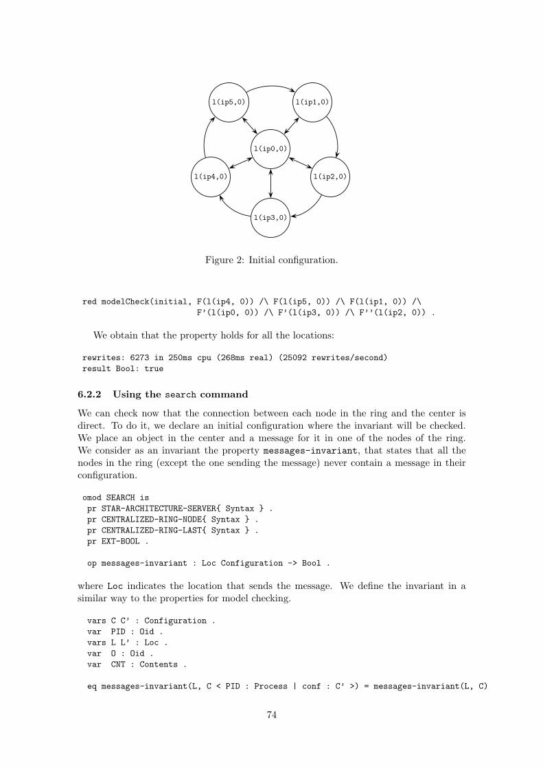
l(ip5,0) l(ip1,0)

l(ip0,0)

l(ip4,0) l(ip2,0)

l(ip3,0)

Figure 2: Initial configuration.

- At the process level, we look for inner configurations.

- At the inner configuration level, we check that the configuration with the requiredlocation does not contain messages.

vars C C’ : Configuration .var O : Oid .vars L : Loc .var CNT : Contents .

eq C < L : Process | conf : C’ (to O : CNT) > |= have-no-message(L) = false .eq C |= have-no-message(L) = true [owise] .

Now we must define the LTL formulas specifying the properties. The formula F ex-presses that the location L receives a message exactly once, and then redirects it. Wecould use it to check if a location receives a message at most once. However, we prefer tocheck the more concrete formula for each location.

ops F F’ F’’ : Loc -> Formula .eq F(L) = have-no-message(L) U (~ have-no-message(L) U [] have-no-message(L)) .

The formula F’ states that L never contains a message. Therefore F ! F’ states thatL receives a message at most once, and then redirects it.

eq F’(L) = [] have-no-message(L) .

Finally, F’’ states that a message reaches L and stays there forever:

eq F’’(L) = have-no-message(L) U ([] ~ have-no-message(L)) .endom

We check this property in the configuration shown in Figure 2 with five nodes in thering (l(ipi, 0), i " 1 . . . 5), and a message from l(ip4, 0) to an object in the locationl(ip2, 0), so it must traverse l(ip5, 0) and l(ip1, 0). The center (l(ip0, 0)) andl(ip3, 0) must receive no messages. Therefore we use the following command:

red modelCheck(initial, F(l(ip4, 0)) /\ F(l(ip5, 0)) /\ F(l(ip1, 0)) /\F’(l(ip0, 0)) /\ F’(l(ip3, 0)) /\ F’’(l(ip2, 0)) .

74

Figure 2: Initial configuration.

red modelCheck(initial, F(l(ip4, 0)) /\ F(l(ip5, 0)) /\ F(l(ip1, 0)) /\F’(l(ip0, 0)) /\ F’(l(ip3, 0)) /\ F’’(l(ip2, 0)) .

We obtain that the property holds for all the locations:

rewrites: 6273 in 250ms cpu (268ms real) (25092 rewrites/second)result Bool: true

6.2.2 Using the search command

We can check now that the connection between each node in the ring and the center isdirect. To do it, we declare an initial configuration where the invariant will be checked.We place an object in the center and a message for it in one of the nodes of the ring.We consider as an invariant the property messages-invariant, that states that all thenodes in the ring (except the one sending the message) never contain a message in theirconfiguration.

omod SEARCH ispr STAR-ARCHITECTURE-SERVER{ Syntax } .pr CENTRALIZED-RING-NODE{ Syntax } .pr CENTRALIZED-RING-LAST{ Syntax } .pr EXT-BOOL .

op messages-invariant : Loc Configuration -> Bool .

where Loc indicates the location that sends the message. We define the invariant in asimilar way to the properties for model checking.

vars C C’ : Configuration .var PID : Oid .vars L L’ : Loc .var O : Oid .var CNT : Contents .

eq messages-invariant(L, C < PID : Process | conf : C’ >) = messages-invariant(L, C)

74

and-then messages-invariant(L, C’) .ceq messages-invariant(L, C < L’ : CRingRouter | > to O : CNT ) = falseif L =/= L’ .eq messages-invariant(L, C) = true [owise] .endom

The command to check the invariant is:

search initial =>* C:Configurationsuch that not messages-invariant(l(ip4, 0), C:Configuration) .

where initial is a configuration with five nodes in the ring, and having the node l(ip4,0) a message for an object in the center. We obtain that no solution is found, so theinvariant is always true and the property holds.

So far we have proved that the message does not traverse the other nodes of the ring,but we must also check that the message disappears from the initial ring node and arrivesto the center. We prove it by using the predicate final-conf, that checks if the messagehas disappeared of the ring node and appeared in the center:

op final-conf : Loc Configuration -> Bool .eq final-conf(L, C < PID : Process | conf : C’ >) = final-conf(L, C)

and-then final-conf(L, C’) .eq final-conf(L, C < L’ : StarCenter | >) = have-message(C) .eq final-conf(L, C < L : CRingRouter | >) = not have-message(C) .eq final-conf(L, C) = true [owise] .

op have-message : Configuration -> Bool .eq have-message(C (to O : CNT)) = true .eq have-message(C) = false [owise] .

The search command does not need to check all the states now, but the final ones, sowe use =>!.

search initial =>! C:Configurationsuch that not final-conf(l(ip4, 0), C:Configuration) .

Again, no solution is found, so we can conclude that the connection between a nodein the ring and the center is direct.

6.3 Analyzing the skeletons

In order to check properties of the skeleton instantiations, we can consider the sequentialversion of the concrete application as the specification of the problem and the distributedversion as the implementation. We use the search command [4] to analyze that in all pos-sible execution of the skeleton (which introduce nondeterminism) the final result obtainedcoincides with the result of the deterministic sequential version.

We define for each skeleton a getResult operation that, given a final configuration,returns the result kept in the master. We use it to compare the results from the sequentialand the distributed implementation. Notice that the comparison can be non trivial, as wewill see in the examples.

75

6.3.1 Euler numbers

In the farm skeleton, we define getResult as follows:

op getResult : Configuration -> P$Result .eq getResult(C < O : Process | conf : (

C’ < M : RW_FD-Master | result : R >) >) = R .

In this Euler numbers example, getResult returns a natural number, that we have tocompare exactly with the result from the specification. The search command used is:

search initial(7) =>! C:Configurationsuch that getResult(C:Configuration) =/= sumEuler(7) .

where initial is a configuration that receives as parameter the Euler number we are lookingfor.

As expected, no different results are found:

No solution.states: 766 rewrites: 465030 in 12780ms cpu (13257ms real)

6.3.2 Ray tracing

In this example the comparison is harder than the last one. In the distributed version wekeep the screen rows in a map (that will be returned by getResult), because the rowscould arrive unordered, while in the sequential version the rows are returned with thejuxtaposition operator. This result cannot be compared directly with the result of thesequential version, so we define an operator map2screen that transforms the map in ascreen, and then the results can be compared:

search initial =>! C:Configurationsuch that map2screen(getResult(C:Configuration)) =/=

rayTracing(-10, 10, 3, -3, 10, 1000000000, figListN(10)) .

where initial is the initial configuration. As expected, no new results are found and thesearch ends successfully:

No solution.states: 127 rewrites: 80774 in 880ms cpu (913ms real)

6.3.3 Atoms interaction

In this example we show a new problem. Although the results from both the sequentialand the distributed version are floats, there are a lot of operations involved with numbersreally small (about 10−24), so the results may vary because of floats precision. Insteadof equality, we check that the difference between the results are not greater than a smallconstant. The getResult function for this skeleton is defined as follows:

op getResult : Configuration -> P$Result .eq getResult(C < O : Process | conf : (C’ < M : SMaster | result : R >) >) = R .

We use the command

76

search initial(12) =>! C:Configurationsuch that abs(getResult(C:Configuration) - attraction(atomGenerator(12)))> 1.0e-20 .

Again, the implementation is correct and the search does not find any solution:

No solution.states: 23 rewrites: 26487 in 60ms cpu (223ms real) (441450 rewrites/second)

6.3.4 Mergesort

We use the same method to prove properties over task parallel programs. For the divideand conquer skeleton, the function getResult extracts the result from the tree:

op getResult : Configuration -> P$Result .eq getResult(C < O : Process | conf : (

C’ < M : DCMaster | resultTree : tree(R, F) >) >) = R .

In the mergesort instantiation, we keep a List as result, that is a container for listsof natural numbers. We only need to extract the NatList from List with a matchingcondition:

search initial(gen(1000)) =>! C:Configurationsuch that l(NL:NatList) := getResult(C:Configuration) /\

NL:NatList =/= mergesort(gen(1000)) .

where initial is the initial configuration that receives as parameter the list to be sorted bythe skeleton. The result confirms that the distributed version was properly implemented:

No solution.states: 64 rewrites: 604306 in 1470ms cpu (2131ms real)

In this case, the problem postcondition is simple enough to avoid the use of the sequen-tial implementation. We can define an ordered operation that checks if a list is orderedand has the same components that other given list:

op ordered : List NatList -> Bool .eq ordered(l(N), N) = true .ceq ordered(l(N N’ NL), NL’ N NL’’) = ordered(l(N’ NL), NL’ NL’’)if N <= N’ .eq ordered(L, NL) = false [owise] .

We can use it now in the search command:

search initial(gen(1000)) =>! C:Configurationsuch that not ordered(getResult(C:Configuration), gen(1000)) .

obtaining the same result with less rewrites:

No solution.states: 64 rewrites: 581555 in 1310ms cpu (1450ms real)

77

6.3.5 Traveling salesman problem

We define getResult for the branch and bound skeleton as follows:

op getResult : Configuration -> P$PartialResult .eq getResult(C < O : Process | conf : (

< M : BBMaster | result : PR > C’) >) = PR .

In the sequential version of this problem, we keep a tuple with the path and its cost,the same that in the distributed version. We define an equal operator that compares thetwo tuples

op equal : Node TravelResult -> Bool .eq equal(node(P, N), result(P’, N’)) = P == P’ and N == N’ .

and use it in the search:

search initial(6) =>! C:Configurationsuch that not equal(getResult(C:Configuration),

travel(city(0), 6, generateCostMatrix(6))) .

where initial is the initial configuration, that receives the number of cities as parameter.We obtain a positive answer again:

No solution.states: 4 rewrites: 1539479 in 11180ms cpu (11643ms real)

7 Implementation in Mobile Maude

A different way in which the applications shown in Section 2 can be executed in a parallelway is by using mobile objects on top of Mobile Maude [6], an extension of Maude allowingmobile computation, where the master and the workers are implemented as mobile objectsthat travel through the architecture. They have an attribute with the concrete code ofthe application.

7.1 Euler numbers case study

We show an implementation of the Euler numbers problem built with a server (the mas-ter) that distributes the work amongst several clients (the workers) and combines theirsubresults. The clients are mobile objects that are created by the server and travel to afree location to compute the solution to the subproblems they have been assigned, in thiscase to compute an Euler number.

We define first the messages that are going to be transmitted, that must have sortContents, defined in MOBILE-OBJECT-INTERFACE. We just need two messages, one sendingnew problems to the workers and another communicating the subresult:

mod MESSAGES isinc MOBILE-OBJECT-INTERFACE .

op new-work : Nat -> Contents .op finished : Mid Nat -> Contents .

endm

78

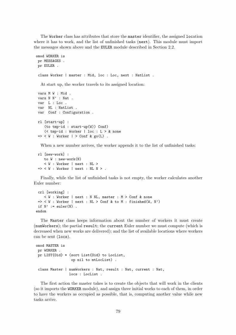
The Worker class has attributes that store the master identifier, the assigned locationwhere it has to work, and the list of unfinished tasks (next). This module must importthe messages shown above and the EULER module described in Section 2.2.

omod WORKER ispr MESSAGES .pr EULER .

class Worker | master : Mid, loc : Loc, next : NatList .

At start up, the worker travels to its assigned location:

vars M W : Mid .vars N N’ : Nat .var L : Loc .var NL : NatList .var Conf : Configuration .

rl [start-up] :(to tmp-id : start-up(W)) Conf)(< tmp-id : Worker | loc : L > & none

=> < W : Worker | > Conf & go(L) .

When a new number arrives, the worker appends it to the list of unfinished tasks:

rl [new-work] :to W : new-work(N)< W : Worker | next : NL >

=> < W : Worker | next : NL N > .

Finally, while the list of unfinished tasks is not empty, the worker calculates anotherEuler number:

crl [working] :< W : Worker | next : N NL, master : M > Conf & none

=> < W : Worker | next : NL > Conf & to M : finished(W, N’)if N’ := euler(N) .endom

The Master class keeps information about the number of workers it must create(numWorkers); the partial result; the current Euler number we must compute (which isdecreased when new works are delivered); and the list of available locations where workerscan be sent (locs).

omod MASTER ispr WORKER .pr LIST{Oid} * (sort List{Oid} to LocList,

op nil to mtLocList) .

class Master | numWorkers : Nat, result : Nat, current : Nat,locs : LocList .

The first action the master takes is to create the objects that will work in the clients(so it imports the WORKER module), and assign three initial works to each of them, in orderto have the workers as occupied as possible, that is, computing another value while newtasks arrive.

79

vars M W : Mid .vars N N’ X Y N’’ R C : Nat .var Conf : Configuration .var L : Loc .var LL : LocList .

rl [new-worker] :< M : Master | numWorkers : s(N), locs : L LL,

current : N’ > Conf & none=> < M : Master | numWorkers : N, locs : LL L,

current : sd(N’, 3) > Conf &newo(upModule(’WORKER, false),

< tmp-id : Worker | master : M,loc : L,next : (N’ sd(N’, 1) sd(N’, 2)) >,

tmp-id) .

Note that the location L is moved from the beginning to the end of the loc list, so itcould be used again if the initial number of workers is bigger that the length of this list.

When a new subresult arrives to the server, it is combined with the current result byadding them, and a new task is sent (if it is possible):

rl [new-result] :to M : finished(W, N’’) Conf & none< M : Master | current : s(N), result : N’ >

=> < M : Master | current : N, result : N’ + N’’ > Conf &to W : new-work(s(N)) .

rl [no-more-work] :to M : finished(W, N’)< M : Master | current : 0, result : N >

=> < M : Master | result : N + N’ > .endom

The initial term for the server in an example with two workers and 1300 as initialnumber to compute is:

erew <> < l(ip0, 0) : ServerRootObject |cnt : 1,guests : o(l(ip0, 0), 0),forward : 0 |-> (l(ip0, 0),0),state : idle,neighbors : empty,defNeighbor : null >

< o(l(ip0, 0), 0) : MobileObject |mod : upModule(’MASTER, false),s : upTerm(< o(l(ip0, 0), 0) : Master |

numWorkers : 2,current : 1300,result : 0,locs : l(ip1, 0) l(ip2, 0) >

& none),gas : 2000,hops : 0,mode : active > .

80

The single difference between the two clients is the name. The initial term for the firstone is:

erew <> < l(ip1, 0) : ClientRootObject |cnt : 0,guests : empty,forward : empty,state : idle,neighbors : empty,defNeighbor : null > .

7.2 Mobile Maude skeletons

We specify skeletons in this case by using “generic” mobile objects, that receive as datathe module solving each concrete problem as initial information. We can simulate inMaude higher order functions by using reflection and the META-LEVEL module (see Section1.1), that allows to use Maude modules as data. Our Mobile Maude skeletons will have aMaster class with the number of workers (numWorkers); the partial result, that is now aTerm, because it represents the result of all possible applications; the current subproblem(a Term too); the list of available locations (locs); the number of initial works assignedto each worker numWorks; and (the metarepresentation of) a module, that will store theconcrete application code:

class Master | numWorkers : Nat, result : Term, current : Term,locs : LocList, numWorks : Nat, module : Module .

The metarepresented module must contain some fixed operators:

- do-work, that solves the subproblems.

- reduce, that updates the current problem by making it smaller.

- next-work, that gets the next subproblem from the current problem.

- combine, that merges the current (partial) result with a subresult.

- finished?, that checks if there are more subproblems.

In the Worker class we still need the master identifier, the assigned location, and thelist of unfinished tasks (that now is a term list), and we need a new attribute with (themetarepresentation of) the application module:

class Worker | master : Mid, loc : Loc, next : TermList, module : Module .

The messages must change in order to dispatch generic data. They transmit now dataof type Term, that will represent the concrete data for each application:

mod MESSAGES isinc MOBILE-OBJECT-ADDITIONAL-DEFS .

op new-work : Term -> Contents .op finished : Mid Term -> Contents .

endm

81

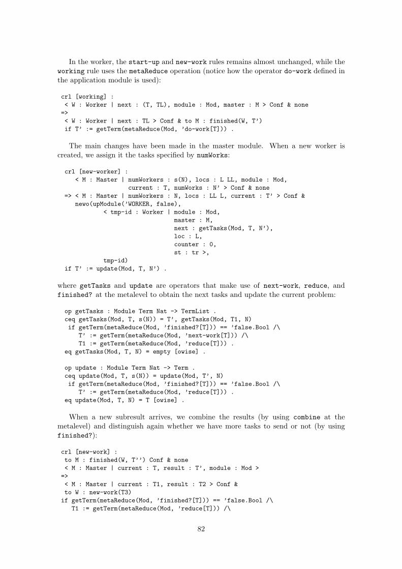
In the worker, the start-up and new-work rules remains almost unchanged, while theworking rule uses the metaReduce operation (notice how the operator do-work defined inthe application module is used):

crl [working] :< W : Worker | next : (T, TL), module : Mod, master : M > Conf & none=>< W : Worker | next : TL > Conf & to M : finished(W, T’)if T’ := getTerm(metaReduce(Mod, ’do-work[T])) .

The main changes have been made in the master module. When a new worker iscreated, we assign it the tasks specified by numWorks:

crl [new-worker] :< M : Master | numWorkers : s(N), locs : L LL, module : Mod,

current : T, numWorks : N’ > Conf & none=> < M : Master | numWorkers : N, locs : LL L, current : T’ > Conf &

newo(upModule(’WORKER, false),< tmp-id : Worker | module : Mod,

master : M,next : getTasks(Mod, T, N’),loc : L,counter : 0,st : tr >,

tmp-id)if T’ := update(Mod, T, N’) .

where getTasks and update are operators that make use of next-work, reduce, andfinished? at the metalevel to obtain the next tasks and update the current problem:

op getTasks : Module Term Nat -> TermList .ceq getTasks(Mod, T, s(N)) = T’, getTasks(Mod, T1, N)if getTerm(metaReduce(Mod, ’finished?[T])) == ’false.Bool /\

T’ := getTerm(metaReduce(Mod, ’next-work[T])) /\T1 := getTerm(metaReduce(Mod, ’reduce[T])) .

eq getTasks(Mod, T, N) = empty [owise] .

op update : Module Term Nat -> Term .ceq update(Mod, T, s(N)) = update(Mod, T’, N)if getTerm(metaReduce(Mod, ’finished?[T])) == ’false.Bool /\

T’ := getTerm(metaReduce(Mod, ’reduce[T])) .eq update(Mod, T, N) = T [owise] .

When a new subresult arrives, we combine the results (by using combine at themetalevel) and distinguish again whether we have more tasks to send or not (by usingfinished?):

crl [new-work] :to M : finished(W, T’’) Conf & none< M : Master | current : T, result : T’, module : Mod >=>< M : Master | current : T1, result : T2 > Conf &to W : new-work(T3)if getTerm(metaReduce(Mod, ’finished?[T])) == ’false.Bool /\

T1 := getTerm(metaReduce(Mod, ’reduce[T])) /\

82

T2 := getTerm(metaReduce(Mod, ’combine[T’, T’’])) /\T3 := getTerm(metaReduce(Mod, ’next-work[T])) .

crl [no-more-work] :to M : finished(W, T’’)< M : Master | current : T, result : T’, module : Mod >=>< M : Master | result : T1 >if getTerm(metaReduce(Mod, ’finished?[T])) == ’true.Bool /\

T1 := getTerm(metaReduce(Mod, ’combine[T’, T’’])) .

For our Euler numbers example we define the following module:

fmod EULER-MM-SKELETON ispr EULER .

vars N N’ : Nat .

op do-work : Nat -> Nat .op reduce : Nat ~> Nat .op next-work : Nat -> Nat .op combine : Nat Nat -> Nat .op finished? : Nat -> Bool .

eq do-work(N) = euler(N) .eq reduce(s(N)) = N .eq next-work(N) = N .eq combine(N, N’) = N + N’ .eq finished?(N) = N == 0 .endfm

The initial configuration of the master, in an example with four workers and initialproblem 15000 is

erew <> < l(ip0, 0) : ServerRootObject |cnt : 1,guests : o(l(ip0, 0), 0),forward : 0 |-> (l(ip0, 0),0),neighbors : empty,state : idle,defNeighbor : null,port : 60039

>< o(l(ip0, 0), 0) : MobileObject |

mod : upModule(’MASTER, false),s : upTerm(< o(l(ip0, 0), 0) : Master |

numWorkers : 4,numWorks : 3,current : upTerm(15000),result : upTerm(0),module : upModule(’EULER-MM-SKELETON, false),locs : l(ip1, 0) l(ip2, 0) l(ip3, 0) l(ip4, 0) >

& none),gas : 20000,hops : 0,mode : active > .

83

where the ipi are strings denoting IP addresses.Notice that the skeleton code (the master and the server) will be metarepresented in

the belly of the mobile objects, so the application code will have two reflection levels.Despite we have obtained an application that can be executed among several hosts, theexecution at the metalevel is so slow that we obtain almost the same time that with thesequential applications.

8 Conclusions

We have presented the implementation of some architectures using sockets, that Maudesupports as external objects. We have implemented several skeletons as parameterizedmodules that receive as parameters the operations solving each concrete problem. Thatallows to instantiate the same skeleton for a concrete problem in different ways, for examplevarying its granularity.

From the Maude side, we show that truly distributed applications can be implementedand that the recently incorporated support for parameterization in Core Maude can beapplied to more complex applications. From the point of view of skeleton development,we describe a methodology to specify, prototype, and check skeletons that can be laterimplemented in other languages such as Java. We plan to study in a near future what isthe best way to achieve it.

We have tested the skeletons with some examples, using three 2 GHz PowerPC G5 andtwo 1.25 GHz PowerPC G4, obtaining a speed-up of 2.5. Although this speed-up is notremarkable, we observed in the executions that all the processors were always computing,so most of the time was wasted in preparing the transmitted data. We have to study howto improve the efficiency; the profiling feature in Maude allows a detailed analysis of whichrules are most expensive to execute in a given application.

Finally, we have started to study how our skeletons can be nested by using the object-oriented inheritance features provided by Maude. We are also investigating how to proveproperties of the skeletons independently of the instantiations, that can be achieved byusing rule induction.Acknowledgments We thank Narciso Martı-Oliet for his continuous support and helpwith Maude foundations; Francisco Duran for the joint work in Mobile Maude; RicardoPena and Fernando Rubio for introducing us in the skeleton’s world; and Ana Gil forclarifying the ray tracing algorithm.

References

[1] G. H. Botorog and H. Kuchen. Efficient parallel programming with algorithmic skeletons.In Proceedings of EuroPar’96, volume 1123 of Lecture Notes for Computer Science, pages718–731. Springer, 1996.

[2] E. M. Clarke, O. Grumberg, and D. A. Peled. Model Checking. MIT Press, 1999.

[3] M. Clavel, F. Duran, S. Eker, P. Lincoln, N. Martı-Oliet, J. Meseguer, and J. Quesada. Maude:specification and programming in rewriting logic. Theoretical Computer Science, 285(2):187–243, 2002.

[4] M. Clavel, F. Duran, S. Eker, P. Lincoln, N. Martı-Oliet, J. Meseguer, and C. Talcott. MaudeManual (Version 2.2), December 2005. http://maude.cs.uiuc.edu/maude2-manual.

[5] J. Darlington, A. J. Field, P. G. Harrison, P. H. J. Kelly, D. W. N. Sharp, Q. Wu, andR. L. While. Parallel programming using skeleton functions. In Proceedings of PARLE’93

84

– Parallel Architectures and Languages Europe, volume 694 of Lecture Notes for ComputerScience, pages 146–160. Springer, 1993.

[6] F. Duran, A. Riesco, and A. Verdejo. A distributed implementation of Mobile Maude. InG. Denker and C. Talcott, editors, Proceedings Sixth International Workshop on RewritingLogic and its Applications, WRLA 2006, Electronic Notes in Theoretical Computer Science,pages 35–55. Elsevier, 2006.

[7] S. Eker, J. Meseguer, and A. Sridharanarayanan. The Maude LTL model checker. In F. Gad-ducci and U. Montanari, editors, Proceedings Fourth International Workshop on RewritingLogic and its Applications, WRLA 2002, Pisa, Italy, September 19–21, 2002, volume 71 ofElectronic Notes in Theoretical Computer Science, pages 115–141. Elsevier, 2002.

[8] A. Farzan and J. Meseguer. State space reduction of rewrite theories using invisible transitions.In M. Johnson and V. Vene, editors, Algebraic Methodology and Software Technology, 11thInternational Conference, AMAST 2006, Kuressaare, Estonia, July 5-8, 2006, Proceedings,volume 4019 of Lecture Notes for Computer Science, pages 142–157. Springer, 2006.

[9] J. F. Ferreira, J. L. Sobral, and A. J. Proenca. Jaskel: A java skeleton-based frameworkfor structured cluster and grid computing. In CCGRID’06: Proceedings of the Sixth IEEEInternational Symposium on Cluster Computing and the Grid, pages 301–304. IEEE ComputerSociety, 2006.

[10] E. Horowitz, S. Sahni, and S. Rajasekaran. Computer Algorithms. Computer Science Press.W. H. Freeman and Company, 1997.

[11] R. Loogen, Y. Ortega-Mallen, R. Pena, S. Priebe, and F. Rubio. Parallelism abstractionsin Eden. In F. A. Rabhi and S. Gorlatch, editors, Patterns and Skeletons for Parallel andDistributed Computing, chapter 4, pages 95–129. Springer, 2002.

[12] Z. Manna and A. Pnueli. The Temporal Logic of Reactive and Concurrent Systems. Specifi-cations. Springer-Verlag, 1992.

[13] N. Martı-Oliet and J. Meseguer. Action and change in rewriting logic. In R. Pareschi andB. Fronhofer, editors, Dynamic Worlds: From the Frame Problem to Knowledge Management,volume 12 of Applied Logic Series, pages 1–53. Kluwer Academic Publishers, 1999.

[14] N. Martı-Oliet and J. Meseguer. Rewriting logic as a logical and semantic framework. InD. M. Gabbay and F. Guenthner, editors, Handbook of Philosophical Logic, Second Edition,Volume 9, pages 1–87. Kluwer Academic Publishers, 2002. First published as SRI TechnicalReport SRI-CSL-93-05, August 1993.

[15] N. Martı-Oliet, J. Meseguer, and A. Verdejo. Towards a strategy language for Maude. InN. Martı-Oliet, editor, Proceedings Fifth International Workshop on Rewriting Logic and itsApplications, WRLA 2004, Barcelona, Spain, March 27 – April 4, 2004, volume 117 of Elec-tronic Notes in Theoretical Computer Science, pages 417–441. Elsevier, 2005.

[16] J. Meseguer. Conditional rewriting logic as a unified model of concurrency. TheoreticalComputer Science, 96(1):73–155, 1992.

[17] J. Meseguer. A logical theory of concurrent objects and its realization in the Maude language.In G. Agha, P. Wegner, and A. Yonezawa, editors, Research Directions in Concurrent Object-Oriented Programming, pages 314–390. The MIT Press, 1993.

[18] J. Meseguer. A rewriting logic sampler. In D. Hung and M. Wirsing, editors, TheoreticalAspects of Computing – ICTAC 2005: Second International Colloquium, Hanoi, Vietnam,October 17-21, 2005. Proceedings, volume 3722 of Lecture Notes in Computer Science, pages1–28. Springer, 2005.

[19] G. Michaelson, N. Scaife, P. Bristow, and P. King. Nested algorithmic skeletons from higherorder functions. Parallel Algorithms and Applications, 16(2-3):181–206, 2001.

[20] F. A. Rabhi and S. Gorlatch. Patterns and Skeletons for Parallel and Distributed Computing.Springer, 2002.

85

[21] P. W. Trinder, H. W. Loidl, and R. F. Pointon. Parallel and distributed haskells. Journal ofFunctional Programming, 12(4-5):469–510, 2002.

86