Maude THOLLON

THESE DE DOCTORAT EN CO-TUTELLE DE

L'UNIVERSITE DE BRETAGNE OCCIDENTALE ECOLE DOCTORALE N° 598 Sciences de la Mer et du littoral Spécialité : Géosciences Marines

AVEC L'UNIVERSITE DE WOLLONGONG

Par

Maude THOLLON

Evolution des temps de transfert sédimentaire océan-continent au regard de la variabilité climatique quaternaire : Apports des isotopes de l'Uranium Thèse présentée et soutenue à l’Institut Universitaire Européen de la Mer, Technopôle Brest-Iroise, Rue Dumont d’Urville, 29280 Plouzané, le 10 Décembre 2020 Unité de recherche : Géosciences marines (IFREMER) Et Wollongong Isotopes Geochronology Laboratory

Rapporteurs avant soutenance :

Hella WITTMANN Docteure, GFZ German Research Centre for Geosciences–Germany Lin MA Professeur, Univ. Texas – USA

Composition du Jury :

Marina RABINEAU Directrice de recherches, UBO / Présidente du jury

Hella WITTMANN Docteure, GFZ German Research Centre for Geosciences– Germany / Rapporteuse

Lin MA Professeur, Univ. Texas – USA / Rapporteur

François CHABAUX Professeur, Univ. De Strasbourg / Examinateur

Jean-Alix BARRAT Professeur, UBO / Directeur de thèse

Invités Samuel TOUCANNE Docteur, Ifremer / Encadrant

Germain BAYON Docteur, Ifremer / Encadrant

REMERCIEMENTS -ACKNOWLEDGEMENTS

Une thèse ne pourrait se faire sans encadrement. C’est pour cela que je tiens dans unpremier temps à remercier Jean Alix Barrat. Merci pour m’avoir présenté cette oppor-tunité et suivi l’évolution du projet. Je remercie ensuite énormément Samuel Toucanne,Germain Bayon et Tony Dosseto de m’avoir accordé leur confiance pour la réalisation decette thèse. Merci à tous les trois de m’avoir encadrée durant ces trois années, pour vosconseils et soutient quand il y avait besoin. Je suis reconnaissante de d’avoir eu la pos-sibilité de découvrir et travailler dans deux unités de recherche, entre Brest et Wollongong.

J’en profite pour remercier également Nathalie Vigier et Stefan Lalonde pour avoir suivimon projet. Merci pour l’intérêt porté au sujet, et d’avoir été toujours si enthousiaste ausujet des résultats. Merci également pour les suggestions et conseils apportés au cours duprojet.

Au cours de ma thèse, de nombreuses personnes m’ont accompagnées et aidées. Je tiensà remercier en particulier à l’Ifremer Yoann Germain et Anne Trinquier pour m’avoir ini-tiée aux rudiments de la spectrométrie de masse. Je remercie aussi Audrey Boissier et San-drine Cheron pour les conseils portant de la préparation des échantillons à l’interprétationde résultats de la mineralogie des échantillons. Je tiens à remercier tous les membres deGM à l’Ifremer qui ont interagi avec le projet. Un merci particulier à toutes les personnesqui ont récoltés les échantillons, tant sur terre qu’en mer, sans qui la thèse n’aurait étépossible.At the university of Wollongong, I would like to particularly thanks Alex Francke, forhaving introducing to me its samples preparation that save me a lot of time. I also thankshim for being always so enthusiastic about uranium isotopes conversations. I thanks Tibicodilean, for his help on the strategy to adopt on the GIS analysis. I also thanks HeidiBrown for helping me with ArcGIS with such enthusiasm. I am thankful to ChristopherRichardson for his help while I was doing IQ analyses and Alan Champion for his avail-ability and helps.

A joint supervision between two countries is not always easy and I thanks Samuel T.,Sylvia Baronne, Denise Alsop, both faculties and Studies up (Anne-Sophie) for the dif-ferent kind of help to handle the administrative part.Ce travail a bénéficié d’une aide de l’Etat gérée par l’Agence Nationale de la Recherche au

3

titre du programme «Investissements d’avenir» portant la référence ANR-17-EURE-0015.Je remercie Isblue pour l’attribution de cette aide qui a facilité la co-tutelle.I would also thanks all the members of the Jury for having accepted to be part of it. Ithank Marina Rabineau for chairing the jury during the defence. I thank Hella Witmannand Lin Ma for being the reviewers of my manuscript, and François Chabaux for be partof the jury. I thank all of you for your constructive remarks during my defence.

Une aventure de trois ans ne se résumant pas seulement au travail, je tiens à remercierl’équipe d’étudiants de l’Ifremer et en particulier Arthur, Aurélien et Vincent.At Wollongong I sincerly thanks all the PhD team. I thanks the Wigals, for the great,friendly and supportive working environment, a particular thanks to Holly, Dafne, Alexand Sally. A huge thanks to Holly for introducing me to the Australian’s life and I shouldmentioned it, for supporting me emotionally.A huge thanks to Maria for being such a great flatemate.Also, thanks to Meagan andNick for having welcoming me in their home.

Je tiens à remercier tous les amis de Beauvais, pour m’avoir accompagnée de loin dansce projet, pour tous les agréables moments qui ont permis de mettre la thèse de côtéle temps d’un week-end. Un énorme merci à Cécile, pour tout et notamment le tempsaccordé durant ces trois années. Un très gros merci à Sophie aussi, dont la compréhensionde la vie de doctorante à été très utile.Je voudrais aussi en profiter pour remercier ma famille. Merci d’avoir été d’un tel soutientout au long de la thèse et de m’avoir permis d’allre jusqu’au bout.Et enfin, un immense merci à Sam.

4

TABLE OF CONTENTS

Remerciements - Acknowledgements 3

Introduction 15General background . . . . . . . . . . . . . . . . . . . . . . . . . . . . . . . . . 15Objectives of this thesis . . . . . . . . . . . . . . . . . . . . . . . . . . . . . . . 16

Introduction 19Généralités . . . . . . . . . . . . . . . . . . . . . . . . . . . . . . . . . . . . . . 19Objectifs de la thèse . . . . . . . . . . . . . . . . . . . . . . . . . . . . . . . . . 20

1 Literature Review 251.1 From source to sink: the sediment’s life . . . . . . . . . . . . . . . . . . . . 26

1.1.1 Concept . . . . . . . . . . . . . . . . . . . . . . . . . . . . . . . . . 261.1.2 Environmental signal propagation in sedimentary systems . . . . . 311.1.3 Soil: the origin of the sediment . . . . . . . . . . . . . . . . . . . . 41

1.2 Uranium isotopes . . . . . . . . . . . . . . . . . . . . . . . . . . . . . . . . 451.2.1 Background . . . . . . . . . . . . . . . . . . . . . . . . . . . . . . . 451.2.2 Radioactive disequilibrium . . . . . . . . . . . . . . . . . . . . . . . 451.2.3 Secular equilibrium . . . . . . . . . . . . . . . . . . . . . . . . . . . 471.2.4 Uranium abundances in rock forming minerals and the fractionation

of (234U/238U) in sedimentary systems . . . . . . . . . . . . . . . . 481.2.5 The concept of comminution age . . . . . . . . . . . . . . . . . . . 53

1.3 Uranium at Earth’s surface . . . . . . . . . . . . . . . . . . . . . . . . . . 591.3.1 From bedrock to soil: weathering processes . . . . . . . . . . . . . . 591.3.2 Uranium isotopes to infer timescale of sedimentary processes and

its control . . . . . . . . . . . . . . . . . . . . . . . . . . . . . . . . 611.3.3 Uncertainties based on the comminution age method . . . . . . . . 62

2 Methodology 652.1 Samples collection . . . . . . . . . . . . . . . . . . . . . . . . . . . . . . . . 66

2.1.1 Sediments from world rivers . . . . . . . . . . . . . . . . . . . . . . 662.1.2 Var sediments . . . . . . . . . . . . . . . . . . . . . . . . . . . . . . 66

2.2 Samples preparation . . . . . . . . . . . . . . . . . . . . . . . . . . . . . . 712.2.1 Reagent and labware . . . . . . . . . . . . . . . . . . . . . . . . . . 712.2.2 Grain-size separation . . . . . . . . . . . . . . . . . . . . . . . . . . 71

5

TABLE OF CONTENTS

2.2.3 Leaching . . . . . . . . . . . . . . . . . . . . . . . . . . . . . . . . . 722.2.4 Sediments dissolution . . . . . . . . . . . . . . . . . . . . . . . . . . 76

2.3 Ion exchange chromatography . . . . . . . . . . . . . . . . . . . . . . . . . 782.3.1 Ifremer method . . . . . . . . . . . . . . . . . . . . . . . . . . . . . 782.3.2 UOW method . . . . . . . . . . . . . . . . . . . . . . . . . . . . . 80

2.4 Uranium analyses . . . . . . . . . . . . . . . . . . . . . . . . . . . . . . . . 822.4.1 Isotopic measurement of Uranium isotopes . . . . . . . . . . . . . . 822.4.2 Concentration . . . . . . . . . . . . . . . . . . . . . . . . . . . . . . 832.4.3 Accuracy and precision of the data . . . . . . . . . . . . . . . . . . 84

2.5 Specific surface analyses . . . . . . . . . . . . . . . . . . . . . . . . . . . . 872.6 Geographic Information System analyses . . . . . . . . . . . . . . . . . . . 89

2.6.1 Basin and sub-basin delineation . . . . . . . . . . . . . . . . . . . . 892.6.2 Extraction of the geomorphologic characteristics . . . . . . . . . . . 89

3 The distribution of (234U/238U) activity ratios in river sediments 913.1 Introduction . . . . . . . . . . . . . . . . . . . . . . . . . . . . . . . . . . . 933.2 Methods . . . . . . . . . . . . . . . . . . . . . . . . . . . . . . . . . . . . . 95

3.2.1 Samples . . . . . . . . . . . . . . . . . . . . . . . . . . . . . . . . . 953.2.2 Analytical procedures . . . . . . . . . . . . . . . . . . . . . . . . . . 97

3.3 Results . . . . . . . . . . . . . . . . . . . . . . . . . . . . . . . . . . . . . . 983.3.1 Leaching experiments . . . . . . . . . . . . . . . . . . . . . . . . . . 983.3.2 Uranium in river sediments . . . . . . . . . . . . . . . . . . . . . . 100

3.4 Discussion . . . . . . . . . . . . . . . . . . . . . . . . . . . . . . . . . . . . 1023.4.1 Influence of grain size on (234U/238U) ratios of detrital sediments . . 1023.4.2 The effect of weathering, climate and erosion on 234U-238U fraction-

ation . . . . . . . . . . . . . . . . . . . . . . . . . . . . . . . . . . . 1023.4.3 The role of lithology . . . . . . . . . . . . . . . . . . . . . . . . . . 1093.4.4 The role of catchment size and sediment residence time on (234U/238U)

sedimentary ratio . . . . . . . . . . . . . . . . . . . . . . . . . . . . 1113.4.5 Complex interactions of environmental controls on sediment resi-

dence time . . . . . . . . . . . . . . . . . . . . . . . . . . . . . . . . 1143.5 Conclusion . . . . . . . . . . . . . . . . . . . . . . . . . . . . . . . . . . . . 1153.6 Acknowledgments . . . . . . . . . . . . . . . . . . . . . . . . . . . . . . . . 116

4 The Var sediment routing system: spatial residence time variation 1174.1 Study site: the Var basin . . . . . . . . . . . . . . . . . . . . . . . . . . . . 118

4.1.1 Environmental setting . . . . . . . . . . . . . . . . . . . . . . . . . 1184.1.2 A source to sink system . . . . . . . . . . . . . . . . . . . . . . . . 120

4.2 Controls on the regolith residence time in an Alpine river catchment . . . . 1244.3 Introduction . . . . . . . . . . . . . . . . . . . . . . . . . . . . . . . . . . . 125

6

TABLE OF CONTENTS

4.4 Study site . . . . . . . . . . . . . . . . . . . . . . . . . . . . . . . . . . . . 1264.5 Materials and Methods . . . . . . . . . . . . . . . . . . . . . . . . . . . . . 1274.6 Results . . . . . . . . . . . . . . . . . . . . . . . . . . . . . . . . . . . . . . 1294.7 Discussion . . . . . . . . . . . . . . . . . . . . . . . . . . . . . . . . . . . . 131

4.7.1 Assessing the role of lithology and weathering regimes on the Uisotope ratio . . . . . . . . . . . . . . . . . . . . . . . . . . . . . . . 131

4.7.2 Geomorphologic control on (234U/238U) ratios . . . . . . . . . . . . 1334.7.3 Quantification of regolith residence times in the Var River catchment1354.7.4 Geomorphic controls on regolith residence time . . . . . . . . . . . 139

4.8 Conclusion and perspectives . . . . . . . . . . . . . . . . . . . . . . . . . . 140

5 The Var sediment routing system: paleo-residence time variations 1435.1 The climatic cyclicity during the Quaternary . . . . . . . . . . . . . . . . . 144

5.1.1 Long terms climatic cycles . . . . . . . . . . . . . . . . . . . . . . . 1445.1.2 Millennial-scale climate changes . . . . . . . . . . . . . . . . . . . . 1455.1.3 The climatic context in the Alps during the Quaternary . . . . . . . 147

5.2 Temporal sediment residence time variations . . . . . . . . . . . . . . . . . 1495.2.1 Stratigraphy of the Var sedimentary ridge . . . . . . . . . . . . . . 1495.2.2 Methods . . . . . . . . . . . . . . . . . . . . . . . . . . . . . . . . . 1515.2.3 Uranium variations over time - Results . . . . . . . . . . . . . . . . 1535.2.4 Interpretation . . . . . . . . . . . . . . . . . . . . . . . . . . . . . . 1575.2.5 Conclusion . . . . . . . . . . . . . . . . . . . . . . . . . . . . . . . . 165

Conclusions and perspectives 167Rationale and objectives of this thesis . . . . . . . . . . . . . . . . . . . . . . . . 167The variation of U-fractionation . . . . . . . . . . . . . . . . . . . . . . . . . . . 168Spatial variation of the sediment residence time in a mountainous river basin . . 169Linking paleo-sediment residence time to paleo-erosional processes . . . . . . . . 170Perspectives . . . . . . . . . . . . . . . . . . . . . . . . . . . . . . . . . . . . . . 172

Conclusions et perspectives 175Rappel des objectifs de la thèse . . . . . . . . . . . . . . . . . . . . . . . . . . . 175La distribution spatiale de (234U/238U) . . . . . . . . . . . . . . . . . . . . . . . 176Variation spatiale du temps de résidence sédimentaire dans un bassin montagneux178Lier les temps de résidence aux évenements passés . . . . . . . . . . . . . . . . . 179Perspectives . . . . . . . . . . . . . . . . . . . . . . . . . . . . . . . . . . . . . . 181

Appendix 183

References 203

7

LIST OF FIGURES

1 Conceptual representation of the sediment residence time. . . . . . . . . . 171 Représentation conceptuelle du temps de résidence sédimentaire. . . . . . . 21

1.1 Representation of a source to sink system. . . . . . . . . . . . . . . . . . . 271.2 Schema of weathering profile. . . . . . . . . . . . . . . . . . . . . . . . . . 281.3 Schema of the bedrock weathering into soil. . . . . . . . . . . . . . . . . . 291.4 Parameters influencing the source to sink system . . . . . . . . . . . . . . . 321.5 Weathering series of both silicate and non silicate minerals . . . . . . . . . 341.6 Parameters influencing the source to sink system . . . . . . . . . . . . . . . 341.7 Denudation rate as function of the hillslope curvature. . . . . . . . . . . . 351.8 Erosion rate depending on the vegetation cover. . . . . . . . . . . . . . . . 371.9 Representation of the sediment supply signal propagation inside a basin. . 381.10 Summary of the sedimentary signal propagation from source to sink . . . 401.11 Schematic representation of the Critical Zone . . . . . . . . . . . . . . . . 411.12 Models of the soil depth production . . . . . . . . . . . . . . . . . . . . . . 431.13 Decay of the U series . . . . . . . . . . . . . . . . . . . . . . . . . . . . . . 461.14 Evolution of daughter-parents isotopes activity ratio to return to secular

equilibrium. . . . . . . . . . . . . . . . . . . . . . . . . . . . . . . . . . . . 471.15 Eh−pH diagram representing the stability of the most common U species . 501.16 Diagram of thoranite solubility . . . . . . . . . . . . . . . . . . . . . . . . 511.17 Schematic representation of the recoil process . . . . . . . . . . . . . . . . 521.18 Secular equilibrium . . . . . . . . . . . . . . . . . . . . . . . . . . . . . . . 571.19 U mobility in weathering profile . . . . . . . . . . . . . . . . . . . . . . . . 60

2.1 Map of the world rivers sediments location . . . . . . . . . . . . . . . . . . 672.2 Location of the sediments from the Var River and its tributaries. . . . . . . 682.3 Map of the cores location. . . . . . . . . . . . . . . . . . . . . . . . . . . . 692.4 Sedimentary facies observed in the studied turbiditic cores. . . . . . . . . . 702.5 Pictures of the turbiditic cores . . . . . . . . . . . . . . . . . . . . . . . . . 742.6 Evolution of (234U/238U) during the leaching . . . . . . . . . . . . . . . . . 742.7 Elution profile before improvement of the method . . . . . . . . . . . . . . 792.8 Elution profile after improvement of the method . . . . . . . . . . . . . . . 802.9 Uranium concentration and (234U/238U) for the standard BCR-2 . . . . . . 852.10 Evolution of (234U/238U) obtained for the standard U005A . . . . . . . . . 86

9

LIST OF FIGURES

2.11 Evolution of U (ppm) obtained for the standard 71A measured on the iCAPQ-ICP MS . . . . . . . . . . . . . . . . . . . . . . . . . . . . . . . . . . . 86

2.12 Adsorption-desorption isotherms . . . . . . . . . . . . . . . . . . . . . . . . 87

3.1 World River sediments location . . . . . . . . . . . . . . . . . . . . . . . . 963.2 Evolution of (234U/238U) trough the leaching steps. . . . . . . . . . . . . . 993.3 U concentration and (234U/238U) histogram. . . . . . . . . . . . . . . . . . 1003.4 Variation of (234U/238U) depending on weathering. . . . . . . . . . . . . . . 1043.5 Variation of (234U/238U) depending on climate. . . . . . . . . . . . . . . . . 1063.6 Variation of (234U/238U) depending on the maximum elevation of the catch-

ment. . . . . . . . . . . . . . . . . . . . . . . . . . . . . . . . . . . . . . . . 1073.7 Variation of (234U/238U) depending on the area of the basin. . . . . . . . . 1103.8 Variation of (234U/238U) depending on the depth to bedrock. . . . . . . . . 1133.9 Model of (234U/238U) evolution depending on the area of the basin. . . . . 1143.10 Evolution of (234U/238U) depending on multi-parameters. . . . . . . . . . . 115

4.1 Elevation model of the Var basin . . . . . . . . . . . . . . . . . . . . . . . 1184.2 Geological map of the Var basin . . . . . . . . . . . . . . . . . . . . . . . . 1194.3 Variation of the denudation rates inside the Var basin. . . . . . . . . . . . 1214.4 Pictures of the Vesubie before and after the tempete Alex (2020) . . . . . . 1224.5 Picture of the Var delta just after the tempete Alex . . . . . . . . . . . . . 1224.6 Localisation of the samples on elevation model of the Var basin. . . . . . . 1264.7 Variation of (234U/238U) depending on lithologic and weathering proxies. . 1314.8 (234U/238U) depending on morphologic parameters . . . . . . . . . . . . . . 1344.9 Variation on U-derived sediment residence time depending on the spatial

analysis-derived sediment residence time. . . . . . . . . . . . . . . . . . . . 1374.10 Variation of regolith residence time depending on morphologic parameters. 1394.11 Variation of calculated regolith residence time as function of the predict

regolith residence time . . . . . . . . . . . . . . . . . . . . . . . . . . . . . 140

5.1 Millenial climatic variations in the Northern Hemisphere. . . . . . . . . . . 1465.2 Location of the cores along the Var canyon and the Var Sedimentary Ridge 1495.3 Composite δ18O (VPDB) and δ18O (NGRIP) variations. . . . . . . . . . . 1505.4 Results . . . . . . . . . . . . . . . . . . . . . . . . . . . . . . . . . . . . . . 1545.5 (234U/238U) in function of the concentration for the Var sediments . . . . . 1555.6 (234U/238U) in function of U-derived sediment residence time. . . . . . . . . 1575.7 (234U/238U) and sediment residence time variation over the last 75 ka in

the Var basin. . . . . . . . . . . . . . . . . . . . . . . . . . . . . . . . . . . 1585.8 Spatial variation of (234U/238U) and εNd in the Var basin. . . . . . . . . . . 1595.9 εNd and denudation rate variation over the last 75 ka in the Var. . . . . . . 161

10

LIST OF FIGURES

5.10 (234U/238U) compared to climatic and vegetation parameters. . . . . . . . . 1635.11 (234U/238U) variations in correlation with the sea surface temperature over

the last 75 ka. . . . . . . . . . . . . . . . . . . . . . . . . . . . . . . . . . . 164

11

LIST OF TABLES

1.1 Relative abundance (% Area) of outcropping rocks in Central Europe (Geo-LiM) and associated mean and standard elevation and slope (from Donniniet al. 2020). . . . . . . . . . . . . . . . . . . . . . . . . . . . . . . . . . . . 33

2.1 Location of the cores from the Var . . . . . . . . . . . . . . . . . . . . . . 692.2 Composition of the tracer-solution used at Ifremer and WIGL . . . . . . . 772.3 U and Th separation protocol (adapted from Edwards et al., 1986) . . . . . 782.4 Purification protocol of the U-fraction . . . . . . . . . . . . . . . . . . . . . 802.5 Purification protocol of the U-fraction at WIGL . . . . . . . . . . . . . . . 812.6 Values of BCR-2 obtained during the thesis compared with the referenced

value. . . . . . . . . . . . . . . . . . . . . . . . . . . . . . . . . . . . . . . 842.7 Quantity of uranium obtained in the blank during the thesis. . . . . . . . . 852.8 Reference Material BCR-173 measured and certified values . . . . . . . . . 882.9 Precision of the specific surface area measurement access using two aliquot

of the Var River sample EST-05 . . . . . . . . . . . . . . . . . . . . . . . . 88

3.1 U isotopic compositions of reference materials. . . . . . . . . . . . . . . . . 983.2 U concentration and activity ratio for silt and clay of Loire River Sediments. 993.3 Uranium concentration and activity ratio of silt and clay size fractions in

river sediments and corresponding basin parameters . . . . . . . . . . . . . 1013.4 Characteristics of the studied samples and their sedimentary system . . . 108

4.1 BCR-2 standard values measured during the Var River sediments study. . . 1294.2 Table of U concentration, (234U/238U) and SBET measured in Var River

sediments. . . . . . . . . . . . . . . . . . . . . . . . . . . . . . . . . . . . . 1304.3 Sediment residence time derived from (234U/238U) . . . . . . . . . . . . . . 138

5.1 BCR-2 standard values measured during the Var cores sediments study. . . 152

13

INTRODUCTION

General background

The landscape morphology of the Earth’s surface is greatly diversified. It results fromcomplex interactions between climate, weathering and tectonic processes. Over the lastdecades, one of the major societal challenges has been the comprehension of these inter-actions, with the aim to investigate the impact they may have on the global carbon cycleand atmospheric CO2 concentrations, which is a significant concern in the context of thecurrent global warming. Briefly, the process of chemical weathering of silicate rocks usescarbonic acid resulting in the formation of secondary clay minerals in soils and releasingdissolved carbonate ions (HCO3) that act as a net sink for atmospheric CO2 (Holland 1978,Berner 1990). Some researchers consider that the main control on weathering is tectonics(Koppes & Montgomery 2009, Willenbring & Jerolmack 2016) and that the long-termCenozoic global cooling is the result of weathering-driven enhanced atmospheric CO2

storage in response to the uplift of the Himalaya-Tibetan plateau (Walker et al. 1981,Molnar & England 1990, Raymo & Ruddiman 1992). In contrast, other researchers haveargued that climate represents the main driver of continental weathering (Peizhen et al.2001, Herman & Champagnac 2016). To date, this “chicken-and-egg theory” still remainsdebated (Molnar & England 1990).

Additional questions relate to the control of climate, weathering and tectonic on land-scape morphology. The complex interactions between both internal (e.g. tectonic, weath-ering) and external (e.g. climate, biological activity) processes shape the morphology ofcontinental surfaces, resulting in a thin soil interface also referred to as Critical Zone (vanBreemen & Buurman 2002, Chorover et al. 2007, Brantley et al. 2007, Amundson et al.2007). While tectonics generate reliefs at the Earth surface, through mountain uplift forexample, the combination of erosion and weathering processes result in their progressivedestruction over time. The climate may accentuate or not these processes. Over geologicaltimescale, the presence of glaciers acting as efficient erosional agents in mountain rangesincreases denudation rates (Hallet et al. 1996, Hinderer 2001, Herman & Champagnac2016). At shorter time scale, precipitation also enhances the denudation of the relief forexample, which is attenuated by the development of vegetation (e.g. temperate forest)that stabilize soils (Löbmann et al. 2020). All these processes affect the formation of thesoil cover at the surface of the continents, and its subsequent export via the source tosink sedimentary system.

15

Introduction

While the global inter-correlations between weathering, climate, and tectonics are nowa-days accepted and relatively well understood, some issues are yet to be settled. One ofthem is the nature of the variability of erosion and weathering processes over glacial-interglacial timescales (Foster & Vance 2006, Vance et al. 2009, Lupker et al. 2012, vonBlanckenburg et al. 2015, Cogez et al. 2015). Another one is the timescale of the sedi-mentary cycle: from the soil production to its erosion and transportation until its finaldeposition. This latter point is particularly important because the duration of these pro-cesses strongly influence the emergence of a sedimentary signal, i.e. the landscape responseto perturbations of environmental variables, such as climate and tectonic, and its trans-mission until its deposition and preservation in the depositional environment (Romanset al. 2016). While erosive processes can be efficiently measured at present, it still re-mains challenging to determine the time elapsed from the formation of the sediment untilits final storage in the deposition area of the sedimentary basin.

Objectives of this thesisThe temporal evolution of the Earth surface and landscape morphology is complex. In

order to unravel it, it is important to clearly understand which parameters (e.g. climate,weathering, tectonic) are involved in the formation of land surfaces and how these variousfactors may interact with each other. This issue is important since our humanity is directlydependent on this Critical Zone., which represents the interface between the atmosphereand the upper continental crust, including the bedrock, the soil, and the vegetation. Soilthickness is a fundamental variable in many Earth science disciplines due to its criticalrole in many hydrological (e.g. runoff, water residence) and ecological processes, but it isdifficult to predict. Soil thickness is highly variable spatially and difficult to practicallymeasure even for a small watershed Dietrich et al. (1995). Inside the soil profile, sedi-ments are formed and can be stored depending on the sedimentary system, before beingexported until they reach their final deposition site. The time spent by the sediment fromits formation until its final deposition can be estimated using U-series and one of theircharacteristics: i.e. the so-called recoil effect. This method is very efficient and can provideestimates of sediment residence time but requires various assumptions and careful samplepreparation in order to analyse selectively the pure detrital fraction of the fine (<63 µm)fraction sediment.

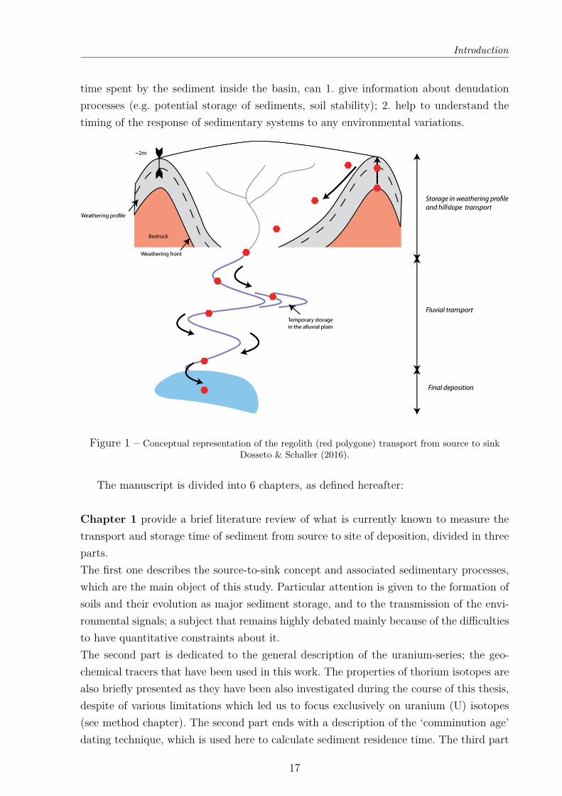
The focus of this PhD thesis is the timescale of sedimentary processes onthe continents, investigated here using geochemical tools that aim at deter-mining the sediment residence time in river catchments. The sediment residencetime is the time elapsed since the formation of the sediment as part of the regolith, andits transfer until its final deposit (Fig. 1). The sediment residence time - by indicating the

16

Introduction

time spent by the sediment inside the basin, can 1. give information about denudationprocesses (e.g. potential storage of sediments, soil stability); 2. help to understand thetiming of the response of sedimentary systems to any environmental variations.

Figure 1 – Conceptual representation of the regolith (red polygone) transport from source to sinkDosseto & Schaller (2016).

The manuscript is divided into 6 chapters, as defined hereafter:

Chapter 1 provide a brief literature review of what is currently known to measure thetransport and storage time of sediment from source to site of deposition, divided in threeparts.The first one describes the source-to-sink concept and associated sedimentary processes,which are the main object of this study. Particular attention is given to the formation ofsoils and their evolution as major sediment storage, and to the transmission of the envi-ronmental signals; a subject that remains highly debated mainly because of the difficultiesto have quantitative constraints about it.The second part is dedicated to the general description of the uranium-series; the geo-chemical tracers that have been used in this work. The properties of thorium isotopes arealso briefly presented as they have been also investigated during the course of this thesis,despite of various limitations which led us to focus exclusively on uranium (U) isotopes(see method chapter). The second part ends with a description of the ‘comminution age’dating technique, which is used here to calculate sediment residence time. The third part

17

Introduction

is a summary of the previous applications of U-series for investigating weathering pro-cesses or providing constraints on the timescale of sediment transport.

In chapter 2, the methodology used during this thesis is detailed, from the sieving of thebulk sediment to the analysis of uranium isotope ratios. A particular attention is givento the leaching protocols used at both Ifremer and UOW laboratory and their carefulevaluation for U isotope studies.

In chapter 3, we focused on the uranium fractionation inside sediments. For this purpose,the influence of external parameters, such as climate, lithology, weathering, and internalparameters, such as grain size, on the degree of fractionation of uranium isotopes in riversediments are discussed. This discussion is based on the measurement of (234U/238U) intwo grain-size fractions from various world river sediments. This large data set allowedus to draw general conclusions about the main factors influencing the distribution of(234U/238U) ratios in river sediments.

In chapter 4, we present the result of a spatial investigation of sediment residence timesinside a small mountainous river system (Var, S-E France) and compare the observed(234U/238U) intra-basin variability with the morphology of each sub-basins. On the ba-sis of these results, we further assess the potential of using sediment residence time toconstrain erosion processes. Conjointly, we also discuss about the validity of U-based sed-iment residence time by comparing them with regolith residence time, which we calculateusing denudation rates and soil thickness estimates.

In chapter 5 we finally investigate past variations in sediment residence time in theVar River basin, over the last 75 kyr, on the basis of the results presented in chapter 4.We discuss on the obtained (234U/238U) cyclicity and inferred changes in sediment resi-dence time, through comparison with various parameters including climate, denudationrate, sediment source, vegetation, to further understand which factors control long-termchanges of erosion.

The chapter 6 concludes with the work conducted during the course of this PhD thesis,and outlines a few perspectives of research for future work.

18

INTRODUCTION

Généralités

La morphologie des paysages à la surface de la Terre est très diversifiée. Elle résulted’interactions complexes entre le climat, l’altération et les processus tectoniques. Au coursdes dernières décennies, l’un des principaux défis scientifiques a été la compréhension deces interactions, afin de connaître l’impact qu’elles peuvent avoir sur le cycle global ducarbone et les concentrations atmosphériques de CO2. Il s’agit d’une préoccupation im-portante dans le contexte du réchauffement climatique actuel. Succinctement, le processusd’altération chimique des roches silicatées utilise l’acide carbonique, ce qui engendre laformation de minéraux argileux secondaires dans les sols et libère des ions carbonatedissous (HCO3). Ceux-ci agissent comme un piège pour le CO2 atmosphérique (Holland1978, Berner 1990). Certains scientifiques considèrent que l’altération est principalementcontrôlée par les processus tectoniques (Koppes & Montgomery 2009, Willenbring & Jerol-mack 2016) et que le refroidissement global sur le long terme depuis le Pléistocène estle résultat de la capture du CO2 atmosphérique (Walker et al. 1981, Molnar & England1990, Raymo & Ruddiman 1992). En opposition, d’autres estiment que le climat a uneinfluence plus prédominante (Peizhen et al. 2001, Herman & Champagnac 2016). C’est la"théorie de l’œuf et de la poule" qui reste débattue (Molnar & England 1990).

D’autres préoccupations concernent l’impact du climat, de l’altération et de la tectoniquesur la morphologie du paysage. Les interactions complexes entre les processus internes(e.g. tectonique, altération) et externes (e.g. climat, activité biologique) façonnent la mor-phologie des surfaces continentales, ce qui se traduit par une interface sol mince égalementappelée zone critique (van Breemen & Buurman 2002, Chorover et al. 2007, Brantley et al.2007, Amundson et al. 2007). Alors que la tectonique génère les reliefs à la surface de laTerre, à travers le soulèvement des montagnes par exemple, la combinaison des processusd’érosion et d’altération entraîne leur destruction progressive au fil du temps. Le climatpeut accentuer ou non ces processus. Sur une échelle de temps géologique, la présencede glaciers, connue pour être un agent d’érosion efficace lors de la déglaciation, dans leschaînes de montagnes augmente les taux de dénudation (Hallet et al. 1996, Hinderer 2001,Herman & Champagnac 2016). À plus petite échelle de temps, les précipitations favorisentla dénudation du relief, atténuée par le développement de la végétation (comme la forêttempérée) qui stabilise les sols (Löbmann et al. 2020). Tous ces processus affectent la for-mation de la couverture du sol à la surface des continents, et son exportation ultérieure

19

Introduction

pour former le système sédimentaire.

L’intercorrélation globale entre l’altération, le climat et la tectonique est aujourd’hui ac-ceptée et relativement bien comprise, mais certaines questions restent encore en suspens.L’une d’elles est la nature de la variabilité des processus d’érosion et d’altération surl’échelle de temps glaciaire-interglaciaire (Foster & Vance 2006, Vance et al. 2009, Lup-ker et al. 2012, von Blanckenburg et al. 2015, Cogez et al. 2015). Une autre est l’échellede temps du cycle sédimentaire : de la production du sol à son érosion et son transportjusqu’à son dépôt final. Ce dernier point est particulièrement important car la durée de cesprocessus influence fortement l’émergence d’un signal sédimentaire, c’est-à-dire la réponsedu paysage aux perturbations des variables environnementales, telles que le climat et latectonique, et sa transmission jusqu’à son dépôt et sa préservation dans le dépôt (Romanset al. 2016). Si les processus érosifs peuvent être efficacement mesurés à l’heure actuelle,il reste encore difficile de déterminer le temps écoulé entre la formation du sédiment etson stockage final dans la zone de dépôt du bassin sédimentaire.

Cette thèse porte sur les temps des processus sédimentaires sur les continents, étudiésici à l’aide d’outils géochimiques dans le but d’estimer le temps de résidence sédimentairedans différents bassins versants. Celui-ci peut donner des informations sur l’efficacité desprocessus de dénudation (par exemple la possibilité de stockage temporaire des sédiments,la stabilité du sol, etc.) et aider à déterminer le temps de réaction du système sédimentaireà s’adapter aux variations environnementales.

Objectifs de la thèseL’évolution de la surface terrestre et ainsi de la morphologie du paysage est com-

plexe. Afin de mieux l’appréhender, il est important de saisir clairement quels paramètres(par exemple, le climat, l’altération atmosphérique, la tectonique) sont impliqués dansle modelage des surfaces terrestres et comment ces différents facteurs peuvent interagir.Cette question est importante car l’humanité dépend directement de cette zone critique,avec l’utilisation des surfaces terrestres, notamment pour l’agriculture. Cette zone, quireprésente l’interface entre l’atmosphère et la croûte continentale supérieure, comprendle substratum rocheux, le sol au-dessus de celui-ci et la végétation. L’épaisseur du solest une variable fondamentale dans de nombreuses disciplines des sciences de la Terre enraison de son rôle critique dans de nombreux processus hydrologiques (par exemple, leruissellement, l’adsorption de l’eau) et écologiques. Elle est très variable dans l’espace etdifficile à mesurer dans la pratique, même pour un petit bassin hydrographique Dietrichet al. (1995). À l’intérieur du profil du sol, les sédiments sont formés et peuvent être

20

Introduction

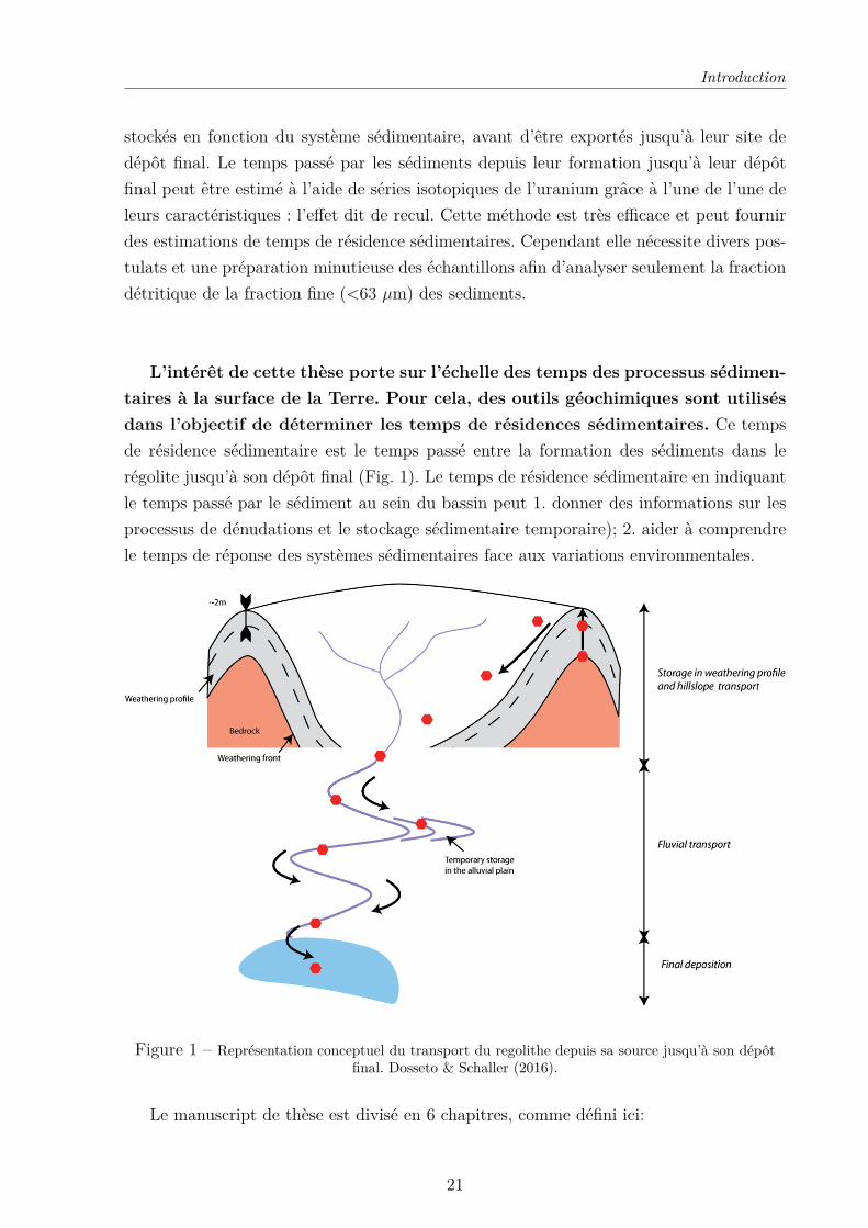
stockés en fonction du système sédimentaire, avant d’être exportés jusqu’à leur site dedépôt final. Le temps passé par les sédiments depuis leur formation jusqu’à leur dépôtfinal peut être estimé à l’aide de séries isotopiques de l’uranium grâce à l’une de l’une deleurs caractéristiques : l’effet dit de recul. Cette méthode est très efficace et peut fournirdes estimations de temps de résidence sédimentaires. Cependant elle nécessite divers pos-tulats et une préparation minutieuse des échantillons afin d’analyser seulement la fractiondétritique de la fraction fine (<63 µm) des sediments.

L’intérêt de cette thèse porte sur l’échelle des temps des processus sédimen-taires à la surface de la Terre. Pour cela, des outils géochimiques sont utilisésdans l’objectif de déterminer les temps de résidences sédimentaires. Ce tempsde résidence sédimentaire est le temps passé entre la formation des sédiments dans lerégolite jusqu’à son dépôt final (Fig. 1). Le temps de résidence sédimentaire en indiquantle temps passé par le sédiment au sein du bassin peut 1. donner des informations sur lesprocessus de dénudations et le stockage sédimentaire temporaire); 2. aider à comprendrele temps de réponse des systèmes sédimentaires face aux variations environmentales.

Figure 1 – Représentation conceptuel du transport du regolithe depuis sa source jusqu’à son dépôtfinal. Dosseto & Schaller (2016).

Le manuscript de thèse est divisé en 6 chapitres, comme défini ici:

21

Introduction

Le chapitre 1 est consacré à une brève revue de la littérature concernant les connais-sances actuelles pour mesurer les temps de transport des sédiment et de leurs stockagestemporaires entre leur source et leur zone de dépôt finale. Le chapitre est divisé en troisparties.La première décrit le concept de source-au-puit et les processus sédimentaires qui s’ydéroulent. Ceux-ci sont l’objet principal de cette étude. Une attention particulière estaccordée à la formation des sols et à leur évolution en tant que stockage majeur desédiments, ainsi qu’à la transmission des signaux environnementaux. Ce sujet reste trèsdébattu, principalement en raison des difficultés à avoir des contraintes quantitatives.La deuxième partie est consacrée à la description générale des isotopes des séries d’uranium,traceurs géochimiques utilisés dans ce travail. Les propriétés des isotopes du thorium sontégalement présentées, car elles ont aussi été étudiées au cours de cette thèse, malgré di-verses limitations qui nous ont amenés à nous concentrer exclusivement sur les isotopesU (voir le chapitre sur la méthode). Cette partie se termine par une explication sur latechnique de datation de « l’âge de comminution », utilisée dans le calcul du temps derésidence sédimentaire.La troisième partie est un résumé des applications antérieures de la série U soit pourl’étude des processus d’altération soit pour fournir des contraintes sur l’échelle de tempsdu transport des sédiments.

Le chapitre 2 détaille la méthodologie utilisée au cours de cette thèse. Du tamisagedes sédiments en vrac aux analyses des isotopes de l’uranium, l’ensemble du processusest présenté. Une attention particulière est portée sur les protocoles de lessivage utilisésà l’Ifremer et au laboratoire WIGL et sur les tests réalisés pour les valider, en raison del’importance d’étudier seulement la fraction détritique des sédiments.

Dans le chapitre 3 est examinée l’influence des paramètres externes, tels que le climat,la lithologie, l’altération et les paramètres internes (par exemple la taille des grains) sur lefractionnement des isotopes d’uranium dans les sédiments fluviaux. Cette étude est baséesur la mesure de (234U/238U) dans deux fractions granulométriques de sédiments fluviauxdu monde (par exemple Amazone, Nil, Fraser, Lule). Ce vaste ensemble de données nousa permis d’obtenir une bonne représentativité de la variabilité de (234U/238U) dans lessystèmes sédimentaires à la surface de la Terre.

Dans le chapitre 4, nous présentons les résultats portant sur les variations spatialeset actuelles du temps de résidence des sédiments à l’intérieur d’un petit système sédimen-taire (Var, S-E France) et nous comparons la variation avec la morphologie du bassin.Sur la base de ces résultats, nous évaluons la possibilité d’utiliser le temps de résidencedes sédiments pour déduire les processus d’érosion. Conjointement, nous discutons de la

22

Introduction

précision du temps de résidence des sédiments en les comparant avec le temps de résidenceau sein du régolite, que nous estimons avec le taux de dénudation et une prédiction del’épaisseur du sol provenant d’une base de données.

Sur la base des résultats présentés au chapitre 4, nous avons étudié la variation du tempsde résidence sédimentaire au cours des 75 derniers ka. Dans le chapitre 5, nous abordonsla cyclicité observée du temps de résidence sédimentaire et nous l’étudions en fonctionparallèle à divers paramètres tels que les variations climatiques, les taux de dénudation,un traceur de source, etc. pour comprendre ce qui contrôle les processus d’érosion et, cequi contraint les périodes de stockage des sédiments.

Le chapitre 6 conclut sur les travaux réalisés dans le cadre de cette thèse et définitdes perspectives de recherche intéressantes qui en découlent.

23

Chapter 1

LITERATURE REVIEW

Contents1.1 From source to sink: the sediment’s life . . . . . . . . . . . . . . . 26

1.1.1 Concept . . . . . . . . . . . . . . . . . . . . . . . . . . . . . . . . . . 261.1.2 Environmental signal propagation in sedimentary systems . . . . . . 311.1.3 Soil: the origin of the sediment . . . . . . . . . . . . . . . . . . . . . 41

1.2 Uranium isotopes . . . . . . . . . . . . . . . . . . . . . . . . . . . . 451.2.1 Background . . . . . . . . . . . . . . . . . . . . . . . . . . . . . . . . 451.2.2 Radioactive disequilibrium . . . . . . . . . . . . . . . . . . . . . . . . 451.2.3 Secular equilibrium . . . . . . . . . . . . . . . . . . . . . . . . . . . . 471.2.4 Uranium abundances in rock forming minerals and the fractionation

of (234U/238U) in sedimentary systems . . . . . . . . . . . . . . . . . 481.2.5 The concept of comminution age . . . . . . . . . . . . . . . . . . . . 53

1.3 Uranium at Earth’s surface . . . . . . . . . . . . . . . . . . . . . . 591.3.1 From bedrock to soil: weathering processes . . . . . . . . . . . . . . 591.3.2 Uranium isotopes to infer timescale of sedimentary processes and its

control . . . . . . . . . . . . . . . . . . . . . . . . . . . . . . . . . . . 611.3.3 Uncertainties based on the comminution age method . . . . . . . . . 62

25

Literature Review

1.1 From source to sink: the sediment’s lifeThe framework of this thesis is to better understand the timescale of the processes

occurring inside a sedimentary basin through the study of sediments. In this regard, it isimportant first to describe the conceptual nature of the source-to-sink principle, and tointroduce the various processes that can affect the sediment’s life.

1.1.1 Concept

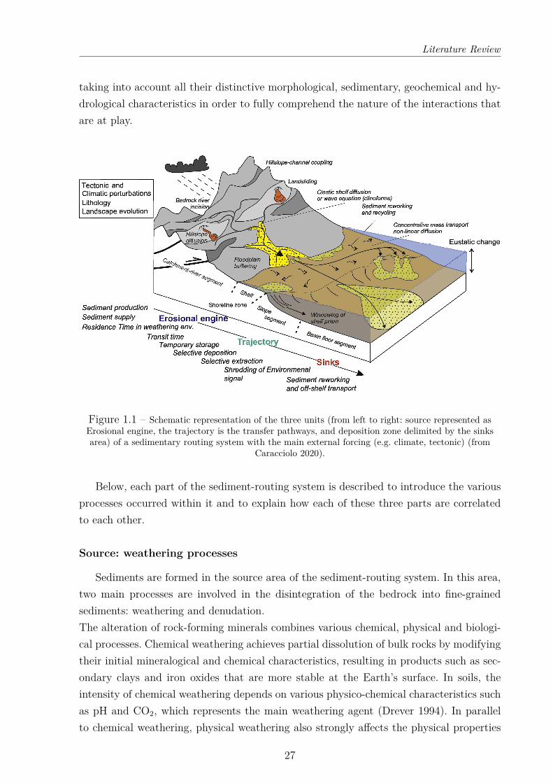
A sedimentary system, also called sediment-routing system (Allen 1997) is defined as a“integrated dynamical system connecting erosion in mountain catchments to downstreamdeposition” (see Romans et al. 2016 for a thorough review). It is the combination of varioustopographic units (and bathymetric units if the system is connected to the ocean) wheresediments are formed, transported, and deposited. In order to simplify natural sediment-routing systems, Schumm (1977) idealized the system by identifying three distinct zones(Fig. 1.1) at the lithosphere-atmosphere interface (Castelltort & Van Den Driessche 2003).These 3 zones (i.e. the source area, the transfer pathways, and the depositional area) areconnected to each other and are characterized by a distinctive behavior of the sedimentfluxes (Schumm 1977, Allen 1997, Castelltort & Van Den Driessche 2003):

— The source area: the elevated part of the basin is the location of erosional pro-cesses principally dominated by the denudation of hillslopes and to a lesser extentby fluvial incision (Hovius 1998, Castelltort & Van Den Driessche 2003).

— The transfer pathways: a sector predominantly dominated by sediment trans-port processes. This zone can be absent depending on the sediment-routing systembeing considered, in particular in those watersheds where the source region is di-rectly connected to the depositional basin, such as in small mountain basins forexample. Alternatively, this region can extend over several thousand of kilometersin the case of the largest river systems (Castelltort & Van Den Driessche 2003).

— Deposition zone: the ultimate location of sediment deposition, which can becontinental and/or marine and can include deep turbiditic system (e.g. Amazon,Congo, Indus).

Several processes occur at different temporal and spatial scales in sediment-routingsystems. For example, the variability of climate can be expressed over relatively short,seasonal, timescales to much longer geological periods (e.g. Swift et al. 2002, Holmgrenet al. 2003, Mayewski et al. 2004, Covault & Graham 2010). Additionally, tectonics canalso influence sediment-routing systems over drastically different timescales: from daily(earthquakes; e.g. Lin et al. 2008, West et al. 2014, Marc et al. 2015) to million-year peri-ods (mountain uplifts; e.g. Allen 2008a, Sømme et al. 2009, Whitchurch et al. 2011, Allen& Heller 2012). For this reason, the study of each of the three sub-systems is necessary,

26

Literature Review

taking into account all their distinctive morphological, sedimentary, geochemical and hy-drological characteristics in order to fully comprehend the nature of the interactions thatare at play.

Figure 1.1 – Schematic representation of the three units (from left to right: source represented asErosional engine, the trajectory is the transfer pathways, and deposition zone delimited by the sinksarea) of a sedimentary routing system with the main external forcing (e.g. climate, tectonic) (from

Caracciolo 2020).

Below, each part of the sediment-routing system is described to introduce the variousprocesses occurred within it and to explain how each of these three parts are correlatedto each other.

Source: weathering processes

Sediments are formed in the source area of the sediment-routing system. In this area,two main processes are involved in the disintegration of the bedrock into fine-grainedsediments: weathering and denudation.The alteration of rock-forming minerals combines various chemical, physical and biologi-cal processes. Chemical weathering achieves partial dissolution of bulk rocks by modifyingtheir initial mineralogical and chemical characteristics, resulting in products such as sec-ondary clays and iron oxides that are more stable at the Earth’s surface. In soils, theintensity of chemical weathering depends on various physico-chemical characteristics suchas pH and CO2, which represents the main weathering agent (Drever 1994). In parallelto chemical weathering, physical weathering also strongly affects the physical properties

27

Literature Review

of the initial rocks (e.g. shape of the grains, size, etc.) through the effect of freeze thawaction or grinding for example. The combination of both chemical and physical weather-ing operates to transform the pristine bedrock into saprolite (i.e. the immobile part of theweathering profile; Fig. 1.2). The evolution of bedrock into soil by weathering is enhancedby biological action caused by the vegetation (e.g. which promotes efficient rock fracturingwith roots) or by any living organisms that interact with the soil profile.

Regolith

Rock

Saprolite

Soil

Figure 1.2 – Weathering profile identifying soil (mobile) and saprolite (immobile) fractions whichrepresent the regolith, i.e. the unconsolidated layer above the bedrock (Adapted from Juilleret et al.

2014.

Chemical and physical weathering are intertwined with erosional processes which alto-gether result in the formation and regulation of soil (Stallard & Edmond 1983, Gaillardetet al. 1999, Millot et al. 2002, Riebe et al. 2001, Riotte et al. 2003, Ferrier & Kirchner 2008,West 2012). On one hand, chemical weathering, by modifying the initial mineralogy ofpristine rocks, also change its strength, increasing its vulnerability to further erosion. Onthe other hand,the removal of regolith by erosion results in the exposition of fresh rockand mineral surfaces available to chemical and physical weathering. This interrelation-ship regulates the development of soils and ultimately shapes the land surfaces. However,the balance between each of these two processes, while being of upmost importance forland use management and landscape evolution (Anderson & Humphrey 1989, Riebe et al.2001), remains difficult to quantify and can vary spatially depending on the system.

28

Literature Review

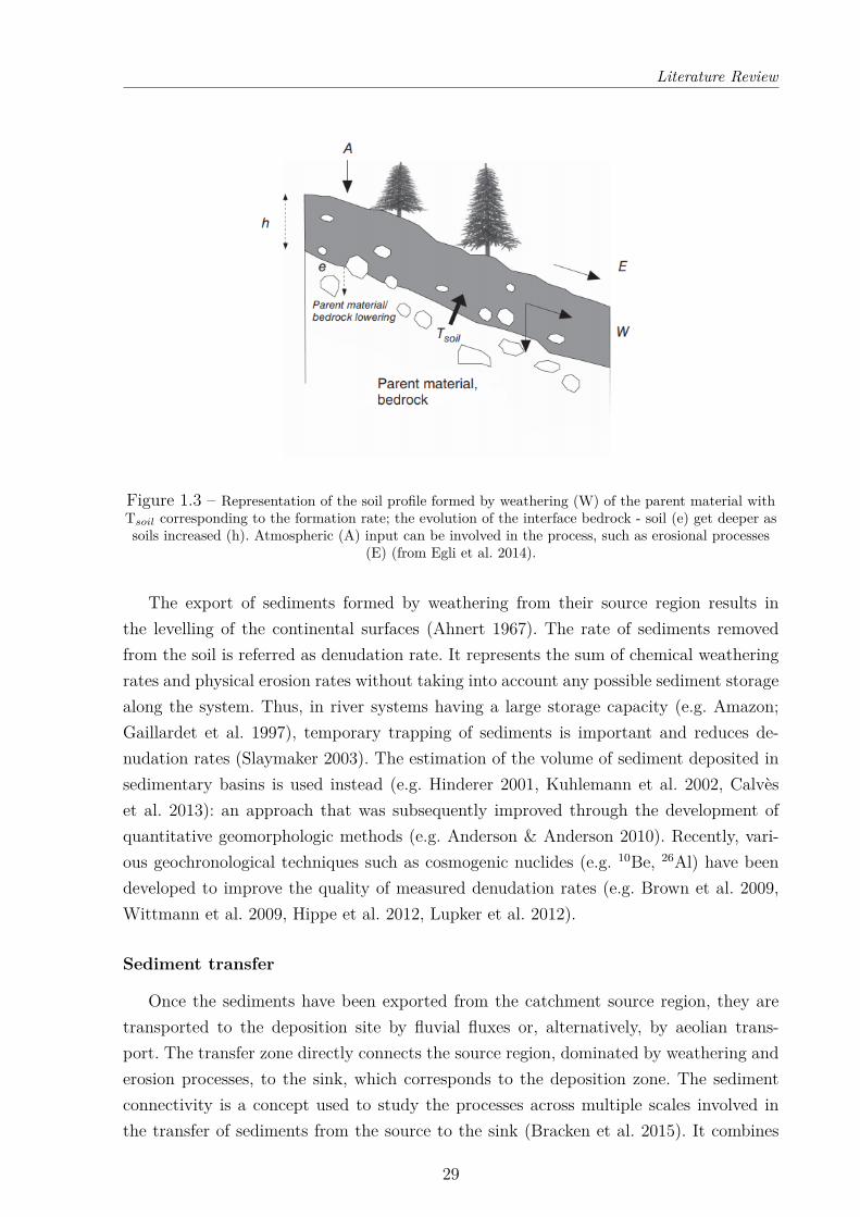
Figure 1.3 – Representation of the soil profile formed by weathering (W) of the parent material withTsoil corresponding to the formation rate; the evolution of the interface bedrock - soil (e) get deeper assoils increased (h). Atmospheric (A) input can be involved in the process, such as erosional processes

(E) (from Egli et al. 2014).

The export of sediments formed by weathering from their source region results inthe levelling of the continental surfaces (Ahnert 1967). The rate of sediments removedfrom the soil is referred as denudation rate. It represents the sum of chemical weatheringrates and physical erosion rates without taking into account any possible sediment storagealong the system. Thus, in river systems having a large storage capacity (e.g. Amazon;Gaillardet et al. 1997), temporary trapping of sediments is important and reduces de-nudation rates (Slaymaker 2003). The estimation of the volume of sediment deposited insedimentary basins is used instead (e.g. Hinderer 2001, Kuhlemann et al. 2002, Calvèset al. 2013): an approach that was subsequently improved through the development ofquantitative geomorphologic methods (e.g. Anderson & Anderson 2010). Recently, vari-ous geochronological techniques such as cosmogenic nuclides (e.g. 10Be, 26Al) have beendeveloped to improve the quality of measured denudation rates (e.g. Brown et al. 2009,Wittmann et al. 2009, Hippe et al. 2012, Lupker et al. 2012).

Sediment transfer

Once the sediments have been exported from the catchment source region, they aretransported to the deposition site by fluvial fluxes or, alternatively, by aeolian trans-port. The transfer zone directly connects the source region, dominated by weathering anderosion processes, to the sink, which corresponds to the deposition zone. The sedimentconnectivity is a concept used to study the processes across multiple scales involved inthe transfer of sediments from the source to the sink (Bracken et al. 2015). It combines

29

Literature Review

the influence of the structure of the catchment (i.e. morphology) and the action of thesediment (i.e. flow, transport of materials), which conjointly impact the long-term behav-ior of the sediment flux (Preston & Schmidt 2003, Turnbull et al. 2008, Bracken et al.2015). Therefore, the sediment connectivity concept includes all the aspects (e.g. spatialand temporal scale, frequency and magnitude of the processes; Bracken et al. 2015) of anysource-to-sink system (Preston & Schmidt 2003, Sandercock & Hooke 2011). In systemswith an efficient connectivity, which leads to rapid landscape response to any environ-mental change, the basin is referred as reactive routing system (Allen 2008b, Covault &Graham 2010, Covault et al. 2013). Conversely, when the connectivity is less efficient,because of sediment storage for example, the system is referred to as a buffered routingsystem as a significant lag is created between the disturbance and the system’s response(Allen 2008b).

For any given sediment-routing system, reactive or buffered, the principle of mass conser-vation applies. from a basic perspective, the amount of sediment input is balanced by thesum of storage and output. Slaymaker (2003) expressed this using the following equation:

Is = ∆Ss +Os (1.1)

where I represents the input, S the storage, O the output and the subscripts letters referto the type of transported matter, i.e. sediments.The principle of mass conservation implies that the amount of sediment being producedin the source region should be equal to the amount of sediment that is deposited alongor at the end of the sediment-routing system. Exceptions are the case of marine sedimentdeposits, which can be subject to intense winnowing effects (e.g. Mozambican channel;Miramontes et al. 2019, Fierens et al. 2019). In these systems, the amount of sedimentsproduce is higher than the amount of sediment reaching the final marine deposit. Whenthe sedimentary contribution from the source is higher than the capacity of transportof the fluvial system, a temporary storage operates in the river channel (Kirkby 1971).Conversely, when the sedimentary supply is lower than the transport capacity, the riverchannel is eroded (Whipple & Tucker 1999, Blum & Törnqvist 2000). Hence, this processof sediments regulation can result in an increase or a decrease of the time spent by thesediment to reach the ultimate sink, causing a dephasing between the source and the sink.

Previous studies have aimed at quantifying sedimentary fluxes (which represent the quan-tity of sediment exported from the transfer zone by units of time; Slaymaker 2003) toinvestigate their variability in river systems. The sedimentary flux is usually expressedin tons per years (t/y) or cubic meters per years (m3/y). To compare sediment-routingsystems amongst each other, the specific sediment yield is generally used, which normal-

30

Literature Review

izes measured sedimentary fluxes to the catchment area (e.g. Milliman & Syvitski 1992,Syvitski et al. 2005, de Vente et al. 2007). Milliman & Syvitski (1992) pointed out thatthe river systems displaying extensive sedimentary transfer zones typically exhibit lowerspecific sedimentary fluxes (e.g. Amur River, Russia: 28 t/km2/years) than smaller rivers(e.g. Lamone River, Italy: 2400 t/km2/years). In other words, small mountainous riversare expected to be reactive by adapting themselves rapidly to any environmental change,which affect the sediment flux and the quantity of sediments reaching the deposition zone(Covault & Graham 2010, Bonneau et al. 2014).

Deposition and storage

The depositional zone is where the sediment is stored. It can be either continental ormarine (Schumm 1977). All sediments formed in the catchment source area do not reachthe ocean, especially in the case of endorheic basins. During the transport, sedimentgrains can transit via lakes or other inland water bodies, where deposition can occur.Along the river paths, sediments can also be trapped in alluvial fans, channel depositsetc., or, for the sediments that ultimately reach the ocean, within estuaries or subaerialdeltas. Once the sediments have reached the depositional zone, some disturbance can occur(e.g. displacement or destruction; Milliman et al. 2007), which affect the conservation ofsediments stored. These processes are detailed thereafter, as part of the environmentalsignal preservation.

1.1.2 Environmental signal propagation in sedimentary systems

Any environmental disturbance (e.g. climate, morphology, anthropogenic presence) re-sults in a modification of the sediment routing system. This adaptation induces a changeinto the sediment cycle (sediments production, transport or deposition) and the vari-ation of the sedimentary flux is then referred to as an environmental signal (Romanset al. 2016). The signal can then propagate within the sediment routing system until itreaches the depositional zone (Allen 2008a). However, the signal can also be trapped ordestroyed depending on the characteristic of the signal and the catchment(Castelltort &Van Den Driessche 2003, Jerolmack & Paola 2010). This section aims to present the pa-rameters that can create signals when they are subject to a change, but also the elementsto take into consideration for a good signal propagation and preservation.

31

Literature Review

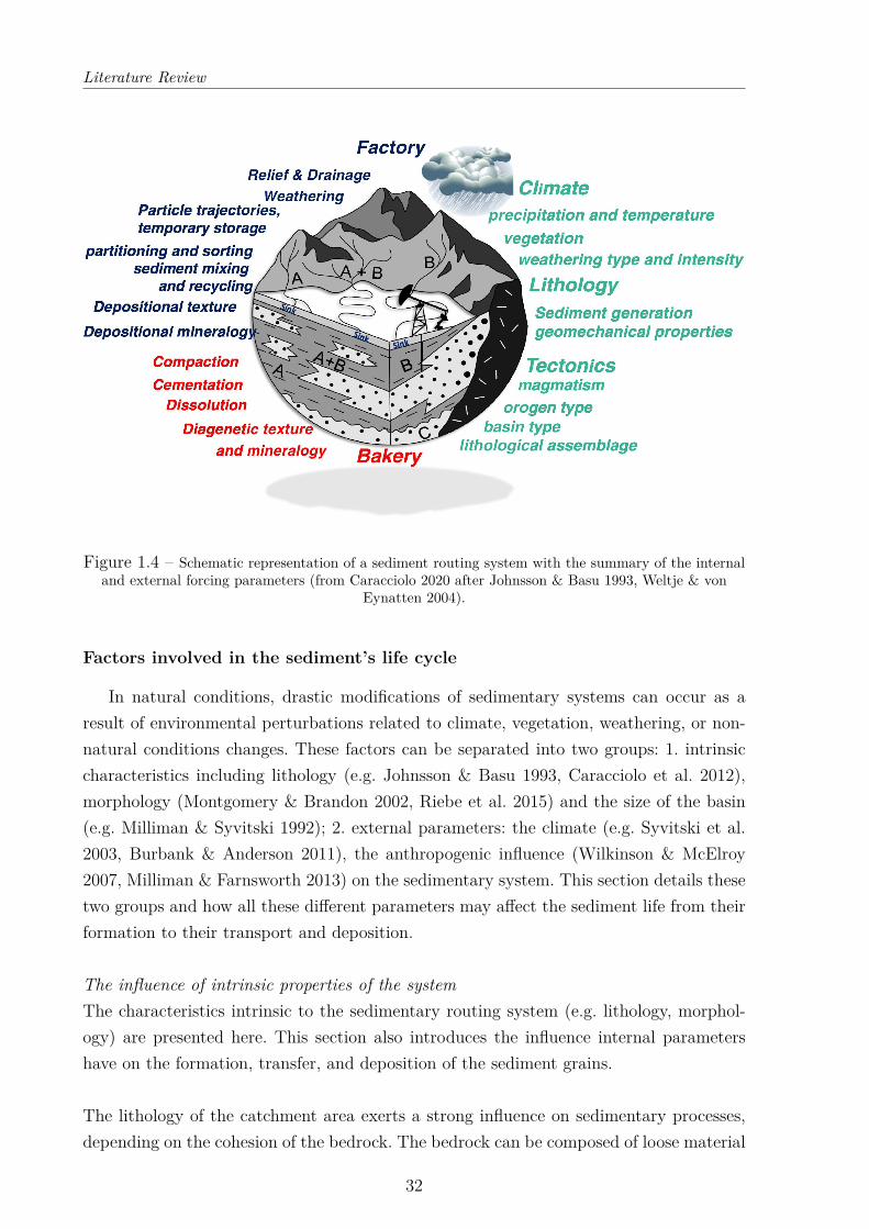
Figure 1.4 – Schematic representation of a sediment routing system with the summary of the internaland external forcing parameters (from Caracciolo 2020 after Johnsson & Basu 1993, Weltje & von

Eynatten 2004).

Factors involved in the sediment’s life cycle

In natural conditions, drastic modifications of sedimentary systems can occur as aresult of environmental perturbations related to climate, vegetation, weathering, or non-natural conditions changes. These factors can be separated into two groups: 1. intrinsiccharacteristics including lithology (e.g. Johnsson & Basu 1993, Caracciolo et al. 2012),morphology (Montgomery & Brandon 2002, Riebe et al. 2015) and the size of the basin(e.g. Milliman & Syvitski 1992); 2. external parameters: the climate (e.g. Syvitski et al.2003, Burbank & Anderson 2011), the anthropogenic influence (Wilkinson & McElroy2007, Milliman & Farnsworth 2013) on the sedimentary system. This section details thesetwo groups and how all these different parameters may affect the sediment life from theirformation to their transport and deposition.

The influence of intrinsic properties of the systemThe characteristics intrinsic to the sedimentary routing system (e.g. lithology, morphol-ogy) are presented here. This section also introduces the influence internal parametershave on the formation, transfer, and deposition of the sediment grains.

The lithology of the catchment area exerts a strong influence on sedimentary processes,depending on the cohesion of the bedrock. The bedrock can be composed of loose material

32

Literature Review

such as loess or unconsolidated clastic sediments, which are more prone to generate highamount of sediments.

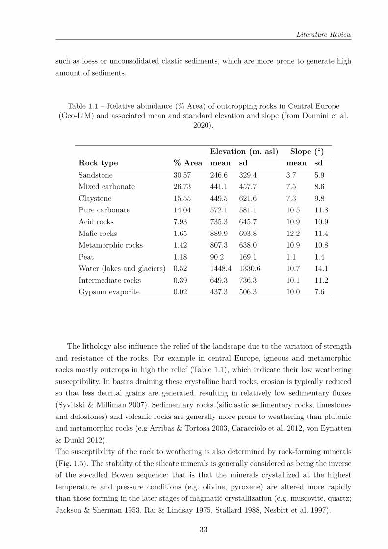
Table 1.1 – Relative abundance (% Area) of outcropping rocks in Central Europe(Geo-LiM) and associated mean and standard elevation and slope (from Donnini et al.

2020).

Elevation (m. asl) Slope (°)Rock type % Area mean sd mean sdSandstone 30.57 246.6 329.4 3.7 5.9Mixed carbonate 26.73 441.1 457.7 7.5 8.6Claystone 15.55 449.5 621.6 7.3 9.8Pure carbonate 14.04 572.1 581.1 10.5 11.8Acid rocks 7.93 735.3 645.7 10.9 10.9Mafic rocks 1.65 889.9 693.8 12.2 11.4Metamorphic rocks 1.42 807.3 638.0 10.9 10.8Peat 1.18 90.2 169.1 1.1 1.4Water (lakes and glaciers) 0.52 1448.4 1330.6 10.7 14.1Intermediate rocks 0.39 649.3 736.3 10.1 11.2Gypsum evaporite 0.02 437.3 506.3 10.0 7.6

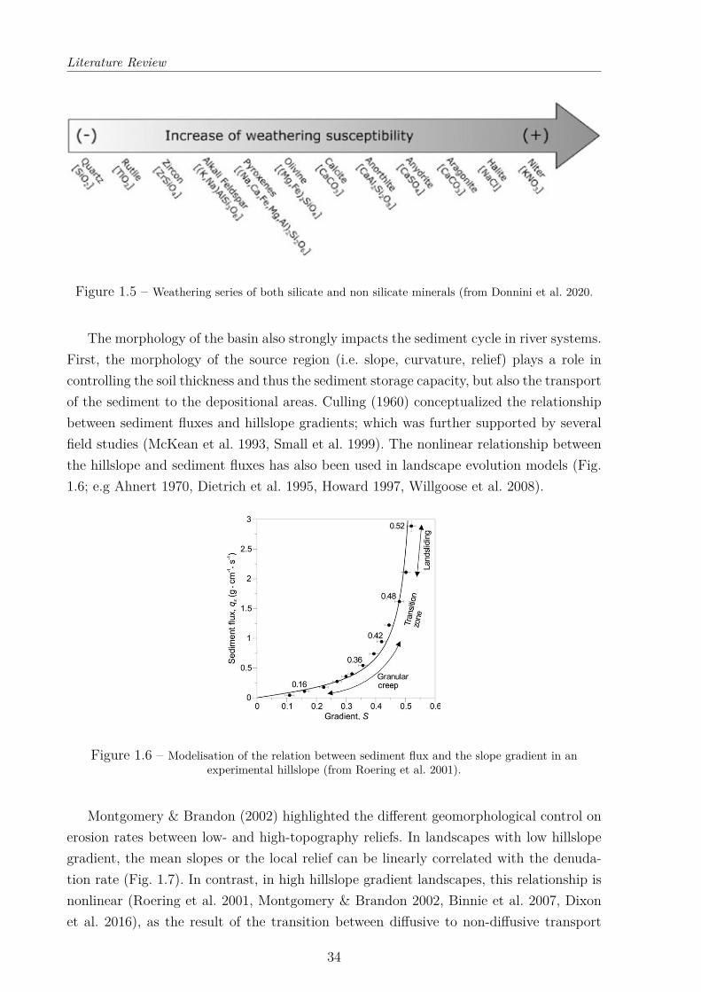
The lithology also influence the relief of the landscape due to the variation of strengthand resistance of the rocks. For example in central Europe, igneous and metamorphicrocks mostly outcrops in high the relief (Table 1.1), which indicate their low weatheringsusceptibility. In basins draining these crystalline hard rocks, erosion is typically reducedso that less detrital grains are generated, resulting in relatively low sedimentary fluxes(Syvitski & Milliman 2007). Sedimentary rocks (siliclastic sedimentary rocks, limestonesand dolostones) and volcanic rocks are generally more prone to weathering than plutonicand metamorphic rocks (e.g Arribas & Tortosa 2003, Caracciolo et al. 2012, von Eynatten& Dunkl 2012).The susceptibility of the rock to weathering is also determined by rock-forming minerals(Fig. 1.5). The stability of the silicate minerals is generally considered as being the inverseof the so-called Bowen sequence: that is that the minerals crystallized at the highesttemperature and pressure conditions (e.g. olivine, pyroxene) are altered more rapidlythan those forming in the later stages of magmatic crystallization (e.g. muscovite, quartz;Jackson & Sherman 1953, Rai & Lindsay 1975, Stallard 1988, Nesbitt et al. 1997).

33

Literature Review

Figure 1.5 – Weathering series of both silicate and non silicate minerals (from Donnini et al. 2020.

The morphology of the basin also strongly impacts the sediment cycle in river systems.First, the morphology of the source region (i.e. slope, curvature, relief) plays a role incontrolling the soil thickness and thus the sediment storage capacity, but also the transportof the sediment to the depositional areas. Culling (1960) conceptualized the relationshipbetween sediment fluxes and hillslope gradients; which was further supported by severalfield studies (McKean et al. 1993, Small et al. 1999). The nonlinear relationship betweenthe hillslope and sediment fluxes has also been used in landscape evolution models (Fig.1.6; e.g Ahnert 1970, Dietrich et al. 1995, Howard 1997, Willgoose et al. 2008).

Figure 1.6 – Modelisation of the relation between sediment flux and the slope gradient in anexperimental hillslope (from Roering et al. 2001).

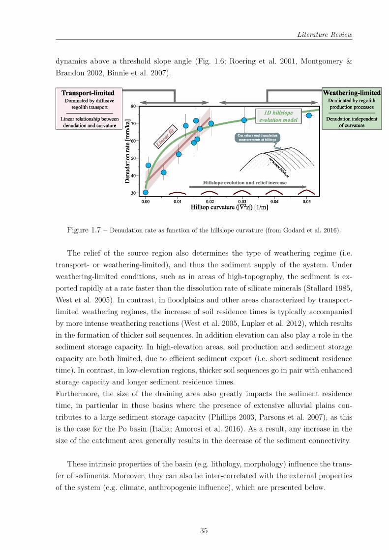
Montgomery & Brandon (2002) highlighted the different geomorphological control onerosion rates between low- and high-topography reliefs. In landscapes with low hillslopegradient, the mean slopes or the local relief can be linearly correlated with the denuda-tion rate (Fig. 1.7). In contrast, in high hillslope gradient landscapes, this relationship isnonlinear (Roering et al. 2001, Montgomery & Brandon 2002, Binnie et al. 2007, Dixonet al. 2016), as the result of the transition between diffusive to non-diffusive transport

34

Literature Review

dynamics above a threshold slope angle (Fig. 1.6; Roering et al. 2001, Montgomery &Brandon 2002, Binnie et al. 2007).

Figure 1.7 – Denudation rate as function of the hillslope curvature (from Godard et al. 2016).

The relief of the source region also determines the type of weathering regime (i.e.transport- or weathering-limited), and thus the sediment supply of the system. Underweathering-limited conditions, such as in areas of high-topography, the sediment is ex-ported rapidly at a rate faster than the dissolution rate of silicate minerals (Stallard 1985,West et al. 2005). In contrast, in floodplains and other areas characterized by transport-limited weathering regimes, the increase of soil residence times is typically accompaniedby more intense weathering reactions (West et al. 2005, Lupker et al. 2012), which resultsin the formation of thicker soil sequences. In addition elevation can also play a role in thesediment storage capacity. In high-elevation areas, soil production and sediment storagecapacity are both limited, due to efficient sediment export (i.e. short sediment residencetime). In contrast, in low-elevation regions, thicker soil sequences go in pair with enhancedstorage capacity and longer sediment residence times.Furthermore, the size of the draining area also greatly impacts the sediment residencetime, in particular in those basins where the presence of extensive alluvial plains con-tributes to a large sediment storage capacity (Phillips 2003, Parsons et al. 2007), as thisis the case for the Po basin (Italia; Amorosi et al. 2016). As a result, any increase in thesize of the catchment area generally results in the decrease of the sediment connectivity.

These intrinsic properties of the basin (e.g. lithology, morphology) influence the trans-fer of sediments. Moreover, they can also be inter-correlated with the external propertiesof the system (e.g. climate, anthropogenic influence), which are presented below.

35

Literature Review

The influence of the external parameters

Here are presented the external conditions (e.g. climate, anthropogenic influence) to thesediment routing system that can impact the cycle of the sediments. The section alsodetails the ways in which these external factors influence the formation and transfer ofthe sediment.

The influence of climate on weathering, erosion and sediment transfer in basins is mostlydependent on two variables: temperature and precipitation. Temperature impacts the ki-netics and intensity of chemical weathering reactions, but also the vegetation patternsand on the development of glacier. Rainfall, on another side, can induce alluvial aggra-dation, incisions and controls the run-off (Romans et al. 2016, Covault et al. 2011). Inaddition, long-term climate change over glacial-interglacial timescales also results in sea-level variations, hence indirectly influencing sediment transport processes by modifyingthe morphology of the lower river course (e.g. river incision when the sea level lowered;Blum & Törnqvist 2000).

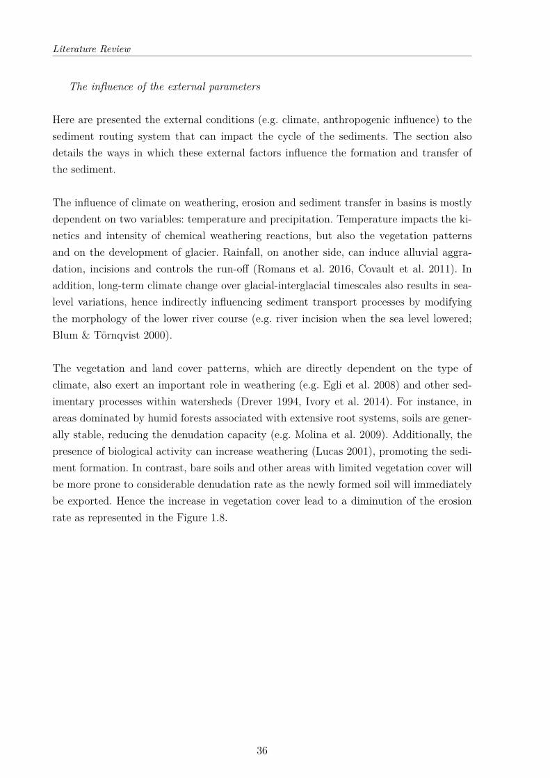
The vegetation and land cover patterns, which are directly dependent on the type ofclimate, also exert an important role in weathering (e.g. Egli et al. 2008) and other sed-imentary processes within watersheds (Drever 1994, Ivory et al. 2014). For instance, inareas dominated by humid forests associated with extensive root systems, soils are gener-ally stable, reducing the denudation capacity (e.g. Molina et al. 2009). Additionally, thepresence of biological activity can increase weathering (Lucas 2001), promoting the sedi-ment formation. In contrast, bare soils and other areas with limited vegetation cover willbe more prone to considerable denudation rate as the newly formed soil will immediatelybe exported. Hence the increase in vegetation cover lead to a diminution of the erosionrate as represented in the Figure 1.8.

36

Literature Review

Figure 1.8 – Evolution of the erosion rate (Etot depending on the vegetation cover in two differentsites (from Vanacker et al. 2014).

Finally, anthropogenic activities also play a major role in the sedimentary cycle oncontinents. On one hand, they have a direct impact on the soil cover with agriculture anddeforestation typically resulting in an increase of denudation rates and reduced sedimentstorage within the alluvial plain (Syvitski et al. 2003, Bayon et al. 2012, Costa et al.2018). Proxy investigations of sedimentary records suggested links between erosion andthe presence of agriculture back to 3000 yr ago in Central Africa (Bayon et al. 2012) and3 500 yr ago in Greece (Rothacker et al. 2018). On the other hand, the urbanisation ofriver systems, in particular the presence of dams can severely reduce sedimentary fluxesand enhance sediment storage, thereby increasing sediment residence time within thewatershed (Yang et al. 2018). Furthermore, human interventions in deltas steadily increase(Syvitski & Saito 2007, Syvitski & Kettner 2011) through trajectory controls (e.g. Po,Colorado), stabilization (Rhone, Fraser) or to attenuate the variations in sediment supplydue to seasonal flooding (Mekong, Indus). As a consequence of the combined effects ofhuman activities on river systems, in Oceania and Indonesia, where less dams have beenconstructed over the last decades, there has been an increase of 80 and 100 % of thesediment flux during the Anthropocene period (i.e. human dominated geological epoch;Lewis & Maslin 2015) respectively. Conversely, in Europe, Africa, and North America,sediment fluxes have decreased since the beginning of anthropization and the advent ofagriculture during the course of the Holocene (Syvitski et al. 2005).

37

Literature Review

Signal propagation

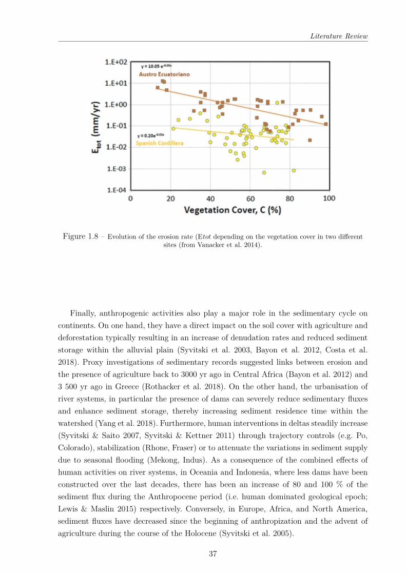
When a change in environmental conditions occurs, causing a sediment disturbance, aparticular ‘sedimentary signal’ induced will be transferred and subsequently archived inthe depositional record (Fig. 1.9). The generation of sedimentary signal depends of thecapacity of the sedimentary routing system to produce sediments (Caracciolo 2020) thatcan record the signal. Some studies have shown that the transmission of ‘sedimentary sig-nals’ can be buffered or delayed along the river system depending on various parameterssuch as the size of the basin (Bull 1991, Dearing & Jones 2003, Lane et al. 2011). Suchriver systems are considered being out of equilibrium (i.e. the sediment input is not equalto the sediment output at the river mouth; Ahnert 1994, Phillips 2003) or in a transientstate (i.e. the relaxation time is larger than the recurrence time of events ; Brunsden &Thornes 1979) characterized by continuous aggradation or degradation. In addition, oncethe sediment has reached the depositional zone, it can be subject to further erosionalprocesses, as for example sediments mixing, that can disturb the original environmentalsignal (e.g. Tofelde et al. 2019). All the above illustrates the potential limitations of sed-iment records for investigating past environmental changes (Jerolmack & Paola 2010).

Figure 1.9 – Representation of the sediment supply signal propagation inside a basin (from Romanset al. 2016).

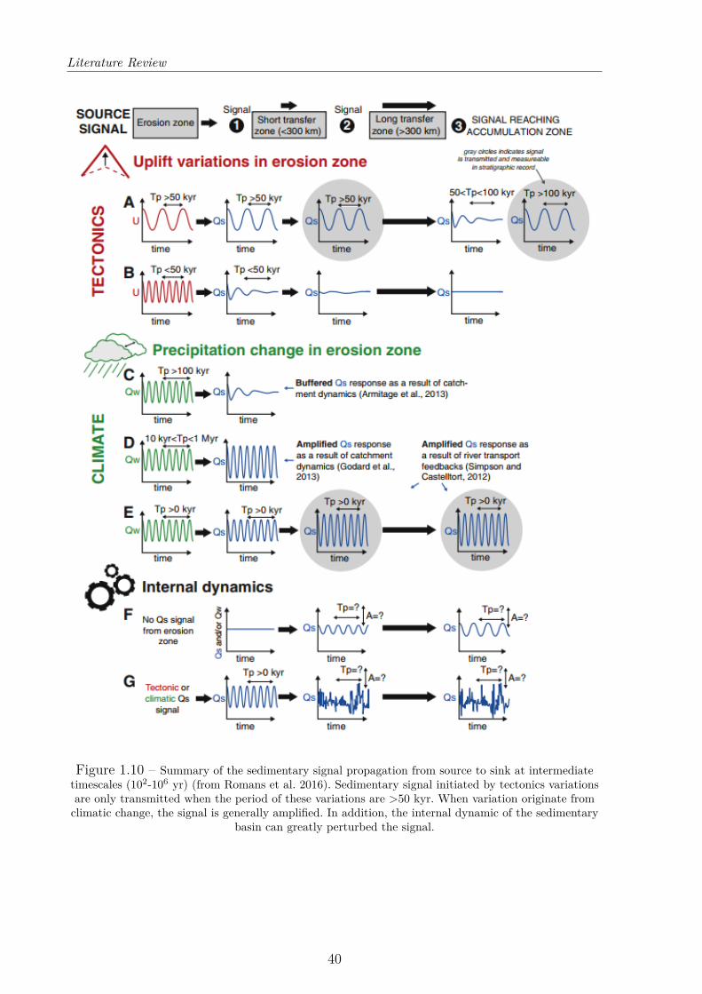
Romans et al. (2016) produced an overview of the environmental signal and its prop-agation along a sediment routing system (Fig. 1.10). They investigated the response ofboth uplift and climatic disturbances occurring in the erosion zone of a given watershed,and their transformation and propagation as sediment supply (Qs) signals in both thetransfer and accumulation zones. In only a few cases environmental signals are faithfully

38

Literature Review

transmitted into the depositional zone and well preserved (gray shaded circles, Fig. 1.10).According to Simpson & Castelltort (2012) it mainly depends on the source of the exter-nal perturbation: climatic variations are more likely to be transmitted when it induceswater discharge (Qw) variations rather than only sediment flux variations. The frequencyand amplitude of the environmental disturbance are important in regard of the inherentsediment transfer cyclicity (Jerolmack & Paola 2010). Indeed, long alluvial rivers (>300km) buffer high-frequency (≤100 kyr) disturbances in sediment input coming from theerosion subsystem (Castelltort & Van Den Driessche 2003). Finally, stratigraphic cyclicityand sediment supply rates may result from both changes in climate and erosions rates aswell as from glacio-eustatic sea-level variations and up-system signal propagation drivenby base level change (see Blum & Törnqvist 2000 for a thorough review).

Despite the significant progress achieved over the last decades in the comprehension ofpaleo-weathering processes (Lerman 1988, Muto & Steel 1992, Tucker & Slingerland 1997,Syvitski & Milliman 2007, Jerolmack & Paola 2010, Phillips & Jerolmack 2016, Romanset al. 2016), it remains difficult to directly link proxy records in sedimentary archives tocorresponding environmental perturbations within any sediment routing system. Conse-quently, some experts are concerned about the accuracy of using landscape or sedimentarydata to detect past environmental change (Wiel & Coulthard 2010, Phillips & Jerolmack2016). However, marine stratigraphic record has shown evidence of sediment inputs corre-lated with long-term (e.g. Milankovitch-type) and short-term (e.g. Dansgaard-Oeschger)climate cycles (Vail et al. 1977, Van der Zwan 2002, Bonneau 2014). Some recent workshave also shown evidence of efficient long-term (glacial-interglacial) signal propagation(Simpson & Castelltort 2012, Macklin et al. 2012, Blum et al. 2018, Watkins et al. 2019).Nevertheless, Watkins et al. (2019) suggested that signals are modified by sediment remo-bilization (see, e.g. Clift et al. 2008 and Clift et al. 2014 for the case of the Indus delta),which can delay, attenuate or emphasize the signals from the landscape adjustment. Thisemphasizes the necessity to quantify (i.e. measure) the transport and storage time of thesediment from source to sink (DePaolo et al. 2006) to be able to detect and quantify thissignal phase shifts.

39

Literature Review

Figure 1.10 – Summary of the sedimentary signal propagation from source to sink at intermediatetimescales (102-106 yr) (from Romans et al. 2016). Sedimentary signal initiated by tectonics variationsare only transmitted when the period of these variations are >50 kyr. When variation originate fromclimatic change, the signal is generally amplified. In addition, the internal dynamic of the sedimentary

basin can greatly perturbed the signal.

40

Literature Review

1.1.3 Soil: the origin of the sediment

Sediments are the products of bedrock weathering and are part of the soil profile be-fore their export down the system. The soil profile acts as an efficient sediment storage,representing in reactive systems a non-negligible part of the sediment residence time. Assoils represent the main interface between atmosphere and bedrock, shaping the land sur-faces, they have become of great interest to study the links between climate, weatheringand White & Blum 1995, Riebe et al. 2001, Millot et al. 2002, von Blanckenburg 2006).Additionally, sediment residence times in small and reactive systems mainly represent thetime spent by the sediments within the weathering profile, i.e. the soil. For these reasons,a particular attention is given to the soil in the following section to detail its structureand the factors that can control its thickness.

Structure of the Critical Zone

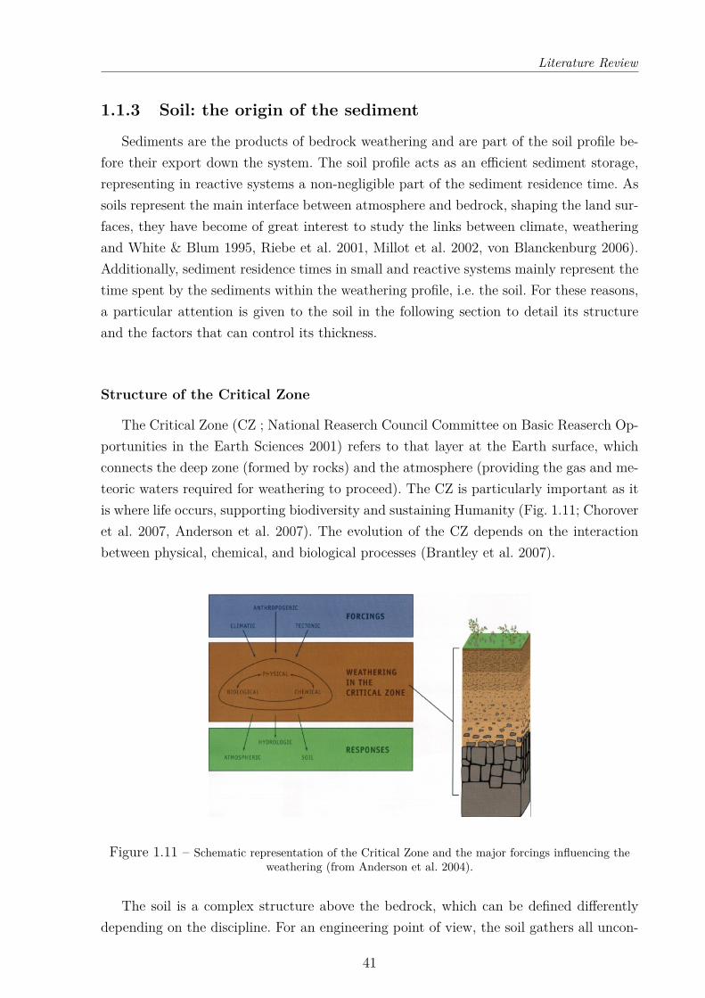
The Critical Zone (CZ ; National Reaserch Council Committee on Basic Reaserch Op-portunities in the Earth Sciences 2001) refers to that layer at the Earth surface, whichconnects the deep zone (formed by rocks) and the atmosphere (providing the gas and me-teoric waters required for weathering to proceed). The CZ is particularly important as itis where life occurs, supporting biodiversity and sustaining Humanity (Fig. 1.11; Choroveret al. 2007, Anderson et al. 2007). The evolution of the CZ depends on the interactionbetween physical, chemical, and biological processes (Brantley et al. 2007).

Figure 1.11 – Schematic representation of the Critical Zone and the major forcings influencing theweathering (from Anderson et al. 2004).

The soil is a complex structure above the bedrock, which can be defined differentlydepending on the discipline. For an engineering point of view, the soil gathers all uncon-

41

Literature Review

solidated material above bedrock (Bates & Jackson 1987) leaving no distinction betweensoil and unconsolidated sediments. To differentiate between these two components, Retal-lack (1984) defined the soil as the immobile part that forms in place, whereas sedimentsrepresent the mobile component that is transported beyond the place of its formation.The geomorphologists considered instead the soil as corresponding to the mobile particleswithin the weathering profile that are no longer binded to the parent rocks (Yoo & Mudd2008). On the other hand, pedologists and geochemists define the soil as the entire verticalweathering sequence, including both the loose material available for erosion but also thatportion of the bedrock that can be highly chemically weathered but still maintains itsstructural integrity (Yoo & Mudd 2008).

Soil thickness: balance between soil production and erosion

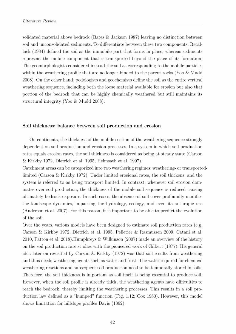
On continents, the thickness of the mobile section of the weathering sequence stronglydependent on soil production and erosion processes. In a system in which soil productionrates equals erosion rates, the soil thickness is considered as being at steady state (Carson& Kirkby 1972, Dietrich et al. 1995, Heimsath et al. 1997).Catchment areas can be categorized into two weathering regimes: weathering- or transported-limited (Carson & Kirkby 1972). Under limited erosional rates, the soil thickens, and thesystem is referred to as being transport limited. In contrast, whenever soil erosion dom-inates over soil production, the thickness of the mobile soil sequence is reduced causingultimately bedrock exposure. In such cases, the absence of soil cover profoundly modifiesthe landscape dynamics, impacting the hydrology, ecology, and even its anthropic use(Anderson et al. 2007). For this reason, it is important to be able to predict the evolutionof the soil.Over the years, various models have been designed to estimate soil production rates (e.g.Carson & Kirkby 1972, Dietrich et al. 1995, Pelletier & Rasmussen 2009, Catani et al.2010, Patton et al. 2018).Humphreys & Wilkinson (2007) made an overview of the historyon the soil production rate studies with the pioneered work of Gilbert (1877). His generalidea later on revisited by Carson & Kirkby (1972) was that soil results from weatheringand thus needs weathering agents such as water and frost. The water required for chemicalweathering reactions and subsequent soil production need to be temporally stored in soils.Therefore, the soil thickness is important as soil itself is being essential to produce soil.However, when the soil profile is already thick, the weathering agents have difficulties toreach the bedrock, thereby limiting the weathering processes. This results in a soil pro-duction law defined as a "humped” function (Fig. 1.12; Cox 1980). However, this modelshows limitation for hillslope profiles Davis (1892).

42

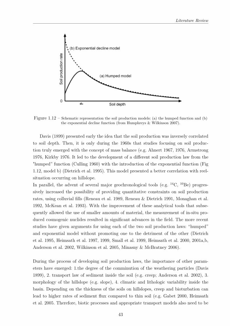
Literature Review

Figure 1.12 – Schematic representation the soil production models: (a) the humped function and (b)the exponential decline function (from Humphreys & Wilkinson 2007).

Davis (1899) presented early the idea that the soil production was inversely correlatedto soil depth. Then, it is only during the 1960s that studies focusing on soil produc-tion truly emerged with the concept of mass balance (e.g. Ahnert 1967, 1976, Armstrong1976, Kirkby 1976. It led to the development of a different soil production law from the"humped” function (Culling 1960) with the introduction of the exponential function (Fig1.12, model b) (Dietrich et al. 1995). This model presented a better correlation with reel-situation occurring on hillslope.In parallel, the advent of several major geochronological tools (e.g. 14C, 10Be) progres-sively increased the possibility of providing quantitative constraints on soil productionrates, using colluvial fills (Reneau et al. 1989, Reneau & Dietrich 1991, Monaghan et al.1992, McKean et al. 1993). With the improvement of these analytical tools that subse-quently allowed the use of smaller amounts of material, the measurement of in-situ pro-duced cosmogenic nuclides resulted in significant advances in the field. The more recentstudies have given arguments for using each of the two soil production laws: “humped”and exponential model without promoting one to the detriment of the other (Dietrichet al. 1995, Heimsath et al. 1997, 1999, Small et al. 1999, Heimsath et al. 2000, 2001a,b,Anderson et al. 2002, Wilkinson et al. 2005, Minasny & McBratney 2006).

During the process of developing soil production laws, the importance of other param-eters have emerged: 1.the degree of the comminution of the weathering particles (Davis1899), 2. transport law of sediment inside the soil (e.g. creep; Anderson et al. 2002), 3.morphology of the hillslope (e.g. slope), 4. climatic and lithologic variability inside thebasin. Depending on the thickness of the soils on hillslopes, creep and bioturbation canlead to higher rates of sediment flux compared to thin soil (e.g. Gabet 2000, Heimsathet al. 2005. Therefore, biotic processes and appropriate transport models also need to be

43

Literature Review

considered (Corenblit & Steiger 2009, Reinhardt et al. 2010, Roering et al. 2010, Richteret al. 2020). Pelletier & Rasmussen (2009) determined a model based on nonlinear depthwith slope dependent transport model to predict soil thicknesses in landscapes dominatedby creep, bioturbation, and mass movements. The remaining limitation of all these mod-els is the absence of consideration of the variation of weathering rate according to thelithology (Pelletier & Rasmussen 2009) and the vegetation cover, which influence the soilstabilization.

The quantification of the soil production rate is important to understand and predictits evolution through time. However, the quantification of the soil production rate re-mains challenging over large spatial scale (i.e. large sediment-routing system) becauseof the internal and external variability along the system (e.g. lithology, climate). In thiscontext, the determination of sediment residence time can bring new perspectives in thesoil production studies by quantifying the time spent by sediments inside the soil profile.This is precisely the aim of this thesis: the quantification of the sediment residence time,using the uranium series isotopes, to better understand erosive processes.

44

Literature Review

1.2 Uranium isotopes

Uranium isotope series are the central point of this thesis, as they are used as a tool toestimate sediment residence times in sediment routing systems. Consequently, after a briefhistory of the uranium isotopes application, the concept required to understand the ap-plication of U-series to sedimentary systems are detailed. Finally, this section presents thecomminution age theory, applied to determine sediment residence time, and the methodrequired to be able to use this model.

1.2.1 Background

The first investigations of the uranium-series began with the initial discovery of theradioactivity in 1896 by Becquerel and the first published version of the radioactive decayscheme by Marie Curie in 1903. The invention of mass spectrometry in 1918 then led tofurther development of isotope studies. At first, the domain of applications of the ura-nium (U) series mostly concerned geochronological studies dealing with deep magmaticprocesses (Newman et al. 1984, McKenzie 1985, Williams & Gill 1989, Hawkesworth et al.1997, Bourdon & Sims 2003, Condomines et al. 2003), in parallel with investigations re-lated to regolith formation (Rosholt et al. 1966, Megumi & Mamuro 1977) or the dating ofcarbonate (carbonate terraces: Sharp et al. 2003; marine carbonate: Edwards et al. 2003;corals: Broecker et al. 1968, Mesolella et al. 1969, Edwards et al. 1986, Muhs et al. 1994,Cheng et al. 2000).

The U geochemistry and isotopic composition of marine sediments have been investi-gated since several decades (Anderson 1982, Anderson & Humphrey 1989, Cochran 1992,Henderson & Anderson 2003). Over the last decades, significant improvements in analyt-ical techniques such as the advent of thermal ionization mass spectrometry (TIMS) and,more recently, since the late 1990s, of multi-collector inductively coupled plasma massspectrometry (MC-ICP-MS) have enabled the determination of U-series isotopic ratioswith much improved precision and the analysis of samples with low U concentration.These analytical advances have made possible the use of U isotopic ratios for the investi-gation sedimentary processes in source to sink systems (e.g. DePaolo et al. 2006, Dossetoet al. 2008a).

1.2.2 Radioactive disequilibrium

In the natural environment, there are three series of radioactive decays that includeuranium and thorium isotopes (Fig. 1.13), as a parent nuclide: 238U;235U, and 232Th.These three decay schemes end with a final stable isotope of lead: 206Pb; 207Pb; 208Pb,respectively. Uranium has three natural isotopes, with different abundance: 238U (99.27%),

45

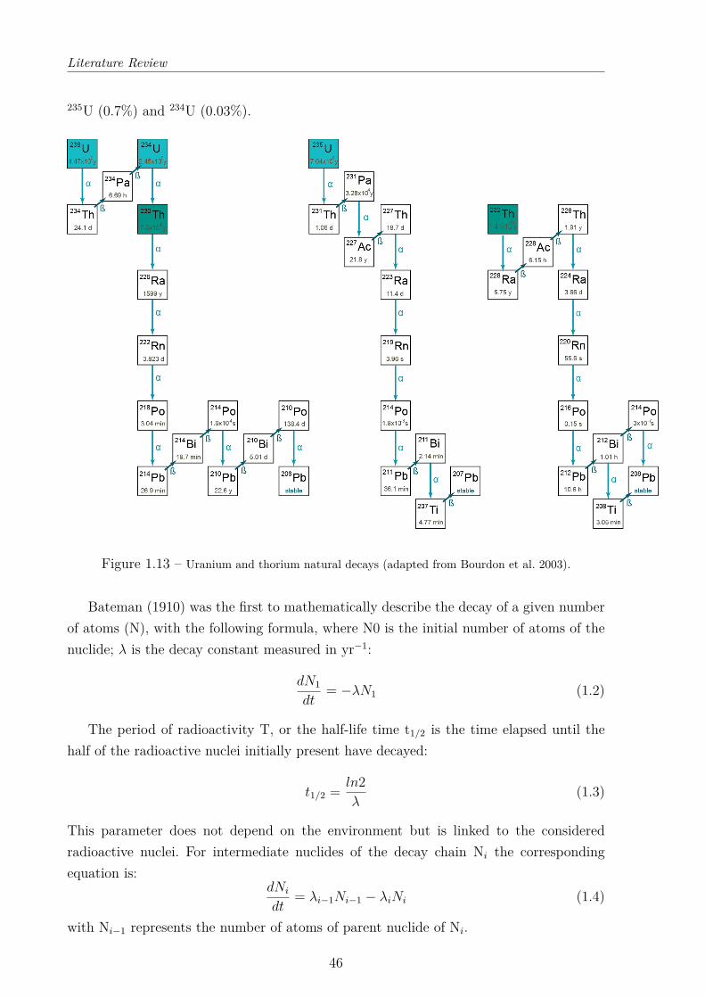
Literature Review

235U (0.7%) and 234U (0.03%).

Figure 1.13 – Uranium and thorium natural decays (adapted from Bourdon et al. 2003).

Bateman (1910) was the first to mathematically describe the decay of a given numberof atoms (N), with the following formula, where N0 is the initial number of atoms of thenuclide; λ is the decay constant measured in yr−1:

dN1

dt= −λN1 (1.2)

The period of radioactivity T, or the half-life time t1/2 is the time elapsed until thehalf of the radioactive nuclei initially present have decayed:

t1/2 = ln2λ

(1.3)

This parameter does not depend on the environment but is linked to the consideredradioactive nuclei. For intermediate nuclides of the decay chain Ni the correspondingequation is:

dNi

dt= λi−1Ni−1 − λiNi (1.4)

with Ni−1 represents the number of atoms of parent nuclide of Ni.

46

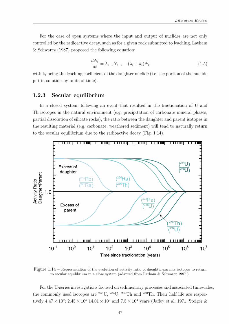
Literature Review

For the case of open systems where the input and output of nuclides are not onlycontrolled by the radioactive decay, such as for a given rock submitted to leaching, Latham& Schwarcz (1987) proposed the following equation:

dNi

dt= λi−1Ni−1 − (λi + ki)Ni (1.5)

with ki being the leaching coefficient of the daughter nuclide (i.e. the portion of the nuclideput in solution by units of time).

1.2.3 Secular equilibrium

In a closed system, following an event that resulted in the fractionation of U andTh isotopes in the natural environment (e.g. precipitation of carbonate mineral phases,partial dissolution of silicate rocks), the ratio between the daughter and parent isotopes inthe resulting material (e.g. carbonate, weathered sediment) will tend to naturally returnto the secular equilibrium due to the radioactive decay (Fig. 1.14).

Figure 1.14 – Representation of the evolution of activity ratio of daughter-parents isotopes to returnto secular equilibrium in a close system (adapted from Latham & Schwarcz 1987 ).

For the U-series investigations focused on sedimentary processes and associated timescales,the commonly used isotopes are 238U, 234U, 232Th and 230Th. Their half life are respec-tively 4.47 × 109; 2.45 × 105 14.01 × 109 and 7.5 × 104 years (Jaffey et al. 1971, Steiger &

47

Literature Review

Jager 1978, Cheng et al. 2000). In a closed system, which considers that there has been nointeraction of U and Th isotopes with the surrounding environment, the time required forthe activity ratio between two isotopes to reach the secular equilibrium is equivalent to fivetimes of t1/2 of the daughter nuclide. For instance, for the case of the (234U/238U) activityratio, the time needed to reach the secular equilibrium, i.e. meaning (234U/238U) beingequal to 1, is five times t1/2 of 234U, hence approximately 1.2 Ma. For the (230Th/234U) ra-tio, the time required to return to secular equilibrium will be approximately 300 kyr. Thequantification of the U-series disequilibrium provides unique information on the timingof the initial U-Th fractionation and of the processes that initially disturbed the secularequilibrium. This approach is particularly useful for investigating processes that occurredat the timescale of the Quaternary period, especially using the following isotopes 234U,230Th, 226Ra.

For clarity, the measurements of U-series isotopes are conventionally reported as ratios oftheir respective activity, which corresponds to the number of disintegrations per units oftime (Bq), calculated as following:

(Ni) = λiNi (1.6)

The parent-daughter activity ratio is also commonly used to study two isotopes:

N2

N1= λ2N2

λ1N1(1.7)

The delta notation (δ234U) can also be used and is expressed as:

δ234U = (λ2N2

λ1N1− 1) × 1000 (1.8)

but it is generally not used in the studies that focused on the timescales of sedimentaryprocesses. For this thesis, the activity ratio notation is used.

1.2.4 Uranium abundances in rock forming minerals and thefractionation of (234U/238U) in sedimentary systems

Despite the relatively low abundance of uranium in most rocks outcropping at theEarth surface (Dahlkamp 1993), some rock-forming minerals do display higher concentra-tions than others (Taylor & McLennan 1995). For instance, this is the case for uraninite,which represents the main uranium ore on Earth, but also, to a lesser degree, for mineralssuch xenotime, monazite and allanite, which are also typically enriched in other traceelements (e.g. rare earth elements). Titanium-enriched minerals are also likely to displayhigh relatively U concentrations, due to the similar ionic radii of Ti and U.

48

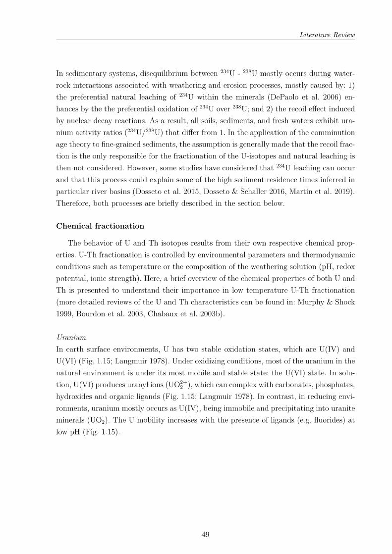
Literature Review

In sedimentary systems, disequilibrium between 234U - 238U mostly occurs during water-rock interactions associated with weathering and erosion processes, mostly caused by: 1)the preferential natural leaching of 234U within the minerals (DePaolo et al. 2006) en-hances by the the preferential oxidation of 234U over 238U; and 2) the recoil effect inducedby nuclear decay reactions. As a result, all soils, sediments, and fresh waters exhibit ura-nium activity ratios (234U/238U) that differ from 1. In the application of the comminutionage theory to fine-grained sediments, the assumption is generally made that the recoil frac-tion is the only responsible for the fractionation of the U-isotopes and natural leaching isthen not considered. However, some studies have considered that 234U leaching can occurand that this process could explain some of the high sediment residence times inferred inparticular river basins (Dosseto et al. 2015, Dosseto & Schaller 2016, Martin et al. 2019).Therefore, both processes are briefly described in the section below.

Chemical fractionation

The behavior of U and Th isotopes results from their own respective chemical prop-erties. U-Th fractionation is controlled by environmental parameters and thermodynamicconditions such as temperature or the composition of the weathering solution (pH, redoxpotential, ionic strength). Here, a brief overview of the chemical properties of both U andTh is presented to understand their importance in low temperature U-Th fractionation(more detailed reviews of the U and Th characteristics can be found in: Murphy & Shock1999, Bourdon et al. 2003, Chabaux et al. 2003b).

UraniumIn earth surface environments, U has two stable oxidation states, which are U(IV) andU(VI) (Fig. 1.15; Langmuir 1978). Under oxidizing conditions, most of the uranium in thenatural environment is under its most mobile and stable state: the U(VI) state. In solu-tion, U(VI) produces uranyl ions (UO2+

2 ), which can complex with carbonates, phosphates,hydroxides and organic ligands (Fig. 1.15; Langmuir 1978). In contrast, in reducing envi-ronments, uranium mostly occurs as U(IV), being immobile and precipitating into uraniteminerals (UO2). The U mobility increases with the presence of ligands (e.g. fluorides) atlow pH (Fig. 1.15).

49

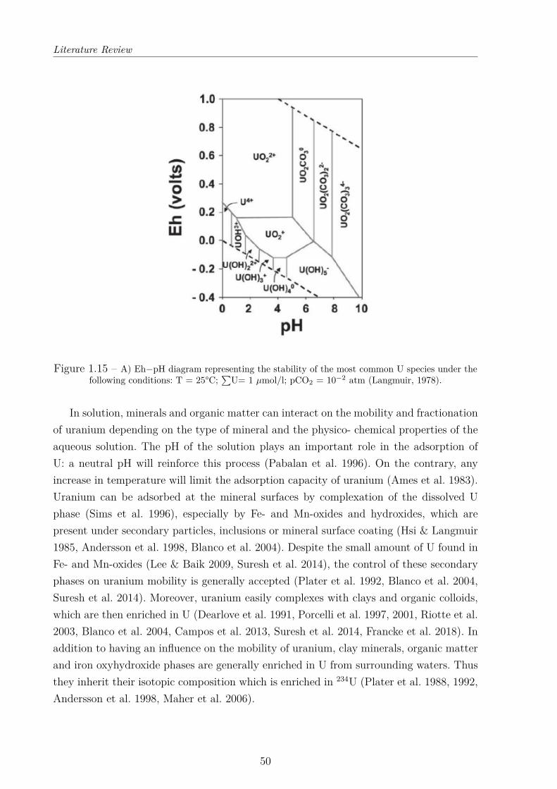
Literature Review

Figure 1.15 – A) Eh−pH diagram representing the stability of the most common U species under thefollowing conditions: T = 25°C;

∑U= 1 µmol/l; pCO2 = 10−2 atm (Langmuir, 1978).

In solution, minerals and organic matter can interact on the mobility and fractionationof uranium depending on the type of mineral and the physico- chemical properties of theaqueous solution. The pH of the solution plays an important role in the adsorption ofU: a neutral pH will reinforce this process (Pabalan et al. 1996). On the contrary, anyincrease in temperature will limit the adsorption capacity of uranium (Ames et al. 1983).Uranium can be adsorbed at the mineral surfaces by complexation of the dissolved Uphase (Sims et al. 1996), especially by Fe- and Mn-oxides and hydroxides, which arepresent under secondary particles, inclusions or mineral surface coating (Hsi & Langmuir1985, Andersson et al. 1998, Blanco et al. 2004). Despite the small amount of U found inFe- and Mn-oxides (Lee & Baik 2009, Suresh et al. 2014), the control of these secondaryphases on uranium mobility is generally accepted (Plater et al. 1992, Blanco et al. 2004,Suresh et al. 2014). Moreover, uranium easily complexes with clays and organic colloids,which are then enriched in U (Dearlove et al. 1991, Porcelli et al. 1997, 2001, Riotte et al.2003, Blanco et al. 2004, Campos et al. 2013, Suresh et al. 2014, Francke et al. 2018). Inaddition to having an influence on the mobility of uranium, clay minerals, organic matterand iron oxyhydroxide phases are generally enriched in U from surrounding waters. Thusthey inherit their isotopic composition which is enriched in 234U (Plater et al. 1988, 1992,Andersson et al. 1998, Maher et al. 2006).

50

Literature Review

ThoriumIn natural environments, thorium exists as Th4+ oxidation state. It is generally assumedthat Th is greatly immobile under neutral pH conditions in fresh waters, but its mobilityincreases as pH decreases (<4). One of the most enriched Th-bearing mineral is thorian-ite (ThO2), which is soluble under acidic condition. The mobility of Th also raises in thepresence of organic and inorganic ligands (Fig. 1.16; from Langmuir & Herman 1980).

Figure 1.16 – Diagram of thoranite solubility depending of pH in pure water, with organic andinorganic ligands, at T = 25°C (from Langmuir & Herman 1980).

As uranium, thorium can be, adsorbed into Fe-oxides and hydroxides (Andersson et al.1998, Porcelli et al. 2001) and into carbonate minerals and clay minerals (Suresh et al.2014). Despite its low mobility, dissolved Th concentrations naturals waters can be quitesignificant, due to its complexation and/or adsorption by organic colloids (Fig. 1.16 ;Porcelli et al. 1997, Dupré et al. 1999, Riotte et al. 2003, Blanco et al. 2004, Rihs et al.2011. Secondary phases, such as clays, and organic matter can be relatively enriched in230Th. Indeed, same as for U, these phases are enriched in Th from surrounding watersthus inherit their isotopic compositions (Plater et al. 1992, Suresh et al. 2014). This en-richment is mainly represented in the Fe- and Mn-oxyhydroxides phases.

In conclusion, the particular chemical properties of uranium and thorium isotopes in-duce in Earth surface environments the preferential leaching of 234U embedded in recoiltracks (Fleischer 1980, 1982) when a solution fills the pore space (Fleischer 1980, Andersenet al. 2009). The 234U-238U fractionation can be enhanced by the preferential oxidation of234U in comparison with 238U. The preferential oxidation is due to the highest probabilityin minerals with low concentration that 234U is close to oxygen atoms (Adloff & Roessler1991) and would therefore be more prone to oxidation to the hexavalent state which ismore mobile compared to 238U (Dosseto et al. 2015).

51

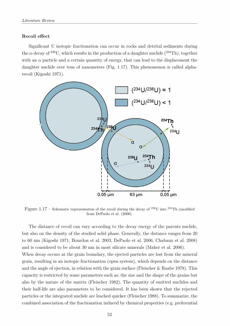
Literature Review

Recoil effect

Significant U isotopic fractionation can occur in rocks and detrital sediments duringthe α-decay of 238U, which results in the production of a daughter nuclide (234Th), togetherwith an α particle and a certain quantity of energy, that can lead to the displacement thedaughter nuclide over tens of nanometers (Fig. 1.17). This phenomenon is called alpha-recoil (Kigoshi 1971).

Figure 1.17 – Schematic representation of the recoil during the decay of 238U into 234Th (modifiedfrom DePaolo et al. (2006).

The distance of recoil can vary according to the decay energy of the parents nuclide,but also on the density of the studied solid phase. Generally, the distance ranges from 20to 60 nm (Kigoshi 1971, Bourdon et al. 2003, DePaolo et al. 2006, Chabaux et al. 2008)and is considered to be about 30 nm in most silicate minerals (Maher et al. 2006).When decay occurs at the grain boundary, the ejected particles are lost from the mineralgrain, resulting in an isotopic fractionation (open system), which depends on the distanceand the angle of ejection, in relation with the grain surface (Fleischer & Raabe 1978). Thiscapacity is restricted by some parameters such as: the size and the shape of the grains butalso by the nature of the matrix (Fleischer 1982). The quantity of emitted nuclides andtheir half-life are also parameters to be considered. It has been shown that the rejectedparticles or the integrated nuclide are leached quicker (Fleischer 1988). To summarize, thecombined association of the fractionation induced by chemical properties (e.g. preferential

52

Literature Review

leaching and oxidation of 234U) and the recoil loss effect is responsible for the observedvariations of U activity ratios measured at the Earth surface. As a result, the soil profilesare generally depleted in 234U, whereas pore waters and freshwaters in river systems areenriched in 234U compared to 238U.

1.2.5 The concept of comminution age

This section presents the concept of the comminution age, which represents the timeelapsed since the formation of the fine sediment grains until their deposition. It alsoprovides details on the methods required in order to obtained accurate comminution agesfrom sediments, with a particular focus on the specific surface area measurement.

Concept

The comminution age dating method is based on the disequilibrium between 234U and238U in fine-grained detrital minerals (DePaolo et al. 2006).As mentioned above, following the disintegration of 238U, the daughter isotope 234Th,which rapidly decay into 234Pa and then 234U, recoils over a short distance (∼ 30 nm). Inthe case where the reaction occurs at the edge of a detrital particle, the daughter isotopesare ejected out of the grain, inducing a disequilibrium in the 234U/238U ratio. When thegrain is small enough and displays a large surface area to volume ratio, the disequilibriumis significant enough to be measured. Following disequilibrium, it then takes about 1.2Ma for the residual detrital grain to reach secular equilibrium, assuming no subsequentexternal disturbance. During this period, the measured disequilibrium indicates the timeelapsed since the disequilibrium occurred, i.e. which corresponds to the time when thegrain was first produced. This dating method is thus based on the α-recoil effect. Thecomminution age tcom can be calculated using the equation determined by DePaolo et al.(2006):

tcom = −1λ234

ln

[A− (1 − fα)A0 − (1 − fα)

](1.9)

with A is the measured (234U/238U) activity ratio in any fine-grained sediment, A0 isthe initial (234U/238U) of the initial rock (i.e. the unaltered bedrock or the grains >63µm), λ234 is the decay constant of 234U (in a−1) and fα is the direct recoil of the fraction.This method considers that only the recoil effect process is important in the fractionationof 234U over 238U.

The degree 234U and 238U fractionation of can also be different before and after thedeposition of the sediment. Therefore, Francke et al. (2018) compared two scenarios: onewith no loss of 234U after deposition (fpost, i.e. the recoil loss factor post deposition =0)and the second with a continuous loss of 234U after deposition (fpre, i.e. the recoil loss

53

Literature Review

factor pre deposition = fpost), using the following equation:

tres = −1λ234

ln

[[A− (1 − fpost)] e−λ234tdep + (1 − fpost) − (1 − fpre)

A0 − (1 − fpre)

](1.10)

with tdep the deposition age (yr). Even though they obtained comparable sedimentresidence time with the two methods (within the error range of each other for the majorityof the sample), they considered the second scenario as being the most probable becauseof the importance of the water content within the samples.The preferential leaching of 234U could also have an influence on the degree of U isotopedisequilibrium, due to preferential oxidation of 234U induced by the recoil effect (Adloff& Roessler 1991, Dosseto et al. 2015, Kolodny et al. 2017). To implement the preferentialleaching of 234U processes in the comminution age method, Dosseto & Schaller (2016)modified the equation 1.9 as following:

tcom = −1λ234 +

(w234w238

− 1)w238

ln

A−

(1−fα)λ234

λ234+(w234w238

−1)w238

A0 −

(1−fα)λ234

λ234+(w234w238

−1)w238

(1.11)

with the leaching coefficients w234 and w238 for 234U and 238U (in a−1), respectively.Studies on leaching coefficients from both field and laboratory-based work determinedw234/w238 around 1.2 ±0.2 (Dequincey et al. 2002, Vigier et al. 2005, Dosseto et al. 2006a,2014, Andersen et al. 2009). Martin et al. (2019) explored the influence of the leachingparameters on the calculated sediment residence time through a Monte Carlo simulation.They obtained younger ages when considering the leaching processes because the directrecoil is then less important. This study pointed out the importance in the determinationof the leaching parameters as this effect can result in a bias of (234U/238U) ratios. Usinga similar approach as Francke et al. (2019) to infer the difference of fractionation pre-and post-deposition, Francke et al. (2020) implemented equation 5.1 to determine the234U loss effect pre- and post-deposition on calculated sediment residence time. For thispurpose, they combined equations 5.1 with 1.11 and proposed the two following equationsto compare the obtained sediment residence time:

54

Literature Review

tres = −1λ234

ln

A−

(1−fpost)λ234

λ234+(w234postw238post

−1)w238

e−λ234tdep + (1−fpost)λ234

λ234+(w234postw238post

−1)w238

− (1 − fpres)

A0 − (1 − fpre)

(1.12)

tres = −1λ234 +

(w234w238

− 1)w238

ln

[A− (1 − fpost)] e−λ234tdep + (1 − fpost) −

(1−fpre)λ234

λ234+(w234prew238pre

−1)w238pre

A0 −

(1−fpre)λ234

λ234+(w234prew238pre

−1)w238pre

(1.13)

The comparison of the sediment residence times calculated with the assumption of postdepositional leaching using realistic and extreme leaching factors are in the same rangeof the sediment residence time obtained without any consideration of leaching processesfrom Francke et al. (2019). This suggests that the effect of preferential 234U leachingafter the deposition has no real impact on the determination of sediment residence time.Conversely, assuming leaching processes pre-deposition, Francke et al. (2020) obtainedlower sediment residence times. The correlation between sediment residence times andclimatic parameters decrease with the consideration of 234U leaching in both modern andpaleo sediment residence times (Martin et al. 2019, Francke et al. 2020). Li et al. (2016a)considered that leaching is only important for sediment with residence time <10,000years because leaching is only high in young material with very high surface areas. Thecomminution age are obtained by resolving of one of the equation mentioned above by aMonte-Carlo inversion method. This method allows to simulate the distribution of possiblecomminution age.

Method

Sample treatmentIn the natural environment, sediments are composed of a mixture of various detrital,authigenic and organic phases. One important requirement prior to applying the commu-nition age method to fine-grained sediments is to remove all non-detrital phases, whichmay strongly influence measured U isotopic ratios. This step is particularly importantbecause any authigenic or organic phases formed from soil pore waters or river waters arelikely to be enriched in 234U due to recoil effect (see section above), hence being charac-terized by (234U/238U) >1. However, the isolation of the detrital fraction needs to be donecarefully in order to prevent any partial dissolution of the surface of the grains (which

55

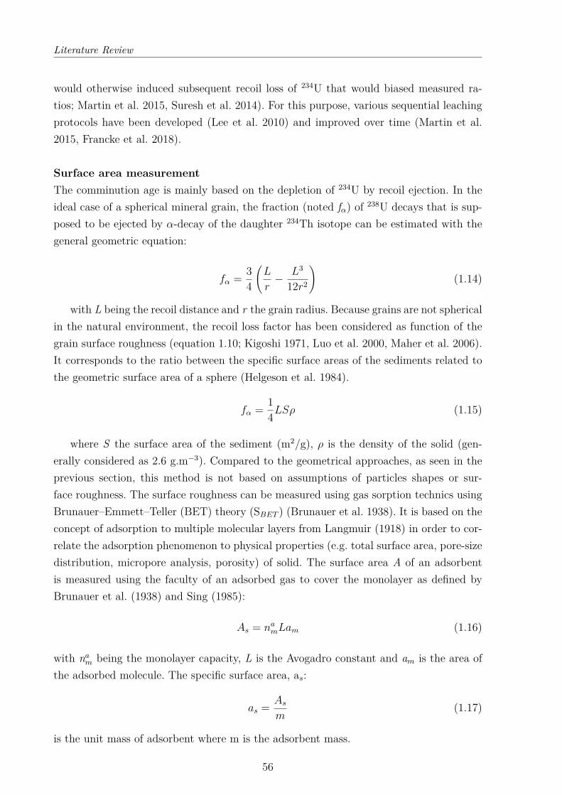
Literature Review

would otherwise induced subsequent recoil loss of 234U that would biased measured ra-tios; Martin et al. 2015, Suresh et al. 2014). For this purpose, various sequential leachingprotocols have been developed (Lee et al. 2010) and improved over time (Martin et al.2015, Francke et al. 2018).

Surface area measurementThe comminution age is mainly based on the depletion of 234U by recoil ejection. In theideal case of a spherical mineral grain, the fraction (noted fα) of 238U decays that is sup-posed to be ejected by α-decay of the daughter 234Th isotope can be estimated with thegeneral geometric equation:

fα = 34

(L

r− L3

12r2

)(1.14)

with L being the recoil distance and r the grain radius. Because grains are not sphericalin the natural environment, the recoil loss factor has been considered as function of thegrain surface roughness (equation 1.10; Kigoshi 1971, Luo et al. 2000, Maher et al. 2006).It corresponds to the ratio between the specific surface areas of the sediments related tothe geometric surface area of a sphere (Helgeson et al. 1984).

fα = 14LSρ (1.15)

where S the surface area of the sediment (m2/g), ρ is the density of the solid (gen-erally considered as 2.6 g.m−3). Compared to the geometrical approaches, as seen in theprevious section, this method is not based on assumptions of particles shapes or sur-face roughness. The surface roughness can be measured using gas sorption technics usingBrunauer–Emmett–Teller (BET) theory (SBET ) (Brunauer et al. 1938). It is based on theconcept of adsorption to multiple molecular layers from Langmuir (1918) in order to cor-relate the adsorption phenomenon to physical properties (e.g. total surface area, pore-sizedistribution, micropore analysis, porosity) of solid. The surface area A of an adsorbentis measured using the faculty of an adsorbed gas to cover the monolayer as defined byBrunauer et al. (1938) and Sing (1985):

As = namLam (1.16)

with nam being the monolayer capacity, L is the Avogadro constant and am is the area ofthe adsorbed molecule. The specific surface area, as:

as = Asm

(1.17)

is the unit mass of adsorbent where m is the adsorbent mass.

56

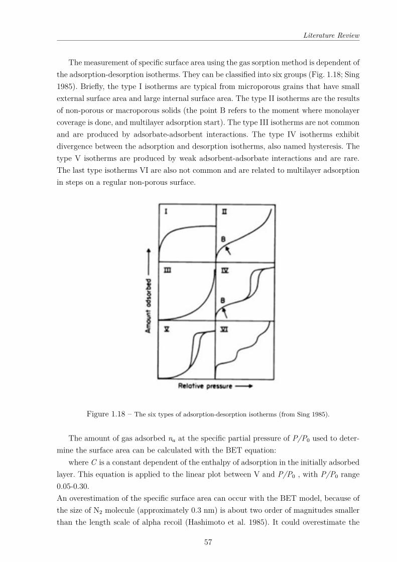
Literature Review

The measurement of specific surface area using the gas sorption method is dependent ofthe adsorption-desorption isotherms. They can be classified into six groups (Fig. 1.18; Sing1985). Briefly, the type I isotherms are typical from microporous grains that have smallexternal surface area and large internal surface area. The type II isotherms are the resultsof non-porous or macroporous solids (the point B refers to the moment where monolayercoverage is done, and multilayer adsorption start). The type III isotherms are not commonand are produced by adsorbate-adsorbent interactions. The type IV isotherms exhibitdivergence between the adsorption and desorption isotherms, also named hysteresis. Thetype V isotherms are produced by weak adsorbent-adsorbate interactions and are rare.The last type isotherms VI are also not common and are related to multilayer adsorptionin steps on a regular non-porous surface.

Figure 1.18 – The six types of adsorption-desorption isotherms (from Sing 1985).

The amount of gas adsorbed na at the specific partial pressure of P/P0 used to deter-mine the surface area can be calculated with the BET equation:

where C is a constant dependent of the enthalpy of adsorption in the initially adsorbedlayer. This equation is applied to the linear plot between V and P/P0 , with P/P0 range0.05-0.30.An overestimation of the specific surface area can occur with the BET model, because ofthe size of N2 molecule (approximately 0.3 nm) is about two order of magnitudes smallerthan the length scale of alpha recoil (Hashimoto et al. 1985). It could overestimate the

57

Literature Review

recoil loss factor (Maher et al. 2006). In order to overcome this issue, Bourdon et al. (2009)suggested a correction inspired by the work of Semkow (1991) using the fractal dimensionD. The corrected direct-recoil fraction is then calculated with:

f = 14

[2D−1

4 −D

(α

L

)D−2]LSρ (1.18)

where α is the adsorbate gas diameter (in m). The fractal dimension of the surface canbe estimated with BET measurement and range from 2 (perfectly smooth surface) to 3(complexes surface). This correction is only necessary for micro- (<2 nm) or mesoporoussediments (2 − 50 nm), in which the pore size is similar to the recoil length and increasethe measured surface area without contributing to the loss of 234U (Francke et al. 2018).

58

Literature Review

1.3 Uranium at Earth’s surface

In this section, I present the application of the uranium isotopes fractionation tostudy Earth’s surface processes. Even if it is not the main focus of this thesis, the firstsection briefly reviews the main results of the applications of the uranium activity ratioin weathering–related studies, as the importance of soil production rates has already beendemonstrated. The second part reviews the comminution age studies to demonstrate theprogress in this field and to highlight its limitation.

1.3.1 From bedrock to soil: weathering processes

Uranium isotope series have been widely used to study weathering processes (e.g.timescale and regime) using soils (e.g. Mathieu et al. 1995, Dequincey et al. 2002, Dossetoet al. 2008b, 2012, Ma et al. 2010, Chabaux et al. 2013, Suresh et al. 2013), but alsosuspended and riverbank sediments and dissolved river loads (e.g. Vigier et al. 2001,2005, 2006, Dosseto et al. 2006a,b, 2008a, Granet et al. 2007, 2010). Because all bedrocksolder than 1 Ma are assumed to be at secular equilibrium, any source effect related tochanging sediment or water provenance on measured (234U/238U) ratios is expected to benegligible (Pogge von Strandmann et al. 2006).

The absence of any significant source effect on measured (234U/238U) inside any riverbasin under investigation (e.g. Amazon river, Murrumbidgee river) generally indicates thatU isotope fractionation during sediment transport can be considered as negligible (Dossetoet al. 2006b, Suresh et al. 2014). Therefore, the measured (234U/238U) is mainly represen-tative of the depletion occurring along the weathering profile and, with the assumptionthat weathering is constant at the timescale of soil formation, 234U-238U fractionation canbe estimated using a continuous weathering model (e.g. Vigier et al. 2001, Dosseto et al.2006a,b, Granet et al. 2007, 2010, Ma et al. 2010; Fig. 1.19). The model is based onthe concentration of any given radioactive isotope as a function of its product by decayfrom the parent isotope, and loss through its own radioactive decay, in addition to theincorporation of the leaching parameter.

The presence of soil fraction with (234U/238U) >1 within the weathering profile in-dicates that 234U can be implemented inside soils grains (e.g. Dequincey et al. 2002,Chabaux et al. 2003b, 2008, Pelt et al. 2008). Therefore, the weathering model has beenimplemented to consider the potential gain by secondary processes or external input (e.g.Dequincey et al. 2002, Chabaux et al. 2003b, Dosseto et al. 2008a,b, Ma et al. 2010, seeChabaux et al. 2011 for a detailed review).

59

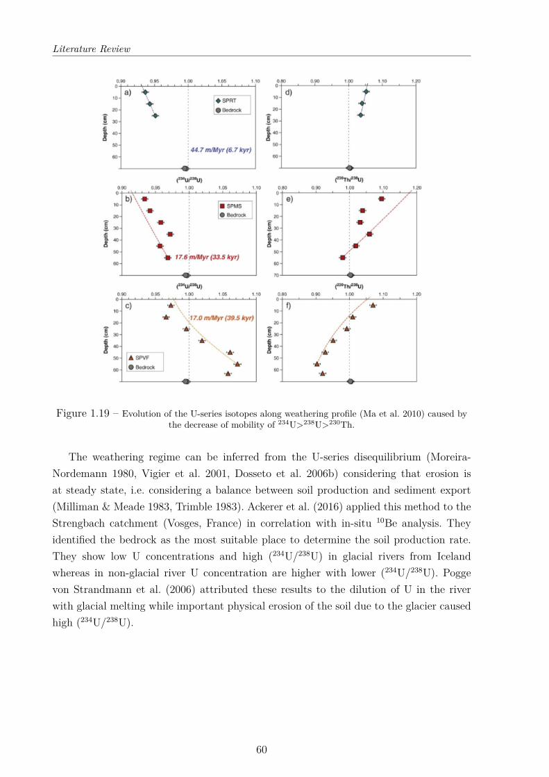
Literature Review

Figure 1.19 – Evolution of the U-series isotopes along weathering profile (Ma et al. 2010) caused bythe decrease of mobility of 234U>238U>230Th.

The weathering regime can be inferred from the U-series disequilibrium (Moreira-Nordemann 1980, Vigier et al. 2001, Dosseto et al. 2006b) considering that erosion isat steady state, i.e. considering a balance between soil production and sediment export(Milliman & Meade 1983, Trimble 1983). Ackerer et al. (2016) applied this method to theStrengbach catchment (Vosges, France) in correlation with in-situ 10Be analysis. Theyidentified the bedrock as the most suitable place to determine the soil production rate.They show low U concentrations and high (234U/238U) in glacial rivers from Icelandwhereas in non-glacial river U concentration are higher with lower (234U/238U). Poggevon Strandmann et al. (2006) attributed these results to the dilution of U in the riverwith glacial melting while important physical erosion of the soil due to the glacier causedhigh (234U/238U).

60

Literature Review

1.3.2 Uranium isotopes to infer timescale of sedimentary pro-cesses and its control

The comminution age is the time elapsed since the sediment has reached a particlesize <63 µm due to the combination of weathering and physical erosion processes. Infine-grained sediments <63 µm, the fractionation between 234U and 238U is mostly causedby the recoil effect and preferential 234U leaching is then considered negligible (DePaoloet al. 2006). When this method is applied to alluvial sediments, the comminution age canbe taken as representative of the sediment residence time. The communition age methodhas been improved over the years in an attempt to address some inherent limitations (e.g.Lee et al. 2010, Handley et al. 2013a,b, Suresh et al. 2014, Martin et al. 2015, Bosia 2016,Francke et al. 2018).

DePaolo et al. (2006) first applied the comminution age method to core sediments from theNorth Atlantic Ocean. They revealed a correlation between (234U/238U) and the glacial-interglacial variability inferred from the δ18O foraminiferal record. This cyclicity onlyapplied for the three-last glacial cycles (sediments <300 kyr). The obtained sedimenttransport times were more elevated during the glacial periods (up to 400 kyr), while be-ing much lower during interglacial periods (within 10 kyr). The longer sediment transporttimes inferred for glacial periods were explained by the occurrence of sediment redis-tribution caused either by strong bottom current or glacier activity, which could havetransported older sediments (i.e. causing sediment recycling).

In small river basins with high topography, generally characterized by the absence ofany alluvial plain (hence with no alluvial storage capacity), the sediment residence timemainly refers to the time spent by the sediment inside the weathering profile and, as aconsequence, can be referred to as the weathering age (Dosseto et al. 2014). However,Suresh et al. (2014) based on the work of Li et al. (2016a,b). The comparison of sedimentresidence times for river basins exhibiting markedly different catchment size indicatesmarked differences. Large sediment residence times (250-600 kyr) were calculated for amainland China catchment (Yangtze) because of the large storage capacity. Conversely,the comminution age calculated for a small mountainous basin in Taiwan was much lower(110 kyr), due presumably to high denudation rates caused by tectonic uplift and sub-tropical climate conditions characterized by extreme rainfall events.

Dosseto et al. (2010) analysed sediments from various paleochannels with depositionalages ranging from 15 ±2 to 100 ±9 kyr in a tributary of the Murray river (SE Australia).They observed a decrease of sediment residence times from 400 to 27 kyr (between thetime interval >100 ka to 15 ka) with a sharp increase after 15 ka. These variations were at-

61

Literature Review

tributed to changes in the sediment source reservoir (upland soils versus alluvial deposits)due to shifts in vegetation patterns. The influence of the vegetation on sediment residencetime has also been also suggested by Martin et al. (2019), in a study that investigatedseven catchments draining the Gulf of Carpentaria basin. This latter study highlightedthe climatic influence on sediment residence time, showing a strong degree of correlationwith mean annual precipitation (R2 = 0.71) , but also with the percentage of vegetationcover, showing that an increase in Eucalyptus and Acacia woodland cover was accompa-nied by a decrease in the sediment residence time. These findings were also supported byFrancke et al. (2019) in a study of a sediment core from the Ohrid lake (Greece), showingthat shorter sediment residence times (34 ±7 kyrs) occurred during wet periods, and viceversa. A transition occurred between the Early and the Mid-Holocene due to enhancedforest cover, resulting in the stabilization of soils on hillslopes (Francke et al. 2019). Onthis basis, Francke et al. (2019) considered that the control on sediment residence timesswitched from precipitation to vegetation cover during that transitional period.

The above-mentioned studies show that sediment residence times display a large variabil-ity in river catchments. The first and main control identified for the sediment residencetime inside a sediment-routing system is its reactivity, which depends on the storage ca-pacity along the river path and thus the size of the catchment. In small and reactivebasins, the influence of tectonics (e.g. Li et al. 2016a), glacier coverage (e.g. DePaoloet al. 2006), climate (e.g. Dosseto et al. 2010) and the vegetation cover (e.g. Martin et al.2019) have been shown to play an important role on the long-term evolution of sedimentresidence time. However, as detailed in the next section, this large sediment residencetime variability could also partly reflect, at least to some extent, some uncertainties andinherent limitations associated with the sediment resident time estimation method.

1.3.3 Uncertainties based on the comminution age method

The studies of the timescale of sediment processes (weathering, transport, deposition)are based on multiple assumptions. For this reason, it is important to mention all theuncertainties related to the communition age method (for a more detailed overview seeHandley et al. 2013b).

Natural leaching effect and comminution

The comminution age model is based on the comminution of the bedrock during theweathering. The theory to estimate the comminution age assumes that no further com-minution processes occurs after the production of the fine-grained sediment (DePaoloet al. 2006). Therefore, if secondary episode of comminution happens, the inferred age isthen considered as a minimal value (Dosseto et al. 2010).

62

Literature Review

Bedrock equilibrium

One of the uncertainties in the comminution age method is related to the assumptionthat the bedrocks older 1.2 Ma are systematically at secular equilibrium (e.g. Dequinceyet al. 1999, Dosseto et al. 2006a, Pelt et al. 2013, Suresh et al. 2014). However, (234U/238U)measurements of bedrock samples are scarce in comminution age studies due to the inher-ent difficulties to accessing the pristine unweathered bedrock. A few studies have pointedout that some bedrocks could depart from secular equilibrium, corresponding generally tonon-volcanic bedrock that otherwise looked pristine and unaltered (Rosholt 1983, Land-stroem & Tullborg 2001, Bourdon et al. 2009, Handley et al. 2013b, Martin et al. 2019).While the causes for U-isotopes disequilibrium in pristine rocks remain unclear, this couldbe possibly related to issues related to porosity or grain-size, at least for the case of sedi-mentary rocks (DePaolo et al. 2006).

Grain size and mineralogical effect

The influence of the grain size on measured (234U/238U) ratios has already been men-tioned by DePaolo et al. (2006), who model the sediment residence time decreased withdecreasing grain size, in contrast to Dosseto et al. (2014), who reported instead a decreaseof the uranium activity ratio with increasing grain size in suspended sediments from theMurray-Darling Basin (from <10 kDa to >25 µm). The influence of grain size has alsobeen also demonstrated in the Ganges river basin, where coarse sediments exhibit resi-dence times >100 kyr while fine-grained sediments display residence time <25 kyr (Granetet al. 2010). However, Chabaux et al. (2012) attributed this size-dependent (234U/238U)variation to sample bias. In addition, Bosia (2016) pointed out the importance of themineralogy in the determination of sediment residence time based on U isotopes. In addi-tion, lithology could play an indirect role on measured sediment residence times, throughdifferences in weathering susceptibility (Dosseto et al. 2014). In large river catchments,with high storage capacity, a particular attention must be also paid to the possibility ofa return to secular equilibrium, which can alterate the interpretation of the measured(234U/238U) (Chabaux et al. 2006, 2012, Granet et al. 2007, 2010).

Methodologic limitation

Over time, the leaching protocols aimed at isolating the detrital fraction of the sedi-ment have been developed and improved as seen in the section 1.2.5 (e.g. Handley et al.2013a, Suresh et al. 2014, Martin et al. 2015, Francke et al. 2018). Furthermore, themeasurement of the recoil loss is also difficult as seen in the section 1.2.5. As SBET mea-surements are time and cost consuming, an estimated value for the recoil loss factor isusually used for calculating comminution ages, but this possibly results in significantuncertainties on calculated sediment residence time.

63

Literature Review

External input

Finally, another parameter that is not often taking into account in communition agestudies is the possibility of an external contamination via atmospheric and/or anthro-pogenic (non-natural) detrital inputs (e.g. atmospheric, anthropogenic) (e.g. Pelt et al.2013).

64

Chapter 2

METHODOLOGY

Contents2.1 Samples collection . . . . . . . . . . . . . . . . . . . . . . . . . . . . 66

2.1.1 Sediments from world rivers . . . . . . . . . . . . . . . . . . . . . . . 662.1.2 Var sediments . . . . . . . . . . . . . . . . . . . . . . . . . . . . . . . 66

2.2 Samples preparation . . . . . . . . . . . . . . . . . . . . . . . . . . . 712.2.1 Reagent and labware . . . . . . . . . . . . . . . . . . . . . . . . . . 712.2.2 Grain-size separation . . . . . . . . . . . . . . . . . . . . . . . . . . . 712.2.3 Leaching . . . . . . . . . . . . . . . . . . . . . . . . . . . . . . . . . . 722.2.4 Sediments dissolution . . . . . . . . . . . . . . . . . . . . . . . . . . 76

2.3 Ion exchange chromatography . . . . . . . . . . . . . . . . . . . . 782.3.1 Ifremer method . . . . . . . . . . . . . . . . . . . . . . . . . . . . . . 782.3.2 UOW method . . . . . . . . . . . . . . . . . . . . . . . . . . . . . . 80

2.4 Uranium analyses . . . . . . . . . . . . . . . . . . . . . . . . . . . . 822.4.1 Isotopic measurement of Uranium isotopes . . . . . . . . . . . . . . 822.4.2 Concentration . . . . . . . . . . . . . . . . . . . . . . . . . . . . . . . 832.4.3 Accuracy and precision of the data . . . . . . . . . . . . . . . . . . . 84

2.5 Specific surface analyses . . . . . . . . . . . . . . . . . . . . . . . . 872.6 Geographic Information System analyses . . . . . . . . . . . . . . 89

2.6.1 Basin and sub-basin delineation . . . . . . . . . . . . . . . . . . . . . 892.6.2 Extraction of the geomorphologic characteristics . . . . . . . . . . . 89

65

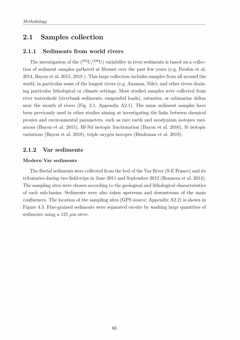
Methodology

2.1 Samples collection

2.1.1 Sediments from world rivers

The investigation of the (234U/238U) variability in river sediments is based on a collec-tion of sediment samples gathered at Ifremer over the past few years (e.g. Freslon et al.2014, Bayon et al. 2015, 2018 ). This large collection includes samples from all around theworld, in particular some of the longest rivers (e.g. Amazon, Nile), and other rivers drain-ing particular lithological or climate settings. Most studied samples were collected fromriver watersheds (riverbank sediments, suspended loads), estuaries, or submarine deltasnear the mouth of rivers (Fig. 2.1, Appendix A2.1). The same sediment samples havebeen previously used in other studies aiming at investigating the links between chemicalproxies and environmental parameters, such as rare earth and neodynium isotopes vari-ations (Bayon et al. 2015), Hf-Nd isotopic fractionation (Bayon et al. 2016), Si isotopicvariations (Bayon et al. 2018), triple oxygen isotopes (Bindeman et al. 2019).

2.1.2 Var sediments

Modern Var sediments

The fluvial sediments were collected from the bed of the Var River (S-E France) and itstributaries during two field-trips in June 2011 and September 2012 (Bonneau et al. 2014).The sampling sites were chosen according to the geological and lithological characteristicsof each sub-basins. Sediments were also taken upstream and downstream of the mainconfluences. The location of the sampling sites (GPS source; Appendix A2.2) is shown inFigure 4.3. Fine-grained sediments were separated on-site by washing large quantities ofsediments using a 125 µm sieve.

66

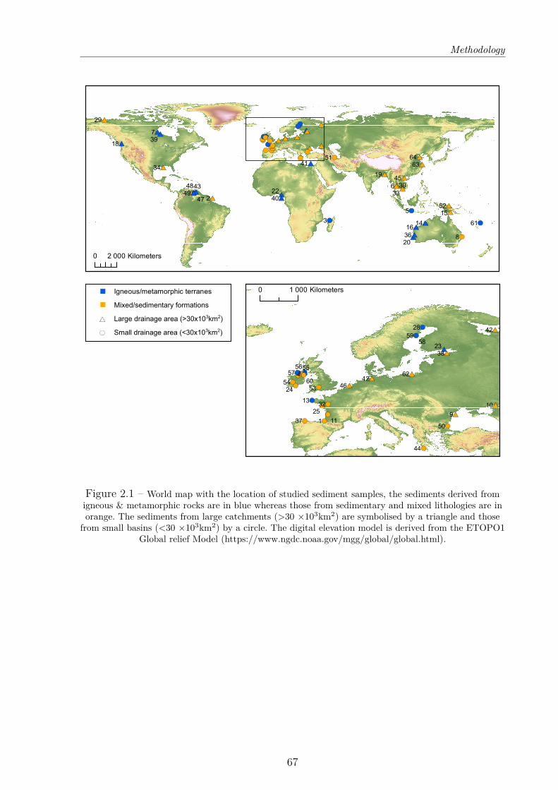
Methodology

&-

#*

&-

&-

&-

#*

#*

&-

#* #*&-

#*&-

#*

#*

#*

&-#*

#*

#*

&-

#*

#*

&-#*

&-&-

&-#*

#*

&-

&-

#*

#*

&-

#*

&-

#*#*

#*

#*

#*

#*

&-

#*

#*

&-#*#*

&-&-

#*

&-&-&-&-&-

&-&-

&-

&-

#*

#*#*

8

7

6

5

3

2

6463

61

52

51

4948

47

4543

41

40

39

36

34

3330

29

22

20

19

18

16

15

14

0 2 000 Kilometers

&-

&-

#*

#*

&-

#*

&-

&-&-

#*

&-

#*

&-&-

&-

&-

&-

&-

&-

#*

#*

#*

&-

#*

&-

&-&-

&-&-&-

&-&-

&- #*

9

4

1

6260

5958

575655

5453

50

46

44

42

38

37

32

28

25

24

23

13

12

11

10

0 1 000 KilometersIgneous/metamorphic terranes

Mixed/sedimentary formations

Large drainage area (>30x103km2)

Small drainage area (<30x103km2)

*

-

Figure 2.1 – World map with the location of studied sediment samples, the sediments derived fromigneous & metamorphic rocks are in blue whereas those from sedimentary and mixed lithologies are inorange. The sediments from large catchments (>30 ×103km2) are symbolised by a triangle and those

from small basins (<30 ×103km2) by a circle. The digital elevation model is derived from the ETOPO1Global relief Model (https://www.ngdc.noaa.gov/mgg/global/global.html).

67

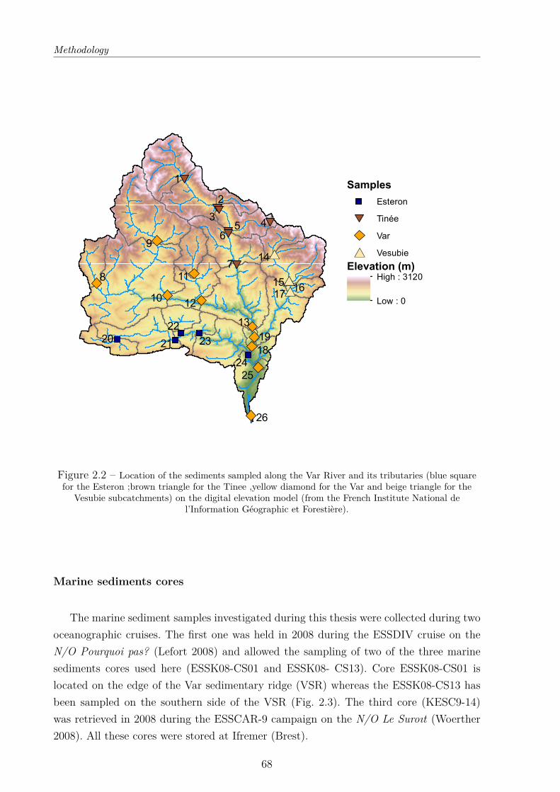
Methodology

"" #*

""

""

"

"

"

"

"

"

#*

#*

#*

9

7

1

3

2

645

8

17

14

15

18

26

13

1210

1922

16

20 21

24

23

25

11

Samples

Esteron

Tinée

" Var

#* Vesubie

Elevation (m)High : 3120

Low : 0

Figure 2.2 – Location of the sediments sampled along the Var River and its tributaries (blue squarefor the Esteron ;brown triangle for the Tinee ,yellow diamond for the Var and beige triangle for the

Vesubie subcatchments) on the digital elevation model (from the French Institute National del’Information Géographic et Forestière).

Marine sediments cores

The marine sediment samples investigated during this thesis were collected during twooceanographic cruises. The first one was held in 2008 during the ESSDIV cruise on theN/O Pourquoi pas? (Lefort 2008) and allowed the sampling of two of the three marinesediments cores used here (ESSK08-CS01 and ESSK08- CS13). Core ESSK08-CS01 islocated on the edge of the Var sedimentary ridge (VSR) whereas the ESSK08-CS13 hasbeen sampled on the southern side of the VSR (Fig. 2.3). The third core (KESC9-14)was retrieved in 2008 during the ESSCAR-9 campaign on the N/O Le Suroıt (Woerther2008). All these cores were stored at Ifremer (Brest).

68

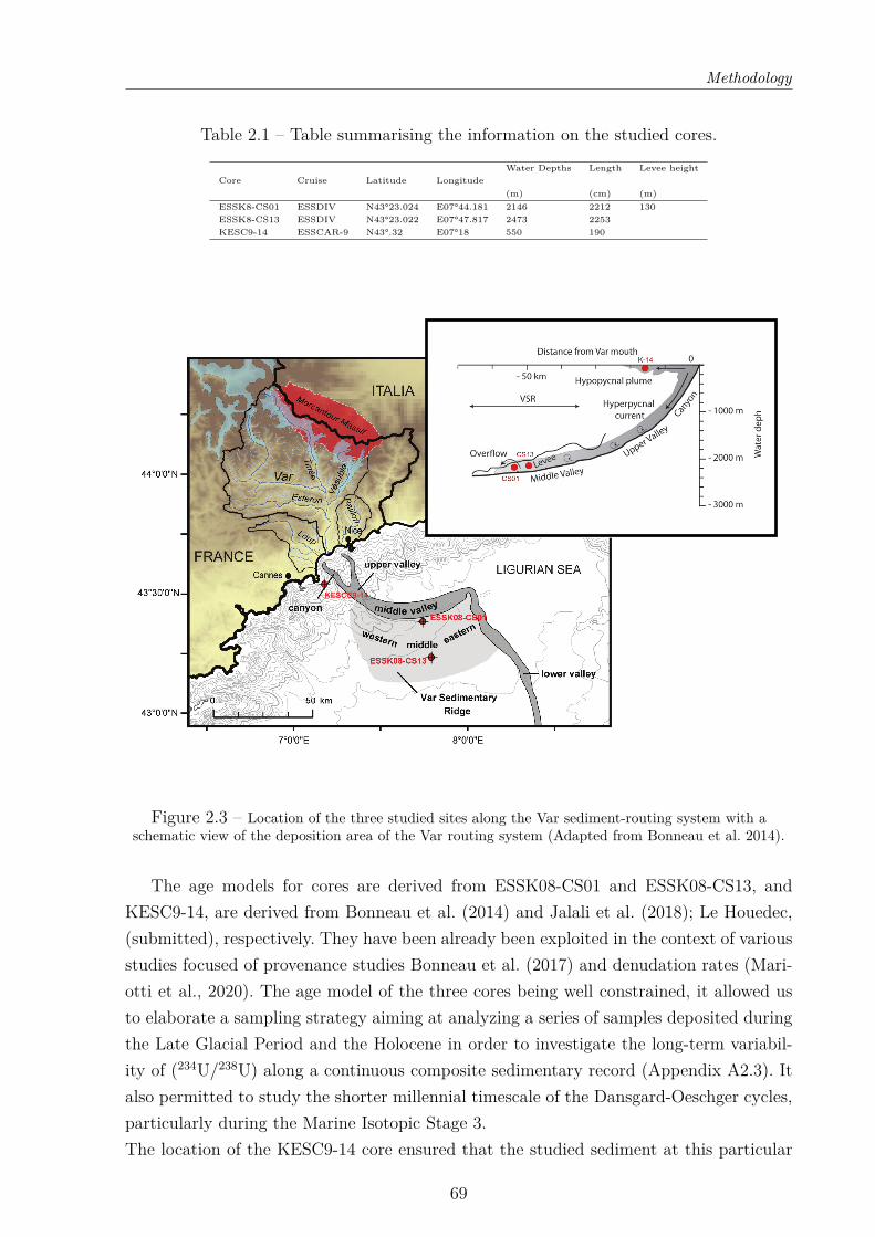
Methodology

Table 2.1 – Table summarising the information on the studied cores.

Core Cruise Latitude LongitudeWater Depths

(m)

Length

(cm)

Levee height

(m)ESSK8-CS01 ESSDIV N43°23.024 E07°44.181 2146 2212 130ESSK8-CS13 ESSDIV N43°23.022 E07°47.817 2473 2253KESC9-14 ESSCAR-9 N43°.32 E07°18 550 190

KESCC9-14

Figure 2.3 – Location of the three studied sites along the Var sediment-routing system with aschematic view of the deposition area of the Var routing system (Adapted from Bonneau et al. 2014).

The age models for cores are derived from ESSK08-CS01 and ESSK08-CS13, andKESC9-14, are derived from Bonneau et al. (2014) and Jalali et al. (2018); Le Houedec,(submitted), respectively. They have been already been exploited in the context of variousstudies focused of provenance studies Bonneau et al. (2017) and denudation rates (Mari-otti et al., 2020). The age model of the three cores being well constrained, it allowed usto elaborate a sampling strategy aiming at analyzing a series of samples deposited duringthe Late Glacial Period and the Holocene in order to investigate the long-term variabil-ity of (234U/238U) along a continuous composite sedimentary record (Appendix A2.3). Italso permitted to study the shorter millennial timescale of the Dansgard-Oeschger cycles,particularly during the Marine Isotopic Stage 3.The location of the KESC9-14 core ensured that the studied sediment at this particular

69

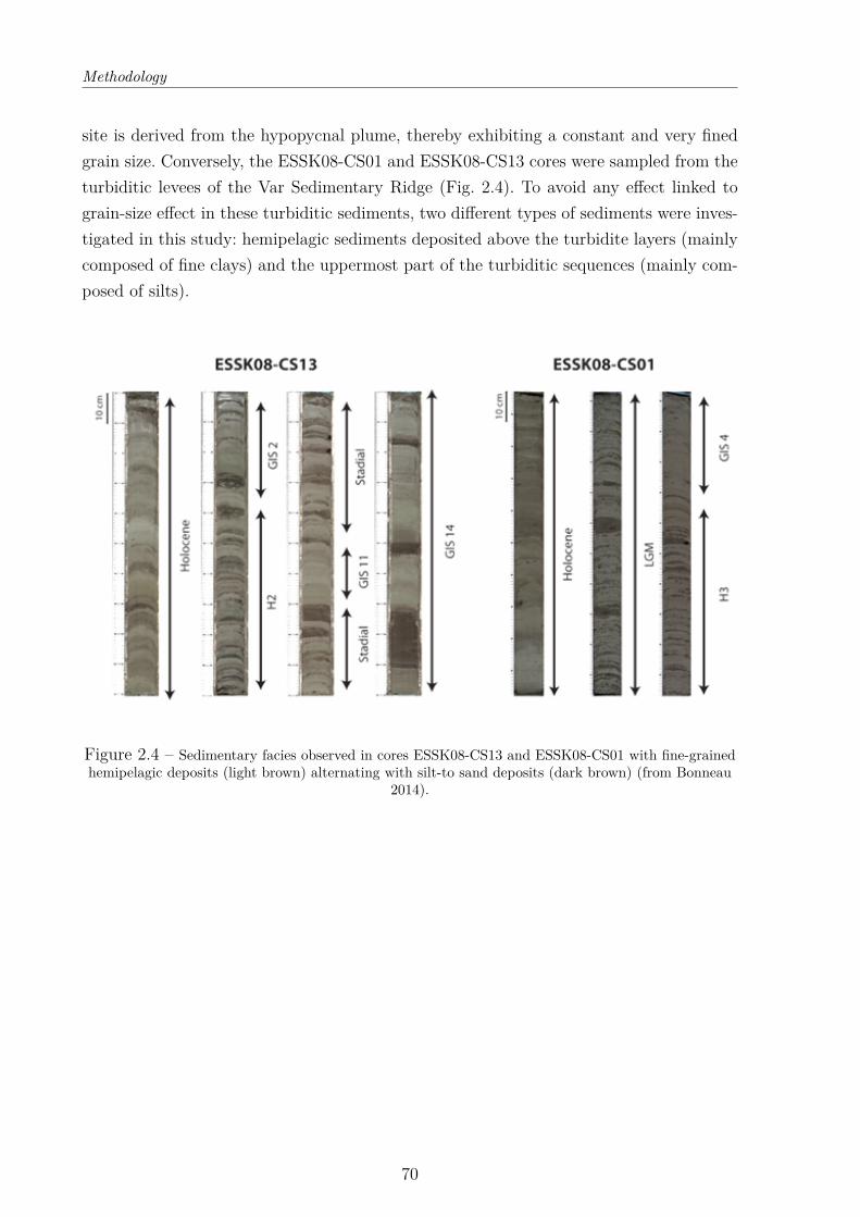
Methodology

site is derived from the hypopycnal plume, thereby exhibiting a constant and very finedgrain size. Conversely, the ESSK08-CS01 and ESSK08-CS13 cores were sampled from theturbiditic levees of the Var Sedimentary Ridge (Fig. 2.4). To avoid any effect linked tograin-size effect in these turbiditic sediments, two different types of sediments were inves-tigated in this study: hemipelagic sediments deposited above the turbidite layers (mainlycomposed of fine clays) and the uppermost part of the turbiditic sequences (mainly com-posed of silts).

Figure 2.4 – Sedimentary facies observed in cores ESSK08-CS13 and ESSK08-CS01 with fine-grainedhemipelagic deposits (light brown) alternating with silt-to sand deposits (dark brown) (from Bonneau

2014).

70

Methodology

2.2 Samples preparation

2.2.1 Reagent and labware

The study dealing with the sediments from the world river systems was performedat Ifremer (Brest, France), with all chemical preparations including the separation andpurification of uranium being conducted in a Class 1000 (ISO 6) clean laboratory. HNO3

and HCl solutions (commercial grade, Merck) were double distilled using a sub-boilingsystem. Hydrogen peroxide H2O2 (Trace select, 30%), acid acetic and hydroxylamine fromFisher Scientific (Loughborough, UK) were also used. All diluted reagents were preparedusing Millipore Milli-Q water (18.2 MΩ·cm at 25°C).

The Var sediments, including both fluvial and marine sediment samples, were preparedand analyzed in a Class 10 cleanroom at the Wollongong Isotopes Geochronology Labo-ratory from the University of Wollongong (Wollongong, Australia). Reagents used duringthe sequential extraction (acetic acid, hydroxylamine hydrochrloride, hydrogen peroxide)and acid dissolution (HF, HCl, HNO3) were of Ultrapure grade. The reagents used for thecolumn chromatography were of Suprapur grade.

2.2.2 Grain-size separation

Because grain size may play an important role in measured uranium activity ratio, anefficient and robust grain size separation method needs to be applied prior to the analyses,aiming at separating the fine <63 µm detrital fraction.

Ifremer methods

About 3 g of dry sediments were placed into 50 mL centrifuge tubes, filled with 18.2MΩ water and shaken manually. The suspended sediments were sieved at <63 µm using18.2 MΩ water.

UOW methods

Bulk sediments were first dry sieved in order to only keep the fraction <2 mm. Ap-proximately 10 g of the finest fraction was placed in a 50 mL centrifuge tube with ∼0.25g of sodium hexametaphosphate. Each centrifuge tubes were then filled up with around30 mL of dionized (DI) water and placed on a mixing wheel overnight. The sediments insuspension were then wet sieved using a 63 µm sieve and DI water. The fraction <63 µmwas transferred to a clean centrifuge tube, and the DI water was removed by centrifuga-tion (15 min – 4000 rpm). The 63-200 µm fraction was removed of the sieved using a clean

71

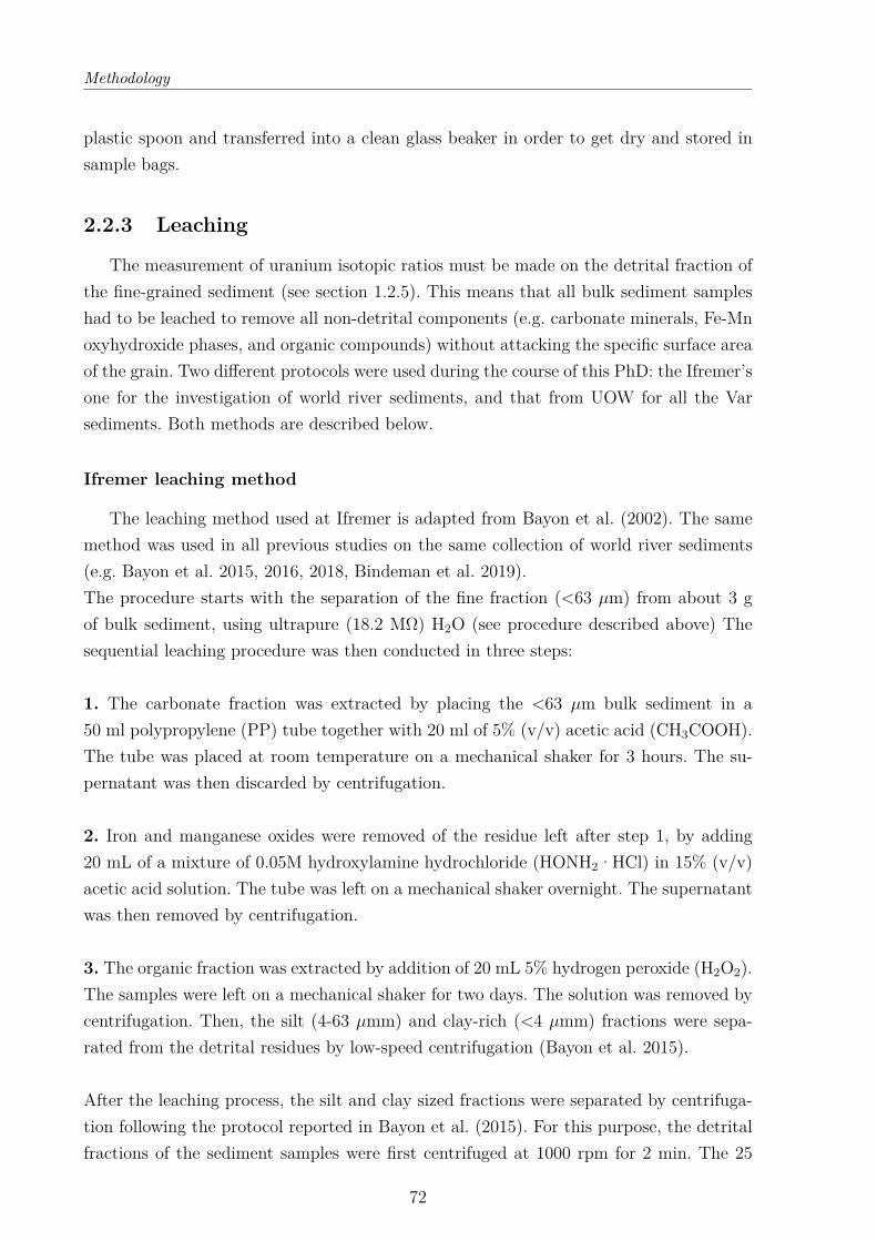
Methodology

plastic spoon and transferred into a clean glass beaker in order to get dry and stored insample bags.

2.2.3 Leaching

The measurement of uranium isotopic ratios must be made on the detrital fraction ofthe fine-grained sediment (see section 1.2.5). This means that all bulk sediment sampleshad to be leached to remove all non-detrital components (e.g. carbonate minerals, Fe-Mnoxyhydroxide phases, and organic compounds) without attacking the specific surface areaof the grain. Two different protocols were used during the course of this PhD: the Ifremer’sone for the investigation of world river sediments, and that from UOW for all the Varsediments. Both methods are described below.

Ifremer leaching method

The leaching method used at Ifremer is adapted from Bayon et al. (2002). The samemethod was used in all previous studies on the same collection of world river sediments(e.g. Bayon et al. 2015, 2016, 2018, Bindeman et al. 2019).The procedure starts with the separation of the fine fraction (<63 µm) from about 3 gof bulk sediment, using ultrapure (18.2 MΩ) H2O (see procedure described above) Thesequential leaching procedure was then conducted in three steps:

1. The carbonate fraction was extracted by placing the <63 µm bulk sediment in a50 ml polypropylene (PP) tube together with 20 ml of 5% (v/v) acetic acid (CH3COOH).The tube was placed at room temperature on a mechanical shaker for 3 hours. The su-pernatant was then discarded by centrifugation.

2. Iron and manganese oxides were removed of the residue left after step 1, by adding20 mL of a mixture of 0.05M hydroxylamine hydrochloride (HONH2·HCl) in 15% (v/v)acetic acid solution. The tube was left on a mechanical shaker overnight. The supernatantwas then removed by centrifugation.

3. The organic fraction was extracted by addition of 20 mL 5% hydrogen peroxide (H2O2).The samples were left on a mechanical shaker for two days. The solution was removed bycentrifugation. Then, the silt (4-63 µmm) and clay-rich (<4 µmm) fractions were sepa-rated from the detrital residues by low-speed centrifugation (Bayon et al. 2015).

After the leaching process, the silt and clay sized fractions were separated by centrifuga-tion following the protocol reported in Bayon et al. (2015). For this purpose, the detritalfractions of the sediment samples were first centrifuged at 1000 rpm for 2 min. The 25

72

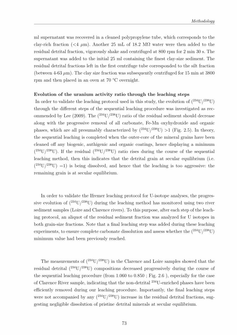
Methodology

ml supernatant was recovered in a cleaned polypropylene tube, which corresponds to theclay-rich fraction (<4 µm). Another 25 mL of 18.2 MΩ water were then added to theresidual detrital fraction, vigorously shake and centrifuged at 800 rpm for 2 min 30 s. Thesupernatant was added to the initial 25 ml containing the finest clay-size sediment. Theresidual detrital fractions left in the first centrifuge tube corresponded to the silt fraction(between 4-63 µm). The clay size fraction was subsequently centrifuged for 15 min at 3800rpm and then placed in an oven at 70 °C overnight.

Evolution of the uranium activity ratio through the leaching stepsIn order to validate the leaching protocol used in this study, the evolution of (234U/238U)through the different steps of the sequential leaching procedure was investigated as rec-ommended by Lee (2009). The (234U/238U) ratio of the residual sediment should decreasealong with the progressive removal of all carbonate, Fe-Mn oxyhydroxide and organicphases, which are all presumably characterized by (234U/238U) >1 (Fig. 2.5). In theory,the sequential leaching is completed when the outer-core of the mineral grains have beencleaned off any biogenic, authigenic and organic coatings, hence displaying a minimum(234U/238U). If the residual (234U/238U) ratio rises during the course of the sequentialleaching method, then this indicates that the detrital grain at secular equilibrium (i.e.(234U/238U) =1) is being dissolved, and hence that the leaching is too aggressive: theremaining grain is at secular equilibrium.

In order to validate the Ifremer leaching protocol for U-isotope analyses, the progres-sive evolution of (234U/238U) during the leaching method has monitored using two riversediment samples (Loire and Clarence rivers). To this purpose, after each step of the leach-ing protocol, an aliquot of the residual sediment fraction was analyzed for U isotopes inboth grain-size fractions. Note that a final leaching step was added during these leachingexperiments, to ensure complete carbonate dissolution and assess whether the (234U/238U)minimum value had been previously reached.

The measurements of (234U/238U) in the Clarence and Loire samples showed that theresidual detrital (234U/238U) compositions decreased progressively during the course ofthe sequential leaching procedure (from 1.060 to 0.850 ; Fig. 2.6 ), especially for the caseof Clarence River sample, indicating that the non-detrital 234U-enriched phases have beenefficiently removed during our leaching procedure. Importantly, the final leaching stepswere not accompanied by any (234U/238U) increase in the residual detrital fractions, sug-gesting negligible dissolution of pristine detrital minerals at secular equilibrium.

73

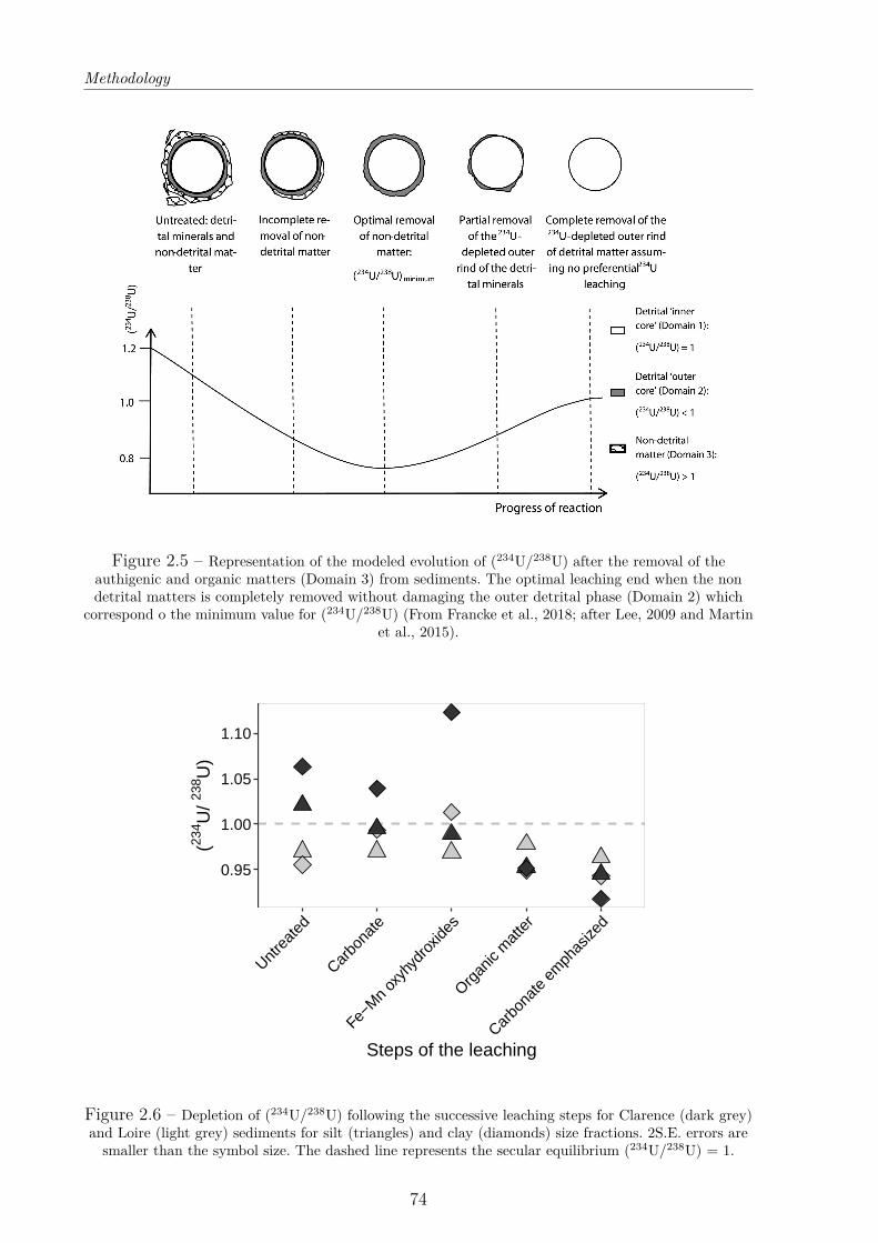
Methodology

Figure 2.5 – Representation of the modeled evolution of (234U/238U) after the removal of theauthigenic and organic matters (Domain 3) from sediments. The optimal leaching end when the nondetrital matters is completely removed without damaging the outer detrital phase (Domain 2) which

correspond o the minimum value for (234U/238U) (From Francke et al., 2018; after Lee, 2009 and Martinet al., 2015).

0.95

1.00

1.05

1.10

Untre

ated

Carbo

nate

Fe−M

n ox

yhyd

roxid

es

Organ

ic m

atte

r

Carbo

nate

em

phas

ized

Steps of the leaching

(234 U

/ 238 U

)

Figure 2.6 – Depletion of (234U/238U) following the successive leaching steps for Clarence (dark grey)and Loire (light grey) sediments for silt (triangles) and clay (diamonds) size fractions. 2S.E. errors aresmaller than the symbol size. The dashed line represents the secular equilibrium (234U/238U) = 1.

74

Methodology

Note that a second test was also conducted to assess whether a possible fractiona-tion could occur between 234U and 238U during the leaching method. To this purpose,two geological reference materials (BCR-2 and BHVO-2), with known (234U/238U) ratios,were leached and analyzed. The obtained (234U/234U) are within the error range of theaccepted values (BCR-2: 1.006 ±0.004 and BHVO-2: 1.006 ±0.002), hence showing thatour leaching method does not involve any particular (234U/234U) fractionation.

Sonication leaching – UOW method

The method used during the process of the Var sediment samples was developed byFrancke et al. (2018) in the Wollongong Isotopes Geochronology Laboratory (WIGL) ofWollongong University. This method is rapid, hence allows to process large datasets ofsamples.The sequential leaching procedure involves five distinct steps.

1. The first step was used to remove the water-soluble fraction. Approximately 1 g ofdry sediment were placed into 50 mL PP centrifuge tubes with 35 mL of water. Thecentrifuges tubes were shaken manually and then placed on a mixing wheel for minimum1 hour. In order to remove the water, they were centrifuged at 4000 rpm for 10 minutesand the supernatant was then discarded.

2. The second stage corresponds to the removal of the exchangeable fraction. For thispurpose, 16 mL of 0.5M magnesium nitrate (Mg(NO3)2) was added to each centrifugetubes inside a fume hood. The centrifuge tubes were manually shaken and then sonicated3 min at 20°C. The sediments were centrifuged at 4000 rpm for 10 min and the super-natant was discarded.

3. The third step corresponds to the removal of the carbonate fraction. In each cen-trifuge tubes, 20 mL of 1M sodium acetate (NaOAc) solution was added. Each tube wasmanually shaken and then sonicated for 15 min at 20°C, taking great care to release anyoverpressure every 5 minutes by opening the tubes. They were centrifuged at 4000 rpmfor 10 minutes to remove the supernatant. The centrifuges tubes were filled with water,shaken and centrifuged again at 4000 rpm for 10 min in order to rinse the residual fraction.The sediments were transferred in PFA centrifuges tubes for the rest of the procedure byadding approximately 15 mL of water. Once transferred, the solution was removed aftercentrifugation at 4000 rpm for 15 min.

4. The fourth step was conducted to extract Fe and Mn oxide phases. About 20 mLof the 0.1M Hydroxylamine hydrochloride (NH2OH*HCl) solution was added in the PFAcentrifuge tubes. They were shaken until all sediments were in suspension and sonicated

75

Methodology

for 18 min at 80°C with releasing the pressure every 6 minutes and shaken then manually.The samples were then cooled off by putting the tubes in cold water for few minutes. Thesediments were centrifuged at 4000 rpm for 10 minutes and the solution is removed andrinsed with 40 mL of water which was then removed by centrifugation at 4000 rpm for 15min.

5. The final step aimed at removing organic matter and sulphides. A quantity of 26mL of 15% hydrogen peroxide (H2O2) and 0.02 M nitric acid (HNO3) solution was addedto each PFA centrifuge tube. They were then transferred into an ultrasonic bath for atotal of 6 times of 3 min each. Between each sonification period, the pressure was released.Whenever the reaction was too strong, the tubes were placed under cold water. Followingthe final ultrasonication step, the solution was removed after 10 minutes of centrifuga-tion at 4000 rpm. In all samples, 5 mL of 3.2M ammonium acetate (CH3COONH4) in20% v/v HNO3 solution was added to completely recover the uranium leach from theprevious solution. The tubes were manually shaken for 1 min and the solution was decantafter 10 min of centrifugation at 4000 rpm. The sediments were transferred into PP tubesback, and rinsed three times with 18.2 MΩ-H2O, followed by centrifugation. The residualsediments were then air dried inside a fume hood.

Comparison of the two-leaching protocol

In order to compare the two leaching protocols used during the course of this PhD,the same sediment samples used by Francke et al. (2018) to develop the UoW sequentialleaching protocol were analyzed using the Ifremer’s method. After each steps of the se-quential leaching procedure, a fraction of the residue was removed to analyze the evolutionof (234U/238U) during the procedure. The (234U/238U) values obtained for these two testsamples using the Ifremer protocol agree well (<5 % of difference) with the data obtainedusing the procedure of Francke et al. (2018).

2.2.4 Sediments dissolution

Alkaline digestion in furnace

The dry powders of detrital fractions were dried in an oven at 70°C for 24 hours toremove all humidity. About 0.100 g of a mixed 229Th-236U tracer-solution (composition inTable 2.2) was added into a cleaned glassy carbon crucible and evaporated on hotplate.Then about 0,050 g of detrital sediment was added in the crucible together with ∼0.300-0.500 g of sodium hydroxide pellets (NaOH) and ∼0.800 g of sodium peroxide powder(Na2O2). The crucibles were placed into an furnace at 650°C for 12 minutes. After alkalinefusion, 10 mL of water 18.2 MΩ-H2O was added into the cooling crucible. The mixture wastransferred into a polypropylene 50 ml centrifuged tubes, and each crucible was cleaned

76

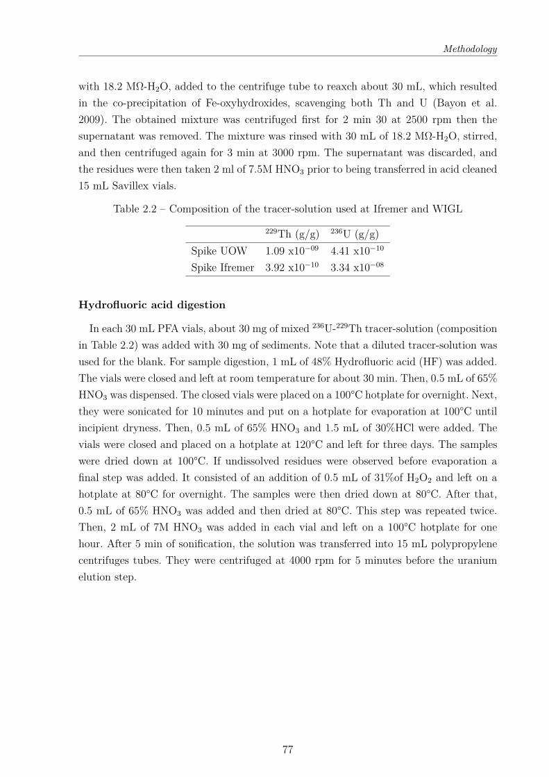
Methodology

with 18.2 MΩ-H2O, added to the centrifuge tube to reaxch about 30 mL, which resultedin the co-precipitation of Fe-oxyhydroxides, scavenging both Th and U (Bayon et al.2009). The obtained mixture was centrifuged first for 2 min 30 at 2500 rpm then thesupernatant was removed. The mixture was rinsed with 30 mL of 18.2 MΩ-H2O, stirred,and then centrifuged again for 3 min at 3000 rpm. The supernatant was discarded, andthe residues were then taken 2 ml of 7.5M HNO3 prior to being transferred in acid cleaned15 mL Savillex vials.

Table 2.2 – Composition of the tracer-solution used at Ifremer and WIGL

229Th (g/g) 236U (g/g)Spike UOW 1.09 x10−09 4.41 x10−10

Spike Ifremer 3.92 x10−10 3.34 x10−08

Hydrofluoric acid digestion

In each 30 mL PFA vials, about 30 mg of mixed 236U-229Th tracer-solution (compositionin Table 2.2) was added with 30 mg of sediments. Note that a diluted tracer-solution wasused for the blank. For sample digestion, 1 mL of 48% Hydrofluoric acid (HF) was added.The vials were closed and left at room temperature for about 30 min. Then, 0.5 mL of 65%HNO3 was dispensed. The closed vials were placed on a 100°C hotplate for overnight. Next,they were sonicated for 10 minutes and put on a hotplate for evaporation at 100°C untilincipient dryness. Then, 0.5 mL of 65% HNO3 and 1.5 mL of 30%HCl were added. Thevials were closed and placed on a hotplate at 120°C and left for three days. The sampleswere dried down at 100°C. If undissolved residues were observed before evaporation afinal step was added. It consisted of an addition of 0.5 mL of 31%of H2O2 and left on ahotplate at 80°C for overnight. The samples were then dried down at 80°C. After that,0.5 mL of 65% HNO3 was added and then dried at 80°C. This step was repeated twice.Then, 2 mL of 7M HNO3 was added in each vial and left on a 100°C hotplate for onehour. After 5 min of sonification, the solution was transferred into 15 mL polypropylenecentrifuges tubes. They were centrifuged at 4000 rpm for 5 minutes before the uraniumelution step.

77

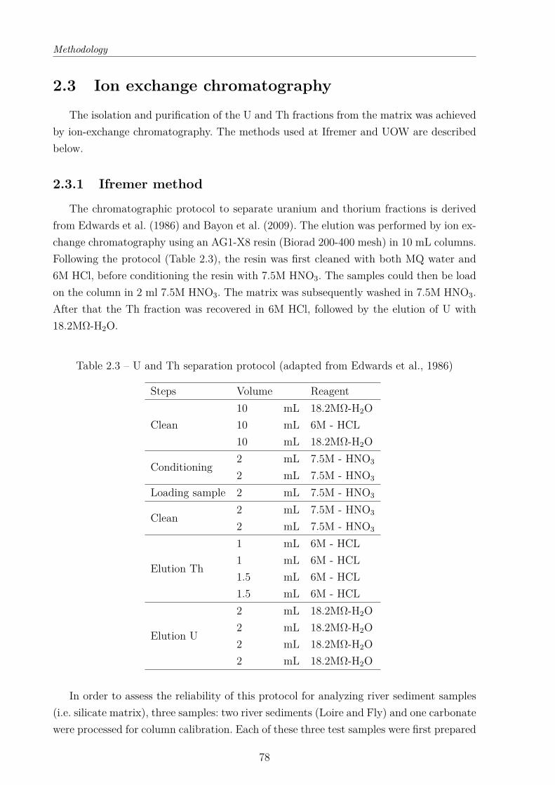
Methodology

2.3 Ion exchange chromatographyThe isolation and purification of the U and Th fractions from the matrix was achieved

by ion-exchange chromatography. The methods used at Ifremer and UOW are describedbelow.

2.3.1 Ifremer method

The chromatographic protocol to separate uranium and thorium fractions is derivedfrom Edwards et al. (1986) and Bayon et al. (2009). The elution was performed by ion ex-change chromatography using an AG1-X8 resin (Biorad 200-400 mesh) in 10 mL columns.Following the protocol (Table 2.3), the resin was first cleaned with both MQ water and6M HCl, before conditioning the resin with 7.5M HNO3. The samples could then be loadon the column in 2 ml 7.5M HNO3. The matrix was subsequently washed in 7.5M HNO3.After that the Th fraction was recovered in 6M HCl, followed by the elution of U with18.2MΩ-H2O.

Table 2.3 – U and Th separation protocol (adapted from Edwards et al., 1986)

Steps Volume Reagent

Clean10 mL 18.2MΩ-H2O10 mL 6M - HCL10 mL 18.2MΩ-H2O

Conditioning2 mL 7.5M - HNO3

2 mL 7.5M - HNO3

Loading sample 2 mL 7.5M - HNO3

Clean2 mL 7.5M - HNO3

2 mL 7.5M - HNO3

Elution Th

1 mL 6M - HCL1 mL 6M - HCL1.5 mL 6M - HCL1.5 mL 6M - HCL

Elution U

2 mL 18.2MΩ-H2O2 mL 18.2MΩ-H2O2 mL 18.2MΩ-H2O2 mL 18.2MΩ-H2O

In order to assess the reliability of this protocol for analyzing river sediment samples(i.e. silicate matrix), three samples: two river sediments (Loire and Fly) and one carbonatewere processed for column calibration. Each of these three test samples were first prepared

78

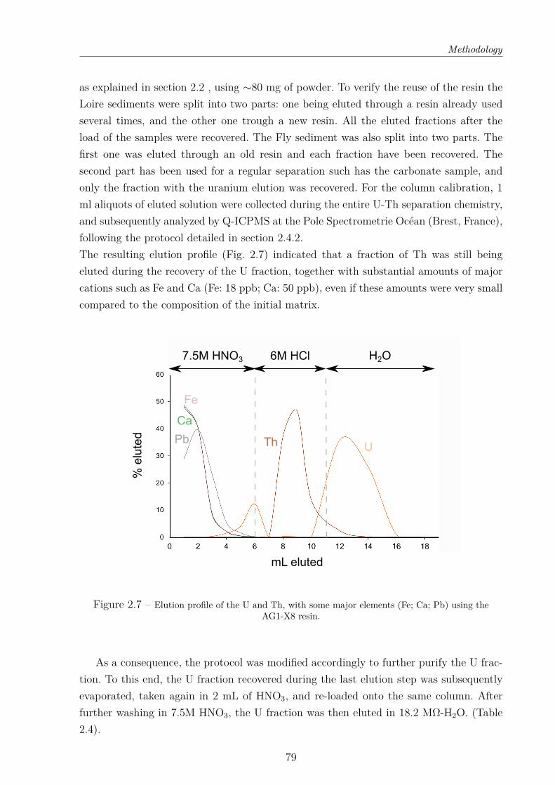
Methodology

as explained in section 2.2 , using ∼80 mg of powder. To verify the reuse of the resin theLoire sediments were split into two parts: one being eluted through a resin already usedseveral times, and the other one trough a new resin. All the eluted fractions after theload of the samples were recovered. The Fly sediment was also split into two parts. Thefirst one was eluted through an old resin and each fraction have been recovered. Thesecond part has been used for a regular separation such has the carbonate sample, andonly the fraction with the uranium elution was recovered. For the column calibration, 1ml aliquots of eluted solution were collected during the entire U-Th separation chemistry,and subsequently analyzed by Q-ICPMS at the Pole Spectrometrie Océan (Brest, France),following the protocol detailed in section 2.4.2.The resulting elution profile (Fig. 2.7) indicated that a fraction of Th was still beingeluted during the recovery of the U fraction, together with substantial amounts of majorcations such as Fe and Ca (Fe: 18 ppb; Ca: 50 ppb), even if these amounts were very smallcompared to the composition of the initial matrix.

7.5M HNO3 6M HCl H2O

% e

lute

d

mL eluted

U

Fe

Pb

Ca

Th

Figure 2.7 – Elution profile of the U and Th, with some major elements (Fe; Ca; Pb) using theAG1-X8 resin.

As a consequence, the protocol was modified accordingly to further purify the U frac-tion. To this end, the U fraction recovered during the last elution step was subsequentlyevaporated, taken again in 2 mL of HNO3, and re-loaded onto the same column. Afterfurther washing in 7.5M HNO3, the U fraction was then eluted in 18.2 MΩ-H2O. (Table2.4).

79

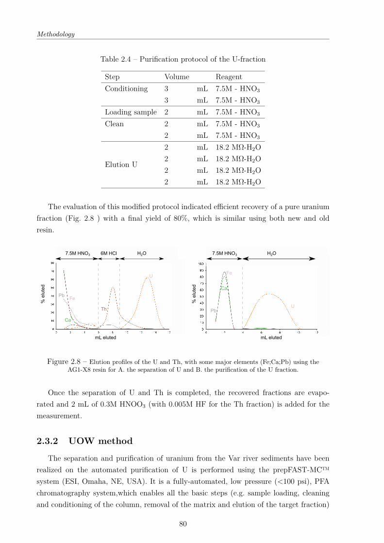
Methodology

Table 2.4 – Purification protocol of the U-fraction

Step Volume ReagentConditioning 3 mL 7.5M - HNO3

3 mL 7.5M - HNO3

Loading sample 2 mL 7.5M - HNO3

Clean 2 mL 7.5M - HNO3

2 mL 7.5M - HNO3

Elution U

2 mL 18.2 MΩ-H2O2 mL 18.2 MΩ-H2O2 mL 18.2 MΩ-H2O2 mL 18.2 MΩ-H2O

The evaluation of this modified protocol indicated efficient recovery of a pure uraniumfraction (Fig. 2.8 ) with a final yield of 80%, which is similar using both new and oldresin.

7.5M HNO3 6M HCl H2O

% e

lute

d

mL eluted

7.5M HNO3 H2O

% e

lute

d

mL eluted

U

U

Fe

Fe

Pb

Pb

Ca

Ca

Th

Figure 2.8 – Elution profiles of the U and Th, with some major elements (Fe;Ca;Pb) using theAG1-X8 resin for A. the separation of U and B. the purification of the U fraction.

Once the separation of U and Th is completed, the recovered fractions are evapo-rated and 2 mL of 0.3M HNOO3 (with 0.005M HF for the Th fraction) is added for themeasurement.

2.3.2 UOW method

The separation and purification of uranium from the Var river sediments have beenrealized on the automated purification of U is performed using the prepFAST-MC™system (ESI, Omaha, NE, USA). It is a fully-automated, low pressure (<100 psi), PFAchromatography system,which enables all the basic steps (e.g. sample loading, cleaningand conditioning of the column, removal of the matrix and elution of the target fraction)

80

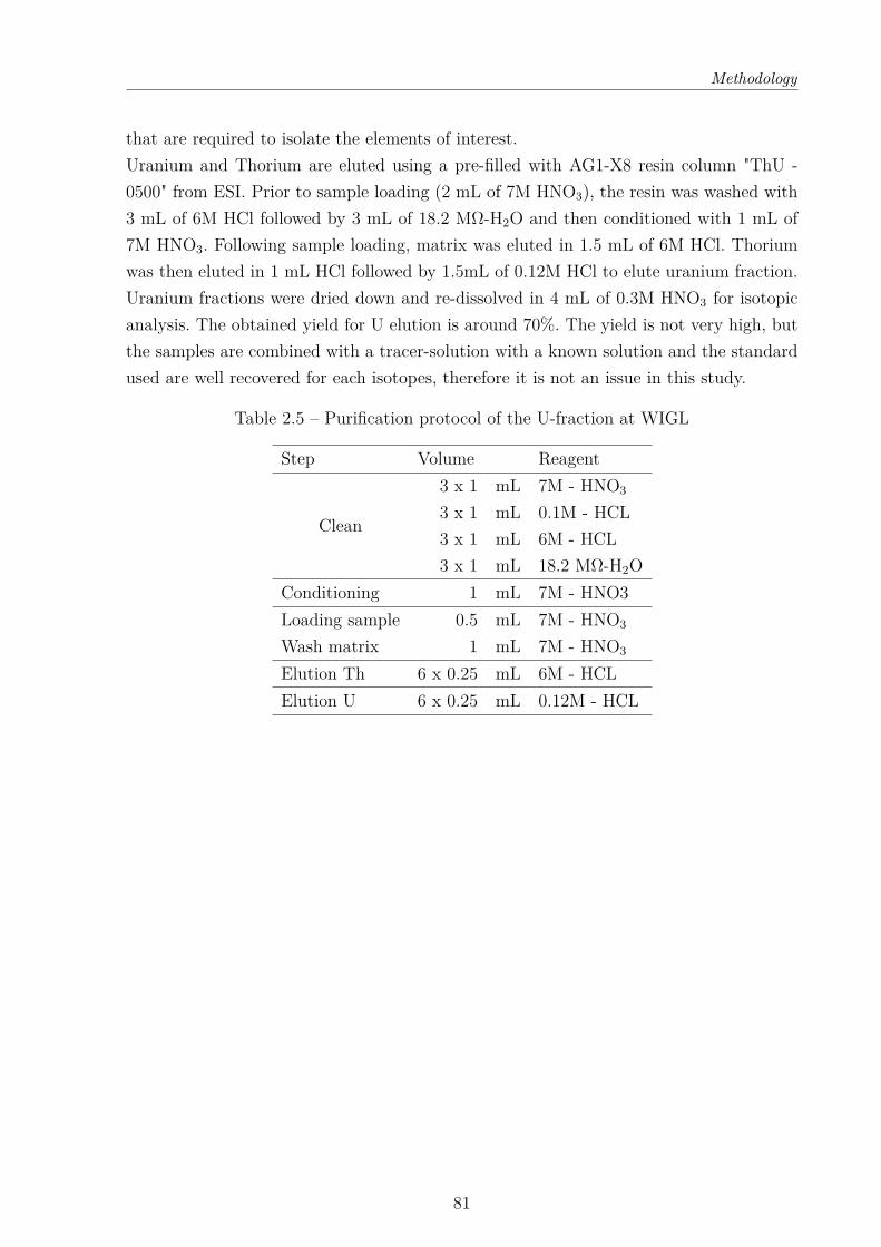
Methodology

that are required to isolate the elements of interest.Uranium and Thorium are eluted using a pre-filled with AG1-X8 resin column "ThU -0500" from ESI. Prior to sample loading (2 mL of 7M HNO3), the resin was washed with3 mL of 6M HCl followed by 3 mL of 18.2 MΩ-H2O and then conditioned with 1 mL of7M HNO3. Following sample loading, matrix was eluted in 1.5 mL of 6M HCl. Thoriumwas then eluted in 1 mL HCl followed by 1.5mL of 0.12M HCl to elute uranium fraction.Uranium fractions were dried down and re-dissolved in 4 mL of 0.3M HNO3 for isotopicanalysis. The obtained yield for U elution is around 70%. The yield is not very high, butthe samples are combined with a tracer-solution with a known solution and the standardused are well recovered for each isotopes, therefore it is not an issue in this study.

Table 2.5 – Purification protocol of the U-fraction at WIGL

Step Volume Reagent

Clean

3 x 1 mL 7M - HNO3

3 x 1 mL 0.1M - HCL3 x 1 mL 6M - HCL3 x 1 mL 18.2 MΩ-H2O

Conditioning 1 mL 7M - HNO3Loading sample 0.5 mL 7M - HNO3

Wash matrix 1 mL 7M - HNO3

Elution Th 6 x 0.25 mL 6M - HCLElution U 6 x 0.25 mL 0.12M - HCL

81

Methodology

2.4 Uranium analysesIsotopic measurements were performed on a ThermoFisher Neptune Multi-Collector

Inductively Coupled Plasma Mass Spectrometry (MC-ICP-MS, Thermo Scientific) at thePole Spectrometrie Océan (Brest, France) and on a ThermoFisher Neptune Plus MC-ICP-MS at the Wollongong Isotope Geochronology Laboratory (WIGL, Australia).Uraniumconcentration of the studied samples were calculated either by isotope dilution, based onthe measured isotopic composition of spiked samples by MC-ICPMS, or using QuadrupoleInductively Coupled Plasma Mass Spectrometry (Q-ICP-MS).

2.4.1 Isotopic measurement of Uranium isotopes

Uranium and thorium isotopes were measured on MC-ICP-MS. At the Pole Spec-trometrie Océan (Brest, France) the instrument was equipped with APEX HF desolvatingsystem and nebulizer PFA ST-2280 (100µL/min) as sample introduction system. Stan-dard sample and X skimmer cones were used. The sensitivity on 238U was generally 5 Vfor 10 ppb at low resolution.At the WIGL, the sample introduction system was composed of an APEX HF desolvatingsystem and nebulizer PFA ST-2280 (100µL/min). Jet sample and X skimmer cones wereused. The sensitivity on 238U was generally 6 V for 10 ppb at low resolution.The measurement of U isotopes required to use a Secondary Electron Multiplier (SEM) toincreased abundance sensitivity of the instrument. The mass 238 and 235 were analysed inthe Faraday cups. Mass 234, 236, 236.5 and 235.5 were measured in ion counting detectors.The purified fractions of U and Th were introduced in 2 mL of 0.3M HNO3 and 2 mL of0.3M HNO3 + 0.005M Hf respectively. Between each sample, the system was rinsed with0.3M HNO3. Samples analyses were realized in bloc of 40 cycles of measurements with anintegration time of 4s. Blank analyses were realized in bloc of 20 cycles of measurementwith an integration time of 4s.

— Mass correction: In order to correct from the instrumental mass bias and theFaraday/SEM yield, measured ratios were normalized to solution known referencematerial, using a standard-sample bracketing (SSB) method, during which onereference standard solution was analyzed every two samples. This standard solutioncorresponded to a synthetic standard (IRMM-184 or CRM U010 for U, and IRMM-035 or Th”U” for Th).

— Pic tailing: The measured signal of the mass of interest can suffer from largeinterferences related to the large abundance of a nearby mass, which creates a so-called tail effect. For instance, 238U is largely more abundant than 234U in naturalsediments (typically with order of magnitude of ∼105), hence the signal 238U pro-duces a ‘tail’ that can contribute to the measured signal on 236U (spiked) isotopes.Therefore, to correct the tail influence of 238U on the 234 and 236 atomic mass

82

Methodology

unit (i.e. amu), intensity between 236 amu are measured (235.5 and 236.5 amu)and substracting to the intensity of 236 amu (it implies that 235U do not createany tail). The same process applies for the possible tail of 232Th on both 230Th and229Th by measuring 231.5, 230.5, 229.5 and 228.5 amu.

2.4.2 Concentration

Measurement by isotopic dilution

The concentration of elements can be precisely calculated by isotopic dilution. For thispurpose, an isotopic tracer solution (i.e. spike) is added into the sample. It is composedspecifically with one or multiple isotopes from the element of interest with known isotopicabundances (Table 2.2). Then, the measurement of the mixture sample-spike allows oneto determine the concentration of the sample. As an example, the following equation wasused to determine U concentration in studied samples:

[U ]sample =[

236U]spike

×M238

M236× mspike

msample

×(

1 + 1137.88

)×(238U

236U samples−

238U236U spike

)(2.1)

with: M238 is the relative atomic mass of 238U, msample and mspike are the mass ofthe sample and the spike, respectively. In this thesis, the concentration of uranium andthorium of the world river sediments and half of the Var sediments were determined usingthis technique. The second half of measured U concentration on the Var core sedimentsamples were measured by Q-ICP-MS.

Measurement on Q-ICP-MS

The uranium and thorium concentrations of the sediment samples that were not de-termined by isotopic dilution were measured using an iCAP Q ICP-MS. The sampleintroduction system comprised a peristaltic pump, a PFA nebulizer and a spray chamber.Sample cone and skimmer cone were used. An internal standard (71D) was added to allsamples to correct from the instrumental derive.The standard (STD) mode was used to measure elements of interest (i.e. 115In, 238U).First, a calibration curve was done by analyzing a series of uranium and thorium standardsolutions (71A, Inorganic VenturesTM ) covering a concentration range from 0.05 ppb to100 ppb , yielding a correlation coefficient R2 >0.995. Prior to the ICP-MS analysis, analiquot of the studied samples was taken from the parent solution in 7M HNO3. It wasthen evaporated and taken up in 0.3M of HNO3 for analyze. Between each sample anal-ysis, the system was rinsed with 0.3M HNO3 and blanks intensity were measured andsubtracted from each sample. In order to validate the data, a quality control was set up

83

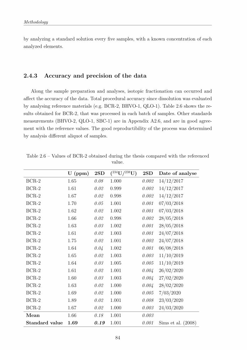
Methodology

by analyzing a standard solution every five samples, with a known concentration of eachanalyzed elements.

2.4.3 Accuracy and precision of the data

Along the sample preparation and analyses, isotopic fractionation can occurred andaffect the accuracy of the data. Total procedural accuracy since dissolution was evaluatedby analysing reference materials (e.g. BCR-2, BHVO-1, QLO-1). Table 2.6 shows the re-sults obtained for BCR-2, that was processed in each batch of samples. Other standardsmeasurements (BHVO-2, QLO-1, SBC-1) are in Appendix A2.6, and are in good agree-ment with the reference values. The good reproductibility of the process was determinedby analysis different aliquot of samples.

Table 2.6 – Values of BCR-2 obtained during the thesis compared with the referencedvalue.

U (ppm) 2SD (234U/238U) 2SD Date of analyseBCR-2 1.65 0.08 1.000 0.002 14/12/2017BCR-2 1.61 0.02 0.999 0.002 14/12/2017BCR-2 1.67 0.02 0.998 0.002 14/12/2017BCR-2 1.70 0.05 1.001 0.001 07/03/2018BCR-2 1.62 0.02 1.002 0.001 07/03/2018BCR-2 1.66 0.02 0.998 0.002 28/05/2018BCR-2 1.63 0.03 1.002 0.001 28/05/2018BCR-2 1.61 0.02 1.003 0.001 24/07/2018BCR-2 1.75 0.02 1.001 0.002 24/07/2018BCR-2 1.64 0.04 1.002 0.001 06/08/2018BCR-2 1.65 0.02 1.003 0.003 11/10/2019BCR-2 1.64 0.03 1.005 0.005 11/10/2019BCR-2 1.61 0.02 1.001 0.004 26/02/2020BCR-2 1.60 0.03 1.003 0.004 27/02/2020BCR-2 1.63 0.02 1.000 0.004 28/02/2020BCR-2 1.69 0.02 1.000 0.005 7/03/2020BCR-2 1.89 0.02 1.001 0.008 23/03/2020BCR-2 1.67 0.02 1.000 0.003 24/03/2020Mean 1.66 0.18 1.001 0.003Standard value 1.69 0.19 1.001 0.001 Sims et al. (2008)

84

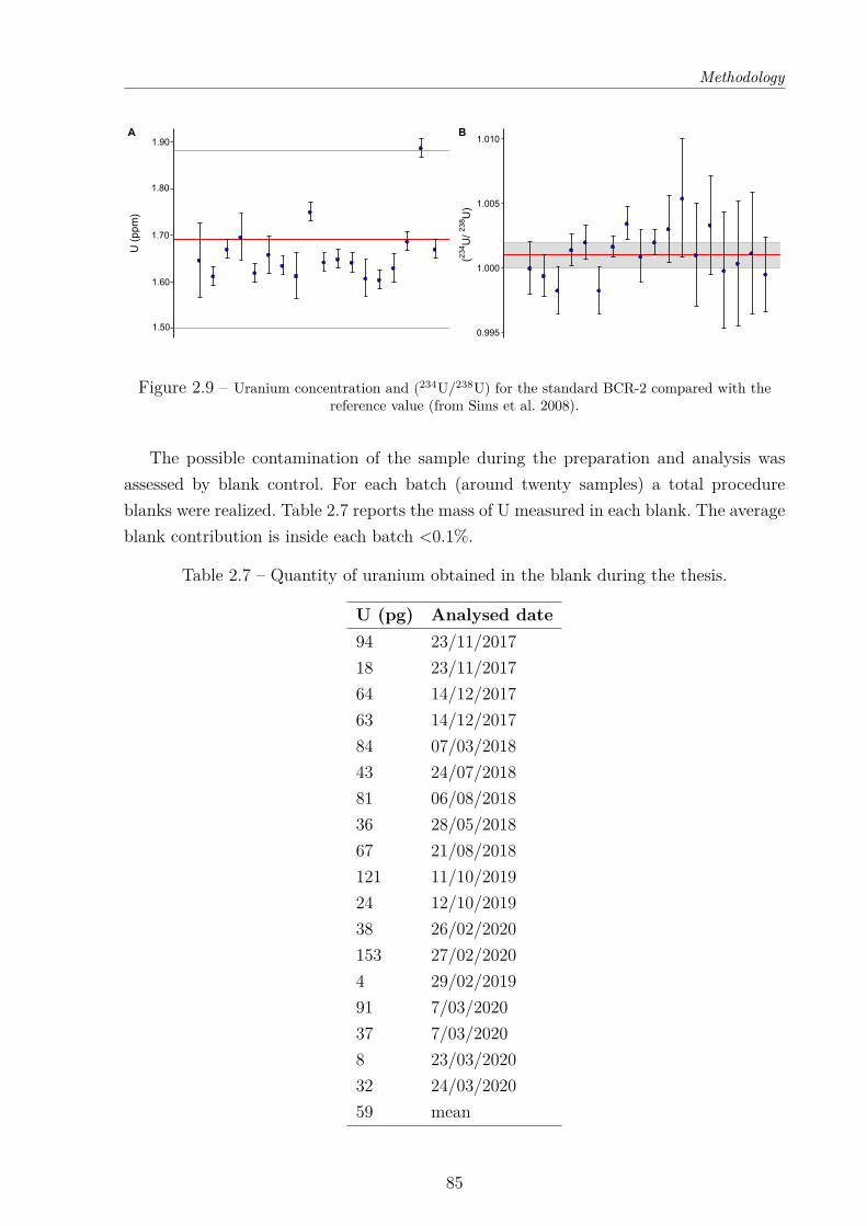
Methodology

1.90U

(pp

m)

A

0.995

1.000

1.005

1.010

(234 U

/ 238 U

)

B

1.80

1.70

1.60

1.50

Figure 2.9 – Uranium concentration and (234U/238U) for the standard BCR-2 compared with thereference value (from Sims et al. 2008).

The possible contamination of the sample during the preparation and analysis wasassessed by blank control. For each batch (around twenty samples) a total procedureblanks were realized. Table 2.7 reports the mass of U measured in each blank. The averageblank contribution is inside each batch <0.1%.

Table 2.7 – Quantity of uranium obtained in the blank during the thesis.

U (pg) Analysed date94 23/11/201718 23/11/201764 14/12/201763 14/12/201784 07/03/201843 24/07/201881 06/08/201836 28/05/201867 21/08/2018121 11/10/201924 12/10/201938 26/02/2020153 27/02/20204 29/02/201991 7/03/202037 7/03/20208 23/03/202032 24/03/202059 mean

85

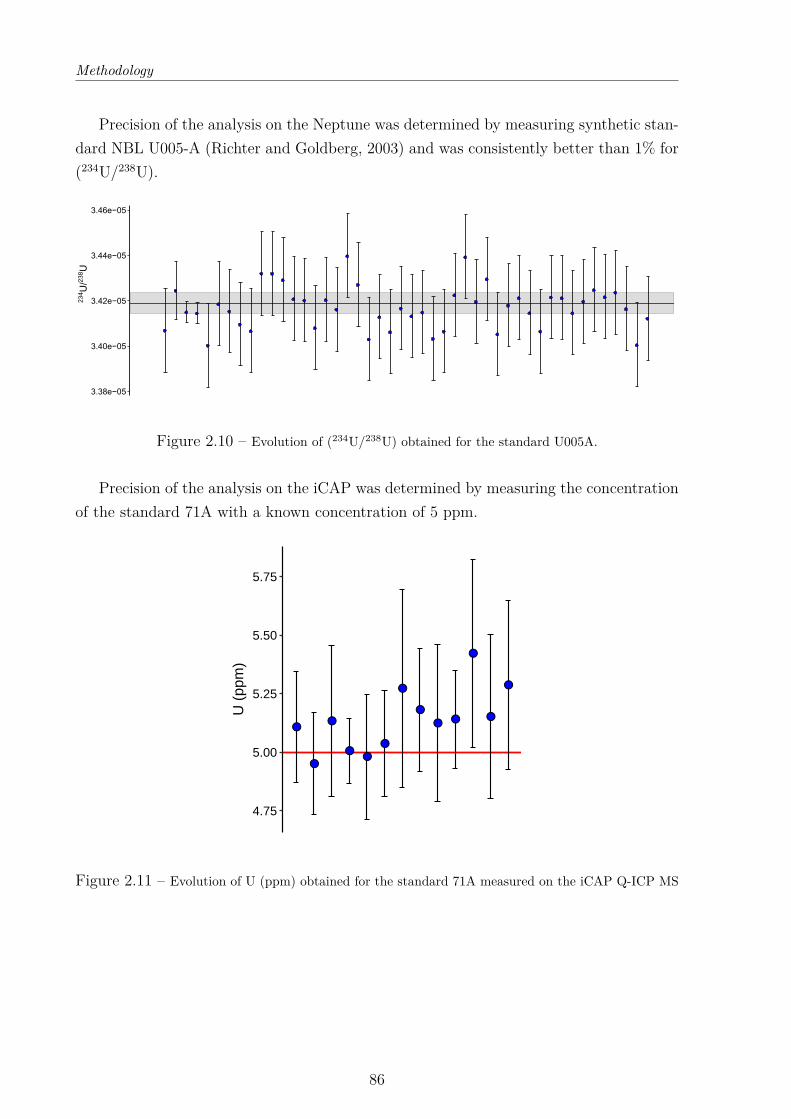
Methodology

Precision of the analysis on the Neptune was determined by measuring synthetic stan-dard NBL U005-A (Richter and Goldberg, 2003) and was consistently better than 1% for(234U/238U).

3.38e−05

3.40e−05

3.42e−05

3.44e−05

3.46e−05

234 U/238U

Figure 2.10 – Evolution of (234U/238U) obtained for the standard U005A.

Precision of the analysis on the iCAP was determined by measuring the concentrationof the standard 71A with a known concentration of 5 ppm.

4.75

5.00

5.25

5.50

5.75

U (

ppm

)

Figure 2.11 – Evolution of U (ppm) obtained for the standard 71A measured on the iCAP Q-ICP MS

86

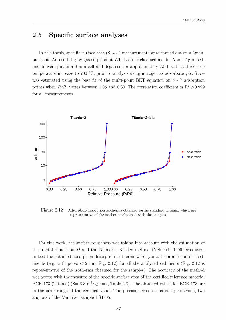
Methodology

2.5 Specific surface analyses

In this thesis, specific surface area (SBET ) measurements were carried out on a Quan-tachrome Autosorb iQ by gas sorption at WIGL on leached sediments. About 1g of sed-iments were put in a 9 mm cell and degassed for approximately 7.5 h with a three-steptemperature increase to 200 °C, prior to analysis using nitrogen as adsorbate gas. SBETwas estimated using the best fit of the multi-point BET equation on 5 - 7 adsorptionpoints when P/P0 varies between 0.05 and 0.30. The correlation coefficient is R2 >0.999for all measurements.

Titania−2 Titania−2−bis

0.00 0.25 0.50 0.75 1.000.00 0.25 0.50 0.75 1.00

3

10

30

100

300

Relative Pressure (P/P0)

Vol

ume

adsorption

desorption

Figure 2.12 – Adsorption-desorption isotherms obtained forthe standard Titania, which arerepresentative of the isotherms obtained with the samples.

For this work, the surface roughness was taking into account with the estimation ofthe fractal dimension D and the Neimark−Kiselev method (Neimark, 1990) was used.Indeed the obtained adsorption-desorption isotherms were typical from microporous sed-iments (e.g. with pores < 2 nm; Fig. 2.12) for all the analyzed sediments (Fig. 2.12 isrepresentative of the isotherms obtained for the samples). The accuracy of the methodwas access with the measure of the specific surface area of the certified reference materialBCR-173 (Titania) (S= 8.3 m2/g; n=2, Table 2.8). The obtained values for BCR-173 arein the error range of the certified value. The precision was estimated by analysing twoaliquots of the Var river sample EST-05.

87

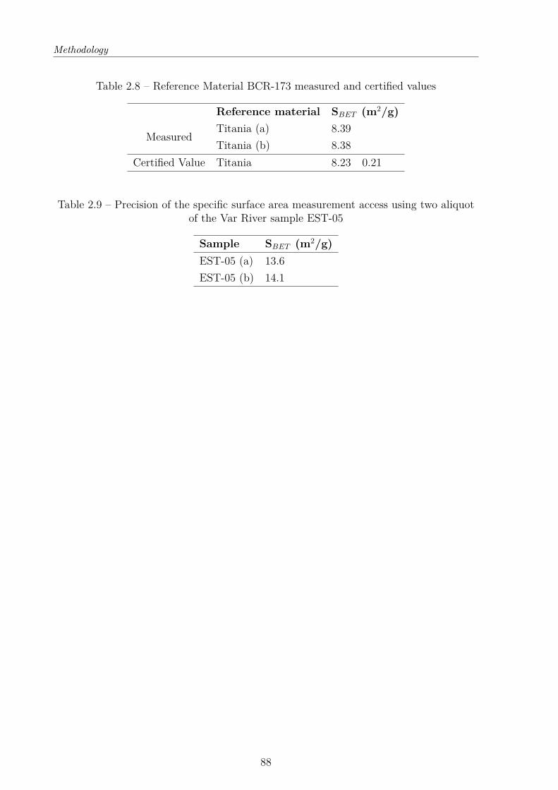
Methodology

Table 2.8 – Reference Material BCR-173 measured and certified values

Reference material SBET (m2/g)

MeasuredTitania (a) 8.39Titania (b) 8.38

Certified Value Titania 8.23 0.21

Table 2.9 – Precision of the specific surface area measurement access using two aliquotof the Var River sample EST-05

Sample SBET (m2/g)EST-05 (a) 13.6EST-05 (b) 14.1

88

Methodology

2.6 Geographic Information System analysesThe spatial distribution of sedimentary (234U/234U) ratios as the scale of a source to

sink system has been studied with the case study of the Var catchment. To this purpose,and to look at the spatial variation of characteristic inherents to the Var basin (e.g. slope,curvature, elevation), we have made extensive use of the Geographic Information System(GIS) method. We used the software ArcGIS, with Hydrology toolboxes.

2.6.1 Basin and sub-basin delineation

The first step required to use correctly the Digital Elevation Model (DEM) is to fillthe sinks in order to remove the imperfections from the DEM. A sink is a cell (or a groupof cells spatially connected) where the flow direction cannot be estimate. It can be causedby the surelevation of the neighbourg cell compared to the considered one, or because twocells flow in each other. The sinks are filled with a value from 1 to the number of sink.After the fill of the sink, the "flow direction" tool can be applied on the obtained DEM.It results in a raster that indicates the direction of flow from each cell to its steepestdownslope neighbor. From this raster, the tool” flow accumulation” is applied to calculatethe accumulated flow to each cell, as determined by the accumulated weight of all cellsthat flow into each downslope cell. Then the pour point to cells of high accumulatedflow need to be determined using the” snap pour points” tool, and the flow accumulationraster. In this case the pour point is the mouth of the Var River to obtain the border ofthe Var watershed. Once these steps realized, the” watershed” tool can be applied withthe flow direction raster and the feature pour point data. The output is a raster withthe delineation of the basin. The last step is to convert the raster into polygon whileonly the border of the considered basin is selected to have a polygon with the shape ofthe watershed. The principle of the sub-basin delineation is similar except that for thedetermination of the pour point, the localization of all the studied samples are imported.Then all the steps are repeated.

2.6.2 Extraction of the geomorphologic characteristics

The slope and curvature were calculated from the DEM raster using the slope andcurvature tools from ArcGis. The minimum, maximum and mean values were then cal-culated and extracted for each sub-catchment. Spatial distribution of soil thickness wasderived from the SoilGrids map with a 250 m resolution Hengl et al. (2017). The esti-mated sediment residence time derived from the geomorphology of the catchment wascalculated by dividing the soil thickness with the denudation rates from Mariotti et al.(2019). The values of the estimation of the sediment residence time were then extractedfor each sub-catchment.

89

Chapter 3

THE DISTRIBUTION OF (234U/238U)ACTIVITY RATIOS IN RIVER SEDIMENTS

Contents3.1 Introduction . . . . . . . . . . . . . . . . . . . . . . . . . . . . . . . 933.2 Methods . . . . . . . . . . . . . . . . . . . . . . . . . . . . . . . . . . 95

3.2.1 Samples . . . . . . . . . . . . . . . . . . . . . . . . . . . . . . . . . . 953.2.2 Analytical procedures . . . . . . . . . . . . . . . . . . . . . . . . . . 97

3.3 Results . . . . . . . . . . . . . . . . . . . . . . . . . . . . . . . . . . . 983.3.1 Leaching experiments . . . . . . . . . . . . . . . . . . . . . . . . . . 983.3.2 Uranium in river sediments . . . . . . . . . . . . . . . . . . . . . . . 100

3.4 Discussion . . . . . . . . . . . . . . . . . . . . . . . . . . . . . . . . . 1023.4.1 Influence of grain size on (234U/238U) ratios of detrital sediments . . 1023.4.2 The effect of weathering, climate and erosion on 234U-238U fraction-

ation . . . . . . . . . . . . . . . . . . . . . . . . . . . . . . . . . . . . 1023.4.3 The role of lithology . . . . . . . . . . . . . . . . . . . . . . . . . . . 1093.4.4 The role of catchment size and sediment residence time on (234U/238U)

sedimentary ratio . . . . . . . . . . . . . . . . . . . . . . . . . . . . . 1113.4.5 Complex interactions of environmental controls on sediment resi-

dence time . . . . . . . . . . . . . . . . . . . . . . . . . . . . . . . . 1143.5 Conclusion . . . . . . . . . . . . . . . . . . . . . . . . . . . . . . . . 1153.6 Acknowledgments . . . . . . . . . . . . . . . . . . . . . . . . . . . . 116

91

The distribution of (234U/238U) activity ratios in river sediments

The distribution of (234U/238U) activity ratios in riversediments

Maude Thollon1,2,3, Germain Bayon1, Samuel Toucanne1, Anne Trinquier1,Yoan Germain1, Anthony Dosseto3

1IFREMER, Marine Geosciences Research Unit, 29280 Plouzané, France.2Wollongong Isotope Geochronology Laboratory, School of Earth and Environmental Sci-ences, University of Wollongong, Wollongong, NSW 2522, Australia3Université de Bretagne Occidentale, 29200 Brest, France.Corresponding author: Maude Thollon; [email protected]

This article is an adapted version for the thesis manuscript of the article published inGeochimica et Cosmochimica Acta in September 2020.

AbstractUranium (U) isotopes can be used to estimate the comminution age of sediments, i.e.

the time elapsed from sediment production on continents, via weathering and physicalerosion, to deposition in the sedimentary record. The calculation of this comminutionage is based on measured (234U/238U) activity ratios in river sediments, and inferredtime-dependent recoil effect, which leads to the preferential release of 234U from minerallattices during erosion processes. In this study, we report on a large-scale (234U/238U)investigation of modern river sediments worldwide, with the aim to determine the extentto which parameters such as grain size, lithology, weathering, climate and geomorphol-ogy may influence the distribution of U isotopes in fine-grained sediments. Our extensivedataset (N=64) includes U isotopic measurements for many of the world’s largest rivers,but also rivers draining particular climatic and geological settings. Our results indicatethat sediments collected from river basins draining mostly igneous, metamorphic or vol-canic rocks often display (234U/238U) ratios >1, with clay-size fractions (<4 µm) being lessdepleted in 234U (higher 234U/238U) than corresponding silt-size fractions (4-63 µm). Incontrast, sediments derived from multi-lithological basins or draining sedimentary rocksare typically characterized by (234U/238U) ratios <1, with clays generally exhibiting moredepleted 234U signatures than silts. Taken together, these observations suggest that theformation of secondary clay minerals in soils from basins draining mostly igneous, meta-morphic rocks, is accompanied by partial incorporation by recoil injection of 234U initiallyreleased during weathering processes, possibly from U-rich minerals, such as sphene orapatite. Instead, in multi-lithological catchments draining sedimentary rocks, we proposethat the erosion of recycled sediments having experienced several cycles of weathering,

92

The distribution of (234U/238U) activity ratios in river sediments

possibly over glacial-interglacial timescales, could explain the much lower (234U/238U) ra-tios observed in clay-size fractions. While no direct relationships can be identified betweensediment (234U/238U) ratios and lithology, weathering intensity, climatic or geomorphicparameters in corresponding river basins, we show that the catchment size probably playsan important role in controlling the distribution of (234U/238U) in river sediments, throughits direct influence on the sediment residence time. Finally, a multiple regression analy-sis of our data, combining various environmental parameters for the lithology, climateand geomorphology of studied river basins, indicates predicted (234U/238U) values thatare very similar to measured values (with R2 ∼0.8). This finding provides further sup-port for the usefulness of (234U/238U) ratios in the sedimentary record for reconstructingpast landscape changes and their effect on sediment transport and residence time in riverbasins.

3.1 IntroductionThe morphology of the Earth’s surface results from complex interactions between cli-

mate, tectonic and weathering (e.g. Dixon et al. 2009, West et al. 2005. Understandingthe factors affecting landscape evolution is essential to predict the consequences of futureclimate change on soil resource availability and sediment discharge to the oceans. Addi-tionally, the study of sediment transport processes and their timescales can be useful toquantify soil production and denudation on continents. Over the past decades, the devel-opment and application of novel geochemical proxies to river materials has significantlyimproved our understanding of the sedimentary and weathering processes occurring inriver catchments (Négrel et al. 1993, Gaillardet et al. 1997, 1999, Vigier et al. 2001, Cliftet al. 2002, Bindeman et al. 2019, Bayon et al. 2016, 2018, 2020). However, the quan-tification of the timescale of these processes, such as the sediment residence time, stillremains challenging (DePaolo et al. 2006, Romans et al. 2016). On the continents, thefractionation of uranium (U) isotopes is initiated in the Critical Zone, associated with thepreferential loss of 234U relative to 238U, whenever chemical weathering and rock fractur-ing start affecting the bedrock. In theory, the degree of U-series fractionation in sedimentscan provide direct temporal constraints on the timing of sediment formation in soils andsubsequent storage within the catchment and the sedimentary system (Chabaux et al.2003a, DePaolo et al. 2006), which can be used to determine the so-called comminutionages, corresponding to the time elapsed since the production of small mineral grains (typ-ically <63 µm).In detail, the preferential depletion of 234U relative to 238U in mineral grains occurs dur-ing the decay of 238U to 234Th, where the daughter is recoiled (and subsequently decayedinto 234U) within the outer ∼10-30 nm periphery of the grains (Hashimoto et al. 1985,Kigoshi 1971, Maher et al. 2006, DePaolo et al. 2006, Chabaux et al. 2008, Lee et al. 2010,

93

The distribution of (234U/238U) activity ratios in river sediments

Dosseto & Schaller 2016). As a consequence, soil solutions and river water are typicallyenriched in 234U, exhibiting (234U/238U) >1 (parentheses denote activity ratio), whilstfine-grained residual sediments in soils and suspended particulate loads in rivers displayvalues <1 (Carl 1987, DePaolo et al. 2006, Maher et al. 2004, 2006, Moreira-Nordemann1980, Plater et al. 1988). The measurement of 234U depletion is only significant (i.e. mea-surable) in fine-grained (<63 µm) sediments (DePaolo et al. 2006, Dosseto et al. 2006b,2008a) where the surface/volume ratio is large enough so that the thin outer layer throughwhich preferential 234U loss occurs is significant compared to the rest of the grain (whichexperiences no net loss of 234U) (DePaolo et al. 2006). In theory, the comminution agemethod is based on two main assumptions: 1) the time-integrated recoil effect representsthe main factor controlling (234U/238U) in fine-grained sediments (DePaolo et al. 2006);and 2) the pristine (unweathered) rocks on continents are at secular equilibrium withregard to U-series (i.e. with activity ratios = 1) (DePaolo et al. 2012). However, a fewstudies have reported evidence that weathering processes can locally influence the degreeof U-series disequilibrium in fine-grained sediments (Li et al. 2016a), or that the bedrockmay depart from the secular equilibrium (Handley et al. 2013a), hence casting doubt onthe validity of the above-mentioned assumptions. In fact, despite recent increasing interestfor the use of U isotopes for tracing Earth surface processes (DePaolo et al. 2006, 2012,Dosseto et al. 2008a, 2010, 2014, 2015, Handley et al. 2013b, Lee et al. 2010, Li et al. 2017),the controls on the (234U/238U) of river sediments are yet to be fully understood. To date,all previous studies focusing on U-series as tracers of continental erosion were dedicatedto the case study of specific river basins, often yielding contrasted comminution ages andinferred sediment transport times. For instance, investigations conducted at the scale ofthe Amazon Basin resulted in a large range of sediment residence time from the Andeantributaries (3-4 kyr; Dosseto et al. 2006a, 2008a) and the lowland tributaries (100-500kyr; Dosseto et al. 2006a). The Ganges tributaries have also been investigated in detail(Chabaux et al. 2006, 2012, Granet et al. 2007, 2010), with inferred sediment residencetimes ranging between 30-350 kyr. Other case studies include the Mackenzie River (Vigieret al. 2001) and smaller river systems in East Asia (Zhuoshui River, Lanyang River; Liet al. 2016b), yielding sediment transfer times of ∼25 kyr and ∼110 kyr, respectively.More recently, Li et al. (2016b) also determined relatively long sediment transfer times(from 250 to 600 kyr) for the Changjiang (Yangtze) River basin. These latter sedimentresidence times are surprisingly long considering the observed variability of the provenanceof the sediment exported from the Yangtze River over the past 400 kyr, which implicitlysuggests a much shorter storage time within the watershed (Beny et al. 2018).An important pre-requirement for quantifying the timescale of sediment transport in con-tinental watersheds using U isotopes, is to assess whether the distribution of (234U/238U)in river suspended loads and sediments can be affected by other parameters, such as grain-size, lithology, climate and tectonic settings. Early works pointed out at the importance

94

The distribution of (234U/238U) activity ratios in river sediments

of removing non detrital sediment fractions prior to analysing sediment samples (e.g. Lee2009, Martin et al. 2015, Francke et al. 2018 and demonstrated the influence of grain sizeon U activity ratios and calculated sediment transfer times (Dosseto et al. 2014, Granetet al. 2010). More recently, Bosia et al. (2018) also emphasize the importance of analysingseparate mineral phases. While it can be difficult to separate different mineral fractionsfrom fine-grained sediments, one alternative option is to focus instead on particular grain-size fractions. In this study, we report (234U/238U) measurements for both clay (<4 µm)and silt (4-63 µµm) size detrital fractions extracted from an extensive set of river sedimentsamples worldwide. This study builds upon previous investigations of the same suite ofsediment samples, which have proven particularly useful for identifying the various ex-ternal factors (e.g. climate, lithology, weathering regime) that control the distribution ofgeochemical proxies in sediments (Bayon et al. 2015, 2016, 2018, 2020, Bindeman et al.2019). Such a proxy evaluation study is of utmost importance prior to applying U iso-topes in ancient sedimentary records for reconstructing past sediment transfer dynamicsthrough time.

3.2 Methods

3.2.1 Samples

A total of 64 sediment samples were analysed during this study, collected from rivercatchments, estuaries, or submarine deltas near the mouth of rivers (Fig. 3.1; Bayonet al. 2015, 2016, 2018, 2020). All studied samples correspond to modern or relativelyrecent sediments presumably deposited during the last few centuries. A few sedimentsamples (n=17) come from igneous/metamorphic terranes from the Precambrian cratonsof North America (Canadian Shield), northern South America (Guiana Shield), Africa(West African and Congo Shields), Fennoscandia, northwest Ireland and a small river fromthe Hercynian Armorican Massif in France (Elorn River). Seven samples are derived fromrivers draining both modern (Indonesia) and ancient (British Tertiary, Northern Ireland)volcanic provinces. The rest of studied samples (n=40) correspond to rivers draining‘mixed/sedimentary’ formations including some of the world’s major rivers (e.g. Amazon,Congo, Mississippi, Nile, Niger, Yangtze, Mackenzie, Volga, Murray, Orinoco), plus riversdraining sedimentary basins (e.g. Adour, Shannon).The studied river catchments can also be classified according to their climate setting(Bayon et al. 2016, 2018), depending on their mean annual temperature (MAT), andmean annual precipitation (MAP). A total of 10 samples are representative of cold anddry regions with MAT <8°C and MAP <800mm (e.g. Don, Fraser, Lule). Other sedimentscorrespond to temperate and warm dry environments (e.g. Murray-Darling, Yellow River;n=18), with MAT >10 °C and MAP <800 mm, or from temperate and humid regions

95

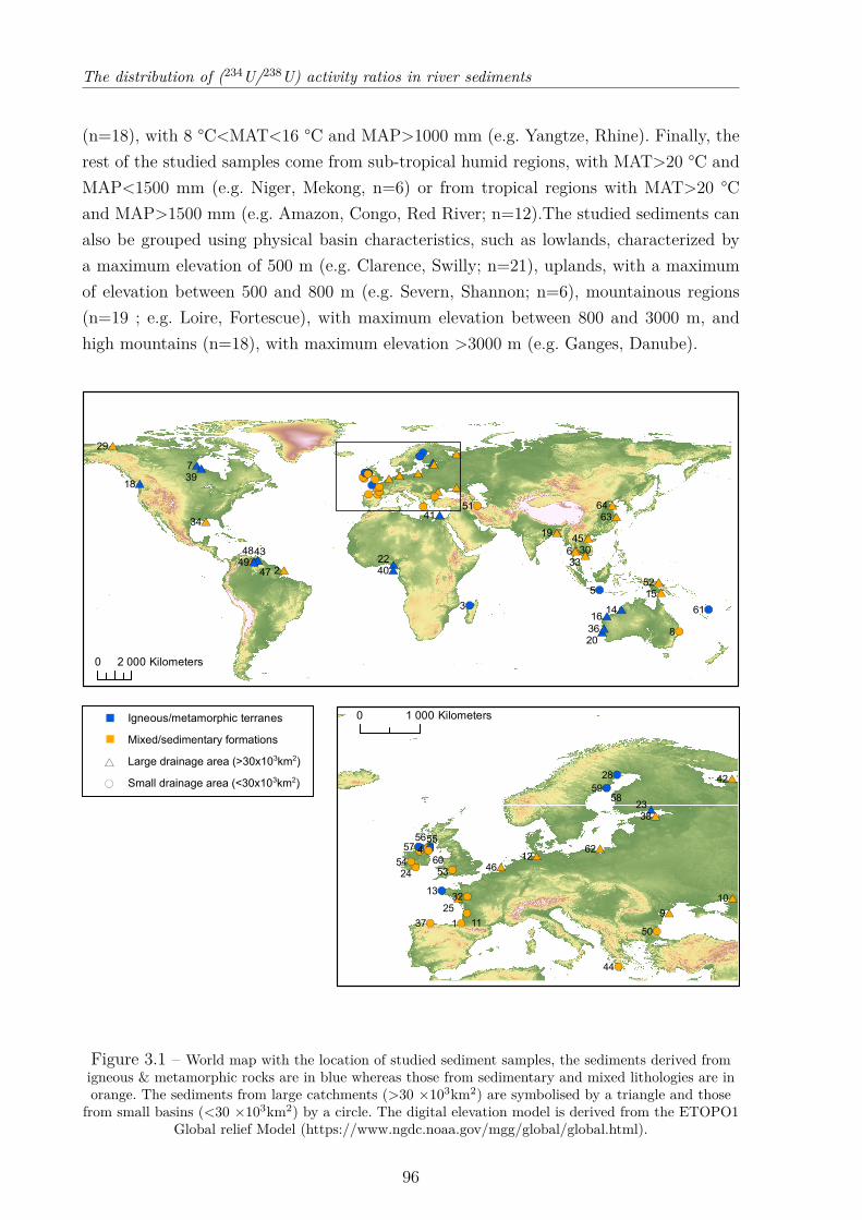
The distribution of (234U/238U) activity ratios in river sediments

(n=18), with 8 °C<MAT<16 °C and MAP>1000 mm (e.g. Yangtze, Rhine). Finally, therest of the studied samples come from sub-tropical humid regions, with MAT>20 °C andMAP<1500 mm (e.g. Niger, Mekong, n=6) or from tropical regions with MAT>20 °Cand MAP>1500 mm (e.g. Amazon, Congo, Red River; n=12).The studied sediments canalso be grouped using physical basin characteristics, such as lowlands, characterized bya maximum elevation of 500 m (e.g. Clarence, Swilly; n=21), uplands, with a maximumof elevation between 500 and 800 m (e.g. Severn, Shannon; n=6), mountainous regions(n=19 ; e.g. Loire, Fortescue), with maximum elevation between 800 and 3000 m, andhigh mountains (n=18), with maximum elevation >3000 m (e.g. Ganges, Danube).

&-

#*

&-

&-

&-

#*

#*

&-

#* #*&-

#*&-

#*

#*

#*

&-#*

#*

#*

&-

#*

#*

&-#*

&-&-

&-#*

#*

&-

&-

#*

#*

&-

#*

&-

#*#*

#*

#*

#*

#*

&-

#*

#*

&-#*#*

&-&-

#*

&-&-&-&-&-

&-&-

&-

&-

#*

#*#*

8

7

6

5

3

2

6463

61

52

51

4948

47

4543

41

40

39

36

34

3330

29

22

20

19

18

16

15

14

0 2 000 Kilometers

&-

&-

#*

#*

&-

#*

&-

&-&-

#*

&-

#*

&-&-

&-

&-

&-

&-

&-

#*

#*

&-

#*

&-

&-&-

&-&-&-

&-&-

&- #*

9

4

1

6260

5958

575655

5453

50

46

44

42

38

37

32

28

25

24

23

13

12

11

10

0 1 000 KilometersIgneous/metamorphic terranes

Mixed/sedimentary formations

Large drainage area (>30x103km2)

Small drainage area (<30x103km2)

*

-

Figure 3.1 – World map with the location of studied sediment samples, the sediments derived fromigneous & metamorphic rocks are in blue whereas those from sedimentary and mixed lithologies are inorange. The sediments from large catchments (>30 ×103km2) are symbolised by a triangle and those

from small basins (<30 ×103km2) by a circle. The digital elevation model is derived from the ETOPO1Global relief Model (https://www.ngdc.noaa.gov/mgg/global/global.html).

96

The distribution of (234U/238U) activity ratios in river sediments

3.2.2 Analytical procedures

Three distinct U pools can be distinguished in any sediment sample (Martin et al.2015): 1) a non-detrital pool hosted by various carbonate minerals, Fe-Mn oxyhydroxidephases, and organic compounds, associated typically with enriched ((234U/238U) >1) sig-natures (Plater et al. 1988, Andersson et al. 1998, 2001, Maher et al. 2006); 2) a depleted((234U/238U) <1) detrital pool corresponding to the outer part of detrital minerals thathave experienced partial dissolution and preferential loss of 234U due to recoil effect; and3) a pristine detrital pool at secular equilibrium ((234U/238U) =1), which corresponds tothe inner part of detrital grains that has not experienced 234U loss.In this study, sequential leaching was conducted on all samples in order to remove anybiogenic, authigenic and organic components prior to preparation for U isotopic measure-ments. First, the <63 µm fraction of the bulk sediment was recovered by wet sieving.About ∼3 g of dry bulk sediment were treated successively with diluted acetic acid (AA),a mixed solution of 15% (v/v) AA and 0.1 M hydroxylamine hydrochloride (HH), anddiluted hydrogen peroxide, in order to remove any carbonate, Fe-Mn oxyhydroxide andorganic phases, respectively (Bayon et al. 2002). Finally, clay- (<4 µm) and silt- (4-63 µm)size fractions of the residual detritus were separated by centrifugation using the two-stepprotocol reported in Bayon et al. (2015).A series of experiments was conducted on different sediment samples in order to assessthe reliability of our leaching protocol for efficiently removing the radiogenic non-detritalcomponent of the sediment characterized by high (234U/238U) ratios. To this purpose,following the approach previously developed by Lee (2009), the effect of each leachingstep of our protocol was successively assessed by measuring U isotopic ratios in bothleachates and corresponding residual phases from two sediment samples from the Loireand Clarence rivers (Fig. 3.2). To assess whether the leaching was completed, an addi-tional final leaching step termed "carbonate emphasized" was performed at the end ofthis series of experiments. The validity of our sequential leaching protocol was also fur-ther assessed by analysing two sediment samples (1B-26H-cc and 1B-17H-cc) previouslystudied by Francke et al. (2018) using a different leaching method. Finally, two certifiedreference rock materials (BCR-2, BHVO-2) were processed using the same experimentalprotocol used in this study, to investigate whether sequential leaching could also lead toany particular U isotopic fractionation.Both clay- and silt-size residual detrital fractions were digested by alkaline fusion (Bayonet al. 2009), to ensure complete dissolution and provide reassurance that the observed(234U/238U) differences between silt and clay samples cannot be possibly caused by thepartial dissolution of any accessory minerals. About 50 mg dry powdered sediment wereplaced into a glassy carbon crucible, after addition of 238U spike, and digested at 650°C(12 min) together with NaOH and Na2O2. Subsequent addition of ultrapure water to the

97

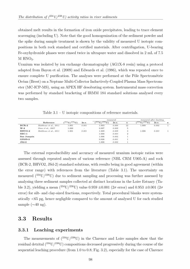
The distribution of (234U/238U) activity ratios in river sediments

obtained melt results in the formation of iron oxide precipitates, leading to trace elementscavenging (including U). Note that the good homogenization of the sediment powder andthe spike during sample treatment is shown by the validity of measured U isotopic com-positions in both rock standard and certified materials. After centrifugation, U-bearingFe-oxyhydroxide phases were rinsed twice in ultrapure water and dissolved in 2 mL of 7.5M HNO3.Uranium was isolated by ion exchange chromatography (AG1X-8 resin) using a protocoladapted from Bayon et al. (2009) and Edwards et al. (1986), which was repeated once toensure complete U purification. The analyses were performed at the Pôle SpectrométrieOcéan (Brest) on a Neptune Multi-Collector Inductively-Coupled Plasma Mass Spectrom-eter (MC-ICP-MS), using an APEX HF desolvating system. Instrumental mass correctionwas performed by standard bracketing of IRMM 184 standard solutions analysed everytwo samples.

Table 3.1 – U isotopic compositions of reference materials.measured measured after leaching

Reference (234U/238U) 2s.e. (234U/238U) 2s.e. n (234U/238U) 2s.e. nBCR-2 Matthews et al., 2011 1.001 0.001 1.003 0.006 12 1.009 0.002 1W-2 Sims et al., 2007 1.000 - 0.997 0.009 5BHVO-2 Matthews et al., 2011 1.001 0.001 1.009 0.009 3 1.006 0.003 1SBC-1 1.000 0.003 2San Joaquin 1.006 0.002 1GSMS-2 0.928 0.001 1JSd-2 1.008 0.002 1

The external reproducibility and accuracy of measured uranium isotopic ratios wereassessed through repeated analyses of various reference (NBL CRM U005-A) and rock(BCR-2, BHVO2, JSd-2) standard solutions, with results being in good agreement (withinthe error range) with references from the literature (Table 3.1). The uncertainty onmeasured (234U/238U) due to sediment sampling and processing was further assessed byanalysing three sediment samples collected at distinct locations in the Loire Estuary (Ta-ble 3.2), yielding a mean (234U/238U) value 0.959 ±0.001 (2σ error) and 0.953 ±0.001 (2σerror) for silt- and clay-sized fractions, respectively. Total procedural blanks were system-atically <65 pg, hence negligible compared to the amount of analysed U for each studiedsample (∼40 ng).

3.3 Results

3.3.1 Leaching experiments

The measurements of (234U/238U) in the Clarence and Loire samples show that theresidual detrital (234U/238U) compositions decreased progressively during the course of thesequential leaching procedure (from 1.0 to 0.8; Fig. 3.2), especially for the case of Clarence

98

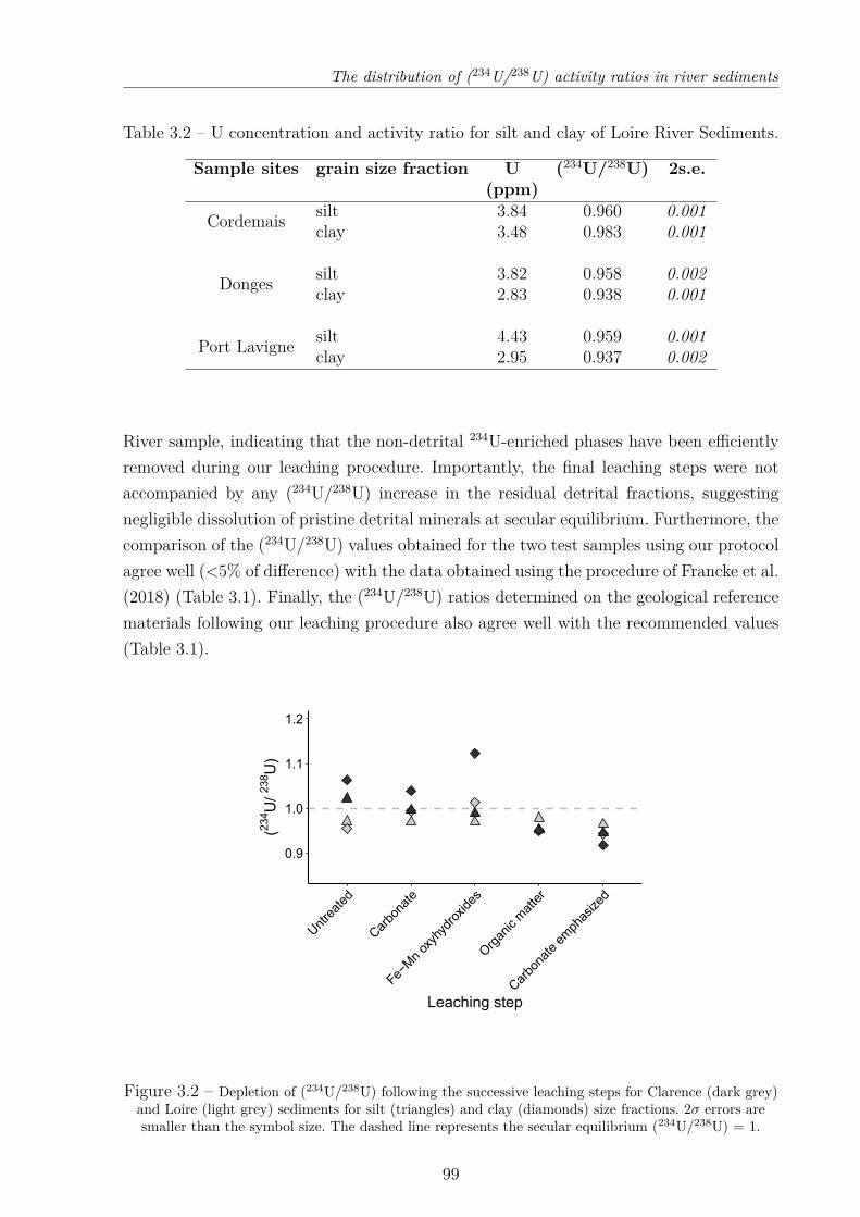
The distribution of (234U/238U) activity ratios in river sediments

Table 3.2 – U concentration and activity ratio for silt and clay of Loire River Sediments.

Sample sites grain size fraction U (234U/238U) 2s.e.(ppm)

Cordemais silt 3.84 0.960 0.001clay 3.48 0.983 0.001

Donges silt 3.82 0.958 0.002clay 2.83 0.938 0.001

Port Lavigne silt 4.43 0.959 0.001clay 2.95 0.937 0.002

River sample, indicating that the non-detrital 234U-enriched phases have been efficientlyremoved during our leaching procedure. Importantly, the final leaching steps were notaccompanied by any (234U/238U) increase in the residual detrital fractions, suggestingnegligible dissolution of pristine detrital minerals at secular equilibrium. Furthermore, thecomparison of the (234U/238U) values obtained for the two test samples using our protocolagree well (<5% of difference) with the data obtained using the procedure of Francke et al.(2018) (Table 3.1). Finally, the (234U/238U) ratios determined on the geological referencematerials following our leaching procedure also agree well with the recommended values(Table 3.1).

0.9

1.0

1.1

1.2

Untre

ated

Carbo

nate

Fe−M

n ox

yhyd

roxid

es

Organ

ic m

atte

r

Carbo

nate

em

phas

ized

Leaching step

(234 U

/ 238 U

)

Figure 3.2 – Depletion of (234U/238U) following the successive leaching steps for Clarence (dark grey)and Loire (light grey) sediments for silt (triangles) and clay (diamonds) size fractions. 2σ errors aresmaller than the symbol size. The dashed line represents the secular equilibrium (234U/238U) = 1.

99

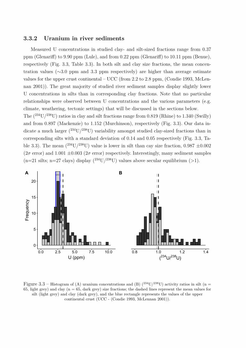
3.3.2 Uranium in river sediments

Measured U concentrations in studied clay- and silt-sized fractions range from 0.37ppm (Glenariff) to 9.90 ppm (Lule), and from 0.22 ppm (Glenariff) to 10.11 ppm (Benue),respectively (Fig. 3.3, Table 3.3). In both silt and clay size fractions, the mean concen-tration values (∼3.0 ppm and 3.3 ppm respectively) are higher than average estimatevalues for the upper crust continental – UCC (from 2.2 to 2.8 ppm, (Condie 1993, McLen-nan 2001)). The great majority of studied river sediment samples display slightly lowerU concentrations in silts than in corresponding clay fractions. Note that no particularrelationships were observed between U concentrations and the various parameters (e.g.climate, weathering, tectonic settings) that will be discussed in the sections below.The (234U/238U) ratios in clay and silt fractions range from 0.819 (Rhine) to 1.340 (Swilly)and from 0.897 (Mackenzie) to 1.152 (Murchinson), respectively (Fig. 3.3). Our data in-dicate a much larger (234U/238U) variability amongst studied clay-sized fractions than incorresponding silts with a standard deviation of 0.14 and 0.05 respectively (Fig. 3.3, Ta-ble 3.3). The mean (234U/238U) value is lower in silt than cay size fraction, 0.987 ±0.002(2σ error) and 1.001 ±0.003 (2σ error) respectively. Interestingly, many sediment samples(n=21 silts; n=27 clays) display (234U/238U) values above secular equilibrium (>1).

UCC

0

5

10

15

20

0.0 2.5 5.0 7.5 10.0

U (ppm)

Fre

quen

cy

A

0.8 1.0 1.2 1.4

(234U/238U)

B

Figure 3.3 – Histogram of (A) uranium concentrations and (B) (234U/238U) activity ratios in silt (n =65, light grey) and clay (n = 65, dark grey) size fractions; the dashed lines represent the mean values for

silt (light grey) and clay (dark grey), and the blue rectangle represents the values of the uppercontinental crust (UCC - (Condie 1993, McLennan 2001)).

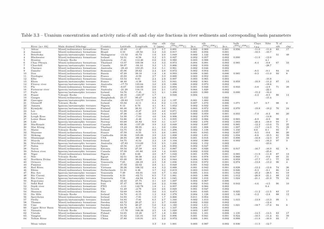
Table 3.3 – Uranium concentration and activity ratio of silt and clay size fractions in river sediments and corresponding basin parametersclay silt clay silt bulk Clays Silts % of

River (n= 64) Main drained lithology Country Latitude Longitude U (ppm) (234U/238U) 2s.e. (234U/238U) 2s.e. (234U/238U) εNd silt clay1 Adour Mixed/sedimentary formations France 43.49 -1.47 2.7 3.7 0.891 0.002 0.969 0.001 0.956 -11.0 -11.6 83 172 Amazon Mixed/sedimentary formations Brazil 3.10 -49.50 3.2 3.0 0.917 0.001 0.956 0.001 -10.5 -10.73 Betsiboka Igneous/metamorphic terranes Madagascar -15.52 45.72 1.6 2.0 1.049 0.002 1.122 0.002 51 494 Blackwater Mixed/sedimentary formations Ireland 54.51 -6.58 3.2 2.5 0.927 0.002 0.957 0.002 0.000 -11.6 -12.65 Brantas Volcanic Rocks Indonesia -7.44 112.46 0.6 0.6 0.980 0.003 0.988 0.003 4.16 Chao Phraya Mixed/sedimentary formations Thailand 13.57 100.58 3.2 3.2 0.972 0.004 0.991 0.002 0.985 -8.4 -9.8 67 337 Churchill Igneous/metamorphic terranes Canada 58.97 -94.10 3.3 1.5 0.866 0.002 0.933 0.002 -28.78 Clarence Mixed/sedimentary formations Australia -29.43 153.25 3.2 5.1 0.961 0.002 0.946 0.0029 Danube Mixed/sedimentary formations Romania 45.06 29.62 2.4 2.8 0.872 0.002 0.954 0.001 -8.5 -9.1 84 1610 Don Mixed/sedimentary formations Russia 47.29 39.10 1.8 1.8 0.993 0.009 0.985 0.006 0.985 -9.3 -11.0 92 811 Dordogne Mixed/sedimentary formations France 45.03 -0.59 2.7 3.3 0.888 0.002 0.952 0.00112 Elbe Mixed/sedimentary formations Germany 53.54 9.81 2.4 2.8 0.897 0.003 0.965 0.003 -10.813 Elorn Igneous/metamorphic terranes France 48.40 -4.38 3.0 3.5 0.941 0.002 0.961 0.002 0.959 -10.9 -11.2 87 1314 Fitzroy river Igneous/metamorphic terranes Australia -17.73 123.64 3.0 2.9 1.098 0.002 0.973 0.002 -18.615 Fly Mixed/sedimentary formations PNG -8.67 144.00 2.6 2.3 0.894 0.001 0.948 0.001 0.933 -3.8 -4.9 71 2916 Fortescue river Igneous/metamorphic terranes Australia -21.29 116.14 2.6 2.1 1.072 0.004 1.029 0.002 -22.117 Foyle Igneous/metamorphic terranes Ireland 54.76 -7.45 3.5 2.1 1.208 0.003 0.989 0.002 0.000 -15.2 -16.018 Fraser Volcanic Rocks Canada 49.16 -123.37 1.7 0.948 0.004 -4.2 -8.5 86 1419 Ganges Mixed/sedimentary formations Bangladesh 23.17 90.47 4.8 2.8 1.022 0.002 -15.420 Gascogne Igneous/metamorphic terranes Australia -29.83 113.77 3.3 2.2 1.197 0.001 1.082 0.00221 Glenariff Volcanic Rocks Ireland 55.02 -6.11 0.4 0.2 1.119 0.007 1.070 0.006 1.071 3.7 3.7 98 222 Jamata Igneous/metamorphic terranes Nigeria 6.13 6.76 4.1 8.1 1.052 0.002 0.932 0.00123 Kymijoki Igneous/metamorphic terranes Finland 60.46 26.91 3.7 3.6 0.961 0.003 0.972 0.002 0.970 -19.8 -19.2 76 2424 Lee Mixed/sedimentary formations Ireland 51.88 -8.27 2.9 4.6 0.871 0.002 0.939 0.00225 Loire Mixed/sedimentary formations France 47.28 -1.90 3.0 4.4 0.937 0.002 0.959 0.001 0.955 -7.9 -8.3 80 2026 Lough Erne Mixed/sedimentary formations Ireland 54.30 -7.64 4.0 3.8 0.908 0.002 0.976 0.003 -14.827 Lower Bann Mixed/sedimentary formations Ireland 54.86 -6.48 1.6 1.5 0.935 0.003 0.966 0.002 0.965 -8.9 -8.9 98 228 Lule Igneous/metamorphic terranes Norway 65.68 21.82 9.9 3.1 1.317 0.002 1.076 0.002 1.093 -20.4 -18.0 93 729 MacKenzie Mixed/sedimentary formations Canada 69.26 -137.29 3.9 3.2 0.848 0.002 0.897 0.002 0.885 -12.2 -13.0 75 2530 Mae Klong Mixed/sedimentary formations Thailand 13.43 99.95 4.1 3.6 1.004 0.001 1.008 0.001 1.007 -13.7 -14.3 71 2931 Maine Volcanic Rocks Ireland 54.75 -6.32 0.6 0.3 1.298 0.002 1.138 0.006 1.150 0.6 0.1 93 732 Mayenne Mixed/sedimentary formations France 47.50 -0.55 3.5 2.6 1.003 0.001 0.945 0.002 0.957 -9.5 -9.6 80 2033 Mekong Mixed/sedimentary formations Cambodia 10.96 105.06 3.9 3.3 1.008 0.002 1.051 0.002 1.034 -8.6 -10.5 61 3934 Mississippi Mixed/sedimentary formations USA 28.93 -89.49 2.8 2.8 0.858 0.001 0.918 0.001 0.898 -10.8 -12.3 67 3335 Moyola Mixed/sedimentary formations Ireland 54.75 -6.52 2.3 1.9 1.104 0.002 0.989 0.001 0.992 -16.1 -16.2 97 336 Murchison Igneous/metamorphic terranes Australia -27.83 114.69 5.9 2.5 1.239 0.002 1.152 0.002 -23.637 Nalon Mixed/sedimentary formations Spain 43.56 -6.07 3.6 4.8 0.892 0.002 0.947 0.00138 Narva Mixed/sedimentary formations Estonia 59.54 27.58 4.9 3.1 0.887 0.001 0.920 0.001 0.917 -16.7 -16.0 92 839 Nelson river Igneous/metamorphic terranes Canada 57.39 -91.80 2.8 1.4 0.823 0.002 0.932 0.002 -25.640 Niger Mixed/sedimentary formations Nigeria 3.20 6.68 4.0 8.7 1.048 0.001 0.976 0.001 0.985 -11.9 -11.9 87 1341 Nile Volcanic Rocks Egypt 32.51 30.38 2.2 3.0 0.947 0.001 0.978 0.001 0.968 -7.1 -9.6 69 3142 Northern Dvina Mixed/sedimentary formations Russia 65.09 39.00 2.5 2.4 0.944 0.004 0.963 0.001 0.959 -17.7 -17.1 77 2343 Orinoco Mixed/sedimentary formations Venezuela 7.65 -66.18 4.3 5.8 1.036 0.016 0.972 0.001 0.974 -13.8 -13.2 96 444 Pamisos Mixed/sedimentary formations Greece 37.02 22.02 2.8 2.1 0.849 0.001 0.942 0.00445 Red River Mixed/sedimentary formations Vietnam 20.26 106.52 4.4 3.2 0.888 0.001 0.942 0.001 0.928 -12.2 -12.8 74 2646 Rhine Mixed/sedimentary formations Netherlands 51.91 4.48 3.7 3.2 0.819 0.003 0.943 0.001 0.926 -9.3 -9.1 86 1447 Rio Aro Igneous/metamorphic terranes Venezuela 7.39 -64.01 3.6 4.7 1.162 0.005 1.014 0.001 1.042 -25.2 -28.5 81 1948 Rio Caroni Igneous/metamorphic terranes Venezuela 8.33 -62.71 6.5 7.3 1.061 0.003 1.006 0.001 1.012 -20.9 -21.1 88 1249 Rio Caura Igneous/metamorphic terranes Venezuela 7.58 -64.94 6.4 6.3 1.045 0.002 1.018 0.001 1.024 -21.1 -21.0 79 2150 Ropotamo Mixed/sedimentary formations Bulgaria 42.32 27.75 2.1 2.0 1.007 0.004 0.967 0.00651 Sefid Rud Mixed/sedimentary formations Iran 37.47 49.94 2.6 2.2 0.946 0.002 0.943 0.002 0.943 -4.6 -4.5 90 1052 Sepik river Mixed/sedimentary formations PNG -3.13 142.78 1.8 1.1 0.957 0.002 0.984 0.003 0.453 Severn Mixed/sedimentary formations UK 51.49 -2.78 2.6 2.6 0.849 0.001 0.947 0.00254 Shannon Mixed/sedimentary formations Eire 52.69 -8.91 3.6 3.3 0.873 0.001 0.935 0.001 0.925 -11.2 -11.5 83 1755 Six Mile Volcanic Rocks Ireland 54.70 -6.15 1.2 0.8 1.278 0.004 1.128 0.002 1.146 -3.2 -2.8 88 1256 Spercheios Mixed/sedimentary formations Ireland 54.93 -7.81 1.0 1.7 0.866 0.011 0.954 0.00457 Swilly Igneous/metamorphic terranes Ireland 54.93 -7.81 6.5 2.7 1.340 0.002 1.013 0.002 1.015 -13.9 -13.3 99 158 Thames Mixed/sedimentary formations Sweden 63.72 20.27 2.1 2.7 0.820 0.002 0.922 0.002 -12.459 Ume Igneous/metamorphic terranes Sweden 63.72 20.27 5.0 3.2 1.180 0.002 1.011 0.002 1.021 -18.7 -17.6 94 660 Upper River Bann Mixed/sedimentary formations Ireland 54.38 -6.33 7.0 4.1 1.337 0.004 1.073 0.00261 Vanuatu Volcanic Rocks Vanuatu -17.76 168.38 2.5 1.9 1.020 0.003 1.007 0.00262 Vistula Mixed/sedimentary formations Poland 54.65 19.28 2.7 1.8 1.300 0.021 1.101 0.008 1.135 -14.5 -14.5 83 1763 Yangtze Mixed/sedimentary formations China 31.62 121.01 3.0 2.6 0.896 0.001 0.941 0.001 0.924 -10.5 -11.4 61 3964 Yellow River Mixed/sedimentary formations China 37.80 118.91 2.5 2.2 0.972 0.003 1.001 0.002 0.999 -11.9 -10.9 93 7

Mean values 3.3 3.0 1.001 0.003 0.987 0.002 0.936 -11.5 -12.7

∗εNd are from Bayon et al. (2015), percentage of silt and clay fraction are from Bindeman et al. (2019)

3.4 Discussion

3.4.1 Influence of grain size on (234U/238U) ratios of detrital sed-iments

As modelled by DePaolo et al. (2006), the recoil loss factor is directly proportionalto grain size, leading to separate time-dependent evolution of (234U/238U) ratios in sep-arate size fractions of the sediment. The influence of grain size on (234U/238U) was alsoassessed by Dosseto et al. (2014), who analysed various size fractions of river suspendedparticulates from the Murray-Darling Basin in south-eastern Australia, ranging from thedissolved load (<10 kilo-daltons - kDa) to coarse silts (>25 µm). The above-mentionedstudies showed that sedimentary (234U/238U) ratios typically decrease with increasinggrain size. To some extent, this ‘grain-size’ effect could explain the observed large rangeof sediment residence time determined in different river systems Granet et al. (2010).In the studied sediment samples, the silt fraction generally represents between 60 and 95%of the bulk (<63 µm) detrital fraction (mean ∼82 ± 23% 2SE; (Bindeman et al. 2019)),meaning that the (234U/238U) values of the silt-size fractions can be taken, to a first ap-proximation, as representative of the bulk (234U/238U) composition of the fine-graineddetrital sediments investigated in this study.A striking feature of our results is the fact that many clay-sized fractions are characterizedby activity ratios higher than >1, often exhibiting higher values than in correspondingsilts. As mentioned above, this observation is opposite to the grain-size effect predictedtheoretically by DePaolo et al. (2006). In previous studies, samples exhibiting activityratios >1 were generally discarded, because they were thought to be affected by thepresence of radiogenic authigenic components (Dosseto et al. 2006a, Vigier et al. 2001,2006, Granet et al. 2010, Martin et al. 2019). However, we are confident here that ourclay-sized fractions solely correspond to detrital material, previously leached from anypossible carbonate, oxide and/organic components. On this basis, we propose that mea-sured activity ratios above 1 could reflect partial incorporation of 234U previously releasedfrom incongruent silicate weathering into neoformed clays (Plater et al. 1992, Dequinceyet al. 2002).

3.4.2 The effect of weathering, climate and erosion on 234U-238Ufractionation

The disequilibrium between 234U and 238U in soils mainly reflects the recoil effect dur-ing water/rock interactions (Osmond & Ivanovich 1992, Riotte et al. 2003) and the pref-erential leaching of 234U relative to 238U embedded in recoil tracks (Fleischer 1980, 1982).It is important to investigate to which extent weathering could influence the distributionof (234U/238U) ratios in river sediments and eventually lead to an over- or underestima-

102

tion of the sediment residence time in watersheds. In theory, bulk mineral dissolutionshould not lead to any significant fractionation between 234U and 238U (Chabaux et al.2003a), so that chemical weathering intensity is not expected to have direct influenceon sediment (234U/238U). However, Li et al. (2016b) reported various correlations be-tween (234U/238U) and chemical weathering indices in leached river sediments (<50 µm),suggesting a link between U-isotope fractionation patterns and the type of weatheringregime. Lower (234U/238U) values (<0.90), indicative of presumably longer sediment res-idence times, were determined in sediments having experienced intense chemical weath-ering in transport-limited regimes. In contrast, in weathering- (or kinetically) limitedweathering regimes associated with high denudation rates and fast sediment transfer, Liet al. (2016b) proposed that high mineral dissolution rates could result in sedimentary(234U/238U) ratios being close to 1. To some extent, this latter observation is counter-intuitive, because enhanced physical erosion in high mountain environments and otherkinetically-limited weathering regimes could be alternatively associated with sedimentshaving lower (234U/238U) ratios, as a result of enhanced production of small grain-sizesediments and associated 234U recoil loss. For these reasons, and because the chemicalweathering signature of the sediments can be partly inherited from previous weatheringcycles and sediment recycling (Dou et al. 2016), but also because the (234U/238U) ratio onlyrecords the last million years of chemical weathering, Li et al. (2016b) remained cautiouswith the interpretation of the relationships between weathering indices and (234U/238U).In our study, the (234U/238U) composition of both silt-and clay size fractions does notdisplay any relationships weathering indices, such as the Chemical Index of Alteration(CIA; Nesbitt & Young (1982); Fig. 3.4A) or the Chemical Index of Weathering (CIW;Harnois (1988); Fig. 3.4B). Considering only small catchments (<30 x103 km2), in orderto exclude any effect related to alluvial storage (which could further modify 234U/238Uactivity ratios), no relationship was observed between (234U/238U) and the CIA in riversediments (Appendix A3.1), while a weak correlation was identified with CIW in silt sizefractions (R2 = 0.56 ; Appendix A3.2), with lower (234U/238U) values being associatedwith higher CIW. Overall, our data indicate that chemical weathering intensity does notexert a first-order control on (234U/238U) in river sediments, although enhanced weather-ing most likely results in preferential leaching of 234U, in agreement with the findings ofLi et al. (2016b).

103

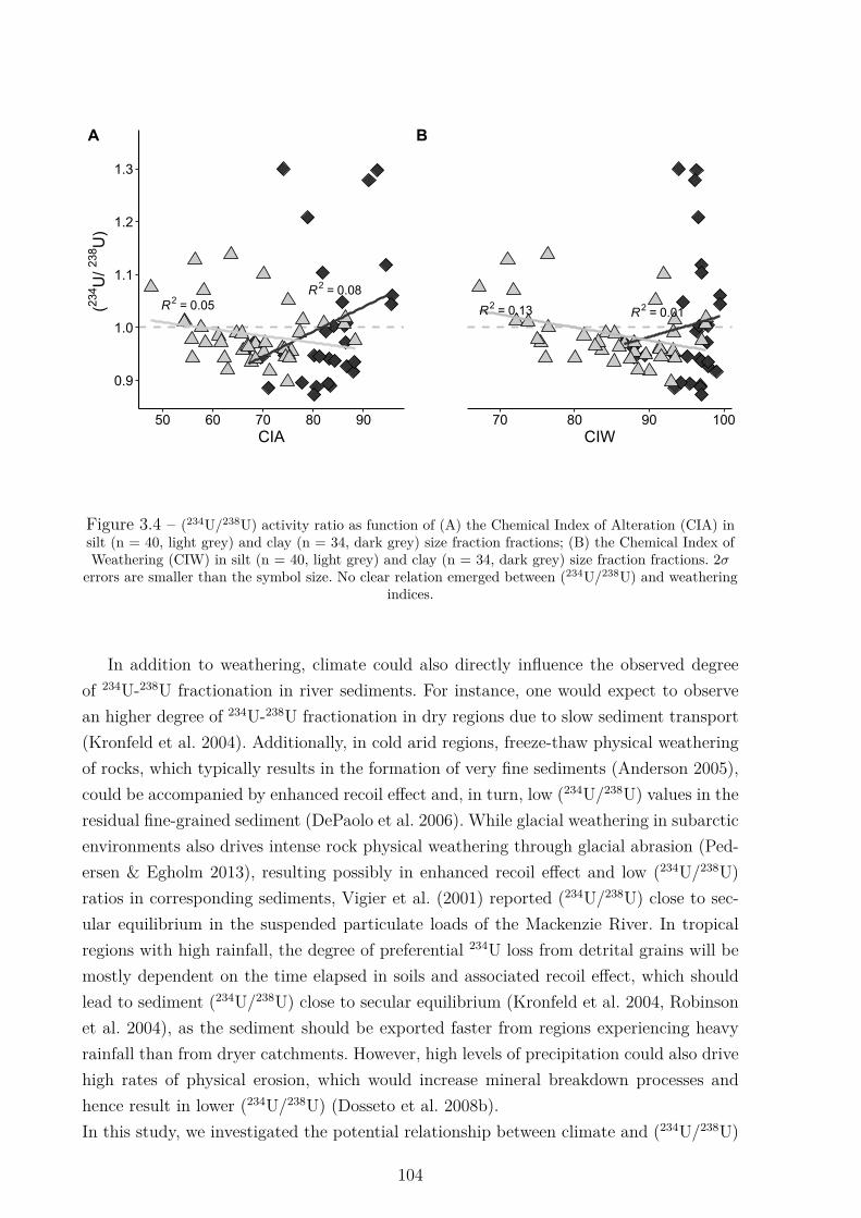
R2 = 0.08R2 = 0.05

0.9

1.0

1.1

1.2

1.3

50 60 70 80 90CIA

(234 U

/ 238 U

)

A

R2 = 0.01R2 = 0.13

70 80 90 100CIW

B

Figure 3.4 – (234U/238U) activity ratio as function of (A) the Chemical Index of Alteration (CIA) insilt (n = 40, light grey) and clay (n = 34, dark grey) size fraction fractions; (B) the Chemical Index ofWeathering (CIW) in silt (n = 40, light grey) and clay (n = 34, dark grey) size fraction fractions. 2σ

errors are smaller than the symbol size. No clear relation emerged between (234U/238U) and weatheringindices.

In addition to weathering, climate could also directly influence the observed degreeof 234U-238U fractionation in river sediments. For instance, one would expect to observean higher degree of 234U-238U fractionation in dry regions due to slow sediment transport(Kronfeld et al. 2004). Additionally, in cold arid regions, freeze-thaw physical weatheringof rocks, which typically results in the formation of very fine sediments (Anderson 2005),could be accompanied by enhanced recoil effect and, in turn, low (234U/238U) values in theresidual fine-grained sediment (DePaolo et al. 2006). While glacial weathering in subarcticenvironments also drives intense rock physical weathering through glacial abrasion (Ped-ersen & Egholm 2013), resulting possibly in enhanced recoil effect and low (234U/238U)ratios in corresponding sediments, Vigier et al. (2001) reported (234U/238U) close to sec-ular equilibrium in the suspended particulate loads of the Mackenzie River. In tropicalregions with high rainfall, the degree of preferential 234U loss from detrital grains will bemostly dependent on the time elapsed in soils and associated recoil effect, which shouldlead to sediment (234U/238U) close to secular equilibrium (Kronfeld et al. 2004, Robinsonet al. 2004), as the sediment should be exported faster from regions experiencing heavyrainfall than from dryer catchments. However, high levels of precipitation could also drivehigh rates of physical erosion, which would increase mineral breakdown processes andhence result in lower (234U/238U) (Dosseto et al. 2008b).In this study, we investigated the potential relationship between climate and (234U/238U)

104

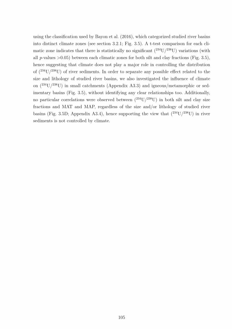
using the classification used by Bayon et al. (2016), which categorized studied river basinsinto distinct climate zones (see section 3.2.1; Fig. 3.5). A t-test comparison for each cli-matic zone indicates that there is statistically no significant (234U/238U) variations (withall p-values >0.05) between each climatic zones for both silt and clay fractions (Fig. 3.5),hence suggesting that climate does not play a major role in controlling the distributionof (234U/238U) of river sediments. In order to separate any possible effect related to thesize and lithology of studied river basins, we also investigated the influence of climateon (234U/238U) in small catchments (Appendix A3.3) and igneous/metamorphic or sed-imentary basins (Fig. 3.5), without identifying any clear relationships too. Additionally,no particular correlations were observed between (234U/238U) in both silt and clay sizefractions and MAT and MAP, regardless of the size and/or lithology of studied riverbasins (Fig. 3.5D; Appendix A3.4), hence supporting the view that (234U/238U) in riversediments is not controlled by climate.

105

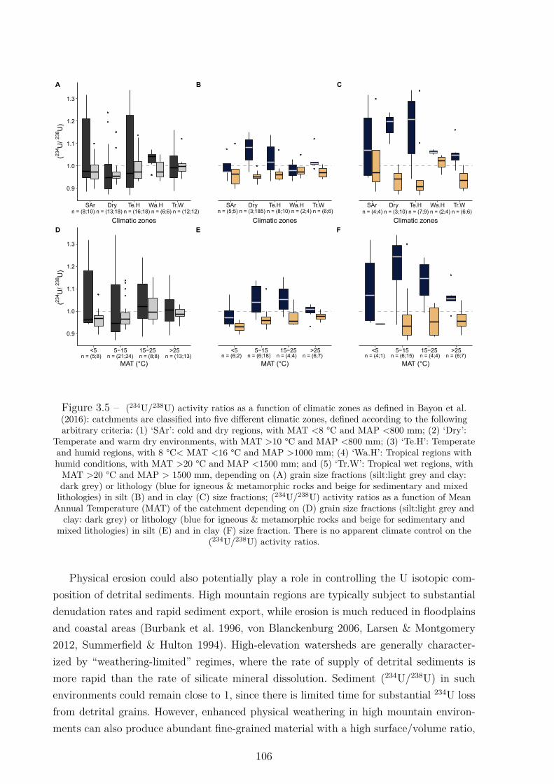
0.9

1.0

1.1

1.2

1.3

SAr Dry Te.H Wa.H Tr.W

Climatic zones

(234 U

/ 238 U

)

A

SAr Dry Te.H Wa.H Tr.W

Climatic zones

B

SAr Dry Te.H Wa.H Tr.W

Climatic zones

C

0.9

1.0

1.1

1.2

1.3

<5 5−15 15−25 >25

MAT (°C)

(234 U

/ 238 U

)

D

<5 5−15 15−25 >25

MAT (°C)

E

<5 5−15 15−25 >25

MAT (°C)

F

n = (8;10) n = (13;18) n = (16;18) n = (6;6) n = (12;12) n = (5;5) n = (3;185) n = (8;10) n = (2;4) n = (6;6) n = (4;4) n = (3;10) n = (7;9) n = (2;4) n = (6;6)

n = (4;1) n = (6;15) n = (4;4) n = (6;7)n = (6;2) n = (6;18) n = (4;4) n = (6;7)n = (5;8) n = (21;24) n = (8;8) n = (13;13)

Figure 3.5 – (234U/238U) activity ratios as a function of climatic zones as defined in Bayon et al.(2016): catchments are classified into five different climatic zones, defined according to the followingarbitrary criteria: (1) ‘SAr’: cold and dry regions, with MAT <8 °C and MAP <800 mm; (2) ‘Dry’:

Temperate and warm dry environments, with MAT >10 °C and MAP <800 mm; (3) ‘Te.H’: Temperateand humid regions, with 8 °C< MAT <16 °C and MAP >1000 mm; (4) ‘Wa.H’: Tropical regions withhumid conditions, with MAT >20 °C and MAP <1500 mm; and (5) ‘Tr.W’: Tropical wet regions, withMAT >20 °C and MAP > 1500 mm, depending on (A) grain size fractions (silt:light grey and clay:dark grey) or lithology (blue for igneous & metamorphic rocks and beige for sedimentary and mixedlithologies) in silt (B) and in clay (C) size fractions; (234U/238U) activity ratios as a function of MeanAnnual Temperature (MAT) of the catchment depending on (D) grain size fractions (silt:light grey and

clay: dark grey) or lithology (blue for igneous & metamorphic rocks and beige for sedimentary andmixed lithologies) in silt (E) and in clay (F) size fraction. There is no apparent climate control on the

(234U/238U) activity ratios.

Physical erosion could also potentially play a role in controlling the U isotopic com-position of detrital sediments. High mountain regions are typically subject to substantialdenudation rates and rapid sediment export, while erosion is much reduced in floodplainsand coastal areas (Burbank et al. 1996, von Blanckenburg 2006, Larsen & Montgomery2012, Summerfield & Hulton 1994). High-elevation watersheds are generally character-ized by “weathering-limited” regimes, where the rate of supply of detrital sediments ismore rapid than the rate of silicate mineral dissolution. Sediment (234U/238U) in suchenvironments could remain close to 1, since there is limited time for substantial 234U lossfrom detrital grains. However, enhanced physical weathering in high mountain environ-ments can also produce abundant fine-grained material with a high surface/volume ratio,

106

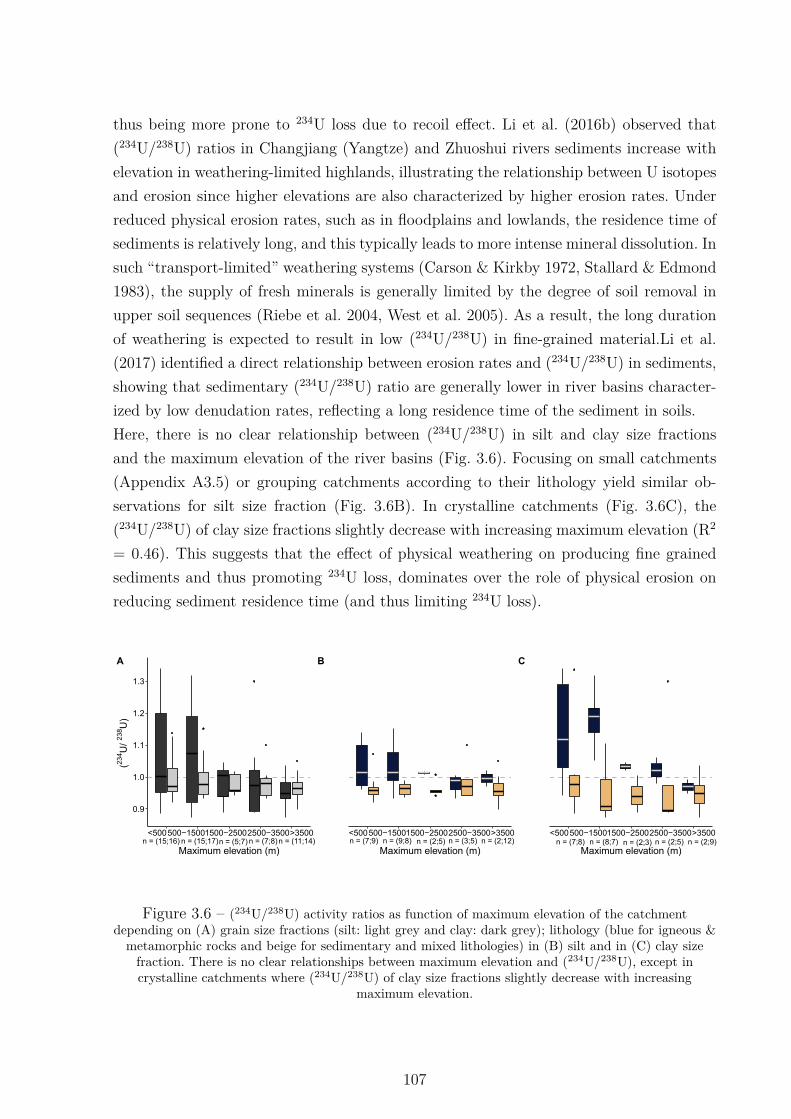
thus being more prone to 234U loss due to recoil effect. Li et al. (2016b) observed that(234U/238U) ratios in Changjiang (Yangtze) and Zhuoshui rivers sediments increase withelevation in weathering-limited highlands, illustrating the relationship between U isotopesand erosion since higher elevations are also characterized by higher erosion rates. Underreduced physical erosion rates, such as in floodplains and lowlands, the residence time ofsediments is relatively long, and this typically leads to more intense mineral dissolution. Insuch “transport-limited” weathering systems (Carson & Kirkby 1972, Stallard & Edmond1983), the supply of fresh minerals is generally limited by the degree of soil removal inupper soil sequences (Riebe et al. 2004, West et al. 2005). As a result, the long durationof weathering is expected to result in low (234U/238U) in fine-grained material.Li et al.(2017) identified a direct relationship between erosion rates and (234U/238U) in sediments,showing that sedimentary (234U/238U) ratio are generally lower in river basins character-ized by low denudation rates, reflecting a long residence time of the sediment in soils.Here, there is no clear relationship between (234U/238U) in silt and clay size fractionsand the maximum elevation of the river basins (Fig. 3.6). Focusing on small catchments(Appendix A3.5) or grouping catchments according to their lithology yield similar ob-servations for silt size fraction (Fig. 3.6B). In crystalline catchments (Fig. 3.6C), the(234U/238U) of clay size fractions slightly decrease with increasing maximum elevation (R2

= 0.46). This suggests that the effect of physical weathering on producing fine grainedsediments and thus promoting 234U loss, dominates over the role of physical erosion onreducing sediment residence time (and thus limiting 234U loss).

0.9

1.0

1.1

1.2

1.3

<500500−15001500−25002500−3500>3500

Maximum elevation (m)

(234 U

/ 238 U

)

A

<500500−15001500−25002500−3500>3500

Maximum elevation (m)

B

<500500−15001500−25002500−3500>3500

Maximum elevation (m)

C

n = (15;16) n = (15;17)n = (5;7) n = (7;8)n = (11;14) n = (7;9) n = (9;8) n = (2;5) n = (3;5) n = (2;12) n = (7;8) n = (8;7) n = (2;3) n = (2;5) n = (2;9)

Figure 3.6 – (234U/238U) activity ratios as function of maximum elevation of the catchmentdepending on (A) grain size fractions (silt: light grey and clay: dark grey); lithology (blue for igneous &metamorphic rocks and beige for sedimentary and mixed lithologies) in (B) silt and in (C) clay sizefraction. There is no clear relationships between maximum elevation and (234U/238U), except incrystalline catchments where (234U/238U) of clay size fractions slightly decrease with increasing

maximum elevation.

107

Table 3.4 – Characteristics of the studied samples and their sedimentary systemType of rocks inside the basin (%) Clays Silts bulk Clays Silts bulkSedimentary Igneous Volcanics CIA CIW Climatic zone MAT MAP Maximum elevation DTB Area

River (n= 64) (°C) (mm) (m) (cm) (103 km2)1 Adour 45.3 15.8 0.3 83.4 68.5 71.0 96.8 86.7 88.4 Te.H 13 1260 2800 1717 162 Amazon 43.8 22.9 4.2 88.0 75.6 99.0 93.2 Tr.W 27 2030 5500 2342 63003 Betsiboka Tr.W4 Blackwater 88.6 0.0 3.3 86.7 66.0 0.0 97.9 83.6 0.0 Te.H 9 1000 360 976 1.15 Brantas 9.0 0.0 65.7 Tr.W 25 2982 3480 3235 116 Chao Phraya 38.2 18.4 5.1 86.5 77.3 80.3 97.7 93.3 94.7 Tr.W 28 1500 2500 6378 1607 Churchill 10.5 57.9 1.4 SAr -3 800 1138 2908 Clarence Wa.H 1500 250 0.1329 Danube 66.9 12.6 3.0 70.1 88.0 Dry 10 760 4100 2106 82010 Don 82.5 61.1 62.9 96.3 81.3 82.5 SAr 7 580 180 42011 Dordogne Dry 800 1700 2412 Elbe Dry 7 800 148.313 Elorn 50.3 49.7 0.0 83.1 73.8 75.0 96.7 91.4 92.1 Te.H 11 1120 340 1289 0.314 Fitzroy river Dry 19 760 490 1305 8615 Fly 32.3 0.3 3.9 82.9 75.0 77.3 95.5 89.5 91.2 Tr.W 26 2850 4000 2456 7616 Fortescue river 10.9 19.4 8.1 Wa.H 25 1150 727 5017 Foyle 2.5 52.7 6.2 78.9 64.7 0.0 96.6 84.2 0.0 Te.H 9 1110 640 1063 2.918 Fraser 33.1 26.9 39.5 74.2 58.5 60.7 89.4 75.4 77.4 SAr 4 760 4000 2162 23019 Ganges 29.6 27.1 6.4 Te.H 18 7000 3061 108020 Gascogne Dry 22 235 500 7921 Glenariff 12.4 0.0 64.4 94.5 58.2 59.1 96.9 71.8 72.4 Te.H 9 1000 410 1129 0.122 Jamata Wa.H 29 82023 Kymijoki 67.1 61.6 62.9 87.8 83.2 84.3 SAr 3 600 100 3724 Lee Te.H 1.225 Loire 56.2 28.1 4.4 84.3 74.3 76.3 97.0 91.5 92.6 Dry 11 750 1900 1650 12026 Lough Erne Te.H 9 650 948 4.427 Lower Bann 88.2 66.9 67.4 97.9 82.7 83.1 Te.H 9 1000 640 943 5.828 Lule 47.7 67.2 SAr -3 700 1000 2529 MacKenzie 77.2 19.9 1.6 79.2 74.9 75.9 96.5 93.0 93.8 SAr -4 380 3600 1099 180030 Mae Klong 62.0 15.2 3.7 86.2 82.1 83.3 97.8 97.6 97.6 Tr.W 28 1200 2200 6785 3131 Maine 0.0 0.0 98.0 92.8 63.7 65.8 96.3 76.4 77.9 Te.H 9 1000 460 1032 0.2932 Mayenne 84.1 74.4 76.4 96.7 91.6 92.6 Dry 12 630 420 1587 4.433 Mekong 86.6 75.0 79.5 97.5 90.8 93.4 Wa.H 21 1270 5100 5292 80034 Mississippi 68.5 4.5 1.8 84.3 71.3 75.6 97.2 90.1 92.4 Dry 13 760 3700 3262 330035 Moyola 47.6 19.2 32.4 81.8 65.8 66.2 97.1 85.4 85.7 Te.H 9 1110 540 1087 0.336 Murchison 2.0 18.1 1.5 Dry 22 520 1442 8237 Nalon Dry 1400 3.738 Narva 71.1 63.0 63.7 93.4 88.5 88.9 SAr 6 640 320 1941 5639 Nelson river 66.5 24.0 3.1 Te.H -3 3400 2829 110040 Niger 5.6 40.3 1.2 85.8 88.3 88.0 94.5 97.0 96.7 Wa.H 29 1140 820 12474 220041 Nile 17.8 34.5 7.3 80.2 55.8 63.3 93.4 75.0 80.7 Dry 27 610 3800 11262 290042 Northern Dvina 56.4 0.0 0.0 69.6 67.1 67.7 87.9 86.0 86.4 SAr 1 740 200 2906 35743 Orinoco 9.8 20.7 2.8 70.4 88.0 Wa.H 24 1400 6000 4587 110044 Pamisos Dry 2300 0.545 Red River 80.4 14.6 1.7 80.7 75.2 76.7 96.9 93.5 94.4 Tr.W 24 1750 3100 1126 16046 Rhine 63.0 12.1 3.2 75.5 55.9 58.7 93.0 76.1 78.5 Te.H 8 1210 3500 1639 22047 Rio Aro 0.0 54.6 25.6 77.9 93.4 Tr.W 25 3700 810 2738 3048 Rio Caroni 1.8 18.0 29.3 95.7 86.2 87.3 99.5 97.6 97.8 Tr.W 25 2800 2660 2082 9549 Rio Caura 1.8 60.6 23.9 95.6 86.3 88.3 99.5 97.7 98.0 Tr.W 25 3700 2350 2086 4850 Ropotamo Dry 400 0.251 Sefid Rud 45.4 7.2 29.1 81.2 62.3 64.2 95.1 80.0 81.5 Dry 14 520 4230 1002 1352 Sepik river 36.3 12.8 1.9 Tr.W 25 4000 1684 7853 Severn Dry 610 11.454 Shannon 96.0 0.0 0.7 80.2 67.6 69.7 97.0 85.3 87.3 Te.H 9 1200 570 923 2355 Six Mile 0.1 0.0 96.6 91.1 56.4 60.6 96.1 71.0 74.0 Te.H 9 1000 420 813 0.356 Spercheios Dry 2300 1.857 Swilly 54.4 54.0 72.1 71.6 Te.H 9 1110 15 905 0.158 Thames Dry 10 330 12.959 Ume 54.3 51.0 73.8 69.3 SAr 1 520 1000 2660 Upper River Bann Te.H 110 261 Vanuatu Tr.W 190062 Vistula 23.5 0.1 0.0 74.0 70.2 70.8 94.0 91.9 92.3 SAr 8 750 2500 2235 20063 Yangtze 69.5 10.6 3.8 77.7 68.5 72.1 94.2 87.5 90.1 Te.H 16 1270 3200 1614 180064 Yellow River 40.3 9.2 2.0 68.3 57.6 58.4 86.6 76.5 77.2 Dry 13 760 5100 2469 750

Percentage of type of rocks inside the basin are from Bayon et al. (2020).CIA values (refers to Chemical Index of Alteration) are from Bayon et al. (2015).CIW calculated based on data from Bayon et al. (2015).Climatic categories are from Bayon et al. (2018) with (1) ‘SAr’: cold and dry regions, with MAT < 8 °C and MAP <800mm; (2) ‘Dry’: Temperate and warm dry environments, with MAT >10 °C and MAP < 800 mm; (3) ‘Te.H’: Temperateand humid regions, with 8 °C< MAT <16 °C and MAP >1000 mm; (4) ‘Wa.H’: Tropical regions with humid conditions,with MAT > 20 °C and MAP < 1500 mm; and (5) ‘Tr.W’: Tropical wet regions, with MAT > 20 °C and MAP > 1500mm.Mean annual temperature (MAT) and mean annual precipitation (MAP) data are from Bayon et al. (2016, 2018).Maximum elevation and area of river basins was either derived from Milliman & Farnsworth (2013), or determined inthe geographical information system (GIS) software ArcGis (ESRI 2001, ArcGis Desktop 10.3.1) using the hydrologicaldata and maps based on shuttle elevation derivatives HydroBASINS (Lehner and Grill, 2013)Depth to bedrock (mean absolute depth to bedrock) were extracted from the SoilGrids system (https://www.soilgrids.org).

108

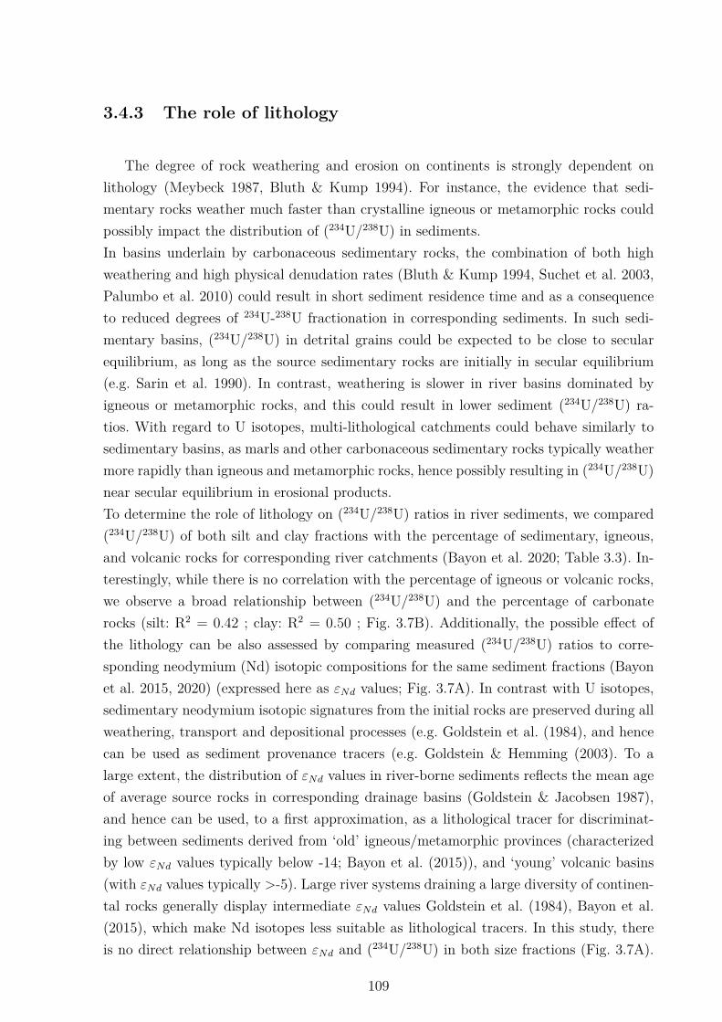
3.4.3 The role of lithology

The degree of rock weathering and erosion on continents is strongly dependent onlithology (Meybeck 1987, Bluth & Kump 1994). For instance, the evidence that sedi-mentary rocks weather much faster than crystalline igneous or metamorphic rocks couldpossibly impact the distribution of (234U/238U) in sediments.In basins underlain by carbonaceous sedimentary rocks, the combination of both highweathering and high physical denudation rates (Bluth & Kump 1994, Suchet et al. 2003,Palumbo et al. 2010) could result in short sediment residence time and as a consequenceto reduced degrees of 234U-238U fractionation in corresponding sediments. In such sedi-mentary basins, (234U/238U) in detrital grains could be expected to be close to secularequilibrium, as long as the source sedimentary rocks are initially in secular equilibrium(e.g. Sarin et al. 1990). In contrast, weathering is slower in river basins dominated byigneous or metamorphic rocks, and this could result in lower sediment (234U/238U) ra-tios. With regard to U isotopes, multi-lithological catchments could behave similarly tosedimentary basins, as marls and other carbonaceous sedimentary rocks typically weathermore rapidly than igneous and metamorphic rocks, hence possibly resulting in (234U/238U)near secular equilibrium in erosional products.To determine the role of lithology on (234U/238U) ratios in river sediments, we compared(234U/238U) of both silt and clay fractions with the percentage of sedimentary, igneous,and volcanic rocks for corresponding river catchments (Bayon et al. 2020; Table 3.3). In-terestingly, while there is no correlation with the percentage of igneous or volcanic rocks,we observe a broad relationship between (234U/238U) and the percentage of carbonaterocks (silt: R2 = 0.42 ; clay: R2 = 0.50 ; Fig. 3.7B). Additionally, the possible effect ofthe lithology can be also assessed by comparing measured (234U/238U) ratios to corre-sponding neodymium (Nd) isotopic compositions for the same sediment fractions (Bayonet al. 2015, 2020) (expressed here as εNd values; Fig. 3.7A). In contrast with U isotopes,sedimentary neodymium isotopic signatures from the initial rocks are preserved during allweathering, transport and depositional processes (e.g. Goldstein et al. (1984), and hencecan be used as sediment provenance tracers (e.g. Goldstein & Hemming (2003). To alarge extent, the distribution of εNd values in river-borne sediments reflects the mean ageof average source rocks in corresponding drainage basins (Goldstein & Jacobsen 1987),and hence can be used, to a first approximation, as a lithological tracer for discriminat-ing between sediments derived from ‘old’ igneous/metamorphic provinces (characterizedby low εNd values typically below -14; Bayon et al. (2015)), and ‘young’ volcanic basins(with εNd values typically >-5). Large river systems draining a large diversity of continen-tal rocks generally display intermediate εNd values Goldstein et al. (1984), Bayon et al.(2015), which make Nd isotopes less suitable as lithological tracers. In this study, thereis no direct relationship between εNd and (234U/238U) in both size fractions (Fig. 3.7A).

109

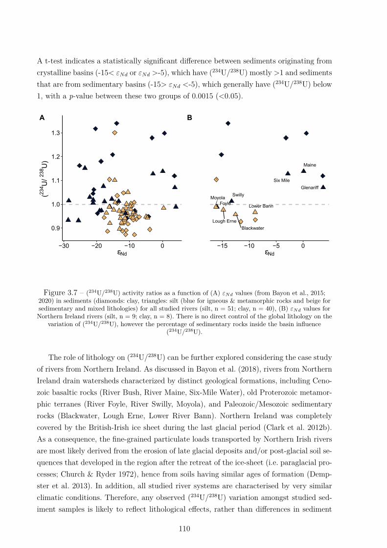
A t-test indicates a statistically significant difference between sediments originating fromcrystalline basins (-15< εNd or εNd >-5), which have (234U/238U) mostly >1 and sedimentsthat are from sedimentary basins (-15> εNd <-5), which generally have (234U/238U) below1, with a p-value between these two groups of 0.0015 (<0.05).

0.9

1.0

1.1

1.2

1.3

−30 −20 −10 0εNd

(234 U

/ 238 U

)

A

Blackwater

Foyle

Glenariff

Lough Erne

Lower Bann

Maine

Moyola

Six Mile

Swilly

−15 −10 −5 0εNd

B

Figure 3.7 – (234U/238U) activity ratios as a function of (A) εNd values (from Bayon et al., 2015;2020) in sediments (diamonds: clay, triangles: silt (blue for igneous & metamorphic rocks and beige forsedimentary and mixed lithologies) for all studied rivers (silt, n = 51; clay, n = 40), (B) εNd values forNorthern Ireland rivers (silt, n = 9; clay, n = 8). There is no direct control of the global lithology on the

variation of (234U/238U), however the percentage of sedimentary rocks inside the basin influence(234U/238U).

The role of lithology on (234U/238U) can be further explored considering the case studyof rivers from Northern Ireland. As discussed in Bayon et al. (2018), rivers from NorthernIreland drain watersheds characterized by distinct geological formations, including Ceno-zoic basaltic rocks (River Bush, River Maine, Six-Mile Water), old Proterozoic metamor-phic terranes (River Foyle, River Swilly, Moyola), and Paleozoic/Mesozoic sedimentaryrocks (Blackwater, Lough Erne, Lower River Bann). Northern Ireland was completelycovered by the British-Irish ice sheet during the last glacial period (Clark et al. 2012b).As a consequence, the fine-grained particulate loads transported by Northern Irish riversare most likely derived from the erosion of late glacial deposits and/or post-glacial soil se-quences that developed in the region after the retreat of the ice-sheet (i.e. paraglacial pro-cesses; Church & Ryder 1972), hence from soils having similar ages of formation (Demp-ster et al. 2013). In addition, all studied river systems are characterised by very similarclimatic conditions. Therefore, any observed (234U/238U) variation amongst studied sed-iment samples is likely to reflect lithological effects, rather than differences in sediment

110

transfer, soil age or climate. Rivers draining the British Tertiary volcanic province carryclay- and silt-sized detrital fractions both characterized by (234U/238U) >1 (Fig. 3.7B).The three rivers draining Proterozoic metamorphic rocks display clays with (234U/238U)>1 and coarser silt fractions with activity ratios close to 1 (Fig. 3.7C). The sedimentsfrom the Paleozoic/Mesozoic sedimentary rocks have (234U/238U) <1 in both silt and claysize fraction. Thus, in the case of Northern Ireland, river sediments derived from sedi-mentary basins also appear to exhibit (234U/238U) ratios lower than those from crystallinebasins. For such sedimentary basins, the presence of relatively low (234U/238U) signaturesin river sediments could reflect a residual (234U/238U) composition <1 in correspondingsource rocks, although it remains unclear how any significant 234U-238U disequilibriumcould possibly occur in rocks older than 1 Ma . A more plausible explanation is that thelower (234U/238U) values determined in sediments from sedimentary basins reflect that thefact that sedimentary rock weathering most likely results in finer particle sizes comparedto the alteration and erosion of crystalline silicate rocks. However, the t-test comparisonbetween grain sizes from each lithological group indicates that there is no statisticallysignificant variation of (234U/238U) with p-values >0.05 (0.94) for sediments from sed-imentary and mixed lithologies, and close to 0.05 (0.06) for sediments from igneous &metamorphic rocks. The observed (234U/238U) >1 in sediments derived from crystallinebasements could reflect the fact that neo-formed clays produced from crystalline silicaterocks are more prone to subsequent re-adsorption of 234U on secondary clays, althoughfurther investigation will be required to test this hypothesis. To summarize, while the lackof any strong relationship between U and Nd isotopes suggests that the lithology doesnot represent a major control on the distribution of (234U/238U) ratios of river sediments,the apparent correlation observed between (234U/238U) and the percentage of carbonaterocks in river catchments implicitly suggests that the degree of U isotope fractionation infine-grained sediments is partially dependent on the lithology of source rocks, probablyreflecting the fact that they are being eroded more rapidly (and presumably into finerparticle sizes) than crystalline silicate rocks.

3.4.4 The role of catchment size and sediment residence timeon (234U/238U) sedimentary ratio

As mentioned in the Introduction, the sediment transfer time within any given wa-tershed is expected to exert a major control on sedimentary U isotopic ratios. The resi-dence time of sediments in river basins is mainly influenced by the possibility of storagealong its pathway from the hillslopes to the alluvial plain or the nearby ocean margin.Sediment transport along river systems is generally complex and mostly related to geo-morphic parameters (Harvey 2002). Several studies highlighted the relationships betweensedimentary fluxes and both external (climate, sea-level) and internal factors (drainage

111

area, relief, lithology) (Milliman & Syvitski 1992, Syvitski et al. 2003). In particular, thedrainage area and relief are the main parameters that govern the quantity of sedimentsdelivered downstream of alluvial plains (Hovius 1998, Milliman & Syvitski 1992, Syvitskiet al. 2003, Walling & Webb 1996).In general, the capacity of sediment storage in river basins is controlled by their geomor-phological characteristics. On hillslopes, storage is dependent on soil thickness and themean slope of the watershed, with thick soil sequences being typically associated with re-duced erosion and vice versa. In this study, no global correlations were identified between(234U/238U) and mean soil thickness (Fig. 3.8A), even when considering small catchmentsonly (Appendix A3.6). However, when investigating separately the relationship between(234U/238U) and soil thickness in igneous/metamorphic and sedimentary basins (Fig 3.8B& C), we can notice a slight decrease of the (234U/238U) ratios as the average depth tobedrock decreases in sedimentary watersheds. In contrast, clays separated from crystallinebasins display a trend exhibiting decreasing (234U/238U) ratios when the depth to bedrockincreases (Fig. 3.8C), in agreement with the fact that sediments will spend more time inthicker soil sequences (thus 234U/238U activity ratios will decrease accordingly). Ideally,sediment samples collected at the bottom of hillslopes would be best suited to investi-gate the role of hillslope storage on the (234U/238U) of sediments, rather than at the rivermouth, where the effect of alluvial storage adds complexity to the interpretation. Thismay explain the apparent lack of clear control of hillslope storage on the (234U/238U) ofsediments.In river basins where alluvial storage is significant, the sediment residence time couldbe a function of the size of the alluvial plain and its storage efficiency. Previous studieshave shown that specific sedimentary fluxes decrease with the size of the drainage area(Milliman & Syvitski 1992, Syvitski & Milliman 2007), whenever storage efficiency is in-creasing. No strong relationship is apparent when looking at the variation of clay- andsilt-size (234U/238U) depending on the size of the catchment (Fig. 3.8D, Table 4), exceptwhen considering the rivers draining igneous & metamorphic rocks, in which activity ra-tios decrease as the size of the catchment increases (Fig. 3.8E & 3.8F). These observationsclearly suggest that the size of the catchment and inferred sediment residence time exertsa major role in controlling the degree of 234U-238U fractionation in river sediments. Theobserved slight increase of (234U/238U) in river sediments from the largest catchmentscould indicate that incorporation of 234U into neo-formed clays occurs during the storageof the sediments along the alluvial plain. It is interesting to note that no trend is visiblefor sediments derived from basins draining sedimentary rocks and mixed lithologies. Onehypothesis to explain this absence of relationship could be that the weathering in sedi-mentary rocks create grains with inherited shapes, by breaking the cement linking them,whereas in crystalline basins silicate weathering generates new grains with fresh mineralsurfaces prone to dissolution. The fractionation of 234U over 238U being influenced by the

112

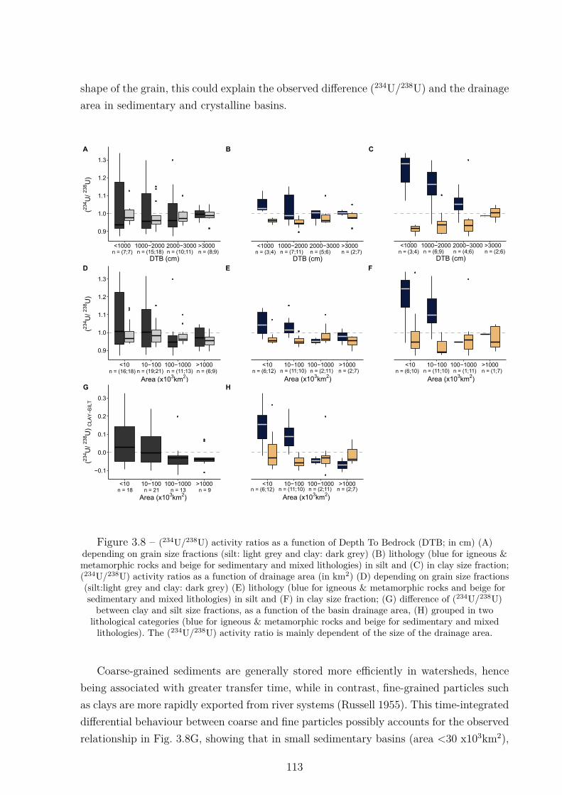
shape of the grain, this could explain the observed difference (234U/238U) and the drainagearea in sedimentary and crystalline basins.

0.9

1.0

1.1

1.2

1.3

<1000 1000−2000 2000−3000 >3000

DTB (cm)

(234 U

/ 238 U

)

A

B

C

0.9

1.0

1.1

1.2

1.3

<10 10−100 100−1000 >1000

Area (x103km2)

(234 U

/ 238 U

)

D

<10 10−100 100−1000 >1000

E

<10 10−100 100−1000 >1000

F

−0.1

0.0

0.1

0.2

0.3

<10 10−100 100−1000 >1000

(234 U

/ 238 U

) C

LAY−S

ILT

G

Area (x103km2)n = (6;12) n = (11;10) n = (2;11) n = (2;7)

<10 10−100 100−1000 >1000

H

n = (7;7) n = (15;18) n = (10;11) n = (8;9)<1000 1000−2000 2000−3000 >3000

DTB (cm)n = (3;4) n = (7;11) n = (5;6) n = (2;7)

<1000 1000−2000 2000−3000 >3000

DTB (cm)n = (3;4) n = (6;9) n = (4;6) n = (2;6)

n = (16;18) n = (19;21) n = (11;13) n = (6;9)

Area (x103km2)n = (6;12) n = (11;10) n = (2;11) n = (2;7)

Area (x103km2)n = (6;10) n = (11;10) n = (1;11) n = (1;7)

Area (x103km2)n = 18 n = 21 n = 13 n = 9

Figure 3.8 – (234U/238U) activity ratios as a function of Depth To Bedrock (DTB; in cm) (A)depending on grain size fractions (silt: light grey and clay: dark grey) (B) lithology (blue for igneous &metamorphic rocks and beige for sedimentary and mixed lithologies) in silt and (C) in clay size fraction;(234U/238U) activity ratios as a function of drainage area (in km2) (D) depending on grain size fractions(silt:light grey and clay: dark grey) (E) lithology (blue for igneous & metamorphic rocks and beige forsedimentary and mixed lithologies) in silt and (F) in clay size fraction; (G) difference of (234U/238U)between clay and silt size fractions, as a function of the basin drainage area, (H) grouped in two

lithological categories (blue for igneous & metamorphic rocks and beige for sedimentary and mixedlithologies). The (234U/238U) activity ratio is mainly dependent of the size of the drainage area.

Coarse-grained sediments are generally stored more efficiently in watersheds, hencebeing associated with greater transfer time, while in contrast, fine-grained particles suchas clays are more rapidly exported from river systems (Russell 1955). This time-integrateddifferential behaviour between coarse and fine particles possibly accounts for the observedrelationship in Fig. 3.8G, showing that in small sedimentary basins (area <30 x103km2),

113

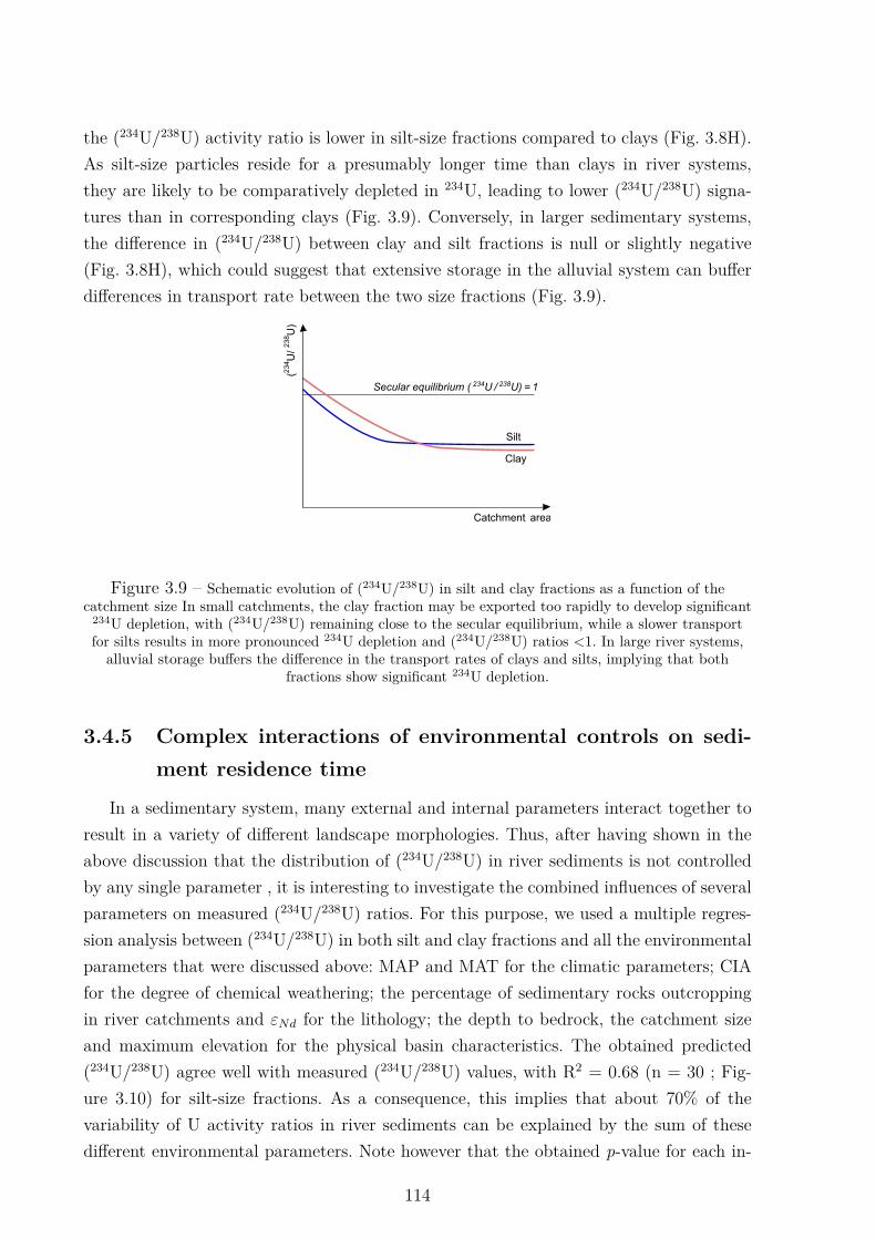
the (234U/238U) activity ratio is lower in silt-size fractions compared to clays (Fig. 3.8H).As silt-size particles reside for a presumably longer time than clays in river systems,they are likely to be comparatively depleted in 234U, leading to lower (234U/238U) signa-tures than in corresponding clays (Fig. 3.9). Conversely, in larger sedimentary systems,the difference in (234U/238U) between clay and silt fractions is null or slightly negative(Fig. 3.8H), which could suggest that extensive storage in the alluvial system can bufferdifferences in transport rate between the two size fractions (Fig. 3.9).

(234 U

/238 U

)

Catchment area

Secular equilibrium ( 234U / 238U) = 1

Silt

Clay

Figure 3.9 – Schematic evolution of (234U/238U) in silt and clay fractions as a function of thecatchment size In small catchments, the clay fraction may be exported too rapidly to develop significant

234U depletion, with (234U/238U) remaining close to the secular equilibrium, while a slower transportfor silts results in more pronounced 234U depletion and (234U/238U) ratios <1. In large river systems,alluvial storage buffers the difference in the transport rates of clays and silts, implying that both

fractions show significant 234U depletion.

3.4.5 Complex interactions of environmental controls on sedi-ment residence time

In a sedimentary system, many external and internal parameters interact together toresult in a variety of different landscape morphologies. Thus, after having shown in theabove discussion that the distribution of (234U/238U) in river sediments is not controlledby any single parameter , it is interesting to investigate the combined influences of severalparameters on measured (234U/238U) ratios. For this purpose, we used a multiple regres-sion analysis between (234U/238U) in both silt and clay fractions and all the environmentalparameters that were discussed above: MAP and MAT for the climatic parameters; CIAfor the degree of chemical weathering; the percentage of sedimentary rocks outcroppingin river catchments and εNd for the lithology; the depth to bedrock, the catchment sizeand maximum elevation for the physical basin characteristics. The obtained predicted(234U/238U) agree well with measured (234U/238U) values, with R2 = 0.68 (n = 30 ; Fig-ure 3.10) for silt-size fractions. As a consequence, this implies that about 70% of thevariability of U activity ratios in river sediments can be explained by the sum of thesedifferent environmental parameters. Note however that the obtained p-value for each in-

114

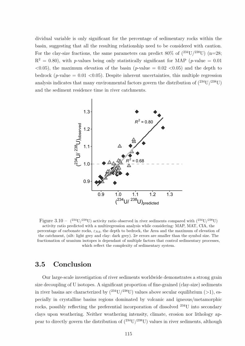
dividual variable is only significant for the percentage of sedimentary rocks within thebasin, suggesting that all the resulting relationship need to be considered with caution.For the clay-size fractions, the same parameters can predict 80% of (234U/238U) (n=28;R2 = 0.80), with p-values being only statistically significant for MAP (p-value = 0.01<0.05), the maximum elevation of the basin (p-value = 0.02 <0.05) and the depth tobedrock (p-value = 0.01 <0.05). Despite inherent uncertainties, this multiple regressionanalysis indicates that many environmental factors govern the distribution of (234U/238U)and the sediment residence time in river catchments.

R2 = 0.80

R2 = 0.68

0.9

1.0

1.1

1.2

1.3

0.9 1.0 1.1 1.2 1.3

(234U/ 238U)predicted

(234 U

/ 238 U

) obs

erve

d

Figure 3.10 – (234U/238U) activity ratio observed in river sediments compared with (234U/238U)activity ratio predicted with a multiregression analysis while considering: MAP, MAT, CIA, the

percentage of carbonate rocks, εNd, the depth to bedrock, the Area and the maximum of elevation ofthe catchment, (silt: light grey and clay: dark grey). 2σ errors are smaller than the symbol size. Thefractionation of uranium isotopes is dependant of multiple factors that control sedimentary processes,

which reflect the complexity of sedimentary system.

3.5 ConclusionOur large-scale investigation of river sediments worldwide demonstrates a strong grain

size decoupling of U isotopes. A significant proportion of fine-grained (clay-size) sedimentsin river basins are characterized by (234U/238U) values above secular equilibrium (>1), es-pecially in crystalline basins regions dominated by volcanic and igneous/metamorphicrocks, possibly reflecting the preferential incorporation of dissolved 234U into secondaryclays upon weathering. Neither weathering intensity, climate, erosion nor lithology ap-pear to directly govern the distribution of (234U/238U) values in river sediments, although

115

the erosion of sedimentary rocks most likely results in a higher degree of 234U-238U frac-tionation compared to crystalline silicate rocks, possibly reflecting the fact that it cangenerate finer sediments that are more prone to 234U loss through recoil effect. Overall,the size of the catchments is identified as being one of the main parameters explainingthe observed distribution of (234U/238U) in river sediments, via its impact on the sedi-ment residence time. In catchments draining crystalline basement rocks, the differencebetween (234U/238U) in silt- and clay-size fractions is best explained by the fact that claysare exported more rapidly than silts, resulting in different size-dependent (234U/238U)signatures. In large river basins, sediment storage in alluvial plains also impact the distri-bution of (234U/238U) in river sediments, causing significant 234U loss regardless of grainsize. Taken together, our findings confirm that U isotopes are sensitive tracers of thesediment residence time in river basins, providing further evidence for their utility in thesedimentary record to reconstruct past variations in sediment residence time and theirlinks to landscape evolution.

3.6 AcknowledgmentsWe gratefully acknowledge all who very kindly provided us with the studied samples:

O. Adeaga, J. Allard, C. Bigler, F. Busschers, G. Calvès, K. Cohen, P. Debrock, B.Dennielou, F.X. Gingele, D. Haynes, P.R. Hill, B. Hoogendoorn, S. Jorry, G. Kowaleska,T. Leipe, S. Leroy, L. Lopez, J. P. Lunkla, I. Mendes, D. Meunier, C. Nittrouer, A.Pasquini, V. Ponomareva, Y. Saito, E. Schefuss, V. Shevchenko, L. Tiron, D. Toucanne,S. VanLaningham, A. Wheeler. We are also thankful to A. Francke for providing samplesto test the leaching protocol. We thank Pr. F. Chabaux and two anonymous reviewers fortheir helpful comments that greatly improved this manuscript. The project was fundedthrough a joint IFREMER - University of Wollongong postgraduate scholarship.

116

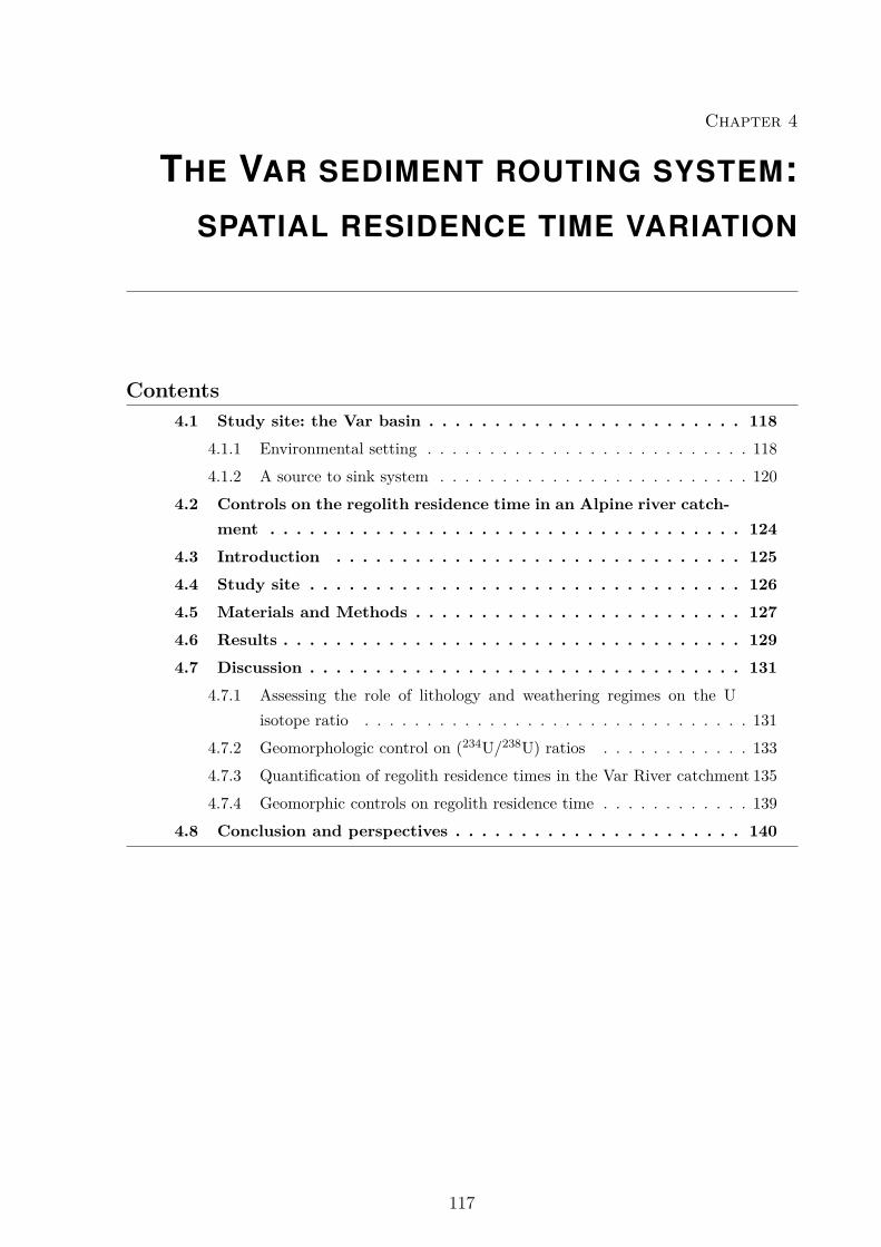
Chapter 4

THE VAR SEDIMENT ROUTING SYSTEM:SPATIAL RESIDENCE TIME VARIATION

Contents4.1 Study site: the Var basin . . . . . . . . . . . . . . . . . . . . . . . . 118

4.1.1 Environmental setting . . . . . . . . . . . . . . . . . . . . . . . . . . 1184.1.2 A source to sink system . . . . . . . . . . . . . . . . . . . . . . . . . 120

4.2 Controls on the regolith residence time in an Alpine river catch-ment . . . . . . . . . . . . . . . . . . . . . . . . . . . . . . . . . . . . 124

4.3 Introduction . . . . . . . . . . . . . . . . . . . . . . . . . . . . . . . 1254.4 Study site . . . . . . . . . . . . . . . . . . . . . . . . . . . . . . . . . 1264.5 Materials and Methods . . . . . . . . . . . . . . . . . . . . . . . . . 1274.6 Results . . . . . . . . . . . . . . . . . . . . . . . . . . . . . . . . . . . 1294.7 Discussion . . . . . . . . . . . . . . . . . . . . . . . . . . . . . . . . . 131

4.7.1 Assessing the role of lithology and weathering regimes on the Uisotope ratio . . . . . . . . . . . . . . . . . . . . . . . . . . . . . . . 131

4.7.2 Geomorphologic control on (234U/238U) ratios . . . . . . . . . . . . 1334.7.3 Quantification of regolith residence times in the Var River catchment 1354.7.4 Geomorphic controls on regolith residence time . . . . . . . . . . . . 139

4.8 Conclusion and perspectives . . . . . . . . . . . . . . . . . . . . . . 140

117

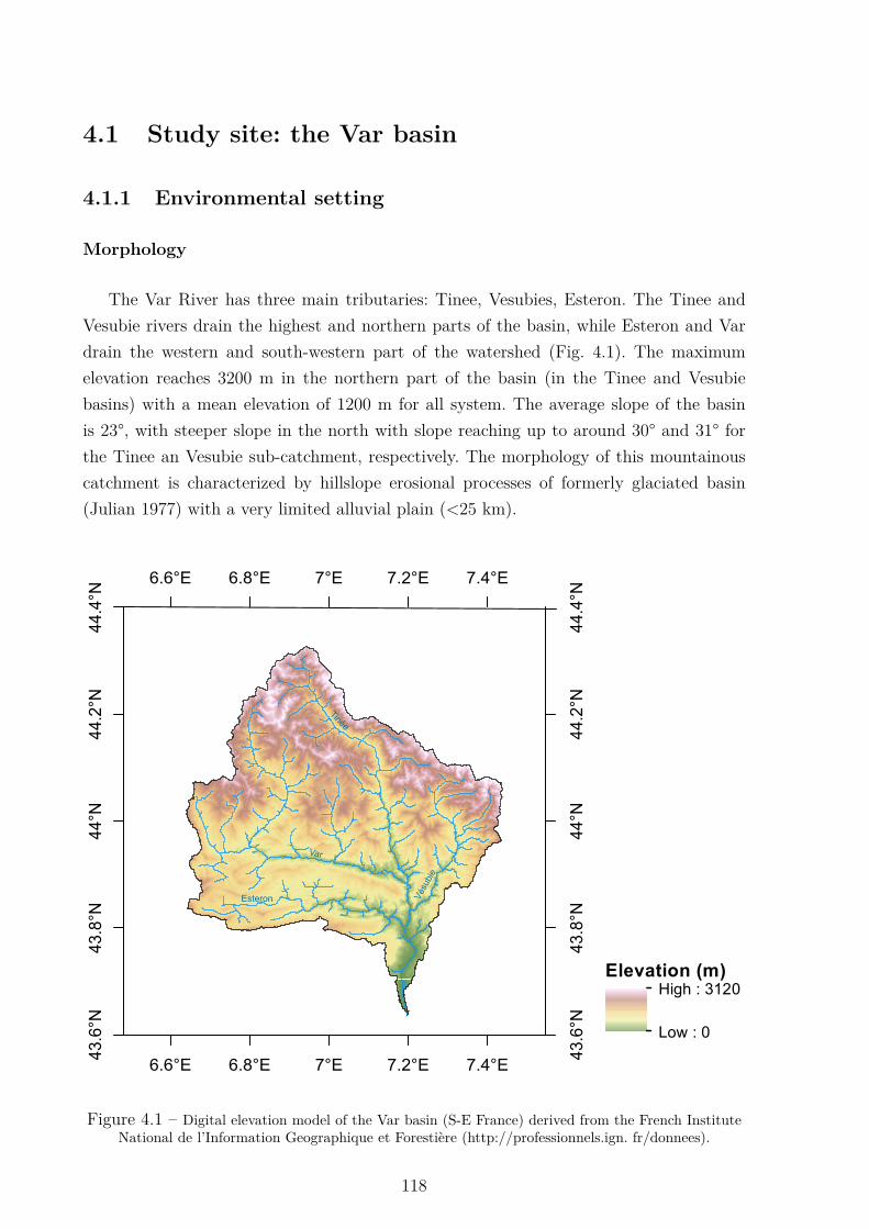
4.1 Study site: the Var basin

4.1.1 Environmental setting

Morphology

The Var River has three main tributaries: Tinee, Vesubies, Esteron. The Tinee andVesubie rivers drain the highest and northern parts of the basin, while Esteron and Vardrain the western and south-western part of the watershed (Fig. 4.1). The maximumelevation reaches 3200 m in the northern part of the basin (in the Tinee and Vesubiebasins) with a mean elevation of 1200 m for all system. The average slope of the basinis 23°, with steeper slope in the north with slope reaching up to around 30° and 31° forthe Tinee an Vesubie sub-catchment, respectively. The morphology of this mountainouscatchment is characterized by hillslope erosional processes of formerly glaciated basin(Julian 1977) with a very limited alluvial plain (<25 km).

Elevation (m)High : 3120

Low : 0

Esteron

Var

Tinée

Vés

ubie

6.6°E 6.8°E 7°E 7.2°E 7.4°E

43.6

°N43

.8°N

44°N

44.2

°N44

.4°N

6.6°E 6.8°E 7°E 7.2°E 7.4°E43

.6°N

43.8

°N44

°N44

.2°N

44.4

°N

Figure 4.1 – Digital elevation model of the Var basin (S-E France) derived from the French InstituteNational de l’Information Geographique et Forestière (http://professionnels.ign. fr/donnees).

118

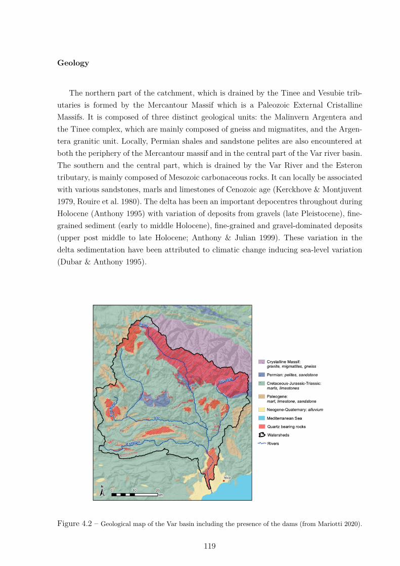
Geology

The northern part of the catchment, which is drained by the Tinee and Vesubie trib-utaries is formed by the Mercantour Massif which is a Paleozoic External CristallineMassifs. It is composed of three distinct geological units: the Malinvern Argentera andthe Tinee complex, which are mainly composed of gneiss and migmatites, and the Argen-tera granitic unit. Locally, Permian shales and sandstone pelites are also encountered atboth the periphery of the Mercantour massif and in the central part of the Var river basin.The southern and the central part, which is drained by the Var River and the Esterontributary, is mainly composed of Mesozoic carbonaceous rocks. It can locally be associatedwith various sandstones, marls and limestones of Cenozoic age (Kerckhove & Montjuvent1979, Rouire et al. 1980). The delta has been an important depocentres throughout duringHolocene (Anthony 1995) with variation of deposits from gravels (late Pleistocene), fine-grained sediment (early to middle Holocene), fine-grained and gravel-dominated deposits(upper post middle to late Holocene; Anthony & Julian 1999). These variation in thedelta sedimentation have been attributed to climatic change inducing sea-level variation(Dubar & Anthony 1995).

Figure 4.2 – Geological map of the Var basin including the presence of the dams (from Mariotti 2020).

119

Climate

The catchment has the characteristic of a Mediterranean climate with hot and drysummers alternating with cool and wet winter. At the river mouth, in Nice (2 metersabove sea level), the mean annual temperature recorded between 1942 and 2020 is 16 °C,with a mean temperature around 24 °C during summer and 10 °C in winter. The meanannual precipitation recorded between 1942 and 2020 is 733 mm on 61 days with precipi-tation >1 mm (climatic data from Meteo France database; https://donneespubliques. me-teofrance.fr). On the northern part of the catchment, the elevation influences the weatherwith a mountainous climate. The records at Saint Martin de Vesubie (1064 meters abovesea level) indicate a mean annual temperature of 11.9 °C between 1981 and 2010 with amean temperature around 20°C in summer and 5°C in winter. Between 1989 and 2010,the mean annual precipitation is 1138 mm divided in 89 days with precipitation >1 mm.Events with extrem rainfall occurs in the Var basin, and are referred as "Mediterraneanepisodes". These Mediterranean episodes are linked to hot, humid and unstable upwellingair from the Mediterranean, which can generate violent thunderstorms that are some-times stationary. They occur particularly in autumn, when the sea is at its warmest,which favours strong evaporation. The precipitation can reach 200 mm in about 24h. Thelast episode occurred in October 2020, with 200 to 300 mm and up to 450-500 mm in theinterland (MeteoFrance).

Land cover

The present day vegetation in southern France depends of the Mediterranean climate.In high elevation area (> 2000 m), the vegetation cover is mainly composed of grass-land. At lower elevation the vegetation is dominated by forest: with from sea-level tothe highest elevation a transition between drought resistant oak to conifers forest above1000 m (Beaudouin et al. 2007; corine land cover from 2012 from the geoportail database,https://www.geoportail.gouv.fr/donnees/corine-land-cover-2012). Downstream, the catch-ment is largely urbanized with the Nice city with an urban area composed of more>1,000,000 habitants (INSEE, 2016).

4.1.2 A source to sink system

Denudation

The denudation rate of the whole Var basin calculated from 10Be (Mariotti et al. 2019)and determined from sediment flux (Bonneau et al. 2017) is around 0.24 ±0.04 mm.yr−1

and 0.22 mm.yr−1 respectively. Within the basin variations between 0.10 ±0.01 to 0.057±0.09 m.yr−1 are observed and is representative of the denudation variability across theAlps (Mariotti et al. 2019).

120

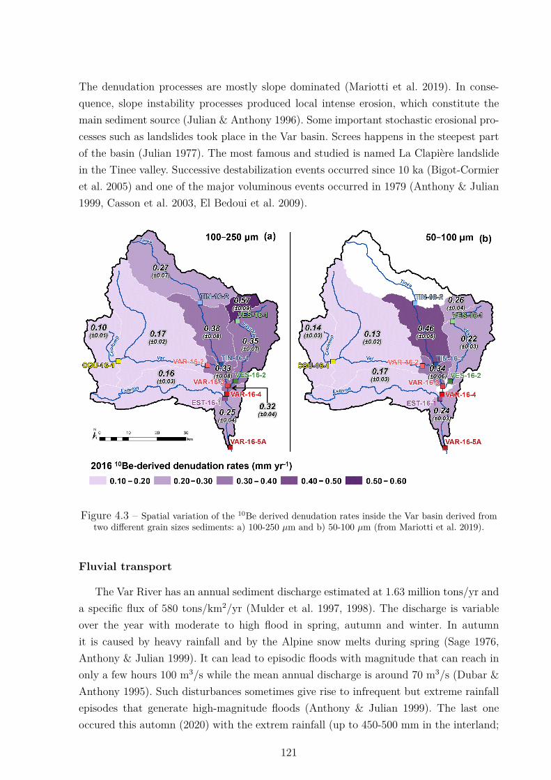
The denudation processes are mostly slope dominated (Mariotti et al. 2019). In conse-quence, slope instability processes produced local intense erosion, which constitute themain sediment source (Julian & Anthony 1996). Some important stochastic erosional pro-cesses such as landslides took place in the Var basin. Screes happens in the steepest partof the basin (Julian 1977). The most famous and studied is named La Clapière landslidein the Tinee valley. Successive destabilization events occurred since 10 ka (Bigot-Cormieret al. 2005) and one of the major voluminous events occurred in 1979 (Anthony & Julian1999, Casson et al. 2003, El Bedoui et al. 2009).

Figure 4.3 – Spatial variation of the 10Be derived denudation rates inside the Var basin derived fromtwo different grain sizes sediments: a) 100-250 µm and b) 50-100 µm (from Mariotti et al. 2019).

Fluvial transport

The Var River has an annual sediment discharge estimated at 1.63 million tons/yr anda specific flux of 580 tons/km2/yr (Mulder et al. 1997, 1998). The discharge is variableover the year with moderate to high flood in spring, autumn and winter. In autumnit is caused by heavy rainfall and by the Alpine snow melts during spring (Sage 1976,Anthony & Julian 1999). It can lead to episodic floods with magnitude that can reach inonly a few hours 100 m3/s while the mean annual discharge is around 70 m3/s (Dubar &Anthony 1995). Such disturbances sometimes give rise to infrequent but extreme rainfallepisodes that generate high-magnitude floods (Anthony & Julian 1999). The last oneoccured this automn (2020) with the extrem rainfall (up to 450-500 mm in the interland;

121

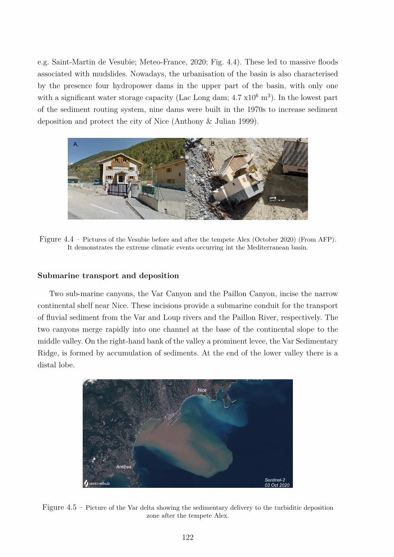
e.g. Saint-Martin de Vesubie; Meteo-France, 2020; Fig. 4.4). These led to massive floodsassociated with mudslides. Nowadays, the urbanisation of the basin is also characterisedby the presence four hydropower dams in the upper part of the basin, with only onewith a significant water storage capacity (Lac Long dam; 4.7 x106 m3). In the lowest partof the sediment routing system, nine dams were built in the 1970s to increase sedimentdeposition and protect the city of Nice (Anthony & Julian 1999).

A. B.

Figure 4.4 – Pictures of the Vesubie before and after the tempete Alex (October 2020) (From AFP).It demonstrates the extreme climatic events occurring int the Mediterranean basin.

Submarine transport and deposition

Two sub-marine canyons, the Var Canyon and the Paillon Canyon, incise the narrowcontinental shelf near Nice. These incisions provide a submarine conduit for the transportof fluvial sediment from the Var and Loup rivers and the Paillon River, respectively. Thetwo canyons merge rapidly into one channel at the base of the continental slope to themiddle valley. On the right-hand bank of the valley a prominent levee, the Var SedimentaryRidge, is formed by accumulation of sediments. At the end of the lower valley there is adistal lobe.

Figure 4.5 – Picture of the Var delta showing the sedimentary delivery to the turbiditic depositionzone after the tempete Alex.

122

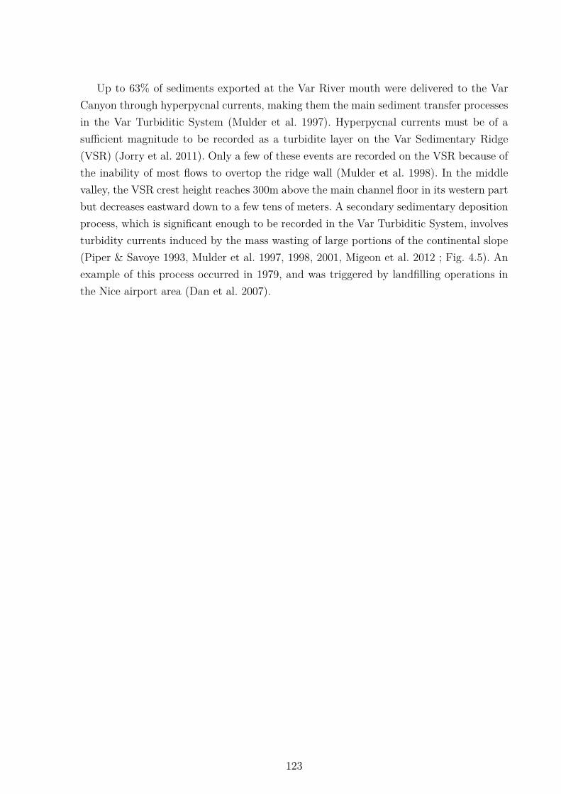
Up to 63% of sediments exported at the Var River mouth were delivered to the VarCanyon through hyperpycnal currents, making them the main sediment transfer processesin the Var Turbiditic System (Mulder et al. 1997). Hyperpycnal currents must be of asufficient magnitude to be recorded as a turbidite layer on the Var Sedimentary Ridge(VSR) (Jorry et al. 2011). Only a few of these events are recorded on the VSR because ofthe inability of most flows to overtop the ridge wall (Mulder et al. 1998). In the middlevalley, the VSR crest height reaches 300m above the main channel floor in its western partbut decreases eastward down to a few tens of meters. A secondary sedimentary depositionprocess, which is significant enough to be recorded in the Var Turbiditic System, involvesturbidity currents induced by the mass wasting of large portions of the continental slope(Piper & Savoye 1993, Mulder et al. 1997, 1998, 2001, Migeon et al. 2012 ; Fig. 4.5). Anexample of this process occurred in 1979, and was triggered by landfilling operations inthe Nice airport area (Dan et al. 2007).

123

4.2 Controls on the regolith residence time in anAlpine river catchment

AbstractUnderstanding the natural mechanisms affecting the evolution and morphology of river

systems through time is important in the context of on-going climate change. To this end,one major challenge is to quantify the timescale of sedimentary processes, such as erosion,transport and deposition, in catchments, and their relationships with geomorphologic pa-rameters (e.g. elevation, curvature, slope).In this study, we report uranium activity ratios (234U/238U), specific surface area mea-surements and derived comminution ages for a series of fine-grained (<63 µm) fluvialsediments from the Var River basin (France). The Var River is a small mountainouscatchment characterized by efficient sediment transport and the absence of alluvial plain,and thus significant alluvial storage. It implies that measured U comminution ages mainlyreflect storage on hillslopes. Our geochemical investigation was combined to a detailed spa-tial analysis of the catchment to investigate how the sediment residence time varies withgeomorphic parameters (e.g. slope, curvature, elevation). Moreover, spatial data on soilthickness and 10Be derived denudations rates were used to infer regolith residence time.Our results indicates an absence of lithologic control on the fractionation of 234U-238U,but (234U/238U) rather reflects the weathering regime. In transport-limited regime, thelonger residence time in well-developed soil results in greater 234U loss. Furthermore, thetopography controls the (234U/238U) ratios with high-elevated catchments, with steeperslopes, characterized by a short regolith residence time and thus a limited 234U depletion.We show that the regolith residence time determined with U isotopes agree well withestimated regolith residence infer with prediction of soil thickness spatial distribution and10Be denudation rate. This validates the use of U isotopes to determine sediment residencetimes and suggests that residence times in the Var basin mostly reflects hillslope storage,i.e. regolithe residence time.

124

4.3 Introduction

Sedimentary processes occurring at the Earth surface (e.g. weathering, sediment trans-port and deposition) control the landscape morphology. To understand the landscapeevolution, it is important to quantify the timescale of these processes and the responsetime of the landscape to adapt to environmental changes. For this purpose, the study ofsediment residence time can provide information on the timescale of Earth surface pro-cesses (DePaolo et al. 2006). This residence time represents the time elapsed since parentmaterial was converted into regolith and encompasses hillslope and alluvial storage andtransport (DePaolo et al. 2006).In basin where alluvial storage and soil creep are negligible, the sediment residence time ismainly controlled by the thickness of soil sequences and the overall denudation rate. Thequantification of sediment residence times in river basins can provide unique informationabout both weathering and erosion processes within catchments, where the average soilthickness can be viewed as reflecting the balance between soil production and soil denuda-tion (Carson & Kirkby 1972, Dietrich et al. 1995, Heimsath et al. 1997). Soil thickness isfunction of several geomorphic parameters including the slope and curvature (Heimsathet al. 1997), which have a direct influence on soil residence times.In fine-grained detrital sediments (typical <63 µm), uranium (U) isotopes fractionate as234U is preferential lost from sediments over 238U, as a result of recoil (Kigoshi 1971) andpreferential leaching (Fleischer 1980, 1982). This time-dependent fractionation has beenused to determine the comminution age of sediments, that is the time elapsed since theproduction of sediments finer than <63 µm (DePaolo et al. 2006, Dosseto et al. 2006a,2008a). In fluvial sediments, the comminution age is equivalent to the regolith residencetime, as defined above. Thus, U isotopes in fluvial sediments can be used to determinethe regolith residence time at the catchment scale.The aim of this study is to investigate the controls on sediment residence time, and com-pare U isotopes to alternative approach for inferring this residence time. To this purpose,we have measured uranium isotopes of a series of sediments from the Var River basin (S.E.France). This mountainous catchment is well constrained by previous studies (sedimentssources: Bonneau et al. 2017; denudation rate: Mariotti et al. 2019) and is considered asa reactive routing system (Julian 1977). Therefore, it should be characterized by shortsediment residence time, as no temporary alluvial storage are expected. Uranium isotopecompositions and inferred residence times are compared to a range of climatic, geologicand geomorphic parameters. Spatial data on soil thickness and 10Be-derived erosion ratesare also used to infer regolith residence times, which are compared to those obtained fromU isotopes.

125

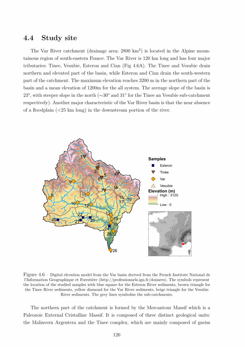
4.4 Study siteThe Var River catchment (drainage area: 2800 km2) is located in the Alpine moun-

tainous region of south-eastern France. The Var River is 120 km long and has four majortributaries: Tinee, Vesubie, Esteron and Cian (Fig 4.6A). The Tinee and Vesubie drainnorthern and elevated part of the basin, while Esteron and Cian drain the south-westernpart of the catchment. The maximum elevation reaches 3200 m in the northern part of thebasin and a mean elevation of 1200m for the all system. The average slope of the basin is23°, with steeper slope in the north (∼30° and 31° for the Tinee an Vesubie sub-catchmentrespectively). Another major characteristic of the Var River basin is that the near absenceof a floodplain (<25 km long) in the downstream portion of the river.

"" #*

""

""

"

"

"

"

"

"

#*

#*

#*

9

7

1

3

2

645

8

17

14

15

18

26

13

1210

1922

16

20 21

24

23

25

11

Samples

Esteron

Tinée

" Var

#* Vesubie

Elevation (m)High : 3120

Low : 0

Figure 4.6 – Digital elevation model from the Var basin derived from the French Institute National del’Information Geographique et Forestière (http://professionnels.ign.fr/donnees). The symbols representthe location of the studied samples with blue square for the Esteron River sediments, brown triangle forthe Tinee River sediments, yellow diamond for the Var River sediments, beige triangle for the Vesubie

River sediments. The grey lines symbolise the sub-catchments.

The northern part of the catchment is formed by the Mercantour Massif which is aPaleozoic External Cristalline Massif. It is composed of three distinct geological units:the Malinvern Argentera and the Tinee complex, which are mainly composed of gneiss

126

and migmatites, and the Argentera granitic unit. Locally, Permian shales and sandstonepelites are also encountered at both the periphery of the Mercantour massif and in thecentral part of the Var river basin. The southern and the central part of the river catch-ment is mainly composed of Mesozoic carbonaceous rocks, being locally associated withvarious sandstones, marls and limestones of Cenozoic age (Kerckhove & Montjuvent 1979,Rouire et al. 1980).

The Var River has an annual sediment discharge estimated at 1.63 million tons/yr anda specific flux of 580 tons/km2/yr (Mulder et al. 1997, 1998). The discharge is variableover the year with moderate to high flood in spring, because of Alpine snow melts, inautumn due to heavy rainfall, and in winter (Sage 1976, Anthony & Julian 1999). It canlead to stochastic erosional process with magnitude that can reach in only a few hours100 m3/s while the mean annual discharge is around 70 m3/s (Dubar & Anthony 1995).The climate is variable inside the catchment with Mediterranean climate in the south(hot and dry summers with cool and wet winter) and the northern part is dominated bya mountainous climate.The present day vegetation in southern France depends of the Mediterranean climate.In high elevation area (> 2000 m), the vegetation cover is mainly composed of grass-land. At lower elevation the vegetation is predominate by forest: with from sea-level tothe highest elevation a transition between drought resistant oak to conifers forest above1000 m (Beaudouin et al. 2007; corine land cover from 2012 from the geoportail database,https://www.geoportail.gouv.fr/donnees/corine-land-cover-2012). Downstream, the catch-ment is largely urbanized with the Nice city with an urban area composed of more>1,000,000 habitants (INSEE, 2016).

4.5 Materials and MethodsTwenty six sediments used were collected in 2011 and 2012 along the Var River and

its main tributaries. They were sieved on site at 135 µm. This suite covers the lithologicaldiversity across the entire catchment. Eleven samples were collected from the Tinee andVesubie catchments, which mainly drain metamorphic rocks, and 15 samples from theVar, Esteron and Cian catchments, which drain sedimentary rocks.

Geomorphic parameters (elevation, slope and curvature) for each sub-catchment were as-sessed using a 5 m resolution digital elevation model (DEM) from the French Institute Na-tional de l’Information Geographique et Forestière (http://professionnels.ign. fr/donnees).Spatial distribution of soil thickness was derived from the SoilGrids map with a 250 mresolution (Shangguan et al. 2017, Hengl et al. 2017). This estimation is based on a com-pilation of soil profiles (132,193 points) and borehole drilling logs (1,574,776 points) with

127

the addition of pseudo-observations of depth to bedrock.

Samples were prepared for U isotopic analysis at the Wollongong Isotope Geochronol-ogy Laboratory (WIGL), University of Wollongong. Determination of comminution age isbased on the preferential loss of 234U over 238U in detrital sediment (DePaolo et al. 2006).This depletion of 234U is only significant in fine-grained (<63 µm) sediments, where thesurface/volume is large enough to induce a substantial loss of 234U Kigoshi (1971), De-Paolo et al. (2006). Therefore, sediments were first wet sieved to recover the <63 µmfraction. Sediments are generally an assembly of detrital minerals and authigenic phases(i.e. carbonates, Fe-Mn oxyhydroxides) and organic matter. These non-detrital compo-nents are generally enriched in U from solutions, which are characterized by (234U/238U)>1, and thus inherit their U isotopic composition (Plater et al. 1988, 1992, Anderssonet al. 1998, 2001, Maher et al. 2006). Consequently, the authigenic phases and organicmatter need to be removed as it can mask the 234U loss. It needs to be realized withoutaltering the surface of the detrital grains as the 234U loss occurs within the first 30 nmof the grains’ surface (Kigoshi 1971). To achieve this, about 1 g of <63 µm sedimentswas treated following the sequential leaching protocol developed by Francke et al. (2018),which allows removal of any non-detrital components without affecting detrital grains.Following leaching, a 229Th - 236U tracer solution was added to 30 mg of the residual de-trital sediment. The mixture was dissolved in HNO3- HF solution, followed by aqua-regiaand finally re-dissolved in 2 mL of 7 M HNO3 prior to chromatography.

Ion exchange chromatography was performed on the dissolved samples to isolate ura-nium prior to isotopic analysis. This was undertaken on an ESI prepFAST automatedchromatography system with a "THU-0500" column prefilled with AG1-X8 resin. Prior tosample loading (2 mL of 7 M HNO3), the resin was washed with 7M HNO3, 0.1M HCl, 6MHCl and water and then conditioned with 7M-HNO3. Following sample loading, matrixwas eluted in 7M-HNO3 and uranium in 0.12M HCl. Uranium elutions were dried downand re-dissolved in 0.3M of HNO3 for isotopic analysis. Uranium isotope analyses were per-formed at WIGL on a ThermoFisher Neptune Plus Multi-Collector Inductively-CoupledPlasma Mass Spectrometer (MC-ICP-MS), using an APEX HF desolvating system andnebulizer PFA ST-2280 as sample introduction system. Jet sample and X skimmer coneswere used. Standard bracketing was used to correct for SEM-Faraday cup yield and massbias, using NBL U010 as primary standard (Richter & Goldberg 2003). Analysis accu-racy was determined by measuring synthetic standard NBL U005-A (Richter & Goldberg2003) and was consistently better than 0.5% for (234U/238U). Total procedural blankswere measured, and the contribution is less than 0.1% to the sample (234U/238U). Totalprocedural accuracy was evaluated by analysing the reference material BCR-2 (Sims etal., 2008), with results in good agreement with reference values (Table 5.1).

128

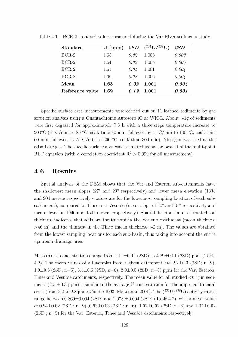
Table 4.1 – BCR-2 standard values measured during the Var River sediments study.

Standard U (ppm) 2SD (234U/238U) 2SDBCR-2 1.65 0.02 1.003 0.003BCR-2 1.64 0.02 1.005 0.005BCR-2 1.61 0.04 1.001 0.004BCR-2 1.60 0.02 1.003 0.004Mean 1.63 0.02 1.001 0.004Reference value 1.69 0.19 1.001 0.001

Specific surface area measurements were carried out on 11 leached sediments by gassorption analysis using a Quantachrome Autosorb iQ at WIGL. About ∼1g of sedimentswere first degassed for approximately 7.5 h with a three-steps temperature increase to200°C (5 °C/min to 80 °C, soak time 30 min, followed by 1 °C/min to 100 °C, soak time60 min, followed by 5 °C/min to 200 °C, soak time 300 min). Nitrogen was used as theadsorbate gas. The specific surface area was estimated using the best fit of the multi-pointBET equation (with a correlation coefficient R2 > 0.999 for all measurement).

4.6 ResultsSpatial analysis of the DEM shows that the Var and Esteron sub-catchments have

the shallowest mean slopes (27° and 23° respectively) and lower mean elevation (1334and 904 meters respectively - values are for the lowermost sampling location of each sub-catchment), compared to Tinee and Vesubie (mean slope of 30° and 31° respectively andmean elevation 1946 and 1541 meters respectively). Spatial distribution of estimated soilthickness indicates that soils are the thickest in the Var sub-catchment (mean thickness>46 m) and the thinnest in the Tinee (mean thickness ∼2 m). The values are obtainedfrom the lowest sampling locations for each sub-basin, thus taking into account the entireupstream drainage area.

Measured U concentrations range from 1.11±0.01 (2SD) to 4.29±0.01 (2SD) ppm (Table4.2). The mean values of all samples from a given catchment are 2.2±0.3 (2SD; n=9),1.9±0.3 (2SD; n=6), 3.1±0.6 (2SD; n=6), 2.9±0.5 (2SD; n=5) ppm for the Var, Esteron,Tinee and Vesubie catchments, respectively. The mean value for all studied <63 µm sedi-ments (2.5 ±0.3 ppm) is similar to the average U concentration for the upper continentalcrust (from 2.2 to 2.8 ppm; Condie 1993, McLennan 2001). The (234U/238U) activity ratiosrange between 0.869±0.004 (2SD) and 1.073 ±0.004 (2SD) (Table 4.2), with a mean valueof 0.94±0.02 (2SD ; n=9) ,0.93±0.03 (2SD ; n=6), 1.02±0.02 (2SD; n=6) and 1.02±0.02(2SD ; n=5) for the Var, Esteron, Tinee and Vesubie catchments respectively.

129

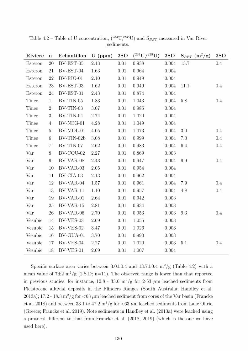
Table 4.2 – Table of U concentration, (234U/238U) and SBET measured in Var Riversediments.

Riviere n Echantillon U (ppm) 2SD (234U/238U) 2SD SBET (m2/g) 2SDEsteron 20 BV-EST-05 2.13 0.01 0.938 0.004 13.7 0.4Esteron 21 BV-EST-04 1.63 0.01 0.964 0.004Esteron 22 BV-RIO-01 2.10 0.01 0.949 0.004Esteron 23 BV-EST-03 1.62 0.01 0.949 0.004 11.1 0.4Esteron 24 BV-EST-01 2.43 0.01 0.874 0.004Tinee 1 BV-TIN-05 1.83 0.01 1.043 0.004 5.8 0.4Tinee 2 BV-TIN-03 3.07 0.01 0.985 0.004Tinee 3 BV-TIN-04 2.74 0.01 1.020 0.004Tinee 4 BV-NEG-01 4.28 0.01 1.049 0.004Tinee 5 BV-MOL-01 4.05 0.01 1.073 0.004 3.0 0.4Tinee 6 BV-TIN-02b 3.08 0.01 0.999 0.004 7.0 0.4Tinee 7 BV-TIN-07 2.62 0.01 0.983 0.004 6.4 0.4Var 8 BV-COU-02 2.27 0.01 0.869 0.003Var 9 BV-VAR-08 2.43 0.01 0.947 0.004 9.9 0.4Var 10 BV-VAR-03 2.05 0.01 0.954 0.004Var 11 BV-CIA-03 2.13 0.01 0.962 0.004Var 12 BV-VAR-04 1.57 0.01 0.961 0.004 7.9 0.4Var 13 BV-VAR-11 1.10 0.01 0.957 0.004 4.8 0.4Var 19 BV-VAR-01 2.64 0.01 0.942 0.003Var 25 BV-VAR-15 2.81 0.01 0.934 0.003Var 26 BV-VAR-06 2.70 0.01 0.953 0.003 9.3 0.4Vesubie 14 BV-VES-03 2.69 0.01 1.055 0.003Vesubie 15 BV-VES-02 3.47 0.01 1.026 0.003Vesubie 16 BV-GUA-01 3.70 0.01 0.990 0.003Vesubie 17 BV-VES-04 2.27 0.01 1.020 0.003 5.1 0.4Vesubie 18 BV-VES-01 2.69 0.01 1.007 0.004

Specific surface area varies between 3.0±0.4 and 13.7±0.4 m2/g (Table 4.2) with amean value of 7±2 m2/g (2.S.D; n=11). The observed range is lower than that reportedin previous studies: for instance, 12.8 - 33.6 m2/g for 2-53 µm leached sediments fromPleistocene alluvial deposits in the Flinders Ranges (South Australia; Handley et al.2013a); 17.2 - 18.3 m2/g for <63 µm leached sediment from cores of the Var basin (Franckeet al. 2018) and between 33.1 to 47.2 m2/g for <63 µm leached sediments from Lake Ohrid(Greece; Francke et al. 2019). Note sediments in Handley et al. (2013a) were leached usinga protocol different to that from Francke et al. (2018, 2019) (which is the one we haveused here).

130

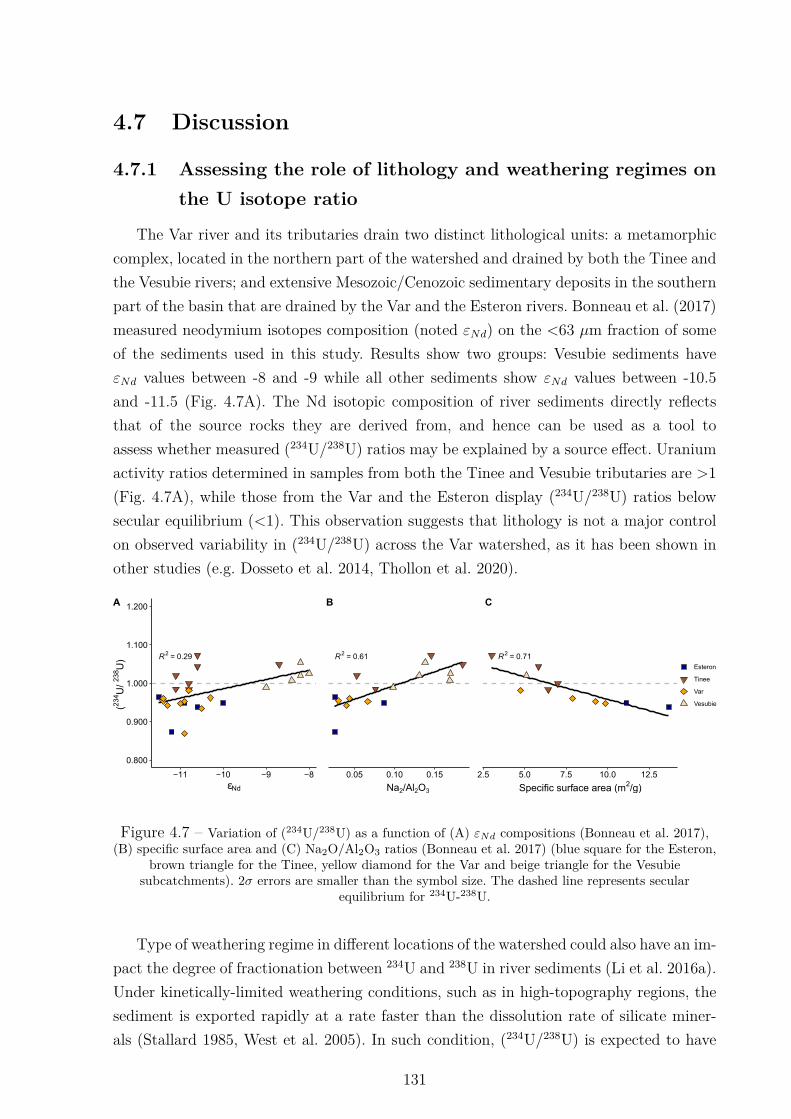
4.7 Discussion

4.7.1 Assessing the role of lithology and weathering regimes onthe U isotope ratio

The Var river and its tributaries drain two distinct lithological units: a metamorphiccomplex, located in the northern part of the watershed and drained by both the Tinee andthe Vesubie rivers; and extensive Mesozoic/Cenozoic sedimentary deposits in the southernpart of the basin that are drained by the Var and the Esteron rivers. Bonneau et al. (2017)measured neodymium isotopes composition (noted εNd) on the <63 µm fraction of someof the sediments used in this study. Results show two groups: Vesubie sediments haveεNd values between -8 and -9 while all other sediments show εNd values between -10.5and -11.5 (Fig. 4.7A). The Nd isotopic composition of river sediments directly reflectsthat of the source rocks they are derived from, and hence can be used as a tool toassess whether measured (234U/238U) ratios may be explained by a source effect. Uraniumactivity ratios determined in samples from both the Tinee and Vesubie tributaries are >1(Fig. 4.7A), while those from the Var and the Esteron display (234U/238U) ratios belowsecular equilibrium (<1). This observation suggests that lithology is not a major controlon observed variability in (234U/238U) across the Var watershed, as it has been shown inother studies (e.g. Dosseto et al. 2014, Thollon et al. 2020).

R2 = 0.29

0.800

0.900

1.000

1.100

1.200

−11 −10 −9 −8εNd

(234 U

/ 238 U

)

A

R2 = 0.61

0.05 0.10 0.15

Na2/Al2O3

Esteron

Tinee

Var

Vesubie

C

R2 = 0.71

2.5 5.0 7.5 10.0 12.5

Specific surface area (m2/g)

B

Figure 4.7 – Variation of (234U/238U) as a function of (A) εNd compositions (Bonneau et al. 2017),(B) specific surface area and (C) Na2O/Al2O3 ratios (Bonneau et al. 2017) (blue square for the Esteron,

brown triangle for the Tinee, yellow diamond for the Var and beige triangle for the Vesubiesubcatchments). 2σ errors are smaller than the symbol size. The dashed line represents secular

equilibrium for 234U-238U.

Type of weathering regime in different locations of the watershed could also have an im-pact the degree of fractionation between 234U and 238U in river sediments (Li et al. 2016a).Under kinetically-limited weathering conditions, such as in high-topography regions, thesediment is exported rapidly at a rate faster than the dissolution rate of silicate miner-als (Stallard 1985, West et al. 2005). In such condition, (234U/238U) is expected to have

131

undergone little fractionation and therefore be close to secular equilibrium. In contrast,in floodplains and other areas characterized by transport-limited weathering regimes, theincrease of sediment residence times in soils is typically accompanied by more intenseweathering reactions (West et al. 2005, Lupker et al. 2012), which results in the formationof thicker soil sequences. Hence the sediment is expected to spend a long time in thesoil profile, increasing the 234U loss possibility, which result in low (234U/238U). In the Varcatchment, the Tinee and Vesubie sub-catchments show characteristics of a kinetic-limitedweathering regime, with high denudation rates (>0.25 mm/yr; Mariotti et al. 2019), steepslopes (mean slope of 29° and 31° for the Tinee and Vesubie) and thin soils (generally lessthan 10 meters). Conversely, the Var and Esteron sub-catchments show characteristics of atransport-limited weathering regime, with slow denudation rates (<0.20 mm/yr; Mariottiet al. 2019), shallow slopes (mean slope of 26° and 22° for the Var and Esteron) and thicksoils (generally above 10 meters; with a great variability for the Var sub-catchment).Sediments from the Tinee and Vesubie show (234U/238U) values >1 (1.022 ±0.069 and1.020 ±0.048, respectively) while those from the Var and Esteron have (234U/238U) valuesoverall <1 (0.945 ±0.063 and 0.935 ±0.070, respectively). This observation suggests thatthe (234U/238U) of sediments is influenced by the weathering regime: in kinetic-limitedregimes, because soils are rapidly eroded, there is not enough time to lose 234U signifi-cantly. This results in (234U/238U) ratios >1, as imparted by authigenic phases (possiblyincompletely removed during leaching). In transport-limited regimes, long storage timesin thick soils results in measurable 234U depletion and (234U/238U) ratios <1. The influenceof chemical weathering can also be investigated using mobile over immobile elemental ra-tios, such as Na2O/Al2O3 (Fig. 4.7B). The Na2O/Al2O3 ratio decreases with (234U/238U)(Fig. 4.7B; R2 = 0.61). Sodium is a highly mobile element that is efficiently removedfrom soils during chemical weathering of primary minerals, whereas Al is immobile andremains incorporated into secondary clays. The positive relationship between (234U/238U)and Na2O/Al2O3 (Fig. 4.7B) suggests that under transport-limited weathering conditions(low Na2O/Al2O3), the longer regolith residence times lead to more extensive 234U loss inmineral grains stored in soils (low (234U/238U)), while sediments derived from the high-topography areas with low chemical weathering intensities (high Na2O/Al2O3) displayreduced or no 234U loss ((234U/238U) close to secular equilibrium). These results do notnecessarily indicate a control of weathering intensity on the fractionation of 234U-238U butrather a co-variation between them as a result of their dependence of residence time.Uranium isotope ratios show a negative correlation with the specific surface area (Fig.4.7C), indicative of the role of physical weathering on the (234U/238U) ratio. This obser-vation suggests that 234U loss is driven by the physical fragmentation of sediments, moreprominent in steep, fast-eroding catchments of the Tinee and Vesubie Rivers.

132

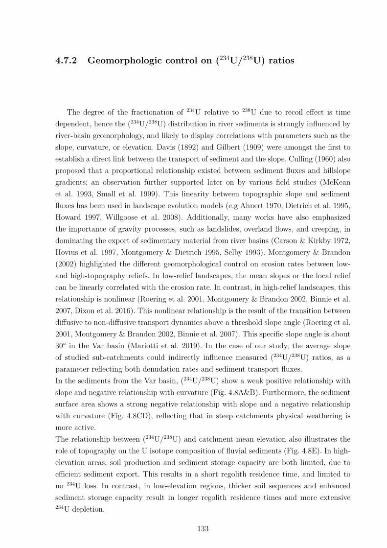
4.7.2 Geomorphologic control on (234U/238U) ratios

The degree of the fractionation of 234U relative to 238U due to recoil effect is timedependent, hence the (234U/238U) distribution in river sediments is strongly influenced byriver-basin geomorphology, and likely to display correlations with parameters such as theslope, curvature, or elevation. Davis (1892) and Gilbert (1909) were amongst the first toestablish a direct link between the transport of sediment and the slope. Culling (1960) alsoproposed that a proportional relationship existed between sediment fluxes and hillslopegradients; an observation further supported later on by various field studies (McKeanet al. 1993, Small et al. 1999). This linearity between topographic slope and sedimentfluxes has been used in landscape evolution models (e.g Ahnert 1970, Dietrich et al. 1995,Howard 1997, Willgoose et al. 2008). Additionally, many works have also emphasizedthe importance of gravity processes, such as landslides, overland flows, and creeping, indominating the export of sedimentary material from river basins (Carson & Kirkby 1972,Hovius et al. 1997, Montgomery & Dietrich 1995, Selby 1993). Montgomery & Brandon(2002) highlighted the different geomorphological control on erosion rates between low-and high-topography reliefs. In low-relief landscapes, the mean slopes or the local reliefcan be linearly correlated with the erosion rate. In contrast, in high-relief landscapes, thisrelationship is nonlinear (Roering et al. 2001, Montgomery & Brandon 2002, Binnie et al.2007, Dixon et al. 2016). This nonlinear relationship is the result of the transition betweendiffusive to non-diffusive transport dynamics above a threshold slope angle (Roering et al.2001, Montgomery & Brandon 2002, Binnie et al. 2007). This specific slope angle is about30° in the Var basin (Mariotti et al. 2019). In the case of our study, the average slopeof studied sub-catchments could indirectly influence measured (234U/238U) ratios, as aparameter reflecting both denudation rates and sediment transport fluxes.In the sediments from the Var basin, (234U/238U) show a weak positive relationship withslope and negative relationship with curvature (Fig. 4.8A&B). Furthermore, the sedimentsurface area shows a strong negative relationship with slope and a negative relationshipwith curvature (Fig. 4.8CD), reflecting that in steep catchments physical weathering ismore active.The relationship between (234U/238U) and catchment mean elevation also illustrates therole of topography on the U isotope composition of fluvial sediments (Fig. 4.8E). In high-elevation areas, soil production and sediment storage capacity are both limited, due toefficient sediment export. This results in a short regolith residence time, and limited tono 234U loss. In contrast, in low-elevation regions, thicker soil sequences and enhancedsediment storage capacity result in longer regolith residence times and more extensive234U depletion.

133

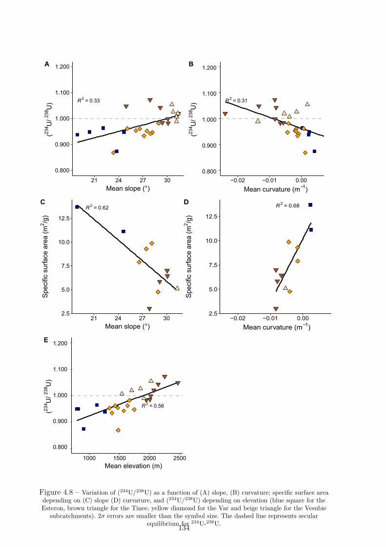
R2 = 0.33

21 24 27 30

Mean slope (°)

(234 U

/ 238 U

)

A

R2 = 0.31

−0.02 −0.01 0.00

Mean curvature (m−1)(23

4 U/ 23

8 U)

B

R2 = 0.62

2.5

5.0

7.5

10.0

12.5

21 24 27 30

Mean slope (°)

Spe

cific

sur

face

are

a (m

2 /g)

CR2 = 0.68

2.5

5.0

7.5

10.0

12.5

−0.02 −0.01 0.00

Mean curvature (m−1)

Spe

cific

sur

face

are

a (m

2 /g)

D

R2 = 0.56

1000 1500 2000 2500

Mean elevation (m)

(234 U

/238 U

)

E

0.800

0.900

1.000

1.100

1.200

0.800

0.900

1.000

1.100

1.200

0.800

0.900

1.000

1.100

1.200

Figure 4.8 – Variation of (234U/238U) as a function of (A) slope, (B) curvature; specific surface areadepending on (C) slope (D) curvature, and (234U/238U) depending on elevation (blue square for theEsteron, brown triangle for the Tinee, yellow diamond for the Var and beige triangle for the Vesubie

subcatchments). 2σ errors are smaller than the symbol size. The dashed line represents secularequilibrium for 234U-238U.134

4.7.3 Quantification of regolith residence times in the Var Rivercatchment

The sediment residence time can be derived from U isotopes using the comminutionage model (DePaolo et al. 2006):

tcom = − 1λ234

ln

[Ameas − (1 − fα)A0 − (1 − fα)

](4.1)

where λ234 is the 234U decay constant (in yr−1), fα the recoil loss factor, Ameas is themeasured (234U/238U) in the sediment and A0 is the (234U/238U) activity ratio at t=0. Intheory, A0 represents the uranium activity ratio from the parent material that should bein secular equilibrium, i.e. (234U/238U) = 1, and Ameas in detrital sediments should exhibitvalues <1 resulting from the preferential loss of 234U. However, some river sediments in theVar catchment displayed (234U/238U) values > 1, implying an evolution of the ration fromA0 >1. Some (234U/238U) higher than 1 have already been reported in river sediments (e.g.Vigier et al. 2001, 2005, Granet et al. 2007, Martin et al. 2015). Therefore, the maximummeasured (234U/238U) value was attributed to A0. The recoil loss factor is calculated asfollows (Kigoshi 1971, Luo et al. 2000):

fα = 14LSρ (4.2)

where L is the 234Th recoil length (taken to be 30 nm; Dosseto & Schaller 2016), ρ isthe density of the sediment (assumed to be 2.65 g/cm3) and S is the surface area (m2/g)measured by gas sorption analysis. Because micro- (<2 nm in diameter) or mesopore (2-50nm in diameter) increase the measured surface area during gas sorption analysis due tothe the diameter of the adsorbent molecule of the same order, without contribution to234U loss in detrital material. It led to an overestimation of the recoil loss factor (Maheret al. 2006). For micro- and mesoporous material a fractal correction need to be applied(Bourdon et al. 2009). The shape of the adsorption-desorption isotherms assessed duringgas sorption analyses indicates the nature of the material (Sing 1985). In this study, theisotherms of the samples are type II isotherms, characteristic of non-porous or macrop-orous material (Sing 1985). Hence, no fractal correction is required (Francke et al. 2018)and the measured surface area was directly used to calculate the recoil loss factor. Inthe case where the surface area was not measured for a given sample, a random valuewas taken between the minimum and the maximum values measured.Sediment residencetimes were calculated using Monte Carlo simulation (10,000 simulations). For each sam-ple, Ameas was taken randomly within the range of measured (234U/238U) activity ratiosand its error as provided in Table 1. As not every specific surface area were measured,for the samples without data, a random value was choose between the minimum andmaximum values measured. As explained above, for fluvial sediments, the comminution

135

age is equivalent to the sediment residence time, which encompasses storage in weatheringprofiles on the hillslope and transport in the fluvial system. Calculated sediment residencetimes vary between 66 and 286 kyr for the Tinee, 78 and 229 kyr for the Vesubie, 219 and636 kyr for the Var and 251 and 643 kyr for the Esteron. The highest value of 642 kyrbeing calculated for EST-01 located at the lower part of the Esteron sub-catchment (Fig.4.9A). These residence times are much longer than what would be expected for a moun-tainous river catchment characterised by efficient sediment transport. However, most ofthe residence time can be explained by hillslope storage (Suresh et al. 2014): while a 4-msoil eroding at 9-24 mm/kyr would yield residence times of only 30 kyr, when consideringsoil creep at a rate of 0.8 mm/kyr down a 265 m long hillslope, this can increase the resi-dence time to values as high as 220 kyr despite the thin soil thickness and fast erosion rates.

In order to validate the U-based sediment residence time, we also estimated the sedi-ment residence combining spatial data for estimated soil thickness (SoilGrids;Shangguanet al. 2017, Hengl et al. 2017) and 10Be-derived denudation rates (Mariotti et al. 2019).For each location where sediments were sampled for in-situ 10Be, soil thickness and de-nudation rates are spatially averaged by the area drained at the sample location. Thus,the ratio of soil thickness to denudation rate yields a spatially averaged soil residencetime. Because there is little accommodation space for fluvial storage, this soil residencetime can be considered equivalent to the regolith residence time, and compared to theregolith residence time inferred from U isotopes at the same location.

136

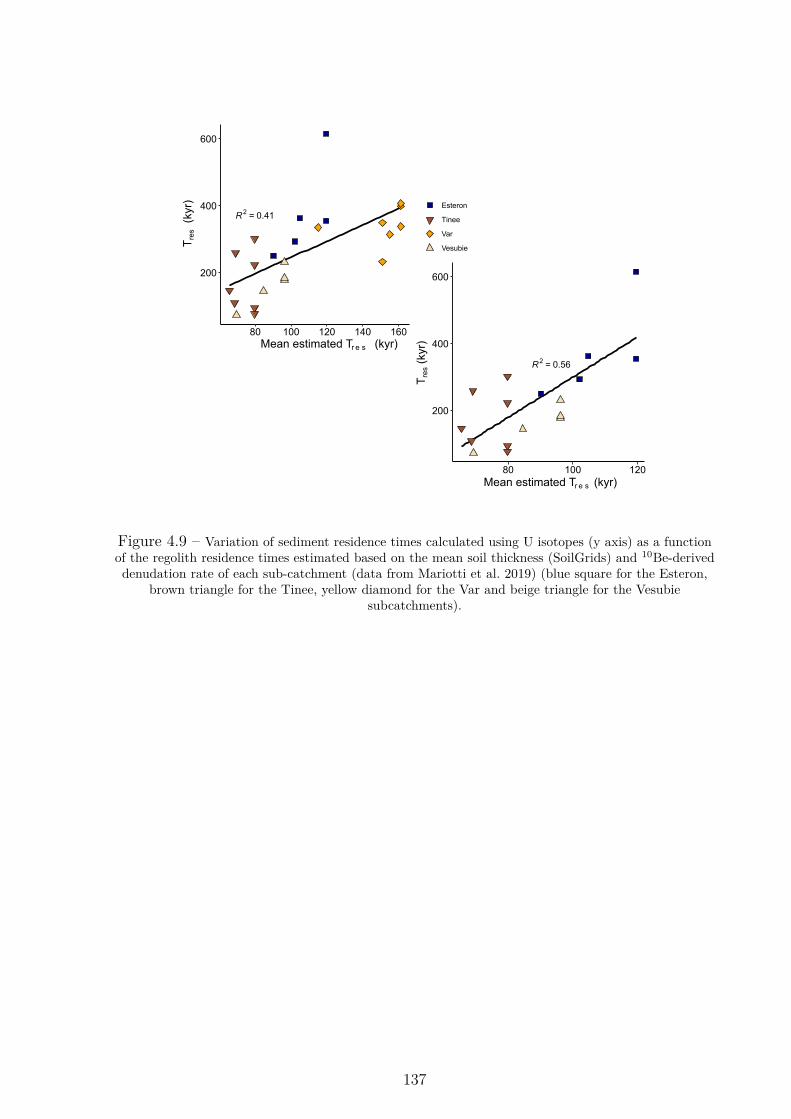
R2 = 0.41

200

400

600

80 100 120 140 160

Esteron

Tinee

Var

Vesubie

R2 = 0.56

200

400

600

80 100 120Mean estimated Tr e s (kyr)

Tre

s (k

yr)Mean estimated Tr e s (kyr)

Tre

s (

kyr)

Figure 4.9 – Variation of sediment residence times calculated using U isotopes (y axis) as a functionof the regolith residence times estimated based on the mean soil thickness (SoilGrids) and 10Be-deriveddenudation rate of each sub-catchment (data from Mariotti et al. 2019) (blue square for the Esteron,

brown triangle for the Tinee, yellow diamond for the Var and beige triangle for the Vesubiesubcatchments).

137

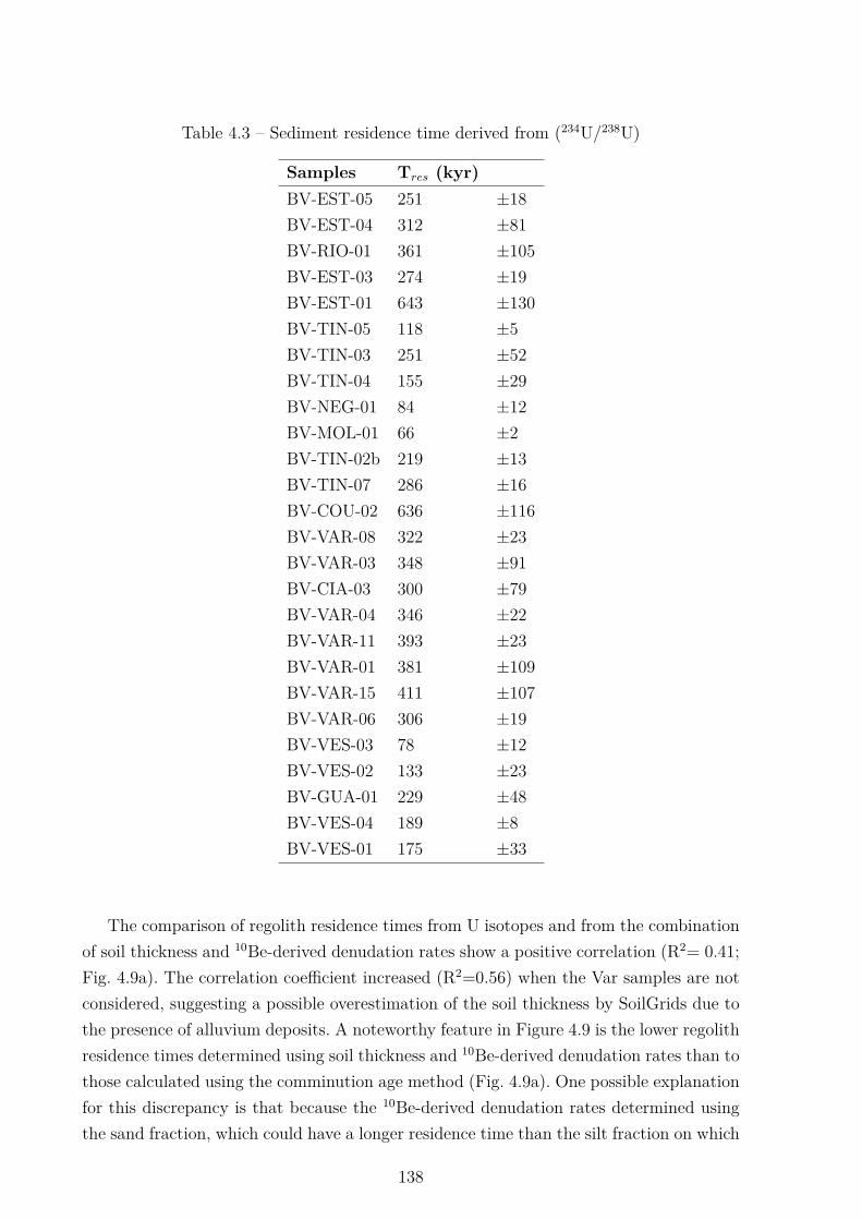
Table 4.3 – Sediment residence time derived from (234U/238U)

Samples Tres (kyr)BV-EST-05 251 ±18BV-EST-04 312 ±81BV-RIO-01 361 ±105BV-EST-03 274 ±19BV-EST-01 643 ±130BV-TIN-05 118 ±5BV-TIN-03 251 ±52BV-TIN-04 155 ±29BV-NEG-01 84 ±12BV-MOL-01 66 ±2BV-TIN-02b 219 ±13BV-TIN-07 286 ±16BV-COU-02 636 ±116BV-VAR-08 322 ±23BV-VAR-03 348 ±91BV-CIA-03 300 ±79BV-VAR-04 346 ±22BV-VAR-11 393 ±23BV-VAR-01 381 ±109BV-VAR-15 411 ±107BV-VAR-06 306 ±19BV-VES-03 78 ±12BV-VES-02 133 ±23BV-GUA-01 229 ±48BV-VES-04 189 ±8BV-VES-01 175 ±33

The comparison of regolith residence times from U isotopes and from the combinationof soil thickness and 10Be-derived denudation rates show a positive correlation (R2= 0.41;Fig. 4.9a). The correlation coefficient increased (R2=0.56) when the Var samples are notconsidered, suggesting a possible overestimation of the soil thickness by SoilGrids due tothe presence of alluvium deposits. A noteworthy feature in Figure 4.9 is the lower regolithresidence times determined using soil thickness and 10Be-derived denudation rates than tothose calculated using the comminution age method (Fig. 4.9a). One possible explanationfor this discrepancy is that because the 10Be-derived denudation rates determined usingthe sand fraction, which could have a longer residence time than the silt fraction on which

138

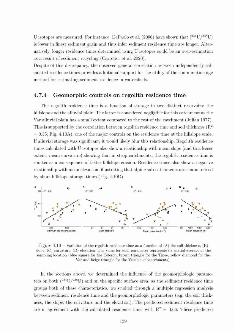
U isotopes are measured. For instance, DePaolo et al. (2006) have shown that (234U/238U)is lower in finest sediment grain and thus infer sediment residence time are longer. Alter-natively, longer residence times determined using U isotopes could be an over-estimationas a result of sediment recycling (Carretier et al. 2020).Despite of this discrepancy, the observed general correlation between independently cal-culated residence times provides additional support for the utility of the comminution agemethod for estimating sediment residence in watersheds.

4.7.4 Geomorphic controls on regolith residence time

The regolith residence time is a function of storage in two distinct reservoirs: thehillslope and the alluvial plain. The latter is considered negligible for this catchment as theVar alluvial plain has a small extent compared to the rest of the catchment (Julian 1977).This is supported by the correlation between regolith residence time and soil thickness (R2

= 0.35; Fig. 4.10A), one of the major controls on the residence time at the hillslope scale.If alluvial storage was significant, it would likely blur this relationship. Regolith residencetimes calculated with U isotopes also show a relationship with mean slope (and to a lesserextent, mean curvature) showing that in steep catchments, the regolith residence time isshorter as a consequence of faster hillslope erosion. Residence times also show a negativerelationship with mean elevation, illustrating that alpine sub-catchments are characterisedby short hillslope storage times (Fig. 4.10D).

R2 = 0.35

200

400

600

500 1000

Minimum soil thickness (cm)

Tre

s (k

ry)

A

R2 = 0.31

21 24 27 30

Mean slope (°)

B

R2 = 0.18

−0.02 −0.01 0.00

Mean curvature (m−1)

C

R2 = 0.39

800 1200 1600 2000

Mean elevation (m)

D

Figure 4.10 – Variation of the regolith residence time as a function of (A) the soil thickness, (B)slope, (C) curvature, (D) elevation. The value for each parameter represents its spatial average at thesampling location (blue square for the Esteron, brown triangle for the Tinee, yellow diamond for the

Var and beige triangle for the Vesubie subcatchments).

In the sections above, we determined the influence of the geomorphologic parame-ters on both (234U/238U) and on the specific surface area, as the sediment residence timegroups both of these characteristics, we studied through a multiple regression analysisbetween sediment residence time and the geomorphologic parameters (e.g. the soil thick-ness, the slope, the curvature and the elevation). The predicted sediment residence timeare in agreement with the calculated residence time, with R2 = 0.66. These predicted

139

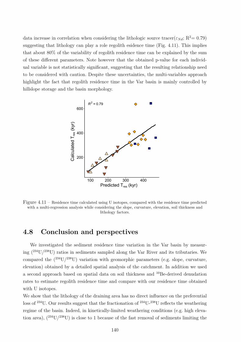
data increase in correlation when considering the lithologic source tracer(εNd; R2= 0.79)suggesting that lithology can play a role regolith esidence time (Fig. 4.11). This impliesthat about 80% of the variability of regolith residence time can be explained by the sumof these different parameters. Note however that the obtained p-value for each individ-ual variable is not statistically significant, suggesting that the resulting relationship needto be considered with caution. Despite these uncertainties, the multi-variables approachhighlight the fact that regolith residence time in the Var basin is mainly controlled byhillslope storage and the basin morphology.

R2 = 0.79

200

400

600

100 200 300 400Predicted Tres (kyr)

Cal

cula

ted

Tre

s (k

yr)

Figure 4.11 – Residence time calculated using U isotopes, compared with the residence time predictedwith a multi-regression analysis while considering the slope, curvature, elevation, soil thickness and

lithology factors.

4.8 Conclusion and perspectivesWe investigated the sediment residence time variation in the Var basin by measur-

ing (234U/238U) ratios in sediments sampled along the Var River and its tributaries. Wecompared the (234U/238U) variation with geomorphic parameters (e.g. slope, curvature,elevation) obtained by a detailed spatial analysis of the catchment. In addition we useda second approach based on spatial data on soil thickness and 10Be-derived denudationrates to estimate regolith residence time and compare with our residence time obtainedwith U isotopes.We show that the lithology of the draining area has no direct influence on the preferentialloss of 234U. Our results suggest that the fractionation of 234U-238U reflects the weatheringregime of the basin. Indeed, in kinetically-limited weathering conditions (e.g. high eleva-tion area), (234U/238U) is close to 1 because of the fast removal of sediments limiting the

140

234U loss. Conversely, (234U/238U) is low in transport-limited regime due to the facilitywith which the soil develops, increasing the sediment storage on hillslope. Furthermore,the morphology shows a control on the variability of (234U/238U) in particular throughthe slope and curvature, which is coherent with the co-variation of weathering regimeand the morphology of the basin. The regolith residence time we estimated using spatialdata on soil thickness and 10Be-derived denudation rates have a good correlation with theresidence time calculate with (234U/238U). This correlation indicates that in a reactivesystem as the Var basin, the sediment residence time represents the regolith residencetime and therefore the duration of the fluvial transport can be considered as negligible.The results of this study confirms the ability of (234U/238U) to infer sediment residencetime and point out there great ability to respond to morphologic variation. This control ofthe morphology on (234U/238U) suggests that sediment residence time based on U isotopescould be used as approximation of weathering regime.

141

Chapter 5

THE VAR SEDIMENT ROUTING SYSTEM:PALEO-RESIDENCE TIME VARIATIONS

Contents5.1 The climatic cyclicity during the Quaternary . . . . . . . . . . . . 144

5.1.1 Long terms climatic cycles . . . . . . . . . . . . . . . . . . . . . . . . 1445.1.2 Millennial-scale climate changes . . . . . . . . . . . . . . . . . . . . . 1455.1.3 The climatic context in the Alps during the Quaternary . . . . . . . 147

5.2 Temporal sediment residence time variations . . . . . . . . . . . . 1495.2.1 Stratigraphy of the Var sedimentary ridge . . . . . . . . . . . . . . . 1495.2.2 Methods . . . . . . . . . . . . . . . . . . . . . . . . . . . . . . . . . . 1515.2.3 Uranium variations over time - Results . . . . . . . . . . . . . . . . . 1535.2.4 Interpretation . . . . . . . . . . . . . . . . . . . . . . . . . . . . . . . 1575.2.5 Conclusion . . . . . . . . . . . . . . . . . . . . . . . . . . . . . . . . 165

143

5.1 The climatic cyclicity during the Quaternary

5.1.1 Long terms climatic cycles

During the Quaternary (since 2.6 Myr), a cyclicity between glacial and interglacialperiods exist. The cyclicity period increased from 40 000 yr between 2.6 and 0.9 Myrto every 100 000 yr for the last 0.9 Myr. The glacial-interglacial variability is controlledby insolation variations caused by terrestrial orbital parameters according to the astro-nomical theory of climate first formulated by M. Milankovitch in 1947 (see Berger 1988for a review). These variations are reinforced by complex retroaction between the ocean,atmosphere and cryosphere.

The alternation of glacial and interglacial periods throughout the Quaternary is nicelydepicted in the oxygen isotopic composition (18O/16O or δ18O) of the sea water and theice trapped at the pole. The cold, glacial periods are characterized by a decrease of lightisotopes compared to the heavy ones in the sea-water as the light isotopes are trapped inthe polar ice. Conversely, during warm, interglacial periods the light oxygen isotopes arereleased into the water, hence δ18O of sea water decreased. This led the community to usethe notion of Oxygen Isotopic Stage - OIS or Marine isotopic Stage – MIS to describe themain climatic features of the Quaternary (Railsback et al. 2015).

The Last Glacial Period

The last glacial period (71 - 11.7 kyr) is characterized by the growth of North Hemi-sphere ice sheets, the two major being the Laurentide Ice Sheet in North American and theEurasian Ice sheet in northern Europe (Ehlers & Gibbard 2007). During the last glacialmaximum (LGM, ca. 26.5 ka - 19 ka; Clark et al. 2009), that occurred during the MIS2, the ice sheets extended to their maximum and covered about 25% of the continentalsurfaces. At that time, the difference with actual value of the mean temperature at theEarth’s surfaces was about 4 to 5 °C lower than the actual values. This difference in-creased in high latitude (2-6 °C) and reached a maximum in the North Atlantic region (6to 10 °C; CLIMAP, 1981; Community Climate System Model Version 3 - CCSM3, 2006).This climate and the development of the ice sheets led to a prominent fall in sea levelof about 110 to 125 meters (Fairbanks 1989, Yokoyama et al. 2000, Siddall et al. 2003,Clark et al. 2009). The arid climatic conditions at every latitudes during the last glacialperiod have impacted the vegetation cover, which was poorly developed in comparison totoday (Sarnthein 1978, Mahowald et al. 1999, Gasse 2000, Baker et al. 2001, Wu et al.2007). The end of the last glacial period occurred from about 19-20 ka when the ice sheetsstarted to retreat and promoted a concomittant rapid sea-level rise of 10-15 meters (Clarket al. 2009) that is considered as the onset of the last glacial-interglacial transition (or

144

Termination I). From that time to the Early Holocene (∼11 ka), the decay of ice sheetscaused global mean sea level to rise by approximately 80 m (Clark et al. 2012). Simulta-neously, the carbon cycle has been affected, resulting in the emission of greenhouse gasesto the atmosphere. The variation in the atmosphere and ocean circulation affected theglobal distribution and fluxes of water and heat (Clark et al. 2012).

Holocene

The Holocene (last 11.7 kyr) is the actual interglacial period. The summer insolationat the beginning of the Holocene period, between 9 and 6 ka, was up to 5-8% higherthan actual (Denton & Karlén 1973). This led to a maximum in both temperature andprecipitation (Holocene thermal Maximum). Around 6 ka the Laurentide and Eurasianice sheets has completely disappeared (Ruddiman 2001) and determined the end of thesea-level rise (Lambeck & Chappell 2001). From then begin the global aridification andthe global cooling until the current conditions (i.e. rapid warming induced by increasinganthropogenic greenhouses gases) are reached (Wanner et al. 2008, Marcott et al. 2013).The physical mechanism responsible for this global cooling in the second part of theHolocene is still debated (Liu et al. 2014).

5.1.2 Millennial-scale climate changes

During the Holocene, the climate was considered as stable in comparison with thegreat instability recorded during the glacial periods and the MIS3 of the last glacial pe-riod in particular (Fig. 5.1). This instability follows a cyclicity of the order of a thousandyears, which is too low to be explained by the orbital variations alone and are namedsuborbital- or millennial variations (Dansgaard et al. 1993, Bond et al. 1993).

The climate at the Earth’s surface is partly controlled by oceanic circulation. This one,on a global scale, is controlled by the density gradients maintained between water massesthat are determined by temperature and salinity. Cold and deep water are producedin the North Atlantic area and are conducted to the south. This process is referenced asthe Atlantic Meridional Overturning Cell (AMOC). Simultaneously, the warm and surfacesaltwater of the northern Pacific circulate through the Indian Ocean to the North Atlantic.During their path, they get cooled and in winter, become denser than the surroundingwaters, and deep. The thermohaline circulation, principally caused by the AMOC, greatlyinfluenced the heat distribution from low to high latitude (Stocker & Schmittner 1997,Cunningham et al. 2007, Moore et al. 2012).

145

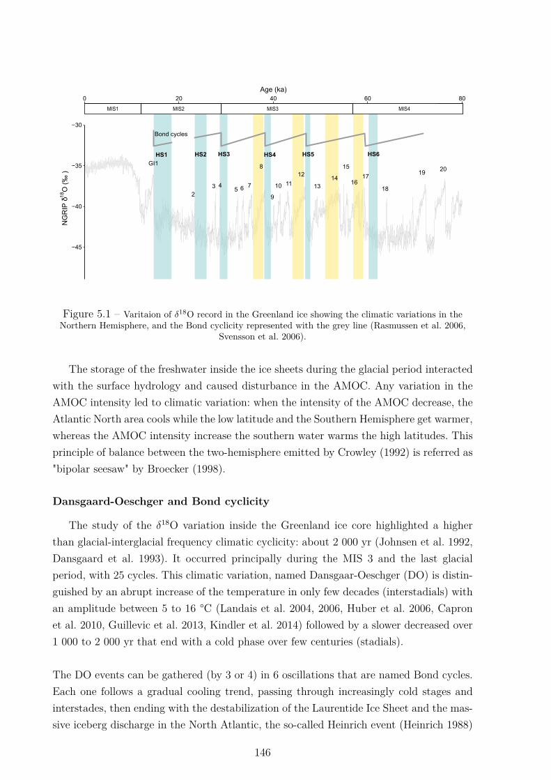
0 20 40 60 80

−45

−40

−35

−30

Age (ka)

NG

RIP

δ18

O (

‰ )

Bond cycles

HS1 HS2 HS3 HS4 HS5 HS6

GI1

23 4

5 6 7

8

9

10 11

12

1314

15

1617

18

1920

MIS1 MIS2 MIS3 MIS4

Figure 5.1 – Varitaion of δ18O record in the Greenland ice showing the climatic variations in theNorthern Hemisphere, and the Bond cyclicity represented with the grey line (Rasmussen et al. 2006,

Svensson et al. 2006).

The storage of the freshwater inside the ice sheets during the glacial period interactedwith the surface hydrology and caused disturbance in the AMOC. Any variation in theAMOC intensity led to climatic variation: when the intensity of the AMOC decrease, theAtlantic North area cools while the low latitude and the Southern Hemisphere get warmer,whereas the AMOC intensity increase the southern water warms the high latitudes. Thisprinciple of balance between the two-hemisphere emitted by Crowley (1992) is referred as"bipolar seesaw" by Broecker (1998).

Dansgaard-Oeschger and Bond cyclicity

The study of the δ18O variation inside the Greenland ice core highlighted a higherthan glacial-interglacial frequency climatic cyclicity: about 2 000 yr (Johnsen et al. 1992,Dansgaard et al. 1993). It occurred principally during the MIS 3 and the last glacialperiod, with 25 cycles. This climatic variation, named Dansgaar-Oeschger (DO) is distin-guished by an abrupt increase of the temperature in only few decades (interstadials) withan amplitude between 5 to 16 °C (Landais et al. 2004, 2006, Huber et al. 2006, Capronet al. 2010, Guillevic et al. 2013, Kindler et al. 2014) followed by a slower decreased over1 000 to 2 000 yr that end with a cold phase over few centuries (stadials).

The DO events can be gathered (by 3 or 4) in 6 oscillations that are named Bond cycles.Each one follows a gradual cooling trend, passing through increasingly cold stages andinterstades, then ending with the destabilization of the Laurentide Ice Sheet and the mas-sive iceberg discharge in the North Atlantic, the so-called Heinrich event (Heinrich 1988)

146

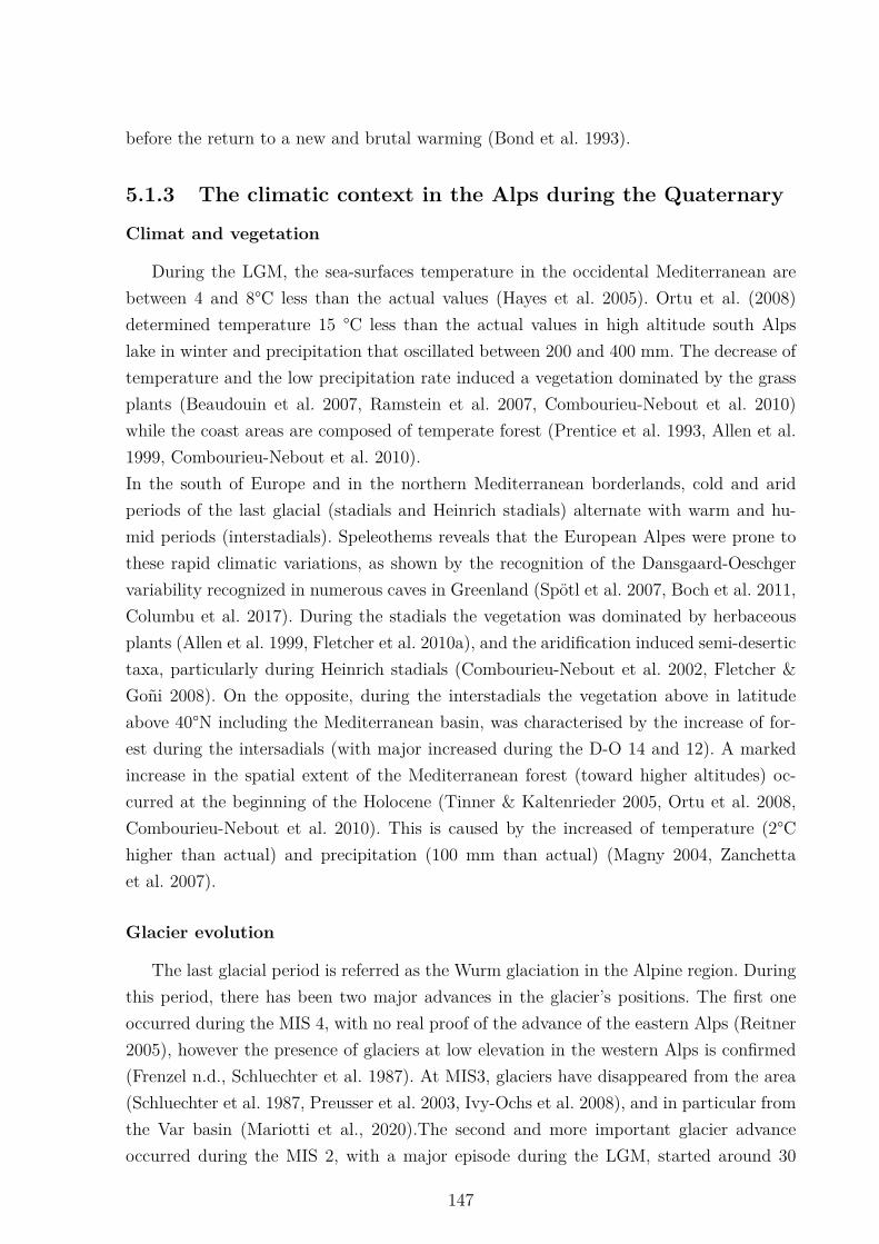
before the return to a new and brutal warming (Bond et al. 1993).

5.1.3 The climatic context in the Alps during the Quaternary

Climat and vegetation

During the LGM, the sea-surfaces temperature in the occidental Mediterranean arebetween 4 and 8°C less than the actual values (Hayes et al. 2005). Ortu et al. (2008)determined temperature 15 °C less than the actual values in high altitude south Alpslake in winter and precipitation that oscillated between 200 and 400 mm. The decrease oftemperature and the low precipitation rate induced a vegetation dominated by the grassplants (Beaudouin et al. 2007, Ramstein et al. 2007, Combourieu-Nebout et al. 2010)while the coast areas are composed of temperate forest (Prentice et al. 1993, Allen et al.1999, Combourieu-Nebout et al. 2010).In the south of Europe and in the northern Mediterranean borderlands, cold and aridperiods of the last glacial (stadials and Heinrich stadials) alternate with warm and hu-mid periods (interstadials). Speleothems reveals that the European Alpes were prone tothese rapid climatic variations, as shown by the recognition of the Dansgaard-Oeschgervariability recognized in numerous caves in Greenland (Spötl et al. 2007, Boch et al. 2011,Columbu et al. 2017). During the stadials the vegetation was dominated by herbaceousplants (Allen et al. 1999, Fletcher et al. 2010a), and the aridification induced semi-desertictaxa, particularly during Heinrich stadials (Combourieu-Nebout et al. 2002, Fletcher &Goñi 2008). On the opposite, during the interstadials the vegetation above in latitudeabove 40°N including the Mediterranean basin, was characterised by the increase of for-est during the intersadials (with major increased during the D-O 14 and 12). A markedincrease in the spatial extent of the Mediterranean forest (toward higher altitudes) oc-curred at the beginning of the Holocene (Tinner & Kaltenrieder 2005, Ortu et al. 2008,Combourieu-Nebout et al. 2010). This is caused by the increased of temperature (2°Chigher than actual) and precipitation (100 mm than actual) (Magny 2004, Zanchettaet al. 2007).

Glacier evolution

The last glacial period is referred as the Wurm glaciation in the Alpine region. Duringthis period, there has been two major advances in the glacier’s positions. The first oneoccurred during the MIS 4, with no real proof of the advance of the eastern Alps (Reitner2005), however the presence of glaciers at low elevation in the western Alps is confirmed(Frenzel n.d., Schluechter et al. 1987). At MIS3, glaciers have disappeared from the area(Schluechter et al. 1987, Preusser et al. 2003, Ivy-Ochs et al. 2008), and in particular fromthe Var basin (Mariotti et al., 2020).The second and more important glacier advanceoccurred during the MIS 2, with a major episode during the LGM, started around 30

147

kyr (Schluechter et al. 1987, Schoeneich 1998, Jorda et al. 2000, Preusser et al. 2003,Monegato et al. 2007). During the LGM, three glaciers respectively covered the valleyof the Vesubie, the Tinee, and the upper part of the Var (Julian 1977, Buoncristiani &Campy 2004). Together they covered about 17% of the drainage air (Jorry et al. 2011).After the LGM, the glaciers have receded very quickly from 21-20 kyr, and they hadentirely disappeared by 17 ka (Ivy-Ochs et al. 2004, Ivy-Ochs et al. 2008). Nowadays,Alpine glaciers are restricted to high elevation sites and there are no more glaciers in theVar region.

148

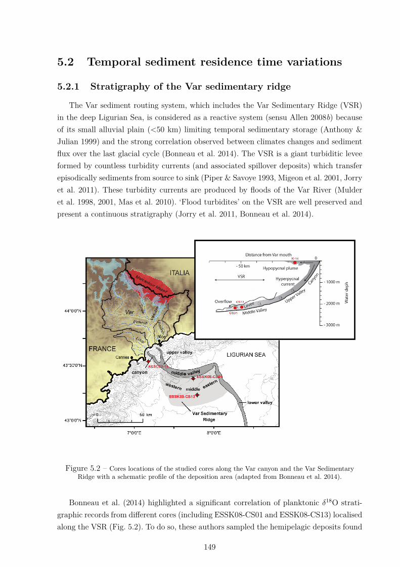
5.2 Temporal sediment residence time variations

5.2.1 Stratigraphy of the Var sedimentary ridge

The Var sediment routing system, which includes the Var Sedimentary Ridge (VSR)in the deep Ligurian Sea, is considered as a reactive system (sensu Allen 2008b) becauseof its small alluvial plain (<50 km) limiting temporal sedimentary storage (Anthony &Julian 1999) and the strong correlation observed between climates changes and sedimentflux over the last glacial cycle (Bonneau et al. 2014). The VSR is a giant turbiditic leveeformed by countless turbidity currents (and associated spillover deposits) which transferepisodically sediments from source to sink (Piper & Savoye 1993, Migeon et al. 2001, Jorryet al. 2011). These turbidity currents are produced by floods of the Var River (Mulderet al. 1998, 2001, Mas et al. 2010). ‘Flood turbidites’ on the VSR are well preserved andpresent a continuous stratigraphy (Jorry et al. 2011, Bonneau et al. 2014).

KESCC9-14

Figure 5.2 – Cores locations of the studied cores along the Var canyon and the Var SedimentaryRidge with a schematic profile of the deposition area (adapted from Bonneau et al. 2014).

Bonneau et al. (2014) highlighted a significant correlation of planktonic δ18O strati-graphic records from different cores (including ESSK08-CS01 and ESSK08-CS13) localisedalong the VSR (Fig. 5.2). To do so, these authors sampled the hemipelagic deposits found

149

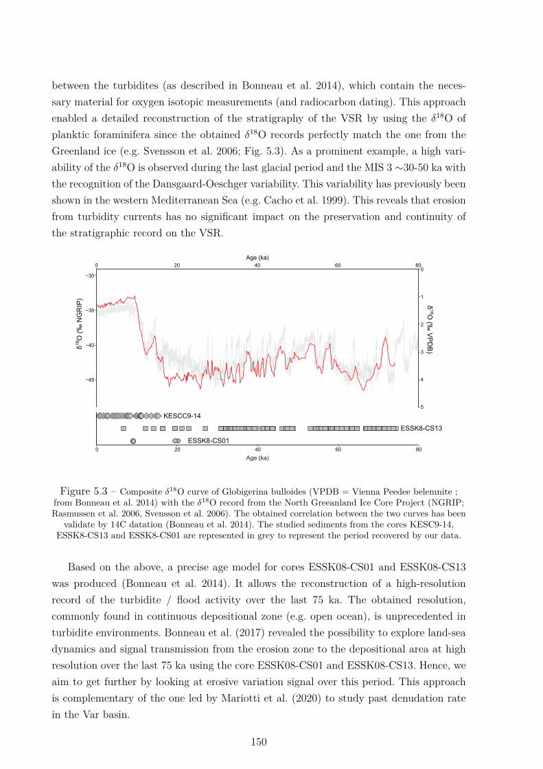
between the turbidites (as described in Bonneau et al. 2014), which contain the neces-sary material for oxygen isotopic measurements (and radiocarbon dating). This approachenabled a detailed reconstruction of the stratigraphy of the VSR by using the δ18O ofplanktic foraminifera since the obtained δ18O records perfectly match the one from theGreenland ice (e.g. Svensson et al. 2006; Fig. 5.3). As a prominent example, a high vari-ability of the δ18O is observed during the last glacial period and the MIS 3 ∼30-50 ka withthe recognition of the Dansgaard-Oeschger variability. This variability has previously beenshown in the western Mediterranean Sea (e.g. Cacho et al. 1999). This reveals that erosionfrom turbidity currents has no significant impact on the preservation and continuity ofthe stratigraphic record on the VSR.

0 20 40 60 80

−45

−40

−35

−30

Age (ka)

0

1

2

3

4

5

Age (ka)

0 20 40 60 80

δ18

O (

‰ N

GR

IP) δ

18O (‰

VP

DB

)

KESCC9-14

ESSK8-CS13

ESSK8-CS01

Figure 5.3 – Composite δ18O curve of Globigerina bulloides (VPDB = Vienna Peedee belemnite ;from Bonneau et al. 2014) with the δ18O record from the North Greeanland Ice Core Project (NGRIP;Rasmussen et al. 2006, Svensson et al. 2006). The obtained correlation between the two curves has been

validate by 14C datation (Bonneau et al. 2014). The studied sediments from the cores KESC9-14,ESSK8-CS13 and ESSK8-CS01 are represented in grey to represent the period recovered by our data.

Based on the above, a precise age model for cores ESSK08-CS01 and ESSK08-CS13was produced (Bonneau et al. 2014). It allows the reconstruction of a high-resolutionrecord of the turbidite / flood activity over the last 75 ka. The obtained resolution,commonly found in continuous depositional zone (e.g. open ocean), is unprecedented inturbidite environments. Bonneau et al. (2017) revealed the possibility to explore land-seadynamics and signal transmission from the erosion zone to the depositional area at highresolution over the last 75 ka using the core ESSK08-CS01 and ESSK08-CS13. Hence, weaim to get further by looking at erosive variation signal over this period. This approachis complementary of the one led by Mariotti et al. (2020) to study past denudation ratein the Var basin.

150

5.2.2 Methods

In this study, sediment from three cores were used. Two cores, ESSK08-CS01 (2146m of water depth) and ESSK08- CS13 (2473 m of water depth), were recovered alongthe VSR during the ESSDIV cruise on the N/O Pourquoi pas? (2008). The third core,KESC9-14 (550 m of water depth), has been sampled in 2008 during the ESSCAR-9cruise on the N/O Le Suroıt. It is located on an interfluve, above surrounding canyons,directly off the Var river mouth. This core covers only the Holocene period (Ciobanuet al. 2012) Houedec et al., submitted). Sediments from the KESC9-14 are fine-graineddeposits (considered in our study as the undifferentiated size fraction; n=27) from hypopy-cnal plumes. Conversely, ESSK08-CS01 and ESSK08- CS13 are levees-channel depositsconsisting of alternations of millimeter to decimeter-scale turbiditic sandy/silty sequencesand hemipelagic (i.e. foram-rich) muds. Therefore for each interval of interest, two grainssize were sampled: first the hemipelagic facies in between the turbidites (considered in ourstudy as the clay size fraction; n= 64) and, second, the uppermost and silty part of theturbidite facies (considered in our study as the silt size fraction; n=52). Two grain sizefractions were sampled to determine if the grain size sorting caused by turbiditic activitycould influence the signal transmission.

Samples were prepared for U isotopic analysis at the Wollongong Isotope Geochronol-ogy Laboratory (WIGL), University of Wollongong. Sediments were first wet sieved toseparate the <63 µm fraction, where the surface/volume is large enough to induce asubstantial loss of 234U (DePaolo et al. 2006, Martin et al. 2015). To remove the authi-genic phases and organic matter, which are generally enriched in 234U (Plater et al. 1988,1992, Andersson et al. 1998, 2001, Maher et al. 2006), about 1 g of <63 µm sedimentswas treated following the sequential leaching protocol developed by Francke et al. (2018).About 30 mg of the residual detrital sediment were dissolved in HNO3 and HF, followedby aqua regia, and finally re-dissolved in 2 mL of 7 M HNO3 prior to chromatography.Ion exchange chromatography was performed on the dissolved samples to isolate uraniumprior to isotopic analysis. This was undertaken on an ESI prepFAST automated chro-matography system with a pre-filled “ThU – 0500” column with AG1-X8 resin from ESI.Prior to sample loading (2 mL of 7 M HNO3), the resin was washed with 7M HNO3, 0.1MHCl, 6M HCl and water and then conditioned with 7M-HNO3. Following sample loading,matrix was eluted in 7M-HNO3 and uranium in 0.12M HCl. Uranium elutions were drieddown and re-dissolved in 0.3M of HNO3 for isotopic analysis.Uranium concentrations were performed at WIGL on a iCAP Q Inductively-CoupledPlasma Mass Spectrometer (ICP-MS). The sample introduction system comprised a peri-staltic pump, a PFA nebulizer and a spray chamber. Sample cone and skimmer cone wereused. An internal standard (71D) was added to all samples to correct from the instru-

151

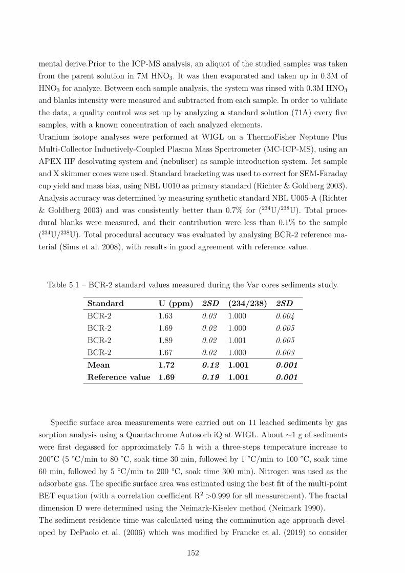
mental derive.Prior to the ICP-MS analysis, an aliquot of the studied samples was takenfrom the parent solution in 7M HNO3. It was then evaporated and taken up in 0.3M ofHNO3 for analyze. Between each sample analysis, the system was rinsed with 0.3M HNO3

and blanks intensity were measured and subtracted from each sample. In order to validatethe data, a quality control was set up by analyzing a standard solution (71A) every fivesamples, with a known concentration of each analyzed elements.Uranium isotope analyses were performed at WIGL on a ThermoFisher Neptune PlusMulti-Collector Inductively-Coupled Plasma Mass Spectrometer (MC-ICP-MS), using anAPEX HF desolvating system and (nebuliser) as sample introduction system. Jet sampleand X skimmer cones were used. Standard bracketing was used to correct for SEM-Faradaycup yield and mass bias, using NBL U010 as primary standard (Richter & Goldberg 2003).Analysis accuracy was determined by measuring synthetic standard NBL U005-A (Richter& Goldberg 2003) and was consistently better than 0.7% for (234U/238U). Total proce-dural blanks were measured, and their contribution were less than 0.1% to the sample(234U/238U). Total procedural accuracy was evaluated by analysing BCR-2 reference ma-terial (Sims et al. 2008), with results in good agreement with reference value.

Table 5.1 – BCR-2 standard values measured during the Var cores sediments study.

Standard U (ppm) 2SD (234/238) 2SDBCR-2 1.63 0.03 1.000 0.004BCR-2 1.69 0.02 1.000 0.005BCR-2 1.89 0.02 1.001 0.005BCR-2 1.67 0.02 1.000 0.003Mean 1.72 0.12 1.001 0.001Reference value 1.69 0.19 1.001 0.001

Specific surface area measurements were carried out on 11 leached sediments by gassorption analysis using a Quantachrome Autosorb iQ at WIGL. About ∼1 g of sedimentswere first degassed for approximately 7.5 h with a three-steps temperature increase to200°C (5 °C/min to 80 °C, soak time 30 min, followed by 1 °C/min to 100 °C, soak time60 min, followed by 5 °C/min to 200 °C, soak time 300 min). Nitrogen was used as theadsorbate gas. The specific surface area was estimated using the best fit of the multi-pointBET equation (with a correlation coefficient R2 >0.999 for all measurement). The fractaldimension D were determined using the Neimark-Kiselev method (Neimark 1990).The sediment residence time was calculated using the comminution age approach devel-oped by DePaolo et al. (2006) which was modified by Francke et al. (2019) to consider

152

234U loss after deposit:

tres = −1λ234

ln

[[A− (1 − fpost)] e−λ234tdep + (1 − fpost) − (1 − fpre)

A0 − (1 − fpre)

](5.1)

In the case where the surface area was not measured for a given sample, a random valuewas taken between the minimum and the maximum values measured.Sediment residencetimes were calculated using Monte Carlo simulation (10,000 simulations). For each sample,Ameas was taken randomly within the range of measured (234U/238U) activity ratios and itserror, and the maximum measured (234U/238U) value was attributed to A0 as we obtained(234U/238U)>1 in sediments. As not every specific surface area were measured, for thesamples without data, a random value was choose between the minimum and maximumvalues measured.

5.2.3 Uranium variations over time - Results

The KESC9-14 core cover mainly the Holocene period, while the ESSK08- CS01 andESSK08- CS13 are principally composed of sediments from the Late Glacial Period. Thesimilarity in the results obtained by these cores for the covered overlaps between 9-15 kaallows us to overcome the possible site effect.

ConcentrationUranium concentration in core KESC9-14 ranges from 2.33 to 5.58 ppm for the Holoceneperiod (mean = 3.7±0.5 2SD; n = 27). In cores ESSK08- CS01 and ESSK08- CS13, Uconcentrations vary from 0.05±0.03 (2SD) to 4.00±0.05 ppm (2SD) in the clay fractionover the last 75 ka (mean = 2.7±0.3 ppm 2SD; n = 64). For the silt size fraction, U rangefrom 0.65±0.05 (2SD) to 4.99±0.05 (2SD) ppm (mean = 2.9±0.3 2SD ppm; n=52, Fig.5.4, Appendix A5.1).During the Holocene (0-11.7 ka), U concentrations are higher (mean=3.83 ppm, n=26)than the value for the upper continental crust (UCC, between 2.5-2.8 ppm; grey rectanglein Fig. 5.4). Conversely, during the last glacial period (>11.7 ka), the concentration isrelatively close to the UCC concentration with a mean of 2.90 ppm (n=116).Over the Last Glacial Period there is some variation in U concentrations. During the MIS4 (75-57 ka), U concentrations are relatively stable, just above the actual values of theUCC. At the beginning of the MIS 3, the uranium concentration decreased and is globallywithin the range of UCC values, with an extreme value close to 0 at 56.8 ka for the claygrain size fraction. In the middle of the MIS 3 (∼39.2 ka), the uranium concentrationincreases slightly above the UCC to decrease abruptly to 0.6 ppm at 32-33ka. In themiddle of the MIS 2 (20 ka), the U concentration for clay-size fractions is in the UCCrange, whereas the indistinct grain size fraction is above and increase until the transition

153

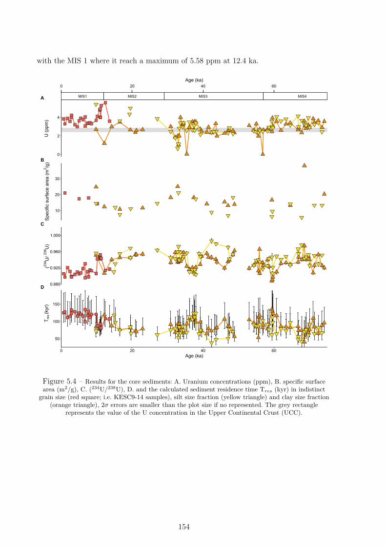
with the MIS 1 where it reach a maximum of 5.58 ppm at 12.4 ka.

0 20 40 60

0

2

4

Age (ka)

U (

ppm

)

A

10

20

30

Spe

cific

sur

face

are

a (m

2 /g)B

0.880

0.920

0.960

1.000

(234 U

/ 238 U

)

C

50

100

150

0 20 40 60Age (ka)

Tre

s (k

yr)

D

MIS1 MIS2 MIS3 MIS4

Figure 5.4 – Results for the core sediments: A. Uranium concentrations (ppm), B. specific surfacearea (m2/g), C. (234U/238U), D. and the calculated sediment residence time Tres (kyr) in indistinct

grain size (red square; i.e. KESC9-14 samples), silt size fraction (yellow triangle) and clay size fraction(orange triangle), 2σ errors are smaller than the plot size if no represented. The grey rectangle

represents the value of the U concentration in the Upper Continental Crust (UCC).

154

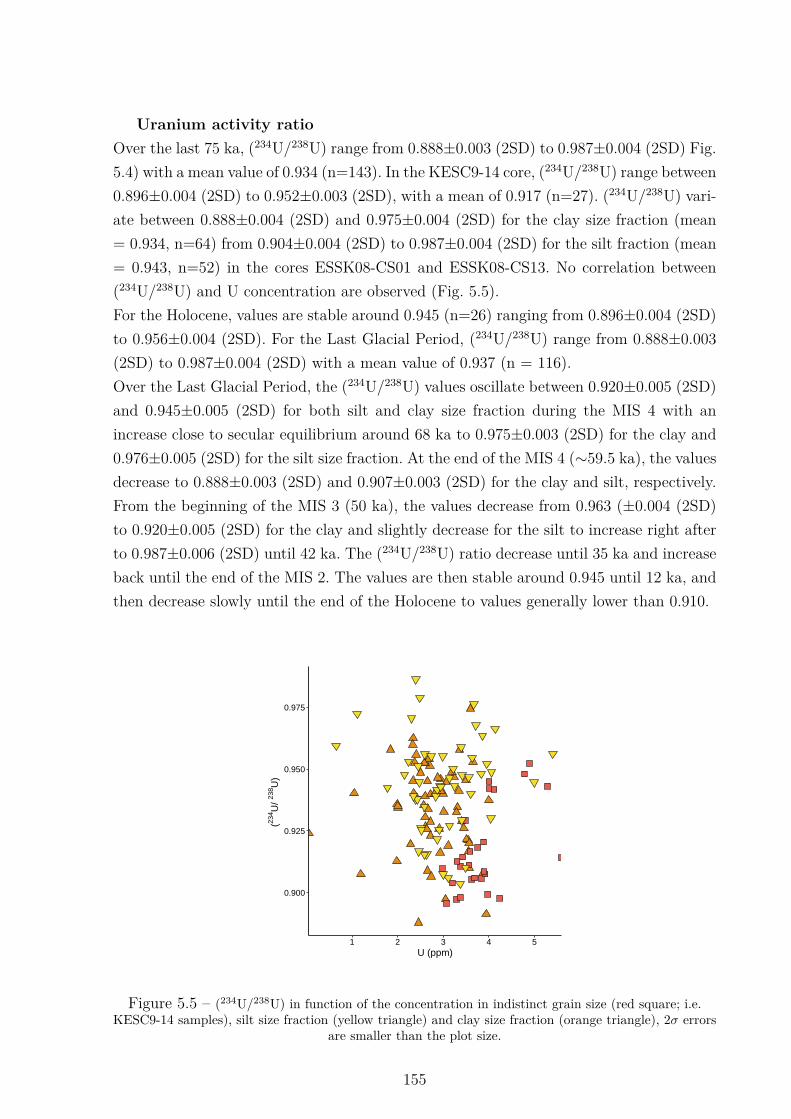
Uranium activity ratioOver the last 75 ka, (234U/238U) range from 0.888±0.003 (2SD) to 0.987±0.004 (2SD) Fig.5.4) with a mean value of 0.934 (n=143). In the KESC9-14 core, (234U/238U) range between0.896±0.004 (2SD) to 0.952±0.003 (2SD), with a mean of 0.917 (n=27). (234U/238U) vari-ate between 0.888±0.004 (2SD) and 0.975±0.004 (2SD) for the clay size fraction (mean= 0.934, n=64) from 0.904±0.004 (2SD) to 0.987±0.004 (2SD) for the silt fraction (mean= 0.943, n=52) in the cores ESSK08-CS01 and ESSK08-CS13. No correlation between(234U/238U) and U concentration are observed (Fig. 5.5).For the Holocene, values are stable around 0.945 (n=26) ranging from 0.896±0.004 (2SD)to 0.956±0.004 (2SD). For the Last Glacial Period, (234U/238U) range from 0.888±0.003(2SD) to 0.987±0.004 (2SD) with a mean value of 0.937 (n = 116).Over the Last Glacial Period, the (234U/238U) values oscillate between 0.920±0.005 (2SD)and 0.945±0.005 (2SD) for both silt and clay size fraction during the MIS 4 with anincrease close to secular equilibrium around 68 ka to 0.975±0.003 (2SD) for the clay and0.976±0.005 (2SD) for the silt size fraction. At the end of the MIS 4 (∼59.5 ka), the valuesdecrease to 0.888±0.003 (2SD) and 0.907±0.003 (2SD) for the clay and silt, respectively.From the beginning of the MIS 3 (50 ka), the values decrease from 0.963 (±0.004 (2SD)to 0.920±0.005 (2SD) for the clay and slightly decrease for the silt to increase right afterto 0.987±0.006 (2SD) until 42 ka. The (234U/238U) ratio decrease until 35 ka and increaseback until the end of the MIS 2. The values are then stable around 0.945 until 12 ka, andthen decrease slowly until the end of the Holocene to values generally lower than 0.910.

0.900

0.925

0.950

0.975

1 2 3 4 5U (ppm)

(234 U

/ 238 U

)

Figure 5.5 – (234U/238U) in function of the concentration in indistinct grain size (red square; i.e.KESC9-14 samples), silt size fraction (yellow triangle) and clay size fraction (orange triangle), 2σ errors

are smaller than the plot size.

155

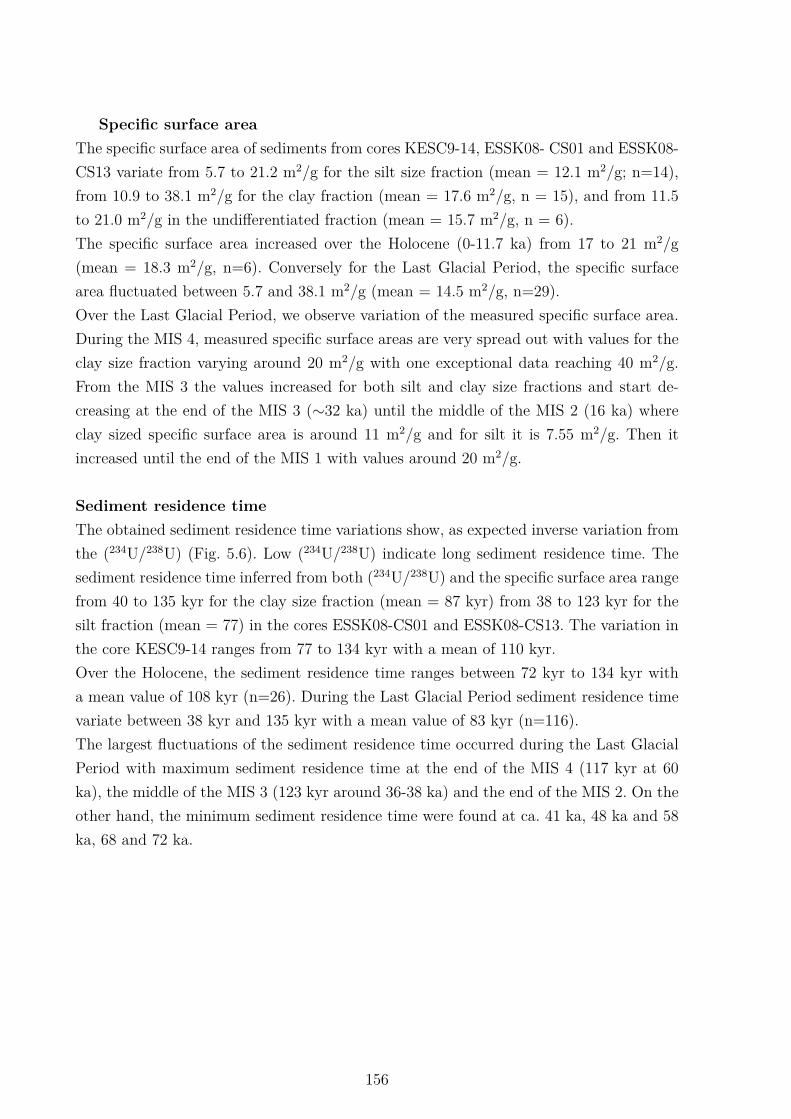
Specific surface areaThe specific surface area of sediments from cores KESC9-14, ESSK08- CS01 and ESSK08-CS13 variate from 5.7 to 21.2 m2/g for the silt size fraction (mean = 12.1 m2/g; n=14),from 10.9 to 38.1 m2/g for the clay fraction (mean = 17.6 m2/g, n = 15), and from 11.5to 21.0 m2/g in the undifferentiated fraction (mean = 15.7 m2/g, n = 6).The specific surface area increased over the Holocene (0-11.7 ka) from 17 to 21 m2/g(mean = 18.3 m2/g, n=6). Conversely for the Last Glacial Period, the specific surfacearea fluctuated between 5.7 and 38.1 m2/g (mean = 14.5 m2/g, n=29).Over the Last Glacial Period, we observe variation of the measured specific surface area.During the MIS 4, measured specific surface areas are very spread out with values for theclay size fraction varying around 20 m2/g with one exceptional data reaching 40 m2/g.From the MIS 3 the values increased for both silt and clay size fractions and start de-creasing at the end of the MIS 3 (∼32 ka) until the middle of the MIS 2 (16 ka) whereclay sized specific surface area is around 11 m2/g and for silt it is 7.55 m2/g. Then itincreased until the end of the MIS 1 with values around 20 m2/g.

Sediment residence timeThe obtained sediment residence time variations show, as expected inverse variation fromthe (234U/238U) (Fig. 5.6). Low (234U/238U) indicate long sediment residence time. Thesediment residence time inferred from both (234U/238U) and the specific surface area rangefrom 40 to 135 kyr for the clay size fraction (mean = 87 kyr) from 38 to 123 kyr for thesilt fraction (mean = 77) in the cores ESSK08-CS01 and ESSK08-CS13. The variation inthe core KESC9-14 ranges from 77 to 134 kyr with a mean of 110 kyr.Over the Holocene, the sediment residence time ranges between 72 kyr to 134 kyr witha mean value of 108 kyr (n=26). During the Last Glacial Period sediment residence timevariate between 38 kyr and 135 kyr with a mean value of 83 kyr (n=116).The largest fluctuations of the sediment residence time occurred during the Last GlacialPeriod with maximum sediment residence time at the end of the MIS 4 (117 kyr at 60ka), the middle of the MIS 3 (123 kyr around 36-38 ka) and the end of the MIS 2. On theother hand, the minimum sediment residence time were found at ca. 41 ka, 48 ka and 58ka, 68 and 72 ka.

156

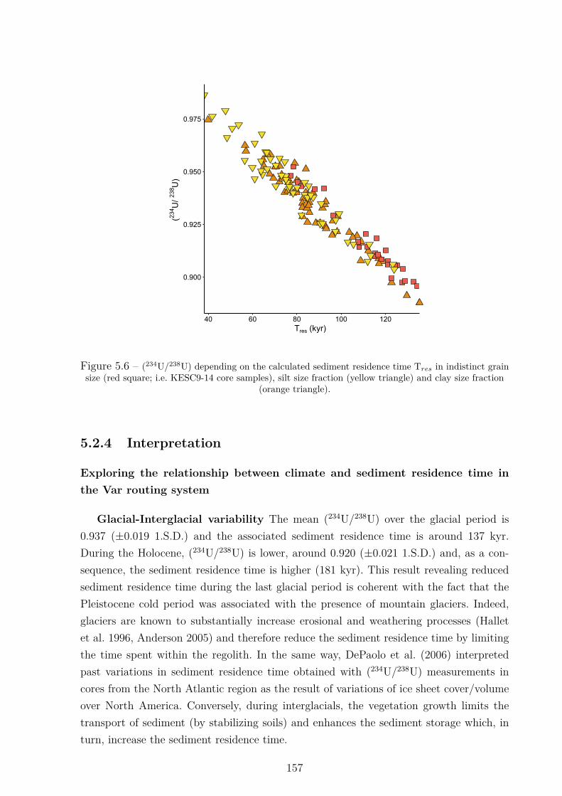
0.900

0.925

0.950

0.975

40 60 80 100 120Tres (kyr)

(234 U

/ 238 U

)

Figure 5.6 – (234U/238U) depending on the calculated sediment residence time Tres in indistinct grainsize (red square; i.e. KESC9-14 core samples), silt size fraction (yellow triangle) and clay size fraction

(orange triangle).

5.2.4 Interpretation

Exploring the relationship between climate and sediment residence time inthe Var routing system

Glacial-Interglacial variability The mean (234U/238U) over the glacial period is0.937 (±0.019 1.S.D.) and the associated sediment residence time is around 137 kyr.During the Holocene, (234U/238U) is lower, around 0.920 (±0.021 1.S.D.) and, as a con-sequence, the sediment residence time is higher (181 kyr). This result revealing reducedsediment residence time during the last glacial period is coherent with the fact that thePleistocene cold period was associated with the presence of mountain glaciers. Indeed,glaciers are known to substantially increase erosional and weathering processes (Halletet al. 1996, Anderson 2005) and therefore reduce the sediment residence time by limitingthe time spent within the regolith. In the same way, DePaolo et al. (2006) interpretedpast variations in sediment residence time obtained with (234U/238U) measurements incores from the North Atlantic region as the result of variations of ice sheet cover/volumeover North America. Conversely, during interglacials, the vegetation growth limits thetransport of sediment (by stabilizing soils) and enhances the sediment storage which, inturn, increase the sediment residence time.

157

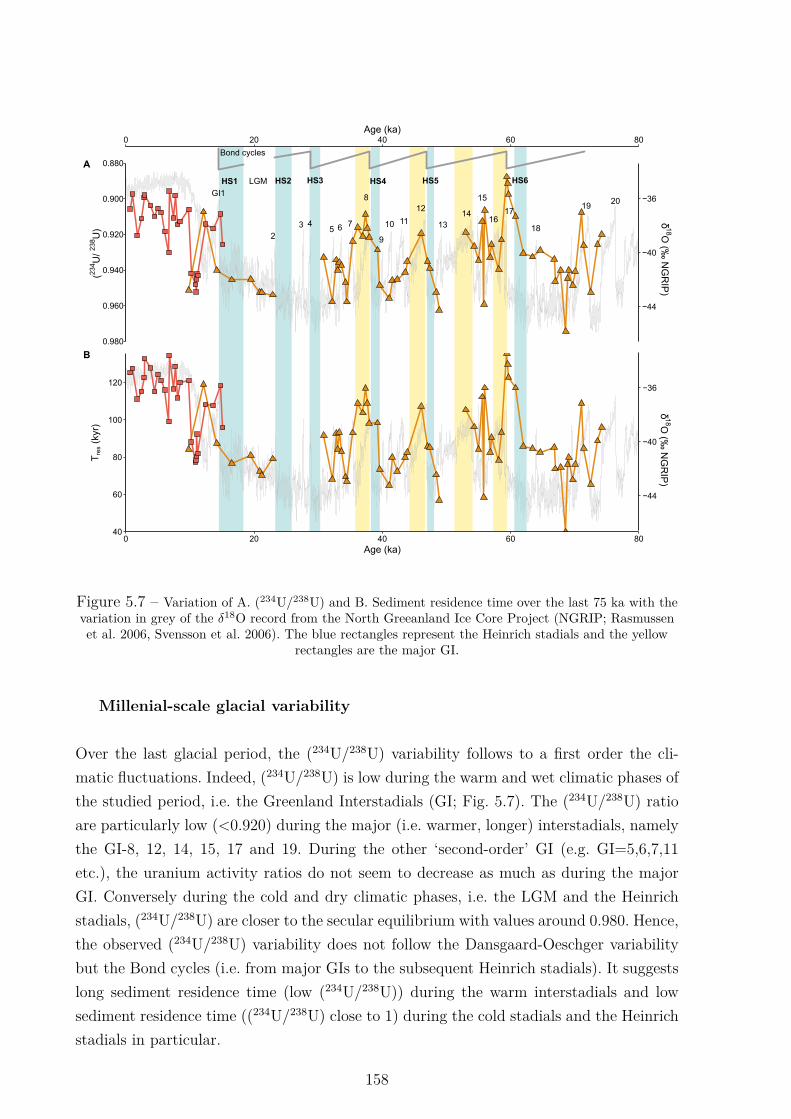
−44

−40

−36

δ18O

(‰ N

GR

IP)

A

0 20 40 60 80

0.880

0.900

0.920

0.940

0.960

0.980

Age (ka)

(234 U

/ 238 U

)

B

40

60

80

100

120

0 20 40 60 80Age (ka)

Tre

s(k

yr)

−44

−40

−36

Bond cycles

HS1 HS2 HS3LGM HS4 HS5 HS6

GI1

23 4

5 6 7

8

9

10 11

12

1314

15

1617

18

1920

δ18O

(‰ N

GR

IP)

Figure 5.7 – Variation of A. (234U/238U) and B. Sediment residence time over the last 75 ka with thevariation in grey of the δ18O record from the North Greeanland Ice Core Project (NGRIP; Rasmussenet al. 2006, Svensson et al. 2006). The blue rectangles represent the Heinrich stadials and the yellow

rectangles are the major GI.

Millenial-scale glacial variability

Over the last glacial period, the (234U/238U) variability follows to a first order the cli-matic fluctuations. Indeed, (234U/238U) is low during the warm and wet climatic phases ofthe studied period, i.e. the Greenland Interstadials (GI; Fig. 5.7). The (234U/238U) ratioare particularly low (<0.920) during the major (i.e. warmer, longer) interstadials, namelythe GI-8, 12, 14, 15, 17 and 19. During the other ‘second-order’ GI (e.g. GI=5,6,7,11etc.), the uranium activity ratios do not seem to decrease as much as during the majorGI. Conversely during the cold and dry climatic phases, i.e. the LGM and the Heinrichstadials, (234U/238U) are closer to the secular equilibrium with values around 0.980. Hence,the observed (234U/238U) variability does not follow the Dansgaard-Oeschger variabilitybut the Bond cycles (i.e. from major GIs to the subsequent Heinrich stadials). It suggestslong sediment residence time (low (234U/238U)) during the warm interstadials and lowsediment residence time ((234U/238U) close to 1) during the cold stadials and the Heinrichstadials in particular.

158

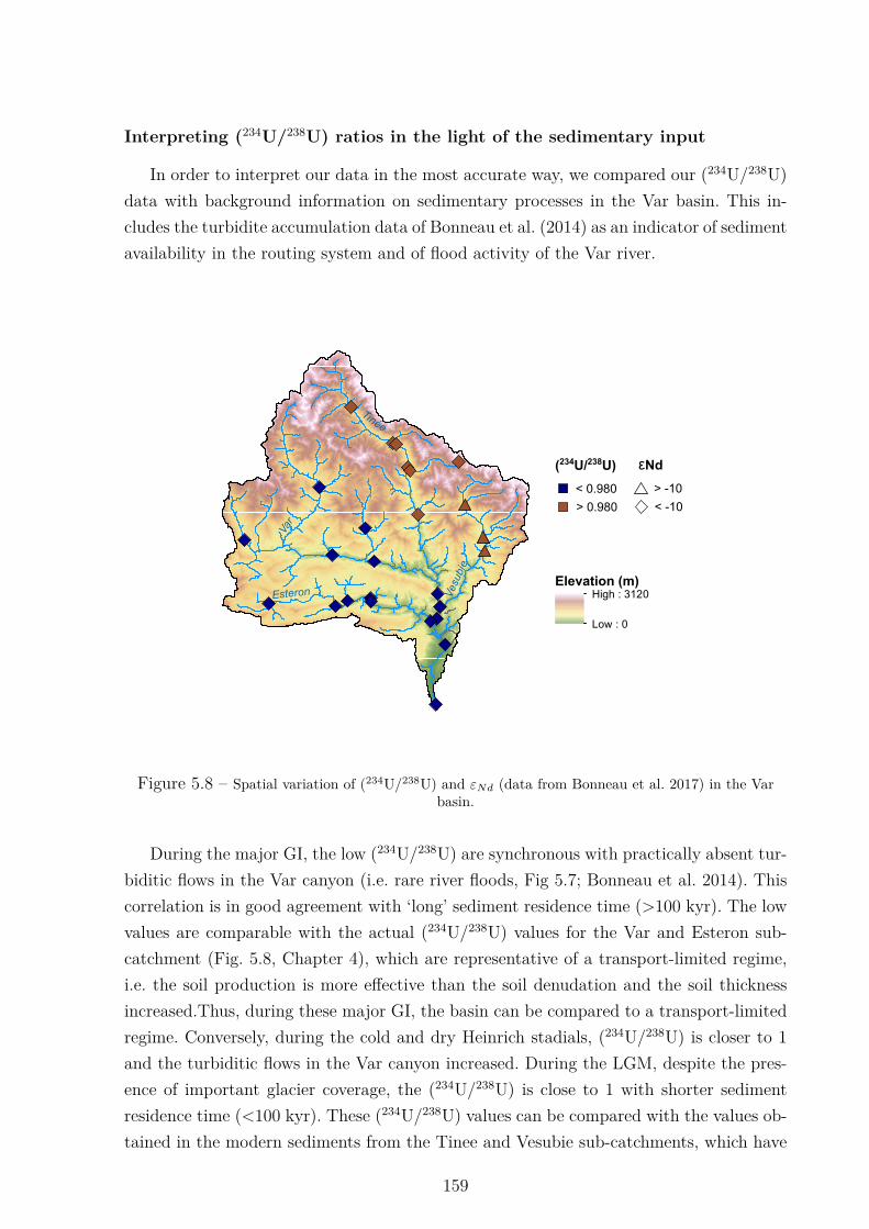
Interpreting (234U/238U) ratios in the light of the sedimentary input

In order to interpret our data in the most accurate way, we compared our (234U/238U)data with background information on sedimentary processes in the Var basin. This in-cludes the turbidite accumulation data of Bonneau et al. (2014) as an indicator of sedimentavailability in the routing system and of flood activity of the Var river.

"" #*

""

""

"

"

"

"

"

"

#

#

#

(234U/238U)

Vesubie

Elevation (m)High : 3120

Low : 0

Esteron

Tinée

Var

"

"

"

"

""

"

"

"""""

""

< 0.980

> 0.980

Nd

> -10

< -10

ε1

Figure 5.8 – Spatial variation of (234U/238U) and εNd (data from Bonneau et al. 2017) in the Varbasin.

During the major GI, the low (234U/238U) are synchronous with practically absent tur-biditic flows in the Var canyon (i.e. rare river floods, Fig 5.7; Bonneau et al. 2014). Thiscorrelation is in good agreement with ‘long’ sediment residence time (>100 kyr). The lowvalues are comparable with the actual (234U/238U) values for the Var and Esteron sub-catchment (Fig. 5.8, Chapter 4), which are representative of a transport-limited regime,i.e. the soil production is more effective than the soil denudation and the soil thicknessincreased.Thus, during these major GI, the basin can be compared to a transport-limitedregime. Conversely, during the cold and dry Heinrich stadials, (234U/238U) is closer to 1and the turbiditic flows in the Var canyon increased. During the LGM, despite the pres-ence of important glacier coverage, the (234U/238U) is close to 1 with shorter sedimentresidence time (<100 kyr). These (234U/238U) values can be compared with the values ob-tained in the modern sediments from the Tinee and Vesubie sub-catchments, which have

159

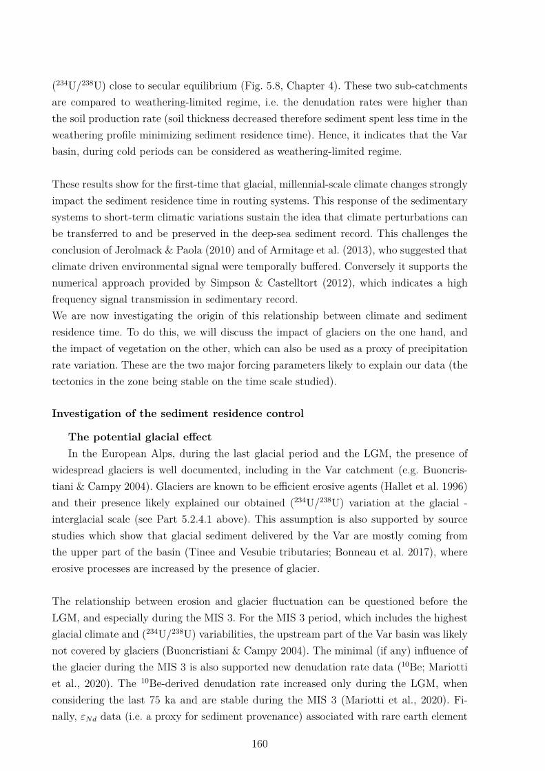
(234U/238U) close to secular equilibrium (Fig. 5.8, Chapter 4). These two sub-catchmentsare compared to weathering-limited regime, i.e. the denudation rates were higher thanthe soil production rate (soil thickness decreased therefore sediment spent less time in theweathering profile minimizing sediment residence time). Hence, it indicates that the Varbasin, during cold periods can be considered as weathering-limited regime.

These results show for the first-time that glacial, millennial-scale climate changes stronglyimpact the sediment residence time in routing systems. This response of the sedimentarysystems to short-term climatic variations sustain the idea that climate perturbations canbe transferred to and be preserved in the deep-sea sediment record. This challenges theconclusion of Jerolmack & Paola (2010) and of Armitage et al. (2013), who suggested thatclimate driven environmental signal were temporally buffered. Conversely it supports thenumerical approach provided by Simpson & Castelltort (2012), which indicates a highfrequency signal transmission in sedimentary record.We are now investigating the origin of this relationship between climate and sedimentresidence time. To do this, we will discuss the impact of glaciers on the one hand, andthe impact of vegetation on the other, which can also be used as a proxy of precipitationrate variation. These are the two major forcing parameters likely to explain our data (thetectonics in the zone being stable on the time scale studied).

Investigation of the sediment residence control

The potential glacial effectIn the European Alps, during the last glacial period and the LGM, the presence of

widespread glaciers is well documented, including in the Var catchment (e.g. Buoncris-tiani & Campy 2004). Glaciers are known to be efficient erosive agents (Hallet et al. 1996)and their presence likely explained our obtained (234U/238U) variation at the glacial -interglacial scale (see Part 5.2.4.1 above). This assumption is also supported by sourcestudies which show that glacial sediment delivered by the Var are mostly coming fromthe upper part of the basin (Tinee and Vesubie tributaries; Bonneau et al. 2017), whereerosive processes are increased by the presence of glacier.

The relationship between erosion and glacier fluctuation can be questioned before theLGM, and especially during the MIS 3. For the MIS 3 period, which includes the highestglacial climate and (234U/238U) variabilities, the upstream part of the Var basin was likelynot covered by glaciers (Buoncristiani & Campy 2004). The minimal (if any) influence ofthe glacier during the MIS 3 is also supported new denudation rate data (10Be; Mariottiet al., 2020). The 10Be-derived denudation rate increased only during the LGM, whenconsidering the last 75 ka and are stable during the MIS 3 (Mariotti et al., 2020). Fi-nally, εNd data (i.e. a proxy for sediment provenance) associated with rare earth element

160

abundances, major and minor elements data indicate that the main driving mechanismof sediment input to the VSR during MIS 3 was not restricted to the upper watershed(where glaciers are expected), but likely impacted the whole Var basin (Bonneau et al.2014, 2017). Taken together, these lines of evidence indicate that glacier fluctuations can-not explain the (234U/238U) ratio variability during MIS 3.

A

B

Figure 5.9 – εNd variation in the Var basin (from Bonneau 2014, Mariotti 2020); turbidites frequencyand 10Be derived denudation rate (from Mariotti 2020).

The vegetation impact on sediment residence timeIf glaciers do not likely explain the obtained variation of sediment residence time dur-

ing the MIS 3, the vegetation could influence it. Indeed, Dosseto et al. (2010) determineda vegetation control of sediment residence time over glacial-interglacial cycles. Later,Francke et al. (2019) corroborate this idea studying Late Glacial to Holocene sedimentfrom the Balkans. Therefore, it is interesting to compare the paleo-variation of sedimentresidence time in the Var sediment routing system with palynological data available in

161

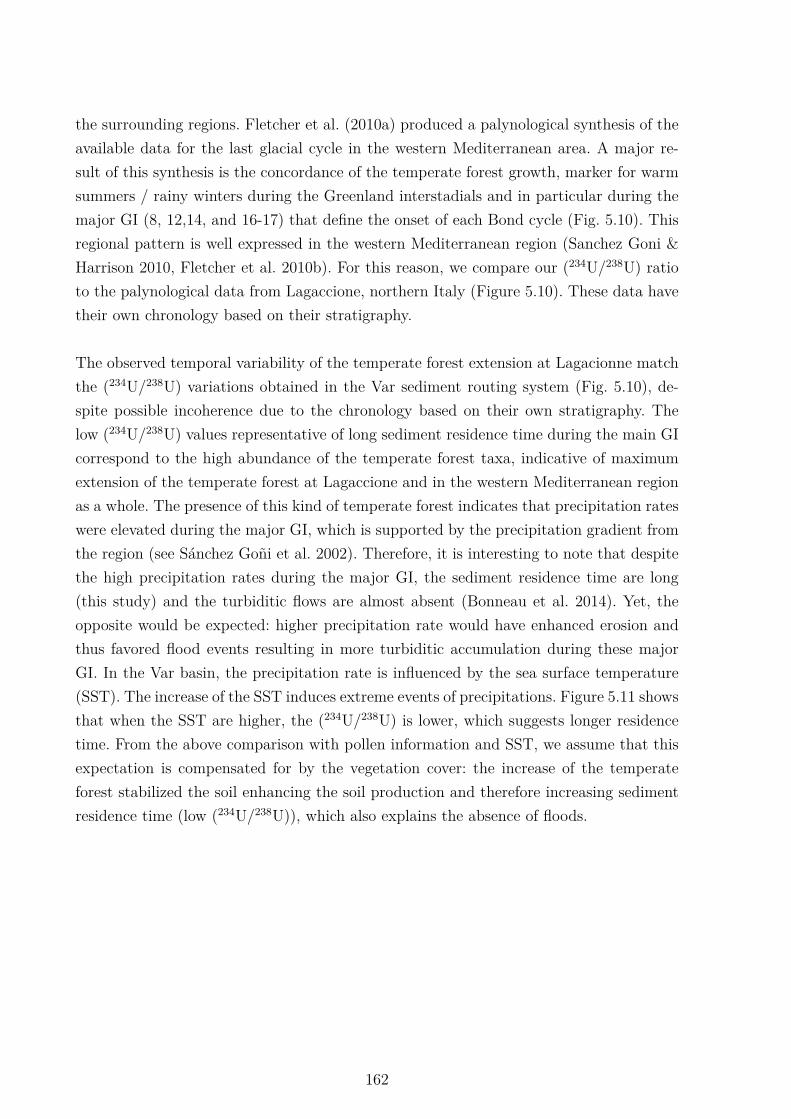
the surrounding regions. Fletcher et al. (2010a) produced a palynological synthesis of theavailable data for the last glacial cycle in the western Mediterranean area. A major re-sult of this synthesis is the concordance of the temperate forest growth, marker for warmsummers / rainy winters during the Greenland interstadials and in particular during themajor GI (8, 12,14, and 16-17) that define the onset of each Bond cycle (Fig. 5.10). Thisregional pattern is well expressed in the western Mediterranean region (Sanchez Goni &Harrison 2010, Fletcher et al. 2010b). For this reason, we compare our (234U/238U) ratioto the palynological data from Lagaccione, northern Italy (Figure 5.10). These data havetheir own chronology based on their stratigraphy.

The observed temporal variability of the temperate forest extension at Lagacionne matchthe (234U/238U) variations obtained in the Var sediment routing system (Fig. 5.10), de-spite possible incoherence due to the chronology based on their own stratigraphy. Thelow (234U/238U) values representative of long sediment residence time during the main GIcorrespond to the high abundance of the temperate forest taxa, indicative of maximumextension of the temperate forest at Lagaccione and in the western Mediterranean regionas a whole. The presence of this kind of temperate forest indicates that precipitation rateswere elevated during the major GI, which is supported by the precipitation gradient fromthe region (see Sánchez Goñi et al. 2002). Therefore, it is interesting to note that despitethe high precipitation rates during the major GI, the sediment residence time are long(this study) and the turbiditic flows are almost absent (Bonneau et al. 2014). Yet, theopposite would be expected: higher precipitation rate would have enhanced erosion andthus favored flood events resulting in more turbiditic accumulation during these majorGI. In the Var basin, the precipitation rate is influenced by the sea surface temperature(SST). The increase of the SST induces extreme events of precipitations. Figure 5.11 showsthat when the SST are higher, the (234U/238U) is lower, which suggests longer residencetime. From the above comparison with pollen information and SST, we assume that thisexpectation is compensated for by the vegetation cover: the increase of the temperateforest stabilized the soil enhancing the soil production and therefore increasing sedimentresidence time (low (234U/238U)), which also explains the absence of floods.

162

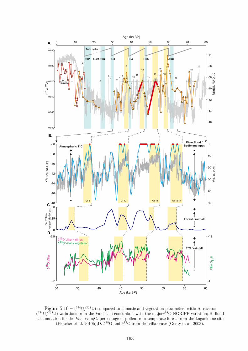
0 10 20 30 40 50 60 70 80

-46

-44

-42

-40

-38

-36

-34

Bond cycles

LGM

Hol.minima

2

GI1

34

12

8

1113

14

15

18

19

20

10

9

76

5

HS1 HS2 HS3 HS4 HS5

16

17

HS6

-48

-46

-44

-42

-40

-38

-36 0

10

20

30

40

50GI-8

% P

olle

nte

mpe

rate

fore

st

GI-12 GI-14 GI-16/17

0

25

50

-

-

δ18 O

(‰

NG

RIP

)

Age (ka BP)

30 35 40 45 50 55 60 65

Flood / 0.5kyr

River flood /Sediment input

-Atmospheric T°C

+

Forest / rainfall

+

+

-2

-5.5

-4

-12

-

T°C / rainfall

+

0.880

0.900

0.920

0.940

0.960

0.980

(234 U

/238 U

)A.

B.

C.

D.

δ18 O

Vill

ar δ 13C V

illar

δ18O Villar ≈ climat δ13C Villar ≈ vegetation

δ18 O

(‰ N

GR

IP)

Age (ka BP)

Figure 5.10 – (234U/238U) compared to climatic and vegetation parameters with: A. reverse(234U/238U) variations from the Var basin concordant with the majorδ18O NGRIPP variation; B. floodaccumulation for the Var basin;C. percentage of pollen from temperate forest from the Lagacionne site

(Fletcher et al. 2010b);D. δ18O and δ13C from the villar cave (Genty et al. 2003).

163

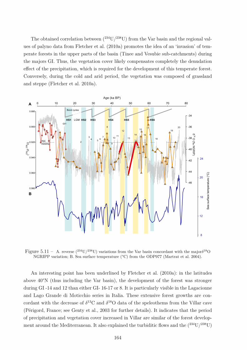
The obtained correlation between (234U/238U) from the Var basin and the regional val-ues of palyno data from Fletcher et al. (2010a) promotes the idea of an ‘invasion’ of tem-perate forests in the upper parts of the basin (Tinee and Vesubie sub-catchments) duringthe majors GI. Thus, the vegetation cover likely compensates completely the denudationeffect of the precipitation, which is required for the development of this temperate forest.Conversely, during the cold and arid period, the vegetation was composed of grasslandand steppe (Fletcher et al. 2010a).

0 10 20 30 40 50 60 70 80

-46

-44

-42

-40

-38

-36

-34

Bond cycles

LGM

Hol.minima

2

GI1

34

12

8

1113

14

15

18

19

20

10

9

76

5

HS1 HS2 HS3 HS4 HS5

16

17

HS6

Age (ka BP)

0.880

0.900

0.920

0.940

0.960

0.980

(234 U

/238 U

)

A

δ18

O (‰

NG

RIP

)

Sea

sur

face

tem

pera

ture

(°C

)

24

20

16

12

8

B

Figure 5.11 – A. reverse (234U/238U) variations from the Var basin concordant with the majorδ18ONGRIPP variation; B. Sea surface temperature (°C) from the ODP977 (Martrat et al. 2004).

An interesting point has been underlined by Fletcher et al. (2010a): in the latitudesabove 40°N (thus including the Var basin), the development of the forest was strongerduring GI -14 and 12 than either GI- 16-17 or 8. It is particularly visible in the Lagacionneand Lago Grande di Moticchio series in Italia. These extensive forest growths are con-cordant with the decrease of δ13C and δ18O data of the speleothems from the Villar cave(Périgord, France; see Genty et al., 2003 for further details). It indicates that the periodof precipitation and vegetation cover increased in Villar are similar of the forest develop-ment around the Mediterranean. It also explained the turbiditic flows and the (234U/238U)

164

variations: during both GI -14 and 12 there is an absence of overflow in the Var basin.The forest extension in the Var basin stabilized the soil and reduced denudation. It ledto a reduction of sediment flow and a limitation in the turbiditic accumulation. Hencethe basin is completely transport limited, which increased the sediment residence time(low (234U/238U)). Note that because of the absence of sediment transfer during these twomajor GI -14 and 12, there is no turbidite material to measure (234U/238U) which explainthe lack of data for these events.

5.2.5 Conclusion

The paleo variation of (234U/238U) in the Var basin, and the associated sediment res-idence time, show first a variation between Holocene (long sediment residence time; low(234U/238U)) and the last Glacial maximum (rapid sediment residence time; (234U/238U)close to 1). This long-term variation can be explained by the presence of LGM glaciers inthe Alps that promote erosion, enhancing the sediment transfer to the deposition zone.A second scale variation is identified in (234U/238U) during the last glacial period, with(234U/238U) and therefore sediment residence time variation following the Bond cycle. This(234U/238U) variation cannot be fully explained by glaciers because of their absence in theVar catchment during the MIS 3. On the other hand, a comparison between (234U/238U)and the percentage of pollen from temperate forest (Laggaccione, Italia) suggests that theincrease of temperate forest in the region during the warmer event (GI) promote the soilstabilization. Hence it increases the sediment residence time. In the major GI events, soilstabilization is such that there is no more turbidites and the highest sediment residencetime. Thus, this observed cyclicity following short-term climatic variation is an indicatorthat land-sea signals can be transmitted and preserved in turbiditic deposits.

In the future, rainfall is expected to be high but erratic with heavy flooding due to globalwarming. According to our data, this is not necessarily synonymous of high denudationrates and seaward sediment transfer as commonly accepted (e.g. Kober et al. 2007). In-deed, the dense vegetation cover under wet climate conditions could counterbalance theerosive effect of rainfall events as evidenced by the residence times of paleo-sediments. De-spite improvements in land cover during the last decades in the Var basin, urbanisationstill greatly impacts the landscape. Human control of the landscape affect greatly soils,which are in consequence generally less prone to adsorb the precipitation water, creatingriver floods. This situation could deteriorate in light of the increase in extreme rainfall inthe French Mediterranean (Ribes et al. 2019), which is already visible with the autumnfloods of this year (e.g. Alex tempete - 3 October 2020).

165

CONCLUSIONS AND PERSPECTIVES

Rationale and objectives of this thesis

The interaction between tectonics, climate and weathering are known to control theevolution of landscape morphology over geological timescales. Tectonic processes result inmountain building, which in turn promotes erosion, weathering and soil formation. Soilsare eroded at different rates depending on the efficiency of sediment routing systems,resulting in the transfer of sediments to depositional areas. Those systems where soildenudation is greater than soil production are called weathering-limited, while those char-acterized higher soil production relative to sediment export are referred to as transport-limited.In source-to-sink systems, the variation of one or multiple controlling factors such as e.g.climate, weathering, tectonic, or morphology, induces an environmental signal (i.e. dis-turbance) in the sediment cycle, from production to deposition. This disturbance can beabrupt (i.e. earthquake) or occurring over long timescale (i.e. glacial - interglacial cyclic-ity). The system then needs to adapt and evolves towards a new equilibrium that createsa change in the sedimentary cycle (e.g. nature of sediments; sediment production, etc.).These variations can propagate into the sediment routing system as an environmentalsignal, which can be stored and preserved in the depositional zone. In the case where thesediment as well as the environmental signals are rapidly transported from source to sink(i.e. without temporary storage along the path), the system is referred to as reactive.However, major limitations in the transmission of these environmental signals exist. Forinstance, the storage of sediments in loodplains can buffer or attenuate any change insedimentary fluxes. Such limitations can result in discrepancies between any given en-vironmental change and its recording in the sedimentary depositional zone. As a result,the extent to which environmental signals are buffered or transferred downstream riversystems and be efficiently preserved in the sedimentary record remains a matter of debate.The sediment residence time, as the time elapsed between the generation of the sedimentgrains in the source areas and the time of deposition in the sedimentary record, is a mea-sure that provide useful information about environmental signals in watersheds and theirpropagation through time.Over the last decades, the uranium series have been used to estimate sediment residencetime through the so-called comminution age method. Previous work highlighted the greatpotential of this approach by demonstrating strong correlations between sediment resi-dence time and long-term climate changes. Nevertheless, the interpretation of sediment

167

residence time is currently limited by the lack of information on the spatial distribution ofsedimentary (234U/238U) in catchments, and on the extent to which the preferential 234Uloss may be affected by factors such as the lithology, the morphology of the catchment,etc.In this study, we aimed at improving our understanding on 234U-238U fractionation inriver sediments. To this purpose, we first investigated the large-scale spatial distributionof sedimentary (234U/238U) ratios at the Earth’s surface, through the analysis of vari-ous sediment samples from many rivers worldwide (Chapter 3). In a second part, wethen focused on the detailed spatial distribution of 234U-238U fractionation inside a smallmountainous catchment, to refine our understanding of the use of (234U/238U) to quantifyerosion and transfer processes (Chapter 4). This latter part was followed by the applica-tion of U isotopes to nearby marine sedimentary records, in order to infer how erosionand transfer times may have changed in the past due to climate change (Chapter 5). Ourmain results are synthesized here after.

The variation of U-fractionationThe first part of this thesis focused on studying the spatial distribution of (234U/238U)

in world river sediments to assess the main parameters (e.g. grain size, lithology, cli-mate, weathering, catchment size) controlling U isotope fractionation in watersheds. Forthis purpose, a series of 64 modern sediment samples from various rivers was analyzed.The same sediments had been previously analyzed for other geochemical tracers (Bayonet al. 2015, 2016, 2018, 2020, Bindeman et al. 2019), demonstrating interesting relation-ships between weathering proxies and various external parameters (e.g. climate, lithology,weathering regime). The new U isotope data acquired during the course of this PhD thesisrepresents the first large scale investigation of (234U/238U) in world river sediments. Thiswork, presented in detail in Chapter 3, has been published in Geochimica et Cosmochim-ica Acta in September 2020.

The measurement of (234U/238U) in two separate size fractions (clay: <4 µm and silt: 4-63 µm) revealed an interesting size-dependent U isotopic fractionation, showing that theclay size fractions derived from small crystalline basins commonly exhibited (234U/238U)>1. This finding was not expected as analyzes were conducted on the detrital part ofthe grains (i.e. the non-detrital part has been previously leached), which is supposed tobe under the secular equilibrium. Because our leaching protocol ensures a quantitativeremoval of all non-detrital components (carbonates, iron oxides, organic compounds), weare confident that these results truly reflect the particular U isotopic composition of clayminerals in many crystalline catchments, highlighting the importance of yet unidentifiedsecondary processes that result in the preferential gain of 234U in secondary weathering

168

products.

The comparison of measured sedimentary (234U/238U) in river sediments with environ-mental parameters (e.g. lithology, weathering, morphology) did not highlight a strongcontrol on the fractionation of 234U over 238U of any of these factors. However, I showedthat (234U/238U) displayed an inverse relationship with the size of the catchment area,pointing towards an increase in the sediment residence time associated with decreasing234U/238U ratios in river sediments, as the storage capacity along the sediment routingsystem increases.

A multi-analysis approach including all the parameters investigated in the global surveyof U isotopes indicates that the observed (234U/238U) variability in river sediments can beaccounted for at about 70-80% by environmental factors (i.e climatic, weathering, depthto bedrock, catchment size and maximum elevation and lithology). Note however that theobtained p-values were not statistically significant, suggesting that this finding, despiteits importance, should be treated with caution. Nevertheless, it shows two interestingpoints: 1. the fractionation of (234U/238U) at the Earth surface is dependent of a multi-ple of factors (e.g. soil thickness, precipitation, lithology, etc.), reflecting the complexityof sedimentary systems and the intercorrelation of many influential parameters; 2. thehigher degree of correlation observed between (234U/238U) in clay size fractions with theenvironmental factors implies that this size fraction might be more prone to adequatelyreflect environmental changes, compared to silt-size fractions. Overall, the large scale sur-vey of (234U/238U) in world river sediments emphasizes the great potential of U isotopesfor investigating the influence of environmental signals on Earth surface processes.

Spatial variation of the sediment residence time in amountainous river basin

A regional investigation of the spatial variability of sediment residence times within areactive sediment routing system was conducted in the Var River basin, a small mountain-ous catchments in the French Southern Alps. For this purpose, (234U/238U) was measuredin a series of river sediment samples collected along the Var River and its tributaries.A publication is currently under preparation, which should be submitted to Earth andPlanetary Science Letters before the end of 2020.

As shown in Chapter 4, the observed variability of (234U/238U) across the Var basinreflects differences in the weathering regime in different parts of the watershed. We showthat in those sub-catchment areas dominated by kinetically-limited weathering regime

169

(e.g. Tinée and Vésubie sub-catchment), characteristic of the high topographic regionsof the basin, soils do not develop, limiting the time required for (234U/238U) to fraction-ate. As a result, the estimated sediment residence times in these areas are low (generally<200 ka). In contrast, in those low elevation regions of the basin (e.g. Var and Esteronsub-catchment), characterized by transport-limited weathering conditions, the weatheringprofile is more developed, leading to an increase in the sediment residence time (>300 ka).

In order to validate these findings based on U isotopes, we used a second approach toinfer regolith residence times. This approach makes use of existing data on the spatialdistribution of soil thickness, combined with 10Be denudation rates. We show that a goodcorrelation exists between the sediment residence times inferred from U isotopes and thoseusing the approach described above. This finding underlines the fact that the residencetimes estimated with U isotopes mostly reflect the time spent in the soil, namely regolithresidence time, at least in reactive sediment routing systems.

Finally, we pointed out the influence of the morphology on the regolith residence time inthe Var basin, demonstrating lower regolith residence time in high elevation regions thanin flatter areas. We also showed that a direct correlation exists between the slope, andto a less extent the curvature, and the regolith residence time inferred with U isotopes,hence supporting the idea that obtained regolith residence times could be used as a proxyfor morphology in addition to tracing weathering.

Linking paleo-sediment residence time to paleo-erosionalprocesses

On the basis of the results of the spatial analysis of sedimentary residence times acrossthe Var River basin (Chapter 4), we moved to the deep-sea depositional area of the sameVar routing system, focusing on long sediment cores with the aim to reconstruct the evo-lution of past sediment residence time. A publication is currently in preparation with theaim to submit in the near future.

A great variability of (234U/238U) and corresponding sediment residence time is observedover the studied time interval. Sediment residence time ranges from 38.2 to 135.4 kyr. Tounderstand the variability of sediment residence time based on U isotopes, we comparedthe obtained results with the climatic variation. The variation of (234U/238U) over le last75ka first indicated an evolution at glacial-interglacial timescale, i.e. between the LastGlacial Period (that ended ca. 11,700 years ago) and the Holocene. We show that dur-ing the Last Glacial Period and the Last Glacial Maximum (ca. 26-29 ka) in particular,

170

sediment residence time were significantly lower ((234U/238U) closer to 1) than during theHolocene ((234U/238U) <1).Superimposed to the glacial-interglacial variability of sediment residence time; the de-tailed study of (234U/238U) variations revealed a ‘cyclicity’ that follows the millennial-scaleglacial climate variability (well-expressed in the Marine Isotope Stage 3, ca. 57-29 ka).Indeed, during the warm but wet climatic phases, i.e. the major Greenland Interstadials ofthe last glacial: (GI-8,12,14,15,17 and 19), our results reveal that the sediment residencetime was particularly long ((234U/238U) <1), reaching values close to those found for theHolocene. Conversely during the cold and dry Heinrich stadials, the sediment residencetime significantly decreased to LGM values, i.e. (234U/238U) close to 1. These results doc-ument for the first time the variability of sediment residence time over the millennial-scaleclimatic variability (well-expressed in the Marine Isotope Stage 3, ca. 57-29 ka), and es-pecially the so-called Bond cyclicity.

The observed differences in the degree of U isotopic fractionation that accompaniesthe alternation of short-lived cold and warm events mostly likely reflect differences in theerosional regime, notably induced by the presence of glaciers in the southern Alps duringthe last glacial period, which are known to act as highly efficient erosive agents. Enhancederosive processes during these periods most likely limited soil development, thus sedimentswere exported down to the system more rapidly. In comparison with the sediment resi-dence time variability observed at the glacial-interglacial timescale, the short-term glacialcyclicity cannot be explained by glacial-induced erosion alone. Indeed, it has been shownrecently that 10Be derived denudation rates were stable throughout the Marine IsotopicStage 3 (Mariotti et al. 2021). Furthermore, the extent of glacier coverage was reduced inthe Var basin at that time (Mariotti et al. 2021).On this basis, we investigated the potential control of the vegetation cover on the sedimentresidence time by comparing our U isotope data to nearby high-resolution palynologicalrecords from the Italian Alps that cover the same period of time. This comparison showedthat the sediment residence time derived from U isotopes varied in pair with the variationof pollen percentage. During the warm / wet interstadials (e.g. GI-8,12,14,16-17), pollendata suggest that temperate forests were at their maximal extension in the northern Italyregion. Widespread forest cover at these times coincided with periods characterized bylong sediment residence time. This relationship can be explained by the effect of the veg-etation on the stabilization of soils, increasing the time spent by the sediment within thesoil profile. As a result, sedimentary fluxes decreased drastically during these short-livedwarm events, in agreement with evidence for the absence of turbidites deposited in theVar Sedimentary Ridge during these same periods. Conversely, during the cold and dryperiods, the temperate forest cover decreased , with opposite effect on soil stabilization.As a consequence, the sediment was more easily exported out of the catchment, resulting

171

in lower sediment residence times.

This investigation, in addition to demonstrating for the first time a short- term variabilityin residence times and thus climate-related erosion processes, underlines the importanceof vegetation cover. It points out the complexity of the sediment routing-system with mul-tiple interactions between parameters such as weathering, climate, and vegetation. Thisalso underlines the natural regulation of Earth surface processes: with the increase inrainfall during the same periods , intense erosion could have been expected. However, thesituation was opposite, because the vegetation cover that developed during these warmmillennial events acted as a shield protecting soils from the erosion due to intense rainfallepisodes. In the near future, higher precipitation levels are expected in the Mediterraneanbasin (Polade et al., 2017), most likely resulting in an intensification of the frequencyof these so-called "Mediterranean episodes", which correspond to episodes of heavy rain-fall (e.g. the Storm Alex, which hit south-eastern France in october 2020). This couldhave important consequences if vegetation does not have time to adapt to these climaticchanges.Overall, the work carried out during this thesis has above all highlighted the utility ofusing an interdisciplinary approach in the study of sedimentary systems.

PerspectivesThe results obtained in this thesis further demonstrates the value of U isotopes for

source-to-sink studies. They also re-emphasize the benefits of studying sediment transfertimes and provide many perspectives for future studies. These perspectives can be sepa-rated in two groups: one of them is to pursue the development of the method aiming atquantifying sediment residence times; the second group is to go further in the applicationof the sediment residence time.

Perspectives to improve the estimation of sediment residence time

The work carried out on modern river sediments has brought unexpected findings, in-cluding the observation of (234U/238U) >1 in a number of clay-size fractions derived fromcrystalline basins. In theory, such high U activity ratios above secular equilibrium shouldnot be found in sediments, considering the particular behavior of U isotopes during Earthsurface processes. While these results questioned the reliability of our leaching protocol,the few experimental tests carried out did not point out any particular deficiencies in thisrespect. Furthermore, the 234U/238U values falling above secular equilibrium in the twostudies focusing on modern sediments (Chapters 3 & 4) shared similarities: in both cases,the high (234U/238U) values were generally encountered in small river basins draining crys-

172

talline rocks. As such, it would be interesting to further investigate what may result inthe preferential 234U incorporation in clays formed in these environments. For this pur-pose, a large scale (234U/238U) survey of unweathered pristine bedrocks, including a greatdiversity of lithology, could be conducted. It would be interesting to focus particularly oncrystalline basements as our results shows that the preferential 234U gain occurs in clayfractions derived from old crystalline basins. The method protocol could then be adaptedto this enrichment in 234U to infer more precise sediment residence time.

In this thesis, we compared the sediment residence time (calculated with uranium iso-topes) with an alternative method to estimate regolith residence time based on the soilthickness and the denudation rate. Both approaches yield similar residence times. As soilthickness can be difficult to estimate correctly, it could be interesting to develop a modelcombining U isotopes and denudation rates (as inferred from 10Be isotope for example) toinfer soil thickness variation between sub-catchment. This approach could be conductedin small monolithological basins, characterized by distinctive weathering regimes, such asthe Tinée (weathering-limited) and the Esteron (transport-limited) sub-catchments of theVar basin, for which (234U/238U) could be measured in bedrocks, soils and sediments.

Perspectives to go further in the application of sediment residence time studies

Our investigation of paleo sediment residence times revealed the presumed importanceof the vegetation on the soil thickness and therefore on weathering processes. One inter-esting future perspective would be to investigate whether similar short-term co-cyclicityalso occurred in other small mountainous glaciated catchments during the Last GlacialPeriod, elsewhere in the Mediterranean region (e.g. Corsica) or in other regions charac-terized by high denudation rates (e.g. New Zeeland).The anthropisation of the Earth’s surface induced a non-natural vegetation cover evolu-tion and deforestation. In order to quantify the impact of human activity on weatheringprocesses, an interesting approach would be to study the recent to modern evolution ofthe Var basin, which is a small and anthropized sediment routing system. With a pre-cise and very fine sampling strategy focusing on Late Holocene deposits it could revealedand quantified the human impact on the sedimentary cycle. For this purpose, sedimentscores obtained during the ENVAR-1-6 campaigns and already described in detailed byMas et al. (2010) could be studied. The quantification of the anthropic influence could berevealed with sediment residence time based on U isotopes, in comparison with sedimentresidence time variation obtained for the last 75 ka, i.e. before the anthropisation of thebasin.Finally, in the light of the extreme rainfall event that recently hit south-eastern France(and in particular the Var River basin), a collaborative investigation led by P-H Blard and

173

co-workers has been set up to sample suspended river particulates on a regular weekly-to-monthly basis in order to assess the short-term response of denudation rates. One excitingperspective would be to take advantage of this forthcoming project to investigate the im-pact of such extreme rainfall event on measured sedimentary (234U/238U) ratios. Such astudy would allow us to test the efficiency of U isotopes for monitoring short-term en-vironmental changes. Should these results be promising, the use of U isotopes combinedwith provenance information inferred from Nd isotopes could provide in future studies anunique means for detecting shifts in erosional patterns following extreme climate events.

174

CONCLUSIONS ET PERSPECTIVES

Rappel des objectifs de la thèse

Il est connu que l’interaction entre les processus tectoniques, climatiques et d’altérationcontrôle l’évolution de la morphologie du paysage sur des échelles de temps géologiques.L’activité tectonique favorise la formation de reliefs, qui eux même intensifient les mécha-nismes d’érosion. Les systèmes sédimentaires où le taux de dénudation sont plus importantque le taux de production de sol sont dits limités par l’altération. Au contraire ceux quisont caractérisés par une production de sol plus élevée que le taux de dénudations sontdits limités par le transport.Dans les systèmes sédimentaires, la variation d’un ou de plusieurs facteurs environnemen-taux tels que le climat, la météorologie, la tectonique ou la morphologie, induit un signalenvironnemental (c’est-à-dire une perturbation) dans le cycle des sédiments, de la pro-duction au dépôt. Cette perturbation peut être instantanée (par exemple un tremblementde terre) ou se produire sur une longue période (par exemple la cyclicité glaciaire - inter-glaciaire). Le système doit alors s’adapter et évoluer vers un nouvel équilibre qui induit unchangement dans le cycle sédimentaire (par exemple, la nature des sédiments ; la produc-tion de sédiments, etc.). Ces variations peuvent se propager dans le système sédimentairesous la forme d’un signal environnemental. Il peut alors être stocké et préservé dans lazone de dépôt. Dans le cas où les sédiments et ainsi les signaux environnementaux sontrapidement transportés de la source au puits (c’est-à-dire sans stockage temporaire le longdu chemin), le système est dit réactif. Toutefois, l’étude de ces signaux environnementauxprésente des limites importantes. Par exemple, le stockage temporaire de sédiments dansle système peut atténuer ou faire disparaitre tout changement de production sédimen-taires. Ces stockages peuvent induire des écarts temporels entre la création du signalenvironnemental donné et son enregistrement dans la zone de dépôt sédimentaire finale .Ainsi le signal peut être accentué, tamponné ou bien tout simplement effacé des archivessédimentaires. Leur bonne conservation et interprétation restent par conséquent sujet àdébat. Le temps de résidence sédimentaire, c’est-à-dire le temps écoulé entre la formationdu sédiment dans la zone d’altération et le moment du dépôt final, est une informationutile dans l’analyse des signaux environnementaux.

Au cours des dernières décennies, les séries isotopiques de l’uranium ont été utilisées pourestimer le temps résidence sédimentaire par la méthode dite de l’âge de comminution. Destravaux antérieurs ont mis en évidence le potentiel de cette approche en présentant de

175

fortes corrélations entre le temps de résidence sédimentaire et les variations climatiquesà long terme. Néanmoins, l’interprétation des variations de temps de résidence sédimen-taire est actuellement limitée par le manque d’informations les variations des rapports(234U/238U) dans les sédiments ainsi que sur l’influence des facteurs tels que la litholo-gie, la morphologie du bassin versant, etc. dans le fractionnement isotopique de l’uranium.

L’objectif de cette thèse est dans un premier temps d’étudier les variations du rapport(234U/238U) dans les sédiments à la surface de la Terre. Pour cela des sédiments provenantde nombreux cours d’eau du monde entier (chapitre 3) sont analysé. Ensuite, l’intérêts’est porté sur la distribution spatiale du fractionnement 234U-238U à l’intérieur d’un petitbassin versant montagneux. L’objectif est d’affiner notre compréhension de l’utilisationde (234U/238U) pour quantifier les processus d’érosion et de transfert (chapitre 4). Cettedernière partie est suivie par l’application de cette méthode aux enregistrements sédimen-taires marins. Le but est d’étudier l’évolution passée des processus d’érosion et des tempsde transfert en fonction des variations climatiques (chapitre 5). Les principaux résultatsobtenus durant cette thèse sont synthétisés ci-après.

La distribution spatiale de (234U/238U)La première partie de cette thèse porte sur l’étude de la répartition spatiale des rap-

ports (234U/238U) dans les sédiments fluviaux mondiaux. L’objectif est d’évaluer les prin-cipaux paramètres (par exemple, la taille des grains, la lithologie, le climat, l’altération, lataille des bassins versants) qui contrôlent le fractionnement des isotopes U dans les bassinsversants. Dans ce contexte, une série de 64 échantillons de sédiments modernes provenantde diverses rivières a été analysée. Ces mêmes sédiments ont été précédemment étudiéavec d’autres traceurs géochimiques (Bayon et al. 2015, 2016, 2018, 2020, Bindeman et al.2019). Ces travaux antérieurs ont permit de démontrer des relations intéressantes entrel’altération et divers paramètres externes (par exemple le climat, la lithologie, les régimesd’altération). Les nouvelles données isotopiques en uranium (U) acquisent au cours decette thèse représente la première étude à grande échelle sur le rapport (234U/238U) dansdes sédiments fluviaux mondiaux. Les résultats, présentés en détail dans le chapitre 3, ontété publiés dans Geochimica et Cosmochimica Acta en septembre 2020.

La mesure de (234U/238U) dans deux fractions de tailles distinctes (argile: <4 µm etsilt: 4-63 µm) a montré un lien entre la fraction granulométrique et (234U/238U). En effet,les fractions argileuses provenant de petits bassins cristallins présentent couramment desrapports (234U/238U) >1. Cette découverte est inattendue du fait que les mesures ontété effectuées dans la partie détritique des grains (i.e. la partie non détritique ayant étépréalablement lessivée). Cette fraction est supposée être inférieure à équilibre séculaire

176

compte tenue des propriétés de la série isotopique de l’uranium. Comme le protocole delessivage appliqué assure l’élimination de tous les composants non détritiques (carbonates,oxydes de fer, matière organique), ces résultats reflètent la composition isotopique en ura-nium distinctive des mineraux argileux dans de nombreux bassins versants cristallins. Celasouligne l’importance de processus d’altération pas encore identifiés qui permetteraientun gain préférentiel de 234U dans les fractions argileuses.

La comparaison des mesures (234U/238U) dans les sédiments fluviaux en fonction desparamètres environnementaux (par exemple la lithologie, l’altération, la morphologie) amis en évidence l’absence de contrôle unique de l’un de ces facteurs sur le fractionnement234U-238U. Toutefois, il a été montré que le rapport (234U/238U) présentait une relationinverse avec la taille du bassin versant. Cela indique une augmentation du temps de rési-dence sédimentaire associée à une diminution des rapports (234U/238U) dans les sédimentsfluviaux, traduisant l’augmentation de la la capacité de stockage temporaire en fonctionde la taille des bassins versants.

Une approche multi-analyse incluant tous les paramètres étudiés dans l’étude mondiale desisotopes U indique que la variabilité observée (234U/238U) dans les sédiments fluviaux peutêtre expliquée à environ 70-80% par des facteurs environnementaux (c’est-à-dire le climat,l’altération, la profondeur du substratum rocheux, la taille du bassin versant et l’altitudemaximale et la lithologie). Il convient toutefois de noter que les valeurs-p obtenues nesont pas statistiquement significatives. Ainsi, malgré son importance, cette constatationdoit être traitée avec prudence. Néanmoins, cela montre deux points intéressants : 1. lefractionnement de 234U-238U à la surface de la Terre dépend de multiples facteurs (parexemple l’épaisseur du sol, les précipitations, la lithologie, etc.). Cela reflète la complexitédes systèmes sédimentaires et l’intercorrélation de nombreux paramètres influents ; 2. lescorrelations observées entre le rapport (234U/238U) et les facteurs environnementaux sontplus élevées dans les fractions argileuses. Cette taille de grains seraient susceptible derefléter avec plus d’exactitude les changements environnementaux, par rapport aux frac-tions silteuses. Dans l’ensemble, l’étude à grande échelle des rapports (234U/238U) dansles sédiments fluviaux mondiaux souligne le grand potentiel des isotopes U pour étudierles signaux environnementaux reflétant les processus à la surface de la Terre.

177

Variation spatiale du temps de résidence sédimentairedans un bassin montagneux

Une étude régionale portant sur la variabilité spatiale des temps de résidence sédimen-taire dans un système réactifs a été menée dans le bassin du Var. C’est un petit bassinversant montagneux dans les Alpes du Sud françaises. À cette fin, le rapport (234U/238U)a été mesuré dans une série d’échantillons de sédiments fluviaux prélevés le long du Varet de ses affluents. Une publication est actuellement en cours de préparation, et devraitêtre soumise à Earth and Planetary Science Letters pour la fin de l’année 2020.

Comme reporté dans le chapitre 4, la variabilité observée du rapport (234U/238U) dansle bassin du Var reflète les différences de régime d’altération dans les différentes par-ties du bassin versant. Nous montrons que dans les sous-bassins dominés par un régimed’altération dit limité (par exemple le sous-bassin de la Tinée et de la Vésubie), carac-téristiques des régions d’altitudes élevées, le rapport (234U/238U) est élevé. Cela est causépar l’absence ou la quasi-absence de sol dans ses région, ce qui limite le fractionnement durapport (234U/238U). En conséquence, les temps de résidence sédimentaire estimés dansces zones sont faibles (généralement <200 kyr). En revanche, dans les régions de faiblealtitude (par exemple le sous-bassin du Var et de l’Esteron), ou le développement des solsest plus important, le rapport (234U/238U) est plus faible. Le temps de résidence sédimen-taire y est plus élevé (>300 kyr).

Afin de valider ces résultats obtenus par les mesures des isotopes d’uranium, nous avonsutilisé une deuxième approche pour déduire les temps de résidence des régolithes. Cetteapproche novatrice utilise les estimations existantes de la répartition de l’épaisseur du sol,combinées aux taux de dénudation. Nous montrons qu’il existe une corrélation entre lestemps de résidence sédimentaire déduits des isotopes d’U et ceux en utilisant l’approchedécrite ci-dessus. Cette constatation souligne le fait que le temps de résidence estimésavec les isotopes U reflètent principalement le temps passé dans le sol, à savoir le tempsde résidence dans le régolithe, au moins dans les systèmes sédimentaires réactifs.

Enfin, nous avons souligné l’influence de la morphologie du bassin sur le temps de rési-dence dans le régolithe dans le bassin du Var. Nous présentons des temps de résidenceplus courts dans les régions de haute altitude que dans des zones de plaines. Nous avonségalement montré qu’il existe une corrélation directe entre la pente, et dans une moindremesure la courbure des pentes, et le temps de résidence déduit avec les isotopes U. Celasuggère que les temps de résidence obtenus pourraient être utilisés comme un substitutpour étudier la morphologie en plus du régime d’altération.

178

Lier les temps de résidence aux évenements passés

Sur la base des résultats de l’analyse spatiale des temps de résidence sédimentairedans le bassin du Var (chapitre 4), nous nous sommes intéressés à l’évolution temporeldes temps de résidence. Pour cela, nous avons étudié des sédiments marins issus de carottesédimentaires prélevées dans le système sédimentaire du Var. Une publication est actuelle-ment en préparation dans le but d’une soumission printemps 2021.

On observe une grande variabilité des rapports (234U/238U) et ainsi du temps de rési-dence sédimentaire sur l’intervalle de temps étudié. Le temps de résidence sédimentairevarie entre 38,2 et 135,4 kyr. Dans l’objectif de comprendre la variabilité du temps de rési-dence sédimentaire déduits par les isotopes U, nous avons comparé les résultats obtenusavec les variations climatiques passées. Les variations de (234U/238U) sur les derniers 75ka présentent premièrement une évolution à l’échelle de temps glaciaire-interglaciaire,c’est-à-dire entre la dernière période glaciaire (qui s’est terminée il y a environ 11 700ans) et l’Holocène. Nous montrons que durant la dernière période glaciaire et en partic-ulier au dernier maximum glaciaire (ca. 26-29 ka), les temps de résidence sédimentairesont été sensiblement plus faibles ((234U/238U) plus proche de 1) que pendant l’Holocène((234U/238U) <1).Ensuite, une étude plus détaillée des variations (234U/238U) a révélé une "cyclicité" qui suitla variabilité du climat l’échelle du millénaire glaciaire (bien exprimée dans MIS (MarineIsotope Stage) 3, à environ 57-29 ka). En effet, pendant les phases climatiques chaudesmais humides, c’est-à-dire les principaux interstades du Groenland durant la dernière péri-ode glaciaire : (GI-8,12,14,15,17 et 19), nos résultats révèlent que les temps de résidencesédimentairs ont été particulièrement longs (avec (234U/238U) <1). Les valeurs atteignentdes valeurs proches de celles mesurées pour la période Holocène. Inversement, lors desstades de Heinrich, froids et secs, les temps de résidence sédimentaires sont courts. Cesrésultats documentent pour la première fois la variabilité du temps de résidence sédimen-taire à l’échelle du millénaire et de la variabilité climatique, et surtout la cyclicité dite deBond.

Les évolutions observées dans le degré de fractionnement entre 234U et 238U qui accom-pagne l’alternance d’événements climatiques froids et chauds de courte durées reflètentprobablement des variations des agents d’érosion. Parmi les agents d’érosion, la présencede glaciers dans les Alpes du Sud pendant la dernière période glaciaire sont connus pouragir comme des agents érosifs très efficaces. Les processus d’érosion durant la dernièrepériode glaciaire ont très probablement limité le développement des sols, les sédimentsont été exportés hors du bassin versant plus rapidement. Contrairement à la variabilitéglaciaire-interglaciaire des temps de résidence sédimentaire qui peut être expliquée par

179

la présence de glacier dans la région, la cyclicité à plus faible échelle ne peut s’expliquerpar la seule érosion induite par les glaciers. En effet, il a été démontré récemment que lestaux de dénudation dérivés du 10Be étaient stables dans l’ensemble du MIS 3 (Mariottiet al. 2021), contrairement au temps de résidence sédimentaire. En outre, l’étendue de lacouverture glaciaire était réduite dans le bassin du Var à cette époque (Mariotti et al.2021).Sur cette base, nous avons étudié le contrôle potentiel de la couverture végétale sur letemps de résidence sédimentaire. Pour cela nous avons comparés les variations des rapports(234U/238U) aux enregistrements palynologiques à haute résolution des Alpes italiennesqui couvrent la même période. Cette comparaison a montré que les temps résidence sédi-mentaire estimés à partir des isotopes de U variaient en concordance avec la variation dupourcentage de pollen des forêts tempérés. Pendant les stades chauds / humides (par ex-emple GI-8,12,14,16-17), les données polliniques suggèrent que les forêts tempérées étaientà leurs extensions maximales dans la région du nord de l’Italie. La couverture forestièreélargie durant ces périodes coïncide avec les périodes caractérisées par un temps de rési-dences élevé. Cette relation peut s’expliquer par l’effet de la végétation sur la stabilisationdes sols, augmentant le temps passé par les sédiments dans le profil d’altération. En con-séquence, les flux sédimentaires ont diminué de façon drastique pendant ces événementschauds de courte durée. Cela est en accord avec les absences d’accumulation de turbiditesdéposées dans le domaine marin du système sédimentaire du Var pendant ces mêmes péri-odes. À l’inverse, pendant les périodes froides et sèches, la couverture forestière tempéréea diminué, avec un effet inverse sur la stabilisation des sols. En conséquence, les sédimentsont été plus facilement exportés hors du bassin versant, ce qui a entraîné une réductiondes temps de résidence sédimentaire.

Cette étude, en plus de démontrer pour la première fois une variabilité à court terme destemps de résidence sédimentaire et donc les processus d’érosion liés au climat, soulignel’importance de la couverture végétale. Cela illustre la complexité du système sédimen-taire avec de multiples interactions entre des paramètres tels que l’altération, le climatet la végétation. Les résultats montrent également la régulation naturelle des processusà la surface de la Terre. Durant les périodes d’intenses précipitations, des phénomènesd’érosion accrues seraient attendues. Hors l’inverse est montré avec le développement dela couverture végétale pendant ces événements millénaires qui a agi en protecteur dessols face à l’érosion. Dans un avenir proche, des niveaux de précipitations plus élevéssont attendus dans le bassin méditerranéen (Polade et al., 2017). Cela se traduira trèsprobablement par une intensification de la fréquence de ces "épisodes méditerranéens",qui correspondent à des épisodes de fortes précipitations (par exemple la tempête Alex,qui a frappé le sud-est de la France en octobre 2020). Cela pourrait engendrer des con-séquences importantes si la végétation n’a pas le temps de s’adapter à ces changements.

180

Dans l’ensemble, les travaux réalisés au cours de cette thèse ont aussi mis en évidencel’utilité d’approches interdisciplinaires dans l’étude des systèmes sédimentaires.

PerspectivesLes résultats obtenus dans le cadre de cette thèse démontrent encore une fois l’intérêt

des isotopes de l’U pour les études des systèmes sédimentaires. Ils soulignent égalementà nouveau les avantages de l’étude des temps de transfert des sédiments et offrent denombreuses perspectives pour les études futures. Ces perspectives peuvent être séparéesen deux groupes : l’un d’eux est de poursuivre le développement de la méthode visant àquantifier les temps de résidence sédimentaire ; le second groupe est d’aller plus loin dansl’application de cette méthode.

Perspectives pour améliorer l’estimation du temps de résidence sédimentaireLes travaux effectués sur les sédiments fluviaux modernes ont permis de faire des décou-vertes inattendues, notamment l’observation de (234U/238U) >1 dans un certain nombrede fractions argileuses provenant de bassins cristallins. En théorie, des rapports d’activitéen uranium aussi élevés (>1) ne devraient pas être découverts dans les parties détritiquesdes sédiments. Bien que ces résultats puissent remettre en question la fiabilité de notreprotocole de lessivage, les quelques tests expérimentaux réalisés n’ont pas mis en évi-dence de lacunes particulières à cet égard. En outre, les valeurs de (234U/238U) dépassantl’équilibre séculaire dans les deux études portant sur les sédiments modernes (chapitres 3et 4) présentaient des similitudes. Dans les deux cas, les valeurs élevées (234U/238U) étaientgénéralement rencontrées dans de petits bassins fluviaux drainant des roches cristallines.Il serait donc intéressant d’étudier plus en détail ce qui peut résulter de l’incorporationpréférentielle de 234U dans les argiles formées dans ces environnements. À cette fin, uneétude à grande échelle (234U/238U) des roches vierges non altérées, y compris une grandediversité de la lithologie, pourrait être menée. L’objectif seraient de se concentrer en par-ticulier sur des sous-sols cristallins, car nos résultats montrent que le gain préférentielde 234U se produit dans les parties argileuses dérivées d’anciens bassins cristallins. Leprotocole de la méthode pourrait alors être adapté à cet enrichissement en 234U pour endéduire des temps de résidences sédimentaires plus précis.

Dans cette thèse, nous avons comparé les temps de résidence sédimentaires avec destemps de résidence dans le régolithe. Ceux-ci ont été déterminé par une approche utilisantl’épaisseur du sol et le taux de dénudation. Les deux approches donnent une concordancedes durées obtenus. Comme l’épaisseur des sols peut être difficile à estimer correctement,il pourrait être intéressant de développer un modèle en combinant les isotopes d’uranium

181

et les taux de pour déduire la variation de l’épaisseur du sol entre les sous-bassins versants.Cette approche pourrait être menée dans de petits bassins mono-lithologiques, caractériséspar des régimes d’altération particuliers. Ainsi les sous-bassins de la Tinée (dont le régimeest dit limité par l’altération) et de l’Esteron (dont le régime est dit limité par le trans-port) dans le bassin du Var, pour lequel (234U/238U) pourrait être mesuré dans les roches,les sols et les sédiments seraient de bons exemples.

Perspectives pour aller plus loin dans l’application de la méthode d’estimationdes temps de résidence sédimentaireNotre enquête sur les paléo-variations des temps de résidence sédimentaire a révélé l’importanceprésumée de la végétation sur l’épaisseur du sol et donc sur les processus d’altération. Uneperspective future intéressante serait d’étudier si une co-cyclicité à court terme similaires’est également produite dans d’autres petits bassins glaciaires montagneux pendant ladernière période glaciaire, ailleurs dans la région méditerranéenne (par exemple en Corse)ou dans d’autres régions caractérisées par un taux de dénudation élevé (par exemple enNouvelle-Zélande).L’anthropisation de la surface de la Terre a induit une évolution du couvert végétal nonnaturel et la déforestation. Afin de quantifier l’impact de l’activité humaine sur l’altérationclimatique une approche intéressante consisterait à étudier l’évolution récente à modernedans le bassin du Var, qui est un petit système sédimentaire anthropisé. Avec une stratégied’échantillonnage très fine et axée sur les dépôts de l’Holocène tardif, cela pourrait révéleret quantifier l’impact anthropique sur le cycle sédimentaire. À cette fin, des carottes desédiments obtenus lors des campagnes ENVAR-1-6 et déjà décrits en détail par Mas et al.(2010) pourraient être étudiés. La quantification de l’influence anthropique pourrait êtrerévélée avec un temps de séjour dans les sédiments basé sur les isotopes U, en comparaisonavec la résidence dans les sédiments variation temporelle obtenue pour les 75 derniers ka,c’est-à-dire avant l’anthropisation du bassin.Enfin, au regard des évenements extrêmes qui ont récemment frappés le sud-est de laFrance (et en particulier le bassin du Var), une étude est menée par P-H Blard et sescollaborateurs. Ils échantillonnent les sédiments de rivières sur une base régulière, de se-maines en mois, afin d’évaluer la réponse à court terme des taux de dénudation face àces évènements climatiques. Un apport intéressant serait de mesurer les variations durapport d’activité de l’uranium dans ces même sédiments pour déterminer l’impact à trèscourt terme de ces précipitations sur les temps de transfert mesurés. Une telle étude nouspermettrait de tester l’efficacité des isotopes U pour l’évolution des changements envi-ronnementaux à court terme. Si ces résultats sont prometteurs, l’utilisation des isotopesU combinés avec les informations sur la provenance déduites des isotopes Nd pourraitfournir dans de futures études un moyen unique de détecter les changements dans lesschémas d’érosion à la suite d’événements climatiques extrêmes.

182

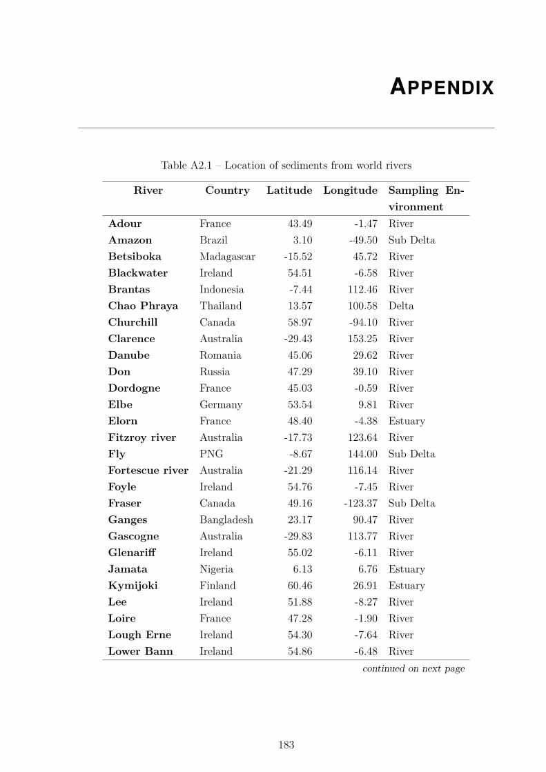
APPENDIX

Table A2.1 – Location of sediments from world rivers

River Country Latitude Longitude Sampling En-vironment

Adour France 43.49 -1.47 RiverAmazon Brazil 3.10 -49.50 Sub DeltaBetsiboka Madagascar -15.52 45.72 RiverBlackwater Ireland 54.51 -6.58 RiverBrantas Indonesia -7.44 112.46 RiverChao Phraya Thailand 13.57 100.58 DeltaChurchill Canada 58.97 -94.10 RiverClarence Australia -29.43 153.25 RiverDanube Romania 45.06 29.62 RiverDon Russia 47.29 39.10 RiverDordogne France 45.03 -0.59 RiverElbe Germany 53.54 9.81 RiverElorn France 48.40 -4.38 EstuaryFitzroy river Australia -17.73 123.64 RiverFly PNG -8.67 144.00 Sub DeltaFortescue river Australia -21.29 116.14 RiverFoyle Ireland 54.76 -7.45 RiverFraser Canada 49.16 -123.37 Sub DeltaGanges Bangladesh 23.17 90.47 RiverGascogne Australia -29.83 113.77 RiverGlenariff Ireland 55.02 -6.11 RiverJamata Nigeria 6.13 6.76 EstuaryKymijoki Finland 60.46 26.91 EstuaryLee Ireland 51.88 -8.27 RiverLoire France 47.28 -1.90 RiverLough Erne Ireland 54.30 -7.64 RiverLower Bann Ireland 54.86 -6.48 River

continued on next page

183

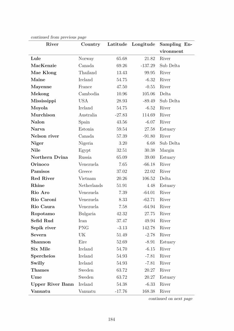
continued from previous pageRiver Country Latitude Longitude Sampling En-

vironmentLule Norway 65.68 21.82 RiverMacKenzie Canada 69.26 -137.29 Sub DeltaMae Klong Thailand 13.43 99.95 RiverMaine Ireland 54.75 -6.32 RiverMayenne France 47.50 -0.55 RiverMekong Cambodia 10.96 105.06 DeltaMississippi USA 28.93 -89.49 Sub DeltaMoyola Ireland 54.75 -6.52 RiverMurchison Australia -27.83 114.69 RiverNalon Spain 43.56 -6.07 RiverNarva Estonia 59.54 27.58 EstuaryNelson river Canada 57.39 -91.80 RiverNiger Nigeria 3.20 6.68 Sub DeltaNile Egypt 32.51 30.38 MarginNorthern Dvina Russia 65.09 39.00 EstuaryOrinoco Venezuela 7.65 -66.18 RiverPamisos Greece 37.02 22.02 RiverRed River Vietnam 20.26 106.52 DeltaRhine Netherlands 51.91 4.48 EstuaryRio Aro Venezuela 7.39 -64.01 RiverRio Caroni Venezuela 8.33 -62.71 RiverRio Caura Venezuela 7.58 -64.94 RiverRopotamo Bulgaria 42.32 27.75 RiverSefid Rud Iran 37.47 49.94 RiverSepik river PNG -3.13 142.78 RiverSevern UK 51.49 -2.78 RiverShannon Eire 52.69 -8.91 EstuarySix Mile Ireland 54.70 -6.15 RiverSpercheios Ireland 54.93 -7.81 RiverSwilly Ireland 54.93 -7.81 RiverThames Sweden 63.72 20.27 RiverUme Sweden 63.72 20.27 EstuaryUpper River Bann Ireland 54.38 -6.33 RiverVanuatu Vanuatu -17.76 168.38 River

continued on next page

184

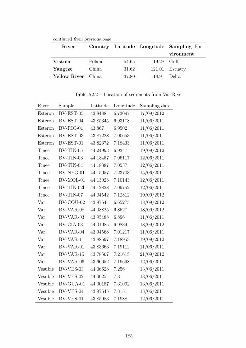
continued from previous pageRiver Country Latitude Longitude Sampling En-

vironmentVistula Poland 54.65 19.28 GulfYangtze China 31.62 121.01 EstuaryYellow River China 37.80 118.91 Delta

Table A2.2 – Location of sediments from Var River

River Sample Latitude Longitude Sampling dateEsteron BV-EST-05 43.8488 6.73097 17/09/2012Esteron BV-EST-04 43.85345 6.93178 11/06/2011Esteron BV-RIO-01 43.867 6.9502 11/06/2011Esteron BV-EST-03 43.87228 7.00653 11/06/2011Esteron BV-EST-01 43.82372 7.18433 11/06/2011Tinee BV-TIN-05 44.24993 6.9347 19/09/2012Tinee BV-TIN-03 44.18457 7.05117 12/06/2011Tinee BV-TIN-04 44.18387 7.0537 12/06/2011Tinee BV-NEG-01 44.15057 7.23703 15/06/2011Tinee BV-MOL-01 44.13028 7.10143 12/06/2011Tinee BV-TIN-02b 44.12828 7.09752 12/06/2011Tinee BV-TIN-07 44.04542 7.12812 19/09/2012Var BV-COU-02 43.9764 6.65273 18/09/2012Var BV-VAR-08 44.08825 6.8527 18/09/2012Var BV-VAR-03 43.95488 6.896 11/06/2011Var BV-CIA-03 44.01085 6.9834 18/09/2012Var BV-VAR-04 43.94568 7.01217 11/06/2011Var BV-VAR-11 43.88597 7.18953 19/09/2012Var BV-VAR-01 43.83663 7.19112 11/06/2011Var BV-VAR-15 43.78567 7.21615 21/09/2012Var BV-VAR-06 43.66652 7.19698 12/06/2011Vesubie BV-VES-03 44.06628 7.256 13/06/2011Vesubie BV-VES-02 44.0025 7.31 13/06/2011Vesubie BV-GUA-01 44.00157 7.31092 13/06/2011Vesubie BV-VES-04 43.97645 7.3151 13/06/2011Vesubie BV-VES-01 43.85983 7.1988 12/06/2011

185

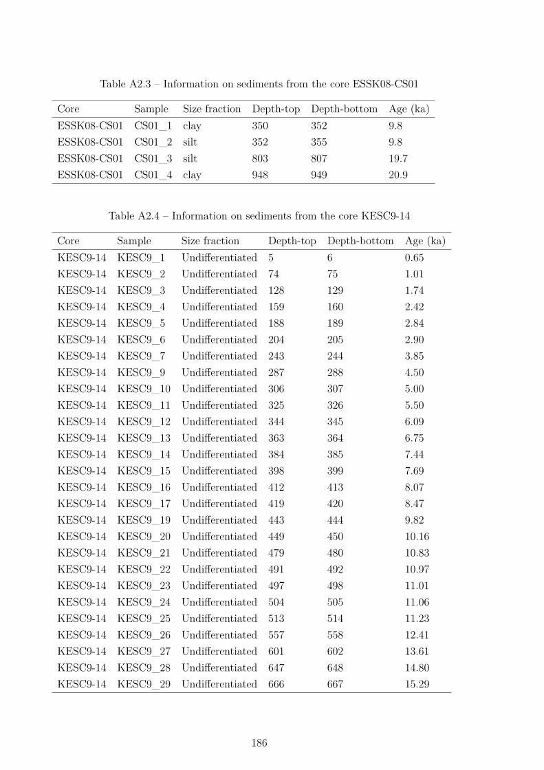
Table A2.3 – Information on sediments from the core ESSK08-CS01

Core Sample Size fraction Depth-top Depth-bottom Age (ka)ESSK08-CS01 CS01_1 clay 350 352 9.8ESSK08-CS01 CS01_2 silt 352 355 9.8ESSK08-CS01 CS01_3 silt 803 807 19.7ESSK08-CS01 CS01_4 clay 948 949 20.9

Table A2.4 – Information on sediments from the core KESC9-14

Core Sample Size fraction Depth-top Depth-bottom Age (ka)KESC9-14 KESC9_1 Undifferentiated 5 6 0.65KESC9-14 KESC9_2 Undifferentiated 74 75 1.01KESC9-14 KESC9_3 Undifferentiated 128 129 1.74KESC9-14 KESC9_4 Undifferentiated 159 160 2.42KESC9-14 KESC9_5 Undifferentiated 188 189 2.84KESC9-14 KESC9_6 Undifferentiated 204 205 2.90KESC9-14 KESC9_7 Undifferentiated 243 244 3.85KESC9-14 KESC9_9 Undifferentiated 287 288 4.50KESC9-14 KESC9_10 Undifferentiated 306 307 5.00KESC9-14 KESC9_11 Undifferentiated 325 326 5.50KESC9-14 KESC9_12 Undifferentiated 344 345 6.09KESC9-14 KESC9_13 Undifferentiated 363 364 6.75KESC9-14 KESC9_14 Undifferentiated 384 385 7.44KESC9-14 KESC9_15 Undifferentiated 398 399 7.69KESC9-14 KESC9_16 Undifferentiated 412 413 8.07KESC9-14 KESC9_17 Undifferentiated 419 420 8.47KESC9-14 KESC9_19 Undifferentiated 443 444 9.82KESC9-14 KESC9_20 Undifferentiated 449 450 10.16KESC9-14 KESC9_21 Undifferentiated 479 480 10.83KESC9-14 KESC9_22 Undifferentiated 491 492 10.97KESC9-14 KESC9_23 Undifferentiated 497 498 11.01KESC9-14 KESC9_24 Undifferentiated 504 505 11.06KESC9-14 KESC9_25 Undifferentiated 513 514 11.23KESC9-14 KESC9_26 Undifferentiated 557 558 12.41KESC9-14 KESC9_27 Undifferentiated 601 602 13.61KESC9-14 KESC9_28 Undifferentiated 647 648 14.80KESC9-14 KESC9_29 Undifferentiated 666 667 15.29

186

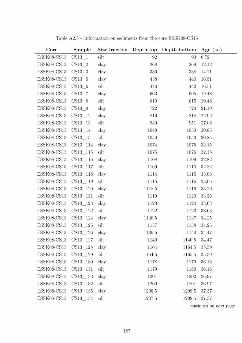
Table A2.5 – Information on sediments from the core ESSK08-CS13

Core Sample Size fraction Depth-top Depth-bottom Age (ka)ESSK08-CS13 CS13_1 silt 92 93 6.72ESSK08-CS13 CS13_2 clay 268 269 12.12ESSK08-CS13 CS13_3 clay 336 338 14.21ESSK08-CS13 CS13_5 clay 438 440 16.51ESSK08-CS13 CS13_6 silt 440 442 16.51ESSK08-CS13 CS13_7 clay 603 605 19.48ESSK08-CS13 CS13_8 silt 610 615 19.48ESSK08-CS13 CS13_9 clay 722 723 21.19ESSK08-CS13 CS13_12 clay 816 818 22.92ESSK08-CS13 CS13_13 silt 949 951 27.06ESSK08-CS13 CS13_14 clay 1048 1050 30.85ESSK08-CS13 CS13_15 silt 1050 1053 30.85ESSK08-CS13 CS13_114 clay 1074 1075 32.15ESSK08-CS13 CS13_115 silt 1075 1076 32.15ESSK08-CS13 CS13_116 clay 1108 1109 32.82ESSK08-CS13 CS13_117 silt 1109 1110 32.82ESSK08-CS13 CS13_118 clay 1114 1115 33.06ESSK08-CS13 CS13_119 silt 1115 1116 33.06ESSK08-CS13 CS13_120 clay 1118.5 1119 33.26ESSK08-CS13 CS13_121 silt 1119 1120 33.26ESSK08-CS13 CS13_123 clay 1123 1124 33.63ESSK08-CS13 CS13_122 silt 1122 1123 33.63ESSK08-CS13 CS13_124 clay 1136.5 1137 34.25ESSK08-CS13 CS13_125 silt 1137 1138 34.25ESSK08-CS13 CS13_126 clay 1139.5 1140 34.47ESSK08-CS13 CS13_127 silt 1140 1140.5 34.47ESSK08-CS13 CS13_128 clay 1164 1164.5 35.39ESSK08-CS13 CS13_129 silt 1164.5 1165.5 35.39ESSK08-CS13 CS13_130 clay 1178 1179 36.16ESSK08-CS13 CS13_131 silt 1179 1180 36.16ESSK08-CS13 CS13_133 clay 1201 1202 36.97ESSK08-CS13 CS13_132 silt 1200 1201 36.97ESSK08-CS13 CS13_135 clay 1208.5 1209.5 37.37ESSK08-CS13 CS13_134 silt 1207.5 1208.5 37.37

continued on next page

187

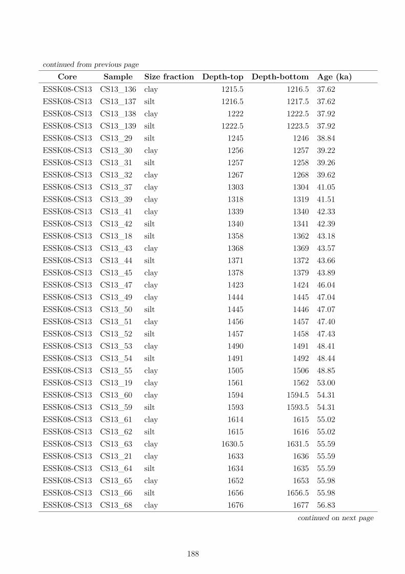
continued from previous pageCore Sample Size fraction Depth-top Depth-bottom Age (ka)

ESSK08-CS13 CS13_136 clay 1215.5 1216.5 37.62ESSK08-CS13 CS13_137 silt 1216.5 1217.5 37.62ESSK08-CS13 CS13_138 clay 1222 1222.5 37.92ESSK08-CS13 CS13_139 silt 1222.5 1223.5 37.92ESSK08-CS13 CS13_29 silt 1245 1246 38.84ESSK08-CS13 CS13_30 clay 1256 1257 39.22ESSK08-CS13 CS13_31 silt 1257 1258 39.26ESSK08-CS13 CS13_32 clay 1267 1268 39.62ESSK08-CS13 CS13_37 clay 1303 1304 41.05ESSK08-CS13 CS13_39 clay 1318 1319 41.51ESSK08-CS13 CS13_41 clay 1339 1340 42.33ESSK08-CS13 CS13_42 silt 1340 1341 42.39ESSK08-CS13 CS13_18 silt 1358 1362 43.18ESSK08-CS13 CS13_43 clay 1368 1369 43.57ESSK08-CS13 CS13_44 silt 1371 1372 43.66ESSK08-CS13 CS13_45 clay 1378 1379 43.89ESSK08-CS13 CS13_47 clay 1423 1424 46.04ESSK08-CS13 CS13_49 clay 1444 1445 47.04ESSK08-CS13 CS13_50 silt 1445 1446 47.07ESSK08-CS13 CS13_51 clay 1456 1457 47.40ESSK08-CS13 CS13_52 silt 1457 1458 47.43ESSK08-CS13 CS13_53 clay 1490 1491 48.41ESSK08-CS13 CS13_54 silt 1491 1492 48.44ESSK08-CS13 CS13_55 clay 1505 1506 48.85ESSK08-CS13 CS13_19 clay 1561 1562 53.00ESSK08-CS13 CS13_60 clay 1594 1594.5 54.31ESSK08-CS13 CS13_59 silt 1593 1593.5 54.31ESSK08-CS13 CS13_61 clay 1614 1615 55.02ESSK08-CS13 CS13_62 silt 1615 1616 55.02ESSK08-CS13 CS13_63 clay 1630.5 1631.5 55.59ESSK08-CS13 CS13_21 clay 1633 1636 55.59ESSK08-CS13 CS13_64 silt 1634 1635 55.59ESSK08-CS13 CS13_65 clay 1652 1653 55.98ESSK08-CS13 CS13_66 silt 1656 1656.5 55.98ESSK08-CS13 CS13_68 clay 1676 1677 56.83

continued on next page

188

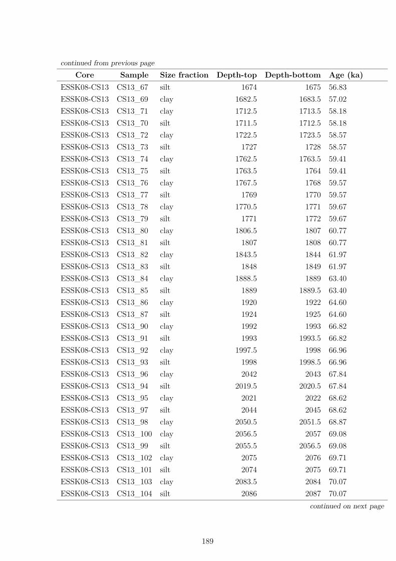
continued from previous pageCore Sample Size fraction Depth-top Depth-bottom Age (ka)

ESSK08-CS13 CS13_67 silt 1674 1675 56.83ESSK08-CS13 CS13_69 clay 1682.5 1683.5 57.02ESSK08-CS13 CS13_71 clay 1712.5 1713.5 58.18ESSK08-CS13 CS13_70 silt 1711.5 1712.5 58.18ESSK08-CS13 CS13_72 clay 1722.5 1723.5 58.57ESSK08-CS13 CS13_73 silt 1727 1728 58.57ESSK08-CS13 CS13_74 clay 1762.5 1763.5 59.41ESSK08-CS13 CS13_75 silt 1763.5 1764 59.41ESSK08-CS13 CS13_76 clay 1767.5 1768 59.57ESSK08-CS13 CS13_77 silt 1769 1770 59.57ESSK08-CS13 CS13_78 clay 1770.5 1771 59.67ESSK08-CS13 CS13_79 silt 1771 1772 59.67ESSK08-CS13 CS13_80 clay 1806.5 1807 60.77ESSK08-CS13 CS13_81 silt 1807 1808 60.77ESSK08-CS13 CS13_82 clay 1843.5 1844 61.97ESSK08-CS13 CS13_83 silt 1848 1849 61.97ESSK08-CS13 CS13_84 clay 1888.5 1889 63.40ESSK08-CS13 CS13_85 silt 1889 1889.5 63.40ESSK08-CS13 CS13_86 clay 1920 1922 64.60ESSK08-CS13 CS13_87 silt 1924 1925 64.60ESSK08-CS13 CS13_90 clay 1992 1993 66.82ESSK08-CS13 CS13_91 silt 1993 1993.5 66.82ESSK08-CS13 CS13_92 clay 1997.5 1998 66.96ESSK08-CS13 CS13_93 silt 1998 1998.5 66.96ESSK08-CS13 CS13_96 clay 2042 2043 67.84ESSK08-CS13 CS13_94 silt 2019.5 2020.5 67.84ESSK08-CS13 CS13_95 clay 2021 2022 68.62ESSK08-CS13 CS13_97 silt 2044 2045 68.62ESSK08-CS13 CS13_98 clay 2050.5 2051.5 68.87ESSK08-CS13 CS13_100 clay 2056.5 2057 69.08ESSK08-CS13 CS13_99 silt 2055.5 2056.5 69.08ESSK08-CS13 CS13_102 clay 2075 2076 69.71ESSK08-CS13 CS13_101 silt 2074 2075 69.71ESSK08-CS13 CS13_103 clay 2083.5 2084 70.07ESSK08-CS13 CS13_104 silt 2086 2087 70.07

continued on next page

189

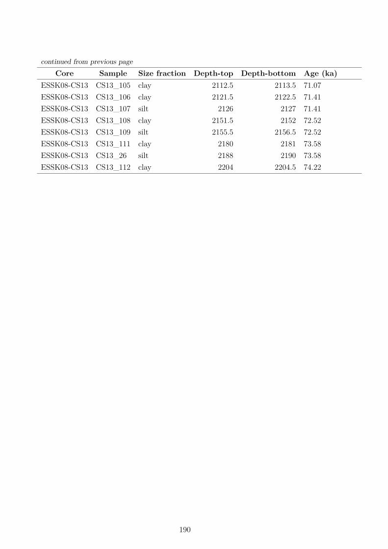
continued from previous pageCore Sample Size fraction Depth-top Depth-bottom Age (ka)

ESSK08-CS13 CS13_105 clay 2112.5 2113.5 71.07ESSK08-CS13 CS13_106 clay 2121.5 2122.5 71.41ESSK08-CS13 CS13_107 silt 2126 2127 71.41ESSK08-CS13 CS13_108 clay 2151.5 2152 72.52ESSK08-CS13 CS13_109 silt 2155.5 2156.5 72.52ESSK08-CS13 CS13_111 clay 2180 2181 73.58ESSK08-CS13 CS13_26 silt 2188 2190 73.58ESSK08-CS13 CS13_112 clay 2204 2204.5 74.22

190

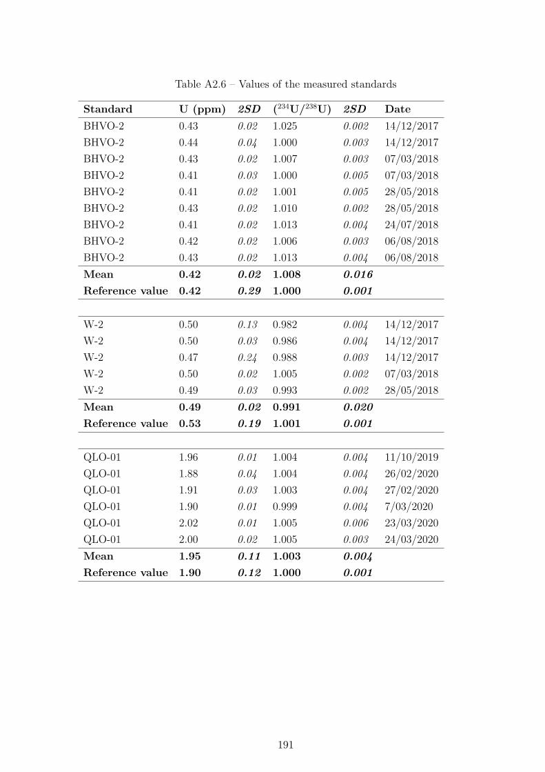
Table A2.6 – Values of the measured standards

Standard U (ppm) 2SD (234U/238U) 2SD DateBHVO-2 0.43 0.02 1.025 0.002 14/12/2017BHVO-2 0.44 0.04 1.000 0.003 14/12/2017BHVO-2 0.43 0.02 1.007 0.003 07/03/2018BHVO-2 0.41 0.03 1.000 0.005 07/03/2018BHVO-2 0.41 0.02 1.001 0.005 28/05/2018BHVO-2 0.43 0.02 1.010 0.002 28/05/2018BHVO-2 0.41 0.02 1.013 0.004 24/07/2018BHVO-2 0.42 0.02 1.006 0.003 06/08/2018BHVO-2 0.43 0.02 1.013 0.004 06/08/2018Mean 0.42 0.02 1.008 0.016Reference value 0.42 0.29 1.000 0.001

W-2 0.50 0.13 0.982 0.004 14/12/2017W-2 0.50 0.03 0.986 0.004 14/12/2017W-2 0.47 0.24 0.988 0.003 14/12/2017W-2 0.50 0.02 1.005 0.002 07/03/2018W-2 0.49 0.03 0.993 0.002 28/05/2018Mean 0.49 0.02 0.991 0.020Reference value 0.53 0.19 1.001 0.001

QLO-01 1.96 0.01 1.004 0.004 11/10/2019QLO-01 1.88 0.04 1.004 0.004 26/02/2020QLO-01 1.91 0.03 1.003 0.004 27/02/2020QLO-01 1.90 0.01 0.999 0.004 7/03/2020QLO-01 2.02 0.01 1.005 0.006 23/03/2020QLO-01 2.00 0.02 1.005 0.003 24/03/2020Mean 1.95 0.11 1.003 0.004Reference value 1.90 0.12 1.000 0.001

191

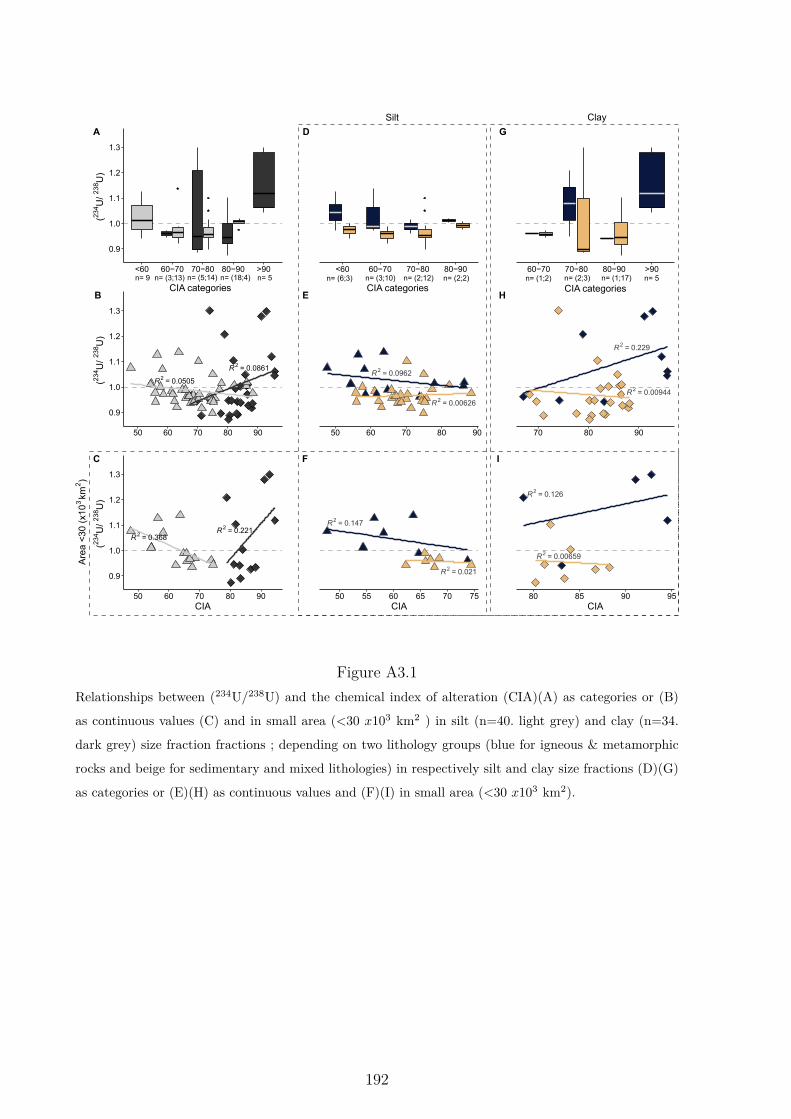
0.9

1.0

1.1

1.2

1.3

<60 60−70 70−80 80−90 >90

(234 U

/ 238 U

)

A

<60 60−70 70−80 80−90

D

60−70 70−80 80−90 >90

G

R2 = 0.0861

R2 = 0.0505

0.9

1.0

1.1

1.2

1.3

50 60 70 80 90

(234 U

/ 238 U

)

B

R2 = 0.0962

R2 = 0.00626

50 60 70 80 90

E

R2 = 0.229

R2 = 0.00944

70 80 90

H

R2 = 0.221R2 = 0.368

0.9

1.0

1.1

1.2

1.3

50 60 70 80 90CIA

(234 U

/ 238 U

)

C

R2 = 0.147

R2 = 0.021

50 55 60 65 70 75CIA

F

R2 = 0.126

R2 = 0.00659

80 85 90 95CIA

I

n= 9 n= (3;13) n= (5;14) n= (18;4) n= 5 n= (6;3) n= (3;10) n= (2;12) n= (2;2) n= (1;2) n= (2;3) n= (1;17) n= 5

Silt Clay

Are

a <

30 (

x10

3km

2)

CIA categories CIA categories CIA categories

Figure A3.1Relationships between (234U/238U) and the chemical index of alteration (CIA)(A) as categories or (B)

as continuous values (C) and in small area (<30 x103 km2 ) in silt (n=40. light grey) and clay (n=34.

dark grey) size fraction fractions ; depending on two lithology groups (blue for igneous & metamorphic

rocks and beige for sedimentary and mixed lithologies) in respectively silt and clay size fractions (D)(G)

as categories or (E)(H) as continuous values and (F)(I) in small area (<30 x103 km2).

192

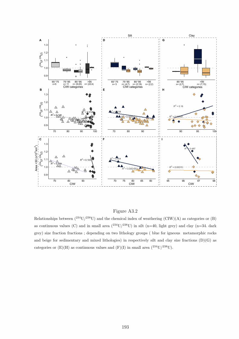
0.9

1.0

1.1

1.2

1.3

65−75 75−85 85−95 >95

(234 U

/ 238 U

)A

65−75 75−85 85−95 >95

D

85−95 >95

G

R2 = 0.0126R2 = 0.138

0.9

1.0

1.1

1.2

1.3

70 80 90 100

(234 U

/ 238 U

)

B

R2 = 0.238

R2 = 0.00557

70 80 90

E

R2 = 0.16

R2 = 0.00505

90 95 100

H

R2 = 0.103

R2 = 0.559

0.9

1.0

1.1

1.2

1.3

70 80 90CIW

(234 U

/ 238 U

)

C

R2 = 0.404

R2 = 0.000165

70 75 80 85 90CIW

F

R2 = 0.497

R2 = 0.00315

95 96 97 98CIW

I

n= 5 n= 11 n= (9;20) n= 5 n= (4;7) n= (2;18) n= (2;2) n= (2;7) n= (7;15)CIW categories CIW categories CIW categories

Silt ClayA

rea

<30

(x1

03km

2)

n= (22;4)

Figure A3.2Relationships between (234U/238U) and the chemical index of weathering (CIW)(A) as categories or (B)

as continuous values (C) and in small area (234U/238U) in silt (n=40, light grey) and clay (n=34. dark

grey) size fraction fractions ; depending on two lithology groups ( blue for igneous metamorphic rocks

and beige for sedimentary and mixed lithologies) in respectively silt and clay size fractions (D)(G) as

categories or (E)(H) as continuous values and (F)(I) in small area (234U/238U).

193

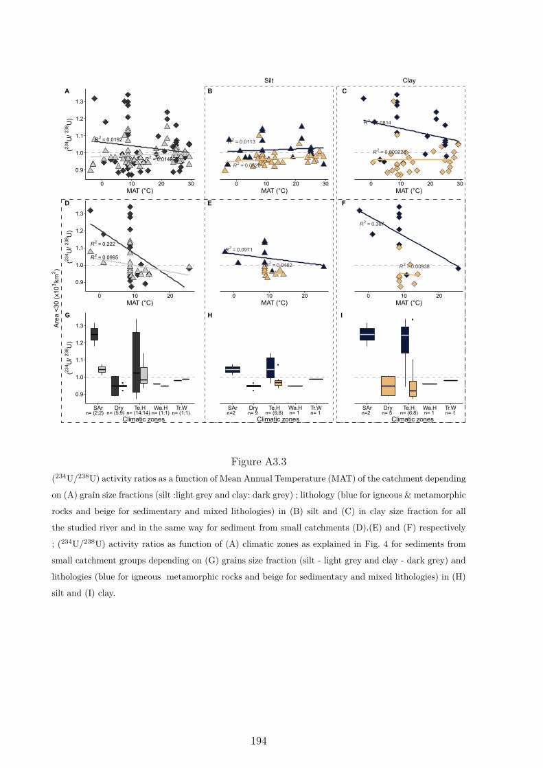
R2 = 0.0192

R2 = 0.0142

0.9

1.0

1.1

1.2

1.3

0 10 20 30MAT (°C)

(234 U

/ 238 U

)

A

R2 = 0.0113

R2 = 0.0626

0 10 20 30MAT (°C)

B

R2 = 0.0814

R2 = 0.000228

0 10 20 30MAT (°C)

C

R2 = 0.222

R2 = 0.0995

0.9

1.0

1.1

1.2

1.3

0 10 20MAT (°C)

(234 U

/ 238 U

)

D

R2 = 0.0971

R2 = 0.0462

0 10 20MAT (°C)

E

R2 = 0.367

R2 = 0.00938

0 10 20MAT (°C)

F

0.9

1.0

1.1

1.2

1.3

SAr Dry Te.H Wa.H Tr.W

Climatic zones

(234 U

/ 238 U

)

G

SAr Dry Te.H Wa.H Tr.W

Climatic zones

H

SAr Dry Te.H Wa.H Tr.W

Climatic zones

I

Silt Clay

Are

a <

30 (

x10

3km

2)

n= (2;2) n= (5;9) n= (14;14) n= (1;1)n= (1;1) n= 2 n= 9 n= (6;8) n= 1 n= 1 n= 2 n= 5 n= (6;8) n= 1 n= 1

Figure A3.3(234U/238U) activity ratios as a function of Mean Annual Temperature (MAT) of the catchment depending

on (A) grain size fractions (silt :light grey and clay: dark grey) ; lithology (blue for igneous & metamorphic

rocks and beige for sedimentary and mixed lithologies) in (B) silt and (C) in clay size fraction for all

the studied river and in the same way for sediment from small catchments (D).(E) and (F) respectively

; (234U/238U) activity ratios as function of (A) climatic zones as explained in Fig. 4 for sediments from

small catchment groups depending on (G) grains size fraction (silt - light grey and clay - dark grey) and

lithologies (blue for igneous metamorphic rocks and beige for sedimentary and mixed lithologies) in (H)

silt and (I) clay.

194

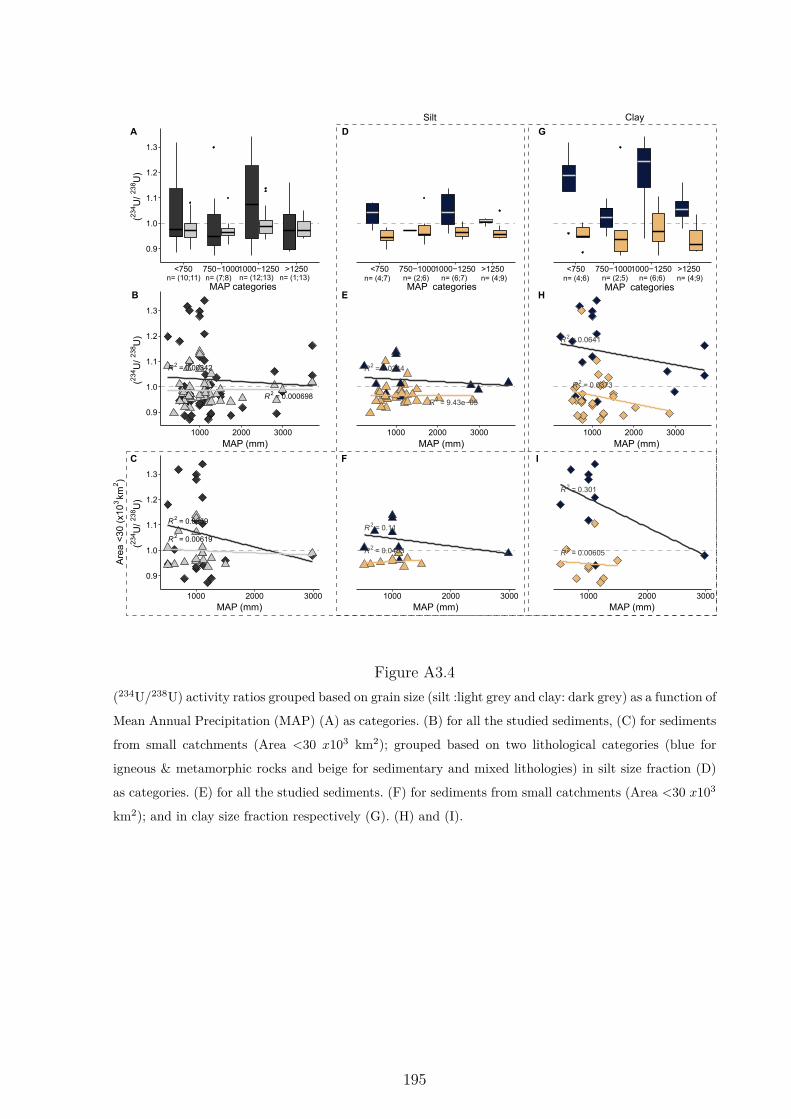
0.9

1.0

1.1

1.2

1.3

<750 750−10001000−1250 >1250

(234 U

/ 238 U

) A

<750 750−10001000−1250 >1250

D

<750 750−10001000−1250 >1250

G

R2 = 0.00342

R2 = 0.000698

0.9

1.0

1.1

1.2

1.3

1000 2000 3000

(234 U

/ 238 U

)

B

R2 = 0.0344

R2 = 9.43e−05

1000 2000 3000

E

R2 = 0.0641

R2 = 0.0373

1000 2000 3000

H

R2 = 0.0359

R2 = 0.00619

0.9

1.0

1.1

1.2

1.3

1000 2000 3000

(234 U

/ 238 U

)

C

R2 = 0.11

R2 = 0.0453

1000 2000 3000

F

R2 = 0.301

R2 = 0.00605

1000 2000 3000

I

MAP (mm) MAP (mm) MAP (mm)

n= (10;11) n= (7;8) n= (12;13) n= (1;13) n= (4;7) n= (2;6) n= (6;7) n= (4;9) n= (4;6) n= (2;5) n= (6;6) n= (4;9)MAP categories MAP categories MAP categories

Silt ClayA

rea

<30

(x1

03km

2)

MAP (mm) MAP (mm) MAP (mm)

Figure A3.4(234U/238U) activity ratios grouped based on grain size (silt :light grey and clay: dark grey) as a function of

Mean Annual Precipitation (MAP) (A) as categories. (B) for all the studied sediments, (C) for sediments

from small catchments (Area <30 x103 km2); grouped based on two lithological categories (blue for

igneous & metamorphic rocks and beige for sedimentary and mixed lithologies) in silt size fraction (D)

as categories. (E) for all the studied sediments. (F) for sediments from small catchments (Area <30 x103

km2); and in clay size fraction respectively (G). (H) and (I).

195

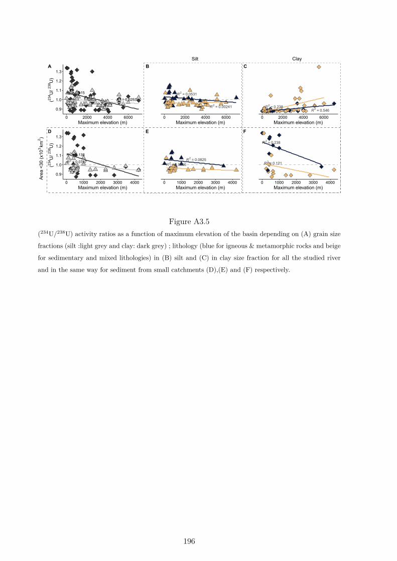
R2 = 0.115

R2 = 0.0253

0.9

1.0

1.1

1.2

1.3

0 2000 4000 6000Maximum elevation (m)

(234 U

/ 238 U

)

A

R2 = 0.0531

R2 = 0.00241

0 2000 4000 6000Maximum elevation (m)

B

R2 = 0.546R2 = 0.238

0 2000 4000 6000Maximum elevation (m)

C

R2 = 0.138

R2 = 0.0707

0.9

1.0

1.1

1.2

1.3

0 1000 2000 3000 4000Maximum elevation (m)

(234 U

/ 238 U

)

D

R2 = 0.0825R2 = 0.0566

0 1000 2000 3000 4000Maximum elevation (m)

E

R2 = 0.238

R2 = 0.121

0 1000 2000 3000 4000Maximum elevation (m)

F

Silt Clay

Are

a <

30 (

x10

3km

2)

Figure A3.5(234U/238U) activity ratios as a function of maximum elevation of the basin depending on (A) grain size

fractions (silt :light grey and clay: dark grey) ; lithology (blue for igneous & metamorphic rocks and beige

for sedimentary and mixed lithologies) in (B) silt and (C) in clay size fraction for all the studied river

and in the same way for sediment from small catchments (D),(E) and (F) respectively.

196

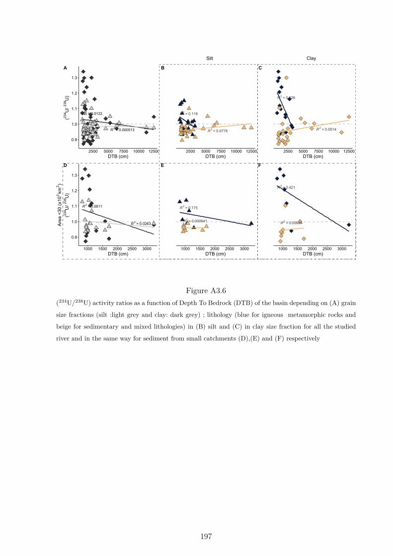
R2 = 0.0122

R2 = 0.000513

0.9

1.0

1.1

1.2

1.3

2500 5000 7500 10000 12500DTB (cm)

(234 U

/ 238 U

) A

R2 = 0.119

R2 = 0.0778

2500 5000 7500 10000 12500DTB (cm)

B

R2 = 0.326

R2 = 0.0514

2500 5000 7500 10000 12500DTB (cm)

C

R2 = 0.0611

R2 = 0.0263

0.9

1.0

1.1

1.2

1.3

1000 1500 2000 2500 3000DTB (cm)

(234 U

/ 238 U

)

D

R2 = 0.175

R2 = 0.000641

1000 1500 2000 2500 3000DTB (cm)

E

R2 = 0.421

R2 = 0.00664

1000 1500 2000 2500 3000DTB (cm)

F

Silt ClayA

rea

<30

(x1

03km

2)

Figure A3.6(234U/238U) activity ratios as a function of Depth To Bedrock (DTB) of the basin depending on (A) grain

size fractions (silt :light grey and clay: dark grey) ; lithology (blue for igneous metamorphic rocks and

beige for sedimentary and mixed lithologies) in (B) silt and (C) in clay size fraction for all the studied

river and in the same way for sediment from small catchments (D),(E) and (F) respectively

197

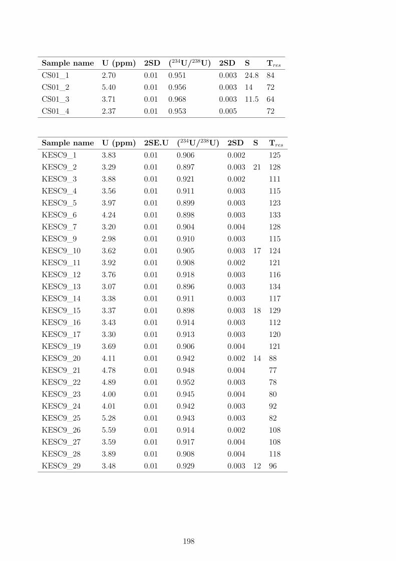
Sample name U (ppm) 2SD (234U/238U) 2SD S Tres

CS01_1 2.70 0.01 0.951 0.003 24.8 84CS01_2 5.40 0.01 0.956 0.003 14 72CS01_3 3.71 0.01 0.968 0.003 11.5 64CS01_4 2.37 0.01 0.953 0.005 72

Sample name U (ppm) 2SE.U (234U/238U) 2SD S Tres

KESC9_1 3.83 0.01 0.906 0.002 125KESC9_2 3.29 0.01 0.897 0.003 21 128KESC9_3 3.88 0.01 0.921 0.002 111KESC9_4 3.56 0.01 0.911 0.003 115KESC9_5 3.97 0.01 0.899 0.003 123KESC9_6 4.24 0.01 0.898 0.003 133KESC9_7 3.20 0.01 0.904 0.004 128KESC9_9 2.98 0.01 0.910 0.003 115KESC9_10 3.62 0.01 0.905 0.003 17 124KESC9_11 3.92 0.01 0.908 0.002 121KESC9_12 3.76 0.01 0.918 0.003 116KESC9_13 3.07 0.01 0.896 0.003 134KESC9_14 3.38 0.01 0.911 0.003 117KESC9_15 3.37 0.01 0.898 0.003 18 129KESC9_16 3.43 0.01 0.914 0.003 112KESC9_17 3.30 0.01 0.913 0.003 120KESC9_19 3.69 0.01 0.906 0.004 121KESC9_20 4.11 0.01 0.942 0.002 14 88KESC9_21 4.78 0.01 0.948 0.004 77KESC9_22 4.89 0.01 0.952 0.003 78KESC9_23 4.00 0.01 0.945 0.004 80KESC9_24 4.01 0.01 0.942 0.003 92KESC9_25 5.28 0.01 0.943 0.003 82KESC9_26 5.59 0.01 0.914 0.002 108KESC9_27 3.59 0.01 0.917 0.004 108KESC9_28 3.89 0.01 0.908 0.004 118KESC9_29 3.48 0.01 0.929 0.003 12 96

198

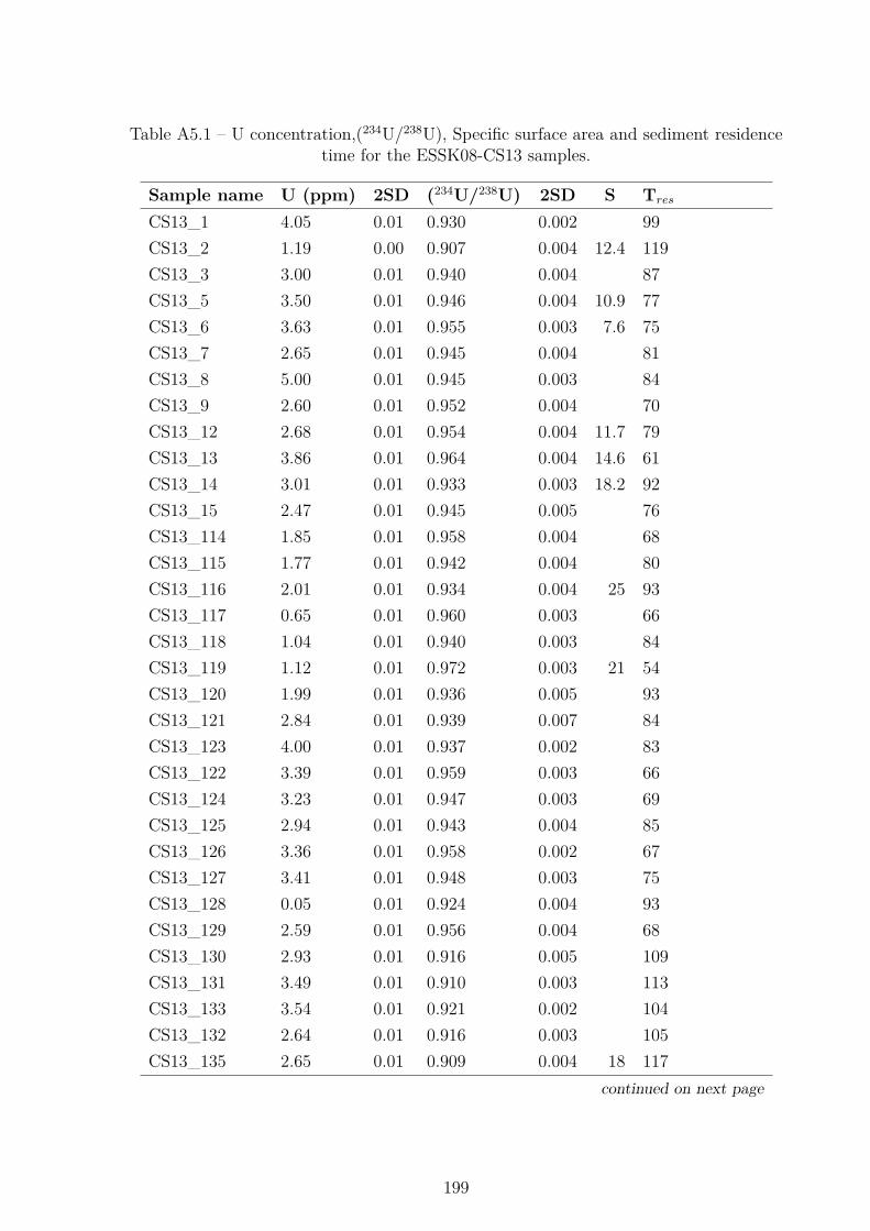
Table A5.1 – U concentration,(234U/238U), Specific surface area and sediment residencetime for the ESSK08-CS13 samples.

Sample name U (ppm) 2SD (234U/238U) 2SD S Tres

CS13_1 4.05 0.01 0.930 0.002 99CS13_2 1.19 0.00 0.907 0.004 12.4 119CS13_3 3.00 0.01 0.940 0.004 87CS13_5 3.50 0.01 0.946 0.004 10.9 77CS13_6 3.63 0.01 0.955 0.003 7.6 75CS13_7 2.65 0.01 0.945 0.004 81CS13_8 5.00 0.01 0.945 0.003 84CS13_9 2.60 0.01 0.952 0.004 70CS13_12 2.68 0.01 0.954 0.004 11.7 79CS13_13 3.86 0.01 0.964 0.004 14.6 61CS13_14 3.01 0.01 0.933 0.003 18.2 92CS13_15 2.47 0.01 0.945 0.005 76CS13_114 1.85 0.01 0.958 0.004 68CS13_115 1.77 0.01 0.942 0.004 80CS13_116 2.01 0.01 0.934 0.004 25 93CS13_117 0.65 0.01 0.960 0.003 66CS13_118 1.04 0.01 0.940 0.003 84CS13_119 1.12 0.01 0.972 0.003 21 54CS13_120 1.99 0.01 0.936 0.005 93CS13_121 2.84 0.01 0.939 0.007 84CS13_123 4.00 0.01 0.937 0.002 83CS13_122 3.39 0.01 0.959 0.003 66CS13_124 3.23 0.01 0.947 0.003 69CS13_125 2.94 0.01 0.943 0.004 85CS13_126 3.36 0.01 0.958 0.002 67CS13_127 3.41 0.01 0.948 0.003 75CS13_128 0.05 0.01 0.924 0.004 93CS13_129 2.59 0.01 0.956 0.004 68CS13_130 2.93 0.01 0.916 0.005 109CS13_131 3.49 0.01 0.910 0.003 113CS13_133 3.54 0.01 0.921 0.002 104CS13_132 2.64 0.01 0.916 0.003 105CS13_135 2.65 0.01 0.909 0.004 18 117

continued on next page

199

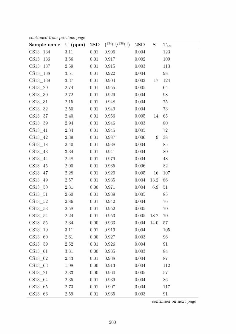
continued from previous pageSample name U (ppm) 2SD (234U/238U) 2SD S Tres

CS13_134 3.11 0.01 0.906 0.004 123CS13_136 3.56 0.01 0.917 0.002 109CS13_137 2.59 0.01 0.915 0.003 113CS13_138 3.51 0.01 0.922 0.004 98CS13_139 3.37 0.01 0.904 0.003 17 124CS13_29 2.74 0.01 0.955 0.005 64CS13_30 2.72 0.01 0.929 0.004 98CS13_31 2.15 0.01 0.948 0.004 75CS13_32 2.50 0.01 0.949 0.004 73CS13_37 2.40 0.01 0.956 0.005 14 65CS13_39 2.94 0.01 0.946 0.003 80CS13_41 2.34 0.01 0.945 0.005 72CS13_42 2.39 0.01 0.987 0.006 9 38CS13_18 2.40 0.01 0.938 0.004 85CS13_43 3.34 0.01 0.941 0.004 80CS13_44 2.48 0.01 0.979 0.004 48CS13_45 2.00 0.01 0.935 0.006 82CS13_47 2.28 0.01 0.920 0.005 16 107CS13_49 2.57 0.01 0.935 0.004 13.2 86CS13_50 2.31 0.00 0.971 0.004 6.9 51CS13_51 2.60 0.01 0.939 0.005 85CS13_52 2.86 0.01 0.942 0.004 76CS13_53 2.58 0.01 0.952 0.005 70CS13_54 2.24 0.01 0.953 0.005 18.2 70CS13_55 2.34 0.00 0.963 0.004 14.0 57CS13_19 3.11 0.01 0.919 0.004 105CS13_60 2.61 0.00 0.927 0.003 96CS13_59 2.52 0.01 0.926 0.004 91CS13_61 3.31 0.00 0.935 0.003 84CS13_62 2.43 0.01 0.938 0.004 87CS13_63 1.98 0.00 0.913 0.004 112CS13_21 2.33 0.00 0.960 0.005 57CS13_64 2.35 0.01 0.939 0.004 86CS13_65 2.73 0.01 0.907 0.004 117CS13_66 2.59 0.01 0.935 0.003 91

continued on next page

200

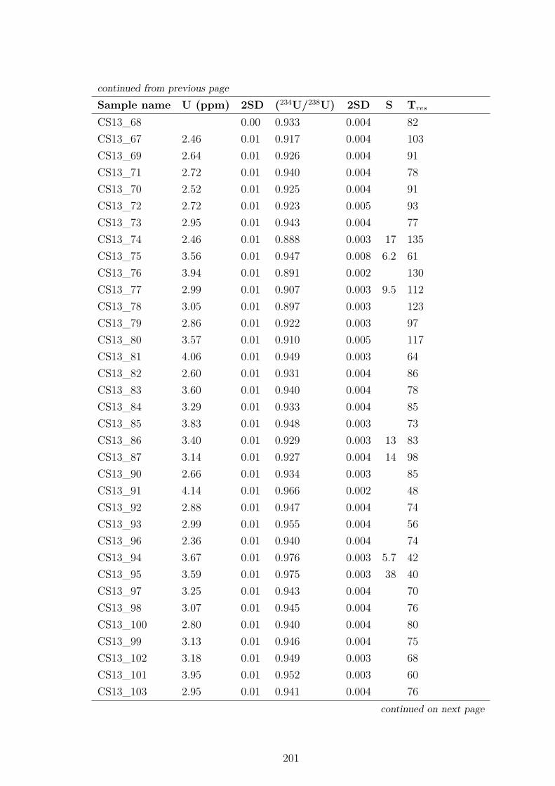
continued from previous pageSample name U (ppm) 2SD (234U/238U) 2SD S Tres

CS13_68 0.00 0.933 0.004 82CS13_67 2.46 0.01 0.917 0.004 103CS13_69 2.64 0.01 0.926 0.004 91CS13_71 2.72 0.01 0.940 0.004 78CS13_70 2.52 0.01 0.925 0.004 91CS13_72 2.72 0.01 0.923 0.005 93CS13_73 2.95 0.01 0.943 0.004 77CS13_74 2.46 0.01 0.888 0.003 17 135CS13_75 3.56 0.01 0.947 0.008 6.2 61CS13_76 3.94 0.01 0.891 0.002 130CS13_77 2.99 0.01 0.907 0.003 9.5 112CS13_78 3.05 0.01 0.897 0.003 123CS13_79 2.86 0.01 0.922 0.003 97CS13_80 3.57 0.01 0.910 0.005 117CS13_81 4.06 0.01 0.949 0.003 64CS13_82 2.60 0.01 0.931 0.004 86CS13_83 3.60 0.01 0.940 0.004 78CS13_84 3.29 0.01 0.933 0.004 85CS13_85 3.83 0.01 0.948 0.003 73CS13_86 3.40 0.01 0.929 0.003 13 83CS13_87 3.14 0.01 0.927 0.004 14 98CS13_90 2.66 0.01 0.934 0.003 85CS13_91 4.14 0.01 0.966 0.002 48CS13_92 2.88 0.01 0.947 0.004 74CS13_93 2.99 0.01 0.955 0.004 56CS13_96 2.36 0.01 0.940 0.004 74CS13_94 3.67 0.01 0.976 0.003 5.7 42CS13_95 3.59 0.01 0.975 0.003 38 40CS13_97 3.25 0.01 0.943 0.004 70CS13_98 3.07 0.01 0.945 0.004 76CS13_100 2.80 0.01 0.940 0.004 80CS13_99 3.13 0.01 0.946 0.004 75CS13_102 3.18 0.01 0.949 0.003 68CS13_101 3.95 0.01 0.952 0.003 60CS13_103 2.95 0.01 0.941 0.004 76

continued on next page

201

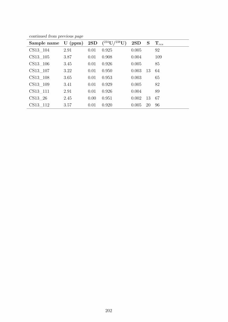
continued from previous pageSample name U (ppm) 2SD (234U/238U) 2SD S Tres

CS13_104 2.91 0.01 0.925 0.005 92CS13_105 3.87 0.01 0.908 0.004 109CS13_106 3.45 0.01 0.926 0.005 85CS13_107 3.22 0.01 0.950 0.003 13 64CS13_108 3.65 0.01 0.953 0.003 65CS13_109 3.41 0.01 0.929 0.005 82CS13_111 2.91 0.01 0.926 0.004 89CS13_26 2.45 0.00 0.951 0.002 13 67CS13_112 3.57 0.01 0.920 0.005 20 96

202

BIBLIOGRAPHY

Ackerer, J., Chabaux, F., Van der Woerd, J., Viville, D., Pelt, E., Kali, E., Lerouge,C., Ackerer, P., di Chiara Roupert, R. & Négrel, P. (2016), ‘Regolith evolution on themillennial timescale from combined U–Th–Ra isotopes and in situ cosmogenic 10Beanalysis in a weathering profile (Strengbach catchment, France)’, Earth and PlanetaryScience Letters 453, 33–43.

Adloff, J. P. & Roessler, K. (1991), ‘Recoil and Transmutation Effects in the MigrationBehaviour of Actinides’, Radiochimica Acta 52-53(1), 269–274.

Ahnert, F. (1967), ‘The role of the equilibrium concept in the interpretation of landformsof fluvial erosion and deposition.’, L’evolution des Versants pp. 23–41.

Ahnert, F. (1970), ‘Functional relationships between denudation, relief, and uplift in large,mid-latitude drainage basins’, American Journal of Science 268(3), 243–263.

Ahnert, F. (1976), ‘Brief description of a comprehensive three-dimensional process-response model of landform development.’, Geographic Institute 25, 29–49.

Ahnert, F. (1994), ‘Equilibrium, scale and inheritance in geomorphology’, Geomorphology11(2), 125–140.

Allen, J. R. M., Brandt, U., Brauer, A., Hubberten, H.-W., Huntley, B., Keller, J., Kraml,M., Mackensen, A., Mingram, J., Negendank, J., Nowaczyk, N., Oberhänsli, H., Watts,W., Wulf, S. & Zolitschka, B. (1999), ‘Rapid environmental changes in southern Europeduring the last glacial period’, Nature 400(6746), 740–743.

Allen, P. A. (1997), Earth Surface Processes.

Allen, P. A. (2008a), ‘From landscapes into geological history’, Nature 451(7176), 274–276.

Allen, P. A. (2008b), ‘Time scales of tectonic landscapes and their sediment routing sys-tems’, Geological Society, London, Special Publications 296(1), 7–28.

Allen, P. & Heller, P. L. (2012), Dispersal and Preservation of Tectonically GeneratedAlluvial Gravels in Sedimentary Basins, in ‘Tectonics of Sedimentary Basins’, JohnWiley & Sons, Ltd, chapter 6, pp. 111–130.

Ames, L., McGarrah, J., Walker, B. & Salter, P. (1983), ‘Uranium and radium sorptionon amorphous ferric oxyhydroxide’, Chemical Geology 40(1), 135–148.

203

Amorosi, A., Maselli, V. & Trincardi, F. (2016), ‘Onshore to offshore anatomy of a lateQuaternary source-to-sink system (Po Plain–Adriatic Sea, Italy)’, Earth-Science Re-views 153, 212–237.

Amundson, R., Richter, D. D., Humphreys, G. S., Jobbagy, E. G. & Gaillardet, J. (2007),‘Coupling between Biota and Earth Materials in the Critical Zone’, Elements 3(5), 327–332.

Andersen, M. B., Erel, Y. & Bourdon, B. (2009), ‘Experimental evidence for 234U–238Ufractionation during granite weathering with implications for 234U/238U in naturalwaters’, Geochimica et Cosmochimica Acta 73(14), 4124–4141.

Anderson, R. F. (1982), ‘Concentration, vertical flux, and remineralization of particulateuranium in seawater’, Geochimica et Cosmochimica Acta 46(7), 1293–1299.

Anderson, R. S. & Anderson, S. P. (2010), Geomorphology: The Mechanics and Chemistryof Landscapes, Cambridge University Press.

Anderson, R. S. & Humphrey, N. F. (1989), ‘Interaction of weathering and transportprocesses in the evolution of arid landscapes.’, pp. 349–361.

Anderson, S. P. (2005), ‘Glaciers show direct linkage between erosion rate and chemicalweathering fluxes’, Geomorphology 67(1), 147–157.

Anderson, S. P., Blum, J., Brantley, S. L., Chadwick, O., Chorover, J., Derry, L. A.,Drever, J. I., Hering, J. G., Kirchner, J. W., Kump, L. R., Richter, D. & White, A. E.(2004), ‘Proposed initiative would study Earth’s weathering engine’, Eos, TransactionsAmerican Geophysical Union 85(28), 265–269.

Anderson, S. P., Dietrich, W. E. & Brimhall, G. H. (2002), ‘Weathering profiles, mass-balance analysis, and rates of solute loss: Linkages between weathering and erosion ina small, steep catchment’, GSA Bulletin 114(9), 1143–1158.

Anderson, S. P., von Blanckenburg, F. & White, A. F. (2007), ‘Physical and ChemicalControls on the Critical Zone’, Elements 3(5), 315–319.

Andersson, P. S., Porcelli, D., Gustafsson, Ö., Ingri, J. & Wasserburg, G. J. (2001), ‘Theimportance of colloids for the behavior of uranium isotopes in the low-salinity zone ofa stable estuary - ScienceDirect’, Geochimica et Cosmochimica Acta 65(1), 13–25.

Andersson, P. S., Porcelli, D., Wasserburg, G. J. & Ingri, J. (1998), ‘Particle Transportof 234U-238U in the Kalix River and in the Baltic Sea’, Geochimica et CosmochimicaActa 62(3), 385–392.

204

Anthony, E. J. (1995), ‘Impacts géomorphologiques côtiers des aménagements du Var etde son delta, Côte d’Azur, France’, Hommes et Terres du Nord 1(1), 73–81.

Anthony, E. J. & Julian, M. (1999), ‘Source-to-sink sediment transfers, environmentalengineering and hazard mitigation in the steep Var River catchment, French Riviera,southeastern France’, Geomorphology 31(1), 337–354.

Armitage, J. J., Dunkley Jones, T., Duller, R. A., Whittaker, A. C. & Allen, P. A. (2013),‘Temporal buffering of climate-driven sediment flux cycles by transient catchment re-sponse’, Earth and Planetary Science Letters 369-370, 200–210.

Armstrong, A. (1976), ‘A three-dimensional simulation of slope forms.’, Z. Geomorphol.Suppl. 25, 20–28.

Arribas, J. & Tortosa, A. (2003), ‘Detrital modes in sedimenticlastic sands from low-orderstreams in the Iberian Range, Spain: The potential for sand generation by differentsedimentary rocks’, Sedimentary Geology 159(3), 275–303.

Baker, P. A., Seltzer, G. O., Fritz, S. C., Dunbar, R. B., Grove, M. J., Tapia, P. M., Cross,S. L., Rowe, H. D. & Broda, J. P. (2001), ‘The History of South American TropicalPrecipitation for the Past 25,000 Years’, Science 291(5504), 640–643.

Bateman, H. (1910), ‘The solution of a system of differential equations occurring in thetheory of radio-active transformations’, Proc. Cambridge Phil. Soc., 1910 15, 423–427.

Bates, R. & Jackson, J. (1987), ‘Glossary of Geology, third edition’, American GeologicalInstitute .

Bayon, G., Burton, K. W., Soulet, G., Vigier, N., Dennielou, B., Etoubleau, J., Ponzev-era, E., German, C. R. & Nesbitt, R. W. (2009), ‘Hf and Nd isotopes in marine sedi-ments: Constraints on global silicate weathering’, Earth and Planetary Science Letters277(3), 318–326.

Bayon, G., Delvigne, C., Ponzevera, E., Borges, A. V., Darchambeau, F., De Deckker,P., Lambert, T., Monin, L., Toucanne, S. & André, L. (2018), ‘The silicon isotopiccomposition of fine-grained river sediments and its relation to climate and lithology’,Geochimica et Cosmochimica Acta 229, 147–161.

Bayon, G., Dennielou, B., Etoubleau, J., Ponzevera, E., Toucanne, S. & Bermell, S.(2012), ‘Intensifying Weathering and Land Use in Iron Age Central Africa’, Science335(6073), 1219–1222.

Bayon, G., German, C. R., Boella, R. M., Milton, J. A., Taylor, R. N. & Nesbitt, R. W.(2002), ‘An improved method for extracting marine sediment fractions and its applica-tion to Sr and Nd isotopic analysis’, Chemical Geology 187(3), 179–199.

205

Bayon, G., Lambert, T., Vigier, N., De Deckker, P., Freslon, N., Jang, K., Larkin, C. S.,Piotrowski, A. M., Tachikawa, K., Thollon, M. & Tipper, E. T. (2020), ‘Rare earthelement and neodymium isotope tracing of sedimentary rock weathering’, ChemicalGeology 553, 119794.

Bayon, G., Skonieczny, C., Delvigne, C., Toucanne, S., Bermell, S., Ponzevera, E. & André,L. (2016), ‘Environmental Hf–Nd isotopic decoupling in World river clays’, Earth andPlanetary Science Letters 438, 25–36.

Bayon, G., Toucanne, S., Skonieczny, C., André, L., Bermell, S., Cheron, S., Dennielou, B.,Etoubleau, J., Freslon, N., Gauchery, T., Germain, Y., Jorry, S. J., Ménot, G., Monin,L., Ponzevera, E., Rouget, M. L., Tachikawa, K. & Barrat, J. A. (2015), ‘Rare earthelements and neodymium isotopes in world river sediments revisited’, Geochimica etCosmochimica Acta 170, 17–38.

Beaudouin, C., Jouet, G., Suc, J.-P., Berné, S. & Escarguel, G. (2007), ‘Vegetation dy-namics in southern France during the last 30kyBP in the light of marine palynology’,Quaternary Science Reviews 26(7), 1037–1054.

Beny, F., Toucanne, S., Skonieczny, C., Bayon, G. & Ziegler, M. (2018), ‘Geochemicalprovenance of sediments from the northern East China Sea document a gradual mi-gration of the Asian Monsoon belt over the past 400,000 years’, Quaternary ScienceReviews 190, 161–175.

Berger, A. (1988), ‘Milankovitch Theory and climate’, Reviews of Geophysics 26(4), 624–657.

Berner, R. A. (1990), ‘Atmospheric Carbon Dioxide Levels Over Phanerozoic Time’, Sci-ence 249(4975), 1382–1386.

Bigot-Cormier, F., Braucher, R., Bourlès, D., Guglielmi, Y., Dubar, M. & Stéphan, J. F.(2005), ‘Chronological constraints on processes leading to large active landslides’, Earthand Planetary Science Letters 235(1), 141–150.

Bindeman, I. N., Bayon, G. & Palandri, J. (2019), ‘Triple oxygen isotope investigation offine-grained sediments from major world’s rivers: Insights into weathering processes andglobal fluxes into the hydrosphere’, Earth and Planetary Science Letters 528, 115851.

Binnie, S. A., Phillips, W. M., Summerfield, M. A. & Fifield, L. K. (2007), ‘Tectonic uplift,threshold hillslopes, and denudation rates in a developing mountain range’, Geology35(8), 743–746.

206

Blanco, P., Tomé, F. V. & Lozano, J. C. (2004), ‘Sequential extraction for radionuclidefractionation in soil samples: A comparative study’, Applied Radiation and Isotopes61(2), 345–350.

Blum, M. D. & Törnqvist, T. E. (2000), ‘Fluvial responses to climate and sea-level change:A review and look forward’, Sedimentology 47(s1), 2–48.

Blum, M., Rogers, K., Gleason, J., Najman, Y., Cruz, J. & Fox, L. (2018), ‘Allogenic andAutogenic Signals in the Stratigraphic Record of the Deep-Sea Bengal Fan’, ScientificReports 8(1), 7973.

Bluth, G. J. S. & Kump, L. R. (1994), ‘Lithologic and climatologic controls of riverchemistry’, Geochimica et Cosmochimica Acta 58(10), 2341–2359.

Boch, R., Spötl, C. & Frisia, S. (2011), ‘Origin and palaeoenvironmental significance oflamination in stalagmites from Katerloch Cave, Austria’, Sedimentology 58(2), 508–531.

Bond, G., Broecker, W., Johnsen, S., McManus, J., Labeyrie, L., Jouzel, J. & Bonani,G. (1993), ‘Correlations between climate records from North Atlantic sediments andGreenland ice’, Nature 365(6442), 143–147.

Bonneau, L. (2014), Impact Des Oscillations Climatiques Rapides Du Dernier CycleGlaciaire Sur l’érosion et Les Transferts Sédimentaires Dans Le Sud Des Alpes (SEFrance) Millennial-Scale Response of a Western Mediterranean River to Late Quater-nary Climate Changes : A View from the Deep Sea Geochemical Evidences for Responseof Erosion and Sediment Transfers to Rapid Climate Change and Glaciation, SW Alps,France, These de doctorat, Paris 6. Sous la direction de Laurent Emmanuel et deCatherine Pierre. Soutenue le 10-12-2014,à Paris 6 , dans le cadre de École doctoraleGéosciences, ressources naturelles et environnement (Paris) .

Bonneau, L., Jorry, S. J., Toucanne, S., Silva Jacinto, R. & Emmanuel, L. (2014),‘Millennial-Scale Response of a Western Mediterranean River to Late Quaternary Cli-mate Changes: A View from the Deep Sea’, The Journal of Geology 122(6), 687–703.

Bonneau, L., Toucanne, S., Bayon, G., Jorry, S. J., Emmanuel, L. & Silva Jacinto, R.(2017), ‘Glacial erosion dynamics in a small mountainous watershed (Southern FrenchAlps): A source-to-sink approach’, Earth and Planetary Science Letters 458, 366–379.

Bosia, C. (2016), Les Séries Radioactives de l’uranium Dans Les Sédiments de La Gandak(Himalaya) : De La Roche Total Aux Analyses in Situ Sur Les Minéraux Séparés,Thesis, Strasbourg.

207

Bosia, C., Chabaux, F., Pelt, E., Cogez, A., Stille, P., Deloule, E. & France-Lanord, C.(2018), ‘U-series disequilibria in minerals from Gandak River sediments (Himalaya)’,Chemical Geology 477, 22–34.

Bourdon, B., Bureau, S., Andersen, M. B., Pili, E. & Hubert, A. (2009), ‘Weathering ratesfrom top to bottom in a carbonate environment’, Chemical Geology 258(3), 275–287.

Bourdon, B. & Sims, K. W. W. (2003), ‘U-series Constraints on Intraplate Basaltic Mag-matism’, Reviews in Mineralogy and Geochemistry 52(1), 215–254.

Bourdon, B., Turner, S., Henderson, G. M. & Lundstrom, C. C. (2003), ‘Introduction toU-series Geochemistry’, Reviews in Mineralogy and Geochemistry 52(1), 1–21.

Bracken, L. J., Turnbull, L., Wainwright, J. & Bogaart, P. (2015), ‘Sediment connectivity:A framework for understanding sediment transfer at multiple scales’, Earth SurfaceProcesses and Landforms 40(2), 177–188.

Brantley, S. L., Goldhaber, M. B. & Ragnarsdottir, K. V. (2007), ‘Crossing Disciplinesand Scales to Understand the Critical Zone’, Elements 3(5), 307–314.

Broecker, W. S. (1998), ‘Paleocean circulation during the Last Deglaciation: A bipolarseesaw?’, Paleoceanography 13(2), 119–121.

Broecker, W. S., Thurber, D. L., Goddard, J., Ku, T.-l., Matthews, R. K. & Mesolella,K. J. (1968), ‘Milankovitch Hypothesis Supported by Precise Dating of Coral Reefs andDeep-Sea Sediments’, Science 159(3812), 297–300.

Brown, A. G., Carey, C., Erkens, G., Fuchs, M., Hoffmann, T., Macaire, J.-J., Molden-hauer, K.-M. & Walling, D. E. (2009), ‘From sedimentary records to sediment budgets:Multiple approaches to catchment sediment flux’, Geomorphology 108(1), 35–47.

Brunauer, s., Emmett, P. & Teller, E. (1938), ‘Adsorption of gases in multimolecularlayers.’, Journal of the American Chemical Society 60, 309–319.

Brunsden, D. & Thornes, J. B. (1979), ‘Landscape Sensitivity and Change’, Transactionsof the Institute of British Geographers 4(4), 463–484.

Bull, W. B. (1991), ‘Geomorphic responses to climatic change’.

Buoncristiani, J. F. & Campy, M. (2004), ‘Expansion and retreat of the Jura ice sheet(France) during the last glacial maximum’, Sedimentary Geology 165(3), 253–264.

Burbank, D. W. & Anderson, R. S. (2011), Tectonic Geomorphology, John Wiley & Sons.

208

Burbank, D. W., Leland, J., Fielding, E., Anderson, R. S., Brozovic, N., Reid, M. R.& Duncan, C. (1996), ‘Bedrock incision, rock uplift and threshold hillslopes in thenorthwestern Himalayas’, Nature 379(6565), 505–510.

Cacho, I., Grimalt, J. O., Pelejero, C., Canals, M., Sierro, F. J., Flores, J. A. & Shackleton,N. (1999), ‘Dansgaard-Oeschger and Heinrich event imprints in Alboran Sea paleotem-peratures’, Paleoceanography 14(6), 698–705.

Calvès, G., Toucanne, S., Jouet, G., Charrier, S., Thereau, E., Etoubleau, J., Marsset, T.,Droz, L., Bez, M., Abreu, V., Jorry, S., Mulder, T. & Lericolais, G. (2013), ‘Inferringdenudation variations from the sediment record; an example of the last glacial cyclerecord of the Golo Basin and watershed, East Corsica, western Mediterranean sea’,Basin Research 25(2), 197–218.

Campos, B., Aguilar-Carrillo, J., Algarra, M., Gonçalves, M. A., Rodríguez-Castellón, E.,Esteves da Silva, J. C. G. & Bobos, I. (2013), ‘Adsorption of uranyl ions on kaolinite,montmorillonite, humic acid and composite clay material’, Applied Clay Science 85, 53–63.

Capron, E., Landais, A., Chappellaz, J., Schilt, A., Buiron, D., Dahl-Jensen, D., Johnsen,S. J., Jouzel, J., Lemieux-Dudon, B., Loulergue, L., Leuenberger, M., Masson-Delmotte,V., Meyer, H., Oerter, H. & Stenni, B. (2010), ‘Millennial and sub-millennial scaleclimatic variations recorded in polar ice cores over the last glacial period’, Climate ofthe Past 6(3), 345–365.

Caracciolo, L. (2020), ‘Sediment generation and sediment routing systems from a quan-titative provenance analysis perspective: Review, application and future development’,Earth-Science Reviews 209, 103226.

Caracciolo, L., Tolosana-Delgado, R., Le Pera, E., von Eynatten, H., Arribas, J. & Tar-quini, S. (2012), ‘Influence of granitoid textural parameters on sediment composition:Implications for sediment generation’, Sedimentary Geology 280, 93–107.

Carl, C. (1987), ‘Investigations of U series disequilibria as a means to study the transportmechanism of uranium in sandstone samples during weathering’, Uranium 3(2-4), 285–305.

Carretier, S., Guerit, L., Harries, R., Regard, V., Maffre, P. & Bonnet, S. (2020), ‘Thedistribution of sediment residence times at the foot of mountains and its implica-tions for proxies recorded in sedimentary basins’, Earth and Planetary Science Letters546, 116448.

Carson, M. A. & Kirkby, M. J. (1972), ‘Hillslope form and process’, Cambridge UniversityPress p. 475pp.

209

Casson, B., Delacourt, C., Baratoux, D. & Allemand, P. (2003), ‘Seventeen years of the“La Clapière” landslide evolution analysed from ortho-rectified aerial photographs’,Engineering Geology 68(1), 123–139.

Castelltort, S. & Van Den Driessche, J. (2003), ‘How plausible are high-frequency sedimentsupply-driven cycles in the stratigraphic record?’, Sedimentary Geology 157(1), 3–13.

Catani, F., Segoni, S. & Falorni, G. (2010), ‘An empirical geomorphology-based approachto the spatial prediction of soil thickness at catchment scale’, Water Resources Research46(5).

Chabaux, F., Blaes, E., Granet, M., Roupert, R. d. C. & Stille, P. (2012), ‘Determinationof transfer time for sediments in alluvial plains using 238U-234U-230Th disequilibria:The case of the Ganges river system’, Comptes Rendus Geoscience 344(11), 688–703.

Chabaux, F., Blaes, E., Stille, P., di Chiara Roupert, R., Pelt, E., Dosseto, A., Ma, L.,Buss, H. L. & Brantley, S. L. (2013), ‘Regolith formation rate from U-series nuclides:Implications from the study of a spheroidal weathering profile in the Rio Icacos water-shed (Puerto Rico)’, Geochimica et Cosmochimica Acta 100, 73–95.

Chabaux, F., Bourdon, B. & Riotte, J. (2008), Chapter 3 U-Series Geochemistry in Weath-ering Profiles, River Waters and Lakes, in S. Krishnaswami & J. K. Cochran, eds, ‘Ra-dioactivity in the Environment’, Vol. 13 of U-Th Series Nuclides in Aquatic Systems,Elsevier, pp. 49–104.

Chabaux, F., Dequincey, O., Lévèque, J.-J., Leprun, J.-C., Clauer, N., Riotte, J. & Paquet,H. (2003a), ‘Tracing and dating recent chemical transfers in weathering profiles by trace-element geochemistry and 238U234U230Th disequilibria: The example of the Kayalateritic toposequence (Burkina-Faso)’, Comptes Rendus Geoscience 335(16), 1219–1231.

Chabaux, F., Granet, M., Pelt, E., France-Lanord, C. & Galy, V. (2006),‘238U–234U–230Th disequilibria and timescale of sedimentary transfers in rivers: Cluesfrom the Gangetic plain rivers’, Journal of Geochemical Exploration 88(1), 373–375.

Chabaux, F., Ma, L., Stille, P., Pelt, E., Granet, M., Lemarchand, D., Roupert, R. d. C.& Brantley, S. L. (2011), ‘Determination of chemical weathering rates from U series nu-clides in soils and weathering profiles: Principles, applications and limitations’, AppliedGeochemistry 26, S20–S23.

Chabaux, F., Riotte, J. & Dequincey, O. (2003b), 13. U-Th-Ra Fractionation Dur-ing Weathering and River Transport, in ‘Uranium-Series Geochemistry’, Vol. 52, DeGruyter, Berlin, Boston.

210

Cheng, H., Edwards, R. L., Hoff, J., Gallup, C. D., Richards, D. A. & Asmerom, Y. (2000),‘The half-lives of uranium-234 and thorium-230’, Chemical Geology 169(1), 17–33.

Chorover, J., Kretzschmar, R., Garcia-Pichel, F. & Sparks, D. L. (2007), ‘Soil Biogeo-chemical Processes within the Critical Zone’, Elements 3(5), 321–326.

Church, M. & Ryder, J. M. (1972), ‘Paraglacial Sedimentation: A Consideration of FluvialProcesses Conditioned by Glaciation’, GSA Bulletin 83(10), 3059–3072.

Ciobanu, M., Rabineau, M., Droz, L., Révillon, S., Ghiglione, J. F., Dennielou, B., Jorry,S. J., Kallmeyer, J., Etoubleau, J., Pignet, P., Crassous, P., Vandenabeele-Trambouze,O., Laugier, J., Guegan, M., Godfroy, A. & Alain, K. (2012), ‘Sedimentological im-print on subseafloor microbial communities in Western Mediterranean Sea Quaternarysediments’, Biogeosciences 9, 3491–3512.

Clark, C. D., Hughes, A. L. C., Greenwood, S. L., Jordan, C. & Sejrup, H. P. (2012b),‘Pattern and timing of retreat of the last British-Irish Ice Sheet’, Quaternary ScienceReviews 44, 112–146.

Clark, P. U., Dyke, A. S., Shakun, J. D., Carlson, A. E., Clark, J., Wohlfarth, B., Mitro-vica, J. X., Hostetler, S. W. & McCabe, A. M. (2009), ‘The Last Glacial Maximum’,Science 325(5941), 710–714.

Clark, P. U., Shakun, J. D., Baker, P. A., Bartlein, P. J., Brewer, S., Brook, E., Carlson,A. E., Cheng, H., Kaufman, D. S., Liu, Z., Marchitto, T. M., Mix, A. C., Morrill, C.,Otto-Bliesner, B. L., Pahnke, K., Russell, J. M., Whitlock, C., Adkins, J. F., Blois, J. L.,Clark, J., Colman, S. M., Curry, W. B., Flower, B. P., He, F., Johnson, T. C., Lynch-Stieglitz, J., Markgraf, V., McManus, J., Mitrovica, J. X., Moreno, P. I. & Williams,J. W. (2012), ‘Global climate evolution during the last deglaciation’, Proceedings of theNational Academy of Sciences 109(19), E1134–E1142.

Clift, P. D., Hodges, K. V., Heslop, D., Hannigan, R., Van Long, H. & Calves, G. (2008),‘Correlation of Himalayan exhumation rates and Asian monsoon intensity’, Nature Geo-science 1(12), 875–880.

Clift, P. D., Lee, J. I., Hildebrand, P., Shimizu, N., Layne, G. D., Blusztajn, J., Blum,J. D., Garzanti, E. & Khan, A. A. (2002), ‘Nd and Pb isotope variability in the IndusRiver System: Implications for sediment provenance and crustal heterogeneity in theWestern Himalaya’, Earth and Planetary Science Letters 200(Issues 1–2), 91–106.

Clift, P. D., Wan, S. & Blusztajn, J. (2014), ‘Reconstructing chemical weathering, physicalerosion and monsoon intensity since 25Ma in the northern South China Sea: A reviewof competing proxies’, Earth-Science Reviews 130, 86–102.

211

Cochran, J. K. (1992), ‘The oceanic chemistry of the uranium- and thorium-series nu-clides’, Uranium-series disequilibrium: applications to earth, marine, and environmentalsciences. 2. ed .

Cogez, A., Meynadier, L., Allègre, C., Limmois, D., Herman, F. & Gaillardet, J. (2015),‘Constraints on the role of tectonic and climate on erosion revealed by two time seriesanalysis of marine cores around New Zealand’, Earth and Planetary Science Letters410, 174–185.

Columbu, A., Chiarini, V., Waele, J. D., Drysdale, R., Woodhead, J., Hellstrom, J. &Forti, P. (2017), ‘Late quaternary speleogenesis and landscape evolution in the northernApennine evaporite areas’, Earth Surface Processes and Landforms 42(10), 1447–1459.

Combourieu-Nebout, N., Peyron, O., Dormoy, I., Desprat, S., Célia, B., Kotthoff, U. &Marret, F. (2010), ‘West Mediterranean rapid climatic variability during the last 25000 years from high resolution vegetation record (ODP site 976, Alboran Sea)’.

Combourieu-Nebout, N., Turon, J. L., Zahn, R., Capotondi, L., Londeix, L. & Pahnke,K. (2002), ‘Enhanced aridity and atmospheric high-pressure stability over the west-ern Mediterranean during the North Atlantic cold events of the past 50 k.y.’, Geology30(10), 863–866.

Condie, K. C. (1993), ‘Chemical composition and evolution of the upper continental crust:Contrasting results from surface samples and shales’, Chemical Geology 104(1), 1–37.

Condomines, M., Gauthier, P.-J. & Sigmarsson, O. (2003), ‘Timescales of Magma Cham-ber Processes and Dating of Young Volcanic Rocks’, Reviews in Mineralogy and Geo-chemistry 52(1), 125–174.

Corenblit, D. & Steiger, J. (2009), ‘Vegetation as a major conductor of geomorphic changeson the Earth surface: Toward evolutionary geomorphology’, Earth Surface Processes andLandforms 34(6), 891–896.

Costa, A., Molnar, P., Stutenbecker, L., Bakker, M., Silva, T. A., Schlunegger, F., Lane,S. N., Loizeau, J.-L. & Girardclos, S. (2018), ‘Temperature signal in suspended sedimentexport from an Alpine catchment’, Hydrology and Earth System Sciences 22(1), 509–528.

Covault, J. A., Craddock, W. H., Romans, B. W., Fildani, A. & Gosai, M. (2013), ‘Spatialand Temporal Variations in Landscape Evolution: Historic and Longer-Term SedimentFlux through Global Catchments’, The Journal of Geology 121(1), 35–56.

212

Covault, J. A. & Graham, S. A. (2010), ‘Submarine fans at all sea-level stands: Tectono-morphologic and climatic controls on terrigenous sediment delivery to the deep sea’,Geology 38(10), 939–942.

Covault, J. A., Romans, B. W., Graham, S. A., Fildani, A. & Hilley, G. E. (2011), ‘Ter-restrial source to deep-sea sink sediment budgets at high and low sea levels: Insightsfrom tectonically active Southern California’, Geology 39(7), 619–622.

Cox, N. J. (1980), ‘On the relationship between bedrock lowering and regolith thickness’,Earth Surface Processes 5(3), 271–274.

Crowley, T. J. (1992), ‘North Atlantic Deep Water cools the southern hemisphere’, Pale-oceanography 7(4), 489–497.

Culling, W. E. H. (1960), ‘Analytical Theory of Erosion’, The Journal of Geology68(3), 336–344.

Cunningham, S. A., Kanzow, T., Rayner, D., Baringer, M. O., Johns, W. E., Marotzke, J.,Longworth, H. R., Grant, E. M., Hirschi, J. J.-M., Beal, L. M., Meinen, C. S. & Bryden,H. L. (2007), ‘Temporal Variability of the Atlantic Meridional Overturning Circulationat 26.5°N’, Science 317(5840), 935–938.

Dahlkamp, F. J. (1993), ‘Geology of the uranium deposits’.

Dan, G., Sultan, N. & Savoye, B. (2007), ‘The 1979 Nice harbour catastrophe revisited:Trigger mechanism inferred from geotechnical measurements and numerical modelling’,Marine Geology 245(1), 40–64.

Dansgaard, W., Johnsen, S. J., Clausen, H. B., Dahl-Jensen, D., Gundestrup, N. S.,Hammer, C. U., Hvidberg, C. S., Steffensen, J. P., Sveinbjörnsdottir, A. E., Jouzel, J.& Bond, G. (1993), ‘Evidence for general instability of past climate from a 250-kyrice-core record’, Nature 364(6434), 218–220.

Davis, W. M. (1892), ‘The convex profil of bad land divied.’, Science ns-20(508), 245–245.

Davis, W. M. (1899), ‘The Geographical Cycle’, The Geographical Journal 14(5), 481–504.

de Vente, J., Poesen, J., Arabkhedri, M. & Verstraeten, G. (2007), ‘The sediment deliveryproblem revisited’, Progress in Physical Geography: Earth and Environment 31(2), 155–178.

Dearing, J. A. & Jones, R. T. (2003), ‘Coupling temporal and spatial dimensions of globalsediment flux through lake and marine sediment records’, Global and Planetary Change39(1), 147–168.

213

Dearlove, J. P. L., Longworth, G., Ivanovich, M., Kim, J. I., Delakowitz, B. & Zeh, P.(1991), ‘A Study of Groundwater-Colloids and their Geochemical Interactions withNatural Radionuclides in Gorleben Aquifer Systems’, Radiochimica Acta 52-53(1), 83–90.

Dempster, M., Dunlop, P., Scheib, A. & Cooper, M. (2013), ‘Principal component analysisof the geochemistry of soil developed on till in Northern Ireland’, Journal of Maps9(3), 373–389.

Denton, G. H. & Karlén, W. (1973), ‘Holocene climatic variations—Their pattern andpossible cause’, Quaternary Research 3(2), 155–205.

DePaolo, D. J., Lee, V. E., Christensen, J. N. & Maher, K. (2012), ‘Uranium comminu-tion ages: Sediment transport and deposition time scales’, Comptes Rendus Geoscience344(11), 678–687.

DePaolo, D. J., Maher, K., Christensen, J. N. & McManus, J. (2006), ‘Sediment transporttime measured with U-series isotopes: Results from ODP North Atlantic drift site 984’,Earth and Planetary Science Letters 248(1), 394–410.

Dequincey, O., Chabaux, F., Clauer, N., Liewig, N. & Muller, J.-P. (1999), ‘Dating ofweathering profiles by radioactive disequilibria: Contribution of the study of authigenicmineral fractions’, Comptes Rendus de l’Académie des Sciences - Series IIA - Earthand Planetary Science 328(10), 679–685.

Dequincey, O., Chabaux, F., Clauer, N., Sigmarsson, O., Liewig, N. & Leprun, J. C.(2002), ‘Chemical mobilizations in laterites: Evidence from trace elements and 238U-234U-230Th disequilibria’, Geochimica et Cosmochimica Acta 66(7), 1197–1210.

Dietrich, W. E., Reiss, R., Hsu, M.-L. & Montgomery, D. R. (1995), ‘A process-basedmodel for colluvial soil depth and shallow landsliding using digital elevation data’,Hydrological Processes 9(3-4), 383–400.

Dixon, J. L., Heimsath, A. M. & Amundson, R. (2009), ‘The critical role of climate andsaprolite weathering in landscape evolution’, Earth Surface Processes and Landforms34(11), 1507–1521.

Dixon, J. L., von Blanckenburg, F., Stüwe, K. & Christl, M. (2016), ‘Glaciation’s topo-graphic control on Holocene erosion at the eastern edge of the Alps’, Earth SurfaceDynamics 4(4), 895–909.

Donnini, M., Marchesini, I. & Zucchini, A. (2020), ‘Geo-LiM: A new geo-lithological mapfor Central Europe (Germany, France, Switzerland, Austria, Slovenia, and Northern

214

Italy) as a tool for the estimation of atmospheric CO2 consumption’, Journal of Maps16(2), 43–55.

Dosseto, A., Bourdon, B., Gaillardet, J., Allègre, C. J. & Filizola, N. (2006a), ‘Time scaleand conditions of weathering under tropical climate: Study of the Amazon basin withU-series’, Geochimica et Cosmochimica Acta 70(1), 71–89.

Dosseto, A., Bourdon, B., Gaillardet, J., Maurice-Bourgoin, L. & Allègre, C. J. (2006b),‘Weathering and transport of sediments in the Bolivian Andes: Time constraints fromuranium-series isotopes’, Earth and Planetary Science Letters 248(3), 759–771.

Dosseto, A., Bourdon, B. & Turner, S. P. (2008a), ‘Uranium-series isotopes in river materi-als: Insights into the timescales of erosion and sediment transport’, Earth and PlanetaryScience Letters 265(1), 1–17.

Dosseto, A., Buss, H. L. & Chabaux, F. (2014), ‘Age and weathering rate of sedimentsin small catchments: The role of hillslope erosion’, Geochimica et Cosmochimica Acta132, 238–258.

Dosseto, A., Buss, H. L. & Suresh, P. O. (2012), ‘Rapid regolith formation over volcanicbedrock and implications for landscape evolution’, Earth and Planetary Science Letters337-338, 47–55.

Dosseto, A., Hesse, P. P., Maher, K., Fryirs, K. & Turner, S. (2010), ‘Climatic and vegeta-tion control on sediment dynamics during the last glacial cycle’, Geology 38(5), 395–398.

Dosseto, A. & Schaller, M. (2016), ‘The erosion response to Quaternary climate changequantified using uranium isotopes and in situ-produced cosmogenic nuclides’, Earth-Science Reviews 155, 60–81.

Dosseto, A., Turner, S. P. & Chappell, J. (2008b), ‘The evolution of weathering profilesthrough time: New insights from uranium-series isotopes’, Earth and Planetary ScienceLetters 274(3), 359–371.

Dosseto, A., Vigier, N., Joannes-Boyau, R., Moffat, I., Singh, T. & Srivastava, P. (2015),‘Rapid response of silicate weathering rates to climate change in the Himalaya’, Facultyof Science, Medicine and Health - Papers: part A pp. 10–19.

Dou, Y., Yang, S., Shi, X., Clift, P. D., Liu, S., Liu, J., Li, C., Bi, L. & Zhao, Y. (2016),‘Provenance weathering and erosion records in southern Okinawa Trough sedimentssince 28ka: Geochemical and Sr–Nd–Pb isotopic evidences’, Chemical Geology 425, 93–109.

Drever, J. I. (1994), ‘The effect of land plants on weathering rates of silicate minerals’,Geochimica et Cosmochimica Acta 58(10), 2325–2332.

215

Dubar, M. & Anthony, E. J. (1995), ‘Holocene Environmental Change and River-MouthSedimentation in the Baie des Anges, French Riviera’, Quaternary Research 43(3), 329–343.

Dupré, B., Viers, J., Dandurand, J.-L., Polve, M., Bénézeth, P., Vervier, P. & Braun, J.-J.(1999), ‘Major and trace elements associated with colloids in organic-rich river waters:Ultrafiltration of natural and spiked solutions’, Chemical Geology 160(1), 63–80.

Edwards, R. L., Chen, J. & Wasserburg, G. (1986), ‘238 U- 234U_ 230 Th- 232 Thsystematics and the precise measurement of time over the past 500,000 years’, Earthand Planetary Science Letters 81(87), 175–192.

Edwards, R. L., Gallup, C. D. & Cheng, H. (2003), ‘Uranium-series Dating of Marine andLacustrine Carbonates’, Reviews in Mineralogy and Geochemistry 52(1), 363–405.

Egli, M., Dahms, D. & Norton, K. (2014), ‘Soil formation rates on silicate parent materialin alpine environments: Different approaches–different results?’, Geoderma 213, 320–333.

Egli, M., Mirabella, A. & Sartori, G. (2008), ‘The role of climate and vegetation in weath-ering and clay mineral formation in late Quaternary soils of the Swiss and Italian Alps’,Geomorphology 102(3), 307–324.

Ehlers, J. & Gibbard, P. L. (2007), ‘The extent and chronology of Cenozoic Global Glacia-tion’, Quaternary International 164-165, 6–20.

El Bedoui, S., Guglielmi, Y., Lebourg, T. & Pérez, J.-L. (2009), ‘Deep-seated failurepropagation in a fractured rock slope over 10,000 years: The La Clapière slope, thesouth-eastern French Alps’, Geomorphology 105(3), 232–238.

Fairbanks, R. (1989), ‘A 17,OOO-year glacio-eustatic sea level record: Influence of glacialmelting rates on the Younger Dryas event and deep-ocean circulation’, p. 6.

Ferrier, K. L. & Kirchner, J. W. (2008), ‘Effects of physical erosion on chemical denuda-tion rates: A numerical modeling study of soil-mantled hillslopes’, Earth and PlanetaryScience Letters 272(3), 591–599.

Fierens, R., Droz, L., Toucanne, S., Raisson, F., Jouet, G., Babonneau, N., Miramontes,E., Landurain, S. & Jorry, S. J. (2019), ‘Late Quaternary geomorphology and sedimen-tary processes in the Zambezi turbidite system (Mozambique Channel)’, Geomorphology334, 1–28.

Fleischer, R. L. (1980), ‘Isotopic Disequilibrium of Uranium: Alpha-Recoil Damage andPreferential Solution Effects’, Science 207(4434), 979–981.

216

Fleischer, R. L. (1982), ‘Nature of alpha-recoil damage: Evidence from preferential solutioneffects’, Nuclear Tracks and Radiation Measurements (1982) 6(1), 35–42.

Fleischer, R. L. (1988), ‘Alpha-recoil damage: Relation to isotopic disequilibrium andleaching of radionuclides’, Geochimica et Cosmochimica Acta 52(6), 1459–1466.

Fleischer, R. L. & Raabe, O. G. (1978), ‘Recoiling alpha-emitting nuclei. Mechanisms foruranium-series disequilibrium’, Geochimica et Cosmochimica Acta 42(7), 973–978.

Fletcher, W. J. & Goñi, M. F. S. (2008), ‘Orbital- and sub-orbital-scale climate impactson vegetation of the western Mediterranean basin over the last 48,000 yr’, QuaternaryResearch 70(3), 451–464.

Fletcher, W. J., Sánchez Goñi, M. F., Allen, J. R. M., Cheddadi, R., Combourieu-Nebout, N., Huntley, B., Lawson, I., Londeix, L., Magri, D., Margari, V., Müller, U. C.,Naughton, F., Novenko, E., Roucoux, K. & Tzedakis, P. C. (2010a), ‘Millennial-scalevariability during the last glacial in vegetation records from Europe’, Quaternary Sci-ence Reviews 29(21), 2839–2864.

Fletcher, W. J., Sanchez Goñi, M. F., Peyron, O. & Dormoy, I. (2010b), ‘Abrupt climatechanges of the last deglaciation detected in a Western Mediterranean forest record’,Climate of the Past 6(2), 245–264.

Foster, G. L. & Vance, D. (2006), ‘Negligible glacial–interglacial variation in continentalchemical weathering rates’, Nature 444(7121), 918–921.

Francke, A., Carney, S., Wilcox, P. & Dosseto, A. (2018), ‘Sample preparation for deter-mination of comminution ages in lacustrine and marine sediments’, Chemical Geology479, 123–135.

Francke, A., Dosseto, A., Just, J., Wagner, B. & Jones, B. G. (2020), ‘Assessment ofthe controls on (234U/238U) activity ratios recorded in detrital lacustrine sediments’,Chemical Geology 550, 119698.

Francke, A., Dosseto, A., Panagiotopoulos, K., Leicher, N., Lacey, J. H., Kyrikou, S.,Wagner, B., Zanchetta, G., Kouli, K. & Leng, M. J. (2019), ‘Sediment residence timereveals Holocene shift from climatic to vegetation control on catchment erosion in theBalkans’, Global and Planetary Change 177, 186–200.

Frenzel, B. (n.d.), ‘Über einen frühen letzteiszeitlichen Vorstoß des Rheingletschers in dasdeutsche Alpenvorland’, p. 24.

Freslon, N., Bayon, G., Toucanne, S., Bermell, S., Bollinger, C., Chéron, S., Etoubleau,J., Germain, Y., Khripounoff, A., Ponzevera, E. & Rouget, M.-L. (2014), ‘Rare earth

217

elements and neodymium isotopes in sedimentary organic matter’, Geochimica et Cos-mochimica Acta 140, 177–198.

Gabet, E. J. (2000), ‘Gopher bioturbation: Field evidence for non-linear hillslope diffu-sion’, Earth Surface Processes and Landforms 25(13), 1419–1428.

Gaillardet, J., Dupre, B., Allegre, C. J. & Négrel, P. (1997), ‘Chemical and physicaldenudation in the Amazon River Basin’, Chemical Geology 142(3), 141–173.

Gaillardet, J., Dupré, B., Louvat, P. & Allègre, C. J. (1999), ‘Global silicate weatheringand CO2 consumption rates deduced from the chemistry of large rivers’, ChemicalGeology 159(1), 3–30.

Gasse, F. (2000), ‘Hydrological changes in the African tropics since the Last GlacialMaximum’, Quaternary Science Reviews 19(1), 189–211.

Genty, D., Blamart, D., Ouahdi, R., Gilmour, M., Baker, A., Jouzel, J. & Van-Exter, S.(2003), ‘Precise dating of Dansgaard–Oeschger climate oscillations in western Europefrom stalagmite data’, Nature 421(6925), 833–837.

Gilbert, G. K. (1877), ‘Report on the Geology of the Henry Mountains.’.

Gilbert, G. K. (1909), ‘The Convexity of Hilltops’, The Journal of Geology 17(4), 344–350.

Godard, V., Ollivier, V., Bellier, O., Miramont, C., Shabanian, E., Fleury, J., Benedetti, L.& Guillou, V. (2016), ‘Weathering-limited hillslope evolution in carbonate landscapes’,Earth and Planetary Science Letters 446, 10–20.

Goldstein, S. J. & Jacobsen, S. B. (1987), ‘The Nd and Sr isotopic systematics of river-water dissolved material: Implications for the sources of Nd and Sr in seawater’, Chem-ical Geology: Isotope Geoscience section 66(3), 245–272.

Goldstein, S. L. & Hemming, S. R. (2003), ‘Long-lived Isotopic Tracers in Oceanography,Paleoceanography, and Ice-sheet Dynamics’, Treatise on Geochemistry 6, 625.

Goldstein, S. L., O’Nions, R. K. & Hamilton, P. J. (1984), ‘A Sm-Nd isotopic study ofatmospheric dusts and particulates from major river systems’, Earth and PlanetaryScience Letters 70(2), 221–236.

Granet, M., Chabaux, F., Stille, P., Dosseto, A., France-Lanord, C. & Blaes, E. (2010), ‘U-series disequilibria in suspended river sediments and implication for sediment transfertime in alluvial plains: The case of the Himalayan rivers’, Geochimica et CosmochimicaActa 74(10), 2851–2865.

218

Granet, M., Chabaux, F., Stille, P., France-Lanord, C. & Pelt, E. (2007), ‘Time-scales ofsedimentary transfer and weathering processes from U-series nuclides: Clues from theHimalayan rivers’, Earth and Planetary Science Letters 261(3), 389–406.

Guillevic, M., Bazin, L., Landais, A., Kindler, P., Orsi, A., Masson-Delmotte, V., Blunier,T., Buchardt, S. L., Capron, E., Leuenberger, M., Martinerie, P., Prié, F. & Vinther,B. M. (2013), ‘Spatial gradients of temperature, accumulation and delta18O-ice inGreenland over a series of Dansgaard-Oeschger events’, Climate of the past 9(3), 1029–1051.

Hallet, B., Hunter, L. & Bogen, J. (1996), ‘Rates of erosion and sediment evacuation byglaciers: A review of field data and their implications’, Global and Planetary Change12(1-4), 213–235.

Handley, H. K., Turner, S., Afonso, J. C., Dosseto, A. & Cohen, T. (2013a), ‘Sedimentresidence times constrained by uranium-series isotopes: A critical appraisal of the com-minution approach’, Geochimica et Cosmochimica Acta 103, 245–262.

Handley, H. K., Turner, S. P., Dosseto, A., Haberlah, D. & Afonso, J. C. (2013b), ‘Con-siderations for U-series dating of sediments: Insights from the Flinders Ranges, SouthAustralia’, Chemical Geology 340, 40–48.

Harnois, L. (1988), ‘The CIW index: A new chemical index of weathering’, SedimentaryGeology 55, 319–322.

Harvey, A. M. (2002), ‘Effective timescales of coupling within fluvial systems’, Geomor-phology 44(3), 175–201.

Hashimoto, T., Aoyagi, Y., Kudo, H. & Sotobayashi, T. (1985), ‘Range calculation ofalpha-recoil atoms in some minerals using LSS-theory’, Journal of Radioanalytical andNuclear Chemistry 90(2), 415–438.

Hawkesworth, C. J., Turner, S. P., McDermott, F., Peate, D. W. & van Calsteren, P.(1997), ‘U-Th Isotopes in Arc Magmas: Implications for Element Transfer from theSubducted Crust’, Science 276(5312), 551–555.

Hayes, A., Kucera, M., Kallel, N., Sbaffi, L. & Rohling, E. J. (2005), ‘Glacial Mediter-ranean sea surface temperatures based on planktonic foraminiferal assemblages’, Qua-ternary Science Reviews 24(7), 999–1016.

Heimsath, A. M., Chappell, J., Dietrich, W. E., Nishiizumi, K. & Finkel, R. C. (2000), ‘Soilproduction on a retreating escarpment in southeastern Australia’, Geology 28(9), 787–790.

219

Heimsath, A. M., Chappell, J., Dietrich, W. E., Nishiizumi, K. & Finkel, R. C. (2001a),‘Late Quaternary erosion in southeastern Australia: A field example using cosmogenicnuclides’, Quaternary International 83-85, 169–185.

Heimsath, A. M., Dietrich, W. E., Nishiizumi, K. & Finkel, R. C. (1997), ‘The soil pro-duction function and landscape equilibrium’, Nature 388(6640), 358–361.

Heimsath, A. M., Dietrich, W. E., Nishiizumi, K. & Finkel, R. C. (2001b), ‘Stochasticprocesses of soil production and transport: Erosion rates, topographic variation and cos-mogenic nuclides in the Oregon Coast Range’, Earth Surface Processes and Landforms26(5), 531–552.

Heimsath, A. M., E. Dietrich, W., Nishiizumi, K. & Finkel, R. C. (1999), ‘Cosmogenic nu-clides, topography, and the spatial variation of soil depth’, Geomorphology 27(1), 151–172.

Heimsath, A. M., Furbish, D. J. & Dietrich, W. E. (2005), ‘The illusion of diffusion: Fieldevidence for depth-dependent sediment transport’, Geology 33(12), 949–952.

Heinrich, H. (1988), ‘Origin and consequences of cyclic ice rafting in the Northeast AtlanticOcean during the past 130,000 years’, Quaternary Research 29(2), 142–152.

Helgeson, H. C., Murphy, W. M. & Aagaard, P. (1984), ‘Thermodynamic and kineticconstraints on reaction rates among minerals and aqueous solutions. II. Rate constants,effective surface area, and the hydrolysis of feldspar’, Geochimica et Cosmochimica Acta48(12), 2405–2432.

Henderson, G. M. & Anderson, R. F. (2003), ‘The U-series Toolbox for Paleoceanography’,Reviews in Mineralogy and Geochemistry 52(1), 493–531.

Hengl, T., Mendes de Jesus, J., Heuvelink, G. B. M., Ruiperez Gonzalez, M., Kilibarda,M., Blagotić, A., Shangguan, W., Wright, M. N., Geng, X., Bauer-Marschallinger, B.,Guevara, M. A., Vargas, R., MacMillan, R. A., Batjes, N. H., Leenaars, J. G. B., Ribeiro,E., Wheeler, I., Mantel, S. & Kempen, B. (2017), ‘SoilGrids250m: Global gridded soilinformation based on machine learning’, PLOS ONE 12(2), e0169748.

Herman, F. & Champagnac, J.-D. (2016), ‘Plio-Pleistocene increase of erosion rates inmountain belts in response to climate change’, Terra Nova 28(1), 2–10.

Hinderer, M. (2001), ‘Late Quaternary denudation of the Alps, valley and lake fillings andmodern river loads’, Geodinamica Acta 14(4), 231–263.

220

Hippe, K., Kober, F., Zeilinger, G., Ivy-Ochs, S., Maden, C., Wacker, L., Kubik, P. W.& Wieler, R. (2012), ‘Quantifying denudation rates and sediment storage on the east-ern Altiplano, Bolivia, using cosmogenic 10Be, 26Al, and in situ 14C’, Geomorphology179, 58–70.

Holland, H. D. (1978), ‘Weathering and other near-surface reactions.’.

Holmgren, K., Lee-Thorp, J. A., Cooper, G. R. J., Lundblad, K., Partridge, T. C., Scott,L., Sithaldeen, R., Siep Talma, A. & Tyson, P. D. (2003), ‘Persistent millennial-scaleclimatic variability over the past 25,000 years in Southern Africa’, Quaternary ScienceReviews 22(21), 2311–2326.

Hovius, N. (1998), ‘Controls on Sediment Supply by Large Rivers’.

Hovius, N., Stark, C. P. & Allen, P. A. (1997), ‘Sediment flux from a mountain belt derivedby landslide mapping’, Geology 25(3), 231–234.

Howard, A. D. (1997), ‘Badland Morphology and Evolution: Interpretation Using a Sim-ulation Model’, Earth Surface Processes and Landforms 22(3), 211–227.

Hsi, C.-k. D. & Langmuir, D. (1985), ‘Adsorption of uranyl onto ferric oxyhydroxides: Ap-plication of the surface complexation site-binding model’, Geochimica et CosmochimicaActa 49(9), 1931–1941.

Huber, C., Leuenberger, M., Spahni, R., Flückiger, J., Schwander, J., Stocker, T. F.,Johnsen, S., Landais, A. & Jouzel, J. (2006), ‘Isotope calibrated Greenland temperaturerecord over Marine Isotope Stage 3 and its relation to CH4’, Earth and PlanetaryScience Letters 243(3), 504–519.

Humphreys, G. S. & Wilkinson, M. T. (2007), ‘The soil production function: A briefhistory and its rediscovery’, Geoderma 139(1), 73–78.

Ivory, S. J., McGlue, M. M., Ellis, G. S., Lézine, A.-M., Cohen, A. S. & Vincens, A. (2014),‘Vegetation Controls on Weathering Intensity during the Last Deglacial Transition inSoutheast Africa’, PLOS ONE 9(11), e112855.

Ivy-Ochs, S., Kerschner, H., Reuther, A., Preusser, F., Heine, K., Maisch, M., Kubik,P. W. & Schlüchter, C. (2008), ‘Chronology of the last glacial cycle in the EuropeanAlps’, Journal of Quaternary Science 23(6-7), 559–573.

Ivy-Ochs, S., Schäfer, J., Kubik, P. W., Synal, H.-A. & Schlüchter, C. (2004), ‘Timing ofdeglaciation on the northern Alpine foreland (Switzerland)’, Eclogae Geologicae Helve-tiae 97(1), 47–55.

221

Jackson, M. L. & Sherman, G. D. (1953), Chemical Weathering of Minerals in Soils, inA. G. Norman, ed., ‘Advances in Agronomy’, Vol. 5, Academic Press, pp. 219–318.

Jaffey, A. H., Flynn, K. F., Glendenin, L. E., Bentley, W. C. & Essling, A. M. (1971),‘Precision Measurement of Half-Lives and Specific Activities of $235\mathrmU$and $238\mathrmU$’, Physical Review C 4(5), 1889–1906.

Jalali, B., Sicre, M.-A., Klein, V., Schmidt, S., Maselli, V., Lirer, F., Bassetti, M.-A.,Toucanne, S., Jorry, S. J., Insinga, D. D., Petrosino, P. & Châles, F. (2018), ‘Deltaic andCoastal Sediments as Recorders of Mediterranean Regional Climate and Human ImpactOver the Past Three Millennia’, Paleoceanography and Paleoclimatology 33(6), 579–593.

Jerolmack, D. J. & Paola, C. (2010), ‘Shredding of environmental signals by sedimenttransport’, Geophysical Research Letters 37(19).

Johnsen, S. J., Clausen, H. B., Dansgaard, W., Fuhrer, K., Gundestrup, N., Hammer,C. U., Iversen, P., Jouzel, J., Stauffer, B. & Steffensen, J. P. (1992), ‘Irregular glacialinterstadials recorded in a new Greenland ice core’, Nature 359(6393), 311–313.

Johnsson, M. J. & Basu, A. (1993), Processes Controlling the Composition of ClasticSediments, Geological Society of America.

Jorda, M., Rosique, T. & Évin, J. (2000), ‘Données nouvelles sur l’âge du dernier maximumglaciaire dans les Alpes méridionales françaises’, Comptes Rendus de l’Académie desSciences - Series IIA - Earth and Planetary Science 331(3), 187–193.

Jorry, S. J., Jégou, I., Emmanuel, L., Silva Jacinto, R. & Savoye, B. (2011), ‘Turbiditiclevee deposition in response to climate changes: The Var Sedimentary Ridge (LigurianSea)’, Marine Geology 279(1), 148–161.

Juilleret, J., Dondeyne, S. & Hissler, C. (2014), What about the Regolith, the Saproliteand the Bedrock? Proposals for Classifying the Subsolum in WRB.

Julian, M. (1977), ‘Une carte géomorphologique des Alpes Maritimes franco-italiennes au1/200 000e en couleurs. Présentation succincte’, Méditerranée 28(1), 45–53.

Julian, M. & Anthony, E. (1996), ‘Aspects of landslide activity in the Mercantour Massifand the French Riviera, southeastern France’, Geomorphology 15(3), 275–289.

Kerckhove, C. & Montjuvent, G. (1979), ‘Carte geologique de la France à 1/250 000.Feuille de Gap (35).’.

Kigoshi, K. (1971), ‘Alpha-Recoil Thorium-234: Dissolution into Water and the Uranium-234/Uranium-238 Disequilibrium in Nature’, Science 173(3991), 47–48.

222

Kindler, P., Guillevic, M., Baumgartner, M. F., Schwander, J., Landais, A. & Leuenberger,M. (2014), ‘Temperature reconstruction from 10 to 120 kyr b2k from the NGRIP icecore’, Climate of the past 10(2), 887–902.

Kirkby, M. J. (1971), ‘Hillslope process-response models based on the continuity equation.’,Institute of British Geographers Special Publication 3, 15–30.

Kirkby, M. J. (1976), ‘Deterministic continuous slope models.’, Z. Geomorphol. Suppl.25, 1–19.

Kober, F., Ivy-Ochs, S., Schlunegger, F., Baur, H., Kubik, P. W. & Wieler, R. (2007), ‘De-nudation rates and a topography-driven rainfall threshold in northern Chile: Multiplecosmogenic nuclide data and sediment yield budgets’, Geomorphology 83(1), 97–120.

Kolodny, Y., Torfstein, A., Weiss-Sarusi, K., Zakon, Y. & Halicz, L. (2017), ‘238U-235U-234U fractionation between tetravalent and hexavalent uranium in seafloor phospho-rites’, Chemical Geology 451, 1–8.

Koppes, M. N. & Montgomery, D. R. (2009), ‘The relative efficacy of fluvial and glacialerosion over modern to orogenic timescales’, Nature Geoscience 2(9), 644–647.

Kronfeld, J., Godfrey-Smith, D. I., Johannessen, D. & Zentilli, M. (2004), ‘Uranium se-ries isotopes in the Avon Valley, Nova Scotia’, Journal of Environmental Radioactivity73(3), 335–352.

Kuhlemann, J., Frisch, W., Székely, B., Dunkl, I. & Kázmér, M. (2002), ‘Post-collisionalsediment budget history of the Alps: Tectonic versus climatic control’, InternationalJournal of Earth Sciences 91(5), 818–837.

Lambeck, K. & Chappell, J. (2001), ‘Sea Level Change Through the Last Glacial Cycle’,Science 292(5517), 679–686.

Landais, A., Barnola, J. M., Masson-Delmotte, V., Jouzel, J., Chappellaz, J., Caillon, N.,Huber, C., Leuenberger, M. & Johnsen, S. J. (2004), ‘A continuous record of temper-ature evolution over a sequence of Dansgaard-Oeschger events during Marine IsotopicStage 4 (76 to 62 kyr BP)’, Geophysical Research Letters 31(22).

Landais, A., Masson-Delmotte, V., Jouzel, J., Raynaud, D., Johnsen, S., Huber, C., Leuen-berger, M., Schwander, J. & Minster, B. (2006), ‘The glacial inception as recorded in theNorthGRIP Greenland ice core: Timing, structure and associated abrupt temperature’,Climate Dynamics 26(2-3), 273 à 284.

Landstroem, O. & Tullborg, E.-L. (2001), Effects of glacial/post-glacial weathering com-pared with hydrothermal alteration - implications for matrix diffusion. Results from

223

drillcore studies in porphyritic quartz monzodiorite from Aespoe SE Sweden, TechnicalReport SKB-R–01-37, Swedish Nuclear Fuel and Waste Management Co.

Lane, P., Donnelly, J. P., Woodruff, J. D. & Hawkes, A. D. (2011), ‘A decadally-resolvedpaleohurricane record archived in the late Holocene sediments of a Florida sinkhole’,Marine Geology 287(1), 14–30.

Langmuir, D. (1978), ‘Uranium solution-mineral equilibria at low temperatures with ap-plications to sedimentary ore deposits’, Geochimica et Cosmochimica Acta 42(6, PartA), 547–569.

Langmuir, D. & Herman, J. S. (1980), ‘The mobility of thorium in natural waters at lowtemperatures’, Geochimica et Cosmochimica Acta 44(11), 1753–1766.

Langmuir, I. (1918), ‘The adsorption of gases on planes surfaces of glass, mica, and plat-inum.’, Journal of the American Chemical Society 40(9), 1361–1403.

Larsen, I. J. & Montgomery, D. R. (2012), ‘Landslide erosion coupled to tectonics andriver incision’, Nature Geoscience 5(7), 468–473.

Latham, A. G. & Schwarcz, H. P. (1987), ‘On the possibility of determining rates ofremoval of uranium from crystalline igneous rocks using U-series disequilibria—1: A U-leach model, and its applicability to whole-rock data’, Applied Geochemistry 2(1), 55–65.

Lee, S. Y. & Baik, M. H. (2009), ‘Uranium and other trace elements’ distribution inKorean granite: Implications for the influence of iron oxides on uranium migration -ProQuest’, 31(3), 413–420.

Lee, V. E. (2009), Radiogenic Isotope Geochemistry and the Evolution of the Earth’sSurface and Interior, PhD thesis, University of California, Berkeley.

Lee, V. E., DePaolo, D. J. & Christensen, J. N. (2010), ‘Uranium-series comminution agesof continental sediments: Case study of a Pleistocene alluvial fan’, Earth and PlanetaryScience Letters 296(3), 244–254.

Lefort, O. (2008), ‘ESSDIV cruise,Pourquoi pas ? R/V’.

Lerman, A. (1988), Weathering Rates and Major Transport Processes an Introduction,in A. Lerman & M. Meybeck, eds, ‘Physical and Chemical Weathering in GeochemicalCycles’, NATO ASI Series, Springer Netherlands, Dordrecht, pp. 1–10.

Lewis, S. L. & Maslin, M. A. (2015), ‘Defining the Anthropocene’, Nature 519(7542), 171–180.

224

Li, C., Francois, R., Yang, S., Barling, J., Darfeuil, S., Luo, Y. & Weis, D. (2016a),‘Constraining the transport time of lithogenic sediments to the Okinawa Trough (EastChina Sea)’, Chemical Geology 445, 199–207.

Li, C., Yang, S., Zhao, J.-x., Dosseto, A., Bi, L. & Clark, T. R. (2016b), ‘The time scale ofriver sediment source-to-sink processes in East Asia’, Chemical Geology 446, 138–146.

Li, L., Liu, X., Li, T., Li, L., Zhao, L., Ji, J., Chen, J. & Li, G. (2017), ‘Uranium com-minution age tested by the eolian deposits on the Chinese Loess Plateau’, Earth andPlanetary Science Letters 467, 64–71.

Lin, G.-W., Chen, H., Hovius, N., Horng, M.-J., Dadson, S., Meunier, P. & Lines, M.(2008), ‘Effects of earthquake and cyclone sequencing on landsliding and fluvial sed-iment transfer in a mountain catchment’, Earth Surface Processes and Landforms33(9), 1354–1373.

Liu, Z., Zhu, J., Rosenthal, Y., Zhang, X., Otto-Bliesner, B. L., Timmermann, A., Smith,R. S., Lohmann, G., Zheng, W. & Timm, O. E. (2014), ‘The Holocene temperatureconundrum’, Proceedings of the National Academy of Sciences 111(34), E3501–E3505.

Löbmann, M. T., Geitner, C., Wellstein, C. & Zerbe, S. (2020), ‘The influence of herba-ceous vegetation on slope stability – A review’, Earth-Science Reviews 209, 103328.

Lucas, Y. (2001), ‘The Role of Plants in Controlling Rates and Products of Weathering:Importance of Biological Pumping’, Annual Review of Earth and Planetary Sciences29(1), 135–163.

Luo, S., Ku, T.-L., Roback, R., Murrell, M. & McLing, T. L. (2000), ‘In-situ radionuclidetransport and preferential groundwater flows at INEEL (Idaho): Decay-series disequi-librium studies’, Geochimica et Cosmochimica Acta 64(5), 867–881.

Lupker, M., Blard, P.-H., Lavé, J., France-Lanord, C., Leanni, L., Puchol, N., Charreau, J.& Bourlès, D. (2012), ‘10Be-derived Himalayan denudation rates and sediment budgetsin the Ganga basin’, Earth and Planetary Science Letters 333-334, 146–156.

Ma, L., Chabaux, F., Pelt, E., Blaes, E., Jin, L. & Brantley, S. (2010), ‘Regolith productionrates calculated with uranium-series isotopes at Susquehanna/Shale Hills Critical ZoneObservatory’, Earth and Planetary Science Letters 297(1), 211–225.

Macklin, M. G., Lewin, J. & Woodward, J. C. (2012), ‘The fluvial record of climatechange’, Philosophical Transactions of the Royal Society A: Mathematical, Physical andEngineering Sciences 370(1966), 2143–2172.

225

Magny, M. (2004), ‘Fluctuations du niveau des lacs dans le Jura, les Préalpes françaisesdu Nord et le Plateau suisse, et variabilité du climat pendant l’Holocène’, Méditerranée102(1), 61–70.

Maher, K., DePaolo, D. J. & Lin, J. C.-F. (2004), ‘Rates of silicate dissolution in deep-sea sediment: In situ measurement using 234U/238U of pore fluids’, Geochimica etCosmochimica Acta 68(22), 4629–4648.

Maher, K., Steefel, C. I., DePaolo, D. J. & Viani, B. E. (2006), ‘The mineral dissolutionrate conundrum: Insights from reactive transport modeling of U isotopes and pore fluidchemistry in marine sediments’, Geochimica et Cosmochimica Acta 70(2), 337–363.

Mahowald, N., Kohfeld, K., Hansson, M., Balkanski, Y., Harrison, S. P., Prentice,I. C., Schulz, M. & Rodhe, H. (1999), ‘Dust sources and deposition during the lastglacial maximum and current climate: A comparison of model results with paleodatafrom ice cores and marine sediments’, Journal of Geophysical Research: Atmospheres104(D13), 15895–15916.

Marc, O., Hovius, N., Meunier, P., Uchida, T. & Hayashi, S. (2015), ‘Transient changesof landslide rates after earthquakes’, Geology 43(10), 883–886.

Marcott, S. A., Shakun, J. D., Clark, P. U. & Mix, A. C. (2013), ‘A Reconstruction ofRegional and Global Temperature for the Past 11,300 Years’, Science 339(6124), 1198–1201.

Mariotti, A. (2020), Impact du dernier cycle glaciaire interglaciaire sur la dénudation dansles Alpes Maritimes Françaises, PhD thesis, Université de Lorraine.

Mariotti, A., Blard, P.-H., Charreau, J., Petit, C., Molliex, S. & Bourles, D. (2019),‘Denudation systematics inferred from in situ cosmogenic 10Be concentrations in fine(50-100 Mm) and medium (100-250 Mm) sediments of the Var River basin, southernFrench Alps’, Earth Surface Dynamics 7(4), 1059–1074.

Mariotti, A., Blard, P.-H., Charreau, J., Toucanne, S., Jorry, S. J., Molliex, S., Bourlès,D. L., Aumaître, G. & Keddadouche, K. (2021), ‘Nonlinear forcing of climate on moun-tain denudation during glaciations’, Nature Geoscience 14(1), 16–22.

Martin, A. N., Dosseto, A. & Kinsley, L. P. J. (2015), ‘Evaluating the removal of non-detrital matter from soils and sediment using uranium isotopes’, Chemical Geology396, 124–133.

Martin, A. N., Dosseto, A., May, J.-H., Jansen, J. D., Kinsley, L. P. J. & Chivas, A. R.(2019), ‘Sediment residence times in catchments draining to the Gulf of Carpentaria,

226

northern Australia, inferred by uranium comminution dating’, Geochimica et Cos-mochimica Acta 244, 264–291.

Martrat, B., Grimalt, J. O., Lopez-Martinez, C., Cacho, I., Sierro, F. J., Flores, J. A.,Zahn, R., Canals, M., Curtis, J. H. & Hodell, D. A. (2004), ‘Abrupt Tempera-ture Changes in the Western Mediterranean over the Past 250,000 Years’, Science306(5702), 1762–1765.

Mas, V., Mulder, T., Dennielou, B., Schmidt, S., Khripounoff, A. & Savoye, B. (2010),‘Multiscale spatio-temporal variability of sedimentary deposits in the Var turbiditesystem (North-Western Mediterranean Sea)’, Marine Geology 275(1), 37–52.

Mathieu, D., Bernat, M. & Nahon, D. (1995), ‘Short-lived U and Th isotope distribu-tion in a tropical laterite derived from granite (Pitinga river basin, Amazonia, Brazil):Application to assessment of weathering rate’, Earth and Planetary Science Letters136(3-4), 703–714.

Mayewski, P. A., Rohling, E. E., Curt Stager, J., Karlén, W., Maasch, K. A.,David Meeker, L., Meyerson, E. A., Gasse, F., van Kreveld, S., Holmgren, K., Lee-Thorp, J., Rosqvist, G., Rack, F., Staubwasser, M., Schneider, R. R. & Steig, E. J.(2004), ‘Holocene climate variability’, Quaternary Research 62(3), 243–255.

McKean, J. A., Dietrich, W. E., Finkel, R. C., Southon, J. R. & Caffee, M. W. (1993),‘Quantification of soil production and downslope creep rates from cosmogenic 10Beaccumulations on a hillslope profile’, Geology 21(4), 343–346.

McKenzie, D. (1985), ‘230Th238U disequilibrium and the melting processes beneath ridgeaxes’, Earth and Planetary Science Letters 72(2), 149–157.

McLennan, S. M. (2001), ‘Relationships between the trace element composition of sed-imentary rocks and upper continental crust’, Geochemistry, Geophysics, Geosystems2(4).

Megumi, K. & Mamuro, T. (1977), ‘Concentration of uranium series nuclides in soil parti-cles in relation to their size’, Journal of Geophysical Research (1896-1977) 82(2), 353–356.

Mesolella, K. J., Matthews, R. K., Broecker, W. S. & Thurber, D. L. (1969), ‘TheAstronomical Theory of Climatic Change: Barbados Data’, The Journal of Geology77(3), 250–274.

Meybeck, M. (1987), ‘Global chemical weathering of surficial rocks estimated from riverdissolved loads’, American Journal of Science 287(5), 401–428.

227

Migeon, S., Mulder, T., Savoye, B. & Sage, F. (2012), ‘Hydrodynamic processes, velocitystructure and stratification in natural turbidity currents: Results inferred from fielddata in the Var Turbidite System’, Sedimentary Geology 245-246, 48–62.

Migeon, S., Savoye, B., Zanella, E., Mulder, T., Faugères, J. C. & Weber, O. (2001),‘Detailed seismic-reflection and sedimentary study of turbidite sediment waves on theVar Sedimentary Ridge (SE France): Significance for sediment transport and depositionand for the mechanisms of sediment-wave construction’, Marine and Petroleum Geology18(2), 179–208.

Milliman, J. D. & Farnsworth, K. L. (2013), River Discharge to the Coastal Ocean: AGlobal Synthesis, Cambridge University Press.

Milliman, J. D., Lin, S. W., Kao, S. J., Liu, J. P., Liu, C. S., Chiu, J. K. & Lin, Y. C. (2007),‘Short-term changes in seafloor character due to flood-derived hyperpycnal discharge:Typhoon Mindulle, Taiwan, July 2004’, Geology 35(9), 779–782.

Milliman, J. D. & Meade, R. H. (1983), ‘World-Wide Delivery of River Sediment to theOceans’, The Journal of Geology 91(1), 1–21.

Milliman, J. D. & Syvitski, J. P. M. (1992), ‘Geomorphic/Tectonic Control of SedimentDischarge to the Ocean: The Importance of Small Mountainous Rivers’, The Journalof Geology 100(5), 525–544.

Millot, R., Gaillardet, J., Dupré, B. & Allègre, C. J. (2002), ‘The global control of silicateweathering rates and the coupling with physical erosion: New insights from rivers ofthe Canadian Shield’, Earth and Planetary Science Letters 196(1), 83–98.

Minasny, B. & McBratney, A. B. (2006), ‘Mechanistic soil–landscape modelling as anapproach to developing pedogenetic classifications’, Geoderma 133(1), 138–149.

Miramontes, E., Penven, P., Fierens, R., Droz, L., Toucanne, S., Jorry, S. J., Jouet, G.,Pastor, L., Silva Jacinto, R., Gaillot, A., Giraudeau, J. & Raisson, F. (2019), ‘Theinfluence of bottom currents on the Zambezi Valley morphology (Mozambique Channel,SW Indian Ocean): In situ current observations and hydrodynamic modelling’, MarineGeology 410, 42–55.

Molina, A., Govers, G., Cisneros, F. & Vanacker, V. (2009), ‘Vegetation and topographiccontrols on sediment deposition and storage on gully beds in a degraded mountain area’,Earth Surface Processes and Landforms 34(6), 755–767.

Molnar, P. & England, P. (1990), ‘Late Cenozoic uplift of mountain ranges and globalclimate change: Chicken or egg?’, Nature 346(6279), 29–34.

228

Monaghan, M. C., McKean, J., Dietrich, W. & Klein, J. (1992), ‘10Be chronometry ofbedrock-to-soil conversion rates’, Earth and Planetary Science Letters 111(2), 483–492.

Monegato, G., Ravazzi, C., Donegana, M., Pini, R., Calderoni, G. & Wick, L. (2007), ‘Ev-idence of a two-fold glacial advance during the last glacial maximum in the Tagliamentoend moraine system (eastern Alps)’, Quaternary Research 68(2), 284–302.

Montgomery, D. R. & Brandon, M. T. (2002), ‘Topographic controls on erosion rates intectonically active mountain ranges’, Earth and Planetary Science Letters 201(3), 481–489.

Montgomery, D. R. & Dietrich, W. E. (1995), ‘Hydrologic Processes in a Low-GradientSource Area’, Water Resources Research 31(1), 1–10.

Moore, G. W. K., Renfrew, I. A. & Pickart, R. S. (2012), ‘Spatial distribution of air-sea heat fluxes over the sub-polar North Atlantic Ocean’, Geophysical Research Letters39(18).

Moreira-Nordemann, L. M. (1980), ‘Use of 234U/238U disequilibrium in measuring chem-ical weathering rate of rocks’, http://dx.doi.org/10.1016/0016-7037(80)90180-5 .

Muhs, D. R., Kennedy, G. L. & Rockwell, T. K. (1994), ‘Uranium-Series Ages of MarineTerrace Corals from the Pacific Coast of North America and Implications for Last-Interglacial Sea Level History’, Quaternary Research 42(1), 72–87.

Mulder, T., Migeon, S., Savoye, B. & Faugeres J.-C. (2001), ‘Inversely graded turbidite se-quences in the deep Mediterranean: A record of deposits from flood-generated turbiditycurrents?’, Geo-Marine Letters 21(2).

Mulder, T., Savoye, B., Piper, D. J. W. & Syvitski, J. P. M. (1998), ‘The Var submarinesedimentary system: Understanding Holocene sediment delivery processes and theirimportance to the geological record’, Geological Society, London, Special Publications129(1), 145–166.

Mulder, T., Savoye, B. & Syvitski, J. P. M. (1997), ‘Numerical modelling of a mid-sizedgravity flow: The 1979 Nice turbidity current (dynamics, processes, sediment budgetand seafloor impact)’, Sedimentology 44(2), 305–326.

Murphy, W. M. & Shock, E. L. (1999), ‘Environmental aqueous geochemistry of actinides’,Reviews in Mineralogy and Geochemistry 38, 221–253.

Muto, T. & Steel, R. J. (1992), ‘Retreat of the front in a prograding delta’, Geology20(11), 967–970.

229

National Reaserch Council Committee on Basic Reaserch Opportunities in the EarthSciences (2001), Basic Research Opportunities in Earth Sciences, National AcademiesPress, Washington, DC.

Négrel, P., Allègre, C. J., Dupré, B. & Lewin, E. (1993), ‘Erosion sources determined byinversion of major and trace element ratios and strontium isotopic ratios in river water:The Congo Basin case’, Earth and Planetary Science Letters 120(1), 59–76.

Neimark, A. V. (1990), ‘Calculating Surface Fractal Dimensions of Adsorbents’, Adsorp-tion Science & Technology 7(4), 210–219.

Nesbitt, H. W., Fedo, C. M. & Young, G. M. (1997), ‘Quartz and Feldspar Stability,Steady and Non-steady-State Weathering, and Petrogenesis of Siliciclastic Sands andMuds’, The Journal of Geology 105(2), 173–192.

Nesbitt, H. W. & Young, G. M. (1982), ‘Early Proterozoic climates and plate motionsinferred from major element chemistry of lutites’, Nature 299(5885), 715–717.

Newman, S., Macdougall, J. D. & Finkel, R. C. (1984), ‘230 Th– 238 U disequilibrium inisland arcs: Evidence from the Aleutians and the Marianas’, Nature 308(5956), 268–270.

Ortu, E., Peyron, O., Bordon, A., de Beaulieu, J. L., Siniscalco, C. & Caramiello, R.(2008), ‘Lateglacial and Holocene climate oscillations in the South-western Alps: Anattempt at quantitative reconstruction’, Quaternary International 190(1), 71–88.

Osmond, J. K. & Ivanovich, M. (1992), ‘Uranium-series mobilization and surface hydrol-ogy’, Uranium-series disequilibrium: applications to earth, marine, and environmentalsciences. 2. ed .

Pabalan, R. T., Bertetti, F. P., Prikryl, J. D. & Turner, D. R. (1996), ‘Uranium (VI)sorption onto selected mineral surfaces: Key geochemical parameters’, (CONF-960376-).

Palumbo, L., Hetzel, R., Tao, M. & Li, X. (2010), ‘Topographic and lithologic controlon catchment-wide denudation rates derived from cosmogenic 10Be in two mountainranges at the margin of NE Tibet’, Geomorphology 117(1), 130–142.

Parsons, D. R., Best, J. L., Lane, S. N., Orfeo, O., Hardy, R. J. & Kostaschuk, R. (2007),‘Form roughness and the absence of secondary flow in a large confluence–diffluence, RioParaná, Argentina’, Earth Surface Processes and Landforms 32(1), 155–162.

Patton, N. R., Lohse, K. A., Godsey, S. E., Crosby, B. T. & Seyfried, M. S. (2018),‘Predicting soil thickness on soil mantled hillslopes’, Nature Communications 9(1), 3329.

230

Pedersen, V. K. & Egholm, D. L. (2013), ‘Glaciations in response to climate variationspreconditioned by evolving topography’, Nature 493(7431), 206–210.

Peizhen, Z., Molnar, P. & Downs, W. R. (2001), ‘Increased sedimentation rates and grainsizes 2–4 Myr ago due to the influence of climate change on erosion rates’, Nature410(6831), 891–897.

Pelletier, J. D. & Rasmussen, C. (2009), ‘Geomorphically based predictive mapping ofsoil thickness in upland watersheds’, Water Resources Research 45(9).

Pelt, E., Chabaux, F., Innocent, C., Navarre-Sitchler, A. K., Sak, P. B. & Brantley,S. L. (2008), ‘Uranium–thorium chronometry of weathering rinds: Rock alteration rateand paleo-isotopic record of weathering fluids’, Earth and Planetary Science Letters276(1), 98–105.

Pelt, E., Chabaux, F., Stille, P., Innocent, C., Ghaleb, B., Gérard, M. & Guntzer, F.(2013), ‘Atmospheric dust contribution to the budget of U-series nuclides in soils fromthe Mount Cameroon volcano’, Chemical Geology 341, 147–157.

Phillips, C. B. & Jerolmack, D. J. (2016), ‘Self-organization of river channels as a criticalfilter on climate signals’, Science 352(6286), 694–697.

Phillips, J. (2003), ‘Alluvial storage and the long-term stability of sediment yields’, BasinResearch 15(2), 153–163.

Piper, D. J. W. & Savoye, B. (1993), ‘Processes of late Quaternary turbidity current flowand deposition on the Var deep-sea fan, north-west Mediterranean Sea’, Sedimentology40(3), 557–582.

Plater, A. J., Dugdale, R. E. & Ivanovich, M. (1988), ‘The application of uranium seriesdisequilibrium concepts to sediment yield determination’, Earth Surface Processes andLandforms 13(2), 171–182.

Plater, A. J., Ivanovich, M. & Dugdale, R. E. (1992), ‘Uranium series disequilibriumin river sediments and waters: The significance of anomalous activity ratios’, AppliedGeochemistry 7(2), 101–110.

Pogge von Strandmann, P. A. E., Burton, K. W., James, R. H., van Calsteren, P., Gíslason,S. R. & Mokadem, F. (2006), ‘Riverine behaviour of uranium and lithium isotopes in anactively glaciated basaltic terrain’, Earth and Planetary Science Letters 251(1), 134–147.

Porcelli, D., Andersson, P. S., Baskaran, M. & Wasserburg, G. J. (2001), ‘Transport ofU- and Th-series nuclides in a Baltic shield watershed and the Baltic sea’, Geochimicaet Cosmochimica Acta 65(15), 2439–2459.

231

Porcelli, D., Andersson, P. S., Wasserburg, G. J., Ingri, J. & Baskaran, M. (1997), ‘Theimportance of colloids and mires for the transport of uranium isotopes through the KalixRiver watershed and Baltic Sea’, Geochimica et Cosmochimica Acta 61(19), 4095–4113.

Prentice, I. C., Sykes, M. T., Lautenschlager, M., Harrison, S. P., Denissenko, O. &Bartlein, P. J. (1993), ‘Modelling Global Vegetation Patterns and Terrestrial Car-bon Storage at the Last Glacial Maximum’, Global Ecology and Biogeography Letters3(3), 67–76.

Preston, N. & Schmidt, J. (2003), Modelling sediment fluxes at large spatial and temporalscales, in A. Lang, R. Dikau & K. Hennrich, eds, ‘Long Term Hillslope and Fluvial Sys-tem Modelling: Concepts and Case Studies from the Rhine River Catchment’, LectureNotes in Earth Sciences, Springer, Berlin, Heidelberg, pp. 53–72.

Preusser, F., Geyh, M. A. & Schlüchter, C. (2003), ‘Timing of Late Pleistocene climatechange in lowland Switzerland’, Quaternary Science Reviews 22(14), 1435–1445.

Rai, D. & Lindsay, W. L. (1975), ‘A Thermodynamic Model for Predicting the Formation,Stability, and Weathering of Common Soil Minerals’, Soil Science Society of AmericaJournal 39(5), 991–996.

Railsback, L. B., Gibbard, P. L., Head, M. J., Voarintsoa, N. R. G. & Toucanne, S.(2015), ‘An optimized scheme of lettered marine isotope substages for the last 1.0million years, and the climatostratigraphic nature of isotope stages and substages’,Quaternary Science Reviews 111, 94–106.

Ramstein, G., Kageyama, M., Guiot, J., Wu, H., Hély, C., Krinner, G. & Brewer, S.(2007), ‘How cold was Europe at the Last Glacial Maximum? A synthesis of the progressachieved since the first PMIP model-data comparison’, Climate of the Past 3(2), 331–339.

Rasmussen, S. O., Andersen, K. K., Svensson, A. M., Steffensen, J. P., Vinther, B. M.,Clausen, H. B., Siggaard-Andersen, M.-L., Johnsen, S. J., Larsen, L. B., Dahl-Jensen,D., Bigler, M., Röthlisberger, R., Fischer, H., Goto-Azuma, K., Hansson, M. E. &Ruth, U. (2006), ‘A new Greenland ice core chronology for the last glacial termination’,Journal of Geophysical Research: Atmospheres 111(D6).

Raymo, M. E. & Ruddiman, W. F. (1992), ‘Tectonic forcing of late Cenozoic climate.’,Nature 359(6391), 117–122.

Reinhardt, L., Jerolmack, D., Cardinale, B. J., Vanacker, V. &Wright, J. (2010), ‘Dynamicinteractions of life and its landscape: Feedbacks at the interface of geomorphology andecology’, Earth Surface Processes and Landforms 35(1), 78–101.

232

Reitner, J. (2005), Quartärgeologie Und Landschaftsentwicklung Im Raum Kitzbühel –St. Johann i. T. – Hopfgarten (Nordtirol) Vom Riss Bis in Das Würm-Spätglazial (MIS6-2), PhD thesis.

Reneau, S. L. & Dietrich, W. E. (1991), ‘Erosion rates in the southern oregon coast range:Evidence for an equilibrium between hillslope erosion and sediment yield’, Earth SurfaceProcesses and Landforms 16(4), 307–322.

Reneau, S. L., Dietrich, W. E., Rubin, M., Donahue, D. J. & Jull, A. J. T. (1989),‘Analysis of Hillslope Erosion Rates Using Dated Colluvial Deposits’, The Journal ofGeology 97(1), 45–63.

Retallack, G. (1984), ‘Completeness of the Rock and Fossil Record: Some Estimates UsingFossil Soils.’, Paleobiology 10(1), 59–78.

Ribes, A., Thao, S., Vautard, R., Dubuisson, B., Somot, S., Colin, J., Planton, S. &Soubeyroux, J.-M. (2019), ‘Observed increase in extreme daily rainfall in the FrenchMediterranean’, Climate Dynamics 52(1), 1095–1114.

Richter, D. D., Eppes, M.-C., Austin, J. C., Bacon, A. R., Billings, S. A., Brecheisen, Z.,Ferguson, T. A., Markewitz, D., Pachon, J., Schroeder, P. A. & Wade, A. M. (2020),‘Soil production and the soil geomorphology legacy of Grove Karl Gilbert’, Soil ScienceSociety of America Journal 84(1), 1–20.

Richter, S. & Goldberg, S. A. (2003), ‘Improved techniques for high accuracy isotoperatio measurements of nuclear materials using thermal ionization mass spectrometry’,International Journal of Mass Spectrometry 229(3), 181–197.

Riebe, C. S., Kirchner, J. W. & Finkel, R. C. (2004), ‘Erosional and climatic effects onlong-term chemical weathering rates in granitic landscapes spanning diverse climateregimes’, Earth and Planetary Science Letters 224(3), 547–562.

Riebe, C. S., Kirchner, J. W., Granger, D. E. & Finkel, R. C. (2001), ‘Strong tectonic andweak climatic control of long-term chemical weathering rates’, Geology 29(6), 511–514.

Riebe, C. S., Sklar, L. S., Lukens, C. E. & Shuster, D. L. (2015), ‘Climate and topographycontrol the size and flux of sediment produced on steep mountain slopes’, Proceedingsof the National Academy of Sciences 112(51), 15574–15579.

Rihs, S., Prunier, J., Thien, B., Lemarchand, D., Pierret, M.-C. & Chabaux, F. (2011),‘Using short-lived nuclides of the U- and Th-series to probe the kinetics of colloidmigration in forested soils’, Geochimica et Cosmochimica Acta 75(23), 7707–7724.

233

Riotte, J., Chabaux, F., Benedetti, M., Dia, A., Gérard, M., Boulègue, J. & Etamé,J. (2003), ‘Uranium colloidal transport and origin of the 234U–238U fractionation insurface waters: New insights from Mount Cameroon’, Chemical Geology 202(3), 365–381.

Robinson, L. F., Henderson, G. M., Hall, L. & Matthews, I. (2004), ‘Climatic Control ofRiverine and Seawater Uranium-Isotope Ratios’, Science 305(5685), 851–854.

Roering, J. J., Kirchner, J. W. & Dietrich, W. E. (2001), ‘Hillslope evolution by nonlin-ear, slope-dependent transport: Steady state morphology and equilibrium adjustmenttimescales’, Journal of Geophysical Research: Solid Earth 106(B8), 16499–16513.

Roering, J. J., Marshall, J., Booth, A. M., Mort, M. & Jin, Q. (2010), ‘Evidence forbiotic controls on topography and soil production’, Earth and Planetary Science Letters298(1), 183–190.

Romans, B. W., Castelltort, S., Covault, J. A., Fildani, A. & Walsh, J. P. (2016), ‘Envi-ronmental signal propagation in sedimentary systems across timescales’, Earth-ScienceReviews 153, 7–29.

Rosholt, J. N. (1983), ‘Isotopic composition of uranium and thorium in crystalline rocks’,Journal of Geophysical Research: Solid Earth 88(B9), 7315–7330.

Rosholt, J. N., Doe, B. R. & Tatsumoto, M. (1966), ‘Evolution of the Isotopic Compositionof Uranium and Thorium in Soil Profiles’, GSA Bulletin 77(9), 987–1004.

Rothacker, L., Dosseto, A., Francke, A., Chivas, A. R., Vigier, N., Kotarba-Morley, A. M.& Menozzi, D. (2018), ‘Impact of climate change and human activity on soil landscapesover the past 12,300 years’, Scientific Reports 8(1), 247.

Rouire, J., Autran, A., Prost, A., Rossi, J. & Rosset, C. (1980), ‘Carte géologique de laFrance à 1/250 000, feuille de Nice (40).’.

Ruddiman, W. F. (2001), ‘Earth’s climate: Past and future.’, Macmillan .

Russell, R. D. (1955), ‘Effects of Transportation on Sedimentary Particles’.

Sage, L. (1976), La Sédimentation à l’embouchure d’un Fleuve Cotier Mediterraneen: LeVar.

Sánchez Goñi, M., Cacho, I., Turon, J., Guiot, J., Sierro, F., Peypouquet, J., Grimalt,J. & Shackleton, N. (2002), ‘Synchroneity between marine and terrestrial responses tomillennial scale climatic variability during the last glacial period in the Mediterraneanregion’, Climate Dynamics 19(1), 95–105.

234

Sanchez Goni, M. F. & Harrison, S. P. (2010), ‘Millennial-scale climate variability and veg-etation changes during the last glacial: Concepts and terminology’, Quaternary ScienceReviews 29(21-22), 2823–2827.

Sandercock, P. J. & Hooke, J. M. (2011), ‘Vegetation effects on sediment connectivityand processes in an ephemeral channel in SE Spain’, Journal of Arid Environments75(3), 239–254.

Sarin, M. M., Krishnaswami, S., somayajulu, B. L. K. & Moore, W. S. (1990), ‘Chemistryof uranium, thorium, and radium isotopes in the Ganga-Brahmaputra river system:Weathering processes and fluxes to the Bay of Bengal’, Geochimica et CosmochimicaActa 54(5), 1387–1396.

Sarnthein, M. (1978), ‘Sand deserts during glacial maximum and climatic optimum’, Na-ture 272(5648), 43–46.

Schluechter, C., Maisch, M., Suter, J., Fitze, P., Keller, W. A., Burga,C. & Wynistorf, E. (1987), ‘Das Schieferkohlenprofil von Gossau (Kt.Zürich) und seine stratigraphische Stellung innerhalb der letzten Eiszeit’,/paper/Das-Schieferkohlenprofil-von-Gossau-(Kt.-Z%C3%BCrich)-Schluechter-Maisch/1b78ee7517dc81e9be224c3ff512113d523a2302.

Schoeneich, P. (1998), ‘Corrélation du dernier maximum glaciaire et de la déglaciationalpine avec l’enregistrement isotopique du Groenland [Correlation of the alpine LGMand déglaciation with the Greenland isotopic record.]’, Quaternaire 9(3), 203–215.

Schumm, S. A. (1977), The Fluvial System, Vol. 338, Wiley, New York.

Selby, M. J. (1993), Hillslope Materials and Processes, Oxford University Press.

Semkow, T. M. (1991), ‘Fractal model of radon emanation from solids’, Physical ReviewLetters 66(23), 3012–3015.

Shangguan, W., Hengl, T., de Jesus, J. M., Yuan, H. & Dai, Y. (2017), ‘Mapping theglobal depth to bedrock for land surface modeling’, Journal of Advances in ModelingEarth Systems 9(1), 65–88.

Sharp, W. D., Ludwig, K. R., Chadwick, O. A., Amundson, R. & Glaser, L. L. (2003), ‘Dat-ing fluvial terraces by 230Th/U on pedogenic carbonate, Wind River Basin, Wyoming’,Quaternary Research 59(2), 139–150.

Siddall, M., Rohling, E. J., Almogi-Labin, A., Hemleben, C., Meischner, D., Schmelzer,I. & Smeed, D. A. (2003), ‘Sea-level fluctuations during the last glacial cycle’, Nature423(6942), 853–858.

235

Simpson, G. & Castelltort, S. (2012), ‘Model shows that rivers transmit high-frequencyclimate cycles to the sedimentary record’, Geology 40(12), 1131–1134.

Sims, K. W. W., Gill, J. B., Dosseto, A., Hoffmann, D. L., Lundstrom, C. C., Williams,R. W., Ball, L., Tollstrup, D., Turner, S., Prytulak, J., Glessner, J. J. G., Standish, J. J.& Elliott, T. (2008), ‘An Inter-Laboratory Assessment of the Thorium Isotopic Com-position of Synthetic and Rock Reference Materials’, Geostandards and GeoanalyticalResearch 32(1), 65–91.

Sims, R., Lawless, T. A., Alexander, J. L., Bennett, D. G. & Read, D. (1996), ‘Ura-nium migration through intact sandstone: Effect of pollutant concentration and thereversibility of uptake’, Journal of Contaminant Hydrology 21(1), 215–228.

Sing, K. S. W. (1985), ‘Reporting physisorption data for gas/solid systems with specialreference to the determination of surface area and porosity (Recommendations 1984)’,Pure and Applied Chemistry 57(4), 603–619.

Slaymaker, O. (2003), ‘The sediment budget as conceptual framework and managementtool’, Hydrobiologia (494), 71–82.

Small, E. E., Anderson, R. S. & Hancock, G. S. (1999), ‘Estimates of the rate of regolithproduction using 10Be and 26Al from an alpine hillslope’, Geomorphology 27(1), 131–150.

Sømme, T. O., Helland-Hansen, W., Martinsen, O. J. & Thurmond, J. B. (2009), ‘Re-lationships between morphological and sedimentological parameters in source-to-sinksystems: A basis for predicting semi-quantitative characteristics in subsurface systems’,Basin Research 21(4), 361–387.

Spötl, C., Holzkämper, S. & Mangini, A. (2007), 31. The last and the penultimate inter-glacial as recorded by speleothems from a climatically sensitive high-elevation cave sitein the alps, in F. Sirocko, M. Claussen, M. F. Sánchez Goñi & T. Litt, eds, ‘Develop-ments in Quaternary Sciences’, Vol. 7 of The Climate of Past Interglacials, Elsevier,pp. 471–491.

Stallard, R. F. (1985), River Chemistry, Geology, Geomorphology, and Soils in the Ama-zon and Orinoco Basins, in J. I. Drever, ed., ‘The Chemistry of Weathering’, Nato ASISeries, Springer Netherlands, Dordrecht, pp. 293–316.

Stallard, R. F. (1988), Weathering and Erosion in the Humid Tropics, in A. Lerman &M. Meybeck, eds, ‘Physical and Chemical Weathering in Geochemical Cycles’, NATOASI Series, Springer Netherlands, Dordrecht, pp. 225–246.

236

Stallard, R. F. & Edmond, J. M. (1983), ‘Geochemistry of the Amazon: 2. The influenceof geology and weathering environment on the dissolved load’, Journal of GeophysicalResearch: Oceans 88(C14), 9671–9688.

Steiger, R. H. & Jager, E. (1978), ‘Subcommission on Geochronology: Convention on theUse of Decay Constants in Geochronology and Cosmochronology’, 116, 67–71.

Stocker, T. F. & Schmittner, A. (1997), ‘Influence of CO 2 emission rates on the stabilityof the thermohaline circulation’, Nature 388(6645), 862–865.

Suchet, P. A., Probst, J.-L. & Ludwig, W. (2003), ‘Worldwide distribution of continen-tal rock lithology: Implications for the atmospheric/soil CO2 uptake by continentalweathering and alkalinity river transport to the oceans’, Global Biogeochemical Cycles17(2).

Summerfield, M. A. & Hulton, N. J. (1994), ‘Natural controls of fluvial denudationrates in major world drainage basins’, Journal of Geophysical Research: Solid Earth99(B7), 13871–13883.

Suresh, P. O., Dosseto, A., Handley, H. K. & Hesse, P. P. (2014), ‘Assessment of a se-quential phase extraction procedure for uranium-series isotope analysis of soils andsediments’, Applied Radiation and Isotopes 83, 47–55.

Suresh, P. O., Dosseto, A., Hesse, P. P. & Handley, H. K. (2013), ‘Soil formation rates de-termined from Uranium-series isotope disequilibria in soil profiles from the southeasternAustralian highlands’, Earth and Planetary Science Letters 379, 26–37.

Svensson, A., Andersen, K. K., Bigler, M., Clausen, H. B., Dahl-Jensen, D., Davies, S. M.,Johnsen, S. J., Muscheler, R., Rasmussen, S. O., Röthlisberger, R., Peder Steffensen,J. & Vinther, B. M. (2006), ‘The Greenland Ice Core Chronology 2005, 15–42ka. Part2: Comparison to other records’, Quaternary Science Reviews 25(23), 3258–3267.

Swift, D. A., Nienow, P. W., Spedding, N. & Hoey, T. B. (2002), ‘Geomorphic implicationsof subglacial drainage configuration: Rates of basal sediment evacuation controlled byseasonal drainage system evolution’, Sedimentary Geology 149(1), 5–19.

Syvitski, J. P. M. & Kettner, A. (2011), ‘Sediment flux and the Anthropocene’, Philo-sophical Transactions of the Royal Society A: Mathematical, Physical and EngineeringSciences 369(1938), 957–975.

Syvitski, J. P. M., Kettner, A. J., Correggiari, A. & Nelson, B. W. (2005), ‘Distributarychannels and their impact on sediment dispersal’, Marine Geology 222-223, 75–94.

237

Syvitski, J. P. M. & Milliman, J. D. (2007), ‘Geology, Geography, and Humans Battle forDominance over the Delivery of Fluvial Sediment to the Coastal Ocean’, The Journalof Geology 115(1), 1–19.

Syvitski, J. P. M., Peckham, S. D., Hilberman, R. & Mulder, T. (2003), ‘Predicting theterrestrial flux of sediment to the global ocean: A planetary perspective’, SedimentaryGeology 162(1), 5–24.

Syvitski, J. P. M. & Saito, Y. (2007), ‘Morphodynamics of deltas under the influence ofhumans’, Global and Planetary Change 57(3), 261–282.

Taylor, S. R. & McLennan, S. M. (1995), ‘The geochemical evolution of the continentalcrust’, Reviews of Geophysics 33(2), 241–265.

Thollon, M., Bayon, G., Toucanne, S., Trinquier, A., Germain, Y. & Dosseto, A. (2020),‘The distribution of (234U/238U) activity ratios in river sediments’, Geochimica etCosmochimica Acta 290, 216–234.

Tinner, W. & Kaltenrieder, P. (2005), ‘Rapid responses of high-mountain vegetation toearly Holocene environmental changes in the Swiss Alps’.

Tofelde, S., Savi, S., Wickert, A. D., Bufe, A. & Schildgen, T. F. (2019), ‘Alluvial channelresponse to environmental perturbations: Fill-terrace formation and sediment-signaldisruption’, Earth Surface Dynamics 7(2), 609–631.

Trimble, S. W. (1983), ‘A sediment budget for Coon Creek basin in the Driftless Area,Wisconsin, 1853-1977’, American Journal of Science 283(5), 454–474.

Tucker, G. E. & Slingerland, R. (1997), ‘Drainage basin responses to climate change’,Water Resources Research 33(8), 2031–2047.

Turnbull, L., Wainwright, J. & Brazier, R. E. (2008), ‘A conceptual framework for under-standing semi-arid land degradation: Ecohydrological interactions across multiple-spaceand time scales’, Ecohydrology 1(1), 23–34.

Vail, P. R., Jr, R. M. M. & Iii, S. T. (1977), ‘Seismic Stratigraphy and Global Changes ofSea Level: Part 4. Global Cycles of Relative Changes of Sea Level.: Section 2. Applica-tion of Seismic Reflection Configuration to Stratigraphic Interpretation’, 165, 83–97.

van Breemen, N. & Buurman, P. (2002), Soil Formation, Springer Science & BusinessMedia.

Van der Zwan, C. J. (2002), ‘The impact of Milankovitch-scale climatic forcing on sedimentsupply’, Sedimentary Geology 147(3), 271–294.

238

Vanacker, V., Bellin, N., Molina, A. & Kubik, P. W. (2014), ‘Erosion regulation as afunction of human disturbances to vegetation cover: A conceptual model’, LandscapeEcology 29(2), 293–309.

Vance, D., Teagle, D. A. H. & Foster, G. L. (2009), ‘Variable Quaternary chemical weather-ing fluxes and imbalances in marine geochemical budgets’, Nature 458(7237), 493–496.

Vigier, N., Bourdon, B., Lewin, E., Dupré, B., Turner, S., Chakrapani, G. J., van Cal-steren, P. & Allègre, C. J. (2005), ‘Mobility of U-series nuclides during basalt weather-ing: An example from the Deccan Traps (India)’, Chemical Geology 219(1), 69–91.

Vigier, N., Bourdon, B., Turner, S. & Allègre, C. J. (2001), ‘Erosion timescales de-rived from U-decay series measurements in rivers’, Earth and Planetary Science Letters193(3), 549–563.

Vigier, N., Burton, K. W., Gislason, S. R., Rogers, N. W., Duchene, S., Thomas, L., Hodge,E. & Schaefer, B. (2006), ‘The relationship between riverine U-series disequilibria anderosion rates in a basaltic terrain’, Earth and Planetary Science Letters 249(3), 258–273.

von Blanckenburg, F. (2006), ‘The control mechanisms of erosion and weathering at basinscale from cosmogenic nuclides in river sediment’, Earth and Planetary Science Letters242(3), 224–239.

von Blanckenburg, F., Bouchez, J., Ibarra, D. E. & Maher, K. (2015), ‘Stable runoff andweathering fluxes into the oceans over Quaternary climate cycles’, Nature Geoscience8(7), 538–542.

von Eynatten, H. & Dunkl, I. (2012), ‘Assessing the sediment factory: The role of singlegrain analysis’, Earth-Science Reviews 115(1), 97–120.

Walker, J. C. G., Hays, P. B. & Kasting, J. F. (1981), ‘A negative feedback mechanismfor the long-term stabilization of Earth’s surface temperature’, Journal of GeophysicalResearch: Oceans 86(C10), 9776–9782.

Walling, D. E. & Webb, B. (1996), Erosion and Sediment Yield: Global and RegionalPerspectives : Proceedings of an International Symposium Held at Exeter, UK, from 15to 19 July 1996, IAHS.

Wanner, H., Beer, J., Bütikofer, J., Crowley, T. J., Cubasch, U., Flückiger, J., Goosse,H., Grosjean, M., Joos, F., Kaplan, J. O., Küttel, M., Müller, S. A., Prentice, I. C.,Solomina, O., Stocker, T. F., Tarasov, P., Wagner, M. & Widmann, M. (2008), ‘Mid- toLate Holocene climate change: An overview’, Quaternary Science Reviews 27(19), 1791–1828.

239

Watkins, S. E., Whittaker, A. C., Bell, R. E., McNeill, L. C., Gawthorpe, R. L., Brooke,S. A. & Nixon, C. W. (2019), ‘Are landscapes buffered to high-frequency climate change?A comparison of sediment fluxes and depositional volumes in the Corinth Rift, centralGreece, over the past 130 k.y.’, GSA Bulletin 131(3-4), 372–388.

Weltje, G. J. & von Eynatten, H. (2004), ‘Quantitative provenance analysis of sediments:Review and outlook’, Sedimentary Geology 171(1), 1–11.

West, A. J. (2012), ‘Thickness of the chemical weathering zone and implications forerosional and climatic drivers of weathering and for carbon-cycle feedbacks’, Geology40(9), 811–814.

West, A. J., Galy, A. & Bickle, M. (2005), ‘Tectonic and climatic controls on silicateweathering’, Earth and Planetary Science Letters 235(1), 211–228.

West, A. J., Hetzel, R., Li, G., Jin, Z., Zhang, F., Hilton, R. G. & Densmore, A. L. (2014),‘Dilution of 10Be in detrital quartz by earthquake-induced landslides: Implications fordetermining denudation rates and potential to provide insights into landslide sedimentdynamics’, Earth and Planetary Science Letters 396, 143–153.

Whipple, K. X. & Tucker, G. E. (1999), ‘Dynamics of the stream-power river incisionmodel: Implications for height limits of mountain ranges, landscape response timescales,and research needs’, Journal of Geophysical Research: Solid Earth 104(B8), 17661–17674.

Whitchurch, A. L., Carter, A., Sinclair, H. D., Duller, R. A., Whittaker, A. C. & Allen,P. A. (2011), ‘Sediment routing system evolution within a diachronously uplifting oro-gen: Insights from detrital zircon thermochronological analyses from the South-CentralPyrenees’, American Journal of Science 311(5), 442–482.

White, A. F. & Blum, A. (1995), Effects of climate on chemical weathering in watersheds.

Wiel, M. J. V. D. & Coulthard, T. J. (2010), ‘Self-organized criticality in river basins:Challenging sedimentary records of environmental change’, Geology 38(1), 87–90.

Wilkinson, B. H. & McElroy, B. J. (2007), ‘The impact of humans on continental erosionand sedimentation’, GSA Bulletin 119(1-2), 140–156.

Wilkinson, M. T., Chappell, J., Humphreys, G. S., Fifield, K., Smith, B. & Hesse, P.(2005), ‘Soil production in heath and forest, Blue Mountains, Australia: Influence oflithology and palaeoclimate’, Earth Surface Processes and Landforms 30(8), 923–934.

Willenbring, J. K. & Jerolmack, D. J. (2016), ‘The null hypothesis: Globally steady ratesof erosion, weathering fluxes and shelf sediment accumulation during Late Cenozoicmountain uplift and glaciation’, Terra Nova 28(1), 11–18.

240

Willgoose, G., Bras, R. L. & Rodriguez-Iturbe, I. (2008), ‘A physical explanation of anobserved link area-slope relationship’, Water Resources Research pp. 1697–1702.

Williams, R. W. & Gill, J. B. (1989), ‘Effects of partial melting on the uranium decayseries’, Geochimica et Cosmochimica Acta 53(7), 1607–1619.

Wittmann, H., von Blanckenburg, F., Guyot, J. L., Maurice, L. & Kubik, P. W. (2009),‘From source to sink: Preserving the cosmogenic 10Be-derived denudation rate signalof the Bolivian Andes in sediment of the Beni and Mamoré foreland basins’, Earth andPlanetary Science Letters 288(3), 463–474.

Woerther, P. (2008), ‘ESSCAR-9 cruise,Le Suroît R/V’.

Wu, H., Guiot, J., Brewer, S. & Guo, Z. (2007), ‘Climatic changes in Eurasia and Africaat the last glacial maximum and mid-Holocene: Reconstruction from pollen data usinginverse vegetation modelling’, Climate Dynamics 29(2), 211–229.

Yang, H. F., Yang, S. L., Xu, K. H., Milliman, J. D., Wang, H., Yang, Z., Chen, Z. &Zhang, C. Y. (2018), ‘Human impacts on sediment in the Yangtze River: A review andnew perspectives’, Global and Planetary Change 162, 8–17.

Yokoyama, Y., Lambeck, K., De Deckker, P., Johnston, P. & Fifield, L. K. (2000), ‘Timingof the Last Glacial Maximum from observed sea-level minima’, Nature 406(6797), 713–716.

Yoo, K. & Mudd, S. M. (2008), ‘Toward process-based modeling of geochemical soil forma-tion across diverse landforms: A new mathematical framework’, Geoderma 146(1), 248–260.

Zanchetta, G., Drysdale, R. N., Hellstrom, J. C., Fallick, A. E., Isola, I., Gagan, M. K. &Pareschi, M. T. (2007), ‘Enhanced rainfall in the Western Mediterranean during deposi-tion of sapropel S1: Stalagmite evidence from Corchia cave (Central Italy)’, QuaternaryScience Reviews 26(3), 279–286.

241

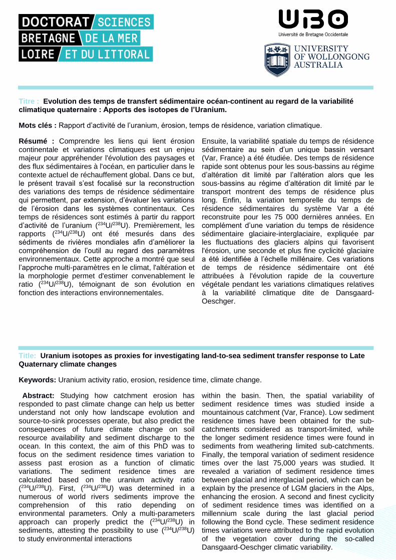
Titre : Evolution des temps de transfert sédimentaire océan-continent au regard de la variabilité climatique quaternaire : Apports des isotopes de l’Uranium.

Mots clés : Rapport d’activité de l’uranium, érosion, temps de résidence, variation climatique.

Résumé : Comprendre les liens qui lient érosion continentale et variations climatiques est un enjeu majeur pour appréhender l'évolution des paysages et des flux sédimentaires à l'océan, en particulier dans le contexte actuel de réchauffement global. Dans ce but, le présent travail s’est focalisé sur la reconstruction des variations des temps de résidence sédimentaire qui permettent, par extension, d’évaluer les variations de l’érosion dans les systèmes continentaux. Ces temps de résidences sont estimés à partir du rapport d’activité de l’uranium (234U/238U). Premièrement, les rapports (234U/238U) ont été mesurés dans des sédiments de rivières mondiales afin d’améliorer la compréhension de l’outil au regard des paramètres environnementaux. Cette approche a montré que seul l’approche multi-paramètres en le climat, l'altération et la morphologie permet d'estimer convenablement le ratio (234U/238U), témoignant de son évolution en fonction des interactions environnementales.

Ensuite, la variabilité spatiale du temps de résidence sédimentaire au sein d’un unique bassin versant (Var, France) a été étudiée. Des temps de résidence rapide sont obtenus pour les sous-bassins au régime d’altération dit limité par l’altération alors que les sous-bassins au régime d’altération dit limité par le transport montrent des temps de résidence plus long. Enfin, la variation temporelle du temps de résidence sédimentaires du système Var a été reconstruite pour les 75 000 dernières années. En complément d’une variation du temps de résidence sédimentaire glaciaire-interglaciaire, expliquée par les fluctuations des glaciers alpins qui favorisent l'érosion, une seconde et plus fine cyclicité glaciaire a été identifiée à l’échelle millénaire. Ces variations de temps de résidence sédimentaire ont été attribuées à l'évolution rapide de la couverture végétale pendant les variations climatiques relatives à la variabilité climatique dite de Dansgaard-Oeschger.

Title: Uranium isotopes as proxies for investigating land-to-sea sediment transfer response to Late Quaternary climate changes

Keywords: Uranium activity ratio, erosion, residence time, climate change.

Abstract: Studying how catchment erosion has responded to past climate change can help us better understand not only how landscape evolution and source-to-sink processes operate, but also predict the consequences of future climate change on soil resource availability and sediment discharge to the ocean. In this context, the aim of this PhD was to focus on the sediment residence times variation to assess past erosion as a function of climatic variations. The sediment residence times are calculated based on the uranium activity ratio (234U/238U). First, (234U/238U) was determined in a numerous of world rivers sediments improve the comprehension of this ratio depending on environmental parameters. Only a multi-parameters approach can properly predict the (234U/238U) in sediments, attesting the possibility to use (234U/238U) to study environmental interactions

within the basin. Then, the spatial variability of sediment residence times was studied inside a mountainous catchment (Var, France). Low sediment residence times have been obtained for the sub-catchments considered as transport-limited, while the longer sediment residence times were found in sediments from weathering limited sub-catchments. Finally, the temporal variation of sediment residence times over the last 75,000 years was studied. It revealed a variation of sediment residence times between glacial and interglacial period, which can be explain by the presence of LGM glaciers in the Alps, enhancing the erosion. A second and finest cyclicity of sediment residence times was identified on a millennium scale during the last glacial period following the Bond cycle. These sediment residence times variations were attributed to the rapid evolution of the vegetation cover during the so-called Dansgaard-Oeschger climatic variability.