Quantum response at finite fields and breakdown of Chern numbers

arX

iv:m

ath-

ph/9

9010

18v2

8 M

ay 1

999

Quantum Response at Finite Fields and Breakdown

of Chern Numbers

J E Avron and Z Kons †

Department of Physics, Technion, 32000 Haifa, Israel.

Abstract. We show that the response to an electric field, in models of the Integral

Quantum Hall effect, is analytic in the field and has isolated essential singularity

at zero field. We also study the breakdown of Chern numbers associated with the

response of Floquet states. We argue, and give evidence, that the breakdown of Chern

numbers in Floquet states is a discontinuous transition at zero field. This follows from

an observation, of independent interest, that Chern numbers for finite dimensional

Floquet operators are generically zero. These results rule out the possibility that the

breakdown of the Hall conductance is a phase transition at finite fields for a large class

of models.

1. Introduction

The principal motivation for the present work is the question: Is the breakdown of the

Integer Quantum Hall effect a (quantum) phase transition? Since the Hall conductance

in the adiabatic limit is identified with a Chern number, the question can also be phrased

as: Is the breakdown of Chern numbers a phase transition?

Experimentally, [9, 4, 5, 12, 18, 8, 19, 23] the breakdown of the Hall effect at finite

driving currents is signaled by the onset of dissipation, and is accompanied by hysteresis

and complex dynamical behavior. The critical current and voltage depend, in general,

on the geometry of the system, the temperature and on the magnetic field. It has

been suggested that a phase diagram for the breakdown resembles the phase diagram

of superfluidity [19].

Is there a theoretical basis for identifying breakdown with a phase transition?

Naively, one can argue both ways. In a class of models of the Integer Hall effect the

Hall conductance (at zero temperature and in the limit of linear response) is related to

a Chern number [21]. Chern numbers, being integers, depend discontinuously, if at all,

on parameters in the Hamiltonian. So, if the strength of the external electric field was

just like any other parameters in the Hamiltonian, one would expect the breakdown of

the Hall conductance to be discontinuous and at non-zero field. This would say that

the breakdown of the Hall effect is indeed a quantum phase transition at finite fields.

† E-mail addresses: [email protected] and [email protected]

http://arXiv.org/abs/math-ph/9901018v2

https://www.researchgate.net/publication/263980366_Topological_Quantum_Numbers_in_Nonrelativistic_Physics?el=1_x_8&enrichId=rgreq-e50f3f5a-c2a2-444e-ac24-9acd6a954ad8&enrichSource=Y292ZXJQYWdlOzIwOTQ0Mjk7QVM6MTAyODEzNTg1NjQxNDg4QDE0MDE1MjQwNzgxOTE=

Quantum Response at Finite Fields and Breakdown of Chern Numbers 2

On closer inspection one realizes that this line of reasoning can not be quite right.

For, if it was, then the Hall conductance would remain precisely quantized also for small

but finite values of the electric field. This would imply that there are no corrections

to the quantization – not even exponentially small correction. Common wisdom is

that while there are no power corrections to the integral Hall conductance, there are

exponentially small corrections [13]. As we shall explain in detail, and this is going to

be a key point of our analysis, the strength of the driving electric field (or the driving

emf) is a special parameter which affects the Hamiltonian and the evolution in a way

that is structurally different from say, the strength of the magnetic field or the disorder

potential.

A simple and common argument, with some experimental support, says that the

breakdown occurs at finite driving fields so that the critical field, Ec, scales like B3/2,

where B is the strength of the magnetic field. This estimate follows from comparison

of the energy gap in Landau levels with the voltage drop on a magnetic length. The

breakdown is then attributed to tunneling between Landau levels. This argument does

not directly address the question if the breakdown is a phase transition. It also has a

weakness in that the Landau Hamiltonian with constant electric and magnetic fields is

explicitly soluble and does not show breakdown. For other theories of the breakdown

see e.g. [22] and references therein.

To address the breakdown as a quantum phase transition, a handle on the

conductance at finite fields is needed. This goes beyond linear response and Kubo’s

formulation.

In this work we shall concentrate on the breakdown of the Hall conductance, rather

than the breakdown that occurs in the dissipative conductance in the Hall effect. This

is done for two reasons. The first is that we are interested in breakdown that occurs in

Chern numbers, for which the Hall conductance is a basic paradigm. The second is for

concreteness sake. Some parts of what we say can be transcribed, mutatis mutandis, for

the dissipative conductance.

We find no theoretical support to the hypothesis that the breakdown in the Hall

effect is a phase transition at finite fields. Rather, we find support to the claim that the

conductance has an essential singularity at zero fields, which can, of course, manifest

itself in what resembles a phase transition.

In section 2 we show that the strength of the driving electric field (or emf), E ,

can be related to a time scale τ . In section 3 we show that the expectation value of

a (bounded) observable, in particular, the current density in tight-binding models of

non-interacting electrons, is an analytic function of E with an essential singularity at

E = 0 when Et is kept fixed. In section 4 we consider the analytic properties of a

natural notion of transport for a class of model Hamiltonians which, in the limit of

linear response, reduces to the usual notion of conductance that coincides with a Chern

number. We show that this observable is analytic in E with an essential singularity

at E = 0. It is interesting that the absence of phase transition at finite fields can be

shown for the same class of models where one can prove quantization. In section 5 we


study the Harper model for which we present numerical results. In section 7 we study

Chern numbers associated with Floquet states, their properties and their interpretation

as Hall conductance of the Floquet states. In section 8 we study the breakdown of Chern

numbers associated to Floquet states. We show that the breakdown is discontinuous and

argue that it occurs at zero fields, E = 0. In section 9 we describe numerical evidence

that supports the claim that non-zero Chern numbers for Floquet states are unstable

against perturbations in the Hamiltonian.

2. Driving Fields Interpreted as a Time Scale

Because gauge invariance allows one to impose one condition on the scalar and vector

potential, it is always possible to choose a gauge where the external electric and magnetic

fields are described only by the vector potential ~A. In order to produce electric field

this potential has to be time dependent. Assume that this dependence is characterized

by some time scale τ as ~A(~x, t/τ). Suppose now that we scale time so that t = τ s.

Maxwell equation gives the external electric field, (in scaled time), as

~E(~x, s) = −1

τc∂s~A(~x, s) . (1)

With ~A fixed, weak electric fields correspond to large τ while strong electric fields

correspond to small τ . In systems that are otherwise time independent, τ interpolates

between weak and strong fields. A similar argument can be made about the emf, which

is a line integral of the electric field.

The identification of the time scale τ with the strength of the external driving, be

it the electric field or an emf, is not a new idea, of course. It lies at the heart of the

identification of the adiabatic limit with linear response. What is perhaps new here

is that we want to use this correspondence for any driving, and in particular identify

strong driving fields and large emfs with short time scales. Equation (1) suggest that

we write

E =

(

~

e

)

1

τ, (2)

where E is a measure of the strength of the driving field. We have put fundamental

constants into this relation so that (in cgs units) E has the dimensions of an emf (or

voltage). Because lattice models also have a natural length scale – the lattice spacing,

one can choose constants so that E has dimensions of an electric field. The identification

of the strength of the field with an inverse time scale is central to our considerations

and turns out to have consequences for transport. The first and easy consequence is

that the question of phase transition in, say, the Hall conductance as function of the

driving electric field, can be phrased as a question about the analytic properties of the

Hall conductance as a function of τ . The second consequence is discussed in the next

section.


3. Analyticity of Observables in τ

The identification of the time scale with the strength of the driving makes the driving

field, be it an electric filed or an emf, a special parameter in the Hamiltonian. This can

be seen from the form of the Schrodinger equation for the time evolution operator in

scaled time:

i Uτ (s) = τH( ~A(s))Uτ (s) , Uτ (0) = 1 . (3)

The τ dependence of the Hamiltonian is linear, and a-fortiori, analytic in τ , irrespective

of how H depends on ~A. This has the consequences:

Proposition 1 Suppose that H( ~A(s)) is bounded and self-adjoint, then Uτ (s) and U †τ (s)

are both entire functions of τ .

Proof. The first part follows from a standard argument about the absolute convergence

of the Dyson series for Uτ . The second assertion is a consequence of the fact that, for

real τ , U †τ satisfies

i U †τ (s) = −τ U †

τ (s)H( ~A(s)) , U †τ (0) = 1 . (4)

The Dyson series implies that one can extend U †τ (s) to an entire function of τ . �

It follows that:

Corollary 2 Suppose that I is a (fixed) bounded operator, and ψ a (τ independent)

initial state then:

I(τ, s) =⟨

ψ∣

∣U †τ (s) I Uτ (s)

∣

∣ψ⟩

(5)

is an entire function of τ .

This leads to the main result of this section:

Theorem 3 Let H( ~A) be bounded self-adjoint operator. Let I be a bounded observable,

then, its expectation value 〈I〉(E , s) is an analytic function of E with isolated essential

singularity at E = 0 and with Laurent expansion

〈I〉(E , s) =

∞∑

n=0

an(s)

En, (6)

with infinitely many of the an 6= 0 (except if 〈I〉 is a constant).

Proof. From proposition 1, 〈I〉(E , s) is an analytic function whose Taylor expansion

about τ = 0 is absolutely convergent with radius of convergence that is infinitely large.

The expansion can not have positive powers of E , for if it did, the response at τ = 0

would not be analytic. The singularity at the E = 0 must be essential for if was a pole

then the response would diverge as τ → ∞ along any direction. But, the response is

bounded on the real τ axis by the self-adjointness of the Hamiltonian. It follows that

the response can not have a pole of finite order at E = 0. �

Remarks:


(i) It is important for the conclusion of the theorem to hold that the scaled time s is

kept finite. If one lets s→ ∞ then, analyticity in τ may be lost.

(ii) We have restricted ourselves to bounded Hamiltonians and bounded observables.

This is because phase transitions are normally a long wavelength, low energy

phenomenon. Some parts of the theorem can also be extended to unbounded

Schrodinger type Hamiltonians provided some care is taken about questions of

domains of operators.

(iii) The smooth dependence of the evolution in τ is not really special to quantum

mechanics. It holds also in classical mechanics under slightly stronger conditions,

namely that ∂pH and ∂xH are both bounded functions (provided the initial state

is analytic in τ).

(iv) A classical model that shows breakdown of analyticity in a constant electric field is

the washboard potential with initial state at rest at a local minimum. When E is

sufficiently small, the velocity stays zero for all times. When E passes a threshold

the particle accelerates indefinitely. This is not a counterexample to the analyticity

of observabales because the initial state in the washboard potential is E dependent

in a non-analytic way.

(v) Two prototype functions for 〈I〉 that satisfy the conclusion of the theorem are

exp(−c/E2) and sin(c/E2).

(vi) The theorem has an interesting implication to the question of power law corrections

to linear response. It follows from the theorem that if 〈I〉 has an asymptotic

expansion in powers of E ∈ R+ at E = 0 then this expansion must vanish identically.

One may wonder if the absence of power law corrections to linear response is a

valid conclusion of equation (6). It is not, as one can see from the second prototype

example in (v), where an asymptotic expansion in powers of E ∈ R+ does not exist.

(vii) Absence of power corrections to linear response in quantized Hall conductance has

been proven rigorously for the quantum Hall effect by Klein and Seiler [13]. Their

proof uses an adiabatic theorem to all orders, to show that an asymptotic expansion

exists and a clever trick that shows that the coefficients must vanish. The theorem

above can be used to replace their clever trick.

In tight-binding models the current operator, for finitely many interacting electrons

or the current density operator for infinitely many non-interacting electrons, is a

bounded. It follows that the currents in such models have an essential singularity at

E = 0, but are analytic at non-zero E provided the time tE is kept fixed.

4. Breakdown of Chern Numbers

In this section we consider the breakdown of an observable associated with quantized

charge transport. Quantized charge transport occurs for a class of Hamiltonians in the

adiabatic limit. This class of Hamiltonians includes models of the quantum Hall effect,

and in particular includes the Harper model. It also includes certain models of the Hall


effect with electron-electron interactions. The observable that we consider reduces to

the Hall conductance in the limit of linear response, and coincides with a Chern number.

In this section we discuss the analytic properties of this observable with τ .

The model Hamiltonians for which quantization occurs have the following struc-

ture [20, 21]: H(φ, k) is a self-adjoint Hamiltonian that depend periodically on two real,

dimensionless parameters, φ and k, with period 2π. H(φ, k) may be associated with

a finite multiparticle system, where φ and k are external parameters, for example, two

Aharonov-Bohm fluxes. Alternatively, H(φ, k) may be a Bloch type Hamiltonian in two

dimensions describing infinitely many non-interacting electrons, where φ and k are two

Bloch momenta. In either case, we shall require that for fixed φ and k the Hamiltonian

H(φ, k) has discrete spectrum with no eigenvalue crossing. For the sake of simplicity we

assume that the φ and k dependence is smooth and that H(φ, k) is a bounded operator

such as a tight binding model and its multiparticle generalizations.

The time dependence comes from a time dependence of φ on a time scale τ‡. We

suppose that φ(s) is a smooth, monotonically non-decreasing function of s with φ(s) = 0

in the past, s < 0, and φ(s) = 2π, in the future, s ≥ 2π. H is therefore time dependent

only on a finite interval of (scaled) time [0, 2π].

Since ∂kH is the current operator in these models the total charge transported by

the action of φ is:

Q(τ ;ψ) =τ

2π

∫ 2π

0

dk

∫ ∞

0

ds

⟨

Uτ (s, k)ψ(k)

∣

∣

∣

∣

∂H(φ(s), k)

∂k

∣

∣

∣

∣

Uτ (s, k)ψ(k)

⟩

, (7)

with initial condition ψ that is an eigenstate of H(φ, k) for s = 0.

There are several special things that happen in the adiabatic limit. First, Q

coincides with the Hall conductance defined via Kubo’s formula [20, 21]. Second, it

is independent of the functional form of φ (provided φ satisfies the limiting conditions).

Third, since in the adiabatic limit there is no current once the driving stops, i.e. when

φ = 0, Q can also be written as

Q(s; τ, ψ) =τ

2π

∫ 2π

0

dk

∫ s

0

ds′⟨

Uτψ

∣

∣

∣

∣

∂H

∂k

∣

∣

∣

∣

Uτψ

⟩

, (8)

provided s ≥ 2π. Q is always a measure of the charge transport, but its identification

with a conductance is valid, in general, only in the adiabatic limit§.

Applying the results of the previous section we see that the breakdown of the Chern

number Q is smooth, and has no phase transition at finite fields. Due to the prefactor

τ in equation (8), a0 = 0 in equation (6).

It is interesting that for the class of models where one can prove that Q is quantized

in the adiabatic limit, one can also show that it is an analytic function of the field away

‡ Here φ plays the role of ~A of the previous section.§ Equation (8) implies that Q vanishes in the limit τ → 0, i.e. in the limit of large external fields,

contrary to common experience. One reason for this is that tight binding models are unreasonable

when the external fields are large on atomic scale. We shall take the point of view that the breakdown

is a low field phenomenon that is divorced from the asymptotic behavior at very large fields.


from E = 0. (For model Hamiltonians with infinitely many interacting electrons there

is, at present, no proof of quantization either.)

There are now three possibilities. The first, and perhaps simplest, is that the

breakdown of the Hall effect is a consequence of an essential singularity at zero field.

The second is that the breakdown of the Hall effect is associated with the limit s→ ∞.

And the third is that the breakdown is a property of infinitely many interacting electrons.

We shall examine the second possibility in section 7.

5. Example: Hall Conductance in the Harper Model

The Harper model is the simplest, non-trivial, model where one can study the breakdown

of the Hall effect in detail, at least numerically. The model is associated with a square

lattice, Z2; an external homogeneous magnetic field B, and homogeneous electric field E

pointing in the x direction. We choose a gauge so that the electric field is described by

a time dependent vector potential. After separation of variable, the model is described

by a Hamiltonian on Z parameterized by one Bloch momentum, k. The Hamiltonian

action on the vector Ψ ∈ ℓ2(Z), while the electric field is acting, is:

eiEtΨx+1 + e−iEtΨx−1 + 2 cos(Bx+ k)Ψx , k ∈ [−π, π] , x ∈ Z . (9)

For rational magnetic field B = 2πp/q with p, q ∈ Z the Hamiltonian is periodic in

x, with period q. One then classifies the solutions by a second Bloch momentum,

ℓ ∈ [−π, π] so that Ψx+q = exp(−iℓ)Ψx. Fixing periodic boundary conditions is achieved

by the unitary transformation Ψx → ei ℓqxΨx. So, finally, the requisite form of the Harper

Hamiltonian we shall study is:(

H(φ, k)Ψ)

x= eiφΨx+1 + e−iφΨx−1 + 2 cos(2π

p

qx+ k)Ψx ,

Ψx+q = Ψx, φ(t) =

ℓ

q, if t < 0;

Et+ℓ

q, if 0 < t < 2π

E;

2π +ℓ

q, otherwise.

(10)

This corresponds to a q×q hermitian matrix, periodic in φ and k. The driving electric

field, E , is related to the adiabaticity parameter τ , by (2) (in units where e = ~ = 1).

In this example φ(s) is continuous and piecewise linear. As a consequence the electric

field is discontinuous in time. It is easy to modify the model so that the electric field is

switched on and off continuously. We have examined also such models and the behavior

is qualitatively similar to models with discontinuous switching.

For p = 1, q = 3, the Harper Hamiltonian is a 3×3 matrix. Its Chern numbers are

{3, 3,−6}. Figure 1 shows the charge transport, Q(2π; τ, ψ), as function of the applied

field. The graph has a rich and complex structure, but no sharp breaking. Substantial

deviation from integral quantization occur near τ = 5.


0 2 4 6 8 10−6

−5

−4

−3

−2

−1

0

1

2

3

τ

Q

Figure 1. The Hall conductance of the 3×3 Harper Hamiltonian as function of the

adiabaticity parameter τ

6. Long-time limit and Floquet states

In this section we consider the long-time limit of observables, in time-periodic (finite

dimensional) Hamiltonians. An example is the current density operator in tight-

binding models, such as the Harper model, driven by a time-independent electric field.

One advantage of using a time dependent representation over the time independent

representation is that one has to deal with finite dimensional matrices. In the time

independent representation the matrices are infinite dimensional.

In the theory of time-periodic Hamiltonians Floquet states [7, 16, 6] play a role

analogous to that of eigenstates for time independent operators. We shall see that

the long-time (Abelian) limit of observables in time periodic systems is related to the

expectation value of the observable in Floquet states.

Consider a time-periodic, self-adjoint, finite dimensional matrix Hamiltonian H(s+

2π) = H(s). The Harper model of section 5 is an example except that now the electric

field is time independent for all (positive) times s ≥ 0.

Let F denote the unitary evolution over one cycle

F = U(2π) . (11)

The time evolution for n ∈ Z periods is clearly

F n = U(2nπ) . (12)


We assume that F is a finite dimensional, non-degenerate, matrix. Its spectral

representation is then

F =∑

n

eiEn|ψFn〉〈ψ

Fn | . (13)

En are the quasienergies, and |ψFn〉 the eigenvectors of F .

Consider the observable associated to the bounded operator I (e.g the current

density operator in tight binding models). Let ψ be the initial state of the system at

s = 0, then the Abelian, long-time, limit of the expectation value of I, when ψ evolves

according to the Schrodinger evolution, is:

limM→∞

1

M

M∑

j=1

〈I(2πj)〉 = limM→∞

1

M

M∑

j=1

⟨

F jψ | I |F jψ⟩

=∑

l,n

⟨

ψFn | I |ψF

l

⟩

〈l|ψ〉〈ψ|n〉

(

limM→∞

1

M

M∑

j=1

ei(El−En)j

)

=∑

l

∣

∣〈ψ|ψFl 〉∣

∣

2 ⟨ψF

l | I |ψFl

⟩

. (14)

The long time behavior is a weighted sum of the expectation value of the operator I in

Floquet states, i.e.⟨

ψFl | I |ψF

l

⟩

.

In particular, if one now defines the Hall conductance as the ratio of the Hall current

density to the electric field in the long time limit, then the breakdown of the Hall effect

is related to analytic properties of the expectation value of the current density operator

in Floquet states. This is the subject of the following sections.

7. Transport in Floquet States

In this section we recall, and extend, results of Ferrari [10] that relate the Hall

conductance of Floquet states to their Chern number and the winding numbers of their

quasienergies.

Consider a time-periodic, self-adjoint, finite dimensional matrix Hamiltonian H(s+

2π, k) = H(s, k), which depends analytically on s and k. The Harper model of section

5 is an example except that now the electric field is time independent for all (positive)

times. s is, as before, the scaled time.

We define the Floquet operator as the unitary evolution over one cycle

Fτ (s, k) = Uτ (s+ 2π, k)U †τ (s, k) . (15)

Floquet theorem can be expressed as

Fτ (s+ 2π, k) = Fτ (s, k) . (16)

We assume that Fτ is a finite dimensional matrix. It therefore has discrete spectrum

and its spectral representation is

Fτ (s, k) =∑

n

eiEn(s,k;τ)Pn(s, k; τ) . (17)


En are the quasienergies, and P are the eigenprojections. We shall denote by |ψFτ 〉 a

unit eigenvector of Fτ .

Lemma 4 For a Floquet operator generated by a bounded and analytic H(s, k),

(1) The quasienergies are independent of s, En(s, k; τ) = En(k; τ).

(2) The eigenfunctions (eigenprojections) obey the Schrodinger (Heisenberg) equations

i∂s|ψFτ (s, k)〉 = τH(s, k)|ψF

τ (s, k)〉 , (18)

i∂sP(s, k; τ) = τ [H(s, k),P(s, k; τ)] . (19)

(3) Fτ (s, k) is an entire function of τ and analytic function of s and k.

Proof. The Floquet operator satisfies

Fτ (s, k) = Uτ (s, k)Fτ (0, k)U†τ (s, k) , (20)

so its eigenvalues are independent of s. The eigenfunctions and eigenprojections

transform in the same way

|ψFτ (s, k)〉 = Uτ (s, k)|ψ

Fτ (0, k)〉 , (21)

P(s, k; τ) = Uτ (s, k)P(0, k; τ)U †τ (s, k) , (22)

from which the second assertion follows. The third item follows from proposition 1. �

F depends on s, τ and k. Because of equations (20) the s variable is uninteresting. It

is a basic fact of perturbation theory [11] that if a (normal) operator depends analytically

on two variables (or more), one can choose, in general, at most, one variable so that

the eigenvectors and eigenvalues are real analytic. We choose real analyticity in the k

variable. The price one has to pay for this is two fold: First, the τ dependence of the

projections will, in general, be discontinuous at crossings‖ and the second is that the 2π

periodicity in k may be lost. (One can not assume that P is both real analytic and 2π

periodic in k.) But, it is 2πN periodic for some finite N . If there are no crossing then

N = 1.

A result of Ferrari [10] identifies the Chern numbers of Floquet eigenstates with the

charge they transport and relates the Chern number of Floquet states to the winding

number of the quasienergies. This identification will play a key role in the next section

where we discuss breakdown.

Proposition 5 Let Fτ (0, k) be a finite dimensional Floquet operator, which is unitary

for real values of τ and k, and analytic in both. Fix τ and label the spectrum so that

Pτ (0, k) is real analytic in k with period 2πN . Then

(1) The quasienergies E(k; τ) and the associated eigenfunctions |ψFτ (s, k)〉 are simul-

taneously real analytic in k and s.

‖ This can be seen already for the 2×2 matrix function τσx + kσz where σ are the Pauli matrices.


(2) The conductance associated to non-interacting electrons that fill a k-band of Floquet

states is a Chern number multiple of 1/N :

Q(τ ;ψFτ ) =

1

2πNIm

∫ 2π

0

ds

∫ 2πN

0

dk 〈∂ψF

τ

∂s|∂ψF

τ

∂k〉 ∈

Z

N. (23)

(3) Q(τ ;ψτ ) is also the winding number of the corresponding eigenvalue,

Q(τ ;ψτ ) = −E(2πN ; τ) −E(0, τ)

2πN. (24)

(4) Q(τ, ψFτ ) = 0 for all E > 2 maxs,k∈[0,2π] ‖H(s, k)‖.

Proof. The first assertion follows from the real analyticity of the projection, (21),

and standard facts from perturbation theory [11]. The second assertion follows from:

τ

⟨

ψτ

∣

∣

∣

∣

∂H

∂k

∣

∣

∣

∣

ψτ

⟩

= τ∂

∂k〈ψτ |H |ψτ 〉 + Im〈

∂ψτ

∂k|∂ψτ

∂s〉 . (25)

The observable on the left hand side of this identity is the ratio of the current to

the driving electric field (in each k channel). This means Q is a conductance. The

identity (25) is a consequence of integration by parts, the equation of motion, and the

periodicity in k. The quantization of Q follows by integrating over the period in k and

using standard facts about Chern numbers. Using the identity(

F †τ

∂Fτ

∂k

)

(0, k) = −iτ

∫ 2π

0

U †τ (s, k)

(

∂H

∂k

)

Uτ (s, k)ds (26)

and equation (17)⟨

ψFτ (0, k)

∣

∣

∣

(

F †τ ∂kFτ

)

(0, k)∣

∣

∣ψF

τ (0, k)⟩

= i∂kE(k; τ) (27)

gives assertion 3. Item 4 follows from the observation that the winding vanishes if

max |E(k; τ)| < π. The maximum can achieved when all the terms in the Dyson

expansion of the evolution operator have the same eigenstate for their maximal

eigenvalue and all the eigenvalues are summed up with the right signs. It follows that

|E| ≤ 2πτ max ‖H‖ , (28)

which implies item 4. �

Finally, we note that for the adiabatic limit, E = 0, eigenstates of the Hamiltonian

are also Floquet eigenstates. This shows that for E = 0 the Chern number for Floquet

states is the Hall conductance of linear response when H(s, k) is the Hamiltonian for

the Hall effect.

8. Breakdown in Floquet States

In the previous section it was shown that the Hall conductance in Floquet states, for any

field strength E , is related to the Chern number of the state. Since the Chern numbers

are integers, this implies that the breakdown in Floquet states is always discontinuous:

a quantum phase transition. For E = 0 the conductance for Floquet states coincide


with the Hall conductance of linear response but when E is large enough Q vanish. This

forces a discontinuous breakdown.

At first, it appears that one can argue that a breakdown must occur for some finite

value of E because Chern numbers do not change under small deformations of the bundle

of eigenstates, and so if the Chern number is non-zero at zero field, should it not be

non-zero also for small fields?

To understand how the breakdown occurs we first make the observation that non-

zero Chern numbers for Floquet operators always come with level crossings:

Theorem 6 Let Fτ (0, k) be a finite dimensional Floquet operator, which is unitary for

τ, k ∈ R, and analytic in both. Label the spectrum of Fτ so that Pτ (0, k) is real analytic

in k with period 2πN . If any Chern number is non-zero then Fτ has eigenvalue crossing

for some value of k.

Proof. By general principles, the sum of all the Chern numbers for any finite

dimensional matrix, such as Fτ , must vanish. Hence, if there is a positive Chern number

for one of the states of Fτ , there must also be a negative Chern number for some other

state. The quasienergy with a positive winding must then cross the one with negative

winding. �

This leads to a puzzle that has Chern on one side, and Wigner von-Neumann

(WVN) on the other: Wigner and von-Neumann [17, 14] say that eigenvalue crossing

tend to be unstable, unless the dimension of parameter space is three or more¶. The

relevant parameter space for the Floquet operators is the τ -k space which has dimension

two. This implies that crossings are unstable. On the other hand Chern numbers give a

topological characterization of the bundle of eigenstates and are stable under continuous

deformations of the bundle. Who wins?

The winners, we claim, are Wigner and von-Neumann. It is, of course, true that

continuous deformation of the bundle keep the Chern number fixed. But, there is no

reason why a continuous deformations of the Hamiltonian or a variation in τ , should

lead to continuous deformations of the bundle of eigenstates. By perturbation theory

a small deformation in the Hamiltonian can result in a discontinuous change of the

bundle at points of crossing. Since non-zero Chern number for Floquet states always

comes with eigenvalue crossing, the bundles always lie at the boundary of the region of

stability. As a consequence, generically, at least, Chern numbers for Floquet operators+

should be zero and the breakdown should therefore occur at E = 0+.

Experimentally, the breakdown of the Hall effect is continuous and consequently,

the breakdown of Floquet states does not appear to be an appropriate theory for the

breakdown of the Hall effect. This suggests that the breakdown is not a large time

phenomenon. Nevertheless, the breakdown in Floquet states is an interesting chapter

in the theory of breakdown of Chern numbers.

¶ In the complex case, which is the case relevant here.+ At least, those of the class we study here, that depend on a single variable k


ϕ

θ

Figure 2. A map from the 2-torus (ϕ, θ) to the sphere (the unit vector pointing from

θ to ϕ). The linking number is the degree of the map.

9. Unstable Chern numbers

We have seen in theorem 6 that non-zero Chern numbers for Floquet operators always

come with eigenvalue crossings. The question whether Floquet operators do or do not

have stable non-zero Chern numbers, is equivalent to the question whether Floquet

operators do or do not have stable eigenvalue winding and crossing.

9.1. Fragile Winding

A simple example, that we owe to B. Simon, illustrates how topological objects that are

normally associated with stability become fragile in the context of eigenvalue problems.

Consider the unitary

Fτ (s = 0, k) =

(

cos(1/τ) eik sin(1/τ)

− sin(1/τ) cos(1/τ) e−ik

)

. (29)

F has unit determinant so its two eigenvalues are determined by a single angle φ. Clearly

cosφ = cos(1/τ) cos k. For 1/τ = πn the two eigenvalues have winding numbers ±1 as

k goes through a period. But, for most value of τ the two eigenvalues repel at 0 and

π, and have zero winding. Winding numbers that arise from an eigenvalue problem are

not stable.

9.2. The Paradigm

The basic paradigm of line bundles associated with Chern numbers ±1 comes from

Berry example of spin 1/2 in a magnetic field. Berry’s spin 1/2 model describes a 2×2

Hamiltonian that is parameterized by the two sphere. In the study of Floquet operators

and adiabatic transport, one is interested in families parameterized by the 2-torus. The

question is how to pick a family of 2×2 Hamiltonians on a 2-torus with Chern numbers

±1. A nice geometric way (figure 2) to think about the family is to consider the pull-

back of Berry’s spin 1/2 on the 2-sphere, by the Gauss map from the 2-torus to the

2-sphere with degree one∗.

∗ We thank I. Klich for pointing this out.


A useful fact about the quasienergies of 2×2 Floquet operators with determinant

1 is that E1 = −E2. Hence, gap closure occur only at E = 0 and E = ±π. A stable

non-zero Chern number then requires a stable crossing at both at E = 0 and E = ±π.

Since this feature simplifies the numerical analysis considerably the 2×2 Hamiltonian

on the torus should also be traceless.

An example of a periodic, traceless 2×2 matrix Hamiltonian with Chern numbers

±1 is

H1(s, k) =1

√

sin(s)2 + |a|2

(

sin(s) a

a − sin(s)

)

(30)

with

a = cos(k +π

4) + i cos(k −

π

4) + (1 + i) (cos(s) + 1) . (31)

The Floquet operator associated to this Hamiltonian has to be calculated by

numerical integration of the Schrodinger equation (3). This Floquet is our basic

paradigm. Now, if non-zero Chern numbers for Floquet operators are generically

unstable, this will manifest itself in the opening of gaps at π and 0. The gaps are

shown in figure figure 3 and are consistent with the claim that Chern numbers of the

Floquet operator are generically zero.

0 1 2 3 4 510

−8

10−6

10−4

10−2

100

τ

gaps

wid

th

Figure 3. Gaps width of the Floquet operators from H1. The solid line is for the gap

near E = π, the dashed line is for the gap near E = 0


9.3. Another Toy Models

We have also carried out extensive numerical studies of the following toy model of a 2×2

traceless periodic matrix family:

H2(s, k, ε) =1

√

a2 + (b+ ε)2 + c2

(

a b− ic + ε

b+ ic + ε −a

)

(32)

a = cos(k) , b = cos(s) , c = cos(s+ k) .

This Hamiltonian is inspired to some extent by the Harper model on a triangular lattice

[1]. It has the following features:

(i) For all s, k, ε 6= ±1 the spectrum is constant Spec(H2(s, k, ε)) = {−1, 1}.

(ii) The Chern numbers associated with the eigenvectors of H2(s, k, ε) are ±2 for

−1 < ε < 1 and zero otherwise♯.

We have added an extra parameter, ε so that the associated Floquet operator, Fτ (0, k; ε),

depends on three variables, {τ, k, ε}. The reason for including ε shall become clear below.

What should one expect for the Floquet operator based on WVN genericity

argument? Since (the unitary) Fτ (0, k; ε) depends on three real variables, one expects

isolated points in {τ, k, ε} space where there is crossing. In other words, for some special

values of ε one expects to find crossing, while for most values of ε, there should be no

crossing, and all Chern numbers should vanish. This turns out to be the case.

Here too the Floquet operator has to be calculated by numerical integration of the

Schrodinger equation (3).

0 2 4 6 8 10

10−8

10−6

10−4

10−2

100

τ

Min

imal

qua

sien

ergi

es g

ap

Figure 4. Plot of the minimal quasienergy gap vs. τ for ε = 0. Notice the logarithmic

y–scale. The calculation accuracy was of order 10−8. The circles represents the

calculation points which are spaced non-uniformly.

♯ This can be seen by examining sections of the bundle.


For ε = 0 the crossing at E = 0 is stable for all τ . The gap at E = ±π is plotted

in figure 4. As can be seen, for most values of τ the gap is wider then the numerical

tolerance. This gap is usually very small. It is easy to mistake these small gaps for

crossing.

Near integers values of τ the gap width decreases rapidly. At these points the gaps

seem to close, up to our numerical accuracy, and the winding numbers change from zero

to ±2.

These results are in conflict with both the putative stability of Chern numbers,

and the WVN instability of crossing. It is in conflict with Chern, as non-zero Chern

numbers appear to occur at isolated points on the τ axis rather than intervals. It is also

in conflict with WVN, for, by the no-crossing rule one expects no crossing in the τ − k

plane at all. The model would be consistent with WVN if the point ε = 0 turns out to

be a special point. Although we do not know if and why ε = 0 is special, one expects

WVN to fail for some ε, and a test would be to see if the crossing disappear when we

wiggle away from ε = 0.

For non-zero values of ε both gaps closure at E = 0, π indeed disappear, as is seen

in figure 5, and Wigner and von-Neumann are vindicate.

0 2 4 6 8 10

10−8

10−6

10−4

10−2

100

τ

gaps

wid

th

Figure 5. Gaps width of the Floquet operators from H2 with ε = 0.2. The solid line

is for the gap near E = ±π, the dashed line is for the gap near E = 0

For more numerical results and description for some of the numerical procedures

see [15].

In conclusion, the numerical results for both toy models are in agreement with

WVN and with our argument that Chern numbers for Floquet operators are generically

zero.


9.4. The Harper Model

We have also studied numerically the question of stability of Chern numbers for the

Floquet operator that is associated with the Harper model.

Telling a true crossing from an avoided crossing in a numerical study is often a

challenge. Often one finds complicated pictures where it is difficult to tell with certainty

which is really the case since even real gaps tend to be very small. This is illustrated

by numerical results for the Harper model with p = 1 and q = 3, 4, see figures 6 and 7.

0 2 4 6−3

−2

−1

0

1

2

3

k

En(k

)

(a) τ=1.5

0 2 4 6k

(b) τ=2.5

Figure 6. The quasienergies E(k) of the Floquet operator associated with the 3×3

Harper Hamiltonian for τ = 1.5, 2.5.

0 2 4 6−3

−2

−1

0

1

2

3

k

En(k

)

(a) τ=1.5

0 2 4 6k

(b) τ=5.0

Figure 7. The quasienergies E(k) of the Floquet operator associated with the 4×4

Harper Hamiltonian for τ = 1.5, 5.0.

Our numerical results are consistent with the assertion that the Harper model has

some stable crossing. It is an open problem to prove or disprove this.


10. Failure of Berry’s method to detect Floquet crossings

One reliable method to identify crossing of self-adjoint matrices, is to compute a Chern

number (in the Hermitian case) or the Longuet-Higgins phase (in the symmetric case)

[2, 3]. Unfortunately, this method does not work for the kind of Floquet operators that

we consider, as we now proceed to explain.

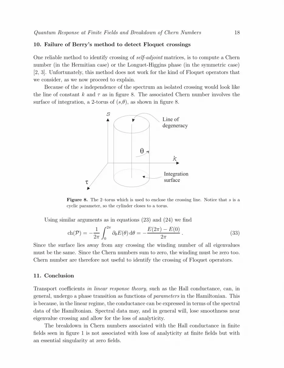
Because of the s independence of the spectrum an isolated crossing would look like

the line of constant k and τ as in figure 8. The associated Chern number involves the

surface of integration, a 2-torus of (s,θ), as shown in figure 8.

Figure 8. The 2–torus which is used to enclose the crossing line. Notice that s is a

cyclic parameter, so the cylinder closes to a torus.

Using similar arguments as in equations (23) and (24) we find

ch(P) = −1

2π

∫ 2π

0

∂θE(θ) dθ = −E(2π) − E(0)

2π. (33)

Since the surface lies away from any crossing the winding number of all eigenvalues

must be the same. Since the Chern numbers sum to zero, the winding must be zero too.

Chern number are therefore not useful to identify the crossing of Floquet operators.

11. Conclusion

Transport coefficients in linear response theory, such as the Hall conductance, can, in

general, undergo a phase transition as functions of parameters in the Hamiltonian. This

is because, in the linear regime, the conductance can be expressed in terms of the spectral

data of the Hamiltonian. Spectral data may, and in general will, lose smoothness near

eigenvalue crossing and allow for the loss of analyticity.

The breakdown in Chern numbers associated with the Hall conductance in finite

fields seen in figure 1 is not associated with loss of analyticity at finite fields but with

an essential singularity at zero fields.


One way to have Chern numbers undergo a phase transition with the applied field

is to define them by a spectral problem. This is the case for Chern numbers of Floquet

states. An external time independent electric field, in an appropriate gauge, leads

to a tight-binding Hamiltonians that is periodic in time and admits Floquet analysis.

The Hall conductance in Floquet states reduces to a spectral problem for the Floquet

operator. This holds for any value of the driving field, and not just in the linear response

regime. Because of this, changing the field can lead to a non-smooth behavior of the

conductance when eigenvalues of the Floquet operator cross. We argue that the Chern

numbers of Floquet operators are generically zero, because non-zero Chern numbers

come with eigenvalue crossing. Non-zero Chern numbers are unstable to small variations

in the Hamiltonian and the breakdown occurs at zero fields.

In conclusion we can say that we find no theoretical reason for the breakdown of

the Hall effect to be a quantum phase transition at nonzero fields, although we do not

rule this out for more complicated models such as models of infinitely many interacting

particles. In addition we observe that under the condition where one can show that the

charge transport is quantized, one can also show that it is an analytic function of the

field with an essential singularity at zero field.

Acknowledgments

We acknowledge useful discussions with A. Auerbach, S. Fishman, I. Klich, K. Malick,

N. Moiseyev, M. Resnikov, B. Simon and D. Thouless, and especially with A. Elgart.

This research was partially supported by the Israel Science Foundation, SFB 288 and

the fund for the promotion of research at the Technion.

References

[1] J. Bellissard, C. Kreft and R. Seiler, J. Phys. A 24 (1991), 2329–2353.

[2] M. V. Berry and M. Wilkinson, Proc. R. Soc. Lond. A 392 (1984), 15-43.

[3] M. V. Berry, Proc. R. Soc. Lond. A 392 (1984), 45.

[4] M. E. Cage, J. Res. Natl. Inst. Stand. Technol. 98 (1993), 361.

[5] M. E. Cage, R. F. Dziuba, B. F. Field and E. R. Williams, Phys. Rev. Lett. 51 (1983), 1374–1377.

[6] G. Casati and L. Molinari, Prog. Theo. Phys. Supp. 98 (1989), 287.

[7] H.L. Cycon, R.G. Froese, W. Kirsch and B. Simon Schrodinger Operators, Springer (1986)

[8] S. Komiyama et. al. , Phys. Rev. Lett. 77 558, (1996).

[9] G. Ebert, K. von Klitzing, K. Ploog and G. Weimann, J. Phys. C: Solid State Phys. 16 (1983),

5441–5448.

[10] R. Ferrari, Int. J. Mod. Phys. B 12 (1998), 1105.

[11] T. Kato, Pertubation theory for linear operators, Berlin, Heidelberg, New York: Springer, 1984.

[12] S. Kawaji, K. Hirakawa, M. Nagata, T. Okamoto, T. Fukase and T. Gotoh, J. Phys. Soc. Japan

63 (1994), 2303–2313.

[13] M. Klein and R. Seiler, Comm. Math. Phys. 123 (1990), 141.

[14] R. S. Knox and A. Gold, Symmetry in the solid state, W. A. Benjamin, INC. New–York, 1964.

[15] Z. Kons, A search for hall effect breakdown in single electron models, Master’s thesis, 1999,

Department of Physics, Technion, 32000 Haifa, Israel., Also available for download from:

http://physics.technion.ac.il/∼konsz/Thesis/Thesis.html.

http://physics.technion.ac.il/~konsz/Thesis/Thesis.html


[16] N. Moiseyev, Phys. Rep. 302 (1998), 212-293.

[17] J. von Neumann and E. P. Wigner, Phys. Z. 30 (1929), 467, Translation to English can be found

in the appendix of [14].

[18] T. Okuno, S. Kawaji, T. Ohrui, T. Okamoto, Y. Kurata and J. Sakai, J. Phys. Soc. Japan 64

(1995), 1881–1884.

[19] L.B. Rigal et. al. , Phys. Rev. Lett 82, 1249 (1999).

[20] M. Stone, Quantum Hall effect, World Scientific, 1992.

[21] D. J. Thouless, Topological quantum numbers in nonrelativistic physics, World Scientific, Singa-

pore, 1998.

[22] V. Tsemekhamn, K. Tsemekhamn, C. Wexler, J. H. Han and D. J. Thouless, Phys. Rev. B 55

(1997), 10201.

[23] J.P. Watts et. al. Phys. Rev. Lett 81, 4220, (1998).

Quantum response at finite fields and breakdown of Chern numbers

Documents