Radiative corrections to the Chern–Simons term at finite temperature in the noncommutative Chern–Simons–Higgs model

arX

iv:h

ep-t

h/03

0112

4v4

12

Mar

200

4

Radiative corrections to the Chern-Simons term at finite

temperature in the noncommutative Chern-Simons-Higgs model

L. C. T. de Brito, M. Gomes, Silvana Perez,∗ and A. J. da Silva

Instituto de Fısica, Universidade de Sao Paulo,

Caixa Postal 66318, 05315-970, Sao Paulo - SP, Brazil†

Abstract

By analyzing the odd parity part of the gauge field two and three point vertex functions, the one-

loop radiative correction to the Chern-Simons coefficient is computed in noncommutative Chern-

Simons-Higgs model at zero and at high temperature. At high temperature, we show that the static

limit of this correction is proportional to T but the first noncommutative correction increases as

T log T . Our results are analytic functions of the noncommutative parameter.

∗Also at Departamento de Fısica, Universidade Federal do Para, Caixa Postal 479, 66075-110, Belem, PA,

Brazil; e-mail:[email protected]†Electronic address: lcbrito,mgomes,silperez, [email protected]

1

I. INTRODUCTION

The analysis of the radiative corrections to the Chern-Simons coefficient has stimulated

considerable interest in the recent years [1]. These studies pointed out that the well known

nonrenormalization theorem [2] may become invalid whenever infrared singularities are

present. Typical of this possibility are situations which potentially modify the long dis-

tance behavior of the relevant models. Examples are the breakdown of some continuous

symmetry, thermal effects and the possible noncommutativity of the underlying space. In

this work we are going to focus on the changes in the Chern-Simons coefficient in a model

where all these effects may occur, the noncommutativeChern-Simons-Higgs model.

The appearance of noncommutative coordinates has an old history [3] but gained impetus

more recently, mainly due to its connection with string theory [4]. One peculiar aspect of

these theories is the ultraviolet/infrared (UV/IR) mixing [5], i. e., the replacement of some

ultraviolet divergences by infrared ones. The UV/IR mixing implies in the existence of

infrared singularities which, at higher orders, may ruin the perturbative expansion. These

infrared singularities are generated even in theories without massless fields. However, such

behavior may be ameliorated in some supersymmetric models [6], so that supersymmetry

seems to play decisive role in the construction of consistent noncommutative theories. Up

to one-loop, the absence of UV/IR mixing has also been verified for the pure U(n) Chern-

Simons model which actually seems to be a theory without any quantum correction [7].

In a noncommutative space, it will appear trigonometric factors and, because of them,

the amplitudes are separated in two parts, the planar and nonplanar ones. Unless by phase

factors which depend only on the external momenta, the planar part of the amplitudes are

proportional to the corresponding amplitude in the commutative case. The main effects

coming from the noncommutativity of the space can be extracted from the nonplanar con-

tributions. These also contain phase factors but, unlike the planar case, they depend on the

loop momenta.

Besides the noncommutativity of the space, thermal effects also modify the long distance

behavior of field theories. Aiming to understand the changes induced by thermal effects

many features of noncommutativity at finite temperature have been examined [8]. At fi-

nite temperature, it is known that for small momenta the amplitudes in a commutative

model are, in general, not well behaved and this feature is understood in terms of the new

2

structure introduced by the temperature, the velocity of the heat bath [9]. On the other

hand, in a noncommutative space, the new structure is the θµν tensor, which measures the

noncommutativity of the space, and it also leads to an infrared nonanalytic behavior.

Another effect which induces changes in the CS coefficient is the spontaneous breakdown

of some continuos symmetry. In the commutative space it is know that classically, in the

absence of spontaneous symmetry breakdown and at zero temperature, the non-Abelian co-

efficient of the Chern-Simons term must be quantized [10]. This was indeed verified first up

to one-loop in [11] and then extended to all orders in the SU(N) Yang-Mills Chern-Simons

model [12]. Similar results hold for noncommutative theories [13]. When spontaneous sym-

metry breakdown is at work, the quantization condition above mentioned is violated [14].

In this work we will study the corrections to the Chern Simons coefficient at finite temper-

ature arising from the one-loop contributions to the gauge field two and three point vertex

functions, in the broken phase of the noncommutative Chern-Simons-Higgs model. Unless

for some special limits, in noncommutative finite temperature field theory there are many

difficulties to evaluate amplitudes in a closed form. Thus, similarly to [15], we will consider

a generalization of the hard thermal loop limit, which involves the noncommutative param-

eter. We then prove that in the static limit and at high temperature the Chern-Simons term

increases like T and actually does not depend on the noncommutative parameter. However,

at the next level of approximation, which is linear in the noncommutative parameter, we

found that the odd part of the two point vertex function increases as T log T . As expected,

although we are considering the Abelian model, because of the noncommutativity, there will

be strong resemblances with the non-Abelian theory.

The work is organized as follows: In Section II the noncommutative version of the Chern-

Simons-Higgs model in the broken phase is presented. Section III contains the one-loop

corrections to the odd parity part of the gauge field two point vertex function, both in

commutative as well as in noncommutative cases and at finite temperature in the imaginary

time formalism. The zero temperature results are obtained as consequence of this evaluation.

The odd parity part of the gauge field three point vertex function is studied in Section IV.

Finally, in Section V the conclusions are presented. One Appendix collects some useful

integrals used in the work.

3

II. NONCOMMUTATIVE CHERN-SIMONS-HIGGS MODEL

Noncommutative quantum field theories are defined in a space where the coordinates do

not commute among themselves. Rather, the commutator between two position operators

is postulated to be

[xµ, xν ] = iθµν , (1)

where θµν is an antisymmetric matrix, which for simplicity we take as commuting with

the x’s. The algebra of operators in such space has been extensively studied [17], and

many properties are known (see [18] for some reviews). A basic result is that, due to the

Wigner-Moyal correspondence, instead of working with functions of the noncommutative

coordinates, one may use ordinary functions of commutative variables embodied with the so

called Moyal product, defined as

f(x) ∗ g(x) =[

e(i/2)θµν ∂(ζ)µ ∂

(η)ν f(x + ζ)g(x + η)

]

ζ=0=η. (2)

Using this definition, one can study quantum field theories in a noncommutative space,

by replacing the standard pointwise product of fields by the Moyal one. For simplicity, in

this work we shall keep θ0i = 0.

In the present work we will study the Chern-Simons-Higgs model in a noncommutative

space. The model is defined by the action

S =1

2

∫

d3xǫµνλ

[

Aµ ∗ ∂νAλ +2ig

3Aµ ∗ Aν ∗ Aλ

]

+ (DµΦ) ∗ (DµΦ)† − λ

4

[

Φ ∗ Φ† − v2]2

∗ , (3)

where v, g and λ are constants. DµΦ is the covariant derivative, defined in such way to

ensure the gauge invariance of the action. Because of the noncommutativity, under a U(1)

gauge transformation U the basic fields may alternatively transform as:

1) Fundamental representation: Φ → Φ ∗ U and the covariant derivative is given by

DµΦ = ∂µΦ − igΦ ∗ Aµ;

2) Anti-fundamental representation: Φ → U−1 ∗ Φ and DµΦ = ∂µΦ + igAµ ∗ Φ;

4

3) Adjoint representation: Φ → U−1∗Φ∗U and DµΦ = ∂µΦ+ig[Aµ, Φ]∗. Throughout this

article we will employ the notation [ , ]∗ and { , }∗ to respectively designate the commutator

and anticommutator using the Moyal product.

In all theses cases

Aµ → U−1 ∗ Aµ ∗ U − 1

ig(∂µU−1) ∗ U. (4)

In the adjoint representation, the Higgs mechanism and the induction of new terms

containing the gauge fields due the spontaneous breakdown of the gauge symmetry are

absent. Because of that we are going to restrict our considerations to the fundamental

representation (the analysis of the anti-fundamental representation is actually very similar).

In the spontaneously broken phase, 〈Φ〉 ≡ v 6= 0, one can choose the decomposition

Φ = v + 1√2(σ + iχ) and rewrite Eq. (3) as

S =

∫

d3x1

2ǫµνλ

(

Aµ ∗ ∂νAλ +2ig

3Aµ ∗ Aν ∗ Aλ

)

+m

2Aµ ∗ Aµ − 1

2ξ(∂µAµ)∗(∂νA

ν)

+1

2(∂µσ) ∗ (∂µσ) − m2

σ

2σ ∗ σ +

1

2(∂µχ) ∗ (∂µχ) −

m2χ

2χ ∗ χ

− g

2Aµ ∗

(

σ ∗↔∂µχ − χ ∗

↔∂µσ − i[σ, ∂µσ]∗ − i[χ, ∂µ χ]∗

)

+g2

2Aµ ∗ Aµ ∗

(

σ ∗ σ + χ ∗ χ + 2√

2vσ + i[σ, χ]∗

)

− λ

2√

2v

{

σ,(σ ∗ σ + χ ∗ χ)

2+

i

2[χ, σ]∗

}

∗− λ

16(σ ∗ σ + χ ∗ σ + i[χ, σ]∗)

2∗ , (5)

where we have chosen the Rξ gauge, specified by the gauge fixing action

SGF = − 1

2ξ

∫

d3x(

∂µAµ + ξ√

2vχ)2

∗, (6)

which has the merit of canceling the nondiagonal terms in the quadratic part of the model.

We have also defined

m = 2(gv)2, m2σ = λv2, m2

χ = ξm. (7)

To complete the action of the model, one has to add to Eq. (5) the Faddeev-Popov action

given by

5

SFP =

∫

d3x [∂µc ∗ ∂µc + i∂µc ∗ (c ∗ Aµ − Aµ ∗ c) + iξvc ∗ χ ∗ c] , (8)

where c and c are the ghost fields.

The propagator for the gauge field is

Dµν(p) =i

p2 − m2

[

−mgµν + pµpνm − ξ

p2 + ξm+ iǫµνλp

λ

]

(9)

and for the other fields they are the standard ones (Dσ(p) = i/(p2 −m2σ), Dχ = i/(p2 −m2

χ)

and Dc = i/p2). These propagators are not affected by the noncommutativity. We will use

the following analytic expression for the vertices in the figure 1 (we list only those that will

contribute in our calculation)

iAµ ∗ Aν ∗ Aρ vertex ↔ 2igǫµρν sin(p1 ∧ p2) (10)

Aµ ∗ Aν ∗ σ vertex ↔ 2√

2ivg2gµνcos(p1 ∧ p2) (11)

iAρ ∗ [σ, ∂ρσ]∗ vertex ↔ 2gpρ3 sin(p2 ∧ p3) (12)

At finite temperature and using the imaginary time formalism, the gauge propagator is

Dµν(p) =1

p2 + m2

[

mδµν − pµpνm − ξ

p2 + ξm− ǫµνλp

λ

]

, (13)

with pµ ≡ (p0, ~p) = (2πnT, ~p).

III. TWO POINT FUNCTION

In this section we will compute the one-loop radiative correction to the gauge field two

point vertex function of the above model at finite temperature, in both commutative and

noncommutative cases, employing the imaginary time formalism. In the noncommutative

situation, to fix the behavior of the Chern-Simons term we will have to examine the correc-

tions to the gauge field two and three point vertex functions. We begin by first considering

the corrections to the two point vertex function.

A. Commutative case

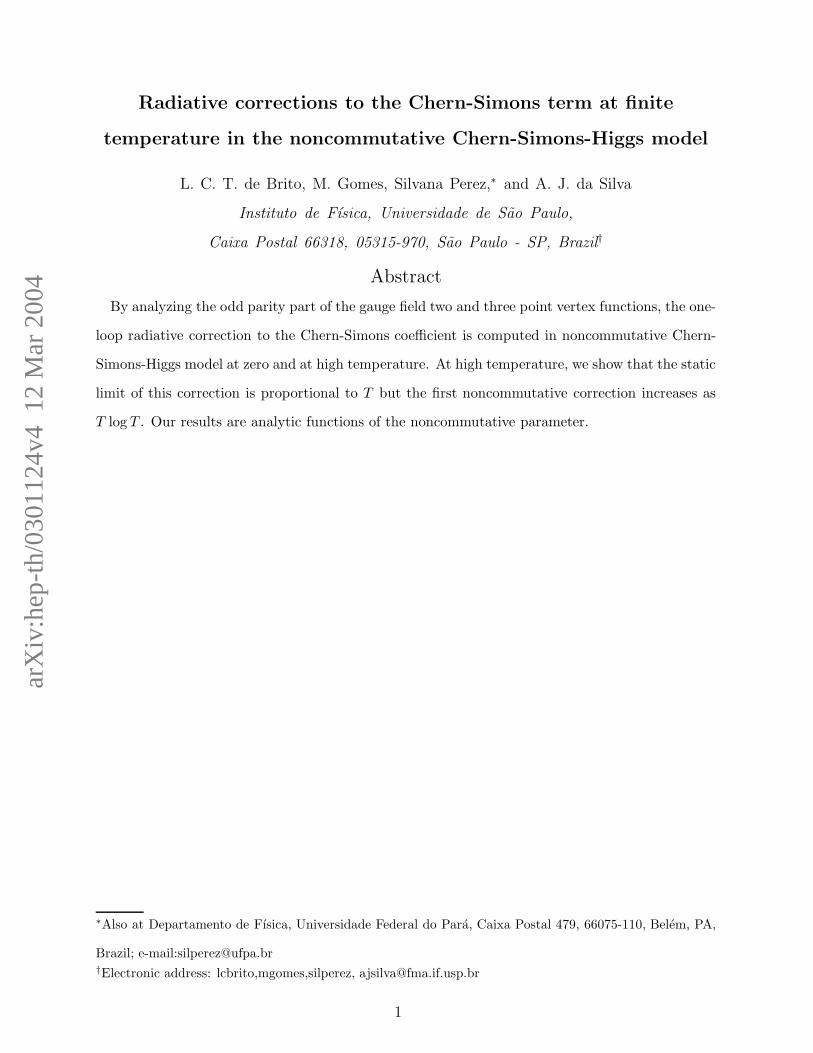
Let us start by evaluating the parity violating part of the polarization tensor Πµν in the

commutative case. There is only one diagram, Fig. 2a, to evaluate. At one loop, the ghost

6

field does not contribute to the parity violating part, as can be seen from SFP . Thus, we

have

Πoddµν (p) ≡ πµν(p) = 8(v g2)2T

∑

n

∫

d2k

(2π)2

ǫµνλkλ

(k2 + m2)[(p − k)2 + m2σ]

. (14)

The consideration of the static limit, where p0 = 0 and | ~p | is small, yields

π0i(p0 = 0) = 8(v g2)2

∫

d2k

(2π)2ǫ0ijk

jT∑

n

1

k20 + w2

m

1

k20 + w2

σ(p). (15)

Note that, in the static limit, πij vanishes as the integrand is an odd function of n. We have

also introduced the notation w2m = ~k2 + m2 and w2

σ(p) = (~p − ~k)2 + m2σ. Using that

1

k20 + (~p − ~k)2 + m2

σ

=1

k20 + w2

σ

+2~k · ~p

(k20 + w2

σ)2+ O(~p 2)

=

(

1 − 2~k · ~p ∂

∂m2σ

)

1

k20 + w2

σ

+ O(~p 2), (16)

where wσ ≡ wσ(0), we write Eq. (15) for small external momentum as

π0i(p0 = 0) = 8(v g2)2

∫

d2k

(2π)2

(

1 − 2~k · ~p ∂

∂m2σ

)

ǫ0ijkjT∑

n

1

k20 + w2

m

1

k20 + w2

σ

+ O(~p 2).

(17)

After that, we evaluate the sum in k0 through the use of

n=+∞∑

n=−∞f(n) = −π

′∑

[f(z) cot(πz)], (18)

where the prime in the sum indicates that it runs over the residues of the poles of f(z).

Thus, we find

π0i(p0 = 0) = 4(v g2)2

∫

d2k

(2π)2ǫ0ijk

j

×(

1 − 2~k · ~p ∂

∂m2σ

){

1

m2σ − m2

[

coth (βwm/2)

wm

− coth (βwσ/2)

wσ

]}

. (19)

Using that coth (βx/2) = 1+ 2eβx−1

, we can separate the zero temperature from the finite

temperature part. The zero temperature part can be computed straightforwardly, giving

7

π0i(p0 = 0; T = 0) = 4(v g2)2

∫

d2k

(2π)2ǫ0ijk

j

(

1 − 2~k · ~p ∂

∂m2σ

)

×[(

1

m2σ − m2

)(

1

wm− 1

wσ

)]

=2g2

3π

(1 + 12

mσ

m)

(1 + mσ

m)2

ǫ0ijpj . (20)

The finite temperature part in Eq. (19) is more complicated but can be expressed in

terms of polylogarithm functions as

π0i(p0 = 0; T ) = −4(v g2)2

πǫ0ijp

j ∂

∂m2σ

(

f(m, mσ, T )

m2σ − m2

)

(21)

where [19]

f(m, mσ, T ) =[

T 3 PolyLog(3, e−βm) + m T 2 PolyLog(2, e−βm)]

− [m → mσ] (22)

and

PolyLog(b, a) ≡∞∑

n=1

an

nb. (23)

In the high temperature limit, the above expression furnishes

π0i(p0 = 0; T ) = −4(v g2)2

πǫ0ijp

jT∂

∂m2σ

[

m2σ log(m/mσ)

m2σ − m2

]

. (24)

The results (20) and (24) agree with the corresponding ones in the Chern-Simons-Higgs

limit of the Maxwell-Chern-Simons-Higgs model calculated in [16].

B. Noncommutative case

Next, let us determine the parity violating part of the polarization tensor in the noncom-

mutative Chern-Simons-Higgs model. In this case, both diagrams in Fig. 2 contribute. As

in the commutative case, at one-loop the ghost field does not give a parity violating part

correction to the polarization tensor. The diagram in Fig. 2a gives

Πodda,µν ≡ πa,µν(p) = 8(v g2)2T

∑

n

∫

d2k

(2π)2

ǫµνλkλ cos2(k ∧ p)

(k2 + m2)[(p − k)2 + m2σ]

, (25)

8

where k ∧ p = 12θµνkµpν = 1

2kµp

µ with pµ ≡ θµνpν . Again, we will consider only the static

limit. Therefore, we have

πa,0i(p0 = 0) = 4(v g2)2

∫

d2k

(2π)2

[

1 + cos(2~k ∧ ~p)]

ǫ0ijkj

× T∑

n

1

k20 + w2

m

1

k20 + w2

σ(p). (26)

By following the same steps as in the calculation presented in the previous subsection we

arrive at

πa,0i(p0 = 0) = 2(v g2)2

∫

d2k

(2π)2

[

1 + cos(~k · ~p)]

ǫ0ijkj

×(

1 − 2~k · ~p ∂

∂m2σ

){

1

m2σ − m2

[

coth (βwm/2)

wm− coth(βwσ/2)

wσ

]}

≡ A0i + B0i (27)

where A0i and B0i are respectively the planar and nonplanar contributions to πa,0i(p0 = 0);

the p ≡| ~p |→ 0 limit will be taken shortly. The planar part is exactly one half of Eq. (20).

Thus, considering the nonplanar contribution, from Eq. (27) we have

B0i = 2(v g2)2

∫

d2k

(2π)2cos(~k · ~p)ǫ0ijk

j

×(

1 − 2~k · ~p ∂

∂m2σ

){

1

m2σ − m2

[

coth (βwm/2)

wm− coth(βwσ/2)

wσ

]}

= −4(v g2)2

∫

d2k

(2π)2cos(~k · ~p)ǫ0ijk

j~k · ~p

× ∂

∂m2σ

{

1

m2σ − m2

[

coth (βwm/2)

wm

− coth(βwσ/2)

wσ

]}

= −4(v g2)2ǫ0ijpj

∫

d2k

(2π)2

cos(~k · ~p)(~k · ~p)2

|~p|2

× ∂

∂m2σ

{

1

m2σ − m2

[

coth (βwm/2)

wm− coth(βwσ/2)

wσ

]}

, (28)

where we have used polar coordinates such that

~k ≡ (~k · ~p)~p

|~p|2 +(~k · ~p)~p

|~p|2. (29)

9

The angular part of the above integral can be expressed in terms of Bessel functions, as

follows

B0i = −2(v g2)2 ǫ0ijpj

π

∂

∂m2σ

{

1

m2σ − m2

∫ ∞

0

dkk2

pJ1(kp)

[

coth (βwm/2)

wm− coth(βwσ/2)

wσ

]}

.

(30)

These integrals are evaluated in the appendix A. Here, we will only write the final results.

So, we have:

B0i(T = 0) = −2(v g2)2

πǫ0ijp

j ∂

∂m2σ

{

1

m2σ − m2

[(

me−pm

(p)2+

e−pm

(p)3

)

− (m → mσ)

]}

(31)

and

B0i(T ) = −4(v g2)2

πǫ0ijp

j ∂

∂m2σ

{

1

m2σ − m2

×[(

mT 2∞∑

n=1

e−βm√

n2+τ2

n2 + τ 2+ T 3

∞∑

n=1

e−βm√

n2+τ2

(n2 + τ 2)3/2

)

− (m → mσ)

]}

, (32)

where τ ≡ pT . Note the apparent singularity in Eq. (31) at p = 0; this kind of structure

is the well known infrared singularity, characteristic of noncommutative field theories [5].

Here, however, as we will shortly see, this singularity cancels in the final result. Next, let us

check if these results are consistent with the θ = 0 limit, namely, if in this limit we obtain

the other half of Eqs. (20) and (24), so that the commutative result is recovered. For the

zero temperature part, expanding Eq. (31) for small values of p, we get

B0i(T = 0) = ǫ0ijpj

[

g2

3π

(1 + 12

mσ

m)

(1 + mσ

m)2

− (v g2)2

4πp

]

+ O(p 2). (33)

When θ → 0, we obtain one half of Eq. (20), completing the expected result for the commu-

tative case.

Now, looking at the temperature dependent part, Eq. (32), when θ = 0, we found that

the result is again proportional to the function defined in Eq. (22):

B0i(T ) = −4(v g2)2

πǫ0ijp

j ∂

∂m2σ

(

f(m, mσ, T )

m2σ − m2

)

. (34)

10

From the asymptotic behavior of the polylogarithm functions [19], we found that in the

high temperature limit this gives

B0i(T ) → −2(v g2)2

πǫ0ijp

jT∂

∂m2σ

[

m2σ log(m/mσ)

m2σ − m2

]

≡ 1

2π0i(p0 = 0, T ). (35)

Once we have obtained the commutative limit, we consider next the first correction, which

in this case is proportional to τ 2. The computations for this term are similar to the ones

that we have done so far, and finally, we can write the result, up to τ 2, as

B0i(T ) = −2(v g2)2

πǫ0ijp

jT∂

∂m2σ

{

1

m2σ − m2

×[

m2σ log(m/mσ) + τ 2 1

8T 2

(

m4 log(m/T ) − m4σ log(mσ/T )

)

]}

+ O(τ 4). (36)

Before proceeding to the computation of the remaining diagram, it is worth noting that

both the temperature independent as well as the temperature dependent parts of B0i, Eqs.

(33) and (36), are analytic functions of p: no infrared singularities shows up.

Evaluating the graph in Fig. 2b, we have

Πb,µν(p) = 2g2T∑

n

∫

d3k

(2π)2ǫµαβǫσρν sin2(k ∧ p)Dαρ(k + p)Dσβ(k) (37)

and considering only the parity violating part of this diagram, we obtain

πb,µν(p) = 2g2T∑

n

∫

d3k

(2π)3

sin2(k ∧ p)ǫµνλ

(k2 + m2)[(k + p)2 + m2]

×{

mpλ − (m − ξ)k · (k + p)

[

kλ

k2 + ξm− (k + p)λ

(k + p)2 + ξm

]}

. (38)

The integrals that appear in this expression are similar to the ones we have computed

before. So, without going into details, for ~p → 0 after taking p0 = 0 the calculation gives

πb,0i(p0 = 0; T = 0) =g2

16π(3m − ξ)p ǫ0ijp

j (39)

so that at T = 0 we obtain the radiative correction to the odd part of the two point function

Πodd0i (T = 0) =

[

2g2

3π

(1 + 12

mσ

m)

(1 + mσ

m)2

+g2p

16π(m − ξ)

]

ǫ0ijpj . (40)

11

Actually, the above expression with the replacement of ǫ0ijpj by ǫµνρp

ρ holds also for πµν .

On the other hand, for high temperature and also small ~p and τ we have

πb,0i(p0 = 0; T ) = −ǫ0ijpj

16π

g2τ 2

T[2m log(m/T ) + (m − ξ)F ] (41)

where

F ≡ ξ2(ξ + m)

(ξ − m)3log(

√

ξm/T ) − m(m2 + 4ξ2 − 3ξm)

(ξ − m)3log(m/T ). (42)

The complete result for the two point function at high T in this limit is

πNC0i (p0 = 0; T ) = −1

πǫ0ijp

jT

×{

2(ve2)2 ∂

∂m2σ

[

2m2σ log(m/mσ) + p2

8(m4 log(m/T ) − m4

σ log(mσ/T ))

m2σ − m2

]

+g2p2

16[2m log(m/T ) + (m − ξ)F ]

}

. (43)

It is worth noting here the gauge dependence of πb. Naively, we could expect that

there would be no gauge dependence at this point of the calculation, as it happens in the

commutative case. But, this graph gives a purely noncommutative contribution to Πµν ,

which will disappear when θ goes to zero. Therefore, there is no relation between it and

what is found in the commutative case. We recall that a dependence on the gauge parameter

was also obtained in the commutative studies of the non-Abelian gauge models [11].

IV. THREE POINT FUNCTION

To complete our analysis on the radiative corrections to the Chern-Simons term we will

now compute the odd parity part of the one-loop contribution to the gauge field three-

point vertex function. For simplicity, we shall calculate only the small momenta leading

corrections. As we will see, this implies that the contributions in which we are interested

are proportional to the product of the Levi-Civita symbol by a trigonometric sine factor.

To extract the T = 0 contribution we will use the identity [20]

i

β

∑

n

f(~k, k0 =2πn

β) =

∫ i∞+ǫ

−i∞+ǫ

dk0f(~k, k0)

eβk0 − 1+

∫ i∞−ǫ

−i∞−ǫ

dk0f(~k, k0)

e−βk0 − 1

12

+

∫ i∞

−i∞dk0f(~k, k0) (44)

and employ the more compact notation∫

T=0

d3k

(2π)3≡∫

d2k

(2π)2

∫ i∞

−i∞

dk0

(2π), (45)

∫

T 6=0

d3k

(2π)3≡∫

d2k

(2π)2

[∫ i∞+ǫ

−i∞+ǫ

dk0

(2π)

1

eβk0 − 1+

∫ i∞−ǫ

−i∞−ǫ

dk0

(2π)

1

e−βk0 − 1

]

. (46)

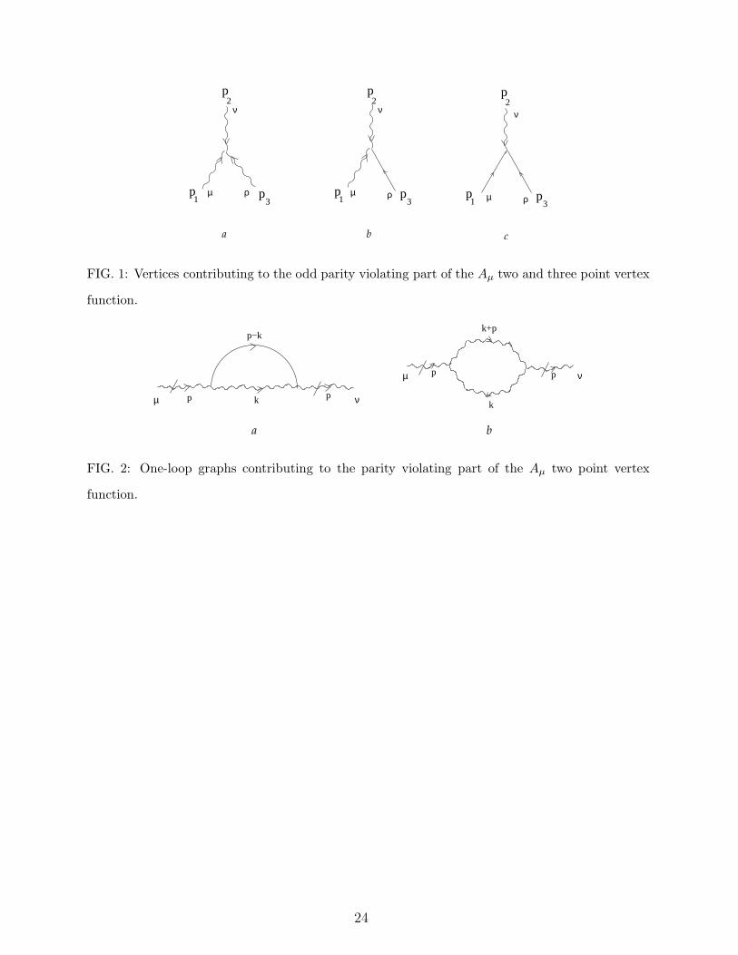
The relevant graphs are drawn in Fig. 3. Here we will present our results for zero and

nonzero temperature.

A. T = 0 results

Using the expressions for the propagators and vertices listed in the previous section, the

amplitudes for the graphs which contribute to the odd parity part of three point vertex

function of the gauge field are:

(1) Graph in Fig. 3a

Γ3aµνρ = −8g3

∫

T=0

d3k

(2π)3Dσα(k + p1)Dβτ (k − p3)Dξλ(k)ǫανβǫλµσǫτρξS1, (47)

where

S1 = sin(k ∧ p1) sin(k ∧ p3) sin[(k + p1) ∧ p2] (48)

= −1

4

{

sin(p1 ∧ p2) + sin[(2k + p2) ∧ p1] + sin[(2k + p1) ∧ p2] + sin[(2k + p1) ∧ p3]}

.

(2) Graph in Fig. 3b

Γ3bµνρ =

−112iv2g5

3

∫

T=0

d3k

(2π)3Dµα(k + p1)Dβρ(k − p3)∆σ(k)ǫ βα

ν S2, (49)

where

S2 = cos(k ∧ p1) cos(k ∧ p3) sin[(k + p1) ∧ p2] (50)

=1

4

{

sin(p1 ∧ p2) − sin[(2k + p2) ∧ p1] + sin[(2k + p1) ∧ p2] − sin[(2k + p1) ∧ p3]}

.

(3) Graph in Fig. 3c

Γ3cµνρ = −80v2g5

∫

T=0

d3k

(2π)3(p2 + k)νDρµ(k)∆σ(k + p1)∆σ(k − p3)S3, (51)

13

where

S3 = cos(k ∧ p2) cos(k ∧ p3) sin[(k + p2) ∧ p1] (52)

=1

4

{

sin(p2 ∧ p1) − sin[(2k + p1) ∧ p2] + sin[(2k + p2) ∧ p1] − sin[(2k + p2) ∧ p3]}

.

In the planar parts, which are the integrals containing the first term in S1, S2 and

S3, we separate the trigonometric factor and set equal to zero the external momenta in

the propagators. In the remaining (nonplanar) parts we approximate the sines by their

arguments and then perform the integrals.

It turns out that within our approximation, Γ3aµνρ does not possess an odd parity part. In

fact, because of momentum conservation it is readily seen that S1 becomes null if the sines

are replace by their arguments. We then consider separately the odd parity part of the other

contributions. We have

[

Γ3bµνρ

]

odd=

−112v2g5

3

∫

T=0

d3k

(2π)3

S2

[(k + p1)2 − m2] [(k − p3)2 − m2] [k2 − m2σ]

×{

−m2ǫµρν + m2

[

ǫρναkαkµ

[(k + p1)2 + ξm]− ǫµναkαkρ

[(k − p3)2 + ξm]

]

− ǫµραkαkν

}

,(53)

for the graph 3b and

[

Γ3cµνρ

]

odd= −80v2g5

∫

T=0

d3k

(2π)3

ǫραµkαkν

[(k + p1)2 − m2σ] [(k − p3)2 − m2

σ] [k2 − m2]S3. (54)

for the graph 3c. Proceeding now in the way above indicated we get

[

Γ3bµνρ

]

odd=

−112v2g5

3

{

[

Γ3bµνρ

]planar

odd+[

X3bµνρ

]

odd

}

, (55)

where

[

Γ3bµνρ

]planar

odd= sin(p1 ∧ p2)

∫

T=0

d3k

(2π)3

1

[k2 − m2]2 [k2 − m2σ]

×{

−m2ǫµρν + m2

[

ǫρναkαkµ

[k2 + ξm]− ǫµναkαkρ

[k2 + ξm]

]

− ǫµραkαkν

}

=

[ −mσ

12π(m + mσ)2

]

sin(p1 ∧ p2)ǫµρν (56)

14

and

[

X3bµνρ

]

odd=

∫

T=0

d3k

(2π)3

(− sin(2k + p2) ∧ p1 + sin(2k + p1) ∧ p2 − sin(2k + p1) ∧ p3)

[(k + p1)2 − m2] [(k − p3)2 − m2] [k2 − m2σ]

×{

−m2ǫµρν + m2

[

ǫρναkαkµ

[(k + p1)2 + ξm]− ǫµναkαkρ

[(k − p3)2 + ξm]

]

− ǫµραkαkν

}

=

[

m2 + mmσ + 2m2σ

30π(m + mσ)3

]

sin(p1 ∧ p2)ǫµρν . (57)

By summing (56) and (57) we obtain the total contribution from the graph 3b

[

Γ3bµνρ

]

odd=

28ig5v2

45π

[

(m2σ − 2m2 + 3mmσ)

(m + mσ)3

]

ǫµνρ sin(p1 ∧ p2). (58)

The computation for[

Γ3cµνρ

]

oddfollows similarly yielding

[

Γ3cµνρ

]

odd=

ig5v2

3π

[

13m2σ + 39mmσ + 28m2

(m + mσ)3

]

ǫµνρ sin(p1 ∧ p2), (59)

so that the complete result for one loop three point vertex function correction at T = 0 is

given by

[Γµνρ]odd =[

Γ3bµνρ

]

odd+[

Γ3cµνρ

]

odd

= − iv2g5

45π(m + mσ)3sin(p1 ∧ p2)ǫµρν

[

476m2 + 501mmσ + 167m2σ

]

. (60)

B. Results for T 6= 0

The amplitudes for T 6= 0 are associated with the same graphs as in the previous section

but using Eq. (46) in the corresponding analytic expressions. With the help of Feynman

parametric integrals the propagators are combined into a sum of terms with only one factor

in the denominator. The k0 integral is then performed by adequately closing the contour of

integration and applying the residue theorem. Afterwards the ~k integrals are calculated in

the static limit. We find

1. T 6= 0 part of the graph 3b

[

Γ3bµνρ

]T

odd=

−112v2g5

3sin(p1 ∧ p2)

15

×{

−2

∫ 1

0

dx

∫

T 6=0

d3k

(2π)3(1 − x)x

[

m2ǫµρν + ǫµραkαkν

(k2 − Λ21)

3

]

+ 6m2

∫ 1

0

dx

∫ 1

0

dy

∫

T 6=0

d3k

(2π)3[2 − y(1 − x)]xy2

[

ǫµανkαkρ + ǫµραkαkν

(k2 − Λ22)

4

]}

,(61)

where Λ21 = m2

σ(1 − x) + m2x and Λ22 = yΛ2

1, whereas, for the graph 3c

[

Γ3cµνρ

]T

odd= −80v2g5 sin(p1 ∧ p2)

∫ 1

0

dx x(1 +x

2)

∫

T 6=0

d3k

(2π)3

ǫµραkαkν

(k2 − Λ23)

3, (62)

where Λ23 = m2(1 − x) + m2

σx.

As a prototype for the calculation of the above expression we consider the typical integral

Iµρν =

∫

T 6=0

d3k

(2π)3

ǫµραkαkν

(k2 − Λ2)3

=

∫

T 6=0

d3k

(2π)3

[

g0νǫµρ0k20 + gνjǫµρik

ikj

(k2 − Λ2)3

]

, (63)

where Λ = Λi with i =, 1, 2, 3. After integrating over k0 we obtain

Iµρν = −2i

∫

d2k

(2π)2[g0νǫµρ0F1(~k

2) + gνiǫµρiF2(~k2)], (64)

where

F1(~k2) =

−1 + e2βωΛ(−1 − βωΛ + β2ω2Λ) + eβωΛ(2 + βωΛ + β2ω2

Λ)

16ω3Λ(eβωΛ − 1)3

β→0≃ 1

32ω3Λ

+ O(β3) (65)

and

F2(~k2) =

3 + e2βωΛ(3 + 3βωΛ + β2ω2Λ) + eβωΛ(−6 − 3βωΛ + β2ω2

Λ)

16ω5Λ(eβωΛ − 1)3

β→0≃ 1

2ω6Λβ

− 3

32ω5Λ

+ O(β4) (66)

The expressions in the right hand side of Eqs. (65) and (66) correspond to the high T

limit of F1 and F2, respectively. In this limit the integrals on the spatial components of k

are very simple, giving

Iµρν =−i

16π

[

1

Λǫµρν −

2

βΛ2gi

νǫµρi

]

+ O(β3). (67)

16

It remains to perform the Feynman parametric integrals which for expressions like (67) are

trivial.

Proceeding as in the example above, the relevant integrals may be straightforwardly

computed. We list the results for each contributing graph

[

Γ3bµνρ

]T

odd=

−iv2g5 sin(p1 ∧ p2)

π

{

1

21β

[

A1(4ǫµρν − giµǫiρν − gi

ρǫµiν) + A2giνǫµρi

]

+ A3ǫµρν

}

, (68)

where

A1 = 2[m2

σm2 − m4 + (m4 + m2m2

σ) ln( mmσ

)]

(m2 − m2σ)3

, (69)

A2 =m4

σ − m4 + 4m2m2σ ln( m

mσ)

(m2 − m2σ)3

, (70)

A3 =28

45(m + mσ)3(m2

σ − 2m2 + 3mmσ), (71)

and

[

Γ3cµνρ

]T

odd=

−80iv2g5 sin(p1 ∧ p2)

π

[

B1

βgi

νǫµρi + B2ǫµνρ

]

, (72)

where

B1 =1

32(m2 − m2σ)3

[

5m4σ − 12m2m2

σ + 7m4 − 4(2m2m2σ − 3m4) ln(

mσ

m)]

(73)

and

B2 =1

240(m + mσ)3(13m2

σ + 39mmσ + 28m2). (74)

Notice that the terms containing A3 and B2 coincide up to a sign with the expressions in

Eqs. (58) and (59), respectively, so that when computing the high temperature limit of the

three point vertex function they mutually cancel.

17

V. CONCLUSIONS

We can now summarize the results obtained in the previous sections.

(1) Zero temperature: For small momenta the corrections to the two and three point

vertex functions given in Eqs. (40) and (60) lead to the conclusion that the following action

is induced (see remark after Eq. (40))

ST=0ind =

κ1

2

∫

d3xǫµνρ

[

Aµ∂νAρ +2ig1

3Aµ ∗ Aν ∗ Aρ

]

, (75)

where

κ1 =2g4v2

3π

(2m + mσ)

(m + mσ)2(76)

and

g1 = g236m2 + 231mmσ + 77m2

σ

60(m + mσ)(2m + mσ). (77)

In the limit mσ = m which is relevant for the supersymmetric Chern-Simons-Higgs model

[21] a great simplification is achieved so that κ1 = g2

4πand g1 = 68

45g.

2) High temperature limit:

STind

β→0≃ κ2

2 β

∫

d3xǫ0ij

[

A0∂iAj +2ig2

3A0 ∗ Ai ∗ Aj

]

, (78)

where

g2 =g

168(m2 − m2σ)

×[

721m4 − 1248m2m2σ + 527m4

σ + (−1248m4 + 860m2m2σ) ln( m

mσ)

m2σ − m2 + 2m2 ln( m

mσ)

]

(79)

and

κ2 =2v2g4

π(m2 − m2σ)2

[m2σ − m2 + 2m2 ln(

m

mσ

)]. (80)

Here again a great simplification occurs for equal masses: κ2 = 14πv2 and g2 = −839g

252.

The leading noncommutative corrections to the two point vertex function were also ob-

tained and are given by

18

Πodd0i (T = 0) =

g2p

16π(m − ξ)ǫ0ijp

j , (81)

at zero temperature, and

πNC0i (p0 = 0; T ) = − p2

8πǫ0ijp

jT

×{

2(ve2)2 ∂

∂m2σ

[

(m4 log(m/T ) − m4σ log(mσ/T ))

m2σ − m2

]

+g2

2[2m log(m/T ) + (m − ξ)F ]

}

, (82)

in the high temperature limit. From Eqs. (81) and (82) we can see that the commutativity

can be recovered straightforwardly, by considering the limit p → 0. In other words, there

are no infrared UV/IR singularity appearing in this limit. Furthermore, looking at the finite

temperature result, Eq. (82), in the static limit we can extract the leading behavior in

the high temperature regime and first order correction in the noncommutative parameter

as being proportional to T logT . So, our calculation provides a logarithm correction to the

result obtained in [16] for the commutative version of the same model.

The results in Eqs. (75) and (78) are formally invariant under small gauge transforma-

tions. Notice however that, because of the spontaneous breakdown of the symmetry, such

property will be certainly lost whenever other corrections are incorporated. This is already

indicated by the form of the noncommutative corrections in Eqs. (81) and (82).

It should be pointed out that previous studies of noncommutative gauge theories have

shown that, as it happens in the commutative non-Abelian CS model, invariance under

large gauge transformation requires that the CS coefficient be quantized [13]. At finite

temperature, the verification of this property for the effective action is a highly non trivial

task which probably involves all orders of perturbation and also other (nonlocal) interactions.

Even in the commutative setting, invariance under large non-Abelian gauge transformation

was verified only in simplified situations [22]. In our calculations invariance under large

gauge transformation is certainly partially broken. In spite of that, our results should still

be a good approximation for small couplings.

19

VI. ACKNOWLEDGMENTS

This work was partially supported by Conselho Nacional de Desenvolvimento Cientıfico

e Tecnologico (CNPq) and Fundacao de Amparo a Pesquisa do Estado de Sao Paulo

(FAPESP).

APPENDIX A: AN USEFUL INTEGRAL

In this appendix, we will compute a basic integral that appear in Eq. (30). Let us define

I(m) ≡∫ ∞

0

k2dkJ1(kp)coth (βwm/2)

wm

.

=

∫ ∞

0

k2dkJ1(kp)1

wm+ 2

∫ ∞

0

k2dkJ1(kp)nB(wm)

wm. (A1)

Using that

1

ex − 1=

∞∑

n=1

e−nx (A2)

we can rewrite I(m) as

I(m) =

∫ ∞

m

dx√

x2 − m2J1[p√

x2 − m2]

+ T 2∞∑

0

∫ ∞

βm

dx√

x2 − βm2J1[τ√

x2 − b2m2]e−nx

= m2

∫ ∞

1

dy√

y2 − 1J1[pm√

y2 − 1]

+ m2∞∑

0

∫ ∞

1

dy√

y2 − 1J1[τβm√

y2 − 1]e−βmyn (A3)

These integrals can be evaluated using the standard result [23]

∫ ∞

1

dx(x2 − 1)ν/2e−αxJν [β√

x2 − 1] =

√

2

πβν(α2 + β2)−ν/2−1/4Kν+1/2(

√

α2 + β2). (A4)

Then, it is straightforward to verify that

20

I(m) = m2e−pm

[

1

pm+

1

(pm)2

]

+ pmT 2

∞∑

n=1

e−βm√

n2+τ2

n2 + τ 2+ pT 3

∞∑

n=1

e−βm√

n2+τ2

(n2 + τ 2)3/2. (A5)

Note that here we have computed both zero temperature and finite temperature parts

together, although in sections II and III they occur separately.

[1] Dunne G V 1999 Aspects of Chern Simons Theory. Les Houches Summer School in Theoretical

Physics: Topological Aspects of Low Dimensional Physics, Les Houches 1968

[2] Coleman S and Hill B 1985 Phys. Lett. B 159 184

[3] Jackiw R 2002 Nucl. Phys. Proc. Suppl. 108 30

[4] Seiberg N and Witten E 1999 JHEP 9909 032

[5] Minwalla S, Van Raamsdonk M and Seiberg N 2000 JHEP 0008 008

[6] Girotti H O, Gomes M, Rivelles V O and da Silva A J 2000 Nucl. Phys. B 587 299

Girotti H O, Gomes M, Petrov A Yu, Rivelles V O and da Silva A J 2001 Phys. Lett. B 521

119

[7] Bichl A, Grimstrup J, Putz V and Schweda M 2000 JHEP 0007 046.

Das A and Sheikh-Jabbari M M 2001 JHEP 0106 028

Martin C P 2001 Phy. Lett. B 515 185

[8] Fischler W, Gommis J, Gorbatov E, Kashani-Poor A, Paban S and Pouliot P 2000 JHEP 05

024

Landsteiner K, Lopez E and Tytgat M H G 2000 JHEP 09 027

Arcioni G and Vazquez-Mozo M A 2000 JHEP 01 028

Brandt F T, Das A, Frenkel J, McKeon D G C and Taylor J C 2002 Phys. Rev. D 66 045011

Chandrasekhar B and Panigrahi P K 2003 JHEP 0303 015

[9] Kapusta J I 1979 Nucl. Phys. B 148 461

Arnold P, Vokos S, Bedaque P and Das A 1993 Phys. Rev. D 47 4698

[10] Deser S, Jackiw R and Templeton S 1982 Annals Phys. 140 372, 1988 Erratum-ibid. 185:406,

2000 Annals Phys. 281 409

21

Redlich A 1984 Phys.Rev. D 29 2366

Redlich A 1984 Phys.Rev.Lett. 52

[11] Pisarski R and Rao S 1985 Phys. Rev. D 32 2081.

[12] Brandt F, Das A and Frenkel J 2000 Phys. Lett. B 494 339.

[13] Nair V P and Polychronakos A P 2001 Phys. Rev. Lett. 87 030403

Sheikh-Jabbari M M 2001 Phys. Lett. B 510 247

Bak D, Lee K and Park J H 2001 Phys. Rev. Lett. 87 030402

Chen Guang-Hong and Wu Yong-Shi 2001 Nucl. Phys. B 593 562

[14] Khlebinikov S and Shaposhnikov M 1991 Phys Lett B 254 148

Khare A, MacKenzie R, Paranjape M and Panigrahi P 1995 Phys. Lett. B 355 236

Khare A, MacKenzie R and Paranjape M 1995 Phys. Lett. B 343 239

Chen L, Dunne G, Haller K and Lim-Lombridas E 1995 Phys. Lett. B 348 468.

Kao H 1998 Phys. Rev. D 57 7416

[15] Brandt F T, Frenkel J and McKeon D G C 2002 Phys. Rev. D 65 125029

[16] Alves V S, Das A, Dunne G V and Perez S 2002 Phys. Rev. D 65 085011

[17] Gronewold H J 1946 Physica (Amsterdan) 12 405

Weyl H 1949 Z. Physik 46 1

Moyal J E 1949 Proc. Cambridge Philos. Soc. 45 99

Doplicher S, Fredenhagem K and Roberts J E 1995 Commun. Math. Phys. 172 187

[18] Douglas M R and Nekrasov N A 2001 Rev. Mod. Phys. 73 977

Szabo R J 2003 Phys. Rept. 378 207

Gomes M 2002 V in Proceedings of the XI Jorge Andre Swieca Summer School, edited by

Alves G, Eboli O and Rivelles V, World Scientific

Girotti H 2003 Noncommutative Quantum Field Theory hep-th/0301237

[19] Lewin L 1958 Dilogarithms and associated functions (London: Macdonald)

[20] Kapusta J I 1993 Finite-temperature field Theory (Cambridge)

[21] Kao H-C, Lee K, Lee C, and Lee T 1994 Phys. Lett. B 341 181

[22] Dunne G, Lee K and Lu C 1997 Phys. Rev. Lett. 78 3434

Deser S, Griguolo L and Seminara D 1997 Phys. Rev. Lett. 79 1976

Deser S, Griguolo L and Seminara D 1998 Phys. Rev. D 57 7444

Deser S, Griguolo L and Seminara D 1998 Commun. Math. Phys. 197 443

22

Deser S, Griguolo L and Seminara D 2003 Phys Rev D 67 065016

Fosco C D, Rossini G L and Schaposnik F A 1997 Phys. Rev. Lett. 79 1980,

Fosco C D, Rossini G L and Schaposnik F A 1997 Phys. Rev. Lett. 79 4296(E)

Brandt F T, Das A and Frenkel J 2002 Phys. Rev. D 65 065013

Brandt F T, Das A, Frenkel J, Pereira S and Taylor J C 2001 Phys. Rev. D 64 065018

[23] Gradshteyn I S and Ryzhik M 1980 Table of Integral, Series and Products Academic Press

New York

23

p1

p2

p3

µ

ν

ρ

a

ν

µ ρ p3

p1

p2

b

p1 p

3

p2

ν

µ ρ

c

FIG. 1: Vertices contributing to the odd parity violating part of the Aµ two and three point vertex

function.

pp

k

k+p

µ ν

b

νpk

p−k

µ p

a

FIG. 2: One-loop graphs contributing to the parity violating part of the Aµ two point vertex

function.

24

p1k + p

1k + p2

+

kp

1

p2

p3

ν

ρ

b

µ

p2

p1k + p

1k + p2

+

kp1 p

3

µ ρ

a

ν

p1

p2

p3

p1k + p

1k + p2

+

k

ν

µ ρ

c

FIG. 3: One-loop graphs contributing to the parity violating part of the Aµ three point vertex

function.

25