Proceedings of CARI 2016 - Hal-Inria

HAL Id: hal-01350039https://hal.inria.fr/hal-01350039v2

Submitted on 2 Aug 2016

HAL is a multi-disciplinary open accessarchive for the deposit and dissemination of sci-entific research documents, whether they are pub-lished or not. The documents may come fromteaching and research institutions in France orabroad, or from public or private research centers.

L’archive ouverte pluridisciplinaire HAL, estdestinée au dépôt et à la diffusion de documentsscientifiques de niveau recherche, publiés ou non,émanant des établissements d’enseignement et derecherche français ou étrangers, des laboratoirespublics ou privés.

Proceedings of CARI 2016Moussa Lo, Eric Badouel, Nabil Gmati

To cite this version:Moussa Lo, Eric Badouel, Nabil Gmati. Proceedings of CARI 2016. Moussa Lo; Eric Badouel; NabilGmati. Oct 2016, Hammamet, Tunisia. pp.513, 2016. hal-01350039v2

https://hal.inria.fr/hal-01350039v2

https://hal.archives-ouvertes.fr

Proceedings of CARI 2016 Actes du CARI 2016

Hammamet, Tunisia, October 2016

EDITORS : MOUSSA LO - ERIC BADOUEL - NABIL GMATI

AVANT-PROPOS Le CARI, Colloque Africain sur la Recherche en Informatique, fruit d’une coopération internationale rassemblant universités africaines, centres de recherche français et organismes internationaux, tient sa treizième édition cette année en Tunisie Organisé tous les deux ans en Afrique, ses précédentes éditions se sont tenues à Yaoundé en 1992, à Ouagadougou en 1994, à Libreville en 1996, à Dakar en 1998, à Antananarivo en 2000, à Yaoundé en 2002, à Hammamet en 2004, à Cotonou en 2006, à Rabat en 2008, à Yamoussoukro en 2010, à Alger en 2012 et à Saint-Louis du Sénégal en 2014.

Le colloque est co-organisé par l'Institut National de Recherche en Informatique et en Automatique (Inria), l'Institut de Recherche pour le Développement (IRD), le Centre de coopération Internationale en Recherche Agronomique pour le Développement (Cirad), le Centre International des Mathématiques Pures et Appliquées (Cimpa), et l'Agence Universitaire de la Francophonie (AUF). Cette treizième édition, confiée à l’Ecole Nationale d’Ingénieur de Tunis (ENIT), sous la coordination du professeur Nabil Gmati , a bénéficié d’un large soutien des institutions universitaires suivantes : la Faculté des Sciences de Tunis (FST), l’Ecole Polytechnique de Tunisie (EPT), l’Ecole Nationale Supérieure d’Informatique (ENSI), l’Ecole Supérieure privée d’Ingénierie et de Technologies (ESPRIT) et de l’Ecole Supérieure des Télécommunications (Sup’Com). Quatre universités du grand Tunis se sont également associées pour la réussite de cette nouvelle édition du colloque : l’Université Tunis El Manar (UTM), l’Université de la Manouba (UM), l’Université de Carthage (UC), l’Université Virtuelle de Tunis (UVT). Ces universités regroupent l'essentiel des institutions scientifiques du grand Tunis. Le CARI a également bénéficié du soutient de l’Institut Français de Tunisie (IFT).

Le CARI est devenu un lieu privilégié de rencontre et d’échanges de chercheurs et décideurs africains et internationaux de haut niveau dans les domaines de l’informatique et des mathématiques appliquées. Le programme scientifique, qui reflète la richesse et la diversité de la recherche menée sur le continent africain, met un accent particulier sur les travaux susceptibles de contribuer au développement technologique, à la connaissance de l'environnement et à la gestion des ressources naturelles. Ce programme se décline en 51 communications scientifiques, sélectionnées parmi 130 articles soumis, et des conférences invitées présentées par des spécialistes de renommée internationale. L’Ecole de recherche Cimpa, qui a porté cette année sur sur les « mathématiques de la biologie », remplace désormais les traditionnels tutoriels organisés en marge du CARI. Bien plus qu'un simple colloque, le CARI est un cadre dynamique de coopération, visant à rompre l'isolement et à renforcer la communauté scientifique africaine. Toute cette activité repose sur l'action forte et efficace de beaucoup d'acteurs. Nous remercions tous nos collègues qui ont marqué leur intérêt dans le CARI en y soumettant leurs travaux scientifiques, les relecteurs qui ont accepté d’évaluer ces contributions et les membres du Comité de programme qui ont opéré à la sélection des articles. L’ensemble des activités liées au CARI sont répertoriées sur le site officiel du CARI (http://www.cari-info.org/) maintenu par l’équipe du professeur Mokhtar Sellami de l’université d’Annaba. Laura Norcy, d'Inria, a apporté son soutien pour la coordination de cette manifestation. L’organisation du colloque a reposé sur le comité local d'organisation, mis en place par le professeur Nabil Gmati. Que les différentes institutions, qui, par leur engagement financier et par la participation de leurs membres, apportent leur soutien, soient également remerciées, et, bien sûr, toutes les institutions précédemment citées, qui soutiennent le CARI au fil de ses éditions. Pour les organisateurs Moussa Lo, Président du CARI Eric Badouel, Secrétaire du Comité permanent du CARI Nabil Gmati, Organisateur du CARI 2016

FOREWORD

CARI, the African Conference on Research in Computer Science, outcome of an international cooperation involving African universities, French research institutes, and international organizations, introduces this year its thirteenth edition in Tunisia. Organized every two years in Africa, its preceding editions were held in Yaoundé in 1992, in Ouagadougou in 1994, Libreville in 1996, Dakar in 1998, Antananarivo in 2000, Yaoundé in 2002, Hammamet in 2004, Cotonou in 2006, Rabat in 2008, Yamoussoukro in 2010, Algers in 2012, and Saint-Louis du Senegal in 2014. The conference is organized by Institut National de Recherche en Informatique et en Automatique (Inria), the Institut de Recherche pour le Développement (IRD), the Centre de coopération Internationale en Recherche Agronomique pour le Développement (Cirad), the International Center for Pure and Applied Mathematics (ICPAM) and the Agence Universitaire de la Francophonie (AUF). This thirteenth edition, entrusted to ENIT (Ecole Nationale d’Ingénieurs de Tunis), under the coordination of Professor Nabil Gmati, has profited from a generous support of the following academic institutions: Faculté des Sciences de Tunis (FST), Ecole Polytechnique de Tunisie (EPT), Ecole Nationale Supérieure d’Informatique (ENSI), Ecole Supérieure privée d’Ingénierie et de Technologies (ESPRIT) and Ecole Supérieure des Télécommunications (Sup’Com). Four universities of the greater Tunis, which are the main scientific institutions of Tunis, also joined for the success of CARI: University of Tunis El Manar (UTM), La Manouba University (UM), University of Carthage (UC), Université Virtuelle de Tunis (UVT). CARI also acknowledge supports from the Institut Français de Tunisie ( IFT).

CARI has evolved into an internationally recognized event in Computer Science and Applied Mathematics. The scientific program, which reflects the richness and the diversity of the research undertaken on the African continent with a special emphasis on works related to the development of new technologies, knowledge in environmental sciences and to the management of natural resources, consists of 51 scientific contributions, selected from 130 submissions, together with invited talks delivered by acknowledged specialists. From now on, the tutorials that used to precede the CARI are replaced by a CIMPA-ICPAM Research school that puts a focus on some particular topic relevant to CARI’s community. For this edition the research school was dedicated to the “Mathematics for Biology”. More than a scientific gathering, CARI is also a dynamic environment for cooperation that brings together African researchers with the end result to break the gap of isolation. The successes of such an initiative rely on the contribution of many actors. We wish first to thank our colleagues who showed their interest in CARI by submitting a paper, the referees who accepted to evaluate these contributions, and the members of the Program Committee who managed the selection of papers. This process rested on the CARI official site (http://www.cari-info.org/) maintained by the team of professor Mokhtar Sellami at the University of Annaba. Laura Norcy, from Inria, was involved in numerous activities for the coordination of the Event. The local organization has been handled by the local organization committee under the supervision of professor Nabil Gmati. Thanks also for all the institutions that support and provide funding for CARI conferences and related activities, and all the institutions involved in the organization of the conference. For the organizing committee Moussa Lo, Chairman of CARI Eric Badouel, Secretary of CARI Permanent Committee Nabil Gmati, Chair of CARI 2016

Comité de Programme / Program Committee Modélisation des systèmes complexes / Complex System Modelling Arnaud GRIGNARD, IRD/UPMC, France Bernard CAZELLES, UMPC, France Christophe LETT, IRD, France Rachid MCHICH, ENCGT - Morocco Tri NGUYEN-HUU, IRD, France Benjamin ROCHE, IRD, France Signal, image et multimédia / Signal, Images and Multimedia Ezzine ABDELHAk, ENSAT, Morocco Olivier ALATA, Univ. Saint-Etienne, France Tarik Boujiha, Univ. ibn tofail-kénitra, Morocco Mohamed DAOUDI, Telecom Lille/LIFL, France Denis HAMAD, Univ. du Littoral Côte d'Opale, France Ahmed HAMMOUCH, CNRST, Morocco Lloussaine MASMOUDI, Univ. Mohammed V, Rabat, Morocco Ahmed MOUSSA, LabTIC ENSAT, Morocco Rachid OULAD HAJ THAMI, ENSIAS, Marocco Abderrahmane SBIHI, ENSA Tanger, Morocco Raja Touahni, Université Ibn Tofail, Morocco Lynda ZAOUI, Oran University, Algeria Djemel ZIOU, Sherbrooke University, Canada Calcul scientifique et parallélisme / Scientific Computing and Parallelism Jocelyne ERHEL, Inria, France El Mostafa DAOUDI, Univ. Mohamed I, Oujda, Morocco Laurent DEBREU, Inria, France Laura GRIGORI, Inria, France Abdou GUERMOUCHE, Univ. Bordeaux, France Pierre MANNEBACK, University of Mons, Belgium Maher MOAKHER, Ecole Nationale d'Ingénieurs de Tunis, Tunisia Yanik NGOKO, Univ. Paris 13, France Boniface NKONGA, University of Nice-Sophia-Antipolis Patrice QUINTON, ENS Rennes, France Denis TRYSTRAM, Grenoble Institute of Technologu, France Intelligence artificielle et environnements informatique pour l'apprentissage humain / Artificial Intelligence and Computer-based Collaborative Environmental Meziane AIDER, USTHB, Algeria Djamil AISSANI, Univ. Bejala, Algeria Monique BARON, Sorbonne UPMC, Lip6, France Mahieddine DJOUDI, Poitiers University, France Abdellatif ENNAJI, Univ. Rouen, France Mokhtar SELLAMI, Annaba University, Algeria Hassina SERIDI, Annaba University,, Algeria Christophe SIBERTIN-BLANC, Irit, France Salvatore TABBONE, Univ. de Lorraine, France Claude TANGHA, FTIC, Yaoundé, Cameroon

Applications avancées en Génie logiciel / Software engineering and advances applications Pascal ANDRE, LINA, University of Nantes, France Eric BADOUEL, Inria Rennes, France Kamel BARKAOUI, Cedric, CNAM, France François CHAROY, LORIA Univ. Henri Poincaré, France Yliès FALCONE, Inria Grenoble, France Christian FOTSING, Institut Universitaire de la Côte, Cameroon Georges-Edouard KOUAMOU, ENSP Yaoundé I University, Cameroon Damien ROBERT, Inria Bordeaux, France William SHU, University of Buea, Cameroon François VERNADAT, LAAS-CNRS, Toulouse, France Extraction et Organisation des Connaissances / Knowledge Organization and Mining Hugo ALATRISTA-SALAS, Pontificia Universidad Catolica del Peru Jérôme AZE, LIRMM, University of Montpellier 2, France Nicolas BECHET, Université de Bretagne Sud Hacene BELHADEF, University of Constantine, Algeria Béatrice BOUCHOU MARKHOFF, Univ. François Rabelais de Tours, France Ibrahim BOUNHAS, LISI, Carthage University, Tunisia Sandra BRINGAY, LIRMM, University Paul Valéry, France Patrice BUCHE, Supagro INRA, France Gaoussou CAMARA, Univ. Alioune Diop, Bambey, Senegal Célia DA COSTA TEREIRA, Univ. Nice Sophia Antipolis, France Cheikh Taliboula DIOP, UGB, Saint-Louis, Senegal Bilel ELAYEB, ENSI, Tunisia Dino IENCO, IRSTEA, France Clement JONQUET, LIRMM, University of Montpellier 2, France Eric KERGOSIEN, University of Lille, France Philippe LEMOISSON, TETIS, Cirad, France Moussa LO, Univ. Gaston Berger, Senegal Cédric LOPEZ, Viseo Research Center, France Isabelle MOUGENOT, Espace-Dev, University of Montpellier 2, France Mathieu ROCHE, TETIS, Cirad, France Fatiha SAIS, LRI, Paris Sud University, France Hassan SANEIFAR, Raja University, Iran Joël SOR, Cirad, France Maguelonne TEISSEIRE, TETIS, Irstea, France Systèmes distribués et réseaux / Distributed systems and networks Soraya AIT CHELLOUCHE, University of Rennes, France Olivier BARAIS, University of Rennes, France Melhem EL HELOU, Univ. Saint-Joseph de Beyrouth, Lebanon Davide FREY, Inria Rennes, France Abdoulaye GAMATIE, LIRMM, France Bamba GUEYE, UCAD, Dakar, Senegal Jean-Claude HOCHON, Airbus SAS, France Michel HURFIN, Inria Rennes, France Marc IBRAHIM, Saint-Joseph University, Lebanon Samer LAHOUD, University of Rennes, France Maryline LAURENT, Telecom Sud-Paris, France Moussa LO, Univ. Gaston Berger, Senegal Pascal LORENZ, Univ. Haute Alsace, France Stéphane MAAG, Telecom Sud-Paris, France Ludovic ME, Supélec Rennes, France Congduc PHAM, University of Pau, France

Pierre ROLIN, Institut Mines-Télécom, France Abed Ellatif SAMHAT, Lebanese University, Lebanon Ousmane THIARE, UGB, Saint-Louis, Senegal César VIHO, Univ. De Rennes 1, France Mathématique pour la biologie / Mathematical biology Nahla ABDELLATIF, ENSI-ENIT, Tunisia Julien ARINO, University of Manitoba, Canada Abdon ATANGANA, University of Free State, South Africa Mejdi AZAIEZ, University of Bordeaux, France Fethi Bin Muhammad BELGACEM, PAAET, Kuwait Monia BELLALOUNA, ENSI, Tunisia Hend BEN AMEUR, LAMSIN-ENIT and IPEST, Tunisia Faker BEN BELGACEM, UTC Compiègne, France Slimane BEN MILED, University Tunis el Manar, Tunisia Adel BLOUZA, University of Rouen, France Fabien CAMPILLO, Inria, France Nicolas CHAMPAGNAT, Inria, France Nadia CHOULAIEB, ENIT, Tunisia Jean CLAIRAMBAULT, Inria Paris- LJLL, UMPC, France Yves DUMONT, Cirad, France Radhouene FEKIH SALEM, University of Monastir, Tunisia Jean-Frédéric GERBEAU, Inria, France Nabil GMATI, LAMSIN-ENIT, Tunisia Lamia GUELLOUZ, ENIT, Tunisia Abderrahmane HABBAL, University of Nice-Inria, France Ridha HAMBLI, Polytech Orleans, France Nejla HARIGA-TATLI, INAT-LAMSIN, Tunisia Yousri HENCHIRI, University of Montpellier 2, France Abderrahman IGGIDR, Inria, France Adil KHALIL, University of Marrakech, Morocco Michel LANGLAIS, University of Bordeaux, France Claude LOBRY, University of Nice, France John MADDOCKS, EPFL, Switzerland Sylvie MELEARD, Ecole Plotechnique, France Ali MOUSSAOUI, Tlemcen University, Algeria Tri NGUYEN-HU, IRD, France Gauthier SALLET, Université de Lorraine, Nancy, France Tewfik SARI, IRSTEA, Montpellier, France Suzanne TOUZEAU, INRA-Inria, France Hatem ZAAG, University Paris 13, France Nejib ZEMZEMI, Inria, France

LISTE DES RELECTEURS – LIST OF REFEREES

Ezzine ABDELHAK Nahla ABDELLATIF Meziane AIDER Soraya AIT CHELLOUCHE Abdelaziz AIT MOUSSA Olivier ALATA Hugo ALATRISTA-SALAS Pascal ANDRE Julien ARINO Abdon ATANGANA Mejdi AZAIEZ Jérôme AZE Eric BADOUEL Olivier BARAIS Kamel BARKAOUI Monique BARON Nicolas BECHET Fethi Bin Muhammad BELGACEM Hacene BELHADEF Monia BELLALOUNA Hend BEN AMEUR Faker BEN BELGACEM Slimane BEN MILED Fethi BIN MUHAMMAD BELGACEM Adel BLOUZA Béatrice BOUCHOU MARKHOFF Tarik BOUJIHA Ibrahim BOUNHAS Sandra BRINGAY Patrice BUCHE Fabien CAMPILLO Gaoussou CAMARA Jérôme CANALS Bernard CAZELLES Nicolas CHAMPAGNAT François CHAROY Nadia CHOULAIEB Jean CLAIRAMBAULT Célia DA COSTA PEREIRA El Mostafa Daoudi Mohamed DAOUDI Laurent DEBREU Cheikh Talibouya DIOP Aissani DJAMIL

Mahieddine DJOUDI Yves DUMONT Bilel ELAYEB Melhem EL HELOU Abdellatif ENNAJI Jocelyne ERHEL Radhouene FEKIH SALEM Davide FREY Yles FALCONE Christian FOTSING Abdoulaye GAMATIE Jean-Frédéric GERBEAU Nabil GMATI Arnaud GRIGNARD Laura GRIGORI Lamia GUELLOUZ Bamba GUEYE Abdou GUERMOUCHE Abderrahmane HABBAL Kais HADDAR Denis HAMAD Ridha HAMBLI Ahmed HAMMOUCH Nejla HARIGA-TATLI Seridi HASSINA Yousri HENCHIRI Jean-Claude HOCHON Michel HURFIN Marc IBRAHIM Dino IENCO Abderrahman IGGIDR Clement JONQUET Eric KERGOSIEN Adil KHALIL Georges-Edouard KOUAMOU Samer LAHOUD Michel LANGLAIS Maryline LAURENT Philippe LEMOISSON Christophe LETT Moussa LO Claude LOBRY Cédric LOPEZ Pascal LORENZ Stéphane MAAG John MADDOCKS

Pierre MANNEBACK Lhoussaine MASMOUDI Rachid MCHICH Ludovic ME Sylvie MELEARD Nizar MESSAI Maher MOAKHER Isabelle MOUGENOT Ahmed MOUSSA Ali MOUSSAOUI Yanik NGOKO Tri NGUYEN-HUU Boniface NKONGA Rachid OULAD HAJ THAMI Congduc PHAM Patrice QUINTON Damien ROBERT Benjamin ROCHE Mathieu ROCHE Pierre ROLIN Gauthier SALLET Abed Ellatif SAMHAT HASSAN SANEIFAR Tewfik SARI Abderrahmane SBIHI Christophe SIBERTIN-BLANC Fathia SAIS Idrissa SARR Mokhtar SELLAMI William SHU Yahya SLIMANI Joël SOR Salvatore TABBONE Claude TANGHA Maguelonne TEISSEIRE Ousmane THIARE Raja TOUAHNi Suzanne TOUZEAU Denis TRYSTRAM François VERNARDAT César VIHO Hatem ZAAG Lynda ZAOUI Nejib ZEMZEMI Djemel ZIOU

TABLE DES MATIERES / TABLE OF CONTENTS Coupled bio-physical models for the transport of banana shrimps of the Sofala Bank, Mozambique Bernardino Sergio Malauene, Atanasio Brito, Coleen L. Moloney, Michael J. Roberts, Francis Marsac, Pierrick Penven, Christophe Lett ........................................................................................................................ 1 – 7 Novel method to find directed community structures based on triads cardinality. Félicité Gamgne Domgue, Norbert Tsopze, René Ndoundam …………………................................................ 8 – 15 A comparative study of three membrane fouling models: Towards a generic model for optimization purposes Nesrine Kalboussi, Jérôme Harmand, Nihel Ben Amar, F. Ellouze ................................................................... 16 – 26 Well’s location in porous media using topological asymptotic expansion Wafa Mansouri, Thouraya Nouri Baranger, Hend Ben Ameur, Nejla Tlatli ....................................................... 27 – 34 Data assimilation for coupled models. Toward variational data assimilation for coupled models: first experiments on a diffusion problem Rémi Pellerej, Arthur Vidard, Florian Lemarié ................................................................................................... 35 – 42 Calcul numérique de solutions de l'équation de Schrödinger non linéaire faiblement amortie avec défaut Laurent Di Menza, Olivier Goubet, Emna Hamraoui, Ezzeddine Zahrouni ........................................................ 43 – 53 Towards a recommender system for healthy nutrition. An automatic planning-based approach Yanik Ngoko ....................................................................................................................................................... 54 – 62 Algorithmes hybrides pour la résolution du problème du voyageur de commerce Baudoin Tsofack Nguimeya, Mathurin Soh, Laure Pauline Fotso ...................................................................... 63 – 74 A systematic approach to derive navigation model from data model in web information systems Mohamed Tahar Kimour, Yassad-Mokhtari Safia ............................................................................................ 75 – 83 Réconciliation par consensus des mises à jour des répliques partielles d’un document structuré Maurice Tchoupé Tchendji, William M. Zekeng Ndadji .................................................................................... 84 – 96 Un dépliage par processus pour calculer le préfixe complet des réseaux de Petri Médésu Sogbohossou, Antoine Vianou ……………………………………………......................................... 97 – 108 Modeling User Interactions in Dynamic Collaborative Processes using Active Workspaces Robert Fondze Jr Nsaibirni, Gaëtan Texier …………………........................................................................... 109 – 116 On Distributing Bayesian Personalized Ranking from Implicit Feedback Modou Gueye …………………………………………………………............................................................ 117 – 125 Requêtes XPath avec préférences structurelles et évaluations à l'aide d'automates Maurice Tchoupé Tchendji, Brice Nguefack ...................................................................................................... 126 – 137 Empirical study of LDA for Arabic topic identification Marwa Naili, Anja Habacha Chaibi, Henda Ben Ghézala ................................................................................... 138 – 145 Approche hybride pour le développement d’un lemmatiseur pour la langue arabe Mohamed Boudchiche, Azzeddine Mazroui ....................................................................................................... 146 – 153 Overview of the social information’s usage in information retrieval and recommendation systems Abir Gorrab, Ferihane Kboubi, Henda Ben Ghezala ........................................................................................... 154 – 161 Vers un système iconique d’aide à la décision pour les praticiens de la médecine traditionnelle Appoh Kouame, Konan Marcelin Brou, Moussa Lo, Jean Baptiste Lamy ......................................................... 162 – 173

Nouvelle taxonomie des méthodes de classification basée sur l’Analyse de Concepts Formels Marwa Trabelsi, Nida Meddouri, Mondher Maddouri ...................................................................................... 174 – 181 Kernel-based performance evaluation of coded QAM systems Pasteur Poda, Samir Saoudi, Thierry Chonavel, Frédéric Guilloud, Thédore Tapsoba ..................................... 182 – 191 Management of Low-density Sensor-Actuator Network in a Virtual Architecture Vianney Kengne Tchendji, Blaise Paho Nana ................................................................................................... 192 – 202 Centre of Mass of single coverage: A comparative study with simulated annealing for mesh router placement in rural regions Jean Louis Fendji Kedieng Ebongue, Christopher Thron ................................................................................... 203 – 214 Linear Token-Based MAC protocol for linear sensor network El Hadji Malick Ndoye, Ibrahima Niang, Frédérique Jacquet, Michel Misson ................................................ 215 – 222 Méthode Tabou d'allocation des slots de fréquence requis sur chaque lien d’un réseau optique flexible Beman Hamidja Kamagaté, Michel Babri, Bi Tra Gooré, Konan Marcelin Brou ............................................. 223 – 232 Evidential HMM Based Facial Expression Recognition in Medical Videos Arnaud Ahouandjinou, Eugène C. Ezin, Koukou Assogba, Cina Motamed, Mikael A. Mousse, Bethel C.A.R.K. Atohoun ................................................................................................................................... 233 – 242 Tatouage vidéo dynamique et robuste basé sur l’insertion multi-fréquentielle Sabrine Mourou, Asma Kerbiche, Ezzedine Zagoubra ...................................................................................... 243 – 251 Dynamic Pruning for Tree-based Ensembles Mostafa El Habib Daho, Mohammed El Amine Lazouni, Mohammed Amine Chikh ..................................... 252 – 261 Fast Polygons Fusion for Multi-Views Moving Object Detection from Overlapping Cameras Mikaël Ange Mousse, Cina Motamed, Eugène C. Ezin ..................................................................................... 262 – 268 A multi-agent model based on Tabu Search for the permutation flow shop problem minimizing total flowtime Soumaya Ben Arfa, Olfa Belkahla Driss ........................................................................................................... 269 – 276 Formation de coalitions A-core: S-NRB Pascal François Faye, Mbaye Sene, Samir Aknine ........................................................................................... 277 – 288 Towards an intelligent prognostic approach based on data mining and knowledge management Safa Ben Salah, Imtiez Fliss, Moncef Tagina ................................................................................................... 289 – 299 Amélioration de la visite de classe de l’enseignement technique : intégration d’un dispositif de médiation Frédéric T. Ouédraogo, Daouda Sawadogo, Solange Traoré, Olivier Tindano ................................................. 300 – 311 Efficient high order schemes for stiff ODEs in cardiac electrophysiology Charlie Douanla Lontsi, Yves Coudière, Charles Pierre ..................................................................................... 312 – 319 A model of flocculation in the chemostat Radhouane Fekih-Salem, Tewik Sari ................................................................................................................. 320 – 331 Modeling the dynamics of cell-sheet: Fisher-KPP equation to study some predictions on the injured Cell sheet Mekki Ayadi, Tunisia, Abderahmane Habbal, Boutheina Yahyaoui ................................................................. 332 – 343 Global weak solution to a 3D Kazhikhov-Smagulov model with Korteweg stress Caterina Calgaro, Meriem Ezzoug, Ezzedine Zahrouni .................................................................................... 344 – 355

Theoretical Analysis of a Water Wave Model using the Diffusive Approach Olivier Goubet, Imen Manoubi ......................................................................................................................... 356 – 366 Mathematical modeling of fouling membrane in an anaerobic membrane bioreactor Boumediene Benyahia, Amine Charfi, Jérôme Harmand, Nihel Ben Amar, Brahim Cherki ........................... 367 – 374 Mathematical modelling of intra-clonal heterogeneity in multiple myeloma Anass Bouchnita, Fatima Ezzahra Belmaati, Rajae Aboulaich, Rachid Ellaia, Vitaly Volpert ........................ 375 – 382 What is the impact of disease-induced death in a Predator-Prey model experiencing an infectious disease ? Valaire Yatat Djeumen, Jean-Jules Tewa, Samuel Bowong ............................................................................. 383 – 392 Identification of Robin coefficient for Stokes Problem Amel Ben Abda, Faten Khayat .......................................................................................................................... 393 – 401 Schistosomia infection: A mathematical analysis of a model with mating structure Mouhamadou Diaby, Abderrahman Iggidr ....................................................................................................... 402 – 411 Analyzing a two strain infectious disease Otto Adamou, M’hammed El Kahoui, Marie-Françoise Roy, Thierry Van Effelterre ..................................... 412 – 423 Sensitivity of the electrocardiographic forward problem to the heart potential measurement noise and conductivity uncertainties Rajae Aboulaich, Najib Fikal, El Mahdi El Guarmah, Nejib Zemzemi ........................................................... 424 – 431 Hopf bifurcation properties of a delayed predator-prey model with threshold prey harvesting Israël Chedjou Tankam, Plaire Tchinda Mouofo, Jean Jules Tewa ................................................................. 432 – 443 Optimal Control of Arboviral Diseases Hamadjam Abboubakar, Jean Claude Kamgang .............................................................................................. 444 – 455 Identification of self-heating effects on the behaviour of HEMA-EGDMA hydrogels biomaterials using non-linear thermo-mechanical modeling Nirina Santatriniaina, Mohamadreza Nassajian Moghadam, Dominique Pioletti, Lalaonirina Rakotomanana .............................................................................................................................................................................. 456 – 473 Mathematical modeling of climate change on tick population dynamics Leila Khouaja, Slimane Ben Miled, Hassan Hbid ............................................................................................. 474 – 483 Stochastic modeling of the anaeorobic model AM2b: Models at different scales Fabien Campillo , Mohsen Chebbi, Salwa Toumi,............................................................................................... 484 – 493 Identification of source for the bidomain equation using topological gradient Jamila Lassoued, Moncef Mahjoub, Nejib Zemzemi ......................................................................................... 494 – 501

Coupled bio-physical models for the transport of banana shrimps of the Sofala Bank, Mozambique

Bernardino S. Malauenea,b,∗, Atanasio Britoa, Coleen L. Moloneyb, Michael J. Robertsc, Francis Marsacd, Pierrick Penvene, Christophe Lettf

a Instituto Nacional de Investigacao Pesqueira, Av. Mao Tse Tung 309, Maputo, [email protected] or [email protected]

b Biological Sciences Dept. and Marine Research Institute, University of Cape Town, Private Bag X3, Rondebosch 7701, South Africa.

c Nelson Mandela Metropolitan University, Port Elizabeth, South Africa

d Institut de Recherche pour le Développement, UMI 209, Centre de Recherche Halieutique Méditerranéenne et Tropicale, Avenue Jean Monnet - BP 171 - 34203 Sète Cedex, France.

e Institut de Recherche pour le Développement, Centre IRB de Bretagne, B.P. 70 – 29280, Plouzane, France.

f Institut de Recherche pour le Développement, UMR 248, Centre de Recherche Halieutique Méditerranéenne et Tropicale, Avenue Jean Monnet - BP 171 - 34203 Sète Cedex, France.

ABSTRACT. The Sofala Bank supports an important penaeid shrimps fishery where Penaeus indicus and Metapenaeus monoceros (banana shrimp) are the two main target species. The purpose of the present paper is to investigate the roles of biophysical processes on transport of larvae of banana shrimps on the Sofala Bank. A high-resolution two-way nested Regional Ocean Modeling System (ROMS) of the Sofala Bank is developed. The ROMS solution agrees well with available observations and literature. An individual-based model (IBM) using Ichthyop coupled to the ROMS outputs is developed for the banana shrimps larvae on the bank. Simulated larval transport are influenced by the offshore mesoscale eddy activity.

KEYWORDS: IBM, mesoscale eddies, larva, Penaeus indicus, Metapenaeus monoceros.

Proceedings of CARI 2016 1

mailto:[email protected]


1. Introduction

The Sofala Bank is located within 16o S (near Angoche) and 21o S (Bazaruto archipelago) on the western side of the Mozambique Channel between Madagascar and the African mainland. The continental shelf is generally wide and shallow, with an average depth 20-30 m. The bank is a key habitat for the shallower water penaeid shrimps in the Southwest Indian Ocean (Ivanov and Hassan, 1976). It supports an important multi-sector and multi-species shrimp fishery. The two most important species are the closely related Penaeus indicus and Metapenaeus monoceros (so-called “banana shrimps) that contribute > 80 % of the total catch (de Sousa et al., 2008). The catch has been declining from >7000 tons in 2004 – 2006 to a low level of ~ 2000 tons in 2012 (de Sousa et al., 2013). This decrease is thought to be related to a combination of detrimental environmental factors and overfishing (de Sousa et al., 2013). However, no conclusive evidence of either overfishing or environmental factors has been found on the Sofala Bank.

Shrimp catch depends to a large extent on recruitment of juveniles into the fishery. This is driven by environmental factors that influence larval transport and dispersal (Ehrhardt and Legault, 1999). It is known that banana shrimps on the Sofala Bank spawn all year round (de Sousa et al., 2008; Malauene 2015) and their eggs develop to first postlarvae within 15 days (i.e. passive pelagic larval duration – PLD). During such PLD currents can transport shrimp larvae either shoreward or offshore (Penn, 1975).

The Mozambique Channel circulation is dominated by mesoscale

eddies and rings. These eddies, and particularly dipole eddies, can generate high velocity offshore-directed boundary currents (Roberts et al., 2014). Many studies have shown that eddy-induced currents can transport coastal biotic and abiotic material offshore (Tew-Kai and Marsac, 2009; Malauene et al., 2014). It is hypothesized that shrimp larvae similarly can be transported to offshore regions where they are unable to survive. The aim of this paper is to investigate the interactive roles of biophysical processes on transport of the banana shrimp larvae in tropical, shallow waters of the Sofala Bank. In the presence of limited observational data the present study is mostly based in numerical models.

2. Model and data

2.1. Hydrodynamic ROMS model for ocean circulation

The Regional Ocean Modeling System (ROMS) is a three-dimensional, split-explicit, free-surface, topography-following vertical and horizontal sigma-coordinate ocean model (Shchepetkin and McWilliams, 2005). The ROMS_AGRIF used in this study uses a fourth-order advection scheme, which reduces dispersive property errors and enhances model resolution of smaller scale processes.

A model domain encompasses the entire Sofala Bank and the offshore adjacent waters between roughly 14 – 24o S. The model uses a structured regular square grid in the horizontal plane with 6.36 km (1\16o) resolution for the large, i.e. parent grid. For a better representation of small-scale coastal features a second fine grid was created using two-way nesting (Debreu et al., 2012); the child grid at 2.12 km (1\48o) resolution.

The model topography was derived from the General Bathymetric Chart of the Oceans (GEBCO) One Minute Grid data set (available at

2 Proceedings of CARI 2016

http://www.gebco.net/data_and_products/gridded_bathymetry_data/) and interpolated to the parent and child grid. Both parent and child grid has 50 vertical sigma-layers.

For surface forcing monthly climatologies are used. Sea surface wind stress from the Quick Scatterometer (QuikSCAT) satellite at a grid resolution of 1\2o. Surface fresh-water and heat fluxes from Comprehensive Ocean-Atmosphere Data Set (COADS) also at 1\2o resolution. Sea surface temperature (SST) from Pathfinder satellite observations at 9 km resolution.

The lateral boundaries of the model domain are open everywhere except at the coast. For the lateral open boundary conditions it was used outputs from the South-West Indian ocean Model (SWIM, Halo et al. 2014) applying the one-way nesting technique (Mason et al., 2010). Tides (ten constituents M2, S2, N2, K2, K1, O1, P1, Q1, Mf and Mm) at 1/4o resolution from the Global Inverse Tide Model data set (TPXO6.2) were also integrated into the model boundaries.

Four rivers Licungo, Zambezi, Pungue and Buzi that drain into the Sofala Bank were considered in one model experiment. Rivers were included as point sources of tracers (temperature and salinity) and momentum (realistic river flow) made available in monthly climatology by the Mozambican National Directorate of Water.

2.2. Individual-based model for larval transport

Individual-based model (IBM) is used here to simulate transport of banana shrimp larvae on the Sofala Bank. The IBM simulations were developed using Ichthyop version 3.1 (Lett et al., 2008, available at http://www.ichthyop.org) coupled to the nested ROMS model of the Sofala Bank. Ichthyop is a Lagrangian transport tool that tracks the trajectories of virtual eggs and larvae providing information of their state: position (longitude, latitude and depth), age (days) and status (alive or dead) at each time step.

Nine release areas (including spawning and non-spawning locations) were defined for the IBM simulations, based in the actual spawning locations for banana shrimp on the Sofala Bank identified by Malauene (2015). Simulations consisted of randomly releasing 30000 virtual banana shrimp eggs within the release areas every three days for five years and tracking their trajectories for 15 days (PLD). During this period simulated larvae could either stay on the bank (considered as successfully retained) or transported out (considered as lost).

2.3. Altimetry data

To evaluate the model ability to reproduce the mesoscale eddy activity, weekly “Delayed Time – DT” mapped absolute dynamic topography (MADT) at grid resolution of 1/4o from 1993 to 1999 data were used. The data combine sea surface height (SSH) observations merged from multi-satellite (TOPEX/Poseidon, Jason-1, GFO, ERS-1, ERS-2 and ENVISAT) altimeter missions processed by SSALTO/Duacs and distributed by AVISO with support from Centre National d'Etudes Spatiales (CNES, http://www.aviso.oceanobs.com), hereafter refereed to as AVISO observations.


http://www.aviso.oceanobs.com/

http://www.ichthyop.org/

http://www.gebco.net/data_and_products/gridded_bathymetry_data/

3. Results

3.1 Simulated eddies variability, circulation and structure

The model sea surface height (SSH) and the AVISO altimetry agree reasonable well (Fig. 1A and B), in particular, the high mean SSH from the northernmost limit down the channel, the offshore low SSH centered at ~22o S and ~40o E, and the west-east SSH gradient over the slope following the bathymetry between 200 and 2000 m depth. A similar strong slope mean SSH gradient was found in another model study of the Mozambique Channel (Quartly et al., 2013).

Mean eddy kinetic energy (EKE) computed from the model SSH and from AVISO observations are in qualitative agreement (Fig. 1C and D), especially, the two centers of maximum energy one between 21-22o S and 38o E and the other between 19-20o S and 39o E. Quantitatively, the model energy doubled that of AVISO observations, suggesting that the model overestimated EKE by some ~50 %.

Figure 1 : Comparison between mean SSH (A) derived from ROMS years 4-10, (B) mean absolute dynamic topography derived from AVISO between 1993-1999. And mean EKE (cm2s-1) from (C) the model and (D) AVISO. Pink lines indicate the 200 and 2000 m bathymetry contours.


3.2 Simulated patterns of the banana shrimp larval transport

Simulated larvae density distribution indicated that larvae were found all over the model domain, with the high concentration on the shelf of the Sofala Bank, but some exited the bank (not shown). Snapshots of trajectories of simulated larvae show that most of the path of the larvae transported out of the bank display a circular shame (Fig. 2A, B and C), supporting the influence of the Mozambique channel eddies in advecting the banana shrimp larvae (Malauene 2015). In other cases, as depicted in Fig. 2D, nearly all larvae stayed on the bank for the full duration of the simulation. This coincided with period of weak or calm Mozambique Channel eddy activity (Malauene 2015). It is apparent that larvae originated from the southern release areas off Beira move little (Fig. 2A-D).

Figure 3 : Snapshots of trajectories of simulated larvae originated from the northern (red), central (green) and southern (blue) release areas. For green and blue releases areas, dark colors indicate inshore and light offshore. for simulations starting: (A) 2 February, (B) 21 March, (C) 3 June and (D) 5 July.


4. Discusion

The strong west-east gradient of mean SSH apparent over the Mozambican continental slope between the 200 and 2000 m isobaths in both the model and AVISO observations is an indication of the presence of a mean “Mozambique Current”. The model current, however, was stronger than that observed from AVISO. This probably because of the high-resolution (~6 km) of the model compared to the global, smoothing and coarser resolution (~25 km) of AVISO observations (Quartly et al., 2013).

The model overestimation of the mean EKE and thus the mean eddy variability in about 50% is gained from the SWIM climatology model used here for the lateral open boundary conditions. The elevated mean EKE from the model and AVISO, however, occurred at the same place, indicating that the model reproduce the Mozambique Channel eddy variability. According to Halo et al. (2014), the SWIM model overestimated the Mozambique Channel eddy variability relative to AVISO by about 40-50 % probably because SWIM reproduces the eddies with larger diameter and higher amplitude than AVISO.

The present study shows that the offshore highly energetic eddies of the Mozambique Channel strongly influence the Sofala Bank circulation and river plume direction. The direction and magnitude of the eddy impact depend on the eddy type, strength and proximity to the shelf. Offshore eddies have little impact on the dominant tidal region off Beira.

Offshore eddies influence the pattern of simulated larval transport on the Sofala Bank except off Beira Bay. Bay of Beira is semi-enclosed and thus protected from the impact of these eddies. Generally in the absence of mesoscale eddy activity larvae stay in the Sofala Bank. Eddies therefore are unlikely to produce a continuous declining in the catch.

5. Reference

de Sousa, L. P., Abdula, S., de Sousa, B. P., Penn, J., and Howell, D. (2013). The shallow water shrimp at Sofala Bank Mozambique 2013. Unpublished report Instituto Nacional de Investigação Pesqueira, Maputo.

de Sousa, L. P., Brito, A., Abdula, S., Penn, J., and Howell, D. (2008). O Camarao do Banco e Sofala 2008. Unpublished report Instituto Nacional de Investigação Pesqueira, Maputo. (In Portuguese).

Debreu, L., Marchesiello, P., Penven, P., and Cambon, G. (2012). Two-way nesting in split-explicit ocean models: Algorithms, implementation and validation. Ocean Modelling, 49 – 50:1 – 21.

Ehrhardt, N. M. and Legault, C. M. (1999). Pink Shrimp, Farfantepenaeus duorarum, Recruitment Variability as an Indicator of Florida Bay Dynamics. Estuaries, 22(2):pp. 471 – 483.

Halo, I., Backeberg, B., Penven, P., Ansorge, I., Reason, C., and Ullgren, J. E. (2014). Eddy properties in the Mozambique Channel: A comparison between observations and two numerical ocean circulation models. Deep Sea Research Part II: Topical Studies in Oceanography, 100(0):38 – 53.

Ivanov, B. G. and Hassan, A. M. (1976). Penaeid Shrimps (Decapoda, Penaeidae) Collected of East Africa by the Fishing Vessel "Van Gogh", 1. Solenocera ramadani sp. nov., and Commercial Species of the Genera Penaeus and Metapenaeus. Crustaceana, 30(3):241 – 251.


Lett, C., Verley, P., Mullon, C., Parada, C., Brochier, T., Penven, P., and Blanke, B. (2008). A Langrangian tool for modelling ichthyoplankton dynamics. Enviromental Modelling & Software, 23:1210 – 1214.

Malauene, B. S., Shillington, F. A., Roberts, M. J., and Moloney, C. L. (2014). Cool, elevated chlorophyll-a waters off northern Mozambique. Deep Sea Research Part II: Topical Studies in Oceanography, 100(0):68 – 78.

Malauene, B. S. (2015). Environmental influences on the banana shrimps of the Sofala Bank, Mozambique Channel. PhD thesis, Department of Biological Sciences - University of Cape Town, South Africa.

Mason, E., Molemaker, J., Shchepetkin, A. F., Colas, F., McWilliams, J. C., and Sangra, P. (2010). Procedures for offine grid nesting in regional ocean models. Ocean Modelling, 35(1-2):1 – 15.

Penn, J. W. (1975). The influence of tidal cycles on the distributional pathway of Penaeus latisulcatus Kishinouye in Shark Bay, Western Australia. Australian Journal of Marine and Freshwater Research, 26:93 – 102.

Quartly, G., de Cuevas, B., and Coward, A. (2013). Mozambique channel eddies in GCMS: A question of resolution and slippage. Ocean Modelling, 63(0):56 – 67.

Roberts, M. J., Ternon, J.-F., and Morris, T. (2014). Interaction of dipole eddies with the western continental slope of the Mozambique Channel. Deep Sea Research Part II: Topical Studies in Oceanography, 100(0):54 – 67.

Shchepetkin, A. F. and McWilliams, J. C. (2005). The regional ocean modeling system (ROMS): A split-explicit, free-surface, topography-following-coordinate oceanic model. Ocean Modell., 9:347 – 404.

Tew-Kai, E. and Marsac, F. (2009). Patterns of variability of sea surface chlorophyll in Mozambique Channel: A quantitative approach. Journal of Marine Systems, (77):77-88.


Rubrique

Social Network Analysis

Novel method to find directed community structuresbased on triads cardinality

Gamgne Domgue Félicité* — Tsopze Norbert* — René Ndoundam*

* Computer Science Department - University of Yaounde IBP 812 Yaounde - [email protected], [email protected], [email protected]

RÉSUMÉ. La détection des communautés est davantage un challenge dans les l’analyse des réseauxorientés. Plusieurs algorithmes de détection de communautés ont été developpés et considèrent larelation entre les nœuds comme symmétrique, car ils ignorent l’orientation des liens, ce qui biaiseles résultats en produisant des communnautés aléatoires. Ce document propose un algorithme pluseff cace, TRICA, basé sur l’extraction des kernels qui sont des ensembles de nœuds inf uents dans leréseau. Cette approche découvre des communautés plus signif catives avec une complexité tempo-relle meilleure que celles produites par certains algorithmes de détection de communautés de l’étatde l’art.

ABSTRACT. Community structure extraction is once more a major issue in Social network analysis.A plethora of relevant community detection methods have been implemented for directed graphs.Most of them consider the relationship between nodes as symmetric by ignoring links directionalityduring their clustering step, this leading to random results. This paper propose TRICA, an eff cientclustering method based on kernels which are inf uencial nodes, that takes into account the cardinalityof triads containing those inf uencial nodes. To validate our approach, we conduct experiments onsome networks which show that TRICA has better performance over some of the other state-of-the-art methods and uncovers expected communities.

MOTS-CLÉS : Réseaux orientés, détection des communautés kernel, Triade

KEYWORDS : Directed graphs, Community kernel detection, Triad.


1. Introduction

Community detection in directed networks appears as one of dominant research worksin network analysis. The top meaning of community is a set of nodes that are denselyconnected with each other while sparsely connected with other nodes in the network [1].This definition is interesting for undirected graphs ; like this many community detectionalgorithms implemented for directed networks simply ignore the directionality during theclustering step while other technics transform the directed graph into an undirected weigh-ted one, either unipartite or bipartite, and then algorithms for undirected graph clusteringproblem can be applied to them.

These simplistic technics are not satisfactory because the underlying semantic is notretained. For example, in a food web network, according to them, the community struc-ture will be corporated of predator species with their prays. This reflexion is not quiteright. To make up for that idea, a generic definition of community detection consists ofclustering nodes with homogeneous semantic characteristics(nodes centred around a setof objects owning the same interest). Our approach is based on extending the idea thatwithin “good”communities, there are influencial nodes [6],kernels, that centralize infor-mation, so that it will easily be attainable. Influancial nodes are crossed by a maximalnumber of triads in a community. A triad is a set of3 nodes whose at least2 are thein-neighbor nodes (target vertices) of the3rd vertex, or according to the triadic closure.Consequently, triads are the basis of many community structures [3]. Here we focus onthe link orientation in triads. The specific contributions of our paper are :

– we mainly define a new concept namedkernel degree to measure the strength ofthe pair of nodes and the similarity of vertices and give a new sense definition to kernelcommunity based on the triadic closure.

– we develop a novel algorithm based on kernel degree to discover kernels and thencommunities from real social networks.

– We conduct to better quality improvement over the commmunity kernel detectionalgorithms.

The rest of paper is organized as follows. Section 2 is an introduction to related works.In Section 3, we formally define several concepts used into the proposed clustering me-thod. In Section 4, we develop the algorithm. Section 5 is experiment study and Section 6concludes this study.

2. Related works

Most approaches focused on symmetric models which lose the semantics of link di-rections, a key factor that distinguishes directed networks from undirected networks. Fordetecting communities in directed networks [2], some studies propose a simple schemethat converts a directed graph into undirected one, this enabling to utilize the richnessand complexity of existing methods to find communities in undirected graphs, thus, tomesure cluster strength, they use an objective function,the modularity. Yet, this mesurehas a limit resolution [1]. More recently, various probabilistic models have been propo-sed for community detection [7]. Among them, stochastic block models are probably themost successful ones in terms of capturing meaningful communities, producing good per-formance, and offering probabilistic interpretations. However, its complexity is enoughbecause in pratice, if the number of iterations goes beyond 20, the method discontinue


and results become insignificant. To make up for this complexity, some authors define“kernels”like described below.

A kernel is considered as a set of influencial nodes inside a group. It seems to beinformation centralizing nodes. Some methods explored the problem of detecting com-munity kernels, in order to either reduce the number of iterations, and consequently thetime-complexity of algorithms defined for complex social networks or uncover the hid-den community structure in large social networks. [4] identifies those influential members,kernel and detects the structure of community kernels and proposed efficient algorithmsfor finding community kernels. Through these algorithms, there is a random choice of theinitial vertex, and the size of communities is fixed, leading to an arbitrary result estima-tion. To keep going, [3] proved that triangles(short cycles) play an important role in theformation of complex networks, especially those with an underlying community structure[5] and converts directed graph into an undirected and weighted one. This transformationmisses the semantic of links. We propose a method which extracts triads based on Socialproperties to characterize the structure of real-world large-scale networks.

3. Method formalization

We propose in this section the kernel community model and introduce several relatedconcepts and necessary notations.

3.1. Kernel community model

In directed networks, the link direction gives a considerable semantic to the graph andto the information flow. On twitter network for example, the notion of authority is pointedup as illustrated in Fig 1.(a), because of the relationship between a set of authoritative orhub blogs (nodesu andv ) and a set of non-popular one called followers (nodesx) aspresented in Fig 1.(b) and Fig 1.(c).

We integrated this concept of authority as one concept namedkernel degree. Fig1.(a) is a visualization of an extract from a twitter network. Kernel communities consistof nodes owning the same “in-neighbourhood ”which corresponds to nodes that havemore connections to the kernel (and not from the kernel) than a vertex outside the kernel.We consider only ingoing edges to the kernel vertices to express the strength these nodesget in some kind of network treated in this paper ; in a twitter network for example, hubblogs are viewed by many others followers and not the opposite ; in a citation networkfor example, authoritative authors like pioneers in a research area are more quoted by theothers junior researchers. On the beginning, the kernel consists of two vertices sharingthe same properties, leading to the notion of “triad ”which consists of the idea that twovertices of the kernel share the same friend, like defined in the following sub-section.

3.2. Basic terminology and concepts

Given a directed graphG(V,E) with n = |V | vertexes andm = |E| edges. LetΓu bethe neighborhood vertices set of vertexu. We now give some following useful definitions :

Definition 1 (Triad weight). Let the identifier of vertexx in G bej. The triad weightof any edge(u, v) in graphG can be represented as∆. We can useTWuv to represent thenumber of triads (triad cardinality) crossingu andv according to the scheme presented inthe Fig 1.(b) and Fig 1.(c).

TWuv = |∆uv||∆j|

.


(a) Illustration of Twitter Net-work

(b) Closed triad (c) Opened triad

Figure 1. Basic structures of our kernel community model.

Definition 2 (Neighborhood overlap). Given two verticesu and v, let Γu be theset of vertices that are the neighborhood of vertexu, let Γv be the set of vertices thatare the neighborhood of vertexv. Let NOuv be the neighborhood overlap ofu andv.NOuv = |Γv∩Γu|

|Γv∪Γu|−2if there is an edge betweenu andv and0 otherwise.

Definition 3 (The kernel degree). The Kernel degree of a pair of vertexu andv is :Kuv = TWuv ∗NOuv. Kuv can measure the strength of the pair(u, v) and the similarityof nodes.

Definition 4 (New sense Kernel Community). A new definition of the kernel commu-nity in the sense of this paper is a set of vertices with the same neighborhood such as theseneighbors expand inward to the kernel, according the kernel degreeKuv gradually untilits minimum.

Definition 5 (Triadic Closure). If two people in a social network have a friend incommon, then there is an increased likelihood that they will become friends themselvesat some point in the future.

The algorithm is structured into two steps : detecting kernel communities and thenmigrating the others vertexes to the kernel to whom they are more connected to.

4. Our Method for extracting communities

The new algorithm is structured in two steps : identifying kernels, then migratingthe other vertices to the kernel as described in the following subsections. The algorithmfor extracting Kernel communities, TRICA (Triads Cardinality Algorithm ) we proposehere makes use of a new conceptKernel degree, that measures the strength of a kernelgradually until it decreases. This concept is based on the triadic closure for emphasis thesemantic proximity that links community members conducting to efficient propagationof information over the network. We focus on triads cardinality that is the number ofneighboors two nodes own.

Data set Vertices Edges TypesExtract from Twitter Network 14 31 DirectedAmerican Football Network 115 613 UndirectedCelegansneural 297 2359 Directed

Tableau 1. Data sets description


4.1. TRICA algorithm

Weassume that the network we want to analyze can be represented as a connected, di-rected, nonvalued graphG of n = |N | nodes andm = |E| edges. This step for identifyingkernels is described in four sub-steps as follow :

1) Detect thein-central vertexv, which is the vertex with the maximal in-degreein the graph.

2) Determine the neighborhood overlap of each edge(u,v) through a variant ofJaccard Index[1] represented byNOuv as defined inDefinition 2

3) Store neighboorhood verticesu of v like NOuv > ε

4) ComputeKuv through thetriad weight TWuv as described inDefinition 1. Thisaction is repeated to measure the strength of a kernel gradually untilKuv decreases.

These4 substeps are repeatedn/k times,k being thein-degree of vertexv.The space complexity of TRICA isO(n+m), and it runs in time more quickly than someof the state-of-the-art algorithms like shown in experiments.

The TRICA implementation for kernel communities is presented in Algorithm 1.

4.2. Deduction of global communities

After extracting kernels, it remains the other nodes which don’t belong to the kernels ;they are callednon-kernels vertices. The process of generatingglobal communities (com-munities containing both kernels and non-kernels vertices) consists of migrating the othermembers (belonging to a set called “auxiliary communities”) to the kernel whith whomthey have a maximum number of connections, as described in Algorithm 2.

Algorithm 1 TRICA implementation for kernels extractionData: Directed graphG = (N,E)Result: K Kernels1: Initialisation :K = ∅ ;2: repeat3: k = din(v)/din(v) = maxdin(t), ∀t ∈ V ;4: CalculateNOuv for each(u, v) ∈ E ;5: Γv[]← t ∈ V/∃t ∈ V,NOtv > 0, 8 ;Γv [].sort ;i← 1 ;6: S ← ∅ ;7: j ← i ; u← Γv[j] ;K∗

uv ← 0 ;8: repeat9: ComputeKuv ;10: if (Kuv > K∗

uv) then11: S ← S ∪ u ;12: end if13: u← Γv[i + +] ;14: until (Kuv < K∗

uv) ;15: K ← K ∪ S ;16: until (|V |/k)17: Return K ;

5. Experiments

To study the effectiveness and accuracy of TRICA, we compare it with followingcomparative methods :

– NEWMAN : Method for finding community structure in directed networks usingthe betweenness based on modularity [6].


Algorithms Extract from Twitter American Football Celegansneural

%∆ Comm Numb %∆ Comm Numb %∆ Comm Numb

Newmann 98% 2 39% 10 28% 194

Louvain 98% 2 63% 9 35% 5

Weba 98% 2 - 8 - -

Triad Cardinality 98% 2 70% 12 64% 21

Tableau 2. Community detection performance on the triad cardinality rate where the bestrate are in bold.

– LOUVAIN : Community detection algorithm based on modularity ; (we use Gephitool for visualizing LOUVAIN results).

– WEBA [4] :Algorithm for community kernel detection in large social networks.

Algorithm 2 Algorithm implementation for non-kernels vertices migrationData: Communities KernelsK = K1,K2, ...,KtResult: Global CommunitiesGK = GK1

, GK2, ...,GKt

LetN be set of auxiliary communities ;N = NK1

, NK2, ...,NGKt

;2: ∀i ∈ 1, ..., t, GKi

= ∅;repeat

4: ∀i ∈ 1, ..., t, GKi= Ki ∪NKi

;For i← 1 to t do

6: S ← v /∈ ∪GKi/∀j ∈ 1, ..., t,

|E(v,GKi)| ≥ |E(v,GKj

)| > 0 ;

8: NKi← NKi

∪ S ;GKi

← Ki ∪NKi;

10: End Foruntil (No more vertices can be added)

12: Return GK ;

Our method is evaluated on directed and undirected networks. We use two levels ofevaluation : The first is based on the time complexity, and the second on thetriad car-dinality rate in communities, that is the percentage of communities in the partition withhighest triad cardinality rate. We use the function TCR defined as following, to evaluateour method :

TCR = Σi|∆i||∆|

wherei is one community and|∆| the number of triads.When we apply TRICA on the data sets described in the table 1, results in Fig 2 are

following : The Fig 2.(a) illustrates the2 expected communities of the Extract from Twit-ter Network, for all of the methods compared, with a triad cardinality rate in communitiesof 98% with kernels and followers [6]. But TRICA CPU time is better than other me-thods CPU time, as shown if 2.(c) The table 2 summarizes the comparison with somestate-of-the-art methods. It shows that Triad Cardinality algorithm provides the highesttriad cardinality rate in communities. As far as the Football network is concerned, Triadscardinality algorithm can divide the network into12 communities exactly as shown in Fig2.(b). In this result,8 communities are completely consistent, this revealed by the triadcardinality rate of70%. Meanwhile Newmann algorithm can divide it into10 communi-ties and LOUVAIN into9. This number of communities does not reflect the real structureof the American College Football network. On the other hand, the result for applying


TRICA to Celegansneural network shown in Table2 presents thatTRICA detects21 com-munities, while LOUVAIN detects5 and NEWMAN194. But the triad cardinality rate isthe best,64%, certifying that our method uncovers a better structure of social networks.

(a) Extract of Twitter Network (b) American College Football network.

(c) Efficiency comparison of TRICA andothers algorithms on Twitter Network.

Figure 2. Results of applying TRICA to data sets.

6. Conclusion

In this paper, we focus on the problem of kernel community detection in directedgraphs, kernels being the key tool for understanding the role of networks and its structure.We mainly interested on extracting kernels which are influential nodes on the network.Our kernel community model define triads according to some social properties to cha-racterize the structure of real-world large-scale network, and we develop a novel methodbased on the proposed new concept, thekernel degree which defines the strength of ker-nel community. Experiments proved that TRICA detects efficiently expected communitiesand achieves 20 % performance improvement over some other state-of-the-art algorithms,but it only works for unweighted graphs. Our next work is to optimize Triad cardinality-


based property, and adjust it to suit for detecting kernel communities from large-scaledirected and weighted networks.

7. Bibliographie

[1] S. FORTUNATO, « Community detection in graphs »,Physics Reports 486(3) 75-174, 2010.

[2] F. D. MALLIAROS and M.VAZIRGIANNIS, « Clustering and community detection in directednetworks : A survey. »,arXiv 1308.0971, 2013.

[3] C.KLYMKO , D.F GLEICH and T.G KOLDA, « Using Triangles to Improve Community De-tection in Directed Networks »,Conference Stanford University.

[4] L IAORUO WANG , TIANCHENG LOU , JIE TANG and JOHN E. HOPCROFT, « Detecting Com-munity Kernels in Large Social Networks ».

[5] A. PRAT-PÉREZ, D. DOMINGUEZ-SAL , J. M. BRUNAT and J. L. LARRIBA-PEY, « Shapingcommunities out of triangles. »,In CIKM 12 no 1677-1681, 2012.

[6] FÉLICITÉ GAMGNE and NORBERTTSOPZE, « Communautés et rôles dans les réseaux sociaux», in : CARI ’14 : Proceedings of the 12th African Conference on Research in Computer scienceand Applied Mathematics no 157 - 164, 2014.

[7] T IANBAO YANG , YUN CHI , SHENGHUOZHU and YIHONG GONGand RONG JIN,« Directednetwork community detection : A popularity and productivity link model. »,In SIAM DataMining’10 no 2010.


A comparative study of three membrane fouling models

Towards a generic model for optimization purposes

N. KALBOUSSIa,* J.HARMANDb N.BEN AMARa,** F.ELLOUZEa,*** a Département de chimie, Institut National des Sciences Appliquées et de Technologie (INSAT) Charguia, Tunis 1080, TUNISIE Laboratoire de Modélisation Mathématique et Numérique dans les Sciences de l'Ingénieur (LAMSIN) b LBE, INRA, 11100, Narbonne, France

[email protected] * [email protected] **[email protected] ***[email protected]

ABSTRACT. Most of the published models of membrane fouling are too complex and contain too many parameters to be estimated from experimental data. This works aims to justify the choice from the literature of a simple model of membrane fouling for control and optimization design purposes. To do so, we identify a simple and generic model from the literature and we show, using preliminary results, that this model can reproduce the same results than those much more complicated and specific published models with less parameters to estimate.

RÉSUMÉ. La plupart des modèles de colmatage de la membrane sont compliqués avec beaucoup de paramètres à estimer à partir des données expérimentales. L'objectif de ce travail est de justifier le choix, à partir de la littérature, d'un model simple de colmatage de la membrane pour des fins de contrôle et d'optimisation. Pour ce faire, on identifie un modèle simple et générique et on montre que ce modèle peut reproduire les mêmes résultats que d'autres modèles publiés plus compliqués et spécifiques, avec moins de paramètres à estimer.

KEYWORDS: membrane bioreactor(MBR), fouling, modeling, mathematical models, optimization.

MOTS-CLÉS : bioréacteur à membrane (BRM), colmatage, modélisation, modèles mathématiques, optimisation.


1. Introduction

The membrane bioreactors (MBR) are an increasingly used technology in wastewater treatment. Such a process combines a biological reactor with a filtration membrane that separates microorganisms and suspended matters from the purified water. The advantages are: a high quality effluent, a high solid retention time (SRT), a high possible biomass concentration and a small footprint. Despite its benefits and its widespread use, the MBR technology is constrained by membrane fouling. Fouling is due to the attachment of particles on membrane surface which leads to sever flux decline and an increase of the operating costs. Therefore, several authors have proposed different mathematical models to simulate the MBR process in order to be used in the prediction and control of membrane fouling. However, those models either include a lot of parameters to be estimated from experimental data and they are thus too complex to be really operational, or they make too many assumptions that limit their interest. In this paper, we propose to evaluate a simple generic mathematical model proposed by Benyahia et al. [1] by comparing this model to two other models published in the literature: the model of Pimentel et al. [2] and the model of Di Bella et al. [3]. In particular, we are interested in investigating the generic character of the model proposed by Benyahia et al. [1] for two purposes. The first is to illustrate its usefulness for control and optimization design purposes by justifying the high prediction capabilities of this model despite its simplicity. The second is to prove that if MBRs are very complex systems, yet they can be modeled by simple and generic mathematical models.

To do so, the models [2] and [3] are used as virtual processes to generate data that are then utilized to identify the model parameters of Benyahia et al. model [1] by using an optimization strategy. Model simulations and parameter estimation were conducted using Matlab.

2. The model proposed by Pimentel et al.

Pimentel et al. [2] have proposed an integrated model coupling a biological model and a filtration model. The coupled model is formed of eight ordinary differential equations (ODEs) with six parameters to be estimated from experimental data. The biological model is designed using a simple chemostat reactor, involving one substrate and one biomass. The short-term evolution of the cake deposit on the membrane surface was modeled by equation (1) and the long-term evolution due to irreversible clogging was described by equation (2). In this model, the total resistance is calculated as the cake resistance while the intrinsic resistance of the membrane was neglected (equations (3) and (4)). The trans-membrane pressure can be determined according to equation (5).


For the relaxation phase, the model is represented by equations (6) to (7). The nomenclature used in the model is presented in Appendix 1.

- Coupled model for the filtration phase: 𝑚 = 𝑄𝑄𝑝𝑝𝑝𝑝𝑝𝑝𝑚𝑚 𝑋𝑋 − 𝐽𝐽𝑎𝑎𝑎𝑎𝑝𝑝 𝜇𝜇𝑎𝑎𝑎𝑎𝑝𝑝 𝑚𝑚 (1) 𝛽𝛽 = − 𝛾𝛾 𝛽𝛽 (2) 𝑅𝑅𝑡𝑡𝑡𝑡𝑡𝑡 = 𝑅𝑅𝑐𝑐𝑎𝑎𝑐𝑐𝑝𝑝 (3)

𝑅𝑅𝑐𝑐𝑎𝑎𝑐𝑐𝑝𝑝 = 𝜌𝜌 𝑚𝑚 + 𝑚𝑚0

𝐴𝐴 (4)

𝑇𝑇𝑇𝑇𝑇𝑇 = 𝑄𝑄𝑝𝑝𝑝𝑝𝑝𝑝𝑚𝑚𝐴𝐴

𝜂𝜂 𝑅𝑅𝑡𝑡𝑡𝑡𝑡𝑡 (5)

- Coupled model for the relaxation phase : 𝑚 = − 𝐽𝐽𝑎𝑎𝑎𝑎𝑝𝑝 𝜇𝜇𝑎𝑎𝑎𝑎𝑝𝑝 𝑚𝑚 (6) 𝛽𝛽 = − 𝛾𝛾 𝛽𝛽 (7)

3. The model proposed by Di Bella et al.

The membrane bioreactor mathematical model of Di Bella et al. [3] consists of two sub-models. The biological activity is described in the first sub-model through twenty-six ODEs. This sub-model is a modified version of the well-know ASM1 [4] to consider the influence of the Soluble Microbial Products (SMPs), known as playing a key role in membrane fouling [5]. The cake layer formation was modeled by equation (10). The latter is regulated by two opposite phenomena: the suction which leads to attachment and the friction drag caused by the turbulent air flow. The attachment is proportional to the total suspended concentration as expressed by equation (8) while the friction drag is proportional to the local shear intensity as in equation (9). During backwashing phase, the detachment action of the cake layer is evaluated by equation (11) where 𝜂𝜂𝑐𝑐 is a calibrated parameter. The nomenclature used in Di Bella et al.'s model is given in Appendix 2.

- The model for the filtration phase: 𝑇𝑇𝑀𝑀𝑀𝑀𝑀𝑀 = 𝑎𝑎𝑀𝑀𝑀𝑀 ,𝑋𝑋𝐼𝐼 𝑋𝑋𝐼𝐼 + 𝑎𝑎𝑀𝑀𝑀𝑀 ,𝑋𝑋𝑀𝑀 𝑋𝑋𝑀𝑀 + 𝑎𝑎𝑀𝑀𝑀𝑀 ,𝐵𝐵𝐵𝐵 𝑋𝑋𝐵𝐵𝐵𝐵 + 𝑎𝑎𝑀𝑀𝑀𝑀 ,𝐵𝐵𝐴𝐴 𝑋𝑋𝐵𝐵𝐴𝐴 (8)

𝐺𝐺 = 𝜌𝜌𝑀𝑀 𝑔𝑔 𝑄𝑄𝑎𝑎𝜇𝜇𝑀𝑀

(9)

𝑇𝑇𝑠𝑠𝑠𝑠 = 24 𝑇𝑇𝑀𝑀𝑀𝑀𝑀𝑀 𝑄𝑄𝑝𝑝𝑝𝑝𝑝𝑝𝑚𝑚2

24 𝑄𝑄𝑝𝑝𝑝𝑝𝑝𝑝𝑚𝑚 + 𝐶𝐶𝑑𝑑 𝑑𝑑𝑝𝑝 𝐺𝐺− 𝛽𝛽 (1 − 𝛼𝛼)𝐺𝐺 𝑇𝑇𝑠𝑠𝑠𝑠

2

𝛾𝛾 𝑉𝑉𝑠𝑠 𝑡𝑡𝑠𝑠 + 𝑇𝑇𝑠𝑠𝑠𝑠 (10)

- The model for the backwashing phase:


𝑇𝑇𝑠𝑠𝑠𝑠 = − 𝜂𝜂𝑐𝑐 𝑇𝑇𝑠𝑠𝑠𝑠 (11)

Di Bella et al. model includes forty-four parameters to be estimated from experimental data and it does not give equations to calculate the resistance of membrane fouling and thus the transmembrane pressure (TMP).

4. The model proposed by Benyahia et al.

Benyahia et al. [1] have proposed a simple model of membrane fouling and have connected it to a b iological process to demonstrate its utility in a large number of situations. In this model, two main fouling phenomena were considered: the attachment of solids onto the membrane surface (cake formation) and the retention of compounds inside the pores (pores clogging), in particular the SMP.

The coupled model of Benyahia et al. is formed of fourteen ODEs: ten ODEs to describe the biological activity and four ODEs to represent the filtration process, with twenty-six parameters. In their work, the authors [1] assume that total filtering membrane surface is not constant, contrary to many models of the literature. Instead, it is modeled by a decreasing function of both the mass of matter attached on the surface of the membrane m(t) and the mass of deposited matter into pores Sp(t) (notably SMP). The dynamic of m(t) is proportional to the particulate matter (XT) and the total soluble (ST and SMP), as in equation (12). The evolution of Sp(t) is proportional to SMP (cf equation 13). The filtration model of Benyahia et al. [1] is represented by the following dynamical equations and the nomenclature used in this model is given in Appendix 3:

- The model for the filtration phase: 𝑚 = 𝛿𝛿 𝑄𝑄𝑡𝑡𝑜𝑜𝑡𝑡 (𝐶𝐶𝑀𝑀 𝑀𝑀𝑇𝑇 + 𝐶𝐶𝑥𝑥 𝑋𝑋𝑇𝑇 + 𝐶𝐶𝑀𝑀𝑇𝑇𝑇𝑇 𝑀𝑀𝑇𝑇𝑇𝑇) − 𝑠𝑠𝑚𝑚 𝑚𝑚 (12)

𝑀𝑀𝑝 = 𝛿𝛿′ 𝑄𝑄𝑡𝑡𝑜𝑜𝑡𝑡 (𝛽𝛽 𝑀𝑀𝑇𝑇𝑇𝑇 +𝛽𝛽

15 (𝑀𝑀1 + 𝑀𝑀2)) (13)

𝑅𝑅𝑡𝑡𝑡𝑡𝑡𝑡 = 𝑅𝑅0 + 𝛼𝛼 𝑚𝑚𝐴𝐴

+ 𝛼𝛼′ 𝑉𝑉𝑝𝑝 𝑀𝑀𝑝𝑝𝜖𝜖 𝐴𝐴

(14)

𝑇𝑇𝑇𝑇𝑇𝑇 = 𝑄𝑄𝑝𝑝𝑝𝑝𝑝𝑝𝑚𝑚𝐴𝐴

𝜂𝜂 𝑅𝑅𝑡𝑡𝑡𝑡𝑡𝑡 (15)

- The model for the relaxation/backwashing phase: 𝑚𝑚 = − 𝜔𝜔 𝑚𝑚 (16) 𝑀𝑀𝑝 = − 𝜔𝜔′ 𝑀𝑀𝑝𝑝 (17)


5. Identification of Benyahia et al. 's model parameters using Pimentel data

At this stage, Pimentel et al. model [2] is considered as a virtual process to generate data in order to identify the parameter of the model [1]. All the hypothesis considered in Pimentel et al. model [2] were applied to Benyahia et al. model [1]. Therefore, the parameter to be optimized of the model [1] are: δ Cx , 𝑠𝑠𝑚𝑚 , α and 𝜔𝜔.

The optimization of these parameters was done by the least squares method programmed with Matlab R2013a. The functional cost that was minimized is the sum of the error between the mass of attached matter calculated according to the model [1] and that determined according to the model [2] and the difference between the trans-membrane pressure calculated with the model [1] and that determined with the model [2]. It should be noticed here that in the model [1] the contribution of the SMP in the fouling was neglected in order to fit the hypothesis considered in [2].

The optimal values of the different parameters of the model [1] are presented in the table 1. The results of the simulation of the optimization problem are shown in the Figs.1 and 2. The comparison of the simulated data of the two models confirms the possibility of the model proposed by Benyahia et al. [1] to capture the mean value and the dynamics of the attached mass and the trans-membrane pressure.

Table 1 Optimal results for parameter estimation of the model [1] from the data of the model [3]

Parameters Unit Value Lower bound Upper bound

δ CX dimensionless 1 0.9 1

𝑠𝑠𝑚𝑚 day-1 184.2 160 190

𝜔𝜔 day-1 184.2 160 190

α m.g-1 2.371e+07 2.2e+07 2.4e+07


6. Identification of Benyahia et al. 's model parameters using Di Bella data

In this part, the model of Di Bella et al.[3] was considered to evaluate the genericity of Benyahia et al. model [1]. To do that, the same approach as before was considered. The objective function that was minimized by the optimization problem is the difference between the mass of attached matter calculated according to the model [1] and that determined according to the model [3]. The optimal solution and the search ranges of the unknown parameters of Benyahia et al. model are presented in the table 2.

Figure 1. the accumulated mass on the membrane surface versus time

Figure 2. the TMP trends versus time


Table 2. Optimal results for parameter estimation of the model [1] from the data of the model [3]

Parameters Unit Value Lower bound Upper bound

δ Cx dimensionless 0.3 0 1

𝑠𝑠𝑚𝑚 day-1 3.25e+3 1e+3 3.5e+3

𝜔𝜔 m.kg-1 3300 3000 3500

Fig.3 shows the simulation results of the mass attached. These results demonstrate

that the model proposed by Benyahia et al. [1] can reproduce well the dynamic of the mass attachment on the membrane. However, this model estimate a mean value of the attached mass slightly different from that evaluated with the model [3]. We explain this difference by the fact that DiBella et al. suppose in their model that the friction drag (the second term of the equation (10)) is a function of the square of the sludge cake which reduce the rate of the sludge deposition in the time. Contrary to DiBella et al., Benyahia et al. model consider that the friction drag is proportional only to the mass attached. For that, the attachment rate evaluated with the model [1] increase much more than that calculated with the model proposed by DiBella et al.

7. Conclusion

The aim of this paper is to investigate the capability of the model of Benyahia et al.[1] to capture the dynamics of more complex models. For this purpose, simulations of

Figure 3. the mass accumulated on the membrane surface versus time


two models of the literature, the model of Pimentel el al.[2] and Di Bella et al.[3], were performed. The generated data are used to identify Benyahia et al. model [1] parameters by minimizing the difference between the models predictions. Simulations of the different models were performed by solving a set of differential equation by using the Matlab function ODE. The optimization problem was resolved with the fmincon function in MATLAB. Certainly the model of Pimentel et al. [2] is a simple model but with many assumptions which limit its application. Likewise, comparing to the model of Benyahia et al.[1], the model of DiBella et al. [3] is not taking into account all the fouling mechanisms and it is composed of large number of ODE with many parameters to estimate.

The optimization results show that Benyahia et al. model [1] can capture important properties of the model proposed by Pimentel et al. [2] as the mean value of the trans-membrane pressure and the attached mass on the membrane and their dynamics. The model of Benyahia et al. [1] was able to reproduce the evolution of the attached mass of the model proposed by DiBella et al. [3] but with a little deviation in the values. This deviation can be explained by the difference in the mathematical formulation of the two models [1] and [3]. So, we suggest to add to the drag force of the model of Benyahia et al. a squared term in order to increase the applicability of this model.

Finally, we conclude that the model of Benyahia et al. is generic enough to be used for optimization and control purposes.

8. Bibliography

1. Benyahia, B., et al. A simple model of anaerobic membrane bioreactor for control design: coupling the “AM2b” model with a simple membrane fouling dynamics. in 13. World Congress on Anaerobic Digestion: Recovering (bio) Resources for the World. AD13. 2013. Juan M. Lema, Fernando Fdez-Polanco, Marta Carballa, Jorge Rodriguez, Sonia Suarez 2013.

2. Pimentel, G.A., et al., Validation of a Simple Fouling Model for a Submerged Membrane Bioreactor. IFAC-PapersOnLine, 2015. 48(1): p. 737-742.

3. Di Bella, G., G. Mannina, and G. Viviani, An integrated model for physical-biological wastewater organic removal in a submerged membrane bioreactor: Model development and parameter estimation. Journal of Membrane Science, 2008. 322(1): p. 1-12.

4. Henze, M., Activated sludge models ASM1, ASM2, ASM2d and ASM3. Vol. 9. 2000: IWA publishing.

5. Le-Clech, P., V. Chen, and T.A.G. Fane, Fouling in membrane bioreactors used in wastewater treatment. Journal of Membrane Science, 2006. 284(1–2): p. 17-53.


Annexe 1: Pimentel et al. model nomenclature

Symbol Meaning and Unit 𝐴𝐴 The membrane area [m2] 𝐽𝐽𝑎𝑎𝑎𝑎𝑝𝑝 Air crossflow [m3/m2.d] 𝑚𝑚 Mass cake state [g] 𝑚𝑚0 Initial value of solids m(t) attached onto the membrane area 𝑄𝑄𝑎𝑎𝑖𝑖 Inflow [m3/d] 𝑄𝑄𝑤𝑤 Waste flux [m3/d]

𝑄𝑄𝑝𝑝𝑝𝑝𝑝𝑝𝑚𝑚 Permeate flux [m3/d] 𝑅𝑅𝑡𝑡𝑡𝑡𝑡𝑡 The total fouling resistance [m-1] 𝑅𝑅𝑐𝑐𝑎𝑎𝑐𝑐𝑝𝑝 The cake resistance [m-1] 𝑀𝑀 Substrate concentration [g/m3]

Sin Input substrate concentration [g/m3] 𝑇𝑇𝑇𝑇𝑇𝑇 The trans-membrane pressure [Pa] 𝑉𝑉 Tank volume [m3] 𝑋𝑋 Solid matter concentration [g/m3] 𝑌𝑌 Yield coefficient of the substrate consumption [-] µ Monod's law [1/d] 𝛾𝛾 Constant [day-1] 𝛽𝛽 Resistance of detachable cake by air crossflow [m-1] 𝜌𝜌 The specific cake resistance [m/g] 𝜂𝜂 The apparent bulk viscosity [Pa.s]


Annexe 2: Di Bella et al. model nomenclature

Symbol Meaning and Unit Cd Lifting force coefficient [dimensionless] dp Particle size [m] 𝐺𝐺 Local shear intensity [day−1] g Gravity acceleration [m s2]

iSS ,XI Mass particular inert/mass COD in biomass [kg XI kgcod−1] iSS ,XS Mass biodegradable organic matter/mass COD in biomass

[kg XS kgcod−1] iSS ,BH Mass active heterotrophic biomass/mass COD in biomass

[kg XBH kgcod−1] iSS ,BA Mass active autotrophic biomass/mass COD in biomass

[kg XBA kgcod−1] MLSS The mixed liquor suspended solids Msf Dynamic sludge film cake on the membrane [kg m2]

Qa Air flow [m3 day−1] Qperm Effluent flow rate [m3 day−1]

Vf Volume of permeate produced [m3] XI Particulate inert organic matter [kg COD m−3] XS Particulate biodegradable organic matter [kg COD m−3]

XBH Active heterotrophic biomass [kg COD m−3] XBA Active autotrophic biomass [kg COD m−3] α Stickiness of biomass [dimensionless] 𝛽𝛽 Erosion rate coefficient of dynamic sludge film [dimensionless]

γ Compression coefficient for dynamic sludge layer [kg m−3 day−1]

ρS Density of activated sludge [kg m−3] ηc Efficiency of backwashing [dimensionless] µS Viscosity of activated sludge [Pa s]


Annexe 3: Benyahia et al. model nomenclature

Symbol Meaning and Unit A Membrane surface [m2] CS Fraction of ST = S1 + S2 attached onto the membrane at a given

time [day−1] Cx Fraction of XT = X1 + X2 attached onto the membrane at a given

time [day−1] CSMP Fraction of SMP attached onto the membrane at a given time

[day−1] 𝑠𝑠𝑚𝑚 Coefficient [day−1]

Qout The output flow of the bioreactor [m3. Day−1] 𝑅𝑅𝑡𝑡𝑡𝑡𝑡𝑡 The total membrane resistance 𝑅𝑅0 Intrinsic membrane resistance m Value of solids attached onto the membrane area [kg]

SMP Soluble microbial products [kg.m-3] ST Total substrate [kg.m-3] Sp Value of the suspended solids blocked into the pores [kg.m-3] Vp The total volume of the pores [m3] XT Total biomass [kg.m-3] α Specific resistance of the sludge [m.kg-1]

α ′ Specific resistance of the sludge [m.kg-1]

β SMP fraction leaving the bioreactor [-]

δ Parameter to normalize units [day]

δ′ Parameter to normalize units [-]

ω Efficiency of backwashing/relaxation [dimensionless]

𝜔𝜔′ Efficiency of backwashing/relaxation [dimensionless] 𝜂𝜂 The permeate viscosity [Pa.s] ∈ A The porous surface [m2]


Rubrique

Well’s location in porous media usingtopological asymptotic expansion

Wafa Mansouri1,2, Thouraya Nouri Baranger2, Hend Ben Ameur1 andNejla Tlatli1

1 National Engineering School of TunisUniversity of Tunis El [email protected]@[email protected] University of Lyon, CNRS, University lyon1LAMCOS UMR5259, [email protected]

ABSTRACT. We study the inverse problem of identification of well’s location in a porous media via

boundary measurements. Our main tool is the topological gradient method applied to a convenient

design function.

RÉSUMÉ. Nous étudions le problème inverse d’identification des positions des puits dans un milieu

poreux par des mesures sur la frontière. Notre outil principal est la méthode du gradient topologique

appliqué à une fonction objectif.

KEYWORDS : Inverse Problem, Topological Gradient, Wells Location.

MOTS-CLÉS : Problème Inverse, Gradient Topologique, Identifications des Puits.


1 Introduction

In hydrogeology, it is very difficult to construct an accurate simulation model for agroundwater system. However, in many real situations, uncertainties can be related toparameters caracterising the aquifer itself, or to external constraints, such as withdrawalrates in wells, drilling and recharge. The knowledge of the aquifer withdrawal rates canrepresent a largely unknown factor in real problems of groundwater resources modelling.The inverse problem under consideration is to determine the location of wells usingboundary measurements. We consider the cases where we have Neumann or Dirichletcondition on boundary of the wells and we use the topological sensitivity method.

The topological sensitivity analysis has been recognized as a promising method tosolve topology optimization problems. It consists to derive an asymptotic expansion of ashape functional with respect to the size of a small hole created inside the domain. Thismethod was introduced by Schumacher [12] in the context of compliance minimization.Then, Sokolowski and Zochowski [13] generalized it to more general shape functionals.

To present the basic idea of this method, let us consider a domain Ω in R2 and a cost

functional j(Ω) = J(uΩ) to be minimized, where uΩ is the solution to a given PDE(model) defined in Ω. For a small parameter ε ≥ 0, let Ω\B(x0, ε) be the perturbeddomain obtained by the creation of a circular hole of radius ε around the point x0 ∈ Ω.The topological sensitivity analysis provides an asymptotic expansion of j when ε goesto zero in the form:

j(Ω\B(x0, ε))− j(Ω) = f(ε)g(x0) + o(f(ε)). (1)

In this expansion, f(ε) is a positive function going to zero with ε. The function g iscommonly called topological gradient, or topological derivative. It is usually simple tocompute and is obtained using the solution of direct and adjoint problems defined on theinitial domain. To minimize the criterion j, one has to create holes at some points x whereg(x) is negative.The topological derivative has been obtained for various problems, arbitrary shaped holesand a large class of shape functionals [5, 10].

This work is outlined as follows: Section 2 is devoted to the model setting; section 3 isdevoted to the formulation of the inverse problem and the introduction of the topologicalasymptotic analysis in the case of a well with a Dirichlet or Neumann condition on itsboundary. In section 4 we illustrate the efficiency of the proposed method by severalnumerical experiments then we conclude.

2 The model setting

Let Ω be a domain of R2 and Γ = ∂Ω. We assume that the wells are well separatedand have a circular formOxk,ε = xk+εOk, 1 ≤ k ≤ m, where ε is the common diameterand Ok ⊂ R

2 are bounded and smooth domains containing the origin. The points xk ∈ Ω,1 ≤ k ≤ m, determine the location of the wells (Figure 1). These are the unknowns ofour inverse problem.


Ω

Ox1,ε

Ox2,ε

Γ

Oxm,ε

Oxk,ε

Figure 1: Domain containing m wells having the same radius.

For simplicity, we assume that Ω is a homogeneous geological zone. Following [4], theforward two-dimensional problem of groundwater flow in isotropic and homogeneousmedium, with wells Oε =

⋃mk=1 Oxk,ε in the domain Ω, can be formulated as follows:

−div(T∇uε) = 0 in Ω\Oε

uε = H on ΓT∇uε.n = 0 (or uε = 0) on Σε

(2)

Where Σε = ∂Oε is the wells boundary; T is the transmissivity and uε is the pieozometrichead . Let Ωε = Ω\Oε.

3 The inverse problem and the misfit function

We consider the inverse problem of determining well’s location from overspecifiedboundary data on Γ. These data correspond to both Neumann and Dirichlet conditions.We split these data in such a way to build two well posed problems:

- The first problem uses a Neumann condition on Γ,

−div(T∇uNε ) = 0 in Ωε

T∇uNε .n = Φ on Γ

T∇uNε .n = 0 (or uN

ε = 0) on Σε

(3)

- The second problem uses a Dirichlet condition on Γ,

−div(T∇uDε ) = 0 in Ωε

uDε = H on Γ

T∇uDε .n = 0 (or uD

ε = 0) on Σε

(4)

We define a misfit function:

J(uDε , uN

ε ) = ‖uNε − uD

ε ‖2L2(Ωε)(5)

One can remark that if Σε coincides with the actual well boundary Σ∗ε then the misfit

between the solutions vanishes uNε = uD

ε .Our identification problem can be formulated as a topological optimization problem

as follows: given a flow φ and the measured H , find the optimal location of wells Oε

inside the domain Ω minimizing the shape function j

(Pmin) minOε⊂Ω

j(ε)


wherej(ε) = J(uD

ε , uNε ). (6)

The solution of this inverse problem depends on the boundary condition on the well’sboundary taken in (4) and (3).

3.1 Case 1: the topological gradient considering Neumanncondition on Σε

The aim of this section is to derive a topological asymptotic expansion for equation(7) with Neumann condition on Σε:

−div(T∇uε) = 0 in Ωε

T∇uε.n = Φ on Γuε = H on ΓT∇uε.n = 0 on Σε

(7)

A topological sensitivity analysis using Neumann boundary condition has already beenobtained for the elasticity equations in [5], for Laplace equation in [2] and for Maxwellequations in [9].

Inspired by the master thesis work [8], the topological gradient method provides anasymptotic expansion of a function j defined in (6) of the form:

j(ε)− j(0) = −2πTε2[∇uD0 (z)∇vD0 (z) +∇uN

0 (z).∇vN0 (z)

+1

2|uN

0 (z)− uD0 (z)|2] + o(ε2),

In this case the topological gradient is defined by:

g(z) = −2πT [∇uD0 (z)∇vD0 (z) +∇uN

0 (z).∇vN0 (z) +1

2|uN

0 (z)− uD0 (z)|2]

where uN0 and uD

0 are respectively the solution of the problems (3) and (4) with ε = 0 (inthe domain without wells). Then vN0 and vD0 are respectively the solution of the adjointproblems associated to the problems (3) and (4) in the domain without wells.

3.2 Case 2: the topological gradient considering Dirichletcondition on Σε

Instead to the case 1, our goal here is to present a topological asymptotic expansionfor equation (8) with Dirichlet condition on Σε:

−div(T∇uε) = 0 in Ωε

T∇uε.n = Φ on Γuε = H on Γuε = 0 on Σε

(8)

Topological sensitivity analysis with Dirichlet boundary condition on the boundary of thehole Oε was considered in [6] for Stokes equations, in [7] for quasi-Stokes equations andin [1] for Navier-Stokes equations.

In this section, we derive a topological asymptotic expansion for function j. It consistsin studying the variation of j with respect to the presence of a small wells Oε with a


Dirichlet boundary condition on Σε. As mentioned above, we will derive an asymptoticexpansion for j on the form:

j(ε)− j(0) =−2Tπ

log(ε)[uN

0 (z)vN0 (z) + uD0 (z)vD0 (z)] + o(

−1

log(ε)),

In this case the topological gradient is defined by:

g(z) = −2πT [uN0 (z)vN0 (z) + uD

0 (z)vD0 (z)].

4 Numerical result

4.1 One-shot reconstruction algorithm

The identification procedure is a one shot algorithm based on the following steps:

– Step 1: solve the direct and adjoint problems,

– Step 2: compute the topological gradient g,

– Step 3: determine the negative local minima of g.To test the efficiency of the proposed reconstruction process, different cases are studied.Wells are likely to be located at spots where the topological gradient g is most negative.The discretization of the direct problems (4) and (3) for ε = 0 with Dirichlet or Neumannconditions is based on triangular mesh and the finite element method. The numericalsimulations are done using a 2D version of the software Comsol and Matlab [3].

The numerical tests are performed on a 20 km × 10 km rectangular domain, with ahomogeneous transmissivity T = 0.001m2s−1.We define the relative errors as:

τz = 100|‖OPex‖ − ‖OPid‖

‖OPex‖|, (9)

for position’s identification: Where OP the position and O is the origin of the coordinatesystem. We denote by subscripts ex and id the exact and identified solutions.

4.2 Effects of mesh size

The aim of these first numerical experiment is to study the influence of mesh size onthe results of the algorithm defined on the previous section. We consider a unique wellcentred at zexact = (0.3, 0.3) and having a radius ε.

Mesh Mesh size h Finite elements number Pid τz [%]1 0.00625 1025 (0.306, 0.305) 1.82 0.02 736 (0.31, 0.312) 3.663 0.1 59 (0.315, 0.315) 5.16

Table 1: Effects of mesh size for the case of single well located at (x = 0.3, y = 0.3).

In Table 1, we give a summury of results obtained with different mesh size h. Thefiner is the mesh the smaller is the error.


4.3 A case of four wells

We identify four wells with Neumann (Case 1) and Dirichlet (Case 2) conditions on theboundary of the wells. Computed positions and the relative errors are shown in Table 2.In both cases, errors indicate that we have a good identification. We observe from theFigure 2 that the region where the most negative gradient is located in the vicinity ofexact wells’ position.

Identified

Exact(0.25, 0.10) (0.45, 0.40) (0.80, 0.10) (0.15, 0.40)

Case 1 (0.26, 0.81) (0.45, 0.41) (0.78, 0.09) (0.17, 0.41)τz [%] 4.29 2 2.82 4.66

Case 2 (0.24, 0.08) (0.45, 0.41) (0.80, 0.11) (0.16, 0.41)τz [%] 4.23 3.23 3.68 3.95

Table 2: Exact and computed wells’ locations and corresponding relative errors.

0 0.2 0.4 0.6 0.8 1-0.1

0

0.1

0.2

0.3

0.4

0.5

exactcomputed

20 km

10 km

(a) Neumann Condition on well’s

boundary.

(b) Neumann Condition on well’s

boundary.

0 0.2 0.4 0.6 0.8 1-0.1

0

0.1

0.2

0.3

0.4

0.5

exactcomputed

20 km

10 km

(c) Dirichlet Condition on well’s

boundary.

(d) Dirichlet Condition on well’s

boundary.

Figure 2: (a) and (c) represent the exact and estimated positions, (b) and (d) are thetopological gradient distribution.

4.4 Sensitivity to the relative position

In the third case, we test the sensitivity to the relative position of two wells. Weconsider two wells separated by a variable distance d, and we compute the relative errorfor each distance (see Table 3). One can observe that if the wells are ”well separated” (farfrom each other), the wells’ locations are well identified, but when the distance betweenthe wells decreases, the identification process is less accurate.


d 0.63 0.53 0.4 0.25 0.18 0.15Case 1 τz [%] 2.4 3.5 5.22 9.48 11.37 14.4Case 2 τz [%] 2.1 3.22 4.84 9.16 10.59 14.2

Table 3: Influence of the relative distance between the wells.

4.5 Effect of noisy data

In the hope to try later this algorithm on real experimental data, we are interested inthis paragraph to the robustness of the algorithm with respect to noisy data. We considerthe case of single well located at point zexact = (0.4, 0.2). Then, we disrupt the over-specified data on Γ by adding relative white noise with different noise level. The resultsare presented in the Table 4. Notice that for noise level less than 6% the method remainsefficient and results are in good agreement with the exact ones, whereas, since the noiselevel is higher fictitious flaws show up (see Table 4).

Noise level (%) 4 6 10Case 1 Location (0.429, 0.197) (0.438, 0.191) (0.459, 0.178)Error τz [%] 5.83 7.81 12.59Case 2 Location (0.381, 0.192) (0.368, 0.181) (0.354, 0.171)Error τz [%] 4.12 7.44 10.87

Table 4: Effects of various noise levels for the case of single well located at (x = 0.4,y = 0.2).

We consider the case of three well separated located at point zi, i = 1 : 3 having thesame radius ε, the coordinates of the wells are z1 = (0.15, 0.4), z2 = (0.8, 0.15) andz3 = (0.45, 0.4). Then, we disrupt the overspecified data on Γ by adding relative whitenoise with different noise level.

Noise level (%) 4 6 10

Cas I

P 1id (0.131, 0.42) (0.123, 0.432) (0.093, 0.476)

τz [%] 2.98 5.14 13.52P 2

id (0.819, 0.159) (0.829, 0.169) (0.839, 0.175)τz [%] 2.5 4 5.29P 3

id (0.455, 0.444) (0.462, 0.44) (0.475, 0.475)τz [%] 5.59 5.96 11.57

Cas II

P 1id (0.136, 0.412) (0.128, 0.425) (0.102, 0.456)

τz [%] 1.56 3.89 9.37P 2

id (0.823, 0.165) (0.85, 0.18) (0.89, 0.21)τz [%] 3.12 6.74 12.34P 3

id (0.459, 0.401) (0.465, 0.42) (0.472, 0.439)τz [%] 1.32 4.07 7.06

Table 5: Effects of various noise levels for three wells.

One can note that for less than 6% of noise the wells are very well located wheras fora noise great than 10% it will be difficult to locate their positions (see Table 5).


5 Conclusion

In this work a new procedure for location of wells from overspecified boundary databased on the minimization of a misfit function type for identifying the positions of thewells. We develop an identification process related to the choice of type of boundarycondition on well boundary.

The developed algorithm is fast since it a one shot algorithm. The method seemsrelevant in all the tested cases: multiplicity of wells with different position and noisydata. However, it is important to note that the present inverse problem is very sensitive tothe quantity and quality of "available" data. The more over-specified data are available,the better are the recovered boundary data.

References

[1] S. AMSTUTZ, “The topological asymptotic for Navier Stokes equations”, ESAIM,Cont. Optim. Cal. Var, vol. 3, p. 401-425, 2005.

[2] S. AMSTUTZ, I. HORCHANI, M. MASMOUDI, “Crack detection by the topologicalgradient methods”, Control and Cybernetics, vol. 34(1), p. 81-101, 2005.

[3] “COMSOL Multiphysics Modeling Guide”, COPYRIGHT by COMSOL AB, , 1998-2008.

[4] M. DE MARSILY, “Cours d’HydrogÃ c©ologie”, UniversitÃ c© de Paris 5, 2004.

[5] S. GARREAU, PH. GUILLAUME, M. MASMOUDI, “The topological asymptotic forpde systems: the elasticity case”, SIAM J. Cont. Optim, vol. 39, p. 1756-1778,2001.

[6] PH. GUILLAUME, K. SID IDRIS, “Topological sensitivity and shape optimizationfor the Stokes equations”, SIAM J. Cont. Optim, vol. 43, p. 1-31, 2004.

[7] M. HASSINE, M. MASMOUDI, “The topological sensitivity analysis for the Quasi-Stokes problem”, ESAIM, COCV J, vol. 10, p. 478-504, 2004.

[8] I. KALLEL, “Analyse de sensibilité topologique pour l’opérateur de Laplaceanisotrope.”, École Supérieur des Sciences et de Technologie, memoire de master ,2012.

[9] M. MASMOUDI, J. POMMIER, B. SAMET, “The topological asymptotic expansionfor the Maxwell equations and some applications”, J. Inverse Problems, vol. 21(2),p. 547-564, 2005.

[10] M. MASMOUDI, “The topological asymptotic, in: Computational Methods for Con-trol Applications (R. Glowinski, H. Karawada and J. Periaux, eds)”, GAKUTOInternat. Ser. Math. Sci. Appl, vol. 16, p. 53-72, 2001.

[11] B. SAMET, S. AMSTUTZ, M. MASMOUDI, “Topological sensitivity analysis”,SIAM J. Control, vol. 2(5), p. 1523-1544, 2003.

[12] A. SCHUMACHER, “Topologieoptimisierung von Bauteilstrukturen unter Verwen-dung von Lopchpositionierungkrieterien, Thesis”, Universitat-Gesamthochschule-Siegen, 1995.

[13] J. SOKOLOWSKIA. ZOCHOWSKI, “On the topological derivative in shape optimiza-tion”, SIAM J. Control, vol. 37, p. 1241-1272, 1999.


CARI 2016

Data assimilation for coupled models

Toward variational data assimilation for coupled models :first experiments on a diffusion problem

Rémi Pellerej1, Arthur Vidard2, Florian Lemarié3

Inria, Univ. Grenoble-Alpes, CNRS, LJK, F-38000 Grenoble, [email protected]@[email protected]

ABSTRACT. Nowadays, coupled models are increasingly used in a wide variety of fields includingweather forecasting. We consider the problem of adapting existing variational data assimilation meth-ods to this type of application while imposing physical constraints at the interface between the modelsto be coupled. We propose three data assimilation algorithms to address this problem. The proposedalgorithms are distinguished by their choice of cost function and control vector as well as their needto reach convergence of the iterative coupling method (the Schwarz domain decomposition methodis used here). The performance of the methods in terms of computational cost and accuracy arecompared using a linear 1D diffusion problem.

RÉSUMÉ. De nos jours, les modèles couplés sont de plus en plus utilisés dans de nombreux do-maines, dont les prévisions météorologiques. Nous essayons ici d’adapter les méthodes courantesd’assimilation de données variationelles à ce type d’applications tout en imposant des contraintes phy-siques entre les deux modèles couplés. Nous proposons trois méthodes d’assimilation de donnéespour ce problème. Les différents algorithmes se distinguent par le choix de leur fonction coût, de leurvecteur de contrôle et du nombre d’itérations de couplage nécessaires (nous utilisons les méthodesde Schwarz pour coupler nos modèles). Ces méthodes sont comparées dans le cadre d’un problèmelinéaire de diffusion 1D en analysant leur coût de calcul et la qualité de leur analyse.

KEYWORDS : Coupled data assimilation, Schwarz methods, Optimal control

MOTS-CLÉS : Assimilation de données couplée, Méthodes de Schwarz, Contrôle optimal


1. IntroductionIn the context of operational meteorology and oceanography, forecast skills heavily

rely on proper combination of model prediction and available observations via data as-similation techniques. Historically, numerical weather prediction is made separately forthe ocean and the atmosphere in an uncoupled way. However, in recent years, fully cou-pled ocean-atmosphere models are increasingly used in operational centers to improvethe reliability of seasonal forecasts and tropical cyclones predictions. For coupled prob-lems, the use of separated data assimilation schemes in each medium is not satisfactorysince the result of such assimilation process is generally inconsistent across the interface,thus leading to unacceptable artefacts [4]. Hence, there is a strong need for adapting ex-isting data assimilation techniques to the coupled framework, as initiated in [5]. In thispaper, three general data assimilation algorithms, based on variational data assimilationtechniques [3], are presented and applied to a simple coupled problem. The dynamicalequations of this problem are coupled using an iterative Schwarz domain decompositionmethod [1]. The aim is to properly take into account the coupling in the assimilationprocess in order to obtain a coupled solution close to the observations while satisfyingthe physical conditions across the air-sea interface. The paper is organized as follows.The model problem and coupling strategy are given in Sec. 2. In Sec. 3 we briefly re-call some theoretical aspects of variational data assimilation techniques, and we introduceand discuss three algorithms to solve coupled constrained minimization problems. Theperformance of the proposed schemes are illustrated by numerical experiments in Sec. 4.

2. Model problem and coupling strategyWe consider a problem defined on Ω = R. We decompose Ω in two nonoverlapping

subdomains Ω1 and Ω2 with an interface Γ = z = 0. A model is defined on each space-time domain Ωd × [0, T ] (d = 1, 2) thanks to a differential operator Ld which acts on thevariable ud. The problem is to couple the two models at their interface Γ. To do so, weintroduce the operators Fd and Gd which define the interface conditions. Those operatorsmust be chosen to satisfy the required consistency on Γ. We propose to use a global-in-time Schwarz algorithm (a.k.a. Schwarz waveform relaxation, see [1] for a review) tosolve the corresponding coupling problem. This method consists in solving iterativelyeach model on their respective space-time subdomain using the interface conditions on Γcomputed during the previous iteration. For a given initial condition u0 ∈ H1(Ω1 ∪ Ω2)and first-guess u0

1(0, t), the corresponding coupling algorithm reads

L2u

k2 = f2 on Ω2 × TW

uk2(z, 0) = u0(z) z ∈ Ω2

G2uk2 = G1u

k−11 on Γ× TW

L1u

k1 = f1 on Ω1 × TW

uk1(z, 0) = u0(z) z ∈ Ω1

F1uk1 = F2u

k2 on Γ× TW

(1)


where k is the iteration number, TW = [0, T ], and fd ∈ L2(0, T ;L2(Ωd)) is a given right-hand side. At convergence, this algorithm provides a mathematically strongly coupledsolution which satisfies F1u1 = F2u2 and G2u2 = G1u1 on Γ × TW . The convergencespeed of the method greatly depends on the choice forFd and Gd operators, and the choiceof the first-guess. Note that in this paper, for the sake of simplicity, we restrict ourselvesto linear differential operators for Ld, Gd, and Fd, and to the multiplicative form of theSchwarz method where each model is run sequentially.

3. Data assimilationLet us now suppose that some discrete estimates y of the solution to problem (1) are

available over an irregular set of points in the interval Ω×TW . In this context we are inter-ested in using a data assimilation (DA) procedure to account for this additional source ofinformation. For the present study we use the variational methods of DA, based on opti-mal control theory. Our aim is to evaluate a set of parameter x0, including for instance theinitial condition u0 of problem (1), through the minimization of a cost function J(x0) (x0

is the control vector) which quantifies in some sense the misfit between the observationsy and the model prediction. This minimization requires the gradient of J(x0), which canbe computed using adjoint methods [3].

3.1. Uncoupled variational data assimilationWe first briefly describe the variational DA approach in the uncoupled case to intro-

duce the necessary notations. The control vector is restricted to subdomain Ωd and isnoted x0,d = u0|z∈Ωd

. The optimal control problem amounts to find xa0,d, the analysedstate, which best fit observations y and a previous estimate of the initial state xbd calledthe background. Noting H the observation operator that goes from model space to theobservations space and xd = ud the state vector, the cost function to minimize reads

J(x0,d) =

Jb(x0,d)︷︸︸︷⟨x0,d − xb

d,B−1(x0,d − xb

d)⟩

Ωd

+

Jo(x0,d)︷︸︸︷∫ T

0

⟨y −H (xd) ,R−1(y −H (xd))

⟩Ωd

dt

(2)where R is the covariance matrix associated to observation errors, B is the background

error covariance matrix, and 〈·〉Σ is the usual Euclidian inner product on a spatial domainΣ. Obviously, if the DA process is done separately on each subdomain (with prescribedboundary conditions on the interface Γ), the initial condition u0 = (xa0,1,x

a0,2)T obtained

on Ω does not satisfy the interface conditions, hence u0 /∈ H1(Ω) and well-posednessof the coupled problem is no longer guaranteed. In practice this type of imbalance in theinitial condition can severely damage the forecast skills of coupled models [4].


3.2. Toward a coupled variational data assimilationOur objective is now to properly take into account the coupling in the assimilation

process. To do this, we introduce in this section three types of variational DA algorithmswhose aim is to provide a solution close to the observations while satisfying the interfaceconditions on Γ; or at least a weak form of it. The key properties of those algorithms aresummarized in Tab. 1.

Full Iterative Method (FIM)A first possibility is to consider a monolithic view of the problem by ignoring the presenceof an interface in the assimilation process. In this case the state vector is x0 = u0(z), z ∈Ω and for each model integration we iterate the models on Ω1 and Ω2 till convergence ofthe Schwarz algorithm. If we note kcvg the number of iterations to satisfy the stoppingcriterion, the cost function for the FIM is

J(x0) = Jb(x0) +

∫ T

0

⟨y −H (xcvg) ,R−1(y −H (xcvg))

⟩Ω

dt (3)

where xcvg = (ukcvg1 , u

kcvg2 )T . Since the first-guess u0

1 in (1) is updated after each mini-mization iteration with the converged solution obtained during the previous model integra-tion, the Schwarz algorithm will converge more rapidly over the minimization iteration. Itcan readily be seen that cost function (3) is identical to the cost function we would use foran uncoupled problem defined on Ω. The solution provided by this approach is stronglycoupled. Note that the FIM requires the adjoint of the strongly coupled model (1) whichcan be tedious to derive. The main drawback of this method is that it possibly requires avery large number of Schwarz iterations since we systematically iterate till convergence.

Truncated Iterative Method (TIM)In order to improve the computational cost of the FIM algorithm, we propose to truncatethe Schwarz iterations in the direct and adjoint model after kmax iterations, with kmax <kcvg. Because we do not iterate till convergence, the coupled solution strictly satisfiesonly one of the two interface conditions, for example we would have F1u1 = F2u2

and G2u2 6= G1u1 if iteration kmax is done first on Ω2 and then on Ω1. As proposedby [2] in the context of river hydraulics, a convenient way to propagate the informationfrom one subdomain to the other during the minimization iterations is to use an extendedcost function which includes the misfit in the interface conditions. The idea behind thisapproach is to enforce a weak coupling within the minimization iterations. The controlvector x0 = (u0(z), u0

1(0, t))T now includes the first-guess on the interface and the costfunction reads

J(x0) = Jb(x0) +

∫ T

0

⟨y −H

(xtrunc

),R−1(y −H

(xtrunc

))⟩

Ωdt + Js (4)

where Js = αF‖F1u1(0, t)−F2u2(0, t)‖2[0,T ]+αG‖G1u1(0, t)−G2u2(0, t)‖2[0,T ] with ‖a‖2Σ =

〈a, a〉Σ and xtrunc = (ukmax1 , ukmax

2 )T . As mentioned above, if the model is integrated


first on Ω2 and then on Ω1 we have F1u1 = F2u2 and only αG is a relevant parameter inthe penalization of the interface conditions in (4). Note that, unlike FIM, the first-guessis part of the control vector here, but this method still requires the adjoint of the coupling.Since the first-guess u0

1 is updated at the end of each minimization iteration, we can expectthat we will converge toward a good approximation of the strongly coupled solution.

Coupled Assimilation Method with Uncoupled models (CAMU)The last possibility we propose to investigate is to suppress the coupling iterations andrely only on the minimization iterations to weakly couple the two models. This approachonly requires the adjoint of each individual model but not the adjoint of the couplingas for the previous algorithms. The control vector is x0 = (x0,1,x0,2)T with x0,d =(u0|z∈Ωd

, u0d(0, t)). The corresponding cost function is

J(x0) =

2∑d=1

(Jb(x0,d) + Jo(x0,d))

+ Js.

It is straightforward to see that this algorithm provides only a weakly coupled solution.We proceed only to one iteration of the models (which can be run in parallel) with bound-ary conditions on Γ provided by the term u0

d(0, t) taken from the control vector. Note thatboth parameters αF and αG have an impact on the solution of the minimisation. In thenext section the three DA algorithms presented so far are compared in terms of computa-tional cost and accuracy.

Algo Controlvector

# of couplingiterations

extendedcost function

Adjoint ofthe coupling

Coupling

FIM (u0(z)) kcvg no yes strongTIM (u0(z), u0

1)T kmax yes yes ∼strongCAMU (u0(z), u0

1, u02)T 0 yes no weak

Table 1. Overview of the properties of the coupled variational DA methods described inSec. 3.2. Notations are consistent with those introduced in the text.

4. Application to a 1D diffusion problemIn this section, previous algorithms are applied on a 1D diffusion problem. We, thus,

consider Ld = ∂t+νd∂2z in (1) with ν1 6= ν2 the diffusion coefficients in each subdomain.

The computational domain is Ω =]−L1, L2[ with L1, L2 ∈ R+∗. We choose the interfaceoperators on Γ to obtain a Dirichlet-Neumann algorithm, i.e. Fd = νd∂z and Gd = Id.


We consider the analytical solution u?d, and the corresponding right hand side fd = Ldu?d,of the coupled problem on each subdomain as :

u?d(z, t) =U0

4e− |z|αd

3 + cos2

(3πt

τ

)on Ωd × TW . (5)

where U0 = 20 C and τ = 22 h. Note α1ν2 = α2ν1 is required to ensure the properregularity of the coupled solution across the interface Γ. To satisfy this constraint wechoose α1 = 4 km, α2 = 0.4 km, ν1 = 1 m2/s, ν2 = 0.1 m2/s. The model problem(1) is discretized using a backward Euler scheme in time and a second-order scheme inspace. The resolution in each subdomain is ∆z = 20 m with L1 = L2 = 1 km and thetime-step is ∆t = 180 s. The total simulation time is T = 12 h and we start the Schwarziterations with a random first-guess.

For the assimilation experiments, we consider that the true-state xt is the solutionof the Schwarz algorithm (1) while the background xb corresponds to the solution ob-tained with a biased initial condition. In both cases, the Schwarz algorithm converges inkcvg = 50 iterations with a tolerance ε = 10−6. Some observations y of the true-stateare generated such that y = H(xt), with H the observation operator. The observationand background errors covariance matrices are considered diagonal such that R = 10 Idand B = 100 Id. For the extended cost function we consider αF = α1

ν1αG with different

values of αG . All the minimisation are done until convergence of a conjugate gradientalgorithm with a stopping criterion ‖ ∇J(x0) ‖∞< 10−5.

Single column observation experimentFor our experiments, we consider that observations are available in Ω\Γ only at the endof the time-window (i.e. at t = T ). In this case, the results obtained for different assimi-lation schemes are reported in table 2 where the performance of each scheme is presentedin terms of the number of minimisation and models runs. Note that the computational costof a given method is almost entirely dominated by the model integration. To evaluate thestrength of the coupling we define an interface imbalance indicator which corresponds tothe value of Js at the end of the DA process, with αG = 0.01 and αF = 40. Values of Js

close to zero indicate that the analysed state is strongly coupled. In table 2, a root meansquare error (RMSE) defined as

√E ((xa − xt)2) on Ω × TW is also used to evaluate

how much the analysed state is close to the true-state.From table 2, we can first note that the FIM algorithm requires few minimisation iter-

ations to obtain a low RMSE value and a strongly coupled analysed state (Js ∼ 10−12).A drawback of this approach is a high computational cost (1169 models runs). Sincein the TIM approach the coupling iterations are truncated and the first-guess u0

1 is partof the control vector, we expect a reduced computational cost compared to FIM. It ishowever the case only if the Js term is included in the cost function (i.e. αG 6= 0 orαF 6= 0), otherwise the TIM requires a very large number of models runs to reach ananalysed state which is of a lesser quality than with FIM. On the one hand decreasing the


Algo αG αF kmax # ofminimisation

iterations

# ofmodels

runs

Interfaceimbalanceindicator

RMSEin C

FIM - - kcvg 58 1169 3.69 10−12 0.220TIM 0 - kcvg 48 2016 5.63 10−12 0.220TIM 0 - 5 320 1600 2.95 10−2 0.216TIM 0 - 2 1521 3042 3.77 0.272TIM 0.01 - 2 391 782 9.25 10−7 0.217TIM 0.01 - 1 350 350 8.60 10−7 0.215

CAMU 0.01 40 0 1308 1308 1.40 10−4 0.229CAMU 0.001 4 0 268 268 9.38 10−3 0.240CAMU 0.0001 0.4 0 758 758 3.30 10−1 0.327

Uncoupled 0 0 0 101 101 29.0 1.717

Table 2. Results obtained for the three coupled variational DA methods described in Sec.3.2 with observations available in Ω \ Γ at the end of the time-window.

value of kmax increases the number of minimization iterations. Indeed, going to Schwarzconvergence (kmax = kcvg) procures the best model solution, it then needs few minimi-sation iterations. However, for the next iteration, the background interface is given bythe control vector rather than the previous converged estimate; therefore it requires againnumerous Schwarz iterations. On the other hand, by reducing the kmax value, the numberof Schwarz iterations is reduced and the update of the first-guess more significant, but thequality of the coupling is affected and this leads to a slower minimisation convergence.Here, a good compromise is to choose kmax = 5. When taking Js into account in TIM(i.e. for αG 6= 0), it leads to a better analysed state with significantly less models runs.Smaller values of kmax provide a faster convergence of the algorithm. With kmax = 1,which corresponds to a one-way coupling, it requires only 350 models runs to provide agood approximate of the strongly coupled solution (Js = 8.6 10−7, RMSE = 0.215 C).In this case, the interface condition F1u1 = F2u2 is imposed in a strong way in thecoupling iterations while the other condition G1u1 = G2u2 is established in a weak waythrough Js during the minimisation. For kmax > 1 the interface condition G1u1 = G2u2

is also imposed in a strong way in the coupling iterations, and seems to conflict with theweak constraint from Js. By considering uncoupled models in the CAMU algorithm, aproper choice for αG and αF to balance Js and Jo in the cost function can lead to anefficient method (268 models runs). Too big values imply a more constrained cost func-tion, which leads to more minimisation iterations. At the opposite, too small values donot constrain enough the interface and therefore produce poor model solutions. The anal-ysed state shows a larger interface imbalance indicator compared to FIM and TIM, whichconfirms that CAMU provides a weakly coupled solution, but is significantly better thanthe uncoupled DA in that respect.


5. Conclusion and perspectivesWe addressed in this paper the problem of variational data assimilation for coupled

models. The aim of was to introduce coupled DA algorithms. In this context, a difficultyis to determine how to combine the two iterative processes at play, namely the Schwarziterations in the coupling and the minimisation iterations in the DA problem. The pro-posed algorithms are distinguished by their choice of cost function and control vector aswell as their need to reach convergence of the Schwarz coupling method. We showed thatadding a physical constraint on the interface conditions in the cost function can have abeneficial effect on the performance of the method and allow to save coupling iterations.Moreover, an approach which only requires the adjoint of each individual model but notthe adjoint of the coupling showed promising results. Since the objective is to apply suchmethods to ocean-atmosphere coupled models, increasingly complex models includingphysical parameterisations for subgrid scales will be considered in future work.

6. AcknowledgementsThe work described in this article was supported by the ERA-CLIM2 project, funded

by the European Union’s Seventh Framework Programme under grant n607029.

References[1] M.J. Gander. Schwarz methods over the course of time. Electron. Trans. Numer.

Anal., 31:228–255, 2008. http://etna.math.kent.edu/vol.31.2008/pp228-255.dir.

[2] I.Y. Gejadze and J. Monnier. On a 2d ‘zoom’ for the 1d shallow water model:Coupling and data assimilation. Comput. Methods Appl. Mech. and Engrg.,196(45–48):4628 – 4643, 2007.

[3] F.X. Le Dimet and O. Talagrand. Variational algorithms for analysis and assimilationof meteorological observations: theoretical aspects. Tellus A, 38A(2):97–110, 1986.

[4] D.P. Mulholland, P. Laloyaux, K. Haines, and M.A. Balmaseda. Origin and im-pact of initialization shocks in coupled atmosphere-ocean forecasts. Mon. Wea. Rev.,143:4631–4644, 2015.

[5] P. Smith, A. Fowler, and A. Lawless. Exploring strategies for coupled 4d-var dataassimilation using an idealised atmosphere-ocean model. Tellus A, 67(0), 2015.


Calcul numérique de solutions de l’équationde Schrödinger non linéaire faiblement

amortie avec défaut

Laurent Di Menza a — Olivier Goubet b , — Emna Hamraoui b,c,* , — Ez-zeddine Zahrouni c,d

a Laboratoire de Mathématiques de Reims (LMR) - EA 4535, U.F.R. Sciences Exactes et Natu-relles, 51687 REIMS cedex 2, [email protected]

b Laboratoire Amiénois de Mathématique Fondamentale et Appliquée, CNRS UMR 7352, Facultédes Sciences, Université de Picardie Jules Verne, 80039 Amiens CEDEX 1, [email protected]

c Unité de Recherche : Multifractals et Ondelettes, Faculté des Sciences de Monastir, Université deMonastir, 5019 Monastir,[email protected]

d Faculté des Sciences Économiques et de Gestion de Nabeul, Université de Carthage, 8000 Nabeul,[email protected]* Corresponding author

RÉSUMÉ. Dans ce travail, on étudie numériquement l’influence d’un défaut ponctuel sur le compor-tement des solutions de l’équation de Schrödinger non linéaire faiblement amortie. Notre méthodenumérique repose sur l’utilisation des couches PML (a Perfectly Matched Layer) pour les conditionsaux limites, d’un schéma Cranck-Nicolson en temps et la méthode des différences finies en espace.On observe tout d’abord que le défaut décompose l’onde incidente en deux parties, une réfléchie etune transmise, dont les normes L2 sont des fonctions décroissantes du temps. D’autre part, on trouveque le défaut peut jouer le rôle d’une barrière.

ABSTRACT. In this work, we study numerically how a single defect influences the behaviour of so-lutions of the weakly damped non linear Schrödinger equation. Our numerical method is based on aCrank-Nicolson scheme in the time, finite difference method in space including a Perfectly MatchedLayer (PML) treatment for the boundary conditions. First, we observe that the defect splits the incidentwave in two parts, one reflected and one transmitted. For each, the L2-norm are decreasing functionswith respect to time. More over, we find that the defect can be considered as a barrier.

MOTS-CLÉS : NLS faiblement amortie, masse de Dirac, couche parfaitement absorbante.

KEYWORDS : weakly damped NLS equation, Dirac potential, perfectly matched layer.


1 IntroductionLes équations de Schrödinger non linéaires (NLS) ont toujours fait l’objet d’études

intensives dans la littérature sur des thèmes variés tels que l’explosion en temps fini ou lapropagation d’états stationnaires. En optique non linéaire, elles sont utilisées pour décrirela propagation d’un faisceau lumineux intense (laser) dans une fibre optique [12]. Ici,plusieurs phénomènes peuvent participer à l’atténuation de la lumière dans la fibre et à laperte de l’énergie lumineuse [1, 11].

Ce travail porte sur deux causes de perte d’énergie. La première est la dispersion dusignal. Dans ce cas, le phénomène est modélisé par l’équation NLS faiblement amortie

i∂u

∂t+ iγu+

∂2u

∂x2+ |u|2u = 0, (1)

où l’inconnue u = u(t, x) est définie sur R× R+ à valeurs dans C, avec γ une constantepositive qui représente le paramètre d’amortissement. Le problème de Cauchy associé à(1) a été étudié par plusieurs auteurs dont J. Ginibre [6], T. Cazenave [2] et T. Kato [9].

La deuxième cause de perte d’énergie résulte de l’existence d’impuretés dans le mi-lieu d’étude et qui sont la conséquence du mode de fabrication. Ici, notre problème estmodélisé par l’équation NLS avec défaut ponctuel à l’origine

i∂u

∂t+ Zuδ0 +

∂2u

∂x2+ |u|2u = 0, (2)

où Z est l’amplitude de défaut et δ0 est la masse Dirac en zéro. L’existence et l’unicité dela solution du problème (2) à été étudiée par R. H Goodmana et all [7], ils ont prouvé quele problème est bien posé en H1(R).

Dans ce travail, on étudie numériquement l’influence du défaut sur le comportementdes solutions de l’équation de NLS faiblement amortie. Notre problème est donné parl’équation de Schrödinger suivante

i∂u

∂t+∂2u

∂x2+ iγu+ Zuδ0 + |u|2u = 0. (3)

L’objectif de notre étude est l’analyse de l’influence du défaut sur le comportementdes solutions de l’équation NLS faiblement amortie (pour γ fixé), et en particulier sur ladécroissance en temps de la norme L2 des solutions numériques calculées.

2 Formulation forte du problème modèle

2.0.0.1 Mise en place des PML

Soit Ω le domaine de calcul, Ω =]xg, xd[⊂ R tel que 0 ∈]xg, xd[. Notre problèmes’écrit

i∂u

∂t+∂2u

∂x2+ iγu+ Zuδ0 + |u|2u = 0, x ∈ Ω, t > 0,

u(0, x) = u0(x), x ∈ Ω,

u(t, xd) = u(t, xg) = 0, t > 0.

(4)

L’utilisation d’une condition aux limites classique aux points xd et xg (par exemple lacondition de type Dirichlet homogène) provoque la réflexion de la solution à l’intérieur


du domaine du calcul, et perturbe ainsi la solution numérique recherchée. D’où l’utilisa-tion des couches PML (a Perfectly Matched Layer), qui sont des bandes ajoutées autourdu domaine du calcul et destinées à absorber les ondes proches du bord sans les réfléchir[13].Soit L la largeur de la bande PML. Le nouveau domaine de calcul est défini par ]xg −L, xd + L[, que l’on note aussi ]xgpml, xdpml[.

xgpml xg xdpmlxd

Figure 1 – Domaine et PML considérés en 1D.

La nouvelle formulation PML est basée sur la transformation suivante de x en coordon-

nées complexes (on se restreint au cas +x)

x′ = x+R

∫ x

xd

σ(s)ds,

où R ∈ C et σ est une fonction positive, continue et nulle à l’extérieur de [xr + ∞)appelée coefficient d’absorption. Soit v = u(t, x′) une solution du problème (4), v vérifiel’équation

i∂v

∂t+∂2v

∂x′2+ iγv + Zvδ0 + |v|2v = 0, (5)

l’équation (5) se réécrit en fonction de la dérivée spatiale en x

i∂v

∂t− 1

1 +Rσ

∂

∂x(

1

1 +Rσ

∂v

∂x) + iγv + Zvδ0 + |v|2v = 0, x ∈]xgpml, xdpml[, (6)

avec des conditions de types Dirichlet homogène sur les deux points limites xgpml, xdpml.Pour l’expression de σ, différents choix existent dans la littérature, dans notre étude onprend le choix des fonctions quadratiques [13]

σ =

σ0(x− xg)2, xgpml < x < xg

0, xg < x < xd

σ0(x− xd)2, xd < x < xdpml

(7)

où σ0 est une constante positive.

2.0.0.2 Modélisation de la masse de Dirac

Pour la modélisation de la masse de Dirac, on utilise l’approche donnée dans les tra-vaux de Le Coz et al. [10], J. Holmer et C. Liu [8] et aussi dans [5]. Elle traduit la présencedu défaut par une condition de transmission en zéro

i∂u

∂t+

1

(1 +Rσ)2∂2u

∂x2− Rσ′

(1 +Rσ)3∂u

∂x+ iγu+ |u|2u = 0, x ∈]xgpml, xdpml[, x 6= 0, t > 0,

∂u

∂x(t, 0+)− ∂u

∂x(t, 0−) = −Zu(t, 0), t > 0.

(8)


3 Discrétisation du problèmeDans cette section, on utilise la méthode des différences finies pour l’approximation en

espace et le schéma de Crank-Nicolson pour la discrétisation en temps. L’approximationnumérique du terme défaut est donnée dans [10].

3.1 Semi-discrétisation en espacePour l’approximation en espace on utilise la méthode des différences finies. Soit ∆x

le pas de discrétisation, ∀xj ∈]xgpml, xdpml[, xj = xgpml + j ∆x, j = 1 : N .

∂u

∂x(t, 0+) =

4u(t,∆x)− u(t, 2∆x)− 3u(t, 0)

2∆x. (9)

∂u

∂x(t, 0−) =

u(t,−2∆x)− 4u(t, 0−∆x) + 3u(t, 0)

2∆x. (10)

Par conséquent, on résout en 0 un schéma d’ordre deux

4u(t,∆x)− u(t, 2∆x) + (2 Z ∆x− 6)u(t, 0)− u(t, 0− 2∆x) + 4u(t,−∆x) = 0.

Pour xj 6= 0, on utilise un schéma centré pour la approximation de la dérivé première

∂u

∂x(t, xj) ≈

u(t, xj+1)− u(t, xj−1)

2∆x,

et un schéma d’ordre deux pour l’approximation de la dérivée seconde

∂2u

∂x2(t, xj) ≈

u(t, xj+1)− 2u(t, xj) + u(t, xj−1)

(∆x)2.

3.2 Semi-discrétisation en tempsPour l’approximation en temps on utilise un schéma de Crank-Nicolson. Soit ∆t le

pas discrétisation en temps, tn = n ∆t. On note unj ≈ u(tn, xj). Pour tout j 6= jδ oùxjδ = 0, on résout un système non linéaire

iun+1j − unj

∆t+

1

2

1

(1 +Rσj)2un+1j+1 − 2un+1

j + un+1j−1

(∆x)2− 1

2

Rσ′j(1 +Rσj)3

un+1j+1 − u

n+1j−1

2∆x

+iγ

2un+1j = −1

2

1

(1 +Rσj)2unj+1 − 2unj + unj−1

(∆x)2+

1

2

Rσ′j(1 +Rσj)3

unj+1 − unj−12∆x

−iγ2unj −

1

2(|un+1

j |2un+1j + |unj |2unj ).

En revanche, en j = jδ (au point défaut) on résout l’équation linéaire suivante

∆t

2(4un+1

jδ+1 − un+1jδ+2 + (2 Z ∆x− 6) un+1

jδ− un+1

jδ−2 + 4un+1jδ−1)

= −∆t

2(4unjδ+1 − unjδ+2 + (2 Z ∆x− 6) unjδ − u

njδ−2 + 4unjδ−1).


Comme le schéma contient des termes non linéaires, l’implémentation nécessite la réso-lution d’un problème de point fixe à chaque pas du temps.

4 Résultats numériquesDans notre étude, on s’intéresse aux solutions issues d’une donnée initiale voyageuse

de type gaussienneu0 = q exp(ikx) exp(−(x− x0)2).

Pour les simulations numériques on pose que t ∈ [0, T ], avec T = 1. On prend xg = −25,xd = 25, L = 2, ∆x = 10−2, ∆t = 10−4, R = exp( iπ4 ), et σ0 = 1. Dans tous les castest, on prend la même donnée initiale

u0 = exp(i10x) exp(−(x− x0)2),

avec x0 = −5.

4.1 Cas test 1 : sans défaut (Z = 0)

On rappelle que l’équation (1) vérifie l’estimations à priori suivante, établi par lamasse

∂

∂t‖u‖2L2 = −2γ‖u‖2L2 , (11)

L’égalité (11) montre que la norme L2 de la solution de l’équation NLS faiblement amor-tie est une fonction décroissante du temps. Dans la figure 2, on visualise pour différentesvaleurs d’amortissement la variation de la masse au cours du temps.

Figure 2 – La norme L2 au cours du temps pour différentes valeurs d’amortissement.

En absence de dissipation (γ = 0), on observe bien la conservation de la masse quiest un invariant pour l’équation NLS. Pour γ > 0, on remarque que plus la valeur del’amortissement est grande, plus la décroissance de la masse est rapide. Maintenant, afinde mieux comprendre l’influence du défaut, on visualise le comportement de la solutionde l’équation NLS faiblement amortie pour γ = 1.


Figure 3 – La donnée initiale.

Figure 4 – La solution numérique calculée pour γ = 1 à l’instant tn = 0.2637.

Figure 5 – La solution solution numérique calculée pour γ = 1 à l’instant final.

On observe que la solution numérique calculée se déplace vers les x positifs, ce quiest en bonne concordance avec le choix de k strictement positif (paramètre de la donnéeinitiale, k = 10). On remarque aussi l’influence du paramètre d’amortissement sur ladécroissance de la norme L2 : Soient Mi = ||u0||2L2 la masse de la donnée initiale, Mn =||un||2L2 la masse de la solution à l’instant n, on a

Mi = 1.2533, MT = 0.1696, et MT << Mi.


4.2 Cas test 2 : avec défaut (Z = 10)Dans ce cas test, on analyse l’influence de la présence du défaut sur le comportement

dynamique de la solution. On prend un défaut localisé à l’origine, d’amplitude Z = 10.


Figure 7 – La solution numérique calculée pour γ = 1, Z = 10 à l’instant tn = 0.2553.

Figure 8 – La solution numérique calculée pour γ = 1, Z = 10 à l’instant tn = 0.5592.


Figure 9 – La solution numérique calculée pour γ = 1, Z = 10 à l’instant final.

On observe que la solution se décompose en deux parties, une onde transmise et uneonde réfléchie à la suite du passage par le défaut. On note tδ le temps lors de l’interactionavec le défaut, ∀t > Tδ , on a u = ut + ur, où ut est l’onde transmise qui représentedans notre cas test la restriction de u sur ]0, xd], pendant que ur est l’onde réfléchie quis’accorde avec la restriction de u sur [xg, 0[.SoientMr la masse associée à l’onde réfléchie etMt la masse associée à l’onde transmise.A l’instant final, on a

Mt = 0.1354, Mr = 0.0342, ainsi Mr < Mt < Mi.où Mi est la masse de la donnée initiale.Les deux figures suivantes représentent la variation de la masse de l’onde réfléchie etl’onde transmise au cours du temps.

Figure 10 – La masse de l’onde réfléchie en fonction du temps pour γ = 1, et Z = 10.

Figure 11 – La masse de l’onde transmise en fonction du temps pour γ = 1, et Z = 10.


On remarque que le défaut décompose l’onde incidente en deux parties (onde trans-mise et onde réfléchie), dont la norme L2 de chacune décroit en fonction du temps.

4.3 Cas test 3 : influence du défaut sur la norme L2

Dans un premier temps, on visualise la variation de la masse de la solution globale (surtout le domaine de calcul) pour deux différentes amplitudes du défaut, Z = 0 et Z = 10,avec γ = 1.

Figure 12 – La masse en fonction du temps pour γ = 1, Z = 0 et Z = 10.

On observe que les valeurs de la norme L2 des solutions calculées se superposent aucours du temps. Ainsi, le présence de défaut n’influe pas sur la manière de la décroissancede la norme L2. Dans la figure suivante, on visualise la norme L2 de l’onde transmise enfonctions du temps et pour différentes valeurs de Z.

Figure 13 – La masse de l’onde transmise en fonction du temps pour γ = 1, et différentesvaleurs de Z.

On remarque que plus l’amplitude du défaut est importante, plus la masse de la partietransmise est faible.

4.4 Cas test 4 : Z assez grandIci, on étudie le comportement de la solution suite au passage par un défaut d’ampli-

tude assez grande, Z = 10000 avec γ = 1.



Figure 15 – La solution numérique calculée pour γ = 1, Z = 10000 à l’instant tn =0.2683.

Figure 16 – La solution numérique calculée pour γ = 1, Z = 10000 à l’instant final.

On observe que le défaut a joué le rôle d’une barrière : la solution est totalementréfléchie et la partie transmise est nulle. On remarque aussi que la masse de la solutionréfléchie à l’instant final est égale à la masse de la solution de l’équation NLS faiblementamortie sans défaut, Mr = MT = 0.1696.

Références[1] B. BALLAND, « Optique géométrique - imagerie et instruments ». Presses poly-

tec, 2007.

[2] T. CAZENAVE « Semilinear Schrodinger Equations ». Courant Lecture Notes inMathematics, vol. 10, New York University Courant Institute of MathematicalSciences, New York, 2003.


[3] M. DELFOUR, M. FORTIN, G. PAYRE. « Finite-difference solutions of a nonlinearSchrödinger equation ». J. Comput. Phys, vol. 44(2) (1981), 277-288

[4] E. EZZOUG, O. GOUBET, E. ZAHROUNI « Semi-discrete weakly damped nonlinear2-D Schrödinger equation ». Differential and Integral Equations, vol. 23, (2010),237-252.

[5] F. GENOUD, B. A. MALOMED, R. M. WEISHÄUPL. « Stable NLS Solitons in acubic-quintic medium with a delta-function potential ». Nonlinear Analysis : Theory,Methods & Applications, vol. 133, (2016), 28-50

[6] J. GINIBRE « Introduction aux équations de Schrödinger non linéaires ». Cours deDEA 1994-1995, Orsay, Paris 11 éditions.

[7] R. H GOODMAN, P. J HOLMES, M. I WEINSTEIN « Strong NLS soliton defectinteractions ». Physica D : Nonlinear Phenomena, 2004.

[8] J. HOLMER, C. LIU. « Blow-up for the 1D nonlinear Schrödinger equation withpoint nonlinearty I : Basic theory ». arXiv :1510.03491, october 2015.

[9] T.KATO « On nonlinear Schrödinger equation ». Ann. Inst. H. Poincaré Phys. Théor.,vol. 46(1987), 113-129.

[10] S. LE COZ, R. FUKUIZUMI, G. FIBICH, B. KSHERIM, Y. SIVAN. « Instability ofbound states of a nonlinear Schrödinger equation with a Dirac potential », PhysicaD, vol. 237 (2008) 1103-1128.

[11] H. C. NGUYEN, B. T. KUHLMEY, E. C. MÄGI , M. J. STEEL, P. DOMACHUK, C.L. SMITH, B. J. EGGLETON, « Tapered photonic crystal fibres : properties, charac-terisation and applications ». Applied Physics B, vol. 81, Issue 2-3, 2005.

[12] C. SULEM, P. L SULEM, « The Nonlinear Schrödinger Equation. Self-Focusingand Wave Collapse ». Applied Mathematical Sciences, vol. 139, 1999.

[13] C. ZHENG. « A perfectly matched layer approach to the nonlinear Schrödinger equa-tions ». Journal of Computational Physics, 2007.


Rubrique

Towards a recommender system for healthynutrition

An automatic planning-based approach

Ngoko Yanik

Laboratoire d’Informatique de Paris NordUniversity of Paris [email protected]

RÉSUMÉ. Ce papier introduit le problème de la planification automatique des repas. Étant donné unensemble de repas caractérisés par une composition calorifique, un prix, des éléments de qualité nu-tritionnelle et la période de consommation (petit-déjeuner, dîner etc.), le but est de construire l’affecta-tion optimale des repas dans les périodes afin d’optimiser la qualité de l’alimentation et/ou le plan. Leproblème de la planification automatique des repas est particulièrement intéressant en Afrique. Avecla récente émergence des systèmes de télécommunications ainsi que la construction des bases dedonnées sur l’alimentation africaine, il peut servir à construire des systèmes de recommandation, per-mettant aux consommateurs d’optimiser leur budget de nutrition tout en maintenant une alimentationéquilibrée. Ce papier contribue sur ce défi en formalisation le problème, l’analysant et en proposantun algorithme par séparation-évaluation pour sa résolution. Enfin, nous effectuons une validation ex-périmentale à partir des données sur l’alimentation en Tanzanie. Les résultats montrent que nouspouvons produire des plans nettement meilleurs que ceux issus d’approches plus naïves.

ABSTRACT. In this paper, we focus on the automatic meal planning problem (AMP). Assuming a setof meals characterized by a calorific composition, a price, a nutrient composition and mealtimes, theobjective is to decide on the meal to assign to each mealtime such as to obtain an optimal plan interm of nutritional quality and prices. AMP is particularly interesting in Africa. Indeed, thanks to theemergence of telecommunication networks and works done on the statistical modeling of nutrition inAfrica, it can serve for designing recommender systems, accessible on cellular phones that will helpconsumers to make a better planning of their budget while keeping a balanced nutrition. Our studycontributes to this objective by formalizing the problem, analyzing it and providing a branch and boundalgorithm for its resolution. Finally, we did an experimental evaluation based on open data available fornutrition in Tanzania. The results show that the plan we produce can largely overpass naive solutions.

MOTS-CLÉS : Système de recommandation, alimentation équilibrée, problème d’optimisation decontraintes

KEYWORDS : Recommender system, balanced nutrition, constraint optimization problem


1. IntroductionThe global objective of this study is to help to improve the world nutrition by providing

adequate numeric tools for a balanced and responsible nutrition. For this purpose, weintroduce the automatic meal planning problem (AMP). Assuming a set of meals thatwe mainly characterize by their ingredients, nutrient composition, price and a window ofmealtimes, the objective is to automatically build a meal plan that states what to eat ineach mealtime while optimizing a budget and a nutritional balance.

The AMP is particularly interesting in African countries. Indeed, it can serve for buil-ding recommender systems that will help people to keep a balanced nutrition. The idea ofbuilding such recommender systems is not new. It is part of a general trend that consistsof investigating nutrition challenges with computer algorithms. Some popular questionsin this tendency are the finding of equivalence between ingredients [1], the analysis offlavor between recipes [2] or the discovery of the structure similarity in recipes [3]. In thispaper, our focus is on the automatic composition of meal plans.

Closer to our objective, we can refer to the CHEF system [4], a recommender systembased on user preference [5], the smart kitchen system [6] or the daily meal plan recom-mender system [8]. Our work shares several common features with these works. Theseare : the formalization of meals through cook recipes, the management of users prefe-rences, the distinction of meals in types or the objective to converge towards a healthynutrition. However our work differs from these studies on three main points. The firstpoint is that these works tackle the problem mainly in an Artificial Intelligence (case-based reasoning, expert systems etc.), information system or data analysis perspective(data clustering, statistical analysis etc.) while we are interesting in modeling, formali-zing and solving the combinatorial problem of meal plan composition. The second no-velty that our work introduces is to consider qualitative evaluation of meals based on thea nutritional score system that we will refer to as the Hercberg score [9]. The Hercbergscore is a classification that ranges foods in distinct classes depending on the quantity ofnutrients they include and the type of ingredients they have. This classification is beco-ming a popular standard and was adopted for food labeling in France. Finally, we providedexperiments that demonstrate how our system can be used for healthy nutrition based onopen data available for nutrition in Tanzania.

The remainder of this paper is organized as follows. In Section 2 , we discuss the rela-ted work. Section 3 introduces the theoretical formulation of the automatic meal planningproblem. In Section 4, we propose a heuristic for solving the problem and evaluate it. Weconclude in Section 5.

2. Related workThe design of automatic meal planner was investigated rather early in Artificial Intel-

ligence. One of the first proposed system was CHEF [4], a case-based reasoning systemthat was able to recommend dishes based on their types and the taste expected by theconsumer. As the CHEF system, in the problem we propose, dishes are ranged in typesand are characterized by their ingredients. Unlike CHEF, we do not explicitly account onthe tasting but consider a general concept of preference. Finally, we consider the quality ofmeals based on the nutrient composition. In [5], the authors propose a recommender sys-tem for recipes based on users preferences. From several observations made on recipeschosen by the users, the system is able to detect what are the user favorite ingredients.


Based on these ingredients, a classification of recipes is proposed and then used for re-commending recipes to users. In our work, we also handle user preferences. However, itis only a criteria for deciding on the best recipes. In [6] the authors introduce the smartkitchen, an intelligent kitchen that returns qualitative data about cooking processes. Thesmart kitchen includes sensors and camera that serve for detecting any cooking action andestimating its nutritional and calorific value. The system also provides recommendationsfor adjusting the real-time composition of a meal towards a nutritional balance. While thesmart kitchen is a hardware and software innovation, we focus in this paper on the soft-ware aspect of meals planning. In [7] the authors propose a planning system for healthynutrition. The system is based on propositional logic and can be used on mobile devices.As our work, the objective of this study is to propose a digital assistant to fill the lackof experts in poor countries. However, we differ from this study on our modeling of themeals planning problem. In [8] the authors propose a recommender system for buildingdaily nutrition plan. They demonstrate that their solution can provide balanced nutritionplans that respect users’ preferences. A common feature between our formulation and thisrecommender system is the idea of considering the quality of meal plans. But, while thispaper proposes a custom classification of foods, we consider the Hercberg score. In ad-dition, we do not only focus on daily plan (as it is the case in this study) : our mealtimewindow can include weeks and months. Finally, it is important to observe that our studyis possible because of existing theoretical formulations for characterizing the quality ofnutrition based on discrete quantity. These are for instance the Hercberg score [9] andnutrient composition tables [11]. In the next, we present our model.

3. Problem description and analysis

3.1. General viewWe consider a family that has a finite set of mealtimesD = t1, t2, . . . , tk. Typically,

we might have k = 3 with t1 being the breakfast, t2 the lunch and t3 the diner. We alsoassume that the family is interested in a meal plan in a horizon of ∆ = 1, . . . , T days.T = 30, 1 are meaningful values when considering cultural notion as the concept of"ration" in Africa 1. At each mealtime, the family can opt for a meal issued from a finiteset M = m1,m2, . . . ,mn. The general goal in AMP is to build an assignment σ thatfor each meal mi, mealtime tu ∈ D and days dj ∈ ∆ is such that σ(mi, tu, dj) = 1if on day dj and at the mealtime tu, the meal mi was chosen. The built assignment mustsatisfy objectives and criteria specified by the family. This general formulation is subjectto constraints and objectives that we will define in the next.

3.2. Formal definition

For the sake of simplicity, we reduce the family to a single person. This choice willimpact the formulation of constraints related to the nutritional balance. We also assumethe following (additional) input data :

– Ki the calories provided by meal mi ;

1. In several African countries, husbands give a budget for cooking to their wives everyday or at thebeginning of the month.


– α1i , α

2i , α

3i the percentage of carbohydrates, fat and proteins in meal mi ;

– pi, the price of the mi ;– A Boolean function γ(i, c) such that γ(i, c) = 1 is meal mi belongs to culture c. We

also assume that we have a set C of cultures.– H,W,G,A the height (cm), weight (kg), gender, age of the person we consider ;

G = 1 for female, 0 for male.– R = R1, . . . , R5 the classes of recommendations the user could follow. R1 cor-

responds to a consumer that makes little or no exercise ;R2 is a consumer that makes 1−3days of exercise per week ; R3 a consumer with 3 − 5 days of exercise ; R4 a consumerwith 6 − 7 days of exercise ; and R5 a consumer with very intensive exercises. We alsoassume the Boolean variables ris that are such that ri = 1 if the user chose the class Ri.

– E(tu) the set of acceptable meal in the mealtime tu ;– qi , the Hercberg score of meal mi ; the lower is qi, the better is the quality of mi.We consider the percentage of proteins, fat and carbohydrates because as mentioned

in [8], they are crucial for a balanced diet. We range each meal in a culture. This choiceis among other things motivated by an observation made in prior studies [6] : consumerschoose their dishes according to cultural preferences. With the set E(tu) of acceptablemeals, our objective is to distinguish between types of meals that are appropriate depen-ding on the mealtime. Finally, we consider the height and weight of the consumer becausethis will serve to estimate his requirement in term of calories. Assuming these data, in thenext, we will now define the constraints.

3.2.1. ConstraintsWe consider the following constraints :

C1 : One meal per mealtime

∀dj , tu,∑

mi∈M

σ(dj , tu,mi) = 1

C2 : The meal must be accepted

∀dj , tu,∑

mi∈M |mi /∈E(tu)

σ(dj , tu,mi) = 0

C3 : Maximum budget limit per day

∀dj ,∑tu∈D

∑mi∈M

σ(dj , tu,mi).pi ≤ B

(the daily budget for eating is B)C4 : Diversity in meal choice

(1)∀mi,∑tu∈D

∑dj∈∆

σ(dj , tu,mi) ≤ Fi; (2)∀mi, dj∑tu∈D

σ(dj , tu,mi) ≤ 1

(1) means that a meal is chosen at most Fi times. (2) means that per day, a meal cannotbe chosen twice.

C5 : Cultural preferences

∀c ∈ C,∑dj∈∆

∑tu∈D

∑mi∈M

σ(dj , tu,mi).γ(i, c) ≥ Ic;


(meal from a culture c will be chosen at least Ic times)C6 : Calorific recommendation based on the Harris-Benedict equation

∀dj ,∑tu∈D

∑mi∈M

σ(dj , tu,mi).Ki = [G.bmr1 + (1−G).bmr2].bmrFactor

Here, bmr1 = 447.593 + 9.247W + 3.098H − 4.330A ; bmr2 = 88.362 + 13.397W +4.799H−5.677A and bmrFactor = 1.2r1+1.375r2+1.55r3+1.725r4+1.9r5+200ε1

This constraint expresses the calorific need according to the Harris-Benedict equa-tion [10]. We added a margin error factor ε1 ∈ [−1, 1] that ensures that the proposed planwill exceed or be lower of at most 200 calories from the standard recommendation.

C7 : Balanced diet requirement

∀dj ,∑tu∈D

∑mi∈M

σ(dj , tu,mi).α1i .Ki = (0.55 + 0.10ε2)

∑tu∈D

∑mi∈M

σ(dj , tu,mi)Ki

∀dj ,∑tu∈D

∑mi∈M

σ(dj , tu,mi).α2i .Ki = (0.275 + 0.75ε3)

∑tu∈D

∑mi∈M

σ(dj , tu,mi)Ki

∀dj ,∑tu∈D

∑mi∈M

σ(dj , tu,mi).α1i .Ki = (0.225 + 0.125ε4)

∑tu∈D

∑mi∈M

σ(dj , tu,mi)Ki

Here, ε2, ε3, ε4 ∈ [−1, 1]. The idea in balanced diet requirement is to ensure that in thecalories gained each day, between 45 to 65% come from carbohydrates, 20 to 35% fromfat and 10 to 35% from proteins. Let us notice that these values are recommended byexperts in nutrition [8].

3.3. Objective functions in the automatic meal planning problemIn AMP, we want to minimize the price and the Hercberg score of the plan : the lower is

this score, the better is the quality. We modelize the price and quality of a plan as follows :Price =

∑tu∈D

∑mi∈M

∑dj∈∆ σ(dj , tu,mi).pi ;Quality =

∑tu∈D

∑mi∈M

∑dj∈∆ σ(dj , tu,mi).qi.

The objective function in AMP is the normalized function

Cost = λPrice

|Price|+ |Quality|+ (1− λ)

Quality

|Price|+ |Quality|

Here λ ∈ [0, 1] is a parameter defined by the consumer to give more interest in eitherprice or quality.

3.4. AnalysisIt is straightforward to notice that AMP is a Constraint Optimization Problem. The in-

terest in the observation is that we can therefore consider general Constraint optimizationframework like Branch and Bound for its resolution. We also have the following result.

Theorem 3.1 If we only consider the constraints C1, C2 and C3 then AMP is NP-hard.

The proof is given in the appendix. It is based on a reduction to the 3-partition problem.Finally, let us notice that several variants of AMP can be proposed. For instance, we canmodel the diversity in considering neighbor meals. A neighbor could refer to meals of thesame day or those in consecutive days.


4. Heuristic and evaluationFrom the mathematical formulation proposed in Section 3.2, we can derive an Integer

Linear Program (ILP) for solving AMP. The only difficulty will could come from thenonlinear objective function. Despite the interest in ILP, let us notice that the runtimecan quickly explode when we consider big problems. However, let us observe that wedescribed AMP as a constraint optimization problem. For such problems, branch andbound algorithms (B&B) are efficient. We will describe such an algorithm in the next.

4.1. A branch and bound algorithm for AMPIn this algorithm, we consider that a solution to AMP is a one dimensional vector X

such that each X(e) states for a pair e = (dj , tu) the meal mi that was chosen. Conse-quently, |X| = |D|.|∆| and the domain of possible values for X(e) is dom(X(e)) =E(tu). In the B&B algorithm, we start by assigning a value to X(0) and evaluate par-tially all the constraints from C3 to C7. For instance, the partial evaluation of C3 consistsof checking whether or not we already exceeded the maximal budget. If no violation isfound, we continue in assigning a value toX(1) and repeating the process. Let us now as-sume that at a moment, we have a sub-vector X(1...i) and that we detect a violation withthe assignment made to X(i+ 1). Then, we backtrack by changing the value of X(i+ 1).If no possible values could be assigned to X(i+ 1) we backtrack to X(i). Finally, in thisalgorithm we keep every time a lower bound : the partial value of Cost for the assignmentwe made. If this bound exceeds the best found solution, we backtrack.

4.2. Experimental evaluationWe evaluated the B&B algorithm in using a database of Tanzanian food composi-

tion [11]. We chose from this database 106 recipes of Tanzanian meals for which we havethe ingredients and nutrient composition. Based on these data, we computed the quality ofeach meal and their calorific values. In the experiments, we randomly generated the priceof each meal in choosing a value between 1 and 50. We also assume that half of the recipesbelong to one culture and the remaining to another one. We also fixed the following valuesk = 3, T = 4, Ic = 3, Fi = 0.3.(3× 4), λ = 0.5. Finally, we assumed different settingswhere the consumer has one of the standard profile defined in [12]. We chose 4 of theseprofiles : female sedentary, 31-50 (Exp. 1), female sedentary, 51+ (Exp.2), male sedentary,51+ (Exp.3), male sedentary, 31-50 (Exp.4). For each experiment, we randomly generated100 price distributions. We then compared the best solution obtained by the B&B algo-rithm after at most 5 min, with a randomized algorithm. This latter solution was obtainedby running a randomized version of the B&B that was interrupted once a feasible solutionwas found. The randomization was applied here on the ordering we used for processingthe X(i)s. The solution issued from the randomized algorithm could correspond to theconsumer choice. Indeed, we do not believe that in practice, consumers will make a deepexploration of the huge space of potential solutions. Therefore, the first feasible solution(naive solution) could probably be the one they will adopt.

The results of our experiments are presented in Figure 1. As expected, the solutions ofthe B&B are better (in cost) than the naive ones. But more interestingly, they are not onlybetter when considering the objective function : as showed by the curves on prices andquality, we are able to find plans that a both cheaper and of better quality. Let us recallindeed that in the Hercberg score, the lower is the score, the better is the quality.


−1

−0.5

0

0.5

1

0 20 40 60 80 100

Cost

Instance

B&BRand

(a) Exp.1, Cost

0

10

20

30

40

50

60

70

0 20 40 60 80 100

Price

Instance

B&B

Rand

(b) Exp.1, Price

−100

−50

0

50

100

0 20 40 60 80 100

Qualit

y

Instance

B&BRand

(c) Exp.1, Quality

−1

−0.5

0

0.5

1

0 20 40 60 80 100

Cost

Instance

B&BRand

(d) Exp.2, Cost

0

10

20

30

40

50

60

70

0 20 40 60 80 100

Price

Instance

B&B

Rand

(e) Exp.2, Price

−100

−50

0

50

100

0 20 40 60 80 100

Qualit

y

Instance

B&BRand

(f) Exp.2, Quality

−1

−0.5

0

0.5

1

0 20 40 60 80 100

Cost

Instance

B&BRand

(g) Exp.3, Cost

0

10

20

30

40

50

60

70

0 20 40 60 80 100

Price

Instance

B&B

Rand

(h) Exp.3, Price

−100

−50

0

50

100

0 20 40 60 80 100

Qualit

y

Instance

B&BRand

(i) Exp.3, Quality

−1

−0.5

0

0.5

1

0 20 40 60 80 100

Cost

Instance

B&BRand

(j) Exp.4, Cost

0

10

20

30

40

50

60

70

0 20 40 60 80 100

Price

Instance

B&B

Rand

(k) Exp.4, Price

−100

−50

0

50

100

0 20 40 60 80 100

Qualit

y

Instance

B&BRand

(l) Exp.4, Quality

Figure 1 – Cost, price and quality in different experiments

5. ConclusionIn this paper, we modeled the automatic design of balanced meals plans and proposed

an algorithm for its construction. Our modeling is based on keys mathematical conceptsin nutrition like the Harris-Benedict equation and the distribution of calories in healthydiet. We then validated our algorithm in considering a database of Tanzanian foods. Theexperimental results showed that with our modeling, we are able to find balanced nutritionplans that outperform naive solutions on both prices and quality. For continuing this work,we have three main perspectives. The first is to refine the modeling and evaluation inincluding other elements like tasting and enlarging the database of meals. The second is


to validate the approach in considering a pool of real consumers. Finally, we envision toreduce the runtime of the B&B algorithm in using parallelism and advanced constraintoptimization techniques.

6. Bibliographie

[1] YUKA SHIDOCHI, TOMOKAZU TAKAHASHI, ICHIRO IDE, HIROSHI MURASE, « Finding re-placeable materials in cooking recipe texts considering characteristic cooking actions », CEA’09 Proceedings of the ACM multimedia 2009 workshop on Multimedia for cooking and eatingactivities, pp. 9-14, 2009.

[2] YONG-YEOL AHN, SEBASTIAN E. AHNERT, JAMES P. BAGROW, ALBERT-LÁZLÓ BA-RABÁSI, « Flavor network and the principles of food pairing », Nature, Scientific Reports,vol. 1, no 196, pp 1-7, 2011.

[3] LIPING WANG, QING LI, NA LI, GUOZHU DON, YU YANG, « Substructure Similarity Mea-surement in Chinese Recipes », Proceedings of the International World Wide Web Conference,pp. 979-988, 2008.

[4] KRISTIAN J. HAMMOND, « CHEF : A model of Case-based Planning », Proceedings of AAAI,pp. 267-271, 1986.

[5] MAYUMI UEDA, SYUNGO ASANUMA, YUSUKE MIYAWAKI, SHINSUKE NAKAJIMA, « Re-cipe Recommendation Method by Considering the User’s Preference and Ingredient Quantity ofTarget Recipe », Proceedings of the International MultiConference of Engineers and ComputerScientists, vol. 1, pp. 519-523, 2014.

[6] JEN-HAO CHEN, PEGGY PEI-YU CHI, YUSUKE MIYAWAKI, HAO-HUA CHU, CHERYL

CHIA-HUI CHEN, POLLY HUANG, « A Smart Kitchen for Nutrition-Aware Cooking », Perva-sive computing, vol. 9, no 4, pp. 58-65, 2010.

[7] FERNANDO ZACARIAS F., ROSALBA CUAPA, ERICK MADRID, DIONICIO ZACARIAS,« Healthy Nutrition Under ASP-PROLOG », International Journal of Computer Networks& Communication, vol. 5, no 3, pp. 91-102, 2013.

[8] DAVID ELSWEILER, MORGAN HARVEY, « Towards Automatic Meal Plan Recommendationsfor Balanced Nutrition », Proceedings of the 9th ACM Conference on Recommender Systems,pp. 313-316, 2015.

[9] SERGE HERCBERG, « Propositions pour un nouvel élan de la politique nutritionnelle françaisede santé publique », http ://www.sante.gouv.fr/IMG/pdf/rapport_Hercberg_15_11_2013.pdf,Accessed 26 October 2015

[10] J. ARTHUR HARRIS, FRANCIS G. BENEDICT, « A Biometric Study of Human Basal Me-tabolism », Published by The Carnegie Institute of Washington. Proc Natl Acad Sci U S A.vol. 4, no 12, pp 370-373, 1918.

[11] ZOHRA LUKMANJI, ELLEN HERTZMARK, NICOLAS MLINGI, VINCENT AS-SEY, GODWIN NDOSSI, WAFAIE FAWZI, « Tanzania Food composition Tables »,http ://www.hsph.harvard.edu/nutritionsource/food-tables/ Accessed 26 October 2015.

[12] KATHLEEN M. ZELMAN, « Estimated Calorie Requirements »,http ://www.webmd.com/diet/estimated-calorie-requirement, Accessed 26 October 2015


7. Appendix

7.1. Proof of theorem 3.1Let us recall that in this proof, we consider a restricted version of AMP that only

includes the constraints C1, C2, C3. The NP-hardness proof is based on a reduction tothe 3-partition problem. Given a set S of 3l positive integers s1, . . . s3l, the objective in3-partition is to subdivide S into l triplets S1, . . . Sl such that the sum of number in eachsubset is equal and the sets S1, . . . , Sl cover S.

From this instance, we propose to build the following AMP instance : We set T = land k = 3. This means that the AMP instance has 3 mealtimes per day and covers l days.We assume 3l meals and associate each meal mi with the price pi = si. We fix Fj = 1(all chosen meals are distinct) and

B =

∑3lu=1 eil

Finally, we set the quality of each meal to 0 (such values exist in the Hercberg score).For solving any instance of the 3-partition problem, we formulate the associated AMP

instance and solve it. If σ is the solution, then we associate each Sj with a day dj asfollows :

Sj = pi|σ(dj , tu,mi) = 1(a)

It is straightforward to notice that if there is a solution to the 3-partition then thereis a solution to the associated AMP instance where the maximal budget spent by day isexactly B. Reciprocally, in any solution of the associated AMP instance, the total valuespent by day is B and each meal corresponds to a distinct si. This implies that the Sj

as defined in (a) will constitute a cover and the sum of each Sj will be equal to B. Forconcluding the proof, we must now ensure that the reduction is done in polynomial time.

Given an instance of 3-partition, the construction of the associated AMP can be donein O(l). Once, the instance is solved, the construction of Sj can be done in O(l2). Indeed,it suffices to loop over each σ(dj , tu,mi). Consequently, we have a polynomial timereduction.


Algorithmes Hybrides Pour la Résolution duProblème du Voyageur de Commerce

Baudoin TSOFACK NGUIMEYA* — Mathurin SOH* — Laure PaulineFOTSO**

* Département de Mathématiques-InformatiqueUniversité de DschangBP 67 Dschang, [email protected]@univ-dschang.org

** Département d’InformatiqueUniversité de Yaoundé I, [email protected]

RÉSUMÉ. Cet article traite de la résolution du Problème du Voyageur de Commerce (PVC). A partirde l’algorithme de Lin-Kernighan (LK) modif é par Helsgaun (LKH) qui est actuellement la meilleureheuristique d’amélioration, nous proposons deux nouvelles heuristiques hybrides de résolution duPVC. Elles sont basées d’une part sur l’hybridation d’un algorithme de colonie de fourmis(ACF) et del’algorithme de LKH, sur la combinaison de l’algorithme génétique (AG) et de l’algorithme LKH d’autrepart. Les résultats obtenus sur 10 problèmes choisis au hasard dans la librairie TSPLIB montrent queles algorithmes proposés sont très eff caces. Une solution optimale a été obtenue au moins 9 fois sur10 pour tous les problèmes avec un optimum connu et à des temps meilleurs. Cela montre ainsi queles hybridations (LKH-AG) et (LKH-ACS) sont d’une grande importance dans la résolution du PVC.

ABSTRACT. This article deals with solving the Traveling Salesman Problem (TSP). From the Lin-Kernighan algorithm (LK) modif ed by Helsgaun (LKH), which is currently the best heuristic improve-ment, we propose two new hybrid heuristic for solving the TSP. They are based in part on the hy-bridization of a Ant Colony Algorithm (ACF) and the LKH algorithm, and on the combination of agenetic algorithm (GA) and the LKH algorithm in other part. The tests on 10 randomly selected prob-lems in the TSPLIB show that the proposed algorithms are very effective. An optimal solution wasobtained at least 9 out of 10 for all the problems with known optimal and better times, showing that(AG-LKH) and (ACS-LKH) hybridizations are of great importance in the resolution of the TSP.

MOTS-CLÉS : Colonie de fourmis, Heuristique, Hybridation, Lin-Kernighan, PVC.

KEYWORDS : Ants colony, Heuristic, Hybridization, Lin-Kernighan, TSP.


1. Introduction

Le Problème du Voyageur de Commerce (en anglais Traveling Salesman Problem,TSP in abbreviated form) consiste pour un voyageur de commerce de visiter un certainnombre de villes, débutant et finissant son parcours dans la même ville en visitant cha-cune des autres villes une et une seule fois. Le voyageur désire sélectionner la tournée quiminimise la distance totale parcourue[1]. Les algorithmes de résolution du TSP peuventêtre répartis en deux classes : les algorithmes déterministes qui trouvent la solution opti-male et les algorithmes d’approximation qui fournissent une solution presque optimale.Cependant, une autre classe dite de méthodes hybrides émerge, tirant profit des avantagesdes deux premières classes de méthodes.

Nous nous intéressons dans ce travail à la problématique des approches hybrides derésolution du PVC. Dans un premier temps, l’algorithme de Lin-Kernighan modifié parHelsgaun (LKH) est hybridé avec un algorithme de colonie de fourmis (ACS). Ensuite, ilest hybridé avec un algorithme génétique (AG). Nous développons ainsi deux nouvellesméthodes hybrides LKH-ACS et LKH-AG en se basant sur les heuristiques LKH, ACS ,et AG. Nous nous appuyons surtout sur deux techniques d’hybridation :l’hybridation debas niveau en ce qui concerne le LKH-ACS et l’hybridation de haut niveau dans le casLKH-AG.

Le reste de ce travail est organisé comme suit. La section 2 présente l’état de l’art. Lasection 3 présente les différentes approches et méthodes de résolution du TSP. Enfin, dansla section 4, nous présentons deux nouvelles techniques hybrides pour la résolution duTSP. Nous combinons ainsi les avantages du LKH avec ceux de ACS et AG. Les résultatsexpérimentaux sont mis en exergue dans la section 5. Dans la section 6, nous interprétonset discutons de ces résultats.

2. Le problème du Voyageur de Commerce (TSP)

Le TSP se définit comme suit : Etant données n points (villes) séparés par des dis-tances, il faut trouver un chemin de longueur totale minimale qui passe exactement unefois par chaque point et revienne au point de départ (une tournée). En effet, selon l’ordredans lequel on visite les villes, on ne parcourt pas la même distance totale. La notionde distance peut-être remplacée par d’autres notions comme le temps qu’il met ou l’ar-gent qu’il dépense : dans tous les cas, on parle de coût. C’est un problème d’optimisationcombinatoire qui consiste à trouver la meilleure solution parmi un ensemble de choixpossibles. Il est généralement modélisé comme un graphe dans lequel chaque noeud re-présente une ville à visiter et les arêtes représentent les routes reliant les villes. En termede complexité, le TSP est considéré comme étant NP-difficile [1, 2]. On ne connaît pas deméthode de résolution permettant d’obtenir des solutions exactes en un temps raisonnablepour de grandes instances (grand nombre de villes) du problème [2].

3. Méthodes de résolution du TSP

Plusieurs méthodes de résolution existent pour résoudre le TSP. Ces méthodes sontclassées en deux groupes. D’un coté, nous avons les méthodes exactes qui donnent des


solutions optimales pour des problèmes de taille raisonnable. Seulement, le temps néces-saire pour trouver cette solution augmente exponentiellement avec la taille du problème.Nous pouvons citer à titre d’exemple, les méthodes de recherche arborescente (branchand bound), la programmation dynamique, la programmation linaire en nombres entiers,la méthode force brute... De l’autre coté, nous avons les méthodes approchées (ou heu-ristiques) qui permettent de trouver une solution dont le coût est proche du coût de lasolution optimale au bénéfice d’un temps meilleur [1, 2]. Elles constituent une alternativetrès intéressante pour traiter les problèmes d’optimisation de grande taille si l’optimalitén’est pas primordiale. Ces méthodes sont fondées principalement sur diverses stratégies(heuristiques).

3.1. Les heuristiques d’amélioration

Leur principe est le suivant : une fois qu’une tournée est générée par une heuristique deconstruction, elles améliorent cette solution pour obtenir une tournée de qualité meilleure.A titre d’exemple, nous avons les procédures k-opt.

3.1.1. Procédures k-opt

L’idée de cette méthode est de partir d’une solution connue et d’explorer systéma-tiquement une sphère de rayon k autour de cette solution à la recherche d’un cycle quiserait plus court encore. Cette transformation consiste à effacer k arêtes (k = 1,2,3,...)du tour, et à recomposer un autre tour en reconnectant cette chaîne d’une autre manière.L’algorithme k-opt, a une complexité en O(nk) [7]. A titre d’illustration, nous présentonsl’heuristique 3-opt.

3.1.2. L’heuristique 3-opt

L’heuristique 3-opt commence avec une tournée admissible donnée et cherche ensuitedans le voisinage de la solution courante toute tournée améliorant la configuration cou-rante. A chaque étape de l’itération, l’algorithme examine si l’échange de 3 arêtes produitune tournée plus courte. L’algorithme continue ainsi jusqu’à ce qu’aucune améliorationne soit plus possible. Cette heuristique, illustrée par la figure 1, est communément uti-lisée dans de nombreuses techniques hybrides comme celle effectuée par Tadunfock etFotso[1]ou celle de Dorigo [5]. Seulement, c’est un inconvénient de spécifier k en avancecar il est difficile de savoir quelle valeur de k utiliser pour accomplir le meilleur compro-mis entre temps courant et qualité de solution.

Figure 1. 3-opt


3.1.3. Procédure de Lin et Kernighan(LK)

Cette procédure consiste à échanger itérativement un certain nombre d’arêtes à partird’une solution donnée pour trouver une solution de meilleur coût.C’est une généralisationsimple du principe du k-opt décrit dans la section précédente[6]. En effet, dans l’algo-rithme, k n’est pas fixé à une valeur précise. Mais, il varie de manière croissante jusquàune valeur de k qui n’améliore plus une solution déjà trouvée par la précédente. De plus,une règle centrale dans l’algorithme original du LK est celle qui restreint l’inclusion deliens dans la visite aux cinq voisins les plus proches à une ville donné [7]. Il a été prouvépar les auteurs [6] que cela permet de diriger la recherche vers une visite plus courte etréduit substantiellement l’effort de recherche mais aussi que le LK est le plus efficacepour résoudre le TSP symétrique actuellement[7].

3.1.4. Algorithme de Lin-Kergnighan- Helsgaun (LKH)

La conception et la mise en uvre d’un algorithme basé sur la procédure de Lin et Ker-nighan(LK) est pas trivial. En effet, elles font appel à beaucoup de décisions de concep-tion et de mise en uvre. La plupart des décisions ont un une grande influence sur lesperformances finales. Helsgaun dans [6] propose une version modifiée et étendue de l’al-gorithme de LK [4, 7]. Son mise en oeuvre s’est avére très efficace et est appelée LKH.De ce fait, elle apporte une amélioration considérable à la procédure de Lin-Kernighan.Cette nouvelle version de l’algorithme implementé par Helsgaun est capable de trouverdes solutions optimales pour tous les instances de problèmes testés, y compris le fameuxproblème de 7397 villes [4, 7, 8].

3.2. Les métaheuristiques

Une méta-heuristique est une classe d’heuristiques adaptable et applicable à une largeclasse de problèmes. C’est une méthode générique pour la résolution de problèmes combi-natoires NP-difficiles. On distingue les approches perturbatives et les approches constructives[10].

Les approches perturbatives explorent l’espace des combinaisons en perturbant itéra-tivement des combinaisons déja construites en partant d’une ou plusieurs combinaisonsinitiales (généralement prises aléatoirement dans l’espace des combinaisons). L’idée estde générer à chaque étape une ou plusieurs nouvelles combinaisons en modifiant une ouplusieurs combinaisons générées précédemment.

Les approches constructives construisent une ou plusieurs combinaisons de façon in-crémentale, c’est-à dire, en partant d’une combinaison vide, et en ajoutant des composantsde combinaison jusqu’à obtenir une combinaison complète[10].

3.2.1. Algorithme de colonie de fourmis

Basé sur l’approche constructive, un algorithme de colonies de fourmis (Ant ColonySystem, en Anglais) est une méthode itérative à population où tous les individus partagentun savoir commun qui leur permet de guider leurs futurs choix et d’indiquer aux autresindividus des directions à suivre ou au contraire à éviter [5, 9, 13]. Cette méthode inspiréedu déplacement des groupes de fourmis, a pour but de construire les meilleures solutionsà partir des éléments qui ont été explorés par d’autres individus. Chaque fois qu’un indi-vidu découvre une solution au problème, bonne ou mauvaise, il enrichit la connaissancecollective de la colonie. Ainsi, chaque fois qu’un nouvel individu aura à faire des choix,il pourra s’appuyer sur la connaissance collective pour pondérer ses choix. Les individussont ici des fourmis qui vont se déplacer à la recherche de solutions et qui vont sécréter


des phéromones1 pour indiquer à leurs congénères si un chemin est intéressant ou non.Si un chemin se retrouve fortement phéromoné, cela signifiera que beaucoup de fourmisl’ont jugé comme faisant partie d’une solution intéressante et que les fourmis suivantesdevront la considérer avec intérêt[5, 13].

3.2.2. Mise en oeuvre du ACS pour la résolution du PVC

L’ACS décrit dans ce paragraphe est un Ant System orienté pour résoudre le problèmedu voyageur de commerce. Chaque noeud du graphe représente une ville. Soit dij ladistance entre les villes i et j. (i,j), l’arête entre ces deux villes. Initialement (au tempst=0), l’algorithme positionne m fourmis sur n villes. À chaque unité de temps, chaquefourmi k choisit la prochaine ville à visiter parmi l’ensemble des villes Vk à l’aide de larègle de transition définie à l’équation 1. L’ensemble de villes Vk contient les villes quela fourmi k n’a pas encore visitées. L’équation 1 représente la probabilité qu’une fourmik se déplace de la ville i à la ville j en considérant la distance à parcourir pour atteindrecette ville en fonction de la visibilité locale entre i et j (ηij) et la quantité de phéromone(τij) présente entre i et j.

ηij = 1dij

p kij =

[ηij ]β [τij(t)]

α

Σu∈vk[ηiu]β [τiu(t)]α(1)

α est le paramètre contrôlant l’importance accordée à la trace de phéromone etβ ce-lui contrôlant l’importance accordée à la visibilité. Une fois la tournée construite, chaquefourmi laisse une trace de phéromone sur les arêtes empruntées en mettant à jour la ma-trice de phéromone selon l’équation 2 ci dessous.

τij(t+ 1) = ρ P kij(t) + τij (2)

On a 0 <ρ < 1 qui est la persistance de la trace et (l -ρ) représente l’évaporation desphéromones.∆ τij = Σm

k=1∆ijk cumule la quantité de phéromone∆ijk laissée par unitéde longueur sur l’arête (i,j) par l’ensemble des m fourmis.En particulier,∆ijk = Q

Lksi la kieme fourmi est passée sur l’arête (i, j) dans sa tournée,

∆ijk = 0 dans le cas contraire. Q est une constante (généralement égale à 1) et Lk est lalongueur de la tournée de la kieme fourmi calculée à la fin de chaque cycle. Ceci complèteun cycle de l’algorithme.

Différents paramètres sont fixés à l’avance, tels que le nombre de fourmis, le nombrede cycles, les constantes Q,α et β. La principale particularité du Ant Colony System(ACS) est la mise-à-jour de la matrice de phéromone à l’aide de la meilleure fourmi dechaque cycle.

3.2.3. Algorithme génétique

Les algorithmes génétiques aussi appelés évolutionnaires, ont été introduits par Hol-land dès 1975. Ils sont issus d’une comparaison entre certains problèmes d’optimisationet la théorie de l’évolution de Darwin.Cette théorie, complétée récemment par la biologie moderne, met en scène des popula-tions d’êtres vivants soumis à une sélection naturelle et confrontés à des conditions de vieplus ou moins favorables. Les individus sont alors contraints d’évoluer de génération engénération, de façon à s’adapter au milieu sous peine d’extinction de l’espèce. Ainsi, ces

1. une substance odorante


algorithmes s’inspirent de l’évolution génétique des espèces. Leurs techniques reposenttoutes sur l’évolution d’une population de solutions qui, sous l’action de règles précises,optimisent un comportement donné exprimé sous forme d’une fonction dite fonction coût,caractérisant l’adaptation à l’environnement. Le principe d’évolution des algorithmes gé-nétiques est le suivant [11] :

– créer une population aléatoire pour chaque génération ;

– déterminer une liste dindividus à muter ;

– faire muter ces individus ;

– déterminer une liste d’individus à croiser ;

– croiser ces individus ;

– injecter ces 2 nouvelles listes d’individus dans la population et choisir les individuspour la génération suivante ;

– choisir les individus pour la génération suivante.

4. Nouvelles approches hybrides de résolution du Problèmedu Voyageur de Commerce

4.1. Justification et motivation

Actuellement,les approches hybrides gagnent en popularité car ce type d’algorithmeproduit généralement de meilleurs résultats pour plusieurs problèmes d’optimisation combinatoire[7].En effet,les approches hybrides permettent d’obtenir de bons résultats dans une grande va-riété de problèmes théoriques d’optimisation combinatoire tels le problème du voyageurde commerce [1].

Etant donné que les heuristiques de construction se limitent généralement à une solu-tion aux problèmes d’optimisation combinatoire difficiles,et que les heuristiques d’amé-lioration sont spécialistes pour améliorer une solution déjà connue, nous pensons quel’hybridation de ces métaheuristiques peut devenir une alternative très intéressante auxTSP symétrique. Les deux méthodes ont des particularités bien différentes qui peuventêtre associées pour produire de meilleurs résultats.

L’hybridation des méthodes peut permettre de bénéficier des points forts de chacunede ces méthodes et de surmonter leurs limites.

4.2. Approche d’hybridation LKH-ACS

4.2.1. Principe et stratégie d’hybridation

Nous supposons que l’on dispose dem fourmis. Chaque fourmi k utilise l’heuristiquede colonies de fourmis (ACS) pour produire une tournée. Une fois que toutes les fourmisont construit leurs tournées, l’algorithme de Lin-Kernighan-Helsgaun (LKH) est appliquéà chacune de ces tournées en l’améliorant par des opérations deλ-opt moveλ ∈ 2,3,4,5jusqu’à ce qu’aucune amélioration ne soit plus possible. Ensuite on effectue la régle demise à jour globale aux solutions pour avoir la solution optimale. Etant donné que lefonctionnement interne de ACS n’est pas en relation avec celui de LKH, et que le second


algorithme fait suite au premier, nous parlons d’une hybridation de haut niveau à relais.L’algorithme proposé est le suivant :

Algorithme 4.1 : Approche d’hybridation LKH-ACS.

1 Début2 Initialisation;3 répéter4 Chaque fourmi est positionnée à un noeud (ville de départ) ;5 répéter6 i. Chaque fourmi applique la règle de transition d’état pour se déplacer

d’une ville à l’autre et construit ainsi une solution.;7 ii. Chaque fourmi applique également la règle de mise à jour locale.8 jusqu’à chaque fourmi achève sa tournée;9 - Appliquer la procédure de LKH aux solutions (tournées) obtenues par

chaque fourmi avec ACS;10 - Appliquer la règle de mise à jour globale;11 jusqu’à condition finale;12 Fin

4.3. Approche d’hybridation LKH-AG

Ondébute avec l’algorithme génetique : Une population de solutions du problème estd’abord initialisée aléatoirement, puis évaluée : c’est la genèse. Certaines solutions de lapopulation sont ensuite sélectionnées pour former la population de parents. Ces parentssont ensuite recombinées et modifiés pour produire une nouvelle population (enfants) enappliquant des opérateurs génétiques : c’est la phase de reproduction. Lors de cette phase,les opérateurs génétiques perturbent les parents afin d’explorer l’espace de recherche. Ex-pliquons cela en détail :

Il existe deux types principaux d’opérateurs génétiques :croisement et mutation.

Croisement

A partir de deux parents (solutions) choisis aléatoirement en fonction de leurs évalua-tions (fitness)[2,10], nous essayons de générer un fils (une solution) qui soit réalisable(quirespecte les contraintes du problème).

Figure 2. Exemple de croisement entre deux parents


Pour choisir les individus (solutions) qui seront en mesure decontribuer à la créa-tion de la nouvelle population, nous avons adopté un mode de sélection qui consiste àattribuer à chaque individu une probabilité de sélection proportionnelle à son évaluation(fitness)(fonction objectif) et à la somme des évaluations des individus en reference auxtravaux de [?].

Si nous appelons f(i) la force de l’individu i, alors la fonction S(i), décrite dans l’équation (3) représente la probabilité de sélectionner ce chromosome i.

S(i) = f(i)∑

n

j=1f(j)

i∈ [1,N] (3)

avec N : la taille de la population.

Les enfants sont évalués via la mise à jour de leurs valeurs de fonction objectif S(i) etle chromosome les étapes de parcours.

Mutation

Au cours du processus d’évolution,la mutation effectue une exploration plus largede l’espace de recherche afin d’éviter toute convergence prématurée ou disparition de ladiversité en apportant de l’innovation dans la population. La procédure consiste à inverserune chaîne de sommets du chromosome et les extrémités sont choisies aléatoirement.

Figure 3. Exemple de mutation

Enfin, un sous ensemble de solutions est choisi parmi les parents et les enfants, pourremplacer la population courante par une nouvelle population pour la génération suivante.Ce processus est répété jusqu’a ce qu’une condition d’arret soit satisfaite.

L’algorithme retourne la (ou les) meilleure(s) solution(s) qu’il a identifié(s), qui estsupposée etre une solution proche de l’optimale ou optimale. Une fois qu’on évalue lesindividus, l’algorithme de Lin-Kernighan - Helsgaun (LKH) est appliqué à l’individule mieux adapté afin de l’améliorer. La méthode hybride résultante est l’algorithme ci-dessous.

5. Résultats expérimentaux

Nous avons implémenté nos algorithmes en langage C. Nous les avons exécutés surplusieurs instances de TSP choisies dans la bibliothèque TSPLIB[12]. L’environnementde programmation présente les caractéristiques suivantes : Système d’exploitation : Dé-bian, Processeur : 1.8 GHz core-Dio, RAM : 4 GHZ, DD : 500 GHz. Chaque résultat


Algorithme 4.2 : Algorithmes hybride LKH-AG.

1 Début2 Données: t : Taille de la population initiale;3 n : Nombre de générations ;4 Résultats: Cycle hamiltonien (Solution);5 t← 0 ;6 I ← CreerPopulation(t) ;7 Tantque (t < n) Faire8 S← Sélection(I) ;9 M ←Mutations (S) ;

10 P1 ← 1ereMoitié(S) ;11 P2 ← 2emeMoitié(S) ;12 F← Croisements(P1 ;P2) ;13 N← Mutation(F) ;14 I ← I ∪M ∪ F∪ N ;15 I ← SupprimerDoublons(I) ;16 t← t+1 ;17 Fintantque18 I’ ← Renvoyer le meilleur individu de I ;19 Sol← Appliquer la procédure de LKH à la solutions(I’) obtenues;20 Fin

obtenu a été testé cent (100) fois. Les tableaux 1, 2 et 3 recapitulent ces résultats. Lesparamètres, Nbre Villes, Coût Op ACS-LKH, Tps de calcul, Nbre Réussite répresententrespectivement le nom du problème considéré, le nombre de villes du problème, le Coûtoptimal obtenu par notre algorithme, le temps mis pour obtenir cette solution exprimé ensecondes, et le nombre de réussite sur 100 tests.

6. Interprétations et discussions

Parmi les techniques d’hybridation, on constate aussi que l’hybridation de haut niveau(LKH-ACS) semble être la meilleure technique actuellement. La figure 2 illustre claire-ment la nouveauté des algorithmes proposés par rapport à l’état de l’art particulièrementcelle duLKH-ACS. En effet, la comparaison de la vitesse de convergence de LKH-ACS

Problème Nbre Villes Coût Op LKH-ACS Temps de calcul Nbre Réussite/100eil51 (426) 51 426 0.1 Sec 100

lin 105 (14379) 105 14379 0.3 100pr124 (59030) 124 59030 0.8 100Pr144 (58537) 144 58537 9.2 100

att532 (276787) 532 27687.7 52.6 100ALi535 (202339) 535 202339 19.4 100

rat783 (8806) 783 8806.00 2.8 100std1655(62128) 1655 62128.6 732.8 100

Vm1748 (336557) 1748 336557 718.6 100pr2392 (378032) 2392 378032 21.9 100

Tableau 1. Résultat optimal obtenu par l’hybridation LKH-ACS


Problèmes Nbre Villes Coût Op LKH-AG Temps de calcul Nbre Réussite/100eil51 (426) 51 426 0.1 100

lin 105 (14379) 105 14379.02 0.3 100pr124 (58537) 124 59030 4.6 100Pr144 (58537) 144 58537 10.2 100

att532 (276787) 532 27691 137.4 100aLi535 (202339) 535 202339 382.6 100

rat783 (8806) 783 8806.012 3.2 100d1655 (62128) 1655 62129 111.28 97

Vm1748 (336557) 1748 336557 1170.70 99pr2392 (378032) 2392 378032.8 317.01 98

Tableau 2. Résultat optimal obtenu par l’hybridation LKH-AGet du LKH-AG avec les meilleurs algorithmes connus pour la résolution du TSP au mo-ment des tests ( LKH, LK-AG, LK-3opt, LK-ACS, ) comme le montre la figure 2 a révéléque tous ces algorithmes aboutissaient certes à la solution optimale pour un grand nombred’instances du problèmes. Mais en plus de cella, le LKH-ACS à réussir à surpasser ces al-gorithmes au niveau du temps mis pour obtenir cette solution optimale avec une différencetrès remarquable. Ce qui était notre objectif à savoir améliorer l’efficacité du LK-ACS ,LK-AG, et LKH meilleurs algorithmes de l’heure pour la résolution du TSP. Sur cettecourbe(figure2) nous remarquons que pour le probleme Pr2392 le LKH-ACS parvient àla solution optimale en 1.19s contre 1114.4s pour LK-AG, 317s pour LKH-AG, 60s pourLKH, 212.9 s pour ACS-3opt et 239.5s pour LK-ACS. Les tests sur d’autres instances ontdonné d’aboutir aux mêmes conclusions.

7. Conclusion

Dans ce travail, nous nous sommes intéressés aux métaheuristiques hybrides de réso-lution du célèbre problème du voyageur de commerce. La revue de littérature faite, nousa permi de recenser une multitude d’approches de résolution du TSP. Parmi celles quiont fait leur preuve, nous avons hybridé un algorithme génétique et un algorithme de co-lonie de fourmis avec l’algorithme de Lin-Kernighan modifié par Helsgaun (LKH) [6].Cela nous à donné deux nouvelles métaheuristiques : LKH-AG, et LKH-ACS. Ces nou-velles méthodes ont été testées sur 10 instances de problèmes TSP choisies au hasard dela librairie TSPLIB. Les résultats expérimentaux nous ont permis de mettre en evidencela supériorité de LKH-ACS ainsi que celle de LKH-AG sur les autres metaheuristiquesd’optimisation connues. Dans les travaux futurs, nous envisageons :

Problème Meilleur Coût Meilleur Coût LKH-ACS Temps de calcul Nbre Réussite/10rl5934 548447.6 556136 41.03 Sec 2fl3795 27487.9 28921 1220.36 Sec 0

usa13509 19849705.9 19983330 1864.74 Sec 0vm1748 332049.8 336556 40.55 Sec 7lin318 41881.1 41882 0.83 Sec 10d1655 61456 62128 28.86 Sec 9

Tableau 3. Résultats d’hybridation LKH-ACS sur de grandes instances


Figure 4. Comparaison de la vitesse de convergence de LKH-ACS et du LKH-AG1) nous intéresser à la structure de la trace de pheromone ou au comportement

de construction des fourmis pour d’avantage renforcer sa capacité a donner la solutionoptimale avant de l’améliorer avec LKH.

2) paralléliser en fonctions des paramétres AG, ACS ces méthodes.

8. Bibliographie

[1] B.TADUNFOCK TETI, L. P.FOTSO, « Heuristiques du problème du voyageur de commerce »,Proceedings CARI06, vol. 1, no 1-8, 2006.

[2] J. GREFENSTETE, R. GOPAL, B. ROSIMAITA , D.V. GUCHT, « Genetic Algorithms for theTraveling Salesman Problem »,Proceedings of an International Conference on Genetic Algo-

Figure 5. Comparaison de la vitesse de convergence de LKH-ACS et du LKH-AG Avecles meilleurs algorithmes connus pour le PVC au moment des tests en fonction du Tempssur le Pr2392


rithms and their Applications, no Carnegie Mellon publishers, 1985.

[3] N.CAHON MELAB, « Designing cellular networks using a parallel hybrid metaheuristic »,Journal of Computer Communications, no pp 698-713, 2007.

[4] K. T. M AK , MORTON, « A modified Lin-Kernighan traveling-salesman heuristic »,Opera-tions Research Letters, no pp 127-13, 1999.

[5] M. D ORIGO, L.M. GAMBARDELLA , « AntColony System : A cooperative learning approachto the traveling salesman problem »,IEEE Transactions on Evolutionary Computation, no pp53-66, 1997.

[6] K. HELSGAUN, « An effective implementation of the Lin-Kernighan traveling salesman heu-ristic », European Journal of Operations Research, vol. 12, no :pp106-130, 2000.

[7] S. LIN, B. W.KERNIGHAN, « An Effective Heuristic Algorithm for the Traveling-SalesmanProblem »,Operations Research, vol. 21, no 2 Pages498516, 1973.

[8] T. STUETZLE, « The Traveling Salesman Problem : State of the Art »,TUD SAP AG Workshopon Vehicle Routing, vol. 12, no July 10, 2003.

[9] M. D ORIGO, T. STÜTZLE, « Ant Colony Optimization »,MIT Press, Cambridge, MA, USA,vol. , no 2004.

[10] L.SAID , « Méthodes bio-inpirées hybrides pour la résolution de problèmes complexes »,Thèse Doctorat en Sciences en Informatique, Université Constantine 2, Tunisie, vol. , no Avril2013.

[11] O.MORIN « Résolution dun problème du voyageur de commerce avec des méta-heuristiqueshybrides », Thèse Doctorat en Sciences en Informatique, Université Constantine 2, Tunisie,vol. , no décembre, 2010.

[12] TSPLIB : « http ://www.iwr.uni-heidelberg.de/iwr/comopt/soft/TSPIB95/TSPLIB.html. », ,vol. , no december, June 2015.

[13] M.DORIGO, L. M.GAMBARDELLA « AntColony System : A cooperative learning approachto the traveling salesman problem »,IEEE Transactions on Evolutionary Computation, vol. ,no 53-66, 1997.


CARI 2016, Tunis, Tunisie, Octobre 2016

A systematic approach to derive navigation model from

data model in web information systems

Mohamed Tahar Kimoura, Yassad-Mokhtari Safiab aDépartement d’informatique Université Badji Mokhtar-Annaba Laboratoire des systèmes embarques (LASE) BP 12, Annaba ALGERIE [email protected] bDépartement d’informatique Université Badji Mokhtar-Annaba Laboratoire des systèmes embarques (LASE) BP 12, Annaba ALGERIE [email protected]

RÉSUMÉ. Les méthodologies de conception de systèmes d'information web présentent le modèle de navigation comme étant un élément très critique dans le processus de développement. Ce dernier est un moyen efficace permettant de représenter la structure et le chemin selon lesquels les données sont présentées à l'utilisateur. Cependant, ces méthodologies ne traitent pas l'aspect comportemental lors de la modélisation de la navigation, où les services et l'interaction avec l'utilisateur ne sont pas présentés. Dans cet article, nous proposons une approche alternative de nature à élaborer un modèle de navigation plus complet et mieux structuré. Il est basé sur l'utilisation de la notion de cas d'utilisation atomique et la combinaison entre le modèle conceptuel de données et le modèle de cas d'utilisation. Ce faisant, notre approche fournit une vue unifiée des aspects structurels et de comportement d'une application Web.

ABSTRACT. The design methodologies of web information systems present the navigation model as a very critical element in the development process. It is considered as an efficient means to represent the structure and the path according to which data is shown to the user. However, such methodologies do not deal with the behavior aspect in the navigation modeling, and services and interaction with the user are not represented. In this paper, we present an alternative approach to build a more complete and better structured navigation model. It is based on the use of the atomic use case concept and the combination between the conceptual data model and the use case model. In doing so, our approach provides a unified view of the structural and behavior aspects of a web application.

MOTS-CLÉS: Système d’information web, modèle de navigation, UWE, Ingénierie du Web.

KEYWORDS: Web Information Systems, Navigation Model, UWE, Web Engineering.



1. Introduction

Nowadays, web information systems are increasingly adopted due to the ubiquity of the

client and also because user experience is becoming each time more interactive [1, 2].

The most notable methods for web application design [4, 5, 8, 9, 10, 11, 12] support the

design of Web applications building conceptual, navigation and presentation models.

Conceptual modeling of Web applications does not differ from conceptual modeling of

other applications.

One of the possible debatable concepts used in the web community is the concept of

navigation. Navigation is an important aspect widely studied by a lot of researchers,

such as comparison between requirements of the methods in [12], comparison business

process development in [13], comparison between UWE, WebML and OOH in [14],

Requirements Engineering In current web engineering methodologies [12], and

comparison study describe advantages and disadvantages of some selected methods

[15].

Navigation design is a critical step in the design of web applications, and the navigation

model is one of the important models in the process of the developing web

applications [7]. However, a navigation model based on a domain model is relatively

rigid when faced to new, often unpredictable, use contexts. The reason is that the OO

paradigm is specially suited to encapsulate data concerns into classes, but it is not so

well suited to represent other concern types, such as business-related or functional.

Usually, navigation model is considered as a means to structure the information to show

to the user, without any reference to the user-view behaviour. The navigation model is

much more than this because it should integrate the system user-view services the web

application should provide to the user.

In this paper, we propose an alternative approach to build a more complete, but also,

better structured navigation model. It is based on the use of the atomic use case concept

and the combination between the conceptual data model and the use case model. In

doing so, our approach provide a unified view of the structural and behavior aspects of a

web application.

The paper is structured as follows: Section 2 explains the background work for typical

information system web engineering processes, especially the derivation process of the

navigation model. Section 3 describes our approach throughout the presentation of

underlying concepts and the method. Finally, Section 4 presents some concluding

remarks and an overview of future work.


2. Navigation modeling

In the past few years, some web engineering methods have suggested an operation to the

development of Web Applications. The significance of the navigation between the

application nodes is the meaning of the navigational model which is one of the fields

[13].

Both in the UML-based Web Engineering (UWE) [4] and the OO-H [5] methods the

navigation model is derived in part from the content or conceptual model respectively.

UWE is an approach that allows the modeling of the architecture, the navigation space

and the interfaces of web systems using UML with some extensions [4]. It defines a

UML profile including stereotypes which denote new modeling elements. The modeling

process proposed by UWE is composed by four steps:

Requirement Analysis with Use Cases.

Conceptual Model.

Navigation Model.

Presentation Model

Based on the standard

UML, the UWE methodology

[4] is an object-oriented

approach, where the notation

and diagrams are restricted

to those provided by UML.

UWE presents a new

approach for improving the

navigation model. In the

navigation space model, a

stereotyped class diagram is used, Fig. 1. UWE navigation package [3].

including the classes of those objects, which can be visited during navigation. The

<<navigation class>> and the <<navigation link>> stereotypes are used to model nodes

and links.

As a refinement of the navigation space model, the navigation structure model

includes stereotypes such as: <<menu>>, <<query>>, <<index>> and <<guided tour>>.

Modeled in UWE by a composite object, index means direct access to instances of a

navigation class. Each index item is in turn an object, which has a name that identifies

the instance and owns a link to an instance of a navigation class.

3. The proposed approach

Usually, the most notable current approaches to model hypermedia depart from any

kind of domain model to define the navigation design model of the system under


development. Our approach, on the contrary, is different. It builds the navigation model

from both the conceptual data model and the use case model (Fig. 2).

Fig. 2 The flow model of our approach.

We is illustrate our approach by taking the case study of a conference management

Web system, which hosts multiple users and conferences, allowing the creation of new

users and conferences at any time. Any user can apply for a new conference. After

approval from the Supervisor, the applicant becomes a conference chair. He can add

new chairs and new PC members. An author can list the conferences awaiting

submissions. He can submit a paper, upload new versions, or indicate other users as co-

authors thereby granting them reading and editing rights. PC members are allowed to

view the submitted papers. PC Chair can assign papers to PC members for reviewing

either manually or automatically based on some rules. Reviewers can download papers

they are concerned with and upload their reviews. The authors can read the reviews and

the accept/reject decision made by the PC chair.

A. The use case model

Use case modeling is widely used in modern software development methods as an

approach for describing a system’s software requirements [4]. A use case represents how

a system interacts with its

environment and who are the

actors involved in such

interactions.

However, to deal with web

pages and navigation, we need

to break use cases into more

reusable units.

Breaking use case down into their smallest size allows breaking them into their most

reusable, most common elements. From there, structuring, planning, and designing

become much more predictable.

To this end, we use the concept of atomic use cases [16]. An atomic use case is used

to decompose a use case in order to identify units of functional behaviour a system

should offer to the user. Such units of functional behaviour will be transformed into

navigation structures.

Use cases Conceptual Data Model

Refined use cases

Filtered Data Model Navigation Model

login

author

submit a

paper Paper modif

Review Result

Fig.3 A use case model.


Atomic use case is defined as an atomic functionality that the system offers to the user.

For instance, the use case “buying a book” may be broken down into the atomic use

cases: “viewing a book catalogue”, “register as a new customer”, deleting an item from

the shopping cart.

We identify two types of

atomic use cases:

structural atomic use case

and functional atomic use

case. An atomic use case

can be structural, when it

provides a data view (i.e.

viewing a catalogue,

viewing the customer’s

data, etc.).

A functional atomic use case implies some interaction with the user, generally requiring

some input data (i.e. searching a book, adding a product to the shopping cart, etc.).

B. The conceptual data model

The conceptual data model of the Web application is built with UML classes models.

This model is the input artifact to the derivation process of navigation and presentation

models. Fig4 depicts an excerpt of a conceptual data model for a conference

management web system.

C. Refining the use case model

To identify

meaningful

interaction units we

refine the use case

model using the

atomic use case

concept as defined

above.

Paper

Paper number

Authors

Title

Keywords

Abstract

file

Conference Title

Submission deadline

PC chair

Author

Last name

First name

Address

Country

Email

User name

passord

1..

*

1..

*

1..

* 1..

1

1..

* 1.

.1

Reviwer

Last name

First name

Address

Country

Email

User name

password

1..

* 1..*

Enter paper

data

registerUser

author

Register as new

author

Modify paper

paper Submit

Display paper

Upload paper

file

Review Result

Show reviews Show decision

«include login

Fig.5 A refined use case model..

Fig.4 An excerpt of a conceptual data

model of a conference management system.


Refining the use case

model consists of

decomposition each

use case into atomic

use cases and

hierarchically

structure theme using

the conceptual data

model. For example

in the use case

“login”, we identify

two atomic use cases:

successful login and

forgot password.

The use case “submit a paper” is decomposed into the following atomic use cases:

register new author data, register new paper data, and upload the paper. Figure 5

depicts the refined use cases model.

D. Deriving the navigation model

In most current web engineering approaches, navigation model is created from

navigation classes, a set of guided tours, indexes, queries and links. Also the navigation

classes and links are parts of conceptual classes.

To build the navigation model, we use as input to our approach both the refined use

case model (Fig.5) and the conceptual data model (Fig.4). Using the refined use case

model, we filter the conceptual data model where only data elements and links that are

relevant to the refined use case model remains.

In a use case, an atomic use case may be organized using include and extend

relationships defined by UML. “Include” and “extend” relationships have the same

semantics that in the use case model: An include relationship specifies the location in a

flow of events in which the base use case includes the behavior of another one that the

behavior of the base use case may be optionally extended by the behavior of another use

case [20g]. UML defines two stereotypes to mark these relationships: the

<<include>>,<<extend>>.

Taking into account the definition of structural atomic use cases, we refine the

conceptual data model in order to represent data and links invoked by such atomic use

cases. In addition, we enrich the obtained conceptual model by adding corresponding

classes invoked by the functional atomic use cases. We start by adding a home class to

represent common data.

enterAuthorData Paper number

Authors

login

user name

password

ConfHome

confInfo

Paper submission

Paper modif

ReviewPaperResult

enterPaperData Paper number

Authors

Upload file Paper number

Authors

ShowPaperData

dataterPaperData Paper number

Authors

Paper number

reviews

ShowPaperData

dataterPaperData Paper number

Authors

Fig.6 the refined conceptual data model


Fig.7 the navigation model..

For an atomic use case we define a class that contains invoked data in the initial

conceptual data model. Figure 6 depicts. A navigation model will be derived from the

two above-mentioned models, while adding the navigational structures such as menus,

indexes, queries, guided tours, etc. Thus, we apply the mapping rules of UWE to derive

the navigation model from our refined conceptual data model. Our navigation model

includes not only navigation between data nodes and behavioral nodes (Fig. 7.).

«Navig. Class»

enterAuthorData

«Navig.Class»

enterPaperData

«Navig. Class»

uploadPaperFile «Navig. Class»

ShowReview

login

«Navig. Class»

confHome

RegisterUser

Menu

«Navig. Class»

user

?

paperSubmission

paperView

reviewResult

«Navig. Class»

paper

«Navig. Class»

showPaperData


4. Conclusion

In web engineering, navigation model is defined as an important model in all the

hypermedia design. In this paper we have presented an approach to systematic

derivation of the navigation model from use cases and the conceptual data model. Use

cases are refined and restructured based on the concept of atomic use case. Then, the

conceptual data model is refined with regard the refined use case model. In doing so, we

have facilitated the derivation process of the navigation model, which incorporates not

only, data and their links but also the user-view related behavioral units. Our approach

allows systematizing the derivation of the navigation model, throughout the definition of

the process, the modeling techniques and the mapping rules. As a future work, we plan

to investigate other case studies to measure the usability of our approach, and also to

integrate it into model-driven design environment.

5. Bibliographie

[1] Valeria de Castro, Esperanza Marcos, Paloma Cáceres, A User Service Oriented Method to model

Web Information Systems, WISE 2004, LNCS 3306, pp. 41-52, Springer-Verlag, 2004.

[2] Ingrid O. Nunes, Uirá Kulesza, Camila Nunes, Elder, Extending web-based applications to

incorporate autonomous behavior, Proceedings of the 14th Brazilian Symposium on Multimedia

and the Web, WebMedia '08, ACM, New York, NY, USA, 2008.

[3] N. Koch and A. Kraus, "Towards a common metamodel for the development of web applications",

Web Engineering, (2003), pp. 419-422.

[4] N. Koch, A. Knapp, G. Zhang, and H. Baumeister, "Uml-based web engineering," Web

Engineering: Modelling and Implementing Web Applications, pp. 157-191, 2008.

[5] Schwabe, D and Rossi, G.: An Object -Oriented Approach to Web-Based Application Design.

Theory and Practice of Object Systems (TAPOS), Vol 4 (1998) 207-225.

[6] Lars Bækgaard, Event-Based Activity Modeling (2004), ALOIS'04 – in proceedings of Action in

Language, Organisation and Information Systems, Linköping, Sweden, 2004.

[7] Karzan Wakil, Amirhossein Safi and Dayang. N. A. Jawawi, Enhancement of UWE Navigation

Model: Homepage Development Case Study, International Journal of Software Engineering and Its

Applications, Vol.8, No.4 (2014), pp.197-212.

[8] G. Rossi, "Web engineering: modelling and implementing web applications", Springer, vol. 12,

(2008).

[9] K. Vlaanderen, F. Valverde and O. Pastor, "Improvement of a web engineering method

applying situational method engineering", ICEIS (3-1), (2008), pp. 147-154.

[10] J. Conallen, "Building Web applications with UML", Addison-Wesley Professional, (2003).

[11] Karzan Wakil, Dayang N. A. Jawawi, and Amirhossein Safi , A Comparison of Navigation Model

between UWE and WebML: Homepage Development Case Study , International Journal of

Information and Education Technology, Vol. 5, No. 9, September 2015

[12] R. Jeyakarthik, "Requirements engineering in current web engineering methodologies,"

International Journal, vol. 2, 2011.


http://www.inf.ufes.br/webmedia2008

http://www.acm.org/publications

[13] T. Bosch, "A web engineering approach for the development of business process-driven web

applications," Ph.D. dissertation, Dept. Information Systems and Computation Technical, Univ. of

Valencia, 2008.

[14] R. Gustavo, O. Pastor, D. Schwabe, and L. Olsina, "Web engineering: modelling and

implementing web applications," Human–Computer Interaction Series, vol. 12, Springer, 2008.

[15] A. L. D. S. Domingues et al., "A comparison study of web development methods," 2008

[16] K. Nguyen, Th. Dillon, Atomic Use Case: A Concept for Precise Modelling of Object-Oriented

Information Systems, Lecture Notes in Computer Science, Vol. 2817, 2003,pp 400-411.


http://link.springer.com/search?facet-creator=%22Kinh+Nguyen%22

http://link.springer.com/search?facet-creator=%22Tharam+Dillon%22

http://link.springer.com/bookseries/558

Réconciliation par consensus des mises à jour desrépliques partielles d’un document structuré

Maurice TCHOUPÉTCHENDJI * , Milliam M. Z EKENG NDADJI*

* Département de Maths-InformatiqueFaculté des Sciences, Université de DschangBP 67, [email protected]@yahoo.fr

RÉSUMÉ. Dans un workf ow d’édition coopérative asynchrone d’un document structuré, chacun des co-auteursreçoit dans les différentes phases du processus d’édition une copie du document pour y insérer sa contribution.Pour des raisons de conf dentialité, cette copie peut n’être qu’une réplique partielle ne contenant que les partiesdu document (global) qui sont d’un intérêt avéré pour le co-auteur considéré. Remarquons que certaines partiespeuvent être d’un intérêt avéré pour plus d’un co-auteur ; elles seront par conséquent accessibles en concur-rence. Quand vient le moment de la synchronisation (à la f n d’une phase du processus d’édition par exemple), ilfaut fusionner toutes les contributions de tous les co-auteurs en un document unique. Du fait de l’asynchronismede l’édition et de l’existence potentielle des parties offrant des accès concurrents, des conf its peuvent surgir etrendre les répliques partielles non fusionnables dans leur entièreté: elles sont incohérentes ou en conf its. Nousproposons dans ce papier une approche de fusion dite par consensus de telles répliques partielles à l’aide desautomates d’arbre. Plus précisément, à partir des mises à jour des répliques partielles, nous construisons unautomate d’arbre dit du consensus qui accepte exactement les documents du consensus. Ces documents sontles préf xes maximums ne contenant pas de conf it des répliques partielles fusionnées.

ABSTRACT. In an asynchronous cooperative editing workf ow of a structured document, each of the co-authorsreceive in the different phases of the editing process a copy of the document to insert its contribution. Forconf dentiality reasons, this copy may be only a partial replica containing only parts of the (global) documentwhich are of demonstrated interest for the considered co-author. Note that some parts may be a demonstratedinterest over a co-author; they will therefore be accessible concurrently. When it’s synchronization time (for eg.at the end of a phase of the process), we want to merge all contributions of all authors in a single document. Dueto the asynchronism of edition and to the potential existence of the document parts offering concurrent access,conf icts may arise and make partial replicas unmergeable in their entirety: they are inconsistent or in conf ict.We propose in this paper a merging approach said by consensus of such partial replicas using tree automata.Specif cally, from the partial replicas update, we build a tree automaton that accepts exactly the consensusdocuments. These documents are the maximum pref xes containing no conf ict of partial replicas merged.

MOTS-CLÉS : Documents Structurés, Workf ow d’Edition Coopérative, Fusion des Répliques Partielles, Conf its,Consensus, Automates d’Arbre, Produit d’automates, Evaluation Paresseuse.

KEYWORDS : Structured Documents, Worf ow of Cooperative Edition, Merging Partial Replicas, Conf ict, Con-sensus, Tree Automata, Automata Product, Lazy Evaluation.


1. Introduction

Une proportion importante des documents manipulés et/ou échangés par les applications pré-sente une structure régulière définie par un modèle grammatical (DTD-Document Type Defini-tion-, schéma, . . . ) : on les appelle desdocuments structurés. La puissance toujours croissantedes réseaux de communication en terme de débit et de sûreté ainsi que le souci d’efficacité a révo-lutionné la façon d’éditer de tels documents : au modèle classique d’un auteur éditant en local etde façon autonome son document, s’est adjoint l’édition coopérative (asynchrone) dans laquelle,plusieurs auteurs situés sur des sites géographiquement éloignés se coordonnent pour éditer defaçon asynchrone un même document structuré (fig. 1). Dans de tels processus d’édition coopé-rative asynchrone, les phases d’éditions désynchronisées dans lesquelles chaque co-auteur éditesur son site sa copie du document, alternent avec les phases de synchronisation-redistributionsdans lesquelles les différentes contributions (répliques locales) sont fusionnées en un unique do-cument, qui est par la suite redistribué aux différents co-auteurs pour la poursuite de l’édition.

Pour des raisons de confidentialité, il est parfois souhaitable qu’un co-auteur n’ait accès qu’àcertaines informations c-à-d, à des parties du document appartenant à des types donnés (dessortes) du modèle du document. Ainsi, la répliqueti éditée par le co-auteurci depuis le sitein’est donc qu’uneréplique partielledu document (global1) t ; elle est obtenue via uneopérationde projectionqui supprime convenablement du document globalt les parties qui ne sont pasaccessibles au co-auteur considéré. Nous appelonsvued’un co-auteur, l’ensemble dessortesquilui sont accessibles [1].

Quand les éditions locales asynchrones se font sur des répliques partielles, on peut supposerque chaque co-auteur possède sur son site un modèle local de document le guidant dans sonédition à l’aide duquel on peut garantir que toute mise à jour d’une réplique partielle valide parrapport à ce modèle local est cohérente vis-à-vis du modèle global du document2. Ainsi, du fait del’asynchronisme de l’édition, les seules incohérences qu’on puisse avoir quand arrive le momentde la synchronisation sont celles issues de l’édition concurrente du même noeud (du point devue du document global) par plusieurs co-auteurs : on dit que les répliques partielles concernéessont en conflits. Ce papier propose une approche de détection et de résolution de tels conflitspar consensuspendant la phase de synchronisation-redistribution, en se servant d’un automated’arbre dit du consensus, pour représenter l’ensemble des documents qui sont les consensusd’éditions concurrentes réalisées sur les répliques partielles.

Un document structurét est représentable intentionnellement par un arbre possèdant éven-tuellement des bourgeons3 [1]. Intuitivement, synchroniser ou fusionner consensuellement les m-à-j t1, . . . tn den répliques partielles d’un documentt, consiste à trouver un documenttc conformeau modèle global, intégrant tous les noeuds desti non en conflits et dans lequel, tous les noeudsen conflits sont remplacés par des bourgeons. L’algorithme de fusion consensuelle présenté dansce papier est une adaptation de celui de fusion présenté dans [1] qui ne gère pas les conflits.Techniquement, la démarche permettant d’obtenir les documents faisant partie du consensus estla suivante : (1) pour chaque m-à-jtma j

i d’une réplique partielleti , nous associons un automated’arbreA(i) reconnaissant les arbres (conforme au modèle global) donttma j

i est une projection.(2) L’automate consensuelA(sc) engendrant les documents du consensus est obtenu en effectuant

1. Nous désignons par document global ou tout simplement document quand il n’y a pas d’ambiguïté, le documentcomprenant toutes les parties.2. Intuitivement, un modèle local de document sera dit cohérent vis-à-vis du modèle global si tout document partiel ti qui

lui est conforme est la réplique partielle d’au moins un document (global) t conforme au modèle global.3. Un bourgeon est un noeud feuille d’un arbre indiquant qu’une édition doit être effectuée à ce niveau dans l’arbre. Editerun bourgeon revient à le remplacer par un sous arbre en se servant des productions de la grammaire du document.


.... ...

.... . ......

G

G1 G2

Projection

du document

Expansion

Cohérente

Projection

du modèle global

Site 2 Site 3

ConformeEdition Edition

Edition

Site 1

Conforme

Conforme

Replique partielle

du document

Document global

(fusion des réplicats)

Modèle global

de documents

Modèle projeté

Figure 1. L’édition coopérative désynchronisée ; site1 : édition+fusion du document (global) conformémentau modèle (global) G de documents ; sites 2 et 3 : éditions des répliques partielles conformément auxmodèles projetés de documents G1 et G2 obtenus à partir du modèle global G.

unproduit synchronedes automatesA(i) au moyen d’un opérateur commutatif et associatif noté⊗Ω : A(sc) = ⊗

Ωi A(i) que nous définissons. Il suffit alors de générer l’ensemble des arbres (ou

ceux les plus représentatifs) acceptés par l’automateA(sc), pour avoir les documents du consen-sus.

Dans ce qui suit, après la présentation (sec. 2) de quelques concepts et définitions relatifs àl’édition coopérative et aux automates d’arbre, nous exposons (sec. 3) le processus de construc-tion de l’opérateur⊗Ω

i . La section 4 est consacrée à la conclusion. En annexe, nous déroulonscomplètement l’exemple introduit dans la section 3 en mettant en exergue les concepts manipulésdans ce papier.

2. Edition coopérative structurée et notion de réplique parti elle

2.1. Document structuré, édition et conformité

Il est usuel de représenter la structure abstraite d’un document structuré par un arbre et sonmodèle par une grammaire algébrique abstraite ; un document structuré valide est alors un arbrede dérivation pour cette grammaire. Une grammaire algébrique définit la structure de ses ins-tances (les documents qui lui sont conformes) au moyen des productions. Une production, gé-néralement notéep : X0→ X1 . . .Xn est assimilable dans ce contexte à une règle de structurationprésentant comment le symboleX0 situé en partie gauche de la production se décompose en uneséquence d’autre symbolesX1 . . .Xn situés dans sa partie droite. Plus formellement,

Définition 1 Une grammaire algébrique abstraiteest la donnéeG = (S ,P ,A) d’un ensemblefini S de symboles grammaticauxou sortesqui correspondent aux différentescatégories syn-taxiquesen jeu, d’un symbole grammatical A∈ S particulier, appeléaxiome, et d’un ensemblefini P ⊆ S×S∗ deproductions. Une production P=

(

XP(0),XP(1) · · ·XP(n))

est notée P: XP(0)→XP(1) · · ·XP(n) et |P| désigne la longueur de la partie droite de P.

Pour certains traitements sur les arbres (documents) il est nécessaire de désigner précisémentun noeud particulier. Plusieurs techniques d’indexation existent parmi lesquelles celle dite denumérotation dynamique par niveau [6] basée sur des identificateurs à longueur variable inspirés


de la classification décimale deDewey. Suivant ce système d’indexation, on peut définir un arbrecomme suit :

Définition 2 Un arbre dont les noeuds sont étiquetés dans un alphabetS est une fonction t:N∗ → S dont le domaine Dom(t) ⊆ N∗ est un ensemble clos par préfixe tel que pour tout u∈Dom(t) l’ensemblei ∈ N | u · i ∈ Dom(t) est un intervalle d’entiers[1, · · · ,n]∩N non vide(ε ∈ Dom(t)(racine)) ; l’entier n est l’arité du noeud d’adresse u. t(w) est la valeur (étiquette)du noeud de t d’adresse w. Si t1, · · · , tn sont des arbres et a∈ S, on note t= a[t1, . . . , tn] l’arbre tde domaine Dom(t) = ε∪i ·u | 1≤ i ≤ n, u∈ Dom(ti) avec t(ε) = a et t(i ·u) = ti(u).

Soientt un document etG = (S ,P ,A) une grammaire.t est un arbre de dérivation pourG sisa racine est étiquetée par l’axiomeA deG, et si pour tout noeud internen0 étiqueté par le sorteX0, et dont les filsn1, . . .nn, sont étiquetés respectivement par les sortesX1, . . .Xn, il existe uneproductionP∈ P telle que,P : X0→X1 · · ·Xn et |P|= n. On dit aussi dans ce cas quet appartientau langage engendré parG à partir du symboleA et on notet ∈L (G, A) ou encoret ∴G.

Un document structuré en cours d’édition est représenté par un arbre contenant desbourgeons(ou noeuds ouverts) qui indiquent dans un arbre, les seuls lieux où des éditions (mises à jour)sont possibles4. Les bourgeons sont typés ; unbourgeon de sorte Xest un noeud feuille étiquetéXω : il ne peut être édité (étendu en un sous-arbre) qu’en utilisant uneX-production(productionayantX en membre gauche). Ainsi donc, un document structuré en cours d’édition et ayant lagrammaireG = (S ,P ,A) pour modèle est un arbre de dérivation pour la grammaire étendueGΩ = (S ,P ∪SΩ,A) obtenue deG en ajoutant à l’ensembleP des productions et pour tout sorteX ∈ S , une nouvelleε-productionXΩ : X→ ε ; SΩ = XΩ : X→ ε, X ∈ S .

Pour décider de la conformité d’un document complètement édité ou en cours d’édition, onpeut utiliser comme outil formel les automates d’arbre. Comme nous le verrons ci-dessous, ilest facile de construire un automate d’arbre (un reconnaisseur/générateur) à partir d’une gram-maire donnée. En effet, quand on regarde les productions d’une grammaire, on peut remarquerque chaque sorte est associé à un ensemble de productions. On peut donc de ce point de vueconsidérer une grammaire comme une applicationgram: symb→ [(prod, [symb])]qui associe àchaque sorte une liste de couples formés d’un nom de production et de la liste des sortes en partiedroite de cette production. Une telle observation suggère qu’une grammaire peut être interprétéecomme un automate d’arbre (descendant) utilisable pour la reconnaissance ou pour la générationde ses instances.

Définition 3 Un automate d’arbre(descendant) défini surΣ est la donnéeA = (Σ,Q,R,q0) d’unensembleΣ de symboles ; ses éléments sont les étiquettes des noeuds des arbres à reconnaître,d’ un ensemble Q d’états, d’un état particulier q0 ∈ Q appelé état initial, et d’un ensemble finiR⊆Q×Σ×Q∗ de transitions.

– Un élément de R est noté q→ (σ, [q1, · · · ,qn]) : intuitivement, il s’agit de la liste des états[q1, · · · ,qn] accessibles à partir d’un état q donné en franchissant une transition étiquetéeσ.

– Si q→(

σ1, [q11, · · · ,q

1n1])

, · · · ,q→(

σk, [qk1, · · · ,q

knk])

désigne l’ensemble des transitionsassociées à l’état q, on note next q= [

(

σ1, [q11, · · · ,q

1n1])

, · · · ,(

σk, [qk1, · · · ,q

knk])

] la liste forméedes couples

(

σi , [qi1, · · · ,q

ini])

. Dans le cas où q est un état terminal (c-à-d. aucune transitionn’est franchissable depuis l’état q), next q= [].

4. Nous nous intéressons dans ce papier qu’à l’édition positive basée sur une réplication optimiste [5] partielle desdocuments édités ; en effet, les documents édités ne font que croitre : il n’y a pas d’effacement possible dès qu’unesynchronisation a été effectuée.


On peut interpréter une grammaireG = (S ,P ,A) comme un automate d’arbre (descendant) [2]A = (Σ,Q,R,q0) en considérant que : (1)Σ = S est le type des étiquettes des noeuds del’arbre à reconnaitre. (2)Q= S est le type des états (tous considérés comme finals) et, (3)q→(σ, [q1, · · · ,qn]) est une transition de l’automate lorsque la paire(σ, [q1, · · · ,qn]) apparait dans laliste (gram q)5. On noteraAG l’automate d’arbre dérivé à partir deG.

Pour reconnaître un arbre à l’aide d’un automate d’arbre à partir d’un état initial, il suffit de :(1) Associer l’état initial à la racine de l’arbre. (2) Si un noeud étiquetéA est associé à l’étatq,alorsA doit être égal àq. Si ce noeud possèden successeurs non encore associés à des états, etque la transitionq→ (A, [q1, · · · ,qn]) est une transition de l’automate, alors on associe les étatsde q1 jusqu’àqn à chacun de cesn successeurs. (3) L’arbre est reconnu si on a ainsi réussi àassocier un état à chacun des noeuds de l’arbre. On noteL (A ,q) (langage d’arbre) l’ensembledes arbres acceptés par l’automateA à partir de l’état initialq.

Comme pour les automates sur les mots, on peut définir un produit synchrone sur les au-tomates d’arbre pour obtenir l’automate reconnaissant l’intersection, l’union, . . . des langagesréguliers d’arbre [2]. Nous introduisons ci-dessous la définition du produit synchrone dek au-tomates d’arbre dont une adaptation sera utilisée dans la section suivante pour la dérivation del’automate du consensus.

Définition 4 Produit synchrone dek automates :SoientA1 = (Σ,Q(1),R(1),q(1)0 ), . . . ,Ak =

(Σ,Q(k),R(k),q(k)0 ) k automates d’arbre. Le produit synchrone de ces k automatesA1⊗ ·· ·⊗Ak

noté⊗iA(i), est l’automateA(sc) = (Σ,Q,R,q0) défini comme suit :(a) Ses états sont les vec-

teurs d’états : Q= Q(1)× ·· · ×Q(k) ; (b) Son état initial est formé par le vecteur des états

initiaux des différents automates : q0 = (q(1)0 , · · · ,q(k)0 ) ; (c) Ses transitions sont données par :

(q(1), . . . ,q(k))a→

(

(q(1)1 , . . . ,q(k)1 ), . . . ,(q(1)n , . . . ,q(k)n ))

⇔(

q(i)a→ (q(i)1 , . . . ,q(i)n ) ∀i, 1≤ i ≤ k

)

2.2. Notions de vue, de projection, de projection inverse et de fusion

2.2.1. Vue, projection associée et fusion

L’arbre de dérivation donnant la représentation (globale) d’un document structuré édité defaçon coopérative, rend visible l’ensemble des symboles grammaticaux de la grammaire ayantparticipé à sa construction. Comme déjà mentionné à la section 1, pour des raisons de confiden-tialité (degré d’accréditation), un co-auteur manipulant un tel document n’aura pas accès néces-sairement à l’ensemble de tous ces symboles grammaticaux ; seul un sous-ensemble d’entre euxpeut être jugé pertinent pour lui : c’est savue. Une vueV est donc un sous-ensemble de symbolesgrammaticaux (V ⊆ S ).

Une réplique partielle det suivant la vueV , est une copie partielle det obtenue en supprimantdanst tous les noeuds étiquétés par des symboles n’appartenant pas àV . La figure 2 présente undocumentt (au centre) ainsi que deux répliques partiellestv1 (à gauche) ettv2 (à droite) obtenuesrespectivement par projections à partir des vuesV1 = A,B et V2 = A,C. Pratiquement, uneréplique partielle est obtenue via une opération deprojectionnotéeπ. On note doncπV (t) = tVle fait quetV est une réplique partielle obtenue par projection det suivant la vueV .

NotonstVi≤ tma j

Vile fait que le documenttma j

Visoit une m-à-j du documenttVi

, c-à-d que

tma jVi

est obtenu detVien remplaçant certains de ses bourgeons par des arbres. Dans un processus

d’édition coopérative asynchrone, il existe des points de synchronisations6 au cours desquels

5. Rappel : gramest l’application obtenue par abstraction de G et a pour type : gram: symb→ [(prod, [symb])].6. Un point de synchronisation peut être déf ni statiquement ou déclenché par un co-auteur dès que certaines propriétéssont satisfaites.


projAB projAC

A

C

A

C

A C

C A

B

A C

C

A

C

A C

A

A

A

B

A

A

Figure 2. Exemple de projections effectuées sur un document.on essaye de fusionner toutes les contributionstma j

Vides différents co-auteurs pour obtenir un

document global uniquet f7. Un algorithme de fusion n’intégrant pas la gestion des conflits et

s’appuyant sur une solution au problème de laprojection inverseest donné dans [1].

2.2.2. Réplique partielle et projection inverse (expansion)

La projection inversed’une réplique partielle mise à jourtma jVi

relativement à une grammaire

G = (S ,P ,A) donnée, c’est l’ensembleTma jiS des documents conformes àG qui admettenttma j

Vi

comme réplique partielle suivant la vueVi : Tma jiS =

tma jiS ∴G | πVi

(tma jiS ) = tma j

Vi

.

Une solution à ce problème utilisant les automates d’arbre est donnée dans [1]. Dans celleci, on se sert des productions de la grammaireG, pour associer à une vueVi ⊆ S un auto-mate d’arbreA(i) tel que les arbres qu’il reconnait à partir d’un état initial construit à partir detma jVi

sont exactement ceux qui ont cette réplique partielle comme projection suivant la vueVi :

Tma jiS = L (A(i), qtVi

). Le lecteur interessé peut consulter [1] pour une description plus détailléedu processus d’association d’un automate d’arbre à une vue et l’annexe pour une illustration.

3. Réconciliation par consensus

3.1. Problématique et principe de la solution de la réconciliation par consensus

Dans un processus d’édition coopérative asynchrone de plusieurs répliques partielles d’undocument, quand on atteint un point de synchronisation, on peut se retrouver avec des répliquesnon fusionnables dans leur entièreté car, contenant des m-à-j non compatibles8 : il faut les récon-cilier. On peut le faire en remettant en cause (annulation) certaines actions d’édition locales afinde lever les conflits et aboutir à une version globale cohérente dite de consensus.

Les études portant sur la réconciliation des versions d’un document reposent sur des heuris-tiques [4] dans la mesure où il n’y a pas de solution générale à ce problème. Dans notre cas, étantdonné que toutes les actions d’édition sont réversibles9 et qu’il est facile de localiser les conflitslors de la tentative de fusion des répliques partielles (voir section 3.2), nous disposons d’uneméthode canonique pour éliminer les conflits : nous remplaçons lors de la fusion tout noeud (dudocument global) dont les répliques sont en conflits par un bourgeon. On élague donc au niveau

7. Il peut arriver que l’édition doit être poursuivie après la fusion (c’est le cas s’il existe encore des bourgeons dans ledocument fusionné) : on doit redistribuer à chacun des n co-auteurs une réplique (partielle) tVi

de t f telle que tVi= πVi

(t f )

pour la poursuite du processus d’édition.8. C’est notamment le cas s’il existe au moins un noeud du document global accessible par plus d’un co-auteur et édité

par au moins deux d’entre eux en utilisant des productions différentes.9. Rappel : Les actions d’éditions effectuées sur une réplique partielle peuvent être annulées tant qu’elles n’ont pas

encore été intégrées dans le document gobal.


des noeuds où un conflit apparaît, en remplaçant le sous arbre correspondant par un bourgeon dutype approprié, indiquant que cette partie du document n’est pas encore éditée : les documentsobtenus sont appelés les consensus. Ce sont les préfixes maximaux sans conflits de la fusion desdocuments issus des différentes expansions des diverses répliques partielles m-à-j.

Le problème de la fusion consensuelle den répliques patielles dont le modèle global estdonné par une grammaireG= (S ,P ,A) peut donc s’énoncer comme suit :Problème de la fusion consensuelle :Etant donnén vues(Vi)1≤i≤n et n répliques partielles(tma j

Vi)1≤i≤n, fusionner consensuellement la famille(tma j

Vi)1≤i≤n consiste à rechercher les plus

grands documentstma jS ∴G satisfaisant :∀i ∈ 1, . . . ,n

(

∃ti ∴G, ti ≤ tma jS , πVi

(ti)≤ tma jVi

)

La solution que nous proposons à ce problème découle d’une instrumentalisation de celle pro-posée pour l’expansion (section 2.2.2). En effet, nous nous servons d’un opérateur associatif etcommutatif noté⊗Ω pour synchroniser les automates d’arbreA(i) construits pour réaliser les dif-férentes expansions afin de générer l’automate d’arbre de la fusion consensuelle. En notantA(sc)cet automate, les documents du consensus sont les arbres du langage engendré par l’automateA(sc) à partir d’un état initial construit à partir du tuple formé des états initiaux des automates

(A(i)) : L (A(sc), (qtma jVi

)) = consensusL (A(i), qtma jVi

). A(sc) est obtenu en procédant de la fa-

çon suivante : (1) Pour chaque vueVi , construire l’automateA(i) qui réalisera l’expansion de laréplique partielletma j

Vicomme indiqué précédemment (sec. 2.2.2) :L (A(i), q

tma jVi

) =Tma jiS . (2) Au

moyen de l’opérateur⊗Ω, calculer l’automate générant le langage du consensusA(sc) =⊗Ωi A(i).

3.2. Calcul du consensus

Avant de présenter l’algorithme du calcul du consensus, précisons en utilisant les notions in-troduites à la section 2.1 que deux documentst1 ett2 sont en conflits (et on notet1 / t2) s’il existeune adressew∈ Dom(t1)∩Dom(t2) telle que l’étiquette du noeudn1 situé à l’adressew danst1est différente de celle du noeudn2 située à la même adresse danst2 ; n1 etn2 ne sont pas des bour-geons. c-à-d.(t1 / t2)⇔ (∃w∈ Dom(t1)∩Dom(t2), t1(w) 6= Xω, t2(w) 6= Xω, t1(w) 6= t2(w))) 10

3.2.1. Consensus entre plusieurs (deux) documents

Soientt1, t2 : N∗ → A deux arbres (documents) en conflits de domaines respectifsDom(t1)et Dom(t2). L’arbre consensueltc : N∗→ A issu det1 et t2 est tel que : (1) Le domaine detc estl’union des domaines des deux arbres auquel on soustrait les éléments appartenant aux domainesdes sous-arbres issus des noeuds en conflits (on élague au niveau des noeuds en conflits).

(2) Quand un noeudn1 det1 est en conflit avec un noeudn2 det2, ils apparaissent dans l’arbreconsensueltc sous la forme d’un (unique) bourgeon. Ainsi,

∀w∈ Dom(tc), tc(w) =

t1(w) si t1(w) = t2(w)t1(w) si t2(w) = Xωt2(w) si t1(w) = Xωt1(w) si w /∈Dom(t2) et ∃u, v∈ N∗ tq w= u.v, t2(u) = Xωt2(w) si w /∈Dom(t1) et ∃u, v∈ N∗ tq w= u.v, t1(u) = XωXω si t1(w) 6= Xω et t2(w) 6= Xω et t1(w) 6= t2(w)

3.2.2. Construction de l’automate du consensus

La prise en compte des documents avec des bourgeons nécessite le réaménagement de cer-tains modèles utilisés. Par exemple, dans ce qui suit, nous manipulerons lesautomates d’arbreavec états de sortieen lieu et place des automates d’arbre introduits dans la définition 3. Intuiti-

10. Rappel : on note Xω l’étiquette d’un bourgeon : (t(w) = Xω)⇔ le noeud situé à l’adresse w est un bourgeon.


vement, un étatq d’un automate est qualifié d’état de sorties’il ne lui est associé qu’une uniquetransitionq→ (Xω, [ ]) permermetant de reconnaitre un arbre réduit à un bourgeon de typeX ∈ Σ.Ainsi, un automate d’arbre à états de sortieA est un quintuplet(Σ,Q,R,q0,exit) où Σ,Q,R,q0

désignent les mêmes objets que ceux introduits dans la définition 3, etexit est un prédicat définisur les états (exit : Q→ Bool). Tout étatq deQ pour lequelexit qestVrai est un état de sortie.

Dans la section 3.2.1 ci-dessus, nous avons dit que, "quand deux noeuds sont en conflits, ilsapparaissent dans l’arbre consensuel sous la forme d’un (unique) noeud ouvert". Du point devue de la synchronisation d’automates, la notion de "noeuds en conflits" se traduit par la notion"d’états en conflits" (que nous précisons ci-dessous) et l’extrait précédent se traduit par "quanddeux états sont en conflits, ils apparaissent dans l’automate du consensus sous la forme d’un(unique) état de sortie". Ainsi, si on considère deux familles de transitionsq1

o−> [(a11,qs1) . . . (a1

n1,qsn1)]

etq1o−> [(a2

1,qs′1) . . . (a2n2,qs′n2

)] associées aux étatsq10 etq2

0 de deux automates d’arbresauto1 etauto2, on dira que les étatsq1

0 etq20 (qui ne sont pas des états de sortie) sont en conflits (et on note

q10 / q2

0) s’il n’existe pas de transition partant de chacun d’eux et portant la même étiquette, c-à-d.il n’existe pas d’étiquette de transitiona3 telle que(a3,qs) appartient à[(a1

1,qs1) . . . (a1n1,qsn1)]

et (a3,qs′) appartient à[(a21,qs′1) . . . (a

2n2,qs′n2

)]. Il est alors évident que deux automates donnésadmettent un automate consensuel si leurs états initials ne sont pas en conflit.

L’automate synchronisé consensuelA(sc) =⊗Ωi A(i) dont le processus de construction est dé-

crit par l’algorithme 1 est un automate à états de sortie. Il est obtenu en considérant lors du calculdu produit synchrone des automatesA(i) que : (1) quand un automateA( j) quelconque a atteintun état de sortie11, il ne contribue plus au comportement mais, ne s’oppose pas à la synchronisa-tion des autres automates : on dit qu’il estendormi(algo. 1 ligne 9). (2) un étatq= (q1, · · · ,qk)est un état de sortie si : (a) tous les états compositesqi sont endormis (algo. 1 ligne 17) ou (b) s’ilexiste deux états quelconquesqi et q j , i 6= j, composants de l’étatq qui sont en conflits (algo. 1

ligne 18)(

exit (q(1), . . . ,q(k)))

⇔((

exit q(i),∀i ∈ 1. . .k)

ou(

∃i, j, i 6= j, q(i) / q( j)))

.

Ainsi, l’automate synchronisé consensuelA(sc) =⊗Ωi A(i) est construit comme suit (algo. 1) :

– Ses états sont les vecteurs d’états :Q= Q(1)×·· ·×Q(k) ;

– Son état initial est formé par le vecteur des états initiaux des différents automates :q0 =

(q(1)0 , · · · ,q(k)0 ) (algo. 1 ligne 2) ;

– Ses transitions sont données par :• Si (exit q) alorsq→ (Xω, [ ]) est une transition deA(sc) (algo. 1 ligne 18),

• sinon(q(1), . . . ,q(k))a→

(

(q(1)1 , . . . ,q(k)1 ), . . . ,(q(1)n , . . . ,q(k)n ))

⇔ ∀i, 1≤ i ≤ k ou bien

∗ exit q(i) et(

q(i)j = q(i),∀ j, 1≤ j ≤ n)

/* q(i) est endormi */, sinon

∗ q(i)a→

(

q(i)1 , . . . ,q(i)n

)

⊗Ωi est donc une relaxation de la synchronisation d’automates que nous avions introduite dans la

définition 4 etL (A(sc), (qtma jVi

)) = consensus(L (A (i), qtma jVi

)). Il ne reste plus qu’à appliquer un

générateur13 à A(sc) comme dans [1] pour obtenir les documents les plus simples qu’il accepte,c-à-d. ceux du consensus.

11. Le noeud correspondant dans le document de la projection inverse est un bourgeon et traduit le fait que l’auteurcorrespondant ne l’a pas édité. Dans le cas où il serait partagé avec un autre co-auteur l’ayant édité dans sa réplique,c’est l’édition réalisée par ce dernier qui sera retenue lors de la fusion.13. Il est facile d’écrire un générateur (voir dans [1]) qui à partir d’un automate d’arbre énumère ses arbres acceptés

les plus simples, c-à-d., dans aucune branche, un état n’est utilisé plus d’une fois pour la génération des noeuds de labranche.


entrée: - k automatesAi = (Σ,Qi ,Ri ,q(i)0 ,exiti) 1≤ i ≤ k, associés auxk répliques ;

- La grammaire globaleG= (S ,P ,A);

sortie : L’AutomateA(sc) = (Σ,Q,R,q0,exit) =⊗Ωi A(i) qui accepte les documents du consensus

1 R← /0 et Ni ← /0, ∀i,1≤ i ≤ k ; /* Ni est un ensemble de transitions */

2 Au départ,q0 = (q(1)0 , · · · ,q(k)0 ) est l’unique état deQ et il est non marqué;

3 si∀i,exiti q(i)0 et q(i)0 → (Xω, [ ]) ∈ Ri alors4 Ajouter àR la transitionq0→ (Xω, [ ]) ; positionner(exiti q0) àTRUE; RetournerA(sc);

5 tantque il existe un état non marqué q= (q(1), · · · ,q(k)) dans Qfaire6 marquerq;7 si not (exit q) alors /* q n’est pas un état de sortie */8 pourTout P : X0→ X1 . . .Xn ∈ P telle que

9[

q(i)→(

P,[

q(i)1 , . . . ,q(i)n

])

∈ Ri ou(

q(i)→ (X0ω , [ ]) ∈ Ri ∪Ni

)]

, ∀i,1≤ i ≤ k faire

10 Ajouter àR la transitionq→(

P,[

(q(1)1 , . . . ,q(k)1 ), . . . ,(q(1)n , . . . ,q(k)n )])

dans laquelle

11 si exiti q(i) alors /* q(i) est endormi */

12 q(i)l = q(i), ∀l , 1≤ l ≤ n

13 pourTout P′: Xi → X

′

1 . . .X′

m′∈ P faire /* Forward état endormi */

14 Ajouter àNi la transitionq(i)→(

X′

lω, [ ]

)

,∀l , 1≤ l ≤m′;

15 pourTout q j = (q(1)j , . . . ,q(k)j ), q j /∈Q, 1≤ j ≤ n faire16 Ajouterq j à Q12 ; /* q j est un nouvel état */ ;

17 si(

∀i, exiti q(i)j

)

ou /* q j est un état de sortie */

18(

∄P′′

: Xj → X′′

1 . . .X′′

m′′∈ P ,

(

q(i)→(

P′′,[

q(i)1 , . . . ,q(i)m′′

])

∈ Ri ou(

q(i)→(

Xjω , [ ])

∈ Ri ∪Ni

)))

, ∀i

/* les états composites de q j sont en conflits */ alors

19 Ajouter àR la transitionq j →(

Xjω , [ ])

et positionner(exit qj ) àTRUE;

20 RetournerA(sc);Algorithm 1: Algorithme de construction de l’automate du consensus

3.3. Illustration

La figure 3 est une illustration d’un processus d’édition coopérative asynchrone engendrantdes répliques partielles (fig. 3c et fig. 3e ) en conflits14 par rapport à la grammaire constituée desproductions suivantes :P1 : A→C B P2 : A→ ε P3 : B→C AP4 : B→ B B P5 : C→ A C P6 : C→C C P7 : C→ ε

Initialement dans ce processus, deux répliques partielles (fig. 3b et fig. 3d) sont obtenuespar projections du document global (fig. 3a). Suite à leur m-à-j (fig. 3c et fig. 3e) un point desynchronisation est atteint et par application de la démarche décrite dans la section 3.1 c-à-d.,association des automates d’arbresA(1) et A(2) respectivement aux répliques partiellestv1 ettv2, leur synchronisation consensuelle en l’automateA(sc) =A(1)⊗Ω A(2) puis, calcul du langageaccepté par cet automate, et enfin, génération des documents du consensus (fig. 3h). Rappelonsque le présent exemple est explicitement repris en annexe (sec. A) et la figure (fig. 4) de cetannexe donne l’ensemble des documents les plus simples du consensus.

14. En réalisant les expansions respectives de chacune des répliques, on obtient les documents des f gures respectivesf g. 3f et f g. 3g sur lesquels on peut observer aisément un conf it mis en exergue par des zones grisées.


Figure 3. Exemple de workflow d’une édition avec conflit et consensus correspondant.

4. Conclusion

Nous avons présenté dans ce papier une approche de réconciliation dite parconsensus, des ré-pliques partielles d’un document soumis à un processus d’édition coopérative asynchrone. L’ap-proche proposée s’appuie sur une relaxation du produit synchrone d’automates pour construireun automate pouvant générer les documents du consensus.

Les algorithmes présentés dans ce papier ont été implémentés en haskell [3] et expérimen-tés sur bien des exemples (dont celui explicité en annexe (sec. A)) avec des résultats probants.Nous nous investissons actuellement à la production d’un prototype d’expérimentation via uneinterface graphique des algorithmes proposés dans un environnement véritablement distribué.

5. Bibliographie

[1] E. Badouel and M. Tchoupé,«Merging hierarchically structured documents in workflow systems »,Proceedings of the Ninth Workshop on Coalgebraic Methods in Computer Science (CMCS 2008), Bu-dapest. Electronic Notes in Theoretical Computer Science, 203(5), pp. 3-24, 2008.

[2] H. Comon, M. Dauchet, R. Gilleron, D. Lugiez, S. Tison and M. Tommasi,«Tree automata techniquesand applications », Draft, Available at http ://www. grappa. univ-lille3. fr/tata/, 2005.

[3] Haskell, A Purely Functional Language. http ://www.haskell.org.

[4] T. Mens,«A State-of-the-Art Survey on Software Merging », Journal of IEEE Transactions on Soft-ware Engineering, 28(5), pp. 449-462, 2002.

[5] Y. Saito and M. Shapiro,«Optimistic replication », In ACM Computing Surveys, Vol. V. No. N. 3,pp. 1-44, 2005.

[6] B. Timo and R. Erhard,«Supporting Efficient Streaming and Insertion of XML Data in RDBMS », InProc. Int. Workshop Data Integration over the Web (DIWeb), pp. 70-81, 2004.

[7] A. VAN DEURSEN, P. KLINT, AND J. VISSER,«Domain-specific languages : An annotated biblio-graphy », ACM SIGPLAN Notices, 35(6), pp. 36-36, June 2000.


A. Annexe

Nous illustrons l’algorithme de fusion consensuelle avec la grammaire de la section 3.3. Nousassocions les automatesA(1) et A(2) respectivement aux répliques partielles m-à-jtv1 et tv2(fig. 3c et fig. 3e), puis nous construisons l’automate du consensusA(sc) = A(1)⊗Ω A(2) parapplication de la démarche décrite dans la section 3.2.2 et enfin, présentons les documents lesplus simples du consensus (fig. 4).

Linéarisation d’un document structuréAfin de simplifier la présentation, nous représentons dans ce qui suit les arbres par leur linéari-sation sous la forme d’un mot de Dyck. Pour ce faire, nous associons une paire (différentes) deparenthèses à chaque symbole grammaticale et la linéarisation d’un arbre est obtenue en effec-tuant un parcours en profondeur d’abord de l’arbre résultant.

Les schémas de transition pour la vueA,BUne liste d’arbres (forêts) est représentée par la concaténation de leurs linéarisations. Nous uti-lisons la parenthèse ouvrante ’(’ et fermante ’)’ pour représenter les symboles de Dyck associésau symbole visibleA et le crochet ouvrant ’[’ et fermant ’]’ pour représenter ceux associés ausymbole visibleB. Chaque transition des automates associés aux répliques partielles suivant lavueA,B est conforme à l’un des schémas de règles suivants :〈A,w1〉 −→ (P1, [〈C,u〉,〈B,v〉]) si w1 = u[v] 〈A,w2〉 −→ (P2, [ ]) si w2 = ε〈B,w3〉 −→ (P3, [〈C,u〉,〈A,v〉]) si w3 = u(v) 〈B,w4〉 −→ (P4, [〈B,u〉,〈B,v〉]) si w4 = [u][v]〈C,w5〉 −→ (P5, [〈A,u〉,〈C,v〉]) si w5 = (u)v 〈C,w6〉 −→ (P6, [〈C,u〉,〈C,v〉]) si w6 = uv 6= ε〈C,w7〉 −→ (Cω, [ ]) si w7 = ε

Ces schémas de règles sont obtenus à partir des productions de la grammaire [1] et les couples〈X,wi〉 sont des états dans lesquelsX est un symbole grammatical etwi une forêt codée dansle langage de Dyck. Le premier schéma par exemple, stipule que les arbres de syntaxe abstraite(AST) générés à partir de l’état〈A,w1〉 sont ceux obtenus en utilisant la productionP1 pour créerun arbre de la formeP1[t1, t2] ; t1 et t2 étant générés respectivement à partir des états〈C,u〉 et〈B,v〉 tel quew1 = u[v]. L’état 〈C,w7〉 avecw7 = ε étant un état de sortie [1], la règle〈C,w7〉 −→(Cω, [ ]) liée à la productionP7 stipule que l’AST généré à partir de l’état〈C,w7〉 est réduit à unbourgeon de typeC (C est le symbole situé en partie gauche deP7).

Construction de l’automateA(1) associé àtv1Ayant associé les symboles de Dyck ’(’ et ’)’ (resp. ’[’ et ’]’) au symbole grammaticalA (resp.B),la linéarisation de la réplique partielletv1 (fig. 3.c) donne(([[()()][()]])[()]). A étant l’axiome dela grammaire, l’état initial de l’automateA(1) estq1

0 = 〈A,([[()()][()]])[()]〉. En ne considérant queles états accessibles à partir deq1

0 et en appliquant les schémas de règles présentés précédemment,nous obtenons l’automate d’arbre suivant pour la répliquetv1 (fig. 3.c) :

q10 −→ (P1, [q1

1,q12]) avec q1

1 = 〈C,([[()()][()]])〉 et q12 = 〈B,()〉

q11 −→ (P5, [q1

3,q14]) avec q1

3 = 〈A, [[()()][()]]〉 et q14 = 〈C,ε〉

q11 −→ (P6, [q1

4,q11]) | (P6, [q1

1,q14])

q12 −→ (P3, [q1

4,q15]) avec q1

5 = 〈A,ε〉q1

3 −→ (P1, [q14,q

16]) avec q1

6 = 〈B, [()()][()]〉q1

4 −→ (Cω, [ ]), q15 −→ (P2, [ ])

q16 −→ (P4, [q1

7,q12]) avec q1

7 = 〈B,()()〉q1

7 −→ (P3, [q18,q

15]) avec q1

8 = 〈C,()〉q1

8 −→ (P5, [q15,q

14]), q1

8 −→ (P6, [q18,q

14]) | (P6, [q1

4,q18])

L’état q14 = 〈C,ε〉 est le seul état de sortie deA(1). Il est aisé de vérifier que le document de la

figure 3f issu de la projection inverse detv1 appartient au langage accepté par l’automateA(1).Construction de l’automateA(2) associé àtv2

Comme précédemment, en associant au symbole grammaticalC (resp.A) les symboles de Dyck


’[’ et ’]’ (resp. ’(’ et ’)’), on obtient les schémas des transitions pour les automates associés auxrépliques partielles suivant la vueA,C.

La linéarisation de la réplique partielletv2 (fig. 3e) donne([([ ][ ]()[ ]())[ ]][[ ][ ]]()). L’au-tomateA(2) associé à cette réplique a pour état initialq2

0 = 〈A, [([ ][ ]()[ ]())[ ]][[ ][ ]]()〉 et pourtransitions :

q20 −→ (P1, [q2

1,q22]) avec q2

1 = 〈C,([ ][ ]()[ ]())[ ]〉 etq22 = 〈B, [[ ][ ]]()〉

q21 −→ (P5, [q2

3,q24]) avec q2

3 = 〈A, [ ][ ]()[ ]()〉 et q24 = 〈C,ε〉

q22 −→ (P3, [q2

5,q26]) avec q2

5 = 〈C, [ ][ ]〉 et q26 = 〈A,ε〉

q23 −→ (P1, [q2

4,q27]) avec q2

7 = 〈B, [ ]()[ ]()〉q2

4 −→ (P7, [ ]) q25 −→ (P6, [q2

4,q24]) q2

6 −→ (P2, [ ])

q27 −→ (P4, [q2

8,q27]) | (P4, [q2

9,q210]) |

(P4, [q211,q

211]) | (P4, [q2

12,q213]) |

(P4, [q27,q

28])

avec q28 = 〈B,ε〉, q2

9 = 〈B, [ ]〉, q210 =

〈B,()[ ]()〉, q211 = 〈B, [ ]()〉, q2

12 =〈B, [ ]()[ ]〉 et q2

13 = 〈B,()〉q2

8 −→ (Bω, [ ]) q29 −→ (P4, [q2

8,q29]) | (P4, [q2

9,q28])

q210 −→ (P4, [q2

8,q210]) | (P4, [q2

13,q211]) |

(P4, [q214,q

213]) | (P4, [q2

10,q28])

avec q214 = 〈B,()[ ]〉

q211 −→ (P3, [q2

4,q26])

q212 −→ (P4, [q2

8,q212]) | (P4, [q2

9,q214]) |

(P4, [q211,q

29]) | (P4, [q2

12,q28])

q213 −→ (P4, [q2

8,q213]) | (P4, [q2

13,q28])

q214 −→ (P4, [q2

8,q214]) | (P4, [q2

13,q29]) |

(P4, [q214,q

28])

L’état q28 = 〈B,ε〉 est le seul état de sortie de l’automateA(2).

Construction de l’automate du consensusA(sc)Par application du produit synchrone de plusieurs automates d’arbres décrit dans la section 3.2.2aux automatesA(1) et A(2), l’automate du consensusA(sc) = A(1)⊗Ω A(2) a pour état initial

q0 = (q10,q

20). A(1) possède une transition deq1

0 vers[q11,q

12] étiquetéeP1. De même,A(2) possède

une transition deq20 vers[q2

1,q22] étiquetéeP1. On a donc dansA(sc) une transition etiquetéeP1

permettant d’accéder aux états[q1 = (q11,q

21),q2 = (q1

2,q22)] à partir de l’état initialq0 = (q1

0,q20).

Suivant ce principe, on construit l’automate consensuel suivant :q0 = (q1

0,q20)

q0 −→ (P1, [q1,q2]) avec q1 = (q11,q

21) et q2 = (q1

2,q22)

q1 −→ (P5, [q3,q4]) avec q3 = (q13,q

23) et q4 = (q1

4,q24)

q2 −→ (P3, [q5,q6]) avec q5 = (q14,q

25) et q6 = (q1

5,q26)

q3 −→ (P1, [q4,q7]) avec q7 = (q16,q

27)

q4 −→ (P7, [ ]), q5 −→ (P6, [q4,q4]), q6 −→ (P2, [ ])

q7 −→ (P4, [q8,q9]) | (P4, [q10,q11]) |(P4, [q12,q13]) | (P4, [q14,q15]) |(P4, [q16,q17])

avec q8 = (q17,q

28), q9 = (q1

2,q27), q10 =

(q17,q

29), q11 = (q1

2,q210), q12 =

(q17,q

211), q13 = (q1

2,q211), q14 =

(q17,q

212), q15 = (q1

2,q213), q16 =

(q17,q

27) et q17 = (q1

2,q28)

q8 −→ (P3, [q18,q19]) avec q18 = (q18,q

28) et q19= (q1

5,q28)

q12 −→ (P3, [q20,q6]) avec q20 = (q18,q

24)

q13 −→ (P3, [q4,q6])q17 −→ (P3, [q21,q19]) avec q21 = (q1

4,q28)

q18 −→ (P5, [q19,q21]) | (P6, [q18,q21]) |(P6, [q21,q18])


q19 −→ (P2, [ ]), q9 −→ (Bω, [ ]) q10 −→ (Bω, [ ]) q11 −→ (Bω, [ ]) q14 −→(Bω, [ ]) q15−→ (Bω, [ ]) q16−→ (Bω, [ ]) q20−→ (Cω, [ ]) q21−→ (Cω, [ ])

Les étatsq9,q10,q11,q14,q15,q16,q20,q21 sont les états de sortie de l’automateA(sc). Cesont des états dont les états composites sont soit en conflits (par exempleq9 = (q1

2,q27) etq1

2 / q27),

soit sont tous des états de sortie (par exempleq21= (q14,q

28)).

L’utilisation de la fonction de génération des AST (avec bourgeons) les plus simples d’unlangage d’arbre à partir de sont automate [1] sur l’automateA(sc), produitquatreAST dont lesarbres de dérivations (les consensus) sont schématisés sur la figure 4.

Figure 4. Arbres consensuels générés à partir de l’automate A(sc)


Un dépliage par processus pour calculer lepréfixe complet des réseaux de Petri

Médésu Sogbohossou — Antoine Vianou

Département Génie Informatique et TélécommunicationsÉcole Polytechnique d’Abomey-Calavi, 01 BP 2009 Cotonou, BENINmedesu.sogbohossou,[email protected]

RÉSUMÉ. La technique d’ordre partiel du dépliage représente implicitement l’espace d’état d’unréseau de Petri (RdP), en conservant notamment les relations de concurrence entre les événements.Cela permet de contenir le phénomène de l’explosion combinatoire en cas de forte concurrence. Unpréfixe complet de dépliage sert à couvrir tout l’espace d’état d’un RdP borné: son calcul suivantl’approche classique se base sur le concept d’ordre adéquat, ne prenant directement en compte queles RdP saufs. Dans cet article, une nouvelle approche indépendante du concept d’ordre adéquat etfidèle à la sémantique d’ordre partiel, consiste à créer les événements du dépliage dans le contexted’un unique processus à la fois. Les résultats des tests sont concluants pour les RdP saufs et nonsaufs. Pour améliorer la compacité du préfixe obtenu, deux solutions sont présentées.

ABSTRACT. The partial-order technique of the unfolding implicitly represents state-space of a Petrinet (PN), by in particular preserving the concurrency relations between the events. That makes itpossible to contain state-space explosion problem in case of strong concurrency. A complete prefixof unfolding is used to cover all the state-space of a bounded PN: its computation according to theclassical approach is based on the concept of adequate order, taking directly into account only safePN. In this paper, a new approach independent of the concept of adequate order and faithful to thepartial-order semantics, consists in creating the events of the unfolding in the context of a singleprocess at the same time. The results of the tests are conclusive for safe and nonsafe PN. To improvecompactness of the prefix obtained, two solutions are presented.

MOTS-CLÉS : réseaux de Petri bornés, préfixe complet de dépliage, ordre adéquat, processus alter-natifs

KEYWORDS : bounded Petri nets, complete prefix of unfolding, adequate order, alternative processes


1. IntroductionLes réseaux de Petri (RdP) [11] constituent un des formalismes bien connus pour mo-

déliser de manière compacte et explicite la concurrence et la synchronisation entre com-posantes dynamiques des systèmes à événement discret. Le modèle établi permet alorsde conduire des vérifications de propriétés sur le système représenté, en passant géné-ralement par la construction de l’espace d’état. Toutefois, l’énumération exhaustive desétats globaux, sous forme d’un graphe d’état, est exponentielle avec la taille du modèleen cas de concurrence : on parle d’explosion combinatoire. Les techniques dites d’ordrepartiel constituent un des moyens utilisés pour endiguer ce problème. Ainsi, les réduc-tions d’ordre partiel [15, 16, 17] visent à générer un espace d’état réduit, en économisantles entrelacements des événements concurrents au cours de la construction du graphed’état. La technique d’ordre partiel du dépliage [2] est une alternative qui préserve unereprésentation des états globaux, mais de manière implicite en conservant notamment lesrelations de concurrence entre les états locaux des composantes et entre les événements.Des travaux récents [12, 1, 13] montrent que ces différentes techniques sont toujours encours d’amélioration. Par exemples, l’article [12] propose un compromis entre rapidité[5] et moindre coût mémoire [8] du dépliage, et l’article [13] intègre certains atouts desdépliages des RdP aux techniques de réduction d’ordre partiel dites dynamiques.

Le calcul d’un préfixe fini du dépliage permet de capturer l’espace d’état du réseau dePetri : ce préfixe est alors dit complet [10, 6]. L’approche classique [6] (et ses généralisa-tions dans [9, 1]) de calcul d’un préfixe complet se base sur le concept d’ordre adéquatqui exclut la catégorie des RdP non saufs. Dans cet article, un nouvel algorithme se pas-sant du concept d’ordre adéquat est défini : il donne des résultats satisfaisants pour lesréseaux saufs. De plus, cet algorithme prend en compte le dépliage des RdP bornés nonsaufs, avec le souci de préserver la concurrence. En effet, pour cette classe de réseaux,l’approche actuelle [6] consiste à passer par une conversion vers un modèle sauf, ce quifait perdre l’expression des relations de concurrence.

La particularité du nouvel algorithme consiste à créer les événements du dépliagedans le contexte d’un unique processus à la fois, à l’instar de travaux précédents [14] quisont valables pour une classe restreinte de réseaux temporels ; ici, aucune restriction nes’applique à la forme des processus générés pour obtenir un préfixe complet qui soit fini.Ainsi, les événements ne sont plus créés en permettant le développement simultané deplusieurs processus en conflit, ce qui évite le recours au concept d’ordre adéquat. Pouraméliorer la compacité du préfixe obtenu, nous esquissons des solutions en envisageantd’une part la détection et la suppression de redondance entre processus alternatifs, etd’autre part en éliminant les auto-conflits apparaissant dans les réseaux non saufs.

La section 2 rappelle les définitions sur les RdP et le dépliage. Ensuite, la section 3présente le nouvel algorithme, son principe, les résultats de sa mise en œuvre, ainsi queles améliorations qui peuvent être intégrées à l’algorithme. Enfin, la section 4 présente lasynthèse des résultats et énonce les perspectives à plus long terme.

2. Rappels

2.1. Réseaux de PetriDéfinition 1. Un réseau de Petri (ou RdP) est un triplet N def

=< P, T,W > :


– P et T sont resp. les ensembles des places et des transitions : P ∩ T = ∅ ;

– W ⊆ P × T ∪ T × P est la relation de flux.

Pour un RdP destiné au calcul d’un espace d’état fini, P et T sont finis. L’ensembledes nœuds prédécesseurs (resp. successeurs) d’un nœud x ∈ P ∪ T est noté •x def

= y ∈P ∪ T | (y, x) ∈W (resp. x• def

= y ∈ P ∪ T | (x, y) ∈W).Un marquage est une applicationm : P → N : il est interprété comme un état global

du système. Le doublet < N,m0 > représente le RdP N de marquage initial m0.Une transition t est sensibilisée par un marquage m, ce qui est noté m t→, si •t ⊆ m.

Le tir de t conduisant au marquage m′ = m\•t∪ t• est noté m t→ m′. Soit m0σ→ m t.q.

σ = t1t2...tn ∈ T ∗ : σ désigne une séquence de tirs à partir de m0.L’ensemble d’accessibilité du RdP marqué < N,m0 > est défini par : A(N,m0)

def=

m | ∃σ ∈ T ∗,m0σ→ m. < N,m0 > est borné si ∃n ∈ N t.q. pour tout marquage

m ∈ A(N,m0), m(p) ≤ n, ∀p ∈ P . L’ensemble d’accessibilité est fini ssi le RdP estborné. Un marquage m sauf signifie m(p) ≤ 1,∀p ∈ P : pour un RdP sauf, tous lesmarquages accessibles sont saufs.

A(N,m0) fini se représente sous la forme d’un graphe des marquages (ou graphed’état) : les nœuds sont les marquages et les arcs représentent les tirs de transition entrecouples de marquages directement accessibles.

2.2. Dépliage

Un dépliage prend la forme d’un RdP O def=< B,E, F > acyclique, dénommé réseau

d’occurrence, t.q. : ∀b ∈ B, |•b| ≤ 1, ∀e ∈ E, •e 6= ∅ et e• 6= ∅, et F+ (la fermeturetransitive de F ) est une relation d’ordre strict.

B (resp. E) est dénommé ensemble des conditions (resp. ensemble des événements).Pour e ∈ E, •e (resp. e•) forme les pré-conditions (resp. post-conditions) de e.

On définit : Min(O)def= b ∈ B | •b = ∅ et Max(O)

def= b ∈ B | b• = ∅.

Trois types de relations sont définis entre deux nœuds quelconques de O :– la causalité (≺) : ∀x, y ∈ B ∪ E, x ≺ y ssi (x, y) ∈ F+ ;– le conflit (]) : ∀e1, e2 ∈ E (e1 6= e2), e1 ] e2 si •e1 ∩ •e2 6= ∅. De plus, si e1 ] e2,

alors ∀x, y ∈ B ∪ E, e1 x ∧ e2 y ⇒ x ] y ;– et la concurrence (o) : ∀x, y ∈ B∪E (x 6= y), xoy ssi ¬((x ≺ y)∨(y ≺ x)∨(x ] y)).Soit B′ ⊆ B t.q. ∀b, b′ ∈ B′, b 6= b′ ⇒ b o b′ : B′ est appelé une coupe.Soient le réseau d’occurrence OF

def=< BF , EF , FF > et la fonction d’étiquetage

λF : BF ∪ EF → P ∪ T t.q. λ(BF ) ⊆ P et λ(EF ) ⊆ T .

Définition 2. Le dépliage (exhaustif) [14] UnfFdef=< OF , λF > de < N,m0 > est

donné par :

1) ∀p ∈ P , sim0(p) 6= ∅, alorsBpdef= b ∈ BF | λF (b) = p∧•b = ∅ etm0(p) = |Bp| ;

2) ∀Bt ⊆ BF t.q. Bt est une coupe, si ∃t ∈ T, λF (Bt) = •t ∧ |Bt| = |•t|, alors :

a) ∃!e ∈ EF t.q. •e = Bt ∧ λF (e) = t ;

b) si t• 6= ∅, alors B′tdef= b ∈ BF | •b = e est t.q. λF (B′t) = t• ∧ |B′t| = |t•| ;

c) si t• = ∅, alors B′tdef= b ∈ BF | •b = e est t.q. λF (B′t) = ∅ ∧ |B′t| = 1 ;

3) ∀Bt ⊆ BF , si Bt n’est pas une coupe, alors @e ∈ EF t.q. •e = Bt.


La définition 2 exprime succinctement l’algorithme d’un dépliage exhaustif. Les ar-ticles de Engelfriet [2] et Esparza et al. [6] par exemples en donnent une définition plusexplicite.

Soit E ⊂ EF . Le réseau d’occurrence O def=< B,E, F > associé à E tel que B def

=

b ∈ BF | ∃e ∈ E, b ∈ •e ∪ e•, Fdef= (x, y) ∈ FF | x ∈ E ∨ y ∈ E et Min(O) =

Min(OF ) est un préfixe de OF . Par extension, Unf def=< O, λ > (avec λ, la restriction

de λF à B ∪ E) est un préfixe du dépliage UnfF .Si les événements E du préfixe de dépliage Unf sont tels que ∀(e, e′) ∈ E ×E, on a

¬(e ] e′), alors E constitue un processus.Soit Ei un processus fini. Le réseau Ci

def=< Bi, Ei, Fi > associé est appelé réseau

causal. Il vérifie : ∀b ∈ Bi, |b•| ≤ 1. Max(Ci) est l’état final de Ci : il correspond aumarquage final du comportement exprimé par Ei, à savoir le multi-ensemble de jetons duRdP résultant de λ(Max(Ci)), et qui est noté Mark(Ei).

La configuration locale d’un événement ei ∈ Ei est le processus Eeidef= ej ∈ EF |

ej ≺ ei ∨ ej = ei. Le marquage Mark(Eei) sera appelé marquage propre de ei.A l’instar d’un graphe d’état, un préfixe fini de dépliage peut capturer l’espace d’état

du RdP : le préfixe est alors dit complet.

Définition 3. Un préfixe Unf def=<< B,E, F >, λ > de UnfF est complet lorsque, pour

tout marquage accessible m de < N,m0 >, il existe un processus Ei ⊆ E t.q. :

1) m =Mark(Ei),

2) si ∃t ∈ T t.q. •t ⊆ m, alors ∃e ∈ E t.q. •e ⊆Max(Ci) ∧ λ(e) = t.

En pratique, pour représenter tous les marquages de A(N,m0) sans énumération ex-haustive de l’espace d’état, la création de chaque événement du dépliage est soumise à unecomparaison entre son marquage propre et ceux des événements déjà produits [10, 6].

2.3. Principe des algorithmes de calcul de préfixe completAu cours du calcul d’un dépliage complet, un événement à produire est candidat cut-

off lorsque son marquage propre est équivalent à celui d’un événement (que nous quali-fions de référence) précédemment ajouté dans le dépliage : ceci autorise à ne pas calcu-ler les événements successeurs d’un événement cut-off. Mais contrairement à un graphed’état où une comparaison de marquage suffit, avoir deux marquages propres identiquesn’est qu’une des conditions nécessaires pour identifier effectivement un cut-off.

L’algorithme de Esparza et al. [6], plus général et plus optimal que celui proposé parMcMillan [10], se base sur le concept d’ordre adéquat. Une relation d’ordre adéquat <identifie les événements cut-off en comparant les configurations locales des événementsproduits au cours du dépliage : c’est l’élément (une configuration locale) plus grand quipeut être cut-off. Bien entendu, le calcul du dépliage complet consiste à produire lesévénements possibles un à un suivant l’ordre < de leurs configurations locales, afin detoujours produire en premier les événements de référence potentiels. L’adéquation de larelation < devra être préservée par toute extension en événement d’une configuration :ceci n’est garanti que pour les réseaux saufs (cf. annexe A pour plus de détails).

Les travaux subséquents [7, 8, 9, 12, 1] sur le dépliage reposent également sur ceconcept. La prise en compte des RdP non saufs passe par une conversion en RdP sauf [6],avec pour conséquence une perte de concurrence qui peut nuire à la compacité du résultat.


3. Le nouvel algorithme

3.1. Processus alternatifsSoit un dépliage << B,E, F >, λ >. Ses événements peuvent toujours être décom-

posés en un ensemble E de processus tel que :–⋃Ei∈E Ei = E et,

– ∀(Ei, Ej) ∈ E × E, si Ei 6= Ej alors les deux processus sont en conflit ; ce quisignifie qu’il existe (ei, ej) ∈ Ei × Ej t.q. ei ] ej et •ei ∪ •ej ⊆ Bi ∩Bj .

Les processus de E sont ainsi qualifiés de processus alternatifs.L’ensemble E sur un préfixe complet E est à rapprocher de l’ensemble des séquences

maximales dont le calcul produit le graphe d’état. Dans le contexte de la sémantiqued’ordre partiel, un processus alternatif Ei est caractérisé par un état final qui, soit est sanssuccesseur (marquage mort), soit constitue la répétition d’un marquage interne d’un cer-tain processus de E. Dans ce dernier cas, les éléments de Ei sans événement successeurdans E sont évidemment tous cut-off. Un processus alternatif est maximal s’il n’a pasd’événement successeur dans E.

3.2. Dépliage par processus : principe et algorithmeDans un graphe d’état, le calcul des successeurs d’un état global ne dépend pas des

événements qui y ont conduit : cet état est une convergence de toutes les séquences de tirpossibles pouvant y conduire.

Par contre, dans un dépliage, même si des séquences (ou entrelacements) de proces-sus alternatifs aboutissent à un même état global de RdP, leur représentation est distincte(sous forme de coupes). La décision de calculer les successeurs d’un seul des états glo-baux équivalents implique que toutes ses extensions possibles sont à ajouter à l’espaced’état, tandis que celles des autres états équivalents ne devraient pas l’être pour éviter desredondances. Les algorithmes actuels de dépliage n’énumérant pas des états globaux, lerisque est que des extensions nécessaires soient ajoutées de manière dispersée à partir dedivers états équivalents, forçant ainsi à calculer les dérivations de plusieurs états au lieud’un seul. Un exemple de Esparza et al. (reproduit à la figure 3 en annexe A), qui a servià introduire le concept d’ordre adéquat, a montré comment des cut-offs dispersés sur lasuccession de plusieurs états équivalents a occasionné l’arrêt prématuré d’un dépliage.

A la différence du concept d’ordre adéquat, la solution adoptée ici est d’éviter de gé-nérer simultanément des états globaux équivalents et incompatibles (du fait de conflit).L’idée est de ne pas produire un dépliage mêlant les productions concomitantes d’évé-nements appartenant à des processus alternatifs. Le dépliage est obtenu en calculant lesprocessus alternatifs dans un ordre total, ce qui permet d’éviter le scénario décrit précé-demment. Dans ce contexte, la définition d’un événement cut-off est simplifiée :

Définition 4. Un événement cut-off e est tel que ∃e′ ∈ E,Mark(Ee) = Mark(Ee′) ∧(e′ ≺ e ∨ e′ ] e).

Bien entendu, cette définition exclut la concurrence qui traduit que le processus Ee ∪Ee′ induit un état global à représenter, avec des dérivations potentielles.

En nous affranchissant du besoin d’ordre adéquat entre les événements, tel que définidans [6], l’avantage immédiat apporté par ce nouveau principe est qu’on ne se restreintplus aux RdP saufs. L’algorithme 1 est l’implémentation proposée.


Créer B0 ; B ← B0;1

E ← e0 ; Ext← ∅ ; CurrentProcess← ∅ ; E ← ∅;2

NewExt← e ∈ EF | •e ⊆ B0;3

Ext← NewExt;4

tant que Ext 6= ∅ faire5

si ∃e ∈ Ext | ∀e′ ∈ CurrentProcess,¬(e ] e′) alors6

CurrentProcess← CurrentProcess ∪ e;7

sinon8

E ← E ∪ CurrentProcess;9

Choisir e ∈ Ext;10

CurrentProcess← Ee;11

fin12

Ext← Ext\e;13

E ← E ∪ e;14

Post_e← e• ; B ← B ∪ Post_e;15

si e n’est pas cut-off alors16

NewExt← e ∈ EF | (•e ⊆ B) ∧ (•e ∩ Post_e 6= ∅);17

Ext← Ext ∪NewExt;18

fin19

fin20

Algorithm 1. Préfixe complet de dépliage par processus

NewExt contient les nouvelles extensions possibles dues aux post-conditions crééesaprès la production de chaque nouvel événement e. L’état initial1 B0 est créé par l’évé-nement fictif e0. CurrentProcess contient les événements du processus maximal encours de calcul, par ajout un à un des extensions possibles et compatibles de Ext (lignes6 et 7). Le développement du processus est arrêté lorsque plus aucun ajout d’extensioncompatible n’est pas possible (ligne 8). Un nouveau processus alternatif est alors chargédans CurrentProcess (lignes 8 à 11), après la production d’une des extensions de Ext(toutes incompatibles avec les processus alternatifs précédents) et en intégrant sa configu-ration locale. Ainsi, les différents processus alternatifs sont dépliés un à un. Le dépliageest complet quand il n’existe plus d’extension possible (Ext devient vide).

En gros, l’algorithme 1 ne diffère essentiellement des précédents que par le fait queles extensions possibles ne s’ajoutent pas suivant un ordre adéquat entre les configurationslocales, mais suivant un ordre imposé par les processus alternatifs générés un à un. Avecles méthodes classiques de calcul de préfixe complet, les extensions choisies permettentau contraire de développer des processus alternatifs simultanément.

En matière de complexité, l’algorithme ne remet pas en cause l’affirmation selon la-quelle le facteur dominant est le calcul des extensions possibles [6] (cf. lignes 3 et 17).En effet, les spécificités de l’algorithme sont d’une complexité qui reste d’ordre polyno-mial. Ainsi, le choix d’une extension (ligne 6) nécessite un test de conflit avec chacun desévénements du processus courant, comparé au choix d’un élément minimal (<) de [6]. Etle test d’événement cut-off (ligne 16) semble globalement plus simple que celui de [6],qui peut nécessiter de comparer des configurations locales en plusieurs étapes (cf. annexe

1. On admet que m0 est produit par l’événement fictif e0, qui est pris en compte par les implémenta-tions disponibles de [6] : en effet, e0 peut constituer un événement de référence.


A). Enfin, le chargement d’un nouveau processus alternatif (la configuration locale d’uneextension ajoutée) est une opération spécifique à l’algorithme, et qui a aussi un certaincoût.

3.3. Résultats expérimentauxL’annexe A illustre le principe du calcul par processus et montre sur quelques exemples

de réseaux la spécificité de l’algorithme comparé aux autres algorithmes.Des résultats de tests sur un bon nombre de RdP bornés, saufs ou non, sont présentés

en annexe B. Ils sont comparés avec ceux obtenus avec l’algorithme classique (pour lesRdP saufs) : les deux algorithmes ne donnent pas toujours le même résultat structurel. Nostests ont toutefois montré que l’espace d’état (généré par un graphe d’état) est toujourscouvert, y compris pour les réseaux non saufs.

3.4. DiscussionsLe principe du dépliage par processus permet d’intégrer aisément le test pour identi-

fier un réseau non borné (en assurant ainsi la terminaison de l’algorithme comme pour lecalcul d’un graphe d’état) : il suffira de mémoriser les états globaux visités par chaqueprocessus au cours du dépliage, leur nombre restant proportionnel au nombre d’événe-ments créés. En effet, un dépliage par processus est similaire au calcul en profondeurd’un graphe d’état.

Avec les réseaux non saufs, le résultat du dépliage peut être parfois moins efficacequ’une conversion préalable en RdP sauf [6] (ce qui fait perdre l’expression de la concur-rence), en raison des auto-conflits (cf. annexe B.2). Nous préconisons la suppression desrépétitions de mêmes instances de transition en conflit et sous forme d’événements cut-off, afin d’avoir un résultat toujours au moins aussi efficace que celui obtenu via uneconversion en réseau sauf.

L’algorithme s’appuie sur le calcul de processus alternatifs pour aboutir au dépliagecomplet. Nos tests ont révélé que plusieurs processus alternatifs pouvaient converger versle même marquage final (avec au besoin leurs développements in extenso, par simulationdu dépliage, pour les rendre maximaux). Dans certains cas, cela offre la possibilité deréduire le préfixe généré au cours du dépliage, par raccourcissement des processus alter-natifs avec un suffixe redondant. Cela peut permettre de minimiser un préfixe complet àl’instar des travaux de [7]. Des illustrations sont données en annexe C.

4. Conclusion et perspectivesDans cet article, nous avons proposé un nouvel algorithme de calcul du préfixe com-

plet de dépliage des réseaux de Petri bornés, valable pour les réseaux non saufs. Il consisteà obtenir les processus alternatifs nécessaires pour composer un préfixe complet. Sanspour autant s’appuyer sur le concept d’ordre adéquat de [6], il produit un espace d’étatcomplet comme l’attestent de nombreux exemples. Faute de place ici, les preuves de fini-tude et de complétude ne sont pas fournies.

Une suite immédiate des travaux consisterait à s’intéresser à l’optimisation du coût dudépliage [12], comme évoqué dans [1] avec la stratégie du calcul en profondeur.

Plus généralement, une perspective serait le développement d’algorithmes de vérifica-tion des propriétés sur les RdP basée sur les processus alternatifs maximaux. Vérifier parexemple les propriétés génériques à l’aide du dépliage devrait être moins coûteux qu’avec


un graphe d’état généré en entrelaçant les tirs de transitions concurrentes. Ceci pourra êtrecomparé avec des travaux similaires [3]. Une autre perspective est de se servir du dépliagepour obtenir une réduction d’ordre partiel, à l’instar des travaux dans [13].

5. Bibliographie

[1] Blai Bonet, Patrik Haslum, Victor Khomenko, Sylvie Thiébaux, and Walter Vogler. Recentadvances in unfolding technique. Theoretical Computer Science, 551 :84–101, 2014.

[2] Joost Engelfriet. Branching processes of Petri nets. Acta Informatica, 28(6) :575– 591, june1991.

[3] Javier Esparza and Keijo Heljanko. Unfoldings : A Partial-Order Approach to Model Che-cking. Monographs in Theoretical Computer Science. An EATCS Series.. Springer PublishingCompany, Incorporated, 1 edition, 2008.

[4] Javier Esparza, Pradeep Kanade, and Stefan Schwoon. A negative result on depth-first net un-foldings. International Journal on Software Tools for Technology Transfer (STTT), 10(2) :161–166, 2008.

[5] Javier Esparza and Stefan Römer. An unfolding algorithm for synchronous products of transi-tion systems. In CONCUR’99 Concurrency Theory, pages 2–20. Springer, 1999.

[6] Javier Esparza, Stefan Römer, and Walter Vogler. An improvement of McMillan’s unfoldingalgorithm. Formal Methods in System Design, 20(3) :285–310, 2002.

[7] Keijo Heljanko. Minimizing finite complete prefixes. Proceedings of the Workshop Concur-rency, Specification & Programming 1999, pages 83–95, Warsaw, Poland, September 1999.Warsaw University.

[8] Victor Khomenko and Maciej Koutny. Towards an efficient algorithm for unfolding Petri nets.In CONCUR 2001 - Concurrency Theory, pages 366–380. Springer, 2001.

[9] Victor Khomenko, Maciej Koutny, and Walter Vogler. Canonical prefixes of Petri net unfol-dings. Acta Informatica, 40(2) :95–118, 2003.

[10] Kenneth L. McMillan. A technique of state space search based on unfolding. Form. MethodsSyst. Des., 6(1) :45–65, 1995.

[11] Tadao Murata. Petri nets : Properties, analysis and applications. In ICATPN, volume 77, pages541–580. IEEE, April 1989.

[12] César Rodríguez and Stefan Schwoon. An improved construction of Petri net unfoldings.Proc. of the French-Singaporean Workshop on Formal Methods and Applications (FSFMA’13),volume 31 of OASICS, pages 47–52. Leibniz-Zentrum für Informatik, july 2013.

[13] César Rodríguez, Marcelo Sousa, Subodh Sharma, and Daniel Kroening. Unfolding-basedpartial order reduction. arXiv preprint arXiv :1507.00980, 2015.

[14] Médésu Sogbohossou and David Delfieu. Dépliage des réseaux de Petri temporels à modèlesous-jacent non sauf. ARIMA, volume 14, pages 185–203, 2011.

[15] Antti Valmari. Stubborn sets for reduced state space generation. In Proceedings of the 10thInternational Conference on Application and Theory of Petri Nets, 1989, Bonn, Germany ; Sup-plement, pages 1–22, 1989.

[16] François Vernadat, Pierre Azéma, and François Michel. Covering step graph. In ICATPN,pages 516–535. Springer-Verlag, 1996.

[17] Pierre Wolper and Patrice Godefroid. Partial-order methods for temporal verification. In EikeBest, editor, CONCUR, volume 715 of Lecture Notes in Computer Science, pages 233–246.Springer, 1993.


A. Illustrations des deux différents algorithmesNous reprenons trois figures2 dans la littérature (respectivement les figure 1 de [4],

figure 3 de [6] et figure 4 de [1]) pour comparer la méthode standard [6] (notée ERV) quiest basée sur le concept d’ordre adéquat, avec notre algorithme proposé (noté DPP).

Figure 1. Exemple 1 (fig. 1 de [4]) Figure 2. Exemple 3 (fig. 4 de [1])

Figure 3. Exemple 2 (fig. 3 de [6]) Figure 4. Dépliage de l’exemple 2

Il est montré que, selon les alternatives basées sur les stratégies depth-first search(DFS) [4] ou breadth-first search (BFS) [1, 6], sans associer un concept d’ordre adéquat(ou de relation bien fondée), le dépliage généré n’est pas toujours complet. C’est les caspar exemples de la figure 1 pour DFS et de la figure 3 pour BFS. Notre approche n’estcomplètement assimilable à aucune de ces deux stratégies.

Selon [6], une extension possible est choisie pour l’intégrer au dépliage s’il est mini-

2. Les réseaux sont édités avec le logiciel Romeo : http://romeo.rts-software.org


mal selon l’ordre adéquat <. La relation d’ordre < est définie selon le critère de compa-raison :

– de la taille de la configuration (locale), et en cas d’égalité,– de l’ordre lexicographique des transitions associées du RdP N à la configuration

locale, et en cas d’égalité,– de l’ordre basé sur la forme normale de Foata3 d’une configuration locale.

L’adéquation de la relation< devra être préservée par toute extension en événement d’uneconfiguration : en appliquant la forme normale de Foata, ceci n’est garanti que pour lesréseaux saufs.

Le tableau 1 résume les résultats obtenus.

Tableau 1. Résultats selon les deux algorithmesERV DPP

Petri nets |E| |B| cut-offs |BE| |EB| |E| |B| cut-offs |BE| |EB|fig. 1 11 18 2 16 17 11 18 2 16 17fig. 3 13 29 4 26 25 13 29 4 26 25fig. 2 11 17 4 15 15 9 13 3 11 11

Pour illustration, le dépliage4 de l’exemple 2 (fig. 4) est obtenu à partir de 2 processus :e1, e3, e4, e5, e6, e7 et e2, e8, e9, e10, e11. Les événements cut-off sont e10 et e11, enréférence resp. à e5 et e6.

Bien que notre approche produise parfois un nombre d’événements différent de celuide [6], le dépliage produit est complet. Le principe utilisé pour tester la complétude sur ledépliage obtenu consiste à énumérer tous les marquages couverts et toutes les transitionsentre ses marquages : à partir des labels des nœuds du dépliage, on traduit les éléments(marquages et transitions) de son graphe d’état en éléments du graphe d’état du RdPinitial, puis on compare le résultat avec le graphe d’état obtenu directement à partir duRdP initial.

B. Présentation des résultats expérimentaux

B.1. Réseaux saufsLes exemples de réseaux testés proviennent du logiciel de dépliage Mole5. Le tableau

2 permet de comparer les résultats de notre implémentation et ceux du dépliage classique.Les résultats coïncident souvent, mais il existe des cas de dépliage pour lesquels ERV

est plus favorable (gasnq3, over3-5) et d’autres pour lesquels notre algorithme est plusfavorable (gasnq2, mmgt3, ring3-7).

3. Elle prend la forme d’une partition des événements de la configuration, partition obtenue en déta-chant itérativement l’ensemble des événements minimaux de la configuration locale [6].4. Nos résultats (DPP) sont convertis en fichiers Romeo.5. http://www.lsv.ens-cachan.fr/~schwoon/tools/mole/


Tableau 2. Résultats du dépliage de réseaux saufs.RdP ERV DPP

|T | |P | Marquages Transitions |E| |B| cut-offs |E| |B| cut-offscyclic6 35 47 638 2176 50 112 7 50 112 7cyclic9 53 71 7422 36608 77 172 10 77 172 10cyclic12 71 95 77822 501760 104 232 13 104 232 13dac6 34 42 640 2144 53 92 0 53 92 0dac9 52 63 7424 35968 95 167 0 95 167 0dac12 70 84 77824 493568 146 260 0 146 260 0dme2 98 135 538 1036 122 487 4 122 487 4dme3 147 202 6795 18312 321 1210 9 321 1210 9dme4 196 269 76468 265868 652 2381 16 652 2381 16dpfm2 5 7 4 5 5 12 2 5 12 5dpfm5 41 27 12 31 31 67 20 31 67 20gasnq2 85 71 192 373 169 338 46 165 330 46gasnq3 223 143 1769 4587 1205 2409 401 1219 2437 401gasq1 21 28 18 23 21 43 4 21 43 4gasq2 97 78 180 357 173 346 54 173 346 54mmgt1 58 50 72 144 58 118 20 58 118 20mmgt2 114 86 816 2047 645 1280 260 641 1272 260mmgt3 172 122 7702 22449 5841 11575 2529 5800 11493 2515over2 32 33 64 133 41 83 10 41 83 10over3 53 52 518 1563 187 369 53 286 566 83over4 74 71 4174 16502 783 1536 237 1208 2378 410over5 95 90 33506 163618 3697 7266 1232 5829 11490 2136ring3 33 39 86 191 47 97 11 46 95 11ring5 55 65 1289 4299 167 339 37 145 295 37ring7 77 91 16999 75919 403 813 79 325 657 80

B.2. Réseaux non saufsNous considérons des réseaux non saufs qui modélisent un système multiprocesseur,

puis un système producteur-consommateur : ils ont la particularité de contenir un grandnombre de conflits de transitions au cours de l’exécution.

Tableau 3. Résultats du dépliage des réseaux non saufs.RdP originel DPP

Marquages Transitions |E| |B| cut-offs ProcessusMultiproc (5 proc, 2 bus) 45 107 91 172 67 49Multiproc (10 proc, 5 bus) 250 845 1600 4036 1516 874ProdCons (5 buf) 48 90 90 169 49 43ProdCons (20 buf) 183 360 810 1429 649 613

Les résultats de dépliage (tableau 3) sont confirmés par le calcul des graphes d’état.On notera, en comparaison avec le nombre de transitions des graphes d’état, le plusgrand nombre d’événements (dominés par les événements cut-off), et également le grandnombre de processus alternatifs nécessaires. Ceci est dû manifestement aux auto-conflits,i.e. le fait qu’un conflit concerne deux mêmes transitions du réseau originel avec despré-conditions en concurrence : dans un graphe d’état, on ne considère jamais plusieursinstances de la même transition à partir d’un marquage. La solution évidente serait doncd’éliminer au cours du dépliage les auto-conflits qui sont des événements cut-off, afinque le nombre possible d’événements n’excède jamais le nombre de transitions du graphed’état.

Les auteurs [6], dans la section 7.2 de leur article, comparent les résultats de la sé-mantique d’ordre partiel et de la sémantique d’exécution (i.e. par conversion préalable enréseau sauf) pour un certain nombre de réseaux non saufs. Notre implémentation donnedes résultats toujours au moins aussi compacts que ceux prévus par la sémantique d’ordrepartiel. Comparativement à la sémantique d’exécution, le résultat défavorable de la figure9(c) de [6] pourra être corrigé en utilisant la solution préconisée au paragraphe précédent.


C. Détection de redondance et perspective de réduction dupréfixe complet de dépliage

Figure 5. Exemple 1 avec redon-dance

Figure 6. Dépliage de l’exemple 1

Le dépliage du RdP de la figure 5 est donné à la figure 6 (absence d’événementcut-off), soit la même structure que l’implémentation Mole (aux numéros des nœudsprès). Il est occasionné par deux processus maximaux, E1 = e1, e2, e4, e5 et E2 =e3, e6, e7, e8, tombant sur le même marquage final P6, P7. Les deux processus ontainsi un suffixe commun, les tirs des transitions T5 et T6, ce qui signifie des expressionsde redondances dans le dépliage.

La question est de savoir si ses redondances peuvent être toujours supprimées, afinde réduire le préfixe complet. L’exemple nous suggère qu’en supprimant les descendantsde b8 et b9 dans le processus E2, la complétude est maintenue. Par contre, l’alternativede supprimer les descendants de b3 et b4 dans le processus E1 ne conviendrait pas, parcequ’on perdrait la représentation des marquages intermédiaires P2P6 (b2b5) et P1P7 (b1b6),et des transitions qui en résultent. En somme, un préfixe réduit à e1, e2, e3, e4, e5, e6 estenvisageable, mais la réduction à e1, e2, e5, e6, e7, e8 serait un dépliage incomplet.

De ce qui précède, pour qu’un des processus maximaux convergents vers le mêmemarquage final soit réductible, l’événement (dit charnière) immédiatement en amont dusuffixe commun doit être un point de convergence pour tous les événements plus anté-rieurs, et doit être une origine pour tous les événements constituants le suffixe commun :cela évite ainsi que des jetons (conditions) constituant un état intermédiaire soient disper-sés sur le suffixe et le préfixe dont l’événement charnière constitue le point de ralliement.

Les travaux de Heljanko [7] ne traitent pas explicitement la question des redondancesnécessaires, qui affectent la complétude du préfixe calculé.

L’extension de notre algorithme consistera à comparer l’état final du dernier processusmaximal généré avec ceux des processus maximaux antérieurs, et en cas d’identité demarquage final, de voir si une réduction est possible sur l’un d’eux (par exemple, par uneco-simulation inverse des deux processus) avant de poursuivre le dépliage.


User Interactions in Dynamic Processes

Modeling User Interactions in Dynamic CollaborativeProcesses using Active Workspaces

Nsaibirni Robert Fondze Jr* — Gäetan Texier**

* LIRIMA, University of Yaounde 1PO Box 812, Yaounde, CameroonCentre Pasteur of [email protected]

** Centre d’épidémiologie et de santé publique des armées (CESPA)UMR 912 - SESSTIM - INSERM/IRD/Aix-Marseille Université[email protected]

ABSTRACT. Flexibility and change at both design- and run-time are fast becoming the Rule ratherthan the Exception in Business Process Models. This is attributed to the continuous advances indomain knowledge, the increase in expert knowledge, and the diverse and heterogeneous nature ofcontextual variables. In such processes, several users with possibly heterogeneous profiles collab-orate to achieve set goals on a processes mostly designed on-the-fly. A model for such processesshould thus natively support human interactions. We show in this paper how the Active Workspacesmodel proposed by Badouel et al. for distributed collaborative systems supports these interactions.

RÉSUMÉ. La flexibilité et la changement pendant la conception et l’éxécution sont de plus en pluscentrale dans les modèles des Business Process. Ceci est dû aux avancées continues des con-naissances dans divers domaines, à l’augmentation des connaissances des experts, et de la naturehétérogènes et multiple des variables contextuelles. Dans ces processus, plusieurs utilisateurs ayantdes profiles hétérogènes collaborent à des fins communs sur un processus défini progressivement.Un modèle pour de tels processus doit donc supporter nativement les interactions utilisateur. Nousmontrons dans ce papier comment le modèle des Active Workspaces proposé par Badouel et al. pourla modélisation des tels processus support les interactions utilisateurs.

KEYWORDS : Collaborative Business Process, Human Interactions Patterns, Active Workspaces

MOTS-CLÉS : Processus Collaboratif, Interactions Utilisateurs, Active Workspaces


1. IntroductionFlexibility and change are fast becoming the Rule rather than the Exception in Busi-

ness Process Models. As domain knowledge advances and expert knowledge increases,data and process definitions are prone to change. The need for dynamic process models iscontinuously being felt. Moreover, it is safe to say that dynamic process models increaseuser satisfaction and motivation at work, and positively influence productivity.

In [16] processes are classified as tightly-framed, loosely-framed, adhoc-framed, orunframed, depending on their predictable and repetitive nature, and on the degree of dy-namism they require. The move from tightly-framed process models to unframed processmodels is characterized by the increasing facilities to manage uncertainty and exceptions,and the increasing influence of users and expert-knowledge in process design and enact-ment.

We focus on adhoc-framed and/or unframed domains, where users carry out processesin a fair degree of uncertainty[2][16] because processes cannot be completely modelledat design time either due to their large numbers or because they are highly data-centricand will have to be discovered as data is produced and as the environment evolves. Inthese domains, users (knowledge workers) are central to the different processes. Theyperform various interconnected knowledge intensive tasks and have to make complexrapid decisions on process models defined on-the-fly[2].

An example of such a domain is the disease surveillance process in public health. Theprocess usually goes through a continuous cycle of collecting, analyzing, and dissipatinginformation about a health condition of interest with the aim of detecting and handlingunwanted events in the general population[8]. Disease surveillance is characterized as be-ing multi-user, multi-organizational, knowledge-intensive, and time-bound[8][5]. Usersand/or organizations need to collaborate and make complex rapid (timely) decisions on asemi-structured process model[2].

Like most organizational structures, a majority of national disease surveillance sys-tems place users in a hierarchical pyramid[8]. In each level of the pyramid, users aregrouped into Roles to carry out related work. Communication between the different lev-els of the pyramid and between the different Roles is usually through the asynchronousexchange of messages.

Our objective in this paper is to illustrate how user interactions (collaboration) in dy-namic processes is supported by the Active Workspaces model[1]. We start by presentingkey forms of human interactions found in business processes, then we present a purelydistributed and informal specification of the Active-Workspaces model and show how itsupports these interactions.

2. User Interaction PatternsBy user interaction, we mean any form of communication between a user and a com-

puter or between two or more users via a computer[14]. Users interact in protean waysto have work done on a variety of task categories. Tasks are seen as work to be done andeither originate from service calls or from work-(re)distribution in a team (work transferand work delegation). In the following paragraphs, we describe the different ways userscan interact. Our descriptions are inspired from the IBM’s Business Spaces [14] that


define a human workflow attached to the underlying process model and on observationsfrom concrete disease surveillance scenarios at the Centre Pasteur of Cameroon.

2.1. User interactionsIn dynamic processes in general, users collaborate in the context of resolving spe-

cific cases. A case is a concrete instance of a business process[1]. For example, a casecan comprise all tasks that will be invoked due to the arrival of a patient at a hospital ordue to some outbreak alarm produced by some automated disease surveillance algorithm.One of the participating users initiates the case by instantiating the main task and provid-ing the initially needed information. He then proceeds with the initial assignments andorchestration of tasks (work) to the other participants.

A simple description of a user’s working environments could be: each of the partici-pating users possess a work-basket which contains pending pieces of work that have beenassigned to the user. In like manner, team-baskets are used to share work among a groupof individuals. Task definitions contain information about the roles that have the abilityto carry them out.

2.1.1. Work assignment or service requestThough users collaborate on processes in a peer-to-peer fashion, there is always a

coordinating user who besides doing work is charged with initiating processes, assign-ing work to users, and coordinating the orchestration of the entire process. Such usersexist throughout the entire process hierarchy, each managing the coordination of workthat originates from him/her. Assigning work to some user (respectively to a group ofusers) consists in placing the work description in the user’s work-basket (respectively ina group’s work-basket).

2.1.2. Claiming/Releasing workUsers claim and carry out work placed in their work-baskets either based on the work-

priorities or on the availability of the required input. A user can on the other hand releasework placed on his/her work-basket when for some reason he is unable to carry it out.

2.1.3. Completing workWhen a user claims work from his work-basket, he can either use an existing process

definition to carry out the work or define a new process to do so. In both cases, heexplicitly choses the method to use and provides the required input data. For certainroutine tasks, he uses a rule-based approach to define a default method to always apply.

2.1.4. Handling situationsOne of the following situations may arise: a user might want to rollback and change

the method he applied to resolve a task, or a user might become overbooked or unavailableor unable to complete work due to the unavailability of some input data. Such situationsare handled in one or more of the following ways: undo, redo, release work, transferwork, delegate work, re-prioritize work. These strategies are applied to take into accountnew constraints and/or facilitate and quicken decision making.

3. User Interactions in Active-WorkspacesExplicitly described in [1], the Active-Workspaces (AW) model uses attribute gram-

mars to represent tasks and their decomposition into sub-tasks. Inherited attributes are


used to pass data from the parent to the sub-tasks while synthesized attributes are used toreturn results from subtasks to parent tasks. Attributes are terms over an ordered alpha-bet and task triggering and execution is guarded by conditions on the inherited attributes(using First Order Logic formulas and Pattern Matching). Hence the name Guarded At-tribute Grammars (GAGs) given to the underlying grammar on which Active-Workspacesare built. In this section, we will show how the Active-Workspace model supports themajor aspects of user interactions presented in the previous section.

3.1. Active-Workspace: User-roles, Users, and ServicesThe main building block in the Active Workspaces model is the user (identified by his

Active-Workspace) and collaboration between users is materialized by the exchange ofservices. Each user can play several roles. Services are attached to Roles and users onlyoffer services that are attached to the Roles they play. An Active-Workspace contains:

– Guarded Attribute Grammars: A (minimal) GAG is defined for each new servicein the system and copied into the workspaces of the users that offer the service (that is,users that play the role to which the service is attached). The axiom of the GAG specifiesthe name of the service and the productions (Business Rules) describe how this serviceis decomposed into subtasks. A service definition contains a unique sort s (the axiom),input variables ti (eventually with guards), and output variables yi.

s(t1, . . . , tn)〈y1, . . . , ym〉

– Artifacts: These are process execution trees corresponding to concrete cases (workcarried out by a user in his workspace). They hold data and computations pertaining tocases from their inception to their completion. The tree contains two types of nodes:Closed nodes corresponding to resolved tasks or tasks for which a resolution method hasbeen assigned, and Open nodes corresponding tasks that await to be assigned a resolutionmethod. Visually, an artifact is a tree with sorted nodes X :: s, where s is the sort of nodeX .

– Input Buffer: A mail box in which any service requests made to a user as well aslocal variables whose values are produced in distant locations are placed. In practicalsituations, it is divided into two; a personal inbox (work-basket) and a role-inbox (team-basket). The former contains task requests made to the user directly and the latter containstasks made to a role the user offers which he can pick-up and execute.

– Output Buffer: Contains information produced locally and used elsewhere in thesystem. This includes information about distant calls to services offered by the active-workspace and distant synthesized attributes whose values will have to be produced lo-cally in the active-workspace.

A task is therefore simply a guarded attribute grammar production (Business Rule). Itis identified by its name (sort), its inherited attributes eventually with guards, its synthe-sized attributes, and a decomposition into subtasks showing how synthesized attributesare produced from inherited attributes. BR1 below is an example of a Business Rule.

BR1 :: caseAnalysis(patient , symps, antecedents, checkRes, labResult) =do (todo, alarm, alert)← manageAlarm(patient , symps, antecedents,

labResult , checkRes)()← manageAlert(alert , patient , symps, checkResult)return(todo, alarm)


The above task caseAnalysis, extracted from the disease surveillance scenario for themonitoring of cases of Ebola[7] depicts what an Epidemiologist does when he receivesa suspect case declaration (an Ebola outbreak alarm). This task receives as input in-formation about the patient, the different checks carried out on him, and his laboratoryresults. It is decomposed into two subtasks manageAlarm and manageAlert, and returnstwo synthsized attributes todo and alarm. In like manner, we give an example of anActive-Workspace system description.

diseaseSurveillance :: 〈consultPatient[clinician],laboratoryAnalysis[biologist],caseAnalysis[epidemiologist]〉

whereclinician = Alice | Bobepidemiologist = Ann | Paulbiologist = Frank | Mary | AlicediseaseSurveillance :: % Modelled systemconsultPatient :: % Service offered by clinicianslaboratoryAnalysis :: % Service offered by biologistscaseAnalysis :: %Service offered by epidemiologists

Three services (consultPatient, laboratoryAnalysis, and caseAnalysis) are modeledin this system each offered by a distinct role (clinician, biologist, and epidemiologistrespectively). A total of six (6) active workspaces will be generated corresponding toeach of the users in the different roles. Parametric Business Rules are used in specifyingBusiness Rules that are service calls. These simply tag the rules with the attached roles.

3.2. Requesting a service and Resolving a case

3.2.1. Requesting a serviceAs mentioned earlier, whatever the organizational structure, users communicate es-

sentially by rendering and requesting services. Communication is enhanced in the ActiveWorkspaces model using variable subscriptions. Subscriptions are equations of the formx = u used to model variables x whose values u are produced at a distant site. Thuswhen a user calls a distant service, the synthesized attributes in the service call becomesubscriptions to values that will be returned by the call. Each variable has a unique de-fined occurrence in some workspace and may have several used occurrences elsewhere.This is enhanced using name generators that produce unique identifiers for newly createdvariables in each workspace.

More formally, let us consider two users: a local user identified by his activeworkspace AW1 and a distant user identified by his active workspaces AW2. When aservice call is made from AW1 to AW2, the following takes place:

– X = s(t1, . . . , tn)〈y1, . . . , ym〉 is added to the output buffer of AW1 indicating thedistant service call. This is distinguished from local calls in that there exist no definingrule for task s in AW1.

– Y = s(t1, . . . , tn)〈y1, . . . , ym〉 is added to the input buffer of AW2, indicating thata distant service call has been made at node Y . This automatically creates a local nodeX and adds Y = X to input buffer of AW2 indicating where this service call is rooted inthe the distant workspace.


– xi = ui are added to the input buffer of AW1, indicating that variables xi in synthe-sized attributes yi subscribe to the values of distant variables ui. In like manner, ui = xiare added to the output buffer of AW2 indicated variable subscriptions it will have tofulfill. These subscriptions are fulfilled incrementally, that is, values are individually re-turned and sent to distant subscriptions as they are produced.

3.2.2. Task orchestration busResolving a Case starts from an initialisation which consists in instantiating the root

node of the main service with the axiom of the GAG. This creates an artifact with a singleopen node. The subsequent steps (micro steps) captured in the Active Workspaces modelare sanctioned either by the application of business rules to open nodes or the consumptionof a fulfilled subscription from its input buffer. Either way, executing a micro step addsdata to the existing system and the only ordering on these steps is imposed by their datadependencies.

A business rule R is applicable at an open node X if its left hand side matches X andif any eventual logical expression on the variables in the inherited attributes evaluates toTRUE. This operation of pattern matching produces a substitution σ which is a redefini-tion of the variables in input positions in terms of variables in output positions of both thenodeX and the ruleR. Several rules may match the open node and the choice of which toapply is made by the user. Once a rule is chosen, node X becomes closed and new opennodes X1, . . . , Xn are created corresponding to subtasks on the right hand side of R. Atthe base, these open nodes are concurrently handled with an implicit ordering imposedby variable dependences. However, it is possible to add priorities, start- and due-time totasks and hence to nodes and recommend a certain order in the execution of these tasks.These additions can be updated at any given moment to take into account new contextualrealities. Open nodes for which no applicable rule is found correspond to services thathave to be requested from a distant users.

Messages received at the input buffer also update the local configuration of the Ac-tive Workspace. These messages correspond either to the reception of a service call or tothe fulfillment of a subscription. The former instantiates a root node for the correspond-ing service in the user’s workspace while the latter recursively applies the effect of thesubscription up the artifact tree.

3.2.2.1. Case Transfer, Delegation, and Synchronization

Case Delegation is naturally supported through service calls and is modeled in GAGsas terminal symbols and grammar axioms. A service is offered by a role and hence byusers who play the role. A user cannot call a service he offers. In other words, users cannotcall services attached to roles they play. Also, each service is designed to serve a particularrole. That is, only users who play that particular role can call the service. Summarily,exchange of services only occur between roles and not within roles. However, users inthe same role can communicate in two ways: Case Transfer and Artifact Synchronization.

In practice, Case Transfer is employed as a strategy to handle situations related touser unavailability and/or inability to complete work. To transfer a case, it suffices totransfer the initial service call to the new active-workspace and update the subscriptionsaccordingly. This creates a new artifact on which the distant user can start working.

Case Synchronization consists in weaving artifacts of the same service enacted in dif-ferent workspaces. Practically, it can be used to share information between users workingon the same case (for example after a case transfer). It can be either unidirectional (a


user shares his artifact with another user) or bidirectional two users synchronize artifactsin their workspaces. This feature considers artifacts as aspects and applies an operationreminiscent to the composition of aspects in aspect oriented programming.

3.2.2.2. Evolving the Active-Workspace

If we abstract the Active-Workspace model a level or two up, it becomes evident thatthis model has two major separate components: a dynamic underlying guarded attributegrammar specification, and an execution engine. New business rules, services, roles,and users added to the underlying grammar are automatically taken into considerationin subsequent executions of the system. This means that users can at any moment add,remove, or change the underlying grammar and these changes are directly visible (withno retrospective effect).

These two components form a single whole to provide users with the needed flexibilityin designing, executing, and managing tasks in their active workspaces which by natureare perpetually evolving.

4. Discussion and ConclusionDynamic processes have been at the center of BPM research recently as per these re-

views: [16] and [2]. Most of these research works have focused on flexible process designwith users considered as part of the external environment[3][17][4][13][10]. A few otherworks show how exceptions and to some extent, uncertainty are managed in dynamicprocesses [12][9]. These works use a set of predefined exception handlers and again donot place users at a central position. The few researchers that have carried out work onuser interactions have had to define an overlying user-workflow on a predefined processworkflow[14][17]. These effectively enhance user interactions by adding flexibility toprocess enactment but lack flexibility in process design as the process has to be definedprior to its execution.

Active workspaces provide a holistic approach to dynamic process management withusers, data, and processes being the essential building blocks. This model possesses tovarying degrees the different forms of process flexibility presented in [16]. This explainswhy it naturally supports most forms of human collaboration in dynamic processes. Wehave used this model to show how such interactions can be supported. It is important tonote that these operations might entail coupling the Active-Workspace model with exter-nal databases, knowledge bases, time servers, process performance monitors, etc. Thesecertainly increase an overhead on the Active-Workspace model but have no negative effecton the specifications.

5. References

[1] Eric Badouel, Loic Helouet, Georges-edouard Kouamou, Christophe Morvan, and RobertFondze Jr Nsaibirni. Active Workspaces : Distributed Collaborative Systems based on GuardedAttribute Grammars. ACM SIGAPP Applied Computing Review, 2015.

[2] Claudio Di Ciccio, Andrea Marrella, and Alessandro Russo. Knowledge-Intensive Processes:Characteristics, Requirements and Analysis of Contemporary Approaches. Journal on DataSemantics, pages 29–57, 2014.


[3] R. Hull, E. Damaggio, F. Fournier, M. Gupta, Fenno Terry Heath, S. Hobson, M. H Linehan,S. Maradugu, A. Nigam, P. Sukaviriya, and R. Vaculín. Introducing the Guard-Stage-MilestoneApproach for Specifying Business Entity Lifecycles. In Web Services and Formal Methods -7th International Workshop, WS-FM 2010, Hoboken, NJ, USA, volume 6551 of Lecture Notesin Computer Science, pages 1–24. Springer, 2011.

[4] Kunzle V, Reichert M PHILharmonicFlows: towards a framework for object-aware processmanagement Journal of Software Maintenance and Evolution: Research and Practice,2011

[5] M.M. Wagner, L.S. Gresham, and V. Dato. Chapter 3 - case detection, outbreak detection, andoutbreak characterization. In M.M. Wagner, A.W. Moore, and R.M. Aryel, editors, Handbookof Biosurveillance, pages 27 – 50. Academic Press, Burlington, 2006.

[6] International Society for Disease Surveillance. Final Recommendation: Core Processes andEHR Requirements for Public Health Syndromic Surveillance. Technical report, ISDS, 2011.

[7] R. Nsaibirni, G. Texier and GE. Kouamou. Modelling Disease Surveillance using ActiveWorkspaces. Conference de Recherche en Informatique (CRI), Yaounde, 2015.

[8] Centers For Disease Control World Health Organization. Technical Guidelines for IntergratedDisease Surveillance and Response in the African Region. Technical report, WHO/CDC, Geor-gia, USA 2001.

[9] Andrea Marrella, Massimo Mecella, Sebastian Sardina SmartPM: An Adaptive Process Man-agement System through Situation Calculus, IndiGolog, and Classical Planning Principles ofKnowledge Representation and Reasoning: Proceedings of the Fourteenth International Con-ference, KR 2014, Vienna, Austria, July 20-24, 2014

[10] Roger Atsa Etoundi, Marcel Fouda Ndjodo, and Ghislain Abessolo Aloo. A FormalFramework for Business Process Modeling. International Journal of Computer Applications,13(6):27–32, 2011.

[11] Claudio Di Ciccio, Andrea Marrella, and Alessandro Russo. Knowledge-intensive Processes:An overview of contemporary approaches. CEUR Workshop Proceedings, 861:33–47, 2012.

[12] Reichert M, Rinderle S, Kreher U, Dadam P Adaptive Process Management with ADEPT2ICDE, 2005

[13] ter Hofstede AHM, van der Aalst WMP, Adams M, Russell N Modern Business ProcessAutomation: YAWL and its Support Environment. Springer, 2009

[14] Friess Michael Business spaces for human-centric BPM , Part 1: Introduction and concepts.IBM DeveloperWorks 2011.

[15] Roman Vaculín, Richard Hull, Terry Heath, Craig Cochran, Anil Nigam, and PiyawadeeSukaviriya. Declarative business artifact centric modeling of decision and knowledge inten-sive business processes. In Proceedings - IEEE International Enterprise Distributed ObjectComputing Workshop, EDOC, number Edoc, pages 151–160, 2011.

[16] Wil M. P. van der Aalst. Business Process Management: A Comprehensive Survey. ISRNSoftware Engineering, 2013:1–37, 2013.

[17] W. M. P. van der Aalst, M. Pesic, H. Schonenberg Declarative workflows: Balancing betweenflexibility and support Computer Science - Research and Development, 2009:99–113, 2009


A Distributed Pairwise Learning

On Distributing Bayesian Personalized Ranking fromImplicit Feedback

Modou Gueye

LIDUniversité Cheikh Anta DiopDakarSéné[email protected]

ABSTRACT. Pairwise learning is a popular technique for collaborative ranking with implicit, positiveonly feedback. Bayesian Personalized Ranking (BPR) was recently proposed for this task and itsranking is among the bests. Because its learning is based on stochastic gradient descent (SGD) withuniformly drawn pairs, it converges slowly especially in the case of a very large pool of items.We propose an approach to distribute its computation in order to face its scalability issue.

RÉSUMÉ. Le classement par pairs d’objets est une approche populaire d’apprentissage pour la re-commandation d’objets à un individu. On se base sur l’hypothèse que ce dernier s’intéresse plus àun objet qu’il pris qu’un autre qu’il n’a pas considéré. De cette hypothèse, un classement des objetsselon les intérêts qu’il porterait sur eux peut-être appris.Nous proposons dans ce papier, une nouvelle approche permettant de paralléliser l’apprentissage duclassement et donc de réduire considérablement le temps de calcul.

KEYWORDS : Distribution, Bayesian pairwise learning, Matrix factorization

MOTS-CLÉS : Distribution, Classement par pair, Factorisation de matrice


1. Introduction

Collaborative ranking with implicit, positive only feedback (so called one-class col-laborative filtering) aims to make personalized ranking by providing a user with a rankedlist of items [4]. In this kind of application, the collected data from user actions/behaviorsare in anone-classform like what they purchased, clicked on or listened. Such data arereferred as “implicit feedback” of users [2]. Contrary to the explicit ones in rating pre-diction where users rate items, and therefore we directly know the preference relationshipbetween users and some items, we have here to infer user preferences from implicit feed-backs. That say to say, we have to only consider the presence or not of some users’ actions(e.g., purchases, clicks, or even search events) in order to rank items for a given user whenmaking recommendations to it.

For more formalization, let us consider an online shop and its users’ history of pur-chasesS ⊆ U × I with U the set of all its users andI the one of items to sell. The taskof the recommender system is here to provide the useru with a personalized total ranking≻u⊂ I2 of all items, where≻u has to meet the properties of a total order [9].

Collaborative ranking has been steadily receiving more attention, mostly due to the“one-class” characteristics of collected data in various services (e.g., “bought” in Ama-zon, “like” in Yahoo!Music, and “clic” in Google Advertisement). Bayesian PersonalizedRanking (BPR) was recently proposed for this task. It is a matrix factorization techniquewhich is able to learn individual ranking from implicit data. BPR is also admitted as oneof the best current RS for item recommendation [9, 5, 8, 6, 3]. It takes pairs of items asbasic units and maximize the likelihood of pairwise preferences over observed items andunobserved items. However BPR uses stochastic gradient descent and converges slowlyespecially if the pool of items is very large.

In this paper, we present a new approach to face the scalability of BPR by distributingits computation. Our proposal can be adapted to both shared-memory configuration orfully-distributed one. In the sequel, we first present the underlying ideas of BPR andits generic algorithm, then we detail our method to parallelize it. Finally we show thatour proposal reduces almost proportionally the execution time according to the degree ofdistribution.

2. Bayesian Personalized Ranking

Thekey idea of BPR is to use partial order of items to train a recommendation model,contrary to previous works which just considered single user-item examples [2, 4]. BPRintroduces the interpretation of positive-only data as partial ordering of items. When weobserve that a useru has selected an itemi (e.g., useru purchases itemi in an onlineshop), we assume that this user prefers this item than the others without observed feed-backs. Thus from this assumption, one can infer partial order of items for the user.Figure 1 shows an example of inference. On the left side, we have a matrix of observa-tions collected from user actions from which user specific pairwise preferencesi ≻u jbetween pairs of items can be inferred. On the right side, we present pairwise preferencesdeduced from useru1. The symbol plus (+) indicates that he prefers an item than another,while minus (-) says the contrary. For items that he has both seen, we cannot infer anypreference.


user

item

X X

XX

XX

X X

X X

u1

+ + ?

? --

? --

+ +?

u1

u2

u3

u4

u5

i1 i2 i3 i4i1 i2 i3 i4

i1

i2

i3

i4

Figure1 – Preferences retrieved from positive user-item occurrences

Let beI+u := i ∈ I : (u, i) ∈ S the set of implicitly-preferred items of useru. Wecan extract a pairwise preference datasetP : U × I × I by uniformly drawing for eachuser couples of an implicitly-preferred item and another one without observed feedbackas follows

P :=

(u, i, j)|i ∈ I+u ∧ j ∈ I\I+u

Each triplet(u, i, j) ∈ P implies that useru prefers itemi thanj. Due to the very largenumber of possible triplets,P is usually extracted by sampling techniques.

As BPR uses matrix factorization, it represents each useru (resp. each itemi) by avectorpu (resp. qi) of latent factors. Thus, for each triplet(u, i, j) ∈ P we have thefollowing order relation between the interests ofu in i andj:

pu · qTi > pu · q

Tj , (u, i, j) ∈ P (1)

Hence, the main goal of BPR’s optimization criterion (BPR-OPT ) is to find an ar-bitrary model class to maximize the following posterior probability over all triplets inP:

BPR-OPT = −∑

(u,i,j)∈P

lnσ(fuij) + λΘ‖Θ‖2 (2)

For simplification, we posedfuij aspu · qTi − pu · qTj . Θ represents the parameter vector

of the arbitrary model class andλΘ the model specific regularization parameters.σ isthe logistic sigmoid. The latter is used to approximate to non-differentiable Heavisideloss function [9]. Stochastic gradient descent (SGD) is used to learn the optimizationcriterion. In each step the gradient over the training data inP is computed and then themodel parameters are updated with a learning rateα:

Θ← Θ+ α∂ BPR-OPT

∂Θ(3)

Algorithm 1 presents the learning of the optimization criterion with SGD.Although BPR is among the best ranking technique, it converges slowly due to its

sequential appraoch and pairs sampling, especially if the number of items is large [8].Because that BPR relies on sampling pairs of items, its computation time grows relativelyto the size of the pool of items to carry out.In many large applications, we have to handle matrices with millions of both users and


Algorithm 1: LearningBPRData: P, ΘResult: Θ

1 InitializeΘ;2 repeat3 Draw (u, i, j) fromP;

4 Θ← Θ+ α(

(1− σ(fuij)) ·∂fuij

∂Θ + λΘΘ)

;

5 until convergence;6 return Θ

items, and so many entries1. At such scales, distributed algorithms for matrix factoriza-tion are essential to achieve reasonable performance as discussed in [1]. This make BPRnot suited for web-scale applications. We propose below a way to do it by generalizingthe Distributed SGD (DSGD) of Gemulla et al. [1]. In our knowledge, there is not cur-rently any proposition on this topic in the literature. Of course, one may think to usedDSGD-liked approaches as in [1, 7, 10]. Thus it can partition the matrix of observationsas illustrated in the left side of Figure 1 into independent blocks as in Figure 2. Indepen-dent blocks constitute a stratum (in gray color). Therefore parallel learning may be doneon each block, stratum-by-stratum. Although this idea seems fine and was well appliedto rating prediction, that is not the case for preference ranking. Indeed here we do notconsider couples of user-item (i.e., the user and an item that he rated) but triplets(u, i, j)where the first item is more preferred by the user than the second. Thus using DSGD lim-its each computation node to take the itemsi andj from only its current block. Thereforethe user-specific rankings that one will make may have partial, and block-limited order.Indeed, in the pairwise preference datasetP, any tripletu, i, j wherei andj are in differ-ent blocks can not be considered.

Figure 2 – Interchangeable blocks for a 3-by-3 gridded matrix

Wepropose a novel pair-blocks strategy which always keeps the notion of interchange-ability of Gemulla et al. in [1]. They formulated it as two blocks which do not share anycolumn nor row are interchangeable (i.e., independent). Thus two SGD instances canseparately process them at the same time without any worrying. They define a stratum asa list of interchangeable blocks. The strata are processed in turn.

In the next section, we formalize and detail our proposal based on “pair-blocks” in-terchangeability. We show how we avoid partial, and block-limited order while ensuringdistributed computing.

1. http://2016.recsyschallenge.com/


3. Distributed Bayesian Personalized Ranking

As we said above, block-based parallel gradient descent as introduced in [1, 7] isan original approach for distributing matrix factorization. Their well-minded concept of“interchangeability” underlies their contribution. We can define it as follows

Definition 1. Blocks interchangeabilityLet beU1 andU2 to subsets ofU , similarly I1 and I2 two subsets ofI. Let beB1 :=U1 × I1 andB2 := U2 × I2 two data blocks. They are interchangeable iffU1 ∩ U2 = ∅andI1 ∩ I2 = ∅ (i.e., they do not share any row nor column).

From this definition, one can run operations completely in parallel on these blocks.Hence we introduce our notion of interchangeable pair-blocks, but for convenience, wedefine first our consideration of pair-block.

Definition 2. Pair-blockA pair-blockϕ is a couple of not interchangeable blocksB1 andB2 such asU1 = U2.

Definition 3. Pair-blocks interchangeabilityTwo pair-blocks are interchangeable if each block of the one is interchangeable with eachblock of the others.

Figure 3 shows two interchangeable pair-blocks represented with different colors. Thematrix of observations can be expressed as unions of strata. Each stratum contains a groupof interchangeable pair-blocks. In Figure 3, we list the sequence of strata that one haveto set up when targeting two processors. As one can remark in this figure, in the two last

I1 I3 I4I2

U2

U1

Figure 3 – Interchangeable pair-blocks-based strata

strata,the couple of blocks in pair-blocks has the same block. This allows us the possi-bility to consider any triplet(u, i, j) ∈ P wherever the position ofi andj in the matrixof observation. As well as the number of block-columns is the double of the number ofprocessors since each processor must have its own input. Therefore the sequence of stratamust be carefully chosen in order to avoid re-using a pair-block in two different strata. Letben the number of processors (e.g., two processors in Figure 3), each stratum must haveits ownn interchangeable pair-blocks to be processed in a distributed manner. From thispoint, it is easy to compute the number of strata to made since it becomes a combinationproblem. Indeed forn processors, the numberNs of strata to consider is the one of all2-combinations of the2n block-columnsC2

2n + 2n in order to cover all the triplets inP


given byNs = C22n + 2n = n(2n+ 1).

One consequence of the use of pair-blocks is that we are able to join all any two blocksof the same block-row. Contrary to DSGD, we can infer preference ranking for each userover all the items. Therefore our ranking is not partial or block-limited while we are ableto process each of our pair-blocks-based stratum in parallel. The processors of computa-tion are synchronized when starting learning on a stratum.We called our approach of distributing bayesian personnalized ranking by DBPR. Algo-rithm 2 details its functioning. Lines 7 to 10 are the distributed part. In Line 2 the strata

Algorithm 2: LearningDBPRData: P, Θ, nResult: Θ

1 InitializeΘ;2 Generate strataS;3 // To balance workloads across the computing resources4 Balance pair-blocks’ data;5 repeat6 foreach s ∈ S do // We take the strata in turn7 for ϕ ∈ s do in parallel // Processing of pair-blocksϕ8 Draw (u, i, j) fromPϕ;

9 Θ← Θ+ α((

1− σ(fuij))

·∂fuij

∂Θ + λΘΘ)

;

10 end11 end12 until convergence;13 return Θ

are generated and their pair-blocks’ data balanced in Line 4.

4. Experimentation

Wedemonstrate in this section the efficiency of our proposal. Due to the limited papersize and the closeness of DBPR and BPR ranking qualities (see Section 7.2), we comparehere their learning times. We led a set of experiments with two publicly available datasets.

4.1. Datasets

Due to the lack of implicit feedback datasets, researchers usually rely to transformingrating datasets [9, 5]. Thus we evaluate our algorithm using two different rating datasets:MovieLens@1M and MovieLens@10M2. As we want to solve an implicit feedback task,we first take only the ratings with a value≥ 4 (the range of ratings is from1 to 5), then wegenerated user-item pairs by removing the rating scores. Thus we obtain implicit, positiveonly feedback datasets. Table 1 shows the final characteristics of the datasets.

2. http://www.grouplens.org/node/73


Table 1 – Characteristics of the datasets

Dataset |U | |I| |S|

MovieLens@1M 6,036 3,483 450,771MovieLens@10M 56,071 10,119 4,010,795

4.2. Setup

Weimplemented DBPR and BPR in C/C++ and used shared-memory processing. Wegenerated all strata by backtracking. Then to balance the amount of data in the pair-blocks,we used a round-robin-based approach which permutes both users and items. Two indexesallow us to find the final position of a user or an item.Our evaluation consisted to run DBPR with increasing degree of parallelism, and com-pares its computation time to the one of BPR3. Of course, we included in the final process-ing time of DBPR the one spent to generate strata and balance data between the blocks.We ran our experiments on a linux computer (Intel/Xeon with 24 cores at 2.93 GHz, and64 GB of memory).

4.3. Learning time vs Parallelism degree

On each dataset, we launched one instance of BPR, and successively instances ofDBPR with increasing degrees of parallelization. To ensure considering the same numberof triplets per iteration for both BPR and DBPR, with compute the number of triplets perboth iteration and pair-blocks as followsNϕ = N

n×Ns, whereN representthe number of

triplets per iteration for BPR. With this consideration, we ensure that all our executionsdo the same amount of calculation. For each dataset, we drew10 × |S| triplets at eachlearning iteration. The number of factors per user and item is fixed to 10 and the totalnumber of iteration to 200.Figure 4 points out the contribution of DBPR on learning time relatively to the one ofBPR. The latter equals 494 and 6,053 seconds for respectively the learning time on Movie-Lens@1M and MovieLens@10M. We can observe that the learning time decreases almost

0

0.2

0.4

0.6

0.8

1

1 2 4 6 8 10

Rel

ativ

e le

arni

ng ti

me

Parallelism degree

(a) MovieLens@1M

0

0.2

0.4

0.6

0.8

1

1 2 4 6 8 10

Rel

ativ

e le

arni

ng ti

me

Parallelism degree

(b) MovieLens@10M

Figure4 – Relative learning time vs Parallelism degree

proportionally to the degree of parallelization thanks to the independence of pair-blocksin each stratum.

3. One can consider that an execution of BPR corresponds to the one of DBPR without paralleliza-tion


5. Conclusion

DBPR is a new proposal to improve the learning time of BPR-liked models. In ourexperimentation, we demonstrated its efficiency as it is able to nearly decrease the compu-tation time proportionally to the degree of parallelization. Time reduction allows to learnBPR models from very large datasets by adapting our proposal to distributed frameworklike MapReduce.

Following the statement of the law of large numbers and the central limit theorem,one can expect a better ranking precision by increasing the size of the datasetP whileensuring moderated learning time with DBPR.

6. References

[1] Rainer Gemulla, Erik Nijkamp, Peter J. Haas, and Yannis Sismanis. Large-scale matrix factor-ization with distributed stochastic gradient descent. InProceedings of the 17th ACM SIGKDDInternational Conference on Knowledge Discovery and Data Mining, KDD ’11, pages 69–77,New York, NY, USA, 2011. ACM.

[2] Yifan Hu, Yehuda Koren, and Chris Volinsky. Collaborative filtering for implicit feedbackdatasets. InProceedings of the 2008 Eighth IEEE International Conference on Data Mining,ICDM ’08, pages 263–272, Washington, DC, USA, 2008. IEEE Computer Society.

[3] Lukas Lerche and Dietmar Jannach. Using graded implicit feedback for bayesian personalizedranking. InProceedings of the 8th ACM Conference on Recommender Systems, RecSys ’14,pages 353–356, New York, NY, USA, 2014. ACM.

[4] Rong Pan, Yunhong Zhou, Bin Cao, Nathan N. Liu, Rajan Lukose, Martin Scholz, and QiangYang. One-class collaborative filtering. InProceedings of the 2008 Eighth IEEE InternationalConference on Data Mining, ICDM ’08, pages 502–511, Washington, DC, USA, 2008. IEEEComputer Society.

[5] Weike Pan and Li Chen. Gbpr: Group preference based bayesian personalized ranking forone-class collaborative filtering. In Francesca Rossi, editor,IJCAI. IJCAI/AAAI, 2013.

[6] Shuang Qiu, Jian Cheng, Ting Yuan, Cong Leng, and Hanqing Lu. Item group based pairwisepreference learning for personalized ranking. InProceedings of the 37th International ACMSIGIR Conference on Research & Development in Information Retrieval, SIGIR ’14, pages1219–1222, New York, NY, USA, 2014. ACM.

[7] Benjamin Recht and Christopher Recht. Parallel stochastic gradient algorithms for large-scalematrix completion.Mathematical Programming Computation, 5(2):201–226, 2013.

[8] Steffen Rendle and Christoph Freudenthaler. Improving pairwise learning for item recommen-dation from implicit feedback. InProceedings of the 7th ACM International Conference on WebSearch and Data Mining, WSDM ’14, pages 273–282, New York, NY, USA, 2014. ACM.

[9] Steffen Rendle, Christoph Freudenthaler, Zeno Gantner, and Lars Schmidt-Thieme. Bpr:Bayesian personalized ranking from implicit feedback. InProceedings of the Twenty-Fifth Con-ference on Uncertainty in Artificial Intelligence, UAI ’09, pages 452–461, Arlington, Virginia,United States, 2009. AUAI Press.

[10] Yong Zhuang, Wei-Sheng Chin, Yu-Chin Juan, and Chih-Jen Lin. A fast parallel sgd formatrix factorization in shared memory systems. InProceedings of the 7th ACM Conference onRecommender Systems, RecSys ’13, pages 249–256, New York, NY, USA, 2013. ACM.


7. Annexes

7.1. Biographie

M. Gueye hold a PhD degree from Telecom ParisTech, a leading French engineeringschool specialized in computer science, under the supervision of Pr Talel Abdessalem(Telecom ParisTech) and Dr Hubert Naacke (University Pierre & Marie Curie, France).His thesis’ subject was about designing scalable and accurate recommender systems.

M. Gueye is currently an Assistant Professor at University Cheikh Anta Diop (Séné-gal). His research interests are in large scale data management and mining, recommendersystems and web information extraction.

7.2. performance of DBPR in terms of ranking

Due to the limited size of the paper, we report here the performance of DBPR interms of quality measures commonly employed in the recommendation field. For theperformance evaluation, we used the Precision, Recall, F1 and NDCG measures whichare references in this field.

Tables 2 and 3 show the ranking qualities of BPR and some instances of DBPR withincreasing parallelism degree (2, 4 and 8 degree).

In almost all the measures, we see that the ranking quality of DBPR is close enoughto the one of BPR. The slight lost of quality when the parallelism degree increases canbe related to the pair-blocks-based learning of DBPR. Indeed, each processor unit is con-strained to sample triplets into its current pair-blocks. Although this ensures independantprocessing, but we can not sample so much different triplets as BPR allows. We target toface this drawback in our future work. Indeed with the decreasing of computation timethanks to the distributed approach of DBPR, we can increase the number of triples to usein each iteration in order to expect better ranking in recommendations.

Table 2 – top@5 comparison of DBPR and BPR on MovieLens@1M

Algorithm Recall Precision F1 NDCG

BPR 0.1057 0.3997 0.1671 0.0782DBPR-2 0.1032 0.39 0.1632 0.0765DBPR-4 0.0997 0.3886 0.1586 0.0732DBPR-8 0.0972 0.3865 0.1553 0.0718

Table 3 – top@10 comparison of DBPR and BPR on MovieLens@1M

Algorithm Recall Precision F1 NDCG

BPR 0.1766 0.3573 0.2363 0.1095DBPR-2 0.1743 0.3502 0.2327 0.1061DBPR-4 0.1726 0.3513 0.2314 0.1023DBPR-8 0.1688 0.3481 0.2273 0.0994


Requêtes XPath avec préférences structurelles etévaluations à l’aide d’automates

Maurice TCHOUPÉTCHENDJI * , Brice NGUEFACK *

* Département de Maths-InformatiqueFaculté des Sciences, Université de DschangBP 67, [email protected][email protected]

RÉSUMÉ. Le concept de requêtes avec préférences a émergé dans la communauté des Bases de DonnéesRelationnelles, pour permettre aux utilisateurs d’obtenir des réponses beaucoup plus pertinentes à leurs préoc-cupations, exprimées via des requêtes dites avec préférences. De telles requêtes ont généralement deux parties: la première permet d’exprimer les contraintes strictes et la seconde, des préférences ou souhaits. Toute ré-ponse à une requête avec préférences doit nécessairement satisfaire la première partie et préférentiellementla seconde. Toutefois, s’il existe au moins une réponse satisfaisant la seconde partie, toutes les réponses nesatisfaisant que la première partie seront exclues du résultat f nal : elles sont dominées. Dans ce papier, nousexplorons une approche d’importation de ce concept dans les Bases de Données XML via le langage XPath. Pource faire, nous proposons le langage PrefSXPath, une extension du langage XPath permettant d’exprimer les re-quêtes XPath avec préférences structurelles, puis, nous présentons un algorithme d’évaluation des requêtesPrefSXPath à l’aide des automates.

ABSTRACT. The concept of preferences queries emerged in the Relational Databases community, allowingusers to get much more relevant responses to their concerns, expressed via requests say with preferences. Suchrequests usually have two parts: the f rst is used to express the strict constraints and the second, preferences orwishes. Any response to a query with preferences must necessarily satisfy the f rst part and preferably the latter.However, if there is at least a satisfactory answer of the second part, those satisfying only the f rst part will beexcluded from the f nal result: they are dominated. In this paper, we explore an approach of importation of thisconcept in a XML Database via XPath language. To do this, we propose the PrefSXPath language, an extensionof XPath for expressing XPath queries with structural preferences, then we present a query evaluation algorithmof PrefSXPath using automata.

MOTS-CLÉS : XML, XPath, Requêtes avec Préférences, Base de Données XML, Skyline, Automates.

KEYWORDS : XML, XPath, Preferences Queries, XML Database, Skyline, Automata.


1. Introduction

Les documents semi-structurés XML ont une structure flexible [1] et ne contiennentque du texte. Ils permettent alors d’échanger et de stocker les données plus aisémentqu’avec les Bases de Données Relationnelles (BDR) classiques : on parle de Bases deDonnées XML (BDs XML).

L’exploitation des données stockées dans une BD se fait généralement via un lan-gage dédié d’interrogation (SQL pour les BDR, XPath [15], XQuery [16] pour les BDXML, . . . ) permettant à l’utilisateur de rédiger des requêtes qui peuvent dans certainscas, contenir d’une part des exigences obligatoires appeléescontraintes, et d’autre part,des exigences optionnelles appeléespréférencesou souhaits: on parle alors derequêtesbipolairesou de requêtes avec préférences1[6, 9].

Des langages spécifiques (généralement des extensions du SQL ou du XPath) ont étéproposés pour l’écriture des requêtes avec préférences :SQLf [3], Preference SQL[8],Preference Queries[5], . . . pour les BDR,XPref [11], Prefrence XPATH[14], . . . pourles BD XML. Les extensions de XPath prenant en compte les préférences ([11, 14]) pro-cèdent généralement par réécriture de requêtes vers le format XPath pure. Bien plus, ilsne s’intéressent généralement qu’aux préférences portant sur les valeurs alors qu’un do-cument XML intègre aussi une structure qu’il convient de prendre en compte lors de soninterrogation.

Ce papier a pour objectif de proposer une autre approche d’importation du conceptde requête avec préférences dans les BDs XML via le langage XPath en se focalisantsur la structure : nous traitons despréférences structurelles. A cet effet, nous proposonsle langagePrefSXPath, une extension du langage XPath permettant d’exprimer les re-quêtes XPath avec préférences structurelles. Bien plus, nous présentons aussi une ap-proche d’évaluation des requêtesPrefSXPathà l’aide des automates suivant la techniqueutilisée par Bin Sun et al. [2] pour l’évaluation des requêtes classiques (sans préférences).Notons que notre proposition se distingue de celles de [14, 11] sur bien des points : ils sesont intéressés principalement aux préférences portant sur les valeurs quand nous le fai-sons sur les structures, leur extension de XPath est localisée au niveau des prédicats alorsque la notre porte également sur des nœuds sans prédicats ; là où ils font une réécriture derequête nous proposons un algorithme d’évaluation, . . .

La figure 1 donne une vue synoptique de la démarche d’évaluation proposée ; elle sedécline en deux étapes. En fait, étant donné une requêtePrefSXPath Qà appliquer à undocument XMLD, après construction comme dans [2] d’un automateA relativement àla requêteQ et extraction d’un indexTq deD, dans la première étape,A est utilisé pourgénérer toutes les réponses deQ dansD sans tenir compte des préférences. Parallèlementà la production des réponses de cette étape, des structures de données contenant des in-formations pour la sélection des meilleures réponses sont produites et utilisées dans laseconde étape pour construire une table relationnellepreferenceTable. Cette table indiquede façon booléenne pour chaque réponser et pour chaque préférencep contenue dansQsi une occurrence dep a été utilisée pour produire la réponser. L’opérateur Skyline [12]est ensuite appliqué sur la tablepreferenceTablepour choisir les meilleures réponses : cesont celles associées à des tuples non dominés.

Dans la suite de ce manuscrit, nous présentons dans la section 2 des notions rela-tives aux documents XML, et respectivement dans les sections 3 et 4 , une grammaire

1. c’est la seconde appellation que nous adopterons par la suite.


Figure 1. une vue synoptique de notre approche d’évaluation de requêtes XPath avec préférences.

pour le langagePrefSXPathet l’algorithme d’évaluation. La section 5 est consacrée à laconclusion ; nous y faisons un bilan de notre travail et présentons quelques pistes pour destravaux futurs.

2. Documents XML et interrogations

2.1. Documents XML : représentations et indexations

Un document XML abstrait2 est représenté par un arbre étiquetéD = (Nd, Ed) oùNd

est un ensemble de nœuds étiquetés,Ed un ensemble d’arcs reliant chacun deux nœuds deNd. Pour tout nœudx∈ Nd la fonctionlabeld(x) retourne son étiquette.

Les documents XML sont généralement exploités à travers un index. Une présentationdétaillée de ceux couramment utilisés est donnée dans [7, 10]. Dans ce papier nous utilise-rons l’indexation basée sur la position des nœuds (aussi appelée la notation positionnelle)[10] dans laquelle chaque nœud du document est représenté par un triplet(Start, End, Le-vel) : StartetEndreprésentent respectivement les positions de début et de fin de l’élémentdans le document ;Levelest la profondeur du nœud dans la représentation arborescente dudocument. Avec cette convention, comme dans [17], l’index d’un document est constituéd’un ensemble de listes chainéesTa d’occurrences de nœuds de typea triées suivant lacomposanteStartdu triplet. L’un des avantages de cette représentation est qu’elle permet,étant donné deux nœudsa et b quelconques représentés respectivement par les triplets(starta, enda, levela)et (startb, endb, levelb), de déterminer les relationsparent-enfantouancêtre-descendanten temps constant. En effet,a est un ancêtre de bsi et seulement sistarta<startb<enda. Si de pluslevela +1=levelb, alors,a est leparentdeb. Par la suite,nous dirons d’un nœuda qu’il recouvreun nœudb si b est un descendant dea.

2.2. Documents XML : requêtes et évaluations

A l’instar d’une BD classique, un document XML contient des informations (des don-nées). Il encapsule aussi une structure dont il faut impérativement tenir compte lors de soninterrogation. Ainsi une requête XML concerne non seulement le contenu (les données)

2. Dans un document abstrait, on fait abstraction des nœuds de textes et des nœuds d’attributs : ceux-ci ne sontpas d’un intérêt avéré pour les traitements purement structurels qui nous intéressent dans ce papier.


mais aussi la structure (les relations structurelles que l’utilisateur souhaite avoir entre lesdifférentes occurrences des éléments). Comme pour la représentation des documents, unerequête XMLQ peut être représentée par un arbreQ = (Nq, Eq) dans lequelNq est unensemble des nœuds étiquetés,Eq un ensemble d’arcs reliant chacun deux nœuds deNq.DansEq on distingue deux types d’arcs : ceux reliant un nœud père à un nœud fils notéx/y et ceux reliant un nœud à un de ses descendants notéx//y. Pour tout arcx ∈ Nq lafonctionlabelq(x) retourne son étiquette, et on noteΣ = labelq(x), x∈ Nq.

Soient,Q= (Nq, Eq) une requête,D= (Nd, Ed) un document XML, deux nœudsnd ∈Nd etnq ∈Nq : On dira quend est une occurrence de nq dansD si labelq(nq) = labeld(nd).On dira aussi que la requêteQ estsatisfaitedansD si chacun des nœud deNq possèdeau moins une occurrence dansNd et telle que les relations de parenté existant entre lesnœuds deNq soient les mêmes qui existent entre leurs occurrences.

2.3. Requêtes XPath et évaluations

XPath (XML Path) [15] est un langage essentiel3 de requête XML permettant de sé-lectionner des nœuds d’un document XML de sorte que le chemin allant de la racinedu document à chacun des nœuds sélectionnés satisfait un motif (la requête) donné. Enplus des relations parent-enfant et ancêtre-descendant, on trouve aussi dans les requêtesXPath des prédicats associés à des nœuds. Ce sont des expressions booléennes comprisesentre les symboles ’[’ et ’]’ et accolées à un nœud requête pour signifier que les oc-currences licites de ce nœud sont celles pour lesquels le prédicat est évalué àTrue. Denombreuses techniques d’évaluation de requêtes XPath existent [13, 4], parmi lesquellescelle développée par Bin Sun et al. [2] sur laquelle nous nous appuyons pour étayer notreapproche d’extension du langage XPath à l’aide des préférences. Dans l’approche de [2]une requête XPath est transformée en un automate en appliquant un ensemble de schémasde construction associés aux différents types de chemin existant dans le langage XPath.Certaines transitions de l’automate produit sont décorées par desactionsdont l’exécu-tion dans l’algorithme de matching, lors du franchissement de telles transitions permet deconstruire progressivement la solution de la requête.

3. PrefSXPath : un langage pour l’expression des requêtes XPat havec préférences

Dans cette section, nous présentons la grammaire dePrefSXPathainsi que des élé-ments du vocabulaire utilisé dans la suite de ce manuscrit.

3.1. Une notation pour les préférences dans la grammaire de XPath

Nous introduisons la notation ’ !’ comme opérateur unaire dans la grammaire dePref-SXPath(voir ligne 7 du listing ci-dessous) pour l’expression des préférences dans un(sous-)chemin XPath. Par exemple, dans la requêtePrefSXPath Q1 = /a/(b[c])!/d lessous-chemins/a et/d représentent descontraintes, alors que/(b[c])! représente unepré-férence. Q1 est interprétée comme une requête retournant toutes les occurrencesdi dunœud résultatd satisfaisant : (1) Le chemin allant de la racine àdi possède (obligatoire-ment) une occurrence dea et éventuellement une occurrence deb si celle-ci est parented’une occurrence dec. Les occurrencesdi candidates à faire partie de la réponse sont

3. Il est utilisé par bien d’autres langages d’interrogation XML comme XQuery [16], XSLT, . . .


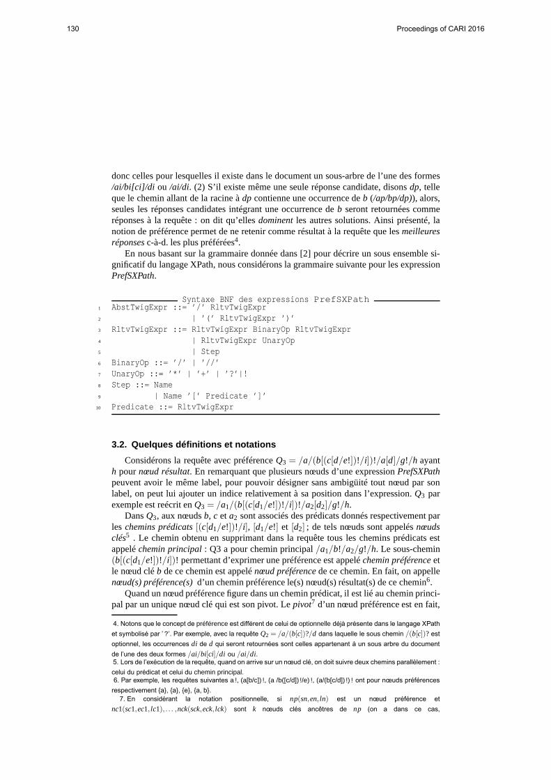
donc celles pour lesquelles il existe dans le document un sous-arbre de l’une des formes/ai/bi[ci]/di ou /ai/di. (2) S’il existe même une seule réponse candidate, disonsdp, telleque le chemin allant de la racine àdp contienne une occurrence deb (/ap/bp/dp)), alors,seules les réponses candidates intégrant une occurrence deb seront retournées commeréponses à la requête : on dit qu’ellesdominentles autres solutions. Ainsi présenté, lanotion de préférence permet de ne retenir comme résultat à la requête que lesmeilleuresréponsesc-à-d. les plus préférées4.

En nous basant sur la grammaire donnée dans [2] pour décrire un sous ensemble si-gnificatif du langage XPath, nous considérons la grammaire suivante pour les expressionPrefSXPath.

Syntaxe BNF des expressions PrefSXPath1 AbstTwigExpr ::= ’/’ RltvTwigExpr2 | ’(’ RltvTwigExpr ’)’3 RltvTwigExpr ::= RltvTwigExpr BinaryOp RltvTwigExpr4 | RltvTwigExpr UnaryOp5 | Step6 BinaryOp ::= ’/’ | ’//’7 UnaryOp ::= ’*’ | ’+’ | ’?’|!8 Step ::= Name9 | Name ’[’ Predicate ’]’

10 Predicate ::= RltvTwigExpr

3.2. Quelques définitions et notations

Considérons la requête avec préférenceQ3 = /a/(b[(c[d/e!])!/i])!/a[d]/g!/h ayanth pournœud résultat. En remarquant que plusieurs nœuds d’une expressionPrefSXPathpeuvent avoir le même label, pour pouvoir désigner sans ambigüité tout nœud par sonlabel, on peut lui ajouter un indice relativement à sa position dans l’expression.Q3 parexemple est reécrit enQ3 = /a1/(b[(c[d1/e!])!/i])!/a2[d2]/g!/h.

DansQ3, aux nœudsb, c et a2 sont associés des prédicats donnés respectivement parles chemins prédicats[(c[d1/e!])!/i], [d1/e!] et [d2] ; de tels nœuds sont appelésnœudsclés5 . Le chemin obtenu en supprimant dans la requête tous les chemins prédicats estappeléchemin principal: Q3 a pour chemin principal/a1/b!/a2/g!/h. Le sous-chemin(b[(c[d1/e!])!/i])! permettant d’exprimer une préférence est appeléchemin préférenceetle nœud cléb de ce chemin est appelénœud préférencede ce chemin. En fait, on appellenœud(s) préférence(s)d’un chemin préférence le(s) nœud(s) résultat(s) de ce chemin6.

Quand un nœud préférence figure dans un chemin prédicat, il est lié au chemin princi-pal par un unique nœud clé qui est son pivot. Lepivot7 d’un nœud préférence est en fait,

4. Notons que le concept de préférence est différent de celui de optionnelle déjà présente dans le langage XPathet symbolisé par ’ ?’. Par exemple, avec la requête Q2 = /a/(b[c])?/d dans laquelle le sous chemin /(b[c])? estoptionnel, les occurrences di de d qui seront retournées sont celles appartenant à un sous arbre du documentde l’une des deux formes /ai/bi[ci]/di ou /ai/di.5. Lors de l’exécution de la requête, quand on arrive sur un nœud clé, on doit suivre deux chemins parallèlement :celui du prédicat et celui du chemin principal.6. Par exemple, les requêtes suivantes a !, (a[b/c]) !, (a /b([c/d]) !/e) !, (a/(b[c/d]) !) ! ont pour nœuds préférences

respectivement a, a, e, a, b.7. En considérant la notation positionnelle, si np(sn,en, ln) est un nœud préférence et

nc1(sc1,ec1, lc1), . . . ,nck(sck,eck, lck) sont k nœuds clés ancêtres de np (on a dans ce cas,


le nœud clé situé sur le chemin principal tel que le chemin qui les relie ne passe pas par unautre nœud clé situé sur le chemin principal. Notons que si un nœud préférence est situésur le chemin principal, il est sont propre pivot. DansQ3, les nœuds préférencesb, c, e etg ont respectivement pour pivots les nœudsb, b, b et g.

L’approche d’évaluation utilisée ici est descendante : on évalue une requête en com-mençant par l’évaluation du nœud le plus proche de la racine et en évoluant vers lesfeuilles. Nous appellerons donc par la suiterequête partielletout (chemin) préfixe d’unerequête :/a/(b[(c[d/e!])!/i])! est une requête partielle deQ3.

4. Evaluation des requêtes PrefSXPath à l’aide des automates

4.1. De l’expression PrefSXPath à l’automate

Le tableau 1 donne à l’exemple de celui présenté dans [2] pour chaque motif de requêtePrefSXPath, le schéma de l’automate à construire correspondant. Les transitions de cesautomates sont étiquetées soit par des éléments deΣ, soit parλ quand la requête permetd’exprimer une relationancêtre-descendant(x//y), soit par le nom d’une des actionsdécrites à la section 4.2.2.

Chemin PrefSXPath Automate correspondant

a∈ Σ, /a

Ch1/Ch2

Ch1//Ch2

Ch?

Ch!, a étant un nœud préfé-rence de Ch

c∈ Σ, c[Ch]

Ch∗

Tableau 1. Motifs de requêtes PrefSXPath et schémas d’automates correspondant

sci < sn≤ en < eci, ∀i,0 < i < k) et situés sur le chemin principal, alors le nœud pivot de np est lenœud ncl (scl,ecl, lcl ), 0< l < k tel que (ecl == minimum(ec1, . . . ,eck)) : c’est le nœud y ayant la plus petitevaleur de endPos. On peut donc statiquement calculer le nœud pivot de tout nœud préférence. On supposeradonc dans la suite qu’on dispose d’une fonction getPivotId qui retourne le pivot d’un nœud préférence donné.Par exemple, getPivotId (c) = b.


4.2. Algorithme d’évaluation

4.2.1. Les structures de données

Rappel : l’évaluation d’une requêtePrefSXPathest descendante. Au cours de l’éva-luation, le résultat de l’évaluation du nœud requête courant est stocké dans une variableappeléecurrentAnswer. Ce qui suit est une description des autres variables utilisées parl’algorithme.partialSolutionStack : pile utilisée lors du traitement des (sous-)chemins optionnels etpréférences. En effet, lors du franchissement d’un arc étiqueté par l’une des actionsBe-ginOPou BeginPrefou encorePush8, la solution partielle courante (contenue danscur-rentAnswer) y est stockée en vue de son utilisation à la fin du traitement du sous-cheminoptionnel ou préférence (traversé d’un arc étiqueté EndOp ou EndPref) pour construire lanouvelle solution courante.prefNodeStack : pile utilisée pour stocker et restituer les nœuds préférences contenusdans le chemin préférence courant : lors du franchissement d’un arc étiquetéBeginPref(a),le nœud préférencea y est empilé et lors du franchissement d’un arc étiquetéEndPref, ony effectue un dépilement.answerPivotTable :tableau associatif dont chaque entrée contient une paire(clé, valeur).clé est un identifiant d’un nœud pivot, et la valeur associée est le résultat de l’évaluationde la sous-requête ayant ce nœud comme nœud résultat ; il est initialisé àcurrentAnswerau moment du franchissement d’un arc étiquetéclé. Lors du franchissement d’un arc éti-quetéEndPref l’entrée associée à la clé du pivot du nœud préférence courant (c’est celuise trouvant actuellement au sommet de la pileprefNodeStack) est utilisée pour filtrer lesoccurrences du pivot à stocker dans l’entrée de la tableinfoPrefNodeTablecorrespondantau nœud préférence courant.infoPrefNodeTable : tableau associatif dont chaque entrée contient une paire(clé, va-leur). clé est un identifiant d’un nœud préférence, et la valeur associée est constituée desoccurrences du pivot de ce nœud recouvrant au moins une de ses occurrences.preferenceTable :tableau de booléens renseignant pour chaque réponser de la requêteet pour chaque nœud préférencep si une occurrence dep a été utilisée pour la productionde la solutionr.

4.2.2. Les actions

Le tableau 2 associe à chaque action la description des traitements à effectuer lors dufranchissement d’un arc étiqueté par cette action.

4.2.3. L’algorithme

Etape1 : évaluation sans tenir compte des préférencesL’algorithme de la première étape d’évaluation d’une requêtePrefSXPath Qsur un

documentD (algo. 1) prend en entrée un indexTq de D et l’automateA associé àQ.Il retourne le triplet(currentAnswer, infoPrefNodeTable, answerPivotTable)utilisé dansla seconde étape pour construire la tablepreferenceTablede laquelle sont extraite lesmeilleures réponses. Dans l’algorithme 1, on parcourt l’automateA à partir de l’état ini-tial en exécutant suivant le type de l’étiquette de la transition qui part de l’état courantle traitement correspondant : si c’est une valeura ∈ Σ, (on est sur un chemin de typech1/a/ch2), alors, on filtre dans la listeTa les occurrences dea qui sont fils d’un élé-ment de la solution courantecurrentAnswer(algo. 1, ligne 15) et sia est un pivot, onremplit l’entrée correspondante dans la tableanswerPivotTable(algo. 1, lignes 16-18) ;

8. Voir la description des actions à la section 4.2.2.


Nom action Description des traitements associésPush Empile la solution partielle courante dans la pilepartialSolutionStackFilterUp Filtre dans le résultat se trouvant au sommet de la pilepartialSolutionStack

ceux qui sont ancêtres d’une occurrence se trouvant danscurrentAnswer.PopRestore Dépile le résultat au sommet de la pilepartialSolutionStacket en fait la solution

courante.BeginPref (a) Annonce le début de traitement d’un chemin préférence ayanta pour nœud

préférence : on doit empiler la solution (partielle) courante danspartialSolu-tionStackainsi que le nœud préférencea du chemin préférence qu’on s’en vatraiter dans la pileprefNodeStack.

BeginOp Annonce le début de traitement d’un chemin optionnel : on doit empiler lasolution (partielle) courante danspartialSolutionStack:

EndOp Annonce la fin de traitement d’un chemin optionnel. On doit mettre à jourla solution courante (currentAnswer) en y ajoutant les occurrences du résultatprésentement au sommet de la pilepartialSolutionStack.

EndPref Annonce la fin du traitement d’un chemin préférence. On doit tout d’abordrestaurer le nœud préférence courant (c’est celui au sommet de la pileprefNo-deStack) puis, filtrer l’entrée correspondant à son pivot dans la tableanswer-PivotTableavec la solution courantecurrentAnswerpour n’y retenir que lesoccurrences du pivot recouvrant au moins une occurrence du nœud préférencecourant contenue danscurrentAnswer. Le résultat du filtrage est stocké dansla tableinfoPrefNodeTableà l’entrée correspondant au nœud préférence cou-rant. Pour finir, on doit effectuer tous les traitements énumérés ci-dessus pourl’action EndOp.

BeginStar Annonce le début de traitement d’un chemin étoilé (chemin avecstar (*)) dutype ch1/(ch)∗ / . On doit ajouter à la solution partielle résultant du traite-ment de la sous requêtech1, les solutions provenant du traitement de zéro ouplusieurs occurrences dech. La solution partielleV de ch1/(ch) ∗ / sera lasommeV = V0+V1+V2 . . .+Vn, oùVi est la solution partielle résultant de laconsommation dech pour lai ime fois. LesVi ne sont pas indépendants :V(i+1)dépend deVi dans la mesure où, les éléments de la solution partielleV(i+1)sont des descendants des éléments deVi qui correspondent à la chaine ch :V(i+1) = vi|∃vk ∈Vi ,viDescch(vk). viDescch(vk) signifie quevi est un descen-dant devk suivant la chainech.

EndStar Annonce la fin de lai ieme consommation d’un chemin étoilé. Si lors de cei ieme

passage on a récolté une solution, c.-à-d. si (V !=φ), on doit l’ajouter à lasolution partielle courante et se reconnecter au début du chemin étoilé. Sinon,on sort de ce chemin pour poursuivre le traitement de la requête résiduelle.

Tableau 2. Actions et traitements associés


sinon si c’estλ, (on est sur un chemin de typea//b) alors, on filtre dans la listeTb lesoccurrences deb qui sont descendants d’un élément de la solution courantecurrentAns-wer (algo 1, lignes 6-8). Enfin, si c’est une action(BeginStar, BeginPref, EndPref, . . . ),les instructions prévues pour le traitement de celle-ci (tableau 2) sont exécutées9.

entrée: - L’index Tq du document ;- L’automateA associé à la requête;

sortie : Toutes les occurrences du nœud résultats de la requête satisfaisant la requête

1 currentState= q0 ;answerPivotTable= φ ; infoPrefNodeTable= φ;2 currentAnswer=’/’ ; /* On initialise à la racine */ ;3 tantquecurrentState != FAfaire4 a=labelTranscurrentState /* On récupère le label de la transition

courante */ ;5 si a= = λ alors /* ch//b */6 currentState= δA(currentState, a);7 b= labelTranscurrentState;8 (currentAnswer, Tb) = filter ANC-DESCcurrentAnswerTb;9 currentState= δA(currentState, b);

10 sinon11 sia∈ Σact alors12 (currentAnswer, qc) = perform_Action (currentAnswer, q, a);13 currentState= qc;

14 sinon /* a∈ Σ */15 (currentAnswer, Ta) = filter CHILDcurrentAnswerTa;16 si (isPivot(a))alors17 indiceA= indice(a, answerPivotTable);18 answerPivotTable[indiceA] =currentAnswer;19 currentState= δA(currentState, a);

20 return (currentAnswer, answerPivotTable, infoPrefNodeTable) ;Algorithm 1: Twig-Automata-Preference-Match pour l’étape 1

Etape 2 : extraction des meilleures réponsesLa seconde étape est divisée en deux phases : dans la phase 1 on construit la table

preferenceTableet dans la phase 2 on sélectionne les meilleures réponses en appliquantl’opérateur skyline10[12] sur les tuples de la tablepreferenceTablepour ne retenir que lesréponses contenues dans l’ensemble constitué des tuples non dominés.

Dans ce qui suit, pour des besoins d’illustrations, nous considérons la requêtePrefSX-Path Q= /a1/. . ./a(k−2)/b![. . .]/ak/. . ./a(k+l)/c[d1/. . ./dkpred/g![. . .]/. . .]/a(k+l+2)/. . ./as/ fayantf comme nœud résultat, possédant deux nœuds préférencesb etg situés respective-

9. La fonction perform_Action(action, q, currentAnswer,) ; (algo. 1 ligne 12) permet d’effectuer les traitementsliés à l’action action étiquetant l’arc associé à l’état q, les réponses courantes étant dans currentAnswer.10. L’opérateur skyline [12] permet de sélectionner les meilleurs n-uplets c.-à-d. ceux qui ne sont pas do-

minés au sens de la relation de préférence. De façon sommaire, il peut être présentée comme suit : soientdeux tuples p = (p1, . . . , pk, pk+1, . . . pn) et q = (q1, . . . ,qk,qk+1, . . .qn) d’une table relationnelle R de schémaR(P1, . . .PK ,PK+1, . . .Pn). Pour les requêtes dans lesquelles les préférences portent sur les champs Pk+1, . . . ,Pn,on dira que p domine q et on note p> q, si les trois conditions suivantes sont satisfaites : (1) pi = qi , pour touti = 1,2, . . . k. (2) pi ≥ qi pour tout i = (k+1), . . . ,n. (3) il existe i, (k+1)≤ i ≤ n, et pi > qi .


ment sur le chemin principal et sur un chemin prédicat. Considérons aussi que :• Q a pour chemin principal/a1/. . ./a(k−2)/b!/ak/. . ./a(k+l)/c/a(k+l+2)/. . ./as/ f delongueur s+1.• /ak/. . ./a(k+l)/c/a(k+l+2)/. . ./as/ f est le suffixe du chemin principal comprenantK =s+1−(k−1)= s−k+2 nœuds, parmi lesquels on suppose avoirp, 0≤ p≤K−1 nœudspréférences.• Le (sous-)chemind1/. . ./d(kpred) contenu dans le prédicat associé au nœudc est le pré-

fixe d’un chemin principal se terminant juste avant le nœudg et contenantkpred nœuds11,parmi lesquels on suppose qu’on aitppred, 0≤ ppred ≤ kpred autres nœuds préférences.• a(k+l+2)/. . ./as/ f sont leskprinci = s+ 1− (k+ l + 1) = s− k− l nœuds du cheminprincipal deQ compris entrec et le nœud résultatf , parmi lesquels on suppose y avoirpprinci, 0≤ pprinci ≤ kprinci nœuds préférences.

A l’aide d’une telle requête, présentons comment s’effectue le remplissage de la tablepreferenceTable. Elle comporte pour le cas de cet exemple au moins deux colonnes éti-quetéesb et g (ce sont les deux seuls nœuds préférences effectivement mis en exerguedans la requêteQ). De façon générale, nous examinerons le cas où le nœud préférence estsitué sur le chemin principal et celui dans lequel il ne l’est pas.

• Cas du nœud préférence « b » situé sur le chemin principalLes occurrencesf j

(

f js, f je, f jl)

12 de f intégrant une occurrencebi(bis,bie,bil ) de b

satisfont :

bis < f js < f je < bie (1)f jl = bil +m, m∈ K− p,K− p+1, . . . ,K (2)

L’équation (1) exprime le fait quebi(bis,bie,bil ) recouvref j(

f js, f je, f jl)

. Tenant comptede ce que le (sous-)chemin allant debi à f i peut événtuellement contenir une occurrencepour chacun desp nœuds préférences compris entre les nœudsb et f , l’équation (2) ex-prime le fait quef j doit être situé à une profondeur comprise entre(K − p) et (K) debi.

• Cas du nœud préférence « g » situé dans un chemin prédicatLes occurrencesf j

(

f js, f je, f jl)

de f qui intègrent une occurrencegi(gis,gie,gil ) degayant pour pivot l’occurrencecv(cvs,cve,cvl) dec13 satisfont :

cvs< f js < f je < cve / ∗ cv recouvre fj ∗ / (3)cvs< gis < gie < cve / ∗ cv recouvre gi ∗ / (4)f jl = cvl +m, m∈ kprinci − pprinci, . . . ,kprinci (5)gil = cvl +n, n∈

kpred− ppred, . . . ,kpred+1

(6)Les équations (3) et (4) expriment le fait quecv doit recouvrir à la foisf j et gi . De

même que pour le cas précédent, le (sous-)chemin allant decv à f j (resp. decv à gi)contient éventuellement des occurrences deskprinci (resp.ppred) nœuds optionnels com-pris entre les nœudscv et f j (resp.cv et gi). L’équation (5) (resp. 6) exprime le fait quef j (resp.gi) doit être situé à une profondeur comprise entre(kprinci − pprinci) et (kprinci)(resp.(kpred+1− ppred) et (kpred+1) decv) decv.

Ainsi donc, pour tout résultatf j de la requête, pour un nœud préférenceb situé surle chemin principal, l’entréepre f erenceTable[ f j , b] = 1 s’il existe au moins une occur-rencebis de b dans la liste présente dans l’entréein f oPre f NodeTable[b] recouvrantf j

(équation 1) et située à la "bonne profondeur"’ dans le sous arbre ayantbis pour racine(équations 2), sinon, elle est mise à zero. De même, pour un nœud préférenceg situé dans

11. Tous appartenant au chemin principal.12. Rappelons que f js, f je, f jl sont respectivement les composants du triplet (start, end, level) représentant le

nœud f j dans le document.13. Rappel : g a pour pivot c.


un prédicat, l’entréepre f erenceTable[ f j , g] = 1 s’il existe au moins une occurrencecvs

du pivot c de g dans la liste présente dansanswerPivotTable[c] recouvrant à la foisf j

(équation 3) et au moins une occurrencegis deg dans la solution partielle contenue dansin f oPre f NodeTable[g] (équation 4).f j et gis doivent être situées à la bonne profondeurdans le sous arbre ayantcvs pour racine (équations 5 et 6) ; sinon, elle est mise à zero.

Enfin, l’opérateur skylineest appliqué aux tuples de la tablePre f erenceTableainsiconstruite pour déterminer les meilleures solutions.

5. Conclusion

Nous avons exploré dans ce papier une approche d’expression et d’évaluation de re-quêtesXPathavec préférences. Pour ce faire le langagePrefSXPatha été proposé et ainsiqu’un algorithme d’évaluation des mots de ce langage (des requêtes) sur un documentXML.

Bien que l’algorithme proposé dans ce manuscrit ait été déroulé sur bien des exemples(faute de place, ils n’ont pas été déroulés ici) avec des résultats très satisfaisants, une étudeanalytique complète de ses performances est en cours de réalisation. Le travail présentédans ce papier est le point de départ d’un travail plus ambitieux ayant pour but la géné-ralisation de l’approche présentée dans ce manuscrit. On projette de considérer les préfé-rences comme desaspectsexprimables via un DSL (Domain Specific Language) qu’onconstruira, et de les injecter dans les algorithmes d’évaluations d’expressionsXPathdéjàexistants par untisseur de préférencesqu’on définira.

6. Bibliographie

[1] Abiteboul, S.« Querying Semi-Structured Data », In Proceedings of the International Confe-rence on Database Theory (ICDT), Delphi, Greece, pp. 1-18, 1997.

[2] Bing Sun, Bo Zhou, Nan Tang, Guoren Wang, Ge Yu, and Fulin Jia.« Answering XML TwigQueries with Automata », In Jeffrey Xu Yu, Xuemin Lin, Hongjun Lu, and Yanchun Zhang,editors, Advanced Web Technologies and Applications, 6th Asia-Pacific Web Conference, AP-Web 2004, Hangzhou, China, April 14-17, 2004, Proceedings, volume 3007 of Lecture Notesin Computer Science, pp. 170-79. Springer, 2004.

[3] Bosc P., Pivert O.« SQLf : a relational database language for fuzzy querying », IEEE Trans.On Fuzzy Systems, vol(3) pp.1-17, 1995.

[4] C.Y. Chan, P. Felber, M.N. Garofalakis, R. Rastogi,« Efficient filtering of XML documentswith XPath expressions », in : Proceedings of the 18th International Conference on DataEngineering (ICDE), IEEE Comput. Soc., pp. 235-244, 2002

[5] Chomicki J.« Preference Formulas in Relational Queries », In ACM Trans. on DatabaseSystems (TODS), vol. 28(4), 2003.

[6] Dubois D., Prade H.Bipolarity in flexible quering. Proc. of the 5th Int. Conf. on FlexibleQuery Answering Systems (FQAS), Copenhagen, Denmark, 2002.

[7] Gang Gou and Rada Chirkova.« Efficiently Querying Large XML Data », Repositories :A Survey IEEE Transactions On Knowledge And Data Engineering, VOL. 19, NO. 10, pp.1381-1402 OCTOBER 2007.

[8] Kiebling W. « Foundations of Preferences in Database Systems », In Proc. of the 28th Int.Conf. on Very Large Databases (VLDB), pp. 311-322., Hong Kong, China, 2002.


[9] Lietard L., Rocacher D. and Tbahriti S.-E.« Preferences and Bipolarity in Query Language», , International Conference of the North American Fuzzy Information Processing Society(NAFIPS 2008), New-York, USA. pp. 1-6, 2008.

[10] Q. Li and B. Moon.« Indexing and querying XML data for regular path expressions », Pro-ceedings of the 27th VLDB Conference, pp. 361-370, 2001.

[11] Rakesh Agrawal , Jerry Kiernan , Ramakrishnan Srikant , Yirong Xu,« An XPath-based pre-ference language for P3P », Proceedings of the 12th international conference on World WideWeb, May 20-24, Budapest, Hungary, 2003

[12] Stephan Börzsönyi, Donald Kossmann, and Konrad Stocker.« The skyline operator », InProceedings of the 17th International Conference on Data Engineering, April 2-6, 2001, Hie-delberg, Germany, pp. 421-430, 2001.

[13] T. Green, G. Miklau, M. Onizuka, D. Suciu,« Processing XML streams with deterministicautomata », in : Proceedings of the 9th International Conference on Database Theory (ICDT),Springer, pp. 173-189, 2003.

[14] W. Kießling, B. Hafenrichter, S. Fischer, S. Holland :« Preference XPATH : A Query Lan-guage for E-Commerce », Proc. 5th Intern. Konf. für Wirtschaftsinformatik, Augsburg, pp.425-440, Sept. 2001.

[15] W3C Consortium.« XML Path Language (XPath) 2.0 », http ://www.w3.org/TR/XPath20/,2006.

[16] W3C Consortium. « XQuery 1.0 : An XML Query Language »,http ://www.w3.org/TR/xquery/. 2006.

[17] Yao, J. T. and Zhang, M.«A Fast Tree Pattern Matching Algorithm for XML Query », Procee-dings of the 2004 IEEE/WIC/ACM International Conference on Web Intelligence, (WI 2004),20-24 September 2004, Beijing, China, pp. 235-241, 2004.


Empirical study of LDA for Arabic topic identification

Marwa Naili, Anja Habacha Chaibi and Henda Ben Ghézala

RIADI-ENSI

University of Manouba

Manouba 2010, Tunisia

[email protected]

RÉSUMÉ. Cet article met l'accent sur l'identification thématique pour la langue arabe. Nous étudions l'Allocation de Dirichlet Latente (LDA) comme une méthode non supervisée pour l'identification thématique. Ainsi, une étude approfondie de LDA a été effectuée à deux niveaux: le processus de lemmatisation et le choix des paramètres. Pour le premier niveau, nous étudions l'effet des différents lemmatiseurs sur LDA. Pour le deuxième niveau, nous nous focalisons sur les paramètres de LDA et leurs impacts sur l'identification. Cette étude montre que LDA est une méthode efficace pour l'identification thématique Arabe surtout avec le bon choix des paramètres. Un autre résultat important est l'impact élevé des lemmatiseurs sur l'identification thématique.

ABSTRACT. This paper focuses on the topic identification for the Arabic language. We study the Latent Dirichlet Allocation (LDA) as an unsupervised method for the Arabic topic identification. Thus, a deep study of LDA is carried out at two levels: Stemming process and the choice of LDA parameters. For the first one, we study the effect of different Arabic stemmers on LDA. For the second one, we focus on LDA parameters and their impact on the topic identification. This study shows that LDA is an efficient method for Arabic topic identification especially with the right choice of parameters. Another important result is the high impact of stemming algorithms on topic identification.

MOTS-CLÉS : Identification thématique, Allocation de Dirichlet Latente, paramètres de LDA, lemmatiseurs Arabes.

KEYWORDS: Topic identification, Latent Dirichlet Allocation, LDA parameters, Arabic stemmers.



1. Introduction

During the last few years, the number of textual documents has been vastly

increasing. Thus, many techniques have been presented to deal with this big number of

documents. However, the real challenge is to manage these documents based on their

content, especially the thematic one. For this reason, topic Identification and

classification draw a lot of intention in research fields dealing with different types of

documents (text [7], XML [2], etc). Yet for Arabic textual documents, there is a flagrant

lack of research. This can be explained by the high complexity of this language and the

lack of Arabic resources. In this paper, we will focus on topic identification by studding

LDA as an unsupervised method for Arabic topic identification.

This paper is organized as follows: Section 2 presents an overview of Arabic topic

identification; Section 3 describes some Arabic stemmers; Section 4 deals with LDA;

Section 5 is dedicated to the evaluation and the discussion; finally, the conclusion and

future works are presented in section 6.

2. Overview of Arabic topic identification

Topic identification is the process of identifying the topic of a textual unity.

According to most researchers, a topic is a cluster of words which are closely related to

the topic. Clusters depend on the stemming process that specifies the type of words

(root, stem, etc). For the Arabic topic identification, some methods have been used as:

- TF-IDF [7]: allows the construction of a vector space. Each vector represents a

document by the combination between TF(w,d) and IDF(w). The topic with the highest

similarity with the document will be considered as the document's topic.

- SVM and MSVM [13]: is a supervised method which classifies documents into two

classes by constructing a hyperplane separator in the 𝑅𝑁vector space. Yet, when the

number of categories is superior than 2, the MSVM is used. In fact, the idea of this

method is to find n hyperplane with n corresponds to the number of categories.

-TR-Classsifier [7]: is based on triggers which are identified by using the Average

Mutual Information. In fact, topics and documents are presented by triggers which are a

set of words that have the highest degree of correlation. Then, based on the TR-distance,

the similarity is calculated between triggers to identify the topic of the document.

-Named Entities approach [10]: The idea of this approach is to reduce the dimension

of vectors by using only the segments bounded by named entities pairs. Then, the

mutual information is used to calculate similarity between topics and documents.

Besides these methods, we can cite other methods used for topic identification such as


TULM and Neural networks in [7]. However, the major limit of these methods is that a

training step is necessary to identify the topics and to construct a vocabulary for each

topic. Thus, we opted to use the unsupervised method LDA. That means that there is no

need to a training step because topics are identified in the process of topic identification.

3. Arabic stemmers

Arabic language is one of the most complex and ambiguous language because of its

wide variety of grammatical forms and its complex morphology. Thus, the stemming

process is more difficult for the Arabic language than other languages. The stemming

process aims to find the lexical root or lemma of words by removing prefixes and

suffixes with are attached to its root. As an example of Arabic stemmers we mention:

- Khoja Stemmer [11]: it extracts the root of a word by removing the longest suffix

and prefix and then by matching the rest with verbal and nouns patterns.

- ISRI Arabic Stemmer [5]: it extracts the root of a word. But, unlike Khoja

Stemmer, it doesn't use any root dictionary or lexicon.

- The Buckwalter Arabic Morphological Analyzer [12]: it returns the stems of words

based on lexicons of stems, prefixes, suffixes and morphological compatibility tables.

- Light Stemmer [6]: Unlike Khoja Stemmer, it removes some defined prefixes and

suffixes instead of extracting the original root words.

According to different studies [5,6] the most efficient stemmers are Khoja and

Light Stemmers. These two stemmers are available freely on the web and might be the

only available Open Source ones. Thus, we will study Khoja and Light Stemmers to

evaluate the effect of the stemming process on the topic identification.

4. Latent dirichlet allocation (LDA)

LDA [3] is a generative model in which documents are represented as a mixture of

topic. Each topic is a multinomial distribution over words that depends on the stemming

process. Therefore, for each document w in the corpus D, the generative process is:

1. We choose N (a document is a sequence of N words) according to Poisson

distribution (N ~ Poisson(𝜉))

2. We choose 𝜃 ( 𝜃𝑑 is the distribution over the topic of the document d)

according to dirichlet allocation (𝜃 ~ 𝐷𝑖𝑟𝑖𝑐ℎ𝑙𝑒𝑡(𝛼))

3. For each of the N words 𝑤𝑛 : Choose a latent topic 𝑧𝑛 according to a

multinomial distribution and choose a word 𝑤𝑛from 𝑝 (𝑤𝑛|𝑧𝑛 , 𝛽)


The 𝜃 variable takes values in the (k-1) simplex and its density is equal to:

p(𝜃|𝛼) =Γ(∑ 𝛼i

ki=1 )

∏ Γ(𝛼i)𝑘𝑖=1

𝜃1𝛼1−1

… 𝜃𝑘𝛼k−1

(1)

Where 𝛼 ∈ ℝ𝑘, αi > 0 and Γ(x) is the Gamma function.

Therefore, given 𝛼 and 𝛽, the joint distribution of 𝜃, z and w is equal to:

𝑝(𝜃, 𝑧, 𝑤|𝛼, 𝛽) = p(𝜃|𝛼) ∏ p(𝑧𝑛|𝜃)𝑁𝑛=1 p(𝑤𝑛|𝑧𝑛, 𝛽) (2)

Finally, by integrating over 𝜃 and summing over z, the marginal distribution of a

document is as follow (equation 3):

𝑝(𝑤|𝛼, 𝛽) = ∫ p(𝜃|𝛼)( ∏ ∑ p(𝑧𝑛|𝜃)p(𝑤𝑛|𝑧𝑛 , 𝛽)𝑧𝑛) d𝜃𝑁

𝑛=1 (3)

According to Steyvers and Griffiths [8], the choice of 𝛼 and 𝛽 has an effect on the

performance of LDA. Besides, these parameters depend on the number of topics and the

vocabulary size. Moreover, Steyvers and Griffiths [8] recommended to use 𝛼 = 50/𝑘

and 𝛽 = 0.01. However, Lu et al. [14] conduct an in-depth analysis of the choice of 𝛼

with 𝛽 = 0.01. According to this analysis, the performance of LDA is influenced by

the initializing choice𝛼. This choice also depends on the field of application such as

topic classification and information retrieval which are tested in this study. As result,

they found that, for the topic classification, the optimal performance is obtained by 𝛼

between 0.1 and 0.5. Yet, for information retrieval, the optimal performance is obtained

by 𝛼 between 0.5 and 2. However, according to Lu et al. [14], the best value of 𝛼 is not

stable and it depends on the collection of documents used for tests. On the other hand,

Heinrich [4] estimated the values of 𝛼 and 𝛽 by using the information available from

the Gibbs sampler. In fact, Heinrich [4] showed that hyper-parameters are best

estimated as parameters of the Dirichlet-multinomial distribution.

Despite the high performance of LDA, few works dealing with LDA were presented

in the field of Arabic topic identification [9,1]. According to these works, promising

results have been obtained by LDA. However, we note that no one has studied LDA

parameters in the field of topic identification. Therefore, in this paper, we will study in

depth the LDA by studding the choice of 𝛼 and more important the effect of different

stemming algorithms to enhance the quality of topic identification.

5. Evaluation and discussion

In this section, we evaluated LDA with different stemmers. Thus, we presented three

different versions: LDA-WS (Without Stemmer), LDA-KS (Khoja Stemmer) and

LDA-LS (Light Stemmer). For this evaluation, we use the Arabic benchmark Al-Watan


which contains 20291 articles from Watan newspaper and it covers six topics: culture

(2782 documents), economy (3468 documents), international news (2035 documents),

local news (3596 documents), religion (3860 documents) and sport (4550 documents).

To report the evaluation results, we use three metrics: Recall, Precision and F-measure.

5.1. Identified topics based on different stemmers

Figure 1. Identified topics based on LDA-WS, LDA-KS and LDA-LS.

By conducting the three versions of LDA on AL-Watan corpus, we were able to

identify all the six topics. As shown in Figure.1, the identified topics depend on the used

stemmer. In fact, without using any stemming algorithms, the different topics were

successfully identified by LDA-WS. However, the problem is that some words can

figure more than once with different affix or suffix such as العام and العامة which mean

public. This problem is resolved by using Khoja stemmer which extracts the root of

words. Thus, by employing LDA-KS, the topics are present by roots. The limit of this

method is that a root can have several meaning such as علم which has many meaning

like: knowledge, flag, aware. Therefore, by using Khoja Stemmer, we might lose the

meaning. Yet, Light Stemmer removes only the prefix to maintain the meaning such as

the word المنتخب (the team) without stemming, نخب (pledge) with Khoja Stemmer and

with Light Stemmer. As conclusion, all the six topics have been (team) منتخب

successfully identified by LDA. Moreover, Light Stemmer is the most efficient stemmer

because it solves the problem of repetition (which is caused by the absence of stemmer:

LDA-WS) and the loss of meaning (which is caused by Khoja Stemmer LDA-KS).

5.2. Study of LDA parameter (𝜶)

We study in depth the 𝛼 parameter of LDA by using three values 0.1, 0.5 and 50/k

(k is number of topics which is 6 in our study). These values are proposed by [8,14]. For


𝛽, we used 𝛽 = 0.01 which is recommended in most research. For each value of 𝛼, the

results of LDA-WS, LDA-KS and LDA-LS are illustrates in table 1. First of all, we

remark that LDA-LS is independent of 𝛼. Yet, LDA-WS and LDA-KS are strongly

influenced by 𝛼 and the best results are obtained by 𝛼 = 0.5. Furthermore, for 𝛼 = 0.5,

the results of LDA-LS and LDA-KS are very close. Based on this result and the results

of the stemming process for the topic identification, Light Stemmer is the most efficient

stemmer to use with LDA. In the other hand, regardless of the value of 𝛼 and the

stemming algorithm, the well identified topics are: sport (F = 91.86%), religion (F =

82.75%), economy (F = 75.13%). Yet, for the other topics, especially the culture topic,

the performance of LDA is not stable. This can be explained by the fact that the

vocabularies of these topics (culture, international and local news) are very close.

Culture Economy Intern News Local News Religion Sport Average

𝜶 = 𝟎. 𝟏

R 9.09% 70.10% 95.23% 84.73% 50.34% 85.25% 65.79%

P 12.02% 80.95% 47.53% 58.73% 96.00% 99.59% 65.80%

F 10.36% 75.13% 63.42% 69.38% 66.04% 91.86% 62.70%

𝜶 = 𝟎. 𝟓

R 48.56% 70.30% 97.49% 81.01% 61.11% 84.13% 73.77%

P 46.73% 79.72% 67.21% 56.98% 97.16% 99.43% 74.54%

F 47.63% 74.72% 79.57% 66.90% 75.03% 91.14% 72.50%

𝜶 = 𝟓𝟎/𝒌

R 46.62% 69.49% 97.59% 80.70% 60.18% 84.28% 73.14%

P 45.40% 79.04% 66.22% 56.47% 97.11% 99.48% 73.95%

F 46.00% 73.96% 78.90% 66.44% 74.31% 91.25% 71.81%

𝜶 = 𝟎. 𝟏

R 68.40% 64.27% 78.52% 50.08% 71.35% 75.82% 68.07%

P 55.53% 57.72% 52.62% 50.75% 93.58% 99.34% 68.26%

F 61.30% 60.82% 63.01% 50.41% 80.96% 86.00% 67.08%

𝜶 = 𝟎. 𝟓

R 69.55% 54.67% 95.92% 78.28% 73.70% 79.98% 75.35%

P 55.76% 82.87% 76.28% 53.18% 94.33% 99.29% 76.95%

F 61.90% 65.88% 84.98% 63.34% 82.75% 88.59% 74.59%

𝜶 = 𝟓𝟎/𝒌

R 68.44% 63.98% 90.47% 50.78% 70.72% 75.54% 69.99%

P 54.84% 57.79% 61.02% 50.79% 93.85% 99.39% 69.61%

F 60.89% 60.73% 72.88% 50.78% 80.66% 85.84% 68.63%

𝜶 = 𝟎. 𝟏

R 60.71% 63.32% 97.00% 77.11% 59.09% 83.49% 73.45%

P 49.38% 75.88% 74.18% 54.20% 96.24% 99.19% 74.84%

F 54.47% 69.03% 84.07% 63.66% 73.23% 90.67% 72.52%

𝜶 = 𝟎. 𝟓

R 63.73% 62.51% 96.36% 77.14% 65.72% 83.54% 74.83%

P 54.19% 75.54% 75.60% 54.57% 96.10% 99.19% 75.86%

F 58.57% 68.41% 84.73% 63.92% 78.06% 90.69% 74.06%

𝜶 = 𝟓𝟎/𝒌

R 62.98% 62.92% 96.46% 76.42% 65.78% 83.36% 74.65%

P 54.12% 75.47% 75.50% 53.97% 96.10% 99.06% 75.70%

F 58.21% 68.63% 84.70% 63.26% 78.10% 90.53% 73.90%

Table 1. LDA-WS, LSA-KS and LDA-LS results with 𝜶 = 𝟎. 𝟏, 𝜶 = 𝟎. 𝟓 and 𝜶 = 𝟓𝟎/𝒌.

LD

A-W

S

L

DA

-KS

L

DA

-LS


But the vocabularies of sport, religion and economy are more representative and

unique for each topic which leads to an efficient topic identification.

5.3. Comparison with related works

To evaluate our work, we choose to compare our methods (LDA-KS and LDA-LS)

with the works of Abbas et al. [7] and Koulali and Meziane [10]. The reason for this

choice is that we used the same test corpus for the evaluation. Yet, we note that in these

works [7,10], 90% of the corpus is used for the training step and only 10% for the test.

This can explain the high performance of TF-IDF [7], MSVM [7], TR-Classifier [7] and

the Named Entities approach (NE) [10]. However, as an unsupervised method which

does not need any kind of training step, the results of LDA-KS and LDA-LS are

promising. In fact, dispute culture and economy topics, the result for the rest of topics

are comparable and even better some times. For example, for the international news

topic, LDA-KS and LDA-LS are better than TF-IDF, MSVM and TR-classifier.

Works Culture Economy Intern News Local News Religion Sport Average

TF-IDF 78.96% 90.03% 81.96% 78.43% 88.60% 96.91% 86.04%

MSVM 76.47% 95.50% 79.02% 68.64% 84.83% 89.75% 82.44%

TR-Classifier 81.60% 89.50% 83.77% 84.35% 91.97% 96.66% 88.02%

NE 75.66% 78.14% 90.15% 77.08% 88.26% 95.46% 84.15%

LDA-KS 61.90% 65.88% 84.98% 63.34% 82.75% 88.59% 74.59%

LDA-LS 58.57% 68.41% 84.73% 63.92% 78.06% 90.69% 74.06%

Table 2. Comparison with related works.

6. Conclusion

In this paper, we presented a deep study of LDA in the field of Arabic topic

identification. In fact, we studied the effect of the stemming process on topic

identification by using Arabic stemmers (Khoja and Light Stemmers). Besides, we

studied in depth the parameters of LDA. As result, we showed that the choice of

parameters influence the performance of LDA and the best result are obtained by

𝛼 = 0.5 . Moreover, LDA depends on the stemming algorithms. Based on our

evaluation, Light Stemmer is the best stemmer for the topic identification. Thus, based

on the best choice of parameters and the stemming algorithm, the result of LDA is very

promising in the field of topic identification. For further studies, we will use LDA for

topic segmentation to realize a complete topic analysis of Arabic documents.


6. References

[1] A. Kelaiaia and H.F. Merouani. “Clustering with Probabilistic Topic Models on

Arabic Texts”. In Modeling Approaches and Algorithms for Advanced Computer

Applications, Springer, 65-74, 2013.

[2] A.A.Y. Yassine, and K. Amrouche. "Réseaux bayésiens jumelés et noyau de Fisher

pondéré pour la classification de documents XML.", ARIMA Journal, Special issue

CARI’12, 17:141-154, 2014.

[3] D.M. Blei, A.Y. Ng and M.I. Jordan, "Latent dirichlet allocation". The Journal of

machine Learning research, 3, 993-1022, 2003.

[4] G. Heinrich. "Parameter estimation for text analysis". University of Leipzig, Tech.

Rep, 2008.

[5] K. Taghva, R. Elkhoury and J. Coombs, "Arabic stemming without a root

dictionary". International conference on Information Technology, 1:52-57, 2005.

[6] L. Larkey, L. Ballesteros and M. Connell, Light stemming for Arabic information

retrieval. Arabic Computational Morphology, book chapter, Springer, 2007.

[7] M. Abbas, K. Smaïli and D. Berkani. "Evaluation of Topic Identification Methods

on Arabic Corpora". JDIM, 9(5), 185-192, 2011.

[8] M. Steyvers and T. Griffiths. Probabilistic topic models. Handbook of latent

semantic analysis, 427(7):424-440, 2007.

[9] M. Zrigui, R. Ayadi, M. Mars and M. Maraoui, "Arabic text classification

framework based on latent dirichlet allocation". CIT. Journal of Computing and

Information Technology, 20(2): 125-140, 2012.

[10] R. Koulali and A. Meziane, "Feature Selection for Arabic Topic Detection Using

Named Entities". In Proceeding of CITALA, Oujda, Morocco, pp. 243-246, 2014.

[11] S. Khoja and R. Garside, "Stemming Arabic text". Computer science, UK, 1999.

[12] T. Buckwalter, "Buckwalter Arabic morphological analyser version 2.0".

LDC2004L02, ISBN 1-58563-324-0, 2004.

[13] V. Vapnik, "The natural of statitical learning theory". Springer, New York, 1995.

[14] Y. Lu, M. Qiaozhu and Z. ChengXiang. "Investigating task performance of

probabilistic topic models: an empirical study of PLSA and LDA."Information

Retrieval 14(2):178-203, 2011.


Approche hybride pour le développement d’un lemmatiseur pour la langue arabe

Mohamed Boudchiche et Azzeddine Mazroui

Département de Mathématiques et Informatique

Faculté des Sciences, Université Mohammed Premier, Oujda, Maroc

B-P 717, 60000, OUJDA

MAROC

[email protected], [email protected]

RÉSUMÉ. Nous présentons dans cet article un système d'analyse morphologique arabe qui attribue, pour chaque mot d'une phrase arabe, un lemme unique en tenant compte du contexte des mots. Le système proposé est composé de deux modules. Le premier consiste en une analyse hors contexte basée sur l’analyseur morphosyntaxique Alkhalil Morpho Sys 2. Dans le deuxième module, nous utilisons le contexte pour identifier le bon lemme parmi tous les lemmes possibles du mot obtenus par le premier module. A cet effet, nous utilisons une approche basée sur les modèles de Markov cachés, où les observations sont les mots de la phrase et les lemmes représentent les états cachés. Nous validons l'approche en utilisant un corpus étiqueté composé d’environ 500000 mots. Le système donne le bon lemme dans plus de 99,5% pour l'ensemble d’apprentissage et environ 94,3% pour l'ensemble de test.

MOTS-CLES : Traitement automatique de la langue arabe, Lemmatisation, Analyseur morphologique, Model de Markov caché, Algorithme de Viterbi.


1. Introduction

L'Internet connaît depuis quelques années une croissance exponentielle dans le

domaine de la recherche d'information. Ainsi, les chercheurs ont développé pour certaines

langues plusieurs outils permettant d’analyser et d’extraire l’information utile dans les

documents numériques. Cependant, les différences entre les structures linguistiques des

différentes langues ne permettent pas toujours d’étendre l’utilisation des programmes

développés pour une langue donnée à une autre langue.

Dans le domaine du traitement automatique des langues naturelles (TALN), la

lemmatisation occupe une place importante étant donné son utilisation dans plusieurs

application du TALN telles que la traduction automatique, l’indexation, les résumeurs

automatiques, la classification des textes et les dictionnaires interactifs [2, 3, 8] . En

particulier, des travaux récents dans les systèmes de recherche d’information en langue

arabe ont montré l’utilité de travailler avec les lemmes au lieu des mots.

La lemmatisation consiste à identifier pour chaque mot du texte son lemme qui

représente la forme minimale du mot portant son sens principal. Les lemmes représentent

les entrées des dictionnaires. Pour la langue arabe, le lemme d’un verbe est sa forme sans

clitiques conjugué à l’accompli à la 3ème personne du singulier (le lemme du verbe

مارس' fsymArswn/ est/ 'فسيمارسون' ' /mArs/). Pour un nom, le lemme est sa forme au singulier

masculin sans clitiques (le lemme du nom 'كمعلماتهم' /kmElmAthm/ est 'معلم' /mElm/). Si le

nom n’a pas de masculin, alors son lemme est sa forme au singulier féminin (le lemme

de 'بمدارسهم' /bmdArshm/ est 'مدرسة' /mdrsp/). Enfin, pour une particule, le lemme est la

particule sans clitiques (le lemme de 'كالذي' /kAl*y/ est 'الذي' /Al*y/). Afin de répondre à une demande de plus en plus forte de lemmatiseurs pour la langue

arabe, nous avons développé un système qui fournit les lemmes des mots d’une phrase

arabe. Notre système commence par réaliser une analyse morphologique en utilisant la

deuxième version de l'analyseur morphologique Alkhalil morpho Sys [1]. Cette analyse

permet l’obtention pour chaque mot pris hors contexte ses différents lemmes potentiels.

Pour identifier le lemme correct parmi ces lemmes potentiels, nous avons utilisé dans une

deuxième étape les modèles de Markov cachés et l’algorithme de Viterbi. Afin de réaliser

les phases d’apprentissage et de test, nous avons utilisé le corpus Nemlar [9] pour lequel

nous avons ajouté au préalable l’étiquette lemme à tous ses mots.

L'article est organisé de la manière suivante. Nous présentons dans la deuxième

section le corpus Nemlar utilisé dans les deux étapes d’apprentissage et de test. Nous

consacrons la section suivante pour un aperçu sur l'analyseur Alkhalil Morpho Sys utilisé

dans la phase morphologique de notre système. Le paragraphe 4 est réservé à une

description de la méthode adoptée dans le développement du lemmatiseur. Les résultats

de l'évaluation du système sont détaillés au paragraphe 5 et nous terminons le papier par

une conclusion.


2. L’Analyseur Alkhalil Morpho Sys1

AlKhalil Morpho Sys 2 [1] est un analyseur morphosyntaxique développé avec le langage de programmation orienté objet Java par le Laboratoire de Recherche en Informatique de l’Université Mohammed Premier, Oujda, Maroc. Il permet d’analyser aussi bien les mots arabes non voyellés que les mots partiellement ou totalement voyellés. L’analyse se fait hors contexte et les taches de l’analyseur pour un mot donné sont :

- retrouver les voyellations possibles du mot (lorsque le mot entré n’est pas voyellé), - identifier pour chaque voyellation possible du mot son lemme accompagné du schème,

les clitiques attachés au mot, sa catégorie grammaticale et son stem accompagné du schème.

Nous avons utilisé cet analyseur dans la première phase de notre système.

3. Description de la méthode

La lemmatisation des mots des textes arabes sera réalisée en deux étapes. Dans la première étape, le système utilise la deuxième version de l’analyseur morphologique Alkhalil Morpho Sys pour analyser les mots de la phrase. Ainsi, l’analyseur nous fournit les différents lemmes potentiels de chaque mot. Ensuite, un traitement statistique basé sur les chaines de Markov cachées et l’algorithme de Viterbi sera réalisé dans la deuxième phase. L’objectif de ce traitement est la désambiguïsation qui consiste à identifier le lemme correct dans le contexte parmi les lemmes potentiels d’un mot obtenus dans la phase morphologique.

3.1. Analyse morphologique

Après une phase de prétraitement du texte entré (tokénisation, normalisation des mots, découpage des textes en phrase puis en mots), ces derniers subissent une analyse morphologique en utilisant la 2ème version de l’analyseur morphologique Alkhalil Morpho Sys. Nous obtenons ainsi tous les lemmes potentiels de chaque mot du texte pris hors contexte accompagnées de leurs informations morphosyntaxiques. En effet, pour chaque voyellation du mot, le système fournit les clitiques attachés aux stems, les POS tags, le stem et le lemme. Dans le cas d’un nom ou d’un verbe, le système fourni également la racine, les schèmes du stem et du lemme et l’état syntaxique.

3.2. Analyse statistique

Après avoir identifié les lemmes potentiels pour chaque mot de la phrase, nous appliquons un traitement statistique dont l’objectif est la sélection du lemme le plus probable parmi ces lemmes potentiels. Ce traitement est basé sur les modèles de Markov cachés, les techniques de lissage et l'algorithme de Viterbi.

Nous donnons dans la suite un bref aperçu de ces trois concepts mathématiques.

1 http://oujda-nlp-team.net/?p=1299&lang=en


3.3. Modèles de Markov Cachés

Les modèles de Markov cachés (HMM) sont utilisés pour modéliser deux processus aléatoires dépendants dont les états du premier sont non observables (états cachés), et ceux du second sont observables (états observés). Les HMM servent à prédire les états cachés à partir des états observés.

En effet, si 𝑂 = 𝑜1, 𝑜2, … , 𝑜𝑟 est un ensemble fini d'observations et 𝐸 =ℎ1, ℎ2, … , ℎ𝑚 est un ensemble fini d’états cachés, alors un double processus (𝑋𝑡 , 𝑌𝑡)𝑡≥1

est un modèle Markov caché du premier ordre si :

- (𝑋𝑡)𝑡 est une chaîne de Markov homogène à valeurs dans l’ensemble d’états cachés E vérifiant : 𝑃𝑟 (𝑋𝑡+1 = ℎ𝑗/𝑋𝑡 = ℎ𝑖 , … , 𝑋1 = ℎ𝑘) = 𝑃𝑟 (𝑋𝑡+1 = ℎ𝑗/𝑋𝑡 = ℎ𝑖 ) = 𝑎𝑖𝑗 . 𝑎𝑖𝑗 est la probabilité de transitions de l’état caché ℎ𝑖 vers l’état caché ℎ𝑗.

- (𝑌𝑡)𝑡 est un processus observable qui prend ses valeurs dans l'ensemble d'observations O vérifiant : 𝑃𝑟(𝑌𝑡 = 𝑜𝑘/𝑋𝑡 = ℎ𝑖 , 𝑌𝑡−1 = 𝑜𝑘𝑡−1 , 𝑋𝑡−1 = ℎ𝑖𝑡−1 , … , 𝑌1 = 𝑜𝑘1 , 𝑋1 = ℎ𝑖1)

= 𝑃𝑟 (𝑌𝑡 = 𝑜𝑘/𝑋𝑡 = ℎ𝑖 ) = 𝑏𝑖(𝑘). 𝑏𝑖(𝑘) est la probabilité d’observer l’état 𝑜𝑘 étant donné l’état caché ℎ𝑗.

Ainsi, les informations sur les états cachés peuvent être déduites à partir des données observées.

Soit S une phrase observée composée des mots 𝑤1, 𝑤2, … , 𝑤𝑛 et 𝐸 = 𝑙1, 𝑙2, … , 𝑙𝑚 l'ensemble de tous les lemmes de la langue arabe.

Afin de rechercher les lemmes les plus probables dans le contexte des mots 𝑤𝑖 de la

phrase S, nous allons utiliser une modélisation par les HMM où les mots de la phrase

représenteront les observations et leurs lemmes les états cachés.

Notre objectif est donc de trouver pour la phrase 𝑆 = (𝑤1, 𝑤2, … , 𝑤𝑛) la séquence de lemmes la plus probable (𝑙1∗, . . . , 𝑙𝑛∗ ) satisfaisant la relation suivante :

(𝑙1∗, … , 𝑙𝑛

∗ ) = argmax𝑙𝑖∈𝐿𝑖

𝑃𝑟(𝑙1, … , 𝑙𝑛 𝑤1 , … , 𝑤𝑛⁄ )

où 𝐿𝑖 est l'ensemble des lemmes possibles du mot 𝑤𝑖 obtenus suite à l’analyse morphologique de la première étape.

3.3.1. Algorithme de Viterbi

Pour trouver la séquence la plus probable des lemmes, nous allons utiliser l'algorithme de Viterbi [5], qui est bien adapté pour la recherche du chemin optimal. Ainsi, si nous notons ∅(𝑡, 𝑙𝑡𝑘) le maximum sur l’ensemble des chemins de longueur (t-1) de la probabilité que les (t-1) premiers mots aient les lemmes du chemin et le tème mot 𝑤𝑡 ait le lemme 𝑙𝑡𝑘 , c.à.d. : ∅(𝑡, 𝑙𝑡𝑘) = max

𝑙𝑖

𝑗𝑖∈𝐿𝑖1≤𝑖≤𝑡−1

.

[Pr (𝑤1, … , 𝑤𝑡 𝑙1𝑘1 , … , 𝑙𝑡

𝑘⁄ )] Pr(𝑙1𝑘1 , … , 𝑙𝑡

𝑘),

alors, en utilisant les hypothèses markoviennes, nous pouvons facilement vérifier que :

∅(𝑡, 𝑙𝑡𝑘) = ( max

𝑙𝑡−1𝑗

∈𝐿𝑡−1

∅(𝑡 − 1, 𝑙𝑡−1𝑗) Pr (𝑙𝑡

𝑘 𝑙𝑡−1𝑗

⁄ )) Pr(𝑤𝑡 𝑙𝑡𝑘⁄ ).


Cette équation permettra de calculer de manière récursive les valeurs de la fonction ∅. Pour obtenir le chemin optimal, nous utilisons la fonction 𝛹 qui mémorise à l’instant

𝑡 l’étiquette cachée qui réalise le maximum dans la définition de ∅. Elle est définie par : 𝛹(𝑡, 𝑙𝑡

𝑘) = 𝑎𝑟𝑔𝑚𝑎𝑥 𝑙𝑡−1𝑗

∈𝑙𝑡−1

∅(𝑡 − 1, 𝑙𝑡−1𝑗) 𝑃𝑟 (𝑙𝑡

𝑘 𝑙𝑡−1𝑗

⁄ ).

3.3.2. Méthodes de lissage

Afin de pouvoir programmer l’algorithme de Viterbi, il faut au préalable estimer les paramètres du modèle statistique, c'est à dire, les coefficients des matrices de transition et d’émission 𝐴 = (𝑎𝑖𝑗) et 𝐵 = (𝑏𝑖(𝑡)) où 𝑎𝑖𝑗 = Pr(𝑙𝑗 𝑙𝑖⁄ ) 𝑒𝑡 𝑏𝑖(𝑡) = 𝑃𝑟 (𝑤𝑡 𝑙𝑖⁄ ).

Pour cela, nous avons appliqué sur un corpus d’apprentissage étiqueté de taille N la méthode d'estimation basée sur le maximum de vraisemblance [6]. Si 𝑤𝑡 est un mot de la phrase 𝑆 et (𝑙𝑖 , 𝑙𝑗) sont deux lemmes, alors nous notons : - 𝑛𝑖 : le nombre d’occurrences de l’état caché 𝑙𝑖 dans le corpus C, - 𝑛𝑖𝑗: le nombre d’occurrences dans C de la transition de l’état caché 𝑙𝑖 vers l’état 𝑙𝑗, - 𝑚𝑖𝑡 : le nombre de fois que le mot 𝑤𝑡 correspond à l’état caché 𝑙𝑖 dans le corpus C,

alors, les coefficients 𝑎𝑖𝑗 et 𝑏𝑖(𝑡) sont estimés en utilisant les équations suivantes : 𝑎𝑖𝑗 =

𝑛𝑖𝑗

𝑛𝑖, 1 ≤ 𝑖 ≤ 𝑁, 1 ≤ 𝑗 ≤ 𝑁 et 𝑏𝑖(𝑡) =

𝑚𝑖𝑡

𝑛𝑖, 1 ≤ 𝑡 ≤ 𝑛, 1 ≤ 𝑖 ≤ 𝑁

Etant donné qu’il n’existe pas de corpus d’apprentissage pouvant contenir toutes les transitions entre les mots de la langue arabe, les coefficients de transition peuvent pour certains exemples être estimés par la valeur zéro. Cela affectera négativement la recherche du chemin optimal par l’algorithme de Viterbi. Pour remédier à ce phénomène, des techniques de lissage sont alors utilisées. Ces techniques seront appliquées avant de faire tourner l'algorithme de Viterbi, et consistent à attribuer une probabilité non nulle à toutes les transitions du corpus de test. Pour cela, nous avons utilisé la méthode Absolute Discounting [4].

Ainsi, si 𝐶 = 𝑃ℎ1, … , 𝑃ℎ𝑀 est le corpus d’apprentissage de la langue arabe formé

par M phrases 𝑃ℎ𝑘 , et si nous posons :

- 𝑁1+(𝑙𝑖 ) : le nombre de tous les mots dont les lemmes correspondants sont

répétés une fois et plus après le lemme li dans le corpus C, - Ni : le nombre de mots annoté dans le corpus C avec le lemme li, - zi : le nombre de mots non annoté dans le corpus C avec le lemme li et pour

lesquels l’analyseur Alkhalil génère ce lemme, alors, les coefficients 𝑎𝑖𝑗 et 𝑏𝑖(𝑡) sont estimés par :

𝑎𝑖𝑗 = 𝑚𝑎𝑥(𝑛𝑖𝑗 −𝐷, 0)

𝑛𝑖+𝐷

𝑛𝑖𝑃𝑎𝑏𝑠(𝑙𝑗)𝑁1+(𝑙𝑖 ) 𝑒𝑡 𝑏𝑖(t) =

𝑚𝑖𝑡 −𝐷

𝑛𝑖𝑠𝑖 𝑚𝑖𝑡 ≠ 0

𝑁𝑖 × 𝐷

𝑛𝑖 × 𝑧𝑖𝑠𝑖𝑛𝑜𝑛

avec la constante D=0.5 et 𝑃𝑎𝑏𝑠(𝑙𝑗) =𝑛𝑗

𝑁


4. Corpus d’apprentissage et de test

Le projet NEMLAR (Network for Euro-Mediterranean Language Resources) lancé en 2003 visait le développement des ressources de la langue arabe dans le cadre d’une collaboration dans la région méditerranéenne. Le projet a réuni 14 partenaires de divers pays dans le cadre du programme MED-Unco soutenu par l'Union européenne [9].

Le corpus Nemlar est un ensemble de textes en langue arabe annotés par la société RDI Egypte pour le compte du Consortium NEMLAR qui détient les droits. Il contient environ 500,000 mots issus de 13 domaines différents répartis sur 489 fichiers.

Les étiquettes disponibles dans le corpus Nemlar pour un mot donné sont sa forme voyellée, son stem, les clitiques attachés au stem et sa catégorie grammaticale et son schème. Ce corpus est disponible sous deux formes : la forme voyellée et la forme non voyellée.

Afin de pouvoir utiliser ce corpus dans les phases d’apprentissage et de test de notre modèle, nous avons procédé à son enrichissement avec l’étiquette lemme en réalisant les trois étapes suivantes :

4.1. Analyse morphologique

Durant cette étape, nous commençons par analyser les mots du corpus voyellé en utilisant l’analyseur AlKhalil Morpho Sys 2. Ensuite, nous ne gardons que les lemmes dont les étiquettes lexicales associées (clitiques+stem+racine), et qui sont fournies par l’analyseur AlKhalil, coïncident avec les étiquettes lexicales du mot dans le corpus Nemlar.

4.2. Identification du lemme correct parmi les lemmes potentiels

Après avoir identifié les lemmes potentiels pour les mots du corpus Nemlar, nous avons demandé à un linguiste spécialisé d’identifier le lemme correct parmi ces lemmes. Dans le cas où le lemme correct ne figure pas parmi les sorties de la première étape, le linguiste attribue au mot son lemme.

4.3. Insertion de l’étiquette lemme

Après que le linguiste ait achevé son travail, nous sommes passés à la dernière étape qui consiste à insérer les lemmes dans le corpus Nemlar.

5. Evaluation

La phase d’apprentissage qui a servi à l’estimation des matrices de transition et d’émission a été réalisée sur 90% du corpus NEMLAR choisi aléatoirement. Des tests ont été ensuite réalisés sur deux sous-ensembles non voyellés du corpus NEMLAR :

- Le premier ensemble, appelé Te, constitue les 10% restants du corpus Nemlar qui n’ont

pas été utilisés dans la phase d’apprentissage.


- Le deuxième ensemble, appelé Tr, constitue environ 25% du corpus d’apprentissage.

Il a été tiré aléatoirement du corpus d’apprentissage. La méthode d'évaluation consiste à comparer le lemme fourni par notre lemmatiseur

avec celui attribué par les annotateurs de corpus. La précision est calculée par la formule suivante :

𝑃𝑟é𝑐𝑖𝑠𝑖𝑜𝑛 =le nombre de mots correctement lemmatisés

la taille de l′ensemble de test.

Les résultats de test sont présentés dans la table 1.

Précision

Ensemble Tr 99,21%

Ensemble Te 94,45%

Table 1. Précision du lemmatiseur

Les résultats obtenus montrent la robustesse de notre lemmatiseur. En effet, le système fourni un lemme correct dans 94.45% des mots du corpus de test Te, alors que ce taux augmente pour atteindre 99,21% dans l'ensemble d’apprentissage Tr.

Afin de situer les performances de notre lemmatiseur, nous avons réalisé une comparaison entre les taux d’erreurs de notre système et le système MADAMIRA2.

MADAMIRA (v1.0) est un système d'analyse morphologique de levée de l’ambigüité dans le contexte [7]. Il fournit plusieurs sorties morphosyntaxiques dont le lemme du mot.

Pour réaliser cette comparaison, nous avons exécuté le système MADAMIRA sur le corpus de test Te, et les résultats obtenus sont présentés dans le tableau 2.

Précision MADAMIRA 90,53%

Notre lemmatiseur 94,45%

Table 2. Comparaison des précisions des deux lemmatiseurs

Nous constatons que les performances de notre lemmatiseur sont largement meilleurs que celles de l’analyseur MADAMIRA. En effet, notre système a atteint une précision de l’ordre de 94.45% alors que celle de l’analyseur MADMIRA est en dessous de 91%.

6. Conclusion

Nous avons présenté dans cet article un lemmatiseur des phrases arabes. L'analyse morphologique opérée dans la première phase propose souvent plusieurs lemmes potentiels pour un mot donné. Pour choisir le lemme correct dans le contexte de la phrase

2 http://innovation.columbia.edu/technologies/cu14012_arabiclanguage-disambiguation-for-naturallanguage-

processing-applications


parmi ces lemmes, nous avons adopté une approche statistique basée sur des modèles de Markov cachés. Les résultats obtenus sont très encourageants. Afin d’améliorer davantage les performances du système, nous prévoyons agir sur deux niveaux :

- Niveau analyse morphologique : exploiter la richesse des informations fournies par

l’analyseur Alkhalil pour mieux filtrer les transitions entre lemmes. En effet, l'absence

d’une transition entre deux lemmes dans le corpus d’apprentissage n’est pas

nécessairement due aux limites du corpus, mais peut être causée par le non

compatibilité entre ces deux lemmes (par exemple, un lemme verbe ne peut succéder

à un حرف جر).

- Niveau corpus : utiliser dans la phase d’apprentissage un corpus de taille plus

importante. Cela permettra de mieux ajuster les estimations des matrices de transition

et d’émission, et par suite améliorer la précision du lemmatiseur.

7. Bibliographie

[1] Boudchiche, M., Mazroui, A., Ould Abdallahi Ould Bebah, M., Lakhouaja, A., Boudlal, A., 2016. AlKhalil Morpho Sys 2: A robust Arabic morpho-syntactic analyzer. J. King Saud Univ. - Comput. Inf. Sci. doi:10.1016/j.jksuci.2016.05.002

[2] Hammouda, F.K., Almarimi, A.A., 2010. Heuristic Lemmatization for Arabic Texts Indexation and Classification. J. Comput. Sci. 6 6, 660–665.

[3] Koulali, R., Meziane, A., 2013. Experiments with arabic topic detection. J. Theor.

Appl. Inf. Technol. 50. [4] Manning, C.D., Schütze, H., 1999. Foundations of Statistical Natural Language

Processing. MIT Press, Cambridge, MA, USA. [5] Neuhoff, D., 1975. The Viterbi algorithm as an aid in text recognition. IEEE Trans.

Inf. Theory 21, 222–226. doi:10.1109/TIT.1975.1055355 [6] Ney, H., Essen, U., 1991. On smoothing techniques for bigram-based natural

language modelling, in: 1991 International Conference on Acoustics, Speech, and

Signal Processing. IEEE, pp. 825–828 vol.2. doi:10.1109/ICASSP.1991.150464 [7] Pasha, A., Al-badrashiny, M., Diab, M., Kholy, A. El, Eskander, R., Habash, N.,

Pooleery, M., Rambow, O., Roth, R.M., 2014. MADAMIRA : A Fast , Comprehensive Tool for Morphological Analysis and Disambiguation of Arabic. Proc. 9th Lang. Resour. Eval. Conf. 1094–1101.

[8] Reqqass, M., Lakhouaja, A., Mazroui, A., Atih, I., 2015. Amelioration of the interactive dictionary of arabic language. Int. J. Comput. Sci. Appl. 12, 94–107.

[9] Yaseen, M., Attia, M., Maegaard, B., Choukri, K., Paulsson, N., Haamid, S., Krauwer, S., Bendahman, C., Fersøe, H., Rashwan, M., Haddad, B., Mukbel, C., Mouradi, A., Shahin, M., Chenfour, N., Ragheb, A., 2006. Building Annotated Written and Spoken Arabic LR’s in NEMLAR Project, in: LREC. pp. 533–538.


Overview of the social information’s usage in Information

Retrieval and Recommendation systems

Abir Gorrab, Ferihane Kboubi and Henda Ben Ghezala

RIADI Laboratory-ENSI

University of Manouba

Manouba 2010, Tunisia

[email protected]

ABSTRACT. Web 2.0 and social networks represent a huge and rewarding source of information. Our work revolves around the issue of access and identification of social information and their use in building a user profile enriched with a social dimension, and operating in a process of personalization and recommendation. We present several approaches of Social IR (Information Retrieval), distinguished by the type of social information integrated; as well as social recommendation approaches. We also expose a study of the modeling techniques of the user profile’s social dimension, followed by a discussion and proposed directions.

RÉSUMÉ. Le web 2.0 et les réseaux sociaux représentent une source d’information énorme et enrichissante. Notre travail s’articule autour de la problématique d’accès et d’identification des informations sociales et leur exploitation dans la construction d’un profil utilisateur enrichi d’une dimension sociale, et son exploitation dans un processus de personnalisation et de recommandation. Nous présentons différentes approches de RI (Recherche d’Information) Sociale, distinguées par le type d’informations sociales intégrées; ainsi que des approches de recommandation sociale. Nous exposons également une étude des techniques de modélisation de la dimension sociale du profil utilisateur, suivie par une discussion et des directions envisagées.

KEYWORDS: social information retrieval, social recommendation, social networks, user profile

MOTS-CLÉS : recherche d’information sociale, recommandation sociale, réseaux sociaux, profil utilisateur.


1. Introduction

With the apparition of the social web and the explosion of social networks, users

become able not only to consume, but also to product informational content. As a matter

of fact, the huge number of web users and time spent daily on internet motivated

researchers in IR and encouraged them to benefit from this content as an enlightening

source of information. Besides, social networks and collaborative sites (such as

Facebook, LinkedIn, Google+, Twitter, YouTube, delicious, CiteUlike, etc) are the most

common and popular source of interactive content. In this paper, we focus on the impact

of social information integration in an IR process and a recommendation system.

This paper is organized as follows: in section 2, we discuss the main approaches

used in Social IR. While section 3 is devoted to the social recommendation, and section

4 is reserved to social dimension in user profile modeling, section 5 is dedicated to

discussion and future directions. Finally, we conclude in section 6.

2. Social IR approaches

Social IR approaches are various. They are mostly based on social information

identification and integration in a search process. In fact, there are several types of

social information specific to each social network, such as folksonomies, tags, social

relations (friends, co-authors, followers), comments, tweets, conversations, hashtags,

like mentions, shares and many others. Proposed approaches widely use many social

information, which can be integrated in different levels in IR process: user profile

construction, query expansion and result ponderation. In this section, we present

different social IR approaches that can be classified in three categories, according to

social information used.

2.1. Approach based on annotations

Social annotations are a valuable informational source that enhances social IR by

including user’s area of interest. Bouhini et al. [2] propose a user profile generation

approach from folksonomies. As a matter of fact, this work combines queries with user

profile based on terms frequency. Actually, it presents two Social IR models inspired

from BM25 model: BM25S Score Comb and BM25S Freq Comb, which combines

query and user profile using respectively scores and terms frequency. Bao et al. [17]

calculate similarity between web query and social annotations. They propose two

algorithms that enhance web IR: SSR (Social Sim Rank) which computes similarity

degree and SPR (Social Page Rank) that estimates web pages popularity. PengLi et al


[15] propose a TR-LDA model of annotations categorization. They introduce

representation and ponderation methods of annotation categories. In this respect, they

study the effect of annotations’ incorporation in IR process.

2.2. Approach based on social relations

At first sight, users may be linked by different relationships that are specific to each

social network, e.g., friend relationships, followers and co-authors. Works based on this

approach usually use this informational content generated by relations, in a way that

combines a social and a thematic score. In this context, Ben Jabeur et al. [9] investigate

on a social model based on Bayesian network, incorporating two social relevance

factors: User social importance, evaluated by a PageRank score; and the number of

temporal neighbors. Moreover, Amer et al. [14] propose a probabilistic model of

conversation indexation in twitter. This model incorporates social relations to measure

users’ influence, activity and expertise.

2.3. Approach based on social signals

Social signals like comments, shares and like mentions are being more explored in

social IR works, due to the significant information they bring. Chelaru et al [16] study

the impact of these social signals in video search on YouTube, by combining social

information such as comments, like and dislike mentions, with basic search criteria

(similarity between the query and video title). Hence, this unification enhances the

performance of videos extraction process. Furthermore, Badache et al. [5] describe a

language model exploiting temporal characteristics of social signals (number of like

mentions, shares and comments) to estimate resources relevance and sort search results.

Moreover, Ramesh et al. [13] examine the personalized social IR process and suggest an

algorithm of user profile construction using pages liked on Facebook, through different

user’s accounts. This social content personalizes search results.

2.4. Comparative study

For more information about Social IR approaches, we led a comparative study of

different categories. For each work we considered the following six points as a

comparative criteria: (1) the social network used for the experimentation, (2) the

techniques used in the presented models, (3) the metrics used for the evaluation, (4) if

there is a combination of information, (5) if there is a combination of social networks

and (6) if the work considered the temporal aspect. Table 1 summarizes the results of

our study.


Social

information

Social

network

Techniques Evaluation Combining

Information

Combining

social

networks

Temporal

aspect

Annotati-

ons

[2] BM25and

derivatives

MAP, P[0,1]

- - -

[17] Del.ic.ious SSR, SPR MAP,

nDCG

- - -

[15] Del.ic.ious TF_IDF,

Inference

algorithm

-

-

-

-

Social

relations

[9] Twitter,

Citulike

PageRank,

language

model,

ImpG:social

score,

TF-IDF

MAP, recall

√

√

√

[14] Twitter BM25,

language

model,

PageRank

Leave One

Out

approach,

MAP

√

-

-

Social

signals

[16] Youtube TF_IDF,

Lucene,

SentiWord-

Net

nDCG

√

-

-

[5] Facebook,

Twitter,

LinkedIn,

Del.ic.ious,

Google+

Language

model

MAP,

nDCG,

Recall,

Precision

√

√

√

[7] Facebook Clustering

data

TF-IDF

Performance

measure

√

-

-

Table1. Comparative table of Social IR approaches categorized by social information types

In table1, we present some works related to the three approaches described in this

section, based on annotations, social relations and social signals. Characteristics studied

are the combination of many social information or social networks and the consideration

of temporal aspect. These features enhance IR processes and improve their

performances. In fact, many networks are used and many techniques are conducted, but


temporal aspect and the combination of different networks represent the greatest

motivation for researchers.

3. Social recommendation

Social recommendation is a set of methods that try to suggest items or entities that

seem to be interesting to the user, using his social information [12]. In fact, there are two

main recommendation techniques. The first one is a content based approach which is

based on recommending items similar to those the user has chosen in the past. The

second one is a collaborative filtering approach; this approach recommends items to the

user based on the choice of other people, who seem to have similar preferences.

Moreover, Hybrid recommendation is a technique that comprises both content-based

and collaborative filtering approaches, so as to provide the user with better

recommendations. Additionally, many researchers have explored social information to

improve recommender systems. Notably, Hafsi et al. [11] exploit user-generated content

(rating and review) in books recommendation system. Their work measures books

reputation and popularity concepts and tests three approaches: book tags and reviews

indexation, themes interrogation and users similarity calculation. Unlike in [6], authors

have proposed a content-based approach that compares users profiles’ information in

order to determine similarities between them and recommend friendship relations. On

the other hand, Wang et al. [18] investigate on tag based social recommendation by

calculating tags similarities and connecting users that are likely to have similar tastes

and preferences. In the same context, Hannon et al. [7] propose an hybrid

recommendation system using content and collaborative-based approaches that

recommends users to follow in the social network Twitter, by analyzing their profiles.

4. Social dimension in user profile modeling

User profile modeling is an essential task in Personalized IR. This entity brings and

organizes the information necessary to define the user and describe his interests.

Following the emergence of social networks, Social IR has widely evolved. Thus, the

social dimension of the user profile has become an essential component in social

personalization systems. A lot of works were directed towards the construction of a

social profile based on annotations [8] [4], given the importance of the data they

generate. Others have focused on the analysis of egocentric social network, they are

interested in friendship relationships in social networks [3] [10]. This information

produces relevant content for collaboration within social IR systems. It solves the cold

start problem, or lack of user's activity on social networks. The temporal aspect is also


reflected in some works [10], which differentiates between recent and old social

activities, to estimate their importance. Other social signals have also been integrated

into the social dimension of user profile such as comments and shares. Once the profiles

are built, some authors have thought of building virtual communities of users, based on

similarity degree between the profiles. These communities are considered as a

dimension in the profile. They are very rewarding and provide additional relevant

information. In [1], Dridi et al model a user profile based on annotations and exploit it

to detect communities based on annotations similarities. For community detection, Katz

index is used. It calculates the similarity taking into account the direct and indirect links

in a graph.

5. Discussion and future directions

In this section, we discuss different aspects related to research in Social IR topic. In

fact, IR classical approaches do not take into account the user’s social content provided

by his interactions and social relations. Moreover, most of the existing approaches in

Social IR use either social signals, tags or relational information. Some works started

leveraging different types of information. Also, combining social content from many

social networks and matching different user’s social profiles improve the collection of

relevant information that better describe the user and enhance his affluence.

The construction of a data collection relative to SIR systems is basically a major

challenge. For this issue, we led a technical study of a set of social networks API that are

likely to be the most known. networks don’t present yet API for developers, like

ResearchGate. Some social In the extraction process, the majority of social networks use

the OAuth 2.0 for connection and authentication authority, like Twitter, Youtube,

Google+, LinkedIn, and Foursquare. Delicious and CiteUlike require basic http

authentication, while some other networks need API keys for authentication (Last.fm,

Flickr). REST is the common API used to have access to resources, and the result is

always a JSON or XML file. Actually, this study is our way to construct a data

collection suitable for Social IR.

Temporality is a fundamental issue and the most central aspect in social content.

This factor is being investigated in several works [10][6][11]but still presents new

contribution areas. Temporal aspect supports the eventual and permanent evolution of

users’ tastes, preferences and behaviors. Indeed, information appreciated by users now

may not remain the same after a moment. Besides, trend events attract users’ attention at

a specific moment and are no more important after a while. Thus, Social IR systems

should be adapted to this evolution. The same as for Social IR systems, the freshness of

the information is essential in recommendation systems. So, to enhance recommendation

quality, temporal factor should be considered.


Social approaches present certainly some limitations. A big challenge is to map

user’s accounts across social networks [19], and to predict missing social information,

by combining for example social information and the social graph [20], in order to have

an enriched social user profile. We will make a deep study in works dealing with these

challenges.

6. Conclusion

In this paper, a review of different aspects of Social IR is proposed. We presented a

classification of Social IR approaches into three main categories, based on social

information used. We also posed a study of Social recommendation systems. Then, we

referred to user profile models proposed in Social IR studies, and specially the social

dimension. In this respect, works included in this review reflect how deep the impact of

social content in IR and recommendation process is. Furthermore, we discuss different

aspects of Social IR. As for coming studies, we start the process of user profile

construction, based on temporal social signals.

7. References

[1] A. Dridi and M. Kacimi. “Information Retrieval Framework based on Social

Document Profile”. CAiSE(Forum/DoctoralConsortium), 2014.

[2] C. Bouhini, M. Géry and C. Largeron. “Integrating user's profile in the query model

for Social Information Retrieval”. Eighth International Conference on Research

Challenges in Information Science (RCIS) ,1-2. IEEE, 2014.

[3] D. Tchuente, M.F. Canut, N. Jessel, A. Péninou and F. Sèdes. “A community-based

algorithm for deriving users' profiles from egocentrics networks: experiment on

Facebook and DBLP”. Social Network Analysis and Mining, 3(3), 667-683, 2013.

[4] H. Xie, X. Li, T. Wang, L. Chen, K. Li, F. L. Wang, Y. Cai, Q. Li and H. Min.

“Personalized Search for Social Media via Dominating Verbal Context.”

Neurocomputing, 172, 27-37, 2016. [5] I. Badache and M. Boughanem. “Document Priors Based On Time-Sensitive Social

Signals.” ECIR, 617-622. Springer,2015.

[6] J. Chen, W. Geyer, C. Dugan, M. Muller and I. Guy. “Make new friends, but keep

the old: recommending people on social networking sites”. InProceedings of the

SIGCHI Conference on Human Factors in Computing Systems, 201-210, ACM, 2009.

[7] J. Hannon, M. Bennett and B. Smyth. “Recommending twitter users to follow using

content and collaborative filtering approaches”. In Proceedings of the fourth ACM

conference on Recommender systems, 199-206, ACM, 2010.


[8] K. Han, J. Park and M. Y. Yi.“Adaptive and multiple interest-aware user profiles for

personalized search in folksonomy: A simple but effective graph-based profiling

model”. In 2015 International Conference on Big Data and Smart Computing

(BIGCOMP), 225-231, IEEE, 2015.

[9] L. Ben Jabeur, L.T. Lechani and M.Boughanem. “Intrégration des facteurs temps et

autorité sociale dans un modèle bayésien de recherche de tweets”. CORIA, 301-316,

2012.

[10] M.F Canut, S. On-at, A. Péninou and F. Sèdes. “Time-aware Egocentric network-

based User Profiling”. In 2015 IEEE/ACM International Conference on Advances in

Social Networks Analysis and Mining (ASONAM), 569-572, IEEE, 2015.

[11] M. Hafsi, M. Géry and M. Beigbeder. “LaHC at INEX 2014: Social Book Search

Track”. Working Notes for CLEF 2014 Conference, 2014.

[12] M. R. Bouadjenek, H. Hacid and M. Bouzeghoub. “Social networks and

information retrieval, how are they converging? A survey, a taxonomy and an analysis

of social information retrieval approaches and platforms”. Information Systems, 56, 1-

18, 2016.

[13] N. Ramesh and J. Andrews. “Personalized Search Engine using Social Networking

Activity”. Indian Journal of Science and Technology, 8(4), 301, 2015.

[14] N. Ould Amer, P. Mulhem and M. Géry. “Recherche de conversations dans les

réseaux sociaux: modélisation et expérimentations sur Twitter”. Conférence en

Recherche d'Infomations et Applications-12th French Information Retrieval Conference,

2015.

[15] P. Li, B. Wang, W. Jin, J. Nie, S; Zhiwei, Z. and B; He. “Exploring categorization

property of social annotations for information retrieval”. In Proceedings of the 20th

ACM international conference on Information and knowledge management, 557-562,

ACM, 2011.

[16] S. Chelaru, C. Orellana-Rodriguez and I. Sengor Altingovde. “Can social features

help learning to rank youtube videos?”. International Conference on Web Information

Systems Engineering, 552-566, Springer Berlin Heidelberg, 2012.

[17] S. Bao, X. Wu, B. Fei , G. Xue , Z. Su and Y. Yu . “Optimizing web search using

social annotations”. In Proceedings of the 16th international conference on World Wide

Web, 501-510, ACM, 2007.

[18] X. Wang, H. Liu and W. Fan. “Connecting users with similar interests via tag

network inference”. In Proceedings of the 20th ACM international conference on

Information and knowledge management, 1019-1024, ACM, 2011.

[19] E. Raad, R. Chbeir and A. Dipanda.“User profile matching in social networks”. In

13th International Conference on, 297-304, IEEE, 2010.

[20] A. Mislove, B. Viswanath, P. Krishna Gummadi and P. Druschel “You are who

you know: inferring user profiles in online social networks”. In Proceedings of the

Third ACM International Conference on Web Search and Web Data

Mining, 251-260, 2010.


Vers un système iconique d’aide à la décision pour les praticiens

de la médecine traditionnelle

KOUAME Appoh12, BROU Konan Marcellin1, LO Moussa2, LAMY Jean Baptiste3.

1(Institut National Polytechnique Félix Houphouët Boigny de Yamoussoukro) (Côte d’Ivoire)

([email protected], [email protected])

2(Université Gaston Berger) (Sénégal) ([email protected])

3(Université Paris 13, Bobigny (France)([email protected])

RÉSUMÉ

«Mise en place d’une plateforme web social et sémantique pour le partage des connaissances des communautés ouest africaines » est un projet dans lequel un volet important concerne les praticiens de la médecine traditionnelle(PMT). Disposer d’un outil collaboratif de travail qui transcende leur état prégnant de non lettré constitue un défi majeur. C’est ce à quoi s’attelle ici, notre réflexion en amorçant l’aspect visuel via une composition iconique à approche ontologique d’ontoMEDTRAD. L’ontoMEDTRAD, avec ses composantes ontoConcept_term et ontoIcone, fait partie du système de gestion de la médecine traditionnelle, sysMEDTRAD. ontoConcept_term dénote les termes des concepts du domaine. ontoIcone devra inclure les icônes en alignement avec ces termes.

ABSTRACT

«Setting up a social and semantic web framework for knowledges sharing in West African communauties» is a project in which we note an important section relating to traditional medicine practitioner (TMP). People TMP, for the most part, are illiterate. Make available, a tool which transcends this characterization, constitutes a scientific issue in this work. Thus, the visual aspect via an iconic composition based on ontological approach of ontoMEDTRAD, is our goal. ontoMEDTRAD includes two modules which are ontoConcept_term and ontoIcone. It is also a part of the management system for traditional medicine (sysMEDTRAD). ontoConcept_term denotes the terms of concepts in this domain. ontoIcone will include the set of icons corresponding or in alignment with those terms.

MOTS-CLÉS : ontologie, web sémantique, Médecine traditionnelle, composition iconique, Afrique de l’Ouest.

KEYWORDS: ontology, semantic web, traditional medicine, iconic composition, West Africa.



2

1. Introduction

En médecine africaine, chaque habitant en zone rurale connaît et utilise les vertus d’un

certain nombre de plantes. Ceci relève de la pharmacopée populaire. Ces usages en plus

d’être culturels, lient les habitants à leurs terres [2]. Parmi les ressources médicinales

traditionnelles, les plantes sont les plus utilisées. Les étalages des tradipraticiens en

Afrique abondent de plantes. Ici, notre contribution vise, à augmenter le potentiel des

soins en santé primaires pour les populations notamment de l’Afrique de l’ouest par la

médecine traditionnelle(MT), persistante avant et depuis l’antiquité jusqu’à nos jours.

L’ambition portée sur la MT d’en faire un système complémentaire de santé ne la rend

pas substitut des offres de soins issues de la médecine moderne (MM). Pour les

populations, l’accès aux soins de santé de la MM n’est pas équitable. Parallèlement à

cette médecine conventionnelle, 80% des populations de l’Afrique de l’ouest, font appel

à la MT locale [21]. A ce titre, sauver tout un réutilisable patrimoine de connaissances et

d’expériences menacé de disparition, est d’un grand intérêt. Bien entendu, la transmission

des savoirs en MT est amplement orale, puis la gestion des faunes et flores, empirique et

à tâtons. Il importe alors de disposer d’un cadre idéal pour les praticiens de la MT (PMT),

afin de partager, mutualiser, co-construire, sauvegarder et pérenniser les connaissances,

les acquis et expériences dans ce domaine. Ici, notre SysMEDTRAD [17] conçu et

s’adossant à un wiki sémantique, répond à cette exigence. Sa composante principale est

ontoMedtrad, elle-même structurée en ontoCONCEPT_term et ontoIcone. La majorité

des PMT étant illettrée, l’aspect visuel leur permet de s’affranchir des barrières

linguistiques, de la lecture et de l’écriture textuelles. En général, une fois la maladie est

déterminée chez un patient, le PMT pense à la plante d’où il tirera la recette des soins.

Nous entamons l’aspect iconique des plantes antipaludiques, suite à la modélisation

conceptuelle (annexe 2) dont le modèle de connaissances obtenu a permis de frmaliser

l’ontoCONCEPT_term. Quatre points structurent ce document : (a) spécificités de la MT ;

(b) approche iconique; (c) amorçage d’un système iconique ; (d) travaux liés.

2. Traits caractéristiques de la MT

Lors du recueil de données, on s’aperçoit que des PMT de grande renommée voilent à

peine leur détermination de mourir avec leur secret [2]. D’autres PMT veulent une

transmission des savoirs par lignée. Entre PMT, le manque d’acceptation et de partage

mutuels des connaissances est avéré. Vu le caractère fortement implicite et caché de la

MT, ont été sensibilisés au moins cinquante (50) PMT pour leur adhésion au projet. Le

directeur du PNPMT1 a eu un rôle de facilitation. En Côte d’Ivoire, depuis 2014 jusqu’à

ce jour, à travers des ateliers et séminaires, ces PMT sont formés, afin de les amener au

respect d’un certain nombre de normes de pratique et d’éthique dans leur art. Leur

1 PNPMT : Programme National de la Promotion de la Médecine traditionnelle, un des démembrements du Ministère ivoirien de la santé et de la

lutte contre le sida(MSLS)


3 capacité en anatomie humaine a été renforcée par un médecin (MM), au premier trimestre

de 2015. Un PMT, pour être enregistré au PNPMT, doit appartenir à une association de

PMT. Une seule fédération des tradipraticiens de santé et naturothérapeutes (FTSN-CI)

regroupe toutes les associations. Le désordre orchestré en leur sein, susceptible de perte

de vies de patients, ne doit plus se perpétuer. La vision globale des gouvernants de la

sous-région d’améliorer la MT et de la valoriser, est bien nette. En partie, la MT constitue

un levier pour des découvertes en MM [4], où la majorité des médicaments obtenus sont

des produits de synthèse suite à une chaîne de production (biologie, principes actifs des

plantes médicinales, adjonction d’adjuvants et d’excipients). Entre MM et MT, les modes

opératoires sont différents. Une autre spécificité de la MT est l’exercice inclusif par le

PMT de deux fonctions, à savoir «médecin prescripteur» et « pharmacien ». En MT, le

mode de prise en charge d’un patient n’est pas celui de la MM ; Dans le processus de

traitement d’un malade, le PMT commence par détecter les signes symptomatiques sur le

patient afin de déterminer la maladie. A ce type de diagnostic, se rajoute un autre d’ordre

métaphysique, en plus de certains déterminants socio-culturels et environnementaux [11].

L’administration de soins par le PMT est en partie sous forme de remèdes appropriés, de

fois, de manière extemporanée au regard de la première des quatre catégories de

médicaments traditionnels selon l’OMS [5]. L’heure, la période et la saison de collecte

de certaines plantes peuvent influer leurs vertus thérapeutiques. L’échange entre patient

et PMT est bidirectionnel, se démarquant nettement de la position très dominante du rôle

de médecin moderne [3] dans le même contexte. En somme, la MT vise un traitement

exhaustif du patient (corps, âme et l’esprit ; environnement social et culturel), autrement

dit du bien-être intégral du patient [11]. Ce qui précède rend impossible, ici, la

réutilisation diligente et automatique des ressources terminologiques et ontologiques

(RTO) existantes en MM.

3. Approche d’ontologie visuelle

Une ontologie est une spécification formelle et explicite d’une conceptualisation [25]. Ce

travail d’«iconisation» est mené sur la base des modèles de données conçus en UML

(annexe 2) puis formalisés (axiomatisation) sous protégé. Vu la complexité visuelle, pour

la construction iconique, nous avons procédé par étape (en spirale et par incrément). Nous

nous focalisons sur les plantes, ressources médicinales les plus prescrites par les PMT.

Nous avons alors utilisé les éléments sémiologiques relatifs à un triptyque de stratégies

de représentation [7]. Aussi avons-nous tenu compte du contexte d’utilisation de l’outil

final dont disposeront les PMT. L’usage d’outils TIC (mobile, ordinateur...) comme

moyen d’accès à SysMETRAD, milite fortement en faveur de l'utilisation de telles

approches. Il est démontré la supériorité de la communication pictographique sur la

communication verbale dans le dialogue homme-ordinateur [12][27].

3.1. Justification, collecte de données et principe de base

En MT africaine, les ressources médicinales sont de différentes origines : végétale,

animale, minérale et métaphysique. La proportion des remèdes à base de plantes est plus


4 forte. Plus de cinq cent (500) plantes médicinales existent en Afrique de l’ouest selon

l’UNESCO [26]. Notre approche d’ontologie visuelle nécessite qu’en plus de modéliser

les concepts de ce domaine (ontoCONCEPT_term), il faut les représenter graphiquement

par des icônes (ontoIcone). Idéalement, une correspondance systématique entre ces deux

modèles devra être établie. Pour amorcer le volet iconique, nous partons du point de vue

d’intérêt majeur « donner des soins de santé primaires à un patient ». Cette exigence est

satisfaite par la définition de trois cas d’utilisations notés UCi avec i=1 à 3 ; UC1 :

déterminer la maladie à partir des symptômes (faire un diagnostic) ; UC2 : déterminer le

remède (définir la recette via les parties des plantes et les plantes, le mode de fabrication

et la forme de fin de préparation); UC3 : déterminer le mode d’administration de la recette.

En termes de scénario, notre choix s’est porté sur le paludisme, maladie classée parmi les

plus mortelles et morbides en Afrique occidentale. Aussi, avons-nous axé notre réflexion

prioritairement sur l’UC2 consistant à spécifier la recette à base de plantes antipaludiques

dont un inventaire est nécessaire. Pour définir une recette, le PMT commence par choisir

la plante. Ensuite, il détermine les parties de plante qui seront utilisées dans cette recette.

Suite à ce constat, il apparaît nécessaire de mettre au point une approche graphique pour

présenter visuellement les plantes médicinales et permettre leur reconnaissance. Dans le

florilège de plantes médicinales antipaludiques collectées en pharmacopée traditionnelle,

nous avons ciblé vingt-deux (22) [22] [15] [14] [1] [23] pour trente (30) recettes (annexe

8). Autant pour ce recueil que pour la modélisation conceptuelle, nous avons parcouru

moult sources et résultats d’études ethnobotaniques en biosciences comme celles

précédemment citées. Notre démarche inclut les retombées en termes de connaissances

reçues suite à notre collaboration directe avec des PMT (visites de terrain). Egalement

avions-nous été instruis d’importants travaux de référence sur les pharmacopées

traditionnelles [14] [19], des séminaires auxquels nous avons participé, et des documents

du PNPMT et des ONG comme la PROMETRA. Une plante médicinale soigne une ou

plusieurs maladies. Une recette peut être monospécifique (à base d’une plante), ou

multispécifique (à base de plus d’une plante). L’association de plantes, mal assortie, est

dangereuse [16] et donc déconseillée sauf en cas de maîtrise suffisante des effets

secondaires. En médecine populaire et rurale, des associations de plantes sont assez

connues pour purge (ou lavement) contre des maux de ventre. Les composantes d’une

recette sont les parties de plantes à savoir : feuille, fruit, écorce, tige, racine, fleur,…, ou

plante entière (herbe). Parmi elles, sont plus fréquentes, les feuilles, les fruits, les écorces.

Majoritairement, les feuilles et les fruits sont sollicités aux taux respectifs de 60% et 15%

[16]. Des critères sont définis pour caractériser les 22 espèces et permettre de les

distinguer individuellement. À partir de la représentation visuelle et iconique d’une

plante, il est aisé pour le PMT de faire sa prescription de recette. La description botanique

au plan morphologique, devient alors intéressante et importante pour la retenue des

critères. La quarantaine de critères extraits, sont réduits progressivement, par le

truchement d’une méthode inclusive d’un logiciel d’apprentissage Weka, d’éléments

sémiologiques, du contexte de travail projeté du PMT. Chaque valeur ou instance prise

par un critère fait l’objet d’un iconème, unité signifiante d'icône. Ces iconèmes sont

ensuite assemblés pour former les icônes. Il apparaît alors un problème d’optimisation


5 consistant à minimiser à la fois le nombre d’iconèmes et celui des icônes pour une

meilleure représentation visuelle de toutes les espèces de plantes, tout en restant capable

de les distinguer entre elles. En botanique, la systématique des végétaux suivant la

hiérarchie «monde du vivant », domaine, règne, embranchement, classe, ordre, famille,

genre, espèce, qui est aussi celle des plantes médicinales, est plus stable. Il est difficile

pour la majorité des PMT de s’en prévaloir au regard de l’objectif ici visé. Au mieux, la

priméité visuelle doit demeurer du fait du caractère prégnant d’illettré des PMT.

3.2. Variabilité descriptive de la botanique physique : les plantes (végétaux)

Le parcours descriptif par les botanistes des plantes est souvent variant. Cela est à même

d’engendrer des divergences et contradictions. Les deux espèces Adansonia digitata L et

Lannea microcarpa Engl. et K. Krause font partie de notre sélection de plantes

médicinales respectivement notées (ad) et (lm). (lm) est à feuille composée alterne et

imparipennée avec 15 m de haut dans [24], tandis qu’elle est décrite comme étant à feuille

opposée, de haut 10 m selon [9]. Notons que la morphologie d’une espèce végétale est

diversement appréciable selon la région d’habitat, le pays, le climat et les saisons. La

morphologie de (ad), plus élancée en Côte d’Ivoire, est différente de celle plus robuste et

imposant au Sénégal, avec plus ou moins le même goût de fruit. Ceci montre bien les

limites et insuffisances d’utiliser des photographies réalistes comme moyen sublime de

reconnaissance visuelle des plantes. Les dimensions morphologiques d’une plante dans

une photographie peuvent s’avérer trompeuses et laisser ainsi apparaître un fossé de

compréhension dans le réel. Le fait de juxtaposer un objet physique connu aux côtés d’un

autre méconnu dans une même image photo, permet d’avoir une vue plus rapprochée des

dimensions réelles de l’objet méconnu. Par ailleurs, selon la FAO [10], un arbre a 5 m de

hauteur minimale, là où l’Institut Forestier National (IFN) de France, donne 7 [13].

L’annexe 3 montre deux classifications par strate des végétaux faites par deux botanistes

et laissant éclore une différence. Toute cette variabilité est à restreindre en utilisant des

éléments visuels, semi-formels ou formels pour atteindre l’«iconisation » plus intelligible

par la machine.

3.3. Technique de réduction et de choix des critères

La technique de réduction et de choix des critères englobe des règles sémiologiques et

contextuelles. A l’aide des algorithmes Ranker et Jrip de Weka, nous avons procédé à

supprimer progressivement les critères en prenant en compte leur poids de distinguabilité,

les aspects visuels liés au PMT et les règles sémiotiques tirées surtout de la pensée

peircienne, quand bien même celle de F. Saussure (diadique) ne nous a pas fait défaut

pour comprendre les signes. Le signe, selon Peirce S, a trois dimensions : son objet, son

icône et son interprétant. F. Saussure en a une perception double : signifiant et signifié.

Ainsi, similarité visuelle, association sémantique et convention arbitraire [7] fondent le

triptyque de stratégies pour notre représentation iconique des individus de plantes. Les

critères retenus en termes de propriétés sur ces individus permettent de mieux les

discriminer. Ranker classe par ordre décroissant les critères selon le poids de

distinguabilité (voir tableau 1). JRip, sur la base des critères retenus parmi ceux

précédemment classés, distingue de la meilleure manière (100%), les individus de plantes


6 par un raisonnement logique. Nous donnons un aperçu d’une partie des associations de

classes (annexe 1). Relativement au paludisme, il y a des symptômes constants, et d’autres

spécifiques à l’état du patient, soit enfant, femme en grossesse ou adulte. On admet que

le paludisme est manifeste sur un patient. Les vingt-deux (22) plantes sont représentées à

travers sept (7) critères selon le tableau ci-après (annexe 4).

4. Amorçage d’un système iconique

Au regard ce qui précède, pour le besoin iconique, on a admis cinq (5) silhouettes que

sont arbre, arbuste, palme, herbe et liane pour représenter l’ensemble des instances de

la classe Plante via aPourSilhouette (Tableau 2).

Tous les iconèmes sont construits via le logiciel vectoriel inkscape. En conséquence, un

iconème a été conçu pour chacune de ces 5 entités de Silhouette (Tableau 4).

Les 22 espèces de plantes sont alors reparties entre ces silhouettes. Nous avons conçu des

icônèmes (génériques et spécifiques) pour les parties de plantes concernées par les 7

critères retenus. L’Owlready-2.0 est une librairie qui a été intégrée dans python [18]. Ceci

a l’effet de rendre accessible ontoMEDTRAD au programme python (annexe 6), dont

l’exécution permet d’obtenir les icônes par composition d’iconèmes (fig.1 et tableau 5).

Un exemple de résultat est l’icône de la plante « Azadirachta indica », obtenu à partir

d’une silhouette arbre et d’un fruit à forme elliptique. Les 33 iconèmes retenus sont

décrits en appendice annexe 5. On admet la couleur verte pour les feuilles. La

« pennation », la disposition de la feuille sont à iconèmes de couleur noire, y comprise la

silhouette. Les fruits et les fleurs peuvent avoir des couleurs d’apparence « réelle ». La

fleur pourrait changer de couleur une seule fois. La plante est reconnaissable à travers ses

traits très caractéristiques au plan visuel.


7

5. Travaux liés

Des travaux connexes à celui-ci sont de deux ordres (1) et (2) : -(1) au titre de la MT :

Armel [6] a réalisé une ontologie sur la MT au Cameroun sans approche visuelle. [11]

An Ontology for African Traditional Medicine (ATM) de G. ATEMEZING a son objet

focalisé sur la validation des connaissances de la MT gérée par un système d’agents. Il

n’aborde pas le fait que les PMT sont non lettrés. N. C. KUICHEU aborde une ontologie

IcOnto en définissant l’icône b d’un concept X via X (a, b) [20], a étant le terme de X. Le

langage utilisé est limité en définition. Dans les ontologies utilisées la description des

plantes, principales ressources des recettes médicales traditionnelles, est très réduite. -(2)

au titre de la MM : On a des thésauri, des taxinomies ou des ontologies pour la plupart

des travaux réalisés. Cependant, ils ne comprennent pas d’ontologie visuelle sauf le

Projet « VCM » de Lamy, où on a un langage iconique pour l'accès aux connaissances

sur le médicament et le guide de bonnes pratiques cliniques. Une ontologie visuelle est

validée sur la MM focalisée sur les aspects de facilité d’apprentissage et de vitesse de

lecture [18] du praticien.

6. Conclusion

L’icône est devenue une réalité pour la plante médicinale, ressource la plus importante

dans les recettes prescrites en MT africaine. Les descriptions botaniques et visuelles,

afférentes à la même espèce de plante sont des plus variées. Il n’en demeure pas moins

du discours des PMT sur la même recette traitant la même maladie. La difficulté liée à

cette varibilité descriptive est surmontable. La composition sémi-formalisée, formalisée

et schématisée est une tâche ardue qui doit s’appuyer sur un minimum de règles, en vue

de son intégration dans un wiki sémantique, puis permettre d’autres catégorisations et

extractions de connaissances. Ce système iconique (ontoIcone), amorcé sur les plantes

devra servir d’outil d’assistance décisionnel pour les PMT à même de transcender la

lecture et l’écriture textuelles voire les barrières linguistiques. Le processus de validation

des icônes est à deux étapes : la première par les PMT lettrés, et la seconde pour

l’ensemble. Ne serait-il pas judicieux d’établir de simple liaison entre icônes et images

photos réalistes afin de pallier à l’insuffisance d’instruction pour des PMT, le temps de la

standardisation. En perspective au terme de cette composition de plante, nous devons

asseoir un véritable langage iconique à but inférentiel pour les PMT.


8

7. Bibliographie

[1]ADOU Lydie et al, 2014, Nephrolepis biserrata, une Ptéridophyte utilisée comme plante

médicinale en Côte d’Ivoire, pp1-9

[2]AKE Assi L., 2011. Abrégé de Médecine et pharmacopée africaines, CI, pp1-150.

[3].A. KONAN, 2012, Place de la médecine traditionnelle dans les soins de santé primaires, (Côte

d’Ivoire), Université Toulouse III-Paul Sabatier, pp54-118

[4]Albert Chominot, 2000, valorisation des plantes médicinales par l'industrie pharmaceutique

complémentarités et contradictions, Courrier de l'environnement de l'INRA n°39, pp7-8

[5]AMARI A. et al, 2006, Adaptabilité des conditions d’enregistrement des médicaments

génériques en RCI aux médicaments traditionnels améliorés, J. sci., Lab. de galénique et législation

pharma., UFR pharma. et bio, Univ de Cocody, pp1-4

[6]ARMEL A. et al, 2012, Using METHONTOLOGY to Build a Deep Ontology for African

Traditional Medicine: First Steps. Départ. Génie Informatique, IUT de Douala, Cameroun pp1-8

[7].Carlos N. et al, 2013, A Taxonomy of Representation Strategies in Iconic Communication,

Department of Biomedical Informatics, University of Utah, USA pp1-20

[8] DOZON J.-P., 1988, Ce que valoriser la médecine traditionnelle veut dire, Politique africaine,

n° 28, pp1-12

[9] Espèces arbustives, commentaire botanique http://www.bamanan.org/ (04/16)

[10] FAO, Archives de documents, http://www.fao.org/docrep/008/ae578f/AE578F05.htm (04/16)

[11]. G. ATEMEZING et al, 2009, An Ontology for African Traditional Medicine, pp1-10

[12].Guastello, et al., 1989, “Verbal versus pictorial representation of objects human computer

interface,” International Journal of Man-Machine Studies, Vol. 31, (1989), pp 99-120.

[13] IFN, https://fr.wikipedia.org/wiki/Arbre (04/16) [14] J. Kerharo et al, 1974, pharmacopée traditionnelle sénégalaise : plantes médicinales et toxique

[15].KOFFI N. et al, 2009, Screening phytochimique de quelques plantes médicinales ivoiriennes

utilisées en pays Krobou, UFR Biosciences, Labo. de Botanique., université de Cocody pp5-15

[16] KOFFI N. et al, 2008, Étude ethnopharmacologique de plantes antipaludiques utilisées en

médecine traditionnelle chez les Abbey et Krobou d’Agboville (Côte d’Ivoire) pp1-9

[17] KOUAME Appoh et al, 2014, Architecture d’un système de gestion des connaissances de la

médecine traditionnelle : sysMEDTRAD, INP-HB LARIMA, UGB LANI, CARI pp1-12

[18] LAMY JB et al, 2014, Validation de la sémantique d'un langage iconique médical à l'aide d'une

ontologie : méthodes et applications (OWLready) ic2014, pp1-12

[19] Michel Arbonnier, 2002, Arbres-arbustes-et-lianes-de-zones sèche de l’Afrique de l’Ouest

pp1-579

[20] N. C. KUICHEU et al, 2012, Description Logic Based Icons Semantics: An Ontology for

Icons, school computer of Beijing Jiaotong University, China, pp1-4

[21]OMS/WHO, 2013, Stratégie de l’OMS pour la Médecine traditionnelle pour 2014-2023, pp1-25

[22] P. Zerbo et al, 2011, Plantes médicinales et pratiques médicales au Burkina Faso : cas des

Sanan pp1-13

[23] Piba S. C. et al, 2015, Inventaire et disponibilité des plantes médicinales dans la forêt classée

de Yapo-abbé, en Côte d’Ivoire, pp1-21

[24] PROTA (Plant Resources of Tropical Africa)

http://uses.plantnet-project.org/fr/Lannea_microcarpa (PROTA) (04/16)

[25] Tom GRUBER, 1993, A Translation Approach to Portable Ontology Specifications pp1-27

[26]Unesco, http://www.unesco.org/africa/VF/pages/afrique/2b.html) (04/16)

[27] Whiteside J., Jones S., Levy P.S., Wixon D., 1985, User performance with command, menu,

and iconic interfaces; CHFCS, 185-191.


http://www.fao.org/docrep/008/ae578f/AE578F05.htm

https://fr.wikipedia.org/wiki/Arbre

http://www.unesco.org/africa/VF/pages/afrique/2b.html

9

8. Appendices

Annexe 1

Annexe 1a : association de classes

Domaine Object_Properties Range

PMT consulter Patient

Patient manifester Symptôme

Symptôme décrire Maladie

Recette soigner Maladie

Recette composer Plante

PartieDePlante provenirde Plante

PMT détenir Recette

Annexe 1b : apercçu des classes selectionnées et utilisées

pour la construction de pictogramme ou icone des

plantes

Annexe 1c : association de classes

pour iconèmes


10 Annexe 2 : modèle de données pour ontoMEDTRAD

Annexe 3 : deux classifications par strate variées des plantes végétales, selon deux botanistes.

selon « Classe des plantes, Types biologiques chez

les végétaux intertropicaux par J.-L. Trochain »

selon « FAMILLES DES PLANTES par M. Adanson »

Académie des Sciences

1-Herbes mineures

2-Sous-arbrisseaux

3-Herbes majeures

4-Plantes herbacées

7-Plantes charnues

6-Arbrisseaux

8-Arbustes

9-Palmiers, bambous,

10-Arbres (des boisements clairs)

11-Arbres (des forêts) ou grand arbre

1 Arbres

2 Arbres fructifères

3 Arbres et Arbrisseaux. Baccifères

4 Siliqués

5 Arbrisseaux

6 Arbrisseaux grimpants

7 Herbes

8 Herbes pommifères et légumineuses

Annexe 4 : critères retenus pour la composition iconique d’une plante


11 Annexe 5 : tableau des iconèmes

critères finaux code de l’objet ou mnémonique type d’objet présence iconème (oui=O et non = N)

nombre d’instances

nombre d’icônes

type arbre ou silhouette Silhouette classe O 5 5

fruit couleur Couleur classe N 8 0

fleur couleur Couleur classe O

forme du fruit

FormeDufruit FormeDeFruitGenerique FormeDeFruitSpecifiqueConnue

classe sous classe sous classe

O O

7 3

7 3

forme de la feuille (de couleur verte d’office)

FormeDeFeuille FormeDeFeuilleGenerique FormeDeFeuilleSpecifiqueConnue

classe sous classe sous classe

O O

8 2

8 2

pennation de la feuille Pennation classe O 2 2

disposition des feuilles DispositionDeFeuille classe O 5 5

Fleur classe O 1 1

NomBotanique Plante Classe résultat 33 33

Annexe 6 : code exécuté sous python (idle)

Annexe 7 : tableau d’extrait de screening phytochimique de quelques plantes médicinales utilisées en

pays Krobou (Agboville, Côte-d’Ivoire) ([15])


12 Annexe 8 : recettes avec modes de préparation et d’administration à base de 22 plantes médicinales

antipaludiques

Plante Partie

utilisée

Mode de préparation Mode

d’administration

Mod

e d

e p

rép

ara

tion

et

d’a

dm

inis

trati

on

Azadirachta indica A. Juss.( Meliaceae)[zerbo] Feuille décoction de l’organe avec les feuilles de Senna

occidentalis

fumigation et

boisson

Senna occidentalis L. (famille Fabaceae, sfamille

Caesalpinaceae ) [zerbo]

Ordre : Fabales.

Feuille décoction de l’organe avec les feuilles de

Azadirachta indica boisson et bain

Senna occidentalis (L.) Link (Fabaceae-

aesalpinioideae) [nguessan]

Feuille décoction boisson

Adenia lobata (Jacq.) Engl. (Passifloraceae) [nguessan]

Feuille Décoction boisson

Adenia lobata (Jacq.) Engl. (Passifloraceae) [Piba]

tige Décoction boisson

Lannea microcarpa Engl. et K. Krause

(Anacardaiceae) [zerbo]

Ecorce-

racine-

feuilles

décoction du mélange boisson et bain

Senna alata (L.) Roxb. (Caesalpinaceae) [zerbo] Feuilles

décoction de l’organe avec les feuilles de

Carica papaya et de celles de Vernonia

colorata

boisson et bain

Senna alata (L.) Roxb. (Fabaceae-

Caesalpinioideae)[nguessan]

Feuille Infusion Boisson

Vernonia colorata (Willd.) Drake(Asteraceae ) [zerbo]

Feuilles décoction de l’organe avec les feuilles de Senna

alata

boisson et bain

Carica papaya L. (Caricaceae) [zerbo] Feuille Décoction Boisson

Carica papaya L. (Caricaceae) [nguessan] Feuille Décoction Boisson

Carica papaya L. (Caricaceae) [nguessan] Fleur Infusion boisson

Carica papaya L. (Caricaceae) [nguessan] Fruit Pétrissage + eau Absorption

Carica papaya L. (Caricaceae) Ananas comosus (L.) Merr. (Bromeliaceae) Citrus aurantifolia (Christm.) Swingle (Rutaceae) Senna occidentalis (L.) Link (Fabaceae-aesalpinioideae) Cocos nucifera L. (Arecaceae) [nguessan]

Fleur

Fruit

Fruit

Feuille

Racine

Décoction Boisson

Cymbopogon citratus (DC.) Stapf (Poaceae) [nguessan] Hibiscus sabdariffa L. (Malvaceae) Manihot esculenta Crantz (Euphorbiaceae)

Feuille

Pétiole

Feuille Décoction+jus citron Boisson

Chrysophyllum africanum A. DC. (Sapotaceae) [nguessan]

Feuille

Ecorce de

tige

Décoction

Pétrissage + eau

Bain de vapeur

Boisson

Senna alata (L.) Roxb. (Fabaceae-Caesalpinioideae) [nguessan] Senna occidentalis (L.) Link (Fabaceae-

Caesalpinioideae) Enantia polycarpa (DC.) Engl. et Diels (Annonaceae)

Feuille

Feuille

Ecorce de

racine

Décoction

Décoction

Pétrissage + eau

Bain de vapeur

Ablution

Purge,

badigeonnage

Enantia polycarpa (DC.) Engl. et Diels (Annonaceae) ou

(Annickia = Enantia) [Piba]

Ecorce décoction -Décocté, macération-macéré Boisson, purge

Ficus exasperata Vahl (Moraceae) [nguessan] Ecorce de

tige

Ecorce de

tige

Macération

Pétrissage avec piment

Boisson

Purge

Combretum micranthum G. Don(Combretaceae )

[zerbo] Tige

feuillée

décoction de l’organe avec la racine de

Cochlospermum tinctorium

boisson et bain

Musa x paradisiaca L. (Musaceae) [nguessan] Feuille Décoction +jus citron boisson

Scaphopetalum amoenum A. Chev. (Malvaceae) [nguessan]

Feuille Feuille

-Décoction

-Macération alcoolique

Bain de vapeur,

Boisson

Cochlospermum tinctorium Perr. Ex A.

Rich.(Cochlospermaceae) [zerbo] Racines

séchées décoction Boisson

Nephrolepis biserrata (Davalliaceae) [adou lydie] feuilles fraîches

décoction de l’organe avec des feuilles sèches

de Carica papaya (mâle), de Musa Paradisiaca,

et de et des jeunes feuilles de Citrus limon

Boisson

Eucalyptus camaldulensis Dehnhardt (Myrtaceae)

[zerbo]

Feuilles décoction chaud de l’organe avec les feuilles de

Carica papaya et celles Senna occidentalis

boisson,

fumigation et bain


Nouvelle taxonomie des méthodes declassification basée sur l’Analyse de Concepts

Formels

Marwa Trabelsi1 — Nida Meddouri1,2 — Mondher Maddouri3

1 Laboratoire d’Informatique, Programmation, Algorithmique et HeuristiqueUniversité d’El Manar, [email protected]

2 Département Technologies Multimédia et WebInstitut Supérieur des Langues Appliquées et Informatique de BejaUniversité de Jendouba, [email protected]

3 Department of Computer Sciences, Community College of HinakyaTaibah University, MedinaKingdom of Saudi [email protected]

RÉSUMÉ. Des diverses approches ont été proposées dans la classification supervisée de donnéesparmi lesquelles l’approche basée sur l’Analyse de Concepts Formels. Cet article présente une vued’ensemble des méthodes de classification basée sur l’Analyse de Concepts Formels. Nous traitonsce sujet en proposant une nouvelle taxonomie de ces méthodes et en présentant une étude compa-rative basée sur la complexité théorique de ces dernières.

ABSTRACT. Various approaches have been proposed in supervised classification, among them theapproach based on Formal Concept Analysis. This paper presents an overview of classification meth-ods based on Formal Concepts Analysis. We address this issue by proposing a new taxonomy ofthese methods and presenting a comparative study based on the theoretical complexity.

MOTS-CLÉS : Fouille de Données, Classification Supervisée, Analyse de Concepts Formels

KEYWORDS : Data Mining, Supervised Classification, Formal Concept Analysis


1. IntroductionLe volume de données connait une évolution considérable et perpétuelle. Plusieurs

travaux se sont focalisés sur l’extraction de connaissances à partir des données. Fayyad etal [21] ont définit l’extraction de connaissances à partir des données comme étant l’acqui-sition de nouvelles connaissances qui sont potentiellement utiles à partir des faits cachésau sein de grandes quantités de données. L’un des processus fondamentaux de l’extrac-tion de connaissances repose sur la fouille de données, en particulier la classificationsupervisée. Ce processus peut être réalisé par les réseaux de neurones, les arbres de dé-cisions, les réseaux bayésiens, les machines à vecteur de support ou encore l’Analyse deConcepts Formels [7]. Le choix de l’Analyse de Concepts Formels repose sur la capacitéde cette dernière de traiter de grandes quantités de données et de simplifier la prédictiondes classes [17, 7]. La classification basée sur l’Analyse de Concepts Formels consiste àconstruire des modèles appelés classifieurs à partir des données permettant de prédire desclasses pour les futures données. Elle vise à découvrir tous les regroupements possiblesde concepts et d’extraire ensuite les règles de classification selon les concepts générés àpartir des données [17]. L’opération est réalisée en deux phases : une phase d’apprentis-sage dans laquelle un classifieur est construit pour décrire un ensemble prédéterminé declasses d’objets à partir d’un ensemble d’apprentissage et une phase de classification oùle classifieur construit est utilisé pour associer une classe à chaque nouvel objet.

Cet article est organisé comme suit : la section 2 présente les notions de base de l’Ana-lyse de Concepts Formels. Nous abordons, ensuite, la nouvelle taxonomie de méthodes declassification supervisée. Enfin, dans la section 3 nous proposons une étude comparativedes méthodes présentées.

2. Classification supervisée basée sur l’Analyse de ConceptsFormels

2.1. Analyse de Concepts FormelsL’Analyse de Concepts Formels est développée autour d’une communauté de mathé-

maticiens. Ensuite, elle a attiré progressivement les chercheurs en informatique et a servide fondement théorique à de nombreuses applications. Des multiples méthodes d’analysede données et de représentation de connaissances ont été proposées. Ces méthodes traitentl’information sous la forme d’une hiérarchie de concepts formels [2].

Un contexte formel relie un ensemble fini d’objets G à un ensemble fini d’attributsM grâce à une relation binaire I. Il est représenté sous forme d’un triplet K=(G,M,I) oùI vaut 1 quand un objet g vérifie l’attribut m avec g et m appartiennent respectivement àG et M notée I(g,m)=1 [2]. Le contexte formel peut ainsi être illustré par un tableau dedeux dimensions où on présente les objets sur les lignes et les attributs sur les colonnes.La case (i,j) indique la valeur de la relation entre l’objet gi et l’attribut mj avec i varie de1 à n et j varie de 1 à m (n est le nombre des objets et m est le nombre des attributs). Ápartir d’un contexte formel K=(G,M,I), nous pouvons extraire tous les concepts formelspossibles. L’ensemble ordonné1 de tous les concepts peut être organisé sous forme d’un

1. Un treillis est un ensemble ordonné dans lequel toute paire d’éléments admet une borne supérieureet une borne inférieure


treillis appelé treillis complet de concepts formels, dit treillis de Galois [2]. Les méthodesde classification basées sur l’Analyse de Concepts Formels adoptent généralement uneapproche exhaustive ou une approche combinatoire. Dans ce qui suit, nous détaillons cesapproches en donnant un survol des méthodes existantes de chaque approche.

2.2. Les méthodes de classification exhaustiveLes méthodes exhaustives se servent d’un seul classifieur et d’un regroupement de

concepts formels durant les phases de la classification supervisée de données2. Cependant,elles varient entre elles selon la taille du treillis (complet ou demi) utilisé.

2.2.1. Méthodes avec treillis completGRAND [5, 18], RULEARNER [10, 18], GALOIS [4, 18], CBALATTICE [1], NA-

VIGALA [11], HMCS-FCA-SC [8] et SPFC [6] ont utilisé des treillis complets commeespace de recherche. Ces méthodes valident les caractéristiques associées aux conceptsniveau par niveau dans les treillis. La navigation dans le treillis commence à partir duconcept minimal où tous les concepts sont considérés comme des candidats.

GRAND3 et GALOIS sont les premières méthodes qui utilisent des treillis complets.GRAND, lors de la phase d’apprentissage, organise l’information extraite d’un contexteformel sous forme d’un treillis complet à l’aide d’un algorithme incrémental qui considèrele contexte ligne par ligne (colonne par colonne) et construit les treillis par ajout successifde concepts. Il réalise la mise à jour des treillis par l’ajout de nouveaux noeuds et parsuppression des connexions redondantes [19]. Ensuite, elle applique les règles les plusspécifiques [5] à chaque objet. GALOIS construit, à l’image de GRAND, un treilliscomplet de façon incrémentale et ascendante. Dans la phase de classification, le systèmecalcule la similarité entre le nouvel objet et chaque concept qui correspond au nombre depropriétés du concept vérifiées par l’objet [4].

D’autres méthodes comme NAVIGALA et RULEARNER sont par la suite issuesde GRAND. NAVIGALA4 a comme par ticularité lors de la construction du treillis,l’utilisation d’un contexte d’objets décrits par des vecteurs numériques de taille fixe. Cesvecteurs sont stockés dans une table discrète qui devient par la suite binaire [11].

De même, RULEARNER utilise un treillis complet pour la recherche des règles declassification. Elle construit le treillis de la même façon que GRAND. Durant la classifi-cation, elle se sert du vote majoritaire pour la détermination des classes des objets [10].

CBALATTICE construit un treillis complet de concepts et applique des règles d’asso-ciation dans le but d’extraire des règles de classification. La méthode est incrémentale etprogressive, toute augmentation du nombre d’objets, d’attributs et des classes peut êtremanipulée de manière très efficace [1].

HMCS-FCA-SC5 a également eu recours à la construction d’un treillis complet afinde créer un modèle de classification hiérarchique. Durant la classification, elle emploieune mesure de similarité cosinus 6 entre le nouvel exemple et les concepts sélectionnéspour la classification des données [8].

2. La plupart des méthodes citées ont utilisé des échantillons de la base d’UCI (http ://ar-chive.ics.uci.edu/ml/)3. Graph-based induction4. Navigation into Galois Lattice5. Hierarchical Multi-label Classifier System - Formal Concept Analysis with Similarity Cosine6. Consiste à calculer la similarité entre deux vecteurs à n dimensions en déterminant le cosinus de

l’angle entre eux.


Après la construction du treillis, SPFC7 affecte à chaque concept un score qui indiquesi les concepts sont convenables pour la génération des règles de classification. SPFCcherche, ensuite, les voisins des concepts pertinents (ayant les scores les plus élevés). Lesobjets inconnus seront classés dans les classes auxquelles appartiennent leurs voisins [6].

Les limites des méthodes exhaustives résident dans la construction d’un classifieurayant une capacité de prédiction insuffisante et une complexité exponentielle de leursalgorithmes d’apprentissage en terme de temps et de ressources mémoires utilisés.

2.2.2. Méthodes avec demi treillisPour remédier à ce problème, d’autres travaux comme LEGAL [9, 18], CIBLE [18],

CLNN & CLNB [23, 18], IPR [12], CLANN [14] et CITREC [3] ont eu recours auxdemi treillis. Un demi treillis de concepts est une structure mathématique permettant dereprésenter une partie du treillis de concepts de façon sélective [3].

LEGAL8 construit un sup-demi treillis9 de concepts en s’appuyant sur certains para-mètres d’apprentissage. Durant la phase d’apprentissage, elle construit un ensemble or-donné de concepts en se basant sur la classe de chaque instance. Les instances positives etnégatives sont les instances étiquetés par une classe positive ou une classe négative dansle contexte formel. Au cours de la classification LEGAL applique le vote majoritaire [9].

CIBLE10 est réalisée en deux étapes successives : elle commence par la construc-tion d’un sup-demi treillis à partir d’un contexte binaire puis il se sert d’une mesure desimilarité pour la classification des nouvelles instances [18].

CLNN & CLNB11 construisent un sup-demi treillis de façon descendante. Ensuite,elles incorporent respectivement un classifieur Bayésien naïf et un classifieur plus prochevoisin dans chaque noeud du demi treillis construit. CLNN & CLNB utilisent la mêmetechnique de vote qui est le vote majoritaire lors de la phase de classification [23].

CITREC12 construit le treillis à partir d’un contexte réduit contenant seulement uneinstance représentative de chaque classe [3]. Dans la phase de classification, CITRECutilise aussi le vote majoritaire comme les méthodes CLNN & CLNB.

CLANN13 construit un sup-demi treillis durant l’apprentissage en traitant les donnéesqui possèdent seulement deux classes. Puis, elle utilise ce demi treillis pour construire unréseau de neurone qui réalise la classification [14].

IPR14 introduit la notion de couverture. Elle fait recours à un algorithme gloutonpour construire la couverture de concepts. L’algorithme choisit les concepts pertinentset chaque concept est déterminé grâce à une optimisation locale de la fonction d’entro-pie [12]. Pour chaque nouvel objet, IPR cherche les règles dont leur prémisse coïncideavec les attributs et applique la règle la plus pondérée pour cet objet.

La classification basée sur un demi treillis se déroule de la même manière que cellebasée sur un treillis complet. Les méthodes basées sur les demi treillis permettent, parcontre, de minimiser l’ensemble de règles de classification générées en gardant les pluspertinentes ce qui engendre un gain considérable aux niveaux du temps et d’apprentissagemais une perte d’information en même temps.

7. Classification by Selecting Plausible Formal Concepts in a Concept Lattice8. Learning with Galois Lattice9. Un sup demi-treillis est un ensemble ordonnée dans lequel deux éléments quelconques x et y

admettent toujours une borne supérieure10. Concept Induction Based Learning11. Concept Lattices Nearest Neignbors and Concept Lattices Naive Bayes12. Classification Indexée par le treillis de concepts13. Concept Lattice-based Artificial Neural Network14. Induction of Production Rules


Concernant les méthodes exhaustives citées auparavant, nous observons plusieurs in-convénients. D’une part, leurs complexités sont élevées. D’autre part, elles utilisent unclassifieur faible et unique. Ainsi, on observe l’absence de l’aspect adaptatif dans la clas-sification. Par conséquent, les chercheurs s’orientent vers les méthodes combinatoires.

2.3. Les méthodes de classification combinatoireDans le but d’améliorer la performance d’un classifieur unique (estimé faible) qui est

adopté par les méthodes exhaustives, les méthodes combinatoires génèrent un ensemblede classifieurs et les combinent par les techniques de votes.

Plusieurs méthodes ont été proposées dans ce cadre : des méthodes qui réalisent l’ap-prentissage séquentiel telles que BFC [15], BNC [16] et bien d’autres basées sur l’ap-prentissage parallèle comme DNC [17], FCA-BRG [13] et RMCS [22].

L’apprentissage séquentiel consiste à générer des classifieurs d’une manière séquen-tielle c’est-à-dire, un classifieur, n’est généré qu’après la génération de son prédécesseur.À titre d’exemple, BFC15 construit à partir d’un contexte formel une couverture forméeseulement des concepts pertinents. Cette dernière se base sur le principe du boosting quiest une approche adaptative basée sur l’utilisation de plusieurs classifieurs du même mo-dèle [20]. L’idée de BFC consiste à affecter des poids égaux aux exemples d’apprentis-sage parmi lesquels un sous-ensemble est sélectionné à l’aide d’un tirage probabiliste. Àce stade, un concept pertinent est extrait à partir du sous ensemble en sélectionnant l’at-tribut qui minimise la fonction d’entropie de Shannon16. BFC permet ensuite de générerune règle de classification déduite à partir du concept pertinent (extraite du sous ensemble)et de faire une mise à jour des poids aux exemples d’apprentissage. Cette procédure estappliquée récursivement pour construire finalement le classifieur final [15].

BNC17 procède de la même manière que BFC dans la génération des classifieurs etle traitement de données d’apprentissage. En revanche, contrairement à BFC qui effectuele traitement de données binaires, BNC manipule des données nominales dans le butd’éviter la perte d’information issue de la représentation binaire [16].

L’apprentissage parallèle basé sur le principe de Dagging [20], consiste à diviser l’en-semble de données en plusieurs groupes à partir desquels les classifieurs sont produits.DNC18 traite des données nominales et se déroule comme suit : un tirage de données esteffectué afin de créer des groupes disjoints contenant des données stratifiés. Un classi-fieur de concept nominal [16] est ensuite construit dans chaque groupe. Enfin, la méthodeutilise la technique de vote pour définir une combinaison de sortie des classifieurs [16].

Dans l’apprentissage parallèle, FCA-BRG19 commence également par la division dela base initiale en des sous ensembles de données. Ces derniers sont, ensuite, utilisés pourla génération des sous contextes formels afin d’extraire les règles de classification. Unalgorithme génétique sera enfin appliqué pour séléctionner les meilleures règles [13].

RMCS20 construit des classifieurs basés sur les voisins. Ils ne réalisent la classifica-tion correcte d’un objet s’ils ont classé correctement ses voisins. RMCS commence parla construction d’une table de classification à partir d’un contexte formel (les objets ducontexte utilisé sont privés d’un ensemble d’objets test). Dans cette table, RMCS affecte

15. Boosting Formal Concepts16. L’entropie de Shannon, est une fonction mathématique qui correspond à la quantité d’informationcontenue ou délivrée par une source d’information.17. Boosting Nominal Concepts18. Dagging Nominal Concepts19. FCA Based Rule Generator20. Recommender based Multiple Classifier System


les classifieurs aux objets existants dans le contexte. Ensuite, RMCS cherche les voisinsdes objets de test à l’aide d’une métrique de similarité, puis elle sélectionne des classi-fieurs qui ont le nombre maximal de voisins trouvés. Les classifieurs sélectionnés sontainsi recommandés pour la classification [22].

3. DiscussionComme nous l’avons indiqué, les méthodes de classification basées sur l’Analyse de

Concepts Formels sont regroupées en deux catégories principales : exhaustives et d’autrescombinatoires. Les méthodes de chaque catégorie se distinguent entre elles sur certainaspects mais en partageant d’autres. Les méthodes exhaustives ont comme point communla génération d’un seul classifieur ordinaire pour la classification des objets.

Le tableau 1 présente les méthodes exhaustives évoquées précédemment. Afin de dé-gager les particularités de chaque méthode, nous avons eu recours à cinq critères qui noussemblent les plus déterminants. Le critère le plus important de cette comparaison consisteà calculer un ordre de compléxité en fonction des paramètres de classification utilisés.D’autres critères ont été utilisés tels que la structure de concepts, le type de données, laméthode de sélection de concepts utilisée lors de la classification et la méthode de classi-fication qui désigne la manière d’affectation des nouveaux objets aux classes.

système structure données sélection classification compléxité

GRAND treillis complet binaires cohérencemaximale

vote majori-taire

O(2k *k4 )k=min(m,n)

CIBLE demi treillis numériques fonction de sé-lection

K-PPV O(|L|*m3 )|L|=demi treillis

IPR couverture binaires entropie règlespondérées

O(n2 *m2 *nm)

CITREC demi treillis binaires support vote O(2m *n)

CLANN demi treillis binaires algorithmesheuristiques

réseau deneurone

O(2min(m,n) )

HMCS-FCA-SC

treillis complet nominales meilleursconcepts

mesure desimilarité

O(2m +n2m )

Tableau 1. Comparaison théorique des méthodes exhaustives

Comme le montre le tableau 1, les méthodes exhaustives possèdent une complexité ex-ponentielle. Cela est dû principalement à la navigation dans la totalité de l’espace derecherche contrairement aux méthodes combinatoires qui distribuent le processus de clas-sification sur des multiples classifieurs. Le problème est ainsi décomposé en plusieurssous-problèmes. Le tableau 2 distingue les méthodes combinatoires. Pour des raisonscomparatives nous avons utilisé les cinq critères du tableau 1 en y ajoutant la méthodede combinaison de classifieurs employés. Les tableaux 1 et 2 montrent que GRAND,IPR, CITREC, CLANN, BFC et RMCS opèrent à partir des données binaires, tandisque BNC et DNC traitent des données nominales. En revanche, CIBLE se distinguepar rapport aux précédentes de sa capacité de traiter des données numériques. BNC etDNC utilisent le gain informationnel dans la sélection des concepts, tandis que IPR etBFC se servent de l’entropie de Shannon. Quant à CLANN, elle utilise des algorithmesheuristiques pour la sélection.


système structure données sélection combinaison classification compléxitéBFC couverture binaires entropie boosting vote pondéré O(nlog(n)+nm)

BNC couverture nominales gain infor-mationnel

boosting vote pondéré O(nlog(n)+nm)m=attribut nominal

DNC couverturede conceptspertinents

nominales gain infor-mationnel

dagging Vote majori-taire

O(n’ ) n’ = souséchantillon stratifié[17]

RMCS treillis com-plet

binaires distance eu-clidienne

dagging maximum devoisin

O(nmlog(n))

Tableau 2. Comparaison théorique des méthodes combinatoiresConcernant la phase de classification, GRAND, CITREC et DNC utilisent le vote

majoritaire. Le vote pondéré a été appliqué par IPR, BFC et BNC. En revanche, CLANNdiffère des autres méthodes par l’utilisation du réseau de neurone.

La technique de combinaison (cf. section 2.3) a joué un rôle important dans l’optimisa-tion de la complexité21. En effet, les méthodes combinatoires qui génèrent des classifieursde manière séquentielle ont une complexité polynomiale logarithmique. De même, lesméthodes qui génèrent des classifieurs parallèles arrivent a une complexité comparablede l’ordre de nmlog(n) pour la méthode RMCS et de n pour DNC.

4. ConclusionDans cet article, nous nous sommes intéressés par la classification supervisée de don-

nées basée sur l’Analyse de Concepts Formels. Nous avons présenté dans un premiertemps les méthodes de classification exhaustive qui se divisent en des méthodes baséessur des treillis complets et des méthodes basées sur des demi treillis. Dans un deuxièmetemps, nous avons décrit les méthodes de classification combinatoire qui elles-mêmes sedécomposent en des méthodes basées sur l’apprentissage séquentiel et des méthodes ba-sées sur l’apprentissage parallèle. Nos perspectives reposent sur la complexité et s’oriententvers les méthodes combinatoires qui offrent une complexité plus raisonnable, en particu-lier les méthodes qui génèrent des classifieurs parallèles.

5. Bibliographie

[1] A. GUPTA, N. KUMAR, V. BHATNAGAR, « Incremental classification rules based on asso-ciation rules using formal concept analysis », Machine Learning and Data Mining in PatternRecognition, vol. 10, no 11-20, 2005.

[2] B. GANTER, G. STUMME, R. WILLE, « Formal concept analysis : foundations and applica-tions », Springer Science Business Media, vol. 3626, 2005.

[3] B. DOUAR, C. LATIRI, Y. SLIMANI, « Approche hybride de classification supervisée à basede treillis de Galois : application à la reconnaissance de visages », Extraction et Gestion desConnaissances, no 309-320, 2008.

[4] C. CARPINETO, G. ROMANO, « Concept data analysis : Theory and applications », Livre,John Wiley Sons, vol. 23, 2004.

21. Notez que ’n’ est le nombre dobjets et ’m’ le nombre dattributs


[5] G. OOSTHUIZEN, « The use of a lattice in knowledge processing », Thesis, University ofStrathclyde, 1988.

[6] I. MADORI, Y. AKIHITO, « Classification by Selecting Plausible Formal Concepts in a ConceptLattice », Formal Concepts Analysis meets information Retrieval , vol. 14, no 22-35, 2013.

[7] J. POELMANS, D. IGNATOV, G. DEDENE, « Formal concept analysis in knowledge proces-sing : A survey on applications », Expert systems with applications, vol. 40(16), no 6538-6560,2013.

[8] M. FERRANDIN, J. NIEVOLA, F. ENEMBRECK, E. SCALABRIN, K. KREDENS, B. AVILA,« Hierarchical Classification Using FCA and the Cosine Similarity Function », InternationalConference on Artificial Intelligence, vol. 6, no 281-287, 2013.

[9] M. LIQUIERE, E. MEPHU NGUIFO, « Legal : learning with galois lattice », Journées Fran-çaises sur lApprentissage, no 93-113, 1990.

[10] M. SAHAMI, « Learning classification rules using lattices » European Conference on MachineLearning, no 343-346, 1995.

[11] M. VISANI, K. BERTET, J. OGIER, « Navigala : An original symbol classifier based onnavigation through a galois lattice », International Journal of Pattern Recognition and ArtificialIntelligence, vol. 25, no 449-473, 2011.

[12] M. MADDOURI, « Towards a machine learning approach based on incremental concept for-mation », Intelligent Data Analysis, vol. 8, no 267-280, 2004.

[13] M. CINTRA, M. MONARD, H. CAMARGO, « FCA-BASED RULE GENERATOR, a frame-work for the genetic generation of fuzzy classification systems using formal concept analysis. »,In Fuzzy Systems (FUZZ-IEEE), no 1-8, 2015.

[14] N. TSOPZÉ, E. MEPHU NGUIFO, G. TINDO, « CLANN : Concept Lattice-based Artifi-cial Neural Network for Supervised Classification » Concept Lattice and their applications,vol. 331, 2007.

[15] N. MEDDOURI, M. MADDOURI, « Boosting formal concepts to discover classificationrules », Next-Generation Applied Intelligence, no 501-510, 2009.

[16] N. MEDDOURI, M. MADDOURI, « Adaptive learning of nominal concepts for supervisedclassification », Knowledge-Based and Intelligent Information and Engineering Systems, no

121-130, 2010.

[17] N. MEDDOURI, H. KHOUFI, M. MADDOURI, « Parallel Learning and Classification for Rulesbased on Formal Concepts », Knowledge-Based and Intelligent Information and EngineeringSystems, vol. 35, no 358-367, 2014.

[18] P. NJIWOUA, E. MEPHU NGUIFO, « Treillis de Concepts et Classification Super-visée. »,Technique et Science Informatiques,vol. 24(4), no 449-488, , 2005.

[19] R. GODIN, R. MISSAOUI, H. ALAOUI, « Incremental concept formation algorithms based onGalois (concept) lattices », Appeared in Computational Intelligence, vol. 11(2), no 246-267,1995.

[20] S. KOTSIANTI, D. KANELLOPOULOS, « Combining bagging, boosting and dagging for clas-sification problems », Knowledge-Based Intelligent Information and Engineering Systems,vol. 7, no 493-500, 2007.

[21] U. FAYYAD, G. PIATETSKY-SHAPIRO, P. SMITH, « Advances in knowledge discovery anddata mining », National Conference on Artificial Intelligence, vol. 2, no 2, 1996.

[22] Y. KASHNITSKY, D. IGNATOV, « Can FCA-based Recommender System Suggest a ProperClassifier ? », What can FCA do for Artificial Intelligence, vol. 2, no 2, 2015.

[23] Z. XIE, W. HSU, Z. LIU, M. LEE, « Concept lattice based composite classifiers for highpredictability », Journal of Experimental & Theoretical Artificial Intelligence, vol. 14(2-3), no

143-156, 2002.


Kernel-based performance evaluation of codedQAM systems

Poda Pasteur1,2 - Saoudi Samir2 - Chonavel Thierry2 - Guilloud Frédéric2

- Tapsoba Théodore1

1 Ecole supérieure d’Informatique, Université polytechnique de Bobo-Dioulasso, Bobo-Dioulasso,Burkina Faso. [email protected], [email protected].

2 Département SC, Telecom Bretagne, Institut Mines-Telecom, Lab-Sticc UMR 6285, Brest, [email protected], [email protected],[email protected].

RÉSUMÉ. Les estimateurs de taux d’erreur binaire par méthode à noyau sont d’un intérêt récentpour la réduction du coût des méthodes de Monte Carlo. Pour le moment, ils sont surtout appliquésà des modulations binaires. Dans ce papier, un estimateur à noyau est conçu pour des systèmesM -aires codés de Modulation d’Amplitude en Quadrature (MAQ). Les observations utilisées pourl’estimation sont définies sous forme de bits à valeurs souples bornées. Un noyau d’Epanechnikovest choisi et son paramètre de lissage obtenu sur la base du concept de bande passante canonique.Des simulations sont réalisées pour des systèmes MAQ-4 et MAQ-16 impliquant des canaux à bruitadditif blanc Gaussien ainsi qu’à évanouïssements de Rayleigh. Les résultats obtenus montrent quel’estimateur proposé produit des gains en coût significatifs qui croissent avec Eb/N0.

ABSTRACT. Kernel Bit Error Rate (BER) estimators are of recent interest for Monte Carlo samplesize reduction. Until now, they mainly addressed binary modulation systems. In this paper, a kernel-based BER estimator is designed for coded M -ary Quadrature Amplitude Modulation (QAM) systems.The observations from which estimations are made are defined in the form of bounded soft bits. AnEpanechnikov kernel function is selected and its smoothing parameter is derived based on the conceptof canonical bandwidth. Simulations are run for 4-QAM and 16-QAM systems, involving additive whiteGaussian noise and frequency-selective Rayleigh fading channels respectively. Simulation resultsshow that the proposed estimator yields significative sample savings that grow with Eb/N0.

MOTS-CLÉS : Taux d’erreur binaire, Estimateur à noyau, Méthode Monte Carlo, Fonction de densitéde probabilité.

KEYWORDS : Bit Error Rate, Kernel estimator, Monte Carlo method, Probability density function.


1. IntroductionThe Bit Error Rate (BER) is a measure of performance largely used in digital commu-

nications domain. Analytical BER estimation techniques have been studied [1], [2]. How-ever, closed-form solutions are generally unavailable when considering complex digitalcommunication systems. More successful have been simulation-based techniques at thecore of which is the Monte Carlo (MC) method. The MC method is a universal techniquethat supplies an empirical determination of the BER estimate and that is commonly usedas a reference for other methods. Its weak point is its high computational cost.

Since the 1970s, simulation-based techniques [3] were developed in order to reducethe sample size that the MC method requires to achieve accurate estimation. Recently, newBER estimation methods based on non-parametric probability density function (pdf) esti-mation have shown to achieve good performance for the uncoded binary-input Gaussianchannel : namely Gaussian mixture models [4] and kernel estimators [5]. In [6], a kernel-based soft BER estimator is applied to Code Division Multiple Access (CDMA) schemes,for which efficient and reliable BER estimates have been reported. In [7], it is shown thatkernel-based BER estimations can perform well in a blind way. Using Maximum Likeli-hood for the smoothing parameter optimisation, kernel method for BER estimation wasapplied to binary coded transmission schemes involving Turbo and Low Density ParityCheck (LDPC) codes over CDMA systems [8].

To the best of our knowledge, BER estimation using kernel methods has been so faronly applied to CDMA systems over Additive White Gaussian Noise (AWGN) channels.In this paper, we first address the issue of general M -ary modulations. Shifting from 2-ary real constellations to M -ary complex modulations involves the estimation of complexpdfs. As QAM systems are largely included in standards, we focus on this family of M -ary modulations. Secondly, we address the issue of estimating the BER when transmittingover frequency-selective fading channels. Hence, the distribution of the soft observationsloses its Gaussian nature and finding an ad-hoc smoothing parameter for the kernel is notstraightforward. In the remainder, we give a theoretical formulation of the Bit Error Prob-ability (BEP) in Section 2 and present the principle of kernel-based estimation techniquein Section 3. We describe the proposed kernel-based BER estimator in Section 4 whilereporting simulation results in Section 5. In Section 6, we conclude the paper.

2. Theoretical formulation of the BEPLet us consider a coded digital communication system that operates with Quadrature

Amplitude Modulation (QAM) schemes. A signal containing coded QAM waveforms ofalphabet S1, S2, . . . , SM is transmitted over a noisy channel. M is the constellationsize. At the receiver-end, we assume that the channel decoder delivers N independentand identically distributed soft bits (Xj)1≤j≤N . Let X denote the univariate real randomvariable that describes the soft bits (Xj)1≤j≤N and let f

(0)X (resp. f (1)

X ) be the conditionalpdf of X such that the transmitted bit bi = 0 (resp. bi = 1). The BEP can be stated as :

pe = Pr[X > 0, bi = 0] + Pr[X < 0, bi = 1] (1)

= Pr[X > 0 | bi = 0]Pr[bi = 0] + Pr[X < 0 | bi = 1] Pr[bi = 1] (2)

= π0

∫ +∞

0

f(0)X (x) dx + π1

∫ 0

−∞f

(1)X (x) dx, (3)


where π0 and π1 are the a priori probabilities of bits values “0” and “1” respectively.The BER is an estimate of the BEP. Based on the MC approach, it is estimated by

counting the errors that occured on the transmitted data. Based on the kernel technique,the principle of its estimation is described in the following.

3. Kernel-based soft BER estimationIn kernel-based BER estimation, the marginal conditional pdfs f

(0)X (x) and f

(1)X (x)

are estimated as follows :

f(bi)X (x) =

1nbi

nbi∑j=1

1hbi

K

(x − Xj

hbi

), (4)

where K is any even regular pdf with zero mean and unit variance called the kernel, nbi

is the cardinality of the subset of the soft observations (Xj)1≤j≤N which are likely to bedecoded into a binary “0” bit value (resp. “1”) and hbi is a parameter called smoothingparameter (or bandwidth) that depends on the soft observations (Xj)1≤j≤nbi

. Then, pe inEq. (3) can be estimated as

pe = π0

∫ +∞

0

f(0)X (x) dx + π1

∫ 0

−∞f

(1)X (x) dx. (5)

The choice of the kernel K is related to the density function under estimation. When-ever the observed samples are distributed over a large scale, distributions with an infinitesupport (e.g., Gaussian distribution) are well suited. However, finite support distributionssuch as Epanechnikov or Quartic distributions should be selected to model K when theobserved samples are bounded.

The design of the smoothing parameter h is a major issue since it significantly governsthe accuracy of the estimation. To the end, optimisation of h with respect to some givenconstraints has been proposed. One of the most popular is the Asymptotic Mean Inte-grated Squared Error (AMISE) criterion. When the AMISE criterion is used, the optimalsmoothing parameter is derived [9] as,

h∗AMISE =

[ ∫K2(x) dx∫

f′′X(x)2 dx

(∫x2K(x) dx

)2]1/5

N−1/5, (6)

where f′′

X(x) is the second derivative of the pdf fX(x). Clearly, the constraint in Eq.(6) is the prior knowledge of the target distribution fX , which is of course unknown andsearched for. In practice, some reference distribution can be used to replace fX , withmean and variance matching those of data. In the literature, the Gaussian distribution isa popular choice for fX . Many designs of h∗

AMISE can be found including this recent onegiven as follows [10] :

h∗Gau = (4/3)1/5 min (σ, IQR/1.34)N−1/5. (7)

where σ is the standard deviation of the data and IQR is their interquartile range.


4. Proposed kernel-based BER estimator schemeLet us consider a digital communication system that includes a channel codec (en-

coder/decoder). The coded BER is the BER that is determined at the output of the channeldecoder. A kernel-based soft coded BER estimator is proposed in this paper. Suited softbits have to be given at the entry of the estimator. We define the soft bits as follows :

Xj = Pr[bj = 1|r] − Pr[bj = 0|r], (8)

where r is the received signal. Let us assume that the channel decoder requires soft in-puts in the form of Log-Likelihood Ratio (LLR). Each M -ary QAM soft symbol at theoutput of the channel carries k = log2(M) LLR bits (Lj)1≤j≤k that can be retrievedby a symbol-to-bit soft demapping [11]. We also assume that the outputs of the channeldecoder are soft LLR bits. The jth LLR, Lj , is defined as

Lj = log(

Pr[bj = 1|r]Pr[bj = 0|r]

). (9)

From Eq. (8), Eq. (9) and constraint Pr[bj = 1|r] + Pr[bj = 0|r] = 1, the soft bit Xj isderived in terms of the channel decoder output Lj as follows :

Xj =1 − e−Lj

1 + e−Lj. (10)

Using the soft bits (Xj)1≤j≤N , the proposed kernel-based estimator can perform, pro-vided a kernel function K and a suitable smoothing parameter h are selected.

As shown in Eq. (10), the soft bits (Xj)1≤j≤N are bounded between −1 and +1.So, among the kernel function with bounded support, the Epanechnikov kernel functionK(x) = 3

4

(1 − x2

)I(|x| ≤ 1) is chosen. Then it can be checked that the kernel estima-

tor with bandwith h will be restricted to interval [−1−h, 1+h]. Since optimaly chosen hremains much smaller than 1 for large samples, we can consider that numericaly the sup-port constraint for the distribution of X is satisfied when using the Epanechnikov kernel.Therefore, we need to find the corresponding smoothing parameter h∗

Epa that approximateswell h∗

AMISE of Eq. (6). As h∗Gau is a good approximation of h∗

AMISE of Eq. (6) in the con-text of a Gaussian kernel, the idea is to derive h∗

Epa from h∗Gau based on the concept of

canonical bandwidth [12]. The parameter h∗Epa is then expressed as

h∗Epa =

δEpa

δGauh∗

Gau, (11)

where, from [12] δGau ≈ (1/4)1/10 = 0.7764 and δEpa ≈ 151/5 = 1.7188 are thecanonical bandwidths of the Gaussian and Epanechnikov kernels.

At this stage, the expressions of the two marginal conditional pdfs f(0)X (x) and f

(1)X (x)

can be derived from Eq. (4) and then, Eq. (5) can be rewritten as follows :

pe = π0

∫ +∞

0

1n0

n0∑j=1

1h∗

0

K

(x − Xj

h∗0

)dx + π1

∫ 0

−∞

1n1

n1∑j=1

1h∗

1

K

(x − Xj

h∗1

)dx,

(12)where h∗

0 (resp. h∗1), computed according to Eq. (11), is the selected optimal bandwidth

which will govern the estimation accuracy of f(0)X (x) (resp. f

(1)X (x)). After transforma-


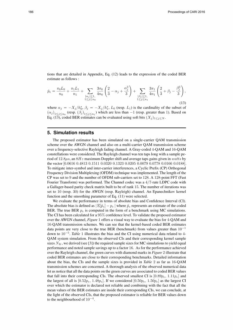
tions that are detailed in Appendix, Eq. (12) leads to the expression of the coded BERestimate as follows :

pe =π0L0

n0+

π1L1

n1+

∑|αj |≤1,1≤j≤n0

3π0

4n0

(23− αj +

α3j

3

)+

∑|βj |≤1,1≤j≤n1

3π1

4n1

(23

+ βj −β3

j

3

),

(13)where αj = −Xj/h∗

0, βj = −Xj/h∗1, L0 (resp. L1) is the cardinality of the subset of

(αj)1≤j≤n0(resp. (βj)1≤j≤n1

) which are less than −1 (resp. greater than 1). Based onEq. (13), coded BER estimates can be evaluated using soft bits (Xj)1≤j≤N .

5. Simulation resultsThe proposed estimator has been simulated on a single-carrier QAM transmission

scheme over the AWGN channel and also on a multi-carrier QAM transmission schemeover a frequency-selective Rayleigh fading channel. A Gray-coded 4-QAM and 16-QAMconstellations were considered. The Rayleigh channel was ten taps long with a sample pe-riod of 12.8µs, an 8Hz maximum Doppler shift and average taps gains given in watts bythe vector [0.0616 0.4813 0.1511 0.0320 0.1323 0.0205 0.0079 0.0778 0.0166 0.0188].To mitigate inter-symbol and inter-carrier interferences, a Cyclic Prefix (CP) OrthogonalFrequency Division Multiplexing (OFDM) technique was implemented. The length of theCP was set to 9 and the number of OFDM sub-carriers set to 128. A 128-point FFT (FastFourier Transform) was performed. The Channel codec was a 4/7-rate LDPC code witha Gallager-based parity check matrix built to be of rank 15. The number of iterations wasset to 10 (resp. 30) for the AWGN (resp. Rayleigh) channel. An Epanechnikov kernelfunction and the smoothing parameter of Eq. (11) were selected.

We evaluate the performance in terms of absolute bias and Confidence Interval (CI).The absolute bias is defined as |E[pe]− pe | where pe represents an estimate of the codedBER. The true BER pe is computed in the form of a benchmark using MC simulations.The CI has been calculated for a 95% confidence level. To validate the proposed estimatorover the AWGN channel, Figure 1 offers a visual way to evaluate the bias for 4-QAM and16-QAM transmission schemes. We can see that the kernel-based coded BER estimatesdata points are very close to the true BER (benchmark) from values greater than 10−1

down to 10−5. Table 1 illustrates the bias and the CI using numerical data related to 4-QAM system simulation. From the observed CIs and their corresponding kernel samplesizes NK , we derived (see [3]) the required sample sizes for MC simulations to yield equalperformance and noted sample savings up to a factor 16. As for the performance achievedover the Rayleigh channel, the green curves with diamond marks in Figure 2 illustrate thatcoded BER estimates are close to their corresponding benchmarks. Detailed informationabout the bias, the CIs and the sample sizes is provided in Table 2 as far as 16-QAMtransmission schemes are concerned. A thorough analysis of the observed numerical datalet us notice that all the data points on the green curves are associated to coded BER valuesthat fall into their corresponding CIs. The observed smallest CI is [0.89pe, 1.11pe] andthe largest of all is [0.52pe, 1.48pe]. If we considered [0.50pe, 1.50pe] as the largest CIover which the estimator is declared not reliable and combining with the fact that all themean values of the BER estimates are inside their corresponding CIs, we can conclude, atthe light of the observed CIs, that the proposed estimator is reliable for BER values downto the neighbourhood of 10−4.


0 2 4 6 8 10

10−5

10−4

10−3

10−2

10−1

100

Eb/No (dB)

Bit

erro

r rat

e (B

ER

)

Theoretical uncoded BERCoded BER: benchmarkCoded BER: Kernel

16−QAM

4−QAM

Figure 1. Performance of the proposed estimator over the AWGN channel

Regarding the efficiency, the two last Columns of Table 2 show that the proposed esti-mator requires less samples than the MC method. The given kernel (Nk) and MC (Nmc)sample sizes are those required for the two methods to achieve (almost) equal bias and CI.To illustrate this, let us consider the row of Eb/N0 = 12 dB in Table 2. The proposed esti-mator achieved an efficiency described by a sample size of 50 000 against 127 995 for theMC estimator. In the same time, the proposed estimator achieved a CI of [0.81pe, 1.19pe]versus [0.80pe, 1.20pe] for the MC estimator. The two estimators performed the estima-tion with almost equal bias (0.0011 for the MC method against 0.0012 for the proposedkernel method). Moreover, for Eb/N0 = 20 dB in Table 2, both the MC and the proposedestimators performed an estimate with equal bias and achieved CIs are [0.62pe, 1.38pe]for the MC estimator against [0.67pe, 1.33pe] for the proposed one. The correspondingsample saving achieved by the proposed estimator is at least of a factor 5.

Behind this efficiency of the proposed estimator is also hidden its performance interms of the power consumption. The MC method and the proposed estimator yield almostequal CPU time for equal sample sizes ; e.g. : at Eb/N0 = 20 dB and for a sample size of

Tableau 1. Numerical results of coded 4-QAM BER estimation over AWGN channel

Eb/N0 Benchmark Bias CI NK

00 dB 1.1 × 10−1 0.03 × 10−1 [0.94pe, 1.06pe] 103

01 dB 6.7 × 10−2 0.22 × 10−2 [0.90pe, 1.10pe] 103

02 dB 3.1 × 10−2 0.22 × 10−2 [0.82pe, 1.18pe] 103

03 dB 1.2 × 10−2 0.11 × 10−2 [0.93pe, 1.07pe] 104

04 dB 3.0 × 10−3 0.18 × 10−3 [0.81pe, 1.19pe] 104

05 dB 4.7 × 10−4 0.30 × 10−4 [0.89pe, 1.11pe] 105

06 dB 4.9 × 10−5 0.38 × 10−5 [0.66pe, 1.34pe] 105

07 dB 4.4 × 10−6 0.09 × 10−6 [0.54pe, 1.46pe] 106


0 5 10 15 20 2510−4

10−3

10−2

10−1

100

Eb/No (dB)

Bit

erro

r rat

e (B

ER

)

Theoretical uncoded BERCoded BER: benchmarkCoded BER: Kernel

16−QAM

4−QAM

Figure 2. Performance of the proposed estimator over Rayleigh channel

100 000, the CPU time engendered over the Rayleigh channel is 33.24 seconds for the MCmethod against 35.27 seconds for the proposed estimator. However, when the sample sizeincreases it causes the CPU time to increase too. So, the sample saving due to the kernelmethod is beneficial in terms of power consumption. As an illustration, the performanceachieved at Eb/N0 = 24 dB (see Table 2) is at the cost of a CPU time of 7.27 minutes forthe proposed estimator while being by far greater than 4.35 hours for the MC method.

6. ConclusionIn this paper, we proposed a kernel-based coded bit error rate estimator involving

soft M -ary Quadrature Amplitude Modulation (QAM) symbols. An Epanechnikov kernelfunction was selected. The corresponding smoothing parameter was determined based onthe concept of canonical bandwidth. Simulation results were reported for coded 4-QAMand 16-QAM single carrier transmissions over the additive white Gaussian noise channelsand for coded multiple carrier modulations over a frequency-selective Rayleigh fadingchannel. Through curves and numerical data, the proposed kernel-based estimator showedto be, for equal reliability, more efficient than the Monte Carlo estimator. In future works,we will be interested in the possible efficiency improvement that might be achieved ifdifferent bandwidth selection strategies were implemented.

AknowledgementsThis work started thanks to the funding of Projet RESEAU, SCAC-Ambassade de

France, Burkina Faso. Part of it has been performed in the framework of the FP7 projectICT-317669 METIS, which is partly funded by the European Union.


Tableau 2. Numerical results of coded 16-QAM BER estimation over Rayleigh channel

Eb/N0 Benchmark Bias CI Nk Nmc

00 dB 2.58 × 10−1 0.13 × 10−1 [0.89pe, 1.11pe] 1.0 × 103 3.0 × 103

04 dB 1.50 × 10−1 0.06 × 10−1 [0.86pe, 1.14pe] 2.0 × 104 1.9 × 104

08 dB 6.28 × 10−2 0.26 × 10−2 [0.87pe, 1.13pe] 5.0 × 104 5.1 × 104

12 dB 2.31 × 10−2 0.12 × 10−2 [0.81pe, 1.19pe] 5.0 × 104 1.3 × 105

16 dB 7.00 × 10−3 1.00 × 10−3 [0.73pe, 1.27pe] 5.0 × 104 1.0 × 105

20 dB 1.50 × 10−3 0.08 × 10−3 [0.67pe, 1.33pe] 1.0 × 105 > 5.1 × 105

24 dB 3.42 × 10−4 0.36 × 10−4 [0.54pe, 1.46pe] 4.1 × 105 > 2.6 × 106

7. Bibliographie

[1] S. BENEDETTO, E. BIGLIERI, R. DAFFARA, « Modeling and performance evaluation of nonlinear satellite links-A volterra series approach », IEEE Journal on Selected Areas in Commu-nications, vol. AES-15, 1979, pp. 494-507.

[2] K. YAO, L. B. MILSTEIN, « The use of moment space bounds for evaluating the performanceof a non linear digital communication system », IEEE Transactions Communications, vol. 31,1983, pp. 677-683.

[3] M. C. JERUCHIM « Techniques for estimating the bit error rate in the simulation of digitalcommunication systems », IEEE Journal on Selected Areas in Communications, vol. 2, no 1,1984, pp. 153-170.

[4] S. SAOUDI, T. DERHAM, T. AIT-IDIR, P. COUPE « A Fast Soft Bit Error RateEstimation Method », EURASIP Journal Wireless Communications and Networking,doi :10.1155/2010/372370, 2010.

[5] M. ROSENBLATT, « Remarks on some non-parametric estimates of a density function », TheAnnals of Mathematical Statistics, vol. 27, no 3, 1956, pp. 832-837.

[6] S. SAOUDI, M. TROUDI, F. GHORBEL, « An Iterative Soft Bit Error Rate Estimation ofAny Digital Communication Systems Using a Nonparametric Probability Density Function »,EURASIP Journal Wireless Commun. and Networking, doi :10.1155/2009/512192, 2009.

[7] S. SAOUDI, T. AIT-IDIR, Y. MOCHIDA, « A Novel Non-Parametric Iterative Soft Bit ErrorRate Estimation Technique for Digital Communications Systems », In : IEEE InternationalConference on Communications, 2011, pp. 1-6.

[8] J. DONG, T. AIT-IDIR, S. SAOUDI, « Unsupervised bit error rate estimation using MaximumLikelihood Kernel methods », In : IEEE Vehicular Technology Conference, 2012, pp. 1-5.

[9] M. C. JONES, J. S. MARRON, S. J. SHEATER, « A brief survey of bandwidth selection fordensity estimation », Journal of the American Statistical Association, vol. 91, no 433, 1996,pp. 401-407.

[10] A. Z. ZAMBOM, R. DIAS, « A review of Kernel density estimation with applications toeconometrics », International Econometric Review, vol. 5, no 1, 2013, pp. 20-42.

[11] Q. WANG, Q. XIE, Z. WANG, S. CHEN, L. HANZO, « A Universal Low-Complexity Symbol-to-Bit Soft Demapper », IEEE Transactions on Vehicular Technology, vol. 63, no 1, 2014, pp.119-130.

[12] J.S. MARRON, D. NOLAN, « Canonical kernels for density estimation », Statistics & Proba-bility Letters, vol. 7, 1988, pp. 195-199.


8. AppendixThe BER estimate as given in Eq. (12) is

pe = π0

∫ +∞

0

1n0

n0∑j=1

1h∗

0

K

(x − Xj

h∗0

)dx + π1

∫ 0

−∞

1n1

n1∑j=1

1h∗

1

K

(x − Xj

h∗1

)dx,

(A.1)where n0 (resp. n1) is the cardinality of the subset of the soft observations among (Xj)1≤j≤N

which are likely to be decoded into a binary “0” bit value (resp. “1”) and h∗0 (resp. h∗

1)is the selected optimal smoothing parameter which will govern the accuracy of the esti-mation of f

(0)X (x) (resp. f

(1)X (x)). More explicitly, as K(x) = 3

4

(1 − x2

)I(|x| ≤ 1), we

have

pe = π0n0

∫ +∞0

∑n0j=1

34h∗

0

[1 −

(x−Xj

h∗0

)2]

I(∣∣∣x−Xj

h∗0

∣∣∣ ≤ 1)

dx

+π1n1

∫ 0

−∞∑n1

j=13

4h∗1

[1 −

(x−Xj

h∗1

)2]

I(∣∣∣x−Xj

h∗1

∣∣∣ ≤ 1)

dx.

(A.2)

Then, using one of the properties of the integral, we get

pe = π0n0

∑n0j=1

∫ +∞0

34h∗

0

[1 −

(x−Xj

h∗0

)2]

I(∣∣∣x−Xj

h∗0

∣∣∣ ≤ 1)

dx

+π1n1

∑n1j=1

∫ 0

−∞3

4h∗1

[1 −

(x−Xj

h∗1

)2]

I(∣∣∣x−Xj

h∗1

∣∣∣ ≤ 1)

dx.

(A.3)

Now, let us set the following changes of variables :u = x−Xj

h∗0

v = x−Xj

h∗1

.

We obtain

pe = 3π04n0

∑n0j=1

∫ +∞−Xj/h∗

0

(1 − u2

)I (|u| ≤ 1) du

+ 3π14n1

∑n1j=1

∫ −Xj/h∗1

−∞(1 − v2

)I (|v| ≤ 1) dv,

(A.4)

and then,

pe =3π0

4n0

n0∑j=1

∫[αj , +∞]∩ [−1, 1]

(1 − u2

)du +

3π1

4n1

n1∑j=1

∫[−∞, βj ]∩ [−1, 1]

(1 − v2

)dv,

(A.5)where αj = −Xj/h∗

0 and βj = −Xj/h∗1. Depending on the values of αj (resp. βj), three

cases are possible among which one leads to zero ; hence we get,


pe = 3π04n0

∑αj<−1,1≤j≤n0

[t − t3

3

]1−1

+∑

|αj |≤1,1≤j≤n0

[t − t3

3

]1αj

+ 3π14n1

∑βj>1,

1≤j≤n1

[t − t3

3

]1−1

+∑

|βj |≤1,1≤j≤n1

[t − t3

3

]βj

−1

.

(A.6)

Finally, the BER estimate expression is as follows :

pe = π0L0n0

+ π1L1n1

+ 3π04n0

∑|αj |≤1,1≤j≤n0

(23 − αj + α3

j

3

)

+ 3π14n1

∑|βj |≤1,1≤j≤n1

(23 + βj −

β3j

3

),

(A.7)

where L0 (resp. L1) is the cardinality of the subset of (αj)1≤j≤n0(resp. (βj)1≤j≤n1

)which are less than −1 (resp. greater than 1).


Management of Low-density Sensor-ActuatorNetwork in a Virtual Architecture

Vianney Kengne Tchendji∗, Blaise Paho Nana∗

∗Department of Mathematics and Computer ScienceFaculty of ScienceUniversity of DschangPO Box 67, [email protected], [email protected]

RÉSUMÉ. Les réseaux de capteurs sans fi (RCSF) font face à de nombreux problèmes dans leurmise en œuvre, notamment la connectivité des nœuds, la sécurité, l’économie d’énergie, la tolérenceaux pannes, le routage [3]. Dans ce document, nous considérons un RCSF peu dense, caractérisépar une mauvaise couverture de la zone d’intérêt, et l’architecture virtuel introduite par Wadaa et al[1] qui permet de partitionner efficacemen ce type de réseau en clusters. Dans l’optique de routeroptimalement les informations collectés par chaque capteur jusqu’à une station de base (nœud sink,supposé au centre du réseau), nous proposons une stratégie de déplacement des capteurs mobiles(actuators) qui permet de: sauvegarder la connectivité du RCSF, optimiser le routage, économiserl’énergie des capteurs, améliorer la couverture de la zone d’intérêt, etc.

ABSTRACT. Wireless sensor networks (WSN) face many implementation’s problems such as con-nectivity, security, energy saving, fault tolerance and routing problems [3]. In this paper, we consider alow-density WSN where the distribution of the sensors is poor, and the virtual architecture introducedby Wadaa et al [1] which provides a powerful and fast partitioning of the network into a set of clusters.In order to effectively route the information collected by each sensor node to the base station (sinknode, located at the center of the network), we propose a strategy to allow mobile sensors (actuators)to move in order to: save connectivity of WSN, improve the routing of collected data, save energy ofthe sensors, improving the coverage of the interested area, etc.

MOTS-CLÉS : Réseau de capteurs sans fil architecture virtuelle, cluster vides, actuator, routage

KEYWORDS : Wireless sensor network, virtual architecture, empty cluster, actuator, routing


1. Introduction

For few years now, many improvements have been made in domains such as micro-electro-mechanical systems (MEMS) technology [9], wireless communications, and digi-tal electronics. This enabled the development of micro components that easily combinedata collection tools and wireless communication devices, and then opens a wide scopeto wireless sensor networks (WSN) [3, 5, 8, 11].

Usually called microsensors or simply sensors, these devices with limited resources(bandwidth, computing power, available memory, embedded energy, etc.) have revolutio-nized traditional networks by bringing the idea to develop sensors networks based on thecollaborative effort of a large number of sensors operating autonomously, and commu-nicating with each other via short-range transmissions [6, 7]. These resource limitationsadded to the radio communication that have sensors, are factors that raise many problems(interference, intrusion, disconnection, data integrity, etc.).In fact, it is common to see WSN composed of several thousand units [4]. In large net-works, the sensors can be grouped into clusters based on their proximity in order to signi-ficantly increase the scalability, economy energy, routing, and consequently the lifetimeof the network. The structure provided by this partitioning allows the use of various tech-niques to improve the quality of a WSN, such as data aggregation [10, 11].

In this paper, we consider a low-density WSN where the distribution of the sensors ispoor, and the virtual architecture introduced by Wadaa et al [1] which provides a powerfuland fast partitioning of the network into a set of clusters. In order to effectively route theinformation collected by each sensor node to the base station (sink node, located at thecenter of the network), we propose a strategy to allow mobile sensors (actuators) to movein order to : save connectivity of WSN, improve the routing of collected data, save energyof the sensors, improving the coverage of the interested area, etc.

The rest of this paper is organised as follows : we first present the virtual architecturein which we work, then we present a technique of detecting empty clusters, followed byour method of strengthening strategic points by the actuators, then the technique used toproper move the actuators is presented. A conclusion ends the paper.

2. Virtual architecture sensor network

2.1. Anatomy of a sensor

This is the basic equipment of any WSN. It has three main tasks : information collec-tion from the deployment area, light treatment (optional) on the collected data and sharingthese data with other sensors through multi-hop routing. Despite the great diversity (tem-perature sensors, humidity, pressure, etc.) existing on the market, they are all mounted onthe same architectural diagram mainly made of a unit of : capture, processing, storage,communication, and energy. This material may be supplemented or reduced according tothe developper [3]. One can for example add a locating system such as a GPS (GlobalPositioning System), a mobilizer (to get an actuator). The main and optional elements(represented by dashed lines) are shown in figure 1.


Figure 1 – Hardware architecture of a sensor.2.2. Virtual network architecture

Let’s consider a special sensor called the sink or base station (BS) unconstrained bycommon sensors’s limits and capable of omnidirectional transmissions according to dif-ferent radius and transmissions at various angles. Once deployed in the supervised area(figure 2a), the sensors can be grouped in clusters (as described in [1]) depending on thecorona and the angular sector in which it is located (see figure 2b). Thus, the intersec-tion of the coronai and the angular sectorj forms the cluster(i, j). Since the network issparse, it is important to identify the empty clusters. This allow to have an overview ofthe area covered by the sensors, and to achieve a better monitoring.

(a) Example of a basic WSN. (b) A sparse virtual architecture.

Figure2 – An virtual architecture representation.

3. Detection of empty clusters and election of clusterheads

Knowing the distribution of sensors allows the sink to detect empty clusters and buildthe message propagation tree of figure 3b. Forc coronas ands sectors, the sink countsc× s clusters in its virtual architecture ; therefore sink regularly updates to each messagereceived two tablesh(c, s) andrelay(c, s). Each entry(i, j) of the tableh(c, s) contains1 if cluster(i, j) is not empty and 0 otherwise, allowing the sink to get a global view of


the sensors’s distribution ; and each entry(i, j) of the tablerelay(c, s) contains the coor-dinates of the relay cluster of the cluster(i, j). For the rest we advance some hypotheses.

3.1. Hypotheses

The network is fully clustered as shown in figure 2b using the technique described in[1]. Each cluster has a gateway node or clusterhead (CH :node by which a message getsout of the cluster. This reduces redundancy.). Furthermore,

– Each sensor has a unique identifierID in the network. The sensors are static andform a connected network. Adding or removing a sensor is a rare event ;

– A node is able to estimate its residual energyEr and the sink has the ability tobroadcast messages in the network at different radius, or at different angles ;

– The time is divided into slots of lengthr, parametersc ands are known to all sensors,and the local clock of each sensor is synchronized with the sink’s ;

– A message sent by a sensor reaches all the sensors located in its transmission rangeafter a slot ;

– Clusterisation is made such that all sensors of a given cluster can communicate witheach other and some sensors of neighbor clusters.

Here is our protocol, its main lines are taken from S. Faye and J. F. Myoupo [2]. Weare introducing the concept of clusterhead (CH).

3.2. Sink’s algorithm

The sink periodically broadcasts the date on which the discovery algorithm will begin.All sensors are awake and sink initiates the detection by spreading in the first corona adiscovery messageDetect(−1,−1). Due to network connectivity, it is certain that at leastone sensor will receive this message. During the algorithm, each message transmitted by asensor towards the sink contains the coordinates of its cluster and those of his relay cluster.Tableh(c, s) is initialized to 0. At each received messages from a sensor of the cluster(i, j), BS puts 1 inh(i, j) and, in the entryrelay(i, j), it assigns the value contained inthe variablerelay of the received message. At the end of the algorithm, a cluster(i, j) isconsidered empty whenh(i, j) = 0 and the relay cluster of the cluster(i, j) is indicatedby relay(i, j).

3.3. Sensors’s algorithm

The network is supposed connected, so for all cluster(i, j) considered non-empty,there is always a path from it to the sink node. Isolated clusters can’t reach the sink andare considered empty even if there are not. There are three main events in the detectionof empty clusters : the reception of a messageDetect asking sensors to indicate theircoordinates ; the reception of a messageHead sent by a node to propose itself as thegateway node and ; the reception of a messageACK sent by the sensors to the sink nodeto indicate their coordinates.

– Reception of a message Detect : On the first slot, after receiving a messageDetect(−1,−1) from BS, the sensors of the first corona build a messageDetect(1, j),and broadcast it to allow sensors in other clusters to reveal their presence. Then, those thatreceived the messageDetect from a neighbor cluster and have an energy higher than thethresholdEs send a messageHead towards their own cluster to be elected as the CH.


– Reception of a message Head : At the reception of a messageHead, the sensorsaves the identifier of the CH in its variablegatewayNode if this is its first reception,otherwise it compares the residual energyEr of gatewayNode with that of the receivedmessage and stores the one that has the biggestEr. If the Er are equal, the one withthe highestID is chosen. A sensor that has already received a messageHead can’t sendmessageHead, because it would have received its messageDetect from a more distantneighbor cluster to the sink than the relay sensor that sent him the first messageHead.Finally, the sensor that is elected in the cluster builds a messageACK((i, j), (−1,−1))and sends towards the sink node which is actually its relay cluster. This process is repeatedfor all the other sensors untill the most distant cluster sends its messageACK.

– Reception of a message ACK : A sensor that receives a messageACK from theneighbor node checks whether this message is for its cluster. In this case, it sends it to hisgateway node which checks if it has not already routed a message from the same cluster.If not, it broadcasts it towards its relay cluster. Otherwise, it simply ignores it.

4. Searching and filling strategic empty clusters by actuators

Thissection is once again inspired from [2]. Here we introduce the actuators : sensorswith a mobilizer, allowing them to move on the sink’s order. They can be used for manypurposes, depending on the user, for example :

– Being the CH in a cluster where all the sensors have a small energy ;

– Collect and route information in isolated areas ;

– Connect a sub isolated connected network to the main network.

– Being sent in strategic empty clusters (purpose of this paper) to optimize the routing.From the tableh(c, s) the sink knows the empty clusters. In order to know which ones

it is going to fill first, it should reproduce the messages spreading tree like in figure 3bby using the two tables it has like this : Take BS as root and the first tree’s leaf. As longas there’s an unvisited leaf(i, j), search in the tablerelay(c, s) the cluster that has thecluster(i, j) as relay cluster and add them as the sons of(i, j).

(a) Propagation of messages in the supervised area. (b) Messages spreading tree.

Figure3 – The messages spreading tree obtained after the detection of the empty clusters.


Filling a strategic empty cluster has the effect of reducing thetree’s height (figure3b). The ideal one would be to reduce this size to the number of coronas of our virtualarchitecture. The routing will be optimal if for any cluster of coronak, the transmissionof a message towards BS passes throughk intermediate clusters.

4.1. Rule of detection of clusters which access can be improved

To optimize the routing to a cluster, it would be good to know whether the currentaccess is optimizable. In figure 3, it is the case of cluster(1, 4) which is at5 intermediateclusters from BS instead of1 if an actuator were placed in cluster(0, 3).

Rule : Let A a message spreading tree similar to that of figure 3b,prof(i, j) denotesthe depth of the cluster(i, j) in the treeA. The path from sink to(i, j) can be improved ifthere is another cluster(i′, j′) with depthprof(i′, j′), such asi′ ≥ i andprof(i′, j′) <prof(i, j), i.e. (i′, j′) is in a corona greater or equal to(i, j)’s but in the treeA, (i′, j′)appears at a depth less than(i, j)’s.

4.2. Detection of strategic empty cluster to fill in priority

To determine this priority cluster (PC), we establish for every coronaa the listL[a]of clusters of this corona which access can be improved (Ccoronas =C lists). Eachlist L[a] contains the coordinates(a, j) of clusters of the coronaa which access can beimproved. It is in the form :L[a] = [(a, j1), (a, j2), . . . , (a, jn)]. From each listL[a], weextract the longest list Ls[a] made of consecutive clusters of L[a]. In the listLs[a], each(a, j) represents the coordinates of the clusters of coronaa that follows in the messagespreading tree. The coordinates(x, y) of PC are deduced from the longest sub listLsp[a]taken among theLs[a] extracted lists.x = a − 1 andy is equals to the default roundingaverage ofj (thej are the second components items(a, j) of the listLsp[a]).As long as there’s available actuators, it is necessary to move an actuator at the cluster(x, y), another at the cluster(x− 1, y) if it is empty, ... another at the cluster(0, y) if it isempty. The process can be repeated until the routing is optimal, i.e. up toprofA ≤ C.For the example of figure 3, the determination of PC is presented in annex A.

Before moving a mobile sensors, the sink node must calculate the distances from itto the target empty cluster, it is better to choose the most appropriate actuator, based ondistance, residual energy, availability, etc.

5. Moving a mobile sensor

We propose to move an actuator from the cluster(x, y) to the empty cluster(j, k).The actuator will need the distance and direction to move. To simplify our calculations,we should be in a cartesian plane. For this we describe here how to transform our currentcoordinate system (Dynamic Coordinate System : DCS) in a Polar Coordinate System(PCS) and then in to a Cartesian Coordinate System (CCS).

5.1. Correspondence between DCS, PCS and CCS

To get the distance and the direction to follow, we must define a reference. Thus theorigin of our reference will the sink. TheY axis is taken such that it coincides with theleft edge of the first section (section 0). TheX axis is at a quarter turn from theY axis sothat the angle X, sink, Y is direct (figure 4a). Any point of the DCS is discoverable usingp (its distance from the sink) andϕ (angle measured from theY axis) as in figure 4b.


(a) Definitio of the reference (b) PCS - CCS

Figure4 – Correspondence between the DCS - PCS - CCS

Denote ’α’ the angle of a sector and ’e’ a thickness of a corona, we can state corollary1.

Corollary 1 Let M be a sensor of the cluster (c, s) assumed at it center. In the PCS, Mhas the coordinates (p, ϕ) where p = c× e+ e

2and ϕ = s× α+ α

2;

Let M(p, ϕ) be a point in the PCS. In the CCS, M has coordinates (x, y) with x = Mx =p sin(ϕ) and y = My = p cos(ϕ).

5.2. Moving the actuator

Now we can start the necessary calculations (distancep and anglesϕ) to move theactuators.

5.2.1. Calculation of the distance (p)

The distance between two pointsA andB of the plane is given by the norm of thevector

−−→AB, denoted||

−−→AB|| or justAB. According to figure 4b, an actuator that moves

from the sink node (with cordinates(0, 0)) to the point M (with cordinates(x, y)) mustcover the distancep = ||

−−−−−→sink M || = ||(x − 0, y − 0)|| = ||(x, y)||. But ||

−−−−−→sink M ||2 =

(sink Mx)2 + (sink My)

2 = x2 + y2. Thus ||−−−−−→sink M || =

√

x2 + y2. So we havecorollary2.

Corollary 2 Moving an actuator from the center of the cluster A(c1, s1) of polar co-ordinates (p1, ϕ1) to the center of the cluster B(c2, s2) of polar coordinates (p2, ϕ2)returns to move this actuator from the point A(Ax, Ay) to the point B(Bx, By) of thecartesian coordinates system on a distance p = ||

−−→AB|| where

−−→AB(Bx − Ax, By − Ay),

p = ||−−→AB|| = 2

√

(Bx −Ax)2 + (By −Ay)2, Ax = p1 cos(ϕ1), Ay = p1 sin(ϕ1),Bx = p2 cos(ϕ2) and By = p2 sin(ϕ2).

5.2.2. Calculation of the angle (ϕ)

To facilitate the calculation of the value ofϕ, let’s make a change of reference.

Change of reference : We want to move a mobile sensor from a pointA to a pointB.For this, we define a new reference in which the base vectors are collinear with those ofthe previous (see figure 5a).


(a) Reference change (b) Angle between the axis Y′ and the dis-

placement vector

Figure 5 – Angle displacement

The referenceR1 = (sink,−→i ,

−→j ) ; R2 = (A,

−→i ,

−→j ) ; R2 = t−−−−→

sink A(R1) wheret

denotes the translation of vector−−−−→sink A. The coordinates of two pointsM(x, y) ∈ R1,

andM ′(x′, y′) ∈ R2 such thatM ′ = t−−−−→sink A

(M) are now linked by the following

relations :x′ = x− xA andy′ = y − yA.Basis vectors of these two referenecs are pairwise collinear, that’s why the angles foundin one of the refeces will be equivalent in the second.

Calculation of the inclination α0 formed by the displacement vector and the Y ′ axis :The displacement angleϕ that we want to calculate is strongly related to the angleα0

formed by the vector−−→AB and theY ′ axis. Figure 5b presents the different situations we

may encounter. We deduced thatsin(α0) =|Bx|AB ⇒ α0 = sin−1

(

|Bx|p

)

wherep = AB.

Determination of the displacement angle ϕ : From figure 5b, pointB can be found inone of the four sectors.

Corollary 3 The displacement angle ϕ of an actuator from the point A(Ax, Ay) to thepoint B(Bx, By) of (A,

−→i ,

−→j ) reference is given by :

1) if B is in the sector 0, i.e. Bx > 0 and By ≥ 0 then ϕ = α0

2) if B is in the sector 1, i.e. Bx ≥ 0 and By < 0 then ϕ = π − α0

3) if B is in the sector 2, i.e. Bx < 0 and By ≤ 0 then ϕ = π + α0

4) if B is in the sector 3, i.e. Bx ≤ 0 and By > 0 then ϕ = 2π − α0

For a practical example of moving a sensor, see annex B.


6. Simulation and analysis of our solution

6.1. Tools and simulation environment

Using an HP computer Intel (R) Core (TM) i7-2630QM CPU @ 2.00 GHz× 8, 8GBof RAM, running Windows 8 Professional ; a discrete event network simulator J-Sim ;and a sample of 1000 sensors randomly deployed within 10 km of the sink ; the virtualarchitecture has 10 coronas and 8 sectors of45o each. We performed repeatedly tests andaverages the results. The energy model is the one adopted by many efficient contributions[13] : E = Etrans +Erecep. Etrans andErecep are respectively the total energy used fortransmissions in the network and receptions, knowing that each sensor has a range of 500meters, and initial energy of 100 joules. He needs35.28 × 10−3joule per transmissionand31.32× 10−3joule per reception. The curves were made with version 5.0 of gnuplotsoftware.

6.2. Analysis of the simulation results

Figure 6 compares the energy consumption of the cluster-heads and ordinary sensorswhen the routing is not optimized and when routing is optimized with actuators. An eco-nomy of energy is observed among both ordinary sensors and cluster-heads sensors. Thisincreases the longevity of the network. The simulation is made for the detection of emptyclusters, the election of cluster-head and routing. A slot is78µs. The great loss of energyobserved at the beginning of the curve is due to the fact that the cluster-head are notelected at the beginning. It is clear that this energy loss is significantly reduced once thecluster-head are elected.

Figure 6 – Improvement of the power consumption using cluster-headsand actuators.

7. Conclusion

In this paper we have presented a virtual architecture that facilitates the managementof WSN. We also introduced the gateways nodes, their election protocol and how to li-mit redundant messages through them. But our main aim was to optimize the routing of


collected data towards de sink. That’s why we started by describinga method of detec-ting and filling strategic empty clusters in which we can send mobile sensors. We alsopresent other possible utilities of the actuators, and show a new way of performing theirmovements to improve the routing of the collected data.

In a very soon future we intend to work on the mechanism of reelection of the cluste-rhead in a cluster ; the mechanism of changing relay cluster if the current relay cluster isno longer accessible and the mechanism of redirection of packets routing after the posi-tioning of the mobile sensor.

8. Bibliographie

[1] A. WADAA , S. OLARIU , L. WILSON, M. ELTOWEISSY, K. JONES, « Training a wirelesssensor network »,Mobile Networks and Applications, Vol. 10, No 1-2, p. 151–168, 2005.

[2] SÉBASTIEN FAYE, JEAN-FRÉDÉRIC MYOUPO, « Deployment and Management of SparseSensor-Actuator Network in a Virtual Architecture »,International Journal of Advanced Com-puter Science, Vol. 2, No 12, December, 2012.

[3] I. F. AKYILDIZ , WEILIAN SU, Y. SANKARASUBRAMANIAM , E. L . CAYIRCI , « A survey onsensor networks »,IEEE Communications Magazine, Vol. 40, No 8, p. 102–114, 2002.

[4] B. WARNEKE, M. LAST, B. LEIBOWITZ AND K. PISTER, « Smart Dust : communicating witha cubic-millimeter computer »,IEEE Computer, Vol. 34, No 1, p. 44–51, 2001.

[5] S. TILAK , N.B. ABU-GHAZALEH , W. HEINZELMAN , « A taxonomy of wireless micro-sensornetwork models »,Mobile Computing and Communications Review, Vol. 6, No 2, p. 28–36,2002.

[6] M ARK A. PERILLO, WENDI B. HEINZELMAN , « Wireless Sensor Network Protocols »,Al-gorithms and Protocols for Wireless and Mobile Networks, Eds. A. Boukerche et al., CRC HallPublishers, 2004.

[7] K. SOHRABI, J. GAO, V. A ILAWADHI , G. J. POTTIE, « Protocols for Self-Organization of aWireless Sensor Network »,IEEE personal communications, Vol. 7, No 5, p. 16–27, 2000.

[8] C. INTANAGONWIWAT AND R. GOVINDAN AND D. ESTRIN, « Directed Diffusion : a scalableand robust communication paradigm for sensor networks »,ACM Press, p. 56–67, 2000.

[9] B. WARNEKE, K.S.J. PISTER, « MEMS for Distributed Wireless Sensor Networks »,9th

International Conference on Electronics, Circuits and Systems, Croatia, Vol. 1, p. 291–294,2002.

[10] S. FAYE , J. F. MYOUPO, « An Ultra Hierarchical Clustering-Based Secure Aggregation Pro-tocol for Wireless Sensor Networks »,AISS : Advances in Information Sciences and ServiceSciences, Vol. 3, No 9, p. 309 – 319, 2011.

[11] A. PERRIG, R. SZEWCZYK, V. WEN, D. CULLER, J.D. TYGAR, « SPINS : Security proto-cols for sensor networks »,Wireless networks, Vol. 8, No 5, p. 521–534, 2002.

[12] C. KARLOF, N. SASTRY AND D. WAGNER, « TinySec : A Link Layer Security Architecturefor Wireless Sensor Networks »,in : Proc. of the 2nd international conference on Embeddednetworked sensor systems, ACM, p. 162–175, 2004.

[13] D. WEI AND S. KAPLAN AND H. A. CHAN, « Energy Efficient Clustering Algorithms forWireless »,in : Sensor Networks, Proceedings of IEEE Conference on Communications, Bei-jing, IEEE, p. 236–240, 2008.


A. Practical example for determination of priority clusters

With the example of figure 3, the determination of priority clusters is performed asfollow :Lists construction :L[0] = ∅ ; L[1] = [(1, 1), (1, 2), (1, 3), (1, 4)] ; L[2] = [(2, 1), (2, 4), (2, 5)]Extraction of clusters sublists which follow :Ls[0] = ∅ ; Ls[1] = [(1, 1), (1, 2), (1, 3), (1, 4)] ; Ls[2] = [(2, 4), (2, 5)]The longest sub-list : Lsp = Ls[1] = [(1, 1), (1, 2), (1, 3), (1, 4)]Calculation of the coordinates (x, y) :x = 1− 1 = 0 andy = floor(Average(1, 2, 3, 4)) = floor(2.5) = 2Filling stategic clusters : The cluster(0, 2) is free, an actuator should be sent into it. Byrepeating the process : We should put an actuator (if there are available) in the cluster(0, 4) ...

B. Practical example of moving a mobile sensor

Let’s move an actuator from the clusterA(1, 1) to the clusterB(0, 3). For our tests,let’s suppose : the scope of the sink is30.0m and the virtual architecture includes 3 coro-nas withe = 10.0m each ; there are 8 angular sectors ofα = π

4radeach.

Polar Coordinates : A(15.0, 1178 rad) andB(5.0, 2.749 rad)

Cartesian coordinates : A(13858, 5740) andB(1913, 4619)

Distance : p = ||−−→AB|| = 15.811

Displacement angle : B′x = Bx −Ax = −11.945 andB′

y = By −Ay = −10.359,thenα0 = 0.856 rad. SinceB′

x < 0 andB′y <= 0 then B is in sector 2 and thus,

ϕ = π + α0 = 3.998 rad orϕ = 229.065˚.

Conclusion : To strengthen the area(0, 3), the sink node asks the actuator of the cluster(1, 1) to cover a distancep = 15.811m with an angle ofϕ = 229, 065˚.


Centre of Mass of single coverage: A

comparative study with Simulated Annealing

for mesh router placement in rural regions

Jean Louis Fendji Kedieng Ebongue* and Christopher Thron**

*The University of Ngaoundéré - CAMEROON

[email protected]

** Texas A&M University Central Texas - USA

[email protected]

RÉSUMÉ. Ce travail s’attaque à un problème critique dans la planification de réseaux maillés sans-fil pour zones rurales : le placement de nœuds maillés. Le but est de maximiser la couverture tout en réduisant autant que possible le nombre de nœud dans le réseau et en assurant la connectivité. Pour atteindre cet objectif, nous proposons une approche basée sur le calcul du barycentre de la zone couverte par un seul routeur. Cette approche est dix fois plus rapide que l’approche basée sur le recuit simulé. En outre, les simulations ont aussi montré une faible variation des solutions, traduisant ainsi une certaine stabilité de l’approche. Toutefois, la qualité des solutions obtenues en termes de couverture des zones d’intérêt avec le recuit simulé reste meilleure.

ABSTRACT. This paper tackles a critical issue in the planning of rural wireless mesh network (RWMN): the mesh node placement. The aim in the planning of RWMN is to maximise the coverage while keeping the number of router as few as possible and ensuring the connectivity. To achieve this, we proposed an approach based on the calculation of the centre of mass of areas covered per router. This approach is ten times more time-efficient than the simulated annealing one. In addition, the simulations results also provide a low variation of the solutions, showing some stability of the approach. However, the quality of the solution in terms of coverage of areas of interest provided by the approach based on Simulated Annealing is better.

MOTS-CLÉS : Centre de Masse, Recuit Simulé, Réseaux maillés sans fil, Placement de router maillé.

KEYWORDS: Centre of mass, Simulated Annealing, Wireless Mesh Networks, Mesh router placement.




1. Introduction

A Wireless Mesh Network (WMN) [1] is a wireless network in which nodes are

connected in a mesh topology. This kind of network is an appealing cost-effective

solution to bridge the digital divide observed between rural and urban regions, since it is

based on off-the-shelf material especially WiFi technology.

Rural Wireless Mesh Networks (RWMN) are usually composed of one gateway

which connects the network to Internet, and a set of mesh routers (MRs). The success of

the planning of such networks depends on the determination of an optimal number and

placement of its mesh nodes. The planning of wireless networks in rural regions is more

coverage-driven than capacity-driven [2], with the aim of minimizing the overall cost of

the architecture, while maximizing the coverage percentage of the area to cover.

For realistic deployment scenarios, the problem of mesh node placement is a NP-

hard combinatorial optimization problem which cannot be solved in polynomial time

[9], [10]. This is why metaheuristics are usually required to optimize the planning.

This paper considers the network model found in [3]. In this model, a given area to

cover is decomposed into elementary areas which can be required or optional in terms

of coverage and where a node can be placed or not. An extension is made to this model

in order to consider the presence of obstacles that can hinder the connectivity. The aim

is therefore to determine the location of mesh routers which maximizes the coverage of

area of interest. To achieve this goal, a placement approach based on the calculation of

the centre of mass (CM) of area covered per router is proposed. This approach is

compared to the simulated annealing (SA) approach defined in [4] to solve the same

problem.

The rest of the paper is organized as follows: Section 2 briefly presents related work in

WMN planning. Section 3 defines the network model and formulates the placement

problem. Section 4 explains the approach based on the calculation of the centre of mass

of area covered alone by a router. Section 5 presents the experimental setup and

discusses the results in comparison with simulated annealing ones. This paper ends with

a conclusion and future work.

2. Related Work

The work in [5] provides a good overview of the planning problem in WMN. This

survey classifies the planning problem according to the flexibility of the network

topology: unfixed (not-predefined) and fixed (predefined). In fixed topology, all the

nodes in the network have a predefined location. The problem is therefore more related


to routing protocols, channel assignment, or joint approaches. In unfixed topology, the

location of at least some nodes is not predefined in the network: either the gateway(s) or

the mesh routers, or both. This problem is usually assimilated to the one of facilities and

locations with mesh routers representing facilities and the users to serve representing

locations.

To solve the placement approach, different formulations have been proposed in the

literature. They depend on the type of node considered in the planning problem: mesh

routers [6], gateways(s) [7], or both [8]. Linear programming based approaches [9] have

been used; but since this problem is known to be hard for real size deployment [9],

search techniques and meta-heuristic are usually used [6, 10, 11, 12]. The region to be

covered, usually called the universe, can be considered as continuous (a whole region),

discrete (a set of predefined positions) or network (undirected weighted graph).

In [10], an approach based on simulated annealing has been proposed to solve the

mesh nodes placement problem. It aims to find optimal locations of routers that

maximize the network connectivity and client coverage, given a two-dimensional area

with a number of fixed client nodes.

The work in [13] introduces the placement problem of mesh routers in a rural region.

It has been extended later in [3], wherein a region is considered as decomposed into a

set of elementary areas which may require the coverage or where a node may be placed.

A placement approach based on metropolis algorithm has been therefore used.

3. Formulation of the Placement Problem

A given region is composed of areas of interest that should be covered as it is in [4].

The coverage of a region is considered as optional when this region is not of interest. A

given region comprised also prohibited areas where a node cannot be placed (lake, river,

road…), and a set of obstacles that could hinder the connectivity.

The area to cover is modelled as a two-dimensional irregular form in a two-dimension

coordinate plane. We consider the smallest rectangle that can contain the irregular form.

Therefore, we assume that this rectangle is decomposed into small square forms. Each

discrete point is called elementary area (EA), which can be of one or more types:

Elementary Area of Interest (EAI); Non-line-of-sight Elementary Area (NEA); or

Prohibitive Elementary Area (PEA).

We define a set of two-dimensional matrices in order to characterise each EA: Cover

indicating whether an EA requires coverage; Place indicating whether we can place a


node in an EA; CoverDepth indicating the number of routers covering an EA; and

Pathloss indicating whether an EA contains an obstacle. Therefore, an EA at position

(𝑥, 𝑦) can be characterised by (1-4).

Cover x, y = 0 → coverage not required 1 → coverage required

(1)

Place x, y = 0 → cannot place a node 1 → can place a node

(2)

CoverDepth x, y = 0 → no coverage n → covered by n routers

(3)

Pathloss x, y = 0 → no obstruction p → attenuation factor = p

(4)

To simplify the problem, we assume that the attenuation factor of any obstacle in the

line of sight between two routers is high enough to prevent any wireless link between

those routers. We also assume that all routers are equipped with an omnidirectional

antenna all having the same coverage radius (r). The radius is expressed as the number

of EAs (r = 6 means that the radius stretches over 6 EAs).

Let 𝑝 be an EA at position (𝑥, 𝑦). If a mesh node is located in 𝑝, then the set of EAs

covered by this mesh node is given by (5).

∀ a, b , x − a 2 + y − b 2 < r2 (5)

The population is not so dense in rural regions when comparing to urban ones; thus, we

consider as in [2] that the planning is coverage-driven, meaning we are more concern by

the space to cover than the throughput to deliver. The mesh router placement problem in

rural regions can be therefore described as the determination of a minimum set of

positions, which maximizes the coverage of areas of interest, while minimising the cost

of the architecture and ensuring the connectivity. This cost can be minimised just by

minimising the number of routers required to cover the region.


4. Centre of mass of single coverage

4.1. Algorithm

The idea behind the approach of the centre of mass of single coverage is to reduce

the area covered by multiple routers by drawing routers to the centre of mass of area

they are covering alone. This approach is motivated by the fact that by moving routers

to the centre of mass of their single coverage, new non-covered EAI can be reached in a

relative short number of moves compared to the number of moves required by the SA

approach. In fact, in the SA approach, the location where to move a selected router is

chosen randomly while ensuring that 𝐶𝑜𝑣𝑒𝑟 = 1, and 𝑃𝑙𝑎𝑐𝑒 = 1. The SA approach is

given in Appendix 1.

Algorithm 1: Centre of mass of single coverage

Input: 𝑓 : the objective function to be maximized

Output: 𝑠: the best solution found

1

2

3

4

5

6

7

8

9

10

11

12

13

Begin

𝑠:= InitialSolution();

𝑣:= 𝑓(𝑠);

while (stopping condition not met) do

𝑖:=selectARouter();

if multiple coverage of𝑖 is too large a fraction then

Search for an EA with 𝐶𝑜𝑣𝑒𝑟𝐷𝑒𝑝𝑡ℎ = 0, 𝐶𝑜𝑣𝑒𝑟 = 1, and 𝑃𝑙𝑎𝑐𝑒 = 1

else

Move 𝑖 to the centre of mass of his single coverage

𝑠 := NewSolution(𝑖); 𝑣 := 𝑓(𝑠)

return𝑠

End

4.2. Algorithm explanation

Initial Solution: The initial solution is obtained by placing routers randomly in the

area to cover while ensuring that 𝐶𝑜𝑣𝑒𝑟 = 1, and 𝑃𝑙𝑎𝑐𝑒 = 1. For each router we

randomly select an EA until Cover(EA)=1 and Place(EA)=1be satisfied. We therefore

place the current router in this EA. A minimal number of routers for covering a given

region can be determined by (6). But this minimal number is not enough to cover the

region since routers should overlap to ensure the connectivity, and the form of the

region is irregular. We use an initial number of routers 1.5*nrmin.


nrmin = Cover x, y /(r2 ∗ 3.14) (6)

Single and multiple coverage: Let us consider 𝑠𝐶𝑜𝑣(𝑖) and 𝑚𝐶𝑜𝑣(𝑖) to be

respectively the single coverage and the multiple coverage of router𝑖. To check whether

multiple coverage is too large a fraction, we use the expression in (7). In this

expression, 𝑟𝑎𝑛𝑑(𝑥) is used to provide some probability. We can remark that when

𝑠𝐶𝑜𝑣 𝑖 is too great compared to 𝑚𝐶𝑜𝑣 𝑖 , expression in (7) has a great probability to

be not satisfied. If it is the case, the router is moved to the centre of mass of its single

coverage; reducing eventually its multiple coverage. Otherwise it is relocated to another

EA selected randomly. However, the EA should be one that requires coverage, which is

not yet covered, and where a node can be placed.

𝑠𝐶𝑜𝑣 𝑖 + 𝑚𝐶𝑜𝑣 𝑖 2∗ 𝑟𝑎𝑛𝑑 x < (𝑚𝐶𝑜𝑣(𝑖))2 (7)

Fitness function (lines 3 and 11): The evaluation of fitness function consists to

count the number of covered EAI. This is done by (8) after the initialisation. Because

we move only one router at the same time, we consider only the EAs of this router

which are concerned by the move.

f = sign CoverDepth .∗ Cover (8)

New Solution (line 10): It is obtained by keeping other routers in their previously

positions and considering the new position of router 𝑖.

Stopping condition: If the value of the fitness function does not improve after a

certain number of iteration (nbtostop), we suppose therefore having reached the optimal.

5. Simulation results

To compare the proposed approach with SA approach, we randomly generate a

region with areas of interest and prohibitive areas. We consider a grid of 100x100 with

nbtostop=1000 and r=6.The unit is the size of an EA. If size (EA)=20m, the radius will

be r=120m, and the grid 2km x 2km=4km². This is realistic since 802.11n routers have a

theoretical outdoor transmission range of 250m. We use a number of routers between

1.5*nrmin and nrmin (1.5*nrmin,1.4*nrmin, 1.3*nrmin, 1.2*nrmin, 1.1*nrmin, nrmin). For each

number of routers, the two algorithms are run ten times. Both approaches are compared

according to the CPU time used for computation, the quality of solutions in terms of

coverage percentage of area of interest, and the ability to provide similar results. Tables

1 to 4 in Appendix 2 provide the results of the simulation phase conducted using Scilab

5.4.


Figure 1 provides the coverage percentage of both approaches. In this figure we can

observe that the SA approach provides better solutions than the centre of mass (CM)

approach in terms of coverage percentage. This can be explained by the fact that in the

SA approach, when the temperature is close to the minimal one, the hop distance is

reduced, allowing reaching better positions that improve the quality of the solution. But

in CM approach, routers are eventually moved to their centre of mass of single

coverage.

Another observation concerns the ability to provide similar results by both

approaches. We observe a great difference between the best and the worst coverage

percentage with the SA approach. For instance, with the number of routers nr=1.2nrmin,

we observe a variation of about 8% between the maximum and the minimum coverage.

But in the CM approach, for each run, the maximum is close to the third quartile while

the minimum is close to the first quartile, with those quartiles close to each other. This

expresses some ability of CM approach to provide similar results. Finally concerning

the CPU time used, the CM approach in all configurations are in average ten times more

efficient than SA approach, as we can observe in Figure 2. This is important when we

are dealing with online optimisation in which we would like to observe a solution in

very short time.

Figure 1: Coverage percentage provided by CM and SA approaches

Figure 2: CPU time used by CM and SA approaches


6. Conclusion and future work

This paper has introduced a new approach based on the calculation of the centre of

mass (CM) for the placement of mesh nodes in rural wireless mesh networks. This

approach has been compared to simulated annealing. Simulation results have shown a

rapid convergence of CM approach compared to SA. In fact CM is in average ten times

faster than SA. This is suitable for online optimisation problems where convergence

time should be minimised. We also observed an ability of CM approach to provide

similar solutions when comparing to SA. However, SA approach provides better

solutions.

Further investigation will be conducted to design a new approach combining CM

and SA approaches in order to take advantage of the stability and the rapid convergence

of CM approach, and the quality of solutions in terms of coverage percentage provided

by SA approach. The new approach could be also used for the problem of sensor

placement in wireless sensor network.

7. Bibliography

[1] I. F. Akyildiz, X. Wang, and W. Wang. Wireless mesh networks: a survey. Computer

Networks 47(4) (2005), 445-487.

[2] Bernardi, G., Marina, M.K.,Talamona, F., Rykovanov, D.: IncrEase: A tool for incremental

planning of rural fixed Broadband Wireless Access networks. In: IEEE Global

Telecommunications Conference (GLOBECOM 2011), pp. 1013-1018.

[3] Fendji, J.L.E.K., Thron, C., Nlong, J.M.: A Metropolis Approach for Mesh Router Nodes

placement in Rural Wireless Mesh Networks. Journal of Computers.10 (2), pp. 101-114,

(2015).

[4] Fendji, J. L., Thron,C., and Nlong, J. M.: Simulated Annealing approach for mesh router

placement in rural Wireless Mesh Networks. 7th International Conference, AFRICOMM

2015, Cotonou, Benin, December 15-16, 2015.

[5] Benyamina, D., Hafid, A.,Gendreau, M.: Wireless mesh networks design—a survey. IEEE

Communications Surveys & Tutorials 14(2), pp. 299-310 (2012).

[6] Xhafa, F., Sánchez, C., Barolli, L.: Genetic algorithms for efficient placement of router nodes

in wireless mesh networks. In: 24th IEEE International Conference onAdvanced Information

Networking and Applications (AINA), pp. 465-472(2010).

[7] Li, F., Wang, Y., Li, X. Y., Nusairat, A., Wu, Y.: Gateway placement for throughput

optimization in wireless mesh networks. Mobile Networks and Applications, 13(1-2), 198-

211(2008).


[8]De Marco, G. (2009, September). MOGAMESH: A multi-objective algorithm for node

placement in wireless mesh networks based on genetic algorithms. In 6th IEEE International

Symposium onWireless Communication Systems(ISWCS 2009), pp. 388-392 (2009).

[9] E. Amaldi, A. Capone, M. Cesana, I. Filippini, F. Malucelli. Optimization models and

methods for planning wireless mesh networks. Computer Networks 52 (2008) 2159-2171.

[10] Xhafa, F., A. Barolli, C. Sánchez, L. Barolli. A simulated annealing algorithm for router

nodes placement problem in Wireless Mesh Networks.Simulation Modelling Practice and

Theory, In Press, 2010.

[11] J. Wang, B. Xie, K. Cai and D.P. Agrawal. Efficient Mesh Router Placement in Wireless

Mesh Networks, MASS 2007, Pisa, Italy (2007).

[12] Xhafa, F., C. Sanchez, and . L. Barolli, Genetic Algorithms for Efficient Placement of Router

Nodes in Wireless Mesh Networks in Advanced Information Networking and Applications

(AINA), 2010 24th IEEE International Conference on p. 465-472.

[13] Fendji, J.L. E. K.,Thron,C., &Nlong,J.M.: Mesh router nodes placement in rural wireless

mesh networks. In M.Sellami, E.Badouel, &M.Lo (Eds.), Actes du CARI 2014

(ColloqueAfricain Sur LA Recherche en InformatiqueetMathématiquesAppliquées).

Inria:Colloques CARI, pp. 265-272.

Appendix 1

Basic algorithm of Simulated Annealing

Algorithm 2: Simulated annealing

Input: 𝑓 : the objective function to be minimised

Output: 𝑠: the best solution found

Begin

𝑇 ∶= 𝑇𝑖𝑛𝑖𝑡𝑖𝑎𝑙 ; 𝑠:= InitialSolution(); 𝑣:= 𝑓(𝑠)

while (stopping condition not met) do

while (equilibrium condition not met) do

𝑠’ := GenerateSolution()

𝑣’ := 𝑓(𝑠’)

∆𝐸 ∶= 𝑣’ − 𝑣

if ∆𝐸 ≤ 0 then 𝑠 ∶= 𝑠’

else accept s’ with probability 𝑒−∆𝐸

𝑇

Update(𝑇)

return 𝑠

End


Particularisation of the SA algorithm

Initialization

Routers are placed randomly in areas of interest in the region during the

initialization phase.

Cooling schedule

The initial temperature T=10. A geometric update scheme with α=0.5 has been selected.

When the temperature is less than Tmin=0.01, the cooling process stops.

Move

Only one router is moved at the same time, in a randomly selected direction and

distance. The movement from the current EAa to the new EAb is simulated if and only if

Cover(EAb)=1 and Place(EAb)=1. Initially great moves are selected to allow a rapid

convergence. The size of moves decreases with the temperature; when the temperature

is close toTmin, the size of moves is one EA.

Fitness function

We also count the number of EAIs that are covered to evaluate the fitness function. This

is done by (7) after the initialisation.

Acceptance criterion

When 𝐶𝑏 ≥ 𝐶𝑎 , the coverage change is directly accepted. But when the coverage

change is negative, the change is accepted with a certain probability following the

Boltzmann distribution and influenced by the temperature 𝑇to avoid local optimum.

Equilibrium state and stopping condition

The equilibrium state is supposed to be reached if after a number (stop) of moves no

solution has been accepted. The stopping condition depends on 𝐼𝑚𝑝 and on Tmin. At

each temperature𝑇𝑖 , 𝐼𝑚𝑝 indicates whether the solution has improved. When the

equilibrium state at a temperature 𝑇𝑖 is reached, before decreasing the temperature we

check whether the solution has improved. In case of an improvement, we decrease the

temperature and move to the next iteration. But if there is no improvement or the

temperature is less than Tmin, we stop the search process and suppose having reached an

optimum.


At the beginning nrmin routers are used. The SA algorithm is running nRun times at each

stage. If the required coverage is satisfied, we remove one router and restart until the

coverage can no longer be satisfied.

Appendix 2

Data from simulation

Routers Run1 Run2 Run3 Run4 Run5 Run6 Run7 Run8 Run9 Run10

1.5nrmin 75 9,17 24,80 11,99 9,67 18,92 7,06 11,74 14,03 15,51 11,92

1.4nrmin 70 11,69 11,94 6,90 7,37 9,88 18,42 10,12 14,59 13,85 12,40

1.3nrmin 65 6,91 12,88 8,18 17,07 8,33 14,47 9,47 17,07 9,14 9,19

1.2nrmin 60 15,13 14,82 8,65 17,47 12,06 10,71 16,88 12,08 9,50 6,19

1.1nrmin 55 12,19 11,72 13,79 10,72 7,70 16,30 11,03 7,95 18,71 7,51

nrmin 50 13,84 8,36 13,36 15,29 12,48 17,44 9,70 7,50 20,56 14,03

Table 1: CM Approach CPU Time


1.5nrmin 75 196,27 223,42 222,76 224,51 174,66 186,27 151,42 195,63 165,97 165,84

1.4nrmin 70 203,54 243,02 187,52 173,54 166,77 167,72 201,57 202,68 271,51 237,25

1.3nrmin 65 192,30 216,68 192,75 168,92 201,00 138,45 281,63 198,06 229,91 333,49

1.2nrmin 60 322,46 266,62 217,05 154,74 195,34 244,87 186,72 257,85 189,71 224,98

1.1nrmin 55 204,20 167,72 212,28 119,11 165,88 206,61 197,04 174,12 179,18 154,24

nrmin 50 147,71 130,44 182,64 159,86 147,97 277,46 172,26 169,05 172,86 154,45

Table 2: SA Approach CPU Time


1.5nrmin 75 95,17 95,77 95,04 95,54 95,20 95,99 96,40 95,47 95,53 95,44

1.4nrmin 70 93,96 94,35 93,69 92,39 94,97 94,31 93,49 94,19 94,08 94,21

1.3nrmin 65 91,41 91,66 90,80 92,41 90,68 92,32 91,41 91,28 91,48 92,01

1.2nrmin 60 89,21 89,00 87,93 88,82 89,41 88,91 88,71 87,50 88,00 87,27


1.1nrmin 55 84,92 84,49 85,40 85,13 85,04 85,52 84,99 84,92 85,95 85,86

nrmin 50 80,37 79,66 80,19 81,14 82,17 80,73 78,77 78,84 81,26 79,96

Table 3: CM Approach Coverage percentage of area of interest


1.5nrmin 75 99,36 99,88 99,57 98,82 99,06 99,70 99,98 98,89 99,82 99,80

1.4nrmin 70 99,25 99,57 94,99 99,59 99,75 98,70 99,88 99,75 98,38 99,30

1.3nrmin 65 98,09 96,86 99,47 96,70 98,77 96,61 97,29 97,52 97,04 98,00

1.2nrmin 60 95,44 95,29 96,68 97,41 97,41 96,84 97,82 97,06 96,18 89,94

1.1nrmin 55 92,03 95,19 94,54 94,06 94,29 94,72 91,05 93,64 94,85 94,56

nrmin 50 91,28 90,62 90,19 89,89 90,32 88,27 89,41 90,21 90,18 90,00

Table 4: SA Approach Coverage percentage of area of interest


LTB-MAC

Linear Token-Based MAC protocol for Linear Sensor Network

El Hadji Malick Ndoye1,2, Ibrahima Niang1 Frédérique Jacquet2 and Michel Misson2 1Laboratoire d’Informatique, Université Cheikh AntaDiop de Dakar (UCAD),B. P. 5005

Dakar, Sénégal 2Clermont Université / LIMOS CNRS - Complexe scientifique des Cézeaux, 63172

Aubière cedex, France E-mail: ndoye, jacquet, [email protected],

[email protected]

ABSTRACT. A wireless sensor network is a large number of sensor nodes deployed in a fixed or random manner over a wide area for environmental monitoring applications. Wireless sensors communicate via wireless links and are powered by batteries. They collect and provide information to the base station usually called sink. The information collected is generally physical, chemical or biological nature. For some of these applications, as pipeline or road monitoring, wireless sensor nodes have to be deployed in a linear manner. We refer to these WSNs as Linear Sensor Networks (LSNs). Suitable MAC protocols for LSN must take account the linearity in order to ensure reliability and optimize parameters such as the end-to-end delay, the delivery ratio, the throughput, etc. In this paper, we present LTB-MAC a Linear Token Based Mac Protocol designed for linear sensor networks. We compare the protocol with CSMA/CA in terms of delay, delivery and throughput.

KEYWORDS: Wireless sensor network, linear topology, throughput, MAC protocol, CSMA/CA, RTS/CTS, token passing, end-to-end delay, delivery ratio.


1. Introduction

In LSNs, MAC protocols must effectively ensure the end-to-end delay, throughput and delivery ratio through a protected and effective access to the channel. This paper focuses on a Linear Token Based MAC protocol for linear sensor network (LTB-MAC). LTB-MAC is based on a synchronization using token generation for the access to the transmission channel. The token contains temporal informations on the periods of activity and inactivity of nodes. So, it gives to a node the right to access to the channel during an amount of time. We evaluate LTB-MAC in terms of throughput, end-to-end delay in comparison to CSMA/CA in order to show its impact on the behavior of LSN. The rest of the paper is outlined as follows: in section 2 we present a state of the art on the MAC protocols used in linear networks. Section 3 gives the hypothesis and the network topology; section 4 presents LTB-MAC. In this section we show the principles of the token by explaining the role of temporal information related to the token We present our simulation results in section 5. Finally, we end this paper with a conclusion and perspectives in section 6.

2. State of art

The linear sensor networks are present in many monitoring applications. They are found in the surveillance of pipelines [1][2][3], mine [4][5][6], volcanoes, bridges or roads [7] [8], etc. They are characterized by a limited neighborhood and extend over long distances [9]. The major challenges of MAC protocols in LSN are therefore equitable load distribution on the nodes in the linear topology, optimizing the rate of delivery packets and the end-to-end delay, fault tolerance, energy saving, etc. Linear sensor network MAC protocols are mainly based on the contention and synchronization. DiS-MAC [10] is a MAC protocol based on time synchronization of sensor nodes linearly deployed for highway surveillance. In DiS-MAC, each node uses directional oriented antennas to reduce its transmission range to a direct neighbor in the line. This minimizes not only the interference between nodes on the same line but also between the nodes of the line on the other side of the highway. LC-MAC [11] is another MAC protocol based on time synchronization. This protocol is designed for linear networks extending over long distances to reduce the end-to-end delay while saving the energy of sensors. CMAC-T [12] is a MAC protocol for linear network designed for forest environment monitoring. It uses token propagation for nodes access to the transmission channel. WiWi [13] is a MAC protocol which synchronizes nodes by using time slots. The 802.15.4 MAC protocol [14] is the main contention MAC protocol used in linear sensor network. The L-CSMA protocol [15] is a MAC protocol based on 802.15.4 CSMA/CA and is designed for linear sensor network. It is assumed that, with CSMA/CA, the probability that a packet collides during its transport is quite high in the case of a linear topology


because of the contention and the problem of hidden terminal. The protocol presented in [16] makes a comparison of CSMA/CA protocol with RTS/CTS and without RTS/CTS in a linear sensor network.

In previous works [17][18], we introduced LTB-MAC as a Token-Based Mac Protrocol for Linear Sensor Networks in conditions where radio links are supposedly stable and identical between nodes uniformly distributed . We considered the Tworayground [19] propagation model in which the reception power for a given link remains constant for a given transmission power. We define a R-redundant LSN according to the neighborhood of the nodes. We compare different LSN using LTB-MAC in terms of throughput, delivery ratio and end-to-end delay. In this paper, we compare LTB-MAC with 802.15.4 with RTS/CTS in term of throughput and delivery ratio in a Linear Sensor Network.

3. Hypothesis and network topology

We focus on a linear sensor network where the access to the transmission channel is managed by a token generation. Three types of sensors can be defined according to the role of the sensor nodes. The basic node that is a simple node with the relay functions of aggregated data. The Token Allocator that creates the token periodically is usually located at the opposite end of the sink. In Fig. 1, it is located at the extreme left of the network. The Token Allocator is also a basic node with the particularity of having no left neighbors. The sink is the base station which aggregates and analyzes data.

Fig. 1. Linear sensor network In this study, we consider a LSN where the Token Allocator is located at the extreme left of the network and the sink at the right end. In this case, for a given node, we define two types of neighbors. (i) The left neighbors which are nearest to the Token Allocator. (ii) The right neighbors which are nearest of the sink. In the LSN data can transit from Token Allocator to the sink node. We refer this traffic as uplink traffic. This traffic consists of information collected by the monitoring application (physical, chemical,


environmental variables, etc.). They can also transit from the sink to the Token Allocator. This is called downlink traffic. This traffic consists of control data of the network or the application. We can also include synchronization or alert settings.

4. LTB-MAC description

In LTB-MAC, the token gives to a given node the access to the transmission channel. This is a data frame containing temporal informations on the synchronization of the nodes. So, a node is either token holder or is waiting for it. When it is the possessor of the token it accesses to the transmission channel during a defined time interval. This time interval is divided as follows as shown in [17]. Fig. 2. shows the sequence of activity time and inactivity for a defined node. Upon awakening, the node goes into reception mode of the uplink traffic of its left neighbor during T0 and the token during T'0. After the T'0 period it receives the token and begins its transmission period (T1 + T2 + T'2). After the transmission of the token, the node goes into reception mode of downlink traffic during T3. At the end of the reception, it then goes into sleep mode to save power during T4.

The way of propagating the token from node to node towards the sink can be seen as the passage of a shuttle [17][18] in which the nodes deposit their traffic towards sink. We define the shuttle duration (Fig. 2) as the amount of time duration of the shuttle duration (SDur) and the amount of information exchanged by a node during the shuttle passage as the shuttle payload (Splo).

Fig. 2. Token process and shuttle propagation


5. Simulations and results

5. 1. Simulations parameters

We simulate our analysis on NS2 with version 2.32. We consider a linear sensor network of 10 nodes and a sink. Local traffic is generated pseudo-randomly per time interval and begins independently between 0 and 1 s for each node. The conditions of propagation are made so that each node has exactly two neighbors: one on the right and one on the left. To do this, let’s consider a transmission power of -5 dBm and a distance equal to 90 m. The size of FIFOs is considered fixed and equal to 50 packets. The possibility of downlink traffic is neglected assuming that the physical characteristics of the sink allow it to receive correctly traffic. In this case, the need to send resynchronization messages or alert is negligible. We focus on three performance parameters: the throughput at the sink, the end-to-end delay and the delivery rate for a given node. The throughput is the average rate of traffic received by the sink per time unit while the delivery ratio is the rate of packets delivered to the sink for a given node. In fact, it represents the ratio between the number of received packets and the number of sent packets by the node. The delivery rate depends on the overall load of the network at a time and the number of hops performed by the packets before reaching the sink. We are mainly interested in two nodes to study the delivery rate: node 1 and node 5. We compare LTB-MAC with the CSMA/CA protocol with and without RTS/CTS. Fig.3 shows the conditions of collision-free transmissions for LTB-MAC protocol and CSMA/CA with RTS/CTS.

Fig. 3. Conditions of collision-free transmissions The simulation parameters are summarized in the following table.


Table 1 Simulations parameters

5.2. Results

Fig. 4 shows the throughput at the sink according to the global load offered in the network for small shuttles 10, 50 and 250 ms. It shows that the LTB-MAC protocol offers better performance than the CSMA/CA with or without RTS/CTS in terms of throughput beyond a 10 ms shuttle. Indeed, for LTB-MAC the maximum received flow rate is about 40 Kbps, while it is 25 Kbps for CSMA/CA with RTS/CTS and 15 Kbps without RTS /CTS. The evolution of the throughput for LTB-MAC protocol can be divided into two phases.

• Between 8 and 40 Kbps of offered load (depending on the shuttle): during this phase the it increases as a function of the overall network load. This is explained by the fact that the network is not overloaded and therefore the FIFOs do not overflow. Thus, during the passage of the shuttle, the nodes are able to send as much data as possible.

• Between 40 and 80 Kbps the throughput is stationary. This phase corresponds to the saturation which is the consequence of the high network load. Therefore, the aggregated data during passage of the shuttle remains constant which explains that the throughput does not progress.

Parameters Values Propagation Model Tworayground

Token size 11 Bytes Frame size 100 Bytes

Number of repetitions 100 Physical Layer 802.15.4

FIFO size 50-60 packets Transmission Power -5 dBm

LSN offered load [10-100] Kbps Simulation start time [0-1] s Simulation end time [199-200] s

Shuttle duration

10, 50, 250 ms

Fig. 4. Throughput at the sink


Fig. 5 and Fig. 6 show the delivery ratio as a function of the network load expressed in number of packets per second for three shuttles. For nodes 1 and 5 we can see that the packet delivery ratio at the sink is more important in the case of LTB-MAC protocol than for CSMA/CA protocols with or without RTS/CTS even in a very small shuttle of 10 ms. Indeed, for node 5, the minimum delivery ratio (maximum resp.) is 0.6 (resp. 1), whereas it is 0.11 (resp. 0.85) and 0.28 (resp. 0.25) respectively for the CSMA/CA protocols with RTS/CTS and without RTS/CTS. For node 1, we find a minimal ratio of 0.4 for LTB-MAC whereas it is 0.1 for the CSMA/CA protocols with or without RTS / CTS.

For LTB-MAC protocol we see that the evolution of the curve is divided into two parts.

• Between 10 and 60 packets per second (depending on the shuttle). In this case the delivery rate is equal to 1 because the network is not loaded. So the packets are not victims of overload of the FIFOs.

• Between 60 and 100 packets per second. In this part, the delivery rate decreases gradually as the network is loaded. This is explained by the fact that the FIFOs are overloaded causing packet drops.

6. Conclusion

In this paper present LTB-MAC based on the generation of a token that gives a node the right to access the transmission channel. It is created by the node that is at the opposite extremity of the sink known as token generator. It contains information on the activity periods of the nodes. The propagation of the token is similar to a shuttle that passes and in which the nodes deposit information to the sink. The shuttle determines the amount of information that a node can send when it is token holder. We compare LTB-MAC protocol to CSMA/CA in terms throughput, delivery ratio and end-to-end delay. We have shown, thanks to simulations, that the LTB-MAC protocol offers better performance than the CSMA/CA in wireless networks of linear sensors.

Fig. 5. Delivery ratio for node 1 Fig. 6. Delivery ratio for node 5


In our future work, we plan study the redundancy in sensors using LTB-MAC protocol to better optimize the performance parameters.

References

[1] S. Yoon, W. Ye, J. Heidemann, B. Littlefield, and C. Shahabi, “SWATS: Wireless sensor networks for steamflood and waterflood pipeline monitoring,” Netw. IEEE, vol. 25, no. 1, pp. 50–56, 2011. [2] I. Jawhar, N. Mohamed, and K. Shuaib, “A framework for pipeline infrastructure monitoring using wireless sensor networks,” in Wireless Telecommunications Symposium, 2007. WTS 2007, 2007, pp. 1–7. [3] T. T.-T. Lai, W.-J. Chen, K.-H. Li, P. Huang, and H.-H. Chu, “Triopusnet: Automating wireless sensor network deployment and replacement in pipeline monitoring,” in Information Processing in Sensor Networks (IPSN), 2012 ACM/IEEE 11th International Conference on, 2012, pp. 61–71. [4] M. Li and Y. Liu, “Underground coal mine monitoring with wireless sensor networks,” ACM Trans. Sens. Netw., vol. 5, no. 2, pp. 1–29, Mar. 2009. [5] M. Li and Y. Liu, “Underground Structure Monitoring with Wireless Sensor Networks,” in Proceedings of the 6th International Conference on Information Processing in Sensor Networks, New York, NY, USA, 2007, pp. 69–78. [6] G. Werner-Allen, J. Johnson, M. Ruiz, J. Lees, and M. Welsh, “Monitoring volcanic eruptions with a wireless sensor network,” in Wireless Sensor Networks, 2005. Proceeedings of the Second European Workshop on, 2005, pp. 108–120. [7] W. Nan, M. Qingfeng, Z. Bin, L. Tong, and M. Qinghai, “Research on Linear Wireless Sensor Networks Used for Online Monitoring of Rolling Bearing in Freight Train,” J. Phys. Conf. Ser., vol. 305, no. 1, p. 012024, Jul. 2011. [8] M. Zimmerling, W. Dargie, and J. M. Reason, “Localized power-aware routing in linear wireless sensor networks,” in Proceedings of the 2nd ACM international conference on Context-awareness for self-managing systems, 2008, pp. 24–33. [9] M. FITZSIMONS, “The langeled approach,” World Pipelines, vol. 5, no. 6, pp. 24–26, 2005. [10] T. Karveli, K. Voulgaris, M. Ghavami, and A. H. Aghvami, “DiS-MAC: A MAC protocol for sensor networks used for roadside and highway monitoring,” in International Conference on Ultra Modern Telecommunications Workshops, 2009. ICUMT ’09, 2009, pp. 1–6. [11] C. Fang, H. Liu, and L. Qian, “Lc-mac: An efficient mac protocol for the long-chain wireless sensor networks,” in Communications and Mobile Computing (CMC), 2011 Third International Conference on, 2011, pp. 495–500. [12] T. Sun, X. J. Yan, and Y. Yan, “A Chain-type Wireless Sensor Network in Greenhouse Agriculture,” J. Comput., vol. 8, no. 9, Sep. 2013. [13] D. De Caneva, P. L. Montessoro, and others, “A synchronous and deterministic MAC protocol for wireless communications on linear topologies,” Intl J Commun. Netw. Syst. Sci., vol. 3, no. 12, p. 925, 2010. [14] L. S. Committee and others, “Part 15.4: wireless medium access control (MAC) and physical layer (PHY) specifications for low-rate wireless personal area networks (LR-WPANs),” IEEE Comput. Soc., 2003. [15] C. Buratti and R. Verdone, “L-CSMA: A MAC Protocol for Multi-Hop Linear Wireless (Sensor) Networks,” 2015. [16] E. H. M. Ndoye, F. Jacquet, M. Misson, and I. Niang, “Evaluation of RTS/CTS with unslotted CSMA/CA algorithm in linear sensor networks,” NICST, France, 2013. [17] E. H. M. NDOYE, F. JACQUET, M. MISSON, and I. NIANG, “A Token-based MAC Protocol for Linear Sensor Networks.,” Sens. Transducers 1726-5479, vol. 189, no. 6, 2015. [18] E. H. M. Ndoye, F. Jacquet, M. Misson, and I. Niang, “Using a token approach for the MAC Layer of Linear Sensor Neworks : Impact of the redundancy on the Throughput,” Sensornet, France, 2015.


Méthode Tabou d’allocation des slots de

fréquence requis sur chaque lien d’un réseau

optique flexible

Kamagaté Beman Hamidja * Babri Michel** Gooré Bi Tra**

Brou Konan Marcelin**

*.Ecole Doctorale Polytechnique de l’Institut National Polytechnique Houphouët Boigny de

Yamoussoukro (EDP/INP-HB).Laboratoire de Recherche en Informatique et Télécommunication

(LaRIT)/ E-mail : [email protected]

**.l’Institut National Polytechnique Houphouët Boigny de Yamoussoukro (INP-HB)

RÉSUMÉ. Les réseaux optiques élastiques constituent à n’en point douter une solution prometteuse face à la croissance exponentielle du trafic généré par les réseaux de télécommunication. Ils allient la flexibilité à la granularité plus fine des ressources optiques pour se positionner comme une meilleure solution que le réseau conventionnel WDM. Cependant la multiplicité des ressources et la possibilité d’avoir plusieurs niveaux de modulation avec l’utilisation de l’OFDM rend plus difficile l’allocation des ressources aux requêtes des clients. Ce présent travail tend par l’utilisation judicieuse d’une méta-heuristique Tabou d’apporter une contribution à l’utilisation optimale des ressources optiques par la minimisation du nombre de slots de fréquence nécessaires sur chaque lien optique.

MOTS-CLÉS : réseau optique élastique/flexible, OFDM, RMSA, méthode Tabou, Slot de fréquence

ABSTRACT. The elastic optical networks represent a promising solution to the exponential growth in traffic generated by the telecommunication network. It combines flexibility with the finest granularity of optical resources to position itself as a better solution than conventional WDM network. However the multiplicity of resources and the ability to have multiple modulation level with the use of OFDM make harder allocating resources to client requests. This present work tends to use a Tabu meta-heuristic to contribute to the optimal utilization of optical resources by minimizing the number of frequency slots required on each optical link.

KEYWORDS: Elastic/Flexible optical network, OFDM, RMSA, Tabu search, Frequency slot.



1. Introduction

Le réseau de communication optique conventionnel WDM (Wavelength Division

Multiplexing) basé sur la grille fixe de 50 GHz de l’Union Internationale des

Télécommunications(UIT) est inadapté aux nouvelles exigences des télécommunications.

Son spectre de fréquence manque de flexibilité et le signal optique subit des détériorations

lorsque la capacité de celui-ci devient très grande comme l’exige les besoins de

transmissions actuelles. C’est pourquoi le nouveau paradigme de réseau de

communication optique basé sur la technologie de multiplexage de division orthogonale

des fréquences(OFDM) connu sous le vocable de réseau optique élastique ou réseau

optique flexible s’avère être un candidat prometteur pour les futures générations de

réseaux de communication optiques à haute capacité. Le réseau optique flexible fournit

des bandes passantes hétérogènes en fonction des débits requis par les requêtes et apporte

une plus grande flexibilité dans l’utilisation du spectre de fréquence grâce à l’architecture

SLICE [1]. Cette architecture est constituée de transpondeurs et de commutateurs à débits

variables, reliés par des liens en fibre optique.

Cependant l’un des principaux défis à relever pour ce réseau est de trouver pour une

requête donnée, la route, le format de modulation et des slots de fréquence appropriés.

Ceci doit se faire dans le respect des contraintes de contiguïté et de continuité auxquelles

sont soumis les slots de fréquence alloués à la requête. Ce problème est connu sous le

nom de Routage, Modulation et Allocation de Spectre de Fréquence (RMSA)[2],[3].

Lorsque la modulation est fixe, il se réduit au Routage et Allocation du Spectre de

Fréquence (RSA). Le RSA est l’équivalent du problème RWA (Routing and Wavelength

Assignment) dans les réseaux WDM. Ce problème comme plusieurs études [3, 4]

l’attestent est réputé NP-difficile. Pour un réseau de grande taille, il est difficile de trouver

une solution exacte en un temps raisonnable. L’un des champs d’étude du RMSA est

l’Allocation Minimum de Slots de Fréquence(AMSF) dans la phase de planification du

réseau qui consiste à minimiser le nombre de slots de fréquence nécessaires sur chaque

lien. Cela participe à l’optimisation de l’utilisation des slots de fréquence. Notre travail

va donc consister à apporter une contribution à la réduction du nombre de slots de

fréquence requis sur chaque lien pour le traitement d’un ensemble de requête connu

d’avance. Pour cela, la suite de ce travail se structure de la façon suivante. Dans la section

2, nous présentons le contexte technologique ainsi que des approches de résolution de

l’AMSF existantes. La section 3 est consacrée à notre contribution qui est une approche

basée sur la méta-heuristique Tabou. Puis nous terminons dans la section 4 par une

simulation et l’analyse des résultats obtenus.


2. Travaux liés

2.1. Contexte technologique

Dans les réseaux optiques élastiques, le spectre optique est subdivisé en plusieurs slots

de fréquence. Chaque slot de fréquence a une bande passante fixée généralement à 12,5

GHz. Un ou plusieurs slots de fréquence adjacents peuvent être alloués à une requête en

fonction de sa capacité et du niveau de modulation adapté à la portée de son signal

optique. La formule (1) indique le nombre de slots de fréquence requis par une requête

de capacité 𝐶𝑖 en Gb/s

𝑁𝑖 = ⌈𝐶𝑖

𝑀𝑖 ∗ 𝐹𝑠𝑙𝑜𝑡

⌉

𝑀 ∗ 𝐶𝑠𝑙𝑜𝑡 représente la capacité d’un slot de fréquence. M (b/s/Hz) est le niveau de

modulation en nombre de bits par symbole et représente l’efficacité du format de

modulation choisi. 𝐹𝑠𝑙𝑜𝑡 est la bande passante d’un slot de fréquence en GHz. 𝑀 peut

prendre les valeurs 1,2,3 ou 4 selon que le format de modulation est BPSK, QPSK, 8-

QAM ou 16-QAM. Le nombre de slots de fréquence requis par une requête est donc

fonction du format de modulation. De plus un lien optique est constitué d’un nombre

connu de slots de fréquence qui sont chacun identifiés par un numéro d’indice qui est

nombre entier positif. Par exemple un lien optique de spectre 5 THz contient 400 slots de

fréquence, les slots de fréquence peuvent être numérotés de 1 à 400. L’utilisation de la

technologie de multiplexage OFDM dans les réseaux optiques élastiques autorise le

chevauchement du spectre des slots de fréquence alloués à un même signal optique.

L’ensemble de ces slots de fréquence constitue un canal unique sans bande de garde entre

les slots de fréquence, ce qui n’est pas le cas du réseau conventionnel WDM où chaque

longueur d’onde est séparée d’une autre par un intervalle rigide de 50 Ghz.

2.2. Approches de résolution existantes

Conceptuellement, le réseau est représenté par un graphe G(V,E) orienté. V est un

ensemble de nœuds qui sont des transpondeurs ou des commutateurs de bandes passantes

variables. E est un ensemble de liens en fibre optique. Chaque requête 𝑅𝑖 doit avoir un

chemin physique 𝑃𝑖 constitué de liens en fibre optique interconnectés par des nœuds. A

chaque requête 𝑅𝑖 est alloué un ensemble de slots de fréquence contigus identifié par

l’indice du premier slot de fréquence noté 𝜑(𝑅𝑖). Le format de modulation qui détermine

le nombre de slots de fréquence 𝑁𝑖 de la requête 𝑅𝑖 dépend de la longueur du chemin

physique 𝑃𝑖[2]. L’Allocation Minimum de Slots de Fréquence(AMSF) consiste à déterminer le

nombre minimal de slots de fréquence pour satisfaire une instance de requêtes connue

d’avance. Elle se fait en respectant les contraintes de continuité, de contiguïté et non

chevauchement des slots de fréquence. C’est un problème d’optimisation linéaire en

(1)


nombre entier dont l’objectif est de minimiser l’indice maximal de slots de fréquence

alloués sur chaque lien optique. Plusieurs travaux [5,6,7] proposent des modèles de

programmation linéaire en nombre entiers et utilisent des méthodes exactes de résolution

tels que Branch and Bound(BB), Branch and Price(BP), Column Generation (CG). Bien

que ces méthodes donnent des solutions optimales, elles ne sont pas utilisables pour les

réseaux de grandes tailles, puisqu’il s’agit d’un problème NP-difficile. C’est pourquoi

d’autres auteurs utilisent des heuristiques et des méta-heuristiques. Ces dernières

permettent d’avoir des solutions approchées, en un temps raisonnable. Parmi ces

heuristiques, on peut citer le Most Subcarriers First (MSF) et le Longest Path First(LPF)

proposés dans [8] qui sont des heuristiques qui résolvent séparément le routage et

l’allocation des slots de fréquence. Dans la même approche de résolution séparée ou

séquentielle du routage et de l’allocation, Wang et al [5] proposent le Shortest Path with

Spectrum Reuse(SPSR) qui utilise les plus courts chemins disjoints afin de favoriser la

réutilisation des slots de fréquence et le Balanced Load Spectrum Allocation (BLSA) qui

choisit le chemin le moins congestionné. En ce qui concerne les méta-heuristiques, une

méthode basée sur les algorithmes génétiques a été proposée dans[9] et plus récemment

une approche basée sur la recherche Tabou plus spécifiquement pour les réseaux optiques

multicast a été proposé dans [10]. Toutes ces approches sur-citées procèdent par une

séparation du problème en deux sous-problèmes, celui du routage, souvent de la

modulation et celui de l’allocation. Si cette séparation simplifie la complexité du

problème, elle n’est pas de nature à préserver l’optimalité des solutions.

C’est pourquoi nous proposons une méta-heuristique basée sur la recherche Tabou qui

prend en compte la résolution simultanée du routage, de la modulation et de l’allocation.

3. Méthode tabou de résolution de l’AMSF La méthode Tabou [11] proposée par F.Glover en 1986, est une méta-heuristique

itérative qui, à partir d’une solution initiale, construit de nouvelles solutions. Chaque

solution notée Γ conduit à un ensemble de solutions voisines notées N(Γ). Pour traiter

l’AMSF par la méthode Tabou, nous procédons comme suit. Etant donnée une instance

de requêtes ∆= 𝑅1, 𝑅2, 𝑅3, . . . , 𝑅𝑚, on associe à chaque requête 𝑅𝑖 ∈ ∆ un

triplet(𝑃𝑖 , 𝜑(𝑅𝑖), 𝑁𝑖). Une solution est un ensemble de triplets noté :

Γ=(𝑃1, 𝜑(𝑅1), 𝑁1), (𝑃2, 𝜑(𝑅2), 𝑁2) … (𝑃𝑚, 𝜑(𝑅𝑚), 𝑁𝑚) et a un coût 𝐶(Γ) définie par la

somme des degrés de conflits des requêtes de l’instance ∆. La formule (2) donne ce coût :

𝐶(Γ) = ∑ 𝐶𝑖|∆|𝑖 (2)

Le degré de conflits d’une requête 𝑅𝑖 noté 𝐶𝑖 est le nombre de requêtes dont les chemins

partagent au moins un lien avec celui de 𝑅𝑖 et auxquelles sont allouées au moins un slot

de fréquence identique à ceux alloués à la requête 𝑅𝑖. C’est-à-dire chacune de ces requêtes

a une plage de slots de fréquence allouée qui se chevauche avec celle de 𝑅𝑖 sur au moins

un lien. Prenons comme exemple illustratif une solution définie par l’ensemble


suivant : Γ = (𝑃1, 𝜑(𝑅1), 𝑁1), (𝑃2, 𝜑(𝑅2), 𝑁2), (𝑃3, 𝜑(𝑅3), 𝑁3). Dans cette solution, si

𝑅1 est en conflit avec 𝑅2 et 𝑅3 alors 𝐶1 = 2. Par contre si 𝑅1 n’est en conflit avec aucune

des requêtes appartenant à la solution Γ alors 𝐶1 = 0 et par la suite si au aucune requête

n’est en conflit avec les autres alors 𝐶(Γ) = 0. Dans ce cas la solution Γ est faisable.

La valeur initiale d’indice de slot de fréquence maximale 𝑀𝑆 doit être suffisamment

grande pour que toute requête 𝑅𝑖 de ∆ puisse être traitée en lui associant son triplet.

Intuitivement MS est l’indice du dernier slot de fréquence occupé sur un lien optique en

supposant que toutes les requêtes traversent ce lien. MS initiale se calcule avec la formule

(3)

𝑀𝑆 = ∑ 𝑁𝑖|Δ|𝑖=1 + (|Δ| − 1) ∗ 𝐵𝐺 (3)

Dans cette formule 𝑁𝑖 se calcule avec la formule (1) en fixant le niveau de modulation 𝑀

à 1 peu importe la longueur du chemin de la requête 𝑅𝑖 .BG représente la bande de garde

entre deux connexions adjacentes et permet d’éviter les interférences. BG est constitué

d’un nombre fixe de slots de fréquence.

La recherche avec Tabou proposée va donc consister à améliorer la valeur initiale MS

en cherchant des solutions d’allocations faisables, c’est-à-dire de coût nul. On rentre dans

la procédure Tabou avec cette valeur initiale, lors de cette procédure les slots de fréquence

alloués aux requêtes auront des indices compris dans l’intervalle[1, 𝑀𝑠]. Lorsqu’une

solution faisable est trouvée, on décrémente MS de 1 et on cherche une nouvelle solution

faisable avec la nouvelle valeur de MS. L’algorithme s’arrête lorsqu’un nombre maximal

d’itération (NbItMax) prédéfini est atteint ou lorsqu’une certaine valeur de MS ne permet

pas d’avoir une solution faisable. Le nombre d’indice maximal de slots de fréquence sur

chaque lien devient finalement la dernière valeur de MS incrémenté de 1. Pour chaque

requête, on calcule k-plus courts chemins avec l’algorithme de Yen[12]. Puis on construit

une solution initiale Γ𝑖𝑛𝑖 en attribuant de façon aléatoire à chaque 𝑅𝑖 un de ses k-plus

courts chemins. Le nombre de slots de fréquence requis par cette requête est calculé en

utilisant la formule (1). Ce qui permet de choisir le niveau de modulation adapté à la

longueur du chemin. Le choix du premier slot de fréquence 𝜑(𝑅𝑖)se fait aussi de façon

aléatoire dans l’intervalle[1, 𝑀𝑠]. On construit l’espace des solutions voisines N(Γ) à la

solution Γ en générant une liste de conflit dérivée de la solution initiale. Cette liste de

conflit (LC) contient les requêtes 𝑅𝑖 en conflits avec d’autres requêtes de la solution Γ

(𝐶𝑖 > 0). On désigne une tête de la liste LC notée 𝑅𝑡. A partir de cette tête de liste, on

génère une solution voisine Γ′ de la solution Γ en allouant une nouvelle valeur à la tête

de liste Rt tout en laissant les valeurs des autres requêtes de Γ inchangées. La Liste de

Conflit (LC) doit aussi être mise à jour. Pour cela, on crée une liste Θf constituée des

requêtes appartenant à Γ et qui sont en conflit avec la tête de liste Rt. On calcule le degré

de conflit de chaque Rx ∈ Θf par rapport à Γ′. Si le degré de conflit de Rx vaut zéro, cela

signifie que la requête Rx n’est en conflit avec aucune des requêtes de Γ′ et donc, on peut

retirer Rx de la liste de conflit LC. Si le degré de conflits Rt vaut zéro, Rt est retirée de la

liste LC et une autre requête de LC devient la tête de liste, dans le cas contraire cela


signifie que 𝑅t est en conflit avec une ou plusieurs requêtes de la solution Γ′. Représentons par Θ′

f cet ensemble de requêtes. Si Ry ∈ Θ′f est déjà dans LC, Ry passe en

tête de la liste LC. Les autres requêtes de Θ′f sont insérées une à une dans la liste LC,

avec cette méthode la tête de liste Rt est renouvelée pour chaque itération et la procédure

de recherche guide vers un nouveau voisin en se basant sur la nouvelle tête de la liste LC.

Cette procédure s’accompagne de deux règles : la Règle Tabou (RT) et la Règle

d’Aspiration (RA). Ces deux règles ainsi les mécanismes de création de la solution

initiale et de mise à jour de la liste de conflits sont explicités dans l’annexe 1.

Algorithme :Pseudo code de l’algorithme tabou de recherche du MS minimale

DEBUT

Calculer le nombre initial d’indice de slot MS avec la formule (3) Solution =faisable Tant que (solution==faisable) Faire

Construire la solution initial Γini ; Créer la liste LC à partir de Γini Γ =Γini ; NbIt=0 ;// Nombre d’itération

Tant que (C(Γ) ≠ 0 et NbIt ≠ NbItMax) Faire

Rt= tête de liste de la liste de conflit LC ; Construire N(Γ) en se basant sur Rt; Appliquer les règles RT et RA pour trouver la meilleure C(Γ′) pour chaque Γ′ ∈ N(Γ) ; Γ = Γ′ ; Mettre à jour la liste LC ; la liste tabou et NbIt ;

Fin tant que

Si C(Γ) = 0

Solution = faisable ; MS=MS-1 ;

Sinon solution =infaisable

Fin tant que

MS=MS+1 ; FIN

4. Simulation et analyse des résultats

Les simulations ont été réalisées avec la topologie du réseau NSFNET de 14 nœuds.

Le matériel utilisé est un PC de processeur 2,16 Ghz (Dual core) et de mémoire RAM 4

Go. Les codes ont été implémentés avec JAVA ( IDE Eclipse). Pour ces simulations, nous

avons fixé le nombre maximal d’itération à 100 et considéré des requêtes dont les

capacités varient entre 20Gb/s et 100Gb/s. Nous avons procédé dans un premier temps à

la comparaison de notre méthode à une autre méta-heuristique basée sur l’algorithme

génétique et proposée dans [9]. Le critère de performance est l’indice maximal de slot de

fréquence minimum nécessaire sur chaque lien. La figure 1 illustre les résultats. De 20 à

200 requêtes, les deux méthodes ont pratiquement le même indice maximal de slots de

fréquence. Par contre au-delà de 200 requêtes comme l’indique la figure 1, notre méthode

fournit un résultat meilleur que la méthode génétique. Dans la deuxième simulation

illustrée par la figure 2, nous procédons à la comparaison de notre méthode avec deux

autres heuristiques, le MSF et le LPF[2]. Le critère de comparaison est le nombre moyen

de slots de fréquence alloué pour 100 requêtes dont les capacités varient entre 20 Gb/s et


100 Gb/s. Il ressort que notre méthode fournit le meilleur résultat car comme l’indique la figure 2, le nombre moyen de slots de fréquence utilisé avec notre méthode est plus petit

que le nombre obtenu avec les deux autres heuristiques.

5. Conclusion

Dans cet article nous avons proposé une approche de réduction du nombre de slots de

fréquence nécessaire à allouer à une instance de requêtes en phase de planification d’un

réseau optique flexible. Cette approche basée sur la recherche Tabou permet d’avoir des

résultats performants comparativement à d’autres méthodes telles que l’approche basée

sur l’algorithme génétique et d’autres heuristiques. Notre approche contribue à

l’utilisation optimale des ressources des réseaux optiques flexibles.

Les perspectives sont de vérifier les performances en termes de temps d’obtention des

résultats et la prise en compte des trafics dynamiques qui interviennent en phase

d’exploitation (opérationnelle) des réseaux.

Indic

e m

axim

al M

S

0

200

400

20 60 100 200 500 1000

GA

0

20

40

60

LPF MSF Notremethode

No

mb

re m

oy

en

de

slo

ts d

e

fréq

uen

ce

Nombre de requêtes

Figure 1 : Indice maximal de slots de fréquence en fonction du nombre de requêtes

Figure 2 : Nombre moyen de slots fréquence alloués selon la méthode utilisée


6. Bibliographie

[1] JINNO, Masahiko, TAKARA, Hidehiko, KOZICKI, Bartlomiej, et al. Spectrum-

efficient and scalable elastic optical path network: architecture, benefits, and enabling

technologies. Communications Magazine, IEEE, 2009, vol. 47, no 11, p. 66-73.

[2] CHRISTODOULOPOULOS, Konstantinos, TOMKOS, I., et VARVARIGOS, E. A.

Elastic bandwidth allocation in flexible OFDM-based optical networks.Journal of

Lightwave Technology, 2011, vol. 29, no 9, p. 1354-1366.

[3] ZHOU, Xiang, LU, Wei, GONG, Long, et al. Dynamic RMSA in elastic optical

networks with an adaptive genetic algorithm. In : Global Communications Conference

(GLOBECOM), 2012 IEEE. IEEE, 2012. p. 2912-2917. [4] KLINKOWSKI, Miroslaw et WALKOWIAK, Krzysztof. Routing and spectrum

assignment in spectrum sliced elastic optical path network. IEEE Communications

Letters, 2011, vol. 15, no 8, p. 884-886.

[5] WANG, Yang, CAO, Xiaojun, et PAN, Yi. A study of the routing and spectrum

allocation in spectrum-sliced elastic optical path networks. In : INFOCOM, 2011

Proceedings IEEE. IEEE, 2011. p. 1503-1511

[6] OTKIEWICZ, Mateusz, PIÓRO, Michał, RUIZ, Marc, et al. Optimization models for

flexgrid elastic optical networks. In : Transparent Optical Networks (ICTON), 2013 15th

International Conference on. IEEE, 2013. p. 1-4. [7] KLINKOWSKI, Mirosław, PIÓRO, Michał, ZOTKIEWICZ, Mateusz, et al.Spectrum

allocation problem in elastic optical networks-a branch-and-price approach,2015

[8] CHRISTODOULOPOULOS, Kostas, TOMKOS, Ioannis, et VARVARIGOS,

Emmanouel A. Routing and spectrum allocation in OFDM-based optical networks with

elastic bandwidth allocation. In : Global Telecommunications Conference (GLOBECOM

2010), 2010 IEEE. IEEE, 2010. p. 1-6

[9] GONG, Long, ZHOU, Xiang, LU, Wei, et al. A two-population based evolutionary

approach for optimizing routing, modulation and spectrum assignments (RMSA) in O-

OFDM networks. IEEE communications letters, 2012, vol. 16, no 9, p. 1520-1523.

[10] GOSCIEN, Roza, KLINKOWSKI, Mirosław, et WALKOWIAK, Krzysztof. A tabu

search algorithm for routing and spectrum allocation in elastic optical networks. In

: Transparent Optical Networks (ICTON), 2014 16th International Conference on. IEEE,

2014. p. 1-4.

[11] GLOVER, Fred et LAGUNA, Manuel. Tabu Search∗. Springer New York, 2013.

[12] YEN, Jin Y. Finding the k shortest loopless paths in a network. management Science,

1971, vol. 17, no 11, p. 712-716.


Annexe 1 : Mécanismes de notre proposition

Construction de la solution initiale Γ𝑖𝑛𝑖

Pour construire la solution initiale, on attribue à chaque requête R𝑖 un de ses k-plus courts

chemins de façon aléatoire. Puis on calcule 𝑁𝑖, le nombre de slots de fréquence nécessaire

à chaque requête avec la formule (1). Ce qui permet de choisir le niveau de modulation

adapté à la longueur du chemin. Enfin, on choisit pour chaque requête R𝑖, l’indice du

premier slot occupé 𝜑(R𝑖) de façon aléatoire dans l’intervalle[1, 𝑀𝑆].

Construction des solutions voisines N(Γ) à une solution Γ

On crée d’abord une liste de conflits dénommée 𝐿𝐶 constitués des requêtes R𝑖 tel

que 𝐶𝑖 > 0. On désigne ensuite une tête de liste 𝑅𝑡, appartenant à la liste de conflits LC.

Enfin on génère une solution voisine Γ′ en allouant une nouvelle valeur (𝑃𝑡 , 𝜑(R𝑡), 𝑁𝑡) à

la tête de liste 𝑅𝑡, les valeurs des autres requêtes de Γ restent inchangées.

Mise à jour de la liste de conflits 𝐿𝐶

On crée une liste auxiliaire notée Θ constituée des requêtes R𝑖 de Γ qui sont en conflits

avec la tête de liste 𝑅𝑡 c’est-à-dire : Θ = R𝑖 ∈ Γ/, 𝑃𝑖 ∩ 𝑃𝑡 ≠ ∅. Ensuite pour chaque

connexion de Θ, on calcule son degré de conflits ∁𝑖 par rapport à Γ′. Si 𝐶𝑖 = 0, alors on

retire R𝑖 de la liste de conflits 𝐿𝐶. De plus si 𝐶𝑡 = 0 par rapport à Γ′, on doit retirer 𝑅𝑡 de

la liste de conflits et choisir une autre tête de liste de façon aléatoire.

Règle de la méthode Tabou

Il y a deux règles, la Règle Tabou (RT) et la Règle d’Aspiration (RA).

RT : Dans le but d’éviter des solutions déjà visitées. Une liste Tabou est utilisée pour

mémoriser les têtes de listes déjà retirées de la liste des conflits. Cette règle consiste à

étiqueter une solution Γ′ qui conduit à une tête de liste Tabou. Et cette solution étiquetée

ne peut être sélectionnée comme la prochaine solution courante.

RA : La règle d’aspiration est utilisée pour enfreindre la règle Tabou quand une bonne

solution existe parmi les solutions étiquetée. Pour chaque itération si le coût de la solution

étiquetée est meilleur que le coût des solutions parmi toutes les itérations, l’étiquette

Tabou est retirée par cette règle.


Annexe 2 : Organigramme de l’algorithme Tabou de recherche du MS minimale

DEBUT

Calculer MS

Solution Faisable

Solution=Faisable ?

Construire la solution initiale Γ𝑖𝑛𝑖

Créer la liste LC à partir de Γ𝑖𝑛𝑖

ΓΓ𝑖𝑛𝑖 ; Nbt0

𝐶(Γ) ≠ 0 et

Nbt≠NbItMax

Construire N(Γ) en se basant sur 𝑅𝑡 Règles RT et RA pour trouver le

meilleur 𝐶(Γ′) ; Γ Γ′ ; Mettre à jour la liste LC ; la liste Tabou et Nbt ;

𝐶(Γ) = 0

Solution faisable

MS MS- 1 Solutioninfaisable

FIN

MS MS+1

Faux Vrai

Vrai

Faux Vrai

Faux


Evidential HMM Based Facial Expression Recognition in Medical Videos

Arnaud Ahouandjinou1, 2, Eugène C. Ezin2, 3, Kokou Assogba4, Cina Motamed1, Mikael. A. Mousse2, Bethel C. A. R. K. Atohoun1 1Laboratoire d'Informatique Signal Image de la Côte d'opale (LISIC)

Université du Littoral de la Côte d'Opale(ULCO), Bat 2, 50 Rue F. Buisson, 62228 Calais, France 2Institut de Formation et de Recherche en Informatique (IFRI), UAC, Bénin 3Institut de Mathématiques et de Sciences Physiques (IMSP), Université d'Abomey-Calavi (UAC) 4Ecole Polytechnique d’Abomey-Calavi (EPAC), Université d'Abomey-Calavi (UAC)

01 BP 2764 Cotonou, Bénin

[email protected]

ABSTRACT. A great challenge of practical significance in a recent research topic is to develop computer vision system which can automatically recognize a variety of facial expressions. Such an automated system enables to detect faces, analyzes and interprets facial expressions in a scene although the accomplishment of this task is rather strenuous. There are several related problems: detection of an image segment as a face, extraction of the facial expression information, classification of the expression (e.g., in emotion categories) and their recognition. In this paper, we proposed system that performs facial expression recognition using an Evidential Hidden Markov (Ev-HMM) model in order to manage efficiently the constraints related to facial expression recognition problem. An application of this method as part of improving the monitoring system in medical intensive care units is carried out through to analysis and interpretation of the patient face behavior. The experimental results are very exciting and have shown a promise of our automatic recognition system. KEYWORDS: Face Detection, Facial Expression Information Extraction, Facial Expression Recognition, Hidden Markov Model, Transferable Belief Model Framework (TB¨M).

RÉSUMÉ. Un défi majeur et d'application importante sur un axe de recherche très actuel est le développement de système automatisé en vision par ordinateur de reconnaître une variété d'expressions faciales. Un tel système intelligent permet de détecter les visages, d'analyser et d'interpréter les expressions faciales dans une vidéo bien que la mise en œuvre d'un tel système est une tâche est plutôt ardue. Des aspects connexes à la réalisation de ce système que sont, la détection d'un segment d'image comme un visage, l'extraction de l'information de l'expression du visage, la classification de l'expression (par exemple, dans les catégories de l'émotion) et enfin la reconnaissance de cette dernière doivent être traités. Dans cet article, nous avons proposé un système de reconnaissance d'expressions faciales en utilisant un modèle de Markov caché évidentiel afin de gérer de façon efficiente les contraintes de reconnaissance d'expression faciale. Une application de cette méthode dans le cadre de l'amélioration du système de surveillance dans les unités de soins intensifs médicaux est effectuée par le biais d'une analyse et d'interprétation du comportement du visage du patient. Les résultats expérimentaux sont très intéressants et ont montré une promesse de notre système de reconnaissance automatique. MOTS-CLÉS : Détection de face, Extraction d’information d’expression faciale, Reconnaissance d’expression faciale, Modèle de Croyance Transférable.


1. Introduction

Facial Expression Recognition (FER) in video scenes is an important topic in computer vision, impacting important applications in areas such as video conferencing, forensics, biomedical applications such as pre or post surgical path planning or clinical improvement prediction, machine vision [1]. The most expressive way humans display emotions is through facial expressions and this latter provides cues about facial behavior. The aim of facial expression recognition methods is to build a system for the classification of facial expressions from continuous video input automatically. Furthermore, development of an automated system that recognizes facial expression is rather a difficult task. There are three main related problems for facial recognition system: detection of an image segment as a face, extraction of the facial expression information, classification of the expression (e.g., in emotion categories) and facial expression recognition. In this paper, we propose a system that detects the face while analyzing and interpreting the behavior of the face of a human in a medical video. Indeed, this system contributed significantly to the recognition of interest events (critical health) that can improve the quality of the patient monitoring system in ICU [3]. An original application is proposed in order to assess the impact of the proposed method for patient monitoring in medical ICUS in cardiology section. Three main contributions can be noted in this work:

i) the first deals with the efficiency of facial expression recognition system based on robust approach by using an evidential HMM. This extension of the HMM allows to take into account at the same time several constraints of the system like physiognomic variability of the human, environment situation-dependent, timing of facial expressions that is a critical factor in the interpretation of expressions. The power of the proposed model lies in the ability and the potential of what the reasoning framework as transferable belief model. ii) The second contribution is related to the combination of facial expression information that uses the maximum intensity of the mouth on the one hand and on the other the maximum intensity of the eyes. iii) Finally, the field of applications is the originality of this work. For this, analysis and understanding of the scene in a video was not done in medical environment. In addition to this, a scenario such as “fields the pain” and “anxious” in a patient had never been studied.

The paper is organized as follows. In the first section, we describe our proposed method for facial expressions recognition in images sequences. To this end, we present at first, the face detection technique in image and then we explain how the facial expressions features are extracted. Finally, the last part of this section is to expose our robust and flexible algorithm for facial expressions recognition. Thus, after a briefly overview on Transferable Belief Model (TBM) framework, the main steps of evidential hidden Markov model for facial expressions recognition are presented. Section 3 is devoted for applying our approach to recognize facial expressions in medical video. The performance analysis of our method is done by comparing some experimental results with a baseline algorithm applied to various databases in section 4.

2. Proposed Method for facial expression recognition

Detailed review of existing methods on facial expression is seen in [5, 8]. A thorough study of the state of the art of existing methods on facial expression is


proposed by Maja Pantic in IEEE transactions on pattern analysis and machine intelligence [8]. Since the mid-1970s, many methods have been proposed for facial expression analysis and their recognition from either static facial images or image sequences. Among these, we have the approaches based on active contours, robust appearance filter, probabilistic tracking, adaptive active appearance model and active appearance model [1]. The aim of this section is to explore the issues in design and implementation of a system that could perform automated facial expression analysis. In general, three main steps can be distinguished for solving this problem. First step, before the analysis of facial expression, the face must be detected in a scene. The next step is to devise mechanisms for extracting the facial expression information from the observed facial image or image sequence. The final step is to define some sets of categories, which will be used for facial expression classification and/or facial expression interpretation, and to devise the mechanism of categorization. To this end, most facial expression recognition systems focus on only six basic expressions (i.e., joy, surprise, anger, sadness, fear, and disgust) proposed in the work of Darwin at the beginning [9] and more recently Ekman [9]. In everyday life, however, these six basic expressions occur relatively infrequently, and emotion or intent is more often communicated by subtle changes in one or two discrete features, such as tightening of the lips which may communicate anger. Facial expression recognition or human emotion analysis remains a very daunting task.

2.1. Face Regions Detection

In response to real-time system development and the homogenous processing system for facial expression recognition, we used Hidden Markov Model (HMM) to detect face in video sequence. HMM consists of two interrelated processes: (1) an underlying, unobservable Markov chain with a finite number of states, a state transition probability matrix and an initial state probability distribution and (2) a set of probability density functions associated with each state. The used approach is based on the technique proposed by A. Nefian and Monson Hayes III in [4]. This technique involves the extraction of the face features in order to detect it. Each face image of width W and height H is divided into overlapping blocks of height L and width W. The amount of overlap between consecutive blocks is P. T is the number of observations which denotes the number of blocks extracted from each face. T is generated using equation 1:

1 +−−=

PL

LHT

(1)

Figure 1 is an illustration of face image parameterization and blocks extractions.

H

W

L P


Particular facial regions such as: hair, forehead, eyes, nose and mouth come in a natural order from top to bottom, even if the images are taken under small rotations in the image plane. Each of these facial regions is assigned to a state from the left to the right topology of HMM. Note that, the state structure of the face model and the non-zero transitions probabilities are shown in Figure 2.

Figure 2: Left to right HMM for face recognition [4].

Two main steps are used by HMM to detect and recognize faces. Among these steps, we have training the face model and their recognition. For the training step, we use an HMM face model to represent each individual in the database. A set of five images representing different instances of the same face are used to train each HMM. In the recognition phase, the probability of the observation vector given each HMM face model is computed after extracting the observation vectors as in the training phase. A face image t is recognized as face k if:

( )( ) ( )( )nt

nt OPMaxOP λλ =k

(2)

After the face detection, the facial expression recognition system performs the mouth and the eye region feature extraction using the pixel intensity code value to recognize facial expression in images sequences.

2.2. Feature Extraction Process from Eye and Mouth Region

This work exploits the temporal intensity change of expressions in videos for facial expression recognition through the HMM. Considering the intensity scale of the different facial expressions, each person has his/her own maximal intensity of displaying a particular facial action. We combine the Mouth region intensity Code Value namely MICV [1] and the Eye region Intensity Code Value namely EICV as features for facial expression recognition.

In this section, we describe how we compute the eye and the mouth region intensity coded value (EICV/MICV). The E/MICV for eye and the mouth region which characterizes the intensity variations between blocks that corresponds respectively to the eye and the mouth region in a video frame is computed using a simple procedure that divides a mouth region into blocks and creates a code called EICV and MICV which represents the intensity difference between blocks in a frame. Eq. (3) illustrates the generation of proposed MICV feature [1]. i and j represent the i th and j th blocks in a frame. MICV is generated using Equation 3 [7]:


( ) ( ) ( ) >

=

++−Otherwise 0

i xif 1

2

1)i(i - j251

jxiy

ji and 252,251 <≤≤≤≤ ji

(3)

Where x(i), x(j) are the average intensities of the ith and j th blocks respectively. To generate the MICV, for example, the frame is divided into 5 x 5 blocks to generate the feature vector. Figure 3 shows the detected mouth region and the 5 x 5 representation of mouth region.

(a) (b)

Figure 3: (a) representation of mouth region and (b) the same for eye region

To generate the MICV [1], for example, the frame is divided into 5 x 5 blocks to

generate the feature vector. Fig. 3a and 3b show the detected eye and mouth region with both their representation. Each block in a frame is compared with every other block to generate EICV and MICV using “Eq. (4)”. For example, if the image is divided into 5 x 5 blocks, then “Eq. (4)” generates 300 dimensional feature vectors. First element in the feature vector compares the intensity of 1st and 2nd block; second element compares the intensity of 1st and 3rd block and so on. The distance or error between the two comparison codes and

can be calculated using equation 4:

( )∑=

⊕=n

kkk qpd

1

(4)

2.3. Robust and Flexible Facial Expression Recognition

The proposed system for facial expressions recognition is using an evidential Hidden Markov Model (EvHMM) developed by E. Ramasso in [6] and first introduced by [9]. This version of HMM is based on an extension of probabilistic reasoning framework to the evidential. This new reasoning framework is very generic and powerful to develop tools to support any type of application with better management of uncertainty and imperfect data. In addition, it is possible to combine information with the careful fusion rules and operators. In this work, we proposed a new and robust approach for event recognition in videos sequences. A substantial benefit of belief functions is their versatility and efficiency in the information fusion process. Transferable Belief Model is a very suitable tool for information combination as it takes into account the nature and quality of sources to provide noisy information [6]. Another advantage of the reasoning part also lies in its ability to manage the imperfections of the data in order to estimate the best accuracy recognition system. In the related work, we noted that facial expression recognition from still image has less precision with respect to video sequence because a single image offers much less information than a sequence of images for expression recognition processing.

( )n321 P,......,,, PPPp= ( )nqqqqq ,........,,, 321=


Feature classification is performed in the last stage of our automatic facial expression analysis system. Hidden Markov Models (HMMs) have been widely used to model the temporal behaviors of facial expressions from image sequences. This work exploits HMM to recognize facial expression. Three basic facial actions are defined (neutral, smile, eyes closed and raised eyebrows) and five emotional or facial expressions (neutral, happy, anxious, painful, and disgusted) can be recognized by the system. For each facial expression, we use an Evidential HMM for training the model and afterwards to recognize its. We define five HMMs to recognize the facial expression which are "neutral", ''happy", "disgust", "pain" , and "anxious". Facial expressions features such as EICV and MICV are computed in probabilistic quantity. And then, we have combined in the belief mass two main information estimated on the eye region features named (Eye Intensity Probability Value: EIPV) and the mouth region features called (Mouth intensity Probability Value: MIPV). The result of EIPV and MIPV combination design Facial Expression Code Value (FECV) is given as input to estimate Ev-HMM parameter from the learning step. The remainder of this section describes the HMM learning process and the recognition of facial expressions through two steps. These steps are implemented using the beliefs parameter input in probabilistic HTK toolkit for the expression recognition.

Figure 4: An illustration for Ev-HMM architecture to recognize facial expressions

3. Applying Method to Recognize Facial Expression in Medical Video

In this section, we present on one hand, an appliance of evidential Markov model for facial expression recognition and on the other hand, the experimental results on real-world facial expression dataset. In addition, we described the used datasets and presented the experimental results of even the performance analysis of the proposed approach compared it to other existing methods. Our Algorithms have been implemented using Matlab, C/C++ using OpenCV library.

3.1. Tested Data Setup

In order to test the algorithms described in the previous sections we use two different databases, a database collected by us and the Cohn-Kanade [10] AU code facial expression database. Full details of this database are given in [10]. The second test database is ours. The data collection method is described in detail in [3], our database has been collected from the experimental video-surveillance system that we installed in the cardiology department at the hospital (have collected roughly 47 videos sequences for three activities with 1500 frames/sequences. An observation sequence is recorded

Feature Vector

Eye feature: MICV

Mouth feature:

Fea

ture

co

mb

inat

ion

usi

ng

T

BM

FECV = EICV MICV

HMM for Neutral FE

HMM for Happy FE

HMM for Disgust FE

HMM for feel Pain FE

HMM for Anxious FE

MA

X

(O/P

) E

xpre

ssio

Rec

ogni

zed

faci

al e

xpre

ssio

n


every one and a half second from the 25fps video. The duration of the video sequences is 300 seconds with an average length of circa 90 seconds. In this database, we have the subjects that were instructed to display facial expressions corresponding to the five types of emotions such as "neutral", ''happy", " disgust", "pain" , and "anxious". Four basic actions (neutral, smile, eyes closed and raised eyebrows) detected over the face feature extraction step are used through like input data of the Evidential HMM to recognize these facial expressions.

3.2. Experiments Results 1: U sing Cohn-Kanade AU database

All the tests of the algorithms are performed on a set of five persons, each one displaying five sequences of each of the five emotions, and always coming back or not to a neutral state between each emotion sequence. The sampling rate of the video sequence was 30 Hz, and a typical emotion sequence is about 150 samples long (5s). Figure 5 in appendix, shows one frame of each emotion for each subject. We used the sequences from a set as test sequences and the remaining sequences were used as training sequences. In this case, we performed person dependent experiments, in which part of the data for each subject was used as training data, and another part as test data. Table 1 show the recognition rate of the test for each HMM version. Note that the results obtained with this database are much better than the ones obtained with our database. This is because in this case we have more training data. Furthermore, it is observed that among the five expressions “happy” expression is well (98% recognition rate) recognized than the others (between 70% and 85% recognition rate). It can also be seen that the evidential HMM with temporal constraints, achieves the best recognition rate (and improves it in some cases) compared to the other used version HMM, even though the input is segmented as continuous video. The other expressions are greatly confused with one another other. See illustration results in Table 1 in Appendix.

3.3. Experiments Results 2: U sing Medical videos database

Our experimental data were collected in an open recording scenario, where the patient was asked to display the expression corresponding to the emotion being induced. This is a simulation process for generating facial expressions in medical context. Although we are aware that this assumption does not take into account all the constraints related to the real conditions of facial expressions data collection, we think that, the experimental result achieved shows involved significantly the technological progress. For complex and highly sensitive applications such as patient monitoring in medical UCIs, power, robustness and efficiency of the proposed model stands out and improves very significant way the performance of the expressions recognition system facial. The specific facial expressions recognition rate to the medical context such as feel the pain and the patient is in anxious condition depends on the performance of the facial feature extraction system for the detection of facial expressions basic such as smile, eyes closed, eyebrows raised and finally neutral. In average, the best results of facial expression recognition were obtained using Ev-HMM. The temporal layer assumption gives a significant improvement in recognition rate comparing with standard probabilistic HMM. In appendix, find in Table 2 & 3, the results reporting the facial expression recognition rate reached depending on the various kinds of HMM we tested. In this used case of Ev-HMM, “Happy” was detected with over 96% accuracy and Disgust with over 83% accuracy. Whereas, the patient’s behavior like fells the pain and anxious state are recognized at respectively 78 % and 70%.


5. Conclusion

We have developed in this work, a computer vision system that automatically recognizes a series of complex facial expressions. Our recognition system applied to psychological research in medical field. In the first instance, the proposed approach has been tested on a generic [14] database of facial expression to assess the system is performance and efficiency. More specifically, the proposed system was used to recognize the patient's specific behaviors closely linked to his facial expressions and emotions (resentment pain and mental state of anguish) in cardiological ICUs. A Robust and powerful approach for automatic facial recognition expression using HMM in belief framework is presented. The proposed work is able to detect human faces over extracting face features using HMM tool by segmenting face from the real time video. Among the facials expressions, happy and disgust expressions has been recognized with an accuracy of 96% but expressions neutral and disgust cannot be distinguished well. Thank to our method, because it provides better rate recognition with complex expressions in a medical environment such as the issue of pain and patient anxious are not easy to recognize. Nevertheless, our system has allowed us to recognize these two expressions with a rate of about 83% on average. Hence the future work aims to apply the feature extracted in this work to the forehead and noise region and also considering more number of expressions. In addition, we think to take into account a generic maximal intensity for all people because that is the lack in current model, each person has his/her own maximal intensity of displaying a particular facial action.

6. References

[1] A. Punitha, M. K. Geetha, HMM Based Real Time Facial Expression Recognition, International Journal of Emerging Technology and Advanced Engineering, Volume 3, Special Issue 1, January 2013.

[2] A. R. M. S. Ahouandjinou, C. Motamed, E. Ezin,Credal Human Activity Recognition Based-HMM by Combining Hierarchical and Temporal Reasoning, The fifth International Conference on ImageProcessing Theory, Tools and Applications IPTA'15, November 10-13,Orléans – France, 2015.

[3] A. R. M. S. Ahouandjinou, C. Motamed, and E. Ezin, Activity Recognition Based on Temporal HMM for Visual Medical Monitoring Using a Multi camera System, Special issue of ARIMA Journal, Special issue of CARI'14, Volume 21 – 2015.

[4] A. V. Nefian, Hidden markov model for Face Recognition, Phd thesis, Georgia Institute of Technology, 1999.

[5] B. Fasel, and J. Luettin, Automatic facial expression analysis: a survey, Pattern Recognition 36, 2003.

[6] E. Ramasso. Contribution of belief functions to Hidden Markov Models., In IEEE Workshop on Machine Learning and Signal Processing, pages 1–6, Grenoble, France, October 2009.

[7] J. Lien. Automatic recognition of facial expressions using hidden Markov models and estimation of expression intensity. PhD thesis, Carnegie Mellon University, 1998.

[8] M. Pantic, and L. Rothkrantz, Automatic analysis of facial expressions: the state of the art, IEEE Trans. Pattern Analysis and Machine Intelligence 22 (12), 2000.

[9] P. Ekman. Strong evidence for universals in facial expressions: A reply to Russell’s mistaken critique. Psychological Bulletin, 115(2):268–287, 1994.

[10] T. Kanade, J. Cohn, and Y. Tian. Comprehensive database for facial expression analysis, 2000.


7. Appendices

7.1. Evidential HMM training and Facial Expression Recognition

In this work, TBM is used to combine the mouth/eye features parameter of facial expression recognition in single parameter named Facial Expression Code Value (FECV). For HMM training step, FECV is computed after the EPIV and MIPV are extracted using respectively eye and mouth region intensity from each frame in the video sequence and is given as input to estimate the parameters of Ev-HMM. We propose to use a Credal version of HMM algorithm proposed in my previous paper [2] in order to handle the spatial and temporal variability and also the uncertainty existing over the machine learning task [6]. To this end, regrouping components into states is made automatically by maximizing likelihood, and a relevant regrouping implies a better recognition of states. Given observations sets how to adjust the HMM parameters to maximize the training set likelihood? Facial Expression Recognition step concerns the test of the data against the model built. The Ev-HMM classification scheme used in this approach is shown in Fig. 4. Initially, separate Ev-HMMs are used for each expression. FECV is fed as input into the Ev-HMM. Finally, the maximum output obtained is considered as the output expression. Upon completion of learning step, the properly so called recognition stage is carried out.

7.2. Results Performance Analysis: Cohn-Kanade AU database

See in following Figure 5, the examples of images from the video sequences used in the experiment.

Figure 5: Used data of Cohn-Kanade AU database

Table I: Facial Expression recognition rate for Cohn-Kanade AU database (average in %)

Facial expressions/HMM Model

Classic HMM

Temporal HMM

Hierarchical HMM Evidential HMM

Neutral 70,00 70,00 72,00 80,00

Happy 80,00 85,00 85,00 98,00

Disgust 60,00 62,00 63,00 70,00

Surprise 70,00 80,00 80,00 85,00


7.3. Results Performance Analysis: Medical videos database

See in following Figure 6, the examples of images from the medical video sequences used in the experiment.

Figure 6: Our used data gathered from experiment video surveillance system in UCIs.

Table II: Facial Expression recognition rate for our test database (average in %)

Table III: Facial Expression recognition rate for our test database (average in %)

8. Acknowledgments

The authors would like to thank Professor Hippolyte AGBOTON who is in charge of the cardiology section research team. We also acknowledge each individual (Fréjus LALEYE, Ulrich AKPACA and Arcadius ABRAHAM) appearing in our face database.


Classic HMM

Temporal HMM


Neutral 70,00 75,00 78,00 80,00

Happy 76,00 80,00 80,00 85,00

Disgust 65,00 70,00 72,00 96,00


Classic HMM

Temporal HMM


Neutral 52,00 55,00 55,00 80,00

Happy 60,00 80,00 80,00 96,00

Disgust 53,00 70,00 70,00 83,00

The patient feels pain 54,00

55,00

55,00

78,00

The patient Anxiety 50,00 52,00 55,00 70,00

Hap

py

Surp

pris

e

Fee

l Pai

n

Anx

ious

Neu

tral


Tatouage vidéo dynamique et robuste basé sur l’insertion multi-fréquentielle

Sabrine Mourou, Asma Kerbiche et Ezzedine Zagrouba

Laboratoire RIADI- Equipe de recherche en Systèmes Intelligents en Imagerie et Vision

Artificielle SIIVA

Institut Supérieur d’Informatique, Université Tunis El Manar

2 Rue Abou Raihane Bayrouni, 2080, Ariana

TUNISIE

[email protected] - [email protected] - [email protected]

RÉSUMÉ. Dans ce papier, nous proposons une nouvelle approche de tatouage vidéo robuste et invisible basée sur l’insertion dynamique et multi-fréquentielle. Dans cette approche, la marque est insérée dans les images qui présentent un fort changement de plan détectées à partir de la vidéo originale. Le choix de l’insertion dans ces images est basé sur leur robustesse face aux attaques vidéo les plus importantes telles que la collusion et la suppression d’images. En plus, pour maximiser la robustesse contre les attaques usuelles nous avons opté pour une insertion multi-fréquentielle basée sur les trois transformées DWT, SVD et ACP. Les résultats expérimentaux, ont montrés que notre approche a permis d’obtenir une meilleure invisibilité et robustesse face aux maximum d’attaques. ABSTRACT. In this paper, we propose a new robust and imperceptible video watermarking approach based on the dynamic multi-frequency insertion. This approach inserts the mark in images that have many plan changes detected from the original video. The choice of the insertion on these frames is based on their robustness against the most important video’s attacks such as collusion and frame suppression. In addition, to maximize the robustness against usual attacks, we opted for a multi-frequency insertion based on the three transforms DWT, SVD and PCA. Experimental results showed that this approach allows obtaining a good invisibility and robustness against the maximum of attacks. MOTS-CLÉS : Tatouage Vidéo, Robustesse, Invisibilité, Ondelette, SVD, ACP. KEYWORDS: Video watermarking, Robustness, Invisibility, DWT, SVD, PCA.


1. Introduction

L’échange et la portabilité des donnés multimédia (texte, image, vidéo etc.)

deviennent de plus en plus fréquents et accessibles à tout le monde et ce, grâce à

l’avancement technologique matériel (disque dur externe, mémoire flash) et logiciel

(techniques de compression) sans oublier Internet et les réseaux d’une façon générale.

Au cours de cette évolution, les techniques d’espionnage et les fraudes se sont

multipliées en parallèle. En effet, les documents numériques sont menacés par le

piratage, la modification et le copiage illégal. Pour satisfaire ce besoin, le tatouage est

apparu pour garantir l’authenticité et assurer un accès autorisé. Dans ce contexte, nous

avons développé une méthode de tatouage vidéo qui maximise le compromis robustesse-

invisibilité et qui est efficace contre les attaques illicites d’une image fixe et les attaques

spécifiques aux vidéos. Dans la section suivante, un état de l’art du tatouage vidéo sera

brièvement présenté. Ensuite, l’approche de tatouage vidéo basée sur l’insertion

dynamique et multi fréquentielle sera détaillée. Les évaluations expérimentales feront

l’objet de la section 4. Enfin, les conclusions ainsi que quelques perspectives seront

présentées.

2. Etat de l’art du tatouage vidéo

Plusieurs algorithmes de tatouage vidéo ont été développés. En effet, nous avons

choisi de classifiées ces méthodes en se basant sur deux critères principaux qui sont le

type d’insertion et le domaine d’insertion. En ce qui concerne le premier critère, nous

avons distingué deux classes. La première classe présente les méthodes basées sur

l’insertion statique [1] où la signature est insérée dans toutes les images composant la

vidéo. La deuxième classe présente les méthodes basées sur l’insertion dynamique [2]

où la signature est insérée dans quelques images de la vidéo. La table 1 présente une

étude comparative de ces deux classes.

Table 1. Tableau comparatif des différentes méthodes selon le type d’insertion

Concernant le deuxième critère, nous distinguons quatre classes : spatiale, mono-

fréquentielle, multi-fréquentielle et hybride. L’insertion dans le domaine spatial [3] se

Classes

Robustesse

Invisibilité Compression Permutation Suppression Insertion Collusion

Statique Robuste - - - - +

Dynamique Robuste Robuste Robuste Robuste Robuste +


fait directement sur les valeurs de pixels de différentes images de la vidéo,

contrairement à l’insertion mono-fréquentielle [4, 5, 6, 7] ou la marque est insérée sur

les coefficients d’une seule transformée appliquée sur les images de la vidéo.

Concernant l’insertion multi-fréquentielle [8, 9] la marque est ajoutée sur les

coefficients de plusieurs transformées appliquées. Et pour finir, l’insertion hybride [10]

consiste à insérer la marque sur les coefficients dans une combinaison entre le domaine

spatial et le domaine fréquentiel qui peut être mono-fréquentiel ou multi-fréquentiel.

Une étude comparative de ces classes est présentée dans la Table 2.

Table 2. Tableau comparatif des différentes méthodes selon le domaine d’insertion

3. Approche proposée

En se basant sur l’état de l’art, nous avons constaté que chaque méthode de tatouage

vidéo présente ses propres avantages et inconvénients. Cependant, nous avons remarqué

que l’insertion dans le domaine multi-fréquentiel assure une robustesse face aux

différentes catégories d’attaques avec une meilleure invisibilité. En plus, l’insertion

dynamique comme étant cible d’insertion permet une robustesse aux attaques les plus

importantes telles que la collusion, la permutation d’images, la suppression d’images et

la compression. L’idée que nous avons conçue consiste alors à profiter des avantages de

ces deux classes en tatouant les images de la vidéo qui présentent un changement de

scène en utilisant une insertion multi-fréquentielle. Le schéma général de cette approche

est présenté dans (figure 1.(a)) et se décompose en sept étapes.

Détection des changements de scène : nous avons choisi comme une insertion

dynamique, l’insertion dans les images qui présentent un changement de scène par

rapport aux autres images composant la vidéo. Pour la détection de ces images nous

Classes Transformations

géométriques

Cropping Filtrage Bruitage Compression Invisibilité

Spatiale [LSB] - - - - - +

Mono DWT Robuste - Robuste Robuste - +

SVD - - Robuste Robuste Robuste +

DCT Robuste - - Robuste Robuste +

PCA Robuste Robuste Robuste - - +

Multi DWT-

DCT-

SVD

Robuste Robuste Robuste Robuste Robuste ++

DWT-

DFT-

SVD

Robuste Robuste Robuste Robuste Robuste ++

Hybride [LSB-

DWT]

- - - Robuste Robuste +


avons utilisé l’algorithme [12] qui est basée sur la détection de changement de scène

par les histogrammes. En effet, afin de détecter les changements, une différence est

calculée entre les deux histogrammes des deux images successives.

Décomposition en RGB : Chaque image résultante est décomposée en trois

composantes RVB (rouge, vert et bleu). L’insertion de la marque se fait sur chaque

image couleur R, V et B.

Transformation en ondelette : Nous appliquons, par la suite, une décomposition en

ondelette jusqu’au 3ème niveau sur chaque image couleur et nous choisissons la sous

bande diagonale de haute fréquence, de chaque image couleur pour l’insertion.

Décomposition en valeurs singulières : Après avoir obtenu les sous blocs

(HH3R(1);HH3V (2);HH3B(3)) de chaque composante de l’image, nous appliquons

la transformée SVD sur chaque sous blocs. Nous choisissons par la suite la matrice S

de chaque sous bande HH de chaque composante couleur.

Transformation avec l’ACP : Dans cette étape, nous appliquons la transformée

ACP sur chaque matrice (SR, SV, SB) résultante de l’étape précédente. Comme

résultat, nous obtenons les coefficients principaux des composantes principales (YR,

YV, YB).

Insertion : Cette étape consiste à insérer la marque dans les images. Pour cela, nous

décomposons la marque en trois composantes couleurs : rouge, vert et bleu (WR,

WV, WB). Par la suite, nous additionnons chaque composante couleur de la marque

avec chaque bloc résultant de la dernière transformation ayant la même couleur.

YTR = YR+ WR* Alpha

YTV= YV+ WV* Alpha (1)

YTB = YB+ WB* Alpha

Transformation inverse : Dans cette étape, nous effectuons l’inverse de chaque

transformée : PCA puis SVD et enfin DWT et après reconstruction des images de la

vidéo nous obtenons notre vidéo tatouée.

Concernant l’étape de détection, elle se décompose en différentes étapes (figure 1.(b))

dont les quatre premières sont identiques à celle de l’insertion. En effet, après la

détection des images qui présentent un changement de scène dans la vidéo tatouée et

originale et l'application des trois transformées DWT-SVD-ACP sur les trois

composantes couleurs (R, V et B) de ces images, nous appliquons une soustraction de

chaque bloc résultant des transformations sur la vidéo tatouée avec chaque bloc résultant

des transformations de la vidéo originale pour extraire la marque.


Figure 1. Schéma général de l’approche proposée, (a) Schéma général de l’insertion,

(b) Schéma général de la détection.

4. Résultats expérimentaux et étude comparative

Pour évaluer notre approche proposée, nous avons choisi deux séquences vidéo

couleur qui sont la séquence de Stefan et la séquence Granguardia en se basant sur les

deux contraintes invisibilité et robustesse. Ensuite, nous avons comparé nos résultat

obtenus avec d’autres méthodes existantes qui sont : la méthode de Saurbh & al [1] qui

ont utilisé une insertion multi-fréquentielle basée sur DWT-PCA, la méthode de Al katib

& al [11] qui ont utilisé une insertion basée sur DWT-SVD et la méthode Masoumi &

al [2] basée sur l’insertion dynamique DWT.

4.1. Invisibilité

Concernant l’invisibilité, la vidéo originale et celle tatouée sont invisible à l’œil nue.

Afin de prouver cette invisibilité, nous avons calculé les valeurs de PSNR (Peak Signal

Noise Ratio) et nous l’avons comparé avec d’autres méthodes existantes. Les résultats

(a) (b)


obtenues (56.194dB « Granguardia » et 53dB « Stefan ») prouvent une meilleure qualité

visuelle (figure 2).

PSNR = 56.194 dB

PSNR = 53 dB

Figure 2. (a) et (c) Image originale, (b) et (d) Image tatouée

En comparant notre approche avec la méthode de Masoumi & al. [2], Saurbh & al

[1] et Al katib & al [11], nous constatons que notre algorithme permet d’obtenir une

meilleure qualité visuelle de la vidéo tatouée comme le montre la Table 3

Table 3. Tableau comparatif d’invisibilité entre notre approche et d’autres approches

existantes.

4.2. Robustesse

Concernant la robustesse, nous avons testé la robustesse de notre approche contre

plusieurs attaques : compression MPEG-4, collusion, permutation, suppression, bruit,

filtrage, cropping, transformation géométrique, les résultats obtenus sont illustrés dans la

Table 4.

Méthode

proposée Saurbh & al [1] Al katib & al [11] Masoumi & al [2]

PSNR 56.194 dB 45.41 dB 48.13 dB 36.77 dB

(a) (b)

(c) (d)


Table 4. Tableau comparatif de robustesse entre notre approche et d’autres approches existantes.

D’après le tableau comparatif, notre approche proposée a vérifié une meilleure

robustesse face aux attaques testées. En effet, elle est robuste face au plus importantes

attaques qui touche le flux vidéo.

5. Conclusion

Dans ce papier, nous avons proposé une nouvelle méthode de tatouage vidéo basée

sur l’insertion multi-fréquentielle en utilisant les trois transformée DWT-SVD-ACP

dans les images qui présentent un fort changement de plan dans la vidéo. Les résultats

expérimentaux obtenus ont prouvé que notre algorithme permet d’obtenir une meilleure

invisibilité et une forte robustesse contre les plus importantes attaques qui touche le flux

vidéo comme les transformations géométriques, le bruit, le filtrage, le Cropping, la

suppression et la permutation d’image, la collusion, et la compression MPEG-4. Comme

perspective à ce travail, nous proposons d’améliorer notre approche en insérant la

marque dans des régions d’intérêt spécifiques, qu’on détectera, ce qui d’après la

littérature [13] peut apporter plus de robustesse en utilisant le domaine multi

fréquentielle.

6. Bibliographie et biographie

[1] Phadtare Saurabh, Dhebe Pooja, Bobade Sharayu and Jawalkar Nishigandha, Video

Watermarking Scheme Based on DWT and PCA for Copyright Protection, Journal of Computer

Engineering, 9(4): 18-24, Mars April 2013.

Méthodes

Transformation

géométriques

Filtrage

Bruit

Cropping

Permutation

Suppression

Collusion

Compression

Méthode

Proposée

Rotation

Changement

d’échelle

Translation

Moyenneur

Gaussien

Sel et

poivre

Speckle

Gaussien

Poisson

Robuste

Robuste

Robuste

Robuste

Robuste

[1]

Rotation

Changement

d’échelle

Translation

- Sel et

poivre - - - - -

[2]

-

-

-

- Robuste Robuste Robuste Robuste

[11] Rotation Sel et

poivre

Gaussien

Robuste Robuste


[2] Majid Masoumi and Shervin Amiri, A Blind Video Watermarking Scheme Based on 3D

Discrete Wavelet Transform, International Journal of Innovation, Management and Technology,

3(4): 487-490, 2012.

[3] M.George, J.-v.Chouinard and N. Georganas, Digital watermarking of images and video

using direct sequence spread spectrum techniques, Electrical and Computer Engineering, IEEE

Canadian Conference, vol.1, pages 116-121, May - 1999.

[4] Saket Kumar, Ashutosh Gupta, Ankur Chandwani, Gaurav Yadav and Rashmi Swarnkar,

RGB Image Watermarking on Video Frames using DWT, IEEE 5th International Conference-

Confluence The Next Generation Information Technology Summit (Confluence), pages 675-680,

2014.

[5] Ruizhen Liu and Tieniu Tan, An SVD based watermarking scheme for protecting rightful

ownership, IEEE Circuits & Systems Society, 4(1):121-128, 2002

[6] Sonjoy Deb Roy, Xin Li, Yonatan Shoshan, Alexander Fish, Orly Yadid-Pecht, Hardware

Implementation of a Digital Watermarking System for Video Authentication, IEEE Transactions on

Circuits and Systems for Video Technology, 23(2):289-301, 2013.

[7] Hanane H.Mirza, Hien D.Thai, Yasunori Nagata and Zensho Nakao, Digital Video

Watermarking Based on Principal Component Analysis, IEEE Innovative Computing,

Information and Control, pages 290-294, 5-7 Septembre 2007.

[8] Nandeesh B, Lohit S Meti, Manjunath G K, A Robust Non-Blind Watermarking Technique

for Color Video Based on Combined DWT-DFT Transforms and SVD Technique, Information

Technology and Computer Science, pages 59-65, 2014.

[9] P. Satyanarayana, C. N. Sujatha, Analysis of Robustness of Hybrid Video Watermarking

against Multiple Attacks, International Journal of Computer Applications, 118(2):12-19, May

2015

[10] Hui-Yu Huang, Cheng-Han Yang and Wen-Hsing Hsu, A video watermarking technique

based on pseudo 3-D DCT and Quantization Index Modulation, IEEE Transactions on Information

Forensics and Security, 5(4):625-637, 2014.

[11] Tahani Al-Khatib, Ali Al-Haj, Lama Rajab and Hiba Mohammed, A Robust Video

Watermarking Algorithm, Journal of Computer Science, 4(11): 910-915, 2008.

[12] Kintu Patel, Mukesh Tiwari and Jaikaran Singh, Video Watermarking using Abrupt Scene

Change Detection, International Journal of Computer Technology and Electronics Engineering,

Volume 1, Issue 2, pages 187-190.

[13] Asma Kerbiche, Ezzedine Zagrouba, Saoussen Ben Jabra, Tatouage video robuste basé sur

les regions d’intérêt, CARI, Volume 1, 2012.


http://ieeexplore.ieee.org/xpl/mostRecentIssue.jsp?punumber=6536

http://ieeexplore.ieee.org/xpl/mostRecentIssue.jsp?punumber=6536

http://ieeexplore.ieee.org/search/searchresult.jsp?searchWithin=%22Authors%22:.QT.Ruizhen%20Liu.QT.&newsearch=true

http://ieeexplore.ieee.org/search/searchresult.jsp?searchWithin=%22Authors%22:.QT.Tieniu%20Tan.QT.&newsearch=true

http://www.computer.org/

http://ieeexplore.ieee.org/search/searchresult.jsp?searchWithin=%22Authors%22:.QT.Sonjoy%20Deb%20Roy.QT.&newsearch=true

http://ieeexplore.ieee.org/search/searchresult.jsp?searchWithin=%22Authors%22:.QT.Xin%20Li.QT.&newsearch=true

http://ieeexplore.ieee.org/search/searchresult.jsp?searchWithin=%22Authors%22:.QT.Yonatan%20Shoshan.QT.&newsearch=true

http://ieeexplore.ieee.org/search/searchresult.jsp?searchWithin=%22Authors%22:.QT.Alexander%20Fish.QT.&newsearch=true

http://ieeexplore.ieee.org/search/searchresult.jsp?searchWithin=%22Authors%22:.QT.Orly%20Yadid-Pecht.QT.&newsearch=true

http://ieeexplore.ieee.org/xpl/RecentIssue.jsp?punumber=76


http://ieeexplore.ieee.org/search/searchresult.jsp?searchWithin=%22Authors%22:.QT.Hui-Yu%20Huang.QT.&newsearch=true

http://ieeexplore.ieee.org/search/searchresult.jsp?searchWithin=%22Authors%22:.QT.Cheng-Han%20Yang.QT.&newsearch=true

http://ieeexplore.ieee.org/search/searchresult.jsp?searchWithin=%22Authors%22:.QT.Wen-Hsing%20Hsu.QT.&newsearch=true




Dynamic Pruning for Tree-based Ensembles

Mostafa EL HABIB DAHO, Mohammed El Amine LAZOUNI, Moham-med Amine CHIKH

Département d’InformatiqueUniversité de TlemcenVille TlemcenPays Algé[email protected]

ABSTRACT. In this paper, we propose a new dynamic pruning based on trees selection in ensemblesmethods. This algorithm allows, for each test instance, the selection of the best trees in the forest. Thisapproach is tested on 10 databases from the UCI Machine Learning Repository. Results show thatusing a few best trees selected by our proposed pruning method, we can improve the performance ofeach dataset compared to classical ensembles methods and pruning techniques.

KEYWORDS : Random Forests, Bagging, Random Subspaces, Sub_RF, Trees selection, DynamicEnsemble Pruning, Supervised Classification.


1. IntroductionThe principle of ensemble methods (for example [6]) is to build a collection of predic-

tors, and then aggregate all of their predictions. In classification, aggregation returns, forexample, a majority vote among the classes provided by each individual predictor.

In this work, tree-based ensemble methods are used. They consist of a set of predic-tion trees ; each one being capable of producing a response when presented a sub-set ofvariables. For classification problems, the response takes the form of a class (label).

Using the sets of trees, a significant improvement in prediction compared with theconventional techniques (like CART) is believed to be obtained. Response of each treedepends on the subset of independently selected variables. One of the most used tree-based ensemble methods called RF (Random Forest)[4].

Despite the efficiency of the random forests, several researchers have tried to improvethe accuracy using only the best trees of the forest. This improved method is called TreesSelection or Pruning. There are two kinds of Pruning : Static Pruning where a subset oftrees is selected once for the whole test set, and Dynamic Pruning where the selection ismade for each test sample individually at prediction time.

In this paper, the main interest is therefore to study the ability of tree selection on amodified version of random forests (called Sub_RF) by selecting the best ensemble oftrees. Our new proposed method for tree selection attempts at improving accuracy. Forthat, this work has been framed as follows : in section 2, methods that we use in our al-gorithm are introduced. After that, related works to the method we made for ensemblepruning is discussed. Then, our results obtained on some benchmarks from the UCI Ma-chine Learning Repository are exposed. At last, a general summary is given that highlightsthe main properties of our technique.

2. Methods

2.1. Random ForestIn random forests, Breiman proposes to use the Bagging [5], but for each data set

generated, the growth of the tree is processed with a random selection of explanatoryvariables at each node. The word Bagging is a contraction of Bootstrap and Aggregating1. The idea of Bagging, is that by applying the basic rule on different bootstrap samples,we modify the predictions, and so we eventually build a collection of various predictors.The aggregation step then allows to obtain a powerful predictor.

The Random Forests algorithm - Random Input (Forest-RI) [4] is one of the mostpopular achievements of research devoted to the aggregation of randomized trees. Syn-thesizing the approaches developed respectively by [5] and [1], it generates a set of treesdoubly disrupted using a randomization operating both at the training sample and internalpartitions. Each tree is thus generated at first from a subsample (a bootstrap sample) of thecomplete training set, similar to the techniques of bagging. Then the tree is constructedusing the CART methodology with the difference that at each node the selection of thebest split based on the Gini index is performed not on the complete set of attributes Mbut on a randomly selected subset of it. During the prediction phase, the individual to be

1. A bootstrap sample L is obtained by randomly drawing n observations with replacement from thetraining sample Ln, each observation has probability 1/n to be pulled.


classified is spread in every tree of the forest and labelled according to the CART rules.The whole forest prediction is provided by a simple majority vote of the class assignmentsof individual trees.

In addition to building a predictor, the algorithm of Random Forests-RI calculates anestimate of its generalization error : the error Out-Of-Bag (OOB). This error was alreadycalculated by the Bagging algorithm ; hence, the presence of "Bag". The calculation pro-cedure of this error is as follows : From a training set "A" of "X" examples , bootstrapssamples are generated by drawing "X" samples with replacement from "A". In average,for each bootstrap sample 63.2% are unique examples of "A", the rest being duplicates.So for each sub base, 1/3 samples of "A" are not selected and are called OOB samples.They will be used in internal evaluation of the forest (estimated error classification ge-neralization of forest) or as a measure to calculate the variable of importance to use it invariable selection.

2.2. Subspaces Random ForestIn this method, the creation of a set of classifiers is made by using the method SubBag

[17] for the generation of training samples. The classifiers are decision trees generatedby using the Forest-RI algorithm [4].This algorithm of tree ensemble creation is calledSub_RF (Subspaces Random Forest) [7].

Algorithm 1 Pseudo code of the Sub_RF algorithm (LearnSubRF)Input : The Training set L, Number of Random Trees N, SubSpace size S.

Output : TreesEnsembleProcess :for i = 1→ N do

T i ← BootstrapSample(T )T i ← SelectRandomSubSpaces(T i, S)Ci ← ConstructRF_tree(T i)E ← E ∪ Ci

end forReturnE

The function ConstructRF_tree() allows to create trees using the principle of ran-dom forests.

3. Related worksEnsemble selection algorithms (also called pruning algorithms) aim at finding the best

subset, among the set of all hypotheses space, which may optimize the computation time(as in static Pruning) and / or improve performances (dynamic pruning). The main aim ofthis experimental work is to fundamentally apply ensemble selection methods for selec-ting best classifiers from a random forest which is generated using the method SubBag.There exist several studies in the literature that we discuss below according to their types(static or dynamic).


3.1. Static PruningStatic pruning consists in creating a set of classifiers (random forest or other) and then

selecting a part of this set (the best classifiers) that performs as well as, or better than,the original ensemble. The selected set will be used for the classification of test instances.Many researchers have shown in their studies on the tree selection in a random forest,that better subsets of decision trees can be obtained by using sub-optimal methods ofclassifier selection [29] [20] [26] [15] [3]. Their results affirm that an induction algorithmof classical random forests is not the best approach to produce well performing tree-basedclassifiers.

Among the most recent works, in this regard, we find the article of Zhao et al. [27]where the authors propose a fast pruning method compared with the existing methods.Their idea is to create a prediction table where each row of the table contains a databaseinstance and each column a classifier. The proposed algorithm chose the best combinationof classifiers that minimizes the error.

[13] in their article, propose a heuristic that respects the compromise accuracy / di-versity for the evaluation of the contribution of each classifier and thus, choose the bestsubset. Their results show that the subset chosen by their algorithm EPIC (for Ensemblepruning via indivdual contribution ordering) outperforms the original set.Other studies present classifiers selection as an optimization problem where we had tolook for the best solution in the space. Most of the proposed algorithms have used optimi-zation algorithms such as greedy search [8] [16] [18], hill climbing [25] or even geneticalgorithms [28].

In [11], the authors have presented an entropy-inspired ordering ensemble pruningalgorithm exploiting an alternative definition of the margin of ensemble methods. Thispruning strategy considers the smallest margin instances as the most significant in buil-ding reliable classifiers. The algorithm combines best classifiers, which classify correctlysmallest margin, for future decisions.

3.2. Dynamic PruningDynamic pruning (also called dynamic ensemble selection or instance-based ensemble

selection) aims at selecting the best subset of classifiers dynamically (ie : for each testexample) from the original set. The selected classifiers are aggregated afterwards by amajority vote. The subset should lead to a greater accuracy compared to the whole set.This type of selection is best suited for offline problems where we privilege accuracy overcomputation time because there is an additional cost in the testing phase.

[24] and [10] are said to be among the first authors who were interested in dynamicselection. Their methods consist in using for each instance of the test base, the best clas-sifiers of its neighborhood (using KNN). Authors propose two methods to calculate theperformance of classifiers. The first is OLA (Overall local Accuracy) ; this metric calcu-lates the rate of correct classifications of each classifier on instances of the neighborhood.The second metric is called LCA (Local Class Accuracy), it allows to calculate, for eachclassifier, the rate of correct classification of examples in the neighborhood that have thesame given class for the test instance. Best Classifiers are combined to classify this ins-tance.

Two other approaches, dynamic selection (DS) and dynamic voting (DV) have beenproposed by [19]. DS uses the same principle as OLA [24] but by weighting selectedclassifiers by their distance. DV does not use KNN but rather all the classifiers weightedby their local competence. An approach between DS and DV was introduced by [21]


where the author proposed to select the 50% best classifiers and then combining themusing DV.

Among the most recent works, one may find that of [12]. The authors proposed fourdifferent versions of a method called KNORA (K-nearest Oracle). The proposed algo-rithms use the KNN to select neighbors of each test instance.

[14] modelled the pruning as a multi-label problem called IBEP-MLC (Instance-BasedEnsemble Pruning via Multi-label Classification). The idea proposed by the authors is toadd, for each instance of the training set, a label with each classifier. If the instance is wellclassified, a positive label is given (+), otherwise it is a negative one (-). The classificationof a new instance is made by taking the classifiers with a positive label in its neighborhood.

In [23] authors developed a probabilistic model method for calculating the classifiercompetence. The competences calculated for a validation set are generalized to an en-tire feature space by constructing a competence function based on a potential functionmodel or regression. Three systems based on a dynamic classifier selection and dynamicensemble selections (DES) were constructed using the method developed.

In [9], they have proposed a dynamic classifier selection strategy for One-vs-Onescheme that tries to avoid the non-competent classifiers when their output is probablynot of interest. This method considers the neighborhood of each instance to decide whichclassifier may correctly classify this instance.

4. Proposed MethodIt has been noticed that all the works previously cited, in the section dynamic pruning,

are based on KNN for the choice of the neighborhood, which is an additional parameter toadjust. Noting that this method is not effective if we do not use all the space of attributes(case of RSM or SubBag). Indeed, two instances may be far in the complete space andclose in a part of it.

As a solution to this problem, a method based on a different notion of neighborhoodis suggested. In this work, the nodes of the trees are used as a heuristic neighborhood.Indeed, two instances are adjacent if they pass through the same nodes in a given tree.Our algorithm involves three steps :

– Generation of a random tree-based ensemble using Sub_RF method [7].– For each tree in the forest, the classification of its OOB elements (with this tree) is

launched and their paths are saved (step (1) in the Algorithm 4).– To classify a new instance, the score of each tree for this instance should be cal-

culated and process to a majority vote among the K-best trees. The score of the tree iscalculated based on the correct classification of its OOB weighted by their distance withthis instance (step (2) in the Algorithm 4.).

For a test instance, the score of a tree, is a value comprised between 0 and 1. A scoreequal to "1" means that the tree is very efficient and will ensure a correct classificationfor this test instance. A tree with a score equal to "0", has a high chance to give a falseclassification for the instance.

The principle of calculating the score of a tree, for an instance, is very simple. It isbased on a Boolean function which weights the distance between the test instance andeach OOB of this tree. This function returns "1" if the element OOB was well classifiedby the tree, otherwise "0".


A distance between a test instance and an OOB equal to "1" means they have gonetogether through all the nodes of the tree. A distance very close to zero means that thetwo elements have gone through different paths.

The notion of neighborhood based paths was introduced by Vens and Costa in [22]. Itis about calculating communes nodes between an OOB and a given instance consideringall the paths and not only leafs. The distance of an OOB compared to an instance is afraction of the number of nodes traversed together over the maximum depth between thistwo paths.

5. Results and interpretationsTo test our algorithm, ten databases from the UCI Machine Learning Repository [2]

were used. Databases which have been used in our experiments are described in the Table1.Our experiments are to implement seven different ensembles : Sub_RF, Sub_RF withStatic Pruning, Sub_RF with Dynamic Pruning, Sub_RF with OEP, Bagging with OEP,Randomized trees with OEP and RF with OEP. The goal is to visualize and study theevolution of the error rate of each method and subsets obtained during the process of treeselection.First, each database has been divided into two sub-data sets, one for learning and theother for test (using 5-fold cross validation). The separation of the data was carried out byrandom draw from the whole set.

Databases Inst Features ClBreast 699 9 2Ecoli 366 7 8

Habermann 306 3 2Isolet 7797 617 26Liver 345 6 2

Pendigits 10992 16 10Pima 768 8 2

Segmentation 2310 19 7Vehicle 846 18 4Yeast 1484 8 10

Tableau 1. Used databases

As it has been already explained, our method uses bootstrapping to generate the bag.OOB will be used for selecting classifiers. Several works in the literature bulk have shownthat a number of attributes equal to

√M is a good compromise to produce an efficient fo-

rest [4] [3].

In this experiments, a comparison of our proposed dynamic pruning method OEP (forOut of bag-based Ensemble Pruning), Static Pruning (SP) and Dynamic Pruning (DP)applied on Random Trees (which uses only one random feature), Random forests (RF),Bagging and Sub_RF was established. Groups of selections were organized to which, eachtime, five trees to the group where added. In the first experiment, a random tree selectionfor Sub_RF, where trees are selected and aggregated according to their order of appea-


rance and without condition, was processed. For the Static pruning, the OOB database isused like a validation database and the performance of each tree is calculated based on thecorrect classification rate of its OOB. At each stage, the K-best trees are selected for theclassification of the test set. OEP Algorithm is used with all cited methods and comparedwith the Dynamic Pruning algorithm based on KNN used with Sub_RF (Sub_RF+DP inthe figures).

Fig.1 show error rates of different combinations as the number of selected trees in-creases. It may be observed that our algorithm of dynamic pruning OEP gives best resultbetween 20 and 50 trees for all databases. The best results are obtained with the forestgenerated by the Sub-RF algorithm. This can be explained by the fact that, unlike Bag-ging and RF, the Sub-RF trees are very different since they do not use all attributes and,unlike the Random Trees, they choose the best variable. Sub_RF thus provides overall thebest tradeoff in terms of randomization in the context of our dynamic pruning algorithm.OEP seems to gives better results than the static pruning and dynamic pruning methodsthat use KNN : it leads globally a lower error rate than all methods and it also reachesits optimum for a smaller set of trees. Therefore, the neighborhood based on tree nodes ismore efficient if we do not use the whole attribute space.

6. ConclusionTo put it in a nutshell ; in this paper, a new instance-based ensemble pruning method

which uses the neighborhood in the tree has been essentially hypothesized. This methodhas, in fact, proven effective on trees that do not use all the attribute space. For this, itsounds quite important to investigate the efficiency of a method of generating tree whichis very similar to SubBag (Sub_RF) and gives better results compared to conventionalrandom forests. For that reason, our approach on ten UCI databases was experimentallytested. Results display that our suggested approach is almost competitive with pruningmethods (static and dynamic) which are based on KNN.



Figure 1. Error rates of different algorithms

7. Bibliographie

Yali Amit and Donald Geman. Shape quantization and recognition with randomized trees. NeuralComputation, 9(7) :1545–1588, 1997.

K. Bache and M. Lichman. UCI machine learning repository, 2013.

Simon Bernard, Laurent Heutte, and Sebastien Adam. Influence of hyperparameters on randomforest accuracy. In Multiple Classifier Systems, volume 5519 of Lecture Notes in ComputerScience, pages 171–180. Springer, 2009.

L. Breiman. Random forests. Machine Learning, 45 :5–32, 2001.

Leo Breiman. Bagging predictors. Machine Learning, 24(2) :123–140, 1996.

T. Dietterich. Ensemble methods in machine learning. Lecture Notes in Computer Science,1857 :1–15, 2000.

Mostafa EL HABIB DAHO and Mohammed El Amine CHIKH. Combining bootstrappingsamples, random subspaces and random forests to build classifiers. Journal of Medical Ima-ging and Health Informatics, 5(3) :539–544, 2015.

Wei Fan, Haixun Wang, Philip S. Yu, and Sheng Ma. Is random model better ? on its accuracy andefficiency. In Third IEEE Int. Conf. on Data Mining, ICDM ’03, pages 51–, Washington, DC,USA, 2003. IEEE Computer Society.

Mikel Galar, Alberto Fernández, Edurne Barrenechea, Humberto Bustince, and Francisco Her-rera. Dynamic classifier selection for one-vs-one strategy : Avoiding non-competent classifiers.Pattern Recognition, 46(12) :3412–3424, December 2013.


Giorgio Giacinto and Fabio Roli. Adaptive selection of image classifiers. In Image Analysis andProcessing, volume 1310, pages 38–45. Springer Berlin Heidelberg, 1997.

Li Guo and Samia Boukir. Margin-based ordered aggregation for ensemble pruning. PatternRecognition Letters, 34(6) :603–609, April 2013.

Albert H.R. Ko, Robert Sabourin, Alceu Souza Britto, and Jr. From dynamic classifier selectionto dynamic ensemble selection. Pattern Recognition, 41(5) :1718 – 1731, 2008.

Zhenyu Lu, Xindong Wu, Xingquan Zhu, and Josh Bongard. Ensemble pruning via individualcontribution ordering. In 16th ACM SIGKDD Int. conf. on Knowledge discovery and datamining, KDD ’10, pages 871–880, New York, NY, USA, 2010. ACM.

F. Markatopoulou, G. Tsoumakas, and L. Vlahavas. Instance-based ensemble pruning via multi-label classification. In 22nd IEEE Int. Conf. on Tools with Artificial Intelligence, volume 1,pages 401–408, 2010.

Gonzalo Martinez-Munoz, Alberto Suarez, Gonzalo Martínez-muñoz, and Alberto Suárez. Usingboosting to prune bagging ensembles. Pattern Recognition Letters, 28 :156–165, 2007.

Gonzalo Martínez-muñoz and Alberto Suárez. Aggregation ordering in bagging. In Int. Conf. onArtificial Intelligence and Applications, pages 258–263. Acta Press, 2004.

Pance Panov and Sašo Džeroski. Combining bagging and random subspaces to create betterensembles. In 7th Int. Conf. on Intelligent data analysis, IDA’07, pages 118–129, Berlin, Hei-delberg, 2007. Springer-Verlag.

Ioannis Partalas, Grigorios Tsoumakas, and Ioannis Vlahavas. A study on greedy algorithms forensemble pruning. Technical report, Aristotle University of Thessaloniki, 2012.

Seppo J. Puuronen, Vagan Terziyan, Artyom Katasonov, and Alexey Tsymbal. Dynamic integra-tion of multiple data mining techniques in a knowledge discovery management system. DataMining and Knowledge Discovery : Theory, Tools, and Technology, 3695 :128–139, 1999.

Grigorios Tsoumakas, Lefteris Angelis, and Ioannis Vlahavas. Selective fusion of heterogeneousclassifiers. Intelligent Data Analysis, 9(6) :511–525, November 2005.

Alexey Tsymbal. Decision committee learning with dynamic integration of classifiers. In East-European Conf. on Advances in Databases and Information Systems, ADBIS-DASFAA ’00,pages 265–278, London, UK, UK, 2000. Springer-Verlag.

Celine Vens and Fabrizio Costa. Random forest based feature induction. IEEE Int. Conf. on DataMining, 0 :744–753, 2011.

Tomasz Woloszynski and Marek Kurzynski. A probabilistic model of classifier competence fordynamic ensemble selection. Pattern Recognition, 44(1011) :2656 – 2668, 2011.

Kevin Woods, W. Philip Kegelmeyer, Jr., and Kevin Bowyer. Combination of multiple classifiersusing local accuracy estimates. IEEE Transactions on Pattern Analysis and Machine Intelli-gence, 19(4) :405–410, April 1997.

Ying Yang, Kevin Korb, KaiMing Ting, and GeoffreyI. Webb. Ensemble selection for superparent-one-dependence estimators. In Advances in Artificial Intelligence, volume 3809, pages 102–112. 2005.

Yi Zhang, Samuel Burer, and W. Nick Street. Ensemble pruning via semi-definite programming.Machine Learning Research, 7 :1315–1338, December 2006.

Qiang-Li Zhao, Yan-Huang Jiang, and Ming Xu. A fast ensemble pruning algorithm based onpattern mining process. Data Mining and Knowledge Discovery, 19(2) :277–292, October 2009.

Z.-H. Zhou, W. Tang, Zhi hua Zhou, and Wei Tang. Selective ensemble of decision trees. InLecture Notes in Artificial Intelligence, pages 476–483. Springer, 2003.

Zhi-Hua Zhou, Jianxin Wu, and Wei Tang. Ensembling neural networks : many could be betterthan all. Artificial Intelligence, 137(1-2) :239–263, May 2002.


Fast Polygons Fusion for Multi-Views MovingObject Detection from Overlapping Cameras

Mikaël A. Mousse1,2, Cina Motamed1 and Eugène C. Ezin2

1Laboratoire d’Informatique Signal et Image de la Côte d’OpaleUniversité du Littoral Côte d’Opale, FranceE-mail : mousse, [email protected]é de Recherche en Informatique et Sciences AppliquéesInstitut de Mathématiques et de Sciences Physiques, BéninE-mail : [email protected]

RÉSUMÉ. Dans cet article, nous proposons un algorithme de fusion rapide de polygones pour ladétection d’objets mobiles par le biais dans un réseau de caméras. Après la détection des pixels depremier plan de chaque camera, nous approximons les contours détectés par des polygones. Cespolygones sont projetées dans le plan de référence. Après cela nous proposons une approche defusion efficiente dans le but d’obtenir une détection multi caméras. Les Différents résultats sur un jeude données publique sont présentés et analysés. La détection des objets mobiles à travers la vue dechaque caméra est obtenue en utilisant un algorithme basé sur le codebook.

ABSTRACT. In this paper, we propose a fast polygons fusion algorithm to address the problem of mov-ing object detection from overlapping cameras. Once the foreground pixels are detected in each view,we approximate their contours with polygons and project them into the reference plane. After this, wepropose an efficient fusion approach to fuse polygons in order to obtain a multi-views foreground area.The different results on open video dataset are presented and analyzed. Each foreground informationis obtained by using a codebook based moving object detection algorithm.

MOTS-CLÉS : Détection d’objet, Codebook, Caméras avec vues chevauchant, Fusion d’informations

KEYWORDS : Motion detection, Codebook, Overlapping camera, Information fusion


1. IntroductionIn computer vision community, the use of multi-camera takes a lot of scope. Indeed,

motivations are multiple and concern various domains as the monitoring and surveillanceof significant protected sites, the control and estimation of flows (car parks, airports, ports,and motorways). Because of the fast evolution in the fields of data processing, commu-nications and instrumentation, such applications become possible. These kind of systemsrequire more cameras to cover overall field-of-view. They reduce the effects of objectsdynamic occlusion and improve the accuracy of estimation of foreground zone.

According to Xu et al., existing multi-camera surveillance systems may be classifiedinto three categories [6]. The system in the first category fuses low-level information. Inthis category, multi camera surveillance systems detect and/or track in a single cameraview. They switch to another camera when the systems predict that the current camerawill not have a good view. In the second category, system extracts features and/or eventracks targets in each individual camera. After this, we integrate all features and tracks inorder to obtain the global estimates.These systems are of intermediate-level informationfusion. The system in the third category fuses high-level information. In these systems, in-dividual cameras don’t extract features but provide foreground bitmap information to thefusion center. Detection and/or tracking are performed by a fusion center [1, 2, 3, 6, 7].This paper will focus on the approaches in the third category. In this category some algo-rithms have been proposed. Authors in [2] proposed to use a planar homographic occu-pancy constraint to combine foreground likelihood images from different views in orderto resolve occlusions and to determine regions on the ground plane that are occupied bypeople. In [3], authors extended the ground plane to a set of planes parallel to it, but atsome heights off the ground plane to reduce false positives and missed detections. Theforeground intensity bitmaps from each individual camera are warped to the referenceimage by authors in [1] and the set of scene planes are at the height of people heads.The head tops are detected by applying intensity correlation to aligned frames from thedifferent cameras. This work is able to handle highly crowded scenes. Yang et al. detectobjects by finding visual hulls of the binary foreground images from multiple cameras [7].These methods fully utilize the visual cues from multiple cameras and are robust in co-ping with occlusion. However the pixel-wise homographic transformation at image levelslows down the processing speed. In order to overcome this drawback, Xu et al. proposedan object detection approach via homography mapping of foreground polygons from mul-tiple camera [6]. They approximate the contour of each foreground region with a polygonand only transmit and project the vertices of the polygons. The foreground regions aredetected by using Gaussian mixture model. After the projection of the polygons vertices,they rebuilt each foreground map in the reference image by considering as foregroundpixels all pixels lying inside a polygon. The multi-view object detection is obtained byconsidering the pixels which have been detected to be a foreground pixels in n differentpolygons (n is the number of cameras). This method provides good results [6]. In [5],authors also propose an algorithm based on polygons fusion for moving object extraction.

In this work, we propose a new strategy based on polygons which reduces the com-plexity of polygons fusion. Indeed a major challenge in computer vision is to get a realtime system. Then it is important to reduce the complexity of each part of a computervision system. This paper consists of four sections. The second section presents the po-


lygons fusion approach. The third section presents experimental results. Conclusion andfuture works are presented in section four.

2. Polygons Fusion ApproachIn this section, we present our fusion approach for moving object detection in a multi

camera system. The goal of our algorithm is to extract the relevant vertices of the poly-gons associated with the various objects in each view.

Let us consider a scene observed by n (n ≥ 2) cameras with overlapping views.The multi-view moving object detection in the ground plane is the intersection of thesingle views foreground polygons projection. Then using our approach, we automati-cally detect the vertices of the polygons resulting from intersections. In our approach,the multi-view foreground map is represented by a codebook D = d1, d2, .., dL andeach codewords di, i = 1, ..., L represents a polygons resulting from intersection. Eachcodewords consists of two vectors. The first vector indexi contains the identifiers of thepolygons which form the intersection whereas the second contenti contains the verticesof the polygon resulting from intersection. In this part, we call vector a sequence contai-ner representing arrays that can change in size.

Firstly, we consider two camera views and we project the vertices of their polygons inthe ground plane by using the principles of the homography. So if V1 = (v11, v21, ..., vk1)is original polygon in the single view plan, the projected polygons becomes V1 = (v′11, v

′21,

..., v′k1) with v′11, v′21, ..., v

′k1 which are respectively the projection of v11, v21, ..., vk1.

Among the two views, we select one view and we seek its projected points which belongto a projected polygon from the view of the second camera. When we find a point whichverify this condition, we compare it to the current codebook to determine which code-word dm (if any) it matches (m is the matching codeword’s index). To determine whichcodeword will be the best match, we create a vector from different polygons identifiers(belonging polygon identifier, origin polygon identifier) and compare it to the first vectorof each codewords. Two vectors will be considered as equivalent if all the elements in oneof the vector is necessarily in the second. If there is no match, we create a new codeworddk by setting indexk to the vector issues from different polygons identifiers (belongingpolygon identifier, origin polygon identifier) and creating contentk in which we insertthe point. This part is resume in Algorithm 1. In this algorithm the two views V1, V2 areconsidered and we select the view V2 in order to seek its projected points which belongto a projected polygon from the view of the second camera.

After that in each codeword di, we have indexi which contains the information aboutpolygons which form the intersection and contenti which contains one point of the inter-section. From this point we rebuild the intersection. For that we update the codeword di.We rewrite the projected polygon to which the point belongs by taking this vertex as thefirst point of the polygon. For example, if V1 = (v′11, v

′21, ..., v

′k1) represents the projected

polygon and v′31 is the point then the rewriting gives V1 = (v′31, v′41, ..., v

′k1, v

′11, v

′21). By

using this polygon, we check from the first segment if in the ground plane a segment has

1. inCod(indexn, 〈idk, idi〉) returns true if indexn contains only idk and idi.


Algorithm 1: Codebook initialization

1 L← 0 (← means assignment),D ← ∅ (empty set)2 for each projected polygons idi of the view V2 do3 for each each vertex vj_idi of the polygon idi do4 if vj_idi

is inside the projected polygon idk of the view V1 then5 Find the codeword dm in D = dn|1 ≤ n ≤ L matching to vj_idi

based on condition (a)6 (a) inCod 1(indexn, 〈idk, idi〉) = true

7 if V = ∅ or there is no match then8 L← L+ 19 create codeword dL by setting parameter indexL ← (idk, idi) and

contentL ← (vj_idi)

an intersection with any segment of the second polygon of the codeword. If we don’t findan intersection then we update codeword by adding at the end of the vector contenti thepoint at the second end of said segment and the initial polygon is considered as defaultpolygon during this part of the process. But if we find an intersection, we add two pointsat the end of the vector contenti : the first point is the intersection and the second is thepoint of the segment from the second polygon which belongs to the first polygon of code-word. In this case, the second polygon becomes default polygon. We repeat the search forintersection between segments from two different polygons by using the default polygonsegment that comes from the last point which is inserted into contenti until obtaining thefirst point of the codeword. We take care to avoid to include this point again. After rea-lizing these instructions on each codeword, our codebook contains information about thepolygons that form intersections using the two chosen views and the vertices of polygonsrepresenting these intersections. This part is resume in Algorithm 2.

For each of the remaining cameras (if any remain), we rebuild the codebook. In orderto perform it, we consider the contents of the vector content of each codeword of theimmediately previous codebook as the vertices of a polygon and the concatenation of thecontents of the vector index of the codeword as the identifier of this polygon. All poly-gons from this codebook are considered as part of an imaginary camera view. And we usethe process for codebook building for two different views (process which is explained inprevious algorithms (Algorithm 2 and Algorithm 3)) to build the new codebook by usingour imaginary camera view and the new input camera view.

Using this method we obtain automatically the vertices of the polygons resulting fromintersection. The multi view moving objects detection are then obtained by set as fore-ground the pixels which are inside these polygons. The ray casting algorithm proposed bySutherland et al. [8] has been used in order to resolve point-in-polygon problem.

1. default segment is the segment which is obtained by considering in default_polygon, default_pointand the vertex that follows its.


Algorithm 2: Extraction of intersection vertices

1 for each codeword dn (with indexn = (idk, idi) and contentn = (vj_idi)) of

codebook D do2 Rewrite the projected polygon idi by taking vj_idi as the first point of the

polygon.3 default_point← vj_idi

, default_polygon_id← idi.4 repeat5 if the default segment2has an intersection with an other segment from a

second polygon forming ci then6 default_polygon_id← default_polygon_id (identifier of the second

polygon which forming ci).7 intersect_point← intersection of the two segments.8 default_point← point of the segment from the default_polygon_id

which belongs to default_polygon_id.9 if intersect_point 6= vj_idi then

10 update dn by inserting intersect_point at the end of contentn.

11 if default_point 6= vj_idiand default_point 6= intersect then

12 update dn by inserting default_point at the end of contentn.

13 else14 default_point← point at the second end of said segment.15 if default_point 6= vj_idi

then16 update dn by inserting default_point at the end of contentn.

17 until default_point = vj_idi

3. Experimental Results and Performance EvaluationIn this section, we present the performance of the proposed approach. Firstly we presentthe experimental environment and results. After that we present and analyze the perfor-mance of our system.

3.1. Experimental ResultsFor the validation of our algorithm, we tested it on video sequence that contains si-

gnificant lighting variation, dynamic occlusion and scene activity. Both qualitative andquantitative evaluations have been carried out by using the PETS’2001 dataset3. We se-lected sequence “Dataset 1” which are also used in other researches works. The size ofeach frame is (768× 576). The experiment environment is Intel® Core i7 CPU L 640 @2.13GHz × 4 processor with 4GB memory and the programming language is C++.

During our experiment, we use foreground pixels detection algorithm presented inMousse et al. [4] for each single view foreground pixels extraction The foreground po-lygons is obtained by finding the convex hull of the foreground pixels. Each region canbe approximated by a polygon. The polygon is obtained by finding the convex hull of allcontours detected in threshold image. The convex hull or convex envelope of a set X ofpoints in the Euclidean plane or Euclidean space is the smallest convex set that containsX. For instance, when X is a bounded subset of the plane, the convex hull may be vi-

3. Available online at http://www.cvg.reading.ac.uk/PETS2001/pets2001-dataset.html


http://www.cvg.reading.ac.uk/PETS2001/pets2001-dataset.html

sualized as the shape enclosed by a rubber band stretched around X. Some segmentationresults are presented in Figure 1.

3.2. Performance Evaluation and DiscussionXu et al. demonstrated the efficiency of the use of single views polygons and of their

intersections in a ground plane for multi-view objects detection [6]. Our experiment re-sults also confirm that the polygon projection results are very close to those from thebitmap projection. Due to this, we only evaluate the performance of our system by usingthe processing time as metric. Xu et al. proved that their algorithm faster than the existingalgorithms [6]. So the discussion about the processing time of our proposed algorithm isdone by comparing its with the processing time of Xu et al.’s algorithm. Then, the overall

Figure 1 : The first two rows show each camera views. In these rows, the first columnpresents the original frame, the second column shows the foreground maps in single viewand the third column presents a foreground approximation with polygons The third rowshows the segmentation result using a multi-view informations.


Tableau 1 : Global performance evaluation.Score Xu et al Algorithm [6] Proposed algorithm

Processing times (f/s) 65.82 73.97execution time of the two algorithms. It is expressed in frames per second. Regarding thecomparison of overall performance, the obtained values are reported in Table 1. Accor-ding to these values we can conclude that our proposed algorithm is faster than algorithmsuggested by Xu et al. The difference between the two execution times will increase whenthe number of cameras will increase and/or the number of objects observed by several ca-meras will become much larger. In fact with more cameras and/or more objects we willobtain more polygons. The complexity of the fusion process strongly depends on thenumber of cameras and/or the number of foreground objects.

4. ConclusionIn this work, we have proposed a fast algorithm for object detection by using overlappingcameras. In each camera, we use an improvement of codebook based algorithm to getforeground pixels. The single moving object detection algorithm integrates superpixelssegmentation in original codebook and extends its on pixel level. In order to obtain themulti-view moving object detection, we propose a fusion approach which enables to de-termine quickly the polygons resulting from intersection of single views polygons. Theexperiment results have shown that the use of our fusion method reduces the computatio-nal complexity of multi-view moving object detection.

5. Bibliographie

Eshel, R., Moses, Y. : Homography based multiple camera detection and tracking of people in adense crowd. 18th IEEE International Conference on Computer Vision and Pattern Recognition,2008.

Khan, S.M., Shah, M. : A multi-view approach to tracking people in crowded scenes using aplanar homography constraint. 9th European Conference on Computer Vision, 2006.

Khan, S.M., Shah, M. : Tracking multiple occluding people by localizing on multiple scene planes.IEEE Transactions on Pattern Analysis and Machine Intelligence, vol. 31, 2009.

Mousse, M.A. , Ezin, E.C. , Motamed, C. : Foreground-background segmentation based on code-book and edge detector. 10th International Conference on Signal Image Technology & InternetBased Systems, 2014.

Mousse, M.A., Motamed, C., Ezin, E.C. : Fast moving object detection from overlapping cameras.International Conference on Informatics in Control, Automation and Robotics, 2015.

Xu, M., Ren, J., Chen, D., Smith, J., Wang, G. : Real-time detection via homography mappingof foreground polygons from multiple cameras. 18th IEEE International Conference on ImageProcessing, 2011.

Yang, D.B., Gonzalez-Banos, H.H., Guibas, L.J. : Counting people in crowds with a real-timenetwork of simple image sensors. 9th IEEE International Conference on Computer Vision,2003.

Sutherland, I.E., Sproull, R.F., Schumacker, R. A. : A characterization of ten hidden surfacealgorithms. ACM Computing Surveys (CSUR), 1974.


A multi-agent model based on Tabu Search forthe permutation flow shop problem minimizing

total flowtime

Soumaya Ben Arfa* — Olfa Belkahla Driss**

* Stratégies d’Optimisation et Informatique intelligentE (SOIE) High Institute of ManagementUniversity of Tunis 41, Street of Liberty Bouchoucha-City CP-2000-Bardo Tunis,Higher Business School of Tunis, University of [email protected]

** Stratégies d’Optimisation et Informatique intelligentE (SOIE) High Institute of ManagementUniversity of Tunis 41, Street of Liberty Bouchoucha-City CP-2000-Bardo Tunis,Higher Business School of Tunis, University of [email protected]

ABSTRACT. In this paper, we treat the permutation flowshop scheduling problem with total flowtimeminimization. We have propose a multi-agent model using tabu search method for solving this typeof problem. Our proposed model MA.TF.PFS « Multi-Agent model to minimize Total Flowtime inPermutation Flow Shop » is composed by two classes of agents which are the supervisor agentand n job agents. The supervisor agent generates an initial solution and each job agent has a keyrole, it is a scheduler looking for a neighbor solution to improve the current solution by tabu searchmetaheuristic. Computational results show that the MA.TF.PFS is performant and it is significantlybetter than the BES (LR) method and three of other metaheuristics.

RÉSUMÉ. Dans cet article, nous traitons le problème d’ordonnancement d’atelier de type flow shopde permutation avec la minimisation de temps d’écoulement total. Nous proposons un modèle Multi-Agents en utilisant la méthode de recherche tabou pour résoudre ce type de problème. Notre modèleproposé MA.TF.PFS « Multi-Agent model to minimize Total Flowtime in Permutation Flow Shop »est composé de deux classes d’agents : Un agent superviseur et n agents jobs. L’agent superviseurgénère une solution initiale et l’agent job a un rôle primordial, c’est un ordonnanceur qui cherche unesolution voisine pour améliorer la solution courante en utilisant la métaheuristique recherche tabou.Les résultats obtenus montrent que MA.TF.PFS est performant et il est nettement meilleur que laméthode BES (LR) et trois autres métaheuristiques.

KEYWORDS : Multi-agent systems, Scheduling, Permutation flow shop, Total flowtime, Tabu search.

MOTS-CLÉS : Système multi-agents, Ordonnancement, Flow shop de permutation, Temps d’écoulementtotal, Recherche tabou


1. IntroductionThe Permutation Flow shop Scheduling Problem (PFSP) is an important manufactur-

ing system widely existing in industrial environments. So it can be described as follows:n different jobs are processed on m machines, where jobs on each machine follows thesame order. The makespan or the minimization of total completion time, is considered tobe the traditional criterion. Nowadays, the minimization of total flowtime has become aninteresting topic in the scheduling literature. The PFSP with total flowtime criterion hasproved to be NP-complete [6], even with two machines. However, so far no method seemsto be the best for total flowtime minimization, including mathematical methods [1] [7],many heuristics and metaheuristics have been proposed. Most researches [5] [11][9][10]have been devoted to developing heuristic algorithms to obtain good solutions. Liu andReeves [8] proposed an effective method LR(x) to generate the initial solution for theircomposite heuristics, by which new best solutions were found for nearly all 120 bench-mark instances [13]. At the same time, many heuristics have been [5] integrated NEHinsertion method as well as the pairwise exchange strategy in their algorithm. Indeed,we are looking for faster solutions leading to the development of several metaheuristics.Rajendran and Ziegler proposed two ant colony algorithms called M-MMAS and PACO[13]. The Particle Swarm Optimization algorithm called PSOvns where a SPV (the small-est position value) rule and VNS (variable neighborhood search) local search were appliedproposed by [14]. Some of the most recent are the artificial bee colony algorithm and adiscrete differential evolution algorithm illustrated by [15]. Dong et al. [3] proposed aMulti-Restart Iterated Local Search algorithm called MRSILS. Nowadays, they showedthat the works are clearly superior to the heuristics addressed by Liu and Reeves unless for100 benchmark instances by Taillard. All works that have been done for solving this typeof problem are centralized, but for the minimization of Makespan, [2] used multi-agentsystems proving best results. Based on these results, we suggest a model based on mul-tiagent paradigm. The remainder of this paper is structured as follows: in section 2, webriefly describe the formulation of PFSP with total flowtime minimisation. We describein details the Multi-Agent model based on Tabu Search in section 3. Section 4 containsthe adaptation of the different elements of the Tabu Search. In section 5, we propose thedynamic of MA.TF.PFS. In section 6, experimental results are proposed. Finally, section7 concludes the paper and suggests some future studies.

2. Problem FormulationThe PFSP with minimizing total flow time can be formally defined as follows: A set

of jobs N= 1, 2 . . ., n available at time zero must be processed on m machines, where n≥1 and m≥1. The processing time for job i on the machine j is noted by pi,j . Ci denotesthe completion time of job i, where the completion time for job i on the machine j notedby C(i, j) whether π (π1,π2,...πn ) a permutation, which represents the completion timeof job πi on the machines j. It Can be calculated as follows:C (π1 , 1) = pπ1,1 ,C (πi , 1) = C (π1 , 1) + pπ1,1 for i=2, ..., n,C (π1 , j) = C (π1 , j − 1) + pπ1,j for j=2, ..., n,C (πi , j) = max C (πi−1, j), C (π1, j − 1) + pπ1,1 ,For i = 2, ..., n; j = 2, ...m.


Since ready times are zero, the flow time C(πi) is equivalent to the completion timeC(πi,m). As a result, The PFSP with the total flow time is to find a π∗ permutationthroughout all Π permutations so that:

n∑i=1

C(π∗i ,m) ≤

n∑i=1

C(πi,m), ∀π ∈ Π [1]

3. The Multi-Agent model based on Tabu Search for PFSPThe different solving approaches that exist in the literature are all centralized archi-

tectures. They are sometimes ineffective given the difficulty of the problem. That’s whywe turned to the solving distribution by the use of Multi-Agent Systems [4]. So thistype of system offers some parallel architectures that save computation time when solv-ing difficult or large problems. We present in this section our multi-agent model namedMulti-Agent model to minimize Total Flow in Permutation Flow Shop (MA.TF.PFS) asillustrated in Figure 1. The model consists of two types of agents: one Supervisor agentand n Job Agents where n is the number of jobs. Each agent in our model has its ownstatic and dynamic knowledge and its own behavior. This behavior depends on its state, itcan be: satisfied, unsatisfied or gives priority to the processing of messages. In addition,each agent has some acquaintances, the agents knows with which to communicate. In theremainder of this section, we show the different types of agents.

Figure 1. MA.TF.PFS model

3.1. The Supervisor AgentThe Supervisor Agent contains the core of the tabu search algorithm. It aims to launch

the program, generating an initial solution and create as many agents as jobs named Job-Agent. In our approach, the Supervisor Agent is a regulator, it can communicate with allthe job agents with the overall goal of finding an optimal schedule minimizing the total


flow time. As the number of iterations has reached the maximum number, the SupervisorAgent is not satisfied. Otherwise, it provides the best solution to the user. The SupervisorAgent has as acquaintances all agents in the system. Its static knowledge includes:

– The system operations to be performed and their respective durations on differentmachines;

– The size of the tabu list ;– The maximal number of iterations allowed;– The initial solution S0 from which the optimization process begin.

Its dynamic knowledge consists of:– The tabu list elements;– The current solution and the total flow time ;– The neighbours and their solution ;– The number of iterations ;– The best solution found by the tabu search until the current iteration and its total

flowtime.

3.2. The Job AgentIn our model, we have n Job Agents (n is the number of jobs of the flow shop problem).

Each Job-Agent has an important role, it is a scheduler that is looking for a neighborsolution in order to improve the current solution. Each agent has its own dynamic andstatic knowledge and his own behavior. This behavior depends on its state: satisfied orunsatisfied and gives priority to the processing of messages. Furthermore, each agent hasacquaintances. Its static knowledge includes:

– The diversification requirement ;– The execution times of each job on all machines;

Its dynamic knowledge consists of:– The common solution sent by the Supervisor Agent;– The tabu list elements;– The best solution met for each Job-Agent.

4. Global dynamicIn our model MA.TF.PFS, the global optimization process is carried out by collabo-

ration between the Supervisor-Agent and the Job-Agents. The Supervisor-Agent knowsthe problem to solve. So, it generates an initial solution and then tries to improve it withapplying the Tabu search method. Once the initial solution is determined, it is consideredas a common solution. The Supervisor-Agent sends a message to the n Job-Agents eachof which contains the current solution and the total flow time. In a parallel manner, theJob-Agents look for other neighbor solutions using a smart search in the diversificationphase to get rid the local optimum. After the total flow time calculations of all neighborsolutions, they will be sent to the Supervisor-Agent. It chooses the best non-tabu neighborwith a minimum Total Flow Time to start a new iteration and inserts its total flow time inthe tabu list. The above process continues until the stopping rule is satisfied. At this point,the Supervisor-Agent kills all the Job-Agents and displays to the user the best scheduling


found and its total flow time. We can see in Algorithm 1 the used tabu search algorithm.

Algorithm 1 The used tabu search algorithm1: List-tabu← ∅2: Nbr-iter← 03: Current-schedule← Receive-initial-schedule(initial-schedule, supervisor-agent)4: Best-schedule← Current-schedule5: Best-TFT← Courrent-Total-Flowtime6: while (Nbr-iteration≤Nbr-iter-max) do /*the Nbr-iter-max can vary between 10-100*/7: Diversification8: List-tabu← add-in-List-Tabu( Best-TFT) /*the list tabu = 50 */9: Nbr-iter ++

10: end while

Despite the effectiveness of tabu search method in solving permutation flow shopscheduling problems, certain limitations have been detected. In fact, the main inconve-nience is summed up in the absence of an effective diversification technique that encour-ages the search process to examine unvisited regions, as the best solutions at the local levelare not necessarily good solutions globally. In our model, the Job-Agent is responsible forthe diversification phase. Indeed, we implement a research method at Job-Agent level toget better neighbor solutions. Hence the research method is proposed in Algo 2. At eachiteration diversification called iter-div, the Job-Agent moves its job to another positionin the current solution and choose the best among them. Once the variable nbr-iter-divexceeds a predetermined number of iterations, called Threshold-Div, then the Job-agentsends the best solution ’Best-Sol’ found and the Best Total Flow Time ’Best-TFT’ toSupervisor-Agent.

Algorithm 2 The research method of Diversification1: Nbr-iter-div = 02: List-tabu = ∅3: while (Nbr-iter-div≤ Threshold-Div) and (current-TFT ≤ Best-TFT) do4: Current-position← Insert-moves (another-position);5: List-tabu← Add(current-position);6: Nbr-iter-div ++7: end while8: Send (Best-Sol, Best-TFT, Supervisor-Agent)

5. Experimental resultsIn this section, MA.TF.PFS is compared with the best method (BES (LR) refers to

the best performing heuristic as investigated by [8]); the two ant colony algorithms (M-MMAS and PACO) by [12]; the Particle Swarm Optimization algorithm with local search(PSOvns) by [15]; the a Discrete Artificial Bee Colony algorithm (DABC) by [14]; and the


Multi-Restart Iterated Local Search algorithm (MRSILS) by [3]. The proposed approachis implemented in the JADE platform and tested on a core i3 2.5 Mhz with 4GB RAM andwe use the Taillard’s instances [13]. We solve 110 problems in which the number of jobsbetween 20 and 200 and the number of resources varies between 5 and 20. Experimentalresults are presented in Table 1 by calculating the Relative Percentage Deviation (RPD)of the obtained results. RPD is calculated by the following equation:

RPD =Obtsol −Bestsol

Bestsol∗ 100 [2]

Hence Obtsol is the solution yielded by a combination of factors for a given instanceand the Bestsol given by all combinations of factors for an instance. From table1, itcan be concluded that the average performance of MA.TF.PFS is better than BES (LR),M-MMAS, PACO, and PSOvns. With respect to the rest of the methods, BES (LR) isoutperformed by other algorithms. However, BES(LR) is rather simple and easily imple-mented compared to other algorithms. Therefore regarding the average performance, itseems that our model is effective in solving flow shop problems with the total flowtimecriterion compared with the existing algorithms. According to the results presented inTable 1, we notice that MMAS, PACO, PSOvns, DABC and MRSILS approaches havenot solved the problems of large size such as n=200. On the other hand, our approach iseffective if the problem size increases. In table 2, we present only instances to that the bestsolution (bold values) are given by MA.TF.PFS. We also remark that the results obtainedby MA.TF.PFS are better performing on 37.4 % of instances. So with n=200, we can seethat the proposed model MA.TF.PFS provided the optimal solution for 11 instances outof 20.

Table 1. Average relative percentage deviation over the best solutionsinstances BES(LR) M-MMAS PACO PSOvns DABC MRSILS MA.TF.PFS20x5 1.361 0.197 0.454 0.000 0.006 0.006 0.08820x10 1.433 0.049 0.323 0.002 0.000 0.000 0.32920x20 1.019 0.118 0.732 2.260 0.000 0.000 0.28450x5 1.835 1.413 1.227 0.526 0.162 0.031 1.02550x10 2.906 1.908 1.644 0.666 0.050 0.083 1.57250x20 2.709 1.600 1.289 2.155 0.019 0.158 0.863100x5 1.067 0.918 1.136 0.310 0.198 0.005 0.369100x10 2.156 1.746 1.402 0.689 0.245 0.005 1.742100x20 3.263 1.991 1.733 1.612 0.156 0.046 1.725average 1.972 1.104 1.104 0.913 0.142 0.029 0.887


Table 2. Best solutions obtained by MA.TF.PFS on Taillard’s benchmarksProblem N/M BES(LR) M-MMAS PACO PSOvns DABC MRSILS MA.TF.PFSTa002 15446 15151 15214 15151 15151 15151 15151Ta003 13676 13416 13403 13301 13301 13301 13301Ta004 15750 15486 15505 15447 15447 15447 15447Ta005 20x5 13633 13529 13529 13529 13529 13529 13529Ta008 13968 13968 14042 13948 13948 13948 13948Ta009 14456 14317 14383 14295 14295 14295 14295Ta010 13036 12968 13021 12943 12943 12943 12943Ta011 21207 20980 20958 20911 20911 20911 20911Ta013 20x10 20072 19833 19968 19833 19833 19833 19833Ta017 18723 18376 18377 18363 18363 18363 18363Ta019 20561 20330 20330 20330 20330 20330 20330Ta022 31918 31604 31597 32659 31587 31587 31587Ta027 20x20 33449 33038 32922 33733 32922 32922 32922Ta028 32611 32444 32533 33008 32412 32412 32412Ta029 33625 33623 34446 33600 33600 33600 33600Ta033 50x5 64378 64166 64149 63577 63162 63241 63162Ta038 65582 64863 65123 64638 64381 64578 64381Ta056 50x20 124061 122369 122262 123217 120850 121083 120850Ta057 126363 125609 125351 125586 123043 123084 123043Ta059 125318 126582 123646 124932 121872 122111 121872Ta066 235793 236225 236409 234082 234017 233651 233651Ta068 100x5 235171 234813 234579 232755 232238 232167 232167Ta069 251291 252384 253325 249959 249884 248999 248999Ta079 100x10 312175 309664 305376 305605 304457 304026 304026Ta091 1063976 - - - - - 1062859Ta092 1049076 - - - - - 1040604Ta094 200x10 1051335 - - - - - 1048682Ta095 1055823 - - - - - 1052832Ta097 1071471 - - - - - 1052832Ta099 1045183 - - - - - 1043902Ta100 1044888 - - - - - 1038016Ta103 1297768 - - - - - 1254529Ta105 200x20 1255708 - - - - - 1236246Ta109 1259311 - - - - - 1237428Ta110 1273354 - - - - - 1253075

6. Conclusion and future worksIn this paper, we have proposed a multi-agent approach by using tabu search method

to solve the permutation Flow Shop scheduling problem with minimizing total flow time.The model MA.TF.PFS (Multi-Agent model to minimize Total Flowtime in PermutationFlow Shop) provides good results and allows to solve large size problems. It is compet-itive with other successful methods. In the future works, we are planning to make somemodifications in order to enhance the performance of our model. We can reinvest ourwork to study Flow shop using other optimization criteria. Another interesting work fieldwould be to adapt our model for multi-objective scheduling problems.


7. References

[1] BANSAL.S. P, “Minimizing the sum of completion times of n jobs over m machines in aflowshop - A branch and bound approach ”, AIIE Transactions , vol. 9, num. 306-311, 1977.

[2] BELKAHLA.DRISS.O, BARGAOUI.H, “ Multi-Agent Model based on Tabu Search for the Per-mutation Flow Shop Scheduling Problem”, Advances in Distributed Computing And ArtificialIntelligence Journal, 2014.

[3] DONG. X, CHEN .P, HUANG.H , NOWAK.M, “ A multi-restart iterated local search algorithmfor the permutation flow shop problem minimizing total flow time”, Computers OperationsResearch, 2013.

[4] FERBER.J, “Les systèmes multi-agents vers une intelligence collective”, InterEditions, 1995.

[5] FRAMINAN.JM, LEISTEN.R, “An efficient constructive heuristic for flowtime minimization inpermutation flow shops”, Omega, 2003.

[6] GAREY.MR, JOHNSON.DS, SETHI.R “The complexity of flow shop and job shop scheduling”,Mathematics of Operations Research, vol. 1 num. 117-29, 1976.

[7] IGNALL.E, SCHRAGE.L, “Application of the branch and bound technique to some flowshopscheduling problem”, Operations Research, vol. 13 num. 400-412, 1965.

[8] LIU.JY, REEVES.CR, “Constructive and composite heuristic solutions to the P//∑

Cischeduling problem”, European Journal of Operational Research, 2001.

[9] LI.XP, WU.C, “An efficient constructive heuristic for permutation flow shops to minimizetotal flow time ”, Chinese Journal of Electronics, 2005.

[10] LAHA.D, SARIN. SC, “A heuristic to minimize total flowtime in permutation flowshop”,Omega,2009.

[11] RAJENDRAN.C, ZIEGLER.H, “An efficient heuristic for scheduling in a flow shop to mini-mize total weighted flow time of jobs”, European Journal of Operational Research, vol. 38num. 103-129 ,1997.

[12] RAJENDRAN.C, ZIEGLER.C, “Ant-colony algorithms for permutation flowshop scheduling tominimize makespan/total flowtime of jobs”, European Journal of Operational Research, 2004.

[13] TAILLARD.E, “Benchmarks for basic scheduling problems”, European Journal of Opera-tional Research, vol. 64 num. 78−285 , 1993.

[14] TASGETIREN.M, PAN.Q.K„ SUGANTHAN.P„ CHEN.AH.L “A discrete artificial bee colonyalgorithm for the total flowtime minimization in permutation flow shops”, Information Sciences,2011.

[15] TASGETIREN.M.F, LIANG.Y.C, SEVKLI.M, GENCYILMAZ.G “A particle swarm optimiza-tion algorithm for makespan and total flowtime minimization in the permutation flowshopsequencing problem”, European Journal of Operational Research, vol. 177 num. 1930-1947,2007.


Formation de coalitions A-core : S-NRB

Pascal François FAYE1,2, Mbaye SENE1, Samir AKNINE2

1 LID UCAD, SENEGAL, 2 LIRIS UCBL, [email protected], [email protected], [email protected]

RÉSUMÉ. Nous proposons un mécanisme décentralisé de formation de coalitions stables dans uncontexte de tâches stochastiques qui tient compte des incertitudes sur, les dépendances, les conflitsde préférences et la disponibilité imprévisible des agents. Nous ne supposons aucune connaissancea priori sur les coalitions stables à former et qu’il n’est pas possible de calculer de façon centraliséeces coalitions avant le début de l’exécution des tâches en raison de ces incertitudes sur les agents etdes contraintes de temps des tâches stochastiques. Nous appelons S-NRB (Sequential Non-ReturnBroadcast), ce mécanisme qui permet de former des coalitions dites A-core, c’est-à-dire, Core-stableet Auto-stables. S-NRB combine les méthodes de la théorie des jeux avec les lois de probabilités pouratteindre les coalitions stables requises. L’analyse théorique et les expérimentations montrent que S-NRB surmonte dynamiquement les incertitudes des agents et des tâches et favorise l’établissementdes coalitions A-core.

ABSTRACT. We focus on devising an efficient parallel and decentralized coalition formation mech-anism dealing with uncertainties on agent’s dependencies, on agent’s conflicts, on agents’ prefer-ences and on agents’ availability when stable agents’ teamwork (coalitions) are required to achievestochastic tasks. We assume no prior knowledge on stable coalitions to form and we consider it isnot possible to compute in a centralized manner these coalitions before tasks’ achievement due toagents’ uncertainties and the time constraint of stochastic tasks. We propose a coalition formationmechanism called S-NRB (Sequential Non-Return Broadcast). The main propertY we emphasize isthe A-Core (Core-stable and Auto-stables coalitions). So, S-NRB combines methods of game theoryand the laws of probability to reach the required stable coalitions. The theoretical analysis and theexperiments show how S-NRB dynamically overcomes uncertainties on agents and on tasks.

MOTS-CLÉS : Agents, Coalition, Stabilité

KEYWORDS : Agents, Coalition, Stability


1. IntroductionLes réseaux de Smart-phones, de robots et de capteurs qui améliorent la sécurité et les

prises de décision des humains, sont de plus en plus étudiés. De nombreux mécanismesde formation de coalitions ont été étudiés dans le domaine des agents [2], cependant, unensemble d’aspects intéressants qui sont sous-jacents à l’utilisation des réseaux ad-hocpour le déploiement des agents, restent faiblement explorés [7] [8]. [1] propose une appli-cation utilisant les réseaux de capteurs pour la surveillance sans tenir compte de la possi-bilité d’indisponibilité de certains capteurs et lorsque les informations sont complètes. [9]considère la dynamique des tâches mais avec des agents homogènes et coopératifs. Leurméthode de formation de coalitions est basée sur les MDP mais sans tenir compte de lapossibilité d’indisponibilité des agents. Il utilise des connaissances a priori sur les pré-férences des agents et sur la dynamique des tâches pour guider le choix des coalitions àformer sans garantir leurs stabilités. Notre contribution principale est la proposition d’unmécanisme de formation de coalitions core stables qui est adaptatif, décentralisé et asyn-chrone. Plus en détail, nous proposons un mécanisme de formation de coalitions appelé S-NRB qui se fonde sur des négociations multilatérales et qui tient compte - des incertitudessur les dépendances qui existent entre les agents, - des préférences des agents et de leurdisponibilité afin que les coalitions requises soient stables pour l’exécution des tâches sto-chastiques. En distribuant le contrôle et les prises de décisions des agents, S-NRB garantitune convergence vers des coalitions core stables malgré les changements dynamiques ducontexte des agents (tâches et voisinages). S-NRB associe : - les lois de probabilités pourprédire les changements sur les tâches et sur la disponibilité des agents, et - les méthodesde la théorie des jeux pour trouver l’ensemble des agents qui peuvent former des coali-tions core stables en profitant des dépendances et de la structure en réseau des agents. Lecontexte applicatif est un environnement de sinistre où les agents sont déployés dans desnœuds ad-hoc (e.g. PDAs, capteurs, Smart-phones) qui ont des disponibilités aléatoires,où il est impossible de prédire a priori les interdépendances des agents et les stratégiesde collaboration à établir avant le début de l’exécution des tâches stochastiques. Nousconsidérons aussi que, le contexte est ouvert (un nœud ad-hoc peut aléatoirement quitterou rejoindre l’environnement de déploiement). Les interdépendances peuvent provenir dufait que des intervenants de spécialités différentes (e.g. pompiers, organismes de secours,volontaires, etc.) qui hébergent des agents dans leur kit de secours, doivent prendre desdécisions en fonction de leur groupe d’appartenance et des informations contextuelles.Il est clair que dans un tel contexte, ces composants ad-hoc intégrés dans les kits d’as-sistances ne peuvent pas avoir des ressources énergétiques et une puissance de calculillimitée. De plus, ils doivent tenir compte de la portée limitée de leur signal et de leur in-disponibilité temporaire ou définitive (e.g. pannes, dysfonctionnement électronique, etc.).Par conséquent, il n’est pas abusif de considérer que ces composants électroniques etces intervenants n’ont pas de connaissances a priori sur les tâches à exécuter ou sur lescoalitions (équipes) à former.

2. Concepts de notre modèleNous définissons une tâche stochastique comme un ensemble d’actions non-déterministes

à exécuter pour résoudre un problème qui peut changer d’états d’un instant à l’autre,par exemple, les actions à effectuer pour éteindre un feu qui peut s’amplifier, rester


stationnaire ou régresser. Le but d’un agent est d’exécuter un ensemble d’actions non-déterministes pour maximiser son utilité. Formellement, soit A=a1, ..., an un ensembledes agents de l’environnement multi-agents où chaque ai ∈ A : i ∈ [1, |A|] est un agentégoïste déployé dans un unique composant ad-hoc. Par C, nous définissons une coali-tion telle que C=Ac, Gc, Tc, Vc, où Ac ⊂ A=a1, a2, ..., ak est un ensemble d’agentsqui partagent la coalition C et qui ont comme ensemble de buts Gc ⊆ Gai : i ∈ N,ai ∈ Ac. Tc définit une tâche stochastique à exécuter par la coalition C et Vc est la ré-compense associée à la coalition C après l’exécution de Tc. En raison du contexte incer-tain et dynamique considéré, les paramètres essentiels que nous prenons en compte pourun agent ai s’expriment à un instant t sous la forme : Rai , Auttai , Hsai , ϑ

tai , Uai , L

Netai .

Pour l’agent ai, l’informationRai décrit sa ressource etAuttai son autonomie énergétiqueà l’instant t. Hsai représente l’historique de ses interactions avec les autres agents. ϑtaiest la vue de l’agent ai à l’instant t. Uai est la fonction d’utilité de ai et LNetai définit, àun instant t, le niveau de dépendance de l’agent ai par rapport aux autres agents de sonvoisinage ϑtai dans une structure réseau notée Net.Définition 1La fonction d’utilité Uai d’un agent ai s’exprime sous la forme Uai=

∑∞c=1 u

aic où uaic est

son utilité suite à sa participation à la coalition C (cf. équation 1) . U tai est la valeur dela fonction d’utilité de l’agent ai à l’instant t.La récompense d’un agent ai dans une coalition C est notée vai , celle de la coalition Cs’exprime par Vc=

∑ai∈c vai .

Définition 2La fonction d’utilité qu’un agent ai cherche à maximiser en participant dans la coalitionC s’écrit :

uaic = vai − Costaic (1)Cette fonction d’utilité est une information privée vue que la fonction de coût Costaic estaussi privée. La seule connaissance partagée par les agents est la récompense Vc.Définition 3Soit LNetai les dépendances de ai avec les agents de sa vue ϑtai qui forment une structureréseauNet telle que ϑtai ⊆ Net. ∀ai ∈ Net,∃L

Netai telle queLNetai = γNetai , HNet

ai , SNetai .γNetai est l’ensemble des agents dont dépend ai. SNetai est l’ensemble des agents qui dé-pendent de ai. HNet

ai =(ϑtai \ γNetai ) \ SNetai est l’ensemble des agents qui ont la même

importance que ai dans l’environnement de déploiement.Cette formulation des dépendances possibles pour un agent s’explique par le fait que, dansun environnement sinistré, des intervenants peuvent être sous les ordres d’un ensemble deleaders ou peuvent avoir des accords antérieurs auxquels ils doivent tenir compte.

3. Mécanisme de formation de coalitions : S-NRBS-NRB fournit un ensemble de stratégies d’interactions que les agents utilisent afin de

trouver le ou les meilleures coalitions A-cores dans un contexte incertain.Définition 4Soit une coalition C et EC un ensemble de coalitions. Si C ∈ EC est une coalition A-core, alors :- Il n’existe aucun agent ou groupe d’agents qui a la possibilité d’augmenter son utilitéen changeant de coalition, c’est-à-dire, ∀ ai ∈ C et ∀ C,C ′ ∈ EC , uaic ≥ u

aic′ .

- Tout agent de C a une alliance non-dominée avec au moins un agent de C, c’est-à-dire,∀ ai ∈ C,∃Alai,aj : aj ∈ C.


- Les agents de C forment un ensemble connexe, (∀ ai ∈ C,∃aj ∈ ϑtai : aj ∈ C.)À cause des incertitudes et de la dynamique du contexte considéré, S-NRB se fonde surun principe de sondage parallèle et asynchrone et sur des offres composées.Définition 5Une offre composée pour la formation d’une coalitionC d’un agent ai est notéeOaic . For-mellement, Oaic =Bi, Bj , Bk, ..., plai : Bi=(Ri,∆i, Ui). Bi est un but à atteindrepar l’offre qui spécifie, la ressource Ri requise pour Tc, les contraintes ∆i de Bi et la ré-compense Ui associée à Bi. plai=ai, aj , ak, ... : ai ∈ A désigne une liste de sondagequi permet de savoir dynamiquement, les agents qui acceptent de s’associer pour un butde l’offre de ai.Définition 6Deux agents aj et ak sont en conflit pour une offre composée Oaic , lorsque aj et ak ontla même contribution marginale (Xaj =Xak ), le même but Bx ∈ Oaic et veulent tous lesdeux participer à la même coalition C.Notations≡ L’équivalence entre deux paramètres. 6≡ La non équivalence entre deux paramètres.%P Dominance au sens de Pareto. %L Dominance au sens de Lorenz.

3.1. Les étapes de notre mécanisme S-NRBLe mécanisme S-NRB (cf. algorithme 1), se résume en ces quatre étapes :

Étape 1 : Stratégies de diffusion des offres de formation de coalition C.Tout agent aj qui reçoit une offre Oaic pour former C doit envoyer au maximum un mes-sage avec un TTL=1 (cf. équation 6) dans son voisinage ϑtaj . Ce message doit indiquersa réponse à l’agent par qui il a reçu cette offre. Nous imposons TTL = 1 pour permettreaux agents de privilégier les agents de leur vue et pour simplifier les négociations.- Un agent aj ne diffuse le message de sondage contenant l’offre Oaic dans ϑtaj que s’ilaccepte de participer à C (cf. ligne 1 - 4 algorithme 1). Cet envoi du message est effectuéaprès avoir vérifié que son but Gaj ≡ Bi : Bi ∈ Oaic , que son utilité U taj à cet instant test supérieure à son utilité U t−1aj à l’instant t− 1 et après avoir inscrit son identifiant dansla liste de sondage plai ⊂ Oaic .À noter que, si un agent accepte une offre, il supprime de cette offre l’information sur sonbut Gaj ≡ Bi : Bi ∈ Oaic afin de n’envoyer dans son voisinage que les buts qui restentà atteindre et pour réduire le nombre de conflits de buts à satisfaire, par la coalition à for-mer, qui peuvent apparaître entre les agents. De plus, cette suppression des informationssur les buts déjà acquis permet dans une certaine mesure, d’accélérer la convergence dumécanisme et de favoriser les agents proches de l’agent qui a initié l’offre de coalition.- Un agent peut répondre à l’offre par un rejet (ResetProbe(Oaic ), cf. ligne 26 - 28 al-gorithme 1) ou par une demande de modification de l’offre (counter(Oaic ), cf. ligne 23 -25 algorithme 1). C’est seulement dans le cas d’une contre-proposition, qu’un agent peutentrer en négociation, si par exemple, il n’y a pas suffisamment d’agents qui ont acceptél’offre ou si la contre-proposition n’engendre pas d’incohérence sur l’offre Oaic proposée.Étape 2 : Stratégies d’optimisation des messages envoyés.∀ aj tel que, ∀ ak ∈ ϑtaj , ak ∈ plai (c’est-à-dire, un agent avec des voisins déjà dans laliste de sondage) ou ϑtaj = ∅ (c’est-à-dire, un agent sans voisin), ak doit rendre sa déci-sion (acceptation ou contre-proposition ou rejet) pour mettre fin au sondage sur le cheminde recherche auquel il appartient.À cause des contraintes des équipements (e.g. portée du signal, débit des liens de commu-nications) où les agents sont hébergés, parfois, un agent ne peut pas contacter au même


moment tous les autres agents de l’environnement de déploiement. Comme conséquence,plusieurs listes de sondage plai , pl

′ai , pl”ai , ..., peuvent coexister, d’où la nécessité de la

détection dynamique des listes de sondage redondantes.Étape 3 : Assurer qu’une offre n’a qu’une liste de sondage.Tout agent qui a reçu plus d’une liste de sondage et qui veut participer à C doit effectuerune fusion des différentes listes de sondage afin de limiter les conflits entre les agents etde diffuser une seule liste de sondage dans sa vue (cf. ligne 11 - 14 algorithme 1). Soitpl1ai , pl

2ai , pl

3ai un ensemble de 3 listes de sondage pour une même offre Oaic . La fusion

signifie la production d’une seule liste de sondage plai résultante qui ne contient pas deconflits entre les agents. Formellement, plai=(pl1ai ∪pl

2ai ∪pl

3ai) : (pl1ai ∩pl

2ai ∩pl

3ai) = ∅

et ∀ax, ay ∈ plai , ax 6= ay , alors Gax 6≡ Gay .Étape 4 : Prise d’une décision collective sur l’état du sondage.Si (∪Bi ⊂ Oaic ) 6= ( ∪

aj∈plai

Gaj ), alors les agents qui sont dans la liste cherchent à

prédire s’ils sont capables de former une coalition stable et dans quelle mesure y par-venir (cf. ligne 20 - 22 algorithme 1). Pour ce faire, ils utilisent la loi de probabilitéhypergéométrique [3], [4] . Cette loi de probabilité est la loi a priori pour la prédictionde l’issue probable d’un sondage. Ainsi, ∀ aj ∈ plai , échantillon=n=Card(plai), po-pulation=N=Card(∪Bi) : Bi ∈ Oaic . Soit Pcounter la probabilité d’avoir un agent quiaccepte de rejoindre la liste de sondage après avoir renégocié l’offre. Soit Preject la pro-babilité d’avoir un agent qui rejette l’offre. ∀ aj ∈ plai : ax ∈ ϑtaj , ax 6∈ plai , il calculeQcounter=1 − (Pcounter + Preject) c’est-à-dire la probabilité de contacter un agent quiaccepte sans renégocier l’offre. Soit k le nombre de fois qu’il est encore nécessaire decontacter des agents pour former C, alors la probabilité de X=k est donnée par :

P [X = k] =CkNQcounter

Cn−kNPcounter

CnN(2)

L’espérance de cette probabilité est :

E(X) = nQcounter (3)

La décision de poursuivre leurs recherches dépend des valeurs de ces indicateurs. En ef-fet, si P [X = k] 6= 0, l’agent responsable de la poursuite du sondage est celui de la listede sondage qui domine au sens de Lorenz les autres agents de cette liste si on considèreles paramètres P [X = k] et E(X). La dominance de Lorenz à été proposée par [5].Considérons deux agents aj et ak, tel que :pour aj , notons la probabilité P [X = k] par Pj [X = k] et l’espérance E(X) par Ej(X).pour ak, notons la probabilité P [X = k] par Pk[X = k] et l’espéranceE(X) parEk(X).La dominance de Lorenz pour faire un choix entre ces deux agents aj et ak, en utilisantP [X = k] et E(X), revient à poser comme vecteur de Lorenz généralisé associé :pour aj , L(x)=(x1, x1 + x2)=(Pj [X = k], Pj [X = k] + Ej(X)) etpour ak, L(y)=(y1, y1 + y2)=(Pk[X = k], Pj [X = k] + Ek(X)).Si

∑2i=1 Li(x) ≥

∑2i=1 Li(y), alors x %L y ⇔ L(x) %P L(y). Cela, signifie que x

domine y au sens de Lorenz et donc aj est responsable de la poursuite du sondage.Notons que le premier identifiant d’une liste de sondage (e.g. plai ) est celui de l’agent aiqui a initié l’offre Oaic . Cela, permet de différencier les offres.Mécanisme de résolution des conflits.Ce mécanisme que nous notons S-NRB-CRP (Sequential Non-Return Broadcast Conflit


Resolution Protocol) est fondé sur :Étape 1 : Matching(comparaison) et mesure de dissemblances.L’indice et la distance de Jaccard [6] sont deux métriques utilisées pour évaluer la simi-larité et la diversité entre des ensembles. Soit n ensembles S1, S2, ..., Sn, l’indice deJaccard est :

J(S1, S2, ..., Sn) =Card(S1 ∩ S2 ∩ ... ∩ Sn)

Card(S1 ∪ S2 ∪ ... ∪ Sn)(4)

La distance de Jaccard mesure la dissemblance entre les ensembles. Elle consiste à sous-traire l’indice de Jaccard à 1, c’est-à-dire, Jδ(S1, S2, ..., Sn) = 1− J(S1, S2, ..., Sn).

Jδ(S1, S2, ..., Sn) =Card(S1 ∪ S2 ∪ ... ∪ Sn)− Card(S1 ∩ S2 ∩ ... ∩ Sn)

Card(S1 ∪ S2 ∪ ... ∪ Sn)(5)

À la ligne 4 de l’algorithme 2, Jacc(aj) et Jacc(ak) signifie que aj et ak doivent donnerrespectivement leur liste LJaccaj et LJaccak

qui contiennent respectivement l’ensemble desagents des listes de sondage plai de aj et pl′ai de ak avec qui, ils ont des accords (al-liances, dépendances) pour participer à C. Si nous notons par AllianceSetax l’ensembledes agents alliés d’un agent ax, alors : LJaccaj =(γNetaj ∪ S

Netaj ∪AllianceSet

aj ) ∩ plai .LJaccak

=(γNetak∪ SNetak

∪AllianceSetak) ∩ plai .Jaccard(aj , ak) est l’indice de Jaccard entre les deux ensembles LJaccaj et LJaccak

.Étape 2 : Prise de décision en se fondant sur la dominance au sens de Lorenz.Il utilise les ensemblesLJaccaj etLJaccak

, sur les fiabilités ρaj et ρak et sur les probabilités destabilité P ajs et P ajs . Si L(x)=(x1, x1+x2, x1+x2+x3)=(Card(LJaccaj ), Card(LJaccaj )+

ρaj , Card(LJaccaj )+ρaj+Pajs ) etL(y)=(y1, y1+y2, y1+y2+y3)=(Card(LJaccak

), Card(LJaccak)+

ρak , Card(LJaccak) + ρak + P aks ). Alors, si

∑3i=1 Li(x) ≥

∑3i=1 Li(y), alors x %L y ⇔

L(x) %P L(y) signifie que x domine y au sens de Lorenz. Alors, la participation de ajest préférée à celle de ak.

3.2. Analyse de S-NRBNous donnons un ensemble de propriétés de S-NRB qui mène à l’existence de coali-

tions A-core.

Lemme 1 Qu’une possibilité de former une coalition core stable existe ou non, S-NRBtermine toujours sans blocage.

Lemme 2 S’il est possible de former une coalition core stable, S-NRB permet aux agentsde converger vers celle-ci.

Théorème 1 S-NRB permet toujours la converge vers une coalition core stable si celle-ciexiste.

Lemme 3 Le processus de sondage de notre mécanisme S-NRB fait émerger une structureconnexe d’agents plai où chaque agent aj de cette structure a au moins un agent voisinak dans plai avec lequel il est accepte de partager la coalition C.

Lemme 4 Les agents les plus proches et les plus fiables du voisinage de l’agent qui ainitié le mécanisme de formation de coalitions S-NRB ont toujours une plus grande pro-babilité d’être choisi pour former la coalition.

Théorème 2 S-NRB permet une auto-stabilisation des coalitions core stables.


4. Évaluations de performances de notre mécanisme S-NRBNous effectuons ces simulations sur notre plateforme basée sur JADE (JAVA Agent

DEvelopment Framework). Les indisponibilités, les préférences et les dépendances desagents et les états des tâches suivent des distributions de probabilités de loi Uniformeou Normale. Ces deux lois sont les lois a priori à chaque fois qu’on ignore l’ensembledes situations qui peuvent justifier l’apparition de certains évènements. Aléatoirement, unagent autonome et égoïste avec des dépendances natives ou non peut initier un processusde formation de coalitions, être libre de toute dépendance ou devenir indisponible. Ladynamique de la localisation, les propriétés et les états des tâches sont générées aléatoi-rement de même que pour les ressources nécessaires pour l’exécution d’une tâche à uninstant t donné. Le nombre d’agents dans l’environnement est choisi entre 10 et 100 et lenombre de tâches simultanées est compris entre 3 et 8 tâches. Les simulations sont effec-tuées dans une machine Intel i7 (4 GHZ) avec 4GB de RAM. À cause de la dynamique desressources disponibles ou requises pour une tâche, nous faisons nos simulations en consi-dérant les ratios. Par exemple, s’il y a 12 agents de même caractéristiques. Si l’objectifest de former deux coalitions où la première requiert 9 agents et la seconde 6 agents, alorsnous avons, ratio= 12

9+6= 1215=0.8. Pour obtenir des valeurs moyennes, nous répétons 10

fois chaque simulation. Nous étudions ici, la capacité des coalitions core stables formées

Figure 1. Auto-stabilisation des coalitions si les changements d’états des tâches et ladisponibilité des agents suivent une distribution de probabilités Uniforme U(a, b) où a=0 etb=10. Évolutions des ratios : 1.42, 1.66, 2, 3.33, 1.66 et 2.

Figure 2. Auto-stabilisation des coalitions si les changements d’états des tâches et ladisponibilité des agents suivent une distribution de probabilités NormaleN(µ, σ2) où µ=0.5et σ=0.1. Évolutions des ratios : 0.90, 3.33, 3.33, 2.50.


à s’auto-stabiliser. L’axe des abscisses (Evènements) répertorie l’ensemble des change-ments sur les ratios et sur les tâches. Les résultats des simulations illustrés par ces figuresmontrent que, si une coalition est core stable, elle le reste même s’il y a des changementsdynamiques sur les ratios et les tâches.

5. ConclusionCe travail aborde la mise en œuvre d’un mécanisme de formation de coalitions core

stables adaptatif, asynchrone et décentralisé qui permet une auto-stabilisation des coali-tions formées d’agents égoïstes (coalitions A-cores). Pour ce faire, nous avons proposé lemécanisme S-NRB. Nous avons, principalement, prouvé de manière théorique et expéri-mentale, sa convergence vers des coalitions A-cores en cas de disparition d’un ensembled’agents ou de changements sur les contraintes des tâches et en présence d’incertitudessur les dépendances, les conflits, les préférences et la disponibilité des agents. À causedes incertitudes et des contraintes, nous ne supposons aucune connaissance a priori surles coalitions stables à former pour les tâches stochastiques à exécuter et qu’il n’est paspossible de calculer de manière centralisée les coalitions à former et qu’il est impossiblede prédire la stabilité des coalitions avant le début de l’exécution des tâches.

6. Bibliographie

[1] B. HORLING, R. VINCENT, R. MAILLER, J. SHEN, R. BECKER , K. RAWLINS , V. LESSER,« Distributed sensor network for real time tracking », AGENTS’01 Autonomous Agents,ACMPress, 417-424, 2001.

[2] O. SHEHORY, S. KRAUS, « Methods for Task Allocation via Agent Coalitions Formation »,AI Journal,May, 165-200, 1998.

[3] R. D. YATES, D. J. GOODMAN, « Probability and Stochastic Processes : A Friendly Introduc-tion for Electrical and Computer Engineers », John Wiley and Sons, INC, 2005.

[4] B. BAYNAT, « Théorie Des Files D’attente - Des Chaînes De Markov Aux Réseaux À FormeProduit », Hermes Science Publications - Lavoisier, June, 1-328, 2000.

[5] A. W. MARSHALL, I OLKIN, « Inequalities : Theory of Majorization and Its Applications »,The Mathematics in Science and Engineering Series, no 143, 1-569, 1979.

[6] K. JAHANBAKHSH, V. KING, G. C. SHOJA, « Predicting missing contacts in mobile socialnetworks », Pervasive and Mobile Computing, Elsevier, no 8, issue 5, 698-716, October, 2012.

[7] P.F. FAYE, S. AKNINE, O. SHEHORY, M. SÈNE, « Stabilizing Agent’s Interactions in DynamicContexts », AINA 2014, May, 925-932, 2014.

[8] P.F. FAYE, S. AKNINE, M. SÈNE, O. SHEHORY, « Dynamic Coalitions formation in DynamicUncertain Environments », IAT 2015, December, 273-276, 2015.

[9] M. A. KHAN, D. TURGUTL. BoLoNI, « Optimizing coalition formation for tasks with dy-namically evolving rewards and nondeterministic action effects », Autonomous Agents andMulti-Agent Systems, May, 415-438, 2011.


7. Annexe APreuve du lemme 1Soit U taj l’utilité de aj à l’instant t. ∀Probe(Oaic ) d’un agent ai, un agent aj 6= ai nediffuse ce message de sondage que si U t−1aj ≤ U taj et ϑtaj 6= ∅, ce qui est une manière degérer les coûts des communications et d’éviter les négociations en boucles. Tout conflitentre ai et aj est géré par les autres agents appartenant à leur liste de sondage grâce aucalcul de la dominance de Lorenz entre ai et aj . Cette méthode évite le cas où ai et ajsont dans une impasse au moment où les agents de leur liste attendent la validation de laliste de sondage en une coalition. Ainsi, les blocages sont évités grâce à cette gestion descommunications et la résolution décentralisée des conflits. Ce qui prouve notre lemme.Preuve du lemme 2Soit U tai l’utilité de ai à l’instant t et U taj l’utilité de aj à l’instant t. ∀Bi ∈ Gc etBi ∈ Oaic , si ∃ai, aj ∈ A : Rai ∈ Bi, Auttai 6= 0, U t−1ai ≤ U tai et Raj ∈ Bi, Auttaj 6=0, U t−1aj ≤ U taj , alors, ai (respectivement aj) va atteindre un accord en utilisant ses dé-pendances LNetai (respectivement LNetaj ). Cela se vérifie à la ligne 1 de l’algorithme 2.L’utilisation de l’index de Jaccard afin d’évaluer les différences entre les agents ai et aj ,par rapport à leurs alliances et à leurs fiabilités, ainsi que la dominance de Lorenz per-mettent de faire un choix entre les deux agents. Si la liste de sondage plai est validéecomme une coalition C, cela signifie que :(1) ∀ai ∈ plai ,∃aj ∈ plai : aj ∈ γNetai ou aj ∈ HNet

ai ou aj ∈ SNetai ;(2) ∀ai ∈ plai , U t−1ai ≤ U tai ;(3) ∀ai ∈ plai ,∃aj ∈ plai : ∃Alai,aj .De là, C sera core stable car aucun agent ai ∈ plai ne sera motivé à quitter C pour uneautre coalition C ′ et risquer ainsi de perdre ses alliance(s), de réduire son utilité et êtreconsidéré comme non fiable par les autres agents. Ce qui prouve notre lemme.Preuve du théorème 1Le lemme 1 montre que S-NRB termine son exécution et le lemme 2 prouve que S-NRBmène à la formation de coalitions core stables si ces dernières peuvent exister entre lesagents. Ainsi, nous pouvons affirmer que S-NRB cherche toujours à déterminer une coa-lition stable qui maximise le bien-être social des agents quels que soient les états initiauxdes agents. Ce qui prouve notre théorème.Preuve du lemme 3∀aj ∈ A, s’il reçoit une offre Oaic , cela signifie que, aj ∈ ϑtaj ou ∃ ax, ay, ... ∈ A :

aj ∈ LNetai et ai ∈ LNetaj . Ainsi, si ai et aj ∈ plai alors, aj ∈ ϑtai ou ∃ ax, ay, ... ∈ plaicar dans notre approche ax ne diffuse plai que s’il appartient à plai (cf. lignes 3 - 5 algo-rithme 1) ou s’il existe un message de mise à jour de plai (UpdateProbe(Oaic )). Dans cedernier cas, si un agent aj souhaite atteindre un but Bi ∈ Oaic il doit appartenir à ϑtai ouà ϑtax : ax ∈ plai . Ce qui prouve notre lemme.Preuve du lemme 4Considérons les agents ai, aj et ak tels que aj ∈ ϑtai et ak ∈ ϑtaj . Si Gaj ≡ Gak ≡Bi ∈ Oaic et U t−1aj ≤ U taj et U t−1ak

≤ U tak alors, aj et ak ne seront pas en conflits carsi aj reçoit l’offre Oaic , il ajoute son identifiant dans la liste de sondage plai et supprimel’information concernant Gaj ≡ Bi ∈ Oaic avant d’envoyer l’offre Oaic à ak ∈ ϑtaj .Ainsi, si ak reçoit Oaic alors l’information Gak ≡ Bi 6∈ Oaic et donc aucun conflit n’ar-rive entre aj et ak. Ce qui prouve qu’un agent plus proche est toujours privilégié s’il fautformer une coalition. Maintenant supposons que, aj , ak ∈ ϑtai alors, les deux agents vontrecevoir l’offre Oaic en même temps.


Si Gaj ≡ Gak ≡ Bi ∈ Oaic et U t−1aj ≤ U taj et U t−1ak≤ U tak alors, ai, aj et ak vont procé-

der à la résolution du conflit en utilisant l’algorithme 2. Cela mène à la détermination del’agent le plus fiable entre aj et ak. Ce qui donne la preuve de notre lemme.Preuve du théorème 2Le lemme 2 prouve la convergence de S-NRB vers des coalitions core stables où au-cun agent n’est motivé à quitter sa coalition. Le lemme 3 montre que, chaque évènementqui impacte dynamiquement l’état d’une (des) tâche(s) ou la disponibilité d’un ensembled’agents sera détecté par au moins un agent de la liste de sondage ou de la coalition.Les lemmes 1 montrent qu’après une instabilité d’une coalition, cette dernière redevientstable après un nombre fini d’étapes. De plus, pour tout agent ajouté dans une coali-tion core stable, les conflits éventuels sont gérés de manière décentralisée et la décisiond’ajouter un ensemble d’agents dans une coalition se fait en respectant les préférencesdes agents qui sont déjà dans la coalition. Avec ces contraintes de participation dans unecoalition, notre mécanisme S-NRB évite le cas où un ensemble d’agents est motivé à quit-ter sa coalition après une instabilité causée par un ensemble de conflits ou à cause d’unedécroissance de leur utilité. Ce qui prouve notre théorème.

8. Annexe BRègle 1 : offre et participation valide. Un agent ai peut proposer une offre Oaic si etseulement si ai ∈ C et chaque but Bi ∈ Oaic est requis pour la formation et la stabilitéde C. ai peut conseiller (cf. règle 2) un autre agent sur les modifications à apporter surson offre pour avoir des participants potentiels à la coalition C. Un agent aj peut accepterBi ≡ Gaj ∈ Oaic si et seulement si Ri ∈ Bi : Ri ∈ Raj . De plus, aj ne peut participer àC que si ∀ai ∈ C, uaic′ ≥ uaic : C ′=C ∪ aj .Règle 2 : Conseiller un agent. Les conseils de modification des offres ont pour objectifde permettre aux agents d’améliorer leurs connaissances sur les autres agents et sur lesoffres pouvant les intéresser. aj peut conseiller ai (Counsel(ai)) sur des modifications àapporter sur Oaic , si Alai,aj existe, si Gai ∈ Oaic et si cela peut éventuellement intéresserun agent appartenant à LNetaj 6= ∅. Ainsi :(1) Un conseil doit assurer que la modification de l’offre pour intéresser un agent aj à Cne va pas diminuer l’utilité d’un agent qui a déjà donné son accord pour participer à C,c’est-à-dire, ∀ai ∈ C uaic′ ≥ uaic : C ′=C ∪ aj ,(2) aj peut conseiller ai s’il existe une alliance Alai,aj , sinon ai ignore le conseil de aj .(3) L’expression formelle d’un conseil est sous la forme : Counsel(ai)=(Oaic , Bi), quisignifie que le conseil de modification de l’offre Oaic de ai concerne le but Bi ∈ Oaic .Règle 3 : Acceptation d’une offre. aj peut accepter une offre si Bi ≡ Gaj ∈ Oaic etRi ∈ Bi : Ri ∈ Raj . aj peut participer dans C si ∀ai ∈ C, uaic′ ≥ uaic : C ′=C ∪ aj .Une fois que aj accepte l’offre de ai, Bi ≡ Gaj ∈ Oaic : ai ∈ C et aj ∈ A \ C, alors lesdeux agents mettent à jour leurs connaissances sur la(les) tâche(s) (état, localisation, etc.)et la stabilité de leur coalition C si elle est validé.Si aj formule une contre-proposition de l’offre Oaic telle que Bi ≡ Gaj ∈ Oaic : ai ∈ C,alors aj est automatiquement désengagé de tout accord précédent et doit refaire une né-gociation avec les autres agents ou avec ai. Cependant, si la coalition a été validée, lafiabilité de aj est d’abord réduite par tous les autres agents avant de vérifier si une autrenégociation peut être entreprise avec aj . Un agent peut se désengager d’un accord s’il doitpénaliser un autre agent de C ou s’il devient indisponible.


Algorithme 1 : : S-NRBRequire: Probe(Oai

c ) : ϑtai6= ∅, Oai

c =Bi : i ∈ [1, |Tc|], plai : i ∈ [1, |A|]RESULT : Coalition C

1: if Gaj ≡ Bi ∈ Oaic et Auttaj 6= 0 et U t−1

aj≤ U t

ajthen

2: if ϑtaj6= ∅ et aj ∈ plai then

3: Envoyer Probe(Oaic ) : plai=ai, aj ∀ ak ∈ ϑt

aj

4: end if5: if ϑt

aj==∅ et aj ∈ plai then

6: Envoyer CommitProbe(Oaic ) : plai=ai, aj ∀ ak ∈ ϑt

aj

7: end if8: if ϑt

aj6= ∅ et aj ∈ plai et ∃ CommitProbe(Oai

c ) then9: Envoyer Commit(plai)

10: end if11: if (∃ aj ∈ plai ) ou (∃ ak ∈ pl′ai

) et (ak 6∈ plai ) then12: UpdateProbe(Oai

c ) //pour mettre à jour plai après fusion de plai et pl′ai

13: end if14: if ∃ conflit entre aj et ak then15: Matching(plai , pl

′ai) //pour initier l’exécution de S-NRB-CRP() (algorithme 2)

16: Envoyer UpdateProbe(Oaic ) //pour mettre à jour plai

17: end if18: if ∪Bi ⊂ Oai

c ==∪aj∈plaiGaj then

19: Valider C=∀ aj ∈ plai et Gc=∪aj∈plaiGaj

20: else21: ∀ aj ∈ plai trouver plus de ressources en utilisant Alaj ,ak : ak ∈ A, LNet

ajet

Counsel(ai) //Le Counsel(ai) est pour guider les recherches de ai (cf. règle 2 sectionrègles générales).

22: end if23: else24: if Gaj ≡ Bi ∈ Oai

c et Auttaj 6= 0 et U t−1aj

> U taj

then25: Envoyer Counter(Oai

c )26: else27: Envoyer ResetProbe(Oai

c )28: end if29: end if

Règle 4 : Schéma de communication. Chaque agent peut formuler une offre, faire unecontre-proposition ou conseiller la modification d’une offre à tout moment car il n’y a pasd’ordonnanceur. Cependant, pour : - assurer une convergence des négociations, - gérer laconsommation de ressources, et - les offres en boucle, (1) toutes les communications sefont en mode non-return broadcast et (2) chaque message à un Time To Live (TTL). Lemode non-return broadcast signifie que lorsqu’une information de mise à jour (dispari-tion d’agents de C, évolution sur une tâche, nouvelle offre, ...) qui arrive d’un agent ak,ses agents voisins ϑtaj ne peuvent pas lui retourner la même information de mise à jour.Le TTL permet de définir le nombre de sauts autorisés pour un message.

1 ≤ TTL ≤ | Sz2 ∗Υ

| (6)

où Sz est la taille de l’environnement couvert par la tâche, Υ la portée du signal du com-posant qui héberge l’agent qui a initié le message (e.g. Bluetooth 100 mWatt, Υ ≤100mètres). Ainsi, le TTL permet de confiner les messages car un message n’est envoyé quesi son TTL n’est pas épuisé. Cependant, même si un agent reçoit un message, il ne répond


ou ne le diffuse en mode non-return broadcast que selon ses propres stratégies qui visentà augmenter son efficacité et à ménager ses ressources.

Algorithme 2 : : S-NRB-CRP()Require: ∃ (aj ∈ plai ) et (ak 6∈ pl′ai

) et Gaj ==Gak et Xaj ==Xak .RESULT : plai ∪ pl′ai

: plai ∩ pl′ai= ∅

1: if aj ∈ SNetak

then2: Notifier à aj que sa demande de participation est annulée3: else4: LJacc

aj=Jacc(aj) et LJacc

ak=Jacc(ak)

5: Jaccard(aj , ak)=|Ljac

aj∩Ljac

ak

Ljacaj∪Ljac

ak

|

6: if 1− Jaccard(aj , ak) 6= 0 then7: if Card(LJacc

aj) < Card(LJacc

ak) then

8: Notifier à aj que sa demande de participation est annulée9: else

10: Notifier à ak que sa demande de participation est annulée11: end if12: else13: L(x)=(x1, x1 + x2, x1 + x2 + x3)=(Card(LJacc

aj), Card(LJacc

aj) +

ρaj , Card(LJaccaj

) + ρaj + Pajs )

14: L(y)=(y1, y1 + y2, y1 + y2 + y3)=(Card(LJaccak

), Card(LJaccak

) +ρak , Card(L

Jaccak

) + ρak + Paks )

15: if x %L y then16: Notifier à ak que sa demande de participation est annulée17: end if18: if y %L x then19: Notifier à aj que sa demande de participation est annulée20: end if21: end if22: if ∃ (aj ∈ plai ) et (ak 6∈ pl′ai

) et Gaj ==Gak et Xaj ==Xak then23: Sélectionner un agent tel que, Max(ρaj , ρak ), Max(Auttaj

, Auttak) et

Max(Pajs , P

aks ).

24: end if25: end if

Règle 5 : Terminaison d’une négociation. Une fois qu’un agent accepte ou reçoit uneacceptation d’une offre, il doit interrompre la négociation en envoyant un message d’in-formation à son voisinage pour faire part de sa décision ou du résultat de la négociation.Tout agent qui voit son offre refusée par un autre doit interrompre sa négociation aveccet agent et se tourner vers ceux susceptibles de l’accepter. Si un ensemble d’agents ri-valisent pour la même offre, les agents retenus pour la coalition sont confirmés par unmessage de validation de participation tandis que les autres reçoivent un message de re-jet. Ces messages mettent fin aux négociations. Ainsi, pour un agent dont la participationest rejetée, il doit interrompre la négociation afin d’avoir la possibilité de négocier uneautre offre. Toute négociation a une durée au-delà de laquelle tout agent qui n’a pas unaccord de participation pour son offre doit la modifier ou utiliser ses dépendances pouraméliorer son offre. Cette offre est supprimée dans l’impossibilité de trouver des accordsde participation à une coalition pour l’offre.


Intelligent prognostic

Towards an intelligent prognostic approach based ondata mining and knowledge management

Safa Ben Salah, Imtiez Fliss and Moncef Tagina

safa.bensalah, imtiez.fliss, [email protected] Laboratory, National School of Computer Sciences, Manouba University, Tunisia

ABSTRACT. Due to the complexity of increasingly growing industrial processes, many of undetectedfaults can lead to catastrophic consequences for the entire system functioning. It is then crucial todetect and better more to anticipate the detection of faults. In this context, this paper presents anintelligent prognostic approach to anticipate the detection of faults that can affect a complex system.The proposed approach consists in proposing a multi-agent system using data mining and knowledgemanagement techniques. It finally displays a list of faults that may appear to inform the human op-erator of the possible state of the system and help him to take the necessary preventive measures.

KEYWORDS : Fault prognostic, Complex Systems, Data Mining, Knowledge Management, Multi-Agent Systems.


1. IntroductionDuring their life cycle, industrial systems are prone to faults, which can cause a great

damage or even disasters. The need to improve the availability, reliability and thus se-curity lead to change the way of maintenance : Passing from corrective maintenance topredictive maintenance (called in literature Condition-Based Maintenance : CBM) [1, 2].In this context, prognostic has become a crucial strategy to avoid "catastrophic" faultresults. The term prognostic founds its origin in the Greek word "prognôstikos", whichmeans "to know in advance" and it is defined as the estimation of the time to fault of acomponent (or a system) and the existence of risk or subsequent occurrence of one ormore fault modes.In order to predict different types of complex systems(continuous, discrete, hybrid, cen-tralized and distributed) and guarantee reuse and better performance of our solution, weopted for the development of a multi-agent system[9]. Different approaches to performfault prognostic have been developed, these methods may be associated with one of thethree main categories according to [2, 3] ; model-based prognostic, data-driven based pro-gnostic and experienced-based prognostic. In model based prognostic, the physical com-ponents or system and its degradation phenomenon are represented by a set of mathema-tical lows. Whereas, the data-driven approach aims at transforming the raw monitoringdata into relevant behavior models of the system including its degradation. Finally, theapproach of prognostic based on experience take into account the data and the knowledgeaccumulated by experience.To ensure performance, computation cost, convenience and accuracy of prognostic, wepropose to combine the use of data mining and knowledge management. In fact, in se-veral cases, it is difficult to obtain a model that translates accurately the system. On theother hand the proper use of expert feedback and the historical data can lead to significantgains.A list of faults that may appear are displayed to inform the user of the possible state ofthe system and help preventive actions. To validate the proposed approach, we rely on asimulation of a complex industrial system : Aircraft Elevator Control System. This paperis organized as follows : the second section is dealing with the prognosis approaches tojustify our choice. The third section is devoted to present the new intelligent prognosticapproach we propose. The forth section is dedicated to the validation of this approach.Finally, some concluding remarks will be made.

2. Prognostic approachesThe main goal of our work is to propose a prognostic approach in order to assist human

operator to properly and timely manage faults. Fault prognostic consists of estimating thetime before fault of a component (or a system) and the existence of risk or subsequentoccurrence of one or more fault modes. Several methods are used to produce powerfulsolutions to anticipate detection of faults in complex systems [17, 16, 14, 12]. These me-thods may be associated with one of the three main categories according to [2, 3]namely :model-based prognostic, experience-based prognostic and data-driven based prognostic.The derived model of each approach is then used to predict the future evolution of thedegradation of industrial system. To choose the best approach to use, we made a study ofthe three approaches.


2.1. Model based prognosticThis approach consists of representing the physical components or system and its

degradation phenomenon by a set of mathematical low. There are several works using thisapproach for instance [11] and [12].

2.2. Data-driven prognosticThis approach aims at transforming historical data into relevant behavior models of the

system including its degradation. The historical surveillance data is often the fastest andmost reliable source of information to understand the degradation phenomena. Indeed,some previously experienced situations can breed and therefore the prognosis system willrecognize it such as the deterioration of a parameter, system transition to monitor in astate of fault, the malfunction of a component, etc. Several prognostic works are based ondata-driven [4, 5, 6], etc.

2.3. Experience-based prognosticThe approach of prognostic based on experience take into account the knowledge

accumulated by experience during the whole exploitation period of the complex system.In fact, the activity of supervision and control of complex systems is a very complex taskthat requires a great experience. This experience is gained by experts over the years.

2.4. The chosen approachTo choice the appropriate approach in our study case, we have done a comparison bet-

ween the three approaches(summed up in table 1).

Advantages disadvantagesData-Drivenappoach

-easy to implement -Need a lot of data-Performance enhances overtime.

-Abscence of physical im-plementation

-Low implementation costModel-basedapproach

-Physical approach :quanti-fication of the degradation

-reduced applicability

-Precise -High implementation costExperience-basedapproach

-No physical model is requi-red.

-Domain expert with strongexperiential knowledge

-Simple to develop and easyto understand

-Domain expert required todevelop rules.

Tableau 1. Comparative study of three prognostic approach

It is obvious that none of approaches has only advantages as shown in table1. There-fore, it would be interesting to combine prognostic approaches to improve their prog-nosis result. The integration of various characteristics is a way to develop new hybridapproaches to overcome the limitations of individual strategies of each method. As it isdifficult and expensive, in several cases, to obtain a model that translates accurately thesystem, we proposed a hybrid approach based on combining the data-driven prognosticand experience-based prognostic.


3. A hybrid intelligent approach for prognostic based on datamining and knowledge management

We recall that the objective of our work is to define a reliable prognostic approachfor monitoring complex systems and predict the faults that may possibly appear. This acomplex task. Moreover, we aim to predict faults in different types of complex systems :continuous, discrete, hybrid, centralized and even distributed ones. To guarantee reuse andbetter performance of our solution, it will be very interesting to exploit the Multi-agentparadigm [9]. Indeed, the contribution of Multi-agent systems in this perspective is todistribute intelligence across multiple entities which can cooperate in the resolution of theprognosis procedure combing the data mining and knowledge management. Each agentin our system is specialized and has a defined role and is able to communicate with others.The used agents are : the user interface agent, data mining agent, Knowledge managementagent, the simulator agent and the predictor agent. The proposed approach is based on thedefinition of reactive and intelligent agents that can participate in the construction of acomprehensive prognosis solution.

3.1. Reactive agentsThe user interface agent and the agent simulator are both reactive agents that perform

their functions without intelligence.

3.1.1. User Interface agentThe User Interface agent handles everything regarding the communication of the sys-

tem with the external environment. It provides user with friendly graphical interfacethrough which the prognosis procedure is initiated or stopped. Furthermore, this agenthas interactions with different agents. Indeed, user interface agent takes care of sendingthe data and knowledge for the prognosis procedure and receipt of the final results.

3.1.2. Simulator agentThe simulator will be used to simulate the system model to send the current state to

data mining agent and knowledge management agent.

3.2. Cognitive agentsThe thee other agents are cognitive : data mining agent, Knowledge management agent

and the predictor agent.

3.2.1. Data mining agentThe data provided by the User Interface agent will serve as input for the prognosis ba-

sed on data mining. Data mining is a process of discovering unknown, hidden informationfrom a large volumes of data, extracting valuable information, and then using the infor-mation to make critical business decisions. We have used very simple and easy but verypowerful data mining technique for predicting the upcoming faults :decision tree [18, 20].The decision tree is applicable to any type of data whether quantitative, qualitative or acombination of both. It allows the graphic representation of a classification procedure andit has an immediate translation in terms of decision rules. We have used C4. 5 algorithmdeveloped by Quinlan[7] as part of our prognostic approach based on data mining. In ourstudy, our data mining approach extracts information from the stored data by building adecision tree from which we can get decision rules as shown in figure 1.


Figure 1. Data mining technique

3.2.2. Knowledge management agentExpert knowledge will be used for the prognosis based on knowledge management[8].

Thus, the rules extracted from the expertise will determine the future state of componentsof the complex system.Knowledge handled and implemented in our project were acquired by the study of books,articles and reference documents concerning the complex system and also from expertinterviews : we directly asked questions to the expert, which helped us to understandhow the system works and define the functioning rules. In fact, in order to properly useexpert knowledge, these knowledge are expressed as logical rules like "If Condition thenConclusion" as shown in figure 2.

Figure 2. Knowledge management technique

3.2.3. predictor agentThe Predictor Agent has as role to identify the overall future state of the system. It

receives the result of prognosis based on data mining and the result of the prognosis basedon knowledge management and subsequently sending the list of faults that can affect thesystem.

3.3. Communication between agentsA fundamental charactistic of multi-agent systems is that individual agents commu-

nicate and interact. This is accomplished through the exchange of messages. The figure4 (in annex) presents a sequence diagram showing messages exchanged between the fiveagents.

4. Validation of the proposed approachTo validate our multi-agent fault prognostic system, we are based on the simulation of

a complex industrial system : Aircraft Elevator Control System[13].


4.1. System descriptionThe aircraft elevator control system consists of two elevators, the control surfaces.

Each of these are controlled by one of two hydraulic actuators while the other one isoperating as a passive load. The four actuators take their power from three hydraulic sub-systems as depicted in figure 7 (in annex). Two primary flight control units are availableto compute actuator control signals and modes.

4.2. Data descriptionThe historical data used in our simulations are the data of 8 variables (7 independent

variables+ 1 dependent variable). The independent variables are the measures that wehave extracted from the simulated system which are data of system components showin figure7(C1 : The right inner actuator, C2 : the right outer actuator, C3 : the left inneractuator, C4 : the left outer actuator to the, H1 : the hydraulic circuit 1, H2 : the hydraulic2circuit H3 : hydraulic3 the circuit). The dependent variable represents the state of thesystem (faulty or in not). All independent variables are digital and the dependent variableis nominal. In our study, more than 10 000 values for each variable were recorded every0. 1 seconds ( as simulation lasts 100 seconds).

4.3. Knowledge DescriptionAfter studying the reference materials and the discussions with experts, the following

rules are generated :– If the aircraft is flying perfectly level, then the actuator position should maintain a

constant value.– If the position of an actuator increases or decreases by 10 cm from this zero point,

then the fault detection system registers a fault in that actuator.– The fault detection system also registers a fault if the change in actuator position is

very rapid (i. e. , the position changes at least 20 cm in 0.01 seconds).– the fault detection system registers a fault in one of the hydraulic circuits if the

pressure is out-of-bounds or if the pressure changes very rapidly.– the fault detection system checks that the pressure in the hydraulic circuit is between

500 kPA and 2 MPa, and that the pressure changes no more than 100 kPa in 0.01 seconds.

4.4. Results and discussionTo assess our fault prognosis multi-agent system (developed using the Jade environ-

ment [15]), we have made 127 tests. Whenever we launch system simulation using MatlabSimulink library [10] (the agent simulator handles the connection between our tool andthe model simulation in Simulink), then we run the prediction of the data mining agentand the knowledge management agent simultaneously. Data mining agent uses the Wekaenvironment[19] to treat the stored data based and generate the decision tree. The resulteddecision tree is given in annex (figure5). The generated rules are given in annex (figure6).The knowledge management agent uses the rules previously presented (section 4.3). Fi-nally, the predictor agent combines the results generated by data mining agent (which usethe data mining technique) and knowledge management agent (which will operate know-ledge management technique) by attributing to each of them a 50% probability. The resultis transmitted to the user interface system to help the user to make the appropriate decisionas shown in figure 3. In this example, a message appears informing the user that there will


Figure 3. Example of prognostic result

be a breakdown in 0.01s with a probability of 100% (50% from prognostic result basedon data mining and 50% prognostic result based on knowledge management). After thevarious tests of our multi-agent system, the results are very encouraging. Indeed, we haveobtained the correct decision in 100% of tests with accuracy the expected timing and like-lihood of occurrence of such faults is case of the example shown in the following figure.This can be explained by the combination of the results of data mining and knowledgemanagement. Indeed, in our study the number of recorded data forms a very good basisfor learning and the effectiveness of the used data mining technique. The step of acquiringknowledge also forms another crucial as a basis step for decision making.

5. ConclusionThe area of Intelligent Decision Support Systems is very interesting as it assist the

decision maker to take the most appropriate decisions at the right time. In this context, weare particularly interested in intelligent prognosis which offers support to decision-makerin case of preventive maintenance. This paper proposed a multi-agent approach to predictfaults that may appear in complex systems. This approach is based on the combinationof data mining and knowledge management techniques. The simulation results of thisapproach for the case of the aircraft elevator control system are very encouraging. Futureworks aim to highlight the potential of such approach in real systems cases.

6. Bibliographie

[1] Jardine, A. K. , Lin, D. , & Banjevic, D. (2006). A review on machinery diagnostics and pro-gnostics implementing condition-based maintenance. Mechanical systems and signal proces-


sing, 20(7), p. 1483-1510.

[2] M. Lebold, M. Thurston (2001). Open standards for condition-based maintenance and prognos-tic systems, in :Maintenance and Reliability Conference (MARCON).

[3] D. A. Tobon-Mejia, K. Medjaher, N. Zerhouni, G. Tripot (2010). A mixture of Gaussians hid-den Markov model for failure diagnostic and prognostic, in :IEEE Conference on AutomationScience and Engineering, CASE10.

[4] P. Wang, G. Vachtsevanos(2001). Fault prognostics using dynamic wavelet neural networks,AI EDAM-Artificial Intelligence for Engineering Design Analysis and Manufacturing 15, p.349-365.

[5] HU, Jinqiu, ZHANG, Laibin, MA, Lin, et al. (2011). An integrated safety prognosis modelfor complex system based on dynamic Bayesian network and ant colony algorithm. ExpertSystems with Applications, vol. 38, no 3, p. 1431-1446.

[6] WIDODO, Achmad et YANG, Bo-Suk(2011). Machine health prognostics using survival pro-bability and support vector machine. Expert Systems with Applications, vol. 38, no 7, p. 8430-8437.

[7] Quinlan, J. R. (2014). C4. 5 : programs for machine learning. Elsevier.

[8] Qureshi, S. , V. Hlupic, et R. O. Briggs (2004). On the convergence of knowledge managementand groupware. In Groupware : Design, Implementation, and Use, p. 25-33. Springer.

[9] Ferber, J. et J. -F. Perrot (1995). Les systèmes multi-agents : vers une intelligence collective.InterEditions.

[10] The Mathworks, I. , Simulink. Simulation and Model-Based Design. http ://www. mathworks.com/products/simulink/.

[11] Jianhui Luo, Krishna R Pattipati, Liu Qiao et Shunsuke Chigusa(2008). Modelbased prognos-tic techniques applied to a suspension system. Systems, Man and Cybernetics, Part A : Systemsand Humans, IEEE Transactions on, vol. 38, no. 5, p. 11561168.

[12] Douglas E Adams et Madhura Nataraju(2002). A nonlinear dynamical systems frameworkfor structural diagnosis and prognosis. International Journal of Engineering Science, vol. 40,no. 17, p. 19191941.

[13] Otter, Martin(2002), Simulation for Analysis of Aircraft Elevator Feedback and RedundancyControl, dynamics (typically not more than three continuous state variables), vol. 5, no. 13, 27.

[14] Kan, Man Shan and Tan, Andy CC and Mathew, Joseph (2015), A review on prognostic tech-niques for non-stationary and non-linear rotating systems, Mechanical Systems and Signal Pro-cessing, vol. 62, p. 1-20, Elsevier.

[15] Bellifemine, Fabio Luigi and Caire, Giovanni and Greenwood, Dominic(2007), Developingmulti-agent systems with JADE, vol. 7, John Wiley & Sons.

[16] El-Koujok, Mohamed and Gouriveau, Rafael and Zerhouni, Noureddine(2014), Developmentof a prognostic tool to perform reliability analysis, Proc. of the ESREL-17th SRA-Europe Conf., Valencia, Spain, sept. 22, vol. 25, p. 191-199.

[17] Widodo, Achmad and Caesarendra, Wahyu(2014), SUMMARY OF THE RECENT DEVE-LOPED TECHNIQUES FOR MACHINE HEALTH PROGNOSTICS, ROTASI, vol. 16, no. 1,p. 21-27.

[18] Quinlan, J. Ross(1986), Induction of decision trees, Machine learning, vol. 1, no. 1, p. 81-106,Springer.

[19] Hall, Mark and Frank, Eibe and Holmes, Geoffrey and Pfahringer, Bernhard and Reutemann,Peter and Witten, Ian H (2009), The WEKA data mining software : an update, ACM SIGKDDexplorations newsletter, vol. 11, no. 1, p. 10-18, ACM.

[20] Kothari, RAVI and Dong, MING(2001), Decision trees for classification : A review and somenew results, Pattern Recognit, vol. 171, p. 169-184, World Scientific.


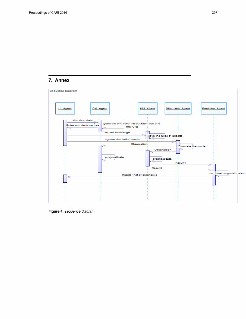
7. Annex

Figure 4. sequence diagram


Figure 5. Decision tree

Figure 6. Decision rules


Figure 7. The aircraft elevator control system[13]


Amélioration de la visite de classe de l’enseignement technique : intégration d’un dispositif de médiation

Frédéric T. Ouédraogo1, Daouda Sawadogo2, Solange Traoré3 et Olivier Tindano1 [email protected] , [email protected], [email protected], [email protected] 1 Ecole Normale Supérieure, Université de Koudougou Burkina Faso. 2 Laboratoire L3i, Université de La Rochelle, France. 3 Inspection de l’enseignement technique de Ouagadougou, Burkina Faso.

RÉSUMÉ. L’amélioration des pratiques de l’enseignant est portée par la visite de classe effectuée par le conseil pédagogique. Cet article présente l’intégration d’un système de partage de document comme un dispositif de médiation dans la visite de classe. Ce système de partage permet d’améliorer les interactions entre l’enseignant et le conseil pédagogique sur l’élaboration des principaux documents pédagogiques relatif à la visite de classe. L’expérimentation a été réalisée avec le service de partage de documents Google Drive sur une population constituée d’une quinzaine d’enseignants et de trois encadreurs pédagogiques de l’enseignement technique. Les résultats ont montré une amélioration de la qualité pédagogique de la visite de classe et une amélioration de la communication entre l’enseignant et l’encadreur pédagogique. Il ressort de cette étude que l’enseignant devient moins stressé et il sollicite beaucoup plus le conseil pédagogique que lorsqu’il n’utilise pas ce dispositif.

ABSTRACT. The improvement of teacher practice is supported by the class visit. This paper presents the integration of a sharing system of documents as a mediation system tool in the class visit. This sharing system enhances the interaction between the teacher and the pedagogical supervisor when they work on the main pedagogical documents of the class visit. We made an experiment with the service Google Drive with fifteen teachers and three pedagogical supervisors of the technical education. The results of this experiment have shown an improvement of the educational quality of the class visit and better communication between teacher and pedagogical supervisor. It appears from this study that the teacher becomes less stressed and he requests much more help of the pedagogical supervisor than usual.

MOTS-CLÉS : visite de classe, Encadrement pédagogique, Médiation, Enseignement, Google Drive.

KEYWORDS: class visit, pedagogical supervision, mediation, Teaching, Google Drive.


1. Introduction

L'éducation tient un rôle fondamental dans toutes les sociétés. Elle représente l’ensemble des activités visant à développer les potentialités physiques, intellectuelles, morales, psychologiques et sociales d’un humain. Elle assure sa socialisation, son autonomie, son épanouissement et sa participation au développement économique, social et culturel1 de sa société. Elle constitue une priorité nationale pour le Burkina Faso. Elle se révèle être nécessaire pour l’individu et pour sa communauté. En dépit de son importance, la qualité de l’enseignement, aussi bien au niveau de l’éducation de base qu’au niveau de l’éducation post-primaire et secondaire, constitue un véritable problème pour l’ensemble des acteurs et des partenaires du système éducatif burkinabé. Cependant, cette recherche de la qualité de l’enseignement passe nécessairement par la qualité professionnelle des enseignants [1]–[4]. D’après l’auteur dans [5], la qualité de l'apprentissage est un facteur important pour la réussite du processus d'apprentissage. C’est pourquoi au cours de ces dernières décennies, les mouvements de réforme du système éducatif se sont appuyés sur la formation des enseignants en tant qu’élément essentiel pour modifier les pratiques pédagogiques et le développement d’outils d’aide à l’amélioration de la qualité de l’enseignement.

Cette préoccupation se traduit sur le terrain par plusieurs actions. Nous pouvons citer entre autres l’organisation des conférences annuelles sur l’enseignement [6] qui ont pour thème de réflexion, la recherche des meilleures stratégies et actions pour améliorer la qualité de l’enseignement. Cette initiative favorise une formation continue des enseignants sur le terrain par un encadrement pédagogique de proximité qui se traduit par des visites de classe. Ces visites ont pour objectif de donner un appui pédagogique adapté aux besoins de chaque enseignant afin d’améliorer sa pratique de classe.

Cependant, les visites de classe telles qu’elles sont organisées connaissent un certain nombre de difficultés. C’est pour ces raisons qu’elles n’arrivent toujours pas à développer la compétence escomptée chez les enseignants [6], [7]. Au regard des insuffisances constatées après plusieurs années de pratique de la visite de classe et avec l’avènement des Technologies de l’Information et de la Communication (TIC), nous nous proposons d’explorer une piste d’amélioration. Les Technologies de l’Information et de la Communication tant renommées dans diverses activités pourront-elles rehausser l’efficacité de la visite de classe ? Nous avons choisi d’expérimenter la plate-forme Google Drive dans la visite de classe en enseignement technique. Cette expérience a montré un apport andragogique dans la formation continue des enseignants.

1 Article 2 de la LOI N°013-2007 / AN portant loi d’orientation de l’éducation au Burkina Faso.


Cet article est structuré de la manière suivante : le contexte et la problématique que nous abordons sont présentés dans le premier point ; le second est consacré à notre méthodologie pour améliorer la visite de classe ; le troisième présente le cadre expérimental et les résultats ; enfin le quatrième point présente une discussion sur notre contribution par rapport aux travaux antérieurs.

2. Contexte

Les encadreurs pédagogiques en service dans les inspections sont chargés principalement de l’encadrement des enseignants. Nous nous intéressons à l’encadrement pédagogique dont bénéficient les enseignants. Cet encadrement pédagogique a pour but de permettre aux enseignants d’améliorer leur pratique de classe. La visite de classe est une activité de l’encadrement pédagogique. Cette visite comporte deux volets : l’analyse du dossier d’intervention pédagogique et l’observation de la conduite de classe de l’enseignant suivie d’un entretien.

L’encadreur pédagogique apporte un appui qui répond aux besoins spécifiques de l’enseignant. L’enseignant devrait pouvoir profiter de la visite de classe comme moyen de renforcement de ses compétences. Mais nous constatons que l’organisation de la visite de classe dans l’enseignement technique ne permet pas à l’encadreur pédagogique de percevoir efficacement les compétences et les insuffisances de l’enseignant afin d’apporter une solution appropriée.

En général, l’encadreur pédagogique prend connaissance du dossier d’intervention pédagogique pendant la visite de classe, au moment où l’enseignant débute sa prestation, voir Figure 1. Pourtant, ce document a un volume qui varie entre vingt et quarante pages qu’il sera difficile à l’encadreur d’exploiter et de suivre la prestation de l’enseignant. Face à cette difficulté, l’encadreur est obligé de faire un choix cornélien :

- soit il privilégie la prestation de l’enseignant au détriment du dossier d’intervention pédagogique. Conséquence, l’entretien sera focalisé sur la prestation au détriment du document ;

- soit il se concentre sur le dossier d’intervention pédagogique. Conséquence, il sera moins attentif à l’observation de la prestation de l’enseignant. Alors, l’entretien sera focalisé sur le dossier d’intervention pédagogique ;

- soit il essaie de suivre les deux volets à la fois. Conséquence, aucun des volets ne sera traité efficacement.

Pourtant, c’est la synthèse de l’évaluation de ces deux parties majeures qui devrait lui permettre de mieux juger l’enseignant, afin de lui proposer des solutions appropriées. De ce qui précède, il ressort que l’enseignant ne profite pas suffisamment de l’expertise de l’encadreur pédagogique.


Figure 1 : Processus de la visite de classe avec et sans un dispositif de médiation De plus, l’insuffisance du nombre d’encadreurs pédagogiques vient aggraver ce

problème. Ceux-ci sont, non seulement fortement sollicités mais, interviennent même au-delà de leur spécialité.

Lors d’une visite de classe, l’encadreur pédagogique joue deux rôles. Il est conseiller et évaluateur. Dans le milieu des enseignants, ce rôle d’évaluateur est mal perçu, de sorte qu’il s’est développé le stéréotype de l’encadreur « gendarme ». Cette situation constitue un blocage à la collaboration enseignant-encadreur et ne favorise pas une interaction constructive dans la formation continue des enseignants.

Dans le processus actuel de la visite de classe, il n’existe pas un cadre de rencontre préparatoire où l’enseignant peut solliciter l’encadreur, comme le montre la Figure 1(a). Un tel cadre permettrait à l’enseignant de bénéficier de l’expertise de l’encadreur pour préparer son dossier d’intervention pédagogique avant la visite de classe. Dans le même temps, l’encadreur serait au même niveau que l’enseignant, car il aurait pris connaissance de son dossier d’intervention pédagogique. L’encadreur aurait alors suffisamment de temps pour se consacrer au second volet de la visite de classe. Ce volet concerne la prestation de l’enseignant. Par ailleurs, l’existence d’un tel cadre de médiation aurait le bénéfice d’améliorer la collaboration entre enseignants et encadreurs et ainsi briser les préjugés de l’encadreur « gendarme » entretenus au milieu des enseignants.

En résumé, les problèmes qui entravent l’efficacité de la visite de classe peuvent être classés à deux niveaux : le processus actuel de la visite de classe et le stéréotype sur l’encadreur pédagogique. Dans ce contexte, l’introduction d’un dispositif de


médiation dans le processus de la visite de classe peut être une solution pour améliorer celle-ci. Dans le présent article, nous proposons une solution axée sur les technologies de l’information et de la communication qui consiste à introduire un cadre de médiation dans le processus de la visite de classe.

3. Méthodologie pour améliorer la visite de classe

Dans cette partie de notre étude, nous présentons premièrement les fondements de l’encadrement pédagogique et de la visite de classe puis nous montrons notre proposition pour l’amélioration de la visite de classe.

3.1. Cadre conceptuel : encadrement pédagogique

Selon le dictionnaire actuel de l’éducation [8], l’encadrement regroupe les activités qui visent à fournir une aide aux apprenants pris individuellement ou en groupe. Cela vise à favoriser la prise en charge par chacun de sa propre formation. Encadrer une personne, c’est assurer auprès d’elle un rôle de directeur de formation. Le terme de direction sous-tend l’action de guider, d’exercer une influence, d’animer et surveiller, alors que celui de formation revêt le sens de développement, d’apprentissage. La pédagogie, selon l’APPAC2, est l'art d'enseigner ou les méthodes d'enseignement propres à une discipline, à une matière, à un ordre d'enseignement, à un établissement d'enseignement ou à une philosophie de l'éducation.

L’encadrement pédagogique représente donc l’ensemble des actions posées par les encadreurs pédagogiques, qui ont pour but de conduire l’enseignant à acquérir des aptitudes pour bien enseigner en utilisant les meilleures méthodes d’enseignement et les contenus adaptés.

3.2. Cadre conceptuel : la visite de classe

La visite de classe se déroule en deux phases, comme les auteurs BOUVIER et OBIN la décrivent [9]. La première phase qui est l’observation et l’analyse d’une conduite de classe d’un enseignant par un encadreur pédagogique suivi de la seconde phase qui est un entretien entre l’encadreur pédagogique et l’enseignant.

Dans le contexte du Burkina Faso, la visite de classe est considérée comme une forme de formation continue adressée régulièrement aux enseignants en poste [7]. Elle est une pratique d’encadrement, de suivi et de contrôle en vue d’aider les enseignants à 2 APPAC : Association Professionnelle des Professeurs et Professeures d’Administration au Collège.


améliorer leurs prestations pédagogiques. Lorsque de nouvelles pratiques sont adoptées, les visites de classe interviennent comme une formation de recyclage des enseignants.

3.3. Outil de médiation : Google Drive

Google Drive est un service de stockage et de partage de fichiers dans le Cloud qui permet le travail collaboratif. Ce service a été lancé par la société Google en avril 2012 [10]. La Figure 2 montre l’interface principale de Drive qui présente de manière analogue à Microsoft Office, une suite bureautique permettant d’éditer plusieurs formats de fichiers de type texte, tableur, présentation, etc. Il est également possible d’avoir une organisation hiérarchique des fichiers en dossiers ou d’importer des fichiers sur Drive.

Figure 2 : Interface du service Drive de Google. A) Edition de plusieurs types de fichiers; B) Accès aux fichiers partagés avec moi.

Avec l’option partage, les utilisateurs peuvent partager avec possibilité de modification ou non. La possibilité de modification permettra à plusieurs utilisateurs d’éditer un même fichier. Les fichiers partagés peuvent être recherchés sur Google Drive par le biais de moteurs de recherche Web.

4. Cadre expérimental

Nous avons opté pour une approche mixte conjuguant l’approche qualitative et l’approche quantitative. Cela se justifie parce que notre étude nécessite plusieurs variables à la fois qualitatives et quantitatives. L’approche qualitative va nous permettre


de recueillir les avis de chaque membre de l’échantillon sur l’introduction d’un dispositif de médiation dans la visite de classe. De l’approche quantitative, on va considérer des résultats issus des données de l’échantillon dont on aura effectué un traitement statistique. Ces données nous permettent d’avoir l’appréciation de l’enseignant et de l’encadreur sur ce cadre de médiation dans la visite de classe.

4.1. Caractéristiques et choix du dispositif

Le dispositif de médiation de la visite de classe doit satisfaire un minium de caractéristiques qui répondent aux besoins suscités. Ces caractéristiques sont : partage de ressources ; communication ; accessibilité sur internet.

Les technologies de l’information et la communication offrent une gamme variée d’outils dans presque tous les domaines d’activité de l’homme. Il nous paraissait alors évident que le choix de l’outil pour le cadre de médiation devait tenir compte des potentialités offertes par les TIC pour être pertinent et aussi pour ne pas être en déphasage avec la tendance générale. Cependant, plusieurs outils TIC peuvent être utilisés comme outil de médiation dans la visite de classe, mais ce choix doit tenir compte d’autres facteurs tels que le coût financier, le niveau de complexité, le temps de mise en œuvre, etc. Il faut donc choisir un outil à moindre coût, facile à maîtriser par les différents acteurs et rapide à mettre en œuvre.

Nous avons fait une recherche comparative des différents outils TIC pouvant être utilisés et nous avons trouvé que les systèmes de partage de fichiers Drive de Google et OneDrive de Microsoft sont adaptés pour être un dispositif de médiation dans le processus de visite de classe. Nous avons donc choisi d’utiliser Google Drive au lieu de OneDrive car les services de Google sont plus connus dans l’environnement de l’expérimentation.

4.2. Cadre expérimental

Les différents documents du dossier d’intervention pédagogique est composé du dossier technique et du dossier pédagogique. Le dossier technique comporte le résumé du cours, la documentation technique permettant de réaliser les travaux pratiques et le mode opératoire. Le dossier pédagogique est constitué de cinq fiches : identification pédagogique, exploitation pédagogique, progression pédagogique, déroulement et évaluation du domaine cognitif et du psychomoteur. Chaque enseignant initie l’élaboration de son dossier d’intervention pédagogique sur Google Drive et le partage avec l’encadreur pédagogique ou le conseil pédagogique, quand il y a plusieurs encadreurs qui interviennent dans la visite de classe.

Les fiches sont remplies au fur et à mesure par l’enseignant, supervisé par l’encadreur, de telle sorte qu’à la fin, les différents acteurs ont connaissance de leurs


contenus. Dans le cadre de la présente étude, chaque enseignant nous donnera accès (en lecture seule) à son dossier d’intervention pédagogique. Ainsi, nous avons accès aux échanges entre enseignant et encadreur, afin de suivre le processus de préparation de la visite sur Google Drive. Quand un enseignant finit d’élaborer ces fiches sur la plateforme, il se prépare pour la visite en poursuivant les échanges avec son encadreur pédagogique. La visite de classe donnera l’occasion à l’encadreur pédagogique d’observer la pratique de l’enseignant.

4.3. Echantillon

L’expérimentation s’est effectuée sur la Région du Centre au Burkina Faso, plus précisément dans les communes de la capitale Ouagadougou. Elle a concerné des établissements publics et privés. Nous avons choisi cette région parce qu’elle regroupe beaucoup d’établissements techniques avec une offre variée dans les spécialités enseignées. D’après les statistiques de l’année 2012 du Ministère des enseignements, cette région possède la majorité des enseignants et encadreurs pédagogiques de l’enseignement technique du Burkina. Nous allons donc constituer notre échantillon dans cette région. Le Tableau 1 montre que la majorité des enseignants, qui constituent l’échantillon, n’est pas sans expérience. En effet, ils cumulent plus de dix ans d’ancienneté dans l’enseignement.

5. Évaluation et résultats

Une présentation de l’environnement Drive de Google a été faite aux différents participants de l’étude, que sont les enseignants et les encadreurs. La mise en œuvre de la visite de classe est faite selon un protocole qui régit les différentes interactions et les supports utilisés. La chronologie de l’expérimentation est comme suit :

1. l’enseignant prépare le dossier d’intervention pédagogique et le partage avec son encadreur pédagogique. Ce dossier est composé de fiches pédagogiques et de fiches techniques ;

2. l’encadreur pédagogique consulte le dossier pédagogique de l’enseignant et apporte des corrections et commentaires ;

3. l’enseignant intègre les corrections et continue les échanges avec son encadreur jusqu’à satisfaction de ce dernier ;

4. la visite de classe est effectuée et l’encadreur analyse la prestation de l’enseignant selon une grille d’observation. L’encadreur fait part à l’enseignant de son appréciation de la visite.


L’expérimentation a été réalisée avec quinze enseignants et trois encadreurs pédagogiques. Elle s’est déroulée de novembre 2013 à mars 2014, soit une période de cinq mois.

Expérience par tranche d’année Inférieure à 5 ans De 5 à 10

ans De 10 à 15 ans Supérieure à 15 ans

Nombre d’enseignants 1 6 5 3

Tableau 1 : Ancienneté professionnelle des enseignants.

La plupart des enseignants possède un diplôme professionnel de l’enseignement. Les autres enseignants exercent uniquement sur la base du diplôme universitaire. Ces derniers sont surtout dans les établissements privés d’enseignements.

L’expérimentation a connu une participation satisfaisante des enseignants. En effet, la fréquentation de la plate-forme témoigne de l’activité des enseignants pendant l’expérimentation. Plus de la moitié des enseignants se connectaient au moins deux fois par jour pendant la préparation des fiches pédagogiques et techniques de la visite de classe.

L’on constate que les enseignants n’ont pas l’habitude de solliciter l’aide d’encadreur pédagogique pour élaborer leurs fiches pédagogiques lors de la préparation de la visite de classe. Par exemple, aucun enseignant participant n’avait eu à solliciter l’aide d’un encadreur pédagogique avant l’expérimentation. Pourtant, ce n’est pas parce que le besoin n’existe pas. Pour preuve, presque tous les enseignants ont fait recours à l’aide d’un encadreur pendant notre étude, comme le montre le Tableau 2. Les encadreurs pédagogiques ont été sollicités par les enseignants pour un appui-conseil.

Nombre de sollicitations 1 2 3 4 5 6

Nombre d’enseignants 0 2 4 5 3 1

Tableau 2 : Répartition des enseignants par nombre de sollicitations de l’encadreur pédagogique dans l’élaboration du dossier d’intervention pédagogique.

Les participants, enseignants comme encadreurs, sont unanimes que Google Drive représente un cadre d’échanges approprié pour l’élaboration d’un dossier d’intervention pédagogique. Les services offerts sont faciles d’utilisation. Enfin, ils trouvent que cet outil favorise une bonne collaboration entre encadreurs pédagogiques et enseignants.


Les enseignants reconnaissent avoir entretenu des échanges plus relaxes et plus ouverts avec leurs encadreurs pédagogiques. En outre, pour l’ensemble des enseignants participants, l’environnement Google Drive maintient un bon climat de travail entre enseignants et encadreurs pédagogiques. Cela facilite le recours à un encadreur pédagogique pour un appui-conseil.

Notons cependant que tous les enseignants ne sont pas satisfaits des réponses données à leurs sollicitations. Mais ce fait est d’un autre ordre et n’est pas lié à l’usage de l’outil. Il est important de savoir que ce feedback de l’enseignant sur une sollicitation de l’encadreur n’est pas envisageable en présentiel, car les rapports entre ces deux corps de l’enseignement sont toujours empreints de l’autorité de l’encadreur. Tous ces éléments nous permettent de dire que les participants sont ouverts aux innovations dans le cadre de la visite de classe.

Pour les enseignants, l’utilisation du dispositif de médiation encourage le recours à l’encadreur pédagogique en cas de difficulté. Les encadreurs pédagogiques, pour leur part, ont une bonne appréciation du dispositif. Selon eux, le dispositif leur a permis de de mieux cerner les difficultés de l’enseignant dans l’exercice de son métier.

Nous considérons que l’augmentation des sollicitations avec l’introduction du dispositif de médiation montre que cet outil est efficace à plusieurs niveaux. Il est non seulement approprié à la visite de classe, mais aussi contribue à une meilleure communication entre les acteurs.

6. Discussions

Notre étude montre que l’utilisation d’un système de partage de documents comme dispositif de médiation entre un enseignant et son encadreur peut améliorer le processus de visite de classe. Ainsi les TIC peuvent-elles constituer un accélérateur vers un enseignement de qualité [11]. Les enseignants et les encadreurs pédagogiques ont favorablement apprécié l’intégration du dispositif de médiation dans le processus de la visite de classe. L’avis des encadreurs est motivé par le fait que le dispositif permet d’avoir un avis d’un autre encadreur sur le dossier technique avant la visite de classe. Rappelons qu’il est courant dans l’enseignement technique que l’encadreur pédagogique assure les visites de classe d’autres disciplines autres que la sienne.

Notons cependant que les enseignants ont soulevé des difficultés concernant les conditions de l’expérimentation qui n’était pas de notre ressort. Il s’agit de la connexion Internet qui était souvent médiocre et ne permettait pas l’utilisation du dispositif. Les enseignants et les encadreurs n’ont pas trouvé nécessaires une formation sur l’utilisation du dispositif de médiation. Cela montre que le choix de Google Drive pour sa simplicité est approprié.


L’amélioration de la pratique de l’enseignant a été abordée dans [2], [4], [12], [13] et [14]. Lebrun, dans son article [2] s’interroge sur les modèles actuels et propose l’élaboration de nouveaux usages et méthodes de formation des enseignants. Il aborde de façon générale l’amélioration de l’enseignement par la formation des enseignants aux TIC. Il aborde très peu l’importance des outils de médiation pour les enseignants. Ainsi notre approche vise-t-elle à offrir aux enseignants des outils de médiation de leurs activités. Nous avons appliqué cette approche dans le cas de la visite de classe. La visite de classe est un aspect très important dans l’amélioration de la qualité de la formation des enseignants.

Les travaux effectués par Lerouge [15] sur la visite de classe proposent une approche praxéologique afin d’améliorer la pratique de l’enseignant en se basant sur l’analyse de sa pratique spontanée lors des visites de classes. Cette approche permet d’améliorer la formation professionnelle de l’enseignant. Contrairement à notre proposition, cette approche ne tient pas compte des outils technologiques. Pourtant, les TIC constituent un facteur indéniable dans le succès de la formation des enseignants.

Une des particularités de notre approche est qu’elle propose un outil simple et facilement utilisable par tous les enseignants. Ainsi la simplicité du dispositif améliore-t-elle son appropriation par ses utilisateurs. En effet, la complexité d’un outil technologique peut entraver son appropriation.

En résumé, notre approche introduit une innovation multidimensionnelle. Elle améliore l’approche pédagogique des enseignants, contribue à une communication efficiente et consolide le rapport socio-professionnel entre enseignant et encadreur pédagogique.

7. Conclusion

Notre travail de recherche a permis de montrer que la pratique actuelle de la visite de classe a besoin d’être reformée. Les outils offerts par les TIC représentent une opportunité pour la réalisation de cette réforme. C’est dans ce contexte que nous avons proposé l’utilisation d’un dispositif technologique de médiation dans le processus de la visite de classe. Nous avons décrit les caractéristiques que doit avoir un tel dispositif, comme le partage de documents dans le processus de la visite de classe. Ainsi lors de notre expérimentation, nous avons proposé un dispositif basé sur le service Drive de Google comme outil de médiation dans la visite de classe.

L’analyse des résultats obtenus lors de l’expérimentation a montré une amélioration de plusieurs aspects de la visite de classe. Par exemple, l’encadreur a une meilleure appréciation des difficultés pédagogiques de l’enseignant. Elle a permis également d’améliorer le rapport socio-professionnel entre enseignant et encadreur. La facilité d’adoption de l’outil permet d’affirmer qu’un dispositif de médiation dans la visite de


classe est important. Ce travail pourrait relancer la revalorisation de la visite de classe dont les enseignants sont souvent très sceptiques.

Nous envisageons dans nos futurs travaux, améliorer les résultats de cette étude avec un échantillon plus important.

7. Références

[1] T. Karsenti, C. Raby, and S. Villeneuve, “Quelles compétences technopédagogiques pour les futurs enseignants du Québec,” Formation et pratiques d’enseignement en questions, vol. 7, pp. 117–136, 2008.

[2] M. Lebrun, “La formation des enseignants universitaires aux TIC: allier pédagogie et innovation.,” Revue internationale des technologies en pédagogie universitaire, vol. 1, no. 1, pp. 11–21, 2004.

[3] G. Sang, M. Valcke, J. van Braak, and J. Tondeur, “Student teachers’ thinking processes and ICT integration: Predictors of prospective teaching behaviors with educational technology,” Computers & Education, vol. 54, no. 1, pp. 103–112, 2010.

[4] L. Talbot, “Les recherches sur les pratiques enseignantes efficaces,” Questions Vives. Recherches en éducation, vol. 6, no. 18, pp. 11–13, 2012.

[5] C. M. Stracke, “The future of learning innovations and learning quality. How do they fit together?,” in Proceedings of the European Conference LINQ 2012, 2012.

[6] MESSRS, “Conférence annuelle de l’enseignement secondaire (CAES),” Ouagadougou, 2010.

[7] INSPECTION du Burkina Faso, “Actes de la 2e Conférence Annuelle des Inspecteurs de l’Enseignement Secondaire,” Bobo-dioulasso, 2001.

[8] R. Legendre, “Dictionnaire actuel de l’éducation,” 1988. [9] A. Bouvier, L. M. Bélair, and J.-P. Obin, La formation des enseignants sur le terrain.

Hachette éducation, 1998. [10] Wikipédia, “Google Drive - Wikipédia,” 2016. [Online]. Available:

https://fr.wikipedia.org/wiki/Google_Drive. [Accessed: 09-Feb-2016]. [11] D. Peraya, J. Viens, and T. Karsenti, “Introduction: Formation des enseignants à l’intégration

pédagogique des TIC: Esquisse historique des fondements, des recherches et des pratiques,” Revue des sciences de l’éducation, vol. 28, no. 2, pp. 243–264, 2002.

[12] K. Assagaye, Agaissa; Achille, “Les Technologies de l’information et de la communication dans la formation continue des enseignants d’un lycée au Niger,” Frantice, vol. 9, 2014.

[13] M. Altet, “L’analyse de pratiques une démarche de formation professionnalisante: Formes et dispositifs de la professionnalisation,” Recherche et formation, no. 35, pp. 25–41, 2000.

[14] C. Depover, T. Karsenti, and V. Komis, Enseigner avec les technologies: favoriser les apprentissages, développer des compétences. PUQ, 2007.

[15] A. Lerouge, “Un dispositif innovant de conseil pédagogique: la visite de classe formative,” Tréma, no. 20–21, pp. 55–78, 2003.


Efficient high order schemes for stiff ODEs incardiac electrophysiology

C. Douanla Lontsi* , Y. Coudière, C. Pierre

INRIA Bordeaux Sud OuestUniversité de Bordeaux* [email protected]

ABSTRACT. In this work, we introduce some exponential high order schemes for stiff ODEs comingfrom the models used in cardiac electrophysiology. We show in this context that despite the stiffnessof the equations, the use of high order (order 3) stabilized schemes is beneficial in terms of costwith the possibility to use large time-steps as for implicit schemes. We describe a methodologyand introduce some tools allowing to compare the numerical schemes used to solve ODEs. Thesetools and methodology are then used through the Beeler Reuter ionic model (BR) [2] to compare theexponential schemes with the classical explicit and implicit schemes at various orders. It comes fromthis comparisons a good alternative in terms of cost, accuracy and ease of implementation.

RÉSUMÉ. Dans ce travail, nous définissons des schémas d’ordre élevé de type exponentiels appli-qués aux EDOs à caractères raides provenant des modèles utilisés en électrophysiologie cardiaque.Nous montrons dans ce contexte que malgré la raideur des équations, le recours à l’ordre élevé (ordre3) des schémas stabilisés est profitable en terme de coût avec une possibilité d’utiliser des pas detemps aussi grands que lors de l’utilisation des schémas implicites. Nous décrivons des outils de com-paraisons et une méthodologie permettant de comparer les schémas numériques pour la résolutiondes EDOs. Cette méthodologie est ensuite utilisée à travers le modèle ionique Beeler Reuter (BR) [2]pour comparer en terme de coût et de précision les schémas exponentiels aux schémas classiquesimplicites et explicites à différents ordres. Il en ressort de cette comparaison l’apport d’une bonnealternative à la fois en terme de coût, de précision et de facilité d’implémentation.

KEYWORDS : Exponential schemes, stiff ordinary differential equations, high order schemes, cardiacelectrophysiology

MOTS-CLÉS : Electrophysiologie cardiaque, schémas d’ordre élevé, équations aux dérivées ordi-naires raides, schémas exponetiels


1. IntroductionThe numerical resolution of stiff ordinary differential equations ODEs is an issue

encountered in many field of applied sciences. In cardiac electrophysiology, the modeldescribing the electrical activity of the heart is a system of parabolic partial differentialequations coupled with a system of ODEs called ionic models that is highly nonlinearand exhibiting a stiff behavior, making their numerical resolution very challenging. Theclassical schemes have serious drawbacks to solve such ODEs. On one hand classicalstable methods are implicit and lead to high computational cost associated with largetime-steps due to nonlinear solvers, on the other hand explicit solvers require very smalltime steps also leading to high computational costs. Meanwhile current solvers in thefield are usually based on order 1 or 2 schemes. In this paper we investigate the resort to aclass of both explicit and stable schemes referred as «exponential methods » of high orderas an alternative to solve cardiac electrophysiological problems. Namely we will considerthe exponential Adams Bashforth (EAB) and the Rush Larsen (RL) techniques.Let us consider the general initial value problem,

dy

dt= F (t, y) t ∈ (0, T ], y(0) = y0 ∈ RN . (1)

EAB and RL schemes take advantage of a splitting of the model function F into somelinear part a and a nonlinear part b,

dy

dt= a(t, y)y + b(t, y), y(0) = y0 ∈ RN . (2)

Notice that in (2), a is not the exact linear part of F (its differential) but, an approximationor a guess thereof. The EAB and RL are built from a transformation of (2) on each timediscretization interval [tn, tn+1] in the following form,

dy

dt= αny + cn(t, y), y(0) = y0 ∈ RN . (3)

Where αn ∈ RN is a stabilizer set at every time step and cn(t, y) = (a(t, y) − an)y +b(t, y) . With formulation (3), the exact solution satisfies the variation of the constantformula,

y(tn+1) = eαnh

(y(tn) +

∫ tn+1

tn

e−αn(τ−tn)cn(τ, y(τ))dτ

). (4)

The aim of this paper is to study the efficiency of EAB and RL methods of order 1 up to4. This efficiency is analyzed both in terms of accuracy and of cost. The comparison ismade using a realistic test case and is completed by including a benchmark with severalclassical methods either of implicit or explicit type, the Crank-Nicolson (CN ), the RungeKutta (RK4), the Adams Bashforth (ABk), and the backward differentiation (BDFk)(see [3]).

The paper is organized as follows. In section 2 are presented the stabilized schemes.A brief description of the transmembrane action potential and ionic model is given in thesection 3. The methodology used to compared the methods are developed in the section 4.The comparison of the methods follows in the section 5 where the methodology definedis used to compare the numerical schemes applied to the Beeler Reuter (BR) ionic model[2].


2. EABk and RLk scheme statementsWhen the function cn(t, y) in (3) is a polynomial Pn =

∑k−1j=0 pj(t−tn)j , the relation

(4) becomes yn+1 = eαnhyn+h∑k−1j=0 pjj!h

jϕj+1(αnh), with ϕ0(z) = ez and ϕj(0) =1j! , j ≥ 0. The schemes introduced in the sequel are multi-steps. We will use notationan = a(tn, yn), bn = b(tn, yn).

– EABk : On one hand we set αn = an, on other hand the function cn in (3) isapproximated by its Lagrange interpolation polynomial cn of degree k − 1 at the timeinstants tn, . . . , tn−k+1. This polynomial satisfies cn(tn−j) = cn(tn−j , yn−j) for j =0, . . . , k − 1. The values cn(tn−j , yn−j) for j = 0, . . . , k − 1 are given by cn−jn =

bn−j + (an−j − an)yn−j . If we write cn(t) =∑k−1j=0

γnj

j!

(t−tnh

)j, the definition of the

EABk scheme is deduced from the formula (4) by

yn+1 = eanhyn + hk−1∑j=0

γnjϕj+1(anh), (5)

where the coefficients γnj are given in the table bellow.

k 1 2 3 4γn0 cnn cnn cnn cnnγn1 – cnn − cn−1n

32cnn − 2cn−1n + 1

2cn−2n

116 c

nn − 3cn−1n + 3

2cn−2n − 1

3cn−3n

γn2 – – cnn − 2cn−1n + cn−2n 2cnn − 5cn−1n + 4cn−2n − cn−3n

γn3 – – – cnn − 3cn−1n + 3cn−2n − cn−3n

Table 1. Coefficients γnj for the EABk schemes.

– RLk : In the case the function cn(t, y) in (4) is a constant cn = βn ∈ R then wehave the following simple scheme definition,

yn+1 = yn + hϕ1(αnh)(αnyn + βn), (6)

that we refer as Rush Larsen schemes as in the continuity of [1]. The following choicesfor defining αn and βn ensure the convergence at order k of the scheme (6) and thus arenamed Rush Larsen schemes of order k (RLk).

- k = 1 : αn = an , βn = bn.- k = 2 : αn = 3

2an −12an−1 and βn = 3

2bn −12bn−1.

- k = 3 : αn = 112 (23an − 16an−1 + 5an−2),

βn = 112 (23bn − 16bn−1 + 5bn−2) +

h12 (anbn−1 − an−1bn).

- k = 4 : αn = 124 (55an − 59an−1 + 37an−2 − 9an−3),

βn = 124 (55bn−59bn−1+37bn−2−9bn−3)+ h

12 (an(3bn−1−bn−2)−(3an−1−an−2)bn).Notice that the EAB1 scheme is the same with RL1 scheme and also the exponentialEuler scheme.

The previous descriptions of the EABk and RLk schemes here have been given verybriefly but, more details for the EABk schemes can be found in [5] (for general ODEs)and in [4] for cardiac electrophysiology application, where the two methods are shown tobe stable under perturbations and convergent at the order k.


3. Modeling in cellular cardiac electrophysiology

3.1. The action potentialThe phenomenon studied here is the so called cellular action potential, that we briefly

present here. A potential difference is observed between the inside and outside of thecell, said membrane potential and denoted V . This potential caused by the differences inion concentrations between the inside and outside of the cells is dynamic in time, as wellas these ionic concentrations. The potential V can abruptly switch from a resting state(during which V = Vr ' −100mV ) to an excited state (where V is in the range of 10mV) in which it is maintained during a few tenth of seconds before returning to its restingstate (see figure 1).

-100-80-60-40-20

02040

0 200 400 600 800 1000

Volta

ge(m

V)

Time (ms)

-160-140-120-100-80-60-40-20

0

0 200 400 600 800 1000

Cur

rent

(A/F/cm

2)

Time (ms)

INa

Figure 1. BR Model [2] illustration. Left, two cellular action potentials : starting at a nega-tive resting value, the transmembrane voltage V (t) has a stiff depolarization followed by aplateau and repolarizing to the resting value. Right : each depolarization is induced by anionic sodium current INa(t)

3.2. Ionic ModelsThe variations of the ionic concentrations are described by ionic models and are sys-

tems of ODE. The innovated ones are consisting of the following variables with theirassociated ordinary differential equation.

– The membrane potential: V in mV. The equation on the potential is written,

dV

dt= −Iion(y(t), Ist(t)) + Ist(t), (7)

where Iion (reaction term) is the total ionic current crossing the membrane cell and Ist isthe stimulation current, it is a source term.

– The gating variables: they are parameters between 0 and 1 expressing the variabil-ity and the permeability of the membrane cell for the specific ionic species. One denoteby W ∈ RP the vector of gating variables. The equations on W are, for i = 1 . . . P ,

dWi

dt=W∞,i(y)−Wi

τi(y), (8)


where W∞,i(y) ∈ R, τi(y) ∈ R are scalar functions given by the model. In these equa-tions the linear and nonlinear parts are encoded in the model and are equal to −1/τi(y)and W∞,i(y)/τi(y) respectively.

– Ionic concentrations: One denote by C ∈ RN−P−1 the vector of concentrations.All these previous variables can be collected in a vector y ∈ RN as follows ,

y =

[WX

, X =

[CV

, W ∈ RP , C ∈ RN−P−1, V = yN ∈ R,

The sub-vectorsW andX correspond to the lines of (1) for which the linear and nonlinearpart is given or null respectively. The associated ODE written in the form (2) is thendefined by,

a(t, y) =

[A1(t, y) 0

0 0

], b(t, y) =

[B1(t, y)B2(t, y)

,

where the matrix A1(t, y) ∈ RP × RP is diagonal, A1(t, y) = Diag(−1/τi(y)), andB1(t, y) = W∞,i(y)/τi(y), i = 1 . . . P ∈ RP .

4. Scheme analysis methods

– Test case : The evaluation and comparisons between differentODE solvers is donewith a test case. Specifically, the Beeler Reuter [2] model is considered and written in theform (2) as described in the section 3.2. We denote by y(t) the solution of the associatedODE (2) in (0, T ] with T = 396 ms. this solution is uniquely defined once the initialcondition y0 and the stimulation current Ist in (7) are fixed. y0 is the resting state asdescribed by the model. The function Ist(t) is positive, null outside the interval (ts −1, ts+1), ts=20 ms and with integral

∫ T0Ist(t)dt = Istim, a typical current of stimulation

fixed by the models, in the range of 50 mA. We also impose to Ist a C4 regularity in oderto observe the convergence orders of schemes up to 4.

– Numerical solution: Let m ≥ 1 be an integer for which one associated the time-step h = T/m and the regular mesh Tm = tn = jh, j = 0 . . .m of the interval (0, T ].The numerical solution (yn) is the element of the space Em, Em = (yn)0≤n≤m, yn ∈RN. The space Em of the numerical solutions is simply (RN )m but to (yn) ∈ Em isimplicitly associated a time-step dt and a mesh Tm, such that each value yn, 0 ≤ n ≤ mof (yn) ∈ Em is supposed to be an approximation of y(tn).

– Reference solution: For a test case given, we cannot access to the exact solutiony(t) of the associated ODE. So for a numerical solution (yn) ∈ Em, we set m′ = 2rmwith r ≥ 0 an integer and define the reference solution associated to (yn) (or m) as thenumerical solution yref ∈ Em′ for the problem (1), computed by the RK4 scheme withthe time-step href = T/m′ = h/2r. The reference solution yref is then not unique anddepend on r. In practice r is chosen large enough such that the error between the exactsolution y and yref is negligible compared to the error between the numerical solution(yn) and yref .

– Interpolation of the solution: To compare the numerical solution with the refer-ence solution and to be able to compute the numerical error in terms of function norm,we define an interpolator πm,i : Em −→ C0(0, T ], transforming the component i of thenumerical solution (yn) ∈ Em in C0(0, T ], the set of the continuous functions on (0, T ].Otherwise, we require to the interpolate πm,iyn to be a polynomial piecewise function


of degree 3, this constraint is necessary to observe the convergence order up to 4. Weassume that m is a multiple of 3 and fix (yn) ∈ Em. We decompose the interval [0, T ] ina sequence of 3 intervals packages Ps = [t3s, t3s+1] ∪ [t3s+1, t3s+2] ∪ [t3s+2, t3(s+1)] ,for s = 0 . . .m/3. The interpolated f := πm,iy

n is the unique polynomial of degree 3 oneach Ps, continuous on [0, T ], such that f(tn) = yni for all n = 0 . . .m. This interpolatoris not Canonical: an H3-Hermite interpolation on each interval (tn, tn+1) is an alterna-tive. The emphasis will be here on the membrane potential V (t) = yN (t) and for moresimplicity we note πm = πm,N and π = πm,N in confusion absence.

– Accuracy: Let (yn) be a numerical solution and yref a reference solution asso-ciated. We denote πyn = V and πYref = Vref the membrane potential interpolatingassociated. The accuracy of each method is evaluated through a relative error between thereference solution and the numerical solution. We define the errors in norm L∞ by :

e∞ =max |V − Vref |

max |Vref |. (9)

Notice that the choice of the membrane potential V is arbitrary and that any other com-ponent of (yn) could have been considered. The accuracy notion will be central here andit is convenient to identify several aspects.

– Cost: The accuracy takes all its meaning when one associate it a cost. Here itis a computational cost and is evaluated with the CPU time during a simulation. It isevaluated by the fortran90 software for each simulation setting by a time-step h. TheCPU times depend on the computer used to perform the solutions. This is balanced byusing the ratio between them for comparisons.

5. Numerical results

5.1. AccuracyThe relative error e(h) is computed for various time-steps h and collected in the table

2 where it can be observed that all the methods exhibit the expected order of convergence.A general view of the table 2 shows that the RLk is always more accurate than EABkand unlike the classical explicit schemes, the stabilized schemes allows the use of largetime-steps as the implicit except at the order four where it is not possible for h = 0.2.

The table 2(a) shows that the CN is the most accurate among the methods of order2 with a factor in the range of 10. The table 2(b) shows that the BDF3 method is betterthan the stabilized schemes for h ≥ 0.0125 with a coefficient 10 for h = 0.2 while forh < 6.25× 10−3 the RL3 is more accurate. The table 2(c) shows that the RK4 methodis the most accurate among the methods of order 4 for h ≤ 0.025 while for h > 0.025 theBDF4 is more accurate than the stabilized schemes.

5.2. CostA general observation of the figure 2 on the top shows that for the error between

1% and 10% the gain in terms of CPU time is high (with a factor in the range of 10)when moving from the order 1 to order 2 schemes. This gain remains important (with afactor in the range of 5) when moving from the order 2 to order 3 schemes while for theerrors between 1% and 10% there is no gain when moving from the order 3 to the order 4schemes. However the order 4 becomes advantageous for the errors less than 0.1%.


(a) AB2, RL2, EAB2 and CN

h AB2 RL2 EAB2 CN0.2 – 0.251 0.284 4.11× 10−2

0.1 – 0.107 9.26× 10−2 1.13× 10−2

0.05 – 3.35× 10−2 2.31× 10−2 2.65× 10−3

0.025 – 8.88× 10−3 5.39× 10−3 6.66× 10−3

0.0125 – 2.23× 10−3 1.29× 10−3 1.68× 10−4

6.25× 10−3 2.07× 10−4 5.6× 10−4 3.17× 10−4 4.25× 10−5

(b) AB3, RL3, EAB3 and BDF3

h AB3 RL3 EAB3 BDF3

0.2 – 0.148 0.516 4.09× 10−2

0.1 – 4.07× 10−2 9.17× 10−2 1.04× 10−2

0.05 – 6.34× 10−3 1.09× 10−2 2.29× 10−3

0.025 – 7.57× 10−4 1.17× 10−3 3.84× 10−4

0.0125 – 9.07× 10−5 1.4× 10−4 5.25× 10−5

6.25× 10−3 1.13× 10−5 8.23× 10−6 1.72× 10−5 2.01× 10−5

(c) RK4, RL4, EAB4 and BDF4

h RK4 RL4 EAB4 BDF4

0.2 – – – 4.98× 10−2

0.1 – 5.86× 10−2 0.119 1.27× 10−2

0.05 – 4.58× 10−3 8.96× 10−3 2.02× 10−3

0.025 4.65× 10−5 2.61× 10−4 4.33× 10−4 1.93× 10−4

0.0125 2.67× 10−6 1.62× 10−5 2.67× 10−5 3.52× 10−5

6.25× 10−3 1.65× 10−7 9.94× 10−7 1.73× 10−6 2.01× 10−5

Table 2. Accuracy for the BR model for various classical and stabilized methods.The figure 2 on the bottom shows that the RL3 and the RL4 are less costly than the

EAB3 and EAB4 respectively. The factor is not so high but in terms of implementation,the RL is easier than the EAB schemes.

The figure 2 on the bottom left shows that when using high order stabilized schemesinstead of implicit schemes, the gain in time CPU is very high with a coefficient greaterthan 10. This is due to the fact that the nonlinear solver is very expensive and its costbecome very high for large time-steps.

The figure 2 on the bottom right shows that the order 4 stabilized schemes are lesscostly than the classical explicit schemes but it is much more better to use theRL4 schemeinstead of the EAB4 scheme. Because of they stability properties the explicit schemesrequire the use of small time-steps that make them sometimes useless. For instance theRK4 is very accurate but its use require to take a small time step. This small time stepsproduces a very small error that might be not needed and then its use will induce anadditional cost.

6. ConclusionTwo families of explicit high order stabilized methods (EABk, RLk) have been intro-

duced in this work. Excepted the order four, both have been shown to be as stable as theclassical implicit methods for the test case we have chosen. Otherwise, it has also been


demonstrated that the use of high order (3 or 4) of the stabilized methods instead of theclassical high order implicit methods allows to decrease the cost almost 50 times.

0.01

0.0001 0.01 1

Cos

tin

CPU

time

e(h)

EAB1EAB2EAB3EAB4

0.01

0.0001 0.01 1

Cos

tin

CPU

time

e(h)

RL1RL2RL3RL4

0.01

0.0001 0.01 1

Cos

tin

CPU

time

e(h)

CNBDF3BDF4EAB3RL3

0.01

0.0001 0.01 1

Cos

tin

CPU

time

e(h)

AB2AB3RK4

EAB4RL4

Figure 2. The CPU time plotted in Log/Log scale against the error for various schemes

7. References

[1] M. PEREGO, A.VENEZIANI, “An efficent generalization of the Rush-Larsen method for solv-ing electro-physiology membrane equations”, ETNA, vol. 35, 2009.

[2] G.W. BEELLER, H. REUTER, “Reconstruction of the Action Potential of Ventricular Myocar-dial Fibres”, J. Physiol, vol. 268, 1977.

[3] E. HAIRER, S.P. NORSETT, G. WANNER, “Solving ordinary differential equations I”,Springer-Verlag, Berlin, vol. 8, 1993.

[4] Y. COUDIÉRE , C. DOUANLA LONTSI, C. PIERRE, “High order Rush Larsen solver for stiffODEs”, Hal, 2016.

[5] M. HOCHBRUCK, A. OSTERMANN, “Exponential multistep methods of Adams-type”, BIT,vol. 51, 2011.


ARIMA

A model of flocculation in the chemostat

R. Fekih-Salem a,c,* — T. Sari b,d

a Université de Tunis El Manar, École Nationale d’Ingénieurs de Tunis, LAMSIN,B.P. 37, Le Belvédère, 1002 Tunis, Tunisie.(E-mail: [email protected])

b IRSTEA, UMR Itap,361 rue Jean-François Breton, 34196 Montpellier, France.(E-mail: [email protected])

c Université de Monastir, ISIMa,BP 49, Av Habib Bourguiba, 5111 Mahdia, Tunisie.

d Université de Haute Alsace, LMIA,4 rue des frères Lumière, 68093 Mulhouse, France.

* Corresponding author.

ABSTRACT. In this work, we study a flocculation model with a single resource and a single specieswhich is present in two forms: isolated bacteria and attached bacteria. With monotonic growth ratesand distinct removal rates, we show that this model presents a rich behavior with multiplicity of positiveequilibria and bi-stability. Whereas, this bi-stability could occur in the classical chemostat model onlywith a non-monotonic growth rate.

RÉSUMÉ. Dans ce travail, nous étudions un modèle de floculation avec une seule ressource et uneseule espèce qui se présente sous deux formes: des bactéries isolées et en flocs. Avec des taux decroissance monotones et des taux de prélèvement distincts, nous montrons que ce modèle présenteun comportement très riche avec multiplicité des équilibres positifs et bi-stabilité. Cependant, dans lemodèle classique du chémostat, cette bi-stabilité ne peut se produire qu’avec un taux de croissancenon monotone.

KEYWORDS : Bifurcation, Bi-stability, Chemostat, Flocculation

MOTS-CLÉS : Bifurcation, Bi-stabilité, Chémostat, Floculation


1. IntroductionFlocculation is a process wherein microorganisms isolated or planktonic bacteria clus-

ter together to form a flocs and reversibly this flocs can split and liberate isolated bacteria[10]. The attachment of planktonic bacteria could be also on a wall as biofilms [1]. Thisflocculation mechanism can explain the coexistence between species when the most com-petitive species inhibits its growth by the formation of flocs [3, 6]. Indeed, the flocsconsume less substrate than isolated bacteria since they have less access to the substrate,given that this access to the substrate is proportional to the outside surface of the floc.

In order to understand and predict these flocculation phenomena, several extensionsof the well-known chemostat model [9] have been proposed and studied in the literatureby considering two compartments of isolated and attached biomass for each species [3].For instance, Pilyugin and Waltman [8] have treated a model of wall growth where the at-tachment and detachment rates are constant, and the population on the wall does not washout of the chemostat. The Freter model [5] describes a microbial population constitutedof planktonic cells in the fluid and adherent cells on the surface. Their model was studiedby Jones et al. [7], assuming that the planktonic bacteria are attracted to the wall at a rateproportional to planktonic cell density and the fraction of unoccupied colonization siteson the wall. More recently, the competition model of two species for a single substratehas been studied by Haegeman and Rapaport [6], assuming that only the most competitivespecies inhibits its growth by the formation of flocs. The study of [6] has been extendedby [2] and [4].

In this paper, we study the model of flocculation considered in [3], where the isolatedbacteria can stick with isolated bacteria or flocs to form new flocs. We do not assumeas in [3] that attachment and detachment dynamics are fast compared to the growth ofbacteria. The paper is organized as follows. In Section 2, we present the model of floc-culation proposed in [3]. In Section 3, we study the existence and the local stability ofthe equilibria of system (1) for non-negative attachment and detachment rates. In Section4, numerical simulations are presented with realistic growth functions (of Monod type)and the conclusion is drawn in the last Section 5. Most of the proofs are reported in theAppendix A.

2. Mathematical modelIn this paper, we consider the model of flocculation proposed in [3] S = D(Sin − S)− µu(S)u− µv(S)v

u = [µu(S)−Du]u− a(u+ v)u+ bvv = [µv(S)−Dv]v + a(u+ v)u− bv

(1)

where S(t) denotes the concentration of the substrate at time t; u(t) and v(t) denote,respectively, the concentration of planktonic and attached bacteria at time t; µu(S) andµv(S) represent, respectively, the per-capita growth rates of planktonic and attached bac-teria; Sin and D denote, respectively, the concentration of the substrate in the feed deviceand the dilution rate of the chemostat; Du and Dv represent, respectively, the removalrates of planktonic and attached bacteria such that Dv 6 Du 6 D.

We assume that the planktonic bacteria can stick with the isolated bacteria or the flocsto form a new flocs, with rate a(u + v), where a is a non-negative constant, and that


the flocs can split and liberate an isolated bacteria, with rate b, where b is a non-negativeconstant. We add the following assumptions on the growth rates:

H1: The functions µu(·) and µv(·) are increasing for all S > 0 and satisfy µu(0) =µv(0) = 0.

Since the bacteria in flocs have less access to the substrate, given that this access to thesubstrate is proportional to the outside surface of the floc, we assume that the bacteria inflocs consume less substrate than isolated bacteria:

H2: µu(S) > µv(S) for all S > 0.

Let φu(S) and φv(S) be the functions defined by

φu(S) = µu(S)−Du and φv(S) = µv(S)−Dv.

When equations µu(S) = Du, µv(S) = Dv and φv(S) = b have solutions, they areunique and we define the usual break-even concentrations

λu = µ−1u (Du), λv = µ−1

v (Dv) and λb = φ−1v (b).

Otherwise, we put λu = +∞ or λv = +∞ or λb = +∞. We have the following result:

Proposition 2.1 For any non-negative initial condition, the solutions of system (1) remainnon-negative and bounded for all t > 0. The set

Ω =

(S, u, v) ∈ R3

+ : S + u+ v 6 D

DvSin

is positively invariant and is a global attractor for (1).

3. Analysis of the model

3.1. Existence of equilibriaIn the following, we propose to study the existence of equilibria of (1). We use the

following definitions

I =

]λu, λv[ if λu < λv

]λv,min(λb, λu)[ if λv < λu.

U(S) =D(Sin − S)φv(S)

Duφv(S)−Dvφu(S)and V (S) =

D(Sin − S)φu(S)

Dvφu(S)−Duφv(S).

H(S) =φu(S)(φv(S)− b)[Duφv(S)−Dvφu(S)]

a[φv(S)− φu(S)]φv(S). (2)

Lemma 3.1 The system (1), with a > 0 and b > 0, admits the following equilibria:

– The washout, E0 = (Sin, 0, 0), which always exists.

– A positive equilibrium, E∗ = (S∗, u∗, v∗) for each S∗ solution of the equation

D(Sin − S) = H(S), (3)

u∗ = U(S∗) and v∗ = V (S∗), which exists if and only if S∗ ∈ I .


The case a = b = 0 is simply the classical model of competition of two microbialspecies for which the competitive exclusion principle takes place [9].In this case, thesystem (1) has an equilibrium of extinction of v, Eu = (λu, u

∗, 0), which exists if andonly if λu < Sin and an equilibrium of extinction of u, Ev = (λv, 0, v

∗), which exists ifand only if λv < Sin with

u∗ = U(λu) =D

Du(Sin − λu) and v∗ = V (λv) =

D

Dv(Sin − λv).

In the following, we study the existence of positive equilibria of (1). Each solution ofthe equation (3) belonging to the interval I gives rise to a positive equilibrium of system.Note that

H ′(S) =µ′u(φv − b)φvF + µ′

vφuG

a(φv − φu)2φ2v

(4)

whereF = [Duφ

2v − 2Dvφuφv +Dvφ

2u] > 0

G = [bDuφ2v + (Dv −Du)φuφ

2v + bDv(φ

2u − 2φuφv)]

(5)

In the case λu < λv , the sign of H ′(S) can be positive or negative for S ∈ I (see Fig.1). In the case λv < λu, one has H ′(S) < 0 on I =]λv,min(λb, λu)[. Therefore, thefunction H(·) is decreasing on I , but equation (3) can have many solutions (see Figs. 2and 3).

µu(S)

Duµv(S)

Dv

φu(S)

φv(S)

λu

Iλv

S

(a)

H(S)

D(Sin − S)

E∗

E0

Sinλu λv

I S

(b)

H(S)

E∗

E∗∗

E∗∗∗

E0

Sinλu λv

I

Figure 1. The case λu < min(λv, Sin): (a) Existence of unique positive equilibrium. (b)Existence of three positive equilibria.

Therefore, the equation (3) may have several solutions whose number is genericallyodd in the case λu < λv or λv < λu < Sin (see Figs. 1 and 3 (b-c)) and even in the caseλv < Sin < λu (see Figs. 2 and 3 (a)). In all figures, we choose the color red to representthe locally exponentially stable equilibria and blue to represent the unstable equilibria.We will show the asymptotic behavior of the equilibria in section 3.2.

In the case λu < λv, the function H(·) is defined and positive on the interval I =]λu, λv[ since φu(S) > 0 and φv(S) < 0 for all S ∈]λu, λv[. Moreover, it vanishes at λu

and tends to infinity as S tends to λv . Hence, we have the following result:

Proposition 3.1 If λu < min(λv, Sin), then there exists at least one positive equilibrium.Generically, there is an odd number of positive equilibria. If Sin 6 λu < λv, then thereis no positive equilibrium.

In the second case λv < λu, the function H(·) is defined and positive on the intervalI =]λv,min(λu, λb)[ since φu(S) < 0 and 0 < φv(S) < b for all S ∈]λv,min(λu, λb)[.Moreover, it vanishes for S = min(λu, λb) and tends to infinity as S tends to λv. Hence,we have the following result:


Proposition 3.2 If λv < min(λu, λb) < Sin, then there exists at least one positive equi-librium. Generically, one has an odd number of positive equilibria. If Sin < min(λu, λb),then the system has generically no positive equilibrium or an even number of positiveequilibria.

µu(S)

Du

µv(S)

Dv

bφv(S)

φu(S)

λv λu λb

IS

H(S)DSin

E∗

E∗∗

E0λv λu

I S

Figure 2. The case λv < λu < λb: Existence of two positive equilibria and bistability forSin < min(λu, λb).

DSin

(a)

E0

Sinλv λu

I S

(b)

E∗

E0

Sinλv λu

I S

(c)

E∗

E∗∗

E∗∗∗

E0

Sinλv λu

IS

Figure 3. The case Sin < min(λu, λb): There is no positive equilibria (a). The caseSin > min(λu, λb): Existence of one (b) or three (c) positive equilibria.

Proposition 3.3 Let E∗ = (S∗, u∗, v∗) and E∗∗ = (S∗∗, u∗∗, v∗∗) be two positive equi-libria of (1) such that S∗ < S∗∗.

1) If λu < λv, then u∗ > u∗∗ and v∗ < v∗∗, this means that the equilibrium E∗

promotes isolated biomass u and E∗∗ promotes biomass in flocs v.

2) If λv < λu, then u∗ > u∗∗ and v∗ > v∗∗, this means that the equilibrium E∗

promotes simultaneously two biomass u and v.

Proposition 3.4 The system (1) with a = 0, b > 0, admits at most three equilibria:


– The equilibrium of extinction of v, Eu = (λu, u∗, 0) with u∗ = U(λu), which exists

if and only if λu < Sin.

– The positive equilibrium, E∗ = (S∗, u∗, v∗) with S∗ = λb, u∗ = U(λb) and v∗ =V (λb), which exists if and only if λv < λb < λu and λb < Sin.

Proposition 3.5 The system (1), with a > 0 and b = 0, admits the following equilibria:


– The equilibrium of extinction of u, Ev = (λv, 0, v∗) with v∗ = V (λv), which exists

if and only if λv < Sin.


– The positive equilibrium E∗ = (S∗, u∗, v∗), with S∗ solution of the equationD(Sin − S) = H(S), u∗ = U(S∗) and v∗ = V (S∗) which exists if and only ifλu < S∗ < λv and S∗ < Sin.

3.2. Stability of equilibriaWe study in the following the local stability of the washout equilibrium of (1).

Proposition 3.6 E0 is locally exponentially stable if and only if Sin < λu and Sin < λb.

In the following, we study the local asymptotic behavior of the positive equilibria of (1).

Proposition 3.7 Let E∗ = (S∗, u∗, v∗) be a positive equilibrium with a > 0 and b > 0.

1) The case λu < λv: E∗ is locally exponentially stable if H ′(S∗) > −D and isunstable if H ′(S∗) < −D.

2) The case λv < λu: E∗ is locally exponentially stable if H ′(S∗) < −D and isunstable if H ′(S∗) > −D.

Table 1 summarizes the previous results:

Equilibria Existence condition Stability condition

E0 Always exists Sin < min(λu, λb)

E∗ (3) has solution S∗ ∈ ICase λu < λv: H ′(S∗) > −DCase λu > λv: H ′(S∗) < −D

Table 1. Existence and local stability of equilibria in system (1).

The proofs of the following results are given in [2].

Proposition 3.8 In the case a = 0 and b > 0:

– Eu is locally exponentially stable if and only if λu < λb.

– Whenever E∗ exists, it is locally exponentially stable.

Similarly to proofs of Props. 3.7 and 3.8 (see [2]), we obtain the following results:

Proposition 3.9 In the case a > 0 and b = 0:

– Ev is locally exponentially stable if and only if Sin > λv +1DH(λv).

– The positive equilibrium E∗ = (S∗, u∗, v∗) is locally exponentially stable ifH ′(S∗) > −D and is unstable if H ′(S∗) < −D.

4. SimulationsIn the case where the growth rates are Monod-type, the equation D(Sin−S) = H(S)

is equivalent to a polynomial equation of fifth degree. Therefore, there is at most fivesolutions of this equation. The positive equilibria correspond to solutions which are inthe interval I . We succeeded in finding parameters sets with 3 solutions at most in thisinterval. The following Monod-type growth rates are considered where all parametervalues used are given in Table 2.

µu(S) =m1S

K1 + Sand µv(S) =

m2S

K2 + S.


Fig. 4 illustrates the case λu < λv < Sin with three positive equilibria

E∗ ≃ (3.06, 12.11, 157.46), E∗∗ ≃ (5.17, 8.53, 524.30), E∗∗∗ ≃ (8.81, 2.64, 1086.32).

The numerical simulations show the bi-stability with two basins of attraction, one towardE∗ and the other toward E∗∗∗ which are stable nodes. These two basins are separated bythe stable manifold of a saddle point E∗∗. As it was proved in Prop. 3.3, u is promoted atE∗ and v is promoted at E∗∗∗.

02468101214

0 2 4 6 8 10 12

0

1 000

200

400

600

800

1 200

1 400

H(S)E∗

E∗∗

E∗∗∗

λu

I

λv

E0

Sin

S

E∗∗∗

E∗∗

E∗

E0

•

v

u S

Figure 4. The case λu < λv < Sin: Three positive equilibria and bi-stability.

Fig. 5 illustrates the case Sin > λu > λv with three positive equilibria

E∗ ≃ (3.31, 2.23, 27.08), E∗∗ ≃ (3.98, 1.67, 4.12), E∗∗∗ ≃ (4.39, 0.63, 0.24).

The numerical simulations show the bi-stability of E∗ and E∗∗∗ which are stable nodes.The two basins of attraction are separated by the stable manifold of a saddle point E∗∗.As it was proved in Prop. 3.3, u and v are both promoted at E∗.

4 33.23.43.63.84.24.44.6

0

21

30

20

10

30

5

15

25

35

H(S)

E∗

E∗∗

E∗∗∗

λv

I

λu

E0

Sin

S

E∗

E∗∗

E∗∗∗E0•

v

u

S

Figure 5. The case λv < λu < Sin: Existence of three positive equilibria and bi-stability.

5. ConclusionIn this work, we have considered a model of the chemostat with a single growth-

limiting resource and one species that is present in two forms: isolated and aggregatedbacteria. We have assumed that the growth rates are increasing and the dilution rates aredistinct. Without assuming that attachment and detachment dynamics are faster than the


growth dynamics of planktonic and attached biomass, the qualitative behavior of threeorder model (1) is analyzed. We have shown the multiplicity of positive equilibria withthe possibility of bi-stability of two positive equilibria which can promote the planktonicand/or aggregated biomass. Whereas, the bi-stability could occur in the classical chemo-stat model only when the growth rate is non monotonic. The simulations illustrate themathematical results demonstrated.

A. ProofsProof of Prop. 2.1. One has

S = 0 ⇒ S = DSin > 0 ,v = 0 ⇒ v = au2 > 0 .

Hence S(t) > 0 and v(t) > 0 for all t > 0. One has also

u = 0 ⇒ u = bv > 0 ,

and then u(t) > 0 for all t > 0. Denote z = S + u + v. The sum of the three equationsof (1) gives

z(t) 6 Dv

[D

DvSin − z(t)

].

Hence, one has

z(t) 6 D

DvSin + (z(0)− D

DvSin)e

−Dvt for all t > 0. (6)

We deduce that

z(t) 6 max

(z(0),

D

DvSin

)for all t > 0.

Thus, the solution of (1) is positively bounded and is defined for all t > 0. From (6), itcan be deduced that the set Ω is positively invariant and is a global attractor for (1). Proof of Lemma 3.1. We must solve the system D(Sin − S) = µu(S)u+ µv(S)v

0 = [µu(S)−Du]u− a(u+ v)u+ bv0 = [µv(S)−Dv]v + a(u+ v)u− bv.

(7)

Making the sum of the second and the third equation of (7), we obtain

φu(S)u+ φv(S)v = 0. (8)

This equation admits positive solutions u and v if and only if φu(S) and φv(S) haveopposite signs, i.e. S is between λu and λv . Therefore, we must seek solutions (S, u, v)of (7) such that S is between λu and λv. In this case, φv(S) = 0 and the equation (8) canbe rewritten as

v = −φu(S)

φv(S)u. (9)

If u = 0, then from the second equation of (7), we deduce v = 0. If v = 0, then from thelast equation of (7), we deduce u = 0. Hence we cannot have an equilibria of extinction


only of u or only of v. Replacing v by its expression (9) in the second equation of (7), weobtain

u = U1(S) with U1(S) =φu(S)(φv(S)− b)

a[φv(S)− φu(S)]. (10)

Note that u defined by (10) is positive if and only if λu < S < λv or λv < S <min(λb, λu), that is to say, if and only if S ∈ I .

Therefore, we must seek the solutions of (7) such that S ∈ I . By replacing u by (10)in (9), we obtain

v = V1(S) with V1(S) = − φ2u(S)(φv(S)− b)

a[φv(S)− φu(S)]φv(S). (11)

Making the sum of three equations of (7) and replacing u and v by (10) and (11), it followsthat S is solution of equation (3). Hence,

φu(S)(φv(S)− b)

a[φv(S)− φu(S)]=

D(Sin − S)φv(S)

Duφv(S)−Dvφu(S).

Therefore, (10) and (11) can be rewritten as u = U(S) and v = V (S). Proof of Prop. 3.3. We show that

1) If λu < λv, then U(·) is decreasing on I∩]0, Sin[ and V1(·) is increasing on I .2) If λv < λu, then U1(·), V (·) and V1(·) are decreasing on I∩]0, Sin[.

Indeed, we have

U ′(S) = D−φv(Duφv −Dvφu)− µ′

vDvφu(Sin − S) + µ′uDvφv(Sin − S)

(Duφv −Dvφu)2,

U ′1(S) =

µ′uφv(φv − b) + µ′

vφu(b− φu)

a(φv − φu)2.

Therefore, if λu < λv , then U ′(S) is negative on I∩]0, Sin[ and if λv < λu, then U ′1(S)

is negative on I . In addition, we have

V ′(S) = D−φu(Dvφu −Duφv)− µ′

uDuφv(Sin − S) + µ′vDuφu(Sin − S)

(Dvφu −Duφv)2,

V ′1(S) =

−µ′u[φuφv(φv − b)](2φv − φu) + µ′

vφ2u(φv − b)(2φv − φu)

a(φv − φu)2φ2v

.

If λu < λv, then V ′1(S) is positive on I and if λv < λu, then V ′(S) is negative on

I∩]0, Sin[ and V ′1(S) is negative on I . Therefore, if λu < λv , then

u∗ = U(S∗) > u∗∗ = U(S∗∗) and v∗ = V1(S∗) < v∗∗ = V1(S

∗∗).

Furthermore, if λv < λu then

u∗ = U1(S∗) > u∗∗ = U1(S

∗∗) and v∗ = V (S∗) > v∗∗ = V (S∗∗).

Proof of Prop. 3.4. When a = 0, the system (7) is written as


D(Sin − S) = µu(S)u+ µv(S)v0 = [µu(S)−Du]u+ bv0 = [µv(S)−Dv]v − bv.

(12)

The third equation of (12) can be rewritten as

φv(S)v − bv = 0.

If v = 0, then from the second equation of (12), we deduce u = 0 or S = λu. Ifu = v = 0, then from the first equation, one has S = Sin. If v = 0 and S = λu, thenfrom the first equation we deduce

u =D(Sin − λu)

Du= U(λu)

which is positive if and only if λu < Sin. If v is nonzero and the equation φv(S) = b hassolution S = λb, then from the second equation of (12), we deduce u is nonzero and

φu(λb)u+ bv = 0.

This equation admits positive solutions u and v if and only if λb < λu. Making the sumof the second and the third equation of (12), we obtain the equation (8) which admitspositive solutions u and v if and only if λb is between λu and λv. Making the sum of thesecond and the third equation of (12), the first equation is rewritten as

D(Sin − λb) = Duu+Dvv.

Replacing v by its expression (9), we obtain

D(Sin − λb) = Duu−Dvφu(λb)

φv(λb)u =

Duφv(λb)−Dvφu(λb)

φv(λb)u.

Hence u = U(λb) and from the equation (9), we deduce that v = V (λb) which arepositive if and only if λv < λb < λu and λb < Sin. Proof of Prop. 3.5. When b = 0, the system (7) is written as D(Sin − S) = µu(S)u+ µv(S)v

0 = (µu(S)−Du)u− a(u+ v)u0 = (µv(S)−Dv)v + a(u+ v)u.

(13)

Note that in this case b = 0, the expression (2) of H(S) is simplified and becomes

H(S) =φu(S)[Duφv(S)−Dvφu(S)]

a[φv(S)− φu(S)]. (14)

Moreover, λb = λv. Therefore, the interval I is empty in the case λv < λu. The secondequation of (13) can be rewritten as

φu(S)u− a(u+ v)u = 0.

If u = 0, from the last equation, we deduce φv(S) = 0, means that S = λv and fromthe first equation v = V (λv) which is positive if and only if λv < Sin. The previouscalculation shows that if u is nonzero then

D(Sin − S) = Duu+Dvv = Duu−Dvφu

φvu.


Hence u = U(S) and v = V (S) which are positive if and only if λu < S < λv with Ssolution of the equation D(Sin − S) = H(S). Proof of Prop. 3.6. The Jacobian matrix at washout E0 = (Sin, 0, 0), is given by

JE0 =

−D −µu(Sin) −µv(Sin)0 φu(Sin) b0 0 φv(Sin)− b

.

The eigenvalues are −D,φu(Sin) and φv(Sin)− b. Proof of Prop. 3.7. The Jacobian matrix at a positive equilibrium E∗ = (S∗, u∗, v∗) isgiven by

JE∗ =

−m11 −m12 −m13

m21 −m22 a23m31 m32 −m33

where m11 = D + µ′

u(S∗)u∗ + µ′

v(S∗)v∗, m12 = µu(S

∗), m13 = µv(S∗),

m21 = µ′u(S

∗)u∗, m22 = a(2u∗ + v∗)− φu(S∗), a23 = b− au∗,

m31 = µ′v(S

∗)v∗, m32 = a(2u∗ + v∗) and m33 = b− au∗ − φv(S∗).

From the second equation of (7), we have

φu(S∗)u∗ − a(u∗ + v∗)u∗ + bv∗ = φu(S

∗)u∗ − a(2u∗ + v∗)u∗ + a(u∗)2 + bv∗

= −m22u∗ + a(u∗)2 + bv∗ = 0.

Hence m22 = au∗ + bv∗/u∗ > 0. From the third equation of (7), we have

φv(S∗)v∗ + a(u∗ + v∗)u∗ − bv∗ = −m33v

∗ + a(u∗)2 = 0.

and therefore,

m33 = a(u∗)2

v∗> 0.

Thus, all mij are positive for all i, j = 1, . . . , 3 with (i, j) = (2, 3). The characteristicpolynomial is given by

P (λ) = |JE∗ − λ ∗ I| = c0λ3 + c1λ

2 + c2λ+ c3,

where I is the 3× 3 identity matrix, c0 = −1, c1 = −(m11 +m22 +m33),

c2 = −m12m21 −m13m31 +m32a23 − (m11m22 +m11m33 +m22m33),

c3 = −m11(m22m33−m32a23)−m21(m12m33+m32m13)−m31(m12a23+m13m22).

It is clear that c0 = −1 < 0 and, since mii > 0, i = 1, . . . , 3, we have c1 < 0. It can beshown by long and tedious calculations (see [2]) that

c2 < 0 and c1c2 − c0c3 > 0

and that we have the following properties1) In the case where λu < λv, we have c3 < 0 if and only if H ′(S∗) > −D.


2) In the case where λv < λu, we have c3 < 0 if and only if H ′(S∗) < −D.The result of stability follows from the Routh-Hurwitz criterion, which asserts that E∗ islocally exponentially stable if and only if

ci < 0, i = 0, . . . , 3c1c2 − c0c3 > 0.

This completes the proof.

B. Parameters used in numerical simulations

Parameter m1 K1 m2 K2 D Du Dv a b Sin λu λv

Fig. 4 60 0.5 0.6 20 50 50 0.2 0.01 0.01 15.8 2.5 10

Fig. 5 20 1.5 2 2.7 47 15 1 1.2 3 4.6 4.5 2.7

Table 2. Parameter values and the corresponding λu and λv.

Acknowledgments. The authors wish to thank the financial support of TREASURE euro-Mediterranean research network (https://project.inria.fr/treasure/). This work was partlydone in the PhD thesis of the first author within the INRA/INRIA team MODEMIC, withthe financial support of the Averroes program, the PHC UTIQUE project No. 13G1120and the COADVISE project.

C. References

[1] J. COSTERTON, “Overview of microbial biofilms”, J. Indust. Microbiol., vol. 15, 1995, 137–140.

[2] R. FEKIH-SALEM, “Modèles mathématiques pour la compétition et la coexistence des espècesmicrobiennes dans un chémostat”, PhD thesis, UM2-UTM, 2013.

[3] R. FEKIH-SALEM, J. HARMAND, C. LOBRY, A. RAPAPORT, T. SARI, “Extensions of thechemostat model with flocculation”, J. Math. Anal. Appl., vol. 397, 2013, 292–306.

[4] R. FEKIH-SALEM, T. SARI, A. RAPAPORT, “La floculation et la coexistence dans le chemo-stat”, Proceedings of the 5th conference on Trends in Applied Mathematics in Tunisia, Algeria,Morocco, 2011, 477–483.

[5] R. FRETER, H. BRICKNER, S. TEMME, “An understanding of colonization resistance ofthe mammalian large intestine requires mathematical analysis”, Microecology and Therapy,vol. 16, 1986, 147–155.

[6] B. HAEGEMAN, A. RAPAPORT, “How flocculation can explain coexistence in the chemostat”,J. Biol. Dyn., vol. 2, 2008, 1–13.

[7] D. JONES, H.V. KOJOUHAROV, D. LE, H.L. SMITH, “The Freter model: A simple model ofbiofilm formation”, J. Math. Biol., vol. 47, 2003, 137–152.

[8] S. PILYUGIN, P. WALTMAN, “The simple chemostat with wall growth”, SIAM J. Appl. Math.,vol. 59, 1999, 1552–1572.

[9] H.L. SMITH, P. WALTMAN, “The Theory of the Chemostat: Dynamics of Microbial Competi-tion”, Cambridge University Press, 1995.

[10] D.N. THOMAS, S.J. JUDD, N. FAWCETT, “Flocculation modelling: a review”, Water Res.,vol. 33, 1999, 1579–1592.


Rubrique

Modeling the dynamics of cell-sheet : FromFisher-KPP equation to bio-mechano-chemical

systems

Fisher-KPP equation to study some predictions on theinjured cell sheet

Mekki Ayadi 1 — Abderahmane Habbal 2 — Boutheina Yahyaoui 1

1 Tunis El Manar University, National Engineering School of TunisENIT-LAMSIN BP 37, 1002 Tunis, LR 95–ES–[email protected]@hotmail.fr2 INRIA, 2004 route des lucioles-BP 9306902 Sophia Antipolis Nice [email protected]

RÉSUMÉ. Dans le cadre de la cicatrisation d’un feuillet cellulaire, nous avons étudié la validité desmodèles de réaction-diffusion de type Fisher-KPP pour la simulation de la migration de feuillets cel-lulaires. Afin d’étudier la validité de ce modèle, nous avons effectué des observations expérimentalessur les monocouches de cellules MDCK. Les videoscopies obtenues permettent, après segmentationet binarisation, d’obtenir avec précision les variations d’aire et de profils de fronts de cicatrice. Nousnous sommes intéressés à comparer les variations des fronts calculés à celles des fronts expérimen-taux, après une étape de calage des paramètres.

ABSTRACT. This paper is devoted to study some predictions on the injured cell sheet mainly basedon reaction-diffusion equations. In the context of healing of cell sheet, we investigated the validity ofthe reaction-diffusion model of Fisher-KPP type for simulation of cellular sheets migration. In order tostudy the validity of this model, we performed experimental observations on the MDCK cell monolay-ers. The obtained videoscopies allow to obtain, after segmentation and binarization, the variations ofarea and of scar fronts profiles with good accuracy. We were interested in comparing the calculatedvariations of fronts to those experimental fronts, after a step of calibration parameters.

MOTS-CLÉS : Cellules MDCK, Fisher-KPP, simulation 2D, dynamique cellulaire, coefficient de diffu-sion D, taux de prolifération r.

KEYWORDS : MDCK, Fisher-KPP, wound edge dynamics, diffusion coefficient D, proliferation rate r,activation, inhibition.


1. Introduction"Medicine and mathematics, this may seem a bold rapprochement. And yet ... medical

imaging provides a unique way to access the inaccessible, the shape and function of in-ternal organs from living human body, without being invasive. Thanks to medical images,physicians and surgeons can see what remains invisible during an examination with thenaked eye. What is also visible, it is the essential role of mathematics and computing notonly in the formation of these images, but also in their use".

Grégoire Malandain [1].

Modeling cell dynamics, for studying the cell-sheet wound healing, is a subject ofgreat importance and at the intersection of three major fields of science. In fact, biologyfor the part of experimental measurements and filtering data, mechanical for modeling themovement of the tissue and its effect on wound healing and mathematical and numericalmodeling to quantify biological and mechanical quantities previously mentioned.

Modeling bio-mechano-chemical behavior coupled with complex biological systems,such as the formation of a pattern in embryogenesis, modeling of tumor growth and woundhealing, is in mathematical term won by partial differential equations of reaction-diffusiontype [2]. This family of equations is well suited to describe in time and in space changesthat occur within the cell population and the production of migration and proliferation.Both mechanisms are most important during wound healing. Basically, the diffusion cellsis related to their roving, while the reaction is related to proliferation. Reaction-diffusionequations coupled to mechanics with viscoelastic behavior, take into account haptotaxisandhaptokinesis of cell movement [3].

Figure 1. Formation of a pattern in embryogenesis, tumor growth and wound healing,http ://www.linternaute.com/science/biologie/dossiers/07/cerveau-sexe/page4.jpg,http ://www.santevitalite.be/wp-content/uploads/2012/12/Croissance-tumorale.jpg,https ://www.simplyscience.ch/system/html/Croute-01b7ea33.jpg

In this study, we consider a particular aspect of wound healing, namely that relativeto the flow of monolayers of wounded epithelial cells of Madin-Darby Canine Kidney(MDCK) [4, 5]. The population of cells in epithelial monolayers, also called cellular sheetcan be considered as a two-dimensional structure. After creating a wound, the cells beginto regrowth in order to fill the empty space. Although wound closure involves bioche-mical and biomechanical process, still far from being understood, which are distributed


throughout the monolayer, particular attention was paid to changes in the front. Moreover,the effects of migration activators of HGF (Hepatocyte Growth Factors) type [6] and theeffects of inhibitors of PI3K (phosphoinositide 3-kinase) type were taken into account inan experimental test campaign.To our knowledge, J.D. Murray published during the 2000s an interesting study descri-bing the relationship between biology and mathematics in his book entitled MathematicalBiology in two parts [7], [8]. He proposes a vision of a mathematician to study reaction-diffusion models that describe the problems of interactions between biological, chemicaland mechanical phenomena. Mathematical biology allows to pass from dynamic analy-sis of cells to a mechano-biochemical system governed by reaction-diffusion equations,coupled to mechanics equations with a visco-elastic behavior, as well as to explain thephenomena of chemotaxis and haptotaxis among other characteristics of cell movement[9, 10, 11].

In order to build a powerful mechanical model for modeling biological problems dif-ficult to solve, we refer interested readers to the articles [12, 13, 14, 15] . The authorsof these articles consider that healing is largely a mechanical process where the chemicaleffect simply acts to increase the overall behavior. Moreover, in the works of Maini, Olsenand Sheratt published in [3], [16], [17] presented a complete coupled model whose basicvariables are cell density n, the density of ECM ρ and the displacement of tissue u, seethe following equations.

∂n

∂t+ div[n

∂u

∂t+ χ(ρ)n∇ρ− D(ρ)∇n] = rn(1− n), (1.1)

∂ρ

∂t+ div[ρ

∂u

∂t] = εn(1− ρ), (1.2)

div(σ) = ρsu, (1.3)

where• div(n∂u∂t ) represents the passive convection, while, div(χ(ρ)n∇ρ) represents the hapto-taxis phenomenon, (−div(D(ρ)∇n) represents the haptokinesis phenomenon and rn(1−n) represents the cell proliferation,• div(ρ∂u∂t ) represents the passive convection, while εn(1 − ρ) represents the ECM bio-synthesis and the degradation of cells fibroplast,• σ = σECM + σcell with σECM = µ1

∂ε∂t + µ2

∂Θ∂t I + E

1+ν (ε(u) + ν1−2νΘI) repre-

sents the viscous and elastic forces, while, σcell = cnI represents the traction forces,ε(u) = 1

2 (∇u + ∇uT ) is the strain tensor and Θ = tr(ε) is the dilatation of the matrixmaterial.

Many scientific articles describe in detail this model. These include for example that ofPerelson and all, [18]. In this paper is shown how the above equations are found as wellas their numerical implementation. In the article [19], Sherratt offers monodimensioneland another bidimensional model which include only biomechanical coupling to describecellular dynamics during healing embryonic dermal wounds. In [20], Goto uses mecha-nochemical model, which is a simplified version of the full model mentioned above, forthe formation of a somite to better understand the role played by the mechanical aspectsof the cells and the extracellular matrix (ECM) in the somitogenesis.


2. Material and methods

2.1. Mathematical methodIn what follows, the mechanical and chemical effects are neglected ; only the biolo-

gical effect is considered. Hence, the full coupled model (1.1) − (1.3) reduces to theFisher-KPP equation.

nt −D∆n+ g(n) = 0, (x, y) ∈ Ω, 0 < t ≤ T, (2.1)

with the initial condititon

n(x, y, 0) = n0(x, y), (x, y) ∈ Ω, (2.2)

and with the boundary conditions

n = 1, on ΓD, (2.3)

∂n

∂y= 0, on ΓN , (2.4)

where g(n) = −rn(1 − n), Ω is a bounded rectangular open set of R2, ΓD and ΓN arerespectively the vertical sides and the horizontal sides of Ω, see Figure 2 [21],D and r area positive constants and stand for the cell diffusion coefficient and the cell proliferationrate respectively.

Figure 2. A neighborhood Ω of the wound.


2.2. Experimental methodThe experimental method has been presented as following : we conducted five experi-

ments for healing wound, which give five data sets, each composed of 360 images. Fromeach set, we extract a series of 120 two-dimensional images of 1392 × 1040 pixels co-ded on 2 bytes, which corresponds to a step time of 6 minutes between two consecutiveimages. The tests are classified as follows :• Assay I (Seq5) : considered as a control test or as a reference test (in which neitheractivator nor inhibitor migration was used).• Assay II (Seq2) and Assay III (Seq4) : control test + HGF activator.• Assay IV (Seq3) and Assay V(Seq6) : control test + inhibitor.

We recorded biological videos filming the various stages of wound closure. The videoswere then segmented to obtain raw images, then they have been binarized to obtain imagesready to deal with : the experimental density of cells, denoted nexp, is provided. Usingthis density, we have successfully implemented experimental area of the wound :

Wexp(t) =

∫Ω

(1− nexp(x, y, t))dxdy. (2.5)

These experimental results were compared to numerical results related to the numeri-cal solution, denoted nnum, of the KPP-Fisher equation discretized in space using a finitedifference scheme of order two and in time using the Crank Nicolson scheme with Split-ting. It is more precisely to minimize with respect to parameters r and D the followingtwo costs

JU (r, D) =

∫[T0,T ]

∫Ω

|nnum(x, y, t)− nexp(x, y, t)|dxdydt, (2.6)

JA(r, D) =

∫[T0,T ]

|Wnum(t)−Wexp(t)|dt. (2.7)

The first cost is the norm of the error between the numerical solution and the experimentalsolution, while the second cost is the norm of the error between the numerical area andthe experimental area. Figure (3) below shows the surfaces cost JU and JA in terms ofparameters r and D.

Figure 3. Cost functions of surfaces JU and JA function of parameters (r,D)

The numerical results on the area of the wound depending on time, obtained by Habbalet al, in the absence of activation and inhibition, published in [21], are shown in thefollowing figures. The blue curve represents the experimental area variation of the wound


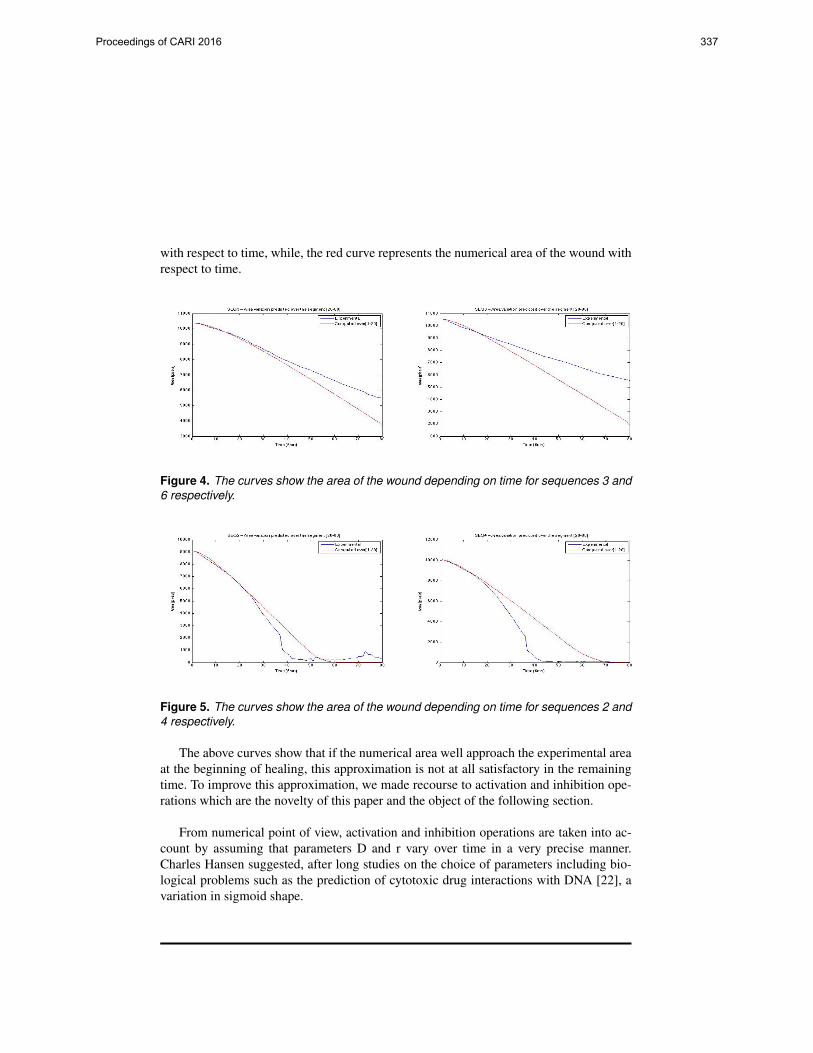
with respect to time, while, the red curve represents the numerical area of the wound withrespect to time.

Figure 4. The curves show the area of the wound depending on time for sequences 3 and6 respectively.

Figure 5. The curves show the area of the wound depending on time for sequences 2 and4 respectively.

The above curves show that if the numerical area well approach the experimental areaat the beginning of healing, this approximation is not at all satisfactory in the remainingtime. To improve this approximation, we made recourse to activation and inhibition ope-rations which are the novelty of this paper and the object of the following section.

From numerical point of view, activation and inhibition operations are taken into ac-count by assuming that parameters D and r vary over time in a very precise manner.Charles Hansen suggested, after long studies on the choice of parameters including bio-logical problems such as the prediction of cytotoxic drug interactions with DNA [22], avariation in sigmoid shape.


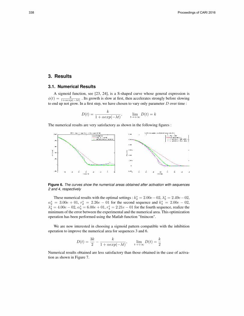
3. Results

3.1. Numerical ResultsA sigmoid function, see [23, 24], is a S-shaped curve whose general expression is

φ(t) = k1+αexp(−λt) . Its growth is slow at first, then accelerates strongly before slowing

to end up not grow. In a first step, we have chosen to vary only parameter D over time :

D(t) =k

1 + αexp(−λt), lim

t→+∞D(t) = k

The numerical results are very satisfactory as shown in the following figures :

Figure 6. The curves show the numerical areas obtained after activation with sequences2 and 4, respectively

These numerical results with the optimal settings : k∗2 = 2.00e−02, λ∗2 = 2.49e−02,α∗2 = 3.00e + 01, r∗2 = 2.26e − 01 for the second sequence and k∗4 = 2.00e − 02,λ∗4 = 4.00e− 02, α∗4 = 6.00e+ 01, r∗4 = 2.21e− 01 for the fourth sequence, realize theminimum of the error between the experimental and the numerical area. This optimizationoperation has been performed using the Matlab function "fmincon".

We are now interested in choosing a sigmoid pattern compatible with the inhibitionoperation to improve the numerical area for sequences 3 and 6.

D(t) =3k

2− k

1 + αexp(−λt), lim

t→+∞D(t) =

k

2

Numerical results obtained are less satisfactory than those obtained in the case of activa-tion as shown in Figure 7.


Figure 7. The curves show the numerical areas obtained after inhibition with sequences 3and 6 respectively

These numerical results, illustrated by the green curve, are obtained with the optimalsettings : k∗3 = 1.32e− 02, λ∗3 = 4.00e− 02, α∗3 = 3.00e+ 01, r∗3 = 2.99e− 02 for thethird sequence and k∗6 = 2.00e−02, λ∗6 = 4.00e−02, α∗6 = 3.00e+01, r∗6 = 2.93e−02for the sixth sequence. If the result obtained with inhibition and sequence 3 is more orless acceptable, that of the sequence 6 is not at all acceptable. Hoping to get better results,we decided to also vary the parameter r over time.

Drawing on results in Figure 7, we choose the following variations of parameters rand D with respect to time :

Figure 8. Diffusion and proliferation coefficients time-dependent

Numerical results obtained become very satisfactory as shown in the following figures.


Figure 9. The curves show the numerical areas obtained after inhibition with sequences 3and 6 respectively

In both cases, the numerical curve (shown in black diamonds) coincides so much withthe experimental curve (shown in continu blue line) that one can not see the latter. Thesenumerical results are obtained with the optimal settings : k∗D3 = 2.00e − 02, λ∗D3 =4.00e− 02, α∗D3 = 3.4631e+ 03, k∗r3 = 1.72e− 02, λ∗r3 = 1.00e− 02, α∗r3 = 12.1045for the third sequence and k∗D6 = 2.00e− 02, λ∗D6 = 4.00e− 02, α∗D6 = 3.4631e+ 03,k∗r6 = 1.93e− 02, λ∗r6 = 1.05e− 02, α∗r6 = 14.5041 for the sixth sequence.

3.2. Theoretical ResultsWe are interested in this section to the theoretical study of Fisher-KPP equation when

the diffusion coefficient D and the proliferation rate r vary over time : estimate the diffe-rence of the wound surface variation for the two cases, constant and time-dependent. Fora similar study we refer to [25] and [26].

3.2.1. Diffusion and proliferation coefficients time-dependentConsider the two following problems :

(P1)

∂tu1 = D∆u1 + ru1(1− u1), (x, y, t) ∈ Ω× (0, T ], (P1.1)u1(x, y, 0) = u1,0(x, y), (x, y) ∈ Ω,u1(x, y, t) = uH(x, y, t), (x, y, t) ∈ ΓD × (0, T ],∂u1

∂n (x, y, t) = g(x, y, t), (x, y, t) ∈ ΓN × (0, T ].

(P2)

∂tu2 = D(t)∆u2 + r(t)u2(1− u2), (x, y, t) ∈ Ω× (0, T ], (P2.1)u2(x, y, 0) = u2,0(x, y), (x, y) ∈ Ω,u2(x, y, t) = uH(x, y, t), (x, y, t) ∈ ΓD × (0, T ],∂u2

∂n (x, y, t) = g(x, y, t), (x, y, t) ∈ ΓN × (0, T ].

Lemme 3.1 Suppose that u1,0, u2,0 ∈ H1(Ω), u1 ∈ L2(0, T ;H2(Ω)) and u2 ∈ L2(0, T ;H1(Ω)),then we have the following estimate :

‖u2 − u1‖0,Ω ≤ eL(t)‖u2,0 − u1,0‖0,Ω + eL(t)∫ t

0eL(s)

[|D(s) − D|‖∆u1‖0,Ω +

|Ω||r(s)−r|]ds. (3.1)


The area of the wound at the instant t, defined by the formula (2.5), yields

|W2(t)−W1(t)| ≤∫

Ω

|u2 − u1|dx

≤√|Ω|‖u2 − u1‖0,Ω,

where |Ω| denotes the measure of Ω.

3.2.2. Estimate of ‖∆u1‖0,ΩWe are now seeking to estimate ‖∆u1‖0,Ω as a function of the data u1,0, D and r.

In order to be reduced to a homogeneous problem, we make the following change ofunknown : w1 = 1 − u1 in the problem (P1). The new unknown w1 is then the solutionto the following problem :

(P4)

∂w1

∂t (x, y, t)−D∆w1(x, y, t) + rw1(1− w1) = 0, (x, y, t) ∈ Ω×]0, T [,w1(x, y, 0) = w0(x, y) = 1− u1,0, (x, y) ∈ Ω,w1(x, y, t) = 0, dans ΓV × [0, T ],∂w1

∂n (x, y, t) = 0, dans ΓH × [0, T ].

Lemme 3.2 Suppose that u1,0 ∈ H1(Ω) and u1 ∈ L2(0, T ;H2(Ω)), we get the follo-wing estimate

‖∆u1‖20,Ω ≤ 2+∞∑n=1

λ2n

(‖1− u1,0‖20,Ωe−2Dλnt + r2|Ω|t

∫ t

0

e−2Dλn(t−s)ds), (3.2)

where (λn)n∈N∗ are eigenvalues of the following eigenvalue problem :

(P5)

−∆v = λv, in Ω,v = 0, on ΓV ,∂v∂n = 0, on ΓH .

4. Conclusion and perspectivesIn order to model cellular dynamics, a simple model of Fisher-KPP type, considering

only the biological effect, was considered in the first step. The comparison of numericalresults obtained, in the case where the proliferation and diffusion parameters are constant,with experimental results shows the insufficiency of Fisher-KPP model to accurately re-present the activated and inhibited dynamics. Nevertheless, the activation and inhibitionoperations (D and r time-dependent) provide more effective results, which is coherentwith the two estimations (3.1) and (3.2).

In order to better model the cellular dynamics, a coupled model is suggested. It consistsat the Fisher-KPP equation coupled with the mechanics equation ; the behavior being pu-rely elastic. Moreover, the numerical implementation of such coupled model is in pro-gress.


5. Bibliographie

[1] MALANDAIN G.,« https ://interstices.info/jcms/i53813/les-mathematiques-cachees-de-la-medecine. 21/05/2010. »

[2] PAGE KAREN M., MAINI PHILIP K., A.M. MONK. NICHOLAS, « Complex pattern formationin reaction-diffusion systems with spatially varying parameters », Physica, vol. 202, no , 2005.

[3] OLSEN L., MAINI P.K., SHERRATT J.A., « Spatially Varying Equilibria of Mechanical Mo-dels : Application to Dermal Wound Contraction », Mathematical Bisciences,vol. 147, no 113,1998.

[4] FENTEANY G., JANMEY P. A., STOSSEL T. P., « Signaling pathways and cell mechanicsinvolved in wound closure by epithelia cell sheets », Current Biology, vol. 10, no 831, 2000.

[5] BAO QI., HUGHES R.C., « Galectin-3 and polarized growth within collagen gels of wild-typeand ricin-resistant mdck renal epithelial cells », Glycobiology, vol. 9, no 5, 1999.

[6] QINGHUI MENG, JAMES M. MASON, DEBRA PORTI, ITZHAK D. GOLDBERG, ELIOT M.ROSEN, SAIJUN FAN, « Hepatocyte growth factor decreases sensitivity to chemotherapeuticagents and stimulates cell adhesion, invasion, and migration », Biochem. Biophys. Res. Com-mun., vol. 274, no 772, 2000.

[7] MURRAY J.D., « Mathematical Biology : I. An Introduction, Third Edition », Sprin-ger,Interdisciplinary Applied Mathematics, vol. 17, 2001.

[8] MURRAY J.D. , « Mathematical Biology : II. Spatial Models and Biomedical Applications »,Springer,Interdisciplinary Applied Mathematics, vol. 18, 2011.

[9] GAFFNEY EAMONN A., MAINI PHILIP K., SHERRATT JONATHAN A., DALE PAUL D.,« Wound healing in the corneal epithelium : Biological mechanisms and mathematical models »,J. Theor. Med., vol. 1, no 13,1997.

[10] MAINI P.K., OLSEN L., SHERRATT J.A., « Mathematical models for cell-matrix interac-tions during dermal wound healing », Int. J. Bifurcation Chaos Appl. Sci. Eng., vol. 12, no 9,2002.

[11] PAGE KAREN M., MAINI PHILIP K., MONK NICHOLAS A.M., « Complex pattern forma-tion in reactionÐdiffusion systems with spatially varying parameters »,Physica D, vol. 202, no

95, 2005.

[12] VEDULA S. R. K., LEONG M. C., LAI T. L. , HERSEN P., KABLA A. J., LIM C.T., LA-DOUX B., « Emerging modes of collective cell migration induced by geometrical constraints »,PNAS, vol. 109, 2012.

[13] LEE P., WOLGEMUTH C. W., « Crawling Cells Can Close Wounds without Purse Strings orSignaling », PLoS Computational Biology, vol. 7, 2011.

[14] SAEZ A., ANON E., GHIBAUDO M., O DU ROURE, MEGLIO J-M DI., HERSEN P., SIL-BERZAN P., BUGUIN A., LADOUX B., « Traction forces exerted by epithelial cell sheets », J.Phys. : Condens. Matter, vol. 22, no 9, 2010.

[15] KABLA A. J., « Collective cell migration : leadership, invasion and segregation », J. R. Soc.Interface, vol. 9, 2012.

[16] OLSEN L., MAINI P.K., SHERRATT J.A., « A mechanochemical model for normal and ab-normal dermal wound repair », Nonlinear Analysis, Theory, Methods & Applications, vol. 30,no 6, 1997.

[17] OLSEN L., MAINI P.K., SHERRATT J.A., « A Mechanochemical Model for Adult DermalWound Contraction and the Permanence of the Contracted Tissue Displacement Profile », J.theor. Biol., vol. 177, 1995.

[18] PERELSON A. S., MAINI P. K., MURRAY J. D., HYMAN J. M. , OSTER G. F.G. F., « Non-linear pattern selection in a mechanical model for morphogenesis », Journal of Mathematical


biology. Springer Veriag, vol. 24, no 525, 1986.

[19] SHERRATT J. A., « Actin aggregation and embryonic epidermal wound healing », Journalof Mathematical biology. Springer Veriag, vol. 31, no 703, 1993.

[20] GOTO Y., « A 2-dimensional mechanical model of the formation of a somite », Internationaljournal of numerical analysis and modeling, vol. 10, no 1, 2013.

[21] HABBAL A., BARELLI H., MALANDAIN G., « Assessing the ability of the 2D Fisher-KPPequation to model cell-sheet would clousure », Mathematical Biosciences, vol. 252, no 45,2014.

[22] HANSEN C. M. , « Polymer science applied to biological problems : prediction to cytotoxicdrug interactions with DNA », European Polymer Journal, vol. 44, 2008.

[23] HAMEL É. , « Modélisation mathématique de la déxpression synaptique et des périodesréfractaires pour le quantron », 2013.

[24] YEGANEFAR N., « Définitions et analyse de stabilité pour les systèmes à retard non li-néaires », Novembre 2006.

[25] BREZIS H., « Analyse fonctionnelle : Théorie et applications », Dunod, 1999.

[26] RAVIART P.A., THOMAS J.M., « Introduction à l’analyse numérique des équations aux déri-vées partielles », Masson, 1983.


Global weak solution to a 3-DKazhikhov-Smagulov model with Korteweg

stress

Caterina Calgaroa — Meriem Ezzougb,* — Ezzeddine Zahrounib,c

a Université LilleCNRS, UMR 8524Laboratoire Paul PainlevéF-59000 [email protected]

b Unité de Recherche : Multifractals et OndelettesFaculté des Sciences de MonastirUniversité de Monastir5019 [email protected]

c Faculté des Sciences Économiques et de Gestion de NabeulUniversité de Carthage8000 [email protected]

* Corresponding author

ABSTRACT. In this article, we consider a multiphasic incompressible fluid model, called the Kazhikhov-Smagulov model, with a specific stress tensor which depends on density derivatives, introduced byKorteweg. We establish the existence of global weak solution to this model in a 3D bounded domain.

RÉSUMÉ. Dans cet article, nous considérons un modèle de fluide incompressible multiphasique, ap-pelé modèle de Kazhikhov-Smagulov, avec un tenseur de contraintes spécifique qui dépend des dé-rivées d’ordre élevé de la densité, introduit par Korteweg. Nous établissons l’existence d’une solutionfaible globale pour ce modèle dans un domaine borné en 3D.

KEYWORDS : Kazhikhov-Smagulov model, Korteweg model, weak solution, global existence result.

MOTS-CLÉS : Modèle de Kazhikhov-Smagulov, modèle de Korteweg, solution faible, existence glo-bale.


1. IntroductionWe are concerned with systems of PDEs describing the evolution of mixture flows.

Let Ω be a bounded open set in R3 with boundary Γ that is regular enough and let n bethe outwards unit normal on the boundary Γ. We denote by [0, T ] the time interval, forT > 0. The mixture of two fluids is described by the density ρ(t,x) ≥ 0, the velocityfield v(t,x) ∈ R3 and the pressure p(t,x), depending on the time and space variables(t,x) ∈ [0, T ]× Ω. According to [4, 7, 8], we consider the Korteweg equations for gen-eralized incompressible fluids whose density and volume change with the concentrationφ(t,x) ≥ 0 and eventually the temperature, but not with pressure. In general, the velocityfield v of such incompressible fluids is not solenoidal, div v 6= 0. Assuming that eachfluid is incompressible, the mass density is conserved in the absence of diffusion. Thetheory of Korteweg, introduced in [9], considers the possibility that stresses are inducedby gradients of concentration and density in a slow process of diffusion of incompressiblemiscible liquids. Such stresses could be important in regions of high gradients and theymimic the surface tension.

In order to model the fluid capillarity effects, Korteweg introduced in the usual com-pressible fluid model a specific stress tensor which depends on density derivatives. Fol-lowing the rigorous formulation presented in [4] (see also [2]) and neglecting thermalfluctuations, the model reads

∂tρ+ div (ρv) = 0,∂t(ρv) + div (ρv ⊗ v) = ρg + div (S +K),

(1)

where g stands for the gravity acceleration (but it can include further external forces). Theviscous stress tensor S and the Korteweg stress tensorK are given by :

S = (ν div v − p)I + 2µD(v),K = (α∆ρ+ β|∇ρ|2)I + δ(∇ρ⊗∇ρ) + γD2

xρ,(2)

where D(v) = (∇v +∇vT )/2 is the strain tensor and D2xρ is the hessian matrix of the

density ρ. Here, the pressure p and the coefficients α, β, γ, δ, µ and ν are functions of ρ.The special case

α = κρ, β =κ

2, δ = −κ, γ = 0,

for some constant κ > 0, corresponds precisely to Korteweg’s original assumptions con-nected with the variational theory of Van Der Waals. In this case, the Korteweg stresstensor yields

K =κ

2(∆ρ2 − |∇ρ|2)I − κ(∇ρ⊗∇ρ). (3)

Writingdiv K = κρ∇(∆ρ) = κ∇(ρ∆ρ)− κ∇ρ∆ρ, (4)

and incorporating∇(ρ∆ρ) in the pressure term, we obtain −κ∇ρ∆ρ as a right hand sideterm in the momentum equation.

The Korteweg’s theory can be applied to processes of slow diffusion on miscible in-compressible fluids, for example, water and glycerin. The two fluids are characterizedby their reference mass density : ρ1 the density of the dilute phase and ρ2 the density ofthe dense phase. We need the velocity field of each constituent : v1(t,x) and v2(t,x),respectively. We define the volume fraction of the dilute phase 0 ≤ φ(t,x) ≤ 1 :

φ(t,x) = limr→0

Volume occupied at time t by the dilute phase in B(x, r)

|B(x, r)|.


Then, admitting that each fluid is incompressible and keeping a constant mass density, thedensity of the mixture is defined by

ρ(t,x) = ρ2

(1− φ(t,x)

)︸︷︷︸:=ρ2(t,x)

+ ρ1φ(t,x)︸︷︷︸:=ρ1(t,x)

= ρ2 + (ρ1 − ρ2)φ(t,x).

Writing the mass conservation for the two phases, we obtain

∂tρ+ div (ρv) = 0,

with ρv(t,x) = (ρ2v2 + ρ1v1)(t,x) presents the mean mass velocity v(t,x), which isnot divergence free, div v 6= 0. Moreover, we define the mean volume velocity

u(t,x) =(1− φ(t,x)

)v2(t,x) + φ(t,x)v1(t,x).

Applying the definitions, we verify that the velocity field u is solenoidal (divu = 0).According to Kazhikhov and Smagulov [10], we consider the following non-standardconstraint associated to the pressure p :

div v = −div (λ∇ ln(ρ)), (5)

where λ > 0 is a diffusion coefficient. This Fick’s law (5) describes the diffusive fluxesof one fluid into the other, see also [3]. Obviously, when we set

v = u− λ∇ ln(ρ), (6)

the relation yields (5). The mixture density ρ verifies the mass conservation and we obtain

∂tρ+ div (ρu) = div (λ∇ρ). (7)

For the momentum equation (1)2, we start by developing each term using the relation (6),in order to eliminate v. After some calculations and using (4), we get

∂t(ρu)

+ div(ρu⊗ u

)− λdiv

(∇ρ⊗ u

)− λdiv

(u⊗∇ρ

)+ λ∇

(u · ∇ρ

)+ λdiv

(2µD2

x ln(ρ))− div

(2µD(u)

)+∇p

− λ2(∇∆ρ− div

(∇ρ⊗∇ρρ

))= ρg + κ∇(ρ∆ρ)− κ∇ρ∆ρ.

(8)

Choosing the dynamic viscosity µ constant, as in [6], we have div(2µD(u)

)= µ∆u

and div(2µD2

x ln(ρ))

= 2µ∇∆ ln(ρ). Including all the gradient terms in the modifiedpressure

P = p+ λ(ν + 2µ)∆ ln(ρ) + λu · ∇ρ− λ2∆ρ− κρ∆ρ.

Then, we obtain the Kazhikhov-Smagulov-Korteweg model in conservative form :∂t(ρu)

+ div(ρu⊗ u

)− λdiv

(∇ρ⊗ u

)− λdiv

(u⊗∇ρ

)− µ∆u

+∇P + λ2div(∇ρ⊗∇ρ

ρ

)= ρg − κ∇ρ∆ρ,

∂tρ+ div(ρu)

= λ∆ρ,divu = 0.

(9)


The tensorial product matrix of two vectors a = (ai)di=1, b = (bi)

di=1 is denoted by a⊗b

with cœfficients (a⊗ b)i,j = aibj . Taking into account the equalities

∂t(ρu)

+ div(ρu⊗ u

)− λdiv

(∇ρ⊗ u

)= ρ∂tu+ ρ(u · ∇)u− λ(∇ρ · ∇)u,

−λdiv(u⊗∇ρ

)= −λ(u · ∇)∇ρ = −λ∇(u · ∇ρ) + λdiv

(ρ∇uT

).

Then, denoting QT

= (0, T ) × Ω, Σ = (0, T ) × Γ, the Kazhikhov-Smagulov-Korteweg(KSK) model can be written in Q

Tas :

ρ(∂tu+ (u · ∇)u

)− λ(∇ρ · ∇)u+ λdiv

(ρ∇uT

)− µ∆u+∇P

+λ2div(∇ρ⊗∇ρ

ρ

)= ρg − κ∆ρ∇ρ,

∂tρ+ div(ρu)

= λ∆ρ,divu = 0.

(10)

The KSK model (10) is completed by the following boundary and initial conditions

u(t,x) = 0,∂ρ

∂n(t,x) = 0, (t,x) ∈ Σ, (11)

u(0,x) = u0(x), ρ(0,x) = ρ0(x), x ∈ Ω, (12)

with the compatibility condition divu0 = 0, where ρ0 : Ω → R and u0 : Ω → R3 aregiven functions. Throughout this work, we assume the hypothesis

0 < m ≤ ρ0(x) ≤M < +∞, x ∈ Ω. (13)

The paper is organized as follows. In Section 2 we present the main results about (10).After some preliminary results recalled in Section 3, the proof of existence of global weaksolution for (10) is given in Section 4. The conclusions are summarized in Section 5.

2. Functional setup and main resultsLet us introduce the following functional spaces (see [11, 13] for their properties):

V =u ∈ D(Ω)3 : divu = 0 in Ω

,

V =u ∈ H1

0(Ω) : divu = 0 in Ω,

H =u ∈ L2(Ω) : divu = 0 in Ω, u · n = 0 on Γ

,

HsN =

ρ ∈ Hs(Ω) :

∂ρ

∂n= 0 on Γ,

∫Ω

ρ(x) dx =

∫Ω

ρ0(x) dx

, s ≥ 2.

The spaces V and H are the closures of V in H10(Ω) and L2(Ω), respectively.

Let us recall the definition of weak solution for the KSK model (10). Such class ofsolutions can be found in [1] for Kazhikhov-Smagulov type models and in [13] for theincompressible Navier-Stokes equations.

Definition 2.1 A pair of functions (u, ρ) is called a weak solution of problem(10),(11),(12) on Ω if and only if the following assumptions are satisfied :


1) u ∈ L∞(0, T ; H

)∩ L2

(0, T ; V

), ρ ∈ L∞

(0, T ;H1(Ω)

)∩ L2

(0, T ;H2

N

)and

0 < m ≤ ρ(t,x) ≤M < +∞, a.e. (t,x) ∈ QT.

2) For all φ ∈ C1([0, T ]; V

)such that φ(T, .) = 0, one has :∫ T

0

−(u, ρ∂tφ+

((ρu− λ∇ρ) · ∇

)φ)

+ µ(∇u,∇φ

)− λ(ρ∇uT ,∇φ

)dt

−λ2

∫ T

0

(1

ρ∇ρ⊗∇ρ,∇φ

)dt =

∫ T

0

(ρg − κ∆ρ∇ρ,φ

)dt+

(ρ0u0,φ(0)

).

(14)3) For all ϕ ∈ C1

([0, T ];H1(Ω)

)such that ϕ(T, .) = 0, one has :∫ T

0

(u · ∇ρ, ϕ

)+ λ(∇ρ,∇ϕ

)−(ρ, ∂tϕ

)dt =

(ρ0, ϕ(0)

). (15)

REMARK. — The pressure P associated with the weak solution (u, ρ) can be obtainedusing (14) and the Rham’s lemma [13].

We present the aim of this work about the Kazhikhov-Smagulov-Korteweg model (10).Under some assumption on the coefficients λ, µ, κ, we prove the global existence of weaksolution of (10) for arbitrary initial data and external force field. Our main result reads :

Theorem 2.2 Let u0 ∈ H, ρ0 ∈ H1(Ω) satisfy (13), T > 0 and g ∈ L2(0, T ; L2(Ω)

). If

λ

µmax(1,

λ2

κ) is sufficiently small, then there exists a weak solution (u, ρ) of (10) global

in time such thatu ∈ L∞

(0, T ; H

)∩ L2

(0, T ; V

),

ρ ∈ L∞(0, T ;H1(Ω)

)∩ L2

(0, T ;H2

N

),

with finite and uniformly bounded energy such that ∀t ≤ T,

‖√ρ(t)u(t) ‖2

L2(Ω)+κ ‖ ∇ρ(t) ‖2

L2(Ω)+

∫ t

0

(µ2‖ ∇u(s) ‖2

L2(Ω)+κλ ‖ ∆ρ(s) ‖2

L2(Ω)

)ds

≤ ‖ √ρ0u0 ‖2L2(Ω)

+κ ‖ ∇ρ0 ‖2L2(Ω)

+CM2

µ

∫ T

0

‖ g(s) ‖2L2(Ω)

ds.

3. Preliminary resultsGiven the initial density ρ0 and the velocity field u, we find the density ρ as solution

of the following Neumann problem :∂tρ + u · ∇ρ = λ ∆ρ in Q

T,

ρ(0,x) = ρ0(x) in Ω,

∂ρ

∂n= 0 on Σ.

(16)

The density ρ satisfies the maximum principle. This result is classical (see [1]).


Proposition 3.1 If (u, ρ) is a weak solution of (10), then

0 < m ≤ ρ(t,x) ≤M < +∞ a.e. (t,x) ∈ QT. (17)

Proposition 3.2 Let ρ0 ∈ H1(Ω) verify (13) and u ∈ C([0, T ]; V ∩H2(Ω)

). Then there

exists a unique solution ρ of (16) such that

ρ ∈ L∞(0, T ;H1(Ω)

)∩ L2

(0, T ;H2

N

).

Moreover, we have

sup0≤t≤T

‖ ρ(t) ‖2L2(Ω)

≤ ‖ ρ0 ‖2H1(Ω)

, (18)

∫ T

0

‖ ∇ρ(t) ‖2L2(Ω)

dt ≤ 1

2λ‖ ρ0 ‖2

H1(Ω), (19)

sup0≤t≤T

‖ ∇ρ(t) ‖2L2(Ω)

≤ Cλ ‖ ρ0 ‖2H1(Ω)

(1 + sup

0≤t≤T‖ u(t) ‖2

L∞(Ω)

), (20)

∫ T

0

‖ ∆ρ(t) ‖2L2(Ω)

dt ≤ Cλλ‖ ρ0 ‖2

H1(Ω)

(1 + sup

0≤t≤T‖ u(t) ‖2

L∞(Ω)

), (21)

where Cλ is a positive constant depending only on λ.

Given ρ0 ∈ H1(Ω) satisfying (13) and u ∈ C([0, T ]; V ∩ H2(Ω)

), let ρ the solution

obtained by Proposition 3.2. Therefore, it is clear that the following map is well defined

S : C([0, T ]; V ∩H2(Ω)

)−→ L∞

(0, T ;H1(Ω)

)∩ L2

(0, T ;H2

N

),

such that ρ = Su is well defined.

Proposition 3.3 Let ρ0 ∈ H1(Ω) verify (13) and u1,u2 ∈ C([0, T ]; V ∩ H2(Ω)

). Set

ρ = ρ1 − ρ2 = Su1 − Su2 and u = u1 − u2, we have the following estimates :

sup0≤t≤T

‖ ρ(t) ‖2L2(Ω)

+λ

∫ T

0

‖ ∇ρ(t) ‖2L2(Ω)

dt ≤ M2

λT sup

0≤t≤T‖ u(t) ‖2

L2(Ω), (22)

sup0≤t≤T

‖ ∇ρ(t) ‖2L2(Ω)

+ λ

∫ T

0

‖ ∆ρ(t) ‖2L2(Ω)

dt

≤ 2T

λsup

0≤t≤T‖ ∇ρ1 ‖2

L2(Ω)sup

0≤t≤T‖ u ‖2

L∞(Ω)+

2M2T

λ3sup

0≤t≤T‖ u2 ‖2L∞(Ω)

sup0≤t≤T

‖ u ‖2L2(Ω)

.

(23)

We recall that there exists an orthonormal basis of L2(Ω) defined by

ωk ∈ V ∩H2(Ω)−P∆ωk = λk ωk on Ω,

where P is the orthogonal projection operator of L2(Ω) onto H. For any n ∈ N∗, wedefine by Xn the finite dimensional subspace of H such that

Xn = Vectωk, k = 1, . . . , n,


and we consider the orthogonal projection Pn : L2(Ω)→ Xn defined by

∀w ∈ H,(Pnw, v

)=(w, v

), ∀v ∈ Xn. (24)

As in [5], we introduce a family of operatorsM[ρ] : Xn −→ Xn defined by

(M[ρ]v, ω

)=

∫Ω

ρ v · ω dx for all v,ω ∈ Xn. (25)

If ρ ∈ L∞(Ω), thenM[ρ] is well defined. Moreover, let m > 0, we set

D =ρ ∈ L∞(Ω); ρ(x) ≥ m > 0

.

Proposition 3.4 M[ρ] is one-to-one and its inverse verifies

‖ M[ρ]−1 ‖L(Xn,Xn) ≤(

infx∈Ω

ρ(x))−1 ∀ρ ∈ D, (26)

‖ M[ρ1]−1 −M[ρ2]−1 ‖L(Xn,Xn) ≤Cnm2‖ ρ1 − ρ2 ‖L2(Ω)

∀ρ1, ρ2 ∈ D, (27)

where Cn is a constant depending on the dimension of the space Xn.

4. Proof of Theorem 2.2

4.1. Faedo-Galerkin methodWe are looking for the approximate solutions

(un, ρn) ∈ C([0, T ]; Xn

)× C

([0, T ];H1(Ω) ∩H2

N

)satisfying

∫Ω

∂t(ρnun

)· vdx+

∫Ω

ρn(un · ∇)un · vdx− λ∫

Ω

(∇ρn · ∇)un · vdx

+

∫Ω

(un · ∇ρn) un · vdx− λ∫

Ω

∆ρnun · vdx− µ∫

Ω

∆un · vdx

+ λ

∫Ω

div(ρn∇uTn

)· vdx+ λ2

∫Ω

div(∇ρn ⊗∇ρn

ρn

)· vdx

=

∫Ω

ρng · vdx− κ∫

Ω

∆ρn∇ρn · vdx, ∀v ∈ Xn,∫Ω

∂t(ρn)η dx+

∫Ω

un · ∇ρn η dx = λ

∫Ω

∆ρn η dx, ∀η ∈ H1(Ω),

un(0) = u0n = Pnu0,ρn(0) = ρ0.

(28)

We set

N [un, ρn] = −((ρnun − λ∇ρn) · ∇

)un − (un · ∇ρn)un + λ∆ρnun

+ µ∆un − λdiv(ρn∇uTn

)− λ2div

(∇ρn ⊗∇ρnρn

)− κ∆ρn∇ρn + ρng.

(29)


Taking (28)1 with v = ωk, for k = 1, . . . , n, and integrating in time between 0 andt ≤ T , the solution un verifies the following integral equations for k = 1, . . . , n :∫

Ω

ρn(t)un(t) · ωk dx =

∫Ω

q0 · ωk dx +

∫ t

0

∫Ω

N [un, ρn] · ωk dx ds, (30)

where ρn = Sun and q0 = ρ0u0n. Thanks to (24) and (25), we rewrite (30) as follows :(M[ρn(t)]un(t), ωk

)=(Pnq0, ωk

)+(Pn∫ t

0

N [un(s), ρn(s)] ds, ωk

),

for k = 1, . . . , n. SinceM[ρn] is invertible, then the resulting equation reads

un ∈ C([0, T ]; Xn

), un(t) =M[ρn(t)]−1Pn

(q0 +

∫ t

0

N [un(s), ρn(s)] ds). (31)

Hence, un appears as a fixed point of a suitable functional Ψ

Ψ : C([0, T ]; Xn

)−→ C

([0, T ]; Xn

)un 7−→ Ψ

(un)

defined by

Ψ(un)(t) =M[ρn(t)]−1Pn

(q0 +

∫ t

0

N [un(s), ρn(s)] ds), for all t ∈ [0, T ].

Let XT be the Banach space C([0, T ]; Xn

)endowed with the norm

‖ un ‖XT= sup

0≤t≤T‖ un(t) ‖

L2(Ω).

In order to apply the Banach fixed point theorem, we establish some uniform estimatesfor Ψ. With Propositions 3.2, 3.3 and 3.4 in mind, we have the following :

Proposition 4.1 There exists a constant C > 0 depending on n, λ, µ, κ, M , m, ‖ρ0 ‖H1(Ω)

, ‖ g ‖L2(0,T ;L2(Ω))

, such that for all un ∈ XT,

‖ Ψ(un)‖

XT≤ M

m‖ u0 ‖L2(Ω)

+ C max(T, T14 )(

1+ ‖ un ‖2XT

), (32)

and for all u1n,u

2n ∈ XT,

‖ Ψ(u1n

)−Ψ

(u2n

)‖

XT≤ C max(T, T

14 )(

1+ ‖ u0 ‖L2(Ω)

+ ‖ u1n ‖2XT

+ ‖ u2n ‖2XT

)‖ u1

n − u2n ‖XT

.(33)

At this stage, we set R = 2M

m‖ u0 ‖L2(Ω)

and BTR =u ∈ XT, ‖ u ‖XT

≤ R.

Proposition 4.2 There exists Tn ∈]0, 1[ small enough and un ∈ BTn

R such that

un = Ψ(un).


Proof. Let 0 < Tn < 1 such that

max(CT

14n

[R+

1

R

], CT

14n

[1+ ‖ u0 ‖L2(Ω)

+2R2])≤ 1

2.

Thanks to Proposition 4.1, we verify that Ψ is a contraction mapping on BTn

R and weconclude the existence of a unique fixed point of Ψ. It is clear that un the fixed point of Ψ, obtained in Proposition 4.2, implies that (un, ρn =Sun) is a local solution of the Galerkin approximate problem (28). Now, we will provethat this local solution is in fact a global one. For this, we establish some uniform esti-mates for (un, ρn) with respect to time.

Proposition 4.3 Ifλ

µmax(1,

λ2

κ) small enough, there exists a constantC > 0 depending

on ρ0,u0, g,M, µ, κ, such that for all t ∈ [0, Tn)

m ‖ un(t) ‖2L2(Ω)

+µ

2

∫ t

0

‖ ∇un(s) ‖2L2(Ω)

ds ≤ C, (34)

κ ‖ ∇ρn(t) ‖2L2(Ω)

+ κλ

∫ t

0

‖ ∆ρn(s) ‖2L2(Ω)

ds ≤ C. (35)

Evidently, thanks to the previous Proposition 4.3, we have the following :

Corollary 4.4 (un, ρn) is a global solution of (28) and for all T > 0,

(un)n is bounded in L∞(0, T ; H

)∩ L2

(0, T ; V

), (36)

(ρn)n is bounded in L∞(0, T ;H1(Ω)

)∩ L2

(0, T ;H2

N

). (37)

4.2. Uniform estimates for time derivativesIn this section, we establish uniform estimates for time derivatives ∂t ρn and ∂t un.

Proposition 4.5 Let T > 0. The sequence (∂t ρn)n is bounded in L4/3(0, T ;L2(Ω)

).

Proof. Taking the L2-norm of ∂t ρn. Applying the Hölder and Gagliardo-Nirenberginequalities and the inequality : ‖ ∇ρ ‖

L4(Ω)≤ C0 ‖ ρ ‖1/2L∞(Ω)

‖ ∆ρ ‖1/2L2(Ω)

, we get

‖ ∂t ρn ‖L2(Ω)≤ λ ‖ ∆ρn ‖L2(Ω)

+C ‖ un ‖1/4L2(Ω)‖ ∇un ‖3/4

L2(Ω)‖ ρn ‖1/2L∞(Ω)

‖ ∆ρn ‖1/2L2(Ω)

.

By the uniform estimate (34) and (17), we get

‖ ∂t ρn ‖L2(Ω)≤ λ ‖ ∆ρn ‖L2(Ω)

+ C ‖ ∇un ‖3/4L2(Ω)‖ ∆ρn ‖1/2

L2(Ω). (38)

Next, applying the Young inequality ab ≤ 1

2(a2 + b2) in (38), we get

‖ ∂t ρn ‖L2(Ω)≤ λ ‖ ∆ρn ‖L2(Ω)

+ C ‖ ∇un ‖3/2L2(Ω)

.

Thanks to the uniform time estimates (34) and (35), we deduce that ‖ ∂t ρn ‖L2(Ω)is

bounded in L4/3(0, T

).

Now, by following [1], we establish an estimation of the fractional time derivative of un.


Proposition 4.6 Let 0 < δ < T such that∫ T−δ

0

‖ un(t+ δ) − un(t) ‖2L2(Ω)

dt ≤ C δ14 , (39)

where C a constant independent of n and δ.

Proof. For all functions φ ∈ XT, the approximate solution (un, ρn) verifies :

d

dτ

∫Ω

ρnun · φ dx−∫

Ω

ρnun ·∂φ

∂τdx−

∫Ω

ρn(un · ∇)φ · un dx

+ µ

∫Ω

∇un : ∇φ dx+ λ

∫Ω

(∇ρn · ∇)φ · un dx− λ∫

Ω

ρn∇uTn : ∇φ dx

− λ2

∫Ω

∇ρn ⊗∇ρnρn

: ∇φ dx =

∫Ω

ρng · φ dx− κ∫

Ω

∆ρn∇ρn · φ dx.

(40)

Integrating (40) with respect to τ between t and t+ δ, and taking φ = un(t+ δ)−un(t)∫Ω

[ρn(t+ δ) un(t+ δ)− ρn(t) un(t)

][un(t+ δ)− un(t)

]dx

=

∫ t+δ

t

∫Ω

(ρn(τ) g(τ)− κ ∆ρn(τ)∇ρn(τ)

)·(un(t+ δ)− un(t)

)dx dτ

+

∫ t+δ

t

∫Ω

((ρn(τ)un(τ)− λ∇ρn(τ)

)· ∇)(un(t+ δ)− un(t)

)· un(τ) dx dτ

−∫ t+δ

t

∫Ω

(µ∇un(τ)− λ ρn(τ)∇uTn (τ)

): ∇(un(t+ δ)− un(t)

)dx dτ

+ λ2

∫ t+δ

t

∫Ω

∇ρn(τ)⊗∇ρn(τ)

ρn(τ): ∇(un(t+ δ)− un(t)

)dx dτ.

(41)Using the following identity

ρn(t+δ)un(t+δ)−ρn(t)un(t) = ρn(t+δ)[un(t+δ)−un(t)

]+[ρn(t+δ)−ρn(t)

]un(t),

then, (41) becomes

‖√ρn(t+ δ)

[un(t+ δ)− un(t)

]‖2L2(Ω)

= −∫

Ω

[ρn(t+ δ)− ρn(t)

][un(t+ δ)− un(t)

]· un(t) dx

+

∫ t+δ

t

∫Ω

(ρn(τ) g(τ)− κ ∆ρn(τ)∇ρn(τ)

)·(un(t+ δ)− un(t)

)dx dτ

+

∫ t+δ

t

∫Ω

((ρn(τ)un(τ)− λ∇ρn(τ)

)· ∇)(un(t+ δ)− un(t)

)· un(τ) dx dτ

−∫ t+δ

t

∫Ω

(µ∇un(τ)− λ ρn(τ)∇uTn (τ)

): ∇(un(t+ δ)− un(t)

)dx dτ

+ λ2

∫ t+δ

t

∫Ω

∇ρn(τ)⊗∇ρn(τ)

ρn(τ): ∇(un(t+ δ)− un(t)

)dx dτ

= I1(t) + I2(t) + I3(t) + I4(t) + I5(t) + I6(t) + I7(t) + I8(t).(42)

Let us estimate I1(t). Applying the Hölder inequality, we get

|I1(t)| ≤ ‖ ρn(t+ δ)− ρn(t) ‖L2(Ω)‖ un(t+ δ)− un(t) ‖

L4(Ω)‖ un(t) ‖

L4(Ω).


In particular, we write

ρn(t+ δ)− ρn(t) =

∫ t+δ

t

∂ρn∂τ

dτ.

Using the Hölder and Young inequalities and the embedding H1(Ω) ⊂ L4(Ω), we obtain

|I1(t)| ≤ Cδ14

(∫ t+δ

t

‖ ∂ρn∂τ‖ 4

3

L2(Ω)dτ) 3

4(‖ ∇un(t+ δ) ‖2

L2(Ω)+ ‖ ∇un(t) ‖2

L2(Ω)

).

In the same way, we verify the following estimations :

|I2(t)| ≤ Cδ12

(∫ t+δ

t

‖ g(τ) ‖2L2(Ω)

dτ) 1

2(‖ ∇un(t+ δ) ‖2

L2(Ω)+ ‖ ∇un(t) ‖2

L2(Ω)

),

|I3(t)| ≤ Cδ14

(∫ t+δ

t

‖ ∆ρn(τ) ‖2L2(Ω)

dτ) 3

4(‖ ∇un(t+ δ) ‖2

L2(Ω)+ ‖ ∇un(t) ‖2

L2(Ω)

).

Similarly, one can obtain the desired estimates of Ij(t) terms, for j = 4, . . . , 8.At last, if we choose 0 < δ < 1 and taking into account Propositions 4.3 and 4.5, then bygathering together all the above estimates, we rewrite (42) as follows :

‖√ρn(t+ δ)

[un(t+ δ)− un(t)

]‖2

L2(Ω)≤ Cδ 1

4

(‖ ∇un(t+ δ) ‖2

L2(Ω)+ ‖ ∇un(t) ‖2

L2(Ω)

).

Thanks to the lower bound of ρn and Proposition 4.3, we finish the proof.

4.3. The existence of solution (u, ρ)

The final step to complete this study is to employ the previous uniform estimates inorder to pass to the limit in the approximate problem (28). When n→ +∞, we have

u0n −→ u0 in H strongly.

Thanks to (36) and (37), choosing the subsequences (un)n and (ρn)n such that

un −→ u in L2(0, T ; V

)weakly,

un −→ u in L∞(0, T ; H

)weakly-star,

andρn −→ ρ in L2

(0, T ;H2

N

)weakly,

ρn −→ ρ in L∞(0, T ;H1(Ω)

)weakly-star,

∂t ρn −→ ∂t ρ in L4/3(0, T ;L2(Ω)

)weakly.

We are able to pass to the limit in the linear terms of (28), thanks to these above conver-gence results. Now, to ensure the passage to the limit in the nonlinear terms of (28), it isnecessary to use the following strong convergence :

Proposition 4.7 There exists a subsequence (un, ρn)n which converges strongly to (u, ρ)in L2

(0, T ; L2(Ω)

)× L2

(0, T ;H1(Ω)

). Moreover, (u, ρ) is a weak solution of (10).

Proof. Applying some compactness theorems [13, Chap.3, Theorem 2.1] for ρn and [12,Theorem 5] for un and using Propositions 4.5 and 4.6, we get to the desired result.


5. ConclusionsIn this paper, we study the system of PDEs derived from the compressible Navier-

Stokes equations with presence of a specific Korteweg stress tensor, called the Kazhikhov-Smagulov-Korteweg (KSK) model. We arrive at verify the existence of a weak solution(u, ρ) of the KSK model (10) global in time with finite and uniformly bounded energy.Then, we conclude the proof of Theorem 2.2, the main result of this paper.

6. References

[1] D. BRESCH, E.H. ESSOUFI, M. SY, “Effects of density dependent viscosities on multiphasicincompressible fluid models”, J. Math. Fluid Mech., vol. 9, num. 3, p. 377-397, 2007.

[2] D. BRESCH, B. DESJARDINS, C.K. LIN, “On some compressible fluid models: Korteweg,lubrication and shallow water systems”, Comm. Partial Diff. Eqs., vol. 28, num. 3-4, p. 843-868, 2003.

[3] C. CALGARO, E. CREUSÉ, T. GOUDON, “Modeling and simulation of mixture flows: Appli-cation to powder-snow avalanches”, Computers and Fluids, vol. 107, p. 100-122, 2015.

[4] J.E. DUNN, J. SERRIN, “On the thermomechanics of interstitial working”, Arch. RationalMech. Anal., vol. 88, num. 2, p. 95-133, 1985.

[5] E. FEIREISL, A. NOVOTNÝ, H. PETZELTOVÁ, “On the existence of globally defined weaksolutions to the Navier-Stokes equations”, J. Math. Fluid Mech., vol. 3, p. 358-392, 2001.

[6] F. FRANCHI, B. STRAUGHAN, “A comparison of Graffi and Kazhikov-Smagulov models fortop heavy pollution instability”, Adv. in Water Resources, vol. 24, p. 585-594, 2001.

[7] P. GALDI, D.D. JOSEPH, L. PREZIOSI, S. RIONERO, “Mathematical problems for miscible,incompressible fluids with Korteweg stresses”, European J. of Mech. B-Fluids, vol. 10, num. 3,p. 253-267, 1991.

[8] D.D. JOSEPH, “Fluid dynamics of two miscible liquids with diffusion and gradient stresses”,European J. of Mech. B-Fluids, vol. 6, p. 565-596, 1990.

[9] D.J. KORTEWEG, “Sur la forme que prennent les équations du mouvement des fluides si l’ontient compte des forces capillaires causées par des variations de densité considérables maiscontinues et sur la théorie de la capillarité dans l’hypothèse d’une variation continue de ladensité”, Archives Néerlandaises des Sciences Exactes et Naturelles, Séries II, vol. 6, p. 1-24,1901.

[10] A. KAZHIKHOV, SH. SMAGULOV, “The correctness of boundary value problems in a dif-fusion model of an inhomogeneous fluid”, Sov. Phys. Dokl., vol. 22, num. 1, p. 249-252,1977.

[11] J.L. LIONS, “Quelques méthodes de résolution des problèmes aux limites non linéaires”,Dunod, Gauthier-Villars, Paris, 1969.

[12] J. SIMON, “Compact sets in the space Lp(0, T ;B

)”, Ann. Mat. Pura Appl., vol. 146, p. 65-

96, 1987.

[13] R. TEMAM, “Navier-Stokes equations, theory and numerical analysis”, Revised Edition, Stud-ies in mathematics and its applications vol. 2, North Holland Publishing Company-Amsterdam,New York, 1984.


Theoretical Analysis of a Water Wave Modelusing the Diffusive Approach

Olivier Goubeta — Imen Manoubi b,*

a Université de Picardie Jules Verne33 rue Saint-Leu 80039Amiens, [email protected]

b UR Multifractales et OndelettesFaculté des Sciences de MonastirAvenue de l’environnement 5019 Monastir, [email protected]

* Corresponding author

ABSTRACT. In this paper, we theoretically study the water wave model with a nonlocal viscous term

ut + ux + βuxxx +

√ν√π

∂

∂t

∫ t

0

u(s)√t− s

ds+ uux = νuxx,

where the Riemann-Liouville half-order derivative1√π

∂

∂t

∫ t

0

u(s)√t− s

ds is represented with a diffusive

realization.

RÉSUMÉ. Dans cet article, nous étudions théoriquement le modèle visqueux asymptotique

ut + ux + βuxxx +

√ν√π

∂

∂t

∫ t

0

u(s)√t− s

ds+ uux = νuxx,

où la demi-dérivée de Riemann-Liouville1√π

∂

∂t

∫ t

0

u(s)√t− s

ds est représentée à l’aide d’une réalisa-

tion diffusive.

KEYWORDS : nonlocal viscous model, Riemann-Liouville half derivative, diffusive realization

MOTS-CLÉS : modèle visqueux non local, demi-dérivée de Riemann-Liouville, réalisation diffusive


1. Introduction

1.1. State of the art.The modeling and the mathematical analysis of viscosity in water wave propagation

are challenging issues. In the last decade, P. Liu and T. Orfila [8], and D. Dutykh and F.Dias [6] have independently derived viscous asymptotic models for transient long-wavepropagation on viscous shallow water. These effects appear as nonlocal terms in the formof convolution integrals. A one-dimensional nonlinear system is presented in [5].In their recent work [4], M. Chen et al. investigated theoretically and numerically thedecay rate for solutions to the following water wave model with a nonlocal viscous dis-persive term as follows

ut + ux + βuxxx +

√ν√π

∫ t

0

ut(s)√t− s

ds+ uux = αuxx, (1)

where1√π

∫ t

0

ut(s)√t− s

ds represents the Caputo half-derivative in time. Here u is the

horizontal velocity of the fluid, −αuxx is the usual diffusion, βuxxx is the geometric

dispersion and1√π

∫ t

0

ut(s)√t− s

ds stands for the nonlocal diffusive-dispersive term. We

denote as β, ν and α the parameters dedicated to balance or unbalance the effects ofviscosity and dispersion against nonlinear effects. Particularly, the authors in [4] consider(1) with β = 0 supplemented with the initial condition u0 ∈ L1(R) ∩ L2(R). Theyproved that if ‖u0‖L1(R) is small enough, then there exists a unique global solution u ∈C(R+;L2

x(R)) ∩ C1(R+;H−2x (R)). In addition, u satisfies

t1/4‖u(t, ·)‖L2x(R) + t1/2‖u(t, ·)‖L∞x (R) < C(u0). (2)

In order to study the effects of the nonlocal term on the existence and on the decay rateof the solutions, the second author considered in her recent work [10] a derived modelfrom (1) where the fractional term is described by the Riemann-Liouville half derivativeinstead of that of Caputo, namely

ut + ux + βuxxx +

√ν√π

∂

∂t

∫ t

0

u(s)√t− s

ds+ uux = αuxx. (3)

She proved the local and global existence of solutions to problem (3) when β = 0 using afixed point theorem. Then she studied theoretically the decay rate of the solutions in thiscase. Precisely, she stated the following theorem

Theorem 1.1 (I. Manoubi, 2014) Let u0 ∈ L2(R), then there exists a unique local solu-tion u ∈ C([0, T );L2

x(R)) of (3).Moreover for u0 ∈ L1(R) ∩ L2(R), there exists a positive constant C0 > 0 that dependson u0 such that if ‖u0‖L1(R) is small enough, there exists a unique global solution u ∈C(R+;L2

x(R)) ∩ C1/2(R+;H−2x (R)) of (3) given by

u(t, x) = [KRL(t, ·) ? u0](x)−N ~ u2(t, x), (4)

where KRL and N are given by

KRL(t, x) =1

2√πte−

x2

4t e−x−

(1− 1

2

∫ +∞

0

e−µ2

4t −µ|x|2t −

µ2 dµ),


and

N(t, x) =1

4√πt∂x

(e−

x2

4t e−x−(

1− 1

2

∫ +∞

0

e−µ2

4t −µ|x|2 −

µ2 dµ

)).

with x− = |x|−x2 = max(−x, 0), ? represents the usual convolution product and~ is the

time-space convolution product defined by

v ~ w(t, x) =

∫ t

0

∫Rv(t− s, x− y)w(s, y)dsdy.

whenever the integrals make sense. In addition, we have the following estimate

max(t1/4, t3/4)‖u(t, ·)‖L2x(R) + max(t1/2, t)‖u(t, ·)‖L∞x (R) ≤ C0. (5)

The proof of this theorem is presented in [10].However, all these results are performed assuming a smallness condition on the initialdata. In order to remove this smallness condition and to investigate the model (3) for alarge class of initial data, we introduce here the concept of diffusive realizations for thehalf-order derivative. This approach was initially developed by Montseny [12], Montsenyet al. [14, 15] and Staffans [16]. Diffusive realization make possible to represent nonlocalin time operators, and more generally causal pseudo-differential operators, in a state spacemodel formulation where the state belongs to an appropriate Hilbert space. Differentapplications of this approach can be found in [1, 7, 11, 13].In this article, we assume that the effects of the geometric dispersion in (3) is less im-portant than the viscosity effects (i.e we take β = 0 in (3)) and we assume that the otherconstants are normalized. Thus, our model is reduced as follows

ut + ux +1√π

∂

∂t

∫ t

0

u(s)√t− s

ds+ uux = uxx. (6)

We prove the well posedness of the model (6) for all initial data u0 ∈ H1(R) usingthe diffusive realization. To this end, we complete the introduction as follows. We firstintroduce the diffusive formulation of the half-order Riemann-Liouville derivative. Then,we deduce the mathematical model that derives from (6) using the diffusive approach.Finally, we present the main results of this article.We note that one can consider the general case of the Caputo or Riemann-Liouville frac-tional derivative of order α where 0 < α < 1. Comparing the effects of these non-local terms with our results is a challenging issue and it may be the subject of a fu-ture work. However, choosing another definition of fractional derivative like Atangana-Baleanu derivative or Caputo-Fabrizio derivative in equation (1) must be justified.

1.2. Diffusive formulation of the modelIn the literature, there are several diffusive realizations of the Riemann-Liouville half-

order derivative. We recall in the following some of these formulations.First, the diagonal form of the diffusive realization of D1/2u(t) which will be used in theremaining of this article is given for all t > 0 by

∂tψ(t, σ) = −σψ(t, σ) + u(t), ψ(0, σ) = 0, σ ∈ R+

D1/2u(t) =

∫ +∞

0

1

π√σ∂tψ(t, σ)dσ.

(7)


Second, the PDE-form of the diffusive realization of D1/2u(t) is given for all t > 0 by∂tΦ(t, y) = Φyy(t, y) + u(t)⊗ δy=0, Φ(0, y) = 0, y ∈ R,

D1/2u(t) = 2 < δy=0, ∂tΦ(t, y) >D′,D= 2d

dtΦ(t, 0).

(8)

where δy=0 is the Dirac delta function at y = 0 and u(t) ⊗ δy=0 is the tensorial productin the distributions sense of the applications t 7→ u(t) and y 7→ δy=0.Finally, another form of the diffusive realization of D1/2u(t) is given for all t > 0 by

∂tφ(t, σ) = −σ2φ(t, σ) +2

πu(t), φ(0, σ) = 0, σ ≥ 0,

D1/2u(t) =

∫ +∞

0

(2

πu(t)− σ2φ(t, σ))dσ.

(9)

We note that the author has used the diffusive realizations (8) and (9) in her PhD Thesis tostudy mathematically and numerically the integro-differential equation (3) when β = 0,ν = α = 1. For more details, we refer the readers to [9]. In the following, we describethe mathematical framework. Thanks to the diffusive realization (7), the problem (6) iswritten as follows

ut(t, x) + ux(t, x) +

∫ +∞

0

(u(t, x)− σψ(t, x, σ))dσ

π√σ

+ u(t, x)ux(t, x) = uxx(t, x), t > 0, x ∈ R,

ψt(t, x, σ) = −σψ(t, x, σ) + u(t, x), t > 0, x ∈ R, σ ≥ 0,

u(0, x) = u0(x), x ∈ R,

ψ(0, x, σ) = 0, x ∈ R, σ ≥ 0.

(10)

Then, We rewrite the system (10) as a first-order semi-linear differential equation as fol-lows

Xt +AX = F (X),

X(0) = X0,(11)

where X = (u, ψ)T , X0 = (u0, 0)T and

AX =

∫ +∞

0

(u− σψ)dσ

π√σ− uxx

−u+ σψ

,

F (X) =

(−ux − uux

0

). (12)

1.3. Main results.We introduce our functional space . First, we define the positive measure dN on R+

by

dN(σ) =dσ

π√σ.


Hence, dN satisfies

CN =

∫ +∞

0

dN(σ)

1 + σ= 1. (13)

Then, we define the spaces

HN = L2(R+, dN),

HN = L2(R+, σdN),

V = L2(R+, (1 + σ)dN).

We suppose that (11) has a regular solution. The following result holds.

Proposition 1.2 The energy function associated to (11)

E(t) =1

2‖u(t)‖2L2

x+

1

2‖ψ(t)‖2

L2(R,HN ), (14)

satisfies the following energetic equilibrium

1

2

d

dtE(t) = −

∫R‖u(t, x)− σψ(t, x, σ)‖2HNdx−

∫R|ux(t, x)|2dx. (15)

The natural energy space of the solution X is

H = L2(R)× L2(R, HN ),

endowed with the scalar product (·, ·)H defined for all X = (u, ψ)T and Y = (v, χ)T inH by

(X,Y )H = (u, v)L2(R) +

∫R

(ψ, χ)HNdx.

Moreover, we define the following Hilbert space

V = H2(R)× L2(R, HN ).

We state the main result of this article.

Theorem 1.3 For all u0 ∈ H1(R), there exists a unique global solutionX ∈ C([0,+∞[, D(A1/2))

of (11) such that X0 =

(u00

)and

X(t) = Φ(X)(t). (16)

2. Proof of Theorem 1.3.

2.1. The linear problemWe first consider the following linear problem associated to (11)

Xt +AX = 0 ∀t > 0,

X(0) = X0,(17)


where X =

(uψ

), X0 =

(u00

)and

AX =

∫ +∞

0

(u− σψ)dσ

π√σ− uxx

−u+ σψ

, (18)

We can establish the following properties of the operator A.

Proposition 2.1 The domain D(A) of the operator A inH is given by

D(A) = (u, ψ) ∈ V;u− σψ ∈ L2(R, V ).

We define the norm of X ∈ D(A) by

‖X‖D(A) =(‖X‖2H + ‖AX‖2H

)1/2.

Moreover A : D(A) ⊂ H −→ H is well-defined and bounded on D(A).

Lemma 2.2 The domain D(A1/2) of the operator A1/2 inH is given by

D(A1/2) = (u, ψ) ∈ H1(R)× L2(R, HN ) and u− σψ ∈ L2(R, HN ).

equipped by the norm

‖X‖D(A1/2) =

(∫R‖u− σψ‖2HNdx+ ‖ux‖2L2(R)

)1/2

.

Proposition 2.3 The operator A is maximal monotone and symmetric. Thus A is auto-adjoint.

In the following, we state results based on the Hille-Yosida Theorem [2, 3].

Proposition 2.4 (Hille-Yosida) For all X0 ∈ D(A), there exists a unique solution

X ∈ C1(]0,+∞[,H)⋂C([0,+∞[, D(A))

of (17). Moreover, formally we have

X(t) = e−tAX0.

Proposition 2.5 For all X0 ∈ H, there exists a unique solution

X ∈ C([0,+∞[,H)⋂C1(]0,+∞[,H)

⋂C(]0,+∞[, D(A))

of (17).

Proposition 2.6 For all X0 ∈ D(A1/2), equation (17) has a unique solution

X ∈ C([0,+∞[, D(A1/2)).


Proof. Let X0 ∈ D(A1/2). We consider the following problem

H1 = D(A1/2),

A1X = AX pour X ∈ H1,

Xt +A1X = 0 ∀t > 0,

X(0) = X0 ∈ H1.

(19)

ThenA1 is unbounded operator and D(A1) is its domain inH1. By construction,A1 is aself-adjoint operator. Moreover,

D(A1) =X ∈ H1;A1X ∈ H1

=X ∈ D(A1/2);AX ∈ D(A1/2)

=X ∈ D(A); (A2X,AX) <∞ = D(A3/2).

In addition, A1 is a maximal and monotone operator. In fact,

(A1X,X)H1= (AX,X)D(A1/2) = (AAX,X)H.

Since A is self-adjoint then

(A1X,X)H1= (AX,AX)H = ‖AX‖2H ≥ 0.

We deduce that A1 is monotone. Now, we establish that A1 is maximal. Let Y ∈ H1 =D(A1/2) and we establish that there exists X ∈ D(A1) such that (I+A1)X = Y . SinceH1 ⊂ H then there exists X ∈ D(A) such that

(I +A)X = X +AX = Y.

In particular, since D(A)) ⊂ D(A1/2), then

X ∈ D(A1/2) et Y ∈ D(A1/2),

This implies thatX ∈ D(A1/2) et AX ∈ D(A1/2).

We conclude that X ∈ D(A3/2) = D(A1) and verifies (I + A)X = (I + A1)X = Y .Hence, using Hille-Yosida Theorem, we conclude that there exists a unique solution of(19)

X(t) = e−tA1X0 ∈ C0([0,+∞[,H1).

Moreover, D(A1/2) = H1 ⊂ H and using the uniqueness of the solution of (17), wededuce that

X(t) = e−tAX0 ∈ C0([0,+∞[, D(A1/2)).

We have the following uniform estimates.


Proposition 2.7 First,

∀X0 ∈ H,∀t > 0, ‖e−tAX0‖H ≤ ‖X0‖H. (20)

Second,

∀X0 ∈ D(A1/2),∀t > 0, ‖e−tAX0‖D(A1/2) ≤ ‖X0‖D(A1/2). (21)

Finally,

∃C > 0,∀X0 ∈ H,∀t > 0, ‖e−tAX0‖D(A1/2) ≤C√t‖X0‖H. (22)

2.2. Resolution in H1(R).In this subsection, we focus on the problem (11). Formally, if X is a solution of (11) thenX satisfies the Duhamel form as follows

X(t) = e−tAX0 +

∫ t

0

e−(t−s)AF (X(s))ds, (23)

Hence X is considered as a fixed point of the functional Φ defined by (23) as

Φ(X)(t, x) = e−tAX0 +

∫ t

0

e−(t−s)AF (X(s))ds. (24)

In the sequel, we establish Theorem 1.3. To this end, we start by proving the local exis-tence of the solution of (16) using the fixed point Theorem.Local existence. First we have the following result.

Proposition 2.8 The function F : D(A1/2) ⊂ H → H, given by (12), is locally lipschitzcontinuous on D(A1/2). Moreover, for all X,Y ∈ D(A1/2) we have

‖F (X)− F (Y )‖H ≤ (‖X‖D(A1/2) + ‖Y ‖D(A1/2) + 1)‖X − Y ‖D(A1/2).

Corollory 2.9 Since F (0) = 0, we deduce that

∀X ∈ D(A1/2), ‖F (X)‖H ≤ ‖X‖2D(A1/2) + ‖X‖D(A1/2). (25)

Let T > 0 and setET = C([0, T ], D(A1/2)),

ET is a Banach space when endowed with the norm

‖X‖ET := supt∈[0,T ]

‖X(t)‖D(A1/2).

In the following, we state some properties satisfied by the functional Φ on ET with X0 ∈D(A1/2)). Let X ∈ ET , we have

‖Φ(X)(t)‖D(A1/2) ≤ ‖e−tAX0‖D(A1/2) +

∫ t

0

‖e−(t−s)AF (X(s))‖D(A1/2)ds

≤ ‖X0‖D(A1/2) +

∫ t

0

c√t− s

‖F (X(s))‖Hds.


Thanks to (25), we obtain

‖Φ(X)(t)‖D(A1/2) ≤ ‖X0‖D(A1/2) +

∫ t

0

c√t− s

(‖X(t)‖2D(A1/2) + ‖X(t)‖D(A1/2))ds.

Hence, for all t ∈ [0, T ] we have

‖Φ(X)(t)‖D(A1/2) ≤ ‖X0‖D(A1/2) + C1

√T (‖X‖2ET + ‖X‖ET ). (26)

Moreover, let X and Y ∈ ET then

‖Φ(X)(t)− Φ(Y )(t)‖D(A1/2) = ‖∫ t

0

e−(t−s)AF (X(s))ds−∫ t

0

e−(t−s)AF (Y (s))ds‖D(A1/2)

≤∫ t

0

‖e−(t−s)A(F (X(s))− F (Y (s)))‖D(A1/2)ds

≤∫ t

0

c√t− s

‖F (X(s))− F (Y (s))‖Hds

≤∫ t

0

c(K)√t− s

‖X(s)− Y (s)‖D(A1/2)ds

≤ c(K)√t‖X − Y ‖ET .

Here K is the constant of Lipschitz of F on the ball B. Hence, for all t ∈ [0, T ]

‖Φ(X)(t)− Φ(Y )(t)‖D(A1/2) ≤ C2

√T‖X − Y ‖ET . (27)

Also, we show that if X0 ∈ D(A1/2)) then Φ is well defined. Next we define a set Binvariant under the action of Φ. Therefore we take R = 2‖X0‖D(A1/2). Let B(0, R) theclosed ball in ET of radius R centered at the origin. Thanks to (26) and (27), we get

∀X ∈ B, ‖Φ(X)(t)‖D(A1/2) ≤R

2+ C1

√T (R2 +R),

∀X,Y ∈ B, ‖Φ(X)(t)− Φ(Y )(t)‖D(A1/2) ≤ C2

√T‖X − Y ‖ET .

Finally, we choose T small such that max(C1R,C2)√T ≤ 1

2 . Hence, with this choice,we get Φ(B) ⊂ B and thus the map Φ is a contraction on B. Using the fixed pointTheorem, we deduce that there exists a unique fixed point X of the functional Φ on B.Moreover, X ∈ C([0, T ], D(A1/2)).In the following, we establish the global existence of the solution of (16).Global existence. We take the scalar product inH of (11) with X , we get

(Xt, X)H + (AX,X)H = (F (X), X)H. (28)

We observe that

(F (X), X)H =

((−ux − uux

0

),

(uψ

))H

=

∫R

(−ux − uux)udx = 0.

Hence (28) is written as

1

2

d

dt‖X(t)‖2H + ‖X(t)‖2D(A1/2) = 0.


We deduce that there exists a constant C > 0 such that

∀t > 0,

∫ t

0

‖X(s)‖2D(A1/2)ds ≤ C‖X0‖2H = C‖u0‖2L2(R). (29)

Moreover, we take the scalar product in H of (11) with AX . Since A is self-adjoint, weget

1

2

d

dt‖X‖2D(A1/2) + ‖AX‖2H = (F (X),AX)H. (30)

Moreover, using Cauchy-Schwarz inequality and the estimation (25), we get

(F (X),AX)H ≤ ‖F (X)‖H‖AX‖H ≤ (‖X‖2D(A1/2) + ‖X‖D(A1/2))‖AX‖H.

Using Young inequality, we obtain

(F (X),AX)H ≤ c(‖X‖2D(A1/2) + ‖X‖D(A1/2))2 +

1

2‖AX‖2H

≤ c‖X‖4D(A1/2) + ‖X‖2D(A1/2) +1

2‖AX‖2H.

We deduce using (30) that for all t ∈ [0, T ]

1

2

d

dt‖X(t)‖2D(A1/2) ≤ c‖X(t)‖4D(A1/2) + ‖X(t)‖2D(A1/2)

≤ c‖X(t)‖2D(A1/2)(‖X(t)‖2D(A1/2) + 1).

Then using Gronwall inequality, we get for all t ∈ [0, T ]

‖X(t)‖2D(A1/2) ≤ ‖X0‖2D(A1/2) exp(c

∫ t

0

(‖X(s)‖2D(A1/2) + 1)ds)

≤ ‖X0‖2D(A1/2) exp(ct) exp(c

∫ t

0

‖X(s)‖2D(A1/2)ds).

Finally, taking in account the estimation (29), we deduce that for all t ∈ [0, T ]

‖X(t)‖2D(A1/2) ≤ Cect‖X0‖2D(A1/2).

Let Tmax ∈]0,+∞] be the maximal existence time of the solution X of (11). We have

∀t < Tmax, ‖X(t)‖2D(A1/2) ≤ Cect‖X0‖2D(A1/2). (31)

We deduce that Tmax = +∞.

3. ConclusionIn this article, we investigate theoretically the well-posedness of an asymptotical wa-

ter wave model with a nonlocal viscous term described by the Riemann-Liouville halfderivative. Here we present the half-derivative using a diffusive realization. We provedthe existence and the uniqueness of solutions for all initial data u0 ∈ H1(R). A challeng-ing issue is to study theoretically and numerically the decay rate of solutions for this classof initial data. This question will be the subject of a future work.


4. References

[1] J. AUDOUNET, V. GIOVANGIGLI, J. ROQUEJOFFRE, “A threshold phenomenon in the propa-gation of a point-source initiated flame”, Physica D, vol. 121, 1998.

[2] H. BREZIS, “ Analyse Fonctionnelle : Théorie et Applications ”, Editions Masson, Paris,1983.

[3] T. CAZENAVE , A. HARAUX, “ An Introduction to Semilinear Evolution Equations ”, OxfordUniversity Press, Oxford, 1998.

[4] M. CHEN, S. DumontL. DUPAIGNE, O. GOUBET “ Decay of solutions to a water wave modelwith a nonlocal viscous dispersive term ”, Discrete Contin. Dyn. Syst., vol. 27, 2010.

[5] D. DUTYKH, “ Viscous-potential free-surface flows and long wave modelling ”, Eur. J. Mech.B Fluids, vol. 28, 2009.

[6] D. DUTYKH , F. DIAS, “ Viscous potential free surface flows in a fluid layer of finite depthC.R.A.S, Série I, vol. 345, 2007.

[7] T. HELIE, D. MATIGNON, “ Diffusive reprentations for the analysis and simulation of flaredacoustic pipes with visco-thermal losse ”, Mathematical Models and Methods in Applied Sci-ences, vol. 16, 2006.

[8] P. LIU, A. ORFILA “ Viscous effects on transient long wave propagation ” J. Fluid Mech.,vol. 520 , 2004.

[9] I. MANOUBI, “ Modèle visqueux asymptotique pour la propagation d’une onde dans un canal” PhD Thesis, 2014.

[10] I. MANOUBI, “ Theoretical and numerical analysis of the decay rate of solutions to a waterwave model with a nonlocal viscous dispersive term with Riemann-Liouville half derivative ”Discrete Contin. Dyn. Syst, vol. 19, 2014.

[11] D. MATIGNON, C. PRIEUR, “ Asymptotic stability of linear conservative systems when cou-pled with diffusive systems”, ESAIM: Control, Optim. and Calc. of Var., vol. 11, 2005.

[12] G. MONTSENY , “ Diffusion monodimensionnelle et intégration d’ordre 1/2 ”, Internal LAASReport N. 91232, 1991.

[13] G. MONTSENY, J. AUDOUNET , D. MATIGNON, “ Diffusive representation for pseudodif-ferentially damped nonlinear systems ”, Nonlinear control in the year 2000, vol. 2, 2000.

[14] G. MONTSENY, J. AUDOUNET , B. MBODGE, “ Modèle simple d’amortisseur viscoélas-tique. Application à une corde vibrante ” , Lecture notes in Control and Information Sciences,Eds. RF.Curtain, A.Bensoussan, JL.Lions-Springer Verlag, vol. 185 (1993),

[15] G. MONTSENY, J. AUDOUNET , B. MBODGE, “ Optimal models of fractional integratorsand application to systems with fading memory ”, IEEE International Conference on Systems,Man and Cybernetics, Le Touquet France, 1993.

[16] O. STAFFANS , “ Well-posedness and stabilizability of a viscoelastic equation in energy space”, Transactions of the American Mathematical Society, vol. 345, 1994.


ARIMA-CARI’2016

Mathematical modeling of fouling membranein an anaerobic membrane bioreactor

BENYAHIA Boumediene(a), CHARFI Amine(b), HARMAND Jérôme(c),BEN AMAR Nihel(b), CHERKI Brahim(a)

(a) Tlemcen Automatics Laboratory, University of Tlemcen, B.P. 230, Tlemcen 13000, ALGERIA([email protected] ; [email protected])

(b) ENIT-LAMSIN, BP 37, 1002 Tunis and, INSAT Centre Urbain Nord BP 676 - 1080, Universityof Tunis El Manar, Tunis Cedex, TUNISIA([email protected] ; [email protected])

(c) INRA, UR050, LBE-INRA, Avenue des étangs, Narbonne F-11100, FRANCE([email protected])

RÉSUMÉ. Dans ce travail, nous proposons un modèle mathématique simple de colmatage mem-

branaire et nous le couplons à un modèle simple de digestion anaérobie (BioRéacteur Membranaire

Anaérobie). Par simulation numérique, nous étudions le comportement qualitatif du modèle et nous

montrons des résultats préliminaires sur des stratégies de contrôle possible pour limiter le colmatage.

ABSTRACT. This paper deals with the development of a simple model of membrane fouling and its

integration with a simple anaerobic digestion model (Anaerobic Membrane BioReactor). Using numer-

ical simulations, we investigate the qualitative behavior of the model and we show some preliminary

results of possible control strategies to limit fouling.

MOTS-CLÉS : BioRéacteur Membranaire Anaérobie, Modélisation des MBRs, Colmatage de mem-

brane, SMP, Traitement des eaux usées

KEYWORDS : Anaerobic Membrane BioReactor, MBR modeling, Membrane Fouling, SMP, Wastew-

ater treatment


1. Introduction

Anaerobic Membrane BioReactor (AnMBR) is an interesting wastewater treatmenttechnology, allowing to obtain a highly purified effluent. Such processes have integratedmodels : biological dynamics models coupled to membrane filtration models. In MBRs,specific components as Soluble Microbial Product (SMP) dynamics play an importantrole in membrane fouling [2] and they must be added to the process model, as it wasproposed in [1], in order to properly describe the entire MBR dynamics. If a number ofsuch integrated models have been proposed for aerobic MBRs (cf. for instance [3, 4]),very few have been proposed for AnMBRs for studying their behavior or control purpose([5], [6], [7]). The aim of the present paper is to propose a simple and generic membranefouling model which the usefulness is illustrated in coupling it with a simple anaerobicmodel [1], to completely describe an AnMBR for control design purposes. Qualitativebehavior of the system is investigated and some control strategies are discussed.

2. Mathematical model

The idea is to adapt the model proposed in [8], which it is not suitable for controlpurposes since it is too complicated, in order to include a feedback of the decreasing fluxdue to membrane fouling into the actual output flow rate Qout(t) leaving the MBR. Wepropose to consider Qout(t) as a decreasing function of the total mass solids attached ontothe membrane surface and of the solute (as SMP) deposited inside the pores, which arethe two main membrane fouling mechanisms considered in this work. Under some realistassumptions used for building the membrane model, this later is given in the followingfor two functioning periods : filtration and relaxation.

2.1. Fouling model for the filtration phase (∆P > 0)

The filtration phase model is given by equations (1)-(5). It predicts the output flowrate Qout as a decreasing function : when the permeate flux dramatically decreases, theprocess must be stopped and backwash or cleaning of the membrane must be realized.

m = δQout(CsST + CxXT + CsmpSMP ), [1]

Sp = δ′Qout

(

β.SMP + f(ST ))

, [2]

R = αm

A+ α′ VpSp

ǫA, [3]

A =A0

1 + mσ +

Sp

σ′

, [4]

Qout = J.A =∆P.A

µ(

R0 +R) . [5]

Where m(t) the mass of solids attached onto the membrane surface,Sp(t) the particles(as SMP) retained inside the membrane pores. Dynamics of these variables depend onsoluble components ST (t), particulate componentsXT (t) and SMP (t), all coming fromreactional medium, with Cs, Cx and Csmp are weighting parameters used to model thecontribution of each component to the membrane fouling, β the fraction of SMP leaving


the MBR (see [1] for more details), f(ST ) is a function used to model the contribution ofST to the pores clogging, δ and δ′ are weighting parameter used to calibrate the rate ofthe fouling (cake formation and pores clogging). R(t) the total fouling resistance definedas the sum of the cake resistance (Rm(t) = αm

A ) depending essentially on m(t), and the

pores clogging resistance (Rs(t) = α′ VpSp

ǫA ) which is assumed to be due mainly to Sp(t),with A(t) the total membrane area, ǫA the porous surface of A, Vp the total volumeof the pores, α and α′ the specific resistances, A0 the initial membrane surface, σ andσ′ parameters in appropriate units. J(t) the permeate flux, ∆P (t) the transmembranepressure, µ the permeate viscosity and R0 the intrinsic membrane resistance.

We consider that the total filtering membrane surface A(t), is not constant during afiltration period nor after several filtration/stop cycles : it is described in a very generalway as a decreasing function of m(t) and Sp(t), as the possible function of (4). Here,A(t) tends to zero as m(t) and/or Sp(t) tend to infinity. The function (4) is also able tomodel the fact that the initial filtering surface A0 is not totally recovered after a backwashor a chemical cleaning, because it will be small remaining quantities of m(t) and Sp(t)which are not detached, causing an irreversible fouling effect, and thus A(t) < A0.

2.2. Fouling model for the relaxation phase (∆P = 0)

The flux is simply stopped (∆P = 0) allowing the natural detachment of matters andparticles. The model is simply given by :

m = −fm(m), [6]

Sp = −fs(Sp), [7]

For instance, we can choose fm(m) = ωm(t) and fs(Sp) = ω′Sp(t), with ω and ω′

positive constants to be adjusted with respect to experimental data. The relaxation timeis neglected compared to the filtration time and it is expected that one has always a cer-tain percentage of attached matter which may remain onto the membrane surface and/orblocked inside the pores, yielding to irreversible fouling.

3. Investigating of qualitative behavior

To investigate the qualitative behavior of the system, we must integrate the foulingmodel (1)-(7) with a biological anaerobic model as illustrated in Fig. 1. For the biologicalcompartment, we suggest to use the AM2b model which includes SMP dynamics and thathas been precisely developed for control purposes [1]. Whatever the considered biologi-cal model, its output variables (soluble and particulate matters ST , XT , SMP , ...) areinjected as inputs for the model (1)-(5).

We perform numerical simulations using parameters values given in Table 1, and weconsider two functioning phases : filtration for 2h and relaxation for 5min. Such sequenceis probably not optimized and is quite far from an optimal adjustment, which remains anopen problem of fouling control.

Simulation results are reported in Fig. 2, where we have plotted the dynamic evolutionof the attached mass m(t) on the membrane surface, the blocked soluble matter Sp(t)(SMP in the majority) inside the pores, the fouling resistances Rm(t), Rs(t) and R(t), theoutput flow rate Qout(t), the permeate flux J(t) and the membrane surfaceA(t). Dynamicresponses are simulated for three different values of both parameters δ = (5; 25; 50) andδ′ = (0.1; 0.75; 1.5), to emphasize effects of deposited and blocked matter rates on the


InfluentQin

PermeateQout

Biogas

Biological model Fouling model

Biomass

withdraw

Volume V

Filtrationpump

Retentate

Figure 1. Schematic representation of the proposed AnMBR model

Table 1. Parameter values used in simulations

Parameter value Parameter value Parameter value Parameter valueβ 0.6 σ′ 10 Cx 0.05 µ 0.001V 50 α 1e10 Csmp 0.005 A0 1Vp 1.4 α′ 1e10 δ 5,20,50 ∆P 0.25σ 10 Cs 0.005 δ′ 0.1,0.75,1.5 R0 1.11e13

fouling dynamic. These rates depend on many parameters as concentrations of soluble andparticulate matters, characteristics of mixed liquor and its viscosity or still temperatureand matters specific capability to contribute to fouling.

m(t)

:[g]

Sp(t)

:[g/L]

R(t)

:[1/m

]Q

out(t)

:[L/h]

Rm

(t)

:[1/m

]R

s(t)

:[1/m

]A

(t)

:[m

2]

J(t)

:[L/(h.m

2])

s

The threshold flux

t1 t2 t3

Time [h]

Time [h]

Time [h]

Time [h]

Time [h]

Time [h]

Time [h]

Time [h]

Figure 2. Simulation results of the membrane fouling model for both phases (filtration and

backwash).

During the first minutes of the filtration process, the fouling is fast and significant. Allvariables have fast dynamics (increasing or decreasing) at the beginning and then attainprogressively (with a decreasing rate) their equilibria (steady state). This can be explainedby the fast clogging of pores which occurs firstly, before that the cake formation increases


in a second time and prevents pores fouling (slow fouling phenomenon). We emphasizehere that the useful filtering surface A(t), the output flow Qout(t) and the permeate fluxJ(t), decrease significantly, especially during first minutes of filtration as it is often thecase in practice.

The trajectories of the main variables are plotted in the case of a slight and strongfouling. Solids plots correspond to a strong fouling due, for example, to a high concen-tration of solid matter. Dashed and doted plots correspond to a slower and softer foulingrespectively : slower the fouling, longer the time period the process may operate withoutswitching in a relaxation mode. For instance, if we define a threshold flux over which theprocess can operate (see sub-figure in bottom-right), then the process will be stopped veryoften and be switched in relaxation phase for strong fouling (t1 is small, solids plots). Inthe case of slower fouling, the process will be switched less frequently to relaxation mode(t3 is large, dashed plots). Such simulations show that δ and δ′ may be adjusted to matcha large range of experimental data.

4. Preliminary results on some control strategies

Membrane fouling is the major drawback of MBRs and one important challenge is topropose new control strategies to minimize fouling and improve treatment efficiency. Veryoften, the control strategies are tuned heuristically and use available process actuators :gas sparging, intermittent filtration and backwash (or relaxation). In the following, weinvestigate in simulation the influence of the previous filtering parameters on the fluxproduction and process performances, by using the simple model (1)-(5) and (6)-(7).

4.1. Influence of the gas sparging

In this section, we investigate how gas sparging can be used for limiting membranefouling. To do so, we need to modify the proposed model (1)-(5) in adding negative termson the right sides of equations (1) and (2). This way, the fouling rates are reduced bygas sparging as illustrated by equations (8) and (9), where functions f(m) and g(Sp) arepositive and depending on the intensity of gas sparging (parameter control).

m = δQout(CsST + CxXT + CsmpSMP )− f(m), [8]

Sp = δ′Qout

(

βSMP + f(ST ))

− g(Sp). [9]

A first simple form of f(m) and g(Sp) which is already used in the literature is kmmand kSp

Sp, which represent quantities of m and Sp detached by shear forces caused bymembrane scouring, where km and kSp

depend on the intensity of injected bubbles usedto detach fouling [5]. Fig. 3, illustrates time evolution of the flux J(t) with respect to dif-ferent values of km (here kSp

= 0, it is assumed that the irreversible fouling detachmentis neglected, since it is not significantly affected by gas sparging). It can be seen that m(t)and Rm(t) are inversely proportional to the control parameter km, for higher values ofthis later, accumulated matter on the membrane surface and its corresponding resistancetake small values. Output flow Qout(t) and permeate flux J(t) are increasing proportio-nally to km during the first minutes of filtration (until 0.6h). On the other hand, one seeson Fig. 3, that deposited matters Sp(t) inside the pores and its relative resistance Rs(Sp)are proportional to km and inversely proportional to m(t). If the value of this parameterincreases, then the quantity of Sp(t) and the value of Rs(Sp) increase likewise leading


to a flux loss at the end of the filtration time (around steady-state). One can explain thisresult as follows : it is known in the literature that the cake layer formed by m(t) repre-sents a second biological membrane, preventing the pores fouling by Sp(t) [4]. Whenthis layer detaches, more particles of different sizes go through pores and cause furtherfouling. Which control strategy can favour the cake formation until acceptable level, toprotect pores from fouling, but at the same time, without influencing permeate flux ? Thisquestion, actually, remains open.

m(t)

(g)

Sp(t)

(g/L)

Qout(t)

(L/h)

Rm

(t)

(1/m

)

Rs(t)

(1/m

)

J(t)

(L/(h.m

2))

Time [h]

Time [h]

Time [h]

Time [h]

Time [h]

Time [h]

Figure 3. Results simulation of the membrane fouling model with control terms using (8)-

(9), solid : km = 0, dash : km = 5, dot : km = 25, (kSp = 0).

4.2. Influence of the number of filtration/relaxation (backwash)cycles per time unit

Given a sufficiently large time horizon, what is the optimal number of filtra-tion/relaxation or backwash cycles allowing a higher mean value for the MBR outputflux ? To illustrate the importance of this functioning mode, we are particularly interestedby the mean value Jmean of the produced flux on the given period of 2h on which, weperformed numerical simulations by changing the number of filtration/relaxation cycleswith a constant ratio between filtration time and relaxation time αt =

Tfiltr

TRelax= 7 for all

cycles. On Fig. 4, results are given for :

– 1 cycle : Tfiltr = 105mn, TRelax = 15mn⇒ Jmean = 17.9 L/(h.m2),

– 2 cycles : Tfiltr = 52.2mn, TRelax = 7.5mn⇒ Jmean = 22.9 L/(h.m2) :

– 5 cycles : Tfiltr = 21mn, TRelax = 3mn⇒ Jmean = 29 L/(h.m2),

– 10 cycles : Tfiltr = 10.5mn, TRelax = 1.5mn⇒ Jmean = 31.5 L/(h.m2).It can be seen that higher the number of cycles, higher the produced mean flux on the givenperiod. A functioning frequency of 10 filtration cycles appears to be the best strategy,since it produces the higher mean flux Jmean = 31.5 L/(h.m2). But if the number ofintermittent filtration cycles is too large on the considered functioning period, then it candamage the process by forcing it to operate very frequently in On/Off mode. It is thussuggested not to wait too long before proceeding to the membrane cleaning by relaxation(or backwash) and to find the best ratio for operated time by benefit in terms of fluxproduced.

4.3. Coupling sparging gas and intermittent filtration controls

Our idea here is to minimize the energy consumption when using gas sparging and theflux loss (resp. the permeate loss) when the process is in relaxation mode. In others words,


Flu

xJ(t)

:[L/(h.m

2)]

Time [h]

1 cycle of filtration/relaxation

Mean flux

Flu

xJ(t)

:[L/(h.m

2)]

Time [h]

5 cycles of filtration/relaxation

Mean flux

Flux for one cycle

Flu

xJ(t)

:[L/(h.m

2)]

Time [h]


Mean flux

Flux for one cycle

Flu

xJ(t)

:[L/(h.m

2)]

Time [h]


Mean flux

Flux for one cycle

Figure 4. Results simulation of different numbers of filtration/relaxation cycles.

instead of using gas sparging and intermittent filtration simultaneously, we propose to usethem sequentially for the following reasons :

– Gas sparging is used to detach the matter deposited on the membrane at the begin-ning of the filtration (fouling is soft and not yet dense).

– Intermittent relaxation is used to detach a denser fouling (strong), which can occurafter an enough long functioning time.

To illustrate this idea, we performed numerical simulations plotted in Fig. 5. The sys-tem is first simulated without any control (black plot). Then this reference scenario iscompared with the proposed coupled control (blue plot). It means that gas sparging isfirst applied until the flux reaches the threshold flux (here Js = 18 L/(h.m2)). At thisinstant (t = 0.64h), we apply intermittent control with km = 5 in the equation (8), wheref(m) = kmm with 4 cycles.

Flu

xJ(t)

:[L/(h

.m2])

Time [h]

Initial flux

Threshold flux Js

(mean flux without

any control)

Flux without

any control

Flux with only

gas sparging

control

Flux with coupled control (blue plot)

Mean flux Jc with

coupled control

Intermittent filtration of 4 cyclesGas sparging

Figure 5. Coupling control based on gas sparging and intermittent filtration.

Simulations show that this control strategy allows one to increase the mean produc-tion flux to 33 L/(h.m2), whereas the mean flux without control was 18 L/(h.m2). Asit is noticed in Fig. 5, when applying the gas sparging control, it has increased favorablythe permeate flux on the control period (until 0.64h). It should be noticed that even ifwe applied only the gas sparging all along the functioning period, without using inter-


mittent filtration cycles (see black doted plot), the mean flux is 28.76 L/(h.m2), lowerthan the produced flux when the two techniques are used together (see blue dashed plot).Thus, intermittent filtration was an appropriate control strategy to obtain over the wholefunctioning period a maximum of flux, while optimizing the energy.

Our study on control strategy is obviously inline with other studies as the work presen-ted in [7]. Their main purpose was to investigate and select the best operating conditionsin terms of aeration intensity, duration of filtration/backwashing cycles and number ofmembrane cleaning to optimize energy demand and operational costs.

5. Conclusion

In this paper we proposed a simple fouling model of AnMBR. The model was deve-loped under certain classical hypotheses on the membrane fouling phenomena, by takinginto account two fouling mechanisms and, was coupled with a reduced order anaerobicdigestion model. It was shown by simulation that the proposed model can predict quitewell the fouling behavior for the considered AnMBR. In a second part of the paper, preli-minary results were obtained about the results of different control strategies over a giventime period : at the beginning stage of the process functioning, it appeared useful to usethe gas sparging and the intermittent filtration at the end of the considered time period.Based on these results, we proposed to couple control benefits in order to produce themaximum mean flux over the total considered functioning period.

6. Bibliographie

[1] BENYAHIA, B., SARI, T., CHERKI, B, AND HARMAND, J., « Anaerobic membrane bioreactormodeling in the presence of Soluble Microbial Products (SMP) - the Anaerobic Model AM2b »,Chemical Engineering Journal, vol. 228, pp 1011–1022, 2013.

[2] MENG, F., CHAE, S.R., DREWS, A., KRAUME, M., SHIN, H.S. AND YANG, F., « Recentadvances in membrane bioreactors (MBRs) : Membrane fouling and membrane material »,Water Research, vol. 43, pp 1489–1512, 2009.

[3] LEE, Y., CHO, J., SEO, Y., LEE, J.W. AND AHN, K.H., « Modeling of submerged membranebioreactor process for wastewater treatment », Desalination, vol. 146, pp 451-457, 2002.

[4] DI BELLA, G., MANNINA, G. AND VIVIANI, G., « An integrated model for physical-biological wastewater organic removal in a submerged membrane bioreactor : Model develop-ment and parameter estimation », Journal of membrane science, vol. 322(1), pp 1–12, 2008.

[5] LIANG, S., SONG, L., TAO, G., KEKRE, K.A. AND SEAH, H., « A modeling study of foulingdevelopment in membrane bioreactors for wastewater treatment », Water environment research,vol. 78(8), pp 857–863, 2006.

[6] ROBLES, A., RUANO, MV., RIBES, J., SECO, A. AND FERRER, J., « A filtration modelapplied to submerged anaerobic MBRs (SAnMBRs) », Journal of membrane science, vol. 444,pp 139–147, 2013.

[7] MANNINA, G., COSENZA, A., « The fouling phenomenon in membrane bioreactors : assess-ment of different strategies for energy saving », Journal of membrane science, vol. 444, pp332–344, 2013.

[8] LI, X., WANG, X., « Modelling of membrane fouling in a submerged membrane bioreactor »,Journal of membrane science, vol. 278, pp 151–161, 2006.


Mathematical modelling of intra-clonalheterogeneity in multiple myeloma

A. Bouchnita1,2, F. E. Belmaati1, R. Aboulaich1, R. Ellaia1, V. Volpert2

1Laboratoire d’Etude et de Recherche en Mathématiques Appliquées (LERMA)Engineering Mohammadia SchoolMohammed V UniversityRabat - AgdalMoroccoe-mails: [email protected], [email protected], [email protected] Camille Jordan (ICJ)Université Lyon 1VilleurbanneFrancee-mails: [email protected], [email protected]

RÉSUMÉ. Cette étude est consacrée à la modélisation mathématique de l’hétérogénéité intra-clonale dumyélome multiple (MM) et de sa résistance aux médicaments qui en résulte. Pour explorer les mécanismesinhérents qui régulent ce processus, nous développons un modèle hybride multi-échelles de la croissancedes tumeurs MM dans la moelle. Les cellules malignes sont représentées par approche individuelle. L’actiondu traitement est introduite. La tumeur consiste en des clones en compétition. Le taux de division des cellulesdans un clone dépend de sa compétition avec les autres. Nous étudions la dynamique de l’hétérogénéitéintra-clonale dans le MM et nous décrivons son rôle dans l’émergence de phénotypes plus résistants autraitement.

ABSTRACT. This study is devoted to the mathematical modelling of multiple myeloma (MM) intra-clonal het-erogeneity and the resulting drug resistance. To explore the underlying mechanisms of intra-clonal hetero-geneity, we develop a multi-scale hybrid model of MM tumor growth in the bone marrow. Malignant plasmacells are represented by individual based approach. Drug action is introduced and its concentration insideeach cell is described by an ordinary differential equation. The tumor consists of competing clones. The rateof cell division in each clone depends on the competition with the other clones. We study the dynamics ofintra-clonal heterogeneity in MM and describe its role in the emergence of drug resisting phenotypes.

MOTS-CLÉS : myélome multiple; hétérogénéité intra-clonale; résistance aux médicaments, modélisation ma-thématique

KEYWORDS : multiple myeloma; intra-clonal heterogeneity; drug resistance; mathematical modelling


1. IntroductionMultiple myeloma (MM) is a malignancy characterized by the infiltration of cancerous plasma

cells into the bone marrow. These cells form multiple tumors that expand and secrete apoptosisinducing cytokines which eliminate erythroid cells resulting in anemia. As in other cancers, MMcells undergo various mutations and the tumor is formed by different clones [1]. This feature isknown as intra-clonal heterogeneity. It is related to the adaptation and natural selection of cancercells. Malignant cells compete for limited nutrients, and more adapted cells survive and multi-ply. In addition to this selective pressure, cancer treatment can act as an additional factor whichfavors the survival of some clones more than others. While there are efficient treatment regimensof MM, drug resistance remains the major concern. In this regard, the resisting clones may beinitially present in the first cells that infiltrate the bone marrow, but they can also emerge duringtreatment leading to relapse. The emergence of novel clones is due to the MM progression inbranching pattern discussed below.

Mathematical models of cancer growth and intra-clonal heterogeneity falls in three maincategories. The first one is continuous models. These are deterministic models that use partialdifferential equations to describe cancer development [7] and treatment [10]. Another type ofmodels uses the discrete approach to describe cancer growth. These can be lattice [12] or off-lattice models [9]. The question of stress-induced drug resistance in tumors was also studiedin some works [7]. Finally, hybrid models combine continuous and discrete approaches wherecells are considered as individual objects, intracellular concentrations are described with ordinarydifferential equations and extracellular concentrations with partial differential equations [4].

Modelling methods previously developed to study hematopoiesis and blood diseases [5, 6]will be adapted in this work to study MM intra-clonal heterogeneity and drug resistance. In thisapproach, each cell is represented as an elastic sphere that can move due to the interaction withother cells. Cells can also divide or die by apoptosis. Each cell is characterized by its genotypewhich can change because of the mutations. When a cell divides, the daughter cells inherit thegenotype of the mother cell with small random mutations. This leads to the emergence of newclones in the process of tumor growth. We use this approach to model the intra-clonal heteroge-neity of MM. Furthermore, we apply it to study the emergence of drug resisting clones duringchemotherapy.

2. The modelWe consider a square computational domain with the side equal to 100 length units corres-

ponding to 10 microns. Cells are represented by elastic spheres with initial diameters equal toone unit. They are removed from the domain when they reach its boundaries. We consider aninitial tumor consisting of 208 malignant cells as initial condition with the same genotype. In theprocess of tumor growth, they can change their genotype due to mutations. Their rate of apoptosisdepends on the competition between clones for resources.

2.1. Cells motionWe model cells as elastic spheres with an incompressible inner part and compressible outer

part. Since cells divide, they push each other and can change their position. Cell motion is des-


cribed by Newton’s second law for their centers. Let xi be the coordinate of the center of the ithcell (two-component vector). Then we have the following equation for its motion :

mxi +mµxi −∑j 6=i

fij = 0, (1)

where

fij =

K

h0 − hijhij − (h0 − h1)

, h0 − h1 < hij < h0

0, hij ≥ h0

. (2)

Here fij is the force acting between cells i and j, hij is the distance between their centers, h0 isthe sum of their radii, K is a positive parameter and h1 represents the incompressible part of eachcell. The second term in Eq. (1) describes the friction by the surrounding medium. Cell radiusincreases in the process of cell division. More detailed description of the method can be found in[8].

2.2. Cells division and mutationsWhen the malignant cell reaches the end of its life cycle, it has two possible fates. Either it

divides and self-renews giving rise to two daughter cells or it dies by apoptosis. The apoptosisprobability is determined by cell genotype.

We characterize cell genotype by a real variable z. Let zm be a cell genotype before division.After cell division, the genotype of the daughter cells can take three values,zm, zm + ε, zm − εwhere ε is a small positive number. The choice between these three values is random with equalprobability. Thus, the genotype of the daughter cell can be the same as the genotype of themother cell or it differs from it by ε. This difference describes small random mutations after eachdivision. If all cells have initially the same genotype z0, then cell density distribution u(z, t) withrespect to the genotype becomes wider with time. The evolution of the function u(z, t) can bedescribed by the diffusion equation.

The probability of cell apoptosis depends on its genotype. We define viable cell clones bysome intervals of genotype where apoptosis probability is less than the probablity of self-renewal.Consider the function p(z) which determines the probability of apoptosis depending on the ge-notype. We set p(z) = p0 for z ∈ [ai, bi] and p = p1 outside these intervals (Figure 1, a). Here[ai, bi] with i = 1..4 are the intervals of genotype characterizing different clones, p0 is the basiclevel of apoptosis of these clones. The ordering and distance between the clones in the functionp(z) mimic the moment of apparition of clones in experiments [13]. We consider the value p0sufficiently small in order for these cells to survive and multiply, p1 is sufficiently close to 1.Then cell clones will survive while cells with different genotypes can appear due to mutationsbut they will mostly die after some time due to apoptosis.

Cell competition for resources increases their apoptosis. Hence apoptosis probability dependsnot only on cell genotype but also on the quantity of cells for different genotypes. We will specifythis dependence below in the case of multiple myeloma.

In application to multiple myeloma, we will consider four cell mutations observed experi-mentally : ATM, FSIP2, GLMN, CLTC [13]. As a result, different clones emerge as shown inFigure 1, b. We denote these clones as c1, c2, c3 and c4. Clones c1 and c2 are sufficiently close toeach other and they compete between themselves. Similarly, clones c3 and c4 are in competition


between each other [13]. We suppose that c1 and c2 do not compete with c3 and c4. We definethe probability pi of cell apoptosis for each clone as follows :

p1 = p0+2α(u1+u2), p2 = p0+α(u1+u2), p3 = p0+α(u3+u4), p4 = p0+α(u3+u4). (3)

Here ui are cell densities for each clone, u1 + u1 + u3 + u4 = 1, p0 is the probability of cellapoptosis without competition for resources taken equal to 0.2, α is a positive number equalto 0.04. We note that apoptosis probability of the clone c1 is greater than that of other clones.According to the biological data it is less adapted to the environment than the others. Apoptosisprobabilities and the genotypes corresponding to different clones will be chosen in numericalsimulations in order to fit the experimental data.

2.3. MM therapy and drug resistanceMultiple myeloma is treated by chemotherapy with myeloma specific drugs (thalidomide, le-

nalidomide and bortezomib), which kill malignant cells and do not influence other hematopoieticcells. Though chemotherapy treatment is efficient in reducing the number of MM cells, it doesnot eradicate them completely. In order to avoid relapse, chemotherapy is usually followed bybone marrow transplantation.

The intracellular drug concentration qi in the ith cell is described by the equation :

dq

dt= k1Q(t)− k2q, (4)

where Q(t) is the drug concentration in the bone marrow. We take it constant and equal to 0.7for t during the administration and 0 elsewhere. The treatment is administrated in the first twoweek of each cycle of 28 days during a four cycle protocol after 25 days of tumor development. Itdepends on time according to the treatment protocol and it is supposed to be equally distributedin space. The first term in the right-hand side of this equation describes drug influx and thesecond term its degradation and efflux. The coefficients k1 and k2 can be different for differentclones. If the intracellular drug concentration reaches some critical value q*, then the cell dies.In numerical simulations dead cells are removed from the computational domain.

Figure 1. (a) The apoptosis probability p(z) as a function of genotype z. The four clones areshown. The values of their apoptosis probabilities (shown in dashed lines) are not fixed and de-pend on cell densities. (b) The branching pattern of multiple myeloma intra-clonal heterogeneity.


3. Results

3.1. Intra-clonal heterogeneity and clones competition dynamics inmultiple myeloma

MM is a genetically complex malignancy characterized by intra-clonal heterogeneity. Mali-gnant myeloma cells undergo a number of mutations as the cancer progresses. We will comparehere the results of our modeling with the biological data presented in [13]. In this work, MMintra-clonal heterogeneity and the presence of different coexisting clones were shown in the se-quencing data. Furthermore, it was proven that more competitive clones emerge in the process oftumor growth. We use the genetic function model described in the previous section. We considera population of malignant cells which initially belongs to clone c1. As the simulation progresses,new clones emerge. The size of the clone c1 population increases in the beginning. After sometime, as clone c2 emerges and starts expanding, clone c1 declines since its apoptosis rate is grea-ter than for clone c2 (Figure 2, a). Clone c3 emerges independently of clone c2 and later than c2

Figure 2. Size of cell populations for clones c1 and c2 (a) and for clones c3 and c4 (b) over time.

since its genetic distance from clone c1 is larger. Clone c4 appears from c3 due to an additionalmutation. As we discussed above, clones c1 and c2 compete with each other as well as clonesc3 and c4. The numbers of cells in these clone in time are shown in Figure 2 and snapshots ofgrowing tumor in Figure 3.

Figure 3. Snapshots of the simulation with different stages of MM progression : (a) the initialcell population belongs to clone c1 (yellow cells), (b) emergence of clone c2 (cyan) followed byappearance of cells c3 (magneta), (c) clones c2 and c3 form sub-populations across the tumor, (d)the tumor now consists primarily of clones c2, c3 and recently emerged clone c4 (blue). The fewcells that do not belong to any clone are also shown (purple).


3.2. Intra-clonal heterogeneity role in MM drug resistanceTo assess the tumor response to therapy, we suppose that the toxic effect of the drug on MM

cells is different for each clone. Therefore the coefficients k1 and k2 in Eq. 4 depend on clonetype. We suppose that the administrated drugs are more prone to eliminate the initial clone c1 butare less efficient in eliminating the cells of c2, c3, c4. We set kc1,1 > kci,1, i = 2, 3, 4. Treatmentis administrated when tumor is formed and clone c1 is predominant while the other clones areonly emerging. The overall population of malignant cells is compared with the population ofclone c1 in Figure 4.

Figure 4. The total population of malignant cells (left) and the population of the clone c1 cells(right) over time. Clone c1 disappears due to treatment while other more resistant clones emergeand multiply in spite of treatment.

At the pre-treatment stage, the tumor grows with an exponential rate. Other clones have emer-ged from the initial cells and, thus, the tumor is no longer homogenous. By the end of the firstcycle of therapy, the cells of the clone c1 were completely eliminated while cells from the otherclones have survived. The remaining cells form separate niches. Each niche consists of cells ofthe same clone. These cells take advantage of the rest period between chemotherapy cycles todivide and form independent tumors. These recently formed tumors are more resistant to treat-ment and they keep growing even after the beginning of the new cycle of therapy. After sometime they form a single large tumor. Different stages of tumor grows are shown in Figure 5.


Figure 5. Snapshots of a simulation of myeloma tumor growth under treatment : (a) the tumorreaches its maximal mass before the treatment, (b) the drugs eliminate the cells of clone c1, thecells belonging to other clones survive and form separate niches, (c) the niches formed by theremaining cells consolidate and form independant tumors, (d) the tumors keep growing and jointogether in a one single tumor.

4. DiscussionThe heterogeneous nature of MM and drug resistance of the emerging clones represents a

difficulty in the MM therapy. Different clones have different sensitivities to treatment and to theother components of the microenvironment. The heterogeneous property of MM usually leadsto the relapse when treatment is finished. To understand the dynamics of clones competitionand its impact on therapy resistance, we have developed a multi-scale model of myeloma tumorgrowth. We used this model to simulate the emergence of cell clones as observed in [13]. Themodel reproduces these phenomena not only qualitatively but also quantitatively. To quantify theresults of the simulations and to compare them with the experiments, we introduce a mutationfrequency variable (m) that corresponds to a scaling from 1 to 0 of the genetic variable z. Itrepresents the inverse of the number of mutations undergone by the cell. We show the kerneldensity plot based on this variable in Figure 6. This plot allows the estimation of the generaldistribution of global mutational frequency in a population using a sample of cells. The resultsare in good agreement with the experimental data (Figure 4, b in [13]).Biological observations show that cancer and mutations are reversible[11]. Hence the emergenceof resistant clones is a reversible process. This property is taken into account in our model andit was observed in the simulations when new clones emerge. It can also be related to relapsewhen eliminated clones reemerge after the end of treatment. In order to prevent relapse, newtherapeutical strategies were developed in MM treatment. In this context, sequential therapy wasused as an induction followed by consolidation and maintenance [3]. In the induction phase, apart of the tumor is surgically removed to reduce its mass. Consolidation therapy is then usedto eliminate cells belonging to all different clones. The remaining clonal cells are treated bymaintenance therapy in which treatment is modified in order to eradicate the different clones.

The model presented here reproduces the main features of MM intra-clonal heterogeneity.More detailed intracellular and extracellular regulations and their influence on the emergenceand competition of different clones will be studied in subsequent works.


Figure 6. Kernel density plot of heterogenous MM population at a certain moment of time duringsimulation. This distribution is similar to the experimentally observed distribution in [13].

5. Bibliographie

[1] Anderson, K. C. "New insights into therapeutic targets in myeloma." ASH Education Program Book2011.1 (2011) : 184-190.

[2] Barlogie, B., et al. "Total therapy with tandem transplants for newly diagnosed multiple myeloma."Blood 93.1 (1999) : 55-65.

[3] Brioli, A., et al. "The impact of intra-clonal heterogeneity on the treatment of multiple myeloma."British journal of haematology 165.4 (2014) : 441-454.

[4] Basanta, D., et al. "The Role of Transforming Growth Factor-β-Mediated Tumor-Stroma Interactionsin Prostate Cancer Progression : An Integrative Approach." Cancer research 69.17 (2009) : 7111-7120.

[5] Bouchnita, A., et al. "Normal erythropoiesis and development of multiple myeloma." ITM Web ofConferences. Vol. 5. EDP Sciences, 2015.

[6] Bouchnita, A., et al. "Bone marrow infiltration by multiple myeloma causes anemia by reversible dis-ruption of erythropoiesis." American journal of hematology (2016).

[7] Chisholm, R. H., et al. "Emergence of drug tolerance in cancer cell populations : An evolutionary out-come of selection, nongenetic instability, and stress-induced adaptation." Cancer research 75.6 (2015) :930-939.

[8] Eymard, N., et al. "The role of spatial organization of cells in erythropoiesis." J. Math. Biol (2014).

[9] Galle, J., et al. "Individual cell-based models of tumor-environment interactions : Multiple effects ofCD97 on tumor invasion." The American journal of pathology 169.5 (2006) : 1802-1811.

[10] Jackson, T. L., and Helen M. B. "A mathematical model to study the effects of drug resistance andvasculature on the response of solid tumors to chemotherapy." Mathematical biosciences 164.1 (2000) :17-38.

[11] Keats, J. J., et al. "Clonal competition with alternating dominance in multiple myeloma." Blood 120.5(2012) : 1067-1076.

[12] Piotrowska, M. J., and Simon D. A. "A quantitative cellular automaton model of in vitro multicellularspheroid tumour growth." Journal of theoretical biology 258.2 (2009) : 165-178.

[13] Walker, B. A., et al. "Intraclonal heterogeneity and distinct molecular mechanisms characterize thedevelopment of t (4 ; 14) and t (11 ; 14) myeloma." Blood 120.5 (2012) : 1077-1086.


What is the impact of disease-induced death ina Predator-Prey model experiencing an

infectious disease ?

Valaire Yatat Djeumena, d, e, ∗- JJ. Tewab, d, e- S. Bowongc, d, e

a,* Department of Mathematics, University of Yaoundé I, PO Box 812 Yaoundé, Cameroon,[email protected], Corresponding author, Tel.+(237) 675 30 57 26b National Advanced School of Engineering University of Yaoundé I, Department of Mathematicsand Physics P.O. Box 8390 Yaoundé, Cameroon, [email protected] Department of Mathematics and Computer Science, Faculty of Science, University of Douala,P.O. Box 24157 Douala, Cameroon, [email protected] UMI 209 IRD/UPMC UMMISCO, University of Yaoundé I, Faculty of Science, LIRIMA Projectteam GRIMCAPE, University of Yaoundé I, Faculty of Science P.O. Box 812, Yaoundé, Cameroone CETIC project, University of Yaoundé I, Yaoundé, Cameroon

RÉSUMÉ. Dans ce travail, nous discutons de l’incidence que peut avoir la surmortalité due à une ma-ladie infectieuse sur la dynamique d’un modèle Proie-Prédateur de type Leslie-Gower avec maladiechez les Proies. La maladie infectieuse a le formalisme épidémiologique SIS (Susceptible-Infecté-Susceptible). Nous procédons à une analyze qualitative du modèle nous permettant de calculer desseuils écologiques qui résument les résultats de stabilité des différents équilibres. Nous mettons enexergue des conditions pour lesquelles la maladie disparaîtrait de la commuanauté ou deviendraitendémique. Finalement, nous présentons des simulations numériques qui illustrent nos résultats ana-lytiques.

ABSTRACT. In this paper, we discuss the incidence of disease-induced death in a Leslie-Gower Prey-Predator model subjects to an infectious disease affecting only Preys. The infectious disease hasthe epidemiological SIS (Susceptible-Infectious-Susceptible) formalism. We carry out a qualitativeanalysis through which we compute ecological thresholds involving biological parameters of Preys,Predators and disease dynamic. We further investigate stability results of model steady states. Wefurther highlight conditions, involving ecological thresholds, under which disease will disappear fromthe community or will become endemic. Finally, we show some numerical simulations in order toillustrate our analytical results.

MOTS-CLÉS : Modélisation, Maladie infectieuse, Surmortalité due à la maladie, Analyse qualitative

KEYWORDS : Modelling, Infectious disease, disease-induced death, Qualitative analysis


1. Introduction

A Leslie-Gower Predator-Prey model is a two species food chain with the particularitythat the carrying capacity of Predator population is proportional to the number of Preys i.e.when there is a few quantity of Preys, predation is negligible so Predators find alternativefoods ([10]). Since Predators and Preys that are involved in this model can be subjected toinfectious disease, a major issue in mathematical modelling is to understand the effects ofinfectious diseases in regulating natural populations, decreasing their population sizes orreducing their natural fluctuations ([2], [9], [10], [8]). Many studies have been carried outin order to analyze the influence of infectious disease in Predator-Prey dynamics throughmathematical modelling. Generally, there are more macroparasitic infections which canaffect only preys, only predators or preys and predators. According to several epidemio-logical models and studies, infectious disease is able to leads a sur-mortality in the hostpopulation ([1], [3]).

Disease-induced death has been identify by a wide of authors as able to lead the so-called ’backward bifurcation’ in epidemiological models ([1], [3] and references therein).Recall that in mathematical modelling theory, a backward bifurcation occurs when thedisease-free equilibrium and the endemic equilibrium are simultaneously stable when agiven threshold takes some values ([1] [3]). In other words, the infectious disease willnot die out from the population. From public health policies, backward bifurcation is theworth think that can happen.

Based on that observations, a natural question that concerns the modelling of Predator-Prey dynamics experiencing infectious disease is : what is the incidence of disease-induced death in the outcomes of the model ? Despite the fact that there exist several studyon Predator-Prey modelling in presence of infectious disease, this particular question hasbeen scarcely addressed. Therefore, this paper aims to give an answer to that question atleast for the particular case of the Leslie-Gower Predator-Prey model that has been widelystudy in the literature ([10] and references therein). For the authors knowledge, this paperis the first that addresses the question of taking into account or not disease-induced deathin eco-epidemiological models.

2. The model formulation

Following ([6], [7]), the Leslie-Gower Predator-Prey model is given by

H(t) = (r1 − a1P (t)− b1H(t))H(t), P (t) =

(

r2 − a2P (t)

H(t)

)

P (t),

H(0) > 0, P (0) ≥ 0[1]

whereH denotes the Prey population,P the Predator population,r1 the intrinsic growthrate of the Preys,r2 is the intrinsic growth rate of the Predators,a1 is the predation rate

per unit of time,K =r1b1

is the carrying capacity of the Prey’s environment andr2a2

H is

the "carrying capacity" of the Predator’s environment which is proportional to the numberof Prey.

The major objective here is to combine the preceding model (1) and an epidemiologi-cal SIS compartmental model, in order to analyze the influence of SIS infectious diseasein a Predator-Prey community. The following hypothesis hold true in our model(H1) The disease transmission follows the mass action law.


(H2) There is a disease-induced death for infectious populations.(H3) The infected population do not become immune.(H4) It is assumed that Predator cannot distinguish the infectious and healthy Preys.(H5) We assume that only susceptible Preys are capable of reproducing.Note that assumptions (H3)-(H5) was already described in [10]. Recall that irrespectiveto [10] our model acknowledges a major mechanism of infectious disease dynamic : thedisease-induced death of infectious individuals.

3. Mathematical analysis

We start this study by recalling some meaningful results of model (1). The followingresults hold for system (1).

Theorem 3.1 1) The nonnegative orthantR2+ is positively invariant by system (1).

2) Letε > 0, the setD =

(H,P ) : 0 < H ≤ K + ε, 0 ≤ P ≤r2a2

(K + ε)

is

a feasible region for system (1).

3) System (1) don’t admit periodic solutions.

4) The predator-free equilibriumE1 =

(

r1b1

, 0

)

= (K, 0) is a saddle point with

stability for Prey population and instability for Predator population.

5) The coexistence equilibriumE2 = (H∗, P ∗) =

(

r1a2a1r2 + a2b1

,r1r2

a1r2 + b1a2

)

is globally asymptotically stable (GAS).

Proof 3.1 See Appendix A.

Now we reach the step of the formulation and the study of the eco-epidemiologicalPredator-Prey model. For this purpose, let the variablesS andI denote respectively thesusceptible and infectious in Prey population. We further assume a density-dependentdemographic mechanisms (birth and death) for Preys ([2]). Specifically, the parameter0 ≤ θ ≤ 1 is such thatb − r1θH

K is the birth rate coefficient,µ + (1−θ)r1HK is the mor-

tality rate,r1 = b − µ is the intrinsic growth rate of Preys. The restricted growth in thelogistic equation is due to a density-dependent death rate whenθ = 0, is due to a density-dependent birth rate whenθ = 1, and is due to a combination of these when0 < θ < 1.σ denotes the recovery rate of infectious Preys.λ is the adequate contact rate betweensusceptibles and infectious in Prey that leads to disease transmission whiled denotes thedisease-induced death rate.Based on these biological premise together with assumptions (H1)-(H6), the Leslie-GowerPredator-Prey model when the disease is present in Preys reads as

H = r1

(

1−H

K

)

H − a1PH − dI,

S =

(

b− r1θH

K

)

H −

[

µ+(1 − θ)r1H

K

]

S − λSI + σI − a1SP,

I = λSI − σI −

[

µ+(1− θ)r1H

K

]

I − a1IP − dI,

P =

(

r2 −a2P

H

)

P,

[2]


Using the fact thatH = S + I, (2) is reduced to

H = r1

(

1−H

K

)

H − a1PH − dI,

I = λ(H − I)I − σI −

[

µ+(1− θ)r1H

K

]

I − a1IP − dI,

P =

(

r2 −a2P

H

)

P,

H(0) > 0, I(0) ≥ 0, P (0) ≥ 0.

[3]

Using a similar reasoning as in Theorem 3.1, the following results hold for system (3).

Lemma 3.1 1) The nonnegative orthantR3+ is positively invariant by system(3).

2) Letε > 0, the setD defined as

D =

(H, I, P ) : 0 < H ≤ K + ε, 0 ≤ I ≤ H, 0 ≤ P ≤r2a2

(K + ε)

is a feasible region for system (3).

In order to analyze the impact of the disease-induced death rate on the outcomes of model(3), in the sequel, we will distinguish to cases. First, the case whered = 0 and second,d > 0.

3.1. The eco-epidemiological model without disease-induced death

Here we start, by assuming that the infectious disease does not lead supplement deaths.Therefore we should setd = 0 in model (3). Let

R1 =λK

σ + µ+ (1− θ)r1, Q1 =

λH∗

σ + µ+ (1− θ)b1H∗ + a1P ∗,

whereH∗ andP ∗ are given in Theorem 3.1. Setting the right hand side of model (3) equalto zero leads the following result.

Lemma 3.2 Model (3) admits at most four equilibria :

1) The pointE1 = (K, 0, 0). That is, both Predators and disease die out.

2) WhenR1>1, the pointE2 =

(

K,K

(

1−1

R1

)

, 0

)

is ecologically meaning-

ful. In other words, Predators die out but disease persists in Preys.

3) The pointE3 = (H∗, 0, P ∗). There is a coexistence between Preys and Preda-tors while disease dies out.

4) WhenQ1 > 1, the endemic pointE4 = (H∗, Ie, P∗) with Ie = H∗

(

1−1

Q1

)

is ecologically meaningful.

Now we turn to investigate asymptotic stability results of equilibria of system (3). Wefirst investigate local stability properties and further characterize their global asymptoticstability properties. To address local stability properties, we will compute jacobian matrixof system (3) at any of its equilibria. Recall that an equilibrium is locally asymptoticallystable (LAS) whenever its jacobian matrix has eigenvalues with real part lying in negativereal axis.


Theorem 3.2 The following result holds for system (3).

1) BothE1 andE2 are unstable.

2) If Q1 < 1 thenE3 is LAS.

3) Assume that the endemic equilibriumE4 exists, that is,Q1 > 1 then it is LAS.

Proof 3.2 See Appendix B.

Remark 3.1 At this step, it is not possible to conclude about what are the outcomes ofmodel (3) when the thresholdQ1 take the critical value 1. This issue will be addressedin the next result. Moreover,Q1 can be seen as the basic reproduction number of Preyswhen Predators are present whileR1 can be seen as the basic reproduction number ofPreys in absence of Predator. Recall that the basic reproduction number is the numberof secondary infectious individuals that can be generated by an infectious individual, allover it infectious time, when he is in a population of susceptible individuals.

We also derive the following result

Theorem 3.3 1) If Q1 ≤ 1 thenE3 is globally asymptotically stable (GAS).

2) Assume that the endemic equilibriumE4 exists, that is,Q1 > 1 then it is GAS.

Proof 3.3 See Appendix C.

At this step, we have characterized, from a qualitative point of view, the outcomes ofmodel (3) when there is no disease-induced death. In the next section, we will carry out asimilar study in order to obtain elements to characterize the impact of the disease-induceddeath in the Leslie-Gower Predator-Prey model with disease in Preys.

3.2. The eco-epidemiological model with disease-induced death

This section is devoted to the study of model (3) withd > 0. As the starting point, wecomputed its equilibria. To achieve that objective, we set the right hand side of system (3)

equal to zero. LetR2 =λ(db1a2 + r1r2a1)

b1d(a1r2 + (1− θ)a2b1). The following result is valid.

Lemma 3.3 Model (3) admits at most four equilibria :

1) The pointe1 = (K, 0, 0). Both Predators and disease die out.

2) AssumeR1 > 1 and let0 < H ≤ K the positive solution of

−b1λH2 +H(λ(r1 − d) + db1(1 − θ)) + d(σ + µ+ d) = 0. [4]

Let alsoQ2 =λH

σ + µ+ (1− θ)b1H + d. Therefore, ifQ2 > 1 then the pointe2 =

(

H,H

(

1−1

Q2

)

, 0

)

is a meaningful equilibrium. In other words, Predators die out

but disease persists in Preys.

3) The pointe3 = (H∗, 0, P ∗). There is a coexistence between Preys and Preda-tors while disease dies out.

4) Suppose thatR2 > 1 and let0 < H† ≤ K the positive solution of

−λ

(

b1 +a1r2a2

)

H2+H

(

λ(r1 − d) + db1(1 − θ) + da1r2a2

)

+d(σ+µ+d) = 0. [5]


Let alsoP † =r2a2

H† andQ3 =λH†

σ + µ+ (1− θ)b1H† + d+ a1P †. Therefore, ifQ3 >

1 then the pointe4 =

(

H†, H†

(

1−1

Q3

)

, P †

)

is a meaningful equilibrium. It denotes

the endemicity of the disease in Preys coexisting with Predators.

Remark 3.2 We stress the fact that in Lemma 3.3, assumptionsR1 > 1 andR2 > 1 arenecessary and sufficient to have the positive solution of (4) and (5), respectively, in thefeasible domain. That is, lower thanK.At this step, a first observation that can be made while comparing model (3) without andwith disease-induced death is the complexity of computations of equilibria in the lattercase.

Now we reach the step of characterizing the stability property of various equilibria. Aspreviously (see Theorem 3.2), we will achieve that goal by characterizing the real parts ofeigenvalues of the jacobian matrices computed at any of these equilibria. The followingresults address that issue. Theorem 3.4 is obtained similarly as Theorem 3.2, so we omitthe proof.

Theorem 3.4 The following result holds for system (3).

1) Bothe1 ande2 are unstable.

2) LetQ∗3 =

λH∗

σ + µ+ (1 − θ)b1H∗ + d+ a1P ∗. If Q∗

3 < 1 thene3 is LAS.

The next result addresses the asymptotic stability of the endemic equilibrium.

Theorem 3.5 Assume that the endemic equilibriume4 =

(

H†, H†

(

1−1

Q3

)

, P †

)

exists, that isR2 > 1 andQ3 > 1. Then is LAS.

Proof 3.4 See Appendix D.

Remark 3.3 From a qualitative point of view, one can conclude that irrespective of epi-demiological models ([1], [3]), the Leslie-Gower Predator-Prey model experiencing in-fectious disease in Preys present similar results without and with disease-induced death.We observe in this study that the disease-induced death only leads more complexity interms of analytical treatments of the model.

4. Numerical simulations

In this section, we provide numerical simulations using an implicit nonstandard al-gorithm (see [10]) to illustrate and validate analytical results obtained in the previoussections. Indeed, as mentioned in [10], standard numerical methods (Euler, Runge Kuttamethods, etc.) included in software package such as Scilab and Matlab sometimes presentspurious behaviors which are not in adequacy with the continuous system properties thatthey aim to approximate i.e., lead to negative solutions, exhibit numerical instabilities, oreven converge to the wrong equilibrium for certain values of the time discretization orthe model parameters ([10]). Moreover, parameter values have been chosen in such a way


that they obey the conditions for stability or bifurcation. For our numerical treatments, weconsider parameter values summarized in Table 1.

Tableau 1. Parameter values for the Leslie-Gower predator-prey models

Parameter Value Reference

r1 1 Sharma et al. (2015) [8]r2 0.2 Sharma et al. (2015) [8]a1 0.1 Tewa et al. (2012) [9]a2 0.4 Sharma et al. (2015) [8]b1 0.01 Assumedσ 0.1 Assumedµ 0.2 Assumedθ 0.8 Tewa et al. (2012) [9]

Figure 1 illustrates the coexistence of Preys and Predators in the disease-free case.

0 10 16.6667 20 30 40 50 60 700

5

8.333310

15

20

25

30

Preys

Pre

dato

rs

Phase diagram of the Leslie−Gower model without disease•

•

••

•

•

Figure 1. Predators and Preys coexist in the disease-free case.

When there is no disease-induced death and as we saw in Theorem 3.3, page 5, thethresholdQ1 captures the whole dynamic of model 3. We illustrate it in figure 2.

0100

200300

0

50

1000

2

4

6

8

10

Preys

(a): disease dies out

Predators

Infe

ctio

us P

reys

050

100150

200250

0

50

1000

20

40

60

80

100

Preys

(b): disease persits

Predators

Infe

ctio

us P

reys

•

•

•

•

••

•

••

•

•

•

Figure 2. Disease dies out (Q1<1) or persists (Q1 > 1). In panel (a), λ = 0.006, d = 0, inpanel (b), λ = 0.2, d = 0. The rest of parameter values in Table 1.


5. Conclusion

In this paper we carry out the study of a Leslie-Gower Predator-prey model expe-riencing an infectious disease only in Preys. We distinguished the cases where the modelacknowledges or not a disease-induced death. Our qualitative analysis have highlightedseveral thresholds that summarize the whole dynamics of the model. We further computeconditions, involving afore-mentioned thresholds, under which the infectious disease willdisappear or will become endemic in the community. Moreover, we can also concludethat, from a qualitative point of view, disease-induced death has not incidence in the out-comes of the model, irrespective of epidemiological finding ([1], [3]). However, this fin-ding should be improved by the study of several other eco-epidemiological models. Atthis step, we just have a first indication, a first study and it remains to be validated by se-veral others works. This paper just gives an insight concerning the question of taking intoaccount or not disease-induced death in eco-epidemiological models. We finally illustrateour theoretical results with relevant numerical simulations.

6. Bibliographie

[1] C. CASTILLO-CHAVEZ GAO, B. SONG, « Dynamical models of of turbeculosis and theirapplications »,Math. Biosc. Eng., vol. 1, 2004, pp. 361-404.

[2] L.Q. GAO, H.W. HETHCOTE, « Disease transmission models with density-dependent demo-graphics »,J. Math. Biol., vol. 30, 1992, pp. 717-731.

[3] A. H AMADJAM , J.C. KAMGANG, L.N. NKAMBA , D. TIEUDJO, L. EMINI , « Modeling theDynamics of Arboviral Diseases with Vaccination Perspective »,Biomath, vol. 4, 2015.

[4] H. HETHCOTE, W. WANG, L. HAN, Z. MA, « A predator-prey model with infected prey« ,Theo. Pop. Biol.vol. 66, pp. 259-268, 2004.

[5] A. K OROBEINIKOV, « A Lyapunov function for Leslie-Gower predator-prey models», Appl.Math. Let., vol. 14, pp. 697-699, 2001.

[6] P.H. LESLIE, « Some further notes on the use of matrices in population mathematics »,Bioe-trika, vol. 35, pp. 231-245, 1948.

[7] P.H. LESLIE, « A stochastic model for studying the properties of certain biological systemsby numerical methods »,Bioetrika, vol. 45, pp. 16-31, 1958.

[8] S. SHARMA , G.P. SAMANTA , « A Leslie-Gower predator-prey model with disease in preyincorporating a prey refuge »,Chaos, Solitons & Fractals, vol. 70, 2015, pp. 39-84.

[9] JJ. TEWA, V. YATAT , S. BOWONG, « Predator-prey model with Holling response function oftype II and SIS infectious disease »,App. Math. Mod., vol. 37, 2012, pp. 4825-4841.

[10] V. YATAT , JJ. TEWA, S. BOWONG, « Dynamic behaviors of a Leslie-Gower Predator-Preymodel subject to a SIS infectious disease and Nonstandard Numerical Schemes »,ProceedingsCARI, 2014, pp. 9-17.


A. Proof of Theorem 3.1

From system (1), one has for allt ≥ 0,

H(t) = H(0) exp

(

∫ t

0

(r1 − a1P (s)− b1H(s)) ds

)

> 0

P (t) = P (0) exp

(

∫ t

0

(

r2 −a2P (s)

H(s)

)

ds

)

≥ 0.

[6]

Therefore, part 1 holds.To prove part 2 we need to establish that the setD is a positively invariant and absor-

bing set. Let([0, T ), X = (H,P )) be the maximal solution of the Cauchy problem (1)with 0 < T ≤ +∞. Let t1 ∈ [0, T ). It suffices to show that

– if H(t1) ≤ K then for allt ∈ [t1, T ), H(t) ≤ K

– if P (t1) ≤r2a2

K then for allt ∈ [t1, T ), P (t) ≤r2a2

K

since we have already shown that solutions are nonnegative. Assume thatε1 > 0 existssuch thatH(t1 + ε1) > K. Let t∗1 = inft ≥ t1|H(t) > K. SinceH(t∗1) = K, thenH(t) = K + H ′(t∗1)(t − t∗1) + o(t − t1)t→t∗1

. Moreover, from the first equation of (1),H ′(t∗1) = −a1P (t∗1)K ≤ 0. Then there existsξ > 0 such that∀t∗1 ≤ t < t∗1 + ξ,H(t) < K which is a contradiction. As a result,∀t ∈ [0, T ), H(t) ≤ K. Similarly one

can prove that ifP (t1) ≤r2a2

K then for allt ∈ [t1, T ), P (t) ≤r2a2

K.

Now we reach the step that aims to show that the setD is an absorbing set. From the first

equation of system (1) one hasH(t) ≤ r1

(

1−H

K

)

H which implies that

H(t) ≤ u(t) → K as t → +∞,

whereu is the unique solution ofu = r1

(

1−u

K

)

u with u(0) = H(0). Hence for

all ε > 0, ∃T1 > 0/H(t) ≤ K + ε, ∀t > T1. Similarly, from the second equation

of system (1) one has∀t > T1, P (t) ≤ r2

(

1−a2P

r2(K + ε)

)

P which also implies

thatP (t) ≤ v(t) →r2a2

(K + ε) as t → +∞, wherev is the unique solution ofv =

r2

(

1−a2v

r2(K + ε)

)

v with v(0) = P (0). Thus there exists∃T2 > 0/P (t) ≤r2a2

(K +

ε). These end the proof of part 2.

To prove part 3, one uses the Dulac functionB(H,P ) =1

HP. Since−r1 < 0 and

r2 > 0 are the eigenvalues of the jacobian matrix of system (1) atE1, it follows thatE1

is a saddle point. Finally, to prove part 5 one can use the Lyapunov function proposed byKorobeinikov (see [5]).

B. Proof of Theorem 3.2

Sincer2 > 0 is an eigenvalue of the jacobian matrices of system (3) atE1 andE2, ittherefore follows that bothE1 andE2 are unstable.

Since the variableI does not appear in the first and the third equation of system (3)and together we Lemma 3.1 it suffices to compute the eigenvalue of the jacobian matrices


of bothE3 andE4 in the I-direction. A direct computation leads that the eigenvalue of

the jacobian matrix atE3 is ηE3,I = λH∗

(

1−1

Q1

)

while atE4 it is ηE4,I = −λIe.

Therefore,E3 is LAS wheneverQ1 < 1 while E4 when it exists, i.e.Ie > 0, it is LAS.This ends the proof.

C. Proof of Theorem 3.3

Since system (3) is dissipative, that is, its solutions are bounded (see the feasible regionD) then one can apply results on triangular systems (see Corollary 4 in [4]). FollowingTheorem 3.1, we deduce thatlim

t→+∞(H,P )(t) = (H∗, P ∗). Therefore, the limiting equa-

tion of variableI is I =

(

λH∗

(

1−1

Q1

)

− λI

)

I. Finally, it follows that ifQ1 ≤ 1

thenI → 0 andE3 is GAS. Similarly, ifQ1 > 1 thenI → Ie andE4 is GAS. Thiscompletes the proof.

D. Proof of Theorem 3.5

Since the endemic equilibriume4 =

(

H†, H†

(

1−1

Q3

)

, P †

)

exists, that isR2 >

1 andQ3 > 1, one hasd− λH† < 0. [7]

For simplicity, in the sequel we noteH (resp.I, P ) instead ofH† (resp.I†, P †). Moreo-

ver, letA1 = −b1H + d

(

1−1

Q3

)

; A2 = −d ; A3 = −a1H ;A4 = (λ− (1 − θ)b1)I ;

A5 = −λI ; A6 = −a1I ; A7 =r22a2

; A8 = −r2.C0 = A1A5A8+A7A2A6−A7A3A5−

A4A2A8 ; C1 = −A1A5+A4A2−A1A8−A5A8+A7A3 ; C2 = A1+A5+A8. Follo-wing Routh-Hurvitz theorem, the endemic equilibriume4 is LAS wheneverC0 < 0 andC2 < 0 andC1C2 + C0 > 0. Straightforward computations leadC2 = −bH + (d −

λH)

(

1−1

Q3

)

< 0 ; C0 = −r2

(

λb1IH + dI(σ+µ+d+a1P )H

)

+r22a2a1I(d− λH) < 0 ;

C1C2 + C0 =(

−b1H + (d− λH)(

1− 1Q3

))(

−d(1− θ)b1I − λb1IH − λd IQ3

−r2b1H + r2(d− λH)(

1− 1Q3

))

+r22a2(a1b1H

2)

−r2

(

−a1Hr22a2

+ r2

(

−b1H + (d− λH)(

1− 1Q3

)))

> 0.[8]

Thus, when the endemic equilibrium,e4, exists, it is LAS.


Identification of Robin coefficient for StokesProblem

A. Ben Abda * — F. Khayat **

* LAMSIN-ENITBP 37, 1002 Tunis le Belvédè[email protected]

** LAMSIN-ENITBP 37, 1002 Tunis le Belvédè[email protected]

RÉSUMÉ. Dans ce travail, on s’intéresse à l’identification d’un coefficient de Robin sur une partie

non accessible du bord d’un domaine à partir de données faiblement surdéterminées sur la partie

accessible. Le modèle est régi par les équations de Stokes. Dans un premier temps, nous utilisons

une méthode du type décomposition de domaine pour calculer les composantes inconnues de la

vitesse et du tenseur des contraintes, puis nous utilisons ces données pour calculer le coefficient

recherché. Nous donnons des tests numériques pour valider la méthode utilisée.

ABSTRACT. In this paper, we deal with the inverse problem of identifying a Robin coefficient on

some inaccessible part of a boundary of a domain from the knowledge of partially overdetermineddata on the accessible part. The underlying PDE’s system is the Stokes one. We use a domain

decomposition-like method to first recover lacking velocity and stress tensor component. Numerical

trials highlights the efficiency of the proposed method.

MOTS-CLÉS : Coefficient de Robin, Conditions aux limites défectueuses, Contrainte de cisaillement,

Equations de Stokes, Problème inverse

KEYWORDS : Robin coefficient, Defective boundary condition, Shear stress, Stokes equations, In-

verse problem

Volume – –


1. Introduction

Consider an incompressible and homogeneous fluid flow governed by Stokes equa-tions into an open bounded and connected domain Ω ⊂ R

2. The boundary Γ = ∂Ω iscomposed of two parts Γc and Γi having non-vanishing measure and such that Γc ∩ Γi isempty. Γc is the accessible part, Γi is the non accessible one. We formulate our problemas follows :

(P)

−ν∆u+∇p = 0 in Ω∇ · u = 0 in Ω

(σ(u) · n) · τ = gc on Γc

u · n = Φc · n on Γc

σ(u) · n+Ru = 0 on Γi

(1)

ν is the viscosity of the fluid that we will assume equal to 1, σ denotes the stress ten-sor σ(u) = σ(u, p) = 2νD(u) − pI , where D(u) is the strain tensor defined by :D(u) = 1

2 (∇u + ∇uT ). n is the outward normal on ∂Ω and τ is the tangential vec-tor of ∂Ω. R is the Robin coefficient assumed hereafter to be a positive number.We want to determine the coefficient R from the knowledge of u.τ on Γc.The method followed here to recoverR lies on the recovery of the velocity and the normalstress on the non accessible part Γi.Notice that the boundary condition on the Γc is not the Neumann condition regarding theStokes operator. Thus, this is a non-trivial situation since on the accessible boundary theinformation on the normal component of the normal stress is unavailable, and only par-tially overspecified data are given. Nonetheless, this condition is natural, one may refer to[1, 2], for instance, for the description and the background on this boundary condition.The Cauchy problem is known since Hadamard to be ill posed in the sense that if a solu-tion exists, it does not depend continuously on the data (Φc, gc). Thus, the lack of com-plete data on the accessible boundaryΓc may increase the degree of the ill-posedness, andnumerically worst behavior is expected.Our work is motivated first by the study of airway resistance in pneumology which cha-racterizes the patient’s ventilation capability and second by the study of the resistivity ofa stent which is a medical device used to prevent rupture of aneurysms [3, 4].The problem of identifying Robin coefficient has been studied by Chaabane and Jaoua [5]for Laplace equations and by Boulakia, Egloffe and Grandmont [6] for Stokes problemwhere they consider the full overdetermined problem namely the velocity and the holestress tensor on Γc.In our case the difficulty is increased as long as the overdetermined data are incomplete.Contrary to the case considered in [6], there is no unique continuation results helping usto prove identifiability results. Neverthless, the authors have studied in [7] the problem ofrecovering the velocity and the stress tensor on the inaccessible part of the boundary fromthese incomplete data on the accessible part and made a full study which will be of greathelp for the present work.


2. Recovering lacking data

Giving a compatible data (Φc, gc) ∈ (H1

2 (Γc))2 ×H− 1

2 (Γc), that is a data for whicha solution (u, p) exists for the problem :

(PI)

−ν∆u+∇p = 0 in Ω∇ · u = 0 in Ωu = Φc on Γc

(σ(u) · n) · τ = gc on Γc

(2)

we want to determine the velocity Φi together with Gi = σ(ui) · n on the non accessiblepart Γi.Assume that Φi and Gi are recovered, we will have therefore the following partially over-determined boundary conditions system :

−ν∆u+∇p = 0 in Ω∇ · u = 0 in Ωu = Φc, (σ(u) · n) · τ = gc on Γc

u = Φi, σ(u) · n = Gi on Γi

(3)

In order to solve this problem, we will use a (fictious) domain decompostion-like method[8, 9] which consists on splitting the problem (3) into two direct and well-posed problemsusing only one data on Γc.Thus, let (uλ

D, pλD) and (uλN , pλN) be respectively the solution of the following Dirichlet

and Neumann problems :

(PD)

−ν∆uλD +∇pλD = 0 in Ω

∇ · uλD = 0 in Ω

uλD = Φc on Γc

uλD = λ on Γi

(PN )

−ν∆uλN +∇pλN = 0 in Ω

∇ · uλN = 0 in Ω

(σ(uλN ) · n) · τ = gc on Γc

uλN · n = Φc · n on Γc

uλN = λ on Γi

A solution of the problem (2) is recovered if and only if the solutions of the well-posedabove problems coïncide. The proposed data-recovering problem therefore amounts tominimizing the gap between uλ

D and uλN .

Following the study done in [10, 11], we define the cost function E which could be inter-preted as an energy-type error functional. E is defined as follows :

E(λ) =1

2

∫

Ω

σ(uλD − uλ

N) : ∇(uλD − uλ

N ) (4)

We have proved in [7] the following proposition :


Proposition 1

1. E is a positive quadratic and convex functional on (H1

2 (Γi))2.

2. For a compatible pair (Φc, gc), the solution (Φi, Gi) of the partially overdetermined

boundary value problem (2) is obtained by the following

Φi = uλmin

D |Γi, Gi = (σ(uλmin

N ) · n)|Γi

where λmin is the solution of the following minimization problem :

λmin = arg minλ∈(H

1

2 (Γi))2E(λ) (5)

2.1. Minimization procedure

We next prove the following result :

Proposition 2

For a compatible pair (Φc, gc), the minimum of E is reached when :

σ(uλD) · n = σ(uλ

N ) · n on Γi (6)

Proof :

We derive the first optimality condition. It’s easy to prove that for h ∈ (H1

2 (Γi))2, we

have :

∂E

∂λ(h) =

1

2

∫

Ω

σ(uλD − uλ

N) : ∇(rhD − rhN )

where (rhD, shD) and (rhN , shN ) are respectively the solutions of :

−ν∆rhD +∇shD = 0 in Ω∇ · rhD = 0 in Ω

rhD = 0 on Γc

rhD = h on Γi

,

−ν∆rhN +∇shN = 0 in Ω∇ · rhN = 0 in Ω

(σ(rhN ) · n) · τ = 0 on Γc

rhN · n = 0 on Γc

rhN = h on Γi

(7)

Green Formula gives :

∂E

∂λ(h) =

1

2

∫

∂Ω

(

σ(uλD − uλ

N) · n)

rhD −1

2

∫

∂Ω

(

σ(rhN ) · n)

(uλD − uλ

N)

since we have rhD = 0 on Γc and uλD − uλ

N = 0 on Γi, then :

∂E

∂λ(h) =

1

2

∫

Γi

(

σ(uλD − uλ

N ) · n)

rhD −1

2

∫

Γc

(

σ(rhN ) · n)

(uλD − uλ

N )


using the boundary condition on (uλD − uλ

N ) ·n and on (σ(rhN ) ·n) · τ , we conclude that :

∂E

∂λ(h) =

1

2

∫

Γi

(

σ(uλD − uλ

N) · n)

h, ∀h ∈ (H1

2 (Γi))2.

thus our statement follows immediately.

2.2. The interfacial operators

Following the classical framework of the Domain Decomposition Community, weintroduce the notations :

(uλD, pλD) = (u0

D, p0D) + (rλD, sλD)(uλ

N , pλN) = (u0N , p0N ) + (rλN , sλN )

thus, the condition (6) can be written as :

σ(rλD) · n− σ(rλN ) · n = −[σ(u0D) · n− σ(u0

N ) · n]

or equivalently by using operator’s modelling

S(λ) = T

with

T = −[σ(u0D) · n− σ(u0

N ) · n]

and S = SD − SN is the Steklov-Poincaré operator defined by :

S(λ) = SD(λ)− SN (λ)

and where

SD : H1/2(Γi)2 → H−1/2(Γi)

2

λ → σ(rλD) · n,

SN : H1/2(Γi)2 → H−1/2(Γi)

2

λ → σ(rλN ) · n(8)

2.3. Reconstruction of Robin coefficient

From the last equation in (1), we can now determine the value of the real parameter Rusing the means of the recovered values of u and σ(u).n on Γi. More precisely, we usethe formula :

|R| =

∣

∣

∣

∣

∣

∫

Γi[σ(uN ).n]1 +

∫

Γi[σ(uN ).n]2

∫

Γi[uN ]1 +

∫

Γi[uN ]2

∣

∣

∣

∣

∣

(9)

where for a vector u of R2, [u]k denotes the kth component of u.We have not deal in the present work with the case of a spatially dependent R which willbe treated later on.


3. Numerical Results

We use a numerical procedure based on the preconditioned gradient algorithm :

Xk+1 = Xk −mP [S(Xk)− T ]

where P is a preconditioning operator and m is a relaxation parameter. The expressionsof S and T are described in the previous section.

3.1. Algorithm

1) Initialization : For k = 0 choose λ0 = 0

2) Solve (PD) and (PN ) whith λ = λk.

3) Compute wk solution of the following "interface" problem :

(PI)

−ν∆wk +∇pk = 0 in Ω∇ · wk = 0 in Ω

wk = 0 on Γc

σ(wk) · n =(

σ(ukD) · n− σ(uk

N ) · n)

on Γi

(10)

4) Update λ :

λk+1 = λk +mwk

5) Stopping Criteria : E(λk) < ε, where ε is the tolerance (selected numerically).

6) Calculate R using formula (9)

3.2. Results and Discussions

We will test our method for two cases corresponding to different choices of the domainΩ. The first choice corresponds to an annular domain and the second to a rectangular one.The overdetermined data are generated from the following test examples given by [12, 9]and refered to by smooth and singular data respectively :

u(x, y) = (4y3 − x2, 4x3 + 2xy − 1), p(x, y) = 24xy − 2x

u(x, y) = 14π

(

log 1√(x−a)2+y2

+ (x−a)2

(x−a)2+y2 ,y(x−a)

(x−a)2+y2

)

,

p(x, y) = 12π

x−a(x−a)2+y2 .

For each case and for different test values of R, we will compare the components of thevelocity and those of the normal stress tensor for the analytical solutionuexact, uD and uN


on Γi. Then we will reconstruct on Γc the unkown values (σ(uD) · n) · n, (σ(uN ) · n) · nand compare them with (σ(uexact) · n) · n.Moreover, we will compare on Γi the normal stress of uD and uN with the limit conditionRuexact.Finally, we will reconstruct the value of the Robin coefficient that we will call ρ and com-pare it with the exact used value R.Computations are done under Freefem++ Software environment.

First example : Let Ω be the annular domain with radius R1 = 1 and R2 = 2. Γc willbe the outer circle and Γi the inner one. we mesh with 150 nodes on Γc and 100 nodes onΓi. ε = 6× 10−4 (80 iterations were required).The reconstructed stress tensor on Γi from uD and uN are compared with the one fromthe exact solution (figure 1). We give the result for R = 20 but the numerical tests aredone for several values of R and the results are satisfying.In table 1 where we compare the exact value of the Robin coefficient R with the identifiedone by our method ρ, we note that the error rate is interesting it varies between 0.5% and8.9%.

Second example : In this case, Ω is a rectangular domain with L = 2 and ℓ = 1.∂Ω = Γc ∪ Γi ∪ ΓN , where Γc = [0, 2] × 1, Γi = [0, 2] × 0, ΓN = (0 ×[0, 1]) ∪ (2 × [0, 1]). We mesh with 60 nodes on Γc and Γi, and with 50 nodes on ΓN .ε = 3× 10−3 (50 iterations were required).

In figure 2 we plot the lacking component of the normal stress on Γc (left) and com-pare the normal stress with Ruexact on Γi (right). Note that these reconstructed fields arein close agreement with the exact ones. We test for several values of R.

In table 2 we reconstruct the value of the Robin coefficient ρ and compare it with theexact one R. The error rate is varing between 1.2% and 7%.

In order to test the robustness of the used method, we introduce a white noise pertur-bation to the data with an amplitude ranging from 1 to 15%. We reconstruct the velocityand the stress tensor on Γi from these noisy data. We observe in figure3 that the methodused is more robust with smooth data (left) than with singular one (right).


-4 -3 -2 -1 0 1 2 3 4-20

-15

-10

-5

0

5

10

15

20

25

30First component of normal stresses, R=-20

x

velo

city

-4 -3 -2 -1 0 1 2 3 4-25

-20

-15

-10

-5

0

5

10

15

20

25

x

velo

city

Second component of normal stresses, R=-20

ExactDirichletNeumann


Figure 1. First example with smooth data, R=20 : the reconstructed stress tensor on Γi

Tableau 1. First example : Comparaison of ρ and R

R 5 10 50 70 100

ρ 5.07301 9.94297 45.5175 67.1686 93.8794

0 0.2 0.4 0.6 0.8 1 1.2 1.4 1.6 1.8 2-0.5

0

0.5

1

1.5

2

2.5

x

Comparaison of the normal component of normal stresses on Γc, R=-100

0 0.2 0.4 0.6 0.8 1 1.2 1.4 1.6 1.8 2-60

-40

-20

0

20

40

60

80

100

x

Comparaison of normal stresses with Ruexact on Γi, R=-100


DirichletNeumannExact

Figure 2. Second example with smooth data, R=100 : the reconstructed data on Γc(left)

and comparing normal stress with Ruexact on Γi (right)

Tableau 2. Comparaison of ρ and R : Rectangular domain

R 2 5 10 20 50 100

ρ 2.05149 4.93797 9.63617 18.8812 46.4296 92.9558


Figure 3. Comparaison of velocity’s first component for noisy data : Smooth data(left),

Singular data with a=0.8 (right)

4. Bibliographie

[1] R. VERFÜRTH, « Finite element approximation on incompressible Navier-Stokes equationswith slip boundary condition », Numerische Mathematik, no 50, 1986.

[2] J. M. URQUIZA, A. GARON, M. I. FARINAS, « Weak imposition of the slip boundary condi-tion on curved boundaries for Stokes flow », Journal of Computational Physics, no 256, 2014.

[3] B. MAURY, « The resistance of the respiratory system, from top to bottom », ESAIM : Procee-

dings and surveys, no 47, 2014.

[4] M.A. FERNANDEZ, J.F. GERBEAU, V. MARTIN, « Numerical simulation of blood flowsthrough a porous interface », ESAIM : Mathematical Modelling and Numerical Analysis, no

42, 2008.

[5] S. CHAABANE, M. JAOUA, « Identification of Robin coefficients by the means of boundarymeasurements », Inverse Problems, no 15, 1999.

[6] M. BOULAKIA, A.C. EGLOFFE, C. GRANDMONT, « Stability estimates for a robin coefficientin the two- dimensional stokes problem », Mathematical control and related field, vol. 3, no 1,2013.

[7] A. B. ABDA, F. KHAYAT, « Reconstruction of missing boundary conditions from partiallyoverspecified data : the Stokes system », Submitted.

[8] T. MATHEW, « Domain Decomposition Methods for the Numerical Solution of Partial Diffe-rentiel Equations », Springer-Verlag Berlin Heidelberg, no 764, 2008.

[9] A. B. ABDA, I. B. SAAD, M. HASSINE, « Recovering boundary data : The Cauchy Stokessystem », Applied Mathematical Modelling, no 37, 2013.

[10] S. ANDRIEUX, T. BARANGER, A. B. ABDA, « Solving Cauchy problems by minimizing anenergy-like functional », Inverse problems, no 22, 2006 .

[11] F. B. BELGACEM, H. E. FEKIH, « On Cauchy’s problem : I. A variational Steklov-Poincarétheory », Inverse Problems, vol. 21, 2005.

[12] G. BASTAY, T. JOHANSSON, V. A. KOZLOV, D. LESNIC, « An alternating method for thestationary Stokes system », Z. Angew. Math. Mech., vol. 86, no 4, 2006.


Rubrique

SCHISTOSOMIA INFECTION

A mathematical analysis of a model with mating structure

Diaby Mouhamadou* , Iggidr Abderrahman **

* LANI, UFR SAT, Université Gaston Berger de Saint-Louis234, Saint-Louis, Sénégal

[email protected]

** INRIA-Nancy Grand-Est & IECL, Université de LorraineMetz, [email protected]

ABSTRACT. Drug treatment, snail control, cercariae control, improved sanitation and health edu-cation are the effective strategies which are used to control the schistosomiasis. In this paper, weconsider a deterministic model for schistosomiasis transmission dynamics in order to explore the roleof the several control strategies. The global stability of a schistosomiasis infection model that involvesmating structure including male schistosomes, female schistosomes, paired schistosomes and snailsis studied by constructing appropriate Lyapunov functions. We derive the basic reproduction numberR0 for the deterministic model, and establish that the global dynamics are completely determined bythe values of R0. We show that the disease can be eradicated when R0 ≤ 1; otherwise, the systemis persistent when R0 > 1.

RÉSUMÉ. Le traitement médicamenteux, le traitement par les molluscicides, l’amélioration de l’assai-nissement et l’éducation sanitaire sont les stratégies efficaces qui sont utilisés pour contrôler la schis-tosomiase. Dans cet article, nous considérons un modèle déterministe pour la dynamique de trans-mission de la schistosomiase dans le but d’explorer le rôle des différentes stratégies de contrôle. Lastabilité globale d’un modèle d’infection de la schistosomiase qui incorpore une structure d’appariementet une dynamique des schistosomes mâles, femelles, pairs et des escargots est étudiée par laconstruction de fonctions de Lyapunov appropriées. Nous calculons le taux de reproduction de baseR0 pour le modèle déterministe, et établissons que la dynamique globale est complètement détermi-née par les valeurs de R0. Nous montrons que la maladie peut être éradiquée quand R0 ≤ 1; parailleurs, le système est persistant lorsque R0 > 1.

KEYWORDS : Epidemic models; Nonlinear dynamical systems; Global stability; Reproduction num-ber; Schistosomiasis.

MOTS-CLÉS : Modèles épidémiologiques; systèmes dynamiques nonlinèaires; Stabilité globale; Tauxde reproduction de base; Bilharziose.


1. IntroductionSchistosomiasis (also known as bilharzia, bilharziasis or snail fever) is a vector-borne

disease caused by infection of the intestinal or urinary venous system by trematode wormsof the genus Schistosoma. More than 207 million people are infected worldwide, withan estimated 700 million people at risk in 74 endemic countries [12]. Schistosomiasisis prevalent in tropical and subtropical areas, especially in poor communities withoutaccess to safe drinking water and adequate sanitation. Of the 207 million people withschistosomiasis, 85% live in Africa [12]. Of the tropical diseases, only malaria accountsfor a greater global burden than schistosomiasis [11]. Therefore, it is vital to prevent andcontrol the schistosomiasis transmission.

Schistosoma requires the use of two hosts to complete its life cycle: the definitivehosts and the intermediate snail hosts. In definitive hosts, schistosoma has two distinctsexes. Mature male and female worms pair and migrate either to the intestines or the blad-der where eggs production occurs. One female worm may lay an average of 200 to 2, 000eggs per day for up to twenty years. Most eggs leave the blood stream and body throughthe intestines. Some of the eggs are not excreted, however, and can lodge in the tissues. Itis the presence of these eggs, rather than the worms themselves, that causes the disease.These eggs pass in urine or feces into fresh water into miracidia which infect the interme-diate snail hosts. In snail hosts, parasites undergo further asexual reproduction, ultimatelyyielding large numbers of the second free-living stage, the cercaria. Free-swimming cer-cariae leave the snail host and move through the aquatic or marine environment, oftenusing a whip-like tail, though a tremendous diversity of tail morphology is seen. Cer-cariae are infective to the second host and turn it into single schistosoma, and infectionmay occur passively (e.g., a fish consumes a cercaria) or actively (the cercaria penetratesthe fish) and terminates the life cycle of the parasite.

Many effective strategies are used in the real world, such as: based on preventivetreatment, snail control, cercariae control, improved sanitation and health education. TheWHO strategy for schistosomiasis control focuses on reducing disease through periodic,targeted treatment with praziquantel. This involves regular treatment of all people in at-risk groups [12]. Over the past few decades, different mathematical models [3], [5], [13],[10] have been constructed to describe the transmission dynamics involving two-sex prob-lems. In [3], [5], [13], a mathematical model is developed for a schistosomiasis infectionthat involves pair-formation models and studied the existence, uniqueness and the stabil-ities of exponential solutions. We note that in [5], [13] authors formulate three forms ofpair-formation functions (also known as mating functions) that are the harmonic meanfunction, the geometric mean function and the minimum function. In [16], Xu et al. haveproposed a multi-strain schistosome model with mating structure. Their goal was to studythe effect of drug treatment on the maintenance of schistosome genetic diversity. How-ever, in their model they only consider the adult parasite populations. Castillo-Chavez etal. [3] have considered a time delay model but also do not include the snails dynamics.But it is important to take into account the snail dynamics as it is shown in the life cycleof schistosoma. In fact, the parasite offspring is produced directly by infected snails butnot by paired parasites as is related in [10].

Recently, Qi et al. [10] have formulated a deterministic mathematical model to studythe transmission dynamics of schistosomiasis with a linear mating function incorporatingthese snail dynamics. This paper gave the expression of a threshold number (and not thebasic reproduction number) with a local stability analysis of the disease free equilibrium.


However, no work has been done to investigate the global stability of the equilibriawhich is more in interest. Here, we take this deterministic schistosomiasis model withmating structure [10] and we propose a complete mathematical analysis. A stability anal-ysis is provided to study the epidemiological consequences of control strategies. Wecompute the basic reproduction number and we show that when it is less or equal to onethen the disease free equilibrium (DFE) is the unique equilibrium of the system and it isglobally asymptotically stable, while when the basic reproduction number is greater thanone we show that the disease persists. This paper is organized as follows. Model formula-tion is carried out and the basic properties are shown in the next section. In Section 3, wedetermine the basic reproductive number R0 of the model and also establish global sta-bility of the disease-free equilibrium. In the end of this section we show that the diseaseis uniformly persistent whenR0 > 1. A general conclusion is given in the last section.

2. Mathematical ModelThe model that we consider has been presented in [10]. It describes the time evolution

of a population divided in three parasites sub-populations and two intermediate snail hostsub-populations. The state variables of the model are:

– Xm(t) the male schistosoma population size.– Xf (t) the female schistosoma population size.– Xp(t) the pair schistosoma population size.– Xs(t) the susceptible (uninfected) snail host population size.– Xi(t) the infected snail host population size.

The time evolution of the different populations is governed by the following systemof equations:

dXmdt = kmXi − (µm + εm)Xm − ρXf ,dXfdt = kf Xi − (µf + εf )Xf − ρXf ,dXpdt = ρXf − (µp + εp)Xp,dXsdt = Λ− (µs + εs)Xs − β XpXs,dXidt = β XpXs − (µs + εs + αs)Xi.

(1)

The different parameters are:– km and kf are the recruitment rates of male schistosoma and female schistosoma

respectively. αs is the disease-induced death rate of snail hosts.– µm, µf , µp, and µs denote the natural death rate for male, female, pair and snail

hosts respectively.– ρ represents the effective mating rate.– Λ is the recruitment rate of snail hosts.– β is the transmission rate from pairs parasite to susceptible snails.– εm, εf , εp and εs are the elimination rates of male shistosoma, female schistosoma,

paired schistosoma and snails respectively. These elimination rates represent the controlstrategies.As it has been done in [10], we shall denote


µm + εm = µmε, µf + εf = µfε,µp + εp = µpε, µs + εs = µsε.

2.1. Basic PropertiesIn this section, we give some basic results concerning solutions of system (1) that will

be subsequently used in the proofs of the stability results.

Proposition 2.1. The set Γ = Msc ≥ Fsc ≥ 0, Psc ≥ 0, Ssn ≥ 0, Isn ≥ 0 is apositively invariant set for system (1).

Proof. The vector field given by the right-hand side of system (1) points inward on theboundary of R5

+. For example, if Xs = 0, then, Xs = Λ > 0. In an analogous manner,the same can be shown for the other system components.

Proposition 2.2. All solutions of system (1) are forward bounded.

Proof. Let us define NX = Xm +Xf +Xp and NY = Xs +Xi. Using system (1), we

havedNYdt

= Λ−µsεNY −αsXi ≤ Λ−µsεNY . This implies that the set NY ≤Λ

µsε

is positively invariant and attracts all the solutions of (1).We also have:

dNXdt

= (km + kf )Xi − µmεXm − (µfε + ρ)Xf − µpεXp

≤ (km + kf )Λ

µsε−minµmε, µfε, µpεNX − ρXf .

Hence, the setNX ≤

(km + kf )Λ

µsε γ

, where γ = minµmε, µfε, µpε, is positively

invariant set and attracts all the solutions of (1).

Therefore all feasible solutions of system (1) enter the region

Ω =

(Xm, Xf , Xp, Xs, Xi) ∈ R5+ : Xs +Xi ≤

Λ

µsε,

Xm +Xf +Xp ≤(km + kf )Λ

µsε γ

,

and the set Ω is a compact positively invariant set for system (1). It is then sufficient toconsider solutions in Ω.

3. The basic reproduction number and the disease-freeEquilibrium

The disease-free equilibrium of system (1) is E0 =(0, 0, 0, X0

s , 0)

=

(0, 0, 0,

Λ

µsε, 0

).

Using the notations of [15] for the model system (1), the matrices F and V for the newinfection terms and the remaining transfer terms are, respectively, given by


F =

0 0 0 00 0 0 00 0 0 0

0 0 βΛ

µsε0

and V =

−km µmε ρ 0

0 ρ+ µfε 0 −kf0 −ρ µpε 00 0 µsε + αs

The basic reproduction numberR0 is equal to the spectral radius of the matrix F V −1,

a simple computation gives:

R0 =β ρ kf Λ

µsε µpε (µfε + ρ) (µsε + αs)=

β ρ kf X0s

µpε (µfε + ρ) (µsε + αs).

One can remark that there is a mistake in the formula forR0 provided in [10].The basic reproductive number for system (1) measures the average number of new

infections generated by a single infected individual in a completely susceptible popula-tion.

As it is well known (see, for instance, [15]), the local asymptotic stability of thedisease-free equilibrium is completely determined by the value ofR0 compared to unity,i.e., The disease-free equilibrium E0 of the system (1) is locally asymptotically stable ifR0 < 1 and unstable ifR0 > 1.

HenceR0 determines whether the disease will be prevalent in the given population orwill go extinct.

Next, we discuss the global stability of infection-free equilibrium by using suitableLyapunov function and LaSalle invariance principle for system (1). In recent years, themethod of Lyapunov functions has been a popular technique to study global properties ofpopulation models. However, it is often difficult to construct suitable Lyapunov functions.

Theorem 3.1. The disease-free equilibrium E0 of system (1) is globally asymptoticallystable (GAS) on the nonnegative orthant R5

+ wheneverR0 ≤ 1.

Proof. See Appendix A.

Biologically speaking, Theorem 3.1 implies that schistosomiasis may be eliminatedfrom the community if R0 ≤ 1. One can remark that R0 does not depend on µmε =µm + εm. Hence it is not helpful to try to control the the male schistosoma populationand then one can take εm = 0. Therefore the only way to eliminate schistosomiasis is toincrease the killing rates of female schistosoma (εf ), paired schistosoma (εp) and snails(εs) in order to haveR0 ≤ 1.

In the rest of this section, we show that the disease persists whenR0 > 1. The diseaseis endemic if the infected fraction of the population persists above a certain positive level.The endemicity of a disease can be well captured and analyzed through the notion ofuniform persistence. System (1) is said to be uniformly persistent in Ω if there exists

constant c > 0, independent of initial conditions inΩ (the interior of Ω), such that all

solutions (Xm(t), Xf (t), Xp(t), Xs(t), Xi(t)) of system (1) satysfy

lim inft→∞

Xm(t) ≥ c, lim inft→∞

Xf (t) ≥ c, lim inft→∞

Xp(t) ≥ c,

lim inft→∞

Xs(t) > c, lim inft→∞

Xi(t) ≥ c,

provided (Xm(0), Xf (0), Xp(0), Xs(0), Xi(0)) ∈Ω, (see [14], [2]).


Theorem 3.2. System (1) is uniformly persistent in Ω if and only ifR0 > 1.

Proof. See Appendix B

4. Numerical simulationIn this section, we use numerical simulations to illustrate the asymptotic stability and

persistent results. Parameter values have been chosen in such a way that they are realistand at the same time obey the conditions for stability or persistent. Figure 1 illustrates theconvergence of the dynamic of the system to the disease-free point.

(a) (b)

Figure 1. Solutions of the schistosomiasis model (1) with parameter values defined asfollows: kf = 100, km = 145, Λ = 150 , β = 0.000018, αs = 0.5, µfε = 0.3, µmε = 0.1,µpε = 0.2, ρ = 0.467, µsε = 0.9. These parameters correspond to R0 = 0.6. The initialcondition is Xm = 50000, Xf = 30000, Xp = 25000, Xs = 4500, Xi = 2500.


Figure 2 presents how the system persists and approaches the endemic point.

(a) (b)

Figure 2. Solutions of the schistosomiasis model (1) with parameter values defined asfollows: kf = 100, km = 145, Λ = 150 , β = 0.000018, αs = 0.5, µfε = 0.2, µmε = 0.1,µpε = 0.02, ρ = 0.467, µsε = 0.1. These parameters correspond to R0 = 157.5. The initialcondition is Xm = 50000, Xf = 30000, Xp = 25000, Xs = 4500, Xi = 2500.


5. CONCLUSIONIn this paper, we have investigated the dynamical properties of a schistosomiasis

model with mating structure which incorporates some control strategies and uses the min-imum mating function. When the basic reproductive number R0 is less than 1, we haveproved the global asymptotic stability of the disease free equilibrium E0. When the basicreproductive number R0 is greater than 1, the persistent of the endemic equilibrium Ehhas been obtained.

6. References

[1] N. P. BHATIA AND G. P. SZEGÖ. “ Dynamical systems: Stability theory and applications ”.Springer Berlin-Heidelberg-New York, 1967.

[2] G. BUTLER, H. FREEDMAN, AND P. WALTMAN. “ Uniformly persistent systems. ” Proceed-ings of the American Mathematical Society, pages 425–430, 1986.

[3] C. CASTILLO-CHAVEZ, Z. FENG, AND D. XU. “ A schistosomiasis model with matingstructure and time delay. ” Mathematical biosciences, 211(2):333–341, 2008.

[4] N. CHITNIS, J. M. HYMAN, AND J. M. CUSHING. “ Determining important parameters inthe spread of malaria through the sensitivity analysis of a mathematical model. ” Bulletin ofmathematical biology, 70(5):1272–1296, 2008.

[5] K. HADELER, R. WALDSTÄTTER, AND A. WÖRZ-BUSEKROS. “ Models for pair formationin bisexual populations. ” Journal of mathematical biology, 26(6):635–649, 1988.

[6] J. HOFBAUER AND J. W.-H. SO. “ Uniform persistence and repellors for maps. ” Proceedingsof the American Mathematical society, 107(4):1137–1142, 1989.

[7] J. LASALLE. “ The stability of dynamical systems, regional conference series in appliedmathematics. ” SIAM, Philadelphia, 1976.

[8] X. LIN AND J. W.-H. SO. “ Global stability of the endemic equilibrium and uniform persis-tence in epidemic models with subpopulations. ” The Journal of the Australian MathematicalSociety. Series B. Applied Mathematics, 34(03):282–295, 1993.

[9] A. PERLOWAGORA-SZUMLEWICZ. “ The reaction of australorbis glabratus (biomphalariaglabrata) to infection with schistosoma mansoni. ” Rev Inst Med Trop Sao Paulo, 10:219–228,1968.

[10] L. QI AND J.-A. CUI. “ A schistosomiasis model with mating structure. ” In Abstract andApplied Analysis, volume 2013. Hindawi Publishing Corporation, 2013.

[11] L. SAVIOLI, S. STANSFIELD, D. A. BUNDY, A. MITCHELL, R. BHATIA, D. ENGELS,A. MONTRESOR, M. NEIRA, AND A. M. SHEIN. “ Schistosomiasis and soil-transmittedhelminth infections: forging control efforts. ” Transactions of The Royal Society of TropicalMedicine and Hygiene, 96(6):577–579, 2002.

[12] “ Schistosomiasis. ” http://www.who.int/mediacentre/factsheets/fs115/en/index.html 2010.

[13] S.-F. H. SCHMITZ AND C. CASTILLO-CHAVEZ. “ A note on pair-formation functions. ”Mathematical and computer modelling, 31(4):83–91, 2000.

[14] H. R. THIEME. “ Epidemic and demographic interaction in the spread of potentially fataldiseases in growing populations. ” Mathematical biosciences, 111(1):99–130, 1992.

[15] P. VAN DEN DRIESSCHE AND J. WATMOUGH. “ Reproduction numbers and sub-thresholdendemic equilibria for compartmental models of disease transmission. ” Mathematical bio-sciences, 180(1):29–48, 2002.


[16] D. XU, J. CURTIS, Z. FENG, AND D. J. MINCHELLA. “ On the role of schistosome mat-ing structure in the maintenance of drug resistant strains. ” Bulletin of mathematical biology,67(6):1207–1226, 2005.

[17] P. ZHANG, G. J. SANDLAND, Z. FENG, D. XU, AND D. J. MINCHELLA. “ Evolutionary im-plications for interactions between multiple strains of host and parasite. ” Journal of theoreticalbiology, 248(2):225–240, 2007.

Appendix A. Proof of Theorem 3.1

Proof. We shall use the following notations: x = (Xm, Xf , Xp, Xs, Xi), and X0s =

Λ

µsε. To show the global stability of infection-free equilibrium of system (1), we use the

following candidate Lyapunov function:

V (x) =µsε + αs

kfXf +

(µsε + αs) (µfε + ρ)

kf ρXp +

∫ Xs

X0s

Xτ −X0s

XτdXτ +Xi (2)

This function satisfies: V (x) ≥ 0 for all x ∈ Ω, and V (x) = 0 if and only if x =(Xm, 0, 0, X

0s , 0).

Taking the time derivative of the function V (defined by 2), along the solutions ofsystem (1), we obtain

V =

(1− X0

s

Xs

)(Λ− µsεXs − β XsXp) + (β XsXp − (µsε + αs)Xi)

+(µsε + αs)

kf(kf Xi − (µfε + ρ)) Xf +


kf ρ(ρXf − µpεXp)

Using Λ− µsεX0s = 0, we get

V =

(1− X0

s

Xs

)(−µsεXs + µsεX

0s

)+

[β X0

s Xp −(µsε + αs) (µfε + ρ)

kf ρµpεXp

]

= µsεX0s

(1− X0

s

Xs

)(1− Xs

X0s

)+β Λ

µsε

[1− (µsε + αs) (µfε + ρ) µmε µpε

kf ρΛβ

]Xp

= µsεX0s

(1− X0

s

Xs

)(1− Xs

X0s

)+β Λ

µsε

[1− 1

R0

]Xp (3)

= −µsεXs

(X0s −Xs

)2+β Λ

µsε

[1− 1

R0

]Xp

Hence, V ≤ 0 ifR0 ≤ 1, and

Ω ∩ V = 0 =

x ∈ Ω : x = (Xm, Xf , 0, X

0s , Xi)

ifR0 < 1

x ∈ Ω : x = (Xm, Xf , Xp, X0s , Xi)

ifR0 = 1

We will show that the largest invariant set L contained in Ω ∩ V = 0 is reduced to thedisease-free equilibrium E0.


Let x = (Xm, Xf , Xp, Xs, Xi) ∈ L and x(t) = (Xm(t), Xf (t), Xp(t), Xs(t), Xi(t))the solution of (1) issued from this point. By invariance of L, we haveXs(t) ≡ X0

s whichimlies Xs(t) = 0 = Λ−µsXs(t)−β Xp(t)Xs(t) = Λ−µsX0

s−β Xp(t)X0s and hence

Xp(t) = 0 for all t. But, Xp(t) ≡ 0 implies that Xp(t) = 0 for all t which implies, usingsystem (1), that Xf (t) = 0 for all t. In the same way, it can be proved that Xi(t) = 0 forall t. Reporting in the first equation of system (1), one obtains that, in L,

Xm(t) = −µmεXm(t) ∀t

Thus the solution of (1) issued from x = (Xm, Xf , Xp, Xs, Xi) ∈ L is given by x(t) =(Xm e

−µmε t, 0, 0, X0s , 0) which clearly leaves Ω and hence L for t < 0 if Xm 6= 0.

Therefore L = E0 and hence E0 is a globally asymptotically stable equilibrium statefor system (1) on the compact set Ω thanks to LaSalle invariance principle [7], (one canalso see [1], Theorem 3.7.11, page 346). Since the set Ω is an attractive set, the DFE isactually GAS on the nonnegative orthant R5

+.

Appendix B. Proof of Theorem 3.2

Proof. WhenR0 ≤ 1, the infection-free equilibrium E0 is globally asymptotically stablewhich precludes any sort of persistence and hence R0 > 1 is a necessary condition forpersistence. In order to show thatR0 > 1 is a sufficient condition for uniform persistence,it suffices to verify conditions (1) and (2) of Theorem 4.1 in [6] (one can also see [8],Theorem 3.5).

We use the notations of [6] with X = Ω and Y = ∂Ω. Let M be the largest invariantcompact set in Y . We have already seen that M = E0, and so M is isolated. Toshow thatWs(M) (the stable set of M ) is contained in Y = ∂Ω, we use the followingfunction:

F =µsε + αs

kfXf +


kf ρXp +Xi

The time derivative of F along the solutions of system (1) is given by

F = β XsXp −(µsε + αs) (µfε + ρ)

kf ρµpεXp

=

(β Xs −


kf ρµpε

)Xp

=µpε (µsε + αs) (µfε + ρ)

kf ρ

(β Xs

kf ρ

µpε (µsε + αs) (µfε + ρ)− 1

)Xp

=µpε (µsε + αs) (µfε + ρ)

kf ρ

(R0

Xs

X0s

− 1

)Xp

Since R0 > 1, we have F > 0 for Xp > 0 andX0s

R0< Xs ≤ X0

s . Therefore F > 0

in a neighborhood N of E0 relative to Ω \ ∂Ω. This implies that any solution startingin N must leave N at finite time and hence the stable set of M ,Ws(M) is contained in∂Ω.


Analysis a two strain infectious disease

Otto Adamou (1), M’hammed El Kahoui (2), Marie-Françoise Roy (3),Thierry van Effelterre (4)

(1) IREM, Université de Niamey, Niamey, [email protected](2) Department of Mathematics, FSSM, Cadi Ayyad University, Marrakesh, [email protected](3) IRMAR, Université de Rennes 1, Rennes, [email protected](4) At the time of the study, Global Epidemiology, GSK Vaccines, Wavre, Belgium

RÉSUMÉ. Un exemple typique de modèle compartimental de transmission avec traitement antibio-tique et vaccination, qui peut être étudié algébriquement est présenté. Les méthodes exactes du cal-cul formel sont utilisées pour déterminer les quatre équilibres du système d’équations différentiellesordinaires représentant le modèle et étudier leur stabilité ainsi que leurs bifurcations.

ABSTRACT. A typical example of a compartmental desease transmission model with antibiotic treat-ment and vaccination that can be dealt with algebraically is presented. Methods from computer alge-bra are used to find the four equilibria of the ordinary differential equations characterizing the modeland to study their stability as well as their bifurcations.

MOTS-CLÉS : modèle, souche, antibiotique, vaccination, équilibre, stabilité, bifurcation transcritique,taux de reproduction effectif.

KEYWORDS : model, strain, antibiotic,vaccination, equilibrium, stability, transcritical bifurcation, ef-fective reproduction number.


1. IntroductionCompartmental models are a classical tool to model the spread of infectious diseases.

Such models have the important feature of being simple enough to allow effective com-putation but also sufficiently flexible to take into account several behaviors of infectiousdiseases such as latency, the effect of treatment as well as vaccination [1]. Usually, com-partmental models lead to systems of ordinary differential equations (ODE) dependingon parameters having a disease free equilibrium E0 characterized by the absence of di-sease in the population. The most fundamental question is then to find conditions on theparameters so that the disease free equilibrium is globally (or at least locally) asymptoti-cally stable. Many compartmental models have the following behavior : the disease freeequilibrium is asymptotically stable if and only if a threshold quantity depending on theparameters, called the basic reproduction number and denotedR0, is< 1. WhenR0 = 1 anew equilibrium E1 called the endemic equilibrium appears and exchanges stability withthe disease free equilibrium through a transcritical bifurcation so that, when R0 > 1, theequilibrium E1 is asymptotically stable while E0 is unstable. Such a behavior no longerholds when for example the pathogen agent responsible of the disease transmission hasseveral strains.

In this paper we introduce and study a compartmental model of an infectious diseasecaused by a two-strain bacterial pathogen. We show how to use methods from real alge-braic geometry [6] and computer algebra [5] to find all the equilibria of the ODE systemdescribing the model and to study their stability as well as their bifurcations.

The paper is structured as follows. In Section 2 we present the details of the model.In Section 3 we compute the equilibria of the model by using Groebner bases theory [5].The stability of these equilibria is then studied in Section 4. A relation between our studyand the effective reproduction number is given in Appendix A. We also give details on thebifurcations of the equilibria in Appendix C and a simulation of the vaccination effect inAppendix D.

2. Presentation of the modelThe model concerns a host population, a part of its individuals are under antibiotic

(Ab) treatment against a two-strain bacterial pathogen. Individuals who are not under Abtreatment can be colonized by an antibiotic-susceptible (Ab-S) strain or by an antibiotic-resistant (Ab-R) strain of a bacterial pathogen, but not by both at the same time (i.e., thereis a maximal competition between the two strains), while those under antibiotic treatmentcan only be colonized by the Ab-R strain. We assume there is a fitness cost for resistancesuch that the Ab-R strain is somewhat less transmissible than the Ab-S strain.

The host population is divided into seven compartments representing the fractions ofthe population in each state. There are four states representing individuals not under Abtreatment, namely susceptible individuals (S), colonized individuals by the Ab-S strain(I1), colonized individuals by the Ab-R strain (I2) and vaccinated individuals (V ). Theindividuals in V are assumed to have a temporary complete immunity to infection byboth strains. There are three states for individuals under Ab treatment, namely susceptibleindividuals (T ), colonized individuals by the Ab-R strain (T2) and vaccinated individualswho are currently under Ab treatment (VT ). As well as individuals in V , those in VT are


assumed to have a temporary complete immunity against infection by both strains. Thetransfer diagram of the model is given in the following figure.

Figure 1. Transfer diagram

Mathematically, the model is represented by a parameter-dependent ODE system (E)of the form x = f(x, u), where the components of f are polynomials in terms of the statesvariables x = (S, I1, T, T2, I2, V, VT ) and the parameters u = (α, β1, β2, γ, δ, µ, τ, ω) aswell. More precisely, the ODE system writes as

S = µ(1− τ) + ωV − αS − β1SI1 + γI1 + δT − µS − β2SI2 − β2ST2 + γI2I1 = β1 I1S − γ I1 − α I1 − µ I1T = ωVT + αS − δ T − β2 TI2 − β2 TT2 + γ T2 + α I1 − µTT2 = β2 TI2 + β2 TT2 − γ T2 + α I2 − δ T2 − µT2

I2 = β2 SI2 + β2 ST2 − γ I2 − α I2 + δ T2 − µ I2V = µτ + δVT − (α+ µ+ ω)V

VT = αV − (µ+ ω + δ)VT

whereα is the Ab treatment rate,δ is the rate at which the effect of Ab treatment ends,β1 is the Ab-S strain transmission rate,β2 is the Ab-R strain transmission rate,γ is the clearance rate,µ is the birth rate which is assumed to be equal to the mortality rate,τ is the vaccination coverage,ω is the waning rate of vaccine efficiency.

The time scale here is the year and rates are expressed in terms of 1/t. For example,α = 0.5 means that an antibiotic treatment takes place every 2 years in average for eachindividual. The parameters (α, γ, δ, τ, ω) are nonnegative while β1, β2, µ are positive.

One readily checks that R7+ est positively invariant under the action of the vector field

f(x, u). On the other hand, if we let P = S + I1 + T + T2 + I2 + V + VT then bysumming up the seven equations in (E) we obtain

P ′ = µ(1− P )


and hence the affine hyperplane P = 1 is invariant under the action of the vector fieldf(x, u). Thus, the set

Ω = (S, I1, T, T2, I2, V, VT ) ∈ R7+ | S + I1 + T + T2 + I2 + V + VT = 1

is positively invariant under the action of f(x, u). As we assume the host population to beconstant we only need to study the dynamics of the ODE system (E) in the compact Ω.

3. Equilibria of the modelAs we already have mentioned, the right hand side of the every equation in (E) is

a polynomial in terms of the state variables and the parameters. Therefore, to find theequilibria of (E) we can resort to Groebner bases theory, e.g. ; [5]. Notice that we areonly interested in equilibria whose components are nonnegative and sum up to 1. Thus,to obtain the equilibria of the model we need first to solve the system of polynomialequations formed by the equation S + I1 + T + T2 + I2 + V + VT = 1 together withthe seven equations obtained from (E) by putting to 0 the left hand side. The two lastequations obtained from (E) form in fact a linear system whose unique solution is

(v, vT ) =

(µ τ (δ + µ+ ω)

(µ+ ω) (α+ δ + µ+ ω),

µ τα

(µ+ ω) (α+ δ + µ+ ω)

).

These will be the two last components of every equilibrium of the model. After respec-tively substituting v and vT to V and VT and then computing a Groebner basis of theobtained system with respect to the lexicographic order S ≺ I1 ≺ T ≺ T2 ≺ I2 weobtain an equivalent, and much simpler, system (G) consisting of 6 equations. The firstone depends only on S and has degree 3. Moreover, its three roots are all nonnegative andare given as

s0 =S0

D0

s1 =c

β1

s2 =S2

D2

with

c = α+ γ + µS0 = µ(α+ δ + µ)(δ + µ+ ω)(1− τ) + ω(αδ + (δ + µ)(δ + µ+ ω))D0 = (µ+ ω) (α+ δ + µ) (α+ δ + µ+ ω)S2 = δ(γ + µ)D0 + (S21 + ω(S22(1− τ) + S23) + ω2S24)β2

D2 = (α+ δ + µ)(α+ δ + µ+ ω) (β2(µ(1− τ) + ω) + (δ + α)(µ+ ω))β2,

whereS21 = µ(α+ δ + µ)(1− τ)(γδ + µ(α+ γ + δ + µ))S22 = µc(α+ δ + µ)S23 = (δ + µ)2(γ + µ) + α(γδ + µ(δ + µ))S24 = γδ + µ(α+ γ + δ + µ)

are positive quantities.


After specializing the variable S to s0 in the system (G) and then solving for the othervariables we obtain a unique solution E0, whose coordinates are(

s0, 0,T0

D0, 0, 0, v, vT

)with

T0 = α(µ(α+ δ + µ)(1− τ) + ω(α+ δ + 2µ+ ω).

This is the disease free equilibrium of the model. Clearly, its coordinates are non-negative and so it has an epidemiological meaning for all the values of the parameters.Moreover the sum of its coordinates is equal to 1.

By substituting s2 to S in the system (G) and then solving for the other variables weobtain a unique solution

E2 =

(s2, 0,

T2

D2,

A2T22

D2(µ+ ω),

A2I22

D2(µ+ ω), v, vT

)where

A2 = (µ(1− τ) + ω)β2 − (γ + µ)(µ+ ω)T2 = T21β2 + (γ + µ)D0

T22 = µ(α+ δ + µ)(1− τ) + ω(α+ δ + 2µ+ ω)β2 +D0

I22 = I221β2 + I222

where

T21 = γµ(α+ δ + µ(1− τ) + ω(γ(α+ δ + 2µ+ ω) + µ(α+ δ + µ)τ)I221 = µ(α+ δ + µ)(δ + µ+ ω)(1− τ) + ω(αδ + (δ + µ+ ω)(δ + µ))I222 = δ((α+ δ + µ)ω(α+ δ2µ+ ω) + µ((δ + µ)2 + α(α+ 2δ + 2µ)))

Clearly, T2 ≥ 0, I22 ≥ 0 et I22 ≥ 0. Thus, E2 has an epidemiological meaning if andonly if A2 ≥ 0. Moreover the sum of its coordinates is equal to 1. This equilibrium, whenits exists, corresponds to the absence of the first strain of the bacterial pathogen.

For S = s1, and when solving (G) for the other variables, we obtain two equilibria E1

and E3. The coordinates of E1 are(s1,

A1

D0β1,T0

D0, 0, 0, v, vT

)with

A1 = S0β1 − cD0

This equilibrium has an epidemiological meaning if and only if A1 ≥ 0. Moreover thesum of its coordinates is equal to 1.

The coordinates of E3 are(s1,

A3

cD0β2 (β1 − β2),T3

β1β2,

A4

D0β1β2,

A4I3cD0β1β2 (β1 − β2)

, v, vT

)where

A3 = δ(γ + µ)D0β1 +A31β2 + (A32(1− τ) + ω(A33ω +A34)β1β2

T3 = (γ + µ)β1 − cβ2

A4 = −(γ + µ)D0β1 + cD0β2 +A41β1β2

I3 = δβ1 + cβ2


with

A31 = −c(α+ δ + µ)(α+ δ + µ+ ω)(((1− τ)µ+ ω)β2 + (α+ δ)(µ+ ω))A32 = µ(α+ δ + µ)(δ(γ − ω) + (µ+ ω)(α+ γ + δ + µ))A33 = γδ + µ(α+ γ + δ + µ)A34 = (δ + µ)2(γ + µ) + α(δ(γ + µ) + µ2)A41 = α((α+ δ + 2µ)ω + µ(α+ δ + µ)(1− τ) + ω2)

The coordinates of E3 are nonnegative if and only if A3 ≥ 0, T3 ≥ 0 and A4 ≥ 0.The fact that T3 ≥ 0 follows from the fact that A3 ≥ 0 (details are given in AppendixB). Moreover the sum of its coordinates is equal to 1. Thus, E3 has an epidemiologicalmeaning if and only if A3 ≥ 0 and A4 ≥ 0.

4. Stability of equilibriaIn this section we study the local asymptotic stability of the four equilibria of the

model. To this aim, we use the classical technique which consists in linearizing the systemaround the given equilibrium.

In the rest of this paper we let

Q0 = (Z + µ)(Z + µ+ ω)(Z + α+ δ + µ)(Z + α+ δ + µ+ ω).

This polynomial is a common factor of the characteristic polynomials of all the four equi-libria.

The characteristic polynomial P0 of the Jacobian matrix ∂xf(u,E0) factorizes as fol-lows [7].

P0 = (Z + c′)

(Z − A1

D0

)(Z − A2

µ+ ω

)Q0,

with c′ = α+γ+δ+µHence, the equilibriumE0 is hyperbolic and locally asymptoticallystable if and only if A1 < 0 and A2 < 0.

Concerning the equilibrium E1, we have the following factorization of the characte-ristic polynomial P1 of the Jacobian matrix ∂xf(u,E1).

P1 = (Z + c′)

(Z +

A1

D0

)(Z − A4

D0β1

)Q0.

This shows that E1 is hyperbolic and locally asymptotically stable if and only if A1 > 0and A4 < 0.

For the equilibriumE2, the characteristic polynomialP2 of the Jacobian matrix ∂xf(u,E2)factorizes as follows.

P2 = (Z + c′)

(Z +

A2

D0

)(Z − A3

D0β1

)Q0.

This shows that E2 is hyperbolic and locally asymptotically stable if and only if A2 > 0and A3 < 0.

The characteristic polynomial P3 of the Jacobian matrix ∂xf(u,E3) at the equilibriumE3 does not completely factorize. We have in fact

P3 = (Z3 + q2Z2 + q1Z + q0)Q0,


where q0, q1, q2 are polynomials in terms of the parameters. We apply for this case theclassical Liénard-Chipart criterion, e.g. ; [6], to the polynomial Z3 + q2Z

2 + q1Z + q0.

When we respectively substitute s3 and t3 to S and T we obtain

q0 = c I1 (I2 + T2)β2 (β1 − β2)q1 = (c′ + (T2 + I2)β2) ((T2 + I2)β2 + I1β1)q2 = c+ 2 (I2 + T2)β2 + I1 β1

All three quantities are positive provided that E3 has positive coordinates, that is A3 >0, A4 > 0. The quantity that remains to check is q0(q2q1 − q0). After simplification weobtain q2q1 − q0 equal to

2(T2 + I2)3β23 + (3(T2 + I2)2I1β1 + (T2 + I2)(cI1 + 3c′(T2 + I2)))β2

2

+(I12(T2 + I2)β1

2 + (3c′ + δ)I1(T2 + I2)β1 + c′2(T2 + I2))β2

+c′I1(I1β1 + c′)β1

which is positive at E3 if A3 > 0, A4 > 0. Thus q2, q1, q0 and q0(q2q1 − q0) are allpositive at E3 if A3 > 0, A4 > 0. The equilibrium E3 is therefore hyperbolic and locallyasymptotically stable if and only if A3 > 0 and A4 > 0.

We have thus the following result.

Theorem 1 The model represented by the system (E) has four equilibria.

1) A disease free equilibrium E0 which exists for all values of the parameters. It ishyperbolic and locally asymptotically stable if and only if A1 < 0 et A2 < 0.

2) An equilibrium E1 which exists if and only if A1 > 0 and is hyperbolic andlocally esymptotically stable if and only if A1 > 0 and A4 < 0.

3) An equilibrium E2 which exists if and only if A2 ≥ 0 and is hyperbolic andlocally asymptotically stable if and only if A2 > 0 and A3 < 0.

4) An equilibrium E3 which exists if and only if A3 ≥ 0 and A4 ≥ 0, and ishyperbolic and locally asymptotically stable if and only if A3 > 0 and A4 > 0.

All the local codimension-one bifurcations of the system (E) are transcritical (detailsare given in Appendix C). To illustrate the results, we represent the curves A1 = 0,A2 = 0, A3 = 0 et A4 = 0 R+×R+ in termes of the parameters 0 < β2 < β1. The otherparameters (α, γ, δ, µ, τ, ω) are given fixed values.

The figure corresponds to α = 0.4, γ = 0.6, δ = 0.3, µ = 0.2, τ = 0.35, ω =0.19. These values have been chosen to make visible the stability domains. More realisticvalues, from the epidemiological point of view, could be α = 0.4, γ = 15, δ = 60, µ =0.0125, τ = 0.70, ω = 0.19.

ConclusionIn this paper we studied a two-strain compartmental model with vaccination and an-

tibiotic treatment. All the equilibria and codimension-one local bifurcations of the modelhave been exactly characterized using computer algebra.


Figure 2. Equilibria in the β1, β2 plane

5. Bibliographie

[1] H. W HETHCOTE. « The mathematic of infectiouse disease. », SIAM Rev. , vol. 42, no 4 :599-653 (electronic), 2000.

[2] S. WIGGINS. « Introduction to applied nonlinear dynamical systemsand chaos », Texts inApplied Mathematics. Springer-Verlag, vol. 2, no 2, 2003.

[3] N. FERGUSON, R. ANDERSON, S. GUPTA. « The effect of antibody-dependant enhancementon the transmissiondynamics and persistence of multiple strain pathogens. », Proc. Natl. Acad.Sci. USA, vol. 96, no , 1999.

[4] L. BILLINGS , A. FIORILLO , I. B. SCHWARTZ. « Vaccinations in disease models withantibody-dependent enhancement. », Math. Biosci., 2008., vol. 211, no 2, 2008.

[5] D. COX , J. LITTLE., D. O’SHEA. « Ideals, varieties, and algorithms. », Undergraduate Textsin Mathematics. Springer, New York, vol. , no 2, 2007.

[6] S. BASU, R. POLLACK , M.-F. ROY. « Algorithms in real algebraic geometry », Algorithmsand Computation in Mathematics. Springer-Verlag, Berlin, vol. 10 , no 2 , 2006.

[7] C. W. BROWN , M. EL KAHOUI , D. NOVOTNI, , A. WEBER.« Algorithmic methods forinvestigating equilibria in epidemic modeling. », J. Symbolic Comput.,vol. 41 , no 11, 2006.

[8] P VAN DEN. DRIESSCHE , J. WATMOUGH. « Reproduction numbers and sub-threshold en-demic equilibria for compartmental models of disease transmission. », Math. Biosci,vol. 180 ,2002.

A. Relation to the effective reproduction numberWe check the results of Section 4 on the stability of the disease free equilibrium by

using the notion of effective reproduction number (see [8]).

It is easy to see that the effective reproduction number of the first strain in the absenceof the second one, i.e. ; β2 = 0, β1 > 0, is

Reff1 =s0β1

c.


Also, one easily checks that the effective reproduction number of the second strain in theabsence of the first one, i.e. ; β1 = 0, β2 > 0, is

Reff2 =(µ(1− τ) + ω)β2

(γ + µ)(µ+ ω).

From the variations of the infectious compartments, namely

I1 = I1Sβ1 − (α+ γ + µ)I1T2 = T (I2 + T2)β2 − ((δ + γ + µ)T2 − αI2)

I2 = S(I2 + T2)β2 − (cI2 − δT2)

and by letting w = (I1, T2, I2) we define

F(w) =

I1Sβ1

T (I2 + T2)β2

S(I2 + T2)β2

This vector captures the rates at which new infected individuals, per infectious compart-ment, appear. We also define

V(w) =

cI1(γ + δ + µ)T2 − αI2

cI2 − δT2

the vector whose components are the differences between the rate of individuals leavingan infectious compartment and the rate of those arriving at the same compartment. Wethen compute the matrices

F = ∂wF(w) =

s0β1 0 00 t0β2 t0β2

0 s0β2 s0β2

and

V = ∂wV(w) =

c 0 00 γ + δ + µ −α0 −δ c

.

The matrix F · V −1 is called the next generation matrix, and its spectral radius is theeffective reproduction number of the model.

F · V −1 =

s0β1

c0 0

0t0β2

γ + µ

t0β2

γ + µ

0s0β2

γ + µ

s0β2

γ + µ

.

Clearly, Reff1 is an eigenvalue of F · V −1. On the other hand, the determinant |F · V −1|is zero, and hence 0 is an eigenvalue of F · V −1. The third eigenvalue of F · V −1 is thetrace of the second block of F · V −1 and it is equal to

(s0 + t0)β2

γ + µ=

(µ(1− τ) + ω)β2

(γ + µ)(µ+ ω)= Reff2.


Thus, the effective reproduction number of the model in question isReff = max(Reff1, Reff2).This shows that E0 hyperbolic and locally asymptotically stable if and only if Reff < 1[8]. This is clearly equivalent to the condition A1 < 0 et A2 < 0.

B. Conditions of the existence of the equilibrium E3

As we have seen in Section 3, the equilibrium E3 has nonnegative coordinates if andonly if A3, T3, A4 ≥ 0. Here we show that A3 ≥ 0 implies T3 ≥ 0, and so E3 has anepidemiological meaning if and only if A3 ≥ 0 and A4 ≥ 0. Let

D = µ (α+ δ + µ) (1− τ) ((µ+ ω)c+ δ(γ + µ))β2 +R,R = ω(αδγ + (δ + µ)(δ + µ+ ω) + µ(α+ δ + µ)(δ + µ+ ω))β2 + δ(γ + µ)D0,

Then we haveT3 =

γ + µ

DA3 +

N

D

with

N = γµ(α+ δ + µ)((1− τ)β2 + (α+ δ + µ)(γ + µ)) + ωL+ ω2MM = µc′ + γ(α+ δ + β2)L = (γ + µ)α2 + ((2δ + 3µ)(γ + µ) + α(γ + µτ)β2) +KK = (γ + µ)δ2 + δ(3µ(γ + µ) + (γ + µτ)β2) + µ(2µ2 + 2µγ + 2(γ + µτ)β2)

which shows that T3 ≥ 0 whenever A3 ≥ 0.

C. Codimension-one bifurcations of equilibriaIn this section we study the local codimension-one bifurcations of the system (E) when

the parameters change. It turns out that all such bifurcations have a transcritical nature.

Stability exchange between E0 and E1. As we have seen, the equilibrium E0 ishyperbolic and locally asymptotically stable if and only ifA1 < 0 andA2 < 0. Moreover,E1 has an epidemiological meaning if and only if A1 ≥ 0. When A1 = 0, E0 and E1

become the same and their common characteristic polynomial

P01 = Z(Z + c′)

(Z − A2

µ+ ω

)Q0

has 0 as a simple root, while the other ones are negative. Thus, when A1 moves fromnegative values to positive ones, E0 becomes unstable while E1 gains stability as long asA2 < 0.

Stability exchange betweenE0 andE2. WhenA2 = 0 andA1 < 0 the two equilibriaE0 and E2 become the same and their common characteristic polynomial

P02 = Z(Z + c′)

(Z − A1

D0

)Q0

has 0 as a simple root, while the others are negative. WhenA2 moves from negative valuesto positive ones the equilibrium E0 becomes unstable, while E2 gains stability as long asA1 < 0.


Stability exchange betweenE2 andE3. WhenA3 = 0 andA2 > 0 the two equilibriaE2 and E3 are the same and their common characteristic polynomial

P23 = Z

(Z +

(µ(1− τ) + ω)β2 + (α+ δ)(µ+ ω)

µ+ ω

)(Z +

A2

µ+ ω

)Q0

has 0 as simple root while the other ones are negative. Thus, when A3 moves from nega-tive values to positive ones the equilibrium E2 becomes unstable while E3 gains stabilityas long as A2 > 0.

Stability exchange betweenE1 andE3. WhenA4 = 0 andA1 > 0 the two equilibriaE1 and E3 become the same and their common characteristic polynomial

P13 = Z(Z + c′)

(Z +

A1

D0

)Q0

has 0 as simple root while the other are negative. Thus, when A4 moves from negativevalues to positive ones E1 becomes unstable while E3 becomes stable as long as A1 > 0

D. Simulation of the vaccination effectIn this section the parameters µ, γ, α and δ are given fixed values. For several values

of τ and ω (the vaccination parameters) we represent the curves A1 = 0, A2 = 0, A3 = 0and A4 = 0 as functions of (β1, β2) ∈ R2

+. The light-colored regions represent thedomain of stability of the disease free equilibrium in the presence of vaccination, whilethe dark-colored ones correspond to the absence of vaccination. The figures show that thestability domain of E0 increases in terms of τ but decreases in terms of ω.



Rubrique

Sensitivity of the electrocardiographic forwardproblem to the heart potential measurement

noise and conductivity uncertainties

Rajae Aboulaich1* — Najib Fikal1 — El Mahdi El Guarmah1,2 — NejibZemzemi3,4

1 Mohammed V University of Rabat, Mohammadia school of Engineering. LERMA and LIRIMALaboratories. Av. Ibn Sina Agdal, Rabat Morocco2 Royal Air School, Informatics and Mathematics Department. DFST, BEFRA, POB40002, Marra-kech, Morocco3 INRIA Bordeaux Sud-Ouest, Carmen project 200 rue de la vieille tour 33405 Talence Cedex,France4 IHU Liryc, Electrophysiology and heart modeling institute. Avenue du Haut-Lévêque, 33604 Pes-sac, France(*) [email protected]

ABSTRACT. In this work we are interested in quantifying the conductivity and epicardial potentialboundary data uncertainties for the forward problem of electrocardiography (ECG). Indeed these inputdata are very important for the computation of the torso potential and consequently for the compu-tation of the ECG. We use a stochastic approach for two dimensional torso geometry. We attributeprobability density functions for the various source of randomness, and apply stochastic finite ele-ments based on generalized polynomial chaos method. This work is the first step in order to quantifythe uncertainties in inverse problem, which the goal is to complete the epicardial data. The efficiencyof this approach to solve the forward ECG problem and the usability to quantify the effect of organsconductivity and epicardial boundary data uncertainties in the torso are demonstrated through a num-ber of numerical simulations on a 2D computational mesh of the torso geometry.

KEYWORDS : electrocardiographic forward problem, stochastic finite elements, polynomial chaos,uncertainty quantification, stochastic processes, stochastic Galerkin


1. IntroductionMany studies have been performed on the forward problem of electrocardiography, in

order to create more accurate methods allowing to find the electrical potential on the heartsurface. However the data required by the mathematical electrocardiographic model, isin practice subject to uncertainties due to measurement errors or modeling assumptionsand the resulting lack of knowledge. Therefore the idea of uncertainties quantification hasattracted much interest in the last few years [5, 4]. The goal is to propagate information onthe uncertainty of input data to the solution of a PDE [6]. Moreover the electrical potentialin the torso depends on some physical parameters and on the geometry of the patient. Inthis work we are interested in studying the effect of the conductivity uncertainties, andalso epicardial boundary data, in the ECG forward problem solved via stochastic finiteelement method (SFEM). For this aim we consider a stochastic approach in which theparameters of the model will be viewed as having statistical distributions, then as resultthe solutions of the stochastic system obtained have statistical characteristics, and we candetermine the mean and the standard deviation of the electrical potential in the torso.

2. Stochastic forward problem of electrocardiography

2.1. Function spaces and notationWe give in the following a short overview of the notations, and definition of the sto-

chastic Sobolev space used throughout this paper. Let D be the spatial domain. Ω issample space that belongs to a probability space (Ω,A,P), A denotes the σ-algebra ofsubsets of Ω, and let P be the probability measure. Following the theory of Wiener [7] ,as well as Xiu and Karniadakis [6] , we can represent any general second-order randomprocess X(ω), ω ∈ Ω, in terms of a collection of finite number of random variables. Werepresent this random process by a vector ξ = ξ(ω) = (ξ1(ω), ..., ξN (ω)) ∈ RN , whereN is the dimension of the approximated stochastic space. We assume that each randomvariable is independent, its image space is given by Θi ≡ ξi(Ω) ⊂ R. Each randomvariable is characterised by a probability density function (PDF) ρi : Θi −→ R+, fori = 1, . . . , N . Then, we define the joint PDF of the random vector ξ

ρ(ξ) =∏Ni=1 ρi(ξi) ∀ξ ∈ Θ ,

where the support of ρ is Θ =∏N

i=1 Θi . The probability measure on Θ is ρ(ξ)dξ. Ascommented in [6], this allows us to conduct numerical formulations in the finite dimen-sional (N-dimensional) random space Θ.In this paper we treat a stochastic problem of electrocardiography, we suppose that theconductivity parameter and the epicardial boundary data acts like two different and inde-pendent sources of uncertainties, which will be represented by two random process. Forthe conductivity parameter we define the probability space (respectively the vector of ran-dom variables, PDF, the PDF support) with (Ω0,A0 ,P0 ), (respectively ξ0, ρ0,Θ0 ) andwith (Ω1,A1 ,P1 ), (respectively ξ1, ρ1,Θ1 ) for the epicardial data.Let us denote Θ = Θ0 × Θ1 and L2(Θ) = L2 (Θ0 ) × L2 (Θ1 ) the space of randomvariables X with finite second moments :

E[X2(ξ0, ξ1)] =

∫Θ1

(∫Θ0

X2(ξ0, ξ1)ρ(ξ0)dξ0

)ρ(ξ1)dξ1 < +∞,


where E[.] denotes the mathematical expectation operator. This space is a Hilbert spacewith respect to the inner product :

〈X,Y 〉L2(Θ) = E[XY ] =

∫Θ1

(∫Θ0

XY (ξ0, ξ1)ρ(ξ0)dξ0

)ρ(ξ1)dξ1

Additionally, we consider a spatial domain D and we define the tensor product Hilbertspace H1(D)⊗ L2(Θ) of second-order random fields as :

L2(D)⊗ L2(Θ) =

u : D ⊗Θ −→ R,

∫Θ1

(∫Θ0

∫D

|u(x , ξ0, ξ1)|2 dxρ(ξ0)dξ0

)ρ(ξ1)dξ1

Analogously, the tensor product spaces H1(D) ⊗ L2(Θ) and H1

0 (D) ⊗ L2(Θ) can bedefined.

2.2. Stochastic formulation of the forward problemUnder our assumption the conductivity uncertainties and epicardial boundary data un-

certainties do not interact, and they are supposed to be independent each other, conse-quently we represent the stochastic forward solution of the Laplace equation as randomfield depending to the both kinds of uncertainties. For the space domain we use a 2Dcomputational mesh of the torso geometry (see Figure 1)

Figure 1 – MRI 2D slice of the torso (left), 2D computational mesh of the torso geometryshowing the different regions of the torso considered in this study : fat, lungs and torsocavity, (right). The angle θ is the second polar coordinate.

Since we suppose that the conductivity parameter (σ) depends on the space (x) and on thestochastic variable (ξ0), and the boundary epicardial data (f) depends on the space (x)and on a stochastic variable (ξ1). Thus, the solution of the Laplace equation will dependon space and the both stochastic variables u(x, ξ0, ξ1). The stochastic forward problem ofelectrocardiography can be written as follows

5.(σ(x, ξ0)5 u(x, ξ0, ξ1)) = 0 in D × Ω,u(x, ξ0, ξ1) = f(x, ξ1) on Γi × Ω,

σ(x, ξ0)∂u(x,ξ0,ξ1)∂n = 0 on Γc × Ω,

(1)


Where, Γi and Γc are the epicardial and torso boundaries respectively.The weak formulation of SPDEs is based on an extension of the deterministic theory [3],test function become random fields and an integration over stochastic space is done withrespect to the corresponding measure. Thus, the weak form involves expectations of theweak problem formulation in the physical space. Then, denoting by uf the extension of fto the whole domain, we look for u ∈ H1

0 (D) ⊗ L2(Θ), where u = u − uf is the weaksolution of (1), if for all v ∈ H1

0 (D)⊗ L2(Θ), we have :

E[∫

D

σ(x, ξ1)∇u(x, ξ0, ξ1).∇v(x, ξ0, ξ1)dx

]+ E

[∫D

σ(x, ξ1)∇uf (x, ξ0).∇v(x, ξ0, ξ1)dx

]= 0. (2)

3. Descretization of the stochastic forward problemA stochastic process X(ξ) of a parameter or a variable X is represented by weigh-

ted sum of orthogonal polynomials Ψi(ξ) denoting the generalized chaos polynomial.More details about the different choices of PDFs could be found in [6].We have

X(ξ) =∑pi=0 XiΨi(ξ),

where Xi are the projections of the random process on the stochastic basis Ψi(ξ)pi=1

with respect to the joint PDF ρ.

Xi =

∫Ω

X(ξ)Ψi(ξ)dρ = 〈X(ξ).Ψi(ξ)〉ρ.

In order to solve the equation (2) we use the stochastic Galerkin (SG) method to com-pute the approximate solutions. To develop this method, we denote Y pσ ⊂ L2(Θ0 ) andY puf⊂ L2(Θ1 ) the stochastic approximation spaces, and we have Y pσ × Y quf

⊂ L2(Θ).In our case we suppose that the conductivity parameter varies uniformly like in [4, 2] andwe use the Legendre chaos polynomials which are more suitable for uniform probabilitydensity, in other hand we assigned Gaussian probability density to the epicardial boundarydata, the corresponding stochastic orthogonal basis to Gaussian random field is Hermitechaos polynomials [6].

Y Pσ = span L0, ...., Lp.

Y Puf= span H0, ....,Hp.

In this study we have targeted to evaluate in the same time, two different source of un-certainties on the electrical potential, then σ, uf and u are now expressed in the Galerkinspace Y pσ × Y quf

as follows :

σ(x, ξ0) =

r∑l=1

σl(x)Ll(ξ0 ). (3)

uf (x, ξ1) =

q∑k=1

(uf )k(x)Hk(ξ1). (4)


u(x, ξ0, ξ1) =

p∑i=1

q∑j=1

uij(x)Li(ξ0)Hj(ξ1) (5)

By substituting (4),(3),(5) into the stochastic diffusion equation (1) and by projecting theresult on the polynomial basis Lm(ξ0 )Hn(ξ1 )(p,q)

m,n=1 :For m = 1, ..., q et n = 1, ..., p,

p∑i=1

q∑j=1

r∑l=1

DjnCiml∇.(σl(x)∇)uij(x)) = 0 in D,

u11(x) = (uf )1(x) on Γi,∀i = 1, ...p,

u12(x) = (uf )2(x) on Γi∀i,= 1, ...p,

uij(x) = 0 on Γi∀i,= 2, ...p, j = 3, ...q,

σl(x)∂uij(x)

∂n= 0 on Γc∀i = 1, ...p, j = 1, ...q,

(6)Where Ciml = E[Li(ξ0 ),Lm(ξ0 ),Ll(ξ0 )] et Djn = E[Hj(ξ1), Hn(ξ1)].For the spatial domain, we define a subspace Vh ⊂ H1

0 (D) of standard Lagrange finiteelement functions on a triangulation of the domain D.

Vh := span φ1, φ2, ...., φNx

Obviously this ordering induces the following block structure of the linear system ofequations :

A(1,1;1,1) A(1,1;1,2) · · · A(1,1;1,q) A(1,1;2,1) · · · A(1,1;p,q)

A(1,2;1,1) A(1,2;1,2) · · · A(1,2;1,q) A(1,2;2,1) · · · A(1,2;p,q)

...... · · ·

...... · · ·

...A(1,q;1,1) A(1,q;1,2) · · · A(1,q;1,q) A(1,q;2,1) · · · A(1,q;p,q)

A(2,1;1,1) A(2,1;1,2) · · · A(2,1;1,q) A(2,1;2,1) · · · A(2,1;p,q)

...... · · ·

...... · · ·

...A(p,q;1,1) A(p,q;1,2) · · · A(p,q;1,q) A(p,q;2,1) · · · A(p,q;p,q)

U11

U12

...U1q

U21

...Upq

=

B11

B12

...B1q

B21

...Bpq

where every matrix A(i,j;m,n) ∈ RNx × RNx is a linear combination of finite elementstiffness matrices

A(i,j;m,n) = Dj,n

r∑l=1

CimlKl ∀i,m = 1, ...p; j, n = 1, ...q, (7)

Kl = [Kl]h,t = (σl∇φh.∇φt) ∀l = 1, ...r, (8)

h denotes the degrees of freedom of the nodes of the mesh in which the electrical potentialvalues is unknown.Similarly, every vector Bij ∈ RNx is a linear combination of finite element load vectors :

Bij =r∑l=1

Cimlfl ∀i = 1, ...p, j = 1, ...q, (9)


fl =∑xh∈Γi

uij (σl∇φh.∇φt) ∀l = 1, ...r, (10)

with h denoting the degrees of freedom of the (known) Dirichlet boundary conditions ofthe solution.

4. ResultsIn this section we conduct the numerical simulation obtained in order to show the

influence of the conductivity variabilities and the epicardial potential data uncertaintieson the electrical potential in the torso. For instance we suppose that the electrical potentialin the heart boundary is equal to Uex.

Uex = sin(y).

Since we assume that the uncertainty of the conductivity value follows a uniform probabi-lity density, as probability density functions ρ0we use the Legendre polynomials definedon the interval Ω = [−1, 1]. We also suppose that the true conductivity uncertainty intervalis centered by σT , the true conductivity see Table 1. In other hand Uex will represent themean of the Gaussian random field representing the epicardial boundary data uncertainty,we denote its stdev by (ν).

organ category conductivity (σT :S/m)lungs 0.096

torso cavity 0.200fat 0.045

Tableau 1 – Conductivity values corresponding to the organs that are considered in themodel.

In the following we present four cases, in the first case we only study the effect ofepicardial boundary data uncertainties where we gradually increase the stdev ν from zeroto 50%. In the second (respectively, third, fourth) case we add the effect of fat (respecti-vely, cavity, lung) with ±50% of uncertainties. Figure 2 summarize the obtained resultsfor all cases. First we see that the forward solution after adding epicardial boundary datauncertainties is more sensitive to the torso cavity and lung conductivities than it is forfat. This result is in line with the numerical results obtained in [4, 2]. Second we remarkthat the influence of organs conductivity uncertainties disappear when ν ≥ 10−1 and allcurves take the same values as the case with only epicardial boundary data uncertainty.Figure 3 displays an example for obtained results with respect to lung with ±50% ofconductivity uncertainties and epicardial boundary data uncertainty with different valuesof ν. Figure 3(a) shows the mean value of u(x, ξ0, ξ1). Figure3 (b) (respectively Figure3(c), Figure3(d), and Figure3(e) ) shows u(x, ξ0, ξ1) stdev with respect to ±50% lunguncertainties and ν = 0.03 (respectively ν = 0.05, ν = 0.1, ν = 0.5), finally Figure3(f)represents the case supposing that there is no conductivity uncertainties.


Figure 2 – The effects of±50% uncertainty to each organ conductivity from it’s referenceconductivity, and different levels of uncertainty on the the epicardial boundary data. X-axis denote the different stdev value (ν) of the Gaussian epicardial data boundary field.Y-axis the mean square of the stdev value of u(x, ξ0, ξ1).

(a) (b) (c)

(d) (e) (f)

Figure 3 – Mean value of the SFE panel (a). Standard deviation of the SFE solutionfor ±50% of uncerainty for lung and epirdial data uncertainty for ν = 0.03 panel(b)(respectively ν = 0.05 panel(c), ν = 0.1 panel(d) , ν = 0.5 panel(e)). Panel(f) shows theStandard deviation of the SFE solution with only epirdial data uncertainty for ν = 0.5


5. Conclusion :This work is a novel approach allowing to study the sensitivity of forward problem

of electrocardiography, taking into account two sources of uncertainty having differentkinds of randomness, using for this the chaos polynomial and SFE method. Compared to[4] in which the authors study the sensitivity of forward problem with respect to a singlesource of uncertainty (organs conductivities), this study leads to a different computationalframework of SFEM. The obtained results permit to classify the influence of each inputparameter. We conclude that epicardial potential boundary data uncertainty have a strongeffect on forward problem solution errors, compared to the organs conductivity, whichat some level of boundary data uncertainty becomes insignificant. This finding suggeststhat the precise determination of the epicardial boundary data is very important. In a nextwork we will solve the inverse problem following the formulation presented in [1, 2],using stochastic approach developed in this work, and we will study the uncertainties inthe case of the inverse problem.

Références[1] R. ABOULAICH, A. BEN ABDA, M. KALLEL, « missing boundary data recons-

truction via an approximate optimal control », Inverse Problems and Imaging,vol. 2, no 4, 2008.

[2] R. ABOULAICH, N. FIKAL, E. EL GUARMAH, N. ZEMZEMI, « Stochastic FiniteElement Method for torso conductivity uncertainties quantification in electrocardio-graphy inverse problem », Accepted in Math. Model. Nat. Phenom., vol. Jan.(2016).

[3] I. BABUSKA, R. TEMPONE, G.E. ZOURARIS, « Galerkin finite element approxi-mations of stochastic elliptic partial differential equations », SIAM Journal on Nu-merical Analysis, vol. 42, no 2, 2005.

[4] S.E. GENESER, R.M. KIRBY, R.S. MACLEOD, RM. KIRBY, « Application ofstochastic finite element methods to study the sensitivity of ECG forward modelingto organ conductivity », Biomedical Engineering, IEEE Transactions, vol. 55, no

1, 2008.

[5] A. OOSTEROM, G.J. HUISKAMP, « The effect of torso inhomogeneities on bodysurface potentials quantified using "tailored" geometry », Journal of electrocardio-logy, vol. 22, no 1, 1989.

[6] D. XIU, G.E. KARNIADAKIS, « Modeling uncertainty in flow simulations via ge-neralized polynomial chaos », Elsevier, J.Comput.Phys., vol. 194, 2003.

[7] S. WIENER, « The homogeneous chaos », Am. J. Math., vol. 60, 1998.


Hopf bifurcation properties of a delayedPredator-Prey model with threshold prey

harvesting

Israël Tankama, d, ∗- M. P. Tchindab, d- JJ. Tewac, d

a,* Department of Mathematics, University of Yaoundé I, PO Box 812 Yaoundé, Cameroon,[email protected], Corresponding author, Tel.+(237) 698 74 58 64b Department of Mathematics, University of Yaoundé I, PO Box 812 Yaoundé, Cameroon,[email protected] National Advanced School of Engineering University of Yaoundé I, Department of Mathematicsand Physics P.O. Box 8390 Yaoundé, Cameroon, [email protected] UMI 209 IRD/UPMC UMMISCO, University of Yaoundé I, Faculty of Science, CETIC Projectteam GRIMCAPE, University of Yaoundé I, Faculty of Science P.O. Box 812, Yaoundé, Cameroon

RÉSUMÉ. Dans cet article, nous étudions les propriétés de la bifurcation de Hopf pour un modèleprédateur-proie à retard avec deux seuils de collecte des proies et la stabilité des solutions pério-diques obtenues via la bifurcation de Hopf en utilisant la théorie des formes normales et la réductionsur la variété centrale pour les équations différentielles fonctionnelles retardées (EDFr). Le long de cetarticle, nous supposerons toujours que les équations subissent une bifurcation de Hopf à l’équilibrepositif G(x∗, y∗) pour τ = τ j0 ,(j = 0, 1, 2, ...) et les ±iω0 correspondent aux racines imaginairespures de l’équation caractéristique.

ABSTRACT. In this paper,we shall study the properties of the Hopf bifurcations obtained for a delayedpredator-prey model with threshold prey harvesting and the stability of bifurcated periodic solutionsoccurring through Hopf bifurcation by using the normal form theory and the center manifold reductionfor retarded functional dfferential equations(RFDEs). Throughout this paper,we always assume thatthe equations undergoes Hopf bifurcation at the positive equilibrium G(x∗, y∗) for τ = τ j0 ,(j =

0, 1, 2, ...) and then ±iω0 is corresponding purely imaginary roots of the characteristic equation.

MOTS-CLÉS : Retard; prédateur-proie; bifurcation de hopf; bifurcations locales.

KEYWORDS : Delay; predator-prey; Hopf bifurcation; local bifurcations.


1. IntroductionIn this paper, we consider a system of delayed differential equations modelling the

predator-prey dynamic with a continuous double thresholds harvesting and a Holling res-ponse function of type III. Recently, Tankam & al. [3] considered the following model :

x(t) = ϕ(x(t))−my(t)p(x(t))−H(x(t)),

y(t) = [−d+ cmp(x(t− τ))]y(t).[1]

where x and y represent the population of preys and predators respectively. d is the naturalmortality rate of the predators. c and m are positive constants. The function

ϕ(x) = rx(

1− x

K

), [2]

models the dynamics of preys in absence of predators, r is the growth rate of preys forsmall values of x, while K is the capacity of the environment to support the preys. Thefunction p(x) is the Holling response function of type III given by :

p(x) =x2

a x2 + b x+ 1, [3]

(where a > 0 is constant and b is nonnegative constant)and H(x) is the double thresholds harvesting function given by :

H(x) =

0 if x < T1,

h(x− T1)

T2 − T1if T1 ≤ x ≤ T2,

h if x ≥ T2,

[4]

This piecewise linear operator policy harvesting has been introduced in [1] in a predator-prey model without delay, where a Holling response function of type II was considered.In 2015, Tankam & al. have prooved that a Hopf bifurcation occurs. The following Theo-rem was given :

Theorem 1 (Tankam & al., 2015) Suppose that a positive equilibrium E exists and islocally asymptotically stable for (1) with τ = 0. Also let η0 = w2

0 be a positive root of

η2 +[ϕ′(x?)−H ′(x?)−mp′(x?)y?

]2η−dmp′(x?)y?2 = 0. Then there exists a τ = τ0

such that E is locally asymptotically stable for τ ∈ (0, τ0] and unstable for τ > τ0.Furthermore, the system undergoes a Hopf bifurcation at E when τ = τ0.

The aim of the following section is to study the properties of the Hopf bifurcation ob-tained by Theorem 1 and stability of bifurcated periodic solutions occuring through theHopf bifurcation.

2. Properties of Hopf BifurcationIn this section, we analyse the properties of the Hopf bifurcation using normal forms

theory as in Hassard et al.[2]. The main result is given in Theorem 2 after having been


proved by pre-calculations.Considering the equations (1) and x1(t) = x(t)−x? and x2(t) = y(t)− y? ; then system(1) is equivalent to the following two dimensional system :

x1(t) =[ϕ′(x?)−my?p′(x?)−H ′(x?)

]x1(t)−mp(x?)x2(t) + f1

(x1(t), x2(t)

),

x2(t) = cmy?p′(x?)x1(t− τ) + f2

(x1(t), x2(t), x1(t− τ)

).

[5]where

f1

(x1(t), x2(t)

)= ϕ

(x1(t) + x?

)−m(x2(t) + y?)p

(x1(t) + x?

)−H

(x1 + x?

)−

[ϕ′(x?)−my?(t)p′(x?)−H ′(x?)

]x1(t) +mp(x?)x2(t)

and

f2

(x1(t), x2(t), x1(t− τ)

)=

[− d+ cmp

(x1(t− τ) + x?

)](x2(t) + y?)

− y?cmp(x?)x1(t− τ)

let τ = τ0j + µ ; then µ = 0 is the Hopf bifurcation value of system (1) at the posi-

tive equilibrium G(x?, y?). Since system (1) is equivalent to system (5), in the followingdiscussion we shall consider mainly system (5).

In system (5), let xk(t) = xk(τt) and drop the bars for simplicity of notation. Thensystem (5) can be rewritten as a system of RFDEs in C

([−1, 0], R2

)of the form :

x1(t) = (τ0j + µ)

[ϕ′(x?)−my?p′(x?)−H ′(x?)

]x1(t)− (τ0

j + µ)mp(x?)x2(t)

+ (τ0j + µ)f1

(x1(t), x2(t)

),

x2(t) = (τ0j + µ)cmy?p′(x?)x1(t− τ) + (τ0

j + µ)f2

(x1(t), x2(t), x1(t− τ)

).

[6]Let us consider the following lemma proved in annex.

Lemma 1 The system [ 6 ] is equivalent to

x(t) = A(µ)xt +R(µ)xt, [7]

where A(µ) is linear. Besides, there exists an inner product < •, • > and eigenvectorsq(θ) and q?(s) respectively of A(0) and A? such as < q?(s), q(θ) >= 1, where A? is theassociate operator of A.

Using the same notations as in [2], we first compute the coordinates to describe thecenter manifold C0 at µ = 0. Let xt be the solution of Equation (5) when µ = 0. Define

z(t) = 〈q∗ , xt〉W (t, θ) = xt(θ)− 2Re

(z(t)q(θ)

)= xt(θ)−

(z(t)q(θ) + z(t)q(θ)

) [8]

On the center manifold C0 we have

W (t, θ) = W (z, z, θ) [9]


where

W (z, z, θ) = W20(θ)z2

2+W11(θ)zz +W02

z2

2+W30(θ)

z3

6+ · · · [10]

z and z are local coordinates for center manifold C0 in the direction of q∗ and q∗. Notethat W is real if xt is real. We only consider real solutions. For solution xt ∈ C0 of (5),since µ = 0, we have

z(t) = iw0τ0j z + q∗(0)f

(0,W (z, z, 0) + 2Re

(z(t)q(θ)

))≡ iw0τ

0j z + q∗(0)f0(z, z)

We rewrite this equation as

z(t) = iw0τ0j z + g

(z, z)

[11]

where

g(z, z)

= g20(θ)z2

2+ g11(θ)zz + g02

z2

2+ g21(θ)

z2z

2+ · · · [12]

The following lemma gives the values of the coefficients of g(z, z).

Lemma 2

g20 = 2τ0j D

[−(rK +mp′(x?)ν1 + my?p′′(x?)

2

)+ ν1

(y?cmp′′(x?)e

−2iw0τ0j

2 + cmp′(x?)ν1e−iw0τ

0j

)

g02 = 2τ0j D

[−(rK +mp′(x?)ν1 + my?p′′(x?)

2

)+ ν1

(y?cmp′′(x?)e

2iw0τ0j

2 + cmp′(x?)ν1eiw0τ

0j

)

g11 = 2τ0j D

[−(rK +mp′(x?)Reν1+ my?p′′(x?)

2

)+ ν1

(y?cmp′′(x?)

2 + cmp′(x?)Reν1e

iw0τ0j

)g21 = τ0

j D[− rK

(4W

(1)11 (0) + 2W

(1)20 (0)

)− mp′(x?)

(2W

(2)11 (0) +W

(2)20 (0) + ν1W

(1)20 (0) + 2ν1W

(1)11 (0)

)− mp′′(x?)

2 (2ν1 + 4ν1)− my?p′′(x?)2

(4W

(1)11 (0) + 2W

(1)20 (0)

)+ ν1my

?p′′(x?)(

2W(1)11 (−1) +W

(1)20 (−1)eiw0τ

0j

)+ ν1cmp

′(x?)(ν1W

(1)20 (−1) +W

(2)20 (0)eiw0τ

0j + 2W

(2)11 (0)e−iw0τ

0j + 2ν1W

(1)11 (−1)

)+ cmp′′(x?)

2

(4ν1 + 2ν1e

−2iw0τ0j

)][13]


Since there are W20(θ) and W11(θ) in g21, we still need to compute them. From (35) (cfAnnex 1) and (8), we have :

W = xt − zq − ˙zq

=

AW − 2Re

q∗(0)f0q(θ)

, θ ∈ [−1; 0) ;

AW − 2Req∗(0)f0q(θ)

+ f0, θ = 0.

≡def AW +H(z, z, θ

)[14]

where

H(z, z, θ

)= H20(θ)

z2

2+H11(θ)zz +H02(θ)

z2

2+ · · · [15]

Substituting the corresponding series into (14) and comparing the coefficients, weobtain

(A− 2iw0τ0j )W20(θ) = −H20(θ)

AW11(θ) = −H11(θ)[16]

From (14), we know that for θ ∈ [−1, 0),

H(z, z, θ) = −q∗(0)f0q(θ)− q∗(0)f0q(θ) = −g(z, z)q(θ)− g(z, z)q(θ) [17]

Comparing the coefficient with (15), we get :

−g20q(θ)− g02q(θ) = H20(θ) [18]

−g11q(θ)− g11q(θ) = H11(θ) [19]

From (16) and (18) and the definition of A, it follows that

W (θ) = 2iw0τ0jW20 + g20q(θ) + g02q(θ) [20]

Notice that q(θ) =(

1, ν1

)Teiw0τ

0j θ. Hence,

W20(θ) =ig20

w0τ0j

q(0)eiw0τ0j θ +

ig02

3w0τ0j

q(0)e−iw0τ0j θ + E1e

2iw0τ0j θ [21]

where E1 =(E

(1)1 , E

(2)1

)∈ R2 is a constant vector. Similarly, from (16) and (19), we

obtainW11(θ) = − ig11

w0τ0j

q(0)eiw0τ0j θ +

ig11

w0τ0j

q(0)e−iw0τ0j θ + E2 [22]

where E2 =(E

(1)2 , E

(2)2

)∈ R2 is also a constant vector.

In what follows, we will seek appropriate E1 and E2. From the definition of A and(16), we obtain ∫ 0

−1

dη(θ)W20(θ) = 2iw0τjW20(0)−H20(0) [23]


∫ 0

−1

dη(θ)W11(θ) = −H11(0) [24]

where η(θ) = η(0, θ). By (14), we have

H20(0) = −g20q(0)− g02q(0) + 2τ0j

− rK −mp

′(x?)ν1 − my?p′′(x?)2

y?cmp′′(x?)2 e−2iw0τ

0j + cmp′(x?)ν1e

−iw0τ0j

[25]

H11(0) = −g11q(0)− g11q(0) + 2τ0j

− rK −mp

′(x?)Reν1 − my?p′′(x?)2

y?cmp′′(x?)2 + cmp′(x?)Re

ν1e

iw0τ0j

[26]

Substituting (21) and (25) into (23) and noticing that(iw0τ

0j I −

∫ 0

−1eiw0τ

0j θdη(θ)

)q(0) = 0

(−iw0τ

0j I −

∫ 0

−1e−iw0τ

0j θdη(θ)

)q(0) = 0

[27]

we obtain (2iw0τ

0j I −

∫ 0

−1

e2iw0τ0j θdη(θ)

)E1 =

2τ0j

− rK −mp

′(x?)ν1 − my?p′′(x?)2


0j + cmp′(x?)ν1e

−iw0τ0j

This leads to 2iw0 − ϕ′(x?) +my?p′(x?) +H ′(x?) mp(x?)

y?cmp′(x?)e−2iw0τ0j 2iw0

E1

= 2

− rK −mp

′(x?)ν1 − my?p′′(x?)2


0j + cmp′(x?)ν1e

−iw0τ0j

Solving this system for E1, we obtain

E(1)1 =

2

σ

∣∣∣∣∣∣∣− rK −mp

′(x?)ν1 − my?p′′(x?)2 mp(x?)


0j + cmp′(x?)ν1e

−iw0τ0j 2iw0

∣∣∣∣∣∣∣E

(2)1 =

2

σ

∣∣∣∣∣∣∣2iw0 − ϕ′(x?) +my?p′(x?) +H ′(x?) − r

K −mp′(x?)ν1 − my?p′′(x?)

2

y?cmp′(x?)e−2iw0τ0j


0j + cmp′(x?)ν1e

−iw0τ0j

∣∣∣∣∣∣∣


where

σ =

∣∣∣∣∣∣2iw0 − ϕ′(x?) +my?p′(x?) +H ′(x?) mp(x?)

y?cmp′(x?)e−2iw0τ0j 2iw0

∣∣∣∣∣∣Similarly, substituting (22) and (26) into (24), we get ϕ′(x?)−my?p′(x?)−H ′(x?) −mp(x?)

−y?cmp′(x?) 0

E2

= 2

− rK −mp

′(x?)Reν1 − my?p′′(x?)2


ν1e

iw0τ0j

and hence

E(1)2 =

2

%

∣∣∣∣∣∣∣− rK −mp

′(x?)Reν1 − my?p′′(x?)2 −mp(x?)


ν1e

iw0τ0j

0

∣∣∣∣∣∣∣

E(2)2 =

2

%

∣∣∣∣∣∣∣ϕ′(x?)−my?p′(x?)−H ′(x?) − r

K −mp′(x?)Reν1 − my?p′′(x?)

2

−y?cmp′(x?) y?cmp′′(x?)2 + cmp′(x?)Re

ν1e

iw0τ0j

∣∣∣∣∣∣∣

where

% =

∣∣∣∣∣∣ϕ′(x?)−my?p′(x?)−H ′(x?) −mp(x?)

−y?cmp′(x?) 0

∣∣∣∣∣∣Thus, we can determine W20 and W11 from (21) and (22). Furthermore, g21 in (13) canbe expressed by the parameters and delay. Thus, we can compute the following values :

C1(0) = i2w0τ0

j

(g20g11 − 2|g11|2 − |g02|2

3

)+ g21

2

ν2 = − ReC1(0)Reλ′(τ0

j)

β2 = 2ReC1(0)

P2 = −ImC1(0)+ν2Imλ′(τ0j )

w0τ0j

[28]

which determine the qualities of bifurcating periodic solution in the center manifold atthe critical value τ0

j .

Theorem 2 : In Eq. (28), the sign of ν2 determines the direction of the Hopf bifurcation.Thus, if ν2 > 0, then the Hopf bifurcation is supercritical and the bifurcating periodic


solution exists for τ1 > τ01 . If ν2 < 0, then the Hopf bifurcation is subcritical and the

bifurcating periodic solution exists for τ1 < τ01 . β2 determines the stability of the bifur-

cating periodic solution : The bifurcating periodic solutions are stable if β2 < 0 andunstable if β2 > 0. T2 determines the period of the bifurcating periodic solutions : theperiod increases if P2 > 0 and decreases if P2 < 0.

3. Bibliographie

[1] BOHN J., REBAZA J., SPEER K., « Continuous Threshold Prey Harvesting in Predator-PreyModels », World Academy of Science, Engineering and Technology, no 79, 2011.

[2] HASSARD B.D., KAZARINOFF N.D., WAN Y.H., « Theory and Applications of Hopf Bifur-cation », Cambridge University, Cambridge, 2011.

[3] TANKAM I., TCHINDA M. P., MENDY A. , Lam M. , Tewa J.J. , BOWONG S., « LocalBifurcations and Optimal Theory in a Delayed Predator-Prey Model with Threshold Prey Har-vesting », International Journal of Bifurcation and Chaos, vol. 25, no 07, 2015.


Annex 1 : Proof of the Lemma 1Define the linear operatorL(µ) : C → R2 and the nonlinear operator f(·, µ) : C → R2

by :

Lµ(φ) = (τ0j + µ)

ϕ′(x?)−my?p′(x?)−H ′(x?) −mp(x?)

0 0

φ1(0)

φ2(0)

+ (τ0

j + µ)

0 0

y?cmp′(x?) 0

φ1(−1)

φ2(−1)

[29]

and

f(φ, µ) = (τ0j + µ)

f1

(φ1(0), φ2(0)

)f2

(φ1(0), φ2(0), φ1(−1)

) [30]

respectively, where φ = (φ1, φ2)T ∈ C.By the Riesz representation theorem, there exists a 2 × 2 matrix function η(θ, µ),

−1 ≤ θ ≤ 0 whose elements are of bounded variation such that

Lµ(φ) =

∫ 0

−1

dη(θ, µ)φ(θ) for φ ∈ C([−1, 0], R2

). [31]

In fact, we can choose

η(θ, µ) = (τ0j + µ)

ϕ′(x?)−my?p′(x?)−H ′(x?) −mp(x?)

0 0

δ(θ)

+ (τ0j + µ)

0 0

y?cmp′(x?) 0

δ(θ + 1)

[32]where δ is the Dirac delta function

For φ ∈ C([−1, 0], R2

), define

A(µ)φ =

dφ(θ)dθ , θ ∈ [−1, 0) ;∫ 0

1dη(µ, s)φ(s), θ = 0.

[33]

and

R(µ)φ =

0, θ ∈ [−1, 0) ;

f(µ, φ), θ = 0.[34]

Then, the system (6) is equivalent to

x(t) = A(µ)xt +R(µ)xt [35]

where xt(θ) = x(t+ θ), θ ∈ [−1, 0].For ψ ∈ C1

([0, 1], R2

), define


A∗ψ =

−dψ(s)ds , s ∈ (0, 1] ;∫ 0

1dη(t, 0)φ(−t), s = 0.

[36]

and a bilinear inner product

〈ψ(s), φ(θ)〉 = ψ(0)φ(0)−∫ 0

−1

∫ θ

ξ=0

ψ(ξ − θ)dη(θ)φ(ξ)dξ [37]

where η(θ) = η(θ, 0). In addition, by Theorem 1 we know that ±iw0τ0j are eigenvalues

of A(0). Thus, they are also eigenvalues of A∗. Let q(θ) be the eigenvector of A(0)corresponding to iw0τ

0j and q∗(s) be the eigenvector of A∗ corresponding to −iw0τ

0j .

Let q(θ) =(

1, ν1

)Teiw0τ

0j θ and q∗(s) = D

(1, ν∗1

)Teiw0τ

0j s. From

the above discussion, it is easy to know that A(0)q(0) = iw0τ0j q(0) and A∗(0)q∗(0) =

−iw0τ0j q∗(0). That is

τ0j

ϕ′(x?)−my?p′(x?)−H ′(x?) −mp(x?)

0 0

q(0)

+τ0j

0 0

y?cmp′(x?) 0

q(−1) = iw0τ0j q(0)

and

τ0j

ϕ′(x?)−my?p′(x?)−H ′(x?) 0

−mp(x?) 0

q∗(0)

+τ0j

0 y?cmp′(x?)

0 0

q∗(−1) = −iw0τ0j q∗(0)

Thus, we can easily obtain

q(θ) =

(1 ,

y?cmp′(x?)e−iw0τ0j

iw0

)Teiw0τ

0j θ [38]

q∗(s) = D

(1 ,

mp(x?)

iw0

)Teiw0τ

0j s [39]

In order to assure 〈q∗(s), q(θ)〉 = 1, we need to determine the value of D. From (37), wehave

〈q∗(s), q(θ)〉 = q∗(0)q(0)−∫ 0

−1

∫ θξ=0

q∗(ξ − θ)dη(θ)q(ξ)dξ

= q∗(0)q(0)−∫ 0

−1

∫ θξ=0

D(

1, ν∗1

)e−iw0τ

0j (ξ−θ)dη(θ)

(1, ν1

)Teiw0τ

0j ξdξ

= q∗(0)q(0)− q∗(0)∫ 0

−1θeiw0τ

0j θdη(θ)q(0)

= q∗(0)q(0)

−q∗(0)τ0j

ϕ′(x?)−my?p′(x?)−H ′(x?) −mp(x?)

0 0

(− e−iw0τ

0j

)q(0)

= D[1 + ν1ν

∗1 + τ0

j e−iw0τ

0j ν∗1 y?cmp′(x?)

]


So, we haveD = 1

1+ν1ν∗1 +τ0je−iw0τ

0jν∗1 y?cmp′(x?)

D = 1

1+ν1ν∗1 +τ0jeiw0τ

0jν∗1 y?cmp′(x?)

[40]

That ends our proof.

Annex 2 : Proof of the Lemma 2We have xt(θ) =

(x1t(θ), x2t(θ)

)and q(θ) =

(1, ν1

)Teiw0τ

0j θ. So, from (8) and (10),

it follows that

xt(θ) = W (t, θ) + 2Re(z(t)q(θ)

)= W20(θ) z

2

2 +W11(θ)zz +W02z2

2 +(1, ν1

)Teiw0τ

0j θz(t) +

(1, ν1

)Te−iw0τ

0j θ z(t) + · · ·

[41]and then we have

x1t(0) = z + z +W(1)20 (0) z

2

2 +W(1)11 (0)zz +W

(1)02 (0) z

2

2 + · · ·

x2t(0) = ν1z + ν1z +W(2)20 (0) z

2

2 +W(2)11 (0)zz +W

(2)02 (0) z

2

2 + · · ·

x1t(−1) = ze−iw0τ0j + zeiw0τ

0j +W

(1)20 (−1) z

2

2 +W(1)11 (−1)zz +W

(1)02 (−1) z

2

2 + · · ·

x2t(−1) = ν1ze−iw0τ

0j + ν1ze

iw0τ0j +W

(2)20 (−1) z

2

2 +W(2)11 (−1)zz +W

(2)02 (−1) z

2

2 + · · ·[42]

It follows together with (30) that

g(z, z) = z2

2

2τ0j D[−(rK +mp′(x?)ν1 + my?p′′(x?)

2

)+ ν1

(y?cmp′′(x?)e

−2iw0τ0j

2 + cmp′(x?)ν1e−iw0τ

0j

)]

+ z2

2

2τ0j D[−(rK +mp′(x?)ν1 + my?p′′(x?)

2

)+ ν1

(y?cmp′′(x?)e

2iw0τ0j

2 + cmp′(x?)ν1eiw0τ

0j

)]

+ zz

2τ0j D[−(rK +mp′(x?)Reν1+ my?p′′(x?)

2

)+ ν1

(y?cmp′′(x?)

2 + cmp′(x?)Reν1e

iw0τ0j

)]

+ z2z2

τ0j D[− r

K

(4W

(1)11 (0) + 2W

(1)20 (0)

)


− mp′(x?)(

2W(2)11 (0) +W

(2)20 (0) + ν1W

(1)20 (0) + 2ν1W

(1)11 (0)

)− mp′′(x?)

2 (2ν1 + 4ν1)− my?p′′(x?)2

(4W

(1)11 (0) + 2W

(1)20 (0)

)+ ν1my

?p′′(x?)(

2W(1)11 (−1) +W

(1)20 (−1)eiw0τ

0j

)+ ν1cmp

′(x?)(ν1W

(1)20 (−1) +W

(2)20 (0)eiw0τ

0j

+2W(2)11 (0)e−iw0τ

0j + 2ν1W

(1)11 (−1)

)+ cmp′′(x?)

2

(4ν1 + 2ν1e

−2iw0τ0j

)]Where f and D are given in the proof of the lemma 1 respectively by (30) and (40).

Comparing the coefficients with (12), we obtain the coefficients of g(z, z).That ends our proof.


Optimal Control of Arboviral Diseases

ABBOUBAKAR Hamadjam⋆,‡ & KAMGANG Jean Claude†

⋆UIT-Department of Computer scienceUniversity of Ngaoundere, [email protected]†ENSAI-Department of Mathematics and Computer scienceUniversity of Ngaoundere, [email protected]‡ Corresponding author.

ABSTRACT. In this paper, we derive and analyse a model for the control of arboviral diseases whichtakes into account an imperfect vaccine combined with some other mechanisms of control alreadystudied in the literature. We use f ve time dependent controls, to assess the impact of vaccinationcombined with treatment, individual protection and vector control strategies such as killing adult vec-tors, reduction of eggs and larvae. By using optimal control theory, we establish optimal conditionsunder which the disease can be eradicated and we examine the impact of a possible combined controltools on the disease transmission. The Pontryagin’s maximum principle is used to characterize the op-timal control. Numerical simulationsshow that, vaccination combined with other control mechanisms,would reduce the spread of the disease appreciably.

RÉSUMÉ. Dans cet article, nous dérivons et analysons un modèle, pour le contrôle des arboviroses,qui prend en compte un vaccin imparfait combiné avec d’autres mécanismes de contrôle déjà étudiésdans la littérature. Nous utilisons cinq contrôles dépendant du temps, pour évaluer l’impact de lavaccination combiné avec le traitement, la protection individuelle et les stratégies de lutte anti-vectorieltelles que l’utilisation des adulticides et des larvicides. En utilisant la théorie du contrôle optimal,nous établissons des conditions optimales dans lesquelles la maladie peut être éradiquée et nousexaminons l’impact d’une éventuelle combinaison de contrôle sur la transmission de la maladie. Leprincipe du maximum de Pontryagin est utilisé pour caractériser le contrôle optimal. Des simulationsnumériques montrent que la vaccination combinée avec d’autres mécanismes de contrôle, permettraitde réduire de façon considérable la propagation de la maladie.

KEYWORDS : Arboviral diseases; Optimal control; Pontryagin’s Maximum Principle.

MOTS-CLÉS : Arboviroses, Contrôle optimal, Maximum de Pontryagin.


1. Introduction

Arboviral diseases are affections transmitted by hematophagous arthropods. There arecurrently 534 viruses registered in the International Catalog of Arboviruses and 25% ofthem have caused documented illness in human populations [6, 11]. Examples of thosekinds of diseases are Dengue, Yellow fever, Saint Louis fever, Encephalitis, West Nilefever and Chikungunya. A wide range of arboviral diseases are transmitted by mosquitobites and constitute a public health emergency of international concern. For example,Dengue, caused by any of four closely-related virus serotypes (DEN-1-4) of the genusFlavivirus, causes 50–100 million infections worldwide every year, and the majority ofpatients worldwide are children aged 9 to 16 years [19, 22].

For all the diseases mentioned above, only yellow fever has a licensed vaccine. Nev-ertheless, considerable efforts are made to obtain vaccines for other diseases. In the caseof dengue, for example, tests carried out in Asia and Latin America, have shown that thefuture dengue vaccine will have a efficacy between 30.2% and 77.7%, and this, dependingon the serotype [18, 21]. Also, the future dengue vaccine will have an overall efficacyof60.8% against all forms of the disease in children and adolescents aged 9-16 years whoreceived three doses of the vaccine[20].

As the future vaccines (e.g., dengue vaccine) will be imperfect, it is therefore nec-essary to combine such vaccines with some control mechanisms (individual protection,treatment, chemical control) [1, 2, 15], to find the best sufficient combination, which per-mit to decrease the expansion of these kind of diseases in human communities.

A number of studies have been conducted to study host-vector models for arboviraldiseases transmission. Some of these works have been conducted to explore optimalcontrol theory for arboviral disease models (see [3, 4, 7, 14, 17]).

None of the above mentioned models takes into account the combination of optimalcontrol mechanisms such as vaccination, individual protection, treatment and vector con-trol strategies. In our effort, we investigate such optimal strategies for vaccination com-bined with individual protection, treatment and two vector controls (adulticiding–killingof adult vectors, and larviciding–killing eggs and larvae), using two systems of ODEswhich consist of a complete stage structured model Eggs-Larvae-Pupae for the vectors,and a SEI/SEIR type model for the vector/host population. This provides a new differentmathematical perspective to the subject.

The rest of the paper is organized as follows. In Section2 we present the optimal con-trol problem and its mathematical analysis. Section3 is devoted to numerical simulations.A conclusion round up the paper.

2. A Model for Optimal Control

There are several possible interventions in order to reduce or limit the proliferationof mosquitoes and the explosion of the number of infected humans and mosquitoes. Inaddition of controls used in [14], we add vaccination and the control of adult vectorsas control variables to reduce or even eradicate the disease. So we introduce five timedependent controls:

1) The first control0 ≤ u1(t) ≤ 1 denotes the percentage of susceptible individu-als that one decides to vaccinate at time t. A parameterω associated to the controlu1(t)represents the waning immunity process [17].


2) The second control0 ≤ u2(t) ≤ 1 represents efforts made to protect humanfrom mosquito bites. It mainly consists to the use of mosquito nets or wearing appropriateclothes [14]. Thus we modify the infection term as follows:

λch = (1− α1u2(t))λh, , λc

v = (1− α1u2(t))λv (1)

whereα1 measures the effectiveness of the prevention measurements against mosquitobites.

3) The third control0 ≤ u3(t) ≤ 1 represents efforts made for treatment. It mainlyconsists in isolating infected patients in hospitals, installing an anti-mosquito electric dif-fuser in the hospital room, or symptomatic treatments [14]. Thus we modify the recoveryrate such thatσc

h := σh + α2u3. α2 is the effectiveness of the anti-arboviral diseasesdrugs withα2 = 0.3 [14]. Note that this control also permit to reduce the disease-induceddeath.

4) The fourth control0 ≤ u4(t) ≤ 1 represents mosquitoes adulticiding effort withkilling efficacycm. Thus the mosquito natural mortality rate becomesµc

v = µv+cmu4(t).

5) The fifth control0 ≤ u5(t) ≤ 1 represents the effect of interventions usedfor the vector control. It mainly consists in the reduction of breeding sites with chem-ical application methods, for instance using larvicides like BTI (Bacillus ThuringensisIsraelensis) which is a biological larvicide, or by introducing larvivore fish. This controlfocuses on the reduction of the number of larvae, and thus eggs, of any natural or artifi-cial water-filled container [14]. Thus the eggs and Larvae natural mortality rate becomeµcE = µE + η1u5(t) and µc

L = µL + η2u5(t) whereη1, η2, represent the chemical eggsand larvae mortality rate, respectively [14].

Note that0 ≤ ui ≤ 1, for i = 1, . . . , 5, means that when the control is zero there isno any effort invested (i.e. no control) and when it is one, the maximum control effort isinvested.

Therefore, our optimal control model of arboviral diseases reads as

Sh = Λh − [(1 − α1u2(t))λh + µh + u1(t)]Sh + ωu1(t)Rh

Eh = (1 − α1u2(t))λhSh − (µh + γh)Eh

Ih = γhEh − [µh + (1− α2u3(t))δ + σ + α2u3(t)] IhRh = (σ + α2u3(t))Ih + u1Sh − (µh + ωu1)Rh

Sv = θP − (1− α1u2(t))λvSv − (µv + cmu4(t))Sv

Ev = (1 − α1u2(t))λvSv − (µv + γv + cmu4(t))Ev

Iv = γvEv − (µv + cmu4(t))Iv

E = µb

(

1−

E

ΓE

)

(Sv +Ev + Iv)− (s+ µE + η1u5(t))E

L = sE

(

1−

L

ΓL

)

− (l + µL + η2u5(t))L

P = lL− (θ + µP )P

(2)

with initial conditions given att = 0.The states variables and parameters of model (2) are described in Table1 and2.For the non-autonomous system (2), the rate of change of the total populations of

humans and adults vectors is given, respectively, by

Nh = Λh − µhNh − (1 − α2u3(t))δIhNv = θP − (µv + cmu4(t))Nv

(3)

For bounded Lebesgue measurable controls and non-negative initial conditions, non-negative bounded solutions to the state system exist [12].


Table 1: The state variables of model (2).

Humans Aquatic Vectors Adult VectorsSh: Susceptible E: Eggs Sv: SusceptibleEh: Infected in latent stage L: Larvae Ev Infected in latent stageIh: Infectious P : Pupae Iv InfectiousRh: Resistant (immune)

Table 2: Description and baseline values/range of parametersof model2. The baselinevalues refer to dengue fever transmission.

Parameter Description Baseline Sourcesvalue/range

Λh Recruitment rate of humans 2.5day−1 [10]µh Natural mortality rate in humans 1

(67×365) day−1 [10]

a Average number of bites 1 day−1 [3, 10]βhv Probability of transmission of 0.1, 0.75day−1 [3, 10]

infection from an infected vectorto a susceptible human

γh Progression rate fromEh to Ih[

115 ,

13

]

day−1 [8]δ Disease–induced death rate 10−3 day−1 [10]σ Recovery rate for humans 0.1428day−1 [3, 10]ηh,ηv Modifications parameter [0, 1) [10]µv Natural mortality rate of vectors

[

130 ,

114

]

day−1 [3, 10]γv Progression rate fromEv to Iv

[

121 ,

12

]

day−1 [8]βvh Probability of transmission of 0.1, 0.75day−1 [3, 10]

infection from an infected humanto a susceptible vector

θ Maturation rate from pupae to adult 0.08day−1 [8, 14]µb Number of eggs at each deposit 6day−1 [8]ΓE Carrying capacity for eggs 103, 106 [3]ΓL Carrying capacity for larvae 5× 102, 5× 105 [3]µE Eggs death rate 0.2 or 0.4 [14]µL Larvae death rate 0.2 or 0.4 [14]µP Pupae death rate 0.4 Assumeds Transfer rate from eggs to larvae 0.7day−1 [14]l Transfer rate from larvae to pupae 0.5day−1 [13]

The objective of control is to minimize: the number of symptomatic humans infectedwith arboviruses (that is, to reduce sub-populationIh ), the number of vector (Nv ) andthe number of eggs and larvae (that is, to reduce sub-populationE andL, respectively),while keeping the costs of the control as low as possible.


To achieve this objective we must incorporate the relative costs associated with eachpolicy (control) or combination of policies directed towards controlling the spread ofarboviral diseases. We define the objective function as

J(u1, u2, u3, u4, u5) =

∫ tf

0

[

D1Ih(t) +D2Nv(t) +D3E(t) +D4L(t) +

5∑

i=1

Biu2

i (t)

]

dt

(4)

and the control set

∆ = (u1, u2, u3, u4, u5)|ui(t) is Lebesgue measurable on[0, tf ], 0 ≤ ui(t) ≤ 1, i = 1, . . . , 5.

The first fourth terms in the integrandJ represent benefit ofIh,Nv,E andL populations,describing the comparative importance of the terms in the functional. A high value ofD1

for example, means that it is more important to reduce the burden of disease as reduce thecosts related to all control strategies [5]. Positive constantsBi, i = 1, . . . , 5 are weightfor vaccination, individual protection (human), treatment and vector control effort respec-tively, which regularize the optimal control. In line with the authors of some studies onthe optimal control (see [7, 14, 17]), we choose a linear function for the cost on infection,D1Ih, D2Nv, D3E, D4L, and quadratic forms for the cost on the controlsB1u

21, B2u

22,

B3u23, B4u

24, andB5u

25. This choice can be justified by the following arguments:

1) An epidemiological control can be likened to an expenditure of energy, by bring-ing to the applications of physics in control theory;

2) In a certain sense, minimizeui is like minimizeu2i , becauseui ≥ 0, i =

1, . . . , 5.

3) Among the nonlinear representation of intervention costs, the quadratic approx-imation is the simplest and most widely used, contrary to the linear controls that usuallylead to the bang-bang controls.We solve the problem using optimal control theory.

Theorem 1. Let X = (Sh, Eh, Ih, Rh, Sv, Ev, Iv, E, L, P ). The following set

Ω =

X ∈ R10 : Nh ≤

Λh

µh

;E ≤ ΓE ;L ≤ ΓL;P ≤

lΓL

k7

;Nv ≤

θlΓL

k7k8

is positively invariant under system (2).

Proof. On the one hand, one can easily see that it is possible to get,

Sh ≥ − (λh + µh)Sh, Eh ≥ −(µh + γh)Eh, Ih ≥ −(µh + δ + σ)Ih, Rh ≥ −µhRh

E ≥ −(µb

KE

+ s+ µE + η1)E, L ≥ −(s

KL

+ l+ µL + η2)L, P ≥ −(θ + µP + η3)P

Sv ≥ −(λv + µv)Sv , Ev ≥ −(µv + γv)Ev, Iv ≥ −µvIv,

(5)

for (Sh(0), Eh(0), Ih(0), Rh(0), E(0), A(0), P (0), Sv(0), Ev(0), Iv(0)) ≥ 0. Thus, so-lutions with initial value inΩ remain nonnegative for allt ≥ 0. On the other hand, wehave


Nh ≤ Λh − µhNh

Nv ≤ θP − µvNv

E ≤ µb

(

1−E

KE

)

(Sv + Ev + Iv)− (s+ µE)E

L ≤ sE

(

1−L

KL

)

− (l + µL)L

P ≤ lL− (θ + µP )P

(6)

The right hand side of the inequalities correspond to the transmission model without con-trol, and it is easy to show that solutions remain inΩ. Then using Gronwall’s inequality,we deduce that solutions of (2) are bounded.

2.1. Existence of an optimal control

The existence of an optimal control can be obtained by using a result of Fleming andRishel [9].

Theorem 2. Consider the control problem with system (2).There exists u⋆ = (u⋆

1, u⋆2, u

⋆3, u

⋆4, u

⋆5) such that

min(u1,u2,u3,u4,u5)∈∆

J(u1, u2, u3, u4, u5) = J(u⋆1, u

⋆2, u

⋆3, u

⋆4, u

⋆5)

Proof. To use an existence result, Theorem III.4.1 from [9], we must check if the follow-ing properties are satisfied:

1) the set of controls and corresponding state variables is non empty;

2) the control set∆ is convex and closed;

3) the right hand side of the state system is bounded by a linear function in thestate and control;

4) the integrand of the objective functional is convex;

5) there exist constantsc1 > 0 , c2 > 0 , andβ > 1 such that the integrand of the

objective functional is bounded below byc1

(

5∑

i=1

|ui|2

)

β

2

− c2.

In order to verify these properties, we use a result from Lukes [12] to give the existenceof solutions for the state system (2) with bounded coefficients, which gives condition 1.Since by definition, the control set∆ is bounded , then condition 2 is satisfied. The righthand side of the state system (2) satisfies condition 3 since the state solutions are bounded.The integrand of our objective functional is clearly convex on∆, which gives condition 4.

There arec1 > 0, c2 > 0 andβ > 1 satisfyingD1Ih+D2Nv+D3E+D4L+5∑

i=1

Biu2i ≥

c1

(

5∑

i=1

|ui|2

)

β

2

− c2, because the states variables are bounded. Thus condition 5 is

satisfied. We conclude that there exists an optimal controlu∗ = (u⋆1, u

⋆2, u

⋆3, u

⋆4, u

⋆5) that

minimizes the objective functionalJ (u1, u2, u3, u4, u5).


2.2. Characterization of an optimal controlThe necessary conditions that an optimal control must satisfy come from the Pontrya-

gin’s Maximum Principle (PMP) [16]. This principle converts (2)-(4) into a problem ofminimizing point wise a HamiltonianH, with respect to(u1, u2, u3, u4, u5):

H = D1Ih +D2Nv +D3E +D4L+5

∑

i=1

Biu2

i

+ λShΛh − [(1− α1u2)λh + µh + u1]Sh + ωu1Rh

+ λEh[1− α1u2] λhSh − (µh + γh)Eh

+ λIhγhEh − (µh + (1− α2u3)δ + σ + α2u3)Ih

+ λRh(σ + α2u3)Ih + u1Sh − (µh + ωu1)Rh

+ λSvθP − [1− α1u2]λvSv − (µv + cmu4)Sv

+ λEv(1− α1u2) λvSv − (µv + γv + cmu4)Ev+ λIv γvEv − (µv + cmu4)Iv

+ λE

µb

(

1−

E

ΓE

)

(Sv + Ev + Iv)− (s+ µE + η1u5)E

+ λL

sE

(

1−

L

ΓL

)

− (l + µL + η2u5)L

+ λP lL− (θ + µP )P

(7)

where theλi, i = Sh, Eh, Ih, Rh, Sv, Ev, Iv, E, L, P are the adjoint variables or co-state variables. Applying Pontryagin’s Maximum Principle [16], we obtain the followingresult.

Theorem 3. Given an optimal control u⋆ = (u⋆1, u

⋆2, u

⋆3, u

⋆4, u

⋆5) and solutions

(S⋆h, E

⋆h, I

⋆h, R

⋆h, S

⋆v , E

⋆v , I

⋆v , E

⋆, A⋆, P ⋆) of the corresponding state system (2), there ex-ist adjoint variables Π = (λSh

, λEh, λIh , λRh

, λSv, λEv

, λIv , λE , λL, λP ) satisfying,

dλSh

dt= µhλSh

+ u1(λSh− λRh

) + (1 − α1u2)λh

(

1−Sh

Nh

)

(λSh− λEh

)

+ (1− α1u2)Svλv

Nh(λEv

− λSv)

(8)

dλEh

dt= µhλEh

+ γh(λEh− λIh ) + (1 − α1u2)

Shλh

Nh(λEh

− λSh)

+ (1− α1u2)Sv

Nh(aβvhηh − λv) (λSv

− λEv)

(9)

dλIh

dt= −D1 + [µh + (1− α2u3)δ]λIh + (σ + α2u3)(λIh − λRh

)

+ (1− α1u2)Shλh

Nh(λEh

− λSh) + (1− α1u2)

Sv

Nh(aβvh − λv) (λSv

− λEv)

(10)


dλRh

dt= µhλRh

+ ωu1(λRh− λSh

) + (1− α1u2)Shλh

Nh(λEh

− λSh)

+ (1− α1u2)Svλv

Nh(λEv

− λSv)

(11)

dλSv

dt= −D2 + (µv + cmu4)λSv

+ (1 − α1u2)λv(λSv− λEv

)− µb

(

1−E

ΓE

)

λE

(12)

dλEv

dt= −D2 + (µv + cmu4)λEv

+ γv(λEv− λIv ) + aηvβhv(1− α1u2)(λSh

− λEh)Sh

Nh

− µb

(

1−E

ΓE

)

λE

(13)

dλIv

dt= −D2 + (µv + cmu4)λIv + aβhv(1− α1u2)

Sh

Nh(λSh

− λEh)− µb

(

1−E

ΓE

)

λE

(14)

dλE

dt= −D3 +

[

µb

ΓENv + s+ µE + η1u5

]

λE − s

(

1−L

ΓL

)

λL (15)

dλL

dt= −D4 − lλP +

[

s

ΓLE + µL + l + η2u5

]

λL (16)

dλP

dt= (µP + θ)λP − θλSv

(17)

and the transversality conditions

λ∗i (tf ) = 0, i = 1, . . . 10. (18)

Furthermore,

u⋆1 = min

1,max

(

0,(Sh − ωRh)(λSh

− λRh)

2B1

)

,

u⋆2 = min

1,max

(

0,α1 [λhSh(λEh

− λSh) + λvSv(λEv

− λSv)]

2B2

)

,

u⋆3 = min

1,max

(

0,α2 [(1− δ)λIh − λRh

] Ih2B3

)

,

u⋆4 = min

1,max

(

0,cm [SvλSv

+ EvλEv+ IvλIv ]

2B4

)

,

u⋆5 = min

1,max

(

0,η1EλE + η2LλL

2B5

)

.

(19)

Proof. The differential equations governing the adjoint variables are obtained by differ-entiation of the Hamiltonian function, evaluated at the optimal control. Then the adjointsystem can be written as


dλSh

dt= −

∂H

∂Sh

,dλEh

dt= −

∂H

∂Eh

,dλIh

dt= −

∂H

∂Ih

,dλRh

dt= −

∂H

∂Rh

,dλSv

dt= −

∂H

∂Sv

dλEv

dt= −

∂H

∂Ev

, ,dλIv

dt= −

∂H

∂Iv

,dλE

dt= −

∂H

∂E,dλL

dt= −

∂H

∂L,dλP

dt= −

∂H

∂P,

with zero final time conditions (transversality).To get the characterization of the optimal control given by (19), we follow [14, 17]

and solve the equations on the interior of the control set,

∂H

∂ui= 0, i = 1, . . . , 5.

Using the bounds on the controls, we obtain the desired characterization. This ends theproof.

3. Numerical simulations and discussion

The simulations were carried out using the values of Table3. We use an iterativescheme to solve the optimality system.

The optimality system for our problem is derived (see Appendix) and numericallysolved by using the so called forward–backward sweep method (FBSM).The process be-gin with an initial guess on the control variable. Then, the state equations are solvedsimultaneously forward in time, and next the adjoint equations (8)– (17) are simultane-ously solved backward in time. The control is updated by inserting the new values ofstates and adjoints into its characterization, and the process is repeated until convergenceoccurs (see e.g. [5, 14]).

The values chosen for the weights in the objective functionalJ (see Eq. (4)) are givenin Table4. Table5 gives the initial conditions of state variables. We simulatedthe sys-tem (2) in a period of twenty days (tf = 20).

Table 3: Value of parameters used in numerical simulations.

Parameter Value Parameter Value Parameter Value Parameter Valueµv

130 l 0.5 α2 0.5 γh

114

a 1 µE 0.2 µh1

67∗365 γv121

Λh 2.5 µb 6 θ 0.08 µP 0.4βhv 0.75 σ 0.1428 ηv 0.35βvh 0.75 ω 0.05 µL 0.4 δ 10−3

ΓE 10000 s 0.7 η1 0.001 η2 0.3ΓL 5000 ηh 0.35 cm 0.2 α1 0.5

3.1. Vaccination combined with individual protection, adul ticide andlarvicide

With this strategy, only the combination of the controlu1 on vaccination, the controlu2 on individual protection, the controlu4 on adulticide and the controlu5 on larvicide,is used to minimise the objective functionJ (4), while the other controlu3 are set to zero.


Table 4: Numerical values for the cost functional parameters.

Parameters Value Source Parameters Value SourceD1: 10,000 [14] B1 10 AssumedD2: 10,000 [14] B2: 10 [14]D3: 5000 Assumed B3: 10 [14]D4: 1 [14] B4: 10 Assumed

B5 10 [14]

Table 5: Initial conditions.

Human states Initial value Adult Vector Initial value Aquaticstates Initial valuestates

Sh0: 700 Sv0 3000 E0 10000

Eh0: 220 Ev0 400 L0 5000

Ih0: 100 Iv0 120 P0 3000

Rh0: 60

On figure1, we observed that the control strategy resulted in a decrease in the numberof infected humans (Ih) while an increase is observed in the number of infected humans(Ih) in strategy without control. The use of this combination have a great impact on thedecreasing total vector population (Nv), as well as aquatic vector populations (E andL).

0 5 10 15 2050

100

150

200

250

Time in days

Ih

0 5 10 15 200

1000

2000

3000

4000

5000

6000

Time in days

Nv

without controlwith control

0 5 10 15 203000

4000

5000

6000

7000

8000

9000

10000

Time in days

E

0 5 10 15 201500

2000

2500

3000

3500

4000

4500

5000

Time in days

L

Figure 1: Simulation results of optimal control model (2) showing the effect of usingoptimal vaccination combined with individual protection, adulticide and larvicide (u1 6=0, u2 6= 0, u4 6= 0, u5 6= 0 ).

3.2. The combination of all the five controls

In this strategy, the combination of all the five controls is applied. On figure2, weobserved that combining all the five controls gives a better result in a decrease in the


number of infected humans (Ih), as well as, the total number of vector population (Nv),and the aquatic vector populations (EandL).

0 5 10 15 200

50

100

150

200

250

Time in days

Ih

0 5 10 15 200

1000

2000

3000

4000

5000

6000

Time in days

Nv

without controlwith control

0 5 10 15 203000

4000

5000

6000

7000

8000

9000

10000

Time in days

E

0 5 10 15 201500

2000

2500

3000

3500

4000

4500

5000

Time in days

L

Figure 2: Simulation results of optimal control model (2) showing the effect of using thecombination of all the five controls (ui 6= 0, i = 1, . . . , 5).

4. Conclusion

In this paper, we derived and analysed a model for the control of arboviral diseaseswith non linear form of infection and complete stage structured model for vectors, andwhich takes into account a vaccination with waning immunity, treatment, individual pro-tection and vector control strategies (adult vectors, eggs and larvae reduction strategies).

We performed optimal control analysis of the model. In this light, we addressed theoptimal control by deriving and analysing the conditions for optimal eradication of thedisease and in a situation where eradication is impossible or of less benefit comparedwith the cost of intervention, we also derived and analysed the necessary conditions foroptimal control of the disease.

From the numerical results, we concluded that the optimal strategy to effectively con-trol arboviral diseases is the combination of vaccination, individual protection, (with orwithout treatment), and other mechanisms of vector control (by chemical intervention).However this conclusion must be taken with caution because of the uncertainties aroundthe parameter values and to the budget/resource limitation.

5. References

[1] H. A BBOUBAKAR, J. C. KAMGANG, D. TIEUDJO, “Backward bifurcation and controlin transmission dynamics of arboviral diseases”, To appear in Mathematical Biosciences,Doi: 10.1016/j.mbs.2016.06.002.

[2] H. A BBOUBAKAR, J.C. KAMGANG, L.N. NKAMBA , D. TIEUDJO, L. EMINI , “Modeling thedynamics of arboviral diseases with vaccination perspective”,Biomath, vol. 4, 2015, pp. 1–30.


10.1016/j.mbs.2016.06.002

[3] D. A LDILA , T. GoTZ, E. SOEWONO, “An optimal control problem arising from a denguedisease transmission model”,Mathematical Biosciences vol. 242, 2013, pp. 9–16.

[4] K. W. BLAYNEHA , A. B. GUMEL, S. LENHART, T. CLAYTON , “Backward bifurcation andoptimal control in transmission dynamics of west nile virus”,Bulletin of Mathematical Biology,vol. 72, 2010, pp. 1006–1028.doi:10.1007/s11538-009-9480-0.

[5] B. BUONOMO, “A simple analysis of vaccination strategies for rubella”,Mathematical Bio-sciences and Engineering vol. 8, num. 3, 2011, pp. 677–687.

[6] A. CHIPPAUX, “Généralités sur arbovirus et arboviroses–overview of arbovirus and arboviro-sis”, Med. Maladies Infect., vol. 33, 2003, pp. 377–384.

[7] W. O. DIAS, E. F. WANNER, R.T.N. CARDOSO, “A multiobjective optimization approach forcombating aedes aegypti using chemical and biological alternated step-size control”,Mathe-matical Biosciences vol. 269, 2015, pp. 37–47.

[8] Y. D UMONT, F. CHIROLEU, “Vector control for the chikungunya disease”,Math. Biosci. Eng.,vol. 7, 2010, pp. 313–345.

[9] W. H. FLEMING, R. W. RISHEL, “Deterministic and Stochastic Optimal Control”,SpringerVerlag, 1975.

[10] S. M. GARBA, A. B. GUMEL, M. R. A. BAKAR , “Backward bifurcations in dengue trans-mission dynamics”,Math. Biosci., vol. 215, 2008 pp. 11–25.

[11] N. KARABATSOS, “International Catalogue of Arboviruses, including certain other virusesof vertebrates”,American Society of Tropical Medicine and Hygiene, San Antonio, TX., 1985,2001 update.

[12] D. L. LUKES, “Differential equations: classical to controlled”,Academic Press, New York,1982.

[13] D. MOULAY , M. A. A ZIZ -ALAOUI , M. CADIVEL , “The chikungunya disease: Modeling,vector and transmission global dynamics”,Math. Biosci. vol. 229, 2011, pp. 50–63.

[14] D. MOULAY , M. A. A ZIZ -ALAOUI , K. HEE-DAE, “Optimal control of chikungunya disease:larvae reduction,treatment and prevention”,Mathemtical Biosciences and Engineering vol. 9,num. 2, April 2012, pp. 369–393.

[15] H. NISHIURA, “Mathematical and statistical analyses of the spread of dengue”,Dengue Bul-letin, vol. 30, 2006, pp. 51–67.

[16] L. S. PONTRYAGIN, V. G. BOLTYANSKII , R. V. GAMKRELIDZE , E. F. MISHCHENKO, “Themathematical theory of optimal processes”,Wiley, New York, 1962.

[17] H. S. RODRIGUES, M. T. T. MONTEIRO, D. F. M. TORRES, “Vaccination models and opti-mal control strategies to dengue”,Mathematical Biosciences, vol. 247, 2014, pp. 1–12.

[18] A. SABCHAREON, D. WALLACE , C. SIRIVICHAYAKUL , K. L IMKITTIKUL ET AL ., “Pro-tective efficacy of the recombinant, live-attenuated, cyd tetravalent dengue vaccine in thaischoolchildren: a randomised, controlled phase 2b trial”,Lancet, vol. 380, 2012, pp. 1559–1567.

[19] SANOFI PASTEUR, “Dengue vaccine, a priority for global health”, 2013.

[20] SANOFI PASTEUR, “Communiqué de presse: The new england journal of medicine publieles résultats de l’étude clinique d’efficacité de phase 3 du candidat vaccin dengue de sanofipasteur”, 2014.

[21] L. V ILLAR , G. H. DAYAN , J. L. ARREDONDO-GARCIA ET AL ., “Efficacy of a tetravalentdengue vaccine in children in latin america”,The New England Journal of Medicine vol. 372,num. (2), 2015, pp. 113–123.

[22] WORLD HEALTH ORGANIZATION, “Dengue and dengue haemorhagic fever”,www.who.int/media entre/fa tsheets/fs117/en, 2009.


doi:10.1007/s11538-009-9480-0

www.who.int/mediacentre/factsheets/fs117/en

Rubrique

Identification of self-heating effects on thebehaviour of HEMA-EGDMA hydrogelsbiomaterials using non-linear thermo-

mechanical modeling

N. Santatriniaina†, M. Nassajian Moghadam††, D. Pioletti††,L. Rakotomanana†

† Mathematical Research Institute of RennesUniversity of Rennes, France.†† Laboratory of Biomechanical Orthopedics LausanneFederal Polytechnic School of Lausanne, Switzerland. [email protected]

RÉSUMÉ. Ce papier est dédié à la quantification de la production de chaleur dans l’hydrogel detype HEMA-EGDMA sous chargement dynamique. On s’intéresse à la modélisation du phénomènede self-heating dans les polymères, les hydrogels et les tissus biologiques. On compare les résultatsthéoriques avec les résultats expérimentaux combinés avec une proposition d’optimisation numériquepour identifier les paramètres influençant le phénomène de self-heating. D’abord, nous nous sommesfocalisés sur la modélisation de la loi constitutive de l’hydrogel de type HEMA-EGDMA. Nous avonsutilisé la théorie des invariants polynomiaux pour définir la loi constitutive du matériau. Ensuite, nousavons mis en place un modèle théorique en thermomécanique couplée d’un milieu continu classiquepour analyser la production de chaleur dans ce matériau. Deux potentiels thermodynamiques ont étéproposés et identifiés avec les mesures expérimentales. Une nouvelle forme d’équation du mouve-ment non-linéaire et couplée a été obtenue. Enfin, une méthode numérique des équations thermo-mécaniques pour les modèles a été utilisée. Cette étape nous a permis, entre autres, de résoudre cesystème couplé. La méthode numérique est basée sur la méthode des éléments finis.

ABSTRACT. This paper is dedicated to the quantification of the heat production in the HEMA-EGDMAhydrogel under dynamic loading. We focus on modeling of the self-heating phenomenon in polymers,hydrogels and biological tissues. We compare the theoretical and experimental results combinedwith numerical optimization proposal to identify the influencing parameters on the self-heating phe-nomenon. We develop constitutive law of the HEMA-EGDMA hydrogel, focusing on the heat effectsin this material. We set up a theoretical model of coupled thermo-mechanical classic continuum for abetter understanding of the heat production in this media. We use polynomial invariants theory to de-fine the constitutive law of the media. Two thermodynamic potentials are proposed and are identifiedwith the experimental measurements. New form of non-linear and coupled governing equations wereobtained. Numerical methods were used to solve thermo-mechanical formalism for the model. Then,this step allows us, among other things, to propose an appropriate numerical methods to solve thissystem. The numerical methods is based on the finite element methods.

MOTS-CLÉS : Hydrogel, self-heating, thermomécanique, méthodes numériques, EDPs.

KEYWORDS : Hydrogel, self-heating, thermomechanics, numerical methods, PDEs.


1. IntroductionHydrogels have been widely employed in biomedical areas [1], [2], [3]. The ther-

momechanical response of these materials depends strongly on temperature, cross-linkdensity and frequency if the hydrogel is under cyclic loading [4]. Particular hydrogel pos-sessing high dissipation properties may induce a heat production under cyclic loading [5].Due to the heat production, an increase of the local temperature can be observed in thematerial, a phenomenon also known as self-heating [4], [5]. In turn, the increase in tem-perature has an effect on its properties and on the thermomechanical behavior [5], [6], [7].Modeling and simulation methods are one of the strong characterization methods of thephysical phenomena in this kind of material [8], [9]. When the sample is simultaneouslysubjected to mechanical and thermal loads, we need to develop experimental tool and cou-pled formulation to investigate and to measure simultaneously the mechanical responseand the heat production in the sample [9], [10], [11]. The goal of this work is to identifya constitutive law based on generalized standard materials in correlation with the experi-mental measurements. Numerical methods for a coupled partial differential equation withdynamic boundary conditions are developed with the conservation laws [12], [13], [14].Nonlinear constitutive law for viscoelastic material without heat effect has been establi-shed by Pioletti, Rakotomanana et al. for biological tissues in large deformation [9]. Thepresent work extends this model to nonlinear constitutive law for thermo-viscoelastic mo-del with heat effect in the particular case of matrix HEMA-EGDMA hydrogel. In thiswork, a general continuum thermomechanical framework describing the effect is adaptedto the description of the self-heating phenomenon. Numerical studies are then carried outto examine the ability of the model to predict the heat production and to define the na-ture of the coupling as well as to evaluate the influence of the main parameters such ascross-link density and frequency of loading. In parallel, microcalorimetric experimentalmeasurements are performed to quantify the heat production and the mechanical responsein the HEMA-EGDMA hydrogel sample.

2. Microcalorimetric testIn order to characterize the heat production in the hydrogel samples, an adiabatic

deformation microcalorimeter is used [4]. The hydrogel sample consists of cylindricalsamples 5 mm of diameter and 8 mm of height are subjected to cyclic mechanical loadat various frequencies f = 0.5, ..., 1Hz. For the mechanical boundary conditions, on thetop of the cylinder we apply the cyclic load, while the bottom is fixed. For the thermalboundary condition, we have an adiabatic condition (non inward and outward flux). Theinitial conditions are : initial stress null and initial temperature 0. The heat productionis measured with a specific sensor inserted within the sample and the data acquisition isdirectly obtained with a computer. For a more detailed description, the reader is refferedto [4]. The displacement is prescibed on the top of the sample to 20% of the sampleheight. The sample loading is done in three parts including preload, cyclic loading andrelaxation. And the bottom of the sample is "fixed". We chose 30 s of preload, 5 mncyclic loading and 5 mn relaxation. For the sample we use the composition is given by :HEMA+40%w+% EGDMA with 8.93 mm diameter, 5.33 mm of height, 40% of water,6% and 8% of crosslink density.


3. Mathematical settingsThe self-heating phenomena are governed by a nonlinear-coupled partial differential

equation system deduced from two conservation equations of classical continuum ther-momechanics. We assume the postulate of the existence of two thermodynamic potentialsthe strain energy function and the dissipation potential defined per unit of the referencevolume. The model is obtained by constructing with the free energy method, new non-negative convex energy functions given by the equation (1). For physical and mathemati-cal considerations, convexity/polyconvexity of the strain energy and dissipation functionsare an essential point since the common methods in computer simulation depend on gra-dient methods.

(E, ) =

2

tr

2E+ µtrE2 (3+ 2µ)↵trE( 0)

cv20

( 0)2

( ˙E,r) = 0

2

tr

2˙

E+ µ0tr

˙

E

2+

2

||r||2 (1)

where , µ, ↵, cv , 0, µ0 and are respectively the Lamé constants, the thermal expansioncoefficient, specific heat capacity coefficient, viscosity coefficient and heat conductioncoefficient. The reference temperature is denoted by 0. Parameters ↵, cv and are consi-dered as constants.

Hypothesis 3.1. For the thermodynamic potentials given by the relations (1), the Lamé’sconstants , µ are known for the hydrogel HEMA-EGDMA, the specific heat capacitycoefficient is estimated by microcalorimetric test. The remaining constant are unknowns(↵[1/K], 0[MPa.s], µ0

[MPa.s] and [W/(m.K)]). We assume the following mechani-cal properties for the sample :

Samples E[MPa] [MPa] µ[MPa] cv[J/(kg.K)]

Sample 1 10-30 0.45 3.10-9.3 0.34-1.02 2900-3200Sample 2 20-50 0.40 2.86-7.15 0.71-1.78 2900-3200

The balance of linear momentum and the energy conservation allow us to express thegoverning equations of the hydrogel sample and can be formulated as :

8<

:DivFS

e+DivFS

v+ B =

@2u

@t2in (B [0, T ])

e = (S

e+ S

v) :

˙

EDivQ+ r in (B [0, T ])(2)

where S

e(E, ) = @ /@E(E, ) and S

v(

˙

E,r) = @/@ ˙

E(

˙

E,r) are the elastic andviscous parts of the second Piola-Kirchhoff stress tensor Q/ = @/@r( ˙E,r) is theheat flux, e = (E, ) + s the internal energy, s = @ /@(E, ) the entropy densityand E = ru+rT

u+rurTu/2 is the Green-Lagrange strain tensor.

Equations of the three-dimensional continuum, developed avove, define the initialboundary value problem of thermomechanics. In detail, these were the description ofdeformation in the context of kinematics, the formulation of the force equilibrium ba-sed on kinetic considerations, the constitutive equation as well as the initial and boundaryconditions. We assume the following mechanical boundary conditions which include threeparts, preloading, cyclic loading and relaxation (St

DN).


8>>>>>>>>>>>><

>>>>>>>>>>>>:

u · n =

8>><

>>:

up

t

if t < tp

up

tp

+ u0 cos(2ft) if tp t tc

on (t [0, T ])

P · n = 0 if t > tc on (t [0, T ])P · n = 0 on (l [0, T ])u · n = u0 on (u [0, T ])P = F(S

e+ S

v) in (B [0, T ])

I.C u(t = 0, ·) := 0, P(t = 0, ·) := 0 in (B 0)

(3)

where 2 R+ is a time constant. up 2 R denotes the prescribed displacement duringthe preloading and the relaxation. u0 2 R denotes the prescribed displacement during thecyclic loading. We consider two time characteristics tp 2 R+ the preloading time andtc 2 R+ the time during which the cyclic load is applied. Experimentally, we apply thepreload as a ramp form during the preload time tp. Then we apply the mechanical cyclicloading during the load time tc. Finally, after tc + tp, the discharge and relaxation timeare beginning for a new tp. For the heat boundary condition, we use the same continuous

tM (n,M)

t

u

ll

q

c

ll(B)(B)

Figure 1. Boundary conditions : mechanical boundary conditions (left), heat transfer boun-dary conditions (right).

media B 2 Rd with the V B the volume. The boundary of B is @B = q [ l [ c withthe surface SB. For each time t 2 R+ this volume is under heat production density r,a heat flux q0 on one parts of the boundary of B and with a prescribed temperature 0 onother parts of the boundary of B. The heat boundary can written as :

8>><

>>:

Q · n = q0 on (q [0, T ])Q · n = 0 on (l [0, T ])Q · n = kc( 1) on (c [0, T ])I.C (t = 0, ·) := ref in (B 0)

(4)

in which, q0 is the prescribed heat flux on (q [0, T ]), kc denotes the convection co-efficient and 0 is the prescribed temperature, ref is the initial local temperature of thesample and 0 is the thermodynamic temperature.


By using the definition of the potential and in the equation (1), the elastic andviscous parts of the second Piola-Kirchhoff hold :

S

e= tr(E)I+ 2µE (3+ 2µ)↵( 0)I; S

v= 0tr( ˙E)I+ 2µ0

˙

E (5)

In order to identify the numerical parameters of the self-heating model with the ex-perimental measurements and for the correlation study, we compute the Cauchy stresstensor in the current configuration. For this purpose, we use the classical formulation withthe deformation gradient. Then, the elastic part and the viscous part of the Cauchy stresstensor are given successively by :

e=

Jtr(E)FIF

T+ 2

µ

JFEF

T (3+ 2µ)↵

J( 0)FIFT

v=

0

Jtr(

˙

E)FIF

T+ 2

µ0

JF

˙

EF

T (6)

Starting from the expression of the heat flux Q = r in (B [0, T ]) , by using thedivergence theorem and rearranging the terms in the heat equation, the governing equation(2) can be written as :8>>>>>><

>>>>>>:

Div [(tr(E)FI+ 2µFE) (3+ 2µ)↵( 0)FI] +Div

h0tr( ˙E)FI+ 2µ0

F

˙

E

i

+b = @2u

@t2in (B [0, T ])

cv0

@

@t = (3+ 2µ)↵tr ˙E+ 0tr2 ˙E+ 2µ0

tr

˙

E

2 + ||r||2+rB.C and I.C (Cf. eq.(3) and (4))

(7)We assume two cases :

– Case 1 : Local self-heating model 0, Q 0 For the hydrogel HEMA-EGDMA, the heat conductivity coefficient is very small ( 0), then the heat flux byconduction in the sample is neglected (Q 0). Analogously, the change in internal energycaused by the sources of heat is local vanishes and there is no heat diffusion in the media.

Hypothesis 3.2 (Local self-heating model). We assume for this case that we have a localheat production. The internal heat production is not function of the space but just functionof time := (t). In this case, the quantity Div [(3+ 2µ)↵( 0)FI] 0 (effect ofthe temperature change on stress) in the governing equation (7). In fact, we have the effectof the velocity on the internal heat production.

For the second approximation we assume that, for the hydrogel HEMA-EGDMA, theheat conductivity coefficient of the sample is significant ( 6= 0), then the heat flux byconduction in the sample is also significant (Q 6= 0). Indeed, the change in internal energyis caused by the sources of heat and the deformation.

– Case 2 : 6= 0,

Hypothesis 3.3 (Total self-heating model). In this case, we assume that the total heatis function of the space, the gradient of temperature and displacement. In fact, the heatconductivity is not neglected, then, the internal heat production is function of the spaceand time := (x, t). In this case, the quantity Div [(3+ 2µ)↵( 0)FI] 6= 0 (effectof the temperature on stress) in the governing equation (7). In fact, we have the twocoupling terms : the effect of the velocity on the internal heat production and the effect ofthe temperature change on the stress.


The character of the initial boundary value problem of structural mechanics depends onthe types of structure and loading that have to be described, which, on the other hand,decisively affect the modeling of the load-carrying behavior. In the previous sections, theessential modeling aspects were already discussed on geometrical and material levels. Insummary, the modeling can be categorized, in essence, according to the aspects of geome-trical linearity or non-linearity, material linearity or non-linearity, and time-dependenceor time-independence. The various approximation levels differ significantly in the com-plexity of the numerical solution of the underlying physical problem. The correlationbetween the simplification of the physical problem and the complexity of the numericalsolution is illustrated in this work. Furthermore, the dynamic or static formulation of theproblem is decisive for the effort expanded on the numerical solution.

We assume linearity of the temperature and the displacement. For physical conside-ration, the sample dimension is small for the hydrogel HEMA-EGDMA, we thereforeassume that the heat production in the sample is local.

Hypothesis 3.4 (Linearity in temperature). We assume small variation of the tempe-rature distribution in the sample the prescribed cyclic displacement. The temperature 2 R+ is expessed as a reference temperature 0 2 R+ plus the perturbation 2 R+.We have : = 0 + and ˙ = ˙.

– Case 1 : Local self-heating model 0, Q 0, Cf. hypothesis 3.2The governing equation can be written as follows :8>>>>>><

>>>>>>:

Div [(tr(E)FI+ 2µFE) (3+ 2µ)↵FI] +Div

h0tr ˙EFI+ 2µ0

F

˙

E

i

+B = @2u

@t2in (B [0, T ])

cv@

@t= (3+ 2µ)↵(0 + )tr ˙E+ 0tr2 ˙E+ 2µ0

tr

˙

E

2+ r in (B [0, T ])

B.C and I.C (Cf. eq.(3) and (4))(8)

– Case 2 : Total self-heating model 6= 0, Q 6= 0, Cf. hypothesis 3.3.The governing equation can be written as follows :8>>>>>>>><

>>>>>>>>:

Div [(tr(E)FI+ 2µFE) (3+ 2µ)↵FI] +Div

h0tr( ˙E)FI+ 2µ0

F

˙

E

i

+B = @2u

@t2in (B [0, T ])

cv@

@t= (3+ 2µ)↵(0 + )tr ˙E+ 0tr2 ˙E+ 2µ0

tr

˙

E

2 0 + R

in (B [0, T ])B.C and I.C (Cf. eq.(3) and (4))

(9)In order to show the solution of the problem with the applicability of the thermovis-

coelastic model as defined in the equation (9), we firstly assume one and two dimensionalproblem.

4. 2D and 1D approachesAs preliminary steps, it is important to recall the two and monodimensional formula-

tion. The thermomechanical formulation will help us to understand each term appearing


in the equation (9). We assume one-dimensional compression. For the deformation analy-sis of two-dimensional continua, the plane stress and the plane strain states are of interest.The plane strain state is mostly used in cases where the dimension in one direction isvery large with the loading in this direction remaining unchanged. The derivation of theseequations can be found in the following sections.

Hypothesis 4.1 (Small strain assumption). As a first approximation the essential compo-nents of the description are small, linear elastic deformations

We used the dimensionless form of the govering equation. For this purpose, we intro-duce new variables as defined in the equation (21) :

x =

x

`; u =

u

u0;

ˆu =

u

u0;

ˆt =t

t0; ˆ =

0. (10)

The governing equation with the initial and the boundary conditions, and keeping thenotation u but not u can be written in the following form :

8>>>>>>>><

>>>>>>>>:

A

C

@2u

@x2

+

G

C

@

@x

+

B

C

@2u

@x2

+ ¯b =

@2u

@t2in (B [0, T ])

@

@t=

D

F(0 + )

@u

@x

+

E

F

@2u

@x2

+

H

F

@2

@x2+ ¯R in (B [0, T ])

(x, 0) = ref ;

@

@x

x=0

= 0;

@

@x

x=`

= 0; u(0, t) = 0

u(`, t) = u` sin(!t); u(x, 0) = 0; u(x, 0) = 0

(11)In which,

A = (+ 2µ)

`2u20; B =

(0 + 2µ0)

`2u20; C =

u0

t20; F = c

0t0; (12)

D =

(3+ 2µ)↵0`

u0; E =

(0 + 2µ0)

`2u20; G =

(3+ 2µ)↵

`0; H =

20`2

. (13)

– Case 1 : Local self-heating model, 0, GC

@@x 0, H

F@2@x2 0, Cf. hypothesis

3.3.For the first approximation, we assume that the heat source r = 0 and the body

force ¯b = 0, then, we introduce K1 :=

AC , K2 :=

BC , K3 :=

DF , K4 :=

EF . For

the first equation, we use the variable (space-time) separation u(x, t) = (x)T (t) inthe first equation, for a physic solution we have ¨T (t) + K2k

2˙T (t) + K1k

2T (t) = 0.The characteristic equation is given by r2 + K2k

2r + K1k2= 0, the discriminant is

= K22k

44K1k2. We define a critical damping for = 0, Kc

2 = 2

pK1

k , the dampingcoefficient is defined as :=

K1Kc

2=

K2k2pK1

. We denote by 0 = K1k2, we have ¨T (t) +

2k0˙T (t) +

20T (t) = 0 The characteristics equation is given by s2 + 20s +

20 =

0, the discriminant is s = 4

20

2 1

. For the solution, we assume that T (0) =

T0, ˙T (0) = 0 and consider following three cases :1) Critical damping = 1, s = 0, s = 0 The solution is T (t) = aest =

ae0t, the expression bte0t also satisfies the differential equation. We have T (t) =

(a+ bt)est, in which a = T0 and b = T0!0, In this case we have

T (t) = T0(1 + 0t)e0t


u(x, t) = T0

+1X

n=1

u`sin(!nt)

sin(k`)sin(knx)(1 + 0t)e

0t

(t;x) =

+1X

n=1

K4

K3ktan(knx)

+

+1X

n=1

exp

e0tkcos(knx)sin(!nt)K3T0u` (1 + t0)

sin(k`)

ref

K4

K3ktan(knx)

S33 =

+1X

n=1

T0u`k`

sin(k`)e0tcos(knx) [!cos(!nt)K2 (1 + 0t)]

+1X

n=1

T0u`k`

sin(k`)e0tcos(knx)

+sin(!nt)

K2

20t+K1 (1 + 0t)

2) Sub-critical damping < 1, s < 0

s1 = 0

+ j

p1 2

, s2 = 0

j

p1 2

, j2 = 1 (14)

We denote by = 0

p1 2 the solution can be written as :

T (t) =T0

2

1 +

j0

e(0+j)t

+

1 j0

e(0j)t

T (t) =T0

2

e0t

1 +

j0

ejt

+

1 j0

ejt

(15)

Using the transformation of ejt and ejt, we have

T (t) = T0e0t

cos(t) +

0

sin(t)

u(x, t) = T0

+1X

n=1

u`sin(!nt)

sin(k`)sin(knx)e

0t

cos(t) +

0

sin(t)

(t;x) =+1X

n=1

K4

K3ktan(knx)

+

+1X

n=1

exp

e0tkcos(knx)sin(!nt)K3T0u` (cos(t) + sin(t)0)

sin(k`)

ref

K4

K3ktan(kx)

S33 =

+1X

n=1

T0u`k`

sin(knx)e0tcos(knx) [!cos(!nt)K2 (cos(t) + sin(t)0)]

+

+1X

n=1

T0u`k`

sin(knx)e0tcos(knx) [sin(!nt) (K1 (cos(t) + sin(t)0))]

+

+1X

n=1

T0u`k`

sin(knx)e0tcos(kx)

sin(!nt)

sin(t)K2

2+ 22

0

3) Super-critical damping > 1, s > 0

s1 = 0

+

p2 1

, s2 = 0

p2 1

(16)


The solution is

T (t) =T0

2

e0th(1 Y ) e0

p21t

+ (1 + Y ) e0

p21t

i

u(x, t) =T0

2

+1X

n=1

u`sin(!nt)

sin(k`)sin(knx)e

0th(1 Y ) e0

p21t

i

T0

2

+1X

n=1

u`sin(!nt)

sin(k`)sin(knx)e

0th+(1 + Y ) e0

p21t

i

(t;x) =+1X

n=1

K4

K3ktan(knx)

+

+1X

n=1

exp

"2e0tkcos(knx)sin(!nt)sinh (Ys0t)K3T0u`

sin(k`)p2 1

#ref

K4

K3ktan(knx)

+

+1X

n=1

exp

2e0tkcos(knx)sin(!t)Yscosh (Ys0t)K3T0u`

sin(k`)Ys

ref

K4

K3ktan(knx)

S33 =

+1X

n=1

T0u`k`cos(knx)sin(kl)Ys

e(+Ys)0t1 + e2Ys0t

+

1 + e2Ys0t

Ys

sin(!nt)K1 +K2

1 + e2Ys0t

+

1 + e2Ys0t

Ys

!cos(!nt)

K2

1 + e2Ys0t

sin(!nt)0

In which Y =

p21

and Ys =

p2 1.

– Case 2 : Total self-heating model, 6= 0, GC

@@x

6= 0, H

F @2@x2 6= 0, Cf. hypothesis

3.3.

Remark 4.1. The local behavior of a thermoviscoelastic body for one dimensional pro-blem was totally described in the previous section by means of the initial boundary valueproblem. Generally, the solution of this differential equation is not analytically explicit.Therefore, approximation methods, in particular the Finite Element Method, are used inorder to find an approximate solution. This method does not solve the strong form of thedifferential equation. It merely solves its integral over the domain, the so-called weakform of the differential equation. This weak formulation forms the basic prerequisite forthe application of approximation methods.

5. Identification of the model parametersFor a given thermodynamic potential, the main problem after the formulation is to

calculate or measure the physical constants in the model. If the physical constants canbe identified with the experimental measurement, it is appropriate to determine theseconstants by using classical identification procedures. In the opposite case, we need toidentify these constants by using analytical/numerical approaches. For that, we use theone dimension analytical description in order to identify the physical constant in the mo-del.


5.1. Cost functionsAccording to the classical method of optimization, the identification method of phy-

sical constant in the model of self-heating (thermoviscoelasticity) can be expressed usingcomplex parameters. The parameters to be identified are ↵, 0, µ0 and

Definition 5.1 (Cost functions). The cost function for the self-heating model is given bythe following equation and we have to minimize the following coupled cost function :

x = inf

↵2R+

inf

02R+

inf

µ02R+

inf

2R+

8<

:f

2

JFSF

T

comp

(↵, 0, µ0) obse

gcomp

(↵, 0, µ0,) obse

9=

; (17)

Where f and g are the functions used to measure the difference between the computedand observed quantity, in general we use the square function f, g :=

12 k · k

2.

S = tr(E)I+ 2µE (3+ 2µ)↵( 0)I+ 0tr( ˙E)I+ 2µ0˙

E (18)

Definition 5.2 (Least square cost functions). For the first approximation, we define leastsquare cost functions to identify the physical parameters of the model :

x = inf

↵2R+

inf

02R+

inf

µ02R+

inf

2R+

1

2

8>><

>>:

2

JFSF

T

comp

/33

(↵, 0, µ0) obse

2

comp(↵, 0, µ0,)

obse + 273.15

2

9>>=

>>;(19)

5.2. Computation, splittingWe present in this section the computation setting using splitting methods. The main

step is summarized by the following scheme.1) Define : Initialization [↵0,

00, µ

00,0]; 0 = 0 + 273.15,

2) Minimize Self-heating model :•LOOP (k = 0 · · ·n)

a) Minimize wave equation : (input [↵k,0k, µ

0k,k])

x = inf

↵k2R+

inf

0k2R+

inf

µ0k2R+

inf

k2R+

1

2

2

JFSF

T

comp

/33

(↵k,0k, µ

0k)

F obs(t)

SB

2

if0k

2(0k + µ0k) (physical condition)

LOOP wave equation (k k + 1)elseEnd (output [↵k,

0k, µ

0k,k])


b) Minimize heat equation : (input [↵k,0k, µ

0k,k])

x = inf

↵k2R+

inf

0k2R+

inf

µ0k2R+

inf

k2R+

1

2

comp(↵k,

0k, µ

0k,k)

obse + 273.15

2

if |↵k ↵k+1,0k 0k+1, µ

0k µ0

k+1,k k+1|

•LOOP (k k + 1)elseEnd (output [↵k,

0k, µ

0k,k])

Hypothesis 5.1 (Cost functions for one dimensional model). For the one dimensionalmodel, the constant K1 is known via , µ. The unknowns are K2,K3,K4. We have tominimize the following cost function.

x = inf

K22R+

inf

K32R+

inf

K42R+

1

2

8<

:

(2S)comp/33 (K1,K2)

F obs(t)

SB

2

,

k comp(K1,K2,K3,K4)

obse + 273.15

k2

9=

;

(20)

6. Numerical approximationsIn this section, we propose a finite element method for a 2D stess elasticity problem.

The equations established in the previous section are solved using a finite elements dis-cretization in space. In time, an implicit Euler scheme is applied for the time integration.In fact, we consider finite element approximations of the pure dynamic displacement trac-tion/compression boundary value in three-dimensional nonlinear thermomechanical vis-coelasticity associated with a homogenous viscoelastic material. We use the followingweak form of the governing equation. The corresponding weak formulation in space-timeis obtained by multiplying by the test functions : firstly, for the balance of momentum, bythe scalar product with a vector-valued test function u which has to be compatible withthe geometric boundary conditions. Then, this equation is integrated over the volume ofthe sample.8>>>>>>>>>>>><

>>>>>>>>>>>>:

Z

BDiv [(tr(E)FI+ 2µFE) (3+ 2µ)↵FI] u dV B

+

Z

BDiv

h0tr( ˙E)FI+ 2µ0

F

˙

E

iu dV B

+

Z

BBu dV B

=

Z

B@v

@tu dV B

Z

Bcv

@

@t dV B

=

Z

B(3+ 2µ)↵(0 + )tr ˙E dV B

+

Z

B0tr2 ˙E dV B

+

Z

B2µ0

tr

˙

E

2 dV B Z

B0

dV B+

Z

Br dV B 8 2 [H1

(B)]d

v =

@u

@tin (B [0, T ])

(21)For all [] = (u, ). In which, dV B and dSB are respectively the volume and surfaceelement. Using the divergence theorem and taking into account the boundary conditions,


the final representation of the weak form of the coupled self-heating model reads as fol-lows :8>>>>>>>>>>>>>>>>>>>><

>>>>>>>>>>>>>>>>>>>>:

Z

B(tr(E)I+ 2µE) : ruT

(ru+ I) dV B Z

B(3+ 2µ)↵I : ruT

(ru+ I) dV B+

Z

B

0tr( ˙E)I+ 2µ0

˙

E

: ruT

(ru+ I) dV B+

Z

BBu dV B

=

Z

B@v

@tu dV B 8u 2 [H1

(B)]dZ

Bcv

@

@t dV B

=

Z

B(3+ 2µ)↵(0 + )tr ˙E dV B

+

Z

B0tr2 ˙E dV B

+

Z

B2µ0

tr

˙

E

2 dV B+

Z

B0r.r dV B

Z

@Br.n. dSB

+

Z

Br dV B 8 2 [H1

(B)]d

v =

@u

@tin (B [0, T ])

(22)

6.1. ComputationsFor the computation we use Comsol Multiphysics to compute the model by using

general form of PDE. This tool allows us to solve systems of time-dependent or stationarypartial differential equations in one, two, and three dimensions with complex geometry.There are two forms of the partial differential equations available, the general form andthe coefficient form. They read

ea@2u

@t2+ da

@u

@t+r · = F in (B [0, T ])

n · = G+

@R

@u

T

µ; 0 = R on (@B [0, T ])

ea@2u

@t2+ da

@u

@t+r · (cru au+ ) + au+ ·ru = f in (B [0, T ])

n(cru au+ ) + qu = g hTµ;hu = R on (@B [0, T ]) (23)

respectively. The second kind of equation (coefficient form) can only be used for mildlynonlinear problems. For most nonlinear problems, the general form needs to be used.

Remark 6.1. The coefficients of the coefficient form may depend both on x, t, and u.Observe that a dependence on u is not recommended. The flux vector and the scalarcoefficient F , G and R can be function of the spatial coordinates the solution u andthe space and time derivatives of u. The variable µ is the Lagrange multiplier, and Tdenotes the transpose. q and g are respectively the boundary absorption coefficient andthe boundary source term.

The second method, to solve numerically the non-linear mechanics in this softwareis to define directly the thermodynamic potential in the software. The thermodynamicconditions as convexity must be verified before introducing the thermodynamic potential.

r · (e+ v

) + b = @2u

@t2; e

= J1FS

eF

T in (B [0, T ])


v= J1

FS

vF

T in (B [0, T ]) F = ru+ I; J = detF;E = (C I)/2; C = F

TF = I+ru+ru+rT

uru/2

S

e= 2

@

@C; S

v= 2

@

@ ˙

C

in (B [0, T ]) (24)

In which, F is the deformation gradient, I is the identity matrix, E and C denote respec-tively the Green-Lagrange and the Cauchy-Green strain tensors. To solve numerically theself-heating model we assume : for the first approximation, we use the general form ofPDE given by the equation (23) (first equation) for the wave and the heat equations. Ina second approximation, we use the second method (24), it consists to introduce directlythe thermodynamic potential for the wave equation and the general form of PDE for theheat equation. In this work, we use these methods to compare the numerical solution ofthe self-heating model.

eua 0

0 ea

@2

@t2

u

+

dua 0

0 da

@

@t

u

+r ·

u

+r ·

"

u

#

=

F

u

F

n · (u+

u) = 0, G = 0, on (` [0, T ])

R = u on (u [0, T ])R = u u0 on (t [0, T ])

n · (+

) = 0, G = 0, on (@B c [0, T ])

n · = h( ref ), G = 0, on (c [0, T ]) (25)

Implementation in Comsol Multiphysics software is based on the equation 25.

6.2. Numerical approximations for local self-heatingUsing the hypothesis for local self-heating in the sample, (Cf. hypothesis 3.2). The

equation (??) becomes : 0

0 0

@2

@t2

u

+

0 0

0 cv

@

@t

u

+r ·

FS

e

0

+r ·

FS

v

0

=

B

r

(26)

In which

B = 0; r = (3+ 2µ)↵(0 + )tr ˙E+ 0tr2 ˙E+ 2µ0tr

˙

E

2

S

e= tr(E)I+ 2µE (3+ 2µ)↵( 0)I; S

v= 0tr( ˙E)I+ 2µ0

˙

E (27)

Implementation in Comsol Multiphysics software is based on the equation (26).

6.3. Numerical approximations for non-local self-heatingCf. hypothesis 3.3. The equation (25) becomes :

0

0 0

@2

@t2

u

+

0 0

0 cv

@

@t

u

+r ·

FS

e

r

+r ·

FS

v

0

=

B

r

(28)


in which

B = 0; r = (3+ 2µ)↵(0 + )tr ˙E+ 0tr2 ˙E+ 2µ0tr

˙

E

2

S

e= tr(E)I+ 2µE; S

v= 0tr( ˙E)I+ 2µ0

˙

E (29)

Implementation in comsol multiphysics software is based on the equation (28).

7. Experimental and numerical resultsAs a first result, we want to verify that the experimental measurement of the tempera-

ture in the sample is not biaised by the friction between the hydrogel and the temperaturesensor in the microcalorimeter during the deformation. We can then conclude that there isno temperature increase due to the friction and, then, eventual temperature increase willbe due to self-heating phenomenon of the tested sample. The effect of the self-heatingand corresponding temperature increase in the hydrogel is presented in figure 2. A clear

50 100 150 200 250 30021

21.5

22

22.5

23

23.5

Time in [s]

Tem

pera

ture

in [°

C]

Observed temperature in HEMA−EGDMA

Observed 1.5 HzObserved 1 HzObserved 0.5 Hz

50 100 150 200 250 30021

21.5

22

22.5

23

23.5

24

24.5

Time in [s]

Tem

pera

ture

in [°

C]

Observed temperature in HEMA−EGDMA

Observed 1.5 HzObserved 1 HzObserved 0.5 Hz

Figure 2. Observed temperature in the sample of HEMA-EGDMA vs. time for = 6% (left)and = 8% (right), f = 0.5 [Hz], f = 1 [Hz] and f = 1.5 [Hz].

temperature increase is obtained over time for the three different frequencies and twodifferent cross-linkers concentration. The temperature increases between the initial andlast cycles read 2.5oC. There is clear dependency of the temperature increase to the ap-plied frequency. The higher the frequency is, the higher the temperature increases. Theseexperimental temperature evolution were used to identify the parameters present in theanalytical 1D model. A good correlation is obtained between the experimental data andthe model as shown in figure 3.

Based on the these correlations, the obtained identified parameters of the model arereported in Table 1.

Samples 0[MPa.s] µ0[MPa.s] ↵[1/K]

Sample 1 357.93 39.77 1.9e-4Sample 2 393.646 51.701 2.1e-4

Tableau 1. Optimized constants of the samples after equation (20)

Finally the parameters reported on table 1 were injected in the FEM model (see equa-tion (21)) and the computed temperature evolutions were then plotted in figure 4 It can


50 100 150 200 250 30021

21.5

22

22.5

23

23.5

Time in [s]

Tem

pera

ture

in [°

C]

Computed−observed temperature in HEMA−EGDMA

Observed 1.5 HzComputed 1.5 HzObserved 1 HzComputed 1 HzObserved 0.5 HzComputed 0.5 Hz

50 100 150 200 250 30021

21.5

22

22.5

23

23.5

24

24.5

Time in [s] T

empe

ratu

re in

[°C

]

Computed−observed temperature in HEMA−EGDMA

Observed 1.5 HzComputed 1.5 HzObserved 1 HzComputed 1 HzObserved 0.5 HzComputed 0.5 Hz

Figure 3. Correlation between computed (analytical solution) and observed temperaturein the sample of HEMA-EGDMA vs. time. for = 6% (left) and = 8% (right), f = 0.5[Hz], f = 1 [Hz] and f = 1.5 [Hz].

50 100 150 200 250 30021

21.5

22

22.5

23

23.5

Time in [s]

Tem

pera

ture

in [°

C]

Computed temperature in HEMA−EGDMA

Computed 1.5 HzComputed 1 HzComputed 0.5 Hz

50 100 150 200 250 30021

21.5

22

22.5

23

23.5

24

24.5

Time in [s]

Tem

pera

ture

in [°

C]

Computed temperature in HEMA−EGDMA

Computed 1.5 HzComputed 1 HzComputed 0.5 Hz

Figure 4. Computed (numerical model) temperature in the sample of HEMA-EGDMA vs.time for = 6% (left) and = 8% (right), f = 0.5 [Hz], f = 1 [Hz] and f = 1.5 [Hz].be obtained that the obtained curves closely match the experimental measurement of thehydrogel self-heating, not only the frequency dependence, but also the cross-linkers de-pendence could be caught by the developed model.

7.1. Influence of the cross-link density on the self-heatingIn order to have a closer look to the influence of cross-link density on the self-heating,

we report on the same graph the temperature evolution of the hydrogels for the two dif-ferent cross-linker density (6% and 8%). It can be observed on figure 5 that the decreasein the cross-linker density caused a significant change in the heat production and conse-quently a more limited temperature increase during cyclic loading. The effect of the cross-link density is implicitly taken into account in the model through the dependency of thecross-link density in the model parameters.

7.2. Dissipation in function of frequency and cross-link densityIn this subsection, we present the experimental results for the dissipation in the hydro-

gel obtained from the force-displacement hysteresis curves. We evaluate the effect of thetemperature increase on the dissipation during the different phase of the test (preloading,cyclic loading and relaxation).


0 100 200 300 400 500 600 70021

21.5

22

22.5

23

23.5

Time in [s]

Tem

pera

ture

in [°

C]

Temperature in HEMA−EGDMA

Cross−link density 6%Cross−link density 8%

0 100 200 300 400 500 600 70021

21.5

22

22.5

23

23.5

24

24.5

Time in [s] T

empe

ratu

re in

[°C

]

Temperature in HEMA−EGDMA

Cross−link density 6%Cross−link density 8%

Figure 5. Temperature (in [oC]) vs. time (in [s]) in the HEMA-EGDMA samples. The curvesshow the effect of the cross-link density on the temperature during test (preloading, cyclicloading and relaxation). f = 1 [Hz] for the cyclic loading.

−19.4 −19.2 −19 −18.8 −18.6 −18.4 −18.2−140

−120

−100

−80

−60

−40

−20

0

20

Total displacement [mm]

For

ce [N

]

Force−displacement during preloading, cyclic loading and relaxation

PreloadingFirst cycleIntermediate cycleLast cycleRelaxation

−19.4 −19.2 −19 −18.8 −18.6 −18.4 −18.2−160

−140

−120

−100

−80

−60

−40

−20

0

20


For

ce [N

]



Figure 6. Hysteresis cycle. The curves represent the response of the sample, force infunction of the total displacement (during the test, preloading, cyclic loading 5 [mn] andrelaxation). = 6%, f = 0.5 [Hz] (left) and f = 1 [Hz] (right).

−19.6 −19.4 −19.2 −19 −18.8 −18.6 −18.4−400

−350

−300

−250

−200

−150

−100

−50

0

50


For

ce [N

]



−19.6 −19.4 −19.2 −19 −18.8 −18.6 −18.4−500

−400

−300

−200

−100

0

100


For

ce [N

]



Figure 7. Hysteresis cycle. The curves represent the response of the sample, force infunction of the total displacement (during the test, preloading, cyclic loading 5 [mn] andrelaxation). = 8%, for f = 0.5 [Hz] (left) and f = 1 [Hz] (right).

We also illustrate the variation of the hydrogel dissipation in function of the cross-link density and the frequency. Without surprise, it can be seen in figures 6 and 7 that


the dissipation is function of the cross-link density and the frequency of loading as forthe temperature evolution. More interestingly, we can also observe from this figure thatthe shape of the hysteresis curves depends on the number of loading cycles. For the samesample under the same loading condition, the shape of the hysteresis curves is completelydifferent if we consider the first, the intermediate or the last cycles. As there is a directcorrespondence between the number of cycles and the corresponding temperature in thesample (through the temperature evolution presented in figure 2 (for example), we candeduce that the dissipation is then also function of the temperature.

Indeed, a closer look to the Figures 6 and 7 highlights that the behavior of the hydrogelpresents a shift between elastic, viscoelastic and again elastic behaviors at two criticaltemperatures. This unexpected (and to the best of our knowledge not reported before)behavior was observed for all tested samples.

8. Concluding remarksIn this paper a combined analytical-numerical-experimental approach was developed

to evaluate the self-heating phenomenon in a specific hydrogel. The proposed methodsare general enough to be used to characterize other types of materials. We demonstrate inthis study that the developed model could adequately describe the self-heating behaviorof the hydrogel. The influence of two main parameters (cross-link density and loadingfrequency) on the temperature evolution could also be taken into account in the model.We have to mention that the ranges of the frequency in this work were limited to 0.1-2 Hzfor the numerical approaches and to 0.5-1.5 Hz for the experimental measurements. Thecross-link density of the hydrogel was limited to 6% and 8% and the percentage in wateris prescribed to 40%.

From the experimental data, it has been observed that the hysteresis characterizingthe dissipation through the loop force-displacement during the harmonic loading changesits shape in function of the cycle numbers. Two phenomena could be taken into accountto explain this observation. First, we can consider that during the loading, the internalstructure of the hydrogel changes adapting its structure to the loading. The second pheno-menon, which could explain the change of the hysteresis curve over time, is the changein temperature of the self-heating hydrogel. As the number of cycles increases so do thehydrogel temperature. It can then be considered that the increase of temperature changesthe mechanical parameters of the hydrogel. For example, in the situation where the elasticparameters would increase with the temperature, as the same displacement was experi-mentally imposed on the hydrogel, an increase mechanical energy will then be transmittedto the hydrogel.

In general, the developed model could be useful in the phase of design of the hydrogelfor a particular application. For example, with the idea of using this kind of dissipativehydrogel for the controlled delivery of a drug through the temperature increase , a link hasto be established between the number of cycles and the targeted temperature increase. Thedeveloped model would then be useful in this situation to determine the cross-link densityneeded and/or the mechanical loading regime that the hydrogel should be exposed to.In another application, it has been shown that the toughness of the hydrogel could beincreased by increasing its dissipative properties . Again in this situation, the developedmodel could be used to design the most dissipative hydrogel under known mechanicalconditions.


AcknowledgmentFinancial supports by the International Doctoral College (CDI) of the Brittany Eu-

ropean University (UEB), the Brittany Region Council (France) and the Laboratory ofBiomechanical Orthopedics (Lausanne, Switzerland) are greatly appreciated.

9. Bibliographie

[1] A.M. LOWMAN, N.A. PEPPAS, « Hydrogels,Encyclopedia of Drug Delivery », John Wiley&Sons, 1999.

[2] N.A. PEPPAS, « Hydrogels in medicine », Boca Raton, CRC Press, 1987.[3] A.S. HOFFMAN , « Hydrogels for biomedical applications, », Advanced Drug Delivery Re-

views, no 60, 2002.[4] M. NASSAJIAN MOGHADAM, V. KASELOV, A. VOGEL, H-A. KLOK « Controlled release

from a mechanically-stimulated thermosensitive self-heating composite hydrogel, », Biomate-rials, no 35, 2014.

[5] P. ABDEL-SAYED, M. NASSAJIAN MOGHADAM, R. SALOMIR, D. TCHERNIN, D. PIOLETTI« Intrinsic viscoelasticity increases temperatures in knee cartilage under physiological loa-ding, », Journal of the mechanical behaviour of biomedical materials, no 30, 2014.

[6] L. RAKOTOMANANA, D. PIOLETTI, « Non-linear viscoelastic laws for soft biological tis-sues », Eur. J. A/Solids, no 19, 2000.

[7] TRUESDELL, COLLEMAN, NOLL « The non-linear theories of mechanics », Springer, 1992.[8] M. NASSAJIAN MOGHADAM, D. PIOLETTI, « Improving hydrogels toughness by increasing

the dissipative properties of their network », J Mech Behav. Biomed. Mat., no 41, 2015.[9] L. RAKOTOMANANA, « Elément de dynamique des solides et structures déformables », Presses

Polytechniques et Universitaires Romandes, 2009.[10] R. ZHENG, P. KENNEDY, N. PHAN-THIEN, X-J. FAN, « Thermoviscoelastic simulation of

thermally and pressure-induced stresses in injection moulding for the prediction of shrinkageand warpage for fiber-renforced thermoplastics », Journal of Non-Newtonian Fluid Mechanics,no 84, 1999.

[11] C. MORIN, Z. MOUMNI, W. ZAKI « Thermomechanical coupling in shape memory alloysunder cyclic loadings : Experimental analysis and consitutive modeling », Journal maths puresApplied, no 27 2011.

[12] N. SANTATRINIAINA, J. DESEURE, T.Q. NGUYEN, T.Q. NGUYEN, H. FONTAINE, C. BEI-TIA, L. RAKOTOMANANA « Coupled system of PDEs to predict the sensitivity of some ma-terials constituents of FOUP with the AMCs cross–contamination », International Journal ofApplied Mathematical Research, no 3 2014.

[13] N. SANTATRINIAINA, J. DESEURE, T.Q. NGUYEN, T.Q. NGUYEN, H. FONTAINE, C. BEI-TIA, L. RAKOTOMANANA « Mathematical modeling of the AMCs cross–contamination remo-val in the FOUPs : Finite element formulation and application in the FOUP’s decontamination »,International Journal of Mathematical, Computational Science Engineering, no 8 2014.

[14] K. KUNISCH , G. LEUGERING , G. LEUGERING , J.SPREKELS , T. FREDI « Optimal Controlof the Coupled Systems of Partial Differential Equations », International Series of NumericalMathematics, no 158, 2009.


Arima

Modélisation en dynamique des populations

Impacts des changements climatiques sur lespopulations de tiques

Leila Khouaja * — Slimane Ben Miled** — Hassan Hbid***

* ENIT-LAMSINUniversité de Tunis el Manar, BP 37, 1002 Tunis, [email protected]** ENIT-LAMSIN & Institut Pasteur de TunisUniversité de Tunis el Manar, BP 37, 1002 Tunis, [email protected]*** Faculté des Sciences SemlaliaUniversité Cadi Ayyad, BP 2390 Marrakech, [email protected]

ABSTRACT. Epidemiology had an important development these last years allowing the resolution ofa large number of problems and had good prediction on disease evolution. However, the transmissionof several vector-borne diseases is closely connected to environmental protagonists, specially in theparasite-host interaction. Moreover, understanding the disease transmission is related to studyingthe ecology of all protagonists. These two levels of complexity(epidemiology and ecology) cannot beseparated and have to be studied as a whole in a systematic way. Our goal is to understand theinteraction of climate change on the evolution of a disease when the vector has ecological niche thatdepends on physiological state of development. We are particularly interested in tick vector diseaseswhich are serious health problem affecting humans as well as domestic animals in many parts of theworld. These infections are transmitted through a bite of an infected tick, and it appears that most ofthese infections are widely present in some wildlife species.

RÉSUMÉ. L’épidémiologie a connu un développement important ces dernières années. Cette disci-pline a permis une meilleure compréhension de l’évolution de maladies. Cependant, plusieurs mala-dies à transmission vectorielle sont étroitement liées aux protagonistes environnementaux. Ce constatest particulièrement vrai dans le contexte des interactions du parasite avec son hôte. De plus, com-prendre la transmission de maladie est lié à l’étude de l’écologie de tous les protagonistes. Notreobjectif est de comprendre l’influence du changement climatique sur l’évolution des maladies lorsquela niche écologique du vecteur dépend de l’état de développement physiologique de son hôte. Noussommes particulièrement intéressés par les maladies vectorielles à tiques qui constituent un graveproblème de santé touchant l’être humain et les animaux domestiques dans de nombreuses régionsdu monde. Ces infections sont généralement transmises par la piqûre d’une tique infectée et il appa-raît que la plupart de ces infections sont largement présentées dans certaines espèces fauniques.

KEYWORDS : Epidemiology, McKendrick-Von Foerster equation, Partial differential equation(PDE),Transport equation

MOTS-CLÉS : Epidemologie, Equation de McKendrick-Von Foerster, Equations aux dérivées par-tielles(EDP), Equation de transport


1. IntroductionTick-borne diseases (theileriosis, rickettsiosis, Lyme disease, Ehrlichiosis, relapsing

fever, TBE(tick-borne encephalitis)) are serious health problem affecting humans as wellas domestic animals in many parts of the world. These infections are generally transmittedthrough a bite of an infected tick, and it appears that most of these infections are widelypresent in some wildlife species; hence, an understanding of tick population dynamicsand its interaction with hosts is essential to understand and control such diseases [6]. Forexample, the vector of tropical theileriosis in North Africa, the tick Hyalomma detritum,has seasonal activity, while Hyalomma anatolicum is active throughout the year in severalparts of Africa and Asia leading to animals being challenged with infection all over theyear, this provides a solid immunity during the year contrasting with a very high infectionleading to possible endemic stability.

The object of the present work is to develop a tick-borne biology model specific toHyalomma detritum species in Tunisia. The model will be fitted to field data that havebeen previously gathered from several Tunisian farms [1].

Our ultimate goal in this paper is to construct models in order to study :– Epidemiology: The effect of climate change on the evolution of tick-borne diseases

particularly Theileriosis.– Ecological question: What is the most important fact of tick life cycle regulation:

Seasonality vs food.– Control result: The effect of different control actions on tick population.

In order to achieve our goal, we need to solve the two following steps:1) Modeling the tick life cycle, taking account of temperature fluctuation and sea-

sonality: In this part our objective is to model tick life cycle in order to study the effect oftemperature and seasonality on density of the ticks. The model used here will be a partialdifferentiable equation. The model will be tested using the data from [12] that have beenpreviously gathered from several Tunisian farms [1]. This model will be the foundationof the late epidemiological model.

2) Integration the preceding model of tick life cycle into an epidemiological model:- Tick: SI model and host: SIR model.Our work is organized as follows: in the next section, we describe the biology of tick

population and present the epidemiological interactions between ticks and their hosts. Insection three, we describe both the tick life cycle and its mathematical models; introducethe model which represents the host-parasite epidemiological interaction. Section four isdevoted to the conclusion and recommendation.

2. Biological ModelSeveral field observations on tick biology show a huge polymorphism in their biology

(prolificity, mortality, phenology). This polymorphism is enhanced during the parasiticstages of the tick (during feeding stages) because of the interaction between the tick andthe host (immunity of the host, surface of exposure, biology of the host). This degreeof interaction is again more complicated when the tick-borne infections are considered.Describing this biology of the tick is possible by monitoring infested animals and questinginstars and presenting the observations as descriptive results. Nevertheless, understanding


and predicting the mechanisms leading to a determined phenology is quite impossible.Moreover, the prediction of the impact of different control actions is difficult. Modelingrepresents a powerful tool offering the opportunity to counter account these difficulties. Itis possible to model in silico both tick dynamic and the impact of different control optionsbefore implementing them, offering then a dramatic decrease of the control costs.

Mathematical modeling represents a powerful tool offering the opportunity to avoidthese difficulties. Indeed, it is possible to model in silico both tick-host and epidemio-logical interactions in order to investigate and understand climate change on disease evo-lution. Moreover, modeling offer tools to test impact of different control options beforeimplementing them, offering then a dramatic decrease of the control costs.

2.1. Effect of vector life cycle on disease transmissionThe tick life cycle includes three post-embryonic developmental stages: larva, nymph

and adult. Each stage can be subdivided in turn according to the activity phases: ’quest-ing’, in which the unfed tick seeks a host and ’feeding’, in which the attached tick feeds,becomes engorged and drops off. After dropping off their hosts, the cattle, ticks gothrough a period of development, after which they emerge as questing ticks at the nextstage (or eggs hatch, if the feeding ticks are adult females). The transition from onestage to an other depends closely on the successful questing period that depends on hostdensity. Moreover, the physiological development depends on temperature fluctuations .These two phenomenons are strictly connected to climate change. Indeed, on one hand,it is evident that temperature fluctuation depends on the climate change and on the otherhand cattle populations are strictly connected to the agricultural habit which depends onenvironment.

A variety of approaches have been used to model the tick population with variousdegrees of complexity. Models often describe in a discrete way the various stages of tickdevelopment from egg-larvae-nymph-adult, whether the ticks are attached to hosts, and ifdisease is part of the model, whether the ticks themselves are infected [15], [16].

Therefore, we propose in this paper two kind of models. The first model is a systemof ordinary differential equations with delay where physiological structure is describedin a discrete form. This time delay cannot be ignored because the development of theticks between stages takes time. Moreover, the time delay depends on the weather andclimate situation. For this first model our aim is to model tick life cycle in order to studythe effect of temperature and seasonality on ticks density. For the second model, thetransition from one physiological stage to an other is considered as a continuous process.In this case, we propose to build a PDE model where tick population density satisfiesthe McKendrick-Von Foerster model with or without blood meal as a limiting factor. Allmodels constructed will be tested using the data from [12], data that have been previouslygathered from several Tunisian farms [1] and several data from laboratory colonies. Thesemodels will be the foundation of the previous epidemiological model.

2.2. Host - Tick epidemiological interactionThe infection transmission is incorporated into models by adding more states to record

the infected status of the ticks and hosts. Typically a mass action law assumption isadopted by the rate of new infections which is directly proportional to the product ofsusceptible hosts and infectious ticks. However, if larval and nymphs bites are statisticallyindependent, then such clustering would tend to reduce tick and host infection prevalence.In this sense, as positive co-variance of larval and nymphal bites would tend to increase


infection prevalence, as larval bites would be clustered on the host individuals most likelyto be infected and infective. An alternative approach to explicitly modeling the host andtick populations was provided by [4] who instead consider the life cycle of the Theileriaparva parasite as it progresses through the vertebrate and tick hosts and estimates thetime in days (from infection) of disease characteristics in cattle considering challengesfrom different numbers of infective ticks. It is often assumed that infected ticks behavein the same way as uninfected ones with the mortality of ticks being independent of theirinfection status. Although as has been seen a pathogen may have a negative impact onthe tick in the same manner as a host. Generally models do not consider non-systemicinfection (see above) although in a study by [16] this possibility was introduced. Howevertrans-ovarian infection is usually excluded due to the lack of evidence for this in theliterature. Reservoir decay or host turnover might enhance positive feedback of infectiontransmission, for example an increasing prevalence of infected nymphs would increase thefrequency at which hosts are re-infected, keeping hosts in a state of high specific infectivewith a greater probability of infecting the next generation of ticks.

Infection is a one-way through the tick vectors, larvae/nymphae can transmit (trans-stadially) to the hosts of the adults they become, and adults can transmit (trans-ovally) tohosts of the larvae/nymphae that they become.There are two basic frameworks: those whotreat the tick density as a parameter, and those who include the processes determining thedensity of ticks.

3. Implementation of models

3.1. Tick life cycle modelsA structured population model is a summary of rules specifying how the number and

distribution of individuals within a population changes over time [17]. Most structuredpopulation models fall into one of three categories: matrix models, ordinary differentialequation (ODE) models, and partial differential equation (PDE) models. In this classifica-tion, model type is determined by whether time is discrete (matrix) or continuous (ODE,PDE), and whether the individual-level state is treated as a discrete (matrix, ODE) or acontinuous (PDE) variable.

Matrix projection models are popular, because they have relatively simple structureand provide useful information. The eigenvalues and eigenvectors of the projection ma-trix provide estimates of the population growth rate, the stable age or stage distribution,reproductive value, and the sensitivities of population growth rate to changes in life his-tory parameters [2]. However, whenever a matrix projection or ODE model is applied topopulation characterized by a continuous state variable (e.g., age, mass, or physiologicalstage), individuals must be divided into a discrete set of classes.

In partial differential equation models, the individual-level state variables are contin-uous, and individuals are not lumped into categories. Like the matrix models, PDE mod-els can incorporate a variety of biological situations, including density dependence, andstage- or age-structured populations [7], that’s why the basic model structure is the samein all cases. Furthermore, tick population dynamics can be expressed by the McKendrick-Von Foerster equation which is based on partial differential equations (PDE).

As we announced previously, our first objective is to construct a physiological stagedependent PDE model for the tick population dynamics. This model will be in order to fit


to field data from Tunisia that have been previously gathered from several Tunisian farmsand several data from laboratory colonies.

As a second step we will investigate the effects of climate on geographic range andseasonality of the tick and compare our results with the ones in [9].

3.2. Parameter definitionWe denote by s the tick physiological parameter and t the time parameter and sup-

pose that host populations are fixed at given densities H . To understand the relationshipbetween our PDE model and classical ODE model: we use a physiological parameterss and interstadal development rate, g and let us define smaxegg , smaxlarvae, s

maxnymph,smaxadult, the

maximum length in the eggs, larvae, nymph and adult class.To properly model the tick population the rates of tick mortality, reproduction rate

(egg-laying) K, and interstadal development rate, g, must be obtained, while to preventthe tick population exponentially increasing issues regarding density dependence shouldbe addressed.

3.3. Mathematical ModelsWe describe here the mathematical models that we propose to study.

3.3.1. Model 1The functional equation considered in this model is derived from a physiological-

structured model for a population divided into several stages in which individuals changetheir stage when a certain magnitude reaches a predetermined threshold value. This meansthat the physiological parameter s of passing from one stage to the next is time-dependent,giving rise to a moving boundary. More details can be found in [10].

To illustrate the ideas underlying the model, consider a population divided into twostages, larvae (l) and adults (L), each one being structured by the age in the stage.

Denote by l(s, t) the density of larvae, n(s, t) the density of nymph and a(s, t) thedensity of adult at time t and in physiological state s. Capitals, L, N and A, denote thetotal population of larvae, nymph and adult respectively at time t.

3.3.1.1. Transition from larvae to nymph stage

Let us describe the passage through the larvae stage. We assume that the larvae turnadult when some variable reaches a prescribed value. For example, in [10] the passage to(n) is described in terms of a blood meal which can be measured by weight function oflarvae wl(s, t) representing the quantity of blood eaten until time t by an individual untilreaches stage s. Larvae turn nymph when the food index reaches a prescribed value Ql >0. We also assume that there is a finite maximum age smaxlarvae > 0 for individuals in thelarval stage: individuals which have not acquired the amount Q of food past smaxlarvae > 0will die or never reach the nymph stage.

In the model considered in [10], the weight function of larvae depends on the totalpopulation of larvae, so that:

wl(s, t) :=

∫ t

t−a

Kl

L(σ) + Jldσ; L(t) :=

∫ smaxlarvae

0

l(s, t) ds (1)

which means that the quantity of food available is shared in equal parts by all theindividuals occupying the same space at time t. Kl > 0 is the quantity of food entering thespecies habitat per unit of volume and per unit of time, which for simplicity is considered


to be constant. The constant J > 0 represents the food (converted into a number ofindividuals) taken per unit of volume by consumers other than larvae.

Then, the age of passage to the (l) stage, denoted by s∗l (t), is defined by the thresholdcondition:

wl(s, t) = Q (2)

so that

s∗l (t) =

s(t) solution to (2), if it exists and satisfies 0 ≤ s(t) ≤ smaxlarvae,smaxlarva otherwise.

Bearing in mind the above considerations, the density of larvae l(s, t) satisfies the follow-ing model:

∂l

∂t(s, t) +

∂

∂s(gl(s, t)l(s, t)) = −µl(s)l(s, t), 0 < s < s∗l (t), t > 0,

l(s, t) = 0, s∗l (t) ≤ s ≤ smaxlarvae, t > 0,

l(s, 0) = 0, 0 ≤ s ≤ smaxlarvae,

l(0, t) = B(t), t > 0,

where µl(s) is the age-dependent mortality rate of larvae, the initial condition ex-presses the fact that at time t = 0 no individuals are in the (l) stage and B(t) is therecruitment of larvae at time t. We will assume that µl is a nonnegative continuous func-tion on [0, smaxlarva) such that

1) l(s, t) is the density of larvae that have absorbed a quantity of blood s at time t.2) n(s, t) is the density of nymphs that have absorbed a quantity of blood s at time

t.3) a(s, t) is the density of adults that have absorbed a quantity of blood s at time t.

The tick population dynamic is given by the following system which is composed bythree PDE:

Equation of larvae:∂l(s, t)

∂t+

∂

∂s(gl(s, t)l(s, t)) = −µl(s)l(s, t),

l(0, t) = λ

∫ smaxl

0

B(σ)a(σ, t)dσ,

l(s, 0) = ψl(s).

(3)

Equation of nymphs∂n(s, t)

∂t+

∂

∂s(gn(s, t)n(s, t)) = −µn(s)n(s, t),

n(0, t) = δ

∫ t

t−snl(s∗n(σ), σ)dσ,

l(s, 0) = ψn(s),

(4)

with sn = sup[0,t]

s∗n(t).


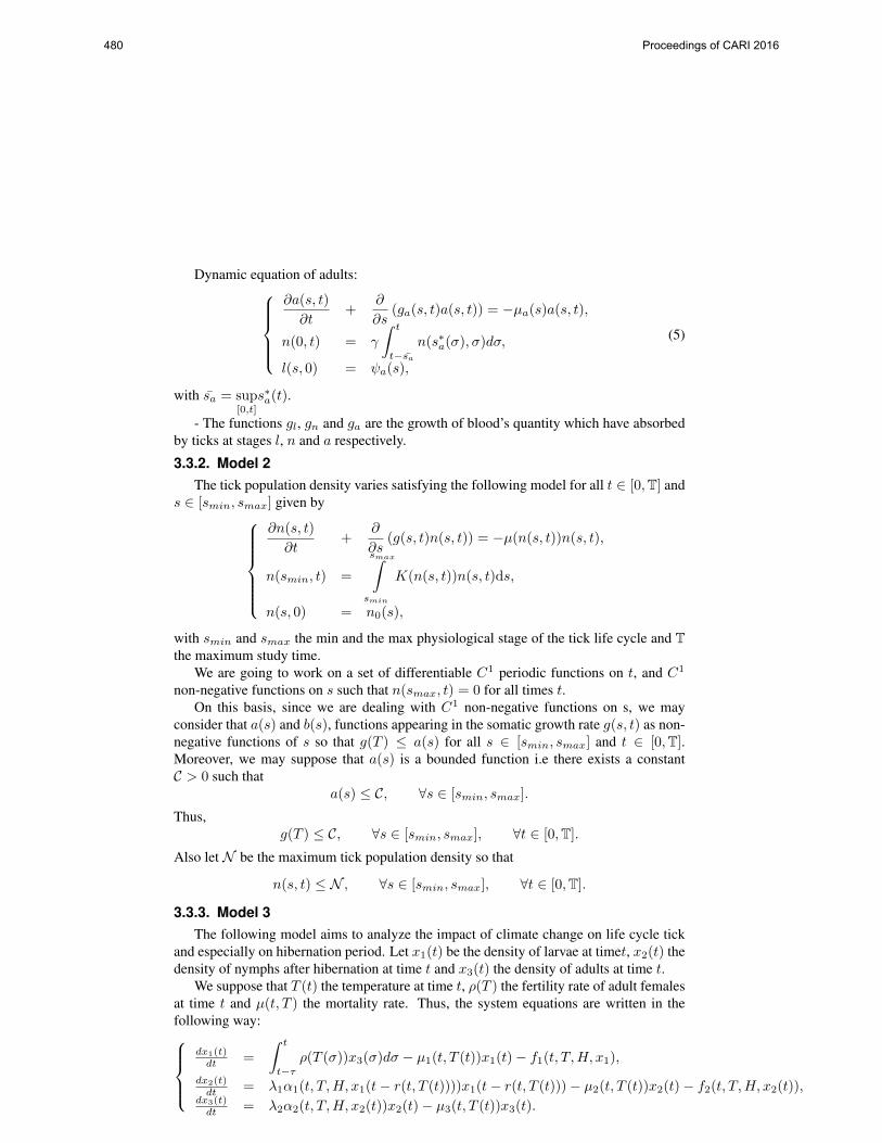
Dynamic equation of adults:∂a(s, t)

∂t+

∂

∂s(ga(s, t)a(s, t)) = −µa(s)a(s, t),

n(0, t) = γ

∫ t

t−san(s∗a(σ), σ)dσ,

l(s, 0) = ψa(s),

(5)

with sa = sup[0,t]

s∗a(t).

- The functions gl, gn and ga are the growth of blood’s quantity which have absorbedby ticks at stages l, n and a respectively.

3.3.2. Model 2The tick population density varies satisfying the following model for all t ∈ [0,T] and

s ∈ [smin, smax] given by

∂n(s, t)

∂t+

∂

∂s(g(s, t)n(s, t)) = −µ(n(s, t))n(s, t),

n(smin, t) =

smax∫smin

K(n(s, t))n(s, t)ds,

n(s, 0) = n0(s),

with smin and smax the min and the max physiological stage of the tick life cycle and Tthe maximum study time.

We are going to work on a set of differentiable C1 periodic functions on t, and C1

non-negative functions on s such that n(smax, t) = 0 for all times t.On this basis, since we are dealing with C1 non-negative functions on s, we may

consider that a(s) and b(s), functions appearing in the somatic growth rate g(s, t) as non-negative functions of s so that g(T ) ≤ a(s) for all s ∈ [smin, smax] and t ∈ [0,T].Moreover, we may suppose that a(s) is a bounded function i.e there exists a constantC > 0 such that

a(s) ≤ C, ∀s ∈ [smin, smax].

Thus,g(T ) ≤ C, ∀s ∈ [smin, smax], ∀t ∈ [0,T].

Also let N be the maximum tick population density so that

n(s, t) ≤ N , ∀s ∈ [smin, smax], ∀t ∈ [0,T].

3.3.3. Model 3The following model aims to analyze the impact of climate change on life cycle tick

and especially on hibernation period. Let x1(t) be the density of larvae at timet, x2(t) thedensity of nymphs after hibernation at time t and x3(t) the density of adults at time t.

We suppose that T (t) the temperature at time t, ρ(T ) the fertility rate of adult femalesat time t and µ(t, T ) the mortality rate. Thus, the system equations are written in thefollowing way:

dx1(t)dt =

∫ t

t−τρ(T (σ))x3(σ)dσ − µ1(t, T (t))x1(t)− f1(t, T,H, x1),

dx2(t)dt = λ1α1(t, T,H, x1(t− r(t, T (t))))x1(t− r(t, T (t)))− µ2(t, T (t))x2(t)− f2(t, T,H, x2(t)),

dx3(t)dt = λ2α2(t, T,H, x2(t))x2(t)− µ3(t, T (t))x3(t).


With– f1(t, T,H, x1) = α1(t, T,H, x1(t))x1(t).– f2(t, T,H, x1) = α2(t, T,H, x2(t))x2(t).

3.4. Physiological SIS for ticks and SIR ODE for host ModelWe consider that the number of tick is governed by the equation of section 3.2 and

that the tick are subdivided in two class Susceptible and Infected. Let nsT (t) and niT (t) berespectively the frequencies of susceptible and infected tick parasites, i.e.,

nsT (t) + niT (t) = P (t).

But

P (t) =

∫ amax

amin

(l(a, t) + n(a, t) + a(a, t))da, ∀a ∈ [amin, amax],

where P (t) is total population of tick parasites, amin and amax are the min and the maxphysiological age of the tick life cycle.

And that the host population number is constant, let nsH(t), niH(t) and nrH(t) berespectively the frequencies of susceptible, infected and removed host population, i.e.nsH(t) + niH(t) + nrH(t) = 1.

Consider the following assumptions:- Let φ(n) be the factor representing the influence of ticks on the host. Thus the model

representing the host-parasite epidemiological interaction is given by the following SIR-SIS model:

dnsH(t)

dt= −K1n

sH(t)niH(t) (6)

dniH(t)

dt= K1n

sH(t)niH(t)−K2n

iT (t)niH(t) (7)

dnrH(t)

dt= K2n

iT (t)niH(t) (8)

dniT (t)

dt= K1n

sH(t)niH(t)− φ(n)K2n

iT (t)niH(t) + nsT (t) (9)

nsT (t) = 1− niT (t) (10)

4. Conclusion and RecommendationIn this paper, we present the various stages of tick population dynamics which is

composed by three partial differential equations.Our aim in the future is to adapt the numerical method developed in subsection 3.2

in order to solve the correlated EDO-EDP equations. This method will be used to testimpact of climate change on transmission of Tick disease, for that the model will befitted to field data that have been previously gathered from several Tunisian farms [1]and several data from laboratory colonies (Darghouth, unpublished data) and with datafrom Tunisian National Institute of Meteorology. Furthermore, our goal is to develop newnumerical methods in order to approximate solutions of the previous type of equations insubsection 3.3.2.


5. References

[1] A. BOUATTOUR, M. A. DARGHOUTH, L. BEN MILED. “Cattle infestation by Hyalomma ticksand prevalence of Theileria in H. detritum species in Tunisia”, Vet. Parasitol., vol. 65:233-245,1996.

[2] H. CASWELL, “Matrix Population Models: construction, analysis, and interpretation”, SinauerAssociates Inc. Sunderland, Massachusetts, 2001.

[3] HOPE-CAWDERY, M.J., GETTINBY, G. AND GRAINGER, J.N.R., “Mathematical modelsfor predicting the prevalence of liver fluke disease and its control from biological and me-teorological data. In: T.E. Gibson (Editor), Weather and Parasitic Animal Disease”, WorldMeteorological Organisation Technical Note, 159:21-38, 1978.

[4] W P GARDINER, G GETTINBY, AND J S GRAY “Modes based on weather for the developmentphases of the sheep tick, ixodes-ricinus”, Veterinary Parasitology, 9(1):75-86, 1981.

[4] G GETTINBY, W BYROM “The dynamics of east coast fever: A modelling perspective for theintegration of knowledge”, Parasitology Today, 5(3):68-73, 1989.

[5] W S C GURNEY, R M NISBET, N GURNEY, “Ecological dynamics”, Oxford University PressNew York, 1998.

[6] PETER J HUDSON, ANDY P DOBSON, ISABELLA M CATTADORI, DAVID NEWBORN, DAN

T HAYDON, DARREN J SHAW, TIM G BENTON , BRYAN T GRENFELL, “Trophic interactionsand population growth rates: describing patterns and identifying mechanisms ”, Philos Trans RSoc Lond B Biol Sci, 357(1425):1259-1271, September 2002.

[7] J A J METZ, O DIEKMANN, “The dynamics of physiologically structured populations”, 1986.

[8] R NORMAN, R G BOWERS, M BEGON, P J HUDSON, “Persistence of tick-borne virus in thepresence of multiple host species: tick reservoirs and parasite mediated competition. J TheorBiol, 200(1):111-118, September 1999.

[9] N H OGDEN, M BIGRAS-POULIN, C J O’CALLAGHAN, I K BARKER, L R LINDSAY, AMAAROUF, K E SMOYER-TOMIC, D WALTNER-TOEWS, D CHARRON “A dynamic popu-lation model to investigate effects of climate on geographic range and seasonality of the tickixodes scapularis”, Int J Parasitol, 35(4):375-389, 2005.

[10] O.ARINO, M.L.HBID, R.BRAVO DE LA PARRA, “A Mathematical model of population offish in the larval stage: density-dependence effects”, Math.Biosci, 150,1-20, 1998.

[11] S RANDOLPH, “Epidemiological uses of a population model for the tick rhipicephalus appen-diculatus”, Trop Med Int Health, 4(9):A34-A42, September 1999.

[12] S E RANDOLPH, “Tick ecology: processes and patterns behind the epidemiological risk posedby ixodid ticks as vectors ”, Parasitology, 129 Suppl:S37-S65, 2004.

[13] S E RANDOLPH, “Dynamics of tick-borne disease systems: minor role of recent climatechange”, Rev Sci Tech, 27(2):367-381, 2008.

[14] SARAH E RANDOLPH, “Abiotic and biotic determinants of the seasonal dynamics of the tickrhipicephalus appendiculatus in south africa”, Medical and Veterinary Entomology, 11(1):25-37, 1997.

[15] R ROSÀ, A PUGLIESE, R NORMAN, P J HUDSON, “Thresholds for disease persistencein models for tick-borne infections including non-viraemic transmission, extended feeding andtick aggregation”, Journal of theoretical biology, 224(3):359-376, 2003.

[16] R ROSÀ, ROBERTO ROSÀ, ANDREA PUGLIESE, “Effects of tick population dynamicsand host densities on the persistence of tick-borne infections”, Mathematical Biosciences,208(1):216-240, 2007.


[17] S TULJAPURKAR, H CASWELL, “ Structured-population models in marine, terrestrial, andfreshwater systems ”, Kluwer Academic Pub, 1997.


Stochastic modelingof the anaeorobic model AM2b

Models at different scales

F. Campilloa — M. Chebbib — S. Toumic

a [email protected] ENIT-Laboratoire LAMSIN-University Tunis el [email protected] INSAT-Carthage [email protected]

ABSTRACT. The AM2B model is conventionally represented, in large population, as a system of ordi-nary differential equations . Our goal is to build several models at different scales. At the microscopicscale (the scale of the individual), we propose a pure jump stochastic model. This model can beexactly simulated. However, when the size of the population is large that type of exact simulationis not feasible, hence we propose approximated simulation methods in discrete time, of the Pois-son type or of the diffusive type. The diffusive type of approximated simulation method can be seenas a discretization of a stochastic differential equation. Finally, we present informally a law of largenumbers/central limit theorem of the functional type and how they can be used to provide models atdifferent scales or hybrid models.

RÉSUMÉ. Le modèle AM2b est classiquement représenté, en grande population, par un systèmed’équations différentielles. Notre objectif est d’établir plusieurs modèles à différentes échelles. Àl’échelle microscopique (individuelle), on propose un modèle stochastique de saut pur. Ce modèlepeut être simulé de façon exacte. Lorsque la taille de la population est grande ce genre de simulationn’est pas praticable, et nous proposons des méthodes de simulation, à pas de temps discret, de typepoissonnien ou de type diffusive. La méthode de simulation de type diffusive peut être vue commeune discrétisation d’une équation différentielle stochastique. Nous présentons enfin de façon infor-melle un résultat de type loi des grands nombres/théorème central limite fonctionnelle et comment cerésultat peut conduire à des modèles selon l’échelle considérée ou encore à des modèles hybrides.

KEYWORDS : AM2b model, pure jump process, ordinary differential equation, diffusion approxima-tion, stochastic differential equation

MOTS-CLÉS : modèle AM2b, processus de saut pure, équation différentielle ordinaire, approximationdiffusion, équation différentielle stochastique


Stochastic models recently gain more credibility and numerical efficiency in chem-istry [7], biotechnology [8], system biology [12] where deterministic models have beenextensively used. Taking the example of a biotechnological model, we explain how astochastic modeling approach deepens the insights allowed by the deterministic classicalmodels.

Wastewater treatment plant aims at reducing the volume of pollutants rejection, pro-ducing potential energy like CH4 in anaerobic treatment, providing treated water for agri-culture and industry. Among these technologies anaerobic membrane bioReactors arepromising technologies provided that membrane fouling phenomenon could be reduced.AM2b is a mathematical model of anaerobic membrane bioreactors developed by [1, 2],it is a variant of model AM2 (2-steps Acidogenesis-Methanogenesis model, see [3]) withsoluble microbial products (SMP) dynamics. The production and the degradation of SMPplay an important role in the membrane fouling phenomenon.

We present the original ODE model of the AM2b. Then we introduce a pure jumpMarkov model of the same device and a exact Monte Carlo simulation method of thisprocess. Next we propose faster approximated simulation methods. Finally we present astochastic differential equation (SDE) model of the AM2b. The validity of these modelsdepends on the scale considered for the problem, this could be cleared with a law of largenumbers/central limit theorem of the functional type presented in the last section.

1. The ODE modelThe state variable of this model is:

xdef=

s1

b1s2

b2s

concentration of organic matterconcentration of acidogenic biomassconcentration of volatile fatty acids (VFA)concentration of methanogenic biomassconcentration of the soluble microbial products (SMP)

The AM2b model describes the dynamics of biological and anaerobic wastewater treat-ment, where the substrate s1 is degraded by a bacterial ecosystem b1 to produce the sub-strate s2 and the SMP s. The substrate s2 is transformed by a consortium of bacteria b2in s. The latter is also produced by the mortality b1 and b2 and will be degraded by b1 forproduct s2. The schematic representation of the AM2b model is (from [1]):

biological model fouling model

biogas CO2, CH4

influent S1in, S2in

euent s1, s2, s

Qin

s1, b1,s2, b2, s

s1, b1, s2, b2, s

volume V

Qout

inflow

outflow

QwitQin = Qout + Qwit withdraw s1, b1, s2, b1, (1 ) s

On the right of these scheme the membrane fouling model is represented; the separationof mater is as follow: the substrates s1 and s2 go through the membrane without retention(the size of their molecules is assumed to be smaller than pore diameter), the biomass


b1 and b2 is retained by the membrane, and a fraction β s of the SMP go through themembrane and leaves the reactor ((1− β) s will me considered as macromolecules).

In Appendix A.1 we describe the AM2b model as a reaction network of J = 15reactions, and in Appendix A.2 we explain how this reaction network can be translatedinto an ODE system thanks to the laws of mass action and mass conservation. The ODEsystem reads:

s1 = Din (S1in − s1) − k1 µ1(s1) b1 , (1a)

b1 =(µ1(s1) + µ(s)−Ddec −Dwit

)b1 , (1b)

s2 = Din (S2in − s2) − k2 µ2(s2) b2 +(c12 µ1(s1) + c02 µ(s)

)b1 , (1c)

b2 =(µ2(s2)−Ddec −Dwit

)b2 , (1d)

s =(c10 µ1(s1) +Ddec − k0 µ(s)

)b1 +

(c20 µ2(s2) +Ddec

)b2 −M s (1e)

orx(t) = f(x(t)) , x(0) = x0 (2)

where:ki degradation rate of si by bi, M = β Dout + (1− β)Dwit

k0 degradation rate of s by b1, β SMP fraction passing through the membrane,c12 production rate of s2 by b1 from s1, Din dilution rate (= Qin/V ),c02 production rate of s2 by b1 from s, Ddec decay rate of biomass,ci0 production rate of s by bi from si, Dwit withdrawal rate of biomass (= Qwit/V ),Siin input concentrations of si, Dout outflow rate of the bioreactor (= Qout/V )

(i = 1, 2). To ensure a constant volume we state that Qin = Qout +Qwit. The rate M statesthat a proportion β of the SMP will leave the bioreactor through the membrane, at rateDin and a proportion 1− β through the withdrawal process, at rate Dwit.

The growth functions are:

µ1(s1) = m1s1

K1+s1, µ(s) = m s

K+s , µ2(s2) = m2s2

K2+s2+s22/Ki. (3)

µ1 and µ are of Monod type; µ2 is of Haldane type to model the phenomenon of inhibi-tion of the eventual accumulation of the volatile fatty acids in the bioreactor during themethanogenesis (the major problem of the anaerobic digestion).

Model (1) relies on the fact that the stochastic effects can be neglected or at least canbe averaged out. Although this level of description is sufficient for a number of appli-cations of interest, it could be a valuable way of accounting for the stochastic nature ofthe system. Indeed, at small population sizes the AM2b model could present stochasticbehaviors. Moreover, whereas the experimental results observed in well-mastered labora-tory conditions match closely the ODE theoretical behavior, a noticeable difference mayoccur in operational conditions. In these cases, stochastic features may not be neglected.We aim to build a model that still relies on a mass balance principle and that encompassesthe useful stochastic information.

2. Pure jump Markov modelFollowing the approach described in [4], we propose a representation of the AM2b

model as a pure jump Markov process:

X(t) = (S1(t), B1(t), S2(t), B2(t), S(t))∗ (4)


taking values in R5+. This process will encompass the J reactions: each reaction j is now

characterized by it’s intensity functions λj(x) and it’s jump functions νj(x), see detailsin Section A.3. The dynamic of the process X(t) is described as follows: X(0) = x0 andconditionally on X(t) = x, we set

X(t+ ∆t) =

x+ νj(x) with probability λj(x) ∆t+ o(∆t) 1 ≤ j ≤ Jx with probability 1−∑J

j=1 λj(x) ∆t+ o(∆t)(5)

where (λj(x), νj(x))1≤j≤J is given by (12) and (13).

2.1. Simulation and representation of X(t)

The process X(t) can be simulated according to the following SSA (stochastic simu-lation algorithm) [6]:

X ← x0, t← 0while t < Tmax doτ ←∑J

j=1 λj(X)

S ∼ Exp(τ)

sample j according to the distribution (λ1(X)τ , . . . , λJ (X)

τ )t← t+ SX ← X + νj(X)

end while

(6)

This Monte Carlo procedure allows us to simulate exact trajectories of the process Xt,the only approximation resides in the algorithms used for simulating the basic probabilitydistributions.

Algorithm (6) is an exact representation of the process X(t), and it leads to the fol-lowing representation of the process:

Xt = X0 +

J∑j=1

∫[0,t]×R+

1[0,λj(Xs− )](v) νj(Xs−) Nj(ds, dv) (7)

whereNj(ds, dv) are independent Poisson random measures of intensity measure ds×dv(the Lebesgue measure on R2

+).

3. Discrete time approximationsThe SSA simulates each reaction of the ecosystem asynchronously in time. In many

situations this detailed simulation is too cumbersome, this is why synchronous discretetime approximations have been proposed. Let tm = m∆t, for ∆t > 0 fixed.

Poisson approximationWe construct an approximation (X(tm))m≥1. On the interval [tm, tm+1) suppose that

the different rate functions are approximated by:

λj(x) ' λj(X(tm)) , ∀x ∈ R5+

so that each of the J reactions are independent and occur at constant rates λj(X(tm)),that is the number of reactions of type j is a Poisson process of intensity λj(X(tm)).


Hence, on the time interval [tm, tm+1) the number of reactions of type j follows a Poissondistribution of parameter ∆t λj(X(tm)). We obtain the following approximation alsocalled τ -leaping:

X(tm+1) =[X(tm) +

J∑j=1

νj(X(tm)) ρj,m

]+

(8)

where ρj,m are independent Poisson distribution variables with parameter ∆t λj(X(tm))and [x]+ is the projection of R5 onto R5

+ (the positive part of each component).

Diffusion approximationThe Poisson distribution with parameter ∆t λj(X(tm)), for ∆t λj(X(tm)) large en-

ough, can be approximated by a Normal distribution of mean ∆t λj(X(tm)) and variance∆t λj(X(tm)). From (8) we get:

ξ(tm+1) =[ξ(tm) +

J∑j=1

νj(ξ(tm))

∆t λj(ξ(tm)) +

√∆t λj(ξ(tm))wj,m

]+

where wj,m are independent N(0, 1) random variables. This last equation can be rewrit-ten:

ξ(tm+1) =[ξ(tm) + F (ξ(tm)) ∆t+

J∑j=1

1√Nj

gj(ξ(tm)) [Wj(tm+1)−Wj(tm)]]

+

(9)

where Wj(t) are independent standard Brownian motions so that Wj(tm+1) −Wj(tm)are independent and N(0,∆t); F (x) is defined in (15) and:

gj(x)def=√Nj√λj(x) νj(x) =

√λj(x)Nj νj(x) .

Let

gj(x)def=√λj(x) νj

so that:gj(x)− gj(x) = 1x∈D

(gj(x)− gj(x)

)and |gj(x)− gj(x)| ≤ C 1x∈D

√1 + |x|.

Stochastic differential equationEquation (9), is an Euler-Maruyama discrete time approximation of the following

stochastic differential equation (SDE):

dξ(t) = F (ξ(t)) dt+J∑j=1

1√Nj

gj(ξ(t)) dWj(t) , ξ(0) = x0 . (10)


4. Scales and asymptoticsAccording to Section A.3, the scale parameters Nj are connected to the “size” of the

jumps in the reactions j . We can assume that the Fj’s range from 104 to 109. When areaction involves only substrate molecules the corresponding Fj’s range from 107 to 109;when a reaction involves only bacteria the corresponding Fj’s range from 104 to 106.Hence for reasonable concentrations, the simulation algorithm (6) will not be feasible asit simulates every single reaction.

First suppose that N = Nj for all j and that N is large. The first well know result canbe understood as a functional law of large numbers (originally proved in this context byTom Kurtz [9, 10]), it states that:

sup0≤t≤T

|X(t)− x(t)| −−−−→N→∞

0 (11)

in L2 or in probability. It is clear that in (11) we can replace X(t) by ξ(t). So under mildconditions, when the population sizes are large and so the number of reaction, the ODEmodel (2) is adapted to this scale.

At an intermediate scale, a functional central limit theorem states that the process√N (X(t)− x(t)) can be approximated in law by

∑Jj=1

∫ t0gj(x(s)) dWj(s) where the

Wj(s) are independent standard Brownian motions, that is formally:

X(t) ' x(t) +1√N

J∑j=1

∫ t

0

gj(x(s)) dWj(s) .

This also proves that the SDE model (10) is adapted to this scale.

In many situation ODE and SDE models are not valid. This is the case when one of thebacterial population is of “small” size but still affects the global dynamic of the process.This so-called “molecular randomness” may influence the global dynamic even when thepopulation sizes are not so small [5]. In this case we may adopt hybride approaches.We just present an example where we separate the dynamics of the substrates from thedynamics of the biomasses: The idea is to break down the reactions between substratetype reactions and biomass type reactions, then to describe the first ones as a system ofODE’s and to describe the second ones as a pure jump Markov process. For example wecan obtain a system of ODE’s describing the continuous evolution of the substrates andthe SMP concentrations:

s1 = Din (S1in − s1) − k1 µ1(s1)B1 ,

s2 = Din (S2in − s2) − k2 µ2(s2)B2 +(c12 µ1(s1) + c02 µ(s)

)B1 ,

s =(c10 µ1(s1) +Ddec − k0 µ(s)

)B1 +

(c20 µ2(s2) +Ddec

)B2 −M s

coupled to a 2-dimensional pure jump process describing the discrete evolution of thebiomasses concentrations:

jump rate jump rateB1 → B1 + δ1 µ1(s1)B1/δ1 B2 → B2 + δ2 µ2(s2)B1/δ1B1 → B1 + δ1 µ(s)B1/δ1 B2 → B2 − δ2 Ddec B1/δ2B1 → B1 − δ1 Ddec B1/δ1 B2 → B2 − δ2 Dwit B1/δ2B1 → B1 − δ1 Dwit B1/δ1


This type of model, known as Piecewise-deterministic Markov process, is very promisingand will be investigated in the near future.

5. ConclusionWe show that an ODE model of microbial dynamics (1) contains all the ingredients

that can be used to establish a pure jump Markov model, see Section 2. This pure jumpMarkov model can be exactly simulated with the Monte Carlo technique (6). This exactMonte Carlo method is not feasible in large population size cases and we proposed aPoissonian discrete time approximation (8) (also called τ -leaping) and a diffusion discretetime approximation (9). This last equation is the Euler-Maruyama time discretization ofthe SDE (10). This SDE is valid in high population size and different recalling so thatalternative formulations of this SDE can be established. In Section 4, we describe thevalidity of these different models according to the scales at which the process should besimulated. All these models share the same ingredient, however the have very differentqualitative properties.

AcknowledgmentsThis work was funded by the NuWat LIRIMA Inria project which funded this work.

6. References

[1] Boumédiène Benyahia, Tewfik Sari, Brahim Cherki and Jérôme Harmand. Anaerobic mem-brane bioreactor modeling in the presence of Soluble Microbial Products (SMP) – the AnaerobicModel AM2b. Chemical Engineering Journal, 228(0):1011–1022, 2013.

[2] Boumédiène Benyahia. Modélisation et observation des bioprocédés à membranes: applica-tion à la digestion anaérobie. PhD thesis, Université de Tlemcen et Université de Montpellier2, 2012.

[3] Olivier Bernard, Zakaria Hadj-Sadock, Denis Dochain, Antoine Genovesi, and Jean-PhilippeSteyer. Dynamical model development and parameter identification for an anaerobic wastewatertreatment process. Biotechnology and Bioengineering, 75:424–438, 2001.

[4] Fabien Campillo, Marc Joannides, and Irène Larramendy-Valverde. Stochastic modeling of thechemostat. Ecological Modelling, 222(15):2676–2689, 2011.

[5] Fabien Campillo and Claude Lobry. Effect of population size in a Predator-Prey model. Eco-logical Modelling, 246:1–10, 2012.

[6] Daniel T. Gillespie. Exact stochastic simulation of coupled chemical reactions. Journal ofPhysical Chemistry, 81(25):2340–2361, 1977.

[7] Desmond J. Higham. Modeling and simulating chemical reactions. SIAM Review, 50(2):347–368, 2008.

[8] Sebastiaan Kops, Krist Gernaey, Olivier Thas and Peter A. Vanrolleghem. The modelling ofnoise processes in stochastic differential equations: Application to biotechnological processes.In Proceedings 7th IFAC Conference on Computer Applications in Biotechnology CAB7. Osaka,Japan, May 31 - June 4, pages 67–72, 1998.

[9] Thomas G. Kurtz. Solutions of ordinary differential equations as limits of pure jump Markovprocesses. Journal of Applied Probability, 7(1):49–58, 1970.


[10] Thomas G. Kurtz. Limit theorems for sequences of jump Markov processes approximatingordinary differential processes. Journal of Applied Probability, 8:344–356, 1971.

[11] Mukhtar Ullah and Olaf Wolkenhauer. Stochastic approaches in systems biology. Springer,2011.

[12] Darren J. Wilkinson. Stochastic Modelling for Systems Biology. Chapman & Hall/CRC, 2006.

A. Appendix: the AMB2b models

A.1. AMB2b as a reaction networkThe first set of reactions describes the biochemical reactions:

Acidogenesis and SMP production 1 k1S1 + B1r1−−→ 2 B1 + c12 S2 + c10 S

Methanogenesis and SMP production 2 k2S2 + B2r2−−→ 2 B2 + c20 S

SMP degradation 3 k0S + B1r3−−→ 2 B1 + c02 S2

SMP production from biomass decay 4 B1r4−−→ S 5 B2

r5−−→ S

The second set of reactions describes the substrate inflow and the substrate outflow throu-gh the membrane:

6 ∅ r6−−→ S1 7 ∅ r7−−→ S2 8 S1r8−−→ ∅ 9 S2

r9−−→ ∅ 10 Sr10−−→ ∅

The third and last set of reactions describes the biomass and substrate withdrawal with :

11 S1r11−−→ ∅ 12 S2

r12−−→ ∅ 13 Sr13−−→ ∅ 14 B1

r14−−→ ∅ 15 B2r15−−→ ∅

The second and third set of reactions are not biochemical reactions they just describe theinflows and outflows in the AM2B process. In reaction 10 only a proportion β of theSMP goes through the membrane, and in reaction 13 a proportion 1 − β of the SMP iswithdrawn, this mechanism will be explicated in the definition of the rates. Let j the indexof the reaction and J = 15 the number of reactions. ( j , rj); j = 1, . . . , J

A.2. AMB2b as an ODE systemThe AMB2b reaction network described in Section A.1 is “translated” to an ODE

system thanks to the laws of mass action and conservation of mass. The state variables ofthe ODE system are the concentration si = [Si], bi = [Bi] (i = 1, 2) and s = [S]. Forexample, for the 1 , the rate of reaction also called speed of reaction, is defined by:

r1 = b1(t+∆)−b1(t)∆ = −k1

s1(t+∆)−s1(t)∆ = c12

s2(t+∆)−s2(t)∆ = c10

s(t+∆)−s(t)∆

(the equalities are due to the mass conservation). This reaction, like reactions 2 and 3 ,is of order two and the mass action law states that r1 = s1 b1, but saturation/inhibitionphenomena suggest to replace in this last expression s1 by µ1(s1) indeed:

Biochemical reactions: The mass action law applied to the second order reactions 1 2 3

states that:

r1 = µ1(s1) b1 , r2 = µ2(s2) b2 , r3 = µ(s) b1

where the growth functions µi and µ are chosen as (3), indeed for low substrat concentra-tion, these growth functions are linear accordingly to the mass action law, but for higher


substrate concentrations, saturation and inhibition phenomena have to be taken into ac-count. The mass action law applied to first order reactions 4 5 gives r4 = Ddec b1 andr5 = Ddec b2 where Ddec is decay rate of biomass.

Inflow and outflows: Inflow is done at rate Din, outflow though the membrane at rateDout and only a proportion β of the SMP is affected by the outflow, so the rates of thesereactions are:

r6 = Din S1in , r7 = Din S2in , r8 = Dout s1 , r9 = Dout s2 , r10 = β Dout s .

Withdrawal: The withdrawal is done at rate Dwit and only a proportion 1− β of the SMPaffected by the withdrawal, so the rates of these reactions are:

r11 = Dwit s1 , r12 = Dwit s2 , r13 = (1− β)Dwit s , r14 = Dwit b1 , r15 = Dwit b2 .

Summing up these expressions and applying the mass conservation law lead to thesystem of differential equations (1).

A.3. AMB2b as a pure jump Markov processThe AMB2b reaction network described in Section A.1 is “translated” into a pure

jump Markov process thanks to the stochastic law of mass action [12]. Now X(t) =[S1(t), B1(t), S2(t), B2(t), S(t)]∗ is a pure jump Markov process defined by (5) whereeach reaction j is described as an instantaneous jumpX(t)→ X(t)+νj(X(t)) occurringwith intensity λj(X(t)) defined respectively by:

λj(x)def= Nj λj(x) , νj(x)

def= [x+ 1

Njνj ]+ − x (12)

([x]+ the orthogonal projection of x onto R5+) with

j λj(x) ν∗j

1 µ1(s1) b1 [−k1 +1 +c12 0 +c10 ]2 µ2(s2) b2 [ 0 0 −k2 +1 +c20 ]3 µ(s) b1 [ 0 +1 +c02 0 −k0 ]4 Ddec b1 [ 0 −1 0 0 +1 ]5 Ddec b2 [ 0 0 0 −1 +1 ]6 Din S1in [ +1 0 0 0 0 ]7 Din S2in [ 0 0 +1 0 0 ]8 Dout s1 [ −1 0 0 0 0 ]9 Dout s2 [ 0 0 −1 0 0 ]10 β Dout s [ 0 0 0 0 −1 ]11 Dwit s1 [ −1 0 0 0 0 ]12 Dwit b1 [ 0 −1 0 0 0 ]13 Dwit s2 [ 0 0 −1 0 0 ]14 Dwit b2 [ 0 0 0 −1 0 ]15 (1− β)Dwit s [ 0 0 0 0 −1 ]

(13)

About the second equation of (12): Basically the jumps are 1Njνj , but near the border

of R5+ to avoid jumps that can lead to negative concentration values, we adopt truncated

jumps so that x + νj(x) ∈ R5+ for all x ∈ R5

+. Indeed, note that −νmin ≤ νij ≤ νmax,so that if xi ≥ νmin/minj Nj then νij(x) = νij/Nj , where νij and νij(x) denote the ithcomponent of νj and νj(x) respectively. Define:

D def= x ∈ R5

+;xi ≥ νmin/minjNj (14)


so that x ∈ D implies that νj(x) = 1Njνj .

The drift coefficient: Given X(t) = x, the expectation of X(t+ ∆t) is

E[X(t+ ∆t)|Xt = x]

=∑Jj=1

(x+ νj

)P[reaction j|Xt = x] + xP[no reaction |Xt = x]

'∑Jj=1

(x+ νj

)(λj(x) ∆t) + x (1−∑J

j=1 λj(x) ∆t)

' x+∑Jj=1 λj(x) νj(x) ∆t = x+ F (x) ∆t

where

F (x)def=∑Jj=1 λj(x) νj(x) (15)

So locally in time, E(X(t)) evolves according to the drift coefficient F (x) (note thatE(X(t)) is not solution of an ODE as the function F is non linear). We can easily checkthat:

F (x) = 1x∈D F (x) + 1x6∈D(x)F (x)

where

F (x)def=∑Jj=1 λj(x) νj (16)

does not depend on the Nj’s. Finally from |F (x)| + |F (x)| ≤ C (1 + |x|) and F (x) −F (x) = 1x6∈D

(F (x)− F (x)

), we get:

|F (x)− F (x)| ≤ C 1x6∈D(1 + |x|) .


Rubrique

Identification of source for the bidomainequation using topological gradient

Jamila Lassoued1, Moncef Mahjoub1, and Nejib Zemzemi2

1 University of Tunis El ManarNational Engineering School of Tunis LAMSIN − ENITBP 37, 1002 Tunis Belvedere, [email protected]@lamsin.rnu.tn

2University of Bordeaux I, INRIA200 Avenue de la vielle Tour 33405 Talence Cedex [email protected]

RÉSUMÉ. Nous présentons une approche pour estimer les sources électriques dans le coeur à partirde mesures non invasives enregistrées sur la surface externe du thorax. L’approche est basée sur laméthode du gradient topologique. Cette méthode consiste à étudier le comportement d’une fonctioncoût via une perturbation locale du domaine. Nous montrons que l’approche proposée est capabled’identifier un terme source quand le support de la source est réduit dans l’espace.

ABSTRACT. We present an approach for estimating electrical sources within the heart domain fromnoninvasive measurements recorded on the outer surface of the torso. The approach is based onthe topological gradient method. This method studies the behavior of a cost function during a localperturbation of the domain. We show that the proposed approach based on the topological gradientmethod has actually been able to identify the source terms when they are clustred in space.

MOTS-CLÉS : Le modèle bidomaine, électrophysiologie cardiaque, gradient topologique, analyse desensibilité.

KEYWORDS : Bidomain model, cardiac electrophsiology , topological gradient, analysis sensibility.


1 IntroductionIn order to localize the electrical sources in the heart, we make use of a recent me-

thod based on the topological gradient introduced by Sokolowski [7] and Masmoudi [6].The topological gradient was originally used as part of the optimization shapes in solidmechanics [5]. This approach has subsequently been applied to a large number of areas :in imaging, it was first used for the detection of contours [4], in image classification [1],inpainting [2] and segmentation [3]. The calculation of topological sensitivity associatedwith the cost function of the inverse problem provides good qualitative information on thelocation of obstacles.

In this work, we are interested in the identification of the source term f from theboundary data obtained from the solution of the following system of equations :

−div((σi + σe)∇ue) = f in ΩH−div(σT∇uT ) = 0 in ΩTσT∇uT .nT = 0 on Γext.ue = uT on Σ,σe∇ue.n+ σT∇uT .nT = 0 on Σ,

(1)

where ΩH (respectively ΩT ) is the heart (respectively, torso) domain (see figure 1), Σ =∂ΩH is the epicardial boundary and Γext is the body surface. The tensors σi,σe and σT

are respectively the intracellular, extracellular and thoracic conductivity tensors. The torsopotential is denoted by uT . The source term f is defined by

f = div(σi∇Vm)

where Vm = ui − ue with ue and ui are respectively the extra-cellular potential and theintra-cellular potential. If we consider the dynamic of the electrical wave, the transmem-brane potential Vm is governed by a reaction diffusion equation and is coupled to theextra-cellular potential, following these equations

χm∂tVm + Iion(Vm, w)− div(σi∇Vm)− div(σi∇ue) = Iapp in Ω× (0, T ),∂tw +G(Vm, w) = 0 in Ω× (0, T )

σi∇Vm.n = 0 on ∂Ω× (0, T ),

(2)

where Iapp is a given external current stimulus. w represents the concentrations ofdifferent chemical species and variables representing the openings or closures of somegates of the ionic channels. The ionic current Iion(Vm, w) and the function G(Vm, w) aredescribed by the Mitchell and Schaeffer model [8]. Note that the equation (1) representsthe diffusion of the electrical potential at a given time. The combination of equations (1)and (2) provides the model of the electrical wave propagation in the heart and the torso.This is known in the litterature as the the bidomain-torso coupled problem. In this study,the dynamic of the electrical wave is not considered in the identification of the source, weonly consider (1). The bidomain-torso coupled problem is only used to generate syntheti-cal observations.

By defining Ω = ΩH ∪ΩT , u =

ue in ΩHuT in ΩT

and σ =

(σi + σe) in ΩHσT in ΩT

,

the problem (1) could be rewritten as follows


Figure 1 – The heart and torso domains

−div(σ∇u) = f1ΩH in Ωσ∇u.nT = 0, on Γext.

(3)

2 Topological gradient methodWe use two notations of the cost function to be minimized : j(ΩH) and J(ue,ΩH ) ,

where ue,ΩH is the solution to the system (1). The idea of topological asymptotic analysisis to measure the effect of a perturbation of the domain ΩH on the cost function. For asmall ε ≥ 0, let Ωε := ΩH \ θε be the perturbed domain by the insertion of an inclusionθε = x0 + εθ, where x0 ∈ ΩH and θ is a given, fixed and bounded domain of Rd, contai-ning the origine, whose boundary ∂ω is C1. The topological sensitivity theory providesthen an asymptotic expansion of the considered cost function when the size of ωε tends tozero. It takes the general form :

j(Ωε)− j(ΩH) = ρ(ε)g(x0) + o(ρ(ε)),

where ρ(ε) is an explicit positive function going to zero with ε, and g(x0) is the topolo-gical gradient at point x0. Then in order to minimize the criterion, one has to insert smallinclusion at points where the topological gradient is the most negative. In our case, thesource would be identified in the zones where the topological gradient is the most nega-tive. j(Ωε) would be a function minimizing the gap between the solution uε solution ofthe following problem and a given observed data.

−div(σ∇uε) = fε1ΩH in Ω,σ∇uε.nT = 0, on Γext,

(4)

where

fε =

f1 on θεf0 on Ωε.

is the unknown source to be identified.

2.1 Variational formulationThe solution of the problem (4) is defined up to a constant, thus we define the suitable

functional space by

V = v ∈ H1(Ω) ,

∫ΩH

v = 0


and the bilinear form Aε and the linear form lε as

Aε(uε, v) =

∫Ω

σ∇uε∇v and lε(v) =

∫Ω

fεv ∀v ∈ V

Then the variational formulation of this problem reads such that∫Ω

σ∇uε∇v =

∫Ω

fεv,∀v ∈ V.

The solution uε is solution of Aε(uε, v) = lε(v),∀v ∈ V. To determine the topologicalgradient we need to compute the adjoint solution of this problem.

2.2 Adjoint problemWe consider the direct solution uε satisfying Aε(uε, v) = lε(v) and we define the

lagrangian Lε(u, p) = J(u) +Aε(u, p)− lε(p), for every u, p ∈ V . One could check thatif uε is solution of (4) we have

Lε(uε, v) = J(uε)

We denote DuLε and DuJ the derivative of Lε and J respectively, so

DuLε(uε, v) = DuJ(uε)

Then we define the abstract adjoint equation by

(DuLε, ψ) = 0,∀ψ ∈ V

we have

(DuJ(u), ψ) +

∫Ω

σ∇p∇ψ = 0

So ∫Ω

σ∇p∇ψ = −(DuJ(u), ψ)

Finally the adjoint solution p associated of the cost function J is given by

−div(σ∇p) = −DuJ(u) in Ω∇p · nT = 0 on Σ,

(5)

We remarque that the computation time and memory space required by the state ad-joint method are largely reasonable. In the next section we will derive the variation of thecost function j with respect to the insertion of a small subdomain ωε in the cardiac domainΩH . We begin our analysis by giving the main hypothesis 1, then the main result of thissection is presented by Theorem 1. It concerns the topological asymptotic expansion of acost function J.


2.3 Main resultLet us consider the following hypothesis :

hypothesis 1 We assume That(i) J is differentiable with respect to u, we denote DJ(u)its derivative.(ii) There exists a real number ∂J(x0) such that

J(uε)− J(u0) = DJ(u0)(uε − u0) + εd|ωε|∂J(x0) + o(εd)

(iii) ‖uε − u‖2L2(∂Γext)= o(εd)

(iv) ‖∇(uε − u)‖2L2(∂Γext)= o(εd)

The expression of the topological gradient for this problem is given by the followingresult :

Theorem 1 Under the hypothesis above the cost function j has the following asymptoticexpansion :

j(Ωε)− j(ΩH) = εd|ωε|∂J(x0)− εd|ωε|(f1 − f0)p(x0)

In other words, the topological gradient at x0 is :

g(x0) = ∂J(x0)− (f1 − f0)p(x0)

where p is the adjoint solution.

Proof 1 We always seek to minimize the function J defined above. We consider the la-grangian

Lε(u, v) = J(u) +Aε(u, v)− lε(v)

uε is solution of problem 4, then we have

j(Ωε) = Lε(uε, v)

So the first variation of the cost function with respect to ε is given by

j(Ωε)− j(ΩH) = Lε(uε, v)− L0(u0, v)

= J(uε)− J(u0) +Aε(uε, v)−A0(u0, v)− lε(v) + l0(v)

Then from the definition of Aε and lε we have :

Aε(uε, v)−A0(u0, v) =

∫Ω

σ∇(uε − u0)∇v

lε(v)− l0(v) =

∫ωε

(f1 − f0)v

Choosing v = p the adjoint solution is solution of (5)∫Ω

σ∇(uε − u0)∇p = −DJ(u0)(uε − u0)

Then we have

j(Ωε)− j(Ω) = J(uε)− J(u0)−DJ(u0)(uε − u0)−∫ωε

(f1 − f0)p


From the hypothesis we have

j(Ωε)− j(ΩH) = εd|ωε|∂J(x0)− εd|ωε|(f1 − f0)p(x0)

So we have

j(Ωε)− j(ΩH) = ρ(ε)g(x0) + o(ρ(ε))

where

g(x0) = ∂J(x0)− (f1 − f0)p(x0)

where ∂J(x0) depends on the cost function. We will present in the next section someexamples of the cost function and the associated ∂J(x0) term.

3 Numerical resultsIn this paragraph we aim to recover the source term with the help of the non-invasive

observations on the external boundary of the torso. We use the bidomain model in orderto create a source term based on reaction diffusion equation. We solve the electrostaticsource identification problem at a given time step. The topological gradient method is im-plemented using the following algorithm :

• Solve the forward solution of the problem 4.

• Compute the adjoint solution of the problem 5.

• Compute the topological gradient g.

• Search for the minimum of the topological gradient.

In order to numerically test the topological gradient method, we consider a two costfunctions J1(u) =

∫∂Γext

|u − uobs|2dx and J2(u) =∫∂Γext

|∇u − ∇uobs|2dx, whereuobs is the observed data at the body surface Γext. We tested this method for both costfunctions in two different scenarios. The first case is for clustered source. The electricalsource in this case is obtained by solving the bidomain equation with a single site stimuliuntil 4ms. The second case is for a distributed source, The electrical source in this case isthe gradient of the transmembrane potential at 20 ms after a single site stimuli.

clustered source :In figure 2 (a), we show the distribution of the extracellular potential in the heart

domain after 4ms of a single site stimulation. The topological gradient distribution isshown in figure 2 (b) for the cost function J1 and figure2 (b) for the cost function J2.The green circle in figures 2 (b,c,e,f) denotes the position of the source at 4 ms and thered point is the source obtained using the topological gradient method. The source attime 4ms could be deduced from figure 2 (e), where we represent the distribution off = div(σi∇Vm). We distinguish two clustered sources. We remark that the electricalsource is globally well localized. The two cost functions seems to capture one of the twosources at time 4ms.


(a) (b) (c)

(e) (f) (g)

Figure 2 – (a) the solution ue at 4 ms, (e) : the source. (b) (respectively,(c)) : the topo-logical gradient for the cost function J1 (respectively,J2) in the heart thorax doamin. (f)(respectively,(g)) : The topological gradient for the cost function J1 (respectively,J2) inthe heart doamin.

Distributed sourceHere we test the capability of the method in localizing distributed sources. We run a

simulation of a single site stimuli and we extract the data after 20 ms. In figure 3 (a), weshow the distribution of the extracellular potential in the heart domain. The topologicalgradient distribution is shown in figure 3 (b) for the cost function J1 and figure3 (b) for thecost function J2. The green circle in figures 3 (b,c,e,f) denotes the position of the source at20 ms and the red point is the source obtained using the topological gradient method. Thesource at time 20ms could be deduced from figure 3 (e). We distinguish two sources farfrom each other. We remark that the first cost function still provides an averaged positionwhich is here very far from both real sources figure 3 (e). By the contrary, the second costfunction still captures with a good accuracy one of the two sources at time 20 ms.

4 ConclusionWe presented a new approach for localizing electrical sources in the heart. This ap-

proach is based on the topological gradient method. We have tested this method on insilico data obtained by solving the bidomain problem. The numerical results show thatthe method is accurate when dealing with clustered sources. Our investigation shows thatthe considering the cost function J2(u) =

∫∂Γext

|∇u−∇uobs|2 is better than consideringJ1(u) =

∫∂Γext

|u−uobs|2. The first capture one of the two sources. The latter tries to findan averaged position. This works well when the source is clustred but when the sourcesare far from each other, the function J2(u) seems to localise the source that is the closestto the body surface. These preliminary results have been conducted in 2D simulations andhave to be confirmed with much more testing with multiple stimuli and multiple sourcesfor the 2D and the 3D cases. This would be the topic of our future investigations.


(a) (b) (c)

(e) (f) (g)

Figure 3 – (a) the solution ue at 20 ms, (e) : the source. (b) (respectively,(c)) : the topo-logical gradient for the cost function J1 (respectively,J2) in the heart thorax doamin. (f)(respectively,(g)) : The topological gradient for the cost function J1 (respectively,J2) inthe heart doamin.

Références[1] AUROUX, DIDIER AND BELAID, L JAAFAR AND MASMOUDI, MOHAMED

« Image restoration and classification by topological asymptotic expansion » Va-riational formulations in mechanics : theory and applications, p. 23–42, 2006.

[2] AUROUX, DIDIER AND MASMOUDI, MOHAMED « A one-shot inpainting algo-rithm based on the topological asymptotic analysis » Computational & AppliedMathematics, vol. 25, no 23, p. 251–267, 2006.

[3] AUROUX, DIDIER « From restoration by topological gradient to medical image seg-mentation via an asymptotic expansion » Mathematical and Computer Modelling,vol. 49, no 11, p. 2191–2205, 2009.

[4] BELAID, L JAAFAR AND JAOUA, M AND MASMOUDI, M AND SIALA, L « Ap-plication of the topological gradient to image restoration and edge detection » En-gineering Analysis with Boundary Elements, vol. 32, no 11, p. 891–899, 2008.

[5] ESCHENAUER, HANS A AND KOBELEV, VLADIMIR V AND SCHUMACHER, A« Bubble method for topology and shape optimization of structures » Structuraloptimization, vol. 8, no 01, p. 42–51, 1994.

[6] MASMOUDI, MOHAMED « The topological asymptotic » PICOF’02 : problèmesinverses, contrôle et optimisation de formes. Colloque, p. 285–289, 2002.

[7] SOKOLOWSKI, J AND ZOCHOWSKI, A « On the Topological Derivative in ShapeOptimization » SIAM Journal on Control and Optimization, vol. 37, no 04,p. 1251–1272, 1999.

[8] COLLEEN CMITCHELL ANDDAVID G SCHAEFFER., « A two-current model for thedynamics of cardiacmembrane », Bulletin of mathematical biology, vol. 5, no 65,p. 767–793, 2003.
