Introducing numerical bounds to improve event ... - Hal-Inria

HAL Id: inria-00382534https://hal.inria.fr/inria-00382534

Submitted on 29 May 2009

HAL is a multi-disciplinary open accessarchive for the deposit and dissemination of sci-entific research documents, whether they are pub-lished or not. The documents may come fromteaching and research institutions in France orabroad, or from public or private research centers.

L’archive ouverte pluridisciplinaire HAL, estdestinée au dépôt et à la diffusion de documentsscientifiques de niveau recherche, publiés ou non,émanant des établissements d’enseignement et derecherche français ou étrangers, des laboratoirespublics ou privés.

Introducing numerical bounds to improve event-basedneural network simulation

Bruno Cessac, Olivier Rochel, Thierry Viéville

To cite this version:Bruno Cessac, Olivier Rochel, Thierry Viéville. Introducing numerical bounds to improve event-basedneural network simulation. [Research Report] RR-6924, INRIA. 2009, pp.31. �inria-00382534�

https://hal.inria.fr/inria-00382534

https://hal.archives-ouvertes.fr

appor t de r ech er ch e

ISS

N02

49-6

399

ISR

NIN

RIA

/RR

--69

24--

FR

+E

NG

Thème BIO

INSTITUT NATIONAL DE RECHERCHE EN INFORMATIQUE ET EN AUTOMATIQUE

Introducing numerical boundsto improve event-based neural network simulation

Bruno Cessac∗† , Olivier Rochel†, Thierry. Viéville †

N° 6924

Mai 2009

Centre de recherche INRIA Sophia Antipolis – Méditerranée2004, route des Lucioles, BP 93, 06902 Sophia Antipolis Cedex

Téléphone : +33 4 92 38 77 77 — Télécopie : +33 4 92 38 77 65

Introducing numerical boundsto improve event-based neural network simulation

Bruno Cessac∗† ∗, † Olivier Rochel†, Thierry. Vieville †

Theme BIO — Systemes biologiquesEquipes-Projets Cortex

Rapport de recherche n° 6924 — Mai 2009 — 31 pages

Abstract: Although the spike-trains in neural networks are mainly constrained bythe neural dynamics itself, global temporal constraints (refractoriness, time precision,propagation delays, ..) are also to be taken into account. These constraints are revisitedin this paper in order to use them in event-based simulation paradigms.

We first review these constraints, and discuss their consequences at the simula-tion level, showing how event-based simulation of time-constrained networks can besimplified in this context: the underlying data-structuresare strongly simplified, whileevent-based and clock-based mechanisms can be easily mixed. These ideas are appliedto punctual conductance-based generalized integrate-and-fire neural networks simu-lation, while spike-response model (SRM) simulations are also revisited within thisframework.

As an outcome, a fast minimal complementary alternative with respect to existingsimulation event-based methods, with the possibility to simulate interesting neuronmodels is implemented and experimented.

Key-words: Spiking neural network, Neural code, Simulation.

∗ Laboratoire J. A. Dieudonne, U.M.R. C.N.R.S. N 6621, Universite de Nice Sophia-Antipolis,France† Cortex & Neuromathcomp EPI, INRIA, 2004 Route des Lucioles,06902 Sophia-Antipolis, France.

Utilisation de bornes numeriquespour ameliorer la simulation evennementielle de

r eseaux de neurones

Resume : Bien que les trains de spikes des reseaux de neurones soientprincipalementcontraints par la dynamique neuronale elle-meme, des contraintes temporelles globales(periode refractaire, precision temporelle limitee,delais de propagation, etc...) sontaussi a prendre en compte. Ces contraintes sont revisitees dans ce papier de facon aetre utilisees lors de simulations evenementielles.

Nous commen cons par revoir ces contraintes et discutons leurs consequences auniveau de la simulation, montrant comment la simulation evenementielle de reseauxcontraints temporellement peut etre simplifiee dans ce contexte: Ces idees sont ap-pliquees aux modeles de ponctuels generalises de neurones integre-et-tire base surdes conductances synaptiques, tandis que les modeles de type SRM sont aussi prisen compte dans ce cadre.

En terme de resultat, une alternative minimale et rapide desimulation est mise adisposition, avec la possibilite de l’utiliser dans le casou les performances de simula-tion sont critiques.

Mots-cles : Reseaux de neurones evenementiels, Code neuronal, Simulation.

Introducing numerical bounds to improve event-based neural network simulation 3

1 Introduction

Let us consider the simulation of large-scale networks of neurons, in a context wherethe spiking nature of neurons activity is made explicit [16], either from a biologicalpoint of view or for computer simulation. From the detailed Hodgkin-Huxley model[18], (still considered as the reference but unfortunatelyintractable when consideringneural maps), back to the simplest integrated and fire (IF) model, a large family ofcontinuous-time models have been produced, often comparedwith respect to their (i)biological plausibility and their (ii) simulation efficiency.

As far as this contribution is concerned, we consider a weaker notion of biologicalplausibility: a simulation is biologically plausible if itverifies an explicit set of con-straints observed in biology. More precisely, we are going to consider a few globaltime constraints and develop their consequences at the simulation level. It appears herethat these biological temporal limits are very precious quantitative elements, allowingus on one hand to bound and estimate the coding capability of such systems and, onthe other hand, to improve simulations.

Simulation efficiency of neural network simulators

Simulation efficiency is a twofold issue of precision and performances. See [4] for arecent review about both event-based and clock-based simulation methods.

Regarding precision, event-based simulations, in which firing times are not regu-larly discretized but calculated event by event at the machine precision level, provides(in principle) anunbiasedsolution. On the reverse, it has been shown that a regu-lar clock-based discretization of continuous neural systems may introduce systematicerrors, with drastic consequences at the numerical level, even when considering verysmall sampling times [39].

Furthermore, the computational cost is in theory an order ofmagnitude better usingevent-based sampling methods [5], although this may be not always the case in practice[29], as further discussed in this paper.

However, using event-based simulation methods is quite tiresome: Models can besimulated if and only if the next spike-time can be explicitly computed in reasonabletime. This is the case only for a subset of existing neuron models so that not all modelscan be used. An event-based simulation kernel is more complicated to use than aclock-based. Existing simulators are essentially clock-based. Some of them integrateevent-based as a marginal tool or in mixtures with clock-based methods [4]. Accordingto this collective review, only the fully supported, scientifically validated, pure event-based simulators is MVASpike [36], the NEURON software proposing a well-definedevent-based mechanism [17], while several other implementations (e.g.: DAMNED[31], MONSTER [38]) exists but are not publicly supported.

In other words, event-based simulation methods may save precision and computa-tion time, but not the scientist time.

The goal of this paper is to propose solutions to overcome these difficulties, in orderto have an easy to use unbiased simulation method.

Considering integrate and fire models.

At the present state of the art, considering adaptive, bi-dimensional, non-linear, integrate-and-fire model with conductance based synaptic interaction(as e.g. in [14, 3, 39]),

RR n° 6924

4 Cortex

called “punctual conductance based generalized integrateand fire models” (gIF), presentsseveral advantages:

- They seem to provide an effective description of the neuronal activity allowing toreproduce several important neuronal regimes [20], with a good adequacy with respectto biological data, especially in high-conductance states, typical of cortical in-vivoactivity [13].

- They provide nevertheless a simplification of Hodgkin-Huxley models, usefulboth for a mathematical analysis and numerical simulations[16, 19].

In addition, though these models have mainly considered oneneuron dynamics,they are easy to extend to network structure, including synaptic plasticity [27, 32].See, e.g. [33] for further elements in the context of experimental frameworks and [7, 8]for a review.

After a spike, it is assumed in such integrate and fired modelsthat aninstanta-neousreset of the membrane potential occurs. This is the case for all models exceptthe Spike Response Model of [16]. From the information theoretic point of view, itis a temptation to relate this spurious property to theerroneousfact that the neuronalnetwork information is not bounded. In the biological reality, time synchronizationis indeed not instantaneous (action potential time-course, synaptic delays, refractori-ness, ..). More than that, these biological temporal limitsare very precious quantitativeelements, allowing one to bound and estimate the coding capability of the system.

Taking time-constraints into account

The output of a spiking neural network is a set of events, defined by their occurrencetimes, up to some precision:

F = {· · · tni · · · }, t1i < t2i < · · · < tni < · · · , ∀i, nwheretni corresponds to thenth spike time of the neuron of indexi, with related inter-spike intervalsdn

i = tni − tn−1i .

In computational or biological contexts, not all sequencesF correspond to spiketrains since they are constrained by the neural dynamic, while temporal constraints arealso to be taken into account [10]. This is the key point here:Spike-times are[C1] bounded by a refractory periodr,[C2] defined up to some absolute precisionδt, while[C3] there is always a minimal delaydt for one spike to propagate to another unit, andthere might be (depending on the model assumptions) a[C4] maximal inter-spike intervalD such that either the neuron fires within a timedelay< D or remains quiescent forever). For biological neurons, orders of magnitudeare typically, in milliseconds:

r δt dt D

1 0.1 10−[1,2] 10[3,4]

The derivations of these numerical values are reviewed elsewhere [10]. This hasseveral consequence. On one hand, this allows us ti derive anupper bound for theamount of information:

N Tr log2

(Tδt

)bits duringT seconds,

while taking the numerical values into account it means for largeT , a straight-forwardnumerical derivation leads to about1Kbits/neuron.

On the other hand [9, 11], it appears that for generalized integrate and fire neu-ron models with conductance synapses and constant externalcurrents, the raster plotis generically periodic, with arbitrary large periods, while there is a one-to-one cor-respondence between orbits and rasters. This last fact, andthe fact that more general

INRIA


models such as Hodgkin-Huxley neuron assemblies can be simulated during a boundedperiod of time [10] provides theoretical justifications forthe present work.

What is the paper about

We develop here the consequences of the reviewed time constraints at the simulationlevel. Section 2 shows how event-based simulation of time-constrained networks canbe impacted and somehow improved in this context. Section 3 considers punctualconductance based generalized integrate and fire neural network simulation, while sec-tion 4 revisits spike-response model simulation within this framework. These mecha-nisms are experimented in section 5, where the computer implementation choices arediscussed.

Since the content of this paper requires the integration of data from the literaturereused here, we have collected these elements in the appendix in order to ease the maintext reading, while maintaining the self-completeness of the contribution.

2 Event-based simulation of time-constrained networks.

Clock-based and event-based simulations of neural networks make already use at dif-ferent level of the global time-constraints reviewed here.See e.g. [4] for an introduc-tion and a large review and [36, 5, 38, 30] for simulations with event-based or hybridmechanisms. However, it appears that existing event-basedsimulation mechanismsgain at being revisited.

In event-based simulation the exact simulation of networksof units (e.g. neurons)and firing events (e.g. spikes) fits in the discrete event system framework [36] and isdefined at the neural unit level by :

-1- the calculation of the next event-time (spike firing),-2- the update of the unit when a new event occurs.

At the network level, the following two-stage mechanism completely implementsthe simulation:

-a- retrieve the next event-time and the related unit,-b- require the update of the state of this unit, inform efferent units that

this unit has emitted an event, and update the related event-times,

repeating -a- and -b- when ever events occur or when some bound is reached.This mechanism may also take external events into account (i.e., not produced by

the network units, but by external mechanisms).Such a strategy is thus based on two key features:

• The calculation of the next event-time, conditioned to thepresent state and to thefact that, by definition, no event is received in the meanwhile for each unit;

• The “future” event-time list, often named “priority queue”, where times aresorted and in which event-times are retrieved and updated.

The goal of this section is to revisit these two features considering [C3] and [C4].Let us consider in this section a network withN units, an average ofC connections

per units, with an average numberM ≤ N of firing units.

RR n° 6924

6 Cortex

2.1 Event-time queue for time-constrained networks

Although, in the general case, spike-times must be sorted among pending events, yield-ing a O(log(M)) complexity for each insertion, there exists data structureallowingto perform retrieve/update operations in constant “O(1)” time. Several efficient datastructures and algorithms have been proposed to handle suchevent scheduling task.They are usually based on heap-like structures [36] or sets of buffers associated withsome time intervals (such as the calendar queue in [5]). Ringbuffers with fixed timestep are used in [29].

The basic idea of these structures is to introduce buckets containing event-times ina given time interval. Indexing these buckets allows one to access to the related timeswithout considering what is outside the given time interval. However, depending onthe fixed or adaptive bucket time intervals, bucket indexingmechanisms and times listmanagements inside a bucket, retrieve/update performances can highly vary.

Let us now consider [C3] and assume that the bucket time-interval is lower thandt,the propagation delay, lower than the refractory periodr and the spike time precisionδt. If an event in this bucket occurs, there is at least adt delay before influencing anyother event. Since other events in this bucket occurs in adt interval they are goingto occur before being influenced by another event. As a consequence, they do notinfluence each others. They thus can be treated independently. This means that, insuch a bucket, events can be taken into account in any order (assuming that for a givenneuron the synaptic effect of incoming spikes can be treatedin any order within adtwindow, since they are considered as synchronous at this time-scale).

It thus appears a simple efficient solution to consider a “time histogram” withdtlarge buckets, as used in [29] under the name of “ring buffer”. This optimization isalso available in [36] as an option, while [5] uses a standardcalendar queue, thus moregeneral, but a-priory less tuned to such simulation. Several simulation methods takeinto account [C3] (e.g. [22, 12]).

The drawback of this idea could be that the buffer size might be huge. Let us nowconsider [C4], i.e. the fact that relative event-time are either infinite (thus not storedin the time queue) or bounded. In this case withD = 10[3,4]ms (considering fire ratedown to0.1Hz) and10−[1,2] (considering gap junctions) the buffer sizeS = D/dt =105−6, which is easily affordable with computer memories. In other words,thanks tobiological order of magnitudes reviewed previously, the histogram mechanism appearsto be feasible.

If [C4] does not hold, the data-structure can be easily adapted using a two scalemechanism. A value ofD, such that almost all relative event-time are lower thanDis to be chosen. Almost all event-times are stored in the initial data structure, whereaslarger event-times are stored in a transient calendar queuebefore being reintroduced inthe initial data structure. This add-on allows one to easilyget rid of [C4] if needed,and still makes profit of the initial data structure for almost all events. In other words,this idea corresponds to considering a sliding window of width D to manage efficientlyevents in a near future. This is not implemented here, since models considered in thesequel verify [C4].

The fact that we use such a time-histogram and treat the events in a bucket in anyorder allows us to drastically simplify and speed-up the simulation.

Considering the software implementation evaluated in the experimental section, wehave observed the following. Event retrieval requires lessthan 5 machine operationsand event update less than 10, including the on-line detection of [C3] or [C4] violation.

INRIA


The simulation kernel1 is minimal (a 10Kb C++ source code), using aO(D/dt + N)buffer size and aboutO(1 + C + ǫ/dt) ≃ 10 − 50 operations/spike, thus we a smalloverheadǫ ≪ 1, corresponding to the histogram scan. In other words, the mechanismis “O(1)” as for others simulation methods. Moreover, the time constant is minimal inthis case. Here, we save computation time, paying the price in memory.

Remarks

The fact that we use such a time-histogram does not mean that we have discretizedthe event-times. The approximation only concerns the way how events are processed.Each event time is stored and retrieved with its full numerical precision. Although [C2]limits the validity of this numerical value, it is indeed important to avoid any additionalcumulative round-off. This is crucial in particular to avoid artificial synchrony [36, 29].

Using [C3] is not only a “trick”. It changes the kind of network dynamics thatcan be simulated. For instance, consider a very standard integrate and fire neuronmodel. It can not be simulated in such a network, since it can instantaneously fire afterreceiving a spike, whereas in this framework adding an additional delay is required.Furthermore, avalanche phenomena (the fact that neurons instantaneously fire afterreceiving a spike, instantaneously driven other neurons and so on..) cannot occur. Astep further, temporal paradoxes (the fact, e.g., that a inhibitory neuron instantaneouslyfires inhibiting itself thus . . is not supposed to fire) cannotoccur and have not tobe taken into account. When considering the simulation of biological systems, [C3]indeed holds.

Only sequential implementation is discussed here. The present data structure isintrinsically sequential. In parallel implementations, acentral time-histogram can dis-tribute the unit next-time and state update calculation on several processors, with thedrawback that the slower calculation limits the performance. Another idea is to con-sider several time-histograms on different processors andsynchronize them. See [31]and [30] for developments of these ideas.

The fact that we use such a tiny simulation kernel has severalpractical advantages.e.g. to use spiking network mechanisms in embedded systems,etc.. However, it isclear that this is not “yet another” simulator because a complete simulator requiresmuch more that an event queue [4]. On the contrary, the implementation has beendesigned to be used as a plug-in in existing simulators, mainly MVASpike [36].

2.2 From next event-time to lower-bound estimation

Let us now consider the following modification in the event-based simulation paradigm.Each unit provides:

-1’- the calculation ofeitherthe next event-time,or the calculation of a lower-boundof the next event-time,

-2- the update of the neural unit when an internal or externaleventoccurs,with the indication whether the previously provided next event-time orlower-bound is still valid.

At the network level the mechanism’s loop is now:

1 Source code available athttp://enas.gforge.inria.fr.

RR n° 6924

8 Cortex

-a’- retrieveeither the next event-time and proceed to -b’-or a lower-bound and proceed to -c-

-b’- require the update of the state of this unit, inform efferent unitsthat this unit has emitted an event, and update the related event-timesonlyif this event-time is lower than its previous estimation,

-c- store the event-time lower-bound in order to re-ask the unit at thattime.

A simple way to interpret this modification is to consider that a unit can generate“silent events” which write: “Ask me again at that time, I will better know”.

As soon as each unit is able toprovide the next event-time after a finite number oflower-bound estimations, the previous process is valid.

This new paradigm is fully compatible with the original, in the sense that unitssimulated by the original mechanism are obviously simulated here, they simply neverreturn lower-bounds.

It appears that the implementation of this “variant” in the simulation kernel is nomore than a few additional line of codes. However, the specifications of an event-unitdeeply change, since the underlying calculations can be totally different.

We refer to this modified paradigm as thelazyevent-based simulation mechanism.The reason of this change of paradigm is twofold:

• Event-based and clock-based calculations can be easily mixed using the samemechanism.

Units that must be simulated with a clock-based mechanism simply return thenext clock-tick as lower-bound, unless they are ready to firean event. Howeverin this case, each unit can choose its own clock, requires low-rate update whenits state is stable or require higher-rate update when in transient stage, etc.. Unitswith different strategies can be mixed, etc..

For instance, in [29] units corresponding to synapses are calculated in event-based mode, while units corresponding to the neuron body arecalculated inclock-based mode, minimizing the overall computation load. They however usea more complicated specific mechanism and introduce approximations on thenext spike-time calculations.

At the applicative level, this changes the point of view withrespect to the choiceof event-based/clock-based simulations. Now, an event-based mechanism canalways simulate clock-based mechanisms, using this usefultrick.

• Computation time can be saved by postponing some calculations.

Event-based calculation is considered as costless than clock-based calculationbecause the neuron state is not recalculated at each time-step, only when a newevent is input. However, as pointed out by several authors, when a large amountof events arrive to a unit, the next event-time is recalculated a large amount oftime which can be much higher than a reasonable clock rate, inducing a fall ofperformances.

Here this drawback can be limited. When a unit receives an event, it does notneed to recalculate the next event-time, as soon as it is known as lower that thelast provided event-time bound. This means that if the inputevent is “inhibitory”(i.e. tends to increase the next event-time) or if the unit isnot “hyper-polarized”

INRIA


(i.e. not close to the firing threshold, which is not trivial to determine) the calcu-lation can be avoided, while the opportunity to update the unit state again later isto be required instead.

Remarks

Mixing event-based and clock-based calculations that way is reasonable, only be-cause the event-time queue retrieve/update operations have a very low cost. Otherwise,clock-ticks would have generated prohibitory time overloads.

Changing the event-based paradigm is not a simple trick and may require to recon-sider the simulation of neural units. This is addressed in the sequel for two importantclasses of biologically plausible neural units, at the edgeof the state of the art andof common use: Synaptic conductance based models [14] and spike response models[16].

3 Event-based simulation of adaptive non-linear gIF mod-els

Let us consider anormalizedand reduced“punctual conductance based generalizedintegrate and fire” (gIF) neural unit model [14] as reviewed in [38].

The model is normalized in the sense that variables have beenscaled and redundantconstants reduced. This is a standard usual one-to-one transformation, discussed in thenext subsection.

The model is reduced in the sense that bothadaptivecurrents and non-linearioniccurrents are no more explicitly depending on the potential membrane, but on time andprevious spikes only. This is a non-standard approximationand a choice of representa-tion carefully discussed in appendix 3.1.

Let v be the normalized membrane potential andωt = {· · · tni · · · } the list of allspike timestni < t. Here tni is then-th spike-time of the neuron of indexi. Thedynamic of the integrate regime writes:

dv

dt+ g(t, ωt) v = i(t, ωt), (1)

while the fire regime (spike emission) writesv(t) = 1 ⇒ v(t+) = 0 with a firingthreshold at 1 and a reset potential at 0, for a normalized potential.

Equation (1) expands:

dv

dt+

1

τL[v − EL] +

∑

j

∑

n

rj

(t− tnj

)[v − Ej ] = im(ωt), (2)

whereτL andEl are the membrane leak time-constant and reverse potential,while rj()andEj the spike responses and reverse potentials for excitatory/inhibitorysynapses andgap-junctions as made explicit in appendix A. Here,im() is the reduced membranecurrent, including simplified adaptive and non-linear ionic current.

3.1 Reduction of internal currents

Let us now discuss choices of modeling forim = Iadapt + Iionic

RR n° 6924

10 Cortex

Adaptive current

In the Fitzhugh-Nagumo reduction of the original Hodgkin-Huxley model [18] the av-erage kinematics of the membrane channels is simulated by a unique adaptive current.Its dynamics is thus defined, between two spikes, by a second equation of the form:

τwdIadp

dt= gw (V − EL)− Iadp + ∆w δ

(V − Vthreshold

),

with a slow time-constant adaptationτw ≃ 144ms, a sub-threshold equivalent conduc-tancegw ≃ 4nS and a level∆w ≃ 0.008nA of spike-triggered adaptation current.It has been shown [19] that when a model with a quadratic non-linear response is in-creased by this adaptation current, it can be tuned to reproduce qualitatively all majorclasses of neuronal in-vitro electro-physiologically defined regimes.

Let us write:

Iadp(V, t) = e−(t−t0)

τw Iadp(t0) + gw

τw

∫ t

t0e

−(t−s)τw (V (s)− EL)ds + ∆w #(t0, t)

≃ e−(t−t0)

τw Iadp(t0) + gw

(

1− e−(t−t0)

τw

)

(V − EL)︸︷︷︸

slow variation

+ ∆w #(t0, t)︸︷︷︸

spike−time dependent

where#(t0, t) is the number of spikes in the[t0, t] interval while V is the averagevalue betweent andt0, the previous spike-time.

Since the time-constant adaptation is slow, and since the past dependency in theexact membrane potential value is removed when resetting, the slow-variation term isalmost constant. This adaptive term is mainly governed by the spike-triggered adap-tation current, the other part of the adaptive current beinga standard leak. This isalso verified, by considering the linear part of the differential system of two equa-tions in V and Iadp, for an average value of the conductanceG+ ≃ 0.3 · · · 1.5nSandG− ≃ 0.6 · · · 2.5nS. It appears that the solutions are defined by two decreasingexponential profiles withτ1 ≃ 16ms << τ2 ≃ 115ms time-constants, the formerbeing very close to the membrane leak time-constant and the latter inducing very slowvariations.

In other wordscurrent adaptation is, in this context, mainly due to spike occur-rencesand the adaptive current is no more directly a function of themembrane potentialbut function of the spikes only.

Non-linear ionic currents

Let us now consider the non-linear active (mainly Sodium andPotassium) currents re-sponsible for the spike generation. In models designed to simplify the complex struc-ture of Hodgkin-Huxley equations, the sub-threshold membrane potential is defined bya supra-linear kinematics, taken as e.g. quadratic or exponential, the latter form closerto observed biological data [3]. It writes, for example:

Iion(V ) =C δa

τLe

V −Eaδa ≥ 0 with

dIion

dV

∣∣∣∣V =Ea

=C

τL(3)

with Ea ≃ −40mV the threshold membrane state at which the slope of the I-V curvevanishes, whileδa = 2mV is the slope factor which determines the sharpness of thethreshold. There is no need to define a precise threshold in this case, since the neuronfires when the potential diverges to infinity.

INRIA

Introducing numerical bounds to improve event-based neural network simulation11

A recent contribution [43] re-analyzes such non-linear currents, proposes an origi-nal form of the ionic current, with an important sub-threshold characteristic not presentin previous models [19, 3] and show that one obtains the correct dynamics, providedthat the profile is mainly non-negative and strictly convex.This is not necessarily aquadratic or exponential function.

Making profit of this general remark, we propose to use a profile of the form of (3),but simply freeze the value ofV to the the previous value obtained at the last spiketime occurrence. This allows us to consider a supra-linear profile which depends onlyon the previous spike times2. This approximation may slightly underestimate the ioniccurrent before a spike, sinceV is increasing with time. However, when many spikesare input, as it is the case for cortical neurons, errors are minimized since the ioniccurrent update is made at high rate.

At a phenomenological level [19] the real goal of this non-linear current in synergywith adaptive currents is to provide several firing regimes.We are going to verifyexperimentally that even coarser approximations allow to attain this goal.

3.2 Derivation of a spike-time lower-bound.

Knowing the membrane potential at timet0 and the list of spike times arrival, one canobtain the membrane potential at timet, from (1):

v(t) = ν(t0, t, ωt0) v(t0) +

∫ t

t0

ν(s, t, ωt0) i(s, ωt0) ds (4)

2In fact a more rigorous result can be derived, although at theimplementation level, the simple heuristicproposed here seems sufficient. Let us writei(V, t, ωt) = i′(t, ωt) + I(ion)(V, t, ωt) thus separate theI(ion) from all other currents writteni′(t, ωt). Let us consider the last spike timet0 of this neuron and letus writeV the solution of the linear differential equation “without”the ionic currentI(ion):

C dVdt

+ g(t, ωt) V = i′(t, ωt)

with V (t0) = Vreset, as obtained above. Define nowV = V − V , with V (t0) = 0, V being the solutionof the previous equation (without the ionic current). This yields:

C dVdt

+ g(t, ωt) V = I(ion)(V + V (t, ωt), t, ωt)as easily obtained by superposition of the linear parts of the equation.Let h(t, ωt) be any regular function andf(V ) any bijective regular function withf(V ) 6= 0. These twofunctions allow us to model a whole family of ionic currents:

I(ion)(V + V (t, ωt), t, ωt) = g(t, ωt) V +h(t,ωt)

f(V ).

The choice ofh andf is simply related to specific properties: The reader can easily verify, by a simpleintegration, that it allows to obtain a closed form:

V (t, ωt) = F−1“

R tt0

h(s, ωt) ds”

with F ′ = f andF (0) = 0.

so thatV is now a function ofωt, t with V (t0, ωt) = 0, and so isI(ion)(V (t, ωt) + V (t, ωt), t, ωt),removing the direct dependence onV . In other words, it now depends only ont and on the spike times (thuson ωt) and not anymore on the membrane potential explicitly. Clearly, this only applies to neurons whichhave fired at least once during the period of observation. Otherwise, we assume that its initial condition wasalsoVreset.We can, .e.g, choose:

I(ion)(V, t, ωt) = C δa

τLe

V (t)−Ea(t,ωt)δa

Ea(t, ωt) = V (t, ωt) − δa ln“

g(t,ωt)g

”

for any g > 0 which allows to control the threshold for different conductance.

Hereh = g andf(v) = (k ev

δa − v)−1 for somek.In this case the threshold is no more fixed, but adaptive with respect tog(t): the higher the conductance, thehigher the threshold (via theV ). This is coherent with what has been observed experimentally [2, 49], sincethe higher the conductance, the higher the frame rate increases with the spiking threshold.

RR n° 6924

12 Cortex

with:

log(ν(t0, t1, ωt0)) = −∫ t1

t0

g(s, ωt0) ds (5)

Furthermore,

g(t, ωt0) = 1τL

+∑

j

∑

n rj

(t− tnj

)> 0

i(t, ωt0) = 1τL

EL +∑

j

∑

n rj

(t− tnj

)Ej + im(ωt0) ≥ 0

(6)

since the leak time-constant, the conductance spike responses are positive, the reversepotential are positive (i.e. they are larger than or equal tothe reset potential) and themembrane current is chosen positive.

The spike-response profile schematized in Fig. 1 and a few elementary algebrayields to the following bounds:

t ∈ [t0, t1]⇒ r∧(t0, t1) ≤ r(t) ≤ r∨(t0, t1) + t r′∨(t0, t1) (7)

writing r′ the time derivative ofr, withr∧(t0, t1) = min(r(t0), r(t1)) andr∨(t0, t1) = max(r(t0), r(t1))

with a similar definition forr′∨(t0, t1).Here we thus consider a constant lower-boundr∧ and a linear or constant upper-

boundr∨ + t r′∨. The related two parameters are obtained considering in sequence thefollowing cases:

t0 ∈ t1 ∈ r∨(t0, t1) r′

∨(t0, t1)

(i) [t1 − r(t1)/r′(t1), ta] [ta, tb] r(t1) − t1 r′(t1) r′(t1)(ii) [ta, tb] [t0, +∞] r(t0) − t0 r′(t0) r′(t0)(iii) [tc, +∞] ]t0, +∞] (r(t0) t1 − r(t1) t0)/(t1 − t0) (r(t1) − r(t0))/(t1 − t0)(iv) ] − ∞, t1] [t0, tb] r(t1) 0(v) ] − ∞, tb] [tb, +∞] r(tb) 0(vi) [tb, t1] [t0, +∞] r(t0) 0

In words, conditions (i) and (ii) correspond to the fact thatthe the convex profile isbelow its tangent (schematized byd in Fig. 1), condition (iii) that the profile is concave(schematized byd′′ in Fig. 1). In other cases, it can be observed that 1st order (i.e.linear) bounds are not possible. We thus use constant bounds(schematized byd′ inFig. 1). Conditions (iv) and (vi) correspond to the fact the profile is monotonic, whilecondition (v) corresponds to the fact the profile is convex. Conditions (iv), (v) and (vi)correspond to all possible cases. Similarly, the constant lower bound corresponds tothe fact the profile is either monotonic or convex.

From these bounds we derive:

g(t, ωt0) ≥ 1τ∧(t0,t1)

def= 1

τL+

∑

j

∑

n rj∧(t0, t1)

i(t, ωt0) ≤ i∨(t0, t1) + t i′∨(t0, t1)def=

[1

τLEL +

∑

j

∑

n rj∨(t0, t1)Ej + im(ωt0)]

+ t[∑

j

∑

n r′j∨(t0, t1)Ej

]

(8)

while i′∨(t0, t1) ≥ 0 as the positive sum ofr′j∨ values is always positive in our case.Combining with (4), since values are positive, yields:

v(t) ≤ v∨(t)def= (v(t0)− v◦) e−

t−t0τ∧ + v• + i• t (9)

INRIA


ttta b c

r(t)d’

d

d’’

t d

t

Figure 1: The spike response profile. It has a flat response during the absolute delay interval[0, ta], an increasing convex profile until reaching its maximum attb, followed by a decreasingconvex and then concave profile, with an inflexion point attc. After td the response is negligible.See text for details aboutd, d′ andd′′.

writing:

i•def= τ∧(t0, t1) i′∨(t0, t1)

v•def= τ∧(t0, t1) (i∨(t0, t1)− τ∧(t0, t1) i′∨(t0, t1))

v◦def= v• + i• t0

(10)

Finally we can solve the equation fort∨def= v−1

∨ (1) and obtain:

t∨(t0, t1) =

t0 , v(t0) ≥ 11−v•

i•+ τ∧ L

(v◦−v(t0)

τ∧ i•e

v◦−1τ∧ i•

)

, i′∨(t0, t1) > 0

t0 + τ∧ log(

v•−v(t0)v•−1

)

, i′∨(t0, t1) = 0, v• > 1

+∞ , otherwise

(11)

Herey = L(x) is the Lambert function defined as the solution, analytic at 0, ofy ey = x and is easily tabulated.

The derivations details are omitted since they have been easily obtained using asymbolic calculator.

In the case wherei′∨(t0, t1) = 0 thusi• = 0, v∨(t) corresponds to a simple leakyintegrate and fire neuron (LIF) dynamics and the method thus consists of upper bound-ing the gIF dynamics by a LIF in order to estimate a spiking time lower-bound. Thisoccurs when constant upper-bounds is used for the currents.Otherwise (9) and (10)corresponds to more general dynamics.

3.3 Event-based iterative solution

Let us apply the previous derivation to the calculation of the next spike-time lower-bound for a gIF model, up to a precisionǫt. One sample run is shown Fig. 2

Given a set of spike-timestnj and an interval[t0, t1], from (8) τ∧, i∨ and i′∨ arecalculated in about101 M C operations, for an average ofC connections per units, andwith an average numberM ≤ N of firing units. This is the costly part of the calcula-tion3, and is equivalent to a single clock-based integration step. Spike response profiles

3It appears, that since each synapse response corresponds toa linear differential equation which couldbe analytically integrated, the global synaptic responserj(t) =

P

n rj(t − tnj ) can be put in closed form,and then bounded by constant values, thus reducing the computation complexity fromO(MC) to O(C)

RR n° 6924

14 Cortex

Figure 2: An example of gIF normalized membrane potential. The left trace corre-sponds to50ms of simulation, the neuron being artificially connected to a periodicexcitatory/inhibitory input neuron pair at 50/33 Hz of highsynaptic weight, in order tomake explicit the double exponential profiles. The right trace corresponds to200msof simulation, with a higher inhibition. The weights have been chosen, in order tomake the neuron adaptation explicit: the firing frequency decreases until obtaining asub-threshold membrane potential.

rj() and profile derivativesr′j() for excitatory/inhibitory synapses and gap junctionsare tabulated with aǫt step. Then, from (10) and (11) we obtaint∨(t0, t1).

The potentialv(t0) is calculated using any well-established method, as detailed in,e.g., [37], and not reviewed here.

The following algorithm guarantees the estimation of a nextspike-time lower-bound aftert0. Let us consider an initial interval of estimationd, sayd ≃ 10ms:

-a- The lower-boundt∨ = t∨(t0, t0 + d) is calculated.

-b- If t0 + d ≤ t∨the lower-bound valuet0 + d is returnedthe estimation interval is doubledd← 2 d

-c- If t0+ǫt < t∨ < t0+dthe lower-bound valuet∨ is returnedthe estimation interval is reducedd← 1/

√2 d

-d- If t0 < t∨ < t0 + d, d ≤ ǫt, the next spike-timet∨ is returned.

Step -b- corresponds to the case where the neuron is not firingin the estimationinterval. Sincev(t) is bounded byv∨(t) and the latter is reaching the threshold onlyoutside[t0, t0 + d], t0 + d is a time lower-bound. In addition, a heuristic is introduced,in order to increase the estimation interval in order to savecomputation steps.

Step -c- corresponds to a strict lower-bound computation, with a relative valuehigher than the precisionǫt.

Step -d- assumes that the lower-bound estimation convergestowards the true spike-time estimation whent1 → t0.

This additional convergence property is easy to derive. Since:limt1→t0 rj∧(t0, t1) = limt1→t0 rj∨(t0, t1) = rj(t0), limt1→t0 r′j∨(t0, t1) = r′j(t0),

then:limt1→t0 1/τ∧(t0, t1) = g(t0), limt1→t0 i∨(t0, t1) = i(t0), limt1→t0 i′∨(t0, t1) = i′(t0),yielding:

limt1→t0 v∨(t) = v∨(t)def= (v(t0)− v◦) e−g(t0) (t−t0) + v• + i• t

as detailed in [37]. This well-known issue is not re-addressed here, simply to avoid making derivations tooheavy.

INRIA


writing:

i•def= 1/g(t0) i′(t0)

v•def= 1/g(t0) (i(t0)− 1/g(t0) i′(t0))

v◦def= v• + i• t0

We thus obtain a limit expressionv∨ of v∨ whent1 → t0. From this limit expressionwe easily derive:

v(t)− v∨(t) = −1/2 g′(t0) v(t0) t2 + O(t3),and finally obtain a quadratic convergence, with an error closed-form estimation.

The methods thus corresponds to a semi-interval estimationmethods of the nextspike-time, the precisionǫt being adjustable at will.

The interval of estimationd is adjusted by a very simple heuristic, which is ofstandard use in non-linear numerical calculation adjustment.

The unit calculation corresponds to one step of the iterative estimation, the estima-tion loop being embedded in the simulator interactions. This is an important propertyas far as real-time computation is concerned, since a minimal amount of calculation isproduced to provide, as soon as possible, as suboptimal answer.

This “lazy” evaluation method is to be completed by other heuristics:- if the input spike is inhibitory thus only delaying the nextspike-time, re-calculationcan be avoided;- if all excitatory contributionsg∨ = M r+(tb) are below the spiking threshold, spike-time is obviously infinity;- after a spike the refractory period allows us to postpone all calculation (althoughsynaptic conductances still integrate incoming spikes).

In any case, comparing to other gIF models event-based simulation methods [5, 6,38], this alternative method allows one to control the spike-time precision, does notconstraint the synaptic response profile and seems of ratherlow computational cost,due to the “lazy” evaluation mechanisms.

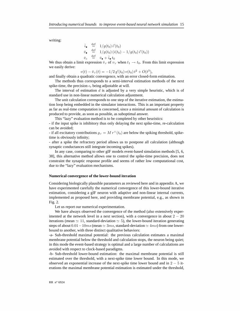
Numerical convergence of the lower-bound iteration

Considering biologically plausible parameters as reviewed here and in appendix A, wehave experimented carefully the numerical convergence of this lower-bound iterativeestimation, considering a gIF neuron with adaptive and non-linear internal currents,implemented as proposed here, and providing membrane potential, e.g., as shown inFig. 2.

Let us report our numerical experimentation.We have always observed the convergence of the method (also extensively exper-

imented at the network level in a next section), with a convergence in about2 − 20iterations (mean≃ 11, standard-deviation≃ 5), the lower-bound iteration generatingsteps of about0.01−10ms (mean≃ 3ms, standard-deviation≃ 4ms) from one lower-bound to another, with three distinct qualitative behaviors:-a- Sub-threshold maximal potential: the previous calculation estimates a maximalmembrane potential below the threshold and calculation stops, the neuron being quiet;in this mode the event-based strategy is optimal and a large number of calculations areavoided with respect to clock-based paradigms.-b- Sub-threshold lower-bound estimation: the maximal membrane potential is stillestimated over the threshold, with a next-spike time lower bound. In this mode, weobserved an exponential increase of the next-spike time lower bound and in2 − 5 it-erations the maximal membrane potential estimation is estimated under the threshold,

RR n° 6924

16 Cortex

switching to mode -a-; in this mode the estimation interval heuristic introduced previ-ously is essential and the next-spike time lower bound estimation allows the calculationto quickly detect if the neuron is quiet.-c- Iterative next-spike time estimation: if a spike is pending, the previous calculationestimates in about10− 20 iterations the next-spike time up to a tunable precision (cor-responding to thedt of the simulation mechanism). The present mechanism acts asaniterative estimation of the next spike time, as expected.

4 About event-based simulation of SRM models

Among spiking-neuron models, the Gerstner and Kistler spike response model (SRM)[16] of a biological neuron defines the state of a neuron via a single variable:

ui(t) = ri j(t) + νi(t− t∗i ) +∑

j

∑

tnj ∈Fj

wij εij(t− t∗i , (t− tnj )− δij) (12)

whereui is the normalized membrane potential,j() is the continuous input currentfor an input resistanceri. The neuron fires whenui(t) ≥ θi, for a given threshold,νi describes the neuronal response to its own spike (neuronal refractoriness),t∗i is thelast spiking time of theith neuron,εij is the synaptic response to pre-synaptic spikes attimetnj post-synaptic potential (see Fig. 3),wij is theconnection strength(excitatory ifwij > 0 or inhibitory if wij < 0) andδij is theconnection delay(including axonal de-lay). Here we consider only the last spiking timet∗i for the sake of simplicity, whereasthe present implementation is easily generalizable to the case where several are takeninto account.

νi εij

Figure 3: Potential profiles used in equation (12). The original exponential profilesderived by the authors of the model are shown as thin curves and the piece-wise linearapproximation as thick lines. Any other piece-wise linear profiles could be considered,including piece-wise finer linear approximation of exponential profiles.

Let us call here lSRM such piece-wise linear approximationsof SRM models.This model is very useful both at the theoretical and simulation levels. At a compu-

tational level, it has been used (see [26] for a review) to show that any feed-forward orrecurrent (multi-layer) analog neuronal network (a-la Hopfield, e.g., McCulloch-Pitts)can be simulated arbitrarily closely by an insignificantly larger network of spiking neu-rons, even in the presence of noise, while the reverse is not true [24, 25]. In this case,inputs and outputs are encoded by temporal delays of spikes.These results highlymotivate the use of spiking neural networks.

This lSRM model has also been used elsewhere (see e.g. [41] for a review), in-cluding high-level specifications of neural network processing related to variationalapproaches [45], using spiking networks [46]. The authors used again a lSRM to im-plement their non-linear computations.

INRIA


Let us make explicit here the fact a lSRM can be simulated on anevent-based sim-ulator for two simple reasons:- the membrane potential is a piece-wise linear function as the sum of piece-wise linearfunctions (as soon as the optional input current is also piece-wise constant or linear),- the next spike-time calculation is obvious to calculate ona piece-wise linear poten-tial profile, scanning the linear segments and detecting the1st intersection withu = 1if any. The related piece-wise linear curve data-structurehas been implemented1 andsupport three main operations:- At each spike occurrence, add linear pieces to the curve corresponding to refractori-ness or synaptic response.- Reset the curve, after a spike occurrence.- Solve the next spike-time calculation.This is illustrated in Fig. 4.

Figure 4: An example of lSRM normalized membrane potential.The traces corre-sponds to100ms of simulation. The leftward trace uses the fastest possiblepiece-wiselinear approximation of the SRM model profiles. The rightward trace is simulated witha lower excitation inhibition and using a thinner piece-wise linear approximation. Theneuron is defined by biologically plausible parameters as reviewed in appendix A . It isconnected to a pair of periodic excitatory and inhibitory input neurons, with differenttime constants, as in Fig. 2.

This is to be compared with other simulations (e.g. [28, 40])where stronger sim-plifications of the SRM models have been introduced to obtaina similar efficiency,whereas other authors propose heavy numerical resolutionsat each step. When switch-ing from piece-wise linear profiles to the original exponential profiles [16], the equationto solve is now of the formal form:

1 =∑n

i=1 λiet/τi ,

without any closed-form solution as soon asn > 1. One elegant solution [6] is toapproximate the time-constant by rational numbers and reduce this problem to a poly-nomial root finding problem. Another solution is to upper-bound the exponential pro-files by piece-wise linear profiles in order to obtain a lower-bound estimation of thenext spike-time and refine in the same way as what has been proposed in the previoussection. Since the mechanism is identical, we are not going to further develop.

In any case, this very powerful phenomenological model of biological dynamicscan be simulated with several event-based methods, including at a fine degree of preci-sion, using more complex piece-linear profiles.

RR n° 6924

18 Cortex

5 Experimental results

5.1 Kernel performances and features

In order to estimate the kernel sampling capability we have used, as a first test, a ran-dom spiking network with parameter less connections, the spiking being purely randomthus not dependent on any input.

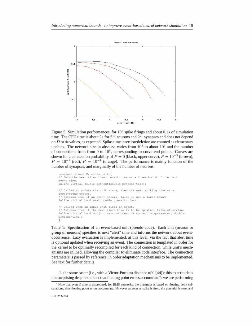
In term of performances, on a standard portable computer (Pentium M 750 1.86 GHz,512Mo of memory) we process about105−7 spike-time updates / second, given the net-work size and connectivity. Performances reported in Fig. 5confirm that the algo-rithmic complexity only marginally depends on the network size, while it is mainlyfunction of the number of synapses (although both quantities are indeed linked). Wealso notice the expected tiny overhead when iterating on empty boxes in the histogram,mainly visible when the number of spikes is small. This overhead is constant for agiven simulation time. The lack of proportionality in performances is due to the intro-duction of some optimization in the evaluation of spike-times, which are not updatedif unchanged.

We have also observed that the spike-time structure upper and lower boundsD anddt have only a marginal influence on the performances, as expected.

Moreover, the numbers in Fig. 5 allows to derive an importantnumber: the over-head for an event-based implementation of a clock-based mechanism. Since we canprocess about2 106 updates/second while we have measured independently that amin-imal clock-based mechanism process about5 107 updates/second, we see that the costthe overhead is of about0.5µs / update. This number is in coherence with the numberof operations to realize at time modification in the underlying data structure.

It is important to clarify these apparently “huge” performances. The reason is thatthe event-based simulation kernel isminimal. As detailed in Table 1, the implementa-tion make a simple but extensive use of the best mechanisms ofobject oriented imple-mentations. The network mechanism (i.e., the kernel) corresponds to about 10Kb ofC++ source code, using aO(D/dt + N) buffer size and aboutO(1 + C + ǫ/dt) ≃10 − 50 operations/spike, for a sizeN network withC connections in average, whileǫ ≪ 1. This ǫ corresponds to the overhead when iterating on empty boxes inthe his-togram. We can use such a simple spike-time data structure because of the temporalconstraints taken into account in our specifications.

As a consequence, not all spiking mechanisms are going to be simulated with thiskernel: units with event-time intervals or input/output event delay belowdt are goingto generate a fatal error; units with inter-event intervalshigher thanD are also goingto defeat this mechanism (unless an extension of the presentmechanism, discussedpreviously, is not implemented). Note that despite these limitations the event-timeaccuracy itself is the notdt but the floating point machine precision.

Clock-based sampling in event-based environment.A step further, we have imple-mented a discretized version of a gIF network, called BMS, asdetailed in [9, 11] (equa-tions not reported here). The interest of this test is the fact that we can compare spikeby spike an event-based and clock-based simulation since the latter is well-defined,thus without any approximation with respect to the former (see [11] for details).

We have run simulation with fully connected networks of size, e.g. N = 100 −1000 over observation periods ofT = 1000 − 10000 clocks, with the same randominitial conditions and the same randomly chosen weights, asshow in Fig.6. We haveobserved:

INRIA


Figure 5: Simulation performances, for105 spike firings and about0.1s of simulationtime. The CPU time is about2s for 213 neurons and221 synapses and does not dependonD ordt values, as expected. Spike-time insertion/deletion are counted as elementaryupdates. The network size in abscissa varies from103 to about106 and the numberof connections from from 0 to108, corresponding to curve end-points. Curves areshown for a connection probability ofP = 0 (black, upper curve),P = 10−3 (brown),P = 10−2 (red), P = 10−1 (orange). The performance is mainly function of thenumber of synapses, and marginally of the number of neurons.

template <class C> class Unit {// Gets the next alter time: event time or a lower-bound of the nextevent time.inline virtual double getNext(double present-time);

// Called to update the unit state, when the next spiking time or alower-bound occurs.// Returns true if an event occurs, false it was a lower-boundinline virtual bool next(double present-time);

// Called when an input unit fires an event.// Returns true if the next alert time is to be updated, false otherwise.inline virtual bool add(int neuron-index, C& connection-parameter, doublepresent-time);};

Table 1: Specification of an event-based unit (pseudo-code). Each unit (neuron orgroup of neurons) specifies is next “alert” time and informs the network about event-occurrence. Lazy evaluation is implemented, at this level,via the fact that alert timeis optional updated when receiving an event. The connectionis templated in order forthe kernel to be optimally recompiled for each kind of connection, while unit’s mech-anisms are inlined, allowing the compiler to eliminate codeinterface. The connectionparameters is passed by reference, in order adaptation mechanisms to be implemented.See text for further details.

-1- the same raster (i.e., with a Victor-Purpura distance of0 [44]); this exactitude isnot surprising despite the fact that floating point errors accumulate4: we are performing

4 Note that even if time is discretized, for BMS networks, the dynamics is based on floating point cal-culations, thus floating point errors accumulate. However as soon as spike is fired, the potential is reset and

RR n° 6924

20 Cortex

the same floating point calculations in both cases, since theevent-based implementationis exact, thus . . with the same errors;

-2- the overhead of the event-based implementation of the clock-based samplingis negligible (we obtain a number< 0.1µs/step), as expected. Again this surpris-ingly slow number is simply due to the minimal implementation, based on global timeconstraints, and the extensive use of theC/C++ optimization mechanisms.

Figure 6: An example of BMS neural network simulation used toevaluate the clock-based sampling in the event-based kernel, forN = 1000 andT = 10000 thus108

events. The first 100 neurons activity is shown at the end of the simulation. The figuresimply shows the strong network activity with the chosen parameters, and .

Kernel usage. A large set of research groups in the field have identified whatare therequired features for such simulation tools [4]. Although the present implementationis not a simulator, but a simple simulator plug-in, we have made theexercise to listto which extends what is proposed here fits with existing requirements, as detailed inTable 3. We emphasize the fact the required programming is very light, for instance a“clock” neuron (allowing to mix clock-based and event-based mechanisms) writes:

class ClockUnit : public Unit<bool> {ClockUnit(double DT) : DT(DT), t(DT) double DT, t;inline virtual double getNext(double present-time) return t; ;inline virtual bool next(double present-time) t += DT; return true; ;inline virtual bool add(int neuron-index, bool connection-parameter,double present-time) return false; ;};

providingDT is the sampling period. It is not easy to make things simple, and sev-eral possible choices of implementations have been investigated before proposing theinterface proposed in Table 1.

previous errors are canceled. This explains why time-discretized simulations of IF networks are numericallyrather stable.

INRIA


See [35] for a further description of how event-based spiking neuron mechanismscan be implemented within such framework. Although presented here at a very prag-matical level, note that these mechanisms are based on the modular or hierarchicalmodeling strategy borrowed from the DEVS formalism (see, e.g., [35]).

5.2 Experimenting reduced adaptive and ionic currents

In order to experiment about our proposal to reduce ionic andadaptive currents toa function depending only on spike time, we consider a very simple model whoseevolution equation at timet for the membrane potentialv is:

if (t = 0)v = 0; u = 0; t 0 = 0;

else if (v ≥ 1)v = 0; u = u + k; t 0 = t;

elsev = -g (v - E) - u + i;if (t > t 0 + d) v = 0

(13)

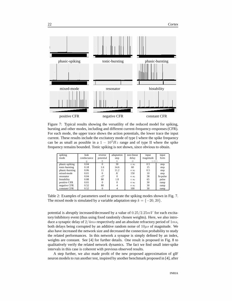
whereu is the adaptive current (entirely defined by equation (13)),t 0 the last spikingtime, d the non-linear current delay. The differential equation issimulated using anEuler interpolation as in [19, 43] to compare our result to what has been obtained bythe other authors. The obvious event-based simulation of this model has been alsoimplemented1. The input currenti is either a step or a ramp as detailed in Fig. 7 andTable 2.

Four parameters, the constant leak conductanceg, the reversal potentialE, theadaptation currentk step and the (eventually infinite) non-linear current delayd allowsto fix the firing regime. These parameters are to be recalculated after the occurrenceof each internal or external spike. In the present context, it was sufficient to use con-stant value except for one regime, as made explicit in Fig. 2.We use the two-stagescurrent whose action is to reset the membrane current after acertain delay. We madethis choice because it was the simplest and leads to a very fast implementation.

Experimental results are given in Fig. 7 for the parameters listed in Fig. 2. Theseresults correspond to almost all well-defined regimes proposed in [19]. The parameteradjustment is very easy, we in fact use parameters given in [19] with some tiny ad-justments. It is an interesting numerical result: The different regimes are generated byparameters values closed to those chosen for the quadratic model, the dynamic phasediagram being likely similar. See [43] for a theoretic discussion.

This places a new point on the performance/efficiency plane proposed by [20] at avery challenging place, and see that we can easily simulate different neuronal regimeswith event-based simulations.

However, it is clear that such model doesnot simulates properly the neuron mem-brane potential as it is the case for the exponential model [3]. It is usable if and only ifspike emission is considered, whereas the membrane potential value is ignored.

5.3 Experimental benchmarks

We have reproduced the benchmark 4 proposed in Appendix 2 of [4] which is ded-icated to event-based simulation: it consists of4000 IF neurons, which80/20% ofexcitatory/inhibitory neurons, connected randomly usinga connection probability of1/32 ≃ 3%. So called “voltage-jump” synaptic interactions are used:the membrane

RR n° 6924

22 Cortex

phasic-spiking tonic-bursting phasic-bursting

mixed-mode resonator bistability

positive CFR negative CFR constant CFR

Figure 7: Typical results showing the versatility of the reduced model for spiking,bursting and other modes, including and different current-frequency-responses (CFR).For each mode, the upper trace shows the action potentials, the lower trace the inputcurrent. These results include the excitatory mode of type Iwhere the spike frequencycan be as small as possible in a1 − 103Hz range and of type II where the spikefrequency remains bounded. Tonic spiking is not shown, since obvious to obtain.

spiking leak reverse adaptation non-linear input inputmode conductance potential step delay magnitude form

g E k d i(t)phasic-spiking 0.04 0 30 +∞ 0.5 steptonic-bursting 0.18 1.6 14.6 60 15 stepphasic-bursting 0.06 11 11.2 +∞ 0.5 stepmixed-mode 0.01 0 K 150 10 stepresonator 0.04 -27 0 +∞ 38 bi-pulsebistability 0.88 80 1.8 +∞ 65 pulsepositive CFR 0.01 0 0 +∞ 30 rampnegative CFR 0.52 80 4 +∞ 30 rampconstant CFR 0.52 0 4 100 30 ramp

Table 2: Examples of parameters used to generate the spikingmodes shown in Fig. 7.The mixed mode is simulated by a variable adaptation stepk = {−20, 20}.

potential is abruptly increased/decreased by a value of0.25/2.25mV for each excita-tory/inhibitory event (thus using fixed randomly chosen weights). Here, we also intro-duce a synaptic delay of2/4ms respectively and an absolute refractory period of1ms,both delays being corrupted by an additive random noise of10µs of magnitude. Wealso have increased the network size and decreased the connection probability to studythe related performances. In this network a synapse is simply defined by an index,weights are constant. See [4] for further details. One result is proposed in Fig. 8 toqualitatively verify the related network dynamics. The fact we find small inter-spikeintervals in this case is coherent with previous observed results.

A step further, we also made profit of the new proposed approximation of gIFneuron models to run another test, inspired by another benchmark proposed in [4], after

INRIA


0 0.1

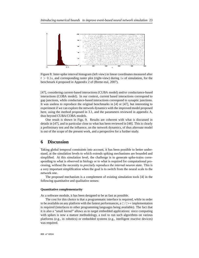
Figure 8: Inter-spike interval histogram (left view) in linear coordinates measured aftert > 0.1s, and corresponding raster plot (right-view) during1s of simulation, for thebenchmark 4 proposed in Appendix 2 of (Brette etal, 2007).

[47], considering current-based interactions (CUBA model) and/or conductance-basedinteractions (COBA model). In our context, current based interactions correspond togap junctions, while conductance-based interactions correspond to synaptic junctions.It was useless to reproduce the original benchmarks in [4] or[47], but interesting toexperiment if we can explore the network dynamics with the improved model proposedhere, using the method proposed in 3.1, and the parameters reviewed in appendix A,thus beyond CUBA/COBA models.

One result is shown in Figs. 9. Results are coherent with whatis discussed indetails in [47], and in particular close to what has been reviewed in [48]. This is clearlya preliminary test and the influence, on the network dynamics, of thus alternate modelis out of the scope of the present work, and a perspective for afurther study.

6 Discussion

Taking global temporal constraints into account, it has been possible to better under-stand, at the simulation levels to which extends spiking mechanisms are bounded andsimplified. At this simulation level, the challenge is to generate spike-trains corre-sponding to what is observed in biology or to what is requiredfor computational pro-cessing, without the necessity toprecisely reproduce the internal neuron state. This isa very important simplification when the goal is to switch from the neural scale to thenetwork one.

The proposed mechanism is a complement of existing simulation tools [4] in thefollowing quantitative and qualitative senses:

Quantitative complementarity

As a software module, it has been designed to be as fast as possible.The cost for this choice is that a programmatic interface is required, while in order

to be available on any platform with the fastest performances, aC/C++ implementationis required (interfaces to other programming languages being available). The fact thatit is also a “small kernel” allows us to target embedded applications: since computingwith spikes is now a mature methodology, a tool to run such algorithms on variousplatforms (e.g., in robotics) or embedded systems (e.g., intelligent reactive devices)was required.

RR n° 6924

24 Cortex

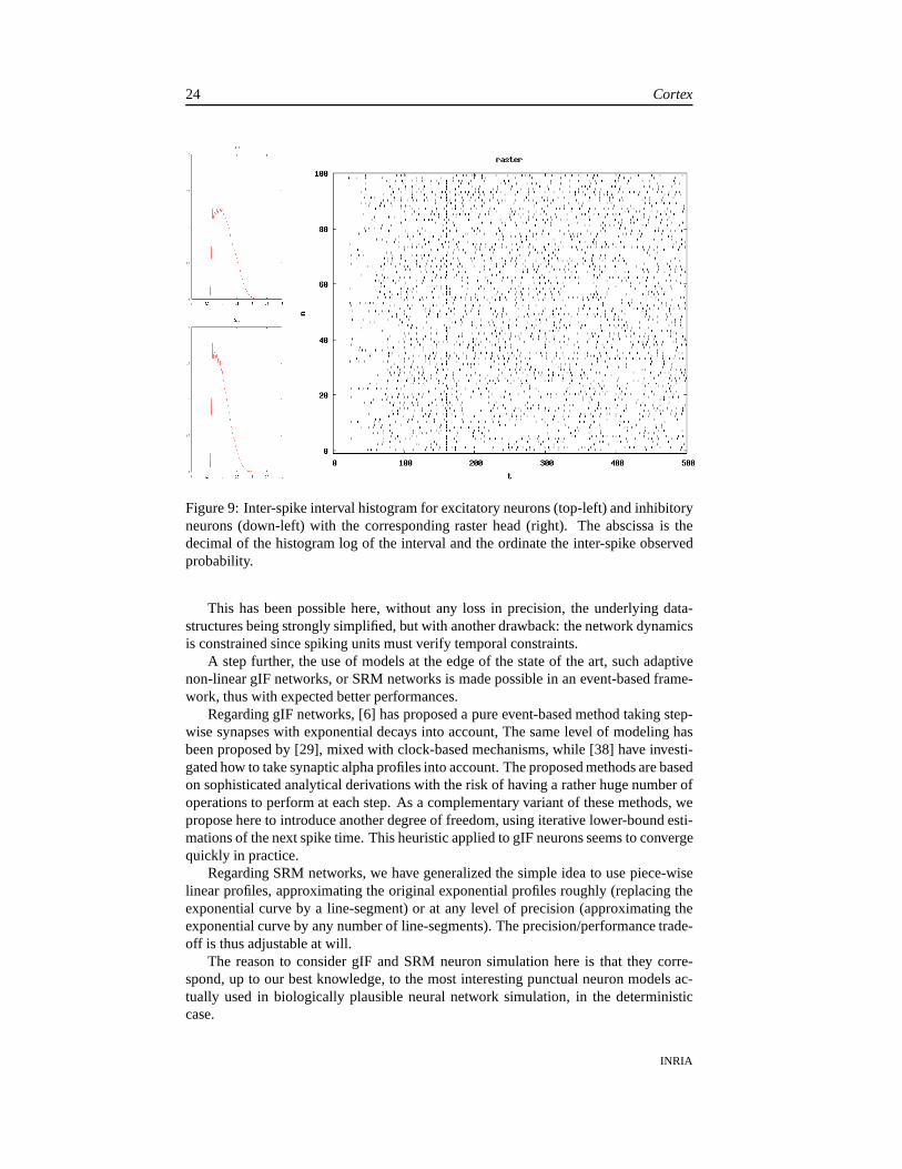
Figure 9: Inter-spike interval histogram for excitatory neurons (top-left) and inhibitoryneurons (down-left) with the corresponding raster head (right). The abscissa is thedecimal of the histogram log of the interval and the ordinatethe inter-spike observedprobability.

This has been possible here, without any loss in precision, the underlying data-structures being strongly simplified, but with another drawback: the network dynamicsis constrained since spiking units must verify temporal constraints.

A step further, the use of models at the edge of the state of theart, such adaptivenon-linear gIF networks, or SRM networks is made possible inan event-based frame-work, thus with expected better performances.

Regarding gIF networks, [6] has proposed a pure event-basedmethod taking step-wise synapses with exponential decays into account, The same level of modeling hasbeen proposed by [29], mixed with clock-based mechanisms, while [38] have investi-gated how to take synaptic alpha profiles into account. The proposed methods are basedon sophisticated analytical derivations with the risk of having a rather huge number ofoperations to perform at each step. As a complementary variant of these methods, wepropose here to introduce another degree of freedom, using iterative lower-bound esti-mations of the next spike time. This heuristic applied to gIFneurons seems to convergequickly in practice.

Regarding SRM networks, we have generalized the simple ideato use piece-wiselinear profiles, approximating the original exponential profiles roughly (replacing theexponential curve by a line-segment) or at any level of precision (approximating theexponential curve by any number of line-segments). The precision/performance trade-off is thus adjustable at will.

The reason to consider gIF and SRM neuron simulation here is that they corre-spond, up to our best knowledge, to the most interesting punctual neuron models ac-tually used in biologically plausible neural network simulation, in the deterministiccase.

INRIA


Qualitative complementarity

Two key points allow us to performs new simulations with thistool:Event-based and clock-based mechanisms can be easily mixedherein an event-

based simulation mechanism, whereas other implementations mix clock-based andevent-based mechanisms in a clock-based simulator (e.g., in [29]), or use spike-timeinterpolation mechanisms in order to better approximate event-based mechanisms insuch clock-based environment. Using an event-based simulator to simulate a clock isobvious, but usually stupid, because the event-based mechanism usually generates anheavy overhead, thus making the clock-based part of the simulation intractable. Thisis not the case here, since we use this minimal data-structure and have been able tosee that the overhead is less than one micro-second on a standard laptop. It is thusappears a good design choice to use an event-based simulation mechanism to mixedboth strategies.

The second key point is that, we have proposed a way toconsider adaptive non-linear gIF networks in an event-based framework. It is easy to get convinced that2D integrate and fire neurons differential equations with non-linear ionic currents (e.g.exponential, quartic or quadratic [42]) do not have closed-form solutions (unless in veryspecial cases). Therefore, the next spike time is not calculable, except numerically, andthe exact event-based implementation is not possible. Alternatives strategies have beenproposed such as simulations with constant voltage steps [51] allowing to implementquadratic 1D (thus without adaptive currents) gIF networksin a modified event-baseframework. In order to get rid of these limitations, one proposal developed here is toconsider adaptive currents which depends only on the previous spiking time neuronstate and non-linear ionic currents updated only at the eachincoming spike occurrence.With these additional approximations, the event-based strategy can be used with suchcomplex models. This is a complementary heuristic with respect to existing choices.

We notice that the present study only considers deterministic models, while thesimulation of stochastic networks is also a key issue. Hopefully, event-based imple-mentations of network of neurons with stochastic dynamics is a topic already investi-gated, both at the computer implementation level [35] and modeling level [34]. In thelatter case, authors propose to reduce the multiple stochastic neuronal input activityto a dedicated stochastic input current, and investigate this choice of modeling in anevent-based framework, making explicit very good performances. This method seemsto be easily implementable in our present kernel, though this is out of the scope of thepresent work.

Conclusion

At a practical level, event-based simulation of spiking networks has been made avail-able, using the simplest possible programmatic interface,as detailed previously. Thekernel usage has been carefully studied, following the analysis proposed in [4] anddetailed in Table 3

The present implementation thus offers a complementary alternative with respectto existing methods, and allows us to enrich the present spiking network simulationcapabilities.

RR n° 6924

26 Cortex

A Appendix: About gIF model normalization

Let us review how to derive an equation of the form of (2). We follow [20, 3, 38] inthis section. We consider here a voltage dynamics of the form:

dV

dt+ I leak + Isyn + Igap = Iext + Iadp + Iion

thus with leak, synaptic, gap-junction, external currentsdiscussed in this section.

Membrane voltage range and passive properties

The membrane potential, outside spiking events, verifies:V (t) ∈ [Vreset, Vthreshold]

with typically Vreset≃ EL ≃ −80mV and a threshold valueVthreshold≃ −50mV ±10mV . When the threshold is reached an action potential of about 1-2 ms is issued andfollowed by refractory period of 2-4 ms (more precisely, an absolute refractory periodof 1-2 ms without any possibility of another spike occurrence followed by a relativerefraction to other firing). Voltage peaks are at about40mV and voltage undershootsabout−90mV . The threshold is in fact not sharply defined.

The reset value is typically fixed, whereas the firing threshold is inversely relatedto the rate of rise of the action potential upstroke [2]. Hereit is taken as constant.This adaptive threshold diverging mechanism can be represented by a non-linear ioniccurrent [20, 3], as discussed in section 3.1.

From now on, we renormalize each voltage between[0, 1] writing:

v =V − Vreset

Vthreshold− Vreset(14)

The membrane leak time constantτL ≃ 20ms is defined for a reversal potentialEL ≃ −80 mV , as made explicit in (2).

The membrane capacityC = S CL ≃ 300pF , whereCL ≃ 1 µFcm−2 and themembrane areaS ≃ 38.013 µm2, is integrated in the membrane time constantτL =CL/GL whereGL ≃ 0.0452 mScm−2 is the membrane passive conductance.

From now on, we renormalize each current and conductance divided by the mem-brane capacity. Normalized conductance units ares−1 and normalized current unitsV/s.

Synaptic currents

In conductance based model the occurrence of a post synapticpotential on a synapseresults in a change of the conductance of the neuron. Consequently, it generates acurrent of the form:

Isyn(V, ωt, t) =∑

j

G+j (t, ωt) [V (t)− E+] +

∑

j

G−j (t, ωt) [V (t)− E−] ,

for excitatory+ and inhibitory− synapses, where conductances are positive and de-pend on previous spike-timesωt.

In the absence of spike, the synaptic conductance vanishes [21], and spikes areconsidered having an additive effect:

G±j (t, ωt) = G±

∑

n

r±(t− tnj )

INRIA


while the conductance time-courser±(t− tnj ) is usually modeled as an “exponential”,“alpha” (see Fig. 10) or two-states kinetic (see Fig. 11) profile, whereH is the Heavi-side function (related to causality).

Note, that the conductances may depend on thewhole past historyof the network,via ωt.

Figure 10: The “alpha” profileα(t) = H(t) tτ e−

tτ plotted here forτ = 1. It is

maximal att = τ with α(τ) = 1/e, the slope at the origin is1/τ and its integralvalue

∫ +∞

0α(s) ds = τ since(

∫α)(t) = (τ − t) e−

tτ + k. This profile is concave for

t ∈]0, 2 τ [ and convex fort ∈]2 τ, +∞[, while α(2 τ) = 2/e2 at the inflexion point.

The “exponential” profile (r(t) = H(t) e−tτ ) introduces a potentially spurious dis-

continuity at the origin. The “beta” profile is closer than the ”alpha” profile to whatis obtained from a bio-chemical model of a synapse. However,it is not clear whetherthe introduction of this additional degree of freedom is significant here. Anyway, anyof these can be used for simulation with the proposed method,since their propertiescorrespond to what is stated in Fig. 1.

Figure 11: The two-states kinetic or “beta” profileβ(t) = H(t) 1κ−1 (e−

tτ − e−κ t

τ )is plotted with a normalized magnitude for the sameτ = 1 as the “alpha” profile butdifferentκ = 1.1, 1.5, 2, 5, 10 showing the effect of this additional degree of freedom,while limκ→1β(t) = α(t). The slope at the origin and the profile maximum can beadjusted independently with “beta” profiles. It is maximal at t• = τ ln(κ)/(κ − 1)the slope at the origin is1/τ and its integral valueτ/κ. The profile is concave fort ∈]0, 2 t•[ and convex fort ∈]2 t•, +∞[.

There are typically, in real neural networks,104 excitatory and about2 103 in-hibitory synapses. The corresponding reversal potential are E+ ≃ 0 mV andE− ≃−75 mV , usually related to AMPA and GABA receptors. In average:G+

j ≃ 0.66 nS, τ+ ≃2 ms andG−

j ≃ 0.63 nS, τ− ≃ 10 ms, for excitatory and inhibitory synapses respec-tively, thus about570ms−1, 600ms−1 in normalized units, respectively. The coeffi-cientsG± give a measure of the synaptic strength (unit of charge) and vary from onesynapse to another and are also subject to adaptation.

RR n° 6924

28 Cortex

This framework affords straightforward extensions involving synaptic plasticity(e.g. STDP, adjusting the synaptic strength), not discussed here.

Gap junctions

It has been recently shown, that many local inter-neuronal connections in the cortexare realized though electrical gap junctions [15], this being predominant between cellsof the same sub-population [1]. At a functional level they seem to have an importantinfluence on the synchronicity between the neuron spikes [23]. Such junctions are alsoimportant in the retina [50].

The electrotonic effect of both the sub-threshold and supra-threshold portion of themembrane potentialVj(t) of the pre-junction neuron of indexj seems an importantcomponent of the electrical coupling. This writes [50, 23]:

Igap(V, t) =∑

j G∗j

[[Vj(t)− V (t)] + E•

∑

n r(t − tnj )]

whereG∗j is the electrical coupling conductance, the termVj(t)−V (t) accounts for the

sub-threshold electrical influence while andE• parametrizes the spike supra-thresholdvoltage influence.

Regarding the supra-threshold influence, a valueE• ≃ 80mV corresponds to theusual spike voltage magnitude of the spiking threshold, while τ• ≃ 1ms correspondsto the spike raise time. Herer() profile accounts for the action potential itself, slightlyfiltered by the biological media, while the gap junction intrinsic delay is of about10µs.These choices seem reasonable with respect to biological data [15, 23]

A step further, we propose to neglect the sub-threshold termfor three main reasons.On one hand, obviously the supra-threshold mechanism has a higher magnitude thanthe sub-threshold mechanism, since related to action potentials. Furthermore, becauseof the media diffusion, slower mechanisms are smoothed by the diffusion, whereasfaster mechanisms better propagate. On the other hand, thiselectrical influence re-mains local (quadratic decrease with the distance) and is predominant between cells ofthe same sub-population which are either synchronized or have a similar behavior, as aconsequence|Vj(t)− V (t)| remains small for cells with non-negligible electrical cou-pling. Furthermore, a careful analysis of such electrical coupling [23] clearly showsthat the sub-threshold part of the contribution has not an antagonist effect on the neu-ron synchrony, i.e., it could be omitted without changing qualitatively the gap junctionfunction.

As a conclusion, we are able to take gap junction into accountwith a minimalincrease of complexity, since we obtain a form similar to synaptic currents, using verydifferent parameters

External currents

Direct input (or external) current is often related to electro-physiological clamps. Atanother level of representation, the average activity of the neuron can be modeled bya constant or random input current. In both cases, the way theproposed simulationmethods is proposed requires to assume such external current to be taken as constantbetween two spikes, i.e. having temporal variations small enough to be neglected. Ifnot, it is easy to associate to the external current an event unit which fires at each newcurrent value, in order the neuron to take this new value intoaccount.

INRIA


References[1] Y. Amitai, J. Gibson, M. Beirleiner, S.L. Patrick, A.M. Ho, B.W.Connors, and D. Golomb. The spatial dimensions of

electrically coupled networks of interneurons in neocortex. J. Neurosci., 22:4142–4152, 2002.

[2] R. Azouz and C.M. Gray. Dynamic spike threshold reveals amechanism for synaptic coincidence detection in cortical.In Proceedings of the National Academy of Science, volume 97, pages 8110–8115, 2000.

[3] R. Brette and W. Gerstner. Adaptive exponential integrate-and-fire model as an effective description of neuronalactivity. Journal of Neurophysiology, 94:3637–3642, 2005.

[4] R. Brette, M. Rudolph, T. Carnevale, M. Hines, D. Beeman,J. M. Bower, M. Diesmann, A. Morrison, P. H. Goodman,F. C. Harris Jr., M. Zirpe, T. Natschlager, D. Pecevski, B. Ermentrout, M. Djurfeldt, A. Lansner, O. Rochel, T. Vieville,E. Muller, A. P. Davison, S. El Boustani, and A. Destexhe. Simulation of networks of spiking neurons: a review oftools and strategies.Journal of Computational Neuroscience, 23(3):349–398, 2007.

[5] Romain Brette. Exact simulation of integrate-and-fire models with synaptic conductances.Neural Computation,18(8):2004–2027, 2006.

[6] Romain Brette. Exact simulation of integrate-and-fire models with exponential currents.Neural Computation,19(10):2604–2609, 2007.

[7] Giancarlo La Camera, Michele Giugliano, Walter Senn, and Stefano Fusi. The response of cortical neurons to invivo-like input current: theory and experiment.Biological Cybernetics, 99(4-5):279–301, 2008.

[8] Giancarlo La Camera, Michele Giugliano, Walter Senn, and Stefano Fusi. The response of cortical neurons to in vivo-like input current: theory and experiment: Ii. time-varying and spatially distributed inputs.Biological Cybernetics,99(4-5):303–318, 2008.

[9] B. Cessac. A discrete time neural network model with spiking neurons. rigorous results on the spontaneous dynamics.J. Math. Biol., 56(3):311–345, 2008.

[10] B. Cessac, H.Rostro-Gonzalez, J.C. Vasquez, and T. Vi´eville. To which extend is the ”neural code” a metric ? InNeurocomp 2008, 2008.

[11] B. Cessac and T. Vieville. On dynamics of integrate-and-fire neural networks with adaptive conductances.Frontiersin neuroscience, 2(2), jul 2008.

[12] C. G. Connolly, I. Marian, and R. G. Reilly.Approaches to efficient simulation with spiking neural networks, vol-ume 15, pages 231–240. World Scientific, London, 2004.

[13] A. Destexhe, M. Rudolph, and D. Pare. The high-conductance state of neocortical neurons in vivo.Nature ReviewsNeuroscience, 4:739–751, 2003.

[14] Alain Destexhe. Conductance-based integrate and fire models.Neural Computation, 9:503–514, 1997.

[15] M. Galarreta and S. Hestrin. Electrical synapses between gaba-releasing interneurons.Nature Reviews Neuroscience,2:425–433, 2001.

[16] W. Gerstner and W. Kistler.Spiking Neuron Models. Cambridge University Press, 2002.

[17] M.L. Hines and N.T. Carnevale. Discrete event simulation in the neuron environment.Neurocomputing, pages 1117–1122, 2004.

[18] A.L. Hodgkin and A.F. Huxley. A quantitative description of membrane current and its application to conduction andexcitation in nerve.Journal of Physiology, 117:500–544, 1952.

[19] E. Izhikevich. Simple model of spiking neurons.IEEE Transactions on Neural Networks, 14(6):1569–1572, 2003.

[20] E.M. Izhikevich. Which model to use for cortical spiking neurons? IEEE Trans Neural Netw, 15(5):1063–1070,September 2004.

[21] C. Koch. Biophysics of Computation: Information Processing in Single Neurons. Oxford University Press: NewYork., 1999.

[22] Geehyuk Lee and Nabil Farhat. The double queue method: anumerical method for integrate-and-fire neuron networks.Neural Networks, 14(6-7):921–932, 2001.

[23] T. J. Lewis and J. Rinzel. Dynamics of spiking neurons connected by both inhibitory and electrical coupling.Journalof Computational Neuroscience, 14(3):283–309, 2003.

[24] W. Maass. Fast sigmoidal networks via spiking neurons.Neural Computation, 9:279–304, 1997.

[25] W. Maass and T. Natschlager. Networks of spiking neurons can emulate arbitrary hopfield nets in temporal coding.Neural Systems, 8(4):355–372, 1997.

RR n° 6924

30 Cortex

[26] Wolfgang Maass and Christopher M. Bishop, editors.Pulsed Neural Networks. MIT Press, 2003.

[27] H. Markram, J. Lubke, M. Frotscher, and B. Sakmann. Regulation of synaptic efficacy by coincidence of postsynapticap and epsp.Science, 275(213), 1997.

[28] Maurizio Mattia and Paolo Del Giudice. Efficient event-driven simulation of large networks of spiking neurons anddynamical synapses.Neural Computation, 12:2305–2329, 2000.

[29] A. Morrison, C. Mehring, T. Geisel, A.D. Aerstsen, and M. Diesmann. Advancing the boundaries of high connectivitynetwork with distributed computing.Neural Comput, 17(8):1776–1801, 2005.

[30] A. Morrison, S. Straube, H.E. Plesser, and M. Diesmann.Exact subthreshold integration with continuous spike timesin discrete-time neural network simulations.Neural Computation, 19:47–79, 2007.

[31] Anthony Mouraud, Helene Paugam-Moisy, and Didier Puzenat. A distributed and multithreaded neural event-drivensimulation framework. InInt. Conf. on Parallel and Distributed Computing and Networks, pages 393–398. ACTAPress, 2006.

[32] Jean-Pascal Pfister and W. Gerstner. Triplets of spikesin a model of spike timing-dependent plasticity.J. Neurosci.,26:9673–9682, 2006.

[33] Alexander Rauch, Giancarlo La Camera, Hans-Rudolf Luscher, Walter Senn, and Stefano Fusi. Neocortical pyramidalcells respond as integrate-and-fire neurons to in vivo-likeinput currents.J Neurophysiol, 90(3):1598–1612, 2003.

[34] J. Reutimann, M. Guigliano, and S. Fusi. Event-driven simulation of spiking neurons with stochastic dynamics.NeuralComput., 15:811830, 2003.

[35] O. Rochel.Une approche evenementielle pour la modelisation et la simulation de neurones impulsionnels. PhD thesis,Universite Henri Poincare - Nancy 1, 2004.

[36] O. Rochel and D. Martinez. An event-driven framework for the simulation of networks of spiking neurons. InProc.11th European Symposium on Artificial Neural Networks, pages 295–300, 2003.

[37] S. Rotter and M. Diesmann. Exact digital simulation of time-invariant linear systems with application to neuronalmodeling.Biol. Cybern., 81:381–402, 1999.

[38] M. Rudolph and A. Destexhe. Analytical integrate and fire neuron models with conductance-based dynamics for eventdriven simulation strategies.Neural Computation, 18:2146–2210, 2006.

[39] M. Rudolph and A. Destexhe. How much can we trust neural simulation strategies?Neurocomputing, 2007. Toappear.

[40] Berthold Ruf. Computing and Learning with Spiking Neurons - Theory and Simulations. PhD thesis, Institute forTheoretical Computer Science, Univ. Graz, Austria, 1998.

[41] Benjamin Schrauwen.Towards Applicable Spiking Neural Networks. PhD thesis, Universiteit Gent, Belgium, 2007.

[42] Jonathan Touboul. Bifurcation analysis of a general class of non-linear integrate and fire neurons. Research ReportRR-6161, Odyssee, INRIA, 2007.

[43] Jonathan Touboul. Bifurcation analysis of a general class of nonlinear integrate-and-fire neurons.SIAM Journal onApplied Mathematics, 68(4):1045–1079, 2008.

[44] J.D. Victor. Spike train metrics.Current Opinion in Neurobiology, 15(5):585–592, 2005.

[45] T. Vieville, S. Chemla, and P. Kornprobst. How do high-level specifications of the brain relate to variational ap-proaches?Journal of Physiology - Paris, 101(1-3):118–135, 2007.

[46] T. Vieville and O. Rochel. One step towards an abstractview of computation in spiking neural-networks. InInterna-tional Conf. on Cognitive and Neural Systems, 2006.

[47] Tim P. Vogels and L. F. Abbott. Signal propagation and logic gating in networks of integrate-and-fire neurons.J.Neuroscience, 25:1078610795, 2005.

[48] Tim P. Vogels, Kanaka Rajan, and L. F. Abbott. Neural network dynamics.Annu. Rev. Neurosci., 28:35776, 2005.

[49] C. J. Wilson, A. Weyrick, D. Terman amd N. E. Hallworth, and M. D. Bevan. A model of reverse spike frequencyadaptation and repetitive firing of subthalamic nucleus neurons.J. Neurophysiol, 91:1963–1980, 2004.

[50] A. Wohrer and P. Kornprobst. Virtual retina : A biological retina model and simulator, with contrast gain control.Journal of Computational Neuroscience, 2008. DOI 10.1007/s10827-008-0108-4.

[51] G. Zheng, A. Tonnelier, and D. Martinez. Voltage-stepping schemes for the simulation of spiking neural networks.J.Comput Neurosci., 26, 2008.

Acknowledgment: Partially supported by the ANR MAPS & the MACCAC ARC projects.We are especially thankful to Helene Paugam-Moisy for precious advices and inputs regardingthis piece of work.

INRIA


FeaturesClock-based : can it simulate clock-based strategies ? yes

: in this case, does it use extrapolation for spike times ? useless1

Event-based : can it simulate event-based strategies ? yes: in this case, is the integration scheme exact ? yes2

Parallelism : does it support parallel processing ? no7

Graphics : does it have a graphical interface ? no, but a programmatic interfaceSimple analysis : is it possible to perform simple analysis ? yes with visualizationComplex analysis : can more complex analysis be done ? it can3

Interface : is interface to outside signals possible ? indeed4

: is it interoperable with other simulators ? yes4

Save option : can simulation be halted / resumed ? yesNeuron models : can it simulate HH models ? it can5

: can it simulate leaky IF models ? yes: can it simulate multivariate IF models ? it can5

: can it simulate conductance-based synaptic interactions? yes: can it simulate short-term plasticity ? it can5

: can it simulate long-term plasticity ? it can5

: can it simulate compartmental models with dendrites ? noUsage

Development : is it currently developed ? yes, stillα-version: how may developers yet ? half-time researcher + students

Support : is it supported yes: what kind of support email + phone: are they user cooperative tools ? not yet, tools available6

Manual : are there tutorials and reference material available ? yes: are there published books on the simulator ? no (useless): is there a list of publications of articles that used it ? yes

Import/export : is standard (XML) specification import/export available ? it can3

Web site : is there a web site where all can be found ? http://enas.gforge.inria.frSource code : are there codes available on the web ? yesOperating system : does it run under Linux yes, tested

: does it run under Max-OS X yes, tested: does it run under Windows likely (untested)

Interoperability : using which language can it be used ? C/C++, Python, Java, Php: can it be used from other platforms ? yes8

Notes:1: Since clock/event-based mechanisms can be mixed in a event-based simulation, spike times extrapolation is no more to be used, but exact event-time instead.

2: Exact integration scheme is to be used when allowed by the model, lower-bound spike time evaluation is a new alternativeproposed here when the former is not

possible.

3: More complex analysis and XML specification import/exportis indeed possible, using this kernel within the PyNN environment. The goal was toonly develop

here, what was not available elsewhere. The API has been carefully designed for this purpose.

4: The interface capability is a key feature of this middle-ware implementation, including in real time applications using spike computations.

5: Plasticity and other existing models, not discussed here,can be implemented with this middle-ware, and STDP is already considered at that time. The real goal

is however not to implement “all” models, other simulators do that better, but to propose also alternatives to existing models, as discussed in this paper.

6: The present development is installed on a forge, thus has all forum/bug-tracking/user-resquest-ticketting, etc.. available.

7: Though parallelism is not available yet, and the issue not addressed here, the network simulation kernel has been designed and implemented in order to be able

to connect to other kernels, via input/output events. It is thus a feasible extension to run several kernels in parallel,with the drawback that the slower kernel is going

to drive other kernels local times.

8: Links with these external platforms such as PyNN (thus NEURON, MvaSpike, ..), NeuroConstruct are made available by themulti-language operability, while

Scilab and Matlab usage is documented.

Table 3: Summary of the main features of the implemented event-based simulationkernel, using the criteria proposed to compare existing simulators, see text for details.

RR n° 6924

Centre de recherche INRIA Sophia Antipolis – Méditerranée2004, route des Lucioles - BP 93 - 06902 Sophia Antipolis Cedex (France)

Centre de recherche INRIA Bordeaux – Sud Ouest : Domaine Universitaire - 351, cours de la Libération - 33405 Talence CedexCentre de recherche INRIA Grenoble – Rhône-Alpes : 655, avenue de l’Europe - 38334 Montbonnot Saint-Ismier

Centre de recherche INRIA Lille – Nord Europe : Parc Scientifique de la Haute Borne - 40, avenue Halley - 59650 Villeneuve d’AscqCentre de recherche INRIA Nancy – Grand Est : LORIA, Technopôle de Nancy-Brabois - Campus scientifique

615, rue du Jardin Botanique - BP 101 - 54602 Villers-lès-Nancy CedexCentre de recherche INRIA Paris – Rocquencourt : Domaine de Voluceau - Rocquencourt - BP 105 - 78153 Le Chesnay CedexCentre de recherche INRIA Rennes – Bretagne Atlantique : IRISA, Campus universitaire de Beaulieu - 35042 Rennes Cedex

Centre de recherche INRIA Saclay – Île-de-France : Parc Orsay Université - ZAC des Vignes : 4, rue Jacques Monod - 91893 Orsay Cedex

ÉditeurINRIA - Domaine de Voluceau - Rocquencourt, BP 105 - 78153 Le Chesnay Cedex (France)

http://www.inria.frISSN 0249-6399

Introducing numerical bounds to improve event ... - Hal-Inria

Documents