HAL Id: hal-00654706 https://hal.inria.fr/hal-00654706 Submitted on 22 Dec 2011 HAL is a multi-disciplinary open access archive for the deposit and dissemination of sci- entific research documents, whether they are pub- lished or not. The documents may come from teaching and research institutions in France or abroad, or from public or private research centers. L’archive ouverte pluridisciplinaire HAL, est destinée au dépôt et à la diffusion de documents scientifiques de niveau recherche, publiés ou non, émanant des établissements d’enseignement et de recherche français ou étrangers, des laboratoires publics ou privés. Proceedings of AUTOMATA 2011: 17th International Workshop on Cellular Automata and Discrete Complex Systems Nazim Fatès, Eric Goles, Alejandro Maass, Ivan Rapaport To cite this version: Nazim Fatès, Eric Goles, Alejandro Maass, Ivan Rapaport. Proceedings of AUTOMATA 2011: 17th International Workshop on Cellular Automata and Discrete Complex Systems. Fatès, Nazim and Goles, Ericand Maass, Alejandro and Rappaport Ivan. Inria Nancy, pp.298, 2011, 978-2-905267-79-5. hal-00654706

Welcome message from author
This document is posted to help you gain knowledge. Please leave a comment to let me know what you think about it! Share it to your friends and learn new things together.
Transcript
HAL Id: hal-00654706https://hal.inria.fr/hal-00654706
Submitted on 22 Dec 2011
HAL is a multi-disciplinary open accessarchive for the deposit and dissemination of sci-entific research documents, whether they are pub-lished or not. The documents may come fromteaching and research institutions in France orabroad, or from public or private research centers.
L’archive ouverte pluridisciplinaire HAL, estdestinée au dépôt et à la diffusion de documentsscientifiques de niveau recherche, publiés ou non,émanant des établissements d’enseignement et derecherche français ou étrangers, des laboratoirespublics ou privés.
Proceedings of AUTOMATA 2011 : 17th InternationalWorkshop on Cellular Automata and Discrete Complex
SystemsNazim Fatès, Eric Goles, Alejandro Maass, Ivan Rapaport
To cite this version:Nazim Fatès, Eric Goles, Alejandro Maass, Ivan Rapaport. Proceedings of AUTOMATA 2011 : 17thInternational Workshop on Cellular Automata and Discrete Complex Systems. Fatès, Nazim andGoles, Ericand Maass, Alejandro and Rappaport Ivan. Inria Nancy, pp.298, 2011, 978-2-905267-79-5.hal-00654706
17 International Workshopon Cellular Automata andDiscrete Complex Systems
th
Proceedings
editors:Nazim FatèsEric GolesAlejandro MaassIvan Rapaport
AUTOMATA 2011

Preface
This volume contains all the contributed papers presented at AUTOMATA 2011, the 17th international workshop on cellular automata and discrete complex systems. The workshop was held on November 21-23, 2011, at the Center for Mathematical Modeling, University of Chile, Santiago, Chile.
AUTOMATA is an annual workshop on the fundamental aspects of cellular automata and related discrete dynamical systems. The spirit of the workshop is to foster collaborations and exchanges between researchers on these areas. The workshop series was started in 1995 by members of the Working Group 1.5 of IFIP, the International Federation for Information Processing.
The volume contains the « full » papers and « short » papers selected by the program committee. The « full papers » will also appear as proceedings in a volume of Discrete Mathematics and Theoretical Computer Science (DMTCS). The program committee consisted of 27 international experts on cellular automata and related models, and the selection was based on 3 peer reviews on each paper.
Papers in this volume represent a rich sample of current research topics on cellular automata and related models. The papers include theoretical studies of the classical cellular automata model, but also many investigations into various variants and generalizations of the basic concept. The versatile nature and the flexibility of the model is evident from the presented papers, making it a rich source of new research problems for scientists representing a variety of disciplines.
In addition to the papers of this volume, the program of AUTOMATA 2011 contained four one-hour plenary lectures given by distinguished invited speakers :
• Peter Gacs (Boston University, USA)• Tom Meyerovitch (University of British Columbia, Canada)• Nicolas Schabanel (CNRS, Universié Paris VII & ENS Lyon, France)• Damien Woods (Caltech, USA)
The organizers gratefully acknowledge the support by the following institutions:
• Centro de Modelamiento Matemático• Departamento de Ingeniería Matemática• Universidad de Chile• Conicyt• CNRS• Universidad Adolfo Ibáñez
As the editors of these proceedings, we thank all contributors to the scientific program of the workshop. We are especially indebted to the invited speakers and the authors of the contributed papers. We would also like to thank the members of the Program Committee and the external reviewers of the papers. Last but not least, the editors thank Nikolaos Vlassopolous for his valuable help in the compilation of these proceedings.
Nazim Fatès, Eric Goles, Alejandro Maass, Iván Rapaport

Program Committee
Andrew Adamatzky University of West England, UKStefania Bandini Università degli Studi di Milano-Bicocca, ItalyMarie-Pierre Béal Université Paris-Est, FranceBruno Durand Université de Provence, FranceNazim Fatès Inria Nancy Grand-Est, France, co-chairPaola Flocchini University of Ottawa, CanadaEnrico Formenti Université de Nice-Sophia Antipolis, FranceHenryk Fuks Brock University. CanadaAnahí Gajardo Universidad de Concepción, ChileEric Goles Universidad Adolfo Ibáñez, Chile, co-chairMartin Kutrib University of Giessen, GermanyAlejandro Maass Universidad de Chile, co-chairAndrés Moreira Universidad Técnica Federico Santa María, ChileKenichi Morita Hiroshima University, JapanPedro de Oliveira Universidade Presbiteriana Mackenzie, BrazilNicolas Ollinger Université de Provence, FranceRonnie Pavlov Denver University, USA Marcus Pivato Trent University, CanadaIvan Rapaport Universidad de Chile, co-chairDipanwita Roychowdhury Indian Institute of Technology, IndiaMathieu Sablik Université de ProvenceMichael Schraudner Universidad de ChileKlaus Sutner Carnegie Mellon, USAGuillaume Theyssier CNRS, Université de Savoie, FranceEdgardo Ugalde Universidad Autónoma de San Luis Potosí, MexicoHiroshi Umeo Osaka Electro-Communication University, JapanThomas Worsch Karlsruhe University, Germany
Table of Contents
A fixed point theorem for Boolean networks expressed in terms of forbidden subnetworks 1
Adrien Richard
Characterization of non-uniform number conserving cellular automata 17
Sukanta Das
On the Reversibility of 1-dimensional Asynchronous Cellular Automata 29
Anindita Sarkar and Sukanta Das
On 1-resilient, radius 2 elementary CA rules 41
E. Formenti, K. Imai, B. Martin and J-B. Yunès
On the set of Fixed Points of the Parallel Symmetric Sand Pile Model 55
Kévin Perrot, Thi Ha Duong Phan and Trung Van Pham
Bifurcations in Boolean Networks 69
Chris J. Kuhlman, Henning S. Mortveit, David Murrugarra and V. S. Anil Kumar
Asymptotic distribution of entry times in a cellular automaton with annihilating particles 89
Petr Kůrka, Enrico Formenti and Alberto Dennunzio
Solving Two-Dimensional Binary Classification Problem with Use of Cellular Automata 101
Anna Piwonska and Franciszek Seredynski
The structure of communication problems in cellular automata 121
Raimundo Briceño and Pierre-Etienne Meunier
Selfsimilarity, Simulation and Spacetime Symmetries 141
Vincent Nesme and Guillaume Theyssier
Orbits of the Bernoulli measure in single-transition asynchronous cellular automata 161
Henryk Fukś and Andrew Skelton
Conservation Laws and Invariant Measures in Surjective Cellular Automata 179
Jarkko Kari and Siamak Taati
Projective subdynamics and universal shifts 189
Pierre Guillon
NOCAS: A Nonlinear Cellular Automata Based Stream Cipher 201
Sandip Karmakar and Dipanwita Roy Chowdhury
Cell damage from radiation-induced bystander effects for different cell densities simulated by cellular automata
215
Sincler Peixoto de Meireles and Adriano Márcio dos Santos and Maria Eugênia Silva Nunes and Suely Epsztein Grynberg
Product decomposition for surjective 2-block 221
Felipe García-Ramos
Garden-of-Eden-like theorems for amenable groups 233
Silvio Capobianco and Pierre Guillon and Jarkko Kari
CA-based Diffusion Layer for an SPN-typeBlock Cipher
243
Jaydeb Bhaumik1† and Dipanwita Roy Chowdhury
Chaos in Fuzzy Cellular Automata in Conjunctive Normal Form 253
David Forrester and Paola Flocchini
Cellular automata-based model with synchronous updating for Task Static Scheduling
263
Murillo G. Carneiro and Gina M. B. de Oliveira
A simple cellular multi-agent model of bacterial biofilm sustainability 273
Tiago Guglielmeti Correale and Pedro P. B. de Oliveira
A simple block representation of reversiblecellular automata with time-symmetry
285
Pablo Arrighi and Vincent Nesme
AUTOMATA 2011, Santiago, Chile local proceedings LP, 2011, 1–16
A fixed point theorem for Boolean networksexpressed in terms of forbidden subnetworks
Adrien Richard†
Laboratoire I3S, CNRS & Universite de Nice-Sophia Antipolis, France
We are interested in fixed points in Boolean networks, i.e. functions f from 0, 1n to itself. We define the sub-networks of f as the restrictions of f to the hypercubes contained in 0, 1n, and we exhibit a class F of Booleannetworks, called even or odd self-dual networks, satisfying the following property: if a network f has no subnetworkin F , then it has a unique fixed point. We then discuss this “forbidden subnetworks theorem”. We show that it gen-eralizes the following fixed point theorem of Shih and Dong: if, for every x in 0, 1n, there is no directed cycle inthe directed graph whose the adjacency matrix is the discrete Jacobian matrix of f evaluated at point x, then f has aunique fixed point. We also show that F contains the class F ′ of networks whose the interaction graph is a directedcycle, but that the absence of subnetwork in F ′ does not imply the existence and the uniqueness of a fixed point.
Keywords: Boolean network, fixed point, self-dual Boolean function, discrete Jacobian matrix, feedback circuit.
1 IntroductionA function f from 0, 1n to itself is often seen as a Boolean network with n components. On on hand, thedynamics of the network is described by the iterations of f ; for instance, with the synchronous iterationscheme, the dynamics is described by the recurrence xt+1 = f(xt). On the other hand, the “structure” ofthe network is described by a directed graph G(f): the vertices are the n components, and there exists anarc from j to i when the evolution of the ith component depends on the evolution of the jth one.
Boolean networks have many applications. In particular, from the seminal works of Kauffman (1969)and Thomas (1973), they are extensively used to model gene networks. In most cases, fixed points are ofspecial interest. For instance, in the context of gene networks, they are often seen as stable patterns ofgene expression at the basis of particular biological processes.
In this paper, we are interested in sufficient conditions for the existence and the uniqueness of a fixedpoint for f . Such a condition was first obtained by Robert (1980), who proved that ifG(f) has no directedcycle, then f has a unique fixed point. This result was then generalized by Shih and Dong (2005). Theyassociated to each point x in 0, 1n a local interaction graphGf(x), which is a subgraph ofG(f) definedas the directed graph whose the adjacency matrix is the discrete Jacobian matrix of f evaluated at point x,and they proved that ifGf(x) has no directed cycle for all x in 0, 1n, then f has a unique fixed point. Up
†Email: [email protected].
c© 2011 AUTOMATA proceedings, Santiago, Chile, 2011
2 Adrien Richard
to our knowledge, this is the weakest condition known to be sufficient for the presence and the uniquenessof a fixed point.
In this paper, we establish a sufficient condition for the existence and the uniqueness of a fixed point thatis not expressed in terms of directed cycles. In Section 2, we defined, in a natural way, the subnetworks off as the restrictions of f to the hypercubes contained in 0, 1n, and we introduce the class F of even andodd self-dual networks. In Section 3, we prove the main result: if f has no subnetworks in F , then it has aunique fixed point. The rest of the paper discusses this “forbidden subnetworks theorem”. In section 4, weshow that it generalizes the fixed point theorem of Shih and Dong mentioned above. In section 5, we studythe effect of the absence of subnetwork in F on the asynchronous state graph of f , which is a directedgraph on 0, 1n constructed from the asynchronous iterations of f and proposed by Thomas (1973) as amodel for the dynamics of gene networks. Finally, in Section 6, we compare F with the well-known classF ′ of networks f whose the interaction graphG(f) is a directed cycle. Mainly, we show that F ′ ⊆ F andthat the absence of subnetwork in F ′ is not sufficient for the existence and the uniqueness of a fixed point.
2 Definitions and notationsIn this section, we introduce the definitions needed to state and prove the main result. Let B = 0, 1, letn be a positive integer, let [n] = 1, . . . , n, and let i ∈ [n]. The ith unit vector of Bn is denoted ei (allthe components are 0, excepted the ith one which is 1). The sum modulo two is denoted ⊕. It is appliedcomponentwise on elements of Bn: for all x, y ∈ Bn,
x⊕ y = (x1 ⊕ y1, . . . , xn ⊕ yn) and x⊕ 1 = (x1 ⊕ 1, . . . , xn ⊕ 1).
Hence, x ⊕ 1 may be seen as the negation of x. The number of ones that x contains is denoted ||x||, i.e.||x|| =
∑ni=1 xi. Thus ||x ⊕ y|| gives the Hamming distance between two points x and y of Bn. We say
that x is even (odd) if ||x|| is even (odd) (there exists 2n−1 even (odd) points in Bn). The point of Bnobtained from x by assigning the ith component to α ∈ B is denoted xiα, i.e.
xiα = (x1, . . . , xi−1, α, xi+1, . . . , xn).
If n > 1, the point of Bn−1 obtained from x be removing the ith component is denoted x−i, i.e.
x−i = (x1, . . . , xi−1, xi+1, . . . , xn).
We call (n-dimensional Boolean) networks any function f from Bn to itself.
Definition 1 (Conjugate) The conjugate of f : Bn → Bn is the following n-dimensional network:
f : Bn → Bn, f(x) = x⊕ f(x) ∀x ∈ Bn.
Remark that f(x) = 0 if and only if x is a fixed point of f , i.e. f(x) = x.
Definition 2 (Self-dual networks and even/odd networks) f is self-dual if
f(x) = f(x⊕ 1)⊕ 1 ∀x ∈ Bn.
f is even (odd) if the image of f is the set of even points of Bn, i.e.
f(x) |x ∈ Bn = x |x ∈ Bn and ||x|| is even (odd).
A fixed point theorem for Boolean networks 3
We say that f is even (odd) self-dual if it is both even (odd) and self-dual. Note that f(x) = f(x⊕1)⊕1if and only if f(x⊕ 1) = f(x). Note also that if f is even (odd) self-dual, then for each even (odd) pointx ∈ Bn, the preimage of x by f is of cardinality two, i.e. there exists exactly two distinct points y, z ∈ Bnsuch that f(y) = f(z) = x. Since f(x) = 0 if and only if f(x) = x, we deduce that if f is even self-dual,then it has exactly two fixed points (obviously, if f is odd self-dual, then it has no fixed point).
Definition 3 (Immediate subnetworks) If n > 1, α ∈ B and i ∈ [n], we call immediate subnetworkof f (obtained by fixing the ith component to α) the following (n− 1)-dimensional network:
f iα : Bn−1 → Bn−1, f iα(x−i) = f(xiα)−i ∀x ∈ Bn.
Remark that conjugate of f iα is equal to the immediate subnetwork f iα of the conjugate f of f :
f iα(x−i) = x−i ⊕ f iα(x−i) = x−i ⊕ f(xiα)−i = (x⊕ f(xiα))−i = f(xiα)−i = f iα(x−i).
Definition 4 (Subnetworks) The subnetworks of f are inductively defined by: (1) if n = 1, then f has aunique subnetwork, which is f itself; and (2) if n > 1, the subnetworks of f are f and the subnetworks ofthe immediate subnetworks of f . A strict subnetwork of f is a subnetwork of f different than f .
3 Main resultTheorem 1 (Forbidden subnetworks theorem) If a network f : Bn → Bn has no even or odd self-dualsubnetwork, then the conjugate of f is a bijection, and in particular, f has a unique fixed point.
The proof of Theorem 1 needs the following two lemmas.
Lemma 1 Let X be a non-empty subset of Bn and V (X) = x ⊕ ei |x ∈ X, i ∈ [n]. If X and V (X)are disjoint and |X| ≥ |V (X)|, thenX is either the set of even points of Bn or the set of odd points of Bn.
Proof: by induction on n. The case n = 1 is obvious. So suppose that n > 1 and that the lemma holds forthe dimensions less than n. Let X be a non-empty subset of Bn satisfying the conditions of the statement.Let α ∈ B, and consider the following subsets of Bn−1:
Xα = x−n |x ∈ X,xn = α, V (X)α = x−n |x ∈ V (X), xn = α.
We first prove that V (Xα) ⊆ V (X)α and Xα ∩ V (Xα) = ∅. Let x ∈ Bn with xn = α be suchthat x−n ∈ V (Xα). To prove that V (Xα) ⊆ V (X)α, it is sufficient to prove that x−n ∈ V (X)α.Since x−n ∈ V (Xα), there exists y ∈ Bn with yn = α and i ∈ [n − 1] such that y−n ∈ Xα andx−n = y−n⊕ ei. So x = y⊕ ei, and since yn = α, we have y ∈ X . Hence x ∈ V (X) and since xn = α,we have x−n ∈ V (X)α. We now prove that Xα ∩ V (Xα) = ∅. Indeed, otherwise, there exists x ∈ Bnwith xn = α such that x−n ∈ Xα ∩ V (Xα). Since V (Xα) ⊆ V (X)α, we have x−n ∈ Xα ∩ V (X)α,and since xn = α, we deduce that x ∈ X ∩ V (X), a contradiction.
Now, since V (Xα) ⊆ V (X)α, we have
|X| = |X0|+ |X1| ≥ |V (X)| = |V (X)0|+ |V (X)1| ≥ |V (X0)|+ |V (X1)|.
So |X0| ≥ |V (X0)| or |X1| ≥ |V (X1)|. Suppose that |X0| ≥ |V (X0)|, the other case being similar.Since X0 ∩ V (X0) = ∅, by induction hypothesis X0 is either the set of even points of Bn−1 or the
4 Adrien Richard
set of odd points of Bn−1. So in both cases, we have |X0| = |V (X0)| = 2n−1. We deduce that|X1| ≥ |V (X1)|, and so, by induction hypothesis, X1 is either the set of even points of Bn−1 or the setof odd points of Bn−1. But X0 and X1 are disjointed: for all x ∈ Bn, if x−n ∈ X0 ∩X1, then xn0 andxn1 are two points of X , and xn1 = xn0 ⊕ en ∈ V (X), a contradiction. So if X0 is the set of even (odd)points of Bn−1, then X1 is the set of odd (even) points of Bn−1, and we deduce that X is the set of even(odd) points of Bn. 2
Lemma 2 Let f : Bn → Bn. Suppose that the conjugate of every immediate subnetwork of f is abijection. If the conjugate of f is not a bijection, then f is even or odd self-dual.
Proof: Suppose that f satisfies the conditions of the statement, and that the conjugate f of f is not abijection. Let X ⊆ Bn be the image of f , and let X = Bn \ X . Since f is not a bijection, X is not empty.We first prove the following property:
(∗) For every x ∈ X and i ∈ [n], the preimage of x⊕ ei by f is of cardinality two.
Let x ∈ X and i ∈ [n]. By hypothesis, the conjugate of f i0 is a bijection, so there exists a unique point inBn−1 whose the image by f i0 is x−i. We deduce that there exists a unique point y ∈ Bn such that yi = 0and f i0(y−i) = x−i. Then, f(y)−i = f(yi0)−i = f i0(y−i) = x−i. We deduce that either f(y) = x orf(y) = x ⊕ ei. Since x ∈ X we have f(y) 6= x so f(y) = x ⊕ ei. Hence, we have proved that thereexists a unique point y ∈ Bn such that yi = 0 and f(y) = x ⊕ ei, and we prove with similar argumentsthat there exists a unique point z ∈ Bn such that zi = 1 and f(z) = x⊕ ei. This proves (∗).
We are now in position to prove that f is even or odd. Let V (X) = x⊕ ei |x ∈ X, i ∈ [n]. We have
|X|+ |X| = 2n = |f−1(X)| = |f−1(V (X))|+ |f−1(X \ V (X))| ≥ |f−1(V (X))|+ |X \ V (X)|.
Following (∗), we have |f−1(V (X))| = 2|V (X)| and V (X) ⊆ X , so
|X|+ |X| ≥ 2|V (X)|+ |X \ V (X)| = 2|V (X)|+ |X| − |V (X)| = |V (X)|+ |X|.
Therefore, |X| ≥ |V (X)|, and since V (X) ⊆ X = Bn \X , we have X ∩ V (X) = ∅. So according toLemma 1, X is either the set of even points of Bn or the set of odd points of Bn. We deduce that in thefirst (second) case, X is the set of odd (even) points of Bn. Thus, f is even or odd.
It remains to prove that f is self-dual. Let x ∈ Bn. For all i ∈ [n], since ||f(x)|| and ||f(x) ⊕ ei||have not the same parity, and since f is even or odd, we have f(x) ⊕ ei ∈ X . Thus, according to (∗),the preimage of (f(x) ⊕ ei) ⊕ ei = f(x) by f is of cardinality two. Consequently, there exists a pointy ∈ Bn, distinct from x, such that f(y) = f(x). Let us proved that x = y ⊕ 1. Indeed, if xi = yi = 0for some i ∈ [n], then f i0(x−i) = f(x)−i = f(y)−i = f i0(y−i). Since x 6= y, we deduce that f i0 isnot a bijection, a contradiction. We show similarly that if xi = yi = 1, then f i1 is not a bijection. Sox = y ⊕ 1. Consequently, f(x⊕ 1) = f(x), and we deduce that f is self-dual. 2
Proof of Theorem 1: by induction on n. The case n = 1 is obvious. So suppose that n > 1 and that thetheorem holds for the dimensions less than n. Suppose that f has no even or odd self-dual subnetwork.Under this condition, f is neither even self-dual nor odd self-dual (since f is a subnetwork of f ), andevery immediate subnetwork of f has no even or odd self-dual subnetwork. So, by induction hypothesis,the dual of every strict subnetwork of f is a bijection, and we deduce from Lemma 2 that the dual of f is a
A fixed point theorem for Boolean networks 5
bijection. Thus, in particular, there exists a unique point x ∈ Bn such that f(x) = 0, and since f(x) = 0if and only if f(x) = x, this point x is the unique fixed point of f . 2
Clearly, if f has no even or odd self-dual subnetwork, then every subnetwork of f has no even or oddself-dual subnetwork, and according to Theorem 1, the conjugate of every subnetwork of f is a bijection.Conversely, if the conjugate of every subnetwork of f is a bijection, then f has no even or odd self-dualsubnetwork, since the conjugate of an even or odd self-dual network is not a bijection. Consequently, wehave the following characterization:
Corollary 1 The conjugate of each subnetwork of f is a bijection if and only if f has no even or oddself-dual network.
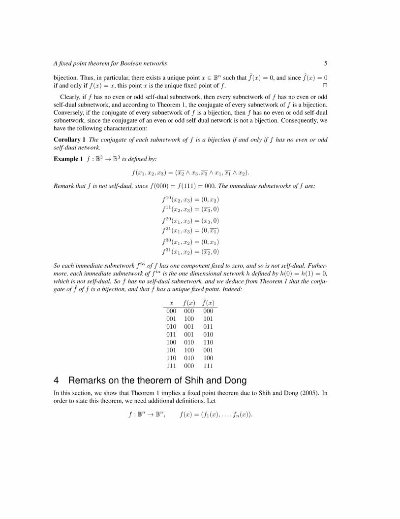
Example 1 f : B3 → B3 is defined by:
f(x1, x2, x3) = (x2 ∧ x3, x3 ∧ x1, x1 ∧ x2).
Remark that f is not self-dual, since f(000) = f(111) = 000. The immediate subnetworks of f are:
f10(x2, x3) = (0, x2)
f11(x2, x3) = (x3, 0)
f20(x1, x3) = (x3, 0)
f21(x1, x3) = (0, x1)
f30(x1, x2) = (0, x1)
f31(x1, x2) = (x2, 0)
So each immediate subnetwork f iα of f has one component fixed to zero, and so is not self-dual. Futher-more, each immediate subnetwork of f iα is the one dimensional network h defined by h(0) = h(1) = 0,which is not self-dual. So f has no self-dual subnetwork, and we deduce from Theorem 1 that the conju-gate of f of f is a bijection, and that f has a unique fixed point. Indeed:
x f(x) f(x)000 000 000001 100 101010 001 011011 001 010100 010 110101 100 001110 010 100111 000 111
4 Remarks on the theorem of Shih and DongIn this section, we show that Theorem 1 implies a fixed point theorem due to Shih and Dong (2005). Inorder to state this theorem, we need additional definitions. Let
f : Bn → Bn, f(x) = (f1(x), . . . , fn(x)).
6 Adrien Richard
Definition 5 (Discrete Jacobian matrix) The discrete Jacobian matrix of f evaluated at point x ∈ Bn isthe following n× n Boolean matrix
f ′(x) = (fij(x)), fij(x) = fi(xj1)⊕ fi(xj0) (i, j ∈ [n]).
In the next definition, we represent f ′(x) under the form of a directed graph, in order to use graphtheoretic notions instead of matrix theoretical notions. In fact, we mainly focus on elementary directedcycles, that we simply call cycles in the following.
Definition 6 (Local interaction graph) The local interaction graph of f evaluated at point x ∈ Bn is thedirected graph Gf(x) defined by: the vertex set is [n], and for all i, j ∈ [n], there exists an arc j → i ifand only if fij(x) = 1.
The discrete Jacobian matrix of f was first defined by Robert (1983), who also introduced the notionof Boolean eigenvalue. This material allowed Shih and Ho (1999) to state a combinatorial analog of theJacobian conjecture: if f has the property that, for each x ∈ Bn, all the boolean eigenvalues of f ′(x) arezero, then f has a unique fixed point. This conjecture was proved by Shih and Dong (2005). Since Robertproved that all the boolean eigenvalues of f ′(x) are zero if and only if Gf(x) has no cycle, the theoremof Shih and Dong can be stated as follows.
Theorem 2 (Shih and Dong (2005)) If Gf(x) has no cycle ∀x ∈ Bn, then f has a unique fixed point.
A short prove of this theorem, independent of Theorem 1, is given in appendix. In the following of thissection, we show, using Theorem 1, that the condition “if Gf(x) has no cycle for all x” can be weakenedinto a condition of the form “if there exists “few” point x such that Gf(x) has a “short” cycle”. Theexact statement is given after the following proposition.
Proposition 1 If f is even or odd, then for every x ∈ Bn the out-degree of each vertex of Gf(x) is odd.In particular, Gf(x) has a cycle.
Proof: The out-degree d+j of any vertex j of Gf(x), which equals the number of ones in the jth columnof f ′(x), is d+j = ||f(xj1)⊕ f(xj0)|| = ||f(x)⊕ f(x⊕ ej)||. Since
||f(x)⊕ f(x⊕ ej)|| = ||(x⊕ f(x))⊕ ((x⊕ ej)⊕ f(x⊕ ej))|| = ||f(x)⊕ f(x⊕ ej)⊕ ej ||,
the parity of d+j is the parity of ||f(x)|| + ||f(x ⊕ ej)|| + 1. Hence, if f is even or odd, then ||f(x)|| +||f(x⊕ ej)|| is even, and d+j is odd. 2
Corollary 2 (Extension of Shih-Dong’s fixed point theorem) If for k = 1, . . . , n, there exists at most2k − 1 points x ∈ Bn such that Gf(x) has a cycle of length at most k, then the conjugate of f is abijection. In particular, f has a unique fixed point.
Proof: According to Theorem 1, it is sufficient to prove, by induction on n, that if f satisfies the conditionsof the statement, then f has no even or odd self-dual subnetwork. The case n = 1 is obvious. Supposethat n > 1 and that f satisfies the conditions of the statement. Let i, j ∈ [n − 1]. For each x ∈ Bn suchthat xn = 0, we have
fn0ij (x−n) = fn0i (xj1−n)⊕ fn0i (xj0−n) = fi(xj1)⊕ fi(xj0) = fij(x).
A fixed point theorem for Boolean networks 7
SoGfn0(x−n) is the subgraph ofGf(x) induced by [n−1], and we deduce that fnα satisfies the conditionof the theorem (for every k ∈ [n− 1], there exists at most 2k − 1 points x ∈ Bn−1 such that Gfn0(x) hasa cycle of length at most k). Thus, by induction hypothesis, fn0 has no even or odd self-dual subnetwork.More generally, we prove with similar arguments, that for all i ∈ [n], f i0 and f i1 have no even or oddself-dual subnetwork. So f has no odd or even self-dual strict subnetwork. If f is itself even or oddself-dual, then by Proposition 1, Gf(x) has a cycle for every x ∈ Bn, so f does not satisfy that conditionsof the statement (for k = n). Therefore, f has no even or odd self-dual subnetwork. 2
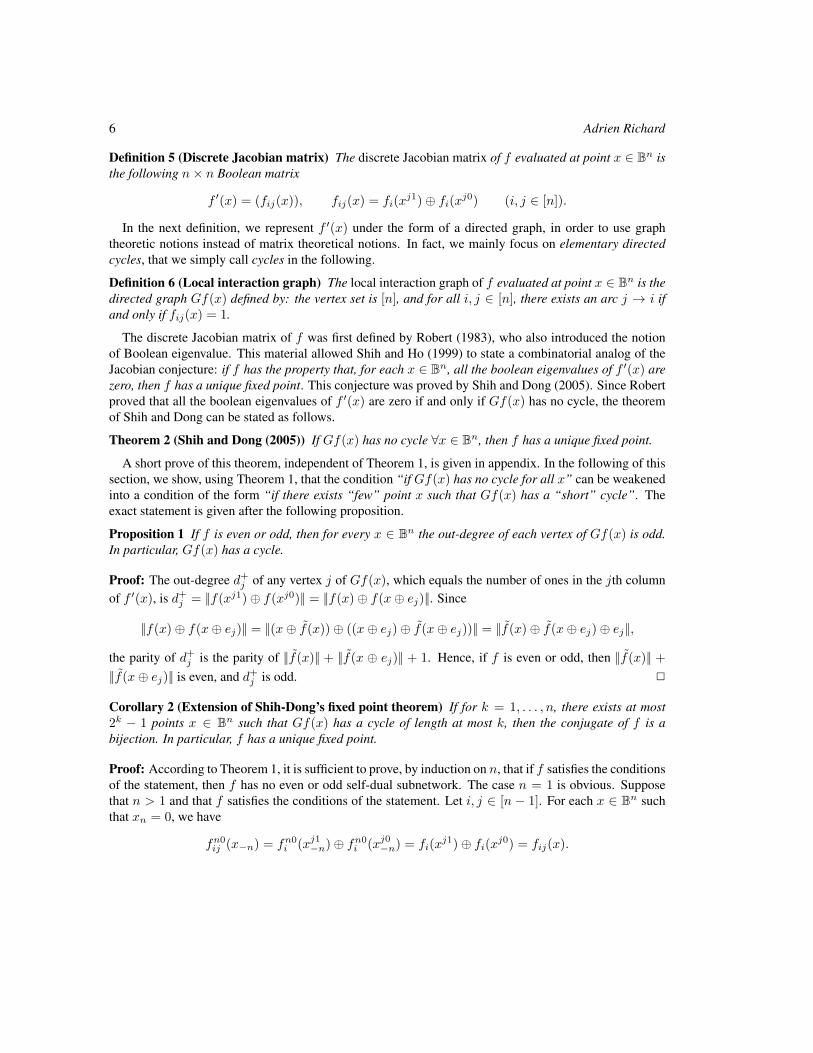
Example 2 (Continuation of Example 1) Take again
f(x1, x2, x3) = (x2 ∧ x3, x3 ∧ x1, x1 ∧ x2).
We have seen that f has no self-dual subnetwork. So it satisfies the conditions of Theorem 1, but not theconditions of Shih-Dong’s theorem, since Gf(000) and Gf(111) have a cycle:
x 000 001 010 011 100 101 110 111
Gf(x)
2
1
3 2
1
3 2
1
3 2
1
3 2
1
3 2
1
3 2
1
3 2
1
3
However, f satisfies the condition of Corollary 2 (there is 0 < 21 point x with a cycle of length at most 1;0 < 22 point x such that Gf(x) has a cycle of length at most 2, and 2 < 23 points x such that Gf(x) hasa cycle of length at most 3).
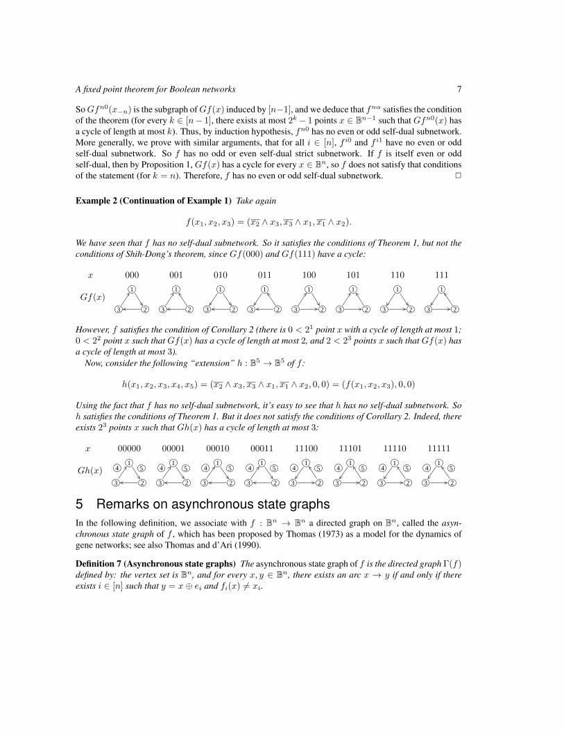
Now, consider the following “extension” h : B5 → B5 of f :
h(x1, x2, x3, x4, x5) = (x2 ∧ x3, x3 ∧ x1, x1 ∧ x2, 0, 0) = (f(x1, x2, x3), 0, 0)
Using the fact that f has no self-dual subnetwork, it’s easy to see that h has no self-dual subnetwork. Soh satisfies the conditions of Theorem 1. But it does not satisfy the conditions of Corollary 2. Indeed, thereexists 23 points x such that Gh(x) has a cycle of length at most 3:
x 00000 00001 00010 00011 11100 11101 11110 11111
Gh(x)
3
5
2
14
3
5
2
14
3
5
2
14
3
5
2
14
3
5
2
14
3
5
2
14
3
5
2
14
3
5
2
14
5 Remarks on asynchronous state graphsIn the following definition, we associate with f : Bn → Bn a directed graph on Bn, called the asyn-chronous state graph of f , which has been proposed by Thomas (1973) as a model for the dynamics ofgene networks; see also Thomas and d’Ari (1990).
Definition 7 (Asynchronous state graphs) The asynchronous state graph of f is the directed graph Γ(f)defined by: the vertex set is Bn, and for every x, y ∈ Bn, there exists an arc x → y if and only if thereexists i ∈ [n] such that y = x⊕ ei and fi(x) 6= xi.
8 Adrien Richard
Remark that Γ(f) and f share the same information. Remark also that for every i ∈ [n] and α ∈ B,Γ(f iα) is isomorphic to the subgraph of Γ(f) induced by the set of points x ∈ Bn such that xi = α.Indeed: for every x, y ∈ Bn,
x−i → y−i is an arc of Γ(f iα) ⇐⇒ ∃j 6= i such that y−i = x−i ⊕ ej and f iαj (x−i) 6= xj
⇐⇒ ∃j 6= i such that yiα = xiα ⊕ ej and fj(xiα) 6= xj
⇐⇒ xiα → yiα is an arc of Γ(f).(?)
Corollary 3 If f has no even or odd self-dual subnetwork, then f has a unique fixed point x, and for ally ∈ Bn, Γ(f) contains a directed path from y to x of length ||x⊕ y||.
By the definition of Γ(f), a path from x to y cannot be of length strictly less than ||x⊕ y||; a path fromx to y of length ||x⊕ y|| can thus be seen has a shortest path.
Proof of Corollary 3: by induction on n. The case n = 1 is obvious, so suppose that n > 1 and thatthe corollary holds for the dimensions less than n. Let f : Bn → Bn, and suppose that f has no even orodd self-dual subnetwork. By Theorem 1, f has a unique fixed point x. Let y ∈ Bn. Suppose first thatthere exists i ∈ [n] such that xi = yi = 0. Then x−i is the unique fixed point of f i0. So, by inductionhypothesis, Γ(f i0) has a path from y−i to x−i of length ||x−i⊕ y−i||. Since xi = yi = 0, we deduce from(?) that Γ(f) has a path from y to x of length ||x−i ⊕ y−i|| = ||x ⊕ y||. The case xi = yi = 1 is similar.So, finally, suppose that y = x⊕ 1. Since y is not a fixed point, there exists i ∈ [n] such that fi(y) 6= yi.Then, Γ(f) has an arc from y to z = y ⊕ ei. So zi = xi, and as previously, we deduce that Γ(f) has apath from z to x of length ||x ⊕ z||. This path together with the arc y → z forms a path from y to x oflength ||x⊕ z||+ 1 = ||x⊕ y||. 2
According to (?), the asynchronous state graph of each subnetwork of f is a subgraph of asynchronousstate graph of f induced by an hypercube contained in Bn. Hence, one can see the asynchronous stategraphs of the subnetworks of f as “dynamical modules” of asynchronous state graph of f . The previouscorollary shows that if f has no even or odd self-dual subnetwork, then the asynchronous state graph of fis “simple”: it describes a “weak convergence” toward a unique fixed point. An interpretation is then thatthe asynchronous state graphs of even and odd self-dual networks are “dynamical modules” thatare necessary for the “emergence” of “complex” asynchronous behaviors.
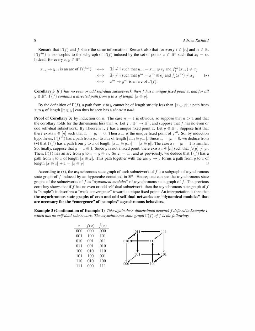
Example 3 (Continuation of Example 1) Take again the 3-dimensional network f defined in Example 1,which has no self-dual subnetwork. The asynchronous state graph Γ(f) of f is the following:
x f(x) f(x)000 000 000001 100 101010 001 011011 001 010100 010 110101 100 001110 010 100111 000 111
011 111
110
101001
100000
010
A fixed point theorem for Boolean networks 9
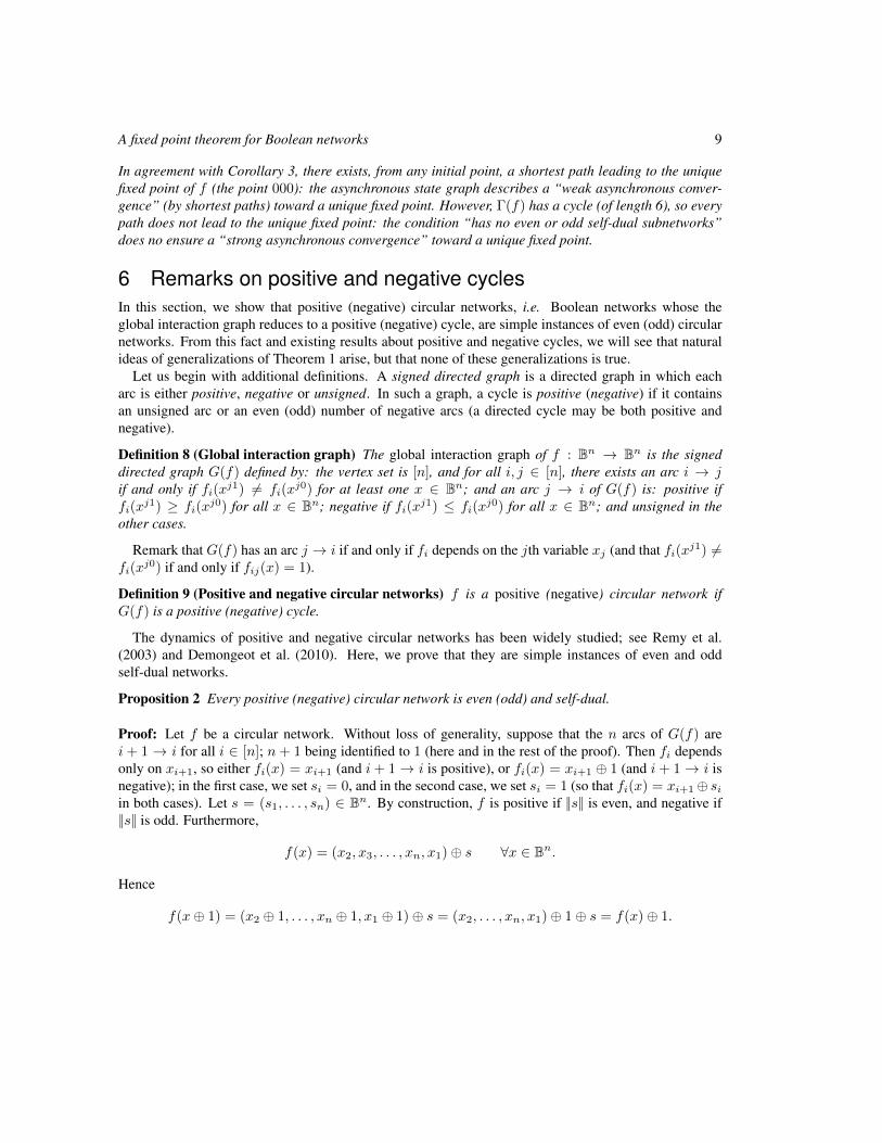
In agreement with Corollary 3, there exists, from any initial point, a shortest path leading to the uniquefixed point of f (the point 000): the asynchronous state graph describes a “weak asynchronous conver-gence” (by shortest paths) toward a unique fixed point. However, Γ(f) has a cycle (of length 6), so everypath does not lead to the unique fixed point: the condition “has no even or odd self-dual subnetworks”does no ensure a “strong asynchronous convergence” toward a unique fixed point.
6 Remarks on positive and negative cyclesIn this section, we show that positive (negative) circular networks, i.e. Boolean networks whose theglobal interaction graph reduces to a positive (negative) cycle, are simple instances of even (odd) circularnetworks. From this fact and existing results about positive and negative cycles, we will see that naturalideas of generalizations of Theorem 1 arise, but that none of these generalizations is true.
Let us begin with additional definitions. A signed directed graph is a directed graph in which eacharc is either positive, negative or unsigned. In such a graph, a cycle is positive (negative) if it containsan unsigned arc or an even (odd) number of negative arcs (a directed cycle may be both positive andnegative).
Definition 8 (Global interaction graph) The global interaction graph of f : Bn → Bn is the signeddirected graph G(f) defined by: the vertex set is [n], and for all i, j ∈ [n], there exists an arc i → jif and only if fi(xj1) 6= fi(x
j0) for at least one x ∈ Bn; and an arc j → i of G(f) is: positive iffi(x
j1) ≥ fi(xj0) for all x ∈ Bn; negative if fi(xj1) ≤ fi(x
j0) for all x ∈ Bn; and unsigned in theother cases.
Remark that G(f) has an arc j → i if and only if fi depends on the jth variable xj (and that fi(xj1) 6=fi(x
j0) if and only if fij(x) = 1).
Definition 9 (Positive and negative circular networks) f is a positive (negative) circular network ifG(f) is a positive (negative) cycle.
The dynamics of positive and negative circular networks has been widely studied; see Remy et al.(2003) and Demongeot et al. (2010). Here, we prove that they are simple instances of even and oddself-dual networks.
Proposition 2 Every positive (negative) circular network is even (odd) and self-dual.
Proof: Let f be a circular network. Without loss of generality, suppose that the n arcs of G(f) arei + 1 → i for all i ∈ [n]; n + 1 being identified to 1 (here and in the rest of the proof). Then fi dependsonly on xi+1, so either fi(x) = xi+1 (and i + 1 → i is positive), or fi(x) = xi+1 ⊕ 1 (and i+ 1 → i isnegative); in the first case, we set si = 0, and in the second case, we set si = 1 (so that fi(x) = xi+1⊕ siin both cases). Let s = (s1, . . . , sn) ∈ Bn. By construction, f is positive if ||s|| is even, and negative if||s|| is odd. Furthermore,
f(x) = (x2, x3, . . . , xn, x1)⊕ s ∀x ∈ Bn.
Hence
f(x⊕ 1) = (x2 ⊕ 1, . . . , xn ⊕ 1, x1 ⊕ 1)⊕ s = (x2, . . . , xn, x1)⊕ 1⊕ s = f(x)⊕ 1.
10 Adrien Richard
So f is self-dual. Also, we have f(x) = x ⊕ (x2, . . . , xn, x1) ⊕ s so the parity of f(x) is the parity of||x||+ ||(x2, . . . , xn, x1)||+ ||s||. Since ||x|| = ||(x2, . . . , xn, x1)||, we deduce that the parity of f(x) is theparity of ||s||. So if f is positive (negative) then the image of f only contains even (odd) points.
It remains to prove that if f is positive (negative) then each even (odd) point is in the image of f .Suppose that f is positive (negative), and let z be an even (odd) point of Bn. Let x ∈ Bn be recursivelydefined by
x1 = zn, xi+1 = zi ⊕ si ⊕ xi for all i ∈ [n− 1].
Then, for every i ∈ [n− 1], we have
fi(x) = xi ⊕ fi(x) = xi ⊕ xi+1 ⊕ si = xi ⊕ (zi ⊕ si ⊕ xi)⊕ si = zi.
If remains to prove that fn(x) = zn. By the definition of x, we have
xn = (zn−1 ⊕ sn−1)⊕ xn−1= (zn−1 ⊕ sn−1)⊕ (zn−2 ⊕ sn−2)⊕ xn−2...= (zn−1 ⊕ sn−1)⊕ (zn−2 ⊕ sn−2)⊕ · · · ⊕ (z1 ⊕ s1)⊕ zn= (z1 ⊕ z2 ⊕ · · · ⊕ zn)⊕ (s1 ⊕ s2 ⊕ · · · ⊕ sn−1).
So z and (s1, s2, . . . , sn−1, xn) have the same parity, and since z and s have the same parity, we deducethat xn = sn. Thus fn(x) = xn ⊕ fn(x) = sn ⊕ x1 ⊕ sn = x1 = zn, and we deduce that f(x) = z. Sof is even (odd) self-dual. 2
Remark 1 There are 2n−1! n-dimensional even (odd) self-dual networks, but “only” (n − 1)!2n−1 n-dimensional positive (negative) circular networks. Since 2n−1! = (n − 1)!2n−1 for n = 1, 2, we deducethat every one or two-dimensional even (odd) self-dual network is a positive (negative) circular network.
Since the class of positive and negative circular networks is contained in the class of even and odd self-dual networks, it is natural to think about the following generalization of Theorem 1: if f has no positiveor negative circular networks, then f has a unique fixed point. However, this is false, as showed by thefollowing example. Hence, Theorem 1 becomes false if “has no even or odd self-dual subnetwork” isreplaced by “has no positive or negative circular subnetwork”.
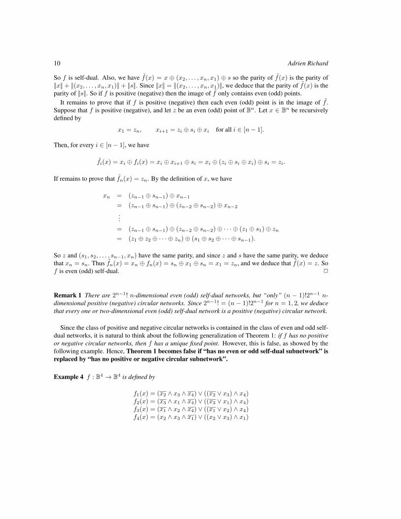
Example 4 f : B4 → B4 is defined by
f1(x) = (x2 ∧ x3 ∧ x4) ∨ ((x2 ∨ x3) ∧ x4)f2(x) = (x3 ∧ x1 ∧ x4) ∨ ((x3 ∨ x1) ∧ x4)f3(x) = (x1 ∧ x2 ∧ x4) ∨ ((x1 ∨ x2) ∧ x4)f4(x) = (x2 ∧ x3 ∧ x1) ∨ ((x2 ∨ x3) ∧ x1)
A fixed point theorem for Boolean networks 11
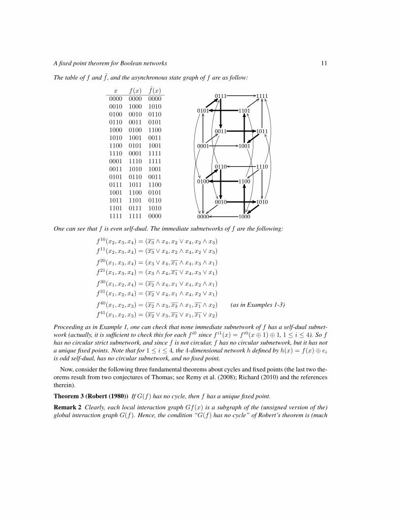
The table of f and f , and the asynchronous state graph of f are as follow:
x f(x) f(x)0000 0000 00000010 1000 10100100 0010 01100110 0011 01011000 0100 11001010 1001 00111100 0101 10011110 0001 11110001 1110 11110011 1010 10010101 0110 00110111 1011 11001001 1100 01011011 1101 01101101 0111 10101111 1111 0000 1000
0010 1010
0100
0110 1110
1100
0001
0101
0111 1111
1101
1011
1001
0011
0000
One can see that f is even self-dual. The immediate subnetworks of f are the following:
f10(x2, x3, x4) = (x3 ∧ x4, x2 ∨ x4, x2 ∧ x3)
f11(x2, x3, x4) = (x3 ∨ x4, x2 ∧ x4, x2 ∨ x3)
f20(x1, x3, x4) = (x3 ∨ x4, x1 ∧ x4, x3 ∧ x1)
f21(x1, x3, x4) = (x3 ∧ x4, x1 ∨ x4, x3 ∨ x1)
f30(x1, x2, x4) = (x2 ∧ x4, x1 ∨ x4, x2 ∧ x1)
f31(x1, x2, x4) = (x2 ∨ x4, x1 ∧ x4, x2 ∨ x1)
f40(x1, x2, x3) = (x2 ∧ x3, x3 ∧ x1, x1 ∧ x2) (as in Examples 1-3)f41(x1, x2, x3) = (x2 ∨ x3, x3 ∨ x1, x1 ∨ x2)
Proceeding as in Example 1, one can check that none immediate subnetwork of f has a self-dual subnet-work (actually, it is sufficient to check this for each f i0 since f i1(x) = f i0(x⊕ 1)⊕ 1, 1 ≤ i ≤ 4). So fhas no circular strict subnetwork, and since f is not circular, f has no circular subnetwork, but it has nota unique fixed points. Note that for 1 ≤ i ≤ 4, the 4-dimensional network h defined by h(x) = f(x)⊕ eiis odd self-dual, has no circular subnetwork, and no fixed point.
Now, consider the following three fundamental theorems about cycles and fixed points (the last two the-orems result from two conjectures of Thomas; see Remy et al. (2008); Richard (2010) and the referencestherein).
Theorem 3 (Robert (1980)) If G(f) has no cycle, then f has a unique fixed point.
Remark 2 Clearly, each local interaction graph Gf(x) is a subgraph of the (unsigned version of the)global interaction graph G(f). Hence, the condition “G(f) has no cycle” of Robert’s theorem is (much
12 Adrien Richard
more) stronger than the condition “Gf(x) has no cycle for every x” of Shih-Dong’s Theorem. Conse-quently, Shih-Dong’s theorem is a generalization of Robert’s theorem. Thus, Theorem 1 is also a general-ization of Robert’s theorem.
Remark 3 Actually, Robert proved, in Robert (1980) and Robert (1995), that if G(f) has no cycle, thenf has a unique fixed point x and: (1) the synchronous iteration xt+1 = f(xt) converges toward x inat most n steps for every initial point x0 ∈ Bn; (2) every path of Γ(f) leads to x in at most n steps(“strong asynchronous convergence by shortest paths toward a unique fixed points”). These results showsthe necessity of cycles for obtaining “complex” synchronous or asynchronous behaviors (e.g. multiplefixed points, cyclic attractors, long transient phases...).
Theorem 4 (Remy et al. (2008)) If G(f) has no positive cycle, then f has at most one fixed point.
Remark 4 Actually, by saying that an arc j → i of Gf(x) is positive if fi(xj1) > fi(xj0) and negative
if fi(xj1) < fi(xj0), Remy et al. (2008) proved the following more general statement: if Gf(x) has no
positive cycle for all x ∈ Bn, then f has at most one fixed point.
Theorem 5 (Richard (2010)) If G(f) has no negative cycle, then f has at least one fixed point.
Hence, Theorems 4 and 5 give a nice proof “by dichotomy” of Robert’s theorem: the absence of posi-tive cycle gives the uniqueness, and absence of negative cycle gives the existence. Seeing the relationshipbetween positive (negative) circular networks and even (odd) self-dual networks, one may ask if a “proofby dichotomy” occurs for Theorem 1, i.e., if the absence of even self-dual subnetwork gives the unique-ness, and if the absence of odd self-dual network gives the existence. The following example shows thatboth cases are false. Hence: if f has no even (odd) self-dual subnetworks, than it has not necessarilyat most (at least) one fixed point.
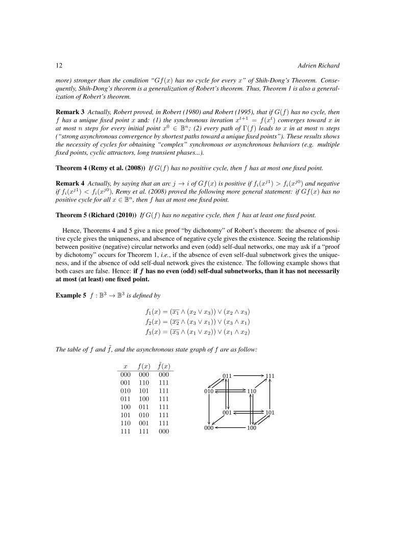
Example 5 f : B3 → B3 is defined by
f1(x) = (x1 ∧ (x2 ∨ x3)) ∨ (x2 ∧ x3)
f2(x) = (x2 ∧ (x3 ∨ x1)) ∨ (x3 ∧ x1)
f3(x) = (x3 ∧ (x1 ∨ x2)) ∨ (x1 ∧ x2)
The table of f and f , and the asynchronous state graph of f are as follow:
x f(x) f(x)000 000 000001 110 111010 101 111011 100 111100 011 111101 010 111110 001 111111 111 000
011 111
110
101001
100000
010
A fixed point theorem for Boolean networks 13
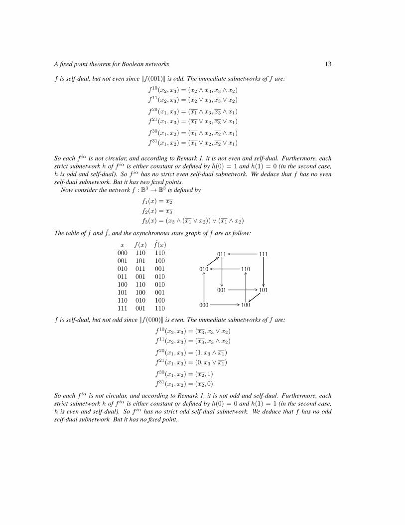
f is self-dual, but not even since ||f(001)|| is odd. The immediate subnetworks of f are:
f10(x2, x3) = (x2 ∧ x3, x3 ∧ x2)
f11(x2, x3) = (x2 ∨ x3, x3 ∨ x2)
f20(x1, x3) = (x1 ∧ x3, x3 ∧ x1)
f21(x1, x3) = (x1 ∨ x3, x3 ∨ x1)
f30(x1, x2) = (x1 ∧ x2, x2 ∧ x1)
f31(x1, x2) = (x1 ∨ x2, x2 ∨ x1)
So each f iα is not circular, and according to Remark 1, it is not even and self-dual. Furthermore, eachstrict subnetwork h of f iα is either constant or defined by h(0) = 1 and h(1) = 0 (in the second case,h is odd and self-dual). So f iα has no strict even self-dual subnetwork. We deduce that f has no evenself-dual subnetwork. But it has two fixed points.
Now consider the network f : B3 → B3 is defined by
f1(x) = x2
f2(x) = x3
f3(x) = (x3 ∧ (x1 ∨ x2)) ∨ (x1 ∧ x2)
The table of f and f , and the asynchronous state graph of f are as follow:
x f(x) f(x)000 110 110001 101 100010 011 001011 001 010100 110 010101 100 001110 010 100111 001 110
011 111
110
101001
100000
010
f is self-dual, but not odd since ||f(000)|| is even. The immediate subnetworks of f are:
f10(x2, x3) = (x3, x3 ∨ x2)
f11(x2, x3) = (x3, x3 ∧ x2)
f20(x1, x3) = (1, x3 ∧ x1)
f21(x1, x3) = (0, x3 ∨ x1)
f30(x1, x2) = (x2, 1)
f31(x1, x2) = (x2, 0)
So each f iα is not circular, and according to Remark 1, it is not odd and self-dual. Furthermore, eachstrict subnetwork h of f iα is either constant or defined by h(0) = 0 and h(1) = 1 (in the second case,h is even and self-dual). So f iα has no strict odd self-dual subnetwork. We deduce that f has no oddself-dual subnetwork. But it has no fixed point.
14 Adrien Richard
AcknowledgementsI wish to thank Julie Boyon and Sebastien Brun for interesting discussions. This work has been partiallysupported by the French National Agency for Reasearch (ANR-10-BLANC-0218 BioTempo project).
A A short proof of the theorem of Shih and DongThe “trick” consists in proving, by induction on n, the following more general statement:
(∗) If Gf(x) has no cycle for all x ∈ Bn, then the conjugate of f is a bijection (so that f hasa unique fixed point).
The case n = 1 is obvious, so suppose that n > 1 and that (∗) holds for the dimensions less than n.Suppose that Gf(x) has no cycle for all x ∈ Bn. Let i, j ∈ [n − 1], and x ∈ Bn such that xn = 0. Wehave
fn0ij (x−n) = fn0i (xj1−n)⊕ fn0i (xj0−n) = fi(xj1)⊕ fi(xj0) = fij(x).
So Gfn0(x−n) is the subgraph of Gf(x) induced by [n − 1], and thus, it has no cycle. We deduce thatfn0 satisfies the conditions of (∗). Thus, by induction hypothesis, the conjugate of fn0 is a bijection. Weprove with similar arguments that f i0 and f i1 are bijections for all i ∈ [n].
Now, suppose, by contradiction, that f is not a bijection. Then, there exists two distinct points x, y ∈ Bnsuch that f(x) = f(y). Let us proved that x = y ⊕ 1. Indeed, if xi = yi = α for some i ∈ [n], thenf iα(x−i) = f(x)−i = f(y)−i = f iα(y−i). Thus f iα is not a bijection, a contradiction. So x = y ⊕ 1.Since Gf(x) has no cycle, it contains at least one vertex of out-degree 0. In other words, there existsi ∈ [n] such that f(xi1) = f(xi0). Thus f(xi1)−i = f(xi0)−i = f(x)−i. Hence, setting α = yi, weobtain
f iα(x−i) = f(xiα)−i = f(x)−i = f(y)−i = f(yi1)−i = f i1(y−i).
So f iα is not a bijection, a contradiction. Thus f is a bijection and (∗) is proved.
ReferencesJ. Demongeot, M. Noual, and S. Sene. On the number of attractors of positive and negative Boolean
automata circuits. In Proceedings of WAINA’10, pages 782–789. IEEE press, 2010.
S. A. Kauffman. Metabolic stability and epigenesis in randomly connected nets. Journal of TheoreticalBiology, 22:437–467, 1969.
E. Remy, B. Mosse, C. Chaouiya, and D. Thieffry. A description of dynamical graphs associated toelementary regulatory circuits. Bioinformatics, 19:172–178, 2003.
E. Remy, P. Ruet, and D. Thieffry. Graphic requirements for multistability and attractive cycles in aboolean dynamical framework. Advances in Applied Mathematics, 41(3):335 – 350, 2008. ISSN 0196-8858.
A. Richard. Negative circuits and sustained oscillations in asynchronous automata networks. Advances inApplied Mathematics, 44(4):378 – 392, 2010. ISSN 0196-8858.
A fixed point theorem for Boolean networks 15
F. Robert. Iterations sur des ensembles finis et automates cellulaires contractants. Linear Algebra and itsApplications, 29:393–412, 1980.
F. Robert. Derivee discrete et convergence locale d’une iteration Booleenne. Linear Algebra Appl., 52:547–589, 1983.
F. Robert. Les systemes dynamiques discrets, volume 19 of Mathematiques et Applications. Springer,1995.
M.-H. Shih and J.-L. Dong. A combinatorial analogue of the Jacobian problem in automata networks.Advances in Applied Mathematics, 34:30–46, 2005.
M.-H. Shih and J.-L. Ho. Solution of the Boolean Markus-Yamabe problem. Advances in Applied Math-ematics, 22:60–102, 1999.
R. Thomas. Boolean formalization of genetic control circuits. Journal of Theoretical Biology, 42(3):563– 585, 1973. ISSN 0022-5193.
R. Thomas and R. d’Ari. Biological Feedback. CRC Press, 1990.

16 Adrien Richard
AUTOMATA 2011, Santiago, Chile local proceedings LP, 2011, 17–28
Characterization of non-uniform numberconserving cellular automata
Sukanta Das†
Department of Information Technology, Bengal Engineering and Science University, Shibpur, India
This paper characterizes the one dimensional two-state 3-neighborhood non-uniform (hybrid) number conservingcellular automata (NCCA). The reachability tree is utilized to do such characterization. The paper has developed a setof theorems targeting the characterization of the NCCA. An algorithm of O(n) time is developed to verify whetherCA with n cells are NCCA. Finally, another algorithm is designed that synthesizes NCCA with given number of cells.
Keywords: Number conserving cellular automata (NCCA), hybrid CA, rule min term (RMT), reachability tree
I IntroductionThe number conserving cellular automata (NCCA) in one dimensional two-state 3-neighborhood depen-dency are the cellular automata (CA) where the number of 1s (0s) of initial configuration is preserved dur-ing the evolution of the CA. Due to their similarity with the physical law of conservation, the NCCA havereceived a wide attention of the researchers in last two decades [HT91, BF98, BF02, DFR03]. The majorapplication area of NCCA is the development of highway traffic models [NS92, FI96, DSS09, Das11].
A few of the pioneering works are due to Boccara and Fuks who gave necessary and sufficient condi-tions for one-dimensional CA to be NCCA [BF98, BF02]. The computational universality, decidability,reversibility and other properties of NCCA also have been studied [DFR03, MI98]. However, all theworks focus on uniform cellular automata, where all the cells are assumed to obey same transition rule.The characterization of non-uniform or hybrid NCCA is not addressed till date. In non-uniform or hybridNCCA, different cells may follow different rules. This work targets such characterization.
To identify the characteristics of non-uniform NCCA, we utilize the reachability tree which was pro-posed as a tool for characterizing CA [DS09]. We present a set of theorems and corollaries to characterizereachability tree for NCCA. Based on such characterization, we develop a linear time algorithm to verifywhether given CA are NCCA. Finally, an algorithm to synthesize NCCA is reported.
The paper is organized as follows. The preliminaries of CA and reachability tree are noted in the nextsection. Section III characterizes the reachability tree for NCCA. Finally, the algorithms are presented inSection IV. Section V concludes the paper.
†This work is supported by AICTE Career Award fund (F.No. 1-51/RID/CA/29/2009-10), awarded to the author. Email:[email protected]
c© 2011 AUTOMATA proceedings, Santiago, Chile, 2011
18 Sukanta Das
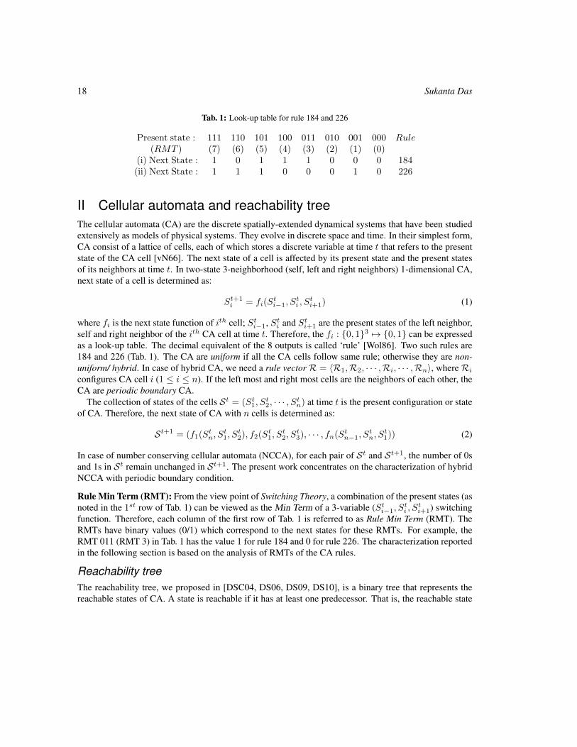
Tab. 1: Look-up table for rule 184 and 226
Present state : 111 110 101 100 011 010 001 000 Rule(RMT ) (7) (6) (5) (4) (3) (2) (1) (0)
(i) Next State : 1 0 1 1 1 0 0 0 184(ii) Next State : 1 1 1 0 0 0 1 0 226
II Cellular automata and reachability treeThe cellular automata (CA) are the discrete spatially-extended dynamical systems that have been studiedextensively as models of physical systems. They evolve in discrete space and time. In their simplest form,CA consist of a lattice of cells, each of which stores a discrete variable at time t that refers to the presentstate of the CA cell [vN66]. The next state of a cell is affected by its present state and the present statesof its neighbors at time t. In two-state 3-neighborhood (self, left and right neighbors) 1-dimensional CA,next state of a cell is determined as:
St+1i = fi(S
ti−1, S
ti , S
ti+1) (1)
where fi is the next state function of ith cell; Sti−1, St
i and Sti+1 are the present states of the left neighbor,
self and right neighbor of the ith CA cell at time t. Therefore, the fi : 0, 13 7→ 0, 1 can be expressedas a look-up table. The decimal equivalent of the 8 outputs is called ‘rule’ [Wol86]. Two such rules are184 and 226 (Tab. 1). The CA are uniform if all the CA cells follow same rule; otherwise they are non-uniform/ hybrid. In case of hybrid CA, we need a rule vectorR = 〈R1,R2, · · · ,Ri, · · · ,Rn〉, whereRi
configures CA cell i (1 ≤ i ≤ n). If the left most and right most cells are the neighbors of each other, theCA are periodic boundary CA.
The collection of states of the cells St = (St1, S
t2, · · · , St
n) at time t is the present configuration or stateof CA. Therefore, the next state of CA with n cells is determined as:
St+1 = (f1(Stn, S
t1, S
t2), f2(S
t1, S
t2, S
t3), · · · , fn(St
n−1, Stn, S
t1)) (2)
In case of number conserving cellular automata (NCCA), for each pair of St and St+1, the number of 0sand 1s in St remain unchanged in St+1. The present work concentrates on the characterization of hybridNCCA with periodic boundary condition.
Rule Min Term (RMT): From the view point of Switching Theory, a combination of the present states (asnoted in the 1st row of Tab. 1) can be viewed as the Min Term of a 3-variable (St
i−1, Sti , S
ti+1) switching
function. Therefore, each column of the first row of Tab. 1 is referred to as Rule Min Term (RMT). TheRMTs have binary values (0/1) which correspond to the next states for these RMTs. For example, theRMT 011 (RMT 3) in Tab. 1 has the value 1 for rule 184 and 0 for rule 226. The characterization reportedin the following section is based on the analysis of RMTs of the CA rules.
Reachability treeThe reachability tree, we proposed in [DSC04, DS06, DS09, DS10], is a binary tree that represents thereachable states of CA. A state is reachable if it has at least one predecessor. That is, the reachable state
Characterization of non-uniform NCCA 19
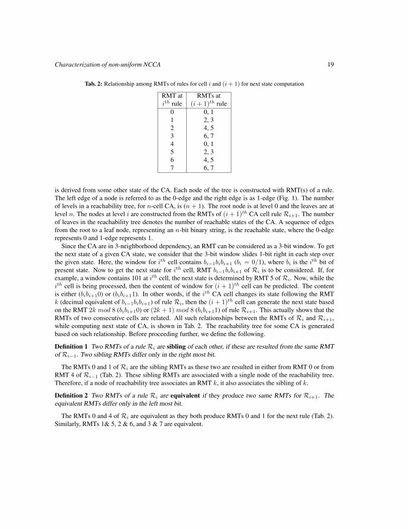
Tab. 2: Relationship among RMTs of rules for cell i and (i+ 1) for next state computation
RMT at RMTs atith rule (i+ 1)th rule
0 0, 11 2, 32 4, 53 6, 74 0, 15 2, 36 4, 57 6, 7
is derived from some other state of the CA. Each node of the tree is constructed with RMT(s) of a rule.The left edge of a node is referred to as the 0-edge and the right edge is as 1-edge (Fig. 1). The numberof levels in a reachability tree, for n-cell CA, is (n + 1). The root node is at level 0 and the leaves are atlevel n. The nodes at level i are constructed from the RMTs of (i+ 1)th CA cell ruleRi+1. The numberof leaves in the reachability tree denotes the number of reachable states of the CA. A sequence of edgesfrom the root to a leaf node, representing an n-bit binary string, is the reachable state, where the 0-edgerepresents 0 and 1-edge represents 1.
Since the CA are in 3-neighborhood dependency, an RMT can be considered as a 3-bit window. To getthe next state of a given CA state, we consider that the 3-bit window slides 1-bit right in each step overthe given state. Here, the window for ith cell contains bi−1bibi+1 (bi = 0/1), where bi is the ith bit ofpresent state. Now to get the next state for ith cell, RMT bi−1bibi+1 of Ri is to be considered. If, forexample, a window contains 101 at ith cell, the next state is determined by RMT 5 ofRi. Now, while theith cell is being processed, then the content of window for (i + 1)th cell can be predicted. The contentis either (bibi+10) or (bibi+11). In other words, if the ith CA cell changes its state following the RMTk (decimal equivalent of bi−1bibi+1) of rule Ri, then the (i + 1)th cell can generate the next state basedon the RMT 2k mod 8 (bibi+10) or (2k + 1) mod 8 (bibi+11) of rule Ri+1. This actually shows that theRMTs of two consecutive cells are related. All such relationships between the RMTs of Ri and Ri+1,while computing next state of CA, is shown in Tab. 2. The reachability tree for some CA is generatedbased on such relationship. Before proceeding further, we define the following.
Definition 1 Two RMTs of a rule Ri are sibling of each other, if these are resulted from the same RMTofRi−1. Two sibling RMTs differ only in the right most bit.
The RMTs 0 and 1 ofRi are the sibling RMTs as these two are resulted in either from RMT 0 or fromRMT 4 of Ri−1 (Tab. 2). These sibling RMTs are associated with a single node of the reachability tree.Therefore, if a node of reachability tree associates an RMT k, it also associates the sibling of k.
Definition 2 Two RMTs of a rule Ri are equivalent if they produce two same RMTs for Ri+1. Theequivalent RMTs differ only in the left most bit.
The RMTs 0 and 4 of Ri are equivalent as they both produce RMTs 0 and 1 for the next rule (Tab. 2).Similarly, RMTs 1& 5, 2 & 6, and 3 & 7 are equivalent.
20 Sukanta Das
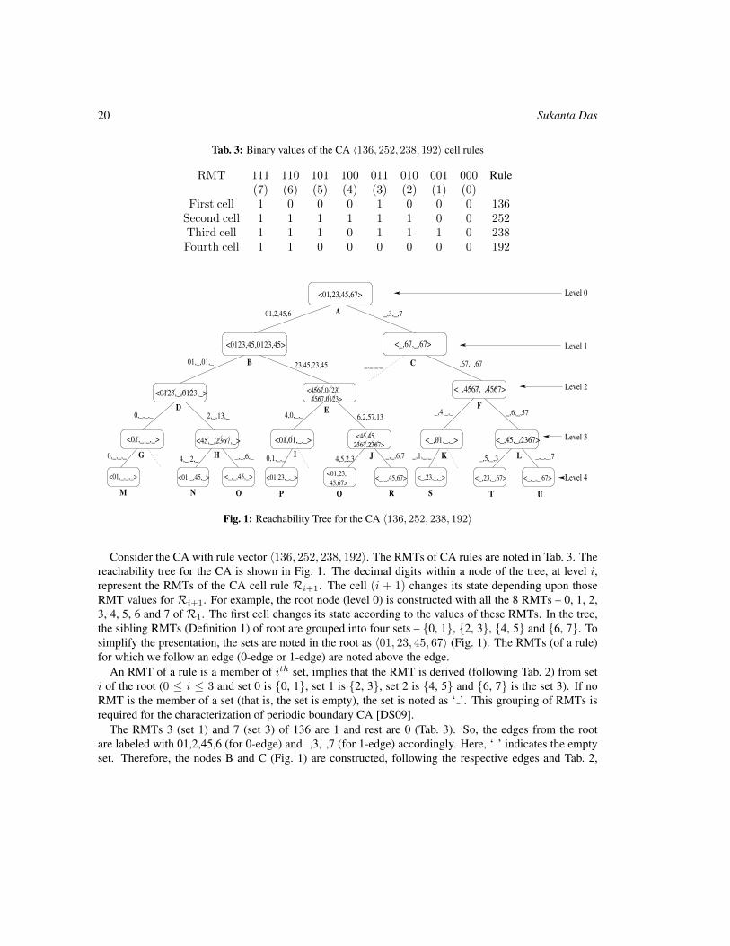
Tab. 3: Binary values of the CA 〈136, 252, 238, 192〉 cell rules
RMT 111 110 101 100 011 010 001 000 Rule(7) (6) (5) (4) (3) (2) (1) (0)
First cell 1 0 0 0 1 0 0 0 136Second cell 1 1 1 1 1 1 0 0 252Third cell 1 1 1 0 1 1 1 0 238Fourth cell 1 1 0 0 0 0 0 0 192
<01,23,45,67>
<0123,45,0123,45> <_,67,_,67>
<_,4567,_,4567>
<_,45,_,2367><_,01,_,_><01,01,_,_><01,_,_,_>
<4567,0123,
4567,0123>
<45,45,
2367,2367>
<01,_,_,_> <01,_,45,_> <01,23,_,_><01,23,
45,67><_,_,45,67> <_,23,_,_> <_,23,_,67> <_,_,_,67><_,_,45,_>
<0123,_,0123,_>
<45,_,2367,_>
EF
G H
P Q
A
B C
T UR SO
LKJI
D
M N
01,2,45,6 _,3,_,7
_,67,_,67_,_,_,_
2,_,13,_ 4,0,_,_ 6,2,57,13_,4,_,_ _,6,_,57
_,_,_,7_,5,_,34,5,2,30,1,_,__,_,6,_
0,_,_,_
0,_,_,_ _,1,_,__,_,6,74,_,2,_
23,45,23,4501,_,01,_
Level 0
Level 1
Level 2
Level 3
Level 4
Fig. 1: Reachability Tree for the CA 〈136, 252, 238, 192〉
Consider the CA with rule vector 〈136, 252, 238, 192〉. The RMTs of CA rules are noted in Tab. 3. Thereachability tree for the CA is shown in Fig. 1. The decimal digits within a node of the tree, at level i,represent the RMTs of the CA cell rule Ri+1. The cell (i + 1) changes its state depending upon thoseRMT values for Ri+1. For example, the root node (level 0) is constructed with all the 8 RMTs – 0, 1, 2,3, 4, 5, 6 and 7 of R1. The first cell changes its state according to the values of these RMTs. In the tree,the sibling RMTs (Definition 1) of root are grouped into four sets – 0, 1, 2, 3, 4, 5 and 6, 7. Tosimplify the presentation, the sets are noted in the root as 〈01, 23, 45, 67〉 (Fig. 1). The RMTs (of a rule)for which we follow an edge (0-edge or 1-edge) are noted above the edge.
An RMT of a rule is a member of ith set, implies that the RMT is derived (following Tab. 2) from seti of the root (0 ≤ i ≤ 3 and set 0 is 0, 1, set 1 is 2, 3, set 2 is 4, 5 and 6, 7 is the set 3). If noRMT is the member of a set (that is, the set is empty), the set is noted as ‘ ’. This grouping of RMTs isrequired for the characterization of periodic boundary CA [DS09].
The RMTs 3 (set 1) and 7 (set 3) of 136 are 1 and rest are 0 (Tab. 3). So, the edges from the rootare labeled with 01,2,45,6 (for 0-edge) and ,3, ,7 (for 1-edge) accordingly. Here, ‘ ’ indicates the emptyset. Therefore, the nodes B and C (Fig. 1) are constructed, following the respective edges and Tab. 2,
Characterization of non-uniform NCCA 21
with 〈0123, 45, 0123, 45〉 and 〈 , 67, , 67〉 respectively. However, there is only a single edge from nodeC which derives the child node F. The dotted edge indicates that no RMT of node C (for rule 252) canderive its 0-edge. Hence, the CA states begin with 10 are non-reachable. There are 9 leaf nodes of Fig. 1,so the CA have 9 reachable states.
A number of RMTs are dropped from the nodes at level (n − 2) (level 2 of Fig. 1) and level (n − 1) –that is, level 3 of Fig. 1. The RMTs of the nodes at level (n − 2) correspond to the CA cell rule Rn−1.The RMTs of set 0 and set 1 assume that the cell n is always 0 while we compute the next state, whereasthe RMTs of set 2 and set 3 assume that the cell n is always 1. Therefore, odd RMTs of set 0 and set 1,and even RMTs of set 2 and set 3 are invalid, and so striked out. For example, RMTs 1 and 3 from set 0,and RMTs 0 and 2 from set 2 in node D are striked out. Similarly, the RMTs of the nodes at level (n− 1)correspond to the CA cell ruleRn. Therefore, the RMTs of set 0 forRn (at level (n−1)) have to generatethe set 0 forR1, since next to the last cell is the first cell. The set 0 for the first cell contains always RMTs0 and 1. However, few RMTs of set 0 at level (n − 1) may not generate RMT 0 and 1 for R1, these aremarked as invalid, and striked out. Similar actions are taken for other sets. In node G (Fig. 1), RMT 1 ofset 0 is striked out as it can not generate set 0 forR1 (0, 1).
We next characterize such reachability tree to get characterization of NCCA.
III Characterization of reachability tree for NCCAThis section characterizes the reachability tree that represents number conserving cellular automata (NCCA).We identify here the required properties of the tree so that the corresponding CA can be NCCA. To facil-itate our further discussion, we define the following.
Definition 3 A sequence of n RMTs those derive a reachable state of CA with n cells is called the RMTsequence (RS).
For example, 〈4012〉 is an RMT sequence (RS). In Fig. 1, this RS derives the state 0010. RMT 4 of rule136 is associated with 0-edge from the root. Similarly, RMTs 0, 1 and 4 of the rules 252, 238 and 192 areassociated with 0-, 1- and 0-edges from nodes B, D and H respectively. 0001 is the previous state of 0010.It can be noted that the middle bits of the RMTs 4, 0, 1 and 2 are 0, 0, 0 and 1. Hence, the RS 〈4012〉corresponds to the state 0001, and derives the state 0010. In the reachability tree, the reachable states areassociated with corresponding RSs. However, one reachable state may be derived from two or more RSs.For example, state 0010 of Fig. 1 is derived from 〈4012〉 as well as from 〈0124〉.
Theorem 1 : The CA are NCCA if and only if the number of 1s (0s) of each RS remains unchanged inthe reachable state derived from the RS.
Proof: The pair of an RS and its derived state forms actually a pair of present state and next state (or,previous state and present state) of CA. To be NCCA, the number of 1s (0s) in a present state of each suchpair has to be equal with that of the next state. Hence the proof. 2
Following result can be derived from the Theorem 1.
Corollary 1 : All-0 and all-1 states in NCCA are reachable and derived only from RS 〈00 · · · 0〉 and〈77 · · · 7〉 respectively.
22 Sukanta Das
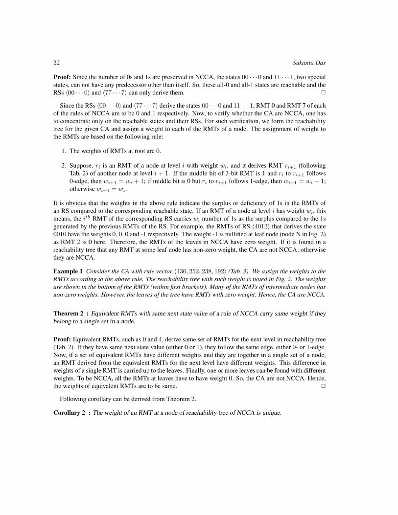
Proof: Since the number of 0s and 1s are preserved in NCCA, the states 00 · · · 0 and 11 · · · 1, two specialstates, can not have any predecessor other than itself. So, these all-0 and all-1 states are reachable and theRSs 〈00 · · · 0〉 and 〈77 · · · 7〉 can only derive them. 2
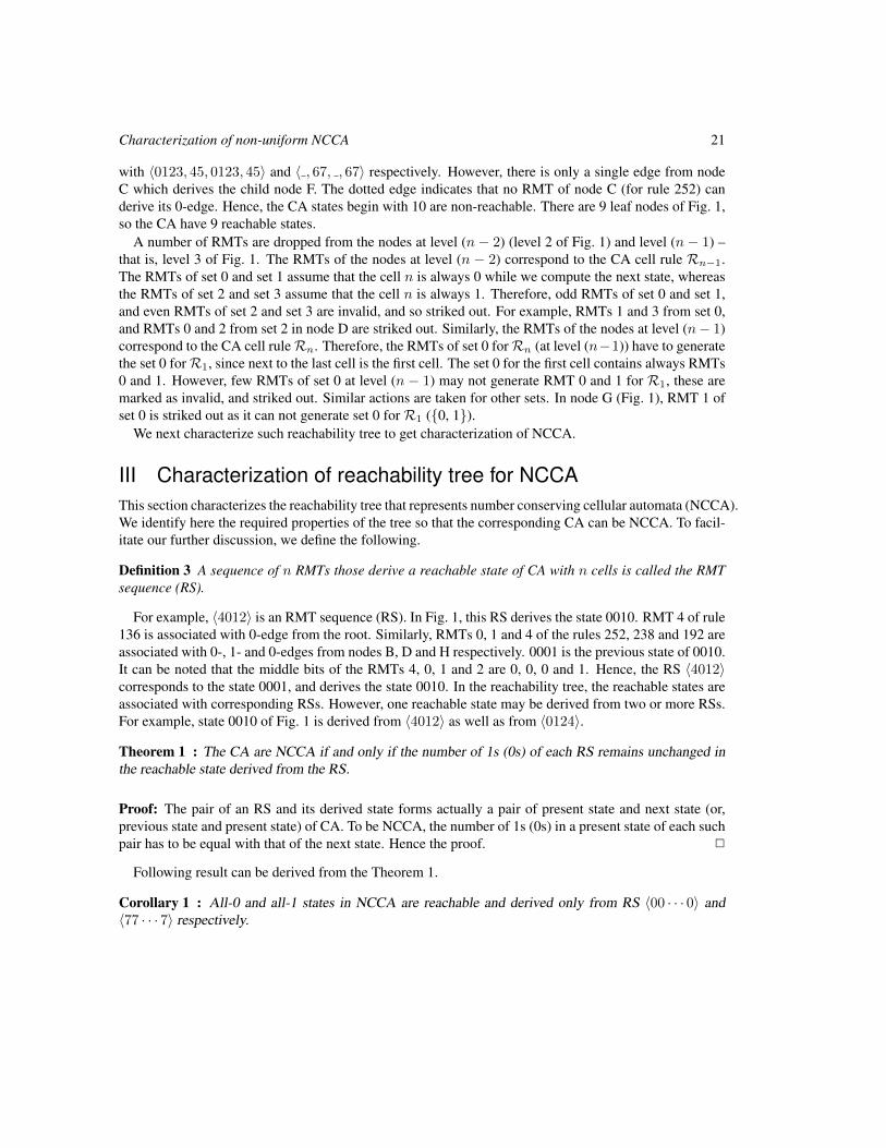
Since the RSs 〈00 · · · 0〉 and 〈77 · · · 7〉 derive the states 00 · · · 0 and 11 · · · 1, RMT 0 and RMT 7 of eachof the rules of NCCA are to be 0 and 1 respectively. Now, to verify whether the CA are NCCA, one hasto concentrate only on the reachable states and their RSs. For such verification, we form the reachabilitytree for the given CA and assign a weight to each of the RMTs of a node. The assignment of weight tothe RMTs are based on the following rule:
1. The weights of RMTs at root are 0.
2. Suppose, ri is an RMT of a node at level i with weight wi, and it derives RMT ri+1 (followingTab. 2) of another node at level i + 1. If the middle bit of 3-bit RMT is 1 and ri to ri+1 follows0-edge, then wi+1 = wi + 1; if middle bit is 0 but ri to ri+1 follows 1-edge, then wi+1 = wi − 1;otherwise wi+1 = wi.
It is obvious that the weights in the above rule indicate the surplus or deficiency of 1s in the RMTs ofan RS compared to the corresponding reachable state. If an RMT of a node at level i has weight wi, thismeans, the ith RMT of the corresponding RS carries wi number of 1s as the surplus compared to the 1sgenerated by the previous RMTs of the RS. For example, the RMTs of RS 〈4012〉 that derives the state0010 have the weights 0, 0, 0 and -1 respectively. The weight -1 is nullified at leaf node (node N in Fig. 2)as RMT 2 is 0 here. Therefore, the RMTs of the leaves in NCCA have zero weight. If it is found in areachability tree that any RMT at some leaf node has non-zero weight, the CA are not NCCA; otherwisethey are NCCA.
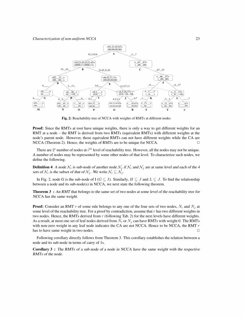
Example 1 Consider the CA with rule vector 〈136, 252, 238, 192〉 (Tab. 3). We assign the weights to theRMTs according to the above rule. The reachability tree with such weight is noted in Fig. 2. The weightsare shown in the bottom of the RMTs (within first brackets). Many of the RMTs of intermediate nodes hasnon-zero weights. However, the leaves of the tree have RMTs with zero weight. Hence, the CA are NCCA.
Theorem 2 : Equivalent RMTs with same next state value of a rule of NCCA carry same weight if theybelong to a single set in a node.
Proof: Equivalent RMTs, such as 0 and 4, derive same set of RMTs for the next level in reachability tree(Tab. 2). If they have same next state value (either 0 or 1), they follow the same edge, either 0- or 1-edge.Now, if a set of equivalent RMTs have different weights and they are together in a single set of a node,an RMT derived from the equivalent RMTs for the next level have different weights. This difference inweights of a single RMT is carried up to the leaves. Finally, one or more leaves can be found with differentweights. To be NCCA, all the RMTs at leaves have to have weight 0. So, the CA are not NCCA. Hence,the weights of equivalent RMTs are to be same. 2
Following corollary can be derived from Theorem 2.
Corollary 2 : The weight of an RMT at a node of reachability tree of NCCA is unique.
Characterization of non-uniform NCCA 23
EF
G H
P Q
A
B C
T UR SO
LKJI
D
M N
01,2,45,6 _,3,_,7
_,67,_,67
2,_,13,_ 4,0,_,_ 6,2,57,13_,4,_,_ _,6,_,57
_,_,_,7_,5,_,34,5,2,30,1,_,__,_,6,_
0,_,_,_
0,_,_,_ _,1,_,__,_,6,74,_,2,_
23,45,23,4501,_,01,_
<0123,45,0123,45>
<4,5,26,37><0,1,_,_><4,_,26,_><0,_,_,_>
<_,46,_,57>
<_,1,_,_>
<_,_,45,_> <01,23,_,_> <_,_,45,67> <_,23,_,_> <_,23,_,67> <_,_,_,67>
(_,00,_00)(00,_,00,_>
(_,_,00,_)
<01,_,_,_> <01,_,45,_> <01,23,45,67>
(00,00,00,00)(00,_,00,_)(00,_,_,_) (00,00,_,_) (_,_,00,00) (_,00,_,_) (_,00,_,00) (_,_,_,00)
<_,5,_,37>(0,0,−10,−10)
<46,02,57,13>
<_,67,_,67>
<01,23,45,67>(00,00,00,00)
<02,_,13,_>(00,00,00,00)
(0000,11,0000,11) (_,00,_,00)
(0,_,_,_) (0,_,−10,_) (0,0,_,_) (_,0,_,_) (_,0,_,−10)
Fig. 2: Reachability tree of NCCA with weights of RMTs at different nodes
Proof: Since the RMTs at root have unique weights, there is only a way to get different weights for anRMT at a node – the RMT is derived from two RMTs (equivalent RMTs) with different weights at thenode’s parent node. However, those equivalent RMTs can not have different weights while the CA areNCCA (Theorem 2). Hence, the weights of RMTs are to be unique for NCCA. 2
There are 2i number of nodes at ith level of reachability tree. However, all the nodes may not be unique.A number of nodes may be represented by some other nodes of that level. To characterize such nodes, wedefine the following.
Definition 4 A node Ni is sub-node of another node Nj if Ni and Nj are at same level and each of the 4sets of Ni is the subset of that of Nj . We write Ni ⊆ Nj .
In Fig. 2, node G is the sub-node of I (G ⊆ I). Similarly, H ⊆ J and L ⊆ J . To find the relationshipbetween a node and its sub-node(s) in NCCA, we next state the following theorem.
Theorem 3 : An RMT that belongs to the same set of two nodes at some level of the reachability tree forNCCA has the same weight.
Proof: Consider an RMT r of some rule belongs to any one of the four sets of two nodes, Ni and Nj atsome level of the reachability tree. For a proof by contradiction, assume that r has two different weights intwo nodes. Hence, the RMTs derived from r (following Tab. 2) for the next levels have different weights.As a result, at most one set of leaf nodes derived from Ni or Nj can have RMTs with weight 0. The RMTswith non-zero weight in any leaf node indicates the CA are not NCCA. Hence to be NCCA, the RMT rhas to have same weight in two nodes. 2
Following corollary directly follows from Theorem 3. This corollary establishes the relation between anode and its sub-node in terms of carry of 1s.
Corollary 3 : The RMTs of a sub-node of a node in NCCA have the same weight with the respectiveRMTs of the node.
24 Sukanta Das
Therefore, during the verification of CA for NCCA, we can remove the sub-nodes from a level ofreachability tree. If the remaining nodes can derive the leaves where the RMTs have zero weight, thenobviously the CA are NCCA. However, the CA are declared as non-NCCA if Theorem 3 is not followed.
Following corollary can also be derived from Theorem 3.
Corollary 4 : The weight of an RMT in the reachability tree for NCCA can vary from -2 to 2.
Proof: An RMT r of a node at level i produces two sibling RMTs (Tab. 2) for the next level in reachabilitytree. The sibling RMTs are at same node with same weight. These two RMTs also produce other RMTsfor the lower layers. If the siblings of r have different next state values, then only the weights of producedRMTs can vary. Obviously, these newly produced RMTs are in different nodes. However, the RMT ris returned back in two nodes at level i + 4. For example, the productions of RMT 0 at level i are thefollowing: 0 → 0 → 0 → 0 → 0 and 0 → 1 → 2 → 4 → 0 (Tab. 2). Here, RMT 0 is returned backafter 4th level. Now, to be NCCA, the weight of r at two nodes are to be same (Theorem 3). Suppose,the weight of r at level i was w. So, minimum and maximum weights of intermediate RMTs that areproduced from r can be w − 2 and w + 2. At root (i = 0), the weights of RMTs are 0. So, minimum andmaximum weights of RMTs in the nodes between level 0 and level 4 are -2 and 2 respectively. The sameis true for the RMTs in the nodes of other levels. Hence the proof. 2
Observation 4 The maximum difference in weight between two RMTs at some level of reachability treefor NCCA that are produced from same RMT at some upper level is 1.
Based on the above characterization of reachability tree for NCCA, we next present two algorithms –the first one is to verify whether given CA are NCCA and the second one synthesizes NCCA for a givensize.
IV Algorithms for NCCAThe reported algorithms are designed considering the reachability tree for NCCA. While we design theverification algorithm, reachability tree for NCCA are virtually generated to apply the above characteri-zation on the tree. On the other hand, the synthesis algorithm generates reachability tree (hence the CA)in such a way that the mentioned properties of the tree for NCCA are maintained.
IV.1 VerificationThe verification algorithm takes the CA rule vector as input. Reachability tree for the given CA is virtuallyconstructed. At each level, the nodes of the tree are generated and it is checked whether the nodes obeyTheorem 2 and Theorem 3. If any one of the nodes disobeys, the CA are reported as not NCCA. Wefollow Corollary 3 to reduce the number of nodes at each level. As a result, the number of nodes neverbecomes exponential. Finally, the algorithm reports that the CA are NCCA if each of the leaves has RMTswith zero weight. Following is the algorithm.
Algorithm 1 VerifyNCCAInput: CA with rule vectorR = 〈R1,R2, · · · ,Rn〉Output: ‘No’, if CA are not NCCA; ‘Yes’ otherwise.Step 1: Form root of reachability tree. Assign weights for RMTs at root as 0.Step 2: For i = 1 to n repeat Step 3 to Step 6.
Characterization of non-uniform NCCA 25
Step 3: Get the nodes of ith level depending on the nodes of (i− 1)th level and ruleRi.Step 4: Remove invalid RMTs from the nodes at level i = n− 2 and i = n− 1.Step 5: If any node disobeys Theorem 2 or Theorem 3, output ‘No’ and return.Step 6: Identify and remove sub-nodes while Corollary 3 is obeyed.Step 7: If there is any (leaf) node with non-zero weight, output ‘No’; otherwise, output ‘Yes’.
Complexity: The time requirement of Algorithm 1 depends on n, the size of CA (Step 2) and the max-imum number of nodes in the reachability tree (Steps 5 & 6). Since the nodes are formed with only 8RMTs and the sub-nodes are removed in each level of the tree, the maximum number of nodes for NCCAwith an arbitrary number of cells remains finite. Hence, the time complexity of Algorithm 1 is O(n).
Observation 5 Maximum number of nodes that represent all the sub-nodes in a level of reachability treefor NCCA is 7.
Example 2 Let consider the input to Algorithm 1 is the rule vector 〈136, 252, 238, 192〉 (Tab. 3). Theroot of the reachability tree is formed with 8 RMTs, and the weights for those RMTs are also set as 0(Step 1). Since R1 = 136, RMTs 3 and 7 derive 1-edge (as they are 1) and the rest derive 0-edge. Twonodes are formed at level 1. The weights for RMTs of the nodes are also assigned. Here, no node disobeysTheorem 2 and Theorem 3. Since there is no sub-node (Step 6), the next level of nodes are formed basedon R2 = 252. In level 2 also, no sub-node is found. However, in level 3, two sub-nodes are found andTheorem 3 is satisfied. Therefore, the sub-nodes can be removed (Step 6). Finally, we get the leaveshaving RMTs with zero weight. Hence, the output is ‘Yes’. The reachability tree for the CA is noted inFig. 2.
IV.2 SynthesisSynthesis is the reverse process of verification. In the synthesis algorithm, input is the number of cells(n) and output is a rule vector for NCCA. The algorithm is designed in such a way that Theorem 2 andTheorem 3 are followed in each step. Moreover, the following properties, obtained from Theorem 1, areto be satisfied in the reachability tree of NCCA.
1. RMT 0 at any set of a node can have weight either 0 or 1.
2. RMT 7 at any set of a node can have weight either 0 or -1.
Reason for the first property: RMT 0 for all the rules of NCCA are 0. RMT 0 produces again RMT 0 forlower layer (0 → 0 → · · ·). So, if RMT 0 at any node of the reachability tree is received any weight, theweight is carried by the successive RMT 0. This weight can only be nullified by the nodes at level n−1 andlevel n. Now, RMT 0 can appear in any of the 4 sets of a node. Consider for example, RMT 0 is generatedat set 1 of a node with weight w. It can be noted that RMT 0 can receive non-zero weight in the reachabilitytree if it is generated from RMT 4. Now, according to the formation of reachability tree, the productionsof RMTs at levels n − 2 and n − 1 are: · · · 0 → 0(level n − 2) → 1(level n − 1) → 2, 3(level n). Tobe NCCA, weights of RMTs 2 and 3 at level n are to be 0. Hence, if RMT 1 at level n− 1 is 0 due to therule Rn−1, w is to be 0; otherwise it is to be 1. So, RMT 0 of any node can have weight either 0 or 1.Similarly consider, RMT 0 is generated at set 2 of a node with weight w. The productions in lower layersare: · · · 0→ 1(level n− 2)→ 2(level n− 1)→ 4, 5(level n). The only way to nullify w is, RMT 1 atlevel n − 2 and RMT 2 at level n − 1 are 0, or they both are 1. Here also, w can either be 0 or 1. Thesame thing is also true for other two sets – set 0 and set 3.
26 Sukanta Das
Reason for the second property: RMT 7 for each rule of NCCA is 1. With similar logic, it can be shownthat RMT 7 of any node can have weight either 0 or -1.
Since the RMT 0 (7) can also be generated from RMT 4 (3) which can again be generated from RMT2 (1) (Tab. 2), the above properties also specify the limit of weight that an RMT can take at any level ofreachability tree. This property takes a role in the synthesis of NCCA. Next we present the algorithm.
Algorithm 2 SynthesizeNCCAInput: n (size if CA)Output: NCCA with rule vectorR = 〈R1,R2, · · · ,Rn〉Step 1: Form root of reachability tree. Assign weights for RMTs at root as 0.Step 2: For i = 1 to n repeat Step 3 to Step 6.Step 3: Randomly synthesize the ruleRi so that
1. RMT 0 and RMT 7 ofRi are 0 and 1 respectively.
2. The above mentioned properties for RMT 0 and RMT 7 are followed in ith level.
3. Theorem 2 and Theorem 3 are obeyed by the nodes of ith level.
Step 4: If no such rule exists, go to Step 1.Step 5: Get the nodes of ith level depending on the nodes of (i− 1)th level and ruleRi.Step 6: Identify and remove sub-nodes while Corollary 3 is obeyed.Step 7: Get the nodes at level n− 2 and n− 1 to synthesizeRn−1 andRn respectively, so that conditionsat Step 3 are satisfied and the leaves can have RMTs with zero weight.Step 8: If no suchRn−1 orRn is found, go to Step 1.Step 9: Output the NCCA rule vectorR = 〈R1,R2, · · · ,Rn〉.
V ConclusionThe paper has presented the characterization of non-uniform or hybrid number conserving cellular au-tomata (NCCA). To characterize such NCCA, we utilize the reachability tree of CA, which was proposedas a tool for characterization of CA. This paper has characterized the reachability tree for NCCA. A setof theorems and corollaries are developed to complete such characterizations. Finally, depending on suchcharacterization two algorithms are developed – one for verification of NCCA and another for the syn-thesis of the same. The major application area of such hybrid NCCA may be the modeling the highwaytraffic.
References[BF98] Nino Boccara and Henryk Fuks. Cellular automaton rules conserving the number of active sites.
Journal of Physics A: math. gen, 31:6007, 1998.
[BF02] Nino Boccara and Henryk Fuks. Number-conserving cellular automaton rules. Fundam. Inf.,52:1–13, April 2002.
[Das11] Sukanta Das. Cellular automata based traffic model that allows the cars to move with a smallvelocity during congestion. Chaos, Solitons & Fractals, 44(4-5):185–190, May 2011.
Characterization of non-uniform NCCA 27
[DFR03] Bruno Durand, Enrico Formenti, and Zsuzsanna Roka. Number-conserving cellular automatai: decidability. Theoretical Computer Science, 299:523–535, April 2003.
[DS06] Sukanta Das and Biplab K Sikdar. Classification of CA Rules Targeting Synthesis of ReversibleCellular Automata. In Proceedings of International Conference on Cellular Automata for Re-search and Industry, ACRI, France, pages 68–77, September 2006.
[DS09] Sukanta Das and Biplab K. Sikdar. Characterization of 1-d periodic boundary reversible ca.Electr. Notes Theor. Comput. Sci., 252:205–227, 2009.
[DS10] Sukanta Das and Biplab K. Sikdar. A scalable test structure for multicore chip. IEEE Trans. onCAD of Integrated Circuits and Systems, 29(1):127–137, 2010.
[DSC04] Sukanta Das, Biplab K Sikdar, and P Pal Chaudhuri. Characterization of Reach-able/Nonreachable Cellular Automata States. In Proceedings of Sixth International Confer-ence on Cellular Automata for Research and Industry, ACRI, The Netherlands, pages 813–822,October 2004.
[DSS09] Sukanta Das, Meghnath Saha, and Biplab K Sikdar. A cellular automata based model for trafficin congested city. In Proc. of IEEE SMC conference, pages 2397–2402, 2009.
[FI96] M. Fukui and Y. Ishibashi. Traffic flow in 1d cellular automaton model including cars movingwith high speed. Journal of the Physical Society of Japan, 65(6):1868–1870, 1996.
[HT91] Tetsuya Hattori and Shinji Takesue. Additive conserved quantities in discrete-time lattice dy-namical systems. Phys. D, 49:295–322, April 1991.
[MI98] Kenichi Morita and Katsunobu Imai. Number-conserving reversible cellular automata and theircomputation-universality. In Proc. of Satellite Workshop on Cellular Automata MFCS’98, pages51–68, 1998.
[NS92] K. Nagel and M. Schreckenberg. A cellular automata model for freeway traffic. Journal dePhysique I, 2:2221 – 2229, December 1992.
[vN66] John von Neumann. The theory of self-reproducing Automata, A. W. Burks ed. Univ. of IllinoisPress, Urbana and London, 1966.
[Wol86] S. Wolfram. Theory and applications of cellular automata. World Scientific, Singapore, 1986.ISBN 9971-50-124-4 pbk.

28 Sukanta Das
AUTOMATA 2011, Santiago, Chile local proceedings LP, 2011, 29–40
On the Reversibility of 1-dimensionalAsynchronous Cellular Automata †
Anindita Sarkar‡ and Sukanta Das§
Department of Information TechnologyBengal Engineering and Science University, ShibpurHowrah, West Bengal, India 711103
The cells of asynchronous cellular automata (ACA) are independent, and they are updated independently. However,two adjacent cells can not act simultaneously since the actions taken by the cells are atomic. This paper addressesthe question of reversibility of such ACA with dimension one. To our knowledge, the reversibility of 1-dimensionalACA is an untouched issue. We classify the CA rules for ACA reversible and irreversible to address this issue. Theirreversible rules can not configure reversible ACA. The reversible rules, on the other hand may configure reversibleACA if update of ACA cells follow some pattern. Finally, we sketch an algorithm to get reversible ACA while somecriteria of the update of ACA cells are fulfilled.
Keywords: Asynchronous cellular automata (ACA), reversibility, CA rules, update pattern
I IntroductionThe concept of asynchronous cellular automata (ACA) was first developed on 1-dimensional lattice[IB84]. Zielonka provided a formal definition of asynchronous automata, as well as asynchronous cellularautomata (ACA) for 2-dimensional CA structure [CMZ93, Zie87]. The property making them differentfrom the usual cellular automata is that they have decentralized control structure and they perform actionsasynchronously. While a cell makes an action, it examines the states of all of its neighbors, and thenchanges its own state in accordance with its transition function [CMZ93, Zie87]. This single action isconsidered as atomic which implies that two neighboring cells cannot act simultaneously.
The reversibility of synchronous cellular automata has been studied extensively for years [AP72, DS06,Tof77]. However, reversibility of ACA is almost an untouched issue. A very few works on the issue for2-dimensional ACA are found in literature [LPA+02]. However, the reversibility of 1-dimensional ACAis an unexplored field. In this scenario, we target to explore the issue for 1-dimensional two-state 3-neighborhood ACA. We use the term reversibility in classical sense – that is, starting from a CA state,reversible ACA can reach to that particular CA state after a number of steps. During their evolution,
†This work is supported by AICTE Career Award fund (F.No. 1-51/RID/CA/29/2009-10), awarded to Sukanta Das.‡Email: [email protected]§Email: [email protected] Corresponding author.
c© 2011 AUTOMATA proceedings, Santiago, Chile, 2011
30 Anindita Sarkar and Sukanta Das
more than one ACA cell may be updated simultaneously. But no two neighboring cells can be updatedin a single step. This is required to achieve the atomicity of an action which makes the action indivisibleto the outside world. However, compromising the atomicity property, another work on reversibility of1-dimensional ACA is also developed [SMD11].
Based on the update of ACA cells in subsequent steps, we, like [Neh04], define update pattern to knowwhich cell is updated when. While an update pattern along with an initial state is given, the transition ofCA states for some ACA can be observed. The update patterns play a major role in the reversibility ofACA.
We have also identified a number of CA ‘rules’ [Wol86] for ACA irreversible rules, which can notconfigure reversible ACA with any set of update patterns. Only reversible rules can configure reversibleACA with a particular set of update patterns. An algorithm is also developed to find an update pattern ofa cycle for some reversible ACA.
The paper is organized as follows. The preliminaries of cellular automata are provided next. SectionIII identifies the irreversible rules for ACA in two different boundary conditions. An algorithm to designreversible ACA is reported in Section IV. Section V concludes the paper.
II Cellular AutomataThe cellular automata (CA) are the discrete spatially-extended dynamical systems that have been studiedextensively as models of physical systems. They evolve in discrete space and time. In their simplest form,as it is proposed by Wolfram [Wol86], CA consist of a lattice of cells, each of which stores a discretevariable at time t that refers to the present state of the CA cell. The next state of a cell is affected by itspresent state and the present states of its neighbors at time t. In 1-dimensional two-state 3-neighborhood(self, left and right neighbors) CA, next state of each cell is determined as:
St+1i = f(St
i−1, Sti , S
ti+1) (1)
where f is the next state function; Sti−1, St
i and Sti+1 are the present states of the left neighbor, self and
right neighbor of the ith CA cell at time t. The f : 0, 13 7→ 0, 1 can be expressed as a look-up tableas shown in Table 1. The decimal equivalent of the 8 outputs is called ‘rule’ [Wol86]. There are 28 (256)CA rules in two-state 3-neighborhood dependency. Two such rules are 123 and 51 (Table 1). From theview point of Switching Theory, a combination of the present states (first row of Table 1) can be viewedas the Min Term of a 3-variable (St
i−1, Sti , S
ti+1) switching function. So, each column of the first row of
Table 1 is referred to as Rule Min Term (RMT).The collection of states of all cells (St
1, St2, · · · , St
n) at time t is called a CA state on that time. If the leftmost and right most cells are the neighbors of each other (that is, St
0 = Stn and St
n+1 = St1 for CA with
n cells), the CA are periodic boundary CA. On the other hand, in null boundary CA, St0 = St
n+1 = 0(null). The present work concentrates on both the boundary conditions – periodic and null.
II.1 Asynchronous CATraditional CA are synchronous where all the cells of CA update their states simultaneously in each dis-crete time step. In asynchronous CA, the cells are updated independently. The asynchronous cellularautomata (ACA) have decentralized control structure, and as a result, any number of ACA cells may beupdated in a single time step. When a cell changes its state, it reads first the states of all of its neighbors,
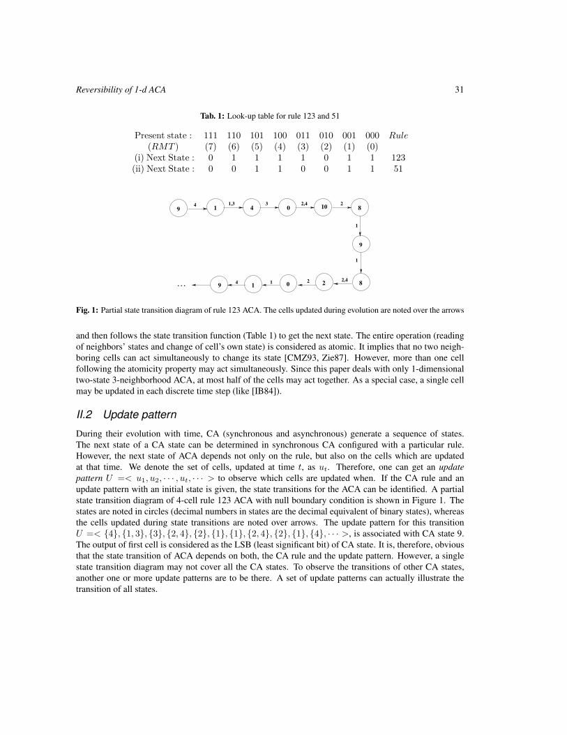
Reversibility of 1-d ACA 31
Tab. 1: Look-up table for rule 123 and 51
Present state : 111 110 101 100 011 010 001 000 Rule(RMT ) (7) (6) (5) (4) (3) (2) (1) (0)
(i) Next State : 0 1 1 1 1 0 1 1 123(ii) Next State : 0 0 1 1 0 0 1 1 51
. . .
4 1,3 3
9 1 4 0
2 419 0
2 1
1
2,4 10 8
8
9
2
2,4
1
Fig. 1: Partial state transition diagram of rule 123 ACA. The cells updated during evolution are noted over the arrows
and then follows the state transition function (Table 1) to get the next state. The entire operation (readingof neighbors’ states and change of cell’s own state) is considered as atomic. It implies that no two neigh-boring cells can act simultaneously to change its state [CMZ93, Zie87]. However, more than one cellfollowing the atomicity property may act simultaneously. Since this paper deals with only 1-dimensionaltwo-state 3-neighborhood ACA, at most half of the cells may act together. As a special case, a single cellmay be updated in each discrete time step (like [IB84]).
II.2 Update pattern
During their evolution with time, CA (synchronous and asynchronous) generate a sequence of states.The next state of a CA state can be determined in synchronous CA configured with a particular rule.However, the next state of ACA depends not only on the rule, but also on the cells which are updatedat that time. We denote the set of cells, updated at time t, as ut. Therefore, one can get an updatepattern U =< u1, u2, · · · , ut, · · · > to observe which cells are updated when. If the CA rule and anupdate pattern with an initial state is given, the state transitions for the ACA can be identified. A partialstate transition diagram of 4-cell rule 123 ACA with null boundary condition is shown in Figure 1. Thestates are noted in circles (decimal numbers in states are the decimal equivalent of binary states), whereasthe cells updated during state transitions are noted over arrows. The update pattern for this transitionU =< 4, 1, 3, 3, 2, 4, 2, 1, 1, 2, 4, 2, 1, 4, · · · >, is associated with CA state 9.The output of first cell is considered as the LSB (least significant bit) of CA state. It is, therefore, obviousthat the state transition of ACA depends on both, the CA rule and the update pattern. However, a singlestate transition diagram may not cover all the CA states. To observe the transitions of other CA states,another one or more update patterns are to be there. A set of update patterns can actually illustrate thetransition of all states.
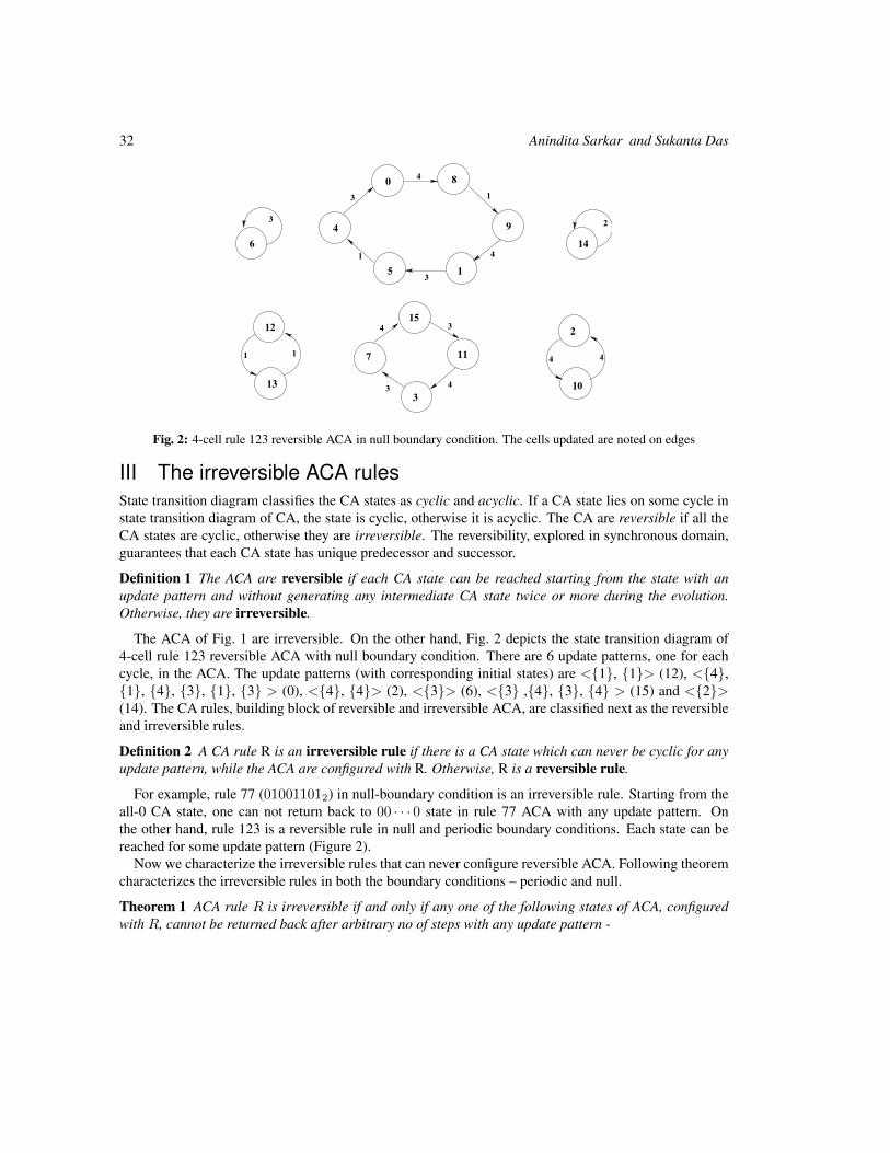
32 Anindita Sarkar and Sukanta Das
15
7
4
4
11
3
3
3
2
10
4 4
12
13
1 1
0 8
9
15
4
6
32
3
4
1
4
3
1
14
Fig. 2: 4-cell rule 123 reversible ACA in null boundary condition. The cells updated are noted on edges
III The irreversible ACA rulesState transition diagram classifies the CA states as cyclic and acyclic. If a CA state lies on some cycle instate transition diagram of CA, the state is cyclic, otherwise it is acyclic. The CA are reversible if all theCA states are cyclic, otherwise they are irreversible. The reversibility, explored in synchronous domain,guarantees that each CA state has unique predecessor and successor.
Definition 1 The ACA are reversible if each CA state can be reached starting from the state with anupdate pattern and without generating any intermediate CA state twice or more during the evolution.Otherwise, they are irreversible.
The ACA of Fig. 1 are irreversible. On the other hand, Fig. 2 depicts the state transition diagram of4-cell rule 123 reversible ACA with null boundary condition. There are 6 update patterns, one for eachcycle, in the ACA. The update patterns (with corresponding initial states) are <1, 1> (12), <4,1, 4, 3, 1, 3 > (0), <4, 4> (2), <3> (6), <3 ,4, 3, 4 > (15) and <2>(14). The CA rules, building block of reversible and irreversible ACA, are classified next as the reversibleand irreversible rules.
Definition 2 A CA rule R is an irreversible rule if there is a CA state which can never be cyclic for anyupdate pattern, while the ACA are configured with R. Otherwise, R is a reversible rule.
For example, rule 77 (010011012) in null-boundary condition is an irreversible rule. Starting from theall-0 CA state, one can not return back to 00 · · · 0 state in rule 77 ACA with any update pattern. Onthe other hand, rule 123 is a reversible rule in null and periodic boundary conditions. Each state can bereached for some update pattern (Figure 2).
Now we characterize the irreversible rules that can never configure reversible ACA. Following theoremcharacterizes the irreversible rules in both the boundary conditions – periodic and null.
Theorem 1 ACA rule R is irreversible if and only if any one of the following states of ACA, configuredwith R, cannot be returned back after arbitrary no of steps with any update pattern -
Reversibility of 1-d ACA 33
(i) all-0 state(ii) all-1 state(iii) 1010... state(iv) 100100...state(v) 110110...state
Proof: If all-0, all-1, 1010 · · ·, 100100 · · · or 110110 · · · state of ACA, configured with R, can not bereturned back with any update pattern, then obviously the ACA, and hence the R are irreversible. Now,we shall show that R is irreversible if only any of these states is acyclic.
A CA state can be viewed as a sequence of RMTs. For example, the state 1100 in periodic boundarycondition can be viewed as 3641, where 3, 6, 4 and 1 are corresponding RMTs. We club the 8 RMTsinto 4 sets – 0, 2, 1, 3, 4, 6 and 5, 7. The 3-bit binary representation of the RMTs show thatthe middle bit of RMTs of each set is the complement of each other. We next show that if a sequence ofRMTs of an arbitrary rule, corresponding to some CA state, contains both the elements of any one of theabove sets i.e. 0, 2 or 1, 3 or 4, 6 or 5, 7 set, the state is cyclic.
Rest of the states whose corresponding RMTs are from different sets (for example, one RMT from 0,2, one from 4, 6 and other from 1, 3 to get RMT sequence < 2, 4, 1, 2 > in null boundary), mayform single length cycles depending upon the RMT values and by updating a single cell. The states whichare not in some cycle, can form two length cycles by updating two or more cells at a time. Hence, thesestates are also cyclic.
Therefore, all the states other than all-0, all-1, 1010 · · ·, 100100 · · · or 110110 · · · of any ACA can becyclic for some update patterns. Hence, if all-0, all-1, 1010 · · ·, 100100 · · · or 110110 · · · states are cyclic,the rule R that configures ACA is reversible, otherwise R is irreversible. 2
To identify the irreversible rules in null and periodic boundary conditions, we next report two corollariesfollowing Theorem 1.
Corollary 1 : A rule R is irreversible while it configures ACA in periodic-boundary condition if(i) the RMTs 0 and 2 of R are 1, or(ii) the RMTs 5 and 7 of R are 0, or(iii) the RMTs 5 and 7 are 1 and RMTs 0 and 2 of R are 0, or(iv)the RMTs 1, 3, 4, 6 of R are 1 and RMTs 0 and 2 are 0, or(v) the RMTs 1, 3, 4, 6 of R are 0 and RMTs 5 and 7 are 1.
Proof: We shall prove the corollary by identifying the RMTs of R for which all-0, all-1, 1010...10,100100...100, 11011...110 state can not be returned back (Theorem 1).
If RMT 0 is 1, the ACA, configured with R in periodic boundary condition, can not form a single lengthcycle with all-0 state. Because, the next state contains at least one 1 while the ACA are updated. To forma cycle, these 1s are to be 0 in subsequent steps. However, these 1s can not be 0 if RMTs 2 is 1. Therefore,all-0 state can not be returned back if the RMTs 0, 2 of R are 1.
Similarly, the ACA can not form a single length cycle with all-1 state if RMT 7 is 0. Moreover, theACA with the state can never form a cycle of any length in periodic boundary condition if RMTs 5 of Ris 0. Hence, all-1 state can not be returned back if the RMTs 5 and 7 are 0.
Similarly, the ACA can not form a single length cycle with 1010 · · · 10 state if RMT 5 is 1 and RMT 2is 0. The ACA with the state can never form cycle of any other length in periodic boundary condition if

34 Anindita Sarkar and Sukanta Das
Tab. 2: Irreversible rules of periodic−boundary ACA0 1 2 3 4 5 6 7 8 9 10
11 12 13 14 15 16 17 20 21 24 2528 29 31 37 39 45 47 53 55 61 6364 65 66 67 68 69 70 71 72 73 7475 76 77 78 79 80 81 84 85 87 8889 90 92 93 94 95 101 103 109 111 117
119 122 125 127 133 135 141 143 149 151 157159 160 161 162 164 165 167 168 170 173 175176 187 181 183 184 186 189 191 197 199 205207 213 215 218 221 223 224 226 229 231 232234 237 239 240 242 245 247 248 250 253 255
RMT 7 of R is 1 and RMT 0 of R is 0. So, this state can not be returned back if the RMTs 5 and 7 are 1and RMTs 0 and 2 are 0.
The state 100100 · · · 100 contains RMTs 1, 2 and 4 in periodic boundary condition. It can not formsingle length cycle if the RMTs 1 and 4 are 1 and RMT 2 is 0. Again, if the RMTs 3 and 6 are 1 and RMT0 is 0 the state 100100 · · · 10 can not returned back from the previous state. Thus the state 100100 · · · 10cannot form cycle if the RMTs 1, 3, 4, 6 are 1 and RMTs 0 and 2 are 0.
Similarly, in periodic boundary condition the state 110110 · · · 110 contains RMTs 3, 5 and 6. To avoidsingle length cycle the RMTs 3 and 6 are needed to be 0 and RMT 5 is to be 1. Further this state will beacyclic if the RMTs 1 and 4 are 0 and RMT 7 is 1. Hence the state 110110 · · · 110 cannot form cycle ofany length if the RMTs 1, 3, 4 and 6 are 0 and RMTs 5 and 7 are 1. 2
For periodic-boundary condition, there are (i) 64 rules where the RMTs 0, 2 of R are 1, (ii) 64 ruleswhere the RMTs 5, 7 are 0, (iii) 16 rules where the RMTs 5 and 7 are 1 and RMTs 0 and 2 are 0, (iv)4 rules where the RMTs 1, 3, 4, 6 are 1 and RMTs 0 and 2 are 0, (v) 4 rules where the RMTs 1, 3,4, 6 are 0 and RMTs 5 and 7 are 1. There are 121 irreversible rules in total. All irreversible rules forperiodic-boundary ACA are listed in Table 2.
To derive the irreversible rules in null-boundary condition, another corollary of Theorem 1 is followed.
Corollary 2 : A rule R is irreversible in null-boundary condition if(i) the RMTs 0, 2 of R are 1, or(ii) the RMTs 1, 3, 4, 5, 6 and 7 are 0, or(iii) the RMTs 5 and 7 are 1 and the RMTs 0 and 2 are 0, or(iv) the RMTs 1, 3, 4, 6 are 1 and 0 and 2 are 0, or(v) the RMTs 1, 3, 4, 6 are 0 and 5 and 7 are 1.
Proof: We shall prove the corollary by identifying the RMTs of R for which all-0, all-1, 10101 · · · 01,100100 · · · 001 or 110110 · · · 11 state can not be returned back (Theorem 1).
If RMT 0 is 1, the ACA, configured with R in null boundary condition, can not form a single lengthcycle with all-0 state, as the next state always contains at least one 1. To form a cycle, these 1s are to be0 in subsequent steps. However, these 1s can not be 0 if RMTs 2 is 1. Therefore, all-0 state can not bereturned back if the RMTs 0, 2 of R are 1.
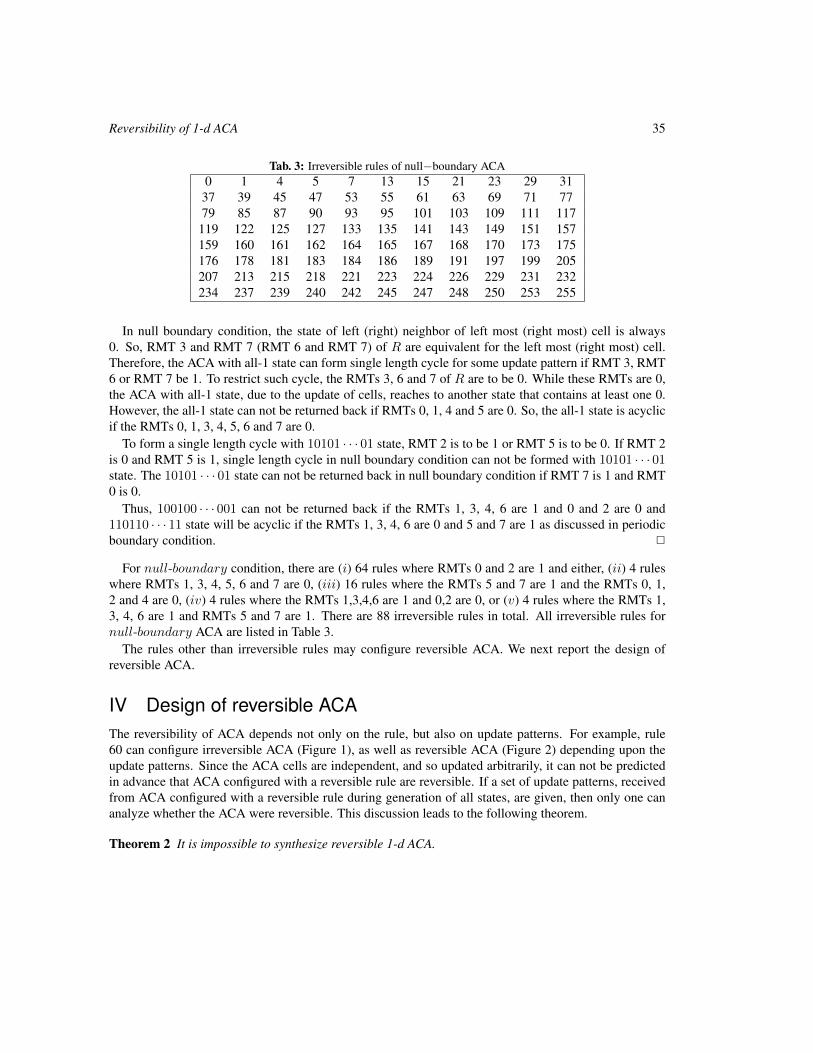
Reversibility of 1-d ACA 35
Tab. 3: Irreversible rules of null−boundary ACA0 1 4 5 7 13 15 21 23 29 31
37 39 45 47 53 55 61 63 69 71 7779 85 87 90 93 95 101 103 109 111 117
119 122 125 127 133 135 141 143 149 151 157159 160 161 162 164 165 167 168 170 173 175176 178 181 183 184 186 189 191 197 199 205207 213 215 218 221 223 224 226 229 231 232234 237 239 240 242 245 247 248 250 253 255
In null boundary condition, the state of left (right) neighbor of left most (right most) cell is always0. So, RMT 3 and RMT 7 (RMT 6 and RMT 7) of R are equivalent for the left most (right most) cell.Therefore, the ACA with all-1 state can form single length cycle for some update pattern if RMT 3, RMT6 or RMT 7 be 1. To restrict such cycle, the RMTs 3, 6 and 7 of R are to be 0. While these RMTs are 0,the ACA with all-1 state, due to the update of cells, reaches to another state that contains at least one 0.However, the all-1 state can not be returned back if RMTs 0, 1, 4 and 5 are 0. So, the all-1 state is acyclicif the RMTs 0, 1, 3, 4, 5, 6 and 7 are 0.
To form a single length cycle with 10101 · · · 01 state, RMT 2 is to be 1 or RMT 5 is to be 0. If RMT 2is 0 and RMT 5 is 1, single length cycle in null boundary condition can not be formed with 10101 · · · 01state. The 10101 · · · 01 state can not be returned back in null boundary condition if RMT 7 is 1 and RMT0 is 0.
Thus, 100100 · · · 001 can not be returned back if the RMTs 1, 3, 4, 6 are 1 and 0 and 2 are 0 and110110 · · · 11 state will be acyclic if the RMTs 1, 3, 4, 6 are 0 and 5 and 7 are 1 as discussed in periodicboundary condition. 2
For null-boundary condition, there are (i) 64 rules where RMTs 0 and 2 are 1 and either, (ii) 4 ruleswhere RMTs 1, 3, 4, 5, 6 and 7 are 0, (iii) 16 rules where the RMTs 5 and 7 are 1 and the RMTs 0, 1,2 and 4 are 0, (iv) 4 rules where the RMTs 1,3,4,6 are 1 and 0,2 are 0, or (v) 4 rules where the RMTs 1,3, 4, 6 are 1 and RMTs 5 and 7 are 1. There are 88 irreversible rules in total. All irreversible rules fornull-boundary ACA are listed in Table 3.
The rules other than irreversible rules may configure reversible ACA. We next report the design ofreversible ACA.
IV Design of reversible ACAThe reversibility of ACA depends not only on the rule, but also on update patterns. For example, rule60 can configure irreversible ACA (Figure 1), as well as reversible ACA (Figure 2) depending upon theupdate patterns. Since the ACA cells are independent, and so updated arbitrarily, it can not be predictedin advance that ACA configured with a reversible rule are reversible. If a set of update patterns, receivedfrom ACA configured with a reversible rule during generation of all states, are given, then only one cananalyze whether the ACA were reversible. This discussion leads to the following theorem.
Theorem 2 It is impossible to synthesize reversible 1-d ACA.
36 Anindita Sarkar and Sukanta Das
However, the update patterns can be designed for the cycles of some reversible ACA. The reversiblerules require different sets of update patterns to get reversible ACA. Even, for a particular reversible rule,various sets of update patterns may be identified that result in different reversible ACA. An update patterncan produce a cycle if the initial state and the ACA are given. In this section, we identify such an updatepattern that forms a cycle for some reversible ACA.
To get a cycle for some reversible ACA, an update pattern along with some initial state is requiredwhich generates l distinct CA states for a cycle of length l. Since the states are to be distinct, the updatepattern should be designed in such a way that at least one bit of a state flips to get the next state. But notwo neighboring bits can be selected at a time. Moreover, in any sub-sequence of states, the bits of statesare not to be flipped in even number of times to get unique states in a cycle of reversible ACA. If they flip,the l states can not be distinct. Therefore, the following points are to be taken care of to design the updatepatterns for some reversible ACA.
1. No two neighbors can get updated simultaneously.
2. At least one bit of a state must be flipped to get the next state.
3. To get cycle of length l, all the bits of an initial state (S) are flipped even number of times intotal to regenerate S. Before regenerating S, the bits are not to be flipped even number of timessimultaneously.
The generation of distinct states depends not only on the update pattern, but also on the initial state.Because, the initial state may not allow an arbitrary bit to flip for some arbitrary reversible rule thatconfigure the ACA. However, rule 51 (Table 1) is the only rule that always allows a cell to flip its previousstate when updated. So, rule 51 ACA do not depend on the initial state to form a cycle. We have designedthe following rule to generate an update pattern for getting a cycle of length 2i (1 ≤ i ≤ n) by updating asingle cell at a time, where n is the number of ACA cells.
• To get a cycle of length 2i (1 ≤ i ≤ n) of rule 51 ACA with n cells, form a sequence of i cells,to be updated, arbitrarily. Start with an arbitrary state. Update (2j−1)th state by updating jth cell(1 ≤ j ≤ i) of the sequence to generate the next state. Repeat the update of the jth cell after each2j state, where j < i. However, update the ith cell again after 2i−1 state to get a cycle of length 2i.
Example 1 To design a full length cycle for 4-cell rule 51 ACA (length = 24), all the cells are to beupdated in some sequence. Consider, the sequence of updating is SEQ =< 1, 2, 3, 4 > and the initialstate is 0100. Each jth cell of SEQ is selected for the first time to update (2j−1)th state. Hence, to getthe second state, the first bit of the initial state ((2j−1)th state, where j = 1) is updated. Similarly, thesecond, third and fourth cells are selected for the first time to update the second, fourth and eighth statesrespectively. The first cell is again selected to update third, fifth, and all odd states (that is, after each2j states where j = 1). After the first time update, the second and third cells are selected repeatedly toupdate after every 22 and 23 states respectively. The last cell is updated for the second time after 23 states(2i−1 states where i = 4) to complete the cycle. Therefore, the sequence of states in the cycle is <0100,1100, 1000, 0000, 0010, 1010, 1110, 0110, 0111, 1111, 1011, 0011, 0001, 1001, 1101, 0101, 0100>.The update pattern is <1, 2, 1, 3, 1, 2, 1, 4, 1, 2, 1, 3, 1, 2, 1, 4>.Here, the update pattern is independent of the initial state, but depends on SEQ. The update pattern andthe cycle of rule 51 ACA are same for both the boundary conditions.
Reversibility of 1-d ACA 37
However, cycles can be formed by updating multiple cells simultaneously. Rule 51 ACA with n cellscan form a cycle of maximum length 2n−m+1 while m cells (1 ≤ m ≤ n) are updated simultaneously. Insuch case, the same rule of single cell update to get a cycle can be followed with an exception that eachentry in the sequence of cells, to be updated, is a set of m cells. Following example illustrates the cycleformation by updating multiple cells.
Example 2 Let us consider, n = 4 and m = 2. To get an 8 length (2n−m+1) cycle of the ACA, asequence SEQ =<1, 3, 2, 4, 1, 4> of cells is formed arbitrarily. Consider that the initial stateis 0100. The first and third bits are updated to generate the second state (1110). Similarly, the cells ofsecond and third entries of SEQ are selected to update the second and forth states. Like Example 1, thecells of first set (1, 3) are repeatedly selected to update the odd states. The cells of second set (2, 4)are selected again to update the sixth state. Therefore, a sequence <0100, 1110, 1011, 0001, 1000, 0010,0111, 1101, 0100> of states is obtained. Here, the update pattern is <1, 3, 2, 4, 1, 3, 1, 4, 1,3, 2, 4, 1, 3, 1, 4>.
The update rule, designed for rule 51 reversible ACA, guides us to develop Algorithm 1, which findsthe update pattern for a cycle of some reversible ACA. The algorithm is independent from the boundarycondition. It takes the ACA, cycle length to be designed (2i), initial state (S) and the number of cellsupdated in a single step (m), as input. However, with arbitrary ACA and arbitrary initial state, a cycle ofgiven length may not be designed. In such cases, the algorithm finds a cycle which is close in length withthe given cycle length. It outputs the update pattern with the cycle length, if cycle can be designed.
The algorithm first forms a sequence of i unique sets arbitrarily. The sets are also designed arbitrarilywith m ACA cells per set. The update style of rule 51 reversible ACA is followed to generate the updatepattern. If no bit flips during the update of a set of m cells, another set of m cells is searched so that atleast one bit flips. If no such set is found, then the algorithm reports that cycle is not possible. While 2i
states are covered but no cycle is formed, the algorithm attempts to form a cycle by generating a very fewstates.
Algorithm 1 ReversibleACAInput: R (rule), n (# cells), 2i (cycle length, 1 ≤ i ≤ n), S (initial state), m (# cells updated in eachstep)Output: Update pattern with cycle length, if cycle is possibleStep 1: Form a sequence, SEQ of i unique sets of m ACA cells such that no two neighboring cells arenot taken at a time, arbitrarily.Step 2: Load the ACA, configured with R, with S.Step 3: For k = 1 to 2i repeat Step 4 to Step 9.Step 4: If k = 2j−1 (1 ≤ j ≤ i), select the jth set of the SEQ.
If k = 2i, select the ith set of SEQ.If k = 2j−1 + p ∗ 2j , where p is some positive integer and 1 ≤ j < i, select the jth set.
Step 5: Update the ACA cells of the selected set.Step 6: If no cell flips during the update, find a set of m cells so that
1. at least one cell flips, and
2. the generated state is unique.
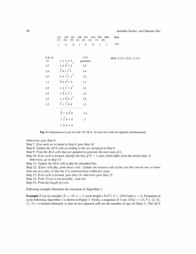
38 Anindita Sarkar and Sukanta Das
51 1 2 3 4 5 generated
3,5 1 0 0 1 0 3,5
2,4 1 0 1 1 1 1,4
3,5 0 0 1 1 1 3,5
1,3 0 0 0 1 0 1,3
3,5 1 0 1 1 0 3,5
2,4 1 0 0 1 1 2,4
3,5 1 1 0 0 1 3,5
1,3 1 1 1 0 0 1,3
0 1 0 0 0 1,4
1 1 0 1 0 2
1 0 0 1 0
(7) (6) (5) (4) (3) (2) (1) (0)
1 0 0 1 0 0 1 1
U.P. of U.P.
111 110 101 100 011 010 001 000 Rule
147
SEQ <3,5 ,2,4, 1,3>
Fig. 3: Generation of cycle for rule 147 ACA. At most two cells are updated simultaneously.
Otherwise, goto Step 9.Step 7: If no such set is found in Step 6, goto Step 14.Step 8: Update the ACA cells according to the set, designed in Step 6.Step 9: Print the ACA cells that are updated to generate the next state of k.Step 10: If no cycle is formed, identify the bits of 2i + 1 state which differ from the initial state, S.
Otherwise, go to Step 15.Step 11: Update the ACA cells to flip the identified bits.Step 12: If few cells flip, print those cells. Update the nearest cells of the rest bits one-by-one or morethan one at a time, so that the S is returned back within few steps.Step 13: If no cycle is formed, goto Step 14, otherwise goto Step 15.Step 14: Print ‘Cycle is not possible’, and exit.Step 15: Print the length of cycle.
Following example illustrates the execution of Algorithm 1.
Example 3 Let us consider, R = 147, n = 5, cycle length = 8 (23), S = 10010 and m = 2. Formation ofcycle following Algorithm 1 is shown in Figure 3. Firstly, a sequence of 3 sets SEQ =<3, 5 , 2, 4,1, 3> is formed arbitrarily so that no two adjacent cells are the member of any set (Step 1). The ACA
Reversibility of 1-d ACA 39
are configured with rule 147 in null boundary condition. To get the next state of 10010 (initial state), thethird and fifth cells are updated (Steps 4 and 5). In Figure 3, update pattern of rule 51 ACA is noted onthe left side of the states, and the update pattern generated by the algorithm is shown on the right side. Toupdate the second state (similarly sixth state), according to the update pattern of rule 51 ACA, the set 2,4 is selected. Since no cell flips here, another set 1, 4 is searched (Step 6). After generation of 8 states,cycle is not formed. So, another 2 states are generated to form a cycle (Steps 10 – 12). Therefore, lengthof cycle is 10.
V ConclusionThe reversibility in 1-dimensional ACA (asynchronous cellular automata) has been addressed in this pa-per. The ACA cells are updated independently. An action taken by a cell to change its state is consideredhere as atomic. Depending upon their update during state transition, update pattern is defined. To facili-tate the design of reversible ACA, CA rules are classified as reversible and irreversible. The irreversiblerules can not configure reversible ACA with any set of update patterns. However, the reversibility of ACAdepends on both – the rule and update patterns. A set of irreversible rules for both the boundary conditionsare identified. The paper has finally reported an algorithm to get an update pattern for a cycle of ACA.
References[AP72] S. Amoroso and Y. N. Patt. Decision procedures for surjectivity and injectivity of parallel
maps for tesselation structures. J. Comput. Syst. Sci., 6:448–464, 1972.
[CMZ93] R. Cori, Y. Metivier, and W. Zielonka. Asynchronous mappings and asynchronous cellularautomata. Inf. Comput., 106:159–202, 1993.
[DS06] Sukanta Das and Biplab K. Sikdar. Classification of CA rules targeting synthesis of reversiblecellular automata. In Proc. of International Conference on Cellular Automata for Researchand Industry, pages 68–77. ACRI, September 2006.
[IB84] T. Ingerson and R. Buvel. Structure in asynchronous cellular automata. Physica D, 10:59–68,1984.
[LPA+02] Jia Lee, Ferdinand Peper, Susumu Adachi, Kenichi Morita, and Shinro Mashiko. Reversiblecomputation in asynchronous cellular automata. In Proc. of the Third International Conferenceon Unconventional Models of Computation, pages 220–229. Springer-Verlag, London, 2002.
[Neh04] Chrystopher L. Nehaniv. Asynchronous automata networks can emulate any synchronousautomata network. International Journal of Algebra and Computation (IJAC), 14:719–739,2004.
[SMD11] Anindita Sarkar, Anindita Mukherjee, and Sukanta Das. Reversibility in asynchronous cellularautomata. Communicated to Complex Systems, March 2011.
[Tof77] T. Toffoli. Computation and construction universality of reversible cellular automata. J. Com-put. System Sci., 15:213–231, 1977.

40 Anindita Sarkar and Sukanta Das
[vN66] John von Neumann. The theory of self-reproducing Automata. Univ. of Illinois Press, 1966.
[Wol86] S. Wolfram. Theory and applications of cellular automata. World Scientific, Singapore, 1986.
[Zie87] Wieslaw Zielonka. Notes on finite asynchronous automata. Theoretical Informatics and Ap-plications, 21:99–135, 1987.
AUTOMATA 2011, Santiago, Chile local proceedings LP, 2011, 41–54
On 1-resilient, radius 2 elementary CA rules
E. Formenti1† and K. Imai2‡ and B. Martin1§ and J-B. Yunes3¶
1Universite Nice–Sophia Antipolis, Laboratoire I3S, UMR 6070 CNRS, BP 121, F-06903 Sophia Antipolis Cedex.2Graduate School of Engineering, Hiroshima University, Japan.3Universite Paris Diderot & CNRS, Laboratoire d’Informatique et Algorithmique, Fondements et Applications (LI-AFA), Case 7014, F-75205 Paris cedex 13.
The study of cellular automata rules suitable for cryptographic applications is under consideration. Cellular automatacan be used to generate pseudo-random sequences as well as for the design of S-boxes in symmetric cryptography.Boolean functions with good properties like resiliency and non-linearity are usually obtained either by exhaustivesearch or by the use of genetic algorithms. We propose here to use some recent research in the classification ofBoolean functions and to link the study of cellular automata rules to the study of such Boolean functions. We illustrateour approach with 5-variable Boolean functions.
Keywords: Cellular automata, Boolean functions, Pseudo-random generators, Symmetric cryptography.
1 IntroductionCellular automata (CA) are models of massive parallel computers based on communicating finite statemachines; they are used in many applications of computer science. In particular, they are utilised for thegeneration of binary pseudo-random (PR) sequences in cryptography. This was first proposed by [Wol86a]who suggested that PR sequences generated by a certain rule (numbered 30) could be used for crypto-graphic purposes as keys for a Vernam-type cipher. This CA rule is also used as one of the PR generatorsincluded in Mathematica R©. It is now well known that rule 30 has several weaknesses and that it is notresistant to the attacks of [MS91]. One of the reasons is that the rule is not resilient, meaning that theoutput of rule 30 is not statistically independent of the combination of some subsets of its inputs. This canbe proved either by an exhaustive search ([Mar08]) or by a simple application of the Siegenthaler boundwhich links the number of variables of a Boolean function with the resiliency.
Despite this negative result, several techniques have been used to pursue the study of PR generation byCA. The first natural idea is to enlarge the neighbourhood and to search for rules with good properties ofnon-linearity and resiliency. [LMS08] investigate the 216 elementary CA rules with four neighbours andgive a complete classification of the functions with good cryptographic properties.
†Email: [email protected]. Work supported by ANR, project EMC (ANR-09-BLAN-0164).‡Email: [email protected]. Work supported by JSPS Grant-in-Aid for Scientific Research (C) 22500015.§Email: [email protected]. Work supported by ANR, project EMC (ANR-09-BLAN-0164).¶Email: [email protected].
c© 2011 AUTOMATA proceedings, Santiago, Chile, 2011
42 E. Formenti and K. Imai and B. Martin and J-B. Yunes
In the present work, we recall how to generate binary PR sequences with uniform CA. We particularlyfocus on the search for good updating functions. By good we mean functions which fulfil the resiliencyproperty. To that purpose, we use the classification of Boolean functions of five variables with respectto cryptographic properties done by [BBNP05] which is related to the cosets classification of the Reed-Muller error-correcting code RM(1, 5) (recall that a code C is a linear subspace of F5
2 and for a vectoru ∈ F5
2, the set u+C = u+x : x ∈ C is a coset ofC and u is called the coset leader. The cosets form apartition of F5
2). The paper by [BBNP05] only gives representatives and the number of Boolean functionsfulfilling some cryptographic properties in the equivalence class. More precisely, their classification tellsthat if there are resilient functions, they have to be in the equivalence class which also contain non-resilientfunctions. We thus explore these equivalence classes to find out good Boolean functions which can beused as CA rules for generating PR sequences. We also propose to extend those CA rules of radius 2 intoBoolean functions of nine variables by selecting the CA rules which preserve the resiliency property. Thefact that resiliency is preserved by the iteration of a rule is not true in general. PR sequences generated bythese rules are then submitted to the Diehard test suite.
The paper is organised as follows: Section 2 defines the notions of pseudo-random generator, cellularautomata and Boolean functions; it also presents some equivalence properties of the Fourier-Hadamard(or Walsh-Hadamard) transform, which is widely used in this study. In Section 3, we propose a study ofthe radius 2, elementary CA for selecting resilient rules and propose an approach to avoid an exhaustivesearch among all the 22
5
possible rules. For the rules we have selected, we propose in Section 4 sometests of the randomness for the sequences which can be generated by radius 2, elementary CA.
2 Definitions and notationsThis section recalls some basic notation and facts on pseudo-randomness, CAs and Boolean functions.
2.1 Pseudo-Randomness
In [Wol02], three mechanisms responsible for random behaviour in systems are described: (1) Random-ness from physics like brownian motion; (2) Randomness from the initial conditions which is studied bychaos theory; and (3) Randomness by design, also called pseudo-randomness. Many algorithms generatePR sequences. The behaviour of the system is fully determined by knowing the seed and the algorithmused. They are quicker methods than getting “true” randomness from the environment, inaccessible forcomputers.
The applications of randomness have led to many different methods for generating random data. Thesemethods may vary as to how unpredictable or statistically random they are, and how quickly they cangenerate random sequences. Before the advent of computational PR sequences, generating large amountof sufficiently random numbers (important in statistics and physical experimentation) required a lot ofwork. Results would sometimes be collected and distributed as random number tables.
In the sequel, we will consider pseudo-random generators (PRG). This corresponds to a deterministicalgorithm which “stretches” a short truly random sequence (the seed) into a polynomially longer sequencethat appear to be “random” (although they are not). In other words, although the output of a PRG is notreally random, it is infeasible to tell the difference. It turns out that pseudorandomness and computationalcomplexity are linked in a fundamental way (see [Gol99] for further details). More practically, this cor-responds to the behaviour of random number generators implemented in operating systems. In this case,
On 1-resilient, radius 2 elementary CA rules 43
the short truly random sequence corresponds to the pseudo-device /dev/random and the output of thePRG to the pseudo-device /dev/urandom for producing more random bits of weaker quality.
2.2 Cellular automataOne-dimensional binary CAs (also called elementary) consist of a line of cells taking their states amongbinary values. For practical implementations, the number of cells is finite. There are two cases: a CAhas periodic boundary conditions if the cells are arranged in a ring and it has null boundary conditionswhen both extremal cells are continuously fixed to zero. All the cells are finite state machines with anupdating function which gives the new state of the cell according to its current state and the current stateof its nearest neighbours.
In [Wol86a], it was proposed to use CA to produce PR sequences. He considered one-dimensionalbinary CA with l cells (l = 2N + 1 for N ∈ N). For a CA, the values of the cells at time t ≥ 0 areupdated synchronously by a Boolean function f with n = r1 + r2 + 1 variables by the rule xi(t + 1) =f(xi−r1(t), . . . , xi(t), . . . , xi+r2(t)). Elementary CA are such that r1 = r2 = 1. For a fixed t, thesequence of the values xi(t) for 1 ≤ i ≤ 2N + 1, is the configuration at time t. It is a mappingc : [[1, l]] → F2 (the finite field with two elements) which assigns a state of F2 to each cell. The initialconfiguration (t = 0) x1(0), . . . , xl(0) is the seed of the generator, the sequence (xN (t))t is the outputsequence and, when r1 = r2 = r, the number r denotes the radius of the rule. The Wolfram numberingassociates a rule number to any one of the 256 elementary CA; it takes the binary expansion of a rulenumber as the truth table of a 3-variable Boolean function.
2.3 Boolean functionsA Boolean function is a mapping from Fn2 into F2. In the sequel, additions in Z (resp. F2) will be denotedby + and Σ (resp. ⊕ and
⊕), products by × and
∏(resp. . and
∏). When there is no ambiguity,
we denote by + the addition of binary vectors. If x and y are binary vectors, their inner product isx ·y =
∑ni=1 xiyi. A very handy representation of Boolean function is the algebraic normal form (ANF):
Definition 1 A Boolean function f with n variables is represented by a binary polynomial in n variables,called algebraic normal form: f(x) =
⊕u∈Fn2
au(∏ni=1 x
uii ) au ∈ F2, ui is the i-th projection of u.
Example 1 If we consider rule (30), its ANF is x1 ⊕ x2 ⊕ x3 ⊕ x2x3 or, more concisely, 1+2+3+23.
The degree of the ANF or algebraic degree of f corresponds to the number of variables in the longest termxu11 . . . xunn in the ANF of f . This makes sense thanks to the existence and uniqueness of the ANF. The
Hamming weight wH(f) of f is the number of x ∈ Fn2 such that f(x)= 1. The Hamming weight wH(x)of x ∈ Fn2 counts the number of 1-valued coordinates in x. f is balanced if wH(f) = wH(1⊕f) = 2n−1.
Definition 2 Two Boolean functions f and g with n variables are equivalent iff
f(x) = g ((x ·A)⊕ a)⊕(x ·BT
)⊕ b, ∀x ∈ Fn2 (1)
where A is a non-singular binary n× n matrix, b a binary constant, a and B ∈ Fn2 .
Let us mention one important tool in the study of Boolean functions. The Fourier-Hadamardtransform is a linear mapping which maps a Boolean function f to the real-valued function f(u) =∑x∈Fn2
f(x)(−1)u·x, which describes the spectrum of the latter. When applied to fχ(x) = (−1)f(x) (the
44 E. Formenti and K. Imai and B. Martin and J-B. Yunes
sign function) the Fourier-Hadamard transform is the Walsh transform: fχ(u) =∑x∈Fn2
(−1)f(x)⊕u·x .
Using the fact that fχ(u) = 1− 2f(u), the Fourier-Hadamard transform is:
f(u) =1
2
∑x∈Fn2
(−1)u·x − 1
2fχ(u) , (2)
since f(u) =∑x∈Fn2
(−1)u·x(
1−fχ(u)2
)= 1
2
∑x∈Fn2
(−1)u·x − 12
∑x∈Fn2
fχ(u)(−1)u·x. And, by
definition, fχ(u) =∑x∈Fn2
fχ(u)(−1)u·x. Using Eq. 2 and, as stated by [Car11], we obtain that
fχ(u) = 2nδ0 − 2f(u), where δ0 denotes the Dirac symbol defined by δ0(u) = 1 if u is the null vectorand δ0(u) = 0 otherwise.
For two equivalent Boolean functions f and g with n variables, the following property holds:
fχ(u) = (−1)a·A−1(ut+BT )+b
gχ((u⊕B)(A−1)T ) . (3)
This property is used by [BBNP05] for counting the number of functions satisfying some cryptographicproperties. The Walsh transform allows us to study the correlation-immunity of a function.
Definition 3 A Boolean function f in n variables is correlation-immune of order k (0<k<n) if, givenany n i.i.d. binary random variables x1, · · · , xn according to a uniform Bernoulli distribution, thenthe random variable Z = f(x1, . . . , xn) is independent from any random vector (xi1 , xi2 , . . . , xik),1≤ i1< · · ·<ik<n. When f is correlation immune of order k and balanced, it is k-resilient.
In [XM88], a spectral characterisation of resilient functions was given:
Theorem 1 A Boolean function f in n variables is k-resilient iff it is balanced and f(u) = 0 for allu ∈ Fn2 s.t. 0<wH(u)≤k. Equivalently, f is k-resilient iff fχ(u)=0 for all u ∈ Fn2 s.t. wH(u)≤k.
Remark that Theorem 1 concerns both transforms (refer to [Car11] for further details).
Theorem 2 (Siegenthaler Bound) For a k-resilient (0 ≤ k < n− 1) Boolean function with n variables,there is an upper bound for its algebraic degree d: d ≤ n− k − 1 if k < n− 1 and d = 1 if k = n− 1.
Theorem 2 shows that the algebraic degree of a 1-resilient function with 3 variables is at most one, i.e. theBoolean function must be linear to be resilient. Linear functions are avoided in cryptography.
2.4 Some properties of the Fourier-Hadamard transformComputing the Fourier-Hadamard transform We use the Fourier-Hadamard transform from [ER82]called the Walsh or Sequency Ordered Transform (WHT)w. This transform is used to study the CA rulesin order to find the best (non-linear) rules for generating PR sequences. To check the rules, we use thefast transform algorithm whose time complexity is O(n log n). It receives as an input an array F of size2n which contains the images by the t iterates of the local rule f of all the configurations of n cells (i.e.f t(0), f t(1), . . . , f t(2n − 1)). Walsh(F, 0, n) outputs F as f t(2n − 1), . . . , f t(0).
Walsh(F, start, n)half = n div 2for index = start to start + half - 1 do
mem = F[index]
On 1-resilient, radius 2 elementary CA rules 45
F[index] -= F[index + half]F[index + half] += mem
endforif half > 1 then
Walsh(F, start, half)Walsh(F, start + half, half)
endifend
Application to CA rules We proceed step by step with increasing values of t, which counts the numberof times the local rule with 5 variables, supposed to be 1-resilient, is iterated on an initial configuration.In this way, we consider the natural extension of f : F5
2 → F2 to f : Fn+42 → Fn2 where:
f(x0, . . . , xn+4) = (y2, . . . , yn) such that yj = f(xj−2, xj−1, xj , xj+1, xj+2), j ∈ [[2, n]]
Using the extended f , one can define the t-th iterate of f which is a function f t : F4t+12 → F2 in the
natural way. We compute next the maximum absolute value of the Fourier-Hadamard transform of thetth-iterate of f at all the points u of Hamming weight 1 and we select the rules with a minimum spectralvalue. The computation is repeated with increasing values of t until we can identify rules with flat spectralor relatively small values which are slowly growing in function of t.
Iterates and Fourier-Hadamard transform In this section we isolate some transformations whichpreserves resiliency (i.e. the spectral values of the Fourier-Hadamard transform) upon iterations.
We first introduce the reverse operator Φ : Fm2 → Fm2 , Φ((v1, . . . , vm)) = (vm, . . . , v1).
Definition 4 Let f : F2m+12 → F2 be the local function of a CA. Then, fR(x−m, . . . , x0, . . . , xm) =
f(xm, . . . , x0, . . . , x−m) is the reflection of f .
Another basic transformation is given by Ψ(x) = 1 ⊕ x for x ∈ F2. It corresponds to the nega-tion of the variable and is used for designing the conjugation and the conjugation-reflection introducedin [Wol86b, p. 492]. With some abuse of notation, Ψ is extended to sequences of Boolean variables:for u = (u1, u2, . . . , un) with ui ∈ F2, Ψ(u) = (Ψ(u1),Ψ(u2), . . . ,Ψ(un)). Moreover, remark thatΨ−1 = Ψ.
Definition 5 Let f : F2m+12 → F2 be the local function of a CA. Then fN (x−m, . . . , x0, . . . , xm) =
Ψ f(Ψ(xm, . . . , x0, x−m)) is the negation of f .
One can see that for any t ∈ N, f t H = H f tR for H = Ψ or H = Φ, this property will be useful later.
Lemma 1 Let Ξ : F2m+12 → F2m+1
2 be 1:1 and f :F2m+12 → F2 a CA. Then, wH(f) = wH(f Ξ).
Proof: Obvious. 2
Proposition 1 shows that resiliency is preserved by the reflection when the local rule is iterated.
Proposition 1 Let f : F2m+12 → F2 be the local function of a CA. For any t ∈ N, let 0 < k ≤ 2mt+ 1.
Then, f tR is k-resilient iff f t is k-resilient.
46 E. Formenti and K. Imai and B. Martin and J-B. Yunes
Proof: The transformation Φ is bijective. Hence, by Lemma 1, we have wH(fR) = wH(f Φ) = wH(f).Since f is balanced, wH(fR) = wH(Ψ f). Now, applying Lemma 1 to Ψ f and using last equation,it holds wH(Ψ f) = wH(Ψ f Φ) = wH(Ψ fR). Let a = B = (0, 0, . . . , 0), b = 0 and A thereverse identity matrix. Remark that A is non-singular, then, by using Eq. 3, one obtains (ftR)χ(u) =
ftχ(u · (A−1)T ) = ftχ(u ·A) = ftχ(A · u) which entails
f tR(u) = f t(A · u) . (4)
Now, assume that f t is k-resilient. Remark that wH(A · u) = wH(u) for any u, therefore, by Theorem 1,if f t(u) = 0 for 0 < wH(u) ≤ k, then, by Eq. 4, f tR(u) = 0 too. For the converse, just remark that A2 isthe identity transformation and then, by Eq. 4, one finds f tR(Φ(u)) = f t(u). Therefore if f tR(Φ(u)) = 0,we have f t(u) = 0. Since Φ is a bijection we have the thesis. 2
Lemma 2 Let f : F2m+12 → F2 be the local function of a CA. For any t ∈ N, f tN is balanced iff f t is
balanced.
Proof: Assume f t balanced for some t ∈ N. By definition of f tN , wH(f tN ) = wH(Ψ f t Ψ). Remarkthat Ψf t is a CA; then by Lemma 1, wH(Ψf tΨ) = wH(Ψf t). Since f t is balanced, wH(Ψf t) =wH(f t). Finally, observing that Ψ2 is the identity and by Lemma 1 again, it holds wH(f t) = wH(Ψ2 f t) = wH(Ψ2 f t Ψ) = wH(Ψ f tN ). For the converse, assume that f tN is balanced for some t ∈ N.Then, wH(f tN ) = wH(Ψf tN ) = wH(Ψ2 f t Ψ) = wH(f t Ψ). By Lemma 1, wH(f t Ψ) = wH(f t)and therefore wH(f t) = wH(f tN ). Again, by Lemma 1, wH(Ψ f t) = wH(Ψ f t Ψ) = wH(f tN ).Hence wH(f t) = wH(Ψ f t). 2
Proposition 2 Let f : F2m+12 → F2 be the local function of a CA. For any t ∈ N, let 0 < k ≤ 2mt+ 1.
Then, f t is k-resilient iff f tN is k-resilient.
Proof: Fix k ∈ N as in the hypothesis. By Lemma 2, it suffices to prove that fN (u) = h(u) · f(u) for anyu ∈ F2m+1
2 such that 0 < wH(u) ≤ k and h : F2m+12 → R+. Let A = Id, a = (1, 1, . . . , 1), b = 1 and
B = (0, 0, . . . , 0). Then, by using Eq. 3, one obtains (ftN )χ(u) = (−1)1+a·u ftχ(u) for any u ∈ F2mt+12
with 0 < wH(u) ≤ 2mt+ 1. This entails f tN (u) = (−1)1+a·uf t(u). 2
Consider the equivalence relation R on CA rules such that fRg iff g = fR or g = fN or g = fRN .According to [CFMM97], there are 22
m
(6 + 22m
) distinct R-classes. Propositions 1 and 2 say that allelements in a class have the same resiliency and hence only one element per class should be tested forstudying this property. However the gain obtained by this quotient of the set of local rules is minor.Therefore, ideas for “quickly” spanning the set of interesting local rules are welcome. Section 4 proposes(among other things) to consider affine transformations. Indeed, even if f and its Boolean equivalent, sayfA have the same resilience characteristics, the same is not true, in general, for their iterates.
This is essentially due to the fact that the proofs of this subsection are based on the existence of abijection φ and a transformation τ on the local rules such that for any local rule f , it holds that ∀t ∈N, [τ(f)]t φ = φ f t. This property is not true, in general, when transformations different from thenegation or the reflection are considered.
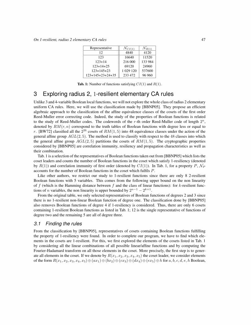
On 1-resilient, radius 2 elementary CA rules 47
Representative NCI(1) NR(1)
12 4840 4120123 16640 11520
123+14 216 000 133 984123+14+25 69120 24960123+145+23 1 029 120 537600
123+145+23+24+35 233 472 96 960
Tab. 1: Number of functions satisfying CI(1) and R(1).
3 Exploring radius 2, 1-resilient elementary CA rulesUnlike 3 and 4-variable Boolean local functions, we will not explore the whole class of radius 2 elementaryuniform CA rules. Here, we will use the classification made by [BBNP05]. They propose an efficientalgebraic approach to the classification of the affine equivalence classes of the cosets of the first orderReed-Muller error correcting code. Indeed, the study of the properties of Boolean functions is relatedto the study of Reed-Muller codes. The codewords of the r-th order Reed-Muller code of length 2n,denoted by RM(r, n) correspond to the truth tables of Boolean functions with degree less or equal tor. [BW72] classified all the 226 cosets of RM(1, 5) into 48 equivalence classes under the action of thegeneral affine group AGL(2, 5). The method is used to classify with respect to the 48 classes into whichthe general affine group AGL(2, 5) partitions the cosets of RM(1, 5). The cryptographic propertiesconsidered by [BBNP05] are correlation immunity, resiliency and propagation characteristics as well astheir combination.
Tab. 1 is a selection of the representatives of Boolean functions taken out from [BBNP05] which lists thecoset leaders and counts the number of Boolean functions in the coset which satisfy 1-resiliency (denotedby R(1)) and correlation immunity of first order (denoted by CI(1)). In Tab. 1, for a property P , NPaccounts for the number of Boolean functions in the coset which fulfils P .
Like other authors, we restrict our study to 1-resilient functions since there are only 8 2-resilientBoolean functions with 5 variables. This comes from the following upper bound on the non linearityof f (which is the Hamming distance between f and the class of linear functions): for k-resilient func-tions of n variables, the non linearity is upper bounded by 2n−1 − 2k+1.
From the original table, we only selected representatives of Boolean functions of degrees 2 and 3 sincethere is no 1-resilient non-linear Boolean function of degree one. The classification done by [BBNP05]also removes Boolean functions of degree 4 if 1-resiliency is considered. Thus, there are only 6 cosetscontaining 1-resilient Boolean functions as listed in Tab. 1; 12 is the single representative of functions ofdegree two and the remaining 5 are all of degree three.
3.1 Finding the rulesFrom the classification by [BBNP05], representatives of cosets containing Boolean functions fulfillingthe property of 1-resiliency were found. In order to complete our program, we have to find which ele-ments in the cosets are 1-resilient. For this, we first explored the elements of the cosets listed in Tab. 1by considering all the linear combinations of all possible linear/affine functions and by computing theFourier-Hadamard transform on all those elements in the coset. More precisely, the first step is to gener-ate all elements in the coset. If we denote by R(x1, x2, x3, x4, x5) the coset leader, we consider elementsof the form R(x1, x2, x3, x4, x5)⊕ (ax1)⊕ (bx2)⊕ (cx3)⊕ (dx4)⊕ (ex5)⊕h for a, b, c, d, e, h Boolean,
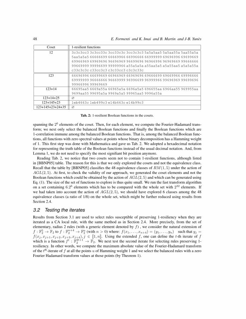
48 E. Formenti and K. Imai and B. Martin and J-B. Yunes
Coset 1-resilient functions12 3c3c3cc3 3c3cc33c 3cc33c3c 3cc3c3c3 5a5a5aa5 5a5aa55a 5aa55a5a
5aa5a5a5 66666699 66669966 66996666 66999999 69696996 6969966969966969 69969696 96696969 96699696 96966996 96969669 9966666699669999 99996699 99999966 a55a5a5a a55aa5a5 a5a55aa5 a5a5a55ac33c3c3c c33cc3c3 c3c33cc3 c3c3c33c
123 66696996 66699669 66966969 66969696 69666699 69669966 6999666669999999 96666666 96669999 96996699 96999966 99696969 9969969699966996 99969669
123+14 66695aa5 6669a55a 66965a5a 6696a5a5 696655aa 6966aa55 969955aa9699aa55 99695a5a 9969a5a5 99965aa5 9996a55a
123+14+25 ∅123+145+23 1eb4663c 1eb499c3 e14b663c e14b99c3
123+145+23+24+35 ∅
Tab. 2: 1-resilient Boolean functions in the cosets.
spanning the 26 elements of the coset. Then, for each element, we compute the Fourier-Hadamard trans-form; we next only select the balanced Boolean functions and finally the Boolean functions which are1-correlation immune among the balanced Boolean functions. That is, among the balanced Boolean func-tions, all functions with zero spectral values at points whose binary decomposition has a Hamming weightof 1. This first step was done with Mathematica and gave us Tab. 2. We adopted a hexadecimal notationfor representing the truth table of the Boolean functions instead of the usual decimal notation. And, fromLemma 1, we do not need to specify the most signifiant bit position anymore.
Reading Tab. 2, we notice that two cosets seem not to contain 1-resilient functions, although listedin [BBNP05] table. The reason for this is that we only explored the cosets and not the equivalence class.Recall that the table by [BBNP05] classifies the 48 equivalence classes of RM(1, 5) under the action ofAGL(2, 5). At first, to check the validity of our approach, we generated the coset elements and not theBoolean functions which could be obtained by the action of AGL(2, 5) and which can be generated usingEq. (1). The size of the set of functions to explore is thus quite small. We run the fast transform algorithmon a set containing 6.26 elements which has to be compared with the whole set with 232 elements. Ifwe had taken into account the action of AGL(2, 5), we should have explored 6 classes among the 48equivalence classes (a ratio of 1/8) on the whole set, which might be further reduced using results fromSection 2.4.
3.2 Testing the iteratesResults from Section 3.1 are used to select rules susceptible of preserving 1-resiliency when they areiterated as a CA local rule, with the same method as in Section 2.4. More precisely, from the set ofelementary, radius 2 rules (with a generic element denoted by f ) , we consider the natural extension off : F5
2 → F2 to f : Fn+42 → Fn2 (with n > 0) where: f(x1, . . . , xn+4) = (y1, . . . , yn) such that yj =
f(xj , xj+1, xj+2, xj+3, xj+4), j ∈ [[1, n]]. Using the extended f , one can define the t-th iterate of fwhich is a function f t : F4t+1
2 → F2. We next test the second iterate for selecting rules preserving 1-resiliency. In other words, we compute the maximum absolute value of the Fourier-Hadamard transformof the tth-iterate of f at all the points u of Hamming weight 1 and we select the balanced rules with a zeroFourier Hadamard transform values at those points (by Theorem 1).
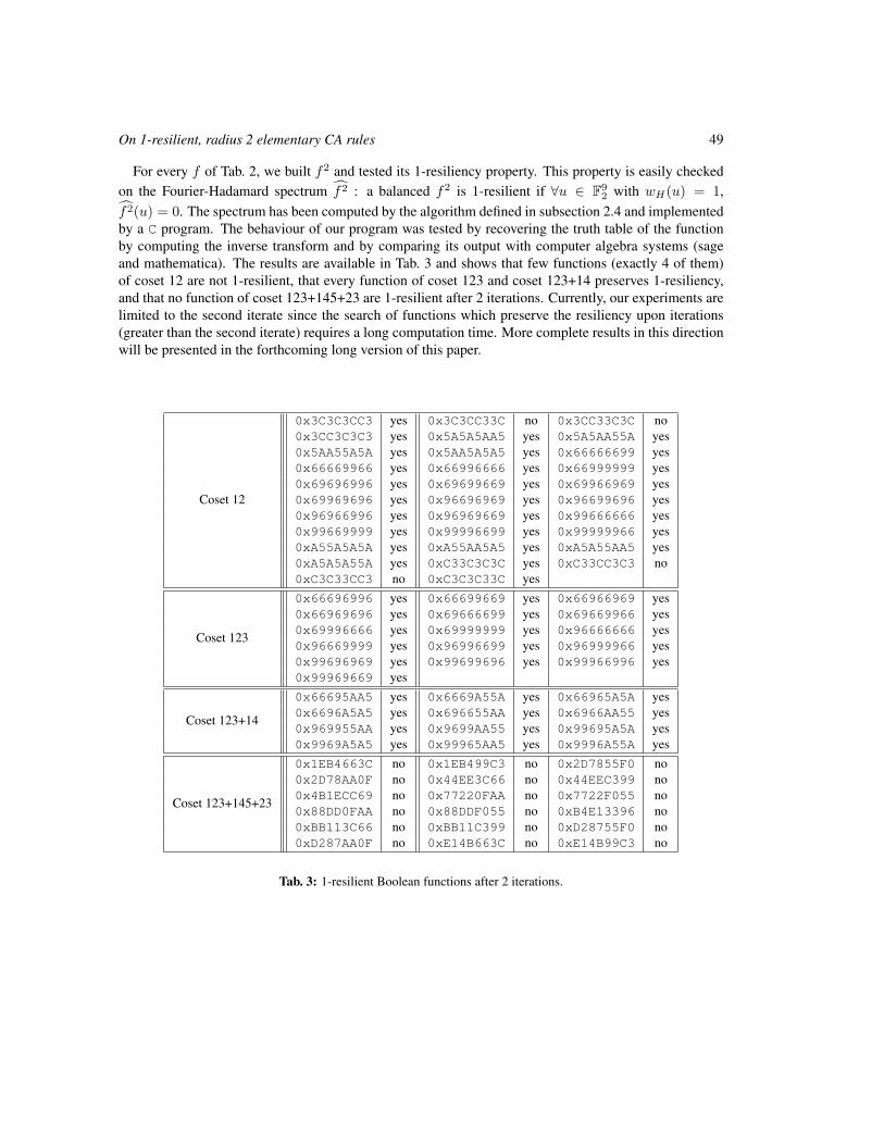
On 1-resilient, radius 2 elementary CA rules 49
For every f of Tab. 2, we built f2 and tested its 1-resiliency property. This property is easily checkedon the Fourier-Hadamard spectrum f2 : a balanced f2 is 1-resilient if ∀u ∈ F9
2 with wH(u) = 1,f2(u) = 0. The spectrum has been computed by the algorithm defined in subsection 2.4 and implementedby a C program. The behaviour of our program was tested by recovering the truth table of the functionby computing the inverse transform and by comparing its output with computer algebra systems (sageand mathematica). The results are available in Tab. 3 and shows that few functions (exactly 4 of them)of coset 12 are not 1-resilient, that every function of coset 123 and coset 123+14 preserves 1-resiliency,and that no function of coset 123+145+23 are 1-resilient after 2 iterations. Currently, our experiments arelimited to the second iterate since the search of functions which preserve the resiliency upon iterations(greater than the second iterate) requires a long computation time. More complete results in this directionwill be presented in the forthcoming long version of this paper.
Coset 12
0x3C3C3CC3 yes 0x3C3CC33C no 0x3CC33C3C no0x3CC3C3C3 yes 0x5A5A5AA5 yes 0x5A5AA55A yes0x5AA55A5A yes 0x5AA5A5A5 yes 0x66666699 yes0x66669966 yes 0x66996666 yes 0x66999999 yes0x69696996 yes 0x69699669 yes 0x69966969 yes0x69969696 yes 0x96696969 yes 0x96699696 yes0x96966996 yes 0x96969669 yes 0x99666666 yes0x99669999 yes 0x99996699 yes 0x99999966 yes0xA55A5A5A yes 0xA55AA5A5 yes 0xA5A55AA5 yes0xA5A5A55A yes 0xC33C3C3C yes 0xC33CC3C3 no0xC3C33CC3 no 0xC3C3C33C yes
Coset 123
0x66696996 yes 0x66699669 yes 0x66966969 yes0x66969696 yes 0x69666699 yes 0x69669966 yes0x69996666 yes 0x69999999 yes 0x96666666 yes0x96669999 yes 0x96996699 yes 0x96999966 yes0x99696969 yes 0x99699696 yes 0x99966996 yes0x99969669 yes
Coset 123+14
0x66695AA5 yes 0x6669A55A yes 0x66965A5A yes0x6696A5A5 yes 0x696655AA yes 0x6966AA55 yes0x969955AA yes 0x9699AA55 yes 0x99695A5A yes0x9969A5A5 yes 0x99965AA5 yes 0x9996A55A yes
Coset 123+145+23
0x1EB4663C no 0x1EB499C3 no 0x2D7855F0 no0x2D78AA0F no 0x44EE3C66 no 0x44EEC399 no0x4B1ECC69 no 0x77220FAA no 0x7722F055 no0x88DD0FAA no 0x88DDF055 no 0xB4E13396 no0xBB113C66 no 0xBB11C399 no 0xD28755F0 no0xD287AA0F no 0xE14B663C no 0xE14B99C3 no
Tab. 3: 1-resilient Boolean functions after 2 iterations.

50 E. Formenti and K. Imai and B. Martin and J-B. Yunes
4 PRNG testingThe quality of pseudo-randomness that can be generated from the Boolean functions mentioned abovehas been evaluated by using the Diehard test suite. It is a widely used tool, especially by cryptographers.The Diehard test suite, developed by Marsaglia from the Florida State University, consists of 17 differenttests which have become something which could be considered as a “benchmarking tool” for PR numbergenerators (see [Mar85]). It is meant to evaluate if a stream of numbers is a good PR sequence. It isnot necessary to explain how Diehard really works and we refer the reader to [Mar95] for further details.But basically, Diehard uses Kolmogorov-Smirnov normality test to quantifiy the distance between thedistribution of a given data set and the uniform distribution; and as the documentation says:
Each Diehard test is able to provide probability values (p-value) which should be uniformlydistributed on [0, 1) if the sequence is made of truly independent bits. Those p-values areobtained by p = F (X) where F is the assumed distribution of the sample random variableX–often normal. But that assumed F is just an asymptotic approximation, for which the fitwill be worse in the tail of the distribution. Thus, we should not be surprised with occasionalp-values close to 0 or 1. When a stream really fails, one gets p-values of 0 or 1 to six or moreplaces. Otherwise, for each test, its p-value should lie in the interval (0.025, 0.975).
So in order to test our data, we designed a C program in which we included the Diehard functions thatwere slightly modified to fit well with our needs. That is to directly use the results of the CA as a PRG.The 17 different and independent statistical tests require about 16 Mbyte of PR values in binary format.
Our goal was to generate different number sequences from the CA and test them against Diehard. Twodifferent tests were made.
4.1 Randomness preservationIn this section we describe the experimentation we made to test if a CA “preserves” the randomnessthrough its dynamics. For this experiment, we consider a CA, whose transition function is f : F5
2 → F2.Given such a CA, we set up an initial sequence of bits (bi)i≥0 that we extract from the /dev/randompseudo-device of a MacOSX system(i). Then we compute the sequence of bits (b′i)i≥0 such that ∀i ≤0, b′i = f(b5i, b5i+1, b5i+2, b5i+3, b5i+4). To ensure some statistical soundness, for a single CA we build30(ii) of such sequences from the same entropic source (each sequence being 16 Mbyte long as requiredby Diehard).
The measure, illustrated in Fig. 1, shows all the distributions of the indicators produced by each singlesequence passing all the Diehard tests. And it can be observed that the p-values are well distributed forevery data pack. Indeed, there are no accumulation points near zero or one.
This means that the input to the tests is made of independent bits. Thus, we can deduce that thesefunctions are good at preserving the randomness of a given source. Or, in other terms, if we feed aCA with a truly random sequence (obtained by the entropy collector of the BSD kernel) as an inputconfiguration and let the CA run, the output configuration is still PR, according to the Diehard test suite.
(i) The entropy collector of the BSD kernel family is considered as a pretty good source of random numbers and MacOSX is builton top of a BSD kernel.
(ii) The repetition of 30 independent experiments comes from statistics. Indeed sample sizes of at least 30 are for many testsconsidered as “large” and allows a better statistical treatment.
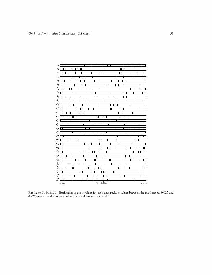
On 1-resilient, radius 2 elementary CA rules 51
0.025 0.975
123456789
10
11
12
13
14
15
16
17
18
19
20
21
22
23
24
25
26
27
28
29
30p-value
Fig. 1: 0x3C3C3CC3: distribution of the p-values for each data pack. p-values between the two lines (at 0.025 and0.975) mean that the corresponding statistical test was successful.

52 E. Formenti and K. Imai and B. Martin and J-B. Yunes
0.025 0.975
even 64
odd 64
even 65
odd 65
p-value
Fig. 2: Distribution of the p-values for the ring CA with rule 0x3C3C3CC3. p-values between the two lines (at 0.025and 0.975) mean that the corresponding statistical test was successful, which is not the case for even 64 and odd 64(all the p-values are almost zero) and barely for even 65 and odd 65.
0.025 0.975
even 64
odd 64
even 65
odd 65
p-value
Fig. 3: Distribution of the p-values for the ring CA with rule 0x69999999. p-values between the two lines (at 0.025and 0.975) mean that the corresponding statistical test was successful.
4.2 Random number generation
Much more classically, these tests were built to evaluate the possible generation of a good PR sequence byCAs. While it is well known that radius 1 elementary CAs are not suitable for generating PR sequences,it is not impossible to build good PR sequence from simple CAs. As we already tested if the radius-2functions are good to preserve the randomness of a random source, it would be interesting to considerthem as PRNG. So, we tried something very similar to [STCS02].
We set up two rings of cells. Although Wolfram used a ring of 127 cells and Preneel (1993) suggesteda ring of 1024 cells to ensure a better quality (both used a slightly different mechanisms for random bitextraction), we use perimeters 64 and 65 as done in [STCS02]. The initial configuration of these ringsis of Hamming weight 1. We let the CA iterate about 2 million times. Then, from each configurationobtained, we extract two 32-bits words: the “even” (resp. “odd”), word is built with the state of the first32 “even” (resp. “odd”) cells. The sequences of these “even” (resp. “odd”) words constitute two differentsequences of 16 Mbyte.
Then, we use Diehard to produce p-values for each test as illustrated in Fig. 2. For the CA with ruleOx3c3c3cc3, we conclude that this PRNG is not satisfactory. But we were able to find some CAs (likethe one with rule Ox69999999 given as an example in Fig. 3) which were able to give much betterresults against Diehard tests. This suggests that it may be possible to obtain a good PRNG from such aCA.
AcknowledgementsThe authors are grateful to C. Carlet who pointed out Reference [Car11] for explaining the differencebetween Fourier-Hadamard and Walsh transforms and to J. Mairesse for its help with statistical testing.

On 1-resilient, radius 2 elementary CA rules 53
References[BBNP05] An Braeken, Yuri Borissov, Svetla Nikova, and Bart Preneel. Classification of boolean func-
tions of 6 variables or less with respect to some cryptographic properties. In Automata,Languages and Programming, volume 3580 of Lecture Notes in Computer Science, pages61–61. Springer Berlin / Heidelberg, 2005.
[BW72] E. Berlekamp and L. Welch. Weight distribution of the cosets of the (32, 6) Reed-Mullercode. IEEE Trans. Inf. Theory, 18:203–207, 1972.
[Car11] C. Carlet. Boolean functions for cryptography and error-correcting codes. Technical report,University of Paris 8, 2011.
[CFMM97] G. Cattaneo, E. Formenti, L. Margara, and G. Mauri. Transformations of the one-dimensionalcellular automata rule space. Parallel Comput., 23:1593–1611, November 1997.
[ER82] D. Elliott and K. Rao. Fast transforms, algorithms, analysis, applications. Academic press,1982.
[Gol99] O. Goldreich. Pseudorandomness. Notices of the AMS, 46:1209–1216, Sep 1999.
[LMS08] P. Lacharme, B. Martin, and P. Sole. Pseudo-random sequences, boolean functions andcellular automata. In Proceedings of Boolean Functions and Cryptographic Applications,2008.
[Mar85] G. Marsaglia. A current view of random number generators. In Computer Sciences andStatistics, pages 3–10, 1985.
[Mar95] G. Marsaglia. Diehard. http://www.stat.fsu.edu/pub/diehard/, 1995.
[Mar08] Bruno Martin. A walsh exploration of elementary ca rules. J. Cellular Automata, 3(2):145–156, 2008.
[MS91] Willi Meier and Othmar Staffelbach. Analysis of pseudo random sequences generated by cel-lular automata. In Proceedings of the 10th annual international conference on Theory andapplication of cryptographic techniques, EUROCRYPT’91, pages 186–199, Berlin, Heidel-berg, 1991. Springer-Verlag.
[STCS02] Barry Shackleford, Motoo Tanaka, Richard J. Carter, and Greg Snider. Fpga implementationof neighborhood-of-four cellular automata random number generators. In Proceedings ofthe 2002 ACM/SIGDA tenth international symposium on Field-programmable gate arrays,FPGA ’02, pages 106–112, New York, NY, USA, 2002. ACM.
[Wol86a] Stephen Wolfram. Cryptography with cellular automata. In Hugh Williams, editor, Advancesin Cryptology CRYPTO 85 Proceedings, volume 218 of Lecture Notes in Computer Science,pages 429–432. Springer Berlin / Heidelberg, 1986.
[Wol86b] Stephen Wolfram. Theory and applications of cellular automata. World Scientific, Singa-pore, 1986.

54 E. Formenti and K. Imai and B. Martin and J-B. Yunes
[Wol02] Stephen Wolfram. A New Kind of Science. Wolfram Media, 2002.
[XM88] G.-Z. Xiao and J. L. Massey. A spectral characterization of correlation-immune combiningfunctions. IEEE Trans. on Information Theory, 34:569–571, 1988.
AUTOMATA 2011, Santiago, Chile local proceedings LP, 2011, 55–68
On the set of Fixed Points of the ParallelSymmetric Sand Pile Model†
Kevin Perrot1‡ and Thi Ha Duong Phan2§ and Trung Van Pham2¶
1LIP (UMR 5668 - CNRS - Universite de Lyon - ENS de Lyon) - 46 alle d’Italie 69364 Lyon Cedex 7, France2Institute of Mathematics, VAST - 18 Hoang Quoc Viet Road, Cau Giay,10307, Hanoi, Vietnam
Sand Pile Models are discrete dynamical systems emphasizing the phenomenon of Self-Organized Criticality. Froma configuration composed of a finite number of stacked grains, we apply on every possible positions (in parallel) twograin moving transition rules. The transition rules permit one grain to fall to its right or left (symmetric) neighboringcolumn if the difference of height between those columns is larger than 2. The model is nondeterministic and grainsalways fall downward. We propose a study of the set of fixed points reachable in the Parallel Symmetric Sand PileModel (PSSPM). Using a comparison with the Symmetric Sand Pile Model (SSPM) on which rules are applied once ateach iteration, we get a continuity property. This property states that within PSSPM we can’t reach every fixed pointsof SSPM, but a continuous subset according to the lexicographic order. Moreover we define a successor relation tobrowse exhaustively the sets of fixed points of those models.
Keywords: Discrete Dynamical System, Sand Pile Model, Fixed point
1 IntroductionSand Pile Models were introduced in 1988 ([BTW88]) to highlight Self-Organized Criticality (SOC).SOC characterizes dynamical systems having critical attractors, i.e., systems that evolve toward a stablestate from which small perturbations have uncontrolled consequences on the system. This property isstraightforward to figure out in the scope of sand pile models : consider a flat table on which we addgrains one by one. After a moment, the amount of grains will look like a circular cone which basediameter will continue to grow as we add grains one by one. Some grain additions create avalanches,chain reactions involving numerous grain falls. Some avalanches stop quickly, others continue until theyreach the table top. Now remark that whatever the size of the pile is, there will always be one more singlegrain addition which will increase the base diameter of the cone. So the tiniest possible perturbation —
†This work is supported in part by the National Fundamental Research Programme in Natural Sciences of Vietnam, and theComplex System Institute of Lyon.
‡[email protected]§[email protected]¶[email protected]
c© 2011 AUTOMATA proceedings, Santiago, Chile, 2011
56 Kevin Perrot and Thi Ha Duong Phan and Trung Van Pham
one single grain addition — can create an unbounded avalanche. This example illustrates the SOC of sandpile models.
There are many variants of sand pile models. All of them consider local grain moving transitions,applied in sequential or parallel mode (one rule application at each iteration or as many rule applicationsas possible at each iteration), starting from a finite number of stacked grains. The first model, introduced in[CK93], considers one rule applied sequentially : if the difference of height between columns i and i+1 islarger than two, then one grain falls from column i to column i+1. The set of reachable configurations hasa lattice structure and some other interesting properties, see [CMP02] and [LMMP01]. Furthermore its setof reachable configurations can be generated efficiently (see [MM11], [MR10] and [Mas09]). Applyingthe rule in parallel on every possible column leads to a completely different description of the model,see [DL98]. We can also add one more rule, symmetric to the previous one : if the difference of heightbetween columns i and i − 1 is larger than two, then one grain can fall from column i to column i − 1.This leads to SSPM (symmetric sand pile model), studied in [Pha08] and [FMP07].
In [FPPT10], the authors studies PSSPM, the parallel variant of SSPM, and they proved that the formof fixed points of the two models are the same. In this paper, we investigate the set of all fixed points ofPSSPM, taking into account their position. We provide a deterministic procedure to reach the extremal(leftmost and rightmost) fixed points of PSSPM according to the total lexicographic order, and prove thatany fixed point between these two extremal fixed points reachable in SSPM is also reachable in PSSPM.We also define a successor relation / which gives a straightforward way of computing the set of fixedpoints of PSSPM.
In [RDMDP06] the authors suggest to add rules to get grains also moving forward and backward, toget closer to real life sand piles. [CLM+04] is a survey on sand pile models. An interesting generalizationof sand pile models is sand automata, which are powerful enough to simulate cellular automata, see[DGM09], [CFM07] and [CF03].
In this paper, n is a given nonnegative integer.
2 Parallel Symmetric Sand Pile ModelIn the theory of discrete dynamical systems, a model is defined by its set of configurations and its transitionrule(s). We say that a configuration b is reachable from a configuration a if b is obtained from a by asequence of transitions. In the scope of sand piles, we are interested in the set of configurations reachablefrom a finite number of stacked grains.
Notation 1 A configuration c is a sequence of nonnegative integers, with only finitely many positive val-ues. We use an underlined number to denote the position 0 of a sequence. For example c = (1, 4, 3, 2, 1)is the configuration such that c−2 = 1, c−1 = 4, c0 = 3, c1 = 2, c2 = 1 and for all i /∈ J−2; 2K, ci = 0.
We now give formal definitions of SSPM and PSSPM.
Definition 1 SSPM is a discrete dynamical system defined by:
• Initial configuration: (n).
• Local left vertical rule L: (. . . , ai−1, ai, . . . )→ (. . . , ai−1 + 1, ai − 1, . . . ) if ai−1 + 2 ≤ ai.
• Local right vertical ruleR: (. . . , ai, ai+1, . . . )→ (. . . , ai − 1, ai+1 + 1, . . . ) if ai ≥ ai+1 + 2.
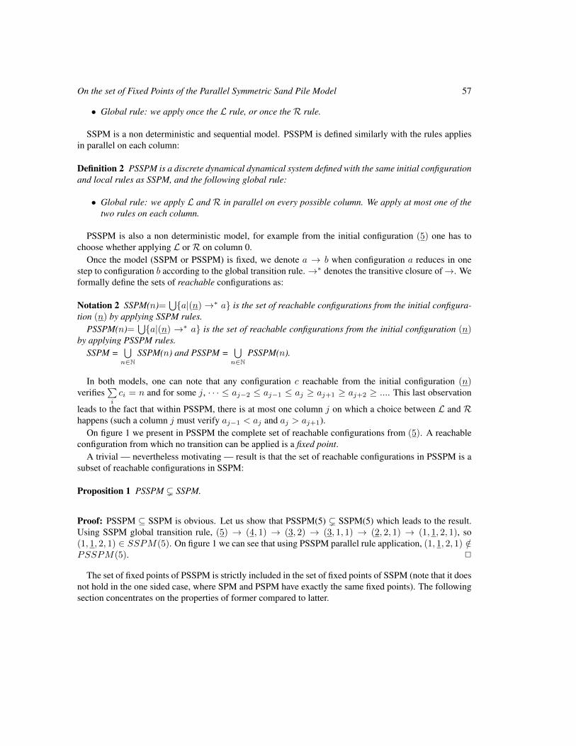
On the set of Fixed Points of the Parallel Symmetric Sand Pile Model 57
• Global rule: we apply once the L rule, or once theR rule.
SSPM is a non deterministic and sequential model. PSSPM is defined similarly with the rules appliesin parallel on each column:
Definition 2 PSSPM is a discrete dynamical dynamical system defined with the same initial configurationand local rules as SSPM, and the following global rule:
• Global rule: we apply L and R in parallel on every possible column. We apply at most one of thetwo rules on each column.
PSSPM is also a non deterministic model, for example from the initial configuration (5) one has tochoose whether applying L orR on column 0.
Once the model (SSPM or PSSPM) is fixed, we denote a → b when configuration a reduces in onestep to configuration b according to the global transition rule. →∗ denotes the transitive closure of→. Weformally define the sets of reachable configurations as:
Notation 2 SSPM(n)=⋃a|(n)→∗ a is the set of reachable configurations from the initial configura-
tion (n) by applying SSPM rules.PSSPM(n)=
⋃a|(n) →∗ a is the set of reachable configurations from the initial configuration (n)
by applying PSSPM rules.SSPM =
⋃n∈N
SSPM(n) and PSSPM =⋃
n∈NPSSPM(n).
In both models, one can note that any configuration c reachable from the initial configuration (n)verifies
∑i
ci = n and for some j, · · · ≤ aj−2 ≤ aj−1 ≤ aj ≥ aj+1 ≥ aj+2 ≥ .... This last observation
leads to the fact that within PSSPM, there is at most one column j on which a choice between L and Rhappens (such a column j must verify aj−1 < aj and aj > aj+1).
On figure 1 we present in PSSPM the complete set of reachable configurations from (5). A reachableconfiguration from which no transition can be applied is a fixed point.
A trivial — nevertheless motivating — result is that the set of reachable configurations in PSSPM is asubset of reachable configurations in SSPM:
Proposition 1 PSSPM ( SSPM.
Proof: PSSPM ⊆ SSPM is obvious. Let us show that PSSPM(5) ( SSPM(5) which leads to the result.Using SSPM global transition rule, (5) → (4, 1) → (3, 2) → (3, 1, 1) → (2, 2, 1) → (1, 1, 2, 1), so(1, 1, 2, 1) ∈ SSPM(5). On figure 1 we can see that using PSSPM parallel rule application, (1, 1, 2, 1) /∈PSSPM(5). 2
The set of fixed points of PSSPM is strictly included in the set of fixed points of SSPM (note that it doesnot hold in the one sided case, where SPM and PSPM have exactly the same fixed points). The followingsection concentrates on the properties of former compared to latter.
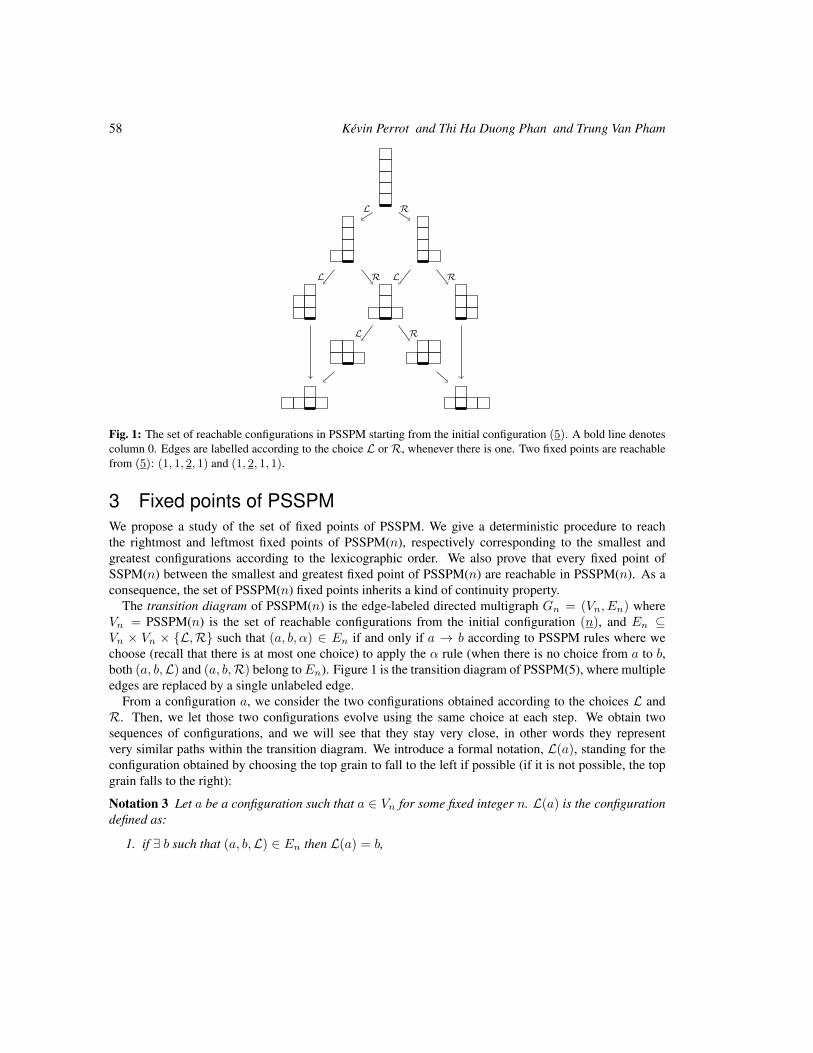
58 Kevin Perrot and Thi Ha Duong Phan and Trung Van Pham
L R
L R L R
L R
Fig. 1: The set of reachable configurations in PSSPM starting from the initial configuration (5). A bold line denotescolumn 0. Edges are labelled according to the choice L or R, whenever there is one. Two fixed points are reachablefrom (5): (1, 1, 2, 1) and (1, 2, 1, 1).
3 Fixed points of PSSPMWe propose a study of the set of fixed points of PSSPM. We give a deterministic procedure to reachthe rightmost and leftmost fixed points of PSSPM(n), respectively corresponding to the smallest andgreatest configurations according to the lexicographic order. We also prove that every fixed point ofSSPM(n) between the smallest and greatest fixed point of PSSPM(n) are reachable in PSSPM(n). As aconsequence, the set of PSSPM(n) fixed points inherits a kind of continuity property.
The transition diagram of PSSPM(n) is the edge-labeled directed multigraph Gn = (Vn, En) whereVn = PSSPM(n) is the set of reachable configurations from the initial configuration (n), and En ⊆Vn × Vn × L,R such that (a, b, α) ∈ En if and only if a → b according to PSSPM rules where wechoose (recall that there is at most one choice) to apply the α rule (when there is no choice from a to b,both (a, b,L) and (a, b,R) belong toEn). Figure 1 is the transition diagram of PSSPM(5), where multipleedges are replaced by a single unlabeled edge.
From a configuration a, we consider the two configurations obtained according to the choices L andR. Then, we let those two configurations evolve using the same choice at each step. We obtain twosequences of configurations, and we will see that they stay very close, in other words they representvery similar paths within the transition diagram. We introduce a formal notation, L(a), standing for theconfiguration obtained by choosing the top grain to fall to the left if possible (if it is not possible, the topgrain falls to the right):
Notation 3 Let a be a configuration such that a ∈ Vn for some fixed integer n. L(a) is the configurationdefined as:
1. if ∃ b such that (a, b,L) ∈ En then L(a) = b,
On the set of Fixed Points of the Parallel Symmetric Sand Pile Model 59
2. else if ∃ b such that (a, b,R) ∈ En then L(a) = b,
3. else L(a) = a.
R(a) is defined similarly.Let ω = ω1 . . . ωk be a word over the alphabet L,R, ω(a) is the configuration defined inductively as
ω(a) = ω2 . . . ωk(ω1(a)).
The idea will be to consider a configuration a of PSSPM(n) for a fixed integer n and the two config-urations R(a) and L(a). Those two configurations are intuitively similar each other. Then we will seethat for every word ω over the alphabet L,R, the configurations ω(R(a)) and ω(L(a)) are also similaraccording to the relation
∗/ defined below. This is the key argument of our study, stated in Proposition 2.
Finally, we use known results about SSPM and further developments to show that when we reach fixedpoints, the configurations are very similar (see / defined below). This leads to Theorem 1, relating the setof fixed points reachable in PSSPM(n) to that reachable in SSPM(n).
Definition 3 Let ∆(a,b) be the sequence of differences between configurations a and b, ∆i(a,b) = ai−bi.We define a notion of similarity or closeness between configurations, denoted by the following relations:
a / b ⇐⇒ ∆(a, b) ∈ 0∗ −10∗10∗
a∗/ b ⇐⇒ ∆(a, b) ∈ (0∗ −10∗10∗)∗
where −1 is a minus one value. As a convention ε = 0ω , so that a = b implies a∗/ b.
The reader should note that∗/ is not the reflexive transitive closure of /, it is just a kind of non-strict
variant of /.The following lemma states the similarity of the configurations obtained when we follow very close
paths in the transition diagram of PSSPM(n). The weak relation∗/ is used to compare obtained configu-
rations all along the evolution toward fixed points. We will see in Proposition 3 that the relation betweenfixed points can be strengthened into /.
Proposition 2 Let a ∈ PSSPM(n). For all ω ∈ L,R∗,
ω(R(a))∗/ ω(L(a))
We first present a technical lemma used to avoid some impossible cases in the proof of Proposition 2.
Lemma 1 (technical) Consider a sequence in PSSPM(n).
c1 → c2 → · · · → ck
If there exists a column i such that
1. i remains one of the highest columns i.e., ∀ 1 ≤ t ≤ k, cti = maxjctj
2. c1i ≤ c1i+1 + 2 (resp. c1i−1 + 2 ≥ c1i )
Then ∀ 1 ≤ t ≤ k, cti ≤ cti+1 + 2 (resp. cti−1 + 2 ≥ cti).
60 Kevin Perrot and Thi Ha Duong Phan and Trung Van Pham
Proof: We proceed by induction on the iterations. The base case is verified according to the secondhypothesis. The top column i can’t receive any grain during the iterations under consideration so theheight difference with column i + 1 (resp. i− 1) can only be increased by 1 if i doesn’t lose a grain andi+ 1 (resp. i− 1) loses a grain. In any other case the height difference doesn’t increase. So if the heightdifference is at most 1, then it can’t be increased to a difference greater than 2. If the height difference is2, then column i loses a grain so the height difference doesn’t increase. 2
Proof of Proposition 2: We proceed by induction on the length of ω. The base case is obvious : eitherthere is no choice from a to L(a) and R(a), and hence L(a) = R(a) implies R(a)
∗/ L(a) or there is a
choice on column i and hence
• R(a)i−1 = L(a)i−1 − 1
• R(a)i = L(a)i
• R(a)i+1 = L(a)i+1 + 1
• ∀j /∈ i− 1, i, i+ 1, R(a)j = L(a)j
soR(a)∗/ L(a). By induction hypothesis, we are considering two configurations b = ω1 . . . ωk−1(R(a))
and c = ω1 . . . ωk−1(L(a)) such that b∗/ c and we will now prove that ωk(b)
∗/ ωk(c).
For the sake of clarity, we denote d (resp. e) the configuration such that b ωk→ d (resp. c ωk→ e).We do an induction on the columns, and construct ∆(d, e) from our knowledge on ∆(b, c), from left to
right according to the behavior of each column i in b and c. Considering the rule application on column iof a configuration h gives us three informations:
• does column i− 1 receive a grain from its right neighbor, denoted←h i−1 ∈ 0, 1;
• does column i give a grain to one of its neighbors, denoted hi ∈ 0, 1;
• does column i+ 1 receive a grain from its left neighbor, denoted→h i+1 ∈ 0, 1.
In order to conclude, we will use the fact that
for all j, ∆j(d, e) = ∆j(b, c) + (←b j −
←c j)− (bj − cj) + (
→b j −
→c j)
At each step of the induction, we will ”update” ∆(b, c) with the three informations we get and see thatit has always the form (0∗ −10∗10∗)∗. We denote ∆i(b, c) the sequence ∆(b, c) updated up to index i,defined at each index j as
∆ij(b, c) =
∆j(b, c) + (
←b j −
←c j)− (bj − cj) + (
→b j −
→c j) = ∆j(d, e) if j < i
∆j(b, c)− (bi − ci) + (→b i −
→c i) if j = i
∆j(b, c) + (→b i −
→c i) if j = i+ 1
∆j(b, c) if j > i+ 1
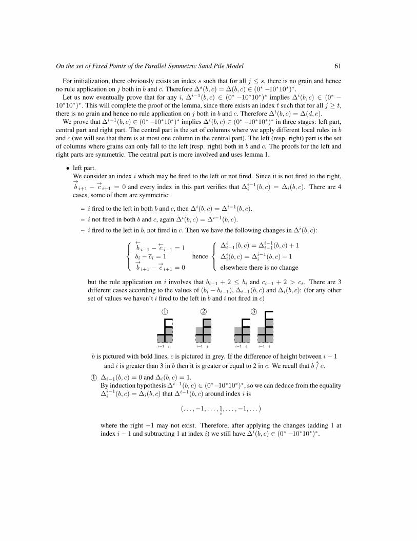
On the set of Fixed Points of the Parallel Symmetric Sand Pile Model 61
For initialization, there obviously exists an index s such that for all j ≤ s, there is no grain and henceno rule application on j both in b and c. Therefore ∆s(b, c) = ∆(b, c) ∈ (0∗ −10∗10∗)∗.
Let us now eventually prove that for any i, ∆i−1(b, c) ∈ (0∗ −10∗10∗)∗ implies ∆i(b, c) ∈ (0∗ −10∗10∗)∗. This will complete the proof of the lemma, since there exists an index t such that for all j ≥ t,there is no grain and hence no rule application on j both in b and c. Therefore ∆t(b, c) = ∆(d, e).
We prove that ∆i−1(b, c) ∈ (0∗ −10∗10∗)∗ implies ∆i(b, c) ∈ (0∗ −10∗10∗)∗ in three stages: left part,central part and right part. The central part is the set of columns where we apply different local rules in band c (we will see that there is at most one column in the central part). The left (resp. right) part is the setof columns where grains can only fall to the left (resp. right) both in b and c. The proofs for the left andright parts are symmetric. The central part is more involved and uses lemma 1.
• left part.We consider an index i which may be fired to the left or not fired. Since it is not fired to the right,→b i+1 −
→c i+1 = 0 and every index in this part verifies that ∆i−1
i (b, c) = ∆i(b, c). There are 4cases, some of them are symmetric:
– i fired to the left in both b and c, then ∆i(b, c) = ∆i−1(b, c).
– i not fired in both b and c, again ∆i(b, c) = ∆i−1(b, c).
– i fired to the left in b, not fired in c. Then we have the following changes in ∆i(b, c):←b i−1 −
←c i−1 = 1
bi − ci = 1→b i+1 −
→c i+1 = 0
hence
∆i
i−1(b, c) = ∆i−1i−1(b, c) + 1
∆ii(b, c) = ∆i−1
i (b, c)− 1
elsewhere there is no change
but the rule application on i involves that bi−1 + 2 ≤ bi and ci−1 + 2 > ci. There are 3different cases according to the values of (bi − bi−1), ∆i−1(b, c) and ∆i(b, c): (for any otherset of values we haven’t i fired to the left in b and i not fired in c)
1©
ii−1
2©
ii−1
3©
ii−1 ii−1
b is pictured with bold lines, c is pictured in grey. If the difference of height between i− 1
and i is greater than 3 in b then it is greater or equal to 2 in c. We recall that b∗/ c.
1© ∆i−1(b, c) = 0 and ∆i(b, c) = 1.By induction hypothesis ∆i−1(b, c) ∈ (0∗−10∗10∗)∗, so we can deduce from the equality∆i−1
i (b, c) = ∆i(b, c) that ∆i−1(b, c) around index i is
(. . . ,−1, . . . , 1i, . . . ,−1, . . . )
where the right −1 may not exist. Therefore, after applying the changes (adding 1 atindex i− 1 and subtracting 1 at index i) we still have ∆i(b, c) ∈ (0∗ −10∗10∗)∗.
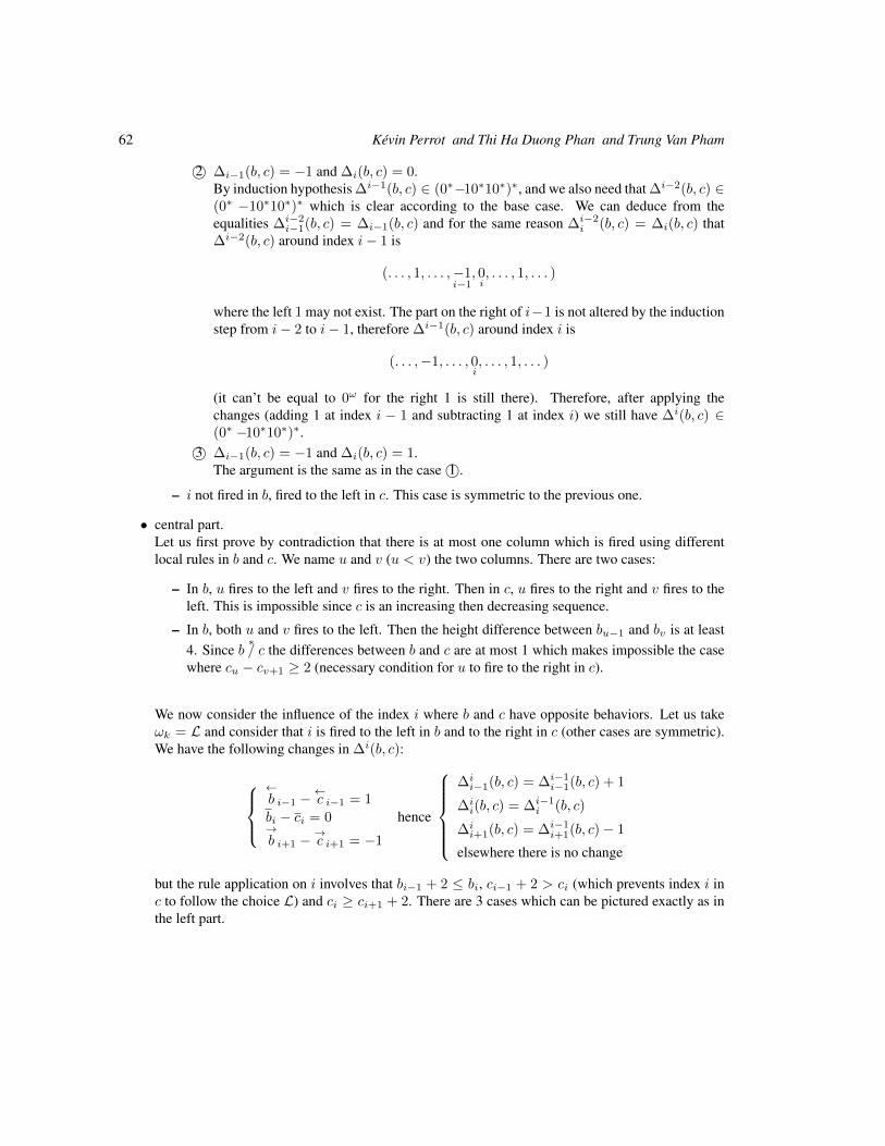
62 Kevin Perrot and Thi Ha Duong Phan and Trung Van Pham
2© ∆i−1(b, c) = −1 and ∆i(b, c) = 0.By induction hypothesis ∆i−1(b, c) ∈ (0∗−10∗10∗)∗, and we also need that ∆i−2(b, c) ∈(0∗ −10∗10∗)∗ which is clear according to the base case. We can deduce from theequalities ∆i−2
i−1(b, c) = ∆i−1(b, c) and for the same reason ∆i−2i (b, c) = ∆i(b, c) that
∆i−2(b, c) around index i− 1 is
(. . . , 1, . . . ,−1i−1
, 0i, . . . , 1, . . . )
where the left 1 may not exist. The part on the right of i−1 is not altered by the inductionstep from i− 2 to i− 1, therefore ∆i−1(b, c) around index i is
(. . . ,−1, . . . , 0i, . . . , 1, . . . )
(it can’t be equal to 0ω for the right 1 is still there). Therefore, after applying thechanges (adding 1 at index i − 1 and subtracting 1 at index i) we still have ∆i(b, c) ∈(0∗ −10∗10∗)∗.
3© ∆i−1(b, c) = −1 and ∆i(b, c) = 1.The argument is the same as in the case 1©.
– i not fired in b, fired to the left in c. This case is symmetric to the previous one.
• central part.Let us first prove by contradiction that there is at most one column which is fired using differentlocal rules in b and c. We name u and v (u < v) the two columns. There are two cases:
– In b, u fires to the left and v fires to the right. Then in c, u fires to the right and v fires to theleft. This is impossible since c is an increasing then decreasing sequence.
– In b, both u and v fires to the left. Then the height difference between bu−1 and bv is at least4. Since b
∗/ c the differences between b and c are at most 1 which makes impossible the case
where cu − cv+1 ≥ 2 (necessary condition for u to fire to the right in c).
We now consider the influence of the index i where b and c have opposite behaviors. Let us takeωk = L and consider that i is fired to the left in b and to the right in c (other cases are symmetric).We have the following changes in ∆i(b, c):
←b i−1 −
←c i−1 = 1
bi − ci = 0→b i+1 −
→c i+1 = −1
hence
∆i
i−1(b, c) = ∆i−1i−1(b, c) + 1
∆ii(b, c) = ∆i−1
i (b, c)
∆ii+1(b, c) = ∆i−1
i+1(b, c)− 1
elsewhere there is no change
but the rule application on i involves that bi−1 + 2 ≤ bi, ci−1 + 2 > ci (which prevents index i inc to follow the choice L) and ci ≥ ci+1 + 2. There are 3 cases which can be pictured exactly as inthe left part.
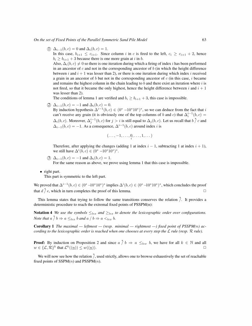
On the set of Fixed Points of the Parallel Symmetric Sand Pile Model 63
1© ∆i−1(b, c) = 0 and ∆i(b, c) = 1.In this case, bi+1 ≤ ci+1. Since column i in c is fired to the left, ci ≥ ci+1 + 2, hencebi ≥ bi+1 + 3 because there is one more grain at i in b.Also, ∆i(b, c) 6= 0 so there is one iteration during which a firing of index i has been performedin an ancestor of c and not in the corresponding ancestor of b (in which the height differencebetween i and i+ 1 was lesser than 2), or there is one iteration during which index i receiveda grain in an ancestor of b but not in the corresponding ancestor of c (in this case, i becameand remains the highest column in the chain leading to b and there exist an iteration where i isnot fired, so that it became the only highest, hence the height difference between i and i + 1was lesser than 2).The conditions of lemma 1 are verified and bi ≥ bi+1 + 3, this case is impossible.
2© ∆i−1(b, c) = −1 and ∆i(b, c) = 0.By induction hypothesis ∆i−1(b, c) ∈ (0∗ −10∗10∗)∗, so we can deduce from the fact that ican’t receive any grain (it is obviously one of the top columns of b and c) that ∆i−1
i (b, c) =
∆i(b, c). Moreover, ∆i−1j (b, c) for j > i is still equal to ∆j(b, c). Let us recall that b
∗/ c and
∆i−1(b, c) = −1. As a consequence, ∆i−1(b, c) around index i is
(. . . ,−1, . . . , 0i, . . . , 1, . . . )
Therefore, after applying the changes (adding 1 at index i − 1, subtracting 1 at index i + 1),we still have ∆i(b, c) ∈ (0∗ −10∗10∗)∗.
3© ∆i−1(b, c) = −1 and ∆i(b, c) = 1.For the same reason as above, we prove using lemma 1 that this case is impossible.
• right part.This part is symmetric to the left part.
We proved that ∆i−1(b, c) ∈ (0∗−10∗10∗)∗ implies ∆i(b, c) ∈ (0∗−10∗10∗)∗, which concludes the proofthat d
∗/ e, which in turn completes the proof of this lemma. 2
This lemma states that trying to follow the same transitions conserves the relation∗/. It provides a
deterministic procedure to reach the extremal fixed points of PSSPM(n):
Notation 4 We use the symbols ≤lex and ≥lex to denote the lexicographic order over configurations.Note that a
∗/ b⇒ a ≤lex b and a / b⇒ a <lex b.
Corollary 1 The maximal — leftmost — (resp. minimal — rightmost —) fixed point of PSSPM(n) ac-cording to the lexicographic order is reached when one chooses at every step the L rule (resp. R rule).
Proof: By induction on Proposition 2 and since a∗/ b ⇒ a ≤lex b, we have for all k ∈ N and all
w ∈ L,Rk that Lk((n)) ≤ w((n)). 2
We will now see how the relation∗/, used strictly, allows one to browse exhaustively the set of reachable
fixed points of SSPM(n) and PSSPM(n).
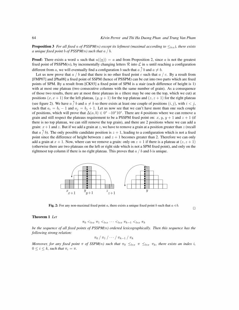
64 Kevin Perrot and Thi Ha Duong Phan and Trung Van Pham
Proposition 3 For all fixed a of PSSPM(n) except its leftmost (maximal according to ≤lex), there existsa unique fixed point b of PSSPM(n) such that a / b.
Proof: There exists a word u such that u((n)) = a and from Proposition 2, since a is not the greatestfixed point of PSSPM(n), by incrementally changing letters R into L in u until reaching a configurationdifferent from a, we will eventually find a configuration b such that a
∗/ b and a 6= b.
Let us now prove that a / b and that there is no other fixed point c such that a / c. By a result from[FMP07] and [Pha08] a fixed point of SSPM (hence of PSSPM) can be cut into two parts which are fixedpoints of SPM. By a result from [CK93] a fixed point of SPM is a stair (each difference of height is 1)with at most one plateau (two consecutive columns with the same number of grain). As a consequenceof those two results, there are at most three plateaus in a (there may be one on the top, which we cut) atpositions (x, x + 1) for the left plateau, (y, y + 1) for the top plateau and (z, z + 1) for the right plateau(see figure 2). We have a
∗/ b and a 6= b so there exists at least one couple of positions (i, j), with i < j,
such that ai = bi − 1 and aj = bj + 1. Let us now see that we can’t have more than one such coupleof positions, which will prove that ∆(a, b) ∈ 0∗ −10∗10∗. There are 4 positions where we can remove agrain and still respect the plateaus requirement to be a PSSPM fixed point on: x, y, y + 1 and z + 1 (ifthere is no top plateau, we can still remove the top grain), and there are 2 positions where we can add agrain: x+1 and z. But if we add a grain at z, we have to remove a grain at a position greater than z (recallthat a
∗/ b). The only possible candidate position is z + 1, leading to a configuration which is not a fixed
point since the difference of height between z and z + 1 becomes greater than 2. Therefore we can onlyadd a grain at x+ 1. Now, where can we remove a grain: only on z + 1 if there is a plateau at (z, z + 1)(otherwise there are two plateaus on the left or right side which is not a SPM fixed point), and only on therightmost top column if there is no right plateau. This proves that a / b and b is unique.
xx+1
yy+1
zz+1
y
Fig. 2: For any non-maximal fixed point a, there exists a unique fixed point b such that a / b.2
Theorem 1 Letπ0 <lex π1 <lex · · · <lex πk−1 <lex πk
be the sequence of all fixed points of PSSPM(n) ordered lexicographically. Then this sequence has thefollowing strong relation:
π0 / π1 / · · · / πk−1 / πkMoreover, for any fixed point π of SSPM(n) such that π0 ≤lex π ≤lex πk, there exists an index i,0 ≤ i ≤ k, such that πi = π.
On the set of Fixed Points of the Parallel Symmetric Sand Pile Model 65
Proof: n2 is an upper bound to the number of iterations from the configuration (n) to a fixed point usingPSSPM rules (at each step a grain loses some height). Therefore, the set of fixed points of PSSPM(n) isequal to
⋃ω∈L,Rn2
ω((n)) because trying every possibility leads to reaching every possible fixed point.
Starting from the word s0 = Rn2
and changing one by one the letters R into L, we get a sequence ofwords (s0, s1, . . . , sn
2
) such that for all k, the size of the word sk is n2 and the number of occurrences ofL in sk is k. From Proposition 2, for all k < n2 we have sk((n))
∗/ sk+1((n)). There are two possibilities:
• sk((n)) = sk+1((n)).
• sk((n)) 6= sk+1((n)).
In the second case, both configurations are fixed points of PSSPM(n) and from Proposition 3 we havesk / sk+1. This gives a simple procedure to construct the set of fixed points of PSSPM(n) from π0 to πkand proves the first part of the theorem (the procedure is described below).
From the SSPM(n) fixed point characterization described in [FMP07] and [Pha08] (presented in theproof of Proposition 3), even if the complete set of reachable fixed points are not the same, the fixedpoints of SSPM(n) and PSSPM(n) between the smallest and greatest fixed points of PSSPM(n) are thesame (the authors of [FMP07] and [Pha08] use exactly the same construction as the one described in theproof of Proposition 3, see figure 2). The fact that PSSPM(n) ⊆ SSPM(n) completes the proof of thesecond part of the theorem. 2
The proofs of Proposition 3 and Theorem 1 provide a simple algorithm to browse the set of fixed pointsof PSSPM(n). First compute the minimal (rightmost πR) and maximal (leftmost πL) fixed points startingfrom (n) by following always the same choice (R to get the minimal configuration, and L to get themaximal one). Then starting from πR, construct the unique fixed point π1 such that πR /π1, as explainedon figure 2. From π1, construct the unique fixed point π2 such that π1 / π2, etc... Until you get πL. Fromwhat precedes, this deterministic procedure browses exhaustively the set of fixed points of PSSPM(n).
4 ConclusionWe have studied the set of fixed points of PSSPM(n) and compared it to the set of fixed points of SSPM(n)using the natural lexicographic order. We proved the intuitive fact that the greatest fixed point can bereached using always the choice L, and that the smallest fixed point can be reached using always thechoiceR. More interestingly, we showed that every fixed point reachable in SSPM(n) between the lowestand the greatest fixed points of PSSPM(n) is also reachable in PSSPM(n). This is a kind of continuityproperty: the set of fixed points reachable in PSSPM(n) is an ”interval” of the set of fixed points reachablein SSPM(n).
Further work may concentrate on finding a bound on the maximal and minimal non-empty columnsin the set of fixed points of PSSPM(n) which is an open question. The bound b
√2nc proved in [Pha08]
holds for PSSPM(n) but it is not satisfying since proposition 1 states that there are strictly less fixed pointsin PSSPM(n) than in SSPM(n).
AcknowledgementsThe authors would like to thank Eric Remila for useful comments.
66 Kevin Perrot and Thi Ha Duong Phan and Trung Van Pham
References[BTW88] P. Bak, C. Tang, and K. Wiesenfeld. Self-organized criticality. Phys. Rev. A, 38(1):364–374,
1988.
[CF03] Julien Cervelle and Enrico Formenti. On sand automata. In Helmut Alt and MichelHabib, editors, STACS, volume 2607 of Lecture Notes in Computer Science, pages 642–653. Springer, 2003.
[CFM07] Julien Cervelle, Enrico Formenti, and Benoıt Masson. From sandpiles to sand automata.Theor. Comput. Sci., 381(1-3):1–28, 2007.
[CK93] Eric Goles Ch. and Marcos A. Kiwi. Games on line graphs and sand piles. Theor. Comput.Sci., 115(2):321–349, 1993.
[CLM+04] Eric Goles Ch., Matthieu Latapy, Clemence Magnien, Michel Morvan, and Ha Duong Phan.Sandpile models and lattices: a comprehensive survey. Theor. Comput. Sci., 322(2):383–407, 2004.
[CMP02] Eric Goles Ch., Michel Morvan, and Ha Duong Phan. Sandpiles and order structure ofinteger partitions. Discrete Applied Mathematics, 117(1-3):51–64, 2002.
[DGM09] Alberto Dennunzio, Pierre Guillon, and Benoıt Masson. Sand automata as cellular au-tomata. Theor. Comput. Sci., 410:3962–3974, September 2009.
[DL98] Jerome Olivier Durand-Lose. Parallel transient time of one-dimensional sand pile. Theor.Comput. Sci., 205(1-2):183–193, 1998.
[FMP07] Enrico Formenti, Benoıt Masson, and Theophilos Pisokas. Advances in symmetric sand-piles. Fundam. Inform., 76(1-2):91–112, 2007.
[FPPT10] E. Formenti, V. T. Pham, T. H. D. Phan, and T. T. H. Tran. Fixed point form of the parallelsymmetric sand pile model. preprint, 2010.
[LMMP01] Matthieu Latapy, Roberto Mantaci, Michel Morvan, and Ha Duong Phan. Structure of somesand piles model. Theor. Comput. Sci., 262(1):525–556, 2001.
[Mas09] Paolo Massazza. A cat algorithm for sand piles. Pure Mathematics and Applications,19:147–158, 2009.
[MM11] Roberto Mantaci and Paolo Massazza. From linear partitions to parallelogram polyominoes.In Proceedings of the 15th international conference on Developments in language theory,DLT’11, pages 350–361, Berlin, Heidelberg, 2011. Springer-Verlag.
[MR10] Paolo Massazza and Roberto Radicioni. A cat algorithm for the exhaustive generation ofice piles. RAIRO - Theor. Inf. and Applic., 44(4):525–543, 2010.
[Pha08] Thi Ha Duong Phan. Two sided sand piles model and unimodal sequences. ITA, 42(3):631–646, 2008.

On the set of Fixed Points of the Parallel Symmetric Sand Pile Model 67
[RDMDP06] Dominique Rossin, Enrica Duchi, Roberto Mantaci, and Ha Duong Phan. Bidimensionnalsand pile and ice pile models. In GASCOM 2006, Dijon, France, 2006.

68 Kevin Perrot and Thi Ha Duong Phan and Trung Van Pham
.
AUTOMATA 2011, Santiago, Chile local proceedings LP, 2011, 69–88
Bifurcations in Boolean Networks
Chris J. Kuhlman1,3 and Henning S. Mortveit1,2† and David Murrugarra2
and V. S. Anil Kumar1,3
1Network Dynamics and Simulation Science Laboratory, Virginia Tech2Department of Mathematics, Virginia Tech3Department of Computer Science, Virginia Tech
This paper characterizes the attractor structure of synchronous and asynchronous Boolean networks induced by bi-threshold functions. Bi-threshold functions are generalizations of standard threshold functions and have separatethreshold values for the transitions 0 → 1 (up-threshold) and 1 → 0 (down-threshold). We show that synchronousbi-threshold systems may, just like standard threshold systems, only have fixed points and 2-cycles as attractors.Asynchronous bi-threshold systems (fixed permutation update sequence), on the other hand, undergo a bifurcation.When the difference ∆ of the down- and up-threshold is less than 2 they only have fixed points as limit sets. However,for ∆ ≥ 2 they may have long periodic orbits. The limiting case of ∆ = 2 is identified using a potential functionargument. Finally, we present a series of results on the dynamics of bi-threshold systems for families of graphs.
Keywords: Boolean networks, graph dynamical systems, synchronous, asynchronous, sequential dynamical systems,threshold, bi-threshold, bifurcation
1 IntroductionA standard Boolean threshold function tk,m : 0, 1m −→ 0, 1 is defined by
tk,m(x1, . . . , xm) =
1, if σ(x1, . . . , xm) ≥ k and0, otherwise,
(1.1)
where σ(x1, . . . , xm) =∣∣1 ≤ i ≤ m | xi = 1
∣∣. This class of functions is a common choice in modelingbiological systems [Kauffman (1969); Karaoz et al. (2004)], and social behaviors (e.g., joining a strike orrevolt, adopting a new technology or contraceptives, spread of rumors and stress, and collective action),see, e.g., [Granovetter (1978); Bulger et al. (1989); Macy (1991); Centola and Macy (2007); Watts (2002);Kempe et al. (2003)].
A bi-threshold function is a function ti,k↑,k↓,m : 0, 1m −→ 0, 1 defined by
ti,k↑,k↓,m(x1, . . . , xm) =
tk↑,m, if xi = 0,
tk↓,m, if xi = 1 .(1.2)
†Email: [email protected] (corresponding author)
c© 2011 AUTOMATA proceedings, Santiago, Chile, 2011
70 Chris J. Kuhlman and Henning S. Mortveit and David Murrugarra and V. S. Anil Kumar
Here i denotes a designated argument – later it will be the vertex or cell index. We call k↑ the up-thresholdand k↓ the down-threshold. When k↑ = k↓ the bi-threshold function coincides with a standard thresholdfunction. Note that unlike the standard threshold function in (1.1) which is symmetric, the bi-thresholdfunction is quasi-symmetric (or outer-symmetric) – with the exception of index i, it only depends on itsarguments through their sum.
In this paper we consider synchronous and asynchronous graph dynamical systems (GDSs), see [Mortveitand Reidys (2007); Macauley and Mortveit (2009)], of the form F : 0, 1n −→ 0, 1n induced by bi-threshold functions. These are natural extensions of threshold GDSs and capture threshold phenomenaexhibiting hysteresis properties. Bi-threshold systems are also prevalent in social systems where eachindividual can change back-and-forth between two states; Schelling states: “Numerous social phenom-ena display cyclic behavior ...”, see (Schelling, 1978, p. 86). Among his examples is whether pick-upvolleyball games will continue through an academic semester or die (e.g., individuals regularly choosingto play or not play). One can also look at public health concerns such as obesity, where an individual’sback-and-forth decisions to diet or not—which are peer influenced, [Christakis and Fowler (2007)], andtherefore can be at least partially described by thresholds—are so commonplace that it has a name: “yo-yo dieting” [Atkinson et al. (1994)]. When k↑ > k↓, a vertex that transitions from state 0 to state 1 ismore likely to remain in state 1 than what would be the case in a standard threshold GDS. For the statetransitions from 1 to 0 the situation is analogous. This suggests that the cost to change back to state 0is great or that a change to state 0 will occur only if the conditions that gave rise to the 0 → 1 transi-tion significantly diminish. A company that acquires and later divests itself of a competitor is such anexample. Examples where k↓ ≥ k↑ are commonplace. For example, [Schelling (1978)] states that heoften witnesses people who start to cross the street against traffic lights, but will return to the curb if theyobserve an insufficient number of others following behind. Overshooting, whereby a group of individualstake some action, and within a short time period, a subset of these pull back from it, is also of interest tothe sociology community [Bischi and Merlone (2009)] and is characterized by k↓ ≥ k↑.
It is convenient to introduce the quantity ∆ = k↓ − k↑. The first of our main results (Theorem 3.1)characterizes limit cycle structure of synchronous bi-threshold GDS (also known as as Boolean networks).Building on the proof for threshold functions in Goles and Olivos (1981), we prove that only fixed pointsand periodic orbits of length 2 can occur for each possible combination of k↑ and k↓. Since we re-useparts of their proof, and also since their proof only appears in French, a condensed English translationis included in the appendix on page 83. The situation is very different for asynchronous bi-thresholdGDSs where a vertex permutation is used for the update sequence. Our second main result states thatwhen ∆ < 2, only fixed points can occur as limit cycles. However, for ∆ ≥ 2 there are graphs forwhich arbitrary length periodic orbits can be generated. The case ∆ = 2 is identified using a potentialfunction argument and represents a (2-parameter) bifurcation in a discrete system, a phenomenon that toour knowledge is novel. We also include a series of results for bi-threshold dynamics on special graphclasses. These offer examples of asynchronous bi-threshold GDSs with long periodic orbits, and may alsoserve as building blocks in construction and modeling of bi-threshold systems with given cycle structures.
Paper organization. We introduce necessary definitions and terminology for graph dynamical systemsin Section 2. The two main theorems are presented in Sections 3.1 and 3.2. Our collection of results ondynamics for graph classes like trees and cycle graphs follow in Section 4 before we conclude in Section 5.
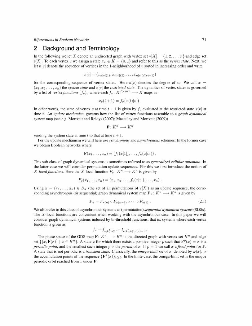
Bifurcations in Boolean Networks 71
2 Background and TerminologyIn the following we let X denote an undirected graph with vertex set v[X] = 1, 2, . . . , n and edge sete[X]. To each vertex v we assign a state xv ∈ K = 0, 1 and refer to this as the vertex state. Next, welet n[v] denote the sequence of vertices in the 1-neighborhood of v sorted in increasing order and write
x[v] = (xn[v](1), xn[v](2), . . . , xn[v](d(v)+1))
for the corresponding sequence of vertex states. Here d(v) denotes the degree of v. We call x =(x1, x2, . . . , xn) the system state and x[v] the restricted state. The dynamics of vertex states is governedby a list of vertex functions (fv)v where each fv : Kd(v)+1 −→ K maps as
xv(t+ 1) = fv(x(t)[v]
).
In other words, the state of vertex v at time t + 1 is given by fv evaluated at the restricted state x[v] attime t. An update mechanism governs how the list of vertex functions assemble to a graph dynamicalsystem map (see e.g. Mortveit and Reidys (2007); Macauley and Mortveit (2009))
F : Kn −→ Kn
sending the system state at time t to that at time t+ 1.For the update mechanism we will here use synchronous and asynchronous schemes. In the former case
we obtain Boolean networks where
F(x1, . . . , xn) = (f1(x[1]), . . . , fn(x[n])) .
This sub-class of graph dynamical systems is sometimes referred to as generalized cellular automata. Inthe latter case we will consider permutation update sequences. For this we first introduce the notion ofX-local functions. Here the X-local function Fv : Kn −→ Kn is given by
Fv(x1, . . . , xn) = (x1, x2, . . . , fv(x[v]), . . . , xn) .
Using π = (π1, . . . , πn) ∈ SX (the set of all permutations of v[X]) as an update sequence, the corre-sponding asynchronous (or sequential) graph dynamical system map Fπ : Kn −→ Kn is given by
Fπ = Fπ(n) Fπ(n−1) · · · Fπ(1) . (2.1)
We also refer to this class of asynchronous systems as (permutation) sequential dynamical systems (SDSs).The X-local functions are convenient when working with the asynchronous case. In this paper we willconsider graph dynamical systems induced by bi-threshold functions, that is, systems where each vertexfunction is given as
fv = fv,k↑v ,k↓v := tv,k↑v ,k↓v ,d(v)+1 .
The phase space of the GDS map F : Kn −→ Kn is the directed graph with vertex set Kn and edgeset
(x,F(x)
)| x ∈ Kn. A state x for which there exists a positive integer p such that Fp(x) = x is a
periodic point, and the smallest such integer p is the period of x. If p = 1 we call x a fixed point for F.A state that is not periodic is a transient state. Classically, the omega-limit set of x, denoted by ω(x), isthe accumulation points of the sequence Fk(x)k≥0. In the finite case, the omega-limit set is the uniqueperiodic orbit reached from x under F.
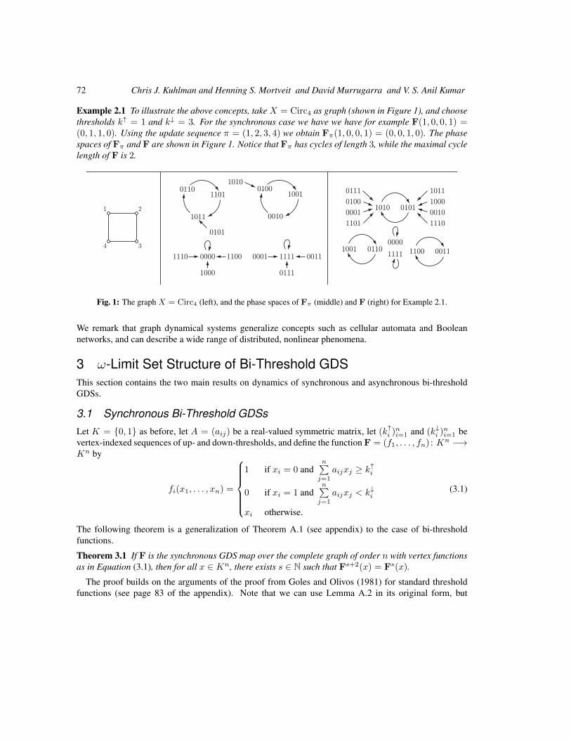
72 Chris J. Kuhlman and Henning S. Mortveit and David Murrugarra and V. S. Anil Kumar
Example 2.1 To illustrate the above concepts, take X = Circ4 as graph (shown in Figure 1), and choosethresholds k↑ = 1 and k↓ = 3. For the synchronous case we have we have for example F(1, 0, 0, 1) =(0, 1, 1, 0). Using the update sequence π = (1, 2, 3, 4) we obtain Fπ(1, 0, 0, 1) = (0, 0, 1, 0). The phasespaces of Fπ and F are shown in Figure 1. Notice that Fπ has cycles of length 3, while the maximal cyclelength of F is 2.
0000
11111001 0110 1100 0011
0001
1110
0100
1011
1000
0111
0010
1101
1010 0101
1000
1110 11000000 0001 0011
0111
1111
0010
01001010
1001
0101
1011
01101101
1 2
4 3
Fig. 1: The graph X = Circ4 (left), and the phase spaces of Fπ (middle) and F (right) for Example 2.1.
We remark that graph dynamical systems generalize concepts such as cellular automata and Booleannetworks, and can describe a wide range of distributed, nonlinear phenomena.
3 ω-Limit Set Structure of Bi-Threshold GDSThis section contains the two main results on dynamics of synchronous and asynchronous bi-thresholdGDSs.
3.1 Synchronous Bi-Threshold GDSsLet K = 0, 1 as before, let A = (aij) be a real-valued symmetric matrix, let (k↑i )ni=1 and (k↓i )ni=1 bevertex-indexed sequences of up- and down-thresholds, and define the function F = (f1, . . . , fn) : Kn −→Kn by
fi(x1, . . . , xn) =
1 if xi = 0 and
n∑j=1
aijxj ≥ k↑i
0 if xi = 1 andn∑j=1
aijxj < k↓i
xi otherwise.
(3.1)
The following theorem is a generalization of Theorem A.1 (see appendix) to the case of bi-thresholdfunctions.
Theorem 3.1 If F is the synchronous GDS map over the complete graph of order n with vertex functionsas in Equation (3.1), then for all x ∈ Kn, there exists s ∈ N such that Fs+2(x) = Fs(x).
The proof builds on the arguments of the proof from Goles and Olivos (1981) for standard thresholdfunctions (see page 83 of the appendix). Note that we can use Lemma A.2 in its original form, but
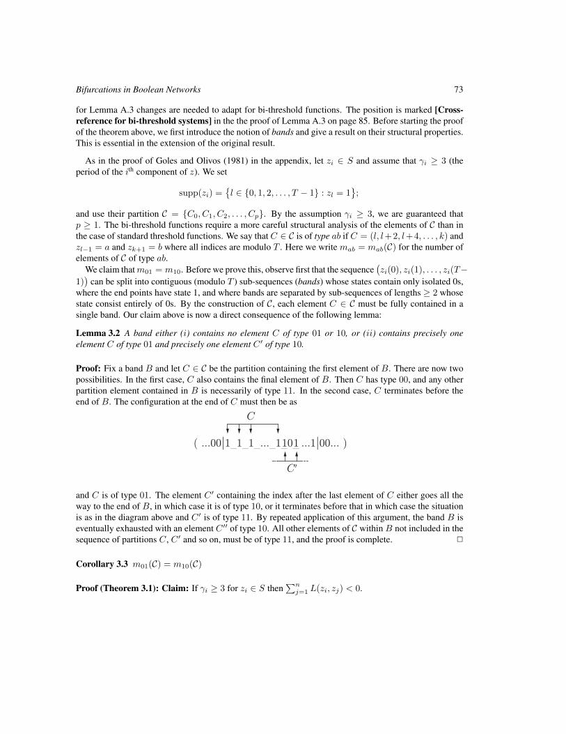
Bifurcations in Boolean Networks 73
for Lemma A.3 changes are needed to adapt for bi-threshold functions. The position is marked [Cross-reference for bi-threshold systems] in the the proof of Lemma A.3 on page 85. Before starting the proofof the theorem above, we first introduce the notion of bands and give a result on their structural properties.This is essential in the extension of the original result.
As in the proof of Goles and Olivos (1981) in the appendix, let zi ∈ S and assume that γi ≥ 3 (theperiod of the ith component of z). We set
supp(zi) =l ∈ 0, 1, 2, . . . , T − 1 : zl = 1
;
and use their partition C = C0, C1, C2, . . . , Cp. By the assumption γi ≥ 3, we are guaranteed thatp ≥ 1. The bi-threshold functions require a more careful structural analysis of the elements of C than inthe case of standard threshold functions. We say that C ∈ C is of type ab if C = (l, l+2, l+4, . . . , k) andzl−1 = a and zk+1 = b where all indices are modulo T . Here we write mab = mab(C) for the number ofelements of C of type ab.
We claim thatm01 = m10. Before we prove this, observe first that the sequence(zi(0), zi(1), . . . , zi(T−
1))
can be split into contiguous (modulo T ) sub-sequences (bands) whose states contain only isolated 0s,where the end points have state 1, and where bands are separated by sub-sequences of lengths ≥ 2 whosestate consist entirely of 0s. By the construction of C, each element C ∈ C must be fully contained in asingle band. Our claim above is now a direct consequence of the following lemma:
Lemma 3.2 A band either (i) contains no element C of type 01 or 10, or (ii) contains precisely oneelement C of type 01 and precisely one element C ′ of type 10.
Proof: Fix a band B and let C ∈ C be the partition containing the first element of B. There are now twopossibilities. In the first case, C also contains the final element of B. Then C has type 00, and any otherpartition element contained in B is necessarily of type 11. In the second case, C terminates before theend of B. The configuration at the end of C must then be as
( ...00j1|1
|1
|...
|1
|0
| ...1j00... )1 1
C
C0
and C is of type 01. The element C ′ containing the index after the last element of C either goes all theway to the end of B, in which case it is of type 10, or it terminates before that in which case the situationis as in the diagram above and C ′ is of type 11. By repeated application of this argument, the band B iseventually exhausted with an element C ′′ of type 10. All other elements of C within B not included in thesequence of partitions C, C ′ and so on, must be of type 11, and the proof is complete. 2
Corollary 3.3 m01(C) = m10(C)
Proof (Theorem 3.1): Claim: If γi ≥ 3 for zi ∈ S then∑nj=1 L(zi, zj) < 0.
74 Chris J. Kuhlman and Henning S. Mortveit and David Murrugarra and V. S. Anil Kumar
We can write
n∑i=1
L(zi, zj) =
p∑k=0
( n∑j=1
aij∑l∈Ck
(zj(l + 1)− zj(l − 1)
))=
p∑k=0
Ψik ,
where
Ψik =
n∑j=1
aij∑l∈Ck
(zj(l + 1)− zj(l − 1)
)=
n∑j=1
aijzj(lk + 2qk + 1)−n∑j=1
aijzj(lk − 1) .
We need to consider Ψik for the four types of partition elements. As in the original proof, note that Ψi0 =0.
Ck is of type 00: in this case zi(lk − 1) = 0, zi(lk) = 1, zi(lk + 2qk + 1) = 0 and zi(lk + 2qk + 2) = 0,which is only possible if
n∑j=1
aijzj(lk − 1) ≥ k↑i andn∑j=1
aijzj(lk + 2qk + 1) < k↑i ,
which implies that Ψik < 0.
Ck is of type 11: this case is completely analogous to the 00 case, and again we conclude that Ψik < 0.
Ck is of type 10: here zi(lk − 1) = 1, zi(lk) = 1, zi(lk + 2qk + 1) = 0 and zi(lk + 2qk + 2) = 0. Thisimplies that ∑
j=1
aijzj(lk − 1) ≥ k↓i and∑j=1
aijzj(lk + 2qk + 1) < k↑i ,
leading to Ψik < k↑i − k↓i .
Ck is of type 01: this case is essentially the same as the 10 case, but here Ψik < k↓i − k↑i .
Using the above four cases, we now have
n∑j=0
L(zi, zj) =
p∑k=0
Ψik < 0 +m00 · 0 +m11 · 0 +m10(k↑i − k↓i ) +m01(k↓i − k
↑i ) = 0 ,
where the last equality follows by Corollary 3.3. Clearly, this leads to the same contradiction as in theproof of Theorem A.1. 2
An immediate consequence of Theorem 3.1 is the following:
Corollary 3.4 A synchronous bi-threshold GDS may only have fixed points and 2-cycles as limit sets.
Bifurcations in Boolean Networks 75
3.2 Asynchronous Bi-Threshold GDSsTheorem 3.5 Let X be a graph, let π ∈ Sx and let (fv)v be bi-threshold functions all satisfying ∆(v) =k↓v − k↑v ≤ 1. The sequential dynamical system map Fπ only has fixed points as limit sets.
As before, the graph X is finite. Note also that the per-vertex thresholds k↑ and k↓ need not be uniformfor the graph.
Proof: The proof uses a potential function based on a construction in Barrett et al. (2006), but seealso Goles-Chacc et al. (1985). For a given state x ∈ Kn we assign to each vertex the potential
P (v, x) =
k↓v , xv = 1
d(v) + 2− k↑v , xv = 0 .
Note that the quantity d(v)+2−k↑v is the smallest number of vertex states in the local state x[v] that mustbe zero to ensure that xv remains in state zero. Similarly, an edge e = v, v′ is assigned the potential
P (e = v, v′, x) =
1, xv 6= xv′
0, xv = xv′ .
For book-keeping, we let ni = ni(v;x) denote the number of vertices adjacent to v in state i for i = 0, 1and note that n0 +n1 = d. The system potential P (x) at the state x is the sum of all the vertex and all theedge potentials. For the theorem statement it is clearly sufficient to show that each application of a vertexfunction that leads to a change in a vertex state causes the system potential to drop.
Consider first the case where xv is mapped from 0 to 1 which implies that n1 ≥ k↑v . Since a change insystem potential only occurs for vertex v and edges incident with v, we may disregard the other potentialswhen determining this change. Denoting the system potential before and after the update by P and P ′,we have P = d+ 2− k↑v + n1 and P ′ = k↓v + n0 which implies that
P ′ − P = k↓v + n0 − d− 2 + k↑v − n1 = k↓v + k↑v − 2n1 − 2
≤ −(k↑v − k↓v)− 2 = ∆(v)− 2 ,
and this is strictly negative whenever ∆ = k↓ − k↑ ≤ 1. Similarly, for the transition where xv maps from1 to 0 one must have n1 + 1 ≤ k↓v − 1 or n1 ≤ k↓v − 2. In this case we have
P ′ − P = [d+ 2− k↑v + n1]− [k↓v + n0] = 2n1 + 2− k↓v − k↑v≤ 2k↓v − 4 + 2− k↑v − k↓v = ∆(v)− 2
as before, concluding the proof. 2
3.3 Bifurcations in Asynchronous GDSA natural question now is what happens in the case where ∆ = k↓ − k↑ = 2 since periodic orbits areno longer excluded by the arguments in the proof above. The following proposition shows that there aregraphs and choices of k↑ and k↓, such that ∆ = 2, for which there are periodic orbits of arbitrary length.
76 Chris J. Kuhlman and Henning S. Mortveit and David Murrugarra and V. S. Anil Kumar
Proposition 3.6 The bi-threshold GDS map over X = Circn with update sequence π = (1, 2, 3, . . . , n),thresholds k↑ = 1 and k↓ = 3, has cycles of length n− 1.
Proof: We claim that the state x = (0, 0, . . . , 0, 1, 0) is on an (n−1)-cycle. Straightforward computationsgive that the single 1-state is shifted one position to the left upon each application of Fπ until the statey = (0, 1, 0, . . . , 0) is reached. The image of this state is z = (1, 0, 0, . . . , 0, 0, 1) which is easily seen tomap to x. The smallest number of iterations required to return to the original state x is n − 1, producinga cycle as claimed. 2
In other words, by taking ∆ as a parameter, we see that the bi-threshold sequential dynamical systemundergoes a bifurcation at ∆ = 2.
4 Dynamics of Bi-Threshold GDSs4.1 Graph UnionsFrom Proposition 3.6, we see that for X = Circn with threshold k↑ = 1 and k↓ = 3 at each vertex, weobtain an (n−1)-cycle for the update sequence π = (1, 2, . . . , n). The following proposition demonstrateshow we can combine graphs to obtain larger cycle sizes for bi-threshold SDSs with arbitrarily nonuniformk↑, k↓. In particular, the result applies to the case where we combine Circn graphs where p = n − 1 isprime.
Proposition 4.1 For i = 1, 2 let Xi be a graph for which the bi-threshold GDS with update sequence πihas a cycle in phase space of length ci. Let ui ∈ v[Xi], and let X be the graph obtained as the disjointunion of X1 and X2 plus additionally the vertex w 6∈ v[X1], v[X2] with the edges u1, w and u2, w.Moreover, let all thresholds of vertices in X1 and X2 be as before, and assign threshold k↑ = 3 to w. Thebi-threshold SDS map over X with update sequence π = (π1|π2|w) [juxtaposition] has a cycle of lengthlcm(c1, c2).
Proof: Let vertex w have k↑ = 3, so that w will never transition to state 1 from state 0. Let x =(x1|x2|xw) be the state over X constructed from states x1 and x2 on the respective ci-cycle over X1
and X2 with xw = 0. The only vertices whose connectivity, and therefore induced vertex function, areaffected by the addition of w are u1 and u2. But the state transitions for u1 and u2 are unaffected becauseeach is predicated on σ(x[u1]) and σ(x[u2]), respectively, and these latter two quantities are not alteredby the state of w because that state is fixed at 0 by construction. Hence, the phase space of X contains acycle of length lcm(c1, c2) as claimed. 2
Thus, for k↑ = 1 and k↓ = 3, there exists a circle graph and permutation π that will produce a cycle inphase space of length three or greater, and multiple circle graphs can be combined to produce graphs withlarge orbit cycles without modifying the thresholds of vertices in X1 and X2.
4.2 TreesPropositions 3.6 and 4.1 show how periodic orbits of length > 2 arise over graphs that contain cycles.This section investigates bi-threshold SDS maps where X is a tree.
To start, we first recall the notion of κ-equivalence of permutations from Macauley and Mortveit (2009,2008). Two permutations π, π′ ∈ SX are κ-equivalent if the corresponding induced acyclic orienta-tions Oπ and Oπ′ of X are related by a sequence of source-to-sink conversions. Here, the orientation Oπ
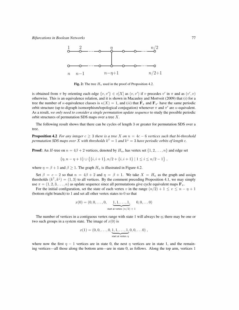
Bifurcations in Boolean Networks 77
1 2 ´
n¡´+1
n/2
n n¡1 n/2+1
Fig. 2: The tree Hn used in the proof of Proposition 4.2.
is obtained from π by orienting each edge v, v′ ∈ e[X] as (v, v′) if v precedes v′ in π and as (v′, v)otherwise. This is an equivalence relation, and it is shown in Macauley and Mortveit (2009) that (i) for atree the number of κ-equivalence classes is κ(X) = 1, and (ii) that Fπ and Fπ′ have the same periodicorbit structure (up to digraph isomorphism/topological conjugation) whenever π and π′ are κ-equivalent.As a result, we only need to consider a single permutation update sequence to study the possible periodicorbit structures of permutation SDS maps over a tree X .
The following result shows that there can be cycles of length 3 or greater for permutation SDS over atree.
Proposition 4.2 For any integer c ≥ 3 there is a tree X on n = 4c − 6 vertices such that bi-thresholdpermutation SDS maps over X with thresholds k↑ = 1 and k↓ = 3 have periodic orbits of length c.
Proof: An H-tree on n = 4β + 2 vertices, denoted by Hn, has vertex set 1, 2, . . . , n and edge set
η, n− η + 1 ∪i, i+ 1, n/2 + i, i+ 1 | 1 ≤ i ≤ n/2− 1
,
where η = β + 1 and β ≥ 1. The graph Hn is illustrated in Figure 4.2.
Set β = c − 2 so that n = 4β + 2 and η = β + 1. We take X = Hn as the graph and assignthresholds (k↑, k↓) = (1, 3) to all vertices. By the comment preceding Proposition 4.1, we may simplyuse π = (1, 2, 3, . . . , n) as update sequence since all permutations give cycle equivalent maps Fπ .
For the initial configuration, set the state of each vertex v in the range (n/2) + 1 ≤ v ≤ n − η + 1(bottom right branch) to 1 and set all other vertex states to 0 so that
x(0) = (0, 0, . . . , 0, 1, 1, . . . , 1,︸ ︷︷ ︸start at vertex (n/2) + 1
0, 0, . . . 0)
The number of vertices in a contiguous vertex range with state 1 will always be η; there may be one ortwo such groups in a system state. The image of x(0) is
x(1) = (0, 0, . . . , 0, 1, 1, . . . , 1,︸ ︷︷ ︸start at vertex η
0, 0, . . . 0) ,
where now the first η − 1 vertices are in state 0, the next η vertices are in state 1, and the remain-ing vertices—all those along the bottom arm—are in state 0, as follows. Along the top arm, vertices 1
78 Chris J. Kuhlman and Henning S. Mortveit and David Murrugarra and V. S. Anil Kumar
through η − 1 will remain in state 0 because all nodes and their neighbors are in state 0. Vertex η, thestate of the vertex incident to the crossbar on the top arm, will change to 1 because its neighbor alongthe crossbar is in state 1. For the given permutation, then, each subsequent vertex vi in the range η + 1through n/2 will change to state 1 because xvi−1 = 1 and k↑ = 1. For the bottom arm, vertex (n/2) + 1will change from state 1 to state 0 because σ(x[v(n/2)+1]) = 2 < k↓. For the same reason, each vertexvi in the range (n/2) + 2 to n − η + 1 will transition to state 0. Vertices from n − η + 2 through n willremain in state 0.
The next state is
x(2) = (0, 0, . . . , 0, 1, 1, . . . , 1︸ ︷︷ ︸start at vertex η−1
, 0, 0, . . . 0, 1, 1, . . . , 1︸ ︷︷ ︸start at vertex n−η+1
) ,
where, for the top arm, the first η − 2 vertices are in state 0, the next η vertices are in state 1, and the lastvertex on the top arm is in state 0. That is, the set of 1’s along the top arm has shifted one vertex left,as follows. Let the set of vertices in the top arm in state 1 (in x(1)) be denoted vi through vi+η . Vertexvi−1 will transition 0→ 1 because xvi = 1. Vertex vi will remain in state 1 because σ(x[vi]) = 3 = k↓.Likewise vi+1 through vi+η−1 will remain in state 1. However, vi+η will transition to state 0 becauseσ(x[vi+η]) = 2 < k↓. We refer to this behavior as a left-shift (the analogous shift to the right is a right-shift). For the bottom arm, the η vertices (labels (n/2) + 1 through n − η) remain in state 0. Vertexn−η+1 transitions to state 1 because the neighbor along the crossbar is in state 1. Subsequently, verticesn− η + 2 through n transition to state 1, in turn, according to π.
The next state is
x(3) = (0, 0, . . . , 0, 1, 1, . . . , 1︸ ︷︷ ︸start at vertex η−2
, 0, 0, . . . 0, 1, 1, . . . , 1︸ ︷︷ ︸start at vertex n−η
) ,
where the set of η vertices in state 1 in the top arm has shifted left, and the set of η vertices in state 1in the bottom arm has shifted left. The shifting process embodied in the transition from state x(2) tox(3)—where there is a group of vertices in state 1 in each of the top and bottom arms—can happen a totalof (η − 2) times. The state after these (η − 2) transitions is
x(η) = (1, 1, . . . , 1︸ ︷︷ ︸start at vertex 1
, 0, 0, . . . 0, 1, 1, . . . , 1,︸ ︷︷ ︸start at vertex n−2η+3
0, 0, . . . , 0) .
The image of x(η) is x(0), the initial state. There are 2 + (η− 2) + 1 state transitions, and we have a limitcycle of length c = η + 1. 2
Of course, the proof does not guarantee that c is the minimal periodic orbit size, nor that Hn is theminimal order tree with a periodic orbit of this length. Additionally, there may be multiple periodic orbitsof length c. The following proposition expands on this in the case where c ≥ 5: there exists a tree ofsmaller order than Hn that also admits a c-cycle, namely the Y -trees.
Proposition 4.3 For any integer c ≥ 3 there is a tree on n = 3c − 2 vertices such that bi-thresholdpermutation SDS maps over this tree with thresholds k↑ = 1 and k↓ = 3 have periodic orbits of length c.
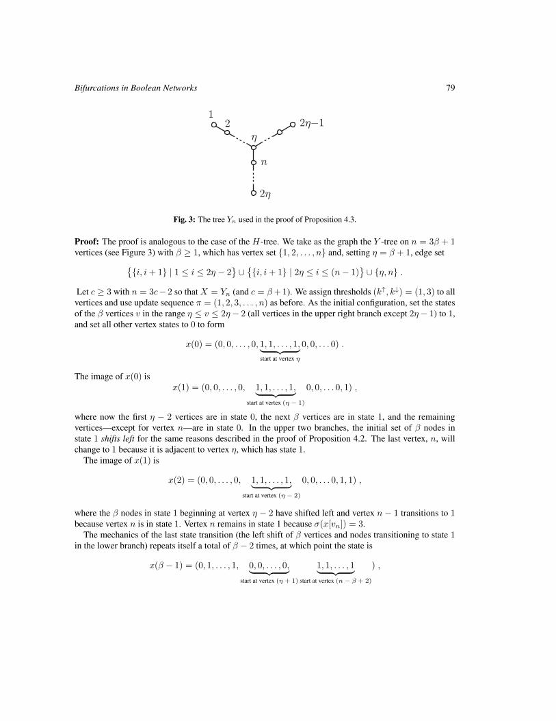
Bifurcations in Boolean Networks 79
12
´2´¡1
2´
n
Fig. 3: The tree Yn used in the proof of Proposition 4.3.
Proof: The proof is analogous to the case of the H-tree. We take as the graph the Y -tree on n = 3β + 1vertices (see Figure 3) with β ≥ 1, which has vertex set 1, 2, . . . , n and, setting η = β + 1, edge set
i, i+ 1 | 1 ≤ i ≤ 2η − 2∪i, i+ 1 | 2η ≤ i ≤ (n− 1)
∪ η, n .
Let c ≥ 3 with n = 3c− 2 so that X = Yn (and c = β+ 1). We assign thresholds (k↑, k↓) = (1, 3) to allvertices and use update sequence π = (1, 2, 3, . . . , n) as before. As the initial configuration, set the statesof the β vertices v in the range η ≤ v ≤ 2η− 2 (all vertices in the upper right branch except 2η− 1) to 1,and set all other vertex states to 0 to form
x(0) = (0, 0, . . . , 0, 1, 1, . . . , 1,︸ ︷︷ ︸start at vertex η
0, 0, . . . 0) .
The image of x(0) isx(1) = (0, 0, . . . , 0, 1, 1, . . . , 1,︸ ︷︷ ︸
start at vertex (η − 1)
0, 0, . . . 0, 1) ,
where now the first η − 2 vertices are in state 0, the next β vertices are in state 1, and the remainingvertices—except for vertex n—are in state 0. In the upper two branches, the initial set of β nodes instate 1 shifts left for the same reasons described in the proof of Proposition 4.2. The last vertex, n, willchange to 1 because it is adjacent to vertex η, which has state 1.
The image of x(1) is
x(2) = (0, 0, . . . , 0, 1, 1, . . . , 1,︸ ︷︷ ︸start at vertex (η − 2)
0, 0, . . . 0, 1, 1) ,
where the β nodes in state 1 beginning at vertex η − 2 have shifted left and vertex n − 1 transitions to 1because vertex n is in state 1. Vertex n remains in state 1 because σ(x[vn]) = 3.
The mechanics of the last state transition (the left shift of β vertices and nodes transitioning to state 1in the lower branch) repeats itself a total of β − 2 times, at which point the state is
x(β − 1) = (0, 1, . . . , 1, 0, 0, . . . , 0,︸ ︷︷ ︸start at vertex (η + 1)
1, 1, . . . , 1︸ ︷︷ ︸start at vertex (n− β + 2)
) ,
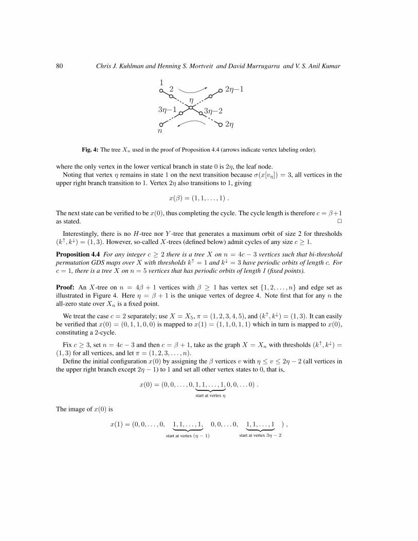
80 Chris J. Kuhlman and Henning S. Mortveit and David Murrugarra and V. S. Anil Kumar
12
´
2´¡1
2´
3´¡23´¡1
n
Fig. 4: The tree Xn used in the proof of Proposition 4.4 (arrows indicate vertex labeling order).
where the only vertex in the lower vertical branch in state 0 is 2η, the leaf node.Noting that vertex η remains in state 1 on the next transition because σ(x[vη]) = 3, all vertices in the
upper right branch transition to 1. Vertex 2η also transitions to 1, giving
x(β) = (1, 1, . . . , 1) .
The next state can be verified to be x(0), thus completing the cycle. The cycle length is therefore c = β+1as stated. 2
Interestingly, there is no H-tree nor Y -tree that generates a maximum orbit of size 2 for thresholds(k↑, k↓) = (1, 3). However, so-called X-trees (defined below) admit cycles of any size c ≥ 1.
Proposition 4.4 For any integer c ≥ 2 there is a tree X on n = 4c − 3 vertices such that bi-thresholdpermutation GDS maps over X with thresholds k↑ = 1 and k↓ = 3 have periodic orbits of length c. Forc = 1, there is a tree X on n = 5 vertices that has periodic orbits of length 1 (fixed points).
Proof: An X-tree on n = 4β + 1 vertices with β ≥ 1 has vertex set 1, 2, . . . , n and edge set asillustrated in Figure 4. Here η = β + 1 is the unique vertex of degree 4. Note first that for any n theall-zero state over Xn is a fixed point.
We treat the case c = 2 separately; use X = X5, π = (1, 2, 3, 4, 5), and (k↑, k↓) = (1, 3). It can easilybe verified that x(0) = (0, 1, 1, 0, 0) is mapped to x(1) = (1, 1, 0, 1, 1) which in turn is mapped to x(0),constituting a 2-cycle.
Fix c ≥ 3, set n = 4c − 3 and then c = β + 1, take as the graph X = Xn with thresholds (k↑, k↓) =(1, 3) for all vertices, and let π = (1, 2, 3, . . . , n).
Define the initial configuration x(0) by assigning the β vertices v with η ≤ v ≤ 2η − 2 (all vertices inthe upper right branch except 2η − 1) to 1 and set all other vertex states to 0, that is,
x(0) = (0, 0, . . . , 0, 1, 1, . . . , 1,︸ ︷︷ ︸start at vertex η
0, 0, . . . 0) .
The image of x(0) is
x(1) = (0, 0, . . . , 0, 1, 1, . . . , 1,︸ ︷︷ ︸start at vertex (η − 1)
0, 0, . . . 0, 1, 1, . . . , 1︸ ︷︷ ︸start at vertex 3η − 2
) ,
Bifurcations in Boolean Networks 81
where now the first η − 2 vertices are in state 0, the next β vertices are in state 1, and the remainingvertices in branch 2 are in state 0. In branch 3, only the vertex neighboring vertex η transitions to state 1,while all vertices in branch 4 transition to state 1 because η is in state 1.
State x(2) is generated by a left-shift of the β contiguous states that are 1 in branches 1 and 2, and by aleft-shift of the β + 1 contiguous state-1 vertices in branches 3 and 4, that is,
x(2) = (0, 0, . . . , 0, 1, 1, . . . , 1,︸ ︷︷ ︸start at vertex (η − 2)
0, 0, . . . 0, 1, 1, . . . , 1,︸ ︷︷ ︸start at vertex 3η − 3
0) .
From x(1) there are β − 2 such transitions that result in the state
x(β − 1) = (0, 1, 1, . . . , 1,︸ ︷︷ ︸start at vertex 2
0, 0, . . . 0, 1, 1, . . . , 1,︸ ︷︷ ︸start at vertex 3η − β
0, 0, . . . , 0) .
The next transition results in all vertices in branches 1 and 2 in state 1 since η remains in state 1. Thecontiguous set of β + 1 vertices in branches 3 and 4 shift left, giving
x(β) = (1, 1, . . . , 1, 0, 0, . . . , 0︸ ︷︷ ︸start at vertex 3η
) .
The image of x(β) is x(0), and, since β is the smallest positive time step with this property, we haveestablished the presence of a periodic orbit of length c = β + 1. 2
Finally, we consider a special class of bi-threshold SDSs on trees with k↑ = 1 and k↓ = k↓(v) =d(v)+1 for each vertex v. Note that the down-threshold for each vertex depends on its degree as indicatedby the index v in k↓(v). We show that such bi-threshold SDS maps always have fixed points. In suchsystems, the state of a vertex v switches from 0 to 1 if it has at least one neighbor in state 1, and from 1to 0 if it has at least one neighbor in state 0. This is an interesting contrast to the classes of bi-thresholdSDSs on trees discussed above which have large limit cycles.
Let X be a tree. We choose some arbitrary vertex r ∈ v[X] as its root, and partition X into levelsX0, X1, . . . , XD with respect to r such that X0 = r, and for any i ≥ 0, we let Xi+1 be the set ofvertices adjacent to vertices in set Xi, but not in the set ∪j<iXj . We sometimes refer to Xi as level-iset. Let D be the number of levels. We can also define a parent-child relationship relative to this rootedtree, and denote p(v) as the parent of vertex v 6= r. In our arguments below, we use any permutation π ofv[X], which consists of all the vertices in Xi before those in Xi−1 for each i. Our result is based on thefollowing property.
Lemma 4.5 Consider a bi-threshold SDS Fπ on a tree X with an arbitrary root r and permutation πas defined above where k↑ = 1 and k↓(v) = d(v) + 1 for each vertex v. Let x be any state vector andx′ = Fπ(x). For each vertex v other than the root, we have x′v = xp(v).
Proof: Our proof is by induction on the levels, starting from the highest, i.e., XD. For the base case,consider a leaf v ∈ XD. We have four cases: xv = xp(v) = 1, xv = 0, xp(v) = 1, xv = 1, xp(v) = 0 andxv = xp(v) = 0. It is easy to verify that in the first two cases, we have x′v = 1 and in the latter two cases,we have x′v = 0, since vertex v is updated before p(v) in π. Therefore, the statement of the lemma holdsin the base case for all vertices v ∈ XD.
82 Chris J. Kuhlman and Henning S. Mortveit and David Murrugarra and V. S. Anil Kumar
Next, consider a vertex v in some level Xj , j < D. If v is a leaf in Xj , the lemma follows by exactlythe same argument as in the base case. Therefore, consider the case v is not a leaf. Let w1, . . . , wc denoteits children. Since level j + 1 vertices are updated before those in level j in π, by induction, we havex′wi
= xv for each wi. Again, we have a case similar to the base case: when vertex v is updated, it has thesame values as its children, and therefore, takes on the state of p(v). Thus, the lemma follows. 2
This property immediately gives us the following:
Corollary 4.6 Let X be a tree. Let π ∈ Sx and let (fv)v be bi-threshold functions satisfying k↑ = 1 andk↓(v) = d(v) + 1 for each vertex v. Any SDS map Fπ only has fixed points as limit sets.
Proof: Without loss of generality, we take π to be the permutation in Lemma 4.5. By applying Lemma 4.5,it is easy to verify that for any state vector x, all the vertices in levels 0 and 1 have the same state value inF (x), namely xr. By induction on i, it is easy to verify that for any i ≥ 1, all vertices in levels 0, . . . , ihave the same state value (of xr) in F i(x). The statement follows since all permutations for a tree givecycle equivalent SDS maps. 2
5 Summary and ConclusionThis paper has analyzed the structure of ω-limit sets of bi-threshold GDS. Unlike the synchronous case,bi-threshold SDS maps can have long periodic orbits, and this is characterized in terms of the difference ofthe up- and down-thresholds. We also analyzed certain classes of trees. The following is a list of questionsand conjectures for possible further research.
5.1 Embedding and Inheritance of DynamicsA fundamental question in the study of GDSs is the following: if a graph X has a graph X ′ as an inducedsubgraph, what are the relations between the dynamics over the two graphs? Here one has to assume thatthe vertex function, and update sequences if applicable, are appropriately related. For example, is there aprojection from the phase space of the GDS over X to the one over X ′?
In initial computational experiments we studied the dynamics for bi-threshold GDS over trees obtainedfrom, e.g. H-trees by adding a collection of edges - results indicate that there are several classes ofoutcomes. While this is hardly a surprise, there are clear patterns in how edges are added and the dynamicsthat result. For example, some classes of edge additions give trees that have long periodic orbits just asin the case of H-trees. For other classes of edge additions, however, the addition of even a single edgecauses all periodic orbits of size ≥ 2 to disappear. Further insight into the mechanisms involved couldshed light on the the fundamental question above.
5.2 Minimality of Trees with Given Periodic Orbit SizesOur results above on the existence of trees admitting bi-threshold SDS with given periodic orbit sizes arenot necessarily minimal. For a given c ≥ 1 there is an X-tree with a periodic orbit of length c, but theremay be a smaller tree (or graph in general) which admits periodic orbits of size c as well. While we haveobtained some insight on this via sampling, no firm results have been established.
Note. For all computational experiments involving dynamics of SDS maps over graphs in this paper weused a variant of InterSim (Kuhlman et al., 2011).
Bifurcations in Boolean Networks 83
AcknowledgementsWe thank our external collaborators and members of the Network Dynamics and Simulation ScienceLaboratory (NDSSL) for their suggestions and comments. This work has been partially supported byNSF Nets Grant CNS-0626964, NSF HSD Grant SES-0729441, NSF PetaApps Grant OCI-0904844,NSF NETS Grant CNS-0831633, NSF Grant CNS-0845700, NSF Netse Grant CNS-1011769, NSF SDCIGrant OCI-1032677, DTRA R&D Grant HDTRA1-0901-0017, DTRA CNIMS Grant HDTRA1-07-C-0113, DOE Grant DE-SC0003957, US Naval Surface Warfare Center Grant N00178-09-D-3017 DELORDER 13, NIH MIDAS project 2U01GM070694-7 and NIAID & NIH project HHSN272201000056C.
A Limit Cycle Structure for Standard Threshold Cellular AutomataThis appendix section contains a condensed version of the proof from Goles and Olivos (1981) for stan-dard threshold functions. We have incorporated their proof for two reasons. First, only a portion of theoriginal proof needs to be adapted to cover bi-threshold systems, and in this way the paper becomes self-contained. Second, the original proof only appears in French, and we here provide an English version.
Let K = 0, 1, let A = (aij)ni,j=1 be a real symmetric matrix, let θ = (θ1, . . . , θn) ∈ Rn, and let
F = (f1, . . . , fn) : Kn −→ Kn be the function defined coordinate-wise by
fi(x1, . . . , xn) =
0, ifn∑j=1
aijxj < θi
1, otherwise .(A.1)
Theorem A.1 For all x ∈ Kn, there exists s ∈ N such that Fs+2(x) = Fs(x).
The proof of this theorem is based on two lemmas which are given below. Note first that since Kn isfinite, for each x ∈ Kn there exist s, T ∈ N (they will generally depend on x) with T > 0 such that
Fs+T (x) = Fs(x) and Fs+r(x) 6= Fs(x)
for all 0 < r < T . Here s is the transient length of the state x. Next define the n× T matrix X(x, T ) =(Fs(x), . . . ,Fs+T−1(x)) by
X(x, T ) =
z1(0) . . . z1(T − 1)... · · ·
...zn(0) . . . zn(T − 1)
,
where Fs(x) = z = (z1(0), . . . , zn(0)) and Fs+T−1(x) = (z1(T −1), . . . , zn(T −1)). In other words, zdenotes the first periodic point reached from x (after s steps) and its period is T . The columns of X(x, T )are the T successive periodic points of the cycle containing z.
In general we haveFs+l(x) = (z1(l), . . . , zn(l)) for 0 ≤ l ≤ T − 1 .
SinceFs(x) = Fs+T (x) = F(z1(T − 1), . . . , zn(T − 1))
84 Chris J. Kuhlman and Henning S. Mortveit and David Murrugarra and V. S. Anil Kumar
we have zi(0) = fi(z1(T − 1), . . . , zn(T − 1)), and from Fs+l+1(x) = F(Fs+l(x)) we have
zi(l + 1) = fi(z1(l), . . . , zn(l)) for l = 0, . . . , T − 2.
We will call zi the ith row of the matrix X(x, T ) and let γi denote the smallest divisor of T such thatzi(l + γi) = zi(l) for l ∈ 0, . . . , T − 1, and will say that γi is the period of the component zi. Clearly,we have zi(l + T ) = zi(l) for i ∈ 1, 2, . . . , n and all l ∈ 0, . . . , T − 1. Let S = z1, . . . , zn be theset of rows of X(x, T ). We define the operator L : S × S → R by
L(zi, zj) = aij
T−1∑l=0
(zj(l + 1)− zj(l − 1))zi(l) ,
with indices taken modulo T .
Lemma A.2 The operator L has the following properties:
(i) L(zi, zj) + L(zj , zi) = 0 for i, j ∈ 1, . . . , n (anti-symmetry).
(ii) If γi ≤ 2 then L(zi, zj) = 0 for j ∈ 1, . . . , n.
Proof: For (i), since aij = aji, we have
L(zi, zj) + L(zj , zi) = aij
T−1∑l=0
([zi(l)zj(l + 1)− zi(l − 1)zj(l)]
+[zi(l + 1)zj(l)− zi(l)zj(l − 1)]),
which clearly evaluates to zero due to periodicity. For part (ii), if γi = 1 then the row zi is constant andL(zi, zj) = 0. If γi = 2 then the value of zi alternates as
zi(0), zi(1), zi(0), zi(1), . . . , zi(0), zi(1)
across the ith row, and the terms in L(zi, zj) cancel in pairs. 2
Let zi ∈ S and suppose in the following that γi ≥ 3. We set
supp(zi) = l ∈ 0, . . . , T − 1 : zi(l) = 1 ,
and write I(l) = l, l + 2, l + 4, . . . , l − 4, l − 2. Next, set
C0 =
∅, if there is no l0 ∈ 0, . . . , T − 1 such that I(l0) ⊂ supp(zi)
I(l0), otherwise.
We define C1 as the setC1 = l1 + 2s ∈ supp(zi) : s = 0, 1, . . . , q1 ,
where l1 is the smallest index not in C0 satisfying zi(l1 − 2) = 0 and q1 satisfies zi(l1 + 2q1 + 2) = 0.For k ≥ 2 we define the sets Ck by
Ck = lk + 2s ∈ supp(zi) : s = 0, 1, . . . , qk ,
Bifurcations in Boolean Networks 85
where lk = lk−1 + rk (mod T ) /∈ l1, . . . , lk−1 is the smallest index for which zi(lk − 2) = 0 and qksatisfies zi(lk + 2qk + 2) = 0.
Since γi ≥ 3 (assumption), there always exists l1 ∈ supp(zi) for which zi(l1 − 2) = 0. This allowsus to build the collection of sets C = C0, . . . , Cp. By construction, C is a partition of supp(zi). Thefollowing lemma provides the final piece needed in the proof of the main result.
Lemma A.3 For zi ∈ S and with γi ≥ 3 we have
n∑j=1
L(zi, zj) < 0 .
Proof: Using the partition C of supp(zi), we have
n∑j=1
L(zi, zj) =
n∑j=1
aij∑
l∈supp(zi)
(zj(l + 1)− zj(l − 1)) · 1
=
n∑j=1
aij
p∑k=0
∑l∈Ck
(zj(l + 1)− zj(l − 1)) =
p∑k=0
n∑j=1
aij∑l∈Ck
(zj(l + 1)− zj(l − 1))
=
p∑k=0
Ψik ,
where we have introduced
Ψik =
n∑j=1
aij∑l∈Ck
(zj(l + 1)− zj(l − 1)) . (A.2)
If C0 = ∅ then Ψi0 = 0, and if C0 = l0, l0 + 2, . . . , l0 − 2 we have∑l∈C0
(zj(l + 1)− zj(l − 1)) = 0 .
In other words, we always have Ψi0 = 0, so we assume k > 0 in the following. From the assumption thatγi ≥ 3, there exists Ck 6= ∅ such that Ck = lk, lk + 2, . . . , lk + 2qk, so we can re-write Ψik as
Ψik =
n∑j=1
aij
qk∑s=0
(zj(lk + 2s+ 1)− zj(lk + 2s− 1))
=
n∑j=1
aijzj(lk + 2qk + 1)−n∑j=1
aijzj(lk − 1) .
[Cross-reference for bi-threshold systems] By the construction of Ck, we have zi(lk + 2qk + 2) = 0and zi(lk) = 1 which, by the definition of f in (A.1), is only possible if
n∑j=1
aijzj(lk + 2qk + 1) < θi, andn∑j=1
aijzj(lk − 1) ≥ θi . (A.3)
86 Chris J. Kuhlman and Henning S. Mortveit and David Murrugarra and V. S. Anil Kumar
This implies that Ψik < 0 and we conclude that
n∑j=1
L(zi, zj) =
p∑k=1
Ψik < 0
as required. 2
Proof of Theorem A.1: From Lemma A.2 we have that L is anti-symmetric so
n∑i=1
n∑j=1
L(zi, zj) = 0 .
However, if we assume that T ≥ 3, then there is zi with γi ≥ 3 and Lemma A.3 produces the desiredcontradiction. We conclude that T ≤ 2. 2
ReferencesR. Atkinson, W. Dietz, J. Foreyt, N. Goodwin, J. Hill, J. Hirsch, F. Pi-Sunyer, R. Weinsier, R. Wing,
J. Hoofnagle, J. Everhart, V. Hubbard, and S. Yanovski. Weight Cycling. Journal of the AmericanMedical Association, 272(15):1196–1202, 1994.
C. L. Barrett, H. B. Hunt III, M. V. Marathe, S. S. Ravi, D. J. Rosenkrantz, and R. E. Stearns. Complexityof reachability problems for finite discrete sequential dynamical systems. Journal of Computer andSystem Sciences, 72:1317–1345, 2006.
G. Bischi and U. Merlone. Global Dynamics in Binary Choice Models with Social Influence. J. Math.Sociology, 33:277–302, 2009.
N. Bulger, A. DeLongis, R. Kessler, and E. Wethington. The Contagion of Stress Across Multiple Roles.Journal of Marriage and the Family, 51:175–183, 1989.
D. Centola and M. Macy. Complex Contagions and the Weakness of Long Ties. American J. Sociology,113(3):702–734, 2007.
N. Christakis and J. Fowler. The Spread of Obesity in a Large Social Network Over 32 Years. N. Engl. J.Med., pages 370–379, 2007.
E. Goles and J. Olivos. Comportement periodique des fonctions a seuil binaires et applications. DiscreteApplied Mathematics, 3:93–105, 1981.
E. Goles-Chacc, F. Fogelman-Soulie, and D. Pellegrin. Decreasing energy functions as a tool for studyingthreshold networks. Discrete Applied Mathematics, 12:261–277, 1985.
M. Granovetter. Threshold Models of Collective Behavior. American J. Sociology, 83(6):1420–1443,1978.
Bifurcations in Boolean Networks 87
U. Karaoz, T. Murali, S. Letovsky, Y. Zheng, C. Ding, C. R. Cantor, and S. Kasif. Whole-genomeannotation by using evidence integration in functional-linkage networks. Proceedings of the NationalAcademy of Sciences, 101(9):2888–2893, 2004.
S. A. Kauffman. Metabolic stability and epigenesis in randomly constructed genetic nets. Journal ofTheoretical Biology, 22:437–467, 1969.
D. Kempe, J. Kleinberg, and E. Tardos. Maximizing the Spread of Influence Through a Social Network.In Proc. ACM KDD, pages 137–146, 2003.
C. Kuhlman, V. Kumar, M. Marathe, H. Mortveit, S. Swarup, G. Tuli, S. Ravi, and D. Rosenkrantz. AGeneral-Purpose Graph Dynamical System Modeling Framework. In Proceedings of the 2011 WinterSimulation Conference (WSC 2011), 2011.
M. Macauley and H. S. Mortveit. On enumeration of conjugacy classes of Coxeter elements.Proceedings of the American Mathematical Society, 136(12):4157–4165, 2008. doi: 10.1090/S0002-9939-09-09884-0. math.CO/0711.1140.
M. Macauley and H. S. Mortveit. Cycle equivalence of graph dynamical systems. Nonlinearity, 22(2):421–436, 2009. doi: 10.1088/0951-7715/22/2/010. math.DS/0709.0291.
M. Macy. Threshold Effects in Collective Action. American Sociological Review, 56:730–747, 1991.
H. S. Mortveit and C. M. Reidys. An Introduction to Sequential Dynamical Systems. Universitext. SpringerVerlag, 2007. ISBN 978-0-387-30654-4. doi: 10.1007/978-0-387-49879-9.
T. Schelling. Micromotives and Macrobehavior. W. W. Norton and Company, 1978.
D. Watts. A Simple Model of Global Cascades on Random Networks. PNAS, 99(9):5766–5771, 2002.

88 Chris J. Kuhlman and Henning S. Mortveit and David Murrugarra and V. S. Anil Kumar
AUTOMATA 2011, Santiago, Chile local proceedings LP, 2011, 89–100
Asymptotic distribution of entry times in acellular automaton with annihilating particles
Petr Kurka1† and Enrico Formenti2‡ and Alberto Dennunzio23§
1Center for Theoretical Study, Academy of Sciences and Charles University in Prague, Jilska 1, CZ-11000 Praha 1,Czechia2Laboratoire I3S, Universite Nice Sophia Antipolis, 2000, route des Lucioles, Les Algorithmes - bat Euclide B, BP121, 06903 Sophia Antipolis - Cedex, France3Dipartimento di Informatica, Sistemistica e Comunicazione, Universita degli Studi di Milano–Bicocca, Viale Sarca336, 20126 Milano (Italy)
This work considers a cellular automaton (CA) with two particles: a stationary particle 1 and left-going one 1. Whena 1 encounters a 1, both particles annihilate. We derive asymptotic distribution of appearence of particles at a givensite when the CA is initialized with the Bernoulli measure with the probabilities of both particles equal to 1/2.
Keywords: Cellular Automata, Particle Systems, Entry Times, Return Times
1 IntroductionCellular automata are a simple formal model for complex systems. They consist of an infinite numberof identical finite automata arranged over a regular lattice (here Z). Each automaton updates its stateaccording to its own state and the one of a fixed set of neighboring automata according to a local rule. Allupdates are synchronous.
The simplicity of the model contrasts with the great variety of different dynamical behaviors. Indeed,exactly this rich variety of behaviors and the ease of being simulated on computers made CA fortune.Actually, they are used in almost all scientific disciplines ranging from Mathematics to Computer Scienceand Natural Sciences. In particular, in Biology, Physics and Economics, they can be used as a discretecounterpart (in the sense of time) of interacting particle systems (IPS).
The advantage of modeling IPS by CA is that one can have information not only about limit distributionsand particle densities but also on their spatial distribution.
On the other hand, as we have already mentioned, the dynamical behavior of CA is complex and notfully understood and IPS can help to understand the dynamics of some CA whenever it can be described
†Email: [email protected]. This research was supported by the Research Program CTS MSM 0021620845‡Email: [email protected]. Supported by the French National Research Agency project EMC (ANR-09-
BLAN-0164)§Email: [email protected]. Supported by the French National Research Agency project EMC (ANR-09-
BLAN-0164)
c© 2011 AUTOMATA proceedings, Santiago, Chile, 2011
90 Petr Kurka and Enrico Formenti and Alberto Dennunzio
in terms of particles or signals that move in a neutral background and interact on encounters. The generalconcept of a signal or particle (in the context of CA) has been elaborated in Formenti and Kurka (2007).
The simplest kind of particles interaction is the annihilation. The classical example is “Just gliders”studied in Gilman (1987). This system consists of a left-going particle 1 and a right-going particle 1which annihilate on encounters. If the system starts in a Bernoulli measure with equal probabilities ofboth particles, then at a specified site both kinds of particles keep appearing with probability one, althoughtheir appearance is more and more rare as it has been shown by Kurka and Maass (2002). Other peculiarparticle systems and related CA models have been studied, see for example Fisch (1990).
In the present paper we address the question of how the time of appearance of a particle dependson the age of the system. We work with a simpler system called asymmetric gliders consisting of onestationary and one left-going particles annihilating on encounters. We show that the appearance of left-going particles time scales linearly with the age of the system and we derive the limit scaled distribution.
The paper is organized as follows. Section 2 and 3 introduce the symmetric and asymmetric glidersCA, respectively. Results are in Section 3. Since the proofs of the main results require several technicallemmata and specific notations, we grouped them in Section 4. The final section draws some conclusionsand give some ideas for future work.
2 Symmetric glidersLet A be a finite alphabet. A 1D CA configuration is a function from Z to A. The 1D CA configurationset AZ is usually equipped with the metric d defined as follows
∀c, c′ ∈ AZ, d(c, c′) = 2−n, where n = mini ≥ 0 : ci 6= c′i or c′−i 6= c′−i
.
If A is finite, AZ is a compact, totally disconnected and perfect topological space (i.e., AZ is a Cantorspace). For any pair i, j ∈ Z, with i ≤ j, and any configuration x ∈ AZ we denote by x[i,j] the wordxi · · ·xj ∈ Aj−i+1, i.e., the portion of c inside the interval [i, j]. In the previous notation, [i, j] can bereplaced by [i, j) with the obvious meaning. A cylinder of block u ∈ Ak and position i ∈ Z is the set[u]i = x ∈ AZ : x[i,i+k−1] = u. Cylinders are clopen sets w.r.t. the metric d and they form a basis forthe topology induced by d.
A 1D CA is a structure 〈1, A, r, f〉, where A is the alphabet, r ∈ N is the radius and f : A2r+1 → A isthe local rule of the automaton. The local rule f induces a global rule F : AZ → AZ defined as follows,
∀c ∈ AZ, ∀i ∈ Z, F (c)i = f(ci−r, . . . , ci, . . . , ci+r) .
In Gilman (1987), Gilman introduced a CA called Just Gliders (or Symmetric Gliders) which is formallydefined as 〈1,
1, 0, 1
, 1, g〉 where g :
1, 0, 1
3 → 1, 0, 1
is such that
∀(x, y, z) ∈
1, 0, 13, g(x, y, z) =
1 if x = 1, y ≥ 0 and y + z ≥ 01 if z = 1, y ≤ 0 and x+ y ≤ 00 otherwise .
In this context a symbol 1 (resp. 1) is interpreted as a right-going (resp. left-going) particle and 0 isthe neutral background. Figure 1 shows an example of evolution of Just Gliders from a random initialconfiguration.
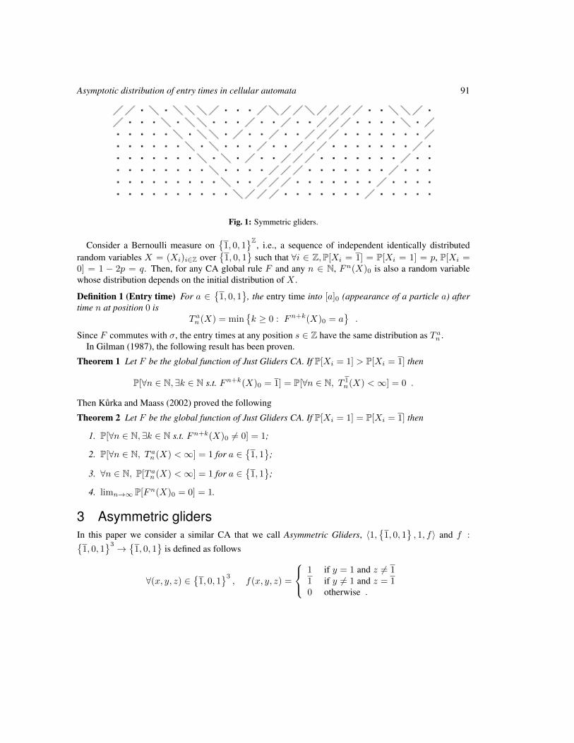
Asymptotic distribution of entry times in cellular automata 91
Fig. 1: Symmetric gliders.
Consider a Bernoulli measure on
1, 0, 1Z
, i.e., a sequence of independent identically distributedrandom variables X = (Xi)i∈Z over
1, 0, 1
such that ∀i ∈ Z,P[Xi = 1] = P[Xi = 1] = p, P[Xi =
0] = 1 − 2p = q. Then, for any CA global rule F and any n ∈ N, Fn(X)0 is also a random variablewhose distribution depends on the initial distribution of X .
Definition 1 (Entry time) For a ∈
1, 0, 1
, the entry time into [a]0 (appearance of a particle a) aftertime n at position 0 is
T an (X) = min
k ≥ 0 : Fn+k(X)0 = a
.
Since F commutes with σ, the entry times at any position s ∈ Z have the same distribution as T an .
In Gilman (1987), the following result has been proven.
Theorem 1 Let F be the global function of Just Gliders CA. If P[Xi = 1] > P[Xi = 1] then
P[∀n ∈ N,∃k ∈ N s.t. Fn+k(X)0 = 1] = P[∀n ∈ N, T 1n(X) <∞] = 0 .
Then Kurka and Maass (2002) proved the following
Theorem 2 Let F be the global function of Just Gliders CA. If P[Xi = 1] = P[Xi = 1] then
1. P[∀n ∈ N,∃k ∈ N s.t. Fn+k(X)0 6= 0] = 1;
2. P[∀n ∈ N, T an (X) <∞] = 1 for a ∈
1, 1
;
3. ∀n ∈ N, P[T an (X) <∞] = 1 for a ∈
1, 1
;
4. limn→∞ P[Fn(X)0 = 0] = 1.
3 Asymmetric glidersIn this paper we consider a similar CA that we call Asymmetric Gliders, 〈1,
1, 0, 1
, 1, f〉 and f :
1, 0, 13 →
1, 0, 1
is defined as follows
∀(x, y, z) ∈
1, 0, 13, f(x, y, z) =
1 if y = 1 and z 6= 11 if y 6= 1 and z = 10 otherwise .
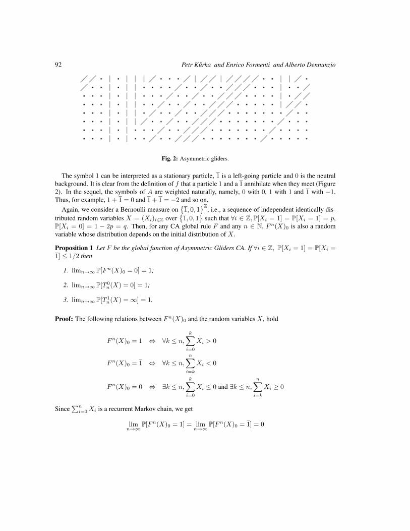
92 Petr Kurka and Enrico Formenti and Alberto Dennunzio
Fig. 2: Asymmetric gliders.
The symbol 1 can be interpreted as a stationary particle, 1 is a left-going particle and 0 is the neutralbackground. It is clear from the definition of f that a particle 1 and a 1 annihilate when they meet (Figure2). In the sequel, the symbols of A are weighted naturally, namely, 0 with 0, 1 with 1 and 1 with −1.Thus, for example, 1 + 1 = 0 and 1 + 1 = −2 and so on.
Again, we consider a Bernoulli measure on
1, 0, 1Z
, i.e., a sequence of independent identically dis-tributed random variables X = (Xi)i∈Z over
1, 0, 1
such that ∀i ∈ Z,P[Xi = 1] = P[Xi = 1] = p,
P[Xi = 0] = 1 − 2p = q. Then, for any CA global rule F and any n ∈ N, Fn(X)0 is also a randomvariable whose distribution depends on the initial distribution of X .
Proposition 1 Let F be the global function of Asymmetric Gliders CA. If ∀i ∈ Z, P[Xi = 1] = P[Xi =1] ≤ 1/2 then
1. limn→∞ P[Fn(X)0 = 0] = 1;
2. limn→∞ P[T 0n(X) = 0] = 1;
3. limn→∞ P[T 1n(X) =∞] = 1.
Proof: The following relations between Fn(X)0 and the random variables Xi hold
Fn(X)0 = 1 ⇔ ∀k ≤ n,k∑
i=0
Xi > 0
Fn(X)0 = 1 ⇔ ∀k ≤ n,n∑
i=k
Xi < 0
Fn(X)0 = 0 ⇔ ∃k ≤ n,k∑
i=0
Xi ≤ 0 and ∃k ≤ n,n∑
i=k
Xi ≥ 0
Since∑n
i=0Xi is a recurrent Markov chain, we get
limn→∞
P[Fn(X)0 = 1] = limn→∞
P[Fn(X)0 = 1] = 0
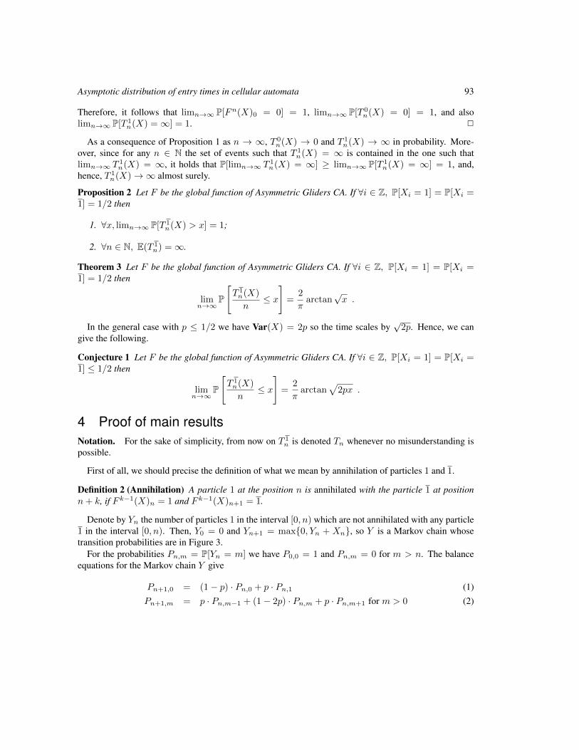
Asymptotic distribution of entry times in cellular automata 93
Therefore, it follows that limn→∞ P[Fn(X)0 = 0] = 1, limn→∞ P[T 0n(X) = 0] = 1, and also
limn→∞ P[T 1n(X) =∞] = 1. 2
As a consequence of Proposition 1 as n → ∞, T 0n(X) → 0 and T 1
n(X) → ∞ in probability. More-over, since for any n ∈ N the set of events such that T 1
n(X) = ∞ is contained in the one such thatlimn→∞ T 1
n(X) = ∞, it holds that P[limn→∞ T 1n(X) = ∞] ≥ limn→∞ P[T 1
n(X) = ∞] = 1, and,hence, T 1
n(X)→∞ almost surely.
Proposition 2 Let F be the global function of Asymmetric Gliders CA. If ∀i ∈ Z, P[Xi = 1] = P[Xi =1] = 1/2 then
1. ∀x, limn→∞ P[T 1n(X) > x] = 1;
2. ∀n ∈ N, E(T 1n) =∞.
Theorem 3 Let F be the global function of Asymmetric Gliders CA. If ∀i ∈ Z, P[Xi = 1] = P[Xi =1] = 1/2 then
limn→∞
P
[T 1n(X)
n≤ x
]=
2
πarctan
√x .
In the general case with p ≤ 1/2 we have Var(X) = 2p so the time scales by√
2p. Hence, we cangive the following.
Conjecture 1 Let F be the global function of Asymmetric Gliders CA. If ∀i ∈ Z, P[Xi = 1] = P[Xi =1] ≤ 1/2 then
limn→∞
P
[T 1n(X)
n≤ x
]=
2
πarctan
√2px .
4 Proof of main resultsNotation. For the sake of simplicity, from now on T 1
n is denoted Tn whenever no misunderstanding ispossible.
First of all, we should precise the definition of what we mean by annihilation of particles 1 and 1.
Definition 2 (Annihilation) A particle 1 at the position n is annihilated with the particle 1 at positionn+ k, if F k−1(X)n = 1 and F k−1(X)n+1 = 1.
Denote by Yn the number of particles 1 in the interval [0, n) which are not annihilated with any particle1 in the interval [0, n). Then, Y0 = 0 and Yn+1 = max0, Yn + Xn, so Y is a Markov chain whosetransition probabilities are in Figure 3.
For the probabilities Pn,m = P[Yn = m] we have P0,0 = 1 and Pn,m = 0 for m > n. The balanceequations for the Markov chain Y give
Pn+1,0 = (1− p) · Pn,0 + p · Pn,1 (1)Pn+1,m = p · Pn,m−1 + (1− 2p) · Pn,m + p · Pn,m+1 for m > 0 (2)
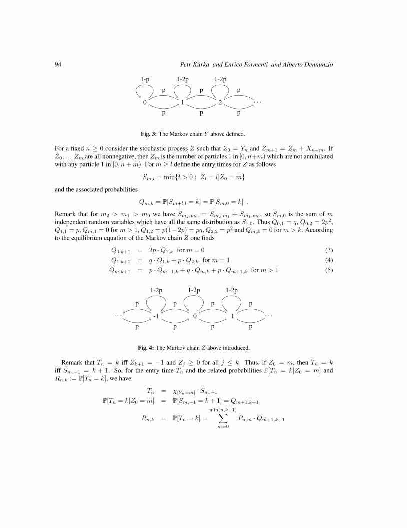
94 Petr Kurka and Enrico Formenti and Alberto Dennunzio
0 1 2 . . .
1-p
p
p
1-2p
p
p
1-2p
p
p
Fig. 3: The Markov chain Y above defined.
For a fixed n ≥ 0 consider the stochastic process Z such that Z0 = Yn and Zm+1 = Zm + Xn+m. IfZ0, . . . Zm are all nonnegative, thenZm is the number of particles 1 in [0, n+m) which are not annihilatedwith any particle 1 in [0, n+m). For m ≥ l define the entry times for Z as follows
Sm,l = mint > 0 : Zt = l|Z0 = m
and the associated probabilities
Qm,k = P[Sm+l,l = k] = P[Sm,0 = k] .
Remark that for m2 > m1 > m0 we have Sm2,m0 = Sm2,m1 + Sm1,m0 , so Sm,0 is the sum of mindependent random variables which have all the same distribution as S1,0. Thus Q0,1 = q, Q0,2 = 2p2,Q1,1 = p,Qm,1 = 0 form > 1,Q1,2 = p(1−2p) = pq,Q2,2 = p2 andQm,k = 0 form > k. Accordingto the equilibrium equation of the Markov chain Z one finds
Q0,k+1 = 2p ·Q1,k for m = 0 (3)Q1,k+1 = q ·Q1,k + p ·Q2,k for m = 1 (4)Qm,k+1 = p ·Qm−1,k + q ·Qm,k + p ·Qm+1,k for m > 1 (5)
0 1 . . .-1. . .
1-2p
p
p
1-2p
p
pp
p
1-2p
p
p
Fig. 4: The Markov chain Z above introduced.
Remark that Tn = k iff Zk+1 = −1 and Zj ≥ 0 for all j ≤ k. Thus, if Z0 = m, then Tn = kiff Sm,−1 = k + 1. So, for the entry time Tn and the related probabilities P[Tn = k|Z0 = m] andRn,k := P[Tn = k], we have
Tn = χ[Yn=m] · Sm,−1
P[Tn = k|Z0 = m] = P[Sm,−1 = k + 1] = Qm+1,k+1
Rn,k = P[Tn = k] =
min(n,k+1)∑m=0
Pn,m ·Qm+1,k+1
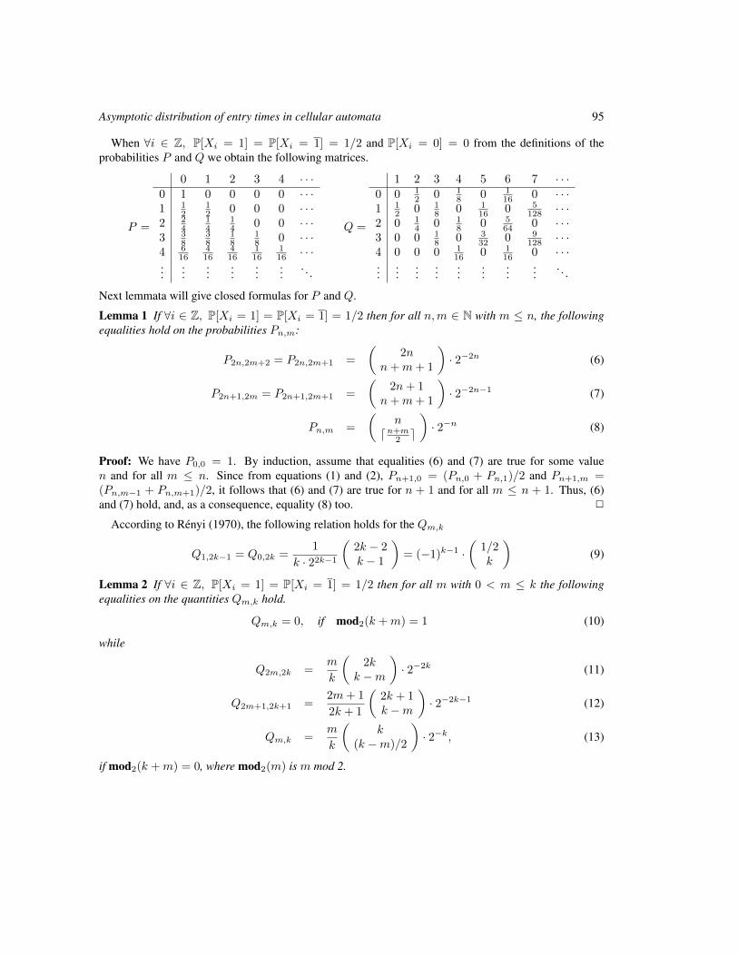
Asymptotic distribution of entry times in cellular automata 95
When ∀i ∈ Z, P[Xi = 1] = P[Xi = 1] = 1/2 and P[Xi = 0] = 0 from the definitions of theprobabilities P and Q we obtain the following matrices.
P =
0 1 2 3 4 · · ·0 1 0 0 0 0 · · ·1 1
212 0 0 0 · · ·
2 24
14
14 0 0 · · ·
3 38
38
18
18 0 · · ·
4 616
416
416
116
116 · · ·
......
......
......
. . .
Q =
1 2 3 4 5 6 7 · · ·0 0 1
2 0 18 0 1
16 0 · · ·1 1
2 0 18 0 1
16 0 5128 · · ·
2 0 14 0 1
8 0 564 0 · · ·
3 0 0 18 0 3
32 0 9128 · · ·
4 0 0 0 116 0 1
16 0 · · ·...
......
......
......
.... . .
Next lemmata will give closed formulas for P and Q.
Lemma 1 If ∀i ∈ Z, P[Xi = 1] = P[Xi = 1] = 1/2 then for all n,m ∈ N with m ≤ n, the followingequalities hold on the probabilities Pn,m:
P2n,2m+2 = P2n,2m+1 =
(2n
n+m+ 1
)· 2−2n (6)
P2n+1,2m = P2n+1,2m+1 =
(2n+ 1
n+m+ 1
)· 2−2n−1 (7)
Pn,m =
(n
dn+m2 e
)· 2−n (8)
Proof: We have P0,0 = 1. By induction, assume that equalities (6) and (7) are true for some valuen and for all m ≤ n. Since from equations (1) and (2), Pn+1,0 = (Pn,0 + Pn,1)/2 and Pn+1,m =(Pn,m−1 + Pn,m+1)/2, it follows that (6) and (7) are true for n + 1 and for all m ≤ n + 1. Thus, (6)and (7) hold, and, as a consequence, equality (8) too. 2
According to Renyi (1970), the following relation holds for the Qm,k
Q1,2k−1 = Q0,2k =1
k · 22k−1
(2k − 2k − 1
)= (−1)k−1 ·
(1/2k
)(9)
Lemma 2 If ∀i ∈ Z, P[Xi = 1] = P[Xi = 1] = 1/2 then for all m with 0 < m ≤ k the followingequalities on the quantities Qm,k hold.
Qm,k = 0, if mod2(k +m) = 1 (10)
while
Q2m,2k =m
k
(2k
k −m
)· 2−2k (11)
Q2m+1,2k+1 =2m+ 1
2k + 1
(2k + 1k −m
)· 2−2k−1 (12)
Qm,k =m
k
(k
(k −m)/2
)· 2−k, (13)
if mod2(k +m) = 0, where mod2(m) is m mod 2.
96 Petr Kurka and Enrico Formenti and Alberto Dennunzio
Proof: Since q = 0, if mod2(k + m) = 1 Equality (10) follows from the definition of Qm,k. Using thatQ2,k = 2 ·Q1,k+1, Qm+1,k = 2 ·Qm,k+1 −Qm−1,k (for m ≥ 1), and Equation (9), Equalities from (11)to (13), are true for Q1,k and Q2,k. The thesis is obtained by proceeding by finite induction on m. 2
Using the expressions found in Lemmata 1 and 2 and substituting them in the definition of Rn,k =P[Tn = k], one can easily find the following.
R2n,2k = 2−2n−2k−1min(n,k)∑
m=0
(2n
n+m
)(2k + 1k −m
)2m+ 1
2k + 1
R2n,2k+1 = 2−2n−2k−2min(n,k)∑
m=0
(2n
n+m+ 1
)(2k + 2k −m
)m+ 1
k + 1
R2n+1,2k = 2−2n−2k−2min(n,k)∑
m=0
(2n+ 1
n+m+ 1
)(2k + 1k −m
)2m+ 1
2k + 1
R2n+1,2k+1 = 2−2n−2k−3min(n,k)∑
m=0
(2n+ 1
n+m+ 1
)(2k + 2k −m
)m+ 1
k + 1
which can be summed up as follows
Rn,k = 2−n−k−1min(bn2 c,b
k2 c)∑
m=0
(n
bn2 c+m+ `n,k
)(k + 1bk2 c −m
)2m+ 1 + mod2(k)
k + 1
where `n,k = maxmod2(n),mod2(k).Finally, we will use the following approximation formula of binomial distribution by the normal distri-
bution.
Theorem 4 (Renyi (1970)) Let kn be a sequence of positive integers such that |2kn − n| < a√n for
some constant a. Then (nkn
)=
2n+1 · e−(2kn−n)2/2n√
2πn(1 +O(1/n))
and the constant in the remainder O(1/n) depends only on a.
Proof of Proposition 2:
1. Using the approximation given by Theorem 4 one finds
limn→∞
Pn,m = limn→∞
2e−m2/2n
√2πn
= 0
and hence
limn→∞
P[Tn ≤ `] = limn→∞
∑k=0
min(n,k)∑m=0
Pn,m ·Qm+1,k+1 = 0
Asymptotic distribution of entry times in cellular automata 97
2. To prove E(Tn) = ∞ we prove first that E(Sm,1) = ∞ for each m. Again, using Theorem 4, onefinds
Qm,k =m
k·(
kdk−m2 e
)· 2−k ≈ m
k· 2k+1 e
−m2
2k
√2πk
· 2−k =2m · e−m2
2k
k√
2πk(14)
whenever m <√k and mod2(k +m) = 0. For each ` we then have
E(Sm,0) =
∞∑k=1
k ·Qm,k ≥∞∑k=`
2m · e−m2
2k
√2πk
=∞ . (15)
Since E(Tn) is a finite linear combination of E(S0,−1), . . . ,E(Sn,−1), we get E(Tn) =∞ as well.
2
Proof of Theorem 3: Recall that the characteristic function of a discrete distribution with P[X = n] = pnis ϕ(t) =
∑∞n=0 pne
int, where i is the imaginary unit. Since by Lemma 2Qm,k = 0 if mod2(k+m) = 1,for the characteristic function ϕ of S1,0 we obtain
ϕ(t) = Q1,1eit +Q1,3e
3it +Q1,5e5it + · · ·
which, by using Equation (9), turns into
ϕ(t) =
(1/21
)eit −
(1/22
)e3it +
(1/23
)e5it − · · ·
= e−it[1−
(1−
(1/21
)e2it +
(1/22
)e4it − · · ·
)]= e−it(1−
√1− e2it) .
Thus, finally we get
limn→∞
ϕ
(t
n2
)n
= limn→∞
(1−√
1− e2it/n2)n = limn→∞
(1−√−2it
n
)n
= e−√−2it
which is the characteristic function of a random variable with distribution function
G(x) = 2(1− Φ(1/√x))
and density
g(x) = G′(x) =1√
2πx3· e−1/2x ,
where Φ(x) is the normal distribution function. Figure 5 plots both G(x) and g(x).Recall that E(Sm,0) = ∞ (see Equation 15). Denote by Gm(x) = P[Sm,0 ≤ x] the distribution
function of Sm,0. Since the characteristic function of Sm,0 is ϕm(t) = ϕ(t)m, we get
limm→∞
Gm+1(m2x) = limm→∞
P[Sm,−1
m2< x
]= G(x) = 2(1− Φ(1/
√x)) (16)
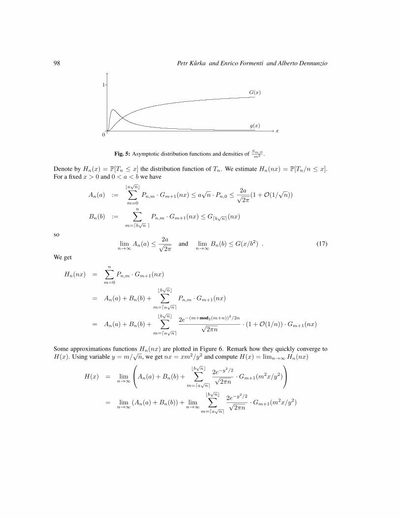
98 Petr Kurka and Enrico Formenti and Alberto Dennunzio
1
0x
g(x)
G(x)
Fig. 5: Asymptotic distribution functions and densities of Sm,0
m2 .
Denote by Hn(x) = P[Tn ≤ x] the distribution function of Tn. We estimate Hn(nx) = P[Tn/n ≤ x].For a fixed x > 0 and 0 < a < b we have
An(a) :=
ba√nc∑
m=0
Pn,m ·Gm+1(nx) ≤ a√n · Pn,0 ≤
2a√2π
(1 +O(1/√n))
Bn(b) :=
n∑m=db
√n e
Pn,m ·Gm+1(nx) ≤ Gdb√ne(nx)
solimn→∞
An(a) ≤ 2a√2π
and limn→∞
Bn(b) ≤ G(x/b2) . (17)
We get
Hn(nx) =
n∑m=0
Pn,m ·Gm+1(nx)
= An(a) +Bn(b) +
bb√nc∑
m=da√ne
Pn,m ·Gm+1(nx)
= An(a) +Bn(b) +
bb√nc∑
m=da√ne
2e−(m+mod2(m+n))2/2n
√2πn
· (1 +O(1/n)) ·Gm+1(nx)
Some approximations functions Hn(nx) are plotted in Figure 6. Remark how they quickly converge toH(x). Using variable y = m/
√n, we get nx = xm2/y2 and compute H(x) = limn→∞Hn(nx)
H(x) = limn→∞
An(a) +Bn(b) +
bb√nc∑
m=da√ne
2e−y2/2
√2πn
·Gm+1(m2x/y2)
= lim
n→∞(An(a) +Bn(b)) + lim
n→∞
bb√nc∑
m=da√ne
2e−y2/2
√2πn
·Gm+1(m2x/y2)
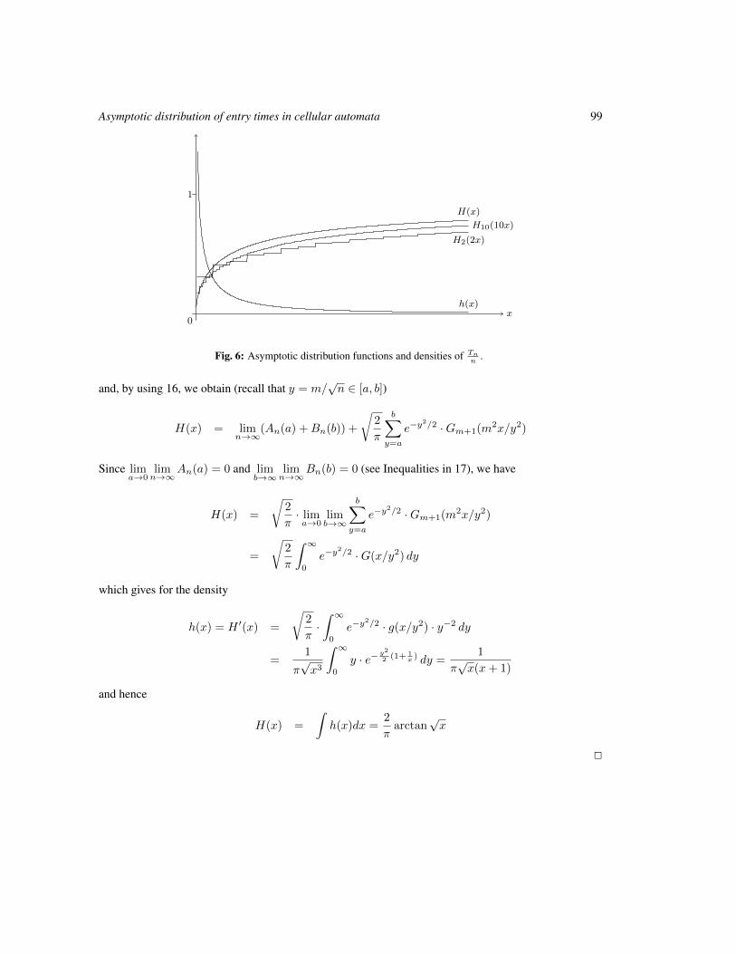
Asymptotic distribution of entry times in cellular automata 99
1
0x
H(x)
h(x)
H2(2x)
H10(10x)
Fig. 6: Asymptotic distribution functions and densities of Tnn
.
and, by using 16, we obtain (recall that y = m/√n ∈ [a, b])
H(x) = limn→∞
(An(a) +Bn(b)) +
√2
π
b∑y=a
e−y2/2 ·Gm+1(m2x/y2)
Since lima→0
limn→∞
An(a) = 0 and limb→∞
limn→∞
Bn(b) = 0 (see Inequalities in 17), we have
H(x) =
√2
π· lima→0
limb→∞
b∑y=a
e−y2/2 ·Gm+1(m2x/y2)
=
√2
π
∫ ∞0
e−y2/2 ·G(x/y2) dy
which gives for the density
h(x) = H ′(x) =
√2
π·∫ ∞0
e−y2/2 · g(x/y2) · y−2 dy
=1
π√x3
∫ ∞0
y · e−y2
2 (1+ 1x ) dy =
1
π√x(x+ 1)
and hence
H(x) =
∫h(x)dx =
2
πarctan
√x
2

100 Petr Kurka and Enrico Formenti and Alberto Dennunzio
5 ConclusionsIn this paper we set up some formal tools that have help to study and to exactly derive the distribution ofentry time for CA viewed a particle system consisting of a stationary particle and a left-going particle.
The program is to develop formal tools in order to be able to study more complex situations starting bythe symmetric case for example. Another interesting case would consider particles with speed differentfrom 1 or 0 allowing in this way more complex interactions between particles other than annihilation.
ReferencesR. Fisch. The one-dimensional cyclic cellular automaton: A system with deterministic dynamics which
emulates an interacting particle system with stochastic dynamics. Journal of Theoretical Probability,3:311–338, 1990.
E. Formenti and P. Kurka. Subshifts attractors in cellular automata. Nonlinearity, 20:105–117, 2007.
R. H. Gilman. Classes of cellular automata. Ergodic Theory and Dynamical Systems, 7:105–118, 1987.
P. Kurka and A. Maass. Stability of subshifts in cellular automata. Fundamenta Informaticae, 52(1-3):143–155, 2002.
A. Renyi. Probability Theory. Elsevier, 1970.
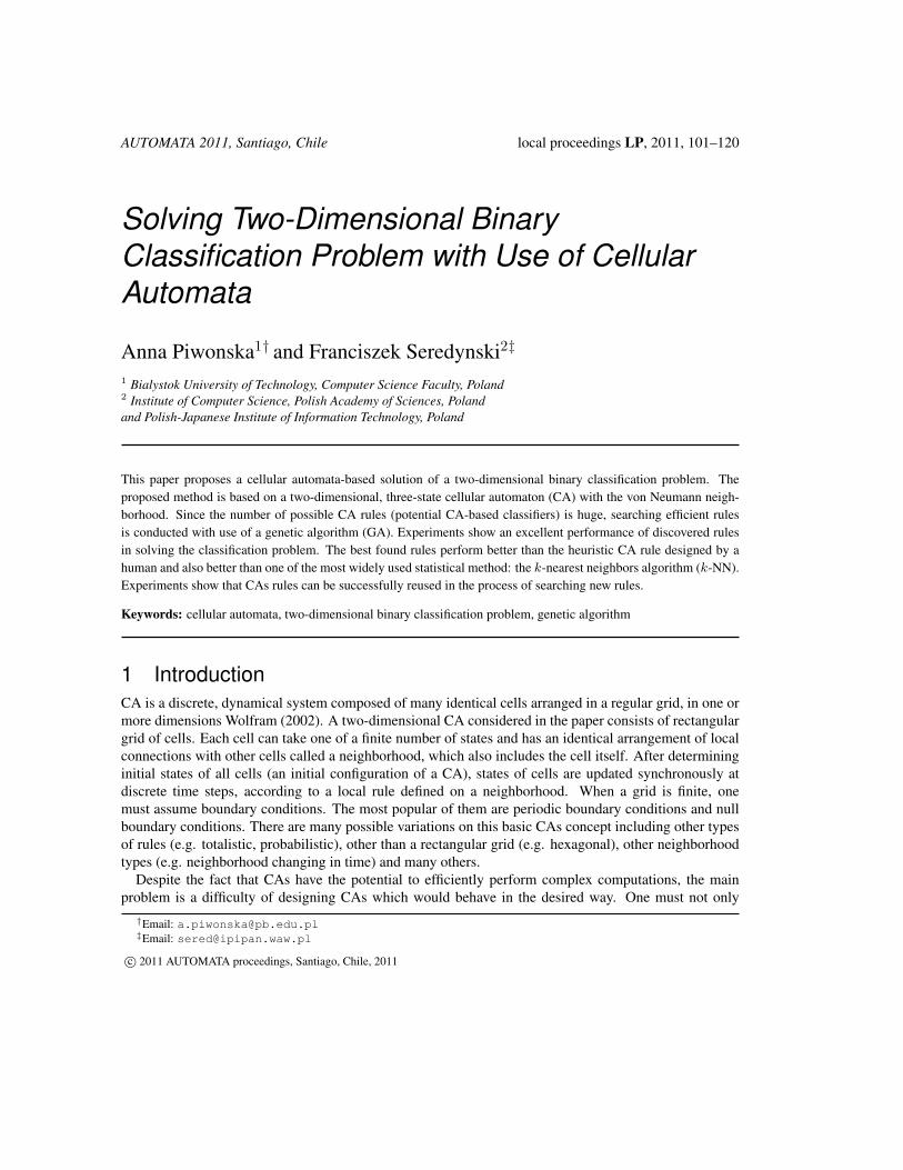
AUTOMATA 2011, Santiago, Chile local proceedings LP, 2011, 101–120
Solving Two-Dimensional BinaryClassification Problem with Use of CellularAutomata
Anna Piwonska1† and Franciszek Seredynski2‡
1 Bialystok University of Technology, Computer Science Faculty, Poland2 Institute of Computer Science, Polish Academy of Sciences, Polandand Polish-Japanese Institute of Information Technology, Poland
This paper proposes a cellular automata-based solution of a two-dimensional binary classification problem. Theproposed method is based on a two-dimensional, three-state cellular automaton (CA) with the von Neumann neigh-borhood. Since the number of possible CA rules (potential CA-based classifiers) is huge, searching efficient rulesis conducted with use of a genetic algorithm (GA). Experiments show an excellent performance of discovered rulesin solving the classification problem. The best found rules perform better than the heuristic CA rule designed by ahuman and also better than one of the most widely used statistical method: the k-nearest neighbors algorithm (k-NN).Experiments show that CAs rules can be successfully reused in the process of searching new rules.
Keywords: cellular automata, two-dimensional binary classification problem, genetic algorithm
1 IntroductionCA is a discrete, dynamical system composed of many identical cells arranged in a regular grid, in one ormore dimensions Wolfram (2002). A two-dimensional CA considered in the paper consists of rectangulargrid of cells. Each cell can take one of a finite number of states and has an identical arrangement of localconnections with other cells called a neighborhood, which also includes the cell itself. After determininginitial states of all cells (an initial configuration of a CA), states of cells are updated synchronously atdiscrete time steps, according to a local rule defined on a neighborhood. When a grid is finite, onemust assume boundary conditions. The most popular of them are periodic boundary conditions and nullboundary conditions. There are many possible variations on this basic CAs concept including other typesof rules (e.g. totalistic, probabilistic), other than a rectangular grid (e.g. hexagonal), other neighborhoodtypes (e.g. neighborhood changing in time) and many others.
Despite the fact that CAs have the potential to efficiently perform complex computations, the mainproblem is a difficulty of designing CAs which would behave in the desired way. One must not only
†Email: [email protected]‡Email: [email protected]
c© 2011 AUTOMATA proceedings, Santiago, Chile, 2011
102 Anna Piwonska and Franciszek Seredynski
select a neighborhood type and size, but most importantly the appropriate rule (or rules). Since the numberof possible rules is usually huge, this is the extremely hard task. In some applications of CAs one candesign an appropriate rule by hand (e.g. the GKL rule designed in 1978 by Gacs, Kurdyumov and Levinfor density classification task Gacs et al. (1978)) or can use partial differential equations describing agiven phenomenon Omohundro (1984). However, it is not always possible. In the 90-ties of the lastcentury Mitchell and collaborators proposed to use GAs to find CAs rules able to perform one-dimensionaldensity classification task Mitchell et al. (1993) and the synchronization task Das et al. (1995). The resultsobtained by Mitchell et al. showed that the GA was able to discover CAs rules demonstrating emergentcomputational strategies.
The literature shows many examples concerning the concept of generating CAs rules using artificialevolution. For example, Sipper presented results of evolving CAs rules to perform thinning and gapfilling in isothetic rectangles Sipper (1997). Breukelaar and Back applied GAs to solve the density classi-fication problem as well as AND and XOR problem in two-dimensional CAs Breukelaar and Back (2004).Swiecicka et al. used GAs to find CAs rules able to solve multiprocessor scheduling problem Swiecickaet al. (2006). Oliveira Jr. and de Oliveira used GA to evolve two-dimensional CAs rules for recognitionof handwritten digits Oliveira Jr. and de Oliveira (2008). Piwonska and Seredynski used a GA to findappropriate CAs rules for pattern reconstruction task Piwonska and Seredynski (2010). It is worth point-ing out that other evolutionary techniques were also proposed to find efficient CAs rules, such as geneticprogramming Andre et al. (1996) and gene expression programming Ferreira (2006).
In a classification problem we wish to determine to which class new observations belong, based onthe training set of data containing observations whose class is known. The binary classification dealswith only two classes, whereas in a multiclass classification observations belong to one of several classes.The well-known classifiers are neural networks, support vector machines, k-NN algorithm, decision treesand others. The idea of using CAs in the classification problem was described by Maji et al. Maji et al.(2004), Povalej et al. Povalej et al. (2004) and recently by Fawcett Fawcett (2008). Fawcett designed theheuristic rule based on the von Neumann neighborhood (so-called voting rule) and tested its performanceon different data sets. This paper proposes a different approach: finding appropriate CAs rules by aGA. The effectiveness of rules discovered by a GA will be compared with the effectiveness of the hand-designed voting rule. Both CA-based approaches will be compared with the k-NN algorithm.
This paper is organized as follows. Section 2 describes two-dimensional CAs used in our approach.Section 3 defines the two-dimensional binary classification problem and describes the proposed CA-basedalgorithm. Experimental results are presented in Section 4. The last section contains conclusions andfuture work plans.
2 Two-Dimensional Cellular AutomataA two-dimensional CA consists of a rectangular grid of N × M cells, each of which can take on kpossible states Packard and Wolfram (1985). After determining initial states of all cells (i.e. the initialconfiguration of a CA), each cell changes its state according to a rule φ which depends on states of cellsin a neighborhood around it. This is usually done synchronously, although asynchronous mode is usedtoo. Two types of neighborhood are commonly used: the von Neumann neighborhood and the Moore one.The first comprises the four cells orthogonally surrounding the central cell while the other consists of theeight cells around the central cell (Fig. 1).
The evolution of a CA with the von Neumann neighborhood can be described by Eq. 1:
Solving Two-Dimensional Binary Classification Problem with Use of Cellular Automata 103
(a) (b)
Fig. 1: CA neighborhood: von Neumann (a), Moore (b).
a(t+1)i,j = φ[a
(t)i,j , a
(t)i,j+1, a
(t)i+1,j , a
(t)i,j−1, a
(t)i−1,j ], (1)
where a(t)i,j denotes the state of a cell at position i, j in the two-dimensional cellular grid, at time step t.The evolution of a CA is usually presented by means of so-called ”space-time diagrams” displaying
grid of cells at subsequent time steps, with each state marked with different color.
3 Binary Classification Problem and Cellular Automata3.1 Two-Dimensional Binary Classification ProblemIn this paper we deal with the classification problem described in Ishibuchi et al. (1993) in the context offuzzy rule-based classification system. Let us assume that the data space is the unit square [0, 1]× [0, 1].Suppose that m data-points xp = (xp1, xp2), p = 1, 2, ...,m are given as a training set from two classes:class 1 and class 2. That is, the classification of each xp = (xp1, xp2), p = 1, 2, ...,m is known as oneof two classes. The classification problem can be stated as follows. Given m training data find a rule (or”classifier”) which divides the data space into two disjoint decision areas (class 1 or 2) such that the classnumber can be assigned to any new observation.
3.2 Proposed CA-based ClassifierThe idea of using CAs to solve the binary classification problem is based on the construction of a CA andfinding an appropriate rule which can perform the classification task. Since the problem is defined in thetwo-dimensional space, our CA will also be the two-dimensional. The CA works on a grid of cells, so wemust partition our data space [0, 1]× [0, 1] into a grid. Let us assume that the considered CA has an equalnumber of cells in each dimension (N =M ). This means that the data space is divided into N ×N cellsand grid lines are placed at nodes: 0, 1
N ,2N ,
3N , ..., 1. These nodes determine the division of the interval
[0, 1] into N subintervals: 〈0, 1N ), 〈 1N ,
2N ), ..., 〈N−1
N , N〉.Our CA is a three-state automaton (k = 3). The initial state of each cell is set by training points
belonging to this cell and is determined in the following way:
• if there is no point in a cell (an empty cell), then a cell is in state 0 (a cell is marked in grey color),
• if there are points only from class 1 in a cell, then a cell is in state 1 (a cell is marked in white color),
104 Anna Piwonska and Franciszek Seredynski
Fig. 2: The exemplary instance of the classification problem.
• if there are points only from class 2 in a cell, then a cell is in state 2 (a cell is marked in black color),
• if there are points from both classes (class 1 and 2) in a cell, then a cell is in state 0 (a cell is markedin grey color).
The interpretation of the above mentioned rules is simply and intuitive. The class of training pointsdetermines the state of a cell. If the state of a cell cannot be assigned, a cell is in state 0 (unknown class).This can happen in two situations: either there are no training points in a cell or there are points from bothclasses in it. Fig. 3 presents the exemplary classification problem: the grid partition in the case ofN = 10(Fig. 3(a)) and the corresponding initial configuration of the CA (Fig. 3(b)).
The performance of the CA-based classifier depends on the size of a partition. If a partition is toocoarse, the performance of the system may be low (many observations may be misclassified). On theother hand, if a partition is too fine, one can observe the lack of training points in corresponding cells.The similar issue was described in Ishibuchi et al. (1993) in the context of generating fuzzy rules. Thisproblem is illustrated in Fig. 4.
Fig. 4 presents three partitions of considered data space, with the same training set consisting ofm = 100 points. Cells in state 2 are displayed as black, cells in state 1 are displayed as white and cells instate 0 are displayed as grey. One can see that in spite of the same training set, the CA with N = 30 (Fig.4(c)) has more cells in state 0 than CAs with N = 10 (Fig. 4(a)) and N = 20 (Fig. 4(b)). This is dueto the fact that the CA with N = 30 has a lot more cells without training points than CAs with N = 10and N = 20. The more empty cells in the initial configuration, the more cells’ states need to be properlyarranged.
The next step is to determine the boundary conditions. We assume null boundary conditions: bordercells have dummy neighbors always in state 0.
After determining initial states of all cells (i.e. the initial configuration of the CA), cells change theirstates synchronously according to a certain rule which must be found. An appropriate rule transforms,during T time steps, the initial configuration of the CA into the final configuration in which there are noempty cells and for which the correct class number can be assigned to any new observation. Finding anappropriate rule is a key factor for performance of CA-based classifier.
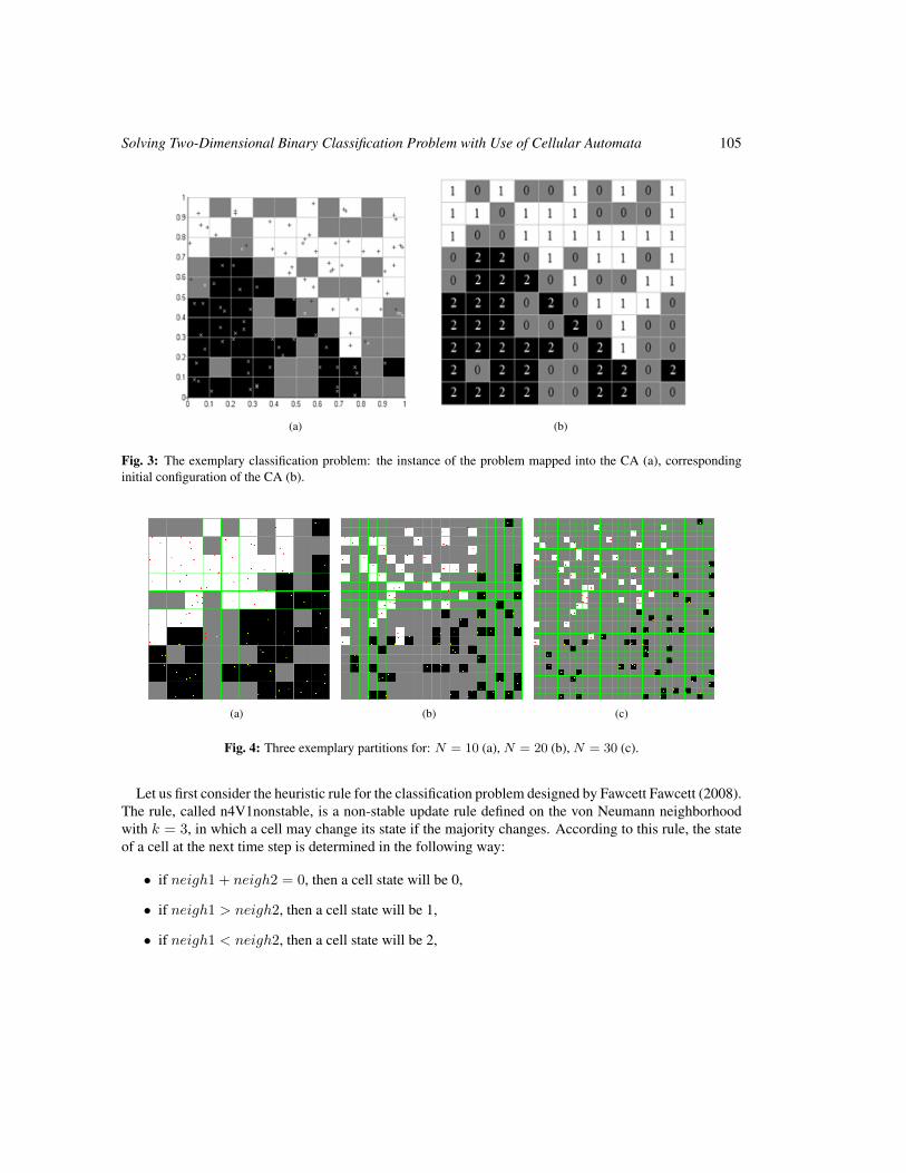
Solving Two-Dimensional Binary Classification Problem with Use of Cellular Automata 105
(a) (b)
Fig. 3: The exemplary classification problem: the instance of the problem mapped into the CA (a), correspondinginitial configuration of the CA (b).
(a) (b) (c)
Fig. 4: Three exemplary partitions for: N = 10 (a), N = 20 (b), N = 30 (c).
Let us first consider the heuristic rule for the classification problem designed by Fawcett Fawcett (2008).The rule, called n4V1nonstable, is a non-stable update rule defined on the von Neumann neighborhoodwith k = 3, in which a cell may change its state if the majority changes. According to this rule, the stateof a cell at the next time step is determined in the following way:
• if neigh1 + neigh2 = 0, then a cell state will be 0,
• if neigh1 > neigh2, then a cell state will be 1,
• if neigh1 < neigh2, then a cell state will be 2,
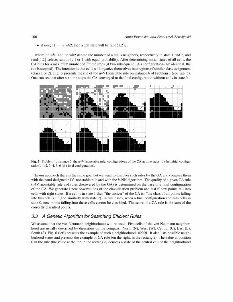
106 Anna Piwonska and Franciszek Seredynski
• if neigh1 = neigh2, then a cell state will be rand1,2,
where neigh1 and neigh2 denote the number of a cell’s neighbors, respectively in state 1 and 2, andrand1,2 selects randomly 1 or 2 with equal probability. After determining initial states of all cells, theCA runs for a maximum number of T time steps (if two subsequent CA’s configurations are identical, therun is stopped). The intention is that cells will organize themselves into regions of similar class assignment(class 1 or 2). Fig. 5 presents the run of the n4V1nonstable rule on instance 6 of Problem 1 (see Tab. 5).One can see that after six time steps the CA converged to the final configuration without cells in state 0.
Fig. 5: Problem 1, instance 6, the n4V1nonstable rule: configurations of the CA at time steps: 0 (the initial configu-ration), 1, 2, 3, 4, 5, 6 (the final configuration).
In our approach there is the same goal but we want to discover such rules by the GA and compare themwith the hand-designed n4V1nonstable rule and with the k-NN algorithm. The quality of a given CA rule(n4V1nonstable rule and rules discovered by the GA) is determined on the base of a final configurationof the CA. We generate l new observations of the classification problem and test if new points fall intocells with right states. If a cell is in state 1 then ”the answer” of the CA is: ”the class of all points fallinginto this cell is 1” (and similarly with state 2). In rare cases, when a final configuration contains cells instate 0, new points falling into these cells cannot be classified. The score of a CA rule is the sum of thecorrectly classified points.
3.3 A Genetic Algorithm for Searching Efficient Rules
We assume that the von Neumann neighborhood will be used. Five cells of the von Neumann neighbor-hood are usually described by directions on the compass: North (N), West (W), Central (C), East (E),South (S). Fig. 6 (left) presents the example of such a neighborhood: 02201. It also lists possible neigh-borhood states and presents the example of CA rule (on the right, in the rectangle). The value at position0 in the rule (the value at the top in the rectangle) denotes a state of the central cell of the neighborhood
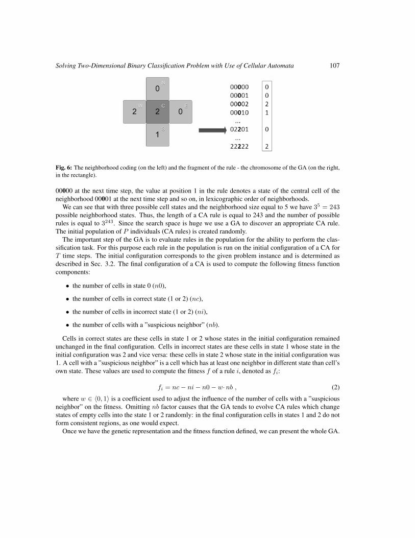
Solving Two-Dimensional Binary Classification Problem with Use of Cellular Automata 107
Fig. 6: The neighborhood coding (on the left) and the fragment of the rule - the chromosome of the GA (on the right,in the rectangle).
00000 at the next time step, the value at position 1 in the rule denotes a state of the central cell of theneighborhood 00001 at the next time step and so on, in lexicographic order of neighborhoods.
We can see that with three possible cell states and the neighborhood size equal to 5 we have 35 = 243possible neighborhood states. Thus, the length of a CA rule is equal to 243 and the number of possiblerules is equal to 3243. Since the search space is huge we use a GA to discover an appropriate CA rule.The initial population of P individuals (CA rules) is created randomly.
The important step of the GA is to evaluate rules in the population for the ability to perform the clas-sification task. For this purpose each rule in the population is run on the initial configuration of a CA forT time steps. The initial configuration corresponds to the given problem instance and is determined asdescribed in Sec. 3.2. The final configuration of a CA is used to compute the following fitness functioncomponents:
• the number of cells in state 0 (n0),
• the number of cells in correct state (1 or 2) (nc),
• the number of cells in incorrect state (1 or 2) (ni),
• the number of cells with a ”suspicious neighbor” (nb).
Cells in correct states are these cells in state 1 or 2 whose states in the initial configuration remainedunchanged in the final configuration. Cells in incorrect states are these cells in state 1 whose state in theinitial configuration was 2 and vice versa: these cells in state 2 whose state in the initial configuration was1. A cell with a ”suspicious neighbor” is a cell which has at least one neighbor in different state than cell’sown state. These values are used to compute the fitness f of a rule i, denoted as fi:
fi = nc− ni− n0− w·nb , (2)
where w ∈ 〈0, 1〉 is a coefficient used to adjust the influence of the number of cells with a ”suspiciousneighbor” on the fitness. Omitting nb factor causes that the GA tends to evolve CA rules which changestates of empty cells into the state 1 or 2 randomly: in the final configuration cells in states 1 and 2 do notform consistent regions, as one would expect.
Once we have the genetic representation and the fitness function defined, we can present the whole GA.
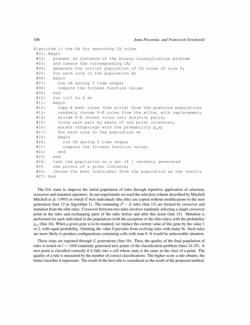
108 Anna Piwonska and Franciszek Seredynski
Algorithm 1: the GA for searching CA rules#01: Begin#02: present an instance of the binary classification problem#03: and create the corresponding CA;#04: generate the initial population of CA rules of size P;#05: for each rule in the population do#06: begin#07: run CA during T time steps;#08: compute the fitness function value;#09: end#10: for i:=1 to G do#11: begin#12: copy E best rules (the elite) from the previous population;#13: randomly choose P-E rules from the elite, with replacement;#14: divide P-E chosen rules into disjoint pairs;#15: cross each pair by means of one point crossover;#16: mutate offsprings with the probability p_m;#17: for each rule in the population do#18: begin#20: run CA during T time steps;#21: compute the fitness function value;#22: end#23: end#24: test the population on a set of l randomly generated#25 new points of a given instance;#26: choose the best individual from the population as the result;#27: End
The GA starts to improve the initial population of rules through repetitive application of selection,crossover and mutation operators. In our experiments we used the selection scheme described by MitchellMitchell et al. (1993) in which E best individuals (the elite) are copied without modifications to the nextgeneration (line 12 in Algorithm 1). The remaining P − E rules (line 13) are formed by crossover andmutation from the elite rules. Crossover between two rules involves randomly selecting a single crossoverpoint in the rules and exchanging parts of the rules before and after this point (line 15). Mutation isperformed for each individual in the population (with the exception of the elite rules) with the probabilitypm (line 16). When a given gene is to be mutated, we replace the current value of this gene by the value 1or 2, with equal probability. Omitting the value 0 prevents from evolving rules with many 0s. Such rulesare more likely to produce configurations containing cells with state 0. It would be unfavorable situation.
These steps are repeated through G generations (line 10). Then, the quality of the final population ofrules is tested on l = 1000 randomly generated new points of the classification problem (lines 24-25). Anew point is classified correctly if it falls into a cell whose state is the same as the class of a point. Thequality of a rule is measured by the number of correct classifications. The higher score a rule obtains, thebetter classifier it represents. The result of the best rule is considered as the result of the proposed method.
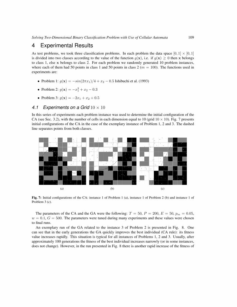
Solving Two-Dimensional Binary Classification Problem with Use of Cellular Automata 109
4 Experimental ResultsAs test problems, we took three classification problems. In each problem the data space [0, 1] × [0, 1]is divided into two classes according to the value of the function g(x), i.e. if g(x) ≥ 0 then x belongsto class 1, else x belongs to class 2. For each problem we randomly generated 10 problem instances,where each of them had 50 points in class 1 and 50 points in class 2 (m = 100). The functions used inexperiments are:
• Problem 1: g(x) = −sin(2πx1)/4 + x2 − 0.5 Ishibuchi et al. (1993)
• Problem 2: g(x) = −x31 + x2 − 0.3
• Problem 3: g(x) = −2x1 + x2 + 0.5
4.1 Experiments on a Grid 10× 10
In this series of experiments each problem instance was used to determine the initial configuration of theCA (see Sec. 3.2), with the number of cells in each dimension equal to 10 (grid 10× 10). Fig. 7 presentsinitial configurations of the CA in the case of the exemplary instance of Problem 1, 2 and 3. The dashedline separates points from both classes.
(a) (b) (c)
Fig. 7: Initial configurations of the CA: instance 1 of Problem 1 (a), instance 1 of Problem 2 (b) and instance 1 ofProblem 3 (c).
The parameters of the CA and the GA were the following: T = 50, P = 200, E = 50, pm = 0.05,w = 0.1, G = 500. The parameters were tuned during many experiments and these values were chosento final runs.
An exemplary run of the GA related to the instance 3 of Problem 2 is presented in Fig. 8. Onecan see that in the early generations the GA quickly improves the best individual (CA rule): its fitnessvalue increases rapidly. This situation is typical for all instances of Problems 1, 2 and 3. Usually, afterapproximately 100 generations the fitness of the best individual increases narrowly (or in some instances,does not change). However, in the run presented in Fig. 8 there is another rapid increase of the fitness of
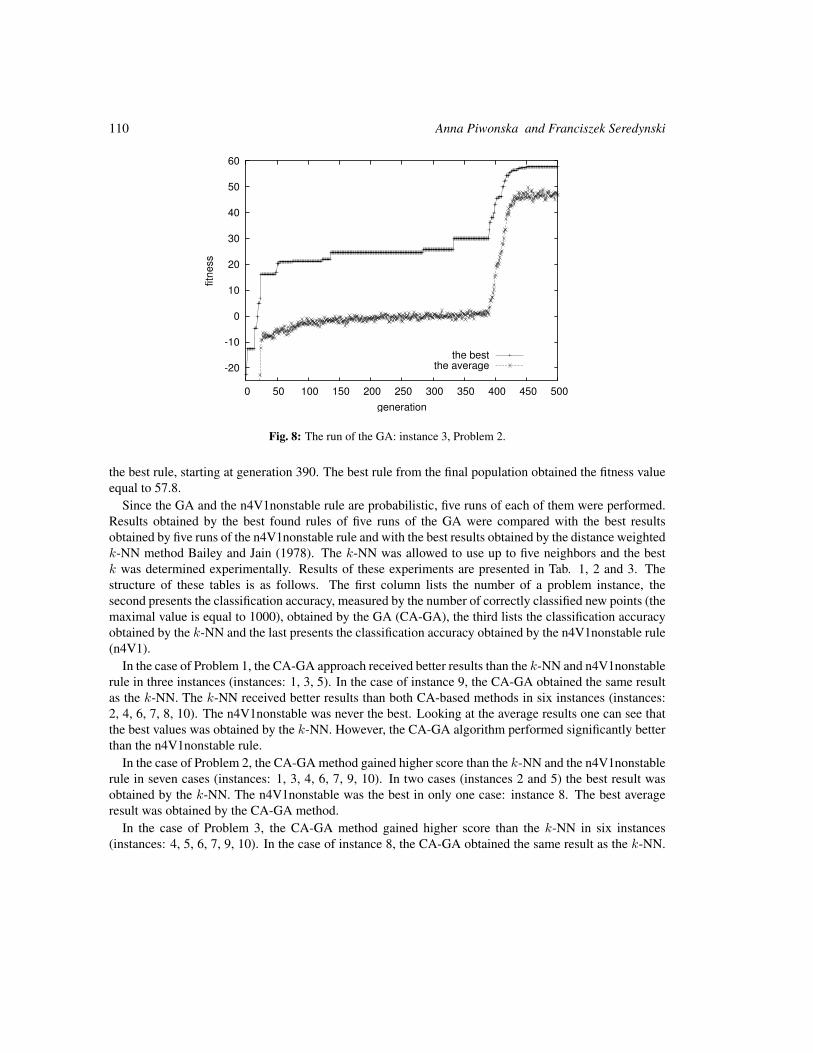
110 Anna Piwonska and Franciszek Seredynski
-20
-10
0
10
20
30
40
50
60
0 50 100 150 200 250 300 350 400 450 500
fitn
ess
generation
the bestthe average
Fig. 8: The run of the GA: instance 3, Problem 2.
the best rule, starting at generation 390. The best rule from the final population obtained the fitness valueequal to 57.8.
Since the GA and the n4V1nonstable rule are probabilistic, five runs of each of them were performed.Results obtained by the best found rules of five runs of the GA were compared with the best resultsobtained by five runs of the n4V1nonstable rule and with the best results obtained by the distance weightedk-NN method Bailey and Jain (1978). The k-NN was allowed to use up to five neighbors and the bestk was determined experimentally. Results of these experiments are presented in Tab. 1, 2 and 3. Thestructure of these tables is as follows. The first column lists the number of a problem instance, thesecond presents the classification accuracy, measured by the number of correctly classified new points (themaximal value is equal to 1000), obtained by the GA (CA-GA), the third lists the classification accuracyobtained by the k-NN and the last presents the classification accuracy obtained by the n4V1nonstable rule(n4V1).
In the case of Problem 1, the CA-GA approach received better results than the k-NN and n4V1nonstablerule in three instances (instances: 1, 3, 5). In the case of instance 9, the CA-GA obtained the same resultas the k-NN. The k-NN received better results than both CA-based methods in six instances (instances:2, 4, 6, 7, 8, 10). The n4V1nonstable was never the best. Looking at the average results one can see thatthe best values was obtained by the k-NN. However, the CA-GA algorithm performed significantly betterthan the n4V1nonstable rule.
In the case of Problem 2, the CA-GA method gained higher score than the k-NN and the n4V1nonstablerule in seven cases (instances: 1, 3, 4, 6, 7, 9, 10). In two cases (instances 2 and 5) the best result wasobtained by the k-NN. The n4V1nonstable was the best in only one case: instance 8. The best averageresult was obtained by the CA-GA method.
In the case of Problem 3, the CA-GA method gained higher score than the k-NN in six instances(instances: 4, 5, 6, 7, 9, 10). In the case of instance 8, the CA-GA obtained the same result as the k-NN.
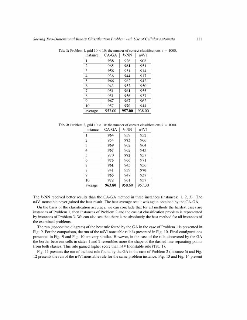
Solving Two-Dimensional Binary Classification Problem with Use of Cellular Automata 111
Tab. 1: Problem 1, grid 10× 10: the number of correct classifications, l = 1000.instance CA-GA k-NN n4V11 938 926 9082 965 981 9513 956 951 9144 936 944 9175 966 962 9426 943 952 9507 951 961 9558 951 956 9379 967 967 96210 957 970 944average 953.00 957.00 938.00
Tab. 2: Problem 2, grid 10× 10: the number of correct classifications, l = 1000.instance CA-GA k-NN n4V11 964 959 9522 954 973 9663 969 962 9644 967 962 9435 970 972 9576 975 966 9717 961 945 9568 941 939 9709 965 947 93710 972 961 957average 963.80 958.60 957.30
The k-NN received better results than the CA-GA method in three instances (instances: 1, 2, 3). Then4V1nonstable never gained the best result. The best average result was again obtained by the CA-GA.
On the basis of the classification accuracy, we can conclude that for all methods the hardest cases areinstances of Problem 1, then instances of Problem 2 and the easiest classification problem is representedby instances of Problem 3. We can also see that there is no absolutely the best method for all instances ofthe examined problems.
The run (space-time diagram) of the best rule found by the GA in the case of Problem 1 is presented inFig. 9. For the comparison, the run of the n4V1nonstable rule is presented in Fig. 10. Final configurationspresented in Fig. 9 and Fig. 10 are very similar. However, in the case of the rule discovered by the GAthe border between cells in states 1 and 2 resembles more the shape of the dashed line separating pointsfrom both classes. This rule gained higher score than n4V1nonstable rule (Tab. 1).
Fig. 11 presents the run of the best rule found by the GA in the case of Problem 2 (instance 6) and Fig.12 presents the run of the n4V1nonstable rule for the same problem instance. Fig. 13 and Fig. 14 present
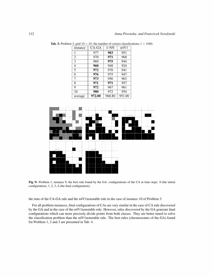
112 Anna Piwonska and Franciszek Seredynski
Tab. 3: Problem 3, grid 10× 10: the number of correct classifications, l = 1000.instance CA-GA k-NN n4V11 977 983 9512 970 971 9683 969 975 9444 960 948 9245 972 970 9416 976 975 9477 973 956 9638 971 971 9579 972 967 96110 980 972 954average 972.00 968.80 951.00
Fig. 9: Problem 1, instance 9, the best rule found by the GA: configurations of the CA at time steps: 0 (the initialconfiguration), 1, 2, 3, 4 (the final configuration).
the runs of the CA-GA rule and the n4V1nonstable rule in the case of instance 10 of Problem 3.
For all problem instances, final configurations of CAs are very similar in the case of CA rule discoveredby the GA and in the case of the n4V1nonstable rule. However, rules discovered by the GA generate finalconfigurations which can more precisely divide points from both classes. They are better tuned to solvethe classification problem than the n4V1nonstable rule. The best rules (chromosomes of the GA) foundfor Problem 1, 2 and 3 are presented in Tab. 4.
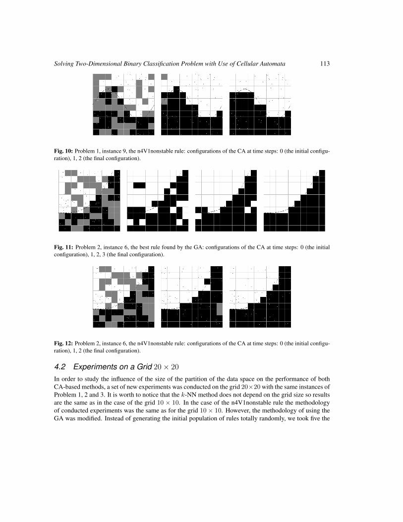
Solving Two-Dimensional Binary Classification Problem with Use of Cellular Automata 113
Fig. 10: Problem 1, instance 9, the n4V1nonstable rule: configurations of the CA at time steps: 0 (the initial configu-ration), 1, 2 (the final configuration).
Fig. 11: Problem 2, instance 6, the best rule found by the GA: configurations of the CA at time steps: 0 (the initialconfiguration), 1, 2, 3 (the final configuration).
Fig. 12: Problem 2, instance 6, the n4V1nonstable rule: configurations of the CA at time steps: 0 (the initial configu-ration), 1, 2 (the final configuration).
4.2 Experiments on a Grid 20× 20
In order to study the influence of the size of the partition of the data space on the performance of bothCA-based methods, a set of new experiments was conducted on the grid 20×20 with the same instances ofProblem 1, 2 and 3. It is worth to notice that the k-NN method does not depend on the grid size so resultsare the same as in the case of the grid 10 × 10. In the case of the n4V1nonstable rule the methodologyof conducted experiments was the same as for the grid 10 × 10. However, the methodology of using theGA was modified. Instead of generating the initial population of rules totally randomly, we took five the
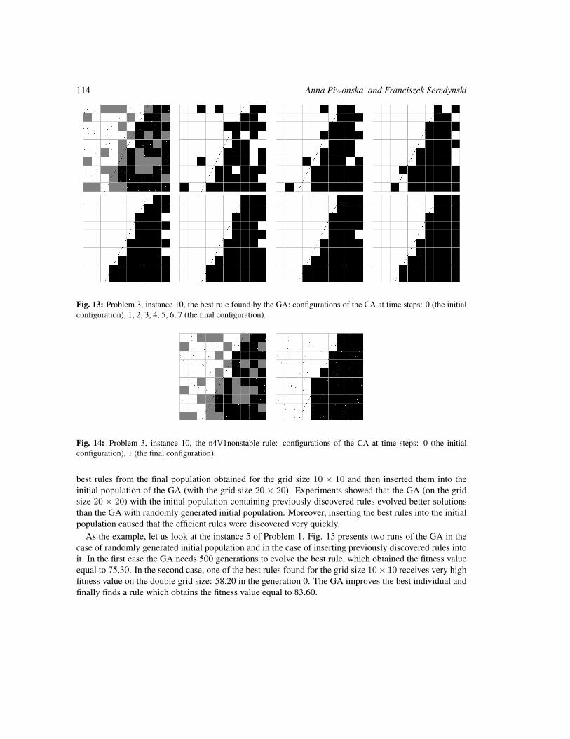
114 Anna Piwonska and Franciszek Seredynski
Fig. 13: Problem 3, instance 10, the best rule found by the GA: configurations of the CA at time steps: 0 (the initialconfiguration), 1, 2, 3, 4, 5, 6, 7 (the final configuration).
Fig. 14: Problem 3, instance 10, the n4V1nonstable rule: configurations of the CA at time steps: 0 (the initialconfiguration), 1 (the final configuration).
best rules from the final population obtained for the grid size 10 × 10 and then inserted them into theinitial population of the GA (with the grid size 20 × 20). Experiments showed that the GA (on the gridsize 20 × 20) with the initial population containing previously discovered rules evolved better solutionsthan the GA with randomly generated initial population. Moreover, inserting the best rules into the initialpopulation caused that the efficient rules were discovered very quickly.
As the example, let us look at the instance 5 of Problem 1. Fig. 15 presents two runs of the GA in thecase of randomly generated initial population and in the case of inserting previously discovered rules intoit. In the first case the GA needs 500 generations to evolve the best rule, which obtained the fitness valueequal to 75.30. In the second case, one of the best rules found for the grid size 10× 10 receives very highfitness value on the double grid size: 58.20 in the generation 0. The GA improves the best individual andfinally finds a rule which obtains the fitness value equal to 83.60.
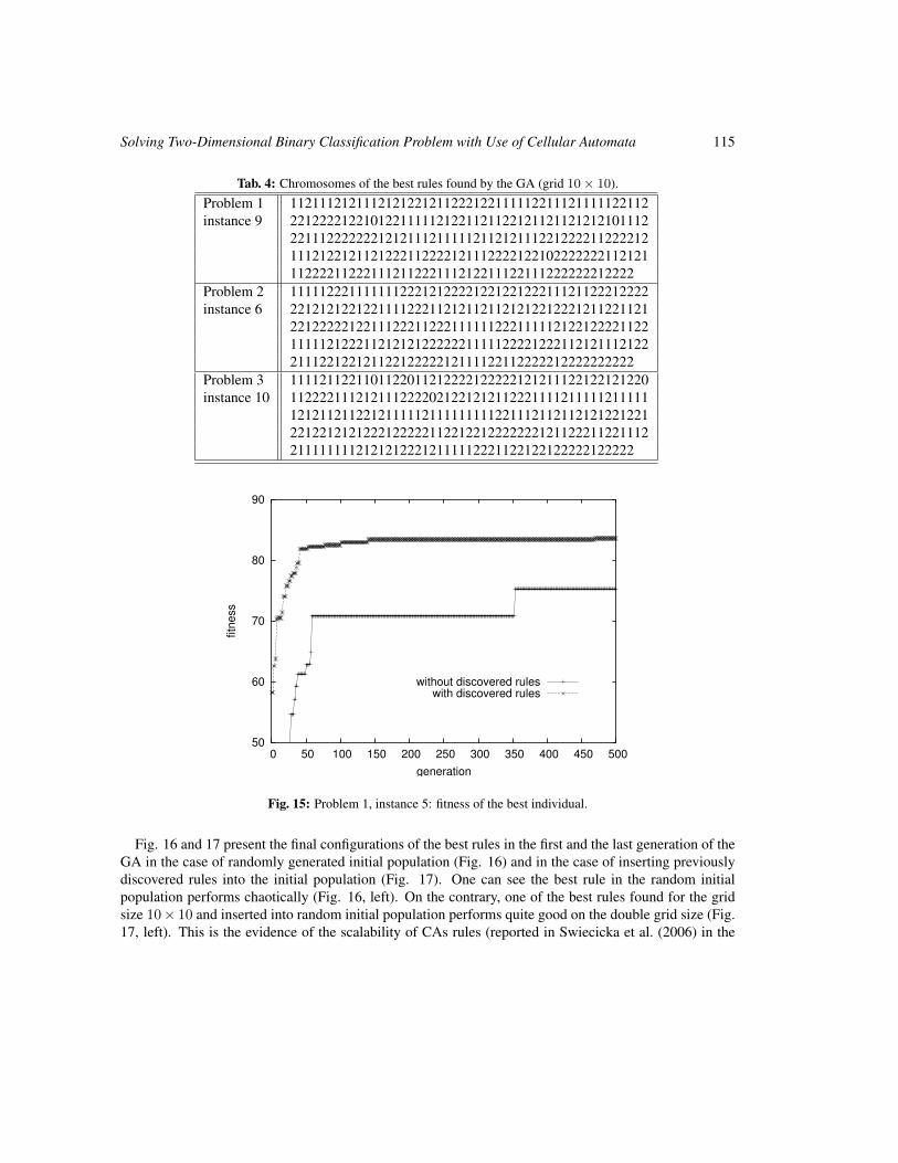
Solving Two-Dimensional Binary Classification Problem with Use of Cellular Automata 115
Tab. 4: Chromosomes of the best rules found by the GA (grid 10× 10).
Problem 1 1121112121112121221211222122111112211121111122112instance 9 2212222122101221111121221121122121121121212101112
2211122222221212111211111211212111221222211222212111212212112122211222212111222212210222222211212111222211222111211222111212211122111222222212222
Problem 2 1111122211111112221212222122122122211121122212222instance 6 2212121221221111222112121121121212212221211221121
2212222212211122211222111111222111112122122221122111112122211212121222222111112222122211212111212221112212212112212222212111122112222212222222222
Problem 3 1111211221101122011212222122222121211122122121220instance 10 1122221112121112222021221212112221111211111211111
1212112112212111112111111111221112112112121221221221221212122212222211221221222222212112221122111221111111121212122212111112221122122122222122222
50
60
70
80
90
0 50 100 150 200 250 300 350 400 450 500
fitn
ess
generation
without discovered ruleswith discovered rules
Fig. 15: Problem 1, instance 5: fitness of the best individual.
Fig. 16 and 17 present the final configurations of the best rules in the first and the last generation of theGA in the case of randomly generated initial population (Fig. 16) and in the case of inserting previouslydiscovered rules into the initial population (Fig. 17). One can see the best rule in the random initialpopulation performs chaotically (Fig. 16, left). On the contrary, one of the best rules found for the gridsize 10× 10 and inserted into random initial population performs quite good on the double grid size (Fig.17, left). This is the evidence of the scalability of CAs rules (reported in Swiecicka et al. (2006) in the
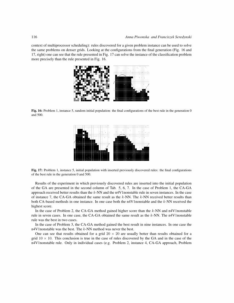
116 Anna Piwonska and Franciszek Seredynski
context of multiprocessor scheduling): rules discovered for a given problem instance can be used to solvethe same problems on denser grids. Looking at the configurations from the final generation (Fig. 16 and17, right) one can see that the rule presented in Fig. 17 can solve the instance of the classification problemmore precisely than the rule presented in Fig. 16.
Fig. 16: Problem 1, instance 5, random initial population: the final configurations of the best rule in the generation 0and 500.
Fig. 17: Problem 1, instance 5, initial population with inserted previously discovered rules: the final configurationsof the best rule in the generation 0 and 500.
Results of the experiment in which previously discovered rules are inserted into the initial populationof the GA are presented in the second column of Tab. 5, 6, 7. In the case of Problem 1, the CA-GAapproach received better results than the k-NN and the n4V1nonstable rule in seven instances. In the caseof instance 7, the CA-GA obtained the same result as the k-NN. The k-NN received better results thanboth CA-based methods in one instance. In one case both the n4V1nonstable and the k-NN received thehighest score.
In the case of Problem 2, the CA-GA method gained higher score than the k-NN and n4V1nonstablerule in seven cases. In one case, the CA-GA obtained the same result as the k-NN. The n4V1nonstablerule was the best in two cases.
In the case of Problem 3, the CA-GA method gained the best result in nine instances. In one case then4V1nonstable was the best. The k-NN method was never the best.
One can see that results obtained for a grid 20 × 20 are usually better than results obtained for agrid 10 × 10. This conclusion is true in the case of rules discovered by the GA and in the case of then4V1nonstable rule. Only in individual cases (e.g. Problem 2, instance 4, CA-GA approach, Problem
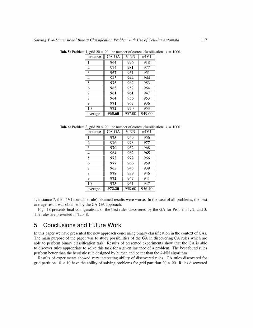
Solving Two-Dimensional Binary Classification Problem with Use of Cellular Automata 117
Tab. 5: Problem 1, grid 20× 20: the number of correct classifications, l = 1000.instance CA-GA k-NN n4V11 964 926 9182 974 981 9773 967 951 9514 943 944 9445 975 962 9536 965 952 9647 961 961 9478 964 956 9539 971 967 93610 972 970 953average 965.60 957.00 949.60
Tab. 6: Problem 2, grid 20× 20: the number of correct classifications, l = 1000.instance CA-GA k-NN n4V11 975 959 9562 976 973 9773 970 962 9684 964 962 9655 972 972 9666 977 966 9597 965 945 9398 978 939 9469 972 947 94110 973 961 947average 972.20 958.60 956.40
1, instance 7, the n4V1nonstable rule) obtained results were worse. In the case of all problems, the bestaverage result was obtained by the CA-GA approach.
Fig. 18 presents final configurations of the best rules discovered by the GA for Problem 1, 2, and 3.The rules are presented in Tab. 8.
5 Conclusions and Future WorkIn this paper we have presented the new approach concerning binary classification in the context of CAs.The main purpose of the paper was to study possibilities of the GA in discovering CA rules which areable to perform binary classification task. Results of presented experiments show that the GA is ableto discover rules appropriate to solve this task for a given instance of a problem. The best found rulesperform better than the heuristic rule designed by human and better than the k-NN algorithm.
Results of experiments showed very interesting ability of discovered rules. CA rules discovered forgrid partition 10 × 10 have the ability of solving problems for grid partition 20 × 20. Rules discovered
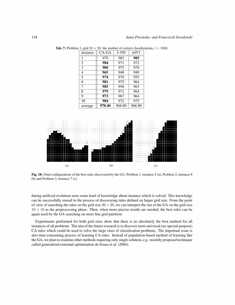
118 Anna Piwonska and Franciszek Seredynski
Tab. 7: Problem 3, grid 20× 20: the number of correct classifications, l = 1000.instance CA-GA k-NN n4V11 979 983 9852 984 971 9723 980 975 9784 965 948 9495 974 970 9556 981 975 9647 985 956 9638 979 971 9649 973 967 96410 984 972 975average 978.40 968.80 966.90
(a) (b) (c)
Fig. 18: Final configurations of the best rules discovered by the GA: Problem 1, instance 5 (a), Problem 2, instance 8(b) and Problem 3, instance 7 (c).
during artificial evolution store some kind of knowledge about instance which is solved. This knowledgecan be successfully reused in the process of discovering rules defined on larger grid size. From the pointof view of searching the rules on the grid size 20× 20, we can interpret the run of the GA on the grid size10 × 10 as the preprocessing phase. Then, when more precise results are needed, the best rules can beagain used by the GA searching on more fine grid partition.
Experiments performed for both grid sizes show that there is no absolutely the best method for allinstances of all problems. The aim of the future research is to discover more universal (no special-purpose)CA rules which could be used to solve the large class of classification problems. The important issue isalso time-consuming process of learning CA rules. Instead of population-based method of learning likethe GA, we plan to examine other methods requiring only single solution, e.g. recently proposed techniquecalled generalized extremal optimization de Sousa et al. (2004).
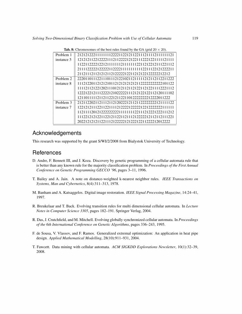
Solving Two-Dimensional Binary Classification Problem with Use of Cellular Automata 119
Tab. 8: Chromosomes of the best rules found by the GA (grid 20× 20).
Problem 1 2121212221111111122221122121122111211112111111121instance 5 1212121122122221112112222121221112221221111121111
1122112222122121111111211111112211212212111221112211112222212222211222211111111111221112212122221121121112112121211212222212211212122122222212212
Problem 2 2220110111221110111212210211211111212112112211222instance 8 1112122011212121011212121212121122222222222101122
1111211212212021110121211211212211212211112221112122212212111222212102222211121212212211212011110212110111112112112212112211012222222212222011222
Problem 3 2121122021121112112120222121121122222222121111122instance 7 1221212111221122111121222212222212212222222111111
1121111201212222222221111111122111212221222111212111221212122112212112211211121222221211211211122120221212121122111212222212122212211222212012222
AcknowledgementsThis research was supported by the grant S/WI/2/2008 from Bialystok University of Technology.
ReferencesD. Andre, F. Bennett III, and J. Koza. Discovery by genetic programming of a cellular automata rule that
is better than any known rule for the majority classification problem. In Proceedings of the First AnnualConference on Genetic Programming GECCO ’96, pages 3–11, 1996.
T. Bailey and A. Jain. A note on distance-weighted k-nearest neighbor rules. IEEE Transactions onSystems, Man and Cybernetics, 8(4):311–313, 1978.
M. Banham and A. Katsaggelos. Digital image restoration. IEEE Signal Processing Magazine, 14:24–41,1997.
R. Breukelaar and T. Back. Evolving transition rules for multi dimensional cellular automata. In LectureNotes in Computer Science 3305, pages 182–191. Springer Verlag, 2004.
R. Das, J. Crutchfield, and M. Mitchell. Evolving globally synchronized cellular automata. In Proceedingsof the 6th International Conference on Genetic Algorithms, pages 336–243, 1995.
F. de Sousa, V. Vlassov, and F. Ramos. Generalized extremal optimization: An application in heat pipedesign. Applied Mathematical Modelling, 28(10):911–931, 2004.
T. Fawcett. Data mining with cellular automata. ACM SIGKDD Explorations Newsletter, 10(1):32–39,2008.

120 Anna Piwonska and Franciszek Seredynski
C. Ferreira. Gene Expression Programming: Mathematical Modeling by an Artificial Intelligence.Springer, 2006.
P. Gacs, G. Kurdyumov, and L. Levin. One dimensional uniform arrays that wash out finite islands.Problemy Peredachi Informatsii, 12:92–98, 1978.
G. Hernandez and H. Herrmann. Cellular automata for elementary image enhancement. Graphical ModelsAnd Image Processing, 58(1):82–89, 1996.
H. Ishibuchi, K. Nozaki, and N. Yamamoto. Selecting fuzzy rules by genetic algorithm for classificationproblems. Fuzzy Systems, 2:1119–1124, 1993.
P. Maji, B. Sikdar, and P. Chaudhuri. Cellular automata evolution for pattern classification. In LectureNotes in Computer Science 3305, pages 660–669. Springer Verlag, 2004.
M. Mitchell, P. Hraber, and J. Crutchfield. Revisiting the edge of chaos: Evolving cellular automata toperform computations. Complex Systems, 7:89–130, 1993.
C. Oliveira Jr. and P. de Oliveira. An approach to searching for two-dimensional cellular automata forrecognition of handwritten digits. In Lecture Notes in Artificial Intelligence 5317, pages 462–471.Springer Verlag, 2008.
S. Omohundro. Modelling cellular automata with partial differential equations. Physica 10D, 10(1-2):128–134, 1984.
N. Packard and S. Wolfram. Two-dimensional cellular automata. Journal of Statistical Physics, 38:901–946, 1985.
A. Piwonska and F. Seredynski. Learning cellular automata rules for pattern reconstruction task. InLecture Notes in Computer Science 6457, pages 240–249. Springer Verlag, 2010.
P. Povalej, M. Lenic, and P. Kokol. Improving ensembles with classificational cellular automata. InLecture Notes in Computer Science 3305, pages 242–249. Springer Verlag, 2004.
M. Sipper. The evolution of parallel cellular machines toward evolware. Biosystems, 42(1):29–43, 1997.
S. Slatnia, M. Batouche, and K. Melkemi. Evolutionary cellular automata based-approach for edge detec-tion. In Lecture Notes in Computer Science 4578, pages 404–411. Springer Verlag, 2007.
A. Swiecicka, F. Seredynski, and A. Zomaya. Multiprocessor scheduling and rescheduling with use ofcellular automata and artificial immune system support. IEEE Transactions on Parallel and DistributedSystems, 17(3):253–262, 2006.
S. Wolfram. A New Kind of Science. Wolfram Media, 2002.
AUTOMATA 2011, Santiago, Chile local proceedings LP, 2011, 121–140
The structure of communication problems incellular automata
Raimundo Briceno1 and Pierre-Etienne Meunier2
1DIM, Universidad de Chile 2LAMA, Universite de Savoie et DIM, Universidad de Chile
Studying cellular automata with methods from communication complexity appears to be a promising approach. Inthe past, interesting connections between communication complexity and intrinsic universality in cellular automatawere shown. One of the last extensions of this theory was its generalization to various “communication problems”,or “questions” one might ask about the dynamics of cellular automata. In this article, we aim at structuring theseproblems, and find what makes them interesting for the study of intrinsic universality and quasi-orders induced bysimulation relations.
Keywords: cellular automata, communication complexity, intrinsic universality, ideals
OutlineIn Section 1, we recall the basic notions of communication complexity and its application to cellularautomata. In Section 2, we show how communication complexity incorporates in the model of cellularautomata, generalizing the previous works to other simulation relations, and developing new communica-tion problems. Then, in Section 3, we study sets of cellular automata closed under simulation (ideals),and how our communication approach relates with them.
1 Introduction and definitions1.1 Cellular automata and shift spacesIn this paper we are always going to consider one-dimensional cellular automata (CA). A CA is definedby a local rule φ : Q2r+1 → Q, where r denotes the radius and Q, the set of states (or alphabet).
We denote by Φ : QZ → QZ the global function induced by φ following the classical definition:
Φ(x)i = φ(xi−r, . . . , xi+r),
where x is some element from QZ (or QZΦ, if we want to avoid ambiguities) called configuration. Finally,
we denote by Φt the t-step iteration of the global function Φ, such that Φt+1 = Φt Φ and Φ1 = Φ.A global function Φ can be represented by different local rules. All properties considered in this paper
depend only on Φ and are not sensitive to the choice of a particular local function. However, to avoid use-less formalism, we will use the following notion of canonical local representation: (φ, r) is the canonical
c© 2011 AUTOMATA proceedings, Santiago, Chile, 2011
122 Raimundo Briceno and Pierre-Etienne Meunier
local representation of Φ if φ has radius r and it is the local function of smallest radius having Φ as itsassociated global function. Throughout this work we are going to refer to a CA Φ with (φ, r).
The limit set of a given CA Φ, denoted ω(Φ), is defined as follows:
ω(Φ) =⋂t∈N
Φt(QZ).
A limit set is always a non-empty shift space. A shift spaceX over an alphabetQ is any subsetX ⊆ QZ
that can be defined by a family of forbidden words F ⊆ Q+, such that X is the set of all configurationswhere no word of F occurs. A shift space is said to be a shift of finite type (SFT) if it can be defined by afinite family F . We denote by L(X) the set of words occurring in configurations that belongs to X and,by Ln(X) := L(X)∩Qn, its restriction to words of length n ∈ N. A shift space is said to be a sofic shiftif L(X) is a regular language. Clearly, every SFT is a sofic shift.
If there exists a time t∗ ∈ N such that ω(Φ) = Φt∗(QZ), Φ is said to be stable, and unstable, otherwise.
A stable limit set is always a sofic shift.Finally, we denote AC the set of one-dimensional CAs.
1.2 Simulations and universalityWe define two parallel notions of simulation between CAs developed in [DMOT11], based on geometricaltransformations of diagram spaces and injections or projections between them.
Definition 1 (Rescaling) The ingredients of a rescaling are simple: packing cells into blocks, iteratingthe rule and composing with a traslation. Formally, given any state set Q and any m ≥ 1, we define thebijective packing map bm : QZ →
(Qm)Z
by:
∀i ∈ Z :(bm(x)
)(i) =
(x(mi), . . . , x(mi+m− 1)
),
for all x ∈ QZ. The rescaling Φ〈m,t,z〉 of Φ by parameters m (packing), t ≥ 1 (iterating) and z ∈ Z(shifting, denoted σ) is the CA of state set Qm and global rule:
bm σz Φt b−1m .
The fact that the above function is the global rule of a cellular automaton follows from Curtis-Lyndon-Hedlund theorem [Hed69] because it is continuous and commutes with traslations.
In the rest of this section, we define various relations between cellular automata. They are all definedin [DMOT11], and we just recall them here.
Definition 2 (Sub-automaton) A CA Φ1 is a sub-automaton of a CA Φ2, denoted by Φ1 v Φ2, if thereis an injective map ι from Q1 to Q2 such that ι Φ1 = Φ2 ι, where ι : QZ
1 → QZ2 denotes the uniform
extension of ι.
Definition 3 (Quotient) A CA Φ1 is a quotient of a CA Φ2, denoted by Φ1 Φ2, if there is a surjectivemap ϕ from Q2 to Q1 such that ϕ Φ2 = Φ1 ϕ, where ϕ : QZ
2 → QZ1 denotes the uniform extension of
ϕ.
Definition 4 (Injective simulation) We say that Φ2 injectively simulates Φ1, denoted Φ1 4i Φ2, if thereexist rescaling parameters m1, m2, t1, t2, z1 and z2 such that Φ1
〈m1,t1,z1〉 v Φ2〈m2,t2,z2〉.
The structure of communication problems in cellular automata 123
Definition 5 (Surjective simulation) We say that Φ2 surjectively simulates Φ1, denoted Φ1 4s Φ2, ifthere exist rescaling parameters m1, m2, t1, t2, z1 and z2 such that Φ1
〈m1,t1,z1〉 Φ2〈m2,t2,z2〉.
Definition 6 (Intrinsic universality) Let 4∈ 4i,4s. Ψ is intrinsically 4-universal if for all Φ it holdsthat Φ 4 Ψ.
It is well known that there exist intrinsically universal cellular automata for the 4i relation, and thisproperty has been shown undecidable (see for instance [Oll03] and [DMOT11]). An open problem, ap-pearing in various contexts (see [The05] or [BT10]), is the existence of a cellular automaton universal forthe 4s relation:
Open Problem 1 Is there some Ψ such that for all Φ it holds that Φ 4s Ψ?
1.3 IdealsInformally speaking, ideals are strict subsets of AC closed under simulation. In the general order theory,the precise definition is the following.
Definition 7 (Ideal) Let 4 be a quasiorder in AC. An ideal I is a subset of AC such that:
1. If Φ2 ∈ I and Φ1 4 Φ2, then Φ1 ∈ I.
2. For any Φ1,Φ2 ∈ I there is some Φ3 ∈ I such that Φ1 4 Φ3 and Φ2 4 Φ3.
Moreover, I is said principal if there is some ΦI such that:
Φ ∈ I ⇐⇒ Φ 4 ΦI .
Adapted to our context, we have the following sufficient conditions to be an ideal.
Proposition 1 ([DMOT11]) I ⊆ AC is an ideal for 4i (resp. 4s) if:
1. ∀m, t ∈ N, z ∈ Z : Φ ∈ I ⇐⇒ Φ〈m,t,z〉 ∈ I;
2. Φ2 ∈ I ∧ Φ1 v Φ2 (resp. Φ1 Φ2) =⇒ Φ1 ∈ I;
3. Φ1 ∈ I ∧ Φ2 ∈ I =⇒ Φ1 × Φ2 ∈ I.
Finally, let us notice that the ideal of reversible CAs is principal, as shown in [DMOT11].
1.4 Communication complexityCommunication complexity is a computational model designed by A. C.-C. Yao in [Yao79] to studyparallel programs. In this framework, we consider two players, Alice and Bob, each with an arbitrarilyhigh computational power, communicating to compute the value of some function f : X × Y → Z. Wesay that f has communication complexity c if, in the best protocol we can design to compute f on allpossible inputs (x, y) ∈ X × Y , where Alice only knows x, and Bob only knows y, they communicate atmost c bits to decide the value of f(x, y).
A more detailed introduction to this framework may be found in [KN97]. Here we just sum up theresults and definitions important for our study. First we define what a protocol is.
124 Raimundo Briceno and Pierre-Etienne Meunier
Definition 8 A protocol P over a domain X × Y with range Z is a binary tree where each internal nodev is labeled either by a map av : X → 0, 1 or by a map bv : Y → 0, 1, and each leaf v is labeledeither by a map Av : X → Z or by a map Bv : Y → Z.
The internal nodes of the protocol tree model communications. If a node v is labeled with an av , Alicesays one bit according to her input. If a node v is labeled with an bv , Bob says one bit according to hisinput. If this bit is 0, they go on to the left child of node v. If it is 1, they go on to its right child. Notsurprisingly, the value of protocols, or the functions they compute, is the label of the leaf Alice and Bobarrive to if they follow all the internal nodes of the protocol tree. Hence the following definition.
Definition 9 The value of protocol P on input (x, y) ∈ X×Y is given byAv(x) (orBv(y)) whereAv (orBv) is the label of the leaf reached by the path over the tree which starts at the root, turns left if av(x) = 0(or bv(y) = 0), and turns right otherwise. We say that a protocol computes a function f : X × Y → Z iffor any (x, y) ∈ X × Y , its value on input (x, y) is f(x, y).
We denote by D(f) the (deterministic) communication complexity of a function f : X × Y → Z. It isthe minimal cost of a protocol, over all protocols computing f , where the cost of a protocol is the depthof its corresponding tree.
In order to prove lower bounds on our constructions, we are going to use the following classical boundson communication complexity (the proofs appear in [KN97]).
Proposition 2 Let n ≥ 1 be fixed. Let EQ and DISJ be the functions “equality” and “disjointness” definedfrom 0, 1n × 0, 1n to 0, 1 by:
EQ(x, y) =
1 if (∀i)(xi = yi),
0 otherwise.
DISJ(x, y) =
1 if (∀i)(xiyi 6= 1),
0 otherwise.
Both problems have maximal communication complexity, i.e. D(EQ) ≥ n and D(DISJ) ≥ n.
In [GMRT09], there is an explanation on how to turn computational problems into communicationalones. Here we just recall the corresponding definition.
Definition 10 Let P : Q+ → Z be a computational problem. The communication complexity of P ,denoted CC (P ), is the function:
n 7→ max1≤i≤n−1
D(P |in
).
2 Communication complexity and simulationsIn this section, we continue the work begun in [GMRT09], incorporating two new communication prob-lems to the three “canonical problems” developed there, and we try to extend the compatibility of theseproblems to the 4s relation.
In order to do this, we consider the following relation between functions from R+ to R+:
f1 ≺ f2 ⇐⇒ ∃α, β, γ increasing affine functions, f1 α ≤ β f2 γ.
The structure of communication problems in cellular automata 125
Also, we use the same notation than in [GMRT09] to represent periodic configurations: if u = u1 . . . ulis a finite word we call pu the infinite configuration where for all i ∈ Z, (pu)i = uimod l. Overmore, wedenote pu(x1, . . . , xn) the configuration obtained by modifying pu as follows:
(pu(x1, . . . , xn))i =
(pu)i for i ≤ 0 or i ≥ n+ 1,
xi otherwise.
The problem called INVASION in [GMRT09], has a good behavior with respect to 4i. Here, we chooseto rename it in order to avoid confusions.
Definition 11 (Spatial invasion (SINV) [GMRT09]) Let Φ be a cellular automaton, and u a finite con-figuration for Φ. The problem SINVuΦ consists in determining whether the differences between pu andpu(x) will expand to an infinite width as times tends to infinity when applying Φ (the answer 1 means yesand the answer 0 means no).
Proposition 3 Let Φ and Ψ be two cellular automata. If Φ 4i Ψ, then for all u ∈ Q+Φ there exists v ∈ Q+
Ψ
(the corresponding word by 4i), such that:
CC (SINVuΦ) ≺ CC (SINVvΨ) .
Corollary 1 If Ψ is intrinsically 4i-universal, then there exists a word u ∈ Q+ such that:
CC (SINVuΨ) ∈ Ω(n).
2.1 Temporal invasionDefinition 12 (Temporal invasion (TINV) [GMRT09]) Let Φ be a cellular automaton, and u a finiteconfiguration for Φ. The TINV problem is the following:
TINVuΦ(x) = ∀t, [t ∈ N⇒ Φt(pu(x)) 6= Φt(pu)].
Proposition 4 Let Φ and Ψ be two cellular automata. If Φ 4i Ψ, then for all u ∈ Q+Φ there exists v ∈ Q+
Ψ
(the corresponding word by 4i), such that:
CC (TINVuΦ) ≺ CC (TINVvΨ) .
Proof: As in the other cases, we need to decompose the simulation relation:
• Φ〈m,1,0〉: to simulate a protocol for Φ with a protocol for Φ〈m,1,0〉, Alice and Bob need to commu-nicate O(m) bits to describe the cell shared between them. The other direction is easy.
• Φ〈1,t,0〉: the protocol is exactly the same, because of the “∀t” in the definition of TINV.
• Φ〈1,1,z〉: this is still the same protocol than for Φ, since the worst case in the partition of the inputwill be the same.
• Φ v Ψ: here Alice and Bob both know the injection given in the simulation. Then, they can applyit and use a protocol for Ψ to solve TINV on a configuration of Φ, with no overhead.
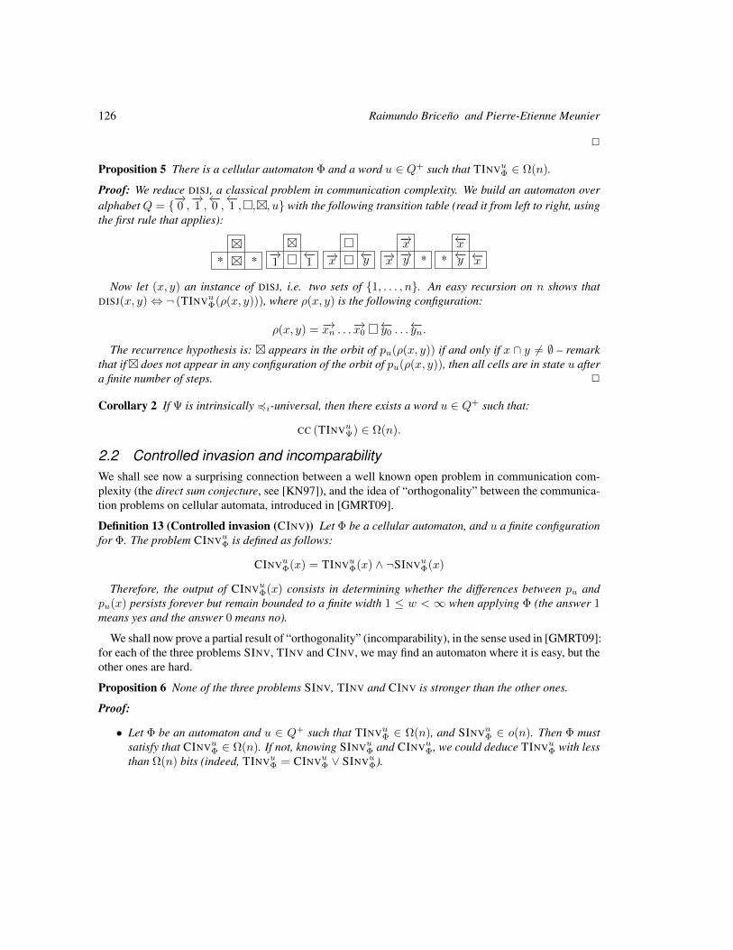
126 Raimundo Briceno and Pierre-Etienne Meunier
2
Proposition 5 There is a cellular automaton Φ and a word u ∈ Q+ such that TINVuΦ ∈ Ω(n).
Proof: We reduce DISJ, a classical problem in communication complexity. We build an automaton overalphabet Q = −→0 ,−→1 ,←−0 ,←−1 , , , u with the following transition table (read it from left to right, usingthe first rule that applies):
* * −→1
←−1−→x ←−y −→x −→y *
−→x* ←−y ←−x
←−x
Now let (x, y) an instance of DISJ, i.e. two sets of 1, . . . , n. An easy recursion on n shows thatDISJ(x, y)⇔ ¬ (TINVuΦ(ρ(x, y))), where ρ(x, y) is the following configuration:
ρ(x, y) = −→xn . . .−→x0←−y0 . . .
←−yn.The recurrence hypothesis is: appears in the orbit of pu(ρ(x, y)) if and only if x ∩ y 6= ∅ – remark
that if does not appear in any configuration of the orbit of pu(ρ(x, y)), then all cells are in state u aftera finite number of steps. 2
Corollary 2 If Ψ is intrinsically 4i-universal, then there exists a word u ∈ Q+ such that:
CC (TINVuΨ) ∈ Ω(n).
2.2 Controlled invasion and incomparabilityWe shall see now a surprising connection between a well known open problem in communication com-plexity (the direct sum conjecture, see [KN97]), and the idea of “orthogonality” between the communica-tion problems on cellular automata, introduced in [GMRT09].
Definition 13 (Controlled invasion (CINV)) Let Φ be a cellular automaton, and u a finite configurationfor Φ. The problem CINVuΦ is defined as follows:
CINVuΦ(x) = TINVuΦ(x) ∧ ¬SINVuΦ(x)
Therefore, the output of CINVuΦ(x) consists in determining whether the differences between pu andpu(x) persists forever but remain bounded to a finite width 1 ≤ w < ∞ when applying Φ (the answer 1means yes and the answer 0 means no).
We shall now prove a partial result of “orthogonality” (incomparability), in the sense used in [GMRT09]:for each of the three problems SINV, TINV and CINV, we may find an automaton where it is easy, but theother ones are hard.
Proposition 6 None of the three problems SINV, TINV and CINV is stronger than the other ones.
Proof:
• Let Φ be an automaton and u ∈ Q+ such that TINVuΦ ∈ Ω(n), and SINVuΦ ∈ o(n). Then Φ mustsatisfy that CINVuΦ ∈ Ω(n). If not, knowing SINVuΦ and CINVuΦ, we could deduce TINVuΦ with lessthan Ω(n) bits (indeed, TINVuΦ = CINVuΦ ∨ SINVuΦ).
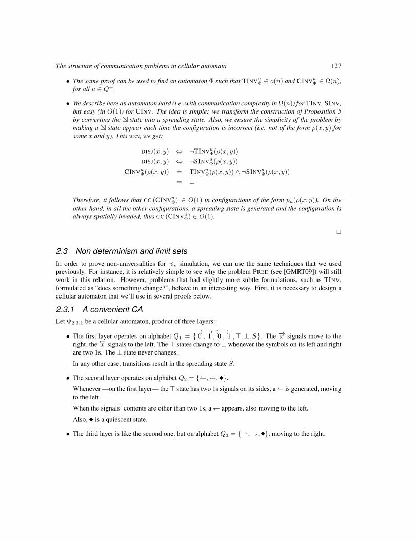
The structure of communication problems in cellular automata 127
• The same proof can be used to find an automaton Φ such that TINVuΦ ∈ o(n) and CINVuΦ ∈ Ω(n),for all u ∈ Q+.
• We describe here an automaton hard (i.e. with communication complexity in Ω(n)) for TINV, SINV,but easy (in O(1)) for CINV. The idea is simple: we transform the construction of Proposition 5by converting the state into a spreading state. Also, we ensure the simplicity of the problem bymaking a state appear each time the configuration is incorrect (i.e. not of the form ρ(x, y) forsome x and y). This way, we get:
DISJ(x, y) ⇔ ¬TINVuΦ(ρ(x, y))
DISJ(x, y) ⇔ ¬SINVuΦ(ρ(x, y))
CINVuΦ(ρ(x, y)) = TINVuΦ(ρ(x, y)) ∧ ¬SINVuΦ(ρ(x, y))
= ⊥
Therefore, it follows that CC (CINVuΦ) ∈ O(1) in configurations of the form pu(ρ(x, y)). On theother hand, in all the other configurations, a spreading state is generated and the configuration isalways spatially invaded, thus CC (CINVuΦ) ∈ O(1).
2
2.3 Non determinism and limit setsIn order to prove non-universalities for 4s simulation, we can use the same techniques that we usedpreviously. For instance, it is relatively simple to see why the problem PRED (see [GMRT09]) will stillwork in this relation. However, problems that had slightly more subtle formulations, such as TINV,formulated as “does something change?”, behave in an interesting way. First, it is necessary to design acellular automaton that we’ll use in several proofs below.
2.3.1 A convenient CALet Φ2.3.1 be a cellular automaton, product of three layers:
• The first layer operates on alphabet Q1 = −→0 ,−→1 ,←−0 ,←−1 ,>,⊥, S. The −→x signals move to theright, the←−x signals to the left. The > states change to ⊥ whenever the symbols on its left and rightare two 1s. The ⊥ state never changes.
In any other case, transitions result in the spreading state S.
• The second layer operates on alphabet Q2 = ,, .Whenever —on the first layer— the> state has two 1s signals on its sides, a is generated, movingto the left.
When the signals’ contents are other than two 1s, a appears, also moving to the left.
Also, is a quiescent state.
• The third layer is like the second one, but on alphabet Q3 = ,, , moving to the right.
128 Raimundo Briceno and Pierre-Etienne Meunier
We shall argue now that this automaton has a trivial SINV problem, as well as a trivial TINV problem.Indeed, there are three cases for the background u:
1. If it has a −→x or ←−x signal on the first layer, then all the other states must be signals in the samedirection. In this case, the configuration is invaded if and only if the input is anything else thansignals in this direction: a spreading state is generated on this component.
2. If it has a spreading state, no invasion can occur.
3. Otherwise, the background can be only , in which case invasion occurs, possibly on the secondlayer, if and only if the input is not only signals in the same direction.
In all three cases, the property can be checked by Alice and Bob with very few communicated bits, thusanswering to the SINV problem. Since the configuration is changed, the TINV problem is also easy.
Proposition 7 There is a cellular automaton Ψ such that Ψ Φ2.3.1 and:
CC (SINVΨ) ∈ Ω(n).
Proof: If the quotient relation identifies states and on the second component, and on the thirdcomponent, there is a set of configurations for which the problem becomes as difficult as the DISJ problem,defined in [KN97], i.e. CC (SINVΨ) ∈ Ω(n). 2
Proposition 8 There is a cellular automaton Ψ such that Ψ Φ2.3.1 and:
CC (TINVΨ) ∈ Ω(n).
Proof: If the quotient relation identifies all states with on the second component and all states with onthe third component, on configurations of the form−→∗ n>←−∗ n, solving the problem TINV requires decidingif the middle > symbol turns ⊥ somewhere in the space-time diagram, which is as difficult as the DISJproblem, defined in [KN97], i.e. CC (TINVΨ) ∈ Ω(n). 2
This raises new questions: is this simulation stronger or weaker than the previous one? As studiedin [DMOT11], we know that they are incomparable. In this section, we introduce a problem whosecommunication complexity grows with respect to 4s, but for which it is not the case in relation 4i. Atthe same time, it may be a clue that our approach with communication complexity will not be able to tellmuch about Open Problem 1.
Definition 14 (Limit set word (LIMIT)) LIMITΦ is the problem of deciding if the input word belongs tothe language of the limit set of Φ:
LIMITΦ(x) =
1 if ∀t,∃y, x = Φt(y),
0 otherwise.
LetCC (LIMITΦ) = max
iD(LIMITΦ(x[0,i], x[i+1,n−1]))
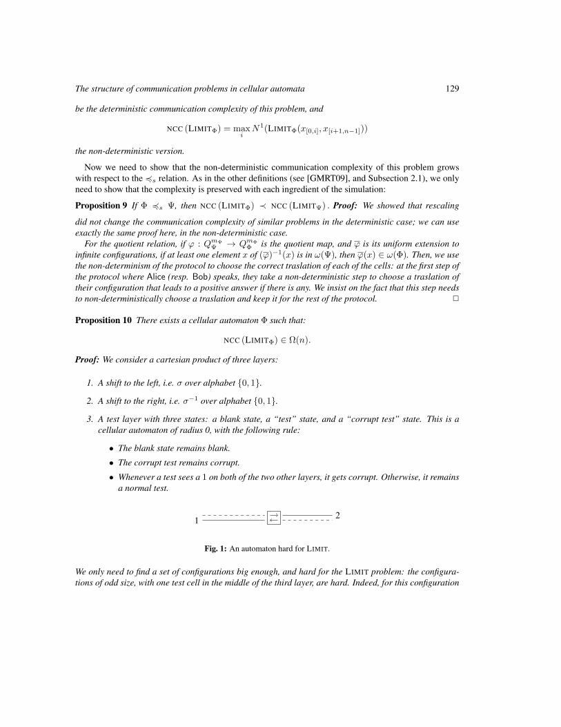
The structure of communication problems in cellular automata 129
be the deterministic communication complexity of this problem, and
NCC (LIMITΦ) = maxiN1(LIMITΦ(x[0,i], x[i+1,n−1]))
the non-deterministic version.
Now we need to show that the non-deterministic communication complexity of this problem growswith respect to the 4s relation. As in the other definitions (see [GMRT09], and Subsection 2.1), we onlyneed to show that the complexity is preserved with each ingredient of the simulation:
Proposition 9 If Φ 4s Ψ, then NCC (LIMITΦ) ≺ NCC (LIMITΨ) . Proof: We showed that rescaling
did not change the communication complexity of similar problems in the deterministic case; we can useexactly the same proof here, in the non-deterministic case.
For the quotient relation, if ϕ : QmΨ
Ψ → QmΦ
Φ is the quotient map, and ϕ is its uniform extension toinfinite configurations, if at least one element x of (ϕ)−1(x) is in ω(Ψ), then ϕ(x) ∈ ω(Φ). Then, we usethe non-determinism of the protocol to choose the correct traslation of each of the cells: at the first step ofthe protocol where Alice (resp. Bob) speaks, they take a non-deterministic step to choose a traslation oftheir configuration that leads to a positive answer if there is any. We insist on the fact that this step needsto non-deterministically choose a traslation and keep it for the rest of the protocol. 2
Proposition 10 There exists a cellular automaton Φ such that:
NCC (LIMITΦ) ∈ Ω(n).
Proof: We consider a cartesian product of three layers:
1. A shift to the left, i.e. σ over alphabet 0, 1.
2. A shift to the right, i.e. σ−1 over alphabet 0, 1.
3. A test layer with three states: a blank state, a “test” state, and a “corrupt test” state. This is acellular automaton of radius 0, with the following rule:
• The blank state remains blank.
• The corrupt test remains corrupt.
• Whenever a test sees a 1 on both of the two other layers, it gets corrupt. Otherwise, it remainsa normal test.
1 2
Fig. 1: An automaton hard for LIMIT.
We only need to find a set of configurations big enough, and hard for the LIMIT problem: the configura-tions of odd size, with one test cell in the middle of the third layer, are hard. Indeed, for this configuration

130 Raimundo Briceno and Pierre-Etienne Meunier
to be in the limit set, an infinite DISJ problem needs to be solved between the word on layer 1, and themirror of the word on layer 2 (i.e. on the whole lines on Figure 1), so Alice and Bob need to solve aninstance of DISJ in order to find out whether the input belongs to the limit set, which, according to [KN97],requires Ω(n) bits to be solved by a non-deterministic protocol. 2
This shows that this problem is compatible with the 4s relation, i.e. that the following holds.
Corollary 3 If Ψ is intrinsically 4s-universal, then:
NCC (LIMITΦ) ∈ Ω(n).
Now, according to the analysis of [GMT10], there exists a cellular automaton universal for 4i, withcomplexity not greater than O(log n) for the LIMIT problem.
This problem may seem an odd counter-example. However, we will see in Proposition 14 how to use itto show that no stable automaton can be intrinsically 4s-universal.
3 Structuring communication problemsIn this section, we explore the links between our approach using communication complexity to studycellular automata and the general theory of bulking, developed in [DMOT10, DMOT11]. In order to dothis, we prove the existence of new ideals and inclusions, giving a more detailed vision of quasi-ordersinduced by simulations. As showing that a given CA belongs to an ideal is a way to prove that it cannot beintrinsically universal, we illustrate here how our tools adapt well to this framework and extend it, beingthe communication approach, to our knowledge, the best way of proving non-universality in cellularautomata.
3.1 Closing CAsIn the following, we ennunciate some results concerning the sets of closing and open CAs. As we suspect,this is closely related with the following open problem.
Open Problem 2 ([DMOT11]) Is the ideal of surjective CA principal, and for which simulation quasi-order?
Definition 15 (Asymptotic configurations [K09]) x, y ∈ QZ are left (right) asymptotic, if there existsm ∈ Z such that xi = yi for all i ≤ m (for all i ≥ m).
Definition 16 (Closingness [K09]) A CA Φ is right closing (resp. left closing), if for every distinct leftasymptotic (right asymptotic) x, y ∈ QZ, Φ(x) 6= Φ(y). A CA is closing if it is either left or right closing.Clearly,
Φ injective =⇒ Φ closing =⇒ Φ preinjective ⇐⇒ Φ surjective.
Theorem 1 Let 4∈ 4i,4s. Then, the set of right closing (left closing) CAs is an ideal for 4.
Proof: See the Appendix. 2
Proposition 11 ([Hed69]) A CA is open if and only if is right-closing and left-closing.
Corollary 4 Let 4∈ 4i,4s. Then, the set of open CAs is an ideal for 4.
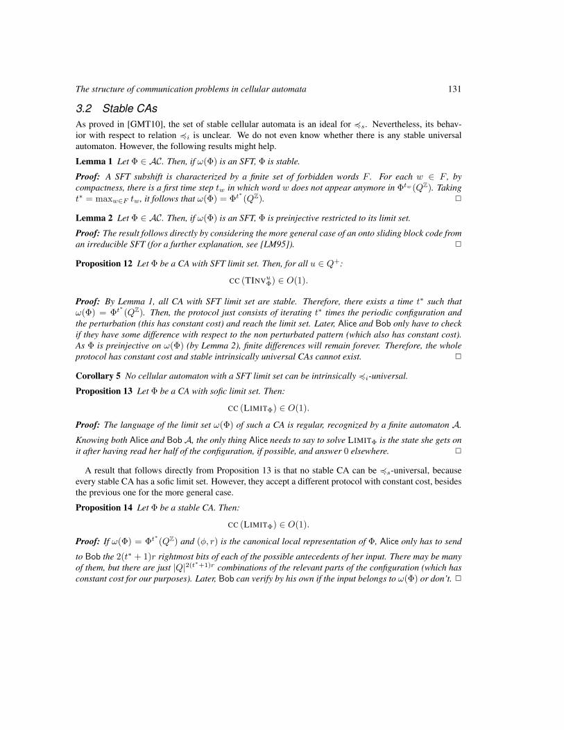
The structure of communication problems in cellular automata 131
3.2 Stable CAsAs proved in [GMT10], the set of stable cellular automata is an ideal for 4s. Nevertheless, its behav-ior with respect to relation 4i is unclear. We do not even know whether there is any stable universalautomaton. However, the following results might help.
Lemma 1 Let Φ ∈ AC. Then, if ω(Φ) is an SFT, Φ is stable.
Proof: A SFT subshift is characterized by a finite set of forbidden words F . For each w ∈ F , bycompactness, there is a first time step tw in which word w does not appear anymore in Φtw(QZ). Takingt∗ = maxw∈F tw, it follows that ω(Φ) = Φt
∗(QZ). 2
Lemma 2 Let Φ ∈ AC. Then, if ω(Φ) is an SFT, Φ is preinjective restricted to its limit set.
Proof: The result follows directly by considering the more general case of an onto sliding block code froman irreducible SFT (for a further explanation, see [LM95]). 2
Proposition 12 Let Φ be a CA with SFT limit set. Then, for all u ∈ Q+:
CC (TINVuΦ) ∈ O(1).
Proof: By Lemma 1, all CA with SFT limit set are stable. Therefore, there exists a time t∗ such thatω(Φ) = Φt
∗(QZ). Then, the protocol just consists of iterating t∗ times the periodic configuration and
the perturbation (this has constant cost) and reach the limit set. Later, Alice and Bob only have to checkif they have some difference with respect to the non perturbated pattern (which also has constant cost).As Φ is preinjective on ω(Φ) (by Lemma 2), finite differences will remain forever. Therefore, the wholeprotocol has constant cost and stable intrinsically universal CAs cannot exist. 2
Corollary 5 No cellular automaton with a SFT limit set can be intrinsically 4i-universal.
Proposition 13 Let Φ be a CA with sofic limit set. Then:
CC (LIMITΦ) ∈ O(1).
Proof: The language of the limit set ω(Φ) of such a CA is regular, recognized by a finite automaton A.
Knowing both Alice and Bob A, the only thing Alice needs to say to solve LIMITΦ is the state she gets onit after having read her half of the configuration, if possible, and answer 0 elsewhere. 2
A result that follows directly from Proposition 13 is that no stable CA can be 4s-universal, becauseevery stable CA has a sofic limit set. However, they accept a different protocol with constant cost, besidesthe previous one for the more general case.
Proposition 14 Let Φ be a stable CA. Then:
CC (LIMITΦ) ∈ O(1).
Proof: If ω(Φ) = Φt∗(QZ) and (φ, r) is the canonical local representation of Φ, Alice only has to send
to Bob the 2(t∗ + 1)r rightmost bits of each of the possible antecedents of her input. There may be manyof them, but there are just |Q|2(t∗+1)r combinations of the relevant parts of the configuration (which hasconstant cost for our purposes). Later, Bob can verify by his own if the input belongs to ω(Φ) or don’t. 2
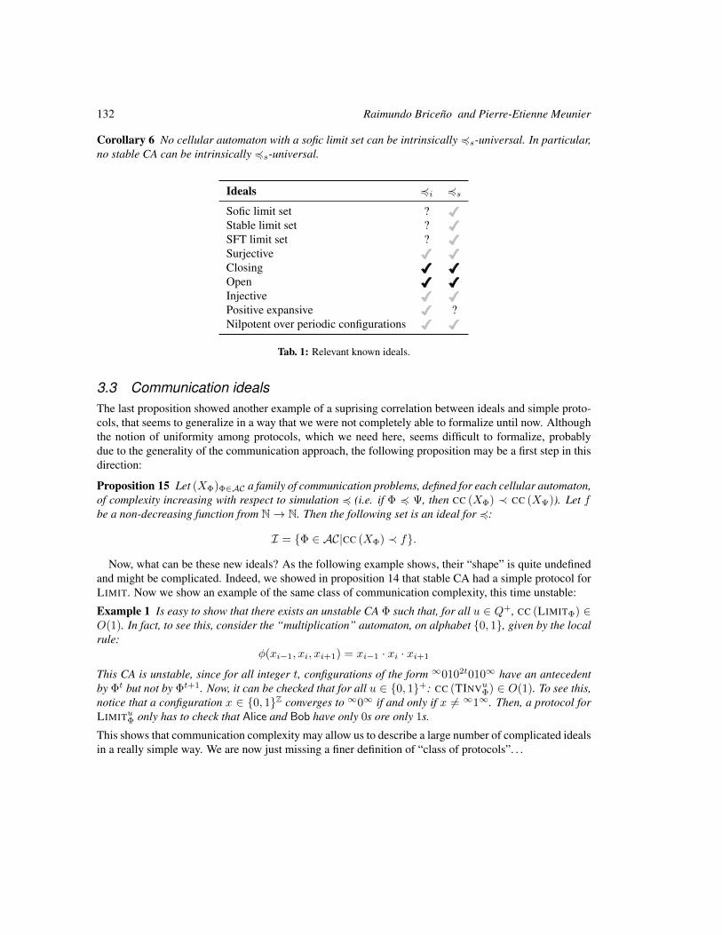
132 Raimundo Briceno and Pierre-Etienne Meunier
Corollary 6 No cellular automaton with a sofic limit set can be intrinsically 4s-universal. In particular,no stable CA can be intrinsically 4s-universal.
Ideals 4i 4s
Sofic limit set ?Stable limit set ?SFT limit set ?SurjectiveClosingOpenInjectivePositive expansive ?Nilpotent over periodic configurations
Tab. 1: Relevant known ideals.
3.3 Communication idealsThe last proposition showed another example of a suprising correlation between ideals and simple proto-cols, that seems to generalize in a way that we were not completely able to formalize until now. Althoughthe notion of uniformity among protocols, which we need here, seems difficult to formalize, probablydue to the generality of the communication approach, the following proposition may be a first step in thisdirection:
Proposition 15 Let (XΦ)Φ∈AC a family of communication problems, defined for each cellular automaton,of complexity increasing with respect to simulation 4 (i.e. if Φ 4 Ψ, then CC (XΦ) ≺ CC (XΨ)). Let fbe a non-decreasing function from N→ N. Then the following set is an ideal for 4:
I = Φ ∈ AC|CC (XΦ) ≺ f.
Now, what can be these new ideals? As the following example shows, their “shape” is quite undefinedand might be complicated. Indeed, we showed in proposition 14 that stable CA had a simple protocol forLIMIT. Now we show an example of the same class of communication complexity, this time unstable:
Example 1 Is easy to show that there exists an unstable CA Φ such that, for all u ∈ Q+, CC (LIMITΦ) ∈O(1). In fact, to see this, consider the “multiplication” automaton, on alphabet 0, 1, given by the localrule:
φ(xi−1, xi, xi+1) = xi−1 · xi · xi+1
This CA is unstable, since for all integer t, configurations of the form ∞0102t010∞ have an antecedentby Φt but not by Φt+1. Now, it can be checked that for all u ∈ 0, 1+: CC (TINVuΦ) ∈ O(1). To see this,notice that a configuration x ∈ 0, 1Z converges to ∞0∞ if and only if x 6= ∞1∞. Then, a protocol forLIMITuΦ only has to check that Alice and Bob have only 0s ore only 1s.
This shows that communication complexity may allow us to describe a large number of complicated idealsin a really simple way. We are now just missing a finer definition of “class of protocols”. . .

The structure of communication problems in cellular automata 133
4 Conclusion and perspectivesThe theory of bulking and intrinsic universality in cellular automata is a fascinating topic, and communi-cation complexity seems well suited to study this complexity.
Among the many open problems and perspectives, we would like to emphasize the following ones:
• How can we characterize a stable family of protocols? Each communication problem we studieduntil now was proved increasing by simulation in a way pretty similar to caracterizations of ideals.What are the exact relations, and how can simple protocols give us ideals “for free”?
• Although [GMT10] proved that there are few relations between the complexity of the limit set andintrinsic universality, it seems impossible that the limit sets of 4i-instrinsic universal CAs be assimple as envisioned in that paper. An automaton with a sofic limit set can have sub-automata withmore complex limit sets? What about SFT limit sets?
• Here, and for the first time, we were forced to introduce non-determinism in our proofs of compat-ibility between simulation and communication complexity. What does this tell us on the relationbetween the two simulations?
• Considering Example 1, how complex can be the limit set of an unstable CA Φ such that, for allu ∈ Q+, CC (TINVuΦ) ∈ O(1)?
• Until now, we only have used deterministic protocols to prove non-universality. Simulation 4s didnot give us the choice: it seems that we really need non-determinism in the proof of proposition 9.Why does this happen? With what consequences?
• In [BR] is showed a way to generalize the framework of communication complexity, using rela-tions instead of functions and giving an unification of some of the problems developed here andin [GMRT09]. What happen when non-determinism is used as in LIMIT? Is there any way toincorporate it to that technique?
AcknowledgementWe would like to thank Mike Boyle for a helpful discussion about closing CAs, as well as GuillaumeTheyssier for the proof of Lemma 1.
References[BR] R. Briceno and I. Rapaport. Letting Alice and Bob choose which problem to solve: implica-
tions to the study of cellular automata (prepublication).
[BT10] L. Boyer and G. Theyssier. On factor universality in symbolic spaces. In P. Hlineny andA. Kucera, editors, MFCS, volume 6281 of Lecture Notes in Computer Science, pages 209–220. Springer, 2010.
[DMOT10] M. Delorme, J. Mazoyer, N. Ollinger, and G. Theyssier. Bulking I: an abstract theory ofbulking. HAL:hal-00451732, 2010.
134 Raimundo Briceno and Pierre-Etienne Meunier
[DMOT11] M. Delorme, J. Mazoyer, N. Ollinger, and G. Theyssier. Bulking II: Classifications of cellularautomata. Theor. Comput. Sci., 412(30):3881–3905, 2011.
[GMRT09] E. Goles, P.-E. Meunier, I. Rapaport, and G. Theyssier. Communication complexity andintrinsic universality in cellular automata. CoRR, abs/0912.1777, 2009.
[GMT10] P. Guillon, P.-E. Meunier, and G. Theyssier. Clandestine simulations in cellular automata.CoRR, abs/1009.5621, 2010.
[Hed69] G. A. Hedlund. Endomorphisms and automorphisms of the shift dynamical systems. Math-ematical Systems Theory, 3(4):320–375, 1969.
[Jun09] U. Jung. On the existence of open and bi-continuing codes. arXiv:0810.4632v2, 2009.
[KN97] E. Kushilevitz and N. Nisan. Communication complexity. Cambridge university press, 1997.
[K09] P. Kurka. Topological dynamics of cellular automata. In Encyclopedia of Complexity andSystems Science, pages 9246–9268. Springer, 2009.
[LM95] D. Lind and B. Marcus. An introduction to symbolic dynamics and coding. CambridgeUniversity Press, 1995.
[Oll03] N. Ollinger. The intrinsic universality problem of one-dimensional cellular automata. InSTACS, pages 632–641, 2003.
[The05] G. Theyssier. Cellular automata : a model of complexities. PhD thesis, ENS Lyon, 2005.
[Yao79] A. C.-C. Yao. Some complexity questions related to distributive computing (preliminaryreport). In STOC, pages 209–213. ACM, 1979.
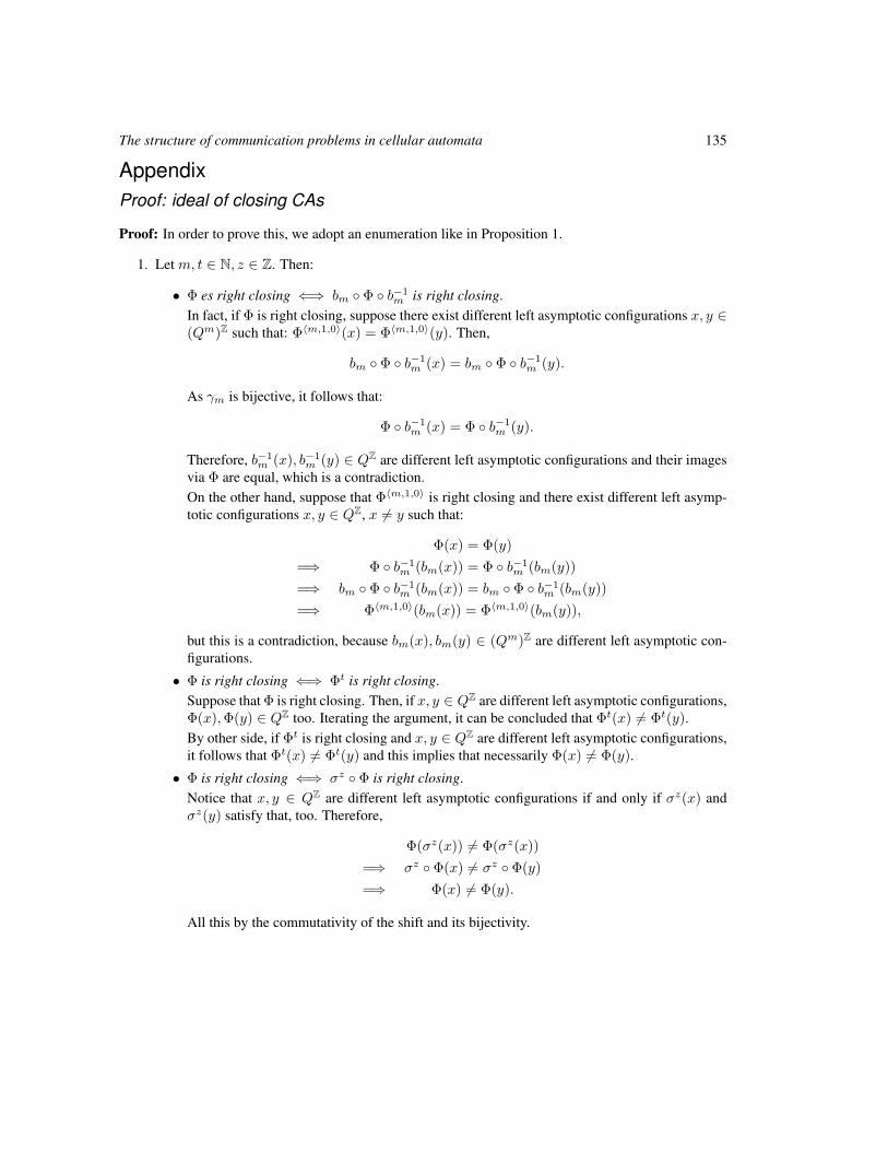
The structure of communication problems in cellular automata 135
AppendixProof: ideal of closing CAs
Proof: In order to prove this, we adopt an enumeration like in Proposition 1.
1. Let m, t ∈ N, z ∈ Z. Then:
• Φ es right closing ⇐⇒ bm Φ b−1m is right closing.
In fact, if Φ is right closing, suppose there exist different left asymptotic configurations x, y ∈(Qm)Z such that: Φ〈m,1,0〉(x) = Φ〈m,1,0〉(y). Then,
bm Φ b−1m (x) = bm Φ b−1
m (y).
As γm is bijective, it follows that:
Φ b−1m (x) = Φ b−1
m (y).
Therefore, b−1m (x), b−1
m (y) ∈ QZ are different left asymptotic configurations and their imagesvia Φ are equal, which is a contradiction.On the other hand, suppose that Φ〈m,1,0〉 is right closing and there exist different left asymp-totic configurations x, y ∈ QZ, x 6= y such that:
Φ(x) = Φ(y)
=⇒ Φ b−1m (bm(x)) = Φ b−1
m (bm(y))
=⇒ bm Φ b−1m (bm(x)) = bm Φ b−1
m (bm(y))
=⇒ Φ〈m,1,0〉(bm(x)) = Φ〈m,1,0〉(bm(y)),
but this is a contradiction, because bm(x), bm(y) ∈ (Qm)Z are different left asymptotic con-figurations.
• Φ is right closing ⇐⇒ Φt is right closing.Suppose that Φ is right closing. Then, if x, y ∈ QZ are different left asymptotic configurations,Φ(x),Φ(y) ∈ QZ too. Iterating the argument, it can be concluded that Φt(x) 6= Φt(y).By other side, if Φt is right closing and x, y ∈ QZ are different left asymptotic configurations,it follows that Φt(x) 6= Φt(y) and this implies that necessarily Φ(x) 6= Φ(y).
• Φ is right closing ⇐⇒ σz Φ is right closing.Notice that x, y ∈ QZ are different left asymptotic configurations if and only if σz(x) andσz(y) satisfy that, too. Therefore,
Φ(σz(x)) 6= Φ(σz(x))
=⇒ σz Φ(x) 6= σz Φ(y)
=⇒ Φ(x) 6= Φ(y).
All this by the commutativity of the shift and its bijectivity.
136 Raimundo Briceno and Pierre-Etienne Meunier
Then, composing all the partial results, we conclude.
2. For the two simulation relations:
• v: let Φ2 ∈ AC be right closing and Φ1 ∈ AC such that Φ1 vι Φ2. Then, if x, y ∈ QZ1 are
distinct left asymptotic configurations, then ι(x), ι(y) ∈ AZ2 satisfy that, too. Therefore,
ι Φ1(x) = Φ2 ι(x) 6= Φ2 ι(y) = ι Φ1(y).
Then, ι Φ1(x) 6= ι Φ1(y), which implies that Φ1(x) 6= Φ1(y).
• : the proof is in Subsection Proof: quotient of closing CAs.
3. Let Φ1,Φ2 ∈ AC be right closing. Then, their cartesian product Φ1 × Φ2 is also right closing. Infact, let (x1, x2), (y1, y2) ∈ QZ
Φ1×Φ2be distinct left asymptotic configurations. Then, so does one
of the pairs x1, y1 or x2, y2. Then, by the closingness of Φ1 o Φ2, respectively, it follows that:
Φ1 × Φ2(x1, x2) = (Φ1(x1),Φ2(x2)) 6= (Φ1(y1),Φ2(y2)) = Φ1 × Φ2(x1, x2).
The proof for the left closing case is analogous. 2
Proof: quotient of closing CAsDefinition 17 (Entropy [LM95]) Let X be a space shiftt. We define the entropy of X as follows:
h(X) = limn→∞
1
nlog |Ln(X)|.
Lemma 3 ([LM95]) Let Φ : X → Y be a sliding block code. Then, Φ is right closing if and only if:
∃N ∈ N : x[−N,0] = y[−N,0] ∧ Φ(x)[−N,N ] = Φ(y)[−N,N ] =⇒ x1 = y1. (1)
The case of a left closing CA is analogous.
Definition 18 A sliding block code Φ : X → Y is a 1-block code if it can be induced by a 1-block mapwith memory m = 0 and anticipation a = 0, namely, it exists φ : A(X)→ A(Y ) such that:
Φ (x)i = φ(xi),
for all i ∈ Z, for all x ∈ X .
Definition 19 A SFT X is said to be M -step if it can be defined by a family of forbidden words F ⊆A(X)M+1.
Definition 20 A sliding block code Φ : X → Y is a conjugacy between X and Y if it is invertible. Twoshift spaces are conjugated if there exists a conjugacy between them.
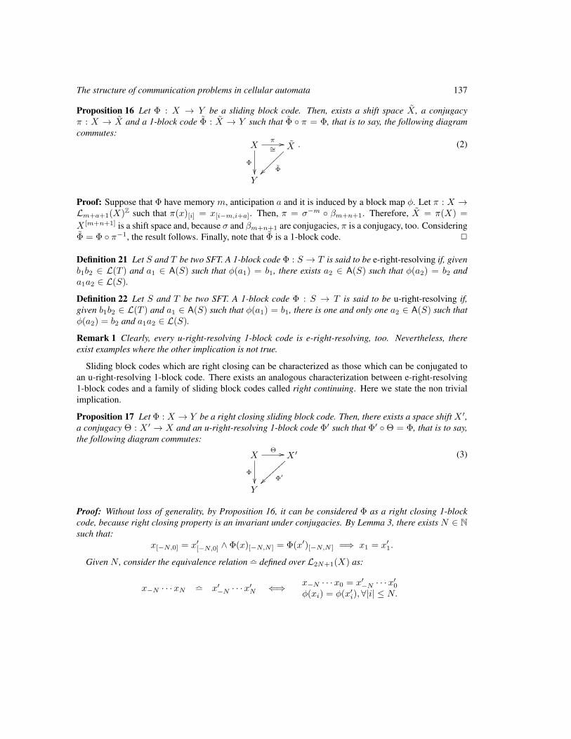
The structure of communication problems in cellular automata 137
Proposition 16 Let Φ : X → Y be a sliding block code. Then, exists a shift space X , a conjugacyπ : X → X and a 1-block code Φ : X → Y such that Φ π = Φ, that is to say, the following diagramcommutes:
Xπ∼=//
Φ
X
Φ~~~~
~~~
Y
. (2)
Proof: Suppose that Φ have memory m, anticipation a and it is induced by a block map φ. Let π : X →Lm+a+1(X)Z such that π(x)[i] = x[i−m,i+a]. Then, π = σ−m βm+n+1. Therefore, X = π(X) =
X [m+n+1] is a shift space and, because σ and βm+n+1 are conjugacies, π is a conjugacy, too. ConsideringΦ = Φ π−1, the result follows. Finally, note that Φ is a 1-block code. 2
Definition 21 Let S and T be two SFT. A 1-block code Φ : S → T is said to be e-right-resolving if, givenb1b2 ∈ L(T ) and a1 ∈ A(S) such that φ(a1) = b1, there exists a2 ∈ A(S) such that φ(a2) = b2 anda1a2 ∈ L(S).
Definition 22 Let S and T be two SFT. A 1-block code Φ : S → T is said to be u-right-resolving if,given b1b2 ∈ L(T ) and a1 ∈ A(S) such that φ(a1) = b1, there is one and only one a2 ∈ A(S) such thatφ(a2) = b2 and a1a2 ∈ L(S).
Remark 1 Clearly, every u-right-resolving 1-block code is e-right-resolving, too. Nevertheless, thereexist examples where the other implication is not true.
Sliding block codes which are right closing can be characterized as those which can be conjugated toan u-right-resolving 1-block code. There exists an analogous characterization between e-right-resolving1-block codes and a family of sliding block codes called right continuing. Here we state the non trivialimplication.
Proposition 17 Let Φ : X → Y be a right closing sliding block code. Then, there exists a space shift X ′,a conjugacy Θ : X ′ → X and an u-right-resolving 1-block code Φ′ such that Φ′ Θ = Φ, that is to say,the following diagram commutes:
XΘ //
Φ
X ′
Φ′~~||||
||||
Y
(3)
Proof: Without loss of generality, by Proposition 16, it can be considered Φ as a right closing 1-blockcode, because right closing property is an invariant under conjugacies. By Lemma 3, there exists N ∈ Nsuch that:
x[−N,0] = x′[−N,0] ∧ Φ(x)[−N,N ] = Φ(x′)[−N,N ] =⇒ x1 = x′1.
Given N , consider the equivalence relation l defined over L2N+1(X) as:
x−N · · ·xN l x′−N · · ·x′N ⇐⇒ x−N · · ·x0 = x′−N · · ·x′0φ(xi) = φ(x′i),∀|i| ≤ N.
138 Raimundo Briceno and Pierre-Etienne Meunier
Later, define A(X ′) as L2N+1(X)/ l, this is to say:
A(X ′) =
W (x−N · · ·x0; y−N · · · yN ) :
x−N · · ·x0 ∈ L(X)y−N · · · yN ∈ L(Y )
,
where:
W (x−N · · ·x0; y−N · · · yN ) =
x′−N · · ·x′N ∈ L2N+1(X) :
x−N · · ·x0 = x′−N · · ·x′0φ(xi) = φ(x′i),∀|i| ≤ N.
.
Then, define X ′ as a 1-step subshift such that:
W (x−N · · ·x0; y−N · · · yN )W (x′−N · · ·x′0; y′−N · · · y′N ) ∈ L2(X ′)
if and only if:x−N+1 · · ·x0 = x′N . . . x
′1, y−N+1 · · · yN = y′−N · · · y′N−1,
being x′0 the state determined by x−N · · ·x0 and y−N · · · yN , because the right closingness of Φ.Considering that, it is defined the 1-block code Θ : X ′ → X by the block map:
θ (W (x−N · · ·x0; y−N · · · yN )) = x0,
with local inverse given by:
θ−1 (x−N , . . . , xN ) = W (x−N · · ·x0;φ(x−N ) · · ·φ(xN )).
Finally, is defined the 1-block code Φ′ : X ′ → Y by the block map:
φ′ (W (x−N · · ·x0, y−N · · · yN )) = yN ,
this is to say, Φ′ = Φ σN Θ. Therefore, Φ′ is u-right-resolving. In fact, suppose there exist yNyN+1 ∈L(Y ) and W ∈ A(X ′) such that φ′(W ) = yN . Then, W should have the following structure:
W = W (x−N · · ·x0; y−N · · · yN ).
By definition of X ′, any W ′ ∈ A(X ′) such that WW ′ ∈ L(X ′) must satisfy that:
W ′ = W (x−N+1 · · ·x0a; y−N+1 · · · yNb),
where a and b must be determined. The value of b is determined by yN+1 and because φ′(W ′) = yN+1.Finally, a is determined (both existence and uniqueness) by the right closingness of Φ. Then, the resultfollows. 2
Lemma 4 ([Jun09]) Let Φ : S → T be an e-right-resolving 1-block code, with S and T two irreducibleSFT such that h(S) = h(T ). Therefore, Φ is u-right-resolving.
Proposition 18 Let Φ : X → X and Ψ : Y → Y be two CAs, such that Ψ is right closing and Φ Ψ.Therefore, Φ is right closing.
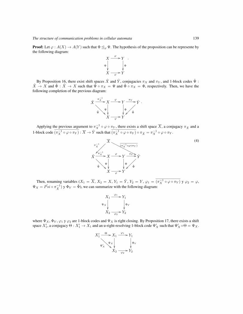
The structure of communication problems in cellular automata 139
Proof: Let ϕ : A(X)→ A(Y ) such that Φϕ Ψ. The hypothesis of the proposition can be represente bythe following diagram:
Xϕ //
Ψ
Y
Φ
X ϕ
// Y
.
By Proposition 16, there exist shift spaces X and Y , conjugacies πX and πY , and 1-block codes Ψ :X → X and Φ : X → X such that Ψ πX = Ψ and Φ πX = Φ, respectively. Then, we have thefollowing completion of the previous diagram:
X
Ψ @@@
@@@@π−1X // X
ϕ //
Ψ
Y
Φ
πY // Y
Φ
X ϕ// Y
.
Applying the previous argument to π−1X ϕ πY , there exists a shift space X , a conjugacy πX and a
1-block code (π−1X ϕ πY ) : X → Y such that (π−1
X ϕ πY ) πX = π−1X ϕ πY .
Xπ−1
X
(π−1
X ϕπY )
''OOOOOOOOOOOOOO
X
Ψ @@@
@@@@π−1X // X
ϕ //
Ψ
Y
Φ
πY // Y
Φ
X ϕ// Y
(4)
Then, renaming variables (X1 = X , X2 = X , Y1 = Y , Y2 = Y , ϕ1 = (π−1X ϕ πY ) y ϕ2 = ϕ,
ΨX = ˜Psi π−1
X) y ΦY = Φ), we can summarize with the following diagram:
X1
ΨX
ϕ1 // Y1
ΦY
X2 ϕ2
// Y2
where ΨX , ΦY , ϕ1 y ϕ2 are 1-block codes and ΨX is right closing. By Proposition 17, there exists a shiftspaceX ′1, a conjugacy Θ : X ′1 → X1 and an u-right-resolving 1-block code Ψ′X such that Ψ′X Θ = ΨX .
X ′1Θ //
Ψ′X BBB
BBBB
BX1
ϕ1 //
ΨX
Y1
ΦY
X2 ϕ2
// Y2
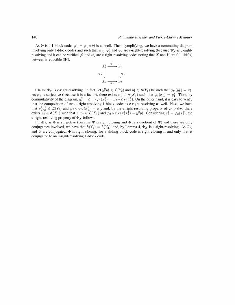
140 Raimundo Briceno and Pierre-Etienne Meunier
As Θ is a 1-block code, ϕ′1 = ϕ1 Θ is as well. Then, symplifying, we have a commuting diagraminvolving only 1-block codes and such that Ψ′X , ϕ′1 and ϕ2 are e-right-resolving (because Ψ′X is u-right-resolving and it can be verified ϕ′1 and ϕ2 are e-right-resolving codes noting that X and Y are full-shifts)between irreducible SFT.
X ′1ϕ′1 //
Ψ′X
Y1
ΦY
X2 ϕ2
// Y2
Claim: ΦY is e-right-resolving. In fact, let y21y
22 ∈ L(Y2) and y2
1 ∈ A(Y1) be such that φY (y11) = y2
1 .As ϕ1 is surjective (because it is a factor), there exists x1
1 ∈ A(X1) such that ϕ1(x11) = y1
1 . Then, bycommutativity of the diagram, y2
1 = φY ϕ1(x11) = ϕ2 ψX(x1
1). On the other hand, it is easy to verifythat the composition of two e-right-resolving 1-block codes is e-right-resolving as well. Next, we havethat y2
1y22 ∈ L(Y2) and ϕ2 ψX(x1
1) = x11, and, by the e-right-resolving property of ϕ2 ψX , there
exists x12 ∈ A(X1) such that x1
1x12 ∈ L(X1) and ϕ2 ψX(x1
1x12) = y2
1y22 . Considering y1
2 = ϕ2(x12), the
e-right-resolving property of ΦX follows.Finally, as Φ is surjective (because Ψ is right closing and Φ is a quotient of Ψ) and there are only
conjugacies involved, we have that h(Y1) = h(Y2), and, by Lemma 4, ΦX is u-right-resolving. As ΦXand Φ are conjugated, Φ is right closing, for a sliding block code is right closing if and only if it isconjugated to an u-right-resolving 1-block code. 2
AUTOMATA 2011, Santiago, Chile local proceedings LP, 2011, 141–160
Selfsimilarity, Simulation and SpacetimeSymmetries
Vincent Nesme1 and Guillaume Theyssier2†
1Freie Universitat Berlin2LAMA (CNRS, Universite de Savoie),Campus Scientifique 73376 Le Bourget-du-Lac Cedex, France
We study intrinsic simulations between cellular automata and introduce a new necessary condition for a CA to simu-late another one. Although expressed for general CA, this condition is targeted towards surjective CA and especiallylinear ones. Following the approach introduced by the first author in an earlier paper, we develop proof techniques totell whether some linear CA can simulate another linear CA. Besides rigorous proofs, the necessary condition for thesimulation to occur can be heuristically checked via simple observations of typical space-time diagrams generatedfrom finite configurations. As an illustration, we give an example of linear reversible CA which cannot simulate theidentity and which is ’time-asymmetric’, i.e. which can neither simulate its own inverse, nor the mirror of its owninverse.
Keywords: cellular automata, simulation, reversibility, time symmetry, space symmetry, linear
1 Introduction and definitionsCellular automata (CA) are well-known for the variety of behaviors they can exhibit. A lot of classifica-tion schemes where proposed in the literature, trying to make this variety of behaviors more intelligible[Wol84, Gil87, Kur97]. Such classifications usually consist in a (finite) list of distinctive properties givingraise to a partition of the class of all CA. Another approach consists in defining a simulation relation be-tween CA, and studying the ordered structure induced by the simulation. We follow this latter approach,and more precisely the simulation relation 4i defined in [DMOT11a, DMOT11b] giving rise to the notionof intrinsic universality [Oll08]. The intuition behind this simulation relation is simple: a CA is simulatedby another if some rescaling of the first is a sub-automaton of a rescaling of the second.
More formally, we restrict ourselves to dimension 1 and the definition is as follows. A CA F is asub-automaton of a CA G, denoted F v G, if there is an injective map ϕ from A to B (state sets of Fand G respectively) such that ϕ F = G ϕ, where ϕ : AZ → BZ denotes the uniform extension of ϕto configurations. We sometimes write F vϕ G to make ϕ explicit. This definition is standard but yieldsa very limited notion of simulation: a given CA can only admit a finite set of (non-isomorphic) CA as
†Research partially supported by project ANR EMC NT09 555297 (French national research agency)
c© 2011 AUTOMATA proceedings, Santiago, Chile, 2011
142 Vincent Nesme and Guillaume Theyssier
sub-automata. Therefore, following works of J. Mazoyer, I. Rapaport and N. Ollinger [MR98, Oll02,DMOT11a, DMOT11b], we will add rescaling operations to the notion of simulation. The ingredientsof rescaling operations are simple: packing cells into blocks, iterating the rule and composing with atranslation (formally, we use shift CA σz , z ∈ Z, whose global rule is given by σz(c)x = cx−z for allx ∈ Z). Given any state set Q and any m ≥ 1, we define the bijective packing map bm : QZ →
(Qm)Z
by:∀z ∈ Z :
(bm(c)
)(z) =
(c(mz), . . . , c(mz +m− 1)
)for all c ∈ QZ. The rescaling F<m,t,z> of F by parameters m (packing), t ≥ 1 (iterating) and z ∈ Z(shifting) is the CA of state set Qm and global rule:
bm σz F t b−1m .
With these definitions, we say that F simulates G, denoted G 4 F , if there are rescaling parameters m1,m2, t1, t2, z1 and z2 such that G<m1,t1,z1> v F<m2,t2,z2>.
Determining whether some given CA simulates another given CA is hard (undecidable in general[DMOT11b, section 4.3]). For instance, looking at typical space time diagrams of two CA gives no clueon whether one simulates another, because the simulation can occur on a set of configurations of measure0. Despite the general undecidability of the simulation relation, one can still hope to better understandits restriction to some specific classes of CA. For instance, the simulation relation is fully understoodon products of shifts [DMOT11b, theorem 3.4] thanks to a ’characteristic sequence’ which is essentiallythe sequence of ratio of translation vectors. Hence, if F = σ0 × σ1 × σ3, one can prove that F cannotsimulate F−1 = σ0 × σ−1 × σ−3 because they do not have the same characteristic sequence.
In this paper, we introduce a general necessary condition for a simulation between two CA to be possi-ble. It focuses on surjective CA, but we will essentially use it on linear reversible CA. This condition isexpressed as a characteristic set χ of points of the real half-plane which is decreasing w.r.t. 4 (Theorem 1below):
F 4 G⇒ χ(G) ⊆ χ(F ).
A striking property of χ is that it can be somewhat visualized on typical space time diagrams of linearCA. Moreover, the set χ is closely related to so-called ’Green functions’ of linear CA for which sys-tematic analysis techniques have been developed in [GNW10]. Hence, formal proofs of impossibility ofsimulation between two linear CA can be derived from heuristic observations of space-time diagrams in aquasi-automatic way.
The set of reversible CA is somewhat structured with respect to 4 since it possesses a maximal element(i.e., a reversible universal CA [DMOT11b, theorem 4.5]) and verifies the following [DMOT11b, theorem4.4]:
F 4 G⇒ F−1 4 G−1
Therefore, a reversible CA is either 4-equivalent to its inverse, or 4-incomparable to it. The most complexreversible CA, reversible universal CA, are all 4-equivalent to their own inverse. Coming back to theexample F above (product of shifts), we have that F and F−1 are 4-incomparable. Following [AN10],let us associate to every reversible CA F its dual F = M F−1M , whereM is the mirror transformationon configurations (M(c)z = c−z). Any product of shifts is self-dual, and generally speaking it seems tobe hard to come up with CA that do not simulate their dual, while non-time-symmetric CA in the sense of[MG10] come in profusion.
Selfsimilarity, Simulation and Spacetime Symmetries 143
An interesting question in this context is how different a reversible CA can be from its dual. As anillustration of the necessary condition for simulation between CA that is given by Theorem 1, we studyin section 3 some reversible linear CA. The first one simulates its inverse, its mirror, its dual, but not theidentity; the second one simulates neither the identity nor its inverse or its mirror image or its dual.
2 Simulation and geometryThe basic ingredient in this section is the collection of functions telling how a change of value of thecenter cell in the initial configuration will affect some other cell’s value at some step in the future. Suchfunctions are often studied for linear cellular automata (see section 3) and are sometimes called ’Greenfunctions’ in this context [Moo98].
Let F be any CA and fix some x ∈ Z and some y ∈ N. For any configuration c ∈ QZ and any q ∈ Q,we denote by φc(q) the following configuration:
φc(q)z =
q if z = 0,
c(z) else.
We then denote by F yx,c : Q → Q the map q 7→ (F y(φc(q)))x.For instance, if F is simply the identity, F yx,c is the identity when x = 0, otherwise it is the constant
function q 7→ c(x). For a less trivial example, consider the cas where F =⊕
is the sum with neigh-borhood 0,−1 over Q = Z/2Z, i.e.
⊕(c)x = c(x) + c(x − 1). Starting from a single nonzero cell,
iterations of this automaton generate Pascal’s triangle modulo 2. For x ∈ N, let x =∑n∈N bx(n)2n, with
bx(n) ∈ 0, 1, be its binary representation, and Bx = n ∈ N|bx(n) = 1. Then⊕y
x,c(q) =
⊕y(c)x + q if x ≥ 0 and Bx ⊆ By⊕y(c)x else .
We are interested in positions in space-time where the influence of the center cell is concentrated,whatever the initial configuration (see figure 1).
Definition 1 F has the property Spot[x, y, l, r] for x ∈ Z and y, l, r ∈ N if
• F yx,c is a bijection for all configurations c; and
• F yz,c is a constant function for all c and all z ∈ [x− l;x+ r] \ x.⊕thus fulfills Spot[x, y, l, r] if and only if, for any z ∈ [x− l;x+ r], Bz ⊆ By is equivalent to x = z
(considering that “Bz ⊆ By” is a false statement when Bz is undefined).
Lemma 1 If F has the property Spot[x, y, l, r], then F y(QZ) contains all the words of size max(l, r)+1.
Proof: Let us suppose, without loss of generality, that l is no larger than r. Let q = (q0, . . . , qr) ∈ Qr+1.We are going to construct c ∈ QZ such that F y(c)0,...,r = q. Start with an arbitrary c ∈ QZ. We canfirst modify cr−x in such way that F y(c)r = qr; then we can change cr−x−1, on which F y(c)r does notdepend, so that F y(c)r−1 = qr−1; and so on, until we choose c−x, on which F (c)1,...,r does not depend,so that F (c)0 = q0. 2
For instance,⊕
fulfills Spot[0, 1,+∞, 0], which implies that it must be surjective.
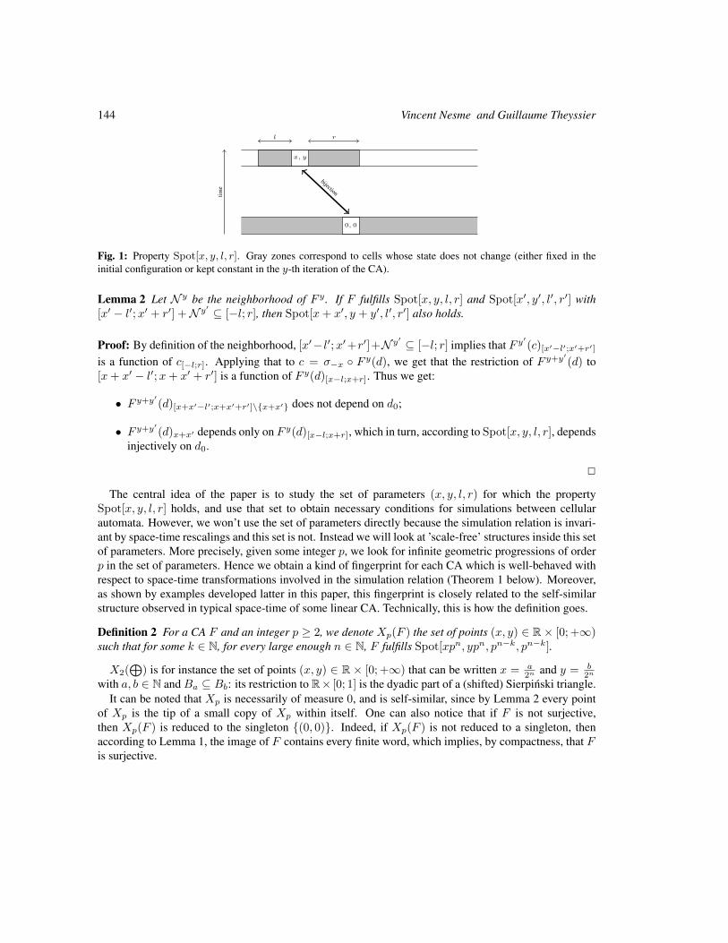
144 Vincent Nesme and Guillaume Theyssier
0, 0
l r
x, y
bijectiontime
Fig. 1: Property Spot[x, y, l, r]. Gray zones correspond to cells whose state does not change (either fixed in theinitial configuration or kept constant in the y-th iteration of the CA).
Lemma 2 Let N y be the neighborhood of F y . If F fulfills Spot[x, y, l, r] and Spot[x′, y′, l′, r′] with[x′ − l′;x′ + r′] +N y′ ⊆ [−l; r], then Spot[x+ x′, y + y′, l′, r′] also holds.
Proof: By definition of the neighborhood, [x′− l′;x′+r′]+N y′ ⊆ [−l; r] implies that F y′(c)[x′−l′;x′+r′]
is a function of c[−l;r]. Applying that to c = σ−x F y(d), we get that the restriction of F y+y′(d) to
[x+ x′ − l′;x+ x′ + r′] is a function of F y(d)[x−l;x+r]. Thus we get:
• F y+y′(d)[x+x′−l′;x+x′+r′]\x+x′ does not depend on d0;
• F y+y′(d)x+x′ depends only on F y(d)[x−l;x+r], which in turn, according to Spot[x, y, l, r], dependsinjectively on d0.
2
The central idea of the paper is to study the set of parameters (x, y, l, r) for which the propertySpot[x, y, l, r] holds, and use that set to obtain necessary conditions for simulations between cellularautomata. However, we won’t use the set of parameters directly because the simulation relation is invari-ant by space-time rescalings and this set is not. Instead we will look at ’scale-free’ structures inside this setof parameters. More precisely, given some integer p, we look for infinite geometric progressions of orderp in the set of parameters. Hence we obtain a kind of fingerprint for each CA which is well-behaved withrespect to space-time transformations involved in the simulation relation (Theorem 1 below). Moreover,as shown by examples developed latter in this paper, this fingerprint is closely related to the self-similarstructure observed in typical space-time of some linear CA. Technically, this is how the definition goes.
Definition 2 For a CA F and an integer p ≥ 2, we denote Xp(F ) the set of points (x, y) ∈ R× [0; +∞)such that for some k ∈ N, for every large enough n ∈ N, F fulfills Spot[xpn, ypn, pn−k, pn−k].
X2(⊕
) is for instance the set of points (x, y) ∈ R× [0; +∞) that can be written x = a2n and y = b
2n
with a, b ∈ N and Ba ⊆ Bb: its restriction to R× [0; 1] is the dyadic part of a (shifted) Sierpinski triangle.It can be noted that Xp is necessarily of measure 0, and is self-similar, since by Lemma 2 every point
of Xp is the tip of a small copy of Xp within itself. One can also notice that if F is not surjective,then Xp(F ) is reduced to the singleton (0, 0). Indeed, if Xp(F ) is not reduced to a singleton, thenaccording to Lemma 1, the image of F contains every finite word, which implies, by compactness, that Fis surjective.
Selfsimilarity, Simulation and Spacetime Symmetries 145
We now detail, in a series of properties, how Xp is modified under the action of the transformationsinvolved in the simulation of a CA by another. First, the shift. Let sz be the transformation of the planedefined by sz(x, y) = (x+ zy, y). The following property is obvious, by definition of Xp.
Property 1 Xp(σz F ) = sz (Xp(F )).
Let us now consider iteration and grouping. Let gt be the transformation of the plane defined bygt(x, y) =
(x, yt
): notice that gp (Xp(F )) = Xp(F ). Let fm be the transformation of the plane defined
by fm(x, y) =(xm , y
).
Property 2 Xp(Ft) is a dense subset of gt (Xp(F )).
Proof: The inclusion is immediate from the definition. What might be slightly less immediate is whythese sets are not obviously equal. Given the definition, Xp(F ) must be included in R2
p, where Rp is theset of real numbers having finite p-adic expansion. Actually, we do have gt (Xp(F )) ∩ R2
p = Xp(Ft), so
the equality without the intersection is certainly true if t ∈ Rp, not quite so in general. Let us now provethe density.
Let (x, y) ∈ Xp(F ). We want to find a sequence (xn, yn) of points ofXp(F ) converging to (x, y) suchthat for all n, yn ∈ tRp. For a finite sequence of integers 0 = in,0 < in,1 < . . . < in,l (l is a constant
independent of n to be fixed later), we define ηn =l∑
j=0
p−in,j and (xn, yn) = ηn(x, y). We have three
requirements:
• (xn, yn) must converge to (x, y): it is sufficient to have limn→+∞
in,1 = +∞
• (xn, yn) must be an element of Xp(F ). This is guaranteed as long as in,j+1 − in,j is alwayslarge enough. More precisely, by definition of Xp there exists some k such that for every largeenough integer n, F fulfills Spot[xpn, ypn, pn−k, pn−k]. Therefore, if in,l− in,l−1 is large enough(depending on k and the neighborhood of F ), we get from Lemma 2 that (1 + p−in,l+in,l−1)(x, y)is in Xp(F ). By recursion on l, we get ultimately (xn, yn) ∈ Xp(F ).
• yn must be in tRp, which means the integer pin,l
l∑j=0
p−in,j must be a multiple of t.
So, it all boils down to finding increasing integer sequences 0 = i0 < i1 < · · · < il where ij+1 − ij is
arbitrary large, and such that t divides pill∑
j=0
p−ij . That is clearly possible: the sequence of powers of p
is ultimately periodic modulo t, so if we choose the ij-s spaced by multiples of this period and l = t, wecan easily meet the conditions. 2
Property 3 Xp(bm F b−1m ) is a dense subset of fm (Xp(F )).
Proof: Let G = bm F b−1m . Let x ∈ Z and y, l, r ∈ N with l ≥ 1 and r ≥ 1. First, it fol-lows from definitions that, for any configuration c of F , Gyx,bm(c) is constant if and only if, for allz ∈ mx−m+ 1, · · · ,mx+m− 1, F yz,c is constant. Moreover Gyx,bm(c) bijective implies F ymx,c bi-jective. This shows that if G has property Spot[x, y, l, r] then F has property Spot[mx, y,ml,mr].
146 Vincent Nesme and Guillaume Theyssier
Now suppose that F has property Spot[mx, y,ml,mr] and fix some configuration c of F . Then it isstraightforward to check that Gyx,bm(c) is bijective (because it sends each component ofQm on itself) andGyz,bm(c) is constant for any z ∈ [x− l;x+ r] \ x.
We have shown that F has property Spot[mx, y,ml,mr] if and only if G has property Spot[x, y, l, r].Thus we have
(x, y) ∈ Xp(G) ⇐⇒ (mx, y) ∈ Xp(F ).
This implies Xp(G) ⊆ fm (Xp(F )). To prove the density, it is sufficient to prove that Xp(F ) ∩mRp isdense in Xp(F ) which can be done using the same argument as in the proof of property 2. 2
It only remains to consider the case of the sub-automaton.
Property 4 If G v F then Xp(F ) ⊆ Xp(G).
Proof: It is straightforward to check that if F has property Spot[x, y, l, r] then so does G. The propertyfollows. 2
Properties 1, 2, 3 and 4 prove the following theorem.
Theorem 1 If F simulatesG, then there exist rational numbers β and α, γ > 0 such that for every integerp ≥ 2, πα,β,γ(Xp(F )) ⊆ Xp(G), where πα,β,γ(x, y) = (αx+ βy, γy).
The determination ofXp is not easy in general, but the following basic facts can be established straight-forwardly from the definitions:
• if F is a shift, then Xp(F ) is a line passing through the origin;
• if F is nilpotent (i.e. ∃t s.t. F t is a constant function), then Xp(F ) = (0, 0);
• Xp(F ×G) = Xp(F ) ∩Xp(G).
Theorem 1 above shows that Xp(F ) represent obstructions for F to simulate other CA: the biggerXp(F ) is, the smaller the family of CA F can simulate. Using the basic facts above, we can give someconcrete formulations of this intuition.
Corollary 1 Let p ≥ 2 be an integer and F a CA. Then we have:
• If F simulates the identity, then Xp(F ) must be included in a line passing through the origin;
• If F is intrinsically universal, then Xp(F ) = (0, 0);
• If F is reversible universal (i.e. it can simulate any reversible CA), then Xp(F ) = (0, 0);
Proof: All items use Theorem 1. Item 1 and 2 are direct consequences of the computation of Xp for theidentity and nilpotent CA (an intrinsically universal CA must simulate any nilpotent CA). Item 3 uses thefact that a reversible universal CA must simulate σ × σ−1 whose Xp is a singleton. 2
The purpose of the next section is to focus on a class of CA that generally have more interesting Xp:linear cellular automata.
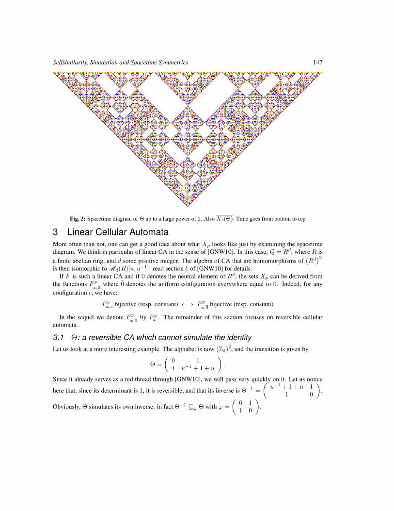
Selfsimilarity, Simulation and Spacetime Symmetries 147
Fig. 2: Spacetime diagram of Θ up to a large power of 2. Also X2(Θ). Time goes from bottom to top
3 Linear Cellular AutomataMore often than not, one can get a good idea about what Xp looks like just by examining the spacetimediagram. We think in particular of linear CA in the sense of [GNW10]. In this case, Q = Rd, where R isa finite abelian ring, and d some positive integer. The algebra of CA that are homomorphisms of
(Rd)Z
is then isomorphic to Md(R)[u, u−1]: read section 1 of [GNW10] for details.If F is such a linear CA and if 0 denotes the neutral element of Rd, the sets Xp can be derived from
the functions F yx,0
where 0 denotes the uniform configuration everywhere equal to 0. Indeed, for anyconfiguration c, we have:
F yx,c bijective (resp. constant) ⇐⇒ F yx,0
bijective (resp. constant)
In the sequel we denote F yx,0
by F yx . The remainder of this section focuses on reversible cellularautomata.
3.1 Θ: a reversible CA which cannot simulate the identityLet us look at a more interesting example. The alphabet is now (Z2)
2, and the transition is given by
Θ =
(0 11 u−1 + 1 + u
).
Since it already serves as a red thread through [GNW10], we will pass very quickly on it. Let us notice
here that, since its determinant is 1, it is reversible, and that its inverse is Θ−1 =
(u−1 + 1 + u 1
1 0
).
Obviously, Θ simulates its own inverse: in fact Θ−1 vϕ Θ with ϕ =
(0 11 0
).
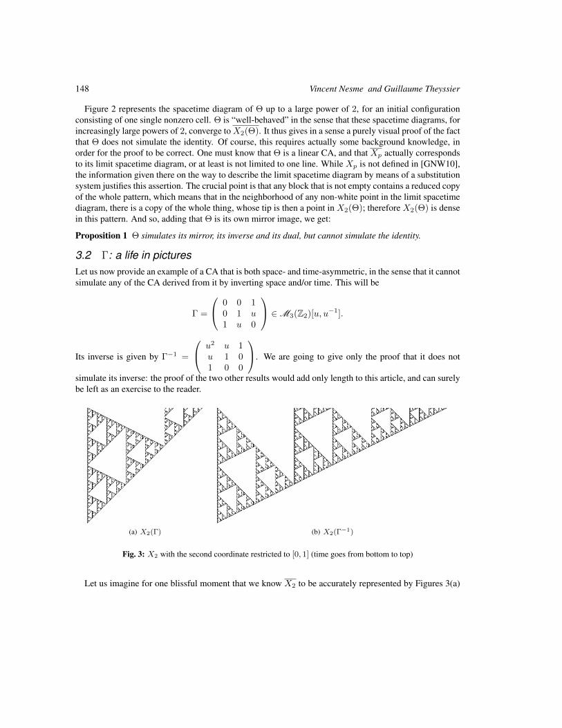
148 Vincent Nesme and Guillaume Theyssier
Figure 2 represents the spacetime diagram of Θ up to a large power of 2, for an initial configurationconsisting of one single nonzero cell. Θ is “well-behaved” in the sense that these spacetime diagrams, forincreasingly large powers of 2, converge toX2(Θ). It thus gives in a sense a purely visual proof of the factthat Θ does not simulate the identity. Of course, this requires actually some background knowledge, inorder for the proof to be correct. One must know that Θ is a linear CA, and that Xp actually correspondsto its limit spacetime diagram, or at least is not limited to one line. While Xp is not defined in [GNW10],the information given there on the way to describe the limit spacetime diagram by means of a substitutionsystem justifies this assertion. The crucial point is that any block that is not empty contains a reduced copyof the whole pattern, which means that in the neighborhood of any non-white point in the limit spacetimediagram, there is a copy of the whole thing, whose tip is then a point in X2(Θ); therefore X2(Θ) is densein this pattern. And so, adding that Θ is its own mirror image, we get:
Proposition 1 Θ simulates its mirror, its inverse and its dual, but cannot simulate the identity.
3.2 Γ: a life in picturesLet us now provide an example of a CA that is both space- and time-asymmetric, in the sense that it cannotsimulate any of the CA derived from it by inverting space and/or time. This will be
Γ =
0 0 10 1 u1 u 0
∈M3(Z2)[u, u−1].
Its inverse is given by Γ−1 =
u2 u 1u 1 01 0 0
. We are going to give only the proof that it does not
simulate its inverse: the proof of the two other results would add only length to this article, and can surelybe left as an exercise to the reader.
(a) X2(Γ) (b) X2(Γ−1)
Fig. 3: X2 with the second coordinate restricted to [0, 1] (time goes from bottom to top)
Let us imagine for one blissful moment that we know X2 to be accurately represented by Figures 3(a)
Selfsimilarity, Simulation and Spacetime Symmetries 149
and 3(b) (actually these figures are mirror images of spacetime diagrams up to a large power of 2). Howdo we conclude then?
Supposing that Γ simulates Γ−1, we know from theorem 1 that for some α, β, γ, πα,β,γ(X2(Γ)) shouldbe included in X2(Γ−1). Since there are only two lines passing through the origin in X2(Γ−1), πα,β,γmust send respectively R(0, 1) and R(−1, 1) on R(0, 1) and R(−2, 1), which implies β = 0. Now if weconsider the lines joining these two axes, they have slope 1
2 for Γ, 1 in Γ−1, which means α = 2γ. So,if Γ simulates its inverse, X2(Γ) should be, modulo a change of scale, included into X2(Γ−1), which isclearly not the case.
To make this proof rigorous, we need a tool to prove properties of X2 for Γ and Γ−1. We are going tofollow section 3 of [GNW10], which gives a procedure to derive, from the transition matrix of the CA, asubstitution system generating the Green functions (see Proposition 4 of [GNW10]). More precisely, wewill associate to each CA F a 2×2 substitution system, that is a finite setE and a function e : Z× N→ Esuch that:
• F yx is a function of e(x, y);
• for i, j ∈ 0, 1, e(2x+ i, 2y + j) is a function of e(x, y) and i and j.
The next two subsections give the substitution systems for Γ and Γ−1, and subsection 3.2.3 uses themto formally prove negative result concerning simulation.
3.2.1 A substitution system for ΓThe minimal polynomial of Γ is X3 +X2 + (1 +u2)X+ 1, so we have the following recurrence relation.
∀x ∈ Z∀n, y ∈ N y < 3 · 2n =⇒ Γ3·2n+yx = Γ2n+1+y
x + Γ2n+yx + Γ2n+y
x−2n+1 + Γyx (1)
Now we define αj(x, y) in the following way: these are the coefficients in Z/2Z such that for everyfunction (x, y) 7→ Ξyx fulfilling equation (1) in lieu of Γ,
Ξyx =
2∑j=0
∑i∈Z
αj(x− i, y)Ξji . (2)
For every x ∈ Z, y ∈ N and s, t ∈ 0, 1, we have
Ξ2y+t2x+s =
∑i∈Z
α0(x− i, y)Ξt2i+s + α1(x− i, y)Ξ2+t2i+s + α2(x− i, y)Ξ4+t
2i+s. (3)
In the case s = t = 0, we have the following derivation:
Ξ2y2x =
∑i
α0(x− i, y)Ξ02i + α1(x− i, y)Ξ2
2i + α2(x− i, y)Ξ42i
=∑i
α0(x− i, y)Ξ02i + α1(x− i, y)Ξ2
2i + α2(x− i, y)(Ξ22i−2 + Ξ1
2i−2 + Ξ02i
)=
∑i
(α0(x− i, y) + α2(x− i, y)) Ξ02i + α2(x− 1− i, y)Ξ1
2i
+ (α1(x− i, y) + α2(x− 1− i, y)) Ξ22i
(4)
150 Vincent Nesme and Guillaume Theyssier
which is to be compared with the definition of αj :
Ξ2y2x =
∑i
2∑j=0
αj(2x− i, 2y)Ξji . (5)
The comparison shows that αj(2x, 2y) is a function of αj(x− i, y) for some values of i. Γ is peculiarin that αj(2x+ 1, 2y) = 0, which simplifies our work. The same operation now has to be performed forαj(2x, 2y + 1).
Ξ2y+12x =
∑i
α0(x− i, y)Ξ12i + α1Ξ3
2i + α2(x− i, y)Ξ52i
=∑i
α0(x− i, y)Ξ12i + α1(x− i, y)
(Ξ22i + Ξ1
2i + Ξ12i−2 + Ξ0
2i
)+α2(x− i, y)
(Ξ12i + Ξ1
2i−2 + Ξ12i−4 + Ξ0
2i−2)
=∑i
(α1(x− i, y) + α2(x− 1− i, y)) Ξ02i
+(α0(x− i, y) + α1(x− 1− i, y) + α1(x− i, y) + α2(x− 2− i, y)+α2(x− 1− i, y) + α2(x− i, y))Ξ1
2i + α1(x− i, y)Ξ22i
(6)
Using the representationα2
α1
α0
, we get the following substitution.
α·(x, y)↓
α·(2x, 2y + 1) α·(2x+ 1, 2y + 1)α·(2x, 2y) α·(2x+ 1, 2y)
=
α1(x, y)α0 (x, y) + α1 (x− 1, y) + α1 (x, y) + α2 (x− 2, y) + α2 (x− 1, y) + α2 (x, y)
α1(x, y) + α2(x− 1, y)
000
α1(x, y) + α2(x− 1, y)α2(x− 1, y)
α0 (x, y) + α2 (x, y)
000
This needs some grouping; for instance, in the present situation, the substitution scheme uses α1(x −1, y), which is not an information contained in the initial cell. For instance, if we want to determineα0(2x, 2y + t) for t ∈ 0, 1, we need to know α0(x, y), α1(x, y), α2(x, y) and α2(x − 1, y). Thesmallest grouping that will allow us to carry all that information is
α2(x− 3, y) α2(x− 2, y) α2(x− 1, y) α2(x, y)α1(x− 2, y) α1(x− 1, y) α1(x, y)
α0(x− 1, y) α0(x, y).
This gives us an alphabet of size 29 = 512, and the substitution scheme is
Selfsimilarity, Simulation and Spacetime Symmetries 151
a b c de f g
h i↓
0 f 0 g f 0 g 0a+ b+ c+ e+ f + h 0 b+ c+ d+ f + g + i 0 b+ c+ d+ f + g + i 0
0 c+ g c+ g 00 b+ f 0 c+ g b+ f 0 c+ g 0
b 0 c 0 c 00 d+ i d+ i 0
The initial state for this substitution system is · · · 0 D 0 · · · , and to a cella b c d
e f gh i
in position (x, y) corresponds the Green function Γyx =
d+ i c gc b+ d+ i+ g c+ fg c+ f b+ d+ i
.
For a letter x in a, b, . . . , i, let X denote the cell where x has the value 1 whereas all other letters
are set to 0. We can notice that A, E and H are completely equivalent: they all substitute toE 00 0
,
and project onto 0 in the computation of Γyx. We can therefore simplify this system a bit by puttingA = E = H = 0:
Whereas we have a theoretical number of 25 = 32 different states in the substitution scheme, only 11of them are accessible from the initial state, namely 0 plus the ones represented in Figure 5. This graphhas two strongly connected components, one composed of BD alone, the other of the remaining vertices.In particular, from any state of the substitution system that has been accessed from the initial state andthat is neither 0 nor BD, there is a path to D; therefore there must be a point of X2 in the correspondingsquare.
3.2.2 A substitution system for Γ−1
We now have to perform the equivalent analysis for Γ−1, which we will name Ω, in order to avoid possibleconfusions with negative exponents. The minimal polynomial of Ω is X3 + (1 +u2)X2 +X + 1, so nowthe recurrence relation is
∀x ∈ Z∀n, y ∈ N y < 3 · 2n =⇒ Ω3·2n+yx = Ω2n+1+y
x + Ω2n+1+yx−2n+1 + Ω2n+y
x + Ωyx. (7)
We introduce β, which is to Ω what α was to Γ in Section 3.2.1.
Ξ2y+t2x+s =
∑i
β0(x− i, y)Ξt2i+s + β1(x− i, y)Ξ2+t2i+s + β2(x− i, y)Ξ4+t
2i+s (8)
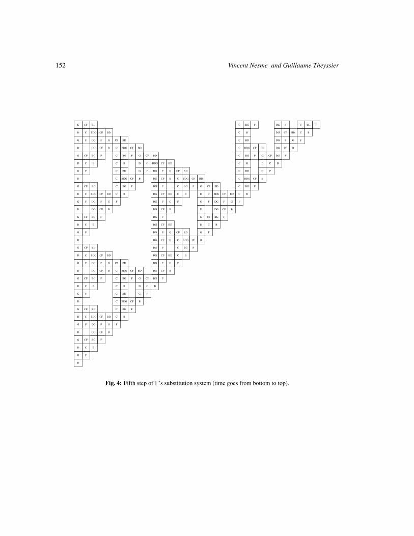
152 Vincent Nesme and Guillaume Theyssier
FBGCFDGFBGCBDCFG
BCBDCFDGBCBDCFBDGCD
FGFDGBDCBDCFGFDGFG
BCFDGBDCFBDGCBDCFBDGCBCFDGD
FBGCFGFBGCBDCFGFBGCFBGCFG
BCDBCBDCFBDGCDBCBCD
FGBDCBDCFGFDGFGBDCFG
BCFBDGCBDCFBDGCBCFDGBCFBDGCD
FBGCBDCFGFBGCFDGFBGCBDCFG
BCBDCFBDGCDBCBDCFDGBCBDCFBDGCD
FGFDGFGFGFDGFGFDGFG
BCFDGDBCFDGBCFDGD
FBGCFGFDGFBGCFG
BCDBDCFDGBCD
FGBDCFGFDGFG
BCFBDGCBCFDGD
FBGCFDGBDCFG
BCBDCFDGBDCFBDGCD
FGFDGBDCFGFDGFG
BCFDGBDCFBDGCBCFDGD
FBGCFGFBGCFBGCFG
BCDBCBCD
FGBDCFG
BCFBDGCD
FBGCBDCFG
BCBDCFBDGCD
FGFDGFG
BCFDGD
FBGCFG
BCD
FG
D
Fig. 4: Fifth step of Γ’s substitution system (time goes from bottom to top).
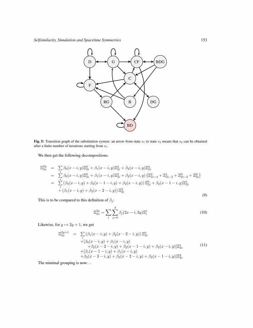
Selfsimilarity, Simulation and Spacetime Symmetries 153
D G CF BDG
F
C
B DGBG
BD
Fig. 5: Transition graph of the substitution system: an arrow from state s1 to state s2 means that s2 can be obtainedafter a finite number of iterations starting from s1.
We then get the following decompositions.
Ξ2y2x =
∑i
β0(x− i, y)Ξ02i + β1(x− i, y)Ξ2
2i + β2(x− i, y)Ξ42i
=∑i
β0(x− i, y)Ξ02i + β1(x− i, y)Ξ2
2i + β2(x− i, y)(Ξ22i−4 + Ξ1
2i−2 + Ξ02i−2 + Ξ0
2i
)=
∑i
(β0(x− i, y) + β2(x− 1− i, y) + β2(x− i, y)) Ξ02i + β2(x− 1− i, y)Ξ1
2i
+ (β1(x− i, y) + β2(x− 2− i, y)) Ξ22i
(9)This is to be compared to this definition of βj :
Ξ2y2x =
∑i
2∑j=0
βj(2x− i, 2y)Ξji (10)
Likewise, for y 7→ 2y + 1, we get
Ξ2y+12x =
∑i
(β1(x− i, y) + β2(x− 2− i, y)) Ξ02i
+[β0(x− i, y) + β1(x− i, y)+β2(x− 2− i, y) + β2(x− 1− i, y) + β2(x− i, y)]Ξ1
2i
+[β1(x− 1− i, y) + β1(x− i, y)+β2(x− 3− i, y) + β2(x− 2− i, y) + β2(x− 1− i, y)]Ξ2
2i
(11)
The minimal grouping is now. . .
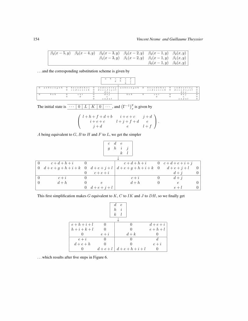
154 Vincent Nesme and Guillaume Theyssier
β2(x− 5, y) β2(x− 4, y) β2(x− 3, y) β2(x− 2, y) β2(x− 1, y) β2(x, y)β1(x− 3, y) β1(x− 2, y) β1(x− 1, y) β1(x, y)
β0(x− 1, y) β0(x, y)
. . . and the corresponding substitution scheme is given by
a b c d e fg h i j
k l
↓0 a + b + c + g + h 0 b + c + d + h + i 0 c + d + e + i + j a + b + c + g + h 0 b + c + d + h + i 0 c + d + e + i + j 0
0 c + d + e + i + k 0 d + e + f + j + l c + d + e + i + k 0 d + e + f + j + l 00 d + j d + j 0
0 b + h 0 c + i 0 d + j b + h 0 c + i 0 d + j 00 d 0 e d 0 e 0
0 e + f + l e + f + l 0
The initial state is · · · 0 L K 0 · · · , and(Γ−1
)yx
is given by l + h+ f + d+ b i+ e+ c j + di+ e+ c l + j + f + d ej + d e l + f
.
A being equivalent to G, B to H and F to L, we get the simpler
c d eg h i j
k l↓
0 c+ d+ h+ i 0 c+ d+ h+ i 0 c+ d+ e+ i+ j0 d+ e+ g + h+ i+ k 0 d+ e+ j + l d+ e+ g + h+ i+ k 0 d+ e+ j + l 0
0 c+ e+ i d+ j 00 c+ i 0 c+ i 0 d+ j0 d+ h 0 e d+ h 0 e 0
0 d+ e+ j + l e+ l 0
This first simplification makes G equivalent to K, C to IK and J to DH , so we finally get
d eh ik l↓
e+ h+ i+ l 0 0 d+ e+ ih+ i+ k + l 0 0 e+ h+ l
0 e+ i d+ k 0e+ i 0 0 d
d+ e+ h 0 0 e+ i0 d+ e+ l d+ e+ h+ i+ l 0
. . . which results after five steps in Figure 6.
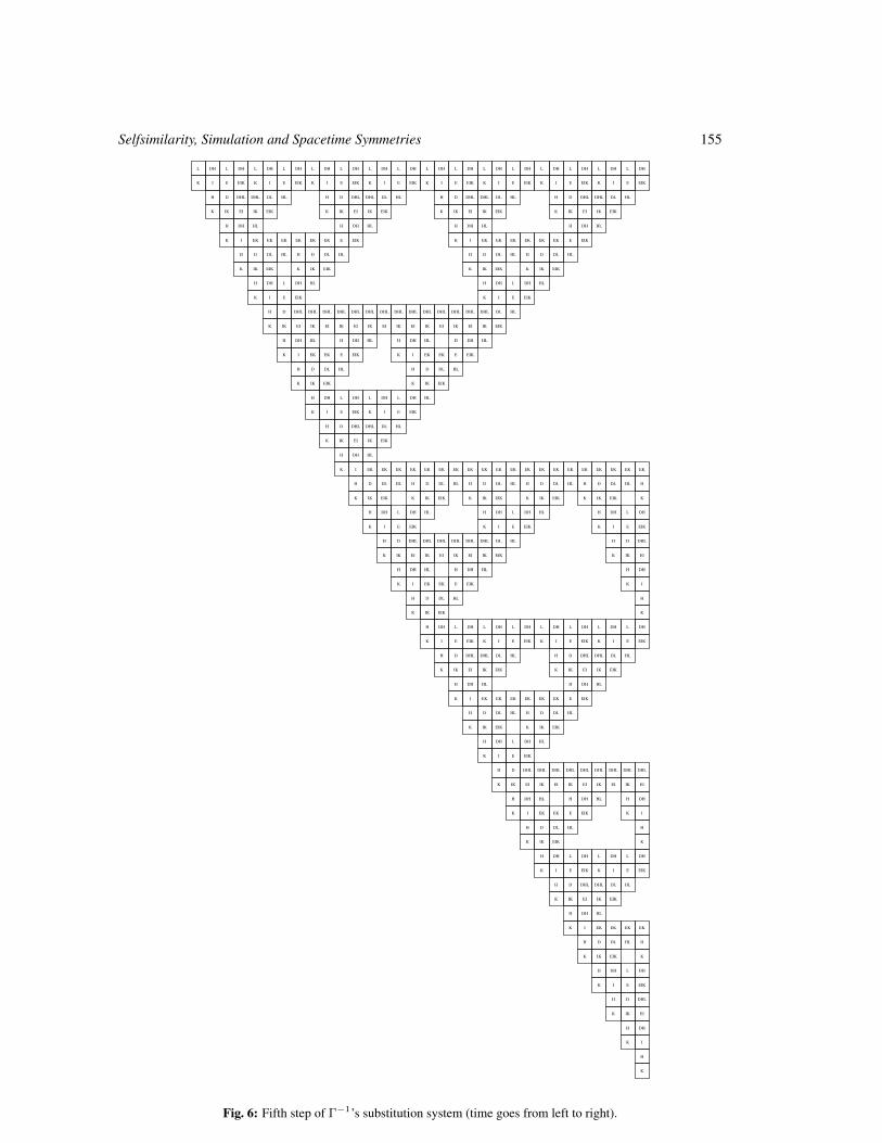
Selfsimilarity, Simulation and Spacetime Symmetries 155
K
H
I
DH
EI
DHL
EIK
DH
K
H
EK
EIK
DH
K
H
I
DH
EI
DHL
EIK
DH
K
H
I
DH
EI
DHL
EIK
DH
K
H
EK
EIK
DH
K
H
IK
D
E
L
HL
EK
HL
E
L
K
H
IK
DHL
HL
E
L
K
H
IK
D
E
L
HL
EK
HL
E
L
K
H
I
DH
EIK
DL
EK
EIK
DL
I
DH
EI
DHL
EIK
DL
I
DH
K
H
I
DH
EIK
DL
EK
EIK
DL
I
DH
K
H
IK
D
EK
HL
IK
DHL
K
L
HL
IK
DHL
HL
IK
DHL
K
L
K
H
IK
D
EK
HL
IK
DHL
K
L
K
H
I
DH
EI
DHL
EIK
DH
EIK
DH
EI
DHL
EIK
DH
EI
DHL
EIK
DH
K
H
EK
EIK
DH
EI
DHL
EIK
DH
K
H
IK
D
E
L
HL
E
H
IK
DHL
HL
E
H
IK
D
E
L
HL
EK
HL
E
H
IK
D
E
L
K
H
I
DH
EIK
DL
EK
EI
DHL
EIK
DL
EK
K
H
I
DH
EIK
DL
EK
EIK
DL
EK
K
H
I
DH
K
H
IK
D
EK
HL
IK
DHL
HL
IK
D
EK
K
L
HL
IK
D
EK
HL
IK
D
EK
K
L
K
H
I
DH
EI
DHL
EIK
DH
K
H
EK
EIK
DH
EIK
DH
K
H
EK
EIK
DH
K
H
EK
EIK
DH
K
H
IK
D
E
L
HL
EK
HL
E
L
HL
E
L
HL
EK
HL
E
L
HL
EK
HL
E
L
K
H
I
DH
EIK
DL
EK
EIK
DL
I
DH
EIK
DL
I
DH
EIK
DL
EK
EIK
DL
I
DH
EIK
DL
EK
EIK
DL
I
DH
K
H
IK
D
EK
HL
IK
DHL
K
L
HL
IK
DHL
K
H
IK
D
EK
HL
IK
DHL
K
H
IK
D
EK
HL
IK
DHL
K
L
K
H
I
DH
EI
DHL
EIK
DH
EIK
DH
EI
DHL
K
H
EK
EIK
DH
EI
DHL
K
H
I
DH
EI
DHL
EIK
DH
K
H
IK
D
E
L
HL
E
H
IK
DHL
HL
EK
HL
E
H
IK
DHL
K
H
IK
D
E
L
K
H
I
DH
EIK
DL
EK
EI
DHL
EIK
DL
EK
EIK
DL
EK
EI
DHL
K
H
I
DH
K
H
IK
D
EK
HL
IK
DHL
HL
IK
D
EK
HL
IK
D
EK
HL
IK
DHL
K
L
K
H
I
DH
EI
DHL
EIK
DH
K
H
EK
EIK
DH
K
H
I
DH
EI
DHL
EIK
DH
K
H
IK
D
E
L
HL
EK
HL
E
L
K
H
IK
DHL
HL
E
L
K
H
I
DH
EIK
DL
EK
EIK
DL
I
DH
EI
DHL
EIK
DL
I
DH
K
H
IK
D
EK
HL
IK
DHL
K
L
HL
IK
DHL
HL
IK
DHL
K
L
K
H
I
DH
EI
DHL
EIK
DH
EIK
DH
EI
DHL
EIK
DH
EI
DHL
EIK
DH
K
H
IK
D
E
L
HL
E
H
IK
DHL
HL
E
H
IK
D
E
L
K
H
I
DH
EIK
DL
EK
EI
DHL
EIK
DL
EK
K
H
I
DH
K
H
IK
D
EK
HL
IK
DHL
HL
IK
D
EK
K
L
K
H
I
DH
EI
DHL
EIK
DH
K
H
EK
EIK
DH
K
H
IK
D
E
L
HL
EK
HL
E
L
K
H
I
DH
EIK
DL
EK
EIK
DL
I
DH
K
H
IK
D
EK
HL
IK
DHL
K
L
K
H
I
DH
EI
DHL
EIK
DH
K
H
IK
D
E
L
K
H
I
DH
K
L
Fig. 6: Fifth step of Γ−1’s substitution system (time goes from left to right).
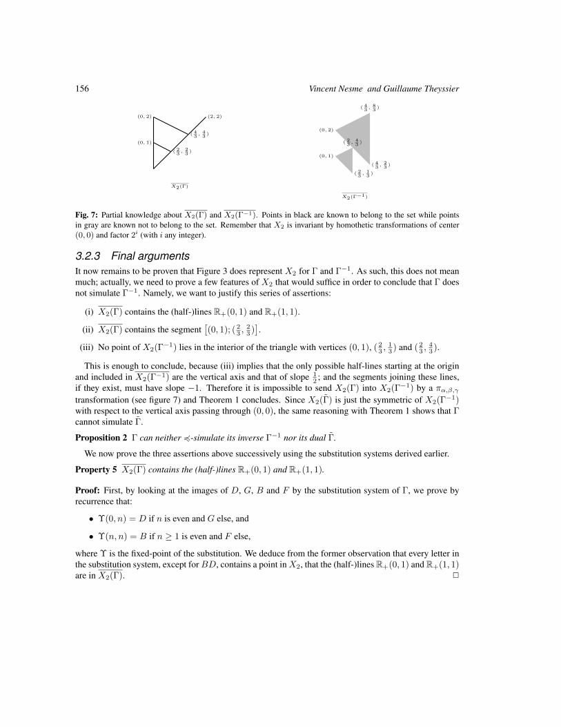
156 Vincent Nesme and Guillaume Theyssier
(2, 2)
(0, 1)
( 23, 2
3)
(0, 2)
( 43, 4
3)
X2(Γ)
(0, 2)
( 43, 2
3)
( 43, 8
3)
(0, 1)
( 23, 1
3)
( 23, 4
3)
X2(Γ−1)
Fig. 7: Partial knowledge about X2(Γ) and X2(Γ−1). Points in black are known to belong to the set while pointsin gray are known not to belong to the set. Remember that X2 is invariant by homothetic transformations of center(0, 0) and factor 2i (with i any integer).
3.2.3 Final argumentsIt now remains to be proven that Figure 3 does represent X2 for Γ and Γ−1. As such, this does not meanmuch; actually, we need to prove a few features of X2 that would suffice in order to conclude that Γ doesnot simulate Γ−1. Namely, we want to justify this series of assertions:
(i) X2(Γ) contains the (half-)lines R+(0, 1) and R+(1, 1).
(ii) X2(Γ) contains the segment[(0, 1); (2
3 ,23 )].
(iii) No point of X2(Γ−1) lies in the interior of the triangle with vertices (0, 1), ( 23 ,
13 ) and ( 2
3 ,43 ).
This is enough to conclude, because (iii) implies that the only possible half-lines starting at the originand included in X2(Γ−1) are the vertical axis and that of slope 1
2 ; and the segments joining these lines,if they exist, must have slope −1. Therefore it is impossible to send X2(Γ) into X2(Γ−1) by a πα,β,γtransformation (see figure 7) and Theorem 1 concludes. Since X2(Γ) is just the symmetric of X2(Γ−1)with respect to the vertical axis passing through (0, 0), the same reasoning with Theorem 1 shows that Γcannot simulate Γ.
Proposition 2 Γ can neither 4-simulate its inverse Γ−1 nor its dual Γ.
We now prove the three assertions above successively using the substitution systems derived earlier.
Property 5 X2(Γ) contains the (half-)lines R+(0, 1) and R+(1, 1).
Proof: First, by looking at the images of D, G, B and F by the substitution system of Γ, we prove byrecurrence that:
• Υ(0, n) = D if n is even and G else, and
• Υ(n, n) = B if n ≥ 1 is even and F else,
where Υ is the fixed-point of the substitution. We deduce from the former observation that every letter inthe substitution system, except forBD, contains a point inX2, that the (half-)lines R+(0, 1) and R+(1, 1)are in X2(Γ). 2
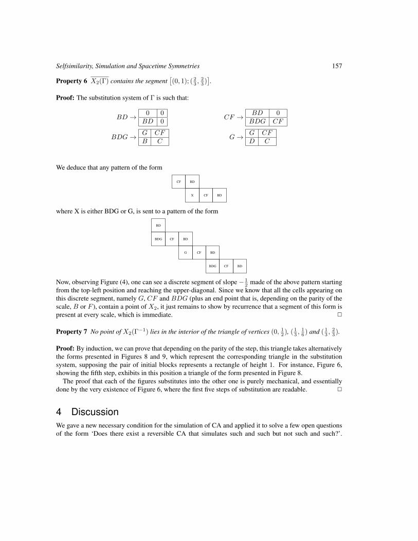
Selfsimilarity, Simulation and Spacetime Symmetries 157
Property 6 X2(Γ) contains the segment[(0, 1); (2
3 ,23 )].
Proof: The substitution system of Γ is such that:
BD → 0 0BD 0
CF → BD 0BDG CF
BDG→ G CFB C
G→ G CFD C
We deduce that any pattern of the form
CF BD
X CF BD
where X is either BDG or G, is sent to a pattern of the form
BD
BDG CF BD
G CF BD
BDG CF BD
Now, observing Figure (4), one can see a discrete segment of slope − 12 made of the above pattern starting
from the top-left position and reaching the upper-diagonal. Since we know that all the cells appearing onthis discrete segment, namely G, CF and BDG (plus an end point that is, depending on the parity of thescale, B or F ), contain a point of X2, it just remains to show by recurrence that a segment of this form ispresent at every scale, which is immediate. 2
Property 7 No point of X2(Γ−1) lies in the interior of the triangle of vertices (0, 12 ), ( 13 ,
16 ) and ( 1
3 ,23 ).
Proof: By induction, we can prove that depending on the parity of the step, this triangle takes alternativelythe forms presented in Figures 8 and 9, which represent the corresponding triangle in the substitutionsystem, supposing the pair of initial blocks represents a rectangle of height 1. For instance, Figure 6,showing the fifth step, exhibits in this position a triangle of the form presented in Figure 8.
The proof that each of the figures substitutes into the other one is purely mechanical, and essentiallydone by the very existence of Figure 6, where the first five steps of substitution are readable. 2
4 DiscussionWe gave a new necessary condition for the simulation of CA and applied it to solve a few open questionsof the form ‘Does there exist a reversible CA that simulates such and such but not such and such?’.
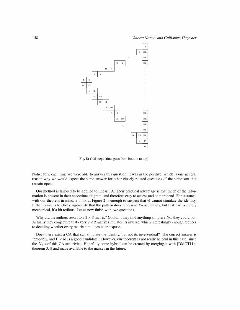
158 Vincent Nesme and Guillaume Theyssier
L
DH EIK
E HL
DL EIK
IK HL
DH EIK
E HL
DL EIK
. . .. . .
. . .. . .
DH EIK
E D
H
DHL
DHL
DHL
DHL
DHL
.
.
.
.
.
.
.
.
.
.
.
.
.
.
.
.
.
.
.
.
.
.
.
.
K
H K
H K
H K
. .. · · ·
K DHL
DL
DHL
DHL
Fig. 8: Odd steps (time goes from bottom to top).
Noticeably, each time we were able to answer this question, it was in the positive, which is one generalreason why we would expect the same answer for other closely related questions of the same sort thatremain open.
Our method is tailored to be applied to linear CA. Their practical advantage is that much of the infor-mation is present in their spacetime diagram, and therefore easy to access and comprehend. For instance,with our theorem in mind, a blink at Figure 2 is enough to suspect that Θ cannot simulate the identity.It then remains to check rigorously that the pattern does represent X2 accurately, but that part is purelymechanical, if a bit tedious. Let us now finish with two questions.
Why did the authors resort to a 3× 3 matrix? Couldn’t they find anything simpler? No, they could not.Actually they conjecture that every 2× 2 matrix simulates its inverse, which interestingly enough reducesto deciding whether every matrix simulates its transpose.
Does there exist a CA that can simulate the identity, but not its inverse/dual? The correct answer is‘probably, and Γ× id is a good candidate’. However, our theorem is not really helpful in this case, sincethe Xp-s of this CA are trivial. Hopefully some hybrid can be created by merging it with [DMOT11b,theorem 3.4] and made available to the masses in the future.
Selfsimilarity, Simulation and Spacetime Symmetries 159
L
DH EIK
E HL
DL EIK
IK HL
DH EIK
E HL
DL EIK
. . .. . .
. . .. . .
IK HL
DH I
K
EK
EK
EK
EK
EK
.
.
.
.
.
.
.
.
.
.
.
.
.
.
.
.
.
.
.
.
.
.
.
.
K
H K
H K
H K
. .. · · ·
H E
EK
EK
Fig. 9: Even steps (time goes from bottom to top).
References[AN10] Pablo Arrighi and Vincent Nesme. The Block Neighborhood. In TUCS, editor, Proceedings
of JAC 2010, pages 43–53, Turku, Finlande, December 2010.
[DMOT11a] Marianne Delorme, Jacques Mazoyer, Nicolas Ollinger, and Guillaume Theyssier. Bulkingi: An abstract theory of bulking. Theor. Comput. Sci., 412(30):3866–3880, 2011.
[DMOT11b] Marianne Delorme, Jacques Mazoyer, Nicolas Ollinger, and Guillaume Theyssier. Bulkingii: Classifications of cellular automata. Theor. Comput. Sci., 412(30):3881–3905, 2011.
[Gil87] Robert H. Gilman. Classes of linear automata. Ergodic Theory and Dynamical Systems,7(1):105–118, 1987.
[GNW10] Johannes Gutschow, Vincent Nesme, and Reinhard F. Werner. The fractal structure of cellu-lar automata on abelian groups. In Proceedings of Automata 2010, pages 55–74, June 2010.Preprint: http://arxiv.org/abs/1011.0313.
[Kur97] Petr Kurka. Languages, equicontinuity and attractors in cellular automata. Ergodic Theoryand Dynamical Systems, 17:417–433, 1997.
[MG10] Andres Moreira and Anahı Gajardo. Time-symmetric cellular automata. In JAC, 2010.
160 Vincent Nesme and Guillaume Theyssier
[Moo98] Cristopher Moore. Predicting nonlinear cellular automata quickly by decomposing theminto linear ones. Physica D: Nonlinear Phenomena, 111(1-4):27–41, 1998.
[MR98] Jacques Mazoyer and Ivan Rapaport. Inducing an order on cellular automata by a groupingoperation. In Proceedings of STACS, pages 116–127, 1998.
[Oll02] Nicolas Ollinger. Automates Cellulaires : structures. PhD thesis, Ecole Normale Superieurede Lyon, decembre 2002.
[Oll08] Nicolas Ollinger. Universalities in cellular automata: a (short) survey. In B. Durand, editor,Symposium on Cellular Automata Journees Automates Cellulaires (JAC’08), pages 102–118. MCCME Publishing House, Moscow, 2008.
[Wol84] Stephen Wolfram. Computation theory of cellular automata. Communications in Mathe-matical Physics, 96(1):15–57, 1984.
AUTOMATA 2011, Santiago, Chile local proceedings LP, 2011, 161–178
Orbits of the Bernoulli measure insingle-transition asynchronous cellularautomata
Henryk Fuks and Andrew SkeltonDepartment of Mathematics and Statistics,Brock University, St. Catharines, Canada.
We study iterations of the Bernoulli measure under nearest-neighbour asynchronous binary cellular automata (CA)with a single transition. For these CA, we show that a coarse-level description of the orbit of the Bernoulli measurecan be obtained, that is, one can explicitly compute measures of short cylinder sets after arbitrary number of iterationsof the CA. In particular, we give expressions for probabilities of ones for all three minimal single-transition rules, aswell as expressions for probabilities of blocks of length 3 for some of them. These expressions can be interpreted as“response curves”, that is, curves describing the dependence of the final density of ones on the initial density of ones.
Keywords: cellular automata. asynchronous rules, measure dynamics
1 IntroductionMathematical theory of cellular automata can be developed using a variety of approaches. The mostextensively used approach is the study of CA in the compact Cantor space AZ of symbolic sequences,where A is some finite alphabet. This approach proved to be very fruitful, and can now be considered afully established sub-discipline of topological dynamics (Kurka, 2009).
The aforementioned approach, however, is not without problems. Suppose, for example, that F :AZ → AZ is a CA rule with local function f , and σ is the shift map. Then F and Fσ determine differentdynamical systems on AZ, with possibly radically different properties. For instance, if F is the identitymap, then it is obviously non-chaotic, yet Fσ = σ is chaotic. This is somewhat unsatisfactory in the viewof the fact that σ is in some sense a “simple” map - it is, after all, just a translation.
To avoid this problem, one can study CA on non-compact spaces, and indeed this approach has beensteadily gaining momentum in recent years (Formenti and Kurka, 2009). Alternatively, the space of mea-sures is often considered, or more precisely, the spaceMA of Borel shift-invariant probability measureson AZ, equipped with the weak? topology. This space has the attractive property that F and Fσ deter-mine the same dynamical system onMA and a number of interesting results have been established fordynamics of CA inMA, e.g. by Kurka and Maass (2000), Pivato (2002), Kurka (2005), and others.
Among all measures in MA, the uniform Bernoulli measure plays a special role in the dynamics ofCA, first, because it is preserved by surjective CA and also, because it is a limit measure for linear CA (a
c© 2011 AUTOMATA proceedings, Santiago, Chile, 2011
162 Henryk Fuks and Andrew Skelton
property known as “asymptotic randomization”) – for a review, see Pivato (2009) and references therein.A very natural question is therefore to ask: what can we say about the orbit of the Bernoulli measure undera CA rule F ? For linear CA, the asymptotic randomization result mentioned above answers this questionto some extent, but what can be said about nonlinear rules?
The approach of the authors was to consider this problem in depth for concrete CA rules, starting fromparticularly simple cases. Even then, it is still difficult to fully characterize consecutive iterates of theBernoulli measure. However, since any shift-invariant probability measure on AZ is fully determinedby its value on cylinder sets, it is often possible to compute measures of certain short cylinder sets aftern iterations of F by taking advantage of the combinatorial structure of the CA rule. This works wellfor simple equicontinuous rules, as well as for almost-equicontinuous ones, as recently demonstratedfor the case of almost-equicontinuous rule 172 (Fuks, 2010). Even for rules which are somewhat morecomplicated, such as the “traffic” rule 184 and its topological factor rule 142, significant results have beenobtained (Fuks, 1999, 2006; Blank, 2003; Belitsky and Ferrari, 2005).
In this paper, we examine the same problem in the context of probabilistic rules. Can one computeiterates of the Bernoulli measure under simple probabilistic rules? Again, the situation appears to besimilar as in the deterministic case. While the full characterization of iterates of the Bernoulli measureturns out to be very hard, measures of short cylinder sets can be computed explicitly if one takes advantageof the combinatorial structure of these rules. We will consider a special class of probabilistic rules, knownas α-asynchronous CA. For the α-asynchronous version of a CA rule with local function f , one appliesto each site rule f with probability α, or leaves the site unchanged with probability 1−α, and this is donefor each site simultaneously and independently. We will furthermore restrict our attention to particularlysimple α-asynchronous rules, namely those for which the local function f differs from the local functionof the identity rule only for one particular neighbourhood configuration.
2 Definitions
We first define probabilistic CA in a traditional way, as a stochastic process. Let A = 0, 1 be called asymbol set, and let elements ofAZ be called configurations. Let s(t) ∈ AZ denote a configuration at timet, where t ∈ N. Suppose that we have a collection of random variables Xi,v taking values in A, indexedwith i ∈ Z and v ∈ A3.
We define define a nearest-neighbour binary probabilistic cellular automaton as a stochastic process
si(t+ 1) = Xi,v(i,t), (1)
where v(i, t) = si−1(t), si(t), si+1(t) will be called a neighbourhood vector. In general, the probabil-ity distribution of Xi,v is assumed to be independent of i, although it may (and normally does) depend onthe neighbourhood vector v.
We will be interested in a very special type of probabilistic CA, in which each cell is independentlyupdated with some probability α. These rules were first studied experimentally by Fates and Morvan(2005), and subsequently called called α-asynchronous rules (Fates et al., 2006). They are formallydefined as follows. Let f : A3 → A be a given function and let α ∈ [0, 1] be a given parameter (calledthe synchrony rate). For these rules, random variables Xi,v take value in the set f (v1, v2, v3) , v2 with
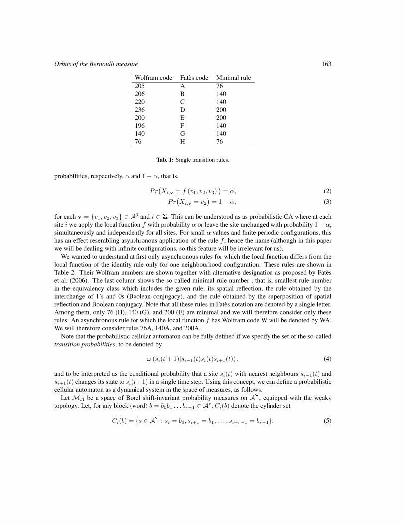
Orbits of the Bernoulli measure 163
Wolfram code Fates code Minimal rule205 A 76206 B 140220 C 140236 D 200200 E 200196 F 140140 G 14076 H 76
Tab. 1: Single transition rules.
probabilities, respectively, α and 1− α, that is,
Pr(Xi,v = f (v1, v2, v3)
)= α, (2)
Pr(Xi,v = v2
)= 1− α, (3)
for each v = v1, v2, v3 ∈ A3 and i ∈ Z. This can be understood as as probabilistic CA where at eachsite i we apply the local function f with probability α or leave the site unchanged with probability 1− α,simultaneously and independently for all sites. For small α values and finite periodic configurations, thishas an effect resembling asynchronous application of the rule f , hence the name (although in this paperwe will be dealing with infinite configurations, so this feature will be irrelevant for us).
We wanted to understand at first only asynchronous rules for which the local function differs from thelocal function of the identity rule only for one neighbourhood configuration. These rules are shown inTable 2. Their Wolfram numbers are shown together with alternative designation as proposed by Fateset al. (2006). The last column shows the so-called minimal rule number , that is, smallest rule numberin the equivalency class which includes the given rule, its spatial reflection, the rule obtained by theinterchange of 1’s and 0s (Boolean conjugacy), and the rule obtained by the superposition of spatialreflection and Boolean conjugacy. Note that all these rules in Fates notation are denoted by a single letter.Among them, only 76 (H), 140 (G), and 200 (E) are minimal and we will therefore consider only theserules. An asynchronous rule for which the local function f has Wolfram code W will be denoted by WA.We will therefore consider rules 76A, 140A, and 200A.
Note that the probabilistic cellular automaton can be fully defined if we specify the set of the so-calledtransition probabilities, to be denoted by
ω (si(t+ 1)|si−1(t)si(t)si+1(t)) , (4)
and to be interpreted as the conditional probability that a site si(t) with nearest neighbours si−1(t) andsi+1(t) changes its state to si(t+1) in a single time step. Using this concept, we can define a probabilisticcellular automaton as a dynamical system in the space of measures, as follows.
Let MA be a space of Borel shift-invariant probability measures on AZ, equipped with the weak?topology. Let, for any block (word) b = b0b1 . . . br−1 ∈ Ar, Ci(b) denote the cylinder set
Ci(b) = s ∈ AZ : si = b0, si+1 = b1, . . . , si+r−1 = br−1. (5)
164 Henryk Fuks and Andrew Skelton
Since we are dealing with shift-invariant measures, we drop the spatial index i in expressions involvingmeasures of cylinder sets. Note that the measure inMA is uniquely defined by its values on cylinder sets.
Suppose now that the function ω(·|·) : A × A3 → [0, 1] is given. We define the transformationF :MA →MA by defining, for any µ ∈MA and c ∈ Ar,
(Fµ)(C(c)
)=
∑b∈Ar+2
r∏i=1
ω(ci|bi−1bibi+1)µ(C(b)
), (6)
where r ∈ N.For convenience, we also define 1-step block transition probability ω so that, for any b = b0b1 . . . brbr+1 ∈Ar+2 and any c = c1c2 . . . cr−1cr ∈ Ar,
ω(c|b) =r∏i=1
ω(ci|bi−1bibi+1). (7)
Moreover, we define a n-step block transition probability ω recursively, so that, when n ≥ 2 and for anyblocks b ∈ Ar+2n, c ∈ Ar,
ωn(c|b) =∑
b′∈Ar+2n−2
ω(b′|b)ωn−1(c|b′), (8)
which may be written explicitly as
ωn(c|b) =∑
bn−1∈Ar+2(n−1)
...
b1∈Ar+2
ω(c|b2)
(n−2∏i=1
ω(bi|bi+1)
)ω(bn−1|b). (9)
Note that the n-step block transition probability ωn(c|b) can be intuitively understood as the conditionalprobability of seeing the block c on sites [1, r] after n iterations of F , conditioned on the fact that theoriginal configuration contained the block b on sites [1− n, r + n].
3 Response SurfaceLet us now suppose that the initial state s(0) is not given explicitly, but that the state of each site isindependently set to 1 with probability ρ or to zero with probability 1 − ρ. This is equivalent to sayingthat the initial probability measure is a shift-invariant Bernoulli measure. We then apply our probabilisticCA n times, and ask: what is the resulting probability measure? Since it is well known that this measureis uniquely determined by its value on all cylinder sets, it would be sufficient to compute probabilitiesof occurrences of all finite blocks in order to describe the measure completely. This, however, is verydifficult even in simple cases, thus we will restrict our attention to a much simpler problem, namelycomputing probabilities of short words, such as words of length one. One can say that such single-symbol probabilities provide only a very coarse description of the measure, yet they are often useful, justlike knowledge of the first moment of some unknown distribution is often valuable. In many practicalproblems, e.g., in mathematical modeling, one wants to know how a CA rule iterated over an initial
Orbits of the Bernoulli measure 165
configuration affects certain aggregate properties of the configuration, such as, for example, the density of1’s. For finite configurations, the density of ones is defined as the number of sites in state 1 divided by thetotal number of sites. For infinite configurations, which are the subject of this article, one could generalizethis notion by taking the appropriate limit, but such limit may not always exist. Since we will be interestedin orbits of translationally-invariant probability measures rather than individual configurations, it will bemore convenient to define the density as the expected value of the cell state. For binary rules, if P (0) andP (1) are probabilities of occurrence of 0 and 1 in a configuration, the expected value of the cell state isP (0) · 0 + P (1) · 1 = P (1). For this reason, we will use the term “density” interchangeably with theprobability of occurrence of 1 in a configuration.
To be more precise, let µρ be the Bernoulli measure such that µρ(C(1)) = ρ, µρ(C(0)) = 1 − ρ. Letus define probability of occurrence of block b after n iterations of F as
Pn(b) := (Fnµρ)(C(b)
). (10)
Using the concept of transition probabilities, we can write
Pn(b) =∑
a∈Ar+2n
P0(a)ωn(b|a). (11)
where the transition probability is defined in eq. (8) and (9). Note that P0(a) is easy to compute,
P0(a) = ρ# of 1’s in a(1− ρ)# of 0’s in a, (12)
by the definition of Bernoulli measure.Since some of the transition probabilities may be zero, we define, for any block b ∈ Gr, the set of
n-step block preimages,suppωn(b|·) = a ∈ Ar+2n : ωn(b|a) > 0. (13)
Then we can write (11) as
Pn(b) =∑
a∈suppωn(b|·)
P0(a)ωn(b|a). (14)
In what follows, we will show how to compute Pn(1) for the three aforementioned asynchronous rules.For a given α and n, the graph of Pn(1) versus P0(1) will be called response curve. We use this terminol-ogy analogous to signal processing theory: a probabilistic CA can be viewed as a black box, for which theinput is given in the form of density of 1’s in the initial measure (P0(1) = ρ), and, after n iterations, weobtain output density, that is, Pn(1). For the special case ρ = 1/2, we use the notation P (s)
n (1) which willbe called a symmetric response curve. We will also plot Pn(1) as a function of both ρ and the synchronyrate α, and this 3D graph will be called response surface. Most of the time, we will be interested in thelimit n→∞, to be denoted as
P (1) = limn→∞
Pn(1), (15)
P (s)(1) = limn→∞
P (s)n (1). (16)
166 Henryk Fuks and Andrew Skelton
4 Rule 200AConsider an α-asynchronous rule defined as
ω(1|b) =
0 if b ∈ 000, 001, 100, 101,1 if b ∈ 011, 110, 111,1− α if b = 010,
(17)
and ω(0|b) = 1−ω(1|b) for all b ∈ A3. Note that if α = 1, then this rule is equivalent to the deterministicRule 200. In order to simplify notation, we define β = 1− α.
We wish to find a response surface for Rule 200A. In order to apply eq. (14), we begin by finding theset of all potential preimage blocks and their respective transition probabilities.
Proposition 4.1 The set suppωn(1|·) consists of all blocks of the form
? · · · ?︸ ︷︷ ︸n
1 ? · · · ?︸ ︷︷ ︸n
. (18)
Proof: From eq. (17), we can see that an element in state 0 will always remain in state 0, so any blockwhich does not have the above form will never be transformed to a single 1 under n iterations of Rule200A. Similarly, a block in our set could produce a single 1, with some non-zero probability. 2
We now define the following subset of suppωn(1|·), Bn = ? · · · ?︸ ︷︷ ︸n−1
010 ? · · · ?︸ ︷︷ ︸n−1
.
Proposition 4.2 For any block b ∈ suppωn(1|·) \Bn, we have ωn(1|b) = 1.
Proof: In every element of the set suppωn(1|·) \ Bn, the central block will either be 011, 110 or 111.From eq. (17), we can see that these blocks will always be preserved under application of Rule 200A. 2
Proposition 4.3 For any block b ∈ Bn, we have ωn(1|b) = βn.
Proof: In each iteration, the 0s in the centre block will be preserved with probability 1, so we only needto consider the transition 010→ 1, which occurs in each iteration of Rule 200A with probability β. 2
We may now use eq. (14) and consider the sets and transition probabilities described in Propositions4.2 and 4.3, to conclude that
Pn(1) =∑
b∗∈suppωn(1|·)\Bn
P0(b∗)ωn(1|b∗) +
∑b∗∈Bn
P0(b∗)ωn(1|b∗)
= 1 ·(2ρ2(1− ρ) + ρ3
)+ βn · ρ(1− ρ)2
= ρ2(2− ρ) + βnρ(1− ρ)2. (19)
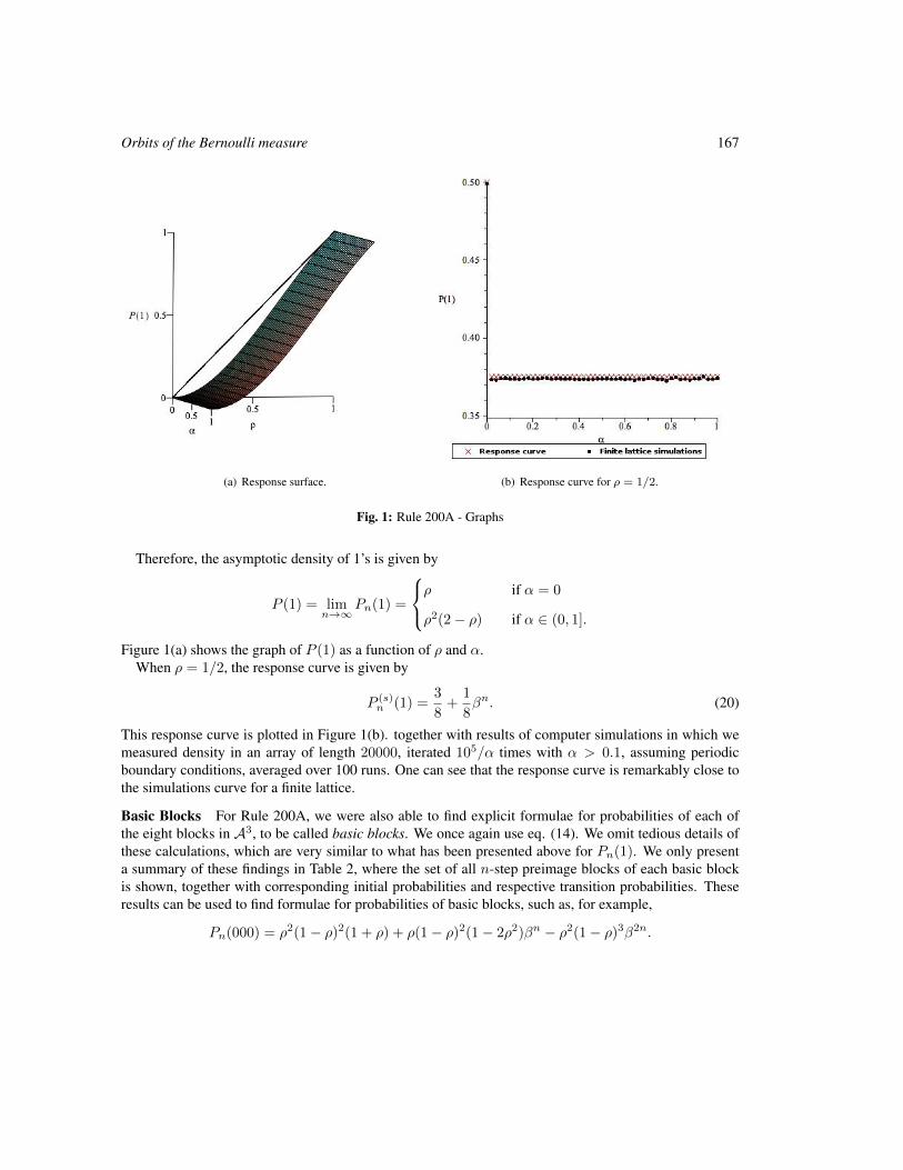
Orbits of the Bernoulli measure 167
(a) Response surface. (b) Response curve for ρ = 1/2.
Fig. 1: Rule 200A - Graphs
Therefore, the asymptotic density of 1’s is given by
P (1) = limn→∞
Pn(1) =
ρ if α = 0
ρ2(2− ρ) if α ∈ (0, 1].
Figure 1(a) shows the graph of P (1) as a function of ρ and α.When ρ = 1/2, the response curve is given by
P (s)n (1) =
3
8+
1
8βn. (20)
This response curve is plotted in Figure 1(b). together with results of computer simulations in which wemeasured density in an array of length 20000, iterated 105/α times with α > 0.1, assuming periodicboundary conditions, averaged over 100 runs. One can see that the response curve is remarkably close tothe simulations curve for a finite lattice.
Basic Blocks For Rule 200A, we were also able to find explicit formulae for probabilities of each ofthe eight blocks in A3, to be called basic blocks. We once again use eq. (14). We omit tedious details ofthese calculations, which are very similar to what has been presented above for Pn(1). We only presenta summary of these findings in Table 2, where the set of all n-step preimage blocks of each basic blockis shown, together with corresponding initial probabilities and respective transition probabilities. Theseresults can be used to find formulae for probabilities of basic blocks, such as, for example,
Pn(000) = ρ2(1− ρ)2(1 + ρ) + ρ(1− ρ)2(1− 2ρ2)βn − ρ2(1− ρ)3β2n.
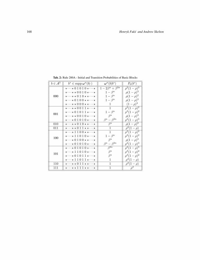
168 Henryk Fuks and Andrew Skelton
Tab. 2: Rule 200A - Initial and Transition Probabilities of Basic Blocks
b ∈ A3 b∗ ∈ suppωn(b|·) ωn(b|b∗) P0(b∗)
000
? · · · ? 0 1 0 1 0 ? · · · ? 1− 2βn + β2n ρ2(1− ρ)3? · · · ? ? 0 0 1 0 ? · · · ? 1− βn ρ(1− ρ)3? · · · ? ? 0 1 0 ? ? · · · ? 1− βn ρ(1− ρ)2? · · · ? 0 1 0 0 ? ? · · · ? 1− βn ρ(1− ρ)3? · · · ? ? 0 0 0 ? ? · · · ? 1 (1− ρ)3
001
? · · · ? ? 0 0 1 1 ? · · · ? 1 ρ2(1− ρ)2? · · · ? 0 1 0 1 1 ? · · · ? 1− βn ρ3(1− ρ)2? · · · ? ? 0 0 1 0 ? · · · ? βn ρ(1− ρ)3? · · · ? 0 1 0 1 0 ? · · · ? βn − β2n ρ2(1− ρ)3
010 ? · · · ? ? 0 1 0 ? ? · · · ? βn ρ(1− ρ)2011 ? · · · ? ? 0 1 1 ? ? · · · ? 1 ρ2(1− ρ)
100
? · · · ? 1 1 0 0 ? ? · · · ? 1 ρ2(1− ρ)2? · · · ? 1 1 0 1 0 ? · · · ? 1− βn ρ3(1− ρ)2? · · · ? 0 1 0 0 ? ? · · · ? βn ρ(1− ρ)3? · · · ? 0 1 0 1 0 ? · · · ? βn − β2n ρ2(1− ρ)3
101
? · · · ? 0 1 0 1 0 ? · · · ? β2n ρ2(1− ρ)3? · · · ? 1 1 0 1 0 ? · · · ? βn ρ3(1− ρ)2? · · · ? 0 1 0 1 1 ? · · · ? βn ρ3(1− ρ)2? · · · ? 1 1 0 1 1 ? · · · ? 1 ρ4(1− ρ)
110 ? · · · ? ? 0 1 1 ? ? · · · ? 1 ρ2(1− ρ)111 ? · · · ? ? 1 1 1 ? ? · · · ? 1 ρ3
Orbits of the Bernoulli measure 169
We show below probabilities of all eight basic blocks in the special case when ρ = 1/2, together withasymptotic probabilities, assuming α 6= 0.
P (s)n (000) =
13
32− 5
16βn +
1
32β2n, P (s)(000) = 13/32,
P (s)n (001) =
3
32+
1
16βn − 1
32β2n, P (s)(001) = 3/32,
P (s)n (010) =
1
8βn, P (s)(010) = 0,
P (s)n (011) =
1
8, P (s)(011) = 1/8,
P (s)n (100) =
3
32+
1
16βn − 1
32β2n, P (s)(100) = 3/32,
P (s)n (101) =
1
32+
1
16βn +
1
32β2n, P (s)(101) = 1/32,
P (s)n (110) =
1
8, P (s)(110) = 1/8,
P (s)n (111) =
1
8, P (s)(111) = 1/8.
5 Rule 140AThe next rule to be considered has transition probabilities defined as
ω(1|b) =
0 if b ∈ 000, 001, 100, 101,1 if b ∈ 010, 011, 111,1− α if b = 110,
(21)
and ω(0|b) = 1 − ω(1|b) for all b ∈ A3. Note that if α = 1, then this rule is equivalent to deterministicRule 140.
We first find the set of all preimage blocks and their respective transition probabilities.
Proposition 5.1 The set suppωn(1|·) consists of all blocks of the form
? · · · ?︸ ︷︷ ︸n
1 ? · · · ?︸ ︷︷ ︸n
. (22)
Proof: From eq. (21), we can see that a site in state 0 will always remain in state 0, so that for any blockb′ ∈ A2n+1 \ suppωn(1|·), we have ωn(1|b′) = 0. A block in suppωn(1|·), however, could produce asingle 1 with some non-zero probability. 2
To determine transition probabilities, we divide the set of preimage blocks into subsets. We start bydefining Ckn ⊂ suppωn(1|·) to be the set of blocks of the form
? · · · ?︸ ︷︷ ︸n−1
1 1 1 · · · 1︸ ︷︷ ︸k−1
0 ? · · · ?︸ ︷︷ ︸n−k
,
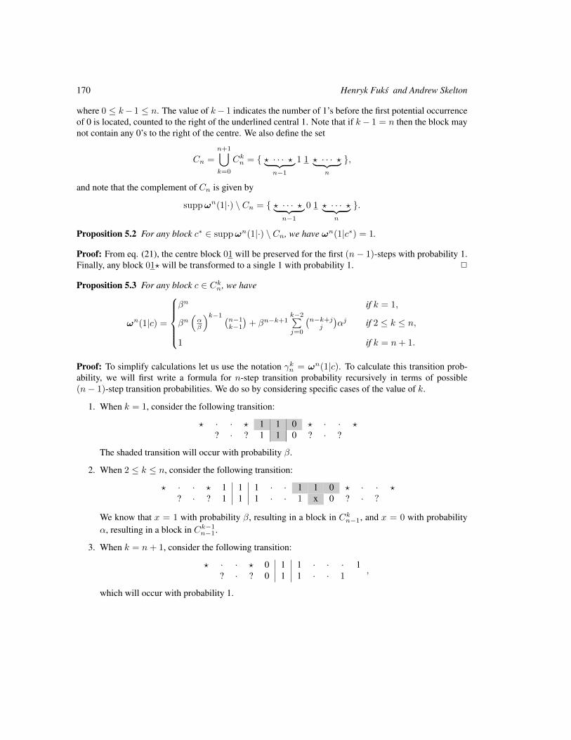
170 Henryk Fuks and Andrew Skelton
where 0 ≤ k− 1 ≤ n. The value of k− 1 indicates the number of 1’s before the first potential occurrenceof 0 is located, counted to the right of the underlined central 1. Note that if k− 1 = n then the block maynot contain any 0’s to the right of the centre. We also define the set
Cn =
n+1⋃k=0
Ckn = ? · · · ?︸ ︷︷ ︸n−1
1 1 ? · · · ?︸ ︷︷ ︸n
,
and note that the complement of Cn is given by
suppωn(1|·) \ Cn = ? · · · ?︸ ︷︷ ︸n−1
0 1 ? · · · ?︸ ︷︷ ︸n
.
Proposition 5.2 For any block c∗ ∈ suppωn(1|·) \ Cn, we have ωn(1|c∗) = 1.
Proof: From eq. (21), the centre block 01 will be preserved for the first (n− 1)-steps with probability 1.Finally, any block 01? will be transformed to a single 1 with probability 1. 2
Proposition 5.3 For any block c ∈ Ckn, we have
ωn(1|c) =
βn if k = 1,
βn(αβ
)k−1 (n−1k−1)+ βn−k+1
k−2∑j=0
(n−k+j
j
)αj if 2 ≤ k ≤ n,
1 if k = n+ 1.
Proof: To simplify calculations let us use the notation γkn = ωn(1|c). To calculate this transition prob-ability, we will first write a formula for n-step transition probability recursively in terms of possible(n− 1)-step transition probabilities. We do so by considering specific cases of the value of k.
1. When k = 1, consider the following transition:
? · · ? 1 1 0 ? · · ?? · ? 1 1 0 ? · ?
The shaded transition will occur with probability β.
2. When 2 ≤ k ≤ n, consider the following transition:
? · · ? 1 1 1 · · 1 1 0 ? · · ?? · ? 1 1 1 · · 1 x 0 ? · ?
We know that x = 1 with probability β, resulting in a block in Ckn−1, and x = 0 with probabilityα, resulting in a block in Ck−1n−1.
3. When k = n+ 1, consider the following transition:
? · · ? 0 1 1 · · · 1? · ? 0 1 1 · · 1
,
which will occur with probability 1.
Orbits of the Bernoulli measure 171
Combining these cases, we obtain the following recursive formula
γkn =
βγ1n−1 if k = 1,
αγk−1n−1 + βγkn−1 if 2 ≤ k ≤ n,1 if k = n+ 1.
(23)
This recursive equation can be solved to give the desired result. To see this, consider first the case ofk = 1 or k = n+1, when our formula follows trivially from eq. (23). When 2 ≤ k ≤ n, our formula canbe proved by induction with respect to n. When n = 2, we only have the case of k = 2, where
γ22 = β1α1
(1
1
)+ β1
0∑j=0
(j
j
)αj = βα+ β = 1− α2.
Now, we consider the following inductive step, for 3 ≤ k ≤ n,
γkn = αγk−1n−1 + βγkn−1
= α
βn−1(αβ
)k−2(n− 2
k − 2
)+ βn−k+1
k−3∑j=0
(n− k + j
j
)αj
+
+ β
βn−1(αβ
)k−1(n− 2
k − 1
)+ βn−k
k−2∑j=0
(n− k + j − 1
j
)αj
= αβn−1
(α
β
)k−2(n− 2
k − 2
)+ ββn−1
(α
β
)k−1(n− 2
k − 1
)+ αβn−k+1
k−3∑j=0
(n− k + j
j
)αj + ββn−k
k−2∑j=0
(n− k + j − 1
j
)αj
= βn(α
β
)k−1(n− 1
k − 1
)+ βn−k+1
k−2∑j=1
(n− k + j − 1
j − 1
)αj + β + β
k−2∑j=1
(n− k + j − 1
j
)αj
= βn
(α
β
)k−1(n− 1
k − 1
)+ βn−k+1
k−2∑j=0
(n− k + j
j
)αj .
A similar procedure can be used to prove the formula when k = 2, thus completing the proof. 2
We may now use eq. (14) and consider the sets and transition probabilities described in Propositions5.2 and 5.3, concluding that
Pn(1) =∑
c∗∈suppωn(1|·)\Cn
P0(c∗)ωn(1|c∗) +
∑c∗∈Cn
P0(c∗)ωn(1|c∗)
= ρ(1− ρ) + ρ2(1− ρ)βn + ρ2(1− ρ)n∑k=2
ρk−1γkn + ρn+2, (24)
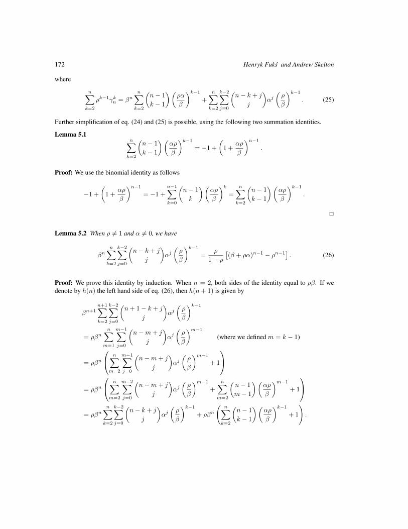
172 Henryk Fuks and Andrew Skelton
where
n∑k=2
ρk−1γkn = βnn∑k=2
(n− 1
k − 1
)(ρα
β
)k−1+
n∑k=2
k−2∑j=0
(n− k + j
j
)αj(ρ
β
)k−1. (25)
Further simplification of eq. (24) and (25) is possible, using the following two summation identities.
Lemma 5.1n∑k=2
(n− 1
k − 1
)(αρ
β
)k−1= −1 +
(1 +
αρ
β
)n−1.
Proof: We use the binomial identity as follows
−1 +(1 +
αρ
β
)n−1= −1 +
n−1∑k=0
(n− 1
k
)(αρ
β
)k=
n∑k=2
(n− 1
k − 1
)(αρ
β
)k−1.
2
Lemma 5.2 When ρ 6= 1 and α 6= 0, we have
βnn∑k=2
k−2∑j=0
(n− k + j
j
)αj(ρ
β
)k−1=
ρ
1− ρ[(β + ρα)n−1 − ρn−1
]. (26)
Proof: We prove this identity by induction. When n = 2, both sides of the identity equal to ρβ. If wedenote by h(n) the left hand side of eq. (26), then h(n+ 1) is given by
βn+1n+1∑k=2
k−2∑j=0
(n+ 1− k + j
j
)αj(ρ
β
)k−1
= ρβnn∑
m=1
m−1∑j=0
(n−m+ j
j
)αj(ρ
β
)m−1(where we defined m = k − 1)
= ρβn
n∑m=2
m−1∑j=0
(n−m+ j
j
)αj(ρ
β
)m−1+ 1
= ρβn
n∑m=2
m−2∑j=0
(n−m+ j
j
)αj(ρ
β
)m−1+
n∑m=2
(n− 1
m− 1
)(αρ
β
)m−1+ 1
= ρβn
n∑k=2
k−2∑j=0
(n− k + j
j
)αj(ρ
β
)k−1+ ρβn
(n∑k=2
(n− 1
k − 1
)(αρ
β
)k−1+ 1
).
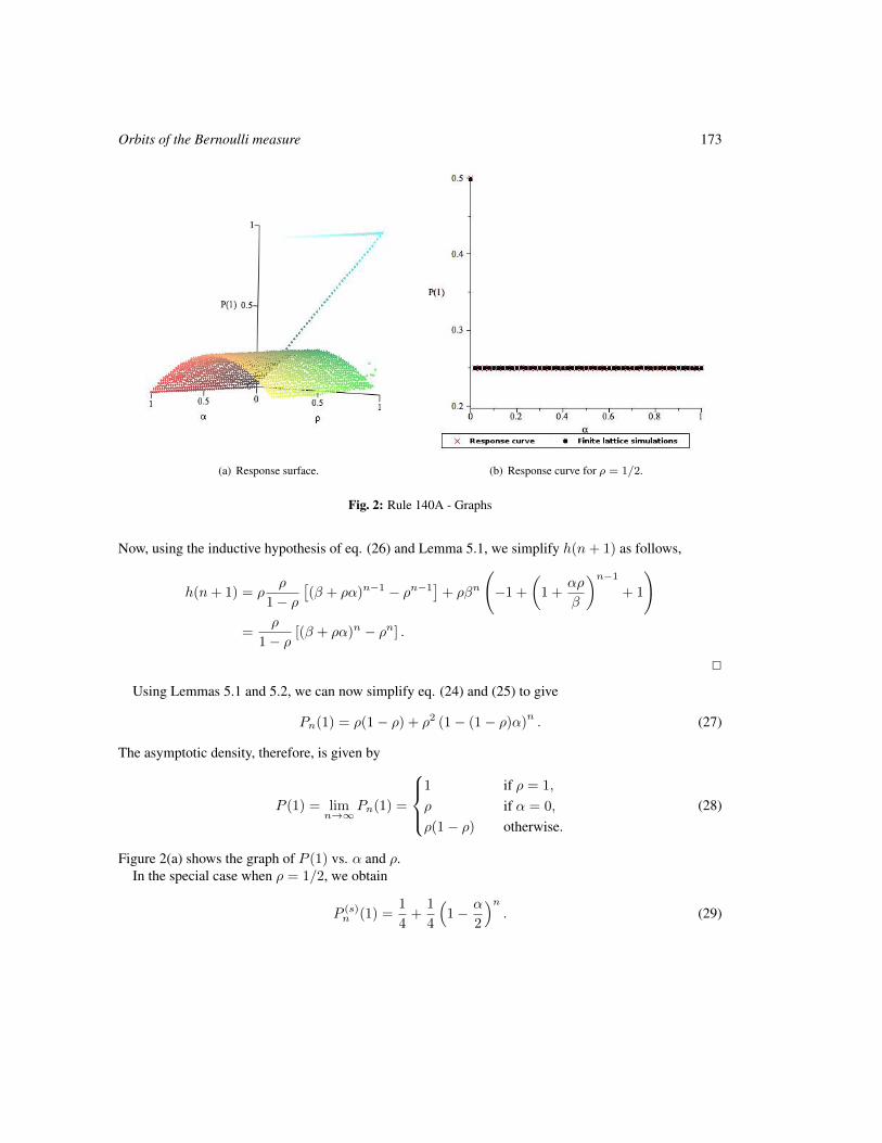
Orbits of the Bernoulli measure 173
(a) Response surface. (b) Response curve for ρ = 1/2.
Fig. 2: Rule 140A - Graphs
Now, using the inductive hypothesis of eq. (26) and Lemma 5.1, we simplify h(n+ 1) as follows,
h(n+ 1) = ρρ
1− ρ[(β + ρα)n−1 − ρn−1
]+ ρβn
(−1 +
(1 +
αρ
β
)n−1+ 1
)=
ρ
1− ρ[(β + ρα)n − ρn] .
2
Using Lemmas 5.1 and 5.2, we can now simplify eq. (24) and (25) to give
Pn(1) = ρ(1− ρ) + ρ2 (1− (1− ρ)α)n . (27)
The asymptotic density, therefore, is given by
P (1) = limn→∞
Pn(1) =
1 if ρ = 1,
ρ if α = 0,
ρ(1− ρ) otherwise.(28)
Figure 2(a) shows the graph of P (1) vs. α and ρ.In the special case when ρ = 1/2, we obtain
P (s)n (1) =
1
4+
1
4
(1− α
2
)n. (29)
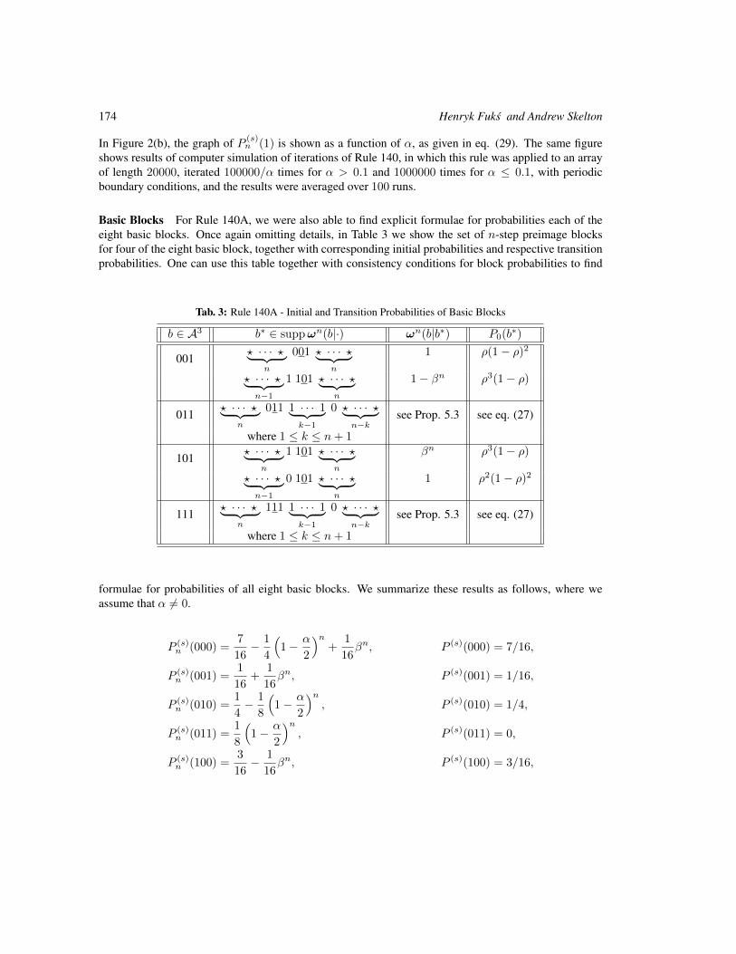
174 Henryk Fuks and Andrew Skelton
In Figure 2(b), the graph of P (s)n (1) is shown as a function of α, as given in eq. (29). The same figure
shows results of computer simulation of iterations of Rule 140, in which this rule was applied to an arrayof length 20000, iterated 100000/α times for α > 0.1 and 1000000 times for α ≤ 0.1, with periodicboundary conditions, and the results were averaged over 100 runs.
Basic Blocks For Rule 140A, we were also able to find explicit formulae for probabilities each of theeight basic blocks. Once again omitting details, in Table 3 we show the set of n-step preimage blocksfor four of the eight basic block, together with corresponding initial probabilities and respective transitionprobabilities. One can use this table together with consistency conditions for block probabilities to find
Tab. 3: Rule 140A - Initial and Transition Probabilities of Basic Blocks
b ∈ A3 b∗ ∈ suppωn(b|·) ωn(b|b∗) P0(b∗)
001 ? · · · ?︸ ︷︷ ︸n
001 ? · · · ?︸ ︷︷ ︸n
1 ρ(1− ρ)2
? · · · ?︸ ︷︷ ︸n−1
1 101 ? · · · ?︸ ︷︷ ︸n
1− βn ρ3(1− ρ)
011 ? · · · ?︸ ︷︷ ︸n
011 1 · · · 1︸ ︷︷ ︸k−1
0 ? · · · ?︸ ︷︷ ︸n−k
see Prop. 5.3 see eq. (27)
where 1 ≤ k ≤ n+ 1
101 ? · · · ?︸ ︷︷ ︸n
1 101 ? · · · ?︸ ︷︷ ︸n
βn ρ3(1− ρ)
? · · · ?︸ ︷︷ ︸n−1
0 101 ? · · · ?︸ ︷︷ ︸n
1 ρ2(1− ρ)2
111 ? · · · ?︸ ︷︷ ︸n
111 1 · · · 1︸ ︷︷ ︸k−1
0 ? · · · ?︸ ︷︷ ︸n−k
see Prop. 5.3 see eq. (27)
where 1 ≤ k ≤ n+ 1
formulae for probabilities of all eight basic blocks. We summarize these results as follows, where weassume that α 6= 0.
P (s)n (000) =
7
16− 1
4
(1− α
2
)n+
1
16βn, P (s)(000) = 7/16,
P (s)n (001) =
1
16+
1
16βn, P (s)(001) = 1/16,
P (s)n (010) =
1
4− 1
8
(1− α
2
)n, P (s)(010) = 1/4,
P (s)n (011) =
1
8
(1− α
2
)n, P (s)(011) = 0,
P (s)n (100) =
3
16− 1
16βn, P (s)(100) = 3/16,
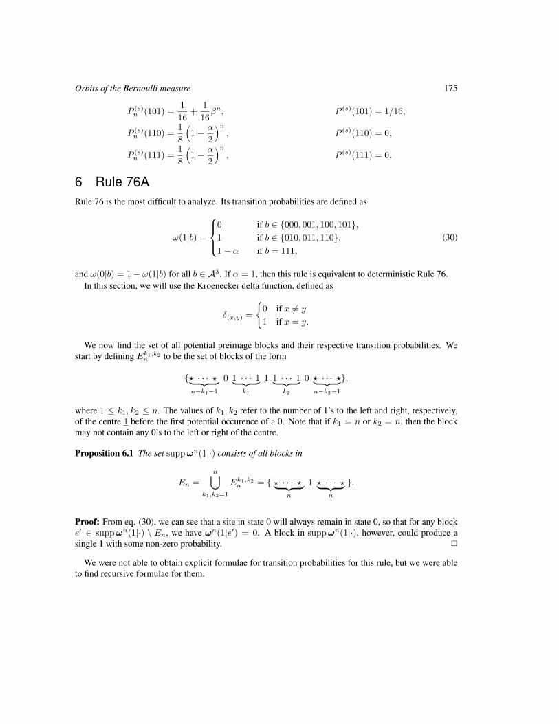
Orbits of the Bernoulli measure 175
P (s)n (101) =
1
16+
1
16βn, P (s)(101) = 1/16,
P (s)n (110) =
1
8
(1− α
2
)n, P (s)(110) = 0,
P (s)n (111) =
1
8
(1− α
2
)n, P (s)(111) = 0.
6 Rule 76ARule 76 is the most difficult to analyze. Its transition probabilities are defined as
ω(1|b) =
0 if b ∈ 000, 001, 100, 101,1 if b ∈ 010, 011, 110,1− α if b = 111,
(30)
and ω(0|b) = 1− ω(1|b) for all b ∈ A3. If α = 1, then this rule is equivalent to deterministic Rule 76.In this section, we will use the Kroenecker delta function, defined as
δ(x,y) =
0 if x 6= y
1 if x = y.
We now find the set of all potential preimage blocks and their respective transition probabilities. Westart by defining Ek1,k2n to be the set of blocks of the form
? · · · ?︸ ︷︷ ︸n−k1−1
0 1 · · · 1︸ ︷︷ ︸k1
1 1 · · · 1︸ ︷︷ ︸k2
0 ? · · · ?︸ ︷︷ ︸n−k2−1
,
where 1 ≤ k1, k2 ≤ n. The values of k1, k2 refer to the number of 1’s to the left and right, respectively,of the centre 1 before the first potential occurence of a 0. Note that if k1 = n or k2 = n, then the blockmay not contain any 0’s to the left or right of the centre.
Proposition 6.1 The set suppωn(1|·) consists of all blocks in
En =
n⋃k1,k2=1
Ek1,k2n = ? · · · ?︸ ︷︷ ︸n
1 ? · · · ?︸ ︷︷ ︸n
.
Proof: From eq. (30), we can see that a site in state 0 will always remain in state 0, so that for any blocke′ ∈ suppωn(1|·) \ En, we have ωn(1|e′) = 0. A block in suppωn(1|·), however, could produce asingle 1 with some non-zero probability. 2
We were not able to obtain explicit formulae for transition probabilities for this rule, but we were ableto find recursive formulae for them.
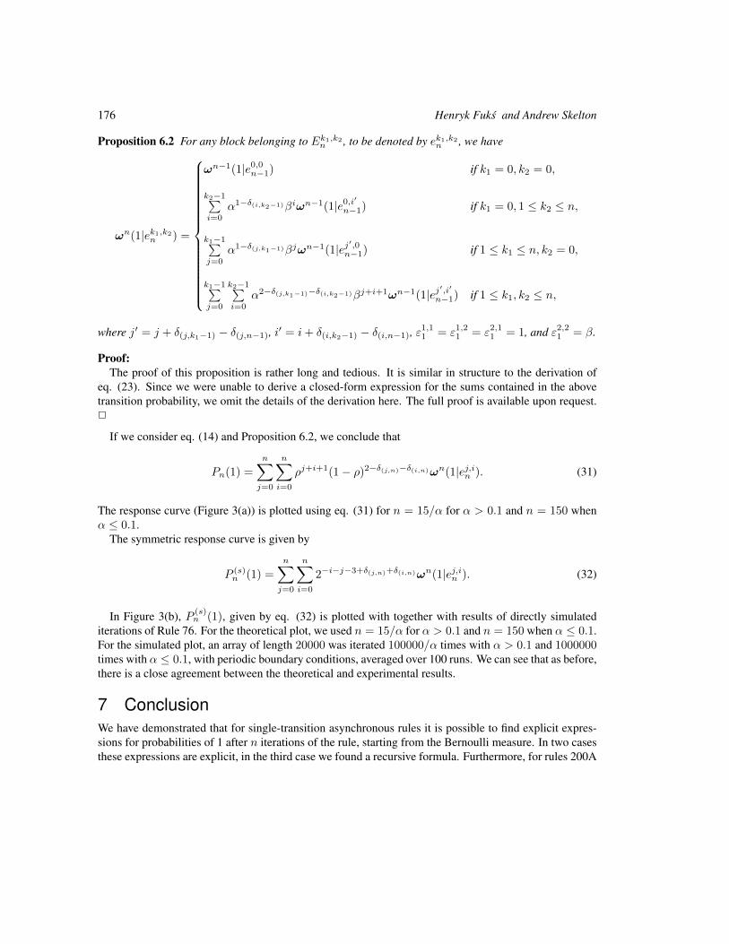
176 Henryk Fuks and Andrew Skelton
Proposition 6.2 For any block belonging to Ek1,k2n , to be denoted by ek1,k2n , we have
ωn(1|ek1,k2n ) =
ωn−1(1|e0,0n−1) if k1 = 0, k2 = 0,
k2−1∑i=0
α1−δ(i,k2−1)βiωn−1(1|e0,i′
n−1) if k1 = 0, 1 ≤ k2 ≤ n,
k1−1∑j=0
α1−δ(j,k1−1)βjωn−1(1|ej′,0n−1) if 1 ≤ k1 ≤ n, k2 = 0,
k1−1∑j=0
k2−1∑i=0
α2−δ(j,k1−1)−δ(i,k2−1)βj+i+1ωn−1(1|ej′,i′
n−1) if 1 ≤ k1, k2 ≤ n,
where j′ = j + δ(j,k1−1) − δ(j,n−1), i′ = i+ δ(i,k2−1) − δ(i,n−1), ε1,11 = ε1,21 = ε2,11 = 1, and ε2,21 = β.
Proof:The proof of this proposition is rather long and tedious. It is similar in structure to the derivation of
eq. (23). Since we were unable to derive a closed-form expression for the sums contained in the abovetransition probability, we omit the details of the derivation here. The full proof is available upon request.2
If we consider eq. (14) and Proposition 6.2, we conclude that
Pn(1) =
n∑j=0
n∑i=0
ρj+i+1(1− ρ)2−δ(j,n)−δ(i,n)ωn(1|ej,in ). (31)
The response curve (Figure 3(a)) is plotted using eq. (31) for n = 15/α for α > 0.1 and n = 150 whenα ≤ 0.1.
The symmetric response curve is given by
P (s)n (1) =
n∑j=0
n∑i=0
2−i−j−3+δ(j,n)+δ(i,n)ωn(1|ej,in ). (32)
In Figure 3(b), P (s)n (1), given by eq. (32) is plotted with together with results of directly simulated
iterations of Rule 76. For the theoretical plot, we used n = 15/α for α > 0.1 and n = 150 when α ≤ 0.1.For the simulated plot, an array of length 20000 was iterated 100000/α times with α > 0.1 and 1000000times with α ≤ 0.1, with periodic boundary conditions, averaged over 100 runs. We can see that as before,there is a close agreement between the theoretical and experimental results.
7 ConclusionWe have demonstrated that for single-transition asynchronous rules it is possible to find explicit expres-sions for probabilities of 1 after n iterations of the rule, starting from the Bernoulli measure. In two casesthese expressions are explicit, in the third case we found a recursive formula. Furthermore, for rules 200A
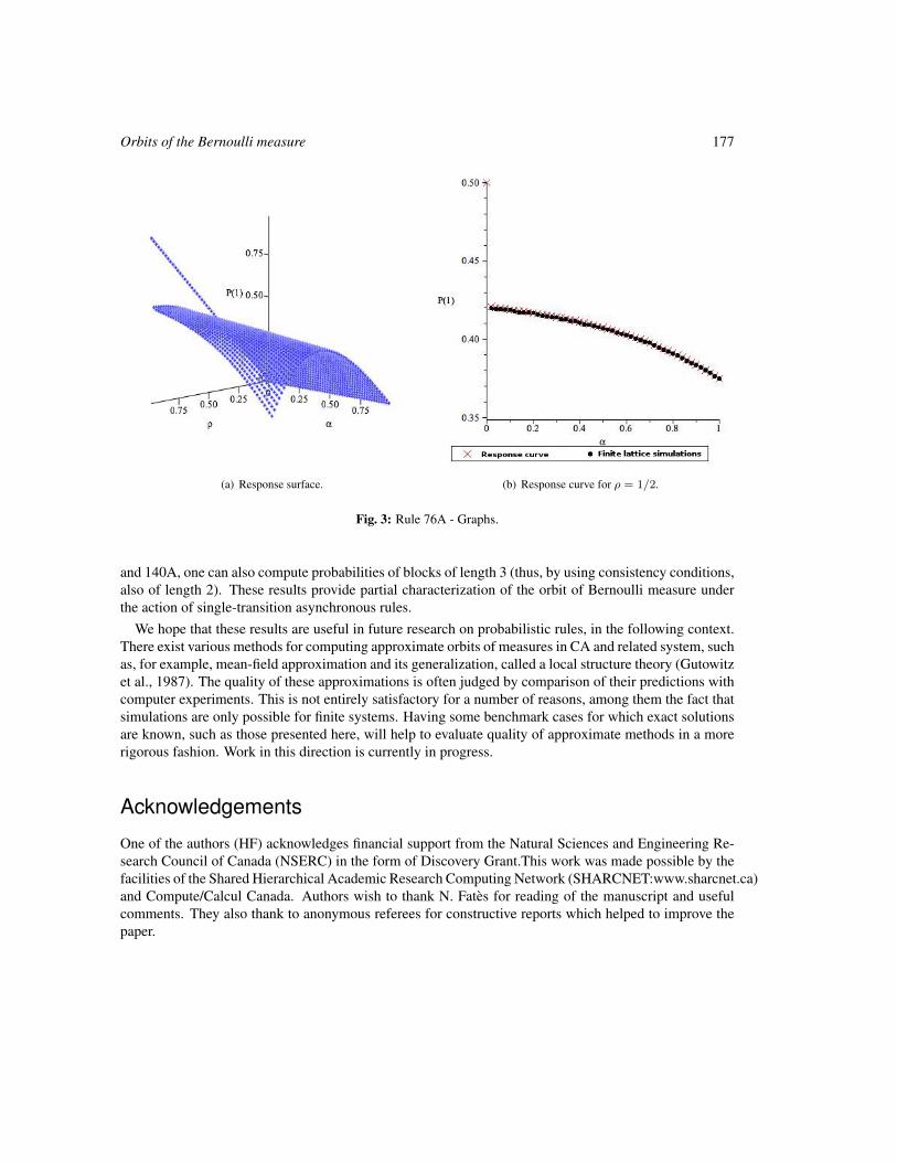
Orbits of the Bernoulli measure 177
(a) Response surface. (b) Response curve for ρ = 1/2.
Fig. 3: Rule 76A - Graphs.
and 140A, one can also compute probabilities of blocks of length 3 (thus, by using consistency conditions,also of length 2). These results provide partial characterization of the orbit of Bernoulli measure underthe action of single-transition asynchronous rules.
We hope that these results are useful in future research on probabilistic rules, in the following context.There exist various methods for computing approximate orbits of measures in CA and related system, suchas, for example, mean-field approximation and its generalization, called a local structure theory (Gutowitzet al., 1987). The quality of these approximations is often judged by comparison of their predictions withcomputer experiments. This is not entirely satisfactory for a number of reasons, among them the fact thatsimulations are only possible for finite systems. Having some benchmark cases for which exact solutionsare known, such as those presented here, will help to evaluate quality of approximate methods in a morerigorous fashion. Work in this direction is currently in progress.
Acknowledgements
One of the authors (HF) acknowledges financial support from the Natural Sciences and Engineering Re-search Council of Canada (NSERC) in the form of Discovery Grant.This work was made possible by thefacilities of the Shared Hierarchical Academic Research Computing Network (SHARCNET:www.sharcnet.ca)and Compute/Calcul Canada. Authors wish to thank N. Fates for reading of the manuscript and usefulcomments. They also thank to anonymous referees for constructive reports which helped to improve thepaper.
178 Henryk Fuks and Andrew Skelton
ReferencesV. Belitsky and P. A. Ferrari. Invariant measures and convergence properties for cellular automaton 184
and related processes. Journal of Statistical Physics, 118:589–623, 2005.
M. Blank. Ergodic properties of a simple deterministic traffic flow model. Journal of Statistical Physics,111:903–930, 2003.
N. Fates and M. Morvan. An experimental study of robustness to asynchronism for elementary cellularautomata. Complex Systems, 16:1–27, 2005.
N. Fates, D. Regnault, N. Schabanel, and E. Thierry. Asynchronous behavior of double-quiescent ele-mentary cellular automata. In J. Correa, A. A. Hevia, and M. Kiwi, editors, LATIN 2006: TheoreticalInformatics, volume 3887 of LNCS, pages 455–466, 2006.
E. Formenti and P. Kurka. Dynamics of cellular automata in non-compact spaces. In R. A. Meyers, editor,Encyclopedia of Complexity and System Science. Springer, 2009.
H. Fuks. Exact results for deterministic cellular automata traffic models. Phys. Rev. E, 60:197–202, 1999.
H. Fuks. Dynamics of the cellular automaton rule 142. Complex Systems, 16:123–138, 2006.
H. Fuks. Probabilistic initial value problem for cellular automaton rule 172. DMTCS proc., AL:31–44,2010.
H. A. Gutowitz, J. D. Victor, and B. W. Knight. Local structure theory for cellular automata. Physica D,28:18–48, 1987.
P. Kurka. On the measure attractor of a cellular automaton. Discrete and Continuous Dynamical Systems,pages 524 – 535, 2005.
P. Kurka. Topological dynamics of cellular automata. In R. A. Meyers, editor, Encyclopedia of Complexityand System Science. Springer, 2009.
P. Kurka and A. Maass. Limit sets of cellular automata associated to probability measures. Journal ofStatistical Physics, 100:1031–1047, 2000.
M. Pivato. Conservation laws in cellular automata. Nonlinearity, 15(6):1781, 2002.
M. Pivato. Ergodic theory of cellular automata. In R. A. Meyers, editor, Encyclopedia of Complexity andSystem Science. Springer, 2009.
AUTOMATA 2011, Santiago, Chile local proceedings LP, 2011, 179–188
Conservation Laws and Invariant Measures inSurjective Cellular Automata
Jarkko Kari1† and Siamak Taati2‡
1Department of Mathematics, University of Turku, Finland2Department of Mathematics, University of Groningen, the Netherlands
We discuss a close link between two seemingly different topics studied in the cellular automata literature: addi-tive conservation laws and invariant probability measures. We provide an elementary proof of a simple correspon-dence between invariant full-support Bernoulli measures and interaction-free conserved quantities in the case of one-dimensional surjective cellular automata. We also discuss a generalization of this fact to Markov measures andhigher-range conservation laws in arbitrary dimension. As a corollary, we show that the uniform Bernoulli measure isthe only shift-invariant, full-support Markov measure that is invariant under a strongly transitive cellular automaton.
Keywords: surjective cellular automata, conservation laws, invariant measures, statistical equilibrium
1 IntroductionLet Φ : SZ −→ SZ be a one-dimensional reversible cellular automaton, and let µ : S −→ R be a quantitythat is conserved by the evolution of Φ, in the sense that the average value of µ over any periodic config-uration remains constant with time. Since adding a constant to µ does not change the latter condition, wemay assume that µ is normalized in such a way that
∑s∈S 2−µ(s) = 1.
Suppose that the cells are initialized randomly and independently so that each state s ∈ S appearswith probability p(s) , 2−µ(s). In particular, if w = w1w2 · · ·wn is a word of length n over S, theprobability that n consecutive cells i + 1, i + 2, . . . , i + n take, respectively, the states w1, w2, . . . , wnis p(w) , p(w1)p(w2) · · · p(wn). There is a simple argument showing that p is a stationary distributionfor Φ; that is, after any number of iterations of Φ, the state of the cells remain independent and with thesame distribution p.
Namely, let u be a word of length l over S. If ϕ : Sk −→ S is the local update rule of Φ, then there are afinite number of words vi of length k+l such that ϕ(vi) = u. Let ci be the periodic configuration obtainedby repeating vi on positions . . . ,−(l+ k), 0, l+ k, . . .. The image of ci is a periodic configuration ei thatis a repetition of a word of the form xi u yi on positions . . . ,−(l + k), 0, l + k, . . .. Conservation of µimplies that
µ(vi) = µ(xi) + µ(u) + µ(yi) . (1)
†Email: [email protected]. Research supported by the Academy of Finland Grant 131558.‡Email: [email protected].
c© 2011 AUTOMATA proceedings, Santiago, Chile, 2011
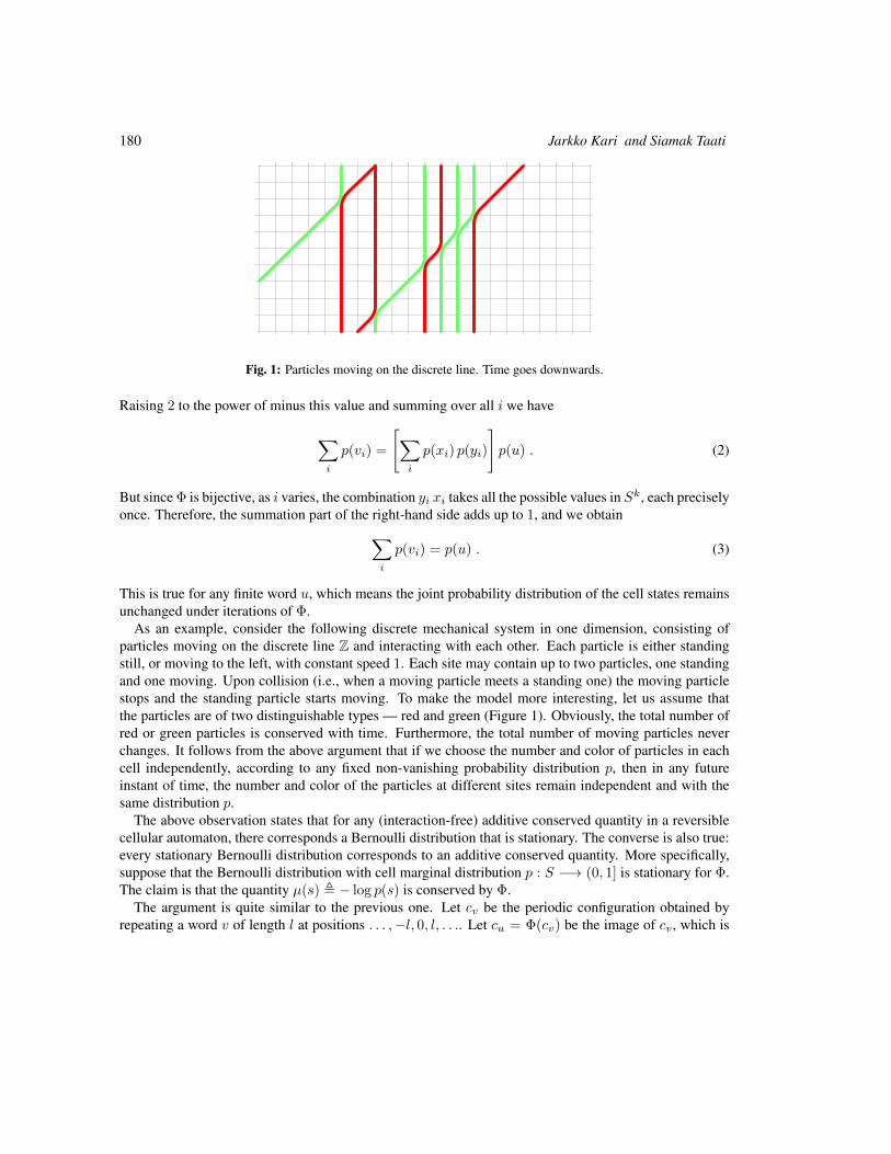
180 Jarkko Kari and Siamak Taati
Fig. 1: Particles moving on the discrete line. Time goes downwards.
Raising 2 to the power of minus this value and summing over all i we have
∑i
p(vi) =
[∑i
p(xi) p(yi)
]p(u) . (2)
But since Φ is bijective, as i varies, the combination yi xi takes all the possible values in Sk, each preciselyonce. Therefore, the summation part of the right-hand side adds up to 1, and we obtain∑
i
p(vi) = p(u) . (3)
This is true for any finite word u, which means the joint probability distribution of the cell states remainsunchanged under iterations of Φ.
As an example, consider the following discrete mechanical system in one dimension, consisting ofparticles moving on the discrete line Z and interacting with each other. Each particle is either standingstill, or moving to the left, with constant speed 1. Each site may contain up to two particles, one standingand one moving. Upon collision (i.e., when a moving particle meets a standing one) the moving particlestops and the standing particle starts moving. To make the model more interesting, let us assume thatthe particles are of two distinguishable types — red and green (Figure 1). Obviously, the total number ofred or green particles is conserved with time. Furthermore, the total number of moving particles neverchanges. It follows from the above argument that if we choose the number and color of particles in eachcell independently, according to any fixed non-vanishing probability distribution p, then in any futureinstant of time, the number and color of the particles at different sites remain independent and with thesame distribution p.
The above observation states that for any (interaction-free) additive conserved quantity in a reversiblecellular automaton, there corresponds a Bernoulli distribution that is stationary. The converse is also true:every stationary Bernoulli distribution corresponds to an additive conserved quantity. More specifically,suppose that the Bernoulli distribution with cell marginal distribution p : S −→ (0, 1] is stationary for Φ.The claim is that the quantity µ(s) , − log p(s) is conserved by Φ.
The argument is quite similar to the previous one. Let cv be the periodic configuration obtained byrepeating a word v of length l at positions . . . ,−l, 0, l, . . .. Let cu = Φ(cv) be the image of cv , which is
Conservation Laws and Invariant Measures in Surjective Cellular Automata 181
again a repetition of a word u of length l at positions . . . ,−l, 0, l, . . .. For an integer n > 0, consider theword un. Since Φ is injective, the pre-images of un under ϕ are words of the form xi v
n−2 yi. (That is,each of the pre-images has several copies of v in the middle and constant-size turbulence on the borders.We have assumed that l is sufficiently large.) Since p is stationary, we have
p(un) =∑i
p(xi vn−2 yi) , (4)
or
p(u)n =
[∑i
p(xi) p(yi)
]p(v)n−2 . (5)
Taking the logarithm on both sides, dividing by n, and letting n −→∞ we obtain that
µ(u) = µ(v) . (6)
This is the case, for any periodic configurations cv and cu = Φ(cv), which means that µ is conservedby Φ.
It turns out that the above correspondence between conserved quantities and stationary Bernoulli dis-tributions generalizes to any number of dimensions. The cellular automaton is merely required to be sur-jective. Finally, the conserved quantity may involve contributions from the interactions between nearbycells, in which case the corresponding probability distribution becomes a Markov measure.
This property can be proved using the variational principle of equilibrium statistical mechanics and theproperties of the pre-injective factor maps on strongly irreducible shifts of finite type. It can be seen as ageneralization of the balance property of the surjective cellular automata.
In the present paper we give an elementary proof of the correspondence between conserved quantitiesand stationary Bernoulli distributions in surjective one-dimensional cellular automata. We also state thegeneral theorem, but the complete proof will appear elsewhere [KT]. In Section 5, we provide an exampleof how this theorem allows us to transmit results concerning conservation laws over to invariant measures.
2 Preliminaries2.1 One-dimensional cellular automataLet S be a finite set of states. A one-dimensional cellular automaton (CA) over S is a translation com-muting continuous map Φ : SZ −→ SZ. Equivalently, according to the Curtis-Hedlund-Lyndon theo-rem [Hed69], Φ is defined by a parallel application of a local rule f : S2r+1 −→ S at all sites, where r isthe neighborhood radius of Φ: for every c ∈ SZ and every i ∈ Z,
Φ(c)i = f(ci−r, ci−r+1, . . . , ci+r).
Elements of SZ are the configurations of the CA. For any word u ∈ Sl of length l ≥ 1, we denote by ωuω
the periodic configuration in which the word u is repeated, starting in positions . . . ,−l, 0, l, 2l, . . ..A cylinder determined by word u and position i ∈ Z is the set
[u]i , c ∈ SZ | cici+1 . . . ci+|u|−1 = u
182 Jarkko Kari and Siamak Taati
of configurations that contain word u, starting in position i. Cylinders form a basis of the standard topol-ogy we use on SZ. Many concepts we consider are indifferent to the exact position i of the cylinder, andin those cases we use the simpler notation [u]. This can be interpreted as any [u]i; for example as [u]0.
A cellular automaton Φ is injective, surjective or bijective if it is one-to-one, onto or a bijection, re-spectively, as a function SZ −→ SZ. A cellular automaton Φ is called reversible if it is bijective and itsinverse is a cellular automaton. It follows from the compactness of SZ that every bijective CA is, in fact,reversible.
Two configurations c, e ∈ SZ are asymptotic if the difference set i ∈ Z | ci 6= ei is finite. A CA Φis called pre-injective if for any asymptotic configurations c, e holds that c 6= e =⇒ Φ(c) 6= Φ(e). Thecelebrated Garden-of-Eden theorem by E. F. Moore and J. Myhill states that Φ is surjective if and onlyif it is pre-injective [Moo62, Myh63]. It then directly follows that every injective CA is also surjective.We see that injectivity, bijectivity and reversibility are equivalent concepts on cellular automata, and theyimply surjectivity which is equivalent to pre-injectivity.
Let Φ be defined by a radius-r local rule. The local rule can be applied on finite words in a natural way,so that it defines functions Sk+2r −→ Sk for every k. We use the same symbol Φ also for these functionson words.
All surjective CA have the following balance property [Hed69]. Every word u of length k has preciselyN , |S|2r pre-images v1, v2 . . . , vN ∈ Sk+2r under the function Φ : Sk+2r −→ Sk. In terms ofcylinders this means that the pre-image of every cylinder [u]i determined by u ∈ Sk is the disjoint unionof the N cylinders [v1]i−r, [v2]i−r, . . . , [vN ]i−r determined by words vj of length k + 2r.
2.2 Conserved quantitiesLet µ : S −→ R be an assignment of real numbers to the states. For a word v ∈ S∗ we define µ(v) ,µ(v1) + µ(v2) + . . . + µ(vk), where v = v1v2 . . . vk and vi ∈ S. Function µ is an (interaction-free)additive quantity.
A cellular automaton Φ : SZ −→ SZ conserves µ if for every u, v ∈ Sk such that Φ(ωuω) = ωvω
holdsµ(u) = µ(v).
In other words, we require the (well defined) average value over periodic configurations to remain un-changed under the application of Φ. Other equivalent characterizations exist (see e.g. [HT91, Piv02,DFR03, MBG04]). In particular, there are simple algorithms for verifying whether a given cellular au-tomaton conserves a given additive quantity. For the proofs we present here, the above characterizationusing periodic configurations is most convenient.
Conserved quantities play an important role in physics, and the concept has been studied in the contextof cellular automata by several authors (see e.g. [HT91, BF98, Piv02, DFR03, FG03, MBG04, Ber07,FKTar]).
2.3 Invariant Bernoulli measuresLet p : S −→ R be a probability distribution on the state set, so that
∑s∈S p(s) = 1. The Bernoulli
distribution determined by p is the probability distribution of a random configuration c ∈ SZ if thevalues ci, for i ∈ Z, are chosen randomly and independently, each with distribution p. It is identified bya Borel probability measure π that assigns probability π([v]) , p(v1)p(v2) . . . p(vk) to each cylinder [v],
Conservation Laws and Invariant Measures in Surjective Cellular Automata 183
where v = v1v2 · · · vk and vi ∈ S. The measure π is translation-invariant. We only consider the casewhere p(s) > 0 for all s ∈ S, which is equivalent to requiring that the Bernoulli measure π is full-support.
A Borel measure π is invariant (or stationary) under a cellular automaton Φ if for all cylinders [u] holdsπ([u]) = π(Φ−1([u])). This means that π is a fixed point of the mapping η 7→ Φ(η) where Φ(η) is thedistribution of the configuration Φ(c) if configuration c is chosen randomly according to η.
The balance property of surjective CA can now be rephrased as follows: the uniform Bernoulli measureis invariant under all surjective CA.
The presence of natural invariant measures allows one to study CA as measure-preserving dynamicalsystems, applying results from ergodic theory (see e.g. [Wal82, Lin84, Piv09]). For instance, knowingthe invariance of the uniform Bernoulli measure, one can apply Poincare’s recurrence theorem to inferthat iterating a surjective CA on a uniformly random initial configuration, almost surely each finite wordappearing in the initial configuration reappears infinitely many times on the same position.
3 A correspondence of conserved quantities and invariant mea-sures on one-dimensional surjective CA
In this section, we state and give an elementary proof for a correspondence between (interaction-free)conserved quantities and invariant, full-support Bernoulli measures on surjective, one-dimensional CA.The balance property is a special case of our theorem, so it is not surprising that the proof is similar to astandard proof of the balance property. The second part of the proof was essentially presented in [Taa09]in a more general set-up.
Theorem 1 Let Φ : SZ −→ SZ be a one-dimensional surjective cellular automaton over state set S =s1, s2, . . . , sn, and let p1, p2, . . . , pn be n positive numbers such that p1 + p2 + . . .+ pn = 1. Let π bethe Bernoulli distribution on SZ defined by π(si) , pi for all i, and let µ be the additive quantity definedby µ(si) , − log pi. Then, π is invariant under Φ if and only if Φ conserves µ.
Proof: The base of the logarithm does not matter — we use base 2 in the proof. Let Φ be defined by aradius-r local rule. Recall that Φ denotes both the CA function and the word functions Sk+2r −→ Sk.Observe also the correspondence
π([v]) = 2−µ(v)
for all words v ∈ S∗.(⇐=) Assume that Φ conserves the quantity µ. Let us first prove that there are positive constants mand M , independent of k, such that for all words v ∈ Sk+2r and for u , Φ(v) ∈ Sk holds
m ≤ π([v])/π([u]) ≤M. (7)
Indeed, let x, y ∈ Sr be the words such that Φ(ωvω) = ω(xuy)ω . Then, due to the conservation of µby Φ, we have that µ(v)− µ(u) = µ(xy). Hence
c ≤ µ(v)− µ(u) ≤ C (8)
for constants c , 2r ·minµ(s) | s ∈ S and C , 2r ·maxµ(s) | s ∈ S. Raising two to the negativepowers of the different sides of (8) gives
2−c ≥ π([v])/π([u]) ≥ 2−C ,
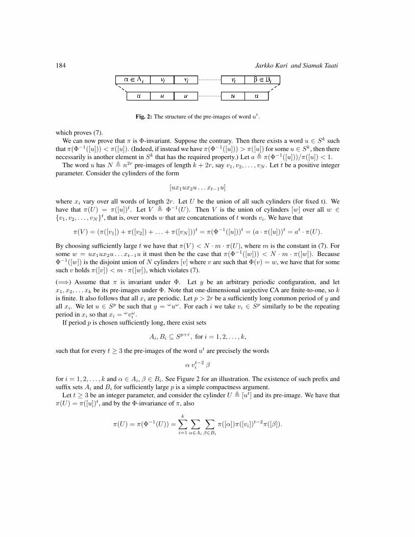
184 Jarkko Kari and Siamak Taati
Fig. 2: The structure of the pre-images of word ut.
which proves (7).We can now prove that π is Φ-invariant. Suppose the contrary. Then there exists a word u ∈ Sk such
that π(Φ−1([u])) < π([u]). (Indeed, if instead we have π(Φ−1([u])) > π([u]) for some u ∈ Sk, then therenecessarily is another element in Sk that has the required property.) Let a , π(Φ−1([u]))/π([u]) < 1.
The word u has N , n2r pre-images of length k + 2r, say v1, v2, . . . , vN . Let t be a positive integerparameter. Consider the cylinders of the form
[ux1ux2u . . . xt−1u]
where xi vary over all words of length 2r. Let U be the union of all such cylinders (for fixed t). Wehave that π(U) = π([u])t. Let V , Φ−1(U). Then V is the union of cylinders [w] over all w ∈v1, v2, . . . , vNt, that is, over words w that are concatenations of t words vi. We have that
π(V ) = (π([v1]) + π([v2]) + . . .+ π([vN ]))t = π(Φ−1([u]))t = (a · π([u]))t = at · π(U).
By choosing sufficiently large t we have that π(V ) < N ·m · π(U), where m is the constant in (7). Forsome w = ux1ux2u . . . xt−1u it must then be the case that π(Φ−1([w])) < N · m · π([w]). BecauseΦ−1([w]) is the disjoint union of N cylinders [v] where v are such that Φ(v) = w, we have that for somesuch v holds π([v]) < m · π([w]), which violates (7).
(=⇒) Assume that π is invariant under Φ. Let y be an arbitrary periodic configuration, and letx1, x2, . . . xk be its pre-images under Φ. Note that one-dimensional surjective CA are finite-to-one, so kis finite. It also follows that all xi are periodic. Let p > 2r be a sufficiently long common period of y andall xi. We let u ∈ Sp be such that y = ωuω . For each i we take vi ∈ Sp similarly to be the repeatingperiod in xi so that xi = ωvωi .
If period p is chosen sufficiently long, there exist sets
Ai, Bi ⊆ Sp+r, for i = 1, 2, . . . , k,
such that for every t ≥ 3 the pre-images of the word ut are precisely the words
α vt−2i β
for i = 1, 2, . . . , k and α ∈ Ai, β ∈ Bi. See Figure 2 for an illustration. The existence of such prefix andsuffix sets Ai and Bi for sufficiently large p is a simple compactness argument.
Let t ≥ 3 be an integer parameter, and consider the cylinder U , [ut] and its pre-image. We have thatπ(U) = π([u])t, and by the Φ-invariance of π, also
π(U) = π(Φ−1(U)) =
k∑i=1
∑α∈Ai
∑β∈Bi
π([α])π([vi])t−2π([β]).
Conservation Laws and Invariant Measures in Surjective Cellular Automata 185
Dividing by π(U) = π([u])t gives
1 =
k∑i
ci
(π([vi])
π([u])
)t,
whereci ,
∑α∈Ai
∑β∈Bi
π([α])π([β])π([vi])−2
are independent of t.The following obvious fact now implies that π([vi]) = π([u]): if positive numbers c1, . . . , ck and
z1, . . . zk satisfy1 = c1z
t1 + . . .+ ckz
tk
for all t = 3, 4, . . ., then necessarily all zi = 1.It follows from π([vi]) = π([u]) that µ(vi) = − log π([vi]) = − log π([u]) = µ(u). This proves the
conservation of µ on periodic configurations.2
4 GeneralizationTheorem 1 can be generalized in several directions. First, suppose that rather than a Bernoulli distribution,π is the distribution of a bi-infinite Markov chain with memory m, given by the transition probabilitiesP (au, ub) for every a, b ∈ S and u ∈ Sm−1. That is, we have π([waub]0 | [wau]0) = P (au, ub) forevery a, b ∈ S, u ∈ Sm−1 and w ∈ S∗. Assuming that all the transition probabilities P (au, ub) arenon-zero, we can define an additive quantity of range m+ 1 by µ(aub) , − logP (au, ub). The averagevalue of µ on a periodic configuration x is defined to be the (well defined) average value of µ on thewords seen through a window of widthm+1 that slides over x, and we say that µ is conserved by cellularautomaton Φ : SZ −→ SZ if the average value of µ on x and Φ(x) are the same for all periodic x. Forevery surjective cellular automaton Φ, it can then be shown that π is invariant under Φ if and only if Φconserves µ.
In higher dimensions, Theorem 1 remains valid as is, relating the invariance of Bernoulli distributionsunder surjective cellular automata and the conservation of range-1 additive quantities.
To state the theorem in its full generality (arbitrary dimensions, arbitrary finite range) we need fewdefinitions. Let d ≥ 1. Let W ⊆ Zd be a finite set. An additive quantity with interaction window W isgiven by an assignment µ : SW −→ R of real numbers to patterns over W . If x ∈ SZd
is a configurationandD ⊆ Zd a finite set, let us define µD(x) as follows: we slide the windowW over x along the elementsof D and sum the values of µ over the patterns seen. That is, µD(x) ,
∑i∈D µ((σix)|W ), where σix
denotes the translation of x by i, and (σix)|W the restriction of σix to W . As before, we can say that ad-dimensional cellular automaton Φ : SZd −→ SZd
conserves µ if µD(Φ(x)) = µD(x) for every finitehypercube D and every periodic configuration x with fundamental domain D.
A Gibbs measure corresponding to µ is a Borel probability measure π satisfying
π([y]D) = 2−(µD(y)−µD(x))π([x]D) , (9)
for every two asymptotic configurations x, y ∈ SZd
and all sufficiently large finite sets D ⊆ Zd. Here,[x]D denotes the cylinder of all configurations that agree with x on D. The set D should be taken large
186 Jarkko Kari and Siamak Taati
enough so that for every i /∈ D, the configurations x and y cannot be distinguished by looking throughthe translated window i+W ; that is, x|i+W = y|i+W .
The Gibbs measures (as defined above) coincide with the full-support Markov measures (seee.g. [Pre74, Geo88]). In particular, the one-dimensional Gibbs measures are precisely the distributionsof Markov chains with positive transition probabilities. However, in higher dimensions, the Gibbs mea-sure corresponding to an additive quantity is not necessarily unique. While it can be shown that for everyadditive quantity there corresponds at least one Gibbs measure, distinct Gibbs measures could satisfy (9)for the same µ. In statistical mechanics, Gibbs measures are used to describe the state of a system inthermal equilibrium. The multiplicity of Gibbs measures is then interpreted as the possibility of distinctequilibrium states at the same temperature (e.g., water vs. gas). See [Geo88, Pre74, KS80] for details andexamples.
Theorem 2 Let Φ : SZd −→ SZd
be a d-dimensional surjective cellular automaton. Let µ be an additivequantity on SZd
, and let Gσ(µ) denote the set of translation-invariant Gibbs measures corresponding to µ.Then, the following conditions are equivalent:
a) Φ conserves µ.
b) Φ maps Gσ(µ) onto itself.
c) There exists an element of Gσ(µ) whose Φ-image is also in Gσ(µ).
The proof will appear in [KT].
5 Strongly Transitive Cellular AutomataIn this section we give an example of how Theorem 2 can be used to transmit results between conservationlaws research and invariant measures.
A cellular automaton Φ : SZd −→ SZd
is strongly transitive if the backward orbit⋃∞i=0 Φ−i(c) of
every configuration c ∈ SZd
is dense in SZd
. Equivalently, Φ is strongly transitive if for every non-emptycylinder U ⊆ SZd
, the forward orbit⋃∞i=0 Φi(U) is the whole configuration space SZd
. A stronglytransitive CA is clearly surjective, and all positively expansive CA are strongly transitive.
Every CA has trivial conserved quantities: we call a quantity µ trivial if it assigns the same averagevalue to all periodic configurations. For example, the interaction-free constant valuation (µ(s) = 1 forall s ∈ S) is trivial. According to (9), the uniform Bernoulli measure is the unique Gibbs measure thatcorresponds to trivial conserved quantities.
The following theorem states that strongly transitive cellular automata only satisfy the trivial conserva-tion laws.
Theorem 3 ([FKTar]) Let Φ : SZd −→ SZd
be a strongly transitive cellular automaton. Then Φ doesnot conserve any non-trivial additive quantities.
Theorems 2 and 3 now immediately give the following result:
Corollary 4 Let Φ : SZd −→ SZd
be a strongly transitive cellular automaton. The uniform Bernoullimeasure is the only translation-invariant Gibbs measure that is invariant under Φ.
Conservation Laws and Invariant Measures in Surjective Cellular Automata 187
References[Ber07] Vincent Bernardi. Lois de conservation sur automates cellulaires. PhD thesis, Universite de
Provence, 2007.
[BF98] Nino Boccara and Henryk Fuks. Cellular automaton rules conserving the number of activesites. Journal of Physics A: Mathematical and General, 31(28):6007–6018, 1998.
[DFR03] Bruno Durand, Enrico Formenti, and Zsuzsanna Roka. Number conserving cellular automataI: decidability. Theoretical Computer Science, 299:523–535, 2003.
[FG03] Enrico Formenti and Aristide Grange. Number conserving cellular automata II: dynamics.Theoretical Computer Science, 304:269–290, 2003.
[FKTar] Enrico Formenti, Jarkko Kari, and Siamak Taati. On the hierarchy of conservation laws in acellular automaton. Natural Computing, To appear.
[Geo88] Hans-Otto Georgii. Gibbs Measures and Phase Transitions. Walter de Gruyter, 1988.
[Hed69] G. A. Hedlund. Endomorphisms and automorphisms of the shift dynamical system. Mathe-matical System Theory, 3:320–375, 1969.
[HT91] Tetsuya Hattori and Shinji Takesue. Additive conserved quantities in discrete-time lattice dy-namical systems. Physica D, 49:295–322, 1991.
[KS80] Ross Kindermann and J. Laurie Snell. Markov Random Fields and Their Applications. Amer-ican Mathematical Society, 1980.
[KT] Jarkko Kari and Siamak Taati. In preparation.
[Lin84] D. A. Lind. Applications of ergodic theory and sofic systems to cellular automata. Physica D:Nonlinear Phenomena, 10(1–2), 1984.
[MBG04] Andres Moreira, Nino Boccara, and Eric Goles. On conservative and monotone one-dimensional cellular automata and their particle representation. Theoretical Computer Science,325:285–316, 2004.
[Moo62] Edward F. Moore. Machine models of self-reproduction. In Proceedings of Symposia inApplied Mathematics, pages 17–33. AMS, 1962.
[Myh63] John Myhill. The converse of Moore’s Garden-of-Eden theorem. Proceedings of the AmericanMathematical Society, 14:685–686, 1963.
[Piv02] Marcus Pivato. Conservation laws in cellular automata. Nonlinearity, 15:1781–1793, 2002.
[Piv09] Marcus Pivato. The ergodic theory of cellular automata. In Encyclopedia of Complexity andSystem Science. Springer, 2009.
[Pre74] Christopher J. Preston. Gibbs states on countable sets. Cambridge University Press, 1974.

188 Jarkko Kari and Siamak Taati
[Taa09] Siamak Taati. Conservation Laws in Cellular Automata. PhD thesis, University of Turku,2009.
[Wal82] Peter Walters. An Introduction to Ergodic Theory. Springer-Verlag, 1982.
AUTOMATA 2011, Santiago, Chile local proceedings LP, 2011, 189–200
Projective subdynamics and universal shifts
Pierre Guillon12†
1CMM, Universidad de Chile2CNRS & IML, Marseille, France
We study the projective subdynamics of two-dimensional shifts of finite type, which is the set of one-dimensionalconfigurations that appear as columns in them. We prove that a large class of one-dimensional shifts can be obtainedas such, namely the effective subshifts which contain positive-entropy sofic subshifts. The proof involves somesimple notions of simulation that may be of interest for other constructions. As an example, it allows us to prove theundecidability of all non-trivial properties of projective subdynamics.
Keywords: multidimensional symbolic dynamics, effective dynamics, tilings, simulation, undecidability
1 IntroductionComputation in dynamical systems has shown an increasing interest in the last decade. One of the ques-tions that arises is the computational power of some models defined dynamically, where the computationresult is seen as the “trace” of the system evolution or (equivalently) as a smaller system that it dynam-ically simulates. For cellular automata, this can be the limit set [Hur87, Maa95] or the column factors[Kur97, CFG07]. For general effective dynamical systems, this can be observation problems with respectto some partitions [DKB05].
The setting of multidimensional symbolic dynamics is one of the most natural and elegant models withfull computational power, as suggested by more recent results [Hoc09a, DRS10, AS10]. These works canbe interpreted both as taking shifts of finite type as a model and subaction projections as a computingprocess or sofic shifts as a model and projective subdynamics as a process.
Independently, [PS10] presents some realization constructions as well as impossibility results in theweaker, yet natural case of projective subdynamics of shifts of finite type. Here, we also prove in thissetting the constructability of a large class of effective shifts. To achieve this, we connect the problem tosome simple notions of simulations over shifts.
Section 2 is devoted to the main definitions; Section 3 defines simulation and characterizes universality;Section 4 defines the main concept of the article, that of projective subdynamics, and recalls the knowncharacterization in the sofic case; Section 5 introduces the intermediary notion of polyfactor, and gives aconstruction of it in the SFT case; Section 6 simulates it as projective subdynamics of SFT; finally Section7 presents an independent application of the construction by proving a “Rice theorem” over projectivesubdynamics.
†Email: [email protected]. This article has been written mainly during a postdoctoral project supportedby ECOS-Sud.
c© 2011 AUTOMATA proceedings, Santiago, Chile, 2011
190 Pierre Guillon
2 PreliminariesWe note Ji, jK the set of integers i, i+ 1, . . . , j, and Ji, jJ= Ji, j − 1K. We also define N1 = N \ 0.
Let A be an alphabet (with 2 ≤ |A| <∞) and d ∈ N1 the dimension. A shape is a subset K b Zd, i.e.,K ⊂ Zd and |K| <∞. A pattern is a finite d-dimensional word u = (ui)i∈K ∈ AK , where K b Zd. Aconfiguration is an infinite one x = (xi)i∈Zd ∈ AZd
. For any K ⊂ Zd and any configuration x ∈ AZd
,we note xK its restriction to K.
A dynamical system is a compact metric space X , on which some group G acts continuously. The fullZd-shift on alphabet A is the set of d-dimensional configurations x ∈ AZd
, endowed with the product ofthe discrete topology, and with the action σ of Zd defined for any c, i ∈ Zd by σc(x)i = xc+i. We willmainly deal with subsystems of this, i.e., closed subsets Σ ⊂ AZd
such that σc(Σ) = Σ for any c ∈ Zd,which will be refered to as Zd-shifts.
Equivalently, a Zd-shift is a set Σ ⊂ AZd
of configurations defined via a collection of finite forbiddenpatterns F , in the sense that Σ =
x ∈ AZd
∣∣∣∀c ∈ Zd,∀K b Zd, σc(x)K /∈ F
. Σ is of finite type (SFT)if F can be taken finite, effective if F can be taken recursively enumerable.
The topological closure of the orbit⋃c∈Zd σc(Z) of Z ⊂ AZd
will be denoted Z. For instance, indimension 1, a word u shall be seen as a map i 7→ ui from J0, |u| J to alphabet A. Then ∞u∞ will denotethe set
z ∈ AZ
∣∣ ∃k ∈ J0, |u| J,∀j ∈ Z, σk+j|u|(z)J0,|u|J = u
of configurations periodically equal to u.If Σ is a Z-shift over alphabetA, its language of shapeK b Zd is the set LK(Σ) = zK | z ∈ Σ of ex-
tendable patterns for this shape. These languages completely characterize Σ; moreover, by compactness,if Σ,Λ are two disjoint Z-shifts, then there exists a finite shape K b Zd such that LK(Σ) ∩ LK(Λ) = ∅.
We will actually essentially deal with Z2-shifts, but the generalization to higher dimensions is obvious.
3 SimulationsWe define here some operations over shifts that can be seen as simulation rules, and which will help us tomake constructions in the next sections. Similar compositions of operations have been recently studied invarious settings [AS09, Hoc09b].
Let X and Y be dynamical systems corresponding to actions of the same group Zd, noted γc : X → Xand δc : Y → Y for c ∈ Zd. We note X f Y if there is a factor map Φ : X → Y , i.e., an ontocontinuous map such that Φγc = δcΦ for any c ∈ Zd; Y is then called a factor of X , and if Φ is bijective,X and Y are called conjugate. We note X i Y if the action δ on Y is conjugate to the action γk onX for some power k ∈ Nd1, where (γk)c = γkc for any c ∈ Zd (and coordinatewise multiplication ofvectors). We note X s Y if, up to conjugacy, Y ⊂ X and δ is the restriction of γ to Y .
Let Σ and Γ be Zd-shifts over alphabets A and B, respectively. The previously-defined simulationscan be visualized in a symbolic way. First note that Σ i Γ means that Γ is essentially the bulkingΣ[K] =
(σKj(x)K)j∈Zd
∣∣x ∈ Σ
(with coordinatewise multiplication) of Σ for some interval productK b Zd, which is a shift over alphabet AK . It can also be seen that for any nonempty K b Zd, Σis conjugate to its K-block representation Σ(K) =
(σi(x)K)i∈Zd
∣∣x ∈ Σ
, which is a Zd-shift overalphabet AK . A particular class of shift factor maps is that of parallelizations Φ : Σ → Γ of alphabetprojections Φ : A → B, i.e., Φ(x)i = Φ(xi) for any x ∈ Σ and i ∈ Zd. It is also known that Σ f Γ
if and only if Γ = Φ(Σ(K)) for some shape K b Zd and some parallel application Φ of some alphabetprojection Φ : AK → B.
Projective subdynamics and universal shifts 191
Γ is called a Zd-sofic if it is a factor of a Zd-SFT. Equivalently from the last point, it is sofic if andonly if it is the image of a Zd-SFT by some parallelization map. The classes of SFT, sofic shifts andeffective shifts are closed under conjugacy, bulking and block representations. By the characterizationabove, that of sofic shifts is also closed under factor. On the contrary, s does not preserve any relevantproperty, which is why the simulation notion below will be very weak (it can be strengthened by taking theintersection with some SFT [AS09]); this will allow us to deal with a rather simple notion of universality,but will be compensated by the fact that our simulating shifts already have some structure (PSD in 9).
If z : I × J → A, for some intervals I and J of Z and i ∈ I , then we note πi(z) = (zi,j)j∈J . IfI = J0,mJ and J = Z, it gives a factor map πi from any Z-shift over alphabet Am onto some Z-shiftover alphabet A. We also note πI′(z) = ((zi,j)i∈I′)j∈J if I ′ ⊂ I .
The product X × Y of two sets X ∈ AZd
and Y ∈ BZd
will be abusively assimilated to thesetw = (xi, yi)i∈Zd) ∈ (A×B)Z
d∣∣∣ (xi)i∈Zd ∈ X and (yi)i∈Zd ∈ Y
(which is a Zd-shift if X and
Y are). We note X<1> = X and X<n+1> = X<n> × X for n ∈ N. Essentially, X<n> =y ∈ (An)Z
d∣∣∣ ∀j ∈ J0, nJ, πj(y) ∈ X
. We note Σ p Γ if Γ is conjugate to some subshift of Σ<n> for
some power n ∈ N.Each of these relations are not that interesting intrinsically, but can be associated together; the com-
positions will be noted ps, ifs, pfs, etc. . . We can see, thanks to some commutation properties, thatthey are transitive whenever i and p are applied before s.
We say that a Z-shift Σ is universal if it simulates any other Z-shift Γ in the sense that Σ is Γ. Thisproperty is easily understood in the sofic case: indeed, uncountable Z-sofic are exactly those that havepositive entropy, and they can be represented on a graph with a non-cyclic strongly connected component(equivalently, they include some infinite transitive subshift).
Proposition 1 Let Σ be a Z-shift. The following statements are equivalent:
1. Σ includes some positive-entropy sofic subshift.
2. There are two words u and v with u0 6= v0, |u| = |v|, and ∞u, v∞ ⊂ Σ.
3. Σ is 0, 1Z.
4. Σ is universal.
Proof:
1⇒2 If Σ includes a positive-entropy sofic subshift, then the graph of this subshift contains a non-cyclicstrongly connected component, i.e., there exists a vertex from which two arcs leave with two distinctlabels, and which start paths that come back to the same vertex. Denoting u, v the labels of thesetwo paths, we can see that u = u|v| and v = v|u| satisfy the wanted conditions.
2⇒3 The J0, |u| J-bulking of ∞u, v∞ is a subshift that includes the full shift over alphabet u, v,which is essentially 0, 1Z.
3⇒1 Remark that a non-trivial full shift is sofic and has positive entropy, as well as any of its iterations.
192 Pierre Guillon
3⇒4 For any Z-shift Σ on some alphabet A, we have 0, 1Z i AZ s Σ, since the letters of A are inbijection with some subset of 0, 1dlog|A|e. Hence the full shift itself is universal, and the notionsof simulation are transitive.
4⇒3 This is by definition of universality.
2
In particular, the class of universal shifts is preserved by closing factor maps. Note that dealing withsimulation ifs instead may widen the notion of universality to other subshifts. For our purpose though,this notion would be difficult to handle in the following.
Clock. Let Cn denote the n-cycle, i.e., the dynamical system J0, nJ on which Z acts by i 7→ i+c mod nfor any c ∈ Z.
We have seen a definition of simulation that involves temporal delay, and one that involves spacialsprawl. The following lemma gives a transformation from the former to the latter.
Lemma 2 If Γ is a Z-shift,AZ a full shift and n ∈ N such that Γ[J0,nJ] fs AZ, then Cn×Γ<n> fs AZ.
Proof: Let Λ ⊂ Γ be closed and σn-invariant, and Φ : Λ → AZ such that Φσn = σΦ. Let Λ′ =(i, y) ∈ J0, nJ×Γ<n>
∣∣∀j ∈ J0, nJ, πj(y) ∈ σj−i mod n(Γ)
.
Ψ : Λ′ → AZ
(i, y) 7→ (Φ(σj(πi+j mod n(y)))0)j∈Z
is also a factor map, since for any (i, y) ∈ Γ′, we have:
Φ(i+ 1 mod n, σ(y)) = (Φ(σj+1(πi+1+j mod n(y)))0)j∈Z = σ(Φ(i, y0, . . . , yn−1)) .
Moreover, Ψ is onto AZ since, if z ∈ AZ, for 0 ≤ i < n, the surjectivity of Φ and σ gives some yi ∈ Ysuch that Φ(σn(yi)) = (znj+i)j∈Z. By construction, for any j ∈ Z and any i ∈ J0, nJ, we have:
Ψ(0, σn(y0), σn−1(y1), . . . , σ(yn−1))nj+i = Φ(σnj+i(σn−i(yi)))0 = σj+1(Φ(yi))0 = znj+i .
2
Proposition 3 If Σ is a Z-shift, the following are also equivalent to universality (and to properties ofProposition 1):
5. Σ ps 0, 1Z.
6. For any subshift Γ, Σ ps Γ.
Proof:
6⇒5⇒1 Positive entropy is preserved by product and supersystem, i.e., the entropy of a system is more thanthat of any of its subsystems.
5⇒6 It is clear that every subshift can essentially be seen on an alphabet of the form 0, 1n with n ∈ N,that is to say as being included in (0, 1Z)<n>.
Projective subdynamics and universal shifts 193
3&2⇒5 One can verify that if u0 6= v0 and |u| = |v| = n, then ∞(uuv)∞ is a word of smallest period 3n,and that ∞(uuv)∞ is then conjugate to C3n, which factors onto Cn. It is also clear that simulationsare compatible with the product of systems. It results that ∞(uuv)∞ × Γ<n> f Cn × Γ<n> fs0, 1Z by Lemma 2 and, by hypothesis, ∞(uuv)∞ ⊂ Γ, which gives Γ<n+1> fs 0, 1Z.
2
4 Projective subdynamicsIf y = (yk,i)k,i∈Z2 ∈ AZ2
is a configuration and k ∈ Z, then τk(y) = (yk,i)i∈Z will denote the projectedkth column. We note τ = τ0. The projective subdynamics (PSD) of some Z2-shift X is the Z-shift τ(X).The (vertical) subaction is the dynamical system where X is seen as being acted on by the restriction ofσ to the subgroup 0 × Z (only shifting vertically). Note that the PSD is a factor of the subaction by themap Φ defined by Φ(x)i = x0,i for x ∈ X and i ∈ Z.
The notions of PSD and subactions can of course be defined with respect to any dimension and anydirection (subgroups of Zd), and all the following results will be adaptable in the general setting, but, forthe sake of clarity, we will stick to the simple case of columns in bidimensional configurations.
If Σ ⊂ AZ is a Z-shift, let ΣZ denote the Z2-shiftx ∈ AZ2
∣∣∣∀j ∈ Z, τ j(x) ∈ Σ
. Remark that if
Σ is an SFT, then so is ΣZ. If Φ is a factor map between the Z-shifts Λ and Σ, then we can define aparallelization Φ from ΛZ onto ΣZ such that τk(Φ(x)) = Φ(τk(x)) for any x ∈ ΛZ and any k ∈ Z.
In the following sections, we will be interested in the PSD of Z2-SFT.
Proposition 4 The class of PSD of Z2-SFT is invariant by product, conjugacy, and by SFT factor preim-ages, i.e., if Φ is a factor map from a Z-SFT Σ onto a Z-shift Λ and X a Z2-SFT with τ(X) ⊂ Λ, thenΦ−1(τ(X)) is the PSD of some Z2-SFT.
Proof:
• Clearly, the PSD of a product Z2-shift is the product Z-shift of their two PSD.
• Assume that Φ is a conjugacy between a Z-shift Σ and τ(X) for some Z2-SFTX , and Φ : ΣZ → ΛZ
its parallelization such that ∀x ∈ ΣZ, τ(Φ(x)) = Φ(τ(x)). It is clear that Φ is a conjugacy betweenΣZ and τ(X)Z, and that Y = Φ−1(X) is a Z2-SFT with τ(Y ) = Φ−1(τ(X) = Σ.
• Let Φ be as in the statement. As above, its parallelization Φ : ΣZ → ΛZ satisfies that the preimageY = Φ−1(X) is a Z2-SFT, since ΣZ and X both are; by construction, τ(Y ) = Φ−1(τ(X)).
2
Before dealing further with the PSD of Z2-SFT, let us state what is known about PSD of Z2-sofic.
Proposition 5 Let Σ be a Z-shift. The following are equivalent.
1. Σ is the PSD of some Z2-sofic.
2. Σ is a factor of the PSD of some Z2-SFT.
3. Σ is the factor of the subaction of some Z2-SFT.
194 Pierre Guillon
Proof:
1⇒2 If Σ = τ(Φ(X)) ⊂ AZ for some Z2-SFT X over alphabet B and some factor map Φ based on analphabet projection Φ : B → A, then Σ = Φ(τ(X)) if we define Φ(x)i = Φ(xi) for any i ∈ Z.
2⇒1 Assume Σ = Φ(τ(X)) for some factor map Φ and some Z2-SFT X . Then the parallelizationΦ : τ(X)Z → ΣZ is such that τ(Φ(X)) = Φ(τ(X)) = Σ, and Φ(X) is sofic as a factor of aZ2-SFT.
2⇒3 The PSD is a factor of the subaction, and the relation of factor is transitive.
3⇒2 Let Φ be a factor map from the vertical subaction of X onto Σ for some Z2-SFT X . By a standarduniform-continuity argument, some block representation ofX will (while still being SFT) transformΦ into a simple projection to the central cell.
2
As a consequence of this, the class of PSD of Z2-sofic is invariant by factor; it actually admits thefollowing elegant characterization.
Let us define for any Z-configuration x ∈ AZ the Z2-configuration A(x) by τ j(A(x)) = x, for anyj ∈ Z. If Σ is a Z-shift over alphabet A, then A(Σ) is a Z2-shift.
Theorem 6 ([DRS10, AS10]) The following are equivalent (and are thus also equivalent to the state-ments in Proposition 5).
4. Σ is effective.
5. A(Σ) is sofic.
The problem of finding a similar characterization of Z-shifts that can be obtained as PSD of Z2-SFTremains. It is clear that this class contains all Z-SFT. In [CFG10], some constructions are given of cellularautomata defined over Z-SFT and that have specific ultimate traces, which actually give projective sub-dynamics of some Z2-SFT: in particular, all positive-entropy sofic subshifts can be obtained that way. Onthe other hand, [GR10] gives some impossibility results in that particular subsetting. In [PS10], both moreconstructions and impossibility results are presented, in the general setting. In particular, a full characteri-zation of Z-sofic PSD of Z2-SFT is given, emphasizing moreover on the difference between the so-calledstable and unstable PSD. Note that the Z2-SFT can realize strictly fewer Z-shifts than Z2-sofic do. Thereare even Z-sofic that are not realizable as PSD of Z2-SFT, such as the shift of the configurations havingstate 0 everywhere except for at most one cell. The next two sections are devoted to realizing some classof Z-shifts that goes further than the sofic case.
5 PolyfactorsThe polyfactor of some Z2-shift X over alphabet Am, with m ∈ N1, is the union
τ (X) =⋃
0≤i<m πi(τ(X)), which can be seen as the projective subdynamics of some system which is invari-ant by some powers of the shift, but not by the whole action (periodic local constraints). Note that thenotion of polyfactor depends on the interpretation of the alphabet as a power of another alphabet. Inparticular, the projective subdynamics of some shift is also its polyfactor (if we interpret m = 1).
Let us see conditions on the subshift that allow it to be the polyfactor of some SFT.

Projective subdynamics and universal shifts 195
Lemma 7 If Σ is a Z-shift and X a Z2-shift such that Σ ps τ(X) f Σ, then Σ is the polyfactor ofsome Z2-shift Y conjugate to X .
Proof: Let n ∈ N be such that τ(X) ⊂ Σ<n>, Ψ be a factor map from τ(X) onto Σ, and Ψ itsparallelization, i.e., ∀x ∈ X, τ(Ψ(x)) = Ψ(τ(x)). The product Y = Ψ(X)×X is conjugate to X (theyare linked by maps Ψ × id and π1). Moreover, it can be seen as a Z2-shift with 1 + n columns; the firstone is equal to Σ, and the other n are included in it. 2
The interest of introducing polyfactors of Z2-SFT is that their class is more robust than that of theirprojective subdynamics, as illustrated by the following remarks (all of which are not useful for our mainconstruction).
Proposition 8 The class of polyfactors of Z2-SFT is invariant by projection union (if the alphabet is apower), product, union, conjugacy, weak iteration (reading every n letters), and by SFT factor preimages(see Proposition 4).
Proof:
• If Σ =τ (X) where X is a Z2-SFT over alphabet (Am)n, with m,n ∈ N1, then
⋃0≤i<m πi(Σ) is
also the polyfactor of X , seen as a Z2-SFT over alphabet Amn.
• Assume Σ =τ (X) ⊂ AZ and Γ =
τ (Y ) ⊂ BZ, i.e., there are m,n ∈ N such that
τ(X) ⊂ Σ<m> and τ(Y ) ⊂ Γ<m>. Then Σ × Γ can be seen as the polyfactor of theZ2-shift z| ∃x ∈ Σ, y ∈ Γ,∀i ∈ J0,mJ,∀j ∈ J0, nJ, πi+jm(z) = (πi(x), πj(m) over alphabet(A×B)mn.
• The previous two points give the union.
• If a Z-shift Σ over alphabet A is conjugate toτ (X) for some Z2-SFT over alphabet Am for some
m ∈ N, then it is clear that this conjugacy can be parallelized into a conjugacy Φ : Σ<m> → τ(X)<m>; by Proposition 4, Φ−1(τ(X)) can be obtained as τ(Y ) for some Z2-SFT Y . One can seethat
τ (Y ) =
⋃0≤i<m πi(Φ
−1(τ(X))) =⋃
0≤i<m Φ−1(πi(τ(X))) = Φ−1(τ (X)) = Σ.
• Invariance by SFT factor preimage comes from 4 in the same way as conjugacy.
• If K b Zd and X is a Z2-SFT, then the bulking X [K] is one also; its polyfactorτ (X [K]) consists
exactly of all weak iterations ofτ (X).
2
Proposition 9 If Σ ps Λ fs τ(X) f Σ for some Z-SFT Λ and some Z2-SFT X , then Σ is thepolyfactor of some Z2-SFT.
Proof: Let n ∈ N be such that Λ ⊂ Σ<n>, Γ ⊂ Λ and Φ : Γ → τ(X) a factor map, which can actuallybe extended to Λ. Then Φ−1(τ(X)) is the PSD of some Z2-SFT Y thanks to Proposition 4. We obtainΣ ps Λ s τ(Y ) and τ(Y ) f τ(X) f Σ, which gives Σ ps τ(Y ) f Σ; Lemma 7 allows toconclude. 2
196 Pierre Guillon
Corollary 10 If Σ is an effective Z-shift and contains some positive-entropy sofic subshift, then it is thepolyfactor of some Z2-SFT.
Proof: It is enough to use Proposition 9 with Λ some full shift simulated by Σ (see Proposition 1) and Xsome Z2-sofic whose projective subdynamics is Σ (see Theorem 6). 2
6 Projective subdynamics of SFTLet us see a construction that turns the polyfactor of some SFT into the projective subdynamics of amodified SFT.
Consider a Z-shift S over alphabet Am for some m ∈ N. S is marking if S0 ∩ Si = ∅ for 0 < i < mand Si =
w ∈ (A2m−1)Z
∣∣πJi,i+mJ(w) ∈ S
. By compactness, we have that S is marking if and onlyif there exists some length l ∈ N such that the languages LJ0,lJ(Si) are pairwise disjoint for i ∈ J0,mJ.
This definition can be seen as the impossibility to interpret a two-dimensional configuration into twodistinct juxtapositions of stripes of S. Of course, any subshift of a marking shift is also marking.
Here are two classes of examples of marking shifts.
Example 11 If Γ and Λ are two disjoint Z-shifts over alphabet A and m ∈ N, then the following set ismarking:
SmΓ,Λ =w ∈ (A2m+2)Z
∣∣∀i ∈ Jm, 2mK, πi(w) ∈ Γ and π2m+1(w) ∈ Λ.
Example 12 If u and v are two distinct words with same length over alphabet A and m ∈ N, then thefollowing set is marking:
Smu,v =w ∈ (A2m+2)Z
∣∣∃j ∈ J0, |u|K,∀i ∈ Jm, 2mK, πi(w) = σj(∞u∞) and π2m+1(w) = σj(∞v∞).
For x ∈ (Am)Z2
, we define the m-unbulking of x with shift i ∈ Z as the configuration y = im(x)over alphabet A defined by τ Ji+km,i+(k+1)mJ(y) = τk(x). For X a Z2-shift over alphabet Am, wedefine the m-unbulking of X as the Z2-shift m(X) =
⋃i∈J0,mJ
im(X) over alphabet A. It flattens
the configurations by alternating the layers (like the contrary of a J0,mJ×0-bulking). In particular,τ(m(X)) =
τ (X). If X is an SFT, then m(X) need not be so, but this is where marking shifts is
useful.
Lemma 13 Let X be a Z2-SFT over alphabet Am for some m ∈ N, such that τ(X) is marking. Thenm(X) is a Z2-SFT over alphabet A, and τ(m(X)) =
τ (X). Moreover, its local constraints can be
effectively computed from that of X .
Proof: Since the Si =w ∈ (A2m−1)Z
∣∣πJi,i+mJ(w) ∈ τ(X)
are disjoint for i ∈ J0,mJ, by compact-ness they actually differ on patterns of a bounded height. Hence some local constraints can impose patternsof this height to cycle through the Si. Moreover, for each i, it is easy to check locally the constraints ofX (that may have a larger range) with respect to this unique interpretation. 2
Lemma 14 LetX be a Z2-SFT over alphabetAm, and Y,Z two nonempty Z2-SFT over alphabetA suchthat τ(Y )∩ τ(Z) = ∅. ThenX ′ = 2m+2(X×Y <m+1>×Z) is a Z2-SFT. It is empty ifX is, otherwise
τ(X ′) =τ (X) ∪ τ(Y ) ∪ τ(Z). Moreover, its local constraints can be effectively computed from that of
X,Y, Z.
Projective subdynamics and universal shifts 197
Proof: The PSD τ(X ′) is included in Smτ(Y ),τ(Z), which is marking by Example 11. Hence Lemma 13gives the result. It is clear that everything is effective. 2
Proposition 15 Let Σ be the polyfactor of some Z2-SFT X over alphabet Am for some m ∈ N1, andY, Z two nonempty Z2-SFT over alphabet A such that τ(Y ) ∩ τ(Z) = ∅. Then Σ ∪ τ(Y ) ∪ τ(Z) is thePSD of some Z2-SFT over A.
Proof: If Σ 6= ∅, then Lemma 14 gives the result; otherwise we can apply the same lemma while fixingm = 0. 2
The interesting case will actually be when τ(Y ) and τ(Z) are contained in Σ.
Theorem 16 Any effective Z-shift including some positive-entropy sofic subshift is the PSD of some Z2-SFT.
Proof: This directly comes from Proposition 15, Corollary 10, and the fact that any positive-entropyZ-sofic contains two disjoint periodic orbits, which are trivially realizable as PSD of periodic Z2-SFT. 2
Any effective universal Z-shift is then realizable in that sense, and note that their class is preserved byclosing maps.
Another consequence of this construction is the following.
Corollary 17 Let (Xi)0≤i<m be a finite family of Z2-SFT among which two have disjoint PSD, sayτ(X0) ∩ τ(X1) = ∅. Then
⋃0≤i<m τ(Xi) is the PSD of some Z2-SFT.
Proof: By Proposition 8,⋃
2≤i<m τ(Xi) is the polyfactor of some Z2-SFT. Then Proposition 15 givesthe result. 2
The simple cases of application of this corollary are in the case of two PSD which are either disjoint orcontain two distinct periodic orbits. We can be more precise: by using Example 12 in Lemma 14, we canreprove [PS10, Proposition 5.3]: if (Xi)0≤i<m is a finite family of Z2-SFT such that Σ =
⋃0≤i<m τ(Xi)
contains two distinct periodic configurations, then Σ is the PSD of some Z2-SFT. This is not a directcorollary of the previous statement, since the two distinct periodic configurations could here be in thesame non-uniform periodic orbit.
7 UndecidabilityThe transformation of polyfactors into projective subdynamics allows the following theorem a la Rice.This is largely inspired by [CG07, CFG10], but note that it is not a direct corollary of the correspondingresult on traces of cellular automata, since we deal here with more non-trivial properties.
Theorem 18 For any property P satisfied by the PSD of some Z2-SFT over alphabet 0, 1, but not allof them, the following problem is undecidable:
Input: a Z2-SFT over alphabet 0, 1.Problem: τ(X) ∈ P?
198 Pierre Guillon
Proof: Assume that the full shift 0, 1Z satisfies P (otherwise consider the complement of P); let Y besome Z2-SFT such that τ(Y ) does not satisfy P , and w ∈ 0, 1J0,lJ2 a forbidden pattern for Y , withl ∈ N. We can consider the (periodic) Z-SFT ∞w∞ over alphabet Al, as a periodic vertical superpositionof these blocks w. Let us prove that, if the problem above was decidable, then we could decide theemptiness of binary Z2-shifts. Indeed, let us be given an arbitrary Z2-shift X over alphabet 0, 1. Wecan compute the Z2-SFT X ′ = (∞w∞)Z ×X ×0, 1Z2
, that we must see over alphabet 0, 1l+2, withl layers representing periodic superpositions of blocks w, a layer representing X and a layer with a fullshift. Then from Lemma 14, we can compute the Z2-SFT X ′′ = 2l+6(X ′ × ∞0∞<l+3> × ∞1∞).Now, since pattern w appears periodically in configurations of X ′′, we have that Y ′ = Y tX ′′ is still aZ2-SFT. If X is empty, then so is X ′, and so is X ′′, hence Y ′ = Y and τ(Y ′) = τ(Y ) /∈ P . Otherwise,τ(Y ′) ⊃ τ(X ′′) ⊃ τ (X ′) ⊃ 0, 1Z, hence τ(Y ′) = 0, 1Z ∈ P . As a consequence, if we coulddecide whether the PSD of the Z2-SFT Y satisfied P or not, then we would be able to decide whetherX is empty. Yet, this problem is known to be undecidable (see [Ber66] for a proof on Wang tile model,which can easily be simulated effectively by binary Z2-SFT). 2
Taking Y sofic instead of SFT allows the same statement for Z2-sofic.
8 ConclusionWe have presented a construction of SFT that have a given PSD among a large class. It is clear that itcould be adapted to PSD corresponding to dimensions higher than 2, codimensions higher than 1, andother subgroups than vertical columns.
However, this construction leaves as open problems a general characterization of PSD of SFT. Someeffective positive-entropy shifts may not include positive-entropy sofic subshifts. A difficult case is alsothe case of null-entropy shifts. It was well understood by [PS10] in the sofic case; this construction can bethought of as some kind of simulation, and maybe Proposition 9 could involve simulations performed bynon-universal shifts. Impossibility results are also lacking outside the sofic one-dimensional case [PS10].
What could be interesting too is to study the case of deterministic SFT (or, equivalently, with somegiven expansiveness directions). But it is already difficult to understand the case of deterministic sofic(for instance whether the construction of [AS10] could be “determinized”). Cellular automata (whichcorrespond to deterministic SFT with additional regularity properties, or seen as actions of N × Z ratherthan Z2) have been the subject of independent works, still far from characterizations, be it the limit set(PSD orthogonal to the expansiveness direction) [Hur87, Maa95] or the trace (parallel) [CFG07, CFG10].
Another question was asked by E. Jeandel and R. Pavlov [Pav10, Question 2]: in a similar flavor toTheorem 6, what can we say about the class of Z-shifts Σ such that ΣZ is a Z2-sofic? It is clear that Σ isSFT if and only if ΣZ is, showing that this kind of dimension increase leaves much less freedom than A.It seems there are no example of non-sofic Σ with ΣZ sofic.
References[AS09] Nathalie Aubrun and Mathieu Sablik. An order on sets of tilings corresponding to an order on
languages. In Susanne Albers and Jean-Yves Marion, editors, 26th International Symposium onTheoretical Aspects of Computer Science (STACS’09), Freiburg, Germany, February 2009. IBFISchloss Dagstuhl.

Projective subdynamics and universal shifts 199
[AS10] Nathalie Aubrun and Mathieu Sablik. Simulation of effective subshifts by two-dimensional sftand a generalization. preprint, 2010.
[Ber66] Robert Berger. The undecidability of the domino problem. Memoirs of the American Mathemat-ical Society, 66:72, 1966.
[CFG07] Julien Cervelle, Enrico Formenti, and Pierre Guillon. Sofic trace of a cellular automaton. InS. Barry Cooper, Benedikt Lowe, and Andrea Sorbi, editors, Computation and Logic in the RealWorld, 3rd Conference on Computability in Europe (CiE07), volume 4497 of Lecture Notes inComputer Science, pages 152–161, Siena, Italy, June 2007. Springer-Verlag.
[CFG10] Julien Cervelle, Enrico Formenti, and Pierre Guillon. Ultimate traces of cellular automata. InJean-Yves Marion, editor, 27th International Symposium on Theoretical Aspects of ComputerScience (STACS’10), Nancy, France, March 2010.
[CG07] Julien Cervelle and Pierre Guillon. Towards a Rice theorem on traces of cellular automata. InLudek Kucera and Antonın Kucera, editors, 32nd International Symposium on the MathematicalFoundations of Computer Science, volume 4708 of Lecture Notes in Computer Science, pages310–319, Cesky Krumlov, Czech Republic, August 2007. Springer-Verlag.
[DKB05] Jean-Charles Delvenne, Petr Kurka, and Vincent Blondel. Decidability and universality insymbolic dynamical systems. Fundamenta Informaticæ, XX:1–25, 2005.
[DRS10] Bruno Durand, Andrei Romashchenko, and Alexander Shen. Fixed-point tile sets and theirapplications. draft, September 2010.
[GR10] Pierre Guillon and Gaetan Richard. Asymptotic behavior of dynamical systems. preprint, April2010.
[Hoc09a] Michael Hochman. On the dynamics and recursive properties of multidimensional symbolicsystems. Inventiones Mathematicæ, 176(1):131–167, April 2009.
[Hoc09b] Michael Hochman. On universality in multidimensional symbolic dynamics. Discrete & Con-tinuous Dynamical Systems, 2(2), 2009.
[Hur87] Lyman P. Hurd. Formal language characterizations of cellular automaton limit sets. ComplexSystems, 1:69–80, 1987.
[Kur97] Petr Kurka. Languages, equicontinuity and attractors in cellular automata. Ergodic Theory &Dynamical Systems, 17(2):417–433, April 1997.
[Maa95] Alejandro Maass. On the sofic limit set of cellular automata. Ergodic Theory & DynamicalSystems, 15:663–684, 1995.
[Pav10] Ronnie Pavlov. A class of nonsofic Zd shift spaces. preprint, 2010.
[PS10] Ronnie Pavlov and Michael Schraudner. Classification of sofic projective subdynamics of mul-tidimensional shifts of finite type. preprint, 2010.

200 Pierre Guillon
AUTOMATA 2011, Santiago, Chile local proceedings LP, 2011, 201–214
NOCAS : A Nonlinear Cellular AutomataBased Stream Cipher
Sandip Karmakar1† and Dipanwita Roy Chowdhury1‡
1Indian Institute of Technology, Kharagpur, WB, India
LFSR and NFSR are the basic building blocks in almost all the state of the art stream ciphers like Trivium and Grain-128. However, a number of attacks are mounted on these type of ciphers. Cellular Automata (CA) has recently beenchosen as a suitable structure for crypto-primitives. In this work, a stream cipher is presented based on hybrid CA.The stream cipher takes 128 bit key and 128 bit initialization vector (IV) as input. It is designed to produce 2128
random keystream bits and initialization phase is made faster 4 times than that of Grain-128. We also analyze thecryptographic strength of this cipher. Finally, the proposed cipher is shown to be resistant against known existingattacks.
Keywords: Cellular Automata, Stream Cipher, NMix, Hybrid Nonlinear Cellular Automata
1 IntroductionThe mass use of hand-held devices/PDA has popularized the use of stream ciphers. Stream ciphers aremuch less power consuming, requires small space for their operations and are faster in operation than othercryptographic algorithms. Generally, in stream ciphers a secret key and a public IV are input. Keystreambits are generated by the cipher per cycle of operation. The plain-text is XORed on the encryption sidewith the generated keystream to produce the cipher-text. Decryption is carried out by simply XORingthe cipher-text with the keystream. The eStream project which started in year 2004 was an attempt tostandardize stream ciphers. A large number of stream ciphers were submitted to this project. After acryptanalysis phase ranging over 4 years, stream ciphers were filtered in 3 phases by their performanceand security. At the final stage has Trivium [CP], Grain [HJM] and MICKEY [BD] which are hardwareefficient and Rabbit [BVCZ], Salsa20/12 [Ber], HC-128 [Wu], SOSEMANUK [BBC+] that are softwarebased stream ciphers.
The eStream project categorized stream ciphers in two sections, hardware based and software based.Software based ciphers are expected to have optimized software performance, while hardware based ci-phers are optimized for hardware. The submitted software based ciphers had a nonlinear filter functionwhich combines LFSR (Linear Feedback Shift Register) and NFSR (Nonlinear Feedback Shift Register)
†Email: [email protected].‡
c© 2011 AUTOMATA proceedings, Santiago, Chile, 2011
202 Sandip Karmakar and Dipanwita Roy Chowdhury
bits. Trivium [CP] is reported as the fastest cipher providing hardware performance. Grain-128 [HJM] isthe next cipher in terms of hardware performance. It combines a LFSR and a NFSR bits by a nonlinearfunction. However, Grain-128 has been subjected to many attacks, like, dynamic cube attack [DS11],fault attacks [BCC+09], [KC11]. [BCC+09] breaks the cipher by inducing faults in the LFSR of Grain-128, while [KC11] breaks the cipher by injecting faults in the NFSR of the cipher. Our design of NOCASfollows the structure of Grain-128, it replaces the LFSR and NFSR by a maximum length CA and a hybridnonlinear CA. The nonlinear filter function is replaced by NMix, a nonlinear key mixing function usedfor block ciphers. NOCAS is shown to be resistant against fault attack and initialization becomes 4 timesfaster than Grain.
Cellular Automata were studied as a good pseudorandom sequence generator. The main requirement ofa stream cipher is good pseudorandom generation. Also parallel operations of CA, which may give hightroughput to ciphers. Rule-30 based CA was studied by Wolfarm as a pseudorandom generator. But it waslater cryptanalyzed by Miere and Stafflebach [MS91] mainly due to its correlation. This shows that onlynonlinear CA needs to be operated to reduce its correlation. [KMC10] studied few hybrid CA structuresfor cryptographic applications. It is shown that those CA can provide good cryptographic characteristics.In this paper, we have chosen one such hybrid CA rule for nonlinear mixing of key bits and a maximumlength CA for linear mixing and high period. The cipher takes 128 bit key and 128 bit initialization vector(IV). It initializes in 64 cycles. Bits from hybrid nonlinear CA and the maximum length linear CA arecombined with a nonlinear filter function NMix to produce output bit. In the current paper, we show thatNOCAS is expected to have high security and provides security against known attacks.
The paper is organized as follows. Following the introduction, we briefly discuss the basic definitionsregarding cellular automata (CA) and give a brief specification of Grain-128 cipher in section 2. NOCASis proposed in section 3. Security analysis of NOCAS is studied in section 4. The hardware implemen-tations of NOCAS and Grain-128 are compared in section 5. Finally, the paper is concluded in section6.
2 PreliminariesIn this section, we provide definitions relating CA and cryptographic properties. We also give a briefspecification of the Grain-128 stream cipher.
2.1 Basics of Cellular Automata
A cellular automaton is a finite array of cells. Each cell is a finite state machine C = (0, 1, f) where, fis a mapping f : 0, 1n → 0, 1. The mapping f , called local transition function. n is the number ofcells the local transition function depends on. On each iteration the CA each cell of the CA updates itselfwith respective f .
The number of neighbouring cells, f depends on, may be same or different on different directions of theautomaton. f may be same or different for cells across the automaton. The array of cells may be multi-dimensional. A 1-dimensional CA, each of whose rule depends on left and right neighbour and the cellitself is called a 3-neighbourhood CA. Similarly, if each cell depends on 2 left and 2 right neighbours anditself only, it is called 5-neighbourhood CA. A CA whose cells depend on 1 left and 2 right neighbouringcells is called a 4-neighbourhood right skew CA. A left skewed 4-neighbourhood CA can be definedsimilarly.
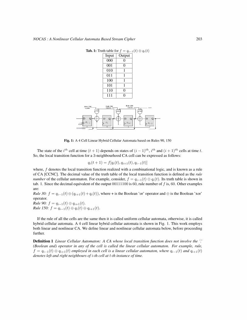
NOCAS : A Nonlinear Cellular Automata Based Stream Cipher 203
Tab. 1: Truth table for f = qi−1(t)⊕ qi(t)
Input Output000 0001 0010 1011 1100 1101 1110 0111 0
Fig. 1: A 4 Cell Linear Hybrid Cellular Automata based on Rules 90, 150
The state of the ith cell at time (t + 1) depends on states of (i− 1)th, ith and (i + 1)th cells at time t.So, the local transition function for a 3-neighbourhood CA cell can be expressed as follows:
qi(t + 1) = f [qi(t), qi+1(t), qi−1(t)]
where, f denotes the local transition function realized with a combinational logic, and is known as a ruleof CA [CCNC]. The decimal value of the truth table of the local transition function is defined as the rulenumber of the cellular automaton. For example, consider, f = qi−1(t)⊕ qi(t). Its truth table is shown intab. 1. Since the decimal equivalent of the output 00111100 is 60, rule number of f is, 60. Other examplesare:Rule 30: f = qi−1(t)⊕ (qi+1(t)+ qi(t)), where + is the Boolean ’or’ operator and⊕ is the Boolean ’xor’operator.Rule 90: f = qi−1(t)⊕ qi+1(t).Rule 150: f = qi−1(t)⊕ qi(t)⊕ qi+1(t).
If the rule of all the cells are the same then it is called uniform cellular automata, otherwise, it is calledhybrid cellular automata. A 4 cell linear hybrid cellular automata is shown in Fig. 1. This work employsboth linear and nonlinear CA. We define linear and nonlinear cellular automata below, before proceedingfurther.
Definition 1 Linear Cellular Automaton: A CA whose local transition function does not involve the ’.’(Boolean and) operator in any of the cell is called the linear cellular automaton. For example, rule,f = qi−1(t) ⊕ qi+1(t) employed in each cell is a linear cellular automaton, where qi−1(t) and qi+1(t)denotes left and right neighbours of i-th cell at t-th instance of time.
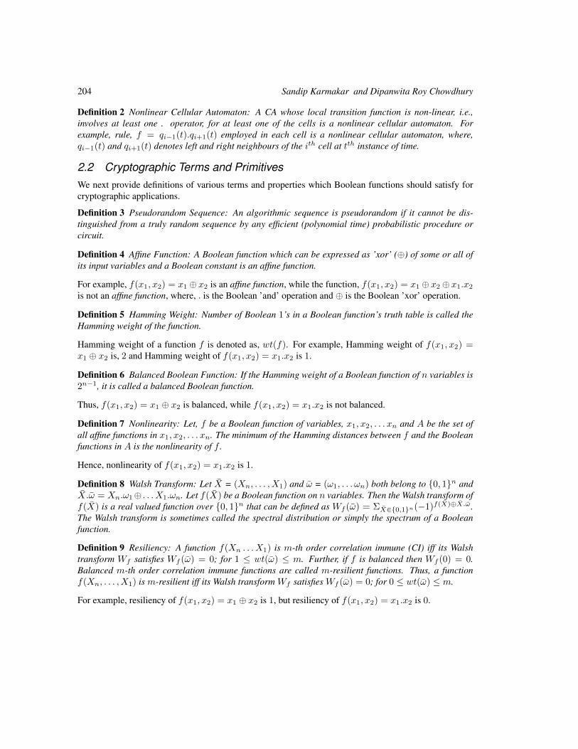
204 Sandip Karmakar and Dipanwita Roy Chowdhury
Definition 2 Nonlinear Cellular Automaton: A CA whose local transition function is non-linear, i.e.,involves at least one . operator, for at least one of the cells is a nonlinear cellular automaton. Forexample, rule, f = qi−1(t).qi+1(t) employed in each cell is a nonlinear cellular automaton, where,qi−1(t) and qi+1(t) denotes left and right neighbours of the ith cell at tth instance of time.
2.2 Cryptographic Terms and PrimitivesWe next provide definitions of various terms and properties which Boolean functions should satisfy forcryptographic applications.
Definition 3 Pseudorandom Sequence: An algorithmic sequence is pseudorandom if it cannot be dis-tinguished from a truly random sequence by any efficient (polynomial time) probabilistic procedure orcircuit.
Definition 4 Affine Function: A Boolean function which can be expressed as ’xor’ (⊕) of some or all ofits input variables and a Boolean constant is an affine function.
For example, f(x1, x2) = x1 ⊕ x2 is an affine function, while the function, f(x1, x2) = x1 ⊕ x2 ⊕ x1.x2
is not an affine function, where, . is the Boolean ’and’ operation and ⊕ is the Boolean ’xor’ operation.
Definition 5 Hamming Weight: Number of Boolean 1’s in a Boolean function’s truth table is called theHamming weight of the function.
Hamming weight of a function f is denoted as, wt(f). For example, Hamming weight of f(x1, x2) =x1 ⊕ x2 is, 2 and Hamming weight of f(x1, x2) = x1.x2 is 1.
Definition 6 Balanced Boolean Function: If the Hamming weight of a Boolean function of n variables is2n−1, it is called a balanced Boolean function.
Thus, f(x1, x2) = x1 ⊕ x2 is balanced, while f(x1, x2) = x1.x2 is not balanced.
Definition 7 Nonlinearity: Let, f be a Boolean function of variables, x1, x2, . . . xn and A be the set ofall affine functions in x1, x2, . . . xn. The minimum of the Hamming distances between f and the Booleanfunctions in A is the nonlinearity of f .
Hence, nonlinearity of f(x1, x2) = x1.x2 is 1.
Definition 8 Walsh Transform: Let X = (Xn, . . . , X1) and ω = (ω1, . . . ωn) both belong to 0, 1n andX.ω = Xn.ω1⊕ . . . X1.ωn. Let f(X) be a Boolean function on n variables. Then the Walsh transform off(X) is a real valued function over 0, 1n that can be defined as Wf (ω) = ΣX∈0,1n(−1)f(X)⊕X.ω .The Walsh transform is sometimes called the spectral distribution or simply the spectrum of a Booleanfunction.
Definition 9 Resiliency: A function f(Xn . . . X1) is m-th order correlation immune (CI) iff its Walshtransform Wf satisfies Wf (ω) = 0; for 1 ≤ wt(ω) ≤ m. Further, if f is balanced then Wf (0) = 0.Balanced m-th order correlation immune functions are called m-resilient functions. Thus, a functionf(Xn, . . . , X1) is m-resilient iff its Walsh transform Wf satisfies Wf (ω) = 0; for 0 ≤ wt(ω) ≤ m.
For example, resiliency of f(x1, x2) = x1 ⊕ x2 is 1, but resiliency of f(x1, x2) = x1.x2 is 0.
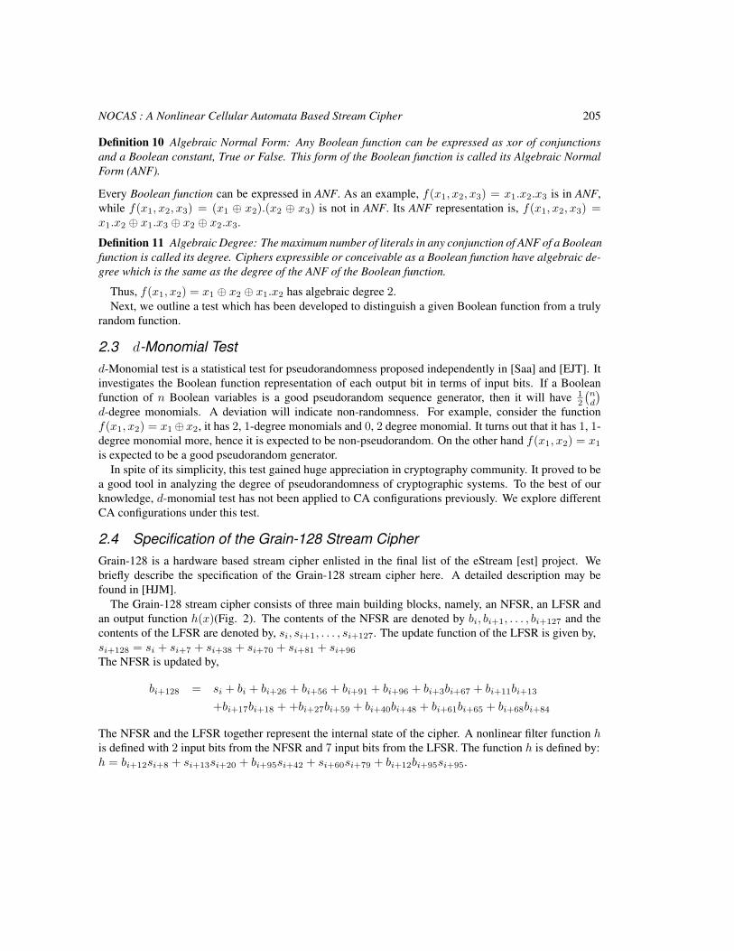
NOCAS : A Nonlinear Cellular Automata Based Stream Cipher 205
Definition 10 Algebraic Normal Form: Any Boolean function can be expressed as xor of conjunctionsand a Boolean constant, True or False. This form of the Boolean function is called its Algebraic NormalForm (ANF).
Every Boolean function can be expressed in ANF. As an example, f(x1, x2, x3) = x1.x2.x3 is in ANF,while f(x1, x2, x3) = (x1 ⊕ x2).(x2 ⊕ x3) is not in ANF. Its ANF representation is, f(x1, x2, x3) =x1.x2 ⊕ x1.x3 ⊕ x2 ⊕ x2.x3.
Definition 11 Algebraic Degree: The maximum number of literals in any conjunction of ANF of a Booleanfunction is called its degree. Ciphers expressible or conceivable as a Boolean function have algebraic de-gree which is the same as the degree of the ANF of the Boolean function.
Thus, f(x1, x2) = x1 ⊕ x2 ⊕ x1.x2 has algebraic degree 2.Next, we outline a test which has been developed to distinguish a given Boolean function from a truly
random function.
2.3 d-Monomial Testd-Monomial test is a statistical test for pseudorandomness proposed independently in [Saa] and [EJT]. Itinvestigates the Boolean function representation of each output bit in terms of input bits. If a Booleanfunction of n Boolean variables is a good pseudorandom sequence generator, then it will have 1
2
(nd
)d-degree monomials. A deviation will indicate non-randomness. For example, consider the functionf(x1, x2) = x1⊕x2, it has 2, 1-degree monomials and 0, 2 degree monomial. It turns out that it has 1, 1-degree monomial more, hence it is expected to be non-pseudorandom. On the other hand f(x1, x2) = x1
is expected to be a good pseudorandom generator.In spite of its simplicity, this test gained huge appreciation in cryptography community. It proved to be
a good tool in analyzing the degree of pseudorandomness of cryptographic systems. To the best of ourknowledge, d-monomial test has not been applied to CA configurations previously. We explore differentCA configurations under this test.
2.4 Specification of the Grain-128 Stream CipherGrain-128 is a hardware based stream cipher enlisted in the final list of the eStream [est] project. Webriefly describe the specification of the Grain-128 stream cipher here. A detailed description may befound in [HJM].
The Grain-128 stream cipher consists of three main building blocks, namely, an NFSR, an LFSR andan output function h(x)(Fig. 2). The contents of the NFSR are denoted by bi, bi+1, . . . , bi+127 and thecontents of the LFSR are denoted by, si, si+1, . . . , si+127. The update function of the LFSR is given by,si+128 = si + si+7 + si+38 + si+70 + si+81 + si+96
The NFSR is updated by,
bi+128 = si + bi + bi+26 + bi+56 + bi+91 + bi+96 + bi+3bi+67 + bi+11bi+13
+bi+17bi+18 + +bi+27bi+59 + bi+40bi+48 + bi+61bi+65 + bi+68bi+84
The NFSR and the LFSR together represent the internal state of the cipher. A nonlinear filter function his defined with 2 input bits from the NFSR and 7 input bits from the LFSR. The function h is defined by:h = bi+12si+8 + si+13si+20 + bi+95si+42 + si+60si+79 + bi+12bi+95si+95.
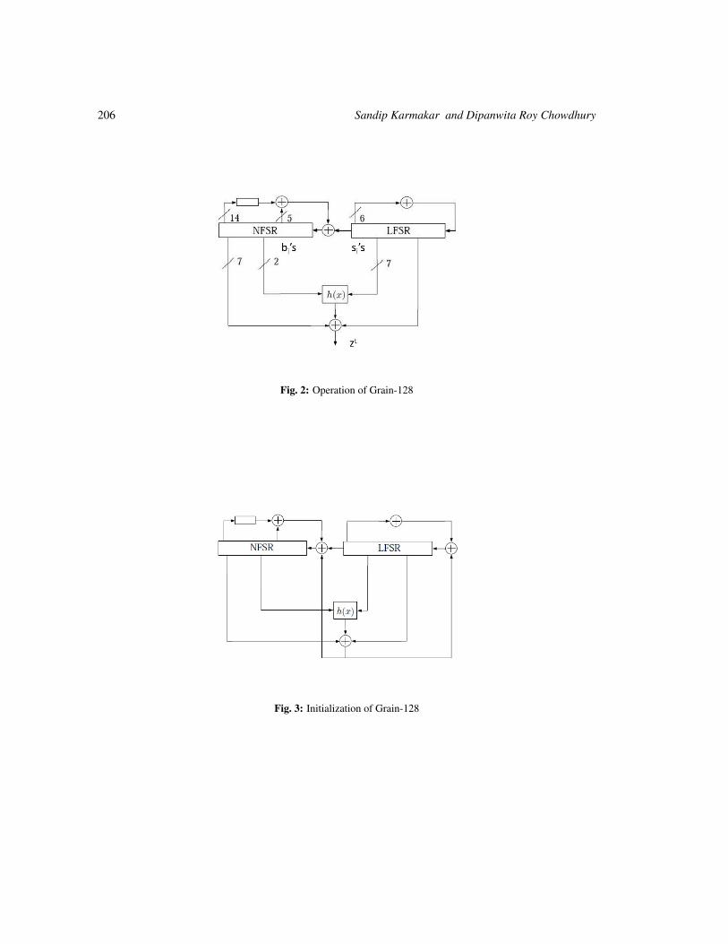
206 Sandip Karmakar and Dipanwita Roy Chowdhury
Fig. 2: Operation of Grain-128
Fig. 3: Initialization of Grain-128
NOCAS : A Nonlinear Cellular Automata Based Stream Cipher 207
Fig. 4: Structure of NOCAS
The output function zt is defined as,zt = bt+2 + bt+15 + bt+36 + bt+45 + bt+64 + bt+73 + bt+89 + h + st+93
An initialization phase is carried out before the cipher generates keystream bits. The 128 bit key,k = (k1, k2, . . . , k128) and the 96 bit initialization vector IV = (IV1, IV2, . . . , IV96) is loaded in theNFSR and the LFSR respectively as, bi = ki, 1 ≤ i ≤ 128 and si = IVi, 1 ≤ i ≤ 96, rest of theLFSR bits, (s97, s98, . . . , s128) are loaded with 1. The cipher is run for 256 rounds without producingany keystream, during initialization the output function is fed back and xored with both the LFSR and theNFSR (Fig. 3).
3 NOCAS: A CA Based Stream CipherIn the previous section, we have seen structure of Grain-128. The cipher is simple in design consisting ofonly a LFSR and an NFSR. It is a lightweight cipher with fast startup and high throughput. Unfortunately,a number of attacks have been mounted on it [DS11], [BCC+09], [KC11]. In [BCC+09], faults areinjected in the LFSR to deduce full secret key in only 22 faults, while [KC11] induces faults in the NFSRto get back the secret key in maximum 256 faults. In this section we present the specification of thecipher NOCAS (Hybrid NOnlinear CA based Stream Cipher), with by replacing the LFSR with a linearmaximum length CA and the NFSR with a hybrid nonlinear CA.
The building blocks of NOCAS are:
• A Hybrid Nonlinear CA of 128-bits with rules < 30, 60, 90, 120, 150, 180, 210, 240 > repeated 16times.
• A Linear Maximum Length CA of 128 bits with combinations of rules 90 and 150.
• The function NMix which is cryptographically suited nonlinear mixing function proposed in [BC09].
A block diagram of NOCAS is given in figure 4. Each of the building blocks are discussed in thefollowing subsections.
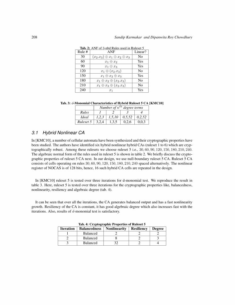
208 Sandip Karmakar and Dipanwita Roy Chowdhury
Tab. 2: ANF of 3-nbd Rules used in Ruleset 5Rule # ANF Linear?
30 (x2.x3)⊕ x1 ⊕ x2 ⊕ x3 No60 x1 ⊕ x2 Yes90 x1 ⊕ x3 Yes
120 x1 ⊕ (x2.x3) No150 x1 ⊕ x2 ⊕ x3 Yes180 x1 ⊕ x2 ⊕ (x2.x3) No210 x1 ⊕ x3 ⊕ (x2.x3) No240 x1 Yes
Tab. 3: d-Monomial Characteristics of Hybrid Ruleset 5 CA [KMC10]Number of nth degree terms
Rules 1 2 3 4Ideal 1,2,3 1,5,10 0,5,52 0,2,52
Ruleset 5 3,2,4 1,3,5 0,2,6 0,0,3
3.1 Hybrid Nonlinear CA
In [KMC10], a number of cellular automata have been synthesized and their cryptographic properties havebeen studied. The authors have identified six hybrid nonlinear hybrid CAs (ruleset 1 to 6) which are cryp-tographically robust. Among these rulesets we choose ruleset 5 i.e., 30, 60, 90, 120, 150, 180, 210, 240.The algebraic normal form of the rules used in ruleset 5 is shown in table 2. We briefly discuss the crypto-graphic properties of ruleset 5 CA next. In our design, we use null-boundary ruleset 5 CA. Ruleset 5 CAconsists of cells operating on rules 30, 60, 90, 120, 150, 180, 210, 240 spaced alternatively. The nonlinearregister of NOCAS is of 128 bits, hence, 16 such hybrid CA cells are repeated in the design.
In [KMC10] ruleset 5 is tested over three iterations for d-monomial test. We reproduce the result intable 3. Here, ruleset 5 is tested over three iterations for the cryptographic properties like, balancedness,nonlinearity, resiliency and algebraic degree (tab. 4).
It can be seen that over all the iterations, the CA generates balanced output and has a fast nonlinearitygrowth. Resiliency of the CA is constant, it has good algebraic degree which also increases fast with theiterations. Also, results of d-monomial test is satisfactory.
Tab. 4: Cryptographic Properties of Ruleset 5Iteration Balancedness Nonlinearity Resiliency Degree
1 Balanced 2 2 22 Balanced 8 2 33 Balanced 32 2 4
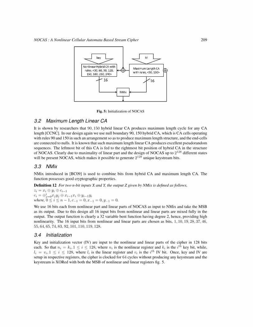
NOCAS : A Nonlinear Cellular Automata Based Stream Cipher 209
Fig. 5: Initialization of NOCAS
3.2 Maximum Length Linear CAIt is shown by researchers that 90, 150 hybrid linear CA produces maximum length cycle for any CAlength [CCNC]. In our design again we use null boundary 90, 150 hybrid CA, which is CA cells operatingwith rules 90 and 150 in such an arrangement so as to produce maximum length structure, and the end-cellsare connected to nulls. It is known that such maximum length linear CA produces excellent pseudorandomsequences. The leftmost bit of this CA is fed to the rightmost bit position of hybrid CA in the structureof NOCAS. Clearly due to maximality of linear part and the design of NOCAS up to 2128 different stateswill be present NOCAS, which makes it possible to generate 2128 unique keystream bits.
3.3 NMixNMix introduced in [BC09] is used to combine bits from hybrid CA and maximum length CA. Thefunction possesses good cryptographic properties.
Definition 12 For two n-bit inputs X and Y, the output Z given by NMix is defined as follows,zi = xi ⊕ yi ⊕ ci−1
ci = ⊕ij=0xjyj ⊕ xi−1xi ⊕ yi−1yi
where, 0 ≤ i ≤ n− 1, c−1 = 0, x−1 = 0, y−1 = 0.
We use 16 bits each from nonlinear part and linear parts of NOCAS as input to NMix and take the MSBas its output. Due to this design all 16 input bits from nonlinear and linear parts are mixed fully in theoutput. The output function is clearly a 32 variable bent function having degree 2, hence, providing highnonlinearity. The 16 input bits from nonlinear and linear parts are chosen as bits, 1, 10, 19, 28, 37, 46,55, 64, 65, 74, 83, 92, 101, 110, 119, 128.
3.4 InitializationKey and initialization vector (IV) are input to the nonlinear and linear parts of the cipher in 128 bitseach. So that ni = ki, 1 ≤ i ≤ 128, where ni is the nonlinear register and ki is the ith key bit, while,li = vi, 1 ≤ i ≤ 128, where li is the linear register and vi is the ith IV bit. Once, key and IV aresetup in respective registers, the cipher is clocked for 64 cycles without producing any keystream and thekeystream is XORed with both the MSB of nonlinear and linear registers fig. 5.
210 Sandip Karmakar and Dipanwita Roy Chowdhury
4 Security Analysis of NOCASIn this section, we present the security analysis of NOCAS. We will see that the employment of hybridnonlinear CA provides resistance against popular existing attacks.
• Linear Cryptanalysis: Nonlinearity and resiliency are the most important requirements for a cryp-tographic system. Good nonlinearity characteristics indicate that the cipher is expected to be safeagainst linear cryptanalysis and also from algebraic attacks. Table 5 shows the nonlinearity of NO-CAS with pass of iteration. In only 4 cycles of operation nonlinearity of NOCAS reaches 12428.It can be noted that the growth rate of nonlinearity is very steep. As complexity of linear crypt-analysis is directly related to nonlinearity, it can be claimed that NOCAS is resistant against linearcryptanalysis.
• Correlation Attack: Good nonlinearity characteristics does not imply correlation immunity, ie, goodnonlinear ciphers can display correlations among key, plain-texts and cipher-texts, which is the basisof correlation attack. Also, balancedness is an important factor to prevent correlation attack. Table 5illustrates the balancedness of the NOCAS output bit with iterations. All the output bit expressionsare balanced in the initial 4 iterations. Hence, the cryptographic property balancedness holds goodfor NOCAS. Table 5 also tabulates the resiliency of NOCAS output bit with iterations. It revealsthat higher resiliency is achieved by NOCAS at much lower number of iterations. Due to the fastergrowth of resiliency of output bit of NOCAS and its balancedness, it is expected to show resistanceagainst correlation attacks.
• Algebraic Attacks: Algebraic cryptanalysis is dependent on the algebraic degree of a cipher. Theincrease of number of nonlinear terms of a cipher also increase the attack complexity. Table 5 showsthe growth of algebraic degree of the output bit of NOCAS with iterations, while table 6 shows d-monomial characteristics of NOCAS with iterations, which shows almost exponential growth innonlinear terms. It can be observed that in NOCAS the algebraic degree increases linearly. Thegrowth in number of terms in the resultant Boolean expression and the number of different degreeterms in the output equation are both high. Considering table 6 once again, note that, at iteration 4only the number of nonlinear terms in the expression of the output bit is more than 400, which ismore than double the number of nonlinear terms at iteration 3, it can be expected that any attempt tolinearize the expression for algebraic attack will have to deal with exponential number of nonlinearterms with pass of iterations. Hence, algebraic attacks are not expected to yield good result againstNOCAS. Ciphers having large algebraic degrees are resistant against linearization and algebraicattacks. So, NOCAS is expected to be resistant to these attacks both in reduced round version andthe full key-IV setup version.
• Scan-based Side Channel Attack: Scan-chain based attack works because of the invertibility ofthe states of the cipher. The same will not be possible for NOCAS because of the presence ofnon-invertible CA rule 30. Though rule 30 is partially reversible, presence of linear and nonlinearrules in the CA configuration reduces the probability of the reversion exponentially with iterations.Hence, scan-based side channel attack will not be successful on NOCAS.
• Cube Attack/AIDA attack: Till date the most successful attacks on stream ciphers were cube attackand dynamic cube attack [DS11]. This attack exploits the fact that the distribution of the d-degree
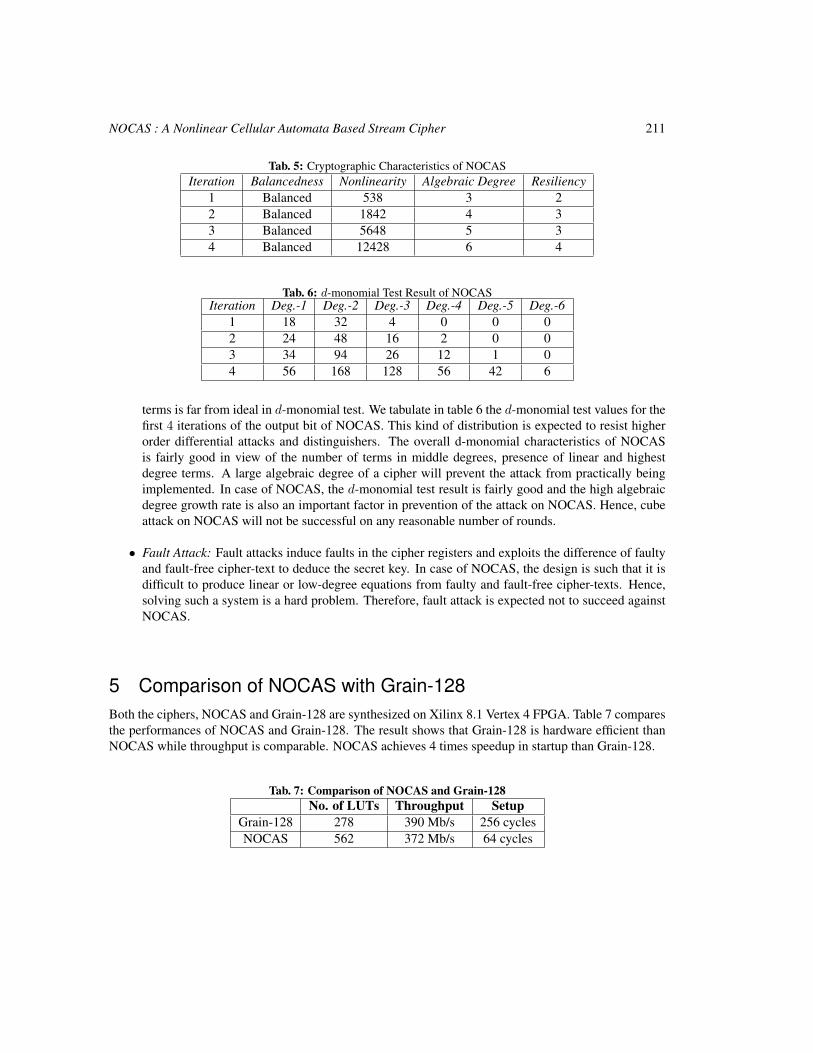
NOCAS : A Nonlinear Cellular Automata Based Stream Cipher 211
Tab. 5: Cryptographic Characteristics of NOCASIteration Balancedness Nonlinearity Algebraic Degree Resiliency
1 Balanced 538 3 22 Balanced 1842 4 33 Balanced 5648 5 34 Balanced 12428 6 4
Tab. 6: d-monomial Test Result of NOCASIteration Deg.-1 Deg.-2 Deg.-3 Deg.-4 Deg.-5 Deg.-6
1 18 32 4 0 0 02 24 48 16 2 0 03 34 94 26 12 1 04 56 168 128 56 42 6
terms is far from ideal in d-monomial test. We tabulate in table 6 the d-monomial test values for thefirst 4 iterations of the output bit of NOCAS. This kind of distribution is expected to resist higherorder differential attacks and distinguishers. The overall d-monomial characteristics of NOCASis fairly good in view of the number of terms in middle degrees, presence of linear and highestdegree terms. A large algebraic degree of a cipher will prevent the attack from practically beingimplemented. In case of NOCAS, the d-monomial test result is fairly good and the high algebraicdegree growth rate is also an important factor in prevention of the attack on NOCAS. Hence, cubeattack on NOCAS will not be successful on any reasonable number of rounds.
• Fault Attack: Fault attacks induce faults in the cipher registers and exploits the difference of faultyand fault-free cipher-text to deduce the secret key. In case of NOCAS, the design is such that it isdifficult to produce linear or low-degree equations from faulty and fault-free cipher-texts. Hence,solving such a system is a hard problem. Therefore, fault attack is expected not to succeed againstNOCAS.
5 Comparison of NOCAS with Grain-128Both the ciphers, NOCAS and Grain-128 are synthesized on Xilinx 8.1 Vertex 4 FPGA. Table 7 comparesthe performances of NOCAS and Grain-128. The result shows that Grain-128 is hardware efficient thanNOCAS while throughput is comparable. NOCAS achieves 4 times speedup in startup than Grain-128.
Tab. 7: Comparison of NOCAS and Grain-128No. of LUTs Throughput Setup
Grain-128 278 390 Mb/s 256 cyclesNOCAS 562 372 Mb/s 64 cycles
212 Sandip Karmakar and Dipanwita Roy Chowdhury
6 ConclusionIn the current paper, we have introduced a new stream cipher based on hybrid nonlinear CA called NO-CAS. The design produces fast initialization in only 64 cycles. We have analyzed the cryptographicproperties like balancedness, nonlinearity, resiliency and algebraic degree of NOCAS, which show it isa cryptographically robust cipher. The d-monomial test also produce fairly good result against NOCAS.Finally, we have shown that NOCAS is expected to resistant against popularly known existing attacks. Itachieves 4 times speedup in initialization than Grain-128.
References[BBC+] Come Berbain, Olivier Billet, Anne Canteaut, Nicolas Courtois, Henri Gilbert, Louis Goubin,
Aline Gouget, Louis Granboulan, Cedric Lauradoux, Marine Minier, Thomas Pornin, andHerve Sibert. Sosemanuk, a fast software-oriented stream cipher. eSTREAM, ECRYPT StreamCipher Project, 2006.
[BC09] Jaydeb Bhowmik and Dipanwita Roy Chowdhury. Nmix : An Ideal Candidate for Key Mix-ing. SecCrypt 2009, pages 285–288, 2009.
[BCC+] Steve Babbage, Christophe De Canniere, Anne Canteaut, Carlos Cid, Henri Gilbert, ThomasJohansson, Matthew Parker, Bart Preneel, Vincent Rijmen, and Matthew Robshaw. The es-tream portfolio. ”http://www.ecrypt.eu.org/stream/portfolio.pdf”.
[BCC+09] Alexandre Berzati, Cecile Canovas, Guilhem Castagnos, Blandine Debraize, Louis Goubin,Aline Gouget, Pascal Paillier, and Stephanie Salgado. Fault analysis of grain-128. Hardware-Oriented Security and Trust, IEEE International Workshop on, 0:7–14, 2009.
[BD] Steve Babbage and Matthew Dodd. The stream cipher mickey 2.0. eSTREAM, ECRYPTStream Cipher Project, 2006.
[Ber] Daniel J. Bernstein. Salsa20. eSTREAM, ECRYPT Stream Cipher Project, 2006.
[BVCZ] Martin Boesgaard, Mette Vesterager, Thomas Christensen, and Erik Zenner. The stream ci-pher rabbit. eSTREAM, ECRYPT Stream Cipher Project, 2006.
[CCNC] P. Pal Chaudhuri, D. Roy Chowdhury, S. Nandi, and S. Chattopadhyay. CA and Its Applica-tions: A Brief Survey, Additive Cellular Automata - Theory and Applications vol.-1, pages6-25. eSTREAM, ECRYPT Stream Cipher Project, 1997.
[CP] Christophe De Canniere and Bart Preneel. Trivium specifications. eSTREAM, ECRYPTStream Cipher Project, 2006.
[DS11] Ita Dinur and Adi Shamir. Dynamic Cube Attack on Full Grain-128. ePrint CryptologyArchive, 2011.
[EJT] H. Englund, T. Johansson, and MS Turan. A Framework for Chosen IV Statistical Analysisof Stream Ciphers. Progress in Cryptology - INDOCRYPT, 2007:268–281.
[est] The estream project. ”http://www.ecrypt.eu.org/stream/”.
NOCAS : A Nonlinear Cellular Automata Based Stream Cipher 213
[HJM] Martin Hell, Thomas Johansson, and Willi Meier. A stream cipher proposal: Grain-128.eSTREAM, ECRYPT Stream Cipher Project, 2006.
[KC11] Sandip Karmakar and Dipanwita Roy Chowdhury. Fault Analysis of Grain-128 by TargetingNFSR. AfricaCrypt 2011, 2011.
[KMC10] Sandip Karmakar, Debdeep Mukhopadhyay, and Dipanwita Roy Chowdhury. d-monomialTests on Cellular Automata for Cryptographic Design. ACRI 2010, 2010.
[MS91] Meier and Staffelbach. Analysis of Pseudo Random Sequences Generated by Cellular Au-tomata. ”EUROCRYPT: Advances in Cryptology: Proceedings of EUROCRYPT”, 1991.
[Saa] Markku-Juhani O. Saarinen. Chosen IV Statistical Attacks on eStream Stream Ciphers.http://www.ecrypt.eu.org/stream.
[Wola] Wolfram. Cryptography with Cellular Automata. CRYPTO: Proceedings of Crypto, 1985.
[Wolb] S. Wolfram. Random Sequence Generation by Cellular Automata. Advances in AppliedMathematics, vol.-7, pages 123-169.
[Wu] Hongjun Wu. Stream cipher hc-128. eSTREAM, ECRYPT Stream Cipher Project, 2006.

214 Sandip Karmakar and Dipanwita Roy Chowdhury

AUTOMATA 2011, Santiago, Chile local proceedings LP, 2011, 215–220
Cell damage from radiation-inducedbystander effects for different cell densitiessimulated by cellular automata
Sincler Peixoto de Meireles1†and Adriano Marcio dos Santos1 and MariaEugenia Silva Nunes2 and Suely Epsztein Grynberg1
1Centro de Desenvolvimento da Tecnologia Nuclear (CDTN/CNEN) - Av. Presidente Antonio Carlos 6627, 31270-901, Belo Horizonte, Minas Gerais, Brasil2Universidade Federal de Ouro Preto (UFOP) - Rua Diogo de Vascomcelos, 122, 35400-000, Ouro Preto , MinasGerais, Brasil
During recent years, there has been a shift from an approach focused entirely on DNA as the main target of ionizingradiation to a vision that considers complex signaling pathways in cells and among cells within tissues. Severalnewly recognized responses were classified as the so-called non-target responses in which the biological effects arenot directly related to the amount of energy deposited in the DNA of cells that were traversed by radiation. In1992 the bystander effect was described referring to a series of responses such as death, chromosomal instability orother abnormalities that occur in non-irradiated cells that came into contact with irradiated cells or medium fromirradiated cells. In this work, we have developed a mathematical model via cellular automata, to quantify cell deathinduced by the bystander effect. The model is based on experiments with irradiated cells conditioned medium (ICCM)which suggests that irradiated cells secrete molecules in the medium that are capable of damaging other cells. Thecomputational model consists of two-dimensional cellular automata which is able to simulate the transmission ofbystander signals via extrinsic route and via Gap junctions. The model has been validated by experimental resultsin the literature. The time evolution of the effect and the dose-response curves were obtained in good accordance tothem. Simulations were conducted for different values of bystander and irradiated cell densities with constant dose.From this work, we have obtained a relationship between cell density and effect.
Keywords: Automata Cellular, Bystander Effect, Computer Simulation, Monte Carlo
1 IntroductionSeveral radiobiological studies over the past decade have profoundly challenged the dogma of classicalradiobiology by which radiation effects would only be observed in cells that have undergone irradiation,or their descendants, through genetic damage produced directly by energy deposition in DNA. Currently,
†Email: [email protected].
c© 2011 AUTOMATA proceedings, Santiago, Chile, 2011
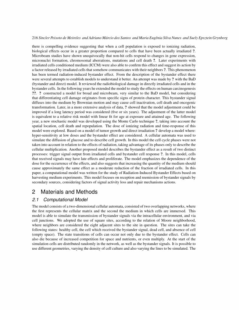
216 Sincler Peixoto de Meireles and Adriano Marcio dos Santos and Maria Eugenia Silva Nunes and Suely Epsztein Grynberg
there is compelling evidence suggesting that when a cell population is exposed to ionizing radiation,biological effects occur in a greater proportion compared to cells that have been actually irradiated ?.Microbeam studies have shown unequivocally that non-hit cells respond to changes in gene expression,micronuclei formation, chromosomal aberrations, mutations and cell death ?. Later experiments withirradiated cells conditioned medium (ICCM) were also able to confirm this effect and suggest its action bya factor released by irradiated cells that somehow communicates with their neighbors ?. This phenomenonhas been termed radiation-induced bystander effect. From the description of the bystander effect therewere several attempts to establish models to understand it better. An attempt was made by ? with the BaD(bystander and direct) model. It reviewed the radiobiological damage in directly irradiated cells and in thebystander cells. In the following years he extended the model to study the effects on human carcinogenesis??. ? constructed a model for broad and microbeam, very similar to the BaD model, but consideringthat differentiating cell damage originates from specific signs of protein character. This bystander signaldiffuses into the medium by Brownian motion and may cause cell inactivation, cell death and oncogenictransformation. Later, in a more extensive analysis of data, ? showed that the model adjustment could beimproved if a long latency period was considered (five or six years). The adjustment of the latter modelis equivalent to a relative risk model with linear fit for age at exposure and attained age. The followingyear, a new stochastic model was developed using the Monte Carlo technique ?, taking into account thespatial location, cell death and repopulation. The dose of ionizing radiation and time-response of thismodel were explored. Based on a model of tumor growth and direct irradiation ? develop a model where:hyper-sensitivity at low doses and the bystander effect are considered. A cellular automata was used tosimulate the diffusion of glucose and to describe cell growth. In this model the cell cycle phases were nottaken into account in relation to the effects of radiation, taking advantage of its phases only to describe thecellular multiplication. Another proposed model describes the bystander effect as a result of two distinctprocesses: trigger signal output from irradiated cells and bystander cell response ?. In this model, cellsthat received signals may have late effects and proliferate. The model emphasizes the dependence of thedose for the occurrence of the effects, and also suggests that increasing the quantity of the medium shouldcause approximately the same effect as a moderate reduction of the fraction of irradiated cells. In thispaper, a computational model was written for the study of Radiation-Induced Bystander Effects based onharvesting medium experiments. This model focuses on reception and reemission of bystander signals bysecondary sources, considering factors of signal activity loss and repair mechanisms actions.
2 Materials and Methods2.1 Computational ModelThe model consists of a two-dimensional cellular automata, consisted of two overlapping networks, wherethe first represents the cellular matrix and the second the medium in which cells are immersed. Thismodel is able to simulate the transmission of bystander signals via the intracellular environment, and viacell junctions. We adopted the use of square sites, according to the relation of Moore neighborhood,where neighbors are considered the eight adjacent sites to the site in question. The sites can take thefollowing states: healthy cell, the cell which received the bystander signal, dead cell, and absence of cell(empty space). The state transitions of cells can occur not only due to the bystander effect. Cells canalso die because of increased competition for space and nutrients, or even multiply. At the start of thesimulation cells are distributed randomly in the network, as well as the bystander signals. It is possible touse different geometries, varying the density of cell culture and also varying the lines to be simulated. The
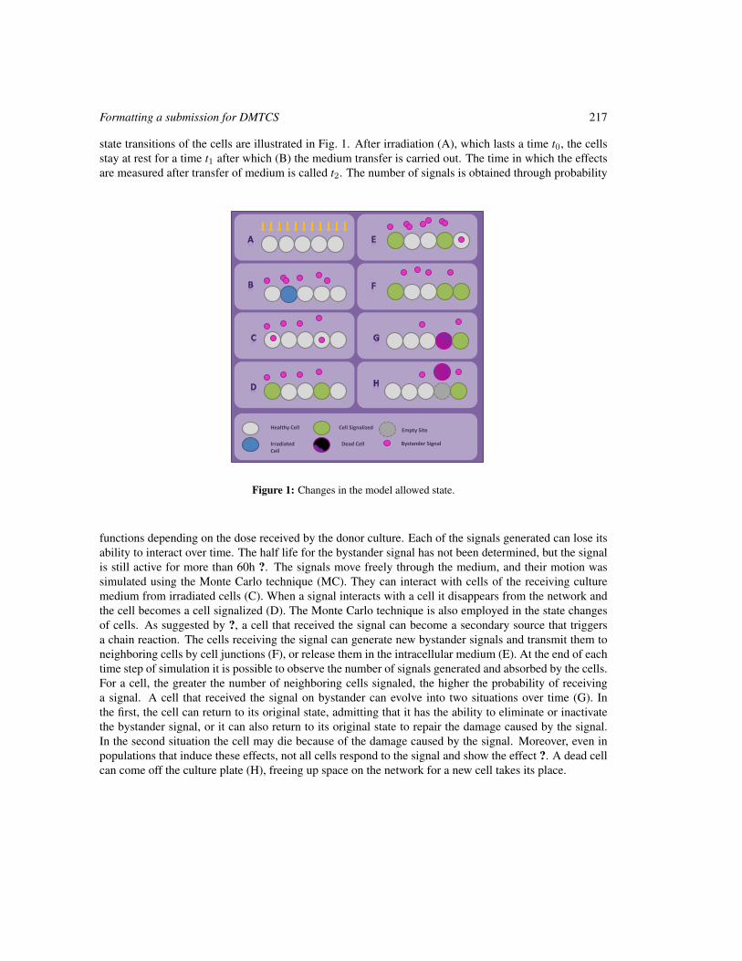
Formatting a submission for DMTCS 217
state transitions of the cells are illustrated in Fig. 1. After irradiation (A), which lasts a time t0, the cellsstay at rest for a time t1 after which (B) the medium transfer is carried out. The time in which the effectsare measured after transfer of medium is called t2. The number of signals is obtained through probability
Healthy Cell
Bystander Signal
Cell Signalized
Dead Cell
Empty Site
IrradiatedCell
Figure 1: Changes in the model allowed state.
functions depending on the dose received by the donor culture. Each of the signals generated can lose itsability to interact over time. The half life for the bystander signal has not been determined, but the signalis still active for more than 60h ?. The signals move freely through the medium, and their motion wassimulated using the Monte Carlo technique (MC). They can interact with cells of the receiving culturemedium from irradiated cells (C). When a signal interacts with a cell it disappears from the network andthe cell becomes a cell signalized (D). The Monte Carlo technique is also employed in the state changesof cells. As suggested by ?, a cell that received the signal can become a secondary source that triggersa chain reaction. The cells receiving the signal can generate new bystander signals and transmit them toneighboring cells by cell junctions (F), or release them in the intracellular medium (E). At the end of eachtime step of simulation it is possible to observe the number of signals generated and absorbed by the cells.For a cell, the greater the number of neighboring cells signaled, the higher the probability of receivinga signal. A cell that received the signal on bystander can evolve into two situations over time (G). Inthe first, the cell can return to its original state, admitting that it has the ability to eliminate or inactivatethe bystander signal, or it can also return to its original state to repair the damage caused by the signal.In the second situation the cell may die because of the damage caused by the signal. Moreover, even inpopulations that induce these effects, not all cells respond to the signal and show the effect ?. A dead cellcan come off the culture plate (H), freeing up space on the network for a new cell takes its place.
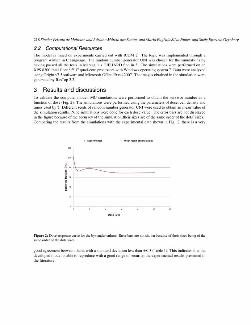
218 Sincler Peixoto de Meireles and Adriano Marcio dos Santos and Maria Eugenia Silva Nunes and Suely Epsztein Grynberg
2.2 Computational ResourcesThe model is based on experiments carried out with ICCM ?. The logic was implemented through aprogram written in C language. The random number generator UNI was chosen for the simulations byhaving passed all the tests in Marsaglia’s DIEHARD find in ?. The simulations were performed on anXPS 8300 Intel Core TM i7 quad-core processors with Windows operating system 7. Data were analyzedusing Origin v7.5 software and Microsoft Office Excel 2007. The images obtained in the simulation weregenerated by RasTop 2.2.
3 Results and discussionsTo validate the computer model, MC simulations were performed to obtain the survivor number as afunction of dose (Fig. 2). The simulations were performed using the parameters of dose, cell density andtimes used by ?. Different seeds of random number generator UNI were used to obtain an mean value ofthe simulation results. Nine simulations were done for each dose value. The error bars are not displayedin the figure because of the accuracy of the simulation(their sizes are of the same order of the dots’ sizes).Comparing the results from the simulations with the experimental data shown in Fig. 2, there is a very
0
20
40
60
80
100
120
0 2 4 6 8 10 12
Surv
ivin
g fr
acti
on
( %
)
Dose (Gy)
Mothersill and Seymor 1997 Average result of simulationsExperimental Mean result of simulations
Figure 2: Dose-response curve for the bystander culture. Error bars are not shown because of their sizes being of thesame order of the dots sizes
good agreement between them, with a standard deviation less than ±0.3 (Table 1). This indicates that thedeveloped model is able to reproduce with a good range of security, the experimental results presented inthe literature.
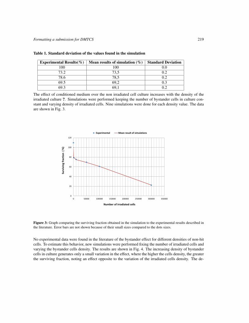
Formatting a submission for DMTCS 219
Table 1. Standard deviation of the values found in the simulation
Experimental Results(%) Mean results of simulation (%) Standard Deviation100 100 0.073.2 73,5 0.278.6 78,5 0.269.5 69,2 0.369.3 69,1 0.2
The effect of conditioned medium over the non irradiated cell culture increases with the density of theirradiated culture ?. Simulations were performed keeping the number of bystander cells in culture con-stant and varying density of irradiated cells. Nine simulations were done for each density value. The dataare shown in Fig. 3.
0
20
40
60
80
100
120
0 50000 100000 150000 200000 250000 300000 350000
Surv
ivin
g fr
acti
on
( %
)
Number of irradiated cells
Experimental Mean result of simulations
Figure 3: Graph comparing the surviving fraction obtained in the simulation to the experimental results described inthe literature. Error bars are not shown because of their small sizes compared to the dots sizes.
No experimental data were found in the literature of the bystander effect for different densities of non-hitcells. To estimate this behavior, new simulations were performed fixing the number of irradiated cells andvarying the bystander cells density. The results are shown in Fig. 4. The increasing density of bystandercells in culture generates only a small variation in the effect, where the higher the cells density, the greaterthe surviving fraction, noting an effect opposite to the variation of the irradiated cells density. The de-
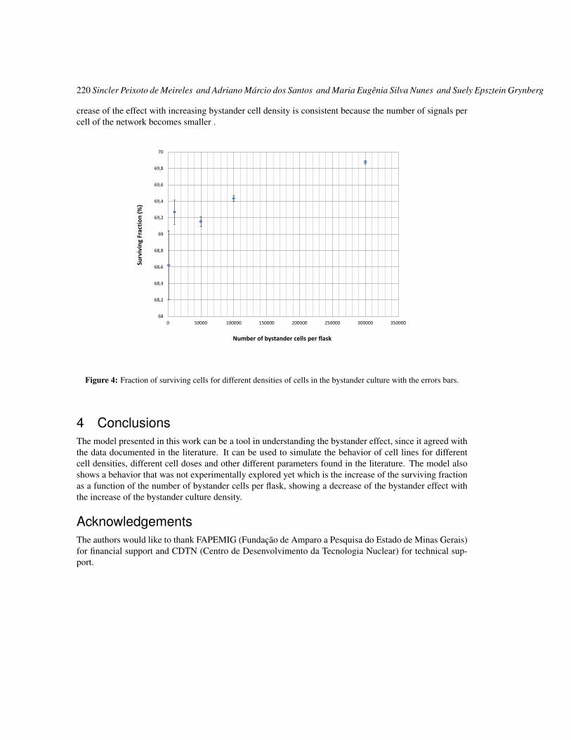
220 Sincler Peixoto de Meireles and Adriano Marcio dos Santos and Maria Eugenia Silva Nunes and Suely Epsztein Grynberg
crease of the effect with increasing bystander cell density is consistent because the number of signals percell of the network becomes smaller .
68
68,2
68,4
68,6
68,8
69
69,2
69,4
69,6
69,8
70
0 50000 100000 150000 200000 250000 300000 350000
Surv
ivin
g Fr
acti
on
(%
)
Number of bystander cells per flask
Figure 4: Fraction of surviving cells for different densities of cells in the bystander culture with the errors bars.
4 ConclusionsThe model presented in this work can be a tool in understanding the bystander effect, since it agreed withthe data documented in the literature. It can be used to simulate the behavior of cell lines for differentcell densities, different cell doses and other different parameters found in the literature. The model alsoshows a behavior that was not experimentally explored yet which is the increase of the surviving fractionas a function of the number of bystander cells per flask, showing a decrease of the bystander effect withthe increase of the bystander culture density.
AcknowledgementsThe authors would like to thank FAPEMIG (Fundacao de Amparo a Pesquisa do Estado de Minas Gerais)for financial support and CDTN (Centro de Desenvolvimento da Tecnologia Nuclear) for technical sup-port.
AUTOMATA 2011, Santiago, Chile local proceedings LP, 2011, 221–232
Product decomposition for surjective 2-blockNCCA
Felipe Garcıa-Ramos1†
1University of British Columbia, Vancouver, Canada
In this paper we define products of one-dimensional Number Conserving Cellular Automata (NCCA) and show thatsurjective NCCA with 2 blocks (i.e radius 1/2) can always be represented as products of shifts and identites. Inparticular, this shows that surjective 2-block NCCA are injective.
Keywords: Discrete dynamical systems, cellular automata, number conserving cellular automata, conservation laws,characterization of surjective NCCA
1 IntroductionIt is known that injective Cellular Automata (CA) are surjective. In general, the converse is not true,and there are many algebraic CA counterexamples. However, there are interesting subclasses where thismight be true. For example, if a surjective CA has entropy 0 then it is almost injective (Moothathu (2011))and it is not known if it is actually injective. The author believes there are some sub-classes of potentialpreserving CA, including Number Conserving CA (NCCA), where there are no surjective but not injectiveCA.
The subclass of NCCA, besides providing interesting mathematical structure, is used for discrete mod-els in scientific disciplines where one simulates systems governed by conservation laws of mass or energy.Many papers have been published on traffic models using NCCA (for example see Maerivoet and Moor(2005)).
The Moore-Myhill theorem says that a CA is surjective iff it is injective on homoclinic classes. Actually,it is easy to see that a NCCA is surjective iff it is bijective on homoclinic classes. This suggests that theremight be a closer relationship between surjective NCCA and injective NCCA. So far, it is known thatsurjective NCCA have dense periodic points (Formenti and Grange (2003)). If it turns out that surjectiveNCCA are injective we would recover this result, since for bijective CA periodic points are dense.
†Email: [email protected]. This paper is part of the author’s Ph.D. thesis. The author is supported is by a CONA-CyT fellowship.
c© 2011 AUTOMATA proceedings, Santiago, Chile, 2011
222 Felipe Garcıa-Ramos
2 Definitions and classical results
LetA be a finite set, which will sometimes be referred to as the alphabet. We define the fullA-shift as thespace of bi-sequences AZ. We will endow this space with the Cantor (product) topology. If ω ∈ AZ, wedenote (ω)i as the ith coordinate of point x. We will use σR : AZ → AZ as the right shift map, i.e. themap that satisfies (ω)i = (σR(ω))i+1 for all ω ∈ AZ and i ∈ Z.
Definition 1 A cellular automaton (CA) is a continuous map φ(·) : AZ → AZ that commutes with theshift.
Theorem 2 (Curtis-Hedlund-Lyndon) Hedlund (1969) Let φ(·) : AZ → AZ . The map φ is a CA iffthere exist two non-negative integers L and R (which represent the left and right radius), and a functionφ [·] : AL+R+1 → A, such that (φ(ω))i = φ
[(ω)i−m (ω)i−m+1 ... (ω)i ... (ω)i+a
](note the use of ( ),
and [ ] to distinguish between the two functions that are related).
We say L+R+ 1 is the neighbourhood size of φ.
Definition 3 In this paper a 2-block CA φ (also known as CA with radius 1/2) is a map with L = 1 andR = 0.
For example the right shift is a 2-block CA. The reader will see that all the results are analogous forL = 0 and R = 1.
We say two points inAZ are equivalent, if they differ only on finitely many coordinates. The homoclinicclass of a point ω is the set of points equivalent to ω.
Theorem 4 (Moore-Myhill) Moore (1963) Myhill (1963) Let φ be a CA. Then φ is surjective iff φ isinjective when restricted to homoclinic classes iff φ is injective when restricted to one homoclinic class.
Definition 5 We say a cellular automaton φ : [0...A)Z → [0...A)
Z is number conserving, also denotedas NCCA, if for every point ω in the homoclinic class of 0∞ we have that
∑i∈Z
(φ(ω))i <∞, and
∑i∈Z
(φ(ω))i =∑i∈Z
(ω)i.
The following result is the particular case for 2-block CA of a general result by Hattori and Takesue(1991), which was used by Boccara and Fuks (2002) to characterize NCCA. We provide a proof of thisweaker result for completeness.
Proposition 6 Let φ : [0...a]Z → [0...a]
Z be a 2-block CA. Then φ is a NCCA iff
φ [pq] = q + φ [p0]− φ [q0] . (1)
Proof: We have that φ(0∞p0∞) = 0∞ φ [0p] φ [p0] 0∞. This means that
p = φ [0p] + φ [p0] . (2)
Product decomposition for surjective 2-block NCCA 223
Similarly consider the image of the point φ(0∞pq0∞) = 0∞abc0∞.We have that a = φ [0p] , b = φ [pq] ,and c = φ [q0] . Since φ is a NCCA we have that
p+ q = a+ b+ c = φ [0p] + φ [pq] + φ [q0] . (3)
Combining (3) and (2) we get (1).Conversely suppose φ satisfies (1). Let ω be a point in the homoclinic class of 0∞. This means there
exist j and k, such that (ω)i = 0 for i > k and i < j. So we get that
∑i∈Z
(φ(ω))i = φ [0(ω)j ] +
k−1∑i=j
φ [(ω)i(ω)i+1] + φ [(ω)k0]
= (ω)j − φ [(ω)j0] +k−1∑i=j
((ω)i+1 + φ [(ω)i0]− φ [(ω)i+10]) + φ [(ω)k0]
=
k∑i=j
(ω)i.
2
This result tells us that a 2-block NCCA is uniquely determined by the values of φ [x0] and if p = q = 0we get φ [00] = 0.
Example 7 The reader can check that φ : [0, 1, 2]Z → [0, 1, 2]
Z, with φ [10] = 0 and φ [20] = 1, is a welldefined (non-surjective) NCCA but there is no 2-block NCCA φ : [0...3)
Z → [0...3)Z with φ [10] = 1 and
φ [20] = 0, because the image of the point 0∞120∞ cannot have sum equal to 3.
In general a specification φ [·0] is defines a 2-block NCCA φ : [0...a]Z → [0...a]
Z via (1) iff
0 ≤ q + φ [p0]− φ [q0] ≤ a ∀p, q ∈ [0...a] .
We will use the following result several times.
Theorem 8 A NCCA is surjective iff it is bijective on the homoclinic class of 0∞.
Proof: Simply apply Theorem 4 and note that the image and preimage of the homoclinic class of 0∞
under φ is in the homoclinic class of 0∞. 2
We would like to characterize NCCA in a more concrete way, at least under some special assumptions.In this paper we will do so for surjective 2-block NCCA.
We will first show how to represent the product of 2-block NCCA’s as a 2-block NCCA. We will estab-lish some properties of the product and finally show that all surjective 2-block NCCA can be representedas the product of shift and identity maps.
224 Felipe Garcıa-Ramos
3 Products of NCCA
For easier notation we define A := a + 1, B := b + 1, and [0...n) := [0...n− 1] . We will use A and Bor a and b, depending on which one gives an easier notation.
Let φ : [0...A)Z → [0...A)
Z and ψ : [0...B)Z → [0...B)
Z be two 2-block codes. Consider the functionF (p1, p2) = p2 + Bp1, where p1 ∈ [0...A) and p2 ∈ [0...B) . This function is a bijection between[0...A)× [0...B) and [0...AB). Furthermore, it satisfies
F (p1 + p′1, p2 + p′2) = F (p1, p2) + F (p′1, p′2),
for p1 + p′1 ∈ [0, a] and p2 + p′2 ∈ [0, b] . Now, for all p, q ∈ [0...AB) , we can define φ × ψ [pq] =F (φ [F1(p)F1(q)] , ψ [F2(p)F2(q)]), where F1 and F2 are the coordinates of the inverse, i.e.
φ× ψ[(p1p2
)(q1q2
)]=
(φ [p1 q1]
ψ [p2 q2]
),
where(αβ
)= F (α, β).
Now we note that if φ and ψ are number conserving, then the product χ = φ × ψ is also numberconserving since
χ
[(p1p2
)(q1q2
)]=
(φ [p1 q1]
ψ [p2 q2]
)=
(q1 + φ [p1 0]− φ [q1 0]q2 + ψ [p2 0]− ψ [q2 0]
)=
(q1q2
)+
(φ [p1 0]
ψ [p2 0]
)−(φ [q1 0]
ψ [q2 0]
)=
(q1q2
)+ χ
[(p1p2
)(0
0
)]− χ
[(q1q2
)(0
0
)],
and therefore χ satisfies equation (1).Since F is not symmetric in general, φ× ψ need not be the same as ψ × φ.
Even though we can make products of any two 2-block codes, we will mainly be interested in productsof shifts and identities (which will be denoted as σR and Id respectively).
If φ = Id, and χ = φ× ψ then
χ
[(p1p2
)(0
0
)]=
(φ [p1 0]
ψ [p2 0]
)=
(0
ψ [p2 0]
)= ψ(p2 0). (4)
If φ = σR, then
χ
[(p1p2
)(0
0
)]=
(φ [p1 0]
ψ [p2 0]
)=
(p1
ψ [p2 0]
)= ψ(p2 0) + p1(b+ 1). (5)
Product decomposition for surjective 2-block NCCA 225
Example 9 Let σR : [0...3)Z → [0...3)
Z, Id : [0...4)Z → [0...4)
Z, and χ = σR × Id : [0...(3 · 4))Z →
[0...(3 · 4))Z . For every x ∈ [0...12) there exists p1 ∈ [0...3) and p2 ∈ [0...4) such that x = p2 + 4p1,where p1 ∈ [0...3) and p2 ∈ [0...4) . Hence χ [x0] = p1. In a table it looks like this.
x 0 1 2 3 4 5 6 7 8 9 10 11χ [x0] 0 0 0 0 1 1 1 1 2 2 2 2
If we take instead Id× σR we get the following table.
x 0 1 2 3 4 5 6 7 8 9 10 11χ [x0] 0 1 2 0 1 2 0 1 2 0 1 2
The following lemma describes an important property when one of the factors is a shift or an identity.The proof uses formulas (4) and (5) and is left to the reader.
Lemma 10 Let φ = Id. We have that χ [x0] = x iff x < B and ψ [x0] = x; and χ [x0] = 0 iff thereexists n ∈ [0...A) such that x = y + nB and ψ [y0] = 0.
Similarly let φ = σR. We also have that χ [x0] = 0 iff x < B and ψ [x0] = 0; and χ [x0] = x iff thereexists n ∈ [0...A) and y ∈ [0...B) such that x = y + nB and ψ [y 0] = y.
Definition 11 Let φ be a 2-block cellular automata. We say φ is a shift-identity product cellular automa(SIPCA) if φ = φn × · · · × φ1, where φi = Id for all even i′s, and φi = σR for all odd (or vice versa).
Notation 12 We will denote fφ(x) = φ [x0] . Notice from (1) that the function fφ(x) = φ [x0] completelydetermines φ.
NCCA arise in the context of particle preserving maps. People have shown (Boccara and Fuks (2002),Pivato (2002), Moreira et al. (2004) for 1-d and recently Kari and Taati (2008) for 2-d) that it is equivalentto give a NCCA as a compatible list of particle displacement representations. In the case of 2-blockNCCA, the particle displacement representations are given by fφ(x), which represent how many particlesmove to the right when you see x particles in a certain position.
The product of two shifts is a shift, and the product of two identities is an identity. Thus all productsof right-shifts and identities are SIPCA. In general if our alphabet is [0...A) , for every way that we canwrite A = An · An−1 · · · A1 (with Ai ∈ N), we have two SIPCA with that alphabet. We can takeχ = φn × · · · × φ1 with φi : [0...Ai)
Z → [0...Ai)Z alternating between shifts and identities with either
φ1 = Id or φ1 = σR.It’s useful to describe the graph of fχ. Suppose φ1 : [0...A)
Z → [0...A)Z is any 2-block NCCA and
φ2 : [0...3)Z → [0...3)
Z. Figure 1 represents the graph of fχ when φ2 = Id, and Figure 2 when φ2 = σR.
Figure 3 and 4 represent the graph of fχ, where χ is a SIPCA and φ1 = Id and σR respectively.
4 Main result
The main goal of this paper is to prove the following result.
Theorem 13 All surjective 2-block NCCA are SIPCA.
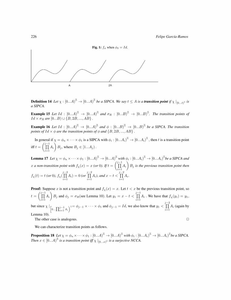
226 Felipe Garcıa-Ramos
Fig. 1: fφ when φ2 = Id.
Definition 14 Let χ : [0...A)Z → [0...A)
Z be a SIPCA. We say t ≤ A is a transition point if χ |[0...t)Z isa SIPCA.
Example 15 Let Id : [0...A)Z → [0...A)
Z and σR : [0...B)Z → [0...B)
Z. The transition points ofId× σR are [0...B) ∪ B, 2B, ..., AB .
Example 16 Let Id : [0...A)Z → [0...A)
Z and φ : [0...B)Z → [0...B)
Z be a SIPCA. The transitionpoints of Id× φ are the transition points of φ and B, 2B, ..., AB .
In general if χ = φn× · · · ×φ1 is a SIPCA with φi : [0...Ai)Z → [0...Ai)
Z, then t is a transition point
iff t =(j−1∏i=1
Ai
)Bj , where Bj ∈ [1...Aj) .
Lemma 17 Let χ = φn×· · ·×φ1 : [0...A)Z → [0...A)
Z with φi : [0...Ai)Z → [0...Ai)
Zbe a SIPCA and
x a non-transition point with fχ(x) = x (or 0). If t =(j−1∏i=1
Ai
)Bj is the previous transition point then
fχ(t) = t (or 0), fχ(j−2∏i=1
Ai) = 0 (orj−2∏i=1
Ai), and x− t <j−2∏i=1
Ai.
Proof: Suppose x is not a transition point and fχ(x) = x. Let t < x be the previous transition point, so
t =
(j−1∏i=1
Ai
)Bj and φj = σR(see Lemma 10). Let y1 = x − t <
j−1∏i=1
Ai . We have that fχ(y1) = y1,
but since χ |[0...∏j−1i=1Ai
)Z= φj−1 × · · · × φ1 and φj−1 = Id, we also know that y1 <j−2∏i=1
Ai (again by
Lemma 10).The other case is analogous. 2
We can characterize transition points as follows.
Proposition 18 Let χ = φn×· · ·×φ1 : [0...A)Z → [0...A)
Z with φi : [0...Ai)Z → [0...Ai)
Zbe a SIPCA.Then x ∈ [0...A)
Z is a transition point iff χ |[0...x)Z is a surjective NCCA.
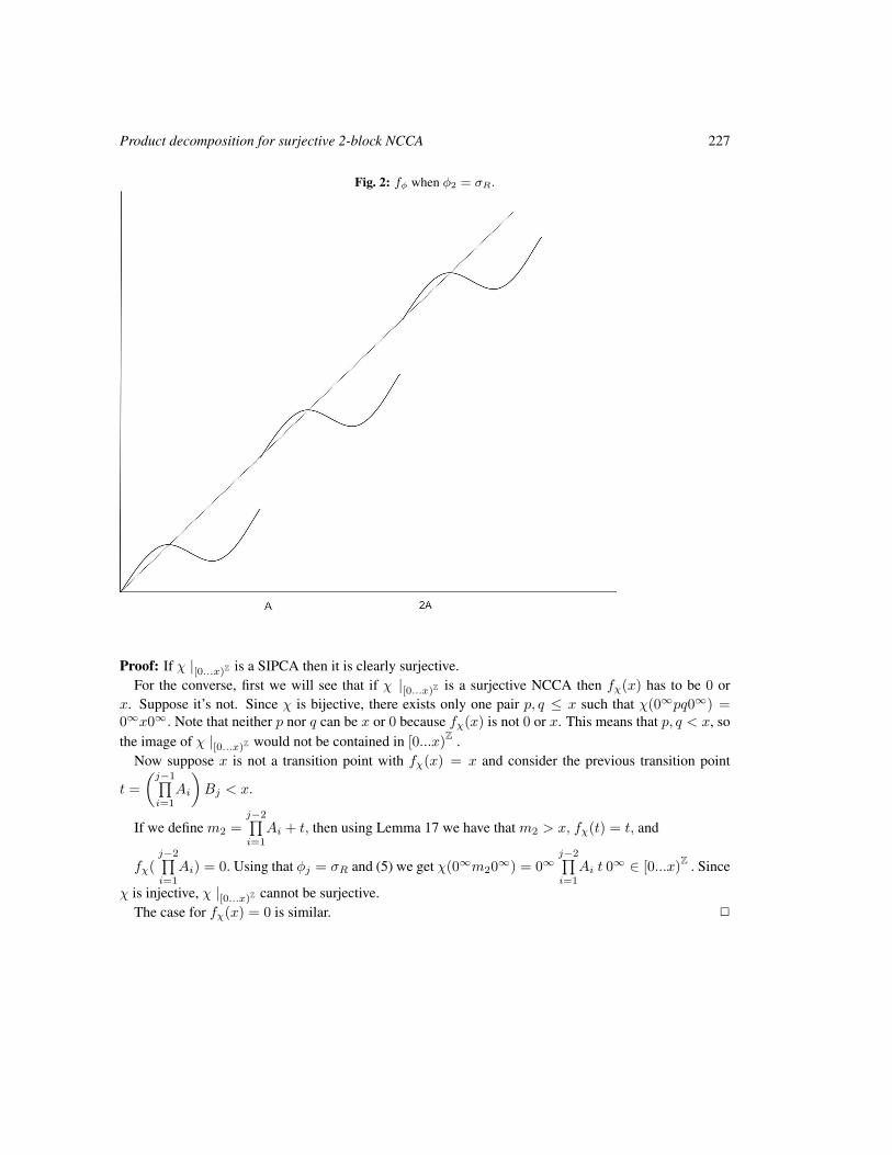
Product decomposition for surjective 2-block NCCA 227
Fig. 2: fφ when φ2 = σR.
Proof: If χ |[0...x)Z is a SIPCA then it is clearly surjective.For the converse, first we will see that if χ |[0...x)Z is a surjective NCCA then fχ(x) has to be 0 or
x. Suppose it’s not. Since χ is bijective, there exists only one pair p, q ≤ x such that χ(0∞pq0∞) =0∞x0∞. Note that neither p nor q can be x or 0 because fχ(x) is not 0 or x. This means that p, q < x, sothe image of χ |[0...x)Z would not be contained in [0...x)
Z .Now suppose x is not a transition point with fχ(x) = x and consider the previous transition point
t =
(j−1∏i=1
Ai
)Bj < x.
If we define m2 =j−2∏i=1
Ai + t, then using Lemma 17 we have that m2 > x, fχ(t) = t, and
fχ(j−2∏i=1
Ai) = 0. Using that φj = σR and (5) we get χ(0∞m20∞) = 0∞
j−2∏i=1
Ai t 0∞ ∈ [0...x)
Z. Since
χ is injective, χ |[0...x)Z cannot be surjective.The case for fχ(x) = 0 is similar. 2
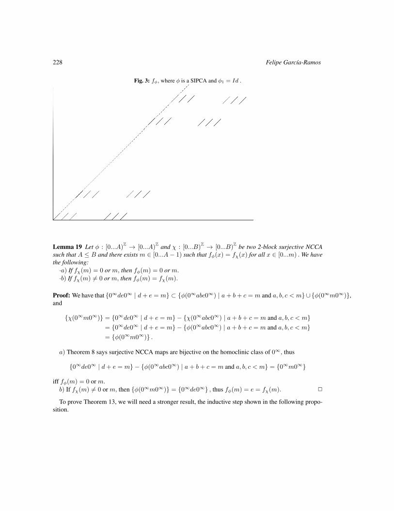
228 Felipe Garcıa-Ramos
Fig. 3: fφ, where φ is a SIPCA and φ1 = Id .
Lemma 19 Let φ : [0...A)Z → [0...A)
Z and χ : [0...B)Z → [0...B)
Z be two 2-block surjective NCCAsuch that A ≤ B and there exists m ∈ [0...A− 1) such that fφ(x) = fχ(x) for all x ∈ [0...m) . We havethe following:·a) If fχ(m) = 0 or m, then fφ(m) = 0 or m.·b) If fχ(m) 6= 0 or m, then fφ(m) = fχ(m).
Proof: We have that 0∞de0∞ | d+ e = m ⊂ φ(0∞abc0∞) | a+ b+ c = m and a, b, c < m ∪ φ(0∞m0∞),and
χ(0∞m0∞) = 0∞de0∞ | d+ e = m − χ(0∞abc0∞) | a+ b+ c = m and a, b, c < m= 0∞de0∞ | d+ e = m − φ(0∞abc0∞) | a+ b+ c = m and a, b, c < m= φ(0∞m0∞) .
a) Theorem 8 says surjective NCCA maps are bijective on the homoclinic class of 0∞, thus
0∞de0∞ | d+ e = m − φ(0∞abc0∞) | a+ b+ c = m and a, b, c < m = 0∞m0∞
iff fφ(m) = 0 or m.b) If fχ(m) 6= 0 or m, then φ(0∞m0∞) = 0∞de0∞ , thus fφ(m) = e = fχ(m). 2
To prove Theorem 13, we will need a stronger result, the inductive step shown in the following propo-sition.
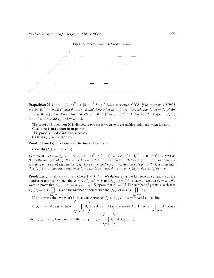
Product decomposition for surjective 2-block NCCA 229
Fig. 4: fφ, where φ is a SIPCA and φ1 = σR.
Proposition 20 Let φ : [0...A)Z → [0...A)
Z be a 2-block surjective NCCA. If there exists a SIPCAχ : [0...B)
Z → [0...B)Z such that A ≤ B and there exists m ∈ [0...A− 1) such that fφ(x) = fχ(x) for
all x ∈ [0...m) , then there exists a SIPCA χ′ : [0...C)Z → [0...C)
Z such that A ≤ C, fχ′(x) = fχ(x)for 0 ≤ x < m, and fχ′(m) = fφ(m).
The proof of Proposition 20 is divided in two cases when m is a transition point and when it’s not.Case 1 (m is not a transition point)This proof is divided into two subcases.Case 1a) (fχ(m) 6= 0 or m)
Proof of Case 1a): It’s a direct application of Lemma 19. 2
Case 1b) (fχ(m) = 0 or m)
Lemma 21 Let χ = φn × · · · × φ1 : [0...A)Z → [0...A)
Z with φi : [0...Ai)Z → [0...Ai)
Zbe a SIPCA.If z is the last zero of fχ (that is the largest value z in the domain such that fχ(z) = 0), then there areexactly z pairs (x, y) such that x < y , fχ(x) = x, and fχ(y) = 0. Analogously if z is the last point suchthat fχ(z) = z, then there exist exactly z pairs (x, y) such that x < y , fχ(x) = 0, and fχ(y) = y.
Proof: Let χj = φj × · · · × φ1, where 1 ≤ j ≤ n. We denote zj as the last zero of χj , and nj as thenumber of pairs (x, y) such that x < y , fχj (x) = x, and fχj (y) = 0. It is easy to see that z1 = n1. Wewant to prove that zj+1 − zj = nj+1 − nj . Suppose that φ1 = Id. The number of points x such thatfχj
(x) = 0 is∏
i≤j odd
Ai and the number of points such that fχj(x) = x is
∏i≤j even
Ai.
If φj+1 = σR then we won’t have any new zeros of fχ, so nj+1 − nj = 0 (see Lemma 10).
If φj+1 = Id then we have
∏i≤j odd
Ai
· (Aj+1 − 1) new zeros of fχ. There are∏
i≤j even
Ai points
where fχ(x) = x, hence we have that nj+1 − nj =
∏i≤j
Ai
·(Aj+1 − 1).
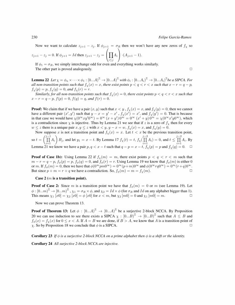
230 Felipe Garcıa-Ramos
Now we want to calculate zj+1 − zj . If φj+1 = σR then we won’t have any new zeros of fχ so
zj+1 − zj = 0. If φj+1 = Id then zj+1 − zj =
∏i≤j
Ai
·(Aj+1 − 1).
If φ1 = σR, we simply interchange odd for even and everything works similarly.The other part is proved analogously. 2
Lemma 22 Let χ = φn×· · ·×φ1 : [0...A)Z → [0...A)
Z with φi : [0...Ai)Z → [0...Ai)
Zbe a SIPCA. Forall non-transition points such that fχ(x) = x, there exist points p < q < r < x such that x− r = q − p,fχ(p) = p, fχ(q) = 0, and fχ(r) = r.
Similarly, for all non-transition points such that fχ(x) = 0, there exist points p < q < r < x such thatx− r = q − p, f(p) = 0, f(q) = q, and f(r) = 0.
Proof: We claim that if we have a pair (x, y) such that x < y , fχ(x) = x, and fχ(y) = 0, then we cannothave a different pair (x′, y′) such that y − x = y′ − x′ , fχ(x′) = x′, and fχ(y′) = 0. That is becausein that case we would have χ(0∞xy′0∞) = 0∞ (x+ y′) 0∞ = 0∞ (x′ + y) 0∞ = χ(0∞x′y0∞), whichis a contradiction since χ is injective. Thus by Lemma 21 we see that if z is a zero of fχ then for everyw ≤ z there is a unique pair x, y ≤ z with x < y, y − x = w, fχ(x) = x, and fχ(y) = 0.
Now suppose x is not a transition point and fχ(x) = x. Let t < x be the previous transition point,
so t =(j−1∏i=1
Ai
)Bj , and let y1 = x − t. By Lemma 17 fχ(t) = t, fχ(
j−2∏i=1
Ai) = 0, and t ≤j−2∏i=1
Ai. By
Lemma 21 we know we have a pair p, q < x− t such that q − p = x− t, fχ(p) = p and fχ(q) = 0. 2
Proof of Case 1b): Using Lemma 22 if fχ(m) = m, there exist points p < q < r < m such thatm− r = q − p, fφ(p) = p, fφ(q) = 0, and fφ(r) = r. Using Lemma 19 we know that fφ(m) is either 0orm. If fφ(m) = 0, then we have that φ(0∞pm0∞) = 0∞(p+m)0∞ and φ(0∞rq0∞) = 0∞(r+q)0∞.But since p+m = r + q we have a contradiction. So, fφ(m) = m = fχ(m). 2
Case 2 (m is a transition point).
Proof of Case 2: Since m is a transition point we have that fφ(m) = 0 or m (see Lemma 19). Letφ : [0...m)
Z → [0...m)Z , χ1 = σR×φ, and χ2 = Id×φ (for σR and Id on any alphabet bigger than 1).
This means χ1 [x0] = χ2 [x0] = φ [x0] for x < m, but χ2 [m0] = 0 and χ1 [m0] = m. 2
Now we can prove Theorem 13.
Proof of Theorem 13: Let φ : [0...A)Z → [0...A)
Z be a surjective 2-block NCCA. By Proposition20 we can use induction to see there exists a SIPCA χ : [0...B)
Z → [0...B)Z such that A ≤ B and
fφ(x) = fχ(x) for 0 ≤ x < A. If A = B we are done, if B > A, we know that A is a transition point ofχ. So by Proposition 18 we conclude that φ is a SIPCA. 2
Corollary 23 If φ is a surjective 2-block NCCA on a prime alphabet then φ is a shift or the identity.
Corollary 24 All surjective 2-block NCCA are injective.

Product decomposition for surjective 2-block NCCA 231
5 Further questionsFor bigger neighbourhoods not all surjective NCCA are SIPCA.
Example 25 The CA φ on the binary alphabet defined by exchanging the blocks 10100001 and 10010001,is a well-defined bijective NCCA which is not a shift or an identity, but φ2 = Id. We can construct severalsimilar examples where φn = σmR for a certain n and m (where σ0
R = Id).
We can construct several similar counter-examples where φn = σmR for a certain n and m (whereσ0R = Id), but we can ask the following questions.
Question 26 Are all binary surjective NCCA ψ generalized subshifts? That is, do there exist naturalnumbers n and m such that ψm = σnR?
Question 27 If φ is a surjective NCCA do there exist natural numbers n and m and a SIPCA ψ such thatφn = ψm?
The author is currently investigating these subjects.NCCA are a particular class of potential conserving CA φ : [0...A)
Z → [0...A)Z, when µ(x) = x. The
result that proves the density of periodic points for surjective NCCA (Formenti and Grange (2003)) can beeasily be extended to unique ground state potentials, that is when µ(x) = 0 for only one state. Theorem8 holds also for surjective CA that conserves ground state potentials.
Question 28 Let φ be a one-dimensional surjective CA that conserves the potential µ, and µ(x) = 0 foronly one state. Is φ injective?
6 addendumIn this appendix we provide a counterexample of a surjective but non injective binary NCCA.
Example 29 Let A = [1000100001] and B = [1001000001] . Notice they do not overlap except at theborders, they have the same length and same weight. Now define the CA as follows.
Everything stays where it is except where there are two of the previous blocks together, in that case theblock in the right changes to A if they are the same and to B if they are different. By together we meanthat they overlap in the border. We can identify strings of n blocks, and they will always remain as stringsof n blocks. This map is surjective and number conserving, but it is not injective because the image of(A′B′)∞ and (B′A′)∞ is B′∞. Where A′ = [000100001] and B′ = [001000001] .
Hence powers of this CA are never the the identity nor the power of a shift, but on the homoclinic classof 0∞ it is a root of the identity so it is a generalized subshift there.
AcknowledgementsI would like to thank Siamak Taati, for conversations that inspired this paper; Brian Marcus (friend andboss) for carefully reading and correcting this paper; the anonymous referees for providing excellentsuggestions; and Nishant Chandgotia for helping to construct Example 25.

232 Felipe Garcıa-Ramos
ReferencesN. Boccara and H. Fuks. Number-conserving cellular automaton rules. Fundamenta Informaticae, 52
(1):1 – 13, 2002. ISSN 2002-01-01. URL http://iospress.metapress.com/content/8R32U119Q5NDJ3KB.
E. Formenti and A. Grange. Number conserving cellular automata ii: dynamics. Theoret-ical Computer Science, 304(1-3):269 – 290, 2003. ISSN 0304-3975. doi: DOI:10.1016/S0304-3975(03)00134-8. URL http://www.sciencedirect.com/science/article/pii/S0304397503001348.
T. Hattori and S. Takesue. Additive conserved quantities in discrete-time lattice dynamical systems.Physica D: Nonlinear Phenomena, 49(3):295 – 322, 1991. URL http://www.sciencedirect.com/science/article/pii/0167278991901508.
G. Hedlund. Endomorphisms and automorphisms of the shift dynamical systems. Mathematical SystemTheory, 3:320 – 375, 1969.
J. Kari and S. Taati. A particle displacement representation for conservation laws in two-dimensionalcellular automata. Proceedings of JAC 2008., pages 65 – 73, 2008.
S. Maerivoet and B. D. Moor. Cellular automata models of road traffic. Physics Reports, 419(1):1 – 64, 2005. ISSN 0370-1573. doi: 10.1016/j.physrep.2005.08.005. URL http://www.sciencedirect.com/science/article/pii/S0370157305003315.
E. Moore. Machine models of self-reproduction. Proc. Symp. Appl. Math., 14:13 – 33, 1963.
T. Moothathu. Surjective cellular automata with zero entropy are almost one-to-one. Chaos, Solitons &Fractals, 44(6):415 – 417, 2011. ISSN 0960-0779. doi: 10.1016/j.chaos.2011.01.013. URL http://www.sciencedirect.com/science/article/pii/S0960077911000440.
A. Moreira, N. Boccara, and E. Goles. On conservative and monotone one-dimensional cellular au-tomata and their particle representation. Theoretical Computer Science, 325(2):285 – 316, 2004. ISSN0304-3975. doi: DOI:10.1016/j.tcs.2004.06.010. URL http://www.sciencedirect.com/science/article/pii/S0304397504003950. Theoretical Aspects of Cellular Automata.
J. Myhill. The converse of moore’s garden-of-eden theorem. Proc. Am. Math. Soc., 14:685 – 686, 1963.
M. Pivato. Conservation laws in cellular automata. Nonlinearity, 15(6), 2002. URL http://stacks.iop.org/0951-7715/15/i=6/a=305.
AUTOMATA 2011, Santiago, Chile local proceedings LP, 2011, 233–242
Garden-of-Eden-like theorems for amenablegroups
Silvio Capobianco1†, Pierre Guillon2,3‡ and Jarkko Kari3§
1Institute of Cybernetics at Tallinn University of Technology, Estonia2CNRS & IML, Marseille, France3Mathematics Department, University of Turku, Finland
In the light of recent results by Bartholdi, we consider several properties that, for classical cellular automata, areknown to be equivalent to surjectivity. We show that the equivalence still holds for amenable groups, and givecounter-examples for non-amenable ones.
Keywords: cellular automata, amenability, group theory, topological dynamics, symbolic dynamics, ergodic theory,random theory
1 IntroductionRetrieving global properties of cellular automata (CA) has been a main topic of research since the field wasestablished. Indeed, the Garden-of-Eden theorem by Moore [Moo62] and its converse by Myhill [Myh62],which link surjectivity of the global map of 2D CA to pre-injectivity (a property that may be described asthe impossibility of erasing finitely many errors in finite time) also have the distinction of being the firstrigorous results of cellular automata theory. Several more properties were later proved to be equivalentto surjectivity in d-dimensional CA, such as balancedness of the local map [MK76] and the sending ofalgorithmically random configurations into algorithmically random configurations [CHJW01].
With the subsequent efforts to extend the definition of CA to more general situations than the usualEuclidean lattices, an unexpected phenomenon appeared: the Garden-of-Eden property actually dependson properties of the involved groups! In particular, counterexamples to both Moore’s and Myhill’s theoremare well known for CA on the free group on two generators (cf. [CSMS99]). However, from a readingof the original proofs, a key fact emerges, which is crucial for the proofs themselves: in Zd, the size ofa hypercube is a d-th power of the side, but the number of sites on its outer surface is a polynomial ofdegree d− 1. In other words, it seems that, to get Moore’s or Myhill’s theorem for CA on a group G, weneed that in G the sphere grows more slowly than the ball. What is actually sufficient is a slightly weakerproperty called amenability, which can be stated as the existence of a translation-invariant finitely additive
†Email: [email protected]‡Email: [email protected]§Email: [email protected]
c© 2011 AUTOMATA proceedings, Santiago, Chile, 2011
234 Silvio Capobianco, Pierre Guillon and Jarkko Kari
probability measure on G. Bartholdi’s theorem [Bar10] states then that the amenable groups are preciselythose where surjective CA are pre-injective, and preserve the product measure on configurations.
In this paper, which illustrates work in progress, we extend the range of Bartholdi’s theorem by charac-terizing amenable groups as those where surjective CA have additional properties. We start by consideringbalancedness [MK76], which is the combinatorial variant of measure preservation. We then include thenonwandering property, an important feature of dynamical systems. Finally, and for groups that have adecidable word problem, we prove that amenable groups are those where, in line with [CHJW01], CApreserve descriptional complexity.
To sum up, we get the following statement.
Theorem 1 Let G be a finitely generated group. The following are equivalent.
1. G is amenable.
2. Every surjective CA on G is pre-injective.
3. Every surjective CA on G preserves the uniform product measure.
4. Every surjective CA on G is balanced.
5. Every surjective CA on G is nonwandering.
If, in addition, G has decidable word problem, then the above are equivalent to the following:
• Every surjective CA sends random configurations into random configurations.
2 Preliminaries2.1 GroupsLet G be a group. We call 1G, or simply 1, its identity element. Given a set X , the family σ = σgg∈Gof transformations of XG, called translations, defined by
σg(c)(z) = cg(z) = c(gz) ∀g ∈ G (1)
is a right action of G on XG, that is, σgh = σh σg for every g, h ∈ G. This is consistent with definingthe product φψ of functions as the composition ψ φ. Other authors (cf. [CSC10]) define σg(c)(x) asc(g−1x), so that σ becomes a left action. However, most of the definitions and properties we deal with donot depend on the “side” of the multiplication: we will therefore stick to (1).
A set of generators for G is a subset S ⊆ G such that for each g ∈ G there is a word w = w1 . . . wnon S ∪ S−1 such that g = w1 · · ·wn. The minimum length of such a word is called length of g w.r.t.S, and indicated by ‖g‖S , or simply ‖g‖. G is finitely generated (briefly, f.g.) if S can be chosen finite.A group G is free on a set S if it is isomorphic to the group of reduced words on S ∪ S−1. For r ≥ 0,g ∈ G the disk of radius r centered in g is Dr(g) = h ∈ G | ‖g−1h‖ ≤ r. The points of Dr(g) canbe “reached” from the “origin” 1G by first “walking” up to g, then making up to r steps: this is consistentwith the definition of translations by (1), where to determine cg(z) we first move from 1 to g, then from gto gz. We write Dr for Dr(1). We also put U−r = z ∈ G | Dr(z) ⊆ U and ∂−rU = U \ U−r. Forour purposes, we will only consider f.g. groups.
Garden-of-Eden-like theorems for amenable groups 235
A group G is residually finite (briefly, r.f.) if for every g 6= 1 there exists a homomorphism φ : G→ Hsuch that H is finite and φ(g) 6= 1. Equivalently, G is r.f. if the intersection of all its subgroups of finiteindex is trivial. It follows from the definitions that, if G is r.f. and U ⊆ G is finite, then there existsH ≤ G s.t. [G : H] ≤ ∞ and U ∩H ⊆ 1G.Lemma 2 ([Fio00, Lemma 2.3.2]) Let G be a residually finite (not necessarily f.g.) group and let F bea finite subset of G not containing 1G. Then there exists a subgroup HF of finite index in G, which doesnot intersect F , and such that the HFu, u ∈ F , are pairwise disjoint.
The word problem (briefly, w.p.) for a group G with a set of generators S is the set of words on S ∪ S−1
that represent the identity element of G. Although this set may depend on the choice of the presentation,its decidability does not; and although the problem is not decidable even for finitely generated groups, itis for the Euclidean groups Zd, the free groups, and more.
The stabilizer of c is the subgroup st(c) = g ∈ G | cg = c: be aware, that st(c) might not be anormal subgroup. c is periodic if [G : st(c)] < ∞. If [G : H] < ∞ and H ≤ st(c) we say that c isH-periodic. The family of periodic configurations in QG is indicated by Per(G,Q).
A group G is amenable if it satisfies one of the following equivalent conditions:
1. There exists a finitely additive probability measure µ on G with ∀A ⊆ G,∀g ∈ G,µ(gA) = µ(A).
2. For every finite U ⊆ G and ε > 0 there exists a finite K ⊆ G such that
|UK \K| < ε|K| (2)
Similar definitions want µ right-invariant and (2) replaced by |KU \ K| < ε|K|, or µ both left- andright-invariant and difference in (2) replaced by symmetric difference: in fact, all these definitions areequivalent. Also, if every f.g. subgroup of a given group is amenable, then the group is itself amenable.
A bounded-propagation 2 : 1 compressing map over a group G is a map φ : G → G such that, forsome finite propagation set S ⊆ G, φ(g)−1g ∈ S for every g ∈ G, and |φ−1(g)| = 2 for every g ∈ G.In particular, such a map must be surjective, and |S| ≥ 2. By [CSC10, Theorem 4.9.2], a group has abounded-propagation 2 : 1 compressing map if and only if it is not amenable. For instance, in the caseof the free group over generators a, b, one can define: φ(x) = y if x /∈ an|n ∈ N is written in anirreducible way as yc for some c ∈ a, b; φ(x) = x otherwise. Here S = 1, a, b and any point y hastwo preimages: y and yb if y is written in an irreducible way as wa−1 or an; y and ya if y is written in anirreducible way as wb−1; ya and yb otherwise.
2.2 Cellular automataA cellular automaton (briefly, CA) on a group G is a triple A = 〈Q,N , f〉 where the alphabet Q is afinite set, the neighborhood index N ⊆ G is finite and nonempty, and f : QN → Q is a local function.This, in turn, induces a global function on any configuration c : G→ Q, defined by
FA(c)(g) = f (cg|N ) = f(c|gN
). (3)
Through (3) we also consider, for every finite E ⊆ G, a function between patterns f : QEN → QE
defined by f(p)j = f(p|jN ). Hedlund’s theorem [CSC10, Theorem 1.8.1] states that global functionsof CA are exactly those functions from QG to itself that commute with translations and are continuous
236 Silvio Capobianco, Pierre Guillon and Jarkko Kari
in the product topology. We recall that a base for this topology is given by the cylinders of the formC(E, p) = c ∈ QG | c|E = p, with E a finite shape of G and p : E → Q a pattern: observe that, forcountable groups, this base is countable. Also, the cylinders of the form C(q, z) = c | c(z) = q form a(countable) subbase. If p = c|E we may write C(p) instead of C(c, E).
An occurrence of a pattern p : E → Q in c ∈ QG is an element g ∈ G such that cg|E = p; the patternpg : gE → Q defined by pg(gz) = p(z) is then a copy of p. For compactness reasons, a CA A has noGarden-of-Eden configurations (i.e., c ∈ QG \ FA(QG)) if and only if it has no orphan patterns, i.e., ifevery pattern has an occurrence in some FA(c). Two configurations are asymptotic if they differ on atmost finitely many points; a CA is pre-injective if distinct asymptotic configurations have distinct images.Moore’s Garden-of-Eden theorem [Moo62] states that surjective CA on Zd are pre-injective; Myhill’stheorem [Myh62] states the converse implication.
A cellular automaton A over QG is nonwandering if for any open set U ⊂ QG there exists t ≥ 1 suchthat F tA(U) ∩ U 6= ∅; it is transitive if for any two open sets U and V there exists some t ≥ 1 suchthat F tA(U) ∩ V 6= ∅. (In particular, a transitive CA is nonwandering). A state q0 ∈ Q is spreading forA = 〈Q,N , f〉 if for any u ∈ QN such that ui = q0 for some i ∈ N we have f(u) = q0.
Remark 3 A nonwandering non-trivial CA has no spreading state.
By non-trivial, we mean that |N | > 1 and |Q| > 1. Indeed, take a cylinder U = C(N ∪ 1G, c) whereci = q0 6= c1G
for some i ∈ N \ 1G: then F t(U) ∩ U = ∅ for any t ≥ 1.Let N ⊆ G ≤ Γ and f : QN → Q. The triple 〈Q,N , f〉 describes both a CA A over G and a CA A′
on Γ. We then say that A′ is the CA induced by A on Γ, or that A is the restriction of A′ to G.
2.3 Measures and randomnessLet Σ be a σ-algebra on QG. If µ : Σ→ [0, 1] is a measure on QG, a measurable function F : QG → QG
determines a new measure Fµ : Σ → [0, 1] defined as Fµ(U) = µ(F−1(U)). We say that F preservesµ if Fµ = µ. If Q is finite, G is countable, and Σ is the Borel σ-algebra generated by the open sets,by standard facts in measure theory, a measure µ is completely determined by its value on the cylinders.In particular, the measure defined by µΠ(C(E, p)) = |Q|−|E| is called the uniform product measure,because it is a product of independent uniform measures on the alphabet. Bartholdi’s theorem [Bar10]states that the amenable groups are precisely those where surjective CA preserve µΠ and are pre-injective.
Let µ be some probability measure over QG. We say that a continuous function F : QG → QG isµ-recurrent if for any measurable set A ⊂ QG of measure µ(A) > 0, there exists some time step t ≥ 1such that µ(A ∩ F t(A)) > 0. If µ has full support, then this implies that F is nonwandering. Moreover,the Poincare recurrence theorem states that any F that preserves µ is µ-recurrent.
We say that µ is F -ergodic (or F is µ-ergodic) if F preserves µ and every F -invariant set U (i.e.,F−1(U) = U ) has µ(U) ∈ 0, 1. In that case, the Birkhoff ergodic theorem gives that µ-almost everypoint is µ-typical for F , that is,
µ
(x ∈ QG | ∀A ∈ Σ, lim
n→∞
1
n
∣∣A ∩ F t(x)|0 ≤ t < n∣∣ = µ(A)
)= 1 . (4)
Let µ and ν be F -ergodic measures; suppose they have a typical point x in common. Then for anymeasurable set A, µ(A) = limn→∞
1n |A ∩ F
t(x)|0 ≤ t < n| = ν(A) : we have thus
Lemma 4 Any two distinct F -ergodic measures have no typical point in common.
Garden-of-Eden-like theorems for amenable groups 237
Let φ : N → G be a total computable enumeration. It is easy to see that it induces a computableenumeration of the cylinders, which we call B′ = B′ii≥0 in accordance with [CHJW01].
Given any two sequences of open sets U = Uii≥0, V = Vjj≥0, we say that U is V-computable ifthere is a recursively enumerable set A ⊆ N s.t.
Ui =⋃
j∈N:π(i,j)∈A
Vj ∀i ≥ 0 , (5)
where π(i, j) = (i + j)(i + j + 1)/2 + i is the standard primitive recursive bijection from N × N to N.A B′-computable family U of open sets is a Martin-Lof µ-test (briefly, a M-L µ-test) if µ(Un) ≤ 2n forevery n ≥ 0. A configuration c ∈ QG fails a M-L µ-test U if c ∈
⋂n≥0 Un. c ∈ QG is µ-random (in
the sense of Martin-Lof) if it does not fail any M-L µ-test. Note that, since the number of M-L µ-tests iscountable, the set of µ-random configurations has full measure.
Given any pattern p, the set of configurations where p has no occurrence is an intersection of a countablyinfinite, computable family of cylinders Ui having equal product measure µΠ(Ui) = m < 1. It isthen straightforward to construct a M-L µΠ-test that every such configuration fails. If we call rich aconfiguration in which any pattern occurs (or, equivalently, whose orbit under the shift action is dense),we then have the following.
Remark 5 Any µΠ-random configuration is rich.
Note that φ : N → G induces φ∗ : QG → QN defined by φ∗(c)(n) = c(φ(n)). If φ is a computablebijection, then so is φ∗: in this case (cf. [GHR10, Proposition 2.5.2]) φ∗ is continuous and preserves theproduct measure. In particular, c is random for the product measure on QG if and only if φ∗(c) is randomfor the product measure on QN, and the set of random configurations has measure 1.
3 ResultsAccording to Maruoka and Kimura [MK76], a d-dimensional CA with neighborhood a hypercube of radiusr is n-balanced if each pattern on a hypercube of side n has |Q|(n+2r)d−nd
pre-images. The authors thenprove that a d-dimensional CA is surjective if and only if it is n-balanced for every n. On the other hand,the majority rule is 1-balanced but has the Garden-of-Eden pattern 01001.
The balancedness condition means that each pattern on a given shape has the same number of pre-images. (Just “patch” arbitrary shapes to “fill” a hypercube.) This works for CA over arbitrary groups.
Definition 6 Let G be a group and let A = 〈Q,N , f〉 be a CA on G. A is balanced if for every finitenonempty E ⊆ G and pattern p : E → Q,
|f−1(p)| = |Q||EN|−|E|. (6)
Since the r.h.s. in (6) is always positive, no pattern is an orphan for a balanced CA. In [CSMS99], two CAon the free group on two generators are shown, one being surjective but not pre-injective, the other pre-injective but not surjective: both have an unbalanced local function. Therefore, balancedness in generalgroups is strictly stronger than surjectivity, and possibly uncorrelated with pre-injectivity.
Remark 7 A cellular automaton is balanced if and only if it preserves the uniform product measure.
238 Silvio Capobianco, Pierre Guillon and Jarkko Kari
The proof is similar to that in [CHJW01]. In fact, letA = 〈Q,N , f〉 and p : E → Q: then µΠ(F−1A (C(E, p))) =∑
f(p′)=p |Q|−|EN|. But balancedness means r.h.s. has |Q||EN|−|E| summands whatever p is, whilepreservation of µΠ means l.h.s. equals |Q|−|E| whatever p is.
By [CSC09, Theorem 1.2] several important properties, including injectivity and surjectivity, are pre-served by induction and restriction: this is also true for balancedness.
Remark 8 LetA = 〈Q,N , f〉 be a CA on G ≤ Γ andA′ the CA induced byA on Γ. ThenA is balancedif and only if A′ is balanced.
Proof: IfA′ is balanced, thenA clearly is. Suppose thenA is balanced; let J be a set of representatives ofthe left cosets of G in Γ. Let E ⊆ Γ: put JE = j ∈ J | jG ∩ E 6= ∅. Then E =
⊔j∈JE (jG ∩ E) and,
sinceN ⊆ G, EN =⊔j∈JE (jG∩EN ), with JE finite since E is. Given p : E → Q, call pj = p|jG∩E
for j ∈ JE . Then, since A′ operates slicewise and A is balanced,
|f−1(p)| =∏j∈JE
|f−1(pj)| =∏j∈JE
|Q||jG∩EN|−|jG∩E| = |Q|∑
j∈JE|jG∩EN|−
∑j∈JE
|jG∩E|,
which is precisely |Q||EN|−|E|. Since E and p are arbitrary, A′ is balanced. 2
With the next statement, we strengthen [Wei00, Theorem 1.3], which states that injective CA on r.f.groups are surjective. We rely on a lemma which is immediate to prove.
Lemma 9 If F : QG → QG commutes with translations, then st(c) ⊆ st(F (c)) for every c ∈ QG. Inparticular, if F is bijective then st(c) = st(F (c)).
Theorem 10 Let G be a residually finite group and A = 〈Q,N , f〉 an injective CA over G. Then A isbalanced.
Proof: Let E be a finite subset of G: it is not restrictive to suppose 1 ∈ E ∩ N , so that E,N ⊆ EN .Suppose, for the sake of contradiction, that p : E → Q satisfies |F−1
A (p)| = M > |Q||EN|−|E|. SinceG is residually finite, by Lemma 2 there exists a subgroup H ≤ G of finite index such that H ∩ EN =H ∩N = 1 : if J is a set of representatives of the right cosets of H such that EN ⊆ J , then
|π : J → Q | FA(π)|E = p| = M · |Q|[G:H]−|EN| > |Q|[G:H]−|E| . (7)
The r.h.s. in (7) is the number of H-periodic configurations that coincide with p on E. Since A isinjective and G is r.f., by [Wei00, Theorem 1.3] A is reversible, and by Lemma 9, FA sends H-periodicconfigurations intoH-periodic configurations. But because of (7) and the pigeonhole principle, there mustexist two H-periodic configurations with the same image according to FA: which contradicts injectivityof A. 2
The proof of Moore’s and Myhill’s theorems for CA on amenable groups given in [CSMS99] is basedon the following lemma.
Lemma 11 ([CSMS99, Step 1 in proof of Theorem 3]) Let G be an amenable group, q ≥ 2, and n >r > 0. For L = Dn there exist m > 0 and B ⊆ G such that B contains m disjoint copies of L and
(q|L| − 1)m · q|B|−m|L| < q|B−r| . (8)
Garden-of-Eden-like theorems for amenable groups 239
We use Lemma 11 to get a combinatorial proof of the equivalence between surjectivity and balancedness,that was already essentially stated in [Bar10].
Theorem 12 Let G be an amenable group and let A a CA on G. If A is surjective then A is balanced.
Proof: Put L = Dn, L′ = Dn−r, q = |Q|. Suppose, for the sake of contradiction, that A is not balanced.Then, for suitable n, there is a pattern p : L′ → Q that has at most q|L|−|L
′|− 1 pre-images. Let m and Bbe as by Lemma 11. Consider the patterns on B whose image under the global rule of A coincides with pon each of the m copies of L′ contained in those of L: their number t is at most(
q|L|−|L′| − 1
)mq|B|−m|L| .
However,(q|L|−|L
′| − 1)≤ q−|L′|
(q|L| − 1
), so that, by Lemma 11,
t ≤ q−m|L′|(q|L| − 1
)mq|B|−m|L| < q|B
−r|−m|L′| .
But the last term is precisely the number of patterns on B−r that coincide with p on each of the given mcopies of L′. There are more of these than available pre-images, so one of them must be an orphan. 2
Thanks again to Lemma 11, [CHJW01, Point 1 of Theorem 4.4] generalizes to amenable groups.
Proposition 13 Let G be an amenable group and let A = 〈Q,Dr, f〉, r > 0, be a CA on G. If c is notrich then FA(c) is not rich.
Proof: Suppose there is a pattern with support L = Dn, n > r, that does not occur in c. Choose m and Baccording to Lemma 11. By hypothesis, the number of patterns with support B that occur in c is at most(q|L|− 1)mq|B|−m|L|, with q = |Q|; therefore, the number of patterns with support B \ ∂rB which occurin FA(c) cannot exceed this number too. By Lemma 11, this is strictly less than q|B|−|∂rB|, which is thetotal number of patterns with support B \ ∂rB: hence, some of those patterns do not occur in FA(c). 2
We now consider another property that, for CA on Zd, is equivalent to surjectivity: sending µΠ-randomconfigurations into µΠ-random configurations. Before going ahead, we must remember that, accordingto [CHJW01], the definition of a random configuration on Zd depends on the existence (and choice!) ofa total computable bijection from N to Zd. This is still ensured for a general group G when it has adecidable word problem: we thus can first enumerate D0 = 1G, then D1 \D0, then D2 \D1, and soon.
The proofs of the following two statements are then similar to the original ones in [CHJW01]
Lemma 14 Let G be a group with decidable word problem, U a B′-computable sequence, and A a CAon G. Then F−1
A (U) is a B′-computable sequence.
Proof: Let A be a r.e. set such that Ui =⋃π(i,j)∈AB
′j for every i ≥ 0, where the B′j are cylinders. Since
A is a CA, F−1A (Ui) is itself a union of cylinders: such union is computable because G has decidable
word problem. By exploiting these facts and the primitive recursive functions L,K : N → N such thatπ(L(n),K(n)) = n for every n ≥ 0, we can construct a r.e. set Z such that F−1
A (Ui) =⋃π(i,j)∈Z B
′j
for every i ≥ 0. 2
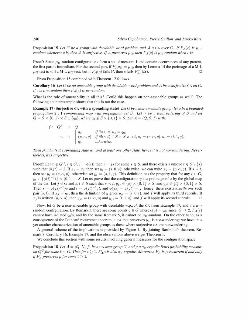
240 Silvio Capobianco, Pierre Guillon and Jarkko Kari
Proposition 15 Let G be a group with decidable word problem and A a CA over G. If FA(c) is µΠ-random whenever c is, then A is surjective. If A preserves µΠ, then FA(c) is µΠ-random when c is.
Proof: Since µΠ-random configurations form a set of measure 1 and contain occurrences of any pattern,the first part is immediate. For the second part, if FAµΠ = µΠ, then by Lemma 14 the preimage of a M-LµΠ-test is still a M-L µΠ-test: but if FA(c) fails U , then c fails F−1
A (U). 2
From Proposition 15 combined with Theorem 12 follows
Corollary 16 Let G be an amenable group with decidable word problem andA be a surjective CA on G.If c is µΠ-random then FA(c) is µΠ-random.
What is the role of amenability in all this? Could this happen on non-amenable groups as well? Thefollowing counterexample shows that this is not the case.
Example 17 (Surjective CA with a spreading state) LetG be a non-amenable group; let φ be a bounded-propagation 2 : 1 compressing map with propagation set S. Let be a total ordering of S and letQ = S × 0, 1 × S t q0, where q0 /∈ S × 0, 1 × S. Let A = 〈Q,S, f〉 with:
f : QS → Q
u 7→
∣∣∣∣∣∣q0 if ∃s ∈ S, us = q0,(p, α, q) if ∃!(s, t) ∈ S × S, s ≺ t, us = (s, α, p), ut = (t, 1, q),q0 otherwise.
Then A admits the spreading state q0, and at least one other state, hence it is not nonwandering. Never-theless, it is surjective.
Proof: Let x ∈ QG, i ∈ G, j = φ(i): then i = js for some s ∈ S, and there exists a unique t ∈ S \ ssuch that φ(jt) = j. If xj = q0, then set yi = (s, 0, s): otherwise, we can write xj = (p, α, q). If s ≺ t,then set yi = (s, α, p); otherwise set yi = (s, 1, q). This definition has the property that for any i ∈ G,yi ∈ φ(i)−1i × 0, 1 × S. Let us prove that the configuration y is a preimage of x by the global mapof the CA. Let j ∈ G and s, t ∈ S such that s ≺ t, yjs ∈ s × 0, 1 × S, and yjt ∈ t × 0, 1 × S.Then s = φ(js)−1js and t = φ(jt)−1jt, and φ(js) = φ(jt) = j: hence, there exists exactly one suchpair (s, t). If xj = q0, then the definition of y gives yjt = (t, 0, t), and f will apply its third subrule. Ifxj is written (p, α, q), then yjs = (s, α, p) and yjt = (t, 1, q), and f will apply its second subrule. 2
Now, let G be a non-amenable group with decidable w.p., A the CA from Example 17, and c a µΠ-random configuration. By Remark 5, there are some points g ∈ G where c(g) = q0: since |S| ≥ 2, FA(c)cannot have isolated q0’s, and by the same Remark 5, it cannot be µΠ-random. On the other hand, as aconsequence of the Poincare recurrence theorem, a CA that preserves µΠ is nonwandering: we have thusyet another characterization of amenable groups as those where surjective CA are nonwandering.
A general scheme of the implications is provided by Figure 1. By joining Bartholdi’s theorem, Re-mark 7, Corollary 16, Example 17, and the observations above we get Theorem 1.
We conclude this section with some results involving general measures for the configuration space.
Proposition 18 LetA = 〈Q,N , f〉 be a CA over groupG, and µ a σk-ergodic Borel probability measureon QG for some k ∈ G. Then for t ≥ 1, F tAµ is also σk-ergodic. Moreover, FA is µ-recurrent if and onlyif F tA preserves µ for some t ≥ 1.
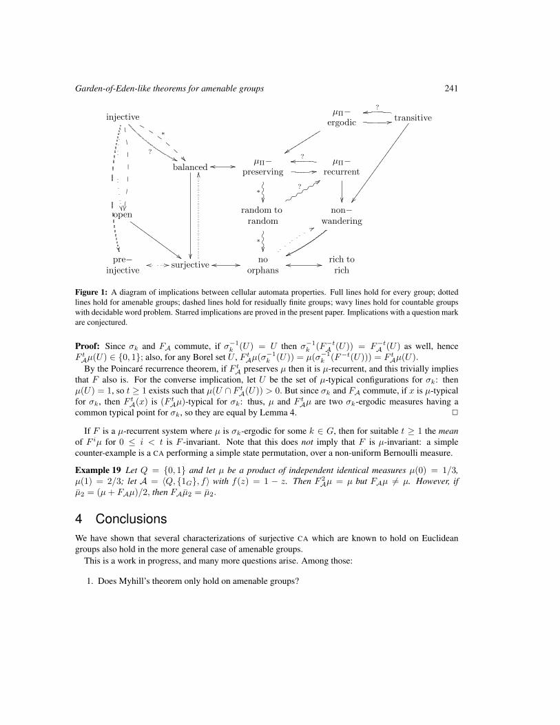
Garden-of-Eden-like theorems for amenable groups 241
injective
∗
NK
HD
A=?
''
$
#
!
µΠ−ergodic
yyssssssssss11 transitive
balanced oo //
µΠ−preserving
∗ OOO
11µΠ−
recurrent
?pp
open
##HHHHHHHHHHHHHHrandom to
random
∗ OOO
?
999y9y9y9y9y9y
non−wandering
wwpre−
injectiveoo // surjective oo //
OO
noorphans
oo //
77
rich torich
Figure 1: A diagram of implications between cellular automata properties. Full lines hold for every group; dottedlines hold for amenable groups; dashed lines hold for residually finite groups; wavy lines hold for countable groupswith decidable word problem. Starred implications are proved in the present paper. Implications with a question markare conjectured.
Proof: Since σk and FA commute, if σ−1k (U) = U then σ−1
k (F−tA (U)) = F−tA (U) as well, henceF tAµ(U) ∈ 0, 1; also, for any Borel set U , F tAµ(σ−1
k (U)) = µ(σ−1k (F−t(U))) = F tAµ(U).
By the Poincare recurrence theorem, if F tA preserves µ then it is µ-recurrent, and this trivially impliesthat F also is. For the converse implication, let U be the set of µ-typical configurations for σk: thenµ(U) = 1, so t ≥ 1 exists such that µ(U ∩ F tA(U)) > 0. But since σk and FA commute, if x is µ-typicalfor σk, then F tA(x) is (F tAµ)-typical for σk: thus, µ and F tAµ are two σk-ergodic measures having acommon typical point for σk, so they are equal by Lemma 4. 2
If F is a µ-recurrent system where µ is σk-ergodic for some k ∈ G, then for suitable t ≥ 1 the meanof F iµ for 0 ≤ i < t is F -invariant. Note that this does not imply that F is µ-invariant: a simplecounter-example is a CA performing a simple state permutation, over a non-uniform Bernoulli measure.
Example 19 Let Q = 0, 1 and let µ be a product of independent identical measures µ(0) = 1/3,µ(1) = 2/3; let A = 〈Q, 1G, f〉 with f(z) = 1 − z. Then F 2
Aµ = µ but FAµ 6= µ. However, ifµ2 = (µ+ FAµ)/2, then FAµ2 = µ2.
4 ConclusionsWe have shown that several characterizations of surjective CA which are known to hold on Euclideangroups also hold in the more general case of amenable groups.
This is a work in progress, and many more questions arise. Among those:
1. Does Myhill’s theorem only hold on amenable groups?

242 Silvio Capobianco, Pierre Guillon and Jarkko Kari
2. What is the actual role of the word problem in Lemma 14 and Proposition 15? Can we find someamenable groups with undecidable word problem but where surjective CA still send µΠ-random toµΠ-random?
3. For the uniform product measure, is every recurrent CA invariant?
AcknowledgementsThis research was supported by the European Regional Development Fund (ERDF) through the EstonianCentre of Excellence in Theoretical Computer Science (EXCS), by the Estonian Research Fund (ETF)through grant nr. 7520, and by the Academy of Finland Grant 131558.
References[Bar10] L. Bartholdi. Gardens of eden and amenability on cellular automata. J. Eur. Math. Soc., 12:141–148,
2010.
[BGH+11] L. Bienvenu, P. Gacs, M. Hoyrup, C. Rojas, and A. Shen. Algorithmic tests of randomness with respectto a class of measures. arXiv:1103.1529v2[math.LO], 2011.
[CHJW01] C. Calude, P. Hertling, H. Jurgensen, and K. Weihrauch. Randomness on full shift spaces. Chaos,Solitons & Fractals, 12:491–503, 2001.
[CSC09] T. Ceccherini-Silberstein and M. Coornaert. Induction and restriction of cellular automata. Ergod. Th. &Dynam. Sys., 29:371–380, 2009.
[CSC10] T. Ceccherini-Silberstein and M. Coornaert. Cellular Automata and Groups. Springer Verlag, 2010.
[CSMS99] T. Ceccherini-Silberstein, A. Machı, and F. Scarabotti. Amenable groups and cellular automata. Annalesde l’Institut Fourier, 49:673–685, 1999.
[Fio00] F. Fiorenzi. Cellular automata and finitely generated groups. PhD thesis, Sapienza Universita di Roma,2000.
[GHR10] S. Galatolo, M. Hoyrup, and C. Rojas. Effective symbolic dynamics, random points, statistical behavior,complexity and entropy. Inform. & Comput., 208:23–41, 2010.
[MK76] A. Maruoka and M. Kimura. Condition for injectivity of global maps for tessellation automata. Inform.Control, 32:158–162, 1976.
[Moo62] E.F. Moore. Machine models of self-reproduction. In Proc. Symp. Appl. Math., volume 14, pages 17–33,1962.
[Myh62] J. Myhill. The converse of moore’s garden-of-eden theorem. In Proc. Amer. Mat. Soc., volume 14, pages685–686, 1962.
[Pet83] K. Petersen. Ergodic theory. Cambridge studies in advanced mathematics 2. Cambridge University Press,1983.
[Wei00] B. Weiss. Sofic groups and dynamical systems. Sankhya: Indian J. Stat., 62:350–359, 2000.
AUTOMATA 2011, Santiago, Chile local proceedings LP, 2011, 243–252
CA-based Diffusion Layer for an SPN-typeBlock Cipher
Jaydeb Bhaumik1† and Dipanwita Roy Chowdhury 2‡
1 Dept.of ECE, HIT Haldia, India2 Dept.of CSE, IIT Kharagpur, India
In this paper, a new method to design a diffusion layer based on a maximum distance separable code for a Substi-tution Permutation Networks(SPN)-type block cipher is proposed. The proposed diffusion layer has been designedemploying Cellular Automata(CA). It is first time, the maximum-length group CA has been used to design diffusionlayer of lengths 16-bit, 32-bit, 64-bit and 128-bit for an SPN-type block cipher. As a case study, a 128-bit diffusionlayer is discussed in detailed. The purpose of using a single 128-bit diffusion layer for a block cipher of block length128-bit is to provide complete diffusion in a single round. Also, superiority of the proposed diffusion over AES-likediffusion has been discussed here.
Keywords: Diffusion, Block cipher, Cellular Automata
1 IntroductionDiffusion is an important cryptographic properties for the design of a secure block cipher. Each roundfunction of an SPN-type block cipher consists of three layers : substitution layer, permutation layer andround key mixing layer. The permutation layer dissipates the statistics of the plaintext in the statisticsof the ciphertext, it is often referred to as the diffusion layer.Only a substitution layer which is strongagainst differential cryptanalysis (DC) and linear cryptanalysis (LC) does not guarantee a secure SPNstructure against DC and LC if a diffusion layer does not provide an avalanche effect. Hence the role ofthe diffusion layer is very important for the design of a secure block cipher.
In Advanced Encryption Standard (AES)[DR02], diffusion is accomplished by combination of Mix-Columns and ShiftRows. MixColumn operates on a 32-bit data at a time and it is based on a MaximumDistance Separable (MDS) code. The distance between any two distinct codewords (called branch num-ber [Dae95]) is five in case of AES. So all plaintext bits diffuse completely after two rounds. Therefore,diffusion in AES is relatively slow. Junod and Vaudenay have presented perfect diffusion primitives forblock ciphers by considering software implementations on various platforms [JV04]. Authors in [JV04]have constructed efficient (4× 4) and (8× 8) matrices over GF (28) for block cipher. Hence, for a 128-bit
†Email: [email protected]‡Email: [email protected]
c© 2011 AUTOMATA proceedings, Santiago, Chile, 2011
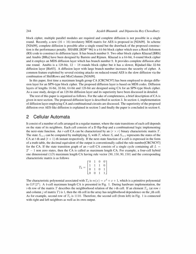
244 Jaydeb Bhaumik and Dipanwita Roy Chowdhury
block cipher, multiple parallel modules are required and complete diffusion is not possible in a singleround. Recently, a new (16 × 16) involutory MDS matrix for AES is proposed in [NJA09]. In scheme[NJA09], complete diffusion is possible after a single round but the drawback of the proposed construc-tion is the performance penalty. SHARK [RDP+96] is a 64-bit block cipher which uses a Reed-Solomon(RS) code to construct its diffusion layer. It has branch number 9. Two other block ciphers Khazad [BRb]and Anubis [BRa] have been designed by Barreto and Rijmen. Khazad is a 64-bit, 8-round block cipherand it employs an MDS diffusion layer which has branch number 9. It provides complete diffusion afterone round. Anubis is a 128-bit, 12 − 18 rounds block cipher but it has a slower, Rijndael-like 32-bitdiffusion layer [Bir03]. A diffusion layer with large branch number increases the security of cipher. Acommon feature exploited by several existing attacks on reduced-round AES is the slow diffusion via thecombination of ShiftRows and MixColumns [NJA09].
In this paper, first time a maximum length group CA [CRCNC97] has been employed to design diffu-sion layer for an SPN-type block cipher. The proposed diffusion layer is based on MDS codes. Diffusionlayers of lengths 16-bit, 32-bit, 64-bit and 128-bit are designed using CA for an SPN-type block cipher.As a case study, design of an 128-bit diffusion layer and its superiority have been discussed in detailed.
The rest of this paper is organized as follows. For the sake of completeness, a brief description of CA isgiven in next section. The proposed diffusion layer is described in section 3. In section 4, implementationof diffusion layer employing CA and combinational circuits are discussed. The superiority of the proposeddiffusion over AES-like diffusion is explained in section 5 and finally the paper is concluded in section 6.
2 Cellular AutomataIt consist of a number of cells arranged in a regular manner, where the state transitions of each cell dependson the state of its neighbors. Each cell consists of a D flip-flop and a combinational logic implementingthe next-state function. An r-cell CA can be characterized by an (r × r) binary characteristic matrix T .The state St+1 can be computed by multiplying St with T , where St and St+1 represents the states of theCA at t-th and (t + 1)-th instant respectively. If the next-state function of a cell is expressed in the formof a truth table, the decimal equivalent of the output is conventionally called the rule number[CRCNC97]for the CA. If the state transition graph of an r-cell CA consists of a single cycle containing all L =2r − 1 non zero states, then the CA is called as maximum length CA. For example, a four-cell hybridone dimensional (1D) maximum length CA having rule vector (90, 150, 90, 150) and the correspondingcharacteristic matrix is as follows
T4 =
0 1 0 01 1 1 00 1 0 10 0 1 1
The characteristic polynomial associated with T4 is m(x) = x4 + x+ 1, which is a primitive polynomialin GF (24). A 4-cell maximum length CA is presented in Fig. 1. During hardware implementation, thei-th row of the matrix T describes the neighborhood relation of the i-th cell. If an element Tij (at row iand column j of matrix T ) is 1, then the ith cell in the array has neighborhood dependence on the jth cell.As for example, second row of T4 is 1110. Therefore, the second cell (from left) in Fig. 1 is connectedwith right and left neighbors as well as its own output.
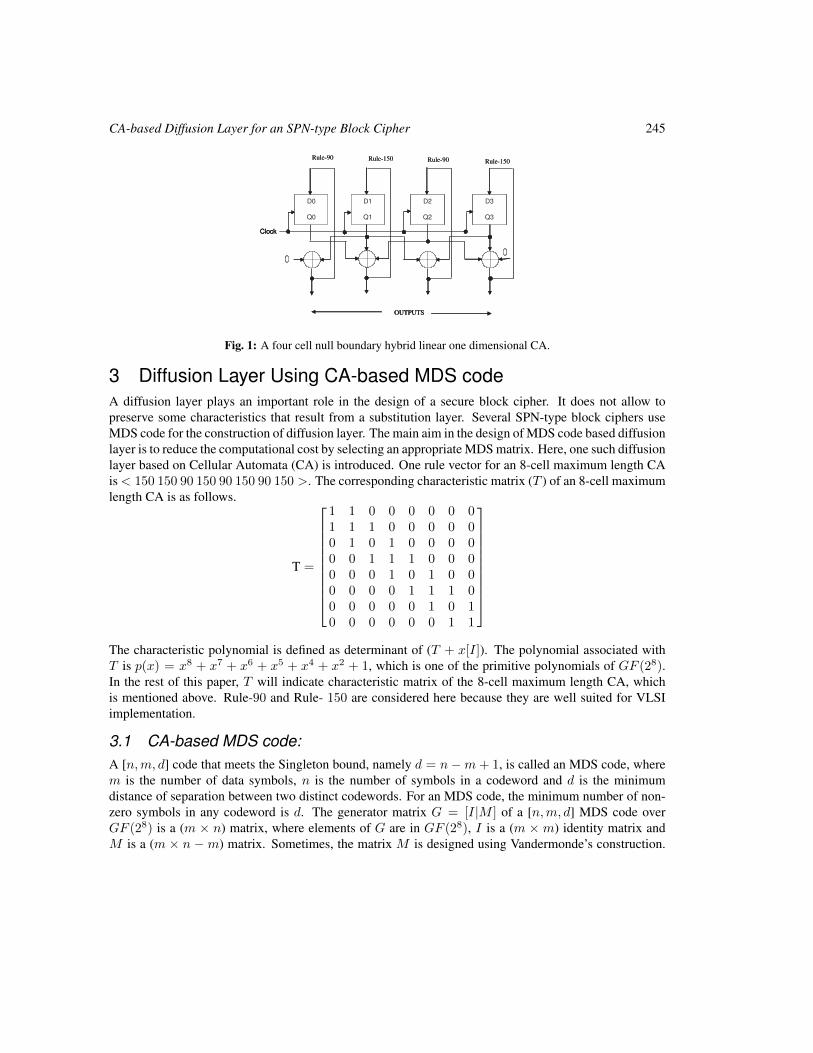
CA-based Diffusion Layer for an SPN-type Block Cipher 245
Clock
D0
Q0
D1
Q1
D2
Q2
D3
Q3
OUTPUTS
Rule - 90 Rule - 90 Rule - 150 Rule - 150
Clock
D0
Q0
D1
Q1
D2
Q2
D3
Q3
OUTPUTS
Clock
D0
Q0
D1
Q1
D2
Q2
D3
Q3
OUTPUTS
Rule - 90 Rule - 90 Rule - 150 Rule - 150
Fig. 1: A four cell null boundary hybrid linear one dimensional CA.
3 Diffusion Layer Using CA-based MDS codeA diffusion layer plays an important role in the design of a secure block cipher. It does not allow topreserve some characteristics that result from a substitution layer. Several SPN-type block ciphers useMDS code for the construction of diffusion layer. The main aim in the design of MDS code based diffusionlayer is to reduce the computational cost by selecting an appropriate MDS matrix. Here, one such diffusionlayer based on Cellular Automata (CA) is introduced. One rule vector for an 8-cell maximum length CAis< 150 150 90 150 90 150 90 150 >. The corresponding characteristic matrix (T ) of an 8-cell maximumlength CA is as follows.
T =
1 1 0 0 0 0 0 01 1 1 0 0 0 0 00 1 0 1 0 0 0 00 0 1 1 1 0 0 00 0 0 1 0 1 0 00 0 0 0 1 1 1 00 0 0 0 0 1 0 10 0 0 0 0 0 1 1
The characteristic polynomial is defined as determinant of (T + x[I]). The polynomial associated withT is p(x) = x8 + x7 + x6 + x5 + x4 + x2 + 1, which is one of the primitive polynomials of GF (28).In the rest of this paper, T will indicate characteristic matrix of the 8-cell maximum length CA, whichis mentioned above. Rule-90 and Rule- 150 are considered here because they are well suited for VLSIimplementation.
3.1 CA-based MDS code:A [n,m, d] code that meets the Singleton bound, namely d = n−m+ 1, is called an MDS code, wherem is the number of data symbols, n is the number of symbols in a codeword and d is the minimumdistance of separation between two distinct codewords. For an MDS code, the minimum number of non-zero symbols in any codeword is d. The generator matrix G = [I|M ] of a [n,m, d] MDS code overGF (28) is a (m × n) matrix, where elements of G are in GF (28), I is a (m × m) identity matrix andM is a (m × n −m) matrix. Sometimes, the matrix M is designed using Vandermonde’s construction.
246 Jaydeb Bhaumik and Dipanwita Roy Chowdhury
In this case, each element of M is power of a primitive element of GF (28). In case of maximum lengthCA, a characteristic matrix T is equivalent to a primitive element α. Therefore, the matrix M16×16 of a[32, 16, 17] code can be constructed from characteristic matrix T , where each element of M is a power ofT and it is as follows.
M16×16 =
T T 2 T 3 . . . T 15 T 16
T 2 T 4 T 6 . . . T 30 T 32
T 3 T 6 T 9 . . . T 45 T 48
. . . . . . . .
. . . . . . . .
. . . . . . . .T 15 T 30 T 45 . . . T 225 T 240
T 16 T 32 T 48 . . . T 240 T
The linear code generated by the generator matrixG = [I|M ] is an MDS code, where I16×16 is an identitymatrix and each element of I is an (8×8) binary matrix. The linear code has dimension 16, length 32 andthe minimum distance of separation between two distinct codewords is 17. The matrix M is sometimescalled MDS matrix.
Similarly, the MDS matrix for a [16, 8, 9] code is as follows.
M8×8 =
T T 2 T 3 . . . T 7 T 8
T 2 T 4 T 6 . . . T 14 T 16
T 3 T 6 T 9 . . . T 21 T 24
. . . . . . . .
. . . . . . . .
. . . . . . . .T 7 T 14 T 21 . . . T 49 T 56
T 8 T 16 T 24 . . . T 56 T 64
In case of a [8, 4, 5] code, the MDS matrix M4×4 is as follows.
M4×4 =
T T 2 T 3 T 4
T 2 T 4 T 6 T 8
T 3 T 6 T 9 T 12
T 4 T 8 T 12 T 16
Similarly, a [4, 2, 3] code can be designed using the generator matrix G4×4 = [I|M2×2], where
M2×2 =
[T T 2
T 2 T 4
]
The code generated by G4×4 has dimension 2, length 4 and the minimum distance between two distinctcodewords is 3.
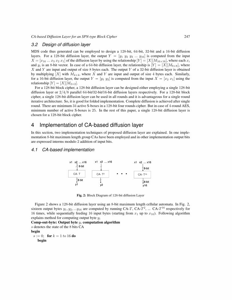
CA-based Diffusion Layer for an SPN-type Block Cipher 247
3.2 Design of diffusion layerMDS code thus generated can be employed to design a 128-bit, 64-bit, 32-bit and a 16-bit diffusionlayers. For a 128-bit diffusion layer, the output Y = [y1 y2 y3 ... y16] is computed from the inputX = [x16 ... x3 x2 x1] of the diffusion layer by using the relationship [Y ] = [X][M16×16], where each xiand yi is an 8-bit vector. In case of a 64-bit diffusion layer, the relationship is [Y ] = [X][M8×8], whereX and Y are input and output of size 8 bytes each. The output Y of a 32-bit diffusion layer is obtainedby multiplying [X] with M4×4, where X and Y are input and output of size 4 bytes each. Similarly,for a 16-bit diffusion layer, the output Y = [y1 y2] is computed from the input X = [x2 x1] using therelationship [Y ] = [X][M2×2].
For a 128-bit block cipher, a 128-bit diffusion layer can be designed either employing a single 128-bitdiffusion layer or 2/4/8 parallel 64-bit/32-bit/16-bit diffusion layers respectively. For a 128-bit blockcipher, a single 128-bit diffusion layer can be used in all rounds and it is advantageous for a single rounditerative architecture. So, it is good for folded implementation. Complete diffusion is achieved after singleround. There are minimum 34 active S-boxes in a 128-bit four rounds cipher. But in case of 4-round AES,minimum number of active S-boxes is 25. In the rest of this paper, a single 128-bit diffusion layer ischosen for a 128-bit block cipher.
4 Implementation of CA-based diffusion layerIn this section, two implementation techniques of proposed diffusion layer are explained. In one imple-mentation 8-bit maximum length group CAs have been employed and in other implementation output bitsare expressed interms modulo 2 addition of input bits.
4.1 CA-based implementation
CA - T CA - T 2 CA - T 16
x1 x2 … x16
y1 y2 y16
8 - bit 8 - bit
x1 x2 … x16 x1 x2 … x16
8 - bit 8 - bit
CA - T CA - T 2 CA - T 16
x1 x2 … x16
y1 y2 y16
8 - bit 8 - bit
x1 x2 … x16 x1 x2 … x16
8 - bit 8 - bit
Fig. 2: Block Diagram of 128-bit diffusion Layer
Figure 2 shows a 128-bit diffusion layer using an 8-bit maximum length cellular automata. In Fig. 2,sixteen output bytes y1, y2, ...y16 are computed by running CA-T , CA-T 2, ... CA-T 16 respectively for16 times, while sequentially feeding 16 input bytes (starting from x1 up to x16). Following algorithmexplains method for computing output byte yiComp-out-byte: Output byte yi computation algorithms denotes the state of the 8 bits CAbegins := 0; for k = 1 to 16 do
begin
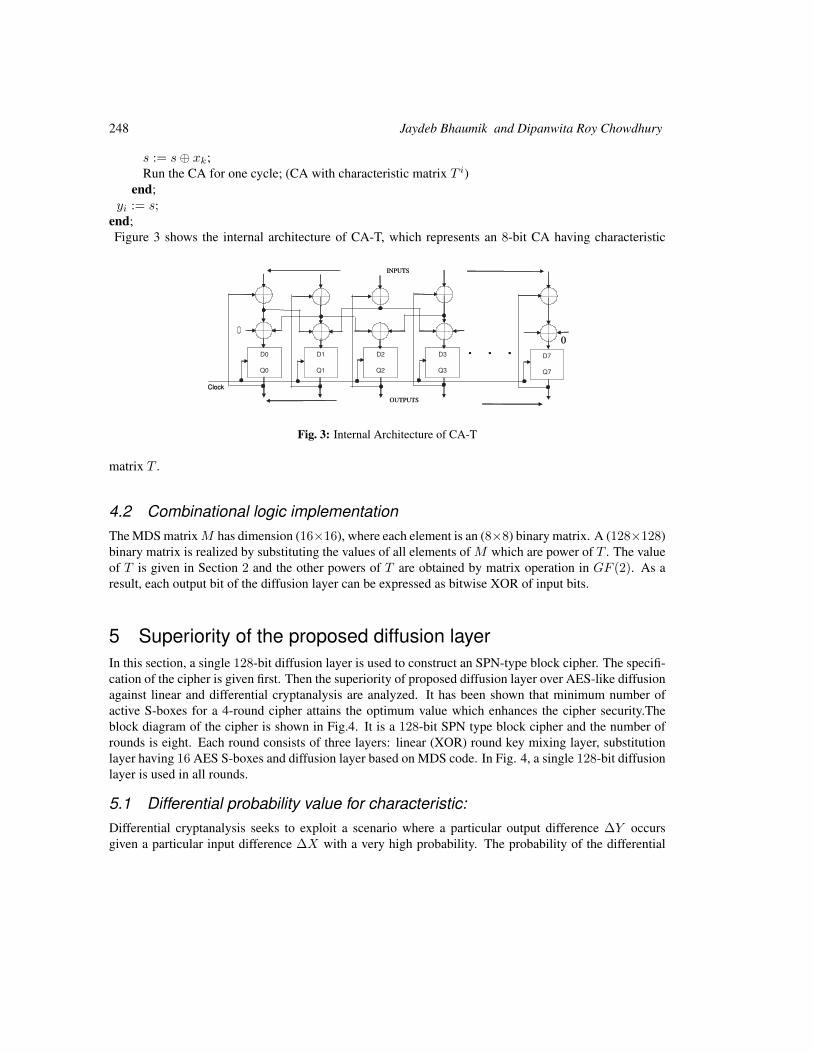
248 Jaydeb Bhaumik and Dipanwita Roy Chowdhury
s := s⊕ xk;Run the CA for one cycle; (CA with characteristic matrix T i)
end;yi := s;
end;Figure 3 shows the internal architecture of CA-T, which represents an 8-bit CA having characteristic
Clock
D0
Q0
D1
Q1
D2
Q2
D3
Q3
INPUTS
OUTPUTS
. . .
D7
Q7
0
Clock
D0
Q0
D1
Q1
D2
Q2
D3
Q3
INPUTS
OUTPUTS
. . .
D7
Q7
0
Fig. 3: Internal Architecture of CA-T
matrix T .
4.2 Combinational logic implementationThe MDS matrixM has dimension (16×16), where each element is an (8×8) binary matrix. A (128×128)binary matrix is realized by substituting the values of all elements of M which are power of T . The valueof T is given in Section 2 and the other powers of T are obtained by matrix operation in GF (2). As aresult, each output bit of the diffusion layer can be expressed as bitwise XOR of input bits.
5 Superiority of the proposed diffusion layerIn this section, a single 128-bit diffusion layer is used to construct an SPN-type block cipher. The specifi-cation of the cipher is given first. Then the superiority of proposed diffusion layer over AES-like diffusionagainst linear and differential cryptanalysis are analyzed. It has been shown that minimum number ofactive S-boxes for a 4-round cipher attains the optimum value which enhances the cipher security.Theblock diagram of the cipher is shown in Fig.4. It is a 128-bit SPN type block cipher and the number ofrounds is eight. Each round consists of three layers: linear (XOR) round key mixing layer, substitutionlayer having 16 AES S-boxes and diffusion layer based on MDS code. In Fig. 4, a single 128-bit diffusionlayer is used in all rounds.
5.1 Differential probability value for characteristic:Differential cryptanalysis seeks to exploit a scenario where a particular output difference ∆Y occursgiven a particular input difference ∆X with a very high probability. The probability of the differential
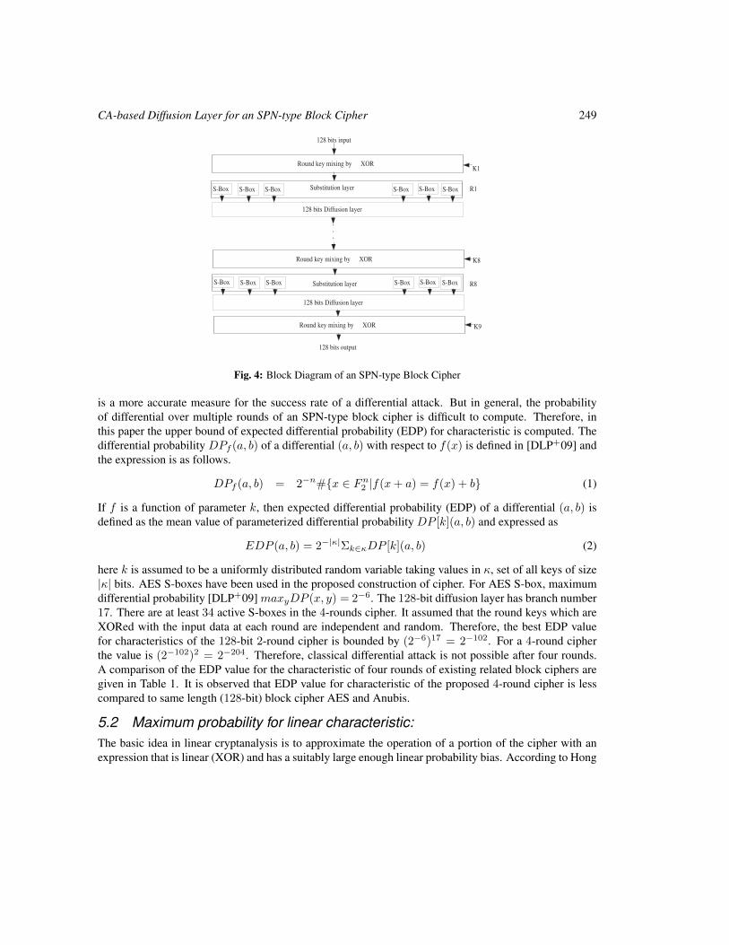
CA-based Diffusion Layer for an SPN-type Block Cipher 249
Round key mixing by XOR
S-Box S-Box S-Box S-Box S-Box S-Box Substitution layer
128 bits Diffusion layer
Round key mixing by XOR
S-Box S-Box S-Box S-Box S-Box S-Box Substitution layer
128 bits Diffusion layer
.
.
.
Round key mixing by XOR
128 bits input
128 bits output
R1
K1
K8
R8
K9
Fig. 4: Block Diagram of an SPN-type Block Cipher
is a more accurate measure for the success rate of a differential attack. But in general, the probabilityof differential over multiple rounds of an SPN-type block cipher is difficult to compute. Therefore, inthis paper the upper bound of expected differential probability (EDP) for characteristic is computed. Thedifferential probability DPf (a, b) of a differential (a, b) with respect to f(x) is defined in [DLP+09] andthe expression is as follows.
DPf (a, b) = 2−n#x ∈ Fn2 |f(x+ a) = f(x) + b (1)
If f is a function of parameter k, then expected differential probability (EDP) of a differential (a, b) isdefined as the mean value of parameterized differential probability DP [k](a, b) and expressed as
EDP (a, b) = 2−|κ|Σk∈κDP [k](a, b) (2)
here k is assumed to be a uniformly distributed random variable taking values in κ, set of all keys of size|κ| bits. AES S-boxes have been used in the proposed construction of cipher. For AES S-box, maximumdifferential probability [DLP+09]maxyDP (x, y) = 2−6. The 128-bit diffusion layer has branch number17. There are at least 34 active S-boxes in the 4-rounds cipher. It assumed that the round keys which areXORed with the input data at each round are independent and random. Therefore, the best EDP valuefor characteristics of the 128-bit 2-round cipher is bounded by (2−6)17 = 2−102. For a 4-round cipherthe value is (2−102)2 = 2−204. Therefore, classical differential attack is not possible after four rounds.A comparison of the EDP value for the characteristic of four rounds of existing related block ciphers aregiven in Table 1. It is observed that EDP value for characteristic of the proposed 4-round cipher is lesscompared to same length (128-bit) block cipher AES and Anubis.
5.2 Maximum probability for linear characteristic:The basic idea in linear cryptanalysis is to approximate the operation of a portion of the cipher with anexpression that is linear (XOR) and has a suitably large enough linear probability bias. According to Hong
250 Jaydeb Bhaumik and Dipanwita Roy Chowdhury
Tab. 1: Comparison of probability of differential for characteristicName of the Cipher Block length Branch no. Prob. of diff.
CharacteristicProposed one 128 17 2−204
SHARK [RDP+96] 64 9 2−108
AES [DR02] 128 5 2−150
KHAZAD [BRb] 64 9 2−90
ANUBIS [BRa] 128 5 2−125
et al., the linear probability [HLL+01] of an S-box Si is defined as follows.
LPSi(Γx→ Γy) = (#x ∈ Zm2 |Γx.x = Γy.Si(x)
2m−1− 1)2
LPSimax = maxΓx,Γy 6=0LP
Si(Γx→ Γy) (3)
where Γx and Γy are input and output mask respectively and 1 ≤ i ≤ n. It has been shown in [HLL+01]that the probability for each linear characteristic of Substitution, Diffusion and Substitution (SDS) func-tion is bounded by qn, where q = LPSi
max is the maximum linear probability of S-boxes in the substitutionlayer and n + 1 is a lower bound for the number of active S-boxes in two consecutive rounds of a lin-ear approximation. In the proposed cipher, all sixteen S-boxes in the substitution layer are same and theAES S-box is used. For AES S-box, the value of LPSi
max = LPS = ( 144128 − 1)2 = 2−6. Therefore, the
probability for linear characteristic of SDS function is bounded by (2−6)16 = 2−96. So the maximumprobability for linear characteristic of the four rounds cipher is (2−96)2 = 2−192. Hence four rounds ofproposed construction is sufficient to resist classical linear attack. A comparison of probability of bestlinear approximation of related block ciphers is shown in Table 2. Therefore, classical differential and
Tab. 2: Comparison of probability for linear characteristicName of the Cipher Block length Branch no. Prob. for linear
CharacteristicProposed one 128 17 2−192
SHARK [RDP+96] 64 9 2−108
AES [DR02] 128 5 2−150
KHAZAD [BRb] 64 9 2−72
ANUBIS [BRa] 128 5 2−115
linear attacks are not possible to succeed after four rounds.
6 ConclusionsIn this paper, a new technique to design a diffusion layer for an SPN-type block cipher based on an MDScode has been introduced. Scheme to design diffusion layer of lengths 16-bit, 32-bit, 64-bit and 128-bit foran SPN-type block cipher has been proposed. As a case study, 128-bit diffusion layer has been discussedin detailed. The superiority of the proposed diffusion scheme over AES-like diffusion is shown in thispaper.
CA-based Diffusion Layer for an SPN-type Block Cipher 251
References[Bir03] Alex Biryukov. Analysis of involutional ciphers: Khazad and anubis. In Fast Software
Encryption, volume 2887 of Lecture Notes in Computer Science, pages 45–53. Springer,2003.
[BRa] P. Barreto and V. Rijmen. The anubis block cipher. Submission to the NESSIE Project.
[BRb] P. Barreto and V. Rijmen. The khazad legacy-level block cipher. Submission to the NESSIEProject.
[CRCNC97] P. P. Chaudhuri, D. Roy Chowdhury, S. Nandi, and S. Chattopadhyay. Additive CellularAutomata: Theory and Applications. IEEE Computer Socity press, 1997.
[Dae95] J. Daemen. Cipher and hash function design strategies based on linear and differentialcryptanalysis. PhD thesis, K. U. Leuven, March 1995.
[DLP+09] J. Daemen, M. Lamberger, N. Pramstaller, V. Rijmen, and F. Vercauteren. Computatioalaspects of the expected differential probability of a 4-round aes and aes-like ciphers. Journalof Computing, 85:85–104, 2009.
[DR02] J. Daemen and V. Rijmen. The Design of Rijndael-AES, The Advanced Encryption Standard.Springer-Verlag, 2002.
[HLL+01] S. Hong, S. Lee, J. Lim, J. Sung, Cheon D., and I. Cho. Provable security against differentialand linear cryptanalysis for the spn structure. In Fast Software Encryption, volume 1978 ofLecture Notes in Computer Science, pages 273–283, 2001.
[JV04] Pascal Junod and Serge Vaudenay. Perfect diffusion primitives for block ciphers - buildingefficient MDS matrices. In Selected Areas in Cryptography, 11th International Workshop,SAC 2004, volume 3357 of Lecture Notes in Computer Science, pages 84–99, 2004.
[NJA09] J. Nakahara Jr and E. Abrahao. A new involutory mds matrix for the aes. Int. Journal ofNetwork Security, 9:109–116, 2009.
[RDP+96] V. Rijmen, J. Daemen, B. Preneel, A. Bosselaers, and E. De Win. The cipher shark. InFast Software Encryption 1996, volume 1039 of Lecture Notes in Computer Science, pages99–111, 1996.

252 Jaydeb Bhaumik and Dipanwita Roy Chowdhury
AUTOMATA 2011, Santiago, Chile local proceedings LP, 2011, 253–262
Chaos in Fuzzy Cellular Automata inConjunctive Normal Form
David Forrester1† and Paola Flocchini1‡
1 School of Electrical Engineering and Computer ScienceUniversity of Ottawa
Fuzzy cellular automata (FCA) are continuous extensions of Boolean cellular automata (CA). Given a Boolean cellularautomata rule we can define a corresponding Fuzzy cellular automata rule by allowing real states in [0, 1] and by “fuzzifying"a Boolean form describing the transition function of the CA.
To date, FCA have only been studied in disjunctive normal form (DNF) and their study has revealed interesting propertiesand links with classical Boolean Cellular Automata.
In this paper, we start the study FCA in conjunctive normal form (CNF). Our main objectives are to see whether thefuzzification of CNF and DNF have similar behaviors and whether, being different representation of the same Boolean truthtable, they capture different aspects of their Boolean counterparts. We start the investigation by focussing on FCA fromhomogeneous configurations, and we classify them analytically. In striking contrast to the periodic behaviours of DNFFCA, we prove that a large class of FCA exhibit chaos in CNF.
Keywords: Fuzzy Cellular Automata, Chaos, Cantor set
1 IntroductionFuzzy cellular automata (FCA) were introduced in [CFM+97] as a particular type of Coupled map lattices[Kan84], that is, a continuous-valued version of elementary discrete cellular automata. FCA employs the con-cept of fuzzy logic [Zad65]. This “many-valued logic” extended the notion of true and false to include in-between values. Rather than having cells which could assume only binary values, FCA cells could assume anyvalue between zero and one, inclusively. Boolean operators are also “fuzzified” by replacing them with standardalgebraic operators. FCA use this process to “fuzzify” the Boolean logic of a corresponding Boolean CA thatis expressed in some normal form.
Disjunctive Normal Form (DNF) is one of the standard canonical normal forms for a Boolean expression,consisting of a disjunction of terms, each of which is the conjunction of variables or their negations. FCA inDNF are derived by first representing elementary Boolean CA transition functions in DNF, and then “fuzzifying”the Boolean logic to derive the real-valued function. While the choice of normal form does not change theBoolean function (all normal forms are logically equivalent), different normal forms will produce differentfuzzy logic equivalents. Generally, FCA have been studied in DNF. Certain equivalences were shown betweenBoolean elementary CA their elementary FCA counterparts in DNF [BF11b]. It was also shown that none of theelementary FCA with circular or null boundary conditions exhibited chaos, and all had a periodic asymptoticbehaviour [BF11a, BF11b, Min06a, Min06b].
In the study of FCA in DNF, the logic operators ∧, ∨ and not are substituted by “fuzzy logic" operatorswhere not corresponds to 1 − x, ∧ to x · y, and ∨ to min1, x + y. It turns out that such a choice is specialin the sense that it is the only fuzzification that is affine in all its variables. Moreover, this transformation
†Email: [email protected]‡Email: [email protected]
c© 2011 AUTOMATA proceedings, Santiago, Chile, 2011
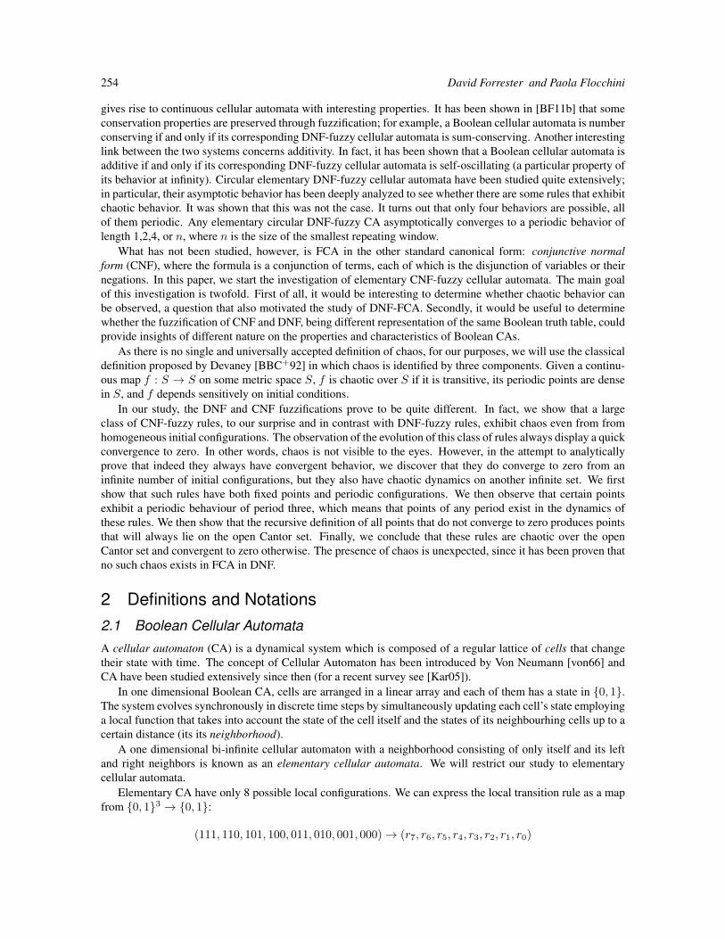
254 David Forrester and Paola Flocchini
gives rise to continuous cellular automata with interesting properties. It has been shown in [BF11b] that someconservation properties are preserved through fuzzification; for example, a Boolean cellular automata is numberconserving if and only if its corresponding DNF-fuzzy cellular automata is sum-conserving. Another interestinglink between the two systems concerns additivity. In fact, it has been shown that a Boolean cellular automata isadditive if and only if its corresponding DNF-fuzzy cellular automata is self-oscillating (a particular property ofits behavior at infinity). Circular elementary DNF-fuzzy cellular automata have been studied quite extensively;in particular, their asymptotic behavior has been deeply analyzed to see whether there are some rules that exhibitchaotic behavior. It was shown that this was not the case. It turns out that only four behaviors are possible, allof them periodic. Any elementary circular DNF-fuzzy CA asymptotically converges to a periodic behavior oflength 1,2,4, or n, where n is the size of the smallest repeating window.
What has not been studied, however, is FCA in the other standard canonical form: conjunctive normalform (CNF), where the formula is a conjunction of terms, each of which is the disjunction of variables or theirnegations. In this paper, we start the investigation of elementary CNF-fuzzy cellular automata. The main goalof this investigation is twofold. First of all, it would be interesting to determine whether chaotic behavior canbe observed, a question that also motivated the study of DNF-FCA. Secondly, it would be useful to determinewhether the fuzzification of CNF and DNF, being different representation of the same Boolean truth table, couldprovide insights of different nature on the properties and characteristics of Boolean CAs.
As there is no single and universally accepted definition of chaos, for our purposes, we will use the classicaldefinition proposed by Devaney [BBC+92] in which chaos is identified by three components. Given a continu-ous map f : S → S on some metric space S, f is chaotic over S if it is transitive, its periodic points are densein S, and f depends sensitively on initial conditions.
In our study, the DNF and CNF fuzzifications prove to be quite different. In fact, we show that a largeclass of CNF-fuzzy rules, to our surprise and in contrast with DNF-fuzzy rules, exhibit chaos even from fromhomogeneous initial configurations. The observation of the evolution of this class of rules always display a quickconvergence to zero. In other words, chaos is not visible to the eyes. However, in the attempt to analyticallyprove that indeed they always have convergent behavior, we discover that they do converge to zero from aninfinite number of initial configurations, but they also have chaotic dynamics on another infinite set. We firstshow that such rules have both fixed points and periodic configurations. We then observe that certain pointsexhibit a periodic behaviour of period three, which means that points of any period exist in the dynamics ofthese rules. We then show that the recursive definition of all points that do not converge to zero produces pointsthat will always lie on the open Cantor set. Finally, we conclude that these rules are chaotic over the openCantor set and convergent to zero otherwise. The presence of chaos is unexpected, since it has been proven thatno such chaos exists in FCA in DNF.
2 Definitions and Notations2.1 Boolean Cellular AutomataA cellular automaton (CA) is a dynamical system which is composed of a regular lattice of cells that changetheir state with time. The concept of Cellular Automaton has been introduced by Von Neumann [von66] andCA have been studied extensively since then (for a recent survey see [Kar05]).
In one dimensional Boolean CA, cells are arranged in a linear array and each of them has a state in 0, 1.The system evolves synchronously in discrete time steps by simultaneously updating each cell’s state employinga local function that takes into account the state of the cell itself and the states of its neighbourhing cells up to acertain distance (its its neighborhood).
A one dimensional bi-infinite cellular automaton with a neighborhood consisting of only itself and its leftand right neighbors is known as an elementary cellular automata. We will restrict our study to elementarycellular automata.
Elementary CA have only 8 possible local configurations. We can express the local transition rule as a mapfrom 0, 13 → 0, 1:
(111, 110, 101, 100, 011, 010, 001, 000)→ (r7, r6, r5, r4, r3, r2, r1, r0)
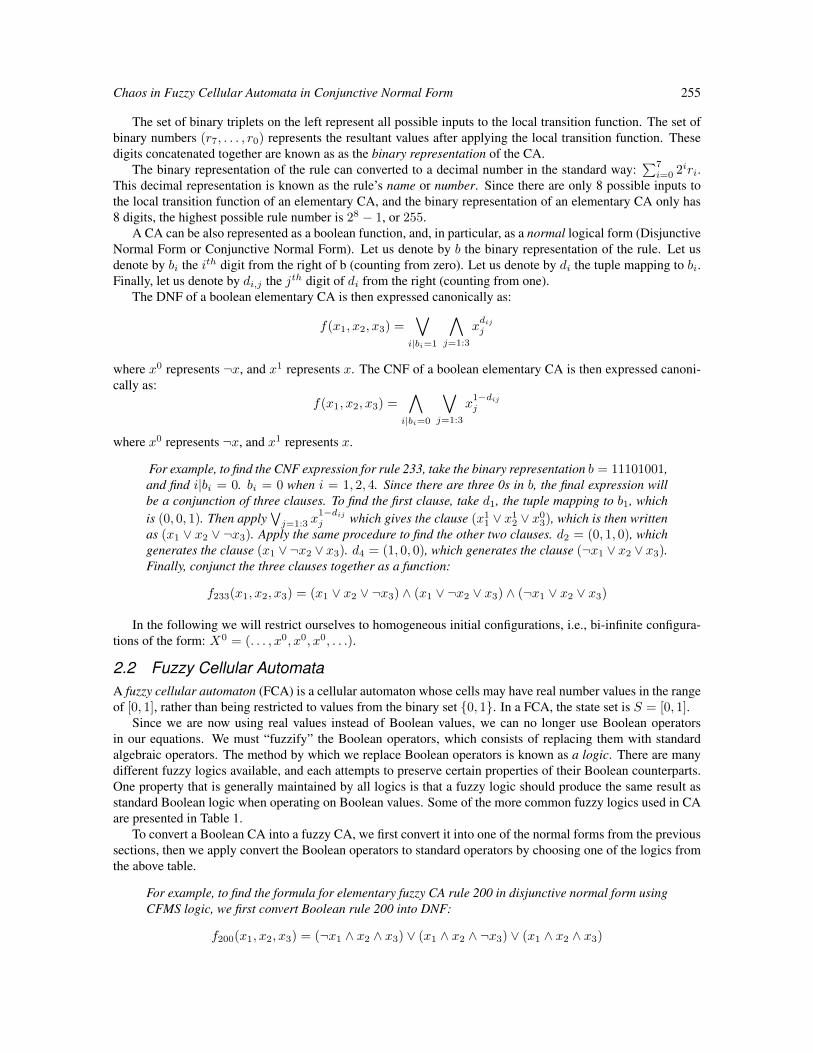
Chaos in Fuzzy Cellular Automata in Conjunctive Normal Form 255
The set of binary triplets on the left represent all possible inputs to the local transition function. The set ofbinary numbers (r7, . . . , r0) represents the resultant values after applying the local transition function. Thesedigits concatenated together are known as as the binary representation of the CA.
The binary representation of the rule can converted to a decimal number in the standard way:∑7
i=0 2iri.This decimal representation is known as the rule’s name or number. Since there are only 8 possible inputs tothe local transition function of an elementary CA, and the binary representation of an elementary CA only has8 digits, the highest possible rule number is 28 − 1, or 255.
A CA can be also represented as a boolean function, and, in particular, as a normal logical form (DisjunctiveNormal Form or Conjunctive Normal Form). Let us denote by b the binary representation of the rule. Let usdenote by bi the ith digit from the right of b (counting from zero). Let us denote by di the tuple mapping to bi.Finally, let us denote by di,j the jth digit of di from the right (counting from one).
The DNF of a boolean elementary CA is then expressed canonically as:
f(x1, x2, x3) =∨
i|bi=1
∧j=1:3
xdij
j
where x0 represents ¬x, and x1 represents x. The CNF of a boolean elementary CA is then expressed canoni-cally as:
f(x1, x2, x3) =∧
i|bi=0
∨j=1:3
x1−dij
j
where x0 represents ¬x, and x1 represents x.
For example, to find the CNF expression for rule 233, take the binary representation b = 11101001,and find i|bi = 0. bi = 0 when i = 1, 2, 4. Since there are three 0s in b, the final expression willbe a conjunction of three clauses. To find the first clause, take d1, the tuple mapping to b1, whichis (0, 0, 1). Then apply
∨j=1:3 x
1−dij
j which gives the clause (x11 ∨ x12 ∨ x03), which is then writtenas (x1 ∨ x2 ∨ ¬x3). Apply the same procedure to find the other two clauses. d2 = (0, 1, 0), whichgenerates the clause (x1 ∨¬x2 ∨ x3). d4 = (1, 0, 0), which generates the clause (¬x1 ∨ x2 ∨ x3).Finally, conjunct the three clauses together as a function:
f233(x1, x2, x3) = (x1 ∨ x2 ∨ ¬x3) ∧ (x1 ∨ ¬x2 ∨ x3) ∧ (¬x1 ∨ x2 ∨ x3)
In the following we will restrict ourselves to homogeneous initial configurations, i.e., bi-infinite configura-tions of the form: X0 = (. . . , x0, x0, x0, . . .).
2.2 Fuzzy Cellular AutomataA fuzzy cellular automaton (FCA) is a cellular automaton whose cells may have real number values in the rangeof [0, 1], rather than being restricted to values from the binary set 0, 1. In a FCA, the state set is S = [0, 1].
Since we are now using real values instead of Boolean values, we can no longer use Boolean operatorsin our equations. We must “fuzzify” the Boolean operators, which consists of replacing them with standardalgebraic operators. The method by which we replace Boolean operators is known as a logic. There are manydifferent fuzzy logics available, and each attempts to preserve certain properties of their Boolean counterparts.One property that is generally maintained by all logics is that a fuzzy logic should produce the same result asstandard Boolean logic when operating on Boolean values. Some of the more common fuzzy logics used in CAare presented in Table 1.
To convert a Boolean CA into a fuzzy CA, we first convert it into one of the normal forms from the previoussections, then we apply convert the Boolean operators to standard operators by choosing one of the logics fromthe above table.
For example, to find the formula for elementary fuzzy CA rule 200 in disjunctive normal form usingCFMS logic, we first convert Boolean rule 200 into DNF:
f200(x1, x2, x3) = (¬x1 ∧ x2 ∧ x3) ∨ (x1 ∧ x2 ∧ ¬x3) ∨ (x1 ∧ x2 ∧ x3)
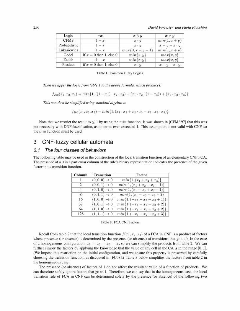
256 David Forrester and Paola Flocchini
Logic ¬x x ∧ y x ∨ yCFMS 1− x x · y min1, x+ y
Probabilistic 1− x x · y x+ y − x · yLukasiewicz 1− x max0, x+ y − 1 min1, x+ y
Gödel if x = 0 then 1, else 0 minx, y maxx, yZadeh 1− x minx, y maxx, y
Product if x = 0 then 1, else 0 x · y x+ y − x · y
Table 1: Common Fuzzy Logics.
Then we apply the logic from table 1 to the above formula, which produces:
f200(x1, x2, x3) = min1, ((1− x1) · x2 · x3) + (x1 · x2 · (1− x3)) + (x1 · x2 · x3)
This can then be simplified using standard algebra to
f200(x1, x2, x3) = min1, (x1 · x2 + x2 · x3 − x1 · x2 · x3)
Note that we restrict the result to ≤ 1 by using the min function. It was shown in [CFM+97] that this wasnot necessary with DNF fuzzification, as no terms ever exceeded 1. This assumption is not valid with CNF, sothe min function must be used.
3 CNF-fuzzy cellular automata3.1 The four classes of behaviorsThe following table may be used in the construction of the local transition function of an elementary CNF FCA.The presence of a 0 in a particular column of the rule’s binary representation indicates the presence of the givenfactor in its transition function.
Column Transition Factor1 (0, 0, 0)→ 0 min1, (x1 + x2 + x3)2 (0, 0, 1)→ 0 min1, (x1 + x2 − x3 + 1)4 (0, 1, 0)→ 0 min1, (x1 − x2 + x3 + 1)8 (0, 1, 1)→ 0 min1, (x1 − x2 − x3 + 2)
16 (1, 0, 0)→ 0 min1, (−x1 + x2 + x3 + 1)32 (1, 0, 1)→ 0 min1, (−x1 + x2 − x3 + 2)64 (1, 1, 0)→ 0 min1, (−x1 − x2 + x3 + 2)128 (1, 1, 1)→ 0 min1, (−x1 − x2 − x3 + 3)
Table 2: FCA CNF Factors
Recall from table 2 that the local transition function f(x1, x2, x3) of a FCA in CNF is a product of factorswhose presence (or absence) is determined by the presence (or absence) of transitions that go to 0. In the caseof a homogeneous configuration, x1 = x2 = x3 = x, so we can simplify the products from table 2. We canfurther simply the factors by applying the knowledge that the value of any cell in the CA is in the range [0, 1].(We impose this restriction on the initial configuration, and we ensure this property is preserved by carefullychoosing the transition function, as discussed in [FC08].) Table 3 below simplifies the factors from table 2 inthe homogeneous case:
The presence (or absence) of factors of 1 do not affect the resultant value of a function of products. Wecan therefore safely ignore factors that go to 1. Therefore, we can say that in the homogeneous case, the localtransition rule of FCA in CNF can be determined solely by the presence (or absence) of the following two
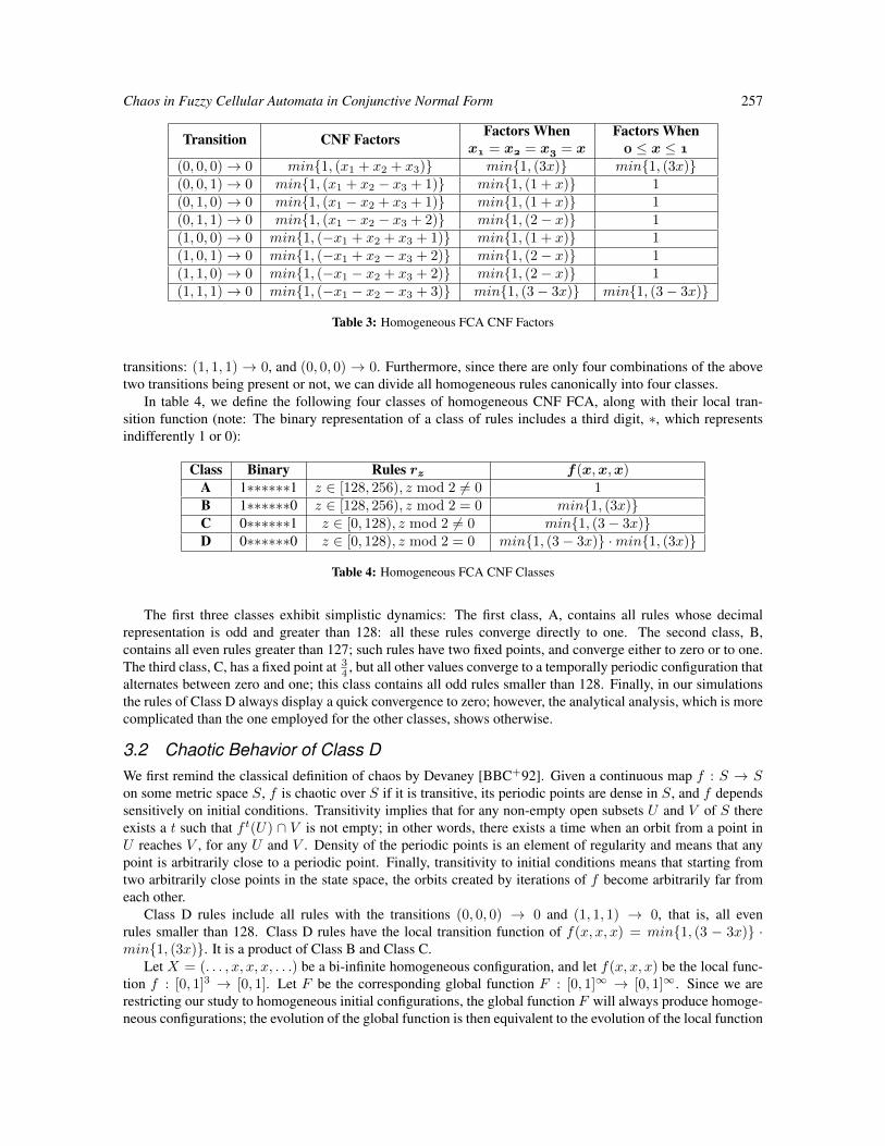
Chaos in Fuzzy Cellular Automata in Conjunctive Normal Form 257
Transition CNF Factors Factors When Factors Whenx = x = x = x ≤ x ≤
(0, 0, 0)→ 0 min1, (x1 + x2 + x3) min1, (3x) min1, (3x)(0, 0, 1)→ 0 min1, (x1 + x2 − x3 + 1) min1, (1 + x) 1(0, 1, 0)→ 0 min1, (x1 − x2 + x3 + 1) min1, (1 + x) 1(0, 1, 1)→ 0 min1, (x1 − x2 − x3 + 2) min1, (2− x) 1(1, 0, 0)→ 0 min1, (−x1 + x2 + x3 + 1) min1, (1 + x) 1(1, 0, 1)→ 0 min1, (−x1 + x2 − x3 + 2) min1, (2− x) 1(1, 1, 0)→ 0 min1, (−x1 − x2 + x3 + 2) min1, (2− x) 1(1, 1, 1)→ 0 min1, (−x1 − x2 − x3 + 3) min1, (3− 3x) min1, (3− 3x)
Table 3: Homogeneous FCA CNF Factors
transitions: (1, 1, 1) → 0, and (0, 0, 0) → 0. Furthermore, since there are only four combinations of the abovetwo transitions being present or not, we can divide all homogeneous rules canonically into four classes.
In table 4, we define the following four classes of homogeneous CNF FCA, along with their local tran-sition function (note: The binary representation of a class of rules includes a third digit, ∗, which representsindifferently 1 or 0):
Class Binary Rules rz f(x,x,x)A 1∗∗∗∗∗∗1 z ∈ [128, 256), z mod 2 6= 0 1B 1∗∗∗∗∗∗0 z ∈ [128, 256), z mod 2 = 0 min1, (3x)C 0∗∗∗∗∗∗1 z ∈ [0, 128), z mod 2 6= 0 min1, (3− 3x)D 0∗∗∗∗∗∗0 z ∈ [0, 128), z mod 2 = 0 min1, (3− 3x) ·min1, (3x)
Table 4: Homogeneous FCA CNF Classes
The first three classes exhibit simplistic dynamics: The first class, A, contains all rules whose decimalrepresentation is odd and greater than 128: all these rules converge directly to one. The second class, B,contains all even rules greater than 127; such rules have two fixed points, and converge either to zero or to one.The third class, C, has a fixed point at 3
4 , but all other values converge to a temporally periodic configuration thatalternates between zero and one; this class contains all odd rules smaller than 128. Finally, in our simulationsthe rules of Class D always display a quick convergence to zero; however, the analytical analysis, which is morecomplicated than the one employed for the other classes, shows otherwise.
3.2 Chaotic Behavior of Class DWe first remind the classical definition of chaos by Devaney [BBC+92]. Given a continuous map f : S → Son some metric space S, f is chaotic over S if it is transitive, its periodic points are dense in S, and f dependssensitively on initial conditions. Transitivity implies that for any non-empty open subsets U and V of S thereexists a t such that f t(U) ∩ V is not empty; in other words, there exists a time when an orbit from a point inU reaches V , for any U and V . Density of the periodic points is an element of regularity and means that anypoint is arbitrarily close to a periodic point. Finally, transitivity to initial conditions means that starting fromtwo arbitrarily close points in the state space, the orbits created by iterations of f become arbitrarily far fromeach other.
Class D rules include all rules with the transitions (0, 0, 0) → 0 and (1, 1, 1) → 0, that is, all evenrules smaller than 128. Class D rules have the local transition function of f(x, x, x) = min1, (3 − 3x) ·min1, (3x). It is a product of Class B and Class C.
Let X = (. . . , x, x, x, . . .) be a bi-infinite homogeneous configuration, and let f(x, x, x) be the local func-tion f : [0, 1]3 → [0, 1]. Let F be the corresponding global function F : [0, 1]∞ → [0, 1]∞. Since we arerestricting our study to homogeneous initial configurations, the global function F will always produce homoge-neous configurations; the evolution of the global function is then equivalent to the evolution of the local function
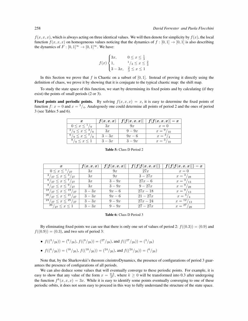
258 David Forrester and Paola Flocchini
f(x, x, x), which is always acting on three identical values. We will then denote for simplicity by f(x), the localfunction f(x, x, x) on homogeneous values noticing that the dynamics of f : [0, 1] → [0, 1] is also describingthe dynamics of F : [0, 1]∞ → [0, 1]∞. We have:
f(x)
3x, 0 ≤ x ≤ 1
3
1, 1/3 ≤ x ≤ 23
3− 3x, 23 ≤ x ≤ 1
In this Section we prove that f is Chaotic on a subset of [0, 1]. Instead of proving it directly using thedefinition of chaos, we prove it by showing that it is conjugate to the typical chaotic map: the shift map.
To study the state space of this function, we start by determining its fixed points and by calculating (if theyexist) the points of small periods (2 or 3).
Fixed points and periodic points. By solving f(x, x, x) = x, it is easy to determine the fixed points offunction f : x = 0 and x = 3/4. Analogously one could determine all points of period 2 and the ones of period3 (see Tables 5 and 6).
x f(x,x,x) f [f(x,x,x)] f [f(x,x,x)] = x0 ≤ x ≤ 1/9 3x 9x x = 0
2/9 ≤ x ≤ 3/9 3x 9− 9x x = 9/106/9 ≤ x ≤ 7/9 3− 3x 9x− 6 x = 3/48/9 ≤ x ≤ 1 3− 3x 3− 9x x = 3/10
Table 5: Class D Period 2
x f(x,x,x) f [f(x,x,x)] ff [f(x,x,x)] ff [f(x,x,x)] = x0 ≤ x ≤ 1/27 3x 9x 27x x = 0
2/27 ≤ x ≤ 3/27 3x 9x 3− 27x x = 3/286/27 ≤ x ≤ 7/27 3x 3− 9x 27x− 6 x = 3/138/27 ≤ x ≤ 9/27 3x 3− 9x 9− 27x x = 9/28
18/27 ≤ x ≤ 19/27 3− 3x 9x− 6 27x− 18 x = 9/1320/27 ≤ x ≤ 21/27 3− 3x 9x− 6 21− 27x x = 3/424/27 ≤ x ≤ 25/27 3− 3x 9− 9x 27x− 24 x = 12/13
26/27 ≤ x ≤ 1 3− 3x 9− 9x 27− 27x x = 27/28
Table 6: Class D Period 3
By eliminating fixed points we can see that there is only one set of values of period 2: f((0.3)) = (0.9) andf((0.9)) = (0.3), and two sets of period 3:
• f((3/28)) = (9/28), f((9/28)) = (27/28), and f((27/28)) = (3/28)
• f((6/26)) = (18/26), f((18/26)) = (24/26), and f((24/26)) = (6/26)
Note that, by the Sharkovskii’s theorem citeintroDynamics, the presence of configurations of period 3 guar-antees the presence of configurations of all periods.
We can also deduce some values that will eventually converge to these periodic points. For example, it iseasy to show that any value of the form x = 0.3
3k, where k ≥ 0 will be transformed into 0.3 after undergoing
the function fk(x, x, x) = 3x. While it is easy to identify some points eventually converging to one of theseperiodic orbits, it does not seem easy to proceed in this way to fully understand the structure of the state space.
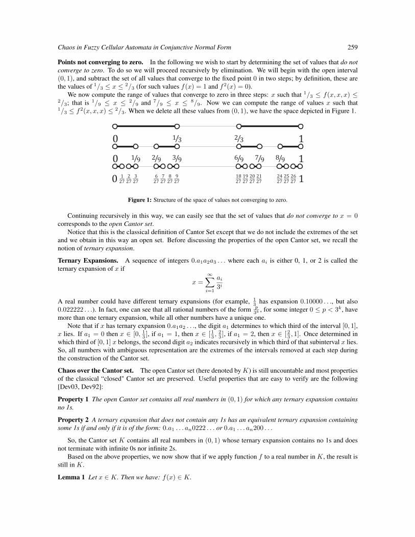
Chaos in Fuzzy Cellular Automata in Conjunctive Normal Form 259
Points not converging to zero. In the following we wish to start by determining the set of values that do notconverge to zero. To do so we will proceed recursively by elimination. We will begin with the open interval(0, 1), and subtract the set of all values that converge to the fixed point 0 in two steps; by definition, these arethe values of 1/3 ≤ x ≤ 2/3 (for such values f(x) = 1 and f2(x) = 0).
We now compute the range of values that converge to zero in three steps: x such that 1/3 ≤ f(x, x, x) ≤2/3; that is 1/9 ≤ x ≤ 2/9 and 7/9 ≤ x ≤ 8/9. Now we can compute the range of values x such that1/3 ≤ f2(x, x, x) ≤ 2/3. When we delete all these values from (0, 1), we have the space depicted in Figure 1.
0 1/1 3 /2 3
0 1/3 9/2 9/1 9 /7 9 /8 9/6 9
0 11 186 212 197 243 208 259 26
27 2727 2727 2727 2727 2727 2727 27
Figure 1: Structure of the space of values not converging to zero.
Continuing recursively in this way, we can easily see that the set of values that do not converge to x = 0corresponds to the open Cantor set.
Notice that this is the classical definition of Cantor Set except that we do not include the extremes of the setand we obtain in this way an open set. Before discussing the properties of the open Cantor set, we recall thenotion of ternary expansion.
Ternary Expansions. A sequence of integers 0.a1a2a3 . . . where each ai is either 0, 1, or 2 is called theternary expansion of x if
x =
∞∑i=1
ai3i
A real number could have different ternary expansions (for example, 13 has expansion 0.10000 . . ., but also
0.022222 . . .). In fact, one can see that all rational numbers of the form p3k
, for some integer 0 ≤ p < 3k, havemore than one ternary expansion, while all other numbers have a unique one.
Note that if x has ternary expansion 0.a1a2 . . ., the digit a1 determines to which third of the interval [0, 1],x lies. If a1 = 0 then x ∈ [0, 13 ], if a1 = 1, then x ∈ [ 13 ,
23 ], if a1 = 2, then x ∈ [ 23 , 1]. Once determined in
which third of [0, 1] x belongs, the second digit a2 indicates recursively in which third of that subinterval x lies.So, all numbers with ambiguous representation are the extremes of the intervals removed at each step duringthe construction of the Cantor set.
Chaos over the Cantor set. The open Cantor set (here denoted byK) is still uncountable and most propertiesof the classical “closed" Cantor set are preserved. Useful properties that are easy to verify are the following[Dev03, Dev92]:
Property 1 The open Cantor set contains all real numbers in (0, 1) for which any ternary expansion containsno 1s.
Property 2 A ternary expansion that does not contain any 1s has an equivalent ternary expansion containingsome 1s if and only if it is of the form: 0.a1 . . . an0222 . . . or 0.a1 . . . an200 . . .
So, the Cantor set K contains all real numbers in (0, 1) whose ternary expansion contains no 1s and doesnot terminate with infinite 0s nor infinite 2s.
Based on the above properties, we now show that if we apply function f to a real number in K, the result isstill in K.
Lemma 1 Let x ∈ K. Then we have: f(x) ∈ K.
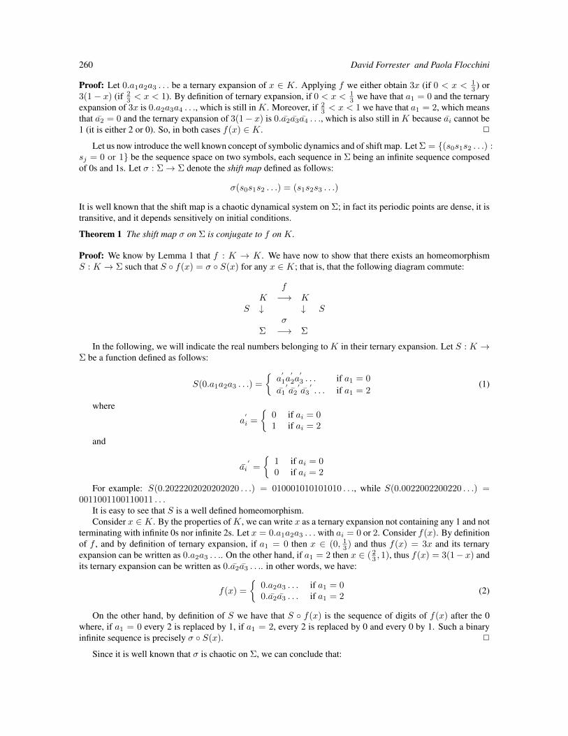
260 David Forrester and Paola Flocchini
Proof: Let 0.a1a2a3 . . . be a ternary expansion of x ∈ K. Applying f we either obtain 3x (if 0 < x < 13 ) or
3(1− x) (if 23 < x < 1). By definition of ternary expansion, if 0 < x < 1
3 we have that a1 = 0 and the ternaryexpansion of 3x is 0.a2a3a4 . . ., which is still in K. Moreover, if 2
3 < x < 1 we have that a1 = 2, which meansthat a2 = 0 and the ternary expansion of 3(1− x) is 0.a2a3a4 . . ., which is also still in K because ai cannot be1 (it is either 2 or 0). So, in both cases f(x) ∈ K. 2
Let us now introduce the well known concept of symbolic dynamics and of shift map. Let Σ = (s0s1s2 . . .) :sj = 0 or 1 be the sequence space on two symbols, each sequence in Σ being an infinite sequence composedof 0s and 1s. Let σ : Σ→ Σ denote the shift map defined as follows:
σ(s0s1s2 . . .) = (s1s2s3 . . .)
It is well known that the shift map is a chaotic dynamical system on Σ; in fact its periodic points are dense, it istransitive, and it depends sensitively on initial conditions.
Theorem 1 The shift map σ on Σ is conjugate to f on K.
Proof: We know by Lemma 1 that f : K → K. We have now to show that there exists an homeomorphismS : K → Σ such that S f(x) = σ S(x) for any x ∈ K; that is, that the following diagram commute:
fK −→ K
S ↓ ↓ Sσ
Σ −→ Σ
In the following, we will indicate the real numbers belonging to K in their ternary expansion. Let S : K →Σ be a function defined as follows:
S(0.a1a2a3 . . .) =
a
′
1a′
2a′
3 . . . if a1 = 0
a1′a2
′a3
′. . . if a1 = 2
(1)
where
a′
i =
0 if ai = 01 if ai = 2
and
ai′
=
1 if ai = 00 if ai = 2
For example: S(0.2022202020202020 . . .) = 010001010101010 . . ., while S(0.0022002200220 . . .) =0011001100110011 . . .
It is easy to see that S is a well defined homeomorphism.Consider x ∈ K. By the properties ofK, we can write x as a ternary expansion not containing any 1 and not
terminating with infinite 0s nor infinite 2s. Let x = 0.a1a2a3 . . . with ai = 0 or 2. Consider f(x). By definitionof f , and by definition of ternary expansion, if a1 = 0 then x ∈ (0, 13 ) and thus f(x) = 3x and its ternaryexpansion can be written as 0.a2a3 . . .. On the other hand, if a1 = 2 then x ∈ ( 2
3 , 1), thus f(x) = 3(1− x) andits ternary expansion can be written as 0.a2a3 . . .. in other words, we have:
f(x) =
0.a2a3 . . . if a1 = 00.a2a3 . . . if a1 = 2
(2)
On the other hand, by definition of S we have that S f(x) is the sequence of digits of f(x) after the 0where, if a1 = 0 every 2 is replaced by 1, if a1 = 2, every 2 is replaced by 0 and every 0 by 1. Such a binaryinfinite sequence is precisely σ S(x). 2
Since it is well known that σ is chaotic on Σ, we can conclude that:
Chaos in Fuzzy Cellular Automata in Conjunctive Normal Form 261
Theorem 2 Rule f is chaotic on the open Cantor set.
So, we can conclude that all elementary fuzzy cellular automata in conjunctive normal form with the transi-tions (0, 0, 0) → 0 and (1, 1, 1) → 0 in the rule table are chaotic on all homogenous configurations (x)n withx ∈ K, and converge to zero otherwise.
4 ConclusionWe began our investigation with the realization that FCA CNF “fuzzification”, being a conjunction of disjunc-tions, produce formulae with too many terms to be easily analyzed. In order to facilitate analysis, we began byrestricting our investigation to the special case of a homogeneous initial configuration.
The case of homogeneous configurations is much easier to analyse that the general case of heterogeneousinitial configurations, because the global rule of the CA can be studied as a simple function from [0, 1] to[01]. We discovered that all 256 such FCA fall into one of four classes. We were able to solve the asymptoticbehaviour of each of these classes.
The first three classes exhibited very simple dynamics: all rules converge directly to one. The second classhas two fixed points, and all rules converge either to zero or to one. The third class has a fixed point at 3
4 , but allother values converge to a temporally periodic configuration that alternates between zero and one.
The final, most interesting class exhibits chaos. In fact we showed that all CNF-fuzzy rules in this classdisplay chaotic behavior on a subset of [0, 1] even with homogeneous initial configurations. This is in strikingcontrast with the periodic behaviors of all DNF-fuzzy rules.
What is not known, is whether the theorems we prove in the homogeneous case are applicable in the generalcase. In particular, does chaos exist in CNF the non-homogeneous case ? It is also unclear to us why certainclasses in the homogeneous and heterogeneous cases seem to be identical, while other classes have no apparentcorrelation. We leave these as open questions.
Further research is under way also regarding the usefulness of the CNF-fuzzification for better understandingBoolean CAs. The current investigation is concerned only with CNF fuzzy rules with homogeneous initialconfigurations; such a setting is very restrictive and the use of CNF does not allow to differentiate enoughamong the rules. This makes it impossible to infer meaningful information regarding the dynamics of theirBoolean counterpart. The more general study of heterogeneous configurations might disclose interesting links.
AcknowledgementsThis work has been partially supported by Dr. Flocchini’s NSERC Discovery Grant.
References[BBC+92] J. Banks, J. Brooks, G. Cairns, G. Davis, and P. Stacey. The american mathematical monthly. On
Devaney’s definition of chaos, 99(4):332–334, 1992.
[BF11a] H. Betel and P. Flocchini. On the asymptotic behavior of fuzzy cellular automata. Journal ofCellular Automata, 6:25–52, 2011.
[BF11b] H. Betel and P. Flocchini. On the relationship between boolean and fuzzy cellular automata. Theo-retical Computer Science, 412(8-10):703–713, 2011.
[CFM+97] G. Cattaneo, P. Flocchini, G. Mauri, C. Quaranta Vogliotti, and N. Santoro. Cellular automata infuzzy backgrounds. Physica D: Nonlinear Phenomena, 105(1-3):105–120, 1997.
[Dev92] R. Devaney. A First Course in Chaotic Dynamical Systems: Theory and Experiment. Addison-Wesley, 1992.
[Dev03] R. Devaney. An Introduction to Chaotic Dynamical Systems, 2nd Edition. Westview Press, 2003.
[FC08] P. Flocchini and V. Cezar. Radial view of continuous cellular automata. Fundamenta Informaticae,87(2):165–183, 2008.

262 David Forrester and Paola Flocchini
[Kan84] K. Kaneko. Quasiperiodicity in antiferro-like structures and spatial intermittency in coupled logisticlattice. Progress of Theoretical Physics, 72, 1984.
[Kar05] J. Kari. Theory of cellular automata: A survey. Theoretical Computer Science, 334(1-3):3–33,2005.
[Min06a] A. Mingarelli. The global evolution of general fuzzy automata. Journal of Cellular Automata,1:141–164, 2006.
[Min06b] A. B. Mingarelli. A study of fuzzy and many-valued logics in cellular automata. Journal of CellularAutomata, 1(3):233–252, 2006.
[von66] J. von Neumann. Theory of Self-Reproducing Automata. University of Illinois Press, 1966.
[Zad65] L. A. Zadeh. Fuzzy sets. Information Control, 8:338–353, 1965.
AUTOMATA 2011, Santiago, Chile local proceedings LP, 2011, 263–272
Cellular automata-based model withsynchronous updating for Task StaticScheduling
Murillo G. Carneiro and Gina M. B. de OliveiraUniversidade Federal de UberlandiaPos-Graduacao em Ciencia da ComputacaoAvenida Joao Naves de Avila, 2121, Santa Monica38400-902 Uberlandia, MG - Brazil
Task Static Scheduling Problem (TSSP) in multiprocessors is an NP-Complete problem. Approaches proposed tosolve it typically use heuristics or meta-heuristics. Previous works have shown the promising use of Cellular Automata(CA) for extraction and reuse of knowledge in TSSP. However, they have not exploited the massive parallelisminherent to CA because good results were obtained only using asynchronous updating of cells. This paper presents anew model called Synchronous CA-based Scheduler (SCAS) that uses parallel updating of cells. Aiming to compareand analyze SCAS, related works were reproduced. Program graphs found in the literature and randomly generatedones were used in experiments. Experiments showed that SCAS improved previous works in terms of quality ofextracted knowledge.
Keywords: SCAS, CA-based scheduler, synchronous updating, Task Static Scheduling
1 IntroductionScheduling is a decision-making process that involves resources and tasks in the search for optimize oneor more objectives Pinedo (2008). Resources can be machines in a workshop or processing units in acomputing environment, while tasks can be operations in a production process, executions of computerprograms, and so on. There are several applications such as production scheduling, employees schedulingand computational tasks scheduling.
Task scheduling aims to allocate a set of computational tasks that compose a parallel application inthe nodes of a multiprocessor architecture. Considering Task Static Scheduling Problem (TSSP), allinformation about the tasks is known a priori. An optimal solution for an instance of TSSP is such thatthe precedence constraints are satisfied and the runtime - or makespan - is minimized. The problem isNP-Complete, even limited to the simplest case: a parallel system with only two processors Garey andJohnson (1979). Furthermore, it is a challenge for many researchers. The proposed approaches to solve ittypically employ heuristics or meta-heuristics. Some of the most known heuristics to TSSP are: HLFET(Hightest Level First with Estimated Time), ISH (Insertion Scheduling Heuristic) and MCP (Modified
c© 2011 AUTOMATA proceedings, Santiago, Chile, 2011
264 Murillo G. Carneiro and Gina M. B. de Oliveira
Critical Path), Kwok and Ahmad (1999) and Jin et al. (2008). However, such heuristics do not havethe ability to extract knowledge of the scheduling process of a parallel application and reuse it in otherinstances.
Cellular Automata (CA) are discrete dynamical systems which have the potential to exhibit a complexglobal behavior from simple interactions between local units. The most investigated update mode of cellsis synchronous - or parallel - because it explores the inherent parallelism in CA. Previous works pointedto the promising use of CA-based approaches to TSSP Seredynski and Zomaya (2002), Swiecicka et al.(2006) and Vidica and Oliveira (2006). Such models combine the use of CA and Genetic Algorithms(GA) Goldberg (1989) due to the employment of transition rule spaces with high cardinality Mitchellet al. (1996). However, they have not exploited the massive parallelism inherent to CA because goodresults were obtained only using asynchronous updating of cells.
The main objective of this work is to present and evaluate a new model with synchronous updating ofcells called Synchronous CA-based Scheduler (SCAS). An important feature of SCAS is that it is suitableto implement in parallel hardware. In addition, the new scheduler should be able to perform the optimal(or at least sub-optimal) scheduling of tasks. Other important feature investigated in SCAS is its abilityto extract knowledge during the process of scheduling of an application and to reuse it while solvingother instances of TSSP. Furthermore, the results obtained in SCAS are compared to results obtained inreproductions of previous works.
The remainder of this paper is organized as follows: Sections 2 presents a background about multipro-cessor scheduling. Section 3 and Section 4 contain concepts about CA-based scheduling and descriptionsof the proposed system, respectively. Section 5 contains experimental results concerning CA applied toscheduling in two processor systems. The last section contains conclusions and future works.
2 Multiprocessor SchedulingA multiprocessor system can be represented by an undirected and not weighted graph Gs = (Vs, Es),called system graph. Vs is the set of P processors of the system graph and Es is the set of bi-directionalchannels between processors that define the topology of the multiprocessor system. In this model it isalso assumed that all processors have the same computational power and the communications betweenthe channels do not consume any extra time of the processor beyond the communication time betweentasks as specified in graph.
A parallel application can be represented by a directed acyclic graph (DAG) defined by G = (V,E,W,C), where V = t1, . . . , tN denotes the set of N graph tasks; E = ei,j | ti, tj ∈ V represents theset of communication edges, also called precedence constraints; W = w1, . . . , wN represents the set ofrun times of the tasks, in others words, for each task t ∈ V a computational weight w(t) ∈ W is assignedrelative to its computational cost; and C = ci,j | ei,j ∈ E denotes the set of communication times ofthe edges, in others words, for each edge ei,j ∈ E is assigned a communication cost ci,j ∈ C related tothe cost of data transfer between tasks ti and tj when they are carried out on different processors. Theset of edges E defines the precedence relations between tasks. So, a task cannot be executed unless allits predecessors complete their executions and all relevant data are available. Tasks are represented bynodes. Tasks without predecessors will be called starting tasks and tasks without successors will be calledexit tasks. Preemption of tasks and redundant executions are not allowed. G is called the precedencegraph of tasks, or simply program graph. Figure 1 shows an example of program graph called gauss18that represents a set of 18 tasks.
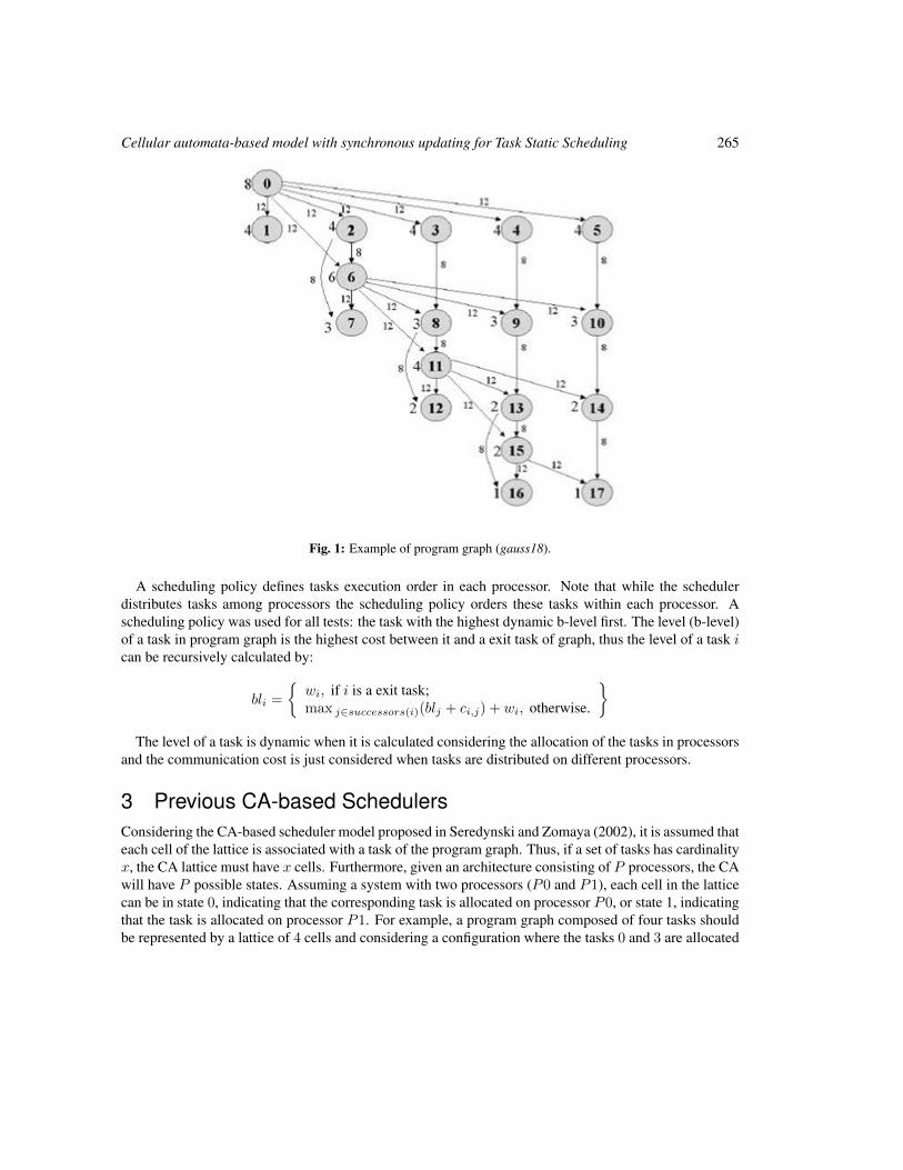
Cellular automata-based model with synchronous updating for Task Static Scheduling 265
Fig. 1: Example of program graph (gauss18).
A scheduling policy defines tasks execution order in each processor. Note that while the schedulerdistributes tasks among processors the scheduling policy orders these tasks within each processor. Ascheduling policy was used for all tests: the task with the highest dynamic b-level first. The level (b-level)of a task in program graph is the highest cost between it and a exit task of graph, thus the level of a task ican be recursively calculated by:
bli =
wi, if i is a exit task;max j∈successors(i)(blj + ci,j) + wi, otherwise.
The level of a task is dynamic when it is calculated considering the allocation of the tasks in processors
and the communication cost is just considered when tasks are distributed on different processors.
3 Previous CA-based SchedulersConsidering the CA-based scheduler model proposed in Seredynski and Zomaya (2002), it is assumed thateach cell of the lattice is associated with a task of the program graph. Thus, if a set of tasks has cardinalityx, the CA lattice must have x cells. Furthermore, given an architecture consisting of P processors, the CAwill have P possible states. Assuming a system with two processors (P0 and P1), each cell in the latticecan be in state 0, indicating that the corresponding task is allocated on processor P0, or state 1, indicatingthat the task is allocated on processor P1. For example, a program graph composed of four tasks shouldbe represented by a lattice of 4 cells and considering a configuration where the tasks 0 and 3 are allocated
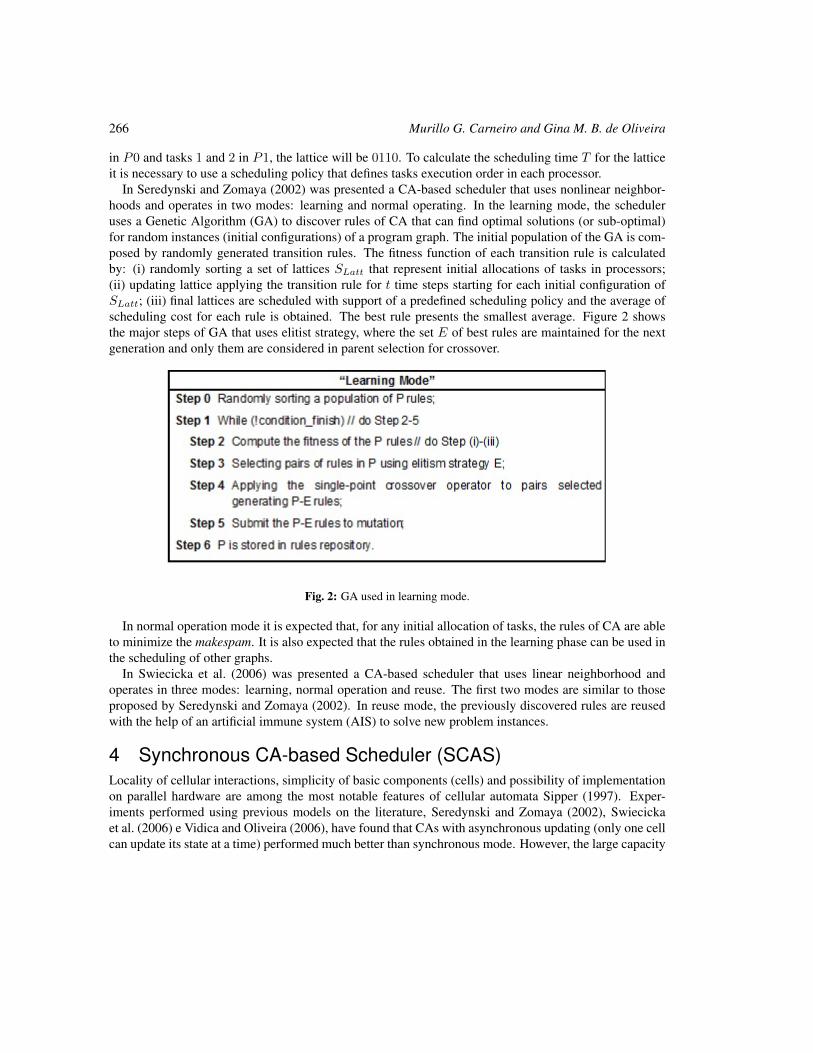
266 Murillo G. Carneiro and Gina M. B. de Oliveira
in P0 and tasks 1 and 2 in P1, the lattice will be 0110. To calculate the scheduling time T for the latticeit is necessary to use a scheduling policy that defines tasks execution order in each processor.
In Seredynski and Zomaya (2002) was presented a CA-based scheduler that uses nonlinear neighbor-hoods and operates in two modes: learning and normal operating. In the learning mode, the scheduleruses a Genetic Algorithm (GA) to discover rules of CA that can find optimal solutions (or sub-optimal)for random instances (initial configurations) of a program graph. The initial population of the GA is com-posed by randomly generated transition rules. The fitness function of each transition rule is calculatedby: (i) randomly sorting a set of lattices SLatt that represent initial allocations of tasks in processors;(ii) updating lattice applying the transition rule for t time steps starting for each initial configuration ofSLatt; (iii) final lattices are scheduled with support of a predefined scheduling policy and the average ofscheduling cost for each rule is obtained. The best rule presents the smallest average. Figure 2 showsthe major steps of GA that uses elitist strategy, where the set E of best rules are maintained for the nextgeneration and only them are considered in parent selection for crossover.
Fig. 2: GA used in learning mode.
In normal operation mode it is expected that, for any initial allocation of tasks, the rules of CA are ableto minimize the makespam. It is also expected that the rules obtained in the learning phase can be used inthe scheduling of other graphs.
In Swiecicka et al. (2006) was presented a CA-based scheduler that uses linear neighborhood andoperates in three modes: learning, normal operation and reuse. The first two modes are similar to thoseproposed by Seredynski and Zomaya (2002). In reuse mode, the previously discovered rules are reusedwith the help of an artificial immune system (AIS) to solve new problem instances.
4 Synchronous CA-based Scheduler (SCAS)Locality of cellular interactions, simplicity of basic components (cells) and possibility of implementationon parallel hardware are among the most notable features of cellular automata Sipper (1997). Exper-iments performed using previous models on the literature, Seredynski and Zomaya (2002), Swiecickaet al. (2006) e Vidica and Oliveira (2006), have found that CAs with asynchronous updating (only one cellcan update its state at a time) performed much better than synchronous mode. However, the large capacity
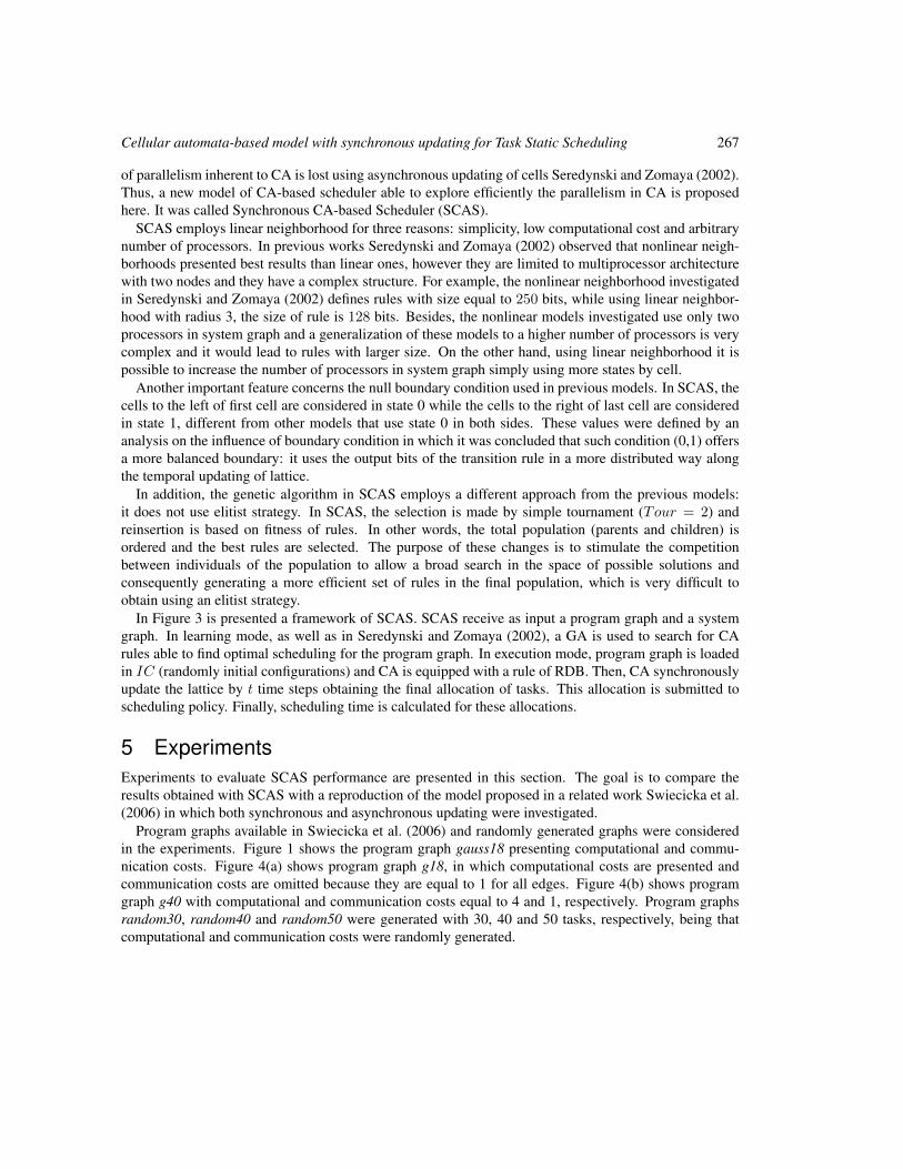
Cellular automata-based model with synchronous updating for Task Static Scheduling 267
of parallelism inherent to CA is lost using asynchronous updating of cells Seredynski and Zomaya (2002).Thus, a new model of CA-based scheduler able to explore efficiently the parallelism in CA is proposedhere. It was called Synchronous CA-based Scheduler (SCAS).
SCAS employs linear neighborhood for three reasons: simplicity, low computational cost and arbitrarynumber of processors. In previous works Seredynski and Zomaya (2002) observed that nonlinear neigh-borhoods presented best results than linear ones, however they are limited to multiprocessor architecturewith two nodes and they have a complex structure. For example, the nonlinear neighborhood investigatedin Seredynski and Zomaya (2002) defines rules with size equal to 250 bits, while using linear neighbor-hood with radius 3, the size of rule is 128 bits. Besides, the nonlinear models investigated use only twoprocessors in system graph and a generalization of these models to a higher number of processors is verycomplex and it would lead to rules with larger size. On the other hand, using linear neighborhood it ispossible to increase the number of processors in system graph simply using more states by cell.
Another important feature concerns the null boundary condition used in previous models. In SCAS, thecells to the left of first cell are considered in state 0 while the cells to the right of last cell are consideredin state 1, different from other models that use state 0 in both sides. These values were defined by ananalysis on the influence of boundary condition in which it was concluded that such condition (0,1) offersa more balanced boundary: it uses the output bits of the transition rule in a more distributed way alongthe temporal updating of lattice.
In addition, the genetic algorithm in SCAS employs a different approach from the previous models:it does not use elitist strategy. In SCAS, the selection is made by simple tournament (Tour = 2) andreinsertion is based on fitness of rules. In other words, the total population (parents and children) isordered and the best rules are selected. The purpose of these changes is to stimulate the competitionbetween individuals of the population to allow a broad search in the space of possible solutions andconsequently generating a more efficient set of rules in the final population, which is very difficult toobtain using an elitist strategy.
In Figure 3 is presented a framework of SCAS. SCAS receive as input a program graph and a systemgraph. In learning mode, as well as in Seredynski and Zomaya (2002), a GA is used to search for CArules able to find optimal scheduling for the program graph. In execution mode, program graph is loadedin IC (randomly initial configurations) and CA is equipped with a rule of RDB. Then, CA synchronouslyupdate the lattice by t time steps obtaining the final allocation of tasks. This allocation is submitted toscheduling policy. Finally, scheduling time is calculated for these allocations.
5 ExperimentsExperiments to evaluate SCAS performance are presented in this section. The goal is to compare theresults obtained with SCAS with a reproduction of the model proposed in a related work Swiecicka et al.(2006) in which both synchronous and asynchronous updating were investigated.
Program graphs available in Swiecicka et al. (2006) and randomly generated graphs were consideredin the experiments. Figure 1 shows the program graph gauss18 presenting computational and commu-nication costs. Figure 4(a) shows program graph g18, in which computational costs are presented andcommunication costs are omitted because they are equal to 1 for all edges. Figure 4(b) shows programgraph g40 with computational and communication costs equal to 4 and 1, respectively. Program graphsrandom30, random40 and random50 were generated with 30, 40 and 50 tasks, respectively, being thatcomputational and communication costs were randomly generated.
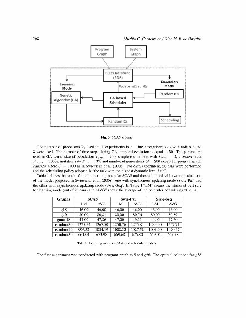
268 Murillo G. Carneiro and Gina M. B. de Oliveira
Fig. 3: SCAS scheme.
The number of processors Vs used in all experiments is 2. Linear neighborhoods with radius 2 and3 were used. The number of time steps during CA temporal evolution is equal to 50. The parametersused in GA were: size of population Tpop = 200, simple tournament with Tour = 2, crossover ratePcross = 100%, mutation rate Pmut = 3% and number of generations G = 200 except for program graphgauss18 where G = 1000 as in Swiecicka et al. (2006). For each experiment, 20 runs were performedand the scheduling policy adopted is “the task with the highest dynamic level first”.
Table 1 shows the results found in learning mode for SCAS and those obtained with two reproductionsof the model proposed in Swiecicka et al. (2006): one with synchronous updating mode (Swie-Par) andthe other with asynchronous updating mode (Swie-Seq). In Table 1,“LM” means the fitness of best rulefor learning mode (out of 20 runs) and “AVG” shows the average of the best rules considering 20 runs.
Graphs SCAS Swie-Par Swie-SeqLM AVG LM AVG LM AVG
g18 46,00 46,00 46,00 46,00 46,00 46,00g40 80,00 80,81 80,00 80,76 80,00 80,89
gauss18 44,00 47,86 47,00 49,31 44,00 47,60random30 1225,84 1267,50 1250,76 1275,81 1239,00 1247,71random40 996,52 1024,19 1008,32 1027,58 1006,00 1020,47random50 661,04 673,98 669,68 676,80 659,04 667,78
Tab. 1: Learning mode in CA-based scheduler models.
The first experiment was conducted with program graph g18 and g40. The optimal solutions for g18
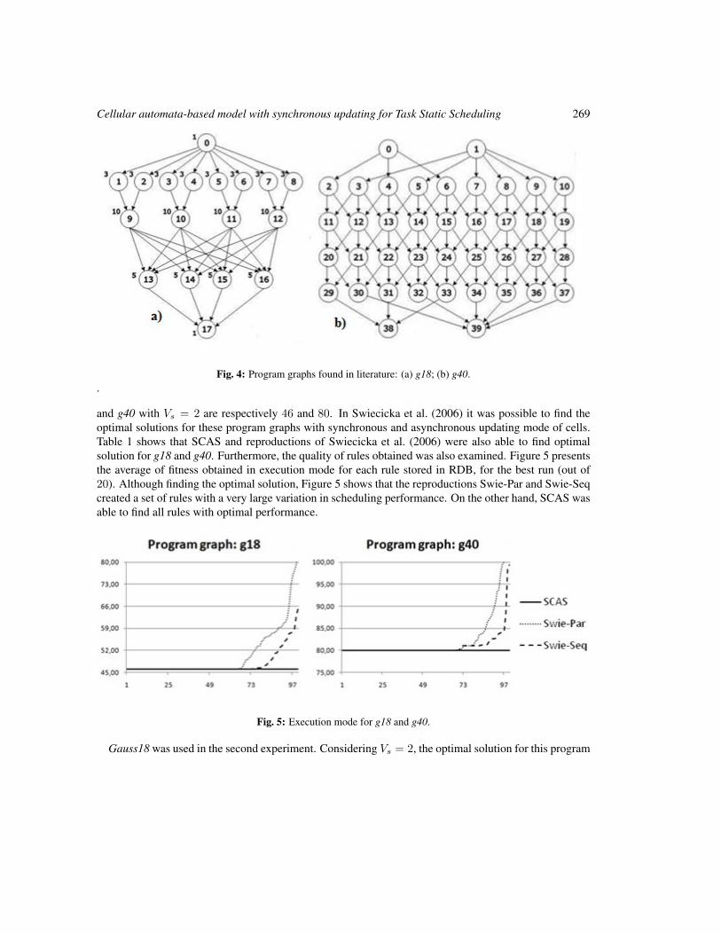
Cellular automata-based model with synchronous updating for Task Static Scheduling 269
Fig. 4: Program graphs found in literature: (a) g18; (b) g40..
and g40 with Vs = 2 are respectively 46 and 80. In Swiecicka et al. (2006) it was possible to find theoptimal solutions for these program graphs with synchronous and asynchronous updating mode of cells.Table 1 shows that SCAS and reproductions of Swiecicka et al. (2006) were also able to find optimalsolution for g18 and g40. Furthermore, the quality of rules obtained was also examined. Figure 5 presentsthe average of fitness obtained in execution mode for each rule stored in RDB, for the best run (out of20). Although finding the optimal solution, Figure 5 shows that the reproductions Swie-Par and Swie-Seqcreated a set of rules with a very large variation in scheduling performance. On the other hand, SCAS wasable to find all rules with optimal performance.
Fig. 5: Execution mode for g18 and g40.
Gauss18 was used in the second experiment. Considering Vs = 2, the optimal solution for this program
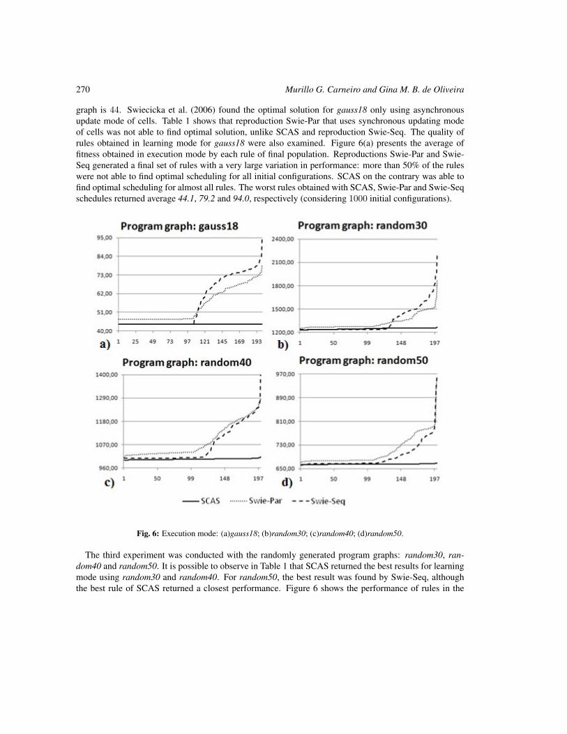
270 Murillo G. Carneiro and Gina M. B. de Oliveira
graph is 44. Swiecicka et al. (2006) found the optimal solution for gauss18 only using asynchronousupdate mode of cells. Table 1 shows that reproduction Swie-Par that uses synchronous updating modeof cells was not able to find optimal solution, unlike SCAS and reproduction Swie-Seq. The quality ofrules obtained in learning mode for gauss18 were also examined. Figure 6(a) presents the average offitness obtained in execution mode by each rule of final population. Reproductions Swie-Par and Swie-Seq generated a final set of rules with a very large variation in performance: more than 50% of the ruleswere not able to find optimal scheduling for all initial configurations. SCAS on the contrary was able tofind optimal scheduling for almost all rules. The worst rules obtained with SCAS, Swie-Par and Swie-Seqschedules returned average 44.1, 79.2 and 94.0, respectively (considering 1000 initial configurations).
Fig. 6: Execution mode: (a)gauss18; (b)random30; (c)random40; (d)random50.
The third experiment was conducted with the randomly generated program graphs: random30, ran-dom40 and random50. It is possible to observe in Table 1 that SCAS returned the best results for learningmode using random30 and random40. For random50, the best result was found by Swie-Seq, althoughthe best rule of SCAS returned a closest performance. Figure 6 shows the performance of rules in the
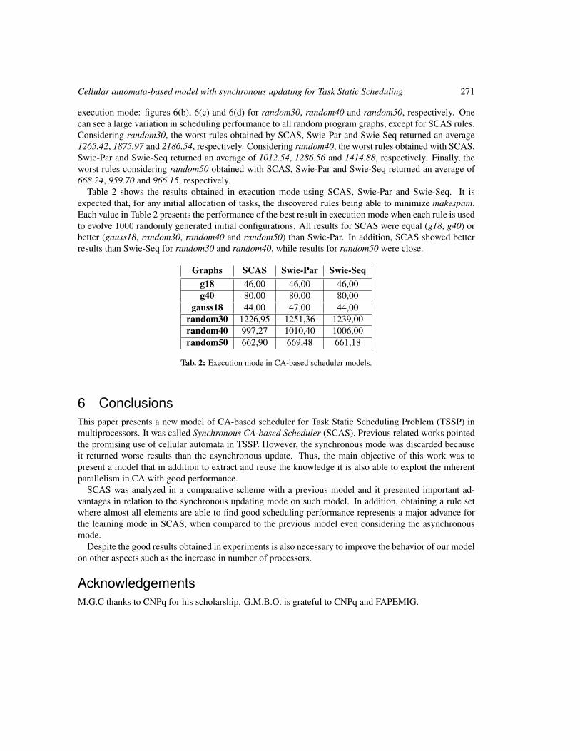
Cellular automata-based model with synchronous updating for Task Static Scheduling 271
execution mode: figures 6(b), 6(c) and 6(d) for random30, random40 and random50, respectively. Onecan see a large variation in scheduling performance to all random program graphs, except for SCAS rules.Considering random30, the worst rules obtained by SCAS, Swie-Par and Swie-Seq returned an average1265.42, 1875.97 and 2186.54, respectively. Considering random40, the worst rules obtained with SCAS,Swie-Par and Swie-Seq returned an average of 1012.54, 1286.56 and 1414.88, respectively. Finally, theworst rules considering random50 obtained with SCAS, Swie-Par and Swie-Seq returned an average of668.24, 959.70 and 966.15, respectively.
Table 2 shows the results obtained in execution mode using SCAS, Swie-Par and Swie-Seq. It isexpected that, for any initial allocation of tasks, the discovered rules being able to minimize makespam.Each value in Table 2 presents the performance of the best result in execution mode when each rule is usedto evolve 1000 randomly generated initial configurations. All results for SCAS were equal (g18, g40) orbetter (gauss18, random30, random40 and random50) than Swie-Par. In addition, SCAS showed betterresults than Swie-Seq for random30 and random40, while results for random50 were close.
Graphs SCAS Swie-Par Swie-Seqg18 46,00 46,00 46,00g40 80,00 80,00 80,00
gauss18 44,00 47,00 44,00random30 1226,95 1251,36 1239,00random40 997,27 1010,40 1006,00random50 662,90 669,48 661,18
Tab. 2: Execution mode in CA-based scheduler models.
6 ConclusionsThis paper presents a new model of CA-based scheduler for Task Static Scheduling Problem (TSSP) inmultiprocessors. It was called Synchronous CA-based Scheduler (SCAS). Previous related works pointedthe promising use of cellular automata in TSSP. However, the synchronous mode was discarded becauseit returned worse results than the asynchronous update. Thus, the main objective of this work was topresent a model that in addition to extract and reuse the knowledge it is also able to exploit the inherentparallelism in CA with good performance.
SCAS was analyzed in a comparative scheme with a previous model and it presented important ad-vantages in relation to the synchronous updating mode on such model. In addition, obtaining a rule setwhere almost all elements are able to find good scheduling performance represents a major advance forthe learning mode in SCAS, when compared to the previous model even considering the asynchronousmode.
Despite the good results obtained in experiments is also necessary to improve the behavior of our modelon other aspects such as the increase in number of processors.
AcknowledgementsM.G.C thanks to CNPq for his scholarship. G.M.B.O. is grateful to CNPq and FAPEMIG.
272 Murillo G. Carneiro and Gina M. B. de Oliveira
ReferencesM. R. Garey and D. S. Johnson. Computers and Interactability. A Guide to the Theory of NPCompleteness.
Freemann And Company, 1979.
D. E. Goldberg. Genetic Algorithms in Search, Optimization, and Machine Learning. Addison-Wesley,1989.
S. Jin, G. Schiavone, and D. Turgut. A performance study of multiprocessor task scheduling algorithms.The Journal of Supercomputing, 2008.
Y. K. Kwok and I. Ahmad. Benchmarking and comparison of the task graph scheduling algorithms.Journal of Parallel and Distributed Computing, 59(3):381–422, 1999.
M. Mitchell, J. P. Crutchfield, and R. Das. Evolving cellular automata with genetic algorithms: A reviewof recent work. In Proceedings of the First International Conference on Evolutionary Computation andIts Applications (EvCA’96), 1996.
M. L. Pinedo. Scheduling: Theory, Algorithms, and Systems. Springer Science, third edition, 2008.
F. Seredynski and A. Y. Zomaya. Sequential and parallel cellular automata-based scheduling algorithms.IEEE Transactions on Parallel and Distributed Systems, 13(10):1009–1022, 2002.
M. Sipper. Evolution of Parallel Cellular Machines, The Cellular Programming Approach. Springer,1997.
A. Swiecicka, F. Seredynski, and A. Y. Zomaya. Multiprocessor scheduling and rescheduling with use ofcellular automata and artificial immune system support. IEEE Transactions on Parallel and DistributedSystems, 17(3):253–262, 2006.
P. M. Vidica and G. M. B. Oliveira. Cellular automata-based scheduling: A new approach to improvegeneralization ability of evolved rules. Brazilian Symposium on Artificial Neural Networks (SBRN’06),2006.
AUTOMATA 2011, Santiago, Chile local proceedings LP, 2011, 273–284
A simple cellular multi-agent model ofbacterial biofilm sustainability
Tiago Guglielmeti Correale2† and Pedro P.B. de Oliveira1,2‡
Universidade Presbiteriana Mackenzie1Faculdade de Computacao e Informatica & 2Pos-Graduacao em Engenharia EletricaSao Paulo, SP - Brazil
A cellular multi-agent system is used to implement a simple and abstract model of bacterial biofilm. Biofilms aresocial organisations of bacteria that allow them much more adaptive and functional roles than when they are foundindividually; in fact, contrarily to commonsense knowledge, this is the most common form of bacteria organisationin nature. A series of experiments are reported with the model, addressing the issue of biofilm sustainability, onceit has been created. The model is based upon two kinds of agents, representing bacteria and food sources, theformer presenting two different roles, according to their ability to sustain the biofilm production. The investigation isfocused on the influence of different proportions of bacterial agents with these roles in the system. Some quantitativecharacterisation to the experiments is given, according to the initial world configuration, its population life span andthe energy levels of the system, which allow for explanations of some qualitative observations. The latter clarify theview that biofilm sustainability depends on a balance between the apparently conflicting roles of the bacterial agentsinvolved.
Keywords: Discrete dynamical system; multi-agent system; cellular world; DRIMA; BacDRIMA; biofilm; quorum-sensing; artificial life.
1 Introduction and motivationMulti-agent systems have been used in a wide range of applications and as conceptual tools (Wooldridge,2009; Jennings et al., 1998). In particular, in biology several efforts have also been made (Khan et al.,2003; Amigoni and Schiaffonati, 2007), supplementing the more traditional modelling techniques (Endyand Brent, 2001). Among those, cellular multi-agent approaches find its niche in terms of the simplicityand abstraction they naturally support, as well as with prospects to bridging the modelling efforts with thewealth of available knowledge in cellular automata theory and applications (Spicher et al., 2009; Edigerand Hoffmann, 2009).
The problem at issue herein is biofilm formation by bacteria, a very important subject in microbiology.Biofilms are defined as matrix-enclosed bacterial populations adherent to each other and/or to surfaces
†Email: [email protected]‡Email: [email protected]
c© 2011 AUTOMATA proceedings, Santiago, Chile, 2011

274 Tiago Guglielmeti Correale and Pedro P.B. de Oliveira
or interfaces (Costerton et al., 1995). Contrarily to commonsense knowledge, the presence of bacteria inbiofilms are much more common in nature than in their individualised (or, planktonic) form (Costerton,2007). Bacteria produce and release molecules known as auto-inducers, whose concentration may beregarded as information about the density of bacteria in some region of the space. When populationdensity of bacteria increases, the auto-inducer concentration also increases, eventually reaching a pointwhere certain changes in the bacteria phenotype are triggered. This is the moment where bacteria can startproducing a certain type of enzyme that allows the effective construction of the biofilm.
In order to explore this theme, we rely upon the current status of the BacDRIMA model, which isaimed at the possibility of addressing a number of issues in the dynamics of formation and sustainabilityof bacterial biofilm, from the perspective of a cellular, multi-agent system. This model is built upon thesimple multi-agent system DRIMA (de Oliveira, 2010), which is totally based on local and simple rulesgoverning the action of agents on a cellular world, much alike cellular automata. Due to space limitation,many aspects of the present conception and implementation of DRIMA are being omitted here.
The model is based upon two kinds of agents, representing bacteria and food sources. Two kindsof bacterial agents are defined, modelling two functional roles of the same kind of bacteria. The firstare standard bacteria type organisms, which are the ones directly involved in biofilm formation, and arereferred to herein as the normal bacteria, for the sake or simplicity. The second functional role definesthe so-called cheaters, which benefit from the work of normal bacteria without directly contributing tobiofilm formation.
BacDRIMA is an abstraction of all these processes. It tries to capture some essential aspects of biofilmdevelopment, without specific details related to specific bacteria, therefore aiming at an understandingof the generic dynamics of biofilm development. In order to go about it, the model was built with thefollowing characteristics:
• Multi-agent based;
• Each agent has some kind of energy, that simulates their strength;
• The system has energy (or food) sources;
• Agents can cooperate, by jointly releasing enzymes to maximize energy production, but they cancheat on the work of others;
• Agents can have different properties; and
• The system must support the existence of cheaters(in the sense that they may exist without produc-ing enzymes).
BacDRIMA was developed in Mathematica, just like the DRIMA system it was built upon (de Oliveira,2010). The results reported are preliminary, and refer to the dynamics of cooperation versus cheating.Specifically, although one might imagine that cheaters are always deleterious for the whole system, interms of always making biofilm development more difficult, the experiments to be reported indicate thatthis is not always the case. In fact, depending on certain conditions, cheaters help the system as a whole.
The remainder of the paper is organised as follows. After very briefly describing DRIMA in the nextsection, the basic concepts behind BacDRIMA are presented in the sequence. Then, artificial experi-mental results are presented, drawn from various experiments, with different initial conditions. Finally, aconclusions section discusses the results obtained, the model itself, and perspectives for the subsequentdevelopments of the work.
A simple cellular multi-agent model of bacterial biofilm sustainability 275
2 DRIMADRIMA, an acronym for Dynamics of Randomly Interacting Moving Agents, is a discrete dynamicalsystem, created around the idea of a set of reactive agents that interact locally, by changing the way theymove (de Oliveira, 2010). It is composed of a regular lattice of cells, with periodic boundary conditions,a set of agents placed on the cells, and parameters that defined the dynamics of the agent’s interactions.As a model and a computational system, DRIMA is a tool that may be used in a spectrum of experiments,as long as the problem at issue would rely on the local interaction among the agents resulting in theirmovement patterns being affected. Agents move on the lattice in a non-deterministic and local way,according to the probabilities defined by their so-called movement pattern; in particular, there is also aprobability of their not moving. Each agent has an interaction radius associated with them, and they caninteract with all agents within that radius. Interactions will change their movement pattern, by altering theprobabilities associated with each direction of movement. The agents follow an interact-first-then-movecycle.
Although various aspects of DRIMA have similarities with cellular automata, a key difference to benoticed is that DRIMA’s grid is only a lattice on top of which the agents can roam about.
Agent movement in DRIMA is in general non-deterministic and the lattice is presently either two- orone-dimensional. In the one-dimensional version, each agent can move to the left or right, or simply stayat its current position. In the two-dimensional case, which is our concern herein, each agent has 9 pos-sibilities: East (E), Northeast (NE), North (N), Northwest (NW), West (W), Southwest (SW), South (S),Southeast (SE), and Stop (X). Each agent have a probability associated with each movement possibility.In the case of deterministic agents, only one possibility has probability one, and all others zero; theirmovement pattern does not change in time, and they are not affected by interactions with other agents. Inthe case of random agents, each direction has an associated probability (jointly total ling 1), representedas a vector that describes the agent’s movement pattern.
The interactions between agents are represented by changes in their movement pattern. Each agent hasa radius of influence, within which the interactions occur, including the possibility of an agent interactingwith various agents at once (an n-ary interaction). At each interaction, only one agent changes theirmovement pattern, referred to as the reference agent.
In the case of n-ary interaction, initially the reference agent is identified, together with the neighbouringagents it will interact with.
Since the reference agent will in fact interact with the resulting vector obtained from the movementpatterns of the agents in its neighbourhood, this resulting vector is first obtained and normalised (to ensurethat its total movement probability remains equal to 1). Only then the actual interaction can occur.
As for the interaction itself, the idea is that the reference agent is ‘attracted’, so to speak, in the directionof the resulting movement vector of its neighbouring agents. This attraction is implemented in terms of arotation of the vector representing the reference agent towards the resulting neighbouring vector, and theamount of rotation depends on the angle between the agents.
The actual interaction is governed by Shannon’s entropy, associated to each interacting vector, definedas H = −
∑Ni=1 pilog(pi) (Borda, 2011). In our case, N = 9 (nine possible movements), pi is the
probability associated with the direction i. The idea here is that entropy indicates the degree of randomnessin the movement pattern of an agent.
In order to calculate the approximation angle the reference agent has to undergo as a result of aninteraction, a function was defined that gives the angle of approximation, according to the entropies of the

276 Tiago Guglielmeti Correale and Pedro P.B. de Oliveira
agents involved in the interaction. The details are being omitted here, but the function definition followedthe three general conditions below:
1. Movement limits: When an agent with maximum entropy interacts with another with minimumentropy, the agent with minimum entropy should not undergo any changes, while the other shouldundergo the maximum possible change.
2. Different random agents with minimum entropy should have a minimum (though not null) changein their movement pattern.
3. Agents with the same movement pattern should not change as the result of an interaction.
The ‘vectorial’ interaction scheme introduced above differs from the one described in (de Oliveira,2010), and will be presented in detail elsewhere.
3 BacDRIMA and BiofilmsBacDRIMA is a biologically inspired multi-agent model, that relies on DRIMA for its basic dynamics.The reader should be aware that BacDRIMA should be regarded as an abstract model, since it neglectsseveral details of its biological counterpart.
In BacDRIMA, two kind of agents are defined: the bacterial agents, and the energy or food source.Both of them are placed on a two-dimensional grid, presently with periodic boundary. The bacterialagents can move about, in a completely random way, while the food source is randomly placed on thegrid, fixed. Each bacterial agent has an active metabolism that consumes energy at each iteration. If theinternal energy goes down to 0 the agent dies, so that it must roam around the grid trying to find energysources to fulfil its energy necessities.
Food sources do not release energy immediately; rather, they require a certain level of enzyme to bereleased on them, after being produced and secreted by normal bacteria. The enzymes degrade with time,i.e. after some number of iterations they will be destroyed. In order to release more energy, more enzymemust be produced. Each food source has a finite amount of energy to be released, and will eventuallycease after some point.
In order to make enzymes, normal bacteria spend energy. Therefore, an energy balance has to beachieved in the system: in order to get energy, an agent must have some energy to produce enzymes,which in turn will be used to liberate energy from the food sources. Since the agents cannot control howmuch energy will be released by the food source, they must find a good strategy to survive, before theirinitial energy level becomes too low.
Both normal bacteria and cheaters can secrete another substance, the auto-inducer, that regulates en-zyme production. Normal bacteria will produce enzymes only after the auto-inducer concentration be-comes greater than a certain value. This is a simple model based on bacteria behaviour. In BacDRIMA,each agent measures its own auto-inducer concentration, as well as those of its neighbours. According tothe total auto-inducer production in the neighbourhood of an agent, it may start the enzyme synthesis.
For the sake of energy release, a food source considers the global production of all agents in its neigh-bourhood, so that the actual release starts when a certain level of enzyme is locally present. But notice thatthis benefits all agents in its neighbourhood, not only those responsible for the enzyme production thattriggered the energy liberation. This is a very important aspect of the model, because it makes it possiblethe definition of cheaters, i.e., agents that receive the released energy, without having contributed to theenzyme production.
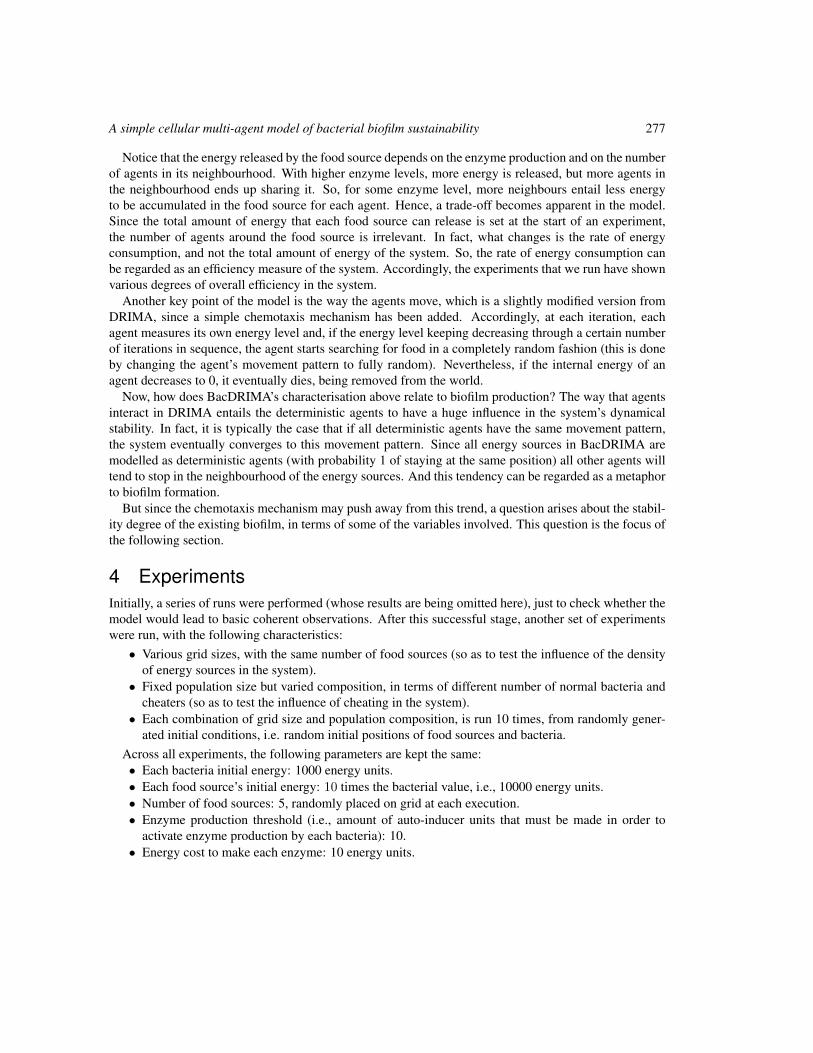
A simple cellular multi-agent model of bacterial biofilm sustainability 277
Notice that the energy released by the food source depends on the enzyme production and on the numberof agents in its neighbourhood. With higher enzyme levels, more energy is released, but more agents inthe neighbourhood ends up sharing it. So, for some enzyme level, more neighbours entail less energyto be accumulated in the food source for each agent. Hence, a trade-off becomes apparent in the model.Since the total amount of energy that each food source can release is set at the start of an experiment,the number of agents around the food source is irrelevant. In fact, what changes is the rate of energyconsumption, and not the total amount of energy of the system. So, the rate of energy consumption canbe regarded as an efficiency measure of the system. Accordingly, the experiments that we run have shownvarious degrees of overall efficiency in the system.
Another key point of the model is the way the agents move, which is a slightly modified version fromDRIMA, since a simple chemotaxis mechanism has been added. Accordingly, at each iteration, eachagent measures its own energy level and, if the energy level keeping decreasing through a certain numberof iterations in sequence, the agent starts searching for food in a completely random fashion (this is doneby changing the agent’s movement pattern to fully random). Nevertheless, if the internal energy of anagent decreases to 0, it eventually dies, being removed from the world.
Now, how does BacDRIMA’s characterisation above relate to biofilm production? The way that agentsinteract in DRIMA entails the deterministic agents to have a huge influence in the system’s dynamicalstability. In fact, it is typically the case that if all deterministic agents have the same movement pattern,the system eventually converges to this movement pattern. Since all energy sources in BacDRIMA aremodelled as deterministic agents (with probability 1 of staying at the same position) all other agents willtend to stop in the neighbourhood of the energy sources. And this tendency can be regarded as a metaphorto biofilm formation.
But since the chemotaxis mechanism may push away from this trend, a question arises about the stabil-ity degree of the existing biofilm, in terms of some of the variables involved. This question is the focus ofthe following section.
4 ExperimentsInitially, a series of runs were performed (whose results are being omitted here), just to check whether themodel would lead to basic coherent observations. After this successful stage, another set of experimentswere run, with the following characteristics:• Various grid sizes, with the same number of food sources (so as to test the influence of the density
of energy sources in the system).• Fixed population size but varied composition, in terms of different number of normal bacteria and
cheaters (so as to test the influence of cheating in the system).• Each combination of grid size and population composition, is run 10 times, from randomly gener-
ated initial conditions, i.e. random initial positions of food sources and bacteria.Across all experiments, the following parameters are kept the same:• Each bacteria initial energy: 1000 energy units.• Each food source’s initial energy: 10 times the bacterial value, i.e., 10000 energy units.• Number of food sources: 5, randomly placed on grid at each execution.• Enzyme production threshold (i.e., amount of auto-inducer units that must be made in order to
activate enzyme production by each bacteria): 10.• Energy cost to make each enzyme: 10 energy units.
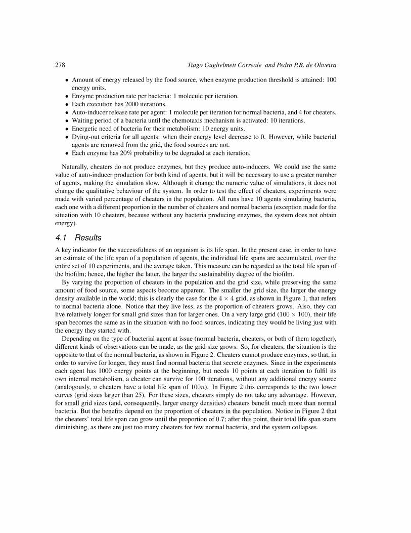
278 Tiago Guglielmeti Correale and Pedro P.B. de Oliveira
• Amount of energy released by the food source, when enzyme production threshold is attained: 100energy units.• Enzyme production rate per bacteria: 1 molecule per iteration.• Each execution has 2000 iterations.• Auto-inducer release rate per agent: 1 molecule per iteration for normal bacteria, and 4 for cheaters.• Waiting period of a bacteria until the chemotaxis mechanism is activated: 10 iterations.• Energetic need of bacteria for their metabolism: 10 energy units.• Dying-out criteria for all agents: when their energy level decrease to 0. However, while bacterial
agents are removed from the grid, the food sources are not.• Each enzyme has 20% probability to be degraded at each iteration.
Naturally, cheaters do not produce enzymes, but they produce auto-inducers. We could use the samevalue of auto-inducer production for both kind of agents, but it will be necessary to use a greater numberof agents, making the simulation slow. Although it change the numeric value of simulations, it does notchange the qualitative behaviour of the system. In order to test the effect of cheaters, experiments weremade with varied percentage of cheaters in the population. All runs have 10 agents simulating bacteria,each one with a different proportion in the number of cheaters and normal bacteria (exception made for thesituation with 10 cheaters, because without any bacteria producing enzymes, the system does not obtainenergy).
4.1 ResultsA key indicator for the successfulness of an organism is its life span. In the present case, in order to havean estimate of the life span of a population of agents, the individual life spans are accumulated, over theentire set of 10 experiments, and the average taken. This measure can be regarded as the total life span ofthe biofilm; hence, the higher the latter, the larger the sustainability degree of the biofilm.
By varying the proportion of cheaters in the population and the grid size, while preserving the sameamount of food source, some aspects become apparent. The smaller the grid size, the larger the energydensity available in the world; this is clearly the case for the 4 × 4 grid, as shown in Figure 1, that refersto normal bacteria alone. Notice that they live less, as the proportion of cheaters grows. Also, they canlive relatively longer for small grid sizes than for larger ones. On a very large grid (100× 100), their lifespan becomes the same as in the situation with no food sources, indicating they would be living just withthe energy they started with.
Depending on the type of bacterial agent at issue (normal bacteria, cheaters, or both of them together),different kinds of observations can be made, as the grid size grows. So, for cheaters, the situation is theopposite to that of the normal bacteria, as shown in Figure 2. Cheaters cannot produce enzymes, so that, inorder to survive for longer, they must find normal bacteria that secrete enzymes. Since in the experimentseach agent has 1000 energy points at the beginning, but needs 10 points at each iteration to fulfil itsown internal metabolism, a cheater can survive for 100 iterations, without any additional energy source(analogously, n cheaters have a total life span of 100n). In Figure 2 this corresponds to the two lowercurves (grid sizes larger than 25). For these sizes, cheaters simply do not take any advantage. However,for small grid sizes (and, consequently, larger energy densities) cheaters benefit much more than normalbacteria. But the benefits depend on the proportion of cheaters in the population. Notice in Figure 2 thatthe cheaters’ total life span can grow until the proportion of 0.7; after this point, their total life span startsdiminishing, as there are just too many cheaters for few normal bacteria, and the system collapses.
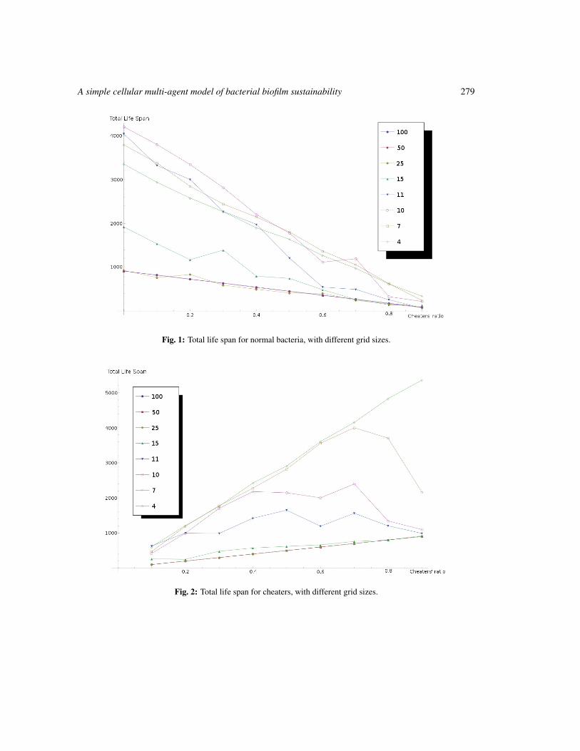
A simple cellular multi-agent model of bacterial biofilm sustainability 279
Fig. 1: Total life span for normal bacteria, with different grid sizes.
Fig. 2: Total life span for cheaters, with different grid sizes.
280 Tiago Guglielmeti Correale and Pedro P.B. de Oliveira
Figure 3 shows the situation for all bacterial agents, normal and cheaters, that is, a characterisation ofthe biofilm as a whole. For grid sizes smaller than 10 × 10, the system has always a tendency to growtheir total life span, until the proportion of cheaters becomes 0.7. So, as a whole, cheaters can make thetotal life span grow, up to a critical point. For grid sizes larger than 25 × 25, the overall total life spanbecomes the same, so that the good influence of the cheaters to the biofilm sustainability can no longerbe observed. In other words, the interesting good effect of the cheaters on the biofilm happens for highenergy densities of the world.
Fig. 3: Total life span for all agents, with different grid sizes.
Figure 4 refers to 10 simulations, with a 7× 7 grid, without any food source. The overall system (i.e.,the biofilm as a whole) has a small increase in its total life span, as the proportion of cheaters increases.The increase is a consequence of the fact that cheaters do not spend energy at enzyme production, butnormal agents do, even though with unfruitful effects. But notice that the maximum life span in all threecases depicted in the figure falls below 1000 iterations, which is the maximum life span of the agents inthe situation where they would rely only upon their initial energy levels, without any energy consumption(due to enzyme production).
Figure 5 depicts two plots of the total internal energy of all agents of the system on a 7× 7 grid. Eachtime an agent obtains energy from a food source, its internal energy increases. But, at each iteration, eachagent spends energy with its own metabolism, and on enzyme production. The total energy of the systemis the sum of the internal energy of all agents. The peak in the solid line plot of Figure 5 corresponds tothe moment at which most agents are getting the largest amount of energy from all sources.
Notice that in the solid line of Figure 5, a peak occurs for 125 iterations. And a similar peak wasalso observed for an ensemble of 60 executions (with the very tight standard deviation of less than 10),with varying proportions of cheaters, up to 60%. For progressively larger proportions, the peak getsdisplaced more and more to the left-hand side, eventually reaching the situation depicted in the dashed
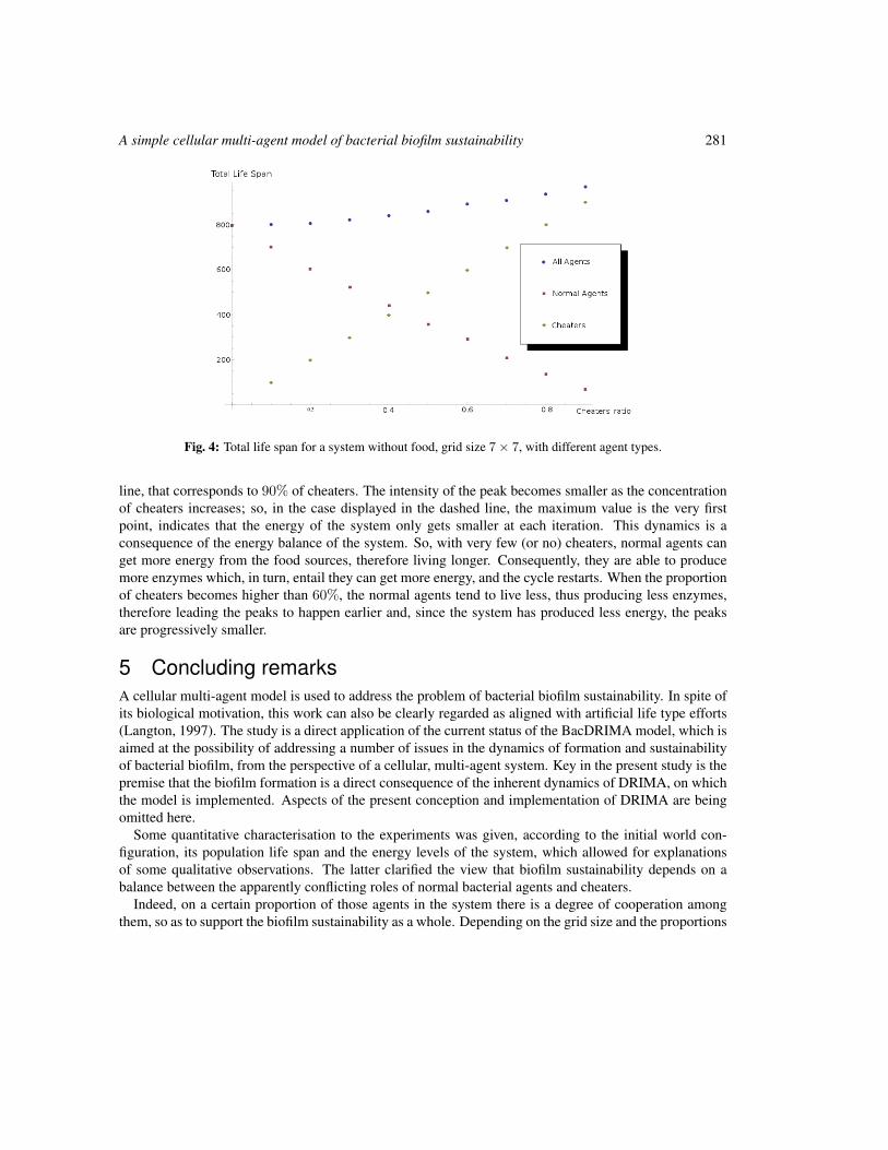
A simple cellular multi-agent model of bacterial biofilm sustainability 281
Fig. 4: Total life span for a system without food, grid size 7× 7, with different agent types.
line, that corresponds to 90% of cheaters. The intensity of the peak becomes smaller as the concentrationof cheaters increases; so, in the case displayed in the dashed line, the maximum value is the very firstpoint, indicates that the energy of the system only gets smaller at each iteration. This dynamics is aconsequence of the energy balance of the system. So, with very few (or no) cheaters, normal agents canget more energy from the food sources, therefore living longer. Consequently, they are able to producemore enzymes which, in turn, entail they can get more energy, and the cycle restarts. When the proportionof cheaters becomes higher than 60%, the normal agents tend to live less, thus producing less enzymes,therefore leading the peaks to happen earlier and, since the system has produced less energy, the peaksare progressively smaller.
5 Concluding remarksA cellular multi-agent model is used to address the problem of bacterial biofilm sustainability. In spite ofits biological motivation, this work can also be clearly regarded as aligned with artificial life type efforts(Langton, 1997). The study is a direct application of the current status of the BacDRIMA model, which isaimed at the possibility of addressing a number of issues in the dynamics of formation and sustainabilityof bacterial biofilm, from the perspective of a cellular, multi-agent system. Key in the present study is thepremise that the biofilm formation is a direct consequence of the inherent dynamics of DRIMA, on whichthe model is implemented. Aspects of the present conception and implementation of DRIMA are beingomitted here.
Some quantitative characterisation to the experiments was given, according to the initial world con-figuration, its population life span and the energy levels of the system, which allowed for explanationsof some qualitative observations. The latter clarified the view that biofilm sustainability depends on abalance between the apparently conflicting roles of normal bacterial agents and cheaters.
Indeed, on a certain proportion of those agents in the system there is a degree of cooperation amongthem, so as to support the biofilm sustainability as a whole. Depending on the grid size and the proportions
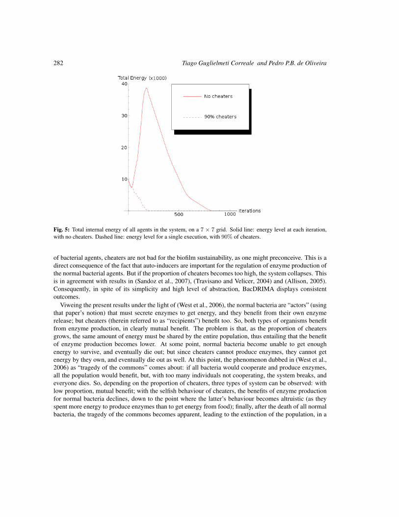
282 Tiago Guglielmeti Correale and Pedro P.B. de Oliveira
Fig. 5: Total internal energy of all agents in the system, on a 7 × 7 grid. Solid line: energy level at each iteration,with no cheaters. Dashed line: energy level for a single execution, with 90% of cheaters.
of bacterial agents, cheaters are not bad for the biofilm sustainability, as one might preconceive. This is adirect consequence of the fact that auto-inducers are important for the regulation of enzyme production ofthe normal bacterial agents. But if the proportion of cheaters becomes too high, the system collapses. Thisis in agreement with results in (Sandoz et al., 2007), (Travisano and Velicer, 2004) and (Allison, 2005).Consequently, in spite of its simplicity and high level of abstraction, BacDRIMA displays consistentoutcomes.
Viweing the present results under the light of (West et al., 2006), the normal bacteria are “actors” (usingthat paper’s notion) that must secrete enzymes to get energy, and they benefit from their own enzymerelease; but cheaters (therein referred to as “recipients”) benefit too. So, both types of organisms benefitfrom enzyme production, in clearly mutual benefit. The problem is that, as the proportion of cheatersgrows, the same amount of energy must be shared by the entire population, thus entailing that the benefitof enzyme production becomes lower. At some point, normal bacteria become unable to get enoughenergy to survive, and eventually die out; but since cheaters cannot produce enzymes, they cannot getenergy by they own, and eventually die out as well. At this point, the phenomenon dubbed in (West et al.,2006) as “tragedy of the commons” comes about: if all bacteria would cooperate and produce enzymes,all the population would benefit, but, with too many individuals not cooperating, the system breaks, andeveryone dies. So, depending on the proportion of cheaters, three types of system can be observed: withlow proportion, mutual benefit; with the selfish behaviour of cheaters, the benefits of enzyme productionfor normal bacteria declines, down to the point where the latter’s behaviour becomes altruistic (as theyspent more energy to produce enzymes than to get energy from food); finally, after the death of all normalbacteria, the tragedy of the commons becomes apparent, leading to the extinction of the population, in a
A simple cellular multi-agent model of bacterial biofilm sustainability 283
clearly spiteful behaviour.Since BacDRIMA is yet an ongoing development, forthcoming improvements in the work include:
− Reproduction: The main focus of the current effort to expand the BacDRIMA model is the intro-duction of an asexual reproduction scheme for the agents, based upon their genome, which encodesthe agent’s enzyme production and auto-inducer production.
− Diffusion of chemical elements: Since in the present model the chemical elements (enzymes andauto-inducers) do not diffuse on the grid, the addition of some kind of diffusion would make theoverall behaviour more natural.
− Addition of energy cost to auto-inducer production: This is meant to allow the study of the relationbetween the metabolism energy cost, enzyme production and auto-inducer production.
AcknowledgementsWe are grateful to MackPesquisa – Fundo Mackenzie de Pesquisa: T.G.C. for academic support, andP.P.B.O. for a sabbatical grant, during which this paper was written.
ReferencesS. Allison. Cheaters, diffusion and nutrients constrain decomposition by microbial enzymes in spatially
structured environments. Ecology Letters, 8(6):626–635, 2005.
F. Amigoni and V. Schiaffonati. Multi-agent-based simulation in biology. Model-Based Reasoning inScience, Technology, and Medicine, pages 179–191, 2007.
M. Borda. Fundamentals in Information Theory and Coding. Springer, 2011.
J. Costerton. The Biofilm Primer. Springer Verlag, 2007.
J. Costerton, Z. Lewandowski, D. Caldwell, D. Korber, and H. Lappin-Scott. Microbial biofilms. AnnualReviews in Microbiology, 49(1):711–745, 1995.
P. P. B. de Oliveira. DRIMA: A Minimal System for Probing the Dynamics of Change in a ReactiveMulti-agent Setting. The Mathematica Journal, 12(1):1–18, 2010.
P. Ediger and R. Hoffmann. CA models for target searching agents. Electr. Notes Theor. Comput. Sci.,252:41–54, 2009.
D. Endy and R. Brent. Modelling cellular behaviour. Nature, 409(6818):391–396, 2001.
N. Jennings, K. Sycara, and M. Wooldridge. A roadmap of agent research and development. AutonomousAgents and Multi-agent Systems, 1(1):7–38, 1998.
S. Khan, R. Makkena, F. Mc Geary, K. Decker, W. Gillis, and C. Schmidt. A multi-agent system forthe quantitative simulation of biological networks. In Proceedings of the Second International JointConference on Autonomous Agents and Multiagent Systems, pages 385–392. ACM, 2003.
C. Langton. Artificial life: An Overview. Complex Adaptive Systems. MIT Press, 1997.
284 Tiago Guglielmeti Correale and Pedro P.B. de Oliveira
K. Sandoz, S. Mitzimberg, and M. Schuster. Social cheating in pseudomonas aeruginosa quorum sensing.Proceedings of the National Academy of Sciences, 104(40):15876, 2007.
A. Spicher, N. Fates, and O. Simonin. From reactive multi-agents models to cellular automata - illustrationon a diffusion-limited aggregation model. In J. Filipe, A. L. N. Fred, and B. Sharp, editors, ICAART,pages 422–429. INSTICC Press, 2009.
M. Travisano and G. Velicer. Strategies of microbial cheater control. Trends in Microbiology, 12(2):72–78, 2004.
S. West, A. Griffin, A. Gardner, and S. Diggle. Social evolution theory for microorganisms. NatureReviews Microbiology, 4(8):597–607, 2006.
S. West, A. Griffin, and A. Gardner. Social semantics: Altruism, cooperation, mutualism, strong reci-procity and group selection. Journal of Evolutionary Biology, 20(2):415–432, 2007.
M. Wooldridge. An Introduction to Multi-Agent Systems. John Wiley & Sons, 2009.
AUTOMATA 2011, Santiago, Chile local proceedings LP, 2011, 285–292
A simple block representation of reversiblecellular automata with time-symmetry
Pablo Arrighi1† and Vincent Nesme2‡
1 Universite de Grenoble, LIG, 220 rue de la chimie, 38400 Saint-Martin-d’Heres, Franceand Ecole Normale Superieure de Lyon, LIP, 46 Allee d’Italie, 69364 Lyon, France2 QMIO, Freie Universitat Berlin, Arnimallee 14, 14195 Berlin, Germany
Reversible Cellular Automata (RCA) are a physics-like model of computation consisting of an array of identical cells,evolving in discrete time steps by iterating a global evolution G. Further, G is required to be shift-invariant (it acts thesame everywhere), causal (information cannot be transmitted faster than some fixed number of cells per time step),and reversible (it has an inverse which verifies the same requirements). An important, though only recently studiedspecial case is that of Time-symmetric Cellular Automata (TSCA), for which G and its inverse are related via a localoperation. In this note we revisit the question of the Block representation of RCA, i.e. we provide a very simpleproof of the existence of a reversible circuit description implementing G. This operational, bottom-up description ofG turns out to be time-symmetric, suggesting interesting connections with TSCA. Indeed we prove, using a similartechnique, that a wide class of them admit an Exact block representation (EBR), i.e. one which does not increase thestate space.
Keywords: Reversible Cellular Automata, Time-symmetric Cellular Automata
IntroductionRCA, Block representation. In [Kar96], Kari showed that any one-dimensional or two-dimensional re-versible cellular automaton (RCA) can be expressed as a composition of finite reversible gates (or ‘blockpermutations’) and partial shifts. In two dimensions the proof is quite involved, the representation re-quires three layers of blocks, and it has been proved that this cannot be brought down to a two-layeredblock representation [Kar99]; The problem is still open in higher dimensions.
However we may not need an exact representation, and be willing to encode our original cells intosome larger ones (or equivalently to interleave some ancillary cells), as proposed in [DL01]. Then theconstruction of [Kar99] shows that even n-dimensional RCA admit a two-layered block representation.In some sense what we are doing then is simulating the original RCA in a way which preserves the spatiallayout of cells, with another, simpler RCA that we know admits a two-layered block representation. In
†Email: [email protected]‡Email: [email protected]
c© 2011 AUTOMATA proceedings, Santiago, Chile, 2011
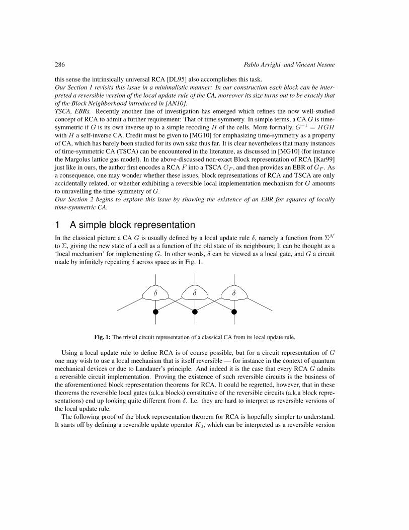
286 Pablo Arrighi and Vincent Nesme
this sense the intrinsically universal RCA [DL95] also accomplishes this task.Our Section 1 revisits this issue in a minimalistic manner: In our construction each block can be inter-preted a reversible version of the local update rule of the CA, moreover its size turns out to be exactly thatof the Block Neighborhood introduced in [AN10].TSCA, EBRs. Recently another line of investigation has emerged which refines the now well-studiedconcept of RCA to admit a further requirement: That of time symmetry. In simple terms, a CA G is time-symmetric if G is its own inverse up to a simple recoding H of the cells. More formally, G−1 = HGHwith H a self-inverse CA. Credit must be given to [MG10] for emphasizing time-symmetry as a propertyof CA, which has barely been studied for its own sake thus far. It is clear nevertheless that many instancesof time-symmetric CA (TSCA) can be encountered in the literature, as discussed in [MG10] (for instancethe Margolus lattice gas model). In the above-discussed non-exact Block representation of RCA [Kar99]just like in ours, the author first encodes a RCA F into a TSCA GF , and then provides an EBR of GF . Asa consequence, one may wonder whether these issues, block representations of RCA and TSCA are onlyaccidentally related, or whether exhibiting a reversible local implementation mechanism for G amountsto unravelling the time-symmetry of G.Our Section 2 begins to explore this issue by showing the existence of an EBR for squares of locallytime-symmetric CA.
1 A simple block representationIn the classical picture a CA G is usually defined by a local update rule δ, namely a function from ΣN
to Σ, giving the new state of a cell as a function of the old state of its neighbours; It can be thought as a‘local mechanism’ for implementing G. In other words, δ can be viewed as a local gate, and G a circuitmade by infinitely repeating δ across space as in Fig. 1.
δ δ δ
Fig. 1: The trivial circuit representation of a classical CA from its local update rule.
Using a local update rule to define RCA is of course possible, but for a circuit representation of Gone may wish to use a local mechanism that is itself reversible — for instance in the context of quantummechanical devices or due to Landauer’s principle. And indeed it is the case that every RCA G admitsa reversible circuit implementation. Proving the existence of such reversible circuits is the business ofthe aforementioned block representation theorems for RCA. It could be regretted, however, that in thesetheorems the reversible local gates (a.k.a blocks) constitutive of the reversible circuits (a.k.a block repre-sentations) end up looking quite different from δ. I.e. they are hard to interpret as reversible versions ofthe local update rule.
The following proof of the block representation theorem for RCA is hopefully simpler to understand.It starts off by defining a reversible update operator K0, which can be interpreted as a reversible version
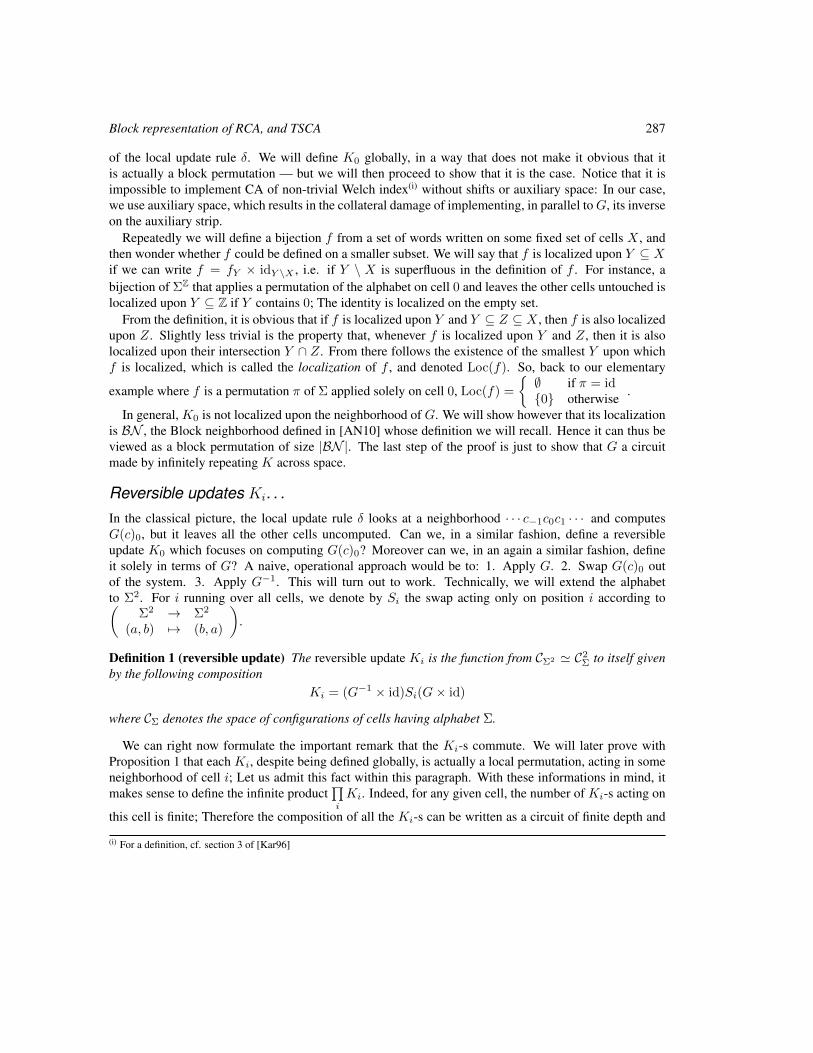
Block representation of RCA, and TSCA 287
of the local update rule δ. We will define K0 globally, in a way that does not make it obvious that itis actually a block permutation — but we will then proceed to show that it is the case. Notice that it isimpossible to implement CA of non-trivial Welch index(i) without shifts or auxiliary space: In our case,we use auxiliary space, which results in the collateral damage of implementing, in parallel toG, its inverseon the auxiliary strip.
Repeatedly we will define a bijection f from a set of words written on some fixed set of cells X , andthen wonder whether f could be defined on a smaller subset. We will say that f is localized upon Y ⊆ Xif we can write f = fY × idY \X , i.e. if Y \ X is superfluous in the definition of f . For instance, abijection of ΣZ that applies a permutation of the alphabet on cell 0 and leaves the other cells untouched islocalized upon Y ⊆ Z if Y contains 0; The identity is localized on the empty set.
From the definition, it is obvious that if f is localized upon Y and Y ⊆ Z ⊆ X , then f is also localizedupon Z. Slightly less trivial is the property that, whenever f is localized upon Y and Z, then it is alsolocalized upon their intersection Y ∩ Z. From there follows the existence of the smallest Y upon whichf is localized, which is called the localization of f , and denoted Loc(f). So, back to our elementary
example where f is a permutation π of Σ applied solely on cell 0, Loc(f) =
∅ if π = id0 otherwise .
In general, K0 is not localized upon the neighborhood of G. We will show however that its localizationis BN , the Block neighborhood defined in [AN10] whose definition we will recall. Hence it can thus beviewed as a block permutation of size |BN |. The last step of the proof is just to show that G a circuitmade by infinitely repeating K across space.
Reversible updates Ki. . .In the classical picture, the local update rule δ looks at a neighborhood · · · c−1c0c1 · · · and computesG(c)0, but it leaves all the other cells uncomputed. Can we, in a similar fashion, define a reversibleupdate K0 which focuses on computing G(c)0? Moreover can we, in an again a similar fashion, defineit solely in terms of G? A naive, operational approach would be to: 1. Apply G. 2. Swap G(c)0 outof the system. 3. Apply G−1. This will turn out to work. Technically, we will extend the alphabetto Σ2. For i running over all cells, we denote by Si the swap acting only on position i according to(
Σ2 → Σ2
(a, b) 7→ (b, a)
).
Definition 1 (reversible update) The reversible update Ki is the function from CΣ2 ' C2Σ to itself given
by the following compositionKi = (G−1 × id)Si(G× id)
where CΣ denotes the space of configurations of cells having alphabet Σ.
We can right now formulate the important remark that the Ki-s commute. We will later prove withProposition 1 that each Ki, despite being defined globally, is actually a local permutation, acting in someneighborhood of cell i; Let us admit this fact within this paragraph. With these informations in mind, itmakes sense to define the infinite product
∏i
Ki. Indeed, for any given cell, the number of Ki-s acting on
this cell is finite; Therefore the composition of all the Ki-s can be written as a circuit of finite depth and
(i) For a definition, cf. section 3 of [Kar96]
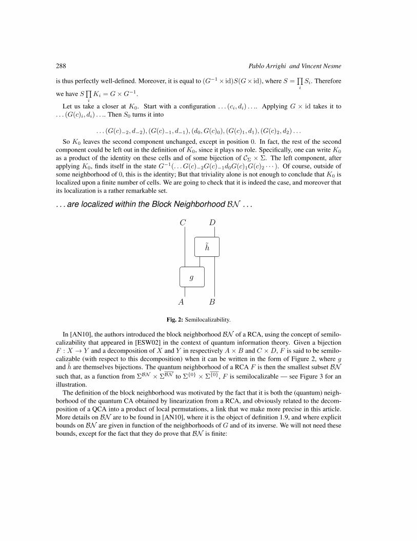
288 Pablo Arrighi and Vincent Nesme
is thus perfectly well-defined. Moreover, it is equal to (G−1× id)S(G× id), where S =∏i
Si. Therefore
we have S∏i
Ki = G×G−1.
Let us take a closer at K0. Start with a configuration . . . (ci, di) . . .. Applying G × id takes it to. . . (G(c)i, di) . . .. Then S0 turns it into
. . . (G(c)−2, d−2), (G(c)−1, d−1), (d0, G(c)0), (G(c)1, d1), (G(c)2, d2) . . .
So K0 leaves the second component unchanged, except in position 0. In fact, the rest of the secondcomponent could be left out in the definition of K0, since it plays no role. Specifically, one can write K0
as a product of the identity on these cells and of some bijection of CΣ × Σ. The left component, afterapplying K0, finds itself in the state G−1(. . . G(c)−2G(c)−1d0G(c)1G(c)2 · · · ). Of course, outside ofsome neighborhood of 0, this is the identity; But that triviality alone is not enough to conclude that K0 islocalized upon a finite number of cells. We are going to check that it is indeed the case, and moreover thatits localization is a rather remarkable set.
. . . are localized within the Block Neighborhood BN . . .
g
h
C D
A B
Fig. 2: Semilocalizability.
In [AN10], the authors introduced the block neighborhood BN of a RCA, using the concept of semilo-calizability that appeared in [ESW02] in the context of quantum information theory. Given a bijectionF : X → Y and a decomposition of X and Y in respectively A×B and C ×D, F is said to be semilo-calizable (with respect to this decomposition) when it can be written in the form of Figure 2, where gand h are themselves bijections. The quantum neighborhood of a RCA F is then the smallest subset BNsuch that, as a function from ΣBN × ΣBN to Σ0 × Σ0, F is semilocalizable — see Figure 3 for anillustration.
The definition of the block neighborhood was motivated by the fact that it is both the (quantum) neigh-borhood of the quantum CA obtained by linearization from a RCA, and obviously related to the decom-position of a QCA into a product of local permutations, a link that we make more precise in this article.More details on BN are to be found in [AN10], where it is the object of definition 1.9, and where explicitbounds on BN are given in function of the neighborhoods of G and of its inverse. We will not need thesebounds, except for the fact that they do prove that BN is finite:
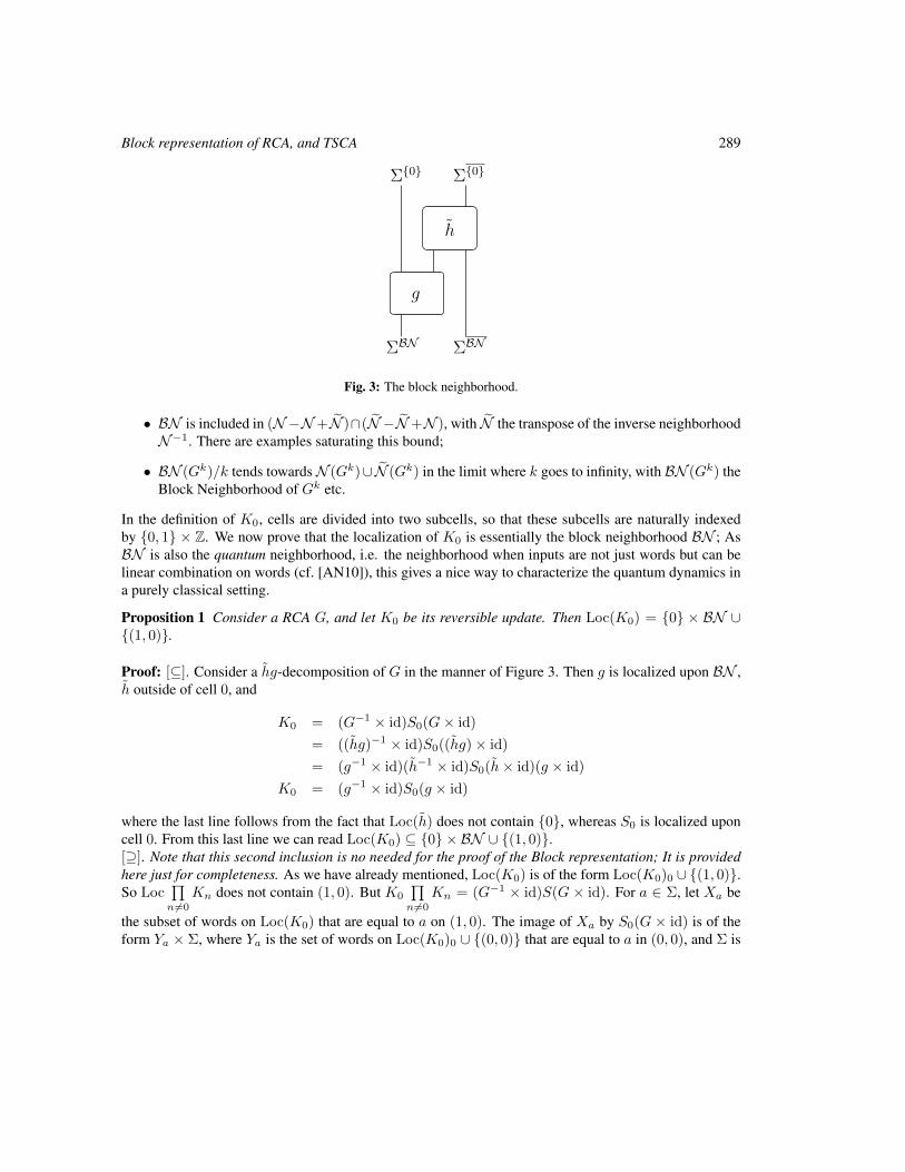
Block representation of RCA, and TSCA 289
g
h
Σ0 Σ0
ΣBN ΣBN
Fig. 3: The block neighborhood.
• BN is included in (N−N+N )∩(N −N+N ), with N the transpose of the inverse neighborhoodN−1. There are examples saturating this bound;
• BN (Gk)/k tends towardsN (Gk)∪N (Gk) in the limit where k goes to infinity, with BN (Gk) theBlock Neighborhood of Gk etc.
In the definition of K0, cells are divided into two subcells, so that these subcells are naturally indexedby 0, 1 × Z. We now prove that the localization of K0 is essentially the block neighborhood BN ; AsBN is also the quantum neighborhood, i.e. the neighborhood when inputs are not just words but can belinear combination on words (cf. [AN10]), this gives a nice way to characterize the quantum dynamics ina purely classical setting.
Proposition 1 Consider a RCA G, and let K0 be its reversible update. Then Loc(K0) = 0 × BN ∪(1, 0).
Proof: [⊆]. Consider a hg-decomposition of G in the manner of Figure 3. Then g is localized upon BN ,h outside of cell 0, and
K0 = (G−1 × id)S0(G× id)
= ((hg)−1 × id)S0((hg)× id)
= (g−1 × id)(h−1 × id)S0(h× id)(g × id)
K0 = (g−1 × id)S0(g × id)
where the last line follows from the fact that Loc(h) does not contain 0, whereas S0 is localized uponcell 0. From this last line we can read Loc(K0) ⊆ 0 × BN ∪ (1, 0).[⊇]. Note that this second inclusion is no needed for the proof of the Block representation; It is providedhere just for completeness. As we have already mentioned, Loc(K0) is of the form Loc(K0)0 ∪ (1, 0).So Loc
∏n 6=0
Kn does not contain (1, 0). But K0
∏n6=0
Kn = (G−1 × id)S(G × id). For a ∈ Σ, let Xa be
the subset of words on Loc(K0) that are equal to a on (1, 0). The image of Xa by S0(G × id) is of theform Ya × Σ, where Ya is the set of words on Loc(K0)0 ∪ (0, 0) that are equal to a in (0, 0), and Σ is
290 Pablo Arrighi and Vincent Nesme
localized on (1, 0). Therefore the image of Xa by K0 is also of the form Za × Σ for some subset Za ofthe words on Loc(K0)0.Furthermore, we know that there exists a bijection finishing the job after the isolation of G(c)0 by K0,namely
∏n 6=0
Kn. We must thus have a semilocalization of G with respect to Loc(K0)0: In figure 3, K0
plays the role of g, BN is Loc(K0)0, and h is∏n 6=0
Kn. Since BN is the smallest set fulfilling this property,
it must then be included in Loc(K0)0. 2
. . . and thus implement G.Combining the above results we obtain the following:
Corollary 1 (G×G−1 = S(∏K)) Consider a RCA G, and let K be its reversible update. Consider the
function G×G−1 from C2Σ to C2
Σ. We have that
G×G−1 = S∏i
Ki with Loc(K0) = 0 × BN ∪ (1, 0) .
Hence we have here a proof that all RCA admit a block representation, the third of its genre [Kar96,DL01], but hopefully also the most straightforward, as it simply takes the form a product of reversibleupdates. There is one bad and one good news about this proof. The bad news is that it provides only anon-exact Block representation of RCA, leaving it open whether n > 2-dimensional RCA admit an EBRor not. The good news is that it provides an EBR for those TSCA which are of the form G × G−1. Thissuggests that we should look at the relation between EBRs and time-symmetry of CA.
2 EBRs and time-symmetryThe core of the argument that we developed in the previous section for the existence of an EBR forG × G−1 could be restated as follows: Say F and H are RCA such that H admits an EBR, then sodoes FHF−1! Indeed, if H =
∏i
Bi, then FHF−1 =∏i
FBiF−1. Moreover following Proposition
1.[⊆], the blocks FBiF−1 are localized, at most, on the localization of Bi extended by BN (F ) the block
neighborhood of F ; Hence each of them is finitely localized, i.e. is itself a block permutation.In Section 1 we applied this argument with F = G−1 × id and H = S, which admits a trivial blockrepresentation S =
∏n∈Z
Sn. This gave an EBR of (G−1 × id)S(G× id), which is only a swap away from
G×G−1. In fewer words, G×G−1 admits an EBR because the set of RCA having this property
• contains the permutations of Σ, and
• is a normal subgroup of the group of RCA.
Having generalized this procedure, let us now have a look at what it tells us in the context of TSCA.
Definition 2 (Locally Time-Symmetric CA) A RCA G is a locally time-symmetric CA (LTSCA) if thereexists an involution h of Σ such that G−1 = HGH , with H =
∏i h.
Block representation of RCA, and TSCA 291
Our definition of LTSCA is identical to that of TSCA given in [MG10] except for one extra condition: Wefurther demand that the RCA H be of radius zero. On this question of the locality of H , let us quote theauthors of this first paper introducing TSCA [MG10]: “Requiring H to be a CA is somewhat arbitrary,[. . . ] the reason for this restriction is that we expect reversibility (including the particular case of time-symmetry) to be a local property.”. Moreover, whilst the theoretical results they prove are valid for H aninvolution RCA of arbitrary radius, it also true that in all of the examples provided, H is of radius zero.In fact, one may wonder whether there LTSCA and TSCA are not equivalent up to a simple encoding.Anyhow, if H has radius zero, then in particular it admits an EBR, and so does GHG−1H = G2.Therefore, the squares of LTSCA have EBRs:
Corollary 2 (EBR of LTSCA2) Let G be an LTSCA with respect to an involution h . We have G2 =H∏i
Li, where Li = G−1hiG, furthermore Loc(B0) ⊆ BN .
Some remarks are in order:
• h0 plays the role that S0 had in section 1. Likewise, in the standard examples of TSCA [MG10],H can be interpreted as a swap. This is certainly the case in particular for the standard time-symmetrizations G×G−1 of any RCA G, as in Prop. 5.3. of [MG10].
• This time the block representation is an exact one, hence it is remarkable that LTSCA have thisproperty given the difficulty of finding the EBRs of n > 2-dimensional RCA. Nevertheless, therepresentation applies to G2 and not G itself. Simply proving that any involutive RCA admits anEBR is probably difficult, as it gets dangerously close to solving the aforementioned open problem.
ConclusionGeneralizations. As in [AN10], the block representation defined in Section 1, and the proof that it is ofminimal size, rely only on notions on neighborhood, while others characteristics of CA, such as finitenessof the alphabet and translation invariance, are simply irrelevant. Moreover, whilst the arguments we haveprovided in this paper are purely classical, they have their counterparts in the field of quantum CA [SW04],some of which were of direct inspirations to this paper [ANW]. Part of our motivation was to make thesetechniques available to classical CS.Questions, answers and more questions. Why is time-symmetry such a key step Block representationsof RCA? In this paper gave a simple proof of the block representation of RCA, which partly explainsthis role. Could it be that TSCA admit an EBR? In this paper we gave a simple proof of the EBR ofsquares of LTSCA. These are all but partial answers, suggesting that many questions remain on the topicof understanding differences in structure between RCA and TSCA, TSCA and LTSCA. There might lie apath towards EBRs of RCA in arbitrary dimensions.
AcknowledgementsThe authors would like to thank Jarkko Kari, Anahı Gajardo, the Deutsche Forschungsgemeinschaft(Forschergruppe 635) and ANR CausaQ.
292 Pablo Arrighi and Vincent Nesme
References[AN10] Pablo Arrighi and Vincent Nesme. The Block Neighborhood. In TUCS, editor, Proceedings of
JAC 2010, pages 43–53, Turku, Finlande, December 2010.
[ANW] Pablo Arrighi, Vincent Nesme, and Reinhard F. Werner. Unitarity plus causality implies local-izability. To appear in Journal of Computer and System Sciences. arXiv:0711.3975v3.
[DL95] Jerome Durand-Lose. Reversible cellular automaton able to simulate any other reversible oneusing partitioning automata. In Proceedings of the Second Latin American Symposium onTheoretical Informatics, LATIN ’95, pages 230–244, London, UK, 1995. Springer-Verlag.
[DL01] Jerome Durand-Lose. Representing reversible cellular automata with reversible block cellularautomata. In Robert Cori, Jacques Mazoyer, Michel Morvan, and Remy Mosseri, editors,Discrete Models: Combinatorics, Computation, and Geometry, DM-CCG ’01, volume AA ofDiscrete Mathematics and Theoretical Computer Science Proceedings, pages 145–154, 2001.
[ESW02] T. Eggeling, Dirk Schlingemann, and Reinhard F. Werner. Semilocal operations are semilocal-izable. Europhysics Letters, 57(6):782–788, 2002.
[Kar96] Jarkko Kari. Representation of reversible cellular automata with block permutations. Mathe-matical Systems Theory, 29(1):47–61, 1996.
[Kar99] Jarkko Kari. On the circuit depth of structurally reversible cellular automata. Fundam. Inf.,38(1-2):93–107, 1999.
[MG10] Andres Moreira and Anahı Gajardo. Time-symmetric Cellular Automata. In TUCS, editor,Proceedings of JAC 2010, pages 180–190, Turku, Finlande, December 2010.
[SW04] Benjamin Schumacher and Reinhard F. Werner. Reversible quantum cellular automata.arXiv:quant-ph/0405174, May 2004.

ISBN : 978-2-905267-79-5
Related Documents


