PERIODIC SOLUTIONS OF INTEGRO-DIFFERENTIAL EQUATIONS IN VECTOR-VALUED FUNCTION SPACES VALENTIN KEYANTUO, CARLOS LIZAMA, AND VER ´ ONICA POBLETE Abstract. Operator-valued Fourier multipliers are used to study well-posedness of integro-differential equations in Banach spaces. Both strong and mild periodic solu- tions are considered. Strong well-posedness corresponds to maximal regularity which has proved very efficient in the handling of nonlinear problems. We are concerned with a large array of vector-valued function spaces: Lebesgue-Bochner spaces L p , the Besov spaces B s p,q (and related spaces such as the H¨older-Zygmund spaces C s ) and the Triebel Lizorkin spaces F s p,q . We note that the multiplier results in these last two scales of spaces involve only boundedness conditions on the resolvents and are therefore applicable to arbitrary Banach spaces. The results are applied to various classes of nonlinear integral and integro-differential equations. 1. Introduction Ever since completion of Fourier’s ground-breaking work on the propagation of heat in solid bodies in 1807, followed by the monograph ”Th´ eorie Analytique de la Chaleur” in 1822, Fourier analysis has become an indispensable tool in analysis. It is not only essential in the analysis of differential equations, but is also a very important tool in most areas of pure and applied mathematics, science and technology. It was discovered recently that in dealing with operator equations in abstract spaces, the theory of Fourier multipliers can be used effectively. New challenges arise in this setting-the operator case- that are not present in the scalar or even the vector-valued case. Although the fundamental problem of characterizing bounded multiplier transformations in L p remains open (that is, for p/ ∈{1, 2, ∞}) even in the scalar case, in the case of resolvent operators, many advances have come to the fore in the last few years. The abstract results developed have concrete applications involving partial differential operators and integral equations arising in mathematical physics. The aim of this paper is to study the integro-differential equation (1.1) μ * u 0 + ν * u - η * Au = f where A is a closed operator in a Banach space X ; μ, ν, and η are finite scalar-valued measures on R,u 0 stands for the time derivative of u and f is a 2π-periodic function with values in X . Here μ*u 0 represents the convolution product i.e. (μ*u 0 )(t)= R R u 0 (t-s)μ(ds), and ν * u and η * Au are defined analogously. The function u is extended to R by periodicity 2000 Mathematics Subject Classification. 45N05, 47D06, 45J05, 47N20, 34G20. Key words and phrases. k-regular sequence, M-boundedness, R-boundedness, UMD spaces, Lebesgue-Bochner spaces, Besov spaces, Triebel-Lizorkin spaces, strong and mild well-posedness, oper- ator valued Fourier multiplier. The first author is supported in part by Convenio de Cooperaci´on Internacional (CONICYT) Grant # 7060064 and the second author is partially financed by FONDECYT Grant #1050084 . 1

Welcome message from author
This document is posted to help you gain knowledge. Please leave a comment to let me know what you think about it! Share it to your friends and learn new things together.
Transcript
PERIODIC SOLUTIONS OF INTEGRO-DIFFERENTIAL EQUATIONSIN VECTOR-VALUED FUNCTION SPACES
VALENTIN KEYANTUO, CARLOS LIZAMA, AND VERONICA POBLETE
Abstract. Operator-valued Fourier multipliers are used to study well-posedness ofintegro-differential equations in Banach spaces. Both strong and mild periodic solu-tions are considered. Strong well-posedness corresponds to maximal regularity whichhas proved very efficient in the handling of nonlinear problems. We are concerned witha large array of vector-valued function spaces: Lebesgue-Bochner spaces Lp, the Besovspaces Bs
p,q (and related spaces such as the Holder-Zygmund spaces Cs) and the TriebelLizorkin spaces F s
p,q. We note that the multiplier results in these last two scales of spacesinvolve only boundedness conditions on the resolvents and are therefore applicable toarbitrary Banach spaces. The results are applied to various classes of nonlinear integraland integro-differential equations.
1. Introduction
Ever since completion of Fourier’s ground-breaking work on the propagation of heatin solid bodies in 1807, followed by the monograph ”Theorie Analytique de la Chaleur”in 1822, Fourier analysis has become an indispensable tool in analysis. It is not onlyessential in the analysis of differential equations, but is also a very important tool inmost areas of pure and applied mathematics, science and technology. It was discoveredrecently that in dealing with operator equations in abstract spaces, the theory of Fouriermultipliers can be used effectively. New challenges arise in this setting-the operator case-that are not present in the scalar or even the vector-valued case. Although the fundamentalproblem of characterizing bounded multiplier transformations in Lp remains open (thatis, for p /∈ 1, 2,∞) even in the scalar case, in the case of resolvent operators, manyadvances have come to the fore in the last few years. The abstract results developed haveconcrete applications involving partial differential operators and integral equations arisingin mathematical physics.
The aim of this paper is to study the integro-differential equation
(1.1) µ ∗ u′ + ν ∗ u− η ∗Au = f
where A is a closed operator in a Banach space X; µ, ν, and η are finite scalar-valuedmeasures on R, u′ stands for the time derivative of u and f is a 2π-periodic function withvalues in X. Here µ∗u′ represents the convolution product i.e. (µ∗u′)(t) =
∫R u′(t−s)µ(ds),
and ν∗u and η∗Au are defined analogously. The function u is extended to R by periodicity
2000 Mathematics Subject Classification. 45N05, 47D06, 45J05, 47N20, 34G20.Key words and phrases. k−regular sequence, M−boundedness, R−boundedness, UMD spaces,
Lebesgue-Bochner spaces, Besov spaces, Triebel-Lizorkin spaces, strong and mild well-posedness, oper-ator valued Fourier multiplier.
The first author is supported in part by Convenio de Cooperacion Internacional (CONICYT) Grant #7060064 and the second author is partially financed by FONDECYT Grant #1050084 .
1
2 VALENTIN KEYANTUO, CARLOS LIZAMA, AND VERONICA POBLETE
without change of notation. We are concerned with strong and mild solutions of (1.1) invarious spaces of vector-valued functions. Specifically, we consider the Lebesgue-Bochnerspaces Lp((0, 2π);X), 1 6 p < ∞, the Besov spaces Bs
p,q((0, 2π);X), 1 6 p, q 6 ∞, andin particular the Holder-Zygmund spaces Cs, s > 0 (these are identified with the Besovspaces Bs∞,∞((0, 2π);X) and correspond to the familiar Holder spaces Cs, if 0 < s < 1).Also considered later in the paper are the Triebel-Lizorkin spaces F s
p,q((0, 2π);X), 1 6p, q < ∞. In the scalar case, the famous Littlewood-Paley inequalities show that F 0
p2 =Lp, 1 < p < ∞, with equivalent norms. This is no longer true in the vector-valued case.In fact, the equality F 0
p2((0, 2π);X) = Lp((0, 2π);X) holds if and only if X is isomorphicto a Hilbert space. See [28] and [11].
Equation (1.1) was studied by Staffans [31]. He considered the case where X is aHilbert space and gave conditions for strong and mild well-posedness for L2 solutions.The main tool he used was Plancherel’s Theorem. As is well known, this theorem is validin Lp((0, 2π);X) if and only if p = 2 and and X is (isomorphic to) a Hilbert space (see e.g.[6]). The more general situation we consider here therefore calls for other methods. In ourstudy of equation (1.1), we employ the method of operator valued Fourier multipliers whichenables us to provide explicit conditions on the measures and on the operator A ensuringwell-posedness. In recent years, the theory of operator valued Fourier multipliers has beenextensively developed and applied to well-posedness of abstract differential equations. Wenote for example the papers [2], [6], [5], [4], [11], [14], [18], [25], [23], [34] and the referencescited therein.
Strong well-posedness for special cases of (1.1) have been studied earlier (see [11], [25],[24]) using Fourier multipliers. There are earlier papers dealing with the special equa-tions treated in [25] and [24] which make the assumption that the operator A generatesan analytic semigroup (not necessarily strongly continuous) and use resolvent families toconstruct the solution (see e.g. [15], [17] and the references given there). Among the equa-tions not previously considered with the new methods, we mention the renewal equationand the delay equation
(1.2) u′(t) = Au(t)− γu(t− τ) + f(t), t ∈ R,
where τ and γ are given real numbers. Of course, the differential equation
(1.3) Pper(f)
u′(t) = Au(t) + f(t), t ∈ [0, 2π],u(0) = u(2π).
is also a special case of (1.1). This is obtained when µ = η is the Dirac measure concen-trated at the origin and ν = 0. This equation is treated in [6], [5] and [11] (see also thesurvey paper [4]).
In the present paper, we make a complete study of well-posedness of (1.1) in the abovementioned function spaces. We consider mild and strong well-posedness. In the caseof mild well-posedness, it turns out that one can consider a one parameter family ofsuch notions. Both strong and mild well-posedness are important in the study of nonlin-ear problems. There are three important notions that are needed in the study, namelyn−regularity of scalar sequences, M -boundedness and MR−boundedness of order n for op-erator sequences. The concept of n−regular sequences was introduced in [25] as a discreteversion of k−regularity used in [27] and was subsequently used in [24] and [11]. On theother hand, M stands for Marcinkiewicz. Define the differences ∆kMn by ∆0Mn = Mn,
PERIODIC SOLUTIONS 3
∆1Mn = ∆Mn = Mn+1 −Mn, and ∆k+1Mn = ∆(∆kMn), for k > 1. If Mn is the oper-ator family under consideration, M− boundedness (resp. MR−boundedness) of order m(m ∈ N ∪ 0) means that the sequences nj∆jMn are bounded (resp. R−bounded) for0 6 j 6 m.
Under appropriate assumptions on the Fourier coefficients of the measures involved, wegive necessary and sufficient conditions for strong well-posedness of (1.1). These conditionsare in terms of the resolvent. In the Lp case, as is shown in [6] (see also [18] and [34]),R−boundedness is a necessary condition for an operator family to be a multiplier. In theBs
p,q((0, 2π);X) case, R−boundedness is not necessary but in general, one has to require aMarcinkiewicz condition of order two. A Marcinkiewicz condition of order one is enoughif the Banach space X has non trivial Fourier type (see [6] and [20]). Likewise, for theTriebel-Lizorkin spaces F s
pq((0, 2π);X) the R−boundedness condition is not necessary.Sufficient conditions for multipliers involve M−boundedness of order 3 in general, andorder 2 if 1 < p < ∞, 1 < q 6 ∞, s ∈ R.
Compared to the previous papers [25] and [24] (see also [11]), we simplify our as-sumptions. They are now more symmetric and depend solely on the differences ∆kMn.Compared to the paper of Staffans even in the L2 context for Hilbert spaces, we give morespecific conditions ensuring well-posedness. For example, we give conditions under whichassumption (i) in [31, Theorem 3.2] already implies assumption (iii) of the same theorem.Moreover, for nonlinear problems, L2 results are sometime not enough and one needs Lp
estimates (see [1]). One surprising feature of our results is that in some cases, it is possi-ble to characterize mild well-posedness directly in terms of boundedness or R−boundenessconditions on the resolvent.
The study of nonlinear equations is one of the main areas of application for maximalregularity. For example, quasilinear equations of convolution type on the real line havebeen studied in Amann [3] in the parabolic case. Maximal regularity is used by Chill andSrivastava [14] for the treatment second order equations, both semilinear and quasilinear.Other references include [4], [15], [24] and [31]. We take up nonlinear equations in Section9. There, we illustrate through various examples the applicability of the results obtainedfor linear problems to nonlinear integral and integro-differential equations in Banach andHilbert spaces. We now describe the content of the various sections. In Section 2, wegive some preliminary definitions on Fourier multipliers and R−boundedness. In Section3, we consider the Marcinkiewicz conditions and their behavior with respect to sums andproducts. Section 4 is devoted to n−regularity of scalar sequences and the behavior undersums, products and quotients. Strong Lp solutions are studied in Section 5. In Section6, we deal with mild Lp solutions. Solutions in Besov spaces are the subject matter ofSection 7 while the corresponding results in the Triebel-Lizorkin spaces are established inSection 8. We apply the results to semilinear problems in Section 9.
2. Preliminaries
Let X, Y be complex Banach spaces. We denote by B(X,Y ) the Banach space of allbounded linear operators from X to Y. When X = Y we write simply B(X) and denoteby I the identity operator in B(X). For a closed linear operator A with domain andrange in X we write ρ(A) for the resolvent set of A. When λ ∈ ρ(A) we denote by
4 VALENTIN KEYANTUO, CARLOS LIZAMA, AND VERONICA POBLETE
R(λ,A) = (λI −A)−1 the resolvent operator. When we consider D(A) as a Banach spacewe always understand that it is equipped with the graph norm.
For a function f ∈ L1((0, 2π);X), we denote by
f(k) =12π
∫ 2π
0e−iktf(t)dt
the kth Fourier coefficient of f , where k ∈ Z. The Fourier coefficients determine the functionf ; i.e., f(k) = 0 for all k ∈ Z if and only if f(t) = 0 a.e. For µ ∈ M(R,C) (the space ofbounded measures) we denote by µ the Fourier transform of µ, that is,
µ(ω) =∫ ∞
−∞e−iωtµ(dt), ω ∈ R.
If µ has a density a ∈ L1(R), then µ is the Fourier transform of the function a and we willcontinue to denote it by a.
Let µ ∈ M(R,C). Let v ∈ L1((0, 2π);X) extended by periodicity to R. Using Fubini’stheorem we obtain, for k ∈ Z,
µ ∗ v(k) =12π
∫ 2π
0e−ik(t−s)v(t− s)dt
∫ ∞
−∞e−iksµ(ds)
and hence
(2.1) µ ∗ v(k) = µ(k)v(k), k ∈ Z.
This is a very important identity in our investigations.As usual, we identify the spaces of (vector or operator-valued) functions defined on
[0, 2π] to their periodic extensions to R. Thus, in this section, we consider the spaceLp((0, 2π);X) (denoted also Lp
2π(R; X)), 1 6 p 6 ∞, of all 2π-periodic Bochner measur-able X-valued functions f such that the restriction of f to [0, 2π] is p-integrable (usualmodification in case p = ∞).
We recall the notion of operator-valued Fourier multiplier in Lp spaces (see [6]). Cor-responding definitions for Besov and Triebel-Lizorkin spaces will appear in sections 7 and8 respectively.
Definition 2.1. Let X, Y Banach spaces and 1 6 p 6 ∞. A sequence Mkk∈Z ⊂ B(X, Y )is an Lp-multiplier if for each f ∈ Lp((0, 2π);X) there exists a function g ∈ Lp((0, 2π);Y )such that
Mkf(k) = g(k), k ∈ Z.
If a sequence Mkk∈Z ⊂ B(X, Y ) is an Lp-multiplier, then and only then, there existsa unique bounded operator M : Lp((0, 2π);X) → Lp((0, 2π);Y ) such that
(Mf)(k) = Mkf(k),
for all k ∈ Z and all f ∈ Lp((0, 2π);X).
Remark 2.2. (i) The set of Fourier multipliers is a vector space. Moreover, it is clear fromthe definition that if X, Y, Z are Banach spaces and Mkk∈Z ⊂ B(X, Y ) and Nkk∈Z ⊂B(Y, Z) are Fourier multipliers then NkMkk∈Z ⊂ B(X, Z) is a Fourier multiplier as well.When X = Y, the space of Fourier multipliers is an operator algebra.
PERIODIC SOLUTIONS 5
(ii) We note that if for some fixed N ∈ N, Mk = 0 for |k| > N then Mkk∈Z is aFourier multiplier. This way, when we check conditions ensuring that a sequence Mkk∈Zis a Fourier multiplier, what really matters is when |k| is large. This observation applies tooperator and scalar valued Fourier multipliers in various contexts considered throughoutthe paper.
Example 2.3. If µ ∈ M(R,C) then the sequence Mk = µ(k)I is an Lp-multiplier forevery 1 6 p 6 ∞. This follows directly from the definition, equation (2.1) and Young’sinequality.
Definition 2.4. For k ∈ Z, let
Mk =
I if k > 0,0 if k < 0.
We say that X is a UMD space if the sequence Mkk∈Z is an Lp-multiplier for all(equivalently one) p ∈ (1,∞).
Equivalently, X is a UMD space if and only if the sequence Nk defined by
Nk =
I if k > 0,−I if k < 0.
is an Lp-multiplier. Note that Mk corresponds to the Riesz projection while Nk is therepresentation of the Hilbert transform in the periodic case. For more on UMD spaceswe refer to [1, Chapter IV], [8], [12], [18], [16] and [27] where examples, properties andseveral equivalent definitions, notably the one involving martingales in Banach spaces canbe found.
We introduce the means
‖(x1, ..., xn)‖R :=12n
∑
εj∈−1,1n
‖n∑
j=1
εjxj‖
for x1, ..., xn ∈ X.
Definition 2.5. Let X, Y be Banach spaces. A subset T of B(X, Y ) is called R-boundedif there exists a constant c > 0 such that
(2.2) ‖(T1x1, ..., Tnxn)‖R 6 c‖(x1, ..., xn)‖R
for all T1, ..., Tn ∈ T , x1, ..., xn ∈ X, n ∈ N. The least c such that (2.2) is satisfied is calledthe R-bound of T and is denoted R(T ).
An equivalent definition using the Rademacher functions can be found in the referencescited below.
The notion of R-boundedness was implicity introduced and used by Bourgain [9] andlater on also by Zimmermann [35]. Explicitly it is due to Berkson and Gillespie [8] andto Clement, de Pagter, Sukochev and Witvliet [16]. Its importance for operator valuedFourier multipliers was realized first by Weis [34] and later by Arendt and Bu [6]. Forabstract multipliers, it is also of great importance (see [16]).
R-boundedness clearly implies boundedness. If X = Y , the notion of R-boundedness isstrictly stronger than boundedness unless the underlying space is isomorphic to a Hilbert
6 VALENTIN KEYANTUO, CARLOS LIZAMA, AND VERONICA POBLETE
space [6, Proposition 1.17]. Some useful criteria for R−boundedness are provided in [6],[18] and [20].
Remark 2.6. a) Let S, T ⊂ B(X,Y ) be R-bounded sets, then S + T := S + T : S ∈S, T ∈ T is R- bounded.
b) Let T ⊂ B(X, Y ) and S ⊂ B(Y,Z) be R-bounded sets, then S · T := S · T : S ∈S, T ∈ T ⊂ B(X,Z) is R- bounded and
R(S · T ) 6 R(S) ·R(T ).
c) Also, each subset M ⊂ B(X) of the form M = λI : λ ∈ Ω is R- bounded wheneverΩ ⊂ C is bounded. This follows from Kahane’s contraction principle (see [6], [16] or [18]).
3. Marcinkiewicz conditions
Sufficient conditions for operator valued Fourier multipliers in the Lp context havebeen derived recently and used by many authors in the study of maximal regularity fordifferential equations. We mention Weis [34], Arendt [4], Arendt and Bu [6], Denk, Hieberand Pruss [18] and the paper by Hytonen [23]. In order to present the conditions thatwe will need later we introduce some notation. Let Mkk∈Z ⊂ B(X, Y ) be a sequence ofoperators. We set
∆0Mk = Mk, ∆Mk = ∆1Mk = Mk+1 −Mk
and for n = 2, 3, ...
∆nMk = ∆(∆n−1Mk).
Definition 3.1. We say that a sequence Mkk∈Z ⊂ B(X, Y ) is M -bounded of order n(n ∈ N ∪ 0), if
(3.1) sup06l6n
supk∈Z
||kl∆lMk|| < ∞.
Observe that for j ∈ Z fixed, we have sup06l6n
supk∈Z
||kl∆lMk|| < ∞ if and only if
sup06l6n
supk∈Z
||kl∆lMk+j || < ∞. This follows directly from the binomial formula.
To be more explicit when n = 0, M -boundedness of order n for Mk means simplythat Mk is bounded. For n = 1 this is equivalent to
(3.2) supk∈Z
||Mk|| < ∞ and supk∈Z
||k (Mk+1 −Mk)|| < ∞.
When n = 2 we require in addition to (3.2) that
(3.3) supk∈Z
||k2 (Mk+2 − 2Mk+1 + Mk)|| < ∞.
and when n = 3, we require in addition to (3.3) and (3.2)
(3.4) supk∈Z
||k3 (Mk+3 − 3Mk+2 + 3Mk+1 −Mk)|| < ∞ .
PERIODIC SOLUTIONS 7
Remark 3.2. (i) The definition of M -boundedness, where M stands for Marcinkiewicz,was introduced in [25] but was already implicit in [5]. Here we reformulate the definitionto make precise the order n.
(ii) Analogously, we define M - boundedness of order n in case of sequences akk∈Z ofreal or complex numbers (this amounts to taking Mk = akI in B(X)).
(iii) Note that if Mkk∈Z and Nkk∈Z are M -bounded of order n then Mk±Nkk∈Zis M -bounded of order n. In fact, the set of n−bounded sequences is a vector space. Thisis obvious from the definition.
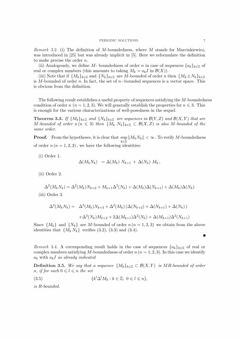
The following result establishes a useful property of sequences satisfying the M -boundednesscondition of order n (n = 1, 2, 3). We will generally establish the properties for n 6 3. Thisis enough for the various characterizations of well-posedness in the sequel.
Theorem 3.3. If Mkk∈Z and Nkk∈Z are sequences in B(Y,Z) and B(X, Y ) that areM -bounded of order n (n 6 3) then Mk Nkk∈Z ⊂ B(X, Z) is also M -bounded of thesame order.
Proof. From the hypotheses, it is clear that supk∈Z
‖MkNk‖ < ∞ . To verify M -boundedness
of order n (n = 1, 2, 3) , we have the following identities:
(i) Order 1.∆(MkNk) = ∆(Mk) Nk+1 + ∆(Nk) Mk ,
(ii) Order 2.
∆2(MkNk) = ∆2(Mk)Nk+2 + Mk+1∆2(Nk) + ∆(Mk)∆(Nk+1) + ∆(Mk)∆(Nk)
(iii) Order 3.
∆3(MkNk) = ∆3(Mk)Nk+3 + ∆2(Mk) (∆(Nk+2) + ∆(Nk+1) + ∆(Nk) )
+∆3(Nk)Mk+2 + 2∆(Mk+1)∆2(Nk) + ∆(Mk+1)∆2(Nk+1)
Since Mk and Nk are M -bounded of order n (n = 1, 2, 3) we obtain from the aboveidentities that Mk Nk verifies (3.2), (3.3) and (3.4).
Remark 3.4. A corresponding result holds in the case of sequences akk∈Z of real orcomplex numbers satisfying M -boundedness of order n (n = 1, 2, 3). In this case we identifyak with akI as already indicated
Definition 3.5. We say that a sequence Mkk∈Z ⊂ B(X, Y ) is MR-bounded of ordern, if for each 0 6 l 6 n the set
(3.5) kl∆lMk : k ∈ Z, 0 6 l 6 n,is R-bounded.
8 VALENTIN KEYANTUO, CARLOS LIZAMA, AND VERONICA POBLETE
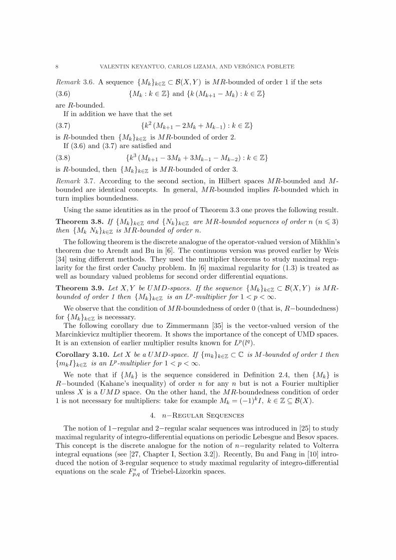
Remark 3.6. A sequence Mkk∈Z ⊂ B(X,Y ) is MR-bounded of order 1 if the sets
(3.6) Mk : k ∈ Z and k (Mk+1 −Mk) : k ∈ Zare R-bounded.
If in addition we have that the set
(3.7) k2 (Mk+1 − 2Mk + Mk−1) : k ∈ Zis R-bounded then Mkk∈Z is MR-bounded of order 2.
If (3.6) and (3.7) are satisfied and
(3.8) k3 (Mk+1 − 3Mk + 3Mk−1 −Mk−2) : k ∈ Zis R-bounded, then Mkk∈Z is MR-bounded of order 3.
Remark 3.7. According to the second section, in Hilbert spaces MR-bounded and M -bounded are identical concepts. In general, MR-bounded implies R-bounded which inturn implies boundedness.
Using the same identities as in the proof of Theorem 3.3 one proves the following result.
Theorem 3.8. If Mkk∈Z and Nkk∈Z are MR-bounded sequences of order n (n 6 3)then Mk Nkk∈Z is MR-bounded of order n.
The following theorem is the discrete analogue of the operator-valued version of Mikhlin’stheorem due to Arendt and Bu in [6]. The continuous version was proved earlier by Weis[34] using different methods. They used the multiplier theorems to study maximal regu-larity for the first order Cauchy problem. In [6] maximal regularity for (1.3) is treated aswell as boundary valued problems for second order differential equations.
Theorem 3.9. Let X, Y be UMD-spaces. If the sequence Mkk∈Z ⊂ B(X, Y ) is MR-bounded of order 1 then Mkk∈Z is an Lp-multiplier for 1 < p < ∞.
We observe that the condition of MR-boundedness of order 0 (that is, R−boundedness)for Mkk∈Z is necessary.
The following corollary due to Zimmermann [35] is the vector-valued version of theMarcinkievicz multiplier theorem. It shows the importance of the concept of UMD spaces.It is an extension of earlier multiplier results known for Lp(lq).
Corollary 3.10. Let X be a UMD-space. If mkk∈Z ⊂ C is M -bounded of order 1 thenmkIk∈Z is an Lp-multiplier for 1 < p < ∞.
We note that if Mk is the sequence considered in Definition 2.4, then Mk isR−bounded (Kahane’s inequality) of order n for any n but is not a Fourier multiplierunless X is a UMD space. On the other hand, the MR-boundedness condition of order1 is not necessary for multipliers: take for example Mk = (−1)kI, k ∈ Z ⊆ B(X).
4. n−Regular Sequences
The notion of 1−regular and 2−regular scalar sequences was introduced in [25] to studymaximal regularity of integro-differential equations on periodic Lebesgue and Besov spaces.This concept is the discrete analogue for the notion of n−regularity related to Volterraintegral equations (see [27, Chapter I, Section 3.2]). Recently, Bu and Fang in [10] intro-duced the notion of 3-regular sequence to study maximal regularity of integro-differentialequations on the scale F s
p,q of Triebel-Lizorkin spaces.
PERIODIC SOLUTIONS 9
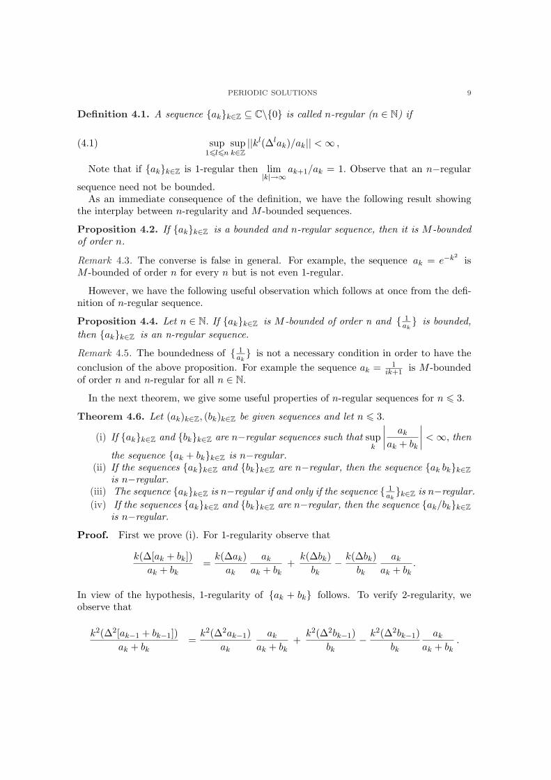
Definition 4.1. A sequence akk∈Z ⊆ C\0 is called n-regular (n ∈ N) if
(4.1) sup16l6n
supk∈Z
||kl(∆lak)/ak|| < ∞ ,
Note that if akk∈Z is 1-regular then lim|k|→∞
ak+1/ak = 1. Observe that an n−regular
sequence need not be bounded.As an immediate consequence of the definition, we have the following result showing
the interplay between n-regularity and M -bounded sequences.
Proposition 4.2. If akk∈Z is a bounded and n-regular sequence, then it is M -boundedof order n.
Remark 4.3. The converse is false in general. For example, the sequence ak = e−k2is
M -bounded of order n for every n but is not even 1-regular.
However, we have the following useful observation which follows at once from the defi-nition of n-regular sequence.
Proposition 4.4. Let n ∈ N. If akk∈Z is M -bounded of order n and 1ak is bounded,
then akk∈Z is an n-regular sequence.
Remark 4.5. The boundedness of 1ak is not a necessary condition in order to have the
conclusion of the above proposition. For example the sequence ak = 1ik+1 is M -bounded
of order n and n-regular for all n ∈ N.
In the next theorem, we give some useful properties of n-regular sequences for n 6 3.
Theorem 4.6. Let (ak)k∈Z, (bk)k∈Z be given sequences and let n 6 3.
(i) If akk∈Z and bkk∈Z are n−regular sequences such that supk
∣∣∣∣ak
ak + bk
∣∣∣∣ < ∞, then
the sequence ak + bkk∈Z is n−regular.(ii) If the sequences akk∈Z and bkk∈Z are n−regular, then the sequence ak bkk∈Z
is n−regular.(iii) The sequence akk∈Z is n−regular if and only if the sequence 1
akk∈Z is n−regular.
(iv) If the sequences akk∈Z and bkk∈Z are n−regular, then the sequence ak/bkk∈Zis n−regular.
Proof. First we prove (i). For 1-regularity observe that
k(∆[ak + bk])ak + bk
=k(∆ak)
ak
ak
ak + bk+
k(∆bk)bk
− k(∆bk)bk
ak
ak + bk.
In view of the hypothesis, 1-regularity of ak + bk follows. To verify 2-regularity, weobserve that
k2(∆2[ak−1 + bk−1])ak + bk
=k2(∆2ak−1)
ak
ak
ak + bk+
k2(∆2bk−1)bk
− k2(∆2bk−1)bk
ak
ak + bk.
10 VALENTIN KEYANTUO, CARLOS LIZAMA, AND VERONICA POBLETE
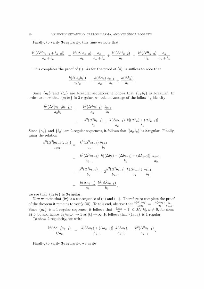
Finally, to verify 3-regularity, this time we note that
k3(∆3[ak−2 + bk−2])ak + bk
=k3(∆3ak−2)
ak
ak
ak + bk+
k3(∆3bk−2)bk
− k3(∆3bk−2)bk
ak
ak + bk.
This completes the proof of (i). As for the proof of (ii), is suffices to note that
k(∆[akbk])akbk
=k(∆ak)
ak
bk+1
bk+
k(∆bk)bk
.
Since ak and bk are 1-regular sequences, it follows that ak bk is 1-regular. Inorder to show that ak bk is 2-regular, we take advantage of the following identity
k2(∆2[ak−1bk−1])akbk
=k2(∆2ak−1)
ak
bk+1
bk
+k2(∆2bk−1)
bk+
k(∆ak−1)ak
k[(∆bk) + (∆bk−1)]bk
.
Since ak and bk are 2-regular sequences, it follows that ak bk is 2-regular. Finally,using the relation
k3(∆3[ak−2bk−2])akbk
=k3(∆3ak−2)
ak
bk+1
bk
+k2(∆2ak−2)
ak−1
k[ (∆bk) + (∆bk−1) + (∆bk−2)]bk
ak−1
ak
+k3(∆3bk−2)
bk+ 2
k2(∆2bk−2)bk−1
k(∆ak−1)ak
bk−1
bk
+k(∆ak−1)
ak
k2(∆2bk−1)bk
,
we see that ak bk is 3-regular.Now we note that (iv) is a consequence of (ii) and (iii). Therefore to complete the proof
of the theorem it remains to verify (iii). To this end, observe that k(∆1/ak)1/ak
= −k(∆ak)ak
akak+1
.
Since ak is a 1-regular sequence, it follows that |ak+1
ak− 1| 6 M/|k|, k 6= 0, for some
M > 0 , and hence ak/ak+1 → 1 as |k| → ∞. It follows that 1/ak is 1-regular.To show 2-regularity, we write
k2(∆2 1/ak−1)1/ak
=k[(∆ak) + (∆ak−1)]
ak−1
k(∆ak)ak+1
− k2(∆2ak−1)ak−1
.
Finally, to verify 3-regularity, we write
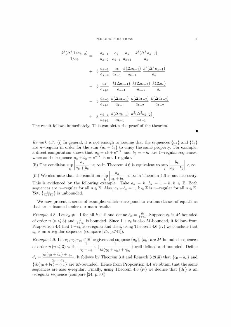
PERIODIC SOLUTIONS 11
k3(∆3 1/ak−2)1/ak
= −ak−1
ak−2
ak
ak−1
ak
ak+1
k3(∆3 ak−2)ak
+ 3ak−1
ak−2
ak
ak+1
k(∆ak−1)ak−1
k2(∆2 ak−1)ak
− 3ak
ak+1
k(∆ak−1)ak−1
k(∆ak−2)ak−2
k(∆ak)ak
− 3ak−2
ak+1
k(∆ak−1)ak−1
k(∆ak−2)ak−2
k(∆ak−2)ak−2
+ 3ak−1
ak+1
k(∆ak−1)ak−1
k2(∆2ak−2)ak−1
.
The result follows immediately. This completes the proof of the theorem.
Remark 4.7. (i) In general, it is not enough to assume that the sequences ak and bkare n−regular in order for the sum ak + bk to enjoy the same property. For example,a direct computation shows that ak = ik + e−ik and bk = −ik are 1−regular sequences,whereas the sequence ak + bk = e−ik is not 1-regular.
(ii) The condition supk
∣∣∣∣ak
ak + bk
∣∣∣∣ < ∞ in Theorem 4.6 is equivalent to supk
∣∣∣∣bk
ak + bk
∣∣∣∣ < ∞.
(iii) We also note that the condition supk
∣∣∣∣ak
ak + bk
∣∣∣∣ < ∞ in Theorem 4.6 is not necessary.
This is evidenced by the following example. Take ak = k, bk = 1 − k, k ∈ Z. Bothsequences are n−regular for all n ∈ N. Also, ak + bk = 1, k ∈ Z is n−regular for all n ∈ N.Yet, ak
ak+bk is unbounded.
We now present a series of examples which correspond to various classes of equationsthat are subsumed under our main results.
Example 4.8. Let ck 6= −1 for all k ∈ Z and define bk = ik1+ck
. Suppose ck is M -boundedof order n (n 6 3) and 1
1+ckis bounded. Since 1 + ck is also M -bounded, it follows from
Proposition 4.4 that 1+ ck is n-regular and then, using Theorem 4.6 (iv) we conclude thatbk is an n-regular sequence (compare [25, p.741]).
Example 4.9. Let c0, γ0, γ∞ ∈ R be given and suppose ak, bk are M -bounded sequences
of order n (n 6 3) with 1c0 − ak
, 1ik(γ0 + bk) + γ∞
well defined and bounded. Define
dk =ik(γ0 + bk) + γ∞
c0 − ak. It follows by Theorem 3.3 and Remark 3.2(iii) that c0 − ak and
ik(γ0 + bk) + γ∞ are M -bounded. Hence from Proposition 4.4 we obtain that the samesequences are also n-regular. Finally, using Theorem 4.6 (iv) we deduce that dk is ann-regular sequence (compare [24, p.30]).
12 VALENTIN KEYANTUO, CARLOS LIZAMA, AND VERONICA POBLETE
Example 4.10. Suppose ak is an M -bounded sequence of order n and such that 1ak
is bounded. Then we obtain from Proposition 4.4 and Theorem 4.6(iv) that dk = −ikak
isan n-regular sequence. This example is important in the scalar case, i.e. with A = I andX = Cn, as we will see later (cf. [22, Theorem 3.11, p.87]).
5. Well-posedness in Lp spaces
Having presented in the previous sections preliminary material on M -boundedness andFourier multipliers we will now show how these tools can be used to handle the integro-differential equation (1.1).
In this section we proceed to study Lp well posedness of the general integro-differentialequation (1.1). Here we do not assume that A is densely defined but merely that A isa closed operator. The results give concrete conditions on the measures ν, µ, η as well asthe operator A under which equation (1.1) is strongly well-posed. Special cases that havebeen studied before are incorporated into the new framework. In the next section we willstudy mild well-posedness in Lp spaces. Strong and mild well-posedness in other scales offunction spaces will be taken up in the subsequent sections.
The definition of strong well-posedness which we investigate in this section is as follows.
Definition 5.1. We say that the problem (1.1) is strongly Lp well-posed (1 6 p <∞) if for each f ∈ Lp((0, 2π);X) there exists a unique function u ∈ H1
p ((0, 2π);X) ∩Lp((0, 2π);D(A)) such that (1.1) is satisfied (for almost every t).
The function u in Definition 5.1 will be called the strong Lp solution of equation (1.1).
For a closed operator A in X with domain D(A) and 1 6 p < ∞, we define the operatorA on Lp((0, 2π);X) by D(A) = H1
p ((0, 2π);X) ∩ Lp((0, 2π);D(A)) and
Au = µ ∗ u′ + ν ∗ u− η ∗Au.
Here H1p ((0, 2π);X) is the vector valued Sobolev space, which is denoted H1 in case p = 2.
Remark 5.2. In terms of the operatorA defined above, Definition 5.1 is equivalent to sayingthat it is one-to-one and surjective. By the closed graph theorem, it follows that A has acontinuous inverse B that maps Lp((0, 2π);X) into H1
p ((0, 2π);X) ∩ Lp((0, 2π);D(A)).
We have the following.
Proposition 5.3. Let X be a UMD space and A a closed linear operator defined on X.Let akk∈Z, bkk∈Z be 1-regular sequences such that bk
ak is bounded and bkk∈Z ⊂ ρ(A).
Then the following assertions are equivalent(i) ak(bkI −A)−1k∈Z is an Lp-multiplier, 1 < p < ∞.(ii) ak(bkI −A)−1k∈Z is R-bounded.
Proof. Let Mk = ak(bkI −A)−1. By [6, Proposition 1.11], it follows that (i) implies (ii).Note that 1
ak is 1-regular by Theorem 4.6 (iii). Then the result is a consequence of the
following identity
k(Mk+1 −Mk) = Mk+1bk
ak+1k(bk − bk+1)
bkMk − k
1ak+1
− 1ak
1ak
Mk+1.
PERIODIC SOLUTIONS 13
When ak = bk we obtain the following special case of Proposition 5.3 which will be usedlater (see also [25, Proposition 2.8]). Note that condition (ii) is independent of p ∈ (1, ∞).
Corollary 5.4. Let X be a UMD space and A a closed linear operator defined on X. Letbkk∈Z be a 1-regular sequence such that bkk∈Z ⊂ ρ(A). Then the following assertionsare equivalent
(i) bk(bkI −A)−1k∈Z is an Lp-multiplier, 1 < p < ∞.(ii) bk(bkI −A)−1k∈Z is R-bounded.
In the remaining part of this section we will assume that η is a finite scalar-valuedmeasure on R which decomposes as
(5.1) η = aδ0 + ζ,
where a 6= 0 and ζ ∈ M(R,C). We now address strong well posedness of the integro-differential equation (1.1).
Theorem 5.5. Assume that X is a UMD-space and 1 < p < ∞. Suppose that the se-quences ik µ(k) + ν(k) and η(k) are 1-regular. Then the following assertions areequivalent:
(i) Problem (1.1) is strongly Lp well-posed;
(ii) ikµ(k)+ν(k)η(k) ⊆ ρ(A) and ik
η(k)(ikµ(k)+ν(k)
η(k) −A)−1 is an Lp-multiplier;
(iii) ikµ(k)+ν(k)η(k) ⊆ ρ(A) and ik
η(k)(ikµ(k)+ν(k)
η(k) −A)−1 is R-bounded.
Proof. Set Mk = ikη(k)
(ikµ(k)+ν(k)
η(k) −A)−1
.
(ii) ⇔ (iii). Let ak =ik
η(k)and bk =
ikµ(k) + ν(k)η(k)
. From the hypotheses and
Theorem 4.6 we have that ak and bk are 1−regular sequences. Since
bk
ak
=
µ(k) +
ν(k)ik
k∈Z\0it follows by the Riemann-Lebesgue lemma that
bk
ak
is bounded,
the assertion now follows from Proposition 5.3.(i) ⇔ (ii). Let Nk = 1
η(k)(ikµ(k)+ν(k)
η(k) − A)−1, k ∈ Z. Thus, Mk = ikNk, k ∈ Z. Thesolution u is constructed through
(5.2) u(k) = Nkf(k), k ∈ Z.
Indeed, as is well known [6, Lemma 2.2], the assumption that Mk is a Lp-multiplier impliesthat Nk is an Lp multiplier as well.
Except for the verification that the solution u constructed using multipliers belongs toLp((0, 2π);D(A)), the proof follows the same lines as that of [24, Theorem 2.9] (see also[25]). In fact, by Theorem 4.6(iii) we have that η(k) is 1-regular. It follows that 1
η(k)is 1-regular and since 1
η(k) = 1a+ζ(k)
is bounded by Riemann-Lebesgue lemma (cf. also(5.1)), we obtain by Proposition 4.2 that the latter sequence is M -bounded of order 1.Hence it is an Lp-multiplier.
14 VALENTIN KEYANTUO, CARLOS LIZAMA, AND VERONICA POBLETE
Letbk
ik=
1η(k)
[µ(k) +ν(k)ik
]. From hypothesis and Remark 4.7 we have that bk
ik
is 1−regular and bounded, hence it is M−bounded of order 1 and therefore is an Lp-multiplier.
From the identity
(5.3) ANk =bk
ikMk − 1
η(k)I
we conclude that ANk is an Lp-multiplier. The proof is complete.
From the proof of Theorem 5.5 we deduce the following result on maximal regularity.
Corollary 5.6. The solution u of problem (1.1) given by Theorem 5.5 satisfies the fol-lowing maximal regularity property: u, u′, Au ∈ Lp((0, 2π);X). Moreover, there exists aconstant C > 0 independent of f ∈ Lp((0, 2π);X) such that
(5.4) ||u||p + ||u′||p + ||Au||p 6 C||f ||p.The result says that under the assumptions of Theorem 5.5, u, u′ as well as all the terms
in the left hand side of (5.4) belong to Lp with continuous dependence on f. Similarlyµ ∗ u′, ν ∗ u, η ∗Au belong to Lp((0, 2π);X) and for some positive constant K we have
||ν ∗ u||p + ||µ ∗ u′||p + ||η ∗Au||p 6 K||f ||p.Example 5.7. Consider the equation
(5.5) u′(t) = Au(t) +∫ t
−∞c(t− s)Au(s)ds + f(t)
with the boundary condition u(0) = u(2π). This is a special case of equation (1.1) corre-sponding to µ = δ0, ν = 0, η = δ0 − c(t)χ[0,∞)(t) where we identify an L1 function withthe associated measure. By Example 4.8, it follows that if
(5.6) ck := c(k) is M-bounded of order 1,
then by Theorem 5.5, equation (5.5) has a unique strong Lp-solution for every f ∈Lp(0, 2π; X) if and only if the equivalent conditions (ii) and (iii) of Theorem 5.5 hold.Hence we recover the results established in [25] in the Lp case (note incidentally that inthat paper, we used c to denote the Laplace transform of c).
Example 5.8. Let γ, τ ∈ R and consider the delay equation
(5.7) u′(t) = Au(t)− γu(t− τ) + f(t), t ∈ R.
This problem is motivated by feedback-systems and control theory, see [7] and the refer-ences therein. In equation (5.7) the operator A corresponds to the system operator whichis generally assumed to be the generator of a C0-semigroup. The term γu(t − τ) can beinterpreted as the feedback. We note that usually the above equation is studied in thecontext of Hilbert spaces. Here we show that our theory applies and we obtain strong wellposedness.
Indeed, here we have µ(k) = 1, ν(k) = γe−ikτ and η(k) = 1. The hypotheses of theTheorem are easily seen to be satisfied if |γ| /∈ N. More precisely, when X is a UMD space,problem (5.7) is strongly Lp well posed (1 < p < ∞) if and only if ik+γe−ikτk∈Z ⊂ ρ(A)
PERIODIC SOLUTIONS 15
and ik(ik+γe−ikτ−A)−1k∈Z is R-bounded. When X is a Hilbert space, the last conditionis equivalent to boundedness of ik(ik + γe−ikτ − A)−1k∈Z. For example, if A generatesan analytic semigroup T = T (t) of type ω(T ) < −|γ| then is easy to check that thiscondition is satisfied.
6. Mild well-posedness in Lp
In this section we study mild solutions of the integro-differential equation (1.1). Thedefinition of mild solution we adopt here first appeared in Staffans [31] in the context ofmild L2 solutions on Hilbert spaces. For the special equation (1.3), another concept ofmild solution is studied in [6] and its relationship to the present approach is considered in[26]. Later in this section we will relate the notion of mild solution to the strong solutionsstudied in Section 5. This will be done in a natural way by constructing a one parameterfamily of concepts of mild solutions.
Definition 6.1. We say that problem (1.1) is (H1p , Lp) mildly well-posed if there exists a
linear operator B that maps Lp((0, 2π);X) continuously into itself as well as H1p ((0, 2π);X)∩
Lp((0, 2π);D(A)) into itself and which satisfies
ABu = BAu = u
for all u ∈ H1p ((0, 2π);X) ∩ Lp((0, 2π);D(A)). In this case the function Bf is called the
(H1p , Lp) mild solution of (1.1) and B the solution operator.
More specifically, we require that the following diagram be commutative:
where I is the natural injection of H1p ((0, 2π);X) ∩ Lp((0, 2π);D(A)) into Lp((0, 2π);X).
Clearly, the solution operator B above is unique, if it exists. Next, we characterize mildsolutions using operator valued Fourier multipliers.
Theorem 6.2. Assume that D(A) = X. Let 1 < p < ∞. Assume that η(k) 6= 0, for allk ∈ Z. Then the following assertions are equivalent:
(i) Problem (1.1) is (H1p , Lp) mildly well-posed ;
(ii) ikµ(k)+ν(k)η(k) k∈Z ⊆ ρ(A) and 1
η(k)(ikµ(k)+ν(k)
η(k) −A)−1 is an Lp-multiplier.
Proof. (ii) ⇒ (i). Consider dk := ikµ(k)+ν(k)η(k) , ck = 1
η(k) and let B be the operator whichmaps f ∈ Lp((0, 2π);X) into the function u ∈ Lp((0, 2π);X) whose kth Fourier coefficient
16 VALENTIN KEYANTUO, CARLOS LIZAMA, AND VERONICA POBLETE
is ckR(dk, A)f(k), i.e.
(6.1) (Bf)(k) = ckR(dk, A)f(k) = u(k),
for all k ∈ Z and all f ∈ Lp((0, 2π);X). By the remark following Definition 2.1, B is abounded linear operator on Lp((0, 2π);X). Let g ∈ H1
p ((0, 2π);X)∩Lp((0, 2π);D(A)) andset h = Bg. Then,
(6.2) ikh(k) = ckR(dk, A)ikg(k) = ckR(dk, A)g′(k),
for all k ∈ Z. Since g′ ∈ Lp((0, 2π);X), by (i) there exists w ∈ Lp((0, 2π);X) such that
(6.3) w(k) = ckR(dk, A)g′(k)
for all k ∈ Z. Hence from (6.2), (6.3) and [6, Lemma 2.1] we obtain h ∈ H1p ((0, 2π);X).
Note that h(k) ∈ D(A), k ∈ Z since h(k) = ckR(dk, A)g(k) and then ABg(k) = BAg(k).Since by assumption Ag ∈ Lp((0, 2π);X), the closedness of A implies thatABf ∈ Lp((0, 2π);X), that is Bf ∈ Lp((0, 2π);D(A)).
We have proved that B that maps H1p ((0, 2π);X) ∩ Lp((0, 2π);D(A)) into itself. Con-
tinuity of B follows from the Closed Graph Theorem since the space H1p ((0, 2π);X) ∩
Lp((0, 2π);D(A)) embeds continuously into Lp((0, 2π);X).Finally, for u ∈ H1
p ((0, 2π);X) ∩ Lp((0, 2π);D(A)) we have
(6.4) (Au)(k) =1ck
(dkI −A)u(k),
for all k ∈ Z. Hence from (6.1) and [6, Lemma 3.1] we obtain ABu = BAu = u.
(i) ⇒ (ii). Let x ∈ X and xn ∈ D(A) such that xn → x. Fix k ∈ Z and let fn(t) = eiktxn
for all n ∈ N and f0(t) = eiktx. Note that fn(k) = xn and fn(j) = 0 for j 6= k. Clearlyfn → f0 in the Lp-norm as n →∞. Let un = Bfn. Then we have
ikµ(k)un(k) + ν(k)un(k)− η(k)Aun(k) = (Aun)(k) = (ABfn)(k) = fn(k) = xn.
Since B is bounded on Lp((0, 2π);X), un → u0 := Bf0 in the Lp-norm, we conclude thatun(k) → u0(k), and
(ikµ(k) + ν(k)− η(k)A)u0(k) = x.
Hence, for all k ∈ Z, (ikµ(k) + ν(k)− η(k)A) is surjective.Let x ∈ D(A) be such that (ikµ(k) + ν(k) − η(k)A)x = 0, for k ∈ Z fixed. Define
u(t) = eiktx. Then, clearly, u ∈ W 1,p((0, 2π);X) ∩ Lp((0, 2π);D(A)) and Au = 0. Hence
u = BAu = 0,
and therefore x = 0. Since A is closed, we have proved that dkk∈Z ⊂ ρ(A).To verify that (ckR(dk, A))k∈Z is an Lp-multiplier, let f ∈ Lp((0, 2π);X). We observe
that since D(A) = X and 1 6 p < ∞, the space H1p ((0, 2π);X)∩Lp((0, 2π);D(A)) is dense
in Lp((0, 2π);X). Hence there exists a sequence fn ∈ H1p ((0, 2π);X) ∩ Lp((0, 2π);D(A))
such that fn → f in the Lp-norm. Define
gn = Bfn, n ∈ N.
Then gn ∈ H1p ((0, 2π);X) ∩ Lp((0, 2π);D(A)) and
Agn = ABfn = fn, n ∈ N.
PERIODIC SOLUTIONS 17
Taking Fourier coefficients and using the fact that dkk∈Z ⊂ ρ(A), we obtain from theabove that
(6.5) gn(k) = ck(dkI −A)−1fn(k)
for all k ∈ Z. Next, we note that gnn∈N is a Cauchy sequence in Lp((0, 2π);X). Bycontinuity of B, there exists g ∈ Lp((0, 2π);X) such that gn → g in the Lp-norm. Fromthis and using Holder’s inequality we deduce that gn(k) → g(k) and, analogously, fn(k) →f(k). Therefore we conclude from (6.5) that g(k) = ck(dkI −A)−1f(k), for all k ∈ Z. Theclaim is proved.
As a direct consequence of Proposition 5.3 and Theorem 4.6, we obtain the followingresult. It is remarkable that in some cases we can characterize mild well posedness interms of R-boundedness of resolvents. This phenomenon seems to be new.
Theorem 6.3. Let 1 < p < ∞. Let X be a UMD space and assume that D(A) = X.Suppose that
(6.6) η(k) is 1-regular and ikµ(k) + ν(k) is 1-regular and bounded.
Then the following assertions are equivalent:(i) Problem (1.1) is (H1
p , Lp) mildly well-posed ;(ii) ikµ(k)+ν(k)
η(k) ⊆ ρ(A) and 1η(k)(
ikµ(k)+ν(k)η(k) −A)−1 is an Lp-multiplier;
(iii) ikµ(k)+ν(k)η(k) ⊆ ρ(A) and 1
η(k)(ikµ(k)+ν(k)
η(k) −A)−1 is R-bounded.
Remark 6.4. Condition 6.6 might seem strong. If we consider ϑ an arbitrary boundedmeasure and set µ = 1
2i(ϑπ − ϑ−π), where ϑa denotes the a-translate of ϑ, then we haveµ(k) = 0 for all k ∈ Z. Another case is when µ has a density f with respect to the Lebesguemeasure and f ∈ W 1,1(R) = g ∈ L1(R), g′ ∈ L1(R) in the distributional sense .Remark 6.5. Observe that when µ = δ0, ν = 0, η = δ0, condition (6.6) is not satisfied. Inthis case, which corresponds to the equation of the first order
(6.7) u′(t) = Au(t) + f(t),
there is no regularization on the first derivative in equation (1.1). This case correspondsto mild solutions for (6.7) and was investigated in [6]. There, it was observed that theycannot be characterized in terms of R-boundedness of the set (ikI −A)−1k∈Z solely.
Example 6.6. (Renewal equation) We take ν = δ0, µ = 0 and η is chosen such that η(k)is 1-regular. Then, an application of Theorem 4.6 (iii) shows that the assumptions inTheorem 6.3 are satisfied and we obtain that the integral equation
u = η ∗Au + f
is (H1p , Lp) mildly well-posed if and only if the equivalent conditions (ii), (iii) in Theorem
6.3 are verified. Note that maximal regularity to the above equation was characterized forperiodic Lp spaces in the scalar case (cf. [22, Theorem 4.7 p.48]). Our result extends suchcharacterization to the infinite dimensional setting.
18 VALENTIN KEYANTUO, CARLOS LIZAMA, AND VERONICA POBLETE
We now introduce a one parameter family of concepts of well-posedness for equation(1.1). Related notions appear in [31]. In [6], the spaces Hα
p ((0, 2π); X) used below arealso considered but just to obtain continuity and even Holder continuity of mild solutionsfrom a different definition.
For 1 < p < ∞ and 0 6 α, We define the space Hαp ((0, 2π);X) as:
Hαp ((0, 2π);X) = f ∈ Lp((0, 2π);X), ∃g ∈ Lp((0, 2π);X) such that g(k) = |k|αf(k), k ∈ Z.We note due to the UMD property (more precisely the continuity of the Hilbert trans-
form on Lp((0, 2π);X), we have
(6.8) Wm,p((0, 2π);X) = Hmp ((0, 2π); X), for 1 < p < ∞ and m ∈ N ∪ 0
(see for example [32, Chapter III], [1] and for the relationship with intermediate spaces, see[13, Chapter IV, especially Section 4.4, p.272]). Now we give the definition of (H1
p ,H1−αp )
well-posedness.
Definition 6.7. Let 0 6 α 6 1. We say that the problem (1.1) is (H1p ,H1−α
p ) mildlywell-posed if there exists a linear operator B that maps Lp((0, 2π);X) continuously intoitself with range in H1−α
p ((0, 2π); X), as well as H1p ((0, 2π);X) ∩ Lp((0, 2π);D(A)) into
itself and which satisfies
ABu = BAu = u
for all u ∈ H1p ((0, 2π);X) ∩ Lp((0, 2π);D(A)).
This means that in the diagram following Definition 6.1, we replace Lp((0, 2π);X) inthe upper right corner with H1−α
p ((0, 2π);X). Thanks to the Closed Graph Theorem, thismeans that B is continuous from Lp((0, 2π);X) into H1−α
p ((0, 2π);X).We have the following result.
Theorem 6.8. Assume that D(A) = X. Let 1 < p < ∞ and 0 6 α 6 1. Assume thatη(k) 6= 0, for all k ∈ Z. Then the following assertions are equivalent:
(i) Problem (1.1) is (H1p ,H1−α
p ) mildly well-posed ;
(ii) ikµ(k)+ν(k)η(k) k∈Z ⊆ ρ(A) and (ik)1−α
η(k) ( ikµ(k)+ν(k)η(k) −A)−1 is an Lp-multiplier.
Proof. The proof is a modification of the proof of Theorem 6.2 and we omit it.
Remark 6.9. When α = 1, Theorem 6.8 corresponds to Theorem 6.2 and when α = 0 theconcept of solution that appears in the new context differs from that of strong solutioncovered by Theorem 5.5. The main difference is that in the new context we do not requirethat the solution operator B map into Lp((0, 2π), D(A)). However, in some cases, therequirement that the range of B be in H1
p automatically implies that B also maps intoLp((0, 2π), D(A)). Such is the case for the assumptions of Theorem 6.2. A specific exampleis equation (6.7) for which the analysis was done in [26]. There, we also justified why it isreasonable to assume that 0 6 α 6 1.
The next theorem characterizes (H1p ,H1−α
p ) mild well-posedness.
PERIODIC SOLUTIONS 19
Theorem 6.10. Let 1 < p < ∞, 0 6 α 6 1 and X a UMD space. Assume that D(A) = Xand η(k) 6= 0, for all k ∈ Z and
(6.9) η(k) is 1-regular and (ik)αµ(k) +ν(k)
(ik)1−αis 1-regular and bounded.
Then the following assertions are equivalent:(i) Problem (1.1) is (H1
p ,H1−αp ) mildly well-posed ;
(ii) ikµ(k)+ν(k)η(k) k∈Z ⊆ ρ(A) and (ik)1−α
η(k) ( ikµ(k)+ν(k)η(k) −A)−1 is an Lp-multiplier;
(iii) ikµ(k)+ν(k)η(k) k∈Z ⊆ ρ(A) and (ik)1−α
η(k) ( ikµ(k)+ν(k)η(k) −A)−1 is R-bounded.
Proof. Thanks to (6.9) we can use Proposition 5.3 to prove the equivalence between (ii)and (iii). The equivalence between (i) and (ii) follows from Theorem 6.8.
Example 6.11. Consider the equation
(6.10) u′(t) =∫ ∞
−∞Au(t− s)η(ds) + f(t).
This case corresponds to equation (1.1) with µ = δ0, ν = 0 and η a bounded measure. Itfollows from Theorem 6.10 with α = 0 that if
(6.11) ak := η(k) is 1-regular,
then equation (6.10) is (H1p ,H1
p ) mildly well-posed if and only if the equivalent conditions(ii) and (iii) hold. Hence we extend the results established in [22, Theorem 3.11, p.87] tothe vector-valued Lp case.
Example 6.12. Let a > 0 and γ > −1. We take in (1.1) µ(dt) =1
Γ(γ + 1)tγe−atdt (t > 0)
and µ(t) = 0 for t < 0; ν = 0 and η a bounded measure. In this case equation (1.1),which reads µ ∗ u′ = η ∗ Au + f , is (H1
p , Lp) mildly well-posed if γ > α − 1, γ > −1and one of the equivalent conditions (ii) or (iii) is satisfied. We note that in this case
µ(k) =1
(ik + a)γ+1.
In case α = 0 we have
Proposition 6.13. Assume that either A is bounded or 1η(k) is an Lp-multiplier. Then,
problem (1.1) is (H1p ,H1
p ) mildly well-posed if and only if problem (1.1) is strongly Lp
well-posed.
Proof. Suppose problem (1.1) is (H1p ,H1
p ) mildly well-posed. In case A is bounded,we note that D(A) = H1
p ((0, 2π);X) and the assertion follows. On the other hand, letNk and Mk be as in the proof of Theorem 5.5. By Theorem 6.8 we have that Mk isan Lp-multiplier. When 1
η(k) is an Lp-multiplier, the identity (5.3) and the fact thatdk
ik=
1η(k)
[µ(k) +ν(k)ik
] show that ANk is an Lp-multiplier as well(see Example 2.3).
Then the solution u, defined by (5.2), satisfies Au ∈ Lp((0, 2π), X) and hence the rangeof B is contained in H1
p ((0, 2π);X) ∩ Lp((0, 2π);D(A)), proving the proposition.
20 VALENTIN KEYANTUO, CARLOS LIZAMA, AND VERONICA POBLETE
We point out that several concrete criteria for R−boundedness have been established(see e.g. [18], [21] and [6]).
7. Well posedness on Besov spaces
In this section we consider solutions in Besov spaces. For the definition and mainproperties of these spaces we refer to [5] or [24]. For the scalar case, see [13], [29]. Contraryto the Lp case the multiplier theorems established so far are valid for arbitrary Banachspaces; see [2], [5] and [20]. Special cases here allow one to treat Holder-Zygmund spaces.Specifically, we have Bs∞,∞ = Cs for s > 0. Moreover, if 0 < s < 1 then Bs∞,∞ is just theusual Holder space Cs. We begin with the definition of operator valued Fourier multipliersin the context of Besov spaces.
Definition 7.1. Let 1 6 p 6 ∞. A sequence Mkk∈Z ⊂ B(X) is a Bsp,q-multiplier if for
each f ∈ Bsp,q((0, 2π);X) there exists a function g ∈ Bs
p,q((0, 2π);X) such that
Mkf(k) = g(k), k ∈ Z.
The following general multiplier theorem for periodic vector-valued Besov spaces is dueto Arendt and Bu [5, Theorem 4.5].The continuous case (multipliers on the real line) wasstudied by Amann [2] and later by Girardi and Weis [20].
Theorem 7.2. (i) Let X be a Banach space and suppose that Mkk∈Z ⊂ B(X) isM -bounded of order 2. Then for 1 6 p, q 6 ∞ , s ∈ R , Mkk∈Z is a Bs
pq−multiplier.(ii) Let X be a Banach space with nontrivial Fourier type. Then any sequence Mkk∈Z ⊂
B(X) which is M -bounded of order 1 is a Bspq−multiplier for all 1 6 p, q 6 ∞ , s ∈ R.
The analogue of Proposition 5.3 in the present context is:
Proposition 7.3. Let A be a closed linear operator defined on the Banach space X. Letakk∈Z, bkk∈Z be 2-regular sequences such that bk
ak is bounded and bkk∈Z ⊂ ρ(A).
Then the following assertions are equivalent(i) ak(bkI −A)−1k∈Z is a Bs
p,q-multiplier, 1 6 p 6 ∞, 1 6 q 6 ∞, s ∈ R,
(ii) ak(bkI −A)−1k∈Z is bounded.
Proof. Let Mk = ak(bkI − A)−1. By [6, Proposition 1.11], it follows that (i) implies(ii). We turn to (ii) implies (i). The part corresponding to 1-regularity is contained inProposition 5.3. To complete the verification of 2-regularity we use the following identity
k2 (Mk+1 − 2Mk + Mk−1) = k2 (ak+1 − 2ak + ak−1)1
ak+1Mk+1
− 2 k[ak − ak−1
ak] k
1ak−1
(bk+1 − bk) Mk Mk−1
− k2 1ak
(bk+1 − 2bk + bk−1) Mk Mk−1
PERIODIC SOLUTIONS 21
+2 k1
ak+1(bk+1 − bk) k
1ak−1
(bk+1 − bk−1) Mk+1 Mk Mk−1
− k1ak
(bk+1 − bk) k1
ak+1(bk+1 − bk−1) Mk+1 Mk Mk−1.
We remark that the case ak = bk was proved in [25, Proposition 3.4].Next, we consider strong well-posedness for equation (1.1).
Definition 7.4. We say that problem (1.1) is strongly Bsp,q well-posed if for each f ∈
Bsp,q((0, 2π);X) there exists a unique function u ∈ Bs+1
p,q ((0, 2π);X) ∩ Bsp,q((0, 2π);D(A))
and (1.1) is satisfied almost everywhere.
As above, we call u the strong solution of (1.1). As in section 5, in what follows we willassume that η is a finite scalar-valued measure on R which decomposes as η = aδ0+ζ, wherea 6= 0 and ζ ∈ M(R,C). Strong well posedness of (1.1) in the Bs
p,q spaces is established inthe following theorem.
Theorem 7.5. Let 1 6 p, q 6 ∞ , s ∈ R. Suppose that the sequences ik µ(k) + ν(k)and η(k) are 2-regular. Then the following assertions are equivalent:
(i) Problem (1.1) is strongly Bsp,q well-posed;
(ii) ikµ(k)+ν(k)η(k) ⊆ ρ(A) and k
η(k)(ikµ(k)+ν(k)
η(k) −A)−1 is a Bsp,q-multiplier;
(iii) ikµ(k)+ν(k)η(k) ⊆ ρ(A) and k
η(k)(ikµ(k)+ν(k)
η(k) −A)−1 is bounded.
Proof. The proof follows the same lines as the proof of Theorem 5.5 using Proposition 7.3with ak = bk instead of Corollary 5.4 and making use of the properties on M -boundednessof order 2 and 2- regularity for sequences established in Section 4 and Section 5.
Example 7.6. In reference to Example 4.9 we consider the following integro-differentialequation with infinite delay studied in [24]
(7.1)
γ0u′(t) +
d
dt(∫ t
−∞b(t− s)u(s)ds) + γ∞u(t)
= c0Au(t)−∫ t
−∞a(t− s)Au(s)ds + f(t), 0 6 t ∈ R,
where γ0, γ∞, c0 are constants and a(·), b(·) ∈ L1(R+). In [24], strong well-posedness onperiodic Besov spaces for equation (7.1) was characterized as in Theorem 7.5 (see [24,Theorem 3.12]) under a set of conditions which we reformulate as
(IDE1) 1c0 − ak
k∈Z is a bounded sequence.
(IDE2) ak and bk are M -bounded of order 2
(IDE3) kak and kbk are bounded sequences.
One easily checks that Theorem 7.5 applies under (IDE1) and (IDE2) and that (IDE3)is not needed.
22 VALENTIN KEYANTUO, CARLOS LIZAMA, AND VERONICA POBLETE
We observe here that the removal of condition (IDE3) is due to Proposition 7.3. Asa consequence the hypotheses are formulated entirely in terms of M−boundedness andn-regularity.
The particular case of equation (7.1) with γ∞ = 0 and c0 = γ∞ = 1 and b ≡ 0 wasconsidered in [25, Theorem 3.9]. From the above, we conclude that there, we only needthe condition
(7.2) ak is M-bounded of order 2
in order to have the characterization of strong well-posedness. It shows that the set ofconditions imposed in Theorem 7.5 are in some sense more natural, giving an improvementof the above mentioned papers.
In analogy to mild solutions in the Lp case we proceed to define mild Bsp,q solutions.
Definition 7.7. Let 1 6 p, q 6 ∞ and s > 0. We say that the problem (1.1) is (Bs+1p,q , Bs
p,q)mildly well-posed if there exists a linear operator B that maps Bs
p,q((0, 2π);X) continuouslyinto itself as well as Bs+1
p,q ((0, 2π);X) ∩Bsp,q((0, 2π);D(A)) into itself and which satisfies
ABu = BAu = u
for all u ∈ Bs+1p,q ((0, 2π);X) ∩ Bs
p,q((0, 2π);D(A)). In this case the function Bf is calledthe (Bs+1
p,q , Bsp,q) mild solution of (1.1) and B the associated solution operator.
The following result follows directly from Proposition 7.3 and Theorem 4.6.
Theorem 7.8. Let 1 6 p, q 6 ∞, s > 0 and X a Banach space. Assume that D(A) = Xand
(7.3) η(k) is 2-regular and ikµ(k) + ν(k) is 2-regular and bounded.
Then the following assertions are equivalent:(i) Problem (1.1) is (Bs+1
p,q , Bsp,q) mildly well-posed ;
(ii) ikµ(k)+ν(k)η(k) k∈Z ⊆ ρ(A) and 1
η(k)(ikµ(k)+ν(k)
η(k) −A)−1 is a Bsp,q-multiplier;
(iii) ikµ(k)+ν(k)η(k) k∈Z ⊆ ρ(A) and 1
η(k)(ikµ(k)+ν(k)
η(k) −A)−1 is bounded.
Remark 7.9. When the space X has non trivial Fourier type, then the assumptions ofM -boundedness of order 2 and 2-regularity in Theorems 7.5 and 7.8 can be replaced byM -boundedness of order 1 and 1-regularity respectively.
8. Well posedness on Triebel-Lizorkin spaces
In this section we study strong and mild well-posedness of problem (1.1) on the scale ofTriebel-Lizorkin spaces of vector-valued functions. The important feature in this case, asin the context of Besov spaces, is that the results do not use R−boundedness but merelyboundedness conditions on resolvents. In concrete applications, one can therefore handleoperators on familiar spaces like C(Ω), the Schauder spaces Cs(Ω), 0 < s < 1 and L1(Ω)where Ω is a bounded open subset of Rn. These spaces are not UMD, and are not evenreflexive. The price to pay is that when p = 1 or q = 1 then one needs a Marcinkiewiczestimate of order 3 whereas, for the Besov scale, order 2 is enough.
We briefly recall the definition of periodic Triebel-Lizorkin spaces in the vector valuedcase used in (see [11]). For the scalar case, these spaces have been studied for a long time,
PERIODIC SOLUTIONS 23
see Triebel[33, Chapter II, Section 9], Schmeisser-Triebel [29] and references therein. Avector-valued Fourier multiplier in the Triebel-Lizorkin scale appears in [32, Chapter 3,Section 15.6].
Let S be the Schwartz space on R and let S ′ be the space of all tempered distributionson R. Let Φ(R) be the set of all systems φ = φjj>0 ⊂ S satisfying
supp(φ0) ⊂ [−2, 2]
supp(φj) ⊂ [−2j+1,−2j−1] ∪ [2j−1, 2j+1], j > 1∑
j>0
φj(t) = 1, t ∈ R
and for α ∈ N ∪ 0, there exists Cα > 0 such that
(8.1) supj>0,x∈R
2αj ||φ(α)j (x)|| 6 Cα.
Recall that such a system can be obtained by choosing φ ∈ S(R) with
supp(φ0) ⊂ [−2, 2]
and φ0(x) = 1 if ‖x‖ 6 1, then setting φ1(x) = φ0(x/2)−φ0(x) and φj(x) = φ1(2j−x), j >2.
Let 1 6 p < ∞, 1 6 q 6 ∞, s ∈ R and φ = (φj)j>0 ∈ Φ(R). The X−valued periodicTriebel-Lizorkin spaces are defined by
F s,φp,q = f ∈ D′(T; X) : ||f ||
F s,φp,q
= ‖(∑
j>0
2sjq||∑
k∈Zek ⊗ φj(k)f(k)||q)1/q‖p < ∞.
The usual modification is adopted when q = ∞.
Here (ek⊗x)(t) := eitx, t ∈ [0, 2π]. The space F s,φp,q is independent of φ ∈ Φ(R) and the
norms || · ||F s,φ
p,qare equivalent. We will simply denote || · ||
F s,φp,q
by || · ||F sp,q
.
We remark that when X is a Banach space, the scale of Triebel-Lizorkin spaces does notin general contain the Lp scale. In fact, the Littlewood-Paley assertions F 0
p,2((0, 2π);X) =Lp((0, 2π);X), 1 < p < ∞ hold if and only if X can be renormed as a Hilbert space.This follows from [28]. In the scalar case, the well-known assertions may be found in [32,Chapter 3, Section 10]. For the non validity of the Littlewood-Paley assertions in thevector-valued case, see also the introduction to [11].
Note that F sp,p((0, 2π);X) = Bs
p,p((0, 2π);X). This relation is true when X is the scalarfield C (see [29, Remark 4, p.164]). Using the definitions of the spaces one easily sees thatthe relation remains true in the vector-valued case.
Definition 8.1. Let 1 6 p < ∞. A sequence Mkk∈Z ⊂ B(X) is an F sp,q-multiplier if, for
each f ∈ F sp,q((0, 2π);X) there exists a function g ∈ F s
p,q((0, 2π);X) such that
Mkf(k) = g(k), k ∈ Z.
The following multiplier theorem for periodic vector-valued Triebel-Lizorkin spaces isdue to Bu and Kim [11, Theorem 3.2 and Remark 3.4].
Theorem 8.2. Let X be a Banach space and suppose Mkk∈Z ⊂ B(X). Then thefollowing assertions hold.
24 VALENTIN KEYANTUO, CARLOS LIZAMA, AND VERONICA POBLETE
(1) Assume that Mkk∈Z is M -bounded of order 3. Then for 1 6 p < ∞, 1 6 q 6∞, s ∈ R , Mkk∈Z is an F s
p,q−multiplier.
(2) Assume that Mkk∈Z is M -bounded of order 2. Then for 1 < p < ∞, 1 < q 6∞, s ∈ R , Mkk∈Z is an F s
p,q−multiplier.
Remark 8.3. When p = q the assertion (2) of Theorem 8.2 holds true for Mkk∈Z M -bounded of order 2. Moreover if X has nontrivial Fourier type, M -boundedness of order 1suffices. This follows from the relation F s
p,p((0, 2π);X) = Bsp,p((0, 2π);X) and [5, Theorems
4.2 and 4.5] (see also [20]).
The following result was proved in [10, Theorem 2.2].
Proposition 8.4. Let X be a Banach space and A a closed linear operator defined onX. Let bkk∈Z be a 3-regular sequence such that bkk∈Z ⊂ ρ(A). Then the followingassertions are equivalent
(i) bk(bkI −A)−1k∈Z is an F sp,q-multiplier, 1 6 p 6 ∞, 1 6 q < ∞, s ∈ R,
(ii) bk(bkI −A)−1k∈Z is bounded.
In case p = q the same observations as in Remark 8.3 allow us to simplify the hypothesesof Proposition 8.4.
We have the following extension of this result (in analogy to Proposition 5.3 and Propo-sition 7.3).
Proposition 8.5. Let X be a Banach space and A a closed linear operator defined onX. Let akk∈Z, bkk∈Z be 3-regular sequences such that bkk∈Z ⊂ ρ(A). Suppose thatbk/ak is bounded. Then the following assertions are equivalent
(i) ak(bkI −A)−1k∈Z is an F sp,q-multiplier, 1 6 p 6 ∞, 1 6 q < ∞, s ∈ R,
(ii) ak(bkI −A)−1k∈Z is bounded.
Proof. Let Mk = ak(bk − A)−1 and Nk = bk(bk − A)−1. Note that Nk =bk
akMk. Since
by hypothesis Mk and bk/ak are bounded, we obtain that Nkk∈Z is bounded.From the proofs of Proposition 5.3 and Proposition 7.3 we obtain that
supk∈Z
||Mk|| < ∞, supk∈Z
||k∆(Mk)|| < ∞ and supk∈Z
||k2∆2(Mk)|| < ∞.
Hence in order to prove that Mk is M−bounded of order 3, we need only checkthat sup
k∈Z||k3∆3(Mk)|| < ∞. In fact, from the proof of Theorem 3.3 part (iii) (writing
Nk = bkak
Mk, k ∈ Z), we have that
∆3(Mk) = ∆3
(ak
bkNk
)= ∆3
(ak
bk
)Nk+3 + ∆2
(ak
bk
)[∆(Nk+2) + ∆(Nk+1) + ∆(Nk)]
+ ∆3(Nk)ak+2
bk+2+ 2∆
(ak+1
bk+1
)∆2(Nk) + ∆
(ak+1
bk+1
)∆2(Nk+1).
PERIODIC SOLUTIONS 25
where, each term in the right hand side of the above identity can be handled separatelyas follows.
∆3
(ak
bk
)Nk+3 =
∆3(ak/bk)ak+2/bk+2
bk+3
bk+2
ak+2
ak+3Mk+3 ,
∆2
(ak
bk
)∆(Nk+2) =
∆2(ak/bk)ak+1/bk+1
[∆(bk+2)
bk+1
ak+1
ak+3Mk+3 − bk+3
bk+1
ak+1
ak+3
bk+2
ak+2Mk+3
∆(bk+2)bk+3
Mk+2
],
∆2
(ak
bk
)∆(Nk+1) =
∆2(ak/bk)ak+1/bk+1
[∆(bk+1)
bk+1
ak+1
ak+2Mk+2 − bk+2
ak+2Mk+2
∆(bk+1)bk+2
Mk+1
],
∆2
(ak
bk
)∆(Nk) =
∆2(ak/bk)ak+1/bk+1
[∆(bk)bk+1
Mk+1 − bk
akMk+1
∆(bk)bk+1
Mk
],
∆3(Nk)ak+2
bk+2= −∆3(bk)
bk+2Mk+2 (Nk+1 − I)
+∆2(bk+1)
bk+2
∆(bk+2) + ∆(bk+1) + ∆(bk)bk+3
Mk+2Nk+3(Nk+1 − I)
+∆2(bk)bk+2
∆(bk+2) + ∆(bk+1) + ∆(bk)bk+3
Mk+2Nk+3(Nk − I)
−2∆(bk)bk+1
∆(bk+1)bk+2
∆(bk+2) + ∆(bk+1) + ∆(bk)bk+3
Nk+1Mk+2Nk+3(Nk − I),
∆(
ak+1
bk+1
)∆2(Nk) =
∆(ak+1/bk+1)ak+1/bk+1
∆(bk)bk
∆(bk+1) + ∆(bk)bk+1
Mk+1Nk(Nk+2 − I)
−∆(ak+1/bk+1)ak+1/bk+1
∆2(bk)bk+1
Mk+1(Nk+2 − I).
∆(
ak+1
bk+1
)∆2(Nk+1) =
∆(ak+1/bk+1)ak+1/bk+1
∆(bk+1)bk+1
∆(bk+2) + ∆(bk+1)bk+2
Nk+2Mk+1(Nk+3 − I)
−∆(ak+1/bk+1)ak+1/bk+1
bk+2
bk+1
ak+1
ak+2
∆2(bk+1)bk+2
Mk+2(Nk+3 − I).
Then a moment of reflection shows that the assertion follows from the hypothesis andTheorem 4.6 (see also the observation after Definition 4.1).
Definition 8.6. We say that the problem (1.1) is strongly F sp,q well-posed if for each
f ∈ F sp,q((0, 2π);X) there exists u ∈ F s+1
p,q ((0, 2π);X) ∩ F sp,q((0, 2π);D(A)) such that (1.1)
is satisfied.
26 VALENTIN KEYANTUO, CARLOS LIZAMA, AND VERONICA POBLETE
We now discuss the conditions on the parameters appearing in equation (1.1) whichensure that the above theorem applies. As in section 5, we assume that η is a finite scalar-valued measure on R which decomposes as η = aδ0 + ζ, where a 6= 0 and ζ ∈ M(R,C).
Theorem 8.7. Let Then for 1 6 p < ∞, 1 6 q 6 ∞, s ∈ R. Suppose that the sequencesik µ(k) + ν(k) and η(k) are 3-regular. Then the following assertions are equivalent:
(i) Problem (1.1) is strongly F sp,q well-posed;
(ii) ikµ(k)+ν(k)η(k) ⊆ ρ(A) and ik
η(k)(ikµ(k)+ν(k)
η(k) −A)−1 is an F sp,q-multiplier;
(iii) ikµ(k)+ν(k)η(k) ⊆ ρ(A) and ik
η(k)(ikµ(k)+ν(k)
η(k) −A)−1 is bounded.
Proof. (ii) ⇔ (iii). The assertion follows from hypothesis, Remark 4.7 and Proposition8.5. The equivalence (ii) ⇔ (iii) is shown in the same way as the analogous parts ofTheorem 7.5 and Theorem 5.5
We note that when p > 1, the requirement can be relaxed to 2−regularity for thesequences ik µ(k) + ν(k) and η(k).
Finally, we observe that one can study mild solutions in this context as well.
9. Application to nonlinear equations
In this section, we apply the above results to nonlinear equations in Banach and Hilbertspaces. We consider three situations where equations can be solved by the method ofmaximal regularity. One corresponds to Theorem 9.1 leading in which one deals with asemi-linear problem. Such problem were previously considered in [24] in Holder spaces.We cover here the complete scale of Lebesgue, Besov and Triebel-Lizorkin spaces. Thesecond application uses a method based on [15, Theorem 4.1] to solve a nonlinear integro-differential equation. The third application is concerned with semi-linear equations inHilbert spaces (Theorem 9.6) corresponds to an extension of Staffans [31]. One of the mainassumptions made in Theorem 9.6 below is that A has compact resolvent. Typically, thisoccurs in problems involving elliptic operators on bounded domains in Rn with appropriateboundary conditions. Such equations arise in heat conduction of materials with memory.
As already indicated, linear results on maximal regularity are very useful in dealingwith non linear problems. For example the following problem was considered in [24], [30].
(9.1)
d
dt(γ0u(t, x) +
∫ t
−∞b(t− s)u(s, x)ds) + γ∞u(t, x) =
c0∆u(t, x)−∫ t
−∞a(t− s)Au(s)ds + g(x, u(t, x)) + f(t, x), x ∈ Ω.
Here, Ω ⊂ Rn is open and bounded, and ∆ =n∑
j=1
∂
∂x2j
is the Laplace operator with
Dirichlet boundary conditions on X = C(Ω). The positive constants γ0 and c0 representthe heat capacity and the thermal conductivity respectively, for the material under study(See e.g. [30] where Holder continuous solutions on the real line are considered).
PERIODIC SOLUTIONS 27
Let X be a Banach space and µ, ν , η be bounded measures. We shall say that a closedlinear operator A belongs to the class K(X) if
(9.2) ikµ(k) + ν(k)η(k)
k∈Z ⊆ ρ(A) and supk∈Z
|| ik
η(k)(ikµ(k) + ν(k)
η(k)−A)−1|| < ∞.
On the other hand, we say that A belongs to the class KR(X) if
(9.3) ikµ(k) + ν(k)η(k)
k∈Z ⊆ ρ(A) and ik
η(k)(ikµ(k) + ν(k)
η(k)−A)−1k∈Z is R−bounded .
Given m ∈ 1, 2, 3, we will say that µ, ν, η are m-admissible if the sequences ik µ(k) +ν(k) and η(k) are m-regular, and η is a finite scalar-valued measure on R and wedecompose η as η = aδ0 + ζ, where a 6= 0 and ζ ∈ M(R,C).
We consider the semi-linear problem:
(9.4) (µ ∗ u′)(t) + (ν ∗ u)(t)− (η ∗Au)(t) = G(u)(t) + ρf(t), 0 6 t 6 2π,
with periodic boundary conditions. Here ρ > 0 is a small parameter and G is a nonlinearmapping.
Suppose a ∈ L1(R) and b ∈ W 1,1(R). Note that equation (9.1) with periodic boundaryconditions corresponds to problem (9.4), where we have µ = γ0δ0, ν = (γ∞ + b(0))δ0 +b′(t)χ[0,∞)(t) and η = −c0δ0 + a(t)χ[0,∞)(t). By Theorem 4.6 it follows that under thehypothesis of n-regularity of a(k) and b(k) we have that µ, η, ν are n- admissible (n =1, 2, 3). In such case, for example condition (9.2) read as
(9.5) dkk∈Z ⊆ ρ(∆) and supk∈Z
|| ik
a(k)− c0(dk −∆)−1|| < ∞.
where dk := ik(γ0+b(k))+(γ∞+b(0))a(k)−c0
.
The following result deals with the general situation.
Theorem 9.1. Let X be a UMD space and suppose A ∈ KR(X); µ, η, ν are 1- admissible.Furthermore, assume that 1 < p < ∞ and
(i) G maps H1p ((0, 2π); X)∩Lp((0, 2π); D(A)) into Lp((0, 2π); X) and f ∈ Lp((0, 2π); X).
(ii) G(0) = 0; G is continuously (Frechet) differentiable at u = 0 and G′(0) = 0.
Then there exists ρ∗ > 0 such that the equation (9.4) is solvable for each ρ ∈ [0, ρ∗),with solution u = uρ ∈ Lp((0, 2π);X).
Proof. Define the operator L0 : H1p ((0, 2π); X) ∩Lp((0, 2π); D(A)) → Lp((0, 2π); X)
where as usual, D(A) is endowed with the graph norm, by:
(9.6) (L0u)(t) = (µ ∗ u′)(t) + (ν ∗ u)(t)− (η ∗Au)(t)
Since A is closed, the space Z := H1p ((0, 2π); X)∩Lp((0, 2π); D(A)) becomes a Banach
space with the norm
(9.7) ||u||Z = ||u||p + ||u′||p + ||Au||p.
28 VALENTIN KEYANTUO, CARLOS LIZAMA, AND VERONICA POBLETE
By hypothesis and Theorem 5.5 it follows that L0 is an isomorphism onto. We considerfor ρ ∈ (0, 1), the one-parameter family of problems:
(9.8) H[u, ρ] = −L0u + G(u) + ρf = 0.
Keeping in mind that G(0) = 0, we see that H[0, 0] = 0. Also, by hypothesis, H is contin-uously differentiable at (0, 0). Since L0 is an isomorphism, the partial Frechet derivativeH1
(0,0) = L0 is invertible. The conclusion of the theorem now follows from the implicitfunction theorem (see [19, Theorem 17.6]).
¤Remark 9.2. When X is an arbitrary Banach space, an analogous result holds for thecases Besov or Triebel-Lizorkin spaces. In such cases we have to assume for the kernelsµ, η, ν the hypothesis of 2 or 3 admissibility, respectively.
Specifically, for the Besov case, we have:
Theorem 9.3. Let 1 6 p, q 6 ∞ and set s > 0. Let X be a Banach space and supposeA ∈ K(X) and µ, η, ν are 2- admissible. Assume that
(i) G maps Bsp,q((0, 2π); X) ∩ Bs+1
p,q ((0, 2π); D(A)) into Bsp,q((0, 2π); X) and f ∈
Bsp,q((0, 2π); X).(ii) G(0) = 0; G is continuously (Frechet) differentiable at u = 0 and G′(0) = 0.Then there exists ρ∗ > 0 such that the equation (9.4) is solvable for each ρ ∈ [0, ρ∗),
with solution u = uρ ∈ Bsp,q((0, 2π);X).
Let a ∈ R \ 0, 0 < α < 1 and b ∈ L1(R, |t|αdt) ∩ L1loc(R). Let D be a Banach
space continuously imbedded in X and let G : D → X be a nonlinear mapping. Letg ∈ Cα((0, 2π);X). We consider next the following nonlinear integral equation:
(9.9) u(t) =∫ t
−∞b(t− s)(G(u(s)) + g(s))ds + aG(u(t)) + ag(t), t > 0,
with the boundary condition u(0) = u(2π). In case a = 0, existence and regularity ofsolutions for equation (9.9) (on the line), in several vector valued spaces, has been studiedin [15] under the assumption that A := G′(0) generates an analytic semigroup.
Define T : Cα((0, 2π);X) → Cα((0, 2π);X) by
(9.10) T (v) = η ∗ v
where η = b(t)χ[0,∞)(t) + aδ0 (we identify an L1 function with the associated measure).
Proposition 9.4. Suppose b(k)k∈Z is 2-regular and b(k) + a 6= 0 for all k ∈ Z. Then Tdefined as above is an isomorphism of Cα((0, 2π);X).
Proof. Suppose T (v) = 0. By (2.1) we have, for all k ∈ ZT (v) = η ∗ v(k) = η(k)v(k) = (b(k) + a)v(k) = 0.
Then v(k) = 0 for all k ∈ Z, i.e. v = 0. Note that b ∈ L1(R) and thus, by the Riemann-Lebesgue lemma, we have lim|s|→∞ b(s) = 0.
Define Mk =1
b(k) + aI. Let k ∈ N. It is not difficult to see, using the results of
Section 4 (specifically Proposition 4.2 and Theorem 4.6), that (Mk) is M -bounded of
PERIODIC SOLUTIONS 29
order 2 if b(k)k∈Z is 2-regular. In particular, it follows from Theorem 8.2 that (Mk) isa Cα-multiplier. Let f ∈ Cα((0, 2π);X). Then there exists u ∈ Cα((0, 2π);X) such thatu(k) = Mkf(k) = 1
b(k)+af(k), for all k ∈ Z. This proves that u ∈ Cα((0, 2π);X) satisfies
T (u) = f.
Other conditions under which T defined as above is an isomorphism (in case a = 0)have been studied in [15, Proposition 2.1].
Theorem 9.5. Suppose that T is an isomorphism and G : D → X is continuously(Frechet) differentiable with G(0) = 0. Let A := G′(0) and assume that A is a closed oper-ator with domain D(A) = D dense in X. Suppose moreover that A ∈ K(X) and b(k)k∈Zis 2- regular. Then there exist r > 0, s > 0 such that for each g ∈ Cα((0, 2π);X) satisfying||g||α < r the equation (9.9) has a unique solution u ∈ Cα+1((0, 2π);X)∩Cα((0, 2π);D(A))verifying the estimate
||u||Cα+1((0,2π);X) + ||u||Cα((0,2π);D(A)) 6 s.
Proof. Define the mapping F : Cα+1((0, 2π);X) ∩ Cα((0, 2π);D(A)) → Cα((0, 2π);X)by
F (u)(t) = T−1(u)(t)−G(u(t)),
where T is defined by (9.10).Since T is an isomorphism, we see that equation (9.9) is equivalent to
(9.11) F (u) = g.
Note that by hypothesis, F is continuously differentiable, F (0) = 0 and
(9.12) F ′(u)v = T−1v −G′(u)v,
for all u, v ∈ Cα+1((0, 2π);X) ∩ Cα((0, 2π);D(A)). Then F ′(0)v = T−1v − Av. Considerthe linear problem(9.13)
v(t) =∫ t
−∞c(t− s)Av(s)ds + aAu(t) +
∫ t
−∞c(t− s)g(s)ds + ag(t) = (η ∗Av)(t) + T (g)(t).
Note that (9.13) is of the form (1.1) with µ = 0, ν = δ0 and η = b(t)χ[0,∞)(t) + aδ0 andf(t) = T (g)(t). Since the sequence (b(k)) is 2-regular and A ∈ K(X), that is,
(9.14) 1b(k) + a
k∈Z ⊆ ρ(A) and supk∈Z
|| ik
b(k) + a(
1b(k) + a
I −A)−1|| < ∞,
we conclude by Theorem 7.5 that equation (9.13) is Cα-well posed. We next prove thatF ′(0) is an isomorphism from Cα+1((0, 2π);X) ∩ Cα((0, 2π);D(A)) to Cα((0, 2π);X) .In fact, for f = T (g) ∈ Cα((0, 2π);X) there exists a unique v ∈ Cα+1((0, 2π);X) ∩Cα((0, 2π);D(A)) such that (9.13) is satisfied, that is F ′(0)v = T−1v − Av = f. Thisshows that F ′(0) is onto. Suppose F ′(0)v = 0. Then v(t) = (η ∗ Av)(t). By uniqueness,v = 0. Hence, F ′(0) is injective, proving the claim. The conclusion of Theorem 9.5 is nowa direct consequence of the implicit function theorem.
30 VALENTIN KEYANTUO, CARLOS LIZAMA, AND VERONICA POBLETE
In the next application, we consider semi-linear equations in Hilbert space associatedwith operators with compact resolvent. Let H be a Hilbert space. We consider theproblem:
(9.15) (µ ∗ u′)(t) + (ν ∗ u)(t)− (η ∗Au)(t) = G(u)(t), t ∈ [0, 2π],
where G is a nonlinear function that maps L2((0, 2π);H) into L2((0, 2π);H).We assume that for some M > 0,
(9.16) sup‖u‖6M
‖G(u)‖L2((0,2π);H) 6 M/‖B‖,
then one proves the following result.
Theorem 9.6. Let H be a Hilbert space, and suppose A ∈ K(H) and µ, η, ν are 1-admissible measures. Assume that the unit ball of D(A) is compact in H. Let G be givensuch that (9.16) is satisfied. Then equation (9.15) has a solution u ∈ H1
2 ((0, 2π);H) ∩L2((0, 2π);D(A)) such that (9.15) is satisfied, with ‖u‖L2((0,2π);H) 6 M.
Proof. We define the bounded linear operator
B : L2((0, 2π);H) → H12 ((0, 2π);H) ∩ L2((0, 2π);D(A))
by B(g) = u where u is the unique solution of the linear problem
(µ ∗ u′)(t) + (ν ∗ u)(t)− (η ∗Au)(t) = g(t), t ∈ [0, 2π].
Observe that B is well defined due to Theorem 5.5. Also, B is a bounded operator regardedas an operator from L2((0, 2π);H) into itself (cf. Corollary 5.6).
Define dk :=ikµ(k) + ν(k)
η(k)and ck :=
1η(k)
. Since A ∈ K(H), for each K ∈ N we can
define operators BK : L2((0, 2π);H) → L2((0, 2π);H) by
(9.17) (BKg)(t) =K∑
k=−K
ckR(dk, A)g(k)eikt, 0 6 t 6 2π.
Since the unit ball of D(A) is compact in H we have that R(dk, A) is compact for allk ∈ Z. Hence for each K, the operator BK is a finite sum of compact operators, hencecompact. Now, because of (9.2), as K →∞, BK converges in norm to B, so B is compact.
Define H : L2((0, 2π);H) → H12 ((0, 2π);H) ∩ L2((0, 2π);D(A)) by H(u) = B(G(u)).
Let E := u ∈ L2((0, 2π);H) : ‖u‖ 6 M be the closed ball of radius M centered at theorigin in L2((0, 2π); H). Owing to (9.16) we have H : E → E and H is compact. Hencethe conclusion of the theorem is achieved by applying Schauder’s fixed point theorem tothe operator H in E.
Of course, if H is finite dimensional, then the assumption that the unit ball of D(A) iscompact in H is redundant.
We remark that in [31, Theorem 6.1] the additional condition supk∈Z || 1η(k)A( ikµ(k)+ν(k)
η(k) −A)−1|| < ∞ was required. Instead, we require admissibility of the kernels µ, ν and η only.
PERIODIC SOLUTIONS 31
We end this paper with the following application of Theorem 9.6. Let us consider theequation
(9.18) u′(t)−M(η ∗ u)(t) = f(t), t ∈ [0, 2π]
where f ∈ L2((0, 2π);Cn) and η is a finite, scalar-valued, measure and M an n×n matrix.Equation (9.18) corresponds to a particular case of an integro-differential equation stud-
ied in [22, Theorem 3.11, p.87]. There, it was proved that the equation (9.18) has a uniquesolution in the same space as f if and only if det[ikI − η(k)M ] 6= 0 for all k ∈ Z. Here weare interested in solutions of the semi-linear version:
u′(t)−M(η ∗ u)(t) = G(u)(t), t ∈ [0, 2π].
To recast (9.18) in the form of equation (1.1) we make µ = δ0 and ν = 0 and A = M.Then Theorem 5.5 gives that, provided η(k) is 1-regular (recall that η decomposes asaδ0 + ζ with a 6= 0), there exists a unique solution u ∈ H1
2 ((0, 2π);Cn) if and only ifdet[ikI − η(k)M ] 6= 0 for all k ∈ Z and
(9.19) supk∈Z
|| ik
η(k)(
ik
η(k)−M)−1|| < ∞.
Observe that condition (9.19) is always satisfied (since ikη(k) →∞ as |k| → ∞ ). We note
that the condition of 1-regularity of η(k), or equivalently 1-regularity of ζ(k), is satisfiedby the class of functions ζ ∈ W 1,1(R+). This follows from [24, Remark 3.5].
The foregoing comments, together with Theorem 9.6, lead to the following corollary.
Corollary 9.7. Assume that(i) det[ikI − η(k)M ] 6= 0 for all k ∈ Z,(ii) η(k) is an 1-regular sequence, where η = aδ0 + ζ, a 6= 0(iii) G maps L2((0, 2π);Cn) into L2((0, 2π);Cn) and there exists δ > 0 such that
∫ 2π
0||G(φ)(s)||2ds 6 δ2
whenever φ ∈ L2((0, 2π);Cn) satisfies∫ 2π
0||φ(s)||2ds 6 ||B||2δ2.
Then there exists a solution u ∈ H12 ((0, 2π);Cn) of the equation
u′(t)−K(η ∗ u)(t) = G(u)(t), t ∈ [0, 2π],
satisfying∫ 2π
0||u(s)||2ds 6 ||B||2δ2.
Acknowledgements. The authors are grateful to Professor Herbert Amann for severaluseful comments and for pointing out to them the reference [28].
32 VALENTIN KEYANTUO, CARLOS LIZAMA, AND VERONICA POBLETE
References
[1] H. Amann. Linear and Quasilinear Parabolic Problems. Monographs in Mathematics. 89. Basel:Birkhauser Verlag, 1995.
[2] H. Amann. Operator-valued Fourier multipliers, vector-valued Besov spaces and applications. Math.Nachr.186 (1997), 5-56.
[3] H. Amann. Quasilinear parabolic functional evolution equations. In: M. Chipot, H. Ninomiya(editors), Recent Avdances in Elliptic and Parabolic Issues. Proc. of the 2004 Swiss - JapaneseSeminar, World Scientific, (2006), 19 - 44.
[4] W. Arendt. Semigroups and evolution equations: functional calculus, regularity and kernel estimates.Evolutionary equations. Vol. I, 1-85, Handb. Differ. Equ., North-Holland, Amsterdam, 2004.
[5] W. Arendt, S. Bu. Operator-valued Fourier multiplier on periodic Besov spaces and applications.Proc. Edin. Math. Soc. (2) 47 (2004), 15-33.
[6] W. Arendt, S. Bu. The operator-valued Marcinkiewicz multiplier theorem and maximal regularity,Math. Z. 240 (2002), 311-343.
[7] A. Batkai, S. Piazzera. Semigroups for Delay Equations, Research Notes in Mathematics, vol 10,A.K. Peters, Ltd., Boston, Mass., 2005.
[8] E. Berkson, T.A. Gillespie. Spectral decompositions and harmonic analysis on UMD-spaces, StudiaMath. 112 (1994), 13-49.
[9] J. Bourgain. Vector-valued singular integrals and the H1 − BMO duality. Probability Theory andHarmonic Analysis, Marcel Dekker, New York, 1986.
[10] S. Bu, Y. Fang. Maximal regularity for integro-differential equation on periodic Triebel spaces,Taiwanese J. Math., to appear.
[11] S. Bu, J. Kim. Operator-valued Fourier multipliers on periodic Triebel spaces. Acta Math. Sin.(Engl. Ser.) 21 (2005), 1049-1056.
[12] D. L. Burkholder. Martingales and Fourier analysis in Banach spaces. Probability and analysis(Varenna, 1985), 61-108, Lecture Notes in Math., 1206, Springer, Berlin, 1986.
[13] P.L. Butzer, H. Berens. Semi-Groups of Operators and Approximation. Die Grundlehren derMathematische Wissenschaften, 145, Springer Verlag, 1967.
[14] R. Chill, S. Srivastava. Lp-maximal regularity for second order Cauchy problems. Math. Z. 251(2005),751–781.
[15] Ph. Clement, G. Da Prato. Existence and regularity results for an integral equation with infinitedelay in Banach space. Integral Equations and Operator Theory 11 (1988), 480- 500.
[16] Ph. Clement, B. de Pagter, F. A. Sukochev, M. Witvliet. Schauder decomposition and multipliertheorems. Studia Math. 138(2000), 135-163.
[17] G. Da Prato, A. Lunardi. Periodic solutions for linear integrodifferential equations with infinitedelay in Banach spaces. Lect. Notes in Math. 1223 (1985), 49-60.
PERIODIC SOLUTIONS 33
[18] R. Denk, M. Hieber and J. Pruss. R−boundedness, Fourier multipliers and problems of elliptic andparabolic type. Mem. Amer. Math. Soc. 166 (2003), no. 788.
[19] D. Gilbarg, N.S. Trudinger. Elliptic Partial Differential Equations of Second Order Grundlehren dermathematischen Wissenschaften 224, Springer-Verlag, 1983.
[20] M. Girardi, L. Weis. Operator-valued Fourier multiplier theorems on Besov spaces. Math. Nachr.251 (2003), 34-51.
[21] M. Girardi, L. Weis. Criteria for R-boundedness of operator families. Evolution equations, 203–221,Lecture Notes in Pure and Appl. Math., 234, Dekker, New York, 2003.
[22] G. Gripenberg, S.O-.Londen, O. Staffans. Volterra Integral and Functional Equations. Encyclopediaof Mathematics and its Applications, 34, Cambridge University Press, Cambridge, New York, 1990.
[23] T. Hytonen. Convolutions, multipliers and maximal regularity on vector-valued Hardy spaces. J.Evol. Equ. 5 (2005), 205–225.
[24] V. Keyantuo, C. Lizama. Maximal regularity for al class of integro-differential equations with infinitedelay in Banach spaces. Studia Math. 168 (1) (2005), 25-49.
[25] V. Keyantuo, C. Lizama. Fourier multipliers and integro-differential equations in Banach spaces. J.London Math. Soc.69 (3) (2004), 737-750.
[26] V. Keyantuo, C. Lizama. Mild Well-posedness of abstract differential equations. Preprint.
[27] J. Pruss. Evolutionary Integral Equations and Applications. Monographs Math., vol87, BirkhauserVerlag, 1993.
[28] J.L. Rubio de Francia, J.L. Torrea. Some Banach space techniques in vector-valued Fourier analysis,Coll. Math. 54 (1987), 273 - 284.
[29] H.J.-Schmeisser, H. Triebel. Topics in Fourier Analysis and Function Spaces. Chichester, Wiley, 1987.
[30] D. Sforza. Existence in the large for a semilinear integrodifferential equation with infinite delay. J.Differential Equations. 120(1995), 289-303.
[31] O.J. Staffans. Periodic L2-solutions of an integrodifferential equation in Hilbert space. Proc. Amer.Math. Soc. 117(3) (1993), 745-751.
[32] H. Triebel. Fractals and Spectra. Related to Fourier Analysis and Function Spaces. Monographs inMathematics, 78. Birkhauser Verlag, Basel, 1983.
[33] H. Triebel. Theory of Function Spaces. Monographs in Mathematics, 91. Birkhauser Verlag, Basel,1997.
[34] L. Weis. Operator-valued Fourier multiplier theorems and maximal Lp-regularity. Math. Ann. 319(2001), 735-758.
[35] F. Zimmermann. On vector-valued Fourier multiplier theorems. Studia Math. 93 (1989), 201-222.
34 VALENTIN KEYANTUO, CARLOS LIZAMA, AND VERONICA POBLETE
University of Puerto Rico, Department of Mathematics, Faculty of Natural Sciences,PO Box 23355, PR - 00931 U.S.A.
E-mail address: [email protected]
Universidad de Santiago de Chile, Departamento de Matematica, Facultad de Ciencias,Casilla 307-Correo 2, Santiago-Chile.
E-mail address: [email protected]
Universidad de Santiago de Chile, Departamento de Matematica, Facultad de Ciencias,Casilla 307-Correo 2, Santiago-Chile.
E-mail address: [email protected]
Related Documents