Performance funnels and tracking control

Performance funnels and tracking control∗

Achim Ilchmann† Eugene P. Ryan‡

April 18, 2008

Abstract: Tracking of an absolutely continuous reference signal (assumed bounded with essentially

bounded derivative) is considered in the context of a class of nonlinear, single-input, single-output, dy-

namical systems modelled by functional differential equations satisfying certain structural hypotheses

(which, interpreted in the particular case of linear systems, translate into assumptions – ubiquitous

in the adaptive control literature – of (i) relative degree one, (ii) positive high-frequency gain and

(iii) stable zero dynamics). The control objective is evolution of the tracking error within a pre-

specified funnel, thereby guaranteeing prescribed transient performance and prescribed asymptotic

tracking accuracy. This objective is achieved by a so-called funnel controller, which takes the form

of linear error feedback with time-varying gain. The gain is generated by a nonlinear feedback law

in which the reciprocal of the distance of the instantaneous tracking error to the funnel boundary

plays a central role. In common with many established high-gain adaptive control methodologies, the

overall feedback structure exploits an intrinsic high-gain property of the system, but differs from these

approaches in two fundamental respects: the funnel control gain is not dynamically generated and

is not necessarily monotone. The main distinguishing feature of the present paper vis a vis previous

contributions on funnel control is twofold: (a) a larger system class can be accommodated – in par-

ticular, nonlinearities of a general nature can be tolerated in the input channel; (b) a wider choice

of formulations of prescribed transient behaviour (including, for example, practical (M,µ)-stability

wherein, for prescribed parameter values M > 1, µ > 0 and λ > 0, the tracking error e(·) is required

to satisfy |e(t)| < maxMe−µt|e(0)| , λ for all t ≥ 0) is encompassed.

Keywords: output feedback, nonlinear systems, functional differential equations, transient behavior,

tracking.

1 Introduction

Feedback stabilization or tracking for nonlinear systems is investigated in many textbooks, see,for example, [8, 9, 14, 16, 13]. Restricting attention to single-input, single-output systems ofrelative degree one (the latter means, loosely speaking, that the input u appears explicitly inthe expression for the first derivative of the output y), many authors study systems in thefollowing Byrnes-Isidori normal form (or variants thereof):

y(t) = a(y(t), z(t)) + b(y(t), z(t)) u(t), z(t) = c(y(t), z(t)), (y(0), z(0)) = (ξ, ζ). (1.1)

Under suitable assumptions on the continuous functions a, b : R×Rn−1 → R and c : R×Rn−1 →R

n−1, the objective is a dynamic control law of the form

u(t) = k(

y(t), η(t))

y(t), η(t) = p(y(t), z(t)), (1.2)

∗Based on research supported by the UK Engineering & Physical Sciences Research Council (Grant Ref:GR/S94582/01).

†Institute of Mathematics, Technical University Ilmenau, Weimarer Straße 25, 98693 Ilmenau, DE,[email protected]

‡Department of Mathematical Sciences, University of Bath, Bath BA2 7AY, United Kingdom,[email protected]

1

where k : R × Rℓ → R and p : R × Rℓ → Rℓ are continuous, which ensures (semi) global(practical) stabilization of the closed-loop system; see, to name but two, [8, pp. 143,174,189]and [9, p. 79]. Standard assumptions are: (i) the continuous function b is bounded away fromzero (the relative-degree-one assumption); (ii) stable zero dynamics, that is in particular, 0 is aglobally asymptotically stable equilibrium of the system z = c(0, z).

Let C(X, Y ) denote the space of continuous functions X → Y , with the conventions C(X,R) ≡C(X) and, for [a, b] ⊂ R, C([a, b]) ≡ C[a, b]. Define R+ := [0,∞). Assuming that the subsystemz = c(y, z) generates a controlled semi-flow φ in the sense that, if we temporarily regard y asan independent (continuous) input, then, for each (z0, y(·)) ∈ Rn−1 × C(R+), the initial-valueproblem z = c(y, z), z(0) = ζ , has unique solution z : R+ → R

n−1 given by z(t) := φ(t; ζ, y).Thus, with the equation z = c(y, z), we may associate a family of operators Tζ : C(R+) →C(R+), parameterized by the initial data ζ , given by

(

Tζy)

(t) := φ(t; ζ, y(·)). IntroducingT : C(R+) → C(R+,R

2) defined by(

Ty)

(t) :=(

y(t), (Tζ)(t))

, the initial-value problem (1.1)may be reformulated (in terms of the input and output variables) as

y(t) = a(

(Ty)(t))

+ b(

(Ty)(t))

u(t), y(0) = ξ.

The above reformulation of (1.1) as an initial-value problem for a functional differential equationmay be regarded as a prototype for the system class considered in the present paper (and madeprecise in Section 2 below) which consists of systems of the form

y(t) = a(

d1(t), (Ty)(t))

+ b(

d2(t), (Ty)(t))

g(

u(t) + d3(t))

(1.3)

wherein a, b and g are continuous functions, d1, d2 and d3 are disturbances, and T is a causaloperator. This class affords considerably more generality than that of system (1.1). Firstly,in (1.1) the variable u occurs affine linearly on the right hand side and thus (with the assumptionthat the function b is bounded away from zero) this system has relative degree one: by contrast,the allowable input nonlinearities g in (1.3) (to be made precise in Section 2) are such thesystem does not necessarily have a well-defined relative degree (for definition of the latter see[8, p. 137] or, more generally, [11]): for example, g may be supported only on a set of finitemeasure. Secondly, (1.1) is finite dimensional whilst the system class of the present paperencompasses – via the generality of the operators T allowable in (1.3) – infinite-dimensionality(e.g. delays, both point and distributed) and hysteretic effects (e.g. backlash, Prandtl andPreisach hysteresis). We elaborate on such examples in Appendix A. In essence, the systemclass of the present paper consists of systems satisfying considerably weaker counterparts of theassumptions of relative-degree-one and stable zero dynamics alluded to above, viz. we assumeonly that (i) T has a bounded-input, bounded-output property and (ii) for each fixed pair(d, w), lim supv→∞ b(d, w)g(v) = +∞ and lim infv→∞ b(d, w)g(−v) = −∞.

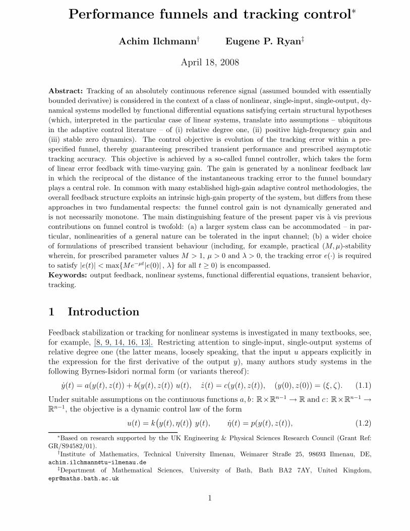
Many approaches in the literature, both adaptive or non-adaptive, are concerned with asymp-totic behaviour of solutions of the feedback system. In contrast, the present paper is concernedwith both asymptotic and transient performance of the feedback system. In particular, thecontrol objective is to ensure that the tracking error, i.e. the difference between output andreference signal, evolves within a prespecified funnel, which is “shaped” to ensure the requisitetransients and asymptotics. With reference to Figure 1, we remark that the funnel radius isnot permitted to shrink to zero at infinity: it may, however, approach an arbitrarily smallprescribed value λ > 0, thereby ensuring tracking with prescribed asymptotic accuracy λ. Themain contribution of the paper is to establish that the above objective is achieved by the appli-cation of a variant of a so-called ‘funnel controller’, introduced in [5]. Novel features of funnel

2

b

Error evolution e(t)

Figure 1: Performance funnel Fϕ

control include the following.– The control law is a simple time-varying error feedback of the form u(t) = −k(t) e(t), wheree = y−r denotes the tracking error between the output y and a given reference signal r and thegain function k is generated by a feedback of the form k(t) = f

(

t, e(t), |e(0)|)

. The intuitionunderpinning this control structure is exploiting an inherent high-gain property of the systemclass in order to maintain the error evolution within the funnel by ensuring that, if the errorapproaches the funnel boundary, then the gain takes values sufficiently large to preclude con-tact with the boundary. Whilst the control exploits an inherent high-gain property, it is nota high-gain controller in the usual sense: in particular, and in contrast to high-gain adaptivecontrol methodologies, k is not monotone and decreases as the error recedes from the funnelboundary.– The gain k is adapted but u(t) = −k(t) e(t) is not an adaptive controller in the usual sense:in particular, and in contrast to (1.2), it is non-dynamic.– The approach does not invoke any identification mechanism or internal model principle.Funnel control has been applied to temperature control in chemical reactor models [7], even inthe presence of input constraints, and to speed control of electric drives [6], the latter has beentested successfully in the laboratory.

The main distinguishing feature of the present paper vis a vis previous contributions on funnelcontrol (see, e.g. [5]) is twofold: (a) a larger system class can be accommodated – in particular,nonlinearities g of a general nature can be tolerated in the input channel; (b) a wider choiceof formulations of prescribed transient behaviour is encompassed, including, for example, avariant of (M,µ)-stability (see [3, Section 5.5]).

The paper is organized as follows. In Section 2, we make precise the underlying system classand the control objective is formulated in Section 3: illustrative examples are provided inAppendix A. The main result is presented in Section 4, wherein the closed-loop system givesrise to an initial-value problem for a functional differential equation: the nature of this problemis such that it falls outside the scope of existence theories in the literature known to the authors.For this reason, an existence theory – of sufficient generality to include the closed-loop initial-value problem – is developed in Appendix B. The paper concludes with a numerical simulation.

3

2 System class

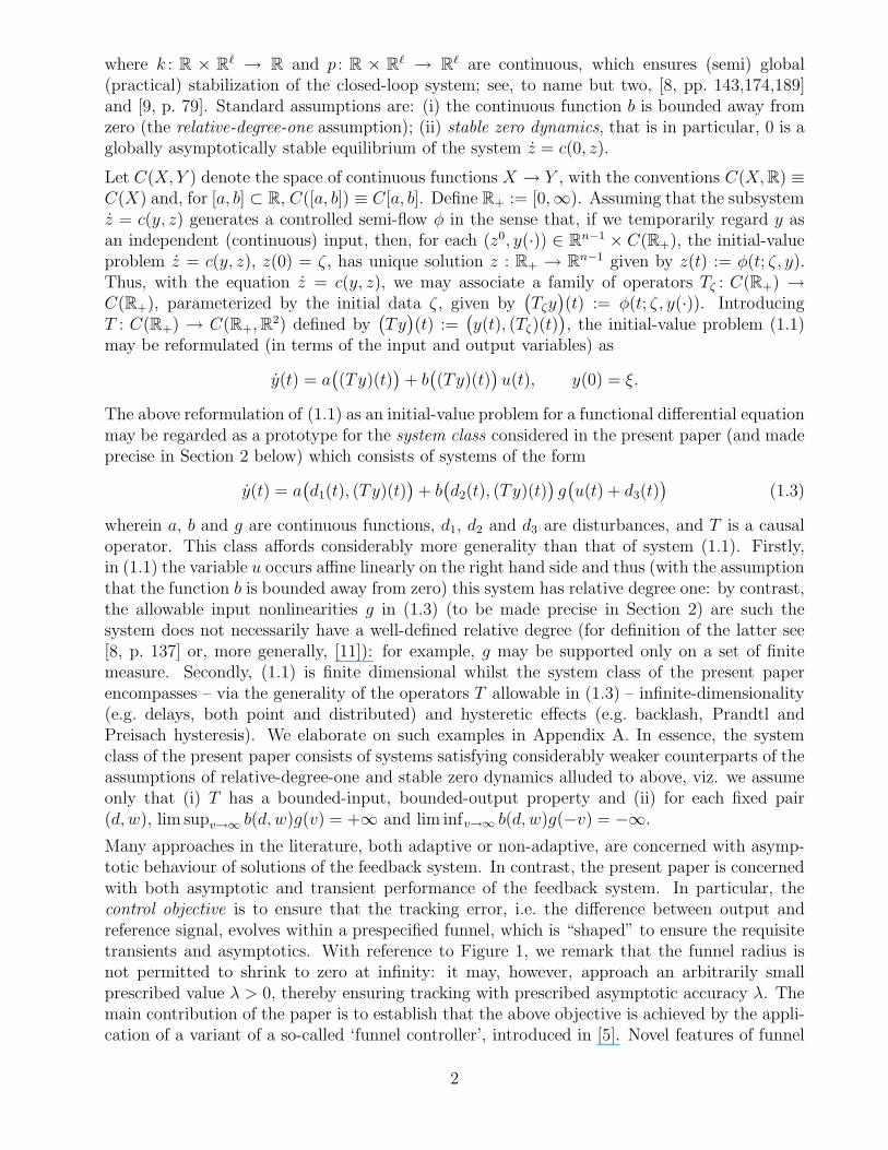
We consider single-input, single-output systems described by a functional differential equationof the form (1.3) and having the general structure depicted in Figure 2, wherein T is a causaloperator and d1, d2 and d3 are extraneous disturbances. For example, as already shown in theIntroduction, the initial-value problem (1.1) may be reformulated (in terms of the input andoutput variables) as an initial-value problem for a disturbance-free system of the form depictedin Figure 2 with g = id (the identity map on R). Other examples can be found in Appendix A.

y = a(d1, w) + b(d2, w)g(u+ d3)

w = Ty

y+u

w

d3 d1 d2

Figure 2: The open loop system

We proceed to a description of the general system class, first making precise the associatedclass of operators T . Throughout, L∞(R+,R

ℓ) is the space of measurable, essentially boundedfunctions R+ → R

ℓ, with norm given by ‖y‖∞ := ess supt∈R+‖y(t)‖; the space of measurable,

locally essentially bounded functions R+ → Rℓ is denoted by L∞

loc(R+,Rℓ); W 1,∞(R+,R

ℓ) is thespace of absolutely continuous functions y : R+ → Rℓ with y, y ∈ L∞(R+,R

ℓ).

Definition 2.1 (Operator class T q

h ) For h, t ∈ R+, w ∈ C[−h, t], τ > t and δ > 0, define

C(w; h, t, τ, δ) :=

v ∈ C[−h, τ ]∣

∣ v|[−h,t] = w, |v(s) − w(t)| ≤ δ ∀ s ∈ [t, τ ]

,

that is, the space of all continuous extensions v of w ∈ C[−h, t] to the interval [−h, τ ] with the

property that |v(s) − w(t)| ≤ δ for all s ∈ [t, τ ].An operator T is said to be of class T q

h , for some q ∈ N, if, and only if, the following hold.

(i) T : C[−h,∞) → L∞loc(R+,R

q) . (ii) T is a causal operator.

(iii) For each t ≥ 0 and each w ∈ C[−h, t], there exist τ > t, δ > 0 and c0 > 0 such that

ess-sups∈[t,τ ]‖(Ty)(s)− (Tz)(s)‖ ≤ c0 maxs∈[t,τ ] |y(s) − z(s)| ∀ y, z ∈ C(w; h, t, τ, δ) .

(iv) For every c1 > 0 there exists c2 > 0 such that, for all y ∈ C[−h,∞),

supt∈[−h,∞)

|y(t)| ≤ c1 =⇒ ‖(Ty)(t)‖ ≤ c2 for a.a. t ≥ 0 .

Remark 2.2 Property (iii) is a technical assumption of local Lipschitz type which is usedin establishing well-posedness of the closed-loop system. To interpret (iii) correctly, we needto give meaning to Ty, for a function y ∈ C(I) on a bounded interval I of the form [−h, ρ) or[−h, ρ], where 0 < ρ < ∞. This we do by showing that T “localizes”, in a natural way, to an

4

operator T : C(I) → L∞loc(J,R

q), where J := I \ [−h, 0). Let y ∈ C(I). For each σ ∈ J , defineyσ ∈ C[−h,∞) by

yσ(t) :=

y(t), t ∈ [−h, σ],y(σ), t > σ .

By causality, we may define T y ∈ L∞loc(J,R

q) by the property T y|[0,σ] = Tyσ|[0,σ] for all σ ∈ J .

Henceforth, we will not distinguish notationally an operator T and its “localisation” T : thecorrect interpretation being clear from context.Property (iv) is a bounded-input, bounded-output assumption on the operator T . This as-sumption is a weak counterpart of the “stable zero dynamics” assumption ubiquitous in thecontext of high-gain control of linear systems.

Definition 2.3 (System class Σp,qh ) Let p, q ∈ N and h ≥ 0. The functional differential

equation

y(t) = a(

d1(t), (Ty)(t))

+ b(

d2(t), (Ty)(t))

g(

u(t) + d3(t))

, (2.1)

defines a system of class Σp,qh , written (a, b, g, T, d1, d2, d3) ∈ Σp,q

h , if, and only if, the following

hold.

(i) a : Rp × Rq → R is continuous.

(ii) b : Rp × Rq → R is continuous and sign definite, that is,

|b(d, s)| > 0 ∀ (d, s) ∈ Rp × R

q . (2.2)

(iii) g : R → R is continuous with

(a) lim supv→∞

b1g(v) = +∞, (b) lim infv→∞

b1g(−v) = −∞ , (2.3)

where b1 := sgn(b), the polarity of the sign-definite function b.

(iv) T ∈ T qh . (v) d1, d2 ∈ L∞(R+,R

p), d3 ∈W 1,∞(R+).

Remark 2.4 Some remarks on the nature of the input nonlinearity are warranted. Thefunction g ∈ C(R,R) can be interpreted in two distinct ways.(i) The function g may form part of the overall control structure in the sense that it is asynthesizable element which may be designed to compensate for lack of knowledge of the sgn(b)of the input connection function b. In this context, the role of g is akin to that of a so-called“Nussbaum function” in adaptive control, see [15]. For example, the choice g : u 7→ u cosuensures that properties (2.3) hold.(ii) Alternatively, g may be regarded as an uncertain intrinsic component of the plant, inwhich case, assumption (2.3) places some restrictions on the manner in which the functionsg and b interact. In this context, note that g may influence/reverse the polarity of a controlinput u in a somewhat arbitrary manner. Note also that (assuming d3 = 0 for simplicity)a control input u is nullified on the zero set g−1(0) ⊂ R of g and the measure of this setmay be infinite in the sense that the function g may be supported only on a set of finiteLebesgue measure: a simple example of such a function is a continuous unbounded odd functiong : R → R with g(u) :=

∑

∞

n=1 sgn(b) gn(u) for all u ∈ R+ (and so g(u) = −g(−u) for all

5

u < 0), where, for each n ∈ N, gn : R+ → R+ is a locally Lipschitz function supported onIn := [n, n+2−n] in which case, the measure of the set R\g−1(0) is bounded from above by thequantity 2

∑

∞

n=1 |In| = 2∑

∞

n=1 2−n = 2.In more extreme cases, the function g may reverse the intended polarity of the control input:moreover, the “bad” set on which the polarity is reversed may be large in comparison withthe “good” set on which polarity is maintained. In particular, assume (2.3) holds and let g+

and g− denote the positive and negative parts of sgn(b)g, in which case sgn(b)g = g+ − g−;the Lebesgue measure of the support of g− (the “bad” polarity-reversing set) may be infinite,whilst the support of g+ (the “good” set) may have only finite measure. Since, in this secondcontext, knowledge of g is not available to the controller, it is perhaps counter-intuitive that theapproximate tracking objective, as described in the next section, is achievable in the presenceof input nonlinearities of such generality.

3 The control objective and performance funnel

Let (a, b, g, T, d1, d2, d3) ∈ Σp,qh and consider the initial-value problem

y(t) = a(

d1(t), (Ty)(t))

+ b(

d2(t), (Ty)(t))

g(

u(t) + d3(t))

, y|[−h,0] = y0 ∈ C[−h, 0] .

The control objective is to design a simple tracking error feedback controller of the formu(t) = −k(t)e(t), with gain k(t) also generated by feedback of the error e(t) = y(t) − r(t),so that, for all initial functions y0 ∈ C[−h, 0] and all reference signals r ∈ W 1,∞(R+), everysolution of the closed-loop initial-value problem is bounded and approximate tracking with pre-scribed asymptotic accuracy and transient behaviour is achieved in the sense that the trackingerror satisfies an a priori bound and asymptotically approaches a prescribed (arbitrarily small)neighbourhood of zero. The prescription of asymptotic and transient behaviour is formulated,in a manner to be made precise, via the following class Ψλ of functions R+ × R+ → R+.

Definition 3.1 (Function class Ψ) A continuous function ψ : R+ × R+ → R+ is of class

Ψ if, and only if, the following hold:

(i) ψ(t, ζ) > 0 ∀ t > 0 ∀ ζ ≥ 0; (ii) ψ(·, ζ) ∈W 1,∞(R+) ∀ ζ ≥ 0; (iii) ψ(0, ζ) < ζ−1 ∀ ζ > 0.

Let ψ ∈ Ψ, y0 ∈ C[−h, 0] and r ∈ W 1,∞(R+) be arbitrary, and write e0 := y0(0)−r(0). Then theperformance objective of prescribed asymptotic and transient behaviour of the tracking error eis now specified in a predetermined manner through choice of the function ψ and captured bythe requirement that

ψ(t, |e0|)|e(t)| < 1 ∀ t ∈ R+ . (3.1)

In addition, if, for some prescribed λ > 0 arbitrarily small, ψ satisfies

lim supt→∞

[ψ(t, ζ)]−1 ≤1

λ∀ ζ ≥ 0 , (3.2)

then asymptotic tracking accuracy lim supt→∞ |e(t)| ≤ λ is achieved. With reference to Figure 1and writing ϕ(·) = ψ(·, |e0|) ∈ W 1,∞(R+), we see that (3.1) may, in turn, be identified as therequirement that the tracking error should evolve within a performance funnel

Fϕ := graph(

t 7→

z ∈ R∣

∣ ϕ(t)|z| < 1

)

,

i.e. the graph of a set-valued map defined on R+, the value of which, at t ∈ R+, is the interval(−1/ϕ(t) , 1/ϕ(t)). Note that the boundary of Fϕ is determined by the reciprocal of ϕ.

6

Example 3.2(A) Fix λ > 0 and choose ϕ ∈ W 1,∞(R+) such that ϕ(0) = 0, ϕ(t) ∈ (0, 1/λ) for all t > 0 andlimt→∞ ϕ(t) = 1/λ. Define ψ ∈ Ψ by the property that ψ(·, ζ) = ϕ(·) for all ζ ∈ R+. Thensatisfaction of (3.1) (equivalently, error evolution within the funnel Fϕ) implies that

|e(t)| < 1/ϕ(t) ∀ t > 0.

For example, the choice

t 7→ ϕ(t) =min t/τ, 1

λ, with τ, λ > 0,

ensures that the modulus of the error decays at rate τλ/t in the “initial (transient) phase”(0, τ ], and, since (3.2) holds, is bounded by λ in the “terminal phase” [τ,∞).

(B) In this second example, and in contrast with Example (A) above, the function ψ hasnon-trivial dependence on its second argument: for M > 1, µ > 0 and λ > 0, define ψ ∈ Ψ by

ψ(t, ζ) := 1/maxMe−µtζ , λ, ∀ t, ζ ∈ R+.

In doing so, we adopt the objective of “practical (M,µ)-stability” of the tracking error in thesense that, for every y0 ∈ C[−h, 0] and r ∈ W 1,∞(R+), the tracking error e = y − r (withe0 = e(0)) is required to satisfy

|e(t)| < max

Me−µt|e0| , λ

∀ t ≥ 0.

For example, if λM |e0| > 1 and (3.1) holds, then, defining τ := ln(λM |e0|)/µ, the tracking errordecays at prescribed exponential rate in the “initial (transient) phase” [0, τ ], and is boundedby λ in the “terminal phase” [τ,∞).

4 Main result: funnel output feedback

Loosely speaking, funnel control exploits an inherent benign high-gain property of the system bydesigning – with appropriate choice of ψ ∈ Ψ – a proportional error feedback u(t) = −k(t) e(t)in such a way that k(t) becomes large if |e(t)| approaches the performance funnel boundary(equivalently, if ψ(t, |e(0)|)|e(t)| approaches the value 1), thereby precluding contact with thefunnel boundary. We emphasize that the gain is non-monotone and decreases as the errorrecedes from the funnel boundary. The essence of the proof of the main result lies in showingthat the closed-loop system is well-posed in the sense that u and k are bounded functions andthe error evolves strictly within the performance funnel.

For ψ ∈ Ψ, the “funnel controller” can be expressed in its simplest form as

u(t) = −k(t) e(t), k(t) =ψ(t, |e(0)|)

1 − ψ(t, |e(0)|)|e(t)|. (4.1)

This form is a special case of a more general structure

u(t) = −k(t) e(t), k(t) = α(

ψ(t, |e(0)|)|e(t)|)

ψ(t, |e(0)|) , (4.2)

7

wherein α is any continuously differentiable unbounded injection [0, 1) → R+ with α(0) > 0.Note that α(s) → ∞ as s ↑ 1 and the choice α : s 7→ 1/(1 − s) yields (4.1). Let p, q ∈ N,h ≥ 0 and consider control (4.2) applied to the system (a, b, g, T, d1, d2, d3) ∈ Σp,q

h . In viewof the potential for “blow up” in the gain generation in (4.2), some care must be exercised informulating the closed-loop system. Introducing

Ω := (t, z, ζ) ∈ R+ × R × R+| ψ(t, ζ)|z| < 1, (4.3)

we definef : Ω → R, (t, z, ζ) → f(t, z, ζ) := α

(

ψ(t, ζ)|z|)

ψ(t, ζ) , (4.4)

in which case, the control (4.1) can be interpreted, in explicit feedback form, as

u(t) = −f(t, e(t), |e(0)|) e(t). (4.5)

Let y0 ∈ C[−h, 0] and r ∈W 1,∞(R+) be arbitrary and write e0 := y0(0)−r(0). The closed-loopinitial-value problem now takes the form

y(t) = a(

d1(t), (Ty)(t))

+ b(

d2(t), (Ty)(t))

g(

d3(t) − f(t, y(t) − r(t), |e0|)e(t))

,

y|[−h,0] = y0 ∈ C[−h, 0].

(4.6)

Setting ϕ(·) := ψ(·, |e0|) (with associated performance funnel Fϕ), (4.6) may, in turn, be rewrit-ten as

y(t) = F (t, y(t), (Ty)(t)), y|[−h,0] = y0 ∈ C[−h, 0], (4.7)

whereF : D × R

q → R, D := (t, v) ∈ R+ × R| (t, v − r(t)) ∈ Fϕ, (4.8)

is a Caratheodory function (see App. B for the definition) given by

F (t, v, w) := a(d1(t), w) + b(d2(t), w)g(

d3(t) − f(t, v − r(t), |e0|)(v − r(t)))

. (4.9)

By a solution of (4.7) we mean a function y ∈ C[−h, ω), 0 < ω ≤ ∞, such that y|[−h,0] =y0, y|[0,ω) is locally absolutely continuous, with (t, y(t)) ∈ D for all t ∈ [0, ω) and y(t) =

F (t, y(t), (T y)(t)) for almost all t ∈ [0, ω). A solution is said to be maximal if it has no properright extension that is also a solution. A solution defined on [−h,∞) is said to be global.

In Appendix B, we develop an existence theory of sufficient generality to encompass the closed-loop initial-value problem (4.7): this theory is a variant of that in [5] – the distinguishing featureof the present paper resides in the nature of the domain of the function F in (4.8) which placesthe initial-value problem (4.7) outside the scope of the existence theory in [5].

Now we are in a position to state the main result.

Theorem 4.1 Let ψ ∈ Ψ specify the prescribed transient behaviour Let α : [0, 1) → R+

be a continuously differentiable unbounded injection with α(0) > 0, and let r ∈ W 1,∞(R+)and y0 ∈ C[−h, 0] be arbitrary. Then the “funnel controller” (4.2) applied to any system

(a, b, g, T, d1, d2, d3) ∈ Σp,qh , with p, q ∈ N, h ≥ 0 and initial data y0 ∈ C[−h, 0], is such that the

resulting closed-loop initial-value problem has a solution and every solution can be extended to

a global solution. Every global solution y has the properties:

(a) the functions y and u (given by (4.5) with e := y − r) are bounded;

8

(b) there exists ε ∈ (0, 1) such that

|e(t)| ≤1 − ε

ψ(t, |e(0)|)∀ t > 0 .

Remark 4.2 Assertion (b) of Theorem 4.1 is its essence. Writing ϕ(·) := ψ(·, |e(0)|), it assertsthat the tracking error evolves within the performance funnel Fϕ as depicted in Figure 1;moreover, the error evolution is strictly bounded away from the funnel boundary, therebyensuring that the gain function k and the control function u in (4.1) are bounded.

Proof of Theorem 4.1:Write e0 := e(0) = y0(0) − r(0) and ϕ(·) := ψ(·, |e0|) ∈ W 1,∞(R+) (by Definition 3.1(ii)). Wehave seen that the closed-loop initial-value problem (4.6) may be expressed in the form (4.7).Invoking Theorem 7.1 of Appendix B, we may conclude that (4.7) has a solution and everysolution can be extended to a maximal solution; moreover (noting that F is locally essentiallybounded), if y : [−h, ω) → R is a maximal solution, then the closure of graph(y|[0,ω)

)

is not acompact subset of D.

Let y : [−h, ω) → R, 0 < ω ≤ ∞, be a maximal solution. Then e := y − r is bounded withϕ(t)|e(t)| < 1, for all t ∈ [0, ω). Since r is bounded, it follows that y = e + r is bounded andso, by property (iv) of T ∈ T q

h , the function w := Ty is also bounded. Define c : [0, ω) → R byc(t) := a(d1(t), w(t)) − r(t). By continuity of a, boundedness of w, and essential boundednessof r and d1, it follows that c ∈ L∞[0, ω). By (4.7) and (4.9), we have

e(t) = c(t) + b(

d2(t), w(t))

g(

u(t) + d3(t))

for a.a. t ∈ [0, ω). (4.10)

Let β : [0, 1) → R+ be the continuously differentiable bijection given by β(s) := sα(s); werecord that β ′(s) = α(s) + sα′(s) ≥ α(0) > 0 for all s ∈ R+. Write

κ(t) := β(ϕ(t)|e(t)|) ∀ t ∈ [0, ω),

in which case, in view of (4.2), we have

t ∈ [0, ω), e(t) 6= 0 =⇒ u(t) = −κ(t) sgn(e(t)) .

Seeking a contradiction, suppose that the function κ is unbounded on [0, ω). Then there existsa strictly-increasing sequence (tn) in [0, ω), with tn ↑ ω as n → ∞, such that the sequence(

κ(tn))

is a strictly-increasing unbounded sequence in R+ and(

ϕ(tn)|e(tn)|)

is a sequence in(0, 1) with ϕ(tn)|e(tn)| → 1 as n → ∞. Since ϕ is bounded with ϕ(t) > 0 for all t ∈ (0, ω)and passing to a subsequence if necessary, we may infer the existence of c0 ∈ −1, 1 suchthat c0e(tn) < 0 for all n ∈ N. By property (2.2) of the continuous function b, together withboundedness of w and essential boundedness of d2, there exists b0 > 0 such that

|b(d2(t), w(t))| ≥ b0 for a.a. t ∈ [0, ω). (4.11)

By properties (2.3) of g, there exist strictly-increasing unbounded sequences (un) and (vn) inR+ such that

b1 g(un) → ∞ and − b1 g(−vn) → ∞ as n→ ∞ . (4.12)

9

(Recall that b1 = sgn(b), the polarity of the sign-definite function b.) Define the sequence (sn)and the continuous function γ : R → R by

sn :=

un, if c0 = +1−vn, if c0 = −1

, γ(s) := b0b1c0 g(s) ∀ s ∈ R.

Clearly,

c0 = +1 =⇒ γ(sn) = b0b1g(un) and c0 = −1 =⇒ γ(sn) = −b0b1g(−vn),

and so, invoking (4.12) and recalling that b0 > 0, we may infer that γ(sn) → ∞ as n → ∞.Passing to a subsequence if necessary, we may assume that (γ(sn)) is a strictly-increasingsequence in R+. Now define the sequence (κn) := (c0sn). Observe that (κn) is a strictly-increasing unbounded sequence in R+ and so, extracting a subsequence (which we do notrelabel), we may assume that κn ≥ 1 + κ(0) + ‖d3‖∞ for all n ∈ N. Again passing to asubsequence of (tn) if necessary, we may also assume that κ(tn) ≥ κn+1 for all n ∈ N. Definethe sequence (t∗n) by

t∗n :=

sup Tn, Tn 6= ∅,

0, Tn = ∅,where Tn :=

t ∈ [0, tn]| e(t) = 0

.

Observe that κ(t∗n) + c0d3(t∗n) ≤ κ(0) + ‖d3‖∞ < κn for all n ∈ N and so the following are well

defined for each n ∈ N

τn := inf

t ∈ [t∗n, tn]∣

∣ κ(t) + c0d3(t) = κn+1

σn := sup

t ∈ [t∗n, τn]∣

∣ γ(c0κ(t) + d3(t)) = γ(sn)

< τn ,

wherein the strict inequality σn < τn holds because

γ(c0κ(τn) + d3(τn)) = γ(c0κn+1) = γ(sn+1) > γ(sn).

Suppose that κ(σn) + c0d3(σn) ≥ κ(τn) + c0d3(τn) for some n ∈ N. Then

κ(t∗n) + c0d3(t∗

n) < κn+1 = κ(τn) + c0d3(τn) ≤ κ(σn) + c0d3(σn)

and so, by continuity, there exists s ∈ (t∗n, σn] such that κ(s) + c0d3(s) = κn+1, whence thecontradiction:

τn = inft ∈ [t∗n, tn]| κ(t) + c0d3(t) = κn+1 ≤ s ≤ σn < τn.

Therefore, κ(σn)+ c0d3(σn) < κ(τn)+ c0d3(τn) for all n ∈ N. Since d3 ∈W 1,∞(R+), there existsc1 > 0 such that

κ(σn) < κ(τn) + c0(d3(τn) − d3(σ)) ≤ κ(τn) + (τn − σn)c1 ∀ n ∈ N . (4.13)

By definition of σn, we have

γ(c0κ(t) + d3(t)) > γ(sn) ∀ t ∈ (σn, τn], ∀ n ∈ N . (4.14)

We also record that

−|e(t)| = c0e(t) < 0 ∀ t ∈ [σn, τn], ∀ n ∈ N. (4.15)

10

We may now conclude that

−c0b(d2(t), w(t))g(u(t) + d3(t)) = −|b(d2(t), w(t))|γ(c0κ(t) + d3(t))/b0

≤ −γ(c0κ(t) + d3(t)) ≤ −γ(sn) ∀ t ∈ [σn, τn], ∀ n ∈ N . (4.16)

Observe that, for almost all t ∈ [σn, τn] and for all n ∈ N,

d

dt

(

ϕ(t)|e(t)|)

= −c0(

ϕ(t)e(t)+ϕ(t)e(t))

= −c0(

ϕ(t)e(t)+h(t)+ b(d2(t), w(t))g(u(t)+d3(t)))

.

By boundedness of e, together with essential boundedness of ϕ and h, and invoking (4.16), wemay conclude that, for some constant c2 > 0,

d

dt

(

ϕ(t)|e(t)|)

≤ c2 − γ(sn) for a.a. t ∈ [σn, τn] ∀ n ∈ N. (4.17)

Fix n ∈ N sufficiently large so that α(0)(

c2 − γ(sn))

< −c1, in which case we have

κ(t) = β ′(ϕ(t)|e(t)|)d

dt

(

ϕ(t)|e(t)|)

≤ α(0)(

c2 − γ(sn))

< −c1 for a.a. t ∈ [σn, τn]

whence κ(τn)− κ(σn) < −(τn − σn)c1, which contradicts (4.13). This proves boundedness of κ.

By boundedness of t 7→ κ(t) = β(ϕ(t)|e(t)|), we may conclude that supt∈[0,ω) ϕ(t)|e(t)| < 1,equivalently, there exists ε ∈ (0, 1) such that ϕ(t)|e(t)| ≤ 1 − ε for all t ∈ [0, ω).

It remains only to show that the solution y : [−h, ω) → R is global. Seeking a contradiction,suppose ω <∞. Then K := (t, y) ∈ D| t ∈ [0, ω], ϕ(t)|y− r(t)| ≤ 1− ε is a compact subsetof D with the property (t, y(t)) ∈ K for all t ∈ [0, ω), which contradicts the fact that the closureof graph

(

y|[0,ω)

)

is not a compact subset of D. Therefore, ω = ∞. 2

5 Illustrative simulation

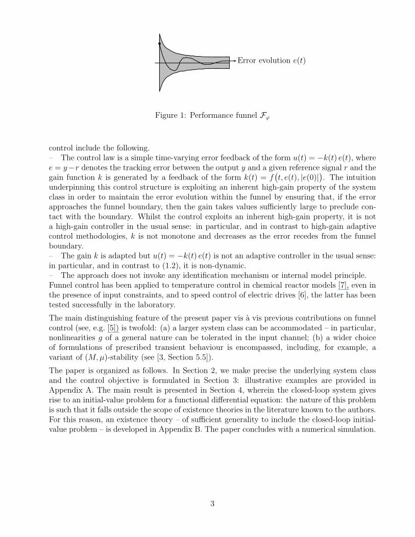
Consider the system shown in Figure 3 consisting of a linear, single-input, single-output system(c, A, b) with state space Rn, disturbance d ∈ L∞(R+), a nonlinearity g in the input channel,and a feedback loop containing a hysteretic nonlinearity H :

x(t) = Ax(t) + b(

d(t) + (H(cx))(t) + g(u(t)))

, x(0) = x0 ∈ Rn , y(t) = cx(t). (5.1)

As discussed in Section 6.2 of Appendix B, under the assumptions that the linear system

(c, A, b)+g yu

d

H

Figure 3: Linear system with hysteretic feedback loop and input nonlinearity

11

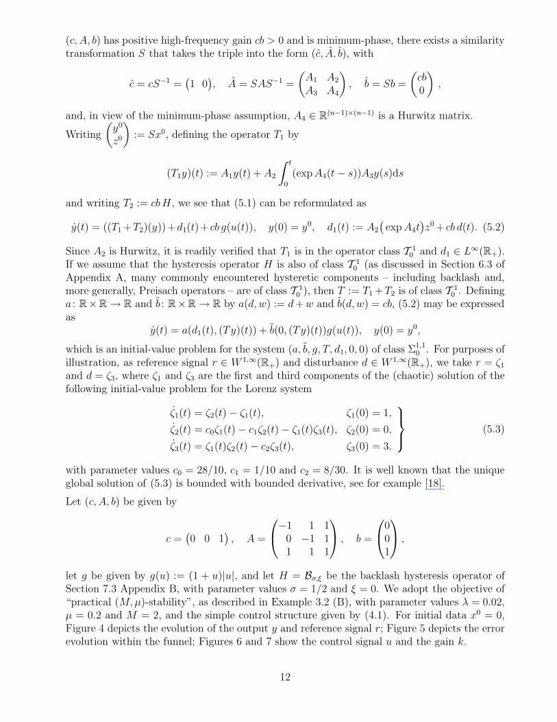
(c, A, b) has positive high-frequency gain cb > 0 and is minimum-phase, there exists a similaritytransformation S that takes the triple into the form (c, A, b), with

c = cS−1 =(

1 0)

, A = SAS−1 =

(

A1 A2

A3 A4

)

, b = Sb =

(

cb0

)

,

and, in view of the minimum-phase assumption, A4 ∈ R(n−1)×(n−1) is a Hurwitz matrix.

Writing

(

y0

z0

)

:= Sx0, defining the operator T1 by

(T1y)(t) := A1y(t) + A2

∫ t

0

(expA4(t− s))A3y(s)ds

and writing T2 := cbH , we see that (5.1) can be reformulated as

y(t) = ((T1 +T2)(y))+d1(t)+ cb g(u(t)), y(0) = y0, d1(t) := A2

(

expA4t)

z0 + cb d(t). (5.2)

Since A2 is Hurwitz, it is readily verified that T1 is in the operator class T 10 and d1 ∈ L∞(R+).

If we assume that the hysteresis operator H is also of class T 10 (as discussed in Section 6.3 of

Appendix A, many commonly encountered hysteretic components – including backlash and,more generally, Preisach operators – are of class T 1

0 ), then T := T1 +T2 is of class T 10 . Defining

a : R×R → R and b : R×R → R by a(d, w) := d+w and b(d, w) = cb, (5.2) may be expressedas

y(t) = a(d1(t), (Ty)(t)) + b(0, (Ty)(t))g(u(t)), y(0) = y0,

which is an initial-value problem for the system (a, b, g, T, d1, 0, 0) of class Σ1,10 . For purposes of

illustration, as reference signal r ∈ W 1,∞(R+) and disturbance d ∈ W 1,∞(R+), we take r = ζ1and d = ζ3, where ζ1 and ζ3 are the first and third components of the (chaotic) solution of thefollowing initial-value problem for the Lorenz system

ζ1(t) = ζ2(t) − ζ1(t), ζ1(0) = 1,

ζ2(t) = c0ζ1(t) − c1ζ2(t) − ζ1(t)ζ3(t), ζ2(0) = 0,

ζ3(t) = ζ1(t)ζ2(t) − c2ζ3(t), ζ3(0) = 3.

(5.3)

with parameter values c0 = 28/10, c1 = 1/10 and c2 = 8/30. It is well known that the uniqueglobal solution of (5.3) is bounded with bounded derivative, see for example [18].

Let (c, A, b) be given by

c =(

0 0 1)

, A =

−1 1 10 −1 11 1 1

, b =

001

,

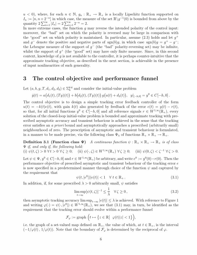
let g be given by g(u) := (1 + u)|u|, and let H = Bσ,ξ be the backlash hysteresis operator ofSection 7.3 Appendix B, with parameter values σ = 1/2 and ξ = 0. We adopt the objective of“practical (M,µ)-stability”, as described in Example 3.2 (B), with parameter values λ = 0.02,µ = 0.2 and M = 2, and the simple control structure given by (4.1). For initial data x0 = 0,Figure 4 depicts the evolution of the output y and reference signal r; Figure 5 depicts the errorevolution within the funnel; Figures 6 and 7 show the control signal u and the gain k.

12

0 5 10 15 20 25 30 35 40−2

−1.5

−1

−0.5

0

0.5

1

1.5

2

2.5

3

Figure 4: The output y (solid line) and reference r (dashed line)

0 5 10 15 20 25 30 35 40−2.5

−2

−1.5

−1

−0.5

0

0.5

1

1.5

2

2.5

Figure 5: Error evolution within funnel

0 5 10 15 20 25 30 35 40−5

−4

−3

−2

−1

0

1

2

Figure 6: The control u

0 5 10 15 20 25 30 35 400

5

10

15

20

25

30

Figure 7: The gain function k

13

6 Appendix A: Examples of the system class Σp,qh and

the operator class T qh

6.1 Finite-dimensional nonlinear prototype

Consider again the initial-value problem for the nonlinear prototype system (1.1). In theIntroduction, we have seen that, if the equation z = c(y, z) is assumed to generate a controlledsemiflow φ, then with this equation we may associate a family of operators Tζ : C(R+) →C(R+,R

n−1), parameterized by the initial data ζ ∈ Rn−1, given by(

Tζy)

(t) := φ(t; ζ, y(·)).Introducing T : C(R+) → C(R+,R × R

n−1) defined by(

Ty)

(t) :=(

y(t), (Tζ)(t))

, the initial-value problem (1.1) may be reformulated (in terms of the input and output variables) as

y(t) = a(

(Ty)(t))

+ b(

(Ty)(t))

u(t), y(0) = ξ . (6.1)

If, in addition, we assume that the system z = c(y, z) is input-to-state stable (ISS) (see, [17]),then it is readily verified that the operator T is of class T n

0 . Assuming that the function b ispositive-valued and bounded away from zero and introducing the functions a : R×Rn → R andb : R × R

n → R (these are simply convenient artifacts) given by

a(d, w) := d+ a(w), b(d, w) := d+ b(w),

we see that (6.1) is equivalent to

y(t) = a(

0, (Ty)(t))

+ b(

0, (Ty)(t))

u(t), y(0) = ξ ,

which is an initial-value problem for the system (a, b, id, T, 0, 0, 0) of class Σ1,n0 . Therefore,

under the assumptions that the system z = c(y, z) is ISS and b is positive-valued and boundedaway from zero, Theorem 4.1 implies that, for all (ζ, ξ) ∈ R

n−1 ×R and all r ∈W 1,∞(R+), thecontrol (4.2) applied to (1.1) ensures attainment of the tracking objectives.

6.2 Linear (retarded) systems with input nonlinearities

Let h > 0, let A be an n×n-matrix with entries in BV [0, h] (the space of real-valued functionsof bounded variation on [a, b] ⊂ R) and let b, cT ∈ Rn. Consider the linear retarded systemwith nonlinearity g in the input channel

x = dA ∗ x+ bg(u) , x|[−h,0] = x0− ∈ C([−h, 0],Rn), y = cx , (6.2)

where (dA ∗ x)(t) :=∫ h

0dA(τ)x(t− τ) for all t ∈ R+, satisfying

• minimum-phase condition, i.e.,

det

(

sI − A(s) −bc 0

)

6= 0 ∀ s ∈ C ,Re(s) > 0, where A(s) :=

∫ h

0

exp(−sτ)dA(τ)

• positive high-frequency gain condition, i.e., cb > 0

• lim supv→∞ g(v) = +∞, lim infv→∞ g(−v) = −∞ .

14

It is well-known that, under these assumptions, there exists a similarity transformation whichtakes system (6.2) into the form

y=dA1 ∗ y + dA2 ∗ z + cb g(u) , y|[−h,0] = y0 , (6.3a)

z=dA3 ∗ y + dA4 ∗ z , z|[−h,0] = z0 , (6.3b)

where, by the minimum-phase condition, A4 has the property that

det(sI − A22(s)) 6= 0 ∀ s ∈ C ,Re(s) > 0, (6.4)

see [4] for details. For given z0 ∈ C([−h, 0],Rn−1) and given ξ ∈ C[−h,∞), let z(·; z0, ξ) denotethe unique solution of the initial-value problem

z = dA4 ∗ z + dA3 ∗ ξ , z|[−h,0] = z0 .

Defining the operator T and function d1 by

T (ξ) := dA1 ∗ ξ + dA2 ∗ z(· ; 0, ξ) , d1 := dA2 ∗ z(· ; z0, 0) ,

equation (6.3a) can be expressed as

y = d1 + T (y) + cb g(u) , y0 = cx0 . (6.5)

By the standard theory of retarded functional differential equations (see [2, Corollary 6.1,p. 215]), (6.4) implies that the zero solution of the retarded equation z = dA4∗z is exponentiallystable, so that there exists K > 0 such that, for all z0 ∈ C([−h, 0],Rn−1) and all ξ ∈ C[−h,∞),

supt∈[0,∞)

|z(t; z0, ξ)| ≤ K(

supt∈[−h,0]

|z0(t)| + supt∈[−h,∞)

|ξ(t)|)

.

We conclude that d is bounded and that T ∈ T 1h . Finally, defining a : R × R → R and

b : R× R → R (as in the previous example, these are simply artifacts) by a(d, w) := d+w andb(d, w) = cb, we see that (6.5) is equivalent to

y(t) = a(

d1(t), (Ty)(t))

+ b(

0, (Ty)(t))

u(t), y0 = cx0 ,

which is an initial-value problem for the system (a, b, g, T, d1, 0, 0) of class Σ1,(n−1)h .

The above example is readily modified to include the non-retarded case h = 0. In this case, wesimply replace dA∗x by Ax (A ∈ Rn×n), and dA1 ∗y, dA2 ∗z, dA3 ∗y, dA4 ∗z by A1, . . . , A4 atthe appropriate places. In this way, we see that the class of linear, single-input, single-output,minimum-phase, relative-degree-one systems (c, A, b), with cb > 0 and with nonlinearity g inthe input channel, is subsumed by our system class Σ1,1

0 .

6.3 Systems with hysteresis

An operator T : C(R+) → C(R+) is a hysteresis operator if it is causal and rate independent.Here rate independence means that T (y ζ) = (Ty) ζ for every y ∈ C(R+) and every timetransformation ζ , where ζ : R+ → R+ is said to be a time transformation if it is continuous,non-decreasing and surjective. The so-called Preisach operators are among the most generaland most important hysteresis operators: in particular, they can model complex hysteresis

15

effects such as nested loops in input-output characteristics.

A basic building block for these operators is the backlash operator. A discussion of the backlash

operator (also called play operator) can be found in a number of references, see for example [1],[10] and [12]. Let σ ∈ R+ and introduce the function bσ : R2 → R given by

bσ(v1, v2) := max

v1 − σ , minv1 + σ, v2

.

Let Cpm(R+) denote the space of continuous piecewise monotone functions defined on R+. Forall σ ∈ R+ and ξ ∈ R, define the operator Bσ, ξ : Cpm(R+) → C(R+) by

Bσ, ξ(y)(t) =

bσ(y(0), ξ) for t = 0 ,bσ(y(t), (Bσ, ξ(u))(ti)) for ti < t ≤ ti+1, i = 0, 1, 2, . . . ,

where 0 = t0 < t1 < t2 < . . ., limn→∞ tn = ∞ and u is monotone on each interval [ti, ti+1]. Weremark that ξ plays the role of an “initial state”. It is not difficult to show that the definitionis independent of the choice of the partition (ti). Figure 8 illustrates how Bσ, ξ acts. It is well-

y

Bσ,ξ(y)

−σ

σ

Figure 8: Backlash hysteresis

known that Bσ, ξ extends to a Lipschitz continuous operator on C(R+) (with Lipschitz constantL = 1), the so-called backlash operator, which we shall denote by the same symbol Bσ, ξ. It iswell-known that Bσ, ξ is a hysteresis operator.

Let ξ : R+ → R be a compactly supported and globally Lipschitz function with Lipschitzconstant 1. Let µ be a signed Borel measure on R+ such that |µ|(K) <∞ for all compact setsK ⊂ R+, where |µ| denotes the total variation of µ. Denoting Lebesgue measure on R by µL,let w : R × R+ → R be a locally (µL ⊗ µ)-integrable function and let w0 ∈ R. The operatorPξ : C(R+) → C(R+) defined by

(Pξ(y))(t) =

∫

∞

0

∫ (Bσ, ξ(σ)(y))(t)

0

w(s, σ)µL(ds)µ(dσ) + w0 ∀ y ∈ C(R+) , ∀ t ∈ R+ , (6.6)

is called a Preisach operator, cf. [1, p. 55]. It is well-known that Pξ is a hysteresis operator (thisfollows from the fact that Bσ, ξ(σ) is a hysteresis operator for every σ ≥ 0). Under the assumptionthat the measure µ is finite and w is essentially bounded, the operator Pξ is Lipschitz continuouswith Lipschitz constant L = |µ|(R+)‖w‖∞ (see [12]) in the sense that

supt∈R+

|Pξ(y1)(t) −Pξ(y2)(t)| ≤ L supt∈R+

|y1(t) − y2(t)| ∀ y1, y2 ∈ C(R+).

This property ensures that the Preisach operator belongs to our operator class T 10 .

16

Setting w(·, ·) = 1 and w0 = 0 in (6.6), yields the Prandtl operator Pξ : C(R+) → C(R+) givenby

Pξ(y)(t) =

∫

∞

0

(Bσ, ξ(σ)(y))(t)µ(dσ) ∀ y ∈ C(R+) , ∀ t ∈ R+ . (6.7)

For ξ ≡ 0 and µ given by µ(E) =∫

Eχ[0,5](σ)dσ (where χ[0,5] denotes the indicator function

of the interval [0, 5]), the Prandtl operator is of class T 10 and is illustrated in Figure 9. These

10−20

0

0

40

t

P0(y)y

−5 10−20

0

40

P0(y

)

y

Figure 9: Example of Prandtl hysteresis

examples serve to illustrate that systems (1.3) incorporating rather general hysteresis operatorsT fall within the scope of our theory.

7 Appendix B: Existence theory

Let D be a domain in R+ × R (that is, a non-empty, connected, relatively open subset ofR+×R). Let q ∈ N and assume that F : D×Rq → R is a Caratheodory function1. Let T ∈ T q

h

and t0 ∈ R+. Consider the initial-value problem

y(t) = F (t, y(t), (Ty)(t)), y|[−h,t0] = y0 ∈ C[−h, t0], (t0, y0(t0)) ∈ D. (7.1)

A solution of (7.1) is a function y ∈ C(I) on an interval of the form I = [−h, ρ], t0 < ρ < ∞,or [−h, ω), t0 < ω ≤ ∞, such that y|[−h,t0] = y0, y|J is locally absolutely continuous, with(t, y(t)) ∈ D for all t ∈ J and y(t) = F (t, y(t), (Ty)(t)) for almost all t ∈ J , where J :=I \ [−h, t0]. A solution is maximal if it has no proper right extension that is also a solution.

Theorem 7.1 For all initial data (t0, y0) ∈ R+ × C[−h, t0] with (t0, y

0(t0)) ∈ D,

(i) the initial-value problem (7.1) has a solution,

(ii) every solution can be extended to a maximal solution y ∈ C[−h, ω),

(iii) if F is locally essentially bounded and y ∈ C[−h, ω) is a maximal solution, then the closure

of graph(

y|[t0,ω)

)

is not a compact subset of D.

1Let D be a domain in R+ × R (that is, a non-empty, connected, relatively open subset of R+ × R). Afunction F : D × R

q → R, is deemed to be a Caratheodory function if, for every “rectangle” [a, b] × [c, d] ⊂ Dand every compact set K ⊂ Rq, the following hold: (i) F (t, ·, ·) : [c, d] × K → R is continuous for all t ∈ [a, b];(ii) F (·, x, w) : [a, b] → R is measurable for each fixed (x, w) ∈ [c, d]×K; (iii) there exists an integrable functionγ : [a, b] → R+ such that |F (t, x, w)| ≤ γ(t) for almost all t ∈ R+ and all (x, w) ∈ [c, d] × K.

17

Proof. By Property (iii) of the class T qh , there exist τ > t0, δ > 0 and c0 > 0 such that

ess-sups∈[t,τ ]‖(Ty)(s) − (Tz)(s)‖ ≤ c0 maxs∈[t,τ ]|y(s) − z(s)| ∀ y, z ∈ C(y0; h, t, τ, δ) .

We may assume that δ ∈ (0, 1) and τ − t0 > 0 are sufficiently small so that

D0 := [t0, τ ] × [y0(t0) − δ , y0(t0) + δ] ⊂ D.

By Property (iv) of T qh , there exists c2 > 0 such that

∀ y ∈ C[−h,∞) & a.a. t ∈ [t0, τ ] : supt∈[−h,∞)

|y(t)| < c1 := δ + ‖y0‖∞ =⇒ ‖(Ty)(t)‖ < c2 .

Since F is a Caratheodory function, there exists integrable γ : [t0, τ ] → R+ such that

|F (t, ξ, ζ)| ≤ γ(t) ∀ (t, ξ, ζ) ∈ D0 × ζ ∈ Rq| ‖ζ‖ < c2 (7.2)

Define Γ ∈ C[−h, τ ] by

Γ(t) :=

0, t ∈ [−h, t0)∫ t

t0γ(s) ds, t ∈ [t0, τ ].

Since Γ is continuous and non-decreasing with Γ(t0) = 0, there exists ρ ∈ (t0, τ) such thatΓ(ρ) ∈ [0, δ). We will establish the existence of a solution of the initial-value problem (7.1) onthe interval [−h, ρ]. This we do by constructing a sequence (yn) in C[−h, ρ] with a subsequenceconverging to a solution y ∈ C[−h, ρ] of (7.1). Let n ∈ N be arbitrary and define

ρm := t0 +m∆n for m = 0, ..., n, ∆n := (ρ− t0)/n .

For each m ∈ 1, ..., n let P (m) be the statement

P (m) :

there exists ym ∈ C[−h, ρm] such that

|ym(t)| < c1 ∀ t ∈ [−h, ρm], |ym(t) − y0(t0)| < δ ∀ t ∈ [t0, ρm]

ym(t) = y0(t) ∀ t ∈ [−h, t0], ym(t) = y0(t0) ∀ t ∈ (t0, ρ1)

ym(t) = y0(t0) +∫ t−∆n

t0F (s, ym(s), (Tym(s))) ds ∀ t ∈ [ρ1, ρm].

Let m ∈ 1, ..., (n− 1) and assume that P (m) is a true statement. Then,

(

s, ym(s), (Tym)(s))

∈ D0 × ζ ∈ Rq| ‖ζ‖ < c2 ∀ s ∈ [t0, ρm]

and so, by (7.2),

∣

∣

∣

∣

∫ t−∆n

t0

F (s, ym(s), (Tym)(s)) ds

∣

∣

∣

∣

≤

∫ t−∆n

t0

γ(s) ds = Γ(t− ∆n) ≤ Γ(ρm) < δ ∀ t ∈ [ρm, ρm+1].

Now, define ym+1 : [−h, ρm+1] → R by

ym+1(t) :=

y0(t), t ∈ [−h, t0]y0(t0), t ∈ (t0, ρ1)

y0(t0) +∫ t−∆n

t0F (s, ym(s), (Tym)(s)) ds, t ∈ [ρ1, ρm+1].

18

It immediately follows that |ym+1(t)| < c1 for all t ∈ [−h, ρm+1] and |ym+1(t) − y0(t0)| < δ forall t ∈ [t0, ρm+1]. Clearly, ym+1 is continuous at all points t ∈ [−h, ρm+1] with t 6= ρ1. Moreover,since ρ1 −∆n = ρ0 = t0, we see that ym+1(ρ1) = y0(t0), whence continuity at t = ρ1. Therefore,ym+1 ∈ C[−h, ρm+1]. Finally, observing that ym+1(t) = ym(t) for all t ∈ [−h, ρm] and invokingcausality of T , we may infer that

ym+1(t) = y0(t0) +

∫ t−∆n

t0

F (s, ym+1(s), (Tym+1)(s)) ds ∀ t ∈ [ρ1, ρm+1].

We have now established the following

P (m) true for some m ∈ 1, ..., (n− 1) =⇒ P (m+ 1) true.

Defining y1 ∈ C[−h, ρ1] by

y1(t) :=

y0(t), t ∈ [−h, ρ0)y0(t0), t ∈ [ρ0, ρ1].

we see that P (1) is a true statement. Therefore, P (m) is true for m = 1, ..., n. We may nowconclude that, for each n ∈ N, there exists yn ∈ C[−h, ρ] such that

yn(t) =

y0(t), t ∈ [−h, t0]

y0(t0), t ∈ (t0, ρ1)

y0(t0) +∫ t−∆n

t0F (s, yn(s), (Tyn)(s)) ds, t ∈ [ρ1, ρ].

Moreover, maxt∈[−h,ρ] |yn(t)| < c1 for all n ∈ N and so (yn) is a bounded sequence in theBanach space C[−h, ρ] with norm ‖y‖∞ = maxt∈[−h,ρ] |y(t)|. We proceed to prove that thebounded sequence (yn) is also equicontinuous. Let ε > 0 be arbitrary. By uniform continuityof Γ ∈ C[−h, ρ], there exists δ > 0 such that

t, s ∈ [−h, ρ] with |t− s| < δ =⇒ |Γ(t) − Γ(s)| < ε.

Let t, s ∈ [t0, ρ] be such that |t− s| < δ. Without loss of generality, we may assume that s ≤ t.Observe that

(a) t, s ∈ [t0, ρ1) =⇒ |yn(t) − yn(s)| = 0,

(b) s ≤ ρ1 ≤ t =⇒ t− ρ1 < δ & |yn(t) − yn(s)| = |yn(t) − y0(t0)| ≤ Γ(t− ∆n)

= |Γ(t− ρ1 + t0) − Γ(t0)| < ε ,

(c) t, s ∈ [ρ1, ρ] =⇒ |yn(t) − yn(s)| ≤ |Γ(t− ∆n) − Γ(s− ∆n)| < ε .

Therefore, the sequence (yn|[t0,ρ]) is equicontinuous. Since yn|[−h,t0] = y0 for all n, it followsthat (yn) is an equicontinuous sequence in C[−h, ρ]. By the Arzela-Ascoli Theorem, it followsthat (yn) has a subsequence (which we do not relabel) converging to y ∈ C[−h, ρ]. Clearly,y|[−h,t0] = y0. By Property (iii) of T q

h , limn→∞(Tyn)(t) = (Ty)(t) for almost all t ∈ [t0, ρ] andso, by continuity of (ξ, ζ) 7→ F (t, ξ, ζ),

limn→∞

F (t, yn(t), (Tyn)(t)) = F (t, y(t), (Ty)(t)) for a.a. t ∈ [t0, ρ].

19

By the Lebesgue Dominated Convergence Theorem, we have

limn→∞

∫ t

t0

F (s, yn(s), (Tyn)(s)) ds =

∫ t

t0

F (s, y(s), (Ty)(s)) ds ∀ t ∈ [t0, ρ] .

Noting that

yn(t) = y0(t0) +

∫ t−∆n

t0

F (s, yn(s), (Tyn)(s)) ds

= y0(t0) +

(∫ t

t0

−

∫ t

t−∆n

)

F (s, yn(s), (Tyn)(s)) ds ∀ t ∈ [t0 + ∆n, ρ],

and since ∆n ↓ 0 as n→ ∞, we may conclude that

y(t) =

y0(t), t ∈ [−h, t0]

y0(t0) +∫ t

t0F (s, y(s), (Ty)(s)) ds, t ∈ (t0, ρ].

Therefore, y ∈ C[−h, ρ] is a solution of the initial-value problem (7.1). This establishes Asser-tion (i) of the theorem.

Let y ∈ C(I) be a solution of (7.1). Define

E :=

(ω, z)| ω = sup J, J ⊃ I, z ∈ C(J) is a solution of (7.1), z|I = y

,

and so, for (ω, z) ∈ E , either z = y or z is a solution which extends y. On this non-empty set,define a partial order by

(ω1, z1) (ω2, z2) ⇐⇒ ω1 ≤ ω2 & z1(t) = z2(t) ∀ t ∈ [−h, ω1).

Assertion (ii) follows if we can establish that E has a maximal element. This we do byan application of Zorn’s Lemma, as follows. Let O be a totally ordered subset of E . Letω∗ := supω| (ω, z) ∈ E and define z∗ ∈ C[0, ω∗) by the property that, for every (ω, z) ∈ O,z∗|[−h,ω) = z. Then (ω∗, z∗) is in E and is an upper bound for O (that is, (ω, z) 4 (ω∗, z∗) forall (ω, z) ∈ O). By Zorn’s Lemma, it follows that E contains at least one maximal element.

Finally, we prove Assertion (iii). Assume that F is locally essentially bounded and let y ∈C[−h, ω) be a maximal solution of (7.1). Seeking a contradiction, suppose thatG := graph

(

y|[t0,ω)

)

has compact closure G in D. Then, by boundedness of y, property (iv) of T qh and local essential

boundedness of F , there exists c3 > 0 such that |y(t)| ≤ c3 for almost all t ∈ [t0, ω). We maynow conclude that y is uniformly continuous on the bounded interval [−h, ω) and so extendsto a function y ∈ C[−h, ω] with graph

(

y|[t0,ω]

)

⊂ G ⊂ D. In particular, we have (ω, y(ω)) ∈ D.An application of Assertion (i) (the the roles of t0 and y0 now being taken by ω and y) yieldsthe existence z ∈ C[−h, ρ] with ω < ρ and z|[−h,ω] = y such that z(t) = F (t, z(t), (T z)(t))for almost all t ∈ [ω, ρ]. Therefore, z is a solution of the initial-value problem (7.1) and is anextension of y. This contradicts maximality of the solution y. 2

References

[1] M. Brokate & J. Sprekels (1996): Hysteresis and Phase Transitions, Springer, New York.

20

[2] J.K. Hale & S.M. Verduyn Lunel (1993): Introduction to Functional Differential Equations,Springer, New York.

[3] D. Hinrichsen & A.J. Pritchard (2005): Mathematical Systems Theory I, Springer, Berlin,Heidelberg, New York.

[4] A. Ilchmann & H. Logemann (1998): Adaptive λ-tracking for a class of infinite-dimensionalsystems, Systems & Control Lett. 34, 11–21.

[5] A. Ilchmann, E.P. Ryan & C.J. Sangwin (2002): Tracking with prescribed transient be-haviour, ESAIM: Control, Optimiz. & Calculus of Variations 7, 471–493.

[6] A. Ilchmann & H. Schuster (2007): PI-funnel control for two mass systems, submitted toIEEE Trans. Autom. Control

[7] A. Ilchmann & S. Trenn (2004): Input constrained funnel control with applications tochemical reactor models, Systems & Control Lett. 53, 361–375.

[8] A. Isidori (1995): Nonlinear Control Systems, 3rd ed., Springer, London.

[9] A. Isidori (1999): Nonlinear Control Systems II, 1st ed., Springer, London.

[10] M.A. Krasnosel’skii & A.V. Pokrovskii (1989): Systems with Hysteresis. Springer, Berlin.

[11] D. Liberzon, A.S. Morse & E.D. Sontag (2002): Output-input stability and minimum-phase nonlinear systems, IEEE Trans. Autom. Control 47, 422–436.

[12] H. Logemann & A.D. Mawby (2001): Low-gain integral control of infinite-dimensionalregular linear systems subject to input hysteresis, in F. Colonius et al. (eds.) Advances in

Mathematical Systems Theory, pp. 255–293, Birkhauser, Boston.

[13] K. S. Narendra & A. M. Annaswamy (1989): Stable Adaptive Systems, Prentice-Hall,London.

[14] R. Marino & P. Tomei (1995): Nonlinear Control Design: Geometric, Adaptive, and Ro-

bust , Prentice Hall, Englewood Cliffs.

[15] R.D. Nussbaum (1983): Some remarks on a conjecture in parameter adaptive control,Syst. Control Lett. 3, 243–246.

[16] S. Sastry (1999): Nonlinear Systems: Analysis, Stability, and Control, Springer, New York.

[17] E.D. Sontag (2007): Input to state stability: basic concepts and results, in P. Nistri &G. Stefani (eds.) Nonlinear and Optimal Control Theory, pp. 163-220, Springer, Berlin.

[18] C. Sparrow (1982): The Lorenz Equations: Bifurcations, Chaos and Strange Attractors,Springer, New York.

21