Optimal smoothing and interpolating splines with constraints Hiroyuki Kano a,⇑ , Hiroyuki Fujioka b , Clyde F. Martin c a Division of Science, Tokyo Denki University, Saitama 350-0394, Japan b Department of System Management, Fukuoka Institute of Technology, Fukuoka 811-0295, Japan c Department of Mathematics and Statistics, Texas Tech University, Lubbock, TX 79409, USA article info Keywords: B-splines Optimal smoothing splines Optimal interpolating splines Equality/inequality constraint Quadratic programming abstract This paper considers the problem for designing optimal smoothing and interpolating splines with equality and/or inequality constraints. The splines are constituted by employ- ing normalized uniform B-splines as the basis functions, namely as weighted sum of shifted B-splines of degree k. Then a central issue is to determine an optimal vector of the so-called control points. By employing such an approach, it is shown that various types of constraints are formulated as linear function of the control points, and the problems reduce to qua- dratic programming problems. We demonstrate the effectiveness and usefulness by numerical examples including approximation of probability density functions, approxima- tion of discontinuous functions, and trajectory planning. Ó 2011 Elsevier Inc. All rights reserved. 1. Introduction Splines are an essential part of the applied mathematics toolbox [1] and for the last several years it has been known that they are closely related to a series of linear control problems [2–5]. In this paper we extend this connection between optimal control and splines by demonstrating that there is a large class of spline problems that can be solved using quadratic pro- gramming techniques. In many applications traditional splines are not sufficient. Often there are constraints imposed on the spline curve because of the nature of the data. For example, if splines are being used to chart the height of a child over a period of years one looses considerable credibility with the pediatrician if the curve is not monotone increasing. Linear con- straints are easy to impose and can systematically be added to the construction of spline curve [6]. Inequality constraints at isolated points have been imposed on splines [2,3], but the construction of the spline then becomes a quadratic program- ming problem. It is interesting to note that although quadratic programs are known to be sometimes non-convergent that no spline construction with pointwise constraints has ever failed to converge. Inequality constraints over intervals are much more difficult. In [7] monotone smoothing splines were constructed but other types of inequality constraints were not at- tempted. In this paper we show that by using B-splines inequality constraints of all forms can be systematically added and the construction of the spline curves reduces to quadratic programming problems. We also show that by using B-splines the Gibbs phenomena can be controlled. This is in sharp contract to classical cubic splines [8]. This paper is organized as follows. In Section 2, we briefly review B-splines and design methods of optimal splines. Then in Section 3, we show that various types of constraints on splines may be incorporated as quadratic programming problems. We examine the performances of the proposed method by numerical examples in Section 4. Concluding remarks are given in Section 5. 0096-3003/$ - see front matter Ó 2011 Elsevier Inc. All rights reserved. doi:10.1016/j.amc.2011.06.067 ⇑ Corresponding author. E-mail addresses: [email protected] (H. Kano), fujioka@fit.ac.jp (H. Fujioka), [email protected] (C.F. Martin). Applied Mathematics and Computation 218 (2011) 1831–1844 Contents lists available at ScienceDirect Applied Mathematics and Computation journal homepage: www.elsevier.com/locate/amc

Welcome message from author
This document is posted to help you gain knowledge. Please leave a comment to let me know what you think about it! Share it to your friends and learn new things together.
Transcript
Applied Mathematics and Computation 218 (2011) 1831–1844
Contents lists available at ScienceDirect
Applied Mathematics and Computation
journal homepage: www.elsevier .com/ locate/amc
Optimal smoothing and interpolating splines with constraints
Hiroyuki Kano a,⇑, Hiroyuki Fujioka b, Clyde F. Martin c
a Division of Science, Tokyo Denki University, Saitama 350-0394, Japanb Department of System Management, Fukuoka Institute of Technology, Fukuoka 811-0295, Japanc Department of Mathematics and Statistics, Texas Tech University, Lubbock, TX 79409, USA
a r t i c l e i n f o
Keywords:B-splinesOptimal smoothing splinesOptimal interpolating splinesEquality/inequality constraintQuadratic programming
0096-3003/$ - see front matter � 2011 Elsevier Incdoi:10.1016/j.amc.2011.06.067
⇑ Corresponding author.E-mail addresses: [email protected] (H. Ka
a b s t r a c t
This paper considers the problem for designing optimal smoothing and interpolatingsplines with equality and/or inequality constraints. The splines are constituted by employ-ing normalized uniform B-splines as the basis functions, namely as weighted sum of shiftedB-splines of degree k. Then a central issue is to determine an optimal vector of the so-calledcontrol points. By employing such an approach, it is shown that various types of constraintsare formulated as linear function of the control points, and the problems reduce to qua-dratic programming problems. We demonstrate the effectiveness and usefulness bynumerical examples including approximation of probability density functions, approxima-tion of discontinuous functions, and trajectory planning.
� 2011 Elsevier Inc. All rights reserved.
1. Introduction
Splines are an essential part of the applied mathematics toolbox [1] and for the last several years it has been known thatthey are closely related to a series of linear control problems [2–5]. In this paper we extend this connection between optimalcontrol and splines by demonstrating that there is a large class of spline problems that can be solved using quadratic pro-gramming techniques. In many applications traditional splines are not sufficient. Often there are constraints imposed on thespline curve because of the nature of the data. For example, if splines are being used to chart the height of a child over aperiod of years one looses considerable credibility with the pediatrician if the curve is not monotone increasing. Linear con-straints are easy to impose and can systematically be added to the construction of spline curve [6]. Inequality constraints atisolated points have been imposed on splines [2,3], but the construction of the spline then becomes a quadratic program-ming problem. It is interesting to note that although quadratic programs are known to be sometimes non-convergent thatno spline construction with pointwise constraints has ever failed to converge. Inequality constraints over intervals are muchmore difficult. In [7] monotone smoothing splines were constructed but other types of inequality constraints were not at-tempted. In this paper we show that by using B-splines inequality constraints of all forms can be systematically addedand the construction of the spline curves reduces to quadratic programming problems. We also show that by using B-splinesthe Gibbs phenomena can be controlled. This is in sharp contract to classical cubic splines [8].
This paper is organized as follows. In Section 2, we briefly review B-splines and design methods of optimal splines. Thenin Section 3, we show that various types of constraints on splines may be incorporated as quadratic programming problems.We examine the performances of the proposed method by numerical examples in Section 4. Concluding remarks are given inSection 5.
. All rights reserved.
no), [email protected] (H. Fujioka), [email protected] (C.F. Martin).
1832 H. Kano et al. / Applied Mathematics and Computation 218 (2011) 1831–1844
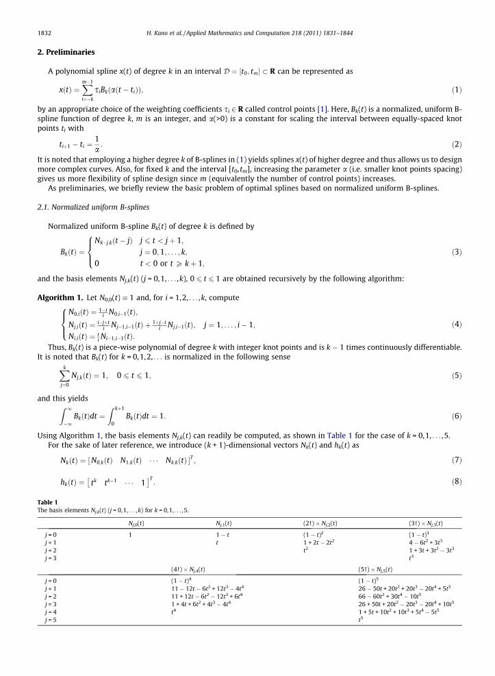
2. Preliminaries
A polynomial spline x(t) of degree k in an interval D ¼ ½t0; tm� � R can be represented as
Table 1The bas
j = 0j = 1j = 2j = 3
j = 0j = 1j = 2j = 3j = 4j = 5
xðtÞ ¼Xm�1
i¼�k
siBkðaðt � tiÞÞ; ð1Þ
by an appropriate choice of the weighting coefficients si 2 R called control points [1]. Here, Bk(t) is a normalized, uniform B-spline function of degree k, m is an integer, and a(>0) is a constant for scaling the interval between equally-spaced knotpoints ti with
tiþ1 � ti ¼1a: ð2Þ
It is noted that employing a higher degree k of B-splines in (1) yields splines x(t) of higher degree and thus allows us to designmore complex curves. Also, for fixed k and the interval [t0, tm], increasing the parameter a (i.e. smaller knot points spacing)gives us more flexibility of spline design since m (equivalently the number of control points) increases.
As preliminaries, we briefly review the basic problem of optimal splines based on normalized uniform B-splines.
2.1. Normalized uniform B-splines
Normalized uniform B-spline Bk(t) of degree k is defined by
BkðtÞ ¼Nk�j;kðt � jÞ j 6 t < jþ 1;
j ¼ 0;1; . . . ; k;0 t < 0 or t P kþ 1;
8><>: ð3Þ
and the basis elements Nj,k(t) (j = 0,1, . . . ,k), 0 6 t 6 1 are obtained recursively by the following algorithm:
Algorithm 1. Let N0,0(t) � 1 and, for i = 1,2, . . . ,k, compute
N0;iðtÞ ¼ 1�ti N0;i�1ðtÞ;
Nj;iðtÞ ¼ i�jþti Nj�1;i�1ðtÞ þ 1þj�t
i Nj;i�1ðtÞ; j ¼ 1; . . . ; i� 1;Ni;iðtÞ ¼ t
i Ni�1;i�1ðtÞ:
8><>: ð4Þ
Thus, Bk(t) is a piece-wise polynomial of degree k with integer knot points and is k � 1 times continuously differentiable.It is noted that Bk(t) for k = 0,1,2, . . . is normalized in the following sense
Xkj¼0
Nj;kðtÞ ¼ 1; 0 6 t 6 1; ð5Þ
and this yields
Z 1�1BkðtÞdt ¼
Z kþ1
0BkðtÞdt ¼ 1: ð6Þ
Using Algorithm 1, the basis elements Nj,k(t) can readily be computed, as shown in Table 1 for the case of k = 0,1, . . . ,5.For the sake of later reference, we introduce (k + 1)-dimensional vectors Nk(t) and hk(t) as
NkðtÞ ¼ N0;kðtÞ N1;kðtÞ � � � Nk;kðtÞ½ �T ; ð7Þ
hkðtÞ ¼ tk tk�1 � � � 1� �T
: ð8Þ
is elements Nj,k(t) (j = 0,1, . . . , k) for k = 0,1, . . . ,5.
Nj,0(t) Nj,1(t) (2!) � Nj,2(t) (3!) � Nj,3(t)
1 1 � t (1 � t)2 (1 � t)3
t 1 + 2t � 2t2 4 � 6t2 + 3t3
t2 1 + 3t + 3t2 � 3t3
t3
(4!) � Nj,4(t) (5!) � Nj,5(t)
(1 � t)4 (1 � t)5
11 � 12t � 6t2 + 12t3 � 4t4 26 � 50t + 20t2 + 20t3 � 20t4 + 5t5
11 + 12t � 6t2 � 12t3 + 6t4 66 � 60t2 + 30t4 � 10t5
1 + 4t + 6t2 + 4t3 � 4t4 26 + 50t + 20t2 � 20t3 � 20t4 + 10t5
t4 1 + 5t + 10t2 + 10t3 + 5t4 � 5t5
t5
H. Kano et al. / Applied Mathematics and Computation 218 (2011) 1831–1844 1833
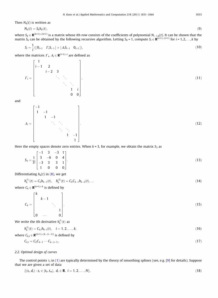
Then Nk(t) is written as
NkðtÞ ¼ SkhkðtÞ; ð9Þ
where Sk 2 R(k+1)�(k+1) is a matrix whose ith row consists of the coefficients of polynomial Ni�1,k(t). It can be shown that thematrix Sk can be obtained by the following recursive algorithm. Letting S0 = 1, compute Si 2 R(i+1)�(i+1) for i = 1,2, . . . ,k by
Si ¼1i
0iþ1 CiSi�1½ � þ DiSi�1 0iþ1½ �ð Þ; ð10Þ
where the matrices Ci, Di 2 R(i+1)�i are defined as
Ci ¼
1i� 1 2
i� 2 3. .
. . ..
. .. . .
.
1 i
0 0
26666666666664
37777777777775; ð11Þ
and
Di ¼
�11 �1
1 �1. .
. . ..
. .. . .
.
1 �11
26666666666664
37777777777775: ð12Þ
Here the empty spaces denote zero entries. When k = 3, for example, we obtain the matrix S3 as
S3 ¼13!
�1 3 �3 13 �6 0 4�3 3 3 11 0 0 0
26664
37775: ð13Þ
Differentiating hk(t) in (8), we get
hð1Þk ðtÞ ¼ Ckhk�1ðtÞ; hð2Þk ðtÞ ¼ CkCk�1hk�2ðtÞ; . . . ð14Þ
where Ck 2 R(k+1)�k is defined by
Ck ¼
k
k� 1. .
.
10 � � � 0
26666664
37777775: ð15Þ
We write the ith derivative hðiÞk ðtÞ as
hðiÞk ðtÞ ¼ Ck;ihk�iðtÞ; i ¼ 1;2; . . . ; k; ð16Þ
where Ck,i 2 R(k+1)�(k�(i�1)) is defined by
Ck;i ¼ CkCk�1 � � �Ck�ði�1Þ: ð17Þ
2.2. Optimal design of curves
The control points si in (1) are typically determined by the theory of smoothing splines (see, e.g. [9] for details). Supposethat we are given a set of data
fðsi; diÞ : si 2 ½t0; tm�; di 2 R; i ¼ 1;2; . . . ;Ng; ð18Þ
1834 H. Kano et al. / Applied Mathematics and Computation 218 (2011) 1831–1844
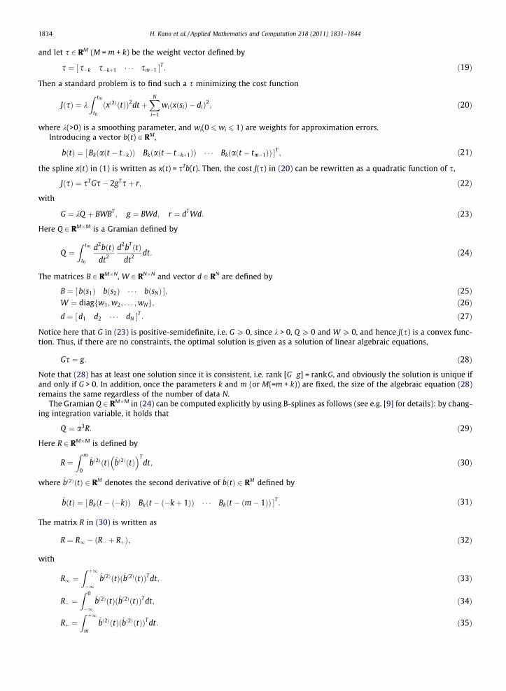
and let s 2 RM (M = m + k) be the weight vector defined by
s ¼ s�k s�kþ1 � � � sm�1½ �T : ð19Þ
Then a standard problem is to find such a s minimizing the cost function
JðsÞ ¼ kZ tm
t0
ðxð2ÞðtÞÞ2dt þXN
i¼1
wiðxðsiÞ � diÞ2; ð20Þ
where k(>0) is a smoothing parameter, and wi(0 6wi 6 1) are weights for approximation errors.Introducing a vector b(t) 2 RM,
bðtÞ ¼ Bkðaðt � t�kÞÞ Bkðaðt � t�kþ1ÞÞ � � � Bkðaðt � tm�1ÞÞ½ �T ; ð21Þ
the spline x(t) in (1) is written as x(t) = sTb(t). Then, the cost J(s) in (20) can be rewritten as a quadratic function of s,
JðsÞ ¼ sT Gs� 2gTsþ r; ð22Þ
with
G ¼ kQ þ BWBT ; g ¼ BWd; r ¼ dT Wd: ð23Þ
Here Q 2 RM�M is a Gramian defined by
Q ¼Z tm
t0
d2bðtÞdt2
d2bTðtÞdt2 dt: ð24Þ
The matrices B 2 RM�N, W 2 RN�N and vector d 2 RN are defined by
B ¼ bðs1Þ bðs2Þ � � � bðsNÞ½ �; ð25ÞW ¼ diagfw1;w2; . . . ;wNg; ð26Þd ¼ d1 d2 � � � dN½ �T : ð27Þ
Notice here that G in (23) is positive-semidefinite, i.e. G P 0, since k > 0, Q P 0 and W P 0, and hence J(s) is a convex func-tion. Thus, if there are no constraints, the optimal solution is given as a solution of linear algebraic equations,
Gs ¼ g: ð28Þ
Note that (28) has at least one solution since it is consistent, i.e. rank [G g] = rankG, and obviously the solution is unique ifand only if G > 0. In addition, once the parameters k and m (or M(=m + k)) are fixed, the size of the algebraic equation (28)remains the same regardless of the number of data N.
The Gramian Q 2 RM�M in (24) can be computed explicitly by using B-splines as follows (see e.g. [9] for details): by chang-ing integration variable, it holds that
Q ¼ a3R: ð29Þ
Here R 2 RM�M is defined by
R ¼Z m
0b̂ð2ÞðtÞ b̂ð2ÞðtÞ
� �Tdt; ð30Þ
where b̂ð2ÞðtÞ 2 RM denotes the second derivative of b̂ðtÞ 2 RM defined by
b̂ðtÞ ¼ Bkðt � ð�kÞÞ Bkðt � ð�kþ 1ÞÞ � � � Bkðt � ðm� 1ÞÞ½ �T : ð31Þ
The matrix R in (30) is written as
R ¼ R1 � ðR� þ RþÞ; ð32Þ
with
R1 ¼Z þ1
�1b̂ð2ÞðtÞðb̂ð2ÞðtÞÞT dt; ð33Þ
R� ¼Z 0
�1b̂ð2ÞðtÞðb̂ð2ÞðtÞÞT dt; ð34Þ
Rþ ¼Z þ1
mb̂ð2ÞðtÞðb̂ð2ÞðtÞÞT dt: ð35Þ
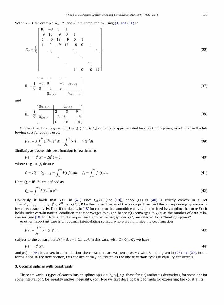
H. Kano et al. / Applied Mathematics and Computation 218 (2011) 1831–1844 1835
When k = 3, for example, R1, R� and R+ are computed by using (3) and (31) as
R1 ¼16
16 �9 0 1�9 16 �9 0 10 �9 16 �9 0 11 0 �9 16 �9 0 1
. .. . .
. . ..
. .. . .
.
. .. . .
.
1 0 �9 16
26666666666666664
37777777777777775
; ð36Þ
ð37Þ
and
ð38Þ
On the other hand, a given function f(t), t 2 [t0, tm] can also be approximated by smoothing splines, in which case the fol-lowing cost function is used.
JðsÞ ¼ kZ tm
t0
ðxð2ÞðtÞÞ2dt þZ tm
t0
ðxðtÞ � f ðtÞÞ2dt: ð39Þ
Similarly as above, this cost function is rewritten as
JðsÞ ¼ sT Gs� 2gTsþ fc; ð40Þ
where G, g and fc denote
G ¼ kQ þ Q 0; g ¼Z tm
t0
bðtÞf ðtÞdt; f c ¼Z tm
t0
f 2ðtÞdt: ð41Þ
Here, Q0 2 RM�M are defined as
Q 0 ¼Z tm
t0
bðtÞbTðtÞdt: ð42Þ
Obviously, it holds that G > 0 in (41) since Q0 > 0 (see [10]), hence J(s) in (40) is strictly convex in s. Letsc ¼ ½sc
�k; sc�kþ1; . . . ; sc
m�1�T 2 RM and xc(t) 2 R be the optimal vector of the above problem and the corresponding approximat-
ing curve respectively. Then if the data di in (18) for constructing smoothing curves are obtained by sampling the curve f(t), itholds under certain natural condition that s converges to sc and hence x(t) converges to xc(t) as the number of data N in-creases (see [10] for details). In the sequel, such approximating splines xc(t) are referred to as ‘‘limiting splines’’.
Another important case is an optimal interpolating splines, where we minimize the cost function
JðsÞ ¼Z tm
t0
ðxð2ÞðtÞÞ2dt ð43Þ
subject to the constraints x(si) = di, i = 1,2, . . . ,N. In this case, with G = Q(P0), we have
JðsÞ ¼ sT Gs; ð44Þ
and J(s) in (44) is convex in s. In addition, the constraints are written as Bs = d with B and d given in (25) and (27). In theformulation in the next section, this constraint may be treated as the one of various types of equality constraints.
3. Optimal splines with constraints
There are various types of constraints on splines x(t), t 2 [t0, tm], e.g. those for x(t) and/or its derivatives, for some t or forsome interval of t, for equality and/or inequality, etc. Here we first develop basic formula for expressing the constraints.
1836 H. Kano et al. / Applied Mathematics and Computation 218 (2011) 1831–1844
Since x(t) is a piece-wise polynomial of degree k, we examine the polynomial in each interval [tj, tj+1) for j = 0,1, . . . ,m�1.Focusing on the interval [tj, tj+1), the spline x(t) in (1) is written as
xðtÞ ¼Xj
i¼�kþj
siBkðaðt � tiÞÞ: ð45Þ
Using (3), we then get
xðtÞ ¼Xk
i¼0
sj�kþiNi;kðaðt � tjÞÞ; t 2 ½tj; tjþ1Þ; ð46Þ
and it depends on only the k + 1 weights sj�k,sj�k+1, . . . ,sj. Moreover, by introducing a new variable u,
u ¼ aðt � tjÞ; ð47Þ
the interval [tj, tj+1) in t is normalized to [0,1) in u, and we may write x(t) as x̂ðuÞ,
x̂ðuÞ ¼Xk
i¼0
sj�kþiNi;kðuÞ; u 2 ½0;1Þ: ð48Þ
Letting s(j) 2 Rk+1 be
sðjÞ ¼ ½sj�k; sj�kþ1; . . . ; sj�T ð49Þ
and using (9), we may rewrite x̂ðuÞ in (48) as x̂ðuÞ ¼ NTkðuÞsðjÞ and hence xðtÞ ¼ NT
kðuÞsðjÞ.In general, the lth derivative x(l)(t) for t 2 [tj, tj+1) is expressed in terms of u 2 [0,1) in (47) by
xðlÞðtÞ ¼ alx̂ðlÞðuÞ; l ¼ 0;1;2; . . . ; ð50Þ
with
x̂ðlÞðuÞ ¼ NðlÞk ðuÞ� �T
sðjÞ: ð51Þ
Here NðlÞk ðuÞ is obtained from (9) and (16) as
NðlÞk ðuÞ ¼ SkhðlÞk ðuÞ ¼ SkCk;lhk�lðuÞ: ð52Þ
Now we are in a position to derive various types of constraints on x(t). For the sake of simplicity, we consider the case ofcubic splines, i.e. k = 3.
3.1. Pointwise constraints
We first consider the case of pointwise constraints. By (50) and (51), we observe that any linear constraint on the value ofx(l)(t) for given t 2 [tj, tj+1) is specified as a linear constraint on the vector s 2 RM, since s(j) in (49) is a sub-vector of s. Specif-ically, x(l)(t) is written as
xðlÞðtÞ ¼ aTs; ð53Þ
where
aT ¼ 0Tj alNðlÞ3 ðuÞ
T 0TM�j�4
h i: ð54Þ
Only the point in [t0, tm] that is not covered in the foregoing arguments is t = tm. However, the values of x(l)(t) at t = tm for l = 0,1, 2 are obtained, by the continuity of these functions. Namely, by letting j = m � 1 and u = 1, we have the expression
xðlÞðtmÞ ¼ aTs; aT ¼ 0TM�4 alNðlÞ3 ð1Þ
Th i
: ð55Þ
If we need to constrain x(3)(t) at t = tm, which is piecewise constant and is discontinuous at the knot points, we simply regardthat xð3ÞðtmÞ ¼ limt!tm xð3ÞðtÞ, implying that (55) holds also for l = 3.
In particular, if t is taken to be the knot point t = tj (j = 0,1, . . . ,m � 1) and hence u = 0, we obtain NðlÞ3 ð0ÞT from (52) as
NðlÞ3 ð0ÞT ¼
16 1 4 1 0½ � l ¼ 012 �1 0 1 0½ � l ¼ 11 �2 1 0½ � l ¼ 2�1 3 �3 1½ � l ¼ 3
8>>><>>>:
: ð56Þ
H. Kano et al. / Applied Mathematics and Computation 218 (2011) 1831–1844 1837
For example, in order to impose the initial condition xðt0Þ ¼ _xðt0Þ ¼ €xðt0Þ ¼ 0, we simply introduce the condition As = 03,where A 2 R3�M is derived from (54) with j = 0 and (56) as
A ¼Nð0Þ3 ð0Þ
T 0TM�4
aNð1Þ3 ð0ÞT 0T
M�4
a2Nð2Þ3 ð0ÞT 0T
M�4
2664
3775 ¼
16
46
16 0 � � � 0
� a2 0 a
2 0 � � � 0a2 �2a2 a2 0 � � � 0
264
375: ð57Þ
Terminal conditions for t = tm may be defined similarly by using (55).To conclude, the above method can be used to specify equality or inequality constraint on x(l)(t) for given t 2 [t0, tm] and
l = 0,1,2, . . . ,k as linear constraint on the control point vector s.
3.2. Constraints over knot point intervals
Next we consider the cases of constraints over knot point intervals. Specifically, we begin with an inequality constraint ina single knot point interval as
xðtÞP f ðtÞ; 8t 2 ½tj; tjþ1Þ ð58Þ
for a given continuous function f(t). Note that this inequality ‘P’ may readily be replaced with ‘6’ and equality ‘=’ in the sub-sequent developments.
First we assume that f(t) is itself a spline expressed in the same form of x(t) as
f ðtÞ ¼Xm�1
i¼�3
sfi B3ðaðt � tiÞÞ: ð59Þ
Then f(t) in the interval [tj, tj+1) is written as
f ðtÞ ¼Xj
i¼j�3
sfi B3ðaðt � tiÞÞ; t 2 ½tj; tjþ1Þ ð60Þ
and, similarly as (45)–(48) with k = 3, we get
f ðtÞ ¼ f̂ ðuÞ ¼X3
i¼0
sfj�3þiNi;3ðuÞ; u 2 ½0;1Þ ð61Þ
with u = a(t � tj). Note that the expression (59) valid for entire interval [t0, tm] is not necessary in the present arguments, butis included for the sake of later convenience.
Then, the constraint in (58) may be realized by imposing the condition si P sfi for i = j � 3, j � 2, j � 1, j, or in terms of the
control point vector s as
Ejs P v ; v ¼ sfj�3; s
fj�2; s
fj�1; s
fj
h iT; ð62Þ
where the matrix Ej 2 R4�M is defined by
Ej ¼ 04;j I4 04;M�j�4½ �: ð63Þ
This is because, if si P sfi holds for i = j � 3, j � 2, j � 1, j, we have from (46)–(48) and (61),
xðtÞ ¼ x̂ðuÞ ¼X3
i¼0
sj�3þiNi;3ðuÞPX3
i¼0
sfj�3þiNi;3ðuÞ ¼ f̂ ðuÞ ¼ f ðtÞ; 8t 2 ½tj; tjþ1Þ
since Ni,3(u) P 0, "u 2 [0,1].A simple but useful example of f(t) in (60) is a linear function in t, say,
f ðtÞ ¼ pðt � t0Þ þ q: ð64Þ
Here we derive an expression for the associated control points sfi . As for (60), the relations (50) and (51) with l = 0 and k = 3
become f ðtÞ ¼ f̂ ðuÞ and f̂ ðuÞ ¼ ðN3ðuÞÞTv for v in (62), and (9) yields
hT3ðuÞS
T3v ¼ f̂ ðuÞ: ð65Þ
Moreover, using u = a(t � tj) and (2) in (64), f̂ ðuÞ is expressed as f̂ ðuÞ ¼ p̂uþ q̂ with p̂ ¼ pa and q̂ ¼ j p
aþ q. Noting (8) in (65), wethen get the following equation on the vector v,
ST3v ¼ r; r ¼ 0 0 p̂ q̂
� �T: ð66Þ
1838 H. Kano et al. / Applied Mathematics and Computation 218 (2011) 1831–1844
Using the matrix S3 in (13), we obtain the solution v as
v ¼ �p̂þ q̂ q̂ p̂þ q̂ 2p̂þ q̂� �T ¼ j�1
a pþ q ja pþ q jþ1
a pþ q jþ2a pþ q
h iT; ð67Þ
or, the expression for each element sfi of v as
sfi ¼
iþ 2a
pþ q; i ¼ j� 3; j� 2; j� 1; j: ð68Þ
On the other hand, if the function f(t) is not expressed as in (59), the constraint in (58) may be imposed by employing theidea of ‘‘limiting splines’’ in (39) as follows: for the given function f(t), we first compute the limiting spline xc(t) with thesame form and the same degree k = 3 as in (1), i.e.
xcðtÞ ¼Xm�1
i¼�3
sci B3ðaðt � tiÞÞ: ð69Þ
From our past works (e.g. see [10]), we have empirically confirmed that the curves xc(t) can approximate functions f(t) fairlyprecisely, i.e. xc(t) � f(t). We thus use the constraint x(t) P xc(t) instead of x(t) P f(t), and then we see that x(t) P xc(t) is real-
ized by the inequality (62) with the vector v ¼ scj�3; sc
j�2; scj�1; sc
j
h iT.
The above arguments for the single knot point interval [tj, tj+1) are easily extended to larger interval [tj, tl) for any j and l(0 6 j < l 6m). For example, the constraint
xðtÞP f ðtÞ; 8t 2 ½tj; tlÞ ð70Þ
is satisfied by the condition si P sfi ; i ¼ j� 3; j� 2; . . . ; l� 1, or equivalently
Ej;ls P v 0; v 0 ¼ ½ sfj�3 sf
j�2 � � � sfl�1 �
T 2 Rl�jþ3; ð71Þ
where Ej,l 2 R(l�j+3)�M is defined by
Ej;l ¼ 0l�jþ3;j Il�jþ3 0l�jþ3;M�l�3½ �: ð72Þ
If we impose the above constraint x(t) P f(t) in (70) on the entire interval [t0, tm), letting j = 0 and l = m in (72) yields
E0,m = IM. Hence, the inequality (71) reduces to s P v0 with v 0 ¼ sf�3s
f�2 � � � sf
m�1
h iT2 RM . If f(t) is given by (64), we see from
(68) that this vector v0 is given as
v 0 ¼ �1a pþ q q 1
a pþ q � � � mþ1a pþ q
� �T: ð73Þ
It is noted that the above inequality conditions on the control point vector s such as (62) are only sufficient for those onfunctions x(t) as (58).
3.3. Constraints on integral values
We finally consider the case of an equality or inequality constraint on the value of integralR tm
t0xðtÞdt. From (50) and (51)
with l = 0 and (47), we get
Z tmt0
xðtÞdt ¼Xm�1
j¼0
Z tjþ1
tj
xðtÞdt ¼ 1aXm�1
j¼0
Z 1
0x̂ðuÞdu ¼ 1
aXm�1
j¼0
sTðjÞ
Z 1
0N3ðuÞdu:
Noting that NT3ðuÞ ¼ ½N0;3ðuÞ; N1;3ðuÞ; N2;3ðuÞ; N3;3ðuÞ� and s(j) = [sj�3, sj�2, sj�1, sj]T, we obtain
aZ tm
t0
xðtÞdt ¼X�1
j¼�3
sj
Xjþ3
i¼0
Z 1
0Ni;3ðuÞduþ
Xm�4
j¼0
sj
X3
i¼0
Z 1
0Ni;3ðuÞduþ
Xm�1
j¼m�3
sj
X3
i¼j�mþ4
Z 1
0Ni;3ðuÞdu:
Here, using (9) and (8), we get
Z 10N3ðuÞdu ¼ 1
241 11 11 1½ �T : ð74Þ
From the above two equations, the integral valueR tm
t0xðtÞdt is expressed as a linear function in s,
Z tmt0
xðtÞdt ¼ aTs; ð75Þ
where a 2 RM is given by
a ¼ 124a
1 12 23 24 � � � 24 23 12 1½ �T : ð76Þ
H. Kano et al. / Applied Mathematics and Computation 218 (2011) 1831–1844 1839
3.4. Constrained splines
As the foregoing development indicates, we can expect that a large number of constrained spline problems may be trea-ted in the above settings. The formulation is simple and is very well fit for numerical solutions as quadratic programing prob-lems. Namely, the optimal smoothing or interpolating splines are obtained by minimizing the convex quadratic cost J(s) asshown in (22), (40) and (44), whereas a number of constraints on the splines as in Sections 3.1–3.3 may be expressed as lin-ear constraints on s, either equality or inequality or both. A general form of problems is
mins2RM
JðsÞ ¼ 12sT Gsþ gTs ð77Þ
subject to the constraints of the form
As ¼ d; f 1 6 Es 6 f2; h1 6 s 6 h2; ð78Þ
for some matrices and vectors of appropriate dimensions. A very efficient numerical algorithm is available for this purpose(see, e.g. [11]).
On the other hand, if only equality constraints As = d in (78) are to be imposed on the spline, we could clearly proceedfurther by using Lagrange function,
Lðs;lÞ ¼ JðsÞ þ lTðAs� dÞ: ð79Þ
By the standard procedure, we get a system of equations in s and the Lagrange multipliers l,
G AT
A 0
" #sl
� �¼�g
d
� �: ð80Þ
This is the case when we specify the initial and/or terminal conditions on x(t) as described in Section 3.1. Periodic splines canalso be treated in this settings by imposing sj = sm+j, j = �k,�k + 1, . . . ,�1, which yields x(i)(t0) = x(i)(tm), i = 0,1, . . . ,k � 1 andhence the periodicity.
4. Numerical examples
We examine the design method presented in the previous sections numerically. As examples, we consider the three prob-lems: approximation of probability density functions (Section 4.1), approximation of discontinuous functions (Section 4.2),and trajectory planning (Section 4.3). In all the cases, cubic splines, i.e. k = 3, is used.
4.1. Approximation of probability density functions
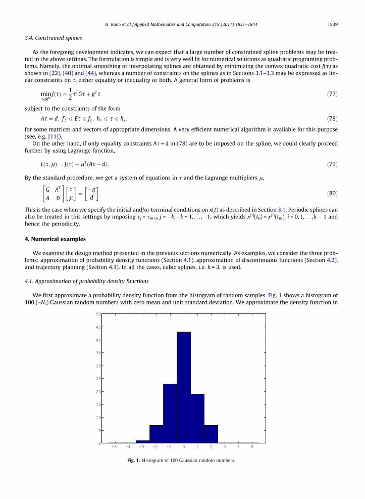
We first approximate a probability density function from the histogram of random samples. Fig. 1 shows a histogram of100 (=Ns) Gaussian random numbers with zero mean and unit standard deviation. We approximate the density function in
Fig. 1. Histogram of 100 Gaussian random numbers.
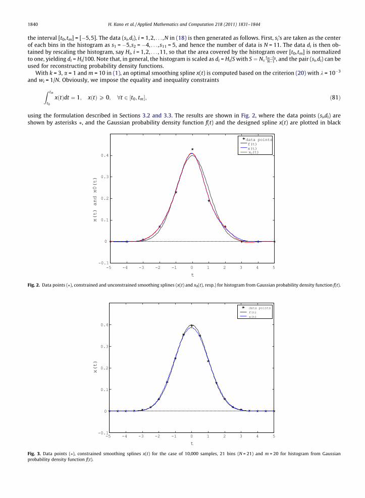
1840 H. Kano et al. / Applied Mathematics and Computation 218 (2011) 1831–1844
the interval [t0, tm] = [�5,5]. The data (si,di), i = 1,2, . . . ,N in (18) is then generated as follows. First, si’s are taken as the centerof each bins in the histogram as s1 = �5,s2 = �4, . . . ,s11 = 5, and hence the number of data is N = 11. The data di is then ob-tained by rescaling the histogram, say Hi, i = 1,2, . . . ,11, so that the area covered by the histogram over [t0, tm] is normalizedto one, yielding di = Hi/100. Note that, in general, the histogram is scaled as di = Hi/S with S ¼ Ns
tm�t0N�1 , and the pair (si,di) can be
used for reconstructing probability density functions.With k = 3, a = 1 and m = 10 in (1), an optimal smoothing spline x(t) is computed based on the criterion (20) with k = 10�3
and wi = 1/N. Obviously, we impose the equality and inequality constraints
Fig. 2.
Fig. 3.probab
Z tm
t0
xðtÞdt ¼ 1; xðtÞP 0; 8t 2 ½t0; tm�; ð81Þ
using the formulation described in Sections 3.2 and 3.3. The results are shown in Fig. 2, where the data points (si,di) areshown by asterisks ⁄, and the Gaussian probability density function f(t) and the designed spline x(t) are plotted in black
Data points (⁄), constrained and unconstrained smoothing splines (x(t) and x0(t), resp.) for histogram from Gaussian probability density function f(t).
Data points (⁄), constrained smoothing splines x(t) for the case of 10,000 samples, 21 bins (N = 21) and m = 20 for histogram from Gaussianility density function f(t).
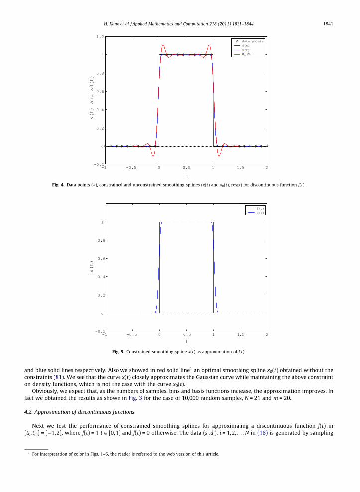
Fig. 4. Data points (⁄), constrained and unconstrained smoothing splines (x(t) and x0(t), resp.) for discontinuous function f(t).
Fig. 5. Constrained smoothing spline x(t) as approximation of f(t).
H. Kano et al. / Applied Mathematics and Computation 218 (2011) 1831–1844 1841
and blue solid lines respectively. Also we showed in red solid line1 an optimal smoothing spline x0(t) obtained without theconstraints (81). We see that the curve x(t) closely approximates the Gaussian curve while maintaining the above constrainton density functions, which is not the case with the curve x0(t).
Obviously, we expect that, as the numbers of samples, bins and basis functions increase, the approximation improves. Infact we obtained the results as shown in Fig. 3 for the case of 10,000 random samples, N = 21 and m = 20.
4.2. Approximation of discontinuous functions
Next we test the performance of constrained smoothing splines for approximating a discontinuous function f(t) in[t0, tm] = [�1,2], where f(t) = 1 t 2 [0,1) and f(t) = 0 otherwise. The data (si,di), i = 1,2, . . . ,N in (18) is generated by sampling
1 For interpretation of color in Figs. 1–6, the reader is referred to the web version of this article.
1842 H. Kano et al. / Applied Mathematics and Computation 218 (2011) 1831–1844
f(t) at 30(=N) points, si, equality spaced in [�1,2], namely di = f(si). Setting the design parameters in (1) as k = 3,a = 100/3 andm = 100, an optimal smoothing spline x(t) is computed based on the criterion (20) with k = 10�8 and wi = 1/N, "i. On design-ing the curve x(t), we imposed the inequality constraints
0 6 xðtÞ 6 1; 8t 2 ½t0; tm� ð82Þ
Fig. 6. Planned trajectories x(t) (top), _xðtÞ (middle) and €xðtÞ (bottom), and their counterparts x0(t), _x0ðtÞ and €x0ðtÞ without (70).
H. Kano et al. / Applied Mathematics and Computation 218 (2011) 1831–1844 1843
by using the formulation described in Section 3.2. The result is shown in Fig. 4 (blue line) together with the true curve f(t)(black line), and a smoothing spline x0(t) (red line) obtained without the constraints (82). Fig. 5 depicts only x(t) and f(t) forthe sake of clarity. Although it seems that the smoothing splines are not very suitable for approximating curve with jumps,we could recover the original function f(t) surprisingly accurately. This is partly due to the design specifications that we usedfairly many basis functions, i.e. m = 100 for the interval [�1,2] and that we used small smoothing parameter k(=10�8). Gibbsphenomenon does not occur in x(t) unlike the case of x0(t).
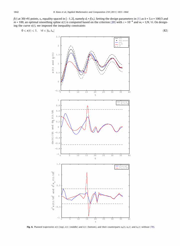
4.3. Trajectory planning
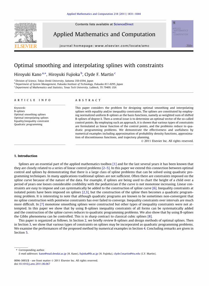
We finally consider a trajectory planning problem with equality and inequality constraints. Specifically, we design anoptimal smoothing spline x(t) in the time interval [t0, tm] = [0,36] such that
z�ðtÞ 6 xðtÞ 6 zþðtÞ; 8t 2 ½0;36�; ð83Þ
where z±(t) is z±(t) = f(t) ± c for a function f(t) and a constant c > 0. Here, we take the function f(t) as
f ðtÞ ¼ �eat cosðbtÞ þ 1 ð84Þ
with a ¼ 1tm
log 14 and b ¼ 6p
tm, and c is set as c = 0.2. We set a = 1 and m = 36 in (1), hence the knot points are ti = i,
i = �3,�2, . . . ,m � 1. The initial and terminal conditions are set as
xðt0Þ ¼ xð1Þðt0Þ ¼ xð2Þðt0Þ ¼ 0;
xðtmÞ ¼ 0:75; xð1ÞðtmÞ ¼ xð2ÞðtmÞ ¼ 0;ð85Þ
and the magnitudes of the velocity and acceleration are limited at all the knot points as
jxð1ÞðtiÞj 6 0:65; jxð2ÞðtiÞj 6 0:35; i ¼ 0;1; . . . ;m: ð86Þ
Now, since the functions z±(t) are not the splines in the form of (59), the constraints in (83) are imposed by employing theassociated limiting splines xc ðtÞ as described in Section 3.2, i.e.
x�c ðtÞ 6 xðtÞ 6 xþc ðtÞ; 8t 2 ½0;36�: ð87Þ
In addition, (85) and (86) are pointwise constraints and the method in Section 3.1 can be used. For designing optimalsmoothing splines x(t), the data di in (18) is obtained by sampling the curve f(t). Here, the number of data is set as N = 15,si’s are randomly spaced in the interval [t0, tm] = [0,36], and the magnitude of the additive Gaussian noise in di is set asr = 0.1. The smoothing parameter k is set as k = 10�3. The optimal weight s is computed together with the associated splinesx(t).
Fig. 6 shows the results, x(t) and its derivatives in blue lines. In the figure, the red lines show the optimal splines x0(t)obtained without the constraints in (86) and (87). We see that the trajectory x(t) satisfies all the constraints. Note thatthe acceleration profile is piecewise linear due to cubic spline (k = 3), and hence the constraints in (87) at the knot pointsguarantees jx(2)(t)j 6 0.35, "t 2 [0,36]. On the other hand, we see that the velocity constraint at the knot points yieldedjx(1)(t)j 6 0.65, "t 2 [0,36] in this case, although it is not guaranteed theoretically.
5. Concluding remarks
We presented a systematic method for designing optimal smoothing and interpolating splines with equality and/orinequality constraints. The splines are constituted employing normalized uniform B-splines as the basis functions, and hencethe central issue is to determine an optimal vector s of the so-called control points. Such an approach enables us to expressvarious types of constraints as linear function of s, including those on the spline x(t), its derivatives and integral. The designproblem becomes the quadratic programming problem in s, where very efficient numerical algorithms are available. Weexamined the performances of the design method by numerical examples, namely, approximation of probability densityfunctions, approximation of discontinuous functions without Gibbs-like phenomenon, and trajectory planning problem withequality and inequality constraints. It is our conclusion that the method is effective as well as very useful for various types ofproblems.
References
[1] C. de Boor, A Practical Guide to Splines, Revised ed., Springer-Verlag, New York, 2001.[2] S. Sun, M. Egerstedt, C.F. Martin, Control theoretic smoothing splines, IEEE Trans. Automat. Control. 45 (12) (2000) 2271–2279.[3] C.F. Martin, S. Sun, M. Egerstedt, Optimal control, statistics and path planning. Computation and control, VI (Bozeman, MT, 1998), Math. Comput.
Model. 33 (1–3) (2001) 237–253.[4] Z. Zhang, J. Tomlinson, C.F. Martin, Splines and linear control theory, Acta Appl. Math. 49 (1) (1997) 1–34.[5] H. Kano, M. Egerstedt, H. Nakata, C. Martin, B-splines and control theory, Appl. Math. Comput. 145 (2-3) (2003) 263–288.[6] Y. Zhou, M. Egerstedt, C.F. Martin, Hilbert space methods for control theoretic splines: a unified treatment, Commun. Inf. Syst. 6 (1) (2006) 55–82.[7] M. Egerstedt, C.F. Martin, Optimal control and monotone smoothing splines, in: New trends in nonlinear dynamics and control, and their applications,
Lecture Notes in Control and Inform. Sci, vol. 295, Springer, Berlin, 2003, pp. 279–294.

1844 H. Kano et al. / Applied Mathematics and Computation 218 (2011) 1831–1844
[8] Z. Zhang, C.F. Martin, Convergence and Gibbs’ phenomenon in cubic spline interpolation of discontinuous functions, J. Comput. Appl. Math. 87 (2)(1997) 359–371.
[9] H. Kano, H. Nakata, C.F. Martin, Optimal curve fitting and smoothing using normalized uniform B-splines: a tool for studying complex systems, Appl.Math. Comput. 169 (1) (2005) 96–128.
[10] H. Fujioka, H. Kano, M. Egerstedt, C. Martin, Smoothing spline curves and surfaces for sampled data, Int. J. Innovative Comput. Inf. Control 1 (3) (2005)429–449.
[11] J. Nocedal, S.J. Wright, Numerical Optimization (Springer Series in Operations Research and Financial Engineering), second ed., Springer, 2006.
Related Documents
![Regression with Ordered Predictors via Ordinal Smoothing Splines · powerful smoothing spline ANOVA framework [15]—provides an appealing approach for including ordinal predictors](https://static.cupdf.com/doc/110x72/5f56b73c555d7b2ea3790a9a/regression-with-ordered-predictors-via-ordinal-smoothing-splines-powerful-smoothing.jpg)