Some performances of local bivariate quadratic C1 quasi-interpolating splines on nonuniform type-2 triangulations

Journal of Computational and Applied Mathematics 173 (2005) 21–37www.elsevier.com/locate/cam

Some performances of local bivariate quadratic C1

quasi-interpolating splines on nonuniform type-2 triangulationsCatterina Dagnino∗, Paola Lamberti∗

Dipartimento di Matematica, Universit�a di Torino, via C. Alberto 10, Torino I-10123, Italy

Received 20 November 2003; received in revised form 22 January 2004

Abstract

We investigate spline quasi-interpolants de1ned by C1 bivariate quadratic B-splines on nonuniform type-2triangulations and by discrete linear functionals based on a 1xed number of triangular mesh-points either inthe support or close to the support of such B-splines.We show they can approximate a real function and its partial derivatives up to an optimal order and we

derive local and global upper bounds.We also present some numerical and graphical results.

c© 2004 Elsevier B.V. All rights reserved.

MSC: 65D07; 65D10; 41A25

Keywords: Bivariate splines; Approximation order by splines

1. Introduction

The spline space with which we are concerned in this paper is the linear space de1ned on anonuniform type-2 triangulation �(2∗)

mn of a rectangular domain S and spanned by the sequence ofbivariate quadratic C1 B-splines introduced in [3,18].

Nonuniform triangulations can be more useful than the uniform ones ([2,4–7,11,14,19], etc.),because they allow to make many subdivisions in the vicinity of a variation or irregularity of theapproximated function.

The above bivariate quadratic C1 spline space is denoted by S12 (�

(2∗)mn ). In particular we consider

spline operators of quasi-interpolating (q-i) kind (i.e. local, bounded in some relevant norm andreproducing a polynomial space of a certain order l¡ 3), that are based only on function values.

∗ Corresponding author.E-mail addresses: [email protected] (C. Dagnino), [email protected] (P. Lamberti).

0377-0427/$ - see front matter c© 2004 Elsevier B.V. All rights reserved.doi:10.1016/j.cam.2004.02.017

22 C. Dagnino, P. Lamberti / Journal of Computational and Applied Mathematics 173 (2005) 21–37

Recently some special q-i operators in S12 (�

(2∗)mn ) have been proposed and studied in [20] and a

computational procedure for their generation has been given in [7,8].In this paper we continue the investigation on how well q-i splines in S1

2 (�(2∗)mn ) approximate a

function f and its partial derivatives.In Section 2 we introduce the q-i spline operators, that we denote by Amn and whose approximation

power for functions f∈Ck(S); k¿ 0, we analyze in Section 3. Our main results lie in proving thatboth Amnf can approximate f and Dr DrAmnf can approximate the partial derivatives Dr Drf, locallyfor r + Dr = 1; 2 and globally for r + Dr = 1 up to an optimal order if l= 3 and nearly optimal orderif l = 2. Moreover we give upper bounds both for the approximation errors and for ‖Dr DrAmnf‖,locally for r + Dr = 1; 2 and globally for r + Dr = 1, in case Amnf is more diGerentiable than f.

In Section 4 we present two interesting choices of q-i operators Amn, already introduced and par-tially studied in [20], for which, thanks to the general results of Section 3, we prove new properties.

Numerical and graphical examples are given in Section 5.Finally in Section 6 we present 1nal remarks and some studies in progress.

2. C 1 bivariate local splines on nonuniform triangulations

Let S = [a; b] × [c; d]. We use horizontal and vertical lines x − xi = 0 and y − yj = 0; i =1; : : : ; m− 1; j=1; : : : ; n− 1, where a= x0 ¡x1 ¡ · · ·¡xm = b and c= y0 ¡y1 ¡ · · ·¡yn = d, topartition S into mn rectangular cells Sij=[xi; xi+1]×[yj; yj+1]; i=0; : : : ; m−1; j=0; : : : ; n−1, wherem; n are given integers. By drawing both diagonals in each Sij we obtain a type-2 triangulation �(2∗)

mn

(Fig. 1). For 16 i6m; 16 j6 n let hi=xi −xi−1; kj=yj −yj−1, respectively. Such a triangulationis said to be uniform if hi=hi−1 and kj=kj−1; i=1; : : : ; m; j=1; : : : ; n and it yields a four-directionalmesh.

Let S12 (�

(2∗)mn ) denote the space of C1 functions whose restrictions on each triangular cell of �(2∗)

mn

are polynomials of total degree 2, i.e.∑

i+j62 aijxiyj; i; j¿ 0; aij ∈R. Such functions are calledbivariate C1 splines of total degree 2. A nontrivial bivariate spline with minimum support is calleda B-spline.

Fig. 1. �(2∗)mn , type-2 nonuniform triangulation of S.

C. Dagnino, P. Lamberti / Journal of Computational and Applied Mathematics 173 (2005) 21–37 23

Fig. 2. Qij , support of Bij .

Fig. 3. Some values of the function Bij on its support Qij .

The B-spline Bij ∈ S12 (�

(2∗)mn ) has been obtained at the same time in [3,14,18]: it has got a local

support Qij given by the union of 28 triangular cells �(ij)k , labeled by k as in Fig. 2, and has center

at ((xi + xi+1)=2; (yj + yj+1)=2). While in the case of a four directional mesh the center cross ofthe support is not active, i.e. the same quadratic polynomial is de1ned in the cells 1a–d, when theoriginal rectangular partition is nonuniform, the center cross is, in general, active and the peak isnot necessarily attained at the center of this cross.

Moreover, since in every triangular cell of Qij the function Bij is a polynomial of total degree 2,it can be uniquely determined by its values at the three vertices and at the mid-points of the sides,as shown in Fig. 3. Such values have been obtained in [3,18].

24 C. Dagnino, P. Lamberti / Journal of Computational and Applied Mathematics 173 (2005) 21–37

Some of the most important properties of Bij are included in the following theorem proved in[3,18].

Theorem 1. Let x−2 ¡x−1 ¡a = x0 ¡x1 ¡ · · ·¡xm = b¡xm+1 ¡xm+2 and y−2 ¡y−1 ¡c =y0 ¡y1 ¡ · · ·¡yn = d¡yn+1 ¡yn+2. Then

1. for −16 i6m and −16 j6 n; Bij is unique and strictly positive inside its support andevery function in S1

2 (�(2∗)mn ) supported by the support of Bij is a constant multiple of Bij;

2.∑m

i=−1

∑nj=−1 Bij(x; y) = 1; ∀(x; y)∈ S;

3.∑m

i=−1

∑nj=−1 (−1)i+jhi+1kj+1Bij(x; y) = 0; ∀(x; y)∈ S;

4. for each (i0; j0); −16 i06m; −16 j06 n, the collection

{Bij : (i; j) = (i0; j0); −16 i6m; −16 j6 n}is a basis of S1

2 (�(2∗)mn ).

Now we consider linear operators

Amn : C(�) → S12 (�

(2∗)mn )

de1ned by

Amnf(x; y) =∑ij

�ijfBij(x; y); (1)

where � is an open set containing S and {�ij} i=−1; :::; mj=−1; :::; n

is a set of linear functionals �ij : C(�) → Rof the form:

�ijf =p∑

�=1

w�f(x(i)� ; y( j)� ); (2)

involving only a 1nite 1xed number p¿ 1 of triangular mesh-points (x(i)� ; y( j)� ) either in the support

or close to the support Qij and of real nonzero weights w�. Moreover the �ij’s are assumed to besuch that Amnf=f for all f∈Pl; 16 l6 3 with Pl the class of all polynomials in two variablesof total degree less than l.

Moreover Amn is a local approximation scheme, because the value of Amnf(x; y) depends only onthe values of f in a neighborhood of (x; y). In fact, if u and v are integers such thatxu6 t ¡ xu+1; yv6 Dt ¡yv+1; 06 u6m − 1; 06 v6 n − 1, then (t; Dt) will belong to one of thefour triangles T (#)

uv of �(2∗)mn ; #= 1; 4, labeled by # in Fig. 4.

On every triangle T (#)uv ; #=1; 4, just seven B-splines Bij are nonzero according to Table 1, where

we report the indices of such B-splines, as functions of u and v.Then if (t; Dt)∈T (#)

uv , for a 1xed #, there results

Amnf(t; Dt) =∑ij=

T (#)uv ∩Qij �=∅

�ijfBij(t; Dt): (3)

C. Dagnino, P. Lamberti / Journal of Computational and Applied Mathematics 173 (2005) 21–37 25

Fig. 4. Four diGerent kinds of cells in �(2∗)mn .

Table 1Indices of nonzero B-splines Bij on the four triangles T (#)

uv ; # = 1; 4

T (1)uv T (2)

uv T (3)uv T (4)

uv

u; v − 1 u − 1; v − 1 u − 1; v − 1 u; v − 1u − 1; v u; v − 1 u; v − 1 u+ 1; v − 1u; v u − 1; v u+ 1; v − 1 u − 1; v

i; j u+ 1; v u; v u − 1; v u; vu − 1; v + 1 u+ 1; v u; v u+ 1; vu; v + 1 u − 1; v + 1 u+ 1; v u; v + 1u+ 1; v + 1 u; v + 1 u; v + 1 u+ 1; v + 1

3. On the approximation power of Amn

Let

Er Drs(t; Dt) =

{Dr Dr(f − Amnf)(t; Dt); 06 r + Dr ¡ s;

Dr DrAmnf(t; Dt); s6 r + Dr ¡ 3;(4)

where (t; Dt)∈ S; Dr Dr=(@r+ Dr)=@xr@y Dr and the parameter s is introduced since the approximation Amnfcould be more diGerentiable than f.

The purpose of this section is to obtain estimates for Er Drs in order to provide some tools todescribe how well q-i splines of form (1) approximate a smooth function f and its derivatives up to(nearly) optimal approximation order. In addition we give a bound for partial derivatives of Amnf.Since Amn reproduces polynomials belonging to Pl, there results ([5,10]) that (4) is equivalent to

Er Drs(t; Dt) =

{Dr DrR(t; Dt) − Dr DrAmnR(t; Dt); 06 r + Dr ¡ s;

Dr DrAmnR(t; Dt); s6 r + Dr ¡ 3(5)

for any g∈Ps and any f such that Dr Drf(t; Dt) exists, where 06 r + Dr ¡ s6 l6 3 and R(x; y) =f(x; y) − g(x; y).

26 C. Dagnino, P. Lamberti / Journal of Computational and Applied Mathematics 173 (2005) 21–37

It is easy to verify that, if g is the Taylor expansion of f at (t; Dt), then R and its derivatives are0 at (t; Dt). Therefore our purpose reduces to obtain estimates for

|Dr DrAmnR(t; Dt)|6∑ij=

T (#)uv ∩Qij �=∅

|�ijR‖Dr DrBij(t; Dt)|: (6)

In the following lemmas we give an upper bound for |Dr DrBij(t; Dt)| and |�ijR|.

Lemma 1. Let T (#)uv be a triangular cell of �(2∗)

mn . For any i and j such that T (#)uv ∩ Qij = ∅ there

results

|Dr DrBij(x; y)|6 )r Drh−ri k− Dr

j ; 16 r + Dr ¡ 3; (7)

where hi =min{hi; hi+1; hi+2}; kj =min{kj; kj+1; kj+2} and )r Dr6 1 for r+ Dr=1; (x; y)∈T (#)uv , )r Dr6 2

for r + Dr = 2; (x; y)∈ int T (#)uv .

Proof. If (x; y)∈T (#)uv and r + Dr = 1, since Dr DrBij(x; y) is a linear polynomial in T (#)

uv , we have

|Dr DrBij(x; y)|6max{|Dr DrBij(x; y)|A |; |Dr DrBij(x; y)|B |; |Dr DrBij(x; y)|C |}; (8)

where we denote by A; B; C the vertices of T (#)uv . Now, in order to obtain the above bound, it is

enough to compute the values of partial derivatives of the B-splines at the vertices of T (#)uv . To do it,

we use the pp-form of Bij given in [3,18] and evaluate Dr DrBij with r+ Dr=1 by Maple [9]. Thereforeby using the results reported in Table 3 of the Appendix and (8), we easily obtain the thesis.If (x; y)∈ int T (#)

uv and r+ Dr=2, we evaluate, again by Maple [9], the constant values of Dr DrBij; r+Dr = 2 (see Tables 4–6 of the Appendix), from which we can deduce the thesis.

We remark that the values of the partial derivatives of the B-spline Bij have been obtained byanother approach in [15].

Now we estimate |�ijR|.Let

Q(#)uv =

⋃ij=

T (#)uv ∩Qij �=∅

Qij

and for any i and j such that T (#)uv ∩Qij = ∅ let Dhi=max{hi; hi+1; hi+2}; Dkj=max{kj; kj+1; kj+2}; �ij=

max{ Dhi; Dkj}; +ij =min{hi; kj}; Dh=maxi{hi}; Dk =maxj{kj}; h=min{hi}; k =min{kj}.We de1ne

!(Ds−1f;�ij;Q(#)uv ) = max

06-6s−1!(D-;s−-−1f;�ij;Q(#)

uv );

where for a function in C(I), with I a compact set in R2, the modulus of continuity of on Iis de1ned by

!( ; +; I) = max{| (x; y) − (u; v)| : (x; y); (u; v)∈ I; ‖(x; y) − (u; v)‖6 +}with ‖(x; y)‖ = (x2 + y2)1=2.

Also, let ‖ · ‖S be as usual the supremum norm over S.

C. Dagnino, P. Lamberti / Journal of Computational and Applied Mathematics 173 (2005) 21–37 27

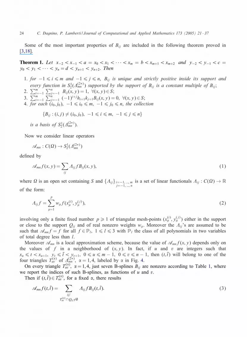
Lemma 2. Let f∈Cs−1(Q(#)uv ), with 16 s6 l6 3. For any i and j such that T (#)

uv ∩ Qij = ∅ thereresults

|�ijR|6Cs�s−1ij !(Ds−1f;�ij;Q(#)

uv ); (9)

where Cs is a constant independent of m and n.

Proof. From the de1nition of R with g the Taylor expansion of f at (t; Dt) [5]

|�ijR|6 max16�6p

|R(x(i)� ; y( j)� )|

p∑�=1

|w�| (10)

and for any � = 1; : : : ; p

|R(x(i)� ; y( j)� )|6 1

(s − 1)!

s−1∑q=0

(s − 1

q

)|Ds−q−1; qR(0(i)� ; 1( j)� )| |x(i)� − t|s−q−1 |y( j)

� − Dt|q (11)

with

Ds−q−1; qR(0(i)� ; 1( j)� ) = Ds−q−1; qf(0(i)� ; 1( j)� ) − Ds−q−1; qf(t; Dt)

and (0(i)� ; 1( j)� ) on the line from (t; Dt) to (x(i)� ; y( j)� ).

If we denote

2(i)1 = max

16�6p|x(i)� − t|; 2( j)

2 = max16�6p

|y( j)� − Dt|;

2(ij)3 = max

16�6p‖(0(i)� ; 1( j)� ) − (t; Dt)‖

for any i and j such that T (#)uv ∩Qij = ∅, then from the hypothesis that the functionals �ij are locally

supported we can deduce

2(i)1 6 3 Dhi; 2( j)

2 6 4 Dkj; 2(ij)3 6 5�ij; (12)

where 3; 4; 5 are real constants independent of m and n. For example, in case of the functionals�ij given in [20], it is easy to verify that the above constants are real numbers less than 3.

Then from (10)–(12) and from the modulus of continuity properties [17], as in [5], we obtain thethesis (9) with

Cs =p∑

�=1

|w�| 2s−1

(s − 1)!(max{3; 4})s−1�5�: (13)

We are now ready to give a local estimate for (4). The constants however are not the best possible.We have exhibited them primarily to show clearly on what they depend.

Theorem 2. Let 16 s6 l6 3 and �(2∗)mn a type-2 triangulation. If f∈Cs−1(Q(#)

uv ), then

‖E00s‖T (#)uv6Cs�s−1

uv !(Ds−1f; �uv;Q(#)uv ); (14)

where Cs is the constant de5ned in (13) and �uv =maxij=T (#)uv ∩Qij �=∅{�ij}.

28 C. Dagnino, P. Lamberti / Journal of Computational and Applied Mathematics 173 (2005) 21–37

Moreover for 16 r + Dr ¡ 3 there results

‖Er Drs‖T (#)uv6Cuvsr Dr�s−r− Dr−1

uv !(Ds−1f; �uv;Q(#)uv ); (15)

where Cuvsr Dr=7)r DrCs(�uv=+uv)r+ Dr with )r Dr de5ned in Lemma 1, T (#)uv =T (#)

uv if r+ Dr=1; T (#)uv =int T (#)

uv

if r + Dr = 2 and +uv =minij=T (#)uv ∩Qij �=∅{+ij}.

Proof. From (5) and (6) with r + Dr =0, Lemma 2 and from the fact that the Bij’s are positive andform a partition of the unity, we immediately obtain the thesis (14). If 16 r + Dr ¡ 3, then from(5), (6), Lemmas 1 and 2 we can deduce thesis (15).

The local estimates lead immediately to the following global results.

Theorem 3. Let 16 s6 l6 3, � = max{ Dh; Dk} and + = min{h; k}. If f∈Cs−1(K), where K is acompact set, closure of �, then

‖E00s‖S6Cs�s−1!(Ds−1f;�;K):

Moreover for 16 r + Dr ¡ 2 there results

‖Er Drs‖S6Csr Dr�s−r− Dr−1!(Ds−1f;�;K);

where Cs is the constant de5ned in (13) and Csr Dr = 2Cs(�=+)r+ Dr .

We recall now the following de1nition.

De!nition 1. A sequence of partitions {�(2∗)mn } of S is quasi-uniform (q-u) if there exists a positive

constant - such that

Dhh6 -;

Dhk6 -;

Dkh6 -;

Dkk6 -:

Moreover a sequence of spline spaces {S12 (�

(2∗)mn )} is q-u if they are based on a sequence of q-u

partitions.

We can remark that Theorem 2 provides the following local convergence results:

1. Amnf → f as �uv → 0 for f∈Cs−1(Q(#)uv ); 16 s6 l6 3,

2. Dr DrAmnf → Dr Drf as �uv → 0 for f∈Cs−1(Q(#)uv ); 16 s6 l6 3; 16 r + Dr ¡ 3 and r + Dr ¡ s

in case of q-u {�(2∗)mn }. Indeed in (15) there results (�uv=+uv)r+ Dr6 -r+ Dr .

Moreover Theorem 3 provides similar global convergence results.Finally local and global upper bounds for ‖Dr DrAmnf‖ are given with s6 r + Dr ¡ 3 by Theorem

2 and s6 r + Dr ¡ 2 by Theorem 3, respectively.

C. Dagnino, P. Lamberti / Journal of Computational and Applied Mathematics 173 (2005) 21–37 29

4. Some q-i functionals �ij

In this section, according to Theorem 3, we analyze two particular choices of functionals �ij thatgive rise to the discrete q-i operators introduced in [20] and generated in [7,8].

1. If in (2) we assume p=1; w1 = 1 and (x(i)1 ; y( j)1 )= ((xi + xi+1)=2; (yj +yj+1)=2), i.e. the center

of the support Qij of Bij (Fig. 5a), then we obtain the following q-i spline, for which l= 2:

Vmnf(x; y) =m∑

i=−1

n∑j=−1

f(xi + xi+1

2;yj + yj+1

2

)Bij(x; y): (16)

Some convergence properties of {Vmnf} to f have been proved by Wang and Lu [20]. Hereby the theorems of Section 3 we can show new local and global results for (16).

In this case we have∑p

�=1 |w�| = 1 and we can easily get 3 = 4 = 32 ; 5 =

√102 . Therefore

in (13) there results Cs = (2 · 3s−1)=(s − 1)!. The in1nite norm of Vmn is uniformly boundedindependently of the partition �(2∗)

mn of the domain S : ‖Vmn‖∞6 1.From Theorem 3 we can get the following estimate of ‖f−Vmnf‖S for f∈Cs−1(K); s=1; 2 :

‖f − Vmnf‖S = ‖E00s‖S = O(�s−1 !(Ds−1f;�;K)): (17)

If in addition we suppose f∈C2(K), then we have

‖f − Vmnf‖S = ‖E002‖S = O(�2): (18)

The above results agree with the ones given in [20].In case r + Dr = 1, always from Theorem 3, we can deduce that, if we suppose that {�(2∗)

mn }is q-u and f∈C1(K), then

‖Dr Dr(f − Vmnf)‖S = ‖Er Dr2‖S = O(!(Df;�;K)): (19)

If in addition we suppose f∈C2(K), then

‖Dr Dr(f − Vmnf)‖S = ‖Er Dr2‖S = O(�): (20)

Finally if f∈C(K) and �(2∗)mn is q-u, then from Theorem 3 with r + Dr = 1 we have

‖Dr DrVmnf‖S = ‖Er Dr1‖S = O(�−1!(f;�;K)):

Fig. 5. Points pattern (a) for Vmn and (b) for Wmn.

30 C. Dagnino, P. Lamberti / Journal of Computational and Applied Mathematics 173 (2005) 21–37

Moreover from Theorem 2 we can derive the following local upper bounds of ‖Dr DrVmnf‖T (#)uv

with r + Dr = 2 for f∈Cs−1(Q(#)uv ); s= 1; 2 :

‖Dr DrVmnf‖T (#)uv= ‖Er Drs‖T (#)

uv= O(�s−3

uv !(Ds−1f;�uv;Q(#)uv )):

Therefore from (17)–(20) we get new informations about the approximation power of theoperator Vmn and in particular from (18) and (20) there results that Vmnf approximates f, asexpected [20], and its partial derivatives to nearly optimal order.

2. If in (2) we let p= 5; w1 = 2; wk = − 14 ; k = 2; : : : ; 5 and

(x(i)1 ; y( j)1 ) =

(xi + xi+1

2;yj + yj+1

2

); (x(i)2 ; y( j)

2 ) = (xi; yj); (21)

(x(i)3 ; y( j)3 ) = (xi+1; yj); (x

(i)4 ; y( j)

4 ) = (xi+1; yj+1); (x(i)5 ; y( j)

5 ) = (xi; yj+1)(Fig:5b);

then we obtain the following q-i spline, for which l= 3:

Wmnf(x; y) =m∑

i=−1

n∑j=−1

{2f(xi + xi+1

2;yj + yj+1

2

)− 1

4[f(xi; yj)

+f(xi+1; yj) + f(xi+1; yj+1) + f(xi; yj+1)]

}Bij(x; y): (22)

We recall that some convergence results of Wmnf to f have been obtained in [20] forf∈Cs(K); s= 2; 3. In the following we can prove new properties for (22).

In this case we have∑p

�=1 |w�|= 3 and we can easily obtain 3= 4= 2; 5=√5. Therefore

in (13) there results Cs = (3222(s−1))=(s − 1)!. The in1nite norm of Wmn is uniformly boundedindependently of the partition �(2∗)

mn of the domain S : ‖Wmn‖∞6 3.From Theorem 3 we obtain the following estimate of ‖f − Wmnf‖S for f∈Cs−1(K); s =

1; 2; 3 :

‖f − Wmnf‖S = ‖E00s‖S = O(�s−1!(Ds−1f;�;K)): (23)

If in addition we suppose f∈C3(K), then we have

‖f − Wmnf‖S = ‖E003‖S = O(�3): (24)

The above results for f∈Cs(K) with s= 2; 3 agree with the ones given in [20].In case r + Dr = 1, always from Theorem 3, we can deduce that, if {�(2∗)

mn } is q-u andf∈Cs−1(K); s= 2; 3, then

‖Dr Dr(f − Wmnf)‖S = ‖Er Drs‖S = O(�s−2 !(Ds−1f;�;K)): (25)

If in addition we suppose f∈C3(K), then

‖Dr Dr(f − Wmnf)‖S = ‖Er Dr3‖S = O(�2): (26)

Moreover, if f∈C2(Q(#)uv ), from Theorem 2 with r+ Dr=2 we can derive the following local

estimate:

‖Dr Dr(f − Wmnf)‖T (#)uv= ‖Er Dr3‖T (#)

uv= O(!(D2f;�uv;Q(#)

uv ): (27)

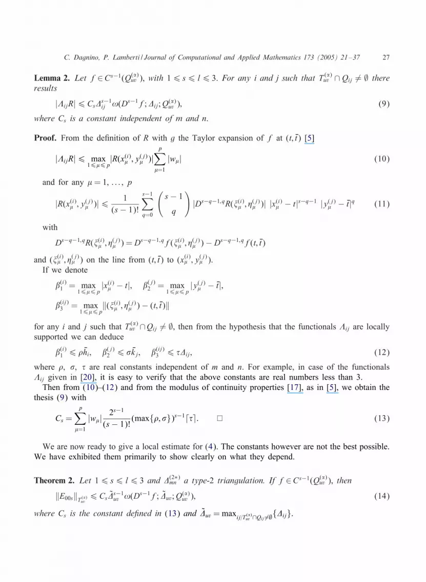
C. Dagnino, P. Lamberti / Journal of Computational and Applied Mathematics 173 (2005) 21–37 31

If in addition we suppose f∈C3(Q(#)uv ), then

‖Dr Dr(f − Wmnf)‖T (#)uv= ‖Er Dr3‖T (#)

uv= O(�uv): (28)

Therefore from (23)–(28) we can get new informations on the approximation power of theoperator Wmn and in particular from (24) and (26) there results that Wmnf approximates f,as expected [20], and, for q-u sequences of triangulations, its partial derivatives to an optimalorder.

We remark that both the above operators need function evaluations outside the domain S.

5. Numerical and graphical results

Here we propose some examples on function approximation based on the described operatorsgenerated by SPLISURF [8] and tested on sets of data, taken from the following functions, usuallytested in function approximation algorithms [1,12,13]:

• f1(x; y) = 19

√64 − 81((x − 1

2)2 + (y − 1

2)2) − 1

2 ,

• f2(x; y) = (y − x)6+,• f3(x; y) = e−(5−10x)2=2 + :75e−(5−10y)2=2 + :75e−(5−10x)2=2e−(5−10y)2=2,

• f4(x; y) =

{ |x|y if xy¿ 0;

0 elsewhere:

For the functions f1; f2; f3 we assume [a; b]× [c; d] = [0; 1]× [0; 1], while for f4 we take [a; b]×[c; d] = [ − 1; 1] × [ − 1; 1].

The function f1 is one of the well-known Franke’s test functions.The function f3 is chosen for its multiple features and abrupt transitions. Thus, while all the test

functions are smooth (except for a 1rst derivative discontinuity in the case of function f4), this oneis quite challenging.

We present now numerical and graphical results obtained for Vmn; Wmn.Moreover we considered several choices of partitions, de1ned by making many subdivisions in

the vicinity of a function high variation or irregularity. Here we present the results obtained by usingthe following three types of partitions, shown for m= n= 32 in Figs. 6 and 7, where for the sakeof clarity only the triangular mesh-points appear:

Pk = {xik = (b − a)0ik + a; yjk = (d − c)1jk + c} i=−2; :::; m+2j=−2; :::; n+2

; k = 1; 2; 3;

where

0−2k = −sin<

4(m+ 1); 1−2k = −sin

<4(n+ 1)

;

0−1k = −sin<

10m; 1−1k = −sin

<10n

;

32 C. Dagnino, P. Lamberti / Journal of Computational and Applied Mathematics 173 (2005) 21–37

0 0.1 0.2 0.3 0.4 0.5 0.6 0.7 0.8 0.9 1

0

0.1

0.2

0.3

0.4

0.5

0.6

0.7

0.8

0.9

1

Fig. 6. m= n= 32; P1.

0 0.1 0.2 0.3 0.4 0.5 0.6 0.7 0.8 0.9 1

0

0.1

0.2

0.3

0.4

0.5

0.6

0.7

0.8

0.9

1

0 0.1 0.2 0.3 0.4 0.5 0.6 0.7 0.8 0.9 1

0

0.1

0.2

0.3

0.4

0.5

0.6

0.7

0.8

0.9

1

(a) (b)

Fig. 7. m= n= 32: (a) P2; (b) P3.

0m+1; k = 1 + sin<

10m; 1n+1; k = 1 + sin

<10n

;

0m+2; k = 1 + sin<

4(m+ 1); 1n+2; k = 1 + sin

<4(n+ 1)

C. Dagnino, P. Lamberti / Journal of Computational and Applied Mathematics 173 (2005) 21–37 33

00.2

0.40.6

0.81

0

0.2

0.4

0.6

0.8

10

0.05

0.1

0.15

0.2

0.25

0.3

0.35

0.4

xy

z

00.2

0.40.6

0.81

0

0.2

0.4

0.6

0.8

10

0.2

0.4

0.6

0.8

1

1.2

1.4

xy

z

(a) (b)

Fig. 8. (a) W88f1 with P2; (b) V88f2 with P1.

00.2

0.40.6

0.81

00.2

0.40.6

0.810

0.5

1

1.5

2

2.5

xy

z

-1-0.5

00.5

1

-1

-0.5

0

0.5

1-1

-0.5

0

0.5

1

xy

z

(a) (b)

Fig. 9. (a) V16;16f3 with P3; (b) V88f4 with P3.

and

(1) 0i1 = 15 sin

im <+ m−i

m ; 1j1 = 15 sin

n−jn <+ j

n ; i = 0; : : : ; m; j = 0; : : : ; n;(2) 0i2 = 1

2(cosm−im <+ 1); 1j2 = 1

2(cosn−jn <+ 1); i = 0; : : : ; m; j = 0; : : : ; n;

(3) 0i3 = 12cos

m=2−im <; 1j3 = 1

2 cosn=2−j

n <; i = 0; : : : ; m=2; j = 0; : : : ; n=2 and 0i3 = 1 − 0m−i;3; 1j3 =1 − 1n−j;3; i = m=2 + 1; : : : ; m; j = n=2 + 1; : : : ; n (m; n even).

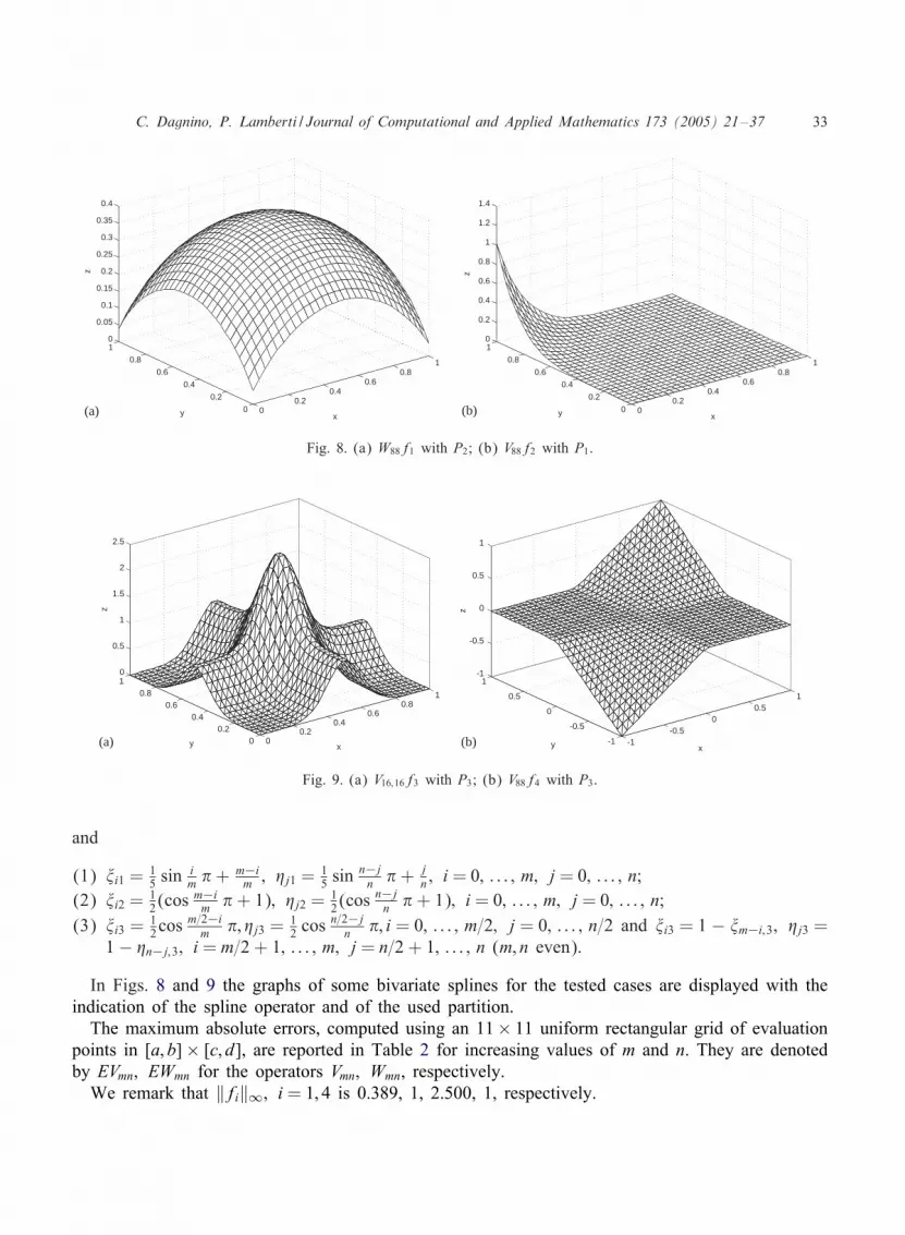
In Figs. 8 and 9 the graphs of some bivariate splines for the tested cases are displayed with theindication of the spline operator and of the used partition.

The maximum absolute errors, computed using an 11× 11 uniform rectangular grid of evaluationpoints in [a; b] × [c; d], are reported in Table 2 for increasing values of m and n. They are denotedby EVmn; EWmn for the operators Vmn; Wmn, respectively.We remark that ‖fi‖∞; i = 1; 4 is 0.389, 1, 2.500, 1, respectively.

34 C. Dagnino, P. Lamberti / Journal of Computational and Applied Mathematics 173 (2005) 21–37

Table 2Maximum absolute errors

m= n EVmnf1 EVmnf2 EWmnf2 EVmnf3 EWmnf4

2 3.88(−2) 3.35(−1) 5.70(−2) 3.40(0) 2.50(−1)4 3.39(−3) 6.60(−2) 1.10(−2) 4.66(−1) 7.32(−2)8 2.51(−4) 1.76(−2) 9.16(−4) 5.76(−2) 1.90(−2)16 2.03(−5) 4.41(−3) 9.78(−5) 6.90(−3) 4.80(−3)32 1.85(−6) 1.09(−3) 8.03(−6) 5.00(−4) 1.20(−3)64 2.03(−7) 2.72(−4) 1.18(−6) 7.10(−5) 3.01(−4)

After the analysis of all numerical and graphical tests, we can conclude that the obtained resultsare consistent with our expectation on the approximation order and we can note that for a suitablenonuniform partition in most cases there is an improvement with respect to the uniform case for thesame m and n [7]. This is due to the fact that we thickened the partition where the test functionhas either a sharp variation or some irregularities.

All computations were carried out on a Sun ULTRA 10.

6. Final remarks

In this paper we have studied local C1 q-i splines de1ned on nonuniform triangulations {�(2∗)mn }

and generated by a sequence of B-splines introduced in [3,18].In particular we have shown that they can approximate a real function and its partial derivatives

up to an optimal order and derived local and global upper bounds both for the error and for thespline partial derivatives, so obtaining more general results with respect to our previous paper [5],dealing only with the uniform case. Moreover we have proposed some applications to prove newproperties of two known q-i spline operators [20], needing function evaluations also outside thedomain S. We have also given some numerical and graphical results.

We recall that C1 q-i splines on nonuniform type-2 triangulations based only on points of thedomain S have been introduced in [16] and, to the best of our knowledge, their study is in progress.

Appendix

We need here the following notation to introduce Tables 3–6:

Ai =hi

hi + hi+1; Bj =

kjkj + kj+1

;

A′i =

hi+1

hi + hi+1= 1 − Ai; B′

j =kj+1

kj + kj+1= 1 − Bj:

C. Dagnino, P. Lamberti / Journal of Computational and Applied Mathematics 173 (2005) 21–37 35

Table 3Bij’s partial derivatives of order 1 at points of Fig. 10

Point D10Bij D01Bij Point D10Bij D01Bij

V1A′i+1−Aihi+1

B′j+1−Bj

kj+1V6 − 1

hi+1+hi+20

V2 −2 Bjhi+1+hi+2

2 A′i+1

kj+kj+1V7 0 − 1

kj+1+kj+2

V3 −2B′j+1

hi+1+hi+2−2 A′

i+1kj+1+kj+2

V8 1hi+hi+1

0

V4 2B′j+1

hi+hi+1−2 Ai

kj+1+kj+2V9 0 1

kj+kj+1

V5 2 Bjhi+hi+1

2 Aikj+kj+1

V10–V21 0 0

Fig. 10. Evaluation points of Dr DrBij(x; y); r + Dr = 1.

Table 4Constant values of D11Bij=2 in the cells of Qij , labeled as in Fig. 2

Cell D11Bij=2 Cell D11Bij=2

1a, 2(A′

i+1−1)(B′j+1−Bj)

hi+1kj+18–11 − B′

j+1−1

kj+1(hi+1+hi+2)

1b, 3(B′

j+1−1)(A′i+1−Ai)

hi+1kj+112 0

1c, 4 − (Ai−1)(B′j+1−Bj)

hi+1kj+113–16 Ai−1

hi+1(kj+1+kj+2)

1d, 5 − (Bj−1)(A′i+1−Ai)

hi+1kj+117 0

6, 23–25 A′i+1−1

hi+1(kj+kj+1)18–21 − Bj−1

kj+1(hi+hi+1)

7 0 22 0

36 C. Dagnino, P. Lamberti / Journal of Computational and Applied Mathematics 173 (2005) 21–37

Table 5Constant values of D20Bij=2 in the cells of Qij , labeled as in Fig. 2

Cell D20Bij=2 Cell D20Bij=2

1a(A′

i+1−1)(Bj+B′j+1)−A′

i+1+Ai

h2i+111

B′j+1(A

′i+1−1)

h2i+1

1b, 3B′j+1(Ai+A′

i+1−2)

h2i+112 0

1c(Ai−1)(Bj+B′

j+1)−Ai+A′i+1

h2i+113

B′j+1(Ai−1)

h2i+1

1d, 5 Bj(Ai+A′i+1−2)

h2i+114–16

B′j+1

hi(hi+hi+1)

2Bj+B′

j+1−1

hi+2(hi+1+hi+2)17 1

hi(hi+hi+1)

4Bj+B′

j+1−1

hi(hi+hi+1)18–20 Bj

hi(hi+hi+1)

6, 24, 25 Bjhi+2(hi+1+hi+2)

21 Bj(Ai−1)

h2i+1

7 1hi+2(hi+1+hi+2)

22 0

8–10B′j+1

hi+2(hi+1+hi+2)23 Bj(A

′i+1−1)

h2i+1

Table 6Constant values of D02Bij=2 in the cells of Qij , labeled as in Fig. 2

Cell D02Bij=2 Cell D02Bij=2

1a, 2A′i+1(Bj+B′

j+1−2)

k2j+19–11 A′

i+1kj+2(kj+1+kj+2)

1b(B′

j+1−1)(Ai+A′i+1)−B′

j+1+Bj

k2j+112 1

kj+2(kj+1+kj+2)

1c, 4Ai(Bj+B′

j+1−2)

k2j+113–15 Ai

kj+2(kj+1+kj+2)

1d(Bj−1)(Ai+A′

i+1)−Bj+B′j+1

k2j+116

Ai(B′j+1−1)

k2j+1

3 Ai+A′i+1−1

kj+2(kj+1+kj+2)17 0

5 Ai+A′i+1−1

kj(kj+kj+1)18 Ai(Bj−1)

k2j+1

6 A′i+1(Bj−1)

k2j+119–21 Ai

kj(kj+kj+1)

7 0 22 1kj(kj+kj+1)

8A′i+1(B

′j+1−1)

k2j+123–25 A′

i+1kj(kj+kj+1)

C. Dagnino, P. Lamberti / Journal of Computational and Applied Mathematics 173 (2005) 21–37 37

References

[1] R.K. Beatson, Z. Ziegler, Monotonicity preserving surface interpolation, SIAM J. Numer. Anal. 22 (1985) 401–411.[2] C. de Boor, K. HQollig, S. Riemenschneider, Box Splines, Springer, New York, 1993.[3] C.K. Chui, R.-H. Wang, Concerning C1 B-splines on triangulations of nonuniform rectangular partition, Approx.

Theory Appl. 1 (1984) 11–18.[4] C.K. Chui, R.-H. Wang, On a bivariate B-spline basis, Sci. Sinica XXVII (1984) 1129–1142.[5] C. Dagnino, P. Lamberti, On the approximation power of bivariate quadratic C1 splines, J. Comput. Appl. Math.

131 (2001) 321–332.[6] C. Dagnino, P. Lamberti, On the construction of bivariate quadratic C1 splines, in: Recent Trends in Numerical

Analysis, Trigiante (Ed.), Nova Science Publisher, New York, 2000, pp. 153–161.[7] C. Dagnino, P. Lamberti, On C1 quasi-interpolating splines with type-2 triangulations, Progetto MURST “Analisi

Numerica: Metodi e Software Matematico”, Monogra1a, Vol. 4, Ferrara, 2000.[8] C. Dagnino, P. Lamberti, SPLISURF for use with Matlab, http://www.unife.it/AnNum97/software.htm.[9] P. Lamberti, On the computation of partial derivatives of quadratic B-splines by Maple, Internal Report, September

2002.[10] T. Lyche, L.L. Schumaker, Local spline approximation methods, J. Approx. Theory 15 (1975) 294–325.[11] G. Micula, S. Micula, Handbook of Splines, Kluwer Academic Publishers, Dordrecht, 1999.[12] G. NQurnberger, Th. Riessinger, Bivariate spline interpolation at grid points, Numer. Math. 71 (1995) 91–119.[13] R.J. Renka, R. Brown, Algorithm 792: accuracy tests of ACM algorithms for interpolation of scattered data in the

plane, ACM Trans. Math. Soft. 25 (1999) 78–94.[14] P. SablonniWere, Bernstein–BXezier methods for the construction of bivariate spline approximants, Comput. Aided

Geom. Design 2 (1985) 29–36.[15] P. SablonniWere, Quadratic B-splines on nonuniform criss-cross triangulations of bounded rectangular domains of the

plane, PrXepublication IRMAR, Institut de Recherche MathXematique de Rennes, 03–14, Mars 2003.[16] P. SablonniWere, Quadratic spline quasi-interpolants on bounded domains of Rd; d= 1; 2; 3, Special issue on splines,

radial basis functions and applications, Rend. Sem. Mat. Univ. Politec. Torino 61 (3) (2003) 229–246.[17] L.L. Schumaker, Spline Functions: Basic Theory, Krieger Publishing Company, Malabar FL, 1993.[18] R.-H. Wang, The dimension and basis of spaces of multivariate splines, J. Comput. Appl. Math. 12& 13 (1985)

163–177.[19] R.-H. Wang, Multivariate spline and its applications in science and technology, Rend. Sem. Mat. Fis. Milano 63

(1993) (1995) 213–229.[20] R.-H. Wang, Y. Lu, Quasi-interpolating operators and their applications in hypersingular integrals, J. Comput. Math.

16 (4) (1998) 337–344.