Topic 12: Interpolating Curves • Intro to curve interpolation & approximation • Polynomial interpolation • Bézier curves • Cardinal splines Some slides and figures courtesy of Kyros Kutulakos Some figures from Peter Shirley, “Fundamentals of Computer Graphics”, 3rd Ed.

Welcome message from author
This document is posted to help you gain knowledge. Please leave a comment to let me know what you think about it! Share it to your friends and learn new things together.
Transcript

Topic 12: Interpolating Curves• Intro to curve interpolation & approximation • Polynomial interpolation • Bézier curves • Cardinal splines
Some slides and figures courtesy of Kyros Kutulakos Some figures from Peter Shirley, “Fundamentals of Computer Graphics”, 3rd Ed.

What are Splines?• Numeric function that is piecewise-defined by polynomial functions • Possesses a high degree of smoothness where pieces connect • These are intuitively called “knots”

History• Used by engineers in ship building and airplane design before computers were around• Used to create smoothly varying
curves • Variations in curve achieved by the
use of weights (like control points)
Applications
• Specify smooth camera path in scene along spline curve • Rollercoaster tracks • Curved smooth bodies and shells (planes, boats, etc)

Motivation and Goal
• Expand the capabilities of shapes beyond lines and conics, simple analytic functions and to allow design constraints.

Design issues• Create curves that can have constraints specified • Have natural and intuitive interaction • Controllable smoothness • Control (local vs global) • Analytic derivatives that are easy to compute • Compactly represented • Other geometric properties (planarity, tangent/curvature control)

Interpolation
• Interpolating splines: pass through all the data points (control points). Example: Hermite splines

Approximation
• Curve approximates but does not go through all of the control points. • Comes close to them.

Extrapolation
• Extend the curve beyond the domain of the control points

Local properties
• Continuity • Position at a specific place on the curve • Direction at a specific place on the curve • Curvature

Global properties
• Closed or open curve • Self intersection • Length

Local vs Global Control
• Local control changes curve only locally while maintaining some constraints
• Modifying point on curve affects local part of curve or entire curve
Parametric and Geometric Continuity
• When piecing together smooth curves, consider the degrees of smoothness at the joints.
• Parametric Continuity: differentiability of the parametric representation (C0, C1, C2, ...)
• Geometric Continuity: smoothness of the resulting displayed shape (G0=C0, G1=tangent-cont., G2=curvature-cont. )

2D Curve Design: General Problem Statement
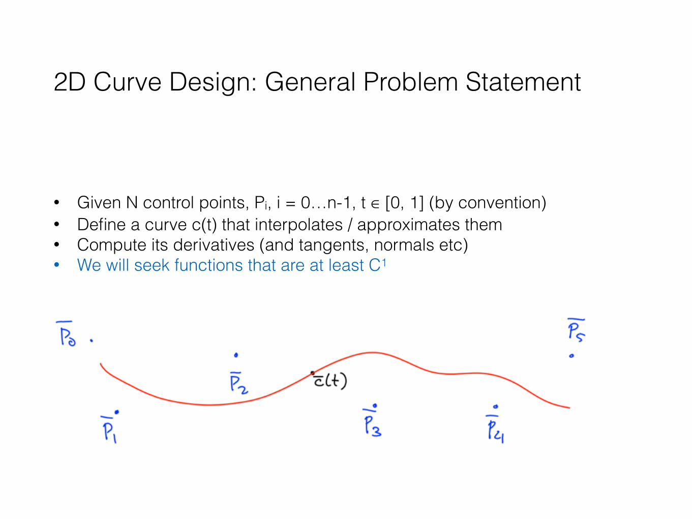
• Given N control points, Pi, i = 0…n - 1, t ∈ [0, 1] (by convention) • Define a curve c(t) that interpolates / approximates them • Compute its derivatives (and tangents, normals etc)
Linear Interpolation
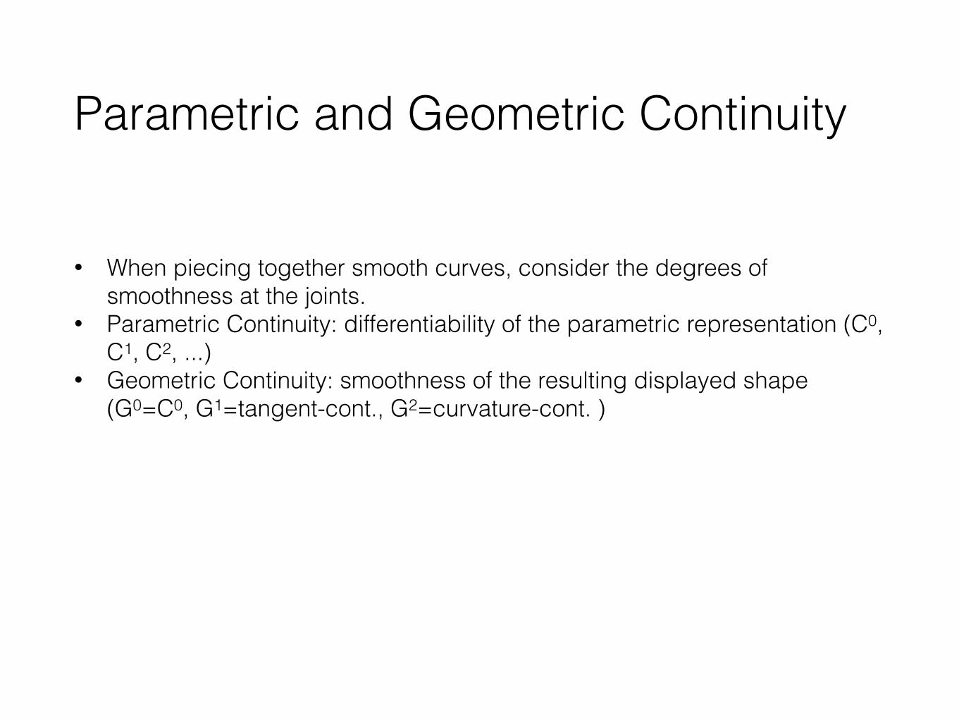
• The simplest possible interpolation technique • Create a piecewise linear curve that connects the control points
• Q: What is the disadvantage of such a technique?

Linear Interpolation
• The simplest possible interpolation technique • Create a piecewise linear curve that connects the control points
• Q: What is the disadvantage of such a technique? • A: The curves may be continuous but its derivatives are not…

Linear Interpolation
• The simplest possible interpolation technique • Create a piecewise linear curve that connects the control points
• Q: What is the disadvantage of such a technique? • A: The curves may be continuous but its derivatives are not…

Cn continuity
• Definition: a function is called Cn if it’s nth order derivative is continuous everywhere

Linear Interpolation
• The simplest possible interpolation technique • Create a piecewise linear curve that connects the control points
• Q: What is the disadvantage of such a technique? • Curve has only C0 continuity
2D Curve Design: General Problem Statement
• Given N control points, Pi, i = 0…n-1, t ∈ [0, 1] (by convention) • Define a curve c(t) that interpolates / approximates them • Compute its derivatives (and tangents, normals etc) • We will seek functions that are at least C1

Polynomial Interpolation
• Given N control points, Pi, i = 0…n-1, t ∈ [0, 1] (by convention) • Define (N-1)-order polynomial x(t), y(t) such that x(i/(N-1) = xi, y(i/(N-1) = yi
for i = 0, …, N-1 • Compute its derivatives (and tangents, normals etc)

Cubic Interpolation
• Given 4 control points, Pi, i = (xi, yi), for i = 0, …, 3 • Define 3rd-order polynomial x(t), y(t) such that x(i/3) = xi, y(i/3) = yi • Compute its derivatives (and tangents, normals etc)

Cubic Interpolation: Basic Equations
Equations for one control point: Equations in matrix form:
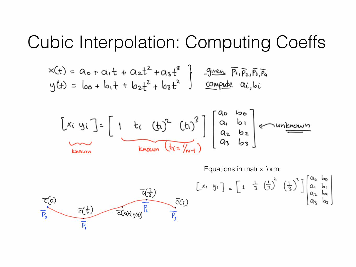
Cubic Interpolation: Computing Coeffs
Equations in matrix form:
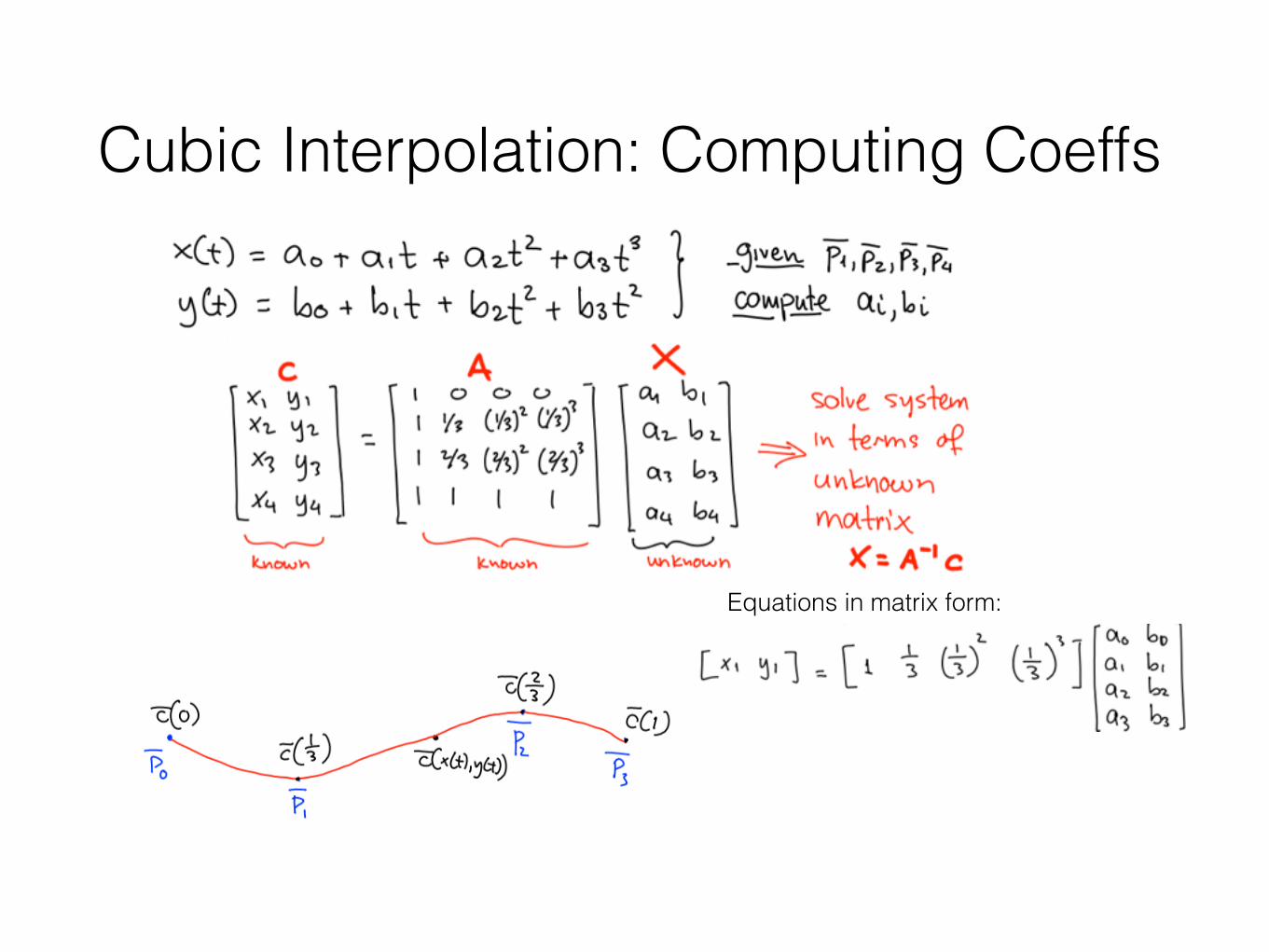
Cubic Interpolation: Computing Coeffs
Equations in matrix form:

Cubic Interpolation: Computing Coeffs
Equations in matrix form:
Coefficients of interpolating polynomial computed by:

Cubic Interpolation: Evaluating the Polynomial
Equations in matrix form:

Cubic Interpolation: What if < 4 Control Points?
Equations in matrix form:
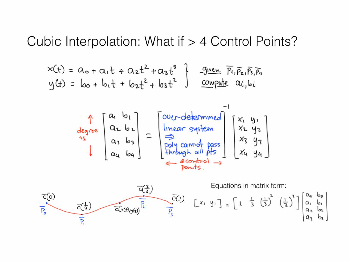
Cubic Interpolation: What if > 4 Control Points?
Equations in matrix form:

Exact Interpolation of N pointsTo interpolate N points perfectly with a single polynomial, we need a polynomial of degree N-1

Cubic Interpolation: Evaluating Derivatives

Specifying the Poly via Tangent Constraints
• Instead of specifying 4 control points, we could specify 2 points and 2 derivatives.

Specifying the Poly via Tangent Constraints
• Instead of specifying 4 control points, we could specify 3 points and a derivative.
• Replace the 4th pair of equations with

Degree-N Poly Interpolation: Major DrawbackTo interpolate N points perfectly with a single polynomial, we need a polynomial of degree N-1
Major drawback: it is a global interpolation scheme
i.e. moving one control point changes the interpolation of all points, often in unexpected, unintuitive and undesirable ways

Topic 12: Interpolating Curves• Intro to curve interpolation & approximation • Polynomial interpolation • Bézier curves• Cardinal splines

Bézier Curves
Properties: • Polynomial curves defined via endpoints and derivative constraints • Derivative constraints defined implicitly through extra control points
(that are not interpolated) • They are approximating curves, not interpolating curves

Bézier Curves: Main Idea
Polynomial and its derivatives expressed as a cascade of linear interpolations
Example: a double cascade
Q: Where have we seen such a cascade before?

Bézier Curves: Control Polygon
A Bézier curve is completely determined by its control polygon
We manipulate the curve by manipulating its polygon
Example: a double cascade

Expressing the Bézier Curve as a Polynomial

Derivatives of the Bézier Curve
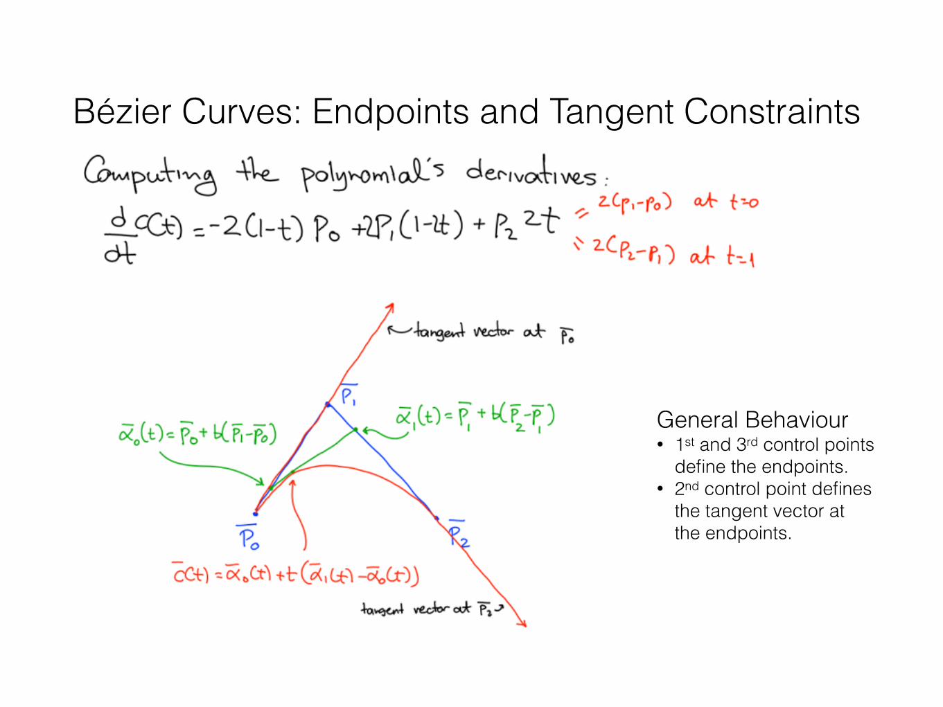
Bézier Curves: Endpoints and Tangent Constraints
General Behaviour • 1st and 3rd control points
define the endpoints. • 2nd control point defines
the tangent vector at the endpoints.

Bézier Curves: Generalization to N+1 points
Example for 4 control points and 3 cascades
Expression in compact form:
Where:
Curve defined by N linear interpolation cascades (De Casteljau's algorithm):

Bézier Curves: A Different Perspective
• Each curve point c(t) is a “blend” of the 4 control points.
• The blend coefficients depend on t
• They are Bernstein polynomials
Expression in compact form:
Where:

Bézier Curves as “blends” of the Control Points
• Each curve point c(t) is a “blend” of the 4 control points. • The blend coefficients depend on t • They are Bernstein polynomials
Expression in compact form:

Bézier Curves: Useful PropertiesExpression in compact form:
Where:
1. Affine Invariance • Transforming a Bézier curve by an affine
transform T is equivalent to transforming its control points by T
2. Diminishing Variation • No line will intersect the curve at more points
than the control polygon • curve cannot exhibit “excessive fluctuations”
3. Linear Precision • If control poly approximates a line, so will the
curve

Bézier Curves: Useful PropertiesExpression in compact form:
Where:
4. Tangents at endpoints are along the 1st and last edges of control polygon:
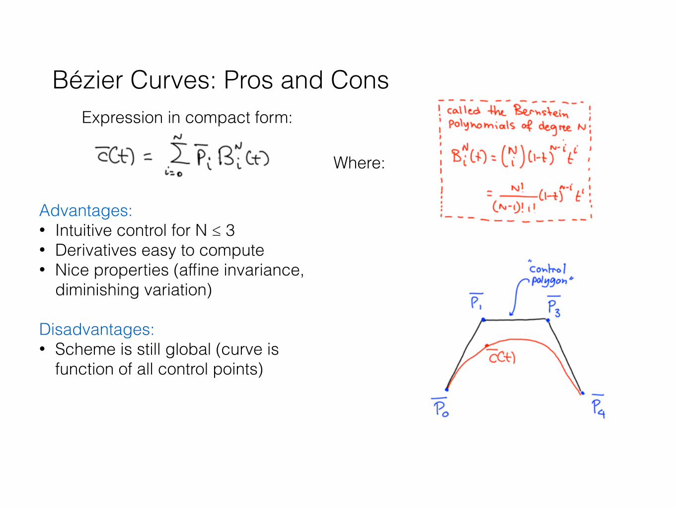
Bézier Curves: Pros and ConsExpression in compact form:
Where:
Advantages: • Intuitive control for N ≤ 3 • Derivatives easy to compute • Nice properties (affine invariance,
diminishing variation)
Disadvantages: • Scheme is still global (curve is
function of all control points)

Topic 12: Interpolating Curves• Intro to curve interpolation & approximation • Polynomial interpolation • Bézier curves • Cardinal splines

Cubic Cardinal Splines: Defining 1st Segment• Approach:
1. A user only specifies points p0, p1, … 2. Tangent at pi set to be parallel to vector connecting pi-1 and pi+1

Cubic Cardinal Splines: Defining 2nd Segment• Approach:
1. A user only specifies points p0, p1, … 2. Tangent at pi set to be parallel to vector connecting pi-1 and pi+1
Example: Adding a fifth point adds a new segment

Cubic Cardinal Splines: General Case• Approach:
1. A user only specifies points p0, p1, … 2. Tangent at pi set to be parallel to vector connecting pi-1 and pi+1

Cubic Cardinal Splines: The Strain Parameter• Approach:
1. A user only specifies points p0, p1, … 2. Tangent at pi set to be parallel to vector connecting pi-1 and pi+1
Tangent at
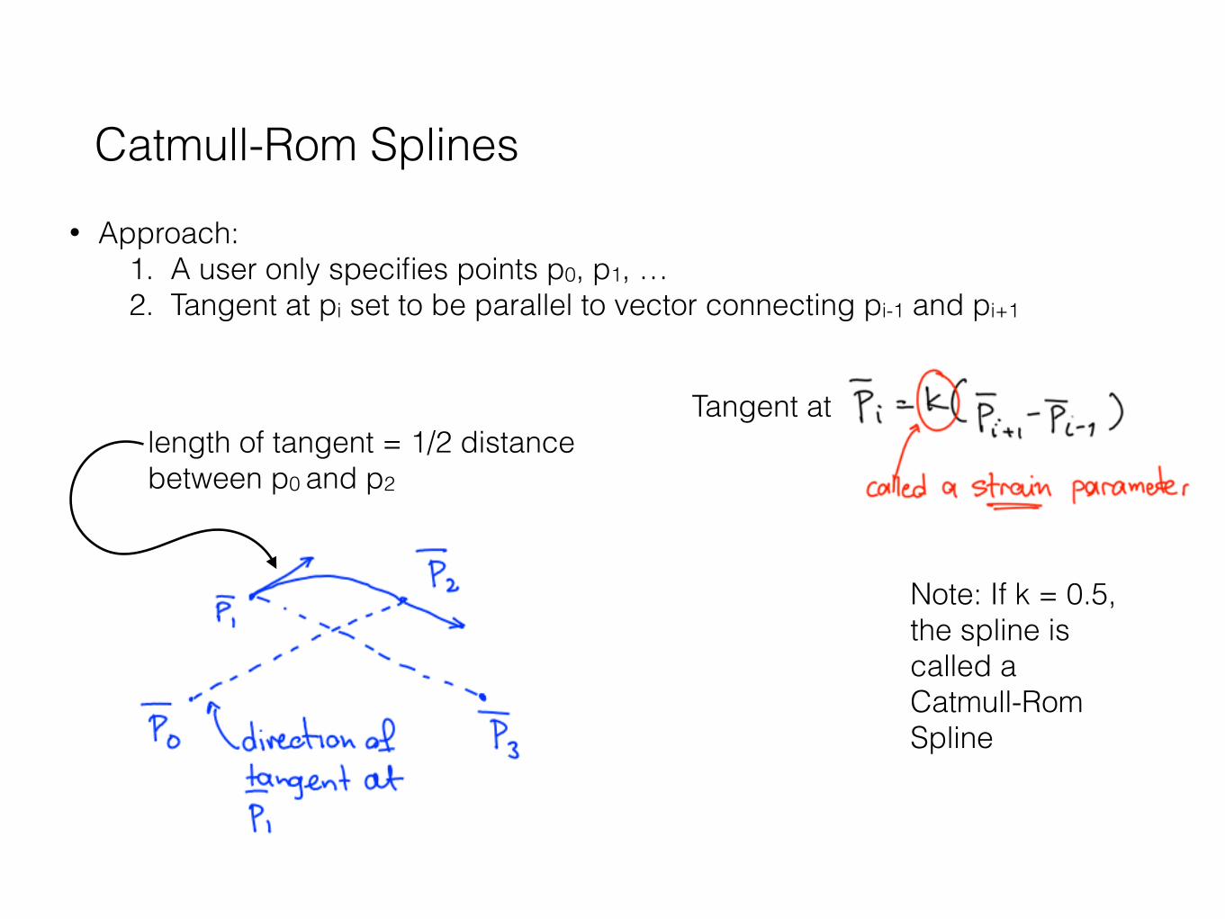
Catmull-Rom Splines• Approach:
1. A user only specifies points p0, p1, … 2. Tangent at pi set to be parallel to vector connecting pi-1 and pi+1
Tangent at
Note: If k = 0.5, the spline is called a Catmull-Rom Spline
length of tangent = 1/2 distance between p0 and p2

Specifying the Poly via Tangent Constraints
• Instead of specifying 4 control points, we could specify 2 points and 2 derivatives

Cardinal Splines: Solving for the Segment Coeffs
for t = 0
+ 2 more equations for other endpoint (t = 1)

Cubic Cardinal Spline Segment vs Bézier Curve
The two curves are actually equivalent: given a cardinal spline, we can compute the control polygon of the
equivalent Bézier curve

Cubic Cardinal Spline Segment vs Bézier Curve
In order to have c(t) = r(t) for all t, it must be:

Cubic Cardinal Spline Segment vs Bézier Curve
In order to have c(t) = r(t) for all t, it must be:
Related Documents