Equivalent Kernels for Smoothing Splines - University of Delaware

Equivalent Kernels for Smoothing Splines

P.P.B. Eggermont, V.N. LaRicciaUniversity of Delaware

To Ken Atkinson on the occasion of his 65-th birthday

November 21, 2005

Abstract

In the study of smoothing spline estimators, some convolution-kernel-like properties of the Green’s function for an appropriate boundaryvalue problem, depending on the design density, are needed. Forthe uniform density, the Green’s function can be computed more orless explicitly. Then, integral equation methods are brought to bearto establish the kernel-like properties of said Green’s function. Webriefly survey how the Green’s function arises in spline smoothingas the equivalent kernel, the reproducing kernel of a suitable Hilbertspace, and as the Green’s function for the Euler equations of a semi-continuous version of the spline smoothing problem.

1. Introduction

In this paper, we study the Green’s function for the boundary value problem,

(1.1)(−h2)m u(2m) + w u = v on ( 0 , 1 ) ,

u(k)(0) = u(k)(1) = 0 , k = m, · · · , 2m− 1 .

Keywords and phrases: Spline smoothing, random designs, equivalent kernels, repro-ducing kernels, Green’s functions.

AMS 2000 Subject Classification: 34B27, 45A05, 62G08.

1

2

Here, m is a positive integer, h is a positive parameter tending to 0, and wis a positive measurable function, which is bounded and bounded away from0, i.e., there exists positive constants w1 and w2 such that

(1.2) w1 6 w( t ) 6 w2 , a.e. t ∈ ( 0 , 1 ) .

Also, u(k) denotes the k-th derivative, for k = 1, 2, · · · . The above Green’sfunction arises in the precise analysis of the smoothing spline estimator forthe following, standard nonparametric regression problem. One observes thedata (X1, Y1), (X2, Y2), · · · , (Xn, Yn), which is interpreted as

(1.3) Yi = fo(Xi) +Di , i = 1, 2, · · · , n .

Here, Xn = (X1, X2, · · · , Xn) , is the random design i.e., X1, X2, · · · , Xn

are independent, identically distributed (iid) random variables with commonprobability density function (pdf) w( t ) on a bounded interval, which we taketo be [ 0 , 1 ]. The noise Dn = (D1, D2, · · · , Dn) are iid, conditional on thedesign Xn, with

(1.4) E[ Dn | Xn ] = 0 , E[ DT

n Dn | Xn ] = σ2 In×n ,

where σ2 is not known. In addition, one needs that, for some constant κ > 3,

(1.5) E[ |D1 |κ | X1 ] <∞ .

The goal is to estimate the function fo, which is assumed to be smooth, i.e.,for some integer m > 1,

(1.6) fo ∈ Wm,2( 0 , 1 ) ,

where Wm,2( 0 , 1 ) is the Sobolev space of order m. Specifically,

(1.7) Wm,2( 0 , 1 ) =

{fo ∈ Cm−1[ 0 , 1 ]

∣∣∣∣∣ f (m−1) absolutely continuous

f (m) ∈ L2(0, 1)

}.

For general introductions to nonparametric regression and the various esti-mators, including smoothing splines, see, e.g., Eubank [17], Wahba [28] andGyorfy et al. [18].

3

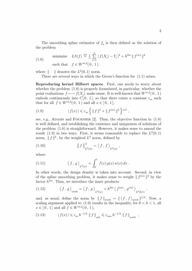
The smoothing spline estimator of fo is then defined as the solution ofthe problem

(1.8)minimize LS(f)

def= 1

n

n∑i=1

| f(Xi)− Yi |2 + h2m ‖ f (m) ‖2

such that f ∈ Wm,2( 0 , 1 ) .

where ‖ · ‖ denotes the L2(0, 1) norm.There are several ways in which the Green’s function for (1.1) arises.

Reproducing kernel Hilbert spaces. First, one needs to worry aboutwhether the problem (1.8) is properly formulated, in particular, whether thepoint evaluations f 7−→ f(Xi) make sense. It is well-known thatWm,2( 0 , 1 )embeds continuously into C[ 0 , 1 ], so that there exists a constant cm suchthat for all f ∈ Wm,2( 0 , 1 ) and all x ∈ [ 0 , 1 ],

(1.9) | f(x) | 6 cm

{‖ f ‖2 + ‖ f (m) ‖2

}1/2 ,

see, e.g., Adams and Fournier [2]. Thus, the objective function in (1.8)is well defined, and establishing the existence and uniqueness of solutions ofthe problem (1.8) is straightforward. However, it makes sense to amend theresult (1.9) in two ways. First, it seems reasonable to replace the L2(0, 1)norm, ‖ f ‖2 , by the weighted L2 norm, defined by

(1.10)∥∥ f ∥∥ 2

L2(w)=

⟨f , f

⟩L2(w)

,

where

(1.11)⟨f , g

⟩L2(w)

=

∫ 1

0

f(x) g(x)w(x) dx .

In other words, the design density is taken into account. Second, in viewof the spline smoothing problem, it makes sense to weight ‖ f (m) ‖2 by thefactor h2m. Thus, we introduce the inner products

(1.12)⟨f , g

⟩wmh

=⟨f , g

⟩L2(w)

+ h2m⟨f (m) , g(m)

⟩L2(0,1)

,

and, as usual, define the norm by ‖ f ‖wmh = { 〈 f , f 〉wmh }1/2 . Now, ascaling argument applied to (1.9) results in the inequality, for 0 < h < 1, allx ∈ [ 0 , 1 ] and all f ∈ Wm,2( 0 , 1 ),

(1.13) | f(x) | 6 cm h−1/2 ‖ f ‖

mh6 cmw h

−1/2 ‖ f ‖wmh

,

4

the last inequality because of (1.2), with cmw = cmw−1/21 . The inequality

(1.13) says that for each h , the space Wm,2( 0 , 1 ) with the innerproduct〈· , ·〉wmh is a reproducing kernel Hilbert space, so that there exists a functionRwmh(x, y), x, y ∈ [ 0 , 1 ], such that Rwmh(x, · ) ∈ Wm,2( 0 , 1 ) for eachx ∈ [ 0 , 1 ], and for all x ∈ [ 0 , 1 ] and all f ∈ Wm,2( 0 , 1 ),

(1.14) f(x) =⟨f , Rwmh(x, · )

⟩wmh

.

Then, (1.13) implies the nifty bound

(1.15) ‖Rwmh(x, · ) ‖wmh6 cmw h

−1/2 ,

with cmw as in (1.13). For more on reproducing kernel Hilbert spaces, seeAronszajn [3]. Of course, the reproducing kernel Rwmh(x, y) is the Green’sfunction for (1.1), see, e.g., Dolph and Woodbury [11].

The reproducing kernel gets used as follows. Taking the existence anduniqueness of the solution of (1.8) for granted, we denote the solution of(1.8) by f = fnh. Then, since we are dealing with a quadratic minimizationproblem, one obtains the quadratic behavior of the objective function aroundits minimizer,

(1.16) 1n

n∑i=1

| ε(Xi) |2 + h2m ‖ ε(m) ‖2 = LS(fo)− LS(fnh) ,

where ε ≡ fnh − fo . After some standard manipulations, as detailed in [14],one then arrives at

(1.17) 1n

n∑i=1

| ε(Xi) |2 + h2m ‖ ε(m) ‖2 6 Sn(ε) + h2m ‖ f (m)o ‖ ‖ ε(m) ‖ ,

where, for f ∈ Wm,2( 0 , 1 ),

(1.18) Sn( f ) = 1n

n∑i=1

Di f(Xi) .

Now, the problem is to bound Sn(ε) in terms of a suitable norm of ε . Sinceε ∈ Wm,2( 0 , 1 ) , one obtains by way of the representation (1.14) that

(1.19) Sn(ε) =⟨ε , Snh

⟩wmh

6 ‖ ε ‖wmh ‖Snh ‖wmh ,

5

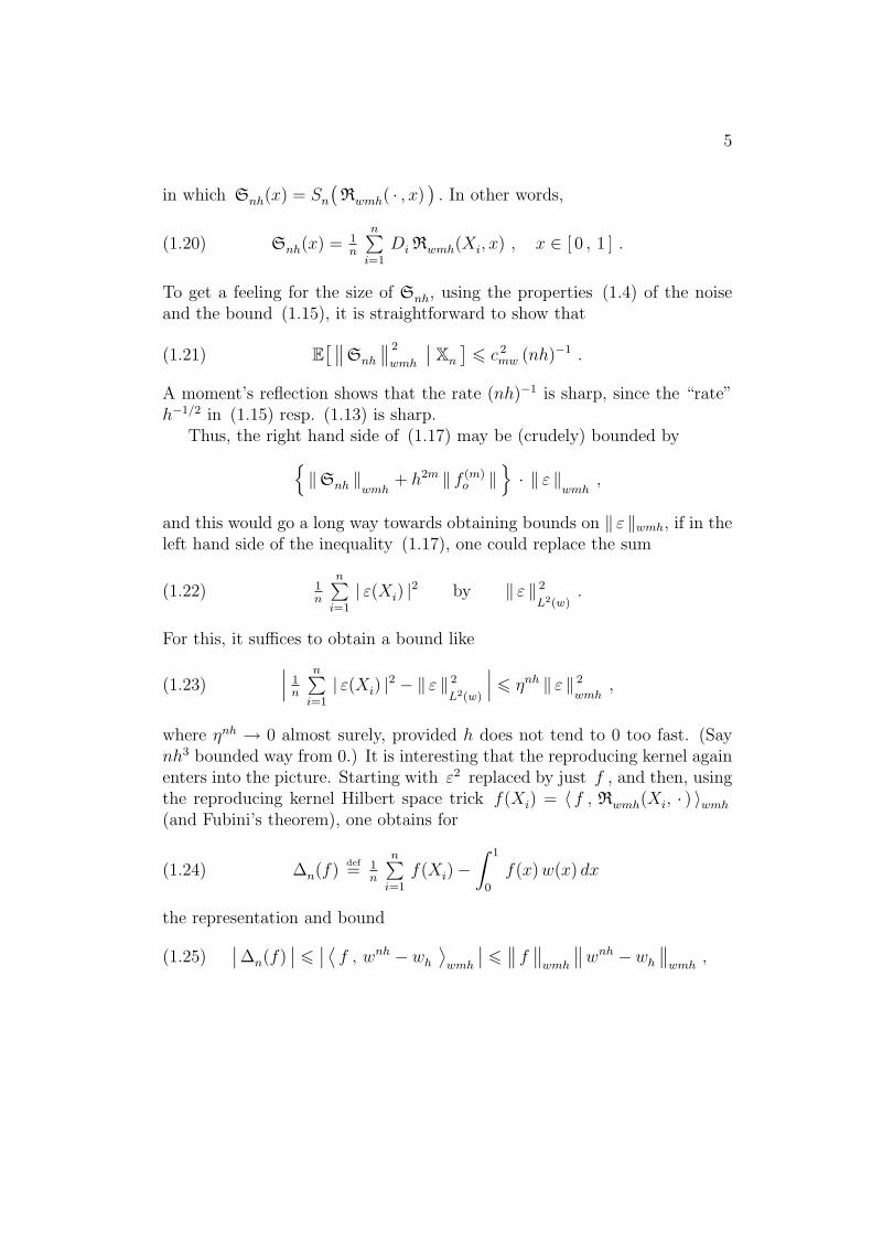
in which Snh(x) = Sn

(Rwmh( · , x)

). In other words,

(1.20) Snh(x) = 1n

n∑i=1

Di Rwmh(Xi, x) , x ∈ [ 0 , 1 ] .

To get a feeling for the size of Snh, using the properties (1.4) of the noiseand the bound (1.15), it is straightforward to show that

(1.21) E[ ∥∥Snh

∥∥ 2

wmh

∣∣ Xn

]6 c 2

mw (nh)−1 .

A moment’s reflection shows that the rate (nh)−1 is sharp, since the “rate”h−1/2 in (1.15) resp. (1.13) is sharp.

Thus, the right hand side of (1.17) may be (crudely) bounded by{‖Snh ‖wmh

+ h2m ‖ f (m)o ‖

}· ‖ ε ‖

wmh,

and this would go a long way towards obtaining bounds on ‖ ε ‖wmh, if in theleft hand side of the inequality (1.17), one could replace the sum

(1.22) 1n

n∑i=1

| ε(Xi) |2 by ‖ ε ‖ 2

L2(w).

For this, it suffices to obtain a bound like

(1.23)∣∣∣ 1

n

n∑i=1

| ε(Xi) |2 − ‖ ε ‖ 2

L2(w)

∣∣∣ 6 ηnh ‖ ε ‖ 2

wmh,

where ηnh → 0 almost surely, provided h does not tend to 0 too fast. (Saynh3 bounded way from 0.) It is interesting that the reproducing kernel againenters into the picture. Starting with ε2 replaced by just f , and then, usingthe reproducing kernel Hilbert space trick f(Xi) = 〈 f , Rwmh(Xi, · ) 〉wmh

(and Fubini’s theorem), one obtains for

(1.24) ∆n(f)def= 1

n

n∑i=1

f(Xi)−∫ 1

0

f(x)w(x) dx

the representation and bound

(1.25)∣∣ ∆n(f)

∣∣ 6∣∣ ⟨f , wnh − wh

⟩wmh

∣∣ 6∥∥ f ∥∥

wmh

∥∥wnh − wh

∥∥wmh

,

6

where

(1.26)

wnh(x) = 1n

n∑i=1

Rwmh(Xi, x) ,

wh(x) = E[wnh(x) ] =

∫ 1

0

Rwmh(x, t )w( t ) d t .

Note that wnh is an estimator of the design density. We are tempted to callit a reproducing kernel density estimator, in analogy with the standard kerneldensity estimator, in which Rwmh(Xi, x) is replaced by a convolution kernelKh(Xi − x) , see the classic Devroye and Gyorfy [10], or the authors’favorite, [13].

Now, the task at hand is to bound ‖wnh − wh ‖wmh , and obviously, thisrequires some properties on the reproducing kernel Rwmh . Finally, one needsto replace f by ε2 . See [14] for the full details.

Remark 1. The above elementary approach is a somewhat nonstandard wayof dealing with the random sums Sn(ε). The standard way is by consideringa suitable closed set F ⊂ Wm,2( 0 , 1 ), e.g., the unit ball, and studying thesupremum of Sn( f ) over f ∈ F . Now, the “size”of F as a subset of L2(0, 1)comes into play, where the “size” is measured in terms of the Kolmogorov (ormetric) entropy of F . We shall not address this further. See, e.g., Dudley[12].

C-splines. In the above, we outlined how the error in the smoothing splineis bounded by a suitable norm of Snh. In fact, the error behaves exactly inthis way. In [14], we show that under the conditions (1.2)- (1.6) that

(1.27) fnh(x)− E[ fnh(x) | Xn ] = Snh(x) + δnh(x) ,

with‖ δnh ‖∞ = o

((nh)−1/2

)almost surely ,

provided n→∞, h→ 0, with nh3 bounded way from 0. The way this comesabout is as follows. Write∣∣ f(Xi)− Yi

∣∣2 =∣∣ f(Xi)− fo(Xi)

∣∣2 − 2Di

(f(Xi)− fo(Xi)

)+

∣∣Di

∣∣2 ,and as in (1.22), approximate the sum 1

n

∑ni=1

∣∣ f(Xi) − fo(Xi)∣∣2 by the

corresponding integral. This leads to the minimization problem

(1.28)minimize CLSn(f − fo) + h2m ‖ f (m) ‖2

subject to f ∈ Wm,2( 0 , 1 ) ,

7

where

(1.29) CLS(f) = ‖ f ‖ 2

L2(w)− 2

n

n∑i=1

Di f(Xi) .

We call the solution a C-spline estimator (C for Continuous). This is slightlydifferent from the “continuous” splines of Cox [7],[8]. The solution of (1.28)should be a pretty good approximation to the solution fnh of (1.8), andindeed it is.

Now, by way of the Euler equations, one verifies that the solution of(1.28), denoted as ψnh(x) , may be written as

(1.30) ψnh(x) = E[ψnh(x) ] + 1n

n∑i=1

Di Rwmh(Xi, x) ,

with

E[ψnh(x) ] =

∫ 1

0

Rwmh(x, y) fo(y)w(y) dy , x ∈ [ 0 , 1 ] .

This uses the fact that Rwmh is the Green’s function for the boundary valueproblem (1.1).

Desirable properties of the Green’s function. It is clear that for a de-tailed study of the random functions Snh(x) and wnh(x) , some informationon the Green’s function Rwmh(x, y) is needed. In the probability literature,powerful results are available on random functions of the form

(1.31) ϕnh(x) = 1n

n∑i=1

DiKh(x−Xi) , x ∈ [ 0 , 1 ] ,

where Kh(x) = h−1K(h−1x

), for some nice function K, in particular,

(1.32) K ∈ L1(R) ∩BV (R) , K(x) = 0 for |x | > 1 .

See, e.g., Deheuvels and Mason [9], and Einmahl and Mason [16], withprecursors like Konakov and Piterbarg [20], and Hardle, Janssen andSerfling [19]. The functions K satisfying (1.32) are usually referred toas “kernels”. To distinguish them from reproducing kernels, we shall callthem “convolution kernels”. Now, the Green’s function Rwmh(x, y) is not aconvolution kernel, but we prove in this paper that it has properties quite

8

analogous: There exist positive constants c, γ and δ such that for all h,0 < h < 1,

(1.33)

supx∈[ 0 , 1 ]

∥∥Rwmh(x, · )∥∥∞ 6 c h−1 ,

supx∈[ 0 , 1 ]

∥∥Rwmh(x, · )∥∥

16 c ,

supx∈[ 0 , 1 ]

∣∣ Rwmh(x, · )∣∣BV (0,1)

6 c h−1 ,

and for all x, y ∈ [ 0 , 1 ],

(1.34)∣∣ Rwmh(x, y)

∣∣ 6 γ h−1 exp(−δ h−1 |x− y |

).

In (1.33), ‖ · ‖p denotes the standard norm on Lp( 0 , 1 ), for 1 6 p 6 ∞, and| · |BV (A) denotes the semi-norm on the space of functions (no equivalenceclasses) of bounded variation onA ( [ 0 , 1 ] or R). See, e.g., Ziemer [29]. Notethat convolution kernels have these properties, except for the exponentialdecay (but obviously, a convolution kernel decays like an L1 function.) Theproperties (1.33) are useful for establishing rates of convergence of Snh invarious norms, e.g., the sup-norm. The exponential decay (1.34) is useful forshowing that

√nhSnh converges to “white noise”, e.g., it implies that for

x 6= y,

(1.35) nh E[ Snh(x) Snh(y) | Xn ] −→ 0 (h→ 0, nh→∞) .

An additional property of convolution kernels deals with measures of com-pactness of the sets

{Kh : a<h<b

}where 0<a<b<1. This comes about

if one wishes to study the behavior of ϕnh as a function of h. This may takethe form of inquiring about the almost sure boundedness of expressions like

(1.36) lim supn→∞

suph∈Hn

Dn(h)/√

nh ( log(1/h) ∨ log log n )

where Dn(h) = ‖ϕnh ‖∞ and Hn is an interval, e.g., Hn = [n−1 log n , 12] .

The difficulty is that one cannot really deal with the supremum, other thanby approximating it with a finite maximum. Ignoring the scaling in (1.36),one may consider

(1.37) suph∈Hn

Dn(h) = max16i6N

Dn(hi) + suph∈H

min16i6N

∣∣Dn(h)−Dn(hi)∣∣ ,

9

where N and a = h1 < h2 < · · · < hN = b must be chosen “appropriately”so as to balance the number of pointsN and the resulting approximation error(the second term on the right). This leads straight to the metric entropy ofthe afore mentioned sets. See, e.g., Dudley [12] and Remark 1. Obviously,some information is required on the behavior of Dn(h) as a function of h.What is required are results like

(1.38)∥∥Kh −Kλ

∥∥1

6 c∣∣ 1− h/λ

∣∣ and∥∥Kh −Kλ

∥∥∞ 6 c

∣∣h−1 − λ−1∣∣ .

It is an exercise to show that K ∈ BV (R) and K having compact supportimply (1.38). In § 6, we formulate and prove the analogue of (1.38) for thereproducing kernels Rwmh.

Equivalent kernels. In the spline smoothing literature, the Green’s func-tion goes under the name of “equivalent kernel”, see, e.g., Speckman [27],Cox [7],[8], Silverman [26], Messer [22], Messer and Goldstein [23],Nychka [24], and Chiang, Rice and Wu [6].

There are two aspects to the equivalent kernel set-up. One aspect con-cerns the convolution-kernel like properties of the reproducing kernel andthe properties of the reproducing kernel estimator of the regression function.The other one deals with the accuracy of the reproducing kernel estimatoras an approximation to the original smoothing spline estimator.

Regarding the first problem, for the uniform design density, Cox [7] com-putes the Green’s function for (1.1) with periodic boundary conditions bymeans of Fourier series, and then fixes the natural boundary conditions (form = 2). Messer and Goldstein [23] determine the Green’s function for(1.1) on the line by means of Fourier transform methods, and then fix thenatural boundary conditions on the finite interval. In § 3, we give the detailsof this construction.

For “arbitrary”, smooth design densities w , Nychka [24] for m = 1 andChiang et al. [6] and Abramovich and Grinshtein [1] for m = 2, use thevenerable WKB method, although only the latter explicitly mention it. TheWKB method applies to the boundary value problem,

(1.39)(−h2)m u(2m) + w u = v , on the line ,

u(k)(x) → 0 for x→ ±∞ , for k = m, · · · , 2m− 1 ,

and deals with the asymptotic behavior of the solution as h → 0. See, e.g.,Mathews and Walker [21]. One drawback of this approach is that the

10

boundary behavior of the Green’s function is inaccessible, since the bound-aries are pushed out to infinity. This implies that the approximations areonly valid away from the boundary.

Regarding the error made when approximating the spline smoother by theequivalent kernel estimator, Nychka [24] and Chiang et al. [6], followingCox [7], employ an interesting operator equation method. First, since thespline smoother fnh is linear in the data, there exist functions

rmh( · , Xi | Xn ) ∈ Wm,2( 0 , 1 ) , i = 1, 2, · · · , n ,

such that

(1.40) fnh(x) =n∑

i=1

Yi rmh(x,Xi | Xn ) , x ∈ [ 0 , 1 ] .

Now, introduce the operator Fn : Wm,2( 0 , 1 ) −→ Wm,2( 0 , 1 ),

(1.41) [Fn g ](x) =

∫ 1

0

Rwmh(x, t ) g( t )(dWn( t )− dW ( t )

),

for x ∈ [ 0 , 1 ] . Here, W ( t ) is the distribution function corresponding tothe pdf w , and Wn( t ) is the empirical distribution function for the designXn, i.e.,

(1.42) W ( t ) =

∫ t

0

w(s) ds , Wn( t ) = 1n

n∑i=1

11(Xi 6 t ) .

Then, they show that η = fnh − ψnh satisfies the operator equation

(1.43) η + Fn η = −Fnψnh .

Since ψnh is given explicitly in terms of Rwmh, see (1.30), it is now usefulto study the Neumann series representation of

(I + Fn

)−1 Fn Rwmh( · , t )to get explicit approximations to the functions rmh( t ,Xi | Xn ) above. Infact, they obtain bounds of the form

(1.44)∣∣ rmh(x,Xi | Xn )−Rwmh(x,Xi)

∣∣ 6 c δn exp(−c1 h−1 |x−Xi |

),

for suitable positive constants c and c1 and

δn = h−2 ‖Wn −W ‖∞ .

11

(So the error is small and decays very fast as |x−Xi | increases.) Informally,(1.43) may be obtained from the Euler equations for the problems (1.8) and(1.28).

In this paper, only the properties of the Green’s function are addressed.First, we more or less explicitly compute the Green’s function for the uniformdensity case, using Fourier methods following Messer and Goldstein [23],including the precise treatment of the natural boundary conditions. Then,we show that the Green’s function for “arbitrary” designs solves a Fredholmintegral equation of the second kind, with the uniform Green’s function asthe kernel (more or less), and we take it from there.

The accuracy of the reproducing kernel estimator is treated in [14], bydirectly comparing the minimization problems (1.8) and (1.28).

Remark 2. In a different context, there is a huge literature dealing withthe case m = 1. With periodic (as opposed to natural) boundary conditions,it is usually referred to as Hill’s equation. Here, for h = 1 and w squareintegrable, the spectral properties are known in detail. See Poschel [25]and the references therein. The relevance of this to the convolution-kernellike properties of the Green’s function for h→ 0 are not clear.

In the next section, we phrase the main theorem on the Green’s function,and outline the proof. The details are provided in later sections.

Notations. For 1 6 p 6 ∞, we let ‖ · ‖p denote the standard norm onLp( 0 , 1 ). The L2(0, 1) norm is denoted simply as ‖ · ‖. We let I denote theidentity operator on Lp( 0 , 1 ) (for all p). If T : Lp( 0 , 1 ) → Lp( 0 , 1 ), thenthe operator norm of T is again denoted as ‖T ‖p, the case p = 2 not beingan exception this time. Also, | · |BV (A) denotes the semi-norm on the spaceof functions (no equivalence classes) of bounded variation on A ( [ 0 , 1 ] orR). If there should be no confusion about the set A in question, we writesimply | · |BV . See, e.g., Ziemer [29].

2. The Main Theorem

In this section, we state the main theorem of the convolution-kernel likeproperties of the families of kernels Rwmh and R

(m)wmh, where R

(m)wmh( t , s )

denotes the m-th order derivative of Rwmh( t , s ) with respect to s (or withrespect to t , because of symmetry).

12

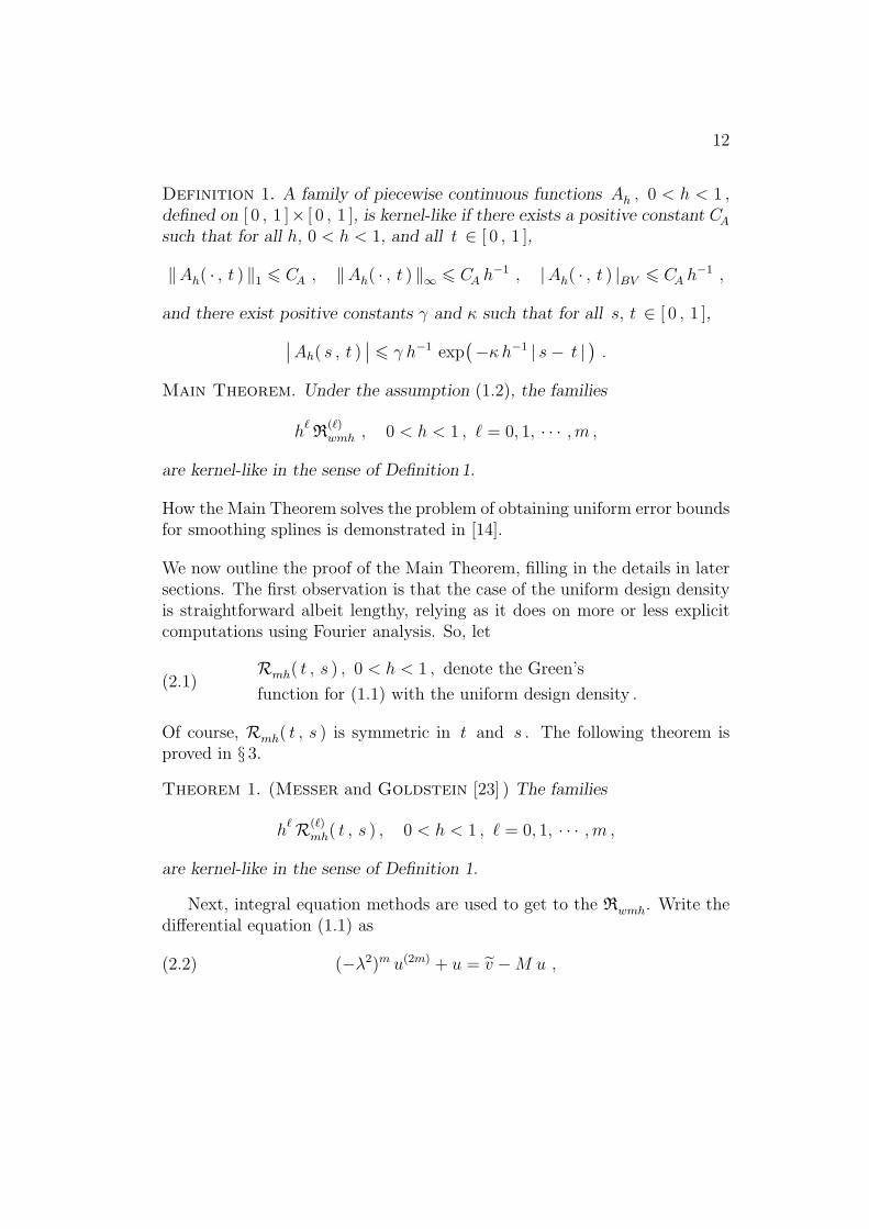
Definition 1. A family of piecewise continuous functions Ah , 0 < h < 1 ,defined on [ 0 , 1 ]× [ 0 , 1 ], is kernel-like if there exists a positive constant CA

such that for all h, 0 < h < 1, and all t ∈ [ 0 , 1 ],

‖Ah( · , t ) ‖1 6 CA , ‖Ah( · , t ) ‖∞ 6 CA h−1 , |Ah( · , t ) |BV 6 CA h

−1 ,

and there exist positive constants γ and κ such that for all s, t ∈ [ 0 , 1 ],∣∣Ah( s , t )∣∣ 6 γ h−1 exp

(−κh−1 | s− t |

).

Main Theorem. Under the assumption (1.2), the families

h`R

(`)wmh , 0 < h < 1 , ` = 0, 1, · · · ,m ,

are kernel-like in the sense of Definition 1.

How the Main Theorem solves the problem of obtaining uniform error boundsfor smoothing splines is demonstrated in [14].

We now outline the proof of the Main Theorem, filling in the details in latersections. The first observation is that the case of the uniform design densityis straightforward albeit lengthy, relying as it does on more or less explicitcomputations using Fourier analysis. So, let

(2.1)Rmh( t , s ) , 0 < h < 1 , denote the Green’s

function for (1.1) with the uniform design density .

Of course, Rmh( t , s ) is symmetric in t and s . The following theorem isproved in § 3.

Theorem 1. (Messer and Goldstein [23] ) The families

h`R(`)

mh( t , s ) , 0 < h < 1 , ` = 0, 1, · · · ,m ,

are kernel-like in the sense of Definition 1.

Next, integral equation methods are used to get to the Rwmh. Write thedifferential equation (1.1) as

(2.2) (−λ2)m u(2m) + u = v −M u ,

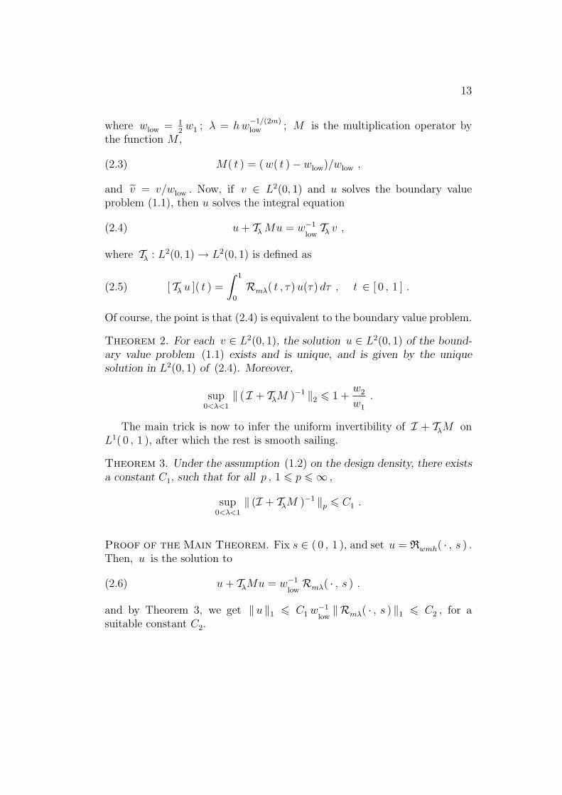
13

where wlow = 12w1 ; λ = hw

−1/(2m)low ; M is the multiplication operator by

the function M ,

(2.3) M( t ) = (w( t )− wlow)/wlow ,

and v = v/wlow . Now, if v ∈ L2(0, 1) and u solves the boundary valueproblem (1.1), then u solves the integral equation

(2.4) u+ TλMu = w−1

lowTλ v ,

where Tλ : L2(0, 1) → L2(0, 1) is defined as

(2.5) [ Tλ u ]( t ) =

∫ 1

0

Rmλ( t , τ)u(τ) dτ , t ∈ [ 0 , 1 ] .

Of course, the point is that (2.4) is equivalent to the boundary value problem.

Theorem 2. For each v ∈ L2(0, 1), the solution u ∈ L2(0, 1) of the bound-ary value problem (1.1) exists and is unique, and is given by the uniquesolution in L2(0, 1) of (2.4). Moreover,

sup0<λ<1

‖ ( I + TλM )−1 ‖2 6 1 +w2

w1

.

The main trick is now to infer the uniform invertibility of I + TλM onL1( 0 , 1 ), after which the rest is smooth sailing.

Theorem 3. Under the assumption (1.2) on the design density, there existsa constant C1, such that for all p , 1 6 p 6 ∞ ,

sup0<λ<1

‖ (I + TλM )−1 ‖p 6 C1 .

Proof of the Main Theorem. Fix s ∈ ( 0 , 1 ), and set u = Rwmh( · , s ) .Then, u is the solution to

(2.6) u+ TλMu = w−1

lowRmλ( · , s ) .

and by Theorem 3, we get ‖u ‖1 6 C1w−1

low‖Rmλ( · , s ) ‖1 6 C2 , for a

suitable constant C2.

14

Now,∣∣ [ TλMu ]( t )

∣∣ 6 ‖Rmλ( t , · ) ‖∞ ‖Mu ‖1 , and of course,

‖Mu‖1 6 w−1

low‖w − w

low‖∞ ‖u ‖1 .

So then, from (2.6),

|u( t ) | 6 w−1

low|Rmλ( t , s ) |+ ‖Rmλ( t , · ) ‖∞ ‖Mu ‖1 ,

and it follows with Theorem 1 that ‖u ‖∞ 6 c1 λ−1 6 c h−1 . Moreover, this

holds uniformly in s ∈ [ 0 , 1 ] .For the BV -property, note that for all f ,

| Tλ f |BV6 sup

s∈[ 0 , 1 ]

|Rmλ( · , s ) |BV

‖ f ‖1,

so that, again from (2.6),

|u |BV

6 w−1

low|Rmλ( · , s ) |

BV+ sup

s∈[ 0 , 1 ]

|Rmλ( · , s ) |BV

‖Mu ‖1,

and the bound |u |BV 6 c h−1 follows. Thus, the family of Green’s functionsRwmh( t , s ), 0 < h < 1, are kernel-like.

Now, let 1 6 ` 6 m. After ` times differentiating both sides of (2.5), theabove derivations may be repeated to show that the kernels

h`R

(`)wmh( t , s )

are kernel-like as well.Apart from the exponential decay, the Main Theorem has been proved.

In the remaining sections, Theorems 1, 2, 3 and the missing part of theMain Theorem regarding the exponential decay are proved.

3. The Green’s function for the uniform design

In this section, we prove Theorem1. There is little doubt that this is all verypredictable: First, we determine a fundamental solution of the differentialequation, ignoring the boundary conditions,

(−h2)m u(2m) + w u = δs ,

with δs the point mass at s, using Fourier methods. Then, all homogeneoussolutions of the differential equation are computed, and finally, the correct

15

linear combination of the homogeneous solutions is added to the fundamentalsolution so as to match the (natural) boundary conditions of (1.1). Thisfollows Cox [7] for the case m = 2 (but he constructs the Green’s functionfor (1.1) with periodic boundary conditions, and then matches the naturalboundary conditions), and Messer and Goldstein [23] (who slightly fudgethe natural boundary conditions, see the remark following (3.17)). When allis said and done, this leads to the following theorem.

Theorem 4. Define the function Bmh(x), x ∈ R , by its Fourier transform

Bmh(ω) =(1 + (2πhω)2m

)−1, ω ∈ R ,

and let

ϕ`,h(x) =

{exp

(h−1$` x

), ` = 0, 1, · · · ,m− 1 ,

exp(h−1$` (x− 1)

), ` = m,m+ 1, · · · , 2m− 1 ,

where

$` = exp( 2`+m+ 1

2mπi

), ` = 0, 1, · · · , 2m− 1 .

Then, for a suitable ho > 0 and for all h < ho, there exist functions a`,h

and positive constants cm, κm such that for all x, y ∈ [ 0 , 1 ] , the Green’sfunction Rmh may be represented as

Rmh(x, y) = Bmh(x− y) +2m−1∑

=0

h−1 ϕ`,h(x) a`,h(y) .

Moreover, for all y ∈ [ 0 , 1 ],

sup06`6m−1

| a`,h(y) | 6 cm exp(−h−1κmy) ,

supm6`62m−1

| a`,h(y) | 6 cm exp(−h−1κm(1− y)) ,

and Rmh(x, y) = Rmh(y, x) for all x, y ∈ [ 0 , 1 ].

Before proving Theorem 4, we show how it may be used to derive The-orem 1. This requires some information regarding the functions Bmh and

ϕ`,h, stated in the next lemma. Notationally, B(k)mh( t ) denotes the k-th or-

der derivative of Bmh( t ) .

16

Lemma 1. Let m > 1. There exist positive constants κm and cm such thatfor x ∈ [ 0 , 1 ], t ∈ R, and k = 0, 1, · · · , 2m− 1,

|ϕ(k)`,h(x) | 6 cm h

−k exp(−h−1κmx ) , 0 6 ` 6 m− 1 ,(a)

|ϕ(k)`,h(x) | 6 cm h

−k exp(h−1κm(x− 1) ) , m 6 ` 6 2m− 1 ,(b)

|B(k)mh( t ) | 6 cm h

−k−1 exp(−h−1κm | t | ) , 0 6 k 6 2m− 1 .(c)

suph>0

sup`

∫ 1

0

hk−1 |ϕ(k)`,h(y) | dy <∞ ,(d)

suph>0

supx∈[ 0 , 1 ]

∫ 1

0

hk |B(k)mh(x− y ) | dy <∞ .(e)

Proof. Only (c) needs some attention. First, define Bm by means of

Bm(hω) = Bmh(ω) , ω ∈ R .

Now, observe that

1 + (2πω)2m =2m−1∏

=1

factor(ω, `) ,

where

factor(ω, `) = 2πω − exp( (2`+ 1)πi

2m

)= 2πω − (−i) exp

( (2`+m+ 1)πi

2m

)= (−i)

(2πiω − exp

( (2`+m+ 1)πi

2m

) )= (−i)

(2πiω −$`

),

with $` as in Theorem 4. Then, the partial fraction decomposition of

B(k)m (ω) = (2πi ω)k Bm(ω) =

(2πi ω)k

1 + (2πω)2m

may be written as

B(k)mh(ω) =

2m−1∑=0

α`,k ( 2πi ω −$` )−1 ,

17

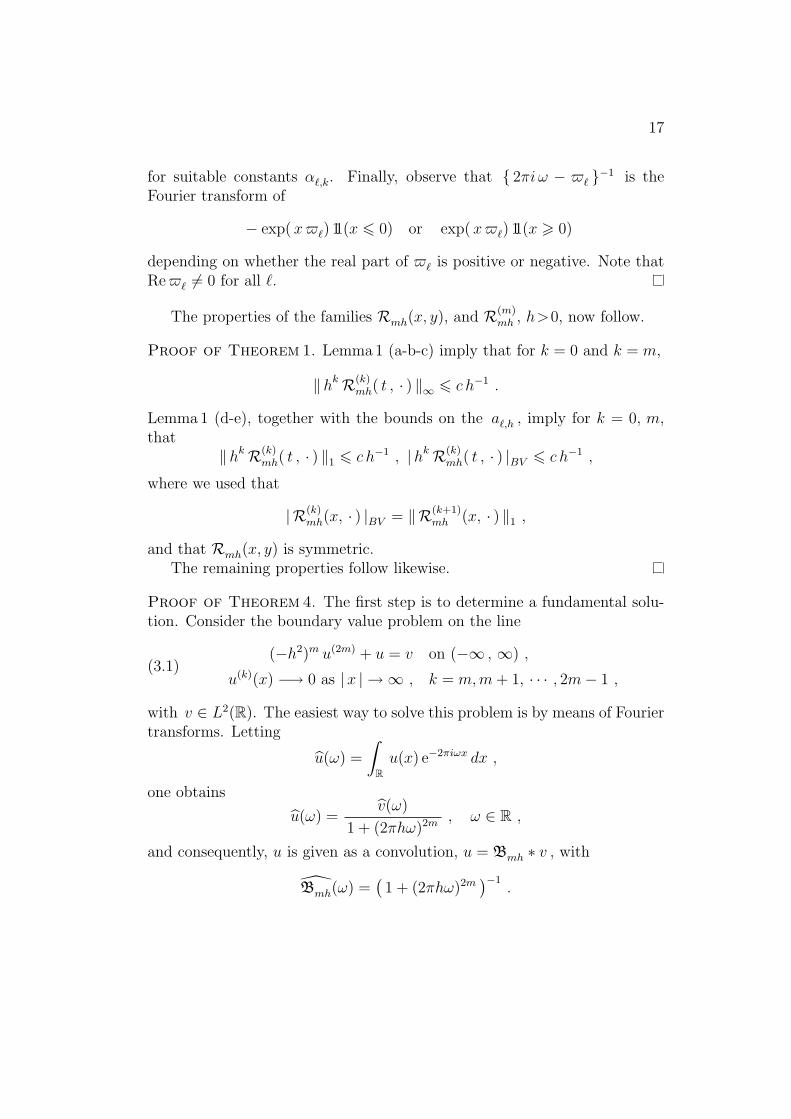
for suitable constants α`,k. Finally, observe that { 2πi ω − $` }−1 is theFourier transform of

− exp(x$`) 11(x 6 0) or exp(x$`) 11(x > 0)

depending on whether the real part of $` is positive or negative. Note thatRe$` 6= 0 for all `.

The properties of the families Rmh(x, y), and R(m)mh , h>0, now follow.

Proof of Theorem 1. Lemma1 (a-b-c) imply that for k = 0 and k = m,

‖hk R(k)mh( t , · ) ‖∞ 6 c h−1 .

Lemma1 (d-e), together with the bounds on the a`,h , imply for k = 0, m,that

‖hk R(k)mh( t , · ) ‖1 6 c h−1 , |hk R(k)

mh( t , · ) |BV 6 c h−1 ,

where we used that

|R(k)mh(x, · ) |BV = ‖R(k+1)

mh (x, · ) ‖1 ,

and that Rmh(x, y) is symmetric.The remaining properties follow likewise.

Proof of Theorem 4. The first step is to determine a fundamental solu-tion. Consider the boundary value problem on the line

(3.1)(−h2)m u(2m) + u = v on (−∞ , ∞) ,

u(k)(x) −→ 0 as |x | → ∞ , k = m,m+ 1, · · · , 2m− 1 ,

with v ∈ L2(R). The easiest way to solve this problem is by means of Fouriertransforms. Letting

u(ω) =

∫Ru(x) e−2πiωx dx ,

one obtains

u(ω) =v(ω)

1 + (2πhω)2m , ω ∈ R ,

and consequently, u is given as a convolution, u = Bmh ∗ v , with

Bmh(ω) =(1 + (2πhω)2m

)−1.

18

It follows that Bmh(x − y) is the Green’s function for the boundary valueproblem (3.2), and a fundamental solution for (1.1). The required propertiesof Bmh follow from Theorem1 and Lemma1.

All homogeneous solutions. Consider the differential equation

(3.2) (−h2)m u(2m) + u = 0 on ( 0 , 1 ) .

The homogeneous solutions are of the form u(x) = exp( i λ x) , for suitableconstants λ. Substituting this into the differential equation shows that λmust satisfy (hλ )2m + 1 = 0 , and one verifies that the solutions are givenby λ = −i h−1$`, 0 6 ` 6 2m− 1. This gives the homogeneous solutions

u`(x) = exp(h−1$` x ) , ` = 0, 1, · · · , 2m− 1 .

It is useful to scale the u` such that

maxx∈[ 0 , 1 ]

|u`(x) | = 1 ,

with the maximum occurring at either x = 0 or x = 1. This leads to the 2mhomogeneous solutions ϕ`,h, ` = 0, 1, · · · , 2m− 1, defined in Theorem 4.

Since these solutions are obviously linearly independent, they are a basisfor the set of all homogeneous solutions of the differential equation (3.3).

Taking care of the boundary conditions. We now construct the Green’sfunction as a linear combination of the fundamental solution and the basichomogeneous solutions, in the form

(3.3) Rmh(x, y) = Bmh(x− y) +2m−1∑

=0

h−1ϕ`,h(x) a`,h(y) .

The coefficients a`,h(y) are to be determined such that the boundary condi-tions of (1.1) are satisfied. This leads to the system of linear equations

(3.4)

2m−1∑=0

$k` ϕ`,h(x) a`,h(y) = B(k)

m

(h−1(x− y)

),

for x = 0, 1, and k = m,m+ 1, · · · , 2m− 1 .

We must show that the a`,h exist, so that Rmh(x, y) may indeed be repre-sented by (3.4), and that the bounds of Theorem4 apply.

19

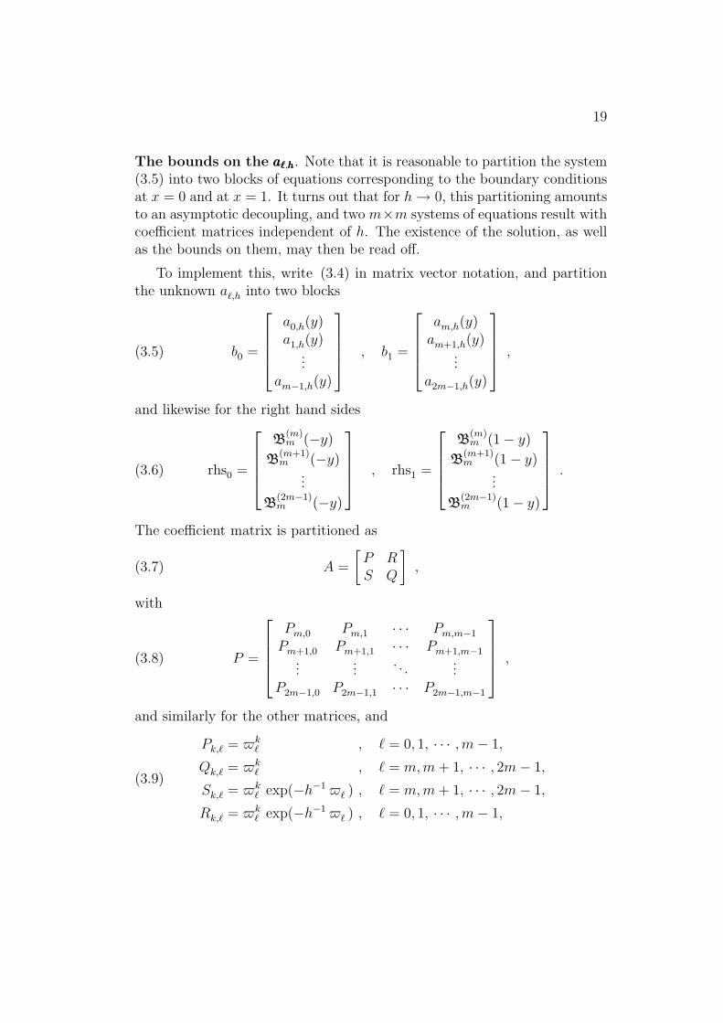
The bounds on the aaa`,hhh. Note that it is reasonable to partition the system(3.5) into two blocks of equations corresponding to the boundary conditionsat x = 0 and at x = 1. It turns out that for h→ 0, this partitioning amountsto an asymptotic decoupling, and two m×m systems of equations result withcoefficient matrices independent of h. The existence of the solution, as wellas the bounds on them, may then be read off.

To implement this, write (3.4) in matrix vector notation, and partitionthe unknown a`,h into two blocks

(3.5) b0 =

a0,h(y)a1,h(y)

...am−1,h(y)

, b1 =

am,h(y)am+1,h(y)

...a2m−1,h(y)

,

and likewise for the right hand sides

(3.6) rhs0 =

B

(m)m (−y)

B(m+1)m (−y)

...

B(2m−1)m (−y)

, rhs1 =

B

(m)m (1− y)

B(m+1)m (1− y)

...

B(2m−1)m (1− y)

.

The coefficient matrix is partitioned as

(3.7) A =

[P RS Q

],

with

(3.8) P =

Pm,0 Pm,1 · · · Pm,m−1

Pm+1,0 Pm+1,1 · · · Pm+1,m−1...

.... . .

...P2m−1,0 P2m−1,1 · · · P2m−1,m−1

,

and similarly for the other matrices, and

(3.9)

Pk,` = $k` , ` = 0, 1, · · · ,m− 1,

Qk,` = $k` , ` = m,m+ 1, · · · , 2m− 1,

Sk,` = $k` exp(−h−1$` ) , ` = m,m+ 1, · · · , 2m− 1,

Rk,` = $k` exp(−h−1$` ) , ` = 0, 1, · · · ,m− 1,

20

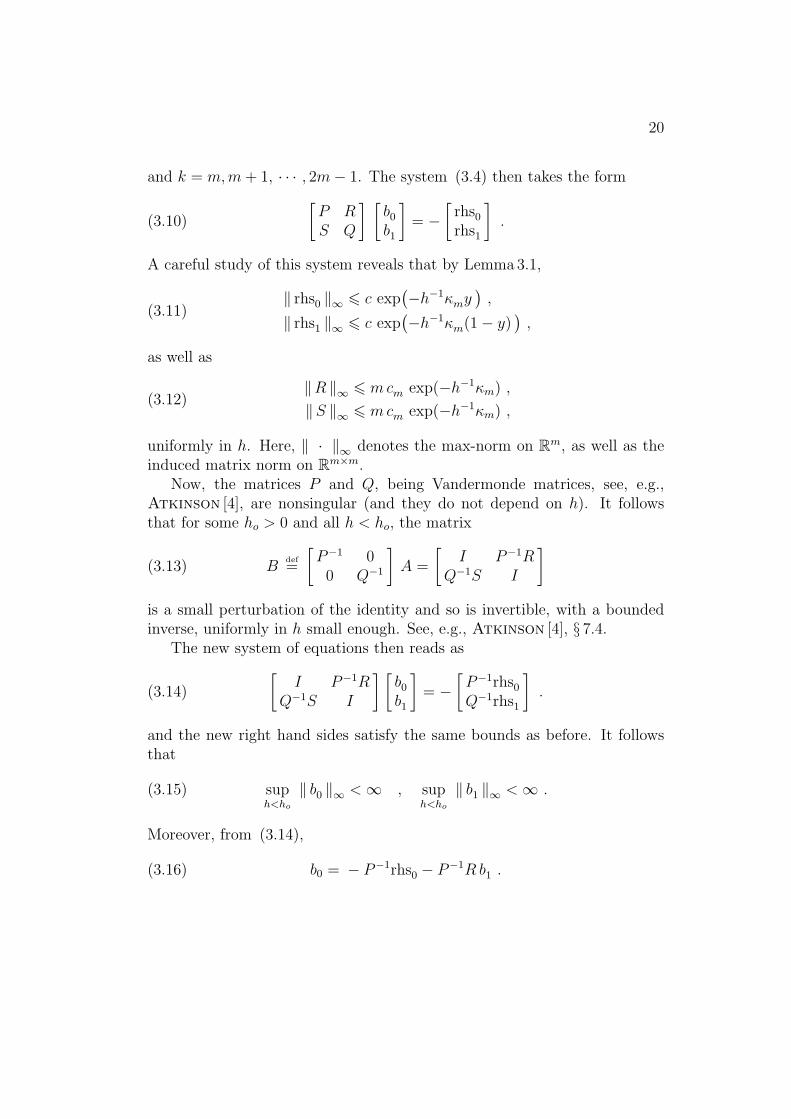
and k = m,m+ 1, · · · , 2m− 1. The system (3.4) then takes the form

(3.10)

[P RS Q

] [b0b1

]= −

[rhs0

rhs1

].

A careful study of this system reveals that by Lemma3.1,

(3.11)‖ rhs0 ‖∞ 6 c exp

(−h−1κmy

),

‖ rhs1 ‖∞ 6 c exp(−h−1κm(1− y)

),

as well as

(3.12)‖R ‖∞ 6 mcm exp(−h−1κm) ,

‖S ‖∞ 6 mcm exp(−h−1κm) ,

uniformly in h. Here, ‖ · ‖∞ denotes the max-norm on Rm, as well as theinduced matrix norm on Rm×m.

Now, the matrices P and Q, being Vandermonde matrices, see, e.g.,Atkinson [4], are nonsingular (and they do not depend on h). It followsthat for some ho > 0 and all h < ho, the matrix

(3.13) Bdef=

[P−1 00 Q−1

]A =

[I P−1R

Q−1S I

]is a small perturbation of the identity and so is invertible, with a boundedinverse, uniformly in h small enough. See, e.g., Atkinson [4], § 7.4.

The new system of equations then reads as

(3.14)

[I P−1R

Q−1S I

] [b0b1

]= −

[P−1rhs0

Q−1rhs1

].

and the new right hand sides satisfy the same bounds as before. It followsthat

(3.15) suph<ho

‖ b0 ‖∞ <∞ , suph<ho

‖ b1 ‖∞ <∞ .

Moreover, from (3.14),

(3.16) b0 = − P−1rhs0 − P−1R b1 .

21

Now, the bound (3.15) on b1, and the bound (3.12) on R imply that for ally ∈ [ 0 , 1 ],

(3.17)‖ b0 ‖∞ = O

(exp(h−1κmy)

)+O

(exp(h−1κm)

)= O

(exp(h−1κmy)

).

A similar derivation applies to b1.

Remark 3. Messer and Goldstein [23] fudge the natural boundary con-ditions slightly, by approximating the solution of (3.14) by the right handside. This introduces a negligible error.

4. Convolution-like integral operators on Lp spaces

In this section, we prove Theorems 2 and 3.

Proof of Theorem 2. One verifies that the boundary value problem (1.1)constitute the Euler equations for the problem

minimize ‖u ‖ 2

L2(w)− 2

⟨u , v

⟩+ h2m ‖u(m) ‖2

subject to u ∈ Wm,2( 0 , 1 ) .

Thus, for each v ∈ L2(0, 1), the (weak) solution of (1.1) exists and is unique.Moreover, u satisfies

‖u ‖ 2

L2(w)+ h2m ‖u(m) ‖2 =

⟨u , v

⟩6 ‖u ‖

L2(w)‖ v ‖

L2(1/w),

so that ‖u ‖L2(w)

6 ‖ v ‖L2(1/w)

, and then, by the assumption (1.2) on the

design density,

(4.1) ‖u ‖ 6 w−11 ‖ v ‖ .

As far as the equivalence of (1.1) and (2.4) is concerned, obviously, if u solves(1.1), then it also is a solution of (2.4). For the converse, consider (2.4) withv ∈ L2(0, 1). The solution is unique: if u ∈ L2(0, 1) and u+ TλMu = 0, thenu = −TλMu , so that u satisfies

(−λ2)m u(2m) + u = −M u

22

together with the natural boundary conditions, but this implies that

(−h2)m u(2m) + w u = 0

and consequently, see above, u = 0. Since TλM : L2(0, 1) → L2(0, 1) is acompact integral operator, the Fredholm alternative, see, e.g., Atkinson[5], now implies that the solution of (2.4) exists. Then, (4.1) implies that

‖ ( I + TλM )−1 Tλ ‖26 w

low/w1 = 1

2,

and so ‖ ( I+TλM )−1 TλM ‖2

6 12(w2−wlow

)/wlow

, and finally, since ( I+

TλM )−1 = I − ( I + TλM )−1 TλM , then

‖ ( I + TλM )−1 ‖2

6 1 + (w2 − wlow

)/(2wlow

) .

This is the bound of the theorem.

Proof of Theorem 3. The goal is to apply Theorem 3.1 of Eggermont andLubich [15], where the finiteness of sup 0<λ<1 ‖ ( I+TλM )−1 ‖∞ is deducedfrom the finiteness of sup 0<λ<1 ‖ ( I + TλM )−1 ‖2 . To that end, we need tointroduce classes of kernels on [ 0 , 1 ] × [ 0 , 1 ] , denoted by F(b, e) whereb ∈ L1(R) and e ∈ C(R), with e(0) = 0 , are given functions. Now, we saythat a function K defined on [ 0 , 1 ]× [ 0 , 1 ] belongs to F(b, e) if there existsan h, with 0 < h < 1, such that

(4.2)|K( t , s ) | 6 h−1 b

(h−1 | t − s |

),

‖K( t + δ, · )−K( t , · ) ‖1 6 e(h−1 δ ) .

Note that by Theorem 1, there exists a constant c, such that for all rele-vant t , s, δ and h, (0 < h < 1),

|Rmλ( t , s )M( s ) | 6 c h−1 exp(− κmh

−1 | t − s |),

as well as

‖Rmλ( t + δ , · )M( · )−Rmλ( t , · )M( · ) ‖1 6 c δ ‖R ′mλ(θ, · ) ‖1 6 c h−1 | δ | .

Thus, the kernels Rmλ( t , s )M(s) of the integral operators TλM belong toa subset A of the class F(b, e) , with

b( t ) = c exp(−κm | t | ) and e( t ) = c | t | ,

23

for a suitable constant c. Thus, by Theorem 3.1 of [15], now Theorem 2implies that there exists a constant C3 such that

sup0<λ<1

‖ ( I + TλM )−1 ‖∞ 6 C3 .

Of course, since Tλ and M are symmetric, then

‖ ( I + TλM )−1 ‖∞ = ‖ ( I +MTλ )−1 ‖1,

and since ( I + TλM )−1 = M−1 ( I +MTλ )−1M , this gives

‖ ( I + TλM )−1 ‖1

6 ‖M ‖1‖M−1 ‖

1‖ ( I +MTλ )−1 ‖

1

6 2(w2 − wlow

)/wlow

· C3

6 C4 <∞ .

and we are d o n e .

5. The decay of the Green’s function

The proof of the missing part of the Main Theorem regarding the exponentialdecay of the Green’s function Rwmh( t , s ) rests on the following result. Forκ > 0, define

(5.1) a( t ) = λ−1 exp(−κλ−1 | t | ) ,

with λ as in (2.2). Also, recall Theorem 1, so that

(5.2)∣∣Rmλ( t , s )

∣∣ 6 cm λ−1 exp(−km λ

−1 | t − s | ) .

Lemma 2. For all 0 < κ < km,∫ 1

0

∣∣∣ a( τ − s )

a( t − s )− 1

∣∣∣ ∣∣∣Rmλ( t , τ)∣∣∣ dτ 6

2 cm κ

( km − κ ) km

.

Proof. First, for | t | > | s |, we have

0 6a( s )

a( t )− 1 = exp

(κλ−1 ( | t | − | s | )

)− 1 6 exp

(κλ−1 | t − s |

)− 1 .

24

For | t | 6 | s |, one obtains likewise

0 6 1− a( s )

a( t )6 1− exp

(−κλ−1 | t − s |

)6 exp

(κλ−1 | t − s |

)− 1 .

It follows that the integral in the lemma is bounded by

cm λ−1

∫ 1

0

(eκ λ−1| t−τ |−1

)e−km λ−1 | t−τ | dτ 6 cm

∫ ∞

−∞

(eκ |τ |−1

)e−km |τ | dτ .

Now, multiply out the integrand and integrate.

Proof of the Exponential Decay of Rwmh. Fix s ∈ [ 0 , 1 ]. Then

v( t ) = Rwmh( t , s )/a( t − s )

satisfies the equation, cf. (2.4),

(5.3) v + Tλ,a v = b ,

where b( t ) = w−1

lowRmλ( t , s )

/a( t − s ) , and Tλ,a is defined by

[Tλ,a g ]( t ) =

∫ 1

0

a( τ−s )

a( t−s )Rmλ( t , τ )M(τ) g(τ) dτ .

Note that b is bounded, uniformly in λ. Now, we may rewrite (5.3) as

v + TλM v + (Tλ,a − Tλ )M v = b

so that

(5.4) v + E v = ( I + TλM )−1 b ,

where E = ( I + TλM )−1 (Tλ,a − Tλ )M . Now,∥∥ E ∥∥∞

6∥∥ ( I + TλM )−1

∥∥∞

∥∥ (Tλ,a − Tλ )∥∥∞

∥∥M ∥∥∞ 6 C κ

for a suitable constant C. This uses Theorem 3 with p = ∞, and Lemma 2to bound

∥∥ (Tλ,a −Tλ )∥∥∞ . Now, choose κ 6 1/(2C). Then,

∥∥ E ∥∥∞ 6 1

2, so

that the Banach contraction principle applied to (5.4) implies the inequality‖ v ‖∞ 6 const ‖ b ‖∞ . Thus, v is bounded, uniformly in λ. But this impliesthe exponential decay of Rwmh( t , s ).

25

6. The dependence on hhh

In this section, we study the dependence of the reproducing kernel Rwmh onthe parameter h, analogous to the inequalities (1.38) for convolution kernels.

Theorem 5. Under the conditions (1.2) on the design density, there existsa constant c such that for all h , θ ∈ ( 0 , 1 ), and all p , 1 6 p 6 ∞,

sups∈[ 0 , 1 ]

∥∥∥Rwmh( · , s )−Rwmθ( · , s )∥∥∥

p6 c h−1+1/p

∣∣∣ 1− h

θ

∣∣∣ .Proof. It suffices to prove the cases p = 1 and p = ∞. Let u = Rwmh( · , s )

and v = Rwmθ( · , s ) . Let λ = hw−1/(2m)low and η = θ w

−1/(2m)low . Then, by

Theorem 2, the functions u and v are the solutions to(I + TλM

)u = w−1

lowRmλ( · , s ) and(I + Tη M

)v = w−1

lowRmη( · , s ) .

It follows that

(6.1) wlow

(u− v ) = first + second ,

with

(6.2)first =

(I + Tη M

)−1{Rmλ( · , s )−Rmη( · , s )

},

second ={(

I + TλM)−1 −

(I + Tη M

)−1}Rmλ( · , s ) .

Everything is in place to bound the two terms. From the semi-explicit repre-sentation of Theorem 4, one obtains just as for convolution kernels that forall p , 1 6 p 6 ∞,

(6.3)∥∥∥Rmλ( · , s )−Rmη( · , s )

∥∥∥p

6 c λ−1+1/p∣∣∣ 1− λ

η

∣∣∣ .and by Theorem 3, the same bound with a different constant applies to thefirst term.

Regarding the second term, observe that(I+TλM

)−1−(I+Tη M

)−1=

(I+TλM

)−1 (Tη−Tλ

)M

(I+Tη M

)−1,

so that, again with Theorem 3,∥∥∥ (I + TλM

)−1 −(I + Tη M

)−1∥∥∥

p6 c

∥∥∥ Tη − Tλ∥∥∥

p.

26

Now, since∥∥∥ Tλ − Tη

∥∥∥p

6 c supx∈[ 0 , 1 ]

∥∥∥Rmλ(x , · )−Rmη(x , · )∥∥∥

16 c2

∣∣∣ 1− λ

η

∣∣∣ ,then, with the bound from Theorem 4 valid for p = 1, and p = ∞,∥∥Rmλ(x · )

∥∥p

6 c λ−1+1/p ,

the second term may be bounded as∣∣ second∣∣ 6 c λ−1+1/p

∣∣∣ 1− λ

η

∣∣∣ .Finally, since λ/η = h/θ, and h = w

lowλ, the theorem follows.

References

[1] Abramovich, F.; Grinshtein, V., Derivation of equivalent kernels for gen-eral spline smoothing: a systematic approach, Bernoulli 5, 359–379 (1999).

[2] Adams, R. A.; Fournier, J. J. F. Sobolev spaces, Second edition, Aca-demic Press, Amsterdam (2003).

[3] Aronszajn, N. Theory of reproducing kernels Trans. Amer. Math. Soc.68,337–404 (1950).

[4] Atkinson, K. E., An introduction to numerical analysis, John Wiley andSons, New York (1989).

[5] Atkinson, K. E., The numerical solution of integral equations of the secondkind, Cambridge University Press, Cambridge (1997).

[6] Chiang, C.; Rice, J. and Wu, C., Smoothing spline estimation for varyingcoefficient models with repeatedly measured dependent variables, J. Amer.Statist. Assoc. 96, 605–619 (2001).

[7] Cox, D. D., Asymptotics of M-type smoothing splines, Ann. Statist. 11,530–551 (1984).

[8] Cox, D. D., Multivariate smoothing spline functions, SIAM J. Numer. Anal.21, 789–813 (1984).

27

[9] Deheuvels, P.; Mason, D. M., General asymptotic confidence bands basedon kernel-type function estimators, Stat. Inference Stoch. Process. 7, 225–277(2004).

[10] Devroye, L., Gyorfi, L., Density estimation : the L1–view, John Wileyand Sons, New York (1985).

[11] Dolph, C. L.; Woodbury, M. A., On the relation between Green’s func-tions and covariances of certain stochastic processes and its application tounbiased linear prediction, Trans. Amer. Math. Soc. 72, 519–550 (1952).

[12] Dudley, R. M., Real analysis and probability. Cambridge University Press,Cambridge, (2002).

[13] Eggermont, P. P. B.; LaRiccia, V. N., Maximum penalized likelihoodestimation, Volume I: Density estimation, Springer-Verlag, New York (2001).

[14] Eggermont, P. P. B.; LaRiccia, V. N., Uniform error bounds for smoothingsplines, Manuscript (2005).

[15] Eggermont, P. P. B.; Lubich, Ch., Uniform error estimates of operationalquadrature methods for nonlinear convolution equations on the half line,Math. Comp. 56, 149–176 (1991).

[16] Einmahl, U.; Mason, D. M., Uniform in bandwidth consistency of kernel-type function estimators, Ann. Statist. 33, 1380–1403 (2005).

[17] Eubank, R. L., Spline smoothing and nonparametric regression, Marcel Dek-ker, New York (1999).

[18] Gyorfi, L.; Kohler, M.; Krzyzak, A.; Walk, A., A distribution-freetheory of nonparametric regression, Springer-Verlag, New York (2002).

[19] Hardle, W., Janssen, P., Serfling, R., Strong uniform consistency ratesfor estimators of conditional functionals, Ann. Statist. 16, 1428–1449 (1988).

[20] Konakov, V. D.; Piterbarg, V. I., On the convergence rate of maximaldeviation distribution for kernel regression estimates, J. Multivariate Anal.15, 279–294 (1984).

[21] Mathews, J.; Walker, R. L., Mathematical methods of physics, Addison-Wesley, New York (1979).

[22] Messer, K., A comparison of a spline estimate to its equivalent kernel esti-mate, Ann. Statist. 19, 817–829 (1991).

28

[23] Messer, K.; Goldstein, L., A new class of kernels for nonparametric curveestimation, Ann. Statist. 21, 179–196 (1993).

[24] Nychka, D., Splines as local smoothers, Ann. Statist. 23, 1175–1197 (1995).

[25] Poschel, J., Hill’s potentials in weighted Sobolev spaces and their spectralgaps, Manuscript, University of Stuttgart (2004).

[26] Silverman, B. W., Spline smoothing : the equivalent variable kernel method,Ann. Statist. 12, 898–916 (1984).

[27] Speckman, P. L., The asymptotic integrated mean squared error for smooth-ing noisy data by splines, Manuscript, University of Oregon (1981).

[28] Wahba, G., Spline models for observational data, SIAM, Philadelphia (1990).

[29] Ziemer, W. P., Weakly differentiable functions, Springer-Verlag, New York(1989).

Food and Resource Economics

University of Delaware

Newark, DE 19717-1303

[email protected], [email protected]