OpenCMISS: A multi-physics & multi-scale computational infrastructure for the VPH/Physiome project

lable at ScienceDirect

Progress in Biophysics and Molecular Biology 107 (2011) 32e47

Contents lists avai

Progress in Biophysics and Molecular Biology

journal homepage: www.elsevier .com/locate/pbiomolbio

Original Research

OpenCMISS: A multi-physics & multi-scale computational infrastructurefor the VPH/Physiome project

Chris Bradley a,b,*, Andy Bowery c, Randall Britten a, Vincent Budelmann a, Oscar Camara d,e,Richard Christie a, Andrew Cookson f, Alejandro F. Frangi d,e, Thiranja Babarenda Gamage a,Thomas Heidlauf g, Sebastian Krittian c, David Ladd a, Caton Little a, Kumar Mithraratne a, Martyn Nash a,h,David Nickerson a, Poul Nielsen a,h, Øyvind Nordbø i, Stig Omholt i, Ali Pashaei d,e, David Paterson b,Vijayaraghavan Rajagopal a, Adam Reeve a, Oliver Röhrle g, Soroush Safaei a, Rafael Sebastián j,Martin Steghöfer d,e, Tim Wu a, Ting Yu a, Heye Zhang k, Peter Hunter a

aAuckland Bioengineering Institute (ABI), The University of Auckland, New ZealandbDepartment of Physiology, Anatomy and Genetics (DPAG), University of Oxford, United KingdomcComputing Laboratory, University of Oxford, United KingdomdCenter for Computational Imaging and Simulation Technologies in Biomedicine (CISTIB), Universitat Pompeu Fabra, Barcelona, SpaineNetworking Biomedical Research Center e Bioengineering, Biomaterials and Nanomedicine (CIBER-BBN), Barcelona, Spainf Imaging Sciences & Biomedical Engineering Division, King’s College London, United Kingdomg Stuttgart Research Centre for Simulation Technology, University of Stuttgart, GermanyhDepartment of Engineering Science, The University of Auckland, New ZealandiCIGENE, Department of Animal and Aquacultural Sciences, Norwegian University of Life Sciences, Aas, NorwayjDepartment of Computer Science, Universitat de Valencia, Spaink Shenzhen Institute of Advanced Technology, Chinese Academy of Sciences, Shenzhen, China

a r t i c l e i n f o

Article history:Available online 7 July 2011

Keywords:Computational modelling softwareMulti-scaleMulti-physicsPhysiome project

* Corresponding author. Auckland Bioengineering Insland, Private Bag 92019, Auckland 1142, New Zealandfax: þ64 9 3677157.

E-mail address: [email protected] (C. Brad

0079-6107/$ e see front matter � 2011 Elsevier Ltd.doi:10.1016/j.pbiomolbio.2011.06.015

a b s t r a c t

The VPH/Physiome Project is developing the model encoding standards CellML (cellml.org) and FieldML(fieldml.org) as well as web-accessible model repositories based on these standards (models.physiome.org). Freely available open source computational modelling software is also being developed to solve thepartial differential equations described by the models and to visualise results. The OpenCMISS code(opencmiss.org), described here, has been developed by the authors over the last six years to replace theCMISS code that has supported a number of organ system Physiome projects.

OpenCMISS is designed to encompass multiple sets of physical equations and to link subcellular andtissue-level biophysical processes into organ-level processes. In the Heart Physiome project, for example,the large deformation mechanics of the myocardial wall need to be coupled to both ventricular flow andembedded coronary flow, and the reactionediffusion equations that govern the propagation of electricalwaves through myocardial tissue need to be coupled with equations that describe the ion channelcurrents that flow through the cardiac cell membranes.

In this paper we discuss the design principles and distributed memory architecture behind theOpenCMISS code. We also discuss the design of the interfaces that link the sets of physical equationsacross common boundaries (such as fluid-structure coupling), or between spatial fields over the samedomain (such as coupled electromechanics), and the concepts behind CellML and FieldML that areembodied in the OpenCMISS data structures. We show how all of these provide a flexible infrastructurefor combining models developed across the VPH/Physiome community.

� 2011 Elsevier Ltd. All rights reserved.

titute, The University of Auck-. Tel.: þ64 9 3737599x89924;

ley).

All rights reserved.

1. Introduction

The last few decades have witnessed a remarkable increase inthe computational power that is available to scientists and engi-neers. The increased power has enabled mathematical andcomputer modelling of physical systems to advance from looking at

C. Bradley et al. / Progress in Biophysics and Molecular Biology 107 (2011) 32e47 33

simple phenomenon in isolation to the analysis of complex coupledmulti-scale and multi-physics processes. The increase in modelcomplexity has driven a corresponding increase in the complexityof the computer codes that solve the models. As modern scientificmodelling codes take a great deal of effort to develop, test, andmaintain, there has been an emerging trend towards collaborativeefforts to develop software libraries which can be used by manygroups. For the case of the finite element method a number oflibraries have been developed. Some of the libraries aim to begeneral purpose e.g., libMesh (Kirk et al., 2006), deal.II (Bangerthet al., 2007), FETK (Holst, 2001) and OOFEM (Patzák and Bittnar,2001; Patzák et al., 2001). Other libraries are more specific toa particular scientific area e.g., in the field of cardiac modellingthere are, to name a few, Continuity (www.continuity.ucsd.edu),CARP (Vigmond et al., 2003) and Chaste (for Cancer and Cardiacapplications) (Pitt-Francis et al., 2009). The computational size ofcomplex coupled models have meant that the computationallibraries have increasingly used parallel processing to reduce therun time of the simulations (Bordas et al., 2009).

The VPH/Physiome1 project is an international collaborativeeffort to understand both the physiology and pathology of thehuman body using quantitative, anatomically and biophysicallybasedmodels that link clinical data at theorgan level (e.g., fromMRI)to patient-specific molecular data. The complexity and range ofspatial and temporal scales involved in this project call for robustdata andmodelling standards. Thedevelopmentof such standards isdescribed briefly below. Model repositories and visualisation tools,based on these standards, have also been established. The purposeof this paper is to describe the development of a computationalsoftware library, called OpenCMISS, which uses the modelsdescribed by the VPH/Physiome standards for solving coupled bio-physically based equations that incorporate multiple spatial andtemporal scales.

We describe the design goals for the software and illustrate thedata structures with a geometrically simple example, relevant tothe cardiac physiome project, which couples biophysical equationsets both within and across tissue regions, and in some caseslinking down to cell level ODE models.

2. Physiome standards

As the computational models inevitably become more complex,it is increasingly difficult for anyone other than the author(s) of thepublication describing the model to decipher, code, and run themodel in order to reproduce the results claimed in a publication. Itcan also be very difficult to then use this model as one componentof a more complex model.

To address these challenges several groups have developedstandards for encoding models over the past ten years. Thesemodelling standards typically use the eXtensible Markup Language(XML) developed by the worldwide web consortium (w3c.org), aswell as a variety of other standards based on XML, such as MathMLfor encoding mathematics, and various metadata standards.

Two XML-based model encoding standards are currently beingdeveloped under the IUPS Physiome Project (Hunter and Nielsen,2005; Hunter, 2004; Hunter and Borg, 2003) and the EuropeanVirtual Physiological Human (VPH) project (vph-noe.eu). CellML

1 The Physiome Project was begun by the International Union of PhysiologicalSciences (IUPS) in 1997 to provide an integrative model-based framework forunderstanding human physiology. The Virtual Physiological Human (VPH) projectwas initiated in 2006 by the European Commission with a focus on clinical appli-cations of the physiome project. These two projects have nowmerged into the VPH/Physiome project.

(cellml.org) is designed to encode lumped parameter biophysicallybased systems of ordinary differential equations (ODEs) andnonlinear algebraic equations e together called differential alge-braic or DAE systems (Cuellar et al., 2003). FieldML (fieldml.org) isdesigned to encode spatially and temporally varying field infor-mation such as anatomical structure, the spatial distribution ofprotein density or computed fields such as the electrical potential oroxygen concentration throughout a tissue (Christie et al., 2009). Athird markup language called the ‘systems biology markuplanguage’ or SBML (sbml.org) has been developed by the systemsbiology community. This has similar expressiveness to CellML but istargeted more specifically to representing models of biochemicaland genetic networks.

CellML separates the syntax of a model (e.g., the mathematicalequations encoded in MathML) and the semantics (the biologicaland biophysical meanings of the model components and parame-ters) defined in the model metadata by reference to suitableontologies. This facilitates building complex models by importingmodular components defined in libraries. SBML is more closely tiedto the concepts of biochemical and genetic networks. FieldML dealswith the encoding of fields, such as geometry and stress, at multiplespatial scales by allowing hierarchies of material coordinatesystems that preserve anatomical relationships (e.g., coronaryarteries embedded in a deforming myocardial tissue that is itselfpart of a heart contained within a torso). These three standards aresupported by the US National Institutes of Health (NIH) and theEuropean Commission’s funding agency (currently operating underFramework 7).

Model repositories are available for all three markup languagese PMR2 (Physiome Model Repository 2, see models.cellml.org) forCellML (Lloyd et al., 2008) and FieldML models and Biomodels(biomodels.net) for SBML models. Various minimum informationstandards are also available including MIRIAM (ebi.ac.uk/miriam)and MIASE (ebi.ac.uk/compneur-srv/miase).

3. Background to CMISS

CMISS is an acronym for ‘Continuum Mechanics, Image anal-ysis, System identification and Signal processing’. Code develop-ment for CMISS began in Auckland in 1980 with the goal ofcreating a bioengineering finite element code for solving multiplecoupled partial differential equations. The initial applicationswere for the heart, primarily for electromechanics (Hunter andSmaill, 1988; Hunter et al., 2003), but it rapidly expanded toinclude other heart processes (Smith et al., 2004) and to supportapplications in other organs such as the lungs, with couplingbetween soft tissue mechanics, heat and moisture transport andairway fluid mechanics (Tawhai et al., 2000, 2004). While finiteelement methods provided the primary numerical technique, thecode was developed in the 1980s to include boundary elementmethods (for electrical current flow in the thorax) and finitedifference equations based on curvilinear grids. The visual displayand graphical user interface aspects of the program were devel-oped in parallel in a program called CMGUI (cmiss.org/cmgui)(Christie et al., 2002).

Some of the unique features of CMISS (in comparison tocommercial finite element codes) that have been carried over intoOpenCMISS are: (i) the use of cubic Hermite basis functions topreserve C1 or G1 continuity across element boundaries (Bradleyet al., 1997) where this is important for efficient field representa-tion; (ii) the use of variable order basis functions (e.g., bicubicHermite by linear Lagrange); and (iii) the close relationship that ispreserved between the representation of tissue structure and theorgan anatomy, through the use of material structure fields definedwith respect to embedded material coordinates.

C. Bradley et al. / Progress in Biophysics and Molecular Biology 107 (2011) 32e4734

The CMISS code (including CMGUI) has been at the heart ofmany multi-scale physiome projects over the past 20 years, but asthe VPH/Physiome modelling standards evolved it became clearthat a redevelopment of both programs was needed to takeadvantage of both the new modelling standards and repositories,and the increasing move (in the academic world at least) to freelyavailable open source software. The OpenCMISS project wastherefore begun in 2005 as an open source collaboration betweenthe University of Auckland in New Zealand and the University ofOxford in the UK. This collaboration was extended last year toinclude King’s College London, Universitat Pompeu Fabra, Barce-lona, Spain, the Norwegian University of Life Sciences and theUniversity of Stuttgart, Germany. This year, the Shenzhen Instituteof Advanced Technology, in Shenzhen, China, has also joined.

4. Design goals

The first goal was that OpenCMISS would be a flexible libraryrather than a large monolithic application. A library-based codemeans that it is considerably easier to incorporate physiome andbioengineering models into clinical or commercial applications asa library that can be wrapped by a customised interface. The libraryshould be modular, extensible, and programmable. This allows forthe library itself to be customised and/or extended inwhatever wayis appropriate for the end application.

The second design goalwas generality. Previous experiencewiththe CMISS modelling environment indicated the importance ofdeveloping code in as general a way as possible. Generalised datastructures, in which the data for diverse modelling problems areexpressed in a common format, allow for easier coupling betweendifferent problems. This is especially true for unforeseen, coupledproblems that may arise from future applications. The goal ofgenerality does, however, often mean that there is some trade-offwith the computational performance of code. As the computa-tional size of bioengineering models can be very large it isextremely important that computational performance is carefullyconsidered. But it is our view that it is better to optimise a moregeneral code armed with the knowledge of exactly what theproblem is than to prematurely optimise a specific code whichcould then limit the applicability of that code.

The third design goal was that OpenCMISS should be an inher-ently parallel code and that the parallel environment should be asgeneral as possible. Parallel processing is required as the computa-tional demands of solving models increases due to increased reso-lution or complexity of the models. However, optimal parallelprocessing strategies dependon theparticular problembeing solved.Also the lifetime of modelling codes is often an order of magnitudegreater than the lifetime of the computer hardware, and it is notablethat the architecture of parallel machines has changed over the lastfew decades from vector processors, to symmetric multiple proces-sors (SMPs), to clusters of processors, to clusters of multiple coreprocessors, through to using General Purpose Graphical ProcessingUnits (GPGPUs). Code that assumes a particular parallel algorithm ora particular parallel architecture may not be appropriate for a futureproblem or future parallel hardware. For these reasons a design goalof OpenCMISS was that the code uses a general n � p(n) � e(p)hierarchical parallel environment where n is the number ofcomputational nodes, p(n) is the number of processing systems onthe computational node and e(p) is the number of processingelements for each processing system. Examples of this hierarchy are:

a) multi-core or SMP n ¼ 1, p(n) > 1, e(p) ¼ 1b) pure cluster n > 1, p(n) ¼ 1, e(p) ¼ 1c) multi-core cluster n > 1, p(n) > 1, e(p) ¼ 1d) multi-core cluster with GPUs n > 1, p(n) > 1, e(p) > 1

The fourth design goal was that OpenCMISS should be able to beused, understood, and developed by novices and experts alike.Modern bioengineering and physiome science requires a team ofscientists, graduate students, and post-doctoral researchers fromvaried backgrounds, eachwith a different skill set. It is unrealistic toexpect that each member of the team will become an expert inevery area of modelling and computation. The design of Open-CMISS thus abstracts and encapsulates model details in a number ofobjects of hierarchical complexity. The hierarchy of these objectsallows complex details to be hidden from the users, if required, andthe object interface allows an expert to manipulate object param-eters whilst the novice user makes use of sensible default param-eter values for the common cases.

The final design goal, as mentioned earlier, was to incorporateApplication Programming Interfaces (APIs) for the physiomemarkup languages CellML (Miller et al., 2010) and FieldML.

5. Software systems

OpenCMISS is written in Fortran 95/2003 with an object-basedapproach for high level objects. It has bindings for Fortran and Cand uses SWIG (swig.org) interfaces for Cþþ and Python. It uses theMozilla trilicense (mozilla.org/MPL) that is being used for otheropen source Physiome projects. Standard software engineeringpractices are followed, including the use of a source code repositoryon SourceForge (sourceforge.net/projects/opencmiss), Doxygen fordocumentation, testing via a Buildbot system, validation againstanalytic test cases, and a tracker system e all described furtherbelow.

Note that although the main source code revision controlsystem for OpenCMISS is hosted on SourceForge using Subversion,we are currently evaluating distributed version control systems(DVCS’s) such as Git or Mercurial, with the possibility of migratingfrom Subversion in the future. One perceived advantage ofdistributed version control systems is the fit with a research-oriented development model, allowing for code to be written forresearch that is destined to eventually be released as open source,but kept closed-source initially until the corresponding researcharticles have been published. DVCS’s allow for version control andcollaboration during the closed phase, and when released as opensource, the original version history can be kept intact, or possiblysummarised.

Other SourceForge services used are:

� a wiki (sourceforge.net/apps/mediawiki/opencmiss/index.php?title¼Main_Page)

� mailing lists (sourceforge.net/mail/?group_id¼201176)� aweb-based source code revision viewer using Trac (sourceforge.net/apps/trac/opencmiss)

Note that the source code revision viewer allows views of thecode revision history via a web browser, and also provides an RSSfeed of code changes. A mirror of the Trac revision viewer is alsoavailable, and is hosted at the ABI (svnviewer.bioeng.auckland.ac.nz/projects/opencmiss).

For project planning, the OpenCMISS project uses the Physiomeproject issue tracker (tracker.physiomeproject.org). The Bugzillatracker system is used for managing both feature planning and bugreporting. A draft version of the OpenCMISS development plan isstored in the issue tracker database. The tracker allows trackeritems to have dependencies on other tracker items, and these canbe viewed by means of interactive web-based tree views and graphviews. This allows for dynamic planning, where the views of theplan are updated instantly as each status is updated. Modificationsto plan are also instantly visible. Stakeholders have the option of

C. Bradley et al. / Progress in Biophysics and Molecular Biology 107 (2011) 32e47 35

receiving status updates via customisable RSS feeds or by means ofcustomisable e-mail alerts.

The OpenCMISS project makes extensive use of exampleprograms. These examples serve a number of purposes includingdemonstrating the capability of OpenCMISS, documenting how tosolve certain equations and as a means for testing and validatingthe code. The set of examples is currently stored in the OpenCMISSsource repository, but this will most likely change in the near futureso that example models and their field descriptions are hosted aspart of a physiome model repository. OpenCMISS examplesundergo an extensive validation process in which example solu-tions are compared with an analytic solution to the problem(if available). The example solutions are checked for convergenceand tested in parallel. Once the example has demonstrated that it issolving correctly it is then tested nightly against the currentcode using a Buildbot testing system. The BuildBot automatedtesting system for OpenCMISS (autotest.bioeng.auckland.ac.nz)is a web-based system used for automated daily building, testing,and documentation generation. BuildBot provides a web-basedconfiguration facility, and views of current and historical testresults. These results are also available via e-mail alerts and an RSSfeed.

The generated documentation is updated daily to match thesource code head revision. The Doxygen documentation system isused to extract specially formatted comments from the source codeand also parses the source code structure and generates docu-mentation targeted at developers using the OpenCMISS library, aswell as developers contributing to the OpenCMISS project (availablefrom cmiss.bioeng.auckland.ac.nz/OpenCMISS/doc/programmer).

A second Subversion system svn.physiomeproject.org/svn/opencmissextras, hosted by the ABI, is used to assist developersin setting up a development environment for OpenCMISS, mainlyby facilitating retrieval of compatible versions of the third-partylibraries and tools on which OpenCMISS depends.

Finally, the main OpenCMISS website (opencmiss.org) uses theModX content management system.

6. Open source libraries

OpenCMISS builds on a number of successful software projectsused in the modelling community. In accordance with an opensource design philosophy, OpenCMISS aims to use softwarelibraries that are, where possible, themselves open source. In caseswhere a library is not open source, that library and its functionalityare considered optional so that it is possible to build a completelyopen-sourced product.

For parallel computations in a heterogeneous multiprocessingenvironment OpenCMISS uses the MPI standard (mpi-forum.org)for distributed parallelisation and the OpenMP (openmp.org)standard for shared memory parallelisation. OpenCMISS has beentested with the MPICH2 (mcs.anl.gov/research/projects/mpich2),Open MPI (open-mpi.org), MVAPICH (mvapich.cse.ohio-state.edu)open source MPI libraries as well as vendor specific MPI librariesfrom Intel and IBM. Recently, OpenCMISS developers have beeninvestigating parallel computations on GPGPUs using CUDA (nvidia.com/object/cuda_home_new.html). However, as CUDA is a propri-etary technology, developers have started to consider OpenCL(khronos.org/opencl) for programming GPGPUs.

In order to calculate optimal mesh partitions, OpenCMISS usesthe parallel graph partitioning package ParMETIS (glaros.dtc.umn.edu/gkhome/metis/parmetis/overview). The licensing options forParMETIS allow it to be used freely only for educational andresearch purposes by non-profit institutions. For situations wherethis copyright is too restrictive OpenCMISS also uses Scotch (gforge.inria.fr/projects/scotch) for graph partitioning.

For numerical solvers, OpenCMISS makes use of a number ofthird-party libraries. Particular use is made of libraries developedthrough the US Department of Energy SciDAC (scidac.gov), TOPS(scidac.gov/math/TOPS.html) and ACTS (acts.nersc.gov) projects.For linear and nonlinear system solvers OpenCMISS uses PETSc(mcs.anl.gov/petsc) for iterative Krylov sub-space linear systemsolvers. In addition a number of direct linear solvers such asMUMPS (graal.ens-lyon.fr/MUMPS), SuperLU_DIST (crd.lbl.gov/wxiaoye/SuperLU) and PaStiX (gforge.inria.fr/projects/pastix) areavailable in OpenCMISS through a PETSc interface. OpenCMISS alsouses

� SUNDIALS (computation.llnl.gov/casc/sundials/main.html) fordifferentialealgebraic equations

� Hypre (computation.llnl.gov/casc/hypre/software.html) forpreconditioners

� TAO (mcs.anl.gov/research/projects/tao) for optimisation� SLEPc (grycap.upv.es/slepc) for eigenproblems� BLACS (netlib.org/blacs) and ScaLAPACK (netlib.org/scalapack)for linear algebra

For input and output OpenCMISS uses the CellML (cellml.org)and FieldML (fieldml.org) APIs. FieldMLwill ultimately use standardlibraries such HDF5 (hdfgroup.org/HDF5) and/or NetCDF (unidata.ucar.edu/software/netcdf) for parallel I/O of large data sets.

7. Multi-physics modelling

The major features in OpenCMISS for dealing with coupledmulti-physics models include a flexible system for describingmultiple physical models and complex problem workflows,methods for coupling different physical systems together and theability to handle different spatial and temporal scales using FieldMLconcepts and CellML models.

In order to provide a general and reusable framework Open-CMISS holds each different set of physical equations (and the datafor those equations) in a separate object within the code base. Forexample, if a coupled system of fluid and solidmechanics was beingconsidered, the equations for the fluid part would be in a separateobject to the solid part. Each set of physical equations can then beconsidered and constructed independently. OpenCMISS furtherabstracts the coupling process by separating the sets of equationsfrom the solver libraries that perform numerical and computationaloperations on those equations. The coupled set of equations whichcan be used with a solver is formed by adding in each individual setof equations and any necessary coupling equations (see below) tothe solver equations. This system for coupling equations has theadvantages that each physical set of equations can be consideredindependently, without the complexity of the final coupled equa-tions, and that the solvers can consider just the numerical equa-tions independently of the actual source of the equations. Ascoupled systems often require a number of different computationaloperations, OpenCMISS allows for a flexible system to describe theproblem workflow in terms of the solvers of the coupled systems.

Coupling of different physical models can occur in a number ofways. Different physicalmodels can be coupled in the same regionofinterest (e.g., a coupled systemof partial differential equations) or indifferent regions of interest (e.g., a fluidesolid interaction system inwhich the fluid is in one region and the solid in another). Couplingcan also occur between the solvers in a problem workflow (e.g.,iterating between two solvers until convergence is reached).

OpenCMISS couples physics in the same region by usinga consistent FieldML description of each physical problem andallowing for coupled equations through the sharing of commonfieldvariables. Because the data about each problem is stored using the

Fig. 1. A geometrically simple example to illustrate the use of regions, coordinatesystems and meshes for solving a coupled multi-physics, multi-scale problem inOpenCMISS.

C. Bradley et al. / Progress in Biophysics and Molecular Biology 107 (2011) 32e4736

same data structures, the individual equations for each problem canbe formulated using variables from different problems as easily asthey can be formulated using variables from their problem.

In OpenCMISS coupling between different regions can be accom-plished using a number of different methods to relate the equations.Thesemethods impose compatibility conditions between thefields ineach region. The conditions are termed interface conditions inOpenCMISS. The simplest interface/compatibilitycondition is to allowthe degrees-of-freedom (DOFs) of the equations in one region to belinearly related to the DOFs in another set of equations in anotherregion. This linearcouplingallows for the interfaceconditionbetweentheequations to be imposeddirectly at eachDOFpoint. InOpenCMISSthis is known as a strong interface condition in the sense that it holdsat a number of points on the interface. This strong interface conditionallows for a coupled set of equations that govern the combinedphysics to be formed through row and column manipulations of theindividual sets of equations. As inter-region coupling involvesdifferent regions, the strong interface condition is defined by usingexplicit interfaces. These interfaces ensure that information is passedbetween regions in a controlled manner.

Other inter-region coupling methods allow for the interfaceconditions to be imposed in an integral sense. Examples of thesemethods supported by OpenCMISS include Lagrange, augmentedLagrange, and penalty methods. Interface conditions from thesemethods are termed weak interface conditions in that thecompatibility condition does not necessarily hold at any particularpoint in the interface, but rather that the condition holds in theaverage or integral sense (Nordsletten et al., 2010).

The final key feature for multi-scale, multi-physics problems inOpenCMISS is the use of CellML and FieldML. CellML models allowfor the physics at a small spatial scale to be abstracted and viewedas a single point model within another model at a larger spatialscale. OpenCMISS also allows for CellML models to be evaluatedand integrated at a different temporal scale than other models.Further spatial and temporal scales can be incorporated intoOpenCMISS problems using hierarchical field concepts fromFieldML which allow data to be viewed at different levels.

8. OpenCMISS data structures

We illustrate the key FieldML data structures and workflowsimplemented in OpenCMISS with a geometrically simple examplethat couples six systems of equations, each representing a differentphysical process. The example couples the equations from thesephysical processes, bothwithin and across their spatial domains andacross spatial scales. It provides a simple data structure prototypefor the anatomically based electromechanical heartmodelling in thecardiac physiome project. The physical regions are shown in Fig. 1.

The key OpenCMISS/FieldML concepts of regions, meshes,decomposed domains, fields, equation sets, equations, problems,control loops, solvers, solver equations, and distributed vectorsand matrices will be discussed below with reference to thisexample.

The physical processes are described briefly below. Note that theequations are givenhere in their ‘strong’partial differential equation(PDE) form to highlight the fields needed for their representation inOpenCMISS. The equations solved within OpenCMISS are ‘weak’ orintegral equation versions of these PDEs in keeping with the stan-dard finite element Galerkin approach. The references quoted foreach equation set give further details including, in most cases, theweak form of the equations.

1. Large deformation soft tissuemechanics onmesh 1 of region 1.Finite elasticity theory (Malvern, 1969; Nash and Hunter, 2000;Oden, 2006) with incompressible, inhomogeneous, nonlinear,

anisotropic material properties, gives the following governingequations, based on conservation of linear momentum andconservation of mass:

vtrv þ ðv �wÞ$Vxv ¼ Vx$sþ f (1)

where r is material density, n is the material velocity vector, s is theCauchy stress tensor, f is the force per unit mass, andw¼ n orw¼ 0for the Lagrangian or Eulerian forms of the equations, respectively.Note that the Cauchy stress tensor s is related to the 2ndPiola-Kirchhoff stress tensor T by s¼J�1FTFT, where F is the defor-mation gradient tensor and J ¼ detF. An additional constraintequation is required to solve Eq. (1). The constraint equation thatenforces incompressibility is J ¼ detF ¼ 1. Further details are givenin Nash and Hunter (Nash and Hunter, 2000). Note also that T is themost appropriate form of stress tensor for defining material prop-erties (being the energy conjugate of the Green-Lagrange straintensor) and is defined as a function of the strain energy functionWand tissue pressure p by

T ¼ 12

�vWvE

þ vWvET

�� pC�1 þ Tactive (2)

where E is the Green-Lagrange strain tensor and C�1¼(FTF)�1 is theinverse of the right Cauchy strain tensor (and is the contravariantmetric tensor for the deformed state of the tissue). This constitutiverelation is specified in a CellML model, where for soft tissues W isa nonlinear function of the components of E and defines ananisotropic stressestrain relation. For problems in which anactively contracting material is deforming (e.g., a contracting heart)the stress tensor is modified by introducing an active stress term.The active stress comes stress Tactive (expressed here as a 2nd Piola-Kirchhoff stress) comes from a CellML encoded model (Hunteret al., 1998; Niederer et al., 2006) in which fibre strain, obtainedfrom the deformation field, is used in a nonlinear integral equationmodel to update the active stress on the fibre direction.

Typical boundary conditions for large deformation mechanicsproblems include specifying an appropriate combination ofdisplacements and normal Cauchy stress on a boundary surface. Forfurther details see Nash and Hunter (Nash and Hunter, 2000). Initialconditions must also be specified for the time-dependent formu-lation given in Eq. (1). For details of the initial conditions seeNordsletten et al. (Nordsletten et al., 2010).

C. Bradley et al. / Progress in Biophysics and Molecular Biology 107 (2011) 32e47 37

The dependent variable fields are the material displacementvector u and, if the tissue is treated as incompressible, the scalartissue pressure field p (effectively a Lagrange multiplier associatedwith the incompressibility constraint).

For further details on the formulation of the finite elasticity (andcoupled fluid flow) equations in OpenCMISS see Nordsletten et al.(Nordsletten et al., 2011).

2. 3D fluid flow on mesh 2 of region 2. The 3D NaviereStokesequations (Batchelor, 2000; Currie, 2002; Nordsletten et al.,2011) are

vtrv þ ðv �wÞ$Vxv ¼ �Vxpþ 2Vx$mDþ f ; (3)

Vx$v ¼ 0 (4)

Where D is the Eulerian strain rate tensor and w is the meshvelocity. The dependent variable field components are the fluidvelocity vector v and the hydrostatic pressure field p.

Typical boundary conditions for 3D fluid flow include a Dirichletspecification of the fluid velocity at inlet and outlets, specificationof zero tangential velocity at walls, Dirichlet specification of fluidpressure at inlets and outlets or of zero pressure for free surfaceflows. Typical initial conditions are the specification of the fluidvelocity in the domain. For further information see Nordslettenet al. (Nordsletten et al., 2010, 2011).

Typical interface conditions for fluidesolid interaction are thatthe fluid velocity is equal to the rate of change of displacement ofthe solid and that there is continuity of traction at the fluidesolidinterface (Nordsletten et al., 2011).

3. 1D fluid flow on mesh 3 of region 1. The one-dimensionalapproximation (1D) of the 3D NaviereStokes equations(Smith et al., 2000, 2002) describe flow within blood vesselsthat are embedded within the deforming soft tissue.

vVvt

þ ð2a� 1ÞVvVvx

þ 2ða� 1ÞV2

RvRvx

þ 1r

vPvx

¼ �2a

a� 1VR2

(5)

vRvt

þ VvRvx

þ R2vVvx

¼ 0 (6)

P ¼ 23Eh0R0

R2

R20� 1

!þ external wall stress term (7)

where a is a parameter defining the assumed velocity profile acrossthe blood vessel of radius R. R0 is the radius at zero pressure P,where the wall thickness is h0.

Typical boundary conditions for 1D fluid flow include specifi-cation of Dirichlet conditions on the fluid velocity or pressure at thebeginning and/or end of the network of vessels. Typical interfaceconditions for coupled 1D fluid flow in deforming elastic tissue isthat the net pressure in the blood vessel is balanced by the externalstress acting on the blood vessel wall.

The dependent variable fields are the scalar fluid velocity V (anaverage over the vessel cross-section) and the hydrostatic pressurefield p.

4. Porous flow on mesh 1 of region 1. The Darcy porous flowequation for poro-elastic problems (Coussy, 2004) is

VX$�JF�1KF�TVXp

�¼ 0 (8)

where VX denotes the gradient operator with respect to the unde-formed configuration. The additional dependent variable field

component for this equationset is theDarcypressurep. In this stronglycoupled poro-elastic model, the equations for the fluid pressure andsolid displacements are assembled together. The fluid pressure issolved using Darcy’s law (with deformation effects accounted for viaF), and the solid displacement is solved using themomentum balanceequations in (1). The constitutive relation for the integrated tissuerepresentation provides the coupling from the fluid pressure to thedeformation and is given by Chapelle (Chapelle et al., 2010)

T ¼ vWMR

vEþ"Ksð J�1Þ�ðp�p0Þ Jþ

12ðp�p0Þ2

Mf 0

f 2J

#C�1 (9)

where WMR is the Mooney-Rivlin strain energy function, Ks is thebulkmodulus, po is a reference fluid pressure,M is the Biotmodulusand f is a function of J that provides compatibility with incom-pressible conditions. In Chapelle (Chapelle et al., 2010) the solid andfluid equations are coupled by iteratively solving each equation inturn. Due to the design of OpenCMISS, we are able to stronglycouple the equations for finite elasticity and fluid pressure andbuild them into a single set of solver equations in order to solve thismulti-physics problem simultaneously.

Typical boundary conditions for porous flow are to set thepressure on the boundary as a Dirichlet condition. A Neumannboundary condition can also be set for pressure as means to specifyfluid velocity.

5. Wavefront propagation (eikonal) equation on submesh 1 ofregion 1, determines the evolution of the activation wavefrontthroughout the myocardium. Two different eikonal formula-tions for cardiac activation have been proposed by Keener(Keener, 1991) and Colli Franzone (Colli Franzone et al., 1990).Eikonal equations have been solved using a finite elementmethod (Tomlinson et al., 2003) and the Fast Marching Method(FMM) (Chinchapatnam et al., 2007; Sethian, 1996; Sethian andVladimirsky, 2000). A variation of the standard cardiac elec-trophysiological activation model suitable for use with theFMM is the HamiltoneJacobi equation of eikonal equation formgiven by

V4TTTV4T � 1 ¼ 0 (10)

where 4 is the activation time and T is the anisotropy tensordefined as T ¼ AF, where A is the orthogonal matrix representingthe unit vectors along the local myofibril coordinate system and F isa diagonal matrix whose diagonal elements are equal to thecomponents of the conduction velocities along the local myofibrilcoordinate axes. The HamiltoneJacobi eikonal equation is used todetermine the position of the propagating activation wavefrontthroughout the myocardium. It assumes a rather simple model forcellular activation but is computationally efficient. It is also some-times used as a first approximation for the wavefront position andfollowed by the more biophysically accurate monodomain equa-tions described below.

Typical initial conditions for the HamiltoneJacobi equation area specification of an associated state field as inactivated.

The dependent variable field is a state variable from which theactivation time 4 is derived.

6. Electrical activity in the deforming soft tissue on mesh/sub-mesh 1. The spread of electrical activity through tissue is, ingeneral, governed by the bidomain equations which relate thespread of electric potential in the intra- and extra-cellularspaces. Under the assumption that the conductivity anisot-ropies are equal in the intra- and extra-cellular spaces thebidomain equations reduce to the monodomain equation

C. Bradley et al. / Progress in Biophysics and Molecular Biology 107 (2011) 32e4738

(Keener and Sneyd, 1998; Pullan et al., 2005). The monodomainequation is given by.

V$ðsVVmÞ ¼ Am

�Cm

vVm

vtþ Iion

�� Is (11)

Where s is the conductivity tensor, Is is the stimulation current andVm is the transmembrane voltage. The capacitive current CmðvVm=vtÞis associatedwith themembranecapacitanceCm,Am is the cell surfaceto volume ratio and the total ion channel current Iion is given by

Iion ¼ INa þ IKrþ IKs

þ IK1þ ICa þ Icl þ :: (12)

Operator splitting techniques (Qu and Garfinkel, 1999; Sundneset al., 2005) are often used to transform the monodomain equationinto two parts. The first part is a set of nonlinear ordinary differ-ential equations (ODEs) which relate the rate of change of thetransmembrane voltage to the ionic currents. The second part isa parabolic equation that governs the reactionediffusion of trans-membrane voltage. The set of nonlinear ODEs which model theionic currents in the cell are described by CellML models.

Typical initial conditions for the monodomain equation are thatthe transmembrane voltage is at the resting potential and that thestate variables for the CellML ionic models are at their steady states.Typical boundary conditions for the monodomain equation area Neumann condition on the transmembrane potential so thatthere is no normal current flux from the domain.

The monodomain equation interacts with other equationsthrough the cell model describing the transmembrane current. Thiscell model can also be used to provide an active stress for couplingto equations of large deformation elasticity, or be used to providean ionic source term for, say, equations that model the diffusion ofion concentration.

The dependent variable field is the transmembrane voltage Vm.An additional dependent field is also required to describe the statevariables associated with the CellML models for the ionic current.

Note that the first two problems are defined on their owndistinct regions (Region 1 for the soft tissue and Region 2 for thefluid) with separate meshes (Mesh 1 and Mesh 2, respectively) andare coupled with a fluid-structure Interface region that sets up theappropriate boundary coupling conditions. The third set of 1D flowequations is solved onMesh 3 that is embedded within the materialcoordinate system of Mesh 1. The final three sets of porous flowequations, eikonal equations, and monodomain equations are allsolved on Mesh 1 in Region 1, or its higher spatial resolution sub-meshes, and are coupled to the equations of large deformationelasticity via the deformation gradient field.

9. Regions, meshes and domain decomposition

A region provides a name space and container for the variousobjects that are required to describe a physical problem, includingfields, the meshes, and other domains they are defined on, and thecoordinate system for geometric fields. In the example of Fig. 1,Region 1 represents the myocardium and Region 2 the left and rightventricles. A third Interface region allows for the coupling of the firsttwo regions. Finally, these three regions are themselves embeddedin a World Region.

A mesh is an OpenCMISS object that includes the topology ofthe computational mesh (elements and global node numbers)together with the basis functions needed for interpolation ofnodal parameters. OpenCMISS is flexible in allowing differentforms of interpolation throughout the mesh. Most standardbasis families and orders are implemented including linear,quadratic, and cubic Lagrange bases, cubic Hermite bases andlinear, quadratic, and cubic simplex bases. Tensor product basis

functions may also be used to allow for different polynomialforms in each interpolation direction e.g., cubic Hermite e linearLagrange basis functions. OpenCMISS also allows for a differentbasis function in each element of the mesh e.g. simplex triangularbases may be used in one part of the mesh, bilinear Lagrangebases in another part, and bicubic Hermite bases in yet anotherpart. OpenCMISS also allows for different numerical quadratureschemes to be used for each basis function. The different quad-rature schemes can be used to allow different numbers of Gauss,or integration, points in each interpolation direction in order topermit optimisations involving higher (or lower) order poly-nomials. Care, however, must be taken to ensure that the Gaussquadrature scheme is consistent when doing integrationsinvolving a number of different basis functions.

OpenCMISS uses domain decomposition methods (Mathew,2008; Smith et al., 1996; Toselli and Widlund, 2005) as the mainmechanism for distributed parallelism. The decomposition ofmeshes in Region 1 onto domains that correspond to computationalnodes, is illustrated in Fig. 2. Note that a computational node couldbe a single CPU in a distributed memory cluster or a multiprocessorshared memory node in a cluster. A similar domain decompositionexists for Region 2.

When choosing a decomposition (or mesh partitioning) fora mesh it is important that computational aspects are considered. Itis desirable that each domain has roughly the same computationalwork load as other domains as this will ensure good computationalload balance when running a parallel simulation. A second aspect isthat the boundary between domains be as small as possible in orderto minimise the amount of communication between the compu-tational domains. To achieve an optimum mesh decomposition,OpenCMISS uses a parallel graph partitioning library (see earlierunder Open source libraries). If required, a user can also specifya decomposition for a mesh.

Once a mesh has been decomposed into a number of compu-tational domains, OpenCMISS performs two operations in order toabstract or hide the distributed nature of the problem. The firstoperation involves computing “ghost” nodes and elements. Whenusing a numerical method in an element or at a node on a decom-posed mesh, information is often required from neighbouringelements and nodes. If the node or element is at the boundary ofa computational domain, then the neighbouring node or elementcould be held on a neighbouring computational domain. To avoidhaving to communicate neighbouring information, a local copy ofthe information is held on each computational domain. This isachieved by expanding the domain obtained from the partitioninglibrary by one extra layer of elements around the boundary of thedomain to provide a degree of overlap between the domains. Theelements in the extra layer are known as ghost elements. All nodesin the ghost elements that are not already in the computationaldomain are also added to the domain as ghost nodes.

The second operation is renumbering. For each distributednumbering scheme (e.g. nodes, elements) OpenCMISS computesa new local numbering scheme that is mapped to the “global”meshnumbering scheme. This renumbering ensures that each schemenow starts at 1 in each computational domain and continuescontiguously until the number of items (including ghosts) isreached. In order to allow further optimisations, OpenCMISS alsocomputes which of the numbers are internal to the domain (i.e. notghosted in any other computational domain), which numbers areon the boundary of the domain (and thus ghosted in othercomputational domains) and which numbers are ghosts (in thisdomain). By convention internal and boundary numbers are first inthe numbering scheme, and ghosts are placed at the end. Thisrenumbering ensures that a programmer working with localnumbers can view each computational domain as just a smaller

Fig. 2. The meshes and their domain decompositions for Region 1. The meshes shown here are designed to illustrate OpenCMISS concepts used in the heart physiomemodels shownin the top right corner. Note that ‘ghost elements’ (see text) are shown by the dotted areas in the domain decomposition.

C. Bradley et al. / Progress in Biophysics and Molecular Biology 107 (2011) 32e47 39

version of the bigger problem, simplifying the programming for thedistributed problem.

10. Fields

In OpenCMISS fields are the central mechanism for describingthe physical problem and for storing any information required forthis description. The extensive use of fields for data storage inOpenCMISS is one of the fundamental linkages to the ideas andconcepts of FieldML. OpenCMISS fields have a hierarchy in thata particular OpenCMISS field contains a number of field variablesand each field variable may contain any number of field variablecomponents. An OpenCMISS field variable can thus be thought of asa conventional scalar, vector, or tensor field.

In accordance with mathematical and FieldML definitions,a field is defined over a domain. In order to allow for distributedproblems, the conceptual domain for a field variable is the entiremesh, but the actual domain is the decomposed computationaldomain. In OpenCMISS each field variable component is allowed touse a different form of interpolation (i.e., a different set of basisfunctions in each element of the computational domain) from otherfield variable components. In addition OpenCMISS allows eachcomponent to have different forms of Degree-Of-Freedom (DOF)structure from other components. The DOFs in each componentmay have the following structures:

� constant structure (i.e., one DOF for the component).� by element structure (one or more DOFs for each element).� by node structure (one or more DOFs for each node).� by Gauss point structure (one or more DOFs for each Gauss orintegration point).

� by data point structure (one or more DOFs for each data point).

For each field variable OpenCMISS combines the DOFs for eachcomponent as a vector of DOFs. This information is then stored ina distributed vector class (see distributed matrices and vectors) sothat the data for each field variable on a computational node arejust those that are required for that computational domain. Thedata in each distributed vector for a field variable is referred to asa parameter set. OpenCMISS allows for multiple parameter sets tobe stored for a field variable. Examples of useful parameter setsinclude the previous values of a field for problems with a time

variation, the set of increments to be applied to field variable DOFvalues, or the set of nonlinear residuals at each DOF.

For the complete coupled multi-physics problem described, thefields, field variables, and their components are listed in Table 1.Note that some of the fields carry anatomical information, somecarry tissue material parameters, and some are dependent variablefields that require the solution of partial differential equations fortheir evaluation.

11. Equation sets and equations

An equation set is the OpenCMISS object that is used to modela particular physical problem. It is the container object for all thenecessary information required to describe the physical equationsin a region (which may contain any number of equation sets). Themain objects that an equation set contains are all the necessaryfields (from the same region) required for the problem descriptionand the mathematical equations that result from applying somesolution method (e.g., the finite element method) to the physicalproblem. The equation set fields can be from the following generalfield classes: equation description field, geometric field, fibre field,materials field, independent field, analytic field, dependent field, andsource field.

Another OpenCMISS object is an equation which contains thematrices and vectors that result from a numerical method beingapplied to the governing equations of an equation set. The equationmatrices and vectors are built using the field variables of anequation set. OpenCMISS abstracts equations into a general formthat allows for linear and nonlinear equations, as well as static,quasistatic, and dynamic temporal equations. The general forminvolves linear matrices Ai, mass M, damping C and stiffness Kmatrices of the dynamic sub-system, a nonlinear residual vectorg(u), a source vector s and a RHS vector b. These are used to formthe following discrete equations:

Xi

Aiui þM€uþ C _uþ Kuþ gðuÞ þ s ¼ b (13)

Each matrix or vector is incorporated into the general equationby mapping a field variable onto the matrix or vector. For example,if the governing equation involved a dynamic component, a corre-sponding field variable u would be mapped to the dynamic

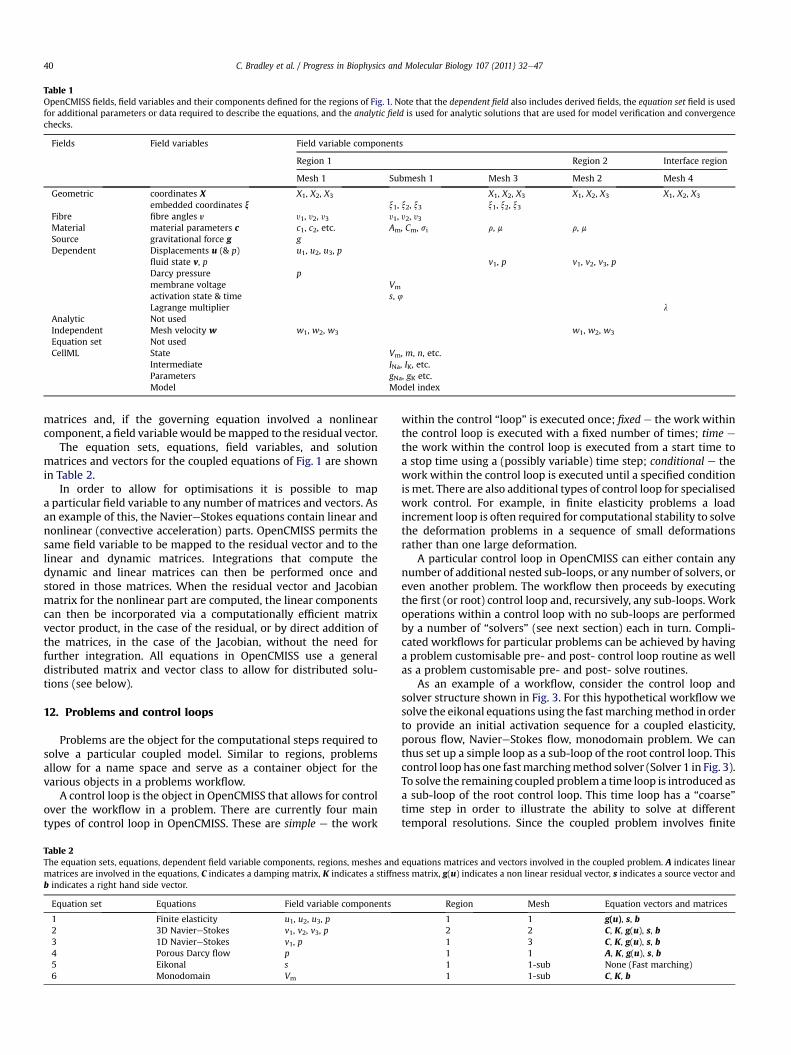
Table 1OpenCMISS fields, field variables and their components defined for the regions of Fig. 1. Note that the dependent field also includes derived fields, the equation set field is usedfor additional parameters or data required to describe the equations, and the analytic field is used for analytic solutions that are used for model verification and convergencechecks.

Fields Field variables Field variable components

Region 1 Region 2 Interface region

Mesh 1 Submesh 1 Mesh 3 Mesh 2 Mesh 4

Geometric coordinates X X1, X2, X3 X1, X2, X3 X1, X2, X3 X1, X2, X3

embedded coordinates x x1, x2, x3 x1, x2, x3Fibre fibre angles y y1, y2, y3 y1, y2, y3Material material parameters c c1, c2, etc. Am, Cm, si r, m r, mSource gravitational force g gDependent Displacements u (& p) u1, u2, u3, p

fluid state v, p v1, p v1, v2, v3, pDarcy pressure pmembrane voltage Vm

activation state & time s, 4Lagrange multiplier l

Analytic Not usedIndependent Mesh velocity w w1, w2, w3 w1, w2, w3

Equation set Not usedCellML State Vm, m, n, etc.

Intermediate INa, IK, etc.Parameters gNa, gK etc.Model Model index

C. Bradley et al. / Progress in Biophysics and Molecular Biology 107 (2011) 32e4740

matrices and, if the governing equation involved a nonlinearcomponent, a field variablewould bemapped to the residual vector.

The equation sets, equations, field variables, and solutionmatrices and vectors for the coupled equations of Fig. 1 are shownin Table 2.

In order to allow for optimisations it is possible to mapa particular field variable to any number of matrices and vectors. Asan example of this, the NaviereStokes equations contain linear andnonlinear (convective acceleration) parts. OpenCMISS permits thesame field variable to be mapped to the residual vector and to thelinear and dynamic matrices. Integrations that compute thedynamic and linear matrices can then be performed once andstored in those matrices. When the residual vector and Jacobianmatrix for the nonlinear part are computed, the linear componentscan then be incorporated via a computationally efficient matrixvector product, in the case of the residual, or by direct addition ofthe matrices, in the case of the Jacobian, without the need forfurther integration. All equations in OpenCMISS use a generaldistributed matrix and vector class to allow for distributed solu-tions (see below).

12. Problems and control loops

Problems are the object for the computational steps required tosolve a particular coupled model. Similar to regions, problemsallow for a name space and serve as a container object for thevarious objects in a problems workflow.

A control loop is the object in OpenCMISS that allows for controlover the workflow in a problem. There are currently four maintypes of control loop in OpenCMISS. These are simple e the work

Table 2The equation sets, equations, dependent field variable components, regions, meshes andmatrices are involved in the equations, C indicates a damping matrix, K indicates a stiffneb indicates a right hand side vector.

Equation set Equations Field variable components

1 Finite elasticity u1, u2, u3, p2 3D NaviereStokes v1, v2, v3, p3 1D NaviereStokes v1, p4 Porous Darcy flow p5 Eikonal s6 Monodomain Vm

within the control “loop” is executed once; fixed e the work withinthe control loop is executed with a fixed number of times; time e

the work within the control loop is executed from a start time toa stop time using a (possibly variable) time step; conditional e thework within the control loop is executed until a specified conditionis met. There are also additional types of control loop for specialisedwork control. For example, in finite elasticity problems a loadincrement loop is often required for computational stability to solvethe deformation problems in a sequence of small deformationsrather than one large deformation.

A particular control loop in OpenCMISS can either contain anynumber of additional nested sub-loops, or any number of solvers, oreven another problem. The workflow then proceeds by executingthe first (or root) control loop and, recursively, any sub-loops. Workoperations within a control loop with no sub-loops are performedby a number of “solvers” (see next section) each in turn. Compli-cated workflows for particular problems can be achieved by havinga problem customisable pre- and post- control loop routine as wellas a problem customisable pre- and post- solve routines.

As an example of a workflow, consider the control loop andsolver structure shown in Fig. 3. For this hypothetical workflow wesolve the eikonal equations using the fastmarchingmethod in orderto provide an initial activation sequence for a coupled elasticity,porous flow, NaviereStokes flow, monodomain problem. We canthus set up a simple loop as a sub-loop of the root control loop. Thiscontrol loop has one fastmarchingmethod solver (Solver 1 in Fig. 3).To solve the remaining coupled problem a time loop is introduced asa sub-loop of the root control loop. This time loop has a “coarse”time step in order to illustrate the ability to solve at differenttemporal resolutions. Since the coupled problem involves finite

equations matrices and vectors involved in the coupled problem. A indicates linearss matrix, g(u) indicates a non linear residual vector, s indicates a source vector and

Region Mesh Equation vectors and matrices

1 1 g(u), s, b2 2 C, K, g(u), s, b1 3 C, K, g(u), s, b1 1 A, K, g(u), s, b1 1-sub None (Fast marching)1 1-sub C, K, b

Fig. 3. A hypothetical example of control loops and solvers for the coupled problem of Fig. 1.

C. Bradley et al. / Progress in Biophysics and Molecular Biology 107 (2011) 32e47 41

elasticity, we can improve the nonlinear convergence behaviour byintroducing a load step loop as a sub-loop of the coarse time loop. Inorder to illustrate weak iterative coupling we introduce a whileconvergence loop as a sub-loop of the load step loop. In order tohave a different time step for the monodomain solution comparedto the over-all problemwe introduce a simple loop and a time loopas sub-loops of the convergence while loop. For the simple loop weintroduce two non-linear dynamic solvers. The first solver in thisloop (Solver 2) solves the combined finite elasticity, porous flow,and 3D NaviereStokes equations. Since we are solving a combinedsystem of equations there is strong (non-iterative) couplingbetween the equations. The second solver in this loop (Solver 3)solves the 1D NaviereStokes equation on the deformed geometrycomputed by Solver 3. For the fine time loopwe use, say, a Gudunovoperator splitting method to split the monodomain into two parts.The first part introduces a CellML integration solver (Solver 4)and the second part introduces a linear dynamic solver (Solver 5).The iterative solution of the elasticity/porous/3D NaviereStokesproblemwith the 1D NaviereStokes problem and the monodomainproblem demonstrates weak iterative coupling.

It should be noted that the ability to construct complicatedproblem workflows with control loops does not necessarily meanthat those workflows will be numerically stable or have desirablenumerical properties. There are often important considerations asto the order of solvers, stability of the schemes, and restrictions onthe various numerical and solver parameters such as the size of thetime step, error, tolerances, etc. Various numerical analysis tech-niques such as stability and error analysis (Butcher, 2008; Higham,2002) are often required to investigate the behaviour of algorithms.This is particularly true for complex, coupled systems of equations.

13. Solvers and solver equations

Solvers are the OpenCMISS objects that perform computationalwork. Solvers are specific to a particular numerical problem orwork

item and are independent of their data source or equations. Ascertain solvers are better at solving particular problems than othersolvers, OpenCMISS aims to support a number of different numer-ical solver libraries. The main classes of solver libraries in Open-CMISS include linear solvers (both iterative and direct), non-linearsolvers (Newton methods, BroydeneFletchereGoldfarbeShanno(BFGS), sequential quadratic programming (SQP)), dynamic solvers(theta based allowing for different schemes, implicit and explicit,various time polynomial order and degree), differentialealgebraicequation (DAE) solvers (including a number of different integra-tors), eigenproblem solvers, optimisation solvers, state iterationsolvers, and CellML model evaluation solvers.

For those solvers that require equations, OpenCMISS allows fora number of solver matrices and vectors. As with the equationsfrom equations sets, solver equations can be classified accordingto their linearity and temporal nature. Solver equations areformed by adding either equations sets (possibly from differentregions) or interface conditions to the solver equations object.Once the adding process has finished OpenCMISS can then forma combined set of equations by looking at the field variablesinvolved and the types of matrices and vectors in the individualequations sets and interface conditions. This flexible approach tothe generation of solver equations allows for multiple physicalsystems in either the same or different regions to be coupledeasily.

14. Integration with CellML

CellML is used to enable OpenCMISS users to define, at run-time,custommathematical models that form parts of a larger model. Forexample, CellML is used to define cellular electrophysiologicalmodels for cardiac electrical models, and to define constitutiverelationships for use in finite elasticity modelling. CellML modelsare also being used to define kinetic models of ion transportproteins that are spatially distributed in a geometric model, and

C. Bradley et al. / Progress in Biophysics and Molecular Biology 107 (2011) 32e4742

used to provide boundary fluxes in a reactionediffusion model.CellML support in OpenCMISS is based on the concept of linkingfield variable components directly to variables in CellML models.This allows for the variable in a CellML model to define the val-ue of each degree-of-freedom in a field variable component.Furthermore, a different CellML model can be used at each degree-of-freedom. This flexibility allows CellML models to be easilyplugged into any of the problem types in OpenCMISS with no needfor problem specific implementation. The result is a very flexibleplug-and-play system for defining custom mathematical models tobe incorporated into the standard bioengineering models sup-ported by OpenCMISS. We have defined the ‘CellML Environment’type to be the container managing CellML models in OpenCMISS.A given OpenCMISS application is able to use multiple CellMLenvironments, and the preliminary best practice would be to havea CellML environment for each spatial scale in the model requiringCellML. For example, in a cardiac electromechanics model onewould have one environment for the cell model(s) and one for thetissue mechanical constitutive relationships.

The first step is to import required CellML models into theenvironment. After importing models into the environment, theuser is able to flag variables from the CellML models to be used byfields outside the CellML environment in which they are defined.CellML model variables are flagged as ‘known’ if their value will becontrolled by a field outside the CellML environment, or as ‘wanted’if the variable value computed by the CellML model will be usedoutside the CellML environment. State variables and the variable ofintegration are automatically flagged as wanted and known,respectively. Once all required variables have been flagged, theCellML environment has enough information to instantiate each ofthe CellML models into computable objects. Currently each modelwill have a simulate-able object generated on each of the compu-tation nodes used in the simulation.

Having been instantiated, the CellML environment is able todefine three fields: the state field, consisting of the state variablesfor each CellML model in the environment; the intermediate field,containing all non-state variables flagged as wanted from all CellMLmodels in the environment; and the parameters field, containing allthe variables flagged as known from all the CellML models in theenvironment. The user is nowable to initialise these fields using thegeneric field methods defined in OpenCMISS (e.g., to set spatiallyvarying cell model parameters not defined or required elsewhere inthe model). Furthermore, the user is able to define mappingsbetween the fields within the CellML environment(s) and fieldsfrom outside the environment. These mappings will ensure that,whenever the relevant CellML model is to be evaluated and/orintegrated, the field values will be transferred in the appropriatedirection (known variables in the CellML model will have theirvalue updated from the mapped source field prior to the evalua-tion; fields mapped to wanted variables will be updated followingthe evaluation of the CellML model).

The final step in this process is to create an equation set withina defined problem and add the necessary CellML environments.Once the appropriate solver for that problem has been defined, theCellML models contained within these environments are able tobe evaluated and/or integrated as appropriate during a generalOpenCMISS problem solution.

Currently, the variable flagging and field mappings describedabove are required to be set up by the user. The plan is that, onceFieldML and CellML become more integrated and use commonmetadata standards, the complete FieldML description of themodelwill include all this information and such mappings would beperformed automatically by OpenCMISS. The ability of the user tooverride or extend such automatic mappings would be preserved insuch future developments.

15. Distributed matrices and vectors

It is important for a distributed computational platform to havegood memory scalability as well as good CPU scalability. In order toachieve a good decrease in the memory usage as the number ofcomputational nodes increases, it is important that each compu-tational node only stores that data which is relevant to that node.Indeed, for certain computer architectures, such as symmetricmultiple processors or multi-core machines, it is extremely ineffi-cient to store data not required for the computational node as thishas the effect of reducing the total amount of memory available bya factor related to the additional data times the number ofprocessors. It is also important for generality reasons that all databe able to be communicated, and for programmability reasons thatthe types of data objects that are communicated in a distributedenvironment is minimised. For these reasons OpenCMISS uses onlya distributed matrix and vector class as the primary data objects.

In addition to its internal distributed data storage requirements,OpenCMISS also needs to communicate data to other (mainlydistributed solver) libraries. In order to allow for multiple currentlibraries or other future libraries to be used with OpenCMISS, it isimportant to encapsulate the data requirements of these librarieswithin the OpenCMISS distributed matrix and vector classes. Thisallows for solverequations tobe formulated independentof theactualsolver that may be used to solve a particular numerical problem.

Both the distributed matrix and distributed vector classes inOpenCMISS distribute the rows of the matrix or vector amongst thecomputational nodes. Each distributedmatrix and vector store onlythe local rows (including ghosts) and columns. In order to allow fordata communication each computational node has methods tochange the local data values held in the distributedmatrix or vector.If a computational node changes the value of a local entry that maybe ghosted on other computational domains, then communicationmust take place so that the other computational nodes can beupdated with the new value. OpenCMISS provides a number ofroutines for the distributed data transfer. The first routine starts thedata transfer and returns, the second routine tests whether or notthe data transfer has finished or not and returns, and the finalroutine finishes the data transfer and returns only when thetransfer is complete. By using a staged approach to transfer, it ispossible to start the transfer and then do additional computationswhilst the data transfer is taking place.

16. Example solutions

To provide an illustration of the framework described above weshow solutions from three coupled problems. The first is a poro-elastic problem on a cube, the second is an HamiltoneJacobieikonal solution on a geometrically simple deforming ventricle, andthe third is amonodomain solution on a square 2D domain, coupledto a CellML electrophysiological model.

16.1. Poro-elastic model

In this example model the fluid pressure and solid displacementequations are coupled together with a volume coupling approach.The equations are defined on the same region and are interde-pendent. The fluid pressure is solved using Darcy’s relation on thedeformed geometry and the solid displacement is solved using themomentum balance equation. The constitutive law used for thecombined material is from Chapelle (Chapelle et al., 2010) asdetailed above.

The coupled equations are solved on a 10mm� 10mm� 10mmblock of myocardiumwith quadratic Lagrange interpolation for thedisplacement field and linear Lagrange interpolation for the fluid

C. Bradley et al. / Progress in Biophysics and Molecular Biology 107 (2011) 32e47 43

pressure field. The displacement in the surface normal directions isfixed for the x ¼ 0, y ¼ 0 and z ¼ 0 faces, and the face at x ¼ 10 mmin the initial configuration is fixed at x ¼ 12 mm. The fluid pressureis constrained to be 0 kPa on the x ¼ 10 mm face and 1 kPa at thex ¼ 0 mm face. The other faces had zero flux boundary conditionsapplied. Fig. 4 shows the deformed cube with swelling towards thex ¼ 0 mm end due to the increased fluid pressure.

16.2. Electro-elastic model

In the heart there is a well ordered interplay between cellularelectrophysiology and cellular force development. Complex feed-back mechanisms support this interplay, which can be modelled bycoupling anatomical, electrophysiological, deformation and forcedevelopment models.

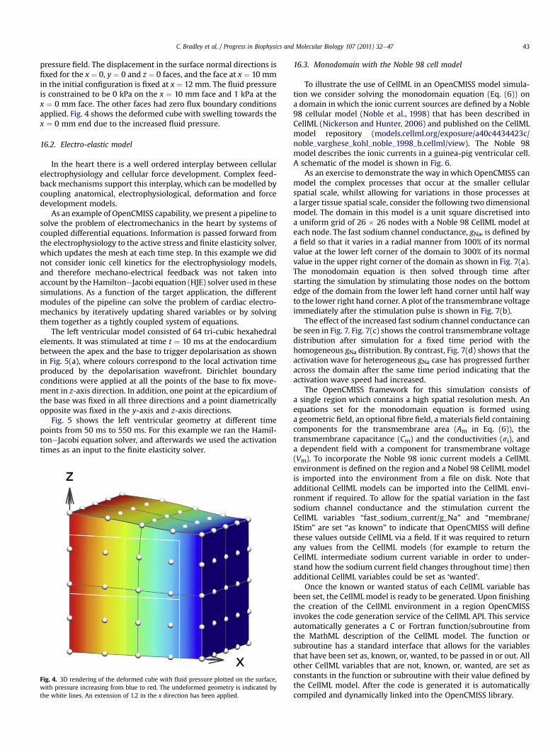
As an example of OpenCMISS capability, we present a pipeline tosolve the problem of electromechanics in the heart by systems ofcoupled differential equations. Information is passed forward fromthe electrophysiology to the active stress and finite elasticity solver,which updates the mesh at each time step. In this example we didnot consider ionic cell kinetics for the electrophysiology models,and therefore mechano-electrical feedback was not taken intoaccount by the HamiltoneJacobi equation (HJE) solver used in thesesimulations. As a function of the target application, the differentmodules of the pipeline can solve the problem of cardiac electro-mechanics by iteratively updating shared variables or by solvingthem together as a tightly coupled system of equations.

The left ventricular model consisted of 64 tri-cubic hexahedralelements. It was stimulated at time t ¼ 10 ms at the endocardiumbetween the apex and the base to trigger depolarisation as shownin Fig. 5(a), where colours correspond to the local activation timeproduced by the depolarisation wavefront. Dirichlet boundaryconditions were applied at all the points of the base to fix move-ment in z-axis direction. In addition, one point at the epicardium ofthe base was fixed in all three directions and a point diametricallyopposite was fixed in the y-axis and z-axis directions.

Fig. 5 shows the left ventricular geometry at different timepoints from 50 ms to 550 ms. For this example we ran the Hamil-toneJacobi equation solver, and afterwards we used the activationtimes as an input to the finite elasticity solver.

Fig. 4. 3D rendering of the deformed cube with fluid pressure plotted on the surface,with pressure increasing from blue to red. The undeformed geometry is indicated bythe white lines. An extension of 1.2 in the x direction has been applied.

16.3. Monodomain with the Noble 98 cell model

To illustrate the use of CellML in an OpenCMISS model simula-tion we consider solving the monodomain equation (Eq. (6)) ona domain in which the ionic current sources are defined by a Noble98 cellular model (Noble et al., 1998) that has been described inCellML (Nickerson and Hunter, 2006) and published on the CellMLmodel repository (models.cellml.org/exposure/a40c4434423c/noble_varghese_kohl_noble_1998_b.cellml/view). The Noble 98model describes the ionic currents in a guinea-pig ventricular cell.A schematic of the model is shown in Fig. 6.

As an exercise to demonstrate the way in which OpenCMISS canmodel the complex processes that occur at the smaller cellularspatial scale, whilst allowing for variations in those processes ata larger tissue spatial scale, consider the following two dimensionalmodel. The domain in this model is a unit square discretised intoa uniform grid of 26 � 26 nodes with a Noble 98 CellML model ateach node. The fast sodium channel conductance, gNa, is defined bya field so that it varies in a radial manner from 100% of its normalvalue at the lower left corner of the domain to 300% of its normalvalue in the upper right corner of the domain as shown in Fig. 7(a).The monodomain equation is then solved through time afterstarting the simulation by stimulating those nodes on the bottomedge of the domain from the lower left hand corner until half wayto the lower right hand corner. A plot of the transmembrane voltageimmediately after the stimulation pulse is shown in Fig. 7(b).

The effect of the increased fast sodium channel conductance canbe seen in Fig. 7. Fig. 7(c) shows the control transmembrane voltagedistribution after simulation for a fixed time period with thehomogeneous gNa distribution. By contrast, Fig. 7(d) shows that theactivation wave for heterogeneous gNa case has progressed furtheracross the domain after the same time period indicating that theactivation wave speed had increased.

The OpenCMISS framework for this simulation consists ofa single region which contains a high spatial resolution mesh. Anequations set for the monodomain equation is formed usinga geometric field, an optional fibre field, a materials field containingcomponents for the transmembrane area (Am in Eq. (6)), thetransmembrane capacitance (Cm) and the conductivities (si), anda dependent field with a component for transmembrane voltage(Vm). To incorporate the Noble 98 ionic current models a CellMLenvironment is defined on the region and a Nobel 98 CellML modelis imported into the environment from a file on disk. Note thatadditional CellML models can be imported into the CellML envi-ronment if required. To allow for the spatial variation in the fastsodium channel conductance and the stimulation current theCellML variables “fast_sodium_current/g_Na” and “membrane/IStim” are set “as known” to indicate that OpenCMISS will definethese values outside CellML via a field. If it was required to returnany values from the CellML models (for example to return theCellML intermediate sodium current variable in order to under-stand how the sodium current field changes throughout time) thenadditional CellML variables could be set as ‘wanted’.

Once the known or wanted status of each CellML variable hasbeen set, the CellML model is ready to be generated. Upon finishingthe creation of the CellML environment in a region OpenCMISSinvokes the code generation service of the CellML API. This serviceautomatically generates a C or Fortran function/subroutine fromthe MathML description of the CellML model. The function orsubroutine has a standard interface that allows for the variablesthat have been set as, known, or, wanted, to be passed in or out. Allother CellML variables that are not, known, or, wanted, are set asconstants in the function or subroutine with their value defined bythe CellML model. After the code is generated it is automaticallycompiled and dynamically linked into the OpenCMISS library.

Fig. 5. A geometrically simple left ventricle example to illustrate the application of OpenCMISS in coupling the HamiltoneJacobi equation (HJE) and finite elasticity solvers inOpenCMISS. (a) Isochrones corresponding to the local activation times of each element obtained from the HJE solver. Blue colour corresponds to 0 ms and red colour to 216 ms. (b)Deformation of the mesh at different time points colour coded by the electrical wavefront propagation.

C. Bradley et al. / Progress in Biophysics and Molecular Biology 107 (2011) 32e4744

After the CellML environment has been established, themapping from OpenCMISS field variable components to CellML,field variable components can be set. For themonodomain problemin question there are two mappings required. The first mapping isfrom the OpenCMISS dependent field component representing thespatially varying transmembrane voltage, Vm, to the CellML statefield variable component for Vm. The secondmapping is the reverseof the first mapping. The definition of the field mappings inOpenCMISS sets the number of instances of CellML models in theOpenCMISS library as a CellMLmodel is defined for each degree-of-freedom (DOF) in the mapped OpenCMISS field.

Fig. 6. A schematic diagram of the ion channels i

After the field mappings have defined the DOF (or field) struc-ture, OpenCMISS is able to set up CellML fields using the mappedstructures. The CellML fields describe the spatial variation of thefree CellML variables in the CellML models. The first CellML field isthe models field. This is an integer field which allows the Open-CMISS user to specify which imported model index to use at eachDOF (OpenCMISS allows for the CellMLmodel to vary spatially). Theremaining CellML fields are the state field, the parameters field, andthe intermediate field. These fields each have one field variable thatcontains as many components as there are free variables in theCellML model. For example the Noble 98 model defines 24 state

n the cell membrane of the Noble 98 model.

Fig. 7. (a) A plot of the fast sodium channel conductance, gNa throughout the monodomain solution domain. The conductance varies in a radial fashion from 100% of its normal valueof 3.855 � 10�5 mS mm�2 (blue) to 300% of its normal value (red). (b) A plot of the transmembrane voltage immediately after the stimulation pulse has finished. The following twoplots show transmembrane voltage after a fixed time period for (c) a control simulation with a uniform gNa distribution at its normal value, and (d) a simulation in which gNa hasbeen altered to the distribution shown in (a). The transmembrane voltage, Vm, in (b)e(d) varies from �95 mV (blue) to þ50 mV (red).

C. Bradley et al. / Progress in Biophysics and Molecular Biology 107 (2011) 32e47 45

variables, so the CellML state field variable has 24 components. TheOpenCMISS simulation defines two parameters as known (gNa andIStim), so the CellML parameters field has two components. NoCellML intermediate variables were set as wanted, so the CellMLintermediate field variable does not contain any field variablecomponents.

The OpenCMISS problem workflow for this monodomainsimulation sets up a root time control loop. In order to solve Eq. (6)an operator splitting approach is used. For Godunov type splitting(other splitting schemes are also defined) two solvers are defined inthe time loop. The first solver is an ODE integration solver tointegrate the CellML ODEs, and the second solver is a lineardynamic solver to solve the parabolic monodomain equation. Theproblem solution then proceeds by stepping through the timecontrol loop. At each time step the CellML integration solver isinvoked first. For this solver the OpenCMISS field to CellML fieldmappings are used to copy the transmembrane voltage componentfrom the dependent field to the transmembrane voltage compo-nent of the CellML state field. The solver then integrates the CellMLmodel ODEs from the current time step to a point in the future asdetermined by the splitting scheme. The OpenCMISS CellML inte-grator works by using a user selectable integration scheme torepeatedly call the appropriate dynamically linked CellML routine.Note that the ODE integration time steps can be smaller than theroot control time loop steps in order to correctly capture processesthat occur on a faster time scale than that of the main problem.Once the integration has finished, the CellML to OpenCMISS fieldmaps are used to copy the transmembrane voltage componentfrom the CellML state field to the OpenCMISS dependent field. Thesecond, dynamic, solver is then invoked to solve the parabolicmonodomain equation for the entire domain.

Note that the above ODE integration solver operates on each ofthe individual CellML models at each dependent field DOF. Thisprocess is ideally suited for parallelisation as each CellML model isindependent and thus can be integrated in parallel. Furtherresearch is currently being undertaken to develop a frameworkthat can take CellML models selected from a model repositoryand/or file and automatically generate CUDA or OpenCL code thatcan integrate these CellML models on a GPGPU (Kirk and Hwu,2010).

17. Discussion and outlook

OpenCMISS is an international open source software project toprovide a computational environment for multi-physics, multi-scale physiological modelling in the VPH/Physiome project. Itbuilds on 30 years of experience with the CMISS code, but adds

more general data structures, copes with awider range of computerarchitectures (distributed memory, GPGPUs, etc) and takes advan-tage of the markup language environments (CellML and FieldML)developed by the VPH/Physiome project over the last 10 years.

In this paper, we have described the OpenCMISS data objects(regions, meshes, decomposed domains, fields, equation sets, equations,problems, control loops, solvers, solver equations) in the context ofa geometrically simple multi-region example that couples severalphysical processes within a single region (large deformation softtissue mechanics, porous flow, eikonal wave propagation, and mon-odomain reactionediffusion equations that incorporate cell electro-physiology) with 1D flow through embedded blood vessels withinthat region, and physical processes in an adjacent region (3D flow inthe ventricles).

Although the examples here are motivated by the Heart Physi-ome project, the FieldML and CellML based data structures aredesigned to handle any coupled system of partial differentialequations. Processes at the tissue level, described by continuousFieldML fields, are coupled to cellular processes described by theCellML modelling framework.

Despite the successful implementation of a large number ofcoupled physical processes, OpenCMISS still requires a largeamount of further development. The current focus for OpenCMISSdevelopment is on optimisation of the code and improved perfor-mance and scaling with processor node code, for both memoryfootprint and solution time. OpenCMISS has also just started to useGPGPUs to accelerate codes. Initial results are promising andOpenCMISS’s field based/CellML approach, in which the dataparallel vector of field DOFs together with a computational kerneldefined by a CellML model, seems to fit well with GPGPU archi-tectures. An important, and often overlooked, part of parallelperformance improvement is to increase parallel IO performance.Currently, the FieldML API used for the input and output of fieldparameters in OpenCMISS is strictly serial. Work is currentlyunderway to integrate HDF5, or other parallel IO libraries, with theFieldML API. This would then allow for the total solution of large,realistic problems to be profiled and optimised.

Another area of development for OpenCMISS and FieldML is theextension of the data structures to cope with more complicatedmesh structures. It is planned to allow for and/or extend hierar-chical, embedded and adaptive meshes. Hierarchical meshes (andfields) are based on the concept of having multiple levels of(increasing) mesh refinement. A coarse mesh (or element) at onelevel can be refined to give a finermesh at another level. The secondmesh level can then also be refined etc. in a hierarchical manner togive further levels. A hierarchical mesh is important for solvingproblems like coupled electromechanics in the same region/mesh

C. Bradley et al. / Progress in Biophysics and Molecular Biology 107 (2011) 32e4746

as the electrical activation problem requires a much higher reso-lution mesh than the large deformation mechanics problem. Hier-archical meshes may also be useful for other solution methods e.g.,multi-grid (Briggs et al., 2000). Embedded meshes and, moregenerally, embedded fields occur when the values of a field areinterpreted with respect to another field. An example of anembedded field is the when the geometric field of coronary arteriesare embedded within the (deforming) geometric field of themyocardium. Adaptive meshes are meshes which can be auto-matically refined so that larger numbers of field degrees-of-freedom are incorporated around areas of large field gradients. Itis also planned to investigate the use of dynamic data structuressuch as oct trees for use in parallel load balancing with hierarchicalor adaptive meshes.

Along with FieldML and CellML the authors are investigatingother markup languages for use with OpenCMISS. One promisinglanguage is the Simulation Experiment Description MarkupLanguage or SED-ML (sed-ml.org) (Köhn and Le Novère, 2008). Itmay be possible to use SED-ML to describe workflows which canthen be implemented using OpenCMISS problems, control loopsand solvers. Some of the ideas in Taverna (www.taverna.org.uk)(Hull et al., 2006) may also be useful in this regard.

The final area of future development for OpenCMISS is todevelop suitable graphical user interfaces (GUIs). Whilst Open-CMISS is primarily a library without a specific GUI, wewish tomakethe use of the library much easier to use for mesh creation andvisualisation of computational results. This GUI may be specific toa particular application or it may be more along the lines ofa general environment for VPH/Physiome problems. Work hasbegun to link together CMGUI and/or GIMIAS (www.gimias.org)(Larrabide et al., 2009) with OpenCMISS.

Please see also related communications in this issue by Bordaset al. (Bordas et al., 2011) and Qu et al. (Qu et al., 2011).

Acknowledgements

C. Bradley, D. Paterson and P. Hunter acknowledge the support ofthe Wellcome Trust for the Cardiac Physiome Project. Workpartially funded by the European Commission under the euHeart’sIntegrated Project (FP7-ICT-2007-224485) and by the SpanishMinistry of Science and Innovation under the cvREMOD CENITProject (CEN20091044). A. Frangi holds an ICREA-Academia Prizefrom the Institucio Catalana de Recerca i Estudis Avancats (ICREA).V. Rajagopal acknowledges the support of a RSNZ Marsden FastStart Grant.

References

Bangerth, W., Hartmann, R., Kanschat, G., 2007. deal.IIda general-purpose object-oriented finite element library. ACM Trans. Math. Software 33, 24/1e24/27.

Batchelor, G.K., 2000. An Introduction to Fluid Dynamics. Cambridge UniversityPress, Cambridge.

Bordas, R., Carpentieri, B., Fotia, G., Maggio, F., Nobes, R., Pitt-Francis, J., Southern, J.,2009. Simulation of cardiac electrophysiology on next-generation high-performance computers. Philos. Transact A Math. Phys. Eng. Sci. 367,1951e1969.

Bordas, R., Gillow, K., Lou, Q., Efimov, I.R., Gavaghan, D., Kohl, P., Grau, V.,Rodriguez, B., 2011. CBG: rabbit-specific ventricular model of cardiac electro-physiological function including specialized conduction system. Prog. Biophys.Mol. Biol. 107, 90e100.

Bradley, C.P., Pullan, A.J., Hunter, P.J., 1997. Geometric modeling of the human torsousing cubic hermite elements. Ann. Biomed. Eng. 25, 96e111.

Briggs, W.L., Henson, V.E., McCormick, S.F., 2000. A Multigrid Tutorial. Society forIndustrial and Applied Mathematics, Philadelphia, PA, pp. xii, 193 p.

Butcher, J.C., 2008. Numerical Methods for Ordinary Differential Equations. JohnWiley & Sons, West Sussex.

Chapelle, D., Gerbeau, J.-F., Sainte-Marie, J., Vignon-Clementel, I.E., 2010.A poroelastic model valid in large strains with applications to perfusion cardiacmodeling. Comput. Mech. 46, 91e101.

Chinchapatnam, P.P., Rhode, K.S., King, A., Gao, G., Ma, Y., Schaeffter, T., Hawkes, D.,Razavi, R.S., Hill, D.L., Arridge, S., Sermesant, M., 2007. Anisotropic wave prop-agation and apparent conductivity estimation in a fast electrophysiologicalmodel: application to XMR interventional imaging. Med. Image Comput.Comput. Assist. Interv. 10, 575e583.

Christie, G.R., Blackett, S.A., Hunter, P.J., Bullivant, D.P., 2002. Modeling and visual-ising the heart. Comput. Vis. Sci. 4, 227e235.

Christie, G.R., Nielsen, P.M., Blackett, S.A., Bradley, C.P., Hunter, P.J., 2009. FieldML:concepts and implementation. Philos. Transact A Math. Phys. Eng. Sci. 367,1869e1884.

Colli Franzone, P., Guerri, L., Tentoni, S., 1990. Mathematical modeling of the exci-tation process in myocardial tissue: influence of fiber rotation on wavefrontpropagation and potential field. Math. Biosci. 101, 155e235.

Coussy, O., 2004. Poromechanics. John Wiley & Sons, West Sussex.Cuellar, A.A., Lloyd, C.M., Nielsen, P.F., Bullivant, D.P., Nickerson, D.P., Hunter, P.J.,

2003. An overview of CellML 1.1, a biological model description language.SIMULATION: Trans. Soc. for Model. Simulation Int. 79, 740e747.

Currie, I.G., 2002. Fundamental Mechanics of Fluids. Marcel Dekker, New York,pp. xiv, 525 p.

Higham, N.J., 2002. Accuracy and Stability of Numerical Algorithms. SIAM,Philadelphia.

Holst, M., 2001. Adaptive numerical treatment of elliptic systems on manifolds. Adv.Comput. Math. 15, 139e191.

Hull, D., Wolstencroft, K., Stevens, R., Goble, C., Pocock, M., Li, P., Oinn, T., 2006.Taverna: a tool fro building and running workflows of services. Nucleic AcidsRes. 34, 729e732.

Hunter, P., Nielsen, P., 2005. A strategy for integrative computational physiology.Physiology (Bethesda) 20, 316e325.

Hunter, P., Smaill, B., 1988. The analysis of cardiac function: a continuum approach.Prog. Biophys. Mol. Biol. 52, 101e164.

Hunter, P.J., 2004. The IUPS physiome project: a framework for computationalphysiology. Prog. Biophys. Mol. Biol. 85, 551e569.

Hunter, P.J., Borg, T.K., 2003. Integration from proteins to organs: the Physiomeproject. Nat. Rev. Mol. Cell Biol. 4, 237e243.

Hunter, P.J., McCulloch, A.D., ter Keurs, H.E., 1998. Modelling the mechanicalproperties of cardiac muscle. Prog. Biophys. Mol. Biol. 69, 289e331.

Hunter, P.J., Pullan, A.J., Smaill, B.H., 2003. Modeling total heart function. Annu. Rev.Biomed. Eng. 5, 147e177.

Keener, J.P., 1991. An eikonal-curvature equation for action potential propagation inmyocardium. J. Math. Biol. 29, 629e651.

Keener, J.P., Sneyd, J., 1998. Mathematical Physiology. Springer, New York.Kirk, B.S., Peterson, J.W., Stogner, R.H., Carey, G.F., 2006. libMesh: a Cþþ library for

parallel adaptive mesh refinement/coarsening simulations. Eng. Comput. 22,237e254.

Kirk, D.B., Hwu, W.W., 2010. Programming Massively Parallel Processors. MorganKaufmann Publishers, Burlington.

Köhn, D., Le Novère, N., 2008. SED-ML e an XML format for the implementation ofthe MIASE guidelines. Computational Methods Syst. Biol. 5307, 176e190.

Larrabide, I., Omedas, P., Martelli, Y., Planes, X., Nieber, M., Moya, J.A., Butakoff, C.,Sebastián, R., Camara, O., De Craene, M., Bijnens, B.H., Frangi, A.F., 2009. GIMIAS:an open source framework for efficient development of research tools andclinical prototypes. In: Ayache, N., Delingette, H., Sermesant, M. (Eds.), Func-tional Imaging and Modeling of the Heart: Proceedings of the 5th InternationalConference, vol. 5528. SpringerLink, Nice, France, pp. 417e426.

Lloyd, C.M., Lawson, J.R., Hunter, P.J., Nielsen, P.F., 2008. The CellML model reposi-tory. Bioinformatics 24, 2122e2123.

Malvern, L.E., 1969. Introduction to the Mechanics of a Continuous Medium.Prentice-Hall, Englewood Cliffs, N.J., pp. xii, 713 p.

Mathew, T.P.A., 2008. Domain decomposition methods for the numerical solution ofpartial differential equations. In: Lecture Notes in Computational Science andEngineering. Springer, Berlin, pp. xiii, 764 p.

Miller, A.K., Marsh, J., Reeve, A., Garny, A., Britten, R., Halstead, M., Cooper, J.,Nickerson, D.P., Nielsen, P.F., 2010. An overview of the CellML API and itsimplementation. BMC Bioinform. 11, 178.

Nash, M.P., Hunter, P.J., 2000. Computational mechanics of the heart e from tissuestructure to ventricular function. J. Elast. 61, 113e141.

Nickerson, D.P., Hunter, P.J., 2006. The Noble cardiac ventricular electrophysiologymodels in CellML. Prog. Biophys. Mol. Biol. 90, 346e359.

Niederer, S.A., Hunter, P.J., Smith, N.P., 2006. A quantitative analysis of cardiacmyocyte relaxation: a simulation study. Biophys. J. 90, 1697e1722.

Noble, D., Varghese, A., Kohl, P., Noble, P., 1998. Improved guinea-pig ventricular cellmodel incorporating a diadic space, IKr and IKs, and length- and tension-dependent processes. Can. J. Cardiol. 14, 123e134.

Nordsletten, D., Kay, D., Smith, N., 2010. A non-conforming monolithic finiteelement method for problems of coupled mechanics. J. Comp. Physiol. 229,7571e7593.

Nordsletten, D.A., Niederer, S.A., Nash, M.P., Hunter, P.J., Smith, N.P., 2011. Couplingmulti-physics models to cardiac mechanics. Prog. Biophys. Mol. Biol. 104, 77e88.

Oden, J.T., 2006. Finite Elements of Nonlinear Continua. Dover Publications.Patzák, B., Bittnar, Z., 2001. Design of object oriented finite element code. Adv. Eng.

Software 32, 759e767.Patzák, B., Rypl, D., Bittnar, Z., 2001. Parallel explicit finite element dynamics with

nonlocal constitutive models. Comput. Struct. 79, 2287e2297.Pitt-Francis, J., Pathmanathan, J., Bernabeu, M.O., Bordas, R., Cooper, J., Fletcher, A.G.,

Mirams, G.R., Murray, P., Osbourne, J.M., Walter, A., Chapman, S.D., Garney, A.,

C. Bradley et al. / Progress in Biophysics and Molecular Biology 107 (2011) 32e47 47

van Leeuwen, I.M.M., Maini, B., Rodriguez, B., Waters, S.L., Whiteley, J.P.,Byrne, H.M., Gavaghan, D.J., 2009. Chaste: a test-driven approach to softwaredevelopment for biological modelling. Comput. Phys. Commun.180, 2452e2471.

Pullan, A.J., Cheng, L.K., Buist, M.L., 2005. Mathematically Modelling the ElectricalActivity of the Heart: From Cell to Body Surface and Back Again. World ScientificPublishing.

Qu, Z., Garfinkel, A., 1999. An advanced algorithm for solving partial differentialequation in cardiac conduction. IEEE Trans. Biomed. Eng. 46, 1166e1168.

Qu, Z., Garfinkel, A., Weiss, J.A., Nivalal, M., 2011. Multi-scale modeling in biology:how to bridge the gaps between scales? Prog. Biophys. Mol. Biol. 107, 21e31.

Sethian, J.A., 1996. A fast marching level set method for monotonically advancingfronts. Proc. Natl. Acad. Sci. U S A 93, 1591e1595.

Sethian, J.A., Vladimirsky, A., 2000. Fast methods for the Eikonal and relatedHamiltoneJacobi equations on unstructured meshes. Proc. Natl. Acad. Sci. U S A97, 5699e5703.

Smith, B.F., Bjørstad, P.E., Gropp, W., 1996. Domain Decomposition: Parallel Multi-level Methods for Elliptic Partial Differential Equations. Cambridge UniversityPress, Cambridge; New York, pp. xii, 224 p.

Smith, N.P., Nickerson, D.P., Crampin, E.J., Hunter, P.J., 2004. Multiscale computa-tional modelling of the heart. Acta Numerica 13, 371e431.

Smith, N.P., Pullan, A.J., Hunter, P.J., 2000. Generation of an anatomically basedgeometric coronary model. Ann. Biomed. Eng. 28, 14e25.

Smith, N.P., Pullan, A.J., Hunter, P.J., 2002. An anatomically based model of transientcoronary blood flow in the heart. SIAM J. Appl. Math. 62, 990e1018.

Sundnes, J., Lines, G.T., Tveito, A., 2005. An operator splitting method for solving thebidomain equations coupled to a volume conductor model for the torso. Math.Biosci. 194, 233e248.

Tawhai, M., Pullan, A.J., Hunter, P.J., 2000. Generation of an anatomically based three-dimensional model of the conducting airways. Ann. Biomed. Eng. 28, 793e802.

Tawhai, M.H., Hunter, P., Tschirren, J., Reinhardt, J., McLennan, G., Hoffman, E.A.,2004. CT-based geometry analysis and finite element models of the human andovine bronchial tree. J. Appl. Phys. 97, 2310e2321.

Tomlinson, K.A., Hunter, P.J., Pullan, A.J., 2003. A finite element method for aneikonal equation model of myocardial excitationwavefront propagation. SIAM J.Appl. Math. 63, 324e350.

Toselli, A., Widlund, O.B., 2005. Domain decomposition methodsealgorithmsand theory. In: Springer Series in Computational Mathematics. Springer,Berlin, pp. xv, 450 p.

Vigmond, E.J., Hughes,M., Plank, G., Leon, L.J., 2003. Computational tools formodelingelectrical activity in cardiac tissue. J. Electrocardiol. 36 (Suppl.), 69e74.