A MULTI-PRODUCT, MULTI-SUPPLIER, MULTI-PERIOD AND MULTI ...

The Pennsylvania State University

The Graduate School

Harold and Inge Marcus Department of Industrial and Manufacturing Engineering

A MULTI-PRODUCT, MULTI-SUPPLIER, MULTI-PERIOD AND MULTI-

PRICE DISCOUNT LEVELS SUPPLIER SELECTION AND ORDER

ALLOCATION MODEL UNDER DEMAND UNCERTAINTY

A Thesis in

Industrial Engineering and Operations Research

` by

Swapnil C. Phansalkar

© 2016 Swapnil C. Phansalkar

Submitted in Partial Fulfillment of the Requirements

for the Degree of

Master of Science

May 2016

The thesis of Swapnil C. Phansalkar will be reviewed and approved* by the following:

M. Jeya Chandra

Professor of Industrial and Manufacturing Engineering

Thesis Advisor

Vittal Prabhu


Janis Terpenny


Department Head, Industrial and Manufacturing Engineering

*Signatures are on file in the Graduate School

ii

Abstract

In this thesis, a multi criteria decision making model for supplier selection and order

allocation is developed under demand uncertainty. The primary goal of this model is to

assist the buyer in making the decision regarding the selection of suppliers and allocation

of order quantities to the selected suppliers to satisfy demand for each product in every

time period.

The multi criteria decision making model has the following three objectives: to

minimize the total cost over planning horizon, to minimize the total number of quality

defects and to minimize the weighted average lead time. The demand is assumed to follow

normal distribution and shortages are allowed in this model. Further, each supplier is

assumed to provide all unit type of price discount for each part. A mathematical

formulation is done for each objective and then a general model for multiple products,

multiple suppliers, multiple time periods and multiple price discount levels is developed.

The multi criteria model includes the buyer’s demand constraints, the supplier’s

capacity constraints and the supplier’s price break constraints. The following decisions are

to be made in this model: to select the appropriate suppliers considering the objectives of

the model and to determine the optimal order quantity from the selected suppliers to satisfy

the buyer’s demand for each time period. This model uses weighted objective method to

determine the optimal solution to the multi criteria decision making problem.

iii

TABLE OF CONTENTS

List of Tables....................................................................................................................vi

Acknowledgements........................................................................................................viii

Chapter 1: Introduction..................................................................................................... 1

1.1 Multi criteria decision making in Supplier selection and order allocation................. 1

1.2 Multi criteria decision making in Supplier selection and order allocation with

deterministic demand .............................................................................................. 2

1.3 Multi criteria decision making in Supplier selection and order allocation with

stochastic demand ....................................................................................................3

1.4 Multi criteria decision making in Supplier selection and order allocation with price

discounts....................................................................................................................4

Chapter 2: Model Formulation...........................................................................................8

2.1 Model Assumptions .................................................................................................8

2.2 Objective functions ................................................................................................10

2.2.1 To minimize the total cost over the planning horizon......................................10

2.2.2 To minimize the number of defective parts ....................................................15

2.2.3 To minimize the weighted average lead time..................................................15

2.3 Constraints..............................................................................................................16

2.4 Weighted objective method....................................................................................17

Chapter 3: Numerical Example and Sensitivity analysis...................................................19

3.1 Problem Description...............................................................................................19

3.2 Mathematical Model...............................................................................................23

3.3 Sensitivity Analysis................................................................................................30

iv

Chapter 4: Summary, Conclusions and scope for future research.....................................39

4.1 Summary and Conclusions.....................................................................................39

4.2 Scope for future research........................................................................................40

References…....................................................................................................................41

v

LIST OF TABLES

Table 3-1: Numerical Example: Fixed order cost related to parts and suppliers.............19

Table 3-2: Numerical Example: Inventory holding cost and shortage cost related to

parts................................................................................................................20

Table 3-3: Numerical Example: Values of parameters related to suppliers and parts.....20

Table 3-4: Numerical Example: Values of unit price and price break quantity.............. 21

Table 3-5: Numerical Example: Weights of three objectives .........................................21

Table 3-6: Numerical Example: Values of demand for each part for each week .......... 22

Table 3-7 Mean values of demand ..................................................................................22

Table 3-8 Standard deviation values of demand..............................................................22

Table 3-9 Order proportions ............................................................................................26

Table 3-10 Order quantities ............................................................................................27

Table 3-11 Selection of Suppliers....................................................................................27

Table 3-12 Selection of price levels.................................................................................28

Table 3-13 Original values of Standard Deviation of demand........................................30

Table 3-14 New values of Standard Deviation of demand..............................................30

Table 3-15 Order proportions ..........................................................................................31




Table 3-19 Comparison of values of objectives.............................................................. 33

Table 3-20 Original values of Mean of demand..............................................................34

Table 3-21 New values of Mean of demand................................................................... 34

vi

Table 3-22 Order proportions .........................................................................................35




Table 3-26 Comparison of values of objectives...............................................................38

vii

ACKNOWLEDGEMENTS

First and foremost, I want to thank my parents, Chintamani Phansalkar and Varsha

Phansalkar, who have always supported me in every step of my life. I cannot imagine

success in any phase of my life without their support. Second, I sincerely thank my thesis

advisor, Dr. M Jeya Chandra, for his guidance throughout my degree and especially during

this research work. He has been an excellent advisor and mentor to me and I have learnt a

lot from him during the course of this degree and the thesis work. I also thank Dr. Vittal

Prabhu for agreeing to be the reader for this thesis.

Finally, I want to thank my family in U.S., Abann Sunny, Sandeep Gagganapalli,

Mohanarangan Tiruppathy, Malav Patel and Abhinav Singh for all the support, memorable

moments and the best two years of my life.

viii

Chapter 1

Introduction

This chapter focuses on presentation of literature review done in the field of multi

criteria optimization for supplier selection and order allocation.

1.1 Multi criteria decision making in Supplier Selection and Order Allocation

Make or buy decisions play a crucial role in any type of industry. If the industry decides

to buy as opposed to make, the important decisions to be made by the buyer are 1) To

decide whether to buy the products from single supplier or multiple suppliers 2) To make

the right choice of suppliers by taking into consideration the buyer’s demand and supplier’s

performance. Davarzani and Norrman (2014) explained the risk of having a single supplier

for a product in their study. The authors concluded that even if a single source may lead to

better quality of the product, buyer may have to compromise on other important criteria

such as product price and lead time of supplier. To make these key decisions, the buyer has

to take into consideration the supplier’s capacity, supplier’s lead time, quality of the

product and price offered per unit product. In case there are multiple suppliers for a single

product, it becomes a multiple criteria decision making problem due to the tradeoff

between cost, quality and lead time. The complexity of the problem increases in case of

supplier selection and order allocation for multiple products and multiple time periods.

Dickson (1966) classified criteria for supplier selection based on their importance. The

criteria such as quality, performance and delivery were classified as extremely important

criteria whereas criteria such as price, technical capability and reputation of supplier were

classified as considerably important. Geographical location of supplier was classified as a

1

criterion of average importance. Different factors are of different level of importance for

every buyer and there is always a tradeoff in a supplier selection problem.

In this thesis, we choose three criteria for supplier selection: 1) The total cost over planning

horizon 2) The number of defective parts procured from supplier 3) Lead time of supplier.

1.2 Multi criteria decision making in Supplier Selection and Order Allocation with

deterministic demand

Mendoza and Ravindran (2008) proposed a multi criteria model for supplier selection

and order allocation to multiple suppliers under deterministic demand. The authors

considered following criteria: the total purchasing expenses, total distance of suppliers

selected, lead time of suppliers selected and percentage of defective parts procured from

suppliers. The multi criteria model is presented in three phases. Phase I concentrates on

screening process for the selection of a small set of suppliers from a large supplier base.

Phase II presents ranking of suppliers based on variety of criteria that are important to the

buyer. Finally, a multi criteria goal programming model is proposed in Phase III. This

model assumes that orders placed over given period of time are equal to the demand. The

optimal solution is obtained using optimization software LINDO.

Feyzan Arikan (2013) proposed a single product multiple supplier multi criteria model

using augmented max-min operator and novel solution approach. The author considered

following criteria for supplier selection: total cost over the planning horizon, weighted

average lead time and weighted average quality defect rate. These objectives were also

used by Ziqi Ding (2014) in her multi criteria model with single product and multiple

suppliers. Demand was assumed to be deterministic in this model and shortages are not

2

allowed. The author takes into account supplier’s capacity constraints and buyer’s demand

constraints and proposes a weighted objective method approach for model formulation.

Mohsen, Majid and Ali (2011) proposed a supplier selection and order allocation model

by considering different transportation alternatives (TAs) used by suppliers. This is a single

product multiple supplier multiple period model under assumption of deterministic

demand. The authors choose a single criteria for supplier selection: total cost over planning

horizon. The total cost is presented as the sum of ordering cost, transportation cost and

inventory cost. Another multi criteria model was proposed using fuzzy multi-attribute

utility approach by Cuiab and Makab (2014). The authors chose following criteria for

supplier selection in their model: total cost of purchasing, quality of products purchased

from suppliers and delivery time of suppliers. Further, the authors proposed a mixed integer

nonlinear programming model using constraint programming to provide optimal solution.


stochastic demand

Guo (2014) considered a supplier selection and order allocation model under stochastic

demand. The author proposed a single product, single buyer and multiple supplier model

by considering different levels viz. suppliers, warehouses and retailers. In this model,

supplier selection is done by warehouses. These warehouses supply items to retailers. This

model chose a single criteria for supplier selection: total cost over planning horizon. Yishan

Sun (2015) developed a multiple product, multiple supplier and multiple time period model

by assuming the demand to follow uniform distribution. Shortages are allowed in this

model. The author considered three objectives for supplier selection: total cost over

3

planning horizon, weighted average lead time and weighted average quality defect rate.

The optimal solution is calculated using weighted average method.

Another supplier selection and order allocation model considering lead time and

demand uncertainty was developed by Andreas Thorsen (2014). The primary objective of

this research paper was to study inventory control under demand and lead time

uncertainties. Fariborz and Yazdian (2011) proposed a multi criteria goal programming

model for multiple products and multiple suppliers for multiple time periods. The authors

also proposed a fuzzy TOPSIS to evaluate the suppliers based on buyer’s criteria in the

first phase. Further, mixed integer linear programming model is developed for two

objectives: periodic budget and total purchasing cost.

Kazemi, Ehsani, Glock and Schwindl (2015) proposed a mathematical programming

model for supplier selection and order allocation. This research paper aimed at studying

the degree of buyer’s satisfaction level using a set of metric distance functions and

comparing the results with an earlier study that used weighted max-min approach. Kannan

et al (2013) provided a fuzzy multi criteria decision making approach to the supplier

selection and order allocation problem. This model assumes that the demand is stochastic.

The mathematical programming model considers two criteria for supplier selection: total

cost of purchasing and total value of purchasing.


price discounts

Price discounts are offered by suppliers depending on the order quantity from the buyer.

Incremental price discount is offered by some suppliers i.e. price discount is offered on the

4

order quantity above the price break quantity. However, some suppliers offer all unit

discounts i.e. price discount is offered on all units of the order quantity if the order quantity

is above the price break quantity. Bundling type of discount is offered by suppliers, in case

two or more types of products are ordered together. Also, business volume type of discount

is offered by suppliers in case the total volume of business (measured in dollars) is handed

to them. In case of a multiple product, multiple supplier and multiple time period model,

price discount offered by suppliers can play a significant role in supplier selection and order

allocation. This thesis assumes that all unit type of discount is offered by each supplier.

Fariborz, Mahsa and Hamidreza (2013) proposed a multi-product multi supplier and

multi period model assuming price discount for deterministic demand. This model does not

allow shortages. Goal programming is used by authors to solve for optimal solution. Total

cost of purchase is the criteria for supplier selection in this model. Shakouri, Javadi and

Karamati (2013) considered an interactive decision making process for the supplier

selection and order allocation problem. The authors developed a fuzzy multi objective

linear programming model and applied piecewise linear membership functions to represent

the following objectives: total ordering cost, total number of defective parts and total

number of late delivered items by suppliers.

Jafar and Elham (2010) developed a multi item supplier selection and lot size planning

model with deterministic demand by considering two types of price discounts viz. business

volume discount and incremental discount. This model has three objectives: total ordering

cost, weighted average lead time and weighted average quality defect rate. Adeinat and

Ventura (2015) proposed a supply chain problem with multiple suppliers where each

supplier offers a price discount. A mathematical programming model is developed

5

considering the following criteria for supplier selection: total replenishment and inventory

cost by taking into consideration supplier’s quality and supplier’s capacity constraints.

Lee and Kang (2013) considered an integrated multi criteria model for supplier

selection with price discounts and proposed a genetic algorithm to tackle the mixed integer

programming problem. The model considers following types of cost in the objective

function: ordering cost, holding cost, transportation cost and purchasing cost. Jadidi and

Zolfaghari (2014) models the multi criteria supplier selection problem considering three

criteria: total cost, number of quality rejects and lead time of supplier. Further, the research

paper provides a comparative analysis of compromise programming and weighted goal

programming techniques, used to solve the problem. A mathematical programming model

with same criteria was modeled by Ayhan and Kilic (2015). Suppliers are first selected

using buyer’s criteria and Analytical Hierarchy Process and a mixed integer linear

programming model is proposed to solve the single period multi product multi supplier

problem. Demand is assumed to be deterministic in this research. All unit type of discount

is assumed by the authors for this model.

Cebi and Otay (2016) developed a single period multi product and multi supplier

programming model for supplier selection and order allocation with price discounts offered

by each supplier. The authors focused on the following criteria of supplier selection: total

procurement costs, total number of late deliveries and total number of defective items.

Fuzzy goal programming is used to optimize the order quantities for selected suppliers.

Many of the previous studies in the research area of supplier selection and order

allocation using multiple criteria decision making focus on products with deterministic

demand. Further, shortages are not considered by most of the studies. Also, many supplier

6

selection and order allocation models are developed for single period planning. The aim of

this thesis is to develop a multiple product, multiple supplier and multiple time period

supplier selection and order allocation model. Further, this thesis also aims to develop a

model in which each supplier offers an all unit price discount for each part. Many studies

have a single objective of minimizing the total cost over the planning horizon. However,

this thesis aims at developing a multi objective supplier selection and order allocation

model with following objectives: minimizing the total cost, minimizing the number of

defective parts and minimizing the weighted average lead time.

Chapter 2 includes the formulation of the model along with all objectives and all

constraints. Chapter 3 presents a numerical example along with the sensitivity analysis.

Conclusions and scope for future research are presented in chapter 4.

7

Chapter 2

Model Formulation

In this chapter, we present a multi-criteria model to solve the supplier selection and order

allocation problem. Multi-criteria optimization techniques are used to solve the problem

that has three objective functions viz. minimize the total cost, minimize the number of

defective parts and minimize the weighted average lead time.

2.1 Model Assumptions

The multi criteria model has the following assumptions;

• A single buyer purchases m different parts from n suppliers in T time periods.

• Buyer can purchase a part from single or multiple suppliers in each period

• Demand for part i in period t is Dit, which follows normal distribution with a mean µit

and a standard deviation σit.

• Fixed order cost fij is constant for supplier j supplying part i in any period.

• Supplier j has a constant quality rejection rate qij, lead time lij and unit transportation

cost cij for part i during the planning horizon.

• Inventory holding cost and shortage cost for part i are assumed to be hi and sci

respectively.

• Capacity of supplier j for part i in each period is CAPij.

• Price discount is assumed to be offered by every supplier. Every supplier offers p price

levels for each part.

8

• Model Indices:

i : part (i = 1,2,….., m). There are m types of parts.

j : supplier (j = 1,2,….., n ). There are n suppliers for each part.

t : time period (t= 1,2,….., T). There are T time periods in planning horizon.

k : price level (k= 1,2,……, p). There are p price levels for each supplier for each part.

• Model Parameters:

lij : lead time of supplier j for part i (in weeks).

Dit : Demand for part i in period t.

µit : mean of demand Dit.

σit : standard deviation of demand Dit.

Φ(Dit) : probability density function for demand Dit.

Cij : unit shipping cost of supplier j for part i.

CAPij : capacity of supplier j for part i in each period.

fij : fixed order cost for supplier j for part i.

qij : quality rejection rate of part i for supplier j.

pijk : price per unit for part i from supplier j at price level k.

bijk : quantity at which price break k occurs for part i from supplier j.

hi : unit holding cost for part i.

sci : unit shortage cost for part i.

• Decision variables

xijtk : proportion of part i purchased from supplier j in period t.

Oit : order quantity for part i in period t.

Iit : inventory level for part i at the end of period t.

9

Sit : shortage quantity for part i at the end of period t.

δijt : 1, if order is placed to supplier j for part i in period t.

: 0, otherwise.

yijkt : 1, if order is placed with supplier j for part i at price level k for period t.

: 0, otherwise.

2.2 Objective functions

The multi criteria model has three objective functions: to minimize total cost, to minimize

number of defective parts and to minimize weighted average lead time.

2.2.1 To minimize the total cost over the planning horizon

In this model, total cost comprises of following five components.

• Fixed cost

• Purchasing cost

• Shipping cost

• Inventory holding cost

• Shortage cost

Each component of total cost is expressed below.

• Fixed cost: If supplier j is used for part i in period t, fixed cost is charged by supplier

j to the buyer. Fixed cost is given by

��𝑓𝑓𝑖𝑖𝑖𝑖

𝑇𝑇

𝑡𝑡=1

∗ 𝛿𝛿𝑖𝑖𝑖𝑖𝑡𝑡

𝑛𝑛

𝑖𝑖=1

𝑚𝑚

𝑖𝑖=1

10

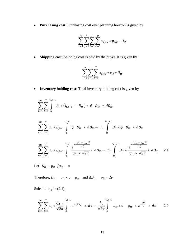
• Purchasing cost: Purchasing cost over planning horizon is given by

��𝑥𝑥𝑖𝑖𝑖𝑖𝑡𝑡𝑖𝑖 ∗ 𝑝𝑝𝑖𝑖𝑖𝑖𝑖𝑖 ∗ 𝑂𝑂𝑖𝑖𝑡𝑡

𝑝𝑝

𝑖𝑖=1

𝑇𝑇

𝑡𝑡=1

𝑛𝑛

𝑖𝑖=1

𝑚𝑚

𝑖𝑖=1

• Shipping cost: Shipping cost is paid by the buyer. It is given by

��𝑥𝑥𝑖𝑖𝑖𝑖𝑡𝑡𝑖𝑖 ∗ 𝑐𝑐𝑖𝑖𝑖𝑖 ∗ 𝑂𝑂𝑖𝑖𝑡𝑡

𝑇𝑇

𝑡𝑡=1

𝑛𝑛

𝑖𝑖=1

𝑚𝑚

𝑖𝑖=1

• Inventory holding cost: Total inventory holding cost is given by

= �� ℎ𝑖𝑖

𝐼𝐼𝑖𝑖,𝑡𝑡−1

0

𝑇𝑇

𝑡𝑡=1

𝑚𝑚

𝑖𝑖=1

∗ �𝐼𝐼𝑖𝑖,𝑡𝑡−1 − 𝐷𝐷𝑖𝑖𝑡𝑡 � ∗ 𝜙𝜙 (𝐷𝐷𝑖𝑖𝑡𝑡) ∗ 𝑑𝑑𝐷𝐷𝑖𝑖𝑡𝑡

= ��ℎ𝑖𝑖 ∗ 𝐼𝐼𝑖𝑖,𝑡𝑡−1 � 𝜙𝜙 (𝐷𝐷𝑖𝑖𝑡𝑡) ∗ 𝑑𝑑𝐷𝐷𝑖𝑖𝑡𝑡


0

𝑇𝑇

𝑡𝑡=1

𝑚𝑚

𝑖𝑖=1

− ℎ𝑖𝑖 � 𝐷𝐷𝑖𝑖𝑡𝑡 ∗ 𝜙𝜙 (𝐷𝐷𝑖𝑖𝑡𝑡) ∗ 𝑑𝑑𝐷𝐷𝑖𝑖𝑡𝑡


0

= ��ℎ𝑖𝑖 ∗ 𝐼𝐼𝑖𝑖,𝑡𝑡−1 �𝑒𝑒−

(𝐷𝐷𝑖𝑖𝑡𝑡 − µ𝑖𝑖𝑡𝑡)2

𝜎𝜎𝑖𝑖𝑡𝑡2

𝜎𝜎𝑖𝑖𝑡𝑡 ∗ √2𝜋𝜋∗ 𝑑𝑑𝐷𝐷𝑖𝑖𝑡𝑡


0

𝑇𝑇

𝑡𝑡=1

𝑚𝑚

𝑖𝑖=1

− ℎ𝑖𝑖 � 𝐷𝐷𝑖𝑖𝑡𝑡 ∗ 𝑒𝑒−

(𝐷𝐷𝑖𝑖𝑡𝑡 − µ𝑖𝑖𝑡𝑡)2




0

(2.1)

Let (𝐷𝐷𝑖𝑖𝑡𝑡 − µ𝑖𝑖𝑡𝑡)/𝜎𝜎𝑖𝑖𝑡𝑡 = 𝑣𝑣

Therefore, 𝐷𝐷𝑖𝑖𝑡𝑡 = 𝜎𝜎𝑖𝑖𝑡𝑡 ∗ 𝑣𝑣 + µ𝑖𝑖𝑡𝑡 and 𝑑𝑑𝐷𝐷𝑖𝑖𝑡𝑡 = 𝜎𝜎𝑖𝑖𝑡𝑡 ∗ 𝑑𝑑𝑣𝑣

Substituting in (2.1),

= ��ℎ𝑖𝑖 ∗𝐼𝐼𝑖𝑖,𝑡𝑡−1√2𝜋𝜋

� 𝑒𝑒−𝑣𝑣2/2 ∗ 𝑑𝑑𝑣𝑣


0

𝑇𝑇

𝑡𝑡=1

𝑚𝑚

𝑖𝑖=1

− ℎ𝑖𝑖√2𝜋𝜋

� (𝜎𝜎𝑖𝑖𝑡𝑡 ∗ 𝑣𝑣 + µ𝑖𝑖𝑡𝑡


0

) ∗ 𝑒𝑒−𝑣𝑣22

∗ 𝑑𝑑𝑣𝑣 (2.2)

11

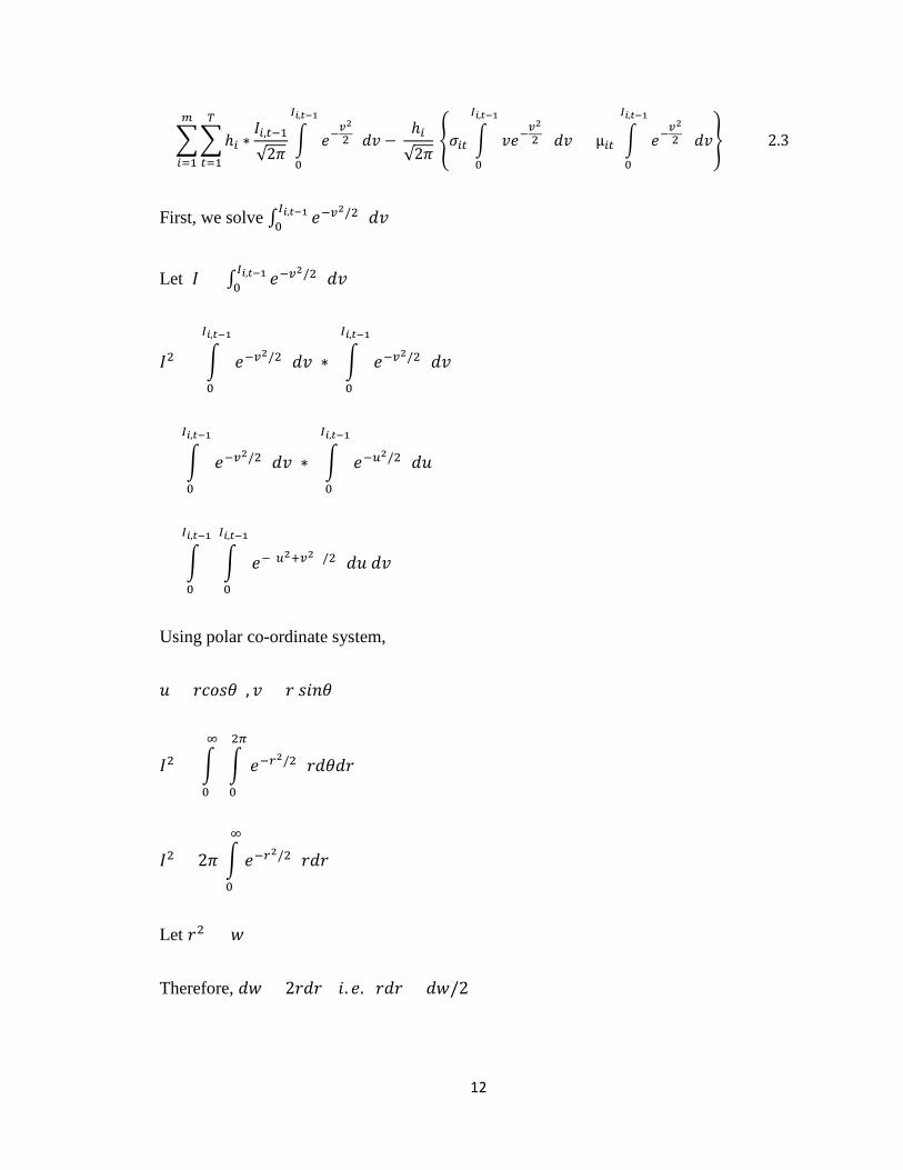
= ��ℎ𝑖𝑖 ∗𝐼𝐼𝑖𝑖,𝑡𝑡−1√2𝜋𝜋

� 𝑒𝑒−𝑣𝑣22

𝑑𝑑𝑣𝑣


0

𝑇𝑇

𝑡𝑡=1

𝑚𝑚

𝑖𝑖=1

− ℎ𝑖𝑖√2𝜋𝜋

�𝜎𝜎𝑖𝑖𝑡𝑡 � 𝑣𝑣𝑒𝑒−𝑣𝑣22


0

𝑑𝑑𝑣𝑣 + µ𝑖𝑖𝑡𝑡 � 𝑒𝑒−𝑣𝑣22


0

𝑑𝑑𝑣𝑣� (2.3)

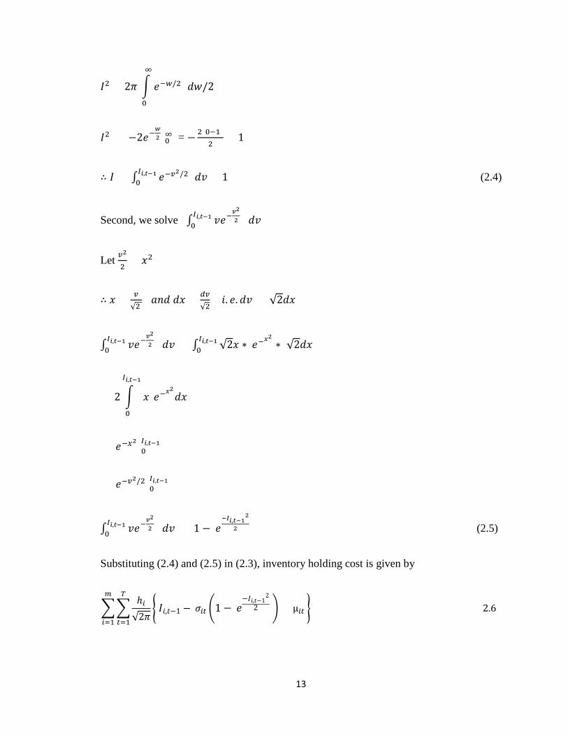
First, we solve ∫ 𝑒𝑒−𝑣𝑣2/2 𝑑𝑑𝑣𝑣𝐼𝐼𝑖𝑖,𝑡𝑡−10

Let 𝐼𝐼 = ∫ 𝑒𝑒−𝑣𝑣2/2 𝑑𝑑𝑣𝑣𝐼𝐼𝑖𝑖,𝑡𝑡−10

𝐼𝐼2 = � 𝑒𝑒−𝑣𝑣2/2 𝑑𝑑𝑣𝑣 ∗ � 𝑒𝑒−𝑣𝑣2/2 𝑑𝑑𝑣𝑣


0


0

= � 𝑒𝑒−𝑣𝑣2/2 𝑑𝑑𝑣𝑣 ∗ � 𝑒𝑒−𝑢𝑢2/2 𝑑𝑑𝑑𝑑


0


0

= � � 𝑒𝑒−(𝑢𝑢2+𝑣𝑣2 )/2 𝑑𝑑𝑑𝑑 𝑑𝑑𝑣𝑣


0


0

Using polar co-ordinate system,

𝑑𝑑 = 𝑟𝑟𝑐𝑐𝑟𝑟𝑟𝑟𝑟𝑟 , 𝑣𝑣 = 𝑟𝑟 𝑟𝑟𝑠𝑠𝑠𝑠𝑟𝑟

𝐼𝐼2 = � � 𝑒𝑒−𝑟𝑟2/2 𝑟𝑟𝑑𝑑𝑟𝑟𝑑𝑑𝑟𝑟2𝜋𝜋

0

∞

0

𝐼𝐼2 = 2𝜋𝜋 � 𝑒𝑒−𝑟𝑟2/2 𝑟𝑟𝑑𝑑𝑟𝑟 ∞

0

Let 𝑟𝑟2 = 𝑤𝑤

Therefore, 𝑑𝑑𝑤𝑤 = 2𝑟𝑟𝑑𝑑𝑟𝑟 𝑠𝑠. 𝑒𝑒. 𝑟𝑟𝑑𝑑𝑟𝑟 = 𝑑𝑑𝑤𝑤/2

12

𝐼𝐼2 = 2𝜋𝜋 � 𝑒𝑒−𝑤𝑤/2 𝑑𝑑𝑤𝑤/2 ∞

0

𝐼𝐼2 = [−2𝑒𝑒−𝑤𝑤2 ]0∞ = −2(0−1)

2= 1

∴ 𝐼𝐼 = ∫ 𝑒𝑒−𝑣𝑣2/2 𝑑𝑑𝑣𝑣𝐼𝐼𝑖𝑖,𝑡𝑡−10 = 1 (2.4)

Second, we solve ∫ 𝑣𝑣𝑒𝑒−𝑣𝑣2

2

𝐼𝐼𝑖𝑖,𝑡𝑡−10 𝑑𝑑𝑣𝑣

Let 𝑣𝑣2

2= 𝑥𝑥2

∴ 𝑥𝑥 = 𝑣𝑣√2

𝑎𝑎𝑠𝑠𝑑𝑑 𝑑𝑑𝑥𝑥 = 𝑑𝑑𝑣𝑣√2

𝑠𝑠. 𝑒𝑒. 𝑑𝑑𝑣𝑣 = √2𝑑𝑑𝑥𝑥

∫ 𝑣𝑣𝑒𝑒−𝑣𝑣2

2

𝐼𝐼𝑖𝑖,𝑡𝑡−10 𝑑𝑑𝑣𝑣 = ∫ √2𝑥𝑥𝐼𝐼𝑖𝑖,𝑡𝑡−1

0 ∗ 𝑒𝑒−𝑥𝑥2∗ √2𝑑𝑑𝑥𝑥

= 2 � 𝑥𝑥


0

𝑒𝑒−𝑥𝑥2𝑑𝑑𝑥𝑥

= [𝑒𝑒−𝑥𝑥2]0𝐼𝐼𝑖𝑖,𝑡𝑡−1

= [𝑒𝑒−𝑣𝑣2/2]0𝐼𝐼𝑖𝑖,𝑡𝑡−1

∫ 𝑣𝑣𝑒𝑒−𝑣𝑣2

2

𝐼𝐼𝑖𝑖,𝑡𝑡−10 𝑑𝑑𝑣𝑣 = [1 − 𝑒𝑒

−𝐼𝐼𝑖𝑖,𝑡𝑡−12

2 ] (2.5)

Substituting (2.4) and (2.5) in (2.3), inventory holding cost is given by

��ℎ𝑖𝑖√2𝜋𝜋

𝑇𝑇

𝑡𝑡=1

𝑚𝑚

𝑖𝑖=1

� 𝐼𝐼𝑠𝑠,𝑡𝑡−1 − 𝜎𝜎𝑖𝑖𝑡𝑡 �1− 𝑒𝑒−𝐼𝐼𝑠𝑠,𝑡𝑡−1

2

2 � + µ𝑖𝑖𝑡𝑡 � (2.6)

13

• Shortage cost: Total shortage cost is given by

�� 𝑟𝑟𝑐𝑐𝑖𝑖


0

𝑇𝑇

𝑡𝑡=1

𝑚𝑚

𝑖𝑖=1

∗ �𝐷𝐷𝑖𝑖𝑡𝑡 − 𝐼𝐼𝑖𝑖,𝑡𝑡−1 � ∗ 𝜙𝜙 (𝐷𝐷𝑖𝑖𝑡𝑡) ∗ 𝑑𝑑𝐷𝐷𝑖𝑖𝑡𝑡

= ��𝑟𝑟𝑐𝑐𝑖𝑖 � 𝐷𝐷𝑖𝑖𝑡𝑡 ∗ 𝜙𝜙 (𝐷𝐷𝑖𝑖𝑡𝑡) ∗ 𝑑𝑑𝐷𝐷𝑖𝑖𝑡𝑡


0

𝑇𝑇

𝑡𝑡=1

𝑚𝑚

𝑖𝑖=1

− 𝑟𝑟𝑐𝑐𝑖𝑖 ∗ 𝐼𝐼𝑖𝑖,𝑡𝑡−1 � 𝜙𝜙 (𝐷𝐷𝑖𝑖𝑡𝑡) ∗ 𝑑𝑑𝐷𝐷𝑖𝑖𝑡𝑡


0

= ��𝑟𝑟𝑐𝑐𝑖𝑖 � 𝐷𝐷𝑖𝑖𝑡𝑡 ∗𝑒𝑒−(𝐷𝐷𝑖𝑖𝑡𝑡 − µ𝑖𝑖𝑡𝑡)2




0

𝑇𝑇

𝑡𝑡=1

𝑚𝑚

𝑖𝑖=1

− 𝑟𝑟𝑐𝑐𝑖𝑖 ∗ 𝐼𝐼𝑖𝑖,𝑡𝑡−1 � 𝑒𝑒−(𝐷𝐷𝑖𝑖𝑡𝑡 − µ𝑖𝑖𝑡𝑡)2




0

(2.7)

Let (𝐷𝐷𝑖𝑖𝑡𝑡 − µ𝑖𝑖𝑡𝑡)/𝜎𝜎𝑖𝑖𝑡𝑡 = 𝑣𝑣

Therefore, 𝐷𝐷𝑖𝑖𝑡𝑡 = 𝜎𝜎𝑖𝑖𝑡𝑡 ∗ 𝑣𝑣 + µ𝑖𝑖𝑡𝑡 and 𝑑𝑑𝐷𝐷𝑖𝑖𝑡𝑡 = 𝜎𝜎𝑖𝑖𝑡𝑡 ∗ 𝑑𝑑𝑣𝑣

Substituting in (2.7), we get

��𝑟𝑟𝑐𝑐𝑖𝑖√2𝜋𝜋

� (𝜎𝜎𝑖𝑖𝑡𝑡 ∗ 𝑣𝑣 + µ𝑖𝑖𝑡𝑡


0

) ∗ 𝑒𝑒−𝑣𝑣22

∗ 𝑑𝑑𝑣𝑣 − 𝑟𝑟𝑐𝑐𝑖𝑖 ∗ 𝐼𝐼𝑠𝑠,𝑡𝑡−1

√2𝜋𝜋 � 𝑒𝑒−𝑣𝑣2/2 ∗ 𝑑𝑑𝑣𝑣


0

𝑇𝑇

𝑡𝑡=1

𝑚𝑚

𝑖𝑖=1

(2.8)

= ��𝑟𝑟𝑐𝑐𝑖𝑖√2𝜋𝜋

𝑇𝑇

𝑡𝑡=1

𝑚𝑚

𝑖𝑖=1

�𝜎𝜎𝑖𝑖𝑡𝑡 � 𝑣𝑣𝑒𝑒−𝑣𝑣22


0

𝑑𝑑𝑣𝑣 + µ𝑖𝑖𝑡𝑡 � 𝑒𝑒−𝑣𝑣22


0

𝑑𝑑𝑣𝑣� − 𝑟𝑟𝑐𝑐𝑖𝑖 ∗ 𝐼𝐼𝑖𝑖,𝑡𝑡−1√2𝜋𝜋

� 𝑒𝑒−𝑣𝑣22

𝑑𝑑𝑣𝑣


0

Using results from (2.4) and (2.5), we get shortage cost as,

��𝑟𝑟𝑐𝑐𝑖𝑖√2𝜋𝜋

𝑇𝑇

𝑡𝑡=1

𝑚𝑚

𝑖𝑖=1

� 𝜎𝜎𝑖𝑖𝑡𝑡 �1− 𝑒𝑒−𝐼𝐼𝑠𝑠,𝑡𝑡−1

2

2 � + µ𝑖𝑖𝑡𝑡 − 𝐼𝐼𝑖𝑖,𝑡𝑡−1� (2.9)

14

• Total cost: Total cost is the sum of fixed cost, purchasing cost, shipping cost, inventory

holding cost and shortage cost. The first objective is given by

𝑀𝑀𝑠𝑠𝑠𝑠 𝑍𝑍1 = ∑ ∑ ∑ 𝑓𝑓𝑖𝑖𝑖𝑖 ∗ 𝛿𝛿𝑖𝑖𝑖𝑖𝑡𝑡𝑇𝑇𝑡𝑡=1

𝑛𝑛𝑖𝑖=1

𝑚𝑚𝑖𝑖=1 + ∑ ∑ ∑ ∑ 𝑥𝑥𝑖𝑖𝑖𝑖𝑡𝑡𝑖𝑖 ∗ 𝑝𝑝𝑖𝑖𝑖𝑖𝑖𝑖 ∗ 𝑂𝑂𝑖𝑖𝑡𝑡

𝑝𝑝𝑖𝑖=1

𝑇𝑇𝑡𝑡=1

𝑛𝑛𝑖𝑖=1

𝑚𝑚𝑖𝑖=1

+ ∑ ∑ ∑ 𝑥𝑥𝑖𝑖𝑖𝑖𝑡𝑡𝑖𝑖 ∗ 𝑐𝑐𝑖𝑖𝑖𝑖 ∗ 𝑂𝑂𝑖𝑖𝑡𝑡𝑇𝑇𝑡𝑡=1

𝑛𝑛𝑖𝑖=1

𝑚𝑚𝑖𝑖=1 +

∑ ∑ ℎ𝑖𝑖√2𝜋𝜋

𝑇𝑇𝑡𝑡=1

𝑚𝑚𝑖𝑖=1 � 𝐼𝐼𝑖𝑖,𝑡𝑡−1 − 𝜎𝜎𝑖𝑖𝑡𝑡 �1 − 𝑒𝑒


2 � + µ𝑖𝑖𝑡𝑡 � +

∑ ∑ 𝑟𝑟𝑐𝑐𝑠𝑠√2𝜋𝜋

𝑇𝑇𝑡𝑡=1

𝑚𝑚𝑠𝑠=1 � 𝜎𝜎𝑠𝑠𝑡𝑡 �1 − 𝑒𝑒


2 � + µ𝑠𝑠𝑡𝑡 − 𝐼𝐼𝑠𝑠,𝑡𝑡−1 � (2.10)

2.2.2 To minimize the number of defective parts

The product of quality rejection rate and quantity supplied is summed over all products,

suppliers and time periods. The number of defective parts should be minimum. The second

objective is given by

𝑀𝑀𝑠𝑠𝑠𝑠 𝑍𝑍2 = ��𝑞𝑞𝑖𝑖𝑖𝑖 ∗ 𝑥𝑥𝑖𝑖𝑖𝑖𝑡𝑡𝑖𝑖 ∗ 𝑂𝑂𝑖𝑖𝑡𝑡

𝑚𝑚

𝑖𝑖=1

𝑛𝑛

𝑖𝑖=1

𝑇𝑇

𝑡𝑡=1

(2.11)

2.2.3 To minimize weighted average lead time

The product of lead time of each part and quantity supplied is summed over all products,

suppliers and time periods and further divided by total order quantity to give weighted

average lead time. The weighted average lead time should be minimum. The third objective

is given by

𝑀𝑀𝑠𝑠𝑠𝑠 𝑍𝑍3 =∑ ∑ ∑ 𝑙𝑙𝑖𝑖𝑖𝑖 ∗ 𝑥𝑥𝑖𝑖𝑖𝑖𝑡𝑡𝑖𝑖 ∗ 𝑂𝑂𝑖𝑖𝑡𝑡𝑚𝑚

𝑖𝑖=1𝑛𝑛𝑖𝑖=1

𝑇𝑇𝑡𝑡=1

∑ ∑ 𝑂𝑂𝑖𝑖𝑡𝑡𝑚𝑚𝑖𝑖=1

𝑇𝑇𝑡𝑡=1

15

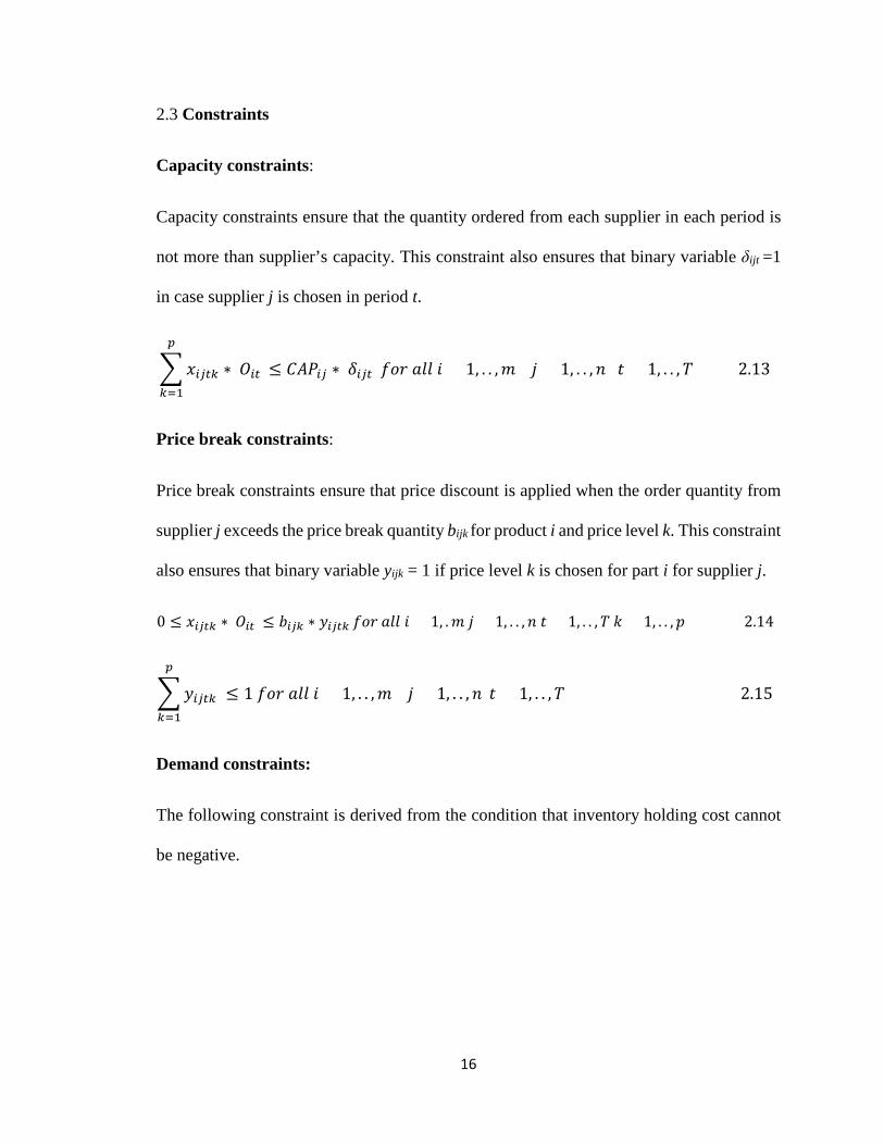
2.3 Constraints

Capacity constraints:

Capacity constraints ensure that the quantity ordered from each supplier in each period is

not more than supplier’s capacity. This constraint also ensures that binary variable δijt =1

in case supplier j is chosen in period t.

�𝑥𝑥𝑖𝑖𝑖𝑖𝑡𝑡𝑖𝑖 ∗ 𝑂𝑂𝑖𝑖𝑡𝑡 ≤ 𝐶𝐶𝐶𝐶𝑃𝑃𝑖𝑖𝑖𝑖 ∗ 𝛿𝛿𝑖𝑖𝑖𝑖𝑡𝑡 𝑓𝑓𝑟𝑟𝑟𝑟 𝑎𝑎𝑙𝑙𝑙𝑙 𝑠𝑠 = 1, . . ,𝑚𝑚 𝑗𝑗 = 1, . . ,𝑠𝑠 𝑡𝑡 = 1, . . ,𝑇𝑇𝑝𝑝

𝑖𝑖=1

(2.13)

Price break constraints:

Price break constraints ensure that price discount is applied when the order quantity from

supplier j exceeds the price break quantity bijk for product i and price level k. This constraint

also ensures that binary variable yijk = 1 if price level k is chosen for part i for supplier j.

0 ≤ 𝑥𝑥𝑖𝑖𝑖𝑖𝑡𝑡𝑖𝑖 ∗ 𝑂𝑂𝑖𝑖𝑡𝑡 ≤ 𝑏𝑏𝑖𝑖𝑖𝑖𝑖𝑖 ∗ 𝑦𝑦𝑖𝑖𝑖𝑖𝑡𝑡𝑖𝑖 𝑓𝑓𝑟𝑟𝑟𝑟 𝑎𝑎𝑙𝑙𝑙𝑙 𝑠𝑠 = 1, .𝑚𝑚 𝑗𝑗 = 1, . . ,𝑠𝑠 𝑡𝑡 = 1, . . ,𝑇𝑇 𝑘𝑘 = 1, . . ,𝑝𝑝 (2.14)

�𝑦𝑦𝑖𝑖𝑖𝑖𝑡𝑡𝑖𝑖 ≤ 1 𝑓𝑓𝑟𝑟𝑟𝑟 𝑎𝑎𝑙𝑙𝑙𝑙 𝑠𝑠 = 1, . . ,𝑚𝑚 𝑗𝑗 = 1, . . ,𝑠𝑠 𝑝𝑝

𝑖𝑖=1

𝑡𝑡 = 1, . . ,𝑇𝑇 (2.15)

Demand constraints:

The following constraint is derived from the condition that inventory holding cost cannot

be negative.

16

𝐼𝐼𝑖𝑖,𝑡𝑡−1 − 𝜎𝜎𝑠𝑠𝑡𝑡 �1 − 𝑒𝑒−𝐼𝐼𝑖𝑖,𝑡𝑡−12

2 � + µ𝑠𝑠𝑡𝑡 ≥ 0

(𝐼𝐼𝑠𝑠,𝑡𝑡−1 + µ𝑖𝑖𝑡𝑡 − 𝜎𝜎𝑖𝑖𝑡𝑡)𝜎𝜎𝑖𝑖𝑡𝑡

≥ − 𝑒𝑒−𝐼𝐼𝑠𝑠,𝑡𝑡−1

2

2 (2.16)

The following constraint is derived from the condition that shortage cost cannot be

negative.

𝜎𝜎𝑖𝑖𝑡𝑡 �1− 𝑒𝑒−𝐼𝐼𝑠𝑠,𝑡𝑡−1

2

2 �+ µ𝑖𝑖𝑡𝑡 − 𝐼𝐼𝑖𝑖,𝑡𝑡−1 ≥ 0

𝑒𝑒−𝐼𝐼𝑖𝑖,𝑡𝑡−12

2 ≤ �𝜎𝜎𝑠𝑠𝑡𝑡 + µ𝑠𝑠𝑡𝑡 − 𝐼𝐼𝑠𝑠,𝑡𝑡−1�

𝜎𝜎𝑠𝑠𝑡𝑡 (2.17)

Other constraints:

These constraints ensure that all decision variables are non-negative and all binary

variables are well defined.

��𝑥𝑥𝑖𝑖𝑖𝑖𝑡𝑡𝑖𝑖 = 1 𝑓𝑓𝑟𝑟𝑟𝑟 𝑎𝑎𝑙𝑙𝑙𝑙 𝑠𝑠 = 1, . . ,𝑚𝑚 𝑡𝑡 = 1, … ,𝑇𝑇 (2.18)𝑝𝑝

𝑖𝑖=1

𝑛𝑛

𝑖𝑖=1

𝑥𝑥𝑖𝑖𝑖𝑖𝑡𝑡𝑖𝑖, 𝐼𝐼𝑖𝑖𝑡𝑡 , 𝑆𝑆𝑖𝑖𝑡𝑡 ≥ 0, 𝛿𝛿𝑖𝑖𝑖𝑖𝑡𝑡 ,𝑦𝑦𝑖𝑖𝑖𝑖𝑖𝑖𝑡𝑡 ∈ (0,1) (2.19)

2.4 Weighted Objective Method

The idea behind formulation of this multi criteria problem is to assign weights to each

objective to transform the problem into a single weighted objective problem. An example

of formulation of weighted objective problem is given below (Masud and Ravindran, 2008)

17

𝑀𝑀𝑠𝑠𝑠𝑠 𝑍𝑍 = ∑ 𝜆𝜆𝑖𝑖𝑓𝑓𝑖𝑖(𝑥𝑥)𝑖𝑖𝑖𝑖=1

𝑟𝑟𝑑𝑑𝑏𝑏𝑗𝑗𝑒𝑒𝑐𝑐𝑡𝑡 𝑡𝑡𝑟𝑟 𝑥𝑥 ∈ 𝑆𝑆

∑ 𝜆𝜆𝑖𝑖 = 1.𝑖𝑖𝑖𝑖=1

𝜆𝜆𝑖𝑖 ≥ 0

where λi is the weight assigned to objective 𝑓𝑓𝑖𝑖(𝑥𝑥)

and S = {x | gi (x) ≤ 0, j= 1, 2,….,m}

where gj (x) ≤ 0 represents constraint j.

Under this method, the multi objective problem becomes a single objective problem

as follows,

𝑀𝑀𝑠𝑠𝑠𝑠 𝑍𝑍 = 𝑤𝑤1 ∗ 𝑍𝑍1 + 𝑤𝑤2 ∗ 𝑍𝑍2 + 𝑤𝑤3 ∗ 𝑍𝑍3

where w1 = weight assigned to objective 𝑍𝑍1 (minimize total cost)

𝑤𝑤2 = weight assigned to objective 𝑍𝑍2 (minimize number of defective parts)

𝑤𝑤3 = weight assigned to objective 𝑍𝑍3 (minimize weighted average lead time)

and 𝑤𝑤1 + 𝑤𝑤2 + 𝑤𝑤3 = 1

18

Chapter 3

Numerical Example and Sensitivity Analysis

3.1 Problem description:

A company wants to purchase 3 different parts for its assembly. There are 3 suppliers for

each part and all these suppliers offer 2 levels of price discounts for each part. The

following values are used as inputs.

• Number of parts=3 , m=3, i= {1,2,3}

• Number of suppliers=3, n=3, j= {1,2,3}

• Number of weeks in planning horizon=5, T=5, t= {1,2,3,4,5}

• Number of price levels offered by each supplier of each part=2, p=2, k= {1,2}

The following inputs are assumed and used in the numerical example

Product Supplier Fixed order

cost i j fij ($) 1 1 500 1 2 400 1 3 600 2 1 500 2 2 400 2 3 600 3 1 500 3 2 400 3 3 600

Table 3-1: Numerical Example: Fixed order cost related to parts and suppliers

19

Part

Inventory holding

cost Shortage

cost i hi ($) sci ($) 1 3 6 2 4.5 7.5 3 5 8

Table 3-2: Numerical Example: Inventory holding cost and shortage cost related to parts

Part Supplier Defect rate Capacity

Lead time

(weeks) Shipping cost ($)

i j qij CAPij lij Cij 1 1 0.04 1000 0.5 1.5 1 2 0.02 800 0.7 2 1 3 0.01 800 0.7 2.1 2 1 0.05 800 0.7 2 2 2 0.03 1000 0.6 1.8 2 3 0.02 600 0.8 1.5 3 1 0.04 600 0.5 2.5 3 2 0.03 900 0.6 1.9 3 3 0.02 700 0.5 2.5

Table 3-3: Numerical Example: Values of parameters related to suppliers and parts

20

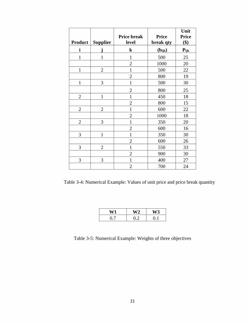
Table 3-4: Numerical Example: Values of unit price and price break quantity

Table 3-5: Numerical Example: Weights of three objectives

Product Supplier Price break

level Price

break qty

Unit Price

($) i j k (bijk) Pijk 1 1 1 500 25 2 1000 20 1 2 1 500 22 2 800 19 1 3 1 500 30 2 800 25 2 1 1 450 18 2 800 15 2 2 1 600 22

2 1000 18 2 3 1 350 20 2 600 16 3 1 1 350 30 2 600 26 3 2 1 550 33 2 900 30 3 3 1 400 27

2 700 24

W1 W2 W3 0.7 0.2 0.1

21

Product Week Demand i t Dit 1 1 1500 1 2 1750 1 3 2000 1 4 1900 1 5 1600 2 1 1700 2 2 2100 2 3 2400 2 4 2200 2 5 2100 3 1 1800 3 2 2000 3 3 1800 3 4 2150 3 5 2000

Table 3-6: Numerical Example: Values of demand for each part for each week

Mean demand μ1t μ2t μ3t

1750 2100 1950

Table 3-7: Mean values of demand

Std. dev.of demand σ1t σ2t σ3t 206 255 150

Table 3-8: Standard deviation values of demand

22

3.2 Mathematical model:

Decision variables:

xijtk : proportion of part i purchased from supplier j in period t at price level k, i=1, 2, 3 and j=1, 2, 3, t=1, 2,., 5 and k=1, 2

Oit : order quantity for part i in period t, i= 1, 2, 3 and t=1, 2, 3, 4, 5.

Iit : inventory level for part i at the end of period t, i=1, 2, 3 and t=1, 2, 3, 4, 5.

Sit : shortage quantity for part i at the end of period t, i=1, 2, 3 and t=1, 2, 3, 4, 5.

δijt =1, if order is placed for part i to supplier j for period t. i=1, 2, 3 and j=1, 2, 3 and t=1,2,3,4, 5.

=0, otherwise.

yijtk = 1, if price break level k is selected for part i from supplier j for period t.

=0, otherwise for i=1, 2, 3 and j=1, 2, 3 and t=1, 2, 3, 4, 5 and k=1, 2

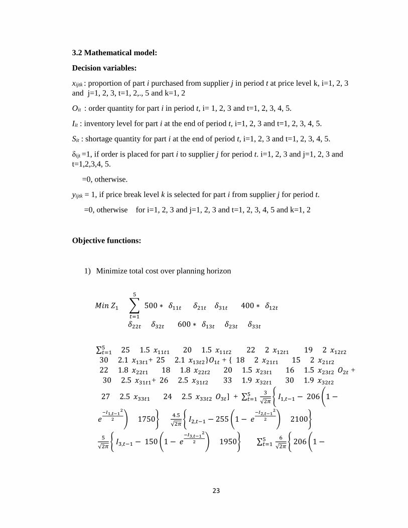
Objective functions:

1) Minimize total cost over planning horizon

𝑀𝑀𝑀𝑀𝑀𝑀 𝑍𝑍1 = �{5

𝑡𝑡=1

500 ∗ (𝛿𝛿11𝑡𝑡 + 𝛿𝛿21𝑡𝑡+ 𝛿𝛿31𝑡𝑡) + 400 ∗ (𝛿𝛿12𝑡𝑡

+ 𝛿𝛿22𝑡𝑡 + 𝛿𝛿32𝑡𝑡) + 600 ∗ (𝛿𝛿13𝑡𝑡 + 𝛿𝛿23𝑡𝑡 + 𝛿𝛿33𝑡𝑡} +

∑ [{(25 + 1.5)𝑥𝑥11𝑡𝑡1 + (20 + 1.5)𝑥𝑥11𝑡𝑡2 + (22 + 2)𝑥𝑥12𝑡𝑡1 5𝑡𝑡=1 + (19 + 2)𝑥𝑥12𝑡𝑡2 +

(30 + 2.1)𝑥𝑥13𝑡𝑡1+(25 + 2.1)𝑥𝑥13𝑡𝑡2}𝑂𝑂1𝑡𝑡 + {(18 + 2)𝑥𝑥21𝑡𝑡1 + (15 + 2)𝑥𝑥21𝑡𝑡2 +(22 + 1.8)𝑥𝑥22𝑡𝑡1 + (18 + 1.8)𝑥𝑥22𝑡𝑡2 + (20 + 1.5)𝑥𝑥23𝑡𝑡1 + (16 + 1.5)𝑥𝑥23𝑡𝑡2}𝑂𝑂2𝑡𝑡 + {(30 + 2.5)𝑥𝑥31𝑡𝑡1+(26 + 2.5)𝑥𝑥31𝑡𝑡2 + (33 + 1.9)𝑥𝑥32𝑡𝑡1 + (30 + 1.9)𝑥𝑥32𝑡𝑡2 +

(27 + 2.5)𝑥𝑥33𝑡𝑡1 + (24 + 2.5)𝑥𝑥33𝑡𝑡2}𝑂𝑂3𝑡𝑡] + ∑ [ 3√2𝜋𝜋

5𝑡𝑡=1 � 𝐼𝐼1,𝑡𝑡−1 − 206�1 −

𝑒𝑒−𝐼𝐼1,𝑡𝑡−1

2

2 � + 1750� + 4.5√2𝜋𝜋

� 𝐼𝐼2,𝑡𝑡−1 − 255 �1 − 𝑒𝑒−𝐼𝐼2,𝑡𝑡−1

2

2 � + 2100� +

5√2𝜋𝜋

� 𝐼𝐼3,𝑡𝑡−1 − 150 �1 − 𝑒𝑒−𝐼𝐼3,𝑡𝑡−1

2

2 � + 1950�] + ∑ [ 6√2𝜋𝜋

5𝑡𝑡=1 � 206 �1 −

23

𝑒𝑒−𝐼𝐼1,𝑡𝑡−1

2

2 � + 1750 − 𝐼𝐼1,𝑡𝑡−1 � + [ 7.5√2𝜋𝜋

� 255�1 − 𝑒𝑒−𝐼𝐼2,𝑡𝑡−1

2

2 � + 2100 − 𝐼𝐼2,𝑡𝑡−1 �

+ 8√2𝜋𝜋

� 150�1 − 𝑒𝑒−𝐼𝐼3,𝑡𝑡−1

2

2 � + 1950 − 𝐼𝐼3,𝑡𝑡−1 �]

2) Minimize number of defective parts

𝑀𝑀𝑀𝑀𝑀𝑀 𝑍𝑍2 = �[{(𝑥𝑥11𝑡𝑡1 + 𝑥𝑥11𝑡𝑡2)0.04 + (𝑥𝑥12𝑡𝑡1 5

𝑡𝑡=1

+ 𝑥𝑥12𝑡𝑡2)0.02 + (𝑥𝑥13𝑡𝑡1

+ 𝑥𝑥13𝑡𝑡2)0.01}𝑂𝑂1𝑡𝑡 + {𝑥𝑥21𝑡𝑡1 + 𝑥𝑥21𝑡𝑡2)0.05 + (𝑥𝑥22𝑡𝑡1 + 𝑥𝑥22𝑡𝑡2)0.03

+ (𝑥𝑥23𝑡𝑡1 + 𝑥𝑥23𝑡𝑡2)0.02}𝑂𝑂2𝑡𝑡 + {(𝑥𝑥31𝑡𝑡1 + 𝑥𝑥31𝑡𝑡2)0.04 + (𝑥𝑥32𝑡𝑡1

+ 𝑥𝑥32𝑡𝑡2)0.03 + (𝑥𝑥33𝑡𝑡1

+ 𝑥𝑥33𝑡𝑡2)0.02} 𝑂𝑂3𝑡𝑡]

3) Minimize weighted average lead time

𝑀𝑀𝑀𝑀𝑀𝑀 𝑍𝑍3 = �[{(𝑥𝑥11𝑡𝑡1 + 𝑥𝑥11𝑡𝑡2)0.5 + (𝑥𝑥12𝑡𝑡1 5

𝑡𝑡=1

+ 𝑥𝑥12𝑡𝑡2)0.7 + (𝑥𝑥13𝑡𝑡1

+ 𝑥𝑥13𝑡𝑡2)0.7}𝑂𝑂1𝑡𝑡 + {𝑥𝑥21𝑡𝑡1 + 𝑥𝑥21𝑡𝑡2)0.7 + (𝑥𝑥22𝑡𝑡1 + 𝑥𝑥22𝑡𝑡2)0.6 + (𝑥𝑥23𝑡𝑡1+ 𝑥𝑥23𝑡𝑡2)0.8}𝑂𝑂2𝑡𝑡 + {(𝑥𝑥31𝑡𝑡1 + 𝑥𝑥31𝑡𝑡2)0.5 + (𝑥𝑥32𝑡𝑡1 + 𝑥𝑥32𝑡𝑡2)0.6 + (𝑥𝑥33𝑡𝑡1+ 𝑥𝑥33𝑡𝑡2)0.5} 𝑂𝑂3𝑡𝑡] /

�{𝑂𝑂1𝑡𝑡

5

𝑡𝑡 =1

+ 𝑂𝑂2𝑡𝑡 + 𝑂𝑂3𝑡𝑡 }

Constraints:

1) Capacity constraints:

�𝑥𝑥𝑖𝑖𝑖𝑖𝑡𝑡𝑖𝑖 ∗ 𝑂𝑂𝑖𝑖𝑡𝑡 ≤ 𝐶𝐶𝐶𝐶𝐶𝐶𝑖𝑖𝑖𝑖 ∗ 𝛿𝛿𝑖𝑖𝑖𝑖𝑡𝑡 𝑓𝑓𝑓𝑓𝑓𝑓 𝑎𝑎𝑎𝑎𝑎𝑎 𝑀𝑀 = 1,2,3 𝑗𝑗 = 1,2,3 𝑡𝑡 = 1,2,3,4,52

𝑖𝑖=1

24

2) Price break constraints:

0 ≤ 𝑥𝑥𝑖𝑖𝑖𝑖𝑡𝑡𝑖𝑖 ∗ 𝑂𝑂𝑖𝑖𝑡𝑡 ≤ 𝑏𝑏𝑖𝑖𝑖𝑖𝑖𝑖 ∗ 𝑦𝑦𝑖𝑖𝑖𝑖𝑡𝑡𝑖𝑖 𝑓𝑓𝑓𝑓𝑓𝑓 𝑎𝑎𝑎𝑎𝑎𝑎 𝑀𝑀 = 1,2,3 𝑗𝑗 = 1,2,3 𝑡𝑡 = 1,2,3,4,5 𝑘𝑘= 1,2

�𝑦𝑦𝑖𝑖𝑖𝑖𝑡𝑡𝑖𝑖 ≤ 1 𝑓𝑓𝑓𝑓𝑓𝑓 𝑎𝑎𝑎𝑎𝑎𝑎 𝑀𝑀 = 1,2,3 𝑗𝑗 = 1,2,3 2

𝑖𝑖=1

𝑡𝑡 = 1,2,3,4,5

3) Demand constraints:

From equation (2.16), we have

(𝐼𝐼𝑖𝑖,𝑡𝑡−1 + µ𝑖𝑖𝑡𝑡 − 𝜎𝜎𝑖𝑖𝑡𝑡)

𝜎𝜎𝑖𝑖𝑡𝑡 ≥ − 𝑒𝑒

−𝐼𝐼𝑖𝑖,𝑡𝑡−122 𝑓𝑓𝑓𝑓𝑓𝑓 𝑎𝑎𝑎𝑎𝑎𝑎 𝑀𝑀 = 1,2,3 𝑎𝑎𝑀𝑀𝑎𝑎 𝑡𝑡 = 1,2,3,4,5

For t=1, i=1, we have µ𝑖𝑖𝑡𝑡 = 1750 and𝜎𝜎𝑖𝑖𝑡𝑡 = 206. Initial inventory is assumed to

be 0.

(0+1750-206)/ (206) ≥ −𝑒𝑒0 . This constraint is satisfied.

From equation (2.17), we have


2 ≤ �𝜎𝜎𝑖𝑖𝑡𝑡 + µ𝑖𝑖𝑡𝑡 − 𝐼𝐼𝑖𝑖,𝑡𝑡−1�

𝜎𝜎𝑖𝑖𝑡𝑡 𝑓𝑓𝑓𝑓𝑓𝑓 𝑎𝑎𝑎𝑎𝑎𝑎 𝑀𝑀 = 1,2,3 𝑎𝑎𝑀𝑀𝑎𝑎 𝑡𝑡 = 1,2,3,4,5


2 ≤ �𝜎𝜎𝑖𝑖𝑡𝑡 + µ𝑖𝑖𝑡𝑡 − 𝐼𝐼𝑖𝑖,𝑡𝑡−1�

𝜎𝜎𝑖𝑖𝑡𝑡 𝑏𝑏𝑒𝑒𝑏𝑏𝑓𝑓𝑏𝑏𝑒𝑒𝑏𝑏

For t=1, i=1, we have µ𝑖𝑖𝑡𝑡 = 1750 and𝜎𝜎𝑖𝑖𝑡𝑡 = 206. 𝑒𝑒0 ≤ (206 + 1750-0) / (206). This constraint is satisfied.

25

4) Other constraints:

� �𝑥𝑥𝑖𝑖𝑖𝑖𝑡𝑡𝑖𝑖 = 1 𝑓𝑓𝑓𝑓𝑓𝑓 𝑎𝑎𝑎𝑎𝑎𝑎 𝑀𝑀 = 1,2,3 𝑎𝑎𝑀𝑀𝑎𝑎 𝑡𝑡2

𝑖𝑖=1

3

𝑖𝑖=1

= 1,2,3,4,5.

𝑥𝑥𝑖𝑖𝑖𝑖𝑡𝑡𝑖𝑖 , 𝐼𝐼𝑖𝑖𝑡𝑡, 𝑆𝑆𝑖𝑖𝑡𝑡 ≥ 0, 𝛿𝛿𝑖𝑖𝑖𝑖𝑡𝑡,𝑦𝑦𝑖𝑖𝑖𝑖𝑖𝑖𝑡𝑡 ∈ (0,1)

Solutions:

For order proportion xijtk

x1111 x1121 x1131 x1141 x1151 x1112 x1122 x1132 x1142 x1152 0 0 0 0 0 0.47 0.54 0.5 0.53 0.5

x1211 x1221 x1231 x1241 x1251 x1212 x1222 x1232 x1242 x1252 0 0 0 0 0 0.53 0.46 0.4 0.42 0.5

x1311 x1321 x1331 x1341 x1351 x1312 x1322 x1332 x1342 x1352 0 0 0.1 0.05 0 0 0 0 0 0

x2111 x2121 x2131 x2141 x2151 x2112 x2122 x2132 x2142 x2152 0 0 0 0 0 0.44 0.38 0.33 0.36 0.38

x2211 x2221 x2231 x2241 x2251 x2212 x2222 x2232 x2242 x2252 0 0 0 0 0 0.35 0.33 0.42 0.36 0.33

x2311 x2321 x2331 x2341 x2351 x2312 x2322 x2332 x2342 x2352 0 0 0 0 0 0.21 0.29 0.25 0.28 0.29

x3111 x3121 x3131 x3141 x3151 x3112 x3122 x3132 x3142 x3152 0 0 0 0 0 0.31 0.3 0.31 0.27 0.3

x3211 x3221 x3231 x3241 x3251 x3212 x3222 x3232 x3242 x3252 0 0 0 0 0 0.31 0.35 0.31 0.4 0.35

x3311 x3321 x3331 x3341 x3351 x3312 x3322 x3332 x3342 x3352 0 0 0 0 0 0.38 0.35 0.38 0.33 0.35

Table 3-9: Order proportions

26

For order quantity Oit

Table 3-10: Order quantities

For binary variable δijt

Table 3-11: Selection of suppliers

O11 O12 O13 O14 O15 1500 1750 2000 1900 1600 O21 O22 O23 O24 O25

1700 2100 2400 2200 2100 O31 O32 O33 O34 O35

1800 2000 1800 2150 2000

δ111 δ112 δ113 δ114 δ115 1 1 1 1 1 δ121 δ122 δ123 δ124 δ125 1 1 1 1 1 δ131 δ132 δ133 δ134 δ135 0 0 1 1 0 δ211 δ212 δ213 δ214 δ215 1 1 1 1 1 δ221 δ222 δ223 δ224 δ225 1 1 1 1 1 δ231 δ232 δ233 δ234 δ235 1 1 1 1 1 δ311 δ312 δ313 δ314 δ315 1 1 1 1 1 δ321 δ322 δ323 δ324 δ325 1 1 1 1 1 δ331 δ332 δ333 δ334 δ335 1 1 1 1 1

27

For binary variable y ijtk

y 1111 y1121 y 1131 y 1141 y 1151 y 1112 y 1122 y 1132 y 1142 y 1152

0 0 0 0 0 1 1 1 1 1

y 1211 y1221 y 1231 y 1241 y 1251 y 1212 y 1222 y 1232 y 1242 y 1252

0 0 0 0 0 1 1 1 1 1

y 1311 y1321 y 1331 y 1341 y 1351 y 1312 y 1322 y 1332 y 1342 y 1352

0 0 1 1 0 0 0 0 0 0

y 2111 y2121 y 2131 y 2141 y 2151 y 2112 y 2122 y 2132 y 2142 y 2152

0 0 0 0 0 1 1 1 1 1

y 2211 y2221 y 2231 y 2241 y 2251 y 2212 y 2222 y 2232 y 2242 y 2252

0 0 0 0 0 1 1 1 1 1

y 2311 y2321 y 2331 y 2341 y 2351 y 2312 y 2322 y 2332 y 2342 y 2352

0 0 0 0 0 1 1 1 1 1 y 3111 y3121 y 3131 y 3141 y 3151 y 3112 y 3122 y 3132 y 3142 y 3152

0 0 0 0 0 1 1 1 1 1 y 3211 y3221 y 3231 y 3241 y 3251 y 3212 y 3222 y 3232 y 3242 y 3252

0 0 0 0 0 1 1 1 1 1 y 3311 y3321 y 3331 y 3341 y 3351 y 3312 y 3322 y 3332 y 3342 y 3352

0 0 0 0 0 1 1 1 1 1

Table 3-12: Selection of price levels

28

Objective 1: Z1 =Total cost = $ 815116.6

Objective 2: Z2 =Number of defective parts= 914

Objective 3: Z3 =Weighted Average lead time: 3.05 weeks

From table 3-5, we have weights for each objective as follows

W1 = 0.7, W2 = 0.2, W3 = 0.1

Objective function value= W1 * Z1 + W2 * Z2 + W3 * Z3

= (0.7*815116.6) + (0.2 * 914) + (0.1*3.05)

= 570764.6

29

3.3 Sensitivity analysis

1) When the values for standard deviation are decreased by 10 % and the mean is kept the

same as original example, we get following input values.


Table 3-13: Original values of Standard deviation of demand

Table 3-14: New values of Standard deviation of demand

All other inputs are kept the same. The optimal solution is as follows,


x1111 x1121 x1131 x1141 x1151 x1112 x1122 x1132 x1142 x1152

0 0 0 0 0 0.54 0.54 0.48 0.53 0.52 x1211 x1221 x1231 x1241 x1251 x1212 x1222 x1232 x1242 x1252

0 0 0 0 0 0.46 0.46 0.4 0.42 0.48 x1311 x1321 x1331 x1341 x1351 x1312 x1322 x1332 x1342 x1352

0 0 0.12 0.05 0 0 0 0 0 0 x2111 x2121 x2131 x2141 x2151 x2112 x2122 x2132 x2142 x2152

0 0 0 0 0 0.42 0.38 0.36 0.39 0.42 x2211 x2221 x2231 x2241 x2251 x2212 x2222 x2232 x2242 x2252

0 0 0 0 0 0.32 0.33 0.36 0.32 0.32


30

x2311 x2321 x2331 x2341 x2351 x2312 x2322 x2332 x2342 x2352

0 0 0 0 0 0.26 0.29 0.28 0.27 0.26 x3111 x3121 x3131 x3141 x3151 x3112 x3122 x3132 x3142 x3152

0 0 0 0 0 0.31 0.3 0.28 0.29 0.26 x3211 x3221 x3231 x3241 x3251 x3212 x3222 x3232 x3242 x3252

0 0 0 0 0 0.31 0.35 0.4 0.31 0.33 x3311 x3321 x3331 x3341 x3351 x3312 x3322 x3332 x3342 x3352

0 0 0 0 0 0.38 0.35 0.32 0.4 0.41





δ111 δ112 δ113 δ114 δ115 1 1 1 1 1 δ121 δ122 δ123 δ124 δ125 1 1 1 1 1 δ131 δ132 δ133 δ134 δ135 0 0 1 1 0

O11 O12 O13 O14 O15 1750 1750 2100 1900 1650

O21 O22 O23 O24 O25 1900 2100 2200 2050 1900

O31 O32 O33 O34 O35 1800 2000 2150 1750 1700

31

δ211 δ212 δ213 δ214 δ215 1 1 1 1 1 δ221 δ222 δ223 δ224 δ225 1 1 1 1 1 δ231 δ232 δ233 δ234 δ235 1 1 1 1 1 δ311 δ312 δ313 δ314 δ315 1 1 1 1 1 δ321 δ322 δ323 δ324 δ325 1 1 1 1 1 δ331 δ332 δ333 δ334 δ335 1 1 1 1 1



y 1111 y1121 y 1131 y 1141 y 1151 y 1112 y 1122 y 1132 y 1142 y 1152

0 0 0 0 0 1 1 1 1 1

y 1211 y1221 y 1231 y 1241 y 1251 y 1212 y 1222 y 1232 y 1242 y 1252

0 0 0 0 0 1 1 1 1 1

y 1311 y1321 y 1331 y 1341 y 1351 y 1312 y 1322 y 1332 y 1342 y 1352

0 0 1 1 0 0 0 0 0 0

y 2111 y2121 y 2131 y 2141 y 2151 y 2112 y 2122 y 2132 y 2142 y 2152

0 0 0 0 0 1 1 1 1 1

y 2211 y2221 y 2231 y 2241 y 2251 y 2212 y 2222 y 2232 y 2242 y 2252

0 0 0 0 0 1 1 1 1 1

32

y 2311 y2321 y 2331 y 2341 y 2351 y 2312 y 2322 y 2332 y 2342 y 2352

0 0 0 0 0 1 1 1 1 1

y 3111 y3121 y 3131 y 3141 y 3151 y 3112 y 3122 y 3132 y 3142 y 3152

0 0 0 0 0 1 1 1 1 1

y 3211 y3221 y 3231 y 3241 y 3251 y 3212 y 3222 y 3232 y 3242 y 3252

0 0 0 0 0 1 1 1 1 1

y 3311 y3321 y 3331 y 3341 y 3351 y 3312 y 3322 y 3332 y 3342 y 3352

0 0 0 0 0 1 1 1 1 1





Objective Original value New value Percentage

decrease

Total cost $815,116.60 $699,834.10 14.14% Total number of quality defects

914 811 11.26%

Weighted average lead

time 3.05 weeks 3.01 weeks 1.31%

Table 3-19: Comparison of values of objectives

33


W1 = 0.7, W2 = 0.2, W3 = 0.1


= (0.7*699834.1) + (0.2 * 811) + (0.1*3.01)

= 490046.4

The percentage decrease in the value of objective function is 570764.6−490046.4570764.6

= 14.12 %

This decrease in the value of objective function is probably because of the decrease in the

standard deviation of demand. Therefore, decrease in the values of standard deviation of

demand by 10% leads to decrease in the value of objective function by 14.12 %, keeping

all other input parameters constant.

2) When the input values for mean of demand are increased by 10% and values for

standard deviation are kept same as original example, we have the following inputs,


1750 2100 1950

Table 3-20: Original Values of Mean of demand

Table 3-21: New values of Mean of demand


1925 2310 2145

34

All other inputs are maintained same. The solution changes as follows.


x1111 x1121 x1131 x1141 x1151 x1112 x1122 x1132 x1142 x1152 0 0 0 0 0 0.43 0.54 0.38 0.56 0.46

x1211 x1221 x1231 x1241 x1251 x1212 x1222 x1232 x1242 x1252 0 0 0 0 0 0.57 0.46 0.38 0.44 0.54

x1311 x1321 x1331 x1341 x1351 x1312 x1322 x1332 x1342 x1352 0 0 0 0 0 0 0 0.24 0 0

x2111 x2121 x2131 x2141 x2151 x2112 x2122 x2132 x2142 x2152 0 0 0 0 0 0.44 0.42 0.36 0.44 0.62

x2211 x2221 x2231 x2241 x2251 x2212 x2222 x2232 x2242 x2252 0 0 0 0 0 0.35 0.32 0.36 0.33 0

x2311 x2321 x2331 x2341 x2351 x2312 x2322 x2332 x2342 x2352 0 0 0 0 0 0.21 0.26 0.28 0.23 0.38

x3111 x3121 x3131 x3141 x3151 x3112 x3122 x3132 x3142 x3152 0 0 0 0 0 0.24 0.32 0.28 0.29 0.42

x3211 x3221 x3231 x3241 x3251 x3212 x3222 x3232 x3242 x3252 0 0 0 0 0.1 0.33 0.32 0.4 0.31 0

x3311 x3321 x3331 x3341 x3351 x3312 x3322 x3332 x3342 x3352 0 0 0 0 0 0.43 0.36 0.32 0.4 0.48




O11 O12 O13 O14 O15 1400 1750 2100 1800 1500

O21 O22 O23 O24 O25 1700 1900 2200 1800 1300

O31 O32 O33 O34 O35 1650 1900 2150 1750 1450

35


δ111 δ112 δ113 δ114 δ115 1 1 1 1 1

δ121 δ122 δ123 δ124 δ125 1 1 1 1 1

δ131 δ132 δ133 δ134 δ135 0 0 1 0 0

δ211 δ212 δ213 δ214 δ215 1 1 1 1 1

δ221 δ222 δ223 δ224 δ225 1 1 1 1 0

δ231 δ232 δ233 δ234 δ235

1 1 1 1 1

δ311 δ312 δ313 δ314 δ315

1 1 1 1 1

δ321 δ322 δ323 δ324 δ325

1 1 1 1 1

δ331 δ332 δ333 δ334 δ335

1 1 1 1 1


36


y 1111 y1121 y 1131 y 1141 y 1151 y 1112 y 1122 y 1132 y 1142 y 1152 0 0 0 0 0 1 1 1 1 1

y 1211 y1221 y 1231 y 1241 y 1251 y 1212 y 1222 y 1232 y 1242 y 1252 0 0 0 0 0 1 1 1 1 1

y 1311 y1321 y 1331 y 1341 y 1351 y 1312 y 1322 y 1332 y 1342 y 1352 0 0 0 0 0 0 0 0 0 0

y 2111 y2121 y 2131 y 2141 y 2151 y 2112 y 2122 y 2132 y 2142 y 2152 0 0 0 0 0 1 1 1 1 1

y 2211 y2221 y 2231 y 2241 y 2251 y 2212 y 2222 y 2232 y 2242 y 2252 0 0 0 0 0 1 1 1 1 1

y 2311 y2321 y 2331 y 2341 y 2351 y 2312 y 2322 y 2332 y 2342 y 2352 0 0 0 0 0 1 1 1 1 1

y 3111 y3121 y 3131 y 3141 y 3151 y 3112 y 3122 y 3132 y 3142 y 3152 0 0 0 0 0 1 1 1 1 1

y 3211 y3221 y 3231 y 3241 y 3251 y 3212 y 3222 y 3232 y 3242 y 3252 0 0 0 0 1 1 1 1 1 0

y 3311 y3321 y 3331 y 3341 y 3351 y 3312 y 3322 y 3332 y 3342 y 3352 0 0 0 0 0 1 1 1 1 1





37

Objective Original value New value Percentage

increase

Total cost $815,116.60 $928,322.20 13.88%

Total number of quality defects

914 1004 9.84%

Weighted average lead

time

3.05 weeks 3.11 weeks 1.96%

Table 3-26: Comparison of values of objectives


W1 = 0.7, W2 = 0.2, W3 = 0.1


= (0.7*928322.2) + (0.2 * 1004) + (0.1*3.11)

= 650026.6

The percentage increase in the value of objective function is 650026.6−570764.6570764.6

= 13.85 %

This increase in the value of objective function is probably because of the increase in the

mean values of demand. Therefore, the value of objective function increases by 13.85%

when values of mean of demand are increased by 10%, keeping all other input parameters

constant.

38

Chapter 4

Summary, Conclusions and scope for future research

In this chapter, we present a summary of the thesis and conclusions from the research

work. This research work can be extended by changing the assumptions or by adding new

parameters to the existing problem to increase the complexity. Scope for future research is

also presented in this chapter.

4.1 Summary and Conclusions

In this thesis, a multi criteria decision making model is developed for supplier selection

and order allocation. The primary objective of this model is to help the buyer make

decisions regarding choice of suppliers in case of procured products. The multi criteria

model is developed for the case of multiple products, multiple suppliers and multiple time

periods procurement activity. Each supplier is assumed to provide all-unit type of discount

for each part. The problem is formulated by considering three objectives: the total cost over

planning horizon, the number of defective parts procured from the supplier and the

weighted average lead time of the supplier. This problem is solved using weighted

objective method.

A numerical example is solved following the model formulation to illustrate the

functioning of the model. The supplier selection and order allocation problem is solved by

assuming that there are three parts to be procured. Each part can be supplied by three

different suppliers. This problem is solved by assuming that the buyer has to plan for five

weeks of procurement i.e. there are five weeks in the planning horizon. Further, each

supplier is assumed to provide two price levels for each part based on the quantity ordered.

39

It is observed that the total cost, the number of quality defects and the weighted average

lead time decreased when the standard deviation of the demand was decreased, keeping all

other input parameters constant. Next, there is increase in the total cost, the number of

quality defects and the weighted average lead time when the mean values of the demand

increased. There is no change in the selection of suppliers with the changes in above

mentioned inputs. A change is observed in selection of price levels offered by the suppliers

when the demand for each week changed. It is observed that the model chose to procure

maximum quantity from the supplier that offered the best price before choosing the next

best supplier.

4.2 Scope for future research

The following can be considered to extend the work done in this thesis.

• Each supplier is assumed to provide all-unit type of discount. However, in reality,

some other types of discounts such as business volume discount and incremental

discount are offered by the suppliers.

• In reality, each supplier has different transportation alternatives (TA) for shipping

the parts to the buyer. Each transportation alternative offers different cost and

different values for lead time. The model can be extended by considering

transportation alternatives for each supplier.

• Selection of suppliers that are located globally increases the supply chain risk due

to delays in shipping or due to delays as a result of occasional natural hazards. The

multi criteria model can be extended by adding an objective of minimizing the

supply chain risk.

40

REFERENCES

Andreas Thorsen: “Robust Optimization models for inventory control under demand and

lead time uncertainty”. PhD Dissertation, Department of Industrial and Manufacturing

Engineering, Pennsylvania State University, 2014.

Cong Guo and Xueping Li. “A multi-echelon Inventory System with Supplier Selection and

Order Allocation under Stochastic Demand.” International Journal of Production Economics,

Volume 151, 37-47, 2014.

Fariborz, J., Mahsa, S. N. and G. Hamidreza: “A multi objective model for multi period, multi

products, supplier order allocation under linear discount”. International Journal of Management

Science and Engineering Management, 8:1, 24-31, 2013.

Fariborz, J. and Seyed, A.Y.: “Integrating Fuzzy TOPSIS and multi period goal

programming for purchasing multiple products from multiple suppliers.” Journal of

Purchasing and Supply Management, 17, 42-53, 2011.

Ferhan Cebi and Irem Otay: “A two stage fuzzy approach for supplier evaluation and order

allocation problem with quantity discounts and lead time.” Information Sciences, Volume 339,

143-157, 2016.

41

Feyzan Arikan: “A fuzzy solution approach for multi-objective supplier selection.” Expert

Systems with Applications, 40, 947-952, 2013.

Hamza Adeinat and Jose A. Ventura: “Quantity Discount decisions considering multiple

suppliers with capacity and quality restrictions”. International Journal of Inventory Research,

Volume 2, Issue 4, 2015.

Hoda, Davarzani and Andreas Norrman: “Dual versus Triple Sourcing: Decision-making under

the risk of Supply Disruption.” Wseas Transactions on Business and Economics, 11, 2224-2899,

2014.

Jadidi, O., Zolfaghari, S. and S. Cavalieri: “A new normalized goal programming model for

multi objective problems: A case of supplier selection and order allocation.” International

Journal of Production Economics, Volume 148, 158-165, 2014.

Jafar, Razmi and Elham Maghool: “Multi item supplier selection and lot sizing planning under

multiple price discounts using augmented ε-constraint and Tchebycheff method.” International

Journal of Advanced Manufacturing Technology, 49: 379-392, 2010.

Lee, Amy H.I., Kang He-Yau, Lai Chun-Mei and Wan –Yu Hong: “An integrated model for lot

sizing with supplier selection and quantity discounts.” Applied Mathematical Modelling,

Volume 37, Issue 7, 4733-4746, 2013.

42

Mendoza, A., Santiago, E. and A. Ravi Ravindran: “A three phase multi criteria method

to supplier selection problem”. International Journal of Industrial Engineering, 15(2), 195-

210, 2008.

Mohsen, J.S., Madjid, T., Ali,A. and H.K. Mohammed: “A supplier selection and order

allocation model with multiple transportation alternatives.” International Journal of Advanced

Manufacturing Technology, 52: 365-376, 2011.

Salman Nazari Shirkouhi, Hamed Shakouri, Babak Javadi and Abbas Keramati: “Supplier

selection and order allocation problem using two-phase fuzzy multi objective liner

programming.” Applied Mathematical Modelling, Volume 37, Issue 22, 9308-9323, 2013.

Yishan Sun: “Multi period multi criteria supplier selection and order allocation under

demand uncertainty”. Master’s thesis, Department of Industrial and Manufacturing

Engineering, Pennsylvania State University, 2015.

Ziqi, Ding: “Multi criteria multi period supplier selection and order allocation models”. Master’s

thesis, Department of Industrial and Manufacturing Engineering, Pennsylvania State

University, 2014.

43

A MULTI-PRODUCT, MULTI-SUPPLIER, MULTI-PERIOD AND MULTI ...

Documents