Novel Sampling Design for Respondent-driven Sampling Mohammad Khabbazian 1 , Bret Hanlon 2 , Zoe Russek 2 , and Karl Rohe 2 1 Department of Electrical and Computer Engineering, University of Wisconsin-Madison 2 Department of Statistics, University of Wisconsin-Madison Abstract Respondent-driven sampling (RDS) is a method of chain referral sampling popular for sampling hidden and/or marginalized populations. As such, even under the ideal sampling assumptions, the performance of RDS is restricted by the underlying social network: if the network is divided into communities that are weakly connected to each other, then RDS is likely to oversample one of these communities. In order to diminish the “referral bottlenecks” between communities, we propose anti-cluster RDS (AC- RDS), an adjustment to the standard RDS implementation. Using a standard model in the RDS literature, namely, a Markov process on the social network that is indexed by a tree, we construct and study the Markov transition matrix for AC-RDS. We show that if the underlying network is generated from the Stochastic Blockmodel with equal block sizes, then the transition matrix for AC-RDS has a larger spectral gap and consequently faster mixing properties than the standard random walk model for RDS. In addition, we show that AC-RDS reduces the covariance of the samples in the referral tree compared to the standard RDS and consequently leads to a smaller variance and design effect. We confirm the effectiveness of the new design using both the Add-Health networks and simulated networks. Keywords: Hard-to-reach population; Social network; Trees; Markov chains; Spectral rep- resentation; Anti-cluster RDS Acknowledgements: Zoe Russek and Karl Rohe are supported by NSF grant DMS-1309998, ARO grant W911NF-15-1-0423, and grants from the Graduate School at UW Madison. 1 arXiv:1606.00387v4 [stat.ME] 1 Nov 2017

Welcome message from author
This document is posted to help you gain knowledge. Please leave a comment to let me know what you think about it! Share it to your friends and learn new things together.
Transcript
Novel Sampling Design forRespondent-driven Sampling
Mohammad Khabbazian1, Bret Hanlon2, Zoe Russek2, and Karl Rohe2
1Department of Electrical and Computer Engineering, University ofWisconsin-Madison
2Department of Statistics, University of Wisconsin-Madison
Abstract
Respondent-driven sampling (RDS) is a method of chain referral sampling popularfor sampling hidden and/or marginalized populations. As such, even under the idealsampling assumptions, the performance of RDS is restricted by the underlying socialnetwork: if the network is divided into communities that are weakly connected to eachother, then RDS is likely to oversample one of these communities. In order to diminishthe “referral bottlenecks” between communities, we propose anti-cluster RDS (AC-RDS), an adjustment to the standard RDS implementation. Using a standard modelin the RDS literature, namely, a Markov process on the social network that is indexedby a tree, we construct and study the Markov transition matrix for AC-RDS. Weshow that if the underlying network is generated from the Stochastic Blockmodelwith equal block sizes, then the transition matrix for AC-RDS has a larger spectralgap and consequently faster mixing properties than the standard random walk modelfor RDS. In addition, we show that AC-RDS reduces the covariance of the samples inthe referral tree compared to the standard RDS and consequently leads to a smallervariance and design effect. We confirm the effectiveness of the new design using boththe Add-Health networks and simulated networks.
Keywords: Hard-to-reach population; Social network; Trees; Markov chains; Spectral rep-resentation; Anti-cluster RDS
Acknowledgements: Zoe Russek and Karl Rohe are supported by NSF grant DMS-1309998,ARO grant W911NF-15-1-0423, and grants from the Graduate School at UW Madison.
1
arX
iv:1
606.
0038
7v4
[st
at.M
E]
1 N
ov 2
017
1 Introduction
Several public policy and public health programs depend on estimating characteristics of
hard-to-reach or hidden populations (e.g. HIV prevalence among people who inject drugs).
These hard-to-reach populations cannot be sampled with standard techniques because there
is no way to construct a sampling frame. Heckathorn (1997, 2002) proposed respondent-
driven sampling (RDS) as a variant of chain-referral methods, similar to snowball sampling
(Goodman, 1961; Handcock and Gile, 2011), for collecting and analyzing data from hard-
to-reach populations. Since then, RDS has been employed in over 460 studies spanning
more than 69 countries (Malekinejad et al., 2008; White et al., 2015).
RDS encompasses a collection of methods to both sample a population and infer pop-
ulation characteristics (Salganik, 2012), referred to as RDS sampling and RDS inference,
respectively. RDS sampling starts with a few “seed” participants chosen by a convenience
sample of the target population. Then, the initial participants are given a few coupons to
refer the second wave of respondents, the second wave refers the third wave, and so on.
The participants receive a dual incentive to (i) take part in the study and (ii) successfully
refer participants. The dual incentive, limited number of coupons, and without replace-
ment sampling, in theory, help RDS mix more quickly than snowball sampling, allowing
for the potential to penetrate the broad target population and reduce its dependency on
the initial convenience sample. In addition, in some cases, participants are provided with
extra instructions to conduct without replacement sampling1 and also reach out to different
types of people in the target population2.
Since Heckathorn’s original RDS paper, the statistical literature on RDS has created sev-
eral estimators that seek to reduce the bias and estimate confidence intervals (Heckathorn,
2011). The most popular RDS estimators are generalized Horvitz-Thompson type esti-
mators where the inclusion probabilities are derived from various models of the sampling
procedure (Volz and Heckathorn, 2008; Gile, 2011; Gile and Handcock, 2011).
RDS performance has been evaluated through simulation studies (Goel and Salganik,
2010; Gile and Handcock, 2010), empirical studies (Wejnert and Heckathorn, 2008; Wejnert,
2009; McCreesh et al., 2012), and theoretical analyses (Goel and Salganik, 2009). The main
message of these studies is that (i) RDS can suffer from bias; (ii) in some cases, the current
RDS estimators do not reduce bias; and, most importantly, (iii) the estimators have higher
variance than what was initially thought (Goel and Salganik, 2009, 2010; White et al.,
2012). To help bridge the gap between theory and practice, Gile et al. (2014) suggests
1“Please make sure that the persons you give the coupons to are (add your eligibility criteria here) and
have not received this coupon from someone else” (Johnston, 2013, p. 330).2“If possible, try and give the coupons to different types of people who you know (e.g. different ages,
different levels of income, from different locations in this city)” (Johnston, 2013, p. 330).
2
various diagnostics to examine the validity of the modeling assumptions.
For the purpose of computing the inclusion probability and designing estimators, the
Markov chain is typically assumed to be the underlying generative model. However, this
model under the standard formulation does not take into account the without replacement
nature of the RDS sampling process (Gile, 2011; Gile and Handcock, 2011) or the effect of
preferential recruitment, the tendency of respondents to refer particular friends (Crawford
et al., 2017; McCoy et al., 2013). As a result, the designed estimators may fail to provide
credible estimations of the target population characteristics.
Goel and Salganik (2009) and Verdery et al. (2015) analytically study the effects of ho-
mophily and community structure on the variance of the estimator. Homophily, a common
property of social networks, is the tendency of people to establish social ties with others
who share common characteristics such as race, gender, and age. Strong homophily creates
community structure in the social network. This in turn creates referral bottlenecks be-
tween different groups in the population; the RDS referral chain can struggle to cross these
bottlenecks, failing to quickly explore the network. In such situations, RDS is sensitive
to the initial convenience sample, leading to biased estimators. Moreover, the bottlenecks
make successive samples dependent, leading to highly variable estimators. Crawford et al.
(2017) gives a rigorous definition of homophily and preferential recruitment, and shows that
it is difficult to precisely measure these quantities in practice. The results in Rohe (2015)
show that if the strength of this bottleneck crosses a critical threshold, then the variance
of the standard estimator decays slower than 1/n, where n is the sample size. Further-
more, Verdery et al. (2016) proposes a set of data collection methods, survey questions,
and estimators for RDS to estimate clustering characteristics and draw inferences about
topological properties of social networks. The basic data they propose to collect is about
connected and closed triplets that participants form by their social ties. They also provide
some measure of clustering levels in RDS samples.
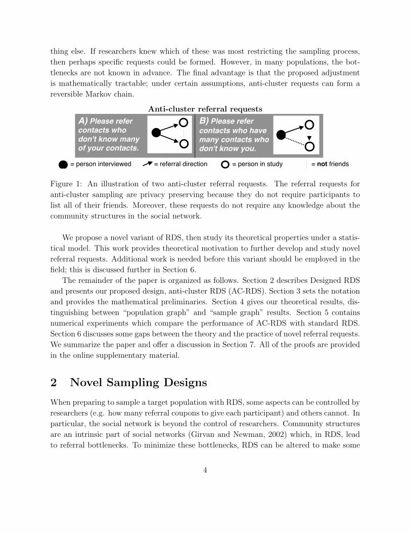
To diminish referral bottlenecks, this paper proposes an adjustment to the current RDS
implementation. Instead of asking participants to refer anyone from the target population,
this paper proposes two basic types of “anti-cluster referral requests,” which are described
in Figure 1. These referral requests diminish referral bottlenecks by producing triples of
participants that do not form a triangle, closed triplet, in the social network. The figure
contains two types of such requests. In fact, as described in Section 3.3, we propose a
procedure that probabilistically alternates between the two requests.
As compared to alternative methods, anti-cluster requests are more successful in di-
minishing referral bottlenecks for three reasons. First, this approach preserves privacy by
refraining from asking participants to list their friends in the population. Second, anti-
cluster requests do not require a priori knowledge about the nature of the bottleneck. For
example, the most salient bottleneck could form on race, gender, neighborhood, or some-
3
thing else. If researchers knew which of these was most restricting the sampling process,
then perhaps specific requests could be formed. However, in many populations, the bot-
tlenecks are not known in advance. The final advantage is that the proposed adjustment
is mathematically tractable; under certain assumptions, anti-cluster requests can form a
reversible Markov chain.
Anti-cluster referral requests
A) Please refer contacts who don't know many of your contacts.
= person interviewed = referral direction = person in study = not friends
B) Please refer contacts who have many contacts who don't know you.
Figure 1: An illustration of two anti-cluster referral requests. The referral requests for
anti-cluster sampling are privacy preserving because they do not require participants to
list all of their friends. Moreover, these requests do not require any knowledge about the
community structures in the social network.
We propose a novel variant of RDS, then study its theoretical properties under a statis-
tical model. This work provides theoretical motivation to further develop and study novel
referral requests. Additional work is needed before this variant should be employed in the
field; this is discussed further in Section 6.
The remainder of the paper is organized as follows. Section 2 describes Designed RDS
and presents our proposed design, anti-cluster RDS (AC-RDS). Section 3 sets the notation
and provides the mathematical preliminaries. Section 4 gives our theoretical results, dis-
tinguishing between “population graph” and “sample graph” results. Section 5 contains
numerical experiments which compare the performance of AC-RDS with standard RDS.
Section 6 discusses some gaps between the theory and the practice of novel referral requests.
We summarize the paper and offer a discussion in Section 7. All of the proofs are provided
in the online supplementary material.
2 Novel Sampling Designs
When preparing to sample a target population with RDS, some aspects can be controlled by
researchers (e.g. how many referral coupons to give each participant) and others cannot. In
particular, the social network is beyond the control of researchers. Community structures
are an intrinsic part of social networks (Girvan and Newman, 2002) which, in RDS, lead
to referral bottlenecks. To minimize these bottlenecks, RDS can be altered to make some
4
referrals more or less likely. This is the essence of novel sampling designs for respondent-
driven sampling.
As a thought experiment, suppose that the population of interest is divided into two
communities, EAST and WEST. Furthermore, assume that people form most of their
friendships within their own community. Under this simple model, referrals between com-
munities are unlikely, creating a bottleneck. Now, suppose that these communities were
known before performing the sample. The researchers could then request referrals from
specific groups (e.g. flip a coin, if heads request WEST and if tails request EAST). This
does not change the underlying social network, but it does change the probability of certain
referrals. If participants followed this request, the referral bottleneck between EAST and
WEST would be diminished. If 90% of a participant’s friends belonged to the same com-
munity as the participant, then the standard approach would obtain a cross-community
referral only 10% of the time. However, with the coin flip implementation, such a referral
happens 50% of the time.
Mouw and Verdery (2012) propose an alternative technique, Network Sampling with
Memory (NSM). In NSM sampling, researchers construct a sampling frame by asking RDS
participants to nominate their friends in the target population. This list is combined with
the friend lists from previous participants to form a sampling frame. In the “List” mode
of the sampling process, the next individual to be recruited and interviewed is selected by
sampling with-replacement from the list of nominated members. In the “Search” mode, to
improve the mixing property of the sampling process, individuals who appeared to be the
“bridge nodes”to the unexplored parts of the network are identified. Then, randomly a
node from friends of the bridge nodes who have only 1 nomination is selected for the next
interview. In computational experiments, Mouw and Verdery (2012) report a decrease in
the design effect, the ratio of the sampling variance to the sampling variance of simple
random sampling, of this novel approach.
These two extensions of RDS (i.e. flipping a coin and NSM) are both forms of Designed
RDS; through novel implementations of the sampling process they adjust the probabil-
ity of certain referrals, thereby diminishing the referral bottlenecks. Unfortunately, the
coin flipping example requires prior information about the social network, which may be
unattainable given the hidden nature of the target population. The NSM approach requires
respondents to reveal partial name and demographic information of their friends. More-
over, it asks respondents to refer (recruit) selected individuals from the list of nominees.
When practically implemented in a hidden population, however, it is not clear if respon-
dents will be willing to provide the requested information or refer the selected individual
from their list of nominees. Furthermore, the referral process may be based more heavily
on participants’ interactions with members of the target population following the survey
than on any plan they make to refer ahead of time.
5

Anti-cluster RDS is a type of Designed RDS that complements and builds upon both
of these approaches. The implementation of anti-cluster RDS does not require a priori
information on the communities in the social network, nor does it require that participants
reveal sensitive information about individuals who have not consented. Anti-cluster sam-
pling is designed to place larger referral probabilities on edges belonging to fewer triangles.
There are at least two ways to consider why this strategy circumvents bottlenecks.
1. Many empirical networks share three properties. First, the number of edges is pro-
portional to the number of nodes (i.e. the network is globally sparse). Second, friends
of friends are likely to be friends (i.e. the network is locally dense). Third, shortest
path lengths are small (i.e. the network has a small diameter); this is also known as
the small-world phenomenon. Watts and Strogatz (1998) shows how a network can
satisfy all three properties; take a deterministic graph that satisfies the first two fea-
tures (e.g. a triangular tessellation), then select a few edges at random and randomly
re-wire these edges to a randomly chosen node. Notice that these “random edges”
are unlikely to be contained in a triangle. So, edges that are not part of triangles
are more likely to lead to quicker network traverse. Anti-cluster RDS makes refer-
ral along that edges more probable, and potentially mixes faster and collects more
representative samples from the target population.
2. The Markov chain has been a popular model for studying theoretical properties of
RDS. Under the with-replacement sampling formulation of this model people make
referrals by selecting uniformly from their set of friends. A similar assumption could
be made about anti-cluster referrals; the referral is drawn uniformly from the set of
referrals that satisfy the anti-cluster request. If the Markov transition matrix for
anti-cluster sampling can be shown to have a larger spectral gap than the Markov
transition matrix for the simple random walk, then this suggests that anti-cluster
sampling will obtain a more representative sample.
In this paper, we pursue the second approach.
3 Preliminaries
3.1 Framework
This paper models the referral process as a Markov chain indexed by a tree (Benjamini
and Peres, 1994). A Markov chain indexed by a tree is a variant of branching Markov
chains in which a fixed deterministic tree indicates branching. This model is a straight-
forward combination of the Markov models developed in the previous literature on RDS
6
(Heckathorn, 1997; Salganik and Heckathorn, 2004; Volz and Heckathorn, 2008; Goel and
Salganik, 2009). This model is built with the following four mathematical pieces: an un-
derlying social graph, a node feature which is measured on each sampled node (e.g. HIV
status), a Markov transition matrix on this graph, and a referral tree to index the Markov
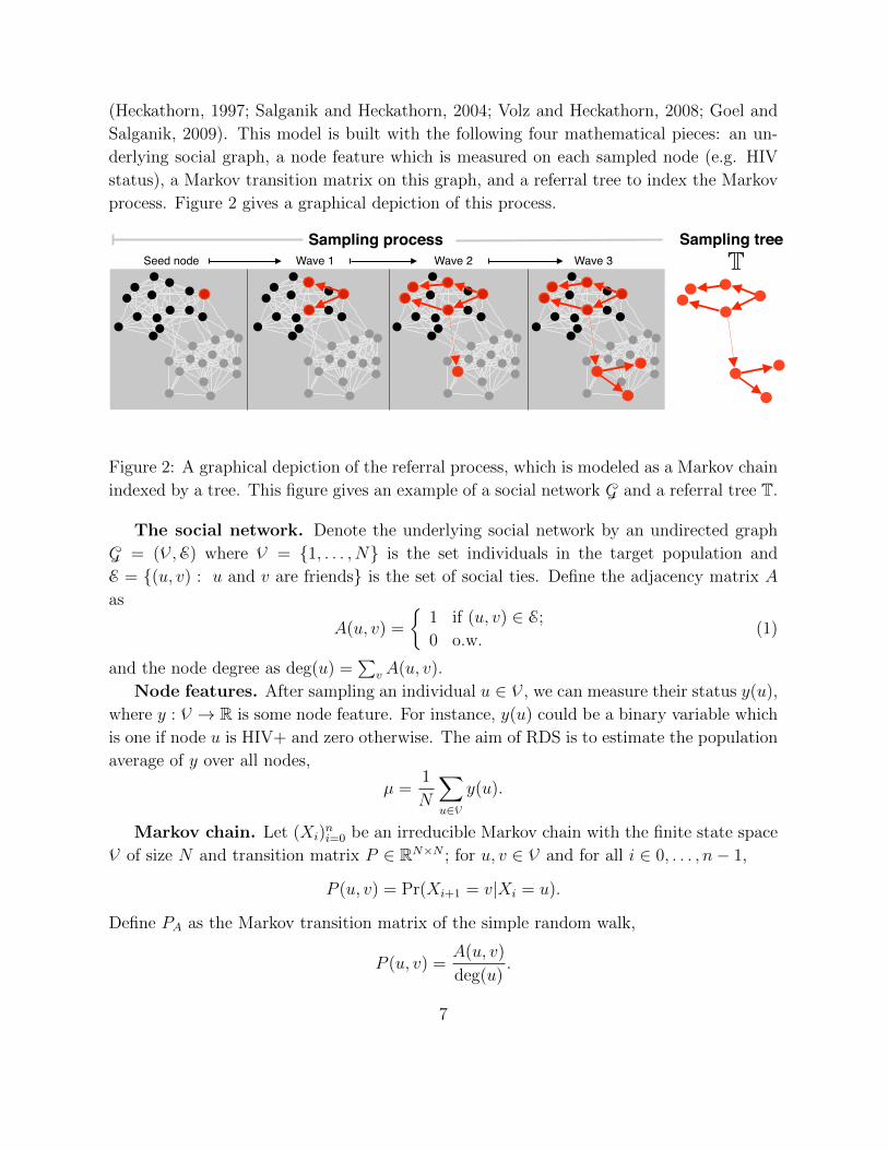
process. Figure 2 gives a graphical depiction of this process.
●
●●●
●
●
●
●
●
●●
●
●
●●
●●
●
●
●●
●
●
●
●
● ●
●
●●
●
●●●
●
●
●
●
●
●●
●
●
●●
●●
●
●
●●
●
●
●
●
● ●
●
●●
●
●●●
●
●
●
●
●
●●
●
●
●●
●●
●
●
●●
●
●
●
●
● ●
●
●●
●
●●●
●
●
●
●
●
●●
●
●
●●
●●
●
●
●●
●
●
●
●
● ●
●
●●
Seed node Wave 1 Wave 2 Wave 3Sampling treeSampling process
the first part of this proposal studies novel ways of assigning sampling weights to the randomwalk.
2) Estimation: The sampling mechanism induces dependence between samples (friends aresimilar in many ways). Current estimators do not correct for this dependence. This proposalshows that current estimators are inadmissible. Moreover, in certain regimes, new estimatorscan obtain faster rates of convergence.
3) Diagnostics: One key limitation of network driven sampling is the dependence between sam-ples. My preliminary theoretical research shows how this dependence manifests and suggestsdiagnostic tools.
2 notation
Denote the population as a node set V with N elements. We obtain a sample of size n from V bystarting from some seed node(s) and following the edges in the graph G = (V, E). If every samplerefers exactly one additional sample, then we obtain a chain of random variables
X(0) ! X(1) ! · · · ! X(n � 1) 2 V.
In the chain sample, the nodes are indexed by the integers 0, 1, 2, . . . , n � 1. In many networksampling applications it is sensible to allow for each sample to refer multiple additional samples.Instead of a chain, this produces a tree–a rooted, directed, and cycle free graph–that will be denotedby T. The root of this tree 0 2 T indexes the seed node.1 The decendents of the root node indexthe nodes that the seed refers. Symbols ⌧ and � will be used to denote generic nodes in T. Bynetwork driven sampling, we obtain the sample of nodes
{X(⌧) 2 V : ⌧ 2 T}.
In this notation, X(0) 2 V is the seed node.
The randomization for the sampling procedure is characterized by a Markov transition matrixP 2 RN⇥N . Denote �0 2 T as the “parent” node of � 2 T. Under the Markov model studied in
1If there are multiple seed nodes, then T is a forest, or a collection of trees and there are multiple roots.
●
●●●
●
●
●
●
●
●●
●
●
●●
●●
●
●
●●
●
●
●
●
● ●
●
●●
●
●●●
●
●
●
●
●
●●
●
●
●●
●●
●
●
●●
●
●
●
●
● ●
●
●●
●
●●●
●
●
●
●
●
●●
●
●
●●
●●
●
●
●●
●
●
●
●
● ●
●
●●
●
●●●
●
●
●
●
●
●●
●
●
●●
●●
●
●
●●
●
●
●
●
● ●
●
●●
Seed node Wave 1 Wave 2 Wave 3TreeSampling process
Figure 1: In the left panel, only the seed node is sampled. In the next panel, the seed node referstwo friends that create wave 1 of the sample. This continues for two more waves. On the right, isthe sampling tree T.
2
Figure 2: A graphical depiction of the referral process, which is modeled as a Markov chain
indexed by a tree. This figure gives an example of a social network G and a referral tree T.
The social network. Denote the underlying social network by an undirected graph
G = (V,E) where V = {1, . . . , N} is the set individuals in the target population and
E = {(u, v) : u and v are friends} is the set of social ties. Define the adjacency matrix A
as
A(u, v) =
{1 if (u, v) ∈ E;
0 o.w.(1)
and the node degree as deg(u) =∑
v A(u, v).
Node features. After sampling an individual u ∈ V, we can measure their status y(u),
where y : V → R is some node feature. For instance, y(u) could be a binary variable which
is one if node u is HIV+ and zero otherwise. The aim of RDS is to estimate the population
average of y over all nodes,
µ =1
N
∑u∈V
y(u).
Markov chain. Let (Xi)ni=0 be an irreducible Markov chain with the finite state space
V of size N and transition matrix P ∈ RN×N ; for u, v ∈ V and for all i ∈ 0, . . . , n− 1,
P (u, v) = Pr(Xi+1 = v|Xi = u).
Define PA as the Markov transition matrix of the simple random walk,
P (u, v) =A(u, v)
deg(u).
7

The standard Markov model for RDS assumes that Xi is a simple random walk.
Novel designs. Designed RDS is any technique that assigns differing weights to the
edges. Define the mapping W : E → R+ as a weighting function on the edges (u, v) ∈ E.
If (u, v) ∈ E and W (u, v) > 0, then u can recruit v. For simplicity, define W (u, v) = 0 if
(u, v) 6∈ E. Then, W can be expressed as a matrix. Define the diagonal matrix T to contain
the row sums of W , so that Tuu =∑
vW (u, v).
Through novel implementations, Designed RDS alters the edge weights. After weighting
the edges, the Markov transition matrix becomes
PW = T−1W. (2)
If Designed RDS increases an edge weight, it makes the edge more likely to be traversed.
We restrict the analysis to symmetric weighting matrices. Because of this restriction,
PW is reversible and has a stationary distribution π : V → R+ that is easily computable,
π(u) =Tuu∑v Tvv
. (3)
Throughout, it will be assumed that X0 is initialized with π. A more thorough treatment
of Markov chains and their stationary distribution can be found in Levin et al. (2009).
Referral tree. In the Markov chain model, participant Xi refers participant Xi+1. This
assumes that each participant refers exactly one individual. In practice, RDS participants
usually refer between zero and three future participants. To allow for this heterogeneity, it
is necessary to index the Markov process with a tree, not a chain. Let T denote a rooted
tree with n nodes. See Figure 2 for a graphical depiction.
To simplify notation, σ ∈ T is used to represent σ belonging to the node set of T. For
any node σ ∈ T with σ 6= root(T), denote parent(σ) ∈ T as the parent node of σ. The
Markov process indexed by T is a set of random variables {Xσ ∈ V : σ ∈ T} such that
Xroot(T) is initialized from π and
Pr(Xσ = v|Xparent(σ) = u) = P (u, v), for u, v ∈ V.
The distribution of Xσ is completely determined by the state of Xparent(σ). Benjamini and
Peres (1994) called this process a (T, P )-walk on G. In the social network G, an edge
represents friendship. In the referral tree, a directed edge (τ, σ) represents that random
individual Xτ ∈ V refers random individual Xσ ∈ V in the (T, P )-walk on G.
Statistical estimation. For any function on the nodes of the graph y : V → R, denote
µπ,y := Eπy :=∑u∈V
y(u)π(u) and µy := Ey :=1
N
∑u∈V
y(u),
8

where N := |V| is the number of nodes in the social network. By assumption, X0 ∼ π. So,
Xτ ∼ π and the sample mean 1/n∑
τ∈T y(Xτ ) consistently estimates µπ,y, the population
mean under stationarity. Thus, it is not a consistent estimator for the parameter of interest,
namely the population mean µy. In order to estimate µy, one can use inverse probability
weighting (IPW), using the stationary distribution. It can be shown that
µIPW =1
n
∑τ∈T
1
N· y(Xτ )
π(Xτ )
is an unbiased and consistent estimator of µy. Typically, N is unknown. The Hajek
estimator circumvents this problem while remaining asymptotically unbiased,
1∑τ∈T 1/π(Xτ )
∑τ∈T
y(Xτ )
π(Xτ ). (4)
The typical “simple random walk” assumption in the RDS literature is that participants
select uniformly from their contacts. This corresponds to Tuu = deg(u), making π(u) ∝deg(u), which is something that can be asked of participants. Under these assumptions,
(4) reduces to the RDS II estimator (Heckathorn, 2007)
µy =1∑
τ∈T 1/ deg(Xτ )
∑τ∈T
y(Xτ )
deg(Xτ ).
3.2 The Variance of RDS
Many empirical and social networks display community structures (Girvan and Newman,
2002). This can lead to referral bottlenecks in the Markov chain. These bottlenecks exist
because respondents are likely to refer people within their own community who have similar
characteristics. This section specifies how bottlenecks make successive samples dependent,
increasing the variance of µy and the design effect of RDS. The spectral properties of the
Markov transition matrix reveal the strength of these bottlenecks and control the variance
of estimators like µIPW . These results motivate the main results of this paper, which
show that anti-cluster sampling improves the relevant spectral properties of the Markov
transition matrix under a certain class of Stochastic Blockmodels. As a result, anti-cluster
sampling can decrease the variance of estimators like µIPW .
Let λ2(PA) be the second largest eigenvalue of the Markov transition matrix for the
simple random walk. The Cheeger bound demonstrates that the spectral properties of PAcan measure the strength of these communities. See Chung (1997) (Chapter 2) and Levin
et al. (2009) (p. 215) for more details. This relationship between communities in G and
the spectral properties of PA is exploited in the literature on spectral clustering. In that
9

literature, G is observed and the spectral clustering algorithm uses the leading eigenvectors
of PA to partition V into communities (Von Luxburg, 2007).
Intuitively, if there are strong communities in G and the node features y are relatively
homogeneous within communities, then successive samples Xi and Xi+t will likely belong
to the same community and have similar values y(Xi) and y(Xi+t). This makes the samples
highly dependent; the auto-covariance Cov(y(Xi), y(Xi+t)) will decay slowly as a function
of t. The next lemma decomposes the auto-covariance in the eigenbasis of the Markov
transition matrix. This proposition shows that the auto-covariance decays like λt2.
The following result applies to any reversible Markov chain with |λ2| < 1. In particular,
it applies to both PA (RDS) and PW (AC-RDS). With a reversible Markov chain, the
assumption |λ2| < 1 is equivalent to assuming that the chain is irreducible and aperiodic.
Proposition 1. Let (Xi)ni=0 be a Markov chain with reversible transition matrix P . Suppose
that X0 is initialized with π, the stationary distribution of P . For j = 1, 2, . . . , N , let
(fj, λj) be the eigenpairs of P , ordered so that |λi| ≥ |λi+1|. Because P is reversible,
fj and λj are real valued and the fj are orthonormal with respect to the inner product
〈f`, fj〉π =∑
i∈V f`(i)fj(i)π(i). If |λ2| < 1, then
Cov(y(Xi), y(Xi+t)) =
|V|∑j=2
〈y, fj〉2πλtj.
In previous research, Bassetti et al. (2006) and Verdery et al. (2015) used a similar
expression to compute the variance.
3.3 Anti-Cluster Random Walk; Constructing the Weights W
This subsection describes a Markov model for AC-RDS. Section 4 then studies the spectral
properties of the resulting AC-RDS Markov transition matrix. To describe the model we
need the following notation. Let · denote element-wise matrix multiplication and let JK×Kdenote a K×K matrix containing all ones. Finally, define the overbar operator for a K×Kmatrix B as B := JK×K −B, so that A = JN×N − A.
This model creates a Markov transition matrix which can be expressed with matrix
notation. Under the model, if i has one coupon, then the probability that i refers j is
proportional to the (i, j)th element of the matrix (AA) ·A. To see this, note that the (i, j)th
element of AA is the number of nodes ` that are friends with i but not friends with j, that
is
[AA]ij =∑`
Ai`(1− Aj`).
10

Then, the element-wise multiplication ensures that i is friends with j, yielding the weight
matrix (AA) · A.
Note that the weight matrix (AA) · A is not symmetric and, thus, does not lead to a
reversible Markov chain. However, we can use a second referral request to augment the
first request to ensure reversibility. To this end, model the referral request “Please refer
someone that knows many people that you do not know” as follows: if i is friends with j,
then the probability that i refers j is proportional to the number of people that j knows
that i does not know. In a similar fashion as above, this request produces the weight matrix
(AA) · A.
To implement AC-RDS, choose between (AA) · A and (AA) · A with equal probability
by flipping a coin. Consider the matrix W given by
W = (AA+ AA) · A. (5)
The (i, j)th element of W is proportional to the probability that i refers j in the process
described above. By design, W is symmetric, making making PW a reversible Markov
transition matrix.
These ideas for connecting implementation instructions for AC-RDS with the Markov
model are summarized in Table 1. The next section studies the spectral properties of PWunder a statistical model for G.
Implementation instructions compared to the Markov modelFlip a coin If heads (type A), If tails (type B),
Implementation
Instructions
Ask “please refer contacts in
the target population who don’t
know many of your contacts.”
Ask “please refer contacts in
the target population who have
many contacts who don’t know
you.”
Markov model,
starting from
node i
List all pairs of nodes (j, k) such
that, (i, j) ∈ E, (i, k) ∈ E, and
(k, j) /∈ E. Then choose a pair
(j, k) uniformly and refer j or k
uniformly at random.
List all pairs of nodes (j, k) such
that (i, j) ∈ E and (i, k) /∈ E.
From this list, uniformly choose
a node pair (j, k). Refer j.
Table 1: The correspondence between AC-RDS implementation instructions and the
Markov model for the referral process. Referral requests A and B from Figure 1 corre-
spond to the left and right columns, respectively, of this table. The first row describes the
verbal request given to a participant. The second row describes the Markov model for this
request, as discussed in Section 3.3.
Finally, we note that the transition matrix PW does not use referral request C in Figure
1, “Please refer someone that does not know the person that referred you.” Such a request
11

cannot form a Markov chain on the nodes in the network because it depends on the previous
participant. This non-Markovian behavior should not preclude the use of request C in
practice; however, it does make establishing theoretical results for request C more difficult.
In this paper, we focus on requests A and B and their Markov transition matrix PW .
4 Theoretical Results
To study the spectral properties of PW under a statistical model for the underlying so-
cial network, we break the analysis into “population results” and “sampling results.” The
“population results” in this section correspond to using the (weighted) adjacency matrix
A = EA, where the expectation is with respect to the statistical model for generating the
network. The expected adjacency matrix is a deterministic matrix and various combinato-
rial techniques can be used to show its properties. Define
W = (AA + AA) ·A. (6)
Define the Markov transition matrices PW and PA as in (2). In these definitions, PA cor-
responds to the population matrix for the simple random walk (RDS) and PW corresponds
to the population matrix for AC-RDS.
The “sampling” referred to in this section introduces an additional layer of randomness
to generate the underlying social network G. The goal of “sample results” is to show that
the random graph generated by the generic model has similar properties to the expected
graph. That is the randomness of the graph doesn’t significantly change the graph from
the expected graph. To refer to the randomness of the Markov chain, this section will refer
to “anti-cluster sampling,” “Markov sampling,” or “respondent-driven sampling.”
The population results will show that under various statistical models for the underlying
social network, the second eigenvalue of PW is less than the second eigenvalue of PA. To
extend these population results to a network which is sampled from the model, the sampling
results use concentration of measure to show that A and W are close (under the operator
norm) to A and W, respectively. Then, perturbation theorems show that the eigenvalues
of PA and PW are close to the eigenvalues of PA and PW, respectively. Theorem 2 combines
these results with Proposition 1 to show that AC-RDS reduces the covariance between
Markov samples.
4.1 Population Graph Results
Anti-cluster sampling is motivated by the need to readily escape communities in a social
network. The Stochastic Blockmodel (SBM) is a standard and popular model that pa-
12

rameterizes communities in the social network (Holland et al., 1983). For this reason, the
analyses below use the SBM to study anti-cluster sampling.
Definition 1. To sample a network from the Stochastic Blockmodel, assign each node
u ∈ {1, 2, . . . , N} to a class z(u) ∈ {1, 2, . . . , K}, where the z(u) are independently gener-
ated from Multinomial(θ). Conditionally on z, edges are independent and the probability of
an edge between nodes u and v is Bz(u)z(v), for some matrix B ∈ [0, 1]K×K.
The results below condition on the partition z. Conditional on this partition, E[A|z]
has a convenient block structure. Define the partition matrix Z ∈ {0, 1}N×K such that
Zuk = 1 if z(u) = k, otherwise Zuk = 0. Define A = E[A|z] and note that
A = ZBZT .
Let A := JN×N −A. Define the population weighting matrix as in (6). The following
lemma shows that W retains the block structure of A.
Lemma 1. Define B := JK×K − B and Θ ∈ RK×K as a diagonal matrix with Θkk equal
to the expected number of nodes in the kth block. Then, W = (AA + AA) ·A can be
expressed as
W = Z((BΘB + BΘB) ·B
)ZT .
The following lemma shows that under a certain class of Stochastic Blockmodels, anti-
cluster sampling decreases the probability of an in-block referral.
Lemma 2. For 0 < r < p+ r < 1, let B = pI + rJK×K. If Θllr < Θkk(p+ r) for all k 6= l,
then for any two nodes u and v with z(u) = z(v),
PW(u, v) < PA(u, v).
Note that if every block has an equal population, then the first assumption, 0 < r <
p + r < 1, implies the second assumption Θllr < Θkk(p + r). The next proposition uses
Lemma 2 to show that anti-cluster sampling reduces the second eigenvalue of the population
Markov transition matrix.
Proposition 2 (Spectral gap of the population graph). Under the SBM with K blocks, let
B = pI + rJK×K, for 0 < r < p+ r < 1. If the K blocks have equal size, then
0 < λ2(PW) + ε < λ2(PA) < 1, (7)
where ε > 0 depends on K, p, and r, but is independent of N , the number of nodes in the
graph. Specifically, λ2(PA) = 1/(R+ 1), where R = Kr/p. In the asymptotic setting where
K grows and r shrinks, while p and R stay fixed,
λ2(PW)→ 1
cR + 1, with c =
R + 1
R + 1− p. (8)
13

For any single node, note that R is roughly the expected number of out-of-block edges
divided by the expected number of in-block edges. To see this, multiply the numerator
and denominator of Kr/p by the block population N/K. As such, it is approximately the
odds that a random walker will change blocks. When R is large, the Markov chain mixes
quickly and λ2(PA) is small to reflect that.
AC-RDS is most useful in social networks with tight communities, where the walk is
slow to mix; this corresponds to a larger value of p and a smaller value of R. In this setting,
c in (8) is large, thus making λ2(PW) much smaller than λ2(PA). In particular, if p is close
to one, then c ≈ 1 +R−1 becomes very large for small values of R. Notice that the second
part of Proposition 2 makes no assumption on N , the number of nodes in the network.
The next proposition shows that anti-cluster sampling continues to perform well, even
when the community structure is exceedingly strong and standard approaches will fail to
mix well. Here, the reduction of λ2 from anti-cluster sampling is dramatic.
Proposition 3. Under the SBM with 2 blocks of equal sizes, let ε > 0 and suppose that
Bkk = (1− ε) and Bkl = ε for k 6= l. Then,
limε↘0
λ2(PA) = 1
and
limε↘0
λ2(PW) = 1/3.
For any Markov transition matrix P , λ2(P ) ≤ 1. The graph is disconnected if and
only if λ2 = 1; this is the most extreme form of a bottleneck. In the above proposition, if
ε = 0, then the sampled graph will contain two disconnected cliques, one for each block.
Under this regime, both PA and PW will have second eigenvalues equal to one. However,
if ε converges to zero from above, then Proposition 3 shows that λ2(PW) approaches 1/3,
while λ2(PA) approaches 1.
Propositions 2 and 3 assume balanced block sizes (i.e. an equal number of nodes).
To study unbalanced cases, the necessary algebra quickly becomes uninterpretable. We
explore the role of unbalanced block sizes with numerical experiments in Section 5.
4.2 Sample Graph Results
Theorem 1 gives conditions which ensure that the population eigenvalues, λ`(PW), are close
to the sample eigenvalues, λ`(PW ). As such, the population results in the previous section
appropriately represent the behavior of Markov sampling (both AC-RDS and RDS) on a
network sampled from the Stochastic Blockmodel. Chung and Radcliffe (2011) prove a
similar result for |λ`(PA)− λ`(PA)|.
14

Theorem 1 (Concentration of the anti-cluster random walk). Let G = (V,E) be a ran-
dom graph with independent edges and A = EA be the expected adjacency matrix. Let
Di :=∑
kAik, Fij :=∑
kAik(1 − Akj), and Gij :=∑
k(1 − Aik)Akj. Define Fmin =
mini,j=1,··· ,|V| Fij. If Fmin = ω (lnN) and there exits a constant c1 such that Fij +Gij ≥ c1Di
for all i, j ∈ {1, · · · , |V|}, then with probability at least 1− ε,∥∥∥T− 12 WT−
12 −T−
12 WT−
12
∥∥∥2
≤ c2 ln 10Nε
Fmin
,
where c2 is a constant, ‖·‖ denotes the operator norm, T is a diagonal matrix with the row
sums of W on its diagonal, and T is defined in the same way with respect to W. Moreover,
with probability at least 1− ε,
|λ`(PW )− λ`(PW)|2 = O
(ln 10N
ε
Fmin
), for all ` ∈ 2, . . . , N.
Remark 1. The theorem uses standard asymptotic notation, which we recall here for conve-
nience. We write f(n) = O (g(n)) to indicate that |f | is bounded above by g asymptotically,
that is
lim supn→∞
|f(n)|g(n)
<∞.
We write f(n) = ω (g(n)) to indicate that f dominates g asymptotically, that is
limn→∞
∣∣∣∣f(n)
g(n)
∣∣∣∣ =∞.
Remark 2. Fij gives the number of friends of node i that are not in the friend list of node
j. So Fmin = ω (lnN) ensures that the number of individuals that a node can refer under
AC-RDS grows with a rate faster than lnN . Roughly speaking, it is similar to the sparsity
condition required for concentration results of random graphs with independent edges. Since
A is a symmetric matrix, Fij = Gji and, consequently,
mini,j=1,··· ,|V|
Fij = mini,j=1,··· ,|V|
Gij.
The condition on c1 ensures that the ratio DiFij+Gij
stays bounded. These sampling results
are sufficiently general to apply to all of the models studied in the previous section.
Theorem 2 presents the asymptotic behavior of AC-RDS in reducing the correlation
among samples collected from a random graph under a Stochastic Blockmodel. The theo-
rem is an aggregation of all the previous results in the paper. The result is asymptotic in
the size of the population, not in the size of the sample.
15

Theorem 2 (Dependency reduction property of AC-RDS). Let G be a random graph with
N nodes sampled from a Stochastic Blockmodel with B = pIK×K + rJK×K, for 0 < r <
p + r < c < 1. Further assume an equal number of nodes in each of the K blocks. Let
(Xi)ni=1 and (Xac
i )ni=1 be two Markov chains with transition matrix PA and PW , respectively.
The parameters p, r and K can change with N . If ln(N)/(pK + rN)→ 0, then asymp-
totically almost surely, for all i, i+ t ∈ {1, . . . , n}, and t 6= 0,
Cov(y(Xaci ), y(Xac
i+t)) < Cov(y(Xi), y(Xi+t)),
where y : V → R is any bounded node feature.
Remark 3. The quantity pNK
+ rN is Dmin, the minimum expected degree. The condition
ln(N)/(pNK
+ rN) → 0 is needed to use Theorem 1. Note that Fij + Gij > 2cDmin for all
i, j ∈ {1, · · · , |V|}.
5 Numerical Experiments
We conduct three sets of numerical experiments to compare the performance of AC-RDS
with standard RDS. The first set investigates the impact of unequal block sizes on the
results of Propositions 2 and 3. The second set investigates the impact of community
structures and homophily using the Stochastic Blockmodel. In the third set, we consider
an empirical social network with unknown community structure. Finally, we consider two
relaxations of the Markov model to allow for more realistic settings: sampling without
replacement and preferential recruitment.
5.1 The Role of Unequal Block Sizes
In this experiment, we numerically calculate the eigenvalues of PA and PW under varying
SBM parameterizations with K = 2. Given θ and B in the definition of the SBM, we can
use results from Rohe et al. (2011) (see the proof of Lemma 3.1) to compute the K non-zero
eigenvalues of the transition matrix.
Consider the setting of Propositions 2 and 3 with K = 2 blocks. These results assume
that the blocks contain an equal number of nodes; here we explore the role of unequal
block sizes. As a measure of unbalance, we use the ratio of the largest block size to the
smallest block size. The results of the study are displayed in Figure 3. The horizontal axis
in both panels gives this ratio of unbalance; when this value is large (farther to the right),
the blocks are exceedingly unbalanced. The vertical axis controls the expected number of
in-block versus out-of-block edges with a parameter ε. In the left panel, ε plays the dual
16
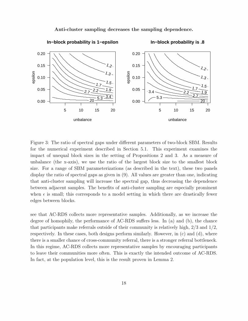
role as in Proposition 3. In the right panel, ε does not control the in-block probabilities
(i.e. the diagonal of B); here, the diagonal of B is set to .8 across all experiments.
The spectral gap is given by 1− λ2, we are interested in exploring the ratio
ratio of spectral gaps =1− λ2(PW)
1− λ2(PA). (9)
For a range of unbalances and values of ε, Figure 3 plots the ratio of spectral gaps. In all of
the parameterizations, this value is greater than one, indicating that anti-cluster sampling
decreases λ2 relative to the random walk model of RDS, even with unequal blocks. For
example, the contour at 5.3 represents the class of models such that anti-cluster sampling
increases the spectral gap by over five-fold.
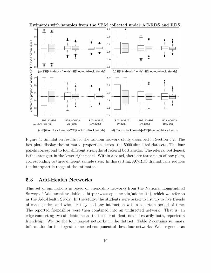
5.2 Random Networks
Here we investigate the impact of community structures and homophily using the Stochastic
Blockmodel. We use a SBM with 2000 nodes and 50 communities of equal size to generate
the underlying social network. To illustrate the impact of community structures, we vary
the ratio of the expected number of in-block edges divided by the expected number of out-
of-block edges. This ratio also controls the probability of generating an out-of-community
referral. For example, with the ratio equal to one, the probability of an out-of-community
referral is 1/2. We examine values of this ratio between 1/2 to 4. To do this, we fix the
in-block probabilities to 0.9 and change the out-of-block probabilities.
We simulate Markovian referral trees in which each participant refers exactly three
members with replacement. The three referrals are samples from the neighbors of the
participant. RDS uses uniform samples, whereas AC-RDS uses non-uniform samples based
on the weights described in (5). To show the effect of the communities, we choose the
binary node feature to be based on the community membership. The value is set to zero
if the node belongs to communities 1 through 25, otherwise, the value is set to one. For
both designs, we use the RDS II estimator to estimate the community proportion, where
the inclusion probabilities are the stationary distribution of the simple random walk.
The datasets are simulated in the following way. First we generate a realization of an
SBM and compute the stationary distribution of the simple random walk. We simulate
the referral procedure of RDS and AC-RDS starting from a uniformly selected node and
continuing until a certain number of samples are collected, either 1%, 5%, or 10% of the
total nodes. We compute the RDS II estimates of the feature from samples collected by
both procedures.
This study is based on 5000 simulated datasets. Figure 4 displays box plots for the 5000
RDS II estimates of the proportion in different settings. Comparing RDS to AC-RDS, we
17
Anti-cluster sampling decreases the sampling dependence.
In−block probability is 1−epsilon
unbalance
epsi
lon
1.2
1.3
1.5 1.7 1.9 2.2 2.7 3.4 5.3 20
5 10 15 20
0.00
0.05
0.10
0.15
0.20
In−block probability is .8
unbalance
epsi
lon
1.2
1.3
1.5 1.7 1.9 2.2
2.7 3.4
5.3 20
5 10 15 20
0.00
0.05
0.10
0.15
0.20
Figure 3: The ratio of spectral gaps under different parameters of two-block SBM. Results
for the numerical experiment described in Section 5.1. This experiment examines the
impact of unequal block sizes in the setting of Propositions 2 and 3. As a measure of
unbalance (the x-axis), we use the ratio of the largest block size to the smallest block
size. For a range of SBM parameterizations (as described in the text), these two panels
display the ratio of spectral gaps as given in (9). All values are greater than one, indicating
that anti-cluster sampling will increase the spectral gap, thus decreasing the dependence
between adjacent samples. The benefits of anti-cluster sampling are especially prominent
when ε is small; this corresponds to a model setting in which there are drastically fewer
edges between blocks.
see that AC-RDS collects more representative samples. Additionally, as we increase the
degree of homophily, the performance of AC-RDS suffers less. In (a) and (b), the chance
that participants make referrals outside of their community is relatively high, 2/3 and 1/2,
respectively. In these cases, both designs perform similarly. However, in (c) and (d), where
there is a smaller chance of cross-community referral, there is a stronger referral bottleneck.
In this regime, AC-RDS collects more representative samples by encouraging participants
to leave their communities more often. This is exactly the intended outcome of AC-RDS.
In fact, at the population level, this is the result proven in Lemma 2.
18
Estimates with samples from the SBM collected under AC-RDS and RDS.●
●●
●
●●●●●●
●
●
● ●
●
●●●
●
●
●●
●
●
●
●
●●●●●
●
●●●●
●●
●
●
●●
●
●
●
●●●
●
●
●
●
●
●
●
●●●
●
●
●●
●
●
●
●●●
●●
●
●
●
●●
●
●
●
●
●
●
●
●
●●●●
●●
●●
●
●●
●
●
●●●
●●
●●
●●
●
●●●
●
●●
●●
●●●●●
●
●
●
●
●
●
●●
●
●
●●●●
●●●
●●
●●●●●
●
●●
●
●
●
●●
0.0
0.2
0.4
0.6
0.8
1.0
(a) 2*E[# in−block friends]=E[# out−of−block friends]
●●
●
●●●●
●●●
●
●
●
●
●●●●●●●●●●
●
●
●
●
●
●●
●●
●●●
●●
●
●●●●●●●●●●
●
●●
●●
●●●●●●
●●●
●
●●●●●
●
●
●●
●
●●
●
●●
●●
●
●●
●●
●
●●
●●
●●
●
0.0
0.2
0.4
0.6
0.8
1.0
(b) E[# in−block friends]=E[# out−of−block friends]
●
●
●●
●
●
●
●
●●
●
●●
●●
●●
●
●●●
●
●●
●
●●●
●
●●
●
0.0
0.2
0.4
0.6
0.8
1.0
RDS RDS RDSAC−RDS AC−RDS AC−RDS
1% (20) 5% (100) 10% (200)
(c) E[# in−block friends]=2*E[# out−of−block friends]
sample %
●
●
●
●
●●
●
●
●
●
●●
●●●●
●●●
●
●
0.0
0.2
0.4
0.6
0.8
1.0
RDS RDS RDSAC−RDS AC−RDS AC−RDS
1% (20) 5% (100) 10% (200)
(d) E[# in−block friends]=4*E[# out−of−block friends]
estim
ate
of p
ropo
rtio
n of
nod
es in
the
even
com
mun
ities
Figure 4: Simulation results for the random network study described in Section 5.2. The
box plots display the estimated proportions across the 5000 simulated datasets. The four
panels correspond to four different strengths of referral bottlenecks. The referral bottleneck
is the strongest in the lower right panel. Within a panel, there are three pairs of box plots,
corresponding to three different sample sizes. In this setting, AC-RDS dramatically reduces
the interquartile range of the estimator.
5.3 Add-Health Networks
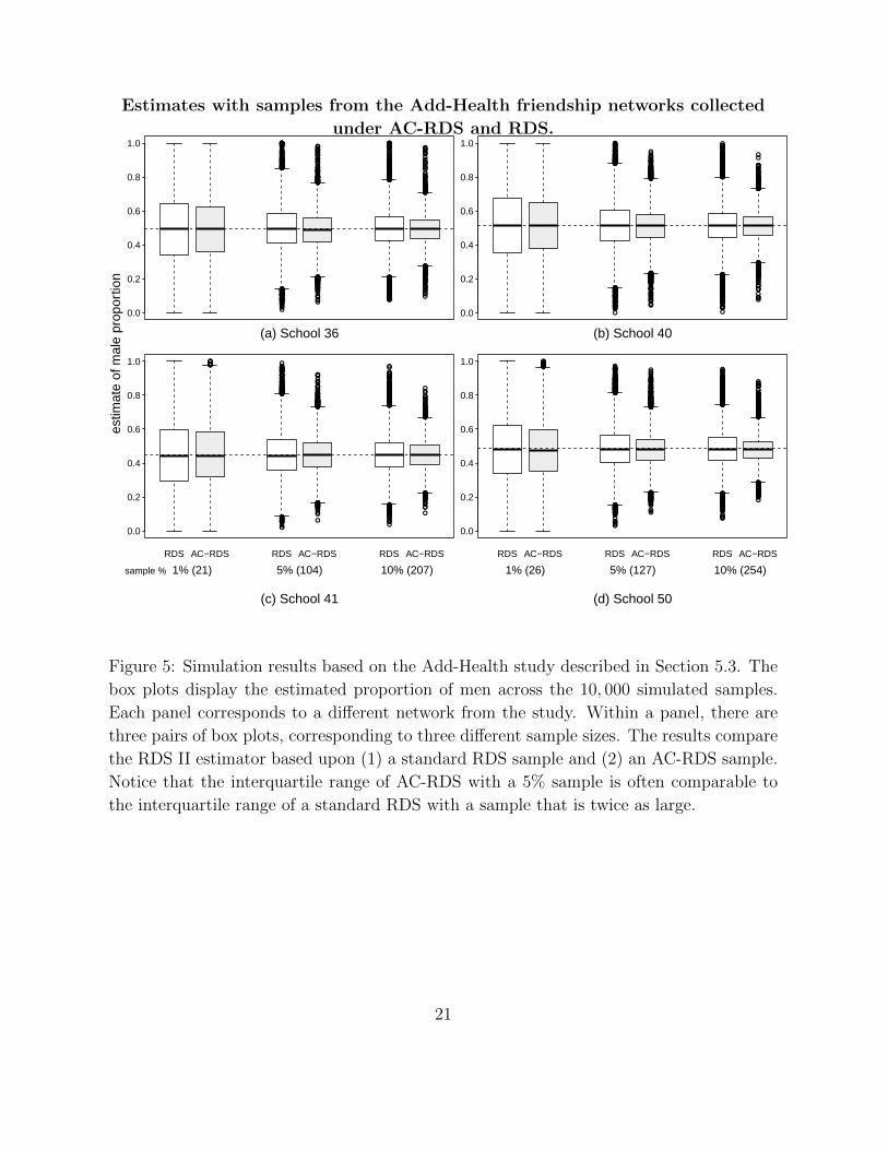
This set of simulations is based on friendship networks from the National Longitudinal
Survey of Adolescent(available at http://www.cpc.unc.edu/addhealth), which we refer to
as the Add-Health Study. In the study, the students were asked to list up to five friends
of each gender, and whether they had any interaction within a certain period of time.
The reported friendships were then combined into an undirected network. That is, an
edge connecting two students means that either student, not necessarily both, reported a
friendship. We use the four largest networks in the dataset. Table 2 contains summary
information for the largest connected component of these four networks. We use gender as
19

the binary node feature and focus on estimating the proportion of males in the population.
School id # Nodes # Edges CC covariance covarianceac
School 36 2152 7986 0.178 0.0260 0.0056
School 40 1996 8522 0.144 0.0265 0.0030
School 41 2064 8646 0.139 0.0243 0.0042
School 50 2539 10455 0.141 0.0276 0.0069
Table 2: Network characteristics for the four largest friendship networks in the Add-Health
study. This table provides characteristics for the largest connected component of each
network. An edge between student nodes indicates that either student reported a friendship.
The clustering coefficient (CC) is the ratio of the number of triangles and connected triplets.
The last two columns represent the covariance of the samples collected under RDS and AC-
RDS, respectively.
We simulate the referral procedure of RDS and AC-RDS starting from a uniformly
selected node and continuing until a certain number of samples are collected, either 1%,
5%, or 10% of the total nodes. In these simulations, each participant refers exactly three
members with replacement. We compute the RDS II estimate of the male proportion using
the node degree for the weights. Similar to the simulations in Goel and Salganik (2010)
and Baraff et al. (2016), these simulations are performed with replacement.
This study is based on 10, 000 simulated samples. Figure 5 and 6 display box plots for
the 10, 000 RDS II estimates of the male proportion under different settings. Notice that
in Figure 5 the interquartile range of AC-RDS with a 5% sample is often comparable to
the interquartile range of a standard RDS with a sample that is twice as large. In Figure
6, only type B request is considered in the implementation of AC-RDS.
20
Estimates with samples from the Add-Health friendship networks collected
under AC-RDS and RDS.
●●
●
●
●●
●
●
●
●●
●
●●
●
●
●●
●
●
●
●
●●
●
●●
●
●
●●
●
●
●●●
●
●●
●
●
●
●
●
●
●●
●●
●
●●●
●
●
●
●
●
●
●
●
●
●
●
●●
●
●
●
●
●
●
●
●●
●
●●
●
●●
●
●
●●
●●
●
●
●
●
●●
●
●●
●
●
●
●
●
●●
●
●
●●
●
●
●●●
●
●●
●
●
●●
●
●
●●
●
●
●●
●
●●
●
●●
●
●●●
●
●
●
●
●●●
●
●
●
●
●●
●
●
●
●●
●●
●
●
●
●
●
●●●
●
●
●
●●
●●
●
●●
●
●
●
●
●
●
●
●
●
●
●
●
●
●
●
●
●●
●
●
●
●
●
●
●●
●●●
●
●
●
●
●
●
●
●
●
●●
●●●
●
●●●●●
●
●
●
●
●
●
●
●
●
●
●●●
●●
●
●
●
●
●●
●
●●
●
●
●●●●
●
●
●
●
●
●●
●
●
●
●●
●●
●
●
●
●
●
●
●
●
●
●
●
●
●
●
●
●
●
●
●
●●
●
●
●
●
●
●
●
●
●
●
●
●●
●
●
●
●
●
●
●●
●
●
●
●
●
●
●
●
●
●
●
●
●
●
●
●
●
●
●●
●
●
●
●
●
●
●
●
●
●
●
●●
●
●
●
●
●
●
●
●
●
●
●
●
●
●●
●●
●
●
●
●
●●●
●
●●
●
●
●●
●●
●
●
●
●
●●●●
●●●●
●
●
●
●
●
●●
●
●
●
●
●●
●
●
●
●●●
●
●
●
●
●
●
●●
●
●
●
●
●
●
●
●●
●
●
●
●
●
●
●
●
●
●
●
●●
●
●
●
●
●
●
●
●●
●
●
●
●●
●
●
●●
●
●●
●●
●●
●
●
●
●
●
●
●●●
●●
●
●
●
●
●
●
●
●●●
●
●
●
●
●●●
●
●
●
●
●
●
●
●
●
●●●●
●
●
●
●
●●
●
●
●
●
●
●
●
●
●
●
●●●●
●
●
●
●●●
●
●
●●
●
●
●
●
●
●
●
●
●
●
●
●
●●
●●●
●
●
●●●
●
●
●
●
●
●
●
●
●
●
●
●
●
●
●
●
●
●
●●
●
●
●
●
●
●
●●●
●
●
●
●
●
●
●●
●●●
●
●
●
●
●
●
●
●
●
●●
●●
●
●
●
●
●
●
●
●
●
●
●
●●●
●
●
●●
●
●
●
●●
●
●
●
●
●●●
●
●●
●
●
●
●●●●●
●
●
●
●●
●
●
●
●●●
●
●
●
●
●●
●
●
●●
●●
●
●
●
●
●
0.0
0.2
0.4
0.6
0.8
1.0
(a) School 36
estim
ate
of m
ale
prop
ortio
n
●●
●●●
●
●
●
●●
●●●
●●
●
●
●
●●
●●
●●
●●●●
●
●
●●
●
●●●●
●
●
●
●
●
●
●
●
●●
●
●
●
●
●●
●
●
●
●●●●●
●
●
●
●
●
●
●
●
●
●
●
●●
●
●
●
●
●
●
●
●
●●●●
●
●
●
●
●
●●
●
●
●
●●
●
●
●●
●●
●●
●
●
●
●●
●●●
●
●
●●
●
●
●
●
●
●●
●
●
●
●
●
●
●
●●
●
●●
●
●●
●
●
●
●
●
●
●
●
●
●
●
●
●
●
●
●●
●
●
●●
●
●●
●
●
●
●
●●●
●
●
●
●●●
●
●
●●
●
●
●
●
●
●
●
●
●
●
●●
●
●●●
●
●
●
●
●
●●
●●●
●
●
●
●●
●
●
●
●
●
●
●
●
●
●
●●
●
●
●
●
●●
●
●
●
●
●
●
●●
●
●
●
●
●
●●●
●●
●
●
●
●
●●●
●
●
●
●
●
●
●●
●
●
●●
●●
●
●
●●
●
●
●●
●●●●●
●
●●
●
●
●
●
●
●
●
●
●●●
●
●●
●
●
●
●
●
●
●●
●
●
●
●
●
●
●
●●●
●
●
●●
●●
●
●
●
●●
●
●
●
●
●●●
●
●
●
●
●
●
●●●
●●
●
●
●
●
●
●
●●
●
●
●●
●
●
●
●
●●●
●
●●●●
●
●
●
●
●
●
●●
●
●
●
●
●
●
●
●
●●●
●●●●
●●
●●
●
●
●
●
●●
●●
●
●
●
●
●
●
●
●
●
●
●
●
●
●
●
●●
●
●
●
●
●
●
●●
●
●
●
●
●
●●●
●
●
●
●
●
●
●
●
●
●
●
●
●
●
●
●
●
●
●
●
●●
●
●
●
●
●●
●
●
●
●
●●●●
●●
●●
●●●
●
●
●
●
●●
●
●
●
●
●●
●
●●
●
●
●
●
●●
●
●
●
●
●
●
●
●
●
●
●
●
●
●
●●
●
●
●
●
●
●
●
●
●
●
●
●
●
●
●
●
●
●●
●
●●
●
●
●●
●
●●
●
●
●
●●
●
●
●
●●
●●
●
●
●
●
●●●
●
●
●
●
●
●
●●●
●
●
●
●
●
●
●
●
●
●
●
●
●●
●
●
●
●
●
●
●
●●●
●
●
●
●
●
●
●
●●
●
●
●
●
●●●
●●
●
●
●
●
●
●
●
●
●
●
●
●
●
●●
●●
●
●
●●
●
●
●
●
●●
●
●
●
●
●
●
●
●
●
●●
●
●
●
●
●
●
●
●●
●
●
●
●
●●●
●
●
●●
●
●
●●
●
●
●
●●
●●
●
●
●
●
●
●
●●●●
●
●
●
●
●
●
●
●
●●
●
●●
●
●
●●●
●
●
●
●
●
●
●
●
●
●
●
●
●
●●●●●
●●
●
●●●
●
●●●
●
●●
●
●
●
●
●
●
●
●
●●●●
●
●
●●
●●
●
●●
●
●
●
●●
●
●
●
●●●●●
●●
●
●●●●
●
●
●
●
●
●
●
●
●
●
●
●
●
●
●
●
●
●
●
●
●
●
●
●
●●
●●
●●
●
●
●
●●
●●
●
●
●●●●●
●
●●
●
●
●
●
●
●
●●●
●
●
●
●
●
●
●
●
●
●●●
●
●
●
●●●
●●●
●
●
●
●
●
●
●
●
●
●●
●
●
●
●
●●
●●●●●
0.0
0.2
0.4
0.6
0.8
1.0
(b) School 40
●●●●●●●●●
●
●
●●
●●●●●●●
●●
●
●
●
●
●
●
●
●
●
●
●
●
●
●
●
●
●
●
●●
●
●●●●
●●
●
●
●
●●●●
●
●
●●
●
●
●
●●
●
●●●●
●
●
●
●●
●●
●
●
●
●
●
●
●●
●
●
●
●
●
●
●
●
●●
●●
●
●●
●
●
●●
●●
●
●
●●
●
●
●●
●●●●
●
●
●●
●●
●●
●
●●●
●
●●●
●
●
●
●●
●
●
●
●
●●
●
●
●●●●
●
●●●
●
●●●●
●●●
●
●●
●
●
●
●
●
●
●
●
●●
●●●
●●●●●
●●
●
●
●
●
●●
●
●
●●
●●●●
●
●
●
●●●
●
●
●●●●
●
●
●●●
●
●
●●●
●
●
●
●
●●
●●
●
●
●
●●
●
●●
●●●
●
●
●
●
●●●
●
●
●
●
●
●
●
●
●
●
●●
●
●●
●
●
●
●●
●
●
●
●
●●●●●
●
●
●
●
●●
●
●
●
●
●
●●
●
●
●
●
●●
●
●
●●●●
●
●●
●
●
●
●
●
●
●
●●
●
●
●
●
●●
●●
●
●●
●
●
●●
●●
●●●
●●
●
●
●
●
●
●
●
●
●●●●
●
●
●
●
●
●
●
●
●●
●
●
●
●
●
●
●
●
●●
●
●
●●
●
●
●
●
●
●
●
●
●
●●
●
●
●
●
●
●
●
●
●
●
●
●
●●
●●●
●
●
●
●
●
●●
●
●
●
●
●
●●
●
●
●
●●
●
●
●●●●
●●
●
●●
●●
●
●
●●
●
●
●
●
●
●●●●●
●●●
●
●●●
●●
●
●
●
●
●
●●●●●●●●
●●
●●
●
●●
●
●
●
●
●
●
●
●
●
●
●
●
●●
●
●●●
●
●●
●
●●
●
●
●●
●
●
●
0.0
0.2
0.4
0.6
0.8
1.0
RDS RDS RDSAC−RDS AC−RDS AC−RDS
1% (21) 5% (104) 10% (207)
(c) School 41
sample %
●●●●●●●●●●●●●●●●●●●●
●
●
●
●
●●
●●
●
●
●
●●
●
●●●
●●●
●●
●
●
●
●
●
●●
●
●
●
●
●
●
●
●●●
●
●●
●
●
●●
●
●
●
●
●
●
●
●
●
●
●
●
●
●
●
●●
●
●●
●
●
●
●
●
●
●
●
●
●
●
●
●
●●●
●
●
●●
●●
●
●
●
●●
●●●●
●
●
●
●
●●
●
●
●
●●
●●
●●
●
●●
●
●●●
●
●
●
●
●
●●
●
●
●
●
●
●●
●
●
●
●
●
●
●
●
●
●
●
●
●●
●
●
●
●●
●
●●
●
●
●●
●
●●
●
●
●●
●
●
●
●
●●●●●
●
●
●
●
●
●●●
●●
●
●
●
●●
●
●
●
●
●
●
●●
●
●●●●
●●
●
●
●●
●
●
●●●
●
●
●
●●
●
●
●
●
●
●
●
●
●
●
●
●●
●●
●
●
●
●●
●
●
●
●
●
●
●●
●
●
●
●
●
●●
●●
●
●
●
●●●●
●
●
●●
●●●
●
●●●
●
●●●
●
●●
●
●
●●●
●
●
●
●
●
●
●
●●
●
●
●
●●●
●
●●
●
●
●
●
●
●
●
●
●●
●●
●
●
●
●
●●
●
●
●●
●●●
●
●●
●
●
●
●
●
●
●
●
●
●
●
●
●
●
●
●
●●
●
●
●
●
●
●●
●
●
●
●
●
●●
●
●
●
●
●
●●
●
●
●
●●
●
●
●
●
●
●
●
●
●●
●
●●
●
●
●
●
●
●●
●●
●●●●
●
●
●
●
●●
●
●
●
●
●
●●●
●
●
●
●
●
●
●●●
●
●
●
●
●
●
●
●
●
●
●
●
●●
●
●
●
●
●
●
●
●
●●
●
●
●
●
●
●●●
●●●●
●
●
●
●
●
●
●
●
●
●
●
●●
●
●
●
●
●●
●
●
●
●
●●
●
●
●
●●
●●
●
●
●●
●
●●●
●
●
●
●●
●
●
●
●
●●
●●
●
●
●
●●●
●●
●
●
●
●
●●
●
●●
●
●
●
●●
●
●
●
●●
●●●
●
●
●
●
●
●●●
●
●
●
●
●
●●
●
●
●
●
●
●
●
●
●
●●
●●●
●●
●
●
●●
●
●
●●
●
●
●
●
●●
●
●
●
●●
●
●
●
●●
●
●
●
●●●
●
●
●
●
●
●
●
●
●
●
●
●
●
●●
●
●●●
●
●
●●
●
●
●
●
●
●
●●
●
●
●
●
●
●
●
●
●●●●
●
●
●●
●●●
●
●
●
●
●●
●●
●
●
●●●
●
●●
●
●
●
●
●
●
●
●
●
●
●●
●●
●●●
●
●
●●●●
●
●●
●
●
●
●
●
●
●●
●
●
●
●
●●
●
●
●●●
●
●
●
●
●
●●
●●
●
●●
●
●
●
●●
●
●
●
●
●
●
●
●
●
●
●
●
●
●
●
●
●
●
●
●
●
●
●
●
●
●
●●
●
●
●
●
●
●
●
●
●●
●●
●
●
●●
●
●
●
●
●
●
●●
●
●
●
●
●●
●
●
●
●
●
●
●
●
●●
●
●
●●
●
●
●
●
●
●●●
●
●
●
●
●
●
●●
●
●
●
●●●●●●●●
●
●●
●
●
●
●●
●
●
●
●
●
●
●
●
●
●
●●
●
●
●
●
●
●
●
●
●
●
●
●●
●
●
●●
●
●
●●
●●
●
●
●
●
●
●●
●●
●
●●●
●●
●
●
●
●●●
●
●
●
●
●
●
●●
●
●
●
●
●
●
●
●
●
●
●
●
●●
●
●
●
●
●●●
●●●●
●
●
●
●
●
0.0
0.2
0.4
0.6
0.8
1.0
RDS RDS RDSAC−RDS AC−RDS AC−RDS
1% (26) 5% (127) 10% (254)
(d) School 50
Figure 5: Simulation results based on the Add-Health study described in Section 5.3. The
box plots display the estimated proportion of men across the 10, 000 simulated samples.
Each panel corresponds to a different network from the study. Within a panel, there are
three pairs of box plots, corresponding to three different sample sizes. The results compare
the RDS II estimator based upon (1) a standard RDS sample and (2) an AC-RDS sample.
Notice that the interquartile range of AC-RDS with a 5% sample is often comparable to
the interquartile range of a standard RDS with a sample that is twice as large.
21
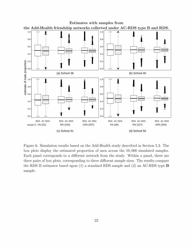
Estimates with samples from
the Add-Health friendship networks collected under AC-RDS type B and RDS.
●
●
●●
●●●
●●
●●●●●●●●
●
●●●
●
●
●
●●●●●
●●●
●●●
●●●
●
●●
●●
●
●
●
●
●
●
●
●●●●●
●
●
●●
●
●●
●
●
●●
●●
●
●
●
●
●
●
●
●
●●●
●
●●
●
●●
●
●
●●●
●●
●
●
●
●
●
●●
●
●●
●
●
●●
●●
●
●
●
●
●●
●
●
●
●
●●
●
●
●●●
●
●
●
●
●
●
●
●●
●
●●
●
●
●●
●
●
●
●
●
●●
●
●
●
●
●
●
●●
●
●●●
●●
●
●
●
●
●
●
●
●●
●●
●
●●
●
●
●●
●
●
●
●●
●
●●
●
●
●
●
●
●
●●
●
●
●●
●
●
●
●
●
●●
●●●
●●●
●
●
●
●
●●●●
●
●
●
●●
●●●
●
●
●
●●
●
●
●
●
●
●
●●
●
●
●
●
●●
●
●
●
●
●●
●
●
●
●
●
●
●●●
●
●
●
●●
●
●
●
●
●●●
●
●
●
●
●●
●
●
●●
●●●
●
●
●●●
●●●●●●
●
●
●
●●
●
●
●
●
●
●
●
●
●
●●
●
●●
●●
●●
●
●
●
●
●●
●
●●
●
●
●
●
●
●
●
●
●●
●
●
●
●
●
●
●●●
●●
●
●●
●
●
●
●
●
●
●
●
●
●
●
●
●
●
●●
●
●●
●
●
●
●●●
●
●
●
●
●●
●
●
●
●
●
●
●
●
●●
●●
●
●
●●
●
●●
●
●
●
●
●
●●
●
●
●
●●
●
●
●
●
●
●
●
●
●
●
●
●●●
●
●
●●
●
●
●
●
●
●
●
●
●
●
●
●
●
●
●
●
●
●
●
●●●
●
●
●●
●
●
●
●
●
●
●
●
●
●
●
●
●
●●●
●
●
●
●●
●
●
●
●
●
●
●
●
●
●
●
●
●●
●
●
●
●
●
●
●
●
●
●
●
●
●●
●●●●
●●
●
●
●
●●
●
●
●
●
●
●
●
●●
●
●
●
●●
●●
●
●
●
●
●
●
●
●
●
●
●
●●
●
●
●
●
●
●
●
●
●
●
●
●●●
●
●
●●
●
●
●●
●
●
●
●
●
●
●
●●●
●
●
●
●
●
●
●
●●●
●
●
●
●●●
●
●
●
●
●
●●
●
●
●
●
●●
●
●●●
●
●
●●
●
●
●●
●
●●
●
●
●
●
●
●
●
●
●
●
●●
●●
●
●
●
●●●●
●
●
●
●
●
●
●
●
●
●
●
●
●
●●●
●
●●
●
●
●●
●
●●●
●
●
●
●
●
●●●
●
0.0
0.2
0.4
0.6
0.8
1.0
(a) School 36
estim
ate
of m
ale
prop
ortio
n
●
●
●●
●
●●●
●
●
●
●
●●●
●
●●●
●●●●
●
●●
●●
●●●●●
●
●
●
●
●
●●
●
●
●
●
●
●
●
●
●
●●
●
●
●●
●
●
●
●●●
●
●
●●●●
●
●●
●
●
●
●
●●
●
●
●
●
●
●
●
●
●●●
●
●
●
●
●
●
●
●
●
●
●
●●●
●
●
●
●●
●
●●
●
●
●
●
●
●●●
●●
●
●
●
●
●
●●●
●
●
●
●
●
●
●●●
●
●
●
●
●
●●
●
●
●●●●
●
●
●
●
●
●
●●●●
●
●
●
●
●
●
●
●
●
●●
●
●●
●
●●
●
●
●
●
●
●
●
●
●
●
●
●
●●●
●●
●
●
●
●●
●
●
●
●
●
●
●
●
●
●
●●
●
●●
●
●
●
●
●
●●●●
●●
●
●●
●
●
●
●
●
●
●
●
●
●
●
●
●
●
●
●
●
●
●
●
●
●
●
●
●●
●
●●●
●
●
●
●
●
●
●
●
●
●●
●
●
●●
●●
●
●
●
●
●●●
●
●
●
●
●
●
●
●
●
●
●●●
●
●
●
●●
●●
●
●●
●
●●●
●
●
●●●
●
●
●●●
●
●
●
●
●
●
●
●
●●
●●
●
●
●●●●
●
●
●
●
●
●
●
●
●
●
●●●
●
●●●
●
●
●●
●●●●●
●
●
●●
●
●
●●●
●
●
●
●
●
●
●
●
●
●
●
●
●
●
●●●●
●
●●●
●
●
●
●●●
●●●
●
●
●●
●●
●
●
●
●●
●
●
●
●
●●
●
●●
●
●
●
●
●
●
●●
●
●
●
●
●
●
●
●
●
●●
●
●●
●
●●●
●
●
●
●
●
●●
●
●
●
●
●
●
●
●
●●
●
●
●●
●
●
●
●
●●
●
●
●
●
●●
●
●
●
●
●
●
●
●
●
●●
●
●●
●●●
●
●
●
●
●
●
●
●
●
●
●●●●
●●
●
●
●
●
●
●
●●
●
●●●
●
●
●
●
●
●●
●
●
●
●
●
●
●●●●
●
●
●
●
●
●
●
●
●
●
●●
●
●
●
●
●
●
●
●
●
●●
●
●●
●
●
●
●
●
●
●
●
●
●
●
●●
●
●●●
●
●●
●
●●
●●
●
●
●
●
●
●
●
●
●
●
●
●
●●
●
●
●
●
●
●
●●
●
●
●
●
●
●
●
●
●
●
●
●
●
●●
●
●
●
●
●
●
●
●
●
●
●
●
●
●
●
●●●●●●●●●
●●
●
●
●●
●●●
●●●
●
●
●
●
●●
●
●●
●
●
●●
●
●●
●
●
●●
●
●
●
●
●
●
●●●●
●
●
●●
●●
●●
●
●
●
●
●
●●
●●●
●
●
●
●
●
●
●
●
●●●
●●
●●
●●
●
●
●
●
●
●
●
●
●●●
●●●●
●
●
●
●●
●
●
●●
●
●
●●
●
●
●
●
●
●
●
●
●
●
●
●
●
●
●
●
●
●●
●
●●
●
●
●
●●
●
●●●●
●
●
●●
●
●●●●
●
●
●
●●●●
●
●●●●
●●
●
●
●
●●
●
●
0.0
0.2
0.4
0.6
0.8
1.0
(b) School 40
●●●●●●●●●●
●●●●●●●
●
●●
●●●●
●●●●●●
●●●●●●●●●●
●●●
●●●
●
●
●●●
●
●●
●
●
●●●●●●
●
●
●
●
●●●
●●
●
●
●
●
●
●
●
●
●
●
●
●●●●●
●
●
●
●
●●
●
●
●
●●
●
●
●
●
●
●●●
●●
●
●
●
●●●
●●●
●
●
●
●
●
●
●●●
●●
●
●
●
●
●
●●
●
●
●
●
●●
●
●
●
●
●
●
●
●
●
●
●
●
●
●●●
●
●●●
●
●●●
●
●●●
●
●
●
●
●●●
●●
●
●●●
●
●
●
●
●●●●●
●
●
●
●
●●●
●
●
●
●
●
●
●
●
●●
●●
●
●●●●●
●
●
●●●
●
●●
●●●●
●
●
●●
●●
●
●●
●●
●
●
●
●
●
●
●
●
●
●●
●●●●
●
●
●●
●
●
●
●
●
●
●
●●
●
●
●
●●
●
●
●
●
●
●
●
●
●
●
●
●
●●
●
●●
●●
●
●
●
●
●
●
●
●
●●
●●●
●
●
●
●
●●●
●
●●●
●●
●●●
●●
●
●
●
●
●
●
●
●●
●
●
●●
●
●
●●●
●
●●●●
●
●
●
●
●
●
●
●
●
●
●
●
●
●
●
●
●
●
●
●
●
●●●
●
●
●
●
●
●
●
●●
●
●
●●
●
●●
●
●
●
●●
●
●
●
●
●
●●
●
●
●
●
●
●
●
●
●
●
●
●
●
●
●
●
●●
●●
●●
●●●●
●
●
●
●●
●
●●●
●●
●●
●
●
●●●
●
●
●
●
●
●●●●●●●
●
●
●
●
●●●
●
●
●
●●
●●
●
●
●●
●
●●●●●
●●
●●
●
●
●●
●
●
●
●●
●
●
●
●
●●
●
●●
●
●
●
●●●●
●●
●
●●●●●●●●●
●
●●●
●
●●
●
●
●●
0.0
0.2
0.4
0.6
0.8
1.0
RDS RDS RDSAC−RDS AC−RDS AC−RDS
1% (21) 5% (104) 10% (207)
(c) School 41
sample %
●
●
●●●●
●
●
●●
●●
●●
●
●
●
●
●
●
●●●●●●●●●
●
●
●
●●
●●●
●
●
●●
●
●
●●
●
●
●
●●●
●
●
●
●●
●
●
●
●
●
●
●●
●
●●
●
●
●
●
●●
●
●●●
●
●●
●
●
●●
●
●
●
●
●●
●
●
●
●
●
●
●
●●
●●
●
●
●
●
●●
●
●
●
●
●
●
●
●●
●
●
●
●●
●
●
●
●
●
●●
●
●
●
●●
●
●
●
●
●
●
●
●
●●●●
●
●
●
●●
●●
●
●
●
●
●●
●
●●●
●
●●●●
●
●
●●
●
●
●●
●●●●●
●●
●
●●
●
●
●●
●
●
●
●●
●
●●
●●
●
●●●
●
●●
●
●
●
●●
●
●●
●
●
●
●●
●
●●●●●
●
●
●
●
●
●●●●
●●●
●●●●●
●
●
●
●
●●
●
●
●
●
●
●●
●
●
●
●●
●●
●●
●
●
●●
●
●
●
●
●●
●
●●
●
●●●
●
●
●
●
●
●
●●
●●●
●
●●
●
●
●
●
●
●
●
●
●●●
●
●
●
●●
●
●
●
●●
●
●
●
●
●●
●
●
●
●
●
●
●
●●
●
●
●●●●
●
●
●
●
●●●
●
●
●
●
●
●●
●
●
●
●
●
●
●●
●
●
●
●
●
●
●
●●●●
●
●●●
●
●
●
●
●
●
●
●
●
●
●
●
●
●
●●●●
●
●●●
●
●●●
●
●●
●
●
●
●
●
●
●
●
●
●
●
●
●●
●●
●
●
●●●
●
●
●●
● ●
●●
●
●
●●
●●
●
●
●
●
●
●
●
●
●
●
●●
●
●
●
●
●
●
●●
●
●
●
●
●
●
●
●
●●
●
●
●
●●
●
●
●
●●
●●
●●●
●●
●●
●
●
●
●●
●
●
●
●
●
●
●●●
●
●
●
●
●
●
●●●
●●
●
●
●●
●●●●●●
●
●
●
●
●●
●
●
●
●
●
●
●
●●
●
●
●
●●●
●
●
●
●
●
●●
●●
●
●●
●●
●
●
●
●
●
●●
●
●●
●
●●●
●
●
●
●●●
●
●
●
●
●
●●●●
●
●
●
●
●●
●
●●●
●
●
●
●
●●
●
●●
●●
●●
●
●
●
●
●●
●
●
●
●●
●
●
●●
●
●
●
●
●
●
●
●
●
●
●
●
●
●
●
●●●●
●
●
●
●
●
●
●
●
●
●
●
●●●
●
●
●
●
●
●
●
●
●●●●
●
●
●●●
●
●
●
●
●
●
●
●
●
●
●
●
●
●●
●
●
●
●
●
●
●●
●●●●
●
●●
●●
●
●
●
●
●●
●
●
●
●●
●
●
●
●
●
●●●
●
●
●
●
●●
●
●●
●
●
●
●
●
●
●●●●
●
●
●
●
●
●
●
●
●●
●
●
●
●●
●●
●
●●
●
●
●
●●●
●
●
●●
●
●
●
●●
●
●
●
●
●
●●●●
●
●
●
●
●
●●
●
●●●
●
●
●
●
●
●●●
●●
●
●
●
●
●
●
●
●●
●
●
●
●
●●●●
●
●●●●
●
●
●
●
●
●
●
●
●
●
●
●
●
●
●
●
●●●
●
●●
●
●
●
●
●
●
●
●
●
●
●
●●●
●
●●
●
●
●
●
●
●
●
●●
●
●
●
●
●
●
●●
●
●
●
●●
●
●●●
●
●●
0.0
0.2
0.4
0.6
0.8
1.0
RDS RDS RDSAC−RDS AC−RDS AC−RDS
1% (26) 5% (127) 10% (254)
(d) School 50
Figure 6: Simulation results based on the Add-Health study described in Section 5.3. The
box plots display the estimated proportion of men across the 10, 000 simulated samples.
Each panel corresponds to a different network from the study. Within a panel, there are
three pairs of box plots, corresponding to three different sample sizes. The results compare
the RDS II estimator based upon (1) a standard RDS sample and (2) an AC-RDS type B
sample.
22

5.4 Without Replacement Sampling
We consider the impact on AC-RDS when simulating the sample with and without re-
placement from the underlying network. In the Random Networks simulation model, there
is only a small difference between the two sampling settings. This is likely because the
network is dense. In smaller networks, one expects there to be a greater difference between
with and without replacement sampling. In fact, in the Add-Health simulation model, un-
der a without replacement setting and a referral rate of one or two, the trees die quickly and
often do not collect enough samples to attain 1% of the total nodes. Figure 7 displays plots
for the 10, 000 RDS II estimates of the male proportion under the without replacement set-
ting. In the simulation study of Add-Health networks type B implementation of AC-RDS
collects more representative samples compare to the two types combined implementation.
23
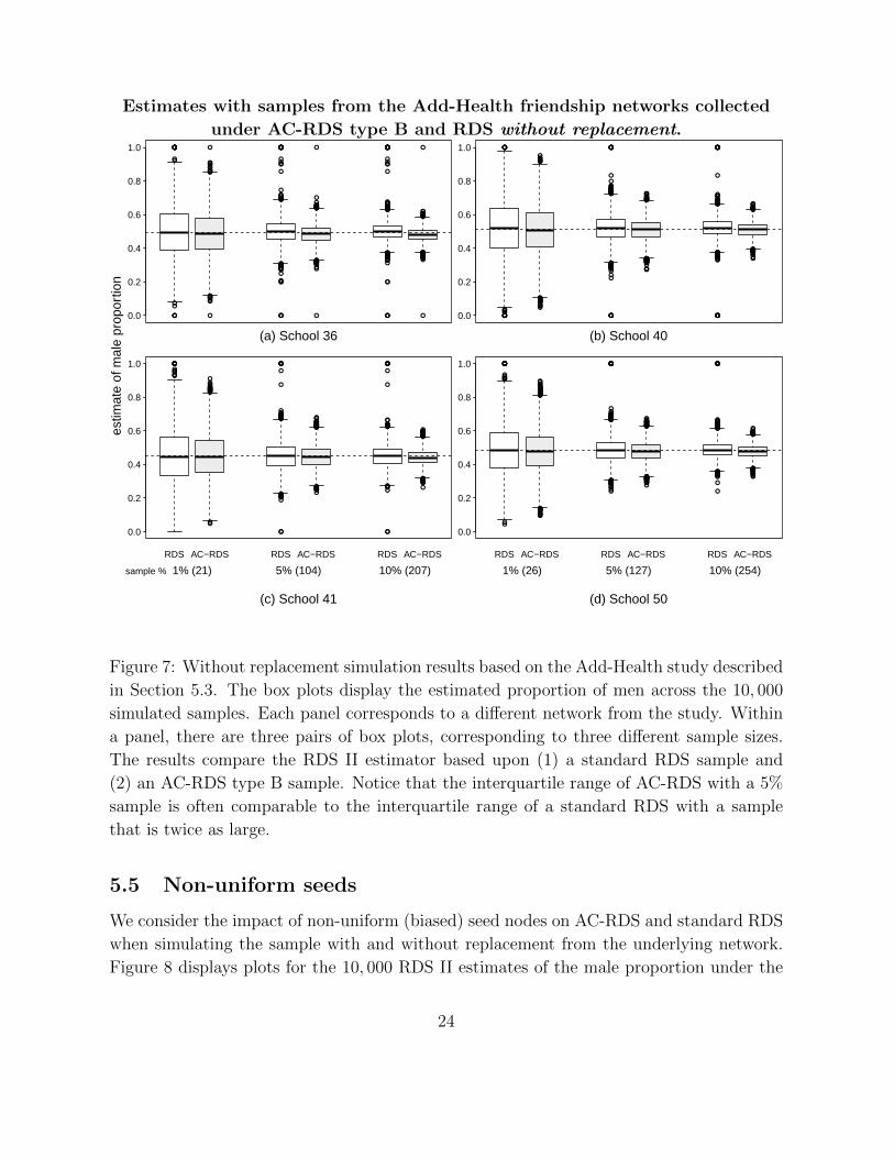
Estimates with samples from the Add-Health friendship networks collected
under AC-RDS type B and RDS without replacement.●●
●
●
●●●
●
●
●
●●●●●●●●
●
●●
●
●
●
●
●●●
●
●
●●
●●●●
●
●
●
●
●
●
●●
●
●
●●●
●
●
●
●
●●
●
●
●●●
●
●
●
●
●
●●
●
●
●
●
●●●
●
●
●
●●●
●
●
●
●
●●●●
●
●
●
●●
●
●
●
●●
●
●
●
●
●●●
●●●
●
●
●
●
●●
●●●
●●
●
●
●
●
●
●●●●
●
●●●●
●●
●
●
●
●
●
●
●
●●●
●●
●
●●●
●●
●
●
●●●
●
●
●
●
●
●
●
●
●
●
●
●●
●
●
●
●●
●
●
●
●●●
●
●
●
●
●
●
●
●
●
●
●
●●●
●●●
●
●
●
●
●●
●
●●●
●
●
●
●
●●●●●
●
●
●
●●
●
●
●●
●
●
●
●●
●
●●●●
●
●
●●
●
●●
●
●
●
●
●
●●●●●●
●
●●
●
●●
●
●
●
●
●
●
●
●
●●●
●●
●●
●
●
●
●●
●●●●
●
●
●
●
●
●
●●
●
●●●●●
●●●
●
●●
●
0.0
0.2
0.4
0.6
0.8
1.0
(a) School 36
estim
ate
of m
ale
prop
ortio
n
●
●●
●●
●
●
●
●
●
●●●●
●
●●●●●●
●
●
●
●
●
●●
●●●●●
●
●●●
●
●
●
●
●●●●
●
●●●●
●
●●
●
●
●
●
●
●
●●●
●
●●●●
●
●
●
●
●
●
●
●
●
●
●
●
●●
●
●
●
●
●
●
●●●
●
●
●
●●
●
●●
●
●
●
●●
●
●●●●
●
●●●
●
●●
●
●
●
●
●
●
●
●●
●
●
●
●
●
●
●
●
●
●●●●●
●
●●
●●●
●●●●●●●
●●●
●
●
●●
●
●
●
●●●●●●●●●
●
●●
●
●
●
●●
●●●
●
●
●
●●
●
●
●
●
●
●
●●
●
●
●
●●
●
●●●●
●●
●
●
●
●
●
●
●
●
●
●
●
●
●●
●
●
●
●
●
●
●
●●●●
●
●
●
●●
●●●
●
●
●
●
●●●●
●
●
●●
●●
●
●●
●●
●
●
●
●●●●●
●●●
●
●
●●●
●
●●●●
●●●●●
●●
●●
●●
●●
●●
●●●
●
●
●●
●●●
●●●
●●
●
●●
●
●
●
●
●●●●●●●
●
●
●●●
●
●
●
●●
●
0.0
0.2
0.4
0.6
0.8
1.0
(b) School 40
●●
●
●
●
●●●
●●●●
●
●●
●
●
●
●
●●●●●●●●
●●●●●
●
●
●
●
●●
●
●
●
●
●●●●
●
●●●
●●●●
●
●
●
●
●
●●
●●
●
●●
●●
●
●
●
●
●
●
●
●●●●●
●
●
●
●●●
●
●●
●
●●●
●●
●●
●●
●
●
●●●●
●
●
●
●
●●
●
●●
●
●
●
●
●
●
●
●
●●●
●
●
●
●
●
●
●
●
●●
●
●
●
●
●
●●●
●
●
●
●
●●
●
●
●●
●●
●
●
●
●●●
●
●●
●
●●
●
●
●
●●●●●●
●●
●●●●
●
●●●●●
●
●
0.0
0.2
0.4
0.6
0.8
1.0
RDS RDS RDSAC−RDS AC−RDS AC−RDS
1% (21) 5% (104) 10% (207)
(c) School 41
sample %
●●●
●
●
●
●
●●●
●
●●
●
●
●●●●
●
●●
●●
●
●●
●
●●
●
●●
●●●●
●
●
●
●●●
●
●●●●●
●
●
●
●
●
●
●●
●●●
●●
●
●●
●
●●
●●
●●●●●
●●
●●
●●●
●
●
●
●
●
●
●
●●
●
●
●
●
●
●
●●
●●
●
●●●●
●
●
●
●
●●
●●
●
●
●●
●●
●●
●
●
●
●
●
●
●●
●●●
●●
●
●
●
●●●●
●
●●●
●
●
●
●
●
●
●●
●
●●●
●
●●
●
●●
●
●
●●
●
●●●●
●●
●
●
●●●●
●●
●
●
●
●
●
●●
●
●●
●
●
●●●●
●
●
●
●
●
●●
●
●
●
●●●●●
●
●●●
●
●●
●
●
●
●
●●
●●
●
●
●
●
●
●
●●
●
●
●
●
●
●
●●
●
●
●
●
●●
●
●●●
●
●
●●
●
●
●●
●●
●
●●
●
●●●●●
●
●●●
●
●
●●●
●●●
●
●
●●
●
●
●
●
●●
●
●●●●
●●●●●
●
●
●
●
●
●●
●
●
0.0
0.2
0.4
0.6
0.8
1.0
RDS RDS RDSAC−RDS AC−RDS AC−RDS
1% (26) 5% (127) 10% (254)
(d) School 50
Figure 7: Without replacement simulation results based on the Add-Health study described
in Section 5.3. The box plots display the estimated proportion of men across the 10, 000
simulated samples. Each panel corresponds to a different network from the study. Within
a panel, there are three pairs of box plots, corresponding to three different sample sizes.
The results compare the RDS II estimator based upon (1) a standard RDS sample and
(2) an AC-RDS type B sample. Notice that the interquartile range of AC-RDS with a 5%
sample is often comparable to the interquartile range of a standard RDS with a sample
that is twice as large.
5.5 Non-uniform seeds
We consider the impact of non-uniform (biased) seed nodes on AC-RDS and standard RDS
when simulating the sample with and without replacement from the underlying network.
Figure 8 displays plots for the 10, 000 RDS II estimates of the male proportion under the
24

biased seed nodes.
25
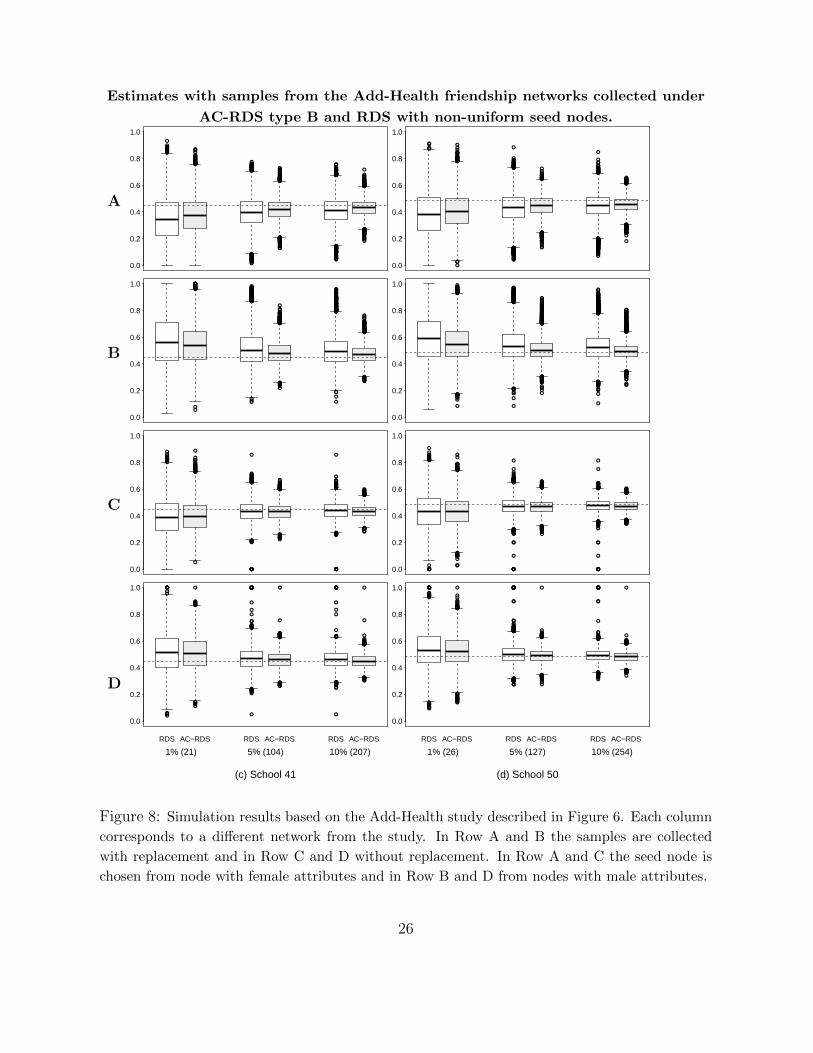
Estimates with samples from the Add-Health friendship networks collected under
AC-RDS type B and RDS with non-uniform seed nodes.
A
●
●●●●●●●●●●
●
●●●
●
●
●
●
●●●●●●●●●●●
●
●●●
●
●●●●
●
●●
●
●●●●
●
●●
●
●●●
●
●
●
●
●
●●●
●
●
●
●
●
●●
●
●●●
●●
●
●●
●
●●●
●
●
●
●
●
●
●●
●●●
●
●
●●
●●
●
●●
●●●●
●●
●
●●
●●
●●
●●
●
●
●
●
●●
●
●
●
●
●●
●
●
●●
●●●
●
●●
●
●●
●●●
●
●●●
●
●
●
●
●
●
●
●●●
●
●
●
●
●●●
●
●
●
●
●●●
●
●
●
●●
●
●
●
●
●●
●●
●●
●●●●
●
●
●●
●●
●●
●
●●●
●
●
●
●
●●●
●
●
●
●●●
●●
●●●
●●
●●
●
●
●
●
●
●●
●
●
●●●
●
●●
●●●
●
●
●
●
●
●
●
●
●●
●
●●●
●
●
●●
●●
●●
●●●●
●●
●
●
●
●
●
●●●
●
●
●●●●
●
●
●
●
●●●●
●
●●
●
●
●
●
●●
●
●
●
●
●
●
●
●
●
●●●
●
●
●
●●●●●
●
●
●
●
●
●
●
●
●
●
●
●
●
●
●
●●
●
●●
●
●●
●
●●●
●●
●
●
●
●
●
●
●●●
0.0
0.2
0.4
0.6
0.8
1.0●●●●●
●●●
●●●●●
●
●●
●
●●●●●
●
●
●
●
●
●
●
●
●
●
●
●
●
●
●●
●
●
●
●●●●
●
●
●
●
●●●
●
●
●●●
●
●
●
●●●
●
●●
●
●●●●●
●
●
●
●●●
●●●●
●
●●●●●●●●●
●
●●
●
●●●●
●●●
●
●●
●
●●
●●
●
●
●●●●
●
●
●
●
●
●●●
●
●
●●
●
●
●
●●●
●
●
●
●
●●
●
●
●●●
●●●
●
●
●
●●
●
●●●
●
●●●
●●●
●●
●●●●
●●●●●
●●
●●
●
●●
●●
●
●
●
●
●
●
●●
●●●●●●
●
●
●
●
●
●
●
●
●
●
●
●
●
●●●●●
●
●
●
●
●
●
●
●
●
●
●●●●●
●●
●
●
●
●
●●
●●
●●
●●
●
●●●
●
●●●
●
●●
●
●●
●
●
●●
●
●●
●
●●
●
●
●
●
●●
●
●
●
●
●
●●
●
●●
●
●
●
●
●
●●●●
●
●
●●
●
●
●
●●●●
●
●●
●●
●
●●
●
●
●
●
●
●
●
●
●●●●
●
●
●
●
●
●
●
●●
●
●●
●●
●●●
●
●
●●
●
●
●
●
●
●●
●
●
●
●●●
●●●●●●●
●
●
●
●
●
●●
●
●
●
●
●
●
●
●
●
●
●
●●●●
●
●
●●●●●●●●●
●
●●
●
●
●●
●●●
●●●●
●●●●
●
●●●●
●
●
●
●●
●●
●
●
●
●
●●●
●●
●
●
●●
●
●●
●
●
●
●●
●●
●
●
●
●
●●
●
●
●●●●
●
●
●
●●●
●
●
●
●●
●
●●
●
●
●
●
●
0.0
0.2
0.4
0.6
0.8
1.0
B
●●
●
●●●●●●
●
●●●●●●
●
●●●●
●
●●
●●●●●●
●
●●
●●
●●●
●●
●●●●
●
●
●
●●●●
●
●●●●
●●
●
●●●●
●
●
●●
●●
●
●
●●
●
●
●●
●●
●
●
●
●
●●●●
●●
●
●●
●
●●●
●●●●
●
●
●●●●
●●
●
●
●●●●●
●●●●
●
●●●●●●●
●
●●
●●●●●
●●
●
●●
●●●●●●●
●●●●●●
●
●●
●
●●●●
●
●●
●
●●●
●
●●●●
●
●●●●
●
●●
●
●
●
●
●●●●
●
●
●●●●
●
●●●●●●●●●
●●●●●●
●●
●
●
●●
●
●●
●
●●
●
●●
●
●
●●●
●
●
●●●●●
●
●●
●
●●●●●●●
●●
●●●●
●●
●
●
●●
●
●●
●
●
●●
●
●
●●
●
●
●
●●
●
●
●
●
●
●
●●
●
●
●●
●●●●
●
●●
●
●●
●
●
●
●●●
●
●●●
●
●●
●●
●●●●
●
●
●
●
●
●
●●●●●
●
●
●
●●●●●●
●
●
●
●
●●
●
●●●●●●●●
●
●●●●●
●
●
●●●
●●●●●
●
●
●●●
●
●●
●
●
●
●
●●●●●
●●●●●●●
●●●●
●
●
●●●
●●
●●●
●
●●
●
●●●●●●●●
●
●●
●
●●●●●●
●
●●●●
0.0
0.2
0.4
0.6
0.8
1.0
●
●●
●
●●
●
●
●
●●
●
●●●
●●
●
●●
●●●●
●●
●●
●●
●
●●
●
●●
●
●
●
●●●●
●●●●
●
●●
●●●●
●
●
●
●●●●●●●●●
●
●●●
●
●●
●
●●●●●●
●
●
●
●
●●●●
●
●●●
●
●
●●●
●
●
●
●
●
●●
●●●●●●
●
●●
●
●
●●●●●
●●
●●
●
●●●●●●●●●
●●
●
●●●●●●●●
●●
●●●
●●●●●●●
●●●●
●
●
●
●●●●
●
●●●●●●
●
●●
●●
●
●●●
●
●
●
●●●
●●
●
●●●
●
●
●●
●
●●●
●
●
●
●
●
●
●
●
●●
●
●
●
●●
●●
●
●
●
●
●●●
●
●
●
●
●●
●
●
●●
●
●
●
●
●
●●
●●
●●●
●
●●●
●
●
●●●
●
●●●●●●
●
●
●●
●
●
●
●
●
●
●
●
●●
●
●
●
●●
●●●
●
●
●
●●
●
●
●
●
●
●●●
●
●●●●
●
●
●●
●●
●●●●●
●●
●
●
●
●
●
●
●
●
●
●
●
●
●
●
●
●
●
●
●
●
●●●●●
●
●
●
●●●●●●●
●●●
●
●
●
●●●●●●
●
●
●
●●●
●
●
●●●
●
●
●●●
●●
●
●
●
●
●●
●●●
●
●
●
●●
●
●
●
●●●●
●
●
●●●
●
●
●
●
●
●●
●
●
●●●
●●
●
●●
●
●●●
●●
●
●●●
●
●●
●
●●
●●
●
●
●
●
●●
●●
●●
●●
●
●
●
●●
●
●
●
●
●
●
●
●●●
●●
●
●
●●●●●
●
●
●
●
●●
●●●
●●●
●
●
●●
●
●
●●●●●●●●●
●●●●
●●●
●
●●●
●
●
●●
●
●
●●●●●
●
●
●●
●
●
●
●
●
●●
●●
●
●
●●
●
●●
●
●●●
●
●
●
●●●
●
●
●
●
●
●●●
●●
●●
●
●
●
●
●●●●●
●
●
●
●
●
●
●
●●
●●
●
●●●
●●●
●●
●
●●●●●
●
●
●
●●●●
●
●
●
●
●●
●
●
●●
●●
●
●
●
●●
●
●●●
●●
●
●
●
●
●●●
●
●
●
●
●
●●
●●
●
●
●●
●
●
●
●
●●●
●
●
●●
●
●
●
●
●
●
●
●
●
●
●
●
●●●●●●●
●●●●●
●●
●
●●
●
●
●
●
●
●
●
●●●●●
●
●
●●
●
●
●●
●
●●
●●●
●
●
●●
●●
●
●
●●●●
●
●
●
●
●●●
●
●●
●
●●
●●
●
●●
●
●●●●
●
●●
●
●
●●
●
●
●●●●●●●
●
●
●
●
0.0
0.2
0.4
0.6
0.8
1.0
C
●●●
●
●
●●●
●●
●●●●
●
●
●
●
●
●
●●●
●
●●
●
●
●●●●●
●●
●●●●●●●●●
●
●●●●●
●●
●●●
●
●
●
●
●
●
●
●
●●●●
●
●
●●●●●●
●
●
●
●●
●
●●
●
●
●
●
●●●
●
●●●
●●
●
●
●
●
●●
●
●
●●●
●
●●
●
●●
●
●●●●●●●
●
●
●●
●●●●
●
●
●
●
●
●●
●
●
●
●
●●●●●●●●●
●
●
●●●●
●
●
●●●
●
●
●
●
●
●
●
●
●●
●●
●
●
●
●
●
●
●
●
●
●●
●
●
●●
●●
●●
●
●
●
●
●
●
●●●●
●
●
●
●
●
●●
●
●
●●
●
●●●
●
●●●
●
●●●●●●●●●●●●
●
●
●
●
●
●
●
●
●
0.0
0.2
0.4
0.6
0.8
1.0
●●
●
●
●
●
●
●
●●●
●●●
●
●●
●
●●
●
●
●●
●●●●●
●
●●●●
●
●●
●
●
●
●
●●
●●
●●
●●
●
●
●
●
●
●
●●●
●
●●
●
●
●
●
●
●●
●
●
●●●
●
●
●
●●
●
●●●●
●●
●●
●
●●
●
●
●
●●
●
●●
●●
●●
●●●
●
●
●
●
●
●
●
●
●●
●
●●●
●
●●
●
●●●
●
●●
●
●
●
●
●
●
●
●
●
●●●●
●●●
●
●
●
●
●
●●●
●●●
●
●●
●
●
●●
●
●
●
●●
●●●
●●●
●●●
●●
●
●
●●
●
●
●
●
●●●
●●
●
●
●●●●
●
●●●
●
●
●●
●
●
●
●
●
●
●●
●
●
●●
●
●
●
●●●●
●
●
●
●●●
●
●
●
●●
●●
●●●●
●●●
●
●
●
●
●
●●
●
●
●●
●●●●
●
●●
●
●
●
●
●●
●●
●●●
●
●
●
●
●
●●
●
●
●●
●●●
●●●
●●
●●
●●
●●●●●●●●●
●●●
●
0.0
0.2
0.4
0.6
0.8
1.0
D
●●
●●●
●
●
●●
●●●
●
●●
●●●
●
●
●
●
●●●
●●●●
●
●●●
●●
●●
●●●
●●
●
●●
●
●
●
●
●
●●
●
●
●●●
●
●●
●
●
●
●
●●
●
●
●
●
●●
●
●
●
●●●
●●
●●
●
●
●
●
●
●
●
●
●●
●
●●●●●
●●●●
●
●
●
●
●●●
●
●
●
●●
●
●
●
●
●●
●
●
●●●●
●
●
●
●
●
●●●
●
●●
●
●●
●●
●●●
●
●●●
●
●
●
●
●
●●
●
●
●
●
●●●
●
●
●
●●
●
●
●
●●●
●
●●●●
●
●
●
●
●●●
●
●●●
●●●
●●●
●
●
●
●●
●
●●●●
0.0
0.2
0.4
0.6
0.8
1.0
RDS RDS RDSAC−RDS AC−RDS AC−RDS
1% (21) 5% (104) 10% (207)
(c) School 41
●
●
●
●
●
●
●
●●
●
●●
●
●●
●●
●
●●●●●
●
●
●●●
●
●●
●
●
●●
●
●
●
●
●●
●
●
●
●
●
●
●
●
●
●
●
●
●●●
●
●●●
●
●●
●●
●
●
●●
●
●
●●●
●●
●
●●
●
●
●
●
●
●
●●
●●
●●●
●●●
●
●
●
●
●●●●
●
●
●
●
●●
●
●
●
●
●●
●
●
●
●
●
●
●
●
●
●●●
●●
●
●●●●●●
●
●
●
●●●
●
●
●●●●●●●●
●
●
●
●
●
●●
●●
●
●
●
●●
●
●
●●●
●
●
●
●
●
●●
●
●●
●
●●
●
●
●
●
●●
●●
●●
●
●
●
●
●
●
●
●
●●
●
●●
●●●
●
●
●
●
●
●●●
●
●●
●
●
●
●●
●
●
●
●
●
●●
●●
●
●
●●
●
●●
●
●
●
●●
●●
●●
●●
●
●
●●
●●
●●
●●●
●
●
●
●
●●
●●●
●●
●●●
●●
●●●●
●●●
●●
●●●
●●●
●●●●●
●●●●
●
●●●
●
●●●
●
●●
●
●
●
●
●
●
●●
●●●
●
●
●●●
●
●
0.0
0.2
0.4
0.6
0.8
1.0
RDS RDS RDSAC−RDS AC−RDS AC−RDS
1% (26) 5% (127) 10% (254)
(d) School 50
Figure 8: Simulation results based on the Add-Health study described in Figure 6. Each column
corresponds to a different network from the study. In Row A and B the samples are collected
with replacement and in Row C and D without replacement. In Row A and C the seed node is
chosen from node with female attributes and in Row B and D from nodes with male attributes.
26

6 Issues remaining
The aim of this research is to highlight how referral requests have the potential to alter
referral patterns in a way that makes the resulting sample more representative of the
target population. The Markov models for RDS and AC-RDS capture important features
of reality, but both are necessarily an approximation to the practicalities of gathering a
sample from a marginalized and hard-to-reach population. These gaps between “theory”
and “practice” have the potential to make AC-RDS either more or less desirable. If AC-
RDS is to be implemented in the field, there are several issues that must be explored.
1. If there are pockets of the marginalized target population which are particularly hard-
to-reach, AC-RDS has the potential to both help and hinder the sampling of these
populations. Novel referral requests could help by encouraging participants to refer
friends from different communities, potentially exposing a new community to the
researchers. Alternatively, because AC-RDS referral requests are likely more difficult
for participants, it could reduce the number of referrals that are made, making it
more difficult to reach a target sample size.
2. Because AC-RDS leads to a reversible Markov chain, there exist formulations for
the sampling weights, akin to the Volz-Heckathorn estimator (Volz and Heckathorn,
2008). Successive Sampling model. The formulation of the sampling weights for AC-
RDS could follow a similar argument as the Volz-Heckathorn weights. Because the
Volz-Heckathorn estimator assumes a reversible Markov transition matrix PA, the
stationary distribution is proportional to the row sums of A (i.e. the node degrees).
Since AC-RDS also assumes a reversible Markov transition matrix PW , the stationary
distribution of AC-RDS is proportional to the row sums of W (i.e. π given in (3)).
In both cases (A and W ), the weights require asking participants questions about
their local social network. Recently, Verdery et al. (2016) introduced data collection
methods, survey questions, and estimators for RDS to estimate clustering properties
of the underlying social network. Their estimators are designed to count the number
of connected triplets and triangles which a participant belongs to. The collected data
is the main part of estimating the sampling weights in AC-RDS.
3. Preferential recruitment, the tendency of participants to refer particular friends, leads
to the violation of uniform referral assumption. AC-RDS gives participants some
instructions for the new referrals. These instructions, since they are more specific,
may lead to a referral process that satisfies the initial assumptions more. However,
studying the reactions of members of a hidden population to this type of requests
and the impact of preferential recruitment on AC-RDS requires rigorous field study
that we will address in future research.
27

4. More generally, it is necessary to investigate how human subjects consider both stan-
dard and non-standard referral requests. Because it is practically infeasible to use
random number generators to ensure participants refer randomly chosen friends, all
statistical approaches to RDS assume that participants refer a random collection of
friends. Whether these statistical models lead to adequate approximations of the
actual referral process is an empirical question that has received some attention and
deserves more. In practice, there are many conditions that are often appended to
this request. These conditions help define your contacts (e.g. as people you (i) know
on a first name basis, (ii) have seen in the last month, and (iii) fit the eligibility
criteria for the study). Page 330 of Johnston (2013) and Appendix Q in Centers
for Disease Control and Prevention (2012) give further discussion on this topic. Of
particular interest is that Johnston (2013), in the section titled “Script for explaining
the recruitment process, says
If possible, try and give the coupons to different types of people who you
know. (e.g. different ages, different levels of income, from different locations
in this city).
The AC-RDS requests provide a formalization for this exact concept. For example,
Wejnert and Heckathorn (2008) designed a web-based method to sample undergrad-
uate students and study the effectiveness and efficacy of RDS; McCreesh et al. (2012)
compared an RDS sample in Uganda with a total population survey on the same
population; McCoy et al. (2013) studied how manipulating incentives might change
referral patterns; Gile et al. (2014) proposed statistical diagnostics to examine the
convergence properties; and Arayasirikul et al. (2015) performed qualitative follow-up
interviews to ask participants about difficulties in finding referrals. Similar techniques
could be used to evaluate whether novel referral requests provide a more representa-
tive sample.
7 Discussion
In respondent-driven sampling, bottlenecks create dependencies between the samples; suc-
cessive samples are more likely to belong to the same community. Because of these depen-
dencies, bottlenecks increase the variability of the resulting estimators. While researchers
cannot alter the social network to diminish bottlenecks, researchers can use novel implemen-
tations of RDS to implicitly encourage participants to refer friends in different communities.
In comparison to other such techniques in the literature, AC-RDS does not require par-
ticipants to reveal sensitive information, nor does it require a priori knowledge on what
28

forms the bottlenecks (e.g. race, gender, neighborhood, some combination of these factors,
or some entirely different factors). In a closer look, AC-RDS, similar to the “Search” mode
of NSM, increases the referrals that are more likely to lead to the unexplored parts of
the network. NSM aims to efficiently explore the network by targeting the best nodes for
each sampling wave, while AC-RDS tries to find and explore the best local edges. Direct
comparison of these two methods requires human subject experiments and is beyond the
scope of the current paper.
We call this approach anti-cluster RDS. This terminology stems from two distinct, but
related, definitions of “clustering” in networks. First, the classical use of “clustering” in
social networks is the clustering coefficient, a summary statistic of a network which describes
the propensity of nodes to form triangles. This idea of “clustering” is a local measure. The
second form of “clustering” is more global and is often used synonymously with community
structure; the idea is that “clusters” of individuals form communities. Both of these types
of clusters emerge due to homophily, the tendency of individuals to become friends with
people who are similar. As such, homophily produces a local-global duality in “clustering.”
AC-RDS requests are built upon local structures in the network (which of your friends are
friends) and immediately access the global network patterns, which could be unknown to
the researchers and/or participants.
This paper shows that AC-RDS is analytically tractable under the Markov model. One
key benefit of the specific construction is that Xaci is reversible and its Markov transition
matrix can be expressed with the underlying adjacency matrix and standard matrix opera-
tions (5). A key limitation of the Markov model is that it samples with replacement, while
in practice the sampling is done without replacement. For further discussion of this topic,
see Ott et al. (2016). The simulations in Section 5 show that the key insights from the
Markov model continue to hold under the sampling without replacement model, so long as
the sample size is not comparable to the population size.
Section 4 studies theoretical properties of AC-RDS. We first argue that AC-RDS can be
approximated by a reversible Markovian process. Propositions 2 and 3 show that AC-RDS
can decrease λ2, the second eigenvalue of the Markov transition matrix, on the population
graph. Theorem 1 shows that these gains from Propositions 2 and 3 will continue to hold if
the graph is sampled with independent edges. In addition, Theorem 2 shows that AC-RDS
reduces the covariance of the samples in the referral tree under the Stochastic Blockmodel
with equal block sizes.
Finally, in Section 6 we discuss some of the gaps between theory and practice, acknowl-
edging that more work needs to be done before AC-RDS could be implemented in the field.
For example, it is not clear how participants will actually respond to AC-RDS requests.
Addressing this issue requires human subject experiments that are beyond the scope of the
current paper. We are addressing this problem in concurrent research.
29

References
Arayasirikul, S., Cai, X., and Wilson, E. C. (2015). A qualitative examination of
respondent-driven sampling (RDS) peer referral challenges among young transwomen
in the San Francisco Bay Area. JMIR Public Health and Surveillance, 1(2).
Baraff, A. J., McCormick, T. H., and Raftery, A. E. (2016). Estimating uncertainty in
respondent-driven sampling using a tree bootstrap method. Proceedings of the National
Academy of Sciences, 113(2), 14668–14673.
Bassetti, F., Diaconis, P., et al. (2006). Examples comparing importance sampling and the
Metropolis algorithm. Illinois Journal of Mathematics, 50(1-4), 67–91.
Benjamini, I. and Peres, Y. (1994). Markov chains indexed by trees. The Annals of
Probability, 22(1), 219–243.
Centers for Disease Control and Prevention (2012). National HIV behavioral surveillance
system in injecting drug users–round 3: Operations manual. Available from: Gabriela
Paz-Bailey ([email protected]).
Chung, F. and Radcliffe, M. (2011). On the spectra of general random graphs. Electronic
Journal of Combinatorics, 18(1), 215–229.
Chung, F. R. (1997). Spectral graph theory, volume 92. American Mathematical Soc.
Crawford, F. W., Aronow, P. M., Zeng, L., and Li, J. (2017). Identification of ho-
mophily and preferential recruitment in respondent-driven sampling. American Journal
of Epidemiology.
Gile, K. J. (2011). Improved inference for respondent-driven sampling data with application
to HIV prevalence estimation. Journal of the American Statistical Association, 106(493).
Gile, K. J. and Handcock, M. S. (2010). Respondent-driven sampling: An assessment of
current methodology. Sociological Methodology, 40(1), 285–327.
Gile, K. J. and Handcock, M. S. (2011). Network model-assisted inference from respondent-
driven sampling data. arXiv preprint arXiv:1108.0298.
Gile, K. J., Johnston, L. G., and Salganik, M. J. (2014). Diagnostics for respondent-driven
sampling. Journal of the Royal Statistical Society: Series A (Statistics in Society).
Girvan, M. and Newman, M. E. (2002). Community structure in social and biological
networks. Proceedings of the National Academy of Sciences, 99(12), 7821–7826.
30

Goel, S. and Salganik, M. J. (2009). Respondent-driven sampling as Markov chain Monte
Carlo. Statistics in medicine, 28(17), 2202–2229.
Goel, S. and Salganik, M. J. (2010). Assessing respondent-driven sampling. Proceedings
of the National Academy of Sciences, 107(15), 6743–6747.
Goodman, L. A. (1961). Snowball sampling. The Annals of Mathematical Statistics, 32(1),
148–170.
Handcock, M. S. and Gile, K. J. (2011). Comment: On the concept of snowball sampling.
Sociological Methodology, 41(1), 367–371.
Heckathorn, D. D. (1997). Respondent-driven sampling: a new approach to the study of
hidden populations. Social Problems, 44(2), 174–199.
Heckathorn, D. D. (2002). Respondent-driven sampling ii: deriving valid population esti-
mates from chain-referral samples of hidden populations. Social Problems, 49(1), 11–34.
Heckathorn, D. D. (2007). Extensions of respondent-driven sampling: Analyzing continuous
variables and controlling for differential recruitment. Sociological Methodology, 37(1),
151–207.
Heckathorn, D. D. (2011). Comment: Snowball versus respondent-driven sampling.
Sociological Methodology, 41(1), 355–366.
Holland, P., Laskey, K., and Leinhardt, S. (1983). Stochastic blockmodels: First steps.
Social Networks, 5(2), 109–137.
Johnston, L. (2013). Introduction to HIV/AIDS and sexually transmitted infection surveil-
lance: module 4: introduction to respondent-driven sampling.
Levin, D. A., Peres, Y., and Wilmer, E. L. (2009). Markov chains and mixing times.
American Mathematical Society.
Malekinejad, M., Johnston, L. G., Kendall, C., Kerr, L. R. F. S., Rifkin, M. R., and Ruther-
ford, G. W. (2008). Using respondent-driven sampling methodology for HIV biological
and behavioral surveillance in international settings: a systematic review. AIDS and
Behavior, 12(1), 105–130.
Mathias, R. (1990). The spectral norm of a nonnegative matrix. Linear Algebra and its
Applications, 139, 269–284.
31

McCoy, S. I., Shiu, K., Martz, T. E., Smith, C. D., Mattox, L., Gluth, D. R., Murgai,
N., Martin, M., and Padian, N. S. (2013). Improving the efficiency of hiv testing with
peer recruitment, financial incentives, and the involvement of persons living with hiv
infection. JAIDS Journal of Acquired Immune Deficiency Syndromes, 63(2), e56–e63.
McCreesh, N., Frost, S., Seeley, J., Katongole, J., Tarsh, M. N., Ndunguse, R., Jichi, F.,
Lunel, N. L., Maher, D., Johnston, L. G., et al. (2012). Evaluation of respondent-driven
sampling. Epidemiology (Cambridge, Mass.), 23(1), 138.
Mouw, T. and Verdery, A. M. (2012). Network sampling with memory: A proposal for
more efficient sampling from social networks. Sociological Methodology, 42(1), 206–256.
Ott, M. Q., Gile, K. J., et al. (2016). Unequal edge inclusion probabilities in link-tracing
network sampling with implications for respondent-driven sampling. Electronic Journal
of Statistics, 10(1), 1109–1132.
Rohe, K. (2015). Network driven sampling; a critical threshold for design effects. arXiv
preprint arXiv:1505.05461.
Rohe, K., Chatterjee, S., and Yu, B. (2011). Spectral clustering and the high-dimensional
stochastic blockmodel. The Annals of Statistics, 39(4), 1878–1915.
Salganik, M. J. (2012). Commentary: respondent-driven sampling in the real world.
Epidemiology, 23(1), 148–150.
Salganik, M. J. and Heckathorn, D. D. (2004). Sampling and estimation in hidden popu-
lations using respondent-driven sampling. Sociological Methodology, 34(1), 193–240.
Stewart, G. W. and Sun, J.-G. (1990). Matrix perturbation theory. Academic Press.
Verdery, A. M., Mouw, T., Bauldry, S., and Mucha, P. J. (2015). Network structure and
biased variance estimation in respondent driven sampling. PLoS ONE, 10(12), e0145296.
Verdery, A. M., Fisher, J. C., Siripong, N., Abdesselam, K., and Bauldry, S. (2016). New
survey questions and estimators for network clustering with respondent-driven sampling
data. arXiv preprint arXiv:1610.06683.
Volz, E. and Heckathorn, D. D. (2008). Probability based estimation theory for respondent
driven sampling. Journal of Official Statistics, 24(1), 79.
Von Luxburg, U. (2007). A tutorial on spectral clustering. Statistics and Computing,
17(4), 395–416.
32
Watts, D. J. and Strogatz, S. H. (1998). Collective dynamics of small-world networks.
Nature, 393(6684), 440–442.
Wejnert, C. (2009). An empirical test of respondent-driven sampling: Point estimates,
variance, degree measures, and out-of-equilibrium data. Sociological Methodology, 39(1),
73–116.
Wejnert, C. and Heckathorn, D. D. (2008). Web-based network sampling: efficiency and effi-
cacy of respondent-driven sampling for online research. Sociological Methods & Research.
White, R. G., Lansky, A., Goel, S., Wilson, D., Hladik, W., Hakim, A., and Frost, S. D.
(2012). Respondent driven sampling: where we are and where should we be going?
Sexually Transmitted Infections, 88(6), 397–399.
White, R. G., Hakim, A. J., Salganik, M. J., Spiller, M. W., Johnston, L. G., Kerr, L.,
Kendall, C., Drake, A., Wilson, D., Orroth, K., et al. (2015). Strengthening the re-
porting of observational studies in epidemiology for respondent-driven sampling studies:
STROBE-RDS statement. Journal of Clinical Epidemiology, 68(12), 1463–1471.
Yu, Y., Wang, T., and Samworth, R. (2015). A useful variant of the Davis–Kahan theorem
for statisticians. Biometrika, 102(2), 315–323.
33

Appendix
This appendix provides the proofs contained in the main document. We begin by pre-
senting some preliminary lemmas. We then provide the proofs for the results given in
Sections 3.2, 4.1, and 4.2.
A Preliminary Lemmas
This section contains lemmas which are used to prove our main results. Lemmas 1 and 2
are contained in the main paper; we start the preliminary results with Lemma 3. First we
state two standard results, given here for convenience.
Lemma 3. Let A be a symmetric matrix and D a diagonal matrix. Then
‖DA‖ = ‖D 12AD
12‖.
Lemma 4 (Bernstein’s inequality). Let X1, · · · , XN be independent random variables and
|Xi − EXi| ≤ S for i = 1, · · · , N . Let σ2 :=∑N
i=1 E[Xi − EXi]2. Then for all t ≥ 0,
Pr
(∣∣∣∣∣N∑i=1
Xi − EXi
∣∣∣∣∣ ≥ t
)≤ 2 exp
(−
12t2
σ2 + 13St
).
We use the following result from Rohe et al. (2011) in the proof of Proposition 2.
Lemma 5. [Rohe et al. (2011)] Under the Stochastic Blockmodel, if B = pI+rJ and there
are an equal number of nodes in each block, then
λi(PA) =
1 i = 1
(Kr/p+ 1)−1 i = 2, . . . , K
0 o.w.
For completeness we include the proof here.
Proof. The matrix B ∈ Rk×k is the sum of two matrices,
B = pI + rJk1Tk ,
where Ik ∈ Rk×k is the identity matrix, 1k ∈ Rk is a vector of ones, r ∈ (0, 1) and p ∈ (0, 1−r). Let Z ∈ {0, 1}N×K be such that ZT1N = s1K for some s ∈ R. This guarantees that
all K blocks have equal size s. The Stochastic Blockmodel has the population adjacency
matrix, A = ZBZT . Moreover, PA = ZBLZT for
BL =1
Nr + sp
(pIK + r1K1TK
).
The eigenvalues are found by construction.
34

• The constant vector 1N is an eigenvector with eigenvalue 1;
ZBLZT1N =
s
Nr + spZ(pIK + r1K1TK
)1K
=s
Nr + spZ(p+Kr)1K +
s(p+Kr)
Nr + sp1N = 1N ,
where the last line follows because N = sK.
• Let b2, . . . , bK ∈ RK be a set of orthogonal vectors which are also orthogonal to 1K .
For any i, Zbi is an eigenvector with eigenvalue (Kr/p+ 1)−1,
ZBLZT (Zbi) = ZBLsIK×Kbi =
s
Nr + spZ(pIK + r1K1TK
)bi =
ps
Nr + sp(Zbi).
Because Zbi and Zbj are orthogonal for i 6= j, the multiplicity of the eigenvalue
(Kr/p+ 1)−1 is at least K − 1.
Because rank(PA) ≤ min(rank(Z), rank(BL), rank(ZT )) ≤ K, there are at most K
nonzero eigenvalues. The results follow.
The following result is used for the computation of the eigenvalues in the proof of
Proposition 3.
Lemma 6. Let P be a block constant Markov transition matrix, with blocks of identical
sizes. Let P contain the block values
P =
(p r
r p
),
then
λ2(P ) =p− rp+ r
.
Proof. This follows from Lemma 5 using K = 2.
Lemma 7 (Operator norm of non-negative irreducible matrices). Let A ∈ RN×N be a
non-negative, irreducible matrix. Define ri(A) :=∑N
j=1 Aij. Then
‖A‖ ≤ maxiri(A).
Proof. By the Perron-Frobenius theorem, A has a real leading eigenvalue. Additionally, for
any y ∈ RN , µ ∈ R, with y ≥ 0, and µ ≥ 0, if Ay ≤ µy, then λ1(A) ≤ µ. Take y = 1 and
µ = maxi ri(A), then
‖A‖ = λ1(A) ≤ maxiri(A).
35

Lemma 8. For any W ∈ RN×N , define diagonal matrix T to contain the row sums down
the diagonal, Tuu =∑
vW (u, v). If Tuu > 0 for all u, then the eigenvalues of PW = T−1W
are equal to the eigenvalues of LW = T−1/2WT−1/2.
Proof. Let x, λ be an eigenpair of LW ,
T−1/2WT−1/2x = λx =⇒ T−1/2(T−1/2W
(T−1/2x
))= λ
(T−1/2x
),
where the left hand side is PW (T−1/2x). This implies that T−1/2x, λ is an eigenpair of
PW .
B Design Effect and Variance
Here we provide the proof of Proposition 1 from Section 3.2.
Proof of Proposition 1. Lemma 12.2 in Levin et al. (2009) shows that (i) fj and λj are real
valued and (ii) the fj are orthonormal with respect to 〈f`, fj〉π. Because λ2 < 1, f1 is the
constant vector. We can express the covariance as
Cov (y(Xi), y(Xi+t)) = E [(y(Xi)− E[y(Xi)])(y(Xi+t)− E[y(Xi+t)])]
= E [y(Xi)y(Xi+t)]− E2[y(X1)]
= E [y(X1)y(X1+t)]− E2[y(X1)]. (10)
Consider the first term of (10)
E[y(X1)y(X1+t)] =∑u,v∈V
y(u)y(v) Pr(X1 = u,X1+t = v)
=∑u,v∈V
y(u)y(v)πuPt(u, v)
=∑u,v∈V
y(u)y(v)πuπv
|V|∑j=1
fj(u)fj(v)λtj
=∑u,v∈V
y(u)y(v)πuπv{1 +
|V|∑j=2
fj(u)fj(v)λtj}
=∑u,v∈V
y(u)y(v)πuπv +
|V|∑j=2
λtj∑u,v∈V
y(u)y(v)πuπvfj(u)fj(v)
= E2[y(X1)] +
|V|∑j=2
〈y, fj〉2πλtj.
36

Hence,
Cov (y(Xi), y(Xi+t)) =
|V|∑j=2
〈y, fj〉2πλtj.
C Population Graph Results
Here we provide the proofs of the results given in Section 4.1—Lemmas 1, 2 and Proposi-
tions 2, 3.
Proof of Lemma 1. From the definition of Z and A it follows that ZTZ = Θ and A =
Jn×n − ZBZT = ZBZT . Then,
AA = ZBZTZBZT = ZBΘBZT
and similarly,
AA = ZBΘBZT .
Hence,
(AA + AA) ·A =(Z(BΘB + BΘB)ZT
)· (ZBZT )
= Z((BΘB + BΘB) ·B
)ZT .
Proof of Lemma 2. We first show that
[(BΘB) ·B]kl[(BΘB) ·B]ll
>Bkl
Bkk
=r
p+ r. (11)
We have
[(BΘB) ·B]kl = r(Θkk(p+ r)(1− r) + Θllr(1− p− r) +∑
m6=k,m6=lΘmmr(1− r))
[(BΘB) ·B]kk = (p+ r)(Θkk(p+ r)(1− p− r) +∑m6=k
Θmmr(1− r)).
With the above, we rewrite (11) as follows:
r(Θkk(p+ r)(1− r) + Θllr(1− p− r) +∑
m 6=km6=l
Θmmr(1− r))
(p+ r)(Θkk(p+ r)(1− p− r) +∑
m 6=k Θmmr(1− r))>
r
p+ r(12)
p(Θkk(p+ r)−Θllr) > 0, (13)
37

where (12) to (13) follows from algebraic manipulation. Note that (13) is always true
because of the lemma assumptions. In addition, by going through the same procedure, it
can be shown that[(BΘB + BΘB) ·B]kl[(BΘB + BΘB) ·B]kk
>Bkl
Bkk
.
In terms of the expected adjacency matrices, the above statement is equivalent to the
following result. Suppose that nodes k and m belong to the same block and l belongs to a
different block, thenWkl
Wkm
>Akl
Akm
. (14)
Now, we show PW(u, v) < PA(u, v), when u and v belong to the same block. We have∑w∈V
PW(u,w) =∑w∈V
PA(u,w) = 1∑w∈V
[T−1W]uw =∑w∈V
[D−1A]uw.
Assume u and v belong to block C of size |C|. Factor out the transition probability
between u and v. Then,
[T−1W]uv
(|C|+
∑w/∈C
[T−1W]uw
[T−1W]uv
)= [D−1A]uv
(|C|+
∑w/∈C
[D−1A]uw[D−1A]uv
).
Since the summations are along the rows, we have
[T−1W]uv
(|C|+
∑w/∈C
Wuw
Wuv
)= [D−1A]uv
(|C|+
∑w/∈C
Auw
Auv
).
Therefore, based on inequality (14),
[T−1W]uv < [D−1A]uv.
Now consider the case where Θkk = Θll for all k and l, then for w /∈ C
[T−1W]uw > [D−1A]uw. (15)
Proof of Proposition 2. The first part of this proof focuses on the inequality λ2(PW) <
λ2(PA). To this end, define BRW := D−1k×kB, and BAC := T−1
k×k[(BΘB + BΘB) · B]. Since
38

Θkk are all equal, then BRW and BAC are symmetric matrices and have equal row sum.
Hence,
λ2(PA) = λ2(D−1A) = λ2(BRW ),
λ2(PW) = λ2(T−1W) = λ2(BAC).
Let f : {1, 2, · · · , k} → R and r be the row sum of BRW and BAC . Then I − 1rBAC and
I − 1rBRW are Laplacian matrices. Therefore,
λ2(I − 1
rBAC) = inf
f :∑u f(u)=0
f :∑u f
2(u)=1
1
2r
∑u,v u6=v
BACuv (f(v)− f(u))2
> inff :∑u f(u)=0
f :∑u f
2(u)=1
1
2r
∑u,v u6=v
BRWuv (f(v)− f(u))2 = λ2(I − 1
rBRW ),
where the inequality follows from inequality (15) and the fact that BACuv > BRW
uv for u 6= v.
So we conclude that
λ2(BAC) < λ2(BRW )
and, therefore
λ2(PW) < λ2(PA).
This result is extended in the calculations below.
The fact that λ2(PA) = 1/(R + 1) follows immediately from Lemma 5.
The rest of the proof is dedicated to equation (8) in the statement of the proposition.
From Lemma 1, W = ZBZT for B = (BΘB + BΘB) · B. Define r′ = 1 − r. Note that
Θ = N/KI, so it can be temporarily ignored as a constant.
We have,
BB = (r′J − pI)(rJ + pI) = (r′rK + r′p− pr)J − p2I.
Now, define u = (r′rK + r′p− pr) and write
(BB) ·B = (uJ − p2I) · (rJ + pI) = p(u− rp− p2)I + urJ.
Reincorporating the constants from Θ = N/KI and a 2 to account for BB, it follows that
B = pI + rJ , for
p = 2p(N/K)(u− rp− p2) and r = 2(N/K)ur.
Note that r and p depend on the block populations N/K and thus the number of nodes
in the graph N . However, this term cancels out in the ratio r/p. So, neither λ2(PW) nor
λ2(PA) depend on N . As such,
λ2(PW) + ε < λ2(PA)
39

for some ε > 0 that is independent of N .
As K grows and r shrinks, u→ p(R + 1) and
p→ 2p(N/K)(p(R + 1)− p2) and r → 2rp(N/K)(R + 1).
Using Lemma 5 on B,
λ2(PW) =1
K(r/p) + 1.
Then,Kr
p→ Krp(R + 1)
p(p(R + 1)− p2)=
Kr(R + 1)
p(R + 1− p) = RR + 1
R + 1− p,
which concludes the proof.
Proof of Proposition 3. Both PA and PW satisfy the conditions of Lemma 6. It is only
necessary to compute the probabilities. For PA, p = 1− ε and r = ε. So,
λ2(PA) =1− 2ε
1→ 1.
To compute λ2 (PW), notice that it is only necessary to determine p and r up to propor-
tionality. Under the assumed model, B11 = ε, B12 = 1 − ε, and Θ ∝ I. Moreover, the
matrix (BΘB + BΘB) · B contains the elements p = 2(1 − ε)2 and r = (1 − ε)2 + ε2 for
PW. By Lemma 6.
λ2(PW) =2(1− ε)2 − (1− ε)2 + ε2
2(1− ε)2 + (1− ε)2 + ε2=
(1− ε)2 + ε2
3(1− ε)2 + ε2→ 1/3.
D Sampled Graph Results
Here we provide the proofs of Theorems 1 and 2 from Section 4.2.
Proof of Theorem 1. By Lemma 8, and Weyl’s inequality,
|λ`(PW )− λ`(PW)| =∣∣∣λ`(T− 1
2 WT−12 )− λ`(T−
12 WT−
12 )∣∣∣ ≤ ∥∥∥T− 1
2 WT−12 −T−
12 WT−
12
∥∥∥ .The rest of the proof studies the right hand side of this inequality.
40

For convenience and compactness, we introduce the following notation,
N := |V|,A := (AA+ AA),
A := (AA + AA),
W := (AA+ AA) · A = A · A,W := (AA + AA) ·A = A ·A.
By the triangle inequality,
‖T− 12 WT−
12 −T−
12 WT−
12‖ ≤ ‖T− 1
2 (W − W)T−12‖+ ‖T− 1
2 WT−12 −T−
12 WT−
12‖.
Also,
‖T− 12 (W − W)T−
12‖ = ‖T− 1
2 (A · A− A ·A)T−12‖
≤ ‖T− 12 ((A− A) · A)T−
12‖+ ‖T− 1
2 ((A−A) · A)T−12‖.
The remainder of the proof is divided into four parts. The terms ‖T− 12 ((A−A)·A)T−
12‖,
‖T− 12 ((A−A) · A)T−
12‖, and ‖T− 1
2 WT−12 −T−
12 WT−
12‖ are bounded in Part 1,2, and 3,
respectively. Finally, Part 4 combines these bounds and completes the argument.
Part 1. Note that T is a diagonal matrix and A and A are both symmetric. Therefore,
we apply Lemma 3 to obtain
‖T− 12 ((A− A) · A)T−
12‖ = ‖T−1(A− A) · A‖≤ ‖T−1(AA−AA) · A‖+ ‖T−1(AA− AA) · A‖. (16)
It is sufficient to prove an upper bound for the first term in (16). The same bound will
hold for the second term. We have
‖T−1(AA−AA) · A‖ ≤ ‖T−1|AA−AA| · A‖, (17)
where | · | is the element-wise absolute value operator. The inequality follows from the fact
that for any matrix M , ‖M‖ ≤ ‖|M |‖ (e.g. Mathias, 1990, Theorem 2.5).
We begin by bounding the row sums of |AA−AA| ·A with a concentration inequality.
Then we use Lemma 7 to bound the operator norm. Define the row sum mapping ri, so
that for a matrix C, ri(C) equals the sum of the ith row of C. We have
ri(T−1|AA−AA| · A
)=
1
Tii
∑j
Aij
∣∣∣∣∣∑k
AikAkj −AikAkj
∣∣∣∣∣ . (18)
41

Define Fij =∑
kAikAkj and Gij =∑
k AikAkj. For fixed i and j, the random variables{AikAkj
}k
are independent with expected value E[AikAkj] = AikAkj and variance
σ2ij =
∑k
E(AikAkj −AikAkj)2 ≤
∑k
E(AikAkj)2 + (AikAkj)
2 ≤ 2Fij.
Let ∆Fij :=√
10Fij ln 2N2
δ. By Bernstein’s Inequality and the union bound,
Pr
(∣∣∣∣∣∑k
AikAkj −AikAkj
∣∣∣∣∣ ≥ ∆Fij
)≤ 2 exp
(−
12∆2Fij
σ2i + 1
3S∆Fij
)(19)
= 2 exp
(− 5Fij ln 2N2
δ
4Fij + 13S∆Fij
)≤ δ
N2,
where the last inequality follows from the assumption that Fmin � lnN . So, with high
probability,
∑j
Aij
∣∣∣∣∣∑k
AikAkj −AikAkj
∣∣∣∣∣ ≤∑j
Aij∆Fij .
Now we bound |∑j(Aij −Aij)∆Fij |. We have E[Aij∆Fij ] = Aij∆Fij and∑j
E[Aij∆Fij −Aij∆Fij ]2 ≤ 2
∑j
Aij∆2Fij.
By Bernstein’s Inequality, the following holds with high probability∣∣∣∣∣∑j
(Aij −Aij)∆Fij
∣∣∣∣∣ ≤√
2∑j
Aij∆2Fij.
Consequently,
∑j
Aij
∣∣∣∣∣∑k
AikAkj −AikAkj
∣∣∣∣∣ ≤∑j
Aij∆Fij +
√2∑j
Aij∆2Fij
(20)
≤ 2∑j
Aij
√10Fij ln
2N2
δ
≤ 10∑j
Aij
√Fij ln
N
δ.
42

Furthermore,
Tii =∑j
Wij =∑j
Aij
∑k
AikAkj + AikAkj =∑j
Aij(Fij +Gij). (21)
From (18), (20) and (21),
ri(T−1|AA−AA| · A
)≤
10∑
j Aij
√Fij ln N
δ∑j AijFij
≤10∑
j AijFij
√ln N
δ
Fij∑j AijFij
≤ 10
√ln N
δ
Fmin
. (22)
Following the same steps, we obtain
ri(T−1|AA− AA| · A
)≤
10∑
j Aij
√Gij ln N
δ∑j AijGij
≤ 10
√ln N
δ
Gmin
. (23)
Therefore,
‖T− 12 ((A− A) · A)T−
12‖ ≤ 10 ln
12 Nδ
min{F12
min, G12min}
. (24)
Part 2. We have
‖T− 12 ((A−A) · A)T−
12 ‖ ≤ ‖T− 1
2 ((A−A) · (AA))T−12 ‖+ ‖T− 1
2 ((A−A) · (AA))T−12 ‖. (25)
Similar to Part 1, it is sufficient to prove an upper bound for the first term in (25). The
same bound will hold for the second term.Let J be the N ×N square matrix comprised of all ones. We have
‖T− 12 ((A−A) ·AA)T−
12 ‖ = ‖T− 1
2 ((A−A) ·A(J −A))T−12 ‖
= ‖T− 12 ((A−A) · (AJ)− (A−A) ·AA)T−
12 ‖
≤ ‖T− 12D(A−A)T−
12 ‖+ ‖T− 1
2 ((A−A) ·AA)T−12 ‖
= ‖T− 12D
12 (A−A)D
12T−
12 ‖+ ‖T− 1
2 ((A−A) ·AA)T−12 ‖. (26)
Consider the first term in (26). For i, j ∈ {1, · · · , N}, define Aij ∈ {0, 1}N×N to be the
matrix with one at elements (i, j) and (j, i), and zero everywhere else. We then have,
T−12D
12 (A−A)D
12T−
12 =
N∑i=1
N∑j>i
√DiiDjj
TiiTjj(Aij −Aij)A
ij.
The right hand side is a sum of independent, symmetric matrices. Therefore, we can apply
Theorem 5 of Chung and Radcliffe (2011) to bound it. Let
M := maxij=1,··· ,N
∥∥∥∥∥√
DiiDjj
TiiTjj(Aij −Aij)A
ij
∥∥∥∥∥ ≤ maxij=1,··· ,N
√DiiDjj
TiiTjj,
43

and
v2 :=
∥∥∥∥∥N∑i=1
N∑j>i
Var
(√DiiDjj
TiiTjj(Aij −Aij)A
ij
)∥∥∥∥∥=
∥∥∥∥∥N∑i=1
N∑j>i
[DiiDjj
TiiTjj(Aij −A2
ij)Aii
]∥∥∥∥∥≤ max
i=1,··· ,N
(N∑j=1
[DiiDjj
TiiTjj(Aij −A2
ij)
])
≤ maxi=1,··· ,N
(N∑j=1
[DiiDjj
TiiTjjAij
])≤ max
ij=1,··· ,N
D2iiDjj
TiiTjj.
Define
∆ := maxij=1,··· ,N
2
√D2iiDjj ln(2N/δ)
TiiTjj.
Note that
M∆ = maxij
√DiiDjj
TiiTjj
√D2iiDjj ln(2N/δ)
TiiTjj= max
ij
D2iiDjj
TiiTjj
√ln(2N/δ)
Dii
≤ v2
√ln(2N/δ)
Dmin
.
Therefore, applying Theorem 5 in Chung and Radcliffe (2011) yields
Pr
(∥∥∥∥∥N∑i=1
N∑j>i
√DiiDjj
TiiTjj(Aij −Aij)A
ij
∥∥∥∥∥ ≥ ∆
)≤ 2N exp
(− ∆2
2v2 + 2M∆/3
)(27)
≤ δ.
For the second term of (26), we obtain
T−12 ((A−A) ·AA)T−
12 =
N∑i=1
N∑j>i
√1
TiiTjj(Aij −Aij)
(N∑k=1
AikAkj
)Aij.
Because |∑kAikAkj| ≤√DiiDjj, we obtain the same bound as (27). Namely,
Pr
(∥∥∥∥∥N∑i=1
N∑j>i
√1
TiiTjj(Aij −Aij)(
N∑k=1
AikAkj)Aij
∥∥∥∥∥ ≥ ∆
)≤ 2N exp
(− ∆2
2v2 + 2M∆/3
)≤ δ.
44

In addition,
Tii =∑j
Aij
∑k
AikAkj + AikAkj
=∑j
Aij(Fij +Gij)
≥∑j
Aijc1Dii ≥ c1D2ii,
where the inequality follows from the assumption that Fij + Gij > c1Dii for all i, j ∈{1, · · · , N}.
Combining the above results, yields
‖T− 12 ((A−A) ·AA)T−
12‖ ≤ 4
√ln N
δ
c1Dmin
. (28)
As noted above, the second term in (25) satisfies the same bound, so that
‖T− 12 ((A−A) · (AA))T−
12‖ ≤ 4
√ln N
δ
c1Dmin
. (29)
Combining (25), (28), and (29), yields
‖T− 12 ((A−A) · A)T−
12‖ ≤ 8
√ln N
δ
c1Dmin
. (30)
Part 3. First we bound |Tii −Tii| and then we bound∥∥∥T− 1
2T+ 12 − I
∥∥∥.
We have
|Tii −Tii| =∣∣∣ri(A · A)− ri(A ·A)
∣∣∣≤∣∣ri((AA) · A)− ri((AA) ·A)
∣∣+∣∣ri((AA) · A)− ri((AA) ·A)
∣∣ . (31)
Consider the first term in (31),
∣∣ri((AA) · A)− ri((AA) ·A)∣∣ =
∣∣∣∣∣∑j
Aij∑k
AikAkj −∑j
Aij
∑k
AikAkj
∣∣∣∣∣ (32)
≤∑j
Aij
∣∣∣∣∣∑k
AikAkj −AikAkj
∣∣∣∣∣+
∣∣∣∣∣∑j
(Aij −Aij)∑k
AikAkj
∣∣∣∣∣ .
45

To bound the first term of (32), we use (19) and (20). With probability at least 1− δ,
∑j
Aij
∣∣∣∣∣∑k
AikAkj −AikAkj
∣∣∣∣∣ ≤ 10∑j
Aij
√Fij ln
N
δ. (33)
Consider the second term in (32),∣∣∣∣∣∑j
(Aij −Aij)∑k
AikAkj
∣∣∣∣∣ =
∣∣∣∣∣∑k
∑j
(Aij −Aij)AikAkj
∣∣∣∣∣≤∑k
Aik
∣∣∣∣∣∑j
AijAkj −AijAkj
∣∣∣∣∣=∑k
Aik
∣∣∣∣∣∑j
AijAjk −AijAjk
∣∣∣∣∣=∑j
Aij
∣∣∣∣∣∑k
AikAkj −AikAkj
∣∣∣∣∣ .Note that, E[AikAkj] = AikAkj. In addition, we can obtain the same upper bound for
the variance to use (19). Hence, with probability at least 1− δ, we have
∑j
Aij
∣∣∣∣∣∑k
AikAkj −AikAkj
∣∣∣∣∣ ≤ 10∑j
Aij
√Fij ln
N
δ. (34)
From (33) and (34), we have
∣∣ri ((AA) · A)− ri
((AA) ·A
)∣∣ ≤ 20∑j
Aij
√Fij ln
N
δ. (35)
For the second term in (31), following the same steps yields
∣∣ri ((AA) · A)− ri
((AA) ·A
)∣∣ ≤ 20∑j
Aij
√Gij ln
N
δ. (36)
Therefore,
|Tii −Tii| ≤ 40∑j
Aij
(√Fij ln
N
δ+
√Gij ln
N
δ
).
46

Now we consider ‖T− 12T+ 1
2 − I‖. We have
∥∥∥T− 12T+ 1
2 − I∥∥∥ ≤ max
i=1,··· ,N
∣∣∣∣∣√TiiTii− 1
∣∣∣∣∣≤ max
i=1,··· ,N
∣∣∣∣TiiTii− 1
∣∣∣∣≤ max
i=1,··· ,N
40∑
j Aij
(√Fij ln N
δ+√Gij ln N
δ
)∑
j Aij(Fij +Gij)≤ 40 ln
12 Nδ
min{G12min, F
12
min}.
Furthermore, ∥∥∥T− 12T+ 1
2
∥∥∥ ≤ 1 +40 ln
12 Nδ
min{G12min, F
12
min}< 2, (37)
where the last inequality follows from the theorem’s assumptions.
Define the Laplacian matrix Lac := T−12 WT−
12 . So,
‖T− 12 WT−
12 −T−
12 WT−
12‖ = ‖T− 1
2 WT−12 −T−
12T+ 1
2T−12 WT−
12T+ 1
2T−12‖
= ‖I − Lac −T−12T+ 1
2{I − Lac}T+ 12T−
12‖
= ‖{T− 12T+ 1
2 − I}{I − Lac}T+ 12T−
12 + {I − Lac}{I − T+ 1
2T−12}‖
≤ ‖T− 12T+ 1
2 − I‖ · ‖T+ 12T−
12‖+ ‖I − T+ 1
2T−12‖,
where the inequality follows from the fact that ‖I − Lac‖ ≤ 1. Now,
‖T− 12 WT−
12 −T−
12 WT−
12‖ ≤ 120 ln
12 Nδ
min{G12min, F
12
min}.
Part 4. Let ε := 10δ. Combining the results of the three preceding parts yields
∥∥∥T− 12 WT−
12 −T−
12 WT−
12
∥∥∥ ≤ 10 ln12 Nδ
min{G12min, F
12
min}+
8 ln12 Nδ
c121 D
12min
+120 ln
12 Nδ
min{G12min, F
12
min}.
Note that Gmin = Fmin and Dmin ≥ Fmin. So∥∥∥T− 12 WT−
12 −T−
12 WT−
12
∥∥∥ ≤ 138 ln12 10N
ε
min{c121 D
12min, F
12
min}≤ 138 ln
12 10N
ε
c121 F
12
min
,
with probability at least 1− ε.
47

Proof of Theorem 2. Define fj as the jth eigenvector of PA with respect to the inner product
〈·, ·〉π; similarly, define facj as the jth eigenvector of PW with respect to the inner product
〈·, ·〉πac . From Proposition 1, to prove the theorem, it is sufficient to show that
|V|∑j=2
〈y, facj 〉2πacλj(PW )t <
|V|∑j=2
〈y, fj〉2πλj(PA)t.
We break the proof into two steps. In the first step, we show that the above holds true in
the population, i.e. we compare the Markov chains on PW and PA. In the second step, we
show that the sample quantities converge almost surely to the population quantities.
Part 1. In this step, we show that
|V|∑j=2
〈y, facj 〉2πλj(PW)t + ε <
|V|∑j=2
〈y, fj〉2πλj(PA)t.
We begin by analyzing the eigenpairs of the transition matrices. From Lemma 5, for
i = 2, . . . , K,
λi(PA) = λ2(PA) and λi(PW) = λ2(PW). (38)
Moreover, for i > K, λi(PA) = λi(PW) = 0. Under the theorem conditions, PW and PA
have the same stationary distribution; refer to this as π (in fact, this distribution is uniform
on the nodes). Define fj and facj as the jth eigenvectors, with respect to 〈·, ·〉π, of PA and
PW, respectively. Therefore, we have
|V|∑j=2
〈y, fj〉2πλj(PA)t = λ2(PA)tK∑j=2
〈y, fj〉2π,
and|V|∑j=2
〈y, facj 〉2πλj(PW)t = λ2(PW)tK∑j=2
〈y, facj 〉2π.
Proposition 2 shows thats λ2(PW)t + ε < λ2(PA)t, where ε does not change asymptotically
as |V| grows. Thus, Part 1 will be finished after showing that∑K
j=2〈y, facj 〉2π =∑K
j=2〈y, fj〉2π.
To compare these terms, note that the construction of the eigenvalues in the proof of Lemma
5 shows that the span of the sets {facj · π12 : j = 1, . . . , K} and {fj · π
12 : j = 1, . . . , K} are
identical. Therefore, Parseval’s Identity implies,
K∑j=1
〈y, facj 〉2π =K∑j=1
〈y, fj〉2π.
48

Note that fac1 = f1 = 1 because these are the lead eigenvectors of Markov transition
matrices. Thus,K∑j=2
〈y, facj 〉2π =K∑j=2
〈y, fj〉2π.
Part 2. To ease notation, let λj := λj(PA) and λj := λj(PA). Finally, let N := |V| denote
the size of the graph. This part of the proof shows that, as N →∞,∣∣∣∣∣∣|V|∑j=2
〈y, fj〉2πλtj − 〈y, fj〉2πλtj
∣∣∣∣∣∣ as−→ 0.
The corresponding proof for the anti-cluster random walk follows from a similar argument.
We have∣∣∣∣∣∣|V|∑j=2
〈y, fj〉2πλtj − 〈y, fj〉2πλtj
∣∣∣∣∣∣ =
∣∣∣∣∣∣|V|∑j=2
〈y, fj〉2πλtj − 〈y, fj〉2π(λtj + (λtj − λtj))
∣∣∣∣∣∣≤∣∣∣∣∣K∑j=2
λtj(〈y, fj〉2π − 〈y, fj〉2π
)∣∣∣∣∣+
∣∣∣∣∣∣|V|∑j=2
〈y, fj〉2π∣∣λtj − λtj∣∣
∣∣∣∣∣∣≤ λt2 ·
∣∣∣∣∣K∑j=2
〈y, fj〉2π − 〈y, fj〉2π
∣∣∣∣∣+ maxj
∣∣λtj − λtj∣∣ · 〈y, y〉2π. (39)
Since y is a bounded function, 〈y, y〉2π is bounded. Therefore, Theorem 1, with ε = 1/N2,
and the Borel-Cantelli Lemma imply that the second term in (39) converges to zero almost
surely.
Now we argue that the first term in (39) converges to zero. Let · denote element-wise
multiplication. Let π12 denote the vector with elements
√πi. Finally, let diag(π
12 ) denote
the diagonal matrix with π12 on the diagonal. For some constant c,
D−12AD−
12 (fj · π
12 ) = D−
12AD−
12diag(π
12 )fj = D−
12AcIfj = cλjfj. (40)
Note that 〈fj · π12 , fi · π
12 〉 ∈ {0, 1}; it is equal to one if and only if i = j. This fact combined
with (40) shows that fj · π12 forms an orthonormal basis of the eigenspace of D−
12AD−
12 .
Similarly, this holds for fj · π12 and D−
12AD−
12 .
Let V ∈ RN×(K−1) and V ∈ RN×(K−1) be matrices with columns defined by Vj :=
fj+1 · π12 and Vj := fj+1 · π
12 , respectively, for j ∈ {1, · · · , K − 1}. Note that the columns
of V and V are orthonormal. Furthermore, define the corresponding orthogonal projection
49

matrices Q = V V T ∈ RN×N and Q = V V T ∈ RN×N . We then have∣∣∣∣∣K∑j=2
〈y, fj〉2π − 〈y, fj〉2π
∣∣∣∣∣ =
∣∣∣∣∣K∑j=2
〈y · π 12 , fj · π
12 〉2 − 〈y · π 1
2 , fj · π12 〉2∣∣∣∣∣
=
∣∣∣∣∥∥∥V T(y · π 1
2
)∥∥∥2
−∥∥∥V T
(y · π 1
2
)∥∥∥2∣∣∣∣
=
∣∣∣∣∥∥∥Q(y · π 12
)∥∥∥2
−∥∥∥Q(y · π 1
2
)∥∥∥2∣∣∣∣
≤∥∥∥Q(y · π 1
2
)− Q
(y · π 1
2
)∥∥∥2
≤∥∥∥(Q− Q) (y · π 1
2
)∥∥∥2
+∥∥∥Q(y · π 1
2 − y · π 12
)∥∥∥2
≤∥∥Q− Q∥∥2 · 〈y, y〉π +
∥∥∥Q(y · (π 12 − π 1
2
))∥∥∥2
. (41)
Consider the first term in (41). Recall that y is a bounded function, hence, it is sufficient
to prove ∥∥Q− Q∥∥ as−→ 0.
Define
δ = min{|λK+1 − λK |, |λ1 − λ2|
}.
From the Davis-Kahan Theorem (e.g. Yu et al., 2015, Theorem 1), it follows that∥∥∥D− 12AD−
12 −D−
12AD−
12
∥∥∥δ
≥∥∥sin Θ
(V, V
)∥∥ =∥∥Q− Q∥∥ , (42)
where the equality follows from Stewart and Sun (1990, Theorem 5.5 pp. 43). Recall,
λK+1 = 0, λ1 = 1, and λ2 ∈ (0, 1). Thus, δ = min {λK , 1− λ2}. Furthermore,
λK >∣∣λK − |λK − λK |∣∣ and λ2 >
∣∣λ2 − |λ2 − λ2|∣∣ .
Additionally, recall that λ2 = λK . Then, Theorem 1 implies |λj − λj| as−→ 0, which is less
than λ2. So, δ > 12λ2. Theorem 1 also implies that the numerator on the left hand side of
(42) converges almost surely to zero. Therefore,∥∥Q− Q∥∥ as−→ 0.
Now, consider the second term in (41). We have∥∥∥QT(y ·(π
12 − π 1
2
))∥∥∥2
≤∥∥∥y · (π 1
2 − π 12
)∥∥∥2
≤ ‖y‖2∞ ·∥∥∥π 1
2 − π 12
∥∥∥2
. (43)
50

It follows from the theorem assumptions that ‖y‖∞ is bounded. Hence, it is sufficient to
prove ∥∥∥π 12 − π 1
2
∥∥∥ as−→ 0.
Note that∥∥∥π 1
2
∥∥∥ =∥∥∥π 1
2
∥∥∥ = 1. So,
∥∥∥π 12 − π 1
2
∥∥∥ = 2 sinΘ(π
12 , π
12 )
2.
Recall that π12 and π
12 are leading eigenvectors of the sample and population Laplacian
matrices, respectively. Then, it follows from the Davis-Kahan Theorem and concentration
of eigenvalues of the Laplacian matrices that∣∣∣sin Θ
(π
12 , π
12
)∣∣∣ as−→ 0. Therefore, we conclude
that∥∥∥π 1
2 − π 12
∥∥∥ as−→ 0.
51
Related Documents


![Overview of RDS from a Statistical Perspectivehandcock/hpmrg/files/II.pdf · 2013. 9. 23. · Workshop on Respondent-driven Sampling Analyst Software Hanoi 23-24-25 Sept 2013 [10]](https://static.cupdf.com/doc/110x72/60d8670c1967ef1e241982c1/overview-of-rds-from-a-statistical-handcockhpmrgfilesiipdf-2013-9-23.jpg)