Non-Periodic Australian Stock Market Cycles - CiteSeerX

Non-Periodic Australian Stock Market Cycles:

Evidence from Rescaled Range Analysis

Michael D McKenzie*

Abstract

The standard compliment of statistical techniques used to identify predictable marketstructure assume that the data are independent and identically distributed. Further,they are only capable of identifying regular periodic cycles. Yet, financial returns dataare not independent and cycles are most probably not periodic. Rescaled rangeanalysis is a nonparametric technique which is able to distinguish the average cyclelength of irregular cycles. Using Australian stock market data, this paper findsevidence of long memory in the returns generating process and non-periodic cycles ofapproximately 3, 6 and 12 years in average duration.

Keywords : Rescaled Range Analysis, Stock Market Returns

JEL classification: C14

The author would like to thank Heather Mitchell, Sinclair Davidson, Robert Brooks,Tim Brailsford and Robert Faff for their helpful comments. 1 INTRODUCTION

* School of Economics and Finance, RMIT University, GPO Box 2476V, Melbourne, 3001.Email : [email protected]

2

Traditionally, events are viewed as either random or deterministic. For markets, the

failure of standard statistical analysis to uncover any long run trends or cycles has led

most to the conclusion that markets must be the former rather than the latter.

However, market returns are not normally distributed as they have been found to be

leptokurtic insomuch as the data exhibits a disproportionately greater number of very

large and very small changes relative to that of a normal distribution. Further,

volatility in the market does not scale according to the square root of time.1 Both of

these observations suggest the possible presence of a long memory system generated

by a nonlinear stochastic process. The standard compliment of statistical techniques

are not well suited to identifying any nonlinear structure in market data. Further, the

leptokurtosis common to financial time series data violates the assumption that the data

are independent and identically distributed (iid).2

Nonparametric statistical techniques provide a viable alternative to testing for such

nonlinear structure and are ideal for modelling financial data as they make no prior

assumption about the distribution of the data. One such nonparametric technique is

rescaled range analysis first introduced by Hurst (1951) and subsequently refined inter

alia by Mandelbrot (1972, 1982), Mandelbrot and Wallis (1969) and Lo (1991).3

Rescaled range analysis centers on the proposition that the dispersion of the returns

generated by a truly random process will scale according to H = 0.5 in D = c * nH

where D is the dispersion of returns, c is a constant and n is a measure of time.4

However, if the dispersion of returns scales at a rate faster than that of a random walk,

(H > 0.50), the return generating process must be related in some way. On the other

hand, where a series reverses itself more often than a random walk, it is antipersistent

1 An assumption necessary to apply the normal distribution is that the standard deviation of a series atone frequency will scale to that of another frequency by multiplying it by the square root of time. Forexample, we may annualise monthly standard deviation estimates by multiplying them by √12.2 Technically speaking, the use of the standard compliment of statistical tools requires independenceof the data or, at best, a very short memory process. Where data is not iid, one may manipulate thedata to create an ‘approximately normal’ distribution by removing outliers and renormalising thedata. This process allows the standard tools to be applied with some modifications. Whilst thisprocess can be justified in some instances, in the context of financial data modelling the case is notclear.3 For a survey see Brock and de Lima (1996) pp. 339 - 341.4 This equation is a generalised form of Einstein’s (1908) R = n0.50 formula for estimating the distancetravelled by a particle in Brownian motion which is the primary model for a random walk process.

3

(H < 0.5). Thus, rescaled range analysis is a robust non-parametric technique for

testing whether or not a market is truly random.5 An added advantage of rescaled

range analysis lay in its ability to discern cycles within data. This not only includes

regular periodic cycles but non-periodic cycles as well. These non-periodic cycles may

be either a biased random walk in which the bias changes at indeterminate intervals or

the result of a nonlinear dynamic system.

The purpose of this paper is to apply rescaled range analysis to Australian stock

market data in an attempt to establish the presence of long memory and market cycles.

One problem with R/S analysis is that is it data intensive, requiring data to be drawn

over a long sample period. A common analogy used to highlight this problem comes

from the field of meteorology. It is well established that the sun exhibits an 11 year

sunspot cycle and to correctly identify this phenomena would require many

observations taken over a long period of time. In the absence of data sampled over a

sufficiently long enough period, taking more observations over a short sample period

would not suffice. For example, testing five years of high frequency data would not

reveal this sunspot pattern regardless of the number of observations taken over the

sample period. This problem is most common for financial market research as most

asset price time series have only been collected for a relatively short period of time. In

the current context, a number of papers have applied R/S analysis to stock market

returns and in each case failed to reject the null hypothesis of a random walk (see inter

alia Lo (1991) and Huang and Yang (1995)).6 However, the sample period for the

data considered in each of these papers was limited. For example, Huang and Yang

(1995) only sampled data over the period January 1988 to June 1992. An exception

may be found in Peters (1994) who applied R/S analysis to the Dow Jones industrial

index sampled over the period 1888 to 1991 and found evidence of a two month and

four year non-periodic cycle. An even longer time series exists for the Australian stock

market which consists of monthly returns to an equally weighted national stock market

index sampled over the period 1875 to 1996. This index is a composite derived from a

number of sources and was constructed with the intention of being comparable to the

5 An alternative to R/S analysis is the Variance Ratio test which assumes normality in the data.

4

returns to the All Ordinaries Index. From 1875 to 1935 the index is the Commercial

and Industrial Index; from 1936 to 1957 the index is the Lamberton Market Index7;

from 1958 to 1973 the index is the AGSM Equally Weighted Industrial Index; and

from 1974 to 1996 the index is the AGSM Equally Weighted Market Index.8 To the

extent that national stock markets are heterogenous, the study of markets outside the

US is interesting as we may find a different pattern of cycles to those already identified

in previous research.9 The 121 year history of the returns to the Australian stock

market provides an ideal sample for the application of R/S analysis. The remainder of

this paper proceeds as follows. Section 2 introduces rescaled range analysis and

discusses its application to financial time series data. Section 3 details the data to be

used in this study and presents the results of the analysis. Section 4 considers the

market cycles uncovered by the rescaled range analysis. Finally, Section 5 presents

some conclusions.

2 EMPIRICAL FRAMEWORK

As a first step to rescaled range analysis, it is necessary to prewhiten the data using an

Auto-Regressive (AR) model as the presence of linear dependence in the data can

favourably bias the results ie., increase the likelihood of detecting the presence of a

long-memory process. While an AR model does not eliminate all linear dependence,

Brock, Dechert, Sheinkman and Le Baron (1996) propose that the effect of any linear

dependence in the residuals will be insignificant.10 Thus, rescaled range analysis is

applied to the residuals (εt) of an AR model. As a first step, the sample (N) was split

into A contiguous subperiods of length n (where n is an integer which evenly divides

6 R/S analysis has been applied to a wide variety of asset prices and economic aggregates. Forevidence on gold prices refer to Cheung and Lai (1993); futures see Corazza, Malliaris and Nardelli(1997); and exchange rates see Batten and Ellis (1996).7 Details of the Lamberton Market Index may be found in Brailsford and Easton (1991).8 The author would like to thank Tim Brailsford for making the data available.9 See Brailsford and Faff (1993) for a discussion of the characteristics which distinguish theAustralian stock market from the US market.10 An alternative technique for dealing with short term dependence has been proposed by Lo (1991).Whilst this technique has the advantage of allowing formal hypothesis testing, it suffers from twoshortcomings as it is sensitive to moment conditional failure (see Hiemstra and Jones (1994)) and theresults are extremely sensitive to the choice of autocorrelations included in the Newey-Westheteroscedasticity and autocorrelation consistent estimator.

5

into the sample length).11 Each subperiod may be denoted as Ia (where a = 1 … A)

and each element of Ia may be denoted as Nk,a (where k = 1 … n). For each Ia, we

must rescale the data by subtracting the subperiod mean:

( )Y N e k nk a k a a, , ...= − = 1 (1)

where ea is the average value of the elements in subperiod Ia and may be estimated as:

e

N

na

k ak

n

= =∑ ,

1 (2)

The resulting series (Yk,a) has a mean of zero and if we cumulatively sum Yk,a we get

the series (Xk,a) in which the last value will always be zero since the series by

construction has a mean value of zero. The range of the cumulative series Xk,a may be

estimated as :

R X XI k a k aa= −max( ) min( ), , where 1 ≤ k ≤ n (3)

We may normalise RIato create the rescaled range by dividing each range by the

sample standard deviation ( S Ia), ie. = RIa

/ S Ia, where S Ia

may be estimated as :

S

N e

nI

k a ak

n

a=

−=

∑ ( ),2

1(4)

The use of rescaled ranges is important as it allows the direct comparison between

periods spread across time. This is potentially useful in nominal financial time series

analysis where inflation typically limits direct comparison. This process will result in A

rescaled ranges and the average rescaled range across the whole sample for subperiod

length n (R/S) may be estimated as :

( / )( / )

R S

R S

An

I Ia

A

a a

= =∑

1 (5)

11 The use of contiguous subperiods means there is no overlap in the data (ie., 1 … n, n+1 … 2n, 2n+1 … and so on).

6

Typically, a number of integers will evenly divide into the sample length and so this

process must be repeated for all successive values of n. Indeed, the sample length

should be chosen so as to maximise the number of integers which evenly divide into

it.12 To test the significance of R/S it may be compared to the expected R/S value

(E(R/S)) which is implied by a ‘true’ random walk process and may be derived as :

E R Sn

n n

n r

rnr

n

( / ).

* *=−

−

=

−

∑0 5 2

1

1

π(6)

This equation is a modified version of that provided by Anis and Lloyd (1976) with an

error correction factor to account for its small sample bias (Peters (1994) p. 69).

The dispersion of the returns generated by a truly random process will exhibit a Hurst

coefficient of H value of 0.50 in D = c * nH where D is the dispersion of returns, c is a

constant and n is a measure of time.13 The Hurst coefficient may be estimated using an

OLS regression of the following form :

log( / ) log( ) * log( )R S c H nn t= + + ε (7)

Further details on this estimation procedure and the relationship between the R/S

statistic and the Hurst exponent maybe found in Cutland, Kopp and Willinger (1993).

H values greater than 0.50 imply the dispersion of returns scales at a rate faster than

that of a random walk. As such, the return generating process must be related in some

way and such persistence is characterised by long memory effects. H values of less

than 0.50 imply the dispersion of returns scales at a slower rate than that of a random

walk. Thus, the series is antipersistent in that it will cover less distance compared to a

random series. Whilst not suggesting mean reversion (the system does not have a

stable mean and so there is no mean to revert to), it does indicate that the system

12 In R/S analysis, the sample length should be chosen so as to maximise the number of integerswhich evenly divide into the sample and so generate the greatest number of R/S values. For example,a data set of 499 observations has only 2 divisors. It is better for the sample length to be reduced toallow a greater number of divisors such as a sample of 450 data points which has 9 divisors.13 The H or Hurst coefficient was named by Mandelbrot in honour of H.E. Hurst, the creator ofrescaled range analysis.

7

reverses itself more frequently than a random one. As the E(R/S) values are random

normally distributed variables, the expected values of the Hurst coefficient (E(H)) are

also normally distributed. In this case, the expected variance of the Hurst coefficient

would be 1/T where T is the total number of observations in the sample. Thus, to test

whether the generated H coefficient is significant its value should be approximately

two standard deviations away from the E(H) value where the standard deviation is

estimated as σ = √1/T.

Estimating and comparing the Hurst coefficient to its expected value is one way to

determine the presence of long memory in the data. A second technique uses the V-

statistic which may be estimated as :

V-statisticn = (R/S)n / √ n (8)

In V-statistic / log(n) space, V is theoretically a horizontal line if the R/S statistic was

scaling with the square root of time ie. the data is random and independent. However,

if the process by which the data is generated is persistent (antipersistent), then R/S

scales at a faster (slower) rate than the square root of time and so would be positively

(negatively) sloped (Peters (1994) p. 92). The use of the V-statistic has an additional

advantage in that it is able to discern cycles within data. This not only includes regular

periodic cycles but non-periodic chaotic cycles as well. The latter refers to

deterministic non-linear dynamic systems which, whilst erratic in behaviour, possess an

average cycle length.14 For example, a stock market may exhibit a annual cycle.

However, the erratic nature of this cycle means that its duration is only one year on

average and any given cycle may actually last a longer or shorter period of time. The

presence of such periodic and non-periodic cycles can be identified by a plot of the V-

statistic. Where the slope of the V-plot flattens out, the long memory process has

dissipated indicating the end of the cycle. If the V-plot subsequently resumes its

14 A second type of periodic cycle is the statistical cycle which refers to a biased random walk pricegenerating process. The bias in this process changes in response to periods of economic reversalwhich itself is unpredictable (such as coming out of a bear or a bull run). For such statistical cycles,there is no average cycle length as the arrival of the reversal is a random event. As such, the V-statistic is unable to identify such cycles and the V-statistic plot will not deviate from its trend.

8

upward path, a longer cycle exists in the data. Thus, the V-plot is able to identify

multiple cycles where they exist.15

3 RESULTS

The data used in this study consists of monthly Australian stock market returns

sampled over the period April, 1876 to March, 1996 giving a total of 1440

observations.16 These returns are the log price relative of a composite representative

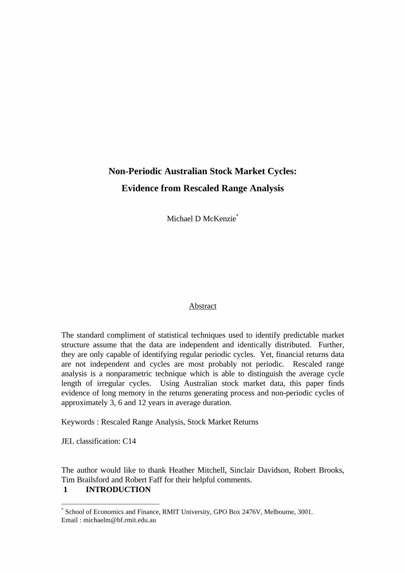
national stock market index. Figure 1 presents the values of a national stock market

index reconstructed using these returns and assuming a base value of 100 (log index

values are presented as they provide a better diagramatic representation of the data).

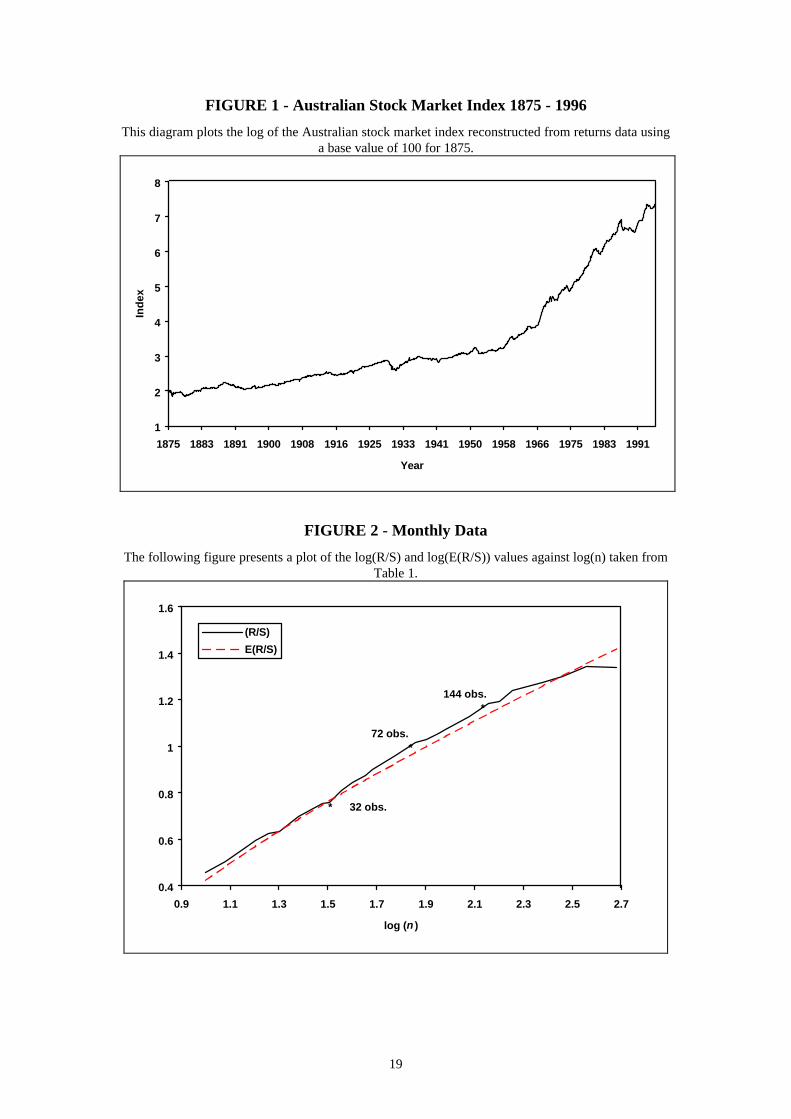
From Figure 1, the Australian stock market has generally appreciated over time and the

crashes of 1930 and 1987 are clearly visible. The descriptive statistics of the data

indicate a mean monthly return of 0.93% and a standard deviation of 4.03%. Most

importantly, the return series exhibits skewness (S = 0.146), excess kurtosis (11.86)

and fails the Jarque Bera test of normality (JB = 4761.0). The presence of

leptokurtosis in the data provides evidence suggestive as to a systematic bias in the

data generating process.

[FIGURE 1 ABOUT HERE]

To test the nature of this systematic bias, rescaled range analysis may be applied. As a

first step it is necessary to prewhiten the data by estimating an AR equation of the

following form :

Rt = α0 + β1 Rt-1 + χ1 D + εt (9)

where Rt are the returns to the Australian share market, D is a dummy variable which

takes on a value of unity for the month of the October 1987 Crash, α, β and χ, are

15 There is a limit to the number of cycles which can be identified. As a general rule, where morethan four cycles are present in the data, they tend to merge. At the limit of an infinite number ofcycles, the log(R/S) plot would not deviate from trend which would normally be taken as indicative ofno average cycle length.16 The data was available from February 1875 (1454 observations), but the sample was manipulated toa length which could be divided by the greatest number of integers after the estimation of the meanmodel.

9

coefficients to be estimated and εt are the residuals from the model.17 Equation (9)

was fitted to the data and the estimated results are :

Rt = 0.0073 + 0.2536 Rt-1 - 0.3952 Crash Dummy (7.35) (10.29) (10.71)

R 2 = 0.1274 S.E. = 0.0368 DW = 2.0351 F-Statistic = 106.11Note : t-statistics in parentheses

Rescaled range analysis may be applied to the residuals of this AR model. As a first

step, it is necessary to divide the sample into subperiods of length n. For financial time

series, Peters (1994) suggests n ≈ 10 as a starting point as values of n < 10 have been

found to produce unstable estimates when sample sizes are small (Peters (1994) p. 63).

Thus, the data may be split into 144 contiguous subperiods of 10 observations. In

each 10 observation subperiod, the data is rescaled to a mean value of zero by

subtracting the sample mean (estimated as Equation (2)) from each observation. The

cumulative sum of these ten rescaled values was then generated and the range

determined according to Equation (3). Each range was then normalised and the

average R/S10 value across all subperiods calculated. The process was then repeated

for higher values of n which were evenly divisible by the total sample. Thus, the

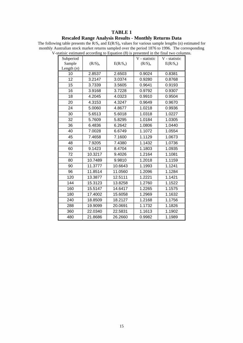
process was repeated for n = 12, 15, 16, 18, … . The estimated R/S values are

presented in Table 1 as are the E(R/S) coefficients which were generated according to

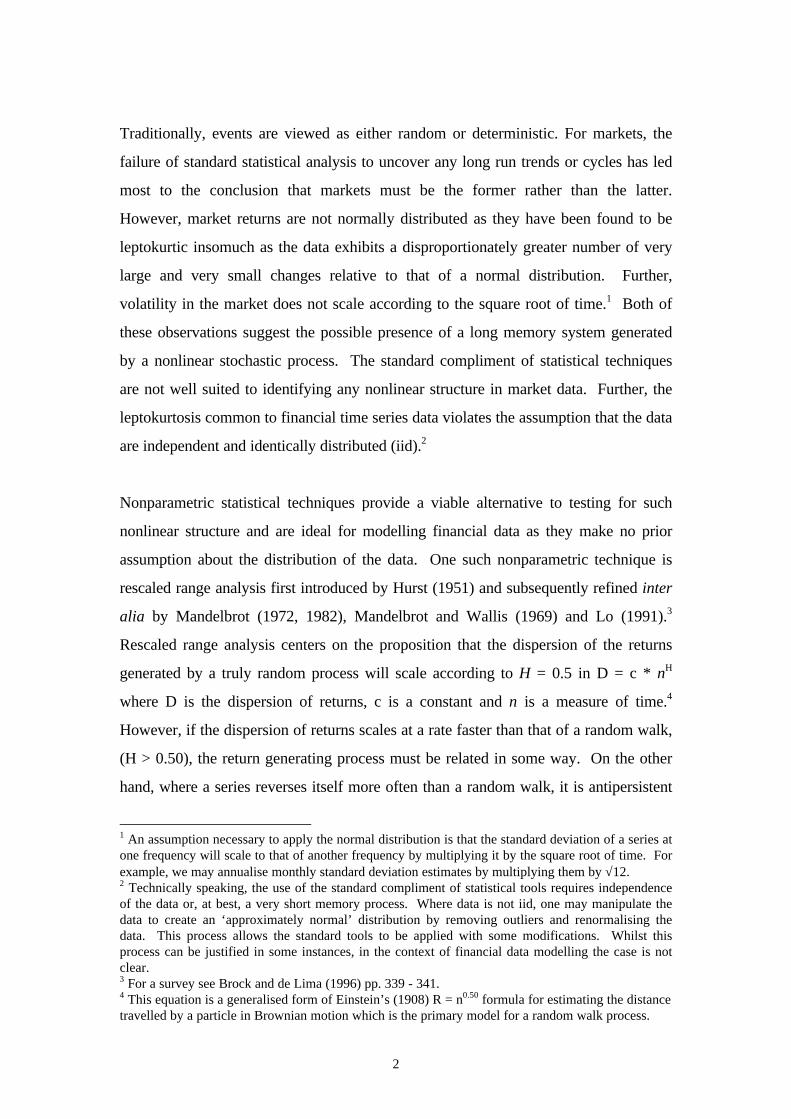
Equation (6). To aid in the interpretation of these estimates, Figure 2 presents a plot

of log(R/S) and log(E(R/S)) against log(n). One can see that the R/S values scale

closely to the E(R/S) values until n = 32 (log(n) = 1.50) as evidenced by the parallel

paths of the two plots. After this point however, a systematic deviation of the R/S and

E(R/S) estimates is visible until a break in this trend which appears at n = 144 (log(n) =

2.15)

[FIGURE 2 AND TABLE 1 ABOUT HERE]

17 This dummy variable was only used to account for the 1987 crash as it was unique in that it occuredin a very short period of time. Other crashes experienced by the Australian market were moreprolonged.

10

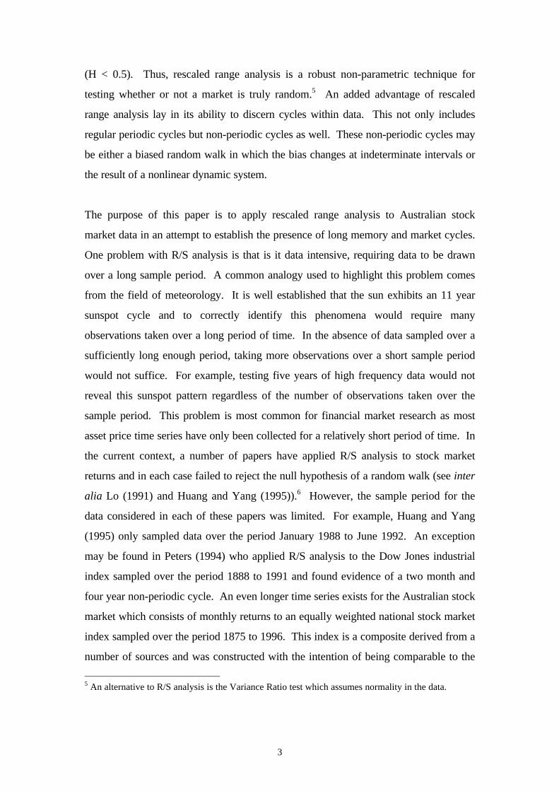
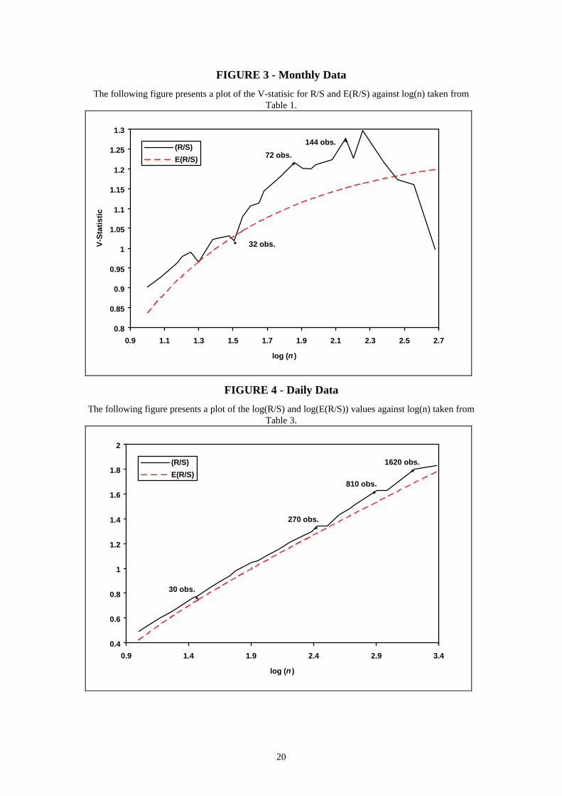
To investigate this deviation of the R/S and E(R/S) series, Figure 3 presents a plot of

the V-statistic against log(n). If the series is persistent, this ratio will increase and a

plot of the V-statistic will exhibit a positive slope. For non-periodic statistical cycles in

which there is no average cycle length, the plot of the V-statistic for R/S will not

deviate from this upward trend. However, a deterministic system which possess an

average cycle length will deviate from its trend line at the end of its cycle. Where more

than one cycle is discernible in the data, a break in the positive slope of the log(R/S)

plot will appear at the end of one cycle before the plot resumes its upward trend to

again deviate at the end of the next cycle. From Figure 3, the plot of the V-statistic for

the monthly Australian stock market data indicates persistence in the returns

generating process as the ratio is increasing at a faster rate than that of the V-statistic

estimated for the E(R/S) series. More specifically, the local slope for n ≤ 32 is not

easily distinguishable from a random walk. Where n > 32 however, the V-statistic for

R/S diverges from the V-statistic for E(R/S) until n > 144 (approximately 12 years).

For values of n > 144, the two series again converge with the exception of the

observation at n = 180. Thus, from n = 32 to 144 the local slope in this region

increases at a faster rate than that implied by a random walk. An additional cycle not

immediately obvious in Figure 2, may be identified as ending at n = 72 (approximately

6 years). The break in the upward trend of the plot of the V-Statistic at n = 72

indicates the end of a non-periodic cycle. However, the resumption of the upward

trend shortly thereafter is consistent with the presence of a longer cycle in the data.

These results clearly support the presence of a non-linear dynamic system driving the

data and suggest the presence of cycles in the stock market which exhibit chaotic

behaviour.

[FIGURE 3 ABOUT HERE]

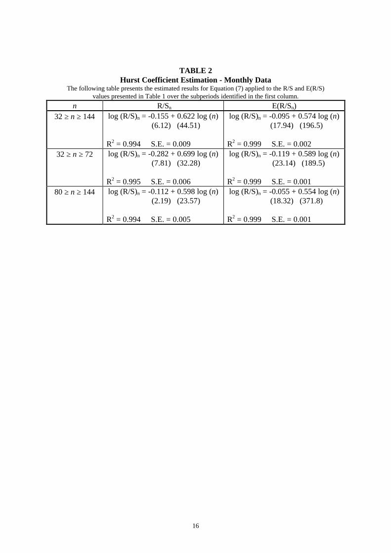
To assess the significance of these visual clues as to cycle length, Equation (7) was

applied to both the R/S and E(R/S) values and H and E(H) coefficient estimated

initially over the period 32 ≥ n ≥ 144. The results are presented in Table 2. The

estimated Hurst coefficient is 0.622 and for the E(R/S) series the E(H) coefficient is

0.574. As the H estimate is 1.85 standard deviations greater than the E(H) coefficient

(standard deviation = 0.026), we may conclude that they are significantly different at

11

the 10% level and so reject the null hypothesis that the system is an independent

process. H may also be estimated within each subperiod identified by Figure 3, ie. H

may be estimated over the period 32 ≥ n ≥ 72 and 80 ≥ n ≥ 144 and the results are

again presented in Table 2. For the first subperiod, H (= 0.699) indicates that R/S

increases at a faster rate than suggested by a random process (E(H) = 0.589) and the

difference is statistically significant (H is 4.17 standard deviations greater than E(H)).

Thus, the market clearly exhibits persistence not consistent with a random walk over

this horizon. In the second subperiod, H (= 0.598) is 1.70 standard deviations greater

than E(H) (= 0.554) and so is significant at the 10% level.

[TABLE 2 ABOUT HERE]

Overall, these results suggest that the returns generating process in the Australian

stock market is persistent and a 6 year (possibly an average business cycle) and a 12

year non-periodic cycle exist in the Australian stock market. The identification of a six

year average cycle in the data is broadly consistent with previous estimates of the

business cycle. For example, Layton (1997a,b) studied the Australian economy over

the period 1950 - 1994 using a coincident index and found evidence of a business cycle

which has a median length of 5.25 years. Unfortunately, a lack of R/S estimates

prevents a more precise identification of the length of this cycle.

3.1 DAILY DATA

In general, the results obtained using monthly data suggest the presence of two cycles

within the Australian stock market which possess a 6 and 12 year duration on average.

The cycles evident in the monthly data should be evident in more frequently sampled

data if they are not a statistical anomaly. That is to say, daily returns should exhibit a

non-periodic cycle of 6 years (ie, 1500 daily observations). Further, if the 12 year

cycle is a genuine non-periodic cycle and not a stochastic boundary due to sample size,

its presence should be largely independent of the sampling frequency.

12

The use of more frequently sampled data does however, bring with it some problems

as it typically contains greater levels of noise compared to less frequently sampled data.

Whilst R/S analysis is robust to the presence of noise (Peters (1994) p. 98 - 101), its

presence may bias the Hurst exponent downward. Further, more frequently sampled

data is typically only available for relatively short periods of time and so suffer from the

‘sunspot’ dilemma discussed in Section 1. This makes it difficult to uncover long

cycles in the data such as the 12 year cycle found in Section 3. These concerns aside,

this study will consider Australian stock market returns data sampled at a higher

frequency. Daily returns to the Australian All Ordinaries stock market index were

available for the period December, 1980 to August, 1998 giving a total of 4862

observations.18 Equation 9 was fitted to this data and the results may be summarised

as:

Rt = 0.0003 + 0.1110 Rt-1 - 0.2837 Crash Dummy (2.71) (8.60) (31.53)

R2 = 0.1833 S.E. = 0.0089 DW = 1.9262 F-Statistic = 1.9262Note : t-statistics in parentheses

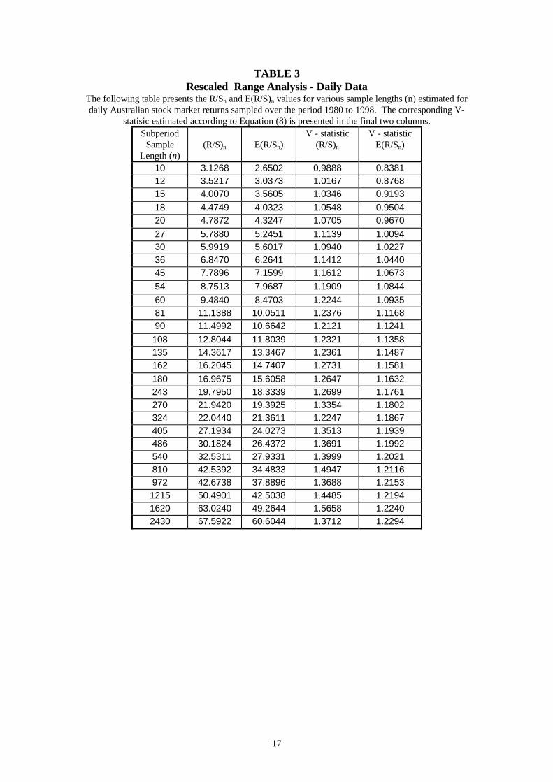
Rescaled range analysis was applied to the residuals of this AR equation and the results

are presented in Table 3. In contrast to the monthly data, none of the daily R/S

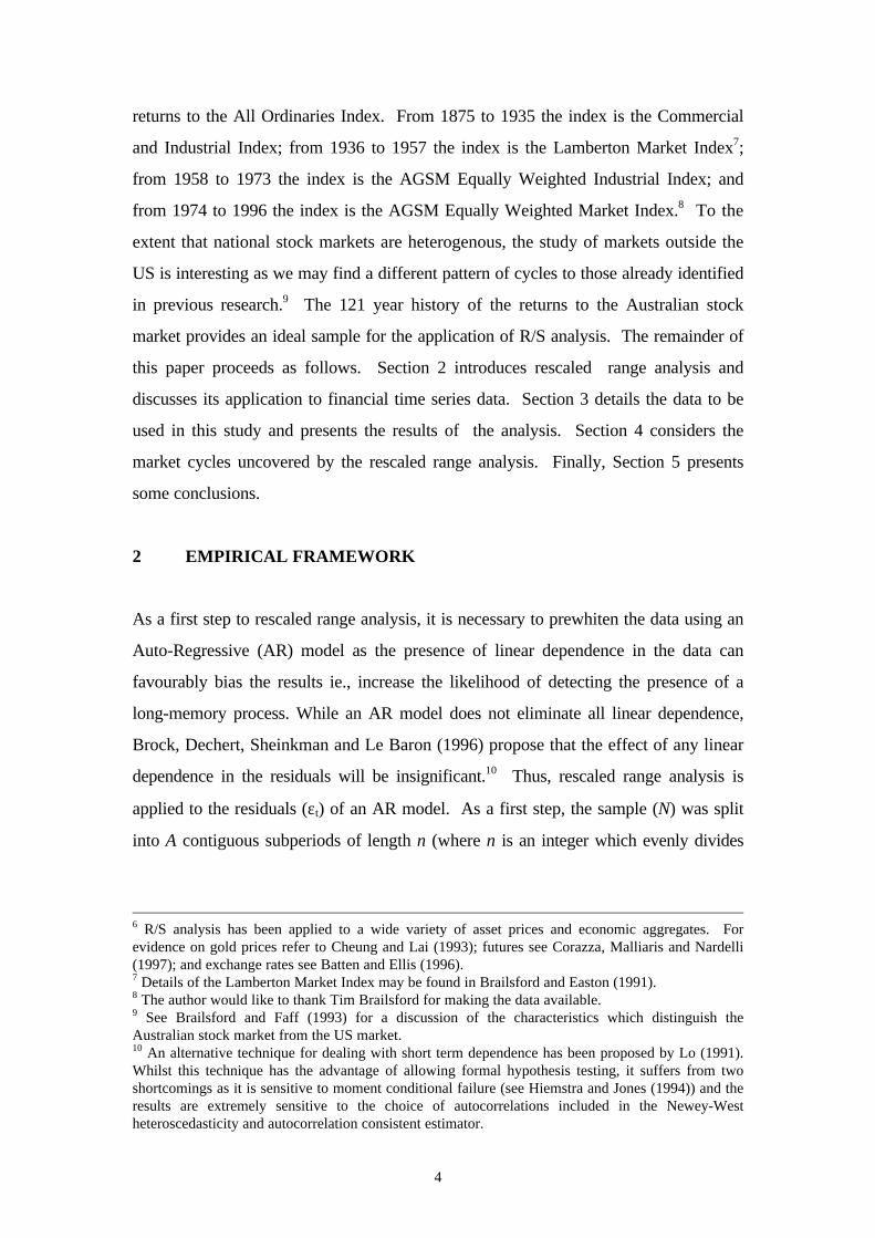
estimates are less than the E(R/S) values. This can be seen in Figure 4 which plots the

log(R/S) and log(E(R/S)) values against log(n). Up to n = 30 (log(n) = 1.47), the R/S

and E(R/S) values scale closely and their difference varies little in one direction or the

other. Where n > 30 however, a systematic deviation between the R/S and E(R/S)

values is evident. This difference is most obvious for values of n > 243 (log(n) = 2.38)

and the trend reverses after n = 1620. Further, the possibility of multiple cycles within

the data exists as a number of break points in the data are apparent at n = 270

(approximately 1 year) and 810 (approximately 3 years). This is more obvious in

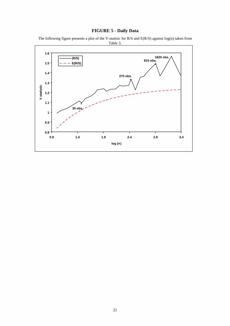
Figure 5 which plots the V-statistic against log(n). Interestingly, the break point at n =

1620 roughly corresponds to the 6 year cycle identified using the monthly data (1620

18 Weekly Australian stock market returns sampled over the same period were also considered and theresults (not reported) were broadly consistent with those reported for the daily data. They areavailable upon request.

13

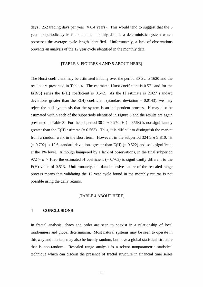
days / 252 trading days per year ≈ 6.4 years). This would tend to suggest that the 6

year nonperiodic cycle found in the monthly data is a deterministic system which

possesses the average cycle length identified. Unfortunately, a lack of observations

prevents an analysis of the 12 year cycle identified in the monthly data.

[TABLE 3, FIGURES 4 AND 5 ABOUT HERE]

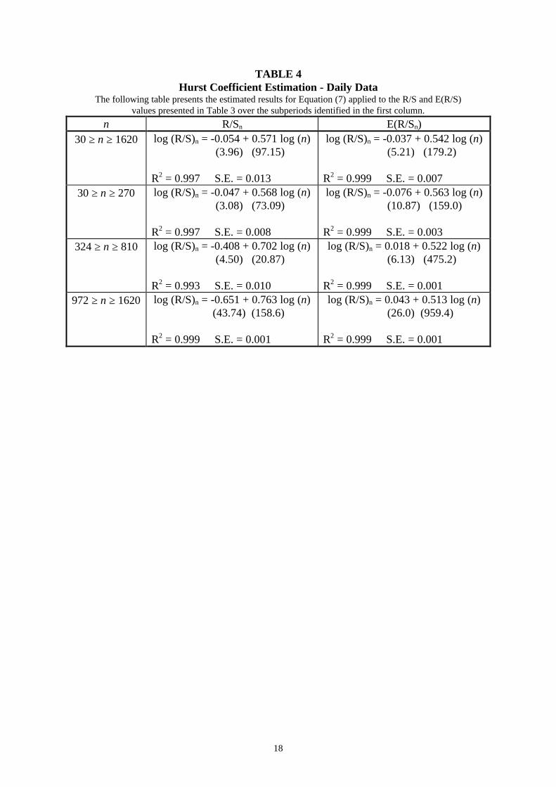
The Hurst coefficient may be estimated initially over the period 30 ≥ n ≥ 1620 and the

results are presented in Table 4. The estimated Hurst coefficient is 0.571 and for the

E(R/S) series the E(H) coefficient is 0.542. As the H estimate is 2.027 standard

deviations greater than the E(H) coefficient (standard deviation = 0.0143), we may

reject the null hypothesis that the system is an independent process. H may also be

estimated within each of the subperiods identified in Figure 5 and the results are again

presented in Table 3. For the subperiod 30 ≥ n ≥ 270, H (= 0.568) is not significantly

greater than the E(H) estimate (= 0.563). Thus, it is difficult to distinguish the market

from a random walk in the short term. However, in the subperiod 324 ≥ n ≥ 810, H

(= 0.702) is 12.6 standard deviations greater than E(H) (= 0.522) and so is significant

at the 1% level. Although hampered by a lack of observations, in the final subperiod

972 > n > 1620 the estimated H coefficient (= 0.763) is significantly different to the

E(H) value of 0.513. Unfortunately, the data intensive nature of the rescaled range

process means that validating the 12 year cycle found in the monthly returns is not

possible using the daily returns.

[TABLE 4 ABOUT HERE]

4 CONCLUSIONS

In fractal analysis, chaos and order are seen to coexist in a relationship of local

randomness and global determinism. Most natural systems may be seen to operate in

this way and markets may also be locally random, but have a global statistical structure

that is non-random. Rescaled range analysis is a robust nonparametric statistical

technique which can discern the presence of fractal structure in financial time series

14

data. In this paper, rescaled range analysis was applied to Australian stock market data

and the market was found to exhibit a highly degree of persistence once short term

effects were removed. Further, the stock market has nonlinear dynamic cycles of

approximately 3, 6 and 12 years. This result has important implications for momentum

and other forms of technical analysis as well as guiding the appropriate period length

for model development. One limiting factor of the analysis was the lack of sufficient

data to complete the full range of tests on more frequent returns to reinforce these

monthly data based findings.

15

TABLE 1Rescaled Range Analysis Results - Monthly Returns Data

The following table presents the R/Sn and E(R/S)n values for various sample lengths (n) estimated formonthly Australian stock market returns sampled over the period 1876 to 1996. The corresponding

V-statisic estimated according to Equation (8) is presented in the final two columns.Subperiod

SampleLength (n)

(R/S)n E(R/Sn)V - statistic

(R/S)n

V - statisticE(R/Sn)

10 2.8537 2.6503 0.9024 0.838112 3.2147 3.0374 0.9280 0.876815 3.7339 3.5605 0.9641 0.919316 3.9168 3.7228 0.9792 0.930718 4.2045 4.0323 0.9910 0.9504

20 4.3153 4.3247 0.9649 0.967024 5.0060 4.8677 1.0218 0.9936

30 5.6513 5.6018 1.0318 1.022732 5.7609 5.8295 1.0184 1.030536 6.4836 6.2642 1.0806 1.044040 7.0028 6.6749 1.1072 1.0554

45 7.4658 7.1600 1.1129 1.0673

48 7.9205 7.4380 1.1432 1.073660 9.1423 8.4704 1.1803 1.093572 10.3217 9.4026 1.2164 1.1081

80 10.7489 9.9810 1.2018 1.115990 11.3777 10.6643 1.1993 1.124196 11.8514 11.0560 1.2096 1.1284

120 13.3877 12.5111 1.2221 1.1421144 15.3123 13.8258 1.2760 1.1522160 15.5147 14.6417 1.2265 1.1575180 17.4002 15.6058 1.2969 1.1632240 18.8509 18.2127 1.2168 1.1756288 19.9099 20.0691 1.1732 1.1826360 22.0340 22.5831 1.1613 1.1902480 21.8686 26.2660 0.9982 1.1989

16

TABLE 2Hurst Coefficient Estimation - Monthly Data

The following table presents the estimated results for Equation (7) applied to the R/S and E(R/S)values presented in Table 1 over the subperiods identified in the first column.

n R/Sn E(R/Sn)32 ≥ n ≥ 144 log (R/S)n = -0.155 + 0.622 log (n)

(6.12) (44.51)

R2 = 0.994 S.E. = 0.009

log (R/S)n = -0.095 + 0.574 log (n) (17.94) (196.5)

R2 = 0.999 S.E. = 0.00232 ≥ n ≥ 72 log (R/S)n = -0.282 + 0.699 log (n)

(7.81) (32.28)

R2 = 0.995 S.E. = 0.006

log (R/S)n = -0.119 + 0.589 log (n) (23.14) (189.5)

R2 = 0.999 S.E. = 0.00180 ≥ n ≥ 144 log (R/S)n = -0.112 + 0.598 log (n)

(2.19) (23.57)

R2 = 0.994 S.E. = 0.005

log (R/S)n = -0.055 + 0.554 log (n) (18.32) (371.8)

R2 = 0.999 S.E. = 0.001

17

TABLE 3Rescaled Range Analysis - Daily Data

The following table presents the R/Sn and E(R/S)n values for various sample lengths (n) estimated fordaily Australian stock market returns sampled over the period 1980 to 1998. The corresponding V-

statisic estimated according to Equation (8) is presented in the final two columns.Subperiod

SampleLength (n)

(R/S)n E(R/Sn)V - statistic

(R/S)n

V - statisticE(R/Sn)

10 3.1268 2.6502 0.9888 0.838112 3.5217 3.0373 1.0167 0.876815 4.0070 3.5605 1.0346 0.9193

18 4.4749 4.0323 1.0548 0.950420 4.7872 4.3247 1.0705 0.9670

27 5.7880 5.2451 1.1139 1.009430 5.9919 5.6017 1.0940 1.022736 6.8470 6.2641 1.1412 1.044045 7.7896 7.1599 1.1612 1.0673

54 8.7513 7.9687 1.1909 1.0844

60 9.4840 8.4703 1.2244 1.093581 11.1388 10.0511 1.2376 1.116890 11.4992 10.6642 1.2121 1.1241

108 12.8044 11.8039 1.2321 1.1358135 14.3617 13.3467 1.2361 1.1487162 16.2045 14.7407 1.2731 1.1581

180 16.9675 15.6058 1.2647 1.1632243 19.7950 18.3339 1.2699 1.1761270 21.9420 19.3925 1.3354 1.1802324 22.0440 21.3611 1.2247 1.1867405 27.1934 24.0273 1.3513 1.1939486 30.1824 26.4372 1.3691 1.1992540 32.5311 27.9331 1.3999 1.2021810 42.5392 34.4833 1.4947 1.2116972 42.6738 37.8896 1.3688 1.21531215 50.4901 42.5038 1.4485 1.21941620 63.0240 49.2644 1.5658 1.22402430 67.5922 60.6044 1.3712 1.2294

18

TABLE 4Hurst Coefficient Estimation - Daily Data

The following table presents the estimated results for Equation (7) applied to the R/S and E(R/S)values presented in Table 3 over the subperiods identified in the first column.

n R/Sn E(R/Sn)30 ≥ n ≥ 1620 log (R/S)n = -0.054 + 0.571 log (n)

(3.96) (97.15)

R2 = 0.997 S.E. = 0.013

log (R/S)n = -0.037 + 0.542 log (n) (5.21) (179.2)

R2 = 0.999 S.E. = 0.00730 ≥ n ≥ 270 log (R/S)n = -0.047 + 0.568 log (n)

(3.08) (73.09)

R2 = 0.997 S.E. = 0.008

log (R/S)n = -0.076 + 0.563 log (n) (10.87) (159.0)

R2 = 0.999 S.E. = 0.003324 ≥ n ≥ 810 log (R/S)n = -0.408 + 0.702 log (n)

(4.50) (20.87)

R2 = 0.993 S.E. = 0.010

log (R/S)n = 0.018 + 0.522 log (n) (6.13) (475.2)

R2 = 0.999 S.E. = 0.001972 ≥ n ≥ 1620 log (R/S)n = -0.651 + 0.763 log (n)

(43.74) (158.6)

R2 = 0.999 S.E. = 0.001

log (R/S)n = 0.043 + 0.513 log (n) (26.0) (959.4)

R2 = 0.999 S.E. = 0.001

19

FIGURE 1 - Australian Stock Market Index 1875 - 1996

This diagram plots the log of the Australian stock market index reconstructed from returns data usinga base value of 100 for 1875.

1

2

3

4

5

6

7

8

1875 1883 1891 1900 1908 1916 1925 1933 1941 1950 1958 1966 1975 1983 1991

Year

Ind

ex

FIGURE 2 - Monthly Data

The following figure presents a plot of the log(R/S) and log(E(R/S)) values against log(n) taken fromTable 1.

0.4

0.6

0.8

1

1.2

1.4

1.6

0.9 1.1 1.3 1.5 1.7 1.9 2.1 2.3 2.5 2.7

log (n )

(R/S)

E(R/S)

144 obs. *

72 obs. *

* 32 obs.

20

FIGURE 3 - Monthly Data

The following figure presents a plot of the V-statisic for R/S and E(R/S) against log(n) taken fromTable 1.

0.8

0.85

0.9

0.95

1

1.05

1.1

1.15

1.2

1.25

1.3

0.9 1.1 1.3 1.5 1.7 1.9 2.1 2.3 2.5 2.7

log (n )

V-S

tati

stic

(R/S)

E(R/S) 72 obs. *

144 obs. *

* 32 obs.

FIGURE 4 - Daily Data

The following figure presents a plot of the log(R/S) and log(E(R/S)) values against log(n) taken fromTable 3.

0.4

0.6

0.8

1

1.2

1.4

1.6

1.8

2

0.9 1.4 1.9 2.4 2.9 3.4

log (n )

(R/S)

E(R/S)

270 obs. *

810 obs. *

1620 obs. *

30 obs. *

21

FIGURE 5 - Daily Data

The following figure presents a plot of the V-statisic for R/S and E(R/S) against log(n) taken fromTable 3.

0.8

0.9

1

1.1

1.2

1.3

1.4

1.5

1.6

0.9 1.4 1.9 2.4 2.9 3.4

log (n )

V s

tati

stic

(R/S)

E(R/S)

270 obs. *

810 obs. *

1620 obs. *

*30 obs.

22

5 BIBLIOGRAPHY

Anis, A.A. and Lloyd, E.H. (1976) “The Expected Value of the Adjusted RescaledRange of Independent Normal Summands” Biometrika, 63.

Batten, J. and Ellis, C. (1996) “Fractal Structures and Naïve Trading Systems:Evidence from the spot US dollar/Japanese yen” Japan and the World Economy, 8,pp. 411 - 421.

Brailsford, T.J. and Easton, S. (1991) “Seasonality in Australian Share Price IndicesBetween 1936 and 1957”Accounting and Finance, 31, pp. 69 - 85

Brailsford, T.J. and Faff, R.W. (1993) “Modelling Australian Stock Market Volatility”Australian Journal of Management, 18, 109-132.

Brock, W.A., Dechert, W.D., Sheinkman, J.A. and Le Baron, B. (1996) “A Test forIndependence Based on Correlation Dimension” Econometric Reviews, 15.

Brock, W.A. and de Lima, P.J.F. (1996) “Nonlinear Time Series, Complexity Theoryand Finance” in Maddala, G.S. and Rao, C.R. eds. Handbook of Statistics, Vol 14,Elsevier Science Publishing.

Cheung, Y.W. and Lai, K.S. (1993) “Do Gold Market Returns Have Long Memory?”The Financial Review, 28, pp. 181 - 202.

Corazza, M., Malliaris, A.G. and Nardelli, C. (1997) “Searching for Fractal Structurein Agricultural Futures Markets” The Journal of Futures Markets, 17, pp. 433 - 473.

Cutland, N.J., Kopp, P.E. and Willinger, W. (1993) “Stock Price Returns and theJoseph Effect: Fractional version of the Black-Scholes model” Mathematics ResearchReports, pp. 297 - 306.

Einstein, A. (1908) “Uber die von der Molekularkinetischen Theorie der WarmeGeforderte Bewegung von in Ruhenden Flussigkeiten Suspendierten Teilchen” Annalsof Physics, 322.

Hiemstra, C. and Jones, J. (1994) “Another Look at Long Memory in Common StockReturns” Discussion Paper 94/077, University of Strathclyde.

Huang, B.N. and Yang, C.W. (1995) “The Fractal Structure in Multinational StockReturns” Applied Economics Letters, 2, pp. 67 - 71.

Hurst, H.E. (1951) “The Long Term Storage Capacity of Reservoirs” Transactions ofthe American Society of Civil Engineers, 116.

Layton, A. (1997a) “A New Approach to Dating and Predicting Australian BusinessCycle Phase Changes” Applied Economics, 29, pp. 861 - 868.

23

Layton, A. (1997b) “Do Leading Indicators Really Predict Australian Business CycleTurning Points” Economic Record, 73, pp. 258 - 269.

Lo, A.W. (1991) “Long-Term Memory in Stock Market Prices” Econometrica, 59,pp. 1279 - 1313.

Mandelbrot, B. (1972) “Statistical Methodology for Non-Periodic Cycles: from thecovariance to R/S analysis” Annals of Economic and Social Measurement, 1.

Mandelbrot, B. (1982) “The Fractal Geometry of Nature” W.H. Freeman, New York.

Mandelbrot, B. and Wallis, J. (1969) “Robustness of the Rescaled Range R/S in theMeasurement of Noncyclic Long Run Statistical Dependence” Water ResourcesResearch, 5.

Peters, E.E. (1994) “Fractal Market Analysis : Applying chaos theory to investmentand economics” John Wiley and Sons, New York.