Journal of Computational and Applied Mathematics 233 (2010) 1937–1953 Contents lists available at ScienceDirect Journal of Computational and Applied Mathematics journal homepage: www.elsevier.com/locate/cam Multivariate time changes for Lévy asset models: Characterization and calibration ✩ Elisa Luciano a,b , Patrizia Semeraro a,* a Dipartimento di Statistica e Matematica Applicata D. De Castro, Università degli Studi di Torino, Italy b ICER and Collegio Carlo Alberto, Italy article info Article history: Received 10 March 2009 Received in revised form 12 August 2009 Keywords: Lévy processes Multivariate subordinators Dependence Correlation Multivariate asset modelling Multivariate time changed processes abstract We build a theoretical framework for multivariate subordination of Brownian motions, with a common and an idiosyncratic component. This follows economic intuition and introduces generalizations of some well known multivariate Lévy processes for financial applications: the compound Poisson, NIG, Variance Gamma and CGMY. In most cases we obtain the characteristic function in closed form. The extension is first kept parsimonious, by adding one parameter only. The empirical fit of (linear) dependence is then increased, by allowing for dependent Brownian motions. © 2009 Elsevier B.V. All rights reserved. 0. Introduction There are theoretical as well as empirical reasons for being interested in time changes. On the theoretical side, price processes under no arbitrage are semimartingales. The latter can be represented as time changed Brownian motions, using as time change either a subordinator or a more general process. When the change of time is a subordinator the resulting process belongs to the (pure jump) Lévy class. This explains the success of subordination in mathematical Finance, in order to represent asset prices. On the empirical side time changes model the flow of information, as measured by trade: one can think that time runs fast when there are a lot of orders, while it slows down when trade is stale. Economic time then does not coincide with calendar time. This relationship between price changes and trade has been extensively studied (see for instance [1,2]). It has been tested in Geman and Ané [3], which cannot reject normality of re-scaled returns, i.e. returns per unit of trade. Most of the time change literature considers one asset at a time. At the multivariate level, time changing has been studied much less. Multivariate Lévy processes have been generally constructed subordinating a multivariate Brownian motion by means of a univariate subordinator. Such processes present a number of drawbacks, including restrictions on the marginal parameters, lack of independence and possibility of spanning a limited range of dependence (see for instance [4]). On top of that, a unique time change for all assets does not seem to be economically sound. Harris [5], while discussing the cross sectional properties of trades, rejects equality across different ✩ We thank Claudio Patrucco for having provided the marginal calibrations and Ksenia Rulik for computational assistance. Comments by R. Cont, D. Madan, C. Sgarra, P. Tankov, M. Yor on the VG case are gratefully acknowledged. The preliminary version has been circulated under the title ‘‘Extending Time-Changed Lévy Asset Models Through Multivariate Subordinators’’. Patrizia Semeraro gratefully acknowledges financial support from Torino Finanza and its associates, in particular Unicredit and Toro Assicurazioni. The grant 2006132713 from the Italian MURST is gratefully acknowledged by both the authors. * Corresponding author. E-mail address: [email protected] (P. Semeraro). 0377-0427/$ – see front matter © 2009 Elsevier B.V. All rights reserved. doi:10.1016/j.cam.2009.08.119

Welcome message from author
This document is posted to help you gain knowledge. Please leave a comment to let me know what you think about it! Share it to your friends and learn new things together.
Transcript
Journal of Computational and Applied Mathematics 233 (2010) 1937–1953
Contents lists available at ScienceDirect
Journal of Computational and AppliedMathematics
journal homepage: www.elsevier.com/locate/cam
Multivariate time changes for Lévy asset models: Characterizationand calibrationI
Elisa Luciano a,b, Patrizia Semeraro a,∗a Dipartimento di Statistica e Matematica Applicata D. De Castro, Università degli Studi di Torino, Italyb ICER and Collegio Carlo Alberto, Italy
a r t i c l e i n f o
Article history:Received 10 March 2009Received in revised form 12 August 2009
Keywords:Lévy processesMultivariate subordinatorsDependenceCorrelationMultivariate asset modellingMultivariate time changed processes
a b s t r a c t
We build a theoretical framework for multivariate subordination of Brownian motions,with a common and an idiosyncratic component. This follows economic intuition andintroduces generalizations of some well known multivariate Lévy processes for financialapplications: the compound Poisson, NIG, Variance Gamma and CGMY. In most cases weobtain the characteristic function in closed form. The extension is first kept parsimonious,by adding one parameter only. The empirical fit of (linear) dependence is then increased,by allowing for dependent Brownian motions.
© 2009 Elsevier B.V. All rights reserved.
0. Introduction
There are theoretical as well as empirical reasons for being interested in time changes.On the theoretical side, price processes under no arbitrage are semimartingales. The latter can be represented as time
changed Brownianmotions, using as time change either a subordinator or a more general process. When the change of timeis a subordinator the resulting process belongs to the (pure jump) Lévy class. This explains the success of subordination inmathematical Finance, in order to represent asset prices.On the empirical side time changes model the flow of information, as measured by trade: one can think that time runs
fast when there are a lot of orders, while it slows down when trade is stale. Economic time then does not coincide withcalendar time. This relationship between price changes and trade has been extensively studied (see for instance [1,2]). It hasbeen tested in Geman and Ané [3], which cannot reject normality of re-scaled returns, i.e. returns per unit of trade.Most of the time change literature considers one asset at a time.At the multivariate level, time changing has been studied much less. Multivariate Lévy processes have been generally
constructed subordinating amultivariate Brownianmotion bymeans of a univariate subordinator. Such processes present anumber of drawbacks, including restrictions on the marginal parameters, lack of independence and possibility of spanninga limited range of dependence (see for instance [4]). On top of that, a unique time change for all assets does not seem tobe economically sound. Harris [5], while discussing the cross sectional properties of trades, rejects equality across different
I We thank Claudio Patrucco for having provided the marginal calibrations and Ksenia Rulik for computational assistance. Comments by R. Cont,D. Madan, C. Sgarra, P. Tankov, M. Yor on the VG case are gratefully acknowledged. The preliminary version has been circulated under the title ‘‘ExtendingTime-Changed Lévy Asset Models Through Multivariate Subordinators’’. Patrizia Semeraro gratefully acknowledges financial support from Torino Finanzaand its associates, in particular Unicredit and Toro Assicurazioni. The grant 2006132713 from the Italian MURST is gratefully acknowledged by both theauthors.∗ Corresponding author.E-mail address: [email protected] (P. Semeraro).
0377-0427/$ – see front matter© 2009 Elsevier B.V. All rights reserved.doi:10.1016/j.cam.2009.08.119
1938 E. Luciano, P. Semeraro / Journal of Computational and Applied Mathematics 233 (2010) 1937–1953
assets. Using an extensive data set from theUS stockmarket, Lo andWang [6] show that trades present a significant commoncomponent.Multivariate subordinators, i.e. different time changes for different assets, appeared only very recently: the theoretical
set up is in [7]. Eberlein andMadan [8] introduce amultivariate subordinator with independent components to time changedependent Brownian motions and fit financial returns.Themultivariate subordinator studied here incorporates both a time transform common to all assets and an idiosyncratic
one. The former can be interpreted in financial applications as a measure of the overall trade or market activity, while thelatter represents asset-specific trade. The empirical analysis performed in [6] justifies our choice.We build on the idea of splitting the multivariate subordinator into a common and an idiosyncratic component, which
we introduced for the Variance Gamma (VG) case in [9] and for the generalized hyperbolic (GH) one in [10]. We extendthe previous papers as follows. We first characterize the change of time, then the corresponding time changed Brownianmotions.We introduce generalizations of themultivariate Compound Poisson (CP), Normal Inverse Gaussian (NIG), VarianceGamma and Carr Geman Madan Yor (CGMY) processes. In order to justify our modelling choices and their usefulness forfinancial applications, we have three desired features in mind: the existence of characteristic functions in closed form,the ability to capture a wide range of (linear dependence) and the possibility of calibrating marginal and joint parametersseparately.We first provide the characteristic functions, for all cases except CGMY.We then study the nonlinear and linear dependence of the processes so obtained. We show that, as long as our
multivariate subordinator is applied to independent Brownian motions, the model is extremely parsimonious in termsof parameters: there is only one additional parameter on top of the marginal ones. The range of linear correlation whichcan be captured is bounded above by the change of time (trade) correlation. Therefore, we extend the model so as toincorporate correlated Brownian motions. The number of parameters needed for calibration increases, but the upper boundon correlation disappears.Last but not least, we provide a calibration technique, which shows that one can fit separately the marginal distributions
and the correlation parameters. Consequently, one can shift from the more to the less parsimonious model, in order toimprove the correlation fit, without re-estimating the marginal distributions.The paper proceeds as follows: Section 1 contains some basic terminology. Section 2 presents our class of multivariate
subordinators. Section 3 applies them to independent Brownian motions and obtains the general properties (Lévy nature,characteristic function, Lévy triplet andmeasure) of the corresponding subordinated processes. The results are then specifiedin relation to the CP, NIG, VG and CGMY cases. Section 4 studies dependence. Section 5 extends the model to correlatedBrownian motions. In view of the empirical applications, Section 6 discusses linear correlation. Section 7 contains acalibration for seven major stock indices. Section 8 concludes.
1. Preliminaries
Let X(t) be a Rn-valued Lévy process. The characteristic function is fundamental in its construction. It admits thefollowing Lévy–Khinchin representation:
ψX(t)(z) = E[ei〈z,X(t)〉] = etΨX (z), z ∈ Rn,with
ΨX (z) = −12〈z, Az〉 + i〈γ, z〉 +
∫Rn(ei〈z,x〉 − 1− i〈z, x〉1|x|≤1)ν(dx),
where A is a symmetric n × nmatrix, γ ∈ Rn and ν is a positive random measure on Rn. (γ, A, ν) is called the Lévy tripletof the process. ΨX (z) is named characteristic exponent of X . In the next section we focus our attention on a particular classof Lévy processes, the subordinators, that are increasing Lévy processes. They have no diffusion component and are of finitevariation. More precisely, we are interested in the multivariate generalization of subordinators. Amultivariate subordinatoris a Lévy process on Rn
+= [0,∞)n, whose trajectories are increasing in each coordinate. See [7] for the main properties of
such processes. The characteristic exponent of a multivariate subordinator has the following expression:
ΨX (z) = i〈m, z〉 +∫
Rn(ei〈z,x〉 − 1)ν(dx), (1.1)
wherem ∈ Rn+and νX is the Lévy measure of X .
A theorem that plays a central role in the characterization in terms of Lévy triplet of the processes we are going toconstruct is in [7]. The theorem requires the introduction of themulti-parameter process notion. Considern real independentLévy processes X1(t), . . . , Xn(t). The stacked process X(t) = (X1(t), . . . , Xn(t))T, where the superscript T denotes thetranspose, is then a Lévy process on Rn. Consider the multi-parameter s = (s1, . . . , sn)T ∈ Rn
+and the partial order on Rn
+:
s1 � s2 ⇔ s1j ≤ s2j , j = 1, . . . , n.
Define the multi-parameter process {X(s), s ∈ Rn+} by
X(s) = (X1(s1), . . . , Xn(sn))T.
E. Luciano, P. Semeraro / Journal of Computational and Applied Mathematics 233 (2010) 1937–1953 1939
Theorem 1.1. Let G be a multivariate subordinator with triplet (γG, 0, νG) and let λt = L(G(t)). Let X(t) be a Lévy processon Rn, independent from G , with independent components and triplet (γX ,ΣX , νX ), where ΣX = diag(σ1, . . . , σn), and letρs = L(X(s)). Define the process Y = {Y (t), t ≥ 0} by the following
Y (t) = (X1(G1(t)), . . . , Xn(Gn(t)))T, t ≥ 0
then the process Y is a Lévy process and
E[ei〈z,Y (t)〉] = exp(tΨG(logψX (z))), z ∈ Rn+,
where, for anyw = (w1, . . . , wn)T ∈ Cn with Re (wj) ≤ 0, j = 1, . . . , n, we let
ΨG(w) = 〈m ·w〉 +∫
Rn(e〈w,x〉 − 1)ν(dx).
Moreover the characteristic triplet (γY ,ΣY , νY ) of Y is as follows
γY =
∫Rn+
νG(ds)∫|x|≤1
xρs(dx)+ 〈m, γX 〉,
ΣY = diag(m1σ1, . . . ,mnσn)νY (B) = ν1(B)+ ν2(B)
where ν1 and ν2 are defined by ν1(0) = 0, ν2(0) = 0 and – for B ∈ B(Rn \ 0) – by
ν1(B) =∫
Rn+
ρs(B)νG(ds),
ν2(B) =∫Bm11A1(x)νX1(dx)+ · · · +mn1An(x)νXn(dx),
where x ∈ R, νXi , i = 1, . . . , n are the Lévymeasures of the independent marginal processes of X and Ai = {x = (x1, . . . , xn)T∈
Rn : xk = 0 fork 6= i, k = 1, . . . , n}, i = 1, . . . , n. If m = 0 and∫|s|≤1 |s|
12 νG(ds) <∞, thenΣY = 0,
∫|x|≤1 |x|ν(dx) <∞, Y
has zero drift and is of bounded variation on any time interval almost surely.
2. A class of multivariate subordinators
In this section we introduce a class of multivariate time changes: each one is a sum of an idiosyncratic and a commoncomponent. A similar construction has been proposed in [9] for the VG case. Since through these changes of time we aim atobtaining Lévy processes, we assume that they are subordinators.We define a multidimensional subordinator as follows: let Xj = {Xj(t), t ≥ 0}, j = 1, . . . , n and Z = {Z(t), t ≥ 0} be
independent subordinators. The Lévy processes G = {G(t), t ≥ 0} defined by:
G(t) = (X1(t)+ α1Z(t), . . . , Xn(t)+ αnZ(t)), αi > 0, i = 1, . . . , n (2.1)
is a multidimensional subordinator. If we denote by Ψj and ΨZ respectively the characteristic exponents of the processesXj, j = 1, . . . , n and Z , namely
Ψj(w) =
∫R+(eiwz − 1)νj(dz)+ iljw, j = 1, . . . , n
ΨZ (w) =
∫R+(eiwz − 1)νZ (dz)+ ilzw, w ∈ C, w ≥ 0,
(2.2)
then the characteristic exponent ΨG of G satisfies:
ΨG(w) =n∑j=1
Ψj(wj)+ ΨZ
(n∑j=1
αjwj
)
=
n∑j=1
∫R+(eiwjzj − 1)νj(dz)+ i(ljwj)+
∫R+
ei(n∑j=1
αjwj
)s− 1
νZ (ds)+ i(lz ( n∑j=1
αjwj
)), (2.3)
for any w = (w1, . . . , wn)T ∈ Cn with Re(wj) ≤ 0, j = 1, . . . , n. Observe that if Xj, j = 1, . . . , n and Z have zero drift, sodoes G . Throughout the paper the subordinators we are going to consider for Xj, j = 1, . . . , n and Z will have zero drift.
1940 E. Luciano, P. Semeraro / Journal of Computational and Applied Mathematics 233 (2010) 1937–1953
Remark 1. The random variables Xi(1), i = 1, . . . , n and Z(1) are independent and infinitely divisible random variables,with characteristic functions respectively ψi, i = 1, . . . , n and ψZ . Therefore the random vectorW :
W = (W1,W2, . . . ,Wn)T = (X1(1)+ α1Z(1), X2(1)+ α2Z(1), . . . , Xn(1)+ αnZ(1))T, (2.4)
where αj, j = 1, . . . , n are positive parameters, is jointly infinitely divisible and its characteristic function, ψW , is:
ψW (u1, u2, . . . un) =n∏j=1
ψj(uj)ψZ
(n∑j=1
αjuj
). (2.5)
Let G = {G(t), t ≥ 0} be the Lévy process which law at time one is L(W ), i.e. L(G(1)) = L(W ). Semeraro [9] provedthatL(G(1)) = L(G(1)). Therefore G and G are the same subordinator in law.
3. Time change for independent Brownian motions
We are ready to use the multivariate subordinators above in order to time change independent Brownian motions.Let Bj = {Bj(t), t ≥ 0} j = 1, . . . , n be independent standard Brownian motions. Consider the process B = {B(t), t > 0}
B(t) = (µ1t + σ1B1(t), . . . , µnt + σnBn(t))T, µi ∈ R, σi ∈ R+ \ {0}. (3.1)
The Lévy triplet of B is obviously (µ,Σ, 0), whereΣ = diag(σ1, . . . , σn) µ = (µ1, . . . , µn).The Rn-valued time changed process Y = {Y (t), t > 0} is defined as:
Y (t) =
(µ1G1(t)+ σ1B1(G1(t))
· · ·
µnGn(t)+ σnBn(Gn(t))
), (3.2)
whereG is amultivariate subordinator defined by (2.1), independent from B. The time changed processeswill be interpretedas log returns or log prices: Y (t) = log S(t)where S(t) collects the time t prices of n assets.The process Y , as given by (3.2), is a Lévy process with characteristic function
E[ei〈z,Y (t)〉] = exp(tΨG(logψB(z))), z ∈ Rn+,
where ψB is the characteristic function of the Brownian motion B and ΨG is the characteristic exponent of G (see (2.3)).Observe that the process Y is pure jump.Using Theorem 1.1 we can state that the characteristic triplet (γY ,ΣY , νY ) of Y is as follows
γY =
∫Rn+
νG(ds)∫|x|≤1
xρs(dx),
ΣY = 0,
νY (B) =∫
Rn+
ρs(B)νG(ds),
(3.3)
where ρs is the law of B(s) (shortly ρs = L(B(s))), s ∈ Rn+and B ∈ Rn \ {0}.
Starting from the previous theorem we can also discuss the regularity of the trajectories of the process Y , namely itsfinite/infinite activity and its bounded/unbounded variation.As concerns the activity, an immediate consequence of
νY (Rd) =∫
Rn+
ρs(Rd)νG(ds) =∫
Rn+
νG(ds) = νG(Rn), (3.4)
is that Y has finite activity (νY (Rd) < ∞) if and only if G does (νG(Rd) < ∞). We can also infer the path regularity of theprocess as a whole from its marginal properties, as follows. The marginal Lévy measures are defined by
νj(A) = νY (R× Aj · · · × R), Aj ∈ B(R), j = 1, . . . , n. (3.5)
It follows that νj(R) <∞ for all j = 1, . . . , n iff ν(Rn) <∞.As concerns the variations, Y has finite variations if and only if the margins do.1We now discuss different specifications of the Y process. They are multivariate generalizations of log prices models
widely studied in Finance. The main properties of the corresponding univariate versions are recalled in Appendix A. Herewe simply recall how the univariate versions can be built via a change of time.
1 The paths of Y are vectorial functions whose components are the paths of its marginal processes. Therefore the previous statement is a consequenceof the fact that a vectorial function has bounded variation (has finite length) if and only if its components have bounded variations.
E. Luciano, P. Semeraro / Journal of Computational and Applied Mathematics 233 (2010) 1937–1953 1941
3.1. Compound Poisson margins
Geman, Madan, Yor [11] proved that the Poisson model with reflected normal jump intensity can be constructed byPoisson time changing a univariate Brownian motion. Consider the univariate compound Poisson process:
Y (t) =N(t)∑j=1
Mj, (3.6)
where N(t) is a Poisson process with rate λ > 0, and the random variables Mj are i.i.d, independent from the process N ,with reflected normal density
f (x) =
√2 exp
(−x2
2σ 2
)σ√π
, x > 0. (3.7)
Geman, et al. [11] considered the log price process defined as
Y (t) = Y1 − Y2, (3.8)
where Y1, Y2 are independent copies of Y . They proved that Y can be defined as a time changed Brownian motion throughthe following construction:
Y (t) = σB(N1(t)+ N2(t)), (3.9)
where B is a standard Brownian motion, N1 and N2 are two independent Poisson processes with the same arrival rate λ andN1 + N2 is a Poisson process with rate 2λ (N1 + N2 ∼ Poisson(2λ)).In order to extend the compound Poisson construction to multivariate subordination, we now specify the subordinator
G defined by (2.1), so that the resulting multivariate log price model has compound Poisson margins, as in (3.9). Let Xi ∼Poisson(2λi − a), i = 1, . . . , n and Z ∼ Poisson(a), where 0 < a < 2λj, j = 1, . . . , n. It follows that Xi + Z ∼ Poisson(2λi).DefineW as in (2.4), and choose unit weighting parameters αi = 1, i = 1, . . . , n. Let G be as (2.1). In this way the marginalprocess Gj is compound Poisson with parameter 2λj:
L(Gj(t)) = Poisson(2λjt), j = 1, . . . , n.
Using (2.3), the characteristic function of G(1) is
ψG(u) = exp
(n∑j=1
(2λi − a)(exp(iuj)− 1)
)+
(a
(exp
(in∑j=1
αjuj
)− 1
)). (3.10)
The log price process Y is defined to have the same marginal processes considered in [11]. Therefore we impose µj = 0,j = 1, . . . , n in the construction of Section 3, namely
Y (t) =
(σ1B1(G1(t))· · ·
σnBn(Gn(t))
). (3.11)
We are able to provide its Lévy triplet, as explained in Section 1. Moreover its characteristic function at time one is thefollowing:
ψY (u) = exp
(n∑j=1
(2λi − a)(exp
(−i12σ 2j u
2j
)− 1
))+ a
(exp
(−i
n∑j=1
αj12σ 2j u
2j
)− 1
).
The process has finite activity, because its margins do.
3.2. Normal inverse Gaussian margins
Barndorff-Nielsen [12] construct a normal inverse Gaussian process by subordination of a Brownian motion using aninverse Gaussian subordinator G. This subordinator belongs to the tempered stable family (see Appendix B). They let{B(t), t ≥ 0} be a standard Brownianmotion and {G(t), t ≥ 0} be an IG process with parameters a = 1 and b = δ
√α2 − β2,
such that α > 0,−α < β < α, δ > 0. The process
Y (t) = βδ2G(t)+ δB(t), (3.12)
is a NIG process with parameters (α, β, δ).We adopt our construction to define a multidimensional time changed Brownian motion of NIG type.

1942 E. Luciano, P. Semeraro / Journal of Computational and Applied Mathematics 233 (2010) 1937–1953
We assume that the subordinator G defined by (2.1) has IG margins: define Xi ∼ IG(1 − aγi, bγi ), i = 1, . . . , n andZ ∼ IG(a, b). The IG distribution is tempered stable: it follows that γ 2i Z ∼ IG(aγi,
bγi). Since the marginal distributions must
have nonnegative parameters, the following constraints must be satisfied:
b > 0, 0 < a <1γi, i = 1, . . . , n. (3.13)
From the closure properties of the IG distribution it follows that Xi+ γ 2i Z is IG; from independence among the processes Xj,j = 1, . . . , n and Z it follows that its characteristic function is
ψXi+γ 2i Z= exp
−γia√−2iu+ ( b
γi
)2−bγi
exp−(1− aγi)
√−2iu+ ( bγi
)2−bγi
= exp
−√−2iu+ ( b
γi
)2−bγi
. (3.14)
Therefore: Xi+ γ 2i Z ∼ IG(1,bγi). LetW be as in (2.4) and choose as weighting parameters αi = γ 2i , i = 1, . . . , n. Let G be as
in (2.1). In this way the marginal process Gj is IG with parameters t and bγj
L(Gj(t)) = IG(t,bγj
), j = 1, . . . , n.
The characteristic function of G(1) is ψG(u) = ψXi+γ 2i Z .We now impose some constraints on the parameters which make the subordinated process have NIG margins. Let
αj, βj, δj be such that αj > 0,−αj < β < αj, δ > 0. In order to get NIGmargins we choose the parameter of the subordinator
so that bj = bγj= δj
√α2j − β
2j . Furthermore, we define the independent Brownian motions Bj(t) = βjδ
2j t + δjBj(t), j =
1, . . . , n, according to (3.12).In accordance to the general construction of the previous section, we form the process Y = {Y (t), t > 0} by time
changing independent Brownian motions:
Y (t) =
β1δ21G1(t)+ δ1B1(G1(t))· · ·
βnδ2nGn(t)+ δnBn(Gn(t))
. (3.15)
The process Y defined in (3.15) is a Lévy process with NIGmargins. Its Lévy triplet (γY ,ΣY , νY ) can be derived from (3.3).Its characteristic function at time one is the following:
ψY (u) = exp
− n∑j=1
(1− aγj)
(√−2i
(iβjδ2j uj −
12δ2j u
2j
)+b2
γ 2j−bγj
)
− aγj
√√√√−2i n∑j=1
γj
(iβjδ2j uj −
12δ2j u
2j
)+b2
γ 2j−bγj
. (3.16)
It has unbounded variation, since the marginal processes do.
3.3. Variance gamma margins
Another example of multivariate subordinator with the features of Section 2 above is the α-gamma process introducedin [9], that leads to a log price model with variance gamma (VG) margins. The α-gamma process is a generalization of themultivariate VG process introduced for the symmetric case in [13] and calibrated in [14]. The latter process was constructedby subordination of a multivariate Brownian motion B using a common gamma subordinator. The starting point is theunivariate VG model Y , which is constructed as follows: let {B(t), t ≥ 0} be a standard Brownian motion, {G(t), t ≥ 0}be a gamma process with parameters ( 1
ν, 1ν) and let σ > 0, µ be real parameters. Then the real process Y is defined as
Y (t) = µG(t)+ σB(G(t)).

E. Luciano, P. Semeraro / Journal of Computational and Applied Mathematics 233 (2010) 1937–1953 1943
The multivariate VG is obtained by extending the previous construction considering n independent Brownian motionssubordinated by a common gamma process.The α-gamma process instead is constructed by time change as follows: consider a, b, αj, j = 1, . . . , n real parameters.
In order to have marginal distributions with nonnegative parameters, let them satisfy the constraints
0 < αj <baj = 1, . . . , n. (3.17)
Let L(Xj) = Γ
(bαj− a, b
αj
)and L(Z) = Γ (a, b); assume that Xj, j = 1, . . . , n and Z are independent random variables;
the random vectorW defined in (2.4) satisfiesL(Wj) = Γ ( bαj ,bαj), j = 1, . . . , n.
The Lévy process G = {G(t), t ≥ 0} associated to the distribution ofW ,
L(Gj(t)) = Γ(tbαj,bαj
), j = 1, . . . , n,
is a subordinator.The Lévy triplet of Y , (γY ,ΣY , νY ) is given by (3.3). Its characteristic function is
ψY (t)(u) =n∏j=1
(1−
αj(iµjuj − 1
2σ2j u2j
)b
)−t( bαj −a)1−n∑j=1αn(iµjuj − 1
2σ2j u2j )
b
−ta
. (3.18)
The α-VG process has infinite activity and bounded variation, as one can show from the properties of its components.
3.4. CGMY margins
Madan and Yor [15] proved that the CGMY process, first introduced in [16], can be constructed as a time changedBrownian motion.Let Y be a CGMY (c, g,m, y) process, with parameters c, g,m > 0 and y < 2. Let us consider the stable subordinator
G′ ∼ S y2(K , γ ), with Lévy measure
ν ′(dx) =K
x1+y2dx. (3.19)
Define as Γk the gamma random variable with law Γ (k, 1), and as Γ (k) the gamma function at k.Madan and Yor [15] take G as a subordinator absolutely continuous with respect to G′, with density
f (z) = e−(B2−A2)z
2 E[exp
{−B2z2Γy/2
Γ1/2
}], (3.20)
where
A =g −m2
, B =g +m2
, K =cΓ (y/4)Γ (1− y/4)2Γ (1+ y/2)
. (3.21)
Let us denote their subordinator as Su(c, g,m, y). They then define the process Y by the following
Y (t) =g −m2G(t)+ B(G(t)). (3.22)
We now construct a multivariate subordinator of the type introduced in Section 1 so as to obtain a multivariate Lévy modelwith CGMY (cj, gj,mj, y)margins, where cj, gj,mj > 0, y < 2.Let Z ∼ Su(c ′, g,m, y), where c ′, g,m > 0 and y < 2. Let also Xj ∼ Su(c ′′j , gj,mj, y), where c
′′
j > 0, gj =g ′√αj,mj = m′
√αj;
then G has marginal processes Gj ∼ Su(cjgjmjy), with cj = c ′j + c′′
j and c′
j = c′αy/2j .
2
In accordance to the general construction of the previous section, define the process Y = {Y (t), t > 0} by time changingn independent Brownian motions:
Y (t) =
g1 −m12
G1(t)+ B1(G1(t))· · ·
gn −mn2
Gn(t)+ Bn(Gn(t))
. (3.23)
2 In fact if Z ∼ Su(c ′, g,m, y) then αjZ ∼ Su(c ′j , gj,mj, y)where gj =g ′√αj,mj = m′
√αjand c ′j = c
′αy/2j .

1944 E. Luciano, P. Semeraro / Journal of Computational and Applied Mathematics 233 (2010) 1937–1953
The process Y is a Lévy process with CGMY margins with parameters cj,mj, gj, y. Since the subordinator has zero driftits L évy triplet (γY ,ΣY , νY ) can be derived from (3.3). The variations of Y depend3 on the parameter Y .
4. Dependence
This section is devoted to discussing the dependence structure of the above models. The subordinated Lévy model Y hasnonlinear dependence. We observe that the process has dependent margins also in the symmetric case (case in which weprove that ρ = 0): indeed the Lévy measure of Y is given by
νY (B) =∫
Rn+
ρs(B)νG(ds). (4.1)
From the expression of νG it follows that the components of Y may jump together. Thus the processes σjBj(Gj(t)) havenonlinear dependence, unless the random variable Z is degenerate.We now turn to linear dependence, which can be useful in order to calibrate the previous models. We spend somewords
about linear correlation for the multivariate time changes and time changed processes of Sections 2 and 3 as a whole. InSection 6 we will specify it for the CP, NIG and VG cases considered above.We start from the correlation matrix ρG(t) = (ρG(t)(l, j)) of the subordinator. Since
Cov(Gl(t),Gj(t)) = αlαjV (Z(t)) and V (Gj(t)) = V (Xj(t))+ α2V (Z(t)), (4.2)
where V (Gj(t)) stands for the variance of Gj(t), we have
ρG(t)(l, j) =αlαjV (Z(t))√
[V (Xl(t))+ α2l V (Z(t))][V (Xj(t))+ α2j V (Z(t))]
.
As concerns the subordinated process Y , the variance of Yj(t) is:
V [Yj(t)] = E[V [Yj(t)|Gj(t)]] + V [E[Yj(t)|Gj(t)]] = σ 2j E[Gj(t)] + µ2j V [Gj(t)]. (4.3)
The lj covariance of the process at time t is:
cov[Yl(t), Yj(t)] = µlµjcov[G1(t),G2(t)] = µlµjαlαjV (Z(t)).
Therefore the linear correlation coefficients are
ρY (t)(l, j) =µlµjαlαjV (Z(t))√V (Yl(t))V (Yj(t))
.
Since all the processes involved are Lévy ones, by infinite divisibilityV (Z(t)) = V (Z)t ,V (Yj(t)) = V (Yj(1))t, j = 1, . . . , nand ρY (t)(l, j) is independent from t .Observe that both linear correlations ρG(t) and ρY (t) only depend on the marginal parameters and on the variance of the
subordinator’s common factor Z . Therefore in order to fit both margins and correlation it is sufficient to have one spareparameter in the distribution of Z . In order to recover well known processes for representation of single asset returns weconsider different specifications for the process Z . When it is a process depending on two or more parameters (such as thegamma process), we can fix all except one of them to simplify the presentation.Wenow list the dependence features of themodel considering advantages and drawbacks. The advantages of theY model
are:
1. each marginal distribution has its own parameters;2. linear correlation can be fitted, and a single additional parameter is necessary to that aim;3. it is possible to model independence.4
These three features cannot be captured by the standard multivariate time changed models with a univariate subordinator.Consider for instance the VG case: all the margins have a common parameter, correlations depends on the marginalparameters only, independence cannot be modelled. On the other hand the limits of the model are:
1. for given marginal parameters the model could be unable to reach very high correlation. In fact the common parameterhas to satisfy some constraints that depend on the marginal parameters;
3 If y < 1 the path have bounded variation, if y ∈ [1, 2) they have unbounded variation. Moreover if y < 0 the process has also finite activity. In factthe marginal yj are CGMY processes and they have finite activity if y < 0. Since the Lévy measures of Gj and Xj only differ for constant terms, also the Lévymeasures of the subordinated processes Yj = Bj(Gj) and Bj(Xj) only differ for constant terms. Thus, if Y < 0 the margins Yj have finite activity then Bj(Xj)have finite activity that implies (see Appendix B) Y has finite activity.4 Under the conditions µj > 0 and αj > 0, j = 1, . . . , n, ρY (t)(l, j) = 0 iff V [Z(t)] = 0, that is Z is degenerate iff the margins are independent. Theprocess Y is a mixture of independent processes and has independent margins.

E. Luciano, P. Semeraro / Journal of Computational and Applied Mathematics 233 (2010) 1937–1953 1945
2. the process correlation is bounded above by the subordinator one: ρY (t)(l, j) ≤ ρG(t)(l, j).5 Equality may hold only ifσi = σj = 0, i.e. if the Brownian components degenerate;
3. the return correlation is zero in the symmetric case, i.e. µi = µj = 0, even if the margins are uncorrelated becauseV (Z(t)) 6= 0.
4. the sign of each return correlation coefficient ρjl depends only on the sign of the product µjµl. This means that for givenmargins we cannot capture both negative and positive correlations.
The above drawbacks characterize also to the models constructed by a univariate time change. In that case it is possibleto increase the range of dependence using correlated Brownian motions instead of independent ones. The same devicecannot be adopted for Y if we want to remain in the Lévy class. Eberlein and Madan [8] adopt it in presence of independentsubordinators. We recover their case if the common component of trade Z is degenerate.An alternative possibility is to consider a linear transformation of Y . The resulting process is Lévy, but it does not preserve
the split of each change of time into a common and an idiosyncratic component which, following economic intuition, havebeen used in its construction. In order to improve the dependence features and satisfy the above intuition, in the next sectionwe will consider a more general construction.
5. A more general model
The generalization is based on the following decomposition, which is proven in [10]:
Y =d Y X + Y αZ , (5.1)
where Y X = (B1(X1), . . . , Bn(Xn))T and Y αZ = (B1(α1Z), . . . , Bn(αnZ))T are multidimensional time changed Brownianmotions. Y X is time changed with independent subordinators X(t) and therefore has independent components. Y αZ is timechanged by a unique subordinator (Z(t)) and therefore has dependent components. Y X and Y αZ are independent.The above decomposition of Y provides a method to correlate the Brownian motions, remain in the Lévy setting and
preserve the time change split. We consider correlated Brownian motion in the Y Z component. Formally, let Y X be as aboveand let Bρ be a multidimensional Brownian motion with drift µjαj, correlations ρlj and diffusions σj
√αj. Let Y Zρ be a time
changed Brownian motion with a common subordinator, Y Zρ = Bρ(Z(t)).Define the Rn valued log price process Yρ = {Yρ(t), t ≥ 0} as:
Yρ = Y X + Y Zρ . (5.2)
The process Yρ is a Lévy process, since it is the sum of two independent Lévy processes. Its characteristic function can beeasily found as ψA(z) = ψYX (z)ψY Zρ (z).
Theorem 5.1. The process Yρ defined in (5.2) has the same marginal processes of Y (in law).
Proof. Let Y be the process in (3.2). Fix any (µj, σj, αj) and let Fj be the marginal distribution of the vector Y = Y (1). From(5.1), Y =d Y X + Y αZ where Y X and Y αZ are independent. Since the margins of a convolution are the convolution of themargins, we get that the convolution ofL(Bj(Xj)) andL(Bj(αjZ)) is Fj.Since also the processes Y X , Y Zρ are independent, the law of Yρ is the convolution of their laws, and its marginal
distributions are the convolutions of the marginal ones of Y X and Y Zρ . Therefore we only need to verify that YZρ has the
same marginal distribution of Y αZ .Let us consider the marginal distribution of Y Zρ .
L(Yρ jZ (t)) = L(µjαjZ(t)+ σj√αjB(Z(t)))
= L(µjαjZ(t)+ σjBj(αjZ(t)))
= L(Y αZj ), (5.3)
where the first equality follows by construction and the scaling property of the Brownian motion. �
5 Indeed, if σi, σj 6= 0,
µ1µ2√V (Yj)V (Yi)
=µ1µ2√
(σ 21 + µ21V (Gj))(σ
22 + µ
22V (Gi))
<µ1µ2√
µ21V (Gj)µ22V (Gi)
≤1√
V (Gj)V (Gi)
implies
µ1µ2αjαiV (Z)√V (Yj)V (Yi)
<αjαiV (Z)√
(V (Gj))(V (Gi)). (4.4)
Therefore
ρY (t)(l, j) < ρG(t)(l, j). (4.5)
1946 E. Luciano, P. Semeraro / Journal of Computational and Applied Mathematics 233 (2010) 1937–1953
The above theorem guarantees that if Y has CP(σj, λj), VG(µj, σj, αj), NIG(αj, βj, δj)margins, the process Yρ has too.
Remark 2. Luciano and Semeraro [10] introduced the following construction for the GH case. Let B(t) = (θ1 + σ1B1(t),. . . , θn+ σnBn(t)) be a Brownianmotion with independent components. Let us consider a n×nmatrix A = (alj) and define:
B = (B1(t), . . . , Bn(t))T = AB. (5.4)
Then B is a correlated n-dimensional Brownian motion with drift θ = Aθ and diffusion matrix Σ = AΣAT, where Σ is thediffusion matrix of B.Let us consider a n-dimensional time changed Brownian motion with one common subordinator:
Y Z= (θ1Z(t)+ σ1B1(Z(t)), . . . , θnZ(t)+ σnBn(Z(t)))T.
Since Y Z is a Lévy process, by means of the linear transformation A, AY Z is an Rn valued Lévy process (see [17]).Define the Rn valued log price process YA = {YA(t), t ≥ 0} as:
YA = Y X + AY Z . (5.5)
The process YA is a Lévy process, since it is the sum of two independent Lévy processes. SinceL(Bρ(Z(t))) = L(AY Z (t)),thenL(YA) = L(Yρ).
The α-VG specification the process Yρ is the convolution of a multidimensional VG with independent margins and a VGwith a common gamma subordinator. A similar model for stock returns has been recently formulated in [18].6The linear correlation coefficients of the process Yρ are:
ρYρ (l, j) =cov((AY Z )l, (AY Z )j)√
V (Yl)V (Yj)
=ρljσlσj
√αl√αjE[Z] + µlµjαlαjV (Z)√V (Yl)V (Yj)
=ρljσlσj
√αl√αjE[Z]√
V (Yl)V (Yj)+ ρY (l, j). (5.6)
The correlations of Yρ have an additional termwith respect to the correlations of Y but are still independent of time. Thecorrelations ρYρ may be greater or smaller than ρY , depending on the sign of ρlj.First of all we observe that the correlation coefficients depend on two moments of the common component. In this case
we have two spare parameters of the common time change in order to improve the fit of the correlation.The above correlations show that Yρ allows to overcome the limits of the model Y .
1. Differently from the independent Brownian motion case, the correlation ρYρ is affected by the Brownian motioncorrelation, which is unrelated to the margins. This means that, for given marginal distributions, correlation can beincreased up to the maximum level ρij = 1;
2. ρY (l, j) can be equal to ρG(l, j) also in a non-degenerate case: we provide an example for the VG case;3. The correlation can be different from zero also in the symmetric case;4. it is possible to have negative return correlation also if µlµj > 0;
Nonetheless, the process Yρ has many more parameters than Y (all the ρlj) that is why we kept both models in ourpresentation, and will calibrate both in the example.
6. Linear correlation
In this section we specify the linear correlation coefficients for the cases VG, CP and NIG. We consider both the modelswith independent Brownian motions and the models with correlated Brownian motions.
6.1. Compound Poisson
Consider the independent Brownian motion model Y . The linear correlation coefficients of the process are:
ρY (t)(l, j) =µlµja
2√λl(σ
2l + µ
2l )λj(σ
2j + µ
2j ).
If we focus on the parametrization in [11], in whichµj = 0, j = 1, . . . , n, the linear correlation of Y is zero, while we cancapture nonlinear dependence. Indeed if a 6= 0, then V [Z(t)] = at 6= 0, the correlation of the subordinator is different from
6 They also recognize that it can be extended to other Lévy processes.
E. Luciano, P. Semeraro / Journal of Computational and Applied Mathematics 233 (2010) 1937–1953 1947
zero and the margins of Y are positively associated. Moreover we have independence if a → 0 and maximal dependence,that corresponds to maximal correlation for the subordinator, if a → 2λj for each j = 1, . . . , n; in the last case G is a.s. aunivariate subordinator.If we consider the more general process Yρ with Poisson margins the linear correlation coefficients are
ρYρ (t)(l, j) =ρljσlσja+ µlµja
2√λl(σ
2l + µ
2l )λj(σ
2j + µ
2j ).
6.2. Normal inverse Gaussian
We now consider the NIG independent Brownian motion model. The linear correlations of the subordinator are
ρG(t)(l, j) =γ 2l γ
2jab3√[
(1−aγl)γ 3lb3
+ γ 2lab3
] [(1−aγj)γ 3j
b3+ γ 2j
ab3
] .Observe that ρG(t)(l, j) = 1 if a = 1
γj=
1γ, j = 1, . . . , n (in this way ρG(t)(l,j) = γ ) and γ = 1. By so doing we obtain the
subcase with one subordinator Z . Its law becomes IG(1, b).The linear correlation coefficients of the subordinated process at time t are:
ρY (t)(l, j) =βlδ
2l βjδ
2j γ2l γ
2jab2√(
δ2l γl +β2l δ
4l γ3l
b2
)(δ2j γj +
β2j δ4j γ3j
b2
)
=βlδ
2l βjδ
2jγ 2lb2
γ 2jb2a
1b
√(δ2l
γlb + β
2l δ4lγ 3lb3
)(δ2j
γjb + β
2j δ4jγ 3jb3
) .From this representation it is clear that in order to study the correlation the assumption b = 1 is not restrictive.7The only way to capture independence is to let a go to zero. In order to capture the maximal dependence, we need a = 1
and we have one subordinator.The linear correlations for the general Yρ return process for the NIG specifications are:
ρYρ (t)(l, j) =βlδ
2l βjδ
2j γ2l γ
2jab2+ ρljδlδjγlγj
ab√(
δ2l γl +β2l δ
4l γ3l
b2
)(δ2j γj +
β2j δ4j γ3j
b2
) .
6.3. α-variance gamma
The linear correlations of the α-gamma subordinator are increasing in αl, αj:
ρG(t)(l, j) =ab√αlαj.
The linear correlation coefficients of the independent Brownian motion process Y are:
ρY (t)(l, j) =µlµjαlαj
ab2√
(σ 2l + µ2lαlb )(σ
2j + µ
2jαjb )
=µlµjαlαja
b√(bσ 2l + µ
2l αl)(bσ
2j + µ
2j αj)
.
The correlations of the process involve all the parameters, and for any couple of fixed marginal distributions the linearcorrelation is a function of a only.8
7 b is a parameter of the common component Z(t), whose distribution is GIG(a, b). Therefore since we only fit the variance of Z(t) it is not restrictive tofix b = 1.8 This is the main contribution of the α-VG generalization with respect to VG correlation, since changing awe can modify the correlation of the process,without modifying the marginal distributions of the process. On the contrary, in the Variance Gamma process with a common gamma subordinator usedin the previous literature (ρG(t) = 1), for fixed parameters of the ljmarginal processes, the correlation coefficient was uniquely determined.

1948 E. Luciano, P. Semeraro / Journal of Computational and Applied Mathematics 233 (2010) 1937–1953
The linear correlation coefficients for Yρ in the VG case are:
ρYρ (t)(l, j) =ρljσlσj
√αl√αjab + µlµjαlαj
ab2√
(σ 2l + µ2lαlb )(σ
2j + µ
2jαjb )
=ρljσlσj
√αl√αjab+ µlµjαlαja
b√(bσ 2l + µ
2l αl)(bσ
2j + µ
2j αj)
.
We show that ρYρ = ρG is possible, also for σl, σj 6= 0. Choose σj = µj√αj for both j and i and ρij = 1. We get:
ρYρ =σlσjρG + σlσjρG√(σ 2l + σ
2l )(σ
2j + σ
2j )=
2σlσjρG√4(σ 2l )(σ
2j )= ρG .
Before attempting the empirical analysis we motivate our choice to consider a simplification in the parameters. As youcan easily verify, the correlations of the NIG and VG processes depend also on a parameter b. This parameter is common toall margins, since it is one of the two parameters of the time change common component. We explained above why, in theindependent Brownian motion case, we can fix it without loss of generality. In the more general model, b could be fitted.We keep it equal to one in the sections to follow, since we want our calibrations for the general model to be comparable tothe independent Brownian motion one.
7. Calibration and correlation flexibility
In this sectionwe provide a calibration technique for the processes introduced above, which separates themarginal fromthe joint fit. We are interested in their correlation – or linear dependence – flexibility. By correlation flexibility we meanthe ability to capture or match the estimated correlation in return data. Since financial returns often present positive andsometimes high correlation, we will be concerned mainly with capturing positive and high correlation.All of the above models allow to capture independence, thanks to the presence of a multivariate – instead of univariate –
subordinator. The models in which the time changed Brownian motions were independent are theoretically able to span awide range of dependence, when themarginal parameters vary. However, in financial applications – andwith our processesin particular – marginal parameters are given (from univariate derivative prices or underlying time series) when it comes todependence calibration (from a correlation matrix). For fixed marginal parameters, such models often span a limited rangeof dependence. For this reasonwe generalized them by considering correlated Brownianmotions. It is clear from expressionthat return correlations in the latter models can be greater or smaller than their counterpart in the former models. We aregoing to show that – for fixed marginal parameters – the latter may reach high correlations.We provide such application on returns from seven major stock indices. For this reason, we limit the application itself to
NIG and α-VG, disregarding the Poisson model. For each of them, and without loss of generality, we fix b to the value 1 (seeSection 6.3). Then, we1. calibrate the marginal parameters;2. choose the value of awhich corresponds to maximal return dependence;3. compute the matrix correlation for returns with independent Brownians first, with maximally dependent Browniansthen;
4. compare the maximal dependencies in the two cases with the sample correlation matrix.9
Weused as raw data the Bloomberg closing prices and the quotes of the call options on seven stock indices: NASDAQ, CAC40, FTSE 100, S & P 500, DAX, Nikkei 225, Hang Seng. The options had threemonths to expiry. For each index, we selected sixstrikes (the closest to the initial price) andwemonitored the corresponding option prices over a one-hundred days window,from 7/14/06 to 11/30/06. These were used in order to infer the marginal parameters, as specified below. The returns on theunderlying indices were computed over the samewindow (via the closing quotes) and used in order to compute the samplelinear correlation matrix.In correspondence to the α-VG marginal model, we estimated the marginal parameters using our knowledge of the
(marginal) characteristic function, namely (A.8). From the characteristic function, call option prices were indeed obtainedusing the Fractional Fast Fourier Transform (FRFT) in [19], which is more efficient than the standard FFT. In correspondenceto the NIG, we adopted moment matching, to make the reader aware of the alternative possibility.For the α-VG, we adopted the following procedure to make the marginal parameters independent of the initial guess
(needed in the Fourier approach): using the option quotes of the first day only, we obtained the parameter values whichminimized themean square error between theoretical and observed prices, the theoretical ones being obtained by FRFT.Weused the results as guess values for the second day, the second day results as guess values for the third day, and so on. Themarginal parameters used here – and presented in Table 1 – are the average ones.For the NIG, we computed the marginal parameters by moment matching. More precisely, we fixed them by matching
the first four moments of the VG and NIG cases. The relationships between the moments and the process parameters are inAppendix A. The values so obtained are in Table 2.The estimated, sample correlation matrix was obtained by standard calculations as in Table 3.
9 Since the risk neutral empirical correlation matrix is not available we use the historical one as a proxy for it.
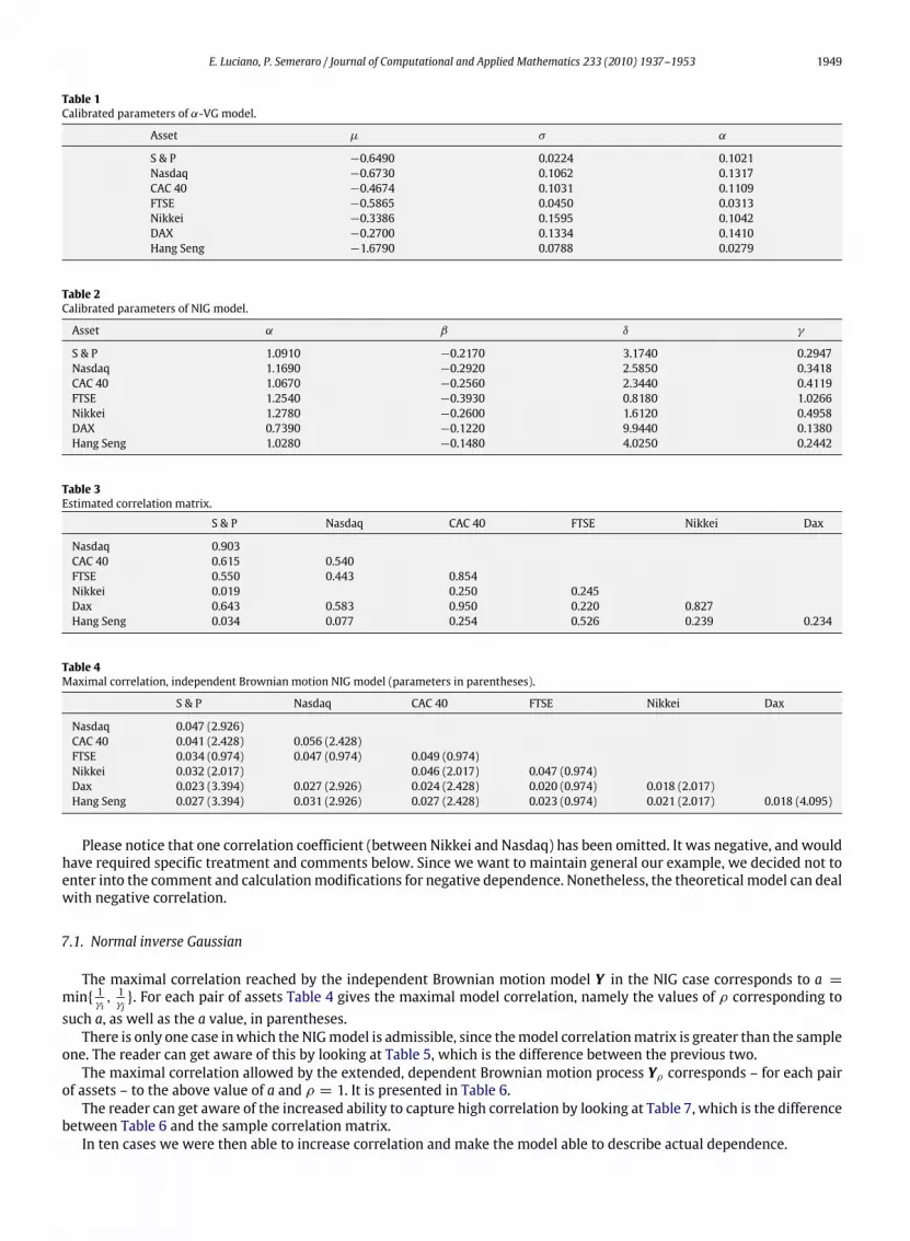
E. Luciano, P. Semeraro / Journal of Computational and Applied Mathematics 233 (2010) 1937–1953 1949
Table 1Calibrated parameters of α-VG model.
Asset µ σ α
S & P −0.6490 0.0224 0.1021Nasdaq −0.6730 0.1062 0.1317CAC 40 −0.4674 0.1031 0.1109FTSE −0.5865 0.0450 0.0313Nikkei −0.3386 0.1595 0.1042DAX −0.2700 0.1334 0.1410Hang Seng −1.6790 0.0788 0.0279
Table 2Calibrated parameters of NIG model.
Asset α β δ γ
S & P 1.0910 −0.2170 3.1740 0.2947Nasdaq 1.1690 −0.2920 2.5850 0.3418CAC 40 1.0670 −0.2560 2.3440 0.4119FTSE 1.2540 −0.3930 0.8180 1.0266Nikkei 1.2780 −0.2600 1.6120 0.4958DAX 0.7390 −0.1220 9.9440 0.1380Hang Seng 1.0280 −0.1480 4.0250 0.2442
Table 3Estimated correlation matrix.
S & P Nasdaq CAC 40 FTSE Nikkei Dax
Nasdaq 0.903CAC 40 0.615 0.540FTSE 0.550 0.443 0.854Nikkei 0.019 0.250 0.245Dax 0.643 0.583 0.950 0.220 0.827Hang Seng 0.034 0.077 0.254 0.526 0.239 0.234
Table 4Maximal correlation, independent Brownian motion NIG model (parameters in parentheses).
S & P Nasdaq CAC 40 FTSE Nikkei Dax
Nasdaq 0.047 (2.926)CAC 40 0.041 (2.428) 0.056 (2.428)FTSE 0.034 (0.974) 0.047 (0.974) 0.049 (0.974)Nikkei 0.032 (2.017) 0.046 (2.017) 0.047 (0.974)Dax 0.023 (3.394) 0.027 (2.926) 0.024 (2.428) 0.020 (0.974) 0.018 (2.017)Hang Seng 0.027 (3.394) 0.031 (2.926) 0.027 (2.428) 0.023 (0.974) 0.021 (2.017) 0.018 (4.095)
Please notice that one correlation coefficient (between Nikkei and Nasdaq) has been omitted. It was negative, and wouldhave required specific treatment and comments below. Since we want to maintain general our example, we decided not toenter into the comment and calculationmodifications for negative dependence. Nonetheless, the theoretical model can dealwith negative correlation.
7.1. Normal inverse Gaussian
The maximal correlation reached by the independent Brownian motion model Y in the NIG case corresponds to a =min{ 1
γi, 1γj}. For each pair of assets Table 4 gives the maximal model correlation, namely the values of ρ corresponding to
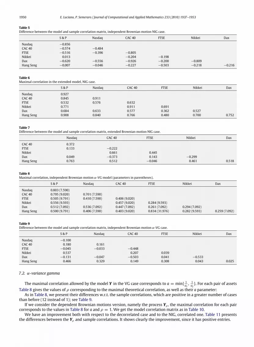
such a, as well as the a value, in parentheses.There is only one case inwhich the NIGmodel is admissible, since themodel correlationmatrix is greater than the sample
one. The reader can get aware of this by looking at Table 5, which is the difference between the previous two.The maximal correlation allowed by the extended, dependent Brownian motion process Yρ corresponds – for each pair
of assets – to the above value of a and ρ = 1. It is presented in Table 6.The reader can get aware of the increased ability to capture high correlation by looking at Table 7, which is the difference
between Table 6 and the sample correlation matrix.In ten cases we were then able to increase correlation and make the model able to describe actual dependence.
1950 E. Luciano, P. Semeraro / Journal of Computational and Applied Mathematics 233 (2010) 1937–1953
Table 5Difference between the model and sample correlation matrix, independent Brownian motion NIG case.
S & P Nasdaq CAC 40 FTSE Nikkei Dax
Nasdaq −0.856CAC 40 −0.574 −0.484FTSE −0.516 −0.396 −0.805Nikkei 0.013 −0.204 −0.198Dax −0.620 −0.556 −0.926 −0.200 −0.809Hang Seng −0.007 −0.046 −0.227 −0.503 −0.218 −0.216
Table 6Maximal correlation in the extended model, NIG case.
S & P Nasdaq CAC 40 FTSE Nikkei Dax
Nasdaq 0.927CAC 40 0.845 0.911FTSE 0.532 0.576 0.632Nikkei 0.771 0.911 0.691Dax 0.684 0.633 0.577 0.362 0.527Hang Seng 0.908 0.840 0.766 0.480 0.700 0.752
Table 7Difference between the model and sample correlation matrix, extended Brownian motion NIG case.
Nasdaq CAC 40 FTSE Nikkei Dax
CAC 40 0.372FTSE 0.133 −0.222Nikkei 0.661 0.445Dax 0.049 −0.373 0.143 −0.299Hang Seng 0.763 0.512 −0.046 0.461 0.518
Table 8Maximal correlation, independent Brownian motion α-VG model (parameters in parentheses).
S & P Nasdaq CAC 40 FTSE Nikkei Dax
Nasdaq 0.803 (7.590)CAC 40 0.795 (9.020) 0.701 (7.590)FTSE 0.505 (9.791) 0.410 (7.590) 0.406 (9.020)Nikkei 0.556 (9.593) 0.457 (9.020) 0.284 (9.593)Dax 0.512 (7.092) 0.536 (7.092) 0.447 (7.092) 0.261 (7.092) 0.294 (7.092)Hang Seng 0.500 (9.791) 0.406 (7.590) 0.403 (9.020) 0.834 (31.976) 0.282 (9.593) 0.259 (7.092)
Table 9Difference between the model and sample correlation matrix, independent Brownian motion α-VG case.
S & P Nasdaq CAC 40 FTSE Nikkei Dax
Nasdaq −0.100CAC 40 0.180 0.161FTSE −0.045 −0.033 −0.448Nikkei 0.537 0.207 0.039Dax −0.131 −0.047 −0.503 0.041 −0.533Hang Seng 0.466 0.329 0.149 0.308 0.043 0.025
7.2. α-variance gamma
The maximal correlation allowed by the model Y in the VG case corresponds to a = min{ 1αi, 1αj}. For each pair of assets
Table 8 gives the values of ρ corresponding to the maximal theoretical correlation, as well as their a parameter:As in Table 8, we present their differences w.r.t. the sample correlations, which are positive in a greater number of cases
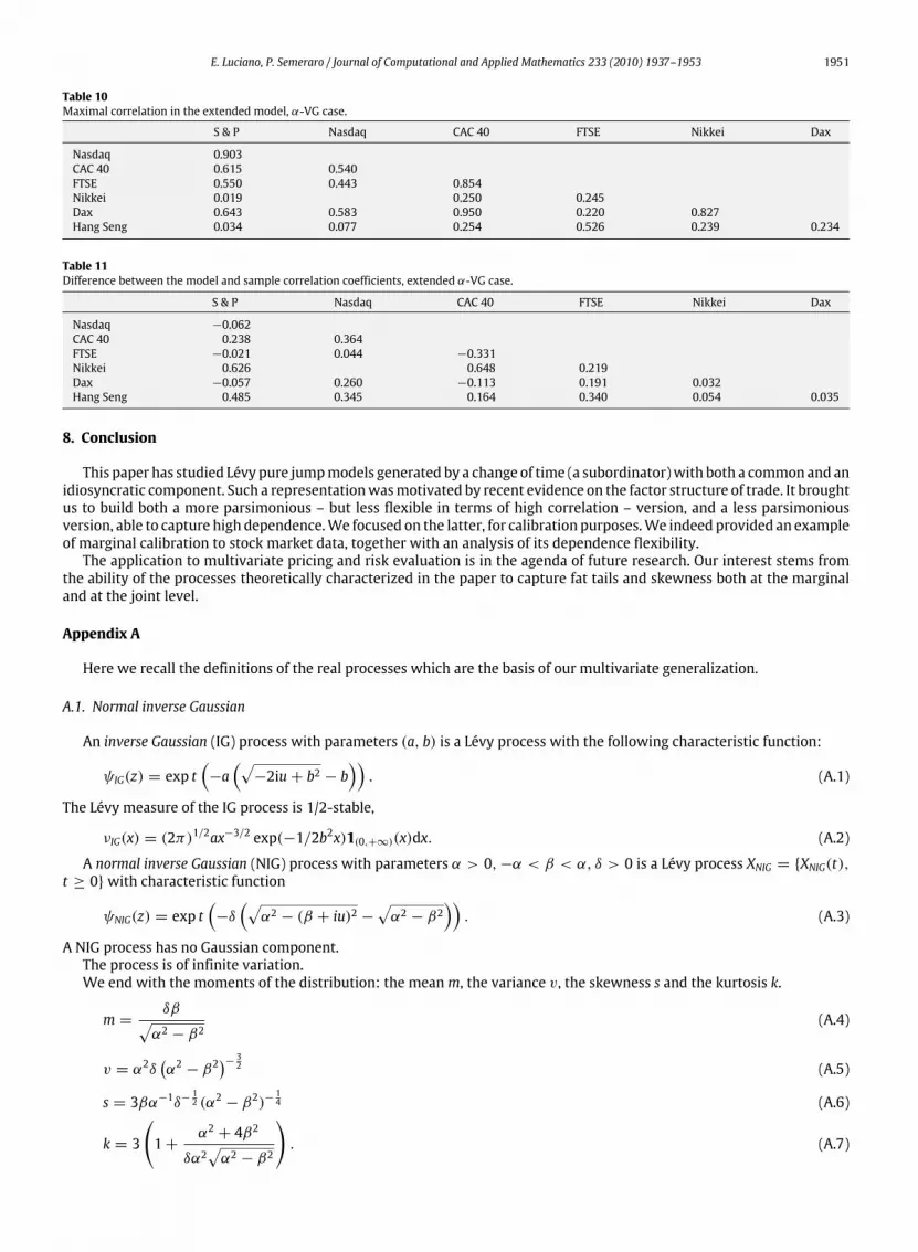
than before (12 instead of 1); see Table 9.If we consider the dependent Brownian motions version, namely the process Yρ , the maximal correlation for each pair
corresponds to the values in Table 8 for a and ρ = 1. We get the model correlation matrix as in Table 10.We have an improvement both with respect to the decorrelated case and to the NIG, correlated one. Table 11 presents
the differences between the Yρ and sample correlations. It shows clearly the improvement, since it has positive entries.
E. Luciano, P. Semeraro / Journal of Computational and Applied Mathematics 233 (2010) 1937–1953 1951
Table 10Maximal correlation in the extended model, α-VG case.
S & P Nasdaq CAC 40 FTSE Nikkei Dax
Nasdaq 0.903CAC 40 0.615 0.540FTSE 0.550 0.443 0.854Nikkei 0.019 0.250 0.245Dax 0.643 0.583 0.950 0.220 0.827Hang Seng 0.034 0.077 0.254 0.526 0.239 0.234
Table 11Difference between the model and sample correlation coefficients, extended α-VG case.
S & P Nasdaq CAC 40 FTSE Nikkei Dax
Nasdaq −0.062CAC 40 0.238 0.364FTSE −0.021 0.044 −0.331Nikkei 0.626 0.648 0.219Dax −0.057 0.260 −0.113 0.191 0.032Hang Seng 0.485 0.345 0.164 0.340 0.054 0.035
8. Conclusion
This paper has studied Lévy pure jumpmodels generated by a change of time (a subordinator)with both a common and anidiosyncratic component. Such a representationwasmotivated by recent evidence on the factor structure of trade. It broughtus to build both a more parsimonious – but less flexible in terms of high correlation – version, and a less parsimoniousversion, able to capture high dependence.We focused on the latter, for calibration purposes.We indeed provided an exampleof marginal calibration to stock market data, together with an analysis of its dependence flexibility.The application to multivariate pricing and risk evaluation is in the agenda of future research. Our interest stems from
the ability of the processes theoretically characterized in the paper to capture fat tails and skewness both at the marginaland at the joint level.
Appendix A
Here we recall the definitions of the real processes which are the basis of our multivariate generalization.
A.1. Normal inverse Gaussian
An inverse Gaussian (IG) process with parameters (a, b) is a Lévy process with the following characteristic function:
ψIG(z) = exp t(−a
(√−2iu+ b2 − b
)). (A.1)
The Lévy measure of the IG process is 1/2-stable,
νIG(x) = (2π)1/2ax−3/2 exp(−1/2b2x)1(0,+∞)(x)dx. (A.2)
A normal inverse Gaussian (NIG) process with parameters α > 0,−α < β < α, δ > 0 is a Lévy process XNIG = {XNIG(t),t ≥ 0}with characteristic function
ψNIG(z) = exp t(−δ
(√α2 − (β + iu)2 −
√α2 − β2
)). (A.3)
A NIG process has no Gaussian component.The process is of infinite variation.We end with the moments of the distribution: the meanm, the variance v, the skewness s and the kurtosis k.
m =δβ√α2 − β2
(A.4)
v = α2δ(α2 − β2
)− 32 (A.5)
s = 3βα−1δ−12 (α2 − β2)−
14 (A.6)
k = 3
(1+
α2 + 4β2
δα2√α2 − β2
). (A.7)
1952 E. Luciano, P. Semeraro / Journal of Computational and Applied Mathematics 233 (2010) 1937–1953
A.2. Variance gamma
A variance gamma process is a real Lévy process XVG = {XVG(t), t ≥ 0}which can be obtained as a Brownian motion withdrift time changed by a gamma process.A gamma process {G(t), t ≥ 0}with parameters (a, b) is a Lévy process so that the defining distribution of X(1) is gamma
with parameters (a, b) (shortlyL(X(1)) = Γ (a, b)). It is a finite variation Lévy process. Its Lévy triplet is
γ =a (1− exp(−b))
b,
A = 0νG(dx) = a exp(−bx)x−11(0,+∞)(x)dx.
Let {B(t), t ≥ 0} be a standard Brownian motion, {G(t), t ≥ 0) be a gamma process with parameters ( 1ν, 1ν) and σ > 0,
θ be real parameters; then the process XVG is defined as
XVG(t) = θG(t)+ σB(G(t)).
The characteristic function of XVG is the following
ψVG(u) =(1− iuθν +
12σ 2νu2
)− tν. (A.8)
The paths of the VG process are of infinite activity and finite variation. We end with the moments of the distribution: themeanm, the variance v, the skewness s and the kurtosis k.
m = θ (A.9)
v = σ 2 + νθ2 (A.10)
s =θν(3σ 2 + 2νθ2)(σ 2 + νθ2)3/2
(A.11)
k = 3(1+ 2ν − 4νσ 4(σ 2 + νθ2)−2). (A.12)
A.3. CGMY
The Carr Geman Madan Yor [16] process is a Lévy process Xcgmy = {Xcgmy(t), t ≥ 0}whose characteristic function is
ψcgmy(u) = exp(CtΓ (−Y )((M − iu)Y −MY + (G+ iu)Y − GY )), (A.13)
where c, g,m > 0 and y < 2. The path regularity changes for different values of the parameter y: if y < 0 the paths havefinite activity; if y ∈ [0, 1) they have infinite activity and finite variation; if y ∈ [1, 2) they have infinite variation.
Appendix B
B.1. Stable subordinators
In this appendix we recall some properties of stable and tempered stable subordinators. For a complete treatmentsee [20].A random variable X has stable distribution with parameters 0 < α ≤ 2, σ > 0, −1 < β < 1 and γ ∈ R, shortly
X ∼ Sα(σ , β, γ ), if its characteristic function has the form:
ψX (z) =
exp
{−σ α|z|α
(1− β(sign z) tan
πα
2
)+ iγ z
}, α 6= 1
exp{−σ |z|
(1+ β(sign z)β
2πln|z|
)+ iγ z
}α = 1.
(B.1)
Since γ affects only location, we assume γ = 0 for simplicity.An α-stable real subordinator G is given by a stable random variable X with support [0,∞), X ∼ Sα(σ , 1, 0) with
0 < α < 1.The Lévy measure of a stable subordinator has the following expression
νG(dx) =cGxα+1
1x>0, (B.2)
where cG = c(α)σ α , c(α) > 0 and 1x>0 is the indicator function of the set x > 0.
E. Luciano, P. Semeraro / Journal of Computational and Applied Mathematics 233 (2010) 1937–1953 1953
If the subordinators Xj and Z are α-stable then G has α-stable margins. Let Xj ∼ Sα(σj, 1, 0) and Z ∼ Sα(σz, 1, 0), so thatαjZ ∼ Sα(σzαj, 1, 0). By Propositions 1.2.1 and 1.2.3 in [20] Xj + αjZ is α-stable and its law is
L(Xj + αjZ) = Sα(σGj , 1, 0), (B.3)
where σGj = (σαj + (σzαj)
α)1/α .Tempered stable subordinators, first introduced in [21], are characterized by the following Lévy measure:
ν(x) =ce−λx
xα+11x>0. (B.4)
Let us denote the corresponding infinitely divisible distribution by X ∼ TSα(c, λ), where 0 < α < 1, λ > 0 and c > 0.The distribution of the sum of two tempered stable processes, analogously to the non-tempered case, can be characterizedas follows: if X ∼ TSα(cX , λ) and Y ∼ TSα(cY , λ) their sum is TSα(cX + cY , λ) and αiX ∼ TSα(cXααi ,
λαi). Therefore if Xi ∼
TSα(ci, λαi ) for i = 1, . . . , n and Z ∼ TSα(cz, γz, λ), then G has margins TSα(ci + czααi ,
λαi).
Consider a stable subordinator GB with Lévy measure given by (B.2). A subordinator GA is absolutely continuous withrespect to GB (see [15,17] for a more general definition), if
νA(dx) = f (x)νB(dx) = f (x)cGx1+α
dx (B.5)
and ∫∞
0νB(dt)(
√f (t)− 1)2 <∞, (B.6)
where f (x) is called the density. Obviously if Xj and Z are α-stable continuous with the same density, their sum is.All the previous classes of subordinators are characterized by the fact that the difference between the Lévy measures of
Xj, Z and Gj is a constant.
References
[1] J. Karpoff, The relation between price changes and trading volume: A survey, Journal of Financial and Quantitative Analysis 22 (1987) 109–126.[2] M. Richardson, T. Smith, A direct test ofmixture distriution hypotesis:Measrnig the daily flow of information, The Journal of Financial andQuantitativeAnalysis 29 (1994) 101–116.
[3] H. Geman, T. Ané, Order flow, transaction clock, and normality of asset returns, Journal of Finance 55 (5) (2000) 2259–2284.[4] R. Cont, P. Tankov, Financial Modelling with Jump Processes, in: Financial Mathematics Series, Chapman and Hall, CRC, 2004.[5] L. Harris, Cross-security tests of the mixture distribution, The Journal of Finacial and Quantitative Analysis 21 (1986) 39–46.[6] A.W. Lo, J. Wang, Trading volume: Definitions, data analysis, and implications of portfolio theory, Review of Financial Studies 13 (2) (2000) 257–300.[7] O.E. Barndorff-Nielsen, J. Pedersen, K.I. Sato, Multivariate subordination, self-decomposability and stability, Advances in Applied Probability 33 (2001)160–187.
[8] E. Eberlein, D.B. Madan, M. Yor, On correlating Lévy processes, 2009, Preprint.[9] P. Semeraro, A multivariate Variance Gamma model for financial application, Journal of Theoretical and Applied Finance 11 (2008) 1–18.[10] E. Luciano, P. Semeraro, A generalized normal mean variance mixture for return processes in finance, International Journal of Theoretical and Applied
Finance (in press).[11] H. Geman, D.B. Madan, M. Yor, Time changes for Lé vy processes, Mathematical Finance 11 (2001) 79–96.[12] O.E. Barndorff-Nielsen, Normal inverse Gaussian distributions and the modeling of stock returns, Research report no. 300, Department of Theoretical
Statistics, Aarhus University, 1995.[13] D.B. Madan, E. Seneta, The v.g. model for share market returns, Journal of Business 63 (1990) 511–524.[14] E. Luciano, W. Schoutens, A multivariate jump-driven financial asset model, Quantitative Finance 6 (5) (2006) 385–402.[15] D.B. Madan, M. Yor, CGMY and Meixner Subordinators are Absolutely Continuous with respect to One Sided Stable Subordinator, 2005, Preprint.[16] P. Carr, H. Geman, D.H. Madan, M. Yor, The fine structure of asset returns: An empirical investigation, Journal of Business 75 (2002) 305–332.[17] K.I. Sato, Lévy processes and Infinitely divisible distributions, in: Cambridge Studies in Advanced Mathematics, Cambridge University Press, 2003.[18] D.B. Madan, J. Wang, A new multivariate variance gamma model and multi-asset option pricing, in: AFMathConf 2009, 2009 (in press).[19] K. Chourdakis, Option pricing using the fractional FFT, Journal of Computational Finance 8 (2) (2005) 1–18.[20] G. Samorodnitsky, M.S. Taqqu, Stable Non-gaussian Random Processes. Stochastic Models with Infinite Variance, Chapman & Hall, 1994.[21] M.C.K. Tweedie, An indexwhic distinguishes between some important exponential families, in: J. Ghosh, J. Roy (Eds.), Statistics: Applications and new
directions: Proc. Indian Statistical Institute Golden Jubilee International Conference, 1984, pp. 579–604.
Related Documents
![Lévy Processes and Lévy White Noise as Tempered Distributions · arXiv:1509.05274v1 [math.PR] 17 Sep 2015 Lévy Processes and Lévy White Noise as Tempered Distributions Robert](https://static.cupdf.com/doc/110x72/5c4bf79693f3c31436469ec3/levy-processes-and-levy-white-noise-as-tempered-distributions-arxiv150905274v1.jpg)