Introduction 1 VRIJE UNIVERSITEIT BRUSSEL Faculteit Geneeskunde en Farmacie Laboratorium voor Farmaceutische en Biomedische Analyse N EW TRENDS IN MULTIVARIATE ANALYSIS AND C ALIBRATION Frédéric ESTIENNE Thesis presented to fulfil the requirements for the degree of doctor in Pharmaceutical Sciences Academic year : 2002/2003 Promotor : Prof. Dr. D.L. MASSART

Welcome message from author
This document is posted to help you gain knowledge. Please leave a comment to let me know what you think about it! Share it to your friends and learn new things together.
Transcript
Introduction
1
VRIJE UNIVERSITEIT BRUSSEL
Faculteit Geneeskunde en Farmacie
Laboratorium voor Farmaceutische en Biomedische Analyse
NEW TRENDS IN MULTIVARIATE ANALYSIS AND CALIBRATION
Frédéric ESTIENNE
Thesis presented to fulfil the requirements for
the degree of doctor in Pharmaceutical Sciences
Academic year : 2002/2003
Promotor : Prof. Dr. D.L. MASSART

New Trends in Multivariate Analysis and Calibration
2

Introduction
3
ACKNOWLEDGMENTS
First of all, I would like to thank Professor Massart for allowing me to spend these almost four years in
his team. The knowledge I acquired, the experience I gained, and most probably the reputation of this
formation gave a new and by far better start to my professional life.
For the rest, the list of people I have to thank would be too long to be printed here. Not even
mentioning I might accidentally omit someone. So I will probably play it the safe way and simply
thank everyone I enjoyed studying, working, having fun, gossiping (etc …) with during all these years.
Thank you all !
New Trends in Multivariate Analysis and Calibration
4
TABLE OF CONTENTS
ACKNOWLEDGMENTS 2
TABLE OF CONTENTS 4
LIST OF ABBREVIATIONS 6
___________ INTRODUCTION ___________
8
___________ I . MULTIVARIATE ANALYSIS AND CALIBRATION ___________
12
“Chemometrics and modelling.” 12
___________ II . COMPARISON OF MULTIVARIATE CALIBRATION METHODS ___________
38
“A Comparison of Multivariate Calibration Techniques Applied to Experimental NIR Data
Sets. Part II : Predictive Ability under Extrapolation Conditions” 40
“A Comparison of Multivariate Calibration Techniques Applied to Experimental NIR Data
Sets. Part III : Robustness Against Instrumental Perturbation Conditions” 70
“The Development of Calibration Models for Spectroscopic Data using Multiple Linear
Regression” 99

Introduction
5
___________ III . NEW TYPES OF DATA : NATURE OF THE DATA SET ___________
168
“Multivariate calibration with Raman spectroscopic data : a case study” 170
“Inverse Multivariate calibration Applied to Eluxyl Raman data“ 200
___________ IV . NEW TYPES OF DATA : STRUCTURE AND SIZE ___________
212
“Multivariate calibration with Raman data using fast PCR and PLS methods” 214
“Multi-Way Modelling of High-Dimensionality Electro-Encephalographic Data” 225
“Robust Version of Tucker 3 Model” 250
___________ CONCLUSION ___________
270
PUBLICATION LIST 274

New Trends in Multivariate Analysis and Calibration
6
LIST OF ABBREVIATIONS
ADPF Adaptative-degree polynomial filter
AES Atomic emission spectroscopy
ALS Alternating least squares
ANOVA Analysis of variance
ASTM American society for testing material
CANDECOMP Canonical Decomposition
CCD Coupled charge device
CV Cross-validation
DTR De-trending
EEG Electro-encephalogram
FFT Fast Fourier transform
FT Fourier Transform
GA Genetic algorithm
GC Gas chromatography
ICP Induced coupled plasma
IR Infrared
k-NN k-nearest neighbours
LMS Least median of squares
LOO Leave-one-out
LV Latent variable
LWR Locally weighted regression
MCD Minimumm covariance determinant
MD Mahalanobis distance
MLR Multiple Linear Regression
MSC Multiple scatter correction
MSEP Mean squared error of prediction
MVE Minimum volume ellipsoid
Introduction
7
MVT Multivariate trimming
NIPALS Nonlinear iterative partial least squares
NIR Near-infrared
NL-PCR Non-linear principal component regression
NN Neural networks
NPLS N-way partial least squares
OLS Ordinary least squares
PARAFAC Parallel factor analysis
PC Principal component
PCA Principal component analysis
PCC Partial correlation coefficient
PCR Principal component regression
PCRS Principal component regression with selection of PCs
PLS Partial least squares
PP Projection pursuit
PRESS Prediction error sum of squares
QSAR Quantitative structure-activity relationship
RBF Radial basis function
RCE Relevant components extraction
RMSECV Root mean squared error of cross validation
RMSEP Root mean squared error of prediction
RVE Relevant variable extraction
SNV Standard normal variate
SPC Statistical process control
SVD Singular value decomposition
TLS Total least squares
UVE Uninformative variables elimination
New Trends in Multivariate Analysis and Calibration
8
NEW TRENDS IN MULTIVARIATE ANALYSIS AND CALIBRATION
INTRODUCTION
Many definitions have been given for Chemometrics. One of the most frequently quoted of these
definitions [1] states the following :
Chemometrics is a chemical discipline that uses mathematics, statistics and formal logic (a) to design
or select optimal experimental procedures; (b) to provide the maximum relevant chemical information
by analysing chemical data; and (c) to obtain knowledge about chemical systems.
This thesis focuses specifically on points (b) and (c) of this definition, and a particular emphasis is
placed on multivariate methods and how they are used to model data. It should be noted that, while
modelling is probably the most important area of chemometrics, there are many other applications such
as method validation, optimisation, statistical process control, signal processing, etc.
Modelling methods can be divided into two groups of methods, even if these two groups are often
widely overlapping. In multivariate data analys is, models are used directly for data interpretation. In
multivariate calibration, models relate the data to a given property in order to predict this property.
Modelling methods in general are introduced in Chapter 1. The most common multivariate data
analysis and calibration methods are presented as well as some more advanced ones, in particular
methods applying to data with complex structure.
A particularity of chemometrics is that many methods used in the field were developed in other areas of
science before they were imported to chemistry. This is for instance the case for Partial Least Squares,
which was initially developed to build economical models. Chemometrics also covers a very wide
domain of application, and specialists in each field develop or modify methods best suited for their
particular applications. These factors lead to the fact that many methods are often available for a given
Introduction
9
problem. The first step of the chemometrical methodology is therefore to select the most appropriate
method to use. The importance of this step is illustrated in Chapter 2. Multivariate calibration methods
are compared on data with different structures. This comparison is performed in situations challenging
for the methods (data extrapolation, instrumental perturbation). A detailed description of the steps
necessary to develop a multivariate calibration model is also provided using Multiple Linear
Regression as a reference method.
Multivariate calibration and Near Infrared (NIR) spectroscopy have a parallel history. NIR could only
be routinely implemented through the use of sophisticated chemometrical tools and the arising of
modern computing. Chemometrical methods were then widely promoted by the remarkable
achievements of multivariate calibration applied to NIR data. For many years, multivariate calibration
and NIR spectroscopy were therefore almost synonym for the non-specialist. In the last few years,
chemometrical methods proved very efficient on other types of analytical data. This was sometimes the
case even for analytical methods that were not considered as necessitating sophisticated data treatment.
It is shown in chapter 3 how Raman spectroscopic data can benefit from chemometrics in general and
multivariate calibration in particular, allowing the use of Raman in a growing number of industrial
applications. This chapter also illustrates the importance of method selection in chemometrics, and
shows that the choice of the most appropriate method to use can depend on many factors, for instance
quality of the data set.
During the last years, data treated by chemometricians tend to become more and more complex. This
complexity can be understood in terms of volume of data, or in terms of data structure. The increasing
size of chemometrical data sets has several causes. For instance, combinatorial chemistry and high
throughput screening are designed to generate important volumes of data. Collections of samples
recorded during time also tend to get larger and larger. The improvement of analytical instruments
leads to better spectral resolutions and therefore larger data sets (sometimes several tens of thousands
of items). This last point is illustrated in chapter 4. It is shown how calibration methods specifically
designed to be fast can considerably reduce computation time required for calibration and prediction of
new samples. Complexity of a data set can also be understood in terms of data structure. Methods
developed in the area of psychometrics allowing to treat data that are not only multivariate, but also
multidimodal were recently introduced in the chemometrical field. Chapter 4 shows how this kind of
New Trends in Multivariate Analysis and Calibration
10
methods can be used to extract information from a very complex data set with up to 6 modes. This
chapter gives another illustration of the fact that chemometrical methods can be applied to new types of
data, even out of the strict domain of chemistry, since the multidimodal methods are applied to
pharmaceutical Electro-Encephalographic Data. Another example is given showing how these methods
can be adapted in order to be made more robust toward difficult data sets.
REFERENCES
[1] D.L. Massart, B.G.M. Vandeginste, L.M.C. Buydens, S. de Jong, P.J. Lewi and J. Smeyers-
Verbeke, Handbook of Chemometrics, Elsevier, Amsterdam, 1997.

Introduction
11
New Trends in Multivariate Analysis and Calibration
12
CHAPTER I
MULTIVARIATE ANALYSIS AND CALIBRATION
Adapted from :
CHEMOMETRICS AND MODELLING
Computational Chemistry Column, Chimia, 55, 70-80 (2001).
F. Estienne, Y. Vander Heyden and D.L. Massart
Farmaceutisch Instituut,
Vrije Universiteit Brussel,
Laarbeeklaan 103,
B-1090 Brussels, Belgium.
E-mail: [email protected]
Chapter 1 – Multivariate Analysis and Calibration
13
1. Introduction
There are two types of modelling. Modelling can in the first place be applied to extract useful
information from a large volume of data, or to achieve a better understanding of complex phenomena.
This kind of modelling is sometimes done through the use of simple visual representations. Depending
on the type of data studied and the field of application, modelling is then referred to as exploratory
multivariate analysis or data mining. Modelling can in the second place be applied when two or more
characteristics of the same objects are measured or calculated and then related to each other. It is for
instance possible to relate the concentration of a chemical compound to an instrumental signal, the
chemical structure of a drug to its activity or instrumental responses to sensory characteristics. In these
situations, the purpose of modelling usually is, after a calibration process, to make predictions (e.g.
predict the concentration of a certain analyte in a sample from a measured signal), but it can sometimes
simply be to verify the nature of the relationship. The two types of modelling strongly overlap. The
methods introduced in this chapter will therefore not be presented as being exploratio n or calibration
oriented, but rather will be introduced by rank of increasing complexity of the type of data or modelling
problem they are applied to.
2. Univariate regression
2.1. Classical univariate least squares : straight line models
Before introducing some of the more sophisticated methods, we should look shortly at the classical
univariate least squares methodology (often called ordinary least squares – OLS), which is what
analytical chemists generally use to construct a (linear) calibration line. In most analytical techniques
the concentration of a sample cannot be measured directly but is derived from a measured signal that is
in direct relation with the concentration. Suppose the vector x represents the concentrations of samples
and y the corresponding measured instrumental signal. To be able to define a model y = f(x) a
relationship between x and y has to exist. The simplest and most convenient situation is when the
relation is linear which leads to a model of the type :
New Trends in Multivariate Analysis and Calibration
14
y = b0 + b1x (1)
which is the equation of a straight line. The coefficients b0 and b1 represent the intercept and the slope
of the line. Relationships between y and x that follow a curved line can for instance be represented by a
regression model of the type :
y = b0 + b1x + b11x2 (2)
The least squares regression analysis is a methodology that allows to estimate the coefficients of a
given model. For calibration purposes one usually focuses on straight- line models which we also will
do in the rest of this section. Conventionally the x-values represent the so-called controlled or
independent variable, i.e. the variable that is considered not to have a measurement error (or a
negligible one), which is the concentration in our case. The y values represent the dependent variable,
i.e. the measured response, which is considered to have a measurement error. The least squares
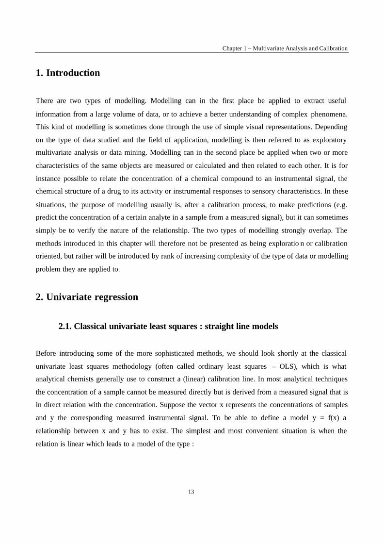
approach allows to obtain b0 and b1 values such that the model fits the measured points (xi, yi) best.
Fig. 1. Straight line fitting through a series of measured points.
The true relationship between x and y is considered to be y = β0 + β1x while the relationship between
each xi and its measured yi can be represented as yi = b0 + b1xi + ei. The signal yi is composed of a
Chapter 1 – Multivariate Analysis and Calibration
15
component predicted by the model, b0 + b1x, and a random component, ei, the residual (Fig. 1). The
least squares regression finds the estimates b0 and b1 for β0 and β1 by calculating the values b0 and b1
for which ∑ei2 = ∑ (yi – b0 – b1xi)2, the sum of the squared residuals, is minimal. This explains the
name “least squares”. Standard books about regression, including least squares approaches are [1,2].
Analytical chemists can find information in [3,4].
2.2. Some variants of the univariate least square straight line models
A fundamental assumption of OLS is that there are only errors in the direction of y. In some instances,
two measured quantities are related to each other and the assumption then does not hold, because there
are also measurement errors in x. This is for instance the case when two analytical methods are
compared to each other. Often one of these methods is a reference method and the other a new method,
which is faster or cheaper and it is wanted to demonstrate that the results of both methods are
sufficiently similar. A certain number of samples are analysed with both methods and a straight line
model relating both series of measurements is obtained. If β0 as estimated from b0 is not more different
from 0 than an a priori accepted bias and β1 as estimated by b1 is not more different from 1 than a given
amount, then one can accept that for practical purposes y = x. In its simplest statistical expression, this
means that it is tested that β0 = 0 and β1 = 1 or to put it in another way that b0 is statistically different
from 0 and/or b1 is statistically different from 1. If this is the case then it is concluded that the two
methods do not yield the same result but that there is a constant (intercept) or proportional (slope)
systematic error or bias. This means that one should calculate b0 and b1 and at first sight this could be
done by OLS. However both regression variables (not only yi but now also xi) are subject to error, as
already mentioned. This violates one of the key assumptions of the OLS calculations.
It has been shown [4-7] that the computation of b0 and b1 according to the OLS-methods leads to wrong
estimates of β0 and β1. Significant errors in the least squares estimate of b1 can be expected if the ratio
between the measurement error on the x values and the range of the x values is large. In that case OLS
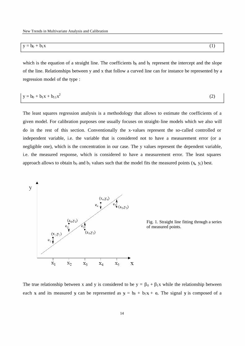
should not be used. To obtain correct values for b0 and b1 the sum of least squares must now be
obtained in the direction given in figure 2. Such methods are sometimes called errors in variables
models or orthogonal least squares. Detailed studies of the application of models of these types can be
found in [8,9].
New Trends in Multivariate Analysis and Calibration
16
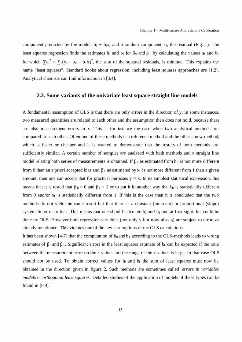
Fig. 2. The errors-in-variables model.
Another possibility is to apply inverse regression. The term inverse is applied in opposition to t he usual
calibration procedure. Calibration consists of measuring samples with a known characteristic and
deriving a calibration line (or more generally a model). A measurement is then carried out for an
unknown sample and its concentration is derived from the measurement result and the calibration line.
In view of the assumptions of OLS, the measurement is the y-value and the concentration the x-value,
i.e.
measurement = f (concentration) (3)
This relationship can be inverted to become
Concentration = f (measurement) (4)
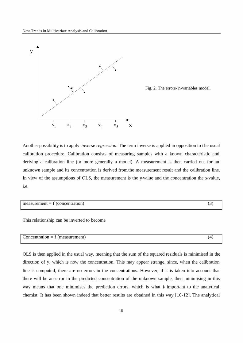
OLS is then applied in the usual way, meaning that the sum of the squared residuals is minimised in the
direction of y, which is now the concentration. This may appear strange, since, when the calibration
line is computed, there are no errors in the concentrations. However, if it is taken into account that
there will be an error in the predicted concentration of the unknown sample, then minimising in this
way means that one minimises the prediction errors, which is what is important to the analytical
chemist. It has been shown indeed that better results are obtained in this way [10-12]. The analytical
Chapter 1 – Multivariate Analysis and Calibration
17
chemist should therefore really apply eq. (4), instead of the usual eq. (3). In most cases the difference in
prediction qua lity between both approaches is very small in practice, so that there is generally no harm
in applying eq. (3). We will see however that when multivariate calibration is applied, inverse
regression is the rule. It should be noted that, when the aim is not to predict y-values, but to obtain the
best possible estimates of β0 and β1, inverse regression performs worse than the usual procedure.
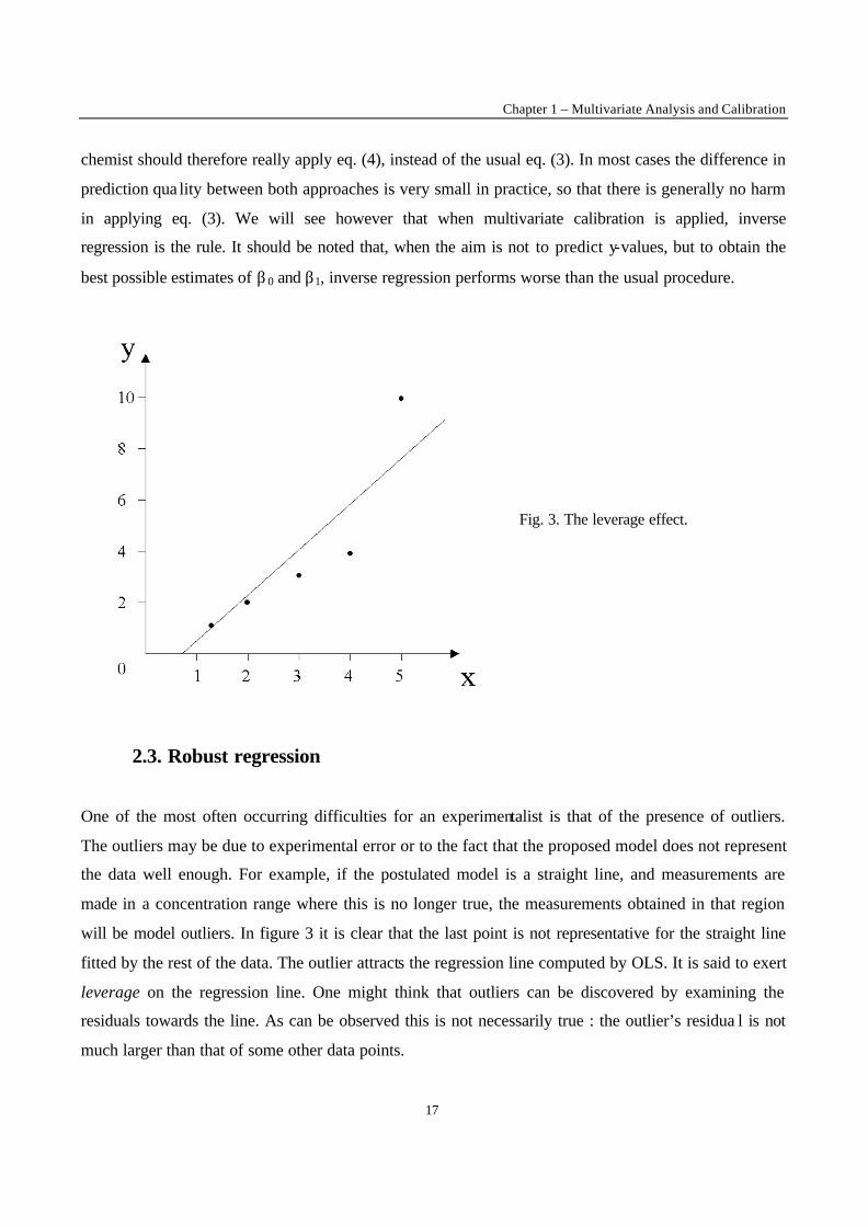
Fig. 3. The leverage effect.
2.3. Robust regression
One of the most often occurring difficulties for an experimentalist is that of the presence of outliers.
The outliers may be due to experimental error or to the fact that the proposed model does not represent
the data well enough. For example, if the postulated model is a straight line, and measurements are
made in a concentration range where this is no longer true, the measurements obtained in that region
will be model outliers. In figure 3 it is clear that the last point is not representative for the straight line
fitted by the rest of the data. The outlier attracts the regression line computed by OLS. It is said to exert
leverage on the regression line. One might think that outliers can be discovered by examining the
residuals towards the line. As can be observed this is not necessarily true : the outlier’s residua l is not
much larger than that of some other data points.
New Trends in Multivariate Analysis and Calibration
18
To avoid the leverage effect, the outlier(s) should be eliminated. One way to achieve this is to use more
efficient outlier diagnostics than simply looking at residuals. Cook’s squared distance or the
Mahalanobis distance can for instance be used.
A still more elegant way is to apply so-called robust regression methods. The easiest to explain is
called the single median method [13]. The slope between each pair of points is computed. For instance
the slope between points 1 and 2 is 1.10, between 1 and 3 1.00, between 5 and 6 6.20. The complete list
is 1.10, 1.00, 1.03, 0.95, 2.00, 0.90, 1.00, 0.90, 2.23, 1.10, 0.90, 2.67, 0.70, 3.45, 6.20. These are now
ranked and the median slope (here the 8-th value 1.03) is chosen. All pairs of points of which the
outlier is one point have high values and end up at the end of the ranking, so that they do not have an
influence on the chosen median slope : even if the outlier was still more distant, the selected media n
would still be the same. A similar procedure for the intercept, which we will not explain in detail, leads
to the straight line equation y = 0.00 + 1.03 x, which is close to the line obtained with OLS after
eliminating the outlier. The single median method is not the best robust regression method. Better
results are obtained with the least median of squares method (LMS) [14], the iteratively re-weighted
[15] or bi-weight regression [16]. Comparing results of calibration lines obtained with OLS and with a
robust method is one way of finding outliers towards a regression model [17].
3. Multiple Linear Regression
3.1. Multivariate (multiple) regression
Multivariate regression, also often called multiple regression or multiple linear regression (MLR) in the
linear case, is used to obtain values for the b-coefficients in an equation of the type :
y = b0 + b1x1 + b2x2 + … bmxm (5)
where x1, x2, …, xm are different variables. In analytical spectroscopic applications, these variables
could be the absorbances obtained at different wavelengths, y being a concentration or other
characteristic of the samples to be predicted, in QSAR (the study of quantitative structure-activity
relationships) they could be variables such as hydrophobicity (log P), the Hammett electronic

Chapter 1 – Multivariate Analysis and Calibration
19
parameter σ, with y being some measure of biological activity. In experimental design, equations of the
type
y = b0 + b1x1 + b2x2 + b12x1x2 + b11x12 + b22x2
2 (6)
are used to describe a response y as a function of the experimental variables x1 and x2. Both equations
(5) and (6) are called linear, which may surprise the non-initiated, since the shape of the relationship
between y and (x1,x2) is certainly not linear. The term linear should be understood as linear in the
regression parameters. An equation such as y = b0 + log (x – b1) is non- linear [2].
It can be observed from the applications cited higher that multiple regression models occur quite often.
We will first consider the classical solution to estimate the coefficients. Later we will describe some
more sophisticated methodologies introduced by chemometricians, such as those based on latent
vectors.
As for the univariate case, the b-values are estimates of the true b-parameters and the estimation is done
by minimising a (sum of) squares. It can be shown that
b = (XTX)-1XTy (7)
where b is the vector containing the b-values from eq. (5), X is an nxm matrix containing the x-values
for n samples (or objects as they are often called) and m variables and y is the vector containing the
measurements for the n samples.
A difficulty is that the inversion of the XTX matrix leads to unstable results when the x-variables are
very correlated. There are two ways to avoid this problem. One is to select variables (variable selection
or feature selection) such that correlation is reduced, the other is to combine the variables in such a way
that the resulting summarising variables are not correlated (feature reduction). Both feature selection
and feature reduction lead to a smaller number of variables than the initial number of variables, which
by itself has important advantages.
New Trends in Multivariate Analysis and Calibration
20
3.2. Wide data matrices
Chemists often produce wide data matrices, characterised by a relatively small number of objects (a
few ten to a few hundred) and a very large number of variables (many hundreds, at least). For instance,
analytical chemists now often apply very fast spectroscopic methods, such as near infrared
spectroscopy (NIR). Because of the rapid character of the analysis, there is no time for dissolving the
sample or separation of certain constituents. The chemist tries to extract the information required from
the spectrum as such and to do so he has to relate a y-value such as an octane number of gasoline
samples or a protein content of wheat samples to the absorbance at 500 to, in some cases, 10 000
wavelengths. The e.g. 1000 variables for 100 objects constitute the X matrix. Such matrices contain
many more columns than rows and are therefore often called wide. Feature selection/reduction the n
takes on a completely different complexity compared to the situations described in the preceding
sections. It should be remarked that variables in such matrices are often very correlated. This can for
instance be expected for two neighbouring wavelengths in a spectrum. In the following sections, we
will explain which methods chemometricians use to model very large, wide and highly correlated data
matrices.
3.3. Feature selection methods
3.3.1. Stepwise Selection
The classical approach, which is found in many statistical packages, is the so-called stepwise
regression, a feature selection method. The so-called forward selection procedure consists of first
selecting the variable that is best correlated with y. Suppose this is found to be xi. The model at this
stage is restricted to y = f (xi). Then, one tests all other variables by adding them to the model, which
then becomes a model in two variables y = f (xi,xj). The variable xj which is retained together with xi is
the one which, when added to the mode l, leads to the largest improvement compared to the original
model y = f (xi). It is then tested whether the observed improvement is significant. If not, the procedure
stops and the model is restricted to y = f(xi). If the improvement is significant, xj is incorporated
definitively in the model. It is then investigated which variable should be added as the third one and
whether this yields a significant improvement. The procedure is repeated until finally no further
Chapter 1 – Multivariate Analysis and Calibration
21
improvement is obtained. The procedure is based on analysis of variance and several variants such as
backwards elimination (starting with all variables and eliminating successively the least important
ones) or a combination of forward and backward methods have been proposed. It should be noted that
the criteria applied in the analysis of variance are such that selected variables are less correlated. In
certain contexts such as in experimental design or QSAR, the reason for applying feature selection is
not only to avoid the numerical difficulties described higher, but also to explain relationships. The
variables that are included in the regression equation have a chemical and physical meaning and when a
certain variable is retained it is considered that the variable influences the y-value, e.g. the biological
activity, which then leads to proposals for causal relationships. Correct feature selection then becomes
very important in those situations to avoid making wrong conclusions. One of the problems is that the
procedures involve regressing many variables on y and chance correlation may then occur [18].
There are other difficulties, for instance, the choice of experimental conditions, the samples or the
objects. These should cover the experimental domain as well as possible and, where possible, follow an
experimental design. This is demonstrated, for instance, in [19]. Outliers can also cause problems.
Detection of multivariate outliers is not evident. As for the univariate regression, robust regression is
possible [14, 20]. An interesting example in which multivariate robust regression is applied concerns an
experimental design [21] carried out to optimise the yield of an organic synthesis.
3.3.2. Genetic algorithms for feature selection
Genetic algorithms are general optimisation tools aiming at selecting the fittest solution to a problem.
Suppose that, to keep it simple, 9 variables are measured. Possible solutions are represented in figure 4.
Selected variables are indicated by a 1, non-selected variables by a 0. Such solutions are sometimes, in
analogy with genetics, called chromosomes in the jargon of the specialists.
By random selection a set of such solutions is obtained (in real applications often several hundreds).
For each solution an MLR model is built using an equation such as (5) and the sum of squares of the
residuals of the objects towards that model is determined. In the jargon of the field, one says that the
fitness of each solution is determined : the smaller the sum of squares the better the model describes the
data and the fitter the corresponding solutions are.

New Trends in Multivariate Analysis and Calibration
22
Fig. 4. A set of solutions for feature selection from nine variables for MLR
Then follows what is described as the selection of the fittest (leading to names such as genetic
algorithms or evolutionary computation). For instance out of the, say 100 original solutions, the 50
fittest are retained. They are called the parent generation. From these is obtained a child generation by
reproduction and mutation.
Reproduction is explained in figure 5. Two randomly chosen parent solutions produce two child
solutions by cross over. The cross over point is also chosen randomly. The first part of solution 1 and
the second part of solution 2 together yield child solution 1’. Solution 2’ results from the first part of
solution 2 and the second of solution 1.

Chapter 1 – Multivariate Analysis and Calibration
23
Fig. 5. Genetic algorithms: the reproduction step
The child solutions are added to the selected parent solutions to form a new generation. This is repeated
for many generations and the best solution from the final generation is retained. Each generation is
additionally submitted to mutation steps. Here and there, randomly chosen bits of the solution string are
changed (0 to 1 or 1 to 0). This is applied in figure 6.
Fig. 6. Genetic algorithms: the mutation step.
The need for the mutation step can be understood from figure 5. Suppose that the best solution is close
to one of the child solutions in that figure, but should not include variable 9. However, because the
New Trends in Multivariate Analysis and Calibration
24
value for variable 9 is 1 in both parents, it is also unavoidably 1 in the children. Mutation can change
this and move the solutions in a better direction.
Genetic algorithms were first proposed by Holland [22]. They were introduced in chemometrics by
Lucasius et al [23] and Leardi et al [24]. They were applied for instance in QSAR and molecular
modeling [25], conformational analysis [26], multivariate calibration for the determination of certain
characteristics of polymers [27] or octane numbers [28]. Reviews about applications in chemistry can
be found in [29,30]. There are several competing algorithms such as simulated annealing [31] or the
immune algorithm [32].
4. Feature reduction : Latent Variables
The alternative to feature selection is to combine the variables in what we called earlier summarising
variab les. Chemometricians call this latent variables and the obtaining of such variables is called
feature reduction. It should be understood that in this case no variables are discarded.
4.1. Principal Component Analysis
The type of latent variable most commonly used is the principal component (PC). To explain the
principle of PCs, we will first consider the simplest possible situation. Two variables (x1 and x2) were
measured for a certain number of objects and the number of variables should be reduced to one. In
principal component analysis (PCA) this is achieved by defining a new axis or variable on which the
objects are projected. The projections are called the scores, s1, along principal component 1, PC1 (Fig.
7).

Chapter 1 – Multivariate Analysis and Calibration
25
Fig. 7. Feature reduction of two variables, x1 and x2, by a principal component.
The projections along PC1 preserve the information present in the x1-x2 plot, namely that there are two
groups of data. By definition, PC1 is drawn in the direction of the largest variation through the data. A
second PC, PC2, can also be obtained. By definition it is orthogonal to the first one (Fig. 8-a). The
scores along PC1 and along PC2 can be plotted against each other yielding what is called a score plot
(Fig. 8-b).
b)
a)
Fig. 8. a) second PC and b) score plot of the data in Fig. 7.
New Trends in Multivariate Analysis and Calibration
26
The reader observes that PCA decorrelates : while the data points in the x1-x2 plot are correlated they
are not longer so in the s1-s2 plot. This also means that there was correlated and therefore redundant
information present in x1 and x2. PCA picks up all the important information in PC1 and the rest, along
PC2, is noise and can be eliminated. By keeping only PC1, feature reduction is applied : the number of
variables, originally two, has been reduced to one. This is achieved by computing the score along PC1
as :
s = w1x1 + w2x2 (8)
In other words the score is a weighted sum of the original variables. The weights are known as loadings
and plots of the loadings are called loading plots.
This can now be generalised to m dimensions. In the m-dimensional space, PC1 is obtained as the axis
of largest variation in the data, PC2 is orthogonal to PC1 and is drawn into the direction of largest
remaining variation around PC1. It therefore contains less variation (and information) than PC1. PC3 is
orthogonal to the plane of PC1 and PC2. It is drawn in the direction of largest variation around that
plane, but contains less variation than PC3. In the same way PC4 is orthogonal to the hyperplane
PC1,PC2,PC3 and contains still less variation, etc. For a matrix with dimensions n x m, N = min (n, m)
PCs can be extracted. However, since each of them contains less and less information, at a certain time
they contain only noise and the process can be stopped before reaching N. If only d << N PCs are
obtained, then feature reduction is achieved.
A very important application of principal components is to visually display the information present in
the data set and most multivariate data applications therefore start with score and/or loading plots. The
score plots give information about the objects and the loading plots about the variables. Both can be
combined into a biplot, which are all the more effective after certain types of data transformation, e.g.
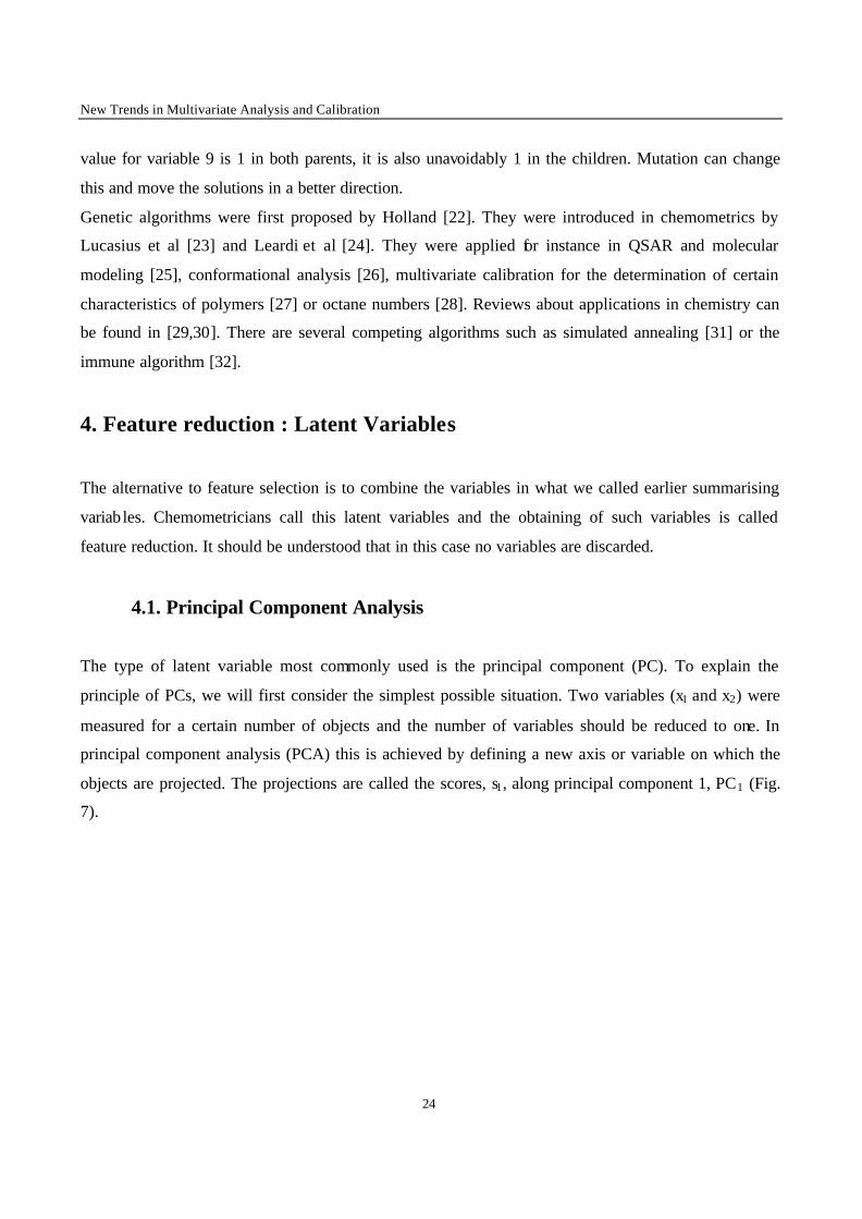
spectral mapping [33]. In figure 9, a score plot is shown for an investigation into the Maillard reaction,
a reaction between sugars and amino acids [34]. The samples consist of reaction mixtures of different
combinations of sugars and aminoacids. The variables are the areas under the peaks of the reaction
mixtures. The reactions are very complex: 159 different peaks were observed. Each of the samples is
therefore characterized by its value for 159 variables. The PC1-PC2 score plot of figure 9 can be seen as
a projection of the samples from 159-dimensional space to the two-dimensional space that preserves
best the variance in the data. In the score plot different symbols are given to the samples according to
Chapter 1 – Multivariate Analysis and Calibration
27
the sugar that was present and it is observed for instance that samples with rhamnose occupy a specific
location in the score plot. This is only possible if they also occupy a different place in the original 159-
dimensional space, i.e. their GC chromatogram is different. By studying different parts of the data and
by including the information from the loading plots, it is then possible to understand the effect of the
starting materials on the obtained reaction mixture.
Fig. 9. PCA score plot of samples from the Maillard reaction. The samples with rhamnose have symbol ¡.
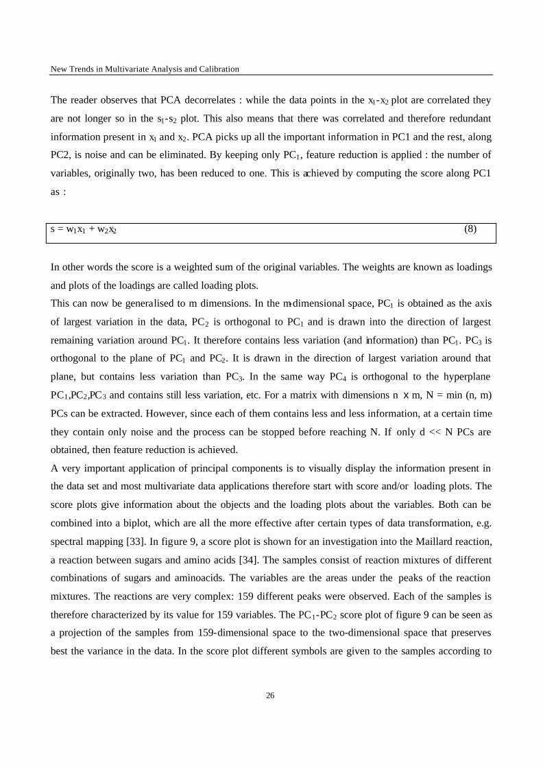
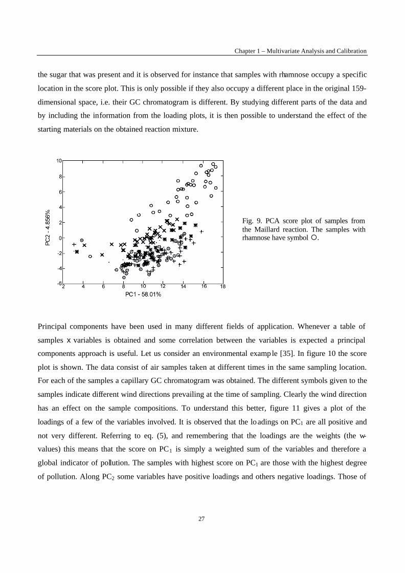
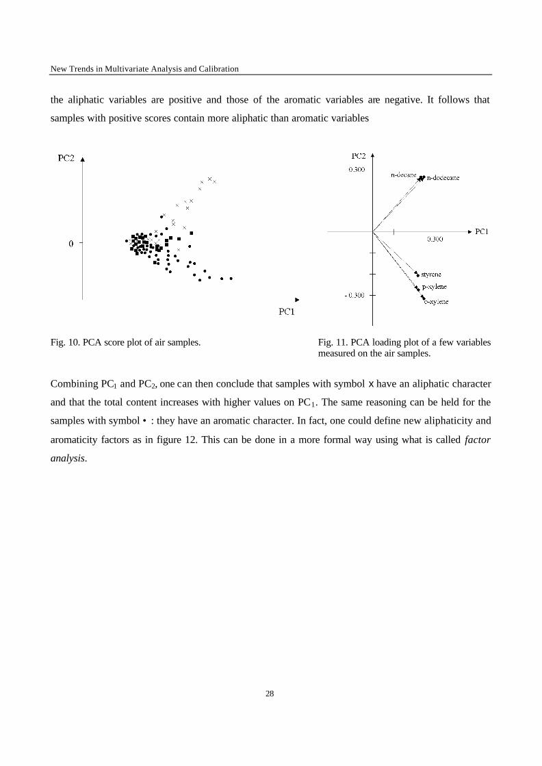
Principal components have been used in many different fields of application. Whenever a table of
samples x variables is obtained and some correlation between the variables is expected a principal
components approach is useful. Let us consider an environmental example [35]. In figure 10 the score
plot is shown. The data consist of air samples taken at different times in the same sampling location.
For each of the samples a capillary GC chromatogram was obtained. The different symbols given to the
samples indicate different wind directions prevailing at the time of sampling. Clearly the wind direction
has an effect on the sample compositions. To understand this better, figure 11 gives a plot of the
loadings of a few of the variables involved. It is observed that the loadings on PC1 are all positive and
not very different. Referring to eq. (5), and remembering that the loadings are the weights (the w-
values) this means that the score on PC1 is simply a weighted sum of the variables and therefore a
global indicator of pollution. The samples with highest score on PC1 are those with the highest degree
of pollution. Along PC2 some variables have positive loadings and others negative loadings. Those of
New Trends in Multivariate Analysis and Calibration
28
the aliphatic variables are positive and those of the aromatic variables are negative. It follows that
samples with positive scores contain more aliphatic than aromatic variables
Fig. 10. PCA score plot of air samples. Fig. 11. PCA loading plot of a few variables measured on the air samples.
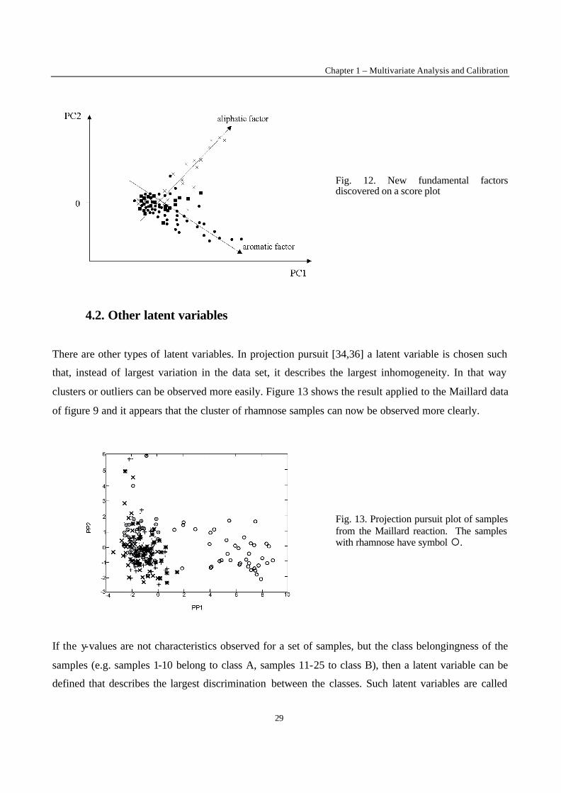
Combining PC1 and PC2, one can then conclude that samples with symbol x have an aliphatic character
and that the total content increases with higher values on PC1. The same reasoning can be held for the
samples with symbol • : they have an aromatic character. In fact, one could define new aliphaticity and
aromaticity factors as in figure 12. This can be done in a more formal way using what is called factor
analysis.
Chapter 1 – Multivariate Analysis and Calibration
29
Fig. 12. New fundamental factors discovered on a score plot
4.2. Other latent variables
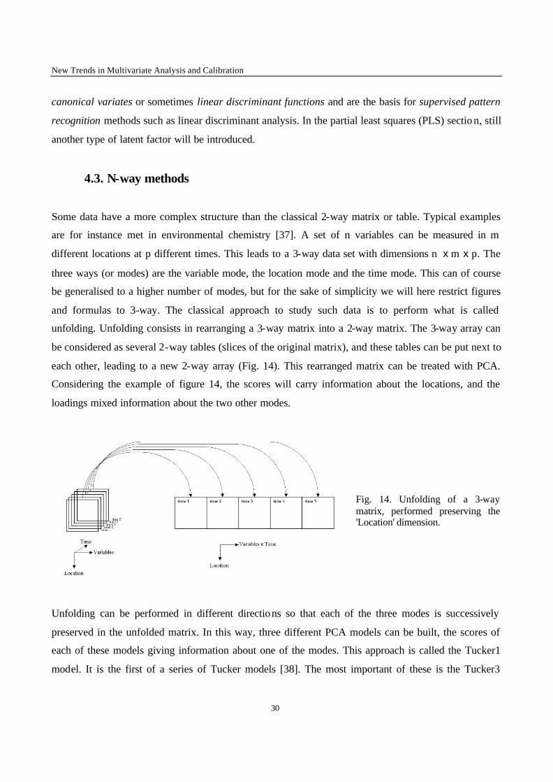
There are other types of latent variables. In projection pursuit [34,36] a latent variable is chosen such
that, instead of largest variation in the data set, it describes the largest inhomogeneity. In that way
clusters or outliers can be observed more easily. Figure 13 shows the result applied to the Maillard data
of figure 9 and it appears that the cluster of rhamnose samples can now be observed more clearly.
Fig. 13. Projection pursuit plot of samples from the Maillard reaction. The samples with rhamnose have symbol ¡.
If the y-values are not characteristics observed for a set of samples, but the class belongingness of the
samples (e.g. samples 1-10 belong to class A, samples 11-25 to class B), then a latent variable can be
defined that describes the largest discrimination between the classes. Such latent variables are called
New Trends in Multivariate Analysis and Calibration
30
canonical variates or sometimes linear discriminant functions and are the basis for supervised pattern
recognition methods such as linear discriminant analysis. In the partial least squares (PLS) sectio n, still
another type of latent factor will be introduced.
4.3. N-way methods
Some data have a more complex structure than the classical 2-way matrix or table. Typical examples
are for instance met in environmental chemistry [37]. A set of n variables can be measured in m
different locations at p different times. This leads to a 3-way data set with dimensions n x m x p. The
three ways (or modes) are the variable mode, the location mode and the time mode. This can of course
be generalised to a higher number of modes, but for the sake of simplicity we will here restrict figures
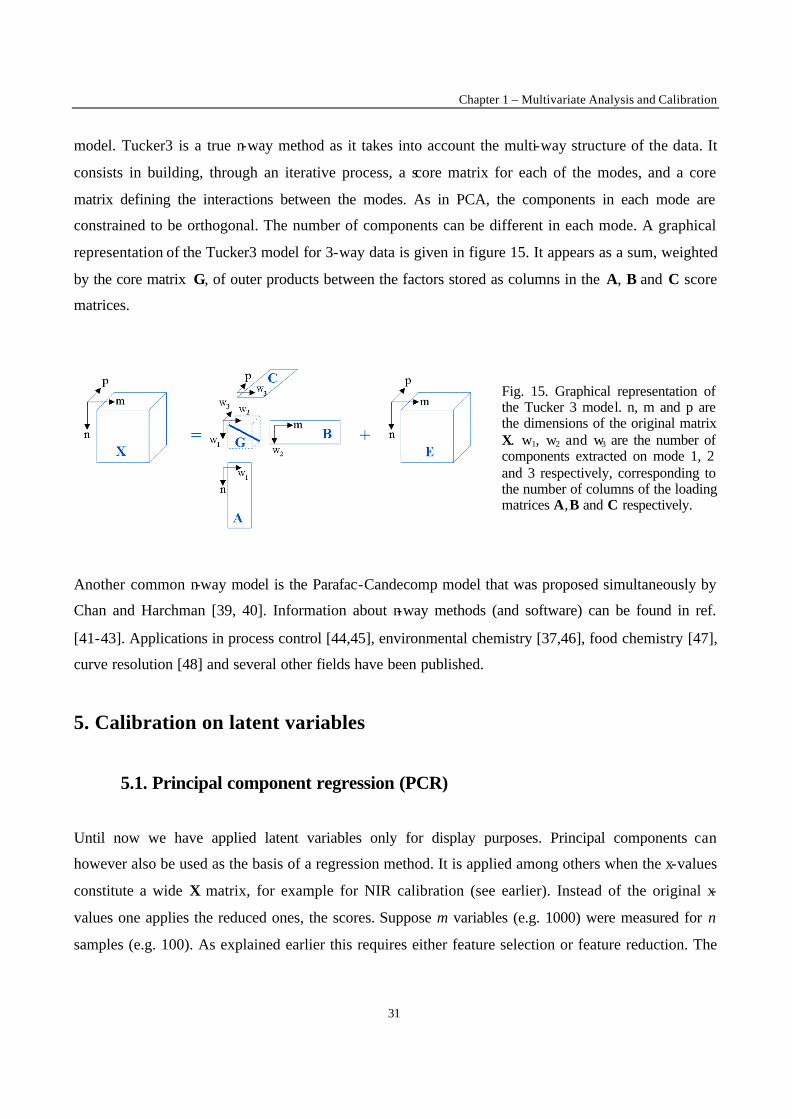
and formulas to 3-way. The classical approach to study such data is to perform what is called
unfolding. Unfolding consists in rearranging a 3-way matrix into a 2-way matrix. The 3-way array can
be considered as several 2-way tables (slices of the original matrix), and these tables can be put next to
each other, leading to a new 2-way array (Fig. 14). This rearranged matrix can be treated with PCA.
Considering the example of figure 14, the scores will carry information about the locations, and the
loadings mixed information about the two other modes.
Fig. 14. Unfolding of a 3-way matrix, performed preserving the 'Location' dimension.
Unfolding can be performed in different directions so that each of the three modes is successively
preserved in the unfolded matrix. In this way, three different PCA models can be built, the scores of
each of these models giving information about one of the modes. This approach is called the Tucker1
model. It is the first of a series of Tucker models [38]. The most important of these is the Tucker3
Chapter 1 – Multivariate Analysis and Calibration
31
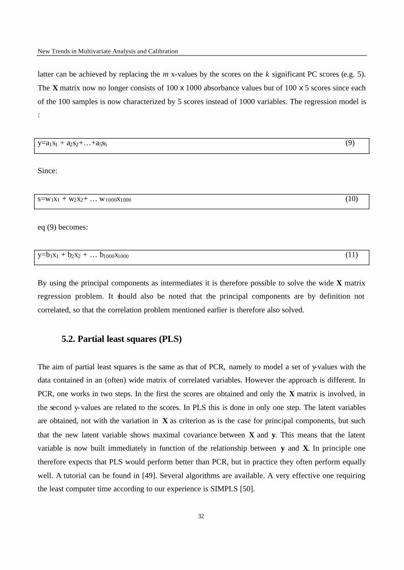
model. Tucker3 is a true n-way method as it takes into account the multi-way structure of the data. It
consists in building, through an iterative process, a score matrix for each of the modes, and a core
matrix defining the interactions between the modes. As in PCA, the components in each mode are
constrained to be orthogonal. The number of components can be different in each mode. A graphical
representation of the Tucker3 model for 3-way data is given in figure 15. It appears as a sum, weighted
by the core matrix G, of outer products between the factors stored as columns in the A, B and C score
matrices.
Fig. 15. Graphical representation of the Tucker 3 model. n, m and p are the dimensions of the original matrix X. w1, w2 and w3 are the number of components extracted on mode 1, 2 and 3 respectively, corresponding to the number of columns of the loading matrices A, B and C respectively.
Another common n-way model is the Parafac-Candecomp model that was proposed simultaneously by
Chan and Harchman [39, 40]. Information about n-way methods (and software) can be found in ref.
[41-43]. Applications in process control [44,45], environmental chemistry [37,46], food chemistry [47],
curve resolution [48] and several other fields have been published.
5. Calibration on latent variables
5.1. Principal component regression (PCR)
Until now we have applied latent variables only for display purposes. Principal components can
however also be used as the basis of a regression method. It is applied among others when the x-values
constitute a wide X matrix, for example for NIR calibration (see earlier). Instead of the original x-
values one applies the reduced ones, the scores. Suppose m variables (e.g. 1000) were measured for n
samples (e.g. 100). As explained earlier this requires either feature selection or feature reduction. The
New Trends in Multivariate Analysis and Calibration
32
latter can be achieved by replacing the m x-values by the scores on the k significant PC scores (e.g. 5).
The X matrix now no longer consists of 100 x 1000 absorbance values but of 100 x 5 scores since each
of the 100 samples is now characterized by 5 scores instead of 1000 variables. The regression model is
:
y=a1s1 + a2s2+…+a5s5 (9)
Since:
s=w1x1 + w2x2+ … w1000x1000 (10)
eq (9) becomes:
y=b1x1 + b2x2 + … b1000x1000 (11)
By using the principal components as intermediates it is therefore possible to solve the wide X matrix
regression problem. It should also be noted that the principal components are by definition not
correlated, so that the correlation problem mentioned earlier is therefore also solved.
5.2. Partial least squares (PLS)
The aim of partial least squares is the same as that of PCR, namely to model a set of y-values with the
data contained in an (often) wide matrix of correlated variables. However the approach is different. In
PCR, one works in two steps. In the first the scores are obtained and only the X matrix is involved, in
the second y-values are related to the scores. In PLS this is done in only one step. The latent variables
are obtained, not with the variation in X as criterion as is the case for principal components, but such
that the new latent variable shows maximal covariance between X and y. This means that the latent
variable is now built immediately in function of the relationship between y and X. In principle one
therefore expects that PLS would perform better than PCR, but in practice they often perform equally
well. A tutorial can be found in [49]. Several algorithms are available. A very effective one requiring
the least computer time according to our experience is SIMPLS [50].
Chapter 1 – Multivariate Analysis and Calibration
33
5.3. Applications of PCR and PLS
PCR and PLS have been applied in many different fields. The following references constitute a
somewhat haphazard selection from a very large literature. There are many analytical applications in
the pharmaceutical industry [51], the petroleum industry [52], food science [53], environmental
chemistry [54]. The methods are used with near or mid infrared [55], chromatographic [56], Raman
[57], UV [58], potentiometric [59] data. A good overview of applications in QSAR is found in [60].
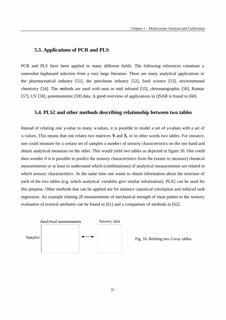
5.4. PLS2 and other methods describing relationship between two tables
Instead of relating one y-value to many x-values, it is possible to model a set of y-values with a set of
x-values. This means that one relates two matrices Y and X, or in other words two tables. For instance,
one could measure for a certain set of samples a number of sensory characteristics on the one hand and
obtain analytical measures on the other. This would yield two tables as depicted in figure 16. One could
then wonder if it is possible to predict the sensory characteristics from the (easier to measure) chemical
measurements or at least to understand which (combinations) of analytical measurements are related to
which sensory characteristics. At the same time one wants to obtain information about the structure of
each of the two tables (e.g. which analytical variables give similar information). PLS2 can be used for
this purpose. Other methods that can be applied are for instance canonical correlation and reduced rank
regression. An example relating 20 measurements of mechanical strength of meat patties to the sensory
evaluation of textural attributes can be found in [61] and a comparison of methods in [62].
Fig. 16. Relating two 2-way tables.
New Trends in Multivariate Analysis and Calibration
34
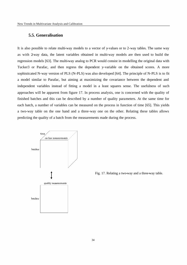
5.5. Generalisation
It is also possible to relate multi-way models to a vector of y-values or to 2-way tables. The same way
as with 2-way data, the latent variables obtained in multi-way models are then used to build the
regression models [63]. The multi-way analog to PCR would consist in modelling the original data with
Tucker3 or Parafac, and then regress the dependent y-variable on the obtained scores. A more
sophisticated N-way version of PLS (N-PLS) was also developed [64]. The principle of N-PLS is to fit
a model similar to Parafac, but aiming at maximizing the covariance between the dependent and
independent variables instead of fitting a model in a least squares sense. The usefulness of such
approaches will be apparent from figure 17. In process analysis, one is concerned with the quality of
finished batches and this can be described by a number of quality parameters. At the same time for
each batch, a number of variables can be measured on the process in function of time [65]. This yields
a two-way table on the one hand and a three-way one on the other. Relating these tables allows
predicting the quality of a batch from the measurements made during the process.
Fig. 17. Relating a two-way and a three-way table.
Chapter 1 – Multivariate Analysis and Calibration
35
6. Conclusion
The most common chemometrical modelling methods were introduced in this chapter, together with
some more advanced ones, in particular methods applying to data with complex structure. These
concepts will be developed in further chapters
REFERENCES
[1] N.R. Draper and H. Smith, Applied Regression Analysis, Wiley, New York, 1981.
[2] J. Mandel, The Statistical Analysis of Experimental Data, Dover reprint, 1984, Wiley &Sons,
1964, New York.
[3] D.L. MacTaggart, S.O. Farwell, J. Assoc.Off. Anal. Chem., 75, 594, 1992.
[4] J.C. Miller and J.N.Miller, Statistics for Analytical Chemistry, Ellis Horwood, Chichester, 3rd
ed., 1993.
[5] W.E. Deming, Statistical Adjustment of Data, Wiley, New York, 1943.
[6] P.T. Boggs, C.H. Spiegelman, J.R. Donaldson and R. B. Schnabel, J. Econometrics, 38, 169,
1988.
[7] P.J.Cornbleet and N.Gochman, Clin. Chem., 25, 432, 1979.
[8] C. Hartmann, J. Smeyers-Verbeke and D.L.Massart, Analusis, 21, 125, 1993.
[9] J.Riu and F.X. Rius, J. Chemometr. 9, 343, 1995.
[10] R.G. Krutchkoff, Technometrics, 9, 425, 1967.
[11] V. Centner, D.L. Massart and S. de Jong, Fresenius J. Anal.Chem., 361, 2, 1998.
[12] B. Grientschnig, Fresenius J. Anal.Chem. 367, 497, 2000.
[13] H. Theil, Nederlandse Akademie van Wetenschappen Proc., Scr. A, 53, 386, 1950.
[14] P.J. Rousseeuw and A.M. Leroy, Robust Regression and Outlier Detection, Wiley, New
York, 1987.
[15] G.R. Phillips and E.R. Eyring, Anal. Chem., 55, 1134, 1983.
[16] F. Mosteller and J.W. Tukey, Data Analysis and regression, Addison-Wesley, Reading, 1977.
[17] P. Van Keerberghen, J. Smeyers-Verbeke, R. Leardi, C.L. Karr and D.L. Massart, Chemom.
Intell. Lab. Systems, 28, 73, 1995.
[18] J.G. Topliss and R.J. Costello, J. Med. Chem., 15, 1066,1972.
New Trends in Multivariate Analysis and Calibration
36
[19] M. Sergent, D. Mathieu, R. Phan-Tan-Luu and G. Drava, Chemom. Intell. Lab. Syst., 27, 153,
1995.
[20] A.C. Atkinson, J. Am. Stat. Assoc. 89, 1329, 1994.
[21] S. Morgenthaler and M.M. Schumacher, Chemom. Intell. Lab. Systems, 47, 127, 1999.
[22] J.H. Holland, Adaption in Natural and Artificial Systems, University of Michigan Press, Ann
Arbor, MI, 1975, revised reprint, MIT Press, Cambridge, 1992.
[23] C.B. Lucasius, M.L.M. Beckers and G. Kateman, Anal. Chim. Acta, 286, 135, 1994.
[24] R. Leardi, R. Boggia and M. Terrile, J. Chemom., 6, 267, 1992.
[25] J. Devillers ed., Genetic Algorithms in Molecular Modeling, Academic Press, London, 1996.
[26] M.L.M. Beckers, E.P.P.A. Derks, W.J. Melssen and L.M.C. Buydens, Comput. Chem., 20, 449,
1996.
[27] D. Jouan-Rimbaud, D.L.Massart, R. Leardi and O.E. de Noord, Anal. Chem., 67, 4295, 1995.
[28] R. Meusinger and R. Moros, Chemom. Intell. Lab. Systems, 46, 67, 1999.
[29] P. Willet, Trends. Biochem, 13, 516, 1995.
[30] D.H. Hibbert, Chemom. Intell. Lab. Syst., 19, 277, 1993.
[31] J.H. Kalivas, J. Chemom., 5, 37, 1991.
[32] X.G. Shao, Z.H. Chen and X.Q. Lin, Fresenius J. Anal. Chem., 366, 10, 2000.
[33] P.J. Lewi, Arzneim. Forschung, 26, 1295, 1976.
[34] Q. Guo, W. Wu, F. Questier, D.L.Massart, C. Boucon and S. de Jong, Anal. Chem., 72, 2846.
[35] J. Smeyers-Verbeke, J.C. Den Hartog, W.H.Dekker, D. Coomans, L. Buydens and D.L.
Massart, Atmos. Environ., 18, 2471, 1984.
[36] J.H. Friedman, J. Am. Stat. Assoc., 82, 249, 1987.
[37] P. Barbieri, C.A. Andersson, D.L. Massart, S. Predonzani, G. Adami and G.E. Reisenhofer,
Anal. Chim. Acta, 398, 227, 1999.
[38] L. R. Tucker, Psychometrika, 31, 279, 1966.
[39] R. Harshman, UCLA working papers in phonetics, 16, 1, 1970.
[40] J. D. Carrol, J. Chang, Psychometrika, 45, 283, 1970.
[41] C. A. Andersson, R. Bro, Chemom. Intell. Lab. Sys., 52, 1, 2000.
[42] M. Kroonenberg, Three-mode Principal Component Analysis. Theory and Applications, DSWO
Press, Leiden, 1983, reprint 1989.
[43] R. Henrion, Chemom. Intell. Lab. Sys., 25, 1, 1994.

Chapter 1 – Multivariate Analysis and Calibration
37
[44] P. Nomikos and J.F. MacGregor, AIChE Journal, 40, 1361, 1994.
[45] D.J. Louwerse and A.K. Smilde, Chem. Eng. Sci., 55, 1225, 2000.
[46] R. Henrion, Chemom. Intell. Lab. Sys., 16, 87, 1992.
[47] R. Bro, Chemom. Intell. Lab. Sys., 46, 133, 1998.
[48] A. de Juan, S.C. Rutan, R. Tauler and D.L. Massart, Chemom. Intell. Lab. Sys., 40, 19, 1998.
[49] P. Geladi and B.R. Kowalski, Anal. Chim. Acta, 185, 1, 1986.
[50] S. de Jong, Chemom. Intell. Lab. Syst., 18, 251, 1993.
[51] K.D. Zissis, R.G. Brereton, S. Dunkerley and R.E.A. Escott, Anal. Chim. Acta, 384, 71, 1999.
[52] C.J. de Bakker and P.M. Fredericks, Applied Spectroscopy, 49, 1766, 1995.
[53] S. Vaira, V.E. Mantovani, J.C. Robles, J.C. Sanchis and H.C. Goicoechea, Anal. Letters, 32,
3131, 1999.
[54] V. Simeonov, S. Tsakovski and D.L. Massart, Toxicological & Environmental Chemistry, 72,
81, 1999.
[55] J.B. Cooper, K.L. Wise, W.T. Welch, M.B. Summer, B.K. Wilt and R.R. Bledsoe, Applied
Spectroscopy, 51, 1613, 1997.
[56] M.P. Montana, N.B. Pappano, N.B. Debattista, J. Raba and J.M. Luco, Chromatographia, 51,
727, 2000.
[57] O. Svensson, M. Josefson and F.W. Langkilde, Chemom. Intell. Lab. Sys., 49, 49, 2000.
[58] F. Vogt, M. Tacke, M. Jakusch and B. Mizaikoff, Anal. Chim. Acta, 422, 187, 2000.
[59] M. Baret, D.L. Massart, P. Fabry, C. Menardo and F. Conesa, Talanta, 50, 541, 1999.
[60] S. Wold in Chemometric Methods in Molecular Design, H. van de Waterbeemd ed., VCH,
Weinheim, 1995.
[61] S. Beilken, L.M. Eadie, I. Griffiths, P.N. Jones and P.V. Harris, J. Food Sci., 56, 1465, 1991.
[62] B.G.M. Vandeginste, D.L. Massart, L.M.C. Buydens, S. de Jong, P.J. Lewi and J. Smeyers-
Verbeke, Handbook of Chemometrics and Qualimetrics: Part B, Chapter 35, Elsevier,
Amsterdam, 1998.
[63] R. Bro and H.Heimdal, Chemom. Intell. Lab. Systems, 34, 85, 1996.
[64] R. Bro, J. Chemom., 10, 47, 1996.
[65] C. Duchesne and J.F. McGregor, Chemom. Intell. Lab. Systems, 51, 125, 2000.
New Trends in Multivariate Analysis and Calibration
38
CHAPTER II
COMPARISON OF MULTIVARIATE CALIBRATION METHODS
This chapter focuses specifically on multivariate calibration. As stated in the introduction of this thesis,
a particularity of chemometrics is that many methods are often available for a given problem. This
chapter therefore includes comparative studies and proposed methodologies aiming at helping in the
selection of the most appropriate multivariate calibration method.
In the first two papers in this chapter : “A Comparison of Multivariate Calibration Techniques
Applied to Experimental NIR Data Sets. Part II : Predictive Ability under Extrapolation
Conditions.” and “A Comparison of Multivariate Calibration Techniques Applied to Experimental
NIR Data Sets. Part III : Robustness Against Instrumental Perturbation Conditions”, methods are
compared in challenging situations where the prediction of new samples requires mild extrapolation
(part II), or where new data is affected by instrumental perturbation (part III). This work follows a first
comparative study (part I) in which the various methods were compared on industrial data sets in
situation where the previously mentioned difficulties did not occur [1]. The conclusions drawn in this
first paper are presented in this chapter.
A third paper published on the internet : “The Development of Calibration Models for Spectroscopic
Data using Multiple Linear Regression” proposes a complete methodology for the development of
multivariate calibration models, from data acquisition to the prediction of new samples. This
methodology is developed here in the case of Multiple Linear Regression. However, most of the
scheme is easily transposable to most calibration methods considering their particularities developed in
the first two publications of this chapter. Some specific aspects of Multiple Linear Regression are
developed in details, in particular the challenging problem of avoiding Random Correlation during
variable selection. This paper is adapted from a publication devoted to Principal Component

Chapter 2 – Comparison of Multivariate Calibration Methods
39
Regression, and to which the author contributed by performing some of the calculations and
participating to the redaction of the manuscript.
This chapter gives an overview of the methods used for multivariate calibration and the way these
methods should be used on data classically treated by chemometricians. In this sense, it can be
considered as a state of the art for multivariate calibration.
REFERENCES
[1] V. Centner, G. Verdú-Andrés, B. Walczak, D. Jouan-Rimbaud, F. Despagne, L. Pasti, R. Poppi,
D.L. Massart and O.E. de Noord, Appl. Spectrometry 54 (4) (2000) 608-623.
New Trends in Multivariate Analysis and Calibration
40
A COMPARISON OF MULTIVARIATE CALIBRATION
TECHNIQUES APPLIED TO EXPERIMENTAL NIR DATA
SETS. PART II : PREDICTIVE ABILITY UNDER
EXTRAPOLATION CONDITIONS.
Chemometrics and Intelligent Laboratory Systems, 58 2 (2001) 195-211.
F. Estienne , L. Pasti, V. Centner, B. Walczak +, F. Despagne,
D. Jouan Rimbaud, O. E. de Noord1 ,D.L. Massart *
ChemoAC, Farmaceutisch Instituut,
Vrije Universiteit Brussel, Laarbeeklaan 103,
B-1090 Brussels, Belgium. E-mail: [email protected]
+ on leave from : Silesian University
Katowice Poland
1 Shell International Chemicals B. V., Shell Research and Technology Centre
Amsterdam P. O. Box 38000
1030 BN Amsterdam The Netherlands
ABSTRACT
The present study compares the performance of different multivariate calibration techniques when new samples to be predicted can fall outside the calibration domain. Results of the calibration methods are investigated for extrapolation of different types and various levels. The calibration methods are applied to five near-IR data sets including difficulties often met in practical cases (non- linearity, non-homogeneity and presence of irrelevant variables in the set of predictors). The comparison leads to general recommendations about what method to use when samples requiring extrapolation can be expected in a calibration application.
* Corresponding author
KEYWORDS : Multivariate calibration, method comparison, extrapolation, non- linearity, clustering.
Chapter 2 – Comparison of Multivariate Calibration Methods
41
1 - Introduction
Calibration techniques enable to relate instrumental responses consisting of a set of predictors X (i.e.
the NIR spectra) to a chemical or physical property of interest y (the response factor). The choice of the
most appropriate calibration method is crucial in order to obtain calibration models with good
performances in prediction of the property y of new samples. When performing calibration, two
situations can occur. The first case is met when it is possible to produce artificially the samples to
analyse. Statistical design such as factorial or mixture designs can then be used to generate the
calibration set [1-2]. The second situation is met when it is not possible to synthesise the calibration
samples, for instance for natural products (e.g. petroleum, wheat) or complex mixtures generated from
industrial plants (e.g. gasoline, polymers). This second situation was considered in the present work. In
this case, the selection of calibration samples is performed over a population of available samples. It is
difficult to foresee the full extent of all sources of variations to be encountered for new samples on
which a prediction will be carried out. Therefore, some samples may fall outside the calibration space,
leading to a certain degree of extrapolation in the prediction of these new samples. Although it is often
stated that extrapolation is not allowed, in many practical situations the time delay caused by new
laboratory analysis and model updating is not acceptable. The aim of the present work is to evaluate in
a general case the performance of calibration methods when such mild extrapolation occurs.
To investigate the effect of the extrapolation on the performance of the different calibration models,
two types of extrapolation were considered :
• X-space extrapolation : objects of the test subset are situated outside the space spanned by the
objects of the calibration set, but may have y-values within the calibration range.
• y-value extrapolation : objects in the test subset have a higher or a lower y value than the objects in
the calibration set.
The methods to be compared were selected on the basis of the results obtained in the first part of this
study [3]. In this first part, the comparison between the performance of calibration methods in terms of
predictive ability was performed under conditions excluding extrapolation. Only the methods that
yielded good results in this first stage of the comparison have been used in this part. The data sets are
the same as those investigated in the first part of the study, except for one that was added because of its
interesting structure (clustered and non-linear). The data sets include difficulties often met in practice,
New Trends in Multivariate Analysis and Calibration
42
namely data clustering, non- linearity, and presence of irrelevant variables in the set of predictors. In
this study, objects of the test subsets were selected so that their prediction requires extrapolation. The
performance of the calibration methods was evaluated on the basis of predictive ability of the models.
2 - Theory
2.1 – Calibration techniques
In the following, a short description of the applied calibration methods is given, essentially to explain
the notation used. More details about the reported methods can be found in Ref. [3] and in the
references mentioned for each method.
2.1.1 - Full spectrum latent variables methods
Principal Component Regression (PCR)
The original data matrix X(n,m) is converted by a linear transformation in a set of orthogonal latent
variables, denoted T(n,a) and called Principal Components (PCs); n is the number of objects and a is the
model complexity. The PCR model relates the response factor y to the scores T :
eTy += ∑=
a
1iiib
(1)
where bi is the ith coefficient, and e is the error vector.
To estimate the model complexity, Leave-One-Out (LOO) Cross Validation (CV) was applied. The
number of PCs leading to the minimum Root Mean Square Error of Prediction by CV (RMSECV) was
chosen as optimal model complexity in first approximation. This value was validated by means of the
randomisation test [4] to reduce the risk of overfitting.
Variants of PCR were also used. Principal Component Regression with variable selection (PCRS) is a
PCR in which the PCs are selected according to correlation with y. Non-linear Principal Component
Chapter 2 – Comparison of Multivariate Calibration Methods
43
Regression (NL-PCR) [5] consists in applying the PCR model to the matrix obtained as the union of
the original variables (X) and their squared values (X2).
Partial Least Squares Regression (PLS)
In PLS, the model can be described as :
u = f(t) + d (2)
where f is a linear function, d is the vector of residuals and u and t are linear combinations of y and X
respectively. The coefficients of the linear transformation (f) can be obtained iteratively by maximising
the square of the product: (u't) [6].
Spline Partial Least Squares (Spline-PLS) was also applied [7]. In the Spline-PLS version of PLS, the
principles of the method are the same but the relationship denoted by f is a spline function (i.e. a
piecewise polynomial function) instead of a linear relationship [6].
The model complexity was optimised by means of the LOO-CV procedure followed by the
randomisation test.
2.1.2 - Variable selection/elimination methods
The variable selection methods used in this study are Stepwise selection (Step) and Genetic Algorithm
(GA) applied in both the original and the Fourier domain (GA-FT). Multiple Linear Regression (MLR)
is applied to the selected variables. The variable elimination methods are essentially based on the
Uninformative Variable Elimination (UVE) algorithm (UVE-PLS), and the Relevant Component
Extraction (RCE) PLS method.
Multiple Linear Regression (MLR)
The MLR model is given by :
y = b P + e (3)

New Trends in Multivariate Analysis and Calibration
44
where b is the vector of the regression coefficients, P is the matrix of the selected variables in the
original or in the transformed domain and e is the error vector.
The randomisation test was applied in Stepwise selection to optimise the model.
Genetic Algorithm [8-9]
The first parameter to choose in GA is the maximum number of variables to be entered in the model.
The algorithm starts by randomly building a subset of solutions having a number of variables smaller or
equal to the given maximum. The possible solutions are selected depending on the fitness of the
obtained model, evaluated on the basis of LOO-RMSECV.
The input parameters of the hybrid GA [10] applied were the following :
Number of chromosomes in the population 20
Probability of cross-over 50%
Probability of mutation 1%
Stopping criterion 200 evaluations
Frequency of the background backward selection 2 per cycle of evaluations
Response to be maximised (RMSEP)-1
A threshold value equal to the PLS RMSECV increased by 10% was introduced for RMSEP, which
means that only solutions with an RMSEP lower than this value were considered as acceptable
solutions. The maximum number of variables allowed in the strings was set equal to the complexity of
the optimal PLS model increased by two. The same parameters were used in the original and in the
Power Spectra (PS) domain to find the optimal solution. In the original domain, all the variables were
entered in the selection procedure for initial random selection. In the PS domain, only the first 50
coefficients were selected as input to GA [11].
Uninformative Variable Elimination-PLS [12]
In PLS methods the calibration model is described by Eq. (2). In the linear case the relationship
between the X scores (i.e. t) and the y scores (i.e. u) can be described by :
Chapter 2 – Comparison of Multivariate Calibration Methods
45
u = b t + d (5)
where b is the coefficients vector. UVE-PLS aims at improving the predictive ability of the final model
by removing from the X matrix information not related to y. The criterion used to identify the non-
informative variables is the stability of the PLS regression coefficient b.
The input parameters used were:
cut-off level: 99%
number of random variables: 200
scaling constant: 10-10
Relevant Component Extraction [13]
RCE is a modification of the UVE algorithm to operate in the wavelet domain. The spectra are
decomposed to the last decomposition level using the Discrete Wavelet Trans form with the optimal
filter selected from the Daubechies family. An algorithm is applied to separate the coefficients related
to the signal from those related to the noise. The PLS model is built using only the selected wavelet
coefficients.
2.1.3 - Local methods
The methods described are Locally Weighted Regression-PLS (LWR-PLS), and Radial Basis Function-
PLS (RBF-PLS).
Locally Weighted Regression-PLS [14]
For each new object, a PLS model is built by considering only the objects of the calibration set that are
similar to the selected one. The similarity is measured on the basis of the Euclidean distance calculated
in the original measurement space [15]. The contribution of each similar object to the model is
weighted using the distance from the selected object. The optimisation of the model complexity and of
the number of similar objects is performed by means of LOO-CV.
New Trends in Multivariate Analysis and Calibration
46
Radial Basis Function-PLS [16]
RBF-PLS is a global method, which means that one model is valid for all the data set objects. The local
property comes from the transformation of the original X matrix. In fact, PLS is applied to the y
response factor and the A activation matrix. The activation matrix represents a non- linear distance
matrix of X. The non- linearity is due to the exponential relationship (i.e. Gaussian function) between
the elements of the activation matrix and the Euclidean distance between pairs of points. The
parameters to be optimised are the width of the Gaussian function and the complexity of the PLS model
The optimisation procedure requires the calibration set to be split into a training and a monitoring set
(see data splitting section).
2.1.4 - Neural Network (NN)
The X data matrix is compressed by means of PC transformation. The most relevant PCs, selected on
the basis of explained variance, are used as input to the NN. The number of hidden layers was set to 1.
The transfer function used in the hidden layer was non- linear (i.e. hyperbolic tangent). Both linear or
non-linear transfer functions were used in the output layer. The weights were optimised by means of
the Levenberg-Marquardt algorithm [17]. A method was applied to find the best number of nodes to be
used in the input and hidden layers based on the contribution of each node [18]. The optimisation
procedure of NN also requires the calibration set to be split into a training and a monitoring set (see
data splitting section).
2.2 – Prediction performance within domain
The first part of this study [3], in which prediction was performed within the calibration domain, led to
several general conclusions. It was shown that Stepwise MLR can lead to very good results with very
simple models for linear cases, sometimes outperforming the full spectrum methods. PCR, when
performed with variable selection, always gave results comparable to PLS, with sometimes slightly
higher complexities. In case of non- linearity, non-linear modifications of PCR and PLS were always
outperformed by Neural Networks or LWR. This last method appeared as a generally good performer
Chapter 2 – Comparison of Multivariate Calibration Methods
47
as its results were always at least as good as those of PCR/PLS. Another approach found to be
interesting was UVE. This method enabled to improve the prediction precision and could be used as a
diagnostic tool to see to what extent variables included in X were useful for the prediction.
2.3 – Calibration and prediction sets
As previously mentioned, the aim of the present work is to evaluate the performance of calibration
methods under mild extrapolation conditions i.e. in the presence of extreme samples in the prediction
subset. The data sets were therefore split into two subsets, the calibration set, for the modelling part
(including optimisation), and the prediction (or test) set, for evaluation of the predictive ability of the
model.
2.3.1 - Data Splitting
The calibration set should contain an appropriate number of objects in order to describe accurately the
relation between X and y. 2/3 of the total number of objects were included in the calibration set and the
other 1/3 were selected to constitute the prediction set. For each data set a certain number of different
prediction sets were considered (i.e. 3 to 4 in X space extrapolation and 2 in y space extrapolation). The
predictive ability of the calibration model was computed for each prediction set and for the combined
prediction set.
X-space extrapolation
For homogeneous data sets the whole data set was considered, whereas for clustered data the extreme
samples were selected from each cluster of the data. The inhomogeneous data sets were therefore
divided in clusters on the basis of a PC score plot. Starting from the obtained clusters, various
algorithms can be applied to select the extreme samples, and the distribution of the selected samples
will depend on the characteristics of the splitting algorithm used. The prediction subset samples had to
be selected so that they contain some extreme samples and span the range of variation. The Kennard
and Stone [19] algorithm was used for this purpose on the PCA scores. This algorithm is appropriate as
it starts with selecting extreme objects. Four different prediction subsets were built for all the data sets,
New Trends in Multivariate Analysis and Calibration
48
except in one case where this number was reduced to three because of a lower total number of objects.
The number of prediction samples selected from each cluster was chosen to be proportional to the ratio
of the number of objects the cluster contains, and the total number of objects present in the data set.
The Kennard and Stone algorithm was applied in the Euclidian distance space, starting from the object
furthest from the mean value. After a first prediction subset was created, the corresponding objects
were removed from the data set, and the selection procedure was iterated on the remaining samples to
obtain the second prediction subset, etc. As a consequence of the applied splitting procedure, the degree
of extrapolation decreases as the number of test subsets increases. This procedure was applied to each
cluster of the data set, and the corresponding prediction subsets were merged to yield the global
prediction subsets for the whole data set.
y-value extrapolation
In this case the data sets were not divided in clusters, and 2 test subsets were selected for each data set.
The objects were sorted in ascending order of y value. The first 1/6 of the total number of objects with
the lowest y values constituted the test subset 1, and the last 1/6 of the total number of objects with the
largest y values constituted the test subset 2. The remaining 2/3 objects were kept in the calibration set.
The test subset obtained as union of the two test subsets was also used to verify the performance of the
models.
2.3.2 - Optimisation of the calibration model
Two different approaches were applied to optimise the parameters of the model, namely cross-
validation and prediction testing. The latter was used to optimise the NN topology and the width of the
Gaussian function in RBF-PLS. It consists in dividing the calibration set in training and monitoring
sets. When applying NN or RBF methods, several models are built with different parameter values. The
optimal model parameters are considered to be those that lead to the best predictive ability when the
models are applied to the monitoring set. The splitting of the calibration set into training and
monitoring sets was achieved by applying the Duplex algorithm [20].
For all the other methods, internal validation (namely LOO-CV) was used to optimise the model. The
squared prediction residual value for object i is given by :
Chapter 2 – Comparison of Multivariate Calibration Methods
49
2ii
2i )yy(e −= (12)
The procedure is repeated for each object of the calibration set, and the prediction error sum of squares
(PRESS) can then be calculated as :
∑∑==
=−=n
1i
2i
n
1i
2ii e)yy(PRESS (13)
The Root Mean Square Error of Cross Validation (RMSECV) is defined as the square root of the mean
value of PRESS
n
)y(y
nPRESSRMSECV
n
1i
2ii∑
=
−== (14)
The RMSECV obtained for different values of the model parameters, for instance the number of
components in a PLS model, are compared in a statistical way by means of the randomisation test, with
the model showing the lowest RMSECV. A model with higher RMSECV but lower complexity can be
retained if its RMSECV is not significantly different from the lowest one.
2.3.3 - Predictive ability of the model
The predictive ability of the optimal model is calculated as a Root Mean Square Error of Prediction
RMSEP, on the test subset
t
n
1i
2ii
n
)yy(RMSEP
t
∑=
−= (15)
where nt is the number of samples in the test subset.
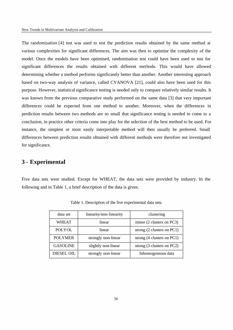
New Trends in Multivariate Analysis and Calibration
50
The randomisation [4] test was used to test the prediction results obtained by the same method at
various complexities for significant differences. The aim was then to optimise the complexity of the
model. Once the models have been optimised, randomisation test could have been used to test for
significant differences the results obtained with different methods. This would have allowed
determining whether a method performs significantly better than another. Another interesting approach
based on two-way analysis of variance, called CVANOVA [21], could also have been used for this
purpose. However, statistical significance testing is needed only to compare relatively similar results. It
was known from the previous comparative study performed on the same data [3] that very important
differences could be expected from one method to another. Moreover, when the differences in
prediction results between two methods are so small that significance testing is needed to come to a
conclusion, in practice other criteria come into play for the selection of the best method to be used. For
instance, the simplest or most easily interpretable method will then usually be preferred. Small
differences between prediction results obtained with different methods were therefore not investigated
for significance.
3 - Experimental
Five data sets were studied. Except for WHEAT, the data sets were provided by industry. In the
following and in Table 1, a brief description of the data is given.
Table 1. Description of the five experimental data sets.
data set linearity/non-linearity clustering
WHEAT linear minor (2 clusters on PC3)
POLYOL linear strong (2 clusters on PC1)
POLYMER strongly non-linear strong (4 clusters on PC1)
GASOLINE slightly non-linear strong (3 clusters on PC2)
DIESEL OIL strongly non-linear Inhomogeneous data
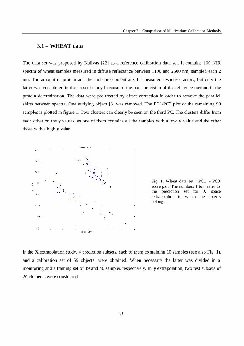
Chapter 2 – Comparison of Multivariate Calibration Methods
51
3.1 – WHEAT data
The data set was proposed by Kalivas [22] as a reference calibration data set. It contains 100 NIR
spectra of wheat samples measured in diffuse reflectance between 1100 and 2500 nm, sampled each 2
nm. The amount of protein and the moisture content are the measured response factors, but only the
latter was considered in the present study because of the poor precision of the reference method in the
protein determination. The data were pre-treated by offset correction in order to remove the parallel
shifts between spectra. One outlying object [3] was removed. The PC1/PC3 plot of the remaining 99
samples is plotted in figure 1. Two clusters can clearly be seen on the third PC. The clusters differ from
each other on the y values, as one of them contains all the samples with a low y value and the other
those with a high y value.
Fig. 1. Wheat data set : PC1 - PC3 score plot. The numbers 1 to 4 refer to the prediction set for X space extrapolation to which the objects belong.
In the X extrapolation study, 4 prediction subsets, each of them containing 10 samples (see also Fig. 1),
and a calibration set of 59 objects, were obtained. When necessary the latter was divided in a
monitoring and a training set of 19 and 40 samples respectively. In y extrapolation, two test subsets of
20 elements were considered.
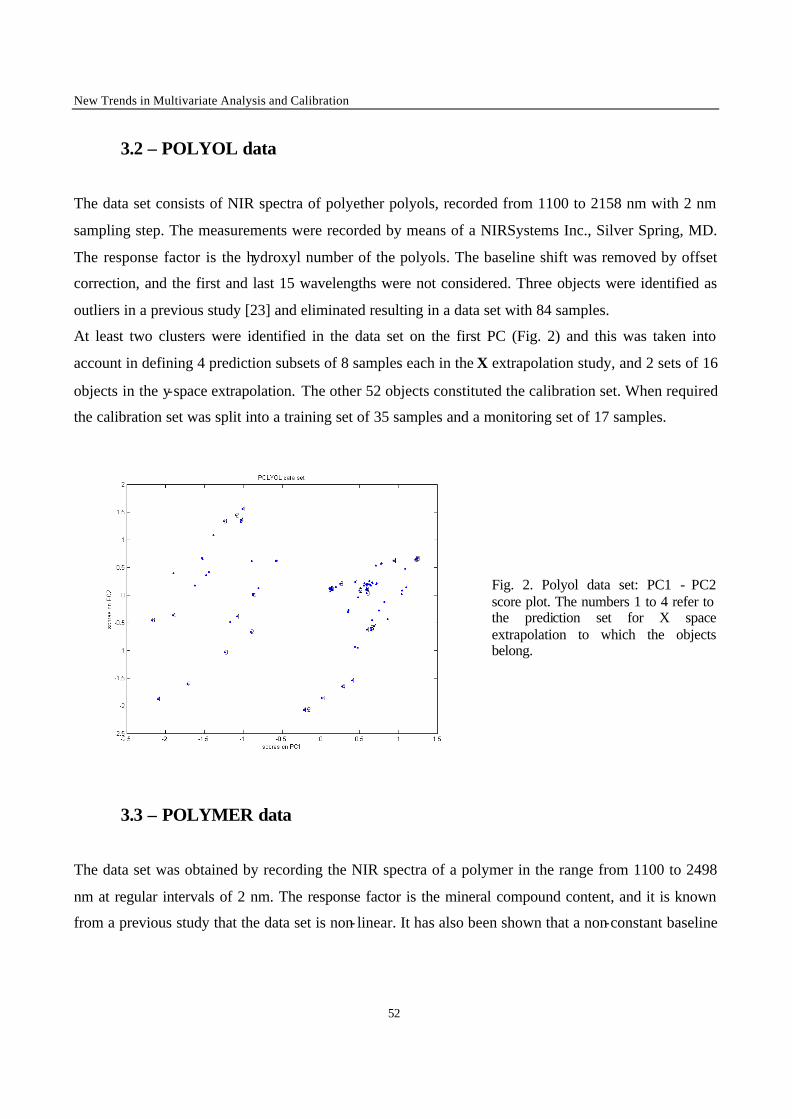
New Trends in Multivariate Analysis and Calibration
52
3.2 – POLYOL data
The data set consists of NIR spectra of polyether polyols, recorded from 1100 to 2158 nm with 2 nm
sampling step. The measurements were recorded by means of a NIRSystems Inc., Silver Spring, MD.
The response factor is the hydroxyl number of the polyols. The baseline shift was removed by offset
correction, and the first and last 15 wavelengths were not considered. Three objects were identified as
outliers in a previous study [23] and eliminated resulting in a data set with 84 samples.
At least two clusters were identified in the data set on the first PC (Fig. 2) and this was taken into
account in defining 4 prediction subsets of 8 samples each in the X extrapolation study, and 2 sets of 16
objects in the y-space extrapolation. The other 52 objects constituted the calibration set. When required
the calibration set was split into a training set of 35 samples and a monitoring set of 17 samples.
Fig. 2. Polyol data set: PC1 - PC2 score plot. The numbers 1 to 4 refer to the prediction set for X space extrapolation to which the objects belong.
3.3 – POLYMER data
The data set was obtained by recording the NIR spectra of a polymer in the range from 1100 to 2498
nm at regular intervals of 2 nm. The response factor is the mineral compound content, and it is known
from a previous study that the data set is non- linear. It has also been shown that a non-constant baseline
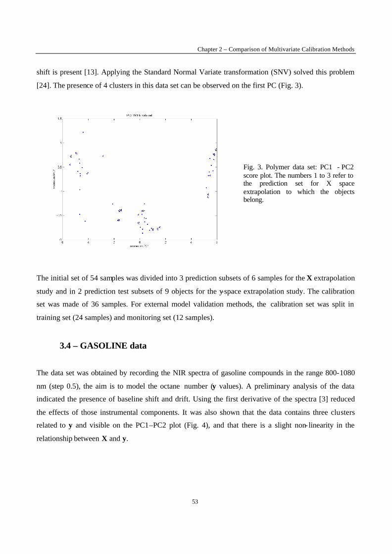
Chapter 2 – Comparison of Multivariate Calibration Methods
53
shift is present [13]. Applying the Standard Normal Variate transformation (SNV) solved this problem
[24]. The presence of 4 clusters in this data set can be observed on the first PC (Fig. 3).
Fig. 3. Polymer data set: PC1 - PC2 score plot. The numbers 1 to 3 refer to the prediction set for X space extrapolation to which the objects belong.
The initial set of 54 samples was divided into 3 prediction subsets of 6 samples for the X extrapolation
study and in 2 prediction test subsets of 9 objects for the y-space extrapolation study. The calibration
set was made of 36 samples. For external model validation methods, the calibration set was split in
training set (24 samples) and monitoring set (12 samples).
3.4 – GASOLINE data
The data set was obtained by recording the NIR spectra of gasoline compounds in the range 800-1080
nm (step 0.5), the aim is to model the octane number (y values). A preliminary analysis of the data
indicated the presence of baseline shift and drift. Using the first derivative of the spectra [3] reduced
the effects of those instrumental components. It was also shown that the data contains three clusters
related to y and visible on the PC1–PC2 plot (Fig. 4), and that there is a slight non- linearity in the
relationship between X and y.
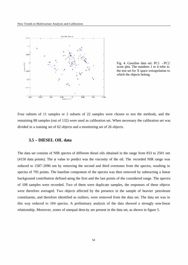
New Trends in Multivariate Analysis and Calibration
54
Fig. 4. Gasoline data set: PC1 - PC2 score plot. The numbers 1 to 4 refer to the test set for X space extrapolation to which the objects belong.
Four subsets of 11 samples or 2 subsets of 22 samples were chosen to test the methods, and the
remaining 88 samples (out of 132) were used as calibration set. When necessary the calibration set was
divided in a training set of 62 objects and a monitoring set of 26 objects.
3.5 – DIESEL OIL data
The data set consists of NIR spectra of different diesel oils obtained in the range from 833 to 2501 nm
(4150 data points). The y value to predict was the viscosity of the oil. The recorded NIR range was
reduced to 1587-2096 nm by removing the second and third overtones from the spectra, resulting in
spectra of 795 points. The baseline component of the spectra was then removed by subtracting a linear
background contribution defined using the first and the last points of the considered range. The spectra
of 108 samples were recorded. Two of them were duplicate samples, the responses of these objects
were therefore averaged. Two objects affected by the presence in the sample of heavier petroleum
constituents, and therefore identified as outliers, were removed from the data set. The data set was in
this way reduced to 104 spectra. A preliminary analysis of the data showed a strongly non- linear
relationship. Moreover, zones of unequal dens ity are present in the data set, as shown in figure 5.
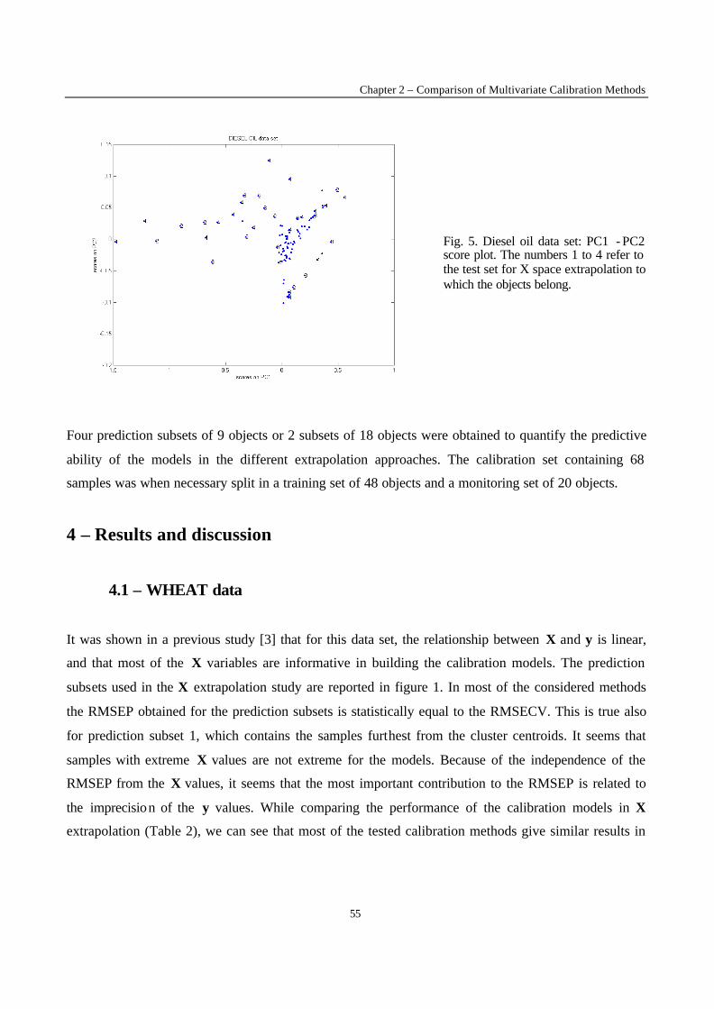
Chapter 2 – Comparison of Multivariate Calibration Methods
55
Fig. 5. Diesel oil data set: PC1 - PC2 score plot. The numbers 1 to 4 refer to the test set for X space extrapolation to which the objects belong.
Four prediction subsets of 9 objects or 2 subsets of 18 objects were obtained to quantify the predictive
ability of the models in the different extrapolation approaches. The calibration set containing 68
samples was when necessary split in a training set of 48 objects and a monitoring set of 20 objects.
4 – Results and discussion
4.1 – WHEAT data
It was shown in a previous study [3] that for this data set, the relationship between X and y is linear,
and that most of the X variables are informative in building the calibration models. The prediction
subsets used in the X extrapolation study are reported in figure 1. In most of the considered methods
the RMSEP obtained for the prediction subsets is statistically equal to the RMSECV. This is true also
for prediction subset 1, which contains the samples furthest from the cluster centroids. It seems that
samples with extreme X values are not extreme for the models. Because of the independence of the
RMSEP from the X values, it seems that the most important contribution to the RMSEP is related to
the imprecision of the y values. While comparing the performance of the calibration models in X
extrapolation (Table 2), we can see that most of the tested calibration methods give similar results in
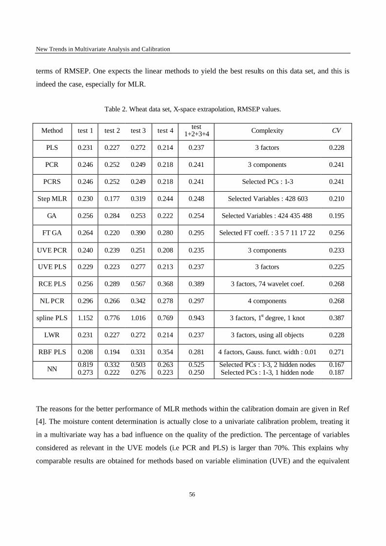
New Trends in Multivariate Analysis and Calibration
56
terms of RMSEP. One expects the linear methods to yield the best results on this data set, and this is
indeed the case, especially for MLR.
Table 2. Wheat data set, X-space extrapolation, RMSEP values.
Method test 1 test 2 test 3 test 4 test 1+2+3+4 Complexity CV
PLS 0.231 0.227 0.272 0.214 0.237 3 factors 0.228
PCR 0.246 0.252 0.249 0.218 0.241 3 components 0.241
PCRS 0.246 0.252 0.249 0.218 0.241 Selected PCs : 1-3 0.241
Step MLR 0.230 0.177 0.319 0.244 0.248 Selected Variables : 428 603 0.210
GA 0.256 0.284 0.253 0.222 0.254 Selected Variables : 424 435 488 0.195
FT GA 0.264 0.220 0.390 0.280 0.295 Selected FT coeff. : 3 5 7 11 17 22 0.256
UVE PCR 0.240 0.239 0.251 0.208 0.235 3 components 0.233
UVE PLS 0.229 0.223 0.277 0.213 0.237 3 factors 0.225
RCE PLS 0.256 0.289 0.567 0.368 0.389 3 factors, 74 wavelet coef. 0.268
NL PCR 0.296 0.266 0.342 0.278 0.297 4 components 0.268
spline PLS 1.152 0.776 1.016 0.769 0.943 3 factors, 1st degree, 1 knot 0.387
LWR 0.231 0.227 0.272 0.214 0.237 3 factors, using all objects 0.228
RBF PLS 0.208 0.194 0.331 0.354 0.281 4 factors, Gauss. funct. width : 0.01 0.271
NN 0.819 0.273
0.332 0.222
0.503 0.276
0.263 0.223
0.525 0.250
Selected PCs : 1-3, 2 hidden nodes Selected PCs : 1-3, 1 hidden node
0.167 0.187
The reasons for the better performance of MLR methods within the calibration domain are given in Ref
[4]. The moisture content determination is actually close to a univariate calibration problem, treating it
in a multivariate way has a bad influence on the quality of the prediction. The percentage of variables
considered as relevant in the UVE models (i.e PCR and PLS) is larger than 70%. This explains why
comparable results are obtained for methods based on variable elimination (UVE) and the equivalent
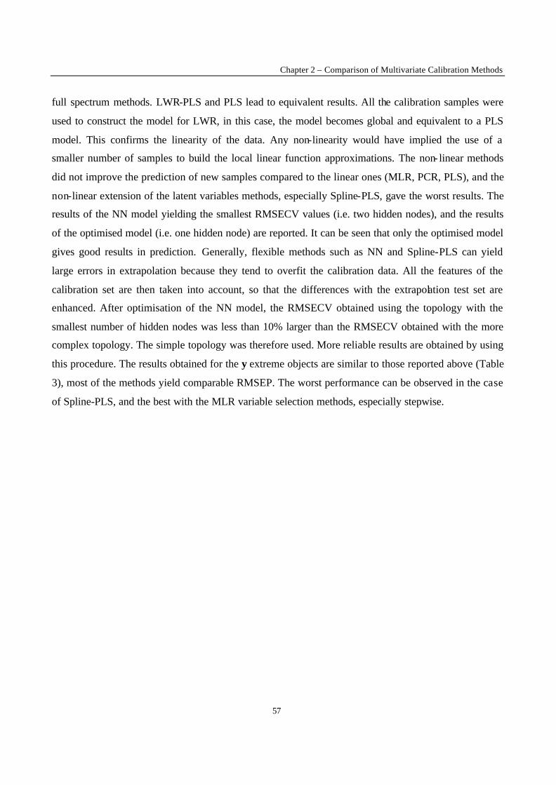
Chapter 2 – Comparison of Multivariate Calibration Methods
57
full spectrum methods. LWR-PLS and PLS lead to equivalent results. All the calibration samples were
used to construct the model for LWR, in this case, the model becomes global and equivalent to a PLS
model. This confirms the linearity of the data. Any non-linearity would have implied the use of a
smaller number of samples to build the local linear function approximations. The non- linear methods
did not improve the prediction of new samples compared to the linear ones (MLR, PCR, PLS), and the
non-linear extension of the latent variables methods, especially Spline-PLS, gave the worst results. The
results of the NN model yielding the smallest RMSECV values (i.e. two hidden nodes), and the results
of the optimised model (i.e. one hidden node) are reported. It can be seen that only the optimised model
gives good results in prediction. Generally, flexible methods such as NN and Spline-PLS can yield
large errors in extrapolation because they tend to overfit the calibration data. All the features of the
calibration set are then taken into account, so that the differences with the extrapolation test set are
enhanced. After optimisation of the NN model, the RMSECV obtained using the topology with the
smallest number of hidden nodes was less than 10% larger than the RMSECV obtained with the more
complex topology. The simple topology was therefore used. More reliable results are obtained by using
this procedure. The results obtained for the y extreme objects are similar to those reported above (Table
3), most of the methods yield comparable RMSEP. The worst performance can be observed in the case
of Spline-PLS, and the best with the MLR variable selection methods, especially stepwise.
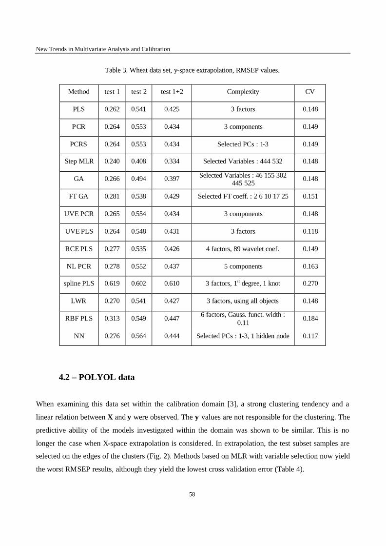
New Trends in Multivariate Analysis and Calibration
58
Table 3. Wheat data set, y-space extrapolation, RMSEP values.
Method test 1 test 2 test 1+2 Complexity CV
PLS 0.262 0.541 0.425 3 factors 0.148
PCR 0.264 0.553 0.434 3 components 0.149
PCRS 0.264 0.553 0.434 Selected PCs : 1-3 0.149
Step MLR 0.240 0.408 0.334 Selected Variables : 444 532 0.148
GA 0.266 0.494 0.397 Selected Variables : 46 155 302 445 525
0.148
FT GA 0.281 0.538 0.429 Selected FT coeff. : 2 6 10 17 25 0.151
UVE PCR 0.265 0.554 0.434 3 components 0.148
UVE PLS 0.264 0.548 0.431 3 factors 0.118
RCE PLS 0.277 0.535 0.426 4 factors, 89 wavelet coef. 0.149
NL PCR 0.278 0.552 0.437 5 components 0.163
spline PLS 0.619 0.602 0.610 3 factors, 1st degree, 1 knot 0.270
LWR 0.270 0.541 0.427 3 factors, using all objects 0.148
RBF PLS 0.313 0.549 0.447 6 factors, Gauss. funct. width : 0.11
0.184
NN 0.276 0.564 0.444 Selected PCs : 1-3, 1 hidden node 0.117
4.2 – POLYOL data
When examining this data set within the calibration domain [3], a strong clustering tendency and a
linear relation between X and y were observed. The y values are not responsible for the clustering. The
predictive ability of the models investigated within the domain was shown to be similar. This is no
longer the case when X-space extrapolation is considered. In extrapolation, the test subset samples are
selected on the edges of the clusters (Fig. 2). Methods based on MLR with variable selection now yield
the worst RMSEP results, although they yield the lowest cross validation error (Table 4).
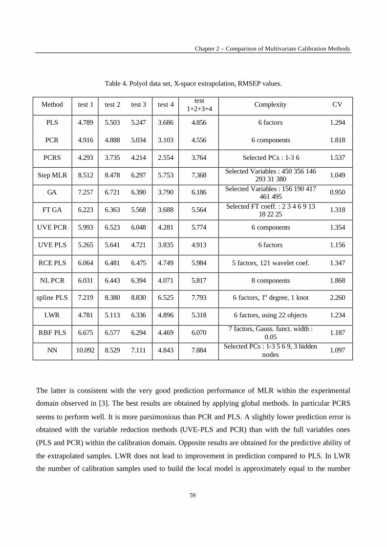
Chapter 2 – Comparison of Multivariate Calibration Methods
59
Table 4. Polyol data set, X-space extrapolation, RMSEP values.
Method test 1 test 2 test 3 test 4 test 1+2+3+4
Complexity CV
PLS 4.789 5.503 5.247 3.686 4.856 6 factors 1.294
PCR 4.916 4.888 5.034 3.103 4.556 6 components 1.818
PCRS 4.293 3.735 4.214 2.554 3.764 Selected PCs : 1-3 6 1.537
Step MLR 8.512 8.478 6.297 5.753 7.368 Selected Variables : 450 356 146 293 31 380 1.049
GA 7.257 6.721 6.390 3.790 6.186 Selected Variables : 156 190 417 461 495
0.950
FT GA 6.223 6.363 5.568 3.688 5.564 Selected FT coeff. : 2 3 4 6 9 13 18 22 25
1.318
UVE PCR 5.993 6.523 6.048 4.281 5.774 6 components 1.354
UVE PLS 5.265 5.641 4.721 3.835 4.913 6 factors 1.156
RCE PLS 6.064 6.481 6.475 4.749 5.984 5 factors, 121 wavelet coef. 1.347
NL PCR 6.031 6.443 6.394 4.071 5.817 8 components 1.868
spline PLS 7.219 8.380 8.830 6.525 7.793 6 factors, 1st degree, 1 knot 2.260
LWR 4.781 5.113 6.336 4.896 5.318 6 factors, using 22 objects 1.234
RBF PLS 6.675 6.577 6.294 4.469 6.070 7 factors, Gauss. funct. width : 0.05
1.187
NN 10.092 8.529 7.111 4.843 7.884 Selected PCs : 1-3 5 6 9, 3 hidden nodes
1.097
The latter is consistent with the very good prediction performance of MLR within the experimental
domain observed in [3]. The best results are obtained by applying global methods. In particular PCRS
seems to perform well. It is more parsimonious than PCR and PLS. A slightly lower prediction error is
obtained with the variable reduction methods (UVE-PLS and PCR) than with the full variables ones
(PLS and PCR) within the calibration domain. Opposite results are obtained for the predictive ability of
the extrapolated samples. LWR does not lead to improvement in prediction compared to PLS. In LWR
the number of calibration samples used to build the local model is approximately equal to the number
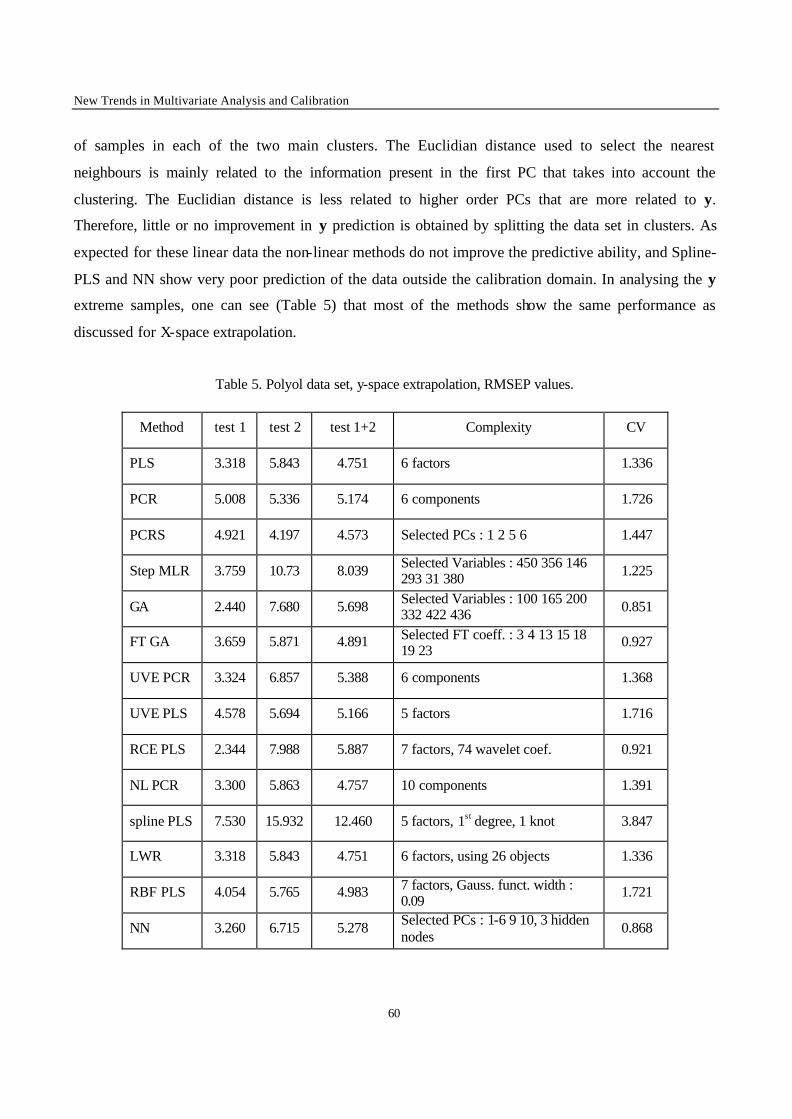
New Trends in Multivariate Analysis and Calibration
60
of samples in each of the two main clusters. The Euclidian distance used to select the nearest
neighbours is mainly related to the information present in the first PC that takes into account the
clustering. The Euclidian distance is less related to higher order PCs that are more related to y.
Therefore, little or no improvement in y prediction is obtained by splitting the data set in clusters. As
expected for these linear data the non-linear methods do not improve the predictive ability, and Spline-
PLS and NN show very poor prediction of the data outside the calibration domain. In analysing the y
extreme samples, one can see (Table 5) that most of the methods show the same performance as
discussed for X-space extrapolation.
Table 5. Polyol data set, y-space extrapolation, RMSEP values.
Method test 1 test 2 test 1+2 Complexity CV
PLS 3.318 5.843 4.751 6 factors 1.336
PCR 5.008 5.336 5.174 6 components 1.726
PCRS 4.921 4.197 4.573 Selected PCs : 1 2 5 6 1.447
Step MLR 3.759 10.73 8.039 Selected Variables : 450 356 146 293 31 380 1.225
GA 2.440 7.680 5.698 Selected Variables : 100 165 200 332 422 436 0.851
FT GA 3.659 5.871 4.891 Selected FT coeff. : 3 4 13 15 18 19 23
0.927
UVE PCR 3.324 6.857 5.388 6 components 1.368
UVE PLS 4.578 5.694 5.166 5 factors 1.716
RCE PLS 2.344 7.988 5.887 7 factors, 74 wavelet coef. 0.921
NL PCR 3.300 5.863 4.757 10 components 1.391
spline PLS 7.530 15.932 12.460 5 factors, 1st degree, 1 knot 3.847
LWR 3.318 5.843 4.751 6 factors, using 26 objects 1.336
RBF PLS 4.054 5.765 4.983 7 factors, Gauss. funct. width : 0.09
1.721
NN 3.260 6.715 5.278 Selected PCs : 1-6 9 10, 3 hidden nodes
0.868
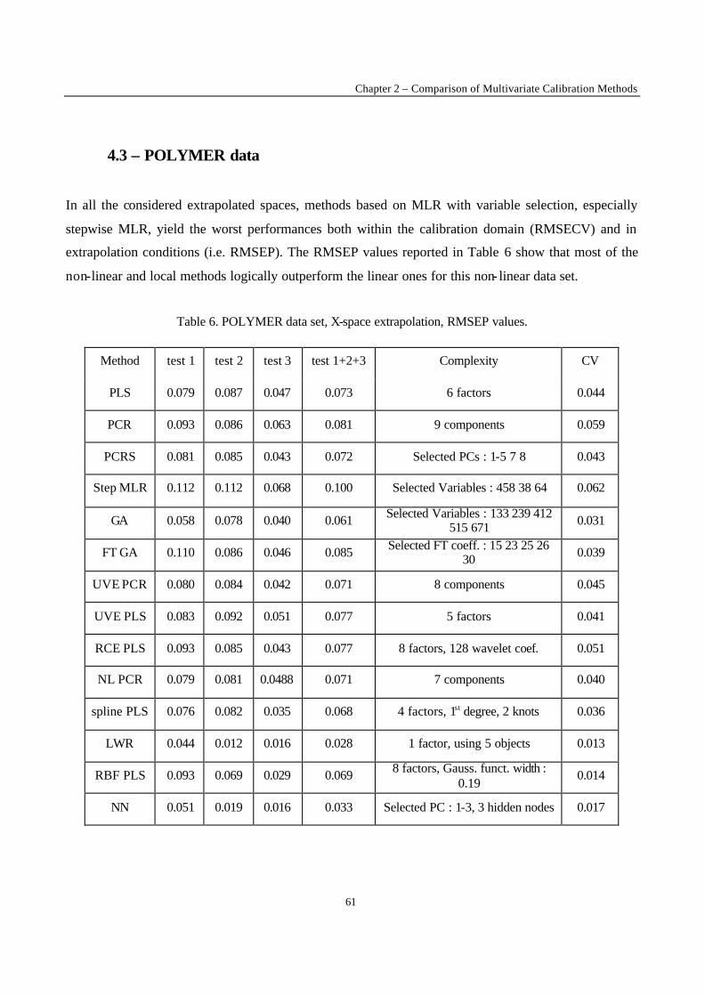
Chapter 2 – Comparison of Multivariate Calibration Methods
61
4.3 – POLYMER data
In all the considered extrapolated spaces, methods based on MLR with variable selection, especially
stepwise MLR, yield the worst performances both within the calibration domain (RMSECV) and in
extrapolation conditions (i.e. RMSEP). The RMSEP values reported in Table 6 show that most of the
non-linear and local methods logically outperform the linear ones for this non- linear data set.
Table 6. POLYMER data set, X-space extrapolation, RMSEP values.
Method test 1 test 2 test 3 test 1+2+3 Complexity CV
PLS 0.079 0.087 0.047 0.073 6 factors 0.044
PCR 0.093 0.086 0.063 0.081 9 components 0.059
PCRS 0.081 0.085 0.043 0.072 Selected PCs : 1-5 7 8 0.043
Step MLR 0.112 0.112 0.068 0.100 Selected Variables : 458 38 64 0.062
GA 0.058 0.078 0.040 0.061 Selected Variables : 133 239 412 515 671 0.031
FT GA 0.110 0.086 0.046 0.085 Selected FT coeff. : 15 23 25 26 30 0.039
UVE PCR 0.080 0.084 0.042 0.071 8 components 0.045
UVE PLS 0.083 0.092 0.051 0.077 5 factors 0.041
RCE PLS 0.093 0.085 0.043 0.077 8 factors, 128 wavelet coef. 0.051
NL PCR 0.079 0.081 0.0488 0.071 7 components 0.040
spline PLS 0.076 0.082 0.035 0.068 4 factors, 1st degree, 2 knots 0.036
LWR 0.044 0.012 0.016 0.028 1 factor, using 5 objects 0.013
RBF PLS 0.093 0.069 0.029 0.069 8 factors, Gauss. funct. width : 0.19
0.014
NN 0.051 0.019 0.016 0.033 Selected PC : 1-3, 3 hidden nodes 0.017
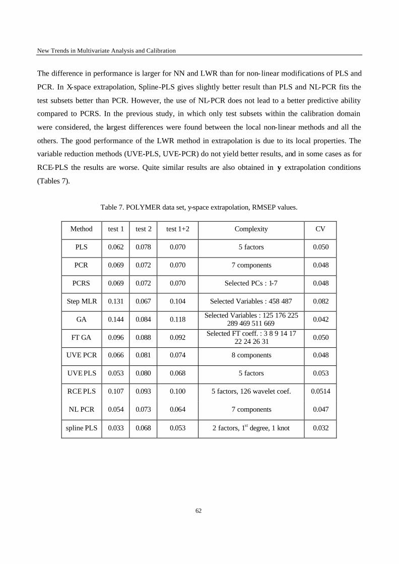
New Trends in Multivariate Analysis and Calibration
62
The difference in performance is larger for NN and LWR than for non- linear modifications of PLS and
PCR. In X-space extrapolation, Spline-PLS gives slightly better result than PLS and NL-PCR fits the
test subsets better than PCR. However, the use of NL-PCR does not lead to a better predictive ability
compared to PCRS. In the previous study, in which only test subsets within the calibration domain
were considered, the largest differences were found between the local non-linear methods and all the
others. The good performance of the LWR method in extrapolation is due to its local properties. The
variable reduction methods (UVE-PLS, UVE-PCR) do not yield better results, and in some cases as for
RCE-PLS the results are worse. Quite similar results are also obtained in y extrapolation conditions
(Tables 7).
Table 7. POLYMER data set, y-space extrapolation, RMSEP values.
Method test 1 test 2 test 1+2 Complexity CV
PLS 0.062 0.078 0.070 5 factors 0.050
PCR 0.069 0.072 0.070 7 components 0.048
PCRS 0.069 0.072 0.070 Selected PCs : 1-7 0.048
Step MLR 0.131 0.067 0.104 Selected Variables : 458 487 0.082
GA 0.144 0.084 0.118 Selected Variables : 125 176 225 289 469 511 669 0.042
FT GA 0.096 0.088 0.092 Selected FT coeff. : 3 8 9 14 17 22 24 26 31 0.050
UVE PCR 0.066 0.081 0.074 8 components 0.048
UVE PLS 0.053 0.080 0.068 5 factors 0.053
RCE PLS 0.107 0.093 0.100 5 factors, 126 wavelet coef. 0.0514
NL PCR 0.054 0.073 0.064 7 components 0.047
spline PLS 0.033 0.068 0.053 2 factors, 1st degree, 1 knot 0.032
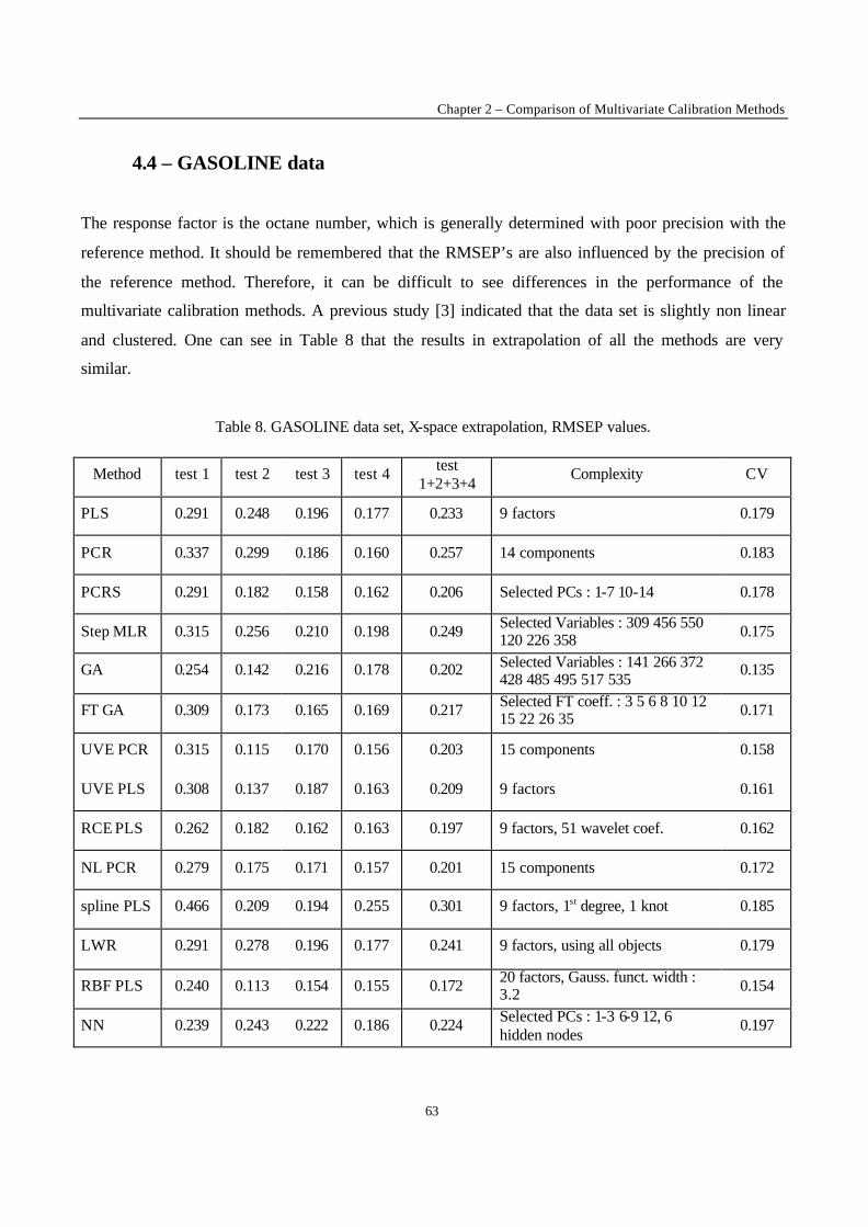
Chapter 2 – Comparison of Multivariate Calibration Methods
63
4.4 – GASOLINE data
The response factor is the octane number, which is generally determined with poor precision with the
reference method. It should be remembered that the RMSEP’s are also influenced by the precision of
the reference method. Therefore, it can be difficult to see differences in the performance of the
multivariate calibration methods. A previous study [3] indicated that the data set is slightly non linear
and clustered. One can see in Table 8 that the results in extrapolation of all the methods are very
similar.
Table 8. GASOLINE data set, X-space extrapolation, RMSEP values.
Method test 1 test 2 test 3 test 4 test 1+2+3+4
Complexity CV
PLS 0.291 0.248 0.196 0.177 0.233 9 factors 0.179
PCR 0.337 0.299 0.186 0.160 0.257 14 components 0.183
PCRS 0.291 0.182 0.158 0.162 0.206 Selected PCs : 1-7 10-14 0.178
Step MLR 0.315 0.256 0.210 0.198 0.249 Selected Variables : 309 456 550 120 226 358 0.175
GA 0.254 0.142 0.216 0.178 0.202 Selected Variables : 141 266 372 428 485 495 517 535
0.135
FT GA 0.309 0.173 0.165 0.169 0.217 Selected FT coeff. : 3 5 6 8 10 12 15 22 26 35 0.171
UVE PCR 0.315 0.115 0.170 0.156 0.203 15 components 0.158
UVE PLS 0.308 0.137 0.187 0.163 0.209 9 factors 0.161
RCE PLS 0.262 0.182 0.162 0.163 0.197 9 factors, 51 wavelet coef. 0.162
NL PCR 0.279 0.175 0.171 0.157 0.201 15 components 0.172
spline PLS 0.466 0.209 0.194 0.255 0.301 9 factors, 1st degree, 1 knot 0.185
LWR 0.291 0.278 0.196 0.177 0.241 9 factors, using all objects 0.179
RBF PLS 0.240 0.113 0.154 0.155 0.172 20 factors, Gauss. funct. width : 3.2 0.154
NN 0.239 0.243 0.222 0.186 0.224 Selected PCs : 1-3 6-9 12, 6 hidden nodes
0.197
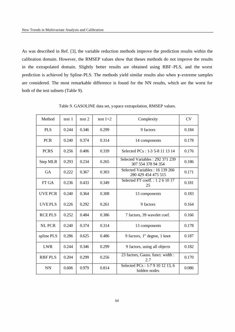
New Trends in Multivariate Analysis and Calibration
64
As was described in Ref. [3], the variable reduction methods improve the prediction results within the
calibration domain. However, the RMSEP values show that theses methods do not improve the results
in the extrapolated domain. Slightly better results are obtained using RBF -PLS, and the worst
prediction is achieved by Spline-PLS. The methods yield similar results also when y-extreme samples
are considered. The most remarkable difference is found for the NN results, which are the worst for
both of the test subsets (Table 9).
Table 9. GASOLINE data set, y-space extrapolation, RMSEP values.
Method test 1 test 2 test 1+2 Complexity CV
PLS 0.244 0.346 0.299 9 factors 0.184
PCR 0.240 0.374 0.314 14 components 0.178
PCRS 0.256 0.406 0.339 Selected PCs : 1-3 5-8 11 13 14 0.176
Step MLR 0.293 0.234 0.265 Selected Variables : 292 371 239 307 554 378 94 354 0.186
GA 0.222 0.367 0.303 Selected Variables : 16 139 266 280 429 454 475 515
0.171
FT GA 0.236 0.433 0.349 Selected FT coeff. : 1 2 6 10 17 25
0.181
UVE PCR 0.240 0.364 0.308 13 components 0.183
UVE PLS 0.226 0.292 0.261 9 factors 0.164
RCE PLS 0.252 0.484 0.386 7 factors, 39 wavelet coef. 0.166
NL PCR 0.240 0.374 0.314 13 components 0.178
spline PLS 0.286 0.625 0.486 9 factors, 1st degree, 1 knot 0.187
LWR 0.244 0.346 0.299 9 factors, using all objects 0.182
RBF PLS 0.204 0.299 0.256 23 factors, Gauss. funct. width : 2.7
0.170
NN 0.606 0.979 0.814 Selected PCs : 1-7 9 10 12 13, 6 hidden nodes
0.086
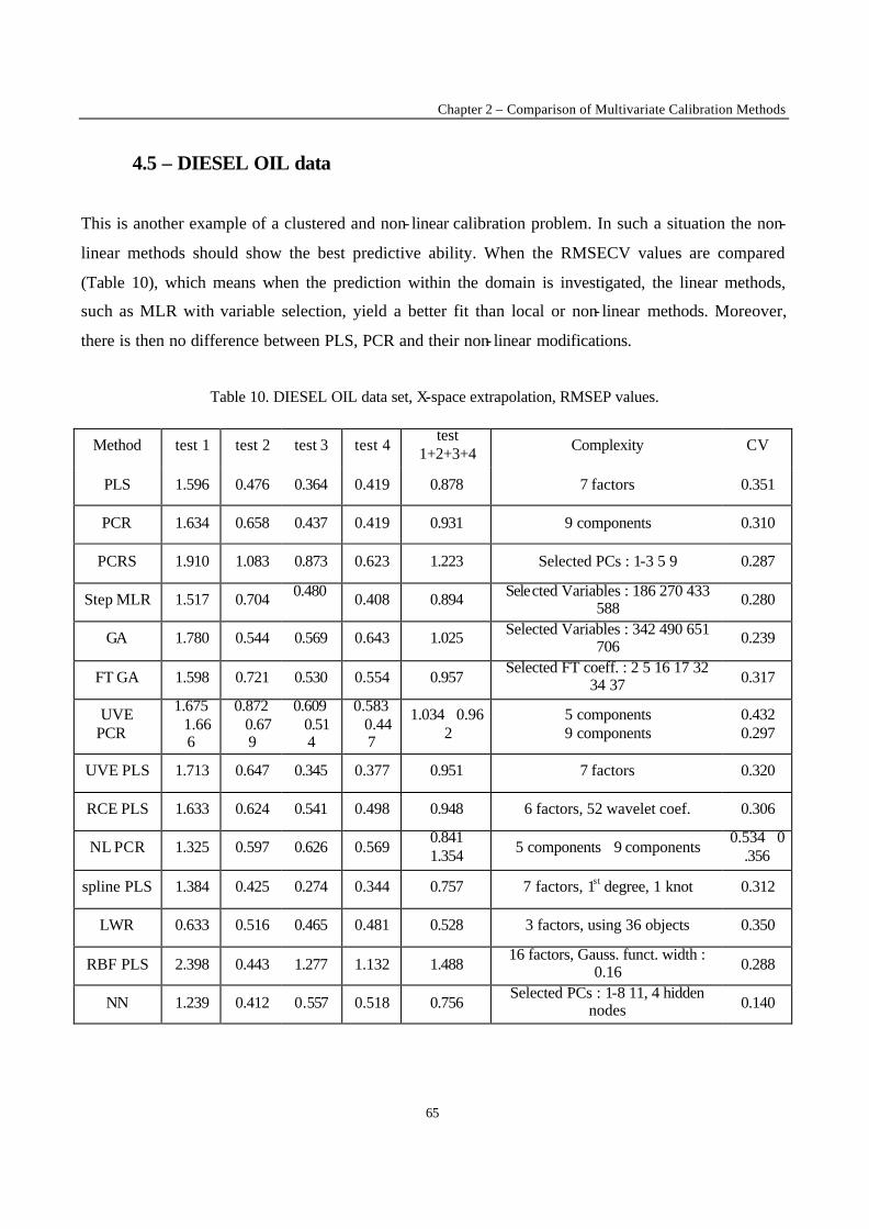
Chapter 2 – Comparison of Multivariate Calibration Methods
65
4.5 – DIESEL OIL data
This is another example of a clustered and non- linear calibration problem. In such a situation the non-
linear methods should show the best predictive ability. When the RMSECV values are compared
(Table 10), which means when the prediction within the domain is investigated, the linear methods,
such as MLR with variable selection, yield a better fit than local or non- linear methods. Moreover,
there is then no difference between PLS, PCR and their non- linear modifications.
Table 10. DIESEL OIL data set, X-space extrapolation, RMSEP values.
Method test 1 test 2 test 3 test 4 test
1+2+3+4 Complexity CV
PLS 1.596 0.476 0.364 0.419 0.878 7 factors 0.351
PCR 1.634 0.658 0.437 0.419 0.931 9 components 0.310
PCRS 1.910 1.083 0.873 0.623 1.223 Selected PCs : 1-3 5 9 0.287
Step MLR 1.517 0.704 0.480 0.408 0.894 Selected Variables : 186 270 433
588 0.280
GA 1.780 0.544 0.569 0.643 1.025 Selected Variables : 342 490 651 706 0.239
FT GA 1.598 0.721 0.530 0.554 0.957 Selected FT coeff. : 2 5 16 17 32
34 37 0.317
UVE PCR
1.6751.666
0.8720.679
0.6090.514
0.5830.447
1.034 0.962
5 components 9 components
0.432 0.297
UVE PLS 1.713 0.647 0.345 0.377 0.951 7 factors 0.320
RCE PLS 1.633 0.624 0.541 0.498 0.948 6 factors, 52 wavelet coef. 0.306
NL PCR 1.325 0.597 0.626 0.569 0.841 1.354 5 components 9 components
0.534 0.356
spline PLS 1.384 0.425 0.274 0.344 0.757 7 factors, 1st degree, 1 knot 0.312
LWR 0.633 0.516 0.465 0.481 0.528 3 factors, using 36 objects 0.350
RBF PLS 2.398 0.443 1.277 1.132 1.488 16 factors, Gauss. funct. width :
0.16 0.288
NN 1.239 0.412 0.557 0.518 0.756 Selected PCs : 1-8 11, 4 hidden
nodes 0.140
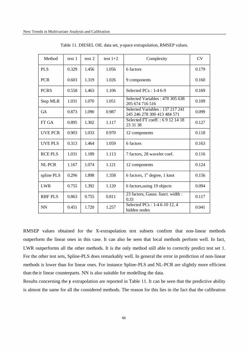
New Trends in Multivariate Analysis and Calibration
66
Table 11. DIESEL OIL data set, y-space extrapolation, RMSEP values.
Method test 1 test 2 test 1+2 Complexity CV
PLS 0.329 1.456 1.056 6 factors 0.179
PCR 0.603 1.319 1.026 9 components 0.160
PCRS 0.558 1.463 1.106 Selected PCs : 1-4 6-9 0.169
Step MLR 1.031 1.070 1.051 Selected Variables : 470 305 638 205 674 716 516 0.109
GA 0.873 1.090 0.987 Selected Variables : 137 217 241 245 246 278 300 413 484 571 0.099
FT GA 0.895 1.302 1.117 Selected FT coeff. : 6 9 12 14 18 23 31 38 0.127
UVE PCR 0.903 1.033 0.970 12 components 0.118
UVE PLS 0.313 1.464 1.059 6 factors 0.163
RCE PLS 1.031 1.189 1.113 7 factors, 28 wavelet coef. 0.116
NL PCR 1.167 1.074 1.121 12 components 0.124
spline PLS 0.296 1.898 1.358 6 factors, 1st degree, 1 knot 0.156
LWR 0.755 1.392 1.120 6 factors,using 19 objects 0.094
RBF PLS 0.863 0.755 0.811 23 factors, Gauss. funct. width : 0.33
0.117
NN 0.451 1.720 1.257 Selected PCs : 1-4 6-10 12, 4 hidden nodes
0.041
RMSEP values obtained for the X-extrapolation test subsets confirm that non- linear methods
outperform the linear ones in this case. It can also be seen that local methods perform well. In fact,
LWR outperforms all the other methods. It is the only method still able to correctly predict test set 1.
For the other test sets, Spline-PLS does remarkably well. In general the error in prediction of non- linear
methods is lower than for linear ones. For instance Spline-PLS and NL-PCR are slightly more efficient
than the ir linear counterparts. NN is also suitable for modelling the data.
Results concerning the y extrapolation are reported in Table 11. It can be seen that the predictive ability
is almost the same for all the considered methods. The reason for this lies in the fact that the calibration
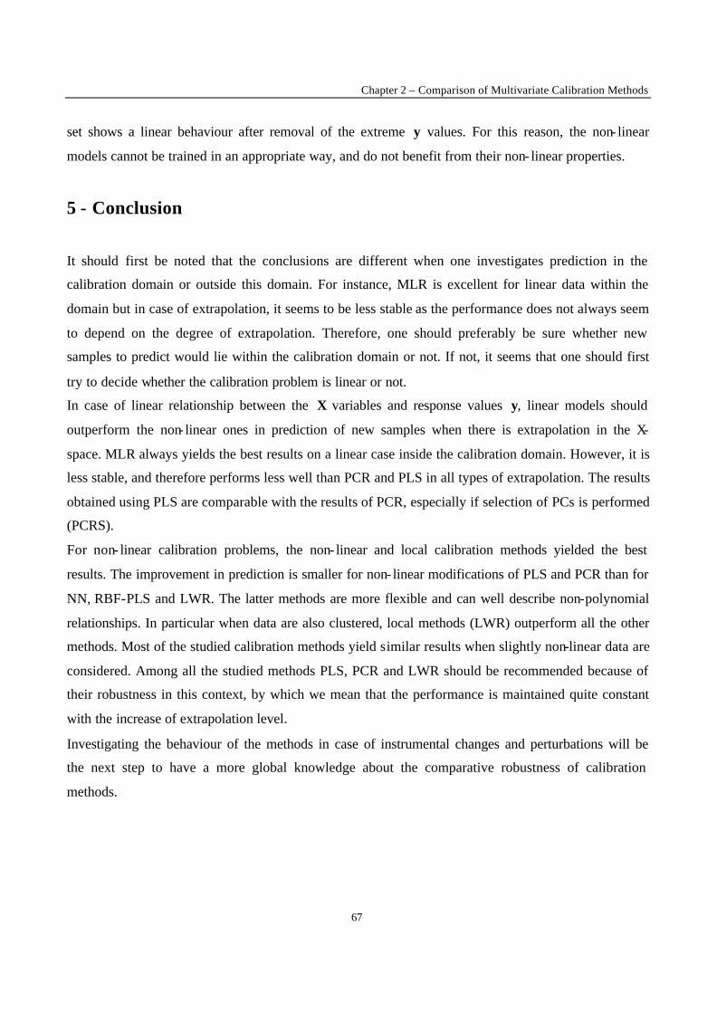
Chapter 2 – Comparison of Multivariate Calibration Methods
67
set shows a linear behaviour after removal of the extreme y values. For this reason, the non- linear
models cannot be trained in an appropriate way, and do not benefit from their non- linear properties.
5 - Conclusion
It should first be noted that the conclusions are different when one investigates prediction in the
calibration domain or outside this domain. For instance, MLR is excellent for linear data within the
domain but in case of extrapolation, it seems to be less stable as the performance does not always seem
to depend on the degree of extrapolation. Therefore, one should preferably be sure whether new
samples to predict would lie within the calibration domain or not. If not, it seems that one should first
try to decide whether the calibration problem is linear or not.
In case of linear relationship between the X variables and response values y, linear models should
outperform the non- linear ones in prediction of new samples when there is extrapolation in the X-
space. MLR always yields the best results on a linear case inside the calibration domain. However, it is
less stable, and therefore performs less well than PCR and PLS in all types of extrapolation. The results
obtained using PLS are comparable with the results of PCR, especially if selection of PCs is performed
(PCRS).
For non- linear calibration problems, the non- linear and local calibration methods yielded the best
results. The improvement in prediction is smaller for non- linear modifications of PLS and PCR than for
NN, RBF-PLS and LWR. The latter methods are more flexible and can well describe non-polynomial
relationships. In particular when data are also clustered, local methods (LWR) outperform all the other
methods. Most of the studied calibration methods yield similar results when slightly non-linear data are
considered. Among all the studied methods PLS, PCR and LWR should be recommended because of
their robustness in this context, by which we mean that the performance is maintained quite constant
with the increase of extrapolation level.
Investigating the behaviour of the methods in case of instrumental changes and perturbations will be
the next step to have a more global knowledge about the comparative robustness of calibration
methods.

New Trends in Multivariate Analysis and Calibration
68
ACKNOWLEDGMENTS
We thank the Fonds voor Wetenschappelijk Onderzoek (FWO), the DWTC, and the Standards
Measurement and Testing program of the EU (SMT Programme contract SMT4 -CT95-2031) for
financial assistance.
REFERENCES
1) F. Cahn, S. Compton, Appl. Spectrosc., 42 (1988) 865-884.
2) L. Zhang, Y. Liang, J. Jiang, R Yu, K. Fang, Anal. Chim. Acta, 370 (1998) 65-77H.
3) V.Centner, J. Verdu-Andreas, B. Walczak, D. Jouan-Rimbaud, F. Despagne, L. Pasti., R. Poppi,
D.L. Massart and O. E. de Noord., Appl. Spectrosc. 54 (2000) 608-623.
4) H. van der Voet, Chemom. Intell. Lab. Syst., 25 (1994) 313-323.
5) J. Verdu-Andres, D. L. Massart, C. Menardo, C. Sterna, Anal. Chim. Acta, 389 (1999) 115-130.
6) I. E. Frank, J. H. Friedman, Technom., 35 (1993) 109-148.
7) Wold, S., Chemom. Intel. lab. syst., 14 (1992) 71-84.
8) C. B. Lucasius, G. Kateman, Chemom. Intel. lab. syst., 25 (1994) 99-145.
9) R. Leardi, J. Chemom., 8 (1994) 65-79.
10) D. Jouan-Rimbaud, R. Leardi, D. L. Massart, O. E. de Noord, Anal. Chem., 67 (1995) 4295-
4301.
11) L. Pasti, D. Jouan-Rimbaud, D. L. Massart, O. E. de Noord, Anal. Chim. Acta, 364 (1998) 253-
263.
12) V. Centner, D. L. Massart, O. E. de Noord, S. de Jong, B. M. Vandeginste, C. Sterna, Anal.
Chem., 68 (1996) 3851-3858.
13) D. Jouan-Rimbaud, R. Poppi, D. L. Massart, O. E. de Noord, Anal. Chem., 69 (1997) 4317-
4323.
14) T. Næs, T. Isaksson, B. R. Kowalski, Anal. Chem., 66 (1994) 249-260.
15) V. Centner, D.L. Massart. Anal. Chem., 70 (1998) 4206-4211.
16) B. Walczak, D. L. Massart, Anal. Chim. Acta, 331 (1996) 177-185.
17) R. Fletcher, Practical Methods of optimization, Wiley, N.Y., 1987.
18) F. Despagne, D.L. Massart, Chemom. Intel. lab. syst., 40 (1998) 145-163.

Chapter 2 – Comparison of Multivariate Calibration Methods
69
19) R.W. Kennard and L.A. Stone, Technometrics, 11 (1969) 137-148.
20) R.D. Snee, Technometrics 19 (1977) 415-428.
21) U.G. Indahl, T. Næs, J. Chemometrics, 12 (1998) 261-278.
22) J.H. Kalivas, Chemom. Intel. lab. syst., 37 (1997) 255-259.
23) V. Centner, D. L. Massart, O. E. de Noord, Anal. Chim. Acta, 330 (1996) 1-17.
24) R.J. Barnes, M.S. Dhanoa and S.J. Lister, Appl. Spectrosc., 43 (1989) 772-777.
New Trends in Multivariate Analysis and Calibration
70
A Comparison of Multivariate Calibration
Techniques Applied to Experimental NIR Data
Sets. Part III : Robustness Against Instrumental
Perturbation Conditions.
Submitted for publication.
F. Estienne , F. Despagne, B. Walczak+, O. E. de Noord1 ,D.L. Massart*
ChemoAC,
Farmaceutisch Instituut, Vrije Universiteit Brussel,
Laarbeeklaan 103, B-1090 Brussels, Belgium.
E-mail: [email protected]
+ on leave from : Silesian University
Katowice Poland
1 Shell International Chemicals B. V., Shell Research and Technology Centre
Amsterdam P. O. Box 38000
1030 BN Amsterdam The Netherlands
ABSTRACT
This work is part of a more general research aiming at comparing the performance of multivariate calibration methods. In the first and second parts of the study, the performances of multivariate calibration methods were compared in situation of interpolation and extrapolation respectively. This third part of the study deals with robustness of calibration methods in the case whe re spectra corresponding to new samples of which the y value has to be predicted can be affected by instrumental perturbations not accounted for in the calibration set. This type of perturbations can happen due to instrument ageing, replacement of one or several parts of the spectrometer (e.g. the detector), use of a new instrument, or modifications in the measurement conditions, like the displacement of the instrument to a different location. Even though no general rules could be drawn, the variety of data sets and calibration methods used enabled to establish some guidelines for multivariate calibration in this unfavourable case when instrumental perturbation arises.
* Corresponding author
KEYWORDS : Multivariate calibration, method comparison, instrumental change, extrapolation, non-
linearity, clustering.
Chapter 2 – Comparison of Multivariate Calibration Methods
71
1 – Introduction
This study is part of a more general research aiming at comparing the performance of multivariate
calibration methods. These methods enable to relate instrumental responses consisting of a set of
predictors X to a chemical or physical property of interest y (the response factor). The choice of the
most appropriate method is a crucial step in order to obtain a good prediction of the property y of new
samples. Methods were compared using sets of industrial Near-Infrared (NIR) data, chosen such that
they include difficulties often met in practice, namely data clustering, non- linearity, and presence of
irrelevant variables in the set of predictors. The comparative study was performed in three separate
steps :
• In the first part of the study [1], the performances of multivariate calibration methods were
compared in the ideal situation where test samples are within the calibration domain (interpolation).
• In the second part of the study [2], the performance of multivariate calibration methods were
compared in a situation which can sometimes not be avoided in practice : the case where some test
samples fall outside the calibration domain (extrapolation). Extrapolation occurring in the X-space and
in the Y-space was considered.
• This third part of the study deals with the case where spectra corresponding to new samples of
which the y value has to be predicted can be affected by instrumental perturbations not accounted for in
the calibration set. The robustness of a calibration model is challenged in this situation in which exactly
superimposing replicate spectra of a stable standard is impossible. The instrumental perturbations can
be due to instrument ageing, replacement of one or several parts of the spectrometer (e.g. the detector),
use of a new instrument, or modifications in the measurement conditions, like the displacement of the
instrument to a different location. In all cases a degradation of the prediction results must be expected.
This third part of the method comparison study aims at evaluating the robustness of the different
calibration methods in the presence of such perturbations.
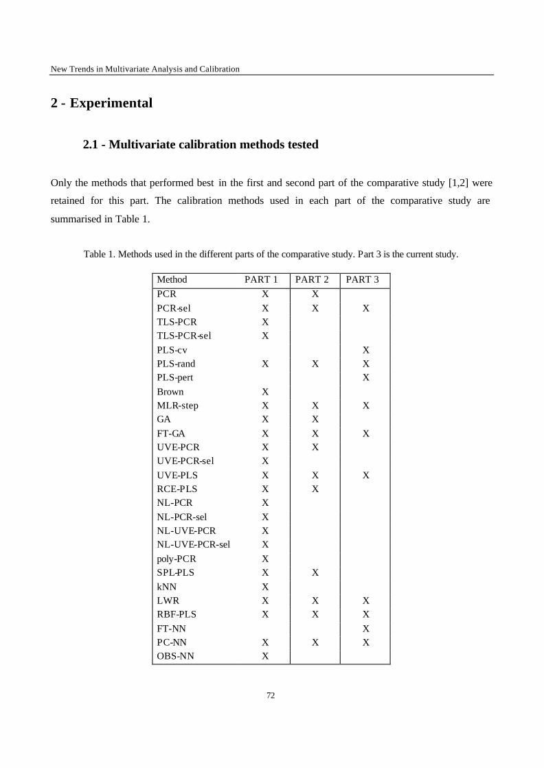
New Trends in Multivariate Analysis and Calibration
72
2 - Experimental
2.1 - Multivariate calibration methods tested
Only the methods that performed best in the first and second part of the comparative study [1,2] were
retained for this part. The calibration methods used in each part of the comparative study are
summarised in Table 1.
Table 1. Methods used in the different parts of the comparative study. Part 3 is the current study.
Method PART 1 PART 2 PART 3 PCR X X PCR-sel X X X TLS-PCR X TLS-PCR-sel X PLS-cv X PLS-rand X X X PLS-pert X Brown X MLR-step X X X GA X X FT-GA X X X UVE-PCR X X UVE-PCR-sel X UVE-PLS X X X RCE-PLS X X NL-PCR X NL-PCR-sel X NL-UVE-PCR X NL-UVE-PCR-sel X poly-PCR X SPL-PLS X X kNN X LWR X X X RBF-PLS X X X FT-NN X PC-NN X X X OBS-NN X
Chapter 2 – Comparison of Multivariate Calibration Methods
73
2.1.1 - Principal component regression (PCR)
In classical PCR (sometimes referred to as top-down PCR) [3], the number A of Principal Components
(PC) is optimised by Leave One Out (LOO) Cross Validation (CV). PCs from PC1 to PCA are retained
in order of the variance in the original data matrix X they explain. A limitation of this approach is that,
in some cases, information related to the property to be predicted y is found in high-order PCs, which
account for only a small amount of spectral variance. An alternative version called PCR with best
subset selection (PCR-sel) was therefore used. In this method, PCs are selected according to their
correlation with the target property y [1]. Model complexity was estimated by LOOCV followed by a
randomisation test [4]. This test allows to determine whether models with lower complexity have
significantly worse predictive ability and should therefore not be used.
2.1.2 - Partial least squares and its variants
Contrarily to PCR, the Latent Variables (LV) in PLS [5,6] are calculated to maximise covariance
between X and y. Latent variable selection as performed in PCR is therefore not necessary. The model
complexity A in PLS can be determined in several ways. The most classical way is to perform LOOCV
and retain the complexity associated with the minimum LOOCV error (PLS-cv). However this
approach is rather conservative since the removal of one sample at a time corresponds to a small
statistical perturbation of the calibration set. The complexity of the model chosen is often too high. Use
of a randomisation test often allows to reduce the complexity of the selected models (PLS-rand), but in
some cases it carries a risk of underfitting, i.e. too few LVs can be retained [7]. This is why an
alternative validation method for selecting optimal model complexity based on the simulation of
instrumental perturbatio ns on a subset of calibration sample spectra (PLS-pert) [7] was developed. This
method aims at determining the number of LVs beyond which models are unnecessarily sensitive to
instrumental perturbations affecting the spectra.
2.1.3 - Methods based on variable selection/elimination
In stepwise Multiple Linear Regression (MLR-step), original variables are selected iteratively
according to their correlation with the target property y [8]. For a selected variable xi, a regression
New Trends in Multivariate Analysis and Calibration
74
coefficient bi is determined and tested for significance using a t-test at a critical level α ( α = 5% was
used in this study). If the coefficient is found to be significant, the variable is retained and another
variable xj is selected according to its partial correlation with the residuals obtained from the model
built with xi. This procedure is called forward selection. The significance of the two regression
coefficients bi and bj associated with the two retained variables is then again tested, and the non-
significant terms are eliminated from the equation (backward elimination). Forward selection and
backward elimination are alternatively repeated until no significant improvement of the model fit can
be achieved by including more variables and all regression terms already selected are significant. In
order to reduce the risk of overfitting due to retaining too many variables, a procedure based on
LOOCV followed by a randomisation test is applied to test different sets of variables for significant
differences in prediction.
Genetic algorithms (GA) are probabilistic optimisation tools inspired by the “survival of the fittest”
principle of Darwinian theory of natural evolution and the mechanisms of natural genetics [9]. They
can be used in calibration to select a small subset of original variables to model y using MLR [10,11].
Instead of performing the selection on the set of numerous correlated original variables, one can apply
GA to transformed variables such as power spectrum coefficients obtained by Fourier transform (FT-
GA) [12]. In this case the variable selection is carried out in the frequency domain, from the first fifty
power spectrum coefficients only.
2.1.4 - Methods based on uninformative variable elimination
The idea behind the uninformative variable elimination PLS (UVE-PLS) method is to reduce
significantly the number of original variable before calculating LVs in the final PLS model [13]. This is
done by removing original variables that are considered unimportant. One first generates vectors of
random variables that are attached to each spectrum in the data set. Then a PLS model is built on the
set of artificially augmented spectra, and all variables with regression coefficients not significantly
more reliable than the regression coefficients of the dummy variables are truncated. (The reliability of a
coefficient is calculated as the ratio of its magnitude to its standard deviation estimated by leave-one-
out jackknifing). After reduction of the number of original variables, a new PLS model is built. Model
complexities for variable elimination and final modelling are determined by LOOCV. The advantage of
Chapter 2 – Comparison of Multivariate Calibration Methods
75
the UVE-PLS approach is that, since noisy or redundant variables have been eliminated, the models
built after variable elimination will be more parsimonious and robust than classical PLS models.
2.1.5 - Methods based on local modelling
In locally weighted regression (LWR), a dedicated local model is developed for each new prediction
sample [14]. This can be advantageous for data sets that exhibit some clustering or some non-linearity
that can be approximated by local linear fits. For each point to be predicted, a local PLS model is built
using the closest (in terms of Euclidian norm in the X space) calibration points. In this study, the points
were given uniform weights in the local model [15].
The radial basis function PLS method (RBF-PLS) bears some similarities with LWR [16]. The PLS
algorithm is applied to the M and y matrices instead of the X and y matrices. M(n× n) is called the
activation matrix (with n the number of samples). Its elements are Gaussian functions placed at the
positions of the calibration objects. Thus a form of local modelling is performed as in LWR. The PLS
algorithm relates the non- linearly transformed distance measures in M to the target property in y. The
width of Gaussian functions and number of LVs are optimised by prediction testing using a training
and a monitoring set similarly to Neural Networks.
2.1.6 - Methods using Neural Networks (NN)
Back-propagation NN using PCs as inputs was used in this study (PC-NN). A method was applied to
find the best number of nodes to be used in the input and hidden layers based on the contribution of
each node [17]. NN models using Fourier transform power spectrum coefficients (FT-NN) were also
used. Optimisation of the set of input coefficients was performed on the first 20 coefficients by trial-
and-error (the variance propagation approach for sensitivity estimation can not be applied in this case
since Fourier coefficients are not orthogonal). All NN models had one hidden layer and were trained
with the Levenberg-Marquardt algorithm [18]. Hyperbolic tangent and/or linear functions were used in
the nodes of the hidden and output layers.
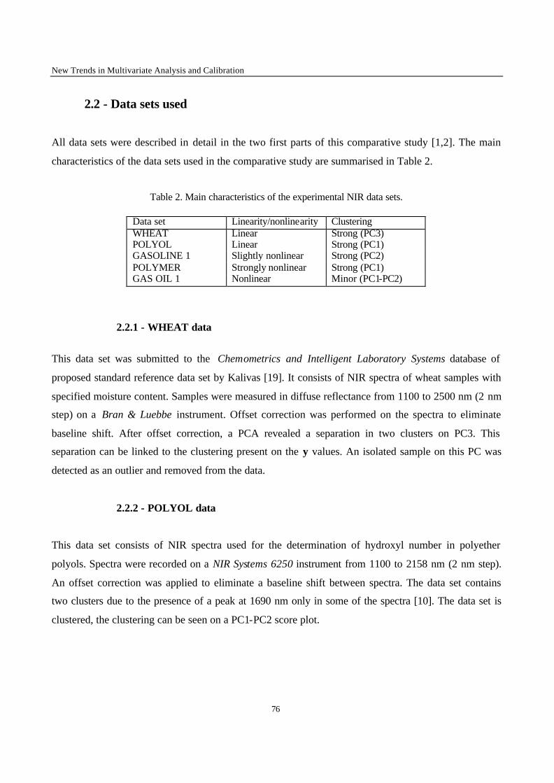
New Trends in Multivariate Analysis and Calibration
76
2.2 - Data sets used
All data sets were described in detail in the two first parts of this comparative study [1,2]. The main
characteristics of the data sets used in the comparative study are summarised in Table 2.
Table 2. Main characteristics of the experimental NIR data sets.
Data set Linearity/nonlinearity Clustering WHEAT Linear Strong (PC3) POLYOL Linear Strong (PC1) GASOLINE 1 Slightly nonlinear Strong (PC2) POLYMER Strongly nonlinear Strong (PC1) GAS OIL 1 Nonlinear Minor (PC1-PC2)
2.2.1 - WHEAT data
This data set was submitted to the Chemometrics and Intelligent Laboratory Systems database of
proposed standard reference data set by Kalivas [19]. It consists of NIR spectra of wheat samples with
specified moisture content. Samples were measured in diffuse reflectance from 1100 to 2500 nm (2 nm
step) on a Bran & Luebbe instrument. Offset correction was performed on the spectra to eliminate
baseline shift. After offset correction, a PCA revealed a separation in two clusters on PC3. This
separation can be linked to the clustering present on the y values. An isolated sample on this PC was
detected as an outlier and removed from the data.
2.2.2 - POLYOL data
This data set consists of NIR spectra used for the determination of hydroxyl number in polyether
polyols. Spectra were recorded on a NIR Systems 6250 instrument from 1100 to 2158 nm (2 nm step).
An offset correction was applied to eliminate a baseline shift between spectra. The data set contains
two clusters due to the presence of a peak at 1690 nm only in some of the spectra [10]. The data set is
clustered, the clustering can be seen on a PC1-PC2 score plot.
Chapter 2 – Comparison of Multivariate Calibration Methods
77
2.2.3 - GASOLINE data
This data set was studied for the determination of gasoline MON. The NIR spectra were recorded on a
PIONIR 1024 spectrometer instrument from 800 to 1080 nm (0.5 nm step). Spectra were pre-processed
with first derivatives to eliminate a baseline shift and to separate overlapping peaks. This data set
contains three clusters due to gasolines with different grades and it is non- linear.
2.2.4 – POLYMER data
This data set was used for the determination of the amount of a minor mineral component in a polymer.
NIR spectra were recorded from 1100 to 2498 nm (2 nm step). SNV transformation was applied to
remove a curved baseline shift between spectra. This data set is clus tered and strongly non- linear in the
X-y relationship and in the X-space.
2.2.5 – GAS OIL data
This data set was studied for modelling the viscosity of hydro-treated gas oil samples. The NIR spectra
were recorded on a NIR interferometer between 4770 and 6300 cm-1 (1.9 cm-1 step). Spectra were
converted from wavenumbers to wavelengths and linear baseline correction was performed to correct
for a baseline drift. Clusters and zones of unequal density are present in the data set due to the fact that
the samples come from three different batches. This data set is non-linear, but this non- linearity can
only be seen due to the presence of two extreme samples. These extreme samples could have been
misinterpreted as outliers, but people in charge of data acquisition established through expert
knowledge that this was not the case.

New Trends in Multivariate Analysis and Calibration
78
2.3 - Design of the method comparison study
Models were developed using calibration samples, and their predictive ability was evaluated on
perturbation- free test samples as was done in the first part of the comparative study [1]. Perturbations
were then simulated on the spectra of the test samples. The following types of perturbation were
studied :
• detector noise
• change in optical pathlength
• wavelength shift
• slope in baseline
• baseline offset
• stray light
For each calibration method, the prediction error on the perturbed test samples was evaluated and
compared to the prediction error on perturbation-free samples. Therefore, this study provided not only
information on the performance of calibration methods in the presence of perturbation, but also on the
relative degradation of performance compared to perturbation-free test samples.
The perturbations were simulated as follows:
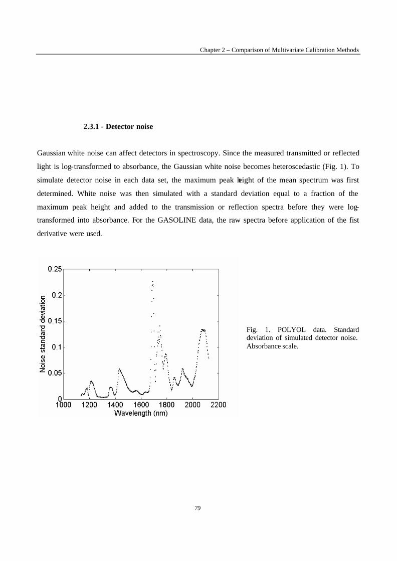
Chapter 2 – Comparison of Multivariate Calibration Methods
79
2.3.1 - Detector noise
Gaussian white noise can affect detectors in spectroscopy. Since the measured transmitted or reflected
light is log-transformed to absorbance, the Gaussian white noise becomes heteroscedastic (Fig. 1). To
simulate detector noise in each data set, the maximum peak height of the mean spectrum was first
determined. White noise was then simulated with a standard deviation equal to a fraction of the
maximum peak height and added to the transmission or reflection spectra before they were log-
transformed into absorbance. For the GASOLINE data, the raw spectra before application of the fist
derivative were used.
Fig. 1. POLYOL data. Standard deviation of simulated detector noise. Absorbance scale.
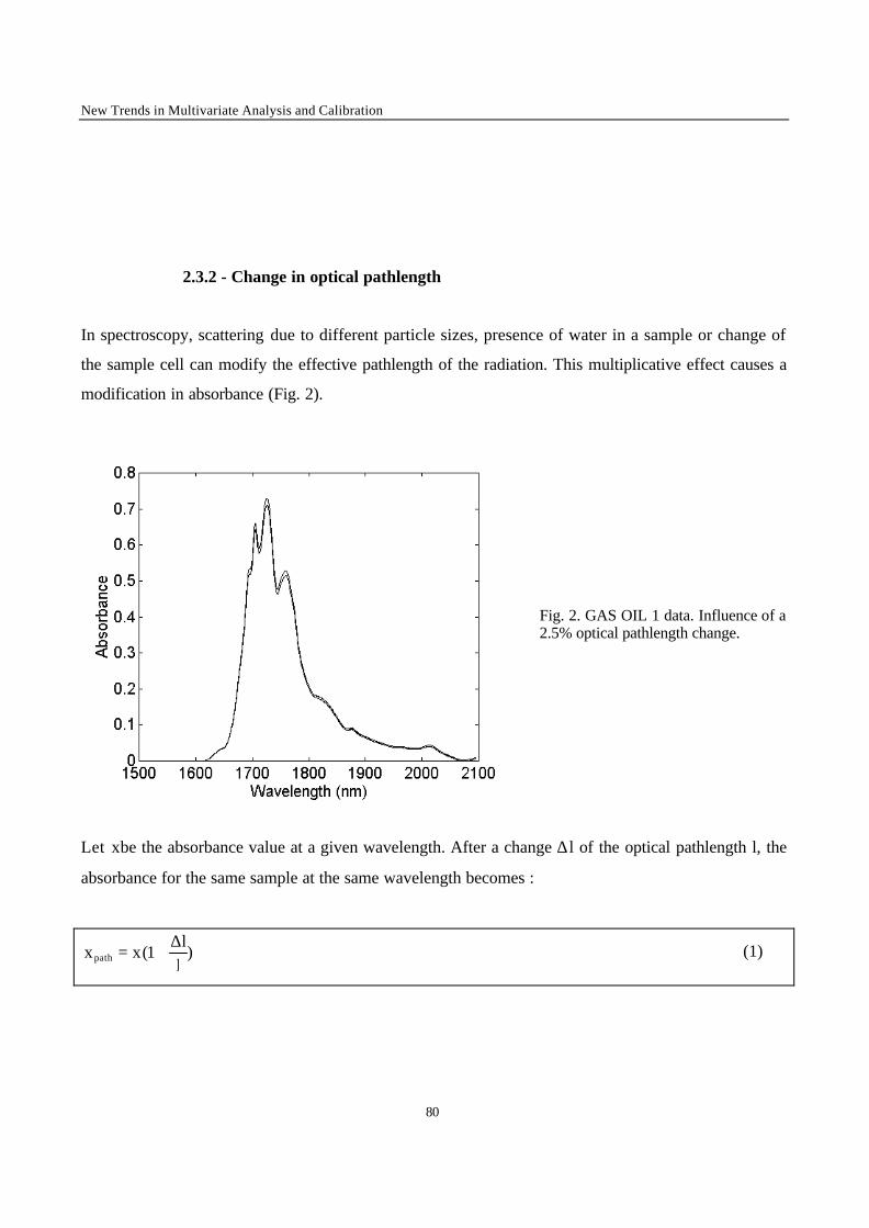
New Trends in Multivariate Analysis and Calibration
80
2.3.2 - Change in optical pathlength
In spectroscopy, scattering due to different particle sizes, presence of water in a sample or change of
the sample cell can modify the effective pathlength of the radiation. This multiplicative effect causes a
modification in absorbance (Fig. 2).
Fig. 2. GAS OIL 1 data. Influence of a 2.5% optical pathlength change.
Let x be the absorbance value at a given wavelength. After a change ∆ l of the optical pathlength l, the
absorbance for the same sample at the same wavelength becomes :
)ll
1(xxpath∆
+= (1)
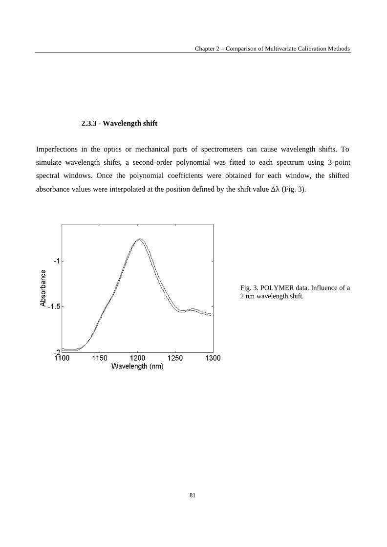
Chapter 2 – Comparison of Multivariate Calibration Methods
81
2.3.3 - Wavelength shift
Imperfections in the optics or mechanical parts of spectrometers can cause wavelength shifts. To
simulate wavelength shifts, a second-order polynomial was fitted to each spectrum using 3-point
spectral windows. Once the polynomial coefficients were obtained for each window, the shifted
absorbance values were interpolated at the position defined by the shift value ∆λ (Fig. 3).
Fig. 3. POLYMER data. Influence of a 2 nm wavelength shift.
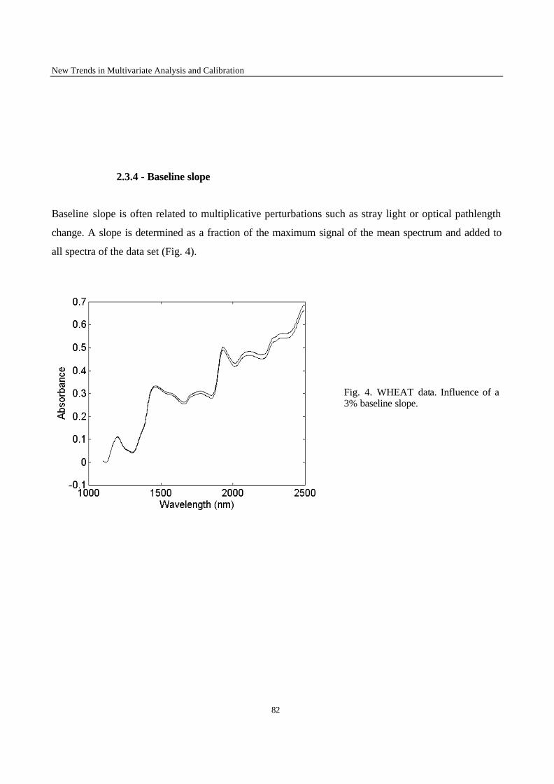
New Trends in Multivariate Analysis and Calibration
82
2.3.4 - Baseline slope
Baseline slope is often related to multiplicative perturbations such as stray light or optical pathlength
change. A slope is determined as a fraction of the maximum signal of the mean spectrum and added to
all spectra of the data set (Fig. 4).
Fig. 4. WHEAT data. Influence of a 3% baseline slope.
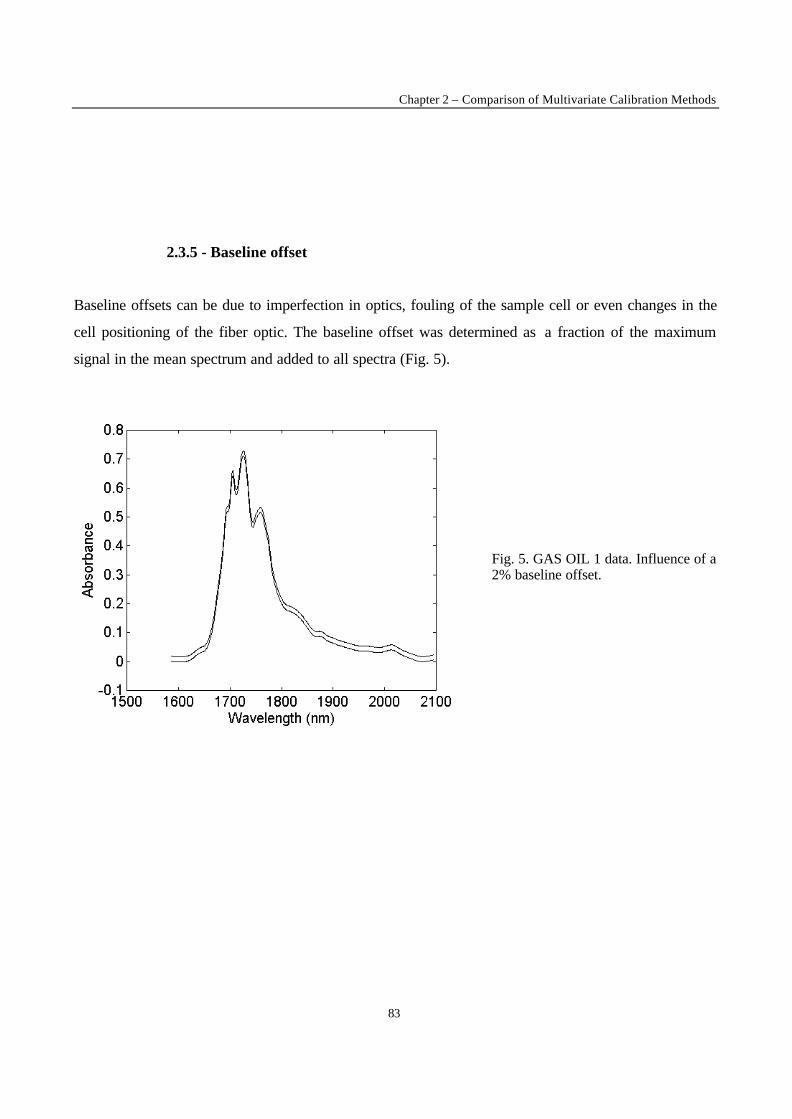
Chapter 2 – Comparison of Multivariate Calibration Methods
83
2.3.5 - Baseline offset
Baseline offsets can be due to imperfection in optics, fouling of the sample cell or even changes in the
cell positioning of the fiber optic. The baseline offset was determined as a fraction of the maximum
signal in the mean spectrum and added to all spectra (Fig. 5).
Fig. 5. GAS OIL 1 data. Influence of a 2% baseline offset.
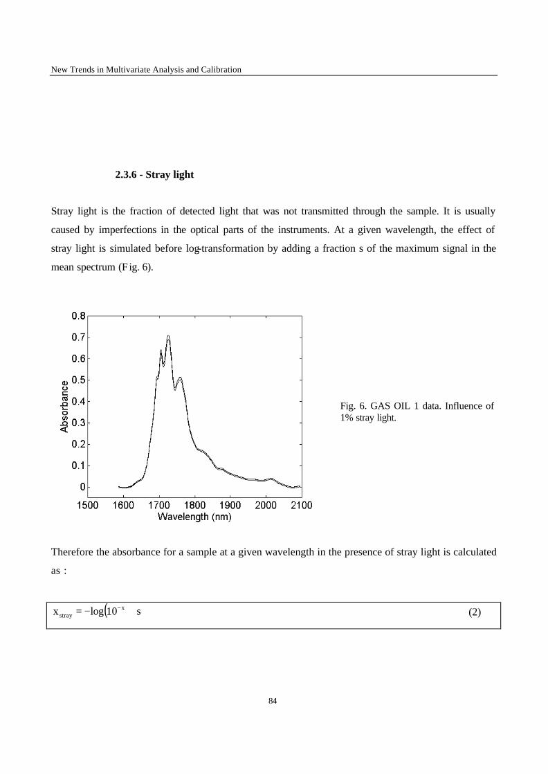
New Trends in Multivariate Analysis and Calibration
84
2.3.6 - Stray light
Stray light is the fraction of detected light that was not transmitted through the sample. It is usually
caused by imperfections in the optical parts of the instruments. At a given wavelength, the effect of
stray light is simulated before log-transformation by adding a fraction s of the maximum signal in the
mean spectrum (F ig. 6).
Fig. 6. GAS OIL 1 data. Influence of 1% stray light.
Therefore the absorbance for a sample at a given wavelength in the presence of stray light is calculated
as :
( )s10logx xstray +−= − (2)
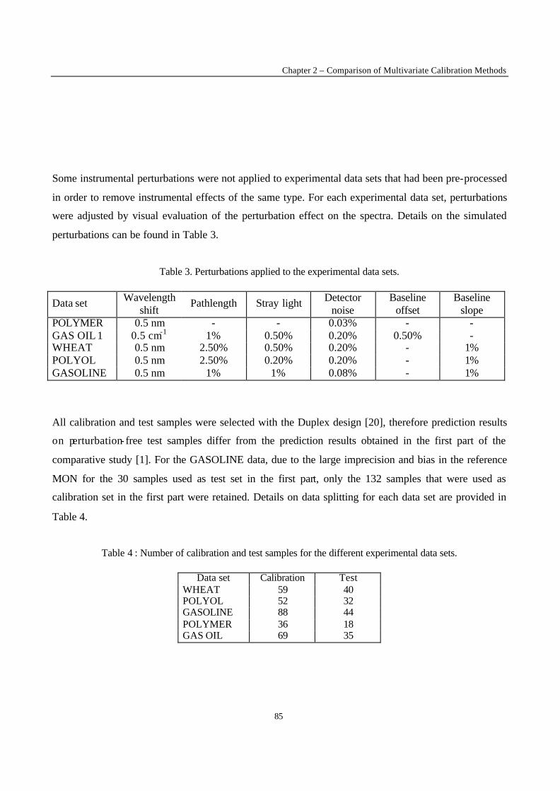
Chapter 2 – Comparison of Multivariate Calibration Methods
85
Some instrumental perturbations were not applied to experimental data sets that had been pre-processed
in order to remove instrumental effects of the same type. For each experimental data set, perturbations
were adjusted by visual evaluation of the perturbation effect on the spectra. Details on the simulated
perturbations can be found in Table 3.
Table 3. Perturbations applied to the experimental data sets.
Data set Wavelength shift
Pathlength Stray light Detector noise
Baseline offset
Baseline slope
POLYMER 0.5 nm - - 0.03% - - GAS OIL 1 0.5 cm-1 1% 0.50% 0.20% 0.50% - WHEAT 0.5 nm 2.50% 0.50% 0.20% - 1% POLYOL 0.5 nm 2.50% 0.20% 0.20% - 1% GASOLINE 0.5 nm 1% 1% 0.08% - 1%
All calibration and test samples were selected with the Duplex design [20], therefore prediction results
on perturbation- free test samples differ from the prediction results obtained in the first part of the
comparative study [1]. For the GASOLINE data, due to the large imprecision and bias in the reference
MON for the 30 samples used as test set in the first part, only the 132 samples that were used as
calibration set in the first part were retained. Details on data splitting for each data set are provided in
Table 4.
Table 4 : Number of calibration and test samples for the different experimental data sets.
Data set Calibration Test WHEAT 59 40 POLYOL 52 32 GASOLINE 88 44 POLYMER 36 18 GAS OIL 69 35
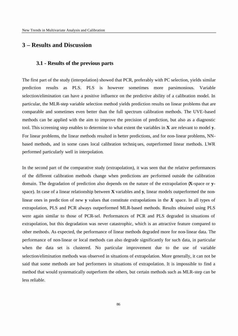
New Trends in Multivariate Analysis and Calibration
86
3 – Results and Discussion
3.1 - Results of the previous parts
The first part of the study (interpolation) showed that PCR, preferably with PC selection, yields similar
prediction results as PLS. PLS is however sometimes more parsimonious. Variable
selection/elimination can have a positive influence on the predictive ability of a calibration model. In
particular, the MLR-step variable selection method yields prediction results on linear problems that are
comparable and sometimes even better than the full spectrum calibration methods. The UVE-based
methods can be applied with the aim to improve the precision of prediction, but also as a diagnostic
tool. This screening step enables to determine to what extent the variables in X are relevant to model y.
For linear problems, the linear methods resulted in better predictions, and for non- linear problems, NN-
based methods, and in some cases local calibration techniq ues, outperformed linear methods. LWR
performed particularly well in interpolation.
In the second part of the comparative study (extrapolation), it was seen that the relative performances
of the different calibration methods change when predictions are performed outside the calibration
domain. The degradation of prediction also depends on the nature of the extrapolation (X-space or y-
space). In case of a linear relationship between X variables and y, linear models outperformed the non-
linear ones in predic tion of new y values that constitute extrapolations in the X space. In all types of
extrapolation, PLS and PCR always outperformed MLR-based methods. Results obtained using PLS
were again similar to those of PCR-sel. Performances of PCR and PLS degraded in situations of
extrapolation, but this degradation was never catastrophic, which is an attractive feature compared to
other methods. As expected, the performance of linear methods degraded more for non- linear data. The
performance of non- linear or local methods can also degrade significantly for such data, in particular
when the data set is clustered. No particular improvement due to the use of variable
selection/elimination methods was observed in situations of extrapolation. More generally, it can not be
said that some methods are bad performers in situations of extrapolation. It is impossible to find a
method that would systematically outperform the others, but certain methods such as MLR-step can be
less reliable.
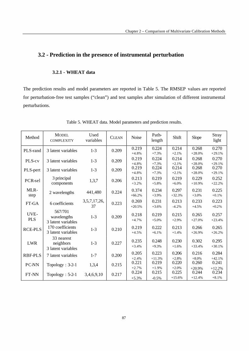
Chapter 2 – Comparison of Multivariate Calibration Methods
87
3.2 - Prediction in the presence of instrumental perturbation
3.2.1 - WHEAT data
The prediction results and model parameters are reported in Table 5. The RMSEP values are reported
for perturbation- free test samples (“clean”) and test samples after simulation of different instrumental
perturbations.
Table 5. WHEAT data. Model parameters and prediction results.
Method MODEL COMPLEXITY
Used variables
CLEAN Noise Path-length
Shift Slope Stray light
PLS-rand 3 latent variables 1-3 0.209 0.219 +4.8%
0.224 +7.3%
0.214 +2.1%
0.268 +28.0%
0.270 +29.1%
PLS-cv 3 latent variables 1-3 0.209 0.219 +4.8%
0.224 +7.3%
0.214 +2.1%
0.268 +28.0%
0.270 +29.1%
PLS-pert 3 latent variables 1-3 0.209 0.219 +4.8%
0.224 +7.3%
0.214 +2.1%
0.268 +28.0%
0.270 +29.1%
PCR-sel 3 principal components 1,3,7 0.206 0.213
+3.2% 0.219 +5.8%
0.219 +6.0%
0.229 +10.9%
0.252 +22.2%
MLR-step 2 wavelengths 441,480 0.224 0.374
+66.2% 0.234 +3.9%
0.297 +32.3%
0.231 +3.0%
0.225 +0.1%
FT-GA 6 coefficients 3,5,7,17,26,37
0.223 0.269 +20.5%
0.231 +3.6%
0.213 -4.2%
0.233 +4.5%
0.223 +0.2%
UVE-PLS
567/701 wavelengths
3 latent variables 1-3 0.209 0.218
+4.7% 0.219 +5.0%
0.215 +2.9%
0.265 +27.0%
0.257 +23.4%
RCE-PLS 170 coefficients 3 latent variables
1-3 0.210 0.219 +4.5%
0.222 +6.1%
0.213 +1.4%
0.266 +26.9%
0.265 +26.2%
LWR 33 nearest neighbors
3 latent variables 1-3 0.227 0.235
+3.4% 0.248 +9.3%
0.230 +1.6%
0.302 +33.4%
0.295 +30.1%
RBF-PLS 7 latent variables 1-7 0.200 0.205 +2.4%
0.223 +11.3%
0.206 +2.8%
0.216 +8.0%
0.284 +42.1%
PC-NN Topology : 3-2-1 1,3,4 0.215 0.221 +2.7%
0.219 +1.9%
0.220 +2.0%
0.260 +20.9%
0.241 +12.2%
FT-NN Topology : 5-2-1 3,4,6,9,10 0.217 0.224 +5.3%
0.215 -0.5%
0.225 +15.6%
0.244 +12.4%
0.234 +8.1%
New Trends in Multivariate Analysis and Calibration
88
In the absence of perturbations, all methods perform equally well and the models are relatively
parsimonious. The models being parsimonious, they can expected to be robust, explaining the fact that
simulated perturbations have very little influence on most calibration methods. The MLR-step model
uses only two variables, which is highly desirable from the point of view of model interpretation and
robustness towards some types of perturbations. This model is however the most sensitive to increasing
detector noise and wavelength shift. The wavelength shift is the same as on the POLYMER data and
the pathlength change is higher than on GAS OIL data, but they have little influence on this data set.
This illustrates that the effect of perturbations on NIR calibration models does not only depend on the
calibration methods and the magnitude of the perturbations, but also on the data themselves. Overall,
pathlength change and wavelength shift have relatively little effect, and changes in slope and stray light
are the most influential perturbations. They mainly affect calibration methods that use LVs or PCs for
modelling or preprocessing, because absorbance values at all wavelengths in the linear combinations
are modified so that the impact of the perturbations is amplified. MLR-step and Fourier transform
based-methods (FT-GA, FT-NN) are more robust with respect to these perturbations.
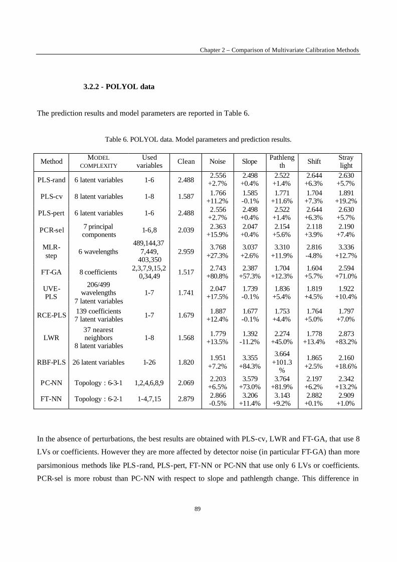
Chapter 2 – Comparison of Multivariate Calibration Methods
89
3.2.2 - POLYOL data
The prediction results and model parameters are reported in Table 6.
Table 6. POLYOL data. Model parameters and prediction results.
Method MODEL COMPLEXITY
Used variables Clean Noise Slope Pathleng
th Shift Stray light
PLS-rand 6 latent variables 1-6 2.488 2.556
+2.7% 2.498
+0.4% 2.522
+1.4% 2.644
+6.3% 2.630
+5.7%
PLS-cv 8 latent variables 1-8 1.587 1.766 +11.2%
1.585 -0.1%
1.771 +11.6%
1.704 +7.3%
1.891 +19.2%
PLS-pert 6 latent variables 1-6 2.488 2.556 +2.7%
2.498 +0.4%
2.522 +1.4%
2.644 +6.3%
2.630 +5.7%
PCR-sel 7 principal components
1-6,8 2.039 2.363 +15.9%
2.047 +0.4%
2.154 +5.6%
2.118 +3.9%
2.190 +7.4%
MLR-step 6 wavelengths
489,144,377,449,
403,350 2.959
3.768 +27.3%
3.037 +2.6%
3.310 +11.9%
2.816 -4.8%
3.336 +12.7%
FT-GA 8 coefficients 2,3,7,9,15,20,34,49 1.517 2.743
+80.8% 2.387
+57.3% 1.704
+12.3% 1.604
+5.7% 2.594
+71.0%
UVE-PLS
206/499 wavelengths
7 latent variables 1-7 1.741 2.047
+17.5% 1.739 -0.1%
1.836 +5.4%
1.819 +4.5%
1.922 +10.4%
RCE-PLS 139 coefficients 7 latent variables 1-7 1.679 1.887
+12.4% 1.677 -0.1%
1.753 +4.4%
1.764 +5.0%
1.797 +7.0%
LWR 37 nearest neighbors
8 latent variables 1-8 1.568 1.779
+13.5% 1.392
-11.2% 2.274
+45.0% 1.778
+13.4% 2.873
+83.2%
RBF-PLS 26 latent variables 1-26 1.820 1.951
+7.2% 3.355
+84.3%
3.664 +101.3
%
1.865 +2.5%
2.160 +18.6%
PC-NN Topology : 6-3-1 1,2,4,6,8,9 2.069 2.203 +6.5%
3.579 +73.0%
3.764 +81.9%
2.197 +6.2%
2.342 +13.2%
FT-NN Topology : 6-2-1 1-4,7,15 2.879 2.866 -0.5%
3.206 +11.4%
3.143 +9.2%
2.882 +0.1%
2.909 +1.0%
In the absence of perturbations, the best results are obtained with PLS-cv, LWR and FT-GA, that use 8
LVs or coefficients. However they are more affected by detector noise (in particular FT-GA) than more
parsimonious methods like PLS-rand, PLS-pert, FT-NN or PC-NN that use only 6 LVs or coefficients.
PCR-sel is more robust than PC-NN with respect to slope and pathlength change. This difference in

New Trends in Multivariate Analysis and Calibration
90
robustness is not due to the intrinsic non-linear nature of NN applied to a linear model, but to the large
sensitivity of PC 9 (retained in PC-NN and not in PCR-sel) with respect to these perturbations. Overall,
PLS-rand, PLS-pert, FT-NN and RCE-PLS are robust with respect to all perturbations. PCR-sel, PLS-
cv and UVE-PLS are also relatively robust. RCE-PLS, PLS-cv, and UVE-PLS offer the best
compromise in terms of performance both in the presence and in the absence of perturbations. The
performances of FT-NN and MLR-step are relatively similar. It seems that for this data set, the most
parsimonious models (MLR-step, PCR-sel, PLS-rand, PLS-pert, PC-NN) lack some explanative power,
and that this loss is not compensated with a better robustness with respect to perturbations, which is
unusual.
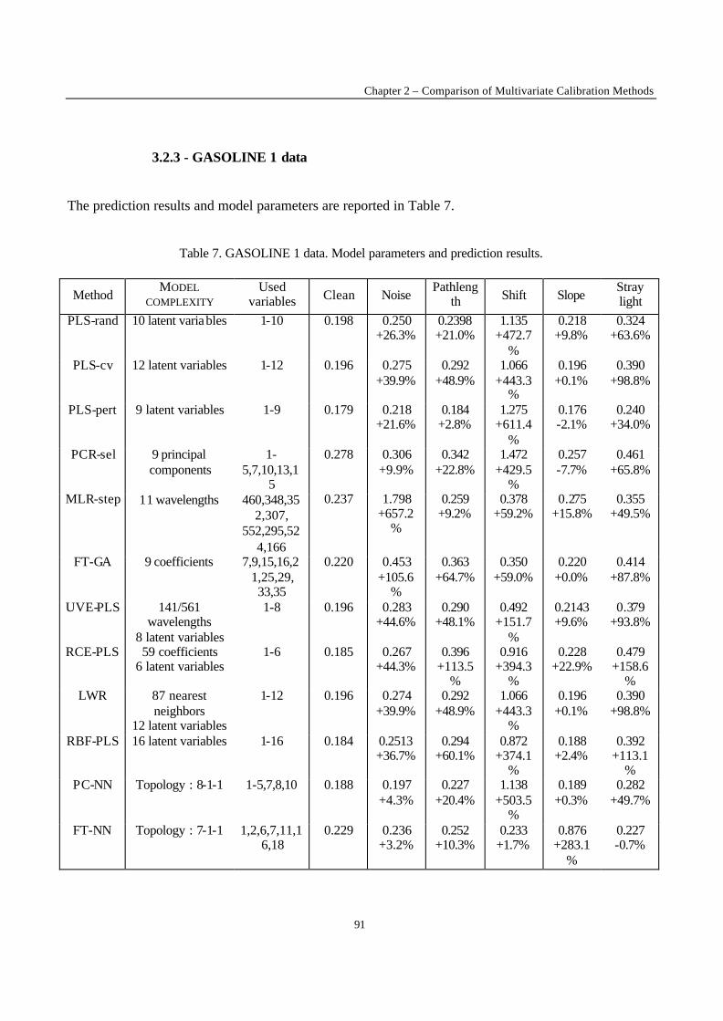
Chapter 2 – Comparison of Multivariate Calibration Methods
91
3.2.3 - GASOLINE 1 data
The prediction results and model parameters are reported in Table 7.
Table 7. GASOLINE 1 data. Model parameters and prediction results.
Method MODEL
COMPLEXITY Used
variables Clean Noise Pathleng
th Shift Slope Stray light
PLS-rand 10 latent variables 1-10 0.198 0.250 +26.3%
0.2398 +21.0%
1.135 +472.7
%
0.218 +9.8%
0.324 +63.6%
PLS-cv 12 latent variables 1-12 0.196 0.275 +39.9%
0.292 +48.9%
1.066 +443.3
%
0.196 +0.1%
0.390 +98.8%
PLS-pert 9 latent variables 1-9 0.179 0.218 +21.6%
0.184 +2.8%
1.275 +611.4
%
0.176 -2.1%
0.240 +34.0%
PCR-sel 9 principal components
1-5,7,10,13,1
5
0.278 0.306 +9.9%
0.342 +22.8%
1.472 +429.5
%
0.257 -7.7%
0.461 +65.8%
MLR-step 11 wavelengths 460,348,352,307,
552,295,524,166
0.237 1.798 +657.2
%
0.259 +9.2%
0.378 +59.2%
0.275 +15.8%
0.355 +49.5%
FT-GA 9 coefficients 7,9,15,16,21,25,29, 33,35
0.220 0.453 +105.6
%
0.363 +64.7%
0.350 +59.0%
0.220 +0.0%
0.414 +87.8%
UVE-PLS 141/561 wavelengths
8 latent variables
1-8 0.196 0.283 +44.6%
0.290 +48.1%
0.492 +151.7
%
0.2143 +9.6%
0.379 +93.8%
RCE-PLS 59 coefficients 6 latent variables
1-6 0.185 0.267 +44.3%
0.396 +113.5
%
0.916 +394.3
%
0.228 +22.9%
0.479 +158.6
% LWR 87 nearest
neighbors 12 latent variables
1-12 0.196 0.274 +39.9%
0.292 +48.9%
1.066 +443.3
%
0.196 +0.1%
0.390 +98.8%
RBF-PLS 16 latent variables 1-16 0.184 0.2513 +36.7%
0.294 +60.1%
0.872 +374.1
%
0.188 +2.4%
0.392 +113.1
% PC-NN Topology : 8-1-1 1-5,7,8,10 0.188 0.197
+4.3% 0.227
+20.4% 1.138
+503.5%
0.189 +0.3%
0.282 +49.7%
FT-NN Topology : 7-1-1 1,2,6,7,11,16,18
0.229 0.236 +3.2%
0.252 +10.3%
0.233 +1.7%
0.876 +283.1
%
0.227 -0.7%
New Trends in Multivariate Analysis and Calibration
92
In the absence of perturbations, the best results are obtained with PLS -pert, RCE-PLS, RBF-PLS and
PC-NN, with RMSEP values on perturbation- free samples around 0.180. Most calibration methods are
very sensitive to the detector noise, which is magnified after pre-processing with first derivative. In
particular, the performance of MLR-step degrades significantly. The most robust methods with respect
to noise are PCR-sel, PLS-pert and PC-NN. Robustness decreases as more LVs are retained for the
three variants of PLS. All methods are sensitive to pathlength change except PLS-pert. MLR-step,
PLS-rand, FT-NN and PC-NN are slightly more robust than the other ones with respect to this
perturbation. The spectral differences due to shift are amplified by first derivation and one must expect
large prediction errors with this perturbation. Indeed, the calibration methods are very sensitive to
wavelength shift except FT-NN, and to a lesser extent MLR-step and FT-GA. The better robustness of
the Fourier transform-based methods is due to the fact that the shape of the spectra is not affected by
the shift. Compared to the other perturbations, the slope change has only a limited influence on all
methods, except FT-NN. Unlike optical pathlength change or stray light whose efffect is wavelength-
dependent, the slope effect is similar at all wavelengths, hence the first Fourier coefficient is very
sensitive to this perturbation. Overall, the most robust method is FT-NN, except after addition of
baseline slope that affects the first Fourier coefficient (sum of absorbances) much more than the other
coefficients. FT-GA always performs worse than FT-NN, except for the baseline slope effect that does
not affects the coefficients retained by GA. However, one must keep in mind that with FT-GA,
selection is performed by GA on the first 50 Fourier coefficients (that contain some high frequency
coefficients likely to be contaminated with noise). In FT-NN, selection of coefficients is performed by
trial-and-error on the first 20 coefficients. The stray light effect has a strong influence on all methods,
except FT-NN. Again, it is likely that this effect has more impact on the higher-order (higher
frequency) coefficients retained by FT-GA than on the coefficients used for modelling with NN.
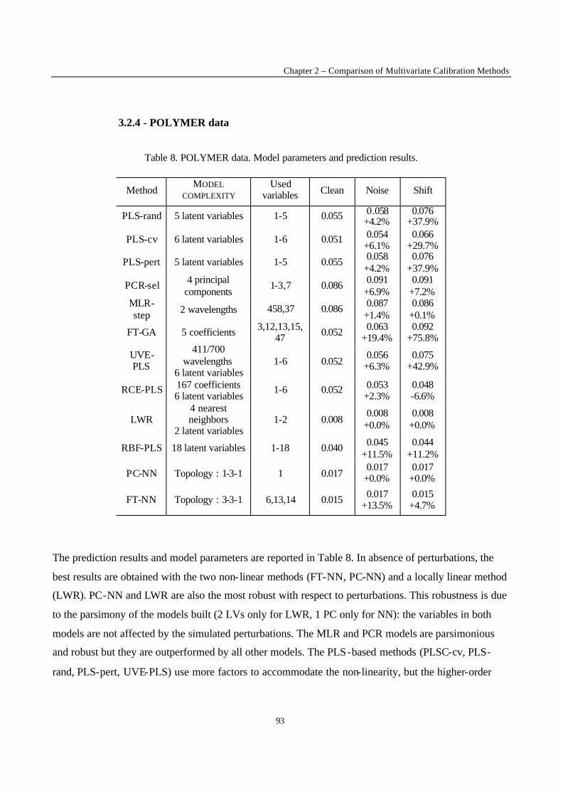
Chapter 2 – Comparison of Multivariate Calibration Methods
93
3.2.4 - POLYMER data
Table 8. POLYMER data. Model parameters and prediction results.
Method MODEL
COMPLEXITY Used
variables Clean Noise Shift
PLS-rand 5 latent variables 1-5 0.055 0.058 +4.2%
0.076 +37.9%
PLS-cv 6 latent variables 1-6 0.051 0.054 +6.1%
0.066 +29.7%
PLS-pert 5 latent variables 1-5 0.055 0.058 +4.2%
0.076 +37.9%
PCR-sel 4 principal components
1-3,7 0.086 0.091 +6.9%
0.091 +7.2%
MLR-step 2 wavelengths 458,37 0.086 0.087
+1.4% 0.086
+0.1%
FT-GA 5 coefficients 3,12,13,15,47 0.052 0.063
+19.4% 0.092
+75.8%
UVE-PLS
411/700 wavelengths
6 latent variables 1-6 0.052
0.056 +6.3%
0.075 +42.9%
RCE-PLS 167 coefficients 6 latent variables
1-6 0.052 0.053 +2.3%
0.048 -6.6%
LWR 4 nearest neighbors
2 latent variables 1-2 0.008
0.008 +0.0%
0.008 +0.0%
RBF-PLS 18 latent variables 1-18 0.040 0.045 +11.5%
0.044 +11.2%
PC-NN Topology : 1-3-1 1 0.017 0.017
+0.0% 0.017
+0.0%
FT-NN Topology : 3-3-1 6,13,14 0.015 0.017 +13.5%
0.015 +4.7%
The prediction results and model parameters are reported in Table 8. In absence of perturbations, the
best results are obtained with the two non- linear methods (FT-NN, PC-NN) and a locally linear method
(LWR). PC-NN and LWR are also the most robust with respect to perturbations. This robustness is due
to the parsimony of the models built (2 LVs only for LWR, 1 PC only for NN): the variables in both
models are not affected by the simulated perturbations. The MLR and PCR models are parsimonious
and robust but they are outperformed by all other models. The PLS -based methods (PLSC-cv, PLS-
rand, PLS-pert, UVE-PLS) use more factors to accommodate the non-linearity, but the higher-order
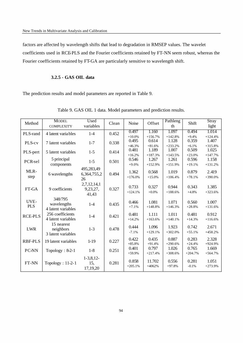
New Trends in Multivariate Analysis and Calibration
94
factors are affected by wavelength shifts that lead to degradation in RMSEP values. The wavelet
coefficients used in RCE-PLS and the Fourier coefficients retained by FT-NN seem robust, whereas the
Fourier coefficients retained by FT-GA are particularly sensitive to wavelength shift.
3.2.5 - GAS OIL data
The prediction results and model parameters are reported in Table 9.
Table 9. GAS OIL 1 data. Model parameters and prediction results.
Method MODEL COMPLEXITY
Used variables
Clean Noise Offset Pathlength
Shift Stray light
PLS-rand 4 latent variables 1-4 0.452 0.497 +10.0%
1.160 +156.7%
1.097 +142.8%
0.494 +9.4%
1.014 +124.4%
PLS-cv 7 latent variables 1-7 0.338 0.495 +46.3%
0.614 +81.6%
1.128 +233.2%
0.359 +6.1%
1.407 +315.8%
PLS-pert 5 latent variables 1-5 0.414 0.481 +16.2%
1.189 +187.3%
1.007 +143.5%
0.509 +23.0%
1.025 +147.7%
PCR-sel 5 principal components
1-5 0.501 0.546 +9.0%
1.267 +152.9%
1.261 +151.9%
0.596 +19.1%
1.158 +131.2%
MLR-step 6 wavelengths
495,283,496,364,755,226
0.494 1.362 +176.0%
0.568 +15.0%
1.019 +106.4%
0.879 +78.1%
2.419 +390.0%
FT-GA 9 coefficients 2,7,12,14,1
9,23,27, 41,43
0.327 0.733 +124.1%
0.327 +0.0%
0.944 +188.6%
0.343 +4.8%
1.385 +323.6%
UVE-PLS
348/795 wavelengths
4 latent variables 1-4 0.435 0.466
+7.1% 1.081
+148.8% 1.071
+146.3% 0.560
+28.8% 1.007
+131.6%
RCE-PLS 256 coefficients 4 latent variables
1-4 0.421 0.481 +14.2%
1.111 +163.6%
1.011 +140.1%
0.481 +14.3%
0.912 +116.6%
LWR 15 nearest neighbors
3 latent variables 1-3 0.478 0.444
-7.1% 1.096
+129.1% 1.923
+302.0% 0.742
+55.1% 2.671
+458.2%
RBF-PLS 19 latent variables 1-19 0.227 0.422 +85.8%
0.435 +91.4%
0.887 +290.6%
0.283 +24.4%
2.328 +924.9%
PC-NN Topology : 8-2-1 1-8 0.251 0.401 +59.9%
0.797 +217.4%
1.026 +308.6%
0.765 +204.7%
1.669 +564.7%
FT-NN Topology : 11-2-1 1-3,8,12-
15, 17,19,20
0.281 0.858 +205.1%
11.702 +4062%
0.556 +97.8%
0.281 -0.1%
1.051 +273.9%
Chapter 2 – Comparison of Multivariate Calibration Methods
95
In absence of perturbations, the best results are obtained with a local linear method (RBF-PLS) and the
two non-linear methods (FT-NN, PC-NN). PC-NN and FT-NN use an unusually large number of input
variables (8 and 11 respectively) and are therefore very sensitive to perturbations, except wavelength
shift that has very little influence on Fourier coefficients with FT-NN. PLS-cv performs well in the
absence of perturbations, but it is less parsimonious than models developed with PCR-sel, PLS-rand,
PLS-pert or UVE-PLS. As a consequence, its performance degrades when noise is added to the test
spectra and it performs similar to the other LV-based methods. Absorbance offset has a strong
influence on all methods except MLR-step (because it retains only 6 original variables) and FT-GA,
since the Fourier coefficients describe the shape of the spectra and this shape is not affected by the
offset. However, the performance of FT-NN degrades significantly after addition of this offset because
contrary to FT-GA, the first Fourier coefficient is retained. This coefficient is the sum of all absorbance
values in the spectrum, and therefore sensitive to absorbance offset. All methods are affected by the
multiplicative effects (change in optical pathlength and stray light). Most methods are relatively robust
with respect to the wavelength shift, except MLR-step, LWR and PC-NN.
4 - Conclusions
The study of prediction results in this third part of the comparative study provided information on the
robustness of the different calibration methods with respect to unmodelled instrumental perturbations.
In most cases, the influence of instrumental perturbations is difficult to predict because it depends on a
large number of factors:
• nature of the perturbation.
• level of the perturbation.
• preprocessing of the data.
• nature of the calibration method.
Some general conclusions can anyway be drawn. It can be observed that complex models (in particular
those concerning GASOLINE or GAS OIL data) are very sensitive to any type of perturbation, but
models with smaller complexities are more robust. Wavelength shift has a catastrophic effect on
models developed with first derivative data. In order to achieve a better overview on method
performances, methods were ranked according to the arbitrary scoring criterion displayed in Table 10 :
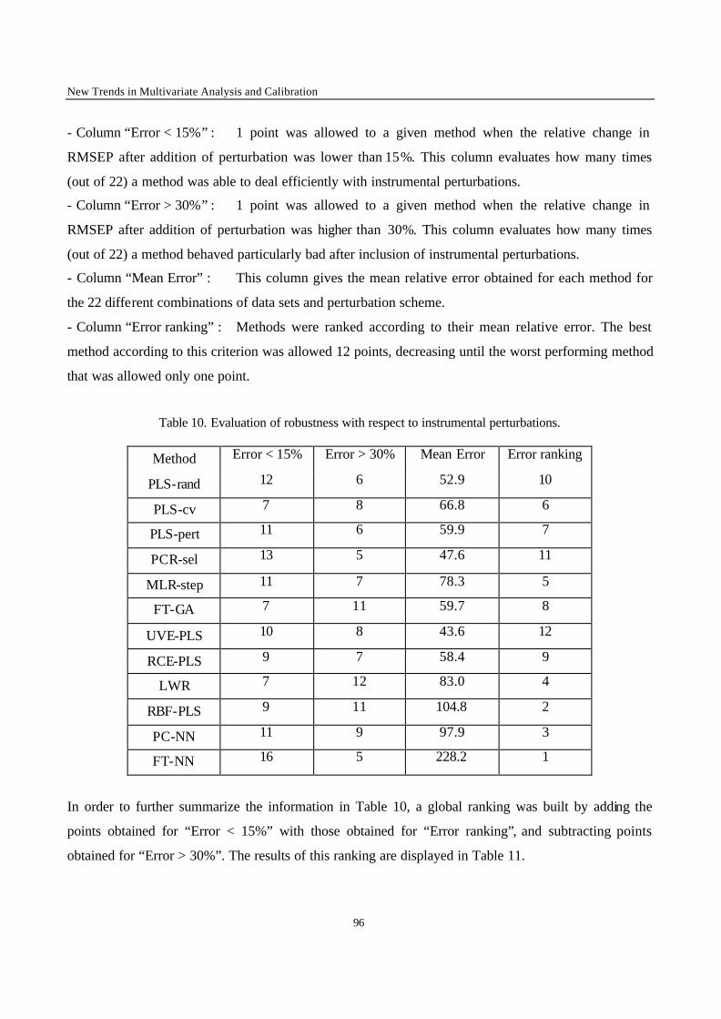
New Trends in Multivariate Analysis and Calibration
96
- Column “Error < 15%” : 1 point was allowed to a given method when the relative change in
RMSEP after addition of perturbation was lower than 15%. This column evaluates how many times
(out of 22) a method was able to deal efficiently with instrumental perturbations.
- Column “Error > 30%” : 1 point was allowed to a given method when the relative change in
RMSEP after addition of perturbation was higher than 30%. This column evaluates how many times
(out of 22) a method behaved particularly bad after inclusion of instrumental perturbations.
- Column “Mean Error” : This column gives the mean relative error obtained for each method for
the 22 different combinations of data sets and perturbation scheme.
- Column “Error ranking” : Methods were ranked according to their mean relative error. The best
method according to this criterion was allowed 12 points, decreasing until the worst performing method
that was allowed only one point.
Table 10. Evaluation of robustness with respect to instrumental perturbations.
Method Error < 15% Error > 30% Mean Error Error ranking
PLS-rand 12 6 52.9 10
PLS-cv 7 8 66.8 6
PLS-pert 11 6 59.9 7
PCR-sel 13 5 47.6 11
MLR-step 11 7 78.3 5
FT-GA 7 11 59.7 8
UVE-PLS 10 8 43.6 12
RCE-PLS 9 7 58.4 9
LWR 7 12 83.0 4
RBF-PLS 9 11 104.8 2
PC-NN 11 9 97.9 3
FT-NN 16 5 228.2 1
In order to further summarize the information in Table 10, a global ranking was built by adding the
points obtained for “Error < 15%” with those obtained for “Error ranking”, and subtracting points
obtained for “Error > 30%”. The results of this ranking are displayed in Table 11.
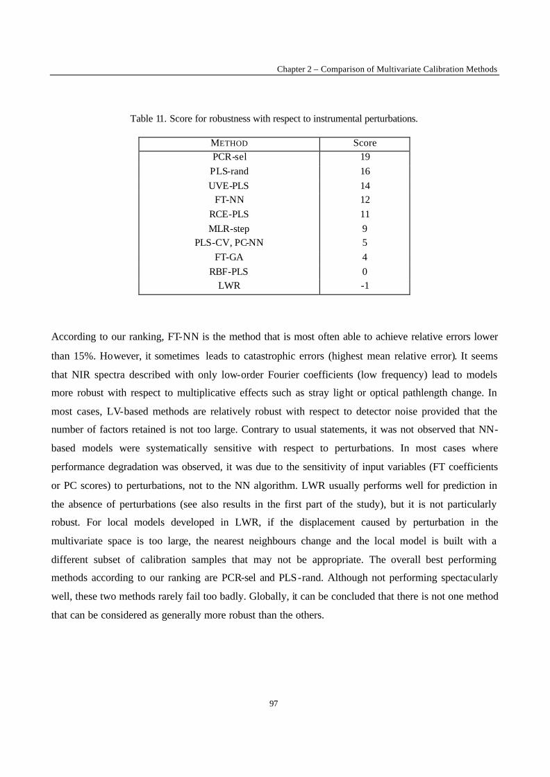
Chapter 2 – Comparison of Multivariate Calibration Methods
97
Table 11. Score for robustness with respect to instrumental perturbations.
METHOD Score PCR-sel 19
PLS-rand 16 UVE-PLS 14
FT-NN 12 RCE-PLS 11 MLR-step 9
PLS-CV, PC-NN 5 FT-GA 4
RBF-PLS 0 LWR -1
According to our ranking, FT-NN is the method that is most often able to achieve relative errors lower
than 15%. However, it sometimes leads to catastrophic errors (highest mean relative error). It seems
that NIR spectra described with only low-order Fourier coefficients (low frequency) lead to models
more robust with respect to multiplicative effects such as stray light or optical pathlength change. In
most cases, LV-based methods are relatively robust with respect to detector noise provided that the
number of factors retained is not too large. Contrary to usual statements, it was not observed that NN-
based models were systematically sensitive with respect to perturbations. In most cases where
performance degradation was observed, it was due to the sensitivity of input variables (FT coefficients
or PC scores) to perturbations, not to the NN algorithm. LWR usually performs well for prediction in
the absence of perturbations (see also results in the first part of the study), but it is not particularly
robust. For local models developed in LWR, if the displacement caused by perturbation in the
multivariate space is too large, the nearest neighbours change and the local model is built with a
different subset of calibration samples that may not be appropriate. The overall best performing
methods according to our ranking are PCR-sel and PLS-rand. Although not performing spectacularly
well, these two methods rarely fail too badly. Globally, it can be concluded that there is not one method
that can be considered as generally more robust than the others.

New Trends in Multivariate Analysis and Calibration
98
REFERENCES
[1] V. Centner, G. Verdú-Andrés, B. Walczak, D. Jouan-Rimbaud, F. Despagne, L. Pasti, R. Poppi,
D.L. Massart and O.E. de Noord, Appl. Spectrometry 54 (4) (2000) 608-623.
[2] F. Estienne, L. Pasti, V. Centner, B. Walczak, F. Despagne, D. Jouan Rimbaud, O. E. de Noord
and D.L. Massart, Chemom. Intell. Lab. Syst. 58 2 (2001) 195-211.
[3] T. Naes, H. Martens, J. Chemom. 2 (1998) 155-167.
[4] H. van der Voet, Chemom. Intell. Lab. Syst. 25 (1994) 313-323.
[5] H. Martens, T. Naes, Multivariate Calibration, Wiley, Chichester (1989).
[6] S. de Jong, Chemom. Intell. Lab. Sys. 18 (1993) 251-263.
[7] F. Despagne, D.L. Massart, O.E. de Noord, Anal. Chem. 69 (1997) 3391-3399.
[8] N.R. Draper, H. Smith, Applied Regression Analysis (2nd edition), Wiley, New-York (1981).
[9] D.E. Goldberg, Genetic Algorithms in Search, Optimisation and Machine Learning, Addison-
Wesley, Reading, MA (1989).
[10] D. Jouan-Rimbaud, D.L. Massart, R. Leardi, O.E. de Noord, Anal. Chem. 67 (1995) 4295-4301.
[11] R. Leardi, R. Boggia, M. Terrile, J. Chemom. 6 (1992) 267-281.
[12] L. Pasti, D. Jouan-Rimbaud, D.L. Massart, O.E. de Noord, Anal. Chim. Acta 364 (1998) 253-
263.
[13] V. Centner, D.L. Massart, O.E. de Noord, S. de Jong, B.G.M. Vandeginste, C. Sterna, Anal.
Chem. 68 (1996) 3851-3858.
[14] T. Naes, T. Isaksson, NIR News 5(4) (1994) 7-8.
[15] V. Centner, D.L. Massart, Anal. Chem. 70 (1998) 4206-4211.
[16] B. Walczak, D.L. Massart, Anal. Chim. Acta 331 (1996) 187-193.
[17] F. Despagne, D.L. Massart, Chemom. Intel. lab. syst. 40 (1998) 145-163.
[18] R. Fletcher, Practical Methods of optimization, Wiley, N.Y., 1987.
[19] J. Kalivas, Chemom. Intell. Lab. Syst. 37 (1997) 255-259.
[20] R.D. Snee, Technometrics 19 (1977) 415-428.
Chapter 2 – Comparison of Multivariate Calibration Methods
99
THE DEVELOPMENT OF CALIBRATION
MODELS FOR SPECTROSCOPIC DATA USING
MULTIPLE LINEAR REGRESSION
Based on :
THE DEVELOPMENT OF CALIBRATION MODELS FOR
SPECTROSCOPIC DATA USING PRINCIPAL COMPONENT
REGRESSION
Internet Journal of Chemistry 2 (1999) 19, URL: http://www.ijc.com/articles/1999v2/19/
R. De Maesschalck, F. Estienne, J. Verdú-Andrés, A. Candolfi, V. Centner, F. Despagne, D. Jouan-Rimbaud, B. Walczak +, D.L. Massart*, S. de Jong 1, O.E. de Noord2, C. Puel3, B.M.G. Vandeginste1
ChemoAC, Farmaceutisch Instituut
Vrije Universiteit Brussel Laarbeeklaan 103 B-1090 Brussels
Belgium. [email protected]
+ on leave from : Silesian University
Katowice Poland
1 Shell International Chemicals B.V.
Shell Research and Technology Centre
Amsterdam P. O. Box 38000
1030 BN Amsterdam The Netherlands
Unilever Research Laboratorium Vlaardingen P.O. Box 114
3130 AC Vlaardingen The Netherlands
Centre de Recherches Elf-Antar
Centre Automatisme et Informatique
BP 22 69360 Solaize
France
ABSTRACT
This article aims at explaining how to develop a calibration model for spectroscopic data analysis by Multiple Linear Regression (MLR). Building an MLR model on spectroscopic data implies selecting variables. Variable selections methods are therefore studied in this article. Before applying the method, the data has to be investigated in oder to detect for instance outliers, clustering tendency or nonlinearities. How to handle replicates and perform different data preprocessings and/or pretreatments is also explained in this tutorial.
* Corresponding author
KEYWORDS : Multivariate calibration, method comparison, extrapolation, non- linearity, clustering.
New Trends in Multivariate Analysis and Calibration
100
1. Introduction
The development of a calibration model for spectroscopic data analysis by Multiple Linear Regression
(MLR) consists of many steps, from the pre-treatment of the data to the utilisation of the calibration
model. This process includes for instance outlier detection (and possible rejection), validation, and
many other topics of chemometrics. Apart from general chemometrics publications [1], many books
and papers are devoted to regression in general and Multiple Linear Regression in particular. This
method can be approached from a general statistical point of view [2,3], or with direct application to
analytical chemistry [4,5]. Readers might get confused since literature often describes several
alternative approaches for each step of the calibration process, e.g. several tests have been described for
the detection of outliers. Our aim is therefore not to present the general theory of involved methods, but
rather to present some of the main alternatives, to help the reader in understanding them and to decide
which ones to apply. Thus, a complete strategy for calibration development is presented. Much of this
strategy is equally applicable to other methods such as Principal Component regression [6], partial least
squares, or to some extent neural networks [7], and can be found in the related tutorials [8,9]. A
specificity of MLR is that the mathematical background of the method is very simple and easy to
understand. Since original variables are used, interpretation can be very straight forward. Moreover,
experience shows that MLR can perform very well, even outperforming latent variables methods on
certain types of spectroscopic data for which it is particularly suited. However, some specific problems
arise when using MLR, e.g. the necessity to perform variable selection before calibration, or the
problem of random correlation. It was therefore decided to develop a particular tutorial for MLR. Even
though the tutorial was written specifically with spectroscopic data in mind, some guidelines also apply
to other types of data, in particular about the specific aspects of MLR described above.
MLR, also often called multivariate regression or multiple regression, is used to obtain values for the b-
coefficients in an equation of the type :
y = b0 + b1x1 + b2x2 + … bmxm (1)
where x1, x2, …, xm are different variables. In analytical spectroscopic applications, these variables
could be the absorbances obtained at different wavelengths, y being a concentration or another

Chapter 2 – Comparison of Multivariate Calibration Methods
101
characteristic of the samples that has to be predicted. The b-values are estimates of the true b-
parameters and the estimation is done by minimising a sum of squares. It can be shown that :
b = (X’X)-1X’y (2)
where b is the vector containing the b-values from eq. (1), X is an nxm matrix containing the x-values
for n samples (or objects as they are often called) and m variables and y is the vector containing the
measurements for the n samples.
A difficulty is that the inversion of the X’X matrix leads to unstable result s when the x-variables are
very correlated, which happens most of the time with spectroscopic data. There are two ways to avoid
this problem. One approach consists in combining the variables in such a way that the resulting
summarising variables are not correlated (feature reduction). For instance, PCR consists in relating the
scores of a Principal Component Analysis (PCA) model to the property of interest y through an MLR
model. This method is not described here but is covered by a specific tutorial [8]. Another way is to
select specific variables such that correlation is reduced. This approach is called variable selection or
feature selection, and is developed in the rest of this tutorial.
As can be seen in Eq. (1), MLR is an inverse calibration method. In classical calibration the basic
equation is :
signal = f (concentration) (3)
The measured signal is subject to noise. In the calibration step we assume that the concentration is
known exactly. In multivariate calibration one often does not know the concentrations of all the
compounds that influence the absorbance at the wavelengths of interest so that this model cannot be
applied. The calibration model is then written as the inverse :
concentration = f (signal) (4)
New Trends in Multivariate Analysis and Calibration
102
In inverse calibration the regression parameters b are biased and so are the concentrations predicted
using the biased model. However, the predictions are more precise than in classical calibration. This
can be explained by considering that the least squares step in inverse calibration involves a
minimisation of a sum of squares in the direction of the concentration and that the determination of the
concentrations is precisely the aim of the calibration. It is found that for univariate calibration the gain
in precision is more important than the increase in bias. The accuracy of the calibration, defined as the
deviation between the experimental and the true result and therefore compromising both random errors
(precision) and systematic errors (bias), is better for inverse than for classical calibration [10]. Having
to use inverse calibration is in no way a disadvantage. In fact, concentrations in the calibration samples
are not usually known exactly but are determined with a reference method. This means that both the y
and the x-values are subject to random error, so that least squares regression is not the optimal method
to use. A comparison between predictions made with regression methods that consider random errors in
both the y and the x-direction (total least squares) with those using ordinary least squares (OLS) in the
y or concentration direction (inverse calibration), show that the results obtained by total least squares
(TLS) [11,12] are no better than those obtained by inverse calibration.
Each step needed to develop a calibration model is discussed in detail in this paper. We have
considered a situation in which the minimum of a priori knowledge is available and where virtually no
decision has been made before beginning the measurement and method development. In many cases
information is available or decisions have been taken which will have an influence on the strategy to
adopt. For instance, it is possible to decide before the measurement campaign that the initial samples
will be collected for developing the model and validation samples will be collected later, so that no
splitting is considered (chapters 8 and 11), or to be aware that there are two types of samples but that a
single model is required. In the latter case, the person responsible for the model development knows or
at least suspects that there are two clusters of samples and will probably not determine a cluster
tendency (chapter 6), but verify visually that there are two clusters as expected. Whatever the situation
and the scheme applied in practice, the following steps are usually present:
• visual evaluation of the spectra before and after pre-treatment: Do replicate spectra largely overlap, is
there a baseline offset, etc.
• visual evaluation of the x-space, usually by looking at score plots resulting from a PCA to look for
gross outliers, clusters, etc. In what follows, it will be assumed that gross outliers have been eliminated.
Chapter 2 – Comparison of Multivariate Calibration Methods
103
• visual evaluation of the y-values to verify that the expected calibration range is properly covered and
to note possible inhomogeneities, which might be remedied by measuring additional samples.
• selection of the samples that will be used to train the model, optimise and validate the model and the
scheme which will be followed.
• a first modelling trial to decide whether it is possible to reach the expected quality of model and to
detect gross non- linearity if it is present.
• refinement of the model by e.g. considering elimination of possible outliers, selecting the optimal
number of variables, etc.
• final validation of the model.
• routine use and updating of the model.
2. Replicates
Different types of replicates should be considered. Replicates in X are defined as replicate
spectroscopic measurements of the same sample. The replicate measurement should preferably include
the whole process of measuring, for instance including filling the sample holders. Replicates of the
reference measurements are called replicates in y. Since the quality of the prediction does not only
depend on the measurement but also on the reference method, the acquisition of replicates both in X
and y, i.e. both in the spectroscopic measurement and the reference analysis, is recommended.
However, since the spectroscopic measurement, e.g. NIR, is usually much easier to carry out, it is more
common to have replicates in X than in y. Replicates in X increase the precision of the predictions
which are obtained. Precision is used here as a general term. Depending on the way in which the
precision is determined, a repeatability, an intermediate precision or a reproducibility will be obtained
[13,14]. For instance, if all replicates are measured by the same person on the same day and the same
instrument a repeatability is obtained.
Replicates of X can be used to select the best pre-processing method (see chapter 3) and to compute the
precision of the predicted values from the multivariate calibration method. The predicted y-values for
replicate calibration samples can be computed. The standard deviation of these values includes
information about the experimental procedure followed, variation between days and/or operators, etc.
The mean spectrum for each set of replicates is used to build the model. If the model does not use the
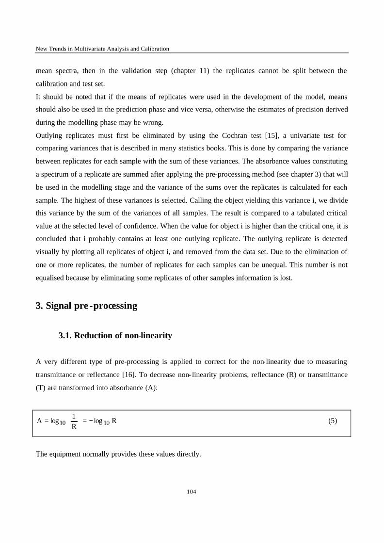
New Trends in Multivariate Analysis and Calibration
104
mean spectra, then in the validation step (chapter 11) the replicates cannot be split between the
calibration and test set.
It should be noted that if the means of replicates were used in the development of the model, means
should also be used in the prediction phase and vice versa, otherwise the estimates of precision derived
during the modelling phase may be wrong.
Outlying replicates must first be eliminated by using the Cochran test [15], a univariate test for
comparing variances that is described in many statistics books. This is done by comparing the variance
between replicates for each sample with the sum of these variances. The absorbance values constituting
a spectrum of a replicate are summed after applying the pre-processing method (see chapter 3) that will
be used in the modelling stage and the variance of the sums over the replicates is calculated for each
sample. The highest of these variances is selected. Calling the object yielding this variance i, we divide
this variance by the sum of the variances of all samples. The result is compared to a tabulated critical
value at the selected level of confidence. When the value for object i is higher than the critical one, it is
concluded that i probably contains at least one outlying replicate. The outlying replicate is detected
visually by plotting all replicates of object i, and removed from the data set. Due to the elimination of
one or more replicates, the number of replicates for each samples can be unequal. This number is not
equalised because by eliminating some replicates of other samples information is lost.
3. Signal pre -processing
3.1. Reduction of non-linearity
A very different type of pre-processing is applied to correct for the non- linearity due to measuring
transmittance or reflectance [16]. To decrease non- linearity problems, reflectance (R) or transmittance
(T) are transformed into absorbance (A):
RlogR1logA 1010 −=
= (5)
The equipment normally provides these values directly.
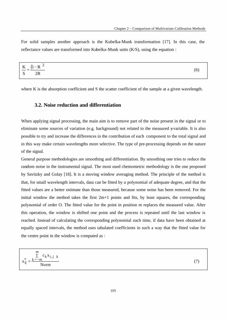
Chapter 2 – Comparison of Multivariate Calibration Methods
105
For solid samples another approach is the Kubelka-Munk transformation [17]. In this case, the
reflectance values are transformed into Kubelka-Munk units (K/S), using the equation :
( )R2R1
SK 2−
= (6)
where K is the absorption coefficient and S the scatter coefficient of the sample at a given wavelength.
3.2. Noise reduction and differentiation
When applying signal processing, the main aim is to remove part of the noise present in the signal or to
eliminate some sources of variation (e.g. background) not related to the measured y-variable. It is also
possible to try and increase the differences in the contribution of each component to the total signal and
in this way make certain wavelengths more selective. The type of pre-processing depends on the nature
of the signal.
General purpose methodologies are smoothing and differentiation. By smoothing one tries to reduce the
random noise in the instrumental signal. The most used chemometric methodology is the one proposed
by Savitzky and Golay [18]. It is a moving window averaging method. The principle of the method is
that, for small wavelength intervals, data can be fitted by a polynomial of adequate degree, and that the
fitted values are a better estimate than those measured, because some noise has been removed. For the
initial window the method takes the first 2m+1 points and fits, by least squares, the corresponding
polynomial of order O. The fitted value for the point in position m replaces the measured value. After
this operation, the window is shifted one point and the process is repeated until the last window is
reached. Instead of calculating the corresponding polynomial each time, if data have been obtained at
equally spaced intervals, the method uses tabulated coefficients in such a way that the fitted value for
the centre point in the window is computed as :
Norm
xcx
m
mkkj,ik
*ij
∑−=
+= (7)

New Trends in Multivariate Analysis and Calibration
106
where *ijx represents the fitted value for the center point in the window, kj,ix + represents the 2m+1
original values in the window, ck is the appropriate coefficient value for each point and Norm is a
normalising constant (Fig. 1a-b). Because the values of ck are the same for all windows, provided the
window size and the polynomial degree are kept constant, the use of the tabulated coefficients
simplifies and accelerates the computations. For computational use, the coefficients for every window
size and polynomial degree can be obtained in [19,20]. The user must decide the size of the window,
2m+1, and the order of the polynomial to be used. Errors in the original tables were corrected later
[21]. These coefficients allow the smoothing of extreme points, which in the original method of
Savitzky-Golay had to be removed. Recently, a methodology based on the same technique has been
proposed [22], where the degree of the polynomial used is optimised in each window. This
methodology has been called Adaptive-Degree Polynomial Filter (ADPF).
Another way of carrying out smoothing is by repeated measurement of the spectrum, i.e. by obtaining
several scans and averaging them. In this way, the signal to noise ratio (SNR), increases with sn , ns
being the number of scans.
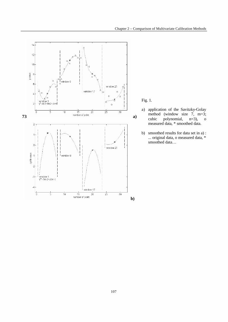
Chapter 2 – Comparison of Multivariate Calibration Methods
107
73 a)
b)
Fig. 1. a) application of the Savitzky-Golay
method (window size 7, m=3; cubic polynomial, n=3), o measured data, * smoothed data.
b) smoothed results for data set in a) :
... original data, o measured data, * smoothed data…
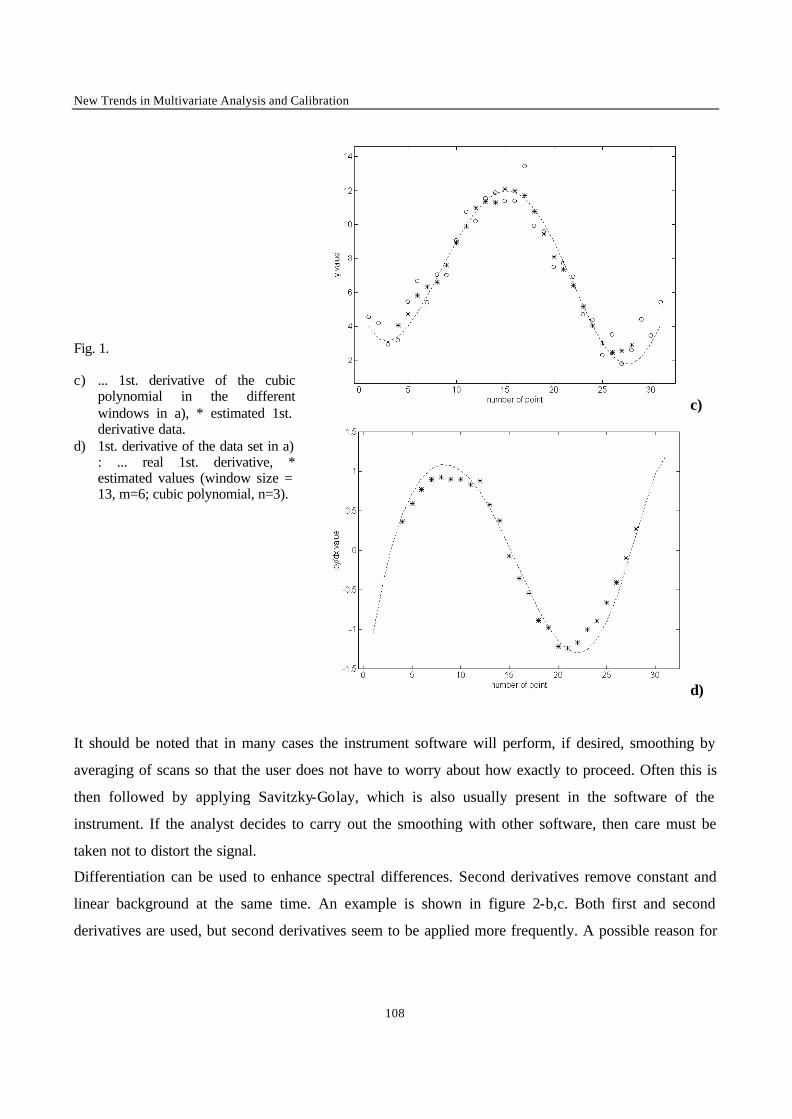
New Trends in Multivariate Analysis and Calibration
108
c)
Fig. 1. c) ... 1st. derivative of the cubic
polynomial in the different windows in a), * estimated 1st. derivative data.
d) 1st. derivative of the data set in a) : ... real 1st. derivative, * estimated values (window size = 13, m=6; cubic polynomial, n=3).
d)
It should be noted that in many cases the instrument software will perform, if desired, smoothing by
averaging of scans so that the user does not have to worry about how exactly to proceed. Often this is
then followed by applying Savitzky-Golay, which is also usually present in the software of the
instrument. If the analyst decides to carry out the smoothing with other software, then care must be
taken not to distort the signal.
Differentiation can be used to enhance spectral differences. Second derivatives remove constant and
linear background at the same time. An example is shown in figure 2-b,c. Both first and second
derivatives are used, but second derivatives seem to be applied more frequently. A possible reason for
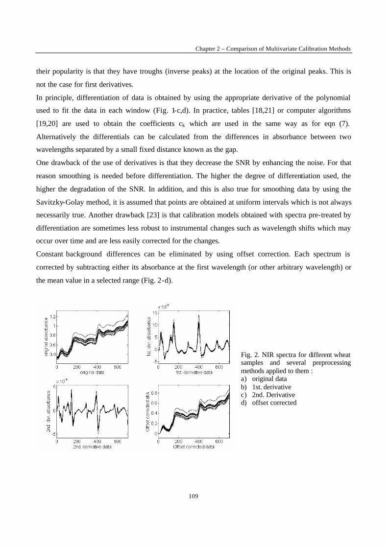
Chapter 2 – Comparison of Multivariate Calibration Methods
109
their popularity is that they have troughs (inverse peaks) at the location of the original peaks. This is
not the case for first derivatives.
In principle, differentiation of data is obtained by using the appropriate derivative of the polynomial
used to fit the data in each window (Fig. 1-c,d). In practice, tables [18,21] or computer algorithms
[19,20] are used to obtain the coefficients ck which are used in the same way as for eqn (7).
Alternatively the differentials can be calculated from the differences in absorbance between two
wavelengths separated by a small fixed distance known as the gap.
One drawback of the use of derivatives is that they decrease the SNR by enhancing the noise. For that
reason smoothing is needed before differentiation. The higher the degree of differentiation used, the
higher the degradation of the SNR. In addition, and this is also true for smoothing data by using the
Savitzky-Golay method, it is assumed that points are obtained at uniform intervals which is not always
necessarily true. Another drawback [23] is that calibration models obtained with spectra pre-treated by
differentiation are sometimes less robust to instrumental changes such as wavelength shifts which may
occur over time and are less easily corrected for the changes.
Constant background differences can be eliminated by using offset correction. Each spectrum is
corrected by subtracting either its absorbance at the first wavelength (or other arbitrary wavelength) or
the mean value in a selected range (Fig. 2-d).
Fig. 2. NIR spectra for different wheat samples and several preprocessing methods applied to them : a) original data b) 1st. derivative c) 2nd. Derivative d) offset corrected
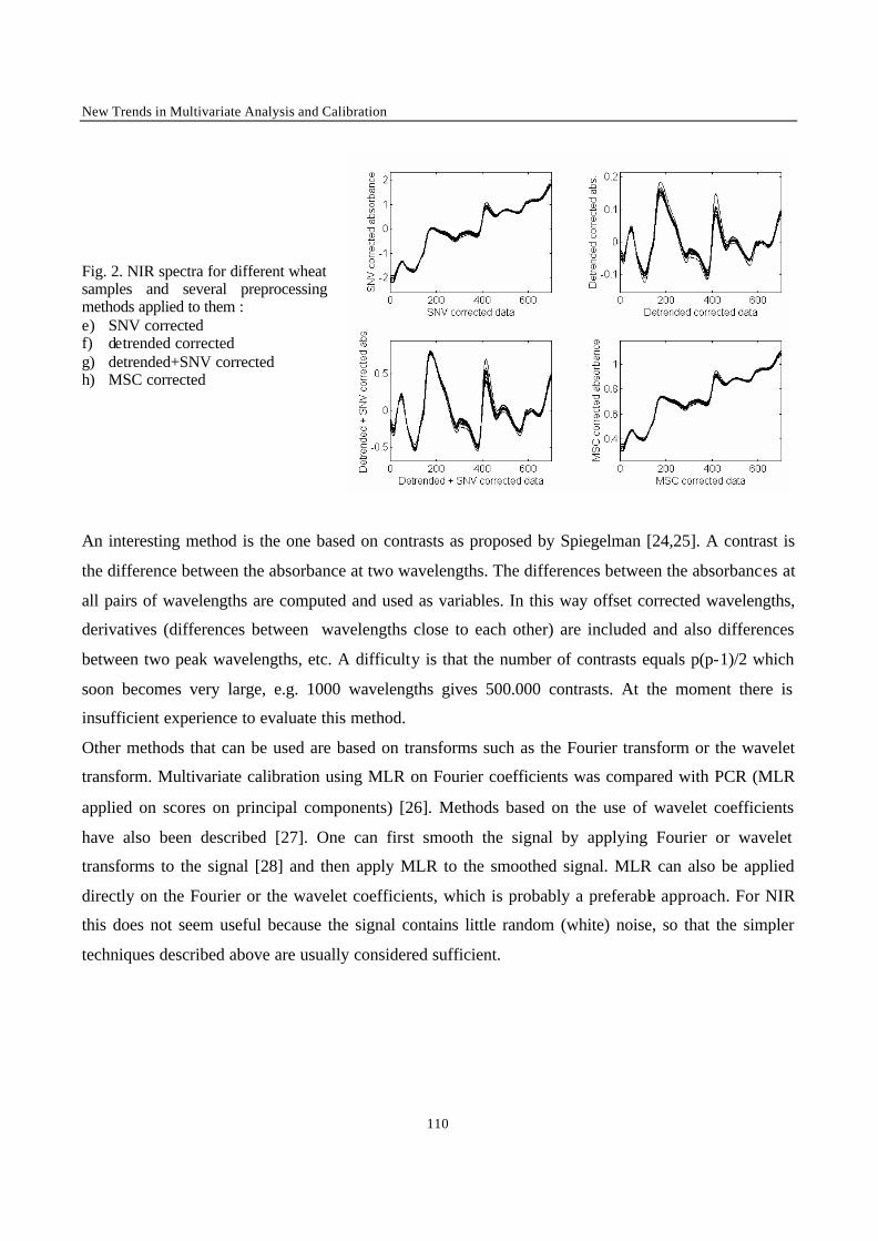
New Trends in Multivariate Analysis and Calibration
110
Fig. 2. NIR spectra for different wheat samples and several preprocessing methods applied to them : e) SNV corrected f) detrended corrected g) detrended+SNV corrected h) MSC corrected
An interesting method is the one based on contrasts as proposed by Spiegelman [24,25]. A contrast is
the difference between the absorbance at two wavelengths. The differences between the absorbances at
all pairs of wavelengths are computed and used as variables. In this way offset corrected wavelengths,
derivatives (differences between wavelengths close to each other) are included and also differences
between two peak wavelengths, etc. A difficulty is that the number of contrasts equals p(p-1)/2 which
soon becomes very large, e.g. 1000 wavelengths gives 500.000 contrasts. At the moment there is
insufficient experience to evaluate this method.
Other methods that can be used are based on transforms such as the Fourier transform or the wavelet
transform. Multivariate calibration using MLR on Fourier coefficients was compared with PCR (MLR
applied on scores on principal components) [26]. Methods based on the use of wavelet coefficients
have also been described [27]. One can first smooth the signal by applying Fourier or wavelet
transforms to the signal [28] and then apply MLR to the smoothed signal. MLR can also be applied
directly on the Fourier or the wavelet coefficients, which is probably a preferable approach. For NIR
this does not seem useful because the signal contains little random (white) noise, so that the simpler
techniques described above are usually considered sufficient.
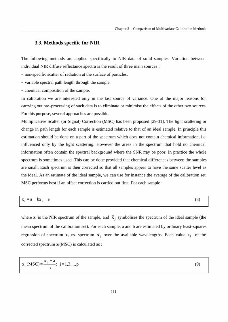
Chapter 2 – Comparison of Multivariate Calibration Methods
111
3.3. Methods specific for NIR
The following methods are applied specifically to NIR data of solid samples. Variation between
individual NIR diffuse reflectance spectra is the result of three main sources :
• non-specific scatter of radiation at the surface of particles.
• variable spectral path length through the sample.
• chemical composition of the sample.
In calibration we are interested only in the last source of variance. One of the major reasons for
carrying out pre-processing of such data is to eliminate or minimise the effects of the other two sources.
For this purpose, several approaches are possible.
Multiplicative Scatter (or Signal) Correction (MSC) has been proposed [29-31]. The light scattering or
change in path length for each sample is estimated relative to that of an ideal sample. In principle this
estimation should be done on a part of the spectrum which does not contain chemical information, i.e.
influenced only by the light scattering. However the areas in the spectrum that hold no chemical
information often contain the spectral background where the SNR may be poor. In practice the whole
spectrum is sometimes used. This can be done provided that chemical differences between the samples
are small. Each spectrum is then corrected so that all samples appear to have the same scatter level as
the ideal. As an estimate of the ideal sample, we can use for instance the average of the calibration set.
MSC performs best if an offset correction is carried out first. For each sample :
eba ji ++= xx (8)
where xi is the NIR spectrum of the sample, and jx symbolises the spectrum of the ideal sample (the
mean spectrum of the calibration set). For each sample, a and b are estimated by ordinary least-squares
regression of spectrum xi vs. spectrum jx over the available wavelengths. Each value xij of the
corrected spectrum xi(MSC) is calculated as :
p1,2,...,j;b
ax(MSC)x ij
ij =−
= (9)

New Trends in Multivariate Analysis and Calibration
112
The mean spectra must be stored in order to transform in the same way future spectra (Fig. 2-h).
Standard Normal Variate (SNV) transformation has also been proposed for removing the multiplicative
interference of scatter and particle size [32,33]. An example is given in figure 2-a, where several
samples of wheat are measured. SNV is designed to operate on individual sample spectra. The SNV
transformatio n centres each spectrum and then scales it by its own standard deviation :
p1,2,...,j;SD
x(SNV)x iij
ij =−
=x
(10)
where xij is the absorbance value of spectrum i measured at wavelength j, ix is the absorbance mean
value of the uncorrected ith spectrum and SD is the standard deviation of the p absorbance values,
( )1
1
2
−
−∑=
p
xp
jiij x
.
Spectra treated in this manner (Fig. 2-e) have always zero mean and variance equal to one, and are thus
independent of original absorbance values.
De-trending of spectra accounts for the variation in baseline shift and curvilinearity of powdered or
densely packed samples by using a second degree polynomial to correct the data [32]. De-trending
operates on individual spectra. The global absorbance of NIR spectra is generally increasing linearly
with respect to the wavelength , but it increases curvilinearly for the spectra of densely packed samples.
A second-degree polynomial can be used to standardise the variation in curvilinearity :
ii ex +++= cba *2* λλ (11)
where xi symbolises the individual NIR spectrum and λ∗ the wavelength. For each sample, a, b and c
are estimated by ordinary least-squares regression of spectrum xi vs. wavelength over the range of
wavelengths. The corrected spectrum xi(DTR) is calculated by :
ic*b2*ai)DTR(i exx =−λ−λ−= (12)
Chapter 2 – Comparison of Multivariate Calibration Methods
113
Normally de-trending is used after SNV transformation (Fig. 2-f,g). Second derivatives can also be
employed to decrease baseline shifts and curvilinearity, but in this case noise and complexity of the
spectra increases.
It has been demonstrated that MSC and SNV transformed spectra are closely related and that the
difference in prediction ability between these methods seems to be fairly small [34,35].
3.4. Selection of pre-processing methods in NIR
The best pre-processing method will be the one that finally produces a robust model with the best
predictive ability. Unfortunately there seem to be no hard rules to decide which pre-processing to use
and often the only approach is trial and error. The development of a methodology that would allow a
systematic approach would be very useful. It is possible to obtain some indication during pre-
processing. For instance, if replicate spectra have been measured, a good pre-processing methodology
will produce minimum differences between replicates [36] though this does not necessarily lead to
optimal predictive value. If only one measure per sample is given, it can be useful to compute the
correlation between each of the original variables and the property of interest and do the same for the
transformed variables (Fig. 3). It is likely that good correlations will lead to a good prediction.
However, this approach is univariate and therefore does not give a complete picture of predictive
ability. Depending on the physical state of the samples and the trend of the spectra, a background
and/or a scatter correction can be applied. If only background correction is required, offset correction is
usually preferable over differentiation, because with the former the SNR is not degraded and because
differentiation may lead to less robust models over time. If additionally scatter correction is required,
SNV and MSC yield very similar results. An advantage of SNV is that spectra are treated individually,
while in MSC one needs to refer to other spectra. When a change is made in the model, e.g. if, because
of clustering, it is decided to make two local models instead of one global one, it may be necessary to
repeat the MSC pre-processing. Non- linear behaviour between X and y appears (or increases) after
some of the pre-processing methods. This is the case for instance for SNV. However this does not
cause problems provided the differences between spectra are relatively small.
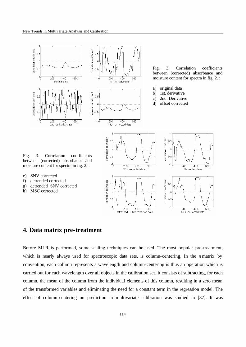
New Trends in Multivariate Analysis and Calibration
114
Fig. 3. Correlation coefficients between (corrected) absorbance and moisture content for spectra in fig. 2. : a) original data b) 1st. derivative c) 2nd. Derivative d) offset corrected
Fig. 3. Correlation coefficients between (corrected) absorbance and moisture content for spectra in fig. 2. : e) SNV corrected f) detrended corrected g) detrended+SNV corrected h) MSC corrected
4. Data matrix pre-treatment
Before MLR is performed, some scaling techniques can be used. The most popular pre-treatment,
which is nearly always used for spectroscopic data sets, is column-centering. In the x-matrix, by
convention, each column represents a wavelength and column-centering is thus an operation which is
carried out for each wavelength over all objects in the calibration set. It consists of subtracting, for each
column, the mean of the column from the individual elements of this column, resulting in a zero mean
of the transformed variables and eliminating the need for a constant term in the regression model. The
effect of column-centering on prediction in multivariate calibration was studied in [37]. It was
Chapter 2 – Comparison of Multivariate Calibration Methods
115
concluded that if the optimal number of variables/factors decreases upon centering, a model should be
made with mean-centered data. Otherwise, a model should be made with the raw data. Because this
cannot be known in advance, it seems reasonable to consider column-centering as a standard operation.
For spectroscopic data it is usually the only pre-treatment performed, although sometimes autoscaling
(also known as column standardisation) is also employed. In this case, each element of a column-
centered table is divided by its corresponding column standard deviation, so that all columns have a
variance of one. This type of scaling can be applied in order to obtain an idea about the relative
importance of the variables [38], but it is not recommended for general use in spectroscopic
multivariate calibration since it unduly inflates the noise in baseline regions.
After pre-treatment, the mean (and the standard deviation for autoscaled data) of the calibration set
must be stored in order to transform future samples, for which the concentration or other characteristic
must be predicted, using the same values.
5. Graphical information
Certain plots should always be made. One of these is to simply plot all spectra on the same graph (Fig.
2). Evident outliers will become apparent. It is also possible to identify noisy regions and perhaps to
exclude them from the model.
Another plot that one should always make is the Principal Component Analysis (PCA) score plot.
Many books and papers are devoted to PCA [39-41]. PCA is not a new method, and was first described
by Pearson in 1901 [42] and by Hotelling in 1933 [43]. Let us suppose that n samples (objects) have
been spectroscopically measured at p wavelengths (variables). This information can be written in
matrix form as:
=
np2n1n
p22221
p11211
x...xx............
x...xxx...xx
X (13)
where x1 = [x11 x12 ...x1p] is the row vector containing the absorbances measured at p wavelengths (the
spectrum) for the first sample, x2 is the row vector containing the spectrum for the second sample and
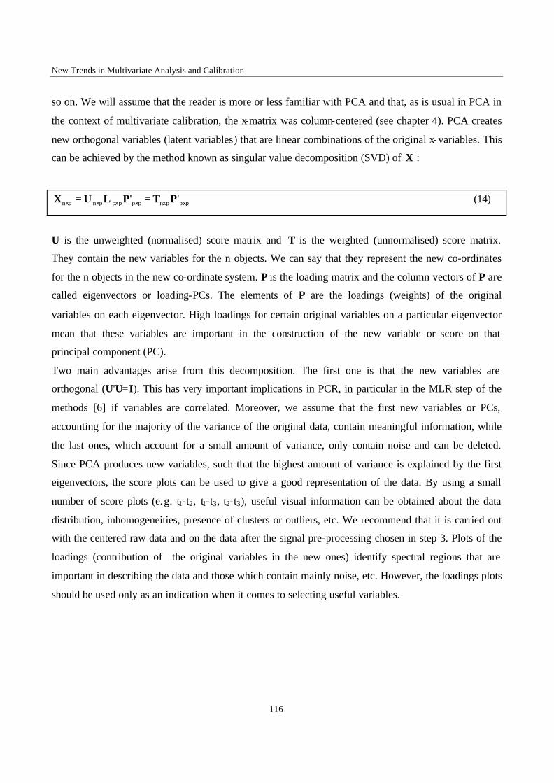
New Trends in Multivariate Analysis and Calibration
116
so on. We will assume that the reader is more or less familiar with PCA and that, as is usual in PCA in
the context of multivariate calibration, the x-matrix was column-centered (see chapter 4). PCA creates
new orthogonal variables (latent variables) that are linear combinations of the original x-variables. This
can be achieved by the method known as singular value decomposition (SVD) of X :
pppnpppppnpn '' xxxxxx PTPUX == Λ (14)
U is the unweighted (normalised) score matrix and T is the weighted (unnormalised) score matrix.
They contain the new variables for the n objects. We can say that they represent the new co-ordinates
for the n objects in the new co-ordinate system. P is the loading matrix and the column vectors of P are
called eigenvectors or loading-PCs. The elements of P are the loadings (weights) of the original
variables on each eigenvector. High loadings for certain original variables on a particular eigenvector
mean that these variables are important in the construction of the new variable or score on that
principal component (PC).
Two main advantages arise from this decomposition. The first one is that the new variables are
orthogonal (U'U=I). This has very important implications in PCR, in particular in the MLR step of the
methods [6] if variables are correlated. Moreover, we assume that the first new variables or PCs,
accounting for the majority of the variance of the original data, contain meaningful information, while
the last ones, which account for a small amount of variance, only contain noise and can be deleted.
Since PCA produces new variables, such that the highest amount of variance is explained by the first
eigenvectors, the score plots can be used to give a good representation of the data. By using a small
number of score plots (e.g. t1-t2, t1-t3, t2-t3), useful visual information can be obtained about the data
distribution, inhomogeneities, presence of clusters or outliers, etc. We recommend that it is carried out
with the centered raw data and on the data after the signal pre-processing chosen in step 3. Plots of the
loadings (contribution of the original variables in the new ones) identify spectral regions that are
important in describing the data and those which contain mainly noise, etc. However, the loadings plots
should be used only as an indication when it comes to selecting useful variables.

Chapter 2 – Comparison of Multivariate Calibration Methods
117
6. Clustering tendency
Clusters are groups of similar objects inside a population. When the population of objects is separated
into several clusters, it is not homogeneous. To perform multivariate calibration modelling, the
calibration objects should preferably belong to the same population. Often this is not possible, e.g. in
the analysis of industrial samples, when these samples belong to different quality grades. The
occurrence of clusters may indicate that the objects belong to different populations. This suggests there
is a fundamental difference between two or more groups of samples, e.g. two different products are
included in the analysis, or a shift or drift has occurred in the measurement technique. When clustering
occurs, the reason must be investigated and appropriate action should be taken. If the clustering is not
due to instrumental reasons that may be corrected (e.g. two sets of samples were measured at different
times and instrumental changes have occurred) then there are two possibilities : to split the data in
groups and make a separate model for each cluster, or to keep all of them in the same calibration
model.
The advantages of splitting the data are that one obtains more homogeneous populations and therefore,
one hopes, better models. However, it also has disadvantages. There will be less calibration objects for
each model and it is also considerably less practical since it is necessary to optimise and validate two or
more models instead of one. When a new sample is predicted, one must first determine to which cluster
it belongs before one can start the actual prediction. Another disadvantage is that the range of y-values
can be reduced, leading to less stable models. For that reason, it is usually preferable to make a single
model. The price one pays in doing this is a more complex and therefore potentially less robust model.
Indeed, the model will contain two types of variables, variables that contain information common to the
two clusters and therefore have similar importance for both, and variables that correct for the bias
between the two clusters. Variables belonging to the second type are often due to peaks in the spectrum
that are present in the objects belonging to one cluster and absent or much weaker in the other objects.
An example where two clusters occur is presented in [44]. Some of the variables selected are directly
related with the property to be measured in both clusters, whereas others are related to the presence or
absence of one peak. This peak is due to a difference in chemical structure and is responsible for the
clustering. The inclusion of the latter variables takes into account this difference and improves the
predictive ability of the model, but also increases the complexity.
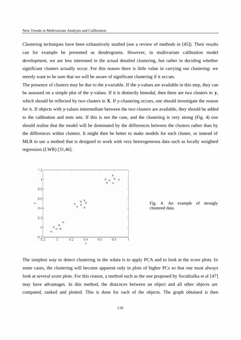
New Trends in Multivariate Analysis and Calibration
118
Clustering techniques have been exhaustively studied (see a review of methods in [45]). Their results
can for example be presented as dendrograms. However, in multivariate calibration model
development, we are less interested in the actual detailed clustering, but rather in deciding whether
significant clusters actually occur. For this reason there is little value in carrying out clustering: we
merely want to be sure that we will be aware of significant clustering if it occurs.
The presence of clusters may be due to the y-variable. If the y-values are available in this step, they can
be assessed on a simple plot of the y-values. If it is distinctly bimodal, then there are two clusters in y,
which should be reflected by two clusters in X. If y-clustering occurs, one should investigate the reason
for it. If objects with y-values intermediate between the two clusters are available, they should be added
to the calibration and tests sets. If this is not the case, and the clustering is very strong (Fig. 4) one
should realise that the model will be dominated by the differences between the clusters rather than by
the differences within clusters. It might then be better to make models for each cluster, or instead of
MLR to use a method that is designed to work with very heterogeneous data such as locally weighted
regression (LWR) [31,46].
Fig. 4. An example of strongly clustered data.
The simplest way to detect clustering in the x-data is to apply PCA and to look at the score plots. In
some cases, the clustering will become apparent only in plots of higher PCs so that one must always
look at several score plots. For this reason, a method such as the one proposed by Szcubialka et al [47]
may have advantages. In this method, the distances between an object and all other objects are
computed, ranked and plotted. This is done for each of the objects. The graph obtained is then
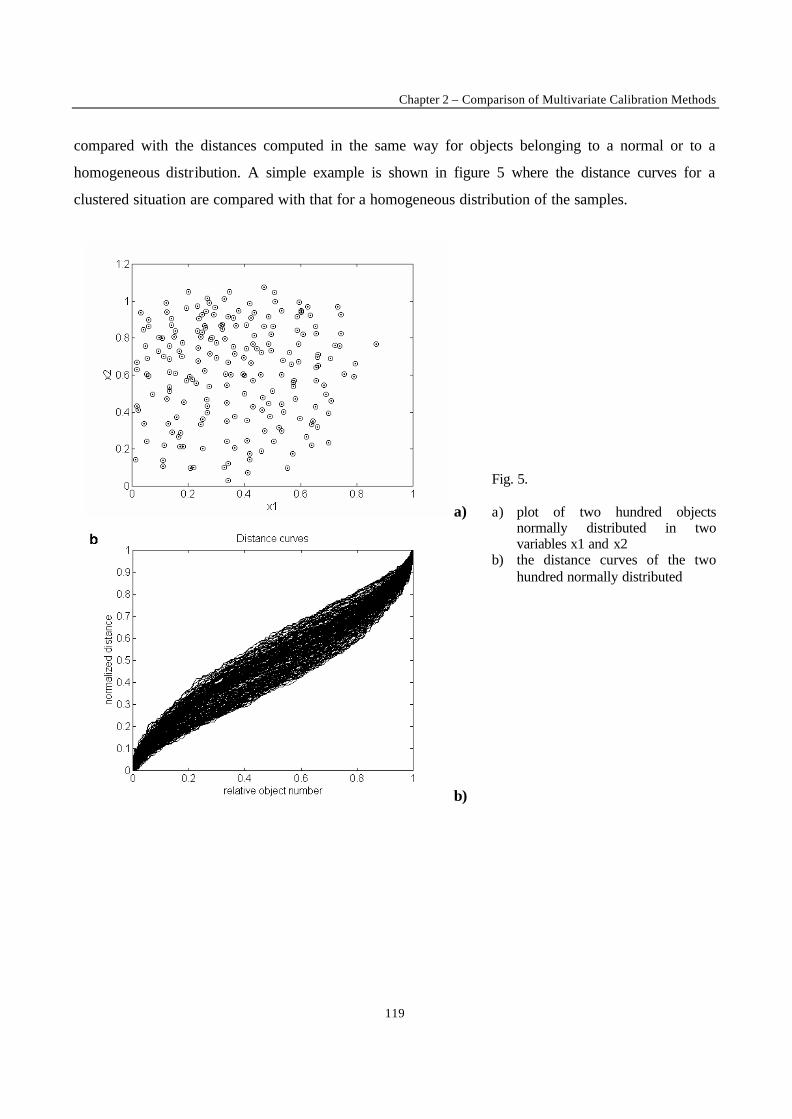
Chapter 2 – Comparison of Multivariate Calibration Methods
119
compared with the distances computed in the same way for objects belonging to a normal or to a
homogeneous distribution. A simple example is shown in figure 5 where the distance curves for a
clustered situation are compared with that for a homogeneous distribution of the samples.
a)
b)
Fig. 5. a) plot of two hundred objects
normally distributed in two variables x1 and x2
b) the distance curves of the two hundred normally distributed
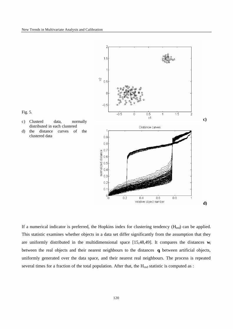
New Trends in Multivariate Analysis and Calibration
120
c)
Fig. 5. c) Clusterd data, normally
distributed in each clustered d) the distance curves of the
clustered data
d)
If a numerical indicator is preferred, the Hopkins index for clustering tendency (Hind) can be applied.
This statistic examines whether objects in a data set differ significantly from the assumption that they
are uniformly distributed in the multidimensional space [15,48,49]. It compares the distances wi
between the real objects and their nearest neighbours to the distances qi between artificial objects,
uniformly generated over the data space, and their nearest real neighbours. The process is repeated
several times for a fraction of the total population. After that, the Hind statistic is computed as :

Chapter 2 – Comparison of Multivariate Calibration Methods
121
∑+∑
∑=
==
=n
1ii
n
1ii
n
1ii
indHwq
q (15)
If objects are uniformly distributed, qi and wi will be similar, and the statistic will be close to 1/2. If
clustering are present, the distances for artificial objects will be larger than for the real ones, because
these artificial objects are homogeneously distributed whereas the real ones are grouped together, and
the value of Hind will increase. A value for Hind higher than 3/4 indicates a clustering tendency at the
90% confidence level [49]. Figures 6-a and 6-b show the application of the Hopkins' statistic, i.e. how
the qi- and wi-values are computed for two different data sets, the first unclustered and the second
clustered. Because the artificial data set is homogeneously generated inside a square box that covers all
the real objects and with co-ordinates determined by the most extreme points, an unclustered data set
lying on the diagonal of the reference axis (Fig. 6-c) might lead to a false detection of clustering [50].
For this reason, the statistic should be determined on the PCA scores. After PCA of the data, the new
axis will lie in the direction of maximum variance, in this case coincident with the main diagonal (Fig.
6-d). Since an outlier in the X-space is effectively a cluster, the Hopkins statistic could detect a false
clustering tendency in this example. A modification of the original statistic has been proposed in [49]
to minimise false positives. Further modifications were proposed by Forina et al [50].
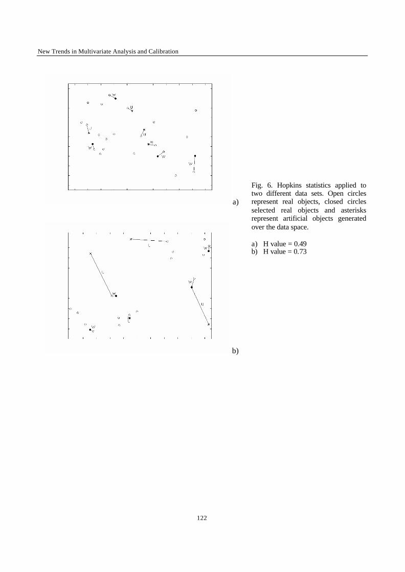
New Trends in Multivariate Analysis and Calibration
122
a)
b)
Fig. 6. Hopkins statistics applied to two different data sets. Open circles represent real objects, closed circles selected real objects and asterisks represent artificial objects generated over the data space. a) H value = 0.49 b) H value = 0.73
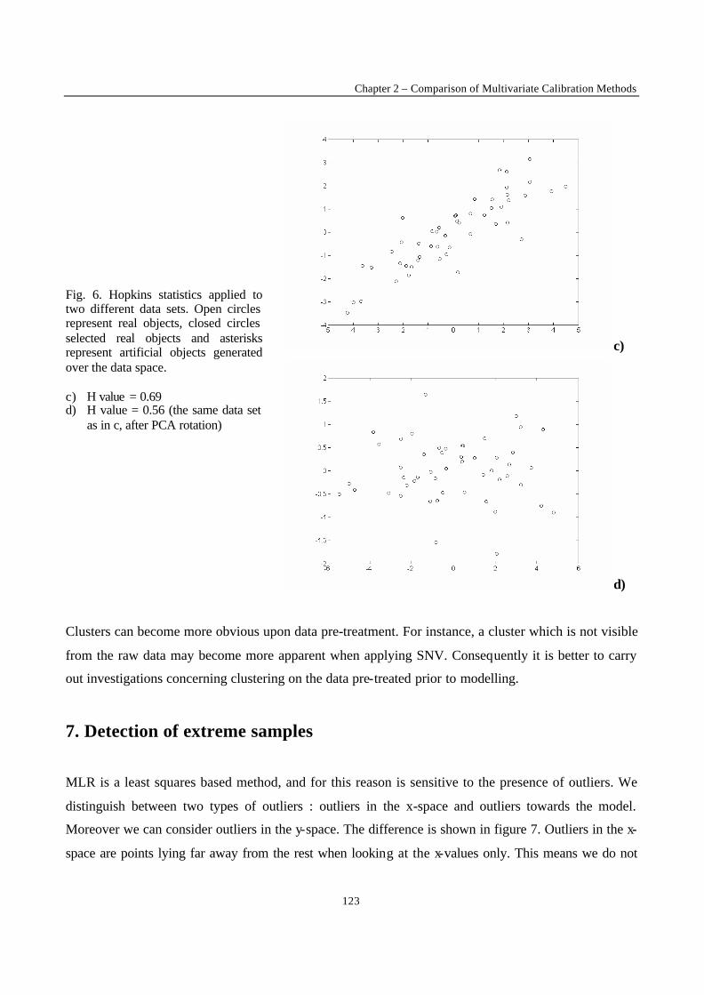
Chapter 2 – Comparison of Multivariate Calibration Methods
123
c)
Fig. 6. Hopkins statistics applied to two different data sets. Open circles represent real objects, closed circles selected real objects and asterisks represent artificial objects generated over the data space. c) H value = 0.69 d) H value = 0.56 (the same data set
as in c, after PCA rotation)
d)
Clusters can become more obvious upon data pre-treatment. For instance, a cluster which is not visible
from the raw data may become more apparent when applying SNV. Consequently it is better to carry
out investigations concerning clustering on the data pre-treated prior to modelling.
7. Detection of extreme samples
MLR is a least squares based method, and for this reason is sensitive to the presence of outliers. We
distinguish between two types of outliers : outliers in the x-space and outliers towards the model.
Moreover we can consider outliers in the y-space. The difference is shown in figure 7. Outliers in the x-
space are points lying far away from the rest when looking at the x-values only. This means we do not
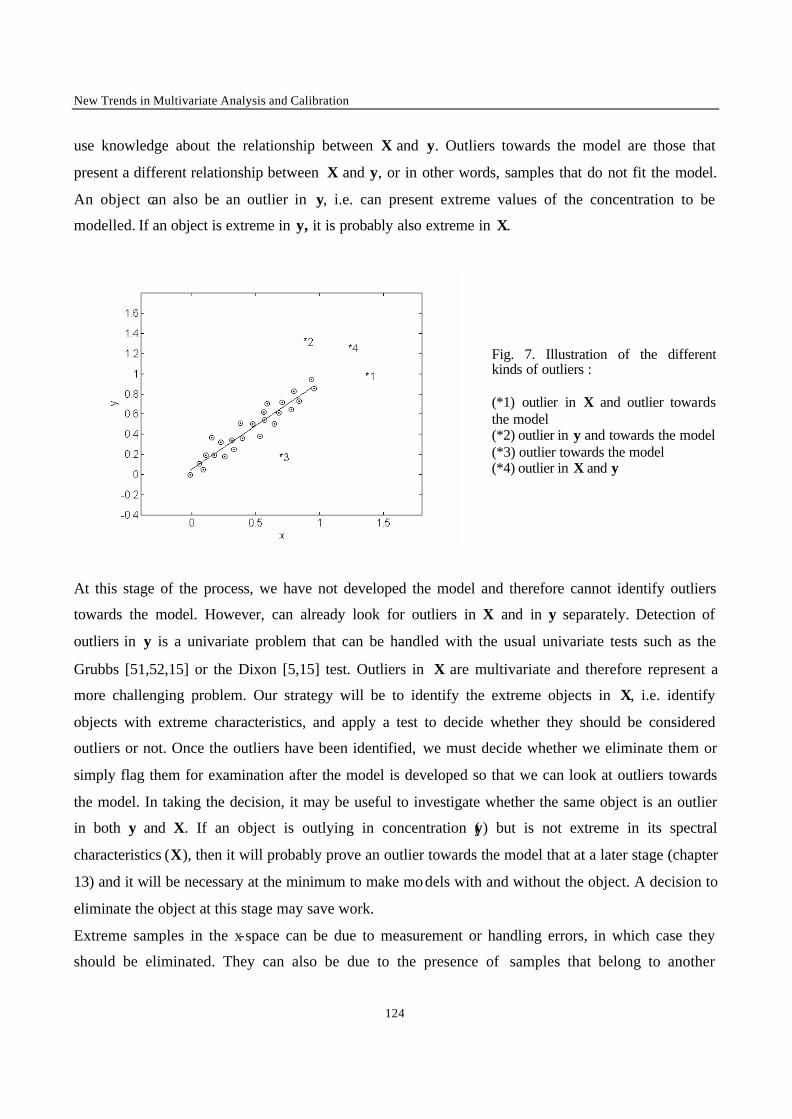
New Trends in Multivariate Analysis and Calibration
124
use knowledge about the relationship between X and y. Outliers towards the model are those that
present a different relationship between X and y, or in other words, samples that do not fit the model.
An object can also be an outlier in y, i.e. can present extreme values of the concentration to be
modelled. If an object is extreme in y, it is probably also extreme in X.
Fig. 7. Illustration of the different kinds of outliers : (*1) outlier in X and outlier towards the model (*2) outlier in y and towards the model (*3) outlier towards the model (*4) outlier in X and y
At this stage of the process, we have not developed the model and therefore cannot identify outliers
towards the model. However, can already look for outliers in X and in y separately. Detection of
outliers in y is a univariate problem that can be handled with the usual univariate tests such as the
Grubbs [51,52,15] or the Dixon [5,15] test. Outliers in X are multivariate and therefore represent a
more challenging problem. Our strategy will be to identify the extreme objects in X, i.e. identify
objects with extreme characteristics, and apply a test to decide whether they should be considered
outliers or not. Once the outliers have been identified, we must decide whether we eliminate them or
simply flag them for examination after the model is developed so that we can look at outliers towards
the model. In taking the decision, it may be useful to investigate whether the same object is an outlier
in both y and X. If an object is outlying in concentration (y) but is not extreme in its spectral
characteristics (X), then it will probably prove an outlier towards the model that at a later stage (chapter
13) and it will be necessary at the minimum to make models with and without the object. A decision to
eliminate the object at this stage may save work.
Extreme samples in the x-space can be due to measurement or handling errors, in which case they
should be eliminated. They can also be due to the presence of samples that belong to another
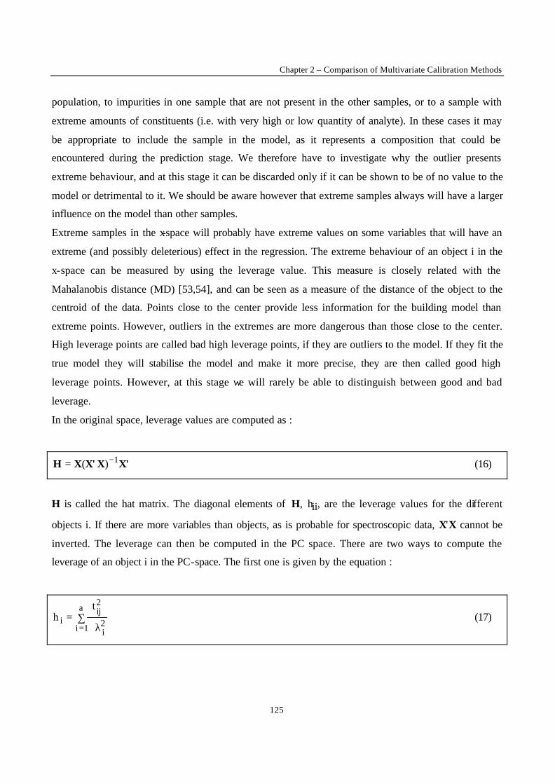
Chapter 2 – Comparison of Multivariate Calibration Methods
125
population, to impurities in one sample that are not present in the other samples, or to a sample with
extreme amounts of constituents (i.e. with very high or low quantity of analyte). In these cases it may
be appropriate to include the sample in the model, as it represents a composition that could be
encountered during the prediction stage. We therefore have to investigate why the outlier presents
extreme behaviour, and at this stage it can be discarded only if it can be shown to be of no value to the
model or detrimental to it. We should be aware however that extreme samples always will have a larger
influence on the model than other samples.
Extreme samples in the x-space will probably have extreme values on some variables that will have an
extreme (and possibly deleterious) effect in the regression. The extreme behaviour of an object i in the
x-space can be measured by using the leverage value. This measure is closely related with the
Mahalanobis distance (MD) [53,54], and can be seen as a measure of the distance of the object to the
centroid of the data. Points close to the center provide less information for the building model than
extreme points. However, outliers in the extremes are more dangerous than those close to the center.
High leverage points are called bad high leverage points, if they are outliers to the model. If they fit the
true model they will stabilise the model and make it more precise, they are then called good high
leverage points. However, at this stage we will rarely be able to distinguish between good and bad
leverage.
In the original space, leverage values are computed as :
X'XX'XH 1)( −= (16)
H is called the hat matrix. The diagonal elements of H, hii, are the leverage values for the different
objects i. If there are more variables than objects, as is probable for spectroscopic data, X'X cannot be
inverted. The leverage can then be computed in the PC space. There are two ways to compute the
leverage of an object i in the PC-space. The first one is given by the equation :
∑λ
==
a
1i 2i
2ij
i
th (17)
New Trends in Multivariate Analysis and Calibration
126
∑λ
+==
a
1i 2i
2ij
it
n1
h (18)
a being the minimum value of n and p and 2iλ the eigenvalue of PCi. The correction by the value 1/n in
eqn (18) is used if column centered data are employed, as is usual in PCA. Then
a = (n-1) if (n-1) < a and a = min (n-1, p)
The leverage values can also be obtained by applying an equation equivalent to eqn (16) :
H = T(T' T)-1 T' (19)
where T is the matrix with the weighted (unnormalised) scores obtained after PCA of X.
Instead of using all the PCs, one can apply only the significant ones. Suppose that r PCs have been
selected to be significant, for instance based on the total percentage of variance they explain [8]. The
total leverage can then be decomposed in contributions due to the significant eigenvectors and the non-
significant ones [53] :
∑∑∑+=
+=λ
+= λ
== λ
=a
1ri
2ih1
ih2i
2ijtr
1i 2i
2ijta
1i 2i
2ijt
ih (20)
For centered data the same correction with 1/n as in eqn (18) is applied. H1 can be also obtained by
using eqn (19) with T being the matrix with the weighted scores from PC1 to PCr. Because we are only
interested in the first r PCs, it seems that hi1 is a more natural leverage concept than hi, and
complications derived by including noisy PCs are avoided.
The value r/n ((r + 1)/n for centered data) is called average partial leverage. If the leverage of an
extreme object exceeds it by a certain factor, the object is considered to be an outlier. As outlier
detection limit one can then set, for example, hi1 > (constant x r/n), where the constant often equals 2.
The leverage is related to the squared Mahalanobis distance of object i to the centre of the calibration
data. One can compute the squared Mahalanobis distance from the covariance matrix, C :
Chapter 2 – Comparison of Multivariate Calibration Methods
127
−−=−−= −
n1h)1n()'()(MD iji
1ji
2i xxCxx (21)
where C is computed as
XX'C1n
1−
= (22)
X being as usual the mean-centered data matrix.
In the same way as the leverage, when the number of variables exceeds the number of objects, C
becomes singular and cannot be inverted. There are also two ways to calculate the Mahalanobis
distance in the PC space, using either all a PCs or using only the r significant ones :
−∑ −=
λ−=
= n1
h)1n(t
)1n(MD ia
1i 2i
2ij2
i (23)
−∑ −=
λ−=
= n1
h)1n(t
)1n(MD 1i
r
1i 2i
2ij2
i (24)
where hi and 1ih are computed using the centered data.
X-space outlier detection can also be performed in the PC space with Rao's statistic [55]. Rao's statistic
sums all the variation from a certain PC on. If there are a PCs, and we start looking at variation from
PCr on, then :
∑=+=
a
1ri
2ij
2i tD (25)
New Trends in Multivariate Analysis and Calibration
128
A high value for 2iD means that object i shows a high score on some of the PCs that were not included
and therefore cannot be explained completely by r PCs. For this reason it is then suspected to be an
outlier. The method is presented here because it uses only information about X. The way in which
Rao's statistic is normally used requires the number of PCs entered in the model. This number is put
equal to r. What can be done to estimate this number of PCs is to follow the D value as a function of r,
starting from r = 0. High values of r indicate that the object is modelled only correctly when higher PCs
are included. If the number of necessary PCs is higher for this object than for the others, it will be an
outlier. A test can be applied for checking the significance of high values for the Rao's statistic by using
these values as input data for the single outlier Grubbs' test [15] :
2
1n
n
1i
2iD
2testD
z
−=
=
∑
(26)
Because the information provided by each of these methods is not necessarily the same, we recommend
that more than one is used, for example by studying both leverage values and Rao's statistic with
Grubbs' test, in order to check if the same objects are detected.
Unfortunately, outlier detection is not easy. This certainly is the case if more than one outlier is present.
In that case all the above methods are subject to what is called masking and swamping. Masking occurs
when an outlier goes undetected because of the presence of another, usually adjacent, one. Swamping
occurs when good observations are incorrectly identified as outliers because of the presence of another,
usually remote, subset of outliers (Fig. 8). Masking and swamping occur because the mean and the
covariance matrix are not robust to outliers.
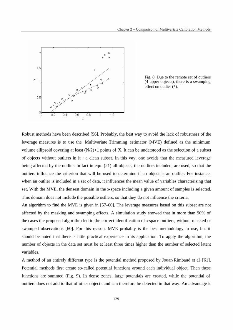
Chapter 2 – Comparison of Multivariate Calibration Methods
129
Fig. 8. Due to the remote set of outliers (4 upper objects), there is a swamping effect on outlier (*).
Robust methods have been described [56]. Probably, the best way to avoid the lack of robustness of the
leverage measures is to use the Multivariate Trimming estimator (MVE) defined as the minimum
volume ellipsoid covering at least (N/2)+1 points of X. It can be understood as the selection of a subset
of objects without outliers in it : a clean subset. In this way, one avoids that the measured leverage
being affected by the outlier. In fact in equ. (21) all objects, the outliers included, are used, so that the
outliers influence the criterion that will be used to determine if an object is an outlier. For instance,
when an outlier is included in a set of data, it influences the mean value of variables characterising that
set. With the MVE, the densest domain in the x-space including a given amount of samples is selected.
This domain does not include the possible outliers, so that they do not influence the criteria.
An algorithm to find the MVE is given in [57-60]. The leverage measures based on this subset are not
affected by the masking and swamping effects. A simulation study showed that in more than 90% of
the cases the proposed algorithm led to the correct identification of x-space outliers, without masked or
swamped observations [60]. For this reason, MVE probably is the best methodology to use, but it
should be noted that there is little practical experience in its application. To apply the algorithm, the
number of objects in the data set must be at least three times higher than the number of selected latent
variables.
A method of an entirely different type is the potential method proposed by Jouan-Rimbaud et al. [61].
Potential methods first create so-called potential functions around each individual object. Then these
functions are summed (Fig. 9). In dense zones, large potentials are created, while the potential of
outliers does not add to that of other objects and can therefore be detected in that way. An advantage is

New Trends in Multivariate Analysis and Calibration
130
that special objects within the x-domain are also detected, for instance, an isolated object between two
clusters. Such objects (we call them inliers) can in certain circumstances have the same effect as
outliers. A disadvantage is that the width of the potential functions around each object has to be
adjusted. It cannot be too small, because many objects would then be isolated; it cannot be too large
because all objects would be part of one global potential function. Moreover, while the method does
very well in flagging the more extreme objects, a decision on their rejection cannot be taken easily.
Fig. 9. Adapted from D. Bouveresse, doctoral thesis (1997), Vrije universiteit Brussel, contour plot corresponding to k=4 with the 10% percentile method and with (*) the identified inlier.
8. Selection and representativity of the calibration sample subset
Because the model has to be used for the prediction of new samples, all possible sources of va riation
that can be encountered later must be included in the calibration set. This means that the chemical
components present in the samples must be included in the calibration set; with a range of variation in
concentration at least as wide, and preferab ly wider than the one expected for the samples to be
analysed; that sources of variation such as different origins or different batches are included and
possible physical variations (e.g. different temperatures, different densities) among samples are also
covered.
In addition, it is evident that the higher the number of samples in the calibration set, the lower the
prediction error [62]. In this sense, a selection of samples from a larger set is contra- indicated.
However, while a random selection of samples may approach a normal distribution, a selection
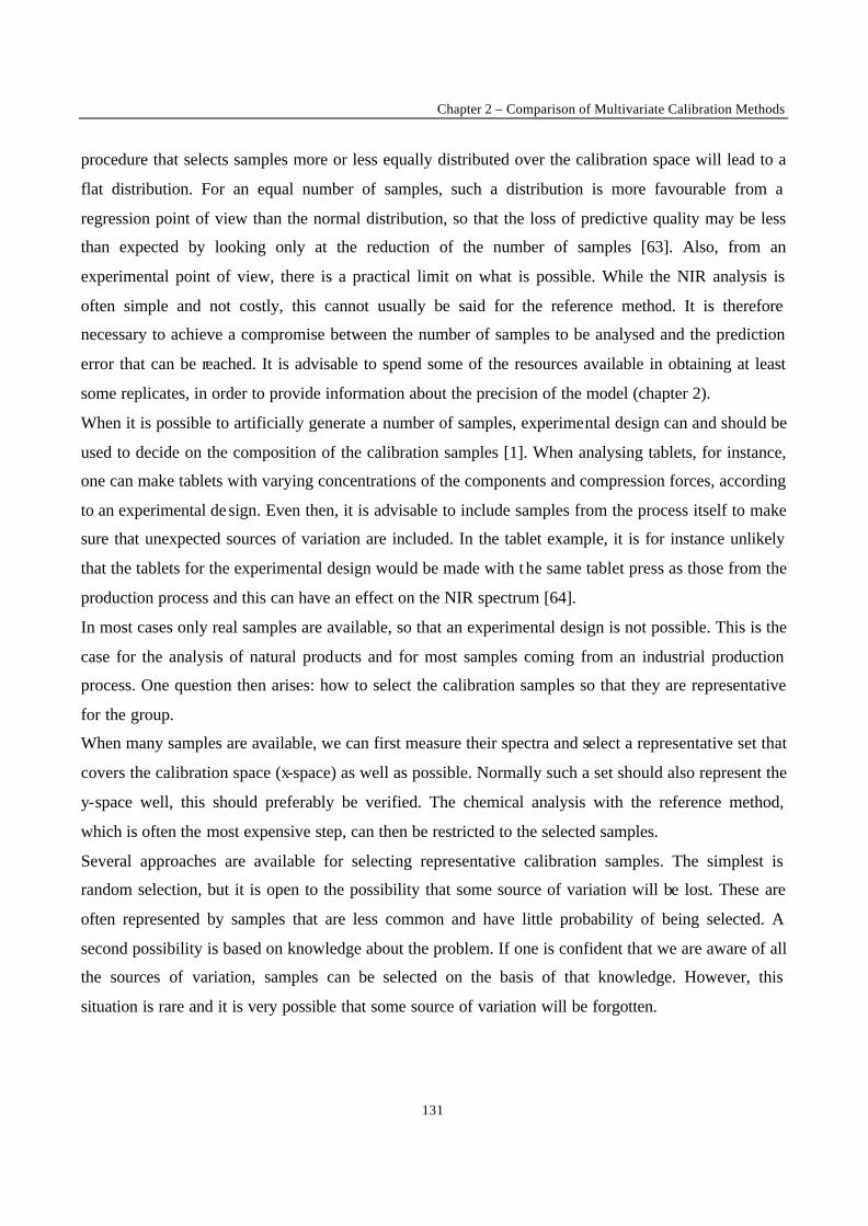
Chapter 2 – Comparison of Multivariate Calibration Methods
131
procedure that selects samples more or less equally distributed over the calibration space will lead to a
flat distribution. For an equal number of samples, such a distribution is more favourable from a
regression point of view than the normal distribution, so that the loss of predictive quality may be less
than expected by looking only at the reduction of the number of samples [63]. Also, from an
experimental point of view, there is a practical limit on what is possible. While the NIR analysis is
often simple and not costly, this cannot usually be said for the reference method. It is therefore
necessary to achieve a compromise between the number of samples to be analysed and the prediction
error that can be reached. It is advisable to spend some of the resources available in obtaining at least
some replicates, in order to provide information about the precision of the model (chapter 2).
When it is possible to artificially generate a number of samples, experimental design can and should be
used to decide on the composition of the calibration samples [1]. When analysing tablets, for instance,
one can make tablets with varying concentrations of the components and compression forces, according
to an experimental de sign. Even then, it is advisable to include samples from the process itself to make
sure that unexpected sources of variation are included. In the tablet example, it is for instance unlikely
that the tablets for the experimental design would be made with t he same tablet press as those from the
production process and this can have an effect on the NIR spectrum [64].
In most cases only real samples are available, so that an experimental design is not possible. This is the
case for the analysis of natural products and for most samples coming from an industrial production
process. One question then arises: how to select the calibration samples so that they are representative
for the group.
When many samples are available, we can first measure their spectra and select a representative set that
covers the calibration space (x-space) as well as possible. Normally such a set should also represent the
y-space well, this should preferably be verified. The chemical analysis with the reference method,
which is often the most expensive step, can then be restricted to the selected samples.
Several approaches are available for selecting representative calibration samples. The simplest is
random selection, but it is open to the possibility that some source of variation will be lost. These are
often represented by samples that are less common and have little probability of being selected. A
second possibility is based on knowledge about the problem. If one is confident that we are aware of all
the sources of variation, samples can be selected on the basis of that knowledge. However, this
situation is rare and it is very possible that some source of variation will be forgotten.

New Trends in Multivariate Analysis and Calibration
132
One algorithm that can be used for the selection is based on the D-optimal concept [65,66]. The D-
optimal criterion minimises the variance of the regression coefficients. It can be shown that this is
equivalent to maximising the covariance matrix, selecting samples such that the variance is maximised
and the correlation minimised. The criterion comes from multivariate regression and experimental
design. In our context, the variance maximisation leads to selection of samples with relatively extreme
characteristics and located on the borders of the calibration domain.
Kennard and Stone proposed a sequential method that should cover the experimental region uniformly
and that was meant for the use in experimental design [67]. The procedure consists of selecting as the
next sample (candidate object) the one that is most distant from those already selected objects
(calibration objects). The distance is usually the Euclidean distance although it is possible, and
probably better, to use the Mahalanobis distance. The distance are usually calculated in the PC space
since spectroscopic data tend to generate a high number of variables. As starting points we either select
the two objects that are most distant from each other, or preferably, the one closest to the mean. From
all the candidate points, the one is selected that is furthest from those already selected and added to the
set of calibration points. To do this, we measure the distance from each candidate point i0 to each point
i which has already been selected and determine which is smallest ))i,i(di
min(0
. From these we select
the one for which the distance is maximal, dselected = 0i
max ))i,i(di
min(0
. In the absence of strong
irregularities in the factor space, the procedure starts first selecting a set of points close to those
selected by the D-optimality method, i.e. on the borderline of the data set (plus the center point, if this
is chosen as the starting point). It then proceeds to fill up the calibration space. Kennard and Stone
called their procedure a uniform mapping algorithm; it yields a flat distribution of the data which, as
explained earlier, is preferable for a regression model.
Næs proposed a procedure based on cluster analysis. The clustering is continued until the number of
clusters matches the number of calibration samples desired [68]. From each cluster, the object that is
furthest away from the mean is selected. In this way the extremes are covered but not necessarily the
centre of the data.
In the method proposed by Puchwein [69], the first step consists in sorting the samples according to the
Mahalanobis distances to the centre of the set and selecting the most extreme point. A limiting distance
is then chosen and all the samples that are closer to the selected point than this distance are excluded.
The sample that is most extreme among the remaining points is selected and the procedure repeated,

Chapter 2 – Comparison of Multivariate Calibration Methods
133
choosing the most distant remaining point, until there are no data points left. The number of selected
points depends on the size of the limiting distance: if it is small, many points will be included; if it is
large, very few. The procedure must therefore be repeated several times for different limiting distances
until the limiting distance is reached for which the desired number of samples is selected.
Figure 10 shows the results of applying these four algorithms to a 2-dimensional data set of 250
objects, designed not to be homogeneous. Clearly, the D-optimal design selects points in a completely
different way from the other algorithms. The Kennard-Stone and Puchwein algorithms provide similar
results. Næs method does not cover the centre. Other methods have been proposed such as "unique-
sample selection" [70]. The results obtained seem similar to those obtained from the previously cited
methods.
An important question is how many samples must be included in the calibration set. This va lue must be
selected by the analyst. This number is related to the final complexity of the model. The term
complexity should be understood as the number of variables or PCs included plus the number of
quadratic and interaction terms. An ASTM standard states that, if the complexity is smaller than three,
at least 24 samples must be used. If it is equal or greater than four, at least 6 objects per degree of
complexity are needed [58,71].
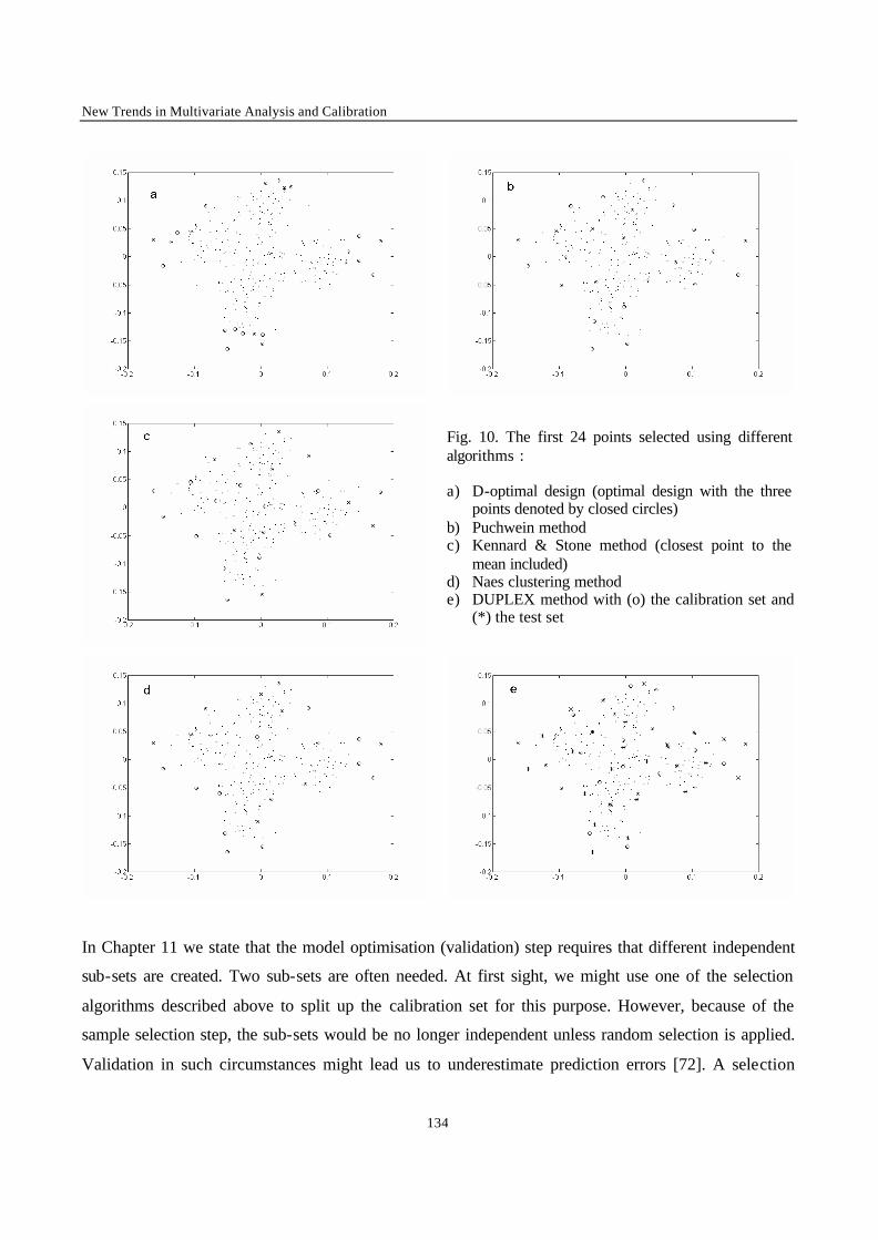
New Trends in Multivariate Analysis and Calibration
134
Fig. 10. The first 24 points selected using different algorithms : a) D-optimal design (optimal design with the three
points denoted by closed circles) b) Puchwein method c) Kennard & Stone method (closest point to the
mean included) d) Naes clustering method e) DUPLEX method with (o) the calibration set and
(*) the test set
In Chapter 11 we state that the model optimisation (validation) step requires that different independent
sub-sets are created. Two sub-sets are often needed. At first sight, we might use one of the selection
algorithms described above to split up the calibration set for this purpose. However, because of the
sample selection step, the sub-sets would be no longer independent unless random selection is applied.
Validation in such circumstances might lead us to underestimate prediction errors [72]. A selection
Chapter 2 – Comparison of Multivariate Calibration Methods
135
method which appears to overcome this drawback is a modification by Snee of the Kennard-Stone
method, called the DUPLEX method [73]. In the first step, the two points which are furthest away from
each other are selected for the calibration set. From the remaining points, the two objects which are
furthest away from each other are included in the test set. In the third step, the remaining point which is
furthest away from the two previously selected for the calibration set is included in that set. The
procedure is repeated selecting a single point for the test set which is furthest from the existing points
in that set. Following the same procedure, points are added alternately to each set. This approach
selects representative calibration and test data sets of equal size. In figure 10 the result of applying the
DUPLEX method is also presented.
Of all the proposed methodologies, the Kennard-Stone, DUPLEX and Puchwein's methods need the
minimum a priori knowledge. In addition, they provide a calibration set homogeneously distributed in
space (flat distribution). However, Puchwein's method must be applied several times. The DUPLEX
method seems to be the best way to select representative calibration and test data sets in a validation
context.
Once the calibration set has been selected, several tests can be employed to determine the
representativity of the selected objects with respect to the total set [74]. This appears to be unnecessary
if one of the algorithms recommended for the selection of the calibration samples has been applied. In
practice, however, little attention is often paid to the proper selection. For instance, it may be that the
analyst simply takes the first n samples for the calibration set. In this case a representativity test is
necessary. One possibility is to obtain PC score plots and to compare visually the selected set of
calibration samples to the whole set. This is difficult when there are many relevant PCs. In such cases a
more formal approach can be useful. We proposed an approach that includes the determination of three
different characteristics [75]. The first one checks if both sets have the same direction in the space of
the PCs. The directions are compared by computing the scalar product of two direction vectors
obtained from the PCA decomposition of both data sets. To do this, the normed scalar product between
the vectors d1 and d2 is obtained :
22
21
21 'P
dd
dd= (27)
New Trends in Multivariate Analysis and Calibration
136
where d1 and d2 are the average direction vector for each data set:
∑ λ==
r
1i,i1
2i,11 pd and i,2
r
1i
2i,22 pd ∑ λ=
= (28)
where 2i,1λ and p1,i are the corresponding eigenvalues and loading vectors for data set 1, and 2
i,2λ and
p2,i are the corresponding eigenvalues and loading vectors for data set 2. If the P value (cosinus of the
angle between the direction of each set) is higher than 0.7, it can be concluded that the original
variables have similar contribution to the latent variables, and they are comparable.
The second test compares the variance-covariance matrices. The intention is to determine whether the
two data sets have a similar volume both in magnitude and direction. The comparison is made by using
an approximation of the Bartlett's test. First the pooled variance-covariance matrix is computed :
CC C
=− + −
+ −( ) ( )n n
n n1 1 2 2
1 2
1 12
(29)
The Box M-statistic is then obtained :
−+−ν= −− CCCC 1
221
11 ln)1n(ln)1n(M (30)
with
−+−
−+
−−−+
−=ν2nn
11n
11n
1)1p(6
1p3p21
2121
2 (31)
and the parameter CV is defined as:
22n1nM
eCV −+−
= (32)

Chapter 2 – Comparison of Multivariate Calibration Methods
137
If CV is close to 1, both the volume and the direction of the data sets are comparable.
The third and last test compares the data set centroids. To do this, the squared Mahalanobis distance D2
between the means of each data set is computed :
xxCxx ) ()'(D 211
212 −−= − (33)
C is defined as in eqn (21), and from this value, a parameter F is defined as:
2
2121
2121 D)2nn)(nn(p
)1pnn(nnF
−++−−+
= (34)
F follows a Fisher-Snedecor distribution, with p and n1+n2-p-1 degrees of freedom.
As already stated these tests are not needed when a selection algorithm is used. With some selection
algorithms they would even be contra- indicated. For instance, the test that compares variances cannot
be applied for calibration sets selected by the D-optimal design, because the most extreme samples are
selected and the calibration set will necessarily have a larger variance than the original set.
9. Non-linearity
Sources of non- linearity in spectroscopic methods are described in [76], and can be summarised as due
to :
1 - violations of the Beer-Lambert law
2 - detector non- linearity's
3 - stray light
4 - non- linearity's in diffuse reflectance/transmittance
5 - chemically-based non- linearities
6 - non- linearities in the property/concentration relationship.
Methods, based on ANOVA, proposed by Brown [77] and Xie et al (non- linearity tracking analysis
algorithm) [78] detect non-linear variables, which one may decide to delete. There seems to be little

New Trends in Multivariate Analysis and Calibration
138
expertise available in the practical use of these methods. Moreover, non-linear regions may contain
interesting information. The methods should therefore be used only as a diagnostic, signalling that non-
linearities occur in specific regions. If it is later found that the MLR model is not as good as was hoped,
or is more complex than expected, it may be useful to see if better results are obtained after elimination
of the more non- linear regions.
Most methods for detection of non- linearity depend on visual evaluation of plots. A classical method is
to plot the residuals against y or the fitted (predicted) response y for the complete model [79,80,54].
The latter is to be preferred, since it removes some of the random error which could make the
evaluation more difficult (Fig. 11-b). This is certainly the case when the imprecision of y is relatively
large. Non-linearity typically leads to residuals of one sign for most of the samples with mid-range y-
values, whereas most of the samples with low or high y-value have residuals of the opposite sign. The
runs test [1] examines whether an unusual pattern occurs in a set of residuals. In this context a run is
defined as a series of consecutive residuals with the same sign. Figure 11-d would lead to 3 runs and
the following pattern: “ + + + + + + + - - - - - - + + +“.
From a statistical point of view long runs are improbable and are considered to indicate a trend in the
data, in this case a non- linearity. The test therefore consists of comparing the number of runs with the
number of samples. Similarly, the Durbin Watson test examines the null hypothesis that there is no
correlation between successive residuals. In this case no trend occurs. The runs or Durbin-Watson tests
should be carried out as a complement to the visual evaluation and not as a replacement.
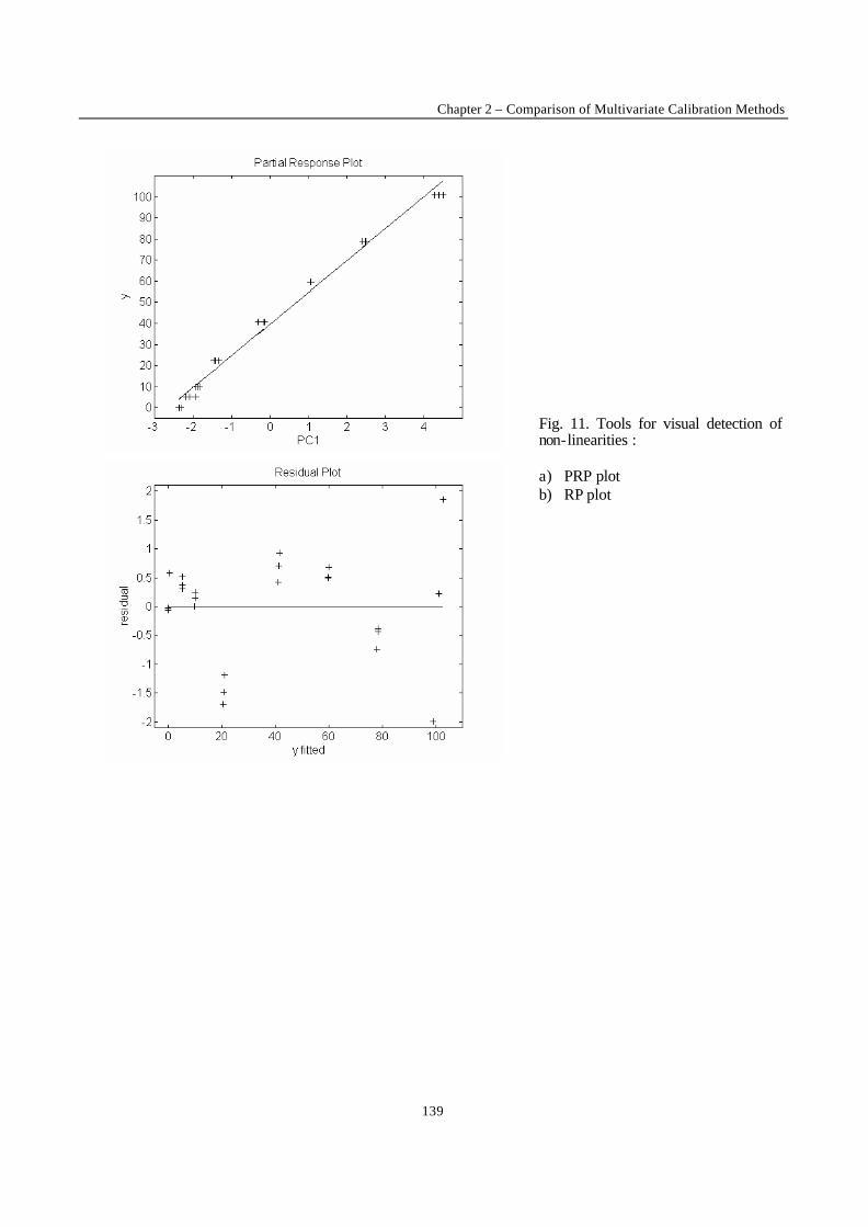
Chapter 2 – Comparison of Multivariate Calibration Methods
139
Fig. 11. Tools for visual detection of non-linearities : a) PRP plot b) RP plot
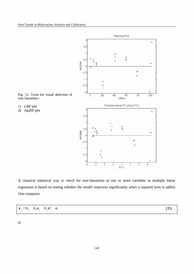
New Trends in Multivariate Analysis and Calibration
140
Fig. 11. Tools for visual detection of non-linearities : c) e-RP plot d) ApaRP plot
A classical statistical way to check for non- linearities in one or more variables in multiple linear
regression is based on testing whether the model improves significantly when a squared term is added.
One compares
i2i2i10i bbb exxy +++= (35)
to

Chapter 2 – Comparison of Multivariate Calibration Methods
141
*i
*1
*0i bb iexy ++= (36)
xi being the values of the x-variable investigated for object i. A one-sided F-test can be employed to
check if the improvement of fit is significant. One can also apply a two-sided t-test for checking if b2 is
significantly different from 0. The calculated t-value is compared to the t-test value with (n-3) degrees
of freedom, at the desired level of confidence. It can be noted that This can be applied also when the
variables are PC scores to the linear model [2].
All these methods are lack-of-fit methods and it is probable that they will also indicate lack-of-fit when
the reason is not non-linearity, but the presence of outliers. Caution is therefore required. We prefer the
runs or the Durbin Watson tests, in conjunction with visual evaluation of the partial response plot or the
Mallows plot.
It should be noted that many of the methods described here require that a model has already been built.
In this sense, this chapter should come after the chapters 10 and 11. However, we recommend that non-
linearity be investigated at least partly before the model is built by plotting very significant variables if
available (e.g. peak maxima in Raman spectroscopy) or the scores of the first PCs as a function of y
(e.g. for NIR data). If a clear non- linear relationship with y is obtained with one of these variables/PCs,
it is very probable that a non-linear approach is to be preferred. If no non-linearity is found in this step,
then one should, after obtaining a linear model (chapters 10 and 11) check again e.g. using Mallows
plot and the runs test to confirm linearity.
10. Building the model
When variables are not correlated and more samples than variables are available, the model can be built
simply using all of the variables. This usually happens for non-spectroscopic data. This situation can
however also arise in the case of very specific spectroscopic applications, for instance when using a
simultaneous ICP-AES instrument equipped with only few photo-multiplicators fixed to emission on
specific wavelengths. In some other particular cases, expert knowledge can be used to select very few
variables out of a spectrum. For instance, in Raman or Atomic Emission spectroscopy, compounds in a
mixture can be represented by neat and narrow peaks. Building the model can then simply consist in
selecting the variables corresponding to the maxima of peaks representative for the product which
New Trends in Multivariate Analysis and Calibration
142
concentration has to be predicted. The extreme case being the situation when only one variable is
necessary to obtain satisfying prediction, leading to a univariate model.
However, modern spectroscopic instruments usually generate a very high number of variables,
exceeding by far the number of available samples (objects). In current applications, and in particular in
NIR spectroscopy, variable selection is therefore needed to overcome the problems of matrix under-
determination and correlated variables. Even when more objects than variables are available, it can be
interesting to select only the most representative variables in order to obtain a simpler model. In the
majority of cases, building the MLR model therefore consists in performing variable selection : finding
the subset of variables that has to be used.
10.1. Stepwise approaches
The most classical variable selection approach, which is found in many statistical packages, is called
stepwise regression [1,2]. This family of methods consists in optimising the subset of variables used for
calibration by adding and/or removing them one by one from the total set.
The so-called forward selection procedure consists in first selecting the variable that is best correlated
with y. Suppose this is found to be xi. The model is at this stage restricted to y = f (xi). The regression
coefficient b obtained from the univariate regression model relating xi to y is tested for significance
using a t-test at the considered critical level α = 1 or 5 %. If it is not found to be significant, the process
stops and no model is built. Otherwise, all other variables are tested for inclusion in the model. The
variable xj which will be retained for inclusion together with xi is the one that, when added to the
model, leads to the largest improvement compared to the original univariate model. It is then tested
whether the observed improvement is significant. If not, the procedure stops and the model is restricted
to y = f(xi). If the improvement is significant, xj is definitively incorporated in the model that becomes
bivariate : y = f (xi,xj). The procedure is repeated for a third variable to be included in the model, and so
on until finally no further improvement can be obtained.
Several variants of this procedure can be used. In backward elimination, the selection is started with all
variables included in the model. The least significant ones are successively eliminated in a comparable
way as in forward selection. Forward and backward steps can be combined in order to obtain a more
sophisticated stepwise selection procedure. As is the case in forward selection, the first variable xi

Chapter 2 – Comparison of Multivariate Calibration Methods
143
entered in the model is the most correlated to the property of interest y. The regression coefficient b
obtained from the univariate regression model relating xi to y is tested for significance. The next step is
forward selection. The variable xj that yields the highest Partial Correlation Coefficient (PCC) is
included in the model. The inclusion of a new variable in the model can decrease the contribution of a
variable already included and make it non-significant. After each inclusion of a new variable, the
significance of the regression terms (b ixi) already in the model is therefore tested, and the non-
significant terms are eliminated from the equa tion. This is the backward elimination step. Forward
selection and backward elimination are repeated until no improvement of the model can be achieved by
including a new variable, and all the variables already included are significant. Such stepwise
approaches using both forward and backward steps are usually the most efficient.
10.2. Genetic algorithms
Genetic algorithms can also be used for variable selection. They were first proposed by Holland [81].
They were introduced in chemometrics by Lucasius et al [82] and Leardi et al [83]. They were applied
for instance in multivariate calibration for the determination of certain characteristics of polymers [84]
or octane numbers [85]. Reviews about applications in chemistry can be found in [86,87]. There are
several competing algorithms such as simulated annealing [88] or the immune algorithm [89].
Genetic Algorithms are general optimisation tools aiming at selecting the fittest solution to a problem.
Suppose that, to keep it simple, 9 variables are measured. Possible solutions are represented in figure
12. Selected variables are indicated by a 1, non-selected variables by a 0.
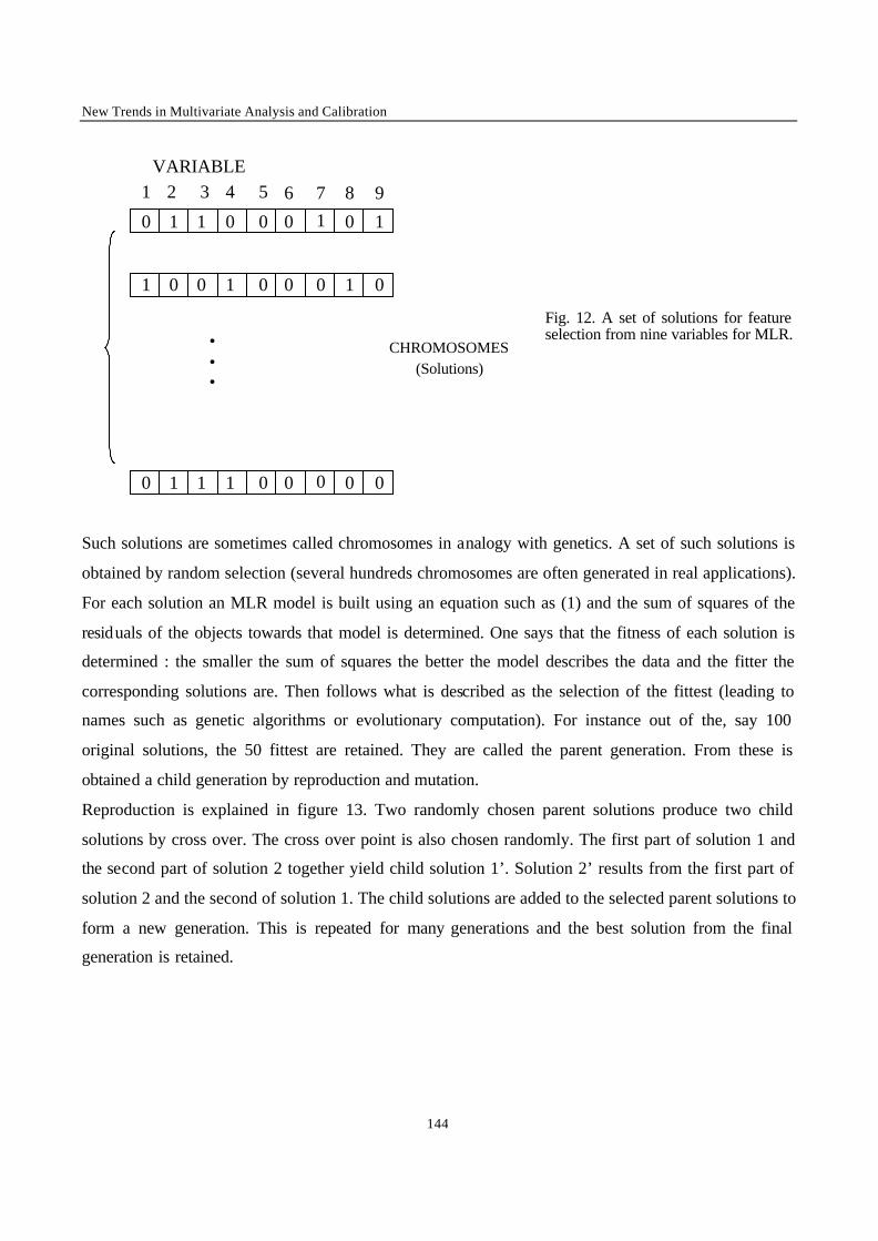
New Trends in Multivariate Analysis and Calibration
144
VARIABLE1 2 3 4 5 6 7 8
CHROMOSOMES
0 1 1 0 0 0 1 0
(Solutions)
���
9
1
1 0 0 1 0 0 1 00
0 1 1 1 0 0 0 0 0
Fig. 12. A set of solutions for feature selection from nine variables for MLR.
Such solutions are sometimes called chromosomes in analogy with genetics. A set of such solutions is
obtained by random selection (several hundreds chromosomes are often generated in real applications).
For each solution an MLR model is built using an equation such as (1) and the sum of squares of the
residuals of the objects towards that model is determined. One says that the fitness of each solution is
determined : the smaller the sum of squares the better the model describes the data and the fitter the
corresponding solutions are. Then follows what is described as the selection of the fittest (leading to
names such as genetic algorithms or evolutionary computation). For instance out of the, say 100
original solutions, the 50 fittest are retained. They are called the parent generation. From these is
obtained a child generation by reproduction and mutation.
Reproduction is explained in figure 13. Two randomly chosen parent solutions produce two child
solutions by cross over. The cross over point is also chosen randomly. The first part of solution 1 and
the second part of solution 2 together yield child solution 1’. Solution 2’ results from the first part of
solution 2 and the second of solution 1. The child solutions are added to the selected parent solutions to
form a new generation. This is repeated for many generations and the best solution from the final
generation is retained.
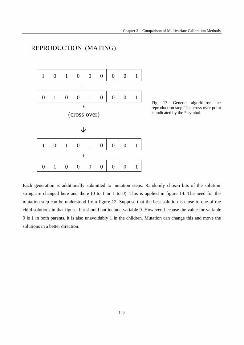
Chapter 2 – Comparison of Multivariate Calibration Methods
145
1 0 1 0 0 0 0 0 1
+
â
+
(cross over)
1 0 0 1 0 0 0 10
0 1 0 1 0 0 0 11
1 0 0 0 0 0 0 10
REPRODUCTION (MATING)
*
Fig. 13. Genetic algorithms: the reproduction step. The cross over point is indicated by the * symbol.
Each generation is additionally submitted to mutation steps. Randomly chosen bits of the solution
string are changed here and there (0 to 1 or 1 to 0). This is applied in figure 14. The need for the
mutation step can be understood from figure 12. Suppose that the best solution is close to one of the
child solutions in that figure, but should not include variable 9. However, because the value for variable
9 is 1 in both parents, it is also unavoidably 1 in the children. Mutation can change this and move the
solutions in a better direction.
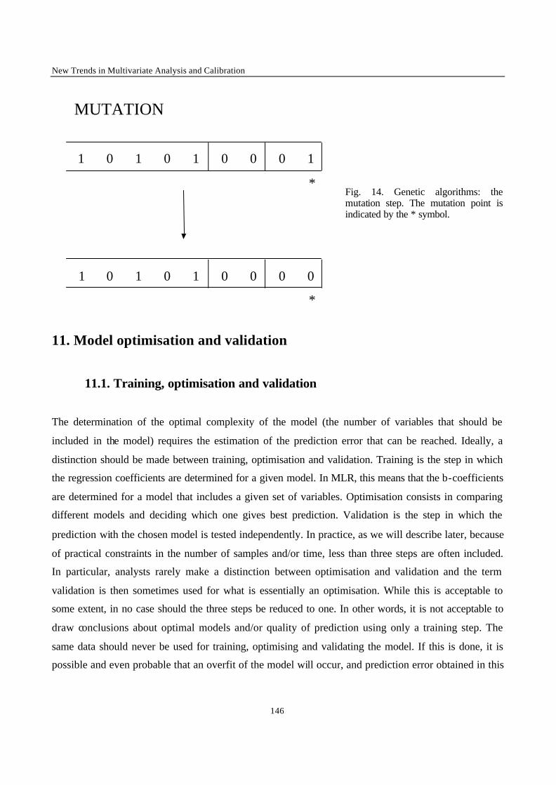
New Trends in Multivariate Analysis and Calibration
146
*
MUTATION
*
1 0 1 0 1 0 0 0 1
0 1 0 1 0 0 0 01
Fig. 14. Genetic algorithms: the mutation step. The mutation point is indicated by the * symbol.
11. Model optimisation and validation
11.1. Training, optimisation and validation
The determination of the optimal complexity of the model (the number of variables that should be
included in the model) requires the estimation of the prediction error that can be reached. Ideally, a
distinction should be made between training, optimisation and validation. Training is the step in which
the regression coefficients are determined for a given model. In MLR, this means that the b-coefficients
are determined for a model that includes a given set of variables. Optimisation consists in comparing
different models and deciding which one gives best prediction. Validation is the step in which the
prediction with the chosen model is tested independently. In practice, as we will describe later, because
of practical constraints in the number of samples and/or time, less than three steps are often included.
In particular, analysts rarely make a distinction between optimisation and validation and the term
validation is then sometimes used for what is essentially an optimisation. While this is acceptable to
some extent, in no case should the three steps be reduced to one. In other words, it is not acceptable to
draw conclusions about optimal models and/or quality of prediction using only a training step. The
same data should never be used for training, optimising and validating the model. If this is done, it is
possible and even probable that an overfit of the model will occur, and prediction error obtained in this
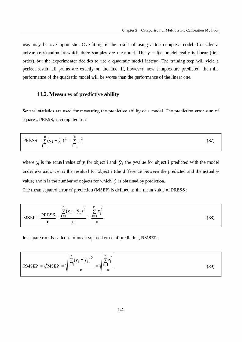
Chapter 2 – Comparison of Multivariate Calibration Methods
147
way may be over-optimistic. Overfitting is the result of using a too complex model. Consider a
univariate situation in which three samples are measured. The y = f(x) model really is linear (first
order), but the experimenter decides to use a quadratic model instead. The training step will yield a
perfect result: all points are exactly on the line. If, however, new samples are predicted, then the
performance of the quadratic model will be worse than the performance of the linear one.
11.2. Measures of predictive ability
Several statistics are used for measuring the predictive ability of a model. The prediction error sum of
squares, PRESS, is computed as :
∑=∑ −===
n
1i
2i
n
1i
2ii e)yy(PRESS (37)
where yi is the actua l value of y for object i and iy the y-value for object i predicted with the model
under evaluation, ei is the residual for object i (the difference between the predicted and the actual y-
value) and n is the number of objects for which y is obtained by prediction.
The mean squared error of prediction (MSEP) is defined as the mean value of PRESS :
n
e
n
)yy(
nPRESSMSEP
n
1i
2i
n
1i
2ii ∑
=∑ −
== == (38)
Its square root is called root mean squared error of prediction, RMSEP:
n
e
n
)yy(MSEPRMSEP
n
1i
2i
n
1i
2ii ∑
=∑ −
== == (39)
New Trends in Multivariate Analysis and Calibration
148
All these quantities give the same information. In the chemometrics literature it seems that RMSEP
values are preferred, partly because they are given in the same units as the y-variable.
11.3. Optimisation
The RMSEP is determined for different models. For instance, with stepwise selection, a models can be
built using a t-test significance level of 1%, and another a t-test significance level of 5%. With genetic
algorithms, various models can be obtained with different numbers of variable. The result can be
presented as a plot showing RMSEP as a function of the number of variables and is called the RMSEP
curve. This curve often shows an intermediate minimum and the number of variables for which this
occurs is then considered to be the optimal complexity of the model. This can be a way of optimising
the output of stepwise selection procedure (optimising the number of variables retained). A problem
which is sometimes encountered is that the global minimum is reached for a model with a very high
complexity. A more parsimonious model is often more robust (the parsimonity principle). Therefore, it
has been proposed to use the first local minimum or a deflection point is used instead of the global
minimum. If there is only a small difference between the RMSEP of the minimum and a model with
less complexity, the latter is often chosen. The decision on whether the difference is considered to be
small is often based on the experience of the analyst. We can also use statistical tests that have been
developed to decide whether a more parsimonious model can be considered statistically equivalent. In
that case the more parsimonious model should be preferred. An F-test [90,91] or a randomisation t-test
[92] have been proposed for this purpose. The latter requires less statistical assumptions about data and
model properties, and is probably to be preferred. However in practice it does not always seem to yield
reliable results.
11.4. Validation
The model selected in the optimisation step is applied to an independent set of samples and the y-
values (i.e. the results obtained with the reference method) and y -values (the results obtained with
multivariate calibration) are compared. An example is shown in figure 15. The interpretation is usually
done visually : does the line with slope 1 and intercept 0 represent the points in the graph sufficiently
well ? It is necessary to check whether this is true over the whole range of concentrations (non-
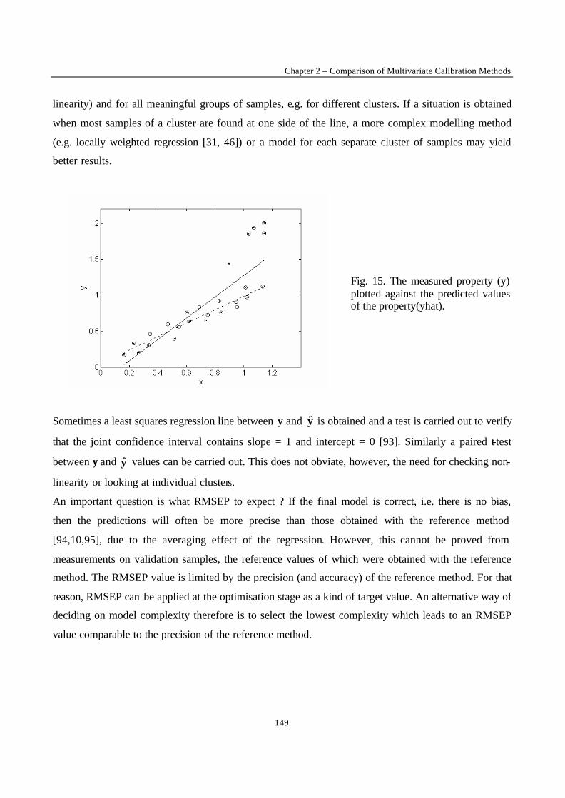
Chapter 2 – Comparison of Multivariate Calibration Methods
149
linearity) and for all meaningful groups of samples, e.g. for different clusters. If a situation is obtained
when most samples of a cluster are found at one side of the line, a more complex modelling method
(e.g. locally weighted regression [31, 46]) or a model for each separate cluster of samples may yield
better results.
Fig. 15. The measured property (y) plotted against the predicted values of the property(yhat).
Sometimes a least squares regression line between y and y is obtained and a test is carried out to verify
that the joint confidence interval contains slope = 1 and intercept = 0 [93]. Similarly a paired t-test
between y and y values can be carried out. This does not obviate, however, the need for checking non-
linearity or looking at individual clusters.
An important question is what RMSEP to expect ? If the final model is correct, i.e. there is no bias,
then the predictions will often be more precise than those obtained with the reference method
[94,10,95], due to the averaging effect of the regression. However, this cannot be proved from
measurements on validation samples, the reference values of which were obtained with the reference
method. The RMSEP value is limited by the precision (and accuracy) of the reference method. For that
reason, RMSEP can be applied at the optimisation stage as a kind of target value. An alternative way of
deciding on model complexity therefore is to select the lowest complexity which leads to an RMSEP
value comparable to the precision of the reference method.
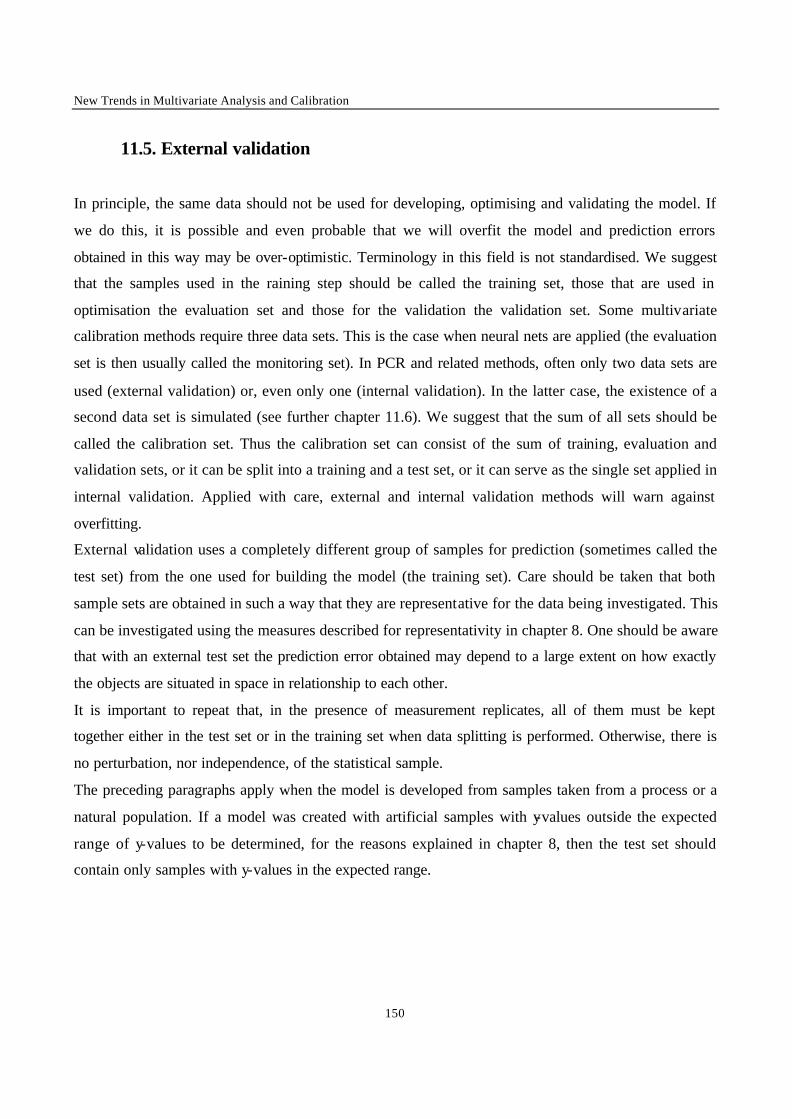
New Trends in Multivariate Analysis and Calibration
150
11.5. External validation
In principle, the same data should not be used for developing, optimising and validating the model. If
we do this, it is possible and even probable that we will overfit the model and prediction errors
obtained in this way may be over-optimistic. Terminology in this field is not standardised. We suggest
that the samples used in the raining step should be called the training set, those that are used in
optimisation the evaluation set and those for the validation the validation set. Some multivariate
calibration methods require three data sets. This is the case when neural nets are applied (the evaluation
set is then usually called the monitoring set). In PCR and related methods, often only two data sets are
used (external validation) or, even only one (internal validation). In the latter case, the existence of a
second data set is simulated (see further chapter 11.6). We suggest that the sum of all sets should be
called the calibration set. Thus the calibration set can consist of the sum of training, evaluation and
validation sets, or it can be split into a training and a test set, or it can serve as the single set applied in
internal validation. Applied with care, external and internal validation methods will warn against
overfitting.
External validation uses a completely different group of samples for prediction (sometimes called the
test set) from the one used for building the model (the training set). Care should be taken that both
sample sets are obtained in such a way that they are representative for the data being investigated. This
can be investigated using the measures described for representativity in chapter 8. One should be aware
that with an external test set the prediction error obtained may depend to a large extent on how exactly
the objects are situated in space in relationship to each other.
It is important to repeat that, in the presence of measurement replicates, all of them must be kept
together either in the test set or in the training set when data splitting is performed. Otherwise, there is
no perturbation, nor independence, of the statistical sample.
The preceding paragraphs apply when the model is developed from samples taken from a process or a
natural population. If a model was created with artificial samples with y-values outside the expected
range of y-values to be determined, for the reasons explained in chapter 8, then the test set should
contain only samples with y-values in the expected range.
Chapter 2 – Comparison of Multivariate Calibration Methods
151
11.6. Internal validation
One can also apply what is called internal validation. Internal validation uses the same data for
developing the model and validating it, but in such a way that external validation is simulated. A
comparison of internal validation procedures usually employed in spectrometry is given in [96]. Four
different methodologies were employed:
a. Random splitting of the calibration set into a training and a test set. The splitting can then
have a large influence on the obtained RMSEP value.
b. Cross-validation (CV), where the data are randomly divided into d so-called cancellation
groups. A large number of cancellation groups corresponds to validation with a small perturbation of
the statistical sample, whereas a small number of cancellation groups corresponds to a heavy
perturbation. The term perturbation is used to indicate that the data set used for developing the model in
this stage is not the same as the one developed with all calibration objects, i.e. the one, which will be
applied in chapters 13 and 14. Too small a perturbation means that overfitting is still possible. The
validation procedure is repeated as many times as there are cancellation groups. At the end of the
validation procedure each object has been once in the test set and d-1 times in the training set. Suppose
there are 15 objects and 3 cancellation groups, consisting of objects 1-5, 6-10 and 11-15. We
mentioned earlier that the objects should be assigned randomly to the cancellation groups, but for ease
of explanation we have used the numbering above. The b-coefficients in the model that is being
evaluated are determined first for the training set consisting of objects 6-15 and objects 1-5 function as
test set, i.e. they are predicted with this model. The PRESS is determined for these 5 objects. Then a
model is made with objects 1-5 and 11-15 as training and 6-10 as test set and, finally, a model is made
with objects 1-10 in the training set and 11-15 in the test set. Each time the PRESS value is determined
and eventually the three PRESS values are added, to give a value representative for the whole data set
(PRESS values are more indicated here to RMSEP values, because PRESS values are variances and
therefore additive).
c. leave-one-out cross-validation (LOO-CV), in which the test sets contain only one object (d =
n). Because the perturbation of the model at each step is small (only one object is set aside), this
procedure tends to overfit the model. For this reason the leave-more-out methods described above may
be preferable. The main drawback of LOO-CV is that the computation is slow because a model has to
be developed for each object.
New Trends in Multivariate Analysis and Calibration
152
d. Repeated random splitting (repeated evaluation set method) (RES) [96]. The procedure
described in a is repeated many times. In this way, at the end of the validation procedure, one hopes
that an object has been in the test set several times with different companions. Stable results are
obtained after repetition of the procedure several times (even hundreds of times). To have a good
picture of the prediction error, low and high percentages of objects in the evaluation set have to be
used.
12. Random correlation
12.1. The Random Correlation issue
Fig. 16. The 16 wavelengths selected by the Stepwise selection method for Stepwise-MLR calibration results (RMSECV) obtained for a random (20 x 100) spectral matrix and a random (1 x 20) concentration vectors.
Let us consider a simulated X spectral matrix made of 20 spectra with 100 wavelengths filed with
random values between 0 and 100. And a y matrix of 20 random values between 0 and 10. The
Stepwise selection applied on such a data set will surprisingly lead to sometimes retain a certain
number of variables (Fig. 16). If cross validation is performed to validate the obtained model,
RMSECV results can even look as the model is very efficient in predicting y (tab le 1). This
phenomenon is common for stepwise variable selection applied to noisy data. It has already been
described [97,98], and is referred to as random correlation or chance correlation.
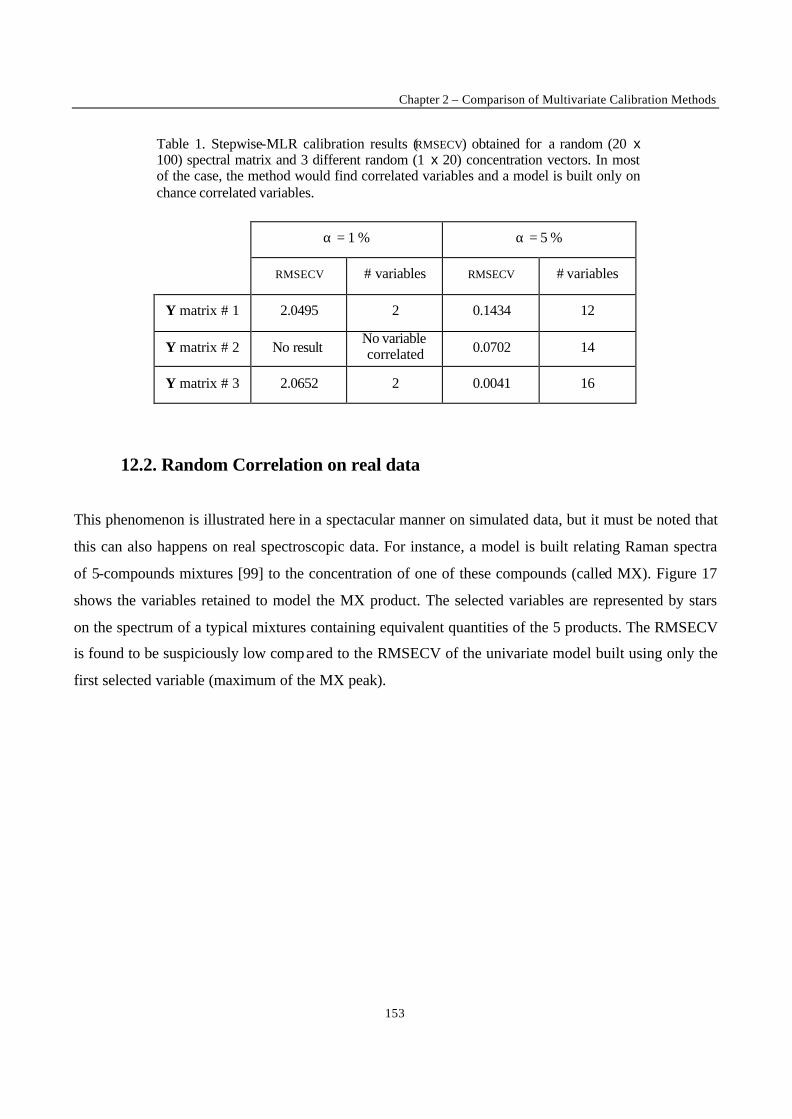
Chapter 2 – Comparison of Multivariate Calibration Methods
153
Table 1. Stepwise-MLR calibration results (RMSECV) obtained for a random (20 x 100) spectral matrix and 3 different random (1 x 20) concentration vectors. In most of the case, the method would find correlated variables and a model is built only on chance correlated variables.
α = 1 % α = 5 %
RMSECV # variables RMSECV # variables
Y matrix # 1 2.0495 2 0.1434 12
Y matrix # 2 No result No variable correlated 0.0702 14
Y matrix # 3 2.0652 2 0.0041 16
12.2. Random Correlation on real data
This phenomenon is illustrated here in a spectacular manner on simulated data, but it must be noted that
this can also happens on real spectroscopic data. For instance, a model is built relating Raman spectra
of 5-compounds mixtures [99] to the concentration of one of these compounds (called MX). Figure 17
shows the variables retained to model the MX product. The selected variables are represented by stars
on the spectrum of a typical mixtures containing equivalent quantities of the 5 products. The RMSECV
is found to be suspiciously low compared to the RMSECV of the univariate model built using only the
first selected variable (maximum of the MX peak).
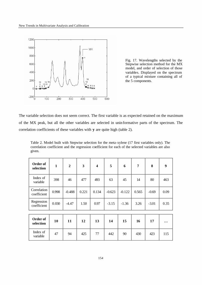
New Trends in Multivariate Analysis and Calibration
154
Fig. 17. Wavelengths selected by the Stepwise selection method for the MX model, and order of selection of those variables. Displayed on the spectrum of a typical mixture containing all of the 5 components.
The variable selection does not seem correct. The first variable is as expected retained on the maximum
of the MX peak, but all the other variables are selected in unin formative parts of the spectrum. The
correlation coefficients of these variables with y are quite high (table 2).
Table 2. Model built with Stepwise selection for the meta-xylene (17 first variables only). The correlation coefficient and the regression coefficient for each of the selected variables are also given.
Order of selection
1 2 3 4 5 6 7 8 9
Index of variable
398 46 477 493 63 45 14 80 463
Correlation coefficient
0.998 -0.488 0.221 0.134 -0.623 -0.122 0.565 -0.69 0.09
Regression coefficient 0.030 -4.47 1.50 0.97 -3.15 -1.36 3.26 -3.01 0.35
Order of selection
10 11 12 13 14 15 16 17 …
Index of variable
47 94 425 77 442 90 430 423 115
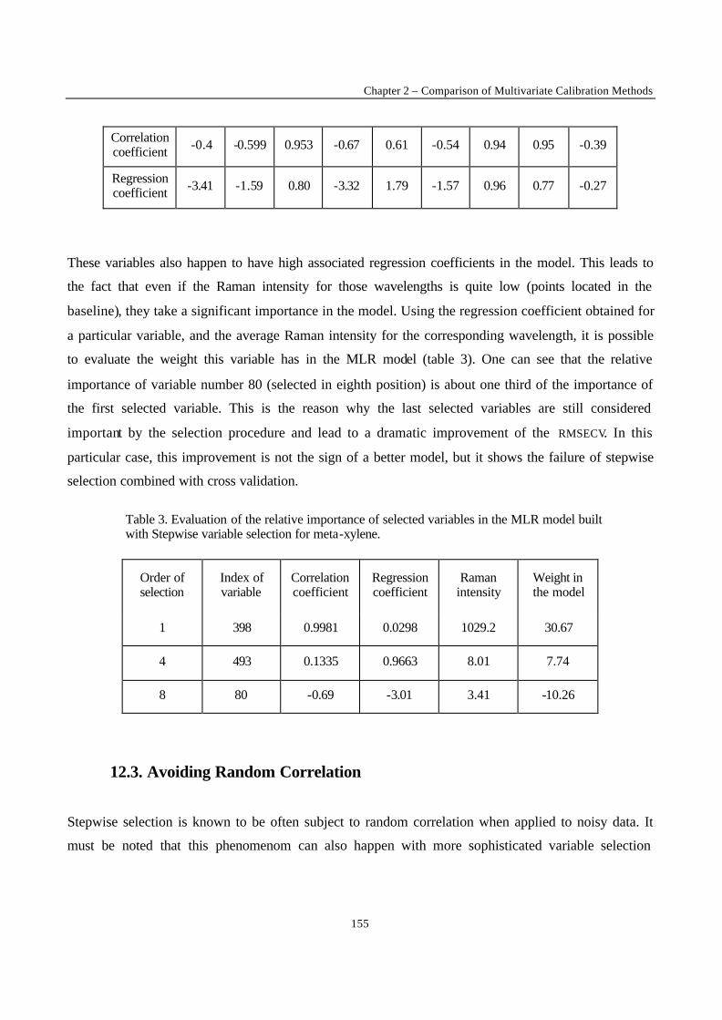
Chapter 2 – Comparison of Multivariate Calibration Methods
155
Correlation coefficient -0.4 -0.599 0.953 -0.67 0.61 -0.54 0.94 0.95 -0.39
Regression coefficient -3.41 -1.59 0.80 -3.32 1.79 -1.57 0.96 0.77 -0.27
These variables also happen to have high associated regression coefficients in the model. This leads to
the fact that even if the Raman intensity for those wavelengths is quite low (points located in the
baseline), they take a significant importance in the model. Using the regression coefficient obtained for
a particular variable, and the average Raman intensity for the corresponding wavelength, it is possible
to evaluate the weight this variable has in the MLR model (table 3). One can see that the relative
importance of variable number 80 (selected in eighth position) is about one third of the importance of
the first selected variable. This is the reason why the last selected variables are still considered
important by the selection procedure and lead to a dramatic improvement of the RMSECV. In this
particular case, this improvement is not the sign of a better model, but it shows the failure of stepwise
selection combined with cross validation.
Table 3. Evaluation of the relative importance of selected variables in the MLR model built with Stepwise variable selection for meta-xylene.
Order of selection
Index of variable
Correlation coefficient
Regression coefficient
Raman intensity
Weight in the model
1 398 0.9981 0.0298 1029.2 30.67
4 493 0.1335 0.9663 8.01 7.74
8 80 -0.69 -3.01 3.41 -10.26
12.3. Avoiding Random Correlation
Stepwise selection is known to be often subject to random correlation when applied to noisy data. It
must be noted that this phenomenom can also happen with more sophisticated variable selection

New Trends in Multivariate Analysis and Calibration
156
methods like Genetic Algorithm [100,99]. Occurrence of random correlation was even reported with
latent variables methods like PCR or PLS [98].
When using variable selection methods, one has therefore to be extremely careful in the interpretation
of the cross-validation results. This shows the necessity of external validation since a model built using
chance correlated variables would see its performances considerably deteriorate when tested on an
external test set.
The most efficient way to eliminate chance correlation on spectroscopic data is to desoise the spectra.
Method such as Fourier or Wavelets filtering (see chapter 3) have proven efficient for this purpose. A
modified version of the stepwise algorithm was also proposed to reduce the risk of random correlation
[99]. The main idea is the same as in Stepwise, the forward selection and backward elimination steps
are maintained. The difference lies in the fact that each time a variable xj is selected for entry in the
model, an iterative process begins :
• A new variable is built. This variable xj1 is made of the average Raman scattering value of a 3-
point window centred on xj (from xj-1 to xj+1). If xj1 yields a higher PCC than xj, it becomes the new
candidate variable.
• A second new variable, xj2 (average Raman scattering value of points xj-2 to xj+2) is built, it is
compared with xj1 , and the process goes on.
• When the enlargement of the window does not lead to a variable xj(n+1) with a better PCC than
xjn , the method stops and xjn enters the model.
Selecting an (2n+1)-points spectral window instead of a single wavelength implies a local averaging of
the signal. This should reduce the effect of noise in the prediction step. Moreover, as the first variables
entered into the model (most important ones) yield a better PCC, less uninformative variables should be
retained since the next best variables will not be able to improve significantly the model.
13. Outlying objects in the model
In Chapter 7 we explained how to detect possible outliers before the modelling, i.e. in the y and/or x-
space. When the model has been built, we should check again for the possibility that outliers in the X-
y-space are present, i.e. objects that do not fit the true model well (outliers toward the model). The
difficulty with this is that such outlying objects influence (bias) the model obtained, often to such an
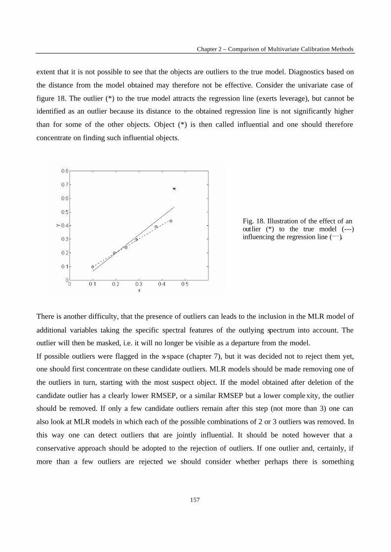
Chapter 2 – Comparison of Multivariate Calibration Methods
157
extent that it is not possible to see that the objects are outliers to the true model. Diagnostics based on
the distance from the model obtained may therefore not be effective. Consider the univariate case of
figure 18. The outlier (*) to the true model attracts the regression line (exerts leverage), but cannot be
identified as an outlier because its distance to the obtained regression line is not significantly higher
than for some of the other objects. Object (*) is then called influential and one should therefore
concentrate on finding such influential objects.
Fig. 18. Illustration of the effect of an outlier (*) to the true model (---) influencing the regression line (___).
There is another difficulty, that the presence of outliers can leads to the inclusion in the MLR model of
additional variables taking the specific spectral features of the outlying spectrum into account. The
outlier will then be masked, i.e. it will no longer be visible as a departure from the model.
If possible outliers were flagged in the x-space (chapter 7), but it was decided not to reject them yet,
one should first concentrate on these candidate outliers. MLR models should be made removing one of
the outliers in turn, starting with the most suspect object. If the model obtained after deletion of the
candidate outlier has a clearly lower RMSEP, or a similar RMSEP but a lower complexity, the outlier
should be removed. If only a few candidate outliers remain after this step (not more than 3) one can
also look at MLR models in which each of the possible combinations of 2 or 3 outliers was removed. In
this way one can detect outliers that are jointly influential. It should be noted however that a
conservative approach should be adopted to the rejection of outliers. If one outlier and, certainly, if
more than a few outliers are rejected we should consider whether perhaps there is something
New Trends in Multivariate Analysis and Calibration
158
fundamentally wrong and review the whole process including the chemistry, the measurement
procedure and the initial selection of samples.
The next step is the study of residuals. A first approach is visual. One can make a plot of y against y. If
this is done for the final model, it is likely that, for the reasons outlined above, an outlier will not be
visible. One way of studying the presence of influential objects, is therefore not to study the residuals
for the final model but the residuals for the model with 1, 2, ..., a variables, because in this way we may
detect outliers on specifics variables. If an object has a large residual on a model using, say, two
variables, but a small residual when three or more variables are added, it is possible these extra
variables are included in the model only to allow for this particular object. This object is then
influential. We can provisionally eliminate the object, carry out MLR again and, if a more
parsimonious model with at least equal predictive ability is reached, may decide to eliminate the object
completely.
Studying residuals from a model can also be done in a more formal way. To do this one predicts all
calibration objects with the partial or full model and computes the residuals as the difference between
the observed and the fitted value :
iii yye −= (40)
where ei is the residual, yi the y-value and iy the fitted y-value for object i.
The residuals are often standardised by dividing ei by the square root of the residual variance s2:
s1
n p e2
i2
i=1
n=
−∑ (41)
Object i has an influence on its own prediction (described by the leverage hi, see chapter 7), and
therefore, some authors recommend using the internally studentized residuals:
i
ii
h1s
et
−= (42)
Chapter 2 – Comparison of Multivariate Calibration Methods
159
The externally studentized residuals, also called the jack-knifed or cross-validatory residuals, can also
be used. They are defined as
i
i
h1s(i)
et(i)
−= (43)
where s(i) is estimated by computing the regression without object i and pi is the leverage. For high
leverages (hi close to 1) ti and t(i) will increase and can therefore reach significance more easily. The
computation of t(i) requires a leave-one-out procedure for the estimation of s(i), which is time
consuming, so that the internally studentized version is often preferred. An observation is considered to
be a large residual observation if the absolute value of its studentized residual exceeds 2.5 (the critical
value at the 1% level of confidence, which is preferred to the 5% level of confidence, as is always the
case when contemplating outlier rejection).
The masking and swamping effects for multiple outliers that we described in chapter 7 in the x-space,
can also occur in regression. Therefore the use of robust methods is of interest. Robust regression
methods are based on strategies that fit the majority of the data (sometimes called clean subsets). The
resulting robust models are therefore not influenced by the outliers. Least median of squares, LMS
[57,101] and the repeated median [102] have been proposed as robust regression techniques. After
robust fitting, outliers are detected by studying the residual of the objects from the robust model. The
performance of these methods has been compared in [103].
Genetic algorithms or simulated annealing can be applied to select clean subsets according to a given
criterion from a larger population. This lead Walczak et al. to develop their evolution program, EP
[104,105]. It uses a simplified version of a genetic algorithm to select the clean subset of objects, using
minimalisation of RMSEP as a criterion for the clean subset objects. The percentage of possible
outliers in the data set must be selected in advance. The method allows the presence of 49% of outlying
points, but the selection of such a high number risks the elimination of certain sources of variation from
the clean subset and the model. The clean subset should therefore contain at least 90%, if not 95%, of
the objects. Other algorithms based on the use of clean subset selection have been proposed by Hadi
and Simeonoff [106] and Hawkins et al [107] and by Atkinson and Mukira [108]. Unfortunately none
of these methods have been studied to such an extent that they can be recommended in practice.

New Trends in Multivariate Analysis and Calibration
160
If a candidate outlier is found to have high leverage and also a high residual, using one of the above
methods, it should be eliminated. High leverage objects that do not have a high standardised residual
stabilise the model and should remain in the model. High residual, low leverage outliers will have a
deleterious effect only if the residual is very high. If such outliers are detected then one should do what
we described in the beginning of this chapter, i.e. try out MLR models without them. They should be
rejected only if the model build without them has a clearly lower RMSEP or a similar RMSEP and
lower complexity.
14. Using the model
Once the final model has been developed, it is ready for use : the calibration model can be applied to
spectra of new samples. It sho uld be noted that the data pre-processing and/or pre-treatment selected
for the calibration model must also be applied to the new spectra and this must be done with the same
parameters (e.g. same ideal spectrum for MSC, same window and polynomial size for Savitzky-Golay
smoothing or derivation, etc.). For mean-centering or autoscaling, the mean and standard deviation
used in the calibration stage must be used for in the pre-treatment of the new spectra.
Although it is not the subject of this article, which is restricted to the development of a model, it should
be noted that to ensure quality of the predictions and validity of the model, the application of the model
over time also requires several applications of chemometrics. The following subjects should be
considered :
• Quality control : it must be verified that no changes have occurred in the measurement system. This
can be done for instance by applying system suitability checks and by measuring the spectra of
standards. Multivariate quality control charts can be applied to plot the measurements and to detect
changes [109,110].
• Detection of outliers and inliers in prediction : the spectra must belong to the same population as the
objects used to develop the calibration model. Outliers in concentration (outliers in y) can occur.
Samples can also be different from the ones used for calibration, because they present sources of
variance not taken into account in the model. Such samples are then outliers in X. In both cases, this
leads to extrapolation outside the calibration space so that the results obtained are less accurate. MLR
can be robust to slight extrapolation, but this is less true when non-linearity occurs. More extreme

Chapter 2 – Comparison of Multivariate Calibration Methods
161
extrapolation will lead to unacceptable results. It is therefore necessary to investigate whether a new
spectrum falls into the spectral domain of the calibration samples.
As stated in chapter 7, we can in fact distinguish outliers and inliers. Outliers in y and in X can be
detected by adaptations of the methods we described in Chapter 7. Inliers are samples which, although
different from the calibration samples, lie within the calibration space. They are located in zones of low
(or null) density within the calibration space: for instance, if the calibration set consists of two clusters,
then an inlier can be situated in the space between the two clusters. If the model is non- linear, their
prediction can lead to interpolation error. Few methods have been developed to detect inliers. One of
them is the potential function method of Jouan-Rimbaud et al. (chapter 7) [61]. If the data set is known
to be relatively homogeneous (by application of the methods of chapter 6), then it is not necessary to
look for inliers.
• Updating the models : when outliers or inliers were detected and it has been verified that no change
has occurred in the measurement conditions, then one may consider adding the new samples to the
calibration set. This makes sense only when it has been verified that the samples are either of a new
type or an extension of the concentration domain and that it is expected that similar new samples can be
expected in the future. Good strategies to perform this updating with a minimum of work, i.e. without
having to take the whole extended data set through all the previous steps, do not seem to exist.
• Correcting the models (or the spectra): when a change has been noticed in the spectra of the
standards, for instance in a multivariate QC chart, and the change cannot be corrected by changes to the
instrumental, this means that spectra or model must be corrected. When the change in the spectra is
relatively small and the reason for it can be established [110], e.g. a wavelength shift, numerical
correction is possible by making the same change to the spectra in the reverse direction. If this is not
the case, it is necessary to treat the data as if they were obtained on another instrument and to apply
methods for transfer of calibration from one instrument to another. A review about such methods is
given in [111].
15. Conclusions
It will be clear from the preceding chapters that developing good multivariate calibration models
requires a lot of work. There is sometimes a tendency to overlook or minimise the need for such a
careful approach. The deleterious effects of outliers are not so easily observed as for univariate
New Trends in Multivariate Analysis and Calibration
162
calibration and are therefore sometimes disregarded. Problems such as heterogeneity or non-
representativity can occur also in univariate calibration models, but these are handled by analytical
chemists who know how to avoid or cope with such problems. When applying multivariate calibration,
the same analysts may have too much faith in the power of the mathematics to worry about such
sources of errors or may have difficulties in understanding how to tackle them. Some chemometricians
do not have analytical backgrounds and may be less aware of the possibility that some sources of error
can be present. It is therefore necessary that strategies should be made available for systematic method
development that include the diagnostics and remedies required and that analysts should have a better
comprehension of the methodology involved. It is hoped that this article will help to some degree in
reaching this goal.
As stated in the introduction, we have chosen to consider MLR, because it is easier to explain. This is
an important advantage, but it does not mean that other methods have no other advantages. By
performing MLR on the scores of a PCA model, PCR avoid the variable selection procedure. Partial
least squares (PLS) and PCR usually give results of equal quality but PLS can be numerically faster
when optimised algorithms such as SIMPLS [112] are applied. Methods that have been specifically
developed for non-linear data, such as neural networks (NN), are superior to the linear methods when
non-linearities do occur, but may be bad at predictions for outliers (and perhaps even inliers). Locally
weighted regression (LWR) methods seem to perform very well for inhomogeneous data and for non-
linear data, but may require somewhat more calibration standards. In all cases however it is necessary
to have strategies available that detect the need to use a particular type of method and that ensure that
the data are such that no avoidable sources of imprecision or inaccuracy are present.
REFERENCES
[1] D.L. Massart, B.G.M. Vandeginste, L.M.C. Buydens, S. de Jong, P.J. Lewi, J. Smeyers-
Verbeke, Handbook of Chemometrics, Elsevier, Amsterdam, 1997.
[2] N.R. Draper, H. Smith, Applied Regression Analysis, Wiley, New York, 1981.
[3] J. Mandel, The Statistical Analysis of Experimental Data, Dover reprint, 1984, Wiley &Sons,
1964, New York.
[4] D.L. MacTaggart, S.O. Farwell, J. Assoc.Off. Anal. Chem., 75, 594, 1992.
Chapter 2 – Comparison of Multivariate Calibration Methods
163
[5] J.C. Miller, J.N.Miller, Statistics for Analytical Chemistry, Ellis Horwood, Chichester, 3rd ed.,
1993.
[6] R. De Maesschalck, F. Estienne, J. Verdú-Andrés, A. Candolfi, V. Centner, F. Despagne, D.
Jouan-Rimbaud, B. Walczak, S. de Jong, O.E. de Noord, C. Puel, B.M.G. Vandeginste, D.L.
Massart, Internet Journal of Chemistry, 2 (1999) 19.
[7] F. Despagne, D.L. Massart, The Analyst, 123 (1998) 157R-178R.
[8] URL : http://minf.vub.ac.be/~fabi/calibration/multi/pcr/.
[9] URL : http://minf.vub.ac.be/~fabi/calibration/multi/nn/.
[10] V. Centner, D.L. Massart, S. de Jong, Fresenius J. Anal. Chem. 361 (1998) 2-9.
[11] S.D. Hodges, P.G. Moore, Appl. Stat. 21 (1972) 185-195.
[12] S. Van Huffel, J. Vandewalle, The Total Least Squares Problem, Computational Aspects and
Analysis, SIAM, Phiadelphia, 1988.
[13] Statistics - Vocabulary and Symbols Part 1, ISO standard 3534 (E/F), 1993.
[14] Accuracy (trueness and precission) of measurement methods and results, ISO standard 5725 1-
6, 1994.
[15] V. Centner, D.L. Massart, O.E. de Noord, Anal. Chim. Acta 330 (1996) 1-17.
[16] B.G. Osborne, Analyst 113 (1988) 263-267.
[17] P. Kubelka, Journal of the optical Society of America 38(5) (1948) 448-457.
[18] A. Savitzky, M.J.E. Golay, Anal. Chem. 36 (1964) 1627-1639.
[19] P.A. Gorry, Anal. Chem. 62 (1990) 570-573.
[20] S.E. Bialkowski, Anal. Chem. 61 (1989) 1308-1310.
[21] J. Steinier, Y. Termonia, J. Deltour, Anal. Chem. 44 (1972) 1906-1909.
[22] P. Barak, Anal. Chem. 67 (1995) 2758-2762.
[23] E. Bouveresse, Maintenance and Transfer of Multivariate Calibration Models Based on Near-
Infrared Spectroscopy, doctoral thesis, Vrije Universiteit Brussel, 1997.
[24] C.H. Spiegelman, Calibration: a look at the mix of theory, methods and experimental data,
presented at Compana, Wuerzburg, Germany, 1995.
[25] W. Wu, Q. Guo, D. Jouan-Rimbaud, D.L. Massart, Using contrasts as a data pretreatment
method in pattern recognition of multivariate data, Chemom. and Intell. Lab. Sys. (in press).
[26] L. Pasti, D. Jouan-Rimbaud, D.L. Massart, O.E. de Noord, Anal. Chim. Acta. 364 (1998) 253-
263.
New Trends in Multivariate Analysis and Calibration
164
[27] D. Jouan-Rimbaud, B. Walczak, D.L. Massart, R.J. Poppi, O.E. de Noord, Anal. Chem. 69
(1997) 4317-4323.
[28] B. Walczak, D.L. Massart, Chem. Intell. Lab. Sys. 36 (1997) 81-94.
[29] P. Geladi, D. MacDougall, H. Martens, Appl. Spectrosc. 39 (1985) 491-500.
[30] T. Isaksson, T. Næs, Appl. Spectrosc. 42 (1988) 1273-1284.
[31] T. Næs, T. Isaksson, B.R. Kowalski, Anal. Chem. 62 (1990) 664-673.
[32] R.J. Barnes, M.S. Dhanoa, S.J. Lister, Appl. Spectrosc. 43 (1989) 772-777.
[33] R.J. Barnes, M.S. Dhanoa, S.J. Lister, J. Near Infrared Spectrosc. 1 (1993) 185-186.
[34] M.S. Dhanoa, S.J. Lister, R. Sanderson, R.J. Barnes, J. Near Infrared Spectrosc. 2 (1994) 43-47.
[35] I.S. Helland, T. Naes, T. Isaksson, Chemom. Intell. Lab. Sys. 29 (1995) 233-241.
[36] O.E. de Noord, Chemom. Intell. Lab. Sys. 23 (1994) 65-70.
[37] M.B. Seasholtz, B.R. Kowalski, J. Chemom. 6 (1992) 103-111.
[38] A. Garrido Frenich, D. Jouan-Rimbaud, D.L. Massart, S. Kuttatharmmakul, M. Martínez
Galera, J.L. Martínez Vidal, Analyst 120 (1995) 2787-2792.
[39] J.E. Jackson, A user's guide to principal components, John Wiley, New York, 1991.
[40] E.R. Malinowski, Factor analysis in chemistry, 2nd. Ed., John Wiley, New York, 1991.
[41] S. Wold, K. Esbensen and P. Geladi, Chemom. Intell. Lab. Syst. 2 (1987) 37-52.
[42] K. Pearson, Mathematical contributions to the theory of evolution XIII. On the theory of
contingency and its relation to association and normal correlation, Drapers Co. Res. Mem.
Biometric series I, Cambridge University Press, London.
[43] H. Hotelling, J. Educ. Psychol., 24 (1933) 417-441, 498-520.
[44] D. Jouan-Rimbaud, B. Walczak, D.L. Massart, I.R. Last, K.A. Prebble, Anal. Chim. Acta 304
(1995) 285-295.
[45] M. Meloun, J. Militký, M. Forina, Chemometrics for analytical chemistry. Vol. 1: PC-aided
statistical data analysis, Ellis Horwood, Chichester (England), 1992.
[46] T. Næs, T. Isaksson, Appl. Spectr. 1992, 46/1 (1992) 34.
[47] K. Szczubialka, J. Verdú-Andrés, D.L. Massart, Chemom. and Intell. Lab. Syst. 41 (1998) 145-
160.
[48] B. Hopkins, Ann. Bot., 18 (1954) 213.
[49] R.G. Lawson, P.J. Jurs, J. Chem. Inf. Comput. Sci. 30 (1990) 36-41.
[50] Forina, M., Drava, G., Boggia, R., Lanteri, S., Conti, P., Anal. Chim. Acta, 295 (1994) 109.

Chapter 2 – Comparison of Multivariate Calibration Methods
165
[51] F.E. Grubbs, G. Beck, Technometrics, 14 (1972) 847-854.
[52] P.C. Kelly, J. Assoc. Off. Anal. Chem. 73 (1990) 58-64.
[53] T. Næs, Chemom. Intell. Lab. Sys. 5 (1989) 155-168.
[54] S. Weisberg, Applied linear regression, 2nd. Edition, John Wiley & Sons, New York, 1985.
[55] B. Mertens, M. Thompson, T. Fearn, Analyst 119 (1994) 2777-2784.
[56] A. Singh, Chemom. Intell. Lab. Sys. 33 (1996) 75-100.
[57] P.J. Rousseeuw, A. Leroy, Robust regression and outlier detection, John Wiley, New York,
1987.
[58] P.J. Rousseeuw, B.C. van Zomeren, J. Am. Stat. Assoc. 85 (1990) 633-651.
[59] A.S. Hadi, J.R. Statist. Soc. B 54 (1992) 761-771.
[60] A.S. Hadi, J.R. Statist. Soc. B 56 (1994) ?1-4?.
[61] D. Jouan-Rimbaud, E. Bouveresse, D.L. Massart, O.E. de Noord, Anal. Chim. Acta, 388, 283-
301 (1999).
[62] A. Lorber, B.R. Kowalski, J. Chemom. 2 (1988) 67-79.
[63] K.I. Hildrum, T. Isaksson, T. Naes, A. Tandberg, Near infra-red spectroscopy; Bridging the
gap between data analysis and NIR applications, Ellis Horwood, Chichester, 1992.
[64] D. Jouan-Rimbaud, M.S. Khots, D.L. Massart, I.R. Last, K.A. Prebble, Anal. Chim. Acta 315
(1995) 257-266.
[65] J. Ferré, F.X. Rius, Anal. Chem. 68 (1996) 1565-1571.
[66] J. Ferré, F.X. Rius, Trends Anal. Chem. 16 (1997) 70-73.
[67] R.W. Kennard, L.A. Stone, Technometrics 11 (1969) 137-148.
[68] T. Næs, J. Chemom. 1 (1987) 121-134.
[69] G. Puchwein, Anal. Chem. 60 (1988) 569-573.
[70] D.E. Honigs, G.H. Hieftje, H.L. Mark, T.B. Hirschfeld, Anal. Chem. 57 (1985) 2299-2303.
[71] ASTM, Standard practices for infrared, multivariate, quantitative analysys". Doc. E1655-94, in
ASTM Annual book of standards, vol. 03.06, West Conshohochen, PA, USA, 1995.
[72] T. Fearn, NIR news 8 (1997) 7-8.
[73] R.D. Snee, Technometrics 19 (1977) 415-428.
[74] D. Jouan-Rimbaud, D.L. Massart, C.A. Saby, C. Puel, Anal. Chim. Acta 350 (1997) 149-161.
[75] D. Jouan-Rimbaud, D.L. Massart, C.A. Saby, C. Puel, Intell. Sys. 40 (1998) 129-144.
[76] C.E. Miller, NIR News 4 (1993) 3-5.

New Trends in Multivariate Analysis and Calibration
166
[77] P.J. Brown, J. Chemom. 7 (1993) 255-265.
[78] Y.L. Xie, Y.Z. Liang, Z.G. Chen, Z.H. Huang, R.Q. Yu, Chemom. Intell. Lab. Sys. 27 (1995)
21-32.
[79] H. Martens, T. Næs, Multivariate calibration, Wiley, Chichester, England, 1989.
[80] R.D. Cook, S. Weisberg, Residuals and influence in Regression, Chapman and Hall, New York,
1982.
[81] J.H. Holland, Adaption in Natural and Artificial Systems, University of Michigan Press, Ann
Arbor, MI, 1975, revised reprint, MIT Press, Cambridge, 1992.
[82] C.B. Lucasius, M.L.M. Beckers, G. Kateman, Anal. Chim. Acta, 286 (1994) 135.
[83] R. Leardi, R. Boggia, M. Terrile, J. Chemom., 6 (1992) 267.
[84] D. Jouan-Rimbaud, D.L.Massart, R. Leardi, O.E. de Noord, Anal. Chem., 67 (1995] 4295.
[85] Meusinger, R. Moros, Chemom. Intell. Lab. Systems, 46 (1999) 67.
[86] P. Willet, Trends. Biochem, 13 (1995) 516.
[87] D.H. Hibbert, Chemom. Intell. Lab. Syst., 19 (1993) 277.
[88] J.H. Kalivas, J. Chemom., 5 (1991) 37.
[89] X.G. Shao, Z.H. Chen, X.Q. Lin, Fresenius J. Anal. Chem., 366 (2000) 10.
[90] D.M. Haaland, E.V. Thomas, Anal. Chem. 60 (1988) 1193-1202.
[91] D.W. Osten, J. Chemom. 2 (1988) 39-48.
[92] H. van der Voet, Chemom. Intell. Lab. Sys. 25 (1994) 313-323 & 28 (1995) 315.
[93] J. Riu, F.X. Rius, Anal. Chem. 9 (1995) 343-391.
[94] R. DiFoggio, Appl. Spectrosc. 49 (1995) 67-75.
[95] N.M. Faber, M.J. Meinders, P. Geladi, M. Sjöström, L.M.C. Buydens, G. Kateman, Anal. Chim.
Acta 304 (1995) 273-283.
[96] M. Forina, G.Drava, R. Boggia, S. Lanteri, P. Conti, Anal. Chim. Acta 295 (1994) 109-118.
[97] J. G. Topliss, R. J. Costello, Journal of Medicinal Chemistry 15 (1971) 1066.
[98] J. G. Topliss, R. P. Edwards, Journal of Medicinal Chemistry 22 (1979) 1238.
[99] F. Estienne, N. Zanier, P. Marteau, D.L. Massart, Analytica Chimica Acta, 424 (2000) 185-201.
[100] D. Jouan-Rimbaud, D.L. Massart, R. Leardi, O.E. de Noord, Anal. Chem. 67 (1995) 4295.
[101] D.L. Massart, L. Kaufman, P.J. Rousseeuw, A.M. Leroy, Anal. Chim. Acta 187 (1986) 171-
179.
[102] A.F. Siegel, Biometrika 69 (1982) 242-244.

Chapter 2 – Comparison of Multivariate Calibration Methods
167
[103] Y. Hu, J. Smeyers-Verbeke, D.L. Massart, Chemom. Intell. Lab. Sys. 9 (1990) 31-44.
[104] B. Walczak, Chemom. Intell. Lab. Sys. 28 (1995) 259-272.
[105] B. Walczak, Chemom. Intell. Lab. Sys. 29 (1995) 63-73.
[106] A.S. Hadi, J.S. Simonoff, J. Am. Stat. Assoc. 88 (1993) 1264-1272.
[107] D.M. Hawkins, D. Bradu, G.V. Kass, Technometrics 26 (1984) 197-208.
[108] A.C. Atkinson, H.M. Mulira, Statistics and computing 3 (1993) 27-35.
[109] N.D. Tracy, J.C. Young, R.L. Mason, Journal of Quality Technology 24 (1992) 88-95.
[110] E. Bouveresse, C. Casolino, Massart DL, Applied Spectroscopy 52 (1998) 604-612.
[111] E. Bouveresse, D.L. Massart, Vibrational Spectroscop y 11 (1996) 3.
[112] S. de Jong, Chem. Intell. Lab. Syst. 18 (1993) 251-263.
New Trends in Multivariate Analysis and Calibration
168
CHAPTER III
NEW TYPES OF DATA : NATURE OF THE DATA SET
Like chapter 2, this chapter focuses on multivariate calibration. The work presented here can be seen as
a direct application of the guidelines and methodology developed in the previous chapter. It shows how
an industrial process can be improved by proper use of chemometrical tools. A very interesting aspect
of this work is that is was performed on Raman spectroscopic data, which is a new field of application
for chemometrical methods.
In the first paper in this chapter : “Multivariate calibration with Raman spectroscopic data : a case
study”, it is shown how Multiple Linear Regression was found to be the most efficient method for this
industrial application. The relatively poor quality of the data implied a huge effort on variable selection
in order in particular to tackle the random correlation issue. Various approaches, including an
innovative variable selection strategy suggested in chapter 2, were successfully tried.
The second paper in this chapter : “Inverse Multivariate calibration Applied to Eluxyl Raman data“
is an internal report written about the same industrial process. New measurements were performed after
a new and more efficient Raman spectrometer was installed. Its quality completely changed the
approach to be used on this data. Due to the improved signal/noise ratio, random correlation was no
longer a problem. However, a slight non- linearity that could not be detected before became visible in
the data, which implied the use of a non- linear method. Treating this high quality data with Neural
Networks enabled to reach a quality in calibration never reached before on Eluxyl data.
Apart from giving illustrations of the principles developed in chapter 2, this chapter shows the
applicability and superiority of chemometrical methods applied to Raman data. This conclusion is
striking since Raman data were typically considered as sufficiently straightforward not to necessitate
any sophisticated approach. It is now proven that Raman data can benefit not only from data pre-

Chapter 3 – New Types of Data : Nature of the Data Set
169
treatment, which was the only mathematical treatment considered necessary, but also from inverse
multivariate calibration and such sophisticated methods as neural networks.
New Trends in Multivariate Analysis and Calibration
170
MULTIVARIATE CALIBRATION WITH RAMAN
SPECTROSCOPIC DATA : A CASE STUDY
Analytica Chimica Acta, 424 (2000) 185-201.
F. Estienne and D.L. Massart *
ChemoAC, Farmaceutisch Instituut,
Vrije Universiteit Brussel, Laarbeeklaan 103,
B-1090 Brussels, Belgium. E-mail: [email protected]
N. Zanier-Szydlowski
Institut Français du Pétrole (I.F.P.), 1-4 Avenue du Bois Préau, 92506 Rueil-Malmaison
France
Ph. Marteau
Université Paris Nord, L.I.M.P.H.,
Av. J.B. Clément, 93430 Villetaneuse
France
ABSTRACT
An industrial process separating p-xylene from mainly other C8 aromatic compounds is monitored with an online remote Raman analyser. The concentrations of six constituents are currently evaluated with a classical calibration method. The aim of the study being to improve the precision of the monitoring of the process, inverse calibration linear methods were applied on a synthetic data set, in order to evaluate the improvement in prediction such methods could yield. Several methods were tested including Principal Component Regression with Variable Selection, Partial Least Square Regression or Multiple Linear Regression with variable selection (Stepwise or based on Genetic Algorithm). Methods based on selected wavelengths are of great interest because the obtained models can be expected to be very robust toward experimental conditions. However, because of the important noise in the spectra due to short accumulation time, variable selection methods selected a lot of irrelevant variables by chance correlation. Strategies were investigated to solve this problem and build reliable robust models. These strategies include the use of signal pre-processing (smoothing and filtering in the Fourier or Wavelets domain), and the use of an improved variable selection algorithm based on the selection of spectral windows instead of single wavelengths when this leads to a better model. The best results were achieved with Multiple Linear Regression and Stepwise variable selection applied to spectra denoised in the Fourier domain.
* Corresponding author
KEYWORDS : Chemometrics, Raman Spectroscopy, Multivariate Calibration, random correlation.
Chapter 3 – New Types of Data : Nature of the Data Set
171
1 - Introduction
The Eluxyl process separates para-xylene from other C 8 aromatic compounds (ortho and meta-xylene,
and either para-di-ethylbenzene or toluene used as solvent) by simulated moving bed chromatography
[1]. The evolution of the process is monitored online using a Raman analyser equipped with optical
fibres. The Raman scattering studied is in the visible range and is collected on a 2-dimensional Charge
Coupled Device (CCD) detector that allows true simultaneous recordings. The Raman technique gives
access to the fundamental vibrations of molecules by using either a visible or a near-IR excitation. This
allows an easy attribution of the vibrational bands and the possibility to use classical calibration
methods for quantitative analysis in non-complex mixtures. Nevertheless, taking into account small
quantities (< 5 %) of impurities (i.e. C9+ compounds), the classical calibration method is naturally
limited in precision if all the impurities are not clearly identified in the spectrum.
The scope of this paper is to evaluate the improvement that could be achieved in terms of precision of
the quantification by us ing inverse calibration methods. The work presented here is at the stage of a
feasibility study aiming at showing that inverse calibration should be applied later on the industrial
installations. Synthetic samples were therefore studied using a laboratory instrument. In order not to
overestimate the possible improvements obtained, the study has been performed in the wavelength
domain currently used and optimised for the classical calibration method. Moreover, the synthetic
samples contained no impurities, leading to a situation optimal for the direct calibration method. It can
therefore be expected that any improvement achieved in these conditions would be even more
appreciable on the real industrial process. It is also important to evaluate which inverse calibration
method is the most efficient, so that the implementation of the new system on the industrial process can
be performed as quickly as possible.

New Trends in Multivariate Analysis and Calibration
172
2 – Calibration Methods
Bold upper-case letters (X) stand for matrices, bold lower-case letters (y) stand for vectors, and italic
lower-case letters (h) stand for scalars.
2.1 - Comparison of classical and inverse calibration
The main assumption when building a classical calibration model to determine concentrations from spectra
is that the error lies in the spectra. The model can be seen as :
Spectra = f (Concentrations). Or, in a matrix form :
R = C . K + E (1)
where R is the spectral response matrix, C the concentration matrix, K the matrix of molar absorptivities
of the pure components, and E the error matrix. This implies that it is necessary to know all the
concentrations in order to build the model, if a high precision is required.
In inverse calibration, one assumes that the error lies in the measurement of the concentrations. The model
can be seen as : Concentrations = f (Spectra). Or, in a matrix form:
C = P . R + E (2)
where R is the spectral matrix, C the concentration matrix, P the regression coefficients matrix, and E the
error matrix. A perfect knowledge about the composition of the system is then not necessary.
2.2 - Method currently used for the monitoring
The concentrations are currently evaluated using a software [2] implementing a classical multivariate
calibration method based on the measurement of the areas of the Raman peaks. It is assumed that there
is a linear relationship between Raman intensity and the molar density of a substance. The Raman
Chapter 3 – New Types of Data : Nature of the Data Set
173
intensity collected also depends on other factors (excitation frequency, laser intensity, etc…), but those
factors are the same for all of the bands in a spectrum. It is therefore necessary to work with relative
concentrations for the substances. The relative concentration of a molecule j in a mixture including n
types of molecules is obtained by calculating :
∑=
= n
1iii
jjj
/ sp
/ spc (3)
where pj is the theoretical integrated intensity of the Raman line due specifically to the molecule j, and
σj the relative cross section of this molecule. The cross section of a molecule represents the fact that
different molecules, even when studied at the same concentration, can induce Raman scattering with
different intensity.
The measured intensity mj of a peak is also due to the contribution of peaks from other molecules. For
the method to take overlapping between peaks into account, the theoretical pj values must therefore be
deduced from the experimentally measured integrated intensities mj (Fig. 1). The following system has
to be solved :
a11 p1 +a21 p2 + a31 p3 + … + a i1 pi = m1
a12 p1 + a22 p2 + a32 p3 + … + a i2 pi = m2
… (4)
a1j p1 + a2j p2 + a3j p3 + … + a ij pi = mn
where the aij coefficients represent the contribution of the ith molecule on the integrated frequency
domain corresponding to the jth molecule (Fig. 1).
The aij coefficients are deduced from the Raman spectra of pure components as being the ratio between
the integrated intensity in the frequency domains of the jth and ith molecules respectively. The aii
coefficients are equal to 1.
The system (4) can be written in a matrix form as :
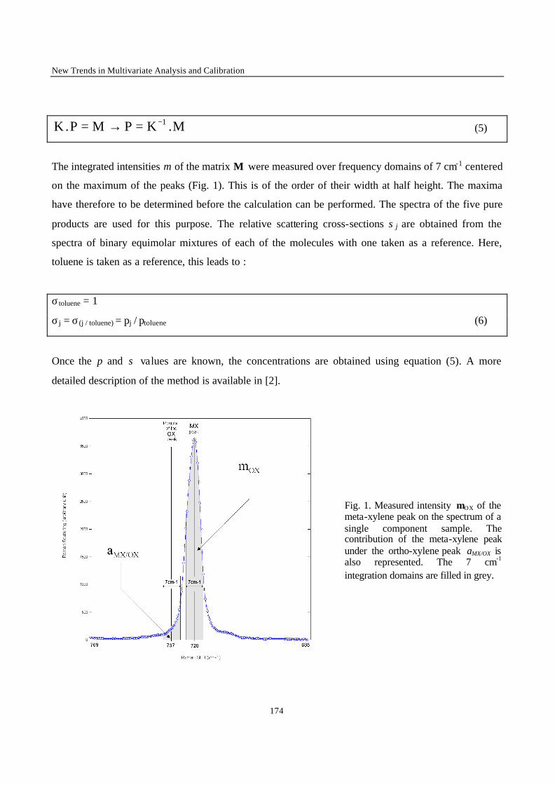
New Trends in Multivariate Analysis and Calibration
174
M.KPMPK 1−=→=. (5)
The integrated intensities m of the matrix M were measured over frequency domains of 7 cm-1 centered
on the maximum of the peaks (Fig. 1). This is of the order of their width at half height. The maxima
have therefore to be determined before the calculation can be performed. The spectra of the five pure
products are used for this purpose. The relative scattering cross-sections σj are obtained from the
spectra of binary equimolar mixtures of each of the molecules with one taken as a reference. Here,
toluene is taken as a reference, this leads to :
σtoluene = 1
σj = σ(j / toluene) = pj / ptoluene (6)
Once the p and σ values are known, the concentrations are obtained using equation (5). A more
detailed description of the method is available in [2].
Fig. 1. Measured intensity mOX of the meta-xylene peak on the spectrum of a single component sample. The contribution of the meta-xylene peak under the ortho-xylene peak aMX/OX is also represented. The 7 cm-1 integration domains are filled in grey.

Chapter 3 – New Types of Data : Nature of the Data Set
175
2.3 - Stepwise Multiple Linear Regression (Stepwise MLR)
Stepwise Multiple Linear Regression [3] is an MLR with variable selection. Stepwise selection is used
to select a small subset of variables from the original spectral matrix X. The first variable xj entered in
the model is the most correlated to the property of interest y . The regression coefficient b obtained
from the univariate regression model relating xj to y is tested for significance using a t-test at the
considered critical level α = 1 or 5 %. The next step is forward selection. This consists in including in
the model the variable xi that yields the highest Partial Correlation Coefficient (PCC). The inclusion of
a new variable in the model can decrease the contribution of a variable already included and make it
non-significant. After each inclusion of a new variable, the significance of the regression terms (biXi)
already in the model is therefore tested, and the non-significant terms are eliminated from the equation.
This is the backward elimination step. Forward selection and backward elimination are repeated until
no improvement of the model can be achieved by including a new variable, and all the variables
already included are significant.
Stepwise variable selection method is known for sometimes selecting uninformative variables because
of chance correlation to the property of interest. This can occur when the method is applied to noisy
signals. In order to reduce this risk, a modified version of this algorithm was proposed. The main idea
is the same as in Stepwise, the forward selection and backward elimination steps are maintained. The
difference lies in the fact that each time a variable xj is selected for entry in the model, an iterative
process begins :
• A new variable is built. This variable xj1 is made of the average Raman scattering value of a 3-
point window centred on xj (from xj-1 to xj+1). If xj1 yields a higher PCC than xj, it becomes the new
candidate variable.
• A second new variable, xj2 (average Raman scattering value of points xj-2 to xj+2) is built, it is
compared with xj1 , and the process goes on.
• When the enlargement of the window does not lead to a variable xj(n+1) with a better PCC than
xjn, the method stops and xjn enters the model.
Selecting an (2n+1)-points spectral window instead of a single wavelength implies a local averaging of
the signal. This should reduce the effect of noise in the prediction step. Moreover, as the first variables
New Trends in Multivariate Analysis and Calibration
176
entered into the model (most important ones) yield a better PCC, less uninformative variables should be
retained.
2.4 - MLR with selection by Genetic Algorithm (GA MLR)
Genetic Algorithms (GA) are used here to select a small subset of original variables in order to build an
MLR model [4]. A population of k strings (or chromosomes) is randomly chosen from the original
predictor matrix X. The chromosomes are made of genes (or bitfields) representing the parameters to
optimise. In the case of variable selection, each gene is made of a single bit corresponding to an
origina l variable. The fitness of each string is evaluated in terms of Root Mean Squared Error of
Prediction, defined as :
n/n
)yiyi(RMSEP t1i
2t
∑=
−= (7)
where nt is the number of objects in the test set, yi the known value of the property of interest for object
i, and yiˆ the value of the property of interest predicted by the model for object i.
With a probability depending on their fitness, pairs of strings are selected to undergo cross-over. Cross-
over is a GA operator consisting in mixing the information contained in two existing (parent) strings to
obtain new (children) strings. In order to enable the method to escape a possible local minimum, a
second GA operator, mutation, is introduced with a much lower probability. This means that each bit in
the children strings may be randomly changed. In the algorithm used here [5], the children strings may
replace members of the population of parent strings yielding a worse fit. This whole procedure is called
a generation. It is iterated unt il convergence to a good solution is reached. In order to improve the
variable selection, a backward elimination was added to ensure that all the selected variables are
relevant for the model. The principle is the same as the backward elimination step in the Stepwise
variable selection method.
Chapter 3 – New Types of Data : Nature of the Data Set
177
This method requires as input parameters the number of strings in each generation (size of the
population), the number of variables in each string (number of genes per chromosome), the frequency
of cross-over, mutations and backward elimination, and the number of generations.
2.5 - Principal Component Regression with variable selection (PCR VS)
This method includes two steps. The original data matrix X(n,p) is approximated by a small set of
orthogonal Principal Components (PCs) T(n,a). A Multiple Linear Regression model is then built
relating the scores of the PCs (independent variables) to the property of interest y(n,1) . The main
difficulty of this method is to choose the number of PCs that have to be retained. This was done here by
means of Leave One Out (LOO) Cross Validation (CV). The predictive ability of the model is
estimated at several complexities (models including 1,2, … etc PCs) in terms of Root Mean Square
Error of Cross Validation (RMSECV). RMSECV is defined as RMSEP (equ. 7) when yiˆ is obtained
by cross validation. The complexity leading to the smallest RMSECV is considered as optimal in a first
approach. In a second step, in order to avoid overfitting, more parsimonious models (smaller
complexities, one or more of the last selected variables are removed) are tested to determine if they can
be considered as equivalent in performance. The slightly worse RMSECV can in that case be
compensated by a better robustness of the resulting model. This is done using a randomisation test [6].
This test is applied to check the equality of performance of two prediction methods or the same
prediction method at two different complexities. In this study, the probability was estimated as the
average of three calculations with 249 iterations each, and the alpha value used was 5%.
In the usual PCR [7], the variables are introduced into the model according to the percentage of
variance they explain. This is called PCR top-down. But the PCs explaining the largest part of the
global variance in X are not always the most related to y. In PCR with variable selection (PCR VS), the
PCs are included in the model according to their correlation [8] with y, or their predictive ability [9].
2.6 - Partial Least Squares Regression (PLS)
Similarly to PCR, PLS [10] reduces the data to a small number of latent variables. The basic idea is to
focus only on the systematic variation in X that is related to y. PLS maximises the covariance between

New Trends in Multivariate Analysis and Calibration
178
the spectral data and the property to be modelled. The original NIPALS [11-12] algorithm was used in
this study. In the same way as for PCR, the optimal complexity is determined by comparing the
RMSECV obtained from models with various complexities. To avoid overfitting, this complexity is
then confirmed or corrected by comparing the model leading to the smaller RMSECV with the more
parsimonious ones using a randomisation test.
3– Signal Processing Methods
3.1 - Smoothing by moving average
Smoothing by moving average (first order Savitzky-Golay algorithm [13]) is the simplest way to
reduce noise in a signal. It has however important drawbacks. For instance, it modifies the shape of
peaks, tending to reduce their height and enlarge their base. The size of the window chosen for the
smoothing must be optimised in order not to reduce the predictive abilities of the models obtained.
3.2 - Filtering in Fourier domain
Filtering was carried out in the Fourier domain [14]. The filtering method consists in applying a low
pass filter [15] on the frequency domain : a frequency value, above which the Fourier coefficients
should be kept, is selected. The cutoff frequency value was here automatically calculated on the bases
of the power spectra (PS). The power spectrum of a function is the measurement of the signal energy at
a given frequency. The narrowest peaks of interest in the signal are related to the minimum frequency
to be kept in the Fourier domain. The energy corresponding to the non- informative peaks is calculated,
and the power spectra are used to determine which frequencies should be kept depending on this value.
3.3 - Filtering in Wavelet Domain
The main steps of signal denoising in Wavelet domain are the decomposition of the signal, the
thresholding, and the reconstruction of the denoised signal [16].
The wavelet transform of a discrete signal f is obtained by :

Chapter 3 – New Types of Data : Nature of the Data Set
179
w = W f (8)
where w is a vector containing wavelet transform coefficients and W is the matrix of the wavelet filter
coefficients.
The coefficients in W are derived from the mother wavelet function. The Daubechies family wavelet
was used here. To choose the relevant wavelet coefficients (those related to the signal) a threshold
value is calculated. Many methods are available. This was done here using the method known as
universal thresholding [17] (ThU) in which the threshold level is calculated from the standard deviation
of the noise. Once the threshold is known, two different approaches are generally used, namely hard
and soft thresholding. Soft thresholding [18] was used here, in this case the wavelet coefficients are
reduced by a quantity equal to the threshold value.
When the relevant wavelet coefficients wt are determined, the denoised signal ft can be rebuilt as :
ft = W’ wt (9)
4 - Experimental
4.1 - Data set
The data set was made of synthetic mixtures prepared from products previously analysed by gas
chromatography in order to assess their purity. Those mixtures were designed to cover a wide range of
concentrations representative for all the possible situations on the process. Only the spectra of the
“pure” products and the binary mixtures are required to build the model in case of the classical
calibration method. For all the inverse calibration methods, all the samples (except the replicates) are
used in the model building phase.
The data set consists of 52 spectra :

New Trends in Multivariate Analysis and Calibration
180
- 1 spectrum for each of the 5 pure products (toluene, meta, para, and ortho-Xylene, and ethyl-
benzene)
- 9 spectra of binary p-xylene / m-xylene mixtures (concentrations from 10/90 to 90/10 with a 10%
step)
- 10 equimolar binary mixtures consisting of all binary mixtures which can be prepared from the five
pure products.
- 10 equimolar ternary mixtures
- 5 quaternary mixtures
- 1 mixture including the five constituents
- 10 replicates of randomly chosen mixtures
Raman spectra were recorded using a spectroscopic device quite similar to the one industrially used in
the ELUXYL separation process. The main differences are that a laser diode (SDL 8530) emitting at
785 nm was used instead of an argon ion laser (514.53 nm), and a 1 meter long optical fibre replaced
the 200 meters one used on the process. Back scattered Raman signal was recovered through a Super
DILOR Head equipped with interferential and Notch filters to prevent the Raman signal of silica to be
superimposed to the Raman signal of the sample. The grating spectrometer was equipped with a CCD
camera used in multiple spectra configuration. The emission line of a neon lamp could therefore also be
recorded to allow wavelength calibration. The spectra were acquired from 930 to 650 cm-1, no rotation
of the grating was needed to cover this spectral range. The maximum available power at the output of
the fibre connected to the laser is 250 mW. However, in order to prevent any damage to the filters, this
power was reduced to a sample excitation power of 30 mW. Each spectrum was acquired during 10
seconds. This corresponds to the conditions on the industrial process, considering that concentration
values have to be provided by the system every 15 seconds. The five remaining seconds should be
enough for data treatment (possible pre-treatment, and concentration predictions).
The wavelength domain retained in the spectra was specifically designed to fit the requirements of the
classical calibration method. Thanks to the relatively simple structure of Raman spectra, it is sometimes
possible to find a spectral region in which each of the peaks is readily assignable to one product of the
mixture, and where there is not too much overlap. The spectral region has therefore been chosen so that
each product is represented mainly by one peak (Fig. 2). There are at least two frequency regions with
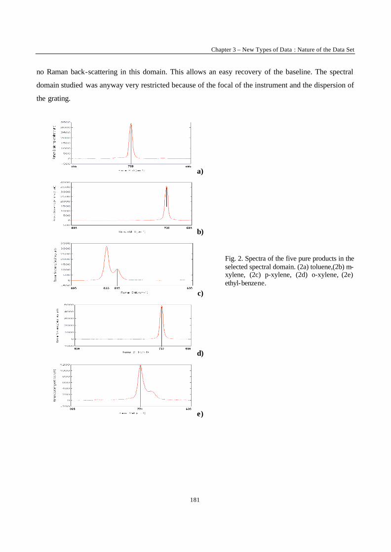
Chapter 3 – New Types of Data : Nature of the Data Set
181
no Raman back-scattering in this domain. This allows an easy recovery of the baseline. The spectral
domain studied was anyway very restricted because of the focal of the instrument and the dispersion of
the grating.
a)
b)
c)
d)
e)
Fig. 2. Spectra of the five pure products in the selected spectral domain. (2a) toluene,(2b) m-xylene, (2c) p-xylene, (2d) o-xylene, (2e) ethyl-benzene.
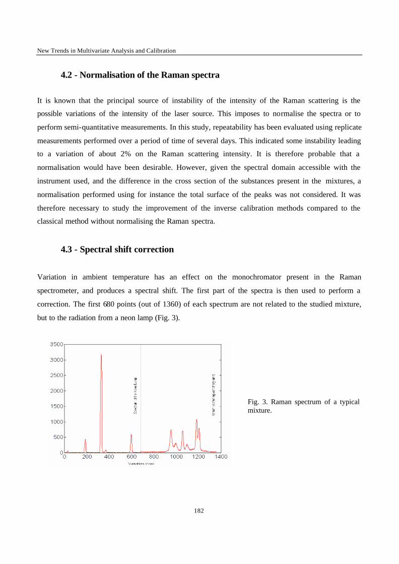
New Trends in Multivariate Analysis and Calibration
182
4.2 - Normalisation of the Raman spectra
It is known that the principal source of instability of the intensity of the Raman scattering is the
possible variations of the intensity of the laser source. This imposes to normalise the spectra or to
perform semi-quantitative measurements. In this study, repeatability has been evaluated using replicate
measurements performed over a period of time of several days. This indicated some instability leading
to a variation of about 2% on the Raman scattering intensity. It is therefore probable that a
normalisation would have been desirable. However, given the spectral domain accessible with the
instrument used, and the difference in the cross section of the substances present in the mixtures, a
normalisation performed using for instance the total surface of the peaks was not considered. It was
therefore necessary to study the improvement of the inverse calibration methods compared to the
classical method without normalising the Raman spectra.
4.3 - Spectral shift correction
Variation in ambient temperature has an effect on the monochromator present in the Raman
spectrometer, and produces a spectral shift. The first part of the spectra is then used to perform a
correction. The first 680 points (out of 1360) of each spectrum are not related to the studied mixture,
but to the radiation from a neon lamp (Fig. 3).
Fig. 3. Raman spectrum of a typical mixture.
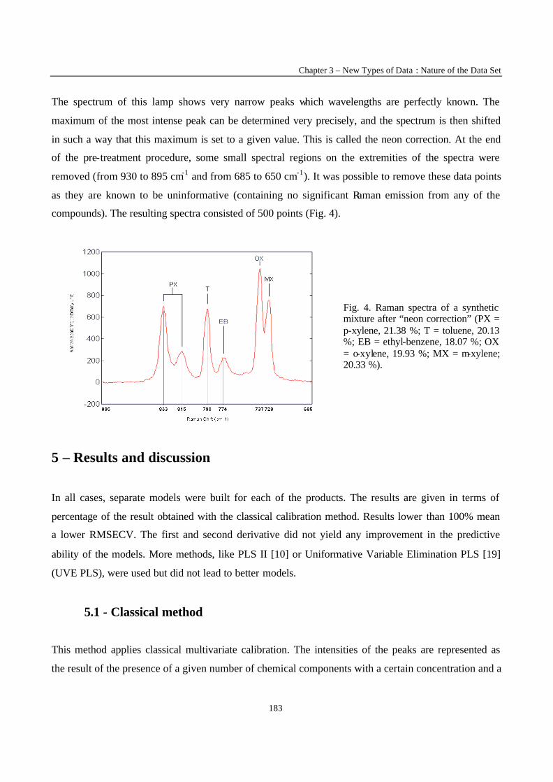
Chapter 3 – New Types of Data : Nature of the Data Set
183
The spectrum of this lamp shows very narrow peaks which wavelengths are perfectly known. The
maximum of the most intense peak can be determined very precisely, and the spectrum is then shifted
in such a way that this maximum is set to a given value. This is called the neon correction. At the end
of the pre-treatment procedure, some small spectral regions on the extremities of the spectra were
removed (from 930 to 895 cm-1 and from 685 to 650 cm-1). It was possible to remove these data points
as they are known to be uninformative (containing no significant Raman emission from any of the
compounds). The resulting spectra consisted of 500 points (Fig. 4).
Fig. 4. Raman spectra of a synthetic mixture after “neon correction” (PX = p-xylene, 21.38 %; T = toluene, 20.13 %; EB = ethyl-benzene, 18.07 %; OX = o-xylene, 19.93 %; MX = m-xylene; 20.33 %).
5 – Results and discussion
In all cases, separate models were built for each of the products. The results are given in terms of
percentage of the result obtained with the classical calibration method. Results lower than 100% mean
a lower RMSECV. The first and second derivative did not yield any improvement in the predictive
ability of the models. More methods, like PLS II [10] or Uniformative Variable Elimination PLS [19]
(UVE PLS), were used but did not lead to better models.
5.1 - Classical method
This method applies classical multivariate calibration. The intensities of the peaks are represented as
the result of the presence of a given number of chemical components with a certain concentration and a
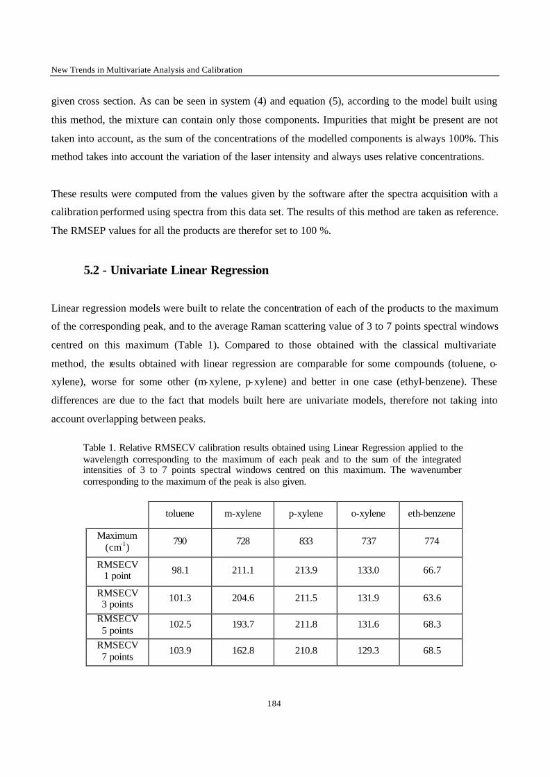
New Trends in Multivariate Analysis and Calibration
184
given cross section. As can be seen in system (4) and equation (5), according to the model built using
this method, the mixture can contain only those components. Impurities that might be present are not
taken into account, as the sum of the concentrations of the modelled components is always 100%. This
method takes into account the variation of the laser intensity and always uses relative concentrations.
These results were computed from the values given by the software after the spectra acquisition with a
calibration performed using spectra from this data set. The results of this method are taken as reference.
The RMSEP values for all the products are therefor set to 100 %.
5.2 - Univariate Linear Regression
Linear regression models were built to relate the concentration of each of the products to the maximum
of the corresponding peak, and to the average Raman scattering value of 3 to 7 points spectral windows
centred on this maximum (Table 1). Compared to those obtained with the classical multivariate
method, the results obtained with linear regression are comparable for some compounds (toluene, o-
xylene), worse for some other (m-xylene, p-xylene) and better in one case (ethyl-benzene). These
differences are due to the fact that models built here are univariate models, therefore not taking into
account overlapping between peaks.
Table 1. Relative RMSECV calibration results obtained using Linear Regression applied to the wavelength corresponding to the maximum of each peak and to the sum of the integrated intensities of 3 to 7 points spectral windows centred on this maximum. The wavenumber corresponding to the maximum of the peak is also given.
toluene m-xylene p-xylene o-xylene eth-benzene
Maximum (cm-1)
790 728 833 737 774
RMSECV 1 point 98.1 211.1 213.9 133.0 66.7
RMSECV 3 points
101.3 204.6 211.5 131.9 63.6
RMSECV 5 points
102.5 193.7 211.8 131.6 68.3
RMSECV 7 points
103.9 162.8 210.8 129.3 68.5
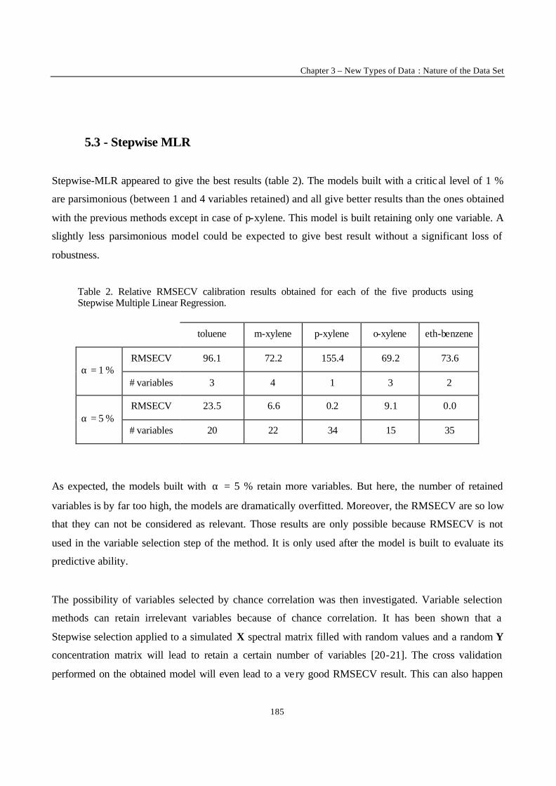
Chapter 3 – New Types of Data : Nature of the Data Set
185
5.3 - Stepwise MLR
Stepwise-MLR appeared to give the best results (table 2). The models built with a critical level of 1 %
are parsimonious (between 1 and 4 variables retained) and all give better results than the ones obtained
with the previous methods except in case of p-xylene. This model is built retaining only one variable. A
slightly less parsimonious model could be expected to give best result without a significant loss of
robustness.
Table 2. Relative RMSECV calibration results obtained for each of the five products using Stepwise Multiple Linear Regression.
toluene m-xylene p-xylene o-xylene eth-benzene
RMSECV 96.1 72.2 155.4 69.2 73.6 α = 1 %
# variables 3 4 1 3 2
RMSECV 23.5 6.6 0.2 9.1 0.0 α = 5 %
# variables 20 22 34 15 35
As expected, the models built with α = 5 % retain more variables. But here, the number of retained
variables is by far too high, the models are dramatically overfitted. Moreover, the RMSECV are so low
that they can not be considered as relevant. Those results are only possible because RMSECV is not
used in the variable selection step of the method. It is only used after the model is built to evaluate its
predictive ability.
The possibility of variables selected by chance correlation was then investigated. Variable selection
methods can retain irrelevant variables because of chance correlation. It has been shown that a
Stepwise selection applied to a simulated X spectral matrix filled with random values and a random Y
concentration matrix will lead to retain a certain number of variables [20-21]. The cross validation
performed on the obtained model will even lead to a very good RMSECV result. This can also happen
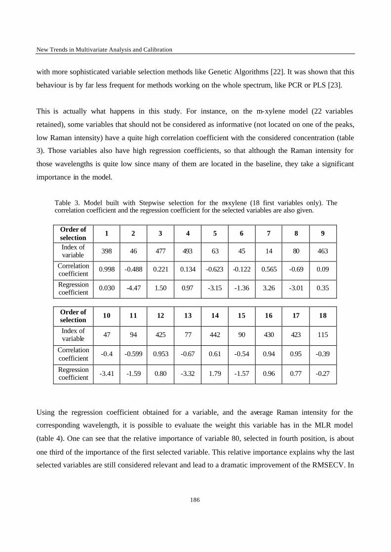
New Trends in Multivariate Analysis and Calibration
186
with more sophisticated variable selection methods like Genetic Algorithms [22]. It was shown that this
behaviour is by far less frequent for methods working on the whole spectrum, like PCR or PLS [23].
This is actually what happens in this study. For instance, on the m-xylene model (22 variables
retained), some variables that should not be considered as informative (not located on one of the peaks,
low Raman intensity) have a quite high correlation coefficient with the considered concentration (table
3). Those variables also have high regression coefficients, so that although the Raman intensity for
those wavelengths is quite low since many of them are located in the baseline, they take a significant
importance in the model.
Table 3. Model built with Stepwise selection for the m-xylene (18 first variables only). The correlation coefficient and the regression coefficient for the selected variables are also given.
Order of selection
1 2 3 4 5 6 7 8 9
Index of variable 398 46 477 493 63 45 14 80 463
Correlation coefficient
0.998 -0.488 0.221 0.134 -0.623 -0.122 0.565 -0.69 0.09
Regression coefficient
0.030 -4.47 1.50 0.97 -3.15 -1.36 3.26 -3.01 0.35
Order of selection
10 11 12 13 14 15 16 17 18
Index of variable 47 94 425 77 442 90 430 423 115
Correlation coefficient
-0.4 -0.599 0.953 -0.67 0.61 -0.54 0.94 0.95 -0.39
Regression coefficient -3.41 -1.59 0.80 -3.32 1.79 -1.57 0.96 0.77 -0.27
Using the regression coefficient obtained for a variable, and the average Raman intensity for the
corresponding wavelength, it is possible to evaluate the weight this variable has in the MLR model
(table 4). One can see that the relative importance of variable 80, selected in fourth position, is about
one third of the importance of the first selected variable. This relative importance explains why the last
selected variables are still considered relevant and lead to a dramatic improvement of the RMSECV. In
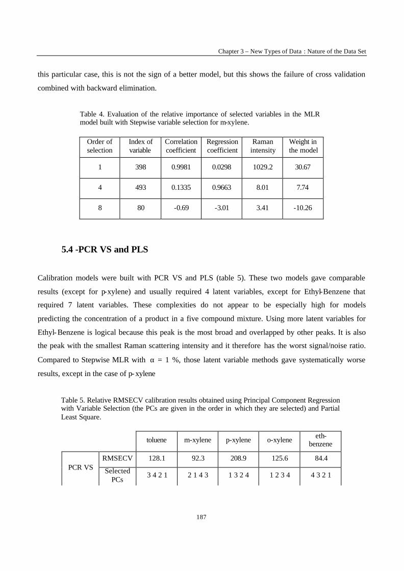
Chapter 3 – New Types of Data : Nature of the Data Set
187
this particular case, this is not the sign of a better model, but this shows the failure of cross validation
combined with backward elimination.
Table 4. Evaluation of the relative importance of selected variables in the MLR model built with Stepwise variable selection for m-xylene.
Order of selection
Index of variable
Correlation coefficient
Regression coefficient
Raman intensity
Weight in the model
1 398 0.9981 0.0298 1029.2 30.67
4 493 0.1335 0.9663 8.01 7.74
8 80 -0.69 -3.01 3.41 -10.26
5.4 -PCR VS and PLS
Calibration models were built with PCR VS and PLS (table 5). These two models gave comparable
results (except for p-xylene) and usually required 4 latent variables, except for Ethyl-Benzene that
required 7 latent variables. These complexities do not appear to be especially high for models
predicting the concentration of a product in a five compound mixture. Using more latent variables for
Ethyl-Benzene is logical because this peak is the most broad and overlapped by other peaks. It is also
the peak with the smallest Raman scattering intensity and it therefore has the worst signal/noise ratio.
Compared to Stepwise MLR with α = 1 %, those latent variable methods gave systematically worse
results, except in the case of p-xylene
Table 5. Relative RMSECV calibration results obtained using Principal Component Regression with Variable Selection (the PCs are given in the order in which they are selected) and Partial Least Square.
toluene m-xylene p-xylene o-xylene eth-benzene
RMSECV 128.1 92.3 208.9 125.6 84.4 PCR VS Selected
PCs 3 4 2 1 2 1 4 3 1 3 2 4 1 2 3 4 4 3 2 1
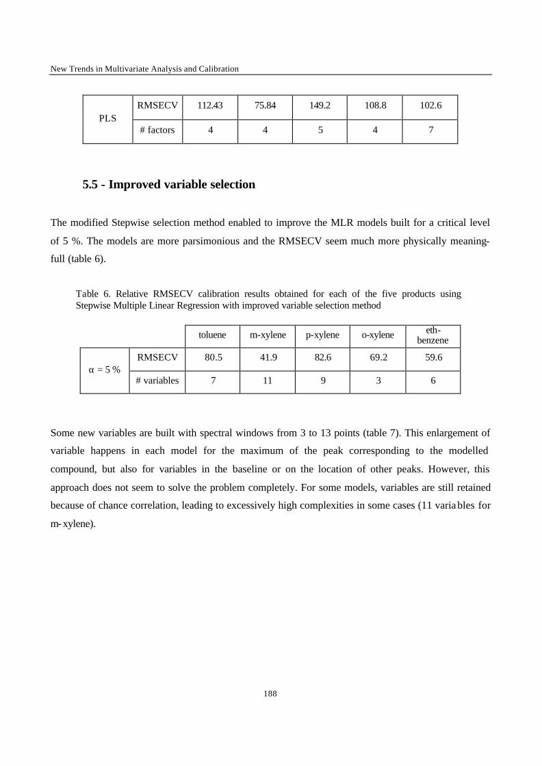
New Trends in Multivariate Analysis and Calibration
188
RMSECV 112.43 75.84 149.2 108.8 102.6 PLS
# factors 4 4 5 4 7
5.5 - Improved variable selection
The modified Stepwise selection method enabled to improve the MLR models built for a critical level
of 5 %. The models are more parsimonious and the RMSECV seem much more physically meaning-
full (table 6).
Table 6. Relative RMSECV calibration results obtained for each of the five products using Stepwise Multiple Linear Regression with improved variable selection method
toluene m-xylene p-xylene o-xylene eth-
benzene
RMSECV 80.5 41.9 82.6 69.2 59.6 α = 5 %
# variables 7 11 9 3 6
Some new variables are built with spectral windows from 3 to 13 points (table 7). This enlargement of
variable happens in each model for the maximum of the peak corresponding to the modelled
compound, but also for variables in the baseline or on the location of other peaks. However, this
approach does not seem to solve the problem completely. For some models, variables are still retained
because of chance correlation, leading to excessively high complexities in some cases (11 varia bles for
m-xylene).
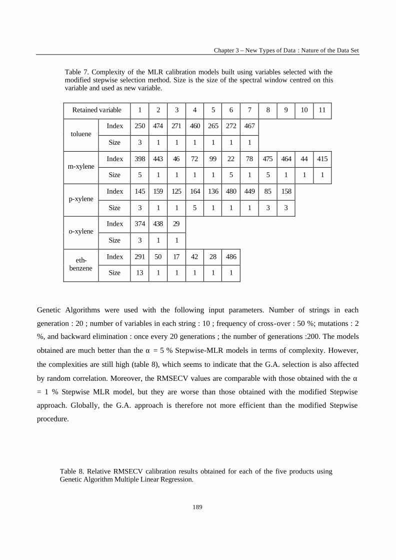
Chapter 3 – New Types of Data : Nature of the Data Set
189
Table 7. Complexity of the MLR calibration models built using variables selected with the modified stepwise selection method. Size is the size of the spectral window centred on this variable and used as new variable.
Retained variable 1 2 3 4 5 6 7 8 9 10 11
Index 250 474 271 460 265 272 467 toluene
Size 3 1 1 1 1 1 1
Index 398 443 46 72 99 22 78 475 464 44 415 m-xylene
Size 5 1 1 1 1 5 1 5 1 1 1
Index 145 159 125 164 136 480 449 85 158 p-xylene
Size 3 1 1 5 1 1 1 3 3
Index 374 438 29 o-xylene
Size 3 1 1
Index 291 50 17 42 28 486 eth-benzene
Size 13 1 1 1 1 1
Genetic Algorithms were used with the following input parameters. Number of strings in each
generation : 20 ; number of variables in each string : 10 ; frequency of cross-over : 50 %; mutations : 2
%, and backward elimination : once every 20 generations ; the number of generations :200. The models
obtained are much better than the α = 5 % Stepwise-MLR models in terms of complexity. However,
the complexities are still high (table 8), which seems to indicate that the G.A. selection is also affected
by random correlation. Moreover, the RMSECV values are comparable with those obtained with the α
= 1 % Stepwise MLR model, but they are worse than those obtained with the modified Stepwise
approach. Globally, the G.A. approach is therefore not more efficient than the modified Stepwise
procedure.
Table 8. Relative RMSECV calibration results obtained for each of the five products using Genetic Algorithm Multiple Linear Regression.
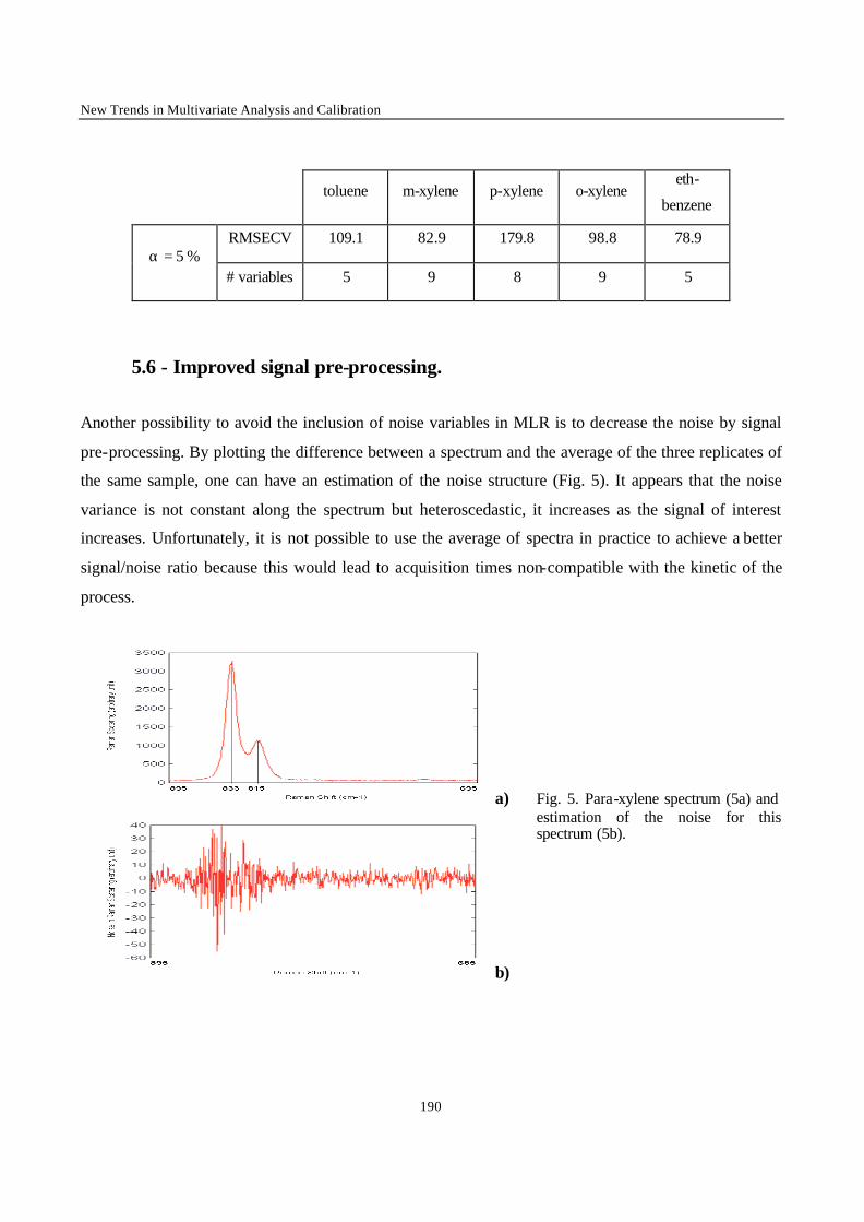
New Trends in Multivariate Analysis and Calibration
190
toluene m-xylene p-xylene o-xylene eth-
benzene
RMSECV 109.1 82.9 179.8 98.8 78.9 α = 5 %
# variables 5 9 8 9 5
5.6 - Improved signal pre-processing.
Another possibility to avoid the inclusion of noise variables in MLR is to decrease the noise by signal
pre-processing. By plotting the difference between a spectrum and the average of the three replicates of
the same sample, one can have an estimation of the noise structure (Fig. 5). It appears that the noise
variance is not constant along the spectrum but heteroscedastic, it increases as the signal of interest
increases. Unfortunately, it is not possible to use the average of spectra in practice to achieve a better
signal/noise ratio because this would lead to acquisition times non-compatible with the kinetic of the
process.
a)
b)
Fig. 5. Para-xylene spectrum (5a) and estimation of the noise for this spectrum (5b).
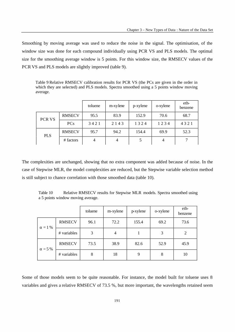
Chapter 3 – New Types of Data : Nature of the Data Set
191
Smoothing by moving average was used to reduce the noise in the signal. The optimisation, of the
window size was done for each compound individually using PCR VS and PLS models. The optimal
size for the smoothing average window is 5 points. For this window size, the RMSECV values of the
PCR VS and PLS models are slightly improved (table 9).
Table 9 Relative RMSECV calibration results for PCR VS (the PCs are given in the order in which they are selected) and PLS models. Spectra smoothed using a 5 points window moving average.
toluene m-xylene p-xylene o-xylene eth-
benzene
RMSECV 95.5 83.9 152.9 70.6 68.7 PCR VS
PCs 3 4 2 1 2 1 4 3 1 3 2 4 1 2 3 4 4 3 2 1
RMSECV 95.7 94.2 154.4 69.9 52.3 PLS
# factors 4 4 5 4 7
The complexities are unchanged, showing that no extra component was added because of noise. In the
case of Stepwise MLR, the model complexities are reduced, but the Stepwise variable selection method
is still subject to chance correlation with those smoothed data (table 10).
Table 10 Relative RMSECV results for Stepwise MLR models. Spectra smoothed using a 5 points window moving average.
toluene m-xylene p-xylene o-xylene eth-
benzene
RMSECV 96.1 72.2 155.4 69.2 73.6 α = 1 %
# variables 3 4 1 3 2
RMSECV 73.5 38.9 82.6 52.9 45.9 α = 5 %
# variables 8 18 9 8 10
Some of those models seem to be quite reasonable. For instance, the model built for toluene uses 8
variables and gives a relative RMSECV of 73.5 %, but more important, the wavelengths retained seem
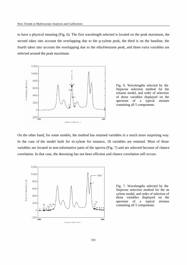
New Trends in Multivariate Analysis and Calibration
192
to have a physical meaning (Fig. 6). The first wavelength selected is located on the peak maximum, the
second takes into account the overlapping due to the p-xylene peak, the third is on the baseline, the
fourth takes into account the overlapping due to the ethyl-benzene peak, and three extra variables are
selected around the peak maximum.
Fig. 6. Wavelengths selected by the Stepwise selection method for the toluene model, and order of selection of those variables displayed on the spectrum of a typical mixture containing all 5 components.
On the other hand, for some models, the method has retained variables in a much more surprising way.
In the case of the model built for m-xylene for instance, 18 variables are retained. Most of those
variables are located in non- informative parts of the spectra (Fig. 7) and are selected because of chance
correlation. In that case, the denoising has not been efficient and chance correlation still occurs.
Fig. 7. Wavelengths selected by the Stepwise selection method for the m-xylene model, and order of selection of those variables displayed on the spectrum of a typical mixture containing all 5 components.
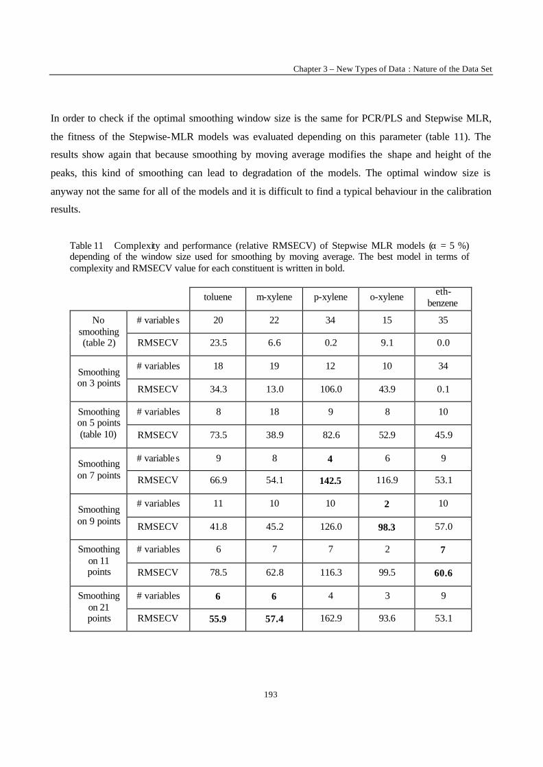
Chapter 3 – New Types of Data : Nature of the Data Set
193
In order to check if the optimal smoothing window size is the same for PCR/PLS and Stepwise MLR,
the fitness of the Stepwise-MLR models was evaluated depending on this parameter (table 11). The
results show again that because smoothing by moving average modifies the shape and height of the
peaks, this kind of smoothing can lead to degradation of the models. The optimal window size is
anyway not the same for all of the models and it is difficult to find a typical behaviour in the calibration
results.
Table 11 Complexity and performance (relative RMSECV) of Stepwise MLR models (α = 5 %) depending of the window size used for smoothing by moving average. The best model in terms of complexity and RMSECV value for each constituent is written in bold.
toluene m-xylene p-xylene o-xylene eth-
benzene
# variables 20 22 34 15 35 No smoothing (table 2) RMSECV 23.5 6.6 0.2 9.1 0.0
# variables 18 19 12 10 34 Smoothing on 3 points
RMSECV 34.3 13.0 106.0 43.9 0.1
# variables 8 18 9 8 10 Smoothing on 5 points (table 10) RMSECV 73.5 38.9 82.6 52.9 45.9
# variables 9 8 4 6 9 Smoothing on 7 points RMSECV 66.9 54.1 142.5 116.9 53.1
# variables 11 10 10 2 10 Smoothing on 9 points RMSECV 41.8 45.2 126.0 98.3 57.0
# variables 6 7 7 2 7 Smoothing on 11 points RMSECV 78.5 62.8 116.3 99.5 60.6
# variables 6 6 4 3 9 Smoothing on 21 points RMSECV 55.9 57.4 162.9 93.6 53.1
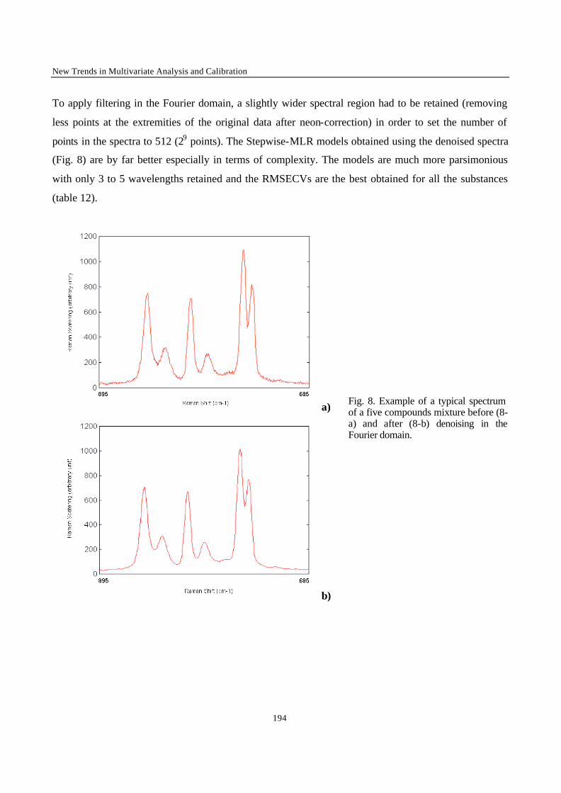
New Trends in Multivariate Analysis and Calibration
194
To apply filtering in the Fourier domain, a slightly wider spectral region had to be retained (removing
less points at the extremities of the original data after neon-correction) in order to set the number of
points in the spectra to 512 (29 points). The Stepwise-MLR models obtained using the denoised spectra
(Fig. 8) are by far better especially in terms of complexity. The models are much more parsimonious
with only 3 to 5 wavelengths retained and the RMSECVs are the best obtained for all the substances
(table 12).
a)
b)
Fig. 8. Example of a typical spectrum of a five compounds mixture before (8-a) and after (8-b) denoising in the Fourier domain.
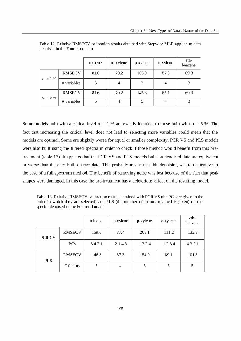
Chapter 3 – New Types of Data : Nature of the Data Set
195
Table 12. Relative RMSECV calibration results obtained with Stepwise MLR applied to data denoised in the Fourier domain.
toluene m-xylene p-xylene o-xylene eth-benzene
RMSECV 81.6 70.2 165.0 87.3 69.3 α = 1 %
# variables 5 4 3 4 3
RMSECV 81.6 70.2 145.8 65.1 69.3 α = 5 %
# variables 5 4 5 4 3
Some models built with a critical level α = 1 % are exactly identical to those built with α = 5 %. The
fact that increasing the critical level does not lead to selecting more variables could mean that the
models are optimal. Some are slightly worse for equal or smaller complexity. PCR VS and PLS models
were also built using the filtered spectra in order to check if those method would benefit from this pre-
treatment (table 13). It appears that the PCR VS and PLS models built on denoised data are equivalent
or worse than the ones built on raw data. This probably means that this denoising was too extensive in
the case of a full spectrum method. The benefit of removing noise was lost because of the fact that peak
shapes were damaged. In this case the pre-treatment has a deleterious effect on the resulting model.
Table 13. Relative RMSECV calibration results obtained with PCR VS (the PCs are given in the order in which they are selected) and PLS (the number of factors retained is given) on the spectra denoised in the Fourier domain
toluene m-xylene p-xylene o-xylene eth-
benzene
RMSECV 159.6 87.4 205.1 111.2 132.3 PCR CV
PCs 3 4 2 1 2 1 4 3 1 3 2 4 1 2 3 4 4 3 2 1
RMSECV 146.3 87.3 154.0 89.1 101.8 PLS
# factors 5 4 5 5 5
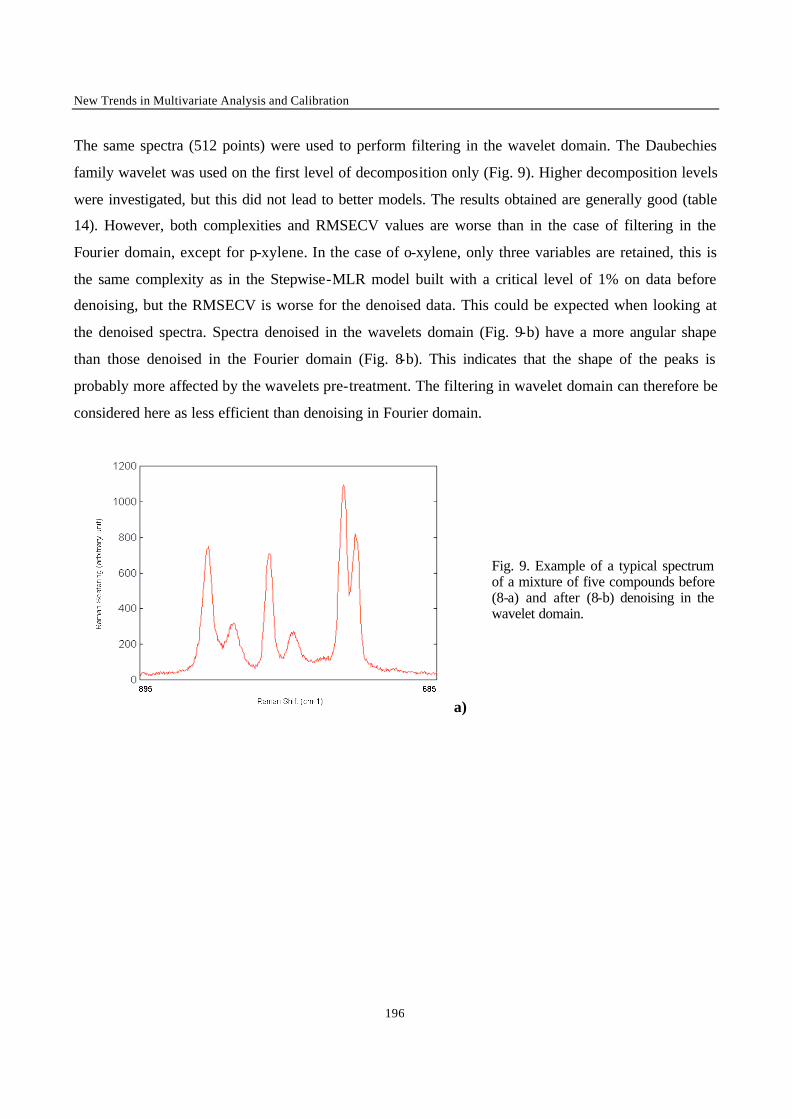
New Trends in Multivariate Analysis and Calibration
196
The same spectra (512 points) were used to perform filtering in the wavelet domain. The Daubechies
family wavelet was used on the first level of decomposition only (Fig. 9). Higher decomposition levels
were investigated, but this did not lead to better models. The results obtained are generally good (table
14). However, both complexities and RMSECV values are worse than in the case of filtering in the
Fourier domain, except for p-xylene. In the case of o-xylene, only three variables are retained, this is
the same complexity as in the Stepwise-MLR model built with a critical level of 1% on data before
denoising, but the RMSECV is worse for the denoised data. This could be expected when looking at
the denoised spectra. Spectra denoised in the wavelets domain (Fig. 9-b) have a more angular shape
than those denoised in the Fourier domain (Fig. 8-b). This indicates that the shape of the peaks is
probably more affected by the wavelets pre-treatment. The filtering in wavelet domain can therefore be
considered here as less efficient than denoising in Fourier domain.
a)
Fig. 9. Example of a typical spectrum of a mixture of five compounds before (8-a) and after (8-b) denoising in the wavelet domain.
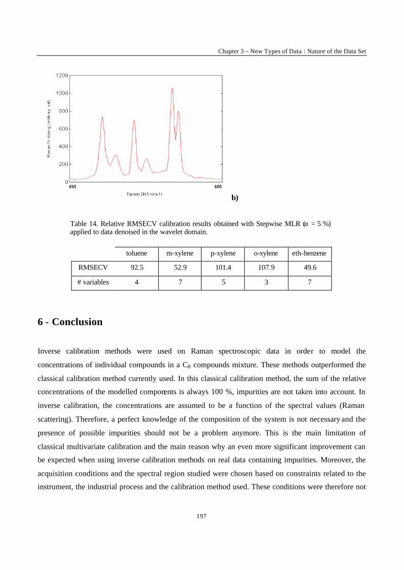
Chapter 3 – New Types of Data : Nature of the Data Set
197
b)
Table 14. Relative RMSECV calibration results obtained with Stepwise MLR (α = 5 %) applied to data denoised in the wavelet domain.
toluene m-xylene p-xylene o-xylene eth-benzene
RMSECV 92.5 52.9 101.4 107.9 49.6
# variables 4 7 5 3 7
6 - Conclusion
Inverse calibration methods were used on Raman spectroscopic data in order to model the
concentrations of individual compounds in a C8 compounds mixture. These methods outperformed the
classical calibration method currently used. In this classical calibration method, the sum of the relative
concentrations of the modelled components is always 100 %, impurities are not taken into account. In
inverse calibration, the concentrations are assumed to be a function of the spectral values (Raman
scattering). Therefore, a perfect knowledge of the composition of the system is not necessary and the
presence of possible impurities should not be a problem anymore. This is the main limitation of
classical multivariate calibration and the main reason why an even more significant improvement can
be expected when using inverse calibration methods on real data containing impurities. Moreover, the
acquisition conditions and the spectral region studied were chosen based on constraints related to the
instrument, the industrial process and the calibration method used. These conditions were therefore not
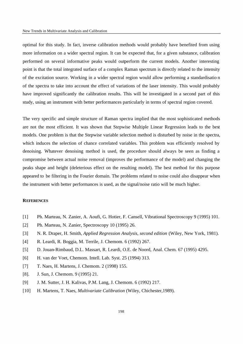
New Trends in Multivariate Analysis and Calibration
198
optimal for this study. In fact, inverse calibration methods would probably have benefited from using
more information on a wider spectral region. It can be expected that, for a given substance, calibration
performed on several informative peaks would outperform the current models. Another interesting
point is that the total integrated surface of a complex Raman spectrum is directly related to the intensity
of the excitation source. Working in a wider spectral region would allow performing a standardisatio n
of the spectra to take into account the effect of variations of the laser intensity. This would probably
have improved significantly the calibration results. This will be investigated in a second part of this
study, using an instrument with better performances particularly in terms of spectral region covered.
The very specific and simple structure of Raman spectra implied that the most sophisticated methods
are not the most efficient. It was shown that Stepwise Multiple Linear Regression leads to the best
models. One problem is that the Stepwise variable selection method is disturbed by noise in the spectra,
which induces the selection of chance correlated variables. This problem was efficiently resolved by
denoising. Whatever denoising method is used, the procedure should always be seen as finding a
compromise between actual noise removal (improves the performance of the model) and changing the
peaks shape and height (deleterious effect on the resulting model). The best method for this purpose
appeared to be filtering in the Fourier domain. The problems related to noise could also disappear when
the instrument with better performances is used, as the signal/noise ratio will be much higher.
REFERENCES
[1] Ph. Marteau, N. Zanier, A. Aoufi, G. Hotier, F. Cansell, Vibrational Spectroscopy 9 (1995) 101.
[2] Ph. Marteau, N. Zanier, Spectroscopy 10 (1995) 26.
[3] N. R. Draper, H. Smith, Applied Regression Analysis, second edition (Wiley, New York, 1981).
[4] R. Leardi, R. Boggia, M. Terrile, J. Chemom. 6 (1992) 267.
[5] D. Jouan-Rimbaud, D.L. Massart, R. Leardi, O.E. de Noord, Anal. Chem. 67 (1995) 4295.
[6] H. van der Voet, Chemom. Intell. Lab. Syst. 25 (1994) 313.
[7] T. Naes, H. Martens, J. Chemom. 2 (1998) 155.
[8]. J. Sun, J. Chemom. 9 (1995) 21.
[9] J. M. Sutter, J. H. Kalivas, P.M. Lang, J. Chemom. 6 (1992) 217.
[10] H. Martens, T. Naes, Multivariate Calibration (Wiley, Chichester,1989).
Chapter 3 – New Types of Data : Nature of the Data Set
199
[11] D. M. Haaland, E. V. Thomas, Anal. Chem. 60 (1988) 1193.
[12] P. Geladi, B. K. Kovalski, Anal. Chim. Acta 185 (1986) 1.
[13] A. Savitzky and M. J. E. Golay, Anal. Chem. 36 (1964) 1627.
[14] G. W. Small, M. A. Arnold, L. A. Marquardt, Anal. Chem. 65 (1993) 3279.
[15] H. C. Smit, Chemom. Intell. Lab. Syst. 8 (1990) 15.
[16] C. R. Mittermayer, S. G. Nikolov, H. Hutter, M. Grasserbauer, Chemom. Intell. Lab. Syst. 34
(1996) 187.
[17] D. L. Donoho in: Y. Mayer and S. Roques, Progress in Wavelet Analysis and Application,
(Edition Frontiers, 1993).
[18] D.L.Donoho, IEEE Transaction on Information Theory 41 (1995) 6143.
[19] V. Centner, D. L. Massart, O. E. de Noord, S. de Jong, B. M. V. Vandeginste, C. Sterna, Anal.
Chem. 68 (1996) 3851.
[20] J. G. Topliss, R. J. Costello, Journal of Medicinal Chemistry 15 (1971) 1066.
[21] J. G. Topliss, R. P. Edwards, Journal of Medicinal Chemistry 22 (1979) 1238.
[22] D. Jouan-Rimbaud, D. L. Massart, O. E. de Noord, Chem. Intell. Lab. Syst. 35 (1996) 213.
[23] M. Clark, R. D. Cramer III, Quantitative. Structure Activity Relationship 12 (1993) 137.
New Trends in Multivariate Analysis and Calibration
200
INVERSE MULTIVARIATE CALIBRATION
APPLIED TO ELUXYL RAMAN DATA
ChemoAC internal Report, 03/2000
F. Estienne and D.L. Massart *
ChemoAC, Farmaceutisch Instituut,
Vrije Universiteit Brussel, Laarbeeklaan 103,
B-1090 Brussels, Belgium. E-mail: [email protected]
ABSTRACT
An industrial process separating p-xylene from mainly other C8 aromatic compounds is monitored with an online remote Raman analyser. The concentrations of six constituents are currently evaluated with a classical calibration method. The aim of the study being to improve the precision of the monitoring of the process, inverse calibration linear methods were applied on a synthetic data set, in order to evaluate the improvement in prediction such methods could yield. Several methods were tested including Principal Component Regression with Variable Selection, Partial Least Square Regression or Multiple Linear Regression with variable selection (Stepwise or based on Genetic Algorithm). Methods based on selected wavelengths are of great interest because the obtained models can be expected to be very robust toward experimental conditions. However, because of the important noise in the spectra due to short accumulation time, variable selection methods selected a lot of irrelevant variables by chance correlation. Strategies were investigated to solve this problem and build reliable robust models. These strategies include the use of signal pre-processing (smoothing and filtering in the Fourier or Wavelets domain), and the use of an improved variable selection algorithm based on the selection of spectral windows instead of single wavelengths when this leads to a better model. The best results were achieved with Multiple Linear Regression and Stepwise variable selection applied to spectra denoised in the Fourier domain.
* Corresponding author
KEYWORDS : Chemometrics, Raman Spectroscopy, Multivariate Calibration, random correlation.
Chapter 3 – New Types of Data : Nature of the Data Set
201
1 - Introduction
The task of our group in this study was to evaluate whether the use of Inverse Calibration methods could
lead to an improvement in the quality of the online monitoring of the Eluxyl process.
The process is currently monitored using the experimental setup and software developed by Philippe
Marteau. This software implements a classical multivariate calibration method based on the measurement
of the areas of the Raman peaks. The main assumption when building a classical calibration model to
determine concentrations from spectra is that the error lies in the spectra. The model can be seen as :
Spectra = f (Concentrations). Or, in a matrix form: R = C . K , where R is the spectral response matrix, C
the concentration matrix, and K the matrix of molar absorptivities of the pure components. This implies
that it is necessary to know the concentrations of all the products present in the mixture in order to build
the model, at least if a high precision is required. Taking into account that a small quantities (<5%) of
impurities (i.e. C9+ compounds) is present in the mixture when working on real data, the classical
calibration method is naturally limited in precision if all the impurities are not clearly identified in the
spectrum.
In inverse calibration, one assumes that the error lies in the measurement of the concentrations. The model
can be seen as : Concentrations = f (Spectra). Or, in a matrix form : C = P . R , where R is the spectral
matrix, C the concentration matrix, and P the regression coefficients matrix. A perfect knowledge about
the composition of the system is then not necessary. Better results are therefore expected as the presence of
impur ities does not affect the prediction of the concentration of the compounds of interest (at least if these
impurities were present in the calibration data set used to build the model).
2 – Data set used in this study
The data set was made of synthetic mixtures prepared from products previously analysed by gas
chromatography in order to assess their purity. Those mixtures were designed to cover a wide range of
concentrations representative for all the possible situations on the process. The data set consists of 71
spectra :
New Trends in Multivariate Analysis and Calibration
202
- 1 spectrum for each of the 5 pure products (toluene, meta, para, and ortho-Xylene, and ethyl-
benzene)
- 10 equimolar binary mixtures consisting of all binary mixtures which can be prepared from the five
pure products.
- 10 equimolar ternary mixtures
- 5 equimolar quaternary mixtures
- 1 equimolar mixture including the five constituents
- 9 spectra of binary para-xylene / meta-xylene mixtures (concentrations from 10/90 to 90/10 with a
10% step)
- 5 spectra of binary toluene / meta-xylene mixtures (concentrations from 10/90 to 90/10 %)
- 10 replicates of randomly chosen mixtures
- 16 mixtures including the five constituents with various concentrations
Spectra were acquired from 0 to 3400 cm-1 with a 1.7 cm-1 step. After interpolation by the instrument
software, the spectra had a 0.3 cm-1 step, leading to 11579 data points per spectrum.
3 – Pre-processing
The main problem in this data set was due to the instability of the excitation source used during the
acquisition of the spectra. The laser used for excitation was in fact ageing, leading to the fact that it
could deliver only one half of its nominal power at the beginning of the acquisition period, and only
one fourth at the end of the acquisitions. This is not a problem when relative concentrations have to be
evaluated, like this is the case with the software developed by Philippe Marteau. But this problem has
to be solved when one wants to evaluate absolute concentrations. The best way would be to have a
reference sample, independent from the sample studied, but measured at the same time with the same
excitation source. The spectra could therefore be corrected to take into account the intensity variations
of the source. This was not available here. The only way left to normalise the spectra was to work on
their surface. It would have been easier if the mixtures studied had contained many products, leading to
very complex spectra which total surfaces could have been considered constant. In this case, it would
have been enough scale all the spectra to a given value. In the present case, the small number of
substances with very different cross-sections forbids the use of such a methodology. It was therefore
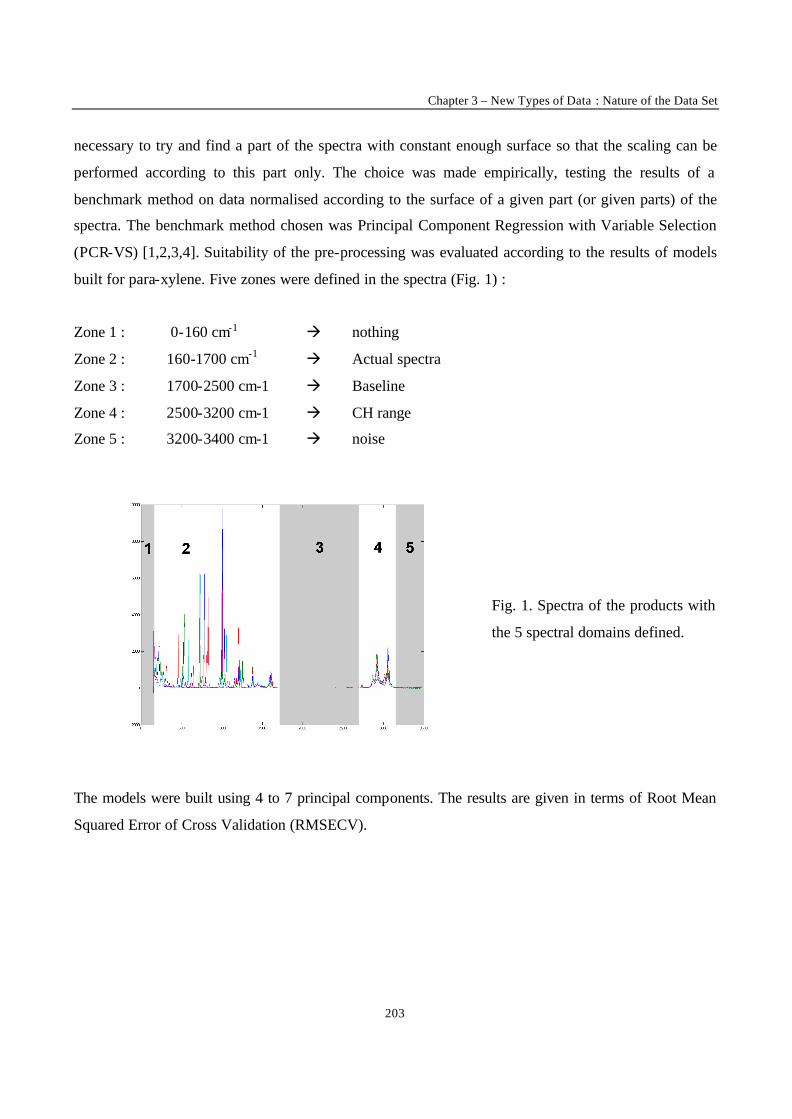
Chapter 3 – New Types of Data : Nature of the Data Set
203
necessary to try and find a part of the spectra with constant enough surface so that the scaling can be
performed according to this part only. The choice was made empirically, testing the results of a
benchmark method on data normalised according to the surface of a given part (or given parts) of the
spectra. The benchmark method chosen was Principal Component Regression with Variable Selection
(PCR-VS) [1,2,3,4]. Suitability of the pre-processing was evaluated according to the results of models
built for para-xylene. Five zones were defined in the spectra (Fig. 1) :
Zone 1 : 0-160 cm-1 à nothing
Zone 2 : 160-1700 cm-1 à Actual spectra
Zone 3 : 1700-2500 cm-1 à Baseline
Zone 4 : 2500-3200 cm-1 à CH range
Zone 5 : 3200-3400 cm-1 à noise
Fig. 1. Spectra of the products with
the 5 spectral domains defined.
The models were built using 4 to 7 principal components. The results are given in terms of Root Mean
Squared Error of Cross Validation (RMSECV).

New Trends in Multivariate Analysis and Calibration
204
Table 1. RMSECV for a PCR-VS model built for para-xylene depending of standardisation.
Reference zone(s) RMSECV value Number of PCs retained No standardisation 4.23 7 1 + 2 + 3 + 4 + 5 0.69 4
2 0.79 5 3 1.54 4 4 0.64 4
2 + 4 0.56 5
It appears that the best way to normalise the spectra is to scale them according to the total surface
corresponding to zones 2 and 4 (actual spectra and CH range). It can be seen also how tremendously
important such a correction is, as the results can be improved by a factor 10. However, the solution is
more than probably not optimal for, as said before, considering that the total surface of these two
spectral zones should theoretically be constant is not a valid hypothesis.
After this standardisation procedure, the baseline shift visible in spectral domain #3 was almost
perfectly removed. The use of a specific baseline removal procedure did not further improve the
calibration results.
The spectra were corrected for wavelength shift using the corresponding Neon spectra. However, with
spectra from this new experimental setup, this correction happened to be by far less crucial than on
previous Eluxyl Raman data we investigated.
3 – Choice of the calibration method to be used
In a previous study performed a synthetic data set simulating ELUXYL data, it had been shown that the
most effective calibration method was Stepwise Multiple Linear Regression (Stepwise-MLR) [5]
applied to spectra denoised in the Fourier domain. At that time, no non- linearity had been detected in
the data set. Considering the much better signal/noise ration and repeatability in this data set, it was
necessary to investigate for non- linearity again. In fac t, it now appears very clearly that the mixture
effects are not linear. It is the case for instance for meta-xylene/para-xylene mixture. The results of a
PCR-VS model of meta-xylene show that there is a clear deviation from linearity (Fig. 2-a) on the first
PC. This is especially visible for samples number 2-3 and 32 to 40 (corresponding to pure meta and
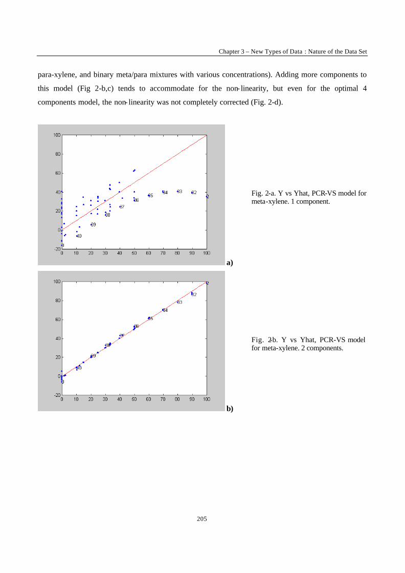
Chapter 3 – New Types of Data : Nature of the Data Set
205
para-xylene, and binary meta/para mixtures with various concentrations). Adding more components to
this model (Fig 2-b,c) tends to accommodate for the non- linearity, but even for the optimal 4
components model, the non- linearity was not completely corrected (Fig. 2-d).
a)
Fig. 2-a. Y vs Yhat, PCR-VS model for meta-xylene. 1 component.
b)
Fig. 2-b. Y vs Yhat, PCR-VS model for meta-xylene. 2 components.
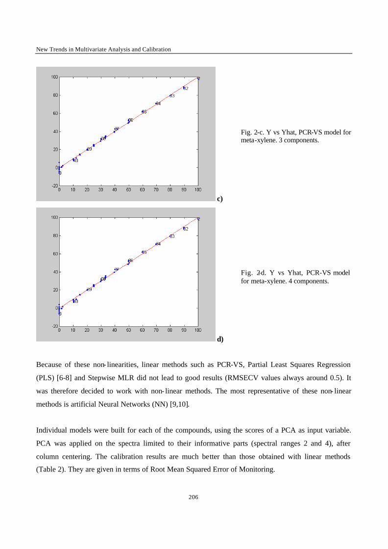
New Trends in Multivariate Analysis and Calibration
206
c)
Fig. 2-c. Y vs Yhat, PCR-VS model for meta-xylene. 3 components.
d)
Fig. 2-d. Y vs Yhat, PCR-VS model for meta-xylene. 4 components.
Because of these non- linearities, linear methods such as PCR-VS, Partial Least Squares Regression
(PLS) [6-8] and Stepwise MLR did not lead to good results (RMSECV values always around 0.5). It
was therefore decided to work with non- linear methods. The most representative of these non- linear
methods is artificial Neural Networks (NN) [9,10].
Individual models were built for each of the compounds, using the scores of a PCA as input variable.
PCA was applied on the spectra limited to their informative parts (spectral ranges 2 and 4), after
column centering. The calibration results are much better than those obtained with linear methods
(Table 2). They are given in terms of Root Mean Squared Error of Monitoring.
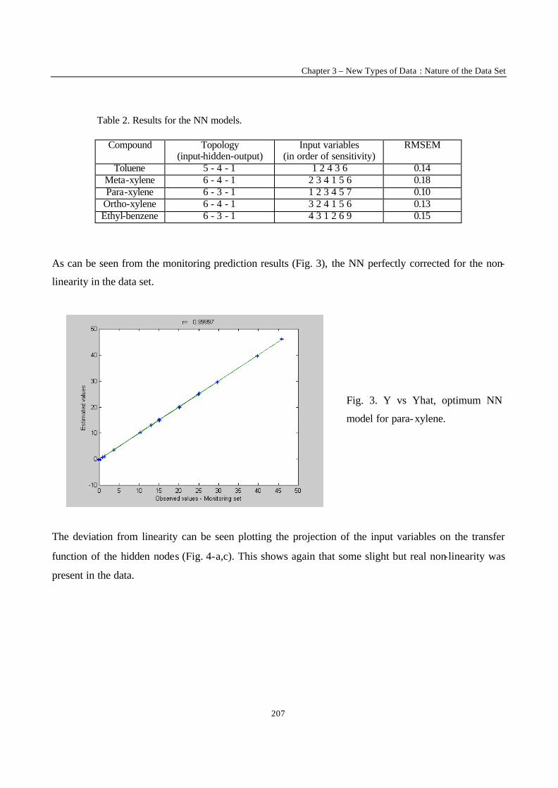
Chapter 3 – New Types of Data : Nature of the Data Set
207
Table 2. Results for the NN models.
Compound Topology (input-hidden-output)
Input variables (in order of sensitivity)
RMSEM
Toluene 5 - 4 - 1 1 2 4 3 6 0.14 Meta-xylene 6 - 4 - 1 2 3 4 1 5 6 0.18 Para-xylene 6 - 3 - 1 1 2 3 4 5 7 0.10
Ortho-xylene 6 - 4 - 1 3 2 4 1 5 6 0.13 Ethyl-benzene 6 - 3 - 1 4 3 1 2 6 9 0.15
As can be seen from the monitoring prediction results (Fig. 3), the NN perfectly corrected for the non-
linearity in the data set.
Fig. 3. Y vs Yhat, optimum NN
model for para-xylene.
The deviation from linearity can be seen plotting the projection of the input variables on the transfer
function of the hidden nodes (Fig. 4-a,c). This shows again that some slight but real non-linearity was
present in the data.
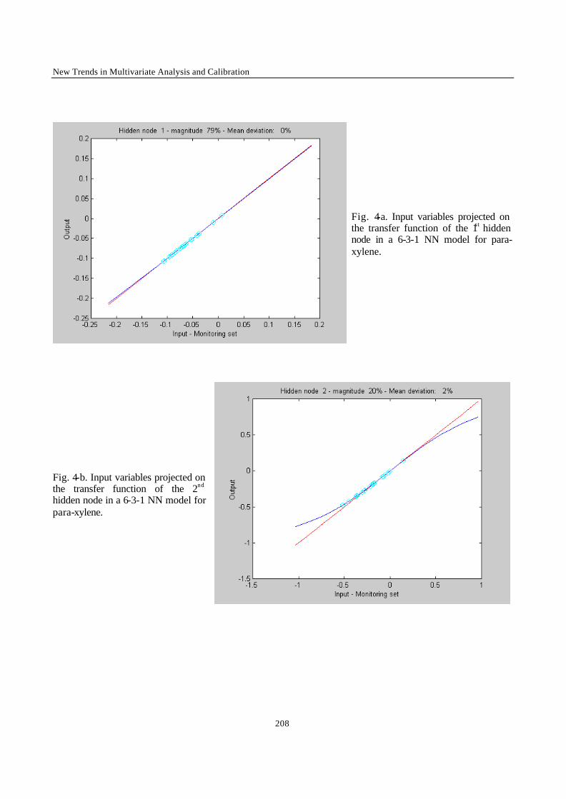
New Trends in Multivariate Analysis and Calibration
208
Fig. 4-a. Input variables projected on the transfer function of the 1st hidden node in a 6-3-1 NN model for para-xylene.
Fig. 4-b. Input variables projected on the transfer function of the 2nd hidden node in a 6-3-1 NN model for para-xylene.
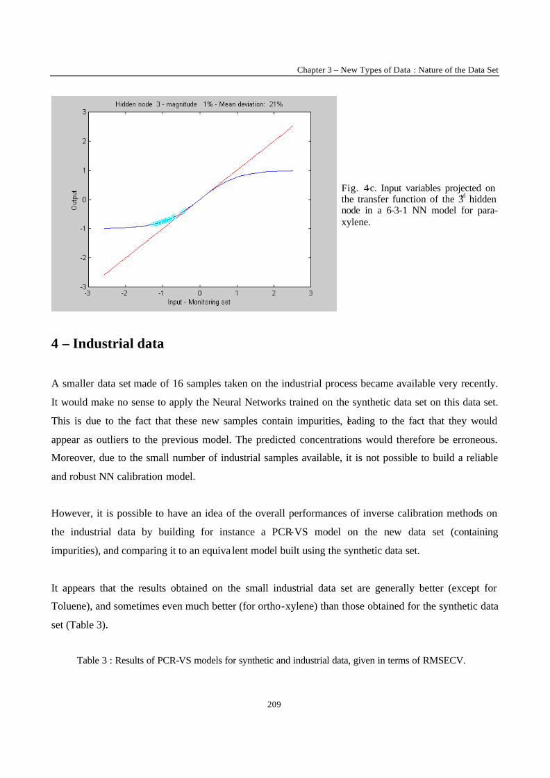
Chapter 3 – New Types of Data : Nature of the Data Set
209
Fig. 4-c. Input variables projected on the transfer function of the 3rd hidden node in a 6-3-1 NN model for para-xylene.
4 – Industrial data
A smaller data set made of 16 samples taken on the industrial process became available very recently.
It would make no sense to apply the Neural Networks trained on the synthetic data set on this data set.
This is due to the fact that these new samples contain impurities, leading to the fact that they would
appear as outliers to the previous model. The predicted concentrations would therefore be erroneous.
Moreover, due to the small number of industrial samples available, it is not possible to build a reliable
and robust NN calibration model.
However, it is possible to have an idea of the overall performances of inverse calibration methods on
the industrial data by building for instance a PCR-VS model on the new data set (containing
impurities), and comparing it to an equiva lent model built using the synthetic data set.
It appears that the results obtained on the small industrial data set are generally better (except for
Toluene), and sometimes even much better (for ortho-xylene) than those obtained for the synthetic data
set (Table 3).
Table 3 : Results of PCR-VS models for synthetic and industrial data, given in terms of RMSECV.
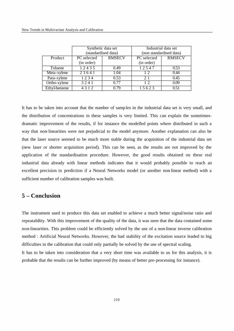
New Trends in Multivariate Analysis and Calibration
210
Synthetic data set
(standardised data) Industrial data set
(non standardised data) Product PC selected
(in order) RMSECV PC selected
(in order) RMSECV
Toluene 1 2 4 3 5 0.49 1 2 5 4 7 0.53 Meta-xylene 2 3 6 4 1 1.04 1 2 0.44 Para-xylene 1 2 3 4 0.53 2 1 0.45
Ortho-xylene 3 2 4 1 0.77 1 2 0.09 Ethyl-benzene 4 3 1 2 0.79 1 5 6 2 3 0.51
It has to be taken into account that the number of samples in the industrial data set is very small, and
the distribution of concentrations in these samples is very limited. This can explain the sometimes-
dramatic improvement of the results, if for instance the modelled points where distributed in such a
way that non- linearities were not prejudicial to the model anymore. Another explanation can also be
that the laser source seemed to be much more stable during the acquisition of the industrial data set
(new laser or shorter acquisition period). This can be seen, as the results are not improved by the
application of the standardisation procedure. However, the good results obtained on these real
industrial data already with linear methods indicates that it would probably possible to reach an
excellent precision in prediction if a Neural Networks model (or another non- linear method) with a
sufficient number of calibration samples was built.
5 – Conclusion
The instrument used to produce this data set enabled to achieve a much better signal/noise ratio and
repeatability. With this improvement of the quality of the data, it was seen that the data contained some
non-linearities. This problem could be efficiently solved by the use of a non-linear inverse calibration
method : Artificial Neural Networks. However, the bad stability of the excitation source leaded to big
difficulties in the calibration that could only partially be solved by the use of spectral scaling.
It has to be taken into consideration that a very short time was available to us for this analysis, it is
probable that the results can be further improved (by means of better pre-processing for instance).

Chapter 3 – New Types of Data : Nature of the Data Set
211
The few industrial samples provided were not enough to build reliable Neural Networks models.
However, the behaviour of linear methods toward these samples indicates that some very good results
can be expected when applying NN on industrial data with a large enough calibration set.
REFERENCES
[1] Principal Component Regression Tutorial
http://minf.vub.ac.be/~fabi/calibration/multi/pcr/
[2] T. Naes, H. Martens, J. Chemom. 2 (1998) 155.
[3] J. Sun, J. Chemom. 9 (1995) 21.
[4] J. M. Sutter, J. H. Kalivas, P.M. Lang, J. Chemom. 6 (1992) 217.
[5] N. R. Draper, H. Smith, Applied Regression Analysis, second edition (Wiley, New York, 1981).
[6] H. Martens, T. Naes, Multivariate Calibration (Wiley, Chichester,1989).
[7] D. M. Haaland, E. V. Thomas, Anal. Chem. 60 (1988) 1193.
[8] P. Geladi, B. K. Kovalski, Anal. Chim. Acta 185 (1986) 1.
[9] Neural Networks Tutorial
http://minf.vub.ac.be/~fabi/calibration/multi/nn/
[10] Smits, J.R.M., Melssen, W.J., Buydens, L.M.C., and Kateman, G., Chemom. Intell. Lab. Syst.,
22 (1994) 165.
New trends in Multivariate Analysis and Calibration
212
CHAPTER IV
NEW TYPES OF DATA : STRUCTURE AND SIZE
This last chapter treats of new approaches in both multivariate calibration and data exploration. These
new approaches are made necessary by data showing new types of structures or very large size.
The first paper in this chapter : “Multivariate calibration with Raman data using fast PCR and PLS
methods” comes back on the high quality Raman data set treated in chapter 3. The focus is this time on
the large size of this data set. This work shows how classical methods like PCR or PLS can be
significantly improved in terms of speed without compromising their prediction quality.
The second paper in this chapter : “Multi-Way Modelling of High-Dimensionality Electro-
Encephalographic Data” presents a data set cumulating novelties and challenges for chemometrical
methodology. First of all, this data set is not chemistry but pharmacy related since it is made of
electroencephalographic measurements performed during the clinical study of a new anti-depressant
drug. It has also a very complex structure with more than 35000 measurements and up to 6 dimensions.
The methods used proved particularly efficient, enabling a deep understanding of the data and
underlying phenomena.
The last paper in this chapter : “Robust Version of Tucker 3 Model” shows how multi-way methods
can be modified the same way classical chemometrical methods are in order to be made robust to
difficult data set. The author’s contribution to this work was to participate in the method development,
to perform calculations on the real data set, and to write the corresponding part of the article (chapter
3.2 and 4.2).
Apart from giving another example of application of chemometrics to a new type of data, this chapter
proves the usefulness of multi-way methods to data with very high dimensionality. The Tucker 3 model

Chapter 4 – New Types of Data : Structure and Size
213
was in particular applied to a 6-way data set. It is probably the first time in the chemometrical field that
a model with such high dimensionality with a real data set proves interpretable.
New trends in Multivariate Analysis and Calibration
214
MULTIVARIATE CALIBRATION WITH RAMAN DATA
USING FAST PCR AND PLS METHODS
Analytica Chimica Acta, 450 1 (2001) 123-129.
F. Estienne and D.L. Massart*
ChemoAC, Farmaceutisch Instituut,
Vrije Universiteit Brussel, Laarbeeklaan 103,
B-1090 Brussels, Belgium. E-mail: [email protected]
ABSTRACT
Linear and non- linear calibration methods (Principal Component Regression, Partial Least Squares Regression and Neural Networks) were applied to a slightly non- linear Raman data set. Because of the large size of this data set, recently introduced linear calibration methods specifically optimised for speed were also used. These fast methods achieve speed improvement by using the Lanczos decomposition for the singular value decomposition steps of the calibration procedures, and for some of their variants, by optimising the models without cross-validation. Linear methods could deal with the slight non-linearity present in the data by including extra components, therefore performing comparably to Neural Networks. The Fast methods performed as well as their classical equivalents in terms of precision in prediction, but the results were obtained considerably faster. It however appeared that cross-validation remains the most appropriate method for model complexity estimation.
* Corresponding author
KEYWORDS : Multivariate Calibration, Raman spectroscopy, Lanczos decomposition, Fast Calibration
methods.
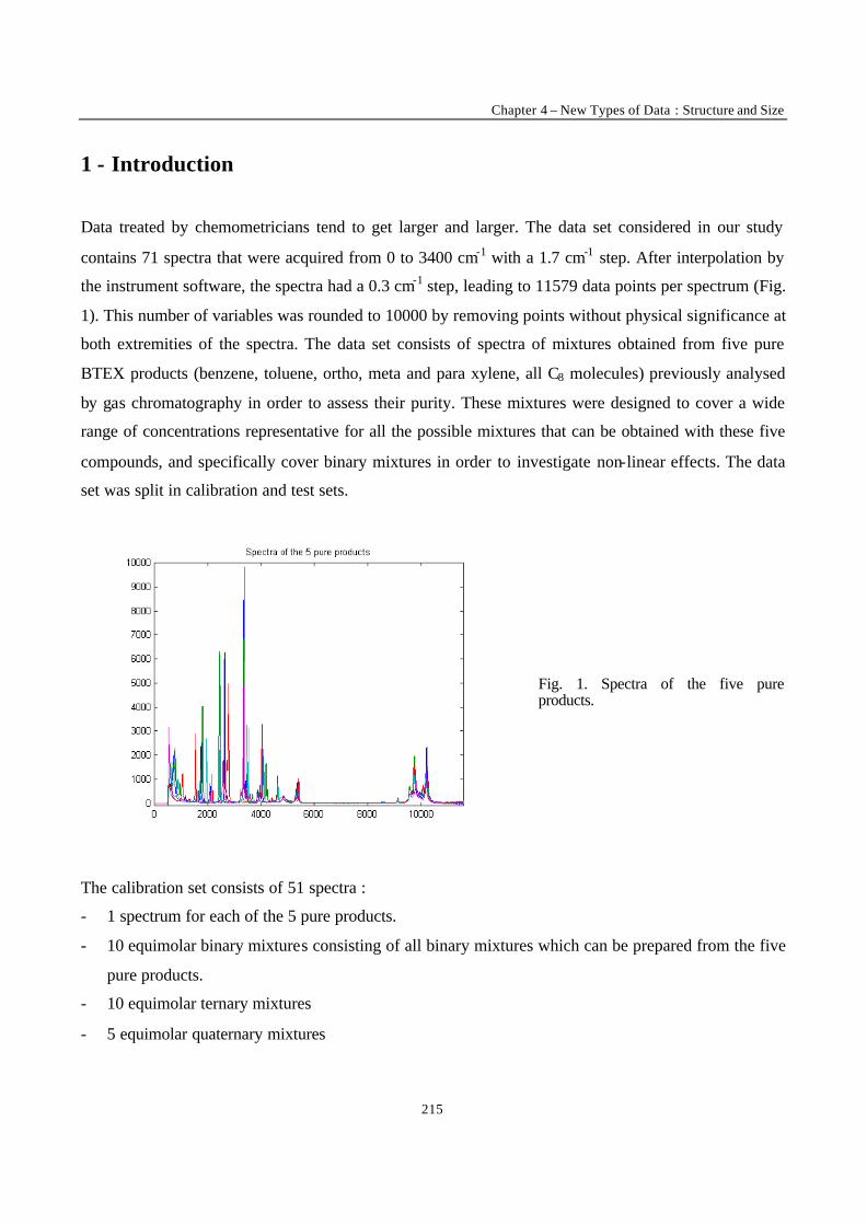
Chapter 4 – New Types of Data : Structure and Size
215
1 - Introduction
Data treated by chemometricians tend to get larger and larger. The data set considered in our study
contains 71 spectra that were acquired from 0 to 3400 cm-1 with a 1.7 cm-1 step. After interpolation by
the instrument software, the spectra had a 0.3 cm-1 step, leading to 11579 data points per spectrum (Fig.
1). This number of variables was rounded to 10000 by removing points without physical significance at
both extremities of the spectra. The data set consists of spectra of mixtures obtained from five pure
BTEX products (benzene, toluene, ortho, meta and para xylene, all C8 molecules) previously analysed
by gas chromatography in order to assess their purity. These mixtures were designed to cover a wide
range of concentrations representative for all the possible mixtures that can be obtained with these five
compounds, and specifically cover binary mixtures in order to investigate non-linear effects. The data
set was split in calibration and test sets.
Fig. 1. Spectra of the five pure products.
The calibration set consists of 51 spectra :
- 1 spectrum for each of the 5 pure products.
- 10 equimolar binary mixtures consisting of all binary mixtures which can be prepared from the five
pure products.
- 10 equimolar ternary mixtures
- 5 equimolar quaternary mixtures
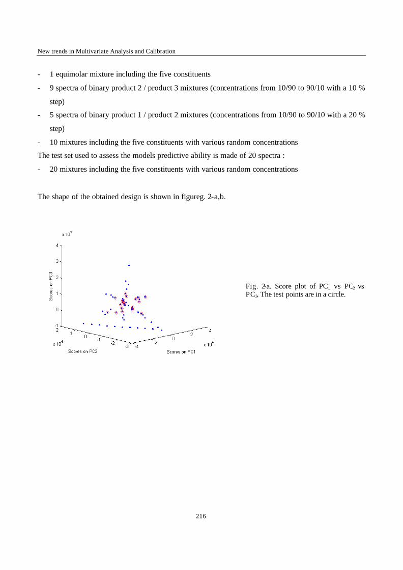
New trends in Multivariate Analysis and Calibration
216
- 1 equimolar mixture including the five constituents
- 9 spectra of binary product 2 / product 3 mixtures (concentrations from 10/90 to 90/10 with a 10 %
step)
- 5 spectra of binary product 1 / product 2 mixtures (concentrations from 10/90 to 90/10 with a 20 %
step)
- 10 mixtures including the five constituents with various random concentrations
The test set used to assess the models predictive ability is made of 20 spectra :
- 20 mixtures including the five constituents with various random concentrations
The shape of the obtained design is shown in figureg. 2-a,b.
Fig. 2-a. Score plot of PC1 vs PC2 vs PC3. The test points are in a circle.
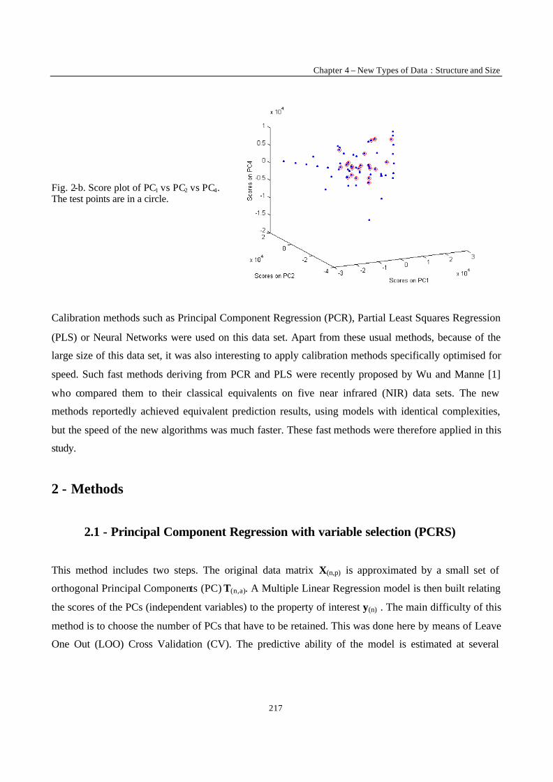
Chapter 4 – New Types of Data : Structure and Size
217
Fig. 2-b. Score plot of PC1 vs PC2 vs PC4. The test points are in a circle.
Calibration methods such as Principal Component Regression (PCR), Partial Least Squares Regression
(PLS) or Neural Networks were used on this data set. Apart from these usual methods, because of the
large size of this data set, it was also interesting to apply calibration methods specifically optimised for
speed. Such fast methods deriving from PCR and PLS were recently proposed by Wu and Manne [1]
who compared them to their classical equivalents on five near infrared (NIR) data sets. The new
methods reportedly achieved equivalent prediction results, using models with identical complexities,
but the speed of the new algorithms was much faster. These fast methods were therefore applied in this
study.
2 - Methods
2.1 - Principal Component Regression with variable selection (PCRS)
This method includes two steps. The original data matrix X(n,p) is approximated by a small set of
orthogonal Principal Components (PC) T(n,a). A Multiple Linear Regression model is then built relating
the scores of the PCs (independent variables) to the property of interest y(n) . The main difficulty of this
method is to choose the number of PCs that have to be retained. This was done here by means of Leave
One Out (LOO) Cross Validation (CV). The predictive ability of the model is estimated at several
New trends in Multivariate Analysis and Calibration
218
complexities (models including 1,2, … etc PCs) in terms of Root Mean Square Error of Cross
Validation (RMSECV). RMSECV is defined as :
nyiyin
/)ˆ(RMSECV1i
2∑=
−= (1)
where n is the number of calibration objects, yi the known value of the property of interest for object i,
and yiˆ the value of the property of interest predicted by the model for object i.
The complexity leading to the smallest RMSECV is considered as optimal in a first approach. In a
second step, in order to avoid overfitting, more parsimonious models (smaller complexities, one or
more of the last selected variables are removed) are tested to determine whether they can be considered
as equivalent in performance. The slightly worse RMSECV can in that case be compensated by a better
robustness of the resulting parsimonious model. This is done using a randomisation test [2,3]. This test
is applied to compare a prediction method at two different complexities. In the usual PCR [4], the
variables are introduced into the model according to the percentage of spectral variance (variance in X)
they explain. This is called PCR top-down. But the PCs explaining the largest part of the global
variance in X are not always the most related to y. PCR with variable selection (PCRS) was used in our
study. In PCRS, the PCs are included in the model according to their correlation [5] with y, or their
predictive ability [6].
2.2 - Partial Least Squares Regression
Similarly to PCR, PLS [7] reduces the data to a small number of latent variables. The basic idea is to
focus only on the systematic variation in X that is related to y. PLS maximises the covariance between
the spectral data and the property to be modelled. De Jong’s modified version [8] of the original
NIPALS [9,10] algorithm was used in this study. In the same way as for PCR, the optimal complexity
is determined by comparing the RMSECV obtained from models with various complexities. To avoid
overfitting, this complexity is then confirmed or corrected by comparing the model leading to the
smaller RMSECV with the more parsimonious ones using a randomisation test.
Chapter 4 – New Types of Data : Structure and Size
219
2.3 - Fast PCR and PLS algorithms
The fast algorithms are based on the Lanczos decomposition scheme [11,12,13]. The Lanczos method
is a way to efficiently solve eigenvalue problems. It has its fast convergence properties when applied to
a large, sparse and symmetric matrix A. The method generates a sequence of tridiagonal matrices T.
These matrices have the property that their extreme eigenvalues are progressively better estimates of
the extreme eigenvalues of A. The method is therefore useful when only a small number of the largest
and/or smallest eigenvalues of A are required. This is the case in calibration methods where
information present in a large X matrix has to be compressed to a small number of PCs. In the present
case, the decomposition scheme is applied on A = X’ X. The speed improvement is achieved only if T
is much smaller than A. In this case, the Singular Value Decomposition (SVD) of T is much faster than
the one of A, nevertheless leading to very similar eigenvalues. Two parameters have to be optimised
when performing a Lanczos-based SVD. The size of the small tridiagonal matrix T has to be set. It
corresponds to the number of Lanczos base vectors that have to be estimated (nl). The number of
factors (PCs) that have to be extracted (nf) also has to be set, considering that nf ≤ nl. These parameters
were estimated in two different ways. The first is based on LOO-CV, that was used to optimise first the
size of the Lanczos basis (nl) and then the number of eigenvectors extracted from the resulting matrix
(nf). A less time consuming approach was also used. The iterations of the Lanczos algorithms were
stopped before the loss of orthogonality between successive base vectors becomes important enough to
require special corrections. This behaviour of the Lanczos algorithm is well known and leads to
rounding errors that greatly affect the outcome of the method. The size of the Lanczos basis (nl) being
set this way, the number of factors to be extracted from the resulting matrix (nf) was estimated based on
model fit, by estimating how much each individual eigenvector contributes to the model of the property
of interest.
The model optimised through the CV procedure is called PCRL (L stands for Lanczos), and the models
obtained through the other approach is called PCRF (F stands for Fast). The PLS versio n of the fast
algorithms is presented by the authors of the original article as a special case in which the full space of
eigenvectors generated in the Lanczos basis is used, leading to nl = nf. The obtained models are denoted
by PLSF.

New trends in Multivariate Analysis and Calibration
220
2.4 - Neural Network (NN)
In our study Neural Networks calibration [14,15] was performed on the X data matrix after it was
compressed by means of PC transformation. The most relevant PCs, selected on the basis of explained
variance, are used as input to the NN. The number of hidden layers was set to 1 in our study. The
transfer function used in the hidden layer was non-linear (i.e. hyperbolic tangent). The weights were
optimised by means of the Levenberg-Marquardt algorithm [16]. A method was applied to find the best
number of nodes to be used in the input and hidden layers based on the contribution of each node [17].
The optimisation procedure of NN also requires the calibration set to be split into training and
monitoring set in order to avoid overfitting. The last 10 spectra of the calibration set (10 mixtures
including the five constituents with various random concentrations) were used as monitoring set since
they can be expected to be most representative of future mixtures to be predicted.
3 - Results and discussion
All calculations were performed on a personal computer equipped with an AMD Athlon 600 Mhz
processor and 256 Megs of RAM, in the Matlab environment. The software used is house made
except for the new methods for which the code provided as annex in the original paper [1] was used.
The results used to assess the predictive ability of the methods are given in terms of Root Mean
Squared Error of Prediction (RMSEP) which is defined as :
nn
yiyi t/)ˆ(RMSEPt
1i
2∑=
−= (2)
where nt is the number of objects in the test set, yi the known value of the property of interest for object
i, and yiˆ the value of the property of interest predicted by the model for object i.
The speed of the methods is measured by estimating the number of operations necessary to perform the
complete calibration and prediction procedure. This number of operations is estimated using the
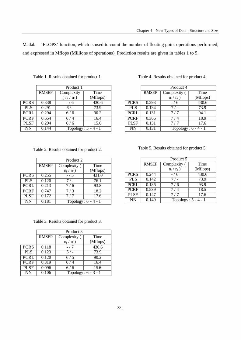
Chapter 4 – New Types of Data : Structure and Size
221
Matlab ‘FLOPS’ function, which is used to count the number of floating-point operations performed,
and expressed in Mflops (Millions of operations). Prediction results are given in tables 1 to 5.
Table 1. Results obtained for product 1.
Product 1 RMSEP Complexity
( nl / nf ) Time
(Mflops) PCRS 0.338 - / 6 430.6 PLS 0.291 6 / - 73.9
PCRL 0.294 6 / 6 90.2 PCRF 0.654 6 / 4 16.4 PLSF 0.294 6 / 6 15.6 NN 0.144 Topology : 5 - 4 - 1
Table 2. Results obtained for product 2.
Product 2 RMSEP Complexity (
nl / nf ) Time
(Mflops) PCRS 0.255 - / 5 431.0 PLS 0.120 7 / - 76.1
PCRL 0.213 7 / 6 93.8 PCRF 0.747 7 / 3 18.2 PLSF 0.172 7 / 7 17.6 NN 0.181 Topology : 6 - 4 - 1
Table 3. Results obtained for product 3.
Product 3 RMSEP Complexity (
nl / nf ) Time
(Mflops) PCRS 0.118 - / 7 430.6 PLS 0.123 5 / - 73.9
PCRL 0.120 6 / 5 90.2 PCRF 0.319 6 / 4 16.4 PLSF 0.096 6 / 6 15.6 NN 0.106 Topology : 6 - 3 - 1
Table 4. Results obtained for product 4.
Product 4 RMSEP Complexity (
nl / nf ) Time
(Mflops) PCRS 0.293 - / 6 430.6 PLS 0.134 7 / - 73.9
PCRL 0.131 7 / 7 94.1 PCRF 0.366 7 / 4 18.9 PLSF 0.131 7 / 7 17.6 NN 0.131 Topology : 6 - 4 - 1
Table 5. Results obtained for product 5.
Product 5 RMSEP Complexity (
nl / nf ) Time
(Mflops) PCRS 0.244 - / 6 430.6 PLS 0.142 7 / - 73.9
PCRL 0.186 7 / 6 93.9 PCRF 0.539 7 / 4 18.5 PLSF 0.147 7 / 7 17.6 NN 0.149 Topology : 5 - 4 - 1
New trends in Multivariate Analysis and Calibration
222
The model complexities can seem surprisingly high. When studying five compounds mixtures,
considering the mixtures contain no other substances, one expects models with a complexity equal to 4
(1 component per compound, reduced by one due to closure effect). This was indeed the case in a
previous study in which the same kind of mixtures was studied [18]. In this new data set, a wider
spectral region is used, the instrument has a much higher resolution, and most important of all, the
signal/noise ration is by far better. This much higher quality of the instruments gave access to more of
the information present in the data. The data set used here was previously studied [19] and it was found
that mixture effects lead to non- linear behaviour. Therefore, the best overall calibration results were
obtained with a non-linear method, namely Neural Networks using non- linear transfer functions. NN
results are therefore presented in this paper as a benchmark. PCR and PLS models give an illustration
of the fact that slight non- linearities can be compensated by the inclusion of extra components [7].
When models with only 4 components are used, all linear methods achieve RMSEPs close to 0.5. The
inclusion of extra components enables to improve greatly these results. Since the results are given in
terms of RMSEP (therefore calculated on an independent test set), this improvement can not be
attributed to overfitting. In case of overfitting, the RMSECV results would be improved after inclusion
of the extra components, but the results obtained for prediction on the test set would not. The quality of
the results obtained for the various methods greatly depends on the complexity used. The PCRF
method retained from 3 to 4 PCs out of a Lanczos base of 6 to 7 vectors. This method achieves as
expected RMSEPs around 0.5. No extra PCs are included in the model, the non- linear effects are not
taken into account, leading to high RMSEP values. The cross validation followed by randomisation test
procedure used for PCRS and PLS lead to models retaining 5 to 7 components. The results are better
for PLS that generally uses a slightly higher complexity in this study. The fast PCR optimised by CV
(PCRF) led to complexities comparable to PLS, therefore leading to equivalent prediction
performances. The best results for PCR/PLS based methods are obtained with PLSF. By using all the
components extractable from the Lanczos base, i.e. 6 to 7 components, it yields results comparable to
those obtained with Neural Networks. However, NN remains the overall best performing method in
terms of prediction quality.
The speed of calculations confirms the conclusions of Wu and Manne [1]. The most time consuming
method is PCR optimised by CV (PCRS). PLS, although optimised by CV as well, performs about 6
times faster. The fast Lanczos PCR optimised by CV (PCRL) performs almost as fast a PLS. The
Chapter 4 – New Types of Data : Structure and Size
223
fastest methods are PCRF and PLSF. They perform about 5 times faster than PLS, which means almost
30 times faster than PCRS.
4 - Conclusions
Neural Networks remain the overall best performing method in terms of prediction on this non- linear
data set. The fast PCR and PLS methods based on the Lanczos decomposition were able to achieve at
least as good results as their classical equivalents, and these results were obtained considerably faster.
However, the PCRF method tended to retain too few components. The PLSF method achieved good
results mainly because it retained the full range of components that could be extracted from the
Lanczos space. The Lanczos based PCR optimised by CV gave good results with more parsimonious
complexities. The Lanczos approach can therefore be used to speed up calculations, however, cross-
validation seems to remain the method of choice to estimate adequate model complexity.
REFERENCES
[1] W. Wu, R. Manne, Chemom. Intell. Lab. Sys. 51, no. 2 (2000) 145-161.
[2] H. van der Voet, Chemom. Intell. Lab. Sys. 25 (1994) 313-323.
[3] H. van der Voet, Chemom. Intell. Lab. Sys. 28 (1995) 315.
[4] T. Naes, H. Martens, J. Chemom. 2 (1998) 155-167.
[5]. J. Sun, J. Chemom. 9 (1995) 21-29.
[6] J. M. Sutter, J. H. Kalivas, P.M. Lang, J. Chemom. 6 (1992) 217-225.
[7] H. Martens, T. Naes, Multivariate Calibration (Wiley, Chichester,1989).
[8] S. de Jong, Chemom. Intell. Lab. Sys. 18 (1993) 251-263.
[9] D. M. Haaland, E. V. Thomas, Anal. Chem. 60 (1988) 1193-1202.
[10] P. Geladi, B. K. Kovalski, Anal. Chim. Acta 185 (1986) 1-17.
[11] C. Lanczos, J. Res. Nat. Bur. Stand, 45 (1950) 255-282.
[12] G. H. Golub, C. F. Van Loan, Matrix Computations, North Oxford Academic, Oxford, 1983.
[13] L. N. Trefethen and D. Bau, III, Numerical linear algebra, SIAM, Philadelphia, 1997.
[14] F. Despagne, D.L. Massart, The Analyst, 123 (1998) 157R-178R

New trends in Multivariate Analysis and Calibration
224
[15] J.R.M. Smits, W.J. Melssen, L.M.C. Buydens, G. Kateman, Chemom. Intell. Lab. Syst., 22
(1994) 165-173.
[16] R. Fletcher, Practical Methods of optimization, Wiley, N.Y., 1987.
[17] F. Despagne, D.L. Massart, Chemom. Intel. lab. syst., 40 (1998) 145-163.
[18] F. Estienne, N. Zanier, P. Marteau, D.L. Massart, Analytica Chimica Acta, 424 (2000) 185-201.
[19] N. Zanier, P. Marteau, F. Estienne. In preparation.
Chapter 4 – New Types of Data : Structure and Size
225
MULTI-WAY MODELLING OF HIGH-DIMENSIONALITY
ELECTRO-ENCEPHALOGRAPHIC DATA
Chemometrics and Intelligent Laboratory Systems, 58 (2001) 59-72.
F. Estienne , N. Matthijs, D. L. Massart*
ChemoAC Farmaceutisch Instituut,
Vrije Universiteit Brussel, Laarbeeklaan 103,
B-1090 Brussels, Belgium. E-mail: [email protected]
P. Ricoux
ELF 69000 Lyon, France
D. Leibovici
Image Analysis Group FMRIB Centre
Oxford University John Radcliffe Hospital Oxford OX3 9DU,
U.K.
ABSTRACT
The aim of this study is to investigate whether useful information can be extracted from an electroencephalographic (EEG) data set with a very high number of modes, and to determine which model is the most appropriate for this purpose. The data was acquired during the testing phase of a new drug expected to have effect on the brain activity. The implemented test program (several patients followed in time, different doses, conditions, etc …) led to a 6-way data set. After it was confirmed that the exploratory analysis of this data set could not be handled with classical PCA, and it was verified that multi-dimensional structure was present, multi-way methods were used to model the data. It appeared that Tucker 3 was the most suited model. It was possible to extract useful information from this high-dimensionality data. Non-relevant sources of variance (outlying patients for instance) were identified so that they can be removed before the in-depth physiological study is performed.
* Corresponding author
KEYWORDS : Multi-way methods, Tucker 3, PARAFAC, Exploratory analysis,
Electroencephalography, EEG
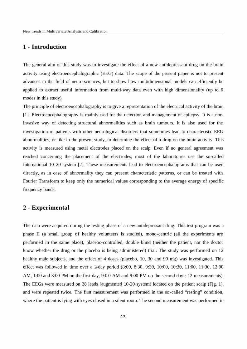
New trends in Multivariate Analysis and Calibration
226
1 - Introduction
The general aim of this study was to investigate the effect of a new antidepressant drug on the brain
activity using electroencephalographic (EEG) data. The scope of the present paper is not to present
advances in the field of neuro-sciences, but to show how multidimensional models can efficiently be
applied to extract useful information from multi-way data even with high dimensionality (up to 6
modes in this study).
The principle of electroencephalography is to give a representation of the electrical activity of the brain
[1]. Electroencephalography is mainly used for the detection and management of epilepsy. It is a non-
invasive way of detecting structural abnormalities such as brain tumours. It is also used for the
investigation of patients with other neurological disorders that sometimes lead to characteristic EEG
abnormalities, or like in the present study, to determine the effect of a drug on the brain activity. This
activity is measured using metal electrodes placed on the scalp. Even if no general agreement was
reached concerning the placement of the elect rodes, most of the laboratories use the so-called
International 10-20 system [2]. These measurements lead to electroencephalograms that can be used
directly, as in case of abnormality they can present characteristic patterns, or can be treated with
Fourier Transform to keep only the numerical values corresponding to the average energy of specific
frequency bands.
2 - Experimental
The data were acquired during the testing phase of a new antidepressant drug. This test program was a
phase II (a small group of healthy volunteers is studied), mono-centric (all the experiments are
performed in the same place), placebo-controlled, double blind (neither the patient, nor the doctor
know whether the drug or the placebo is being administered) trial. The study was performed on 12
healthy male subjects, and the effect of 4 doses (placebo, 10, 30 and 90 mg) was investigated. This
effect was followed in time over a 2-day period (8:00, 8:30, 9:30, 10:00, 10:30, 11:00, 11:30, 12:00
AM, 1:00 and 3:00 PM on the first day, 9:0 0 AM and 9:00 PM on the second day : 12 measurements).
The EEGs were measured on 28 leads (augmented 10-20 system) located on the patient scalp (Fig. 1),
and were repeated twice. The first measurement was performed in the so-called “resting” condition,
where the patient is lying with eyes closed in a silent room. The second measurement was performed in
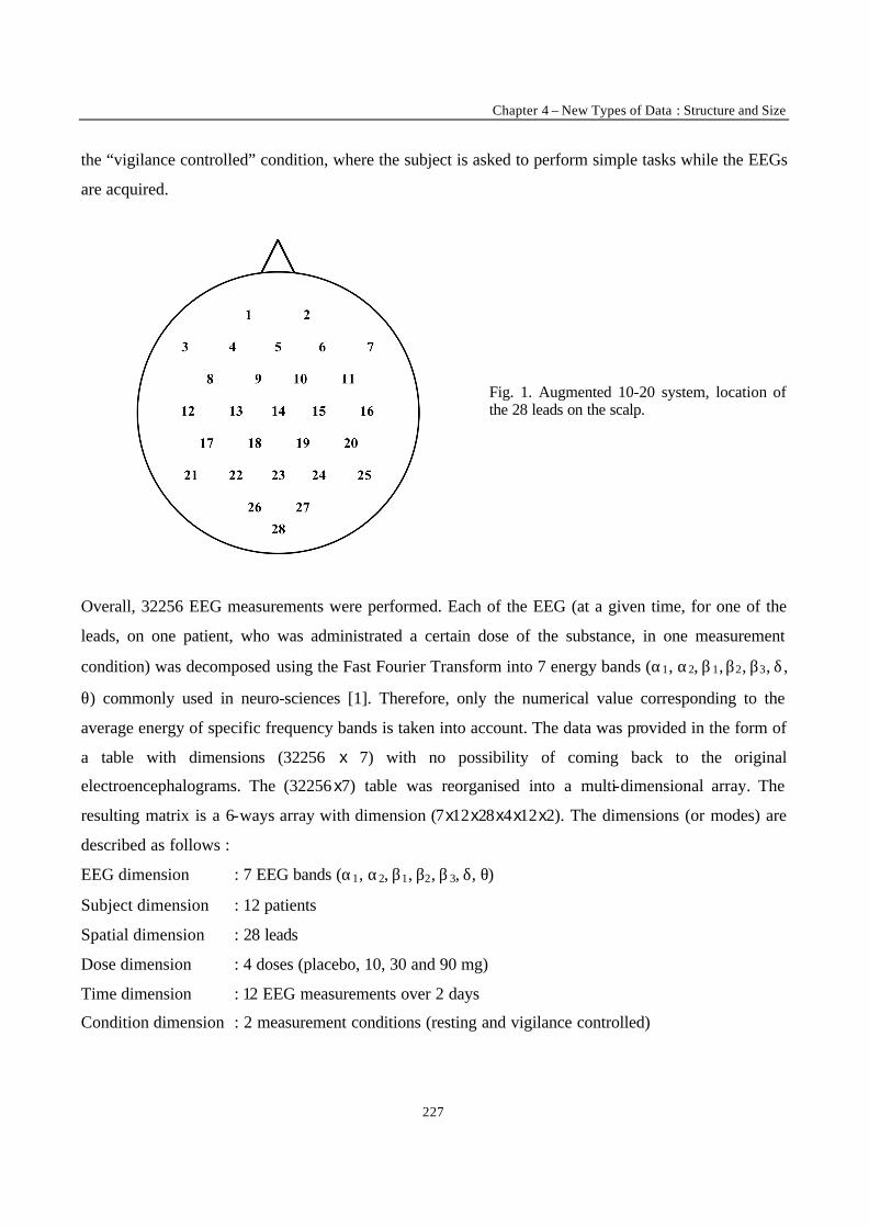
Chapter 4 – New Types of Data : Structure and Size
227
the “vigilance controlled” condition, where the subject is asked to perform simple tasks while the EEGs
are acquired.
Fig. 1. Augmented 10-20 system, location of the 28 leads on the scalp.
Overall, 32256 EEG measurements were performed. Each of the EEG (at a given time, for one of the
leads, on one patient, who was administrated a certain dose of the substance, in one measurement
condition) was decomposed using the Fast Fourier Transform into 7 energy bands (α1, α2, β1, β2, β3, δ ,
θ) commonly used in neuro-sciences [1]. Therefore, only the numerical value corresponding to the
average energy of specific frequency bands is taken into account. The data was provided in the form of
a table with dimensions (32256 x 7) with no possibility of coming back to the original
electroencephalograms. The (32256x7) table was reorganised into a multi-dimensional array. The
resulting matrix is a 6-ways array with dimension (7x12x28x4x12x2). The dimensions (or modes) are
described as follows :
EEG dimension : 7 EEG bands (α1, α2, β1, β2, β3, δ, θ)
Subject dimension : 12 patients
Spatial dimension : 28 leads
Dose dimension : 4 doses (placebo, 10, 30 and 90 mg)
Time dimension : 12 EEG measurements over 2 days
Condition dimension : 2 measurement conditions (resting and vigilance controlled)
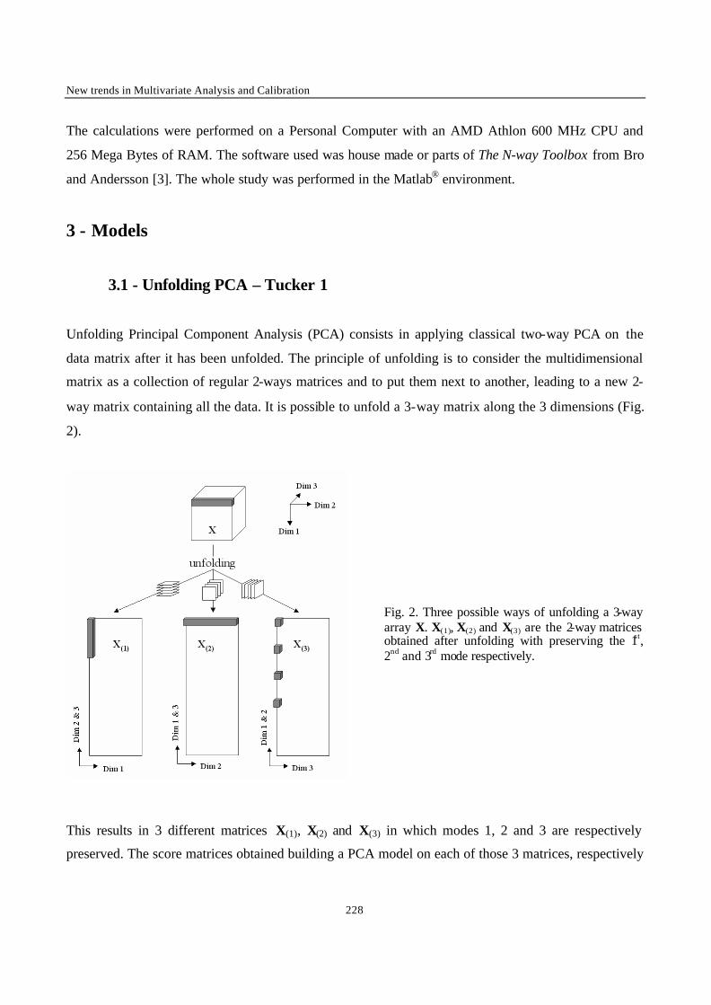
New trends in Multivariate Analysis and Calibration
228
The calculations were performed on a Personal Computer with an AMD Athlon 600 MHz CPU and
256 Mega Bytes of RAM. The software used was house made or parts of The N-way Toolbox from Bro
and Andersson [3]. The whole study was performed in the Matlab® environment.
3 - Models
3.1 - Unfolding PCA – Tucker 1
Unfolding Principal Component Analysis (PCA) consists in applying classical two-way PCA on the
data matrix after it has been unfolded. The principle of unfolding is to consider the multidimensional
matrix as a collection of regular 2-ways matrices and to put them next to another, leading to a new 2-
way matrix containing all the data. It is possible to unfold a 3-way matrix along the 3 dimensions (Fig.
2).
Fig. 2. Three possible ways of unfolding a 3-way array X. X(1), X(2) and X(3) are the 2-way matrices obtained after unfolding with preserving the 1st, 2nd and 3rd mode respectively.
This results in 3 different matrices X(1), X(2) and X(3) in which modes 1, 2 and 3 are respectively
preserved. The score matrices obtained building a PCA model on each of those 3 matrices, respectively
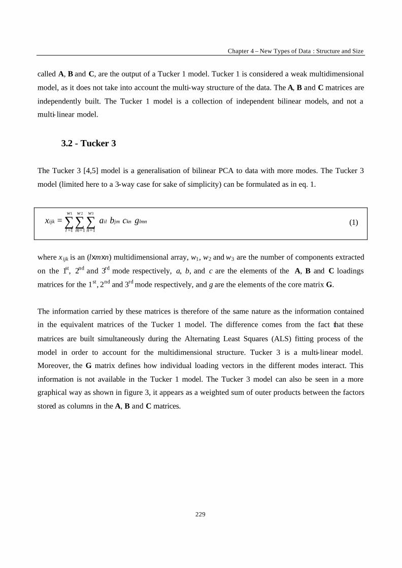
Chapter 4 – New Types of Data : Structure and Size
229
called A, B and C, are the output of a Tucker 1 model. Tucker 1 is considered a weak multidimensional
model, as it does not take into account the multi-way structure of the data. The A, B and C matrices are
independently built. The Tucker 1 model is a collection of independent bilinear models, and not a
multi- linear model.
3.2 - Tucker 3
The Tucker 3 [4,5] model is a generalisation of bilinear PCA to data with more modes. The Tucker 3
model (limited here to a 3-way case for sake of simplicity) can be formulated as in eq. 1.
∑∑∑= = =
=1 2 3
1 1 1
w
l
w
m
w
n
lmnknjmilijk gcbax (1)
where x ijk is an (lxmxn) multidimensional array, w1, w2 and w3 are the number of components extracted
on the 1st, 2nd and 3rd mode respectively, a, b, and c are the elements of the A, B and C loadings
matrices for the 1st, 2nd and 3rd mode respectively, and g are the elements of the core matrix G.
The information carried by these matrices is therefore of the same nature as the information contained
in the equivalent matrices of the Tucker 1 model. The difference comes from the fact that these
matrices are built simultaneously during the Alternating Least Squares (ALS) fitting process of the
model in order to account for the multidimensional structure. Tucker 3 is a multi-linear model.
Moreover, the G matrix defines how individual loading vectors in the different modes interact. This
information is not available in the Tucker 1 model. The Tucker 3 model can also be seen in a more
graphical way as shown in figure 3, it appears as a weighted sum of outer products between the factors
stored as columns in the A, B and C matrices.
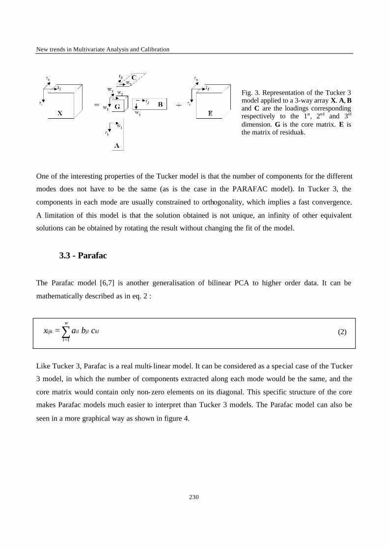
New trends in Multivariate Analysis and Calibration
230
Fig. 3. Representation of the Tucker 3 model applied to a 3-way array X. A, B and C are the loadings corresponding respectively to the 1st, 2nd and 3rd dimension. G is the core matrix. E is the matrix of residuals.
One of the interesting properties of the Tucker model is that the number of components for the different
modes does not have to be the same (as is the case in the PARAFAC model). In Tucker 3, the
components in each mode are usually constrained to orthogonality, which implies a fast convergence.
A limitation of this model is that the solution obtained is not unique, an infinity of other equivalent
solutions can be obtained by rotating the result without changing the fit of the model.
3.3 - Parafac
The Parafac model [6,7] is another generalisation of bilinear PCA to higher order data. It can be
mathematically described as in eq. 2 :
∑=
=w
l
kljlilijk cbax1
(2)
Like Tucker 3, Parafac is a real multi- linear model. It can be considered as a special case of the Tucker
3 model, in which the number of components extracted along each mode would be the same, and the
core matrix would contain only non-zero elements on its diagonal. This specific structure of the core
makes Parafac models much easier to interpret than Tucker 3 models. The Parafac model can also be
seen in a more graphical way as shown in figure 4.

Chapter 4 – New Types of Data : Structure and Size
231
Fig. 4. Representation of the Parafac model applied to a 3-way array X. A, B and C are the loadings corresponding to the 1st, 2nd and 3rd dimension. G is the super-diagonal core matrix. E is the matrix of residuals.
The most interesting feature of the Parafac model is uniqueness. The model provides unique factor
estimates, the solution obtained cannot be rotated without modification of its fit. As components on
each mode are not constrained to orthogonality, the convergence is usually quite slower than observed
with the Tucker 3 model.
4 - Results and discussion
4.1 - Linear and bi-linear models
Because of the nature of the data set, it was very difficult to explore it visually the way it is usually
done for instance with spectral data. In order to get a better insight of the data, some averages were
computed directly from the original variables. This corresponds to building simple linear models. The
global average (on patients, doses and conditions) for the energy bands can then be displayed on a map
of the brain for each of the measurement times. It is then possible to see in a rough way the evolution of
the activity of the brain as a function of time and of the location in the brain (Fig. 5).
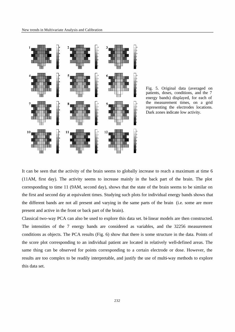
New trends in Multivariate Analysis and Calibration
232
Fig. 5. Original data (averaged on patients, doses, conditions, and the 7 energy bands) displayed, for each of the measurement times, on a grid representing the electrodes locations. Dark zones indicate low activity.
It can be seen that the activity of the brain seems to globally increase to reach a maximum at time 6
(11AM, first day). The activity seems to increase mainly in the back part of the brain. The plot
corresponding to time 11 (9AM, second day), shows that the state of the brain seems to be similar on
the first and second day at equivalent times. Studying such plots for individual energy bands shows that
the different bands are not all present and varying in the same parts of the brain (i.e. some are more
present and active in the front or back part of the brain).
Classical two-way PCA can also be used to explore this data set. bi- linear models are then constructed.
The intensities of the 7 energy bands are considered as variables, and the 32256 measurement
conditions as objects. The PCA results (Fig. 6) show that there is some structure in the data. Points of
the score plot corresponding to an individual patient are located in relatively well-defined areas. The
same thing can be observed for points corresponding to a certain electrode or dose. However, the
results are too complex to be readily interpretable, and justify the use of multi-way methods to explore
this data set.
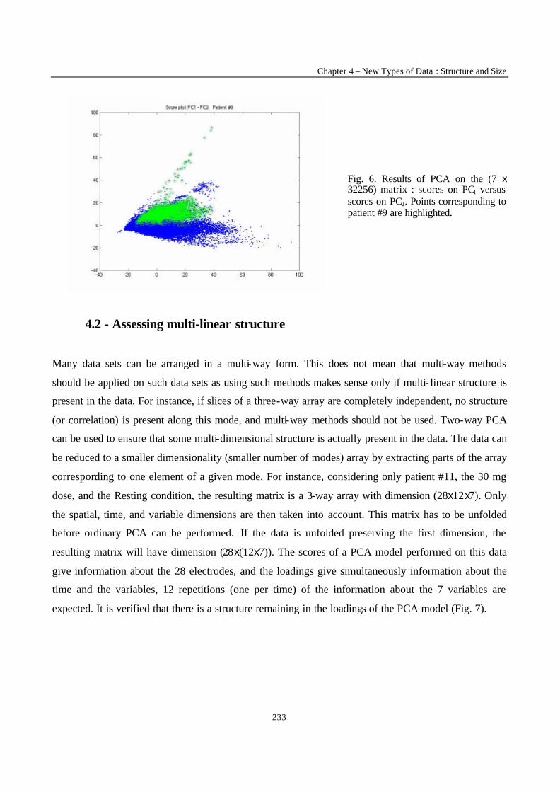
Chapter 4 – New Types of Data : Structure and Size
233
Fig. 6. Results of PCA on the (7 x 32256) matrix : scores on PC1 versus scores on PC2. Points corresponding to patient #9 are highlighted.
4.2 - Assessing multi-linear structure
Many data sets can be arranged in a multi-way form. This does not mean that multi-way methods
should be applied on such data sets as using such methods makes sense only if multi- linear structure is
present in the data. For instance, if slices of a three-way array are completely independent, no structure
(or correlation) is present along this mode, and multi-way methods should not be used. Two-way PCA
can be used to ensure that some multi-dimensional structure is actually present in the data. The data can
be reduced to a smaller dimensionality (smaller number of modes) array by extracting parts of the array
corresponding to one element of a given mode. For instance, considering only patient #11, the 30 mg
dose, and the Resting condition, the resulting matrix is a 3-way array with dimension (28x12x7). Only
the spatial, time, and variable dimensions are then taken into account. This matrix has to be unfolded
before ordinary PCA can be performed. If the data is unfolded preserving the first dimension, the
resulting matrix will have dimension (28x(12x7)). The scores of a PCA model performed on this data
give information about the 28 electrodes, and the loadings give simultaneously information about the
time and the variables, 12 repetitions (one per time) of the information about the 7 variables are
expected. It is verified that there is a structure remaining in the loadings of the PCA model (Fig. 7).
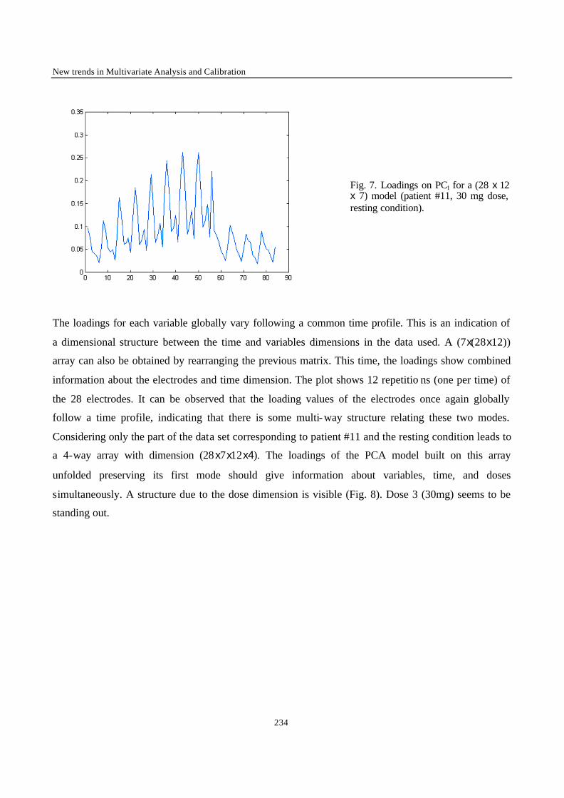
New trends in Multivariate Analysis and Calibration
234
Fig. 7. Loadings on PC1 for a (28 x 12 x 7) model (patient #11, 30 mg dose, resting condition).
The loadings for each variable globally vary following a common time profile. This is an indication of
a dimensional structure between the time and variables dimensions in the data used. A (7x(28x12))
array can also be obtained by rearranging the previous matrix. This time, the loadings show combined
information about the electrodes and time dimension. The plot shows 12 repetitio ns (one per time) of
the 28 electrodes. It can be observed that the loading values of the electrodes once again globally
follow a time profile, indicating that there is some multi-way structure relating these two modes.
Considering only the part of the data set corresponding to patient #11 and the resting condition leads to
a 4-way array with dimension (28x7x12x4). The loadings of the PCA model built on this array
unfolded preserving its first mode should give information about variables, time, and doses
simultaneously. A structure due to the dose dimension is visible (Fig. 8). Dose 3 (30mg) seems to be
standing out.
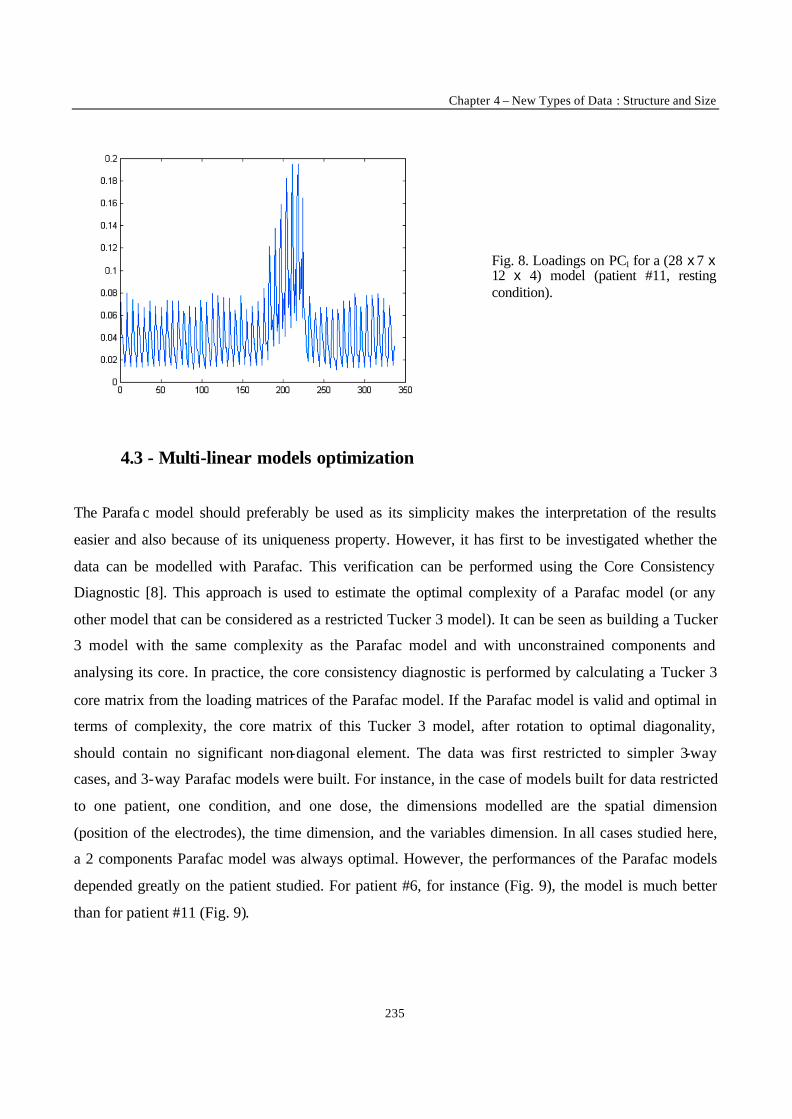
Chapter 4 – New Types of Data : Structure and Size
235
Fig. 8. Loadings on PC1 for a (28 x 7 x 12 x 4) model (patient #11, resting condition).
4.3 - Multi-linear models optimization
The Parafa c model should preferably be used as its simplicity makes the interpretation of the results
easier and also because of its uniqueness property. However, it has first to be investigated whether the
data can be modelled with Parafac. This verification can be performed using the Core Consistency
Diagnostic [8]. This approach is used to estimate the optimal complexity of a Parafac model (or any
other model that can be considered as a restricted Tucker 3 model). It can be seen as building a Tucker
3 model with the same complexity as the Parafac model and with unconstrained components and
analysing its core. In practice, the core consistency diagnostic is performed by calculating a Tucker 3
core matrix from the loading matrices of the Parafac model. If the Parafac model is valid and optimal in
terms of complexity, the core matrix of this Tucker 3 model, after rotation to optimal diagonality,
should contain no significant non-diagonal element. The data was first restricted to simpler 3-way
cases, and 3-way Parafac models were built. For instance, in the case of models built for data restricted
to one patient, one condition, and one dose, the dimensions modelled are the spatial dimension
(position of the electrodes), the time dimension, and the variables dimension. In all cases studied here,
a 2 components Parafac model was always optimal. However, the performances of the Parafac models
depended greatly on the patient studied. For patient #6, for instance (Fig. 9), the model is much better
than for patient #11 (Fig. 9).
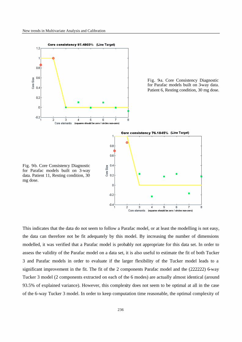
New trends in Multivariate Analysis and Calibration
236
Fig. 9-a. Core Consistency Diagnostic for Parafac models built on 3-way data. Patient 6, Resting condition, 30 mg dose.
Fig. 9-b. Core Consistency Diagnostic for Parafac models built on 3-way data. Patient 11, Resting condition, 30 mg dose.
This indicates that the data do not seem to follow a Parafac model, or at least the modelling is not easy,
the data can therefore not be fit adequately by this model. By increasing the number of dimensions
modelled, it was verified that a Parafac model is probably not appropriate for this data set. In order to
assess the validity of the Parafac model on a data set, it is also useful to estimate the fit of both Tucker
3 and Parafac models in order to evaluate if the larger flexibility of the Tucker model leads to a
significant improvement in the fit. The fit of the 2 components Parafac model and the (222222) 6-way
Tucker 3 model (2 components extracted on each of the 6 modes) are actually almost identical (around
93.5% of explained variance). However, this complexity does not seem to be optimal at all in the case
of the 6-way Tucker 3 model. In order to keep computation time reasonable, the optimal complexity of
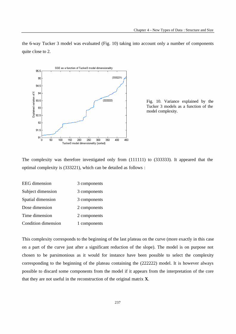
Chapter 4 – New Types of Data : Structure and Size
237
the 6-way Tucker 3 model was evaluated (Fig. 10) taking into account only a number of components
quite close to 2.
Fig. 10. Variance explained by the Tucker 3 models as a function of the model complexity.
The complexity was therefore investigated only from (111111) to (333333). It appeared that the
optimal complexity is (333221), which can be detailed as follows :
EEG dimension 3 components
Subject dimension 3 components
Spatial dimension 3 components
Dose dimension 2 components
Time dimension 2 components
Condition dimension 1 components
This complexity corresponds to the beginning of the last plateau on the curve (more exactly in this case
on a part of the curve just after a significant reduction of the slope). The model is on purpose not
chosen to be parsimonious as it would for instance have been possible to select the complexity
corresponding to the beginning of the plateau containing the (222222) model. It is however always
possible to discard some components from the model if it appears from the interpretation of the core
that they are not useful in the reconstruction of the original matrix X.
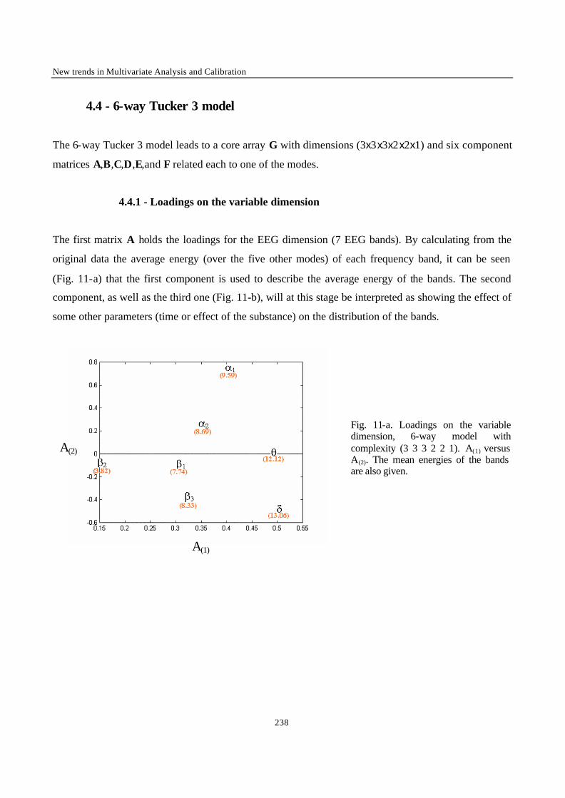
New trends in Multivariate Analysis and Calibration
238
4.4 - 6-way Tucker 3 model
The 6-way Tucker 3 model leads to a core array G with dimensions (3x3x3x2x2x1) and six component
matrices A,B,C,D,E,and F related each to one of the modes.
4.4.1 - Loadings on the variable dimension
The first matrix A holds the loadings for the EEG dimension (7 EEG bands). By calculating from the
original data the average energy (over the five other modes) of each frequency band, it can be seen
(Fig. 11-a) that the first component is used to describe the average energy of the bands. The second
component, as well as the third one (Fig. 11-b), will at this stage be interpreted as showing the effect of
some other parameters (time or effect of the substance) on the distribution of the bands.
Fig. 11-a. Loadings on the variable dimension, 6-way model with complexity (3 3 3 2 2 1). A(1) versus A(2). The mean energies of the bands are also given.
A(1)
A(2)
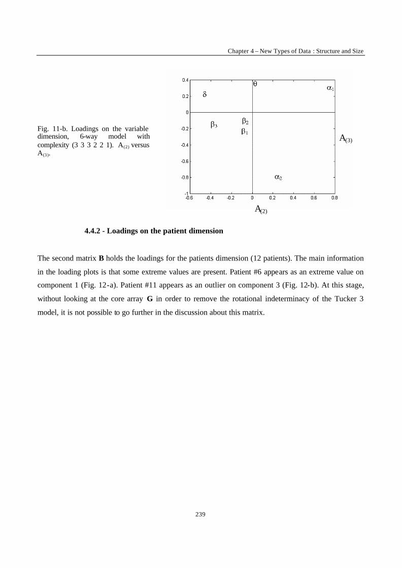
Chapter 4 – New Types of Data : Structure and Size
239
Fig. 11-b. Loadings on the variable dimension, 6-way model with complexity (3 3 3 2 2 1). A(2) versus A(3).
4.4.2 - Loadings on the patient dimension
The second matrix B holds the loadings for the patients dimension (12 patients). The main information
in the loading plots is that some extreme values are present. Patient #6 appears as an extreme value on
component 1 (Fig. 12-a). Patient #11 appears as an outlier on component 3 (Fig. 12-b). At this stage,
without looking at the core array G in order to remove the rotational indeterminacy of the Tucker 3
model, it is not possible to go further in the discussion about this matrix.
A(3)
A(2)
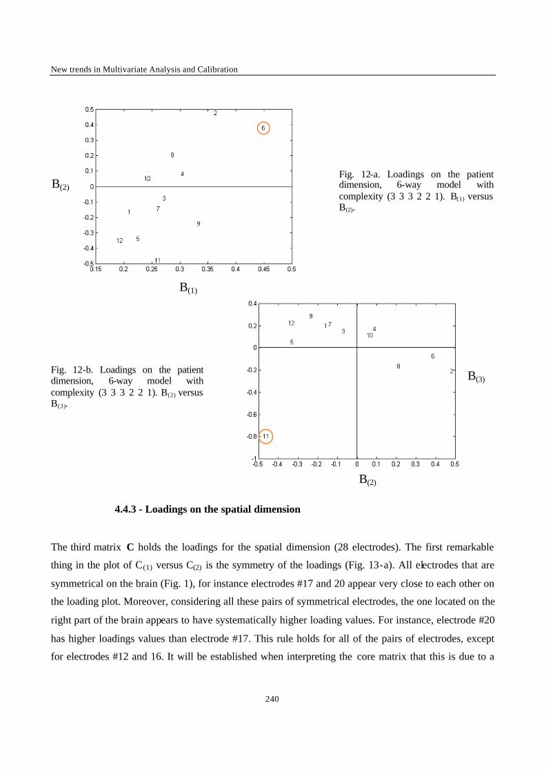
New trends in Multivariate Analysis and Calibration
240
Fig. 12-a. Loadings on the patient dimension, 6-way model with complexity (3 3 3 2 2 1). B(1) versus B(2).
Fig. 12-b. Loadings on the patient dimension, 6-way model with complexity (3 3 3 2 2 1). B(2) versus B(3).
4.4.3 - Loadings on the spatial dimension
The third matrix C holds the loadings for the spatial dimension (28 electrodes). The first remarkable
thing in the plot of C(1) versus C(2) is the symmetry of the loadings (Fig. 13-a). All electrodes that are
symmetrical on the brain (Fig. 1), for instance electrodes #17 and 20 appear very close to each other on
the loading plot. Moreover, considering all these pairs of symmetrical electrodes, the one located on the
right part of the brain appears to have systematically higher loading values. For instance, electrode #20
has higher loadings values than electrode #17. This rule holds for all of the pairs of electrodes, except
for electrodes #12 and 16. It will be established when interpreting the core matrix that this is due to a
B(2)
B(1)
B(3)
B(2)
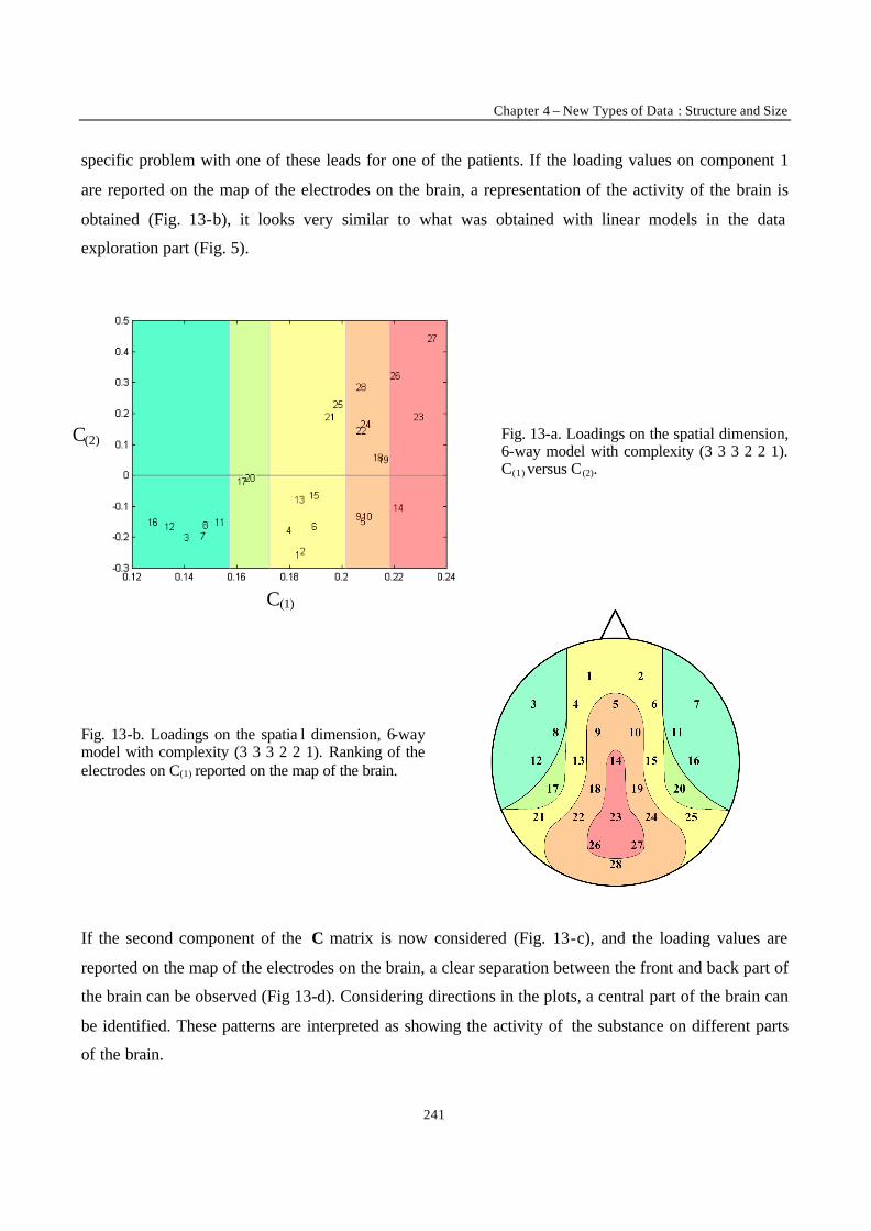
Chapter 4 – New Types of Data : Structure and Size
241
specific problem with one of these leads for one of the patients. If the loading values on component 1
are reported on the map of the electrodes on the brain, a representation of the activity of the brain is
obtained (Fig. 13-b), it looks very similar to what was obtained with linear models in the data
exploration part (Fig. 5).
Fig. 13-a. Loadings on the spatial dimension, 6-way model with complexity (3 3 3 2 2 1). C(1) versus C (2).
Fig. 13-b. Loadings on the spatia l dimension, 6-way model with complexity (3 3 3 2 2 1). Ranking of the electrodes on C(1) reported on the map of the brain.
If the second component of the C matrix is now considered (Fig. 13-c), and the loading values are
reported on the map of the electrodes on the brain, a clear separation between the front and back part of
the brain can be observed (Fig 13-d). Considering directions in the plots, a central part of the brain can
be identified. These patterns are interpreted as showing the activity of the substance on different parts
of the brain.
C(2)
C(1)
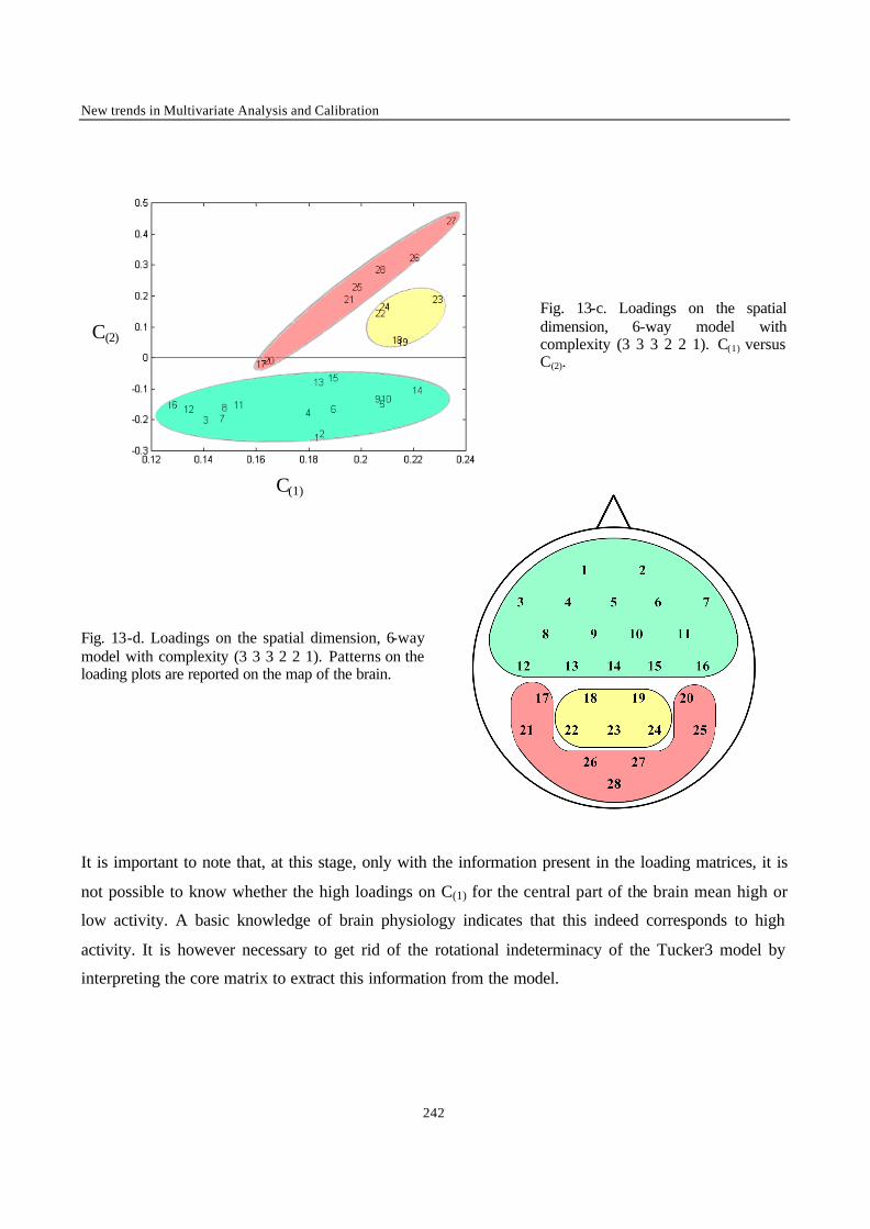
New trends in Multivariate Analysis and Calibration
242
Fig. 13-c. Loadings on the spatial dimension, 6-way model with complexity (3 3 3 2 2 1). C(1) versus C(2).
Fig. 13-d. Loadings on the spatial dimension, 6-way model with complexity (3 3 3 2 2 1). Patterns on the loading plots are reported on the map of the brain.
It is important to note that, at this stage, only with the information present in the loading matrices, it is
not possible to know whether the high loadings on C(1) for the central part of the brain mean high or
low activity. A basic knowledge of brain physiology indicates that this indeed corresponds to high
activity. It is however necessary to get rid of the rotational indeterminacy of the Tucker3 model by
interpreting the core matrix to extract this information from the model.
C(2)
C(1)
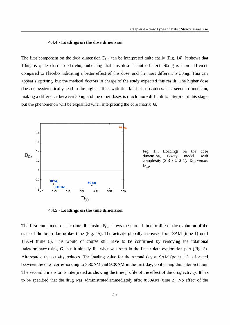
Chapter 4 – New Types of Data : Structure and Size
243
4.4.4 - Loadings on the dose dimension
The first component on the dose dimension D(1) can be interpreted quite easily (Fig. 14). It shows that
10mg is quite close to Placebo, indicating that this dose is not efficient. 90mg is more different
compared to Placebo indicating a better effect of this dose, and the most different is 30mg. This can
appear surprising, but the medical doctors in charge of the study expected this result. The higher dose
does not systematically lead to the higher effect with this kind of substances. The second dimension,
making a difference between 30mg and the other doses is much more difficult to interpret at this stage,
but the phenomenon will be explained when interpreting the core matrix G.
Fig. 14. Loadings on the dose dimension, 6-way model with complexity (3 3 3 2 2 1). D(1) versus D(2).
4.4.5 - Loadings on the time dimension
The first component on the time dimension E(1) shows the normal time profile of the evolution of the
state of the brain during day time (Fig. 15). The activity globally increases from 8AM (time 1) until
11AM (time 6). This would of course still have to be confirmed by removing the rotational
indeterminacy using G, but it already fits what was seen in the linear data exploration part (Fig. 5).
Afterwards, the activity reduces. The loading value for the second day at 9AM (point 11) is located
between the ones corresponding to 8:30AM and 9:30AM in the first day, confirming this interpretation.
The second dimension is interpreted as showing the time profile of the effect of the drug activity. It has
to be specified that the drug was administrated immediately after 8:30AM (time 2). No effect of the
D(2)
D(1)
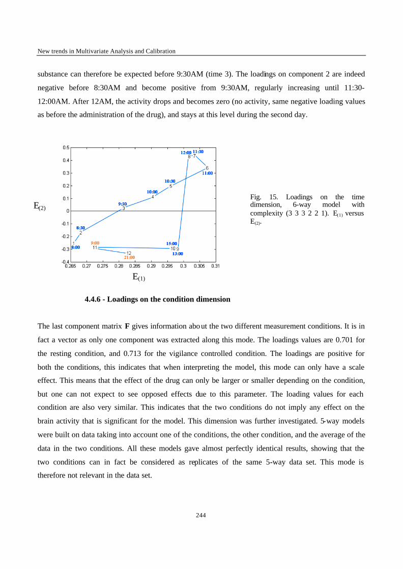
New trends in Multivariate Analysis and Calibration
244
substance can therefore be expected before 9:30AM (time 3). The loadings on component 2 are indeed
negative before 8:30AM and become positive from 9:30AM, regularly increasing until 11:30-
12:00AM. After 12AM, the activity drops and becomes zero (no activity, same negative loading values
as before the administration of the drug), and stays at this level during the second day.
Fig. 15. Loadings on the time dimension, 6-way model with complexity (3 3 3 2 2 1). E(1) versus E(2).
4.4.6 - Loadings on the condition dimension
The last component matrix F gives information about the two different measurement conditions. It is in
fact a vector as only one component was extracted along this mode. The loadings values are 0.701 for
the resting condition, and 0.713 for the vigilance controlled condition. The loadings are positive for
both the conditions, this indicates that when interpreting the model, this mode can only have a scale
effect. This means that the effect of the drug can only be larger or smaller depending on the condition,
but one can not expect to see opposed effects due to this parameter. The loading values for each
condition are also very similar. This indicates that the two conditions do not imply any effect on the
brain activity that is significant for the model. This dimension was further investigated. 5-way models
were built on data taking into account one of the conditions, the other condition, and the average of the
data in the two conditions. All these models gave almost perfectly identical results, showing that the
two conditions can in fact be considered as replicates of the same 5-way data set. This mode is
therefore not relevant in the data set.
E(2)
E(1)
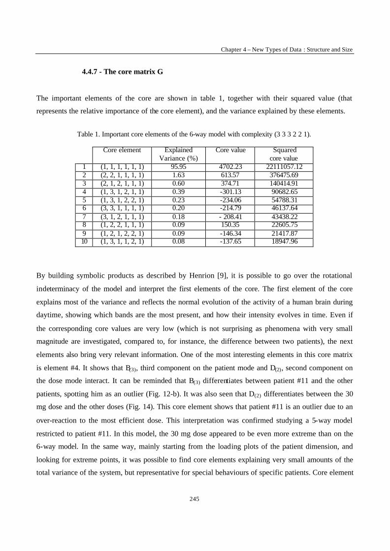
Chapter 4 – New Types of Data : Structure and Size
245
4.4.7 - The core matrix G
The important elements of the core are shown in table 1, together with their squared value (that
represents the relative importance of the core element), and the variance explained by these elements.
Table 1. Important core elements of the 6-way model with complexity (3 3 3 2 2 1).
Core element Explained Variance (%)
Core value Squared core value
1 (1, 1, 1, 1, 1, 1) 95.95 4702.23 22111057.12 2 (2, 2, 1, 1, 1, 1) 1.63 613.57 376475.69 3 (2, 1, 2, 1, 1, 1) 0.60 374.71 140414.91 4 (1, 3, 1, 2, 1, 1) 0.39 -301.13 90682.65 5 (1, 3, 1, 2, 2, 1) 0.23 -234.06 54788.31 6 (3, 3, 1, 1, 1, 1) 0.20 -214.79 46137.64 7 (3, 1, 2, 1, 1, 1) 0.18 - 208.41 43438.22 8 (1, 2, 2, 1, 1, 1) 0.09 150.35 22605.75 9 (1, 2, 1, 2, 2, 1) 0.09 -146.34 21417.87 10 (1, 3, 1, 1, 2, 1) 0.08 -137.65 18947.96
By building symbolic products as described by Henrion [9], it is possible to go over the rotational
indeterminacy of the model and interpret the first elements of the core. The first element of the core
explains most of the variance and reflects the normal evolution of the activity of a human brain during
daytime, showing which bands are the most present, and how their intensity evolves in time. Even if
the corresponding core values are very low (which is not surprising as phenomena with very small
magnitude are investigated, compared to, for instance, the difference between two patients), the next
elements also bring very relevant information. One of the most interesting elements in this core matrix
is element #4. It shows that B(3), third component on the patient mode and D(2), second component on
the dose mode interact. It can be reminded that B(3) differentiates between patient #11 and the other
patients, spotting him as an outlier (Fig. 12-b). It was also seen that D(2) differentiates between the 30
mg dose and the other doses (Fig. 14). This core element shows that patient #11 is an outlier due to an
over-reaction to the most efficient dose. This interpretation was confirmed studying a 5-way model
restricted to patient #11. In this model, the 30 mg dose appeared to be even more extreme than on the
6-way model. In the same way, mainly starting from the loading plots of the patient dimension, and
looking for extreme points, it was possible to find core elements explaining very small amounts of the
total variance of the system, but representative for special behaviours of specific patients. Core element
New trends in Multivariate Analysis and Calibration
246
#7, for instance, relates B(1), the first component on the patients mode (showing patient #6 as an
outlier), to A(3), third component on the EEG mode (differentiating α2 from the other energy bands).
This core element accounts for a specific repartition of the energy bands for patient #6. This was
confirmed by investigating a 5-way model restricted to this patient. On this model, the distribution of
energy bands showed in particular extremely high values of the α bands. The special behaviour of
electrode #12 compared to its symmetrical on figure 13-a can be explained by focusing on patient #9.
All measurements on this patient have an extreme value for electrode #12. This was confirmed by
studying a 5-way model restricted to this patient, clearly differentiating electrode #12 from the others.
It can be seen that the energy values for this electrode are wrong, the high-energy bands (especially β2
and β3) are strongly over-estimated. This happens for all the measurements performed on this patient
for the 90mg dose (which also corresponds to a certain period in time, as the doses are tested
successively with a ‘wash-out’ period between each dose). This systematic and very localised problem
seems to indicate that the corresponding electrode was either damaged or badly installed on the scalp
during this part of the data acquisition.
4.5 - Analyzing subject variability
Since many of the core elements seemed to be used only to account for specific behaviours of
individual patients, it was decided to study more thoroughly the patients mode. The idea was to
simplify the problem by removing the non-typical patients. This way, the number of relevant core
elements should be reduced, as well as the optimal complexity of the model. For this purpose, it was
decided to center the patients mode in order to highlight the differences between patients, and hopefully
identify easily the suspected outliers. Moreover, as it was shown to be not relevant, the 6th dimension
(related to the two measurement conditions) was collapsed. The average of the two conditions was used
leading to a simpler 5-way array.
The plots of the loading matrix B obtained for the patient dimension show that outliers already spotted
with the 6-way model appear now much more clearly (Fig. 16-a,b).
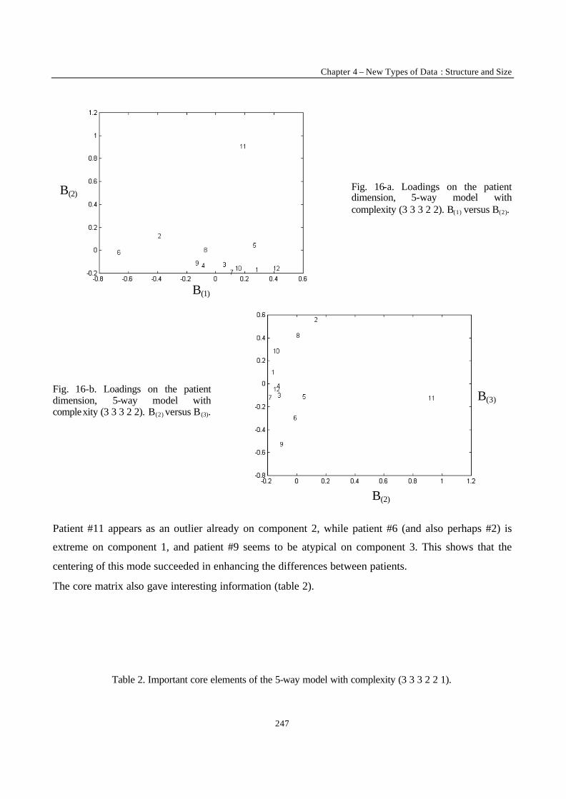
Chapter 4 – New Types of Data : Structure and Size
247
Fig. 16-a. Loadings on the patient dimension, 5-way model with complexity (3 3 3 2 2). B(1) versus B(2).
Fig. 16-b. Loadings on the patient dimension, 5-way model with complexity (3 3 3 2 2). B(2) versus B (3).
Patient #11 appears as an outlier already on component 2, while patient #6 (and also perhaps #2) is
extreme on component 1, and patient #9 seems to be atypical on component 3. This shows that the
centering of this mode succeeded in enhancing the differences between patients.
The core matrix also gave interesting information (table 2).
Table 2. Important core elements of the 5-way model with complexity (3 3 3 2 2 1).
B(2)
B(1)
B(3)
B(2)
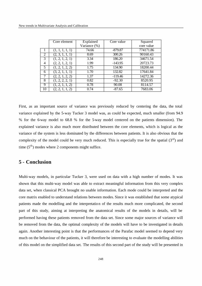
New trends in Multivariate Analysis and Calibration
248
Core element Explained
Variance (%) Core value Squared
core value 1 (1, 1, 1, 1, 1) 74.66 -879.87 774171.86 2 (2, 3, 1, 1, 1) 8.69 300.26 90160.43 3 (1, 2, 1, 2, 1) 3.34 186.20 34671.54 4 (2, 2, 1, 2, 1) 1.99 -143.95 20723.73 5 (1, 2, 1, 2, 2) 1.75 134.90 18200.44 6 (3, 2, 1, 1, 1) 1.70 132.82 17641.84 7 (2, 2, 1, 2, 2) 1.37 -119.46 14272.36 8 (1, 2, 2, 2, 1) 0.82 -92.30 8520.95 9 (1, 2, 1, 1, 2) 0.78 90.08 8114.57
10 (2, 2, 1, 1, 2) 0.74 -87.65 7683.06
First, as an important source of variance was previously reduced by centering the data, the total
variance explained by the 5-way Tucker 3 model was, as could be expected, much smaller (from 94.9
% for the 6-way model to 68.8 % for the 5-way model centered on the patients dimension). The
explained variance is also much more distributed between the core elements, which is logical as the
variance of the system is less dominated by the differences between patients. It is also obvious that the
complexity of the model could be very much reduced. This is especially true for the spatial (3rd) and
time (5th) modes where 2 components might suffice.
5 - Conclusion
Multi-way models, in particular Tucker 3, were used on data with a high number of modes. It was
shown that this multi-way model was able to extract meaningful information from this very complex
data set, when classical PCA brought no usable information. Each mode could be interpreted and the
core matrix enabled to understand relations between modes. Since it was established that some atypical
patients made the modelling and the interpretation of the results much more complicated, the second
part of this study, aiming at interpreting the anatomical results of the models in details, will be
performed having these patients removed from the data set. Since some major sources of variance will
be removed from the data, the optimal complexity of the models will have to be investigated in details
again. Another interesting point is that the performances of the Parafac model seemed to depend very
much on the behaviour of the patients, it will therefore be interesting to evaluate the modelling abilities
of this model on the simplified data set. The results of this second part of the study will be presented in

Chapter 4 – New Types of Data : Structure and Size
249
a forthcoming publication. It is anyhow already possible to say that the optimal complexities of the
models established on the simplified data set are indeed much lower. The simplified data set also
happens to conform much better to a Parafac model. This model can therefore be used, which will
hopefully enable an easier interpretation of the results.
REFERENCES
[1] M. J. Aminoff, Electodiagnosis in Clinical Neurology, third edition, Churchill Livingstone,
Edimburgh (1987).
[2] H. H. Jasper, Report of the committee on methods of clinical examination in
electroencephalography, Electroencephalor Clin Neurophysiol, 10 (1958) 370.
[3] C. A. Andersson, R. Bro, Chemom. Intell. Lab. Sys., 52 (2000) 1-4.
[4] L. R. Tucker, Psychometrika, 31 (1966) 279-311.
[5] P. M. Kroonenberg, Three-mode Principal Component Analysis. Theory and Applications,
DSWO Press, Leid en (1983).
[6] R. Harshman, UCLA working papers in phonetics, 16 (1970) 1-84.
[7] J. D. Carrol, J. Chang, Psychometrika, 45 (1970) 283-319.
[8] R. Bro, H.A.L. Kiers, In press, J. Chemom. (2001).
[9] H. Henrion, Chemom. Intell. Lab. Sys., 25 (1994) 1-23.
New trends in Multivariate Analysis and Calibration
250
ROBUST VERSION OF TUCKER 3 MODEL
Chemometrics and Intelligent Laboratory Systems, Vol. 59, 2001, 75-88.
V. Pravdova, F. Estienne, B. Walczak*+, D. L. Massart
ChemoAC
Farmaceutisch Instituut, Vrije Universiteit Brussel,
Laarbeeklaan 103, B-1090 Brussels, Belgium. E-mail: [email protected]
+ on leave from : Silesian University
Katowice Poland
ABSTRACT
A new procedure for identification of outliers in Tucker3 model is proposed. It is based on robust initialization of the Tucker3 algorithm using Multivariate trimming or Minimum covariance determinant. The performance of the algorithm is tested by a Monte Carlo study on simulated data sets and also on a real data set known to contain outliers.
* Corresponding author
KEYWORDS : Multivariate Calibration, Raman spectroscopy, Lanczos decomposition, Fast Calibration
methods.
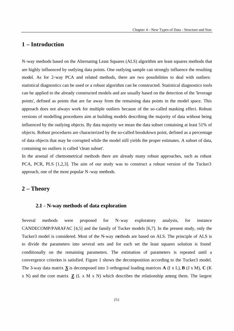
Chapter 4 – New Types of Data : Structure and Size
251
1 – Introduction
N-way methods based on the Alternating Least Squares (ALS) algorithm are least squares methods that
are highly influenced by outlying data points. One outlying sample can strongly influence the resulting
model. As for 2-way PCA and related methods, there are two possibilities to deal with outliers:
statistical diagnostics can be used or a robust algorithm can be constructed. Statistical diagnostics tools
can be applied to the already constructed models and are usually based on the detection of the 'leverage
points', defined as points that are far away from the remaining data points in the model space. This
approach does not always work for multiple outliers because of the so-called masking effect. Robust
versions of modelling procedures aim at building models describing the majority of data without being
influenced by the outlying objects. By data majority we mean the data subset containing at least 51% of
objects. Robust procedures are characterized by the so-called breakdown point, defined as a percentage
of data objects that may be corrupted while the model still yields the proper estimates. A subset of data,
containing no outliers is called 'clean subset'.
In the arsenal of chemometrical methods there are already many robust approaches, such as robust
PCA, PCR, PLS [1,2,3]. The aim of our study was to construct a robust version of the Tucker3
approach, one of the most popular N-way methods.
2 – Theory
2.1 - N-way methods of data exploration
Several methods were proposed for N-way exploratory analysis, for instance
CANDECOMP/PARAFAC [4,5] and the family of Tucker models [6,7]. In the present study, only the
Tucker3 model is considered. Most of the N-way methods are based on ALS. The principle of ALS is
to divide the parameters into several sets and for each set the least squares solution is found
conditionally on the remaining parameters. The estimation of parameters is repeated until a
convergence criterion is satisfied. Figure 1 shows the decomposition according to the Tucker3 model.
The 3-way data matrix X is decomposed into 3 orthogonal loading matrices A (I x L), B (J x M), C (K
x N) and the core matrix Z (L x M x N) which describes the relationship among them. The largest

New trends in Multivariate Analysis and Calibration
252
squared elements of the core matrix Z indicate the most important factors in the model of X.
Mathematically, the Tucker3 model can be expressed as
∑∑∑= = =
+=L
1l
M
1m
N
1nijklmnknjmilijk ezcbax (1)
Fig. 1. The Tucker3 model.
2.2 - Data unfolding
For computational convenience, the Tucker3 algorithm used does not perform calculations directly on
N-way arrays. The X matrix is unfolded to standard 2-way matrices. This can be done in three different
ways (see Fig. 2). Unfolded matrices are denoted as: X(I x JK), X(J x IK) and X(K x IJ) . To calculate the
loading matrices several procedures can be used. Anderson and Bro [8] tested most of them with
respect to speed and found NIPALS to be the fastest for large data arrays. In our algorithm, SVD is
used for the estimation of A, B and C matrices.
Fig. 2. Three different ways of unfolding of a 3-way data matrix.
Chapter 4 – New Types of Data : Structure and Size
253
2.3 - Algorithm of Tucker3 model
0) - Initialize B and C (as random orthogonal matrices)
1) - [A,v,d] = svd(X(I x JK) (C ⊗ B), L)
2) - [B,v,d] = svd(X(J x IK) (C ⊗ A), M)
3) - [C,v,d] = svd(X(K x IJ) (B ⊗ A), N)
4) - Go to step 1 until the relative change in fit is small
5) - Z = AT X (C ⊗ B)
where symbols L, M, N denote numbers of factors in matrix A, B and C respectively and symbol ⊗
denotes Kronecker multiplication: A ⊗ B yields the element-by-element multiplication of B with the
elements from A, expressed as :
=⊗
OMM
LL
BBBB
BA 2221
1211
aaaa
2.4 - Robust PCA
One could think about robust initialization of the ALS algorithm, i.e. finding a clean subset for the
matrix X(I x JK), but in reality, as the loadings matrices B and C are only just initialized, the resulting
matrix (X(I x JK) (C ⊗ B)) of dimensionality IxMN should be taken into account. The clean subset can
be determined using such methods as for instance, Multivariate Trimming (MVT) [11] or Minimum
Covariance Determinant (MCD) [12]. Robust initialization of the Tucker3 algorithm seems to be the
most important step to determine the final model and because this step is placed out of the main loop,
the algorithm does not lead to oscillations. In the consecutive steps of ALS algorithm the clean subset
is constructed to decrease an objective function (see eq. 4), so that oscillations are avoided and
convergence of the algorithm is achieved.
New trends in Multivariate Analysis and Calibration
254
2.4.1 - Multivariate Trimming (MVT) [11]
The MVT procedure can be used for 'clean' subset selection when the input data matrix contains at least
two times more objects than variables. The squared Mahalanobis distance (MD2) is calculated
according to the following equation:
MDi2 =(ti- t ) S-1 (ti- t ) T (2)
where ti denotes the i-th object, t denotes the vector containing means of data matrix columns and S is
the covariance matrix.
A fixed percentage of objects (here 49%) with the highest MD2 are removed and the remaining ones
are used to calculate a mean and covariance matrix. MD2 is calculated again for all objects using the
new estimates of the mean and covariance matrix. Again the 49% of objects with highest MD2 are
removed and the process is repeated until convergence of successive estimates of covariance matrix
and mean. The subset of objects for which covariance and mean are stable is considered to be a clean
subset of data.
2.4.2 - Minimum Covariance Determinant (MCD) [12]
MCD aims at selecting a subset of h (out of m) objects, with the smallest determinant, i.e. the smallest
volume in the p-dimensional space.
h = (m + p + 1)/2 (3)
The MCD algorithm can be summarized as follows:
1) - Randomly select 500 subsets of data containing p+1 objects
2) - For each subset:
a) Calculate its mean and covariance, t and S
b) Calculate Mahalanobis distances for all objects using the estimates of data mean and
covariance matrix calculated in step 2 a

Chapter 4 – New Types of Data : Structure and Size
255
c) Sort MD and take h objects with the smallest MD to calculate the next estimate of mean and
covariance matrix,
d) Repeat steps b and c twice
3) - Take the 10 best solutions, i.e. the 10 subsets of h objects with the smallest determinants, and for
each of them, repeat steps b and c until two subsequent determinants are equal
4) - Report the best solution, i.e. the subset with the smallest determinant
The procedure starts with many very small data subsets (containing only p+1 objects) to increase the
probability that these subsets do not contain outliers. Two iterations only are performed for all 500
subsets (steps 2b and 2c) to speed up the MCD procedure and, as demonstrated by P. Rousseeuw [12],
small number of iterations is sufficient to find good candidates of clean subsets. Only for the 10 best
subsets the calculations are repeated till convergence of the algorithm.
2.5 - Algorithm for robust Tucker3 model
To find possible multiple outliers in the first mode of the X the following algorithm is proposed:
0) - Initialize loadings B and C
1) - Calculate X(I x JK) (C ⊗ B) and determine clean subset (using MVT or MCD)
2) - [A*,v,d] = svd (X(I* x JK) (C ⊗ B), L)
3) - [B*,v,d] = svd (X(J x I*K) (C ⊗ A*), M)
4) - [C*,v,d] = svd (X(K x I*J) (B* ⊗ A*), N)
5) - Z = A*T X* (C* ⊗ B*)
6) - Predict loadings A for all objects
7) - Reconstruct X(I x JK) : X(I x JK)=A Z(L x MN)(C⊗B)T
8) - Calculate the sum of squared residuals for I objects in the first mode as the differences between the
original data and the reconstructed one :
residuals = sum(((X(I x JK)- X (I x JK))2)T)
9) - Sort residuals along the first mode
10) -Find h objects with the smallest residuals. They constitute the clean subset
11) - Go to step 2 until the relative change in fit is small
New trends in Multivariate Analysis and Calibration
256
A*, X* etc. are the matrices A, X etc. limited to the clean subset of objects, and the notation X(I* x JK)
means that the unfolded data set contains objects reduced to the clean subset I*. h is the number of
objects in the clean subset.
In each iteration of the ALS subroutine, the loadings A*, B* and C* are calculated for the clean subset
of objects only. In step 6 the loadings A are predicted for all objects and the set X(I x JK) is reconstructed
with the predefined number of factors. Residuals between the initial X(I x JK) and the reconstructed X (I x
JK) are calculated and sorted, and 51 % of objects with the smallest residuals is selected to form the
clean subset for the next ALS iteration. The objective function, F, to be minimized, is the sum of
squared residuals for the h clean objects from the first mode:
2)ˆ(F ∑∑ −= *X*X (4)
There is no guarantee that the selected clean subset is optimal, but convergence of the ALS approach is
secured.
In this algorithm, the outliers are identified in the first mode only, but as all modes are treated
symmetrically, one can look for outliers in any mode. This can be done simply by inputting the X
matrix with dimension of interest in the first mode.
2.5.1 - Outlier identification
Once the robust Tucker3 model is constructed, the standardized residuals from that model are
calculated for all objects of the first mode according to the following equation [10] :
)]))res(medianres((median*48.1*3/[resrs 2iiii −= (5)
where
])ˆ[(res2
ijijji ∑ −= XX (6)
Chapter 4 – New Types of Data : Structure and Size
257
for i = 1,…,I and j = 1,…JK. In eq. 5, the residuals are divided by the robust version of standard
deviation. Using )))res(medianres((median48.1 2ii −∗ , the residuals for 51% of objects, which fit
the model best, are calculated. This corresponds to the robust standard deviation of the data residuals.
Objects with standardized residuals higher than 3 times the robust standard deviation are considered as
outlying and are removed from the data set. This is equivalent with using the ratio prese nted in eq. 5
and cut-off equals one. The final Tucker3 model is constructed as the least squares model for the data
after outlier elimination.
3 - Data
3.1 - Simulated data set
A systematic Monte Carlo study was performed to evaluate performance of the algorithm. A data set of
dimensionality (50 x 10 x 10) was simulated with 2 factors in all modes. Two Tucker3 models (X1 and
X2) were constructed to explain 60 % and 90 % of data variance. The initial data sets were then
contaminated with different types (T1-T4) and different percentages (20% and 40%) of outliers.
The different types of outliers (T1-T4) can be characterized as follows:
T1 data set constructed according to the same model as the initial data, but with a certain
percentage of randomly permuted variables.
T2 data set with the same dimensionality and the same level of noise, but constructed
according to a different tri-linear model
T3 data set with the same level of noise but with a higher dimensionality than the initial data
set
T4 data set with the same level of noise but with a lower dimensionality than the initial data
set
The simulation of tri- linear data structure was performed as follows: first, orthogonal loading matrices
A, B and C with predefined dimensions were randomly initialized. For the selected structure and core
matrix Z, the X matrix was constructed as XIxJK = A * ZLxMN * (C ⊗ B)T . Then, the Tucker3 model was
built, and new X was reconstructed with chosen number of factors in each mode and used as initial data
set with tri- linear structure. At the end, white Gaussian noise was added to X. In this way models,
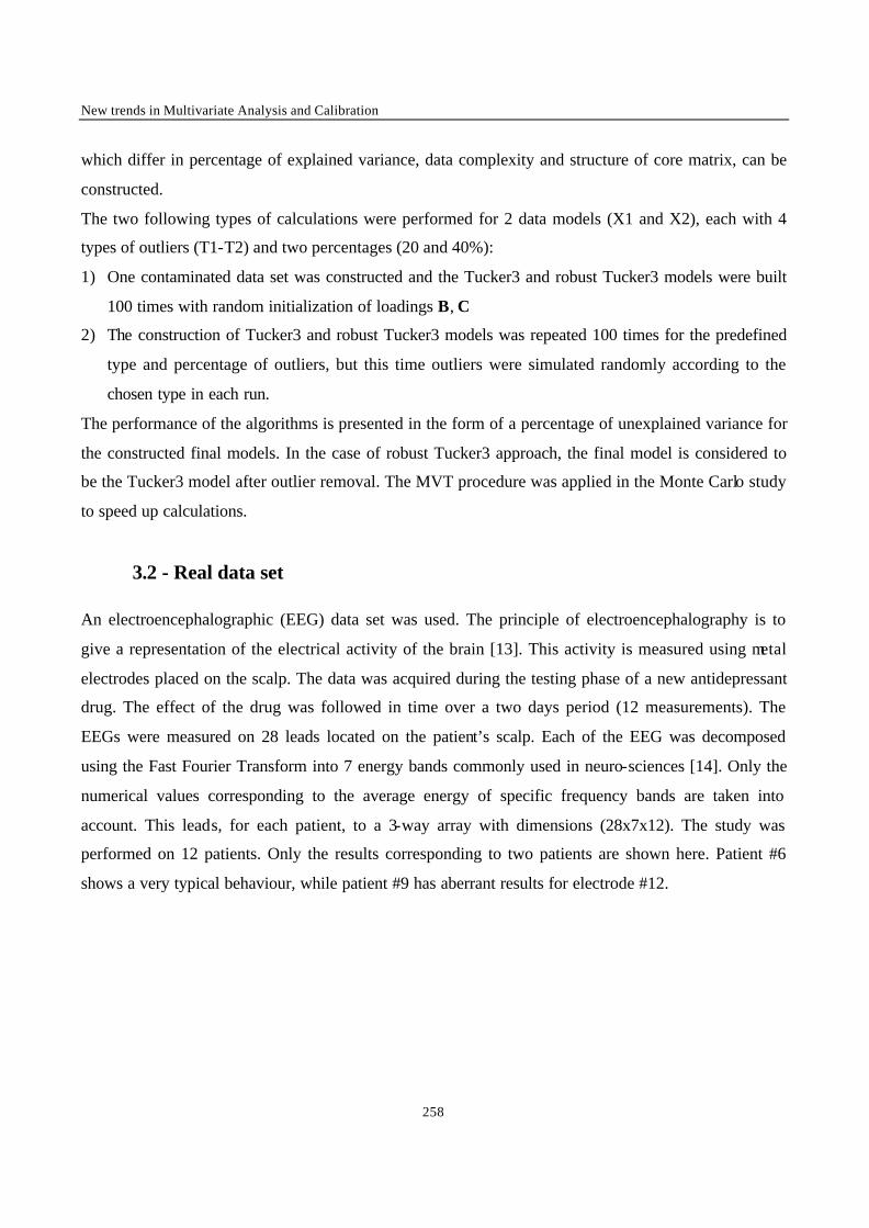
New trends in Multivariate Analysis and Calibration
258
which differ in percentage of explained variance, data complexity and structure of core matrix, can be
constructed.
The two following types of calculations were performed for 2 data models (X1 and X2), each with 4
types of outliers (T1-T2) and two percentages (20 and 40%):
1) One contaminated data set was constructed and the Tucker3 and robust Tucker3 models were built
100 times with random initialization of loadings B, C
2) The construction of Tucker3 and robust Tucker3 models was repeated 100 times for the predefined
type and percentage of outliers, but this time outliers were simulated randomly according to the
chosen type in each run.
The performance of the algorithms is presented in the form of a percentage of unexplained variance for
the constructed final models. In the case of robust Tucker3 approach, the final model is considered to
be the Tucker3 model after outlier removal. The MVT procedure was applied in the Monte Carlo study
to speed up calculations.
3.2 - Real data set An electroencephalographic (EEG) data set was used. The principle of electroencephalography is to
give a representation of the electrical activity of the brain [13]. This activity is measured using metal
electrodes placed on the scalp. The data was acquired during the testing phase of a new antidepressant
drug. The effect of the drug was followed in time over a two days period (12 measurements). The
EEGs were measured on 28 leads located on the patient’s scalp. Each of the EEG was decomposed
using the Fast Fourier Transform into 7 energy bands commonly used in neuro-sciences [14]. Only the
numerical values corresponding to the average energy of specific frequency bands are taken into
account. This leads, for each patient, to a 3-way array with dimensions (28x7x12). The study was
performed on 12 patients. Only the results corresponding to two patients are shown here. Patient #6
shows a very typical behaviour, while patient #9 has aberrant results for electrode #12.
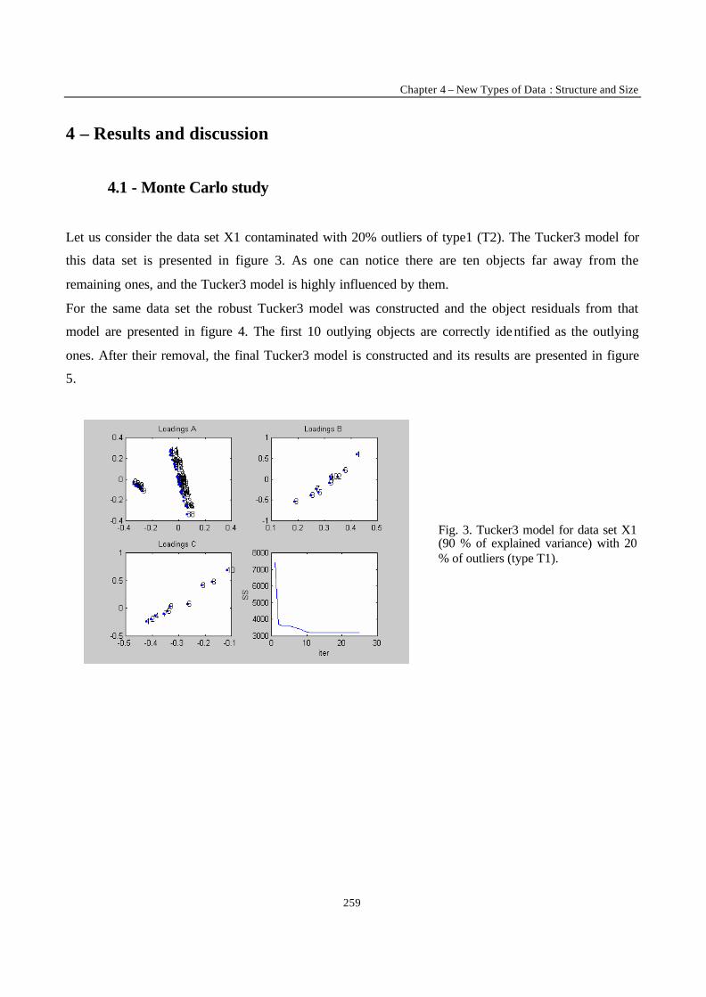
Chapter 4 – New Types of Data : Structure and Size
259
4 – Results and discussion
4.1 - Monte Carlo study
Let us consider the data set X1 contaminated with 20% outliers of type1 (T2). The Tucker3 model for
this data set is presented in figure 3. As one can notice there are ten objects far away from the
remaining ones, and the Tucker3 model is highly influenced by them.
For the same data set the robust Tucker3 model was constructed and the object residuals from that
model are presented in figure 4. The first 10 outlying objects are correctly identified as the outlying
ones. After their removal, the final Tucker3 model is constructed and its results are presented in figure
5.
Fig. 3. Tucker3 model for data set X1 (90 % of explained variance) with 20 % of outliers (type T1).
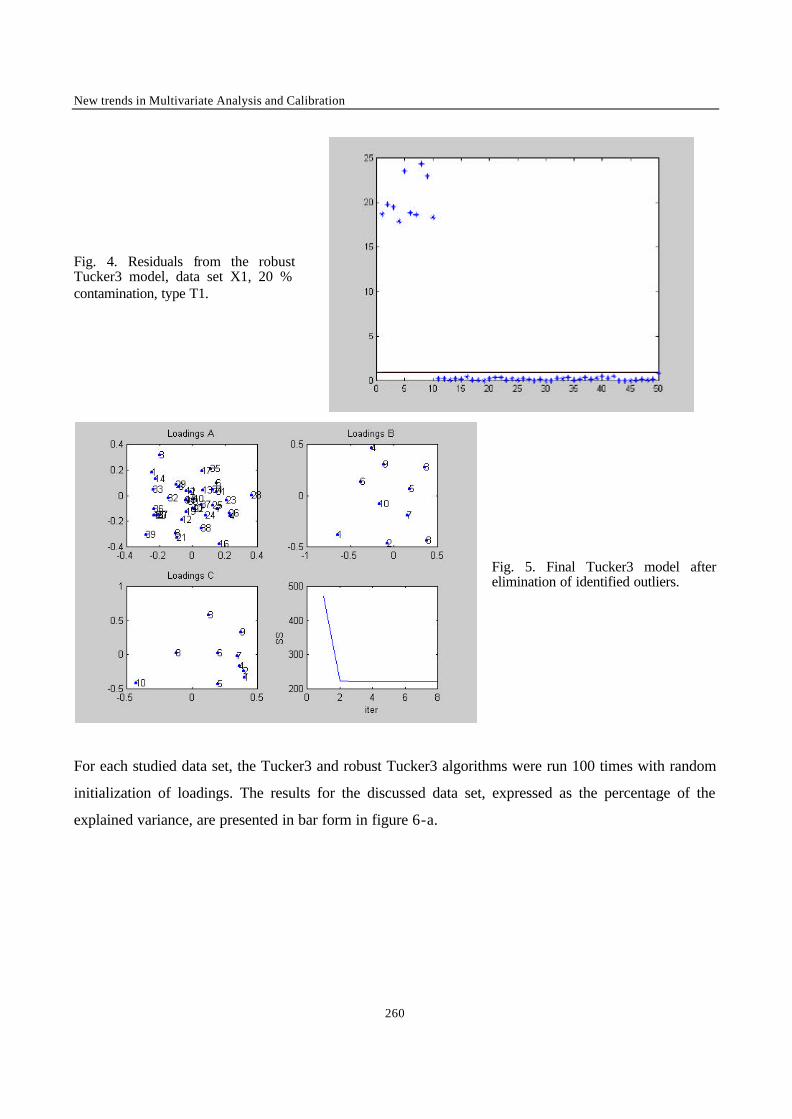
New trends in Multivariate Analysis and Calibration
260
Fig. 4. Residuals from the robust Tucker3 model, data set X1, 20 % contamination, type T1.
Fig. 5. Final Tucker3 model after elimination of identified outliers.
For each studied data set, the Tucker3 and robust Tucker3 algorithms were run 100 times with random
initialization of loadings. The results for the discussed data set, expressed as the percentage of the
explained variance, are presented in bar form in figure 6-a.
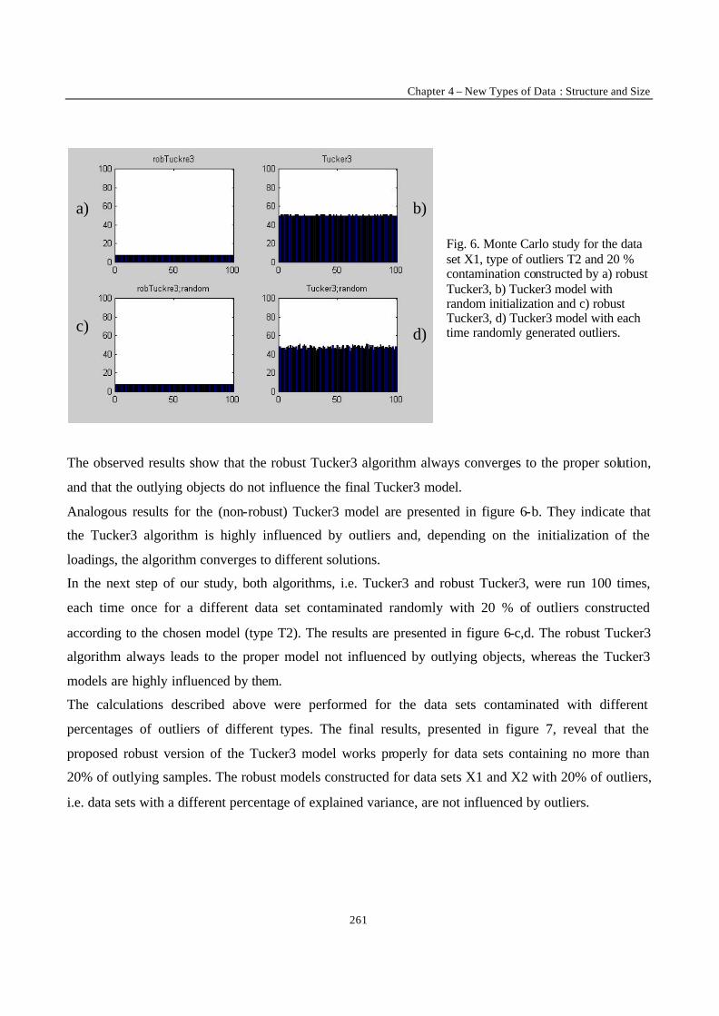
Chapter 4 – New Types of Data : Structure and Size
261
Fig. 6. Monte Carlo study for the data set X1, type of outliers T2 and 20 % contamination constructed by a) robust Tucker3, b) Tucker3 model with random initialization and c) robust Tucker3, d) Tucker3 model with each time randomly generated outliers.
The observed results show that the robust Tucker3 algorithm always converges to the proper solution,
and that the outlying objects do not influence the final Tucker3 model.
Analogous results for the (non-robust) Tucker3 model are presented in figure 6-b. They indicate that
the Tucker3 algorithm is highly influenced by outliers and, depending on the initialization of the
loadings, the algorithm converges to different solutions.
In the next step of our study, both algorithms, i.e. Tucker3 and robust Tucker3, were run 100 times,
each time once for a different data set contaminated randomly with 20 % of outliers constructed
according to the chosen model (type T2). The results are presented in figure 6-c,d. The robust Tucker3
algorithm always leads to the proper model not influenced by outlying objects, whereas the Tucker3
models are highly influenced by them.
The calculations described above were performed for the data sets contaminated with different
percentages of outliers of different types. The final results, presented in figure 7, reveal that the
proposed robust version of the Tucker3 model works properly for data sets containing no more than
20% of outlying samples. The robust models constructed for data sets X1 and X2 with 20% of outliers,
i.e. data sets with a different percentage of explained variance, are not influenced by outliers.
a) b)
c) d)
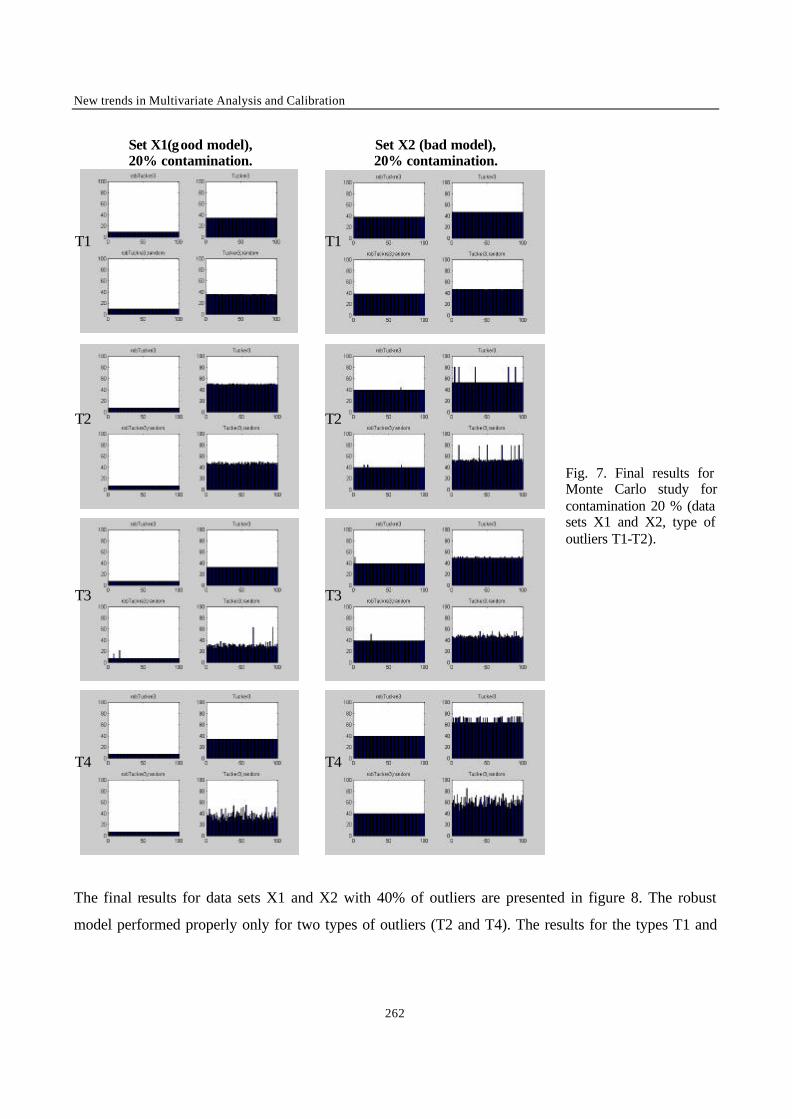
New trends in Multivariate Analysis and Calibration
262
Set X1(good model), 20% contamination.
Set X2 (bad model), 20% contamination.
Fig. 7. Final results for Monte Carlo study for contamination 20 % (data sets X1 and X2, type of outliers T1-T2).
The final results for data sets X1 and X2 with 40% of outliers are presented in figure 8. The robust
model performed properly only for two types of outliers (T2 and T4). The results for the types T1 and
T1 T1
T2 T2
T3 T3
T4 T4
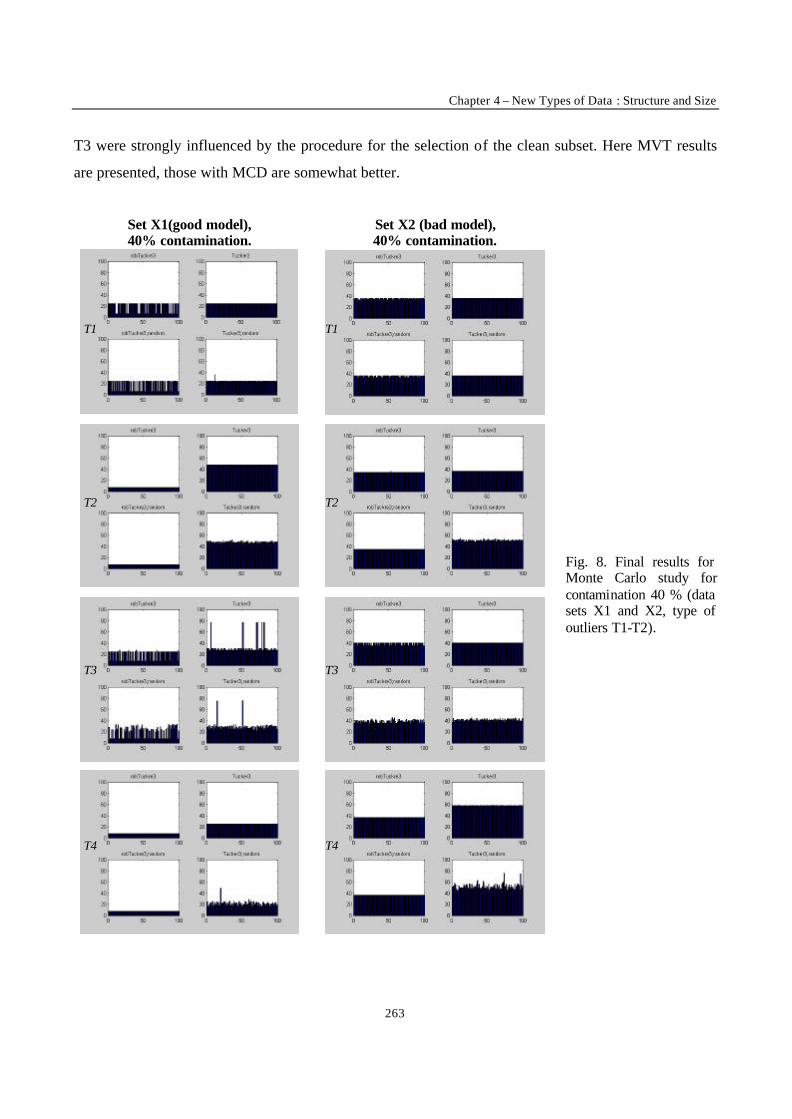
Chapter 4 – New Types of Data : Structure and Size
263
T3 were strongly influenced by the procedure for the selection of the clean subset. Here MVT results
are presented, those with MCD are somewhat better.
Set X1(good model), 40% contamination.
Set X2 (bad model), 40% contamination.
Fig. 8. Final results for Monte Carlo study for contamination 40 % (data sets X1 and X2, type of outliers T1-T2).
T1 T1
T2 T2
T3 T3
T4 T4
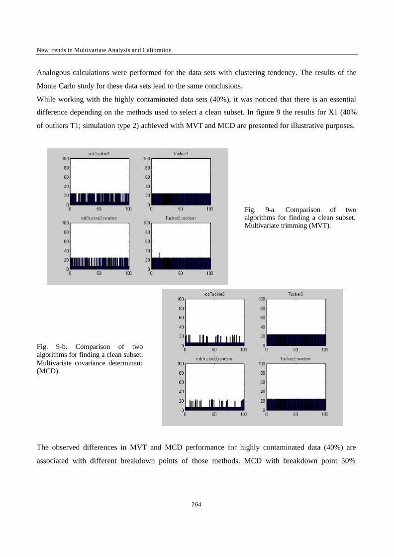
New trends in Multivariate Analysis and Calibration
264
Analogous calculations were performed for the data sets with clustering tendency. The results of the
Monte Carlo study for these data sets lead to the same conclusions.
While working with the highly contaminated data sets (40%), it was noticed that there is an essential
difference depending on the methods used to select a clean subset. In figure 9 the results for X1 (40%
of outliers T1; simulation type 2) achieved with MVT and MCD are presented for illustrative purposes.
Fig. 9-a. Comparison of two algorithms for finding a clean subset. Multivariate trimming (MVT).
Fig. 9-b. Comparison of two algorithms for finding a clean subset. Multivariate covariance determinant (MCD).
The observed differences in MVT and MCD performance for highly contaminated data (40%) are
associated with different breakdown points of those methods. MCD with breakdown point 50%
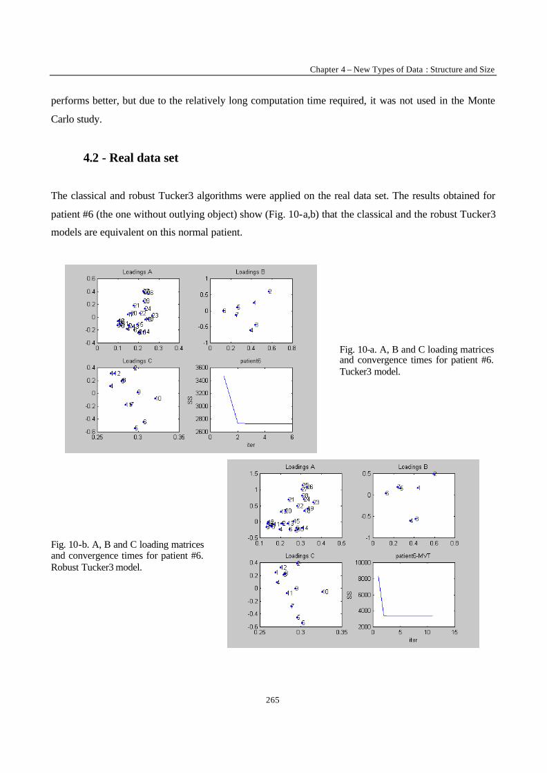
Chapter 4 – New Types of Data : Structure and Size
265
performs better, but due to the relatively long computation time required, it was not used in the Monte
Carlo study.
4.2 - Real data set
The classical and robust Tucker3 algorithms were applied on the real data set. The results obtained for
patient #6 (the one without outlying object) show (Fig. 10-a,b) that the classical and the robust Tucker3
models are equivalent on this normal patient.
Fig. 10-a. A, B and C loading matrices and convergence times for patient #6. Tucker3 model.
Fig. 10-b. A, B and C loading matrices and convergence times for patient #6. Robust Tucker3 model.
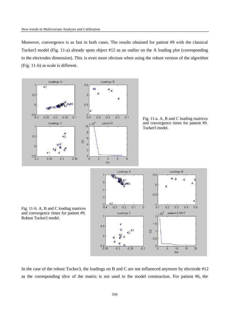
New trends in Multivariate Analysis and Calibration
266
Moreover, convergence is as fast in both cases. The results obtained for patient #9 with the classical
Tucker3 model (Fig. 11-a) already spots object #12 as an outlier on the A loading plot (corresponding
to the electrodes dimension). This is even more obvious when using the robust version of the algorithm
(Fig. 11-b) as scale is different.
Fig. 11-a. A, B and C loading matrices and convergence times for patient #9. Tucker3 model.
Fig. 11-b. A, B and C loading matrices and convergence times for patient #9. Robust Tucker3 model.
In the case of the robust Tucker3, the loadings on B and C are not influenced anymore by electrode #12
as the corresponding slice of the matrix is not used in the model construction. For patient #6, the
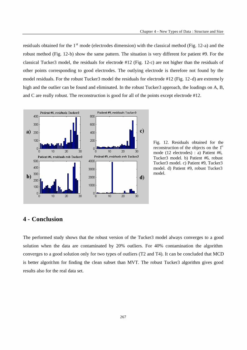
Chapter 4 – New Types of Data : Structure and Size
267
residuals obtained for the 1st mode (electrodes dimension) with the classical method (Fig. 12-a) and the
robust method (Fig. 12-b) show the same pattern. The situation is very different for patient #9. For the
classical Tucker3 model, the residuals for electrode #12 (Fig. 12-c) are not higher than the residuals of
other points corresponding to good electrodes. The outlying electrode is therefore not found by the
model residuals. For the robust Tucker3 model the residuals for electrode #12 (Fig. 12-d) are extreme ly
high and the outlier can be found and eliminated. In the robust Tucker3 approach, the loadings on A, B,
and C are really robust. The reconstruction is good for all of the points except electrode #12.
Fig. 12. Residuals obtained for the reconstruction of the objects on the 1st mode (12 electrodes) : a) Patient #6, Tucker3 model. b) Patient #6, robust Tucker3 model. c) Patient #9, Tucker3 model. d) Patient #9, robust Tucker3 model.
4 - Conclusion
The performed study shows that the robust version of the Tucker3 model always converges to a good
solution when the data are contaminated by 20% outliers. For 40% contamination the algorithm
converges to a good solution only for two types of outliers (T2 and T4). It can be concluded that MCD
is better algorithm for finding the clean subset than MVT. The robust Tucker3 algorithm gives good
results also for the real data set.

New trends in Multivariate Analysis and Calibration
268
ACKNOWLEDGEMENT
Professor Massart thanks the FWO project (G.0171.98) and EU project NWAYQUAL (G6RD-CT-
1999-00039) for founding this research.
REFERENCES
[1] Y. L. Xie, J. H. Wang, Y. Z. Liang, L. X. Sun, X. H. Song, R. Q. Yu, J. Chemom., 7 (1993)
527-541.
[2] B. Walczak, D. L. Massart, Chemom. Intell. Lab. Syst., 27 (1995) 354-362.
[3] I. N. Wakeling, H. J. H. Macfie, J. Chemom., 6 (1992) 189-198.
[4] J. D. Carroll, J. J. Chang, Psychometrica, 35 (1970) 283-319.
[5] R. A. Harshman, UCLA working papers in Phonetic, 16 (1970) 1-84.
[6] L. R. Tucker, Problems in measuring change, The University of Wisconsin Press, Madison,
(1963) 122-137.
[7] L. R. Tucker, Psychometrica, 31 (1966) 279-311.
[8] C. A. Andersson, R. Bro, Chemom. Intell. Lab. Syst., 42 (1998) 93.
[9] L. P. Ammann, J. Am. Stat. Assoc., 88 (1994) 505-514.
[10] P. J. Rousseeuw and A. M. Leroy, Robust Regression and Outlier Detection, Wiley, New York,
1987.
[11] R. Gnanadesikan, J. R. Kettenring, Biometrics, 28 (1972) 81-124.
[12] P. J. Rousseeuw, K. Van Driessen, Technometrics, 41 (1999) 212.
[13] M. J. Aminoff, Electrodiagnosis in Clinical Neurology, second edition (Churchill Livingstone).
[14] H. H. Jasper, Electroencephalor. Clin. Neurophysiol., 10 (1958) 370.

Chapter 4 – New Types of Data : Structure and Size
269
New trends in Multivariate Analysis and Calibration
270
NEW TRENDS IN MULTIVARIATE ANALYSIS AND CALIBRATION
CONCLUSION
Chemometrics is by definition a discipline at the interface of several branches of science (chemistry,
statistics, process engineering, etc …). Chemometricians often have very different backgrounds and our
discipline was in time enriched with a lot of techniques from their respective original fields of research.
The most common chemometrical modelling methods, together with some more advanced ones, in
particular methods applying to data with complex structure, were presented in Chapter 1. Even from
this necessarily non-exhaustive introduction, it can be seen that a very wide range of methods is
available. The profusion of available options for the resolution of a given problem is usually the first
issue encountered by chemometricians during a typical study. The choice of the best method to be used
is very often done following subjective considerations such as personal preferences or software
availability. The second chapter of this thesis was an attempt to rationalise this step of method selection
in the process of building a multivariate calibration model. A part of the work had already been done
covering the simplest and somehow ideal case where the robustness of calibration methods is not
challenged. A very frequently occurring difficulty is extrapolation. In other words, a prediction has to
be done and the new sample is out of the space covered by the calibration samples. From a purely
statistical point of view, the answer to the problem is simple : no model should be used to predict an
object out of the calibration domain. However, this problem can very often not be avoided when
models are used on real-life industrial applications. All possible sources of variance cannot be foreseen
when the model is constructed and some are therefore not taken into account. The robustness of 14
methods toward extrapolation was studied using 5 reference data sets presenting challenging
characteristics often found in industrial data (non- linearity, inhomogeneity). Some important
conclusions were drawn from this study. First of all, it illustrated that the inevitable problem of
extrapolation can indeed be dealt with in industria l applications. Some general recommendations and
guidelines could also be made about the best method to be used depending on the expected level of
extrapolation and the structure of the data set.
Conclusion
271
Another problem currently occurs in real-life industrial conditions. Modifications in measurement
conditions, aging, maintenance, or replacement of an instrument can induce drift and changes in the
instrumental response. It is most of the time not possible to take these perturbations into account in the
calibration step. The quality of prediction for new samples can therefore be expected to degrade over
time. The second study presented in Chapter 2 aimed at evaluating the robustness of calibration
methods in the case of instrumental perturbations. It was performed on 12 multivariate calibration
methods, using the same 5 industrial data sets as the previous study, and by simulating 6 different
instrumental perturbations on the response obtained for the samples to be predicted. Some general
recommendations could be made in particular about the type of model, in terms of complexity or pre-
treatment, that has to be avoided in order to increase robustness toward instrumental perturbations.
The third and final part of Chapter 2 follows naturally the comparative studies presented. It aims at
explaining, step by step, from data pre-processing to the prediction of new samples, how to develop a
calibration model. Even though this tutorial describes the construction of a Multiple Linear Regression
model on spectroscopic data, most of the strategy can be applied to other calibration methods and/or
data sets of different nature.
The third chapter of this thesis presents some specific case studies. The aim of this chapter is twofold.
First of all, the strategy and guidelines developed in Chapter 2 are applied on industrial data. The whole
chapter illustrates how an industrial process can be improved by proper use of chemometrical tools. It
also gives another illustration of the importance of the method selection step. The fact of using another
instrument for data acquisition can have a dramatic influence on the multivariate calibration model
building process. Even though the studied process was the same and the nature of the spectroscopic
technique remained unchanged, the fact that an instrument with better resolution was used implied that
the best results were achieved by a different calibration method.
The second important aspect of this study is that it was performed on Raman spectroscopic data.
Sophisticated data treatment is usually not considered necessary for Raman data. Specialists in the field
mostly employ direct calibration, as opposed to inverse calibration methods used by chemometricians.
It was demonstrated that chemometrical tools cannot only match the results obtained by the methods
classically used on Raman data, but can even outperform them. When classical methods could only
predict relative concentration for the monitored chemical process, using inverse calibration it was for
New trends in Multivariate Analysis and Calibration
272
the first time possible to evaluate absolute concentrations, moreover achieving a much better precision
level.
The fourth chapter of this thesis continues with the effort in broadening the field of applicability of
chemometrics. This chapter is devoted to methodologies used to deal with data that can be considered
original because of their structure and/or size. The first study in this chapter shows that data sets with
very a high number of variables can be treated very efficiently by new algorithms designed specifically
for such computationally intensive cases. Even though current computers have enough power and
speed to deal with very big matrices in relatively short amounts of time, the existence of such methods
can be very important in situations where the time factor is critical, for instance for online analysis or
Statistical Process Control (SPC).
The rest of this chapter was devoted to rather new techniques in the field of chemometrics : N-way
methods. These methods take into account data with a more complex structure than the traditional
tables (2 dimensions ). It is important to realise that the N-way structure is not only dealt with, it is
actually used to achieve a better understanding of the data structure, and a more efficient extraction of
information contained in the data. A case study on a pharmaceutical data set with very high
dimensionality (6 dimensions, over 225000 data points) showed that these methods (in particular the
Tucker 3 model) are unmatched for the exploration of such data sets.
The study of this data set however confirmed that N-way models are just as sensible to outliers or
extreme samples as classical method. It was therefore investigated how the Tucker 3 model could be
made more robust, and a methodology was proposed in this sense. This methodology proved efficient
both on synthetic data set and on the 6-way pharmaceutical data set.
Overall, this thesis confirmed that chemo metrical methods can be applied to data coming from other
spectroscopic techniques than NIR, and of course also to non-spectroscopic data. As was illustrated by
the study of electro-encephalographic data with N-way models, new methods can help chemometrics to
step foot in new fields of science. Another example of this phenomenon is the current merging of
chemometrics and Quantitative Structure Activity Relationship (QSAR), which hopefully represents a
step forward in the direction of the unification of all branches of computer-chemistry.

Conclusion
273
New trends in Multivariate Analysis and Calibration
274
PUBLICATION LIST
“A Comparison of Multivariate Calibration Techniques Applied to Experimental NIR Data Sets. Part
III : Predictive Ability under Instrumental Perturbation Conditions.”
F. Estienne , L. Pasti, V. Centner, B. Walczak, F. Despagne, D. Jouan Rimbaud, O.E. de Noord, D.L.
Massart.
Submitted for publication.
“Chemometrics and Modelling.”
F. Estienne , Y. Vander Heyden, D.L. Massart.
Chimia, 55 (2001) 70-80.
“Multi-way Modelling of Electro-encephalographic Data.”
F. Estienne , Ph. Ricoux, D. Leibovici, D.L. Massart.
Chemometrics and Intelligent Laboratory System, 58 (2001) 59-72.
“Multivariate Calibration with Raman data using Fast PCR and PLS methods.”
F. Estienne , D.L. Massart.
Analytica Chimica Acta, 450 (2001) 123-129..
“A Comparison of Multivariate Calibration Techniques Applied to Experimental NIR Data Sets. Part
II : Predictive Ability under Extrapolation Conditions.”
F. Estienne , L. Pasti, V. Centner, B. Walczak, F. Despagne, D. Jouan Rimbaud, O.E. de Noord, D.L.
Massart.
Chemometrics and Intelligent Laboratory Systems, 58 (2001) 195-211.
Conclusion
275
“Robust Version of Tucker 3 Model.”
V. Pravdova, F. Estienne, B. Walczak, D.L. Massart.
Chemometrics and Intelligent Laboratory System, 59 (2001) 75-88.
“Multivariate Calibration with Raman Spectroscopic Data : A case Study.”
F. Estienne , N. Zanier, P. Marteau, D.L. Massart. Analytica Chimica Acta, 424 (2000) 185-201.
“The Development of Calibration Models for Spectroscopic Data Using Principal Component
Regression.”
R. De Maesschalck, F. Estienne, J. Verdú-Andrés, A. Candolfi, V. Centner, F. Despagne, D. Jouan-
Rimbaud, B. Walczak, D.L. Massart, S. de Jong, O.E. de Noord, C. Puel, B.M.G. Vandeginste.
Internet Journal of Chemistry, 2 (1999) 19.

New trends in Multivariate Analysis and Calibration
276
Related Documents