Multi-Linear Interactive Matrix Factorization

arX

iv:1

404.

1653

v1 [

cs.I

R]

7 A

pr 2

014

Multi-Linear Interactive Matrix Factorization

Lu Yua, Chuang Liua, Zi-Ke Zhanga,∗

aAlibaba Research Center for Complexity Sciences, Hangzhou Normal University,

Hangzhou 311121, PR China

Abstract

Recommender systems, which can significantly help users find their inter-ested items from the information era, has attracted an increasing attentionfrom both the scientific and application society. One of the widest appliedrecommendation methods is the Matrix Factorization (MF). However, mostof MF based approaches focus on the user-item rating matrix, but ignoringthe ingredients which may have significant influence on users’ preferences onitems. In this paper, we propose a multi-linear interactive MF algorithm(MLIMF) to model the interactions between the users and each event asso-ciated with their final decisions. Our model considers not only the user-itemrating information but also the pairwise interactions based on some empiri-cally supported factors. In addition, we compared the proposed model withthree typical other methods: user-based collaborative filtering (UCF), item-based collaborative filtering (ICF) and regularized MF (RMF). Experimentalresults on two real-world datasets, MovieLens 1M andMovieLens 100k, showthat our method performs much better than other three methods in the ac-curacy of recommendation. This work may shed some light on the in-depthunderstanding of modeling user online behaviors and the consequent deci-sions.

Keywords:

Recommender Systems, Collaborative Filtering, Matrix Factorization,Latent Factor Model, Time-aware Recommendation

∗Corresponding author.Email address: [email protected] (Zi-Ke Zhang)

Preprint submitted to XXXXX April 8, 2014

http://arxiv.org/abs/1404.1653v1

1. Introduction

In recent years, the unprecedented proliferation of information has ex-tremely changed our lifestyles. People all around the world are connectedclosely because of the daily basis millions of micro-blog posts, tweets andstatus updates of the social network. The popular online consumption isbecoming an essential part of people’s daily life, with the result that millionsof e-commercial orders are generated per day. However, people are sufferingfrom a serious and widely known problem: how to acquire quality recommen-dations from the numerous web service providers? Since the early works in1990s [1], personalized recommender systems (RS) [2, 3] has been a thrivingsubfield of data mining to tackle this concern.

In general, RS, serving as a special category of knowledge-based sys-tems, attempts to automatically measure the relationship between user biasand items, then deliver items to fit user’s tastes via two basic strategies:Content Based (CB) [4] and Collaborative F iltering (CF) [5]. CB profilesitems and users by extracting characteristic units from their content (e.g.demographic data, product information/description), and then identifies thematching-degree by comparing the corresponding profiles. However, due tothe high cost to collect the necessary information about items and the lack ofmotivated users to share their personal data, CB fails to be the most popularrecommendation approach. In contrast with CB, CF generates recommen-dations according to the structure of virtual community [6]. The virtualcommunity is based on the underlying assumption that a group of peoplesharing similar characteristics in the past would also agree on their tastes infuture. In addition, CF requires no domain knowledge and offers an alterna-tive approach to reveal the latent patterns that are difficult to be capturedby CB methods.

According to pioneering research, CF mainly contains two families: theNeighborhood Based Models (NBMs) [7, 8] and the Latent Factor Models

(LFMs) [9, 10]. NBMs namely outline the act of working together with neigh-bors. Here the term “neighbor” does not only point to users, but also items,who share characteristics and interact in essence. Noteworthiness, user- anditem- based CF [7, 8] are two typical strategies to implement NBMs by mea-suring the likelihood of neighborhood between users or items with specificequations. NBMs make predictions based on the known ratings involvedwith the active users’/items’ neighbors. Comparatively, LFMs represent thepairwise interactions in a latent factor space, and identify a couple of entities

2

with the same dimensional feature vector inferred from the existing ratings,and straightly express the preference power with the inner-product of thecorresponding feature vector pairs. On the basis of previous works, LFMsoffer another idea to express various aspects or patterns of data, usually alongwith high accuracy and scalability.

As the most representative technique of LFM, Matrix Factorization (MF)results in numerous variants validated against the real data sets because ofits high accuracy, scalability and expressive ability to capture various con-text factors (e.g. emotion, location, time). The earliest work of employingMF to implement CF was proposed by Sarwar et al., who conducted a casestudy on the application of dimension reduction in CF by Singular Value De-composition (SVD) [11]. Recently, Hofmann [9] reported on applying LatentSemantic Model to implementing LFM. At the beginning of Netflix PrizeCompetition [12] in 2006, Brandyn Webb detailed how the Regularized Ma-trix Factorization (RMF) [13] helped his team rank in the third place underthe pseudonym Simon Funk. Subsequently, several works [10, 14, 15, 16, 17]showed that RMF has played a significant role in the solution that won theNetflix Prize (NP). The attractive characteristics (e.g. methodological sim-plicity, easy incorporation of additional information, high accuracy) of RMFinspire many researchers to mine its potential from different aspects, such as[10, 14, 15, 18, 19, 20, 21, 22] and so on.

As the aforementioned principles of LFMs, the standard RMF can be eas-ily used to discover the latent relationship hidden in the interactions betweentwo entities. In real life, people could take a number of factors into accountbefore making a decision. However, it is difficult for RMF to integrate theinteractions between users and the factors beyond items themselves. Thoughthis challenge can be addressed by the Tensor Factorization (TF) [23], themodel complexity will grow exponentially with the number of contextual fac-tors. Recently, Koren [14] claimed a methodology to incorporate the RMFwith neighborhood information. In addition, Koren [15] proposed a novelwork on addressing temporal changes in user behaviors with matrix factor-ization models. Baltrunas et al. [24] presented the context-aware matrixfactorization, which models the interaction of the contextual factors withitems. Ma et al. [25] extended the RMF by integrating the social regulariza-tion terms under the assumption that two users tend to have similar featurevectors if they are closely connected in social networks.

In this paper, we present a novel approach, namely the Multi-Linear In-teractive Matrix Factorization (MLIMF), to model the interactions between

3

users and the factors (e.g. emotions, locations, the time when the rating isgiven, movie genres, movie directors), which may have significant influenceon the user’s decision process. Generally, web systems could log multipleinformation correlated with customer’s rating over a specific item. In ourmodel, besides the interaction between the user-item pair, we represent therelationship between a specific user-factor pair in a same latent space. Then,through extending the standard RMF, we linearly integrate the total pairwiseinteractions together as the components of the customer’s final rating deci-sion to construct MLIMF. To clear the principles and application scenariosof MLIMF, we conduct two examples in two real datasets of Movielens withdifferent size. Experimental results prove that, comparing with the standardRMF and other baseline algorithms, MLIMF could obtain better accuracywith linear complexity. The main contributions of this work include:

- In addition to the rating matrix, online users’ rating decision couldbe probably influenced by some other factors. We propose that usercould have a special interaction with each factor, and such pairwiserelationship could be represented in a same latent space.

- MLIMF, maintaining the principles and expressive scalability of MF,presents an alternative approach to take into account extra informationbased on the RMF. In fact, the key idea of MLIMF can be incorporatedinto other invariants of RMF.

- Two application scenarios of MLIMF are given. First, we show that theextracted different feasible features from the training sample serving asthe accessorial information which could have significant influence on theuser’s rating action. Then, we describe how to model the user’s tem-poral dynamic preferences by integrating the time factor into MLIMF.

The remainder of this paper is organized as follows. Section 2 describesthe preliminaries. In Section 3 we detail our proposed recommendationmodel. Section 4 gives two application scenarios. Experimental results aregiven in Section 5. Finally, Section 6 summarises this work and outlooksfuture work.

2. Preliminaries

The CF problem can be simply defined as generating personalized recom-mendations for a given user by seeking for a group of people or items with

4

similar features from a finite data sample. In the area of CF, the user pref-erences over involved items are quantized into the user-item rating matrixR|U |×|I|, where |U | and |I| respectively denote the size of the given user set Uand item set I. Each entry r at position (u, i) of R ∈ R

|U |×|I|, denoted by rui,presents the user u’s preference on item i, usually with high value expressingthe strong relationship between the user-item pair. Typically, in terms ofsystem’s received specific feedback, rui can be binary (rui ∈ {0, 1}), integersfrom a given range (e.g. rui ∈ {1, 2, 3, 4, 5}), or a continuous numerical in-terval (e.g. rui ∈ [−5, 5]). In practice, matrix R is usually very sparse andwe can only observe a limited set, X = {(u1, i1, r1), (u2, i2, r2), ..., (ut, it, rt)},normally |X| ≪ |U | × |I|. Thereby, CF based recommendation tasks canbe regarded as missing data estimation through the known user-item ratingpairs.

2.1. Regularized Matrix Factorization

Among the huge amount of solutions to CF problem, RMF has beendemonstrated to be superior to classic NBMs on the grand NP competition.Furthermore, numerous RMF variants are proposed to discuss the probableapplications of MF and show their high efficiency and accuracy on several realrating data sets as well. Different from traditional NBMs, the goal of RMF isto approximate R by constructing two low-rank matrices. The basic principleof RMF is to map a pair of entities into the same low-dimension featurespace. Thus each entity could be represented as a low-dimension featurevector. Taking the rating prediction problem as an example, let f denote thedimension of the feature space. P ∈ R

|U |×f denotes the user feature matrixwhere each row corresponds to a particular user u and Q ∈ R

|I|×f representsthe item feature matrix where each row corresponds to a particular item i

(usually f ≪ min(|U |, |I|)). Then the rating approximation of user u on itemi could be transformed as calculation of the dot-product of correspondinguser-item feature vector pair,

rui = puqTi , (1)

where rui is the estimate of rui. Usually, the values of parameters in P and Q

can be learned from the training samples by applying the stochastic gradientdecent (SGD) to optimize the objective function J(P, Q):

minU,I

J(P, Q) =1

2

∑

u∈U

∑

i∈I

1(u, i)(rui − puq

Ti

)2+

λ

2(‖pu‖

2F + ‖qi‖

2F ), (2)

5

where ||·||F represents the Frobenius norm. 1(u, i) is an indicator functionand 1(u, i) = 1 if user u rates item i, otherwise 1(u, i) = 0. The second term ofEq. (2) serves as the regularizing bulk for avoiding overfitting, meaning thatthe trained model has bad generalization for the new coming case. Accordingto [19], λ is the weight parameter for the regularized term. As Eq. (2) shows,J is a quadratic function with local minimum. Under the principles of SGDsolver, the involved parameters of feature matrices, P and Q, can be updatedby moving in the opposite direction of the gradient for each training example.The optimized result could always be found after looping through all trainingsamples for limited times, each of which is called a training epoch. In [19],initializing each entry in P and Q with random values chosen from a pre-defined scale could speed up the convergence rate. For each training case, thealgorithm generates estimation of rui and computes the associated predictionerror

eui = rui − puqTi , (3)

Then the corresponding feature vectors can be updated by the following rules:

∂J

∂pu= −eui · qi + λpu

∂J

∂qi= −eui · pu + λqi

pu ← pu − γ∂J

∂pu

qi ← qi − γ∂J

∂qi

(4)

where γ denotes the learning rate. As the updating range of feature vectorsgoes up in proportion to learning rate, γ is the key ingredient to influencenot only the procedures of seeking for optimized parameters, but also theconvergence rate for J . However, it’s a tough job to set a suitable value to γ

in real application of SGD. Though Luo et al. [21] recently tried to deal withthe dilemma of learning rate tuning through learning rate adaptation, it’s stilllack of uniformed policy to set the value of γ. Like most of proposed MF-based works, we regard γ as an empirical parameter, adapting to differentdata sets. Besides setting suitable value to γ and λ, Takacs et al. [19]suggested that an early stopping criterion is necessary for avoiding overfitting.Usually, we can repeat validating the trained model on the testing set untilthe model performs the best on a series of selected measurement metrics.

6

The basic RMF has been proved to be highly accurate and scalable. How-ever, many users offer very few ratings, which makes it difficult to identifytheir tastes. Fortunately, the MF approach is flexible in dealing with thisproblem by incorporating additional sources of information beyond the user-item rating matrix. In real applications, besides the users’ explicit ratings,RS could easily capture the implicit feedback (e.g. browsing or purchases his-tory, time effects) and social relationships to deeply analyze user preferences.To utilize the implicit feedback, Koren [14] presented an alternative approach,named SVD++, to incorporate implicit information and user attributes intoMF model. Jamali et al. [26] reported the effect of trust propagation forrecommendation in social networks. These works regard extra sources assignificant elements that extensively influence the interactions between usersand items. Alternatively, in this paper, we suppose that people tend to weighteach extra factor into the final rating decision. This weighting-process justseems that in the sports competition, judgers could firstly measure athlete’sperformance in various aspects, then give the final score by syntheticallytaking into account the weights of all involved elements. Thereby, we modeluser’s process of weighting each factor as an unique interactive result basedon the RMF model. The final estimation of user’s preferences on item ismade by a simple linear combination of the interactive weight involved witheach factor.

2.2. Temporal Dynamic Matrix Factorization

The aforementioned applications of MF models can not adapt to dy-namic customer preferences. Usually concepts (e.g. customer preferences,item popularity, social structure) involved with data are changing over time,and models should distinguish short term effects from the longer term trendsthat reflect the intrinsic patterns of the data. Nonetheless, temporal changesin data bring unique challenges. With the detailed analysis, the possibilityof modeling time effects on the performance of CF has been demonstratedby the recent works. Lathia et al. [27] analysed the evolution of retrievedcharacteristics over time and gave insightful explanations why certain CFsimilarity measures outperform others. In Ref. [15], Koren suggested thattemporal modeling should be a predominant factor in building RS, and pro-posed timeSVD++ to model the temporal drifting concepts. Therefore, ac-cording to previous researches [15, 28], incorporating time effects into MFmodels has become a comparative mature topic.

7

Note that, those models include day-specific parameters for each user,which limits the feasibility for predicting their future ratings. In this paper,due to the pioneering discussions of the possible types of time effects, weattempt to model time effect as a decision factor for users to express the ideaof our proposed MLIMF in the following section.

3. Recommendation With MLIMF

In this section, we will describe the definition of our focused problem,extending RMF to model the interactions between users and decision factors.In order to offer a better understanding, we conduct two applications of theproposed model.

3.1. Problem Definition

Decision Factors

Item

Location

Time when

rating is given

Movie genres

+ + + +

#rating decision

user-item

Interaction strength Interaction strength

between user and other factors

( a )

Collected Data

1

u_id item_id location time ......

123 232 l t ......1

rate

2

1121 234 l t ......2 4

1123 234 l t ......3 4

212 1232 l t ......4 5

312 232 l t ......2 3

41213 2132 l t ......5 4

2123 22 l t ......6 2

51236 2 l t ......2 5

311 232 l t ......5 2

1 1

1 2

1 3

2 4

3 2

4 5

2 6

5 2

3 5

( b ) ( c )

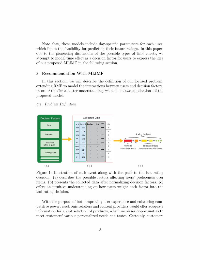
Figure 1: Illustration of each event along with the path to the last ratingdecision. (a) describes the possible factors affecting users’ preferences overitems. (b) presents the collected data after normalizing decision factors. (c)offers an intuitive understanding on how users weight each factor into thelast rating decision.

With the purpose of both improving user experience and enhancing com-petitive power, electronic retailers and content providers would offer adequateinformation for a vast selection of products, which increases opportunities tomeet customers’ various personalized needs and tastes. Certainly, customers

8

profit from the abundant data, which provide enough evidences to demon-strate the quality of involved products. As the figure 1 shows, the finaldecision for purchasing a product may be influenced by many factors, suchas emotion, seasonal discount, comments on the product and so on, andthe impact of each on users is unbalanced. For example, as a big fan ofStar Wars, user u prefers to pay for another exemplary analogical movie(e.g. THX 1138), directed by George Lucas (an American director famousfor the series of Star Wars). However, such delicate information is notalways available. Alternatively, extra sources associated with an active cus-tomer’s ratings can always be captured by RS. In this paper, we model sucheffect under the assumption that user u’s preference to item i can be partedinto limited weighted components, each of which denotes the significance ofinvolved factor in the final decision of u. Based on the framework of RMF,the interaction between user u and specific factor j can be represented as thedot-product of corresponding low-rank feature vectors. Thereby, rui can bemodified as the following:

rui = puqTi +

∑

j∈D

∑

dj∈Dj

1(u, i, dj)pudjqTdj, (5)

where D denotes the decision factor set. In Eq. (5), the first term presentsuser u’s preference on item i, and the bulk behind

∑notion denotes the

interactions between user u and possible decision factor j, which is always acategorical attribute with a set, denoted as Dj, of limited amount of values.It’s noted that the indicator function 1(u, i, dj) is set as 1 if user u focuseson the specific value of factor j, denoted as dj ∈ Dj, when giving ratingon item i, otherwise 1(u, i, dj) is set as 0. For example, a user who hs everrated “5 stars” on a Jackie Chan’s movie Rush Hour1, might give higherweight to another movie played or directed by him. Here, in order to modelthe relationship between users and extra information, a new set of decisionfactor feature vectors are necessary, where dj is associated with feature vector

qdj ∈ RfDj . Correspondingly, we define a new set of user feature vectors,

where user u involved with factor j is associated with pudj ∈ RfDj . Then the

9

objective function J is modified as follow:

minU,I,D

J =1

2

∑

u∈U

∑

i∈I

1(u, i)(rui − puqTi −

∑

j∈D

∑

dj∈Dj

1(u, i, dj)pudjqTdj)2

+λ

2(∑

u∈U

∑

j∈D

∑

dj∈Dj

∥∥pudj∥∥2F+∑

j∈D

∑

dj∈Dj

∥∥qdj∥∥2F)

+λ

2

(‖pu‖

2F + ‖qi‖

2F

)

, (6)

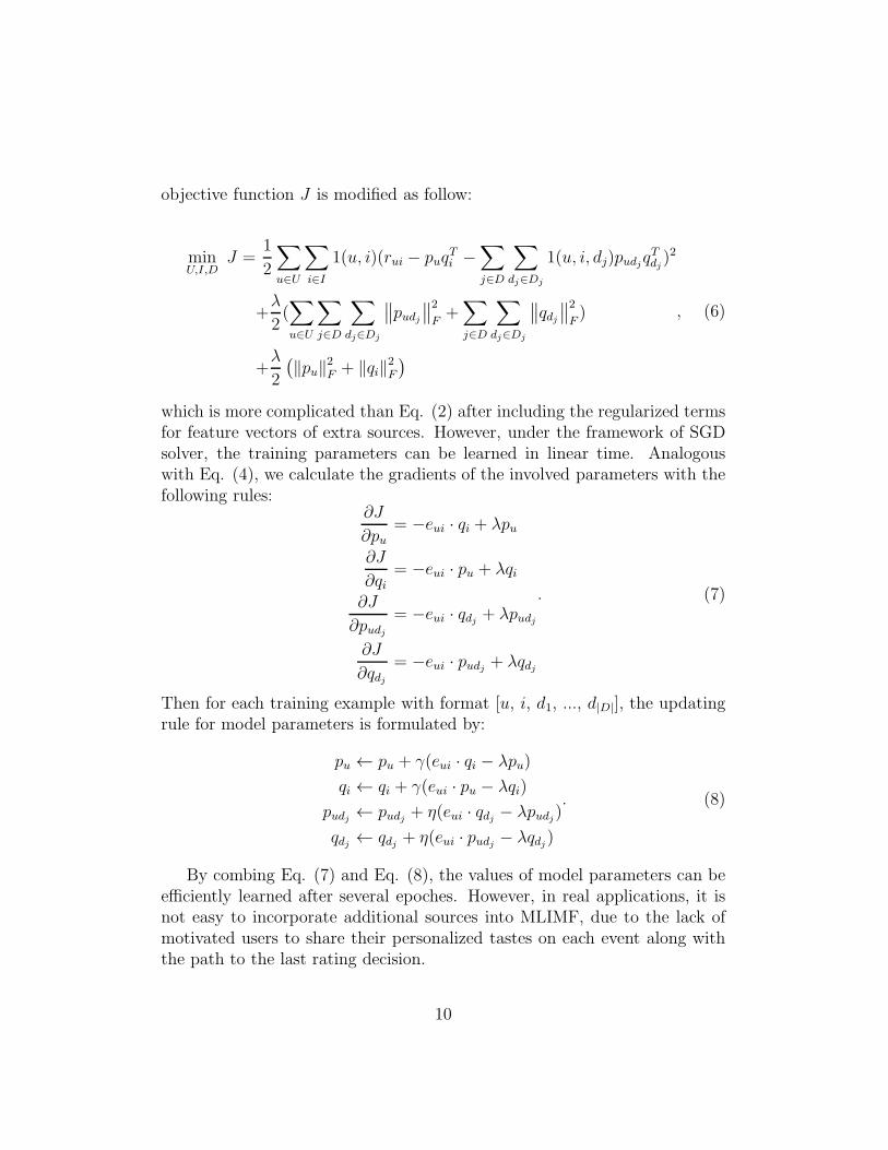
which is more complicated than Eq. (2) after including the regularized termsfor feature vectors of extra sources. However, under the framework of SGDsolver, the training parameters can be learned in linear time. Analogouswith Eq. (4), we calculate the gradients of the involved parameters with thefollowing rules:

∂J

∂pu= −eui · qi + λpu

∂J

∂qi= −eui · pu + λqi

∂J

∂pudj= −eui · qdj + λpudj

∂J

∂qdj= −eui · pudj + λqdj

. (7)

Then for each training example with format [u, i, d1, ..., d|D|], the updatingrule for model parameters is formulated by:

pu ← pu + γ(eui · qi − λpu)

qi ← qi + γ(eui · pu − λqi)

pudj ← pudj + η(eui · qdj − λpudj )

qdj ← qdj + η(eui · pudj − λqdj )

. (8)

By combing Eq. (7) and Eq. (8), the values of model parameters can beefficiently learned after several epoches. However, in real applications, it isnot easy to incorporate additional sources into MLIMF, due to the lack ofmotivated users to share their personalized tastes on each event along withthe path to the last rating decision.

10

Nevertheless, online service providers still carefully polish the design ofthe software systems to capture more details for better understanding userbehaviors, which plays an essential role in offering personalized and novelservices to users, as well as enhancing the company reputation and competi-tive strength. In fact, the logged data in the database offer a highly possibleapproach to model users’ rating action. Thereby, the issue of modeling theusers’ procedure of weighting decision factors becomes a problem on how toweight the modified and extracted probable features that might influence theusers’ rating decision for a particular item. To deeply clarify the principlesof MLIMF, we conduct two possible applications on two real data sets.

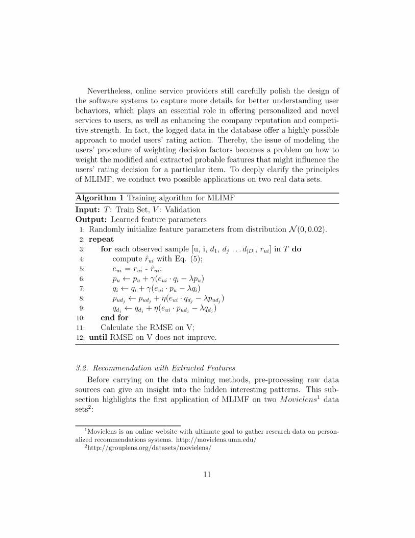
Algorithm 1 Training algorithm for MLIMF

Input: T : Train Set, V : ValidationOutput: Learned feature parameters1: Randomly initialize feature parameters from distribution N (0, 0.02).2: repeat

3: for each observed sample [u, i, d1, dj . . . d|D|, rui] in T do

4: compute rui with Eq. (5);5: eui = rui - rui;6: pu ← pu + γ(eui · qi − λpu)7: qi ← qi + γ(eui · pu − λqi)8: pudj ← pudj + η(eui · qdj − λpudj )9: qdj ← qdj + η(eui · pudj − λqdj )10: end for

11: Calculate the RMSE on V;12: until RMSE on V does not improve.

3.2. Recommendation with Extracted Features

Before carrying on the data mining methods, pre-processing raw datasources can give an insight into the hidden interesting patterns. This sub-section highlights the first application of MLIMF on two Movielens1 datasets2:

1Movielens is an online website with ultimate goal to gather research data on person-alized recommendations systems. http://movielens.umn.edu/

2http://grouplens.org/datasets/movielens/

11

- MovieLens 100k (ML100k) is collected by the GroupLens ResearchProject at the University of Minnesota via the MovieLens web site.ML100k contains 100,000 ratings (1-5) from 943 users on 1682 moviesduring the seven-month period from September 19th, 1997 to April22nd, 1998. Each user has rated at least 20 movies. The density ofthe rating matrix in ML100k is 6.30%. In addition to movie ratings,ML100k also provides various information on individual films, such asa group of genres and release date, which are used to increase the filmrecommendation system’s accuracy.

- MovieLens 1M (ML1m) is another collected data set on Movielensweb site, which contains 1,000,209 anonymous ratings (1-5) of approxi-mately 3,900 movies and 6,040 MovieLens users who joined MovieLensin 2000. The density of the rating matrix in ML1m is 4.25%. Like theML100k, ML1m provides the same information on individual films.

Obviously, the published MovieLens data sets only collect one type ofexplicit feedback (users’ ratings on movies), which simplifies users’ decisionprocedure of giving ratings to movies. In fact, the rating on a specific moviereflects an user’s personalized attitude to the corresponding information offilms. Although users do not explicitly express their viewpoints on eachpiece of movie information, the accumulative rating behaviors may implyinteresting patterns. The core idea of CF is to utilize the accumulative datato estimate user preference on items under the assumption that a groupof close neighbors with similar tastes could help each other rate objects.Based on the available information in the data, we can distill several feasibleingredients, which might affect user’s rating decision. Then we incorporatethose ingredients into the proposed MLIMF to model users’ rating behaviors.By combing the previous Eqs. (7-8), we can automatically learn the strengthof interactions between user and those ingredients from the given data.

In this example, it’s noted that besides the rating on item i ∈ I by useru ∈ U at time t ∈ R, ML100k and ML1m also offer information on each film,denoted as set S, where

S = {(A, T itanic, 2010.01.02, 5), (A, Star Wars, 2010.04.01, 1),

(B, Star Wars, 2009.05.04, 4), (C, T ime Tracers, 2010.04.01, 4)}.

Both ML100k and ML1m contain 19 types of genres and release date for eachindividual film and every movie can have multiple genres, namely genre group,

12

which can highly reflect the users’ tastes. The size of genre group describesindividual bias on multi-genre movies. Through the feasible transformationon the observed data, we extract three additional features, release date (RD),genre group (GG), the size of corresponding genre group (GS). Consequently,each piece of observed data can be denoted as (u, i, RD,GG,GS, rui). Letthe modified observed data S be:

S = {(A, T itanic, 1997, G1, 2, 5), (A, Star Wars, 1999, G2, 4, 1),

(B, Star Wars, 1999, G2, 4, 4), (C, T ime Tracers, 1995, G3, 4, 4)}

G1 ={Drama, Romance}

G2 ={Action, Adventure, Fantasy, Science F iction}

G3 ={Action, Adventure, Science F iction}

Usually we denote the user-item pairwise relationship as the rating matrix R.Thus the interactions between user and a specific factor j can be analogicallydenoted as user-factor matrix Rj , each entry of which is a binary indicator,which is set as 1 if user u is associated with factor j, otherwise set as 0.

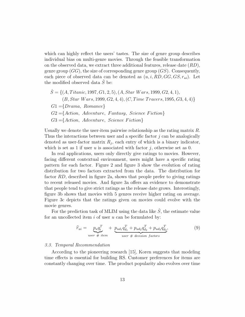
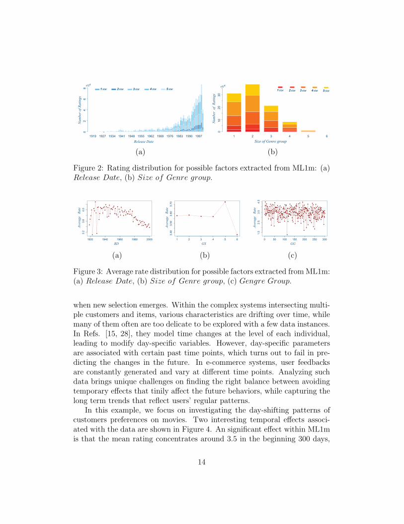
In real applications, users only directly give ratings to movies. However,facing different contextual environment, users might have a specific ratingpattern for each factor. Figure 2 and figure 3 show the evolution of ratingdistribution for two factors extracted from the data. The distribution forfactor RD, described in figure 2a, shows that people prefer to giving ratingsto recent released movies. And figure 3a offers an evidence to demonstratethat people tend to give strict ratings as the release date grows. Interestingly,figure 3b shows that movies with 5 genres receive higher rating on average.Figure 3c depicts that the ratings given on movies could evolve with themovie genres.

For the prediction task of MLIM using the data like S, the estimate valuefor an uncollected item i of user u can be formulated by:

rui = puqTi︸︷︷︸

user # item

+ pud1qTd1+ pud2q

Td2+ pud3q

Td3︸︷︷︸

user # decision factors

, (9)

3.3. Temporal Recommendation

According to the pioneering research [15], Koren suggests that modelingtime effects is essential for building RS. Customer preferences for items areconstantly changing over time. The product popularity also evolves over time

13

Nu

mb

er o

f R

ati

ng

s

Release Date

02

6

1919 1927 1934 1941 1948 1955 1962 1969 1976 1983 1990 1997

48

x104

1 star 2 star 3 star 4 star 5 star

01

02

03

0

1 2 3 4 5 6

Nu

mb

er

of

Ra

tin

gs

1 star 2 star 3 star 4 star 5 star

Size of Genre group

x104

(a) (b)

Figure 2: Rating distribution for possible factors extracted from ML1m: (a)Release Date, (b) Size of Genre group.

RD

Ave

rag

e

Ra

te3

.23

.64

.0

1920 1940 1960 1980 2000

Ave

rag

e

Ra

te

GS

3.4

03

.50

3.6

03

.70

1 2 3 4 5 6

GG

Ave

rag

e

Ra

te1

.52

.53

.54

.5

0 50 100 150 200 250 300

(a) (b) (c)

Figure 3: Average rate distribution for possible factors extracted fromML1m:(a) Release Date, (b) Size of Genre group, (c) Gengre Group.

when new selection emerges. Within the complex systems intersecting multi-ple customers and items, various characteristics are drifting over time, whilemany of them often are too delicate to be explored with a few data instances.In Refs. [15, 28], they model time changes at the level of each individual,leading to modify day-specific variables. However, day-specific parametersare associated with certain past time points, which turns out to fail in pre-dicting the changes in the future. In e-commerce systems, user feedbacksare constantly generated and vary at different time points. Analyzing suchdata brings unique challenges on finding the right balance between avoidingtemporary effects that tinily affect the future behaviors, while capturing thelong term trends that reflect users’ regular patterns.

In this example, we focus on investigating the day-shifting patterns ofcustomers preferences on movies. Two interesting temporal effects associ-ated with the data are shown in Figure 4. An significant effect within ML1mis that the mean rating concentrates around 3.5 in the beginning 300 days,

14

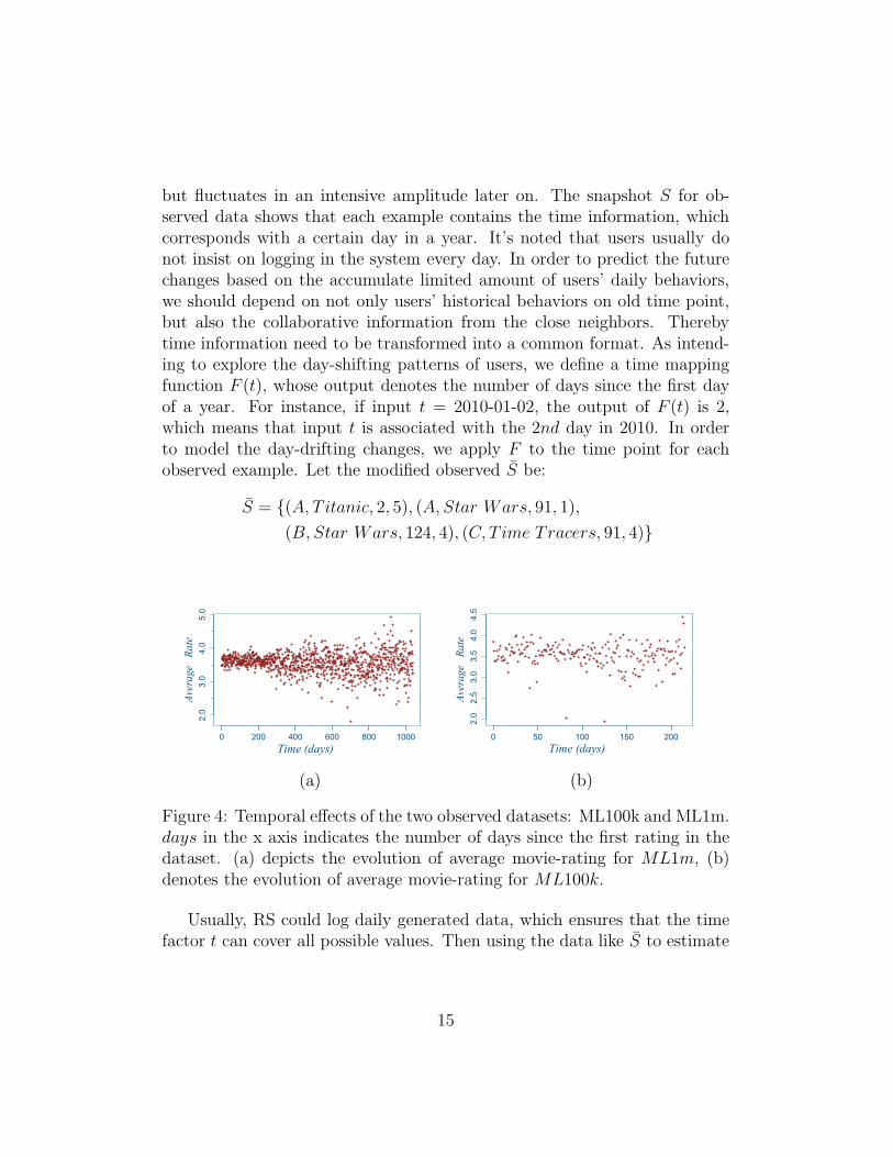
but fluctuates in an intensive amplitude later on. The snapshot S for ob-served data shows that each example contains the time information, whichcorresponds with a certain day in a year. It’s noted that users usually donot insist on logging in the system every day. In order to predict the futurechanges based on the accumulate limited amount of users’ daily behaviors,we should depend on not only users’ historical behaviors on old time point,but also the collaborative information from the close neighbors. Therebytime information need to be transformed into a common format. As intend-ing to explore the day-shifting patterns of users, we define a time mappingfunction F (t), whose output denotes the number of days since the first dayof a year. For instance, if input t = 2010-01-02, the output of F (t) is 2,which means that input t is associated with the 2nd day in 2010. In orderto model the day-drifting changes, we apply F to the time point for eachobserved example. Let the modified observed S be:

S = {(A, T itanic, 2, 5), (A, Star Wars, 91, 1),

(B, Star Wars, 124, 4), (C, T ime Tracers, 91, 4)}

++

++

+

++++

+

+

+++

++

+

+

+++

+++

+++

++++

+

+

++

+

+

+++

+

+

++

+

+

+

+

++

++

+++

+

++

+++

+++

+

+

+

+++++++++

+

+

+

+

+++++

+

+++

+

+

+

+

+

+

+

++++++++++

+

++

+

+++++++++++

++++

++

++

++

++++

+

+

++

+

+

+

+

+

+++++

+++

+++

+

++

+

++

+++

+

++

+

+

++

+

+

+

++

+

+++

+

+

+

+++++

+++++++++++

+++

+

+++++++++

++

++

++++++++

+

+++++

++

++++

+++

+++

+

+

+

+

+

+++

++

+

+

+

+++

+

+

++

+++

++

+

+

+

+

+

+

+++

++

+

++

+

+

+

+

+

++

+++++

++

+

+

+

+

+

+

+

++

+

+

++

+

+

+

+

++

+

+

+

+

+

++

+

+

+

+

+++++

+

+++

+

+

+

+

+++

+

+

+

+

+

+

++

++

+

++

+

+

+

+

+

+++++

+

+

+

+

+

+

+++++

+

+

+

+

+

+

++

+

+++

++

+++

+

++

+

+

+

+

+

+

+

+++

+

+

++

+

+++

+

+

++

++

++

+

+

++

++

+

+

+

++

+

+

+

+

+

+

+

+

++

+

+

+

+

+

+

+

+

++++

+

++

+

+

+

+

+

+

++

+

++

+

+

+

++

+

+

+

+

++

+

++

+

+

+

+

++

+++

+

++

++

+

++

++

+

+

+

+

+

+

+

++

+

+

+

+

+

++

+

+

+

+

+

+

+

+

+

+

++

+

+++

+

++

+

+

+

+

+

+

+

+

+

++++

+

++

+

++

+

+

+

+

+

+

+

+

+

++

+

++

+

+

+

+

+

+

+

++

++

++++

+

+

+

+

++

+

+

+

+

+

+

+

+

+

+

+

+

+++

+

++

+

++

+

+

+

+

+++

+++

+

+

+

+

+

++

+

+

+

+

++

+

+

+

+

+

+

+

+

+

+

+

++

+

+++

+

+

+

++

+

+

+

+

+

+

+

+++++

+

++

+

++

++

+

+

+

+

+

+

+

+

+

+

+

+

+

+

+++

+

++

++

+

+

+

+

+

+

+

+

+

+

+++++

+

+

+

+++

+

++

+

+

+

++

+

+

+

+

+

++

+

+

+

+

++

+

+

+

+

+

+

+

+

++++

++

++

+

+

+

++

+

+

+

+

+

+

++

++

+

+

+

+

++

+

+

++

+

+

+

+

+

+

+

++

++

+

++++

+

+

++

+

++

+

+

++

+

+

+

+

+

+

+

+

+

+

+

+

+

+

+

+

+

+

++

+

+

+

+

+

+

+

+

+

+

+

+

+

+

+

+

+

++

++

+

+

+

++

+

+

+

+

+

+

+

+

++

+

+

++

+

+++

+

+

+

+

+

+

++

+

+

+

+

+

+

+

+

+

+

+

+

+

+

+

+

+++

+

++

+

+

+

++

+

+

+

+

++

+

+

+

+

+

+

+

+

++

+

+

+

+

+

+

+

+

++

+

+

+

+

++

+

+

+++++

+

+

+

+

+

+

+

+

+

+

++

+

+

+

+

+

+

+

+

++

+

+

+++

+

+

+

+

+

+

+

+

+

+

+

++

+

++

+

+

++

+

+

+

+

+

+

+

+

+

+

+

+

+

+

+

+

++

+

+

+

+

+

+

+

+

+

+

+

+

+

+

++

+

+

+

+

+

++

+

+

+

Time (days)

Ave

rag

e

Ra

te

2.0

3.0

4.0

5.0

0 200 400 600 800 1000

+

+

++

+

++

++

++

+

++

++

+

+

+

++++++

++

+

+

+

++

+

+

+

+

+

+

+

+

+

+

+

+

+

+

++

+

+

+

+

+

+

+++

++++

++

+

+

+

++

++

+

+

+

+

+

+++

+

++

+

+

++

+

+

++++++++

+

+

++

+

+

++

+

+

+

+

++

++

+

+

+

+

+++

++

+

+

+

+

+

+

+

+

+

+

+

+

++

+

+

+

+

++

+

+

+

+

+

+

++

+

+

++

+

+

+

+

+

+

+

+

+

+

+

+

+

+

+

+

+

+

+

+

+

+

+

++

++

++

+

+

++

+

+

++

+

+

++

+

+

+

+

+

+

+

+

+

+

+

+

+

+

+

+

+

+

+

+

+

+

Time (days)

Ave

rag

e

Ra

te

2.0

2.5

3.0

3.5

4.0

4.5

0 50 100 150 200

(a) (b)

Figure 4: Temporal effects of the two observed datasets: ML100k and ML1m.days in the x axis indicates the number of days since the first rating in thedataset. (a) depicts the evolution of average movie-rating for ML1m, (b)denotes the evolution of average movie-rating for ML100k.

Usually, RS could log daily generated data, which ensures that the timefactor t can cover all possible values. Then using the data like S to estimate

15

user u’s preferences an uncollected item i at time t can be formulated by:

rui = puqTi︸︷︷︸

user # item

+ putqTt︸︷︷︸

user # time

. (10)

4. Empirical Analysis

The experiments were conducted on two MovleLens data sets as describedin Section 3.2. In the experiments, we applied the 5-fold cross-validationmethod on both data sets for the first application of MLIMF on extractedfeatures. In order to simulate real recommendation occasion for predictiontask on the future changes, we apply all-but-two3 experiment setting for thesecond application of MLIMF on modeling the time effects. The specific valueof temporal recommendation on the evaluation metric means the averageresults for 5 runs with random initialization.

Evaluation Metric. The performance of recommendation algorithms ismeasured by the root mean squared error (RMSE), a widely used metric forevaluating the rating prediction accuracy of recommenders, given by:

RMSE =

√∑(u,i)∈V (rui − rui)2

|V |, (11)

where V denotes the validation set. RMSE measures the errors betweenthe true values and the predictions. Obviously lower RMSE means higherprediction accuracy.

4.1. Baseline Methods

In this section, in order to show efficiency of our proposed recommenda-tion method, we compare the recommendation results with the three baselinealgorithms.

User-based CF (UCF) [2]. UCF is a typical implementation of CF. InUCF, the prediction task for an active user depends on a group of neighborswith similar interests. UCF generates recommendations by two steps: (i)calculate the similarity suv, which denotes the correlation or distance betweenuser u and v; (ii) generate the predictions for an active user by taking the

3all-but-two: Only the last two ratings of each individual are split into the validationset.

16

weighted average of all ratings of his/her k Nearest Neighbors (kNN). In thispaper, the similarity suv between user u and v is calculated with cosine-basedmetric. Let R denote the set of common items rated by both user u and v.Then the similarity is formulated by:

sim(u, v) =

∑i∈R ruirvi√∑i∈R r2uir

2vi

. (12)

To predict an active user u’s rating on an uncollected item i, we can take aweighted average of all the ratings on that item according to the followingformula [1]:

rui = ru +

∑v∈Nu

(rvi − rv)suv∑v∈Nu

suv, (13)

where ru and rv denote the mean rating of user u and v, respectively Nu

denotes the set of user u’s nearest neighbors who has collected item i.Item-based CF (ICF) [7]. Rather than computing the similarity between

user pairs, ICF starts from matching the user’s rated items with similaritems, then combines the most similar ones into recommendation list. Weemploy the cosine-based correlation to measure the similarity between itempairs. Let the C denote the set of common users involved with both item i

and j. Then the similarity is calculated by:

sim(i, j) =

∑u∈C ruiruj√∑u∈C r2uir

2uj

. (14)

The prediction step is significant in producing recommendation list. In ICF,generating recommendation results to an active user is based on his/herhistorical rated items. In this work, the estimate of rui for active user u iscomputed by:

rui = ri +

∑j∈Ru

(ruj − rj)sij∑j∈Ru

sij, (15)

where Ru denotes the set of rated items by user u. ri and rj respectivelydenote the mean rating of item i and j.

RMF [13, 10]: This method has been described in the Section 2. It usesonly the user-rating matrix to generate recommendations.

17

4.2. Performance validation for MLIMF

Experiment settings. In this part we intend to validate the performanceof our proposed MLIMF with other three baseline algorithms. In order tomake MF models converge at the optimized result, the initial values of fea-ture vectors for both RMF and MLIMF are randomly drawn from a normaldistribution N (0, 0.02), following the suggestion from [19]. Note that, theincorporation of extra factors makes MLIMF more difficulty to set the valueof dimension parameter for the comparative experiments on MLIMF andRMF. As the basic MF method, RMF only models the interactions betweenuser-item pairs, which simplifies the procedure of pre-defining the dimensionparameter f for user and item feature vectors. Usually, user-item pairs arematched into the same latent feature space with dimension f according to theprinciples of RMF. f is the key parameter to influence the efficiency of mod-eling user preferences on items. Therefore, we should redefine the parameterf for MLIMF because MLIMF models the interactions between users andextra factors besides user-item pairs. Since the objective is to validate theperformance of the proposed MLIMF, we design the experimental processesas follows:

- Firstly, we modify the settings of dimension parameters for RMF andMLIMF. The given value of dimension parameter f for RMF equals tothe sum of dimension variables for MLIMF, which can be denoted as:

f = fi +∑

j∈D

fDj, (16)

where fi and fDjare respectively the pre-defined parameters for the

dimension of the user-item and user-factor feature spaces. In the ap-plication of MLIMF on extracted features, dimension parameter fDj

for each decision factor j equals to 20% of the given value of f , whichmeans fi = 0.4∗f and fDj

= 0.2∗f . In applying MLIMF to modelingtime effects, the only parameter fDt

for decision factors equals to 60%of the given value of f .

- After implementing detailed analysis on experiment datasets, we carryon two possible examples to deeply clarify the idea of MLIMF. Fur-thermore, comparative experiments for those examples are conductedfor MLIMF and other three baseline approaches, including UCF, ICF,RMF. The experimental results are depicted in Tab. 1.

18

- According to [19], the dimension of feature space can greatly affectthe accuracy of MF-based approaches. Then we explore the impact ofdifferent values of dimension parameter f on the accuracy of RMF andMLIMF. The experimental results are shown in Tab. 2 and Tab. 3.

In the experimental processes, all aforementioned methods have manypre-defined parameters that greatly influence the accuracy. For UCF, thenumber of nearest neighbors k is significant for building UCF with highaccuracy. After conducting several experiments to explore the accuracy ofUCF, we decide to use the top 25% neighbors of each user to generate pre-dictive score of an uncollected item. The initial values of all features vectorsare randomly chosen from a normal distribution N (0, 0.02). For both ex-periment data sets ML1m and ML100k, the regularizing parameter λ forRMF and MLIMF is set to 0.01. In terms of the learning rate for RMF andMLIMF, initially γ and η are both set to 0.01 to ensure a comparative fastconvergence rate for ML100k and ML1m. According to Ref. [19], in additionto the setting of learning rate, the optimized result of the objective functionJ is correlated with the density of user-item rating matrix R. Interestingly,in MLIMF the user-factor matrix Rj is always denser than R because inreal-world application |Dj| is much less than |I|. Based on the above consid-eration, we decline the value of η to slow down the updating amplitude afterseveral epoches.

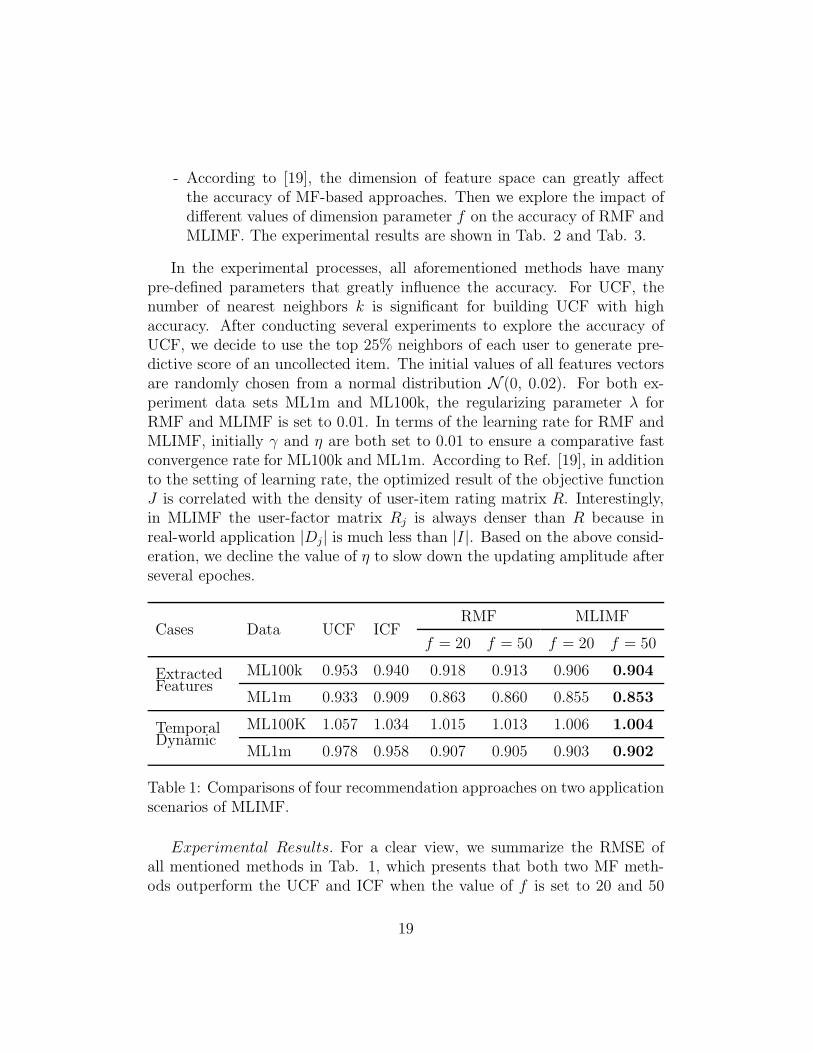
Cases Data UCF ICFRMF MLIMF

f = 20 f = 50 f = 20 f = 50

ExtractedFeatures

ML100k 0.953 0.940 0.918 0.913 0.906 0.904

ML1m 0.933 0.909 0.863 0.860 0.855 0.853

TemporalDynamic

ML100K 1.057 1.034 1.015 1.013 1.006 1.004

ML1m 0.978 0.958 0.907 0.905 0.903 0.902

Table 1: Comparisons of four recommendation approaches on two applicationscenarios of MLIMF.

Experimental Results. For a clear view, we summarize the RMSE ofall mentioned methods in Tab. 1, which presents that both two MF meth-ods outperform the UCF and ICF when the value of f is set to 20 and 50

19

respectively. Tab. 1 also shows that the effects of incorporating extra infor-mation make MLIMF work better than RMF with the same value of f ontwo applications of MLIMF.

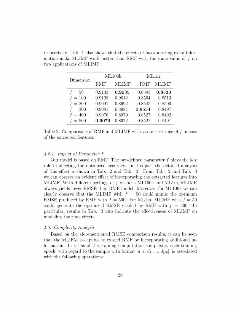
DimensionML100k ML1m

RMF MLIMF RMF MLIMF

f = 50 0.9133 0.9035 0.8593 0.8530

f = 100 0.9108 0.9012 0.8564 0.8513f = 200 0.9091 0.8992 0.8545 0.8500f = 300 0.9081 0.8984 0.8534 0.8497f = 400 0.9076 0.8979 0.8527 0.8492f = 500 0.9070 0.8972 0.8522 0.8491

Table 2: Comparisons of RMF and MLIMF with various settings of f in caseof the extracted features.

4.2.1. Impact of Parameter f

Our model is based on RMF. The pre-defined parameter f plays the keyrole in affecting the optimized accuracy. In this part the detailed analysisof this effect is shown in Tab. 2 and Tab. 3. From Tab. 2 and Tab. 3we can observe an evident effect of incorporating the extracted features intoMLIMF. With different settings of f on both ML100k and ML1m, MLIMFalways yields lower RMSE than RMF model. Moreover, for ML100k we canclearly observe that the MLIMF with f = 50 could mimic the optimumRMSE produced by RMF with f = 500. For ML1m, MLIMF with f = 50could generate the optimized RMSE yielded by RMF with f = 300. Inparticular, results in Tab. 3 also indicate the effectiveness of MLIMF onmodeling the time effects.

4.3. Complexity Analysis

Based on the aforementioned RMSE comparison results, it can be seenthat the MLIFM is capable to extend RMF by incorporating additional in-formation. In terms of the training computation complexity, each trainingepoch, with regard to the sample with format [u, i, d1, ..., d|D|], is associatedwith the following operations:

20

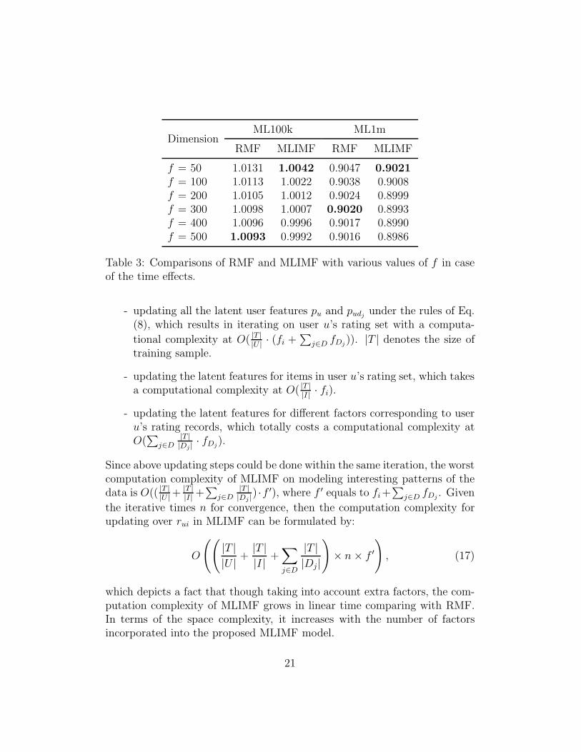
DimensionML100k ML1m

RMF MLIMF RMF MLIMF

f = 50 1.0131 1.0042 0.9047 0.9021

f = 100 1.0113 1.0022 0.9038 0.9008f = 200 1.0105 1.0012 0.9024 0.8999f = 300 1.0098 1.0007 0.9020 0.8993f = 400 1.0096 0.9996 0.9017 0.8990f = 500 1.0093 0.9992 0.9016 0.8986

Table 3: Comparisons of RMF and MLIMF with various values of f in caseof the time effects.

- updating all the latent user features pu and pudj under the rules of Eq.(8), which results in iterating on user u’s rating set with a computa-

tional complexity at O( |T ||U |· (fi +

∑j∈D fDj

)). |T | denotes the size oftraining sample.

- updating the latent features for items in user u’s rating set, which takesa computational complexity at O( |T |

|I|· fi).

- updating the latent features for different factors corresponding to useru’s rating records, which totally costs a computational complexity atO(∑

j∈D|T ||Dj |· fDj

).

Since above updating steps could be done within the same iteration, the worstcomputation complexity of MLIMF on modeling interesting patterns of thedata is O(( |T |

|U |+ |T |

|I|+∑

j∈D|T ||Dj |

) ·f ′), where f ′ equals to fi+∑

j∈D fDj. Given

the iterative times n for convergence, then the computation complexity forupdating over rui in MLIMF can be formulated by:

O

((|T |

|U |+|T |

|I|+∑

j∈D

|T |

|Dj|

)× n× f ′

), (17)

which depicts a fact that though taking into account extra factors, the com-putation complexity of MLIMF grows in linear time comparing with RMF.In terms of the space complexity, it increases with the number of factorsincorporated into the proposed MLIMF model.

21

5. Conclusions and Discussion

Many pioneering researches have proved that Matrix Factorization (MF)based approaches are effective and flexible in dealing with various aspectsof user-item rating data. Generally, the final rating decisions of online usersshould be affected by various underlying factors, such as emotions, time,genres, and so on. In this paper, based on classical MF method, we proposea multi-linear interactive MF (MLIMF) approach, trying to gain insight intouser preferences. Firstly, we assume that users are willing to implicitly orexplicitly weigh the impact of each factor when they rate items. Secondly,we extract possible factors correlated with users’ decisions from empiricalanalyses. Thirdly, to model the multiple pairwise relationship, we linearlyintegrate the total pairwise interactions to predict their ratings. Finally,experiments results show that the proposed MLIMF method perform muchbetter than three baseline algorithms (UCF, ICF and RMF) with the RMSEmetric.

Overall, MLIMF is a simple yet general approach since it mainly focuseson modeling the interactions between user and other information beyond rat-ings. Similar inspiration can be easily applied to other MF based models as abulk denoting the user-factor interactions. In this paper, we just simply ex-tend the basic RMF to explore the impact of categorical attributes on users’rating patterns. However, there are many data mining tasks which need todeal with attributes of continuous values. Therefore, in order to addressmore general data mining challenges, it is necessary to design an effectiveframework to extend the proposed MLIMF. We attempt to study the pos-sible applications of MLIMF to solve tough recommendation challenges likeestimating click-through rate (CTR) in the era of computational advertising,building effective binary classifiers to predict the potential tastes of onlineusers.

6. Acknowledgements

This work was partially supported by the National Natural Science Foun-dation of China (Grant Nos. 11105024, 11205040, 11305043 and 11301490),the EU FP7 Grant 611272 (project GROWTHCOM), and the Zhejiang Provin-cial Qianjiang Talents Project (Grant No. QJC1302001), the start-up foun-dations of Hangzhou Normal University.

22

References

[1] P. Resnick, N. Iacovou, M. Suchak, P. Bergstrom, J. Riedl, Grouplens:an open architecture for collaborative filtering of netnews, in: Proceed-ings of the 1994 ACM conference on Computer supported cooperativework, ACM, 1994, pp. 175–186.

[2] L. Lu, M. Medo, C. H. Yeung, Y.-C. Zhang, Z.-K. Zhang, T. Zhou,Recommender systems, Physics Reports 519 (1) (2012) 1–49.

[3] J. Bobadilla, F. Ortega, A. Hernando, A. Gutierrez, Recommender sys-tems survey, Knowledge-Based Systems 46 (2013) 109–132.

[4] M. Balabanovic, Y. Shoham, Fab: content-based, collaborative recom-mendation, Communications of the ACM 40 (3) (1997) 66–72.

[5] J. L. Herlocker, J. A. Konstan, A. Borchers, J. Riedl, An algorithmicframework for performing collaborative filtering, in: Proceedings of the22nd annual international ACM SIGIR conference on Research and de-velopment in information retrieval, ACM, 1999, pp. 230–237.

[6] W. Hill, L. Stead, M. Rosenstein, G. Furnas, Recommending and eval-uating choices in a virtual community of use, in: Proceedings of theSIGCHI conference on Human factors in computing systems, ACMPress/Addison-Wesley Publishing Co., 1995, pp. 194–201.

[7] B. Sarwar, G. Karypis, J. Konstan, J. Riedl, Item-based collaborativefiltering recommendation algorithms, in: Proceedings of the 10th inter-national conference on World Wide Web, ACM, 2001, pp. 285–295.

[8] G. Linden, B. Smith, J. York, Amazon. com recommendations: Item-to-item collaborative filtering, Internet Computing, IEEE 7 (1) (2003)76–80.

[9] T. Hofmann, Latent semantic models for collaborative filtering, ACMTransactions on Information Systems (TOIS) 22 (1) (2004) 89–115.

[10] Y. Koren, R. Bell, C. Volinsky, Matrix factorization techniques for rec-ommender systems, Computer 42 (8) (2009) 30–37.

23

[11] B. Sarwar, G. Karypis, J. Konstan, J. Riedl, Application of dimension-ality reduction in recommender system-a case study, Tech. rep., DTICDocument (2000).

[12] J. Bennett, S. Lanning, The netflix prize, in: Proceedings of KDD cupand workshop, 2007, p. 35.

[13] B. Webb, Netflix prize: Try this at home (December 11, 2006).URL http://sifter.org/~simon/journal/20061211.html

[14] Y. Koren, Factorization meets the neighborhood: a multifaceted collab-orative filtering model, in: Proceedings of the 14th ACM SIGKDD in-ternational conference on Knowledge discovery and data mining, ACM,2008, pp. 426–434.

[15] Y. Koren, Collaborative filtering with temporal dynamics, Communica-tions of the ACM 53 (4) (2010) 89–97.

[16] G. Takacs, I. Pilaszy, B. Nemeth, D. Tikk, Investigation of various ma-trix factorization methods for large recommender systems, in: Data Min-ing Workshops, 2008. ICDMW’08. IEEE International Conference on,IEEE, 2008, pp. 553–562.

[17] G. Takacs, I. Pilaszy, B. Nemeth, D. Tikk, Matrix factorization andneighbor based algorithms for the netflix prize problem, in: Proceedingsof the 2008 ACM conference on Recommender systems, ACM, 2008, pp.267–274.

[18] A. Paterek, Improving regularized singular value decomposition for col-laborative filtering, in: Proceedings of KDD cup and workshop, 2007.

[19] G. Takacs, I. Pilaszy, B. Nemeth, D. Tikk, Scalable collaborative filter-ing approaches for large recommender systems, The Journal of MachineLearning Research 10 (2009) 623–656.

[20] X. Luo, Y. Xia, Q. Zhu, Incremental collaborative filtering recommenderbased on regularized matrix factorization, Knowledge-Based Systems 27(2012) 271–280.

[21] X. Luo, Y. Xia, Q. Zhu, Applying the learning rate adaptation to thematrix factorization based collaborative filtering, Knowledge-Based Sys-tems 37 (2013) 154–164.

24

http://sifter.org/~simon/journal/20061211.html

http://sifter.org/~simon/journal/20061211.html

[22] C.-X. Zhang, Z.-K. Zhang, L. Yu, C. Liu, H. Liu, X.-Y. Yan, Informationfiltering via collaborative user clustering modeling, Physica A 396 (2014)195–203.

[23] A. Karatzoglou, X. Amatriain, L. Baltrunas, N. Oliver, Multiverse rec-ommendation: n-dimensional tensor factorization for context-aware col-laborative filtering, in: Proceedings of the fourth ACM conference onRecommender systems, ACM, 2010, pp. 79–86.

[24] L. Baltrunas, B. Ludwig, F. Ricci, Matrix factorization techniques forcontext aware recommendation, in: Proceedings of the fifth ACM con-ference on Recommender systems, ACM, 2011, pp. 301–304.

[25] H. Ma, D. Zhou, C. Liu, M. R. Lyu, I. King, Recommender systems withsocial regularization, in: Proceedings of the fourth ACM internationalconference on Web search and data mining, ACM, 2011, pp. 287–296.

[26] M. Jamali, M. Ester, A matrix factorization technique with trust prop-agation for recommendation in social networks, in: Proceedings of thefourth ACM conference on Recommender systems, ACM, 2010, pp. 135–142.

[27] N. Lathia, S. Hailes, L. Capra, knn cf: a temporal social network, in:Proceedings of the 2008 ACM conference on Recommender systems,ACM, 2008, pp. 227–234.

[28] L. Xiang, Q. Yang, Time-dependent models in collaborative filteringbased recommender system, in: IEEE/WIC/ACM International JointConferences on Web Intelligence and Intelligent Agent Technologies,Vol. 1, 2009, pp. 450–457.

25

Multi-Linear Interactive Matrix Factorization

Documents