The Incremental Multiresolution Matrix Factorization ...

The Incremental Multiresolution Matrix Factorization AlgorithmSupplementary Material

Vamsi K. Ithapu†, Risi Kondor§, Sterling C. Johnson†, Vikas Singh††University of Wisconsin-Madison, §University of Chicagohttp://pages.cs.wisc.edu/˜vamsi/projects/incmmf.html

2. Multiresolution Matrix Factorization

Explanation for Equation 3: This directly follws from Proposition 1 and 2 in [4].

3. Incremental MMF

Algorithm 1 INSERTROW(C,w, {t`, s`}L`=1)

Output: {t`, s`}L+1`=1

C0 ← Cz1 ← m + 1for ` = 1 to L− 1 do{t`, s`, z`+1,Q`}←CHECKINSERT(C`−1; t`, s`, z`)C` = Q`C`−1(Q`)T

end forT ← GENERATETUPLES([m + 1] \ ∪L−1`=1 s

`(C))

{O, tL, sL} ← argminO,t∈T ,s∈t E(CL−1;O; t, s)

QL = Im+1, QLtL,tL

= O

CL = QLCL−1(QL)T

Algorithm 2 CHECKINSERT(A, t, s, z)

Output: t, s, z, QT ← GENERATETUPLES(t, z){O, t, s} ← argminO,t∈T ,s∈t E(A;O; t, s)if s ∈ z thenz ← (z ∪ s) \ s

end ifQ = Im+1, Qt,t = O

Algorithm 1 adds one extra row/column is to a given MMF, and clearly, the incremental procedure can be repeated asmore and more rows/columns are added. Algorithm 3 summarizes this incremental factorization for arbitrarily large anddense matrices. It has two components: an initialization on some randomly chosen small block (of size m × m) of theentire matrix C; followed by insertion of the remaining m− m rows/columns using Algorithm 1 in a streaming fashion Theinitialization entails computing a batch-wise MMF on this small block (m ≥ k).BATCHMMF – EXHAUSTIVE: Note that at each level `, the error criterion can be explicitly minimized via an exhaustivesearch over all possible k-tuples from S`−1 (the active set) and a randomly chosen (using properties of QR decomposition

1

Algorithm 3 INCREMENTAL MMF(C)Output: M(C)

C = C[m],[m], L = m− k + 1

{t`, s`}m−k+11 ← BATCHMMF(C)

for j ∈ {m + 1, . . . ,m} do{t`, s`}j−k+1

1 ← INSERTROW(C,Cj,:, {t`, s`}j−k1 )C = C[j],[j]

end forM(C) := {t`, s`}L1

[7]) dictionary of kth order rotations. If the dictionary is large enough, the exhaustive procedure would lead to the smallestpossible decomposition error. However, it is easy to see that this is combinatorially large, with an overall complexity ofO(nk) [5] and will not scale well beyond k = 4 or so. Note from Algorithm 1 that the error criterion E(·) in this secondstage which inserts the rest of the m− m rows is performing an exhaustive search as well.

Other Variants: The are two alternatives that avoid this exhaustive search.• BATCHMMF – EIGEN: Since Q`’s job is to diagonalize some k rows/columns.one can simply pick the relevant k × k

block of C` and compute the best O (for a given t`). Hence the first alternative is to bypass the search over O, and simplyuse the eigen-vectors of C`

t`,t` for some tuple t`. Nevertheless, the search over S`−1 for t` still makes this approximationreasonably costly.

• BATCHMMF – RANDOM: Instead, the k-tuple selection may be approximated while keeping the exhaustive search overO intact [5]. Since diagonalization effectively nullifies correlated dimensions, the best k-tuple can be the k rows/columnsthat are maximally correlated. This is done by choosing some s1 ∼ S`−1 (from the current active set), and picking the restby

s2, . . . , sk ← argminsi∼S`−1\s1

k∑i=2

(C`−1:,s1 )TC`−1

:,si

‖C`−1:,s1 ‖‖C`−1

:,si ‖(1)

This second heuristic has been shown to be robust [5], however, for large k it might miss some k-tuples that are vital to thequality of the factorization. Depending on m, and the available computational resources at hand, these alternatives can beused instead of the earlier proposed exhaustive procedure for the initialization.

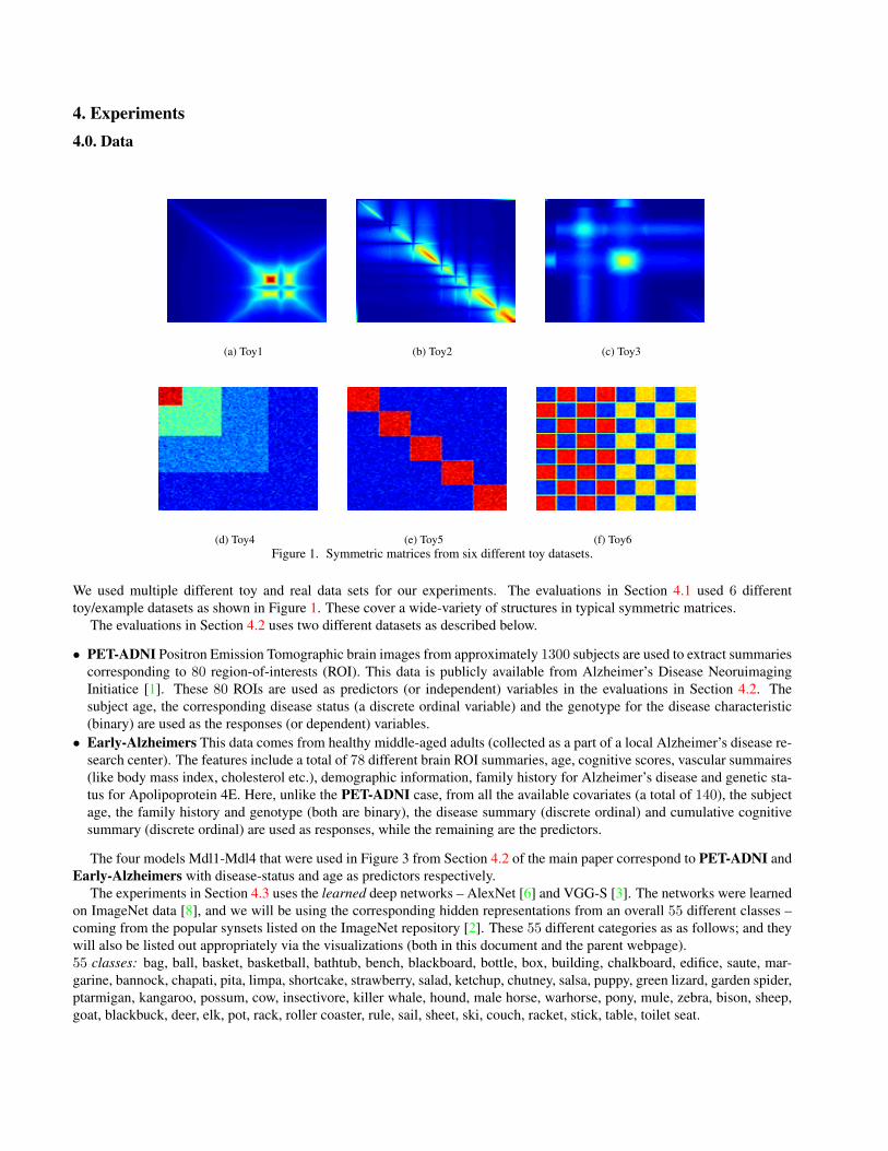
4. Experiments4.0. Data

(a) Toy1 (b) Toy2 (c) Toy3

(d) Toy4 (e) Toy5 (f) Toy6Figure 1. Symmetric matrices from six different toy datasets.

We used multiple different toy and real data sets for our experiments. The evaluations in Section 4.1 used 6 differenttoy/example datasets as shown in Figure 1. These cover a wide-variety of structures in typical symmetric matrices.

The evaluations in Section 4.2 uses two different datasets as described below.

• PET-ADNI Positron Emission Tomographic brain images from approximately 1300 subjects are used to extract summariescorresponding to 80 region-of-interests (ROI). This data is publicly available from Alzheimer’s Disease NeoruimagingInitiatice [1]. These 80 ROIs are used as predictors (or independent) variables in the evaluations in Section 4.2. Thesubject age, the corresponding disease status (a discrete ordinal variable) and the genotype for the disease characteristic(binary) are used as the responses (or dependent) variables.

• Early-Alzheimers This data comes from healthy middle-aged adults (collected as a part of a local Alzheimer’s disease re-search center). The features include a total of 78 different brain ROI summaries, age, cognitive scores, vascular summaires(like body mass index, cholesterol etc.), demographic information, family history for Alzheimer’s disease and genetic sta-tus for Apolipoprotein 4E. Here, unlike the PET-ADNI case, from all the available covariates (a total of 140), the subjectage, the family history and genotype (both are binary), the disease summary (discrete ordinal) and cumulative cognitivesummary (discrete ordinal) are used as responses, while the remaining are the predictors.

The four models Mdl1-Mdl4 that were used in Figure 3 from Section 4.2 of the main paper correspond to PET-ADNI andEarly-Alzheimers with disease-status and age as predictors respectively.

The experiments in Section 4.3 uses the learned deep networks – AlexNet [6] and VGG-S [3]. The networks were learnedon ImageNet data [8], and we will be using the corresponding hidden representations from an overall 55 different classes –coming from the popular synsets listed on the ImageNet repository [2]. These 55 different categories as as follows; and theywill also be listed out appropriately via the visualizations (both in this document and the parent webpage).55 classes: bag, ball, basket, basketball, bathtub, bench, blackboard, bottle, box, building, chalkboard, edifice, saute, mar-garine, bannock, chapati, pita, limpa, shortcake, strawberry, salad, ketchup, chutney, salsa, puppy, green lizard, garden spider,ptarmigan, kangaroo, possum, cow, insectivore, killer whale, hound, male horse, warhorse, pony, mule, zebra, bison, sheep,goat, blackbuck, deer, elk, pot, rack, roller coaster, rule, sail, sheet, ski, couch, racket, stick, table, toilet seat.

4.1. Incremental vs. Batch MMF

Fraction of Batch Initialization

0 0.2 0.4 0.6

Incre

me

nta

l vs.

Exh

au

stive

No

rma

lize

d E

rro

r

0

0.005

0.01

0.015

0.02

0.025Exhaus-Exhaus

Random-Exhaus

Eigen-Exhaus

(a) Error vs. Enhaus InsertFraction of Batch Initialization

0 0.2 0.4 0.6

Incre

me

nta

l vs.

Exh

au

stive

No

rma

lize

d E

rro

r

0

0.01

0.02

0.03

0.04

Exhaus-Exhaus

Exhaus-Random

Exhaus-Eigen

(b) Error vs. Enhaus InitFraction of Batch Initialization

0 0.2 0.4 0.6

Incre

me

nta

l vs.

Exh

au

stive

No

rma

lize

d E

rro

r

0

0.005

0.01

0.015

0.02

0.025

Exhaus-Eigen

Random-Eigen

Eigen-Eigen

(c) Error vs. Eigen Insert

(d) Error Conf. Mat. (e) Error Conf. Mat. (f) Error Conf. Mat. (g) Error Conf. Mat.Figure 2. Incremental versus Batch MMFs on Toy1 dataset [ERROR]: Comparing factorization errors between the exhaustive batchversion and different versions of incremental versions (a–c), including incremental MMFs with exhaustive insertion step (a), exhaustiveinitialization step (b) and eigen insertion step (c). Confusion matrix of factorization errors between the 9 versions of incremental MMFs –three initilizations and three insertions (exhaustive, random and eigen).

Fraction of Batch Initialization

0 0.2 0.4 0.6

Speedup (

log10

scale

) vs. Id

eal

0

0.5

1

1.5

2

2.5Exhaus-Exhaus

Random-Exhaus

Eigen-Exhaus

(a) Speed-up vs. Enhaus InsertFraction of Batch Initialization

0 0.2 0.4 0.6

Sp

ee

du

p (

log

10

sca

le)

vs.

Ide

al

0

1

2

3

4

5Exhaus-Exhaus

Exhaus-Random

Exhaus-Eigen

(b) Speed-up vs. Enhaus InitFraction of Batch Initialization

0 0.2 0.4 0.6

Incre

me

nta

l vs.

Exh

au

stive

No

rma

lize

d E

rro

r

0

0.005

0.01

0.015

0.02

0.025

Exhaus-Eigen

Random-Eigen

Eigen-Eigen

(c) Speed-up vs. Eigen Insert

(d) Time Conf. Mat. (e) Time Conf. Mat. (f) Time Conf. Mat. (g) Time Conf. Mat.Figure 3. Incremental versus Batch MMFs on Toy1 dataset [SPEED-UP]: Comparing factorization speed-ups between the exhaustivebatch version and different versions of incremental versions (a–c), including incremental MMFs with exhaustive insertion step (a), ex-haustive initialization step (b) and eigen insertion step (c). Confusion matrix of factorization times between the 9 versions of incrementalMMFs – three initilizations and three insertions (exhaustive, random and eigen).

Fraction of Batch Initialization

0 0.2 0.4 0.6

Incre

me

nta

l vs.

Exh

au

stive

No

rma

lize

d E

rro

r

0

0.02

0.04

0.06

0.08

0.1 Exhaus-Exhaus

Random-Exhaus

Eigen-Exhaus

(a) Error vs. Enhaus InsertFraction of Batch Initialization

0 0.2 0.4 0.6

Incre

me

nta

l vs.

Exh

au

stive

No

rma

lize

d E

rro

r

0

0.02

0.04

0.06

0.08

0.1 Exhaus-Exhaus

Exhaus-Random

Exhaus-Eigen

(b) Error vs. Enhaus InitFraction of Batch Initialization

0 0.2 0.4 0.6

Incre

me

nta

l vs.

Exh

au

stive

No

rma

lize

d E

rro

r

0

0.01

0.02

0.03

0.04

0.05 Exhaus-Eigen

Random-Eigen

Eigen-Eigen

(c) Error vs. Eigen Insert

(d) Error Conf. Mat. (e) Error Conf. Mat. (f) Error Conf. Mat. (g) Error Conf. Mat.Figure 4. Incremental versus Batch MMFs on Toy2 dataset [ERROR]: Comparing factorization errors between the exhaustive batchversion and different versions of incremental versions (a–c), including incremental MMFs with exhaustive insertion step (a), exhaustiveinitialization step (b) and eigen insertion step (c). Confusion matrix of factorization errors between the 9 versions of incremental MMFs –three initilizations and three insertions (exhaustive, random and eigen).

Fraction of Batch Initialization

0 0.2 0.4 0.6

Speedup (

log10 s

cale

) vs. Id

eal

0

0.5

1

1.5

2

2.5Exhaus-Exhaus

Random-Exhaus

Eigen-Exhaus

(a) Speed-up vs. Enhaus InsertFraction of Batch Initialization

0 0.2 0.4 0.6

Sp

ee

du

p (

log

10

sca

le)

vs.

Ide

al

0

1

2

3

4

5Exhaus-Exhaus

Exhaus-Random

Exhaus-Eigen

(b) Speed-up vs. Enhaus InitFraction of Batch Initialization

0 0.2 0.4 0.6

Sp

ee

du

p (

log

10

sca

le)

vs.

Ide

al

0

1

2

3

4

5Exhaus-Eigen

Random-Eigen

Eigen-Eigen

(c) Speed-up vs. Eigen Insert

(d) Time Conf. Mat. (e) Time Conf. Mat. (f) Time Conf. Mat. (g) Time Conf. Mat.Figure 5. Incremental versus Batch MMFs on Toy2 dataset [SPEED-UP]: Comparing factorization speed-ups between the exhaustivebatch version and different versions of incremental versions (a–c), including incremental MMFs with exhaustive insertion step (a), ex-haustive initialization step (b) and eigen insertion step (c). Confusion matrix of factorization times between the 9 versions of incrementalMMFs – three initilizations and three insertions (exhaustive, random and eigen).

Fraction of Batch Initialization

0 0.2 0.4 0.6

Incre

me

nta

l vs.

Exh

au

stive

No

rma

lize

d E

rro

r

0

0.005

0.01

0.015

0.02

0.025

0.03

Exhaus-Exhaus

Random-Exhaus

Eigen-Exhaus

(a) Error vs. Enhaus InsertFraction of Batch Initialization

0 0.2 0.4 0.6

Incre

me

nta

l vs.

Exh

au

stive

No

rma

lize

d E

rro

r

0

0.005

0.01

0.015

0.02

0.025

0.03 Exhaus-Exhaus

Exhaus-Random

Exhaus-Eigen

(b) Error vs. Enhaus InitFraction of Batch Initialization

0 0.2 0.4 0.6

Incre

me

nta

l vs.

Exh

au

stive

No

rma

lize

d E

rro

r

0

0.005

0.01

0.015

0.02

0.025

0.03 Exhaus-Eigen

Random-Eigen

Eigen-Eigen

(c) Error vs. Eigen Insert

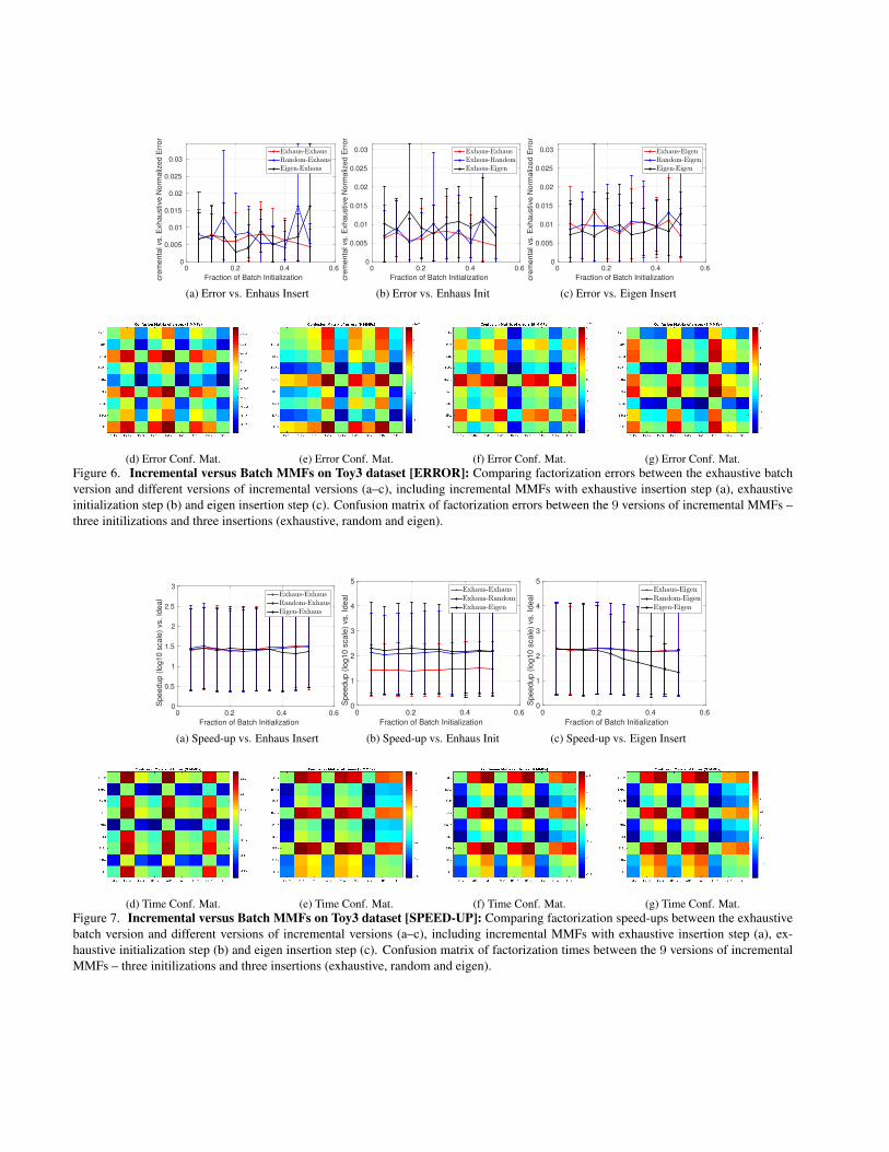
(d) Error Conf. Mat. (e) Error Conf. Mat. (f) Error Conf. Mat. (g) Error Conf. Mat.Figure 6. Incremental versus Batch MMFs on Toy3 dataset [ERROR]: Comparing factorization errors between the exhaustive batchversion and different versions of incremental versions (a–c), including incremental MMFs with exhaustive insertion step (a), exhaustiveinitialization step (b) and eigen insertion step (c). Confusion matrix of factorization errors between the 9 versions of incremental MMFs –three initilizations and three insertions (exhaustive, random and eigen).

Fraction of Batch Initialization

0 0.2 0.4 0.6

Speedup (

log10 s

cale

) vs. Id

eal

0

0.5

1

1.5

2

2.5

3Exhaus-Exhaus

Random-Exhaus

Eigen-Exhaus

(a) Speed-up vs. Enhaus InsertFraction of Batch Initialization

0 0.2 0.4 0.6

Sp

ee

du

p (

log

10

sca

le)

vs.

Ide

al

0

1

2

3

4

5Exhaus-Exhaus

Exhaus-Random

Exhaus-Eigen

(b) Speed-up vs. Enhaus InitFraction of Batch Initialization

0 0.2 0.4 0.6

Sp

ee

du

p (

log

10

sca

le)

vs.

Ide

al

0

1

2

3

4

5Exhaus-Eigen

Random-Eigen

Eigen-Eigen

(c) Speed-up vs. Eigen Insert

(d) Time Conf. Mat. (e) Time Conf. Mat. (f) Time Conf. Mat. (g) Time Conf. Mat.Figure 7. Incremental versus Batch MMFs on Toy3 dataset [SPEED-UP]: Comparing factorization speed-ups between the exhaustivebatch version and different versions of incremental versions (a–c), including incremental MMFs with exhaustive insertion step (a), ex-haustive initialization step (b) and eigen insertion step (c). Confusion matrix of factorization times between the 9 versions of incrementalMMFs – three initilizations and three insertions (exhaustive, random and eigen).

Fraction of Batch Initialization

0 0.2 0.4 0.6

Incre

me

nta

l vs.

Exh

au

stive

No

rma

lize

d E

rro

r

0

0.01

0.02

0.03

0.04

Exhaus-Exhaus

Random-Exhaus

Eigen-Exhaus

(a) Error vs. Enhaus InsertFraction of Batch Initialization

0 0.2 0.4 0.6

Incre

me

nta

l vs.

Exh

au

stive

No

rma

lize

d E

rro

r

0

0.01

0.02

0.03

0.04

0.05

0.06

0.07 Exhaus-Exhaus

Exhaus-Random

Exhaus-Eigen

(b) Error vs. Enhaus InitFraction of Batch Initialization

0 0.2 0.4 0.6

Incre

me

nta

l vs.

Exh

au

stive

No

rma

lize

d E

rro

r

0

0.005

0.01

0.015

0.02

Exhaus-Eigen

Random-Eigen

Eigen-Eigen

(c) Error vs. Eigen Insert

(d) Error Conf. Mat. (e) Error Conf. Mat. (f) Error Conf. Mat. (g) Error Conf. Mat.Figure 8. Incremental versus Batch MMFs on Toy4 dataset [ERROR]: Comparing factorization errors between the exhaustive batchversion and different versions of incremental versions (a–c), including incremental MMFs with exhaustive insertion step (a), exhaustiveinitialization step (b) and eigen insertion step (c). Confusion matrix of factorization errors between the 9 versions of incremental MMFs –three initilizations and three insertions (exhaustive, random and eigen).

Fraction of Batch Initialization

0 0.2 0.4 0.6

Speedup (

log10 s

cale

) vs. Id

eal

0

0.5

1

1.5

2

2.5

3Exhaus-Exhaus

Random-Exhaus

Eigen-Exhaus

(a) Speed-up vs. Enhaus InsertFraction of Batch Initialization

0 0.2 0.4 0.6

Sp

ee

du

p (

log

10

sca

le)

vs.

Ide

al

0

1

2

3

4

5Exhaus-Exhaus

Exhaus-Random

Exhaus-Eigen

(b) Speed-up vs. Enhaus InitFraction of Batch Initialization

0 0.2 0.4 0.6

Sp

ee

du

p (

log

10

sca

le)

vs.

Ide

al

0

1

2

3

4

5Exhaus-Eigen

Random-Eigen

Eigen-Eigen

(c) Speed-up vs. Eigen Insert

(d) Time Conf. Mat. (e) Time Conf. Mat. (f) Time Conf. Mat. (g) Time Conf. Mat.Figure 9. Incremental versus Batch MMFs on Toy4 dataset [SPEED-UP]: Comparing factorization speed-ups between the exhaustivebatch version and different versions of incremental versions (a–c), including incremental MMFs with exhaustive insertion step (a), ex-haustive initialization step (b) and eigen insertion step (c). Confusion matrix of factorization times between the 9 versions of incrementalMMFs – three initilizations and three insertions (exhaustive, random and eigen).

Fraction of Batch Initialization

0 0.2 0.4 0.6

Incre

me

nta

l vs.

Exh

au

stive

No

rma

lize

d E

rro

r

0

0.05

0.1

0.15

0.2

0.25

0.3Exhaus-Exhaus

Random-Exhaus

Eigen-Exhaus

(a) Error vs. Enhaus InsertFraction of Batch Initialization

0 0.2 0.4 0.6

Incre

me

nta

l vs.

Exh

au

stive

No

rma

lize

d E

rro

r

0

0.05

0.1

0.15

0.2

0.25

0.3

0.35 Exhaus-Exhaus

Exhaus-Random

Exhaus-Eigen

(b) Error vs. Enhaus InitFraction of Batch Initialization

0 0.2 0.4 0.6

Incre

me

nta

l vs.

Exh

au

stive

No

rma

lize

d E

rro

r

0

0.05

0.1

0.15

0.2

0.25

0.3

0.35 Exhaus-Eigen

Random-Eigen

Eigen-Eigen

(c) Error vs. Eigen Insert

(d) Error Conf. Mat. (e) Error Conf. Mat. (f) Error Conf. Mat. (g) Error Conf. Mat.Figure 10. Incremental versus Batch MMFs on Toy5 dataset [ERROR]: Comparing factorization errors between the exhaustive batchversion and different versions of incremental versions (a–c), including incremental MMFs with exhaustive insertion step (a), exhaustiveinitialization step (b) and eigen insertion step (c). Confusion matrix of factorization errors between the 9 versions of incremental MMFs –three initilizations and three insertions (exhaustive, random and eigen).

Fraction of Batch Initialization

0 0.2 0.4 0.6

Speedup (

log10 s

cale

) vs. Id

eal

0

0.5

1

1.5

2

2.5

3Exhaus-Exhaus

Random-Exhaus

Eigen-Exhaus

(a) Speed-up vs. Enhaus InsertFraction of Batch Initialization

0 0.2 0.4 0.6

Sp

ee

du

p (

log

10

sca

le)

vs.

Ide

al

0

1

2

3

4

5Exhaus-Exhaus

Exhaus-Random

Exhaus-Eigen

(b) Speed-up vs. Enhaus InitFraction of Batch Initialization

0 0.2 0.4 0.6

Sp

ee

du

p (

log

10

sca

le)

vs.

Ide

al

0

1

2

3

4

5Exhaus-Eigen

Random-Eigen

Eigen-Eigen

(c) Speed-up vs. Eigen Insert

(d) Time Conf. Mat. (e) Time Conf. Mat. (f) Time Conf. Mat. (g) Time Conf. Mat.Figure 11. Incremental versus Batch MMFs on Toy5 dataset [SPEED-UP]: Comparing factorization speed-ups between the exhaus-tive batch version and different versions of incremental versions (a–c), including incremental MMFs with exhaustive insertion step (a),exhaustive initialization step (b) and eigen insertion step (c). Confusion matrix of factorization times between the 9 versions of incrementalMMFs – three initilizations and three insertions (exhaustive, random and eigen).

Fraction of Batch Initialization

0 0.2 0.4 0.6

Incre

me

nta

l vs.

Exh

au

stive

No

rma

lize

d E

rro

r ×10-3

0

1

2

3

4

Exhaus-Exhaus

Random-Exhaus

Eigen-Exhaus

(a) Error vs. Enhaus InsertFraction of Batch Initialization

0 0.2 0.4 0.6

Incre

me

nta

l vs.

Exh

au

stive

No

rma

lize

d E

rro

r ×10-3

0

2

4

6

8

Exhaus-Exhaus

Exhaus-Random

Exhaus-Eigen

(b) Error vs. Enhaus InitFraction of Batch Initialization

0 0.2 0.4 0.6

Incre

me

nta

l vs.

Exh

au

stive

No

rma

lize

d E

rro

r

0

0.002

0.004

0.006

0.008

0.01

Exhaus-Eigen

Random-Eigen

Eigen-Eigen

(c) Error vs. Eigen Insert

(d) Error Conf. Mat. (e) Error Conf. Mat. (f) Error Conf. Mat. (g) Error Conf. Mat.Figure 12. Incremental versus Batch MMFs on Toy6 dataset [ERROR]: Comparing factorization errors between the exhaustive batchversion and different versions of incremental versions (a–c), including incremental MMFs with exhaustive insertion step (a), exhaustiveinitialization step (b) and eigen insertion step (c). Confusion matrix of factorization errors between the 9 versions of incremental MMFs –three initilizations and three insertions (exhaustive, random and eigen).

Fraction of Batch Initialization

0 0.2 0.4 0.6

Speedup (

log10 s

cale

) vs. Id

eal

0

0.5

1

1.5

2

2.5Exhaus-Exhaus

Random-Exhaus

Eigen-Exhaus

(a) Speed-up vs. Enhaus InsertFraction of Batch Initialization

0 0.2 0.4 0.6

Sp

ee

du

p (

log

10

sca

le)

vs.

Ide

al

0

1

2

3

4

5Exhaus-Exhaus

Exhaus-Random

Exhaus-Eigen

(b) Speed-up vs. Enhaus InitFraction of Batch Initialization

0 0.2 0.4 0.6

Sp

ee

du

p (

log

10

sca

le)

vs.

Ide

al

0

1

2

3

4

5Exhaus-Eigen

Random-Eigen

Eigen-Eigen

(c) Speed-up vs. Eigen Insert

(d) Time Conf. Mat. (e) Time Conf. Mat. (f) Time Conf. Mat. (g) Time Conf. Mat.Figure 13. Incremental versus Batch MMFs on Toy6 dataset [SPEED-UP]: Comparing factorization speed-ups between the exhaus-tive batch version and different versions of incremental versions (a–c), including incremental MMFs with exhaustive insertion step (a),exhaustive initialization step (b) and eigen insertion step (c). Confusion matrix of factorization times between the 9 versions of incrementalMMFs – three initilizations and three insertions (exhaustive, random and eigen).

4.2. MMF Scores

#Features used

0 0.2 0.4 0.6 0.8

F-s

tatistic o

f linear

model

0

10

20

30

40

50

60

70

LevScore

MMFScore

(a) F -stat Comp; k = 6

#Features used

0 0.2 0.4 0.6 0.8

F-s

tatistic o

f linear

model

0

10

20

30

40

50

LevScore

MMFScore

(b) F -stat Comp; k = 8

#Features used

0 0.2 0.4 0.6 0.8

F-s

tatistic o

f linear

model

0

10

20

30

40

LevScore

MMFScore

(c) F -stat Comp; k = 10

#Features used

0 0.2 0.4 0.6 0.8

F-s

tatistic o

f linear

model

0

10

20

30

40

50

60

70

LevScore

MMFScore

(d) F -stat Comp; k = 12

#Features used

0 0.2 0.4 0.6 0.8

F-s

tatistic o

f linear

model

0

10

20

30

40

50

60

70

LevScore

MMFScore

(e) F -stat Comp; k = 14

#Features used

0 0.2 0.4 0.6 0.8

F-s

tatistic o

f linear

model

0

10

20

30

40

50

60

LevScore

MMFScore

(f) F -stat Comp; k = 16

#Features used

0 0.2 0.4 0.6 0.8

F-s

tatistic o

f linear

model

0

10

20

30

40

LevScore

MMFScore

(g) F -stat Comp; k = 18

#Features used

0 0.2 0.4 0.6 0.8

F-s

tatistic o

f linear

model

0

10

20

30

40

50

60

70

LevScore

MMFScore

(h) F -stat Comp; k = 20

Figure 14. Importance Sampling from MMF Scores (black) vs. Leverage Scores (blue) – F -statistic: The F -statistic of the linearmodel ‘fitted’ using the features (ROIs) from PET-ADNI data, selected according to the MMF Score (black) or Leverage Score (blue)importance samplers. The response is the disease status. The x-axis denotes the fraction of such features selected. The errorbars on theplots correspond to 10 repetitions of the linear model. Each plot corresponds to different order of the MMFs (k = 6 to 20 at steps of 2).

#Features used

0 0.2 0.4 0.6 0.8

R-s

quare

d o

f lin

ear

model

0

0.1

0.2

0.3

0.4

0.5

0.6LevScore

MMFScore

(a) F -stat Comp; k = 6

#Features used

0 0.2 0.4 0.6 0.8

R-s

quare

d o

f lin

ear

model

0

0.1

0.2

0.3

0.4

0.5

0.6LevScore

MMFScore

(b) F -stat Comp; k = 8

#Features used

0 0.2 0.4 0.6 0.8

R-s

quare

d o

f lin

ear

model

0

0.1

0.2

0.3

0.4

0.5

0.6LevScore

MMFScore

(c) F -stat Comp; k = 10

#Features used

0 0.2 0.4 0.6 0.8

R-s

quare

d o

f lin

ear

model

0

0.1

0.2

0.3

0.4

0.5

0.6LevScore

MMFScore

(d) F -stat Comp; k = 12

#Features used

0 0.2 0.4 0.6 0.8

R-s

quare

d o

f lin

ear

model

0

0.1

0.2

0.3

0.4

0.5

0.6LevScore

MMFScore

(e) F -stat Comp; k = 14

#Features used

0 0.2 0.4 0.6 0.8

R-s

quare

d o

f lin

ear

model

0

0.1

0.2

0.3

0.4

0.5

0.6LevScore

MMFScore

(f) F -stat Comp; k = 16

#Features used

0 0.2 0.4 0.6 0.8

R-s

quare

d o

f lin

ear

model

0

0.1

0.2

0.3

0.4

0.5

0.6LevScore

MMFScore

(g) F -stat Comp; k = 18

#Features used

0 0.2 0.4 0.6 0.8

R-s

quare

d o

f lin

ear

model

0

0.1

0.2

0.3

0.4

0.5

0.6LevScore

MMFScore

(h) F -stat Comp; k = 20

Figure 15. Importance Sampling from MMF Scores (black) vs. Leverage Scores (blue) – R2: The R2 of the linear model ‘fitted’ usingthe features (ROIs) from PET-ADNI data, selected according to the MMF Score (black) or Leverage Score (blue) importance samplers.The response is the disease status. The x-axis denotes the fraction of such features selected. The errorbars on the plots correspond to 10repetitions of the linear model. Each plot corresponds to different order of the MMFs (k = 6 to 20 at steps of 2).

#Features used

0 0.2 0.4 0.6 0.8

F-s

tatistic o

f linear

model

0

10

20

30

40

50

LevScore

MMFScore

(a) F -stat Comp; k = 6

#Features used

0 0.2 0.4 0.6 0.8

F-s

tatistic o

f linear

model

0

10

20

30

40

50

60

70

LevScore

MMFScore

(b) F -stat Comp; k = 8

#Features used

0 0.2 0.4 0.6 0.8

F-s

tatistic o

f linear

model

0

10

20

30

40

50

60

LevScore

MMFScore

(c) F -stat Comp; k = 10

#Features used

0 0.2 0.4 0.6 0.8

F-s

tatistic o

f linear

model

0

10

20

30

40

50

60

LevScore

MMFScore

(d) F -stat Comp; k = 12

#Features used

0 0.2 0.4 0.6 0.8

F-s

tatistic o

f linear

model

0

10

20

30

40

50

60

LevScore

MMFScore

(e) F -stat Comp; k = 14

#Features used

0 0.2 0.4 0.6 0.8

F-s

tatistic o

f linear

model

0

10

20

30

40

50

60

70

LevScore

MMFScore

(f) F -stat Comp; k = 16

#Features used

0 0.2 0.4 0.6 0.8

F-s

tatistic o

f linear

model

0

10

20

30

40

50

60

LevScore

MMFScore

(g) F -stat Comp; k = 18

#Features used

0 0.2 0.4 0.6 0.8

F-s

tatistic o

f linear

model

0

10

20

30

40

50

60

LevScore

MMFScore

(h) F -stat Comp; k = 20

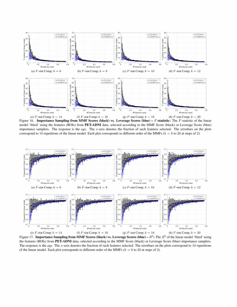
Figure 16. Importance Sampling from MMF Scores (black) vs. Leverage Scores (blue) – F -statistic: The F -statistic of the linearmodel ‘fitted’ using the features (ROIs) from PET-ADNI data, selected according to the MMF Score (black) or Leverage Score (blue)importance samplers. The response is the age. The x-axis denotes the fraction of such features selected. The errorbars on the plotscorrespond to 10 repetitions of the linear model. Each plot corresponds to different order of the MMFs (k = 6 to 20 at steps of 2).

#Features used

0 0.2 0.4 0.6 0.8

R-s

quare

d o

f lin

ear

model

0.1

0.2

0.3

0.4

0.5

0.6

0.7LevScore

MMFScore

(a) F -stat Comp; k = 6

#Features used

0 0.2 0.4 0.6 0.8

R-s

quare

d o

f lin

ear

model

0.1

0.2

0.3

0.4

0.5

0.6

0.7LevScore

MMFScore

(b) F -stat Comp; k = 8

#Features used

0 0.2 0.4 0.6 0.8

R-s

quare

d o

f lin

ear

model

0.1

0.2

0.3

0.4

0.5

0.6

0.7LevScore

MMFScore

(c) F -stat Comp; k = 10

#Features used

0 0.2 0.4 0.6 0.8

R-s

quare

d o

f lin

ear

model

0.1

0.2

0.3

0.4

0.5

0.6

0.7LevScore

MMFScore

(d) F -stat Comp; k = 12

#Features used

0 0.2 0.4 0.6 0.8

R-s

quare

d o

f lin

ear

model

0.1

0.2

0.3

0.4

0.5

0.6

0.7LevScore

MMFScore

(e) F -stat Comp; k = 14

#Features used

0 0.2 0.4 0.6 0.8

R-s

quare

d o

f lin

ear

model

0.1

0.2

0.3

0.4

0.5

0.6

0.7LevScore

MMFScore

(f) F -stat Comp; k = 16

#Features used

0 0.2 0.4 0.6 0.8

R-s

quare

d o

f lin

ear

model

0.1

0.2

0.3

0.4

0.5

0.6

0.7LevScore

MMFScore

(g) F -stat Comp; k = 18

#Features used

0 0.2 0.4 0.6 0.8

R-s

quare

d o

f lin

ear

model

0.1

0.2

0.3

0.4

0.5

0.6

0.7LevScore

MMFScore

(h) F -stat Comp; k = 20

Figure 17. Importance Sampling from MMF Scores (black) vs. Leverage Scores (blue) – R2: The R2 of the linear model ‘fitted’ usingthe features (ROIs) from PET-ADNI data, selected according to the MMF Score (black) or Leverage Score (blue) importance samplers.The response is the age. The x-axis denotes the fraction of such features selected. The errorbars on the plots correspond to 10 repetitionsof the linear model. Each plot corresponds to different order of the MMFs (k = 6 to 20 at steps of 2).

#Features used

0 0.2 0.4 0.6 0.8

F-s

tatistic o

f linear

model

0

10

20

30

40

LevScore

MMFScore

(a) F -stat Comp; k = 6

#Features used

0 0.2 0.4 0.6 0.8

F-s

tatistic o

f linear

model

0

5

10

15

20

25

LevScore

MMFScore

(b) F -stat Comp; k = 8

#Features used

0 0.2 0.4 0.6 0.8

F-s

tatistic o

f linear

model

0

5

10

15

20

LevScore

MMFScore

(c) F -stat Comp; k = 10

#Features used

0 0.2 0.4 0.6 0.8

F-s

tatistic o

f linear

model

0

5

10

15

20

LevScore

MMFScore

(d) F -stat Comp; k = 12

#Features used

0 0.2 0.4 0.6 0.8

F-s

tatistic o

f linear

model

0

5

10

15

20

LevScore

MMFScore

(e) F -stat Comp; k = 14

#Features used

0 0.2 0.4 0.6 0.8

F-s

tatistic o

f linear

model

0

5

10

15

20

LevScore

MMFScore

(f) F -stat Comp; k = 16

#Features used

0 0.2 0.4 0.6 0.8

F-s

tatistic o

f linear

model

0

5

10

15

20

LevScore

MMFScore

(g) F -stat Comp; k = 18

#Features used

0 0.2 0.4 0.6 0.8

F-s

tatistic o

f linear

model

0

5

10

15

20

25

LevScore

MMFScore

(h) F -stat Comp; k = 20

Figure 18. Importance Sampling from MMF Scores (black) vs. Leverage Scores (blue) – F -statistic: The F -statistic of the linearmodel ‘fitted’ using the features (ROIs) from PET-ADNI data, selected according to the MMF Score (black) or Leverage Score (blue)importance samplers. The response is the genotype. The x-axis denotes the fraction of such features selected. The errorbars on the plotscorrespond to 10 repetitions of the linear model. Each plot corresponds to different order of the MMFs (k = 6 to 20 at steps of 2).

#Features used

0 0.2 0.4 0.6 0.8

R-s

quare

d o

f lin

ear

model

0

0.1

0.2

0.3

0.4LevScore

MMFScore

(a) F -stat Comp; k = 6

#Features used

0 0.2 0.4 0.6 0.8

R-s

quare

d o

f lin

ear

model

0

0.1

0.2

0.3

0.4LevScore

MMFScore

(b) F -stat Comp; k = 8

#Features used

0 0.2 0.4 0.6 0.8

R-s

quare

d o

f lin

ear

model

0

0.1

0.2

0.3

0.4LevScore

MMFScore

(c) F -stat Comp; k = 10

#Features used

0 0.2 0.4 0.6 0.8

R-s

quare

d o

f lin

ear

model

0

0.1

0.2

0.3

0.4LevScore

MMFScore

(d) F -stat Comp; k = 12

#Features used

0 0.2 0.4 0.6 0.8

R-s

quare

d o

f lin

ear

model

0

0.1

0.2

0.3

0.4LevScore

MMFScore

(e) F -stat Comp; k = 14

#Features used

0 0.2 0.4 0.6 0.8

R-s

quare

d o

f lin

ear

model

0

0.1

0.2

0.3

0.4LevScore

MMFScore

(f) F -stat Comp; k = 16

#Features used

0 0.2 0.4 0.6 0.8

R-s

quare

d o

f lin

ear

model

0

0.1

0.2

0.3

0.4LevScore

MMFScore

(g) F -stat Comp; k = 18

#Features used

0 0.2 0.4 0.6 0.8

R-s

quare

d o

f lin

ear

model

0

0.1

0.2

0.3

0.4LevScore

MMFScore

(h) F -stat Comp; k = 20

Figure 19. Importance Sampling from MMF Scores (black) vs. Leverage Scores (blue) – R2: The R2 of the linear model ‘fitted’ usingthe features (ROIs) from PET-ADNI data, selected according to the MMF Score (black) or Leverage Score (blue) importance samplers.The response is the genotype. The x-axis denotes the fraction of such features selected. The errorbars on the plots correspond to 10repetitions of the linear model. Each plot corresponds to different order of the MMFs (k = 6 to 20 at steps of 2).

#Features used

0 0.2 0.4 0.6 0.8

F-s

tatistic o

f linear

model

-20

0

20

40

60

80

100

120

LevScore

MMFScore

(a) F -stat Comp; k = 6

#Features used

0 0.2 0.4 0.6 0.8

F-s

tatistic o

f linear

model

-20

0

20

40

60

80

100

120

LevScore

MMFScore

(b) F -stat Comp; k = 8

#Features used

0 0.2 0.4 0.6 0.8

F-s

tatistic o

f lin

ea

r m

od

el

-20

0

20

40

60

80

LevScore

MMFScore

(c) F -stat Comp; k = 10

#Features used

0 0.2 0.4 0.6 0.8

F-s

tatistic o

f linear

model

-20

0

20

40

60

80

100

120

LevScore

MMFScore

(d) F -stat Comp; k = 12

#Features used

0 0.2 0.4 0.6 0.8

F-s

tatistic o

f linear

model

-20

0

20

40

60

80

100

LevScore

MMFScore

(e) F -stat Comp; k = 14

#Features used

0 0.2 0.4 0.6 0.8

F-s

tatistic o

f linear

model

-20

0

20

40

60

80

100

LevScore

MMFScore

(f) F -stat Comp; k = 16

#Features used

0 0.2 0.4 0.6 0.8

F-s

tatistic o

f linear

model

-20

0

20

40

60

80

100

120

LevScore

MMFScore

(g) F -stat Comp; k = 18

#Features used

0 0.2 0.4 0.6 0.8

F-s

tatistic o

f lin

ea

r m

od

el

-20

0

20

40

60

80

LevScore

MMFScore

(h) F -stat Comp; k = 20

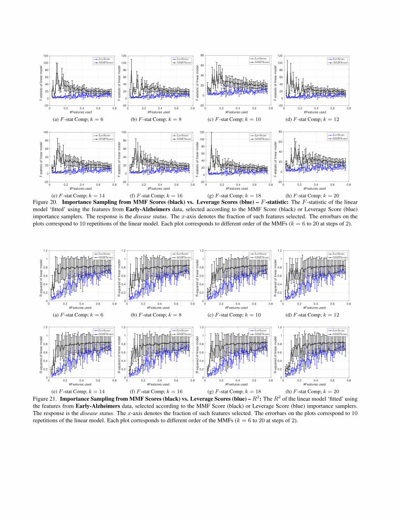
Figure 20. Importance Sampling from MMF Scores (black) vs. Leverage Scores (blue) – F -statistic: The F -statistic of the linearmodel ‘fitted’ using the features from Early-Alzheimers data, selected according to the MMF Score (black) or Leverage Score (blue)importance samplers. The response is the disease status. The x-axis denotes the fraction of such features selected. The errorbars on theplots correspond to 10 repetitions of the linear model. Each plot corresponds to different order of the MMFs (k = 6 to 20 at steps of 2).

#Features used

0 0.2 0.4 0.6 0.8

R-s

quare

d o

f lin

ear

model

0

0.2

0.4

0.6

0.8

1

1.2LevScore

MMFScore

(a) F -stat Comp; k = 6

#Features used

0 0.2 0.4 0.6 0.8

R-s

quare

d o

f lin

ear

model

0

0.2

0.4

0.6

0.8

1

1.2LevScore

MMFScore

(b) F -stat Comp; k = 8

#Features used

0 0.2 0.4 0.6 0.8

R-s

quare

d o

f lin

ear

model

0

0.2

0.4

0.6

0.8

1

1.2LevScore

MMFScore

(c) F -stat Comp; k = 10

#Features used

0 0.2 0.4 0.6 0.8

R-s

quare

d o

f lin

ear

model

0

0.2

0.4

0.6

0.8

1

1.2LevScore

MMFScore

(d) F -stat Comp; k = 12

#Features used

0 0.2 0.4 0.6 0.8

R-s

quare

d o

f lin

ear

model

0

0.2

0.4

0.6

0.8

1

1.2LevScore

MMFScore

(e) F -stat Comp; k = 14

#Features used

0 0.2 0.4 0.6 0.8

R-s

quare

d o

f lin

ear

model

0

0.2

0.4

0.6

0.8

1

1.2LevScore

MMFScore

(f) F -stat Comp; k = 16

#Features used

0 0.2 0.4 0.6 0.8

R-s

quare

d o

f lin

ear

model

0

0.2

0.4

0.6

0.8

1

1.2LevScore

MMFScore

(g) F -stat Comp; k = 18

#Features used

0 0.2 0.4 0.6 0.8

R-s

quare

d o

f lin

ear

model

0

0.2

0.4

0.6

0.8

1

1.2LevScore

MMFScore

(h) F -stat Comp; k = 20

Figure 21. Importance Sampling from MMF Scores (black) vs. Leverage Scores (blue) – R2: The R2 of the linear model ‘fitted’ usingthe features from Early-Alzheimers data, selected according to the MMF Score (black) or Leverage Score (blue) importance samplers.The response is the disease status. The x-axis denotes the fraction of such features selected. The errorbars on the plots correspond to 10repetitions of the linear model. Each plot corresponds to different order of the MMFs (k = 6 to 20 at steps of 2).

#Features used

0 0.2 0.4 0.6 0.8

F-s

tatistic o

f linear

model

-5

0

5

10

15

LevScore

MMFScore

(a) F -stat Comp; k = 6

#Features used

0 0.2 0.4 0.6 0.8

F-s

tatistic o

f linear

model

-5

0

5

10

15

LevScore

MMFScore

(b) F -stat Comp; k = 8

#Features used

0 0.2 0.4 0.6 0.8

F-s

tatistic o

f linear

model

-5

0

5

10

15

LevScore

MMFScore

(c) F -stat Comp; k = 10

#Features used

0 0.2 0.4 0.6 0.8

F-s

tatistic o

f linear

model

-5

0

5

10

15

20

25

LevScore

MMFScore

(d) F -stat Comp; k = 12

#Features used

0 0.2 0.4 0.6 0.8

F-s

tatistic o

f linear

model

-5

0

5

10

15

LevScore

MMFScore

(e) F -stat Comp; k = 14

#Features used

0 0.2 0.4 0.6 0.8

F-s

tatistic o

f linear

model

-2

0

2

4

6

8

10

12

LevScore

MMFScore

(f) F -stat Comp; k = 16

#Features used

0 0.2 0.4 0.6 0.8

F-s

tatistic o

f linear

model

-5

0

5

10

15

LevScore

MMFScore

(g) F -stat Comp; k = 18

#Features used

0 0.2 0.4 0.6 0.8

F-s

tatistic o

f linear

model

-5

0

5

10

15

20

LevScore

MMFScore

(h) F -stat Comp; k = 20

Figure 22. Importance Sampling from MMF Scores (black) vs. Leverage Scores (blue) – F -statistic: The F -statistic of the linearmodel ‘fitted’ using the features from Early-Alzheimers data, selected according to the MMF Score (black) or Leverage Score (blue)importance samplers. The response is the age. The x-axis denotes the fraction of such features selected. The errorbars on the plotscorrespond to 10 repetitions of the linear model. Each plot corresponds to different order of the MMFs (k = 6 to 20 at steps of 2).

#Features used

0 0.2 0.4 0.6 0.8

R-s

qua

red o

f lin

ea

r m

ode

l

-0.1

0

0.1

0.2

0.3

0.4

0.5

0.6LevScore

MMFScore

(a) F -stat Comp; k = 6

#Features used

0 0.2 0.4 0.6 0.8

R-s

qua

red o

f lin

ea

r m

ode

l

-0.1

0

0.1

0.2

0.3

0.4

0.5

0.6LevScore

MMFScore

(b) F -stat Comp; k = 8

#Features used

0 0.2 0.4 0.6 0.8

R-s

qua

red o

f lin

ea

r m

ode

l

-0.1

0

0.1

0.2

0.3

0.4

0.5

0.6LevScore

MMFScore

(c) F -stat Comp; k = 10

#Features used

0 0.2 0.4 0.6 0.8

R-s

qua

red o

f lin

ea

r m

ode

l

-0.1

0

0.1

0.2

0.3

0.4

0.5

0.6LevScore

MMFScore

(d) F -stat Comp; k = 12

#Features used

0 0.2 0.4 0.6 0.8

R-s

qu

are

d o

f lin

ea

r m

ode

l

-0.2

0

0.2

0.4

0.6

0.8LevScore

MMFScore

(e) F -stat Comp; k = 14

#Features used

0 0.2 0.4 0.6 0.8

R-s

qu

are

d o

f lin

ea

r m

ode

l

-0.1

0

0.1

0.2

0.3

0.4

0.5

0.6LevScore

MMFScore

(f) F -stat Comp; k = 16

#Features used

0 0.2 0.4 0.6 0.8

R-s

qu

are

d o

f lin

ea

r m

ode

l

-0.1

0

0.1

0.2

0.3

0.4

0.5

0.6LevScore

MMFScore

(g) F -stat Comp; k = 18

#Features used

0 0.2 0.4 0.6 0.8

R-s

qu

are

d o

f lin

ea

r m

ode

l

-0.1

0

0.1

0.2

0.3

0.4

0.5

0.6LevScore

MMFScore

(h) F -stat Comp; k = 20

Figure 23. Importance Sampling from MMF Scores (black) vs. Leverage Scores (blue) – R2: The R2 of the linear model ‘fitted’ usingthe features from Early-Alzheimers data, selected according to the MMF Score (black) or Leverage Score (blue) importance samplers.The response is the age. The x-axis denotes the fraction of such features selected. The errorbars on the plots correspond to 10 repetitionsof the linear model. Each plot corresponds to different order of the MMFs (k = 6 to 20 at steps of 2).

#Features used

0 0.2 0.4 0.6 0.8

F-s

tatistic o

f linear

model

0

0.2

0.4

0.6

0.8

1

1.2

LevScore

MMFScore

(a) F -stat Comp; k = 6

#Features used

0 0.2 0.4 0.6 0.8

F-s

tatistic o

f linear

model

0

0.5

1

1.5

2

2.5

LevScore

MMFScore

(b) F -stat Comp; k = 8

#Features used

0 0.2 0.4 0.6 0.8

F-s

tatistic o

f linear

model

0

0.2

0.4

0.6

0.8

1

1.2

LevScore

MMFScore

(c) F -stat Comp; k = 10

#Features used

0 0.2 0.4 0.6 0.8

F-s

tatistic o

f linear

model

0

0.2

0.4

0.6

0.8

1

1.2

1.4

LevScore

MMFScore

(d) F -stat Comp; k = 12

#Features used

0 0.2 0.4 0.6 0.8

F-s

tatistic o

f linear

model

0

0.2

0.4

0.6

0.8

1

1.2

LevScore

MMFScore

(e) F -stat Comp; k = 14

#Features used

0 0.2 0.4 0.6 0.8

F-s

tatistic o

f linear

model

0

0.5

1

1.5

LevScore

MMFScore

(f) F -stat Comp; k = 16

#Features used

0 0.2 0.4 0.6 0.8

F-s

tatistic o

f linear

model

0

0.2

0.4

0.6

0.8

1

1.2

LevScore

MMFScore

(g) F -stat Comp; k = 18

#Features used

0 0.2 0.4 0.6 0.8

F-s

tatistic o

f linear

model

0

0.5

1

1.5

2

LevScore

MMFScore

(h) F -stat Comp; k = 20

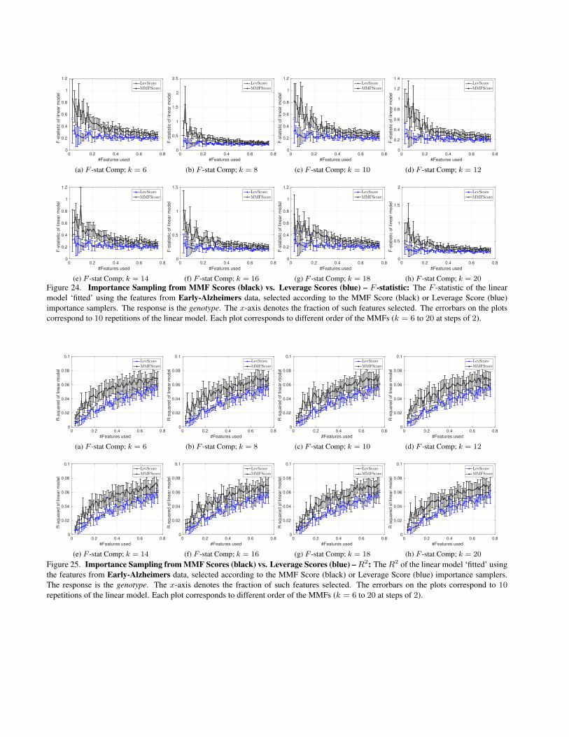
Figure 24. Importance Sampling from MMF Scores (black) vs. Leverage Scores (blue) – F -statistic: The F -statistic of the linearmodel ‘fitted’ using the features from Early-Alzheimers data, selected according to the MMF Score (black) or Leverage Score (blue)importance samplers. The response is the genotype. The x-axis denotes the fraction of such features selected. The errorbars on the plotscorrespond to 10 repetitions of the linear model. Each plot corresponds to different order of the MMFs (k = 6 to 20 at steps of 2).

#Features used

0 0.2 0.4 0.6 0.8

R-s

qua

red o

f lin

ear

mo

de

l

0

0.02

0.04

0.06

0.08

0.1LevScore

MMFScore

(a) F -stat Comp; k = 6

#Features used

0 0.2 0.4 0.6 0.8

R-s

qua

red o

f lin

ear

mo

de

l

0

0.02

0.04

0.06

0.08

0.1LevScore

MMFScore

(b) F -stat Comp; k = 8

#Features used

0 0.2 0.4 0.6 0.8

R-s

qua

red o

f lin

ear

mo

de

l

0

0.02

0.04

0.06

0.08

0.1LevScore

MMFScore

(c) F -stat Comp; k = 10

#Features used

0 0.2 0.4 0.6 0.8

R-s

qua

red o

f lin

ear

mo

de

l

0

0.02

0.04

0.06

0.08

0.1LevScore

MMFScore

(d) F -stat Comp; k = 12

#Features used

0 0.2 0.4 0.6 0.8

R-s

qu

are

d o

f lin

ea

r m

ode

l

0

0.02

0.04

0.06

0.08

0.1LevScore

MMFScore

(e) F -stat Comp; k = 14

#Features used

0 0.2 0.4 0.6 0.8

R-s

qu

are

d o

f lin

ea

r m

ode

l

0

0.02

0.04

0.06

0.08

0.1LevScore

MMFScore

(f) F -stat Comp; k = 16

#Features used

0 0.2 0.4 0.6 0.8

R-s

qu

are

d o

f lin

ea

r m

ode

l

0

0.02

0.04

0.06

0.08

0.1LevScore

MMFScore

(g) F -stat Comp; k = 18

#Features used

0 0.2 0.4 0.6 0.8

R-s

qu

are

d o

f lin

ea

r m

ode

l

0

0.02

0.04

0.06

0.08

0.1LevScore

MMFScore

(h) F -stat Comp; k = 20

Figure 25. Importance Sampling from MMF Scores (black) vs. Leverage Scores (blue) – R2: The R2 of the linear model ‘fitted’ usingthe features from Early-Alzheimers data, selected according to the MMF Score (black) or Leverage Score (blue) importance samplers.The response is the genotype. The x-axis denotes the fraction of such features selected. The errorbars on the plots correspond to 10repetitions of the linear model. Each plot corresponds to different order of the MMFs (k = 6 to 20 at steps of 2).

#Features used

0 0.2 0.4 0.6 0.8

F-s

tatistic o

f linear

model

0

0.1

0.2

0.3

0.4

0.5

LevScore

MMFScore

(a) F -stat Comp; k = 6

#Features used

0 0.2 0.4 0.6 0.8

F-s

tatistic o

f linear

model

0

0.1

0.2

0.3

0.4

0.5

LevScore

MMFScore

(b) F -stat Comp; k = 8

#Features used

0 0.2 0.4 0.6 0.8

F-s

tatistic o

f linear

model

0

0.1

0.2

0.3

0.4

0.5

0.6

LevScore

MMFScore

(c) F -stat Comp; k = 10

#Features used

0 0.2 0.4 0.6 0.8

F-s

tatistic o

f linear

model

0

0.2

0.4

0.6

0.8

1

LevScore

MMFScore

(d) F -stat Comp; k = 12

#Features used

0 0.2 0.4 0.6 0.8

F-s

tatistic o

f linear

model

0

0.1

0.2

0.3

0.4

0.5

LevScore

MMFScore

(e) F -stat Comp; k = 14

#Features used

0 0.2 0.4 0.6 0.8

F-s

tatistic o

f linear

model

0

0.1

0.2

0.3

0.4

0.5

LevScore

MMFScore

(f) F -stat Comp; k = 16

#Features used

0 0.2 0.4 0.6 0.8

F-s

tatistic o

f linear

model

0

0.1

0.2

0.3

0.4

0.5

LevScore

MMFScore

(g) F -stat Comp; k = 18

#Features used

0 0.2 0.4 0.6 0.8

F-s

tatistic o

f linear

model

0

0.1

0.2

0.3

0.4

0.5

0.6

LevScore

MMFScore

(h) F -stat Comp; k = 20

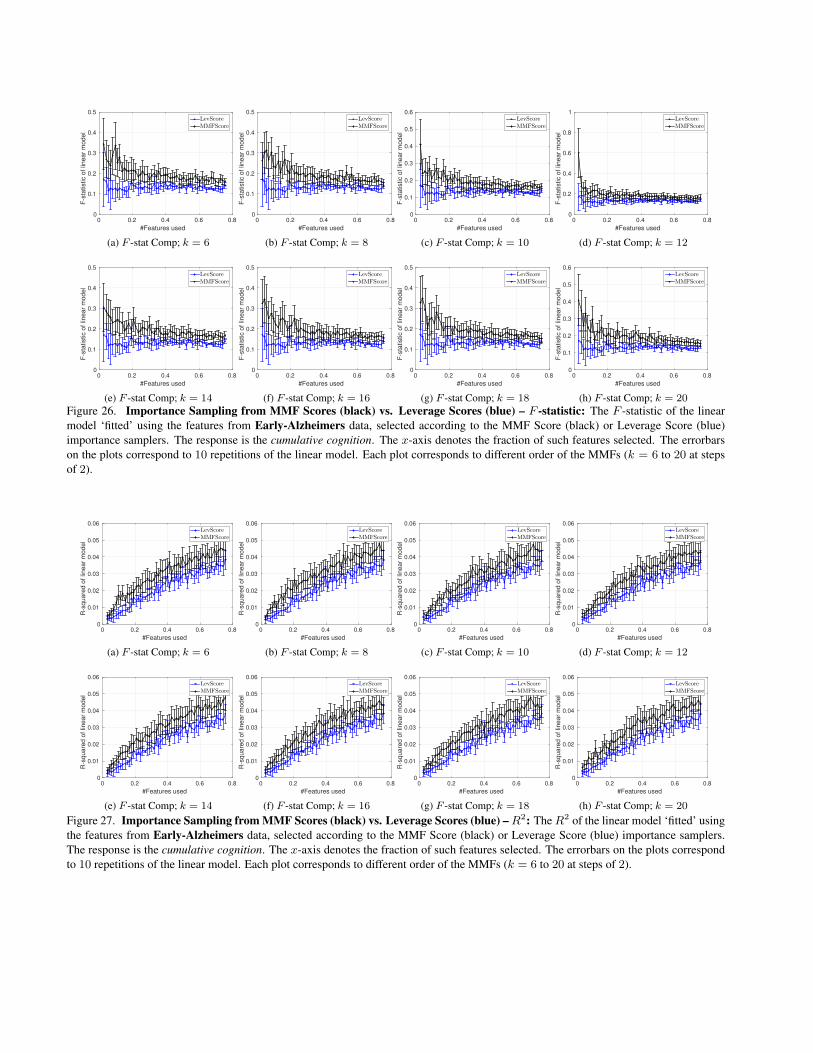
Figure 26. Importance Sampling from MMF Scores (black) vs. Leverage Scores (blue) – F -statistic: The F -statistic of the linearmodel ‘fitted’ using the features from Early-Alzheimers data, selected according to the MMF Score (black) or Leverage Score (blue)importance samplers. The response is the cumulative cognition. The x-axis denotes the fraction of such features selected. The errorbarson the plots correspond to 10 repetitions of the linear model. Each plot corresponds to different order of the MMFs (k = 6 to 20 at stepsof 2).

#Features used

0 0.2 0.4 0.6 0.8

R-s

qua

red o

f lin

ear

mo

de

l

0

0.01

0.02

0.03

0.04

0.05

0.06LevScore

MMFScore

(a) F -stat Comp; k = 6

#Features used

0 0.2 0.4 0.6 0.8

R-s

qua

red o

f lin

ear

mo

de

l

0

0.01

0.02

0.03

0.04

0.05

0.06LevScore

MMFScore

(b) F -stat Comp; k = 8

#Features used

0 0.2 0.4 0.6 0.8

R-s

qua

red o

f lin

ear

mo

de

l

0

0.01

0.02

0.03

0.04

0.05

0.06LevScore

MMFScore

(c) F -stat Comp; k = 10

#Features used

0 0.2 0.4 0.6 0.8

R-s

qua

red o

f lin

ear

mo

de

l

0

0.01

0.02

0.03

0.04

0.05

0.06LevScore

MMFScore

(d) F -stat Comp; k = 12

#Features used

0 0.2 0.4 0.6 0.8

R-s

qu

are

d o

f lin

ea

r m

od

el

0

0.01

0.02

0.03

0.04

0.05

0.06LevScore

MMFScore

(e) F -stat Comp; k = 14

#Features used

0 0.2 0.4 0.6 0.8

R-s

qu

are

d o

f lin

ea

r m

od

el

0

0.01

0.02

0.03

0.04

0.05

0.06LevScore

MMFScore

(f) F -stat Comp; k = 16

#Features used

0 0.2 0.4 0.6 0.8

R-s

qu

are

d o

f lin

ea

r m

od

el

0

0.01

0.02

0.03

0.04

0.05

0.06LevScore

MMFScore

(g) F -stat Comp; k = 18

#Features used

0 0.2 0.4 0.6 0.8

R-s

qu

are

d o

f lin

ea

r m

od

el

0

0.01

0.02

0.03

0.04

0.05

0.06LevScore

MMFScore

(h) F -stat Comp; k = 20

Figure 27. Importance Sampling from MMF Scores (black) vs. Leverage Scores (blue) – R2: The R2 of the linear model ‘fitted’ usingthe features from Early-Alzheimers data, selected according to the MMF Score (black) or Leverage Score (blue) importance samplers.The response is the cumulative cognition. The x-axis denotes the fraction of such features selected. The errorbars on the plots correspondto 10 repetitions of the linear model. Each plot corresponds to different order of the MMFs (k = 6 to 20 at steps of 2).

#Features used

0 0.2 0.4 0.6 0.8

F-s

tatistic o

f lin

ea

r m

od

el

-20

0

20

40

60

80

LevScore

MMFScore

(a) F -stat Comp; k = 6

#Features used

0 0.2 0.4 0.6 0.8

F-s

tatistic o

f lin

ea

r m

od

el

-10

0

10

20

30

40

50

LevScore

MMFScore

(b) F -stat Comp; k = 8

#Features used

0 0.2 0.4 0.6 0.8

F-s

tatistic o

f lin

ea

r m

od

el

-20

0

20

40

60

80

LevScore

MMFScore

(c) F -stat Comp; k = 10

#Features used

0 0.2 0.4 0.6 0.8

F-s

tatistic o

f lin

ea

r m

od

el

-20

0

20

40

60

80

LevScore

MMFScore

(d) F -stat Comp; k = 12

#Features used

0 0.2 0.4 0.6 0.8

F-s

tatistic o

f lin

ea

r m

od

el

-20

0

20

40

60

80

LevScore

MMFScore

(e) F -stat Comp; k = 14

#Features used

0 0.2 0.4 0.6 0.8

F-s

tatistic o

f lin

ea

r m

od

el

-20

0

20

40

60

80

LevScore

MMFScore

(f) F -stat Comp; k = 16

#Features used

0 0.2 0.4 0.6 0.8

F-s

tatistic o

f lin

ea

r m

od

el

-20

0

20

40

60

80

LevScore

MMFScore

(g) F -stat Comp; k = 18

#Features used

0 0.2 0.4 0.6 0.8

F-s

tatistic o

f lin

ea

r m

od

el

-20

0

20

40

60

80

LevScore

MMFScore

(h) F -stat Comp; k = 20

Figure 28. Importance Sampling from MMF Scores (black) vs. Leverage Scores (blue) – F -statistic: The F -statistic of the linearmodel ‘fitted’ using the features from Early-Alzheimers data, selected according to the MMF Score (black) or Leverage Score (blue)importance samplers. The response is the family history. The x-axis denotes the fraction of such features selected. The errorbars on theplots correspond to 10 repetitions of the linear model. Each plot corresponds to different order of the MMFs (k = 6 to 20 at steps of 2).

#Features used

0 0.2 0.4 0.6 0.8

R-s

quare

d o

f lin

ear

model

0

0.1

0.2

0.3

0.4

0.5

0.6

0.7LevScore

MMFScore

(a) F -stat Comp; k = 6

#Features used

0 0.2 0.4 0.6 0.8

R-s

quare

d o

f lin

ear

model

0

0.1

0.2

0.3

0.4

0.5

0.6

0.7LevScore

MMFScore

(b) F -stat Comp; k = 8

#Features used

0 0.2 0.4 0.6 0.8

R-s

quare

d o

f lin

ear

model

0

0.1

0.2

0.3

0.4

0.5

0.6

0.7LevScore

MMFScore

(c) F -stat Comp; k = 10

#Features used

0 0.2 0.4 0.6 0.8

R-s

quare

d o

f lin

ear

model

0

0.1

0.2

0.3

0.4

0.5

0.6

0.7LevScore

MMFScore

(d) F -stat Comp; k = 12

#Features used

0 0.2 0.4 0.6 0.8

R-s

quare

d o

f lin

ear

model

0

0.1

0.2

0.3

0.4

0.5

0.6

0.7LevScore

MMFScore

(e) F -stat Comp; k = 14

#Features used

0 0.2 0.4 0.6 0.8

R-s

quare

d o

f lin

ear

model

0

0.1

0.2

0.3

0.4

0.5

0.6

0.7LevScore

MMFScore

(f) F -stat Comp; k = 16

#Features used

0 0.2 0.4 0.6 0.8

R-s

quare

d o

f lin

ear

model

0

0.1

0.2

0.3

0.4

0.5

0.6

0.7LevScore

MMFScore

(g) F -stat Comp; k = 18

#Features used

0 0.2 0.4 0.6 0.8

R-s

quare

d o

f lin

ear

model

0

0.1

0.2

0.3

0.4

0.5

0.6

0.7LevScore

MMFScore

(h) F -stat Comp; k = 20

Figure 29. Importance Sampling from MMF Scores (black) vs. Leverage Scores (blue) – R2: The R2 of the linear model ‘fitted’ usingthe features from Early-Alzheimers data, selected according to the MMF Score (black) or Leverage Score (blue) importance samplers.The response is the family history. The x-axis denotes the fraction of such features selected. The errorbars on the plots correspond to 10repetitions of the linear model. Each plot corresponds to different order of the MMFs (k = 6 to 20 at steps of 2).

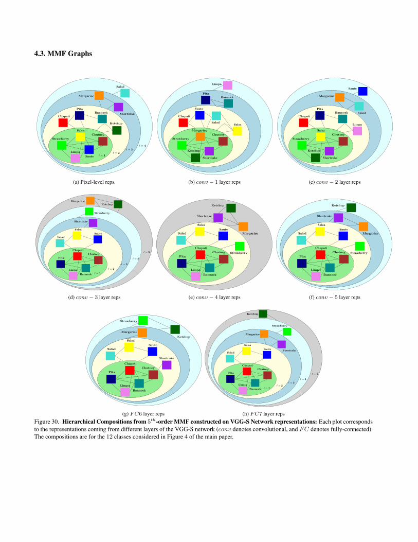
4.3. MMF Graphs

` = 1` = 2

` = 3

` = 4

Chutney

Limpa

Margarine

Shortcake

Salsa

Strawberry

Saute

PitaBannock

Chapati

Ketchup

Salad

(a) Pixel-level reps.

Chutney

Strawberry

Chapati

Shortcake

Ketchup

Margarine

Salsa

PitaBannock

Saute

Salad

Limpa

(b) conv − 1 layer reps

Chutney

Margarine

Salsa

Strawberry

PitaBannock

Chapati

Saute

Salad

Shortcake

Ketchup

Limpa

(c) conv − 2 layer reps

` = 1

` = 2

` = 3

` = 4

` = 5Chapati

Salad

Ketchup

Chutney

Bannock

Saute

Limpa

Pita

Salsa

Strawberry

Shortcake

Margarine

(d) conv − 3 layer reps

Chapati

Salad

Chutney

Bannock

Saute

Limpa

Pita

Salsa

Shortcake

Strawberry

Margarine

Ketchup

(e) conv − 4 layer reps

Chapati

Salad

Chutney

Bannock

Saute

Limpa

Pita

Salsa

Shortcake

Strawberry

Margarine

Ketchup

(f) conv − 5 layer reps

Chapati

Salad

Chutney

Bannock

Saute

Limpa

Pita

Salsa

Shortcake

Margarine

Strawberry

Ketchup

(g) FC6 layer reps

` = 1` = 2

` = 3

` = 4

` = 5

Chapati

Salad

Ketchup

Chutney

Bannock

Saute

Limpa

Pita

Salsa

Margarine

Strawberry

Shortcake

(h) FC7 layer repsFigure 30. Hierarchical Compositions from 5th-order MMF constructed on VGG-S Network representations: Each plot correspondsto the representations coming from different layers of the VGG-S network (conv denotes convolutional, and FC denotes fully-connected).The compositions are for the 12 classes considered in Figure 4 of the main paper.

Salsa

Pita

Ketchup

Chutney

Limpa

Strawberry

Saute

Salad

Chapati

Bannock

Shortcake

Margarine

(a) Pixel-level reps.

Salsa

Bannock

Limpa

Salad

Chapati

Saute

Shortcake

Pita

Strawberry

KetchupMargarine

Chutney

(b) conv − 1 layer reps

Salsa

Margarine

Chapati

Chutney

Strawberry

Salad

Saute

Ketchup

Shortcake

Pita

Bannock

Limpa

(c) conv − 2 layer reps

Chapati

Margarine

Chutney

Ketchup

Salad

Salsa

Saute

Bannock

LimpaPita

Shortcake

Strawberry

(d) conv − 3 layer reps

Chapati

Margarine

Chutney

Salad

Salsa

Saute

Bannock

LimpaPita

Ketchup

Strawberry

Shortcake

(e) conv − 4 layer reps

Chapati

Margarine

Chutney

Ketchup

Salad

Salsa

Saute

Bannock

LimpaPita

Shortcake

Strawberry

(f) conv − 5 layer reps

Chapati

Salad

Bannock

Saute

Limpa

Pita

Salsa

Margarine

Chutney

Shortcake

Ketchup

Strawberry

(g) FC6 layer reps

Chapati

Salad

Ketchup

Bannock

Saute

Limpa

Pita

Salsa

Shortcake

Chutney

Margarine

Strawberry

(h) FC7 layer repsFigure 31. Hierarchical Compositions from 4th-order MMF constructed on VGG-S Network representations: Each plot correspondsto the representations coming from different layers of the VGG-S network (conv denotes convolutional, and FC denotes fully-connected).The compositions are for the 12 classes considered in Figure 4 of the main paper.

Strawberry

Pita

Salad

Saute

Limpa

Chutney

Salsa

Chapati

KetchupBannock

Shortcake

Margarine

(a) Pixel-level reps.

Saute

Salsa

Salad

Limpa

Bannock

Ketchup

Strawberry

Chapati

Chutney

Margarine

ShortcakePita

(b) conv − 1 layer reps

Salsa

Chapati

Strawberry

Chutney

Ketchup

Salad

Saute

Margarine

Bannock

Pita

Limpa

Shortcake

(c) conv − 2 layer reps

Salsa

Chapati

Shortcake

Limpa

Bannock

Pita

Margarine

Strawberry

Chutney

Salad

Saute

Ketchup

(d) conv − 3 layer reps

Saute

Salsa

Salad

Strawberry

Chutney

Chapati

Shortcake

Limpa

Bannock

Pita

Margarine

Ketchup

(e) conv − 4 layer reps

Saute

Salsa

Salad

Shortcake

Chapati

Strawberry

Chutney Pita

Bannock

Limpa

Margarine

Ketchup

(f) conv − 5 layer reps

Strawberry

Pita Saute

Salsa

Salad

Chutney

Bannock

Limpa Chapati

Margarine

Shortcake

Ketchup

(g) FC6 layer reps

Salad

Ketchup

Salsa

Shortcake

Chutney

Margarine

Strawberry

BannockLimpa

Pita

Chapati

Saute

(h) FC7 layer repsFigure 32. Hierarchical Compositions from 3rd-order MMF constructed on VGG-S Network representations: Each plot correspondsto the representations coming from different layers of the VGG-S network (conv denotes convolutional, and FC denotes fully-connected).The compositions are for the 12 classes considered in Figure 4 of the main paper.

Hierarchical Agglomerative Clustering: The following figure shows the dendrogram corresponding to the agglomerativeclustering (based on mean distance of the clusters) on the FC6 and FC7 representations of the 12 classes from Figures30–32. Observe that the categories like bannok and chapati, or saute and salad are closer to each other here in hierarchicalclustering. However, the compositional relationships inferred from the MMF graphs, see Figures 30–32, especially in theFC7 and FC6 layers, are not apparent in these dendrogram outputs (also see Section 4.3.2 in the main paper). Similar suchcluster trees can be produced using other layers’ representations, where in the compositions from MMF based graphs aremuch more informatice and contextual.

Salad Chutney SalsaSaute ChapatiPita BannockMargarine Limpa KetchupShortcake Strawberry

(a) FC6 layer reps

Salad Chutney SalsaSaute ChapatiPita BannockMargarine Limpa KetchupShortcakeStrawberry

(b) FC7 layer repsFigure 33. Hierarchical clustering (Dendrograms) constructed on VGG-S Network representations: Plots correspond to the repre-sentations coming from FC6 and FC7 layers of the VGG-S network (FC denotes fully-connected). The clustering is for the 12 classesconsidered in Figure 4 of the main paper (and Figures 30–32 above).

References[1] http://adni.loni.usc.edu. 3[2] http://image-net.org/explore_popular.php. 3[3] K. Chatfield, K. Simonyan, A. Vedaldi, and A. Zisserman. Return of the devil in the details: Delving deep into convolutional nets.

arXiv preprint arXiv:1405.3531, 2014. 3[4] R. Kondor, N. Teneva, and V. Garg. Multiresolution matrix factorization. In Proceedings of the 31st International Conference on

Machine Learning (ICML-14), pages 1620–1628, 2014. 1[5] R. Kondor, N. Teneva, and P. K. Mudrakarta. Parallel mmf: a multiresolution approach to matrix computation. arXiv preprint

arXiv:1507.04396, 2015. 2[6] A. Krizhevsky, I. Sutskever, and G. E. Hinton. Imagenet classification with deep convolutional neural networks. In Advances in neural

information processing systems, pages 1097–1105, 2012. 3[7] F. Mezzadri. How to generate random matrices from the classical compact groups. arXiv preprint math-ph/0609050, 2006. 2[8] O. Russakovsky, J. Deng, H. Su, J. Krause, S. Satheesh, S. Ma, Z. Huang, A. Karpathy, A. Khosla, M. Bernstein, et al. Imagenet large

scale visual recognition challenge. International Journal of Computer Vision, 115(3):211–252, 2015. 3