SIAM REVIEW c 2000 Society for Industrial and Applied Mathematics Vol. 42, No. 1, pp. 68–82 Two Purposes for Matrix Factorization: A Historical Appraisal ∗ Lawrence Hubert † Jacqueline Meulman ‡ Willem Heiser § Abstract. Matrix factorization in numerical linear algebra (NLA) typically serves the purpose of restating some given problem in such a way that it can be solved more readily; for example, one major application is in the solution of a linear system of equations. In contrast, within applied statistics/psychometrics (AS/P), a much more common use for matrix factorization is in presenting, possibly spatially, the structure that may be inherent in a given data matrix obtained on a collection of objects observed over a set of variables. The actual components of a factorization are now of prime importance and not just as a mechanism for solving another problem. We review some connections between NLA and AS/P and their respective concerns with matrix factorization and the subsequent rank reduction of a matrix. We note in particular that several results available for many decades in AS/P were more recently (re)discovered in the NLA literature. Two other distinctions between NLA and AS/P are also discussed briefly: how a generalized singular value decomposition might be defined, and the differing uses for the (newer) methods of optimization based on cyclic or iterative projections. Key words. rank reduction, matrix factorization, matrix decomposition, singular value decomposi- tion, cyclic projection AMS subject classifications. 62H25, 65F15 PII. S0036144598340483 1. Introduction. Matrix factorization in the context of numerical linear algebra (NLA) generally serves the purpose of rephrasing through a series of easier subprob- lems a task that may be relatively difficult to solve in its original form. For example, given the typical linear system Ax = b for A ∈ R n×n , x and b ∈ R n , a factorization of A as LU for L a unit lower triangular matrix (thus, with ones along its main diagonal) and an upper triangular U is a mechanism for characterizing what occurs in Gaussian elimination. We replace Ax = b by two (easier to solve) triangular systems: find y so Ly = b and then find x so Ux = y. The point being made here is that the factorization of A as LU has no real importance in and of itself other than as a computationally convenient means for obtaining a solution to the original linear system. ∗ Received by the editors June 15, 1998; accepted for publication (in revised form) May 28, 1999; published electronically January 24, 2000. http://www.siam.org/journals/sirev/42-1/34048.html † Department of Psychology, The University of Illinois, 603 East Daniel Street, Champaign, IL 61820 ([email protected]). ‡ Department of Education, Leiden University, Leiden, the Netherlands ([email protected]. leidenuniv.nl). § Department of Psychology, Leiden University, Leiden, the Netherlands ([email protected]. leidenuniv.nl). 68

Welcome message from author
This document is posted to help you gain knowledge. Please leave a comment to let me know what you think about it! Share it to your friends and learn new things together.
Transcript
SIAM REVIEW c© 2000 Society for Industrial and Applied MathematicsVol. 42, No. 1, pp. 68–82
Two Purposes for MatrixFactorization: A HistoricalAppraisal∗
Lawrence Hubert†
Jacqueline Meulman‡
Willem Heiser§
Abstract. Matrix factorization in numerical linear algebra (NLA) typically serves the purpose ofrestating some given problem in such a way that it can be solved more readily; for example,one major application is in the solution of a linear system of equations. In contrast, withinapplied statistics/psychometrics (AS/P), a much more common use for matrix factorizationis in presenting, possibly spatially, the structure that may be inherent in a given datamatrix obtained on a collection of objects observed over a set of variables. The actualcomponents of a factorization are now of prime importance and not just as a mechanismfor solving another problem. We review some connections between NLA and AS/P andtheir respective concerns with matrix factorization and the subsequent rank reduction ofa matrix. We note in particular that several results available for many decades in AS/Pwere more recently (re)discovered in the NLA literature. Two other distinctions betweenNLA and AS/P are also discussed briefly: how a generalized singular value decompositionmight be defined, and the differing uses for the (newer) methods of optimization based oncyclic or iterative projections.
Key words. rank reduction, matrix factorization, matrix decomposition, singular value decomposi-tion, cyclic projection
AMS subject classifications. 62H25, 65F15
PII. S0036144598340483
1. Introduction. Matrix factorization in the context of numerical linear algebra(NLA) generally serves the purpose of rephrasing through a series of easier subprob-lems a task that may be relatively difficult to solve in its original form. For example,given the typical linear system Ax = b for A ∈ Rn×n, x and b ∈ Rn, a factorization ofA as LU for L a unit lower triangular matrix (thus, with ones along its main diagonal)and an upper triangular U is a mechanism for characterizing what occurs in Gaussianelimination. We replace Ax = b by two (easier to solve) triangular systems: find y soLy = b and then find x so Ux = y. The point being made here is that the factorizationof A as LU has no real importance in and of itself other than as a computationallyconvenient means for obtaining a solution to the original linear system.
∗Received by the editors June 15, 1998; accepted for publication (in revised form) May 28, 1999;published electronically January 24, 2000.
http://www.siam.org/journals/sirev/42-1/34048.html†Department of Psychology, The University of Illinois, 603 East Daniel Street, Champaign, IL
61820 ([email protected]).‡Department of Education, Leiden University, Leiden, the Netherlands ([email protected].
leidenuniv.nl).§Department of Psychology, Leiden University, Leiden, the Netherlands ([email protected].
leidenuniv.nl).
68
MATRIX FACTORIZATION AND RANK REDUCTION 69
In contrast to its usage as a mechanism for obtaining another end, within thefield of applied statistics/psychometrics (AS/P), matrix factorization also plays a verymajor role but usually not just for the purpose of solving systems of equations (al-though many exemplars for that specific application exist as well). Typically, a matrixA ∈ Rn×p represents a data matrix containing numerical observations on n objects(subjects) over p attributes (variables), or possibly B ∈ Rp×p and the entries are somemeasure of proximity between attributes, such as the correlation between columns ofA.1 The major purpose of a matrix factorization in this context is to obtain some formof lower-rank (and therefore simplified) approximation to A (or possibly to B) for un-derstanding the structure of the data matrix, particularly the relationship within theobjects and within the attributes, and how the objects relate to the attributes. If wecan further interpret the matrix factorization geometrically and actually present theresults spatially through coordinates obtained from the components of the factoriza-tion, we will be able to better communicate to others what structure may be present inthe original data matrix. In any case, matrix factorizations are again directed towardthe issue of simplicity, but now the actual components making up a factorization areof prime concern and not solely as a mechanism for solving another problem.
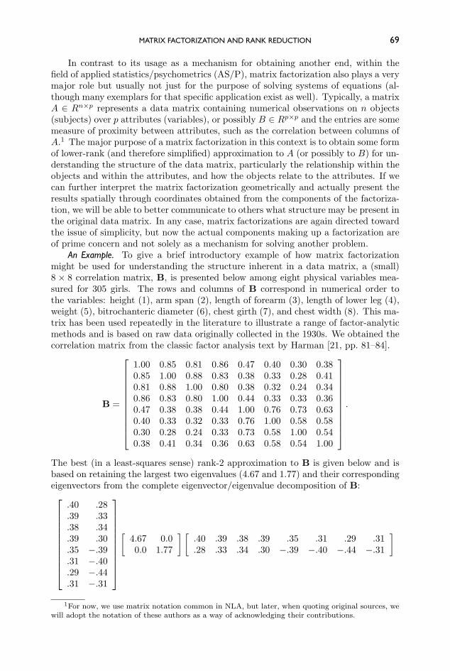
An Example. To give a brief introductory example of how matrix factorizationmight be used for understanding the structure inherent in a data matrix, a (small)8 × 8 correlation matrix, B, is presented below among eight physical variables mea-sured for 305 girls. The rows and columns of B correspond in numerical order tothe variables: height (1), arm span (2), length of forearm (3), length of lower leg (4),weight (5), bitrochanteric diameter (6), chest girth (7), and chest width (8). This ma-trix has been used repeatedly in the literature to illustrate a range of factor-analyticmethods and is based on raw data originally collected in the 1930s. We obtained thecorrelation matrix from the classic factor analysis text by Harman [21, pp. 81–84].
B =
1.00 0.85 0.81 0.86 0.47 0.40 0.30 0.380.85 1.00 0.88 0.83 0.38 0.33 0.28 0.410.81 0.88 1.00 0.80 0.38 0.32 0.24 0.340.86 0.83 0.80 1.00 0.44 0.33 0.33 0.360.47 0.38 0.38 0.44 1.00 0.76 0.73 0.630.40 0.33 0.32 0.33 0.76 1.00 0.58 0.580.30 0.28 0.24 0.33 0.73 0.58 1.00 0.540.38 0.41 0.34 0.36 0.63 0.58 0.54 1.00
.
The best (in a least-squares sense) rank-2 approximation to B is given below and isbased on retaining the largest two eigenvalues (4.67 and 1.77) and their correspondingeigenvectors from the complete eigenvector/eigenvalue decomposition of B:
.40 .28
.39 .33
.38 .34
.39 .30
.35 −.39
.31 −.40
.29 −.44
.31 −.31
[4.67 0.00.0 1.77
] [.40 .39 .38 .39 .35 .31 .29 .31.28 .33 .34 .30 −.39 −.40 −.44 −.31
]
1For now, we use matrix notation common in NLA, but later, when quoting original sources, wewill adopt the notation of these authors as a way of acknowledging their contributions.
70 LAWRENCE HUBERT, JACQUELINE MEULMAN, AND WILLEM HEISER
=
.89 .89 .88 .88 .46 .38 .32 .43
.88 .89 .89 .88 .41 .33 .26 .38
.87 .89 .87 .86 .38 .30 .24 .35
.87 .88 .86 .86 .43 .36 .29 .40
.46 .41 .38 .43 .85 .79 .77 .73
.38 .33 .30 .36 .79 .73 .72 .66
.32 .27 .25 .29 .78 .73 .74 .66
.42 .38 .35 .40 .73 .68 .66 .62
.
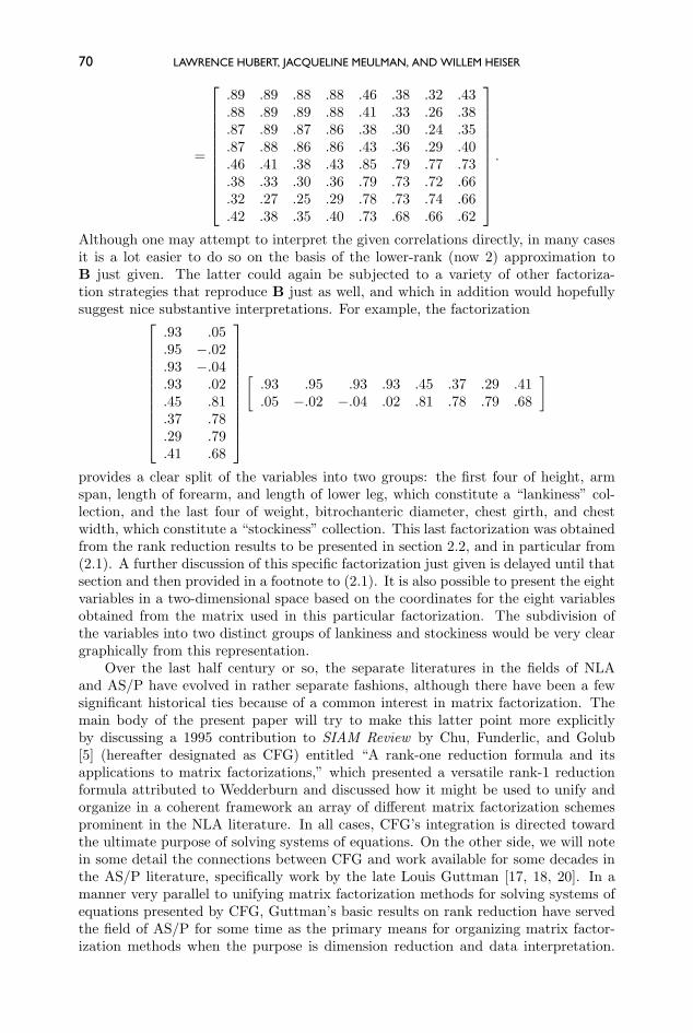
Although one may attempt to interpret the given correlations directly, in many casesit is a lot easier to do so on the basis of the lower-rank (now 2) approximation toB just given. The latter could again be subjected to a variety of other factoriza-tion strategies that reproduce B just as well, and which in addition would hopefullysuggest nice substantive interpretations. For example, the factorization
.93 .05
.95 −.02
.93 −.04
.93 .02
.45 .81
.37 .78
.29 .79
.41 .68
[.93 .95 .93 .93 .45 .37 .29 .41.05 −.02 −.04 .02 .81 .78 .79 .68
]
provides a clear split of the variables into two groups: the first four of height, armspan, length of forearm, and length of lower leg, which constitute a “lankiness” col-lection, and the last four of weight, bitrochanteric diameter, chest girth, and chestwidth, which constitute a “stockiness” collection. This last factorization was obtainedfrom the rank reduction results to be presented in section 2.2, and in particular from(2.1). A further discussion of this specific factorization just given is delayed until thatsection and then provided in a footnote to (2.1). It is also possible to present the eightvariables in a two-dimensional space based on the coordinates for the eight variablesobtained from the matrix used in this particular factorization. The subdivision ofthe variables into two distinct groups of lankiness and stockiness would be very cleargraphically from this representation.
Over the last half century or so, the separate literatures in the fields of NLAand AS/P have evolved in rather separate fashions, although there have been a fewsignificant historical ties because of a common interest in matrix factorization. Themain body of the present paper will try to make this latter point more explicitlyby discussing a 1995 contribution to SIAM Review by Chu, Funderlic, and Golub[5] (hereafter designated as CFG) entitled “A rank-one reduction formula and itsapplications to matrix factorizations,” which presented a versatile rank-1 reductionformula attributed to Wedderburn and discussed how it might be used to unify andorganize in a coherent framework an array of different matrix factorization schemesprominent in the NLA literature. In all cases, CFG’s integration is directed towardthe ultimate purpose of solving systems of equations. On the other side, we will notein some detail the connections between CFG and work available for some decades inthe AS/P literature, specifically work by the late Louis Guttman [17, 18, 20]. In amanner very parallel to unifying matrix factorization methods for solving systems ofequations presented by CFG, Guttman’s basic results on rank reduction have servedthe field of AS/P for some time as the primary means for organizing matrix factor-ization methods when the purpose is dimension reduction and data interpretation.
MATRIX FACTORIZATION AND RANK REDUCTION 71
There are several such organizing presentations available, but probably none is moreaggressively comprehensive than the textbook by Horst [27]. Horst reviews and in-tegrates some 50 years of data representation through matrix factorization and doesso almost exclusively through the mechanism of Guttman’s rank reduction results.Some of this integration will be reviewed briefly in the next section.
The fields of NLA and AS/P, as noted above, have had some very significanthistorical ties. The prime example is probably the development of what has becomethe major tool for both NLA (the singular value decomposition (SVD) of a matrix)and AS/P (in which it is more commonly called the Eckart–Young decompositionof a matrix after Eckart and Young [12], which as Stewart [37, p. 563] commentsis probably an incorrect attribution given the precedent of Schmidt’s earlier work[36]. In the last section of this paper, we point to two of these historical issues. Wealso present a brief review of a generalization of the SVD that has been developedfor the purpose of data representation, as well as for uses in a data representationcontext for another technique of importance in NLA that involves applications ofiterative or cyclic projection methods. Pointing out these connections may be of someinterdisciplinary interest for those likely to rely on the SVD and associated methodsonly indirectly along the route to constructing a solution to another problem that isof more primary concern.2
2. The CFG and Guttman Rank Reduction Theorems.
2.1. CFG. The CFG review paper is built around three main theorems that wereference below as CFG1, CFG2, and CFG3, with CFG1 being the main result fromwhich the various matrix factorizations reviewed are unified.
CFG1. If A ∈ Rm×n, and x ∈ Rn, y ∈ Rm are vectors such that ω = yTAx = 0,then the matrix B := A− ω−1AxyTA has rank exactly one less than the rank of A.
CFG2. Let u ∈ Rm and v ∈ Rn. Then the rank of the matrix B = A− σ−1uvT
is less than that of A if and only if there are vectors x ∈ Rn and y ∈ Rm such thatu = Ax, v = AT y, and σ = yTAx, in which case rank(B) = rank(A) −1.
CFG3. Suppose U ∈ Rm×k, R ∈ Rk×k, and V ∈ Rn×k. Then rank(A−UR−1V T )= rank(A) − rank(UR−1V T ) if and only if there exist X ∈ Rn×k and Y ∈ Rm×k
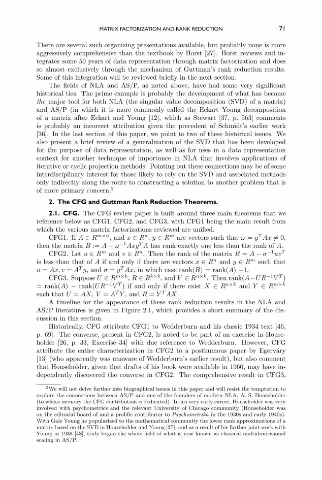
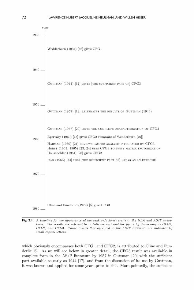
such that U = AX, V = ATY , and R = Y TAX.A timeline for the appearance of these rank reduction results in the NLA and
AS/P literatures is given in Figure 2.1, which provides a short summary of the dis-cussion in this section.
Historically, CFG attribute CFG1 to Wedderburn and his classic 1934 text [46,p. 69]. The converse, present in CFG2, is noted to be part of an exercise in House-holder [26, p. 33, Exercise 34] with due reference to Wedderburn. However, CFGattribute the entire characterization in CFG2 to a posthumous paper by Egervary[13] (who apparently was unaware of Wedderburn’s earlier result), but also commentthat Householder, given that drafts of his book were available in 1960, may have in-dependently discovered the converse in CFG2. The comprehensive result in CFG3,
2We will not delve further into biographical issues in this paper and will resist the temptation toexplore the connections between AS/P and one of the founders of modern NLA, A. S. Householder(to whose memory the CFG contribution is dedicated). In his very early career, Householder was veryinvolved with psychometrics and the relevant University of Chicago community (Householder wason the editorial board of and a prolific contributor to Psychometrika in the 1930s and early 1940s).With Gale Young he popularized to the mathematical community the lower rank approximations of amatrix based on the SVD in Householder and Young [27], and as a result of his further joint work withYoung in 1938 [48], truly began the whole field of what is now known as classical multidimensionalscaling in AS/P.
72 LAWRENCE HUBERT, JACQUELINE MEULMAN, AND WILLEM HEISER
1980
1970
1960
1950
1940
year
1930
Wedderburn (1934) [46] gives CFG1
Guttman (1944) [17] gives [the sufficient part of] CFG3
Guttman (1957) [20] gives the complete characterization of CFG3
Egervary (1960) [13] gives CFG2 (unaware of Wedderburn [46])
Harman (1960) [21] reviews factor analysis integrated by CFG3Horst (1963, 1965) [23, 24] uses CFG3 to unify matrix factorizationHouseholder (1964) [26] gives CFG2
Rao (1965) [34] uses [the sufficient part of] CFG3 as an exercise
Cline and Funderlic (1979) [6] give CFG3
Guttman (1952) [18] reiterates the results of Guttman (1944)
Fig. 2.1 A timeline for the appearance of the rank reduction results in the NLA and AS/P litera-tures. The results are referred to in both the text and the figure by the acronyms CFG1,CFG2, and CFG3. Those results that appeared in the AS/P literature are indicated bysmall capital letters.
which obviously encompasses both CFG1 and CFG2, is attributed to Cline and Fun-derlic [6]. As we will see below in greater detail, the CFG3 result was available incomplete form in the AS/P literature by 1957 in Guttman [20] with the sufficientpart available as early as 1944 [17], and from the discussion of its use by Guttman,it was known and applied for some years prior to this. More pointedly, the sufficient
MATRIX FACTORIZATION AND RANK REDUCTION 73
condition in CFG3 has been a long-standing unifying principle in AS/P. For example,the 1963 applied text Matrix Algebra for Social Scientists by Horst [23] includes acomplete chapter devoted to its applications (Chapter 22, pp. 477–487, “The generalmatrix reduction theorems”); the seminal text in linear statistical inference by Rao[34] includes the sufficient condition of CFG3 merely as an exercise (that we repeatverbatim below in the original notation [34, p. 55, Exercise 4]), with an attribution(to be discussed more fully later) to Lagrange’s theorem.
Lagrange’s Theorem. Let S be any square matrix of order n and rank r > 0, and X,Y be column vectors such that X′SY = 0. Then the residual matrix
S1 = S− SYX′SX′SY
is exactly of rank r − 1.More generally, if S is n×m of rank r > 0, A and B are of order s×n and s×m,
respectively, where s ≤ r, and ASB′ is nonsingular, the residual matrix
S1 = S− SB′(ASB′)−1AS
is exactly of rank (r − s) and S1 is Gramian if S is Gramian.3
The primary emphasis in CFG is on the repeated use of CFG1 to obtain a varietyof matrix factorizations and to unify a substantial literature that has gone before.They summarize this usage as follows.
For A ∈ Rm×n, rank(A) = γ, and vectors x1, . . . , xγ ∈ Rn and y1, . . . , yγ ∈ Rm,
A = ΦΩ−1ΨT ,(2.1)
where Ω := diagonalω1, . . . , ωγ, Φ := [φ1, . . . , φγ ] ∈ Rm×γ , and Ψ := [ψ1, . . . , ψγ ] ∈Rn×γ , with
φk := Akxk, ψk := ATk yk,
and letting A1 := A, Ak+1 := Ak − ω−1k Akxky
Tk Ak, where (it is assumed that
x1, . . . , xγ and y1, . . . , yγ are chosen so) ωk := yTk Akxk = 0.4
Alternatively, if u1, . . . , uγ ∈ Rn and v1, . . . , vγ ∈ Rm are defined by u1 := x1 andv1 := y1, and for k > 1,
uk := xk −k−1∑i=1
(vTi AxkvTi Aui
)ui,
3The statement that “S1 is Gramian if S is Gramian” needs the further qualification of “andA = B” to be correct. In this summary statement, and probably to economize on words in theexercise, Rao put together the sufficient condition of CFG3 with a more specific result from Guttman[17] that dealt separately with Gramian matrices. We label this latter Guttman result as G3 in section2.2. This observation that the constraint of equality is needed for the matrices A and B to make thephrasing given by Rao completely correct was pointed out to us by Yoshio Takane [39].
4In the earlier numerical example of section 1, (2.1) was used to generate a factorization for therank-2 approximation of the given correlation matrix. In (2.1), the matrix A is interpreted as the 8×8rank-2 approximation to B (so m = n = 8 and γ = 2), and the vectors x1 = y1 = [11110000]T andx2 = y2 = [00001111]T . The factorization of A that is given corresponds to A = (ΦΩ−
12 )(ΨΩ−
12 )T ,
where in this case
ΦΩ−12 = ΨΩ−
12 =
[.93 .95 .93 .93 .45 .37 .29 .41.05 −.02 −.04 .02 .81 .78 .79 .68
]T.
74 LAWRENCE HUBERT, JACQUELINE MEULMAN, AND WILLEM HEISER
vk := yk −k−1∑i=1
(yTk AuivTi Aui
)vi,
then for U := [u1, . . . , uγ ] and V := [v1, . . . , vγ ],
V TAU = Ω,(2.2)
and the factorization in (2.1) can be rewritten as
A = (AU)Ω−1(V TA).(2.3)
Depending on the initial matrix A and the choice of the vector sets x1, . . . , xγand y1, . . . , yγ , a variety of factorizations of A ensue. (In fact, even the ubiquitousGram–Schmidt orthogonalization process is a very simple special case: let A be theidentity matrix and suppose the two collections, x1, . . . , xγ and y1, . . . , yγ , are identicaland contain the vectors for which an orthogonal basis is desired. The columns ofU = V define the set of basis vectors with the orthogonality condition given by (2.2).)To allow some comparisons later when the factorization of A for purposes of datarepresentation are reviewed, we list three of the more common (and simplest) onesbelow in schematic summary form (assuming the condition ωk = 0 obtains in therecursive process), but will not discuss, for example, CFG’s further extension to theQR decomposition, the Lanczos process, or to ABS methods; the latter are morerelevant to the solution of systems of equations, but usage in the context of matrixfactorization with the aim of data representation would be more limited.
(a) For A ∈ Rm×n of rank γ, if X and Y are upper trapezoidal matrices in Rn×γ
and Rm×γ , respectively, then (2.3) provides a trapezoidal LDU decomposition whereAU and V TA are lower and upper trapezoidal matrices, respectively.5
(b) For A ∈ Rn×n of rank n, if X and Y are both the identity matrix, then (2.3)provides an LDMT factorization of A, where A = V −TΩU−1 for V −T and U−T unitlower triangular matrices (with ones on the main diagonal).
If A ∈ Rn×n is symmetric, then U = V and A = U−TΩU−1.If A ∈ Rn×n is symmetric and positive definite, then A = (Ω
12U−1)T (Ω
12U−1)
gives the Cholesky factorization of A.(c) If A ∈ Rm×n is of rank γ, the singular value factorization of A can be given
as A = PΩQT , where P ∈ Rm×γ and PTP = I; Q ∈ Rn×γ and QTQ = I; Ω ∈ Rγ×γand is diagonal with positive (and nonincreasing) entries along the main diagonal. IfX = Q and Y = P , then the SVD of A is retrieved by (2.2) since U = Q and V = P ,so V TAU = Ω.
2.2. Guttman. The three papers by Guttman mentioned earlier [17, 18, 20] arerather remarkable in that they served to completely characterize the issue of rankreduction for the purpose of data representation within AS/P by 1957, with thesufficiency clearly delineated in 1944 and completely integrated within the literatureby the 1950s (e.g., see Harman’s 1960 comprehensive review [21]). We state the majortheorems below in their original forms (as well as using most of the original notation)as G1, G2, and G3. We proceed thereafter to make several historical comments andplace these rank reduction results in the framework of interpreting the structure of adata matrix.
5An upper (lower) trapezoidal matrix is one in which the (i, j) entry is zero for j < i (i < j),which naturally generalizes the notion of an upper or lower triangular matrix when A is square.
MATRIX FACTORIZATION AND RANK REDUCTION 75
G1 [17, p. 4]: Let S be any matrix of order n×N and of rank r > 0. Let X andY be of orders s × n and s ×N , respectively (where s ≤ r), and such that XSY′ isnonsingular. Then the residual matrix
S1 = S− SY′(XSY′)−1XS
is exactly of rank r − s.Guttman comments that G1 can be considered as generalizing a result due to
Lagrange, and he references Wedderburn [46, p. 68] with an apparent allusion to theintroductory phrase “The Lagrange method of reducing quadratic and bilinear formsto a normal form is . . ..” Wedderburn uses this phrase before discussing the rank-1reduction result (which was given earlier as CFG1). Guttman then presents what heexplicitly labels as Lagrange’s theorem: Let S be any matrix of order n × n and ofrank r > 0. Let x and y be row vectors of n elements each and such that xSy′ = 0.Then the residual matrix
S1 = S− Sy′xSxSy′
is exactly of rank r − 1.Although Guttman gave the label of Lagrange’s theorem only to this latter special
case of G1 (and by implication indicated that the more general form of G1 and itsproof were his own), as we noted earlier in the exercise from Rao [34, p. 55] givenverbatim, Rao attached the label of Lagrange’s theorem to Guttman’s G1 result aswell. Rao provided no reference to Guttman in this context, although he does so foranother exercise [34, Exercise 14, p. 57] dealing with the minimum rank possible for a(reduced) correlation matrix, but then lists a reference to a completely different paper(Guttman [19]).
Guttman only gave a proof for the sufficiency of the rank reduction result of G1in his 1944 paper, but he came back to prove its necessity in a short article in 1957[20]. Thus, the complete characterization given earlier in CFG3 was available in theAS/P literature by 1957—and Guttman should appropriately be given credit for it.6
The next two results from Guttman [17, pp. 11, 12], G2 and G3, also concernthe issue of rank reduction but not in terms of the original n × N matrix S. Many(if not most) uses of matrix factorizations for purposes of data representation rely onmatrices that must be Gramian (e.g., correlation or covariance matrices), and it isvery relevant to know how such factorizations relate back to the original data matrixfrom which the Gramian matrices were constructed. G2 concerns a factorization ofthe n × n positive semidefinite (Gramian) matrix SS′ and how this could then berelated to a factorization of S; G3 is a restatement of G1, but for a matrix that isassumed to be Gramian. We restate G2 from Guttman [17, p. 11] in a slight variantform that deals just with the cross-product matrix SS′ and we include an explicit
6Although Guttman’s results appear in the AS/P literature, that does not preclude them frombeing rediscovered and republished in this same literature, where eventually no credit at all is given.As a case in point, Overall [33] presented some of Guttman’s results independently and noted inpassing, “It has been called to the attention of this writer that Guttman (1944, 1952) has presentedwhat is essentially the same general factor model in somewhat different form” (p. 652). However,secondary sources are not always so careful in attribution, and when providing a separate chapterand accompanying Fortran program in their classic text, Cooley and Lohnes (1971) [7, Chapter 5]reference Overall [33] but fail to mention any of Guttman’s original contributions. Unfortunately,when cited for applications in the substantive literature, Cooley and Lohnes [7] is now made theprimary (and only) reference for methodology directly attributable to Guttman.
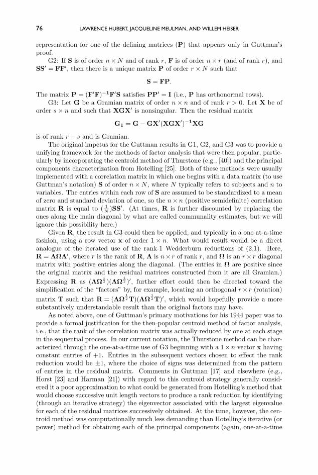
76 LAWRENCE HUBERT, JACQUELINE MEULMAN, AND WILLEM HEISER
representation for one of the defining matrices (P) that appears only in Guttman’sproof.
G2: If S is of order n×N and of rank r, F is of order n× r (and of rank r), andSS′ = FF′, then there is a unique matrix P of order r ×N such that
S = FP.
The matrix P = (F′F)−1F′S satisfies PP′ = I (i.e., P has orthonormal rows).G3: Let G be a Gramian matrix of order n × n and of rank r > 0. Let X be of
order s× n and such that XGX′ is nonsingular. Then the residual matrix
G1 = G−GX′(XGX′)−1XG
is of rank r − s and is Gramian.The original impetus for the Guttman results in G1, G2, and G3 was to provide a
unifying framework for the methods of factor analysis that were then popular, partic-ularly by incorporating the centroid method of Thurstone (e.g., [40]) and the principalcomponents characterization from Hotelling [25]. Both of these methods were usuallyimplemented with a correlation matrix in which one begins with a data matrix (to useGuttman’s notation) S of order n×N , where N typically refers to subjects and n tovariables. The entries within each row of S are assumed to be standardized to a meanof zero and standard deviation of one, so the n× n (positive semidefinite) correlationmatrix R is equal to ( 1
N )SS′. (At times, R is further discounted by replacing theones along the main diagonal by what are called communality estimates, but we willignore this possibility here.)
Given R, the result in G3 could then be applied, and typically in a one-at-a-timefashion, using a row vector x of order 1 × n. What would result would be a directanalogue of the iterated use of the rank-1 Wedderburn reductions of (2.1). Here,R = ΛΩΛ′, where r is the rank of R, Λ is n× r of rank r, and Ω is an r× r diagonalmatrix with positive entries along the diagonal. (The entries in Ω are positive sincethe original matrix and the residual matrices constructed from it are all Gramian.)Expressing R as (ΛΩ
12 )(ΛΩ
12 )′, further effort could then be directed toward the
simplification of the “factors” by, for example, locating an orthogonal r× r (rotation)matrix T such that R = (ΛΩ
12 T)(ΛΩ
12 T)′, which would hopefully provide a more
substantively understandable result than the original factors may have.As noted above, one of Guttman’s primary motivations for his 1944 paper was to
provide a formal justification for the then-popular centroid method of factor analysis,i.e., that the rank of the correlation matrix was actually reduced by one at each stagein the sequential process. In our current notation, the Thurstone method can be char-acterized through the one-at-a-time use of G3 beginning with a 1×n vector x havingconstant entries of +1. Entries in the subsequent vectors chosen to effect the rankreduction would be ±1, where the choice of signs was determined from the patternof entries in the residual matrix. Comments in Guttman [17] and elsewhere (e.g.,Horst [23] and Harman [21]) with regard to this centroid strategy generally consid-ered it a poor approximation to what could be generated from Hotelling’s method thatwould choose successive unit length vectors to produce a rank reduction by identifying(through an iterative strategy) the eigenvector associated with the largest eigenvaluefor each of the residual matrices successively obtained. At the time, however, the cen-troid method was computationally much less demanding than Hotelling’s iterative (orpower) method for obtaining each of the principal components (again, one-at-a-time
MATRIX FACTORIZATION AND RANK REDUCTION 77
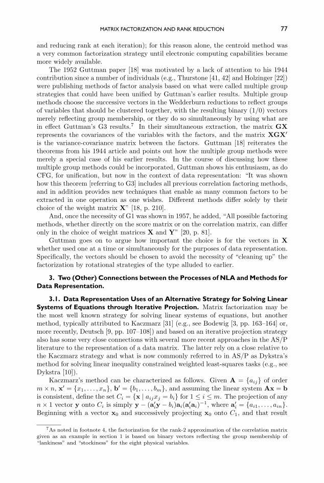
and reducing rank at each iteration); for this reason alone, the centroid method wasa very common factorization strategy until electronic computing capabilities becamemore widely available.
The 1952 Guttman paper [18] was motivated by a lack of attention to his 1944contribution since a number of individuals (e.g., Thurstone [41, 42] and Holzinger [22])were publishing methods of factor analysis based on what were called multiple groupstrategies that could have been unified by Guttman’s earlier results. Multiple groupmethods choose the successive vectors in the Wedderburn reductions to reflect groupsof variables that should be clustered together, with the resulting binary (1/0) vectorsmerely reflecting group membership, or they do so simultaneously by using what arein effect Guttman’s G3 results.7 In their simultaneous extraction, the matrix GXrepresents the covariances of the variables with the factors, and the matrix XGX′
is the variance-covariance matrix between the factors. Guttman [18] reiterates thetheorems from his 1944 article and points out how the multiple group methods weremerely a special case of his earlier results. In the course of discussing how thesemultiple group methods could be incorporated, Guttman shows his enthusiasm, as doCFG, for unification, but now in the context of data representation: “It was shownhow this theorem [referring to G3] includes all previous correlation factoring methods,and in addition provides new techniques that enable as many common factors to beextracted in one operation as one wishes. Different methods differ solely by theirchoice of the weight matrix X” [18, p. 210].
And, once the necessity of G1 was shown in 1957, he added, “All possible factoringmethods, whether directly on the score matrix or on the correlation matrix, can differonly in the choice of weight matrices X and Y” [20, p. 81].
Guttman goes on to argue how important the choice is for the vectors in Xwhether used one at a time or simultaneously for the purposes of data representation.Specifically, the vectors should be chosen to avoid the necessity of “cleaning up” thefactorization by rotational strategies of the type alluded to earlier.
3. Two (Other) Connections between the Processes of NLA and Methods forData Representation.
3.1. Data Representation Uses of an Alternative Strategy for Solving LinearSystems of Equations through Iterative Projection. Matrix factorization may bethe most well known strategy for solving linear systems of equations, but anothermethod, typically attributed to Kaczmarz [31] (e.g., see Bodewig [3, pp. 163–164] or,more recently, Deutsch [9, pp. 107–108]) and based on an iterative projection strategyalso has some very close connections with several more recent approaches in the AS/Pliterature to the representation of a data matrix. The latter rely on a close relative tothe Kaczmarz strategy and what is now commonly referred to in AS/P as Dykstra’smethod for solving linear inequality constrained weighted least-squares tasks (e.g., seeDykstra [10]).
Kaczmarz’s method can be characterized as follows. Given A = aij of orderm× n, x′ = x1, . . . , xn, b′ = b1, . . . , bm, and assuming the linear system Ax = bis consistent, define the set Ci = x | aijxj = bi for 1 ≤ i ≤ m. The projection of anyn× 1 vector y onto Ci is simply y − (a′iy − bi)ai(a′iai)−1, where a′i = ai1, . . . , ain.Beginning with a vector x0 and successively projecting x0 onto C1, and that result
7As noted in footnote 4, the factorization for the rank-2 approximation of the correlation matrixgiven as an example in section 1 is based on binary vectors reflecting the group membership of“lankiness” and “stockiness” for the eight physical variables.
78 LAWRENCE HUBERT, JACQUELINE MEULMAN, AND WILLEM HEISER
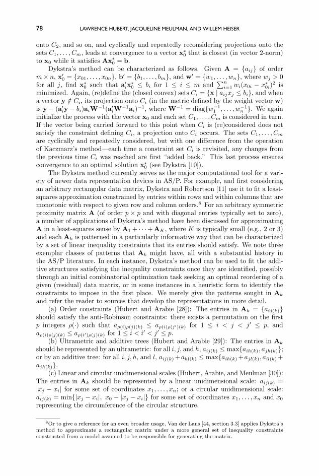
onto C2, and so on, and cyclically and repeatedly reconsidering projections onto thesets C1, . . . , Cm, leads at convergence to a vector x∗0 that is closest (in vector 2-norm)to x0 while it satisfies Ax∗0 = b.
Dykstra’s method can be characterized as follows. Given A = aij of orderm× n, x′0 = x01, . . . , x0n, b′ = b1, . . . , bm, and w′ = w1, . . . , wn, where wj > 0for all j, find x∗0 such that a′ix
∗0 ≤ bi for 1 ≤ i ≤ m and
∑ni=1 wi(x0i − x∗0i)
2 isminimized. Again, (re)define the (closed convex) sets Ci = x | aijxj ≤ bi, and whena vector y /∈ Ci, its projection onto Ci (in the metric defined by the weight vector w)is y − (a′iy − bi)aiW−1(a′iW
−1ai)−1, where W−1 = diagw−11 , . . . , w−1
n . We againinitialize the process with the vector x0 and each set C1, . . . , Cm is considered in turn.If the vector being carried forward to this point when Ci is (re)considered does notsatisfy the constraint defining Ci, a projection onto Ci occurs. The sets C1, . . . , Cmare cyclically and repeatedly considered, but with one difference from the operationof Kaczmarz’s method—each time a constraint set Ci is revisited, any changes fromthe previous time Ci was reached are first “added back.” This last process ensuresconvergence to an optimal solution x∗0 (see Dykstra [10]).
The Dykstra method currently serves as the major computational tool for a vari-ety of newer data representation devices in AS/P. For example, and first consideringan arbitrary rectangular data matrix, Dykstra and Robertson [11] use it to fit a least-squares approximation constrained by entries within rows and within columns that aremonotonic with respect to given row and column orders.8 For an arbitrary symmetricproximity matrix A (of order p × p and with diagonal entries typically set to zero),a number of applications of Dykstra’s method have been discussed for approximatingA in a least-squares sense by A1 + · · ·+ AK , where K is typically small (e.g., 2 or 3)and each Ak is patterned in a particularly informative way that can be characterizedby a set of linear inequality constraints that its entries should satisfy. We note threeexemplar classes of patterns that Ak might have, all with a substantial history inthe AS/P literature. In each instance, Dykstra’s method can be used to fit the addi-tive structures satisfying the inequality constraints once they are identified, possiblythrough an initial combinatorial optimization task seeking an optimal reordering of agiven (residual) data matrix, or in some instances in a heuristic form to identify theconstraints to impose in the first place. We merely give the patterns sought in Ak
and refer the reader to sources that develop the representations in more detail.(a) Order constraints (Hubert and Arabie [28]): The entries in Ak = aij(k)
should satisfy the anti-Robinson constraints: there exists a permutation on the firstp integers ρ(·) such that aρ(i)ρ(j)(k) ≤ aρ(i)ρ(j′)(k) for 1 ≤ i < j < j′ ≤ p, andaρ(i)ρ(j)(k) ≤ aρ(i′)ρ(j)(k) for 1 ≤ i < i′ < j′ ≤ p.
(b) Ultrametric and additive trees (Hubert and Arabie [29]): The entries in Ak
should be represented by an ultrametric: for all i, j, and h, aij(k) ≤ maxaih(k), ajh(k);or by an additive tree: for all i, j, h, and l, aij(k) +ahl(k) ≤ maxaih(k) +ajl(k), ail(k) +ajh(k).
(c) Linear and circular unidimensional scales (Hubert, Arabie, and Meulman [30]):The entries in Ak should be represented by a linear unidimensional scale: aij(k) =|xj − xi| for some set of coordinates x1, . . . , xn; or a circular unidimensional scale:aij(k) = min|xj − xi|, x0 − |xj − xi| for some set of coordinates x1, . . . , xn and x0representing the circumference of the circular structure.
8Or to give a reference for an even broader usage, Van der Lans [44, section 3.3] applies Dykstra’smethod to approximate a rectangular matrix under a more general set of inequality constraintsconstructed from a model assumed to be responsible for generating the matrix.
MATRIX FACTORIZATION AND RANK REDUCTION 79
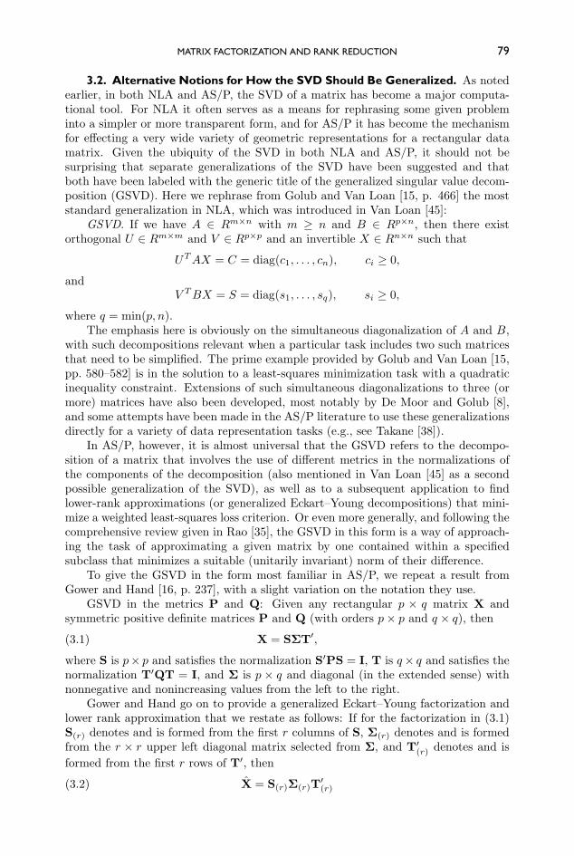
3.2. Alternative Notions for How the SVD Should Be Generalized. As notedearlier, in both NLA and AS/P, the SVD of a matrix has become a major computa-tional tool. For NLA it often serves as a means for rephrasing some given probleminto a simpler or more transparent form, and for AS/P it has become the mechanismfor effecting a very wide variety of geometric representations for a rectangular datamatrix. Given the ubiquity of the SVD in both NLA and AS/P, it should not besurprising that separate generalizations of the SVD have been suggested and thatboth have been labeled with the generic title of the generalized singular value decom-position (GSVD). Here we rephrase from Golub and Van Loan [15, p. 466] the moststandard generalization in NLA, which was introduced in Van Loan [45]:
GSVD. If we have A ∈ Rm×n with m ≥ n and B ∈ Rp×n, then there existorthogonal U ∈ Rm×m and V ∈ Rp×p and an invertible X ∈ Rn×n such that
UTAX = C = diag(c1, . . . , cn), ci ≥ 0,
andV TBX = S = diag(s1, . . . , sq), si ≥ 0,
where q = min(p, n).The emphasis here is obviously on the simultaneous diagonalization of A and B,
with such decompositions relevant when a particular task includes two such matricesthat need to be simplified. The prime example provided by Golub and Van Loan [15,pp. 580–582] is in the solution to a least-squares minimization task with a quadraticinequality constraint. Extensions of such simultaneous diagonalizations to three (ormore) matrices have also been developed, most notably by De Moor and Golub [8],and some attempts have been made in the AS/P literature to use these generalizationsdirectly for a variety of data representation tasks (e.g., see Takane [38]).
In AS/P, however, it is almost universal that the GSVD refers to the decompo-sition of a matrix that involves the use of different metrics in the normalizations ofthe components of the decomposition (also mentioned in Van Loan [45] as a secondpossible generalization of the SVD), as well as to a subsequent application to findlower-rank approximations (or generalized Eckart–Young decompositions) that mini-mize a weighted least-squares loss criterion. Or even more generally, and following thecomprehensive review given in Rao [35], the GSVD in this form is a way of approach-ing the task of approximating a given matrix by one contained within a specifiedsubclass that minimizes a suitable (unitarily invariant) norm of their difference.
To give the GSVD in the form most familiar in AS/P, we repeat a result fromGower and Hand [16, p. 237], with a slight variation on the notation they use.
GSVD in the metrics P and Q: Given any rectangular p × q matrix X andsymmetric positive definite matrices P and Q (with orders p× p and q × q), then
X = SΣT′,(3.1)
where S is p× p and satisfies the normalization S′PS = I, T is q× q and satisfies thenormalization T′QT = I, and Σ is p × q and diagonal (in the extended sense) withnonnegative and nonincreasing values from the left to the right.
Gower and Hand go on to provide a generalized Eckart–Young factorization andlower rank approximation that we restate as follows: If for the factorization in (3.1)S(r) denotes and is formed from the first r columns of S, Σ(r) denotes and is formedfrom the r × r upper left diagonal matrix selected from Σ, and T′(r) denotes and isformed from the first r rows of T′, then
X = S(r)Σ(r)T′(r)(3.2)
80 LAWRENCE HUBERT, JACQUELINE MEULMAN, AND WILLEM HEISER
is a rank-r matrix minimizing the weighted least-squares criterion of
Trace[(P12 (X− X)Q
12 )(P
12 (X− X)Q
12 )′].
In practice, X would be obtained from a standard singular value factorization ofP
12 XQ
12 , with the appropriate deletion of rows and columns in the components of
the factorization to obtain a rank-r (unweighted) least-squares approximation; i.e.,we first construct P
12 XQ
12 , and from the latter, X can be retrieved.
The first application of the GSVD in the form just presented appears to be in apaper by Young [47], but it now serves as the computational engine for a number ofpopular data representation methods, e.g., various forms of what might generically becalled biplots. To be more explicit, suppose we interpret the rectangular p× q matrixX = xij in (3.1) as a data matrix on p objects (subjects) and q variables (attributes),so the entry xij refers to the ith object’s score on the jth variable, 1 ≤ i ≤ p and1 ≤ j ≤ q. The lower-rank approximation to X given by X = xij in (3.2) providesa mechanism for displaying this approximation graphically in terms of a joint plot (ora biplot) of the objects and variables in a common r-dimensional Euclidean space.Specifically, if X = GH′, where G = S(r)Σα
(r) and H = T(r)Σ(1−α)(r) , where α is some
chosen constant, 0 ≤ α ≤ 1, the rows of G provide r-dimensional coordinates for eachof the p objects (which are typically represented as points in the joint plot); the rowsof H provide r-dimensional coordinates for each of the q variables (which are typicallyrepresented as vectors in the joint plot). Irrespective of the chosen value for α, theapproximating entry xij is the inner product of the ith row of G and the jth row ofH; consequently, considering just the column vector representing the jth variable inX, graphically these inner products are proportional to the lengths of the orthogonalprojections of the objects onto the vector.9
The GSVD has probably found its most widespread use in the data analysis tech-nique known as correspondence analysis, sometimes limited (unnecessarily) to theanalysis of a two-way contingency table F = fij, expressing the relationships be-tween the categories of two categorical variables U and V , where the entry fij denotesthe count of individual units of observation (objects) in category i of variable U andin category j of variable V . Classical “Analyse des Correspondances” a la Benzecri[1, 2], however, stands for a much more general technique to analyze any type ofpositive measure of correspondence; thus, correspondence analysis is best describedas the analysis of a correspondence table, characterized as any table containing posi-tive entries. Whatever interpretation is given to the technique, the marginals of thetwo-way table play an important role in that they define the metrics. In terms oflower-rank approximation, the product GH′ of row scores G and column scores Happroximates Mr
−1(F − 1NMruruc
′Mc)Mc−1, where Mr and Mc denote diagonal
matrices with the row and column marginals, respectively, along the main diagonal;ur and uc are vectors of ones of size R (number of rows) and C (number of columns);
9The joint representation of rows and columns as points and vectors in a common space originateswith Tucker [43] and has found applications in psychometrics in the analysis of preference data(Carroll [4]) before the display became well known in applied statistics as the biplot (through Gabriel[14]). The prefix “bi” in the term “biplot” refers to two sets of different entities, objects and variables,and not to two dimensions, as is sometimes incorrectly assumed. This same connotation for the term“bi” is used by Kruskal [32] in his characterization of principal components analysis as a bilinearmodel.
MATRIX FACTORIZATION AND RANK REDUCTION 81
and N is the total frequency.10
REFERENCES
[1] J.-P. Benzecri, L’Analyse des donnees, Dunod, Paris, 1973.[2] J.-P. Benzecri, Correspondence Analysis Handbook, Marcel Dekker, New York, 1992.[3] E. Bodewig, Matrix Calculus, North–Holland, Amsterdam, 1956.[4] J. D. Carroll, Individual differences and multidimensional scaling, in Multidimensional Scal-
ing: Theory and Applications in the Behavioral Sciences, R. N. Shepard, A. K. Romney,and S. B. Nerlove, eds., Seminar Press, New York, 1972, pp. 105–155.
[5] M. T. Chu, R. E. Funderlic, and G. H. Golub, A rank-one reduction formula and itsapplications to matrix factorizations, SIAM Rev., 37 (1995), pp. 512–530.
[6] R. E. Cline and R. E. Funderlic, The rank of a difference of matrices and associatedgeneralized inverses, Linear Algebra Appl., 24 (1979), pp. 185–215.
[7] W. W. Cooley and P. R. Lohnes, Multivariate Data Analysis, John Wiley, New York, 1971.[8] B. L. R. De Moor and G. H. Golub, The restricted singular value decomposition: Properties
and applications, SIAM J. Matrix Anal. Appl., 12 (1991), pp. 401–425.[9] F. Deutsch, The method of alternating orthogonal projections, in Approximation Theory,
Spline Functions and Applications, S. P. Singh, ed., Kluwer Academic Publishers, Dor-drecht, the Netherlands, 1992, pp. 105–121.
[10] R. L. Dykstra, An algorithm for restricted least squares regression, J. Amer. Statist. Assoc.,78 (1983), pp. 837–842.
[11] R. L. Dykstra and R. Robertson, An algorithm for isotonic regression for two or moreindependent variables, Ann. Statist., 10 (1982), pp. 708–716.
[12] C. Eckart and G. Young, The approximation of one matrix by another of lower rank,Psychometrika, 1 (1936), pp. 211–218.
[13] E. Egervary, On rank-diminishing operators and their applications to the solution of linearequations, Z. Angew. Math. Phys., 11 (1960), pp. 376–386.
[14] K. R. Gabriel, The biplot graphic display of matrices with application to principal compo-nents analysis, Biometrika, 58 (1971), pp. 453–467.
[15] G. H. Golub and C. F. Van Loan, Matrix Computations, 3rd ed., The Johns HopkinsUniversity Press, Baltimore, 1996.
[16] J. C. Gower and D. J. Hand, Biplots, Chapman and Hall, London, 1996.[17] L. Guttman, General theory and methods for matric factoring, Psychometrika, 9, (1944), pp.
1–16.[18] L. Guttman, Multiple group methods for common-factor analysis: Their basis, computation,
and interpretation, Psychometrika, 17 (1952), pp. 209–222.[19] L. Guttman, Some necessary conditions for common factor analysis, Psychometrika, 19
(1954), pp. 149–161.[20] L. Guttman, A necessary and sufficient formula for matrix factoring, Psychometrika, 22
(1957), pp. 79–81.[21] H. H. Harman, Modern Factor Analysis, The University of Chicago Press, Chicago, 1960.[22] K. J. Holzinger, A simple method of factor-analysis, Psychometrika, 9 (1944), pp. 257–262.[23] P. Horst, Matrix Algebra for Social Scientists, Holt, Rinehart and Winston, New York, 1963.[24] P. Horst, Factor Analysis of Data Matrices, Holt, Rinehart and Winston, New York, 1965.[25] H. Hotelling, Analysis of a complex of statistical variables into principal components, J.
Educ. Psych., 24 (1933), pp. 417–441 and 498–520.[26] A. S. Householder, The Theory of Matrices in Numerical Analysis, Blaisdell, New York,
1964.[27] A. S. Householder and G. Young, Matrix approximations and latent roots, Amer. Math.
Monthly, 45 (1938), pp. 165–171.
10The Gower and Hand [16] reference, as well as the comprehensive survey of Rao [35], detailsmany uses for the GSVD. We might mention another particular application, because of the generalform of the rank reduction results discussed in the main body of the paper, which is discussed andused in some depth by Gower and Hand [16, pp. 245–246]: For given matrices Y, A, and B oforders p × q, p × s, and q × t, respectively (where for convenience s ≤ p and t ≤ q), the rank-r matrix Γ (which we can identify with the search for X in (3.2)) of order s × t that minimizesTrace[(Y−AΓB′)(Y−AΓB′)′] is obtained from the GSVD of (A′A)−1A′YB(B′B)−1 (which wecan identify with X in (3.1)) in the metrics P = A′A and Q = B′B (and if the notation of (3.2) isused), with the normalizations of S′(r)(A
′A)S(r) = I and T′(r)(B′B)T(r) = I.
82 LAWRENCE HUBERT, JACQUELINE MEULMAN, AND WILLEM HEISER
[28] L. J. Hubert and P. Arabie, The analysis of proximity matrices through sums of matriceshaving (anti-)Robinson forms, Brit. J. Math. Statist. Psych., 47 (1994), pp. 1–40.
[29] L. J. Hubert and P. Arabie, Iterative projection strategies for the least-squares fitting oftree structures to proximity data, Brit. J. Math. Statist. Psych., 48 (1995), pp. 281–317.
[30] L. J. Hubert, P. Arabie, and J. Meulman, Linear and circular unidimensional scaling forsymmetric proximity matrices, Brit. J. Math. Statist. Psych., 50 (1997), pp. 253–284.
[31] S. Kaczmarz, Angenaherte Auflosung von Systemen linearer Gleichungen, Bull. Internat.Acad. Pol. Sci. Lett., A35 (1937), pp. 355–357.
[32] J. B. Kruskal, Factor analysis and principal components analysis: Bilinear methods, inInternational Encyclopedia of Statistics, W. H. Kruskal and J. M. Tanur, eds., The FreePress, New York, 1978, pp. 307–330.
[33] J. E. Overall, Orthogonal factors and uncorrelated factor scores, Psych. Rep., 10 (1962),651–662.
[34] C. R. Rao, Linear Statistical Inference and Its Applications, John Wiley, New York, 1965.[35] C. R. Rao, Matrix approximations and reduction of dimensionality in multivariate statistical
analysis, in Multivariate Analysis, V, P. R. Krishnaiah, ed., North–Holland, Amsterdam,1980, pp. 3–22.
[36] E. Schmidt, Zur Theorie der linearen und nichtlinearen Integralgleichungen. I. Teil. Entwick-lung willkurlichen Funktionen nach System vorgeschriebener, Math. Ann., 63 (1907), pp.433–476.
[37] G. W. Stewart, On the early history of the singular value decomposition, SIAM Rev., 35(1993), pp. 551–566.
[38] Y. Takane, The use of PSVD and QSVD in psychometrics, in Bull. Internat. Statist. Inst.,Proceedings of the 51st Session, Tome LVII, Book 2, 1997, pp. 255–258.
[39] Y. Takane, personal communication, June 17, 1998.[40] L. L. Thurstone, The Vectors of the Mind, University of Chicago Press, Chicago, 1935.[41] L. L. Thurstone, A multiple group method of factoring the correlation matrix, Psychome-
trika, 10 (1945), pp. 73–78.[42] L. L. Thurstone, Note about the multiple group method, Psychometrika, 14 (1949), pp. 43–45.[43] L. R. Tucker, Intra-individual and inter-individual multidimensionality, in Psychological
Scaling: Theory and Applications, H. Guilliksen and S. Messick, eds., John Wiley, NewYork, 1960, pp. 155–167.
[44] I. A. Van der Lans, Nonlinear Multivariate Analysis for Multiattribute Preference Data,DSWO Press, Leiden, the Netherlands, 1992.
[45] C. F. Van Loan, Generalizing the singular value decomposition, SIAM J. Numer. Anal., 13(1976), pp. 76–83.
[46] J. H. M. Wedderburn, Lectures on Matrices, Colloquium Publications, Vol. 17, AmericanMathematical Society, New York, 1934.
[47] G. Young, Maximum likelihood estimation and factor analysis, Psychometrika, 6 (1941), pp.49–53.
[48] G. Young and A. S. Householder, Discussion of a set of points in terms of their mutualdistances, Psychometrika, 3 (1938), pp. 11–22.
Related Documents