DEVELOPMENT OF A WIRELESS NETWORK MODEL FOR CONTROLING ENVIRONMENTAL AND WORK SAFETY IN PORTS OF DEVELOPING COUNTRIES A Degree Thesis Submitted to the Faculty of the Escola Tècnica d'Enginyeria de Telecomunicació de Barcelona Universitat Politècnica de Catalunya by Joan Colomer Rodriguez In partial fulfilment of the requirements for the degree in Science and Telecommunication Technologies Engineering Advisors: Prof. Anke Schmeink & Sanja Bauk (RWTH-Aachen) Javier Rodriguez Fonollosa (UPC) Barcelona, June 2014

Welcome message from author
This document is posted to help you gain knowledge. Please leave a comment to let me know what you think about it! Share it to your friends and learn new things together.
Transcript
DEVELOPMENT OF A WIRELESS NETWORK MODEL
FOR CONTROLING ENVIRONMENTAL AND WORK
SAFETY IN PORTS OF DEVELOPING COUNTRIES
A Degree Thesis
Submitted to the Faculty of the
Escola Tècnica d'Enginyeria de Telecomunicació de
Barcelona
Universitat Politècnica de Catalunya
by
Joan Colomer Rodriguez
In partial fulfilment
of the requirements for the degree in
Science and Telecommunication Technologies
Engineering
Advisors:
Prof. Anke Schmeink & Sanja Bauk (RWTH-Aachen)
Javier Rodriguez Fonollosa (UPC)
Barcelona, June 2014
1
Abstract
The project goal is to propose cost effective and feasible scenarios of employing Wireless
Network Sensors (WSN) in improving occupational health and safety at harsh industrial
environment. The Port of Bar (Montenegro) is taken as the example area [2].
The purpose of this research work is to control the safety and health of the workers on
docks in the Port of Bar by implementing individually tailored and sustainable WSN
solutions. The proposed solutions can be transferred latter into the developing seaports in
transitional economies within South Adriatic Sea region (e.g. Port of Durres in Albania,
and Port of Ploce in Bosnia and Herzegovina).
Within this context, the simulations of WSN performances are realised in Matlab and
OMNET++ software environments. The obtained results are presented numerically and
graphically, along with the appropriate discussions. The directions for further research
work in this domain are given, as well.
2
Resum
L'objectiu del projecte és proposar un escenari viable emprant sensors de xarxa sense fils ( WSN ) per millorar el control de la salut i seguretat del treball en entorns industrials durs. El port de Bar ( Montenegro ) es pren com a exemple la zona [2] . El propòsit d'aquest treball d'investigació és el control de la seguretat i salut dels treballadors en els molls al port de Bar implementant solucions WSN individualment adaptades i sostenibles . Les solucions proposades en aquest treball es poden transferir en els ports de mar en les economies en transició dins de la regió del Sud del Mar Adriàtic (per exemple, port de Durres a Albània, i el Port de Ploce a Bòsnia i Hercegovina). Dins d'aquest context , les simulacions d'actuacions WSN es realitzen en entorns de programari Matlab i OMNET ++ . Els resultats obtinguts es presenten numèrica i gràficament , juntament amb les discussions corresponents . També es donen les instruccions per a futurs treballs de recerca en aquest àmbit.
3
Resumen
El objetivo del proyecto es proponer un escenario viable empleando sensores de red inalámbrica (WSN) para mejorar el control de la salud y seguridad del trabajo en entornos industriales duros. El puerto de Bar (Montenegro) se toma como ejemplo la zona [2]. El propósito de este trabajo de investigación es el control de la seguridad y salud de los trabajadores en los muelles en el puerto de Bar implementando soluciones WSN individualmente adaptadas y sostenibles. Las soluciones propuestas en este trabajo se pueden transferir en los puertos de mar en las economías en transición dentro de la región del Sur del Mar Adriático (por ejemplo, puerto de Durres en Albania, y el Puerto de Ploce en Bosnia y Herzegovina). Dentro de este contexto, las simulaciones de actuaciones WSN se realizan en entornos de software Matlab y OMNET ++. Los resultados obtenidos se presentan numérica y gráficamente, junto con las discusiones correspondientes. También se dan las instrucciones para futuros trabajos de investigación en este ámbito.

4
Acknowledgements
I would like to express gratitude to Prof. Dr. Javier Rodriguez Fonollosa who has
supported my work during the undergraduate studies at University of Barcelona, school
Universitat Politècnica de Catalunya. Also I would like to thanks Prof. Dr-Ing. Anke
Schmeink and Prof. Dr. Sanja Bauk for giving me support in defining the topic of my
thesis and its accomplishing at the RWTH University Aachen. I owe gratitude to my
colleague M. Sc. Jose León, as well, who help me a lot with his advices in successful
realization of simulations in Matlab and OMNET++.

5
Revision history and approval record
Revision Date Purpose
0 05/08/2015 Document creation
1 15/08/2015 Document revision
2 27/08/2017 Document revision
DOCUMENT DISTRIBUTION LIST
Name e-mail
[Student name] Joan Colomer Rodriguez [email protected]
[Project Supervisor 1] Prof. Dr. Javier Rodriguez
Fonollosa [email protected]
[Project Supervisor 2] Prof. Dr-Ing. Anke Schmeink [email protected]
[Project Supervisor 3] Prof. Dr. Sanja Bauk [email protected]
Written by: Reviewed and approved by:
Date 05/08/2015 Date 01/09/2015
Name Joan Colomer Rodriguez Name Javier Rodriguez Fonollosa
Position Project Author Position Project Supervisor

6
Table of contents
The table of contents must be detailed. Each chapter and main section in the thesis must
be listed in the “Table of Contents” and each must be given a page number for the
location of a particular text.
Abstract ............................................................................................................................ 1
Resum .............................................................................................................................. 2
Resumen .......................................................................................................................... 3
Acknowledgements .......................................................................................................... 4
Revision history and approval record ................................................................................ 5
Table of contents .............................................................................................................. 6
List of Figures ................................................................................................................... 8
List of Tables: ................................................................................................................... 9
1. Introduction .............................................................................................................. 10
1.1. Statement of purpose ....................................................................................... 10
1.2. Methods and Procedures .................................................................................. 10
1.3. Work Packages, Milestones and Gant Diagram ................................................ 10
1.4. Incidences ........................................................................................................ 14
2. State of the art of the technology used or applied in this thesis ................................ 15
2.1. Wireless Sensor Networks ................................................................................ 15
2.1.1. Wi-Fi .......................................................................................................... 16
2.1.2. Zigbee ....................................................................................................... 18
2.1.3. White-Fi ..................................................................................................... 19
2.2. Path Loss ......................................................................................................... 20
2.2.1. Rayleigh Fading ........................................................................................ 22
2.2.2. Rician fading: ............................................................................................. 23
2.3. Receptor ........................................................................................................... 24
2.3.1. Wiener filter ............................................................................................... 24
3. Methodology / project development ......................................................................... 27
3.1. Scenario 1: WBANSs as part of personal protective equipment........................ 27
3.2. Scenario 2: As scanners of workers’ vital signs ................................................ 28
3.3. Matlab Simulation ............................................................................................. 29
3.4. OMNET++ Simulation ....................................................................................... 30
7
3.4.1. OMNET ++ scenario 1: .............................................................................. 31
3.4.2. OMNET++ scenario 2 ................................................................................ 34
4. Results .................................................................................................................... 37
4.1. Matlab simulation.............................................................................................. 37
4.2. OMNET++ simulation ....................................................................................... 39
4.2.1. OMNET++ scenario 1 ................................................................................ 39
4.2.2. OMNET++ scenario 2 ................................................................................ 42
4.2.3. Comparison of Scenario 1 and 2 ............................................................... 45
5. Conclusions and future development ....................................................................... 46
5.1. Future work ...................................................................................................... 46
Bibliography .................................................................................................................... 48
8
List of Figures
Figure 1. Scheme of Direct-Sequence Spread Spectrum (DSSS) [5] ....................................... 16
Figure 2. White-Fi IEEE 802.11af concept ................................................................................... 19
Figure 3. Line of sight path .......................................................................................................... 22
Figure 4. Rayleigh probability density function (pdf) ................................................................ 22
Figure 5. Power variation over a second after passing through a single-path Rayleigh
channel. Different Doppler shift 10 Hz (up) and 100 Hz (down) ................................................ 23
Figure 6. Diagram of the Wiener filter ......................................................................................... 25
Figure 7. The WBANs on worker's personal protective equipment with RFID tags [2] ......... 27
Figure 8. WBANSs for scanning some of worker's vital electrophysiological data [2] ......... 28
Figure 9. First scenario of the OMNET++ simulation ................................................................. 31
Figure 10. Constellation of 16QAM (left) and 64QAM (right) .................................................... 33
Figure 11. Example of ping messages of the OMNET++ simulation ........................................ 33
Figure 12. Second scenario of the OMNET++ simulation ......................................................... 35
Figure 13. Example of ping messages and rectangular movements of the OMNET++
simulation ....................................................................................................................................... 36
Figure 14. SNR vs. BER for QPSK modulation for different frequencies ................................ 37
Figure 15. SNR vs. BER for QPSK modulation for 2.4 GHz and 710 MHz for different
distances ........................................................................................................................................ 38
Figure 16. Scatter function of the Distance vs. Received power. Scenario 1 ......................... 40
Figure 17. Cumulative probability function of reception power [dB] scenario 1 .................... 40
Figure 18. SNR vs. BER for QPSK, BPSK, 16QAM, 64QAM for a non-obstacles scenario .... 41
Figure 19. Scatter function of the Distance vs. Received power. Scenario 2 ......................... 43
Figure 20. Cumulative probability function of reception power [dB] scenario 2 .................... 43
Figure 21. SNR vs. BER for QPSK, BPSK, 16QAM, 64QAM for the obstacles scenario ........ 44

9
List of Tables:
Table 1. Adapted Table from [6] contains characteristics of Wi-Fi standards ........................ 17
Table 2. Adapted table from [8] contains characteristic of the White-Fi technology ............. 20
Table 3. Table adapted from [2] ................................................................................................... 29
Table 4. Parameters of the delay of the first non-obstacle environment ................................ 45
Table 5. Parameters of the delay of the obstacle environment ................................................ 45
10
1. Introduction
1.1. Statement of purpose
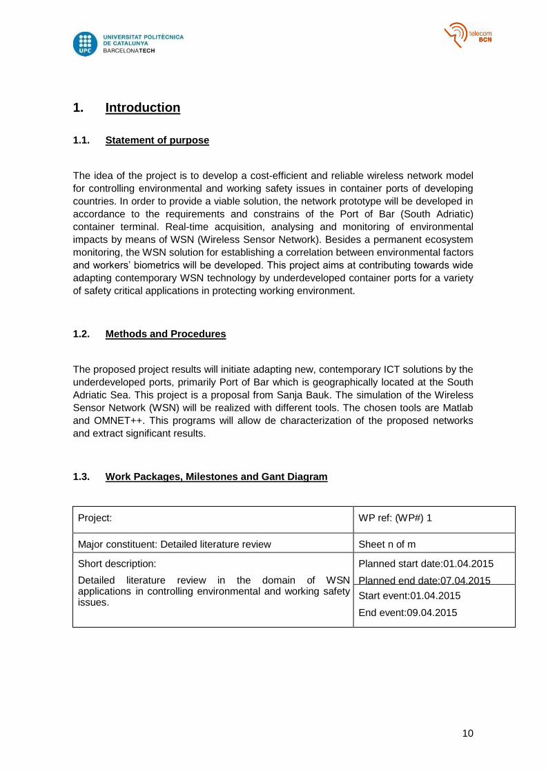
The idea of the project is to develop a cost-efficient and reliable wireless network model
for controlling environmental and working safety issues in container ports of developing
countries. In order to provide a viable solution, the network prototype will be developed in
accordance to the requirements and constrains of the Port of Bar (South Adriatic)
container terminal. Real-time acquisition, analysing and monitoring of environmental
impacts by means of WSN (Wireless Sensor Network). Besides a permanent ecosystem
monitoring, the WSN solution for establishing a correlation between environmental factors
and workers’ biometrics will be developed. This project aims at contributing towards wide
adapting contemporary WSN technology by underdeveloped container ports for a variety
of safety critical applications in protecting working environment.
1.2. Methods and Procedures
The proposed project results will initiate adapting new, contemporary ICT solutions by the
underdeveloped ports, primarily Port of Bar which is geographically located at the South
Adriatic Sea. This project is a proposal from Sanja Bauk. The simulation of the Wireless
Sensor Network (WSN) will be realized with different tools. The chosen tools are Matlab
and OMNET++. This programs will allow de characterization of the proposed networks
and extract significant results.
1.3. Work Packages, Milestones and Gant Diagram
Project: WP ref: (WP#) 1
Major constituent: Detailed literature review Sheet n of m
Short description:
Detailed literature review in the domain of WSN applications in controlling environmental and working safety issues.
Planned start date:01.04.2015
Planned end date:07.04.2015
Start event:01.04.2015
End event:09.04.2015
11
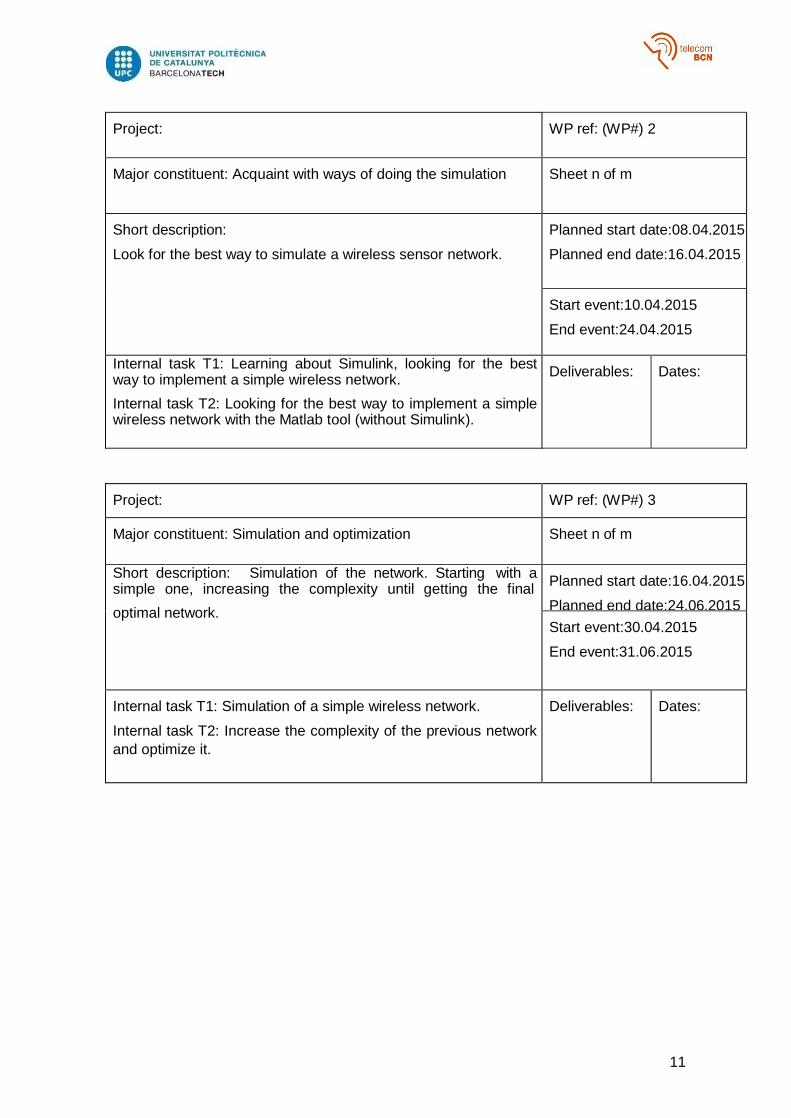
Project: WP ref: (WP#) 2
Major constituent: Acquaint with ways of doing the simulation Sheet n of m
Short description:
Look for the best way to simulate a wireless sensor network.
Planned start date:08.04.2015
Planned end date:16.04.2015
Start event:10.04.2015
End event:24.04.2015
Internal task T1: Learning about Simulink, looking for the best way to implement a simple wireless network.
Internal task T2: Looking for the best way to implement a simple wireless network with the Matlab tool (without Simulink).
Deliverables: Dates:
Project: WP ref: (WP#) 3
Major constituent: Simulation and optimization Sheet n of m
Short description: Simulation of the network. Starting with a simple one, increasing the complexity until getting the final
optimal network.
Planned start date:16.04.2015
Planned end date:24.06.2015
Start event:30.04.2015
End event:31.06.2015
Internal task T1: Simulation of a simple wireless network.
Internal task T2: Increase the complexity of the previous network
and optimize it.
Deliverables: Dates:
12
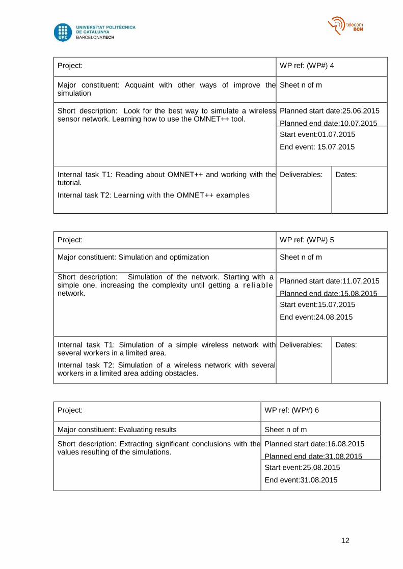
Project: WP ref: (WP#) 4
Major constituent: Acquaint with other ways of improve the simulation
Sheet n of m
Short description: Look for the best way to simulate a wireless sensor network. Learning how to use the OMNET++ tool.
Planned start date:25.06.2015
Planned end date:10.07.2015
Start event:01.07.2015
End event: 15.07.2015
Internal task T1: Reading about OMNET++ and working with the tutorial.
Internal task T2: Learning with the OMNET++ examples
Deliverables: Dates:
Project: WP ref: (WP#) 5
Major constituent: Simulation and optimization Sheet n of m
Short description: Simulation of the network. Starting with a simple one, increasing the complexity until getting a re l iable network.
Planned start date:11.07.2015
Planned end date:15.08.2015
Start event:15.07.2015
End event:24.08.2015
Internal task T1: Simulation of a simple wireless network with several workers in a limited area.
Internal task T2: Simulation of a wireless network with several workers in a limited area adding obstacles.
Deliverables: Dates:
Project: WP ref: (WP#) 6
Major constituent: Evaluating results Sheet n of m
Short description: Extracting significant conclusions with the values resulting of the simulations.
Planned start date:16.08.2015
Planned end date:31.08.2015
Start event:25.08.2015
End event:31.08.2015
13
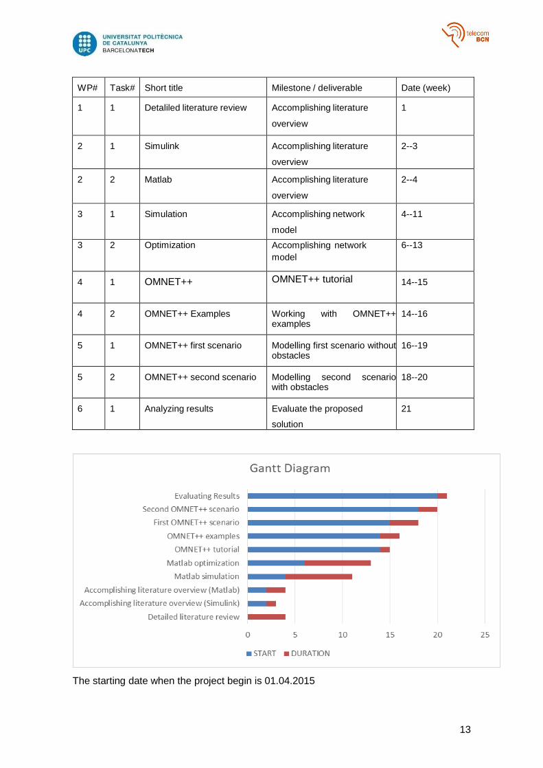
WP# Task# Short title Milestone / deliverable Date (week)
1 1 Detaliled literature review Accomplishing literature
overview
1
2 1 Simulink Accomplishing literature
overview
2--3
2 2 Matlab Accomplishing literature
overview
2--4
3 1 Simulation Accomplishing network
model
4--11
3 2 Optimization Accomplishing network
model
6--13
4 1 OMNET++ OMNET++ tutorial 14--15
4 2 OMNET++ Examples Working with OMNET++ examples
14--16
5 1 OMNET++ first scenario Modelling first scenario without obstacles
16--19
5 2 OMNET++ second scenario Modelling second scenario with obstacles
18--20
6 1 Analyzing results Evaluate the proposed
solution
21
The starting date when the project begin is 01.04.2015

14
1.4. Incidences
There has been some noticeable incidences during the project. First of all, as the aim of
the project was to built a network and to realize some simulations, finding the software
that better fits to the model was not an easy task.
The main problem during the project was that in the beggining of the second and
improved simulation, the laptop where the project where realized in broke. The softwares
used for the project realization melted the motherboard of the laptop. In order to recover
all the data and simulations, a lot of days and money were lost.
15
2. State of the art of the technology used or applied in this
thesis
A background, comprehensive review of the literature is required. This is known as the
Review of Literature and should include relevant, recent research that has been done on
the subject matter.
2.1. Wireless Sensor Networks
The interest in Wireless Sensor Networks (WSN) has increased a lot in recent years.
These types of sensors are built with limited computing resources and processing, they
are cheap and smaller in comparison with the traditional sensors. Measuring and
gathering information from the environment are the main utilities, and this sensed data is
transmitted to the users.
Smart sensor nodes are devices with low power that can be equipped with more than one
sensor, a power supply, memory, a processor, etc. Several varieties of sensors may be
attached to de sensor node to measure different environmental parameters, e.g., thermal,
biological, chemical, magnetic sensor, etc. As this type of sensor nodes have limited
memory and are placed in difficult access locations, a radio is implemented for wireless
communication in order to transfer the date to a base station (access point, fixed
computer).
A WSN consists of a number of sensor nodes (few tens to thousands) working all
together in order to obtain data about the environment, this means that WSN typically has
little or no infrastructure. Structured and unstructured are the two types of WSN. Some of
the sensors in a structured network are placed in a planned manner. On the other hand,
unstructured networks contain a dense collection of nodes and they are deployed in an
ad hoc manner (randomly located into the field). Once the network is deployed, it is left
unattended to perform monitoring and reporting functions. The disadvantage of the
unstructured WSN is the maintenance: detecting failures is difficult because there are a
lot of nodes. The advantage of structured network is the lower maintenance,
management cost and fewer nodes can coverage specific locations while ad hoc
deployment can have uncovered regions.
A lot of applications are possible with the implementation of WSN. Military tracking and
surveillance, for example, WSN helps to detect and identify an intrusion. On the other
hand, with natural disasters, sensor nodes can detect and alert the environment to
forecast disasters before they occur. Another important implementation of WSN is in
biomedical applications, the monitoring of a patient’s health is possible with surgical
implants sensors.
The difference between traditional networks and WSN is that WSN has resource
constraints. These constraints include a limited amount of energy, low bandwidth, limited
processing and storage in each node and short communication range. The environment
is an important factor to take into account; it plays a key role in order to determine the
16
size and the topology of the network and also the deployment scheme. For outdoor
environments the requirement is to cover a large area, so a lot of nodes are needed,
whereas for indoor environments, with a few number of node is possible to cover a limited
space. When the environment is inaccessible by humans or the network has a lot of
components a random deployment (ad hoc) is preferred over a planned one. Another
important matter is the obstructions, which can limit the communication between nodes.
Several standards for wireless communications exists for different applications: broadcast
radio, satellite communications, cellular telephony, etc. Four standards for wireless data
communication have been proposed for use in WSN, each with certain advantages.
However, WSN do not have widely accepted standard communication protocols in any of
the layers in the OSI model. The purpose of this section is to expose the standards
showing their disadvantages and advantages and their use in WSN.
2.1.1. Wi-Fi
Wi-Fi is based on the IEEE 802.11 family of standards and is basically a local area
networking (LAN) technology designed to provide in-building broadband coverage.
The 802.11 standard is defined through several specifications of Wireless Local Area
Networks (WLANs). It defines an over-the-air interface between a wireless client and a
base station (or between two wireless clients).There are several specifications in the
802.11 family:
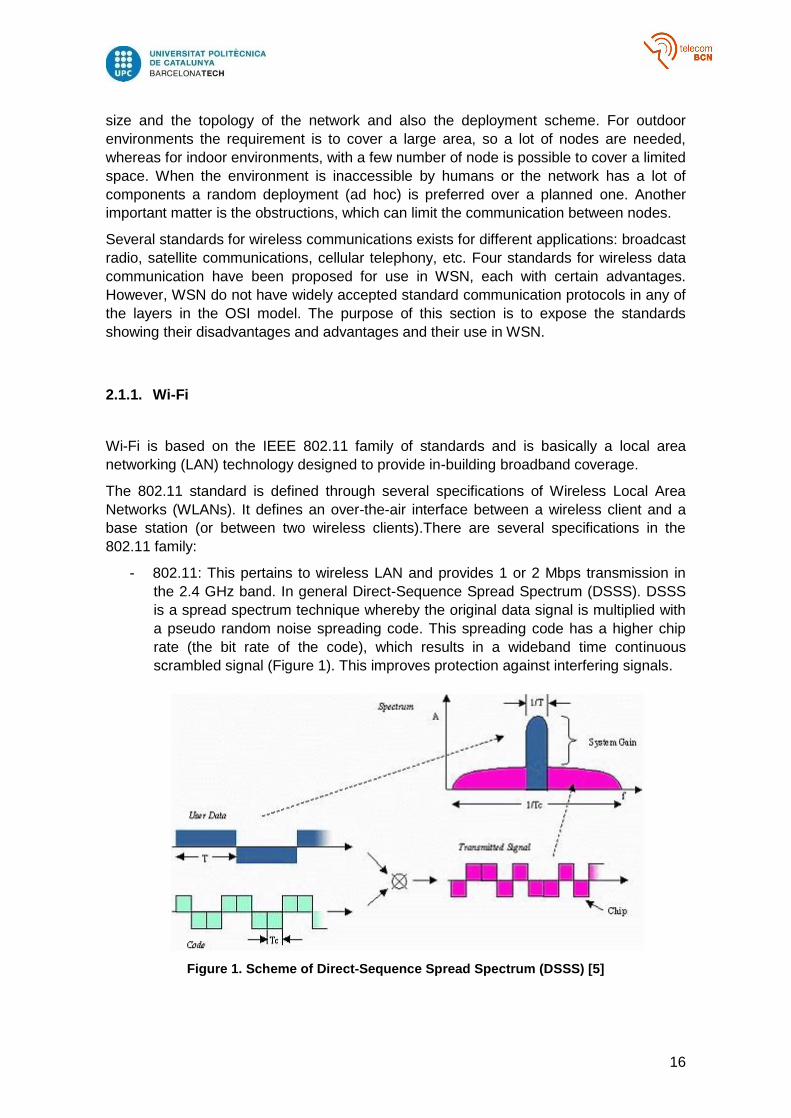
- 802.11: This pertains to wireless LAN and provides 1 or 2 Mbps transmission in
the 2.4 GHz band. In general Direct-Sequence Spread Spectrum (DSSS). DSSS
is a spread spectrum technique whereby the original data signal is multiplied with
a pseudo random noise spreading code. This spreading code has a higher chip
rate (the bit rate of the code), which results in a wideband time continuous
scrambled signal (Figure 1). This improves protection against interfering signals.
Figure 1. Scheme of Direct-Sequence Spread Spectrum (DSSS) [5]
17
- 802.11a: this is an extension to 802.11, which pertains to wireless LANs and goes
as fast as 54 Mbps in the 5 GHz band. 802.11a employs the Orthogonal
Frequency Division Multiplexing (OFDM) encoding scheme as opposed to DSSS.
OFDM consists on a large number of closely spaced orthogonal sub-carrier
signals that are used to carry data on several parallel data channels.
- 802.11b: the 802.11b high Wi-Fi is an extension that pertains to wireless LANs
and yields a connection as fast as 11 Mbps transmission in the 2.4 GHz band
(depending on strength of signal it can fall to 5.5, 2 or 1 Mbps). The 802.11b uses
DSSS.
- 802.11g: This pertains to wireless LANs and provides 20Mbps in the 2.4 GHz
frequency band.
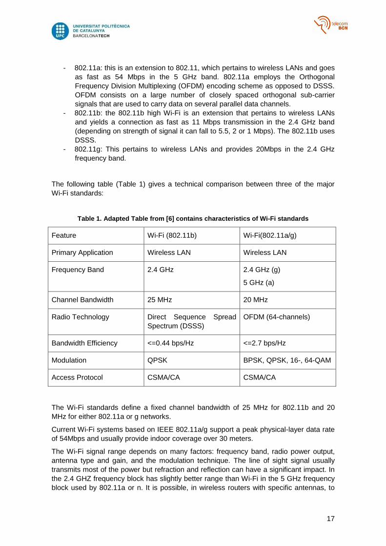
The following table (Table 1) gives a technical comparison between three of the major
Wi-Fi standards:
Table 1. Adapted Table from [6] contains characteristics of Wi-Fi standards
Feature Wi-Fi (802.11b) Wi-Fi(802.11a/g)
Primary Application Wireless LAN Wireless LAN
Frequency Band 2.4 GHz 2.4 GHz (g)
5 GHz (a)
Channel Bandwidth 25 MHz 20 MHz
Radio Technology Direct Sequence Spread
Spectrum (DSSS)
OFDM (64-channels)
Bandwidth Efficiency <=0.44 bps/Hz <=2.7 bps/Hz
Modulation QPSK BPSK, QPSK, 16-, 64-QAM
Access Protocol CSMA/CA CSMA/CA
The Wi-Fi standards define a fixed channel bandwidth of 25 MHz for 802.11b and 20
MHz for either 802.11a or g networks.
Current Wi-Fi systems based on IEEE 802.11a/g support a peak physical-layer data rate
of 54Mbps and usually provide indoor coverage over 30 meters.
The Wi-Fi signal range depends on many factors: frequency band, radio power output,
antenna type and gain, and the modulation technique. The line of sight signal usually
transmits most of the power but refraction and reflection can have a significant impact. In
the 2.4 GHZ frequency block has slightly better range than Wi-Fi in the 5 GHz frequency
block used by 802.11a or n. It is possible, in wireless routers with specific antennas, to
18
improve range by fitting upgraded antennas which gave higher gain in particular
directions. Outdoor ranges can be improved to many kilometres through the use of high
gain directional antennas at the router and remote devices. The maximum power that can
transmit a Wi-Fi device (limited by regulations) is 20dBm (100mW). To reach
requirements for wireless LAN applications, Wi-Fi has fairly high power consumption
compared to other standards.
Wi-Fi standards (IEEE 802.11a, b or g) wireless LANs use a media access control protocol
called Carrier Sense Multiple Access with Collision Avoidance (CSMA/CA). That is, the node
talk in the same way that human converse: they check if there is no one talking before
they start.
2.1.2. Zigbee
Zigbee is a wireless technology developed as an open global standard to address the
unique needs of low power and low costs wireless networks. This standard operates on
the IEEE 802.15.4 physical radio specification and operates in bands including 2.4 GHz,
900 MHz and 868 MHz.
Zigbee devices can transmit data over long distances by passing data through a mesh
network of intermediate devices to reach a larger range. Zigbee is typically used in low
data rate applications that need long battery life and secure networking. Zigbee has
defined a rate of 250 kbps best suited for intermittent data transmissions from a sensor or
input device. It is used in applications that require short range and low-rate wireless data
transfer. The technology defined by the Zigbee specification is intended to be simpler and
less expensive than Bluetooth or Wi-Fi.
The Zigbee standard specifies operation in 2.4 GHz for worldwide. The 915 MHz for
America and Australia and 868 MHz for Europe bands. Binary phase-shift keying
modulation (BPSK) is used in the 868 and 915 MHz bands and offset quadrature phase-
shift keying (OQPSK) is used in the 2.4 GHz band. The difference between these two
modulations is that OQPSK transmits two bits per symbol while BPSK only transmits one.
In the 2.4 GHz band, the data rate is 250 kbps, in the 915 MHz is 40 kbps and finally 20
kbit/s for the 868 MHz band. The actual data throughput will be less than the maximum
specified bit rate due to the processing delays and the packet overhead. For indoor
applications, the range will be near 10-20 m, depending on the number of walls,
construction materials… On the other hand, outdoors with line of sight, the range may
reach 1500 m depending on power output the environmental characteristics. The output
power of the radios is generally 1-100 mW (0-20 dBm).
ZigBee devices are required to conform to the IEEE 802.15.4 Low-Rate Wireless
Personal Area Network (LR-WPAN) standard. This standard specifies the lower protocol
layers, such as the physical layer and the Media Access Control (MAC) layer. The basic
channel access mode is the CSMA/CA (carrier sense, multiple access/collision
avoidance). The routing protocol used by the network layer is called Ad hoc On-demand
Distance Vector (AODV). In order to find the destination device, it broadcasts out a route
request to all of its neighbours. This process is made several times until the destination is
reached. When the message is in the destination, it sends its route reply via unicast
19
transmission following the lowest cost path back to the source. Once the source has
received the reply, it will update its routing table for the destination address with the next
hop in the past and the past cost.
2.1.3. White-Fi
In order to describe the Wi-fi technology within the TV unused spectrum, the term White-fi
is used. The IEEE 802.11af has been set up to define a standard to implement this
technology.
With a number of administrations around the globe taking a more flexible approach to
spectrum allocations, the low power system ideas that are able to work within portions of
spectrum that may need to be kept clear of high power transmitters to ensure coverage
areas do not overlap is being seriously investigated.
If the system used implements the White-fi technology, IEEE 802.11af that use TV white
space, the overall system must not cause interference to the primary users. With the
processing technology developing further, this is now becoming more of a possibility.
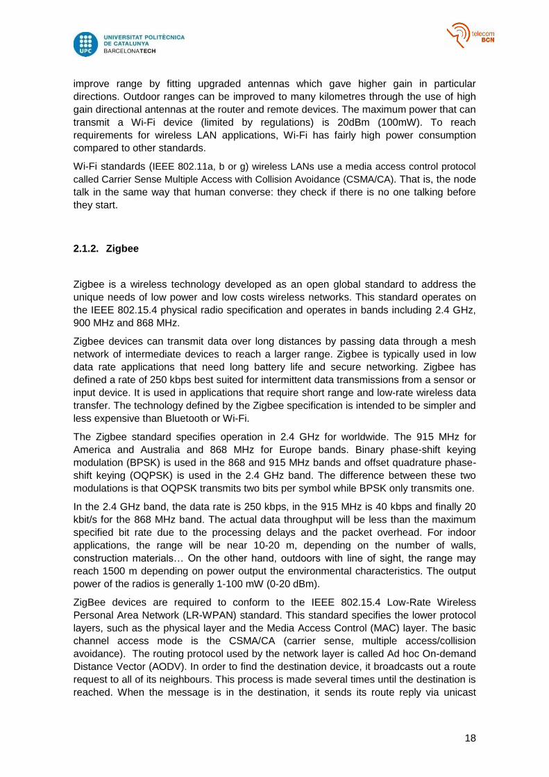
The concept of IEEE802.11af is that broadcast television coverage has to be organised
so that there is space left between the coverage areas of different transmitters using the
same channel so that interference does not occur.
This means that there are significant areas where these channels are unused and this
leads to very poor spectrum efficiency.
Figure 2. White-Fi IEEE 802.11af concept
There are many benefits for a system such as IEEE 802.11af from a using TV white
space. Taking into account that the exact nature of IEEE 802.11af has not been defined
entirely, it is possible to analyse many of the benefits that can be gained from White-Fi
technology:
20
- Propagation characteristics: in the view of the fact that the 802.11af white-fi
system operating the TV white spaces would use frequencies below 1 GHz, this
will allow to achieve larger distances. Wi-fi systems use frequencies where the
lowest band is 2.4 GHz, this implies that the signals are easily absorbed.
- Additional bandwidth: One of the advantages of using TV white space is that
additional otherwise unused frequencies can be accessed. To achieve the
required data throughput rates, it will be necessary to aggregate several TV
channels. It is possible that vacant channels in any given area will vary widely in
frequency and this presents some challenges in managing the data sharing
across different channels (this has been successfully achieved in technologies
such as LTE).
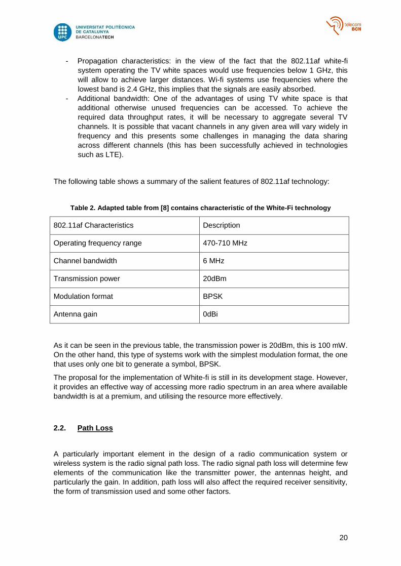
The following table shows a summary of the salient features of 802.11af technology:
Table 2. Adapted table from [8] contains characteristic of the White-Fi technology
802.11af Characteristics Description
Operating frequency range 470-710 MHz
Channel bandwidth 6 MHz
Transmission power 20dBm
Modulation format BPSK
Antenna gain 0dBi
As it can be seen in the previous table, the transmission power is 20dBm, this is 100 mW.
On the other hand, this type of systems work with the simplest modulation format, the one
that uses only one bit to generate a symbol, BPSK.
The proposal for the implementation of White-fi is still in its development stage. However,
it provides an effective way of accessing more radio spectrum in an area where available
bandwidth is at a premium, and utilising the resource more effectively.
2.2. Path Loss
A particularly important element in the design of a radio communication system or
wireless system is the radio signal path loss. The radio signal path loss will determine few
elements of the communication like the transmitter power, the antennas height, and
particularly the gain. In addition, path loss will also affect the required receiver sensitivity,
the form of transmission used and some other factors.
21
The signal path loss can be determined mathematically and these calculations are often
undertaken when designing system activities. These depend on knowledge of the signal
propagation proprieties.
In order to determine signal strength at various locations path loss calculations are used
in wireless survey tools. These tools are being widely used to help determine which the
radio signal strengths will be. Also, they provide a very valuable service for installing
wireless LAN systems in different places because the enable problems to be solved
before installation, enabling costs to be considerably reduced.
The signal radio path loss consists mainly in a reduction in power density of a signal as it
propagates through the environment in which it is travelling. The main reasons are the
following:
- Free space path loss: the free space path loss occurs as the signal travels
through space without any other effects attenuating the signal. This can be
thought of as the signal spreading out as an ever increasing sphere. The energy
in any given area will reduce as the area covered becomes larger.
- Absorption losses: when a radio signal passes into a medium which is not
transparent to radio signals absorption losses occur.
- Diffraction: These losses occur when an object appears in the signal’s path. The
signal can diffract around the object, but losses occur. The loss is higher the more
rounded the object. Around sharp edges, the radio signals tend to diffract better.
- Multipath: in the real world, signals will reach the receiver via several different
paths due to a lot of reflections. This signal reflections may add or subtract from
each other depending on the relative phases of the signals. One clear example is
cellular telecommunication phones, because they are subjected to this effect that
is known as Rayleigh fading.
- Atmosphere: radio signal paths are affected by the atmosphere. Below 30-50MHz,
lower frequencies, the ionosphere has a significant effect, refracting them back to
the earth. Above 50 MHz, the troposphere has a major effect, refracting also the
signals back to the earth.
- Obstacles: For mobile applications, for example, buildings and vegetation (and
other obstructions) have a remarkable effect. The buildings not only reflect the
signal, they will absorb them too. On the other hand, particularly when wet, trees
and foliage can attenuate radio signals. Moreover, the hills, obviously will obstruct
the path and considerably attenuate the signal, perhaps making the reception
impossible.
The environment that surrounds a transmitter and a receiver generates a lot of pahts that
can traverse the transmitted signal. Consequently, the signal received is a superposition
of several copies of the transmitted signal. Each of this copy, has suffered different
attenuation, phase shift and delay. As a result, the signal may have been amplified or
attenuated. Strong destructive interference is frequently referred to as a deep fade and
may result in temporary failure of communication because of significant drop in the
channel signal to noise ratio.
The following sections explains the most known statistical models for the effect of a
propagation environment on a radio signal, the used by wireless devices.
22
2.2.1. Rayleigh Fading
Rayleigh fading model assume that the magnitude of a communication channel will vary
randomly or fade, according to a Rayleigh distribution (the radial component of the sum of
two uncorrelated Gaussian random variables).
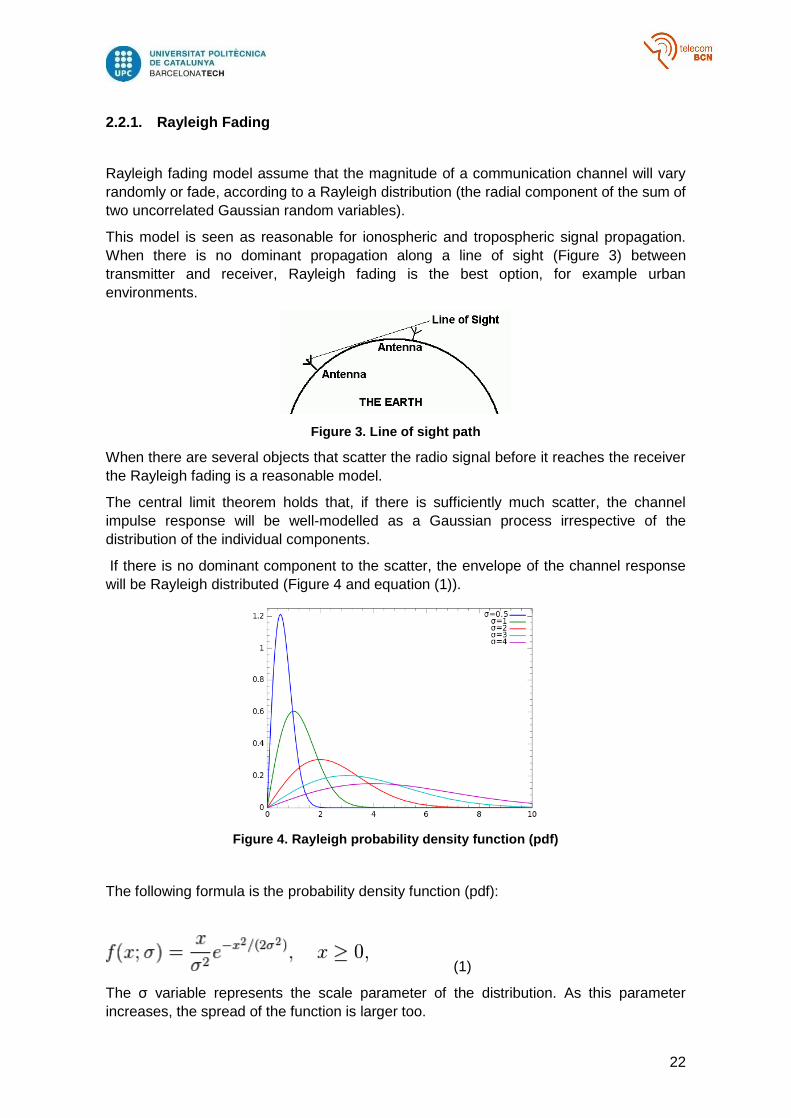
This model is seen as reasonable for ionospheric and tropospheric signal propagation.
When there is no dominant propagation along a line of sight (Figure 3) between
transmitter and receiver, Rayleigh fading is the best option, for example urban
environments.
Figure 3. Line of sight path
When there are several objects that scatter the radio signal before it reaches the receiver
the Rayleigh fading is a reasonable model.
The central limit theorem holds that, if there is sufficiently much scatter, the channel
impulse response will be well-modelled as a Gaussian process irrespective of the
distribution of the individual components.
If there is no dominant component to the scatter, the envelope of the channel response
will be Rayleigh distributed (Figure 4 and equation (1)).
Figure 4. Rayleigh probability density function (pdf)
The following formula is the probability density function (pdf):
(1)
The σ variable represents the scale parameter of the distribution. As this parameter
increases, the spread of the function is larger too.
23
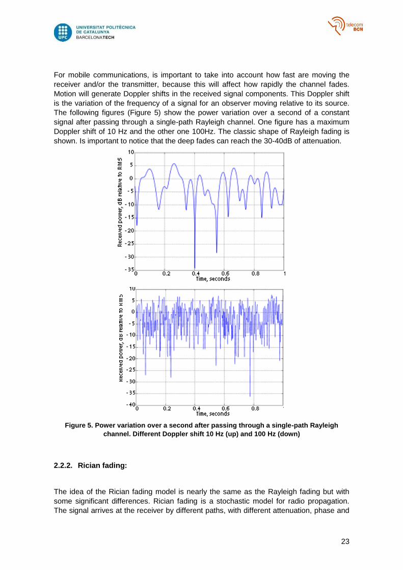
For mobile communications, is important to take into account how fast are moving the
receiver and/or the transmitter, because this will affect how rapidly the channel fades.
Motion will generate Doppler shifts in the received signal components. This Doppler shift
is the variation of the frequency of a signal for an observer moving relative to its source.
The following figures (Figure 5) show the power variation over a second of a constant
signal after passing through a single-path Rayleigh channel. One figure has a maximum
Doppler shift of 10 Hz and the other one 100Hz. The classic shape of Rayleigh fading is
shown. Is important to notice that the deep fades can reach the 30-40dB of attenuation.
Figure 5. Power variation over a second after passing through a single-path Rayleigh
channel. Different Doppler shift 10 Hz (up) and 100 Hz (down)
2.2.2. Rician fading:
The idea of the Rician fading model is nearly the same as the Rayleigh fading but with
some significant differences. Rician fading is a stochastic model for radio propagation.
The signal arrives at the receiver by different paths, with different attenuation, phase and
24
delay. The main difference between Rayleigh and Rician is that Rician fading occurs
when one of the paths is much stronger than the others, in general is the line of sight
signal. In Rician fading, the amplitude gain follows the Rice distribution.
The Rician channel is mainly described by two parameters. Κ is the ratio between the
power of the direct path and the power in the scattered paths. On the other hand, Ω is the
power of both paths and acts as a scaling factor to the distribution [4].
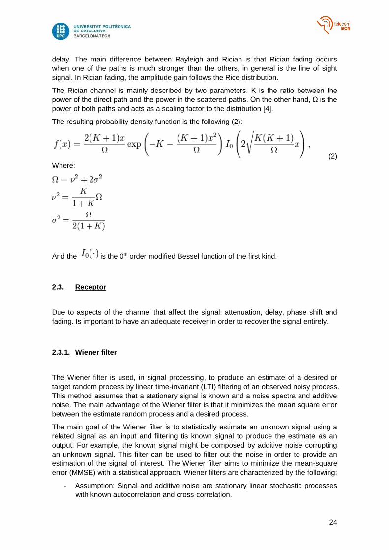
The resulting probability density function is the following (2):
(2)
Where:
And the is the 0th order modified Bessel function of the first kind.
2.3. Receptor
Due to aspects of the channel that affect the signal: attenuation, delay, phase shift and
fading. Is important to have an adequate receiver in order to recover the signal entirely.
2.3.1. Wiener filter
The Wiener filter is used, in signal processing, to produce an estimate of a desired or
target random process by linear time-invariant (LTI) filtering of an observed noisy process.
This method assumes that a stationary signal is known and a noise spectra and additive
noise. The main advantage of the Wiener filter is that it minimizes the mean square error
between the estimate random process and a desired process.
The main goal of the Wiener filter is to statistically estimate an unknown signal using a
related signal as an input and filtering tis known signal to produce the estimate as an
output. For example, the known signal might be composed by additive noise corrupting
an unknown signal. This filter can be used to filter out the noise in order to provide an
estimation of the signal of interest. The Wiener filter aims to minimize the mean-square
error (MMSE) with a statistical approach. Wiener filters are characterized by the following:
- Assumption: Signal and additive noise are stationary linear stochastic processes
with known autocorrelation and cross-correlation.
25
- Requirement: the filter must be realizable, this means, casual (the requirement
can be dropped because of a non-casual solution).
- Performance criterion: MMSE.
The casual finite impulse response (FIR: is a filter whose impulse response has a finite
duration, because it settles to zero in finite time) Wiener filter finds optimal tap weights by
using the statistics of the input and output signal.
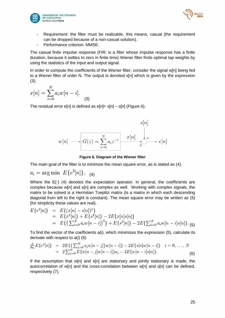
In order to compute the coefficients of the Wiener filter, consider the signal w[n] being fed
to a Wiener filter of order N. The output is denoted x[n] which is given by the expression
(3).
(3)
The residual error e[n] is defined as e[n]= x[n] – s[n] (Figure 6).
Figure 6. Diagram of the Wiener filter
The main goal of the filter is to minimize the mean square error, as is stated as (4).
(4)
Where the E{·} (4) denotes the expectation operator. In general, the coefficients are
complex because w[n] and s[n] are complex as well. Working with complex signals, the
matrix to be solved is a Hermitian Toeplitz matrix (is a matrix in which each descending
diagonal from left to the right is constant). The mean square error may be written as (5)
(for simplicity these values are real).
(5)
To find the vector of the coefficients a(i), which minimizes the expression (5), calculate its
derivate with respect to a(i) (6)
(6)
If the assumption that w[n] and s[n] are stationary and jointly stationary is made, the
autocorrelation of w[n] and the cross-correlation between w[n] and s[n] can be defined,
respectively (7).
26
(7)
The derivate of MSE may be rewritten as (8).
(8)
Notice that:
If the derivate is equal to zero, the result is (9).
(9)
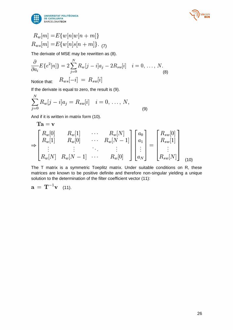
And if it is written in matrix form (10).
(10)
The T matrix is a symmetric Toeplitz matrix. Under suitable conditions on R, these
matrices are known to be positive definite and therefore non-singular yielding a unique
solution to the determination of the filter coefficient vector (11):
(11).
27
3. Methodology / project development
In the following sections, two proposed scenarios are briefly described, and then the
methodology of the simulation process is explained, firstly by means of Matlab tool, and
secondly by OMNET++ one.
3.1. Scenario 1: WBANSs as part of personal protective equipment
The operators in the Port of Bar are exposed to many risks, due to they are working
mainly in open space (at docks, open stacking and warehousing areas, gangways, etc.)
under various weather conditions. In order to reduce potential risks of accidents, the
workers on the port should wear personal protective equipment which includes, for
example: safety vest, helmet, and protective shoes. Over these garments are attached
Radio Frequency IDentificantion (RFID) passive tags [3, 10], which provide ID for each of
the personal equipment parts. These RFID tags are working as WBANSs. Tags attached
to the workers’ helmets provide information about temperature. The protective shoes give
information about the plantar pressure. According to the findings given in [14], it is
possible to classify fifteen different behaviours (walking, running, etc.). This tag able to
infer information about actions performed by the workers.
This first scenario has been already employed and presented in the papers [1, 3]. This
scenario fits well into the occupational safety requirements in the Port of Bar, but some
different simulations between the sink node (access point) and the Body Central Unit
(BCU) will be realized in this project, in comparison to [1, 3, 13].
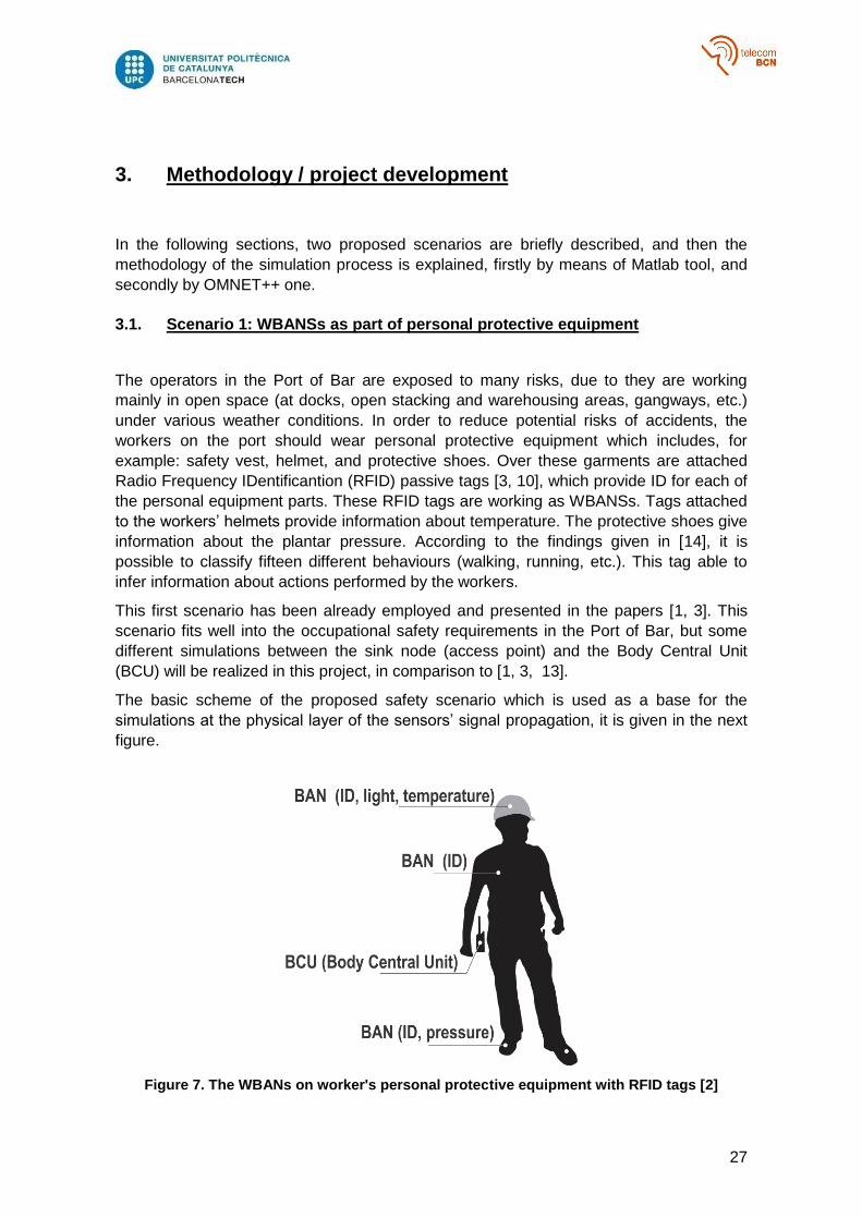
The basic scheme of the proposed safety scenario which is used as a base for the
simulations at the physical layer of the sensors’ signal propagation, it is given in the next
figure.
Figure 7. The WBANs on worker's personal protective equipment with RFID tags [2]
28
By means of RFID tag it is possible to infer the information that are very important from
the safety point: if the worker wears the safety vest, the helmet and if he put on the
protective shoes too. Also, it is possible to asset the temperature inside the helmet on the
workers head and the pressure that worker makes according to his movements in the
area.
3.2. Scenario 2: As scanners of workers’ vital signs
The second scenario proposed in the project is based on the concept of wearable
sensors for measuring in real time electrophysiological data of workers engaged on port
operations in the Port of Bar. There is no reliable data on professional diseases in
Montenegro, so the choice of the vital signal sensors is based mainly on some empirical
assessments and intuition. Here the proposed model might be interesting one for health
institutions in Montenegro in terms of starting collecting reliable real-time data on
employees’ health conditions in a specific commercial and industrial area such as the
Port of Bar.
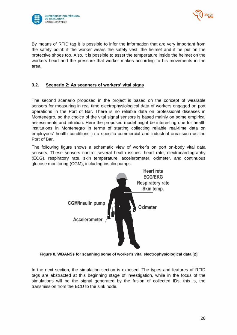
The following figure shows a schematic view of worker’s on port on-body vital data
sensors. These sensors control several health issues: heart rate, electrocardiography
(ECG), respiratory rate, skin temperature, accelerometer, oximeter, and continuous
glucose monitoring (CGM), including insulin pumps.
Figure 8. WBANSs for scanning some of worker's vital electrophysiological data [2]
In the next section, the simulation section is exposed. The types and features of RFID
tags are abstracted at this beginning stage of investigation, while in the focus of the
simulations will be the signal generated by the fusion of collected IDs, this is, the
transmission from the BCU to the sink node.
29
3.3. Matlab Simulation
The first set of simulations are performed with the Matlab tool. The reason why the
simulation has been made with this tool is that Matlab offers several advantages that are
very useful for the realization of the task. Matlab offers an easy way of programming, a lot
of instructions and already written functions. With all of the easy-way using applications
and the useful way to treat vectors and matrix, Matlab able an easy way of modelling a
simple network.
The main basis of this simulation is the connection between the Body Central Unit (BCU)
that the worker is carrying with himself and the sink node (access point), the node that
collects all the data of several workers. The BCU (or called base station too) will collect
the data of each RFID and send it to the access point. This node, once it has received all
the data of every worker, fusion all the data and send it to the “outside world”.
For this first simulation, the communication will be only one hop, this means that the
simulation will only modelate a point to point transmission, the simplest one. Obviously,
he workers in the port will be moving around in some limited area but for this simulation
the movements of the workers will be not considered.
The simulation is realized in Matlab (ver 7.12.1), by Inter® Core i5 processor on 2.4 GHz
(4GB RAM). The simulation includes the number of bits that want to be transmitted
(sequence of random bits), assuming that is the data that the access point receives from
all the body sensors. With the sequence of bits, different type of modulation is
implemented depending on the wishes: each bit can represent a symbol, BPSK
modulation, or the bits can be joined in groups of two to generate a QPSK modulation.
With the QPSK modulation, the symbol is presented as a complex number, exposing his
real and complex components. When the signal is generated, the fading effects are
applied and the noise addition, the signal reconstruction is realized by the Wiener filter,
and finally the computation of the relation between the BER and the SNR is made [3, 8, 9,
11].
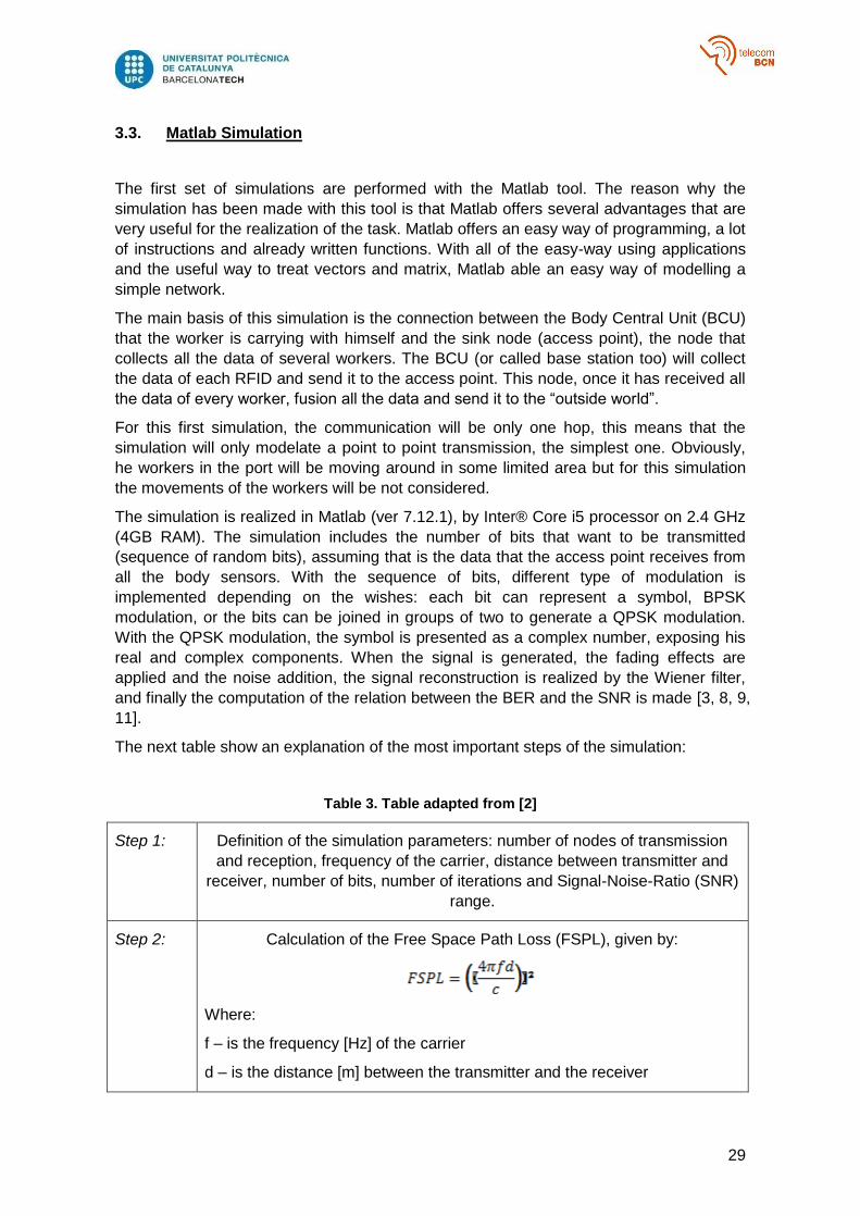
The next table show an explanation of the most important steps of the simulation:
Table 3. Table adapted from [2]
Step 1: Definition of the simulation parameters: number of nodes of transmission
and reception, frequency of the carrier, distance between transmitter and
receiver, number of bits, number of iterations and Signal-Noise-Ratio (SNR)
range.
Step 2: Calculation of the Free Space Path Loss (FSPL), given by:
Where:
f – is the frequency [Hz] of the carrier
d – is the distance [m] between the transmitter and the receiver
30
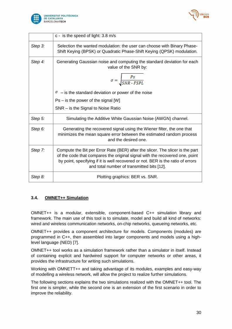
c - is the speed of light: 3.8 m/s
Step 3: Selection the wanted modulation: the user can choose with Binary Phase-
Shift Keying (BPSK) or Quadratic Phase-Shift Keying (QPSK) modulation.
Step 4: Generating Gaussian noise and computing the standard deviation for each
value of the SNR by:
– is the standard deviation or power of the noise
Ps – is the power of the signal [W]
SNR – is the Signal to Noise Ratio
Step 5: Simulating the Additive White Gaussian Noise (AWGN) channel.
Step 6: Generating the recovered signal using the Wiener filter, the one that
minimizes the mean square error between the estimated random process
and the desired one.
Step 7: Compute the Bit per Error Rate (BER) after the slicer. The slicer is the part
of the code that compares the original signal with the recovered one, point
by point, specifying if it is well recovered or not. BER is the ratio of errors
and total number of transmitted bits [12].
Step 8: Plotting graphics: BER vs. SNR.
3.4. OMNET++ Simulation
OMNET++ is a modular, extensible, component-based C++ simulation library and
framework. The main use of this tool is to simulate, model and build all kind of networks:
wired and wireless communication networks, on-chip networks, queueing networks, etc.
OMNET++ provides a component architecture for models. Components (modules) are
programmed in C++, then assembled into larger components and models using a high-
level language (NED) [7].
OMNET++ tool works as a simulation framework rather than a simulator in itself. Instead
of containing explicit and hardwired support for computer networks or other areas, it
provides the infrastructure for writing such simulations.
Working with OMNETT++ and taking advantage of its modules, examples and easy-way
of modelling a wireless network, will allow the project to realize further simulations.
The following sections explains the two simulations realized with the OMNET++ tool. The
first one is simpler, while the second one is an extension of the first scenario in order to
improve the reliability.
31
3.4.1. OMNET ++ scenario 1:
This first scenario consist on several number of hosts (Ad hoc hosts) moving over a
limited area sending data messages. The aim of this simulation is to evaluate a simple
scenario where a number of moving hosts (nodes) are sending data to fixed receivers
(sink nodes).
OMNET++ able the user to configure physical parameters in order to define the area as
the user wants. Particularly, the area can be limited in the three dimensions, the user can
define the maximum and minimum constraint for the three axes (x, y, z). In addition, this
tool allows to define the initial position of the modules (in this case hosts). The exact
initial position can be predefined or let the tool position the host randomly. For this first
scenario, the area will be limited with 1000 meters in both directions x and y. As this first
scenario will count with fixed and mobile hosts defining the initial position will be very
useful. In particular, it is important to define the specific location of the fixed host (sink
node).
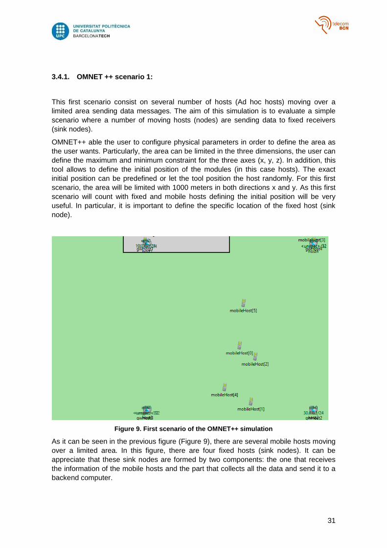
Figure 9. First scenario of the OMNET++ simulation
As it can be seen in the previous figure (Figure 9), there are several mobile hosts moving
over a limited area. In this figure, there are four fixed hosts (sink nodes). It can be
appreciate that these sink nodes are formed by two components: the one that receives
the information of the mobile hosts and the part that collects all the data and send it to a
backend computer.
32
Another option within OMNET++ environment is the capability of configuring the type of
motion of the mobile hosts. The movement can be modelling as random, linear, following
a specific shape, etc. In this case, the movement will be random. All the motion
parameters like the movement interval and the speed will be settled as the user needs or
preferences. In order to improve the reliability of the simulation, as the intention is to
control the security and health of the workers in a seaport area, the movement will be
settled to be like the human movement.
On the other hand, all the specifications on how each node works have to be defined. In
this simulation the physical and the link layers play a very important role.
In the physical layer, it is possible to define the type of antenna that the node is using,
with his antenna gain. In order to ensure a possible communication, this means that the
receiver can read the message with data without errors, is important to define several
physical layer parameters:
- Transmitter power: a range of transmitter power has to be defined in order to
ensure a good reception.
- Receiver sensitivity and Signal to Noise and Interference Ratio (SNIR) threshold:
The ability of the radio receiver to pick up the required level of radio signals will
enable it to operate more effectively within its application.
The channel where the signal pass through it is important to be well modelled. The
OMNET++ offers a large list of classes of different path loss channels: Free Space Path
Loss, Rayleigh Fading Channel, Rician Fading Channel, Nakagami Channel, etc. In this
scenario the chosen channel is the Rician Fading Channel. In the code, the tool allows to
settle the channel parameters as needed.
As it has been commented, the link layer plays a very important role in this simulation, as
well. In order to realize several experiments and be able to extract significant conclusions,
the simulation includes the possibility of changing important parameters in the link layer
(MAC layer). It is possible to change the carrier frequency of the signal, as well as his
bandwidth. In addition, the bit rate can be also settled. Moreover, the OMNET++ offers
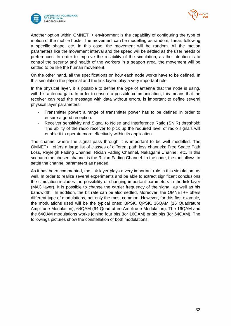
different type of modulations, not only the most common. However, for this first example,
the modulations used will be the typical ones: BPSK, QPSK, 16QAM (16 Quadrature
Amplitude Modulation), 64QAM (64 Quadrature Amplitude Modulation). The 16QAM and
the 64QAM modulations works joining four bits (for 16QAM) or six bits (for 64QAM). The
followings pictures show the constellation of both modulations.
33
Figure 10. Constellation of 16QAM (left) and 64QAM (right)
The configuration of the Internet and transport layer is also possible. Transmission
Control Protocol and Internet Protocol (TCP/IP) have been chosen for the Internet layer
and the User Datagram Protocol (UDP) protocol for the transport layer.
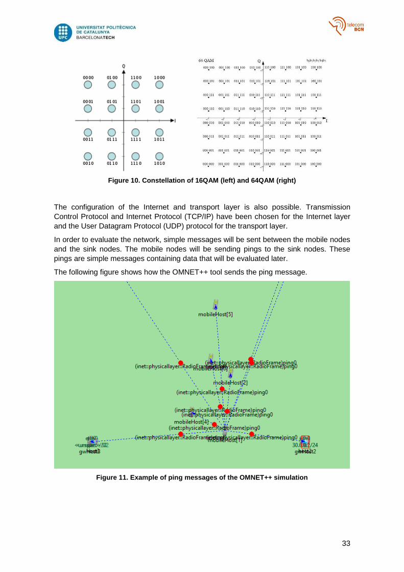
In order to evaluate the network, simple messages will be sent between the mobile nodes
and the sink nodes. The mobile nodes will be sending pings to the sink nodes. These
pings are simple messages containing data that will be evaluated later.
The following figure shows how the OMNET++ tool sends the ping message.
Figure 11. Example of ping messages of the OMNET++ simulation
34
The OMNET++ tool works fine to simulate discrete events and model wireless networks
but, in order to show the results of the simulation, all the values will be treated with
Matlab.
In order to show some significant results, a treatment of several results of the simulation
is needed. The intention is to show some graphics as a result, for this reason, the path
loss value of every message (even if is not data message) is saved. In order to
distinguish if the path loss value is from a data message or not, is important to take into
account the simulation time. Comparing the simulation time of the computed path loss
with the time when the link layer (MAC layer) receives a package with data, an exclusion
of the non-significant path loss values is possible. From the OMNET simulation, the value
of the transmission power is also extracted. With the previous value and this one, it is
possible to compute the received power. In addition, the computation of the Signal-to-
Noise Ratio (SNR) in reception is realized with the received power and the power of the
noise. With the value of the SNR, it is possible to calculate the Bit Error Rate (BER)
depending on the type of modulation used in the simulation:
(12)
(13)
(14)
(15)
Depending on the modulation used the BER formula is one of the previous equations (12,
13, 14 and 15). These formulas are extracted from the constellation of each modulation.
With the values of the power received values, plotting the shape of the cumulative
probability function will allow to deduct some conclusions.
The class that configures the channel in the OMNET++ simulation works with the
propagation speed and computes the delay of the transmission between the source node
and the sink node. Collecting all these values and working with them in the Matlab tool,
allow to plot a scatter function: combining the values of the path loss, the delay and the
distance vector.
3.4.2. OMNET++ scenario 2
The basis of this simulation are the same as the other one. The idea is to maintain fixed
several nodes, which will represent the sink node, the ones that collect all the data. On
the other hand, there will be a specific number of moving hosts, which are the body
central unit of each worker, going over a limited area.
The parameters of the communication, for the physical and link layer, can be changed
and settled in the same way as the previous simulation. The antenna parameters,
sensitivity and the SNIR threshold are the parameters that can be modified from the
35
physical layer. On the other hand, type of modulation, bit rate and carrier frequency are
the link layer parameters. About the transport layer, the protocol used is TCP/IP, like in
the first simulation.
This model still uses the same propagation mode. The channel proposed for this
simulation is the Rician Fading channel. Moreover, every message between the
transmitter and the receiver travels with the speed of light (ca. 3x10⁸ m/s).
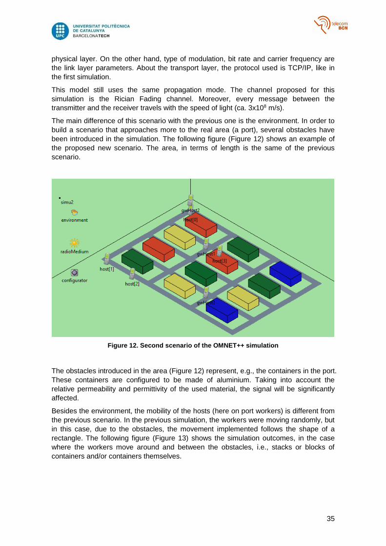
The main difference of this scenario with the previous one is the environment. In order to
build a scenario that approaches more to the real area (a port), several obstacles have
been introduced in the simulation. The following figure (Figure 12) shows an example of
the proposed new scenario. The area, in terms of length is the same of the previous
scenario.
Figure 12. Second scenario of the OMNET++ simulation
The obstacles introduced in the area (Figure 12) represent, e.g., the containers in the port.
These containers are configured to be made of aluminium. Taking into account the
relative permeability and permittivity of the used material, the signal will be significantly
affected.
Besides the environment, the mobility of the hosts (here on port workers) is different from
the previous scenario. In the previous simulation, the workers were moving randomly, but
in this case, due to the obstacles, the movement implemented follows the shape of a
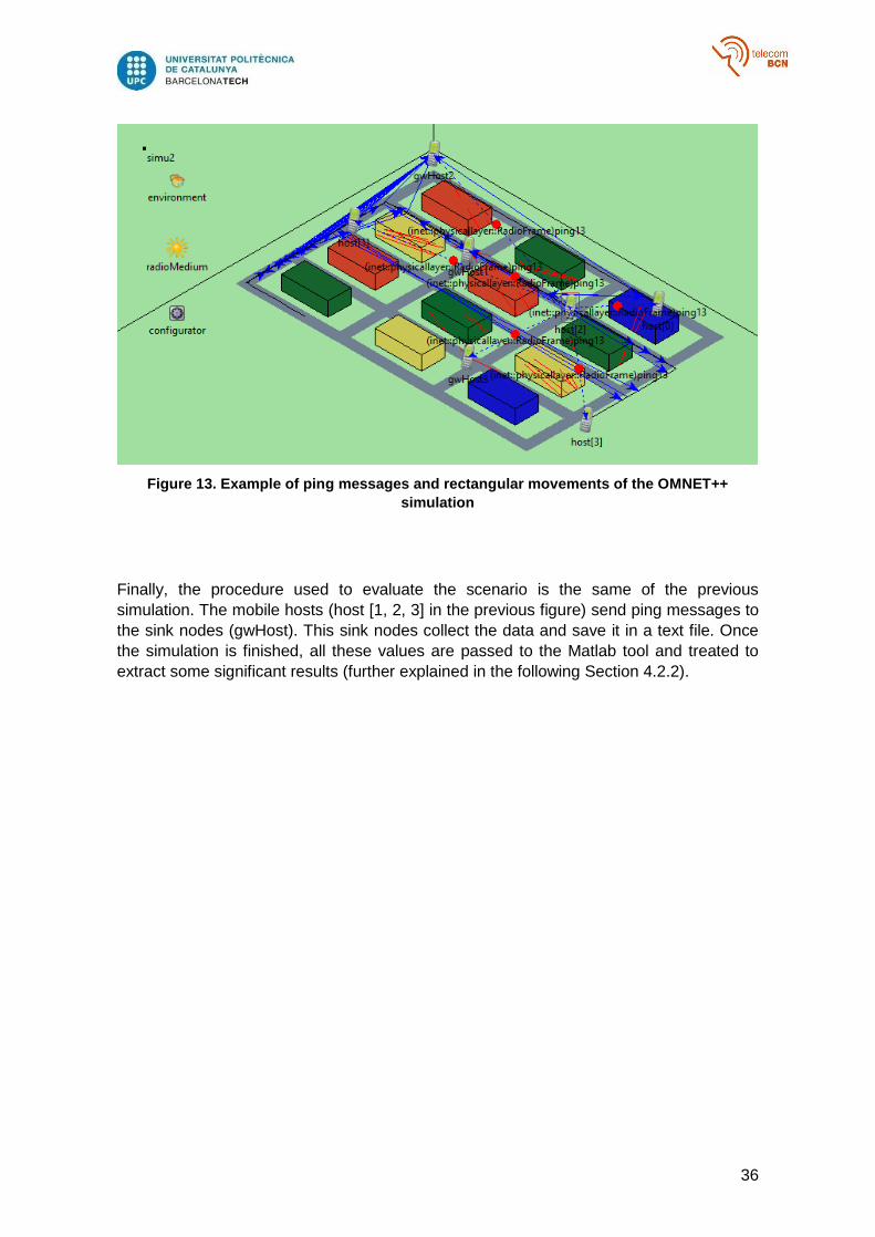
rectangle. The following figure (Figure 13) shows the simulation outcomes, in the case
where the workers move around and between the obstacles, i.e., stacks or blocks of
containers and/or containers themselves.
36
Figure 13. Example of ping messages and rectangular movements of the OMNET++
simulation
Finally, the procedure used to evaluate the scenario is the same of the previous
simulation. The mobile hosts (host [1, 2, 3] in the previous figure) send ping messages to
the sink nodes (gwHost). This sink nodes collect the data and save it in a text file. Once
the simulation is finished, all these values are passed to the Matlab tool and treated to
extract some significant results (further explained in the following Section 4.2.2).
37
4. Results
4.1. Matlab simulation
On the basis of Matlab code briefly described in the previous section (Section 3.3) and
summarized in Table 3, the relations between the transmitted signal BER and SNR are
presented. In the first case, the considered relation is evaluated for characteristic carrier
frequencies in different wireless technologies. The technologies are been explained
previously and are the following: ZigBee or IEEE 802.15.4 (carrier frequency of 915 MHz),
Wi-Fi protocol (carrier frequency of 2.4 GHz) and the Ultra Wide Band (UWB) (carrier
frequency of 3.1 GHz). In addition to the simulations for typical Wireless Local Area
Networks (WLANs) carriers’ frequencies, the simulation for White-Fi has been performed
too. For the White-Fi protocol, two frequencies have been chosen in order to do the
analysis: the maximum frequency in the domain, this is 710 MHz, and the minimum
frequency 470 MHz. It is to be pointed that by using White-Fi signal absorption can be
easily avoid and otherwise unused TV frequencies might be exploited.
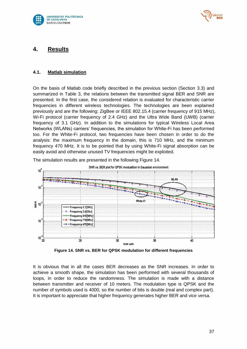
The simulation results are presented in the following Figure 14.
Figure 14. SNR vs. BER for QPSK modulation for different frequencies
It is obvious that in all the cases BER decreases as the SNR increases. In order to
achieve a smooth shape, the simulation has been performed with several thousands of
loops, in order to reduce the randomness. The simulation is made with a distance
between transmitter and receiver of 10 meters. The modulation type is QPSK and the
number of symbols used is 4000, so the number of bits is double (real and complex part).
It is important to appreciate that higher frequency generates higher BER and vice versa.
38
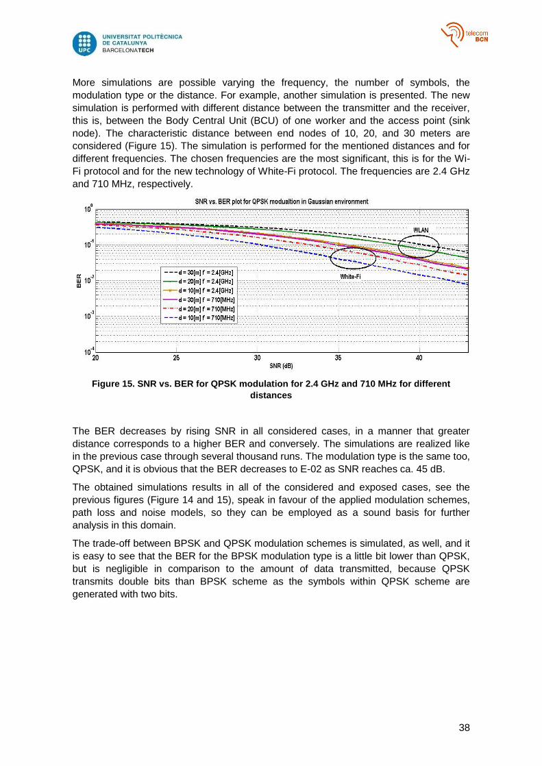
More simulations are possible varying the frequency, the number of symbols, the
modulation type or the distance. For example, another simulation is presented. The new
simulation is performed with different distance between the transmitter and the receiver,
this is, between the Body Central Unit (BCU) of one worker and the access point (sink
node). The characteristic distance between end nodes of 10, 20, and 30 meters are
considered (Figure 15). The simulation is performed for the mentioned distances and for
different frequencies. The chosen frequencies are the most significant, this is for the Wi-
Fi protocol and for the new technology of White-Fi protocol. The frequencies are 2.4 GHz
and 710 MHz, respectively.
Figure 15. SNR vs. BER for QPSK modulation for 2.4 GHz and 710 MHz for different
distances
The BER decreases by rising SNR in all considered cases, in a manner that greater
distance corresponds to a higher BER and conversely. The simulations are realized like
in the previous case through several thousand runs. The modulation type is the same too,
QPSK, and it is obvious that the BER decreases to E-02 as SNR reaches ca. 45 dB.
The obtained simulations results in all of the considered and exposed cases, see the
previous figures (Figure 14 and 15), speak in favour of the applied modulation schemes,
path loss and noise models, so they can be employed as a sound basis for further
analysis in this domain.
The trade-off between BPSK and QPSK modulation schemes is simulated, as well, and it
is easy to see that the BER for the BPSK modulation type is a little bit lower than QPSK,
but is negligible in comparison to the amount of data transmitted, because QPSK
transmits double bits than BPSK scheme as the symbols within QPSK scheme are
generated with two bits.
39
4.2. OMNET++ simulation
In this section the results of the OMNETT++ simulations will be commented and
compared. First of all, the section exposes the used parameters for each simulation, then
showing and commenting results and finally, comparing both scenarios.
4.2.1. OMNET++ scenario 1
On the basis of OMNET++ code briefly described in the previous section (Section 3.4.1),
some results and graphics are exposed.
For this first simulation a two dimension scenario is presented. This scenario is limited
with 1000m in both directions. In this simple simulation the area only contains the workers,
which are represented as a mobile host (the Body Central Unit (BCU) of the worker). In
this case, the number of workers (mobile hosts) is four and the number of access point
(sink nodes) is also four.
In this limited area all the mobile host are configured to move randomly. The OMNET++
tool allow to settle the type of mobility, the change interval and the speed of movement.
As all the hosts are moving in a random way, the change interval is 1 second with 0.1
second of standard deviation. This means that over 1 second each host will make a move
with a specified speed. The speed is settled to emulate the movement of a human person
so 3 meters/second (mps).
As explained in the previous section (Section 3), the type of selected channel is Rician
Fading channel. The reason why this is the channel selected is that as the scenario is a
simple one, the line of sight signal will contain most of the power, this means that the
reflected signals will have significant less power. The ratio of power between the line of
sight signals and the power of the others is settled in 8 dB. This value and the value of
alpha, which computes the attenuation of the path, is two and affects the path loss value.
The following figure (Figure 16) show a scatter function of the received power and the
distance of the path.
The transmission power is 1 mW (-30 dB) of power because all the nodes try to consume
the less power possible in order to have the minimum battery consumption.
After the simulation with the OMNET++ tool, all the result values are passed and treated
in Matlab, as explained in the previous section (Section 3). The next figure (Figure 16) is
the first Matlab plot.
40
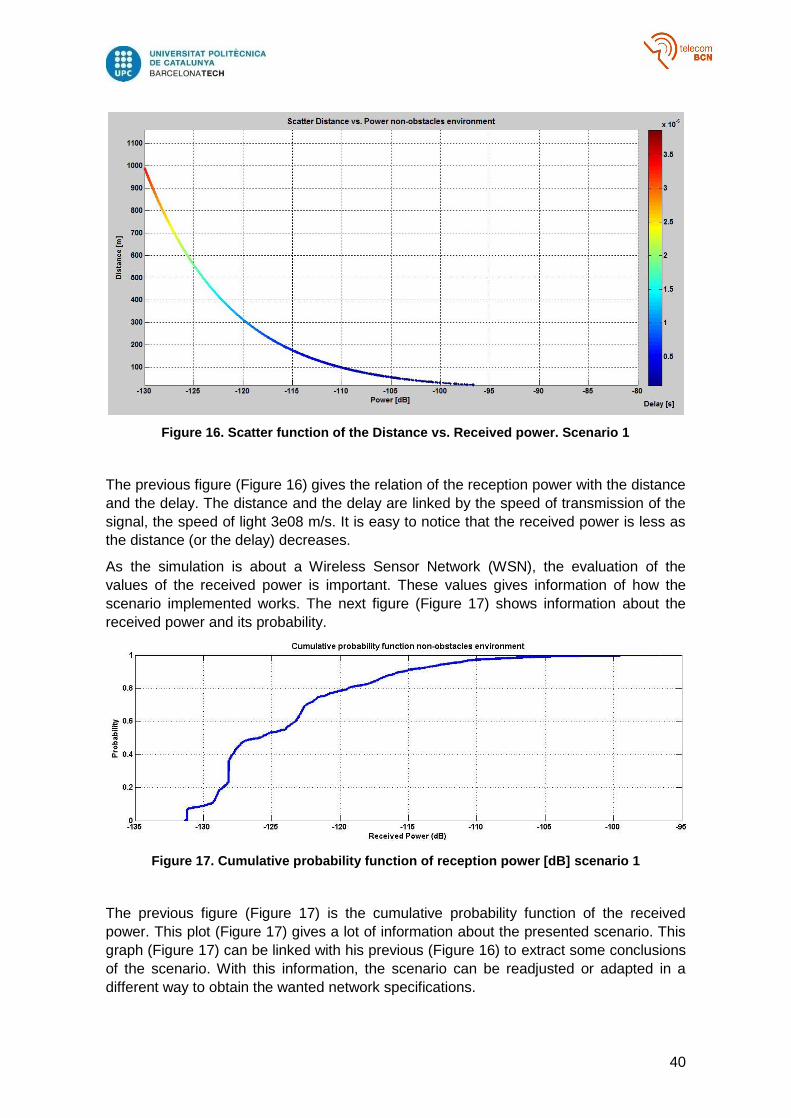
Figure 16. Scatter function of the Distance vs. Received power. Scenario 1
The previous figure (Figure 16) gives the relation of the reception power with the distance
and the delay. The distance and the delay are linked by the speed of transmission of the
signal, the speed of light 3e08 m/s. It is easy to notice that the received power is less as
the distance (or the delay) decreases.
As the simulation is about a Wireless Sensor Network (WSN), the evaluation of the
values of the received power is important. These values gives information of how the
scenario implemented works. The next figure (Figure 17) shows information about the
received power and its probability.
Figure 17. Cumulative probability function of reception power [dB] scenario 1
The previous figure (Figure 17) is the cumulative probability function of the received
power. This plot (Figure 17) gives a lot of information about the presented scenario. This
graph (Figure 17) can be linked with his previous (Figure 16) to extract some conclusions
of the scenario. With this information, the scenario can be readjusted or adapted in a
different way to obtain the wanted network specifications.
41
As explained in the previous section (Section 3), the OMNET++ tool offers a big range of
possibilities. Several simulations have been run, with different values of carrier frequency,
bit rate, modulation type, etc. The results exposed for this scenario work with a carrier
frequency of 2.412 GHz, like the Wi-Fi or Zigbee protocol explained in previous sections
(Section 2.1.1 and Section 2.1.2 respectively).
In order to get some significant results and extract some conclusions the same simulation
has been run four times but with different modulation types. The simulations are made
with the four modulation type explained and mentioned in this project: QPSK, BPSK,
16QAM, 64QAM.
The program is configured in the following way: all of the four moving nodes, send a ping
message (simple already built data message) to the fixed nodes (sink nodes or access
point). This messages are sent for the mobile nodes in a random way. The sending timing
is a uniform value between 1 second and 5 seconds. With this, the transmission and
reception of data is configured in a more reliable way. Besides, avoidance of collision
between packages is achieved, because this is not the main goal of these simulations.
The results are presented in the following plot (Figure 18), showing the relation between
the Bit per Error Rate (BER) and the Signal-to-Noise Ratio (SNR).
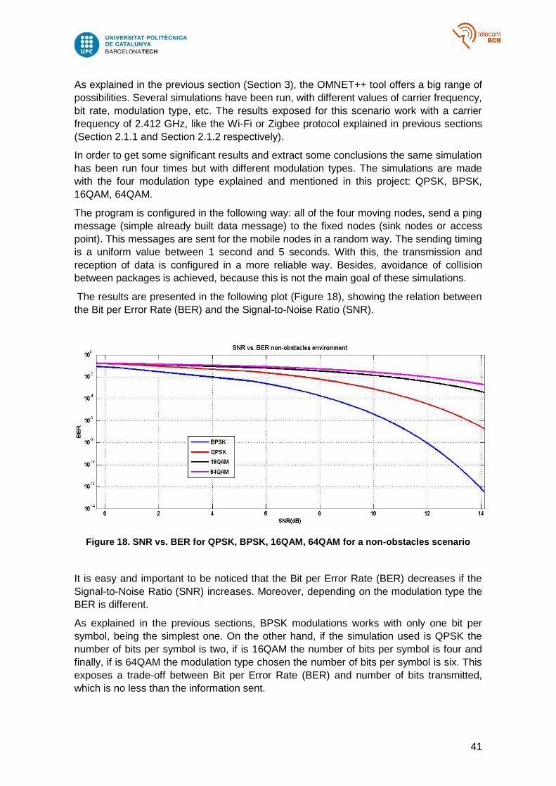
Figure 18. SNR vs. BER for QPSK, BPSK, 16QAM, 64QAM for a non-obstacles scenario
It is easy and important to be noticed that the Bit per Error Rate (BER) decreases if the
Signal-to-Noise Ratio (SNR) increases. Moreover, depending on the modulation type the
BER is different.
As explained in the previous sections, BPSK modulations works with only one bit per
symbol, being the simplest one. On the other hand, if the simulation used is QPSK the
number of bits per symbol is two, if is 16QAM the number of bits per symbol is four and
finally, if is 64QAM the modulation type chosen the number of bits per symbol is six. This
exposes a trade-off between Bit per Error Rate (BER) and number of bits transmitted,
which is no less than the information sent.
42
4.2.2. OMNET++ scenario 2
The implementation (code) of this scenario is explained in previous section (Section
3.4.2). As explained before, this scenario is an extension of the previous one (scenario 1).
This second simulation is realized in a three-dimensional area. As the other scenario, the
area is limited in the base with 1000x1000 meters, but now in the three dimension, with
height of 4 meters (usually containers are arranged up to 3 levels in height). This allows
to work with different size of obstacles. In order to make comparisons, this simulation will
work with the same number of nodes as the previous one. The number of mobile hosts
and sink or fixed nodes is going to be four.
The main difference between this scenario and the previous one is the obstacles. In the
limited area, several obstacles are introduced. As the simulation is of a port, these
obstacles will work as the containers or group of containers. This obstacles measure
200x100x4 meters and his material is aluminium. This material has a specific relative
permittivity and permeability that affects significantly to the communication between the
transmitter and the receiver.
Like in the first scenario, the mobility of the hosts is configured in a specific way. The
mobile hosts will be moving between the containers so the movement will be rectangular.
The parameters of the mobility are going to be the same as the previous simulation. The
speed will be settled to be as the human person, this is 3 meters/second (mps) and the
change interval the same as before: 1 second.
The Rician Fading channel is also selected for the simulation of this second scenario.
The values chosen for this second scenario are the same as the previous simulation. The
k parameter (the ratio between the power of the line of sight signal and the power of the
reflected signals) is 8 dB. Also the attenuation parameter (alpha) will be settled to two. It
is true that the environment is not the same, but it is reliable to work with the same
channel parameters.
The next figure (Figure 19) is the same type of scatter function but with the values of the
new simulation, the environment with obstacles. The Matlab code, the one that treats the
obtained OMNET++ values, is not the same like in the previous scenario. The reason is
that due to the obstacles, the number of reflections has increased a lot, so the number of
computed path losses.
43
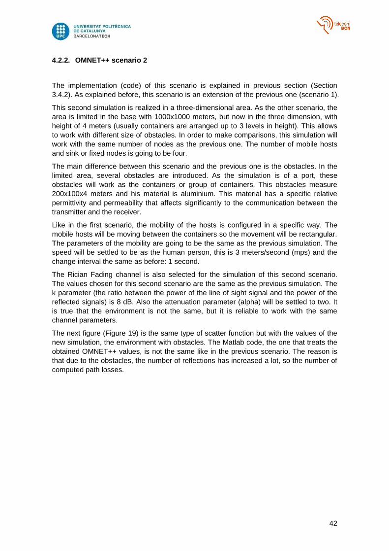
Figure 19. Scatter function of the Distance vs. Received power. Scenario 2
Like in the scenario presented before, this figure (Figure 19) shows the relation between
distance (meters) and received power (dB). It is clear that when the distance or the delay
is big the received power is very low and vice versa. It is to notice that in this scatter are
two significant shapes. The thin one represents the line of sight signal and the other one
the reflection or the signals that pass through an obstacle. The difference between the
received power of the line of sight signal and the received power of a reflected or a signal
that pass through an obstacle is almost 5 dB. This is completely meaningful as long as a
signal through an obstacle or a reflected signal is received with less power.
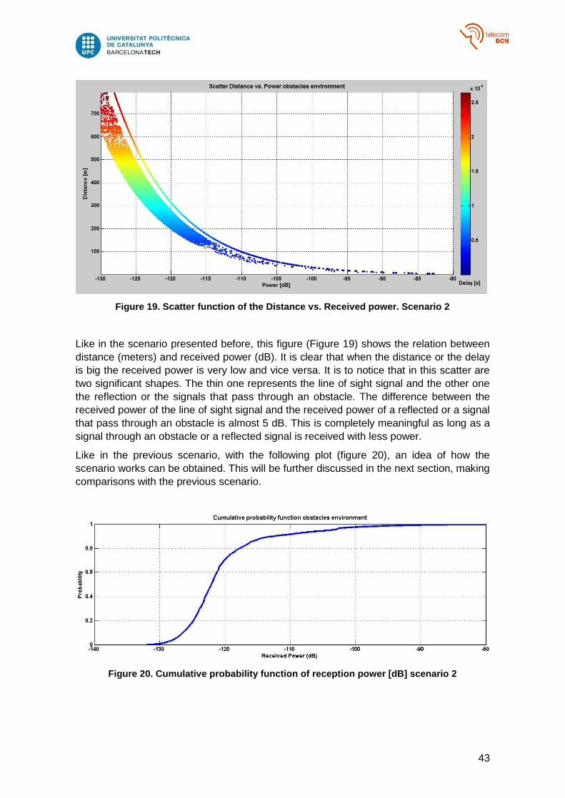
Like in the previous scenario, with the following plot (figure 20), an idea of how the
scenario works can be obtained. This will be further discussed in the next section, making
comparisons with the previous scenario.
Figure 20. Cumulative probability function of reception power [dB] scenario 2
44
This scenario works the same as the previous one (explained in Section 4.2.1). In order
to make some comparisons in the following section, almost all the parameters will be the
same.
The carrier frequency will be settled to 2.412 GHz to simulate protocols that Wireless
Sensor Network uses. Moreover, the transmission power will be 1 mW again for the same
reasons explained before: to achieve a low battery consumption.
About the type of modulation the signal, four experiments will be run as before. Each
simulation will be run with a different modulation type: BPSK, QPSK, 16QAM, 64QAM.
With this a comparison with the modulation type in the same scenario is possible, and
allow to compare with the scenario without obstacles.
The communication between mobile nodes (mobile hosts) and sink nodes (fixed nodes or
access point) is as follows: like in the previous section the type of message that will
gather the data will be a ping. Every mobile node sends a ping with the same timing as in
the first scenario.
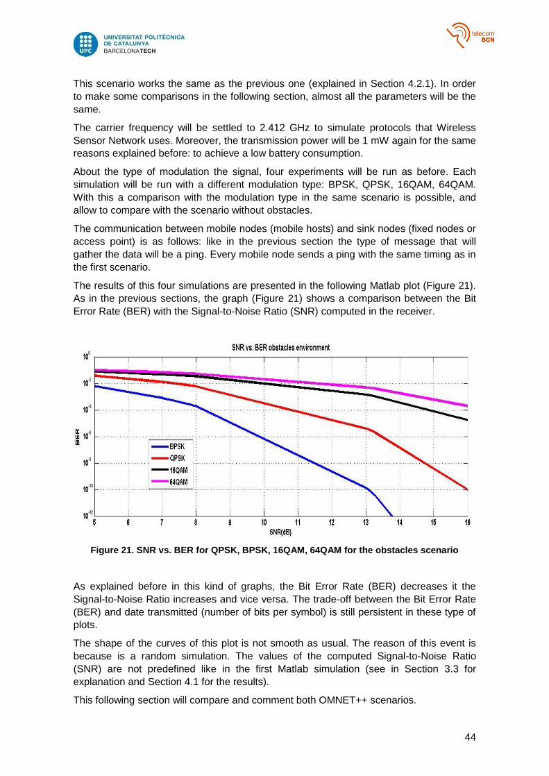
The results of this four simulations are presented in the following Matlab plot (Figure 21).
As in the previous sections, the graph (Figure 21) shows a comparison between the Bit
Error Rate (BER) with the Signal-to-Noise Ratio (SNR) computed in the receiver.
Figure 21. SNR vs. BER for QPSK, BPSK, 16QAM, 64QAM for the obstacles scenario
As explained before in this kind of graphs, the Bit Error Rate (BER) decreases it the
Signal-to-Noise Ratio increases and vice versa. The trade-off between the Bit Error Rate
(BER) and date transmitted (number of bits per symbol) is still persistent in these type of
plots.
The shape of the curves of this plot is not smooth as usual. The reason of this event is
because is a random simulation. The values of the computed Signal-to-Noise Ratio
(SNR) are not predefined like in the first Matlab simulation (see in Section 3.3 for
explanation and Section 4.1 for the results).
This following section will compare and comment both OMNET++ scenarios.
45
4.2.3. Comparison of Scenario 1 and 2
The reason why both simulations have been realized with the same values is that now is
possible to extract meaningful conclusions after a simple comparison.
First of all, looking to the first plots from the two simulations (Figure 16 and Figure 19)
some consideration can be appreciate. Both scatter functions contain the line of sight
signal, and it is to be noticed that the values are the same. These values must be the
same because represents the part of the signal that have no-extra attenuation due to
obstacles. In the second simulation (Figure 19), can be observed the signals with
attenuation of the containers, with less received power (between 1 and 5 dB less).
About the delay of each scenario, some values are shown in the following tables (Table 4
and 5).
Table 4. Parameters of the delay of the first non-obstacle environment
Root mean square (rms) 2.231651300650208e-006
Standard deviation 9.990952366782697e-007
Maximum delay 3.867210000000000e-006 s
Minimum delay 7.107630000000000e-008 s
Table 5. Parameters of the delay of the obstacle environment
Root mean square (rms) 1.234990741410496e-006
Standard deviation 5.134206593344932e-007
Maximum delay 2.645290000000000e-006 s
Minimum delay 2.231570000000000e-009 s
The root mean square, also known as the quadratic mean, in statistics is a statistical
measure defined as the square root of the mean of the squares of a sample. Theoretically,
due to the reflections the parameters of the delay value should be higher for the obstacle
case, but seeing in Figure 16 and 19 that the maximum distance is 1000 meters for non-
obstacles environment and 700 for the obstacles environment, these values of Table 4
and 5 are logical.
Finally, comparing the Figure 18 and Figure 21, it is easy to notice that the results are the
expected. In order to obtain the same Bit Error Rate (BER), the scenario with obstacles
need a higher value of Signal-to-Noise Ratio.
46
5. Conclusions and future development
The goal of the thesis was to build and simulate a Wireless Sensor Network (WSN). It is
true that the first idea was to work with the Matlab tool, but the changes suffered did not
turn off the development of the thesis.
The idea of the RFID tags implanted in the worker equipment, or the concept of wearable
sensors for measuring in real time electrophysiological data of workers, will provide a
very significant increase in the security in work areas like ports. In order to control the
security or the health of the workers, implementing WBANs is the future.
The simulations in Matlab exposes the communication between a Body Central Unit
(BCU) and the access point (sink node). With this point-to-point simulation, the evaluation
of the channel for different frequencies (for Wi-Fi protocol and White-Fi protocol) was
possible. The comparison of these frequencies and the comparison of different
modulation types (trade-off BPSK and QPSK) was possible in the plot with the
relationship between BER and SNR.
The OMNET++ simulations are a step forward in comparison with the first simulation.
First, in the OMNET++ simulation the scenario had several nodes moving in a limited
area. This is more reliable in terms of simulating the real world. With several hosts, the
possibility of collision between messages shows up as the term of interference between
different hosts. The second simulation in OMNET++ is an extension of the previous one.
The idea is practically the same but with an important difference: the obstacles. It is
important because in a real environment the reflection of the signal due to obstacles is
really important.
The results obtained in the OMNET++ simulation (see Figure 16, 17, 18, 19, 20, and 21
and Table 4 and 5) allow to extract conclusions and be positive to a future work. With all
these graphs an idea of how the environment works, how the channel affects to the
transmitted signal can be evaluated. Depending on the application of the Wireless Sensor
Network (WSN), it is possible to realize a simulation with different frequencies or different
modulation types. As in the Matlab simulation, a trade-off between sent data and
probability of error can be seen, but now with four modulation types.
5.1. Future work
This thesis opens a large range of possibilities for a future work. The idea of WSN and
WBANs and their implementation are really large. Implementing different protocols is
possible in the OMNET++ tool.
Apart of that, taking into account the parameters evaluated of the delay, a new the
Wiener filter can be built in order to reduce the Intersymbol Interference (ISI). If the new
filter do not achieve the required specifications maybe another receptor can be proposed
or build.
Finally, it is to be known that the final scenario presented can be improved. In order to
have a reliable Wireless Sensor Network (WSN), the multihop option can be introduced.

47
The mobile nodes could send messages to each other to get a specific destination, or if
they can not reach an access point (sink node). Moreover, optimal algorithms can be
applied to the simulation in order to obtain the best location for the access points,
depending on the defined area.
48
Bibliography
[1] Bangash J.I., Abdullah A.H., et al., A survey of Routing Protocols in Wireless Body Sensor Networks, Sensors, 2014, 14, doi: 10.3390/s140101322, pp. 1322-1357.
[2] Bauk S., A. Schmeink, J. Colomer. “Employing wireless networks in enhancing occupational safety at a developing seaport – Two proposals”, Paper submitted on 6th July, 2015.
[3] Bauk S., Džankić R., O izazovima primjene RFID tehnologije u lancima snabdijevanja [Upon challenges of RFID technology implementation in supply chains, eng.] Proc. of the 19th Internet Technologies Conference, 23rd-28th February, 2015, Žabljak, Montenegro, pp. 39-42..
[4] URL: http://www.propagation.gatech.edu/ECE4370/notes/Notes_on_Rician_PDFs.pdf (last access: 15 July 2015)
[5] URL: http://www.telecomabc.com/d/dsss.html
[6] URL: http://www.tutorialspoint.com/wi-fi/wifi_ieee_standards.htm
[7] URL: https://omnetpp.org/ (last access: 25 July 2015)
[8] IEEE 802.11af White-Fi Technology - an overview of the IEEE 802.11af or White-Fi proposal for Wi-Fi using the TV White spaces and cognitive radio technology, URL:http://www.radio-electronics.com/info/wireless/wi-fi/ieee-802-11af-white-fi-tv-space.php (last access 20th June, 2015)
[9] Javaid N., Khan N. A., Shakir M., et al., Ubiquitous Health Care in Wireless Body Area Networks - A Survey, URL: http://arxiv.org/ftp/arxiv/papers/1303/1303.2062.pdf (last access: 1st June 2015)
[10] Kahn J.Y., Yuce M.R., Wireless Body Area Network (WBAN) for Medical Applications, in New Developments in Biomedical Engineering (Compolo D., Ed.), Chapter 31, In Tech, January, 2010, pp. 591-627.
[11] Khan J.Y., Yuce M. R., and Karami F., Performance evaluation of a wireless body area sensor network for remote patient monitoring, URL: http://www.eng.newcastle.edu.au/~mry122/EMBC08_OPNET_Zigbee_Final.pdf (last access: 3rd June 2015)
[12] Ragesh G. K., Baskaran K., A Survey on Futuristic Health Care System: WBANs, International Conference on Communication Technology and System Design 2011, Procedia Engineering 30, 2012, pp. 889 – 896.
[13] Sole M., Musu C., Boi F., Giusto D., Popescu V., Control system for workplace safety in cargo terminal, Proc. of the 9th IEEE International Wireless Communications and Mobile Computing Conference, 1st-5th July 2013, Sardinia, pp. 1035-1039.
[14] Sole M., Musu C., Boi F., Giusto D., Popescu V., RFID sensor network for workplace safety management, Proc. of 18th IEEE Conference Emerging Technologies & Factory Automation - ETFA, 10th – 13th September 2013, Cagliari, Italy, pp. 1-4.
Related Documents