POLITECNICO DI TORINO Corso di Laurea Magistrale in Ingegneria Civile Master Thesis Application of B.I.M. methodology for long steel deck bridge Lectures: Prof. Rosario CERAVOLO Eng. Andrea ALBERTO, phD. Candidate: Pier Paolo CAIRO Marzo 2020

Welcome message from author
This document is posted to help you gain knowledge. Please leave a comment to let me know what you think about it! Share it to your friends and learn new things together.
Transcript
POLITECNICO DI TORINO
Corso di Laurea Magistrale in Ingegneria Civile
Master Thesis
Application of B.I.M. methodology for long steel deck bridge
Lectures:
Prof. Rosario CERAVOLO
Eng. Andrea ALBERTO, phD.
Candidate:
Pier Paolo CAIRO
Marzo 2020

CONTENTS 1. INTRODUCTION ........................................................................................................................... 1
1.1. DECK ...................................................................................................................................... 1
1.2. CRITERIA FOR CALCULATION ........................................................................................ 2
1.3 EXECUTION CLASS ............................................................................................................. 2
1.4. MATERIAL USED ................................................................................................................. 3
1.4.1. REINFORCEMENT STEEL (C.A) ................................................................................ 3
1.4.2. STEELWORK ................................................................................................................. 3
1.4.3. CONCRETE .................................................................................................................... 3
1.5. EFFECTIVE WIDTH OF CONCRETE SLAB ...................................................................... 5
1.6. GEOMETRICAL PROPERTIES ............................................................................................ 8
1.6.1. MAIN BEAMS ................................................................................................................ 8
1.6.2. DIAFRAGM .................................................................................................................. 12
1.6.3. HORIZONTAL BRACE ............................................................................................... 14
2. LOAD ANALYSIS ....................................................................................................................... 16
2.1. DEAD LOAD - Deck ............................................................................................................ 16
2.2. PERMANENT LOADS ........................................................................................................ 16
2.3. ACCIDENTAL LOADS ....................................................................................................... 17
2.3.1. TRAFFIC LOADS ........................................................................................................ 17
2.3.2. DIVISIONS OF THE CARRIAGEWAY INTO NOTIONAL LANES ....................... 18
2.3.3. LOAD MODEL 1, LM1 ................................................................................................ 18
2.3.4. DISPERSAL OF CONCENTRATED LOADS ............................................................ 19
2.3.5. HORIZONTAL FORCES – BRAKING, ACCELERATION & CENTRIFUGAL. ..... 20
2.4. VARIABLE LOADS ............................................................................................................ 21
2.4.1. WIND EFFECTS .......................................................................................................... 21
2.4.1.1. REFERENCE BASE VELOCITY ........................................................................ 21
2.4.1.2. WIND KINETIC PRESSURE .............................................................................. 22
2.4.1.3. EXPOSURE COEFFICIENT ................................................................................ 22
2.4.1.4. LOCAL DYNAMIC EFFECT .............................................................................. 25
2.4.1.4.1. STRUCTURAL NATURAL FREQUENCY ..................................................... 25
2.4.1.4.2. WIND NATURAL FREQUENCY .................................................................... 26
2.4.1.4.3. VORTEX SEPARATION FROM STEEL BEAM ............................................ 29
2.5. SEISMIC LOAD ................................................................................................................... 30
2.5.1. DETERMINATION OF SEISMIC ACTION ............................................................... 30
2.5.1.1. NOMINAL LIFE ................................................................................................... 30
2.5.1.2. CLASS OF USE .................................................................................................... 30
2.5.1.3. LIMIT STATES AND THEIR PROBABILITY ................................................... 30
2.5.1.4. DESIGN PARAMETERS ..................................................................................... 31
2.6. TEMPERATURE EFFECT .................................................................................................. 35
2.6.1. UNIFORM THERMAL VARIATION ......................................................................... 35
2.7. SHRINKAGE EFFECTS ...................................................................................................... 36
2.7.1. RHEOLOGIC EFFECTS .............................................................................................. 36
2.7.2. TIME AND ENVIRONMENT ..................................................................................... 36
2.7.3. ELASTIC MODULUS .................................................................................................. 36
2.7.4. SHRINKAGE EVALUATION ..................................................................................... 37
2.7.5. VISCOUS EFFECTS ON YOUNG MODULUS ......................................................... 39
3. LOAD COMBINATION CRITERIONS ...................................................................................... 40
3.1. SAFETY CONTROL ............................................................................................................ 41
3.2. LOAD COMBINATIONS .................................................................................................... 42
3.2.1. ULS AND SLS LOAD COMBINATIONS .................................................................. 44
3.2.2. SEISMIC LOAD COMBINATIONS ............................................................................ 45
3.2.3. GENERAL STRUCTURAL MODEL .......................................................................... 46
4. STRESS ANALYSIS .................................................................................................................... 47
4.1. GRAPHICAL RESULTS ...................................................................................................... 47
4.1.1. STEEL DECK – PHASE 1............................................................................................ 47
4.1.2. STEEL DECK WITH PREDALLES – PHASE 1......................................................... 48
4.1.3. DECK WITH CASTING CONCRETE – PHASE 1 ..................................................... 49
4.1.4. PERMANENT LOADS – PHASE 2A .......................................................................... 50
4.1.5. WIND EFFECT – PHASE 3 ......................................................................................... 51
4.2. VERIFICATION OF MAIN BEAM ................................................................................. 52
4.2.1. MEMBRANE RESISTANCE ................................................................................... 54
4.2.2. MEMBRANE STABILITY ...................................................................................... 55
4.3. DIAFRAGMS & BRACES ................................................................................................... 58
4.3.1. MEMBRANE RESISTANCE ................................................................................... 59
4.3.2. MEMBRANE STABILITY ...................................................................................... 60
4.4. DEFORMAZION VERIFICATION ..................................................................................... 62
4.5. FORCES ACTING ON SUPPORTS .................................................................................... 63
4.5.1. VERTICAL ACTIONS ................................................................................................. 63
4.5.2. HORIZONTAL ACTIONS ........................................................................................... 63
4.5.2.1. LONGITUDINAL BRAKING ACTION .............................................................. 63
4.5.2.2. TRASVERSAL CENTRIFUGAL ACTION......................................................... 63
4.5.2.3. WIND ACTION AT UNLOADED DECK ........................................................... 63
4.5.2.4. WIND ACTION AT LOADED DECK................................................................. 64
4.6. CONCRETE SLAB ............................................................................................................... 65
4.6.1. DEAD LOAD ................................................................................................................ 65
4.6.2. PERMANENT LOAD .................................................................................................. 65
4.6.3. ACCIDENTAL CROWD LOAD.................................................................................. 65
4.6.4. ACCIDENTAL TRUCK LOAD ................................................................................... 65
4.6.4.1. CANTILEVER ZONE .......................................................................................... 66
4.6.4.2. CENTRAL SPAN ................................................................................................. 68
4.6.5. VEHICLES IMPACT .................................................................................................... 69
4.6.6. DIAGRAMS .................................................................................................................. 70
4.6.7. REINFORCEMENT ..................................................................................................... 72
4.6.7.1. SLE -CANTILEVER............................................................................................. 73
4.6.7.2. SLE -MIDDLE ...................................................................................................... 78
4.6.7.3. SLE -SPAN ........................................................................................................... 84
4.6.7.4. SLU ....................................................................................................................... 90
4.7. SHEAR BOLTS VERIFICATION ....................................................................................... 93
4.8. BOLTED AND WELDED JOINTS VERIFICATION......................................................... 95
4.8.1. BOLTED CONNECTIONS .......................................................................................... 95
4.8.1.1. CATEGORIES OF BOLT CONNECTION .......................................................... 96
4.8.1.2. FORCE TRANSMISSION AND COLLAPSE MODE IN SHEAR-LOADED CONNECTIONS ....................................................................................................................... 96
4.8.2. DESIGN RESISTANCE OF A SINGLE SHEAR BOLT ......................................... 97
4.8.2.1. SHEAR DESIGN RESISTANCE ......................................................................... 98
4.8.2.2. DESIGN RESISTANCE TO BURRING .............................................................. 98
4.8.2.3. FULLY RESTORED BOLTED JOINT ................................................................ 99
4.8.2. WELDED CONNECTIONS ....................................................................................... 100
4.8.2.1. CLASSIFICATION OF WELDED JOINTS .......................................................... 100
4.8.2.1.1. CORNER BEAD WELDING .......................................................................... 101
4.8.2.2. DESIGN RESISTANCE PER UNIT LENGTH ................................................. 102
4.8.2.2.1. DIRECTIONAL METHOD ............................................................................. 102
4.8.2.2.2. SIMPLIFIED METHOD .................................................................................. 103
4.8.3. WELDING OF SHEAR CONNECTORS ............................................................... 104
5. B.I.M. METHODOLOGY .......................................................................................................... 105
5.1. GENERAL PURPOSES ...................................................................................................... 105
5.2. ADVANCE DESIGN .......................................................................................................... 108
5.3. IDEA STATICA.................................................................................................................. 109
5.4. ADVANCE STEEL ............................................................................................................ 110
5.5. EFFECTIVE INTEROPERABILITY ................................................................................. 111
CONCLUSION ................................................................................................................................... 121
ACKNOWLEDGEMENTS ................................................................................................................ 122
BIBLIOGRAPHY ............................................................................................................................... 123
WEBSITE CITATIONS...................................................................................................................... 124
ANNEX A – MODEL CALIBRATION ............................................................................................. 125
BEAM LOADED ON Z-DIRECTION ........................................................................................... 125
BEAM LOADED ON Y-DIRECTION .......................................................................................... 129
BEAM LOADED ON Z-DIRECTION WITH TRANSVERSAL ELEMENT TORSION ANALISYS ..................................................................................................................................... 132
LOAD P=568,2 daN VERIFICATION ....................................................................................... 136
ANNEX B – INTEROPERABILITY CALIBRATION ..................................................................... 139
ANNEX C – ELEMENT RESULTS .................................................................................................. 141
MAIN BEAMS ANALYSIS ........................................................................................................... 141
DIAPHRAGMS ANALYSIS .......................................................................................................... 169
BRACES RESULTS ....................................................................................................................... 186
SHEAR CONNECTORS ................................................................................................................ 189
FULLY RESTORED BOLTED JOINT OF MAIN BEAMS ......................................................... 198
SEISMIC ANALYSIS .................................................................................................................... 207
ANNEX D – LOCAL ANALYSIS with IDEA STATICA OUTPUT ................................................ 210
FULLY RESTORED BOLTED JOINT .......................................................................................... 210
1ST JOINT SEGMENT: C1-C2 ................................................................................................... 210
2nd JOINT SEGMENT: C2-C3 .................................................................................................... 211
3rd JOINT SEGMENT: C3-C4 .................................................................................................... 213
PILOT NODE - ABUTMENT POSITION ..................................................................................... 214
PILOT NODE - MIDDLE POSITION ........................................................................................... 216
DIAPHRAGM NODE – TYPE A ................................................................................................... 218
DIAPHRAGM NODE – TYPE B ................................................................................................... 220
DIAPHRAGM NODE – TYPE ABUTMENT ................................................................................ 222
DIAPHRAGM NODE – TYPE PIER ............................................................................................. 224
FIGURE INDEX
Figure 1:longitudinal profile of the deck. All measures are in mm. ........................................................ 1 Figure 2: Longitudinal profile of lower braces. All measures are in mm. .............................................. 1 Figure 3: Longitudinal profile of upper braces. All measures are in mm. .............................................. 1 Figure 4:Effective width of the concrete slab .......................................................................................... 5 Figure 5:Determination of effective length. ............................................................................................ 5 Figure 6:Final result of Effective width for each segment. ..................................................................... 8 Figure 7: C1 and C2 cross-sections. Values in mm. .............................................................................. 10 Figure 8: C3 and C4 cross-sections. Values in mm. .............................................................................. 10 Figure 9: C5 and C5a cross-sections. Values in mm. ............................................................................ 11 Figure 10: C6 and C7 cross-sections. Values in mm. ............................................................................ 11 Figure 11:C8 cross-section. Values in mm............................................................................................ 12 Figure 12: Diaphragm scheme in axonometric view. Source Advance design model. ......................... 12 Figure 13: Cross section of one diaphragm element. ............................................................................ 14 Figure 14: Cross section of single brace element. ................................................................................. 14 Figure 15: General Scheme of cross section. Values in mm. ................................................................ 16 Figure 16: Load model characteristics. Source: EN 1991-2. ................................................................. 17 Figure 17: Classification of notional lanes. Source EN1991................................................................. 18 Figure 18: Geometrical condition of LM1. Source EN1991 ................................................................. 19 Figure 19: Representation of load distribution through the pavement. Source EN 1991 ...................... 19 Figure 20: Description of italian zone. Source NTC 2018. ................................................................... 21 Figure 21:Geographical subdivision of base reference velocity. Source NTC2018 ............................. 22 Figure 22: Exposure coefficients related to each case. Source NTC 2018. ........................................... 23 Figure 23: Definition of the class of exposure related to the case. Source NTC2018. .......................... 23 Figure 24:Structure description with respect to the structural model. ................................................... 26 Figure 25:Integral turbulence scale chart. ............................................................................................. 27 Figure 26:Turbulence intensity chart. ................................................................................................... 27 Figure 27: Reference life determination. Source NTC 2018 ................................................................. 30 Figure 28:Definition of soil category .................................................................................................... 32 Figure 29: Topographic definition ........................................................................................................ 32 Figure 30:Reference life determination. ................................................................................................ 33 Figure 31:Limit state curves. ................................................................................................................. 34 Figure 32: Limit state parameters .......................................................................................................... 34 Figure 33: Displacement due to dead load ............................................................................................ 47 Figure 34: Von Mises Tension due to dead load ................................................................................... 48 Figure 35: Displacement due to steel deck with predalles .................................................................... 48 Figure 36: Von Mises tension due to steel deck with predalles ............................................................ 49 Figure 37: Displacement due to steel deck with predalles and casting concrete ................................... 49 Figure 38: Von Mises tension due to steel deck with predalles and casting concrete ........................... 50 Figure 39: Displacement of the deck ..................................................................................................... 50 Figure 40: Von Mises tension of the deck ............................................................................................. 51 Figure 41: Displacement due wind load ................................................................................................ 51 Figure 42: Von Mises tension due wind load ........................................................................................ 52 Figure 43: Vertical load diffusion.. ....................................................................................................... 65 Figure 44: Application of tandem system ............................................................................................. 66 Figure 45:Horizontal diffusion of traffic load. ...................................................................................... 66 Figure 46: General scheme of load model 2 from Eurocode 1. ............................................................. 67 Figure 47:Horizzontal diffusion of load. ............................................................................................... 68 Figure 48:Horizzontal diffusion of vehicle impact ............................................................................... 69 Figure 49: Bending moment of concrete slab........................................................................................ 70
Figure 50:Bending moment of permanent load ..................................................................................... 70 Figure 51: Bending moment of crowd effect. ....................................................................................... 71 Figure 52:Bending moment of traffic load ............................................................................................ 71 Figure 53:General system of predalle. Unit of major is in cm up and mm the cross-section below. .... 72 Figure 54:Stress result of rare combination. .......................................................................................... 74 Figure 55:Stress result of frequent combination ................................................................................... 75 Figure 56:Stress result of frequent combination ................................................................................... 77 Figure 57:Stress result of rare combination. .......................................................................................... 79 Figure 58:Stress result of frequent combination ................................................................................... 80 Figure 59:Stress result of frequent combination ................................................................................... 82 Figure 60:Stress result of rare combination. .......................................................................................... 85 Figure 61:Stress result of frequent combination ................................................................................... 86 Figure 62:Stress result of frequent combination ................................................................................... 88 Figure 63:SLU analysis of cantilever zone. .......................................................................................... 90 Figure 64:Accidental SLU analysis results. .......................................................................................... 91 Figure 65:Quasi-permanent SLU combination analysis and results. .................................................... 92 Figure 66:Computation of neutral axis position .................................................................................... 93 Figure 67: Bolt elements. ...................................................................................................................... 95 Figure 68: kind of bolt breakage ........................................................................................................... 96 Figure 69:Fully restored bolted joint initial scheme. ............................................................................. 99 Figure 70:Position of welding ............................................................................................................. 100 Figure 71:Type of welding .................................................................................................................. 101 Figure 72:Effective way to calculate the welding length and cross-section. ...................................... 101 Figure 73:Welding stress ..................................................................................................................... 102 Figure 74:Scheme of welding forces ................................................................................................... 103 Figure 75:Interoperability concept. Source BIM and InfraBim slides ................................................ 105 Figure 76:Comparison between traditional and integrated process. Source BIM and InfraBim slides106 Figure 77:Updating of IFC format during the years. (Acampa, 2018) ................................................ 106 Figure 78: Conceptual scheme of LOD increasing. Source BIM and InfraBim slides ....................... 108 Figure 79: Advance Design model. ..................................................................................................... 109 Figure 80: Graphical representation of plate elements. ....................................................................... 111 Figure 81: Graphical representation of first deck segment.................................................................. 112 Figure 82:Mesh used for modelling .................................................................................................... 112 Figure 83:Effect of load on mesh. Source Graitec website. ................................................................ 113 Figure 84: Selection of prop. elements in Advance Design. ............................................................... 113 Figure 85: Step 1 of interoperability with Idea Statica connection. .................................................... 114 Figure 86:Idea Statica representation of elements. .............................................................................. 115 Figure 87: Choose of cross-section type ............................................................................................. 115 Figure 88: Final geometrical and FEM result...................................................................................... 117 Figure 89: Assonometric view of importation steel deck from Advance Design to Advance Steel. .. 118 Figure 90:Local view of exportation in assonometric visualisation. ................................................... 118 Figure 91: Final Assonometric view of detailed drawing from Advance Steel. ................................. 119 Figure 92: Detailed drawing of single plate used ................................................................................ 120 Figure 93:Exportation into Idea Statica environmental. ...................................................................... 120 Figure 94: General scheme. Beam loaded on z direction. ................................................................... 125 Figure 95:Dead load effect. left is expressed the continuous behaviour. ............................................ 125 Figure 96: Variable load effect. Left is expressed the continuous behaviour. .................................... 126 Figure 97: load combination effect. Left is expressed the continuous behaviour. ............................. 126 Figure 98: Dead load stress effect. left is expressed the continuous behaviour. ................................. 126 Figure 99: Variable load stress effect. left is expressed the continuous behaviour. ............................ 127 Figure 100: Load combination stress effect. left is expressed the continuous behaviour ................... 127
Figure 101: Load combination Von Mises stress effect. left is expressed the continuous behaviour . 128 Figure 102:General scheme. Beam loaded on y direction. .................................................................. 129 Figure 103:Dead load effect. left is expressed the continuous behaviour ........................................... 129 Figure 104: Variable load effect. Left is expressed the continuous behaviour. .................................. 129 Figure 105: Load combination displacement effect. Left is expressed the continuous behaviour. ..... 130 Figure 106:Load combination stress effect, Left is expressed the continuous behaviour. .................. 130 Figure 107: Load combination Von Mises stress effect. Left is expressed the continuous behaviour.131 Figure 108:General scheme of torsional analysis. ............................................................................... 132 Figure 109:Dead load effect. Left is expressed the continuous behaviour. ......................................... 132 Figure 110: Variable load effect. Left is expressed the continuous behaviour. .................................. 133 Figure 111:Load combination effect. left is expressed the continuous behaviour. ............................. 133 Figure 112: Load combination stress effect. Left is expressed the continuous behaviour. ................. 133 Figure 113: Load combination Von Mises stress effect. Left is expressed the continuous behaviour.134 Figure 114:Dead load effect. Left is expressed the continuous behaviour. ......................................... 136 Figure 115:Variable load effect. Left is expressed the continuous behaviour. ................................... 137 Figure 116:Load combination effect. Left is expressed the continuous behaviour. ............................ 137 Figure 117:Load combination stress effect. Left is expressed the continuous behaviour. .................. 137 Figure 118: Load combination Von Mises stress effect. Left is expressed the continuous behaviour.138 Figure 119: IFC result of Advance Steel modelling ............................................................................ 139 Figure 120:Import File in Advance Design; Highlighting interoperability ......................................... 140 Figure 121:Interoperability check between Advance design and Idea Statica. ................................... 140 Figure 122:Final result of Idea Statica manipulations ......................................................................... 140
TABLE INDEX
Table 1: Execution class determination ................................................................................................... 2 Table 2: Concrete parameters .................................................................................................................. 3 Table 3:Effective width for the external main longitudinal beams. ........................................................ 6 Table 4: Effective width of pilot beam .................................................................................................... 7 Table 5: Main Beams properties. ............................................................................................................ 9 Table 6: Diaphragm cross section type. ................................................................................................ 13 Table 7: Brace girder cross-sectional properties. .................................................................................. 15 Table 8: Traffic loads ............................................................................................................................ 18 Table 9: Reference Parameters of wind................................................................................................. 24 Table 10:Geometrical values and pressures. ......................................................................................... 24 Table 11: Bending and Torsional frequency of the bridge .................................................................... 25 Table 12: Wind frequency ..................................................................................................................... 28 Table 13: Strouhal parameters ............................................................................................................... 29 Table 14: Limit state probability ........................................................................................................... 31 Table 15: Limit state parameters and values ......................................................................................... 33 Table 16: Design seismic parameters .................................................................................................... 34 Table 17:Shrinkage parameters ............................................................................................................. 38 Table 18: Effective Elastic modulus during the time. ........................................................................... 39 Table 19:Maximum diameter of bar to crack control. NTC2018 .......................................................... 41 Table 20: Maximum span between bars to crack control. NTC2018 .................................................... 41 Table 21: Characteristics action values due traffic loads. ..................................................................... 42 Table 22:Partial coefficient for ULS load combinations. ...................................................................... 43 Table 23:Partial combination coefficients for variable loads. ............................................................... 44 Table 24:Maximum width to thickness table. Used to establish steel class. From EN 1993-1-1 ......... 53 Table 25: Used to understand the parts subject to bending and compression. From EN 1993-1-1. ...... 53 Table 26:Partial Factors......................................................................................................................... 54 Table 27:Internal compression elements. Stress relationship and buckling factor. ............................... 56 Table 28:Maximum width to thickness table. Used to establish steel class. From EN 1993-1-1 ......... 58 Table 29: Used to understand the parts subject to bending and compression. From EN 1993-1-1. ...... 59 Table 30:Partial Factors......................................................................................................................... 59 Table 31:Deformations values ............................................................................................................... 62 Table 32:Final apply deformation to the main beams ........................................................................... 62 Table 33:wind action parameters at unloaded deck .............................................................................. 63 Table 34:wind action parameters at loaded deck .................................................................................. 64 Table 35: Rare combination values ....................................................................................................... 73 Table 36:Frequent combination values ................................................................................................. 74 Table 37: frequent SLE verification ...................................................................................................... 75 Table 38:Quasi-permanent combination values .................................................................................... 76 Table 39: Quasi-permanent SLE verification ........................................................................................ 77 Table 40: Rare combination values ....................................................................................................... 78 Table 41:Frequent combination values ................................................................................................. 80 Table 42: Frequent SLE verification .................................................................................................... 81 Table 43:Quasi-permanent combination values .................................................................................... 82 Table 44: Quasi-permanent SLE verification ........................................................................................ 83 Table 45: Rare combination values ....................................................................................................... 84 Table 46:Frequent combination values ................................................................................................. 85 Table 47: Frequent SLE verification .................................................................................................... 86 Table 48:Quasi-permanent combination values .................................................................................... 87 Table 49: Quasi-permanent SLE verification ........................................................................................ 88

Table 50:General set of concrete slab ................................................................................................... 90 Table 51:Displacement values. Beam loaded on z direction. .............................................................. 126 Table 52:Stress values. Beam loaded on z direction. .......................................................................... 127 Table 53: Von Mises values. Bema loaded on z direction .................................................................. 128 Table 54:Displacement values. Beam loaded on y direction............................................................... 130 Table 55: Stress values. Beam loaded on y direction. ......................................................................... 130 Table 56: Von Mises values. Beam loaded on y direction. ................................................................. 131 Table 57: Displacement values. Torsional analysis ............................................................................ 133 Table 58:Stress values. Torsional analysis .......................................................................................... 134 Table 59:Von mises values. Torsional analysis. ................................................................................. 134 Table 60:Displacement values. Torsional analysis with the max concentrated apply load ................. 137 Table 61:Stress values. Torsional analysis with the max concentrated apply load ............................. 138 Table 62: Von mises Stress values. Torsional analysis with the max concentrated apply load .......... 138
ABSTRACT
La scelta di sviluppare la tesi adottando la metodologia B.I.M. (Building Information Modeling) è dovuta al fatto che il B.I.M. rappresenta il metodo di progettazione innovativo che nei prossimi anni troverà larga scala di applicazione nella progettazione, sia in campo edilizio che non. Questa metodica, che già da qualche anno sta sostituendo i metodi tradizionali di progettazione, ha il vantaggio di inglobare in un singolo modello tutte le fasi progettuali, operative e di manutenzione dal progetto costruttivo. Esse saranno visualizzate a 360 gradi dai tecnici grazie al concetto essenziale di “interoperabilità” tra discipline.
La prima parte della tesi è dedicata allo studio progettuale di un viadotto a struttura composta. Il viadotto presenta una larghezza complessiva di 13,5m, in senso longitudinale è costituito da tre campate di luce +49,5, + 70,0, +49,5m misurate in asse agli appoggi. L’impalcato è realizzato con una sezione mista acciaio-calcestruzzo ed è costituito da due travi principali metalliche di altezza costante pari 2,5m e una trave pilota centrale di altezza pari a 0,45m. La struttura è segmentata da 8 diverse tipologie di conci, presenta 4 tipologie di diaframmi trasversali, irrigidite nel piano orizzontali da controventi superiori e inferiori con distribuzione variabile longitudinalmente. All’estradosso delle travi è solidarizzata la soletta in calcestruzzo, mediante uso di predalles, per mezzo di
connettori a taglio opportunamente saldati sulla piattabanda superiore delle travi principali, al fine di garantire il comportamento torsionale.
La seconda parte della tesi riguarda l’applicazione del B.I.M. della struttura in esame, utilizzata per incrementare
il livello di dettaglio e verificare l’interoperabilità tra i modelli strutturali nelle specifiche verifiche progettuali. La progettazione B.I.M. è indipendente dai software che si utilizzano. In caso sono state utilizzate 3 tipologie di programmi per ottenere indipendentemente senza vincoli: la modellazione dell’impalcato mediante elementi
superficiali bidimensionali (elementi al continuo) ed elementi di tipo trave (teoria di De Saint Venant), con successivo calcolo strutturale sotto carico. Successivamente sono stati analizzati i giunti trave-trave, identificandoli tutti come giunti a completo ripristino. Infine, la terza tipologia è stata impiegata per incrementare il livello di dettaglio (LOD) degli elementi in struttura metallica e renderli gestibili in officina.
ABSTRACT
The choice to develop the thesis by adopting the B.I.M. (Building Information Modeling) methodology is due to the fact that the B.I.M. represents the innovative design method that in the coming years will find wide application in the design, both in the building and non-building field. This method, which has been replacing traditional design methods for some years now, has the advantage of incorporating in a single model all the design, operational and maintenance phases of the construction project. They will be displayed at 360 degrees by technicians thanks to the essential concept of "interoperability" between disciplines.
The first part of the thesis is dedicated to the design study of a viaduct with a compound structure. The viaduct has a total width of 13.5m, in the longitudinal direction it consists of three spans of +49.5, +70.0, +49.5m measured in axis to the supports. The deck is made of a mixed steel-concrete section and consists of two main metal beams with a constant height of 2.5m and a central pilot beam with a height of 0.45m. The structure is segmented by 8 different types of segments and has 4 types of transverse diaphragms, stiffened in the horizontal plane by upper and lower bracing with longitudinally variable distribution. The concrete slab is solidified to the extrados of the beams, by means of predalles, by means of shear connectors suitably welded to the upper flange of the main beams, in order to guarantee the torsional behaviour.
The second part of the thesis concerns the application of the B.I.M. methodology of the structure, used to increase the level of detail and verify the interoperability between the structural models in the specific design checks. The B.I.M. design is independent of the software used. In this case, 3 types of programs have been used to obtain independently without constraints: the deck modelling using two-dimensional surface elements (continuous elements) and beam type elements (De Saint Venant's theory), with subsequent structural calculation under load. Subsequently the beam-beam joints were analysed, identifying them all as fully restored bolted joints. Finally, the third type was used to increase the level of detail (LOD) of the metal structure elements and make them manageable in the workshop.

1
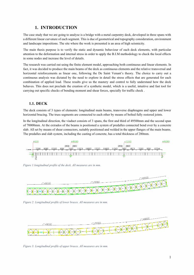
1. INTRODUCTION The case study that we are going to analyse is a bridge with a metal carpentry deck, developed in three spans with a different linear curvature of each segment. This is due of geometrical and topography consideration, environment and landscape impositions. The site where the work is presented is an area of high seismicity.
The main thesis purpose is to verify the static and dynamic behaviour of each deck elements, with particular attention to the deformation and internal stress in order to apply the B.I.M methodology to check the local effects in some nodes and increase the level of details.
The research was carried out using the finite element model, approaching both continuous and linear elements. In fact, it was decided to produce the main beams of the deck as continuous elements and the relative transversal and horizontal reinforcements as linear one, following the De Saint Venant’s theory. The choice to carry out a continuous analysis was dictated by the need to explore in detail the stress effects that are generated for each combination of applied load. These results give us the mastery and control to fully understand how the deck behaves. This does not preclude the creation of a synthetic model, which is a useful, intuitive and fast tool for carrying out specific checks of bending moment and shear forces, specially for traffic check .
1.1. DECK
The deck consists of 3 types of elements: longitudinal main beams, transverse diaphragms and upper and lower horizontal bracing. The truss segments are connected to each other by means of bolted fully restored joints.
In the longitudinal direction, the viaduct consists of 3 spans, the first and third of 49500mm and the second span of 70000mm. At the extrados of the beams is positioned a system of predalles connected bend over by a concrete slab. All set by means of shear connectors, suitably positioned and welded in the upper flanges of the main beams. The predalles and slab system, including the casting of concrete, has a total thickness of 280mm.
Figure 1:longitudinal profile of the deck. All measures are in mm.
Figure 2: Longitudinal profile of lower braces. All measures are in mm.
Figure 3: Longitudinal profile of upper braces. All measures are in mm.
2
1.2. CRITERIA FOR CALCULATION
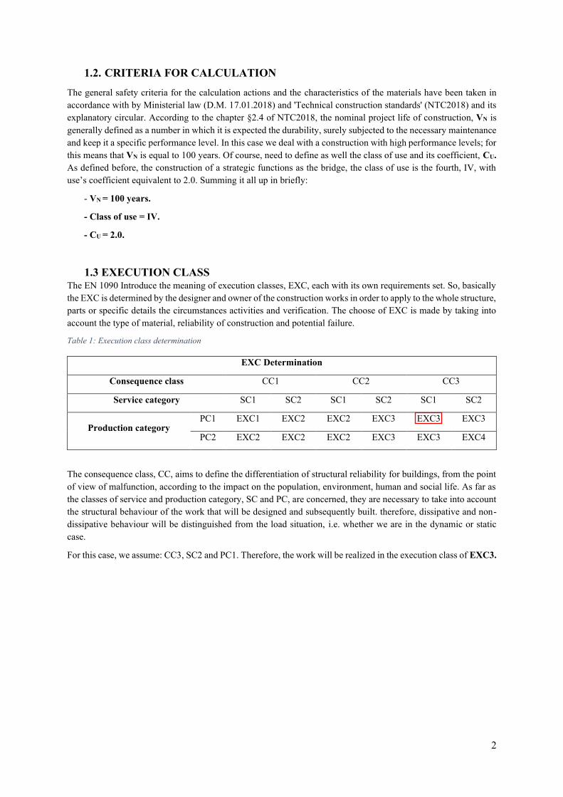
The general safety criteria for the calculation actions and the characteristics of the materials have been taken in accordance with by Ministerial law (D.M. 17.01.2018) and 'Technical construction standards' (NTC2018) and its explanatory circular. According to the chapter §2.4 of NTC2018, the nominal project life of construction, VN is generally defined as a number in which it is expected the durability, surely subjected to the necessary maintenance and keep it a specific performance level. In this case we deal with a construction with high performance levels; for this means that VN is equal to 100 years. Of course, need to define as well the class of use and its coefficient, CU. As defined before, the construction of a strategic functions as the bridge, the class of use is the fourth, IV, with use’s coefficient equivalent to 2.0. Summing it all up in briefly:
- VN = 100 years.
- Class of use = IV.
- CU = 2.0.
1.3 EXECUTION CLASS The EN 1090 Introduce the meaning of execution classes, EXC, each with its own requirements set. So, basically the EXC is determined by the designer and owner of the construction works in order to apply to the whole structure, parts or specific details the circumstances activities and verification. The choose of EXC is made by taking into account the type of material, reliability of construction and potential failure.
Table 1: Execution class determination
EXC Determination
Consequence class CC1 CC2 CC3
Service category SC1 SC2 SC1 SC2 SC1 SC2
Production category PC1 EXC1 EXC2 EXC2 EXC3 EXC3 EXC3
PC2 EXC2 EXC2 EXC2 EXC3 EXC3 EXC4
The consequence class, CC, aims to define the differentiation of structural reliability for buildings, from the point of view of malfunction, according to the impact on the population, environment, human and social life. As far as the classes of service and production category, SC and PC, are concerned, they are necessary to take into account the structural behaviour of the work that will be designed and subsequently built. therefore, dissipative and non-dissipative behaviour will be distinguished from the load situation, i.e. whether we are in the dynamic or static case.
For this case, we assume: CC3, SC2 and PC1. Therefore, the work will be realized in the execution class of EXC3.
3
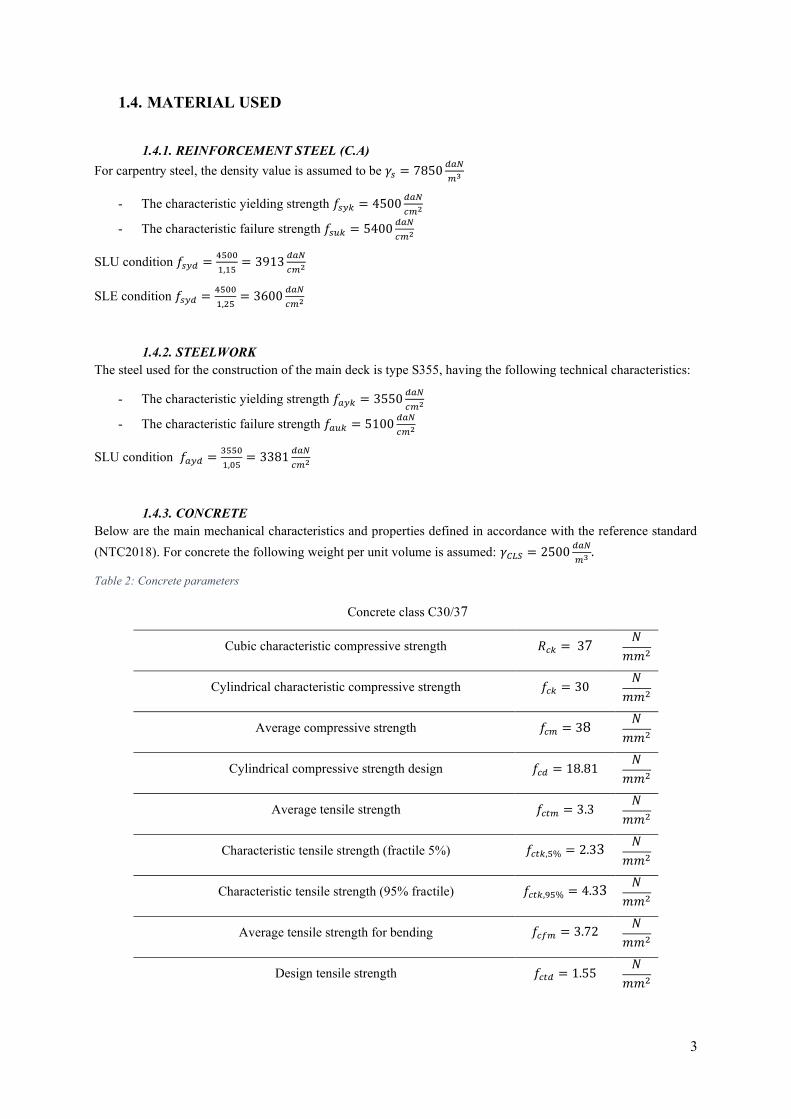
1.4. MATERIAL USED
1.4.1. REINFORCEMENT STEEL (C.A) For carpentry steel, the density value is assumed to be 𝛾𝑠 = 7850
𝑑𝑎𝑁
𝑚3
- The characteristic yielding strength 𝑓𝑠𝑦𝑘 = 4500𝑑𝑎𝑁
𝑐𝑚2
- The characteristic failure strength 𝑓𝑠𝑢𝑘 = 5400𝑑𝑎𝑁
𝑐𝑚2
SLU condition 𝑓𝑠𝑦𝑑 =4500
1,15= 3913
𝑑𝑎𝑁
𝑐𝑚2
SLE condition 𝑓𝑠𝑦𝑑 =4500
1,25= 3600
𝑑𝑎𝑁
𝑐𝑚2
1.4.2. STEELWORK The steel used for the construction of the main deck is type S355, having the following technical characteristics:
- The characteristic yielding strength 𝑓𝑎𝑦𝑘 = 3550𝑑𝑎𝑁
𝑐𝑚2
- The characteristic failure strength 𝑓𝑎𝑢𝑘 = 5100𝑑𝑎𝑁
𝑐𝑚2
SLU condition 𝑓𝑎𝑦𝑑 =3550
1,05= 3381
𝑑𝑎𝑁
𝑐𝑚2
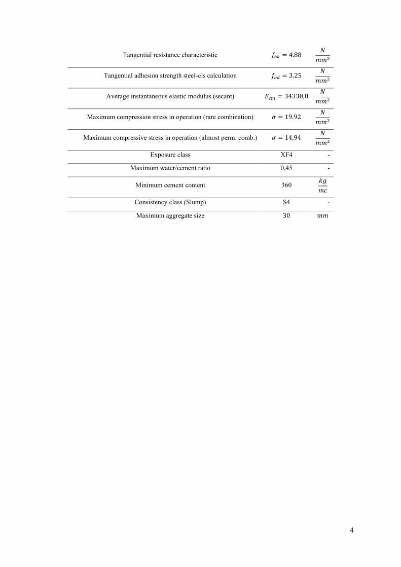
1.4.3. CONCRETE Below are the main mechanical characteristics and properties defined in accordance with the reference standard (NTC2018). For concrete the following weight per unit volume is assumed: 𝛾𝐶𝐿𝑆 = 2500
𝑑𝑎𝑁
𝑚3 .
Table 2: Concrete parameters
Concrete class C30/37
Cubic characteristic compressive strength 𝑅𝑐𝑘 = 37 𝑁
𝑚𝑚2
Cylindrical characteristic compressive strength 𝑓𝑐𝑘 = 30 𝑁
𝑚𝑚2
Average compressive strength 𝑓𝑐𝑚 = 38 𝑁
𝑚𝑚2
Cylindrical compressive strength design 𝑓𝑐𝑑 = 18.81 𝑁
𝑚𝑚2
Average tensile strength 𝑓𝑐𝑡𝑚 = 3.3 𝑁
𝑚𝑚2
Characteristic tensile strength (fractile 5%) 𝑓𝑐𝑡𝑘,5% = 2.33 𝑁
𝑚𝑚2
Characteristic tensile strength (95% fractile) 𝑓𝑐𝑡𝑘,95% = 4.33 𝑁
𝑚𝑚2
Average tensile strength for bending 𝑓𝑐𝑓𝑚 = 3.72 𝑁
𝑚𝑚2
Design tensile strength 𝑓𝑐𝑡𝑑 = 1.55 𝑁
𝑚𝑚2
4
Tangential resistance characteristic 𝑓𝑏𝑘 = 4.88 𝑁
𝑚𝑚2
Tangential adhesion strength steel-cls calculation 𝑓𝑏𝑑 = 3.25 𝑁
𝑚𝑚2
Average instantaneous elastic modulus (secant) 𝐸𝑐𝑚 = 34330,8 𝑁
𝑚𝑚2
Maximum compression stress in operation (rare combination) 𝜎 = 19.92 𝑁
𝑚𝑚2
Maximum compressive stress in operation (almost perm. comb.) 𝜎 = 14,94 𝑁
𝑚𝑚2
Exposure class XF4 -
Maximum water/cement ratio 0,45 -
Minimum cement content 360 𝑘𝑔
𝑚𝑐
Consistency class (Slump) S4 -
Maximum aggregate size 30 𝑚𝑚
5
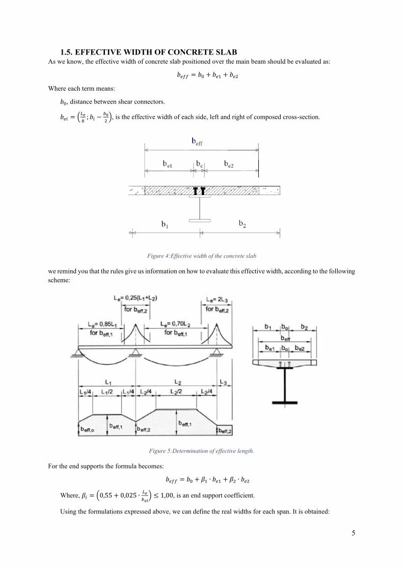
1.5. EFFECTIVE WIDTH OF CONCRETE SLAB As we know, the effective width of concrete slab positioned over the main beam should be evaluated as:
𝑏𝑒𝑓𝑓 = 𝑏0 + 𝑏𝑒1 + 𝑏𝑒2
Where each term means:
𝑏0, distance between shear connectors.
𝑏𝑒𝑖 = (𝐿𝑒
8; 𝑏𝑖 −
𝑏0
2), is the effective width of each side, left and right of composed cross-section.
Figure 4:Effective width of the concrete slab
we remind you that the rules give us information on how to evaluate this effective width, according to the following scheme:
Figure 5:Determination of effective length.
For the end supports the formula becomes:
𝑏𝑒𝑓𝑓 = 𝑏0 + 𝛽1 ∙ 𝑏𝑒1 + 𝛽2 ∙ 𝑏𝑒2
Where, 𝛽𝑖 = (0,55 + 0,025 ∙𝐿𝑒
𝑏𝑒𝑖) ≤ 1,00, is an end support coefficient.
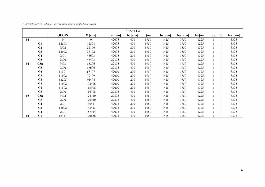
Using the formulations expressed above, we can define the real widths for each span. It is obtained:
6
Table 3:Effective width for the external main longitudinal beams.
BEAM 1-3 QUOIN X [mm] Le [mm] b0 [mm] b1 [mm] b2 [mm] be1 [mm] be2 [mm] 1 2 beff [mm]
P1 0 0 42075 400 1950 1425 1750 1225 1 1 3375 C1 12598 12598 42075 400 1950 1425 1750 1225 1 1 3375 C2 9502 22100 42075 200 1950 1425 1850 1325 1 1 3375 C3 12002 34102 42075 200 1950 1425 1850 1325 1 1 3375 C4 9501 43603 42075 200 1950 1425 1850 1325 1 1 3375 C5 2800 46403 29875 400 1950 1425 1750 1225 1 1 3375
P2 C5a 7403 53806 29875 400 1950 1425 1750 1225 1 1 3375 C5 2800 56606 29875 400 1950 1425 1750 1225 1 1 3375 C6 11501 68107 49000 200 1950 1425 1850 1325 1 1 3375 C7 11002 79109 49000 200 1950 1425 1850 1325 1 1 3375 C8 12295 91404 49000 200 1950 1425 1850 1325 1 1 3375 C7 11002 102406 49000 200 1950 1425 1850 1325 1 1 3375 C6 11502 113908 49000 200 1950 1425 1850 1325 1 1 3375 C5 2800 116708 29875 400 1950 1425 1750 1225 1 1 3375
P3 C5a 7402 124110 29875 400 1950 1425 1750 1225 1 1 3375 C5 2800 126910 29875 400 1950 1425 1750 1225 1 1 3375 C4 9501 136411 42075 200 1950 1425 1850 1325 1 1 3375 C3 12002 148413 42075 200 1950 1425 1850 1325 1 1 3375 C2 9501 157914 42075 400 1950 1425 1750 1225 1 1 3375
P4 C1 12744 170658 42075 400 1950 1425 1750 1225 1 1 3375
7
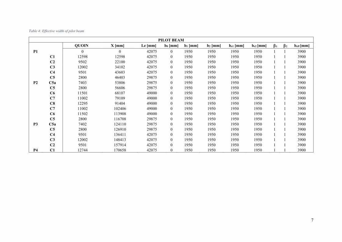
Table 4: Effective width of pilot beam
PILOT BEAM QUOIN X [mm] Le [mm] b0 [mm] b1 [mm] b2 [mm] be1 [mm] be2 [mm] 1 2 beff [mm]
P1 0 0 42075 0 1950 1950 1950 1950 1 1 3900 C1 12598 12598 42075 0 1950 1950 1950 1950 1 1 3900 C2 9502 22100 42075 0 1950 1950 1950 1950 1 1 3900 C3 12002 34102 42075 0 1950 1950 1950 1950 1 1 3900 C4 9501 43603 42075 0 1950 1950 1950 1950 1 1 3900 C5 2800 46403 29875 0 1950 1950 1950 1950 1 1 3900
P2 C5a 7403 53806 29875 0 1950 1950 1950 1950 1 1 3900 C5 2800 56606 29875 0 1950 1950 1950 1950 1 1 3900 C6 11501 68107 49000 0 1950 1950 1950 1950 1 1 3900 C7 11002 79109 49000 0 1950 1950 1950 1950 1 1 3900 C8 12295 91404 49000 0 1950 1950 1950 1950 1 1 3900 C7 11002 102406 49000 0 1950 1950 1950 1950 1 1 3900 C6 11502 113908 49000 0 1950 1950 1950 1950 1 1 3900 C5 2800 116708 29875 0 1950 1950 1950 1950 1 1 3900
P3 C5a 7402 124110 29875 0 1950 1950 1950 1950 1 1 3900 C5 2800 126910 29875 0 1950 1950 1950 1950 1 1 3900 C4 9501 136411 42075 0 1950 1950 1950 1950 1 1 3900 C3 12002 148413 42075 0 1950 1950 1950 1950 1 1 3900 C2 9501 157914 42075 0 1950 1950 1950 1950 1 1 3900
P4 C1 12744 170658 42075 0 1950 1950 1950 1950 1 1 3900
8
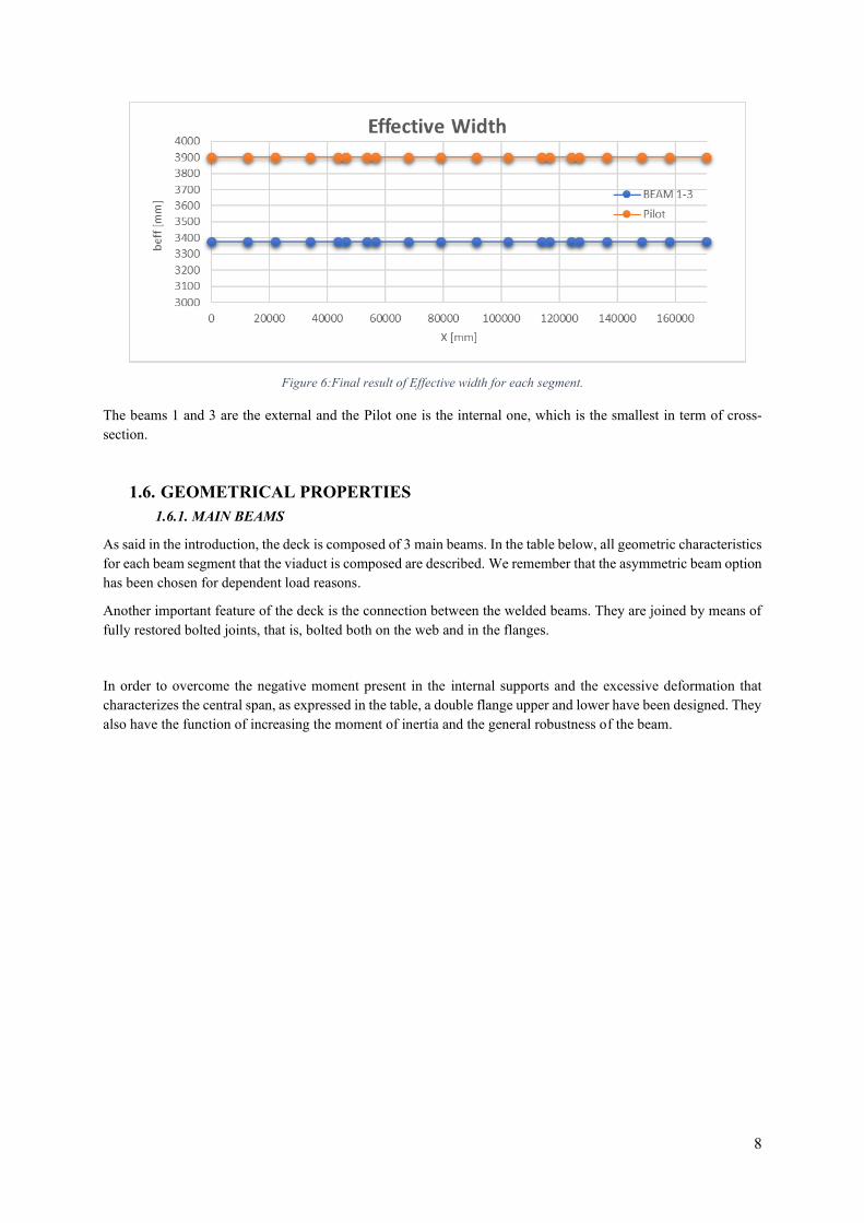
Figure 6:Final result of Effective width for each segment.
The beams 1 and 3 are the external and the Pilot one is the internal one, which is the smallest in term of cross-section.
1.6. GEOMETRICAL PROPERTIES 1.6.1. MAIN BEAMS
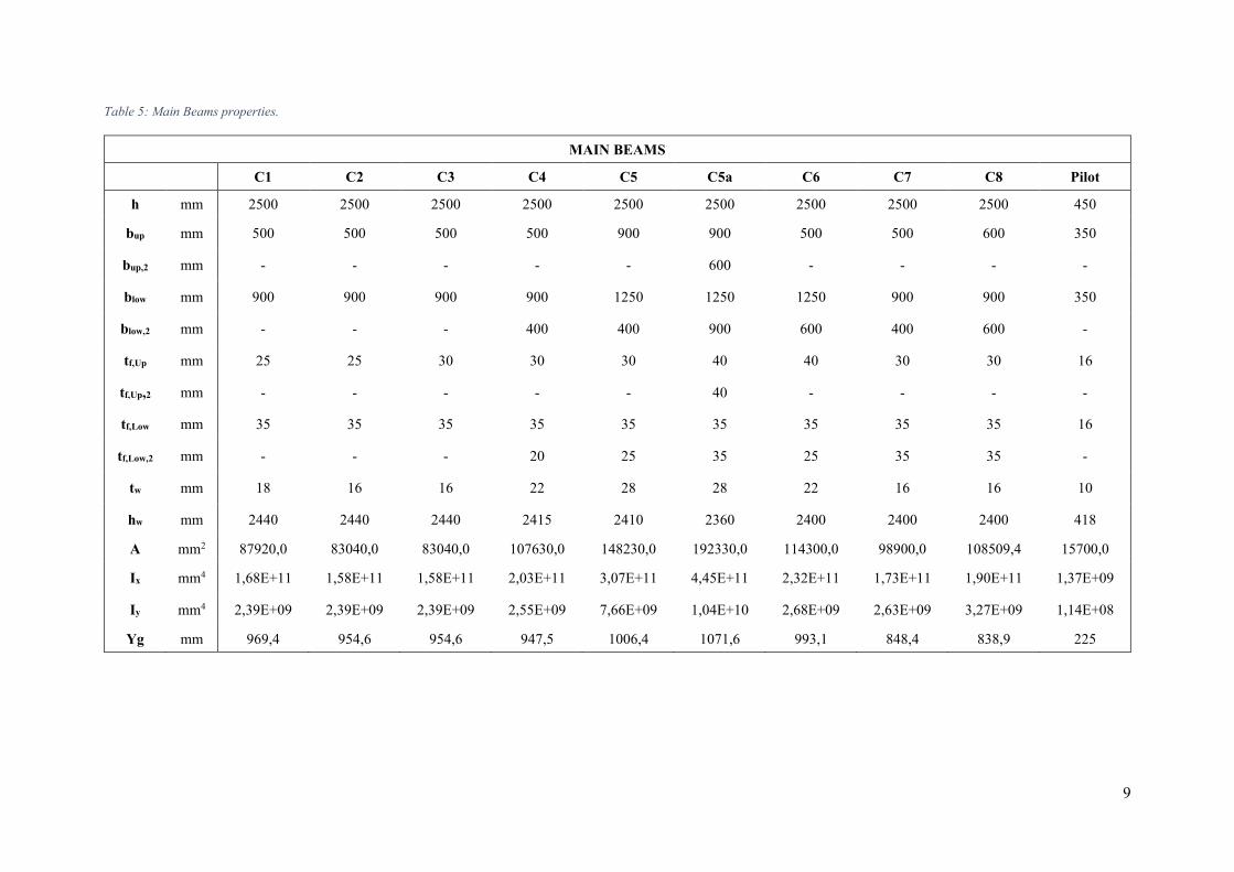
As said in the introduction, the deck is composed of 3 main beams. In the table below, all geometric characteristics for each beam segment that the viaduct is composed are described. We remember that the asymmetric beam option has been chosen for dependent load reasons.
Another important feature of the deck is the connection between the welded beams. They are joined by means of fully restored bolted joints, that is, bolted both on the web and in the flanges.
In order to overcome the negative moment present in the internal supports and the excessive deformation that characterizes the central span, as expressed in the table, a double flange upper and lower have been designed. They also have the function of increasing the moment of inertia and the general robustness of the beam.
9
Table 5: Main Beams properties.
MAIN BEAMS C1 C2 C3 C4 C5 C5a C6 C7 C8 Pilot
h mm 2500 2500 2500 2500 2500 2500 2500 2500 2500 450
bup mm 500 500 500 500 900 900 500 500 600 350
bup,2 mm - - - - - 600 - - - -
blow mm 900 900 900 900 1250 1250 1250 900 900 350
blow,2 mm - - - 400 400 900 600 400 600 -
tf,Up mm 25 25 30 30 30 40 40 30 30 16
tf,Up,2 mm - - - - - 40 - - - -
tf,Low mm 35 35 35 35 35 35 35 35 35 16
tf,Low,2 mm - - - 20 25 35 25 35 35 -
tw mm 18 16 16 22 28 28 22 16 16 10
hw mm 2440 2440 2440 2415 2410 2360 2400 2400 2400 418
A mm2 87920,0 83040,0 83040,0 107630,0 148230,0 192330,0 114300,0 98900,0 108509,4 15700,0
Ix mm4 1,68E+11 1,58E+11 1,58E+11 2,03E+11 3,07E+11 4,45E+11 2,32E+11 1,73E+11 1,90E+11 1,37E+09
Iy mm4 2,39E+09 2,39E+09 2,39E+09 2,55E+09 7,66E+09 1,04E+10 2,68E+09 2,63E+09 3,27E+09 1,14E+08
Yg mm 969,4 954,6 954,6 947,5 1006,4 1071,6 993,1 848,4 838,9 225
10
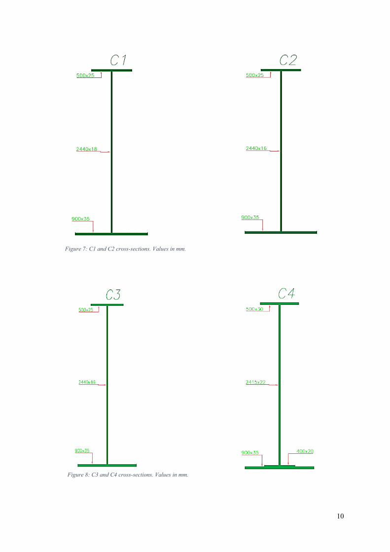
Figure 7: C1 and C2 cross-sections. Values in mm.
Figure 8: C3 and C4 cross-sections. Values in mm.
11
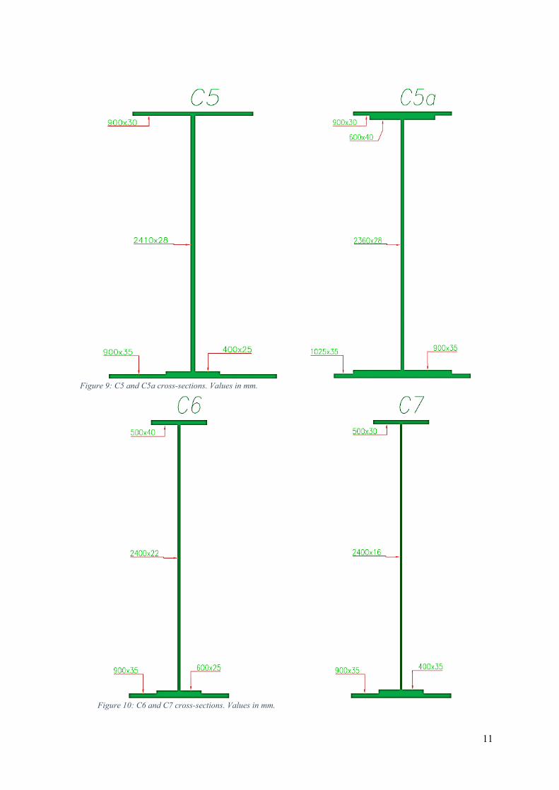
Figure 9: C5 and C5a cross-sections. Values in mm.
Figure 10: C6 and C7 cross-sections. Values in mm.
12
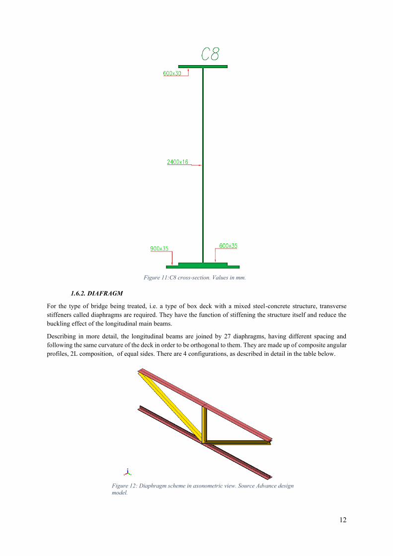
1.6.2. DIAFRAGM
For the type of bridge being treated, i.e. a type of box deck with a mixed steel-concrete structure, transverse stiffeners called diaphragms are required. They have the function of stiffening the structure itself and reduce the buckling effect of the longitudinal main beams.
Describing in more detail, the longitudinal beams are joined by 27 diaphragms, having different spacing and following the same curvature of the deck in order to be orthogonal to them. They are made up of composite angular profiles, 2L composition, of equal sides. There are 4 configurations, as described in detail in the table below.
Figure 11:C8 cross-section. Values in mm.
Figure 12: Diaphragm scheme in axonometric view. Source Advance design model.
13
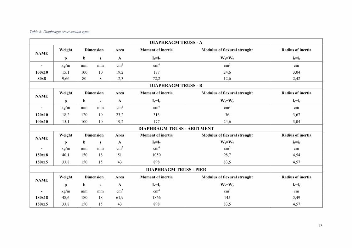
Table 6: Diaphragm cross section type.
DIAPHRAGM TRUSS - A
NAME Weight Dimension Area Moment of inertia Modulus of flexural strenght Radius of inertia
p b s A Ix=Iy Wx=Wy ix=iy
- kg/m mm mm cm2 cm4 cm3 cm 100x10 15,1 100 10 19,2 177 24,6 3,04
80x8 9,66 80 8 12,3 72,2 12,6 2,42
DIAPHRAGM TRUSS - B
NAME Weight Dimension Area Moment of inertia Modulus of flexural strenght Radius of inertia
p b s A Ix=Iy Wx=Wy ix=iy - kg/m mm mm cm2 cm4 cm3 cm
120x10 18,2 120 10 23,2 313 36 3,67
100x10 15,1 100 10 19,2 177 24,6 3,04
DIAPHRAGM TRUSS - ABUTMENT
NAME Weight Dimension Area Moment of inertia Modulus of flexural strenght Radius of inertia
p b s A Ix=Iy Wx=Wy ix=iy - kg/m mm mm cm2 cm4 cm3 cm
150x18 40,1 150 18 51 1050 98,7 4,54
150x15 33,8 150 15 43 898 83,5 4,57
DIAPHRAGM TRUSS - PIER
NAME Weight Dimension Area Moment of inertia Modulus of flexural strenght Radius of inertia
p b s A Ix=Iy Wx=Wy ix=iy - kg/m mm mm cm2 cm4 cm3 cm
180x18 48,6 180 18 61,9 1866 145 5,49 150x15 33,8 150 15 43 898 83,5 4,57
14
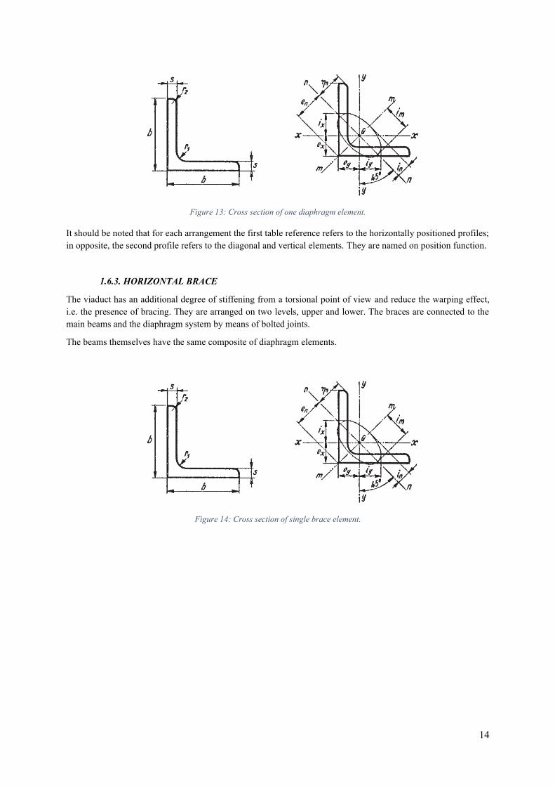
Figure 13: Cross section of one diaphragm element.
It should be noted that for each arrangement the first table reference refers to the horizontally positioned profiles; in opposite, the second profile refers to the diagonal and vertical elements. They are named on position function.
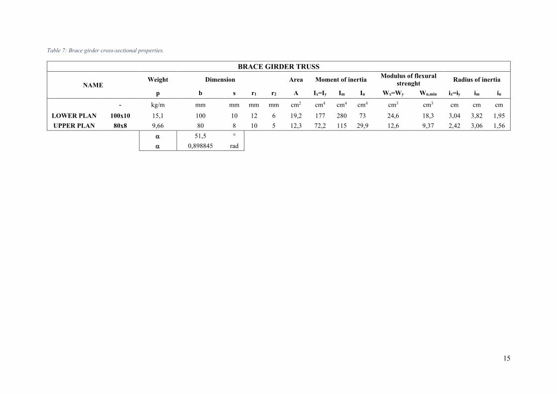
1.6.3. HORIZONTAL BRACE
The viaduct has an additional degree of stiffening from a torsional point of view and reduce the warping effect, i.e. the presence of bracing. They are arranged on two levels, upper and lower. The braces are connected to the main beams and the diaphragm system by means of bolted joints.
The beams themselves have the same composite of diaphragm elements.
Figure 14: Cross section of single brace element.
15
Table 7: Brace girder cross-sectional properties.
BRACE GIRDER TRUSS
NAME Weight Dimension Area Moment of inertia Modulus of flexural
strenght Radius of inertia
p b s r1 r2 A Ix=Iy Im In Wx=Wy Wn,min ix=iy im in
- kg/m mm mm mm mm cm2 cm4 cm4 cm4 cm3 cm3 cm cm cm
LOWER PLAN 100x10 15,1 100 10 12 6 19,2 177 280 73 24,6 18,3 3,04 3,82 1,95 UPPER PLAN 80x8 9,66 80 8 10 5 12,3 72,2 115 29,9 12,6 9,37 2,42 3,06 1,56
51,5 ° 0,898845 rad
16
2. LOAD ANALYSIS In this chapter we want to describe in detail the loads used and all the loading conditions to be carried out according to Eurocode and Italian technical standard.
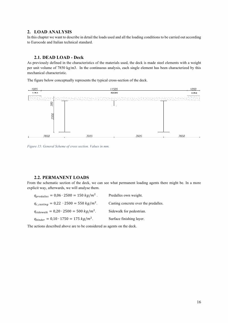
2.1. DEAD LOAD - Deck As previously defined in the characteristics of the materials used, the deck is made steel elements with a weight per unit volume of 7850 kg/m3. In the continuous analysis, each single element has been characterized by this mechanical characteristic.
The figure below conceptually represents the typical cross-section of the deck.
Figure 15: General Scheme of cross section. Values in mm.
2.2. PERMANENT LOADS From the schematic section of the deck, we can see what permanent loading agents there might be. In a more explicit way, afterwards, we will analyse them.
𝑞𝑝𝑟𝑒𝑑𝑎𝑙𝑙𝑒𝑠 = 0,06 ∙ 2500 = 150 𝑘𝑔/𝑚2 . Predalles own weight.
𝑞𝑐_𝑐𝑎𝑠𝑡𝑖𝑛𝑔 = 0,22 ∙ 2500 = 550 𝑘𝑔/𝑚2. Casting concrete over the predalles.
𝑞𝑠𝑖𝑑𝑒𝑤𝑎𝑙𝑘 = 0,20 ∙ 2500 = 500 𝑘𝑔/𝑚2. Sidewalk for pedestrian.
𝑞𝑏𝑖𝑛𝑑𝑒𝑟 = 0,10 ∙ 1750 = 175 𝑘𝑔/𝑚2. Surface finishing layer.
The actions described above are to be considered as agents on the deck.
17
2.3. ACCIDENTAL LOADS
2.3.1. TRAFFIC LOADS The EN 1991-2 standard defines traffic load models for the design of road bridges, footbridges and railway bridges. For the design of new bridges, EN 1991-2 is intended to be used, for direct application, together with the EN 1990-1999 Eurocodes. It is intended to be used as a design guide. They will have to be compared with the national reference guides.
As defined, EN 1991-2 specifies the imposed loads (models and representative values) associated with road traffic, pedestrian actions and rail traffic which include, when relevant, dynamic effects and centrifugal, braking and acceleration actions and accidental design actions.
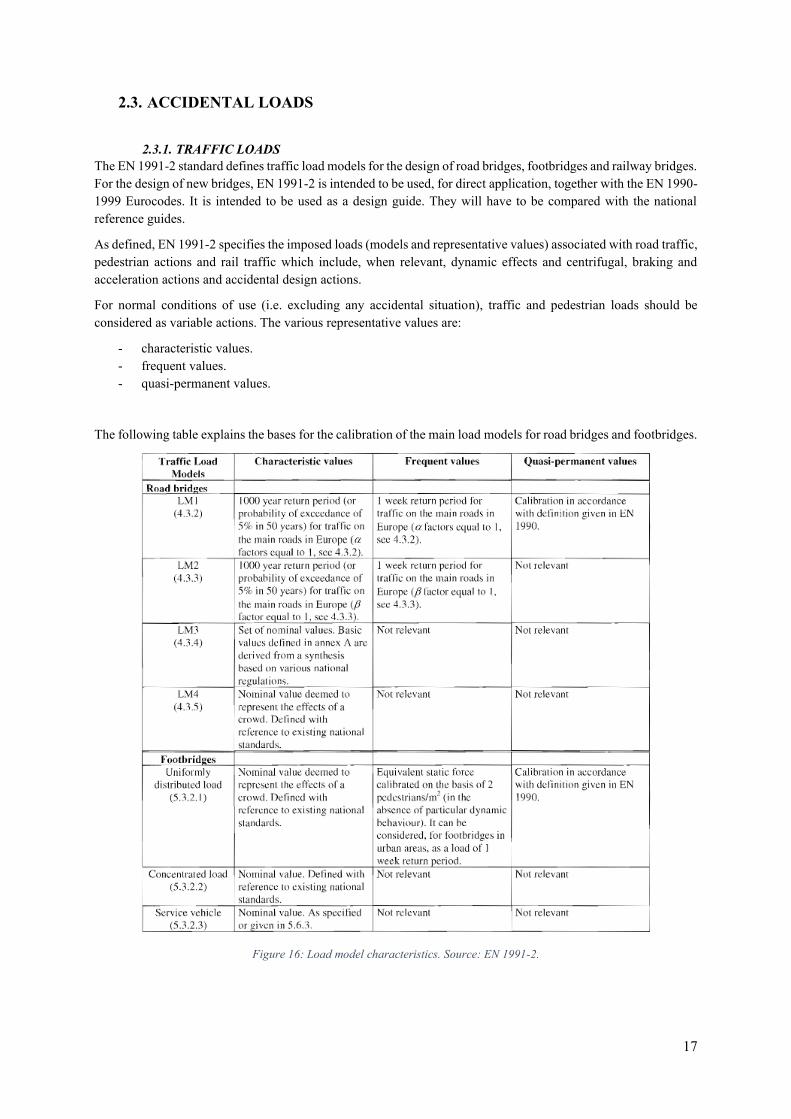
For normal conditions of use (i.e. excluding any accidental situation), traffic and pedestrian loads should be considered as variable actions. The various representative values are:
- characteristic values. - frequent values. - quasi-permanent values.
The following table explains the bases for the calibration of the main load models for road bridges and footbridges.
Figure 16: Load model characteristics. Source: EN 1991-2.
18
The calculation model used for the design of this bridge is Load model 1, LM1, concentrated and uniformly distributed loads, which cover most of the effects of the traffic of lorries and cars. This model should be used for general and local verifications.
In order to describe the actions that are part of this variable action, there is a need to specify what the moving loads are. They are loads due to road traffic, such as vehicles, trucks, lorries and other special transport vehicles for industrial transport. Taking into account all the pedestrian and transient components that may arise during their lifetime.
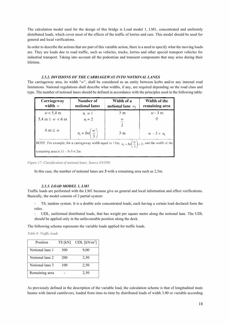
2.3.2. DIVISIONS OF THE CARRIAGEWAY INTO NOTIONAL LANES The carriageway area, its width “w”, shall be considered as an entity between kerbs and/or any internal road
limitations. National regulations shall describe what widths, if any, are required depending on the road class and type. The number of notional lanes should be defined in accordance with the principles used in the following table:
Figure 17: Classification of notional lanes. Source EN1991
In this case, the number of notional lanes are 3 with a remaining area such as 2,5m.
2.3.3. LOAD MODEL 1, LM1 Traffic loads are performed with the LM1 because give us general and local information and effect verifications. Basically, the model consists of 2 partial system:
- TS, tandem system. It is a double axle concentrated loads, each having a certain load declared form the rules. - UDL, uniformed distributed loads, that has weight per square metre along the notional lane. The UDL should be applied only in the unfavourable position along the deck.
The following scheme represents the variable loads applied for traffic loads.
Table 8: Traffic loads
Position TS [kN] UDL [kN/m2]
Notional lane 1 300 9,00
Notional lane 2 200 2,50
Notional lane 3 100 2,50
Remaining area - 2,50
As previously defined in the description of the variable load, the calculation scheme is that of longitudinal main beams with lateral cantilevers, loaded from time-to-time by distributed loads of width 3.00 or variable according
19
to the destination of use, arranged in such a way as to obtain and determine the heaviest loading conditions on the external beams or on the middle beam.
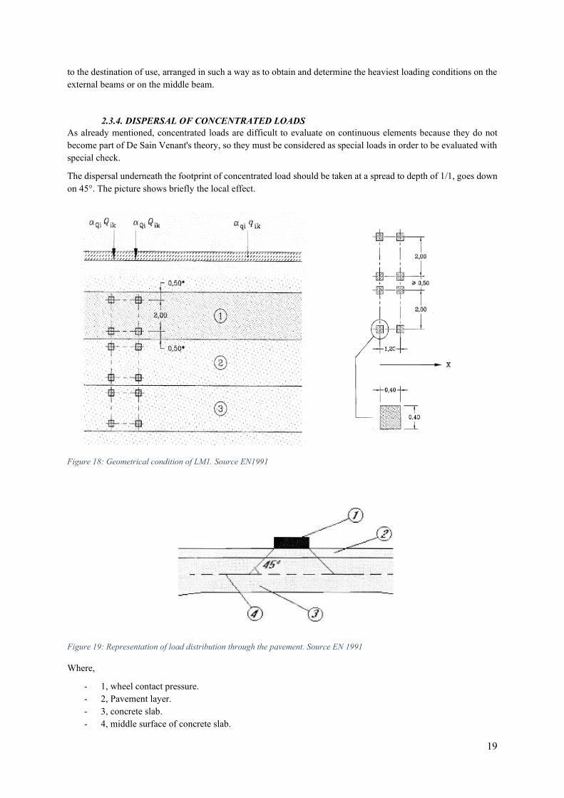
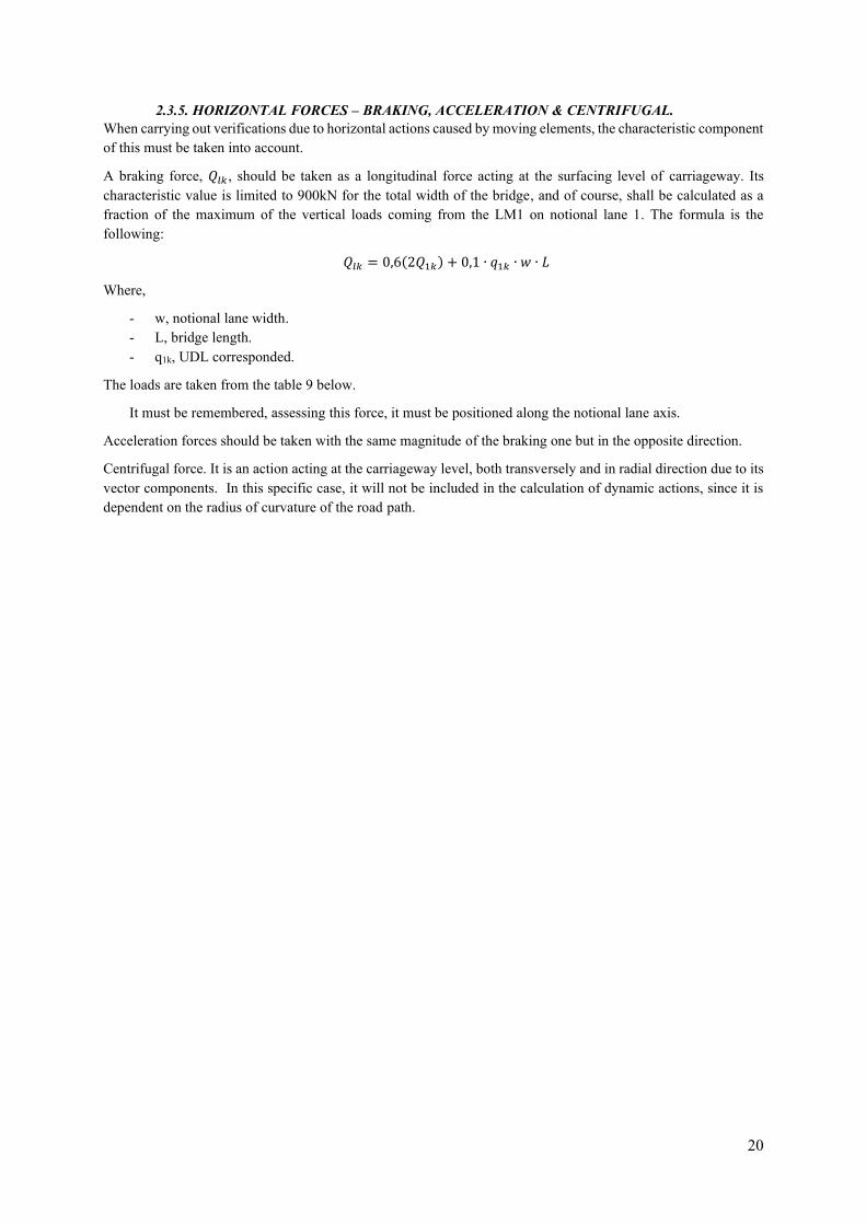
2.3.4. DISPERSAL OF CONCENTRATED LOADS As already mentioned, concentrated loads are difficult to evaluate on continuous elements because they do not become part of De Sain Venant's theory, so they must be considered as special loads in order to be evaluated with special check.
The dispersal underneath the footprint of concentrated load should be taken at a spread to depth of 1/1, goes down on 45°. The picture shows briefly the local effect.
Figure 19: Representation of load distribution through the pavement. Source EN 1991
Where,
- 1, wheel contact pressure. - 2, Pavement layer. - 3, concrete slab. - 4, middle surface of concrete slab.
Figure 18: Geometrical condition of LM1. Source EN1991
20
2.3.5. HORIZONTAL FORCES – BRAKING, ACCELERATION & CENTRIFUGAL. When carrying out verifications due to horizontal actions caused by moving elements, the characteristic component of this must be taken into account.
A braking force, 𝑄𝑙𝑘 , should be taken as a longitudinal force acting at the surfacing level of carriageway. Its characteristic value is limited to 900kN for the total width of the bridge, and of course, shall be calculated as a fraction of the maximum of the vertical loads coming from the LM1 on notional lane 1. The formula is the following:
𝑄𝑙𝑘 = 0,6(2𝑄1𝑘) + 0,1 ∙ 𝑞1𝑘 ∙ 𝑤 ∙ 𝐿
Where,
- w, notional lane width. - L, bridge length. - q1k, UDL corresponded.
The loads are taken from the table 9 below.
It must be remembered, assessing this force, it must be positioned along the notional lane axis.
Acceleration forces should be taken with the same magnitude of the braking one but in the opposite direction.
Centrifugal force. It is an action acting at the carriageway level, both transversely and in radial direction due to its vector components. In this specific case, it will not be included in the calculation of dynamic actions, since it is dependent on the radius of curvature of the road path.
21
2.4. VARIABLE LOADS
2.4.1. WIND EFFECTS
The wind action is calculated according to chapter §3.3 of NTC2018 in accordance with Eurocode EN 1991-1-4. This action is comparable to a static horizontal action, having orthogonal direction to the axis of the bridge and in projection in the vertical plane of the involved surfaces. In the case of a loaded bridge, the exposed surface increases due to the presence of moving vehicles. This surface is such as a continuous rectangular wall 3 metres above the road surface.
2.4.1.1. REFERENCE BASE VELOCITY
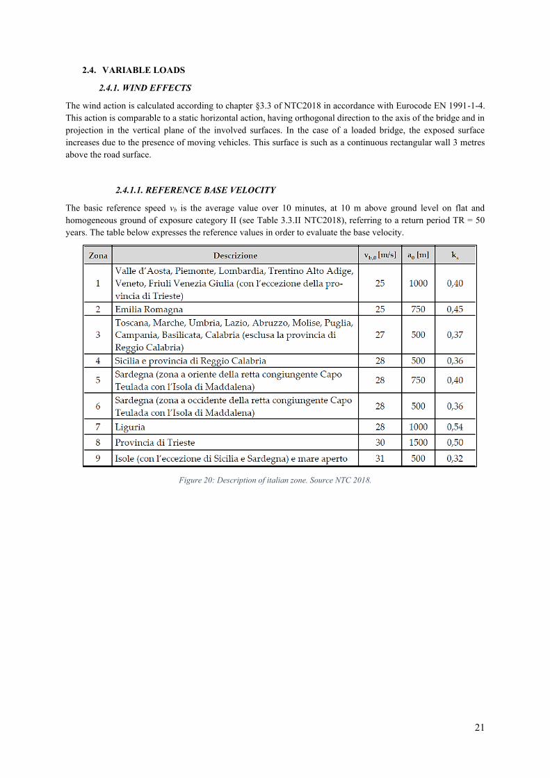
The basic reference speed vb is the average value over 10 minutes, at 10 m above ground level on flat and homogeneous ground of exposure category II (see Table 3.3.II NTC2018), referring to a return period TR = 50 years. The table below expresses the reference values in order to evaluate the base velocity.
Figure 20: Description of italian zone. Source NTC 2018.
22
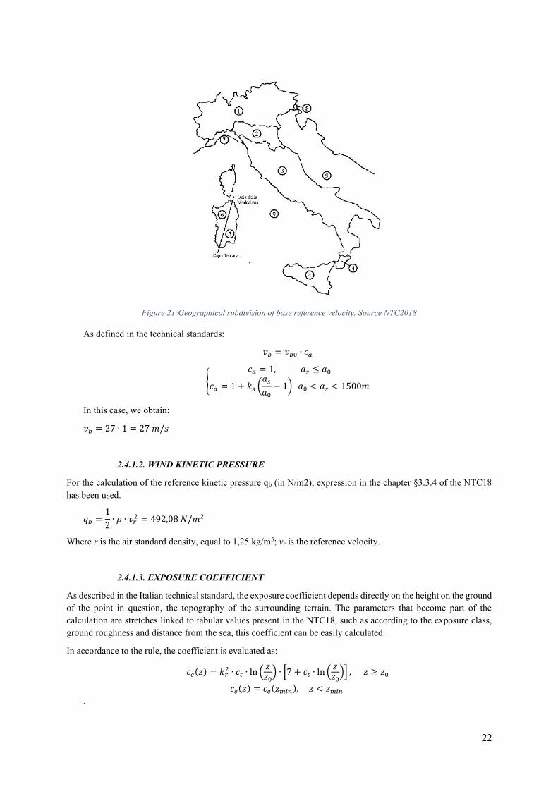
Figure 21:Geographical subdivision of base reference velocity. Source NTC2018
As defined in the technical standards:
𝑣𝑏 = 𝑣𝑏0 ∙ 𝑐𝑎
{
𝑐𝑎 = 1, 𝑎𝑠 ≤ 𝑎0
𝑐𝑎 = 1 + 𝑘𝑠 (𝑎𝑠
𝑎0
− 1) 𝑎0 < 𝑎𝑠 < 1500𝑚
In this case, we obtain:
𝑣𝑏 = 27 ∙ 1 = 27 𝑚/𝑠
2.4.1.2. WIND KINETIC PRESSURE
For the calculation of the reference kinetic pressure qb (in N/m2), expression in the chapter §3.3.4 of the NTC18 has been used.
𝑞𝑏 =1
2∙ 𝜌 ∙ 𝑣𝑟
2 = 492,08 𝑁/𝑚2
Where r is the air standard density, equal to 1,25 kg/m3; vr is the reference velocity.
2.4.1.3. EXPOSURE COEFFICIENT
As described in the Italian technical standard, the exposure coefficient depends directly on the height on the ground of the point in question, the topography of the surrounding terrain. The parameters that become part of the calculation are stretches linked to tabular values present in the NTC18, such as according to the exposure class, ground roughness and distance from the sea, this coefficient can be easily calculated.
In accordance to the rule, the coefficient is evaluated as:
𝑐𝑒(𝑧) = 𝑘𝑟2 ∙ 𝑐𝑡 ∙ ln (
𝑧𝑧0
) ∙ [7 + 𝑐𝑡 ∙ ln (𝑧𝑧0
)] , 𝑧 ≥ 𝑧0
𝑐𝑒(𝑧) = 𝑐𝑒(𝑧𝑚𝑖𝑛), 𝑧 < 𝑧𝑚𝑖𝑛
.
23
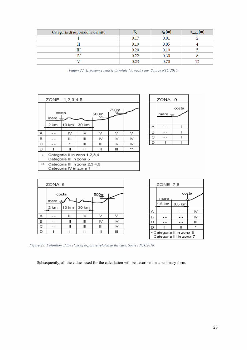
Figure 22: Exposure coefficients related to each case. Source NTC 2018.
Figure 23: Definition of the class of exposure related to the case. Source NTC2018.
Subsequently, all the values used for the calculation will be described in a summary form.
24
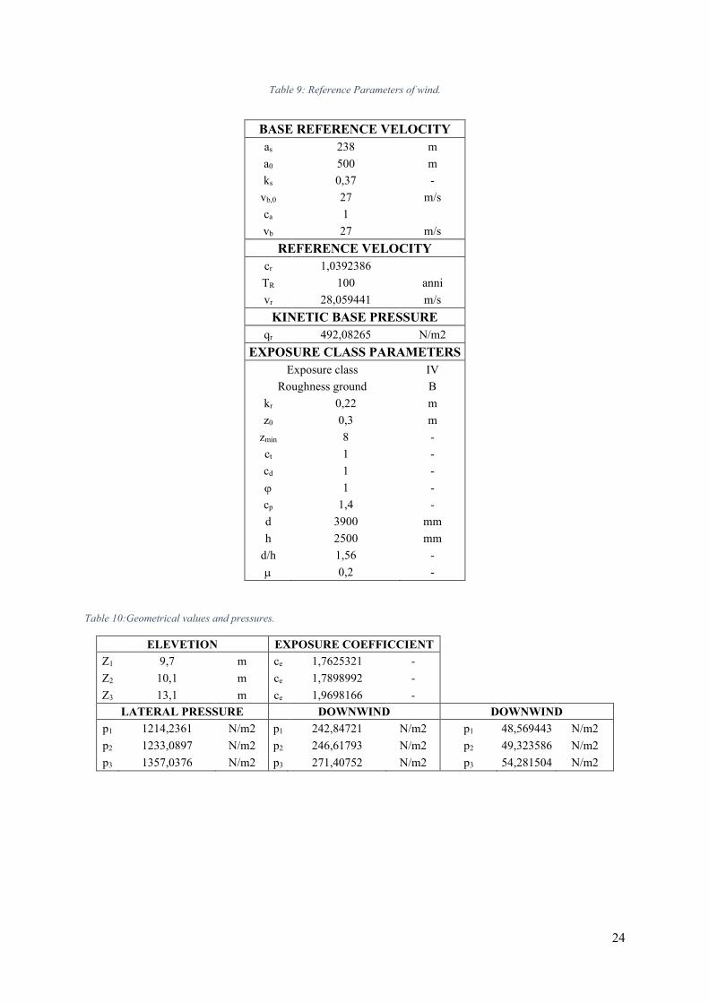
Table 9: Reference Parameters of wind.
Table 10:Geometrical values and pressures.
ELEVETION EXPOSURE COEFFICCIENT
Z1 9,7 m ce 1,7625321 -
Z2 10,1 m ce 1,7898992 -
Z3 13,1 m ce 1,9698166 -
LATERAL PRESSURE DOWNWIND DOWNWIND p1 1214,2361 N/m2 p1 242,84721 N/m2 p1 48,569443 N/m2 p2 1233,0897 N/m2 p2 246,61793 N/m2 p2 49,323586 N/m2 p3 1357,0376 N/m2 p3 271,40752 N/m2 p3 54,281504 N/m2
BASE REFERENCE VELOCITY as 238 m a0 500 m ks 0,37 -
vb,0 27 m/s ca 1
vb 27 m/s REFERENCE VELOCITY
cr 1,0392386
TR 100 anni vr 28,059441 m/s
KINETIC BASE PRESSURE qr 492,08265 N/m2
EXPOSURE CLASS PARAMETERS Exposure class IV
Roughness ground B kr 0,22 m z0 0,3 m
zmin 8 - ct 1 - cd 1 - 1 - cp 1,4 - d 3900 mm h 2500 mm
d/h 1,56 - 0,2 -
25
2.4.1.4. LOCAL DYNAMIC EFFECT In this chapter we are going to analyze the effects of local instability that could occur caused by the wind. They are directly related to the frequencies of the structure under examination and the average speed that the site is characteristic of it. First of all, the calculations for the determination of the frequency proper to the structure will be made and then the steps for the calculation of the frequency due to the effect of the wind action and control of the lock-in phenomenon will follow.
2.4.1.4.1. STRUCTURAL NATURAL FREQUENCY In order to understand the own frequency of the structure, the natural one, the EN 1991-1-4 defines a guideline procedure for dynamic response of itself. The equation F.6 describes the fundamental vertical bending frequency of girder bridge from:
𝑛1,𝐵 =𝑘2
2𝜋𝐿2√
𝐸𝐼𝑏
𝑚
Where,
- L is the main span length. - E is the Young Modulus. - Ib is the second moment inertia of cross-section at mid-span. - m is the mass per unit length of full cross section. - K is a dimensionless factor.
Other important fundamental frequency for what concern bridge case is the torsional frequency. The Eurocode defines approximately as:
𝑛1,𝑇 = 𝑛1,𝐵√𝑃1(𝑃2 + 𝑃3)
Where,
P1, P2 and P3 are coefficients defined on Eurocode.
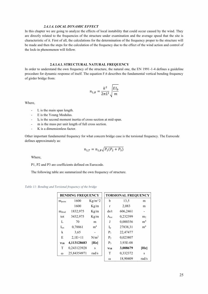
The following table are summarized the own frequency of structure.
Table 11: Bending and Torsional frequency of the bridge
BENDING FREQUENCY TORSIONAL FREQUENCY mperm 1600 Kg/m^2 b 13,5 m
1600 Kg/m r 2,083 m mdead 1832,975 Kg/m ds/t 606,2461 - tot 3432,975 Kg/m Atot 0,232399 m2 L 70 m J 0,000356 m4 Itot 0,78861 m4 Ip 27838,31 m6 k 3,65 - P1 22,47477
E 2,1E+11 N/m2 P2 0,023807
1B 4,113128683 [Hz] P3 3,93E-08
T 0,243123928 s 1B 3,008679 [Hz] 25,84354971 rad/s T 0,332372 s 18,90409 rad/s
26
As we can see in tab.11, they represent the characteristic frequencies of the structure. Naturally, as previously mentioned, they will have to be compared with the dynamic action of the wind and then with modal analysis due to the earthquake, to avoid possible resonance scenarios.
2.4.1.4.2. WIND NATURAL FREQUENCY In order to rigorously calculate the frequency of the wind in question, we have used Eurocode 1 part 4 and a study conducted by the National Research Council (CNR), a study carried out on 19 February 2009. Having no suitable software available to be able to discretize the action of the wind in order to visualize the effects that could occur in the structure, we made use of European legislation and national studies, as mentioned above.
The procedure that follows will be at the end the natural frequency of the wind on our structure and to evaluate the dynamic longitudinal coefficient, a dimensional quantity that has the effect of modifying the static actions calculated above.
The calculation procedure will indeed be as follows:
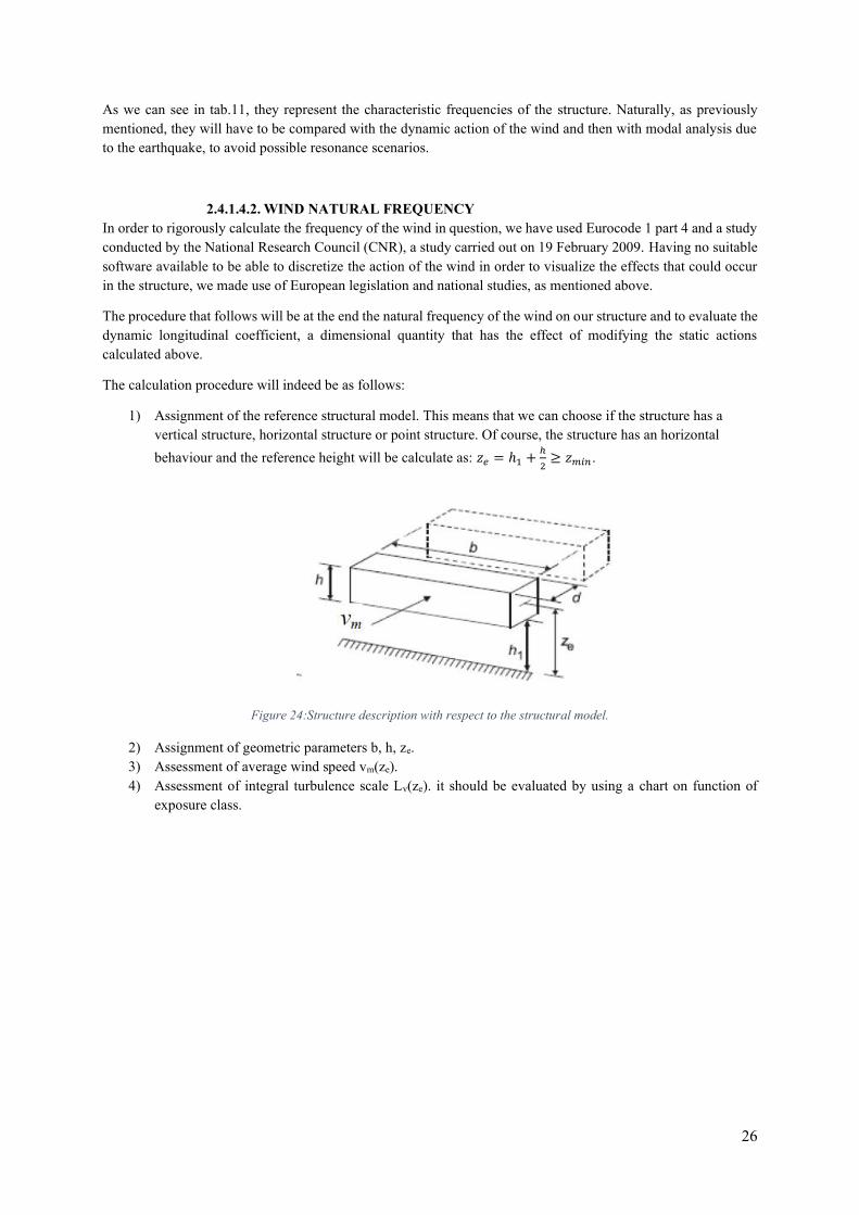
1) Assignment of the reference structural model. This means that we can choose if the structure has a vertical structure, horizontal structure or point structure. Of course, the structure has an horizontal behaviour and the reference height will be calculate as: 𝑧𝑒 = ℎ1 +
ℎ
2≥ 𝑧𝑚𝑖𝑛 .
Figure 24:Structure description with respect to the structural model.
2) Assignment of geometric parameters b, h, ze. 3) Assessment of average wind speed vm(ze). 4) Assessment of integral turbulence scale Lv(ze). it should be evaluated by using a chart on function of
exposure class.
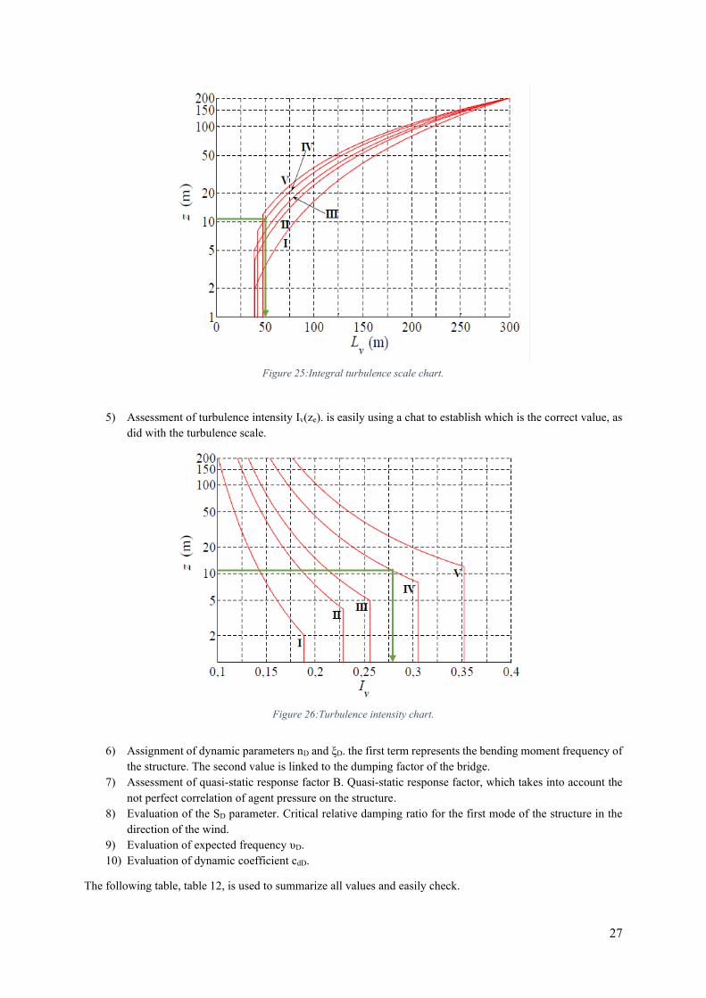
27
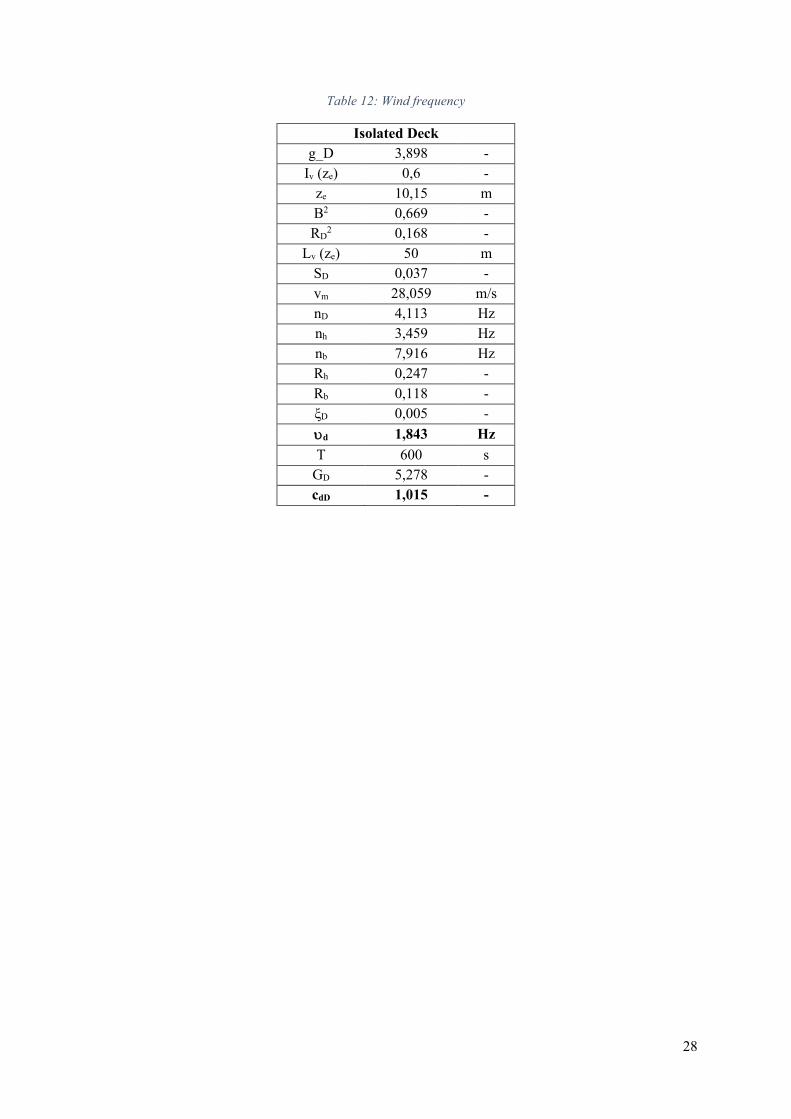
5) Assessment of turbulence intensity Iv(ze). is easily using a chat to establish which is the correct value, as did with the turbulence scale.
6) Assignment of dynamic parameters nD and ξD. the first term represents the bending moment frequency of the structure. The second value is linked to the dumping factor of the bridge.
7) Assessment of quasi-static response factor B. Quasi-static response factor, which takes into account the not perfect correlation of agent pressure on the structure.
8) Evaluation of the SD parameter. Critical relative damping ratio for the first mode of the structure in the direction of the wind.
9) Evaluation of expected frequency υD. 10) Evaluation of dynamic coefficient cdD.
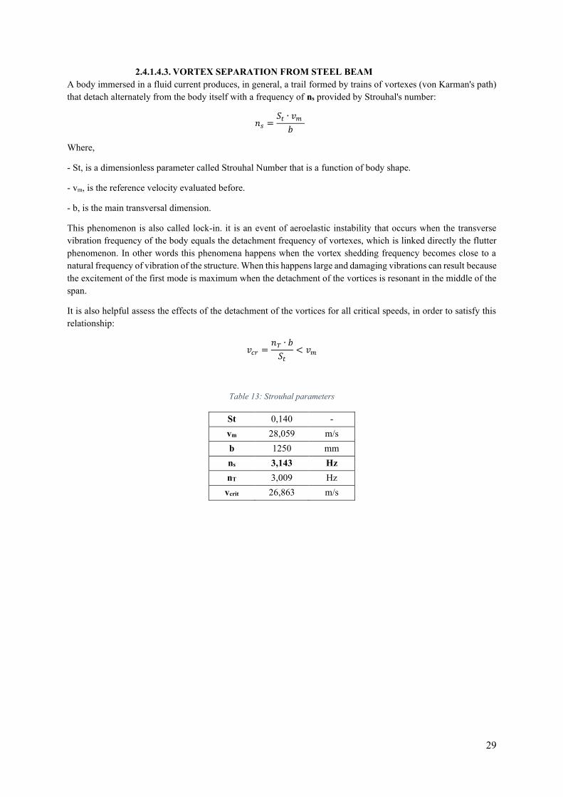
The following table, table 12, is used to summarize all values and easily check.
Figure 25:Integral turbulence scale chart.
Figure 26:Turbulence intensity chart.
28
Table 12: Wind frequency
Isolated Deck g_D 3,898 -
Iv (ze) 0,6 - ze 10,15 m B2 0,669 - RD
2 0,168 - Lv (ze) 50 m
SD 0,037 - vm 28,059 m/s nD 4,113 Hz nh 3,459 Hz nb 7,916 Hz Rh 0,247 - Rb 0,118 - ξD 0,005 - d 1,843 Hz T 600 s
GD 5,278 - cdD 1,015 -
29
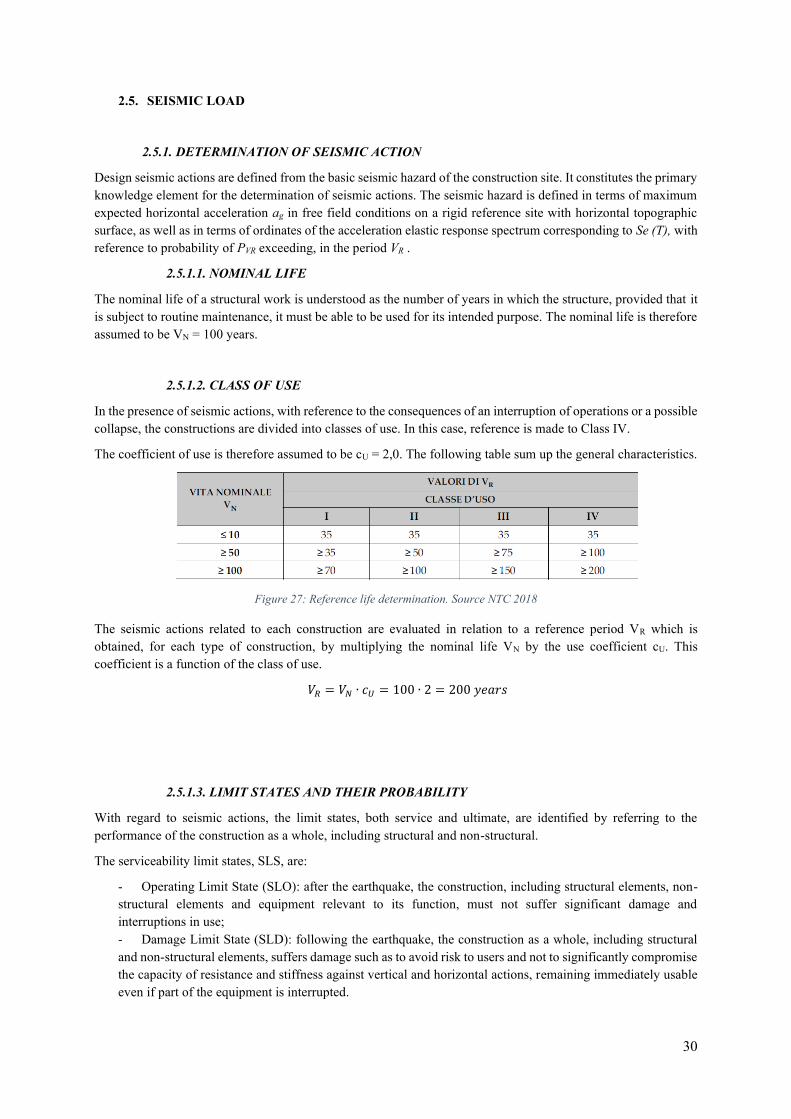
2.4.1.4.3. VORTEX SEPARATION FROM STEEL BEAM A body immersed in a fluid current produces, in general, a trail formed by trains of vortexes (von Karman's path) that detach alternately from the body itself with a frequency of ns provided by Strouhal's number:
𝑛𝑠 =𝑆𝑡 ∙ 𝑣𝑚
𝑏
Where,
- St, is a dimensionless parameter called Strouhal Number that is a function of body shape.
- vm, is the reference velocity evaluated before.
- b, is the main transversal dimension.
This phenomenon is also called lock-in. it is an event of aeroelastic instability that occurs when the transverse vibration frequency of the body equals the detachment frequency of vortexes, which is linked directly the flutter phenomenon. In other words this phenomena happens when the vortex shedding frequency becomes close to a natural frequency of vibration of the structure. When this happens large and damaging vibrations can result because the excitement of the first mode is maximum when the detachment of the vortices is resonant in the middle of the span.
It is also helpful assess the effects of the detachment of the vortices for all critical speeds, in order to satisfy this relationship:
𝑣𝑐𝑟 =𝑛𝑇 ∙ 𝑏
𝑆𝑡
< 𝑣𝑚
Table 13: Strouhal parameters
St 0,140 - vm 28,059 m/s b 1250 mm ns 3,143 Hz nT 3,009 Hz
vcrit 26,863 m/s
30
2.5. SEISMIC LOAD
2.5.1. DETERMINATION OF SEISMIC ACTION
Design seismic actions are defined from the basic seismic hazard of the construction site. It constitutes the primary knowledge element for the determination of seismic actions. The seismic hazard is defined in terms of maximum expected horizontal acceleration ag in free field conditions on a rigid reference site with horizontal topographic surface, as well as in terms of ordinates of the acceleration elastic response spectrum corresponding to Se (T), with reference to probability of PVR exceeding, in the period VR .
2.5.1.1. NOMINAL LIFE
The nominal life of a structural work is understood as the number of years in which the structure, provided that it is subject to routine maintenance, it must be able to be used for its intended purpose. The nominal life is therefore assumed to be VN = 100 years.
2.5.1.2. CLASS OF USE
In the presence of seismic actions, with reference to the consequences of an interruption of operations or a possible collapse, the constructions are divided into classes of use. In this case, reference is made to Class IV.
The coefficient of use is therefore assumed to be cU = 2,0. The following table sum up the general characteristics.
Figure 27: Reference life determination. Source NTC 2018
The seismic actions related to each construction are evaluated in relation to a reference period VR which is obtained, for each type of construction, by multiplying the nominal life VN by the use coefficient cU. This coefficient is a function of the class of use.
𝑉𝑅 = 𝑉𝑁 ∙ 𝑐𝑈 = 100 ∙ 2 = 200 𝑦𝑒𝑎𝑟𝑠
2.5.1.3. LIMIT STATES AND THEIR PROBABILITY
With regard to seismic actions, the limit states, both service and ultimate, are identified by referring to the performance of the construction as a whole, including structural and non-structural.
The serviceability limit states, SLS, are:
- Operating Limit State (SLO): after the earthquake, the construction, including structural elements, non-structural elements and equipment relevant to its function, must not suffer significant damage and interruptions in use; - Damage Limit State (SLD): following the earthquake, the construction as a whole, including structural and non-structural elements, suffers damage such as to avoid risk to users and not to significantly compromise the capacity of resistance and stiffness against vertical and horizontal actions, remaining immediately usable even if part of the equipment is interrupted.
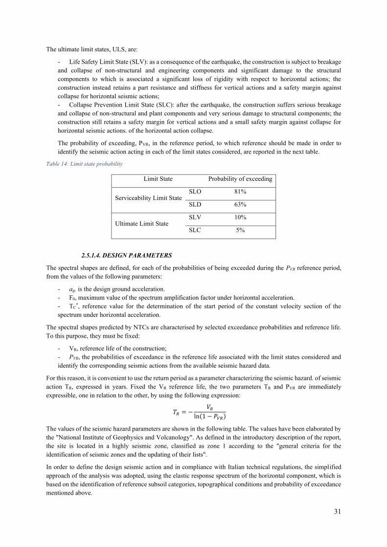
31
The ultimate limit states, ULS, are:
- Life Safety Limit State (SLV): as a consequence of the earthquake, the construction is subject to breakage and collapse of non-structural and engineering components and significant damage to the structural components to which is associated a significant loss of rigidity with respect to horizontal actions; the construction instead retains a part resistance and stiffness for vertical actions and a safety margin against collapse for horizontal seismic actions; - Collapse Prevention Limit State (SLC): after the earthquake, the construction suffers serious breakage and collapse of non-structural and plant components and very serious damage to structural components; the construction still retains a safety margin for vertical actions and a small safety margin against collapse for horizontal seismic actions. of the horizontal action collapse.
The probability of exceeding, PVR, in the reference period, to which reference should be made in order to identify the seismic action acting in each of the limit states considered, are reported in the next table.
Table 14: Limit state probability
Limit State Probability of exceeding
Serviceability Limit State SLO 81%
SLD 63%
Ultimate Limit State SLV 10%
SLC 5%
2.5.1.4. DESIGN PARAMETERS
The spectral shapes are defined, for each of the probabilities of being exceeded during the PVR reference period, from the values of the following parameters:
- ag, is the design ground acceleration. - F0, maximum value of the spectrum amplification factor under horizontal acceleration. - TC
*, reference value for the determination of the start period of the constant velocity section of the spectrum under horizontal acceleration.
The spectral shapes predicted by NTCs are characterised by selected exceedance probabilities and reference life. To this purpose, they must be fixed:
- VR, reference life of the construction; - PVR, the probabilities of exceedance in the reference life associated with the limit states considered and identify the corresponding seismic actions from the available seismic hazard data.
For this reason, it is convenient to use the return period as a parameter characterizing the seismic hazard. of seismic action TR, expressed in years. Fixed the VR reference life, the two parameters TR and PVR are immediately expressible, one in relation to the other, by using the following expression:
𝑇𝑅 = −𝑉𝑅
ln(1 − 𝑃𝑉𝑅)
The values of the seismic hazard parameters are shown in the following table. The values have been elaborated by the "National Institute of Geophysics and Volcanology". As defined in the introductory description of the report, the site is located in a highly seismic zone, classified as zone 1 according to the "general criteria for the identification of seismic zones and the updating of their lists".
In order to define the design seismic action and in compliance with Italian technical regulations, the simplified approach of the analysis was adopted, using the elastic response spectrum of the horizontal component, which is based on the identification of reference subsoil categories, topographical conditions and probability of exceedance mentioned above.
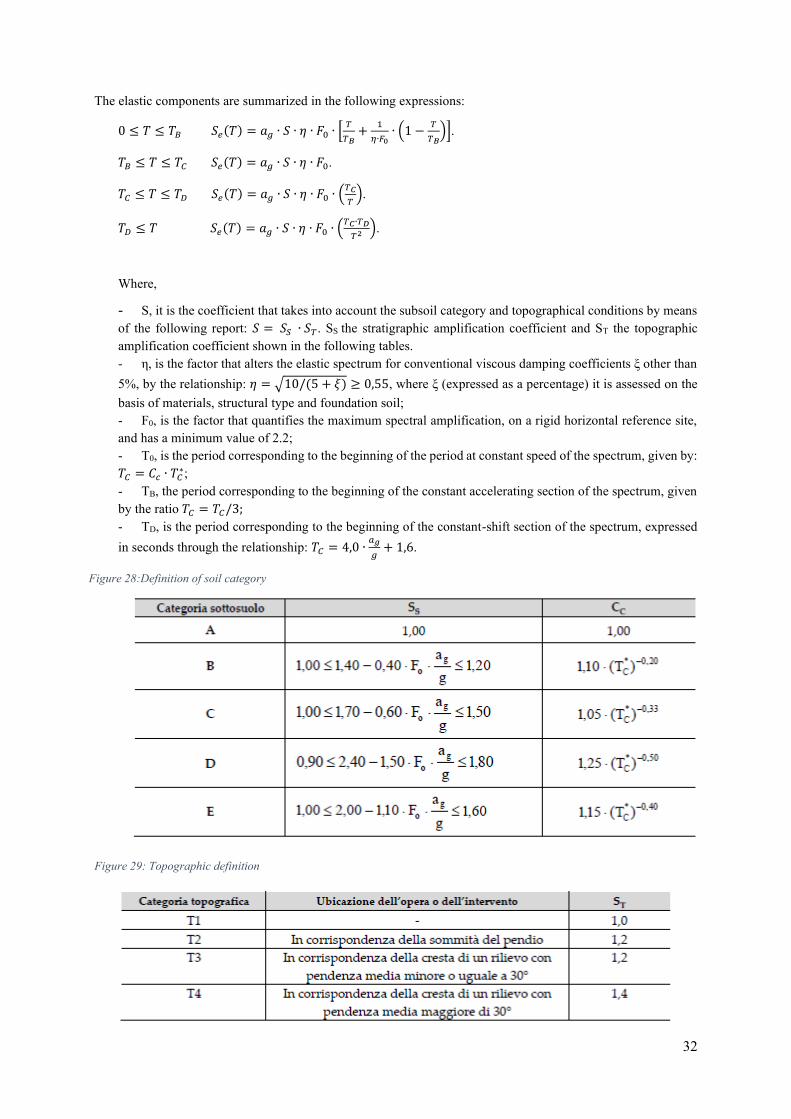
32
The elastic components are summarized in the following expressions:
0 ≤ 𝑇 ≤ 𝑇𝐵 𝑆𝑒(𝑇) = 𝑎𝑔 ∙ 𝑆 ∙ 𝜂 ∙ 𝐹0 ∙ [𝑇
𝑇𝐵+
1
𝜂∙𝐹0∙ (1 −
𝑇
𝑇𝐵)].
𝑇𝐵 ≤ 𝑇 ≤ 𝑇𝐶 𝑆𝑒(𝑇) = 𝑎𝑔 ∙ 𝑆 ∙ 𝜂 ∙ 𝐹0.
𝑇𝐶 ≤ 𝑇 ≤ 𝑇𝐷 𝑆𝑒(𝑇) = 𝑎𝑔 ∙ 𝑆 ∙ 𝜂 ∙ 𝐹0 ∙ (𝑇𝐶
𝑇).
𝑇𝐷 ≤ 𝑇 𝑆𝑒(𝑇) = 𝑎𝑔 ∙ 𝑆 ∙ 𝜂 ∙ 𝐹0 ∙ (𝑇𝐶∙𝑇𝐷
𝑇2 ).
Where,
- S, it is the coefficient that takes into account the subsoil category and topographical conditions by means of the following report: 𝑆 = 𝑆𝑆 ∙ 𝑆𝑇. SS the stratigraphic amplification coefficient and ST the topographic amplification coefficient shown in the following tables. - η, is the factor that alters the elastic spectrum for conventional viscous damping coefficients ξ other than
5%, by the relationship: 𝜂 = √10/(5 + 𝜉) ≥ 0,55, where ξ (expressed as a percentage) it is assessed on the basis of materials, structural type and foundation soil; - F0, is the factor that quantifies the maximum spectral amplification, on a rigid horizontal reference site, and has a minimum value of 2.2; - T0, is the period corresponding to the beginning of the period at constant speed of the spectrum, given by: 𝑇𝐶 = 𝐶𝑐 ∙ 𝑇𝐶
∗; - TB, the period corresponding to the beginning of the constant accelerating section of the spectrum, given by the ratio 𝑇𝐶 = 𝑇𝐶/3; - TD, is the period corresponding to the beginning of the constant-shift section of the spectrum, expressed in seconds through the relationship: 𝑇𝐶 = 4,0 ∙
𝑎𝑔
𝑔+ 1,6.
Figure 29: Topographic definition
Figure 28:Definition of soil category
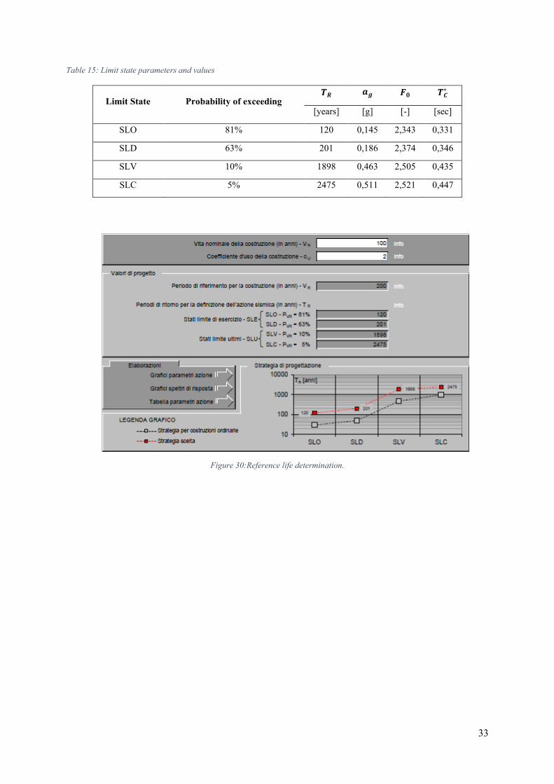
33
Table 15: Limit state parameters and values
Limit State Probability of exceeding 𝑻𝑹 𝒂𝒈 𝑭𝟎 𝑻𝑪
∗
[years] [g] [-] [sec]
SLO 81% 120 0,145 2,343 0,331
SLD 63% 201 0,186 2,374 0,346
SLV 10% 1898 0,463 2,505 0,435
SLC 5% 2475 0,511 2,521 0,447
Figure 30:Reference life determination.
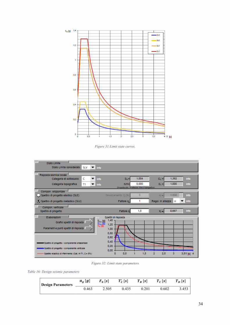
34
Figure 31:Limit state curves.
Figure 32: Limit state parameters
Table 16: Design seismic parameters
Design Parameters 𝒂𝒈 [𝒈] 𝑭𝟎 [𝒔] 𝑻𝑪
∗ [𝒔] 𝑻𝑩 [𝒔] 𝑻𝑪 [𝒔] 𝑻𝑫 [𝒔]
0.463 2.505 0.435 0.201 0.602 3.453
35
2.6. TEMPERATURE EFFECT
Daily and seasonal variations in outdoor temperature, sun radiation and convection lead to variations in the temperature distribution in the individual structural elements.
The severity of thermal actions is generally influenced by several factors, such as the climatic conditions of the site, exposure, the overall mass of the structure and the possible presence of insulating non-structural elements.
2.6.1. UNIFORM THERMAL VARIATION
The uniform temperature component depends of course on the minimum and maximum temperature which the bridge achieves. Following the European standard EN 1991-1-5, which describes that the temperature variation of a composite deck, i.e. of type 2, the maximum and minimum values can be defined as:
𝑇𝑒,𝑚𝑎𝑥 = 𝑇𝑚𝑎𝑥 + 4 = 41,5 + 4 = 45,5°𝐶.
𝑇𝑒,𝑚𝑖𝑛 = 𝑇𝑚𝑖𝑛 + 4 = −4,1 + 4 = 0,1°𝐶.
36
2.7. SHRINKAGE EFFECTS
Shrinkage and creep, as we know, are time-dependent characteristics of concrete. The effects could generally be taken into account for the verification of SLS. Of course, when they are considered, should be evaluated under the quasi-permanent combination of the design situation considered.
The parameters for axial deformation due to shrinkage of the concrete slab are indicated and described in Eurocode 2, EN 1992-1.
Now, the parameters are evaluated.
𝐴𝑐 = 𝑐𝑜𝑛𝑐𝑟𝑒𝑡𝑒 𝑐𝑟𝑜𝑠𝑠 − 𝑠𝑒𝑐𝑡𝑖𝑜𝑛𝑎𝑙 𝑎𝑟𝑒𝑎 = 3999999,99 𝑚𝑚2.
𝑢 = 𝑒𝑥𝑝𝑜𝑠𝑒𝑑 𝑝𝑒𝑟𝑖𝑚𝑒𝑡𝑒𝑟 = 28000,00 𝑚𝑚.
ℎ0 = 𝑛𝑜𝑡𝑖𝑜𝑛𝑎𝑙 𝑠𝑖𝑧𝑒 = 2 ∙𝐴𝑐
𝑢= 285,71𝑚𝑚.
𝐸𝑐𝑚 = 𝑌𝑜𝑢𝑛𝑔 𝑚𝑜𝑑𝑢𝑙𝑢𝑠 𝑜𝑓 𝑐𝑜𝑛𝑐𝑟𝑒𝑡𝑒 = 22000 (𝑓𝑐𝑚
10)
0,3
= 34330,8 𝑁/𝑚𝑚2.
𝐸𝑠 = 𝑌𝑜𝑢𝑛𝑔 𝑚𝑜𝑑𝑢𝑙𝑢𝑠 𝑜𝑓 𝑠𝑡𝑒𝑒𝑙 = 210000 𝑁/𝑚𝑚2.
2.7.1. RHEOLOGIC EFFECTS Rheologic effects depend on the ambient humidity, dimension of the element and concrete composition, such as defined above. Creep is also influence by the degree of maturation of concrete when the load will be applied and of course on its magnitude.
It is useful introduce a creep coefficient 𝜑(𝑡, 𝑡0) related to concrete young modulus tangent, 𝐸𝑐 = 1,05 𝐸𝑐𝑚 .
2.7.2. TIME AND ENVIRONMENT 𝑡0 = 2 𝑑. Represents the beginning of drying creep
𝑡0 = 28 𝑑. It defines the day of permanent loads application
𝑡0 = 2 𝑑. It defines the day of shrinkage application
𝑡 = 𝑉𝑁 = 100 𝑦 = 36525 𝑑.
In this specific analysis will be considered a relative humidity equal to 75%, 𝑅𝐻 = 75%.
2.7.3. ELASTIC MODULUS The phenomenon of viscosity has the effect of increasing deformation over time caused by a load kept constant for a long period. However, the viscous deformations occur without changing the stress state. The phenomenon of viscosity is assimilated to a fictitious decrease in the modulus of elasticity of the concrete over time (in reality, the mechanical characteristics of the concrete improve over time so that the modulus of elasticity, understood as the ratio of stress to deformation under a short duration load, increases over time). The modulus of elasticity therefore goes from the initial value at the instant t0 of application of the load to the conventional final value at time t.
So, the variation of the modulus of elasticity with time can be estimated by:
𝐸𝑐𝑚(𝑡) = (𝑓𝑐𝑚(𝑡)
𝑓𝑐𝑚
)
0,3
𝐸𝑐𝑚
37
2.7.4. SHRINKAGE EVALUATION The total shrinkage strain is composed of two elements, the drying and autogenous strain. The drying shrinkage develops slowly, since it starts the migration of water through the concrete. Instead, the autogenous shrinkage strain develops during the hardening phase of concrete, after some days of concrete casting. The last one is a linear function of concrete strength and should be considered when the new added concrete is cast against hardened one.
𝜀𝑐𝑠 = 𝜀𝑐𝑑 + 𝜀𝑐𝑎
Where,
𝜀𝑐𝑠, is the total shrinkage strain.
𝜀𝑐𝑑, is the drying shrinkage strain.
𝜀𝑐𝑎, is the autogenous shrinkage strain.
The development of the drying shrinkage strain follows from:
𝜀𝑐𝑑(𝑡) = 𝛽𝑑𝑠(𝑡, 𝑡𝑠) ∙ 𝑘ℎ ∙ 𝜀𝑐𝑑,0
Where,
𝑘ℎ is a coefficient depending on the notional size. This case it is 0,78.
𝑡 is the age of concrete at the moment considered.
𝑡𝑠 is the age of the concrete at the beginning of drying shrinkage.
The autogenous shrinkage strain is defined as:
𝜀𝑐𝑎 = 𝛽𝑎𝑠(𝑡)𝜀𝑐𝑎(∞)
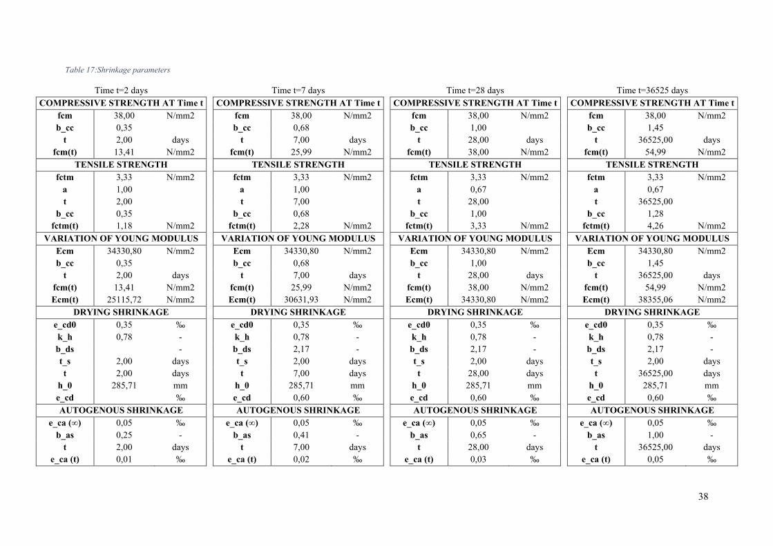
38
Table 17:Shrinkage parameters
Time t=2 days Time t=7 days Time t=28 days Time t=36525 days COMPRESSIVE STRENGTH AT Time t COMPRESSIVE STRENGTH AT Time t COMPRESSIVE STRENGTH AT Time t COMPRESSIVE STRENGTH AT Time t
fcm 38,00 N/mm2 fcm 38,00 N/mm2 fcm 38,00 N/mm2 fcm 38,00 N/mm2 b_cc 0,35 b_cc 0,68 b_cc 1,00 b_cc 1,45
t 2,00 days t 7,00 days t 28,00 days t 36525,00 days fcm(t) 13,41 N/mm2 fcm(t) 25,99 N/mm2 fcm(t) 38,00 N/mm2 fcm(t) 54,99 N/mm2
TENSILE STRENGTH TENSILE STRENGTH TENSILE STRENGTH TENSILE STRENGTH fctm 3,33 N/mm2 fctm 3,33 N/mm2 fctm 3,33 N/mm2 fctm 3,33 N/mm2
a 1,00 a 1,00 a 0,67 a 0,67 t 2,00 t 7,00 t 28,00 t 36525,00
b_cc 0,35 b_cc 0,68 b_cc 1,00 b_cc 1,28 fctm(t) 1,18 N/mm2 fctm(t) 2,28 N/mm2 fctm(t) 3,33 N/mm2 fctm(t) 4,26 N/mm2
VARIATION OF YOUNG MODULUS VARIATION OF YOUNG MODULUS VARIATION OF YOUNG MODULUS VARIATION OF YOUNG MODULUS Ecm 34330,80 N/mm2 Ecm 34330,80 N/mm2 Ecm 34330,80 N/mm2 Ecm 34330,80 N/mm2 b_cc 0,35 b_cc 0,68 b_cc 1,00 b_cc 1,45
t 2,00 days t 7,00 days t 28,00 days t 36525,00 days fcm(t) 13,41 N/mm2 fcm(t) 25,99 N/mm2 fcm(t) 38,00 N/mm2 fcm(t) 54,99 N/mm2 Ecm(t) 25115,72 N/mm2 Ecm(t) 30631,93 N/mm2 Ecm(t) 34330,80 N/mm2 Ecm(t) 38355,06 N/mm2
DRYING SHRINKAGE DRYING SHRINKAGE DRYING SHRINKAGE DRYING SHRINKAGE e_cd0 0,35 ‰ e_cd0 0,35 ‰ e_cd0 0,35 ‰ e_cd0 0,35 ‰ k_h 0,78 - k_h 0,78 - k_h 0,78 - k_h 0,78 - b_ds - b_ds 2,17 - b_ds 2,17 - b_ds 2,17 - t_s 2,00 days t_s 2,00 days t_s 2,00 days t_s 2,00 days t 2,00 days t 7,00 days t 28,00 days t 36525,00 days
h_0 285,71 mm h_0 285,71 mm h_0 285,71 mm h_0 285,71 mm e_cd ‰ e_cd 0,60 ‰ e_cd 0,60 ‰ e_cd 0,60 ‰ AUTOGENOUS SHRINKAGE AUTOGENOUS SHRINKAGE AUTOGENOUS SHRINKAGE AUTOGENOUS SHRINKAGE
e_ca (∞) 0,05 ‰ e_ca (∞) 0,05 ‰ e_ca (∞) 0,05 ‰ e_ca (∞) 0,05 ‰ b_as 0,25 - b_as 0,41 - b_as 0,65 - b_as 1,00 -
t 2,00 days t 7,00 days t 28,00 days t 36525,00 days e_ca (t) 0,01 ‰ e_ca (t) 0,02 ‰ e_ca (t) 0,03 ‰ e_ca (t) 0,05 ‰
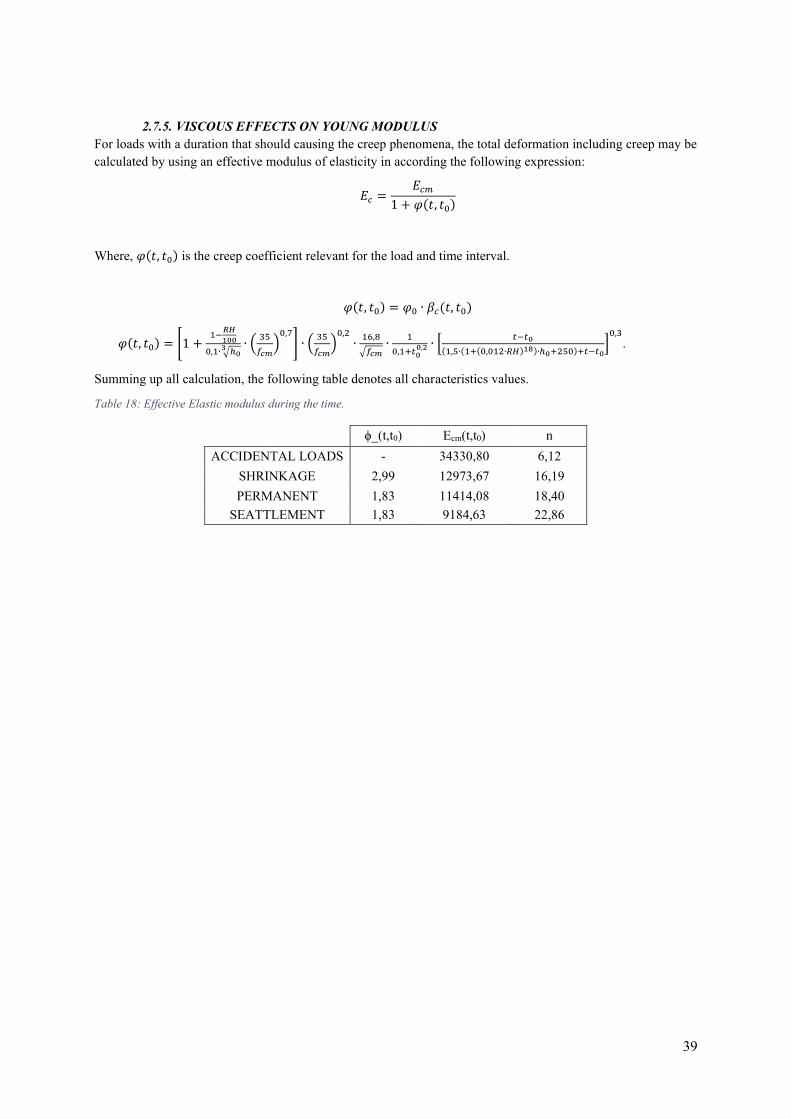
39
2.7.5. VISCOUS EFFECTS ON YOUNG MODULUS For loads with a duration that should causing the creep phenomena, the total deformation including creep may be calculated by using an effective modulus of elasticity in according the following expression:
𝐸𝑐 =𝐸𝑐𝑚
1 + 𝜑(𝑡, 𝑡0)
Where, 𝜑(𝑡, 𝑡0) is the creep coefficient relevant for the load and time interval.
𝜑(𝑡, 𝑡0) = 𝜑0 ∙ 𝛽𝑐(𝑡, 𝑡0)
𝜑(𝑡, 𝑡0) = [1 +1−
𝑅𝐻
100
0,1∙ √ℎ03 ∙ (
35
𝑓𝑐𝑚)
0,7
] ∙ (35
𝑓𝑐𝑚)
0,2
∙16,8
√𝑓𝑐𝑚∙
1
0,1+𝑡00,2 ∙ [
𝑡−𝑡0
(1,5∙(1+(0,012∙𝑅𝐻)18)∙ℎ0+250)+𝑡−𝑡0]
0,3
.
Summing up all calculation, the following table denotes all characteristics values.
Table 18: Effective Elastic modulus during the time.
ϕ_(t,t0) Ecm(t,t0) n ACCIDENTAL LOADS - 34330,80 6,12
SHRINKAGE 2,99 12973,67 16,19 PERMANENT 1,83 11414,08 18,40
SEATTLEMENT 1,83 9184,63 22,86
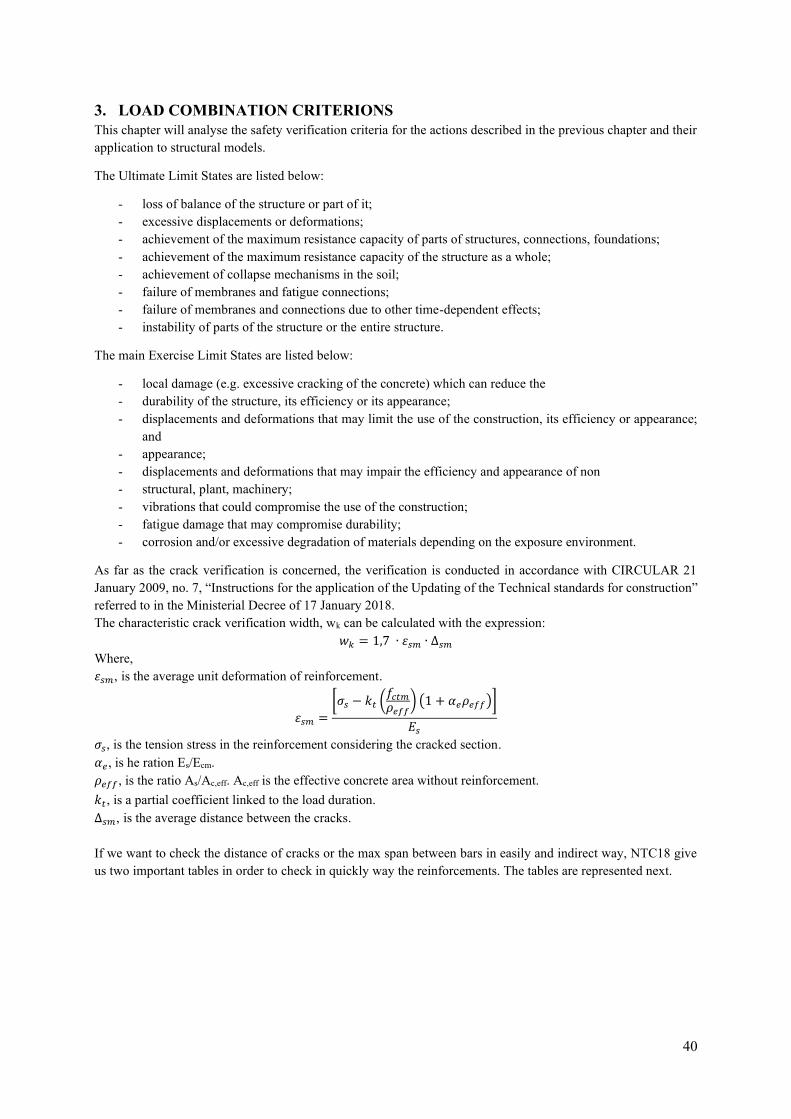
40
3. LOAD COMBINATION CRITERIONS This chapter will analyse the safety verification criteria for the actions described in the previous chapter and their application to structural models.
The Ultimate Limit States are listed below:
- loss of balance of the structure or part of it; - excessive displacements or deformations; - achievement of the maximum resistance capacity of parts of structures, connections, foundations; - achievement of the maximum resistance capacity of the structure as a whole; - achievement of collapse mechanisms in the soil; - failure of membranes and fatigue connections; - failure of membranes and connections due to other time-dependent effects; - instability of parts of the structure or the entire structure.
The main Exercise Limit States are listed below:
- local damage (e.g. excessive cracking of the concrete) which can reduce the - durability of the structure, its efficiency or its appearance; - displacements and deformations that may limit the use of the construction, its efficiency or appearance;
and - appearance; - displacements and deformations that may impair the efficiency and appearance of non - structural, plant, machinery; - vibrations that could compromise the use of the construction; - fatigue damage that may compromise durability; - corrosion and/or excessive degradation of materials depending on the exposure environment.
As far as the crack verification is concerned, the verification is conducted in accordance with CIRCULAR 21 January 2009, no. 7, “Instructions for the application of the Updating of the Technical standards for construction”
referred to in the Ministerial Decree of 17 January 2018. The characteristic crack verification width, wk can be calculated with the expression:
𝑤𝑘 = 1,7 ∙ 𝜀𝑠𝑚 ∙ ∆𝑠𝑚 Where, 𝜀𝑠𝑚, is the average unit deformation of reinforcement.
𝜀𝑠𝑚 =
[𝜎𝑠 − 𝑘𝑡 (𝑓𝑐𝑡𝑚
𝜌𝑒𝑓𝑓) (1 + 𝛼𝑒𝜌𝑒𝑓𝑓)]
𝐸𝑠
𝜎𝑠, is the tension stress in the reinforcement considering the cracked section. 𝛼𝑒, is he ration Es/Ecm. 𝜌𝑒𝑓𝑓 , is the ratio As/Ac,eff. Ac,eff is the effective concrete area without reinforcement. 𝑘𝑡, is a partial coefficient linked to the load duration. ∆𝑠𝑚, is the average distance between the cracks. If we want to check the distance of cracks or the max span between bars in easily and indirect way, NTC18 give us two important tables in order to check in quickly way the reinforcements. The tables are represented next.
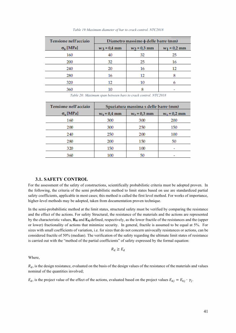
41
Table 19:Maximum diameter of bar to crack control. NTC2018
Table 20: Maximum span between bars to crack control. NTC2018
3.1. SAFETY CONTROL For the assessment of the safety of constructions, scientifically probabilistic criteria must be adopted proven. In the following, the criteria of the semi probabilistic method to limit states based on use are standardized partial safety coefficients, applicable in most cases; this method is called the first level method. For works of importance, higher-level methods may be adopted, taken from documentation proven technique.
In the semi-probabilistic method at the limit states, structural safety must be verified by comparing the resistance and the effect of the actions. For safety Structural, the resistance of the materials and the actions are represented by the characteristic values, Rki and Ekj defined, respectively, as the lower fractile of the resistances and the (upper or lower) fractionality of actions that minimize security. In general, fractile is assumed to be equal at 5%. For sizes with small coefficients of variation, i.e. for sizes that do not concern univocally resistances or actions, can be considered fractile of 50% (median). The verification of the safety regarding the ultimate limit states of resistance is carried out with the “method of the partial coefficients” of safety expressed by the formal equation:
𝑅𝑑 ≥ 𝐸𝑑
Where,
𝑅𝑑, is the design resistance, evaluated on the basis of the design values of the resistance of the materials and values nominal of the quantities involved;
𝐸𝑑, is the project value of the effect of the actions, evaluated based on the project values 𝐸𝑑𝑗 = 𝐸𝑘𝑗 ∙ 𝛾𝑗.
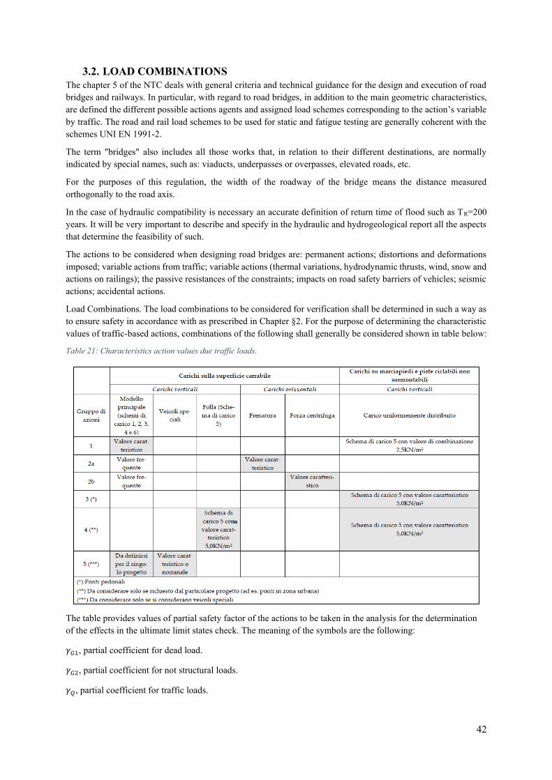
42
3.2. LOAD COMBINATIONS The chapter 5 of the NTC deals with general criteria and technical guidance for the design and execution of road bridges and railways. In particular, with regard to road bridges, in addition to the main geometric characteristics, are defined the different possible actions agents and assigned load schemes corresponding to the action’s variable
by traffic. The road and rail load schemes to be used for static and fatigue testing are generally coherent with the schemes UNI EN 1991-2.
The term "bridges" also includes all those works that, in relation to their different destinations, are normally indicated by special names, such as: viaducts, underpasses or overpasses, elevated roads, etc.
For the purposes of this regulation, the width of the roadway of the bridge means the distance measured orthogonally to the road axis.
In the case of hydraulic compatibility is necessary an accurate definition of return time of flood such as TR=200 years. It will be very important to describe and specify in the hydraulic and hydrogeological report all the aspects that determine the feasibility of such.
The actions to be considered when designing road bridges are: permanent actions; distortions and deformations imposed; variable actions from traffic; variable actions (thermal variations, hydrodynamic thrusts, wind, snow and actions on railings); the passive resistances of the constraints; impacts on road safety barriers of vehicles; seismic actions; accidental actions.
Load Combinations. The load combinations to be considered for verification shall be determined in such a way as to ensure safety in accordance with as prescribed in Chapter §2. For the purpose of determining the characteristic values of traffic-based actions, combinations of the following shall generally be considered shown in table below:
Table 21: Characteristics action values due traffic loads.
The table provides values of partial safety factor of the actions to be taken in the analysis for the determination of the effects in the ultimate limit states check. The meaning of the symbols are the following:
𝛾𝐺1, partial coefficient for dead load.
𝛾𝐺2, partial coefficient for not structural loads.
𝛾𝑄, partial coefficient for traffic loads.
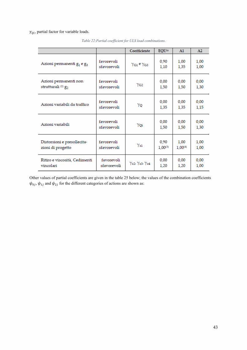
43
𝛾𝑄𝑖 , partial factor for variable loads.
Table 22:Partial coefficient for ULS load combinations.
Other values of partial coefficients are given in the table 25 below; the values of the combination coefficients 𝜓0𝑗, 𝜓1𝑗 and 𝜓2𝑗 for the different categories of actions are shown as:
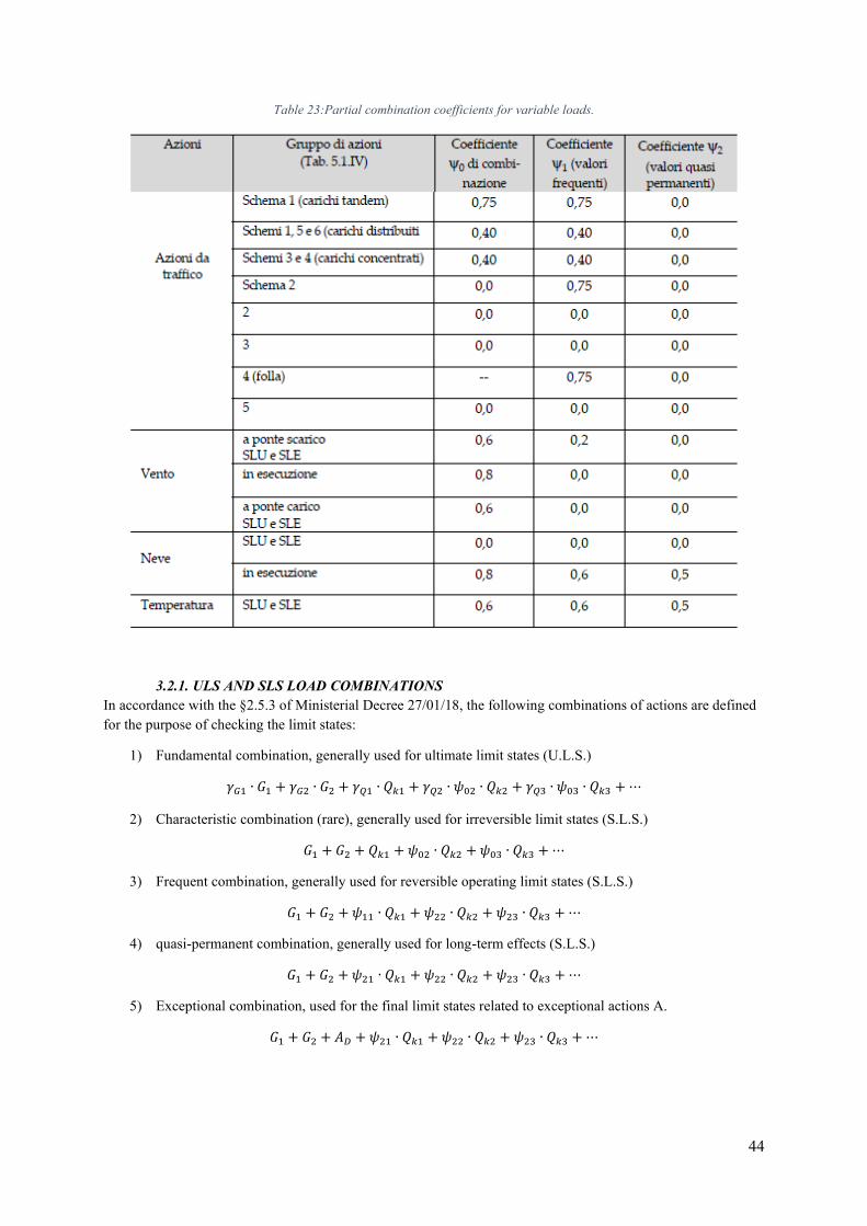
44
Table 23:Partial combination coefficients for variable loads.
3.2.1. ULS AND SLS LOAD COMBINATIONS In accordance with the §2.5.3 of Ministerial Decree 27/01/18, the following combinations of actions are defined for the purpose of checking the limit states:
1) Fundamental combination, generally used for ultimate limit states (U.L.S.)
𝛾𝐺1 ∙ 𝐺1 + 𝛾𝐺2 ∙ 𝐺2 + 𝛾𝑄1 ∙ 𝑄𝑘1 + 𝛾𝑄2 ∙ 𝜓02 ∙ 𝑄𝑘2 + 𝛾𝑄3 ∙ 𝜓03 ∙ 𝑄𝑘3 + ⋯
2) Characteristic combination (rare), generally used for irreversible limit states (S.L.S.)
𝐺1 + 𝐺2 + 𝑄𝑘1 + 𝜓02 ∙ 𝑄𝑘2 + 𝜓03 ∙ 𝑄𝑘3 + ⋯
3) Frequent combination, generally used for reversible operating limit states (S.L.S.)
𝐺1 + 𝐺2 + 𝜓11 ∙ 𝑄𝑘1 + 𝜓22 ∙ 𝑄𝑘2 + 𝜓23 ∙ 𝑄𝑘3 + ⋯
4) quasi-permanent combination, generally used for long-term effects (S.L.S.)
𝐺1 + 𝐺2 + 𝜓21 ∙ 𝑄𝑘1 + 𝜓22 ∙ 𝑄𝑘2 + 𝜓23 ∙ 𝑄𝑘3 + ⋯
5) Exceptional combination, used for the final limit states related to exceptional actions A.
𝐺1 + 𝐺2 + 𝐴𝐷 + 𝜓21 ∙ 𝑄𝑘1 + 𝜓22 ∙ 𝑄𝑘2 + 𝜓23 ∙ 𝑄𝑘3 + ⋯
45
3.2.2. SEISMIC LOAD COMBINATIONS The reference linear analysis method to determine the effects of seismic action on both dissipative systems both on non-dissipative systems, is modal analysis with response spectrum or dynamic linear analysis. The linear dynamic analysis consists on:
- determining the vibration modes of the construction (modal analysis); - calculation of the effects of seismic action, represented by the design response spectrum, for each of the
modes of vibration detected; - combination of these effects.
All modes with significant participating mass must be considered. It is appropriate in this respect consider all modes with a participating mass greater than 5% and in any case a number of modes whose mass total participant is more than 85%.
The checks on the final or operating limit states must be carried out for the combination of the seismic actions with the other actions, as suggested by the technical regulations:
𝐺1 + 𝐺2 + 𝐸 + ∑ 𝜓2𝑗 ∙ 𝑄𝑘𝑗
The effects of seismic action will be evaluated taking into account the masses associated with the following gravitational loads:
𝐺1 + 𝐺2 + ∑ 𝜓2𝑗 ∙ 𝑄𝑘𝑗
Using the Advance design calculation program, the following seismic load combinations have been defined according to Newmark's coefficients:
1) 1,00 ∙ 𝐸𝑥 + 0,30 ∙ 𝐸𝑦 + 0,30 ∙ 𝐸𝑧 . Longitudinal actions as dominant. 2) 0,30 ∙ 𝐸𝑥 + 1,00 ∙ 𝐸𝑦 + 0,30 ∙ 𝐸𝑧 . Transversal actions as dominant. 3) 0,30 ∙ 𝐸𝑥 + 0,30 ∙ 𝐸𝑦 + 1,00 ∙ 𝐸𝑧 . Vertical actions as dominant.
46
3.2.3. GENERAL STRUCTURAL MODEL The stress calculation was carried out using the finite element code provide by Advance Design. The entire structure was discretized into a surface and plate elements. The stress analysis was carried out in several distinct phases.
Phase 1. Stress analysis by steel own weight and slab own weight; in the beam frame the inertia of the longitudinal and transoms only was considered.
Phase 2. Analysis of stresses due to permanent loads; in the frame girders the contribution of the inertia of the reinforced concrete slab to the longitudinal beams was considered, with homogenisation coefficient n=18,40.
Phase 2b. Analysis of stresses due to loads due to shrinkage; the contribution of the inertia of the reinforced concrete slab to the longitudinal beams was considered in the lattice girders, with homogenisation coefficient n=16,19.
Phase 2c. Analysis of stresses induced by differential failure; in the lattice girders the contribution of the inertia of the AC slab to the longitudinal beams was considered, with homogenisation coefficient n=22,86.
Phase 3. Analysis of stresses due to accidental loads (vehicles, crowd, wind); the contribution of the inertia of the reinforced concrete slab to the longitudinal beams was considered in the lattice girders, with homogenisation coefficient n=6,12.
Phase 3f. Analysis of stresses due to accidental fatigue loads; the contribution of the inertia of the reinforced concrete slab to the longitudinal beams was considered in the lattice girders, with homogenization coefficient n=6,12.
Seismic phase. Analysis of stresses due to seismic loads; the contribution of the inertia of the reinforced concrete slab to the longitudinal beams has been considered in the lattice girders, with homogenization coefficient n=6,12. The modal analysis was carried out with reference to the three main directions, with the X and Y axes coinciding respectively with the longitudinal and transversal direction of the decks, and the Z axis coinciding with the vertical direction. The modal combinations were performed with the CQC rule.
Deformation phase. Analysis of the upper bracing by own weight steel and slab; in the frame girders the inertia of the longitudinal and cross beams only was considered.
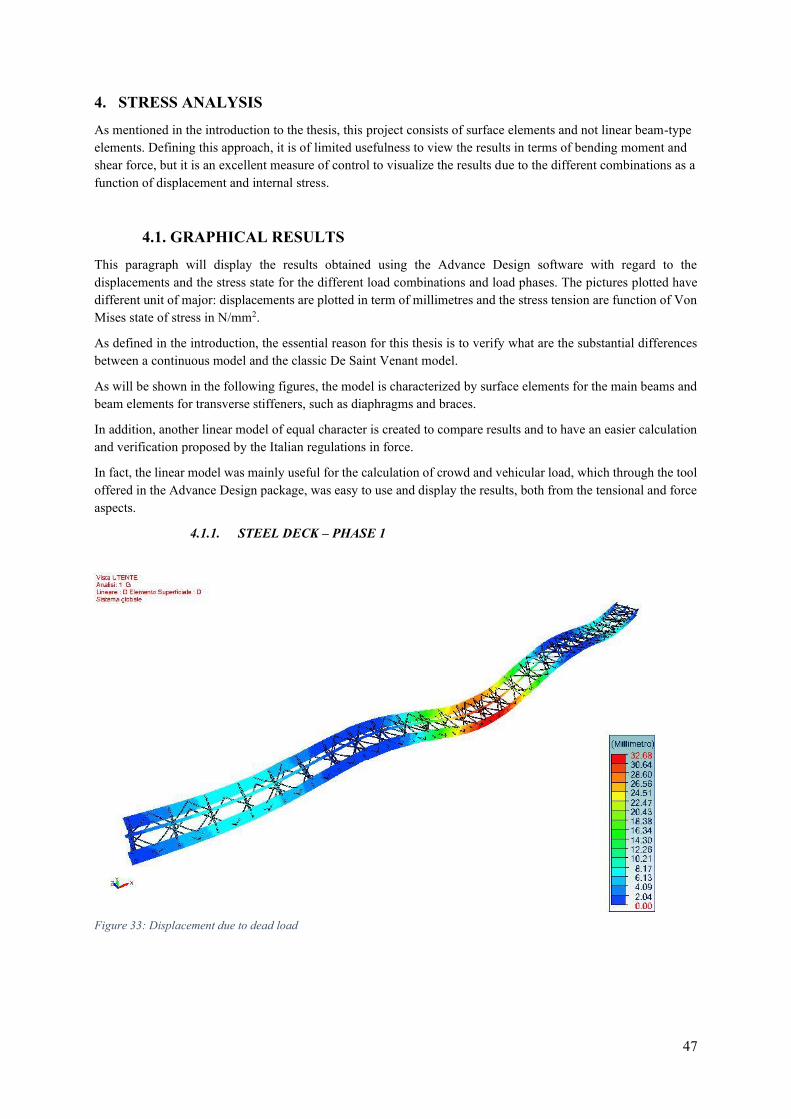
47
4. STRESS ANALYSIS
As mentioned in the introduction to the thesis, this project consists of surface elements and not linear beam-type elements. Defining this approach, it is of limited usefulness to view the results in terms of bending moment and shear force, but it is an excellent measure of control to visualize the results due to the different combinations as a function of displacement and internal stress.
4.1. GRAPHICAL RESULTS
This paragraph will display the results obtained using the Advance Design software with regard to the displacements and the stress state for the different load combinations and load phases. The pictures plotted have different unit of major: displacements are plotted in term of millimetres and the stress tension are function of Von Mises state of stress in N/mm2.
As defined in the introduction, the essential reason for this thesis is to verify what are the substantial differences between a continuous model and the classic De Saint Venant model.
As will be shown in the following figures, the model is characterized by surface elements for the main beams and beam elements for transverse stiffeners, such as diaphragms and braces.
In addition, another linear model of equal character is created to compare results and to have an easier calculation and verification proposed by the Italian regulations in force.
In fact, the linear model was mainly useful for the calculation of crowd and vehicular load, which through the tool offered in the Advance Design package, was easy to use and display the results, both from the tensional and force aspects.
4.1.1. STEEL DECK – PHASE 1
Figure 33: Displacement due to dead load
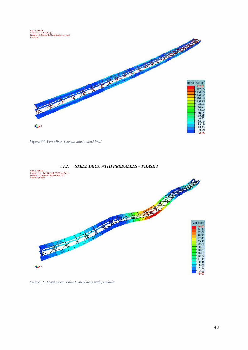
48
Figure 34: Von Mises Tension due to dead load
4.1.2. STEEL DECK WITH PREDALLES – PHASE 1
Figure 35: Displacement due to steel deck with predalles
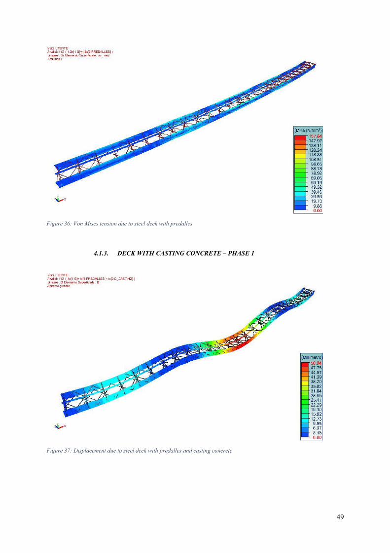
49
Figure 36: Von Mises tension due to steel deck with predalles
4.1.3. DECK WITH CASTING CONCRETE – PHASE 1
Figure 37: Displacement due to steel deck with predalles and casting concrete
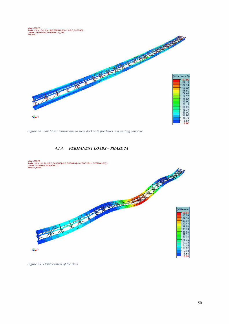
50
Figure 38: Von Mises tension due to steel deck with predalles and casting concrete
4.1.4. PERMANENT LOADS – PHASE 2A
Figure 39: Displacement of the deck
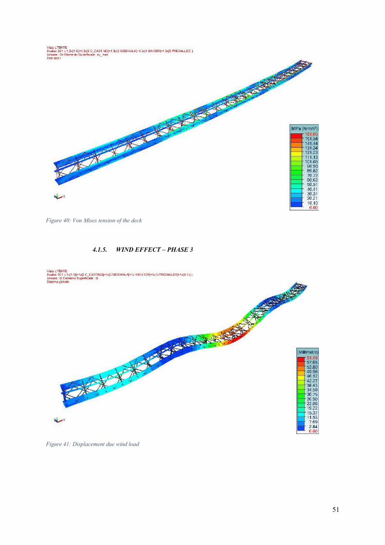
51
Figure 40: Von Mises tension of the deck
4.1.5. WIND EFFECT – PHASE 3
Figure 41: Displacement due wind load
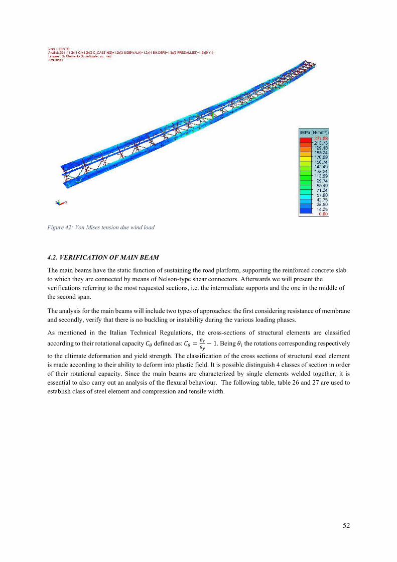
52
Figure 42: Von Mises tension due wind load
4.2. VERIFICATION OF MAIN BEAM
The main beams have the static function of sustaining the road platform, supporting the reinforced concrete slab to which they are connected by means of Nelson-type shear connectors. Afterwards we will present the verifications referring to the most requested sections, i.e. the intermediate supports and the one in the middle of the second span.
The analysis for the main beams will include two types of approaches: the first considering resistance of membrane and secondly, verify that there is no buckling or instability during the various loading phases.
As mentioned in the Italian Technical Regulations, the cross-sections of structural elements are classified according to their rotational capacity 𝐶𝜃 defined as: 𝐶𝜃 =
𝜃𝑟
𝜃𝑦− 1. Being 𝜃𝑖 the rotations corresponding respectively
to the ultimate deformation and yield strength. The classification of the cross sections of structural steel element is made according to their ability to deform into plastic field. It is possible distinguish 4 classes of section in order of their rotational capacity. Since the main beams are characterized by single elements welded together, it is essential to also carry out an analysis of the flexural behaviour. The following table, table 26 and 27 are used to establish class of steel element and compression and tensile width.
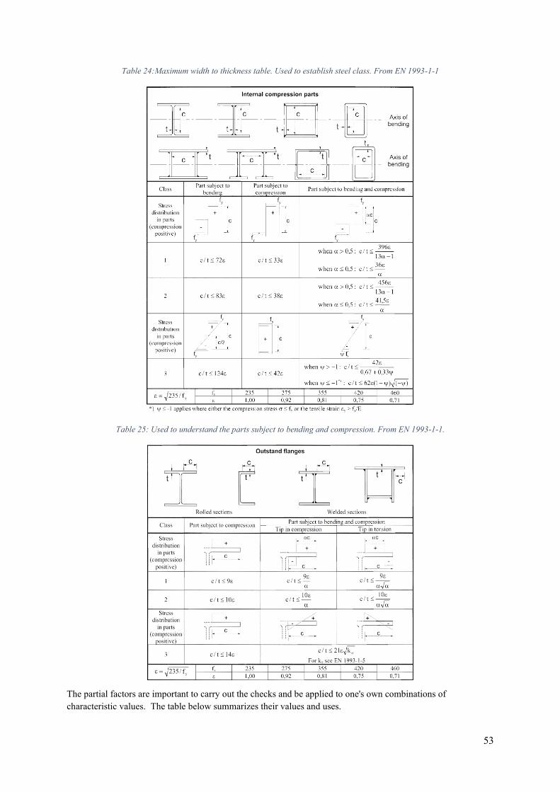
53
Table 24:Maximum width to thickness table. Used to establish steel class. From EN 1993-1-1
Table 25: Used to understand the parts subject to bending and compression. From EN 1993-1-1.
The partial factors are important to carry out the checks and be applied to one's own combinations of characteristic values. The table below summarizes their values and uses.
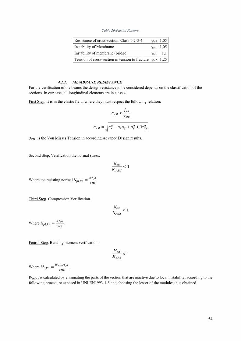
54
Table 26:Partial Factors.
Resistance of cross-section. Class 1-2-3-4 M0 1,05 Instability of Membrane M1 1,05 Instability of membrane (bridge) M1 1,1 Tension of cross-section in tension to fracture M2 1,25
4.2.1. MEMBRANE RESISTANCE For the verification of the beams the design resistance to be considered depends on the classification of the sections. In our case, all longitudinal elements are in class 4.
First Step. It is in the elastic field, where they must respect the following relation:
𝜎𝑉𝑀 <𝑓𝑦𝑘
𝛾𝑀0
𝜎𝑉𝑀 = √𝜎𝑥2 − 𝜎𝑥𝜎𝑦 + 𝜎𝑦
2 + 3𝜏𝑥𝑦2
𝜎𝑉𝑀, is the Von Misses Tension in according Advance Design results.
Second Step. Verification the normal stress.
𝑁𝑒𝑑
𝑁𝑝𝑙,𝑅𝑑
< 1
Where the resisting normal 𝑁𝑝𝑙,𝑅𝑑 =𝐴∙𝑓𝑦𝑘
𝛾𝑀0.
Third Step. Compression Verification.
𝑁𝑒𝑑
𝑁𝑐,𝑅𝑑
< 1
Where 𝑁𝑝𝑙,𝑅𝑑 =𝐴∙𝑓𝑦𝑘
𝛾𝑀0
.
Fourth Step. Bending moment verification.
𝑀𝑒𝑑
𝑀𝑐,𝑅𝑑
< 1
Where 𝑀𝑐,𝑅𝑑 =𝑊𝑚𝑖𝑛∙𝑓𝑦𝑘
𝛾𝑀0.
𝑊𝑚𝑖𝑛, is calculated by eliminating the parts of the section that are inactive due to local instability, according to the following procedure exposed in UNI EN1993-1-5 and choosing the lesser of the modules thus obtained.
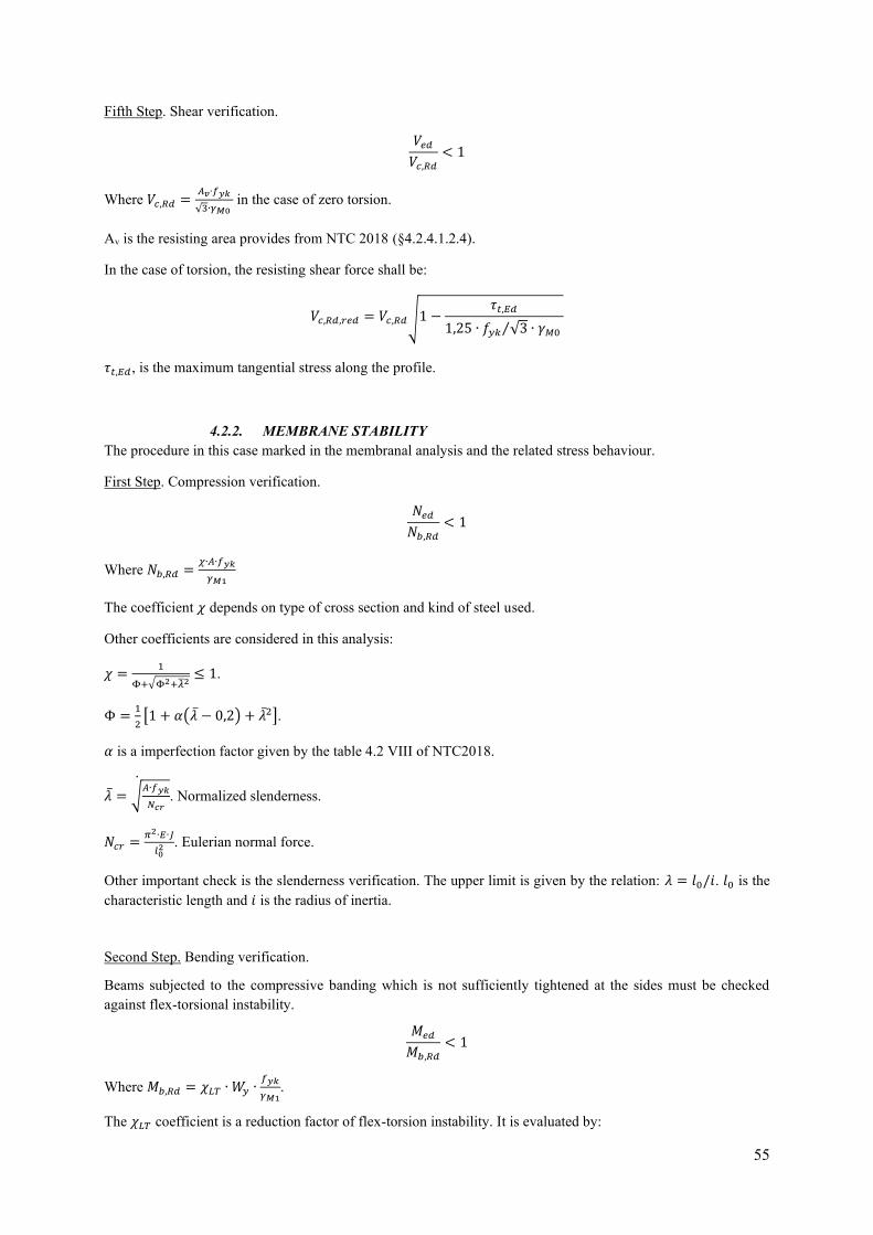
55
Fifth Step. Shear verification.
𝑉𝑒𝑑
𝑉𝑐,𝑅𝑑
< 1
Where 𝑉𝑐,𝑅𝑑 =𝐴𝑣∙𝑓𝑦𝑘
√3∙𝛾𝑀0
in the case of zero torsion.
Av is the resisting area provides from NTC 2018 (§4.2.4.1.2.4).
In the case of torsion, the resisting shear force shall be:
𝑉𝑐,𝑅𝑑,𝑟𝑒𝑑 = 𝑉𝑐,𝑅𝑑√1 −𝜏𝑡,𝐸𝑑
1,25 ∙ 𝑓𝑦𝑘 √3 ∙ 𝛾𝑀0 ⁄
𝜏𝑡,𝐸𝑑, is the maximum tangential stress along the profile.
4.2.2. MEMBRANE STABILITY The procedure in this case marked in the membranal analysis and the related stress behaviour.
First Step. Compression verification.
𝑁𝑒𝑑
𝑁𝑏,𝑅𝑑
< 1
Where 𝑁𝑏,𝑅𝑑 =𝜒∙𝐴∙𝑓𝑦𝑘
𝛾𝑀1
The coefficient 𝜒 depends on type of cross section and kind of steel used.
Other coefficients are considered in this analysis:
𝜒 =1
Φ+√Φ2+𝜆2≤ 1.
Φ =1
2[1 + 𝛼(𝜆 − 0,2) + 𝜆2].
𝛼 is a imperfection factor given by the table 4.2 VIII of NTC2018.
𝜆 = √𝐴∙𝑓𝑦𝑘
𝑁𝑐𝑟
. Normalized slenderness.
𝑁𝑐𝑟 =𝜋2∙𝐸∙𝐽
𝑙02 . Eulerian normal force.
Other important check is the slenderness verification. The upper limit is given by the relation: 𝜆 = 𝑙0/𝑖. 𝑙0 is the characteristic length and 𝑖 is the radius of inertia.
Second Step. Bending verification.
Beams subjected to the compressive banding which is not sufficiently tightened at the sides must be checked against flex-torsional instability.
𝑀𝑒𝑑
𝑀𝑏,𝑅𝑑
< 1
Where 𝑀𝑏,𝑅𝑑 = 𝜒𝐿𝑇 ∙ 𝑊𝑦 ∙𝑓𝑦𝑘
𝛾𝑀1.
The 𝜒𝐿𝑇 coefficient is a reduction factor of flex-torsion instability. It is evaluated by:
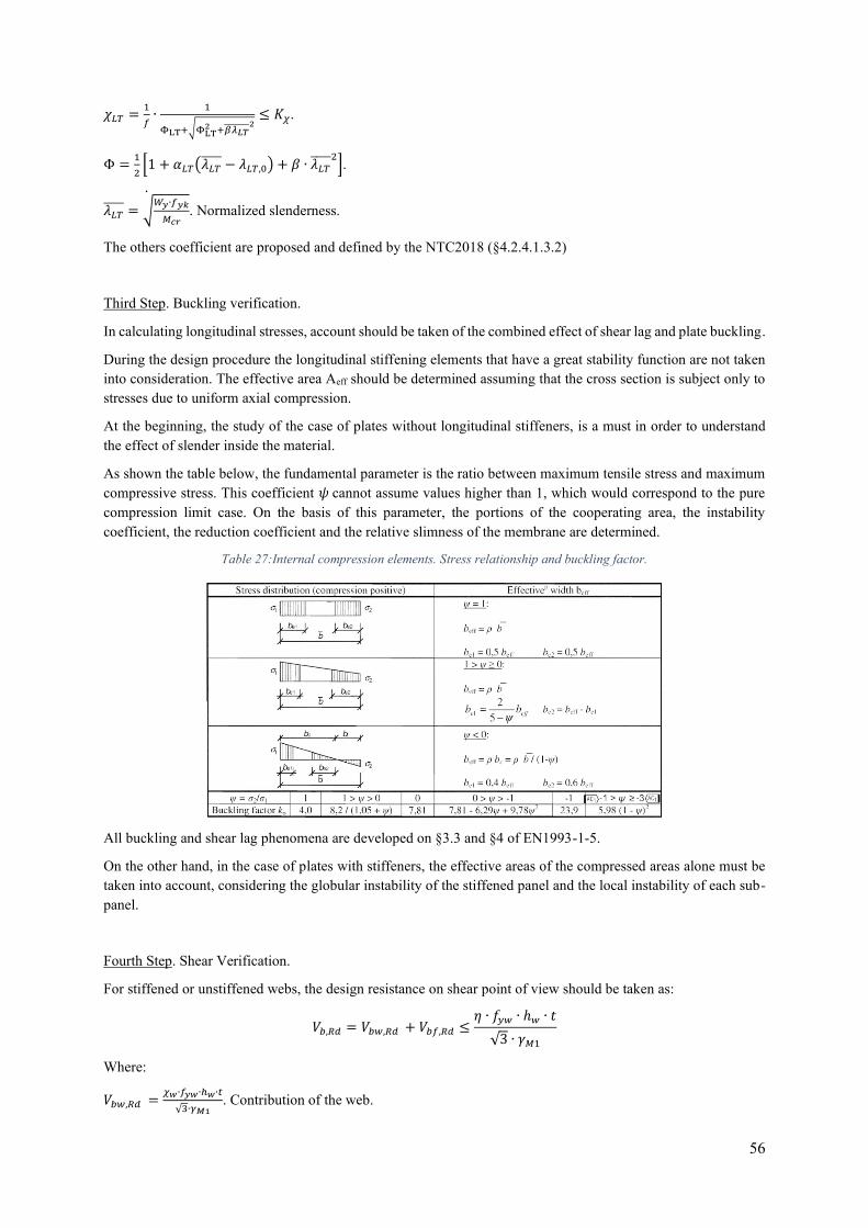
56
𝜒𝐿𝑇 =1
𝑓∙
1
ΦLT+√ΦLT2 +𝛽𝜆𝐿𝑇 2
≤ 𝐾𝜒.
Φ =1
2[1 + 𝛼𝐿𝑇(𝜆𝐿𝑇
− 𝜆𝐿𝑇,0) + 𝛽 ∙ 𝜆𝐿𝑇 2
].
𝜆𝐿𝑇 = √
𝑊𝑦∙𝑓𝑦𝑘
𝑀𝑐𝑟
. Normalized slenderness.
The others coefficient are proposed and defined by the NTC2018 (§4.2.4.1.3.2)
Third Step. Buckling verification.
In calculating longitudinal stresses, account should be taken of the combined effect of shear lag and plate buckling.
During the design procedure the longitudinal stiffening elements that have a great stability function are not taken into consideration. The effective area Aeff should be determined assuming that the cross section is subject only to stresses due to uniform axial compression.
At the beginning, the study of the case of plates without longitudinal stiffeners, is a must in order to understand the effect of slender inside the material.
As shown the table below, the fundamental parameter is the ratio between maximum tensile stress and maximum compressive stress. This coefficient 𝜓 cannot assume values higher than 1, which would correspond to the pure compression limit case. On the basis of this parameter, the portions of the cooperating area, the instability coefficient, the reduction coefficient and the relative slimness of the membrane are determined.
Table 27:Internal compression elements. Stress relationship and buckling factor.
All buckling and shear lag phenomena are developed on §3.3 and §4 of EN1993-1-5.
On the other hand, in the case of plates with stiffeners, the effective areas of the compressed areas alone must be taken into account, considering the globular instability of the stiffened panel and the local instability of each sub-panel.
Fourth Step. Shear Verification.
For stiffened or unstiffened webs, the design resistance on shear point of view should be taken as:
𝑉𝑏,𝑅𝑑 = 𝑉𝑏𝑤,𝑅𝑑 + 𝑉𝑏𝑓,𝑅𝑑 ≤𝜂 ∙ 𝑓𝑦𝑤 ∙ ℎ𝑤 ∙ 𝑡
√3 ∙ 𝛾𝑀1
Where:
𝑉𝑏𝑤,𝑅𝑑 =𝜒𝑤∙𝑓𝑦𝑤∙ℎ𝑤∙𝑡
√3∙𝛾𝑀1. Contribution of the web.

57
𝑉𝑏𝑓,𝑅𝑑 =𝑏𝑓∙𝑡𝑓∙
2 𝑓𝑦𝑓
𝑐∙𝛾𝑀1[1 − (
𝑀𝐸𝑑
𝑀𝑓,𝑘 𝛾𝑀0⁄)
2
]. Flange contribution.
The final verification is made by:
𝑉𝐸𝑑
𝑉𝑏,𝑅𝑑
< 1
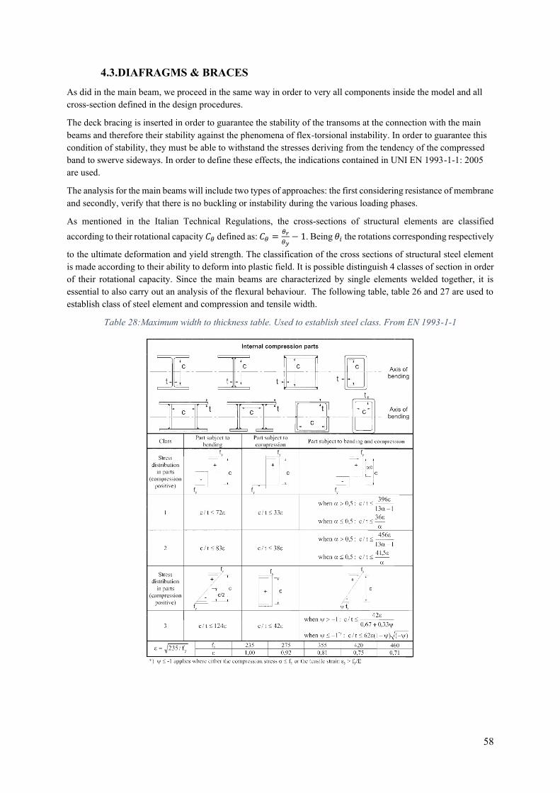
58
4.3.DIAFRAGMS & BRACES
As did in the main beam, we proceed in the same way in order to very all components inside the model and all cross-section defined in the design procedures.
The deck bracing is inserted in order to guarantee the stability of the transoms at the connection with the main beams and therefore their stability against the phenomena of flex-torsional instability. In order to guarantee this condition of stability, they must be able to withstand the stresses deriving from the tendency of the compressed band to swerve sideways. In order to define these effects, the indications contained in UNI EN 1993-1-1: 2005 are used.
The analysis for the main beams will include two types of approaches: the first considering resistance of membrane and secondly, verify that there is no buckling or instability during the various loading phases.
As mentioned in the Italian Technical Regulations, the cross-sections of structural elements are classified according to their rotational capacity 𝐶𝜃 defined as: 𝐶𝜃 =
𝜃𝑟
𝜃𝑦− 1. Being 𝜃𝑖 the rotations corresponding respectively
to the ultimate deformation and yield strength. The classification of the cross sections of structural steel element is made according to their ability to deform into plastic field. It is possible distinguish 4 classes of section in order of their rotational capacity. Since the main beams are characterized by single elements welded together, it is essential to also carry out an analysis of the flexural behaviour. The following table, table 26 and 27 are used to establish class of steel element and compression and tensile width.
Table 28:Maximum width to thickness table. Used to establish steel class. From EN 1993-1-1
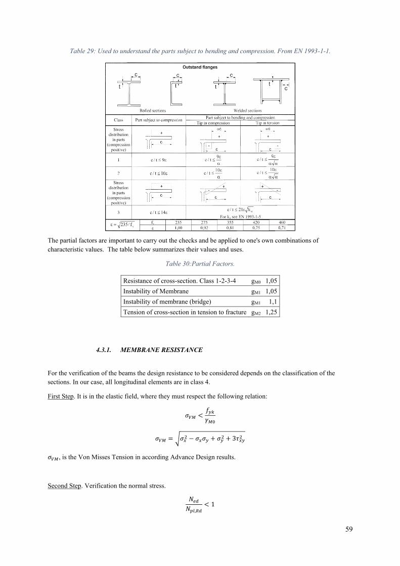
59
Table 29: Used to understand the parts subject to bending and compression. From EN 1993-1-1.
The partial factors are important to carry out the checks and be applied to one's own combinations of characteristic values. The table below summarizes their values and uses.
Table 30:Partial Factors.
Resistance of cross-section. Class 1-2-3-4 gM0 1,05 Instability of Membrane gM1 1,05 Instability of membrane (bridge) gM1 1,1 Tension of cross-section in tension to fracture gM2 1,25
4.3.1. MEMBRANE RESISTANCE
For the verification of the beams the design resistance to be considered depends on the classification of the sections. In our case, all longitudinal elements are in class 4.
First Step. It is in the elastic field, where they must respect the following relation:
𝜎𝑉𝑀 <𝑓𝑦𝑘
𝛾𝑀0
𝜎𝑉𝑀 = √𝜎𝑥2 − 𝜎𝑥𝜎𝑦 + 𝜎𝑦
2 + 3𝜏𝑥𝑦2
𝜎𝑉𝑀, is the Von Misses Tension in according Advance Design results.
Second Step. Verification the normal stress.
𝑁𝑒𝑑
𝑁𝑝𝑙,𝑅𝑑
< 1
60
Where the resisting normal 𝑁𝑝𝑙,𝑅𝑑 =𝐴∙𝑓𝑦𝑘
𝛾𝑀0.
Third Step. Compression Verification.
𝑁𝑒𝑑
𝑁𝑐,𝑅𝑑
< 1
Where 𝑁𝑝𝑙,𝑅𝑑 =𝐴∙𝑓𝑦𝑘
𝛾𝑀0
.
Fourth Step. Bending moment verification.
𝑀𝑒𝑑
𝑀𝑐,𝑅𝑑
< 1
Where 𝑀𝑐,𝑅𝑑 =𝑊𝑚𝑖𝑛∙𝑓𝑦𝑘
𝛾𝑀0.
𝑊𝑚𝑖𝑛, is calculated by eliminating the parts of the section that are inactive due to local instability, according to the following procedure exposed in UNI EN1993-1-5 and choosing the lesser of the modules thus obtained.
4.3.2. MEMBRANE STABILITY The procedure in this case marked in the membranal analysis and the related stress behaviour.
First Step. Compression verification.
𝑁𝑒𝑑
𝑁𝑏,𝑅𝑑
< 1
Where 𝑁𝑏,𝑅𝑑 =𝜒∙𝐴∙𝑓𝑦𝑘
𝛾𝑀1
The coefficient 𝜒 depends on type of cross section and kind of steel used.
Other coefficients are considered in this analysis:
𝜒 =1
Φ+√Φ2+𝜆2≤ 1.
Φ =1
2[1 + 𝛼(𝜆 − 0,2) + 𝜆2].
𝛼 is a imperfection factor given by the table 4.2 VIII of NTC2018.
𝜆 = √𝐴∙𝑓𝑦𝑘
𝑁𝑐𝑟
. Normalized slenderness.
𝑁𝑐𝑟 =𝜋2∙𝐸∙𝐽
𝑙02 . Eulerian normal force.
Other important check is the slenderness verification. The upper limit is given by the relation: 𝜆 = 𝑙0/𝑖. 𝑙0 is the characteristic length and 𝑖 is the radius of inertia.
Second Step. Bending verification.
61
Beams subjected to the compressive banding which is not sufficiently tightened at the sides must be checked against flex-torsional instability.
𝑀𝑒𝑑
𝑀𝑏,𝑅𝑑
< 1
Where 𝑀𝑏,𝑅𝑑 = 𝜒𝐿𝑇 ∙ 𝑊𝑦 ∙𝑓𝑦𝑘
𝛾𝑀1.
The 𝜒𝐿𝑇 coefficient is a reduction factor of flex-torsion instability. It is evaluated by:
𝜒𝐿𝑇 =1
𝑓∙
1
ΦLT+√ΦLT2 +𝛽𝜆𝐿𝑇 2
≤ 𝐾𝜒.
Φ =1
2[1 + 𝛼𝐿𝑇(𝜆𝐿𝑇
− 𝜆𝐿𝑇,0) + 𝛽 ∙ 𝜆𝐿𝑇 2
].
𝜆𝐿𝑇 = √
𝑊𝑦∙𝑓𝑦𝑘
𝑀𝑐𝑟
. Normalized slenderness.
The others coefficient are proposed and defined by the NTC2018 (§4.2.4.1.3.2)
Third Step. Method A of NTC2018
Since we are in a situation of prismatic rods subject to NEd compression and bending moments My,Ed and Mz,Ed agents in the two main planes of inertia, in the presence of constraints that prevent torsional displacement, it will be necessary to check that this equation proposed by the Italian legislation.
𝑁𝐸𝑑 ∙ 𝛾𝑀1
𝜒𝑚𝑖𝑛 ∙ 𝑓𝑦𝑘 ∙ 𝐴+
𝑀𝑦,𝐸𝑑 ∙ 𝛾𝑀1
𝑊𝑦 ∙ 𝑓𝑦𝑘 ∙ (1 −𝑁𝐸𝑑
𝑁𝑐𝑟,𝑦)
+𝑀𝑧,𝐸𝑑 ∙ 𝛾𝑀1
𝑊𝑧 ∙ 𝑓𝑦𝑘 ∙ (1 −𝑁𝐸𝑑
𝑁𝑐𝑟,𝑧)
≤ 1
Where:
𝜒𝑚𝑖𝑛, in the minimum inflection factor related to the main inertial axis.
𝑁𝑐𝑟,𝑦 𝑎𝑛𝑑 𝑁𝑐𝑟,𝑧, Eulerian critic loads related to the own axis.
𝑀𝑦,𝐸𝑑 𝑎𝑛𝑑 𝑀𝑧,𝐸𝑑, equivalent mending moment according to the law.
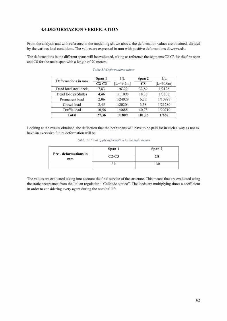
62
4.4.DEFORMAZION VERIFICATION
From the analysis and with reference to the modelling shown above, the deformation values are obtained, divided by the various load conditions. The values are expressed in mm with positive deformations downwards.
The deformations in the different spans will be evaluated, taking as reference the segments C2-C3 for the first span and C8 for the main span with a length of 70 meters.
Table 31:Deformations values
Deformations in mm Span 1 1/L
[L=49,5m] Span 2 1/L
[L=70,0m] C2-C3 C8 Dead load steel deck 7,83 1/6322 32,89 1/2128 Dead load predalles 4,46 1/11098 18.38 1/3808
Permanent load 2,06 1/24029 6,37 1/10989 Crowd load 2,45 1/20204 3,38 1/21280 Traffic load 10,56 1/4688 40,75 1/20710
Total 27,36 1/1809 101,76 1/687
Looking at the results obtained, the deflection that the both spans will have to be paid for in such a way as not to have an excessive future deformation will be:
Table 32:Final apply deformation to the main beams
Pre - deformations in mm
Span 1 Span 2
C2-C3 C8
30 130
The values are evaluated taking into account the final service of the structure. This means that are evaluated using the static acceptance from the Italian regulation: “Collaudo statico”. The loads are multiplying times a coefficient
in order to considering every agent during the nominal life.
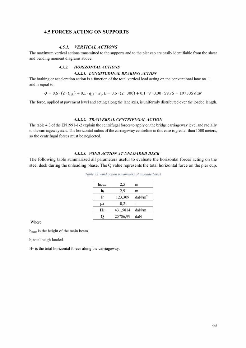
63
4.5.FORCES ACTING ON SUPPORTS
4.5.1. VERTICAL ACTIONS The maximum vertical actions transmitted to the supports and to the pier cap are easily identifiable from the shear and bending moment diagrams above.
4.5.2. HORIZONTAL ACTIONS 4.5.2.1. LONGITUDINAL BRAKING ACTION
The braking or acceleration action is a function of the total vertical load acting on the conventional lane no. 1 and is equal to:
𝑄 = 0,6 ∙ (2 ∙ 𝑄1𝑘) + 0,1 ∙ 𝑞1𝑘 ∙ 𝑤1. 𝐿 = 0,6 ∙ (2 ∙ 300) + 0,1 ∙ 9 ∙ 3,00 ∙ 59,75 = 197335 𝑑𝑎𝑁
The force, applied at pavement level and acting along the lane axis, is uniformly distributed over the loaded length.
4.5.2.2. TRASVERSAL CENTRIFUGAL ACTION The table 4.3 of the EN1991-1-2 explain the centrifugal forces to apply on the bridge carriageway level and radially to the carriageway axis. The horizontal radius of the carriageway centreline in this case is greater than 1500 meters, so the centrifugal forces must be neglected.
4.5.2.3. WIND ACTION AT UNLOADED DECK The following table summarized all parameters useful to evaluate the horizontal forces acting on the steel deck during the unloading phase. The Q value represents the total horizontal force on the pier cup.
Table 33:wind action parameters at unloaded deck
hbeam 2,5 m hi 2,9 m P 123,309 daN/m2 1 0,2 - HT 431,5814 daN/m Q 25786,99 daN
Where:
hbeam is the height of the main beam.
hi total heigh loaded.
HT is the total horizontal forces along the carriageway.

64
4.5.2.4. WIND ACTION AT LOADED DECK As did before for the unloaded case, now the following table explains the parameters used to calculate the total horizontal load acting at the carriageway and oh pier cap.
Table 34:wind action parameters at loaded deck
hbeam 2,5 m hi 5,9 m P 135,7038 daN/m2
m1 0,2 - HT 882,0744 daN/m Q 52703,95 daN
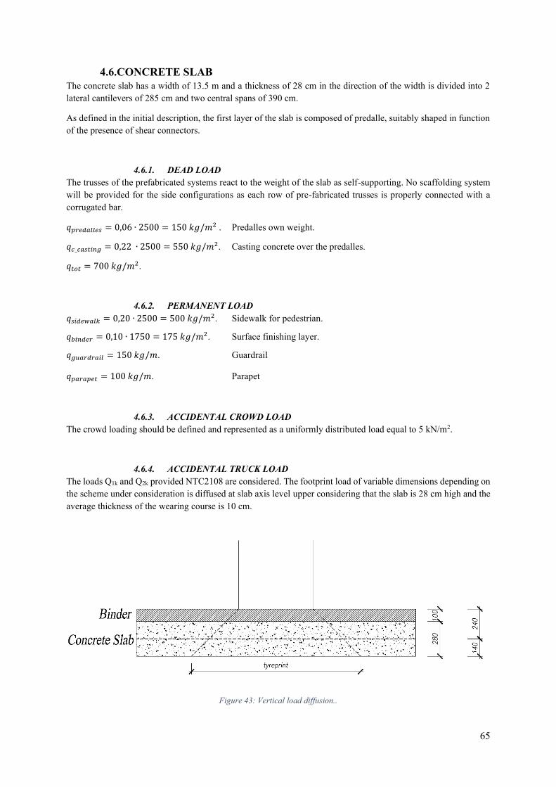
65
4.6.CONCRETE SLAB The concrete slab has a width of 13.5 m and a thickness of 28 cm in the direction of the width is divided into 2 lateral cantilevers of 285 cm and two central spans of 390 cm.
As defined in the initial description, the first layer of the slab is composed of predalle, suitably shaped in function of the presence of shear connectors.
4.6.1. DEAD LOAD The trusses of the prefabricated systems react to the weight of the slab as self-supporting. No scaffolding system will be provided for the side configurations as each row of pre-fabricated trusses is properly connected with a corrugated bar.
𝑞𝑝𝑟𝑒𝑑𝑎𝑙𝑙𝑒𝑠 = 0,06 ∙ 2500 = 150 𝑘𝑔/𝑚2 . Predalles own weight.
𝑞𝑐_𝑐𝑎𝑠𝑡𝑖𝑛𝑔 = 0,22 ∙ 2500 = 550 𝑘𝑔/𝑚2. Casting concrete over the predalles.
𝑞𝑡𝑜𝑡 = 700 𝑘𝑔/𝑚2.
4.6.2. PERMANENT LOAD 𝑞𝑠𝑖𝑑𝑒𝑤𝑎𝑙𝑘 = 0,20 ∙ 2500 = 500 𝑘𝑔/𝑚2. Sidewalk for pedestrian.
𝑞𝑏𝑖𝑛𝑑𝑒𝑟 = 0,10 ∙ 1750 = 175 𝑘𝑔/𝑚2. Surface finishing layer.
𝑞𝑔𝑢𝑎𝑟𝑑𝑟𝑎𝑖𝑙 = 150 𝑘𝑔/𝑚. Guardrail
𝑞𝑝𝑎𝑟𝑎𝑝𝑒𝑡 = 100 𝑘𝑔/𝑚. Parapet
4.6.3. ACCIDENTAL CROWD LOAD The crowd loading should be defined and represented as a uniformly distributed load equal to 5 kN/m2.
4.6.4. ACCIDENTAL TRUCK LOAD The loads Q1k and Q2k provided NTC2108 are considered. The footprint load of variable dimensions depending on the scheme under consideration is diffused at slab axis level upper considering that the slab is 28 cm high and the average thickness of the wearing course is 10 cm.
Figure 43: Vertical load diffusion..
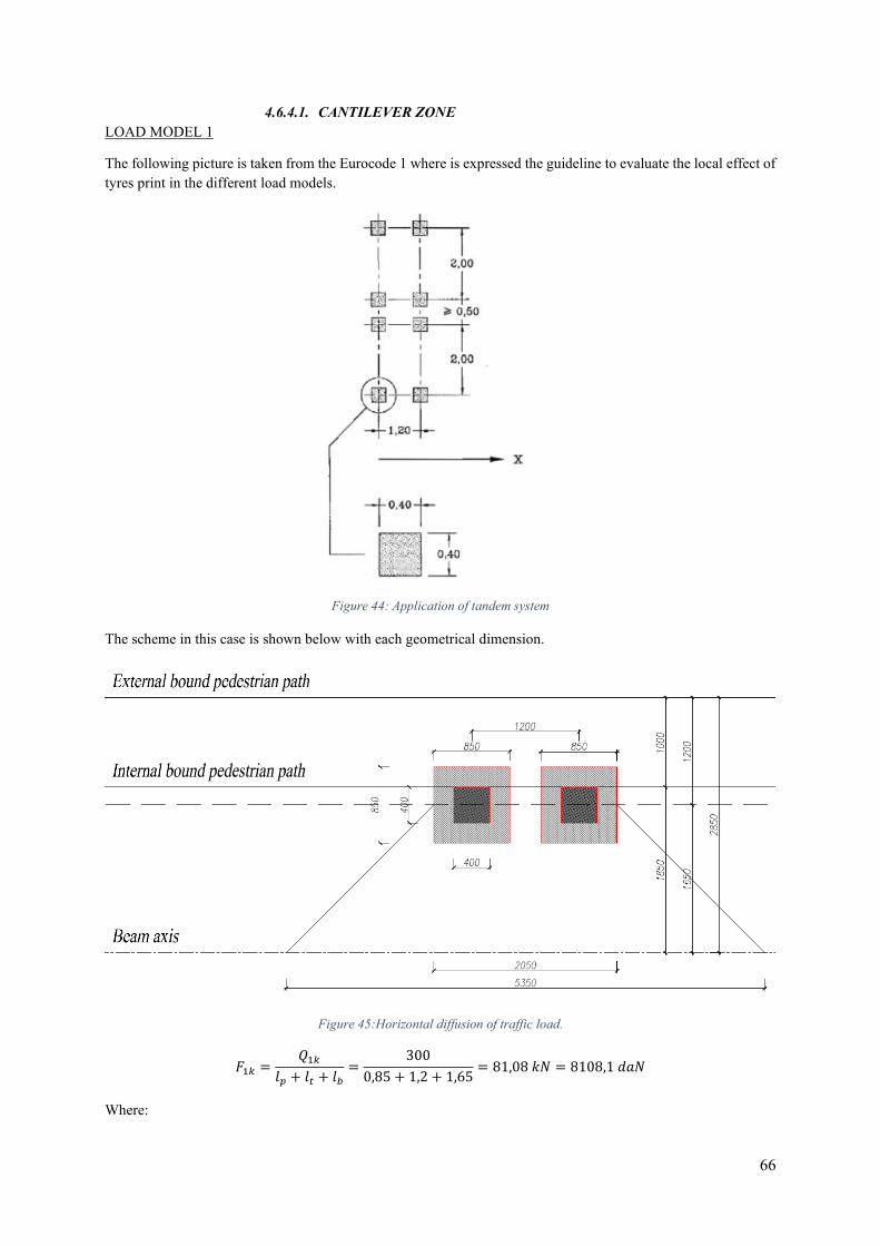
66
4.6.4.1. CANTILEVER ZONE LOAD MODEL 1
The following picture is taken from the Eurocode 1 where is expressed the guideline to evaluate the local effect of tyres print in the different load models.
Figure 44: Application of tandem system
The scheme in this case is shown below with each geometrical dimension.
Figure 45:Horizontal diffusion of traffic load.
𝐹1𝑘 =𝑄1𝑘
𝑙𝑝 + 𝑙𝑡 + 𝑙𝑏
=300
0,85 + 1,2 + 1,65= 81,08 𝑘𝑁 = 8108,1 𝑑𝑎𝑁
Where:
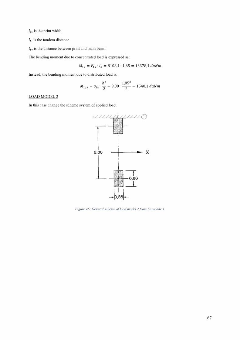
67
𝑙𝑝, is the print width.
𝑙𝑡, is the tandem distance.
𝑙𝑏, is the distance between print and main beam.
The bending moment due to concentrated load is expressed as:
𝑀1𝑘 = 𝐹1𝑘 ∙ 𝑙𝑏 = 8108,1 ∙ 1,65 = 13378,4 𝑑𝑎𝑁𝑚
Instead, the bending moment due to distributed load is:
𝑀1𝑞𝑘 = 𝑞1𝑘 ∙𝑏2
2= 9,00 ∙
1,852
2= 1540,1 𝑑𝑎𝑁𝑚
LOAD MODEL 2
In this case change the scheme system of applied load.
Figure 46: General scheme of load model 2 from Eurocode 1.
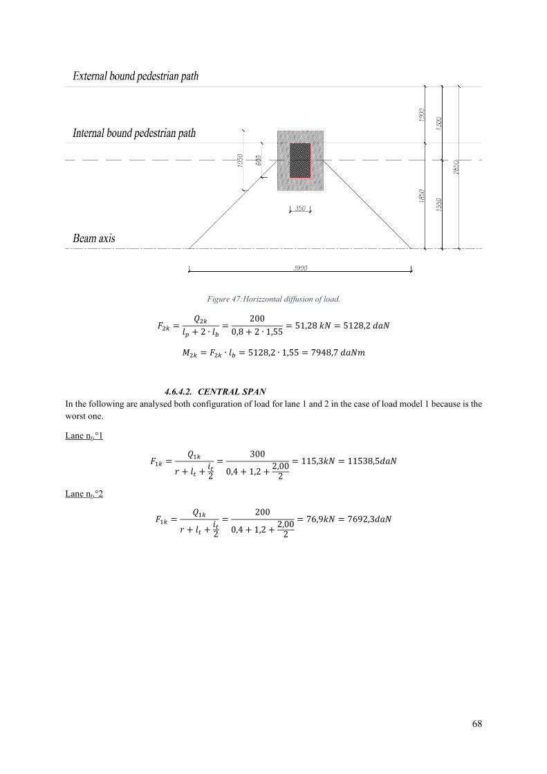
68
Figure 47:Horizzontal diffusion of load.
𝐹2𝑘 =𝑄2𝑘
𝑙𝑝 + 2 ∙ 𝑙𝑏
=200
0,8 + 2 ∙ 1,55= 51,28 𝑘𝑁 = 5128,2 𝑑𝑎𝑁
𝑀2𝑘 = 𝐹2𝑘 ∙ 𝑙𝑏 = 5128,2 ∙ 1,55 = 7948,7 𝑑𝑎𝑁𝑚
4.6.4.2. CENTRAL SPAN In the following are analysed both configuration of load for lane 1 and 2 in the case of load model 1 because is the worst one.
Lane nr.°1
𝐹1𝑘 =𝑄1𝑘
𝑟 + 𝑙𝑡 +𝑖𝑡
2
=300
0,4 + 1,2 +2,00
2
= 115,3𝑘𝑁 = 11538,5𝑑𝑎𝑁
Lane nr.°2
𝐹1𝑘 =𝑄1𝑘
𝑟 + 𝑙𝑡 +𝑖𝑡
2
=200
0,4 + 1,2 +2,00
2
= 76,9𝑘𝑁 = 7692,3𝑑𝑎𝑁
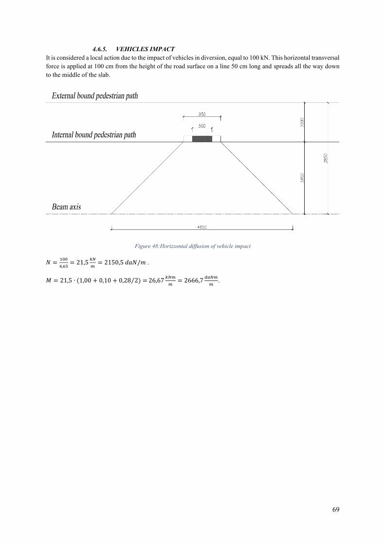
69
4.6.5. VEHICLES IMPACT It is considered a local action due to the impact of vehicles in diversion, equal to 100 kN. This horizontal transversal force is applied at 100 cm from the height of the road surface on a line 50 cm long and spreads all the way down to the middle of the slab.
Figure 48:Horizzontal diffusion of vehicle impact
𝑁 =100
4,65= 21,5
𝑘𝑁
𝑚= 2150,5 𝑑𝑎𝑁/𝑚 .
𝑀 = 21,5 ∙ (1,00 + 0,10 + 0,28 2) =⁄ 26,67𝑘𝑁𝑚
𝑚= 2666,7
𝑑𝑎𝑁𝑚
𝑚.
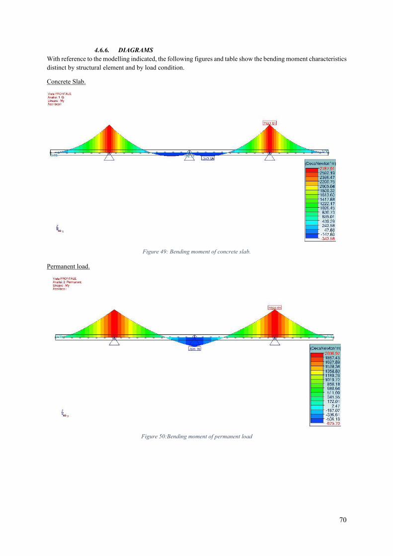
70
4.6.6. DIAGRAMS With reference to the modelling indicated, the following figures and table show the bending moment characteristics distinct by structural element and by load condition.
Concrete Slab.
Figure 49: Bending moment of concrete slab.
Permanent load.
Figure 50:Bending moment of permanent load
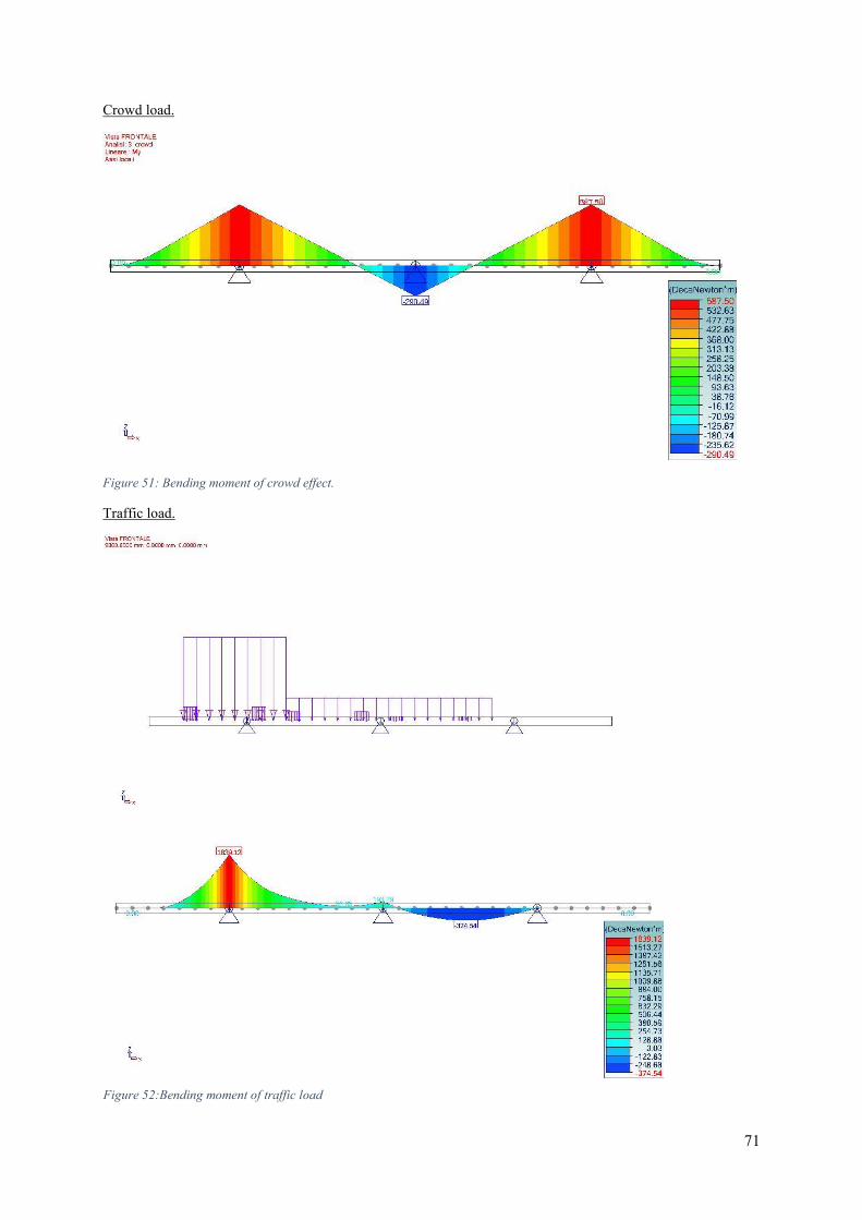
71
Crowd load.
Figure 51: Bending moment of crowd effect.
Traffic load.
Figure 52:Bending moment of traffic load
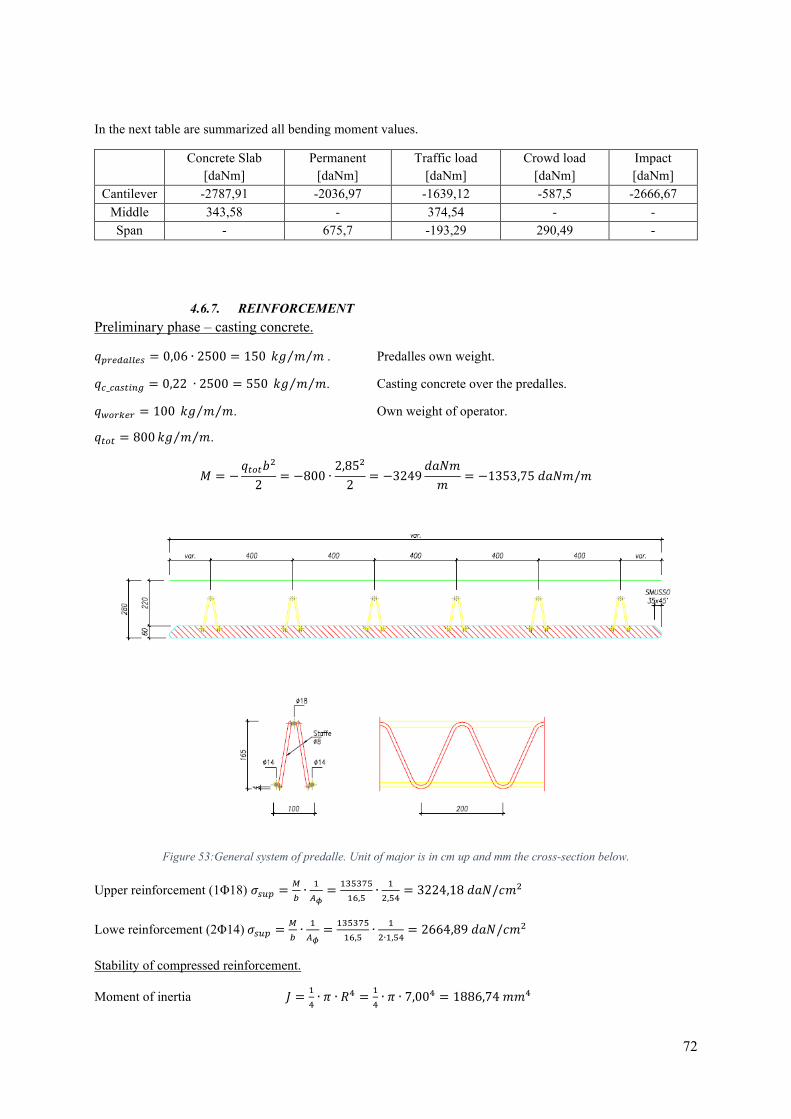
72
In the next table are summarized all bending moment values.
Concrete Slab
[daNm] Permanent
[daNm] Traffic load
[daNm] Crowd load
[daNm] Impact [daNm]
Cantilever -2787,91 -2036,97 -1639,12 -587,5 -2666,67 Middle 343,58 - 374,54 - - Span - 675,7 -193,29 290,49 -
4.6.7. REINFORCEMENT Preliminary phase – casting concrete.
𝑞𝑝𝑟𝑒𝑑𝑎𝑙𝑙𝑒𝑠 = 0,06 ∙ 2500 = 150 𝑘𝑔 𝑚 𝑚⁄⁄ . Predalles own weight.
𝑞𝑐_𝑐𝑎𝑠𝑡𝑖𝑛𝑔 = 0,22 ∙ 2500 = 550 𝑘𝑔 𝑚 𝑚⁄⁄ . Casting concrete over the predalles.
𝑞𝑤𝑜𝑟𝑘𝑒𝑟 = 100 𝑘𝑔 𝑚 𝑚⁄⁄ . Own weight of operator.
𝑞𝑡𝑜𝑡 = 800 𝑘𝑔 𝑚 𝑚⁄⁄ .
𝑀 = −𝑞𝑡𝑜𝑡𝑏2
2= −800 ∙
2,852
2= −3249
𝑑𝑎𝑁𝑚
𝑚= −1353,75 𝑑𝑎𝑁𝑚/𝑚
Figure 53:General system of predalle. Unit of major is in cm up and mm the cross-section below.
Upper reinforcement (1Φ18) 𝜎𝑠𝑢𝑝 =𝑀
𝑏∙
1
𝐴𝜙=
135375
16,5∙
1
2,54= 3224,18 𝑑𝑎𝑁/𝑐𝑚2
Lowe reinforcement (2Φ14) 𝜎𝑠𝑢𝑝 =𝑀
𝑏∙
1
𝐴𝜙=
135375
16,5∙
1
2∙1,54= 2664,89 𝑑𝑎𝑁/𝑐𝑚2
Stability of compressed reinforcement.
Moment of inertia 𝐽 =1
4∙ 𝜋 ∙ 𝑅4 =
1
4∙ 𝜋 ∙ 7,004 = 1886,74 𝑚𝑚4
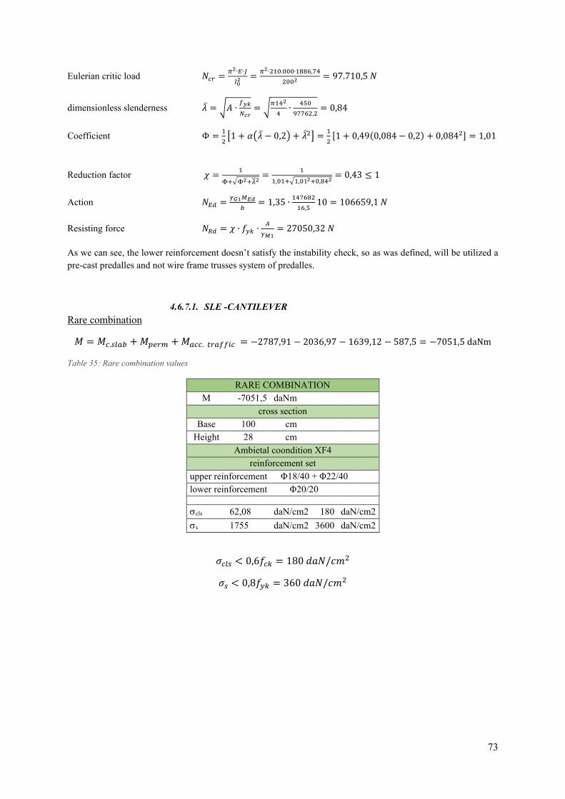
73
Eulerian critic load 𝑁𝑐𝑟 =𝜋2∙𝐸∙𝐽
𝑙02 =
𝜋2∙210.000∙1886,74
2002 = 97.710,5 𝑁
dimensionless slenderness 𝜆 = √𝐴 ∙𝑓𝑦𝑘
𝑁𝑐𝑟= √
𝜋142
4∙
450
97762,2= 0,84
Coefficient Φ =1
2[1 + 𝛼(𝜆 − 0,2) + 𝜆2] =
1
2[1 + 0,49(0,084 − 0,2) + 0,0842] = 1,01
Reduction factor 𝜒 =1
Φ+√Φ2+𝜆2=
1
1,01+√1,012+0,842= 0,43 ≤ 1
Action 𝑁𝐸𝑑 =𝛾𝐺1𝑀𝐸𝑑
𝑏= 1,35 ∙
147682
16,510 = 106659,1 𝑁
Resisting force 𝑁𝑅𝑑 = 𝜒 ∙ 𝑓𝑦𝑘 ∙𝐴
𝛾𝑀1= 27050,32 𝑁
As we can see, the lower reinforcement doesn’t satisfy the instability check, so as was defined, will be utilized a pre-cast predalles and not wire frame trusses system of predalles.
4.6.7.1. SLE -CANTILEVER Rare combination
𝑀 = 𝑀𝑐.𝑠𝑙𝑎𝑏 + 𝑀𝑝𝑒𝑟𝑚 + 𝑀𝑎𝑐𝑐. 𝑡𝑟𝑎𝑓𝑓𝑖𝑐 = −2787,91 − 2036,97 − 1639,12 − 587,5 = −7051,5 daNm
Table 35: Rare combination values
RARE COMBINATION M -7051,5 daNm
cross section Base 100 cm
Height 28 cm Ambietal coondition XF4
reinforcement set upper reinforcement Φ18/40 + Φ22/40 lower reinforcement Φ20/20 cls 62,08 daN/cm2 180 daN/cm2 s 1755 daN/cm2 3600 daN/cm2
𝜎𝑐𝑙𝑠 < 0,6𝑓𝑐𝑘 = 180 𝑑𝑎𝑁/𝑐𝑚2
𝜎𝑠 < 0,8𝑓𝑦𝑘 = 360 𝑑𝑎𝑁/𝑐𝑚2
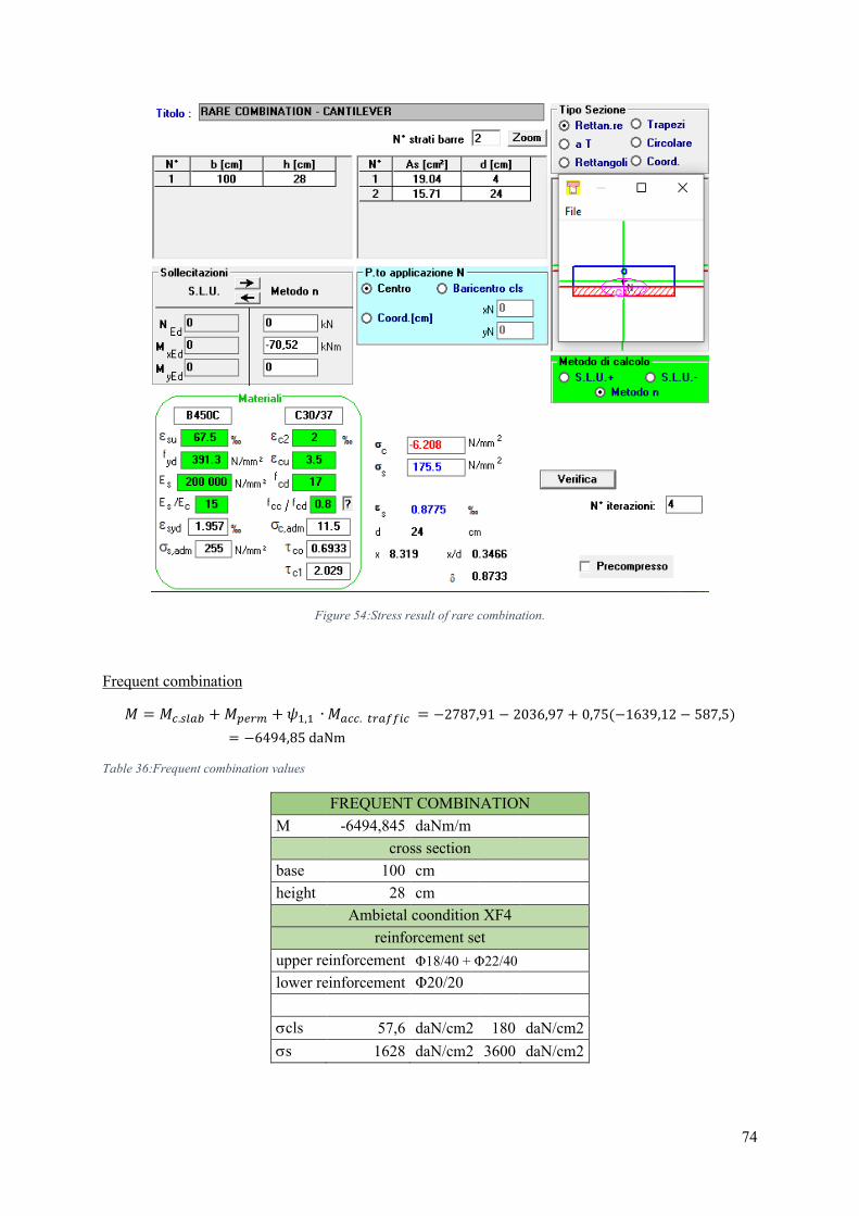
74
Figure 54:Stress result of rare combination.
Frequent combination
𝑀 = 𝑀𝑐.𝑠𝑙𝑎𝑏 + 𝑀𝑝𝑒𝑟𝑚 + 𝜓1,1 ∙ 𝑀𝑎𝑐𝑐. 𝑡𝑟𝑎𝑓𝑓𝑖𝑐 = −2787,91 − 2036,97 + 0,75(−1639,12 − 587,5)
= −6494,85 daNm
Table 36:Frequent combination values
FREQUENT COMBINATION M -6494,845 daNm/m
cross section base 100 cm height 28 cm
Ambietal coondition XF4 reinforcement set
upper reinforcement Φ18/40 + Φ22/40 lower reinforcement Φ20/20 cls 57,6 daN/cm2 180 daN/cm2 s 1628 daN/cm2 3600 daN/cm2
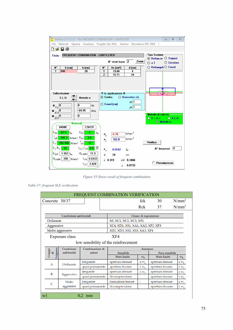
75
\
Figure 55:Stress result of frequent combination
Table 37: frequent SLE verification
FREQUENT COMBINATION VERIFICATION Concrete 30/37 fck 30 N/mm2 Rck 37 N/mm2
Exposure class XF4 low sensibility of the reinforcement
w1 0,2 mm
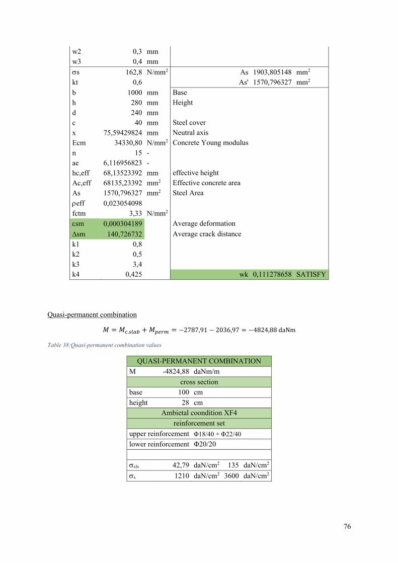
76
w2 0,3 mm w3 0,4 mm s 162,8 N/mm2 As 1903,805148 mm2 kt 0,6 As' 1570,796327 mm2 b 1000 mm Base h 280 mm Height d 240 mm c 40 mm Steel cover x 75,59429824 mm Neutral axis Ecm 34330,80 N/mm2 Concrete Young modulus n 15 - ae 6,116956823 - hc,eff 68,13523392 mm effective height Ac,eff 68135,23392 mm2 Effective concrete area As 1570,796327 mm2 Steel Area eff 0,023054098 fctm 3,33 N/mm2 sm 0,000304189 Average deformation sm 140,726732 Average crack distance k1 0,8 k2 0,5 k3 3,4 k4 0,425 wk 0,111278658 SATISFY
Quasi-permanent combination
𝑀 = 𝑀𝑐.𝑠𝑙𝑎𝑏 + 𝑀𝑝𝑒𝑟𝑚 = −2787,91 − 2036,97 = −4824,88 daNm
Table 38:Quasi-permanent combination values
QUASI-PERMANENT COMBINATION M -4824,88 daNm/m
cross section base 100 cm height 28 cm
Ambietal coondition XF4 reinforcement set
upper reinforcement Φ18/40 + Φ22/40 lower reinforcement Φ20/20 cls 42,79 daN/cm2 135 daN/cm2 s 1210 daN/cm2 3600 daN/cm2
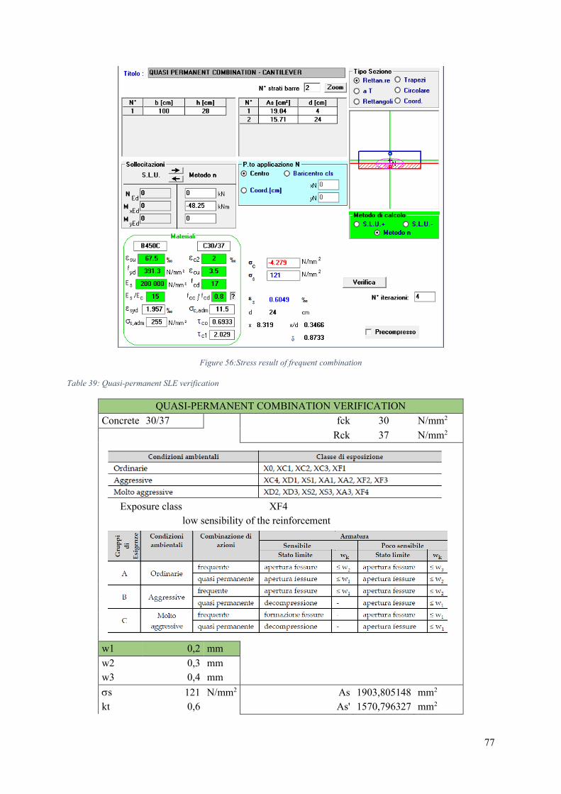
77
Figure 56:Stress result of frequent combination
Table 39: Quasi-permanent SLE verification
QUASI-PERMANENT COMBINATION VERIFICATION Concrete 30/37 fck 30 N/mm2 Rck 37 N/mm2
Exposure class XF4 low sensibility of the reinforcement
w1 0,2 mm w2 0,3 mm w3 0,4 mm s 121 N/mm2 As 1903,805148 mm2 kt 0,6 As' 1570,796327 mm2
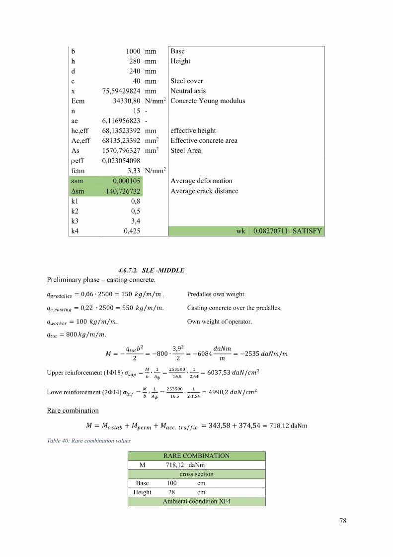
78
b 1000 mm Base h 280 mm Height d 240 mm c 40 mm Steel cover x 75,59429824 mm Neutral axis Ecm 34330,80 N/mm2 Concrete Young modulus n 15 - ae 6,116956823 - hc,eff 68,13523392 mm effective height Ac,eff 68135,23392 mm2 Effective concrete area As 1570,796327 mm2 Steel Area eff 0,023054098 fctm 3,33 N/mm2 sm 0,000105 Average deformation sm 140,726732 Average crack distance k1 0,8 k2 0,5 k3 3,4 k4 0,425 wk 0,08270711 SATISFY
4.6.7.2. SLE -MIDDLE Preliminary phase – casting concrete.
𝑞𝑝𝑟𝑒𝑑𝑎𝑙𝑙𝑒𝑠 = 0,06 ∙ 2500 = 150 𝑘𝑔 𝑚 𝑚⁄⁄ . Predalles own weight.
𝑞𝑐_𝑐𝑎𝑠𝑡𝑖𝑛𝑔 = 0,22 ∙ 2500 = 550 𝑘𝑔 𝑚 𝑚⁄⁄ . Casting concrete over the predalles.
𝑞𝑤𝑜𝑟𝑘𝑒𝑟 = 100 𝑘𝑔 𝑚 𝑚⁄⁄ . Own weight of operator.
𝑞𝑡𝑜𝑡 = 800 𝑘𝑔 𝑚 𝑚⁄⁄ .
𝑀 = −𝑞𝑡𝑜𝑡𝑏2
2= −800 ∙
3,92
2= −6084
𝑑𝑎𝑁𝑚
𝑚= −2535 𝑑𝑎𝑁𝑚/𝑚
Upper reinforcement (1Φ18) 𝜎𝑠𝑢𝑝 =𝑀
𝑏∙
1
𝐴𝜙=
253500
16,5∙
1
2,54= 6037,53 𝑑𝑎𝑁/𝑐𝑚2
Lowe reinforcement (2Φ14) 𝜎𝑖𝑛𝑓 =𝑀
𝑏∙
1
𝐴𝜙=
253500
16,5∙
1
2∙1,54= 4990,2 𝑑𝑎𝑁/𝑐𝑚2
Rare combination
𝑀 = 𝑀𝑐.𝑠𝑙𝑎𝑏 + 𝑀𝑝𝑒𝑟𝑚 + 𝑀𝑎𝑐𝑐. 𝑡𝑟𝑎𝑓𝑓𝑖𝑐 = 343,58 + 374,54 = 718,12 daNm
Table 40: Rare combination values
RARE COMBINATION M 718,12 daNm
cross section Base 100 cm
Height 28 cm Ambietal coondition XF4
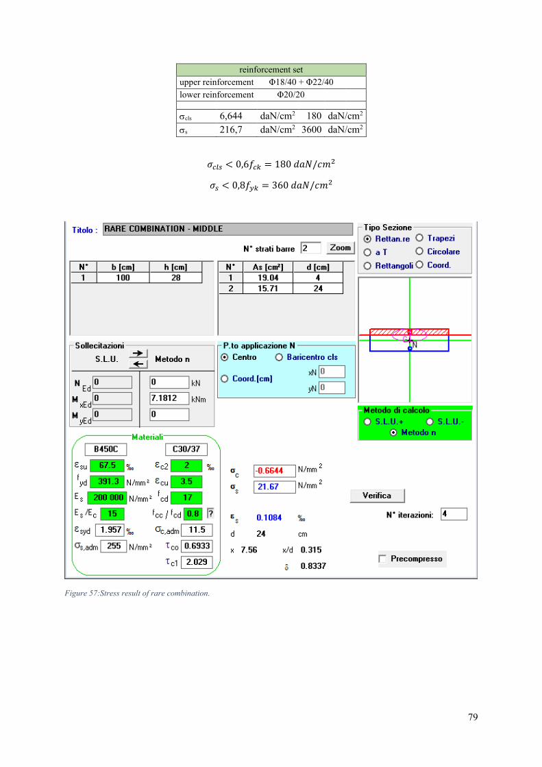
79
reinforcement set upper reinforcement Φ18/40 + Φ22/40
lower reinforcement Φ20/20 cls 6,644 daN/cm2 180 daN/cm2 s 216,7 daN/cm2 3600 daN/cm2
𝜎𝑐𝑙𝑠 < 0,6𝑓𝑐𝑘 = 180 𝑑𝑎𝑁/𝑐𝑚2
𝜎𝑠 < 0,8𝑓𝑦𝑘 = 360 𝑑𝑎𝑁/𝑐𝑚2
Figure 57:Stress result of rare combination.
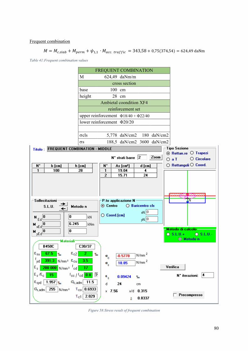
80
Frequent combination
𝑀 = 𝑀𝑐.𝑠𝑙𝑎𝑏 + 𝑀𝑝𝑒𝑟𝑚 + 𝜓1,1 ∙ 𝑀𝑎𝑐𝑐. 𝑡𝑟𝑎𝑓𝑓𝑖𝑐 = 343,58 + 0,75(374,54) = 624,49 daNm
Table 41:Frequent combination values
FREQUENT COMBINATION M 624,49 daNm/m
cross section base 100 cm height 28 cm
Ambietal coondition XF4 reinforcement set
upper reinforcement Φ18/40 + Φ22/40 lower reinforcement Φ20/20 cls 5,778 daN/cm2 180 daN/cm2 s 188,5 daN/cm2 3600 daN/cm2
Figure 58:Stress result of frequent combination
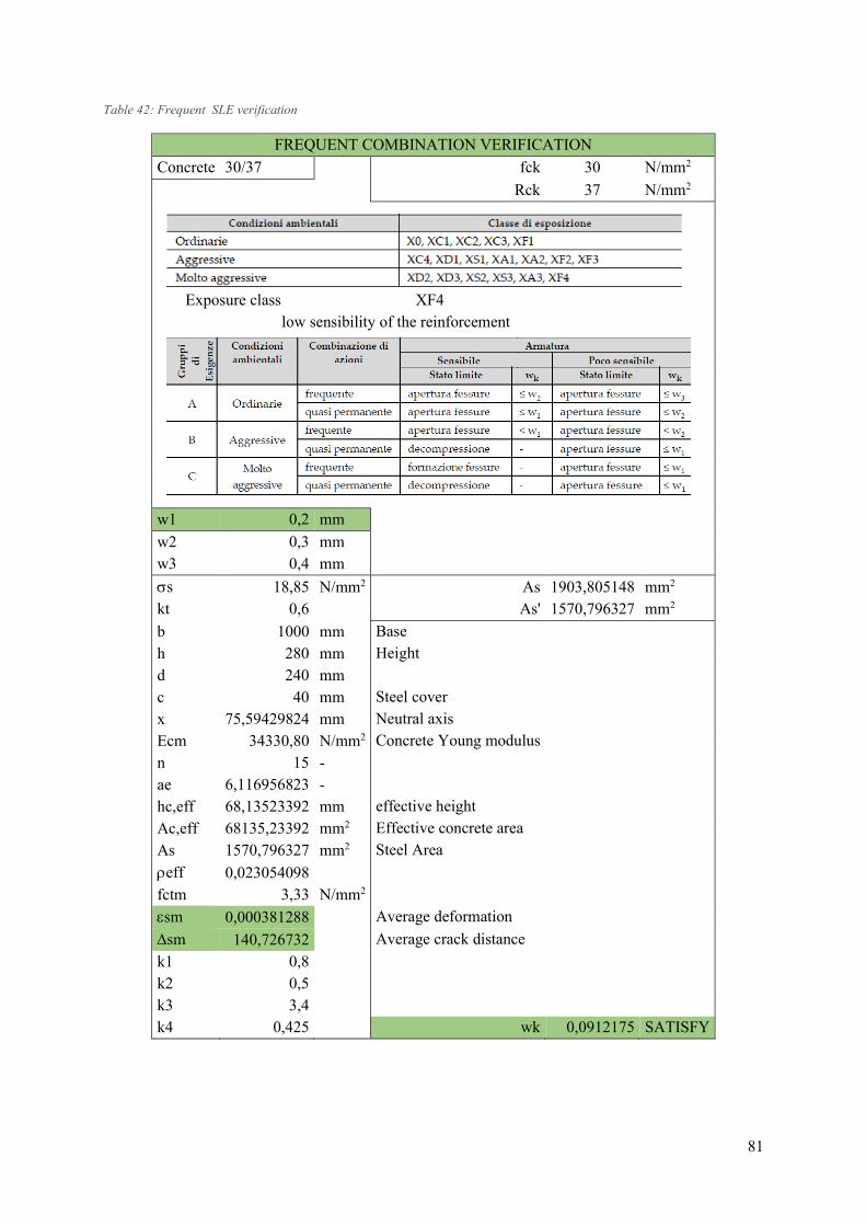
81
Table 42: Frequent SLE verification
FREQUENT COMBINATION VERIFICATION Concrete 30/37 fck 30 N/mm2 Rck 37 N/mm2
Exposure class XF4 low sensibility of the reinforcement
w1 0,2 mm w2 0,3 mm w3 0,4 mm s 18,85 N/mm2 As 1903,805148 mm2 kt 0,6 As' 1570,796327 mm2 b 1000 mm Base h 280 mm Height d 240 mm c 40 mm Steel cover x 75,59429824 mm Neutral axis Ecm 34330,80 N/mm2 Concrete Young modulus n 15 - ae 6,116956823 - hc,eff 68,13523392 mm effective height Ac,eff 68135,23392 mm2 Effective concrete area As 1570,796327 mm2 Steel Area eff 0,023054098 fctm 3,33 N/mm2 sm 0,000381288 Average deformation sm 140,726732 Average crack distance k1 0,8 k2 0,5 k3 3,4 k4 0,425 wk 0,0912175 SATISFY
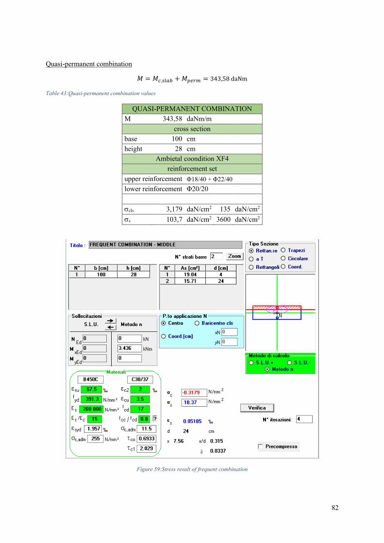
82
Quasi-permanent combination
𝑀 = 𝑀𝑐.𝑠𝑙𝑎𝑏 + 𝑀𝑝𝑒𝑟𝑚 = 343,58 daNm
Table 43:Quasi-permanent combination values
QUASI-PERMANENT COMBINATION M 343,58 daNm/m
cross section base 100 cm height 28 cm
Ambietal coondition XF4 reinforcement set
upper reinforcement Φ18/40 + Φ22/40 lower reinforcement Φ20/20 cls 3,179 daN/cm2 135 daN/cm2 s 103,7 daN/cm2 3600 daN/cm2
Figure 59:Stress result of frequent combination
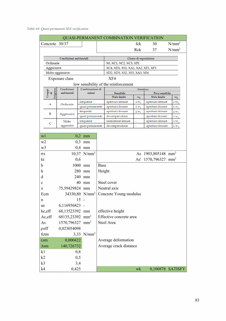
83
Table 44: Quasi-permanent SLE verification
QUASI-PERMANENT COMBINATION VERIFICATION Concrete 30/37 fck 30 N/mm2 Rck 37 N/mm2
Exposure class XF4 low sensibility of the reinforcement
w1 0,2 mm w2 0,3 mm w3 0,4 mm s 10,37 N/mm2 As 1903,805148 mm2 kt 0,6 As' 1570,796327 mm2 b 1000 mm Base h 280 mm Height d 240 mm c 40 mm Steel cover x 75,59429824 mm Neutral axis Ecm 34330,80 N/mm2 Concrete Young modulus n 15 - ae 6,116956823 - hc,eff 68,13523392 mm effective height Ac,eff 68135,23392 mm2 Effective concrete area As 1570,796327 mm2 Steel Area eff 0,023054098 fctm 3,33 N/mm2 sm 0,000422 Average deformation sm 140,726732 Average crack distance k1 0,8 k2 0,5 k3 3,4 k4 0,425 wk 0,100878 SATISFY
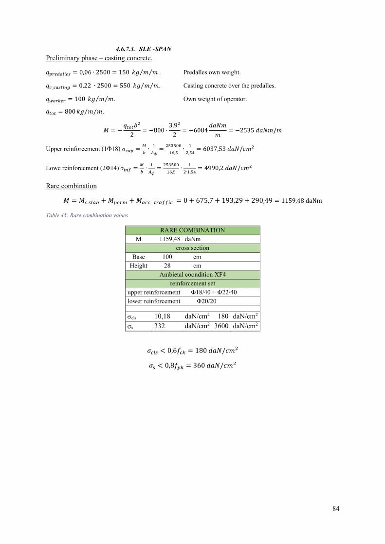
84
4.6.7.3. SLE -SPAN Preliminary phase – casting concrete.
𝑞𝑝𝑟𝑒𝑑𝑎𝑙𝑙𝑒𝑠 = 0,06 ∙ 2500 = 150 𝑘𝑔 𝑚 𝑚⁄⁄ . Predalles own weight.
𝑞𝑐_𝑐𝑎𝑠𝑡𝑖𝑛𝑔 = 0,22 ∙ 2500 = 550 𝑘𝑔 𝑚 𝑚⁄⁄ . Casting concrete over the predalles.
𝑞𝑤𝑜𝑟𝑘𝑒𝑟 = 100 𝑘𝑔 𝑚 𝑚⁄⁄ . Own weight of operator.
𝑞𝑡𝑜𝑡 = 800 𝑘𝑔 𝑚 𝑚⁄⁄ .
𝑀 = −𝑞𝑡𝑜𝑡𝑏2
2= −800 ∙
3,92
2= −6084
𝑑𝑎𝑁𝑚
𝑚= −2535 𝑑𝑎𝑁𝑚/𝑚
Upper reinforcement (1Φ18) 𝜎𝑠𝑢𝑝 =𝑀
𝑏∙
1
𝐴𝜙=
253500
16,5∙
1
2,54= 6037,53 𝑑𝑎𝑁/𝑐𝑚2
Lowe reinforcement (2Φ14) 𝜎𝑖𝑛𝑓 =𝑀
𝑏∙
1
𝐴𝜙=
253500
16,5∙
1
2∙1,54= 4990,2 𝑑𝑎𝑁/𝑐𝑚2
Rare combination
𝑀 = 𝑀𝑐.𝑠𝑙𝑎𝑏 + 𝑀𝑝𝑒𝑟𝑚 + 𝑀𝑎𝑐𝑐. 𝑡𝑟𝑎𝑓𝑓𝑖𝑐 = 0 + 675,7 + 193,29 + 290,49 = 1159,48 daNm
Table 45: Rare combination values
RARE COMBINATION M 1159,48 daNm
cross section Base 100 cm
Height 28 cm Ambietal coondition XF4
reinforcement set upper reinforcement Φ18/40 + Φ22/40
lower reinforcement Φ20/20 cls 10,18 daN/cm2 180 daN/cm2 s 332 daN/cm2 3600 daN/cm2
𝜎𝑐𝑙𝑠 < 0,6𝑓𝑐𝑘 = 180 𝑑𝑎𝑁/𝑐𝑚2
𝜎𝑠 < 0,8𝑓𝑦𝑘 = 360 𝑑𝑎𝑁/𝑐𝑚2
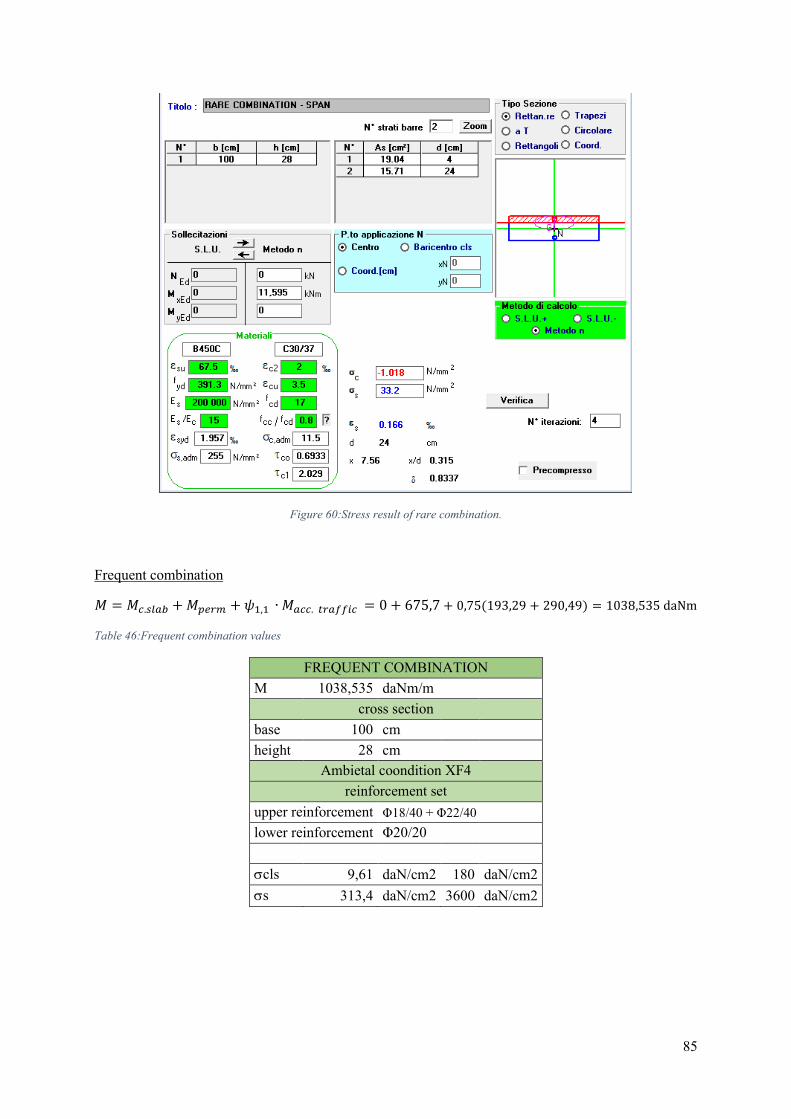
85
Figure 60:Stress result of rare combination.
Frequent combination
𝑀 = 𝑀𝑐.𝑠𝑙𝑎𝑏 + 𝑀𝑝𝑒𝑟𝑚 + 𝜓1,1 ∙ 𝑀𝑎𝑐𝑐. 𝑡𝑟𝑎𝑓𝑓𝑖𝑐 = 0 + 675,7 + 0,75(193,29 + 290,49) = 1038,535 daNm
Table 46:Frequent combination values
FREQUENT COMBINATION M 1038,535 daNm/m
cross section base 100 cm height 28 cm
Ambietal coondition XF4 reinforcement set
upper reinforcement Φ18/40 + Φ22/40 lower reinforcement Φ20/20 cls 9,61 daN/cm2 180 daN/cm2 s 313,4 daN/cm2 3600 daN/cm2
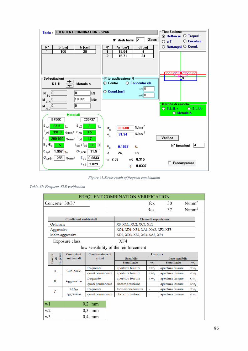
86
Figure 61:Stress result of frequent combination
Table 47: Frequent SLE verification
FREQUENT COMBINATION VERIFICATION Concrete 30/37 fck 30 N/mm2 Rck 37 N/mm2
Exposure class XF4 low sensibility of the reinforcement
w1 0,2 mm w2 0,3 mm w3 0,4 mm
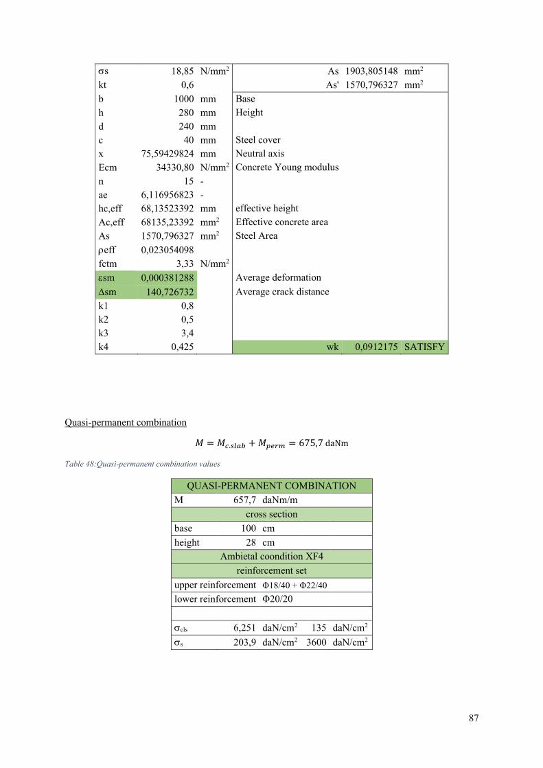
87
s 18,85 N/mm2 As 1903,805148 mm2 kt 0,6 As' 1570,796327 mm2 b 1000 mm Base h 280 mm Height d 240 mm c 40 mm Steel cover x 75,59429824 mm Neutral axis Ecm 34330,80 N/mm2 Concrete Young modulus n 15 - ae 6,116956823 - hc,eff 68,13523392 mm effective height Ac,eff 68135,23392 mm2 Effective concrete area As 1570,796327 mm2 Steel Area eff 0,023054098 fctm 3,33 N/mm2 sm 0,000381288 Average deformation sm 140,726732 Average crack distance k1 0,8 k2 0,5 k3 3,4 k4 0,425 wk 0,0912175 SATISFY
Quasi-permanent combination
𝑀 = 𝑀𝑐.𝑠𝑙𝑎𝑏 + 𝑀𝑝𝑒𝑟𝑚 = 675,7 daNm
Table 48:Quasi-permanent combination values
QUASI-PERMANENT COMBINATION M 657,7 daNm/m
cross section base 100 cm height 28 cm
Ambietal coondition XF4 reinforcement set
upper reinforcement Φ18/40 + Φ22/40 lower reinforcement Φ20/20 cls 6,251 daN/cm2 135 daN/cm2 s 203,9 daN/cm2 3600 daN/cm2
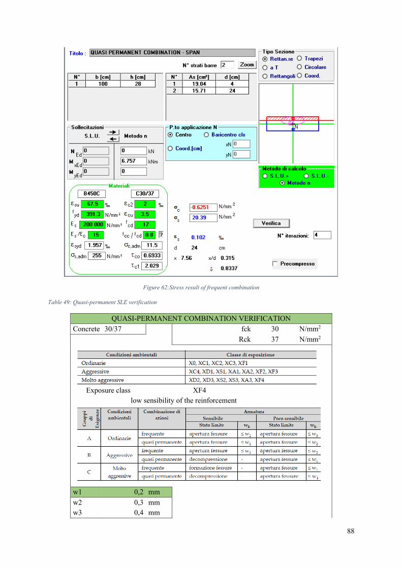
88
Figure 62:Stress result of frequent combination
Table 49: Quasi-permanent SLE verification
QUASI-PERMANENT COMBINATION VERIFICATION Concrete 30/37 fck 30 N/mm2 Rck 37 N/mm2
Exposure class XF4 low sensibility of the reinforcement
w1 0,2 mm w2 0,3 mm w3 0,4 mm
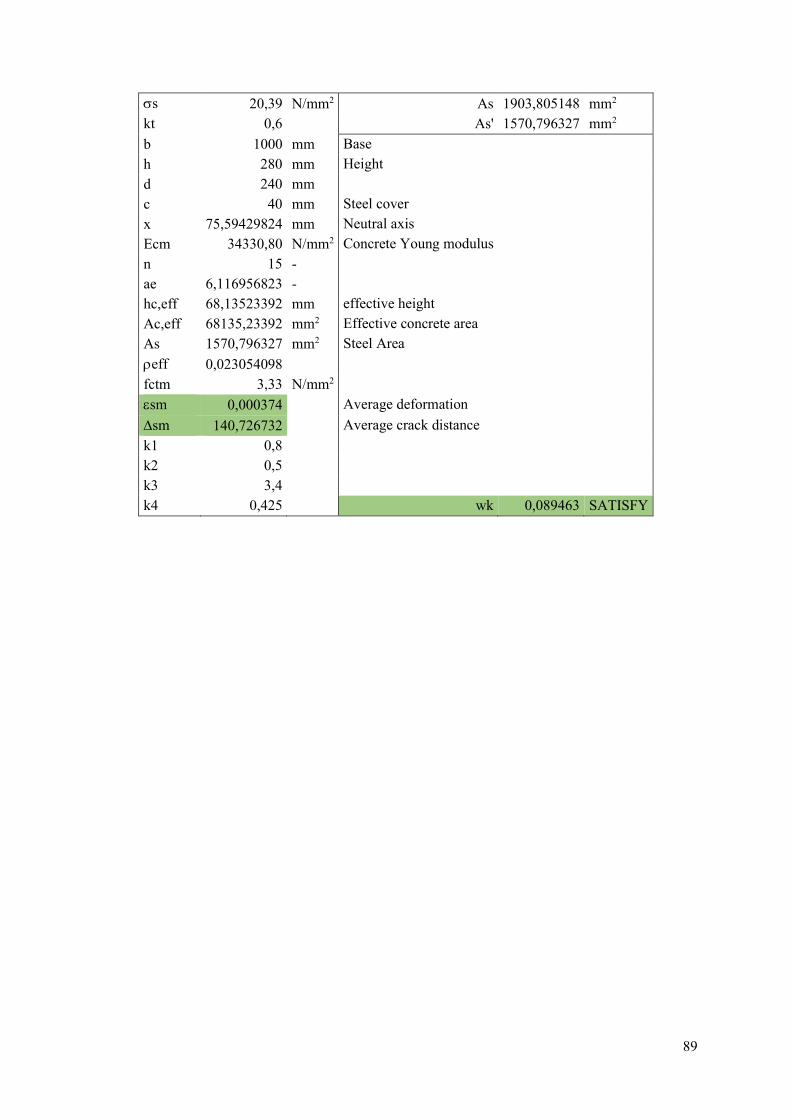
89
s 20,39 N/mm2 As 1903,805148 mm2 kt 0,6 As' 1570,796327 mm2 b 1000 mm Base h 280 mm Height d 240 mm c 40 mm Steel cover x 75,59429824 mm Neutral axis Ecm 34330,80 N/mm2 Concrete Young modulus n 15 - ae 6,116956823 - hc,eff 68,13523392 mm effective height Ac,eff 68135,23392 mm2 Effective concrete area As 1570,796327 mm2 Steel Area eff 0,023054098 fctm 3,33 N/mm2 sm 0,000374 Average deformation sm 140,726732 Average crack distance k1 0,8 k2 0,5 k3 3,4 k4 0,425 wk 0,089463 SATISFY
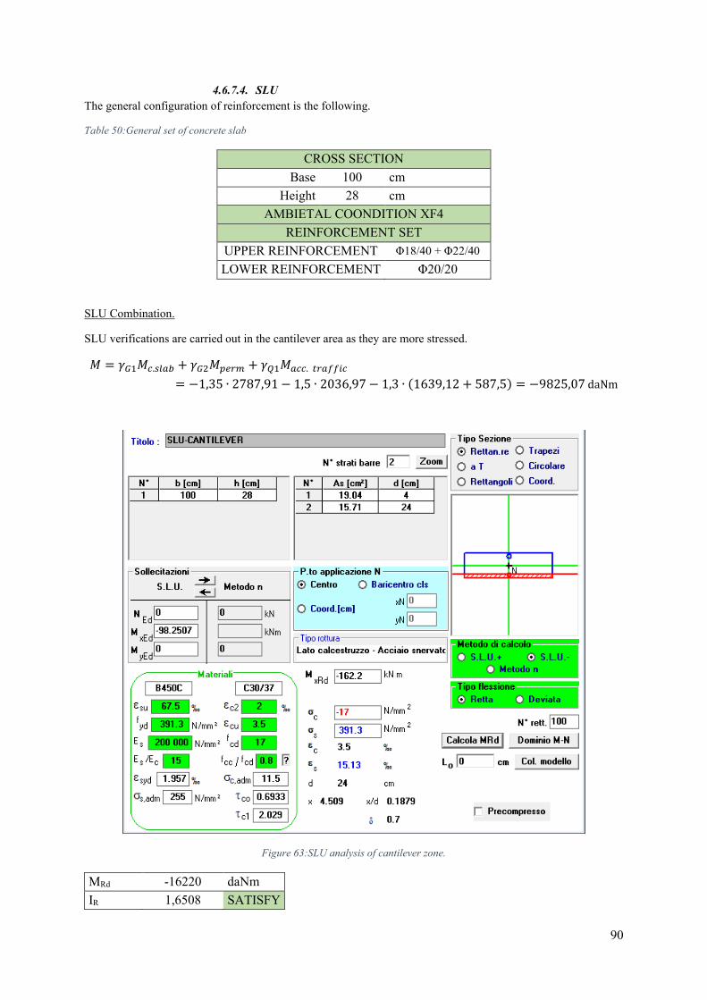
90
4.6.7.4. SLU The general configuration of reinforcement is the following.
Table 50:General set of concrete slab
CROSS SECTION Base 100 cm
Height 28 cm AMBIETAL COONDITION XF4
REINFORCEMENT SET UPPER REINFORCEMENT Φ18/40 + Φ22/40 LOWER REINFORCEMENT Φ20/20
SLU Combination.
SLU verifications are carried out in the cantilever area as they are more stressed.
𝑀 = 𝛾𝐺1𝑀𝑐.𝑠𝑙𝑎𝑏 + 𝛾𝐺2𝑀𝑝𝑒𝑟𝑚 + 𝛾𝑄1𝑀𝑎𝑐𝑐. 𝑡𝑟𝑎𝑓𝑓𝑖𝑐
= −1,35 ∙ 2787,91 − 1,5 ∙ 2036,97 − 1,3 ∙ (1639,12 + 587,5) = −9825,07 daNm
Figure 63:SLU analysis of cantilever zone.
MRd -16220 daNm IR 1,6508 SATISFY
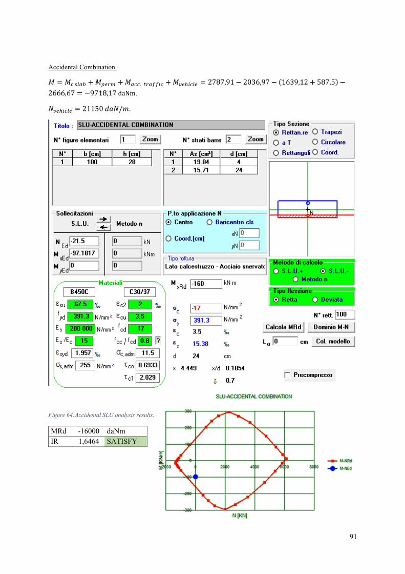
91
Accidental Combination.
𝑀 = 𝑀𝑐.𝑠𝑙𝑎𝑏 + 𝑀𝑝𝑒𝑟𝑚 + 𝑀𝑎𝑐𝑐. 𝑡𝑟𝑎𝑓𝑓𝑖𝑐 + 𝑀𝑣𝑒ℎ𝑖𝑐𝑙𝑒 = 2787,91 − 2036,97 − (1639,12 + 587,5) −
2666,67 = −9718,17 daNm.
𝑁𝑣𝑒ℎ𝑖𝑐𝑙𝑒 = 21150 𝑑𝑎𝑁/𝑚.
Figure 64:Accidental SLU analysis results.
MRd -16000 daNm IR 1,6464 SATISFY
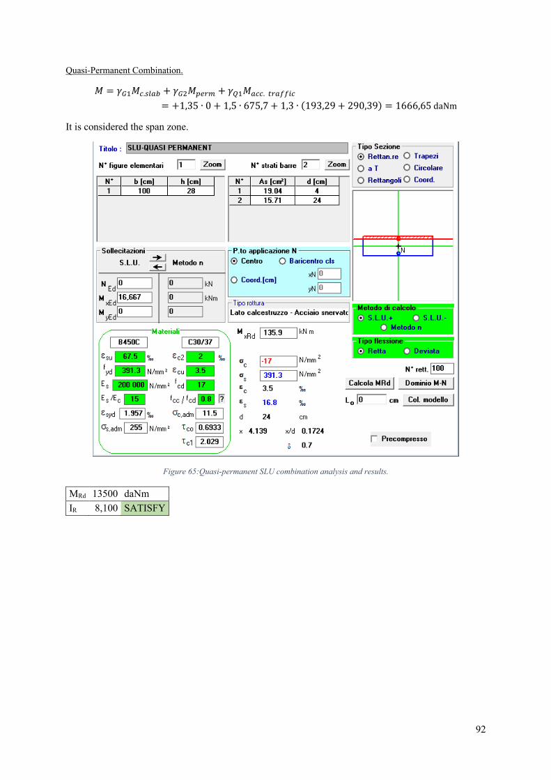
92
Quasi-Permanent Combination.
𝑀 = 𝛾𝐺1𝑀𝑐.𝑠𝑙𝑎𝑏 + 𝛾𝐺2𝑀𝑝𝑒𝑟𝑚 + 𝛾𝑄1𝑀𝑎𝑐𝑐. 𝑡𝑟𝑎𝑓𝑓𝑖𝑐
= +1,35 ∙ 0 + 1,5 ∙ 675,7 + 1,3 ∙ (193,29 + 290,39) = 1666,65 daNm
It is considered the span zone.
Figure 65:Quasi-permanent SLU combination analysis and results.
MRd 13500 daNm IR 8,100 SATISFY
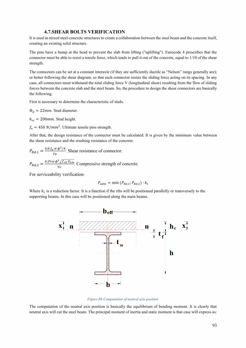
93
4.7.SHEAR BOLTS VERIFICATION It is used in mixed steel-concrete structures to create a collaboration between the steel beam and the concrete itself, creating an existing solid structure.
The pins have a bump at the head to prevent the slab from lifting ("uplifting"). Eurocode 4 prescribes that the connector must be able to resist a tensile force, which tends to pull it out of the concrete, equal to 1/10 of the shear strength.
The connectors can be set at a constant interaxle (if they are sufficiently ductile as “Nelson” rungs generally are); or better following the shear diagram, so that each connector resists the sliding force acting on its spacing. In any case, all connectors must withstand the total sliding force V (longitudinal shear) resulting from the flow of sliding forces between the concrete slab and the steel beam. So, the procedure to design the shear connectors are basically the following.
First is necessary to determine the characteristic of studs.
Φ𝑝 = 22𝑚𝑚. Stud diameter.
ℎ𝑠𝑐 = 200𝑚𝑚. Stud height.
𝑓𝑢 = 450 𝑁/𝑚𝑚2. Ultimate tensile pins strength.
After that, the design resistance of the connector must be calculated. It is given by the minimum value between the shear resistance and the crushing resistance of the concrete.
𝑃𝑅𝑑,1 =0,8∙𝑓𝑢∙𝜋∙𝜙2 4⁄
𝛾𝑉. Shear resistance of connector.
𝑃𝑅𝑑,2 =0,29∙𝛼∙𝜙2√𝑓𝑐𝑘∙𝐸𝑐𝑚
𝛾𝑉. Compressive strength of concrete.
For serviceability verification:
𝑃𝑎𝑑𝑚 = min (𝑃𝑅𝑑,1; 𝑃𝑅𝑑,2) ∙ 𝑘𝑡
Where 𝑘𝑡 is a reduction factor. It is a function if the ribs will be positioned parallelly or transversely to the supporting beams. In this case will be positioned along the main beams.
The computation of the neutral axis position is basically the equilibrium of bending moment. It is clearly that neutral axis will cut the steel beam. The principal moment of inertia and static moment is that case will express as:
Figure 66:Computation of neutral axis position

94
𝐴𝑐 ∙ (𝑥 −ℎ𝑐
2) = 𝑛 ∙ 𝐴𝑎 (
ℎ
2+ ℎ𝑐 − 𝑥) .
𝐽𝑜𝑚𝑜 = 𝐽𝑎 +𝐽𝑐
𝑛+ 𝐴𝑎 (
ℎ
2+ ℎ𝑐 − 𝑥)
2
+𝐴𝑐
𝑛(𝑥 − ℎ𝑐)2 .
Remember that the 𝑛 factor is directly dependent of time of apply loading, as did previous in the shrinkage chapter.
As EN1994-1 suggests, the shifting forces per unit length proposed by Jouraswki shall be write as: 𝑠 = 𝑉 ∙𝑆∗
𝐽𝑜𝑚𝑜,
where the ratio 𝑆∗
𝐽𝑜𝑚𝑜 is the internal arm that the shear bolts are able to absorb in terms of longitudinal shear.
Determining the internal arm, that it is function of “n” factor, it is easily understanding which the maximum action is acting on each pin, 𝑃𝑚𝑎𝑥 =
𝑠
𝑛𝑟∙𝑖 . The 𝑛𝑟 represents the number of bolts positioned on each raw.
The Eurocode proposes a minimum spacing between connectors: 𝑖 = 22 ∙ 𝑡𝑓√235 𝑓𝑦𝑘⁄ .
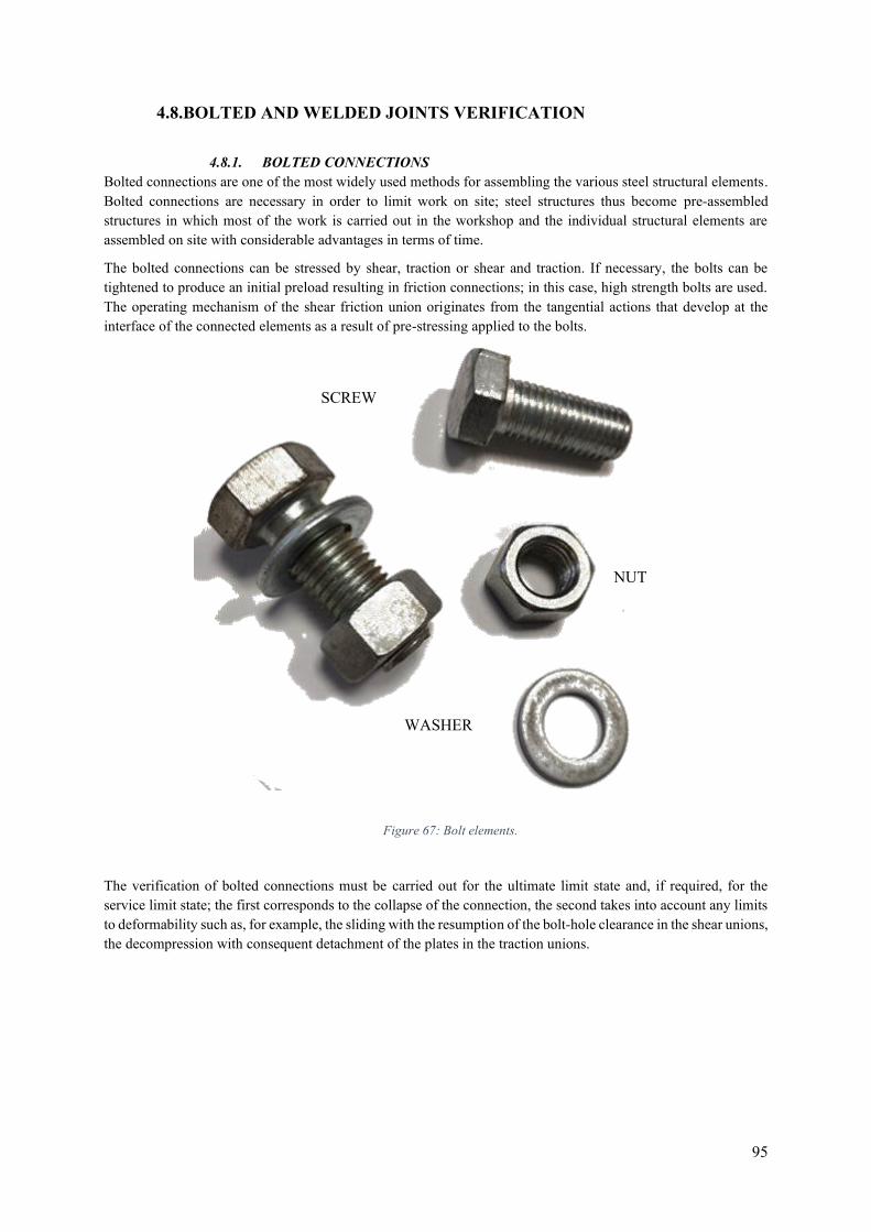
95
4.8.BOLTED AND WELDED JOINTS VERIFICATION
4.8.1. BOLTED CONNECTIONS Bolted connections are one of the most widely used methods for assembling the various steel structural elements. Bolted connections are necessary in order to limit work on site; steel structures thus become pre-assembled structures in which most of the work is carried out in the workshop and the individual structural elements are assembled on site with considerable advantages in terms of time.
The bolted connections can be stressed by shear, traction or shear and traction. If necessary, the bolts can be tightened to produce an initial preload resulting in friction connections; in this case, high strength bolts are used. The operating mechanism of the shear friction union originates from the tangential actions that develop at the interface of the connected elements as a result of pre-stressing applied to the bolts.
The verification of bolted connections must be carried out for the ultimate limit state and, if required, for the service limit state; the first corresponds to the collapse of the connection, the second takes into account any limits to deformability such as, for example, the sliding with the resumption of the bolt-hole clearance in the shear unions, the decompression with consequent detachment of the plates in the traction unions.
Figure 67: Bolt elements.
NUT
SCREW
WASHER
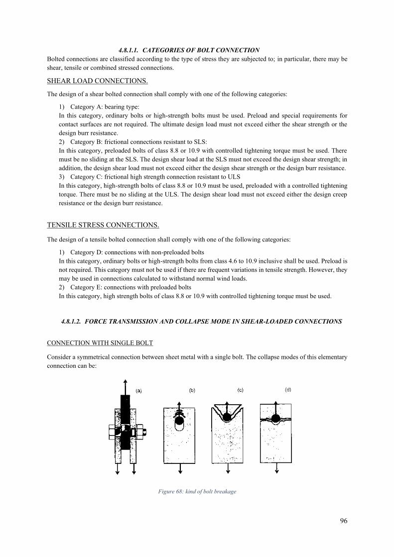
96
4.8.1.1. CATEGORIES OF BOLT CONNECTION Bolted connections are classified according to the type of stress they are subjected to; in particular, there may be shear, tensile or combined stressed connections.
SHEAR LOAD CONNECTIONS.
The design of a shear bolted connection shall comply with one of the following categories:
1) Category A: bearing type: In this category, ordinary bolts or high-strength bolts must be used. Preload and special requirements for contact surfaces are not required. The ultimate design load must not exceed either the shear strength or the design burr resistance. 2) Category B: frictional connections resistant to SLS: In this category, preloaded bolts of class 8.8 or 10.9 with controlled tightening torque must be used. There must be no sliding at the SLS. The design shear load at the SLS must not exceed the design shear strength; in addition, the design shear load must not exceed either the design shear strength or the design burr resistance. 3) Category C: frictional high strength connection resistant to ULS In this category, high-strength bolts of class 8.8 or 10.9 must be used, preloaded with a controlled tightening torque. There must be no sliding at the ULS. The design shear load must not exceed either the design creep resistance or the design burr resistance.
TENSILE STRESS CONNECTIONS.
The design of a tensile bolted connection shall comply with one of the following categories:
1) Category D: connections with non-preloaded bolts In this category, ordinary bolts or high-strength bolts from class 4.6 to 10.9 inclusive shall be used. Preload is not required. This category must not be used if there are frequent variations in tensile strength. However, they may be used in connections calculated to withstand normal wind loads. 2) Category E: connections with preloaded bolts In this category, high strength bolts of class 8.8 or 10.9 with controlled tightening torque must be used.
4.8.1.2. FORCE TRANSMISSION AND COLLAPSE MODE IN SHEAR-LOADED CONNECTIONS
CONNECTION WITH SINGLE BOLT
Consider a symmetrical connection between sheet metal with a single bolt. The collapse modes of this elementary connection can be:
Figure 68: kind of bolt breakage
97
- Breakage due to bolt cutting (a) - Breakage due to sheet burring (b) - Breakage due to sheet cutting (c) - Breakage due to sheet tensile stressing (d)
For each of these collapse mechanisms, resistance must be determined; the weakest mechanism will be the one that governs the problem. Bolts do not always have sufficient ductility to allow the redistribution of internal action in the structure. Therefore, it is necessary to dimension the bolts so that ductile mechanisms are formed before the bolt collapses by shearing. However, a bolted connection is correctly designed when the resistances associated with the collapse mechanisms are close together.
The analysis in the elastic field of the tensional state, whether stretched or compressed, is complex. In practice, it is advisable to refer to simplified diagrams justified by the plastic redistribution of the stresses.
BREAKAGE DUE TO BOLT CUTTING
To define the design shear strength of each strong section of the bolt [mechanism (a)] it makes no sense to use the Huber Von Mises criterion because the bolt cannot be considered as a deflected beam as it is a stocky element in which the diameter is of the same order of magnitude as the thickness of the connected elements. It is more logical to assume as design resistance a conventional value directly connected to the area of the resistant section, distinguishing whether or not the cutting plane passes through the threaded part of the bolt.
BREAKAGE DUE TO BURRING AND CUTTING OF THE SHEET
The design resistance to rolling or shearing of the sheet metal [mechanisms (b) and (c)] depend on the distance of the bolt from the end of the plate measured in the direction of the force; the behaviour will be different for compressive and tensile stresses. The rolling resistance depends on the type of material of the plates, the diameter of the bolt and the minimum distances imposed by the standard prevent the mode of breaking by shearing of the sheet, as the latter is a break of the fragile type.
BREAKAGE DUE TO SHEET TENSILE STRESSING
The presence of the holes determines a distribution of tensions in the sheet metal which, in the elastic field, is characterized by the presence of particularly expensive local points. The redistribution of the collapsing stresses, following the ductility of the material, allows the use of a conventional average value of tension on the net section.
4.8.2. DESIGN RESISTANCE OF A SINGLE SHEAR BOLT As suggest the Italian and European law, the design procedure to define if each single bolt is correctly dimensioned is described in the following, taking into account the shear resistance, tensile resistance and other local instability as burring and punching phenomena.
The nodes in the pilot beam, the lower diaphragm joints and especially the main beam joints that will be verified as fully restored bolted joints will be subject to bolting.
As all know, at ULS the design shear force FV,Ed on a bolt must not exceed between:
𝐹𝑉,𝐸𝑑 ≤ min(𝐹𝑉,𝑅𝑑; 𝐹𝑏,𝑅𝑑)
Where,
- 𝐹𝑉,𝑅𝑑, shear design resistance. - 𝐹𝑏,𝑅𝑑, design resistance to burring.
98
4.8.2.1. SHEAR DESIGN RESISTANCE The shear strength for each bolt shear plane must be assumed as:
𝐹𝑉,𝑅𝑑 =𝛼𝑉 𝑓𝑢𝑏 𝐴
𝛾𝑀2
When the cutting plane passes through the threaded portion of the bolt (A=As, the bolt's tensile strength area):
- For strength classes 4.6, 5.6, 8.8 → 𝛼𝑉=0,6. - For strength classes 6,8 e 10.9 → 𝛼𝑉=0,5.
When the cutting plane passes through the unthreaded portion of the bolt (A= gross section area of the bolt):
- For all strength classes → 𝛼𝑉=0,6.
The function of the coefficient av is to transform the tensile strength of the fub into an equivalent shear strength. According to Von Mises 0.57 or 1/√3
4.8.2.2. DESIGN RESISTANCE TO BURRING The burring resistance must be assumed:
𝐹𝑏,𝑅𝑑 =𝑘1 𝛼𝑏 𝑓𝑢 𝑑 𝑡
𝛾𝑀2
Where: 𝛼𝑏 = min ( 𝛼𝑑;𝑓𝑢𝑏
𝑓𝑢; 1,0)
In the direction of the applied load:
- For end bolts o 𝛼𝑑 =
𝑒1
3𝑑0
- For internal bolts o 𝛼𝑑 =
𝑝1
3𝑑0−
1
4
Perpendicular to the direction of application of the load:
- For end bolts
o 𝑘1 = min (2,8𝑒2
𝑑0− 1,7; 2,5)
- For internal bolts o 𝑘1 = min (1,4
𝑝2
𝑑0− 1,7; 2,5)
The burring coefficient k1 amplifies the ultimate resistance (k1>1) because it takes into account the actual phenomenon of plasticization, which does not only concern the contact area conventionally evaluated through its diametric projection (d⋅t), but which affects, following the diffusion of the tensional flows, a larger area of the plate.
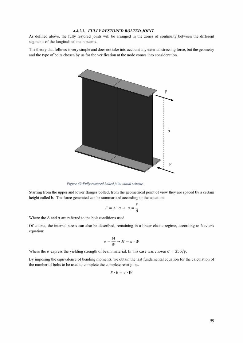
99
4.8.2.3. FULLY RESTORED BOLTED JOINT As defined above, the fully restored joints will be arranged in the zones of continuity between the different segments of the longitudinal main beams.
The theory that follows is very simple and does not take into account any external stressing force, but the geometry and the type of bolts chosen by us for the verification at the node comes into consideration.
Starting from the upper and lower flanges bolted, from the geometrical point of view they are spaced by a certain height called b. The force generated can be summarized according to the equation:
𝐹 = 𝐴 ∙ 𝜎 → 𝜎 =𝐹
𝐴
Where the A and 𝜎 are referred to the bolt conditions used.
Of course, the internal stress can also be described, remaining in a linear elastic regime, according to Navier's equation:
𝜎 =𝑀
𝑊→ 𝑀 = 𝜎 ∙ 𝑊
Where the 𝜎 express the yielding strength of beam material. In this case was chosen 𝜎 = 355/𝛾.
By imposing the equivalence of bending moments, we obtain the last fundamental equation for the calculation of the number of bolts to be used to complete the complete reset joint.
𝐹 ∙ 𝑏 = 𝜎 ∙ 𝑊
F
F
b
Figure 69:Fully restored bolted joint initial scheme.
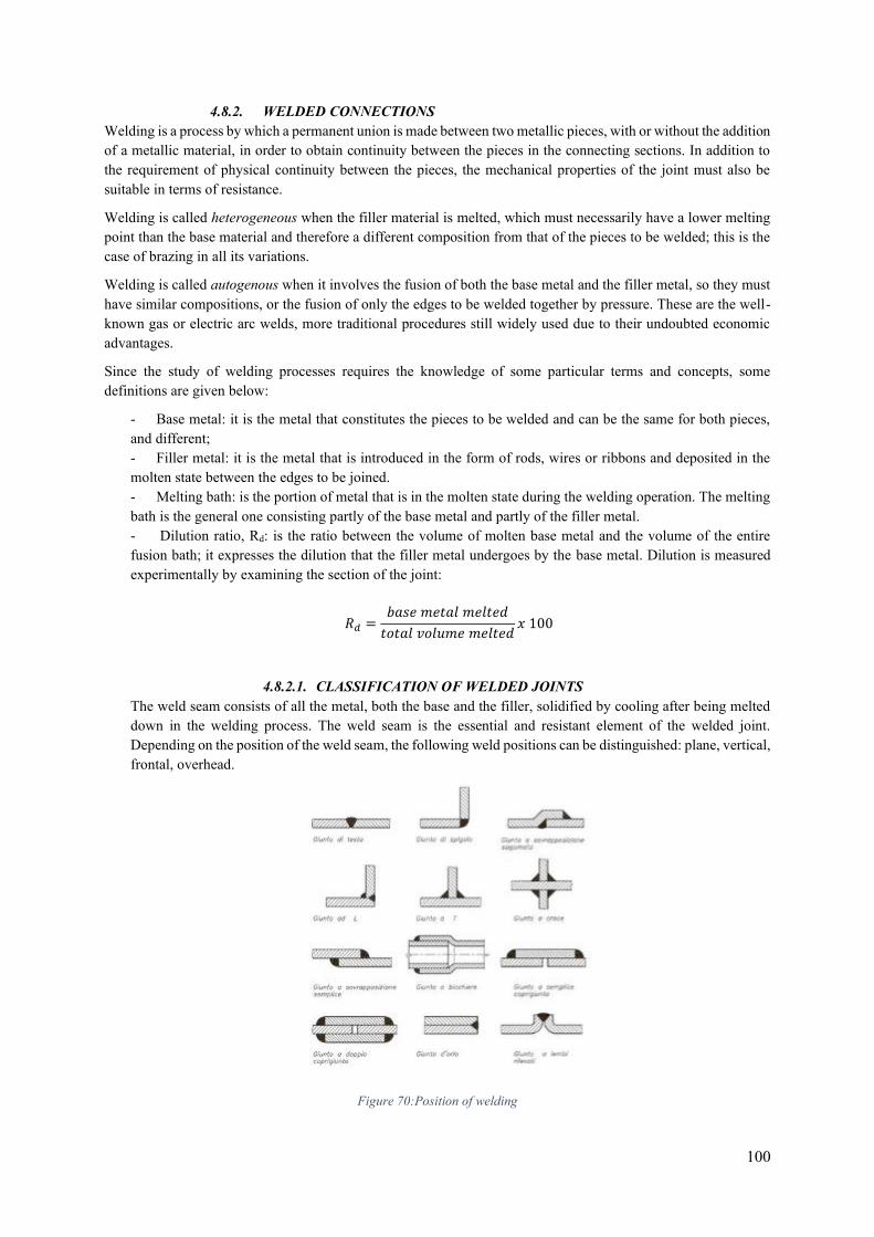
100
4.8.2. WELDED CONNECTIONS Welding is a process by which a permanent union is made between two metallic pieces, with or without the addition of a metallic material, in order to obtain continuity between the pieces in the connecting sections. In addition to the requirement of physical continuity between the pieces, the mechanical properties of the joint must also be suitable in terms of resistance.
Welding is called heterogeneous when the filler material is melted, which must necessarily have a lower melting point than the base material and therefore a different composition from that of the pieces to be welded; this is the case of brazing in all its variations.
Welding is called autogenous when it involves the fusion of both the base metal and the filler metal, so they must have similar compositions, or the fusion of only the edges to be welded together by pressure. These are the well-known gas or electric arc welds, more traditional procedures still widely used due to their undoubted economic advantages.
Since the study of welding processes requires the knowledge of some particular terms and concepts, some definitions are given below:
- Base metal: it is the metal that constitutes the pieces to be welded and can be the same for both pieces, and different; - Filler metal: it is the metal that is introduced in the form of rods, wires or ribbons and deposited in the molten state between the edges to be joined. - Melting bath: is the portion of metal that is in the molten state during the welding operation. The melting bath is the general one consisting partly of the base metal and partly of the filler metal. - Dilution ratio, Rd: is the ratio between the volume of molten base metal and the volume of the entire fusion bath; it expresses the dilution that the filler metal undergoes by the base metal. Dilution is measured experimentally by examining the section of the joint:
𝑅𝑑 =𝑏𝑎𝑠𝑒 𝑚𝑒𝑡𝑎𝑙 𝑚𝑒𝑙𝑡𝑒𝑑
𝑡𝑜𝑡𝑎𝑙 𝑣𝑜𝑙𝑢𝑚𝑒 𝑚𝑒𝑙𝑡𝑒𝑑𝑥 100
4.8.2.1. CLASSIFICATION OF WELDED JOINTS The weld seam consists of all the metal, both the base and the filler, solidified by cooling after being melted down in the welding process. The weld seam is the essential and resistant element of the welded joint. Depending on the position of the weld seam, the following weld positions can be distinguished: plane, vertical, frontal, overhead.
Figure 70:Position of welding
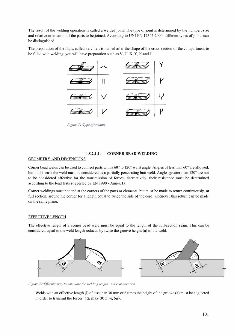
101
The result of the welding operation is called a welded joint. The type of joint is determined by the number, size and relative orientation of the parts to be joined. According to UNI EN 12345:2000, different types of joints can be distinguished.
The preparation of the flaps, called kerchief, is named after the shape of the cross-section of the compartment to be filled with welding, you will have preparation such as V, U, X, Y, K and J.
4.8.2.1.1. CORNER BEAD WELDING GEOMETRY AND DIMENSIONS
Corner bead welds can be used to connect parts with a 60° to 120° waist angle. Angles of less than 60° are allowed, but in this case the weld must be considered as a partially penetrating butt weld. Angles greater than 120° are not to be considered effective for the transmission of forces; alternatively, their resistance must be determined according to the load tests suggested by EN 1990 - Annex D.
Corner weldings must not end at the corners of the parts or elements, but must be made to return continuously, at full section, around the corner for a length equal to twice the side of the cord, whenever this return can be made on the same plane.
EFFECTIVE LENGTH
The effective length of a corner bead weld must be equal to the length of the full-section seam. This can be considered equal to the weld length reduced by twice the groove height (a) of the weld.
Figure 72:Effective way to calculate the welding length and cross-section.
Welds with an effective length (l) of less than 30 mm or 6 times the height of the groove (a) must be neglected in order to transmit the forces. 𝑙 ≥ max(30 𝑚𝑚; 6𝑎).
Figure 71:Type of welding
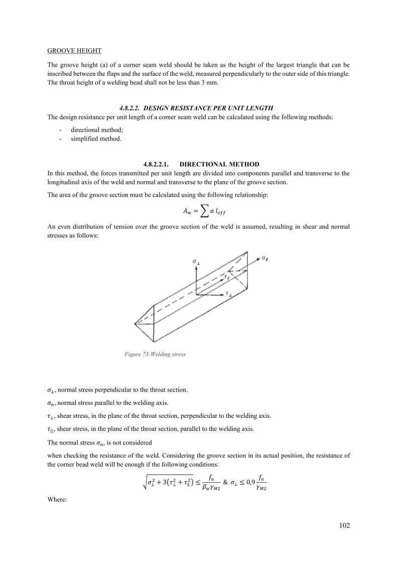
102
GROOVE HEIGHT
The groove height (a) of a corner seam weld should be taken as the height of the largest triangle that can be inscribed between the flaps and the surface of the weld, measured perpendicularly to the outer side of this triangle. The throat height of a welding bead shall not be less than 3 mm.
4.8.2.2. DESIGN RESISTANCE PER UNIT LENGTH The design resistance per unit length of a corner seam weld can be calculated using the following methods:
- directional method; - simplified method.
4.8.2.2.1. DIRECTIONAL METHOD In this method, the forces transmitted per unit length are divided into components parallel and transverse to the longitudinal axis of the weld and normal and transverse to the plane of the groove section.
The area of the groove section must be calculated using the following relationship:
𝐴𝑤 = ∑ 𝑎 𝑙𝑒𝑓𝑓
An even distribution of tension over the groove section of the weld is assumed, resulting in shear and normal stresses as follows:
𝜎⊥, normal stress perpendicular to the throat section.
𝜎𝑛, normal stress parallel to the welding axis.
𝜏⊥, shear stress, in the plane of the throat section, perpendicular to the welding axis.
𝜏||, shear stress, in the plane of the throat section, parallel to the welding axis.
The normal stress 𝜎𝑛, is not considered
when checking the resistance of the weld. Considering the groove section in its actual position, the resistance of the corner bead weld will be enough if the following conditions:
√𝜎⊥2 + 3(𝜏⊥
2 + 𝜏∥2) ≤
𝑓𝑢
𝛽𝑤𝛾𝑀2
& 𝜎⊥ ≤ 0,9𝑓𝑢
𝛾𝑀2
Where:
Figure 73:Welding stress
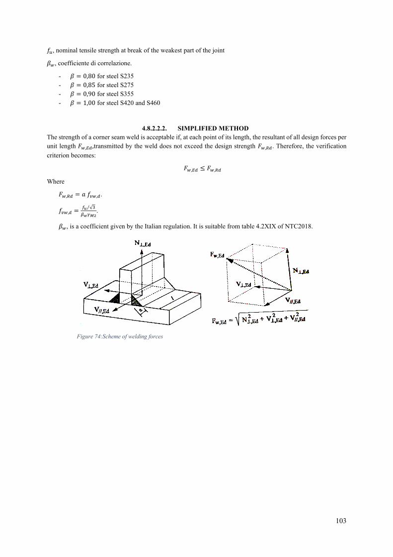
103
𝑓𝑢, nominal tensile strength at break of the weakest part of the joint
𝛽𝑤, coefficiente di correlazione.
- 𝛽 = 0,80 for steel S235 - 𝛽 = 0,85 for steel S275 - 𝛽 = 0,90 for steel S355 - 𝛽 = 1,00 for steel S420 and S460
4.8.2.2.2. SIMPLIFIED METHOD The strength of a corner seam weld is acceptable if, at each point of its length, the resultant of all design forces per unit length 𝐹𝑤,𝐸𝑑,transmitted by the weld does not exceed the design strength 𝐹𝑤,𝑅𝑑. Therefore, the verification criterion becomes:
𝐹𝑤,𝐸𝑑 ≤ 𝐹𝑤,𝑅𝑑
Where
𝐹𝑤,𝑅𝑑 = 𝑎 𝑓𝑣𝑤,𝑑.
𝑓𝑣𝑤,𝑑 =𝑓𝑢 √3⁄
𝛽𝑤𝛾𝑀2.
𝛽𝑤, is a coefficient given by the Italian regulation. It is suitable from table 4.2XIX of NTC2018.
Figure 74:Scheme of welding forces
104
4.8.3. WELDING OF SHEAR CONNECTORS As defined in the chapter §4.7, the shear connectors are used to control the resist at shear loading acting on the top of the concrete-steel composite structure.
How is composed the welding shear connectors? Basically, it is characterized by the release of very high current peaks voltage in an extremely short time. When the gun is operated by pressing a button, an electric arc is created between the base or head of the pin and the base surface, melting and fixing both materials.
The procedure shall be distinguished in:
- Choose bolt and type of welding. - Loading the welding gun. - Place the machine close to the welding base. - Activation of welding process. - Get off the gun from the point.
There are different types of guns suitable for different welding processes with specific internal components. they are distinguished by long arc welding, short arc welding or condensation. Each of them has the ability, depending on the voltage transferred to it, to perform welds of different joint thicknesses.
In this thesis, we have taken into consideration the Nelson shear connectors, commercially known as KB, produced in compliance with the European reference standards EN ISO and EN 10025-2 respecting the minimum requirements indicated for the material making up the connector.
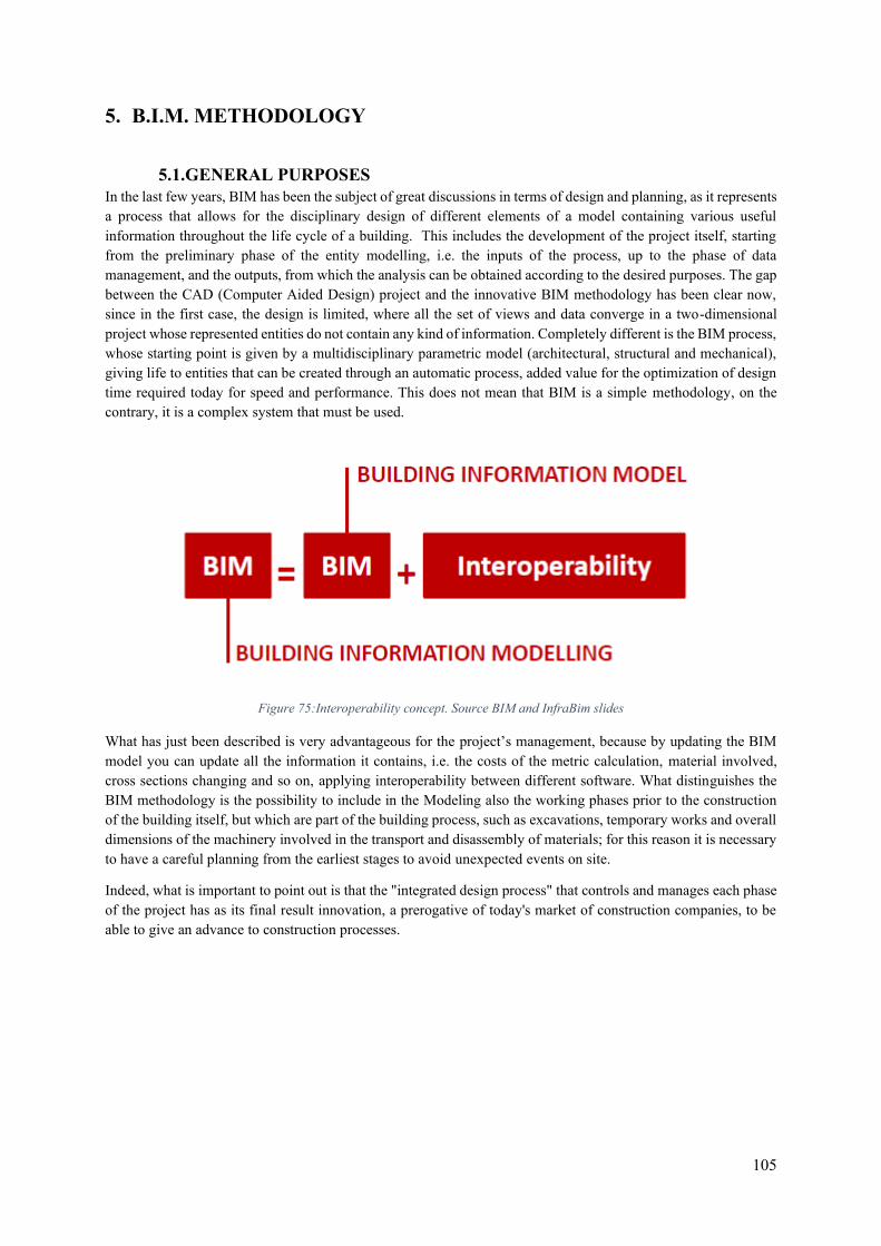
105
5. B.I.M. METHODOLOGY
5.1.GENERAL PURPOSES In the last few years, BIM has been the subject of great discussions in terms of design and planning, as it represents a process that allows for the disciplinary design of different elements of a model containing various useful information throughout the life cycle of a building. This includes the development of the project itself, starting from the preliminary phase of the entity modelling, i.e. the inputs of the process, up to the phase of data management, and the outputs, from which the analysis can be obtained according to the desired purposes. The gap between the CAD (Computer Aided Design) project and the innovative BIM methodology has been clear now, since in the first case, the design is limited, where all the set of views and data converge in a two-dimensional project whose represented entities do not contain any kind of information. Completely different is the BIM process, whose starting point is given by a multidisciplinary parametric model (architectural, structural and mechanical), giving life to entities that can be created through an automatic process, added value for the optimization of design time required today for speed and performance. This does not mean that BIM is a simple methodology, on the contrary, it is a complex system that must be used.
Figure 75:Interoperability concept. Source BIM and InfraBim slides
What has just been described is very advantageous for the project’s management, because by updating the BIM model you can update all the information it contains, i.e. the costs of the metric calculation, material involved, cross sections changing and so on, applying interoperability between different software. What distinguishes the BIM methodology is the possibility to include in the Modeling also the working phases prior to the construction of the building itself, but which are part of the building process, such as excavations, temporary works and overall dimensions of the machinery involved in the transport and disassembly of materials; for this reason it is necessary to have a careful planning from the earliest stages to avoid unexpected events on site.
Indeed, what is important to point out is that the "integrated design process" that controls and manages each phase of the project has as its final result innovation, a prerogative of today's market of construction companies, to be able to give an advance to construction processes.
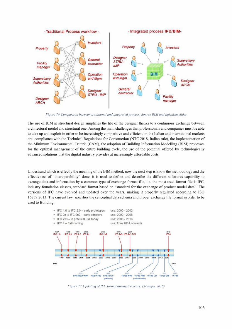
106
Figure 76:Comparison between traditional and integrated process. Source BIM and InfraBim slides
The use of BIM in structural design simplifies the life of the designer thanks to a continuous exchange between architectural model and structural one. Among the main challenges that professionals and companies must be able to take up and exploit in order to be increasingly competitive and efficient on the Italian and international markets are: compliance with the Technical Regulations for Construction (NTC 2018, Italian rule), the implementation of the Minimum Environmental Criteria (CAM), the adoption of Building Information Modelling (BIM) processes for the optimal management of the entire building cycle, the use of the potential offered by technologically advanced solutions that the digital industry provides at increasingly affordable costs.
Undestrand which is effectly the meaning of the BIM method, now the next step is know the methodology and the effectivness of “interoperability” done. it is used to define and describe the different softwares capability to excange data and information by a common type of exchange format file, i.e. the most used format file is IFC, industry foundation classes, standard format based on “standard for the exchange of product model data”. The versions of IFC have evolved and updated over the years, making it properly regulated according to ISO 16739:2013. The current law specifies the cenceptual data schema and proper exchange file format in order to be used to Building.
Figure 77:Updating of IFC format during the years. (Acampa, 2018)

107
Basically IFC is an open source standard for the exchange of construction data models in the design and construction of buildings with different software products. It aims to exchange information within a team or professionals figures and between different software applications at different stages of design, construction, maintenance and installation. IFC extension files support 2D and 3D property and geometry data. Since IFC definitions are regularly updated and developed over the years, as described in Figure 68 above, it is necessary to define what the differences of the extensions used are.
- IFC4: this is used to transfer IFC models in order to import and modify them in a BIM-enabled software; it allows to transfer parametric projects and complex contexts (possible manual adjustments to manage software differences).
- IFC2x3: it is also defined as coordination View Version 2.0. optimized for the coordinated exchange of BIM models between the main disciplines of the building industry; it is currently the most widely used model view definition supported by the BIM market. coordination view also supports an elementary parametric derivation of building components when they are imported into planning tools, which is mostly used for the exchange of architectural models, building technology and engineering.
- IFC2x2: also called CoordinationView. it is only used in isolated cases, for example when exporting MVD definitions for software products that do not support IFC2x3. Each of these operations can be manually adapted to specific workflow needs.
All extension file seen before should be summarized in a generic acrnonymous: MVD. Model View Definition, is used for the targeted exchange of specialized models, taking into account the graphical information and content that the planner needs, as described before for each ot these.
Of course, the IFC extension file was used in this thesis to exchange data e information from softwares in order to loss as less as possible data information. The goal will be test the interoperability between software used and test if parameters are loss and reach an high value of level of detail, LOD, in order to built a detail construction drawing and present it to the steel factory.
In essence, the level of detail should be thought as input to the element in such a way to update the information and detail informations.
- LOD 100: the model must be presented as symbol or generic representation, just conceptual position and possible behaviour.
- LOD 200: the model element may be graphically represented within the model as a generic system or assembly with approximate quantities, size, orientatio and so on.
- LOD 300: the model element within the element as a specific system, object or assembly in term of defined information but not graphic informations attached to the model.
- LOD 400: the model is graphically represented within the model as a specif system, object, quantity, size orientation and other characteristics, with a detailing fabrication installation information.
- LOD 500: the model is a field verified representation in term of size and components quntity.
The figure 68 explains basically the conceptual scheme of LOD, from the conceptual design process until reach the end process of construction , called As-built final scheme.
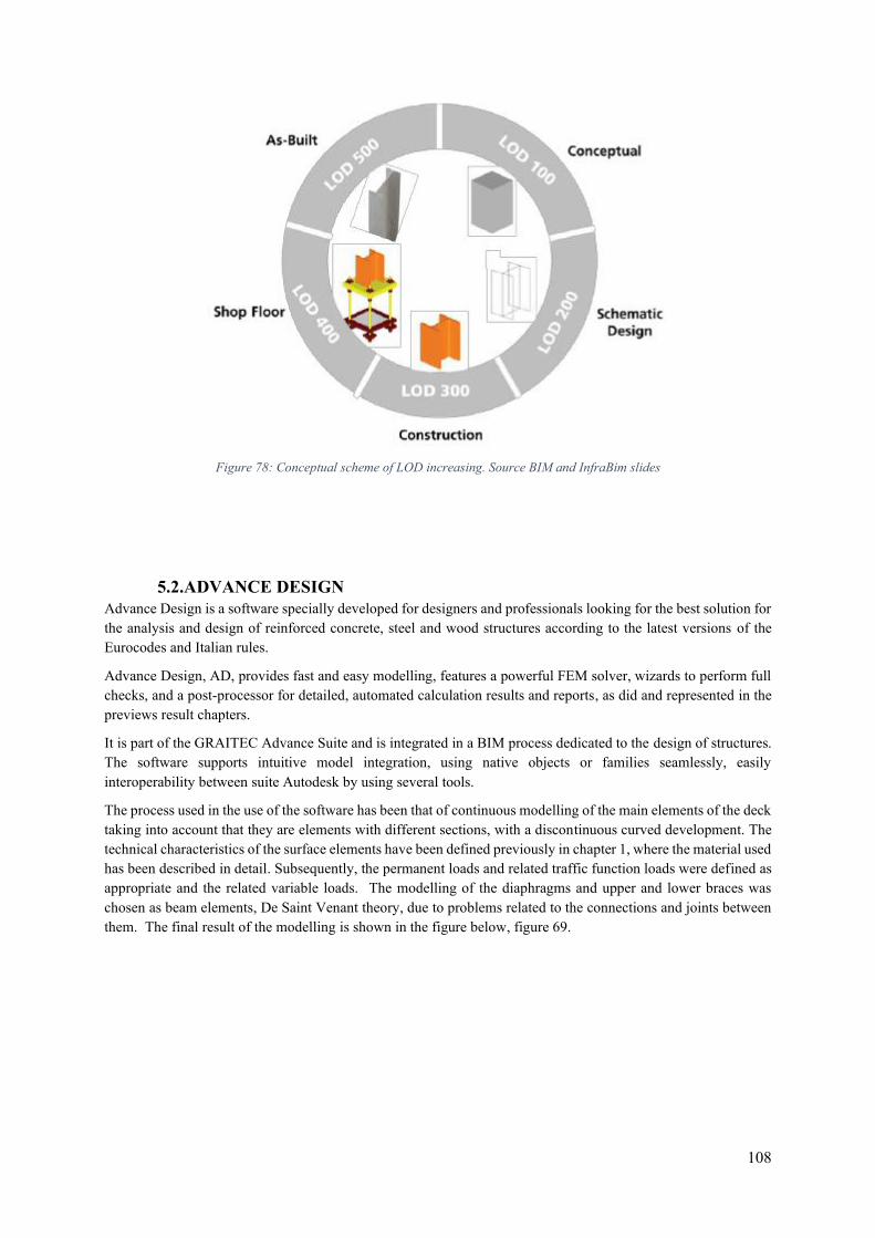
108
Figure 78: Conceptual scheme of LOD increasing. Source BIM and InfraBim slides
5.2.ADVANCE DESIGN Advance Design is a software specially developed for designers and professionals looking for the best solution for the analysis and design of reinforced concrete, steel and wood structures according to the latest versions of the Eurocodes and Italian rules.
Advance Design, AD, provides fast and easy modelling, features a powerful FEM solver, wizards to perform full checks, and a post-processor for detailed, automated calculation results and reports, as did and represented in the previews result chapters.
It is part of the GRAITEC Advance Suite and is integrated in a BIM process dedicated to the design of structures. The software supports intuitive model integration, using native objects or families seamlessly, easily interoperability between suite Autodesk by using several tools.
The process used in the use of the software has been that of continuous modelling of the main elements of the deck taking into account that they are elements with different sections, with a discontinuous curved development. The technical characteristics of the surface elements have been defined previously in chapter 1, where the material used has been described in detail. Subsequently, the permanent loads and related traffic function loads were defined as appropriate and the related variable loads. The modelling of the diaphragms and upper and lower braces was chosen as beam elements, De Saint Venant theory, due to problems related to the connections and joints between them. The final result of the modelling is shown in the figure below, figure 69.
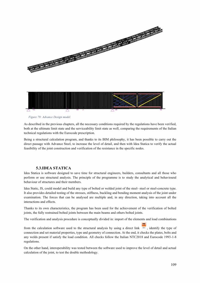
109
As described in the previous chapters, all the necessary conditions required by the regulations have been verified, both at the ultimate limit state and the serviceability limit state as well, comparing the requirements of the Italian technical regulations with the Eurocode prescription.
Being a structural calculation program, and thanks to its BIM philosophy, it has been possible to carry out the direct passage with Advance Steel, to increase the level of detail, and then with Idea Statica to verify the actual feasibility of the joint construction and verification of the resistance in the specific nodes.
5.3.IDEA STATICA Idea Statica is software designed to save time for structural engineers, builders, consultants and all those who perform or use structural analysis. The principle of the programme is to study the analytical and behavioural behaviour of structures and their members.
Idea Static, IS, could model and build any type of bolted or welded joint of the steel- steel or steel-concrete type. It also provides detailed testing of the stresses, stiffness, buckling and bending moment analysis of the joint under examination. The forces that can be analysed are multiple and, in any direction, taking into account all the interactions and effects.
Thanks to its own characteristics, the program has been used for the achievement of the verification of bolted joints, the fully restrained bolted joints between the main beams and others bolted joints.
The verification and analysis procedure is conceptually divided in: import of the elements and load combinations
from the calculation software used to the structural analysis by using a direct link , identify the type of connection and set material properties, type and geometry of connection. At the end, it checks the plates, bolts and any welds present if satisfy the load condition. All checks follow the Italian NTC2018 and Eurocode 1993-1-8 regulations.
On the other hand, interoperability was tested between the software used to improve the level of detail and actual calculation of the joint, to test the double methodology.
Figure 79: Advance Design model.

110
5.4.ADVANCE STEEL Advance Steel (AS) is part of Autodesk and GRAITEC suite, CAD software application for 3D modelling and local detail of steel structures. AS has many functions, among which we can highlight: the creation of 3D models using with ease the pre-set libraries such as beams, metal plates, bolts, welds and others; creation of arrangement and shop drawings, fabrication drawings; modelling of complex structures as spiral stairs or barriers; Automatic determination of lists of elements.
Thanks to its huge potential and vast library, it has been possible to perform all the operations of constraints between the different elements previously modelled with the calculation program. As explained before, this software has been used to increase the level of detail of each single node, going to arrange in a constructively accessible way each single component, previously verified.
Moreover, this programme was used to achieve the final objective of the thesis, which is to produce the construction details and then present them in the workshop and subsequently produce them.
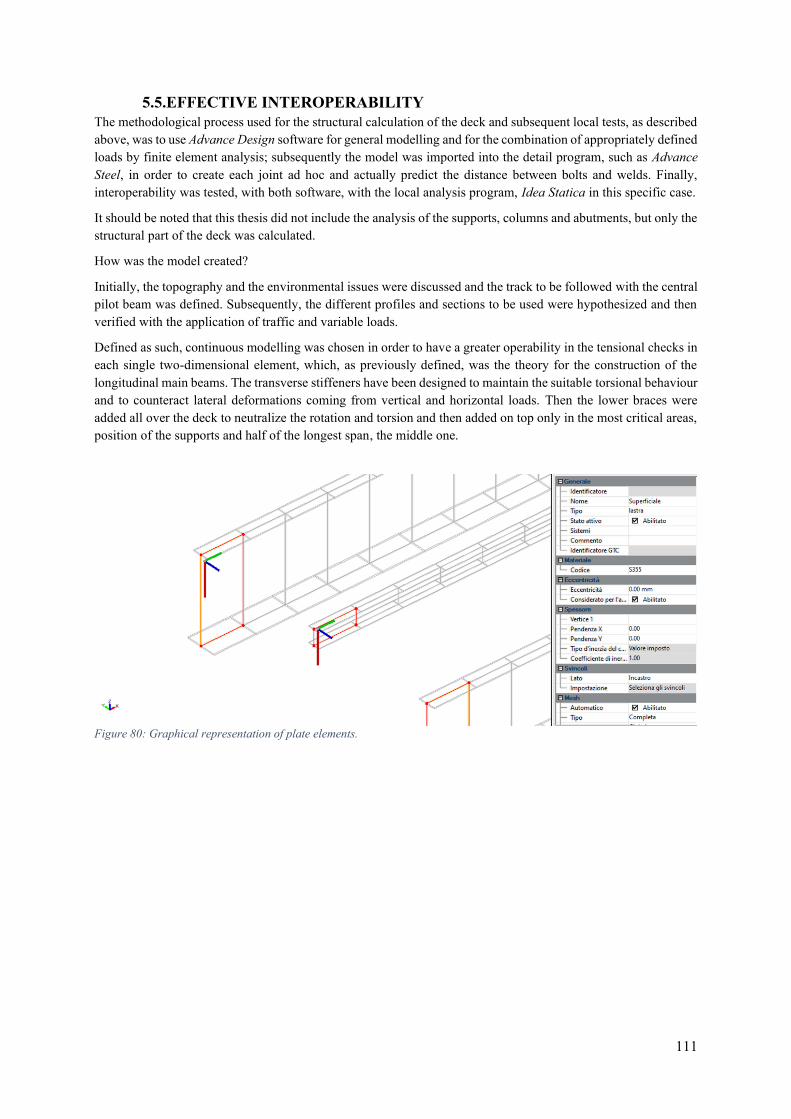
111
5.5.EFFECTIVE INTEROPERABILITY The methodological process used for the structural calculation of the deck and subsequent local tests, as described above, was to use Advance Design software for general modelling and for the combination of appropriately defined loads by finite element analysis; subsequently the model was imported into the detail program, such as Advance Steel, in order to create each joint ad hoc and actually predict the distance between bolts and welds. Finally, interoperability was tested, with both software, with the local analysis program, Idea Statica in this specific case.
It should be noted that this thesis did not include the analysis of the supports, columns and abutments, but only the structural part of the deck was calculated.
How was the model created?
Initially, the topography and the environmental issues were discussed and the track to be followed with the central pilot beam was defined. Subsequently, the different profiles and sections to be used were hypothesized and then verified with the application of traffic and variable loads.
Defined as such, continuous modelling was chosen in order to have a greater operability in the tensional checks in each single two-dimensional element, which, as previously defined, was the theory for the construction of the longitudinal main beams. The transverse stiffeners have been designed to maintain the suitable torsional behaviour and to counteract lateral deformations coming from vertical and horizontal loads. Then the lower braces were added all over the deck to neutralize the rotation and torsion and then added on top only in the most critical areas, position of the supports and half of the longest span, the middle one.
Figure 80: Graphical representation of plate elements.
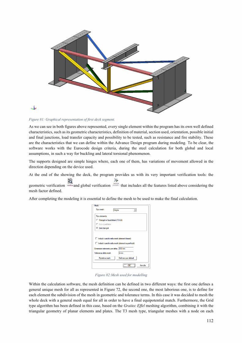
112
As we can see in both figures above represented, every single element within the program has its own well defined characteristics, such as its geometric characteristics, definition of material, section used, orientation, possible initial and final junctions, load transfer capacity and possibility to be tested, such as resistance and fire stability. These are the characteristics that we can define within the Advance Design program during modeling. To be clear, the software works with the Eurocode design criteria, during the steel calculation for both global and local assumptions, in such a way for buckling and lateral torsional phenomenon.
The supports designed are simple hinges where, each one of them, has variations of movement allowed in the direction depending on the device used.
At the end of the showing the deck, the program provides us with its very important verification tools: the
geometric verification and global verification that includes all the features listed above considering the mesh factor defined.
After completing the modeling it is essential to define the mesh to be used to make the final calculation.
Figure 82:Mesh used for modelling
Within the calculation software, the mesh definition can be defined in two different ways: the first one defines a general unique mesh for all as represented in Figure 72, the second one, the most laborious one, is to define for each element the subdivision of the mesh in geometric and tolerance terms. In this case it was decided to mesh the whole deck with a general mesh equal for all in order to have a final equipotential match. Furthermore, the Grid type algorithm has been defined in this case, based on the Graitec Effel meshing algorithm, combining it with the triangular geometry of planar elements and plates. The T3 mesh type, triangular meshes with a node on each
Figure 81: Graphical representation of first deck segment.
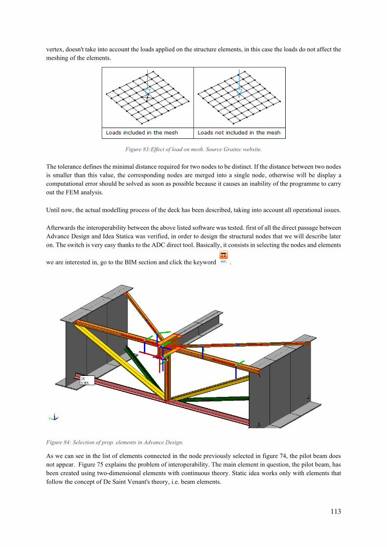
113
vertex, doesn't take into account the loads applied on the structure elements, in this case the loads do not affect the meshing of the elements.
Figure 83:Effect of load on mesh. Source Graitec website.
The tolerance defines the minimal distance required for two nodes to be distinct. If the distance between two nodes is smaller than this value, the corresponding nodes are merged into a single node, otherwise will be display a computational error should be solved as soon as possible because it causes an inability of the programme to carry out the FEM analysis.
Until now, the actual modelling process of the deck has been described, taking into account all operational issues.
Afterwards the interoperability between the above listed software was tested. first of all the direct passage between Advance Design and Idea Statica was verified, in order to design the structural nodes that we will describe later on. The switch is very easy thanks to the ADC direct tool. Basically, it consists in selecting the nodes and elements
we are interested in, go to the BIM section and click the keyword .
Figure 84: Selection of prop. elements in Advance Design.
As we can see in the list of elements connected in the node previously selected in figure 74, the pilot beam does not appear. Figure 75 explains the problem of interoperability. The main element in question, the pilot beam, has been created using two-dimensional elements with continuous theory. Static idea works only with elements that follow the concept of De Saint Venant's theory, i.e. beam elements.
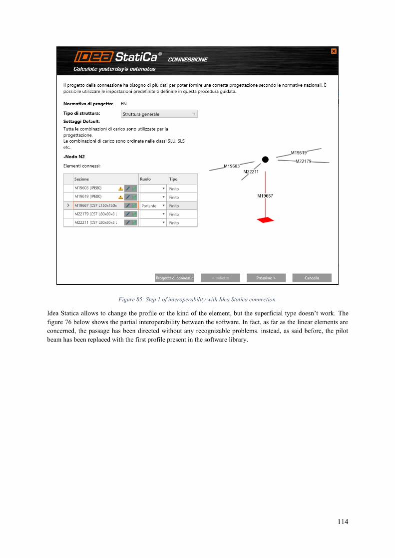
114
Figure 85: Step 1 of interoperability with Idea Statica connection.
Idea Statica allows to change the profile or the kind of the element, but the superficial type doesn’t work. The figure 76 below shows the partial interoperability between the software. In fact, as far as the linear elements are concerned, the passage has been directed without any recognizable problems. instead, as said before, the pilot beam has been replaced with the first profile present in the software library.
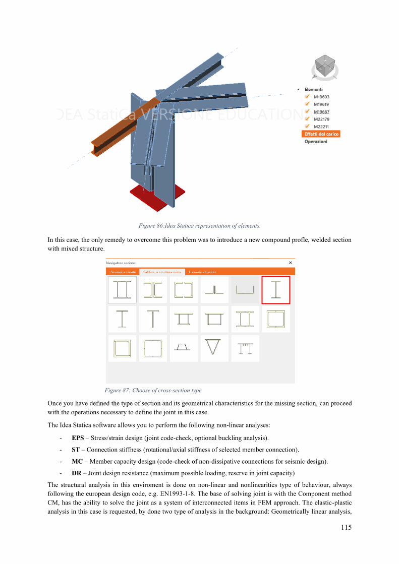
115
Figure 86:Idea Statica representation of elements.
In this case, the only remedy to overcome this problem was to introduce a new compound profle, welded section with mixed structure.
Once you have defined the type of section and its geometrical characteristics for the missing section, can proceed with the operations necessary to define the joint in this case.
The Idea Statica software allows you to perform the following non-linear analyses:
- EPS – Stress/strain design (joint code-check, optional buckling analysis).
- ST – Connection stiffness (rotational/axial stiffness of selected member connection).
- MC – Member capacity design (code-check of non-dissipative connections for seismic design).
- DR – Joint design resistance (maximum possible loading, reserve in joint capacity)
The structural analysis in this enviroment is done on non-linear and nonlinearities type of behaviour, always following the european design code, e.g. EN1993-1-8. The base of solving joint is with the Component method CM, has the ability to solve the joint as a system of interconnected items in FEM approach. The elastic-plastic analysis in this case is requested, by done two type of analysis in the background: Geometrically linear analysis,
Figure 87: Choose of cross-section type
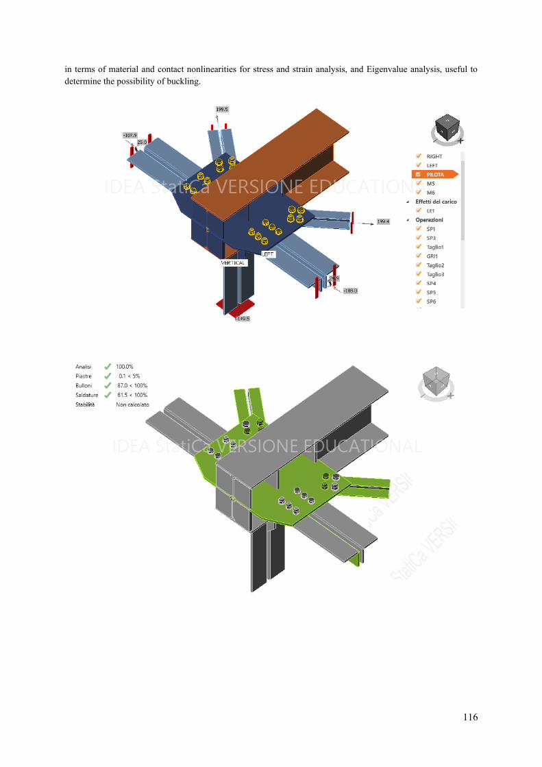
116
in terms of material and contact nonlinearities for stress and strain analysis, and Eigenvalue analysis, useful to determine the possibility of buckling.
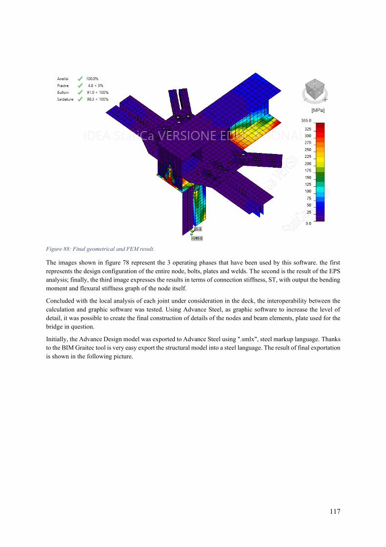
117
Figure 88: Final geometrical and FEM result.
The images shown in figure 78 represent the 3 operating phases that have been used by this software. the first represents the design configuration of the entire node, bolts, plates and welds. The second is the result of the EPS analysis; finally, the third image expresses the results in terms of connection stiffness, ST, with output the bending moment and flexural stiffness graph of the node itself.
Concluded with the local analysis of each joint under consideration in the deck, the interoperability between the calculation and graphic software was tested. Using Advance Steel, as graphic software to increase the level of detail, it was possible to create the final construction of details of the nodes and beam elements, plate used for the bridge in question.
Initially, the Advance Design model was exported to Advance Steel using ".smlx", steel markup language. Thanks to the BIM Graitec tool is very easy export the structural model into a steel language. The result of final exportation is shown in the following picture.
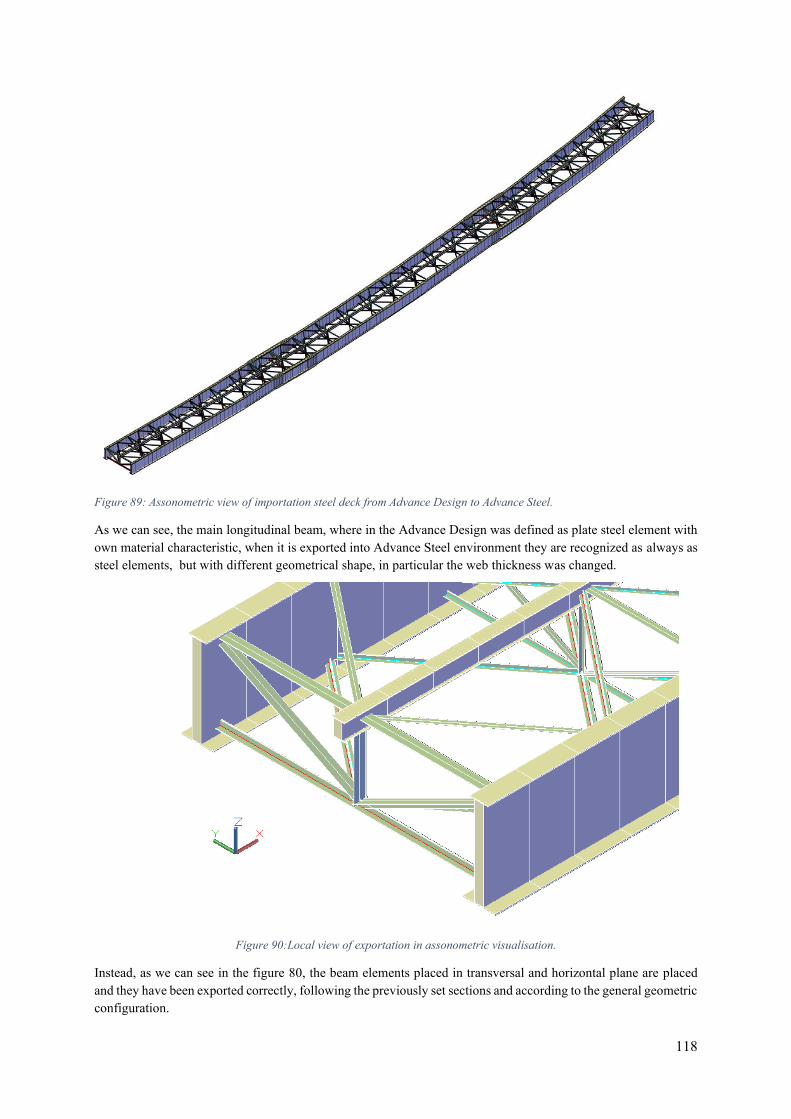
118
Figure 89: Assonometric view of importation steel deck from Advance Design to Advance Steel.
As we can see, the main longitudinal beam, where in the Advance Design was defined as plate steel element with own material characteristic, when it is exported into Advance Steel environment they are recognized as always as steel elements, but with different geometrical shape, in particular the web thickness was changed.
Figure 90:Local view of exportation in assonometric visualisation.
Instead, as we can see in the figure 80, the beam elements placed in transversal and horizontal plane are placed and they have been exported correctly, following the previously set sections and according to the general geometric configuration.
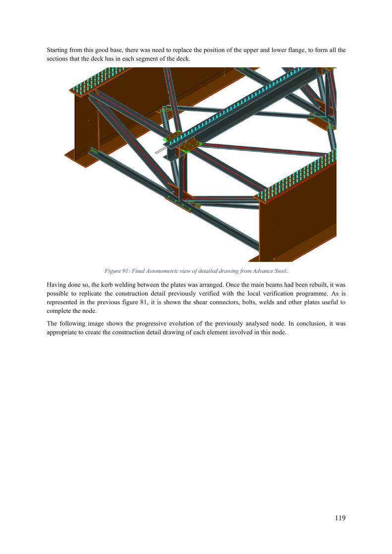
119
Starting from this good base, there was need to replace the position of the upper and lower flange, to form all the sections that the deck has in each segment of the deck.
Figure 91: Final Assonometric view of detailed drawing from Advance Steel.
Having done so, the kerb welding between the plates was arranged. Once the main beams had been rebuilt, it was possible to replicate the construction detail previously verified with the local verification programme. As is represented in the previous figure 81, it is shown the shear connectors, bolts, welds and other plates useful to complete the node.
The following image shows the progressive evolution of the previously analysed node. In conclusion, it was appropriate to create the construction detail drawing of each element involved in this node.
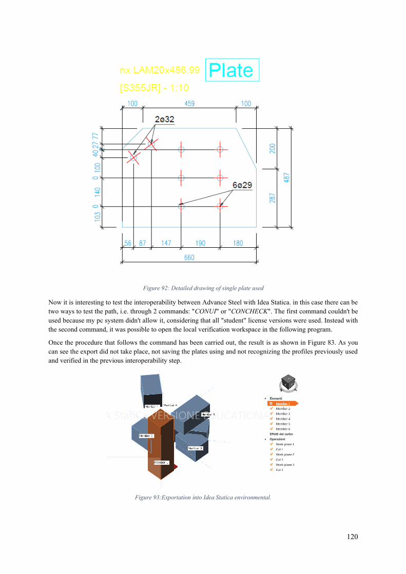
120
Figure 92: Detailed drawing of single plate used
Now it is interesting to test the interoperability between Advance Steel with Idea Statica. in this case there can be two ways to test the path, i.e. through 2 commands: "CONUI" or "CONCHECK". The first command couldn't be used because my pc system didn't allow it, considering that all "student" license versions were used. Instead with the second command, it was possible to open the local verification workspace in the following program.
Once the procedure that follows the command has been carried out, the result is as shown in Figure 83. As you can see the export did not take place, not saving the plates using and not recognizing the profiles previously used and verified in the previous interoperability step.
Figure 93:Exportation into Idea Statica environmental.
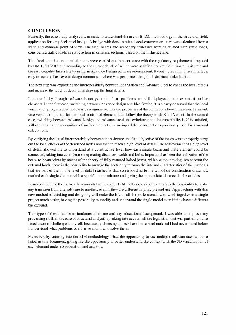
121
CONCLUSION Basically, the case study analysed was made to understand the use of B.I.M. methodology in the structural field, application for long deck steel bridge. A bridge with deck in mixed steel-concrete structure was calculated from a static and dynamic point of view. The slab, beams and secondary structures were calculated with static loads, considering traffic loads as static action in different sections, based on the influence line.
The checks on the structural elements were carried out in accordance with the regulatory requirements imposed by DM 17/01/2018 and according to the Eurocode, all of which were satisfied both at the ultimate limit state and the serviceability limit state by using an Advance Design software environment. It constitutes an intuitive interface, easy to use and has several design commands, where was performed the global structural calculations.
The next step was exploiting the interoperability between Idea Statica and Advance Steel to check the local effects and increase the level of detail until drawing the final details.
Interoperability through software is not yet optimal, as problems are still displayed in the export of surface elements. In the first case, switching between Advance design and Idea Statica, it is clearly observed that the local verification program does not clearly recognize section and properties of the continuous two-dimensional element, vice versa it is optimal for the local control of elements that follow the theory of de Saint Venant. In the second case, switching between Advance Design and Advance steel, the switchover and interoperability is 90% satisfied, still challenging the recognition of surface elements but saving all the beam sections previously used for structural calculations.
By verifying the actual interoperability between the software, the final objective of the thesis was to properly carry out the local checks of the described nodes and then to reach a high level of detail. The achievement of a high level of detail allowed me to understand at a constructive level how each single beam and plate element could be connected, taking into consideration operating distances, welds and bolts. Important has been the realization of the beam-to-beam joints by means of the theory of fully restored bolted joints, which without taking into account the external loads, there is the possibility to arrange the bolts only through the internal characteristics of the materials that are part of them. The level of detail reached is that corresponding to the workshop construction drawings, marked each single element with a specific nomenclature and giving the appropriate distances in the articles.
I can conclude the thesis, how fundamental is the use of BIM methodology today. It gives the possibility to make any transition from one software to another, even if they are different in principle and use. Approaching with this new method of thinking and designing will make the life of all the professionals who work together in a single project much easier, having the possibility to modify and understand the single model even if they have a different background.
This type of thesis has been fundamental to me and my educational background. I was able to improve my processing skills in the case of structural analysis by taking into account all the legislation that was part of it. I also faced a sort of challenge to myself, because by choosing a thesis based on a steel material I had never faced before I understood what problems could arise and how to solve them.
Moreover, by entering into the BIM methodology I had the opportunity to use multiple software such as those listed in this document, giving me the opportunity to better understand the context with the 3D visualization of each element under consideration and analysis.

122
ACKNOWLEDGEMENTS At the end of this work I would like to express my thanks to all those who have helped me, in one way or another, to achieve this important goal.
I thank my parents with great affection and gratitude for their daily moral and economic support in this path of my life.
A special thanks to my brother and sister-in-law, capable with the carefreeness of my nephew Daniele, to make me live moments of serenity, peacefulness and to distract me from everyday life.
I would like to sincerely thank Giulia for having always been there for me, for having shared with me positive and negative moments, having endured and supported us in this journey of our life together, reaching important goals.
To my fellow students that I met at the Polytechnic of Turin. With them I shared everything, from studying to everyday life, facing challenges and travelling together, giving me each of them important advice in any situation.
Thanks to Linda, for having shared this two year of life together, helping us in every academic difficulty and solving every problem we faced.
Thanks to the "Magnifici 4 of Casa Vespucci", Gianluigi, Matia, Alberto, Albertino and Gino. Buddies of a thousand adventures and misadventures, traumatic awakenings and dinners based on "frico and polenta".
I would like to thank my friends, for believing in me and for the beautiful relationship that binds us constantly, especially sharing smart aperitifs in this tricky period.
A sincere thanks to the company LGA Engineering from Savigliano (CN), especially to Engineer Andrea Alberto and his team for helping and teaching me important knowledge during this period of writing my thesis.

123
BIBLIOGRAPHY - Acampa, G. (2018). Test for interoperability: from theory to practice. 3D modelling & BIM, 48-61.
- Ballio G., Bernuzzi C. (2004). Progettare costruzioni in acciaio. Ulrico Hoepli Editore S.p.A., Milano, Italy.
- Belluzzi O. (1989). Scienza delle costruzioni. Vol.2. Zanichelli Editore, Milano, Italy.
- Carpinteri A. (1992). Scienza delle costruzioni 1. Pitagora Editrice, Bologna, Italy.
- Carpinteri A. (1992). Scienza delle costruzioni 2. Pitagora Editrice, Bologna, Italy.
- Commissione di studio per la predisposizione e l'analisi di norme tecniche relative alle costruzioni, CNR-DT 207/2008, (2009). Istruzioni per la valutazione delle azioni e degli effetti del vento sulle costruzioni.
- Cordova B. (2013). Costruzioni in acciaio. Manuale pratico per l'impiego delle norme tecniche per le costruzioni e dell'Eurocodice 3 (UNI EN 1993). Ulrico Hoepli Editore S.p.A., Milano, Italy.
- Ren R and Zhang JModel Information Checking to Support Interoperable BIM Usage in Structural Analysis Computing in Civil Engineering 2019, (361-368).
Technical regulations consulted
- “Norme Tecniche per le costruzioni” adottate con il D.M. of 17 January 2018.
- UNI EN 1991, Actions on structures.
- UNI EN 1992, Design of concrete structures.
- UNI EN 1993, Design of steel structures.
- UNI EN 1994, Design of composite steel and concrete structures.
- UNI EN 1998, Design of structures for earthquake resistance.
User’s guide:
- Advance design user guide.
- Idea Statica theoretical background.
- Advance Steel user guide.
- Workbook di implementazione pilota del BIM, Autodesk.
- Pilota BIM. Manuale introduttivo, Autodesk.
- Guida all’interoperabilità, Autodesk.

124
WEBSITE CITATIONS www.buildingsmart.org
https://www.buildingsmart.org/standards/bsi-standards/industry-foundation-classes/
https://www.autodesk.com/solutions/bim/hub/bim-interoperability
https://www.autodesk.com/solutions/bim
https://knowledge.autodesk.com/support/revit-products/learn-explore/caas/simplecontent/content/useful-useful-ifc-links.html
https://www.ideastatica.com/it/idea-statica-and-graitec/
https://www.ideastatica.com/idea-statica-and-trimble/
https://www.ideastatica.com/steel/?gclid=EAIaIQobChMItM2Tt_-M6AIVSsKyCh0J2gerEAAYASAAEgK9qfD_BwE
https://www.steelconstruction.info/Bridges
esse1-gis.mi.ingv.it
https://it.graitec.com/advance-design/
http://www.ibimi.it/lod-livello-di-dettaglio-per-il-bim/
http://www.nelsonsaldaturaperni.it
https://www.promozioneacciaio.it/

125
ANNEX A – MODEL CALIBRATION
CALIBRATION OF SAINT VENANT AND CONTINUOUS MODELS Model calibration gives us the possibility to compare the behaviour of the elements in a more detailed way and closer to the real tensional development. Therefore, our aim in this chapter is to study what the differences are from the De Saint Venant model to the continuous one in term of displacement, forces and tension, in order to understand in a better way how the program works. All analytical tests are conducted by Advance Design Software
As the first analysis, the general static system is composed of beam IPE 300 (S355), placed on pinned and rolled supports and loaded with a concentrated load of 1000 daN on different position and direction.
The meshes used for the FEM analysis are [dimension/tolerance]: De Saint Venant element [150mm/50mm], Continuous element [50mm/10mm].
The following images explain the general characteristics in order to compare the methodologies (firstly is shown the continuous result then the De Saint Venant).
De Saint Venant element are kept in consideration as linear element which has own cross-section, type of material, orientation, constraint and mesh. We must remember that there are some limitations on Saint-Venant principle’s:
constraints, volume forces, apply forces only at the end-sections and decay region around twice the main dimension of cross-section, constant cross section along all straight beam axis.
Instead of DSV (De Saint Venant) theory element, continuous one is created as superficial type, properly defined as thin walled element. Even in this case, the element has own thickness, length, deep, material, constraint, orientation and mesh.
BEAM LOADED ON Z-DIRECTION STATIC SCHEME
DISPLACEMENT – G
Figure 95:Dead load effect. left is expressed the continuous behaviour.
Figure 94: General scheme. Beam loaded on z direction.
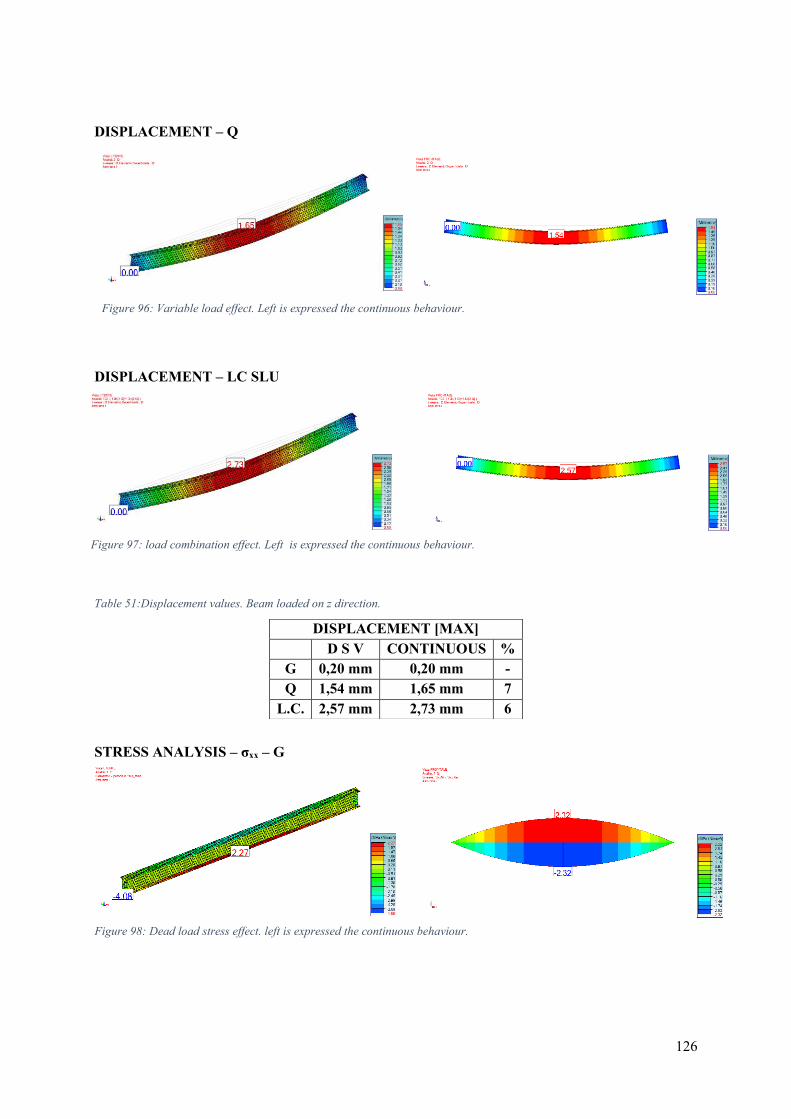
126
DISPLACEMENT – Q
DISPLACEMENT – LC SLU
Table 51:Displacement values. Beam loaded on z direction.
STRESS ANALYSIS – σxx – G
DISPLACEMENT [MAX] D S V CONTINUOUS %
G 0,20 mm 0,20 mm - Q 1,54 mm 1,65 mm 7
L.C. 2,57 mm 2,73 mm 6
Figure 96: Variable load effect. Left is expressed the continuous behaviour.
Figure 97: load combination effect. Left is expressed the continuous behaviour.
Figure 98: Dead load stress effect. left is expressed the continuous behaviour.
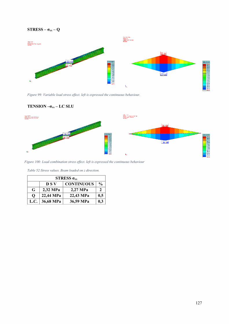
127
STRESS – σxx – Q
TENSION –σxx – LC SLU
Table 52:Stress values. Beam loaded on z direction.
STRESS σxx D S V CONTINUOUS %
G 2,32 MPa 2,27 MPa 2 Q 22,44 MPa 22,43 MPa 0,5
L.C. 36,68 MPa 36,59 MPa 0,3
Figure 99: Variable load stress effect. left is expressed the continuous behaviour.
Figure 100: Load combination stress effect. left is expressed the continuous behaviour
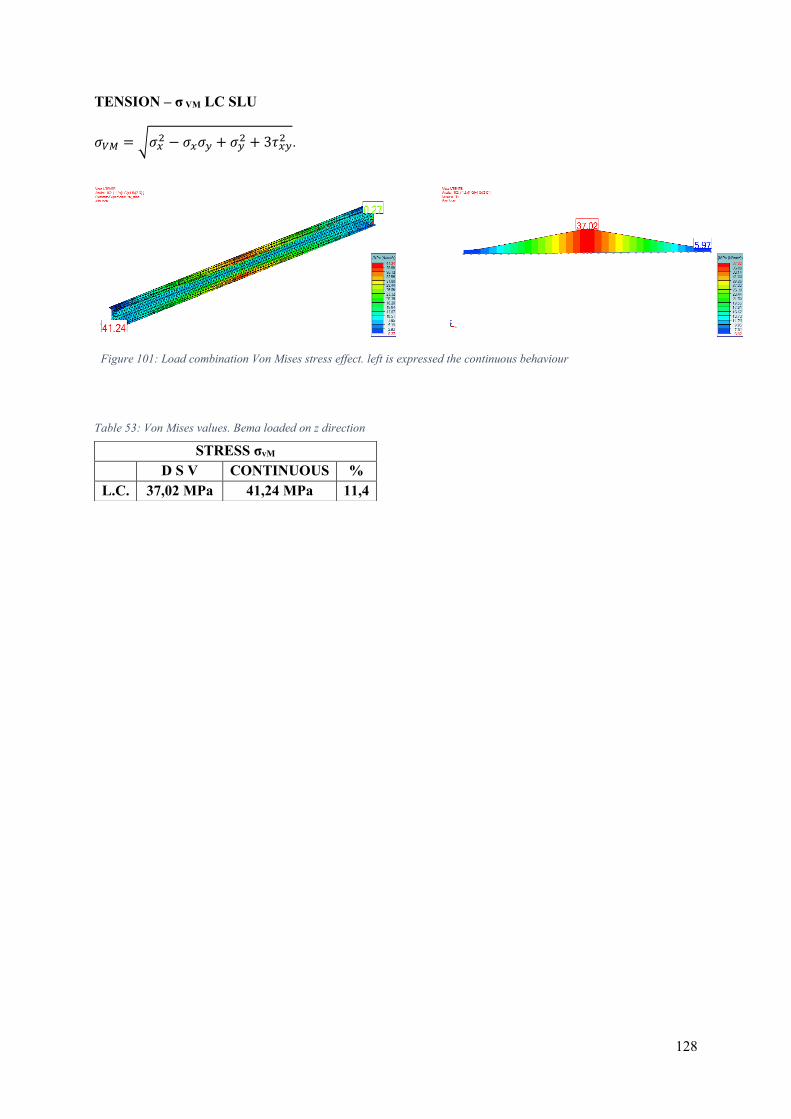
128
TENSION – σ VM LC SLU
𝜎𝑉𝑀 = √𝜎𝑥2 − 𝜎𝑥𝜎𝑦 + 𝜎𝑦
2 + 3𝜏𝑥𝑦2 .
Table 53: Von Mises values. Bema loaded on z direction
STRESS σvM D S V CONTINUOUS %
L.C. 37,02 MPa 41,24 MPa 11,4
Figure 101: Load combination Von Mises stress effect. left is expressed the continuous behaviour
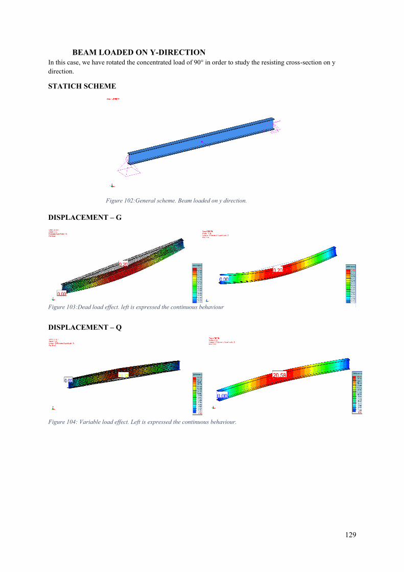
129
BEAM LOADED ON Y-DIRECTION In this case, we have rotated the concentrated load of 90° in order to study the resisting cross-section on y direction.
STATICH SCHEME
DISPLACEMENT – G
DISPLACEMENT – Q
Figure 103:Dead load effect. left is expressed the continuous behaviour
Figure 102:General scheme. Beam loaded on y direction.
Figure 104: Variable load effect. Left is expressed the continuous behaviour.
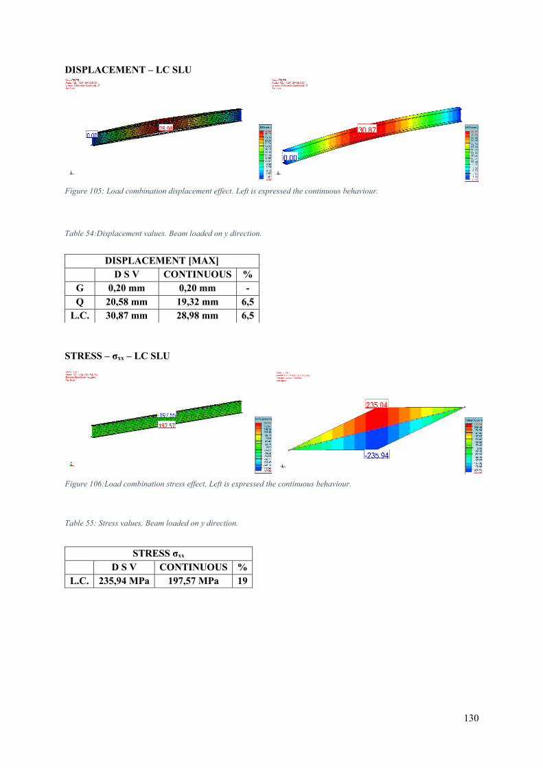
130
DISPLACEMENT – LC SLU
Table 54:Displacement values. Beam loaded on y direction.
STRESS – σxx – LC SLU
Table 55: Stress values. Beam loaded on y direction.
DISPLACEMENT [MAX] D S V CONTINUOUS %
G 0,20 mm 0,20 mm - Q 20,58 mm 19,32 mm 6,5
L.C. 30,87 mm 28,98 mm 6,5
STRESS σxx D S V CONTINUOUS %
L.C. 235,94 MPa 197,57 MPa 19
Figure 105: Load combination displacement effect. Left is expressed the continuous behaviour.
Figure 106:Load combination stress effect, Left is expressed the continuous behaviour.
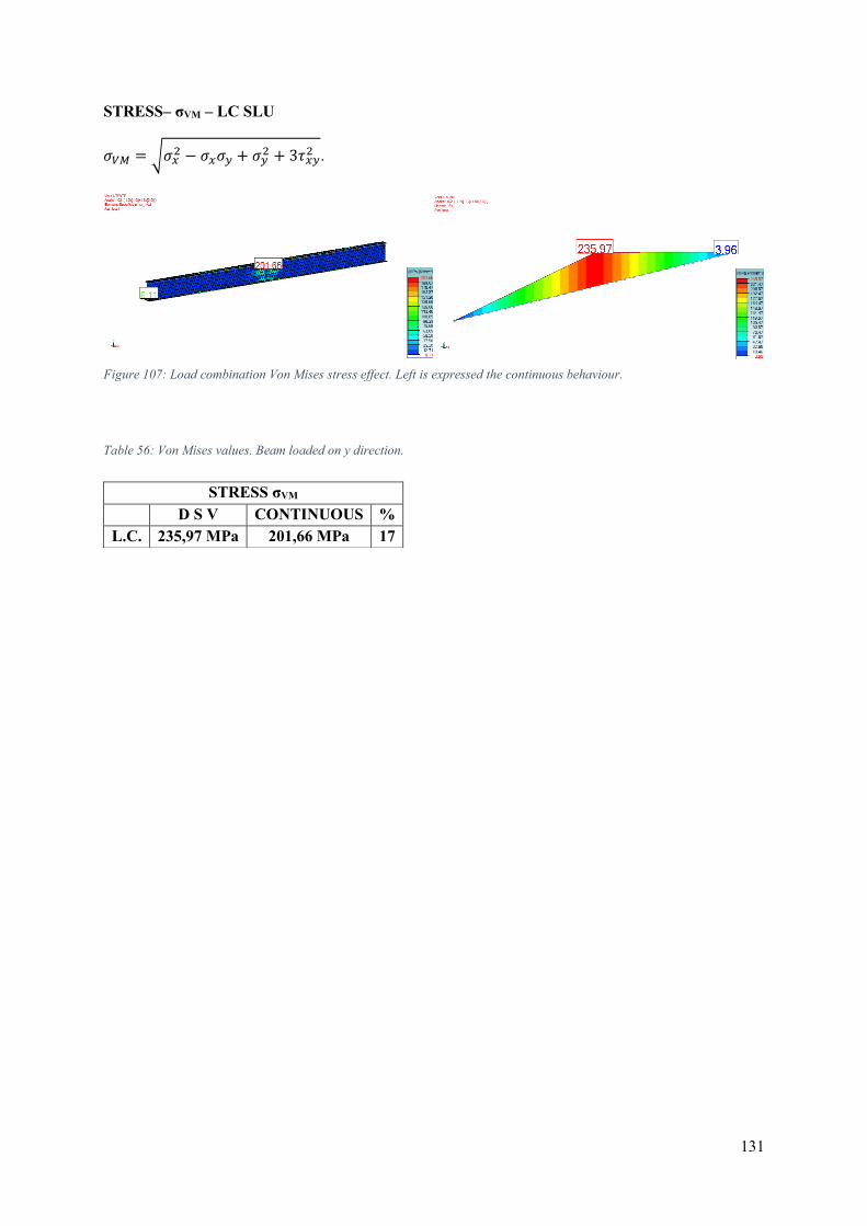
131
STRESS– σVM – LC SLU
𝜎𝑉𝑀 = √𝜎𝑥2 − 𝜎𝑥𝜎𝑦 + 𝜎𝑦
2 + 3𝜏𝑥𝑦2 .
Table 56: Von Mises values. Beam loaded on y direction.
STRESS σVM D S V CONTINUOUS %
L.C. 235,97 MPa 201,66 MPa 17
Figure 107: Load combination Von Mises stress effect. Left is expressed the continuous behaviour.
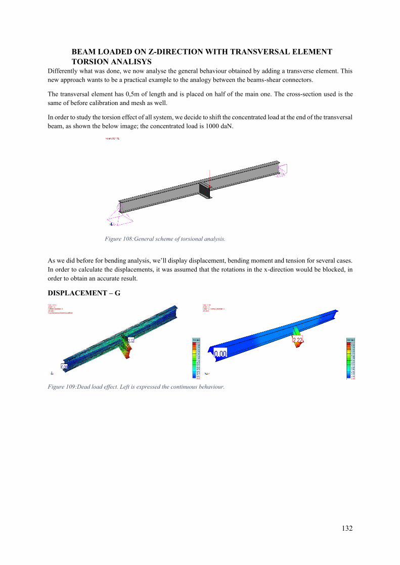
132
BEAM LOADED ON Z-DIRECTION WITH TRANSVERSAL ELEMENT TORSION ANALISYS
Differently what was done, we now analyse the general behaviour obtained by adding a transverse element. This new approach wants to be a practical example to the analogy between the beams-shear connectors.
The transversal element has 0,5m of length and is placed on half of the main one. The cross-section used is the same of before calibration and mesh as well.
In order to study the torsion effect of all system, we decide to shift the concentrated load at the end of the transversal beam, as shown the below image; the concentrated load is 1000 daN.
As we did before for bending analysis, we’ll display displacement, bending moment and tension for several cases.
In order to calculate the displacements, it was assumed that the rotations in the x-direction would be blocked, in order to obtain an accurate result.
DISPLACEMENT – G
Figure 108:General scheme of torsional analysis.
Figure 109:Dead load effect. Left is expressed the continuous behaviour.
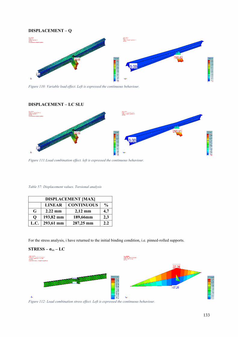
133
DISPLACEMENT – Q
DISPLACEMENT – LC SLU
Table 57: Displacement values. Torsional analysis
For the stress analysis, i have returned to the initial binding condition, i.e. pinned-rolled supports.
STRESS – σxx – LC
DISPLACEMENT [MAX] LINEAR CONTINUOUS %
G 2.22 mm 2,12 mm 4,7 Q 193,82 mm 189,66mm 2,3
L.C. 293,61 mm 287,25 mm 2.2
Figure 110: Variable load effect. Left is expressed the continuous behaviour.
Figure 111:Load combination effect. left is expressed the continuous behaviour.
Figure 112: Load combination stress effect. Left is expressed the continuous behaviour.
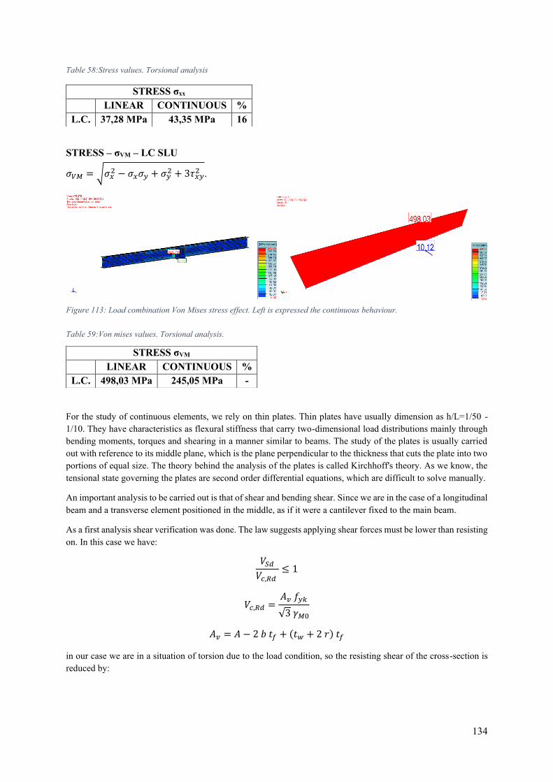
134
Table 58:Stress values. Torsional analysis
STRESS – σVM – LC SLU
𝜎𝑉𝑀 = √𝜎𝑥2 − 𝜎𝑥𝜎𝑦 + 𝜎𝑦
2 + 3𝜏𝑥𝑦2 .
Table 59:Von mises values. Torsional analysis.
For the study of continuous elements, we rely on thin plates. Thin plates have usually dimension as h/L=1/50 - 1/10. They have characteristics as flexural stiffness that carry two-dimensional load distributions mainly through bending moments, torques and shearing in a manner similar to beams. The study of the plates is usually carried out with reference to its middle plane, which is the plane perpendicular to the thickness that cuts the plate into two portions of equal size. The theory behind the analysis of the plates is called Kirchhoff's theory. As we know, the tensional state governing the plates are second order differential equations, which are difficult to solve manually.
An important analysis to be carried out is that of shear and bending shear. Since we are in the case of a longitudinal beam and a transverse element positioned in the middle, as if it were a cantilever fixed to the main beam.
As a first analysis shear verification was done. The law suggests applying shear forces must be lower than resisting on. In this case we have:
𝑉𝑆𝑑
𝑉𝑐,𝑅𝑑 ≤ 1
𝑉𝑐,𝑅𝑑 =𝐴𝑣 𝑓𝑦𝑘
√3 𝛾𝑀0
𝐴𝑣 = 𝐴 − 2 𝑏 𝑡𝑓 + (𝑡𝑤 + 2 𝑟) 𝑡𝑓
in our case we are in a situation of torsion due to the load condition, so the resisting shear of the cross-section is reduced by:
STRESS σxx LINEAR CONTINUOUS %
L.C. 37,28 MPa 43,35 MPa 16
STRESS σVM LINEAR CONTINUOUS %
L.C. 498,03 MPa 245,05 MPa -
Figure 113: Load combination Von Mises stress effect. Left is expressed the continuous behaviour.
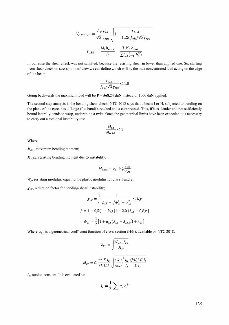
135
𝑉𝑐,𝑅𝑑,𝑟𝑒𝑑 =𝐴𝑣 𝑓𝑦𝑘
√3 𝛾𝑀0
√1 −𝜏𝑡,𝑆𝑑
1,25 𝑓𝑦𝑘 √3𝛾𝑀0⁄
𝜏𝑡,𝑆𝑑 =𝑀𝑡𝑏𝑚𝑎𝑥
𝐼𝑡=
3 𝑀𝑡 𝑏𝑚𝑎𝑥
∑ (𝑎1 𝑏𝑖3)𝑛
𝑖=1
In our case the shear check was not satisfied, because the resisting shear in lower than applied one. So, starting from shear check on stress point of view we can define which will be the max concentrated load acting on the edge of the beam.
𝜏𝑡,𝑆𝑑
𝑓𝑦𝑘 √3 𝛾𝑀0⁄≤ 1,0
Going backwards the maximum load will be P = 568,24 daN instead of 1000 daN applied.
The second step analysis is the bending shear check. NTC 2018 says that a beam I or H, subjected to bending on the plane of the core, has a flange (flat band) stretched and a compressed. This, if it is slender and not sufficiently bound laterally, tends to warp, undergoing a twist. Once the geometrical limits have been exceeded it is necessary to carry out a torsional instability test.
𝑀𝑆𝑑
𝑀𝑏,𝑅𝑑 ≤ 1
Where,
𝑀𝑆𝑑, maximum bending moment;
𝑀𝑏,𝑅𝑑, resisting bending moment due to instability.
𝑀𝑏,𝑅𝑑 = 𝜒𝐿𝑇 𝑊𝑦
𝑓𝑦𝑘
𝛾𝑀1
𝑊𝑦, resisting modulus, equal to the plastic modulus for class 1 and 2;
𝜒𝐿𝑇 , reduction factor for bending-shear instability;
𝜒𝐿𝑇 =1
𝑓
1
𝜙𝐿𝑇 + √𝜙𝐿𝑇2 − 𝜆𝐿𝑇
2≤ 𝐾𝜒
𝑓 = 1 − 0,5(1 − 𝑘𝑐) [1 − 2,0 (𝜆𝐿𝑇 − 0,8)2]
𝜙𝐿𝑇 =1
2[1 + 𝛼𝐿𝑇(𝜆𝐿𝑇 − 𝜆𝐿𝑇,0 ) + 𝜆𝐿𝑇]
Where 𝛼𝐿𝑇 is a geometrical coefficient function of cross-section (H/B), available on NTC 2018.
𝜆𝐿𝑇 = √𝑊𝑦,𝑃𝑙 𝑓𝑦𝑘
𝑀𝑐𝑟
𝑀𝑐𝑟 = 𝐶1
𝜋2 𝐸 𝐼𝑧
(𝑘 𝐿)2 √(
𝑘
𝑘𝑤
)2 𝐼𝑤
𝐼𝑧
(𝑘𝐿)2 𝐺 𝐼𝑡
𝐸 𝐼𝑧
𝐼𝑡, torsion constant. It is evaluated as:
𝐼𝑡 =1
3 ∑ 𝑎𝑖 𝑏𝑖
3
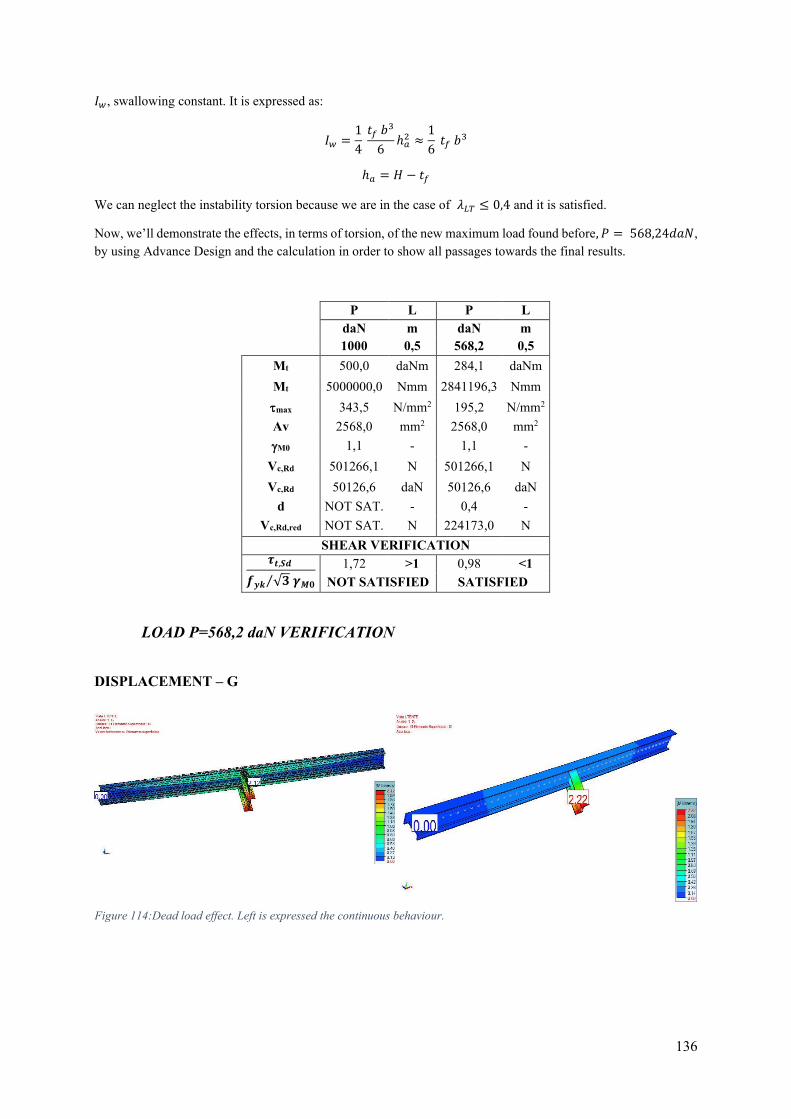
136
𝐼𝑤, swallowing constant. It is expressed as:
𝐼𝑤 =1
4 𝑡𝑓 𝑏3
6ℎ𝑎
2 ≈1
6 𝑡𝑓 𝑏3
ℎ𝑎 = 𝐻 − 𝑡𝑓
We can neglect the instability torsion because we are in the case of 𝜆𝐿𝑇 ≤ 0,4 and it is satisfied.
Now, we’ll demonstrate the effects, in terms of torsion, of the new maximum load found before, 𝑃 = 568,24𝑑𝑎𝑁, by using Advance Design and the calculation in order to show all passages towards the final results.
P L P L daN m daN m 1000 0,5 568,2 0,5
Mt 500,0 daNm 284,1 daNm Mt 5000000,0 Nmm 2841196,3 Nmm max 343,5 N/mm2 195,2 N/mm2 Av 2568,0 mm2 2568,0 mm2 M0 1,1 - 1,1 -
Vc,Rd 501266,1 N 501266,1 N Vc,Rd 50126,6 daN 50126,6 daN
d NOT SAT. - 0,4 - Vc,Rd,red NOT SAT. N 224173,0 N
SHEAR VERIFICATION 𝝉𝒕,𝑺𝒅
𝒇𝒚𝒌 √𝟑 𝜸𝑴𝟎⁄ 1,72 >1 0,98 <1
NOT SATISFIED SATISFIED
LOAD P=568,2 daN VERIFICATION
DISPLACEMENT – G
Figure 114:Dead load effect. Left is expressed the continuous behaviour.
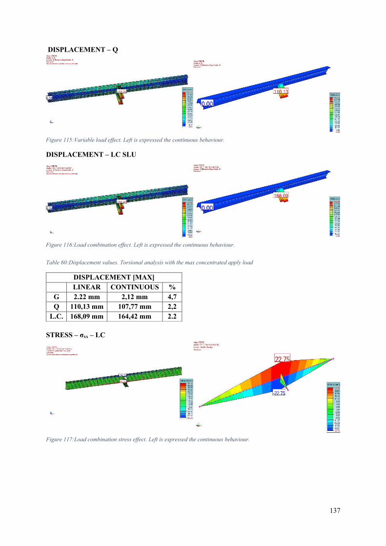
137
DISPLACEMENT – Q
DISPLACEMENT – LC SLU
Table 60:Displacement values. Torsional analysis with the max concentrated apply load
STRESS – σxx – LC
DISPLACEMENT [MAX] LINEAR CONTINUOUS %
G 2.22 mm 2,12 mm 4,7 Q 110,13 mm 107,77 mm 2,2
L.C. 168,09 mm 164,42 mm 2.2
Figure 115:Variable load effect. Left is expressed the continuous behaviour.
Figure 116:Load combination effect. Left is expressed the continuous behaviour.
Figure 117:Load combination stress effect. Left is expressed the continuous behaviour.
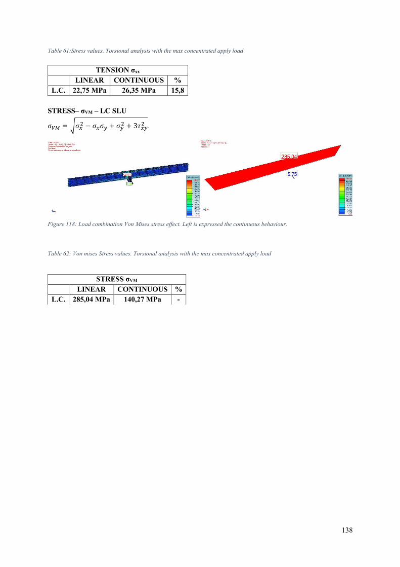
138
Table 61:Stress values. Torsional analysis with the max concentrated apply load
STRESS– σVM – LC SLU
𝜎𝑉𝑀 = √𝜎𝑥2 − 𝜎𝑥𝜎𝑦 + 𝜎𝑦
2 + 3𝜏𝑥𝑦2 .
Table 62: Von mises Stress values. Torsional analysis with the max concentrated apply load
TENSION σxx LINEAR CONTINUOUS %
L.C. 22,75 MPa 26,35 MPa 15,8
STRESS σVM LINEAR CONTINUOUS %
L.C. 285,04 MPa 140,27 MPa -
Figure 118: Load combination Von Mises stress effect. Left is expressed the continuous behaviour.
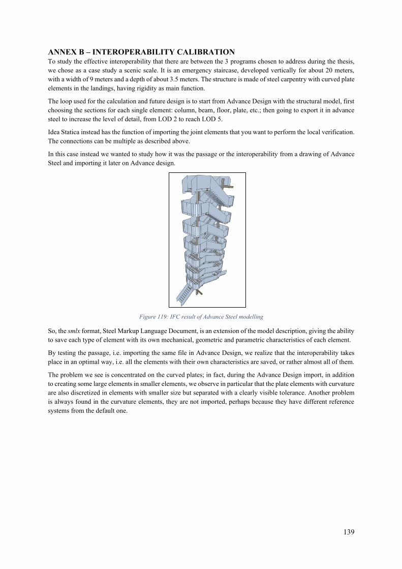
139
ANNEX B – INTEROPERABILITY CALIBRATION To study the effective interoperability that there are between the 3 programs chosen to address during the thesis, we chose as a case study a scenic scale. It is an emergency staircase, developed vertically for about 20 meters, with a width of 9 meters and a depth of about 3.5 meters. The structure is made of steel carpentry with curved plate elements in the landings, having rigidity as main function.
The loop used for the calculation and future design is to start from Advance Design with the structural model, first choosing the sections for each single element: column, beam, floor, plate, etc.; then going to export it in advance steel to increase the level of detail, from LOD 2 to reach LOD 5.
Idea Statica instead has the function of importing the joint elements that you want to perform the local verification. The connections can be multiple as described above.
In this case instead we wanted to study how it was the passage or the interoperability from a drawing of Advance Steel and importing it later on Advance design.
Figure 119: IFC result of Advance Steel modelling
So, the smlx format, Steel Markup Language Document, is an extension of the model description, giving the ability to save each type of element with its own mechanical, geometric and parametric characteristics of each element.
By testing the passage, i.e. importing the same file in Advance Design, we realize that the interoperability takes place in an optimal way, i.e. all the elements with their own characteristics are saved, or rather almost all of them.
The problem we see is concentrated on the curved plates; in fact, during the Advance Design import, in addition to creating some large elements in smaller elements, we observe in particular that the plate elements with curvature are also discretized in elements with smaller size but separated with a clearly visible tolerance. Another problem is always found in the curvature elements, they are not imported, perhaps because they have different reference systems from the default one.
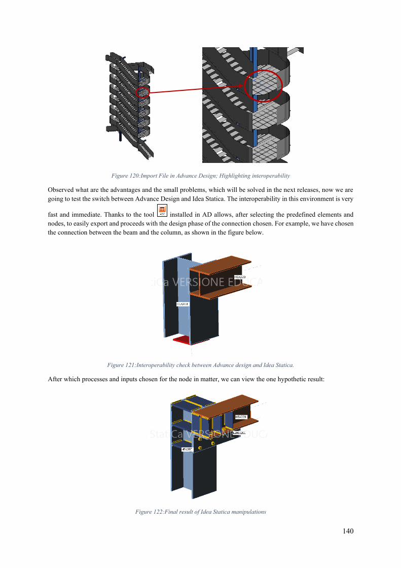
140
Figure 120:Import File in Advance Design; Highlighting interoperability
Observed what are the advantages and the small problems, which will be solved in the next releases, now we are going to test the switch between Advance Design and Idea Statica. The interoperability in this environment is very
fast and immediate. Thanks to the tool installed in AD allows, after selecting the predefined elements and nodes, to easily export and proceeds with the design phase of the connection chosen. For example, we have chosen the connection between the beam and the column, as shown in the figure below.
Figure 121:Interoperability check between Advance design and Idea Statica.
After which processes and inputs chosen for the node in matter, we can view the one hypothetic result:
Figure 122:Final result of Idea Statica manipulations

141
ANNEX C – ELEMENT RESULTS
MAIN BEAMS ANALYSIS

142
PRO
FIL
E
Height [mm] 2500 Reference lenght [mm] 12744 C1 thickness upper flange [mm] 25 Number of beams 2
width upper flange [mm] 500
thickness added uuper flange [mm] 0 Type of steel S 355 JR width added upper flange [mm] 0
web thickness [mm] 18
thickness lower flange [mm] 35
width lower flange [mm] 900
thickness added lower flange [mm] 0
width added lower flange [mm] 0
As [mm2] 87920,00
Iy [mm4] 2,39E+09
Yg [mm] 969,37
CO
NC
RE
TE
Rck [N/mm2] 37
Thickness [mm] 280
Thickness predalles [mm] 60
Effective width [mm] 3375
CO
EFF
ICIE
NT
S Permanent loads 18,40
Accidental loads 6,12
Shrinkage 16,19
Seattlement 22,86

143
SHE
AR
BO
LT
S Resistence [N/mm2] 450
Safity factor 1,25
Diameter [mm] 22
number on set 3
span [mm] 110,00
n A [mm2] YG,i [mm] Yn,i [mm] J [mm4] Jtor [mm4]
Steel element 0 87920,00 969,37 969,37 2,39E+09 20210026,7 Steel element + phase 2a 18,40 17474348,46 2497,80 1099,84376 6,59E+10 4,5439E+11 Steel element + phase 3 6,12 5868444,20 2497,80 670,771985 1,06E+11 1,5108E+11
Steel element + phase 2b 16,19 15384282,08 2497,80 1047,24231 7,04E+10 3,9977E+11 Steel element + phase 2c 22,86 21694677,28 2497,80 1187,50045 5,86E+10 5,6468E+11
ACTIONS
M [daNm] N [daN] T [daN] Mt [daNm] Dead load Steel 128525,08 5634,23 15894,89 3,46
Dead load concrete 76486,64 197343,43 59476,48 12,8 Permanent 76144,73 74706 29933,06 18,16
Accidental load + crowd 46096 75911,66 49069 24,07 Wind 10215,5 9088,41 4523,81 11,87
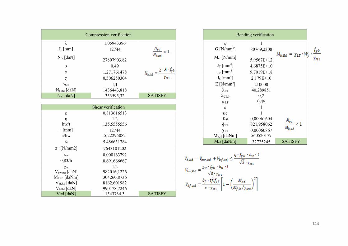
144
Compression verification
Bending verification
1,05943396 1 L [mm] 12744 G [N/mm2] 80769,2308
Ncr [daN] 27807903,82
Mcr [N/mm] 5,9567E+12
0,49 JT [mm4] 4,6875E+10
1,271761478 Jw [mm6] 9,7019E+18
0,506250304 Jx [mm4] 2,179E+10
M1 1,1 E [N/mm2] 210000
Nb,Rd [daN] 1436443,818 LT 40,289851 Ned [daN] 353595,32 SATISFY LT,0 0,2
LT 0,49 Shear verification 1
0,813616513 c 1 1,2 Kc 0,00061604
hw/t 135,5555556 LT 821,958062 a [mm] 12744 LT 0,00060867 a/hw 5,22295082 Mb,rd [daNm] 560520177
kt 5,486631784 Med [daNm] 32725245 SATISFY E [N/mm2] 7643101202
w 0,000163792
0,83/h 0,691666667
w 1,2
Vbw,Rd [daN] 982016,1226
Mf,red [daNm] 304260,8736
Vbf,Rd [daN] 8162,601982
Vb,Rd [daN] 990178,7246 Ved [daN] 1543734,3 SATISFY
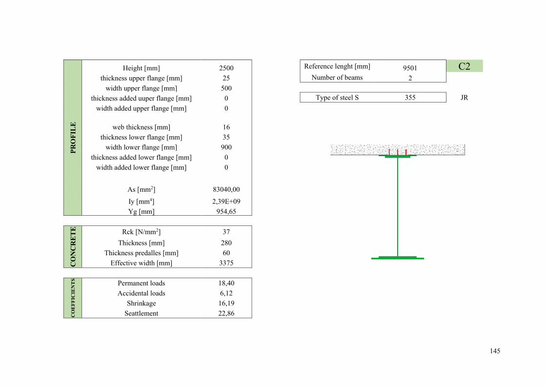
145
PRO
FIL
E Height [mm] 2500 Reference lenght [mm] 9501 C2
thickness upper flange [mm] 25 Number of beams 2
width upper flange [mm] 500
thickness added uuper flange [mm] 0 Type of steel S 355 JR width added upper flange [mm] 0
web thickness [mm] 16
thickness lower flange [mm] 35
width lower flange [mm] 900
thickness added lower flange [mm] 0
width added lower flange [mm] 0
As [mm2] 83040,00
Iy [mm4] 2,39E+09
Yg [mm] 954,65
CO
NC
RE
TE
Rck [N/mm2] 37
Thickness [mm] 280
Thickness predalles [mm] 60
Effective width [mm] 3375
CO
EFF
ICIE
NT
S Permanent loads 18,40
Accidental loads 6,12
Shrinkage 16,19
Seattlement 22,86

146
SHE
AR
BO
LT
S Resistence [N/mm2] 450
Safity factor 1,25
Diameter [mm] 22
number on set 2
span [mm] 110,00
n A [mm2] YG,i [mm] Yn,i [mm] J [mm4] Jtor [mm4]
Steel element 0 83040,00 954,65 954,65 2,39E+09 15497593,33 Steel element + phase 2a 18,40 17469468,46 2503,87 1076,439773 6,43E+10 4,54381E+11 Steel element + phase 3 6,12 5863564,20 2503,87 651,8259424 1,02E+11 1,5108E+11
Steel element + phase 2b 16,19 15379402,08 2503,87 1023,705861 6,85E+10 3,9976E+11 Steel element + phase 2c 22,86 21689797,28 2503,87 1164,74632 5,73E+10 5,64672E+11
ACTIONS
M [daNm] N [daN] T [daN] Mt [daNm] Dead load Steel 132949,08 5626,03 5436,88 0,89
Dead load concrete 224841,4 242948,46 18828,64 14,85 Permanent 84006,64 90105,46 7075,18 2,26
Accidental load + crowd 105672,87 107078,48 14541,76 8,08 Wind 10863,97 9468,44 949,85 2,21
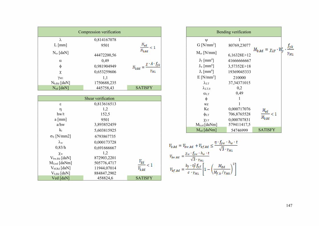
147
Compression verification
Bending verification
0,814167078 1 L [mm] 9501 G [N/mm2] 80769,23077
Ncr [daN] 44472200,56
Mcr [N/mm] 6,16328E+12
0,49 JT [mm4] 41666666667
0,981904949 Jw [mm6] 3,57352E+18
0,653259606 Jx [mm4] 19369045333
M1 1,1 E [N/mm2] 210000
Nb,Rd [daN] 1750688,235 LT 37,34371015 Ned [daN] 445758,43 SATISFY LT,0 0,2
LT 0,49 Shear verification 1
0,813616513 c 1 1,2 Kc 0,000717076
hw/t 152,5 LT 706,8765528 a [mm] 9501 LT 0,000707831 a/hw 3,893852459 Mb,rd [daNm] 579411417,5
kt 5,603815925 Med [daNm] 54746999 SATISFY E [N/mm2] 6793867735
w 0,000173728
0,83/h 0,691666667
w 1,2
Vbw,Rd [daN] 872903,2201
Mf,red [daNm] 505776,4717
Vbf,Rd [daN] 11944,07014
Vb,Rd [daN] 884847,2902 Ved [daN] 458824,6 SATISFY
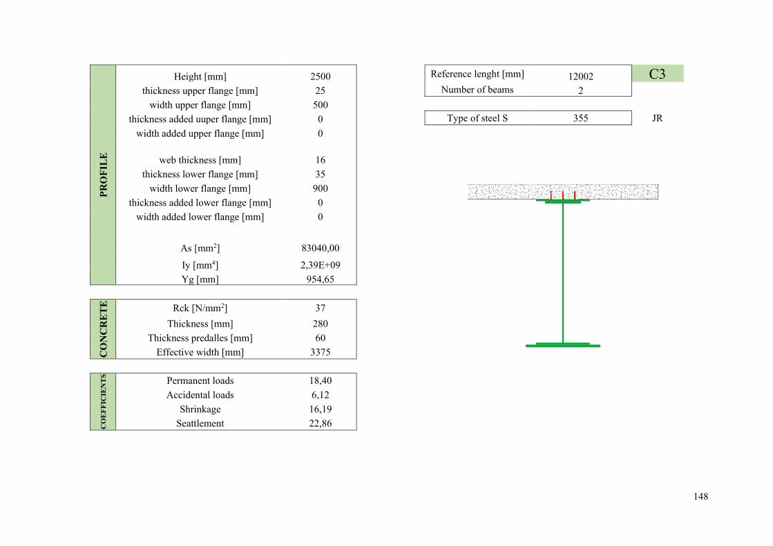
148
PRO
FIL
E
Height [mm] 2500 Reference lenght [mm] 12002 C3 thickness upper flange [mm] 25 Number of beams 2
width upper flange [mm] 500
thickness added uuper flange [mm] 0 Type of steel S 355 JR width added upper flange [mm] 0
web thickness [mm] 16
thickness lower flange [mm] 35
width lower flange [mm] 900
thickness added lower flange [mm] 0
width added lower flange [mm] 0
As [mm2] 83040,00
Iy [mm4] 2,39E+09
Yg [mm] 954,65
CO
NC
RE
TE
Rck [N/mm2] 37
Thickness [mm] 280
Thickness predalles [mm] 60
Effective width [mm] 3375
CO
EFF
ICIE
NT
S Permanent loads 18,40
Accidental loads 6,12
Shrinkage 16,19
Seattlement 22,86
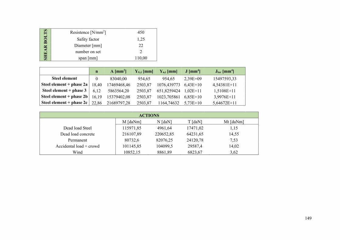
149
SHE
AR
BO
LT
S Resistence [N/mm2] 450
Safity factor 1,25
Diameter [mm] 22
number on set 2
span [mm] 110,00
n A [mm2] YG,i [mm] Yn,i [mm] J [mm4] Jtor [mm4]
Steel element 0 83040,00 954,65 954,65 2,39E+09 15497593,33 Steel element + phase 2a 18,40 17469468,46 2503,87 1076,439773 6,43E+10 4,54381E+11 Steel element + phase 3 6,12 5863564,20 2503,87 651,8259424 1,02E+11 1,5108E+11
Steel element + phase 2b 16,19 15379402,08 2503,87 1023,705861 6,85E+10 3,9976E+11 Steel element + phase 2c 22,86 21689797,28 2503,87 1164,74632 5,73E+10 5,64672E+11
ACTIONS
M [daNm] N [daN] T [daN] Mt [daNm] Dead load Steel 115971,85 4961,64 17471,02 1,15
Dead load concrete 216107,89 220652,85 64231,65 14,55 Permanent 80732,6 82076,25 24120,78 7,53
Accidental load + crowd 101145,85 104099,5 29587,4 14,02 Wind 10852,15 8861,89 6823,67 3,62

150
Compression verification
Bending verification
1,028484714 1 L [mm] 12002 G [N/mm2] 80769,23077
Ncr [daN] 27868911,79
Mcr [N/mm] 5,46109E+12
0,49 JT [mm4] 41666666667
1,231869158 Jw [mm6] 7,2036E+18
0,523588634 Jx [mm4] 19369045333
M1 1,1 E [N/mm2] 210000
Nb,Rd [daN] 1403179,461 LT 39,67195872 Ned [daN] 411790,24 SATISFY LT,0 0,2
LT 0,49 Shear verification 1
0,813616513 c 1 1,2 Kc 0,000635379
hw/t 152,5 LT 797,1027841 a [mm] 12002 LT 0,000627661 a/hw 4,918852459 Mb,rd [daNm] 513785869,4
kt 5,505322666 Med [daNm] 51395819 SATISFY E [N/mm2] 6793867735
w 0,000173728
0,83/h 0,691666667
w 1,2
Vbw,Rd [daN] 872903,2201
Mf,red [daNm] 475934,5048
Vbf,Rd [daN] 9163,579092
Vb,Rd [daN] 882066,7992 Ved [daN] 135410,85 SATISFY

151
PRO
FIL
E
Height [mm] 2500 Reference lenght [mm] 9501 C4 thickness upper flange [mm] 30 Number of beams 2
width upper flange [mm] 500
thickness added uuper flange [mm] 0 Type of steel S 355 JR width added upper flange [mm] 0
web thickness [mm] 22
thickness lower flange [mm] 35
width lower flange [mm] 900
thickness added lower flange [mm] 20
width added lower flange [mm] 400
As [mm2] 107630,00
Iy [mm4] 2,55E+09
Yg [mm] 947,51
CO
NC
RE
TE
Rck [N/mm2] 37
Thickness [mm] 280
Thickness predalles [mm] 60
Effective width [mm] 3375
CO
EFF
ICIE
NT
S Permanent loads 18,40
Accidental loads 6,12
Shrinkage 16,19
Seattlement 22,86

152
SHE
AR
BO
LT
S Resistence [N/mm2] 450
Safity factor 1,25
Diameter [mm] 22
number on set 3
span [mm] 110,00
n A [mm2] YG,i [mm] Yn,i [mm] J [mm4] Jtor [mm4]
Steel element 0 107630,00 947,51 947,51 2,55E+09 20708393,33 Steel element + phase 2a 18,40 17494058,46 2445,37 1181,529247 7,20E+10 4,54386E+11 Steel element + phase 3 6,12 5888154,20 2445,37 741,5627364 1,20E+11 1,51085E+11
Steel element + phase 2b 16,19 15403992,08 2445,37 1130,067901 7,72E+10 3,99766E+11 Steel element + phase 2c 22,86 21714387,28 2445,37 1265,844183 6,35E+10 5,64677E+11
ACTIONS
M [daNm] N [daN] T [daN] Mt [daNm] Dead load Steel 264294,77 2042,33 29788,59 38,38
Dead load concrete 433687,1 503061,41 117592 14,32 Permanent 159215,81 186326,75 43516,2 11,12
Accidental load + crowd 185264,92 195180,46 57047,37 32,98 Wind 19758,23 18706,73 5534,88 9,48
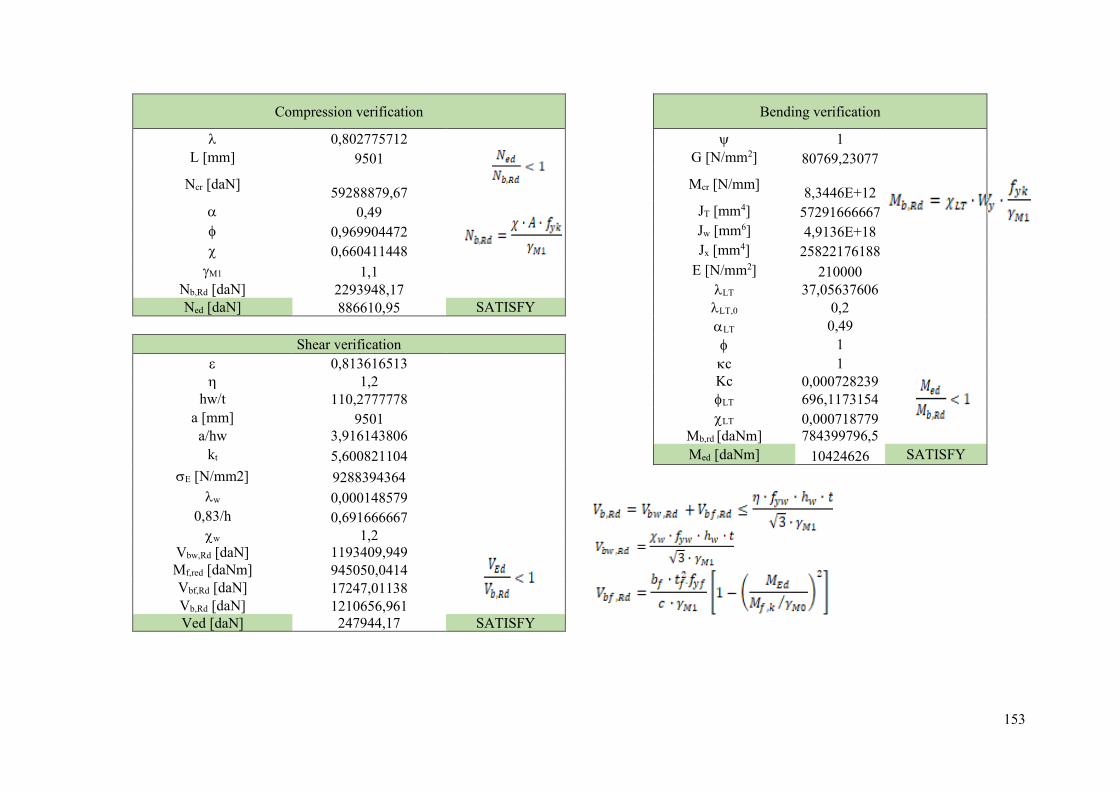
153
Compression verification
Bending verification
0,802775712 1 L [mm] 9501 G [N/mm2] 80769,23077
Ncr [daN] 59288879,67
Mcr [N/mm] 8,3446E+12
0,49 JT [mm4] 57291666667
0,969904472 Jw [mm6] 4,9136E+18
0,660411448 Jx [mm4] 25822176188
M1 1,1 E [N/mm2] 210000
Nb,Rd [daN] 2293948,17 LT 37,05637606 Ned [daN] 886610,95 SATISFY LT,0 0,2
LT 0,49 Shear verification 1
0,813616513 c 1 1,2 Kc 0,000728239
hw/t 110,2777778 LT 696,1173154 a [mm] 9501 LT 0,000718779 a/hw 3,916143806 Mb,rd [daNm] 784399796,5
kt 5,600821104 Med [daNm] 10424626 SATISFY E [N/mm2] 9288394364
w 0,000148579
0,83/h 0,691666667
w 1,2
Vbw,Rd [daN] 1193409,949
Mf,red [daNm] 945050,0414
Vbf,Rd [daN] 17247,01138
Vb,Rd [daN] 1210656,961 Ved [daN] 247944,17 SATISFY
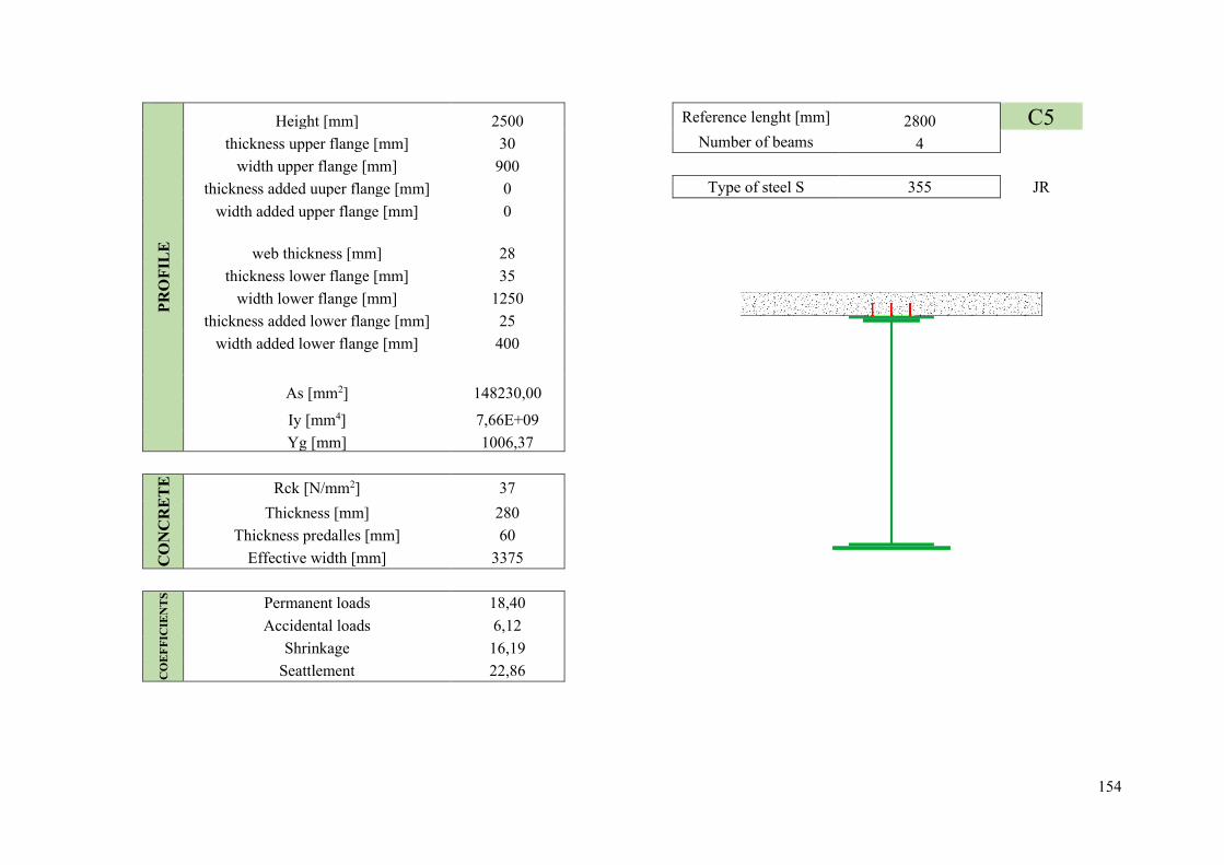
154
PRO
FIL
E
Height [mm] 2500 Reference lenght [mm] 2800 C5 thickness upper flange [mm] 30 Number of beams 4
width upper flange [mm] 900
thickness added uuper flange [mm] 0 Type of steel S 355 JR width added upper flange [mm] 0
web thickness [mm] 28
thickness lower flange [mm] 35
width lower flange [mm] 1250
thickness added lower flange [mm] 25
width added lower flange [mm] 400
As [mm2] 148230,00
Iy [mm4] 7,66E+09
Yg [mm] 1006,37
CO
NC
RE
TE
Rck [N/mm2] 37
Thickness [mm] 280
Thickness predalles [mm] 60
Effective width [mm] 3375
CO
EFF
ICIE
NT
S Permanent loads 18,40
Accidental loads 6,12
Shrinkage 16,19
Seattlement 22,86
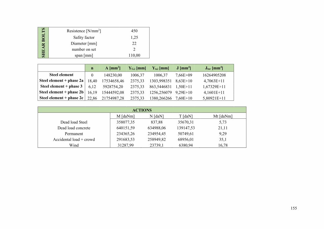
155
SHE
AR
BO
LT
S Resistence [N/mm2] 450
Safity factor 1,25
Diameter [mm] 22
number on set 2
span [mm] 110,00
n A [mm2] YG,i [mm] Yn,i [mm] J [mm4] Jtor [mm4]
Steel element 0 148230,00 1006,37 1006,37 7,66E+09 16264905208 Steel element + phase 2a 18,40 17534658,46 2375,33 1303,998351 8,63E+10 4,7063E+11 Steel element + phase 3 6,12 5928754,20 2375,33 863,5446831 1,50E+11 1,67329E+11
Steel element + phase 2b 16,19 15444592,08 2375,33 1256,256079 9,29E+10 4,1601E+11 Steel element + phase 2c 22,86 21754987,28 2375,33 1380,266266 7,60E+10 5,80921E+11
ACTIONS
M [daNm] N [daN] T [daN] Mt [daNm] Dead load Steel 358077,35 837,88 35670,31 5,73
Dead load concrete 640151,59 634988,06 139147,53 21,11 Permanent 234365,26 234954,45 50749,61 9,29
Accidental load + crowd 291683,53 258949,82 68956,01 35,1 Wind 31287,99 23739,1 6380,94 16,78

156
Compression verification
Bending verification
0,246957297 1 L [mm] 2801 G [N/mm2] 80769,23077
Ncr [daN] 862821057,1
Mcr [N/mm] 2,03975E+13
0,49 JT [mm4] 72916666667
0,541998491 Jw [mm6] 1,60238E+17
0,976118724 Jx [mm4] 32660882333
M1 1,1 E [N/mm2] 210000
Nb,Rd [daN] 4669543,44 LT 26,65600785 Ned [daN] 1129730,21 SATISFY LT,0 0,2
LT 0,49 Shear verification 1
0,813616513 c 1 1,2 Kc 0,001407375
hw/t 86,67857143 LT 362,2530992 a [mm] 2801 LT 0,001382124 a/hw 1,154099712 Mb,rd [daNm] 1907760946
kt 8,343124426 Med [daNm] 152427773 SATISFY E [N/mm2] 11825924072
w 0,000131677
0,83/h 0,691666667
w 1,2
Vbw,Rd [daN] 1519441,886
Mf,red [daNm] 1391621,647
Vbf,Rd [daN] 75803,4342
Vb,Rd [daN] 1595245,32 Ved [daN] 294523,46 SATISFY

157
PRO
FIL
E Height [mm] 2500 Reference lenght [mm] 2800 C5a
thickness upper flange [mm] 30 Number of beams 4
width upper flange [mm] 900
thickness added uuper flange [mm] 40 Type of steel S 355 JR width added upper flange [mm] 600
web thickness [mm] 28
thickness lower flange [mm] 35
width lower flange [mm] 1250
thickness added lower flange [mm] 35
width added lower flange [mm] 900
As [mm2] 148230,00
Iy [mm4] 1,04E+10
Yg [mm] 1006,37
CO
NC
RE
TE
Rck [N/mm2] 37
Thickness [mm] 280
Thickness predalles [mm] 60
Effective width [mm] 3375
CO
EFF
ICIE
NT
S Permanent loads 18,40
Accidental loads 6,12
Shrinkage 16,19
Seattlement 22,86

158
SHE
AR
BO
LT
S Resistence [N/mm2] 450
Safity factor 1,25
Diameter [mm] 22
number on set 3
span [mm] 110,00
n A [mm2] YG,i [mm] Yn,i [mm] J [mm4] Jtor [mm4]
Steel element 0 148230,00 1006,37 1006,37 1,04E+10 24802318125 Steel element + phase 2a 18,40 17534658,46 2282,04 1394,619771 9,65E+10 4,79168E+11 Steel element + phase 3 6,12 5928754,20 2282,04 968,8709124 1,74E+11 1,75867E+11
Steel element + phase 2b 16,19 15444592,08 2282,04 1351,218178 1,04E+11 4,24547E+11 Steel element + phase 2c 22,86 21754987,28 2282,04 1462,674372 8,46E+10 5,89459E+11
ACTIONS
M [daNm] N [daN] T [daN] Mt [daNm] Dead load Steel 503361,9 13967,18 46552,05 62,23
Dead load concrete 1108978,78 818834,63 165948,03 45,58 Permanent 402124,58 295974,65 59377,98 38,92
Accidental load + crowd 547641,56 403977,11 86827,49 141,95 Wind 56046,77 30606,71 7331,48 59,64

159
Compression verification
Bending verification
0,747934078 1 L [mm] 7401 G [N/mm2] 80769,23077
Ncr [daN] 122053079,7
Mcr [N/mm] 1,19877E+13
0,49 JT [mm4] 72916666667
0,913946541 Jw [mm6] 2,95596E+18
0,69482968 Jx [mm4] 32256000000
M1 1,1 E [N/mm2] 210000
Nb,Rd [daN] 4312817,299 LT 34,55466719 Ned [daN] 1532753,57 SATISFY LT,0 0,2
LT 0,49 Shear verification 1
0,813616513 c 1 1,2 Kc 0,000837503
hw/t 85,11190476 LT 605,9294057 a [mm] 7401 LT 0,000825851 a/hw 3,105575293 Mb,rd [daNm] 1125799576
kt 5,754739945 Med [daNm] 256210682 SATISFY E [N/mm2] 11612177114
w 0,000132883
0,83/h 0,691666667
w 1,2
Vbw,Rd [daN] 1491978,824
Mf,red [daNm] 2352480,406
Vbf,Rd [daN] 39244,28795
Vb,Rd [daN] 1531223,112 Ved [daN] 358705,55 SATISFY

160
PRO
FIL
E Height [mm] 2500 Reference lenght [mm] 11501 C6
thickness upper flange [mm] 40 Number of beams 2
width upper flange [mm] 500
thickness added uuper flange [mm] 0 Type of steel S 355 JR width added upper flange [mm] 0
web thickness [mm] 22
thickness lower flange [mm] 35
width lower flange [mm] 900
thickness added lower flange [mm] 25
width added lower flange [mm] 400
As [mm2] 114300,00
Iy [mm4] 2,68E+09
Yg [mm] 993,10
CO
NC
RE
TE
Rck [N/mm2] 37
Thickness [mm] 280
Thickness predalles [mm] 60
Effective width [mm] 3375
CO
EFF
ICIE
NT
S Permanent loads 18,40
Accidental loads 6,12
Shrinkage 16,19
Seattlement 22,86
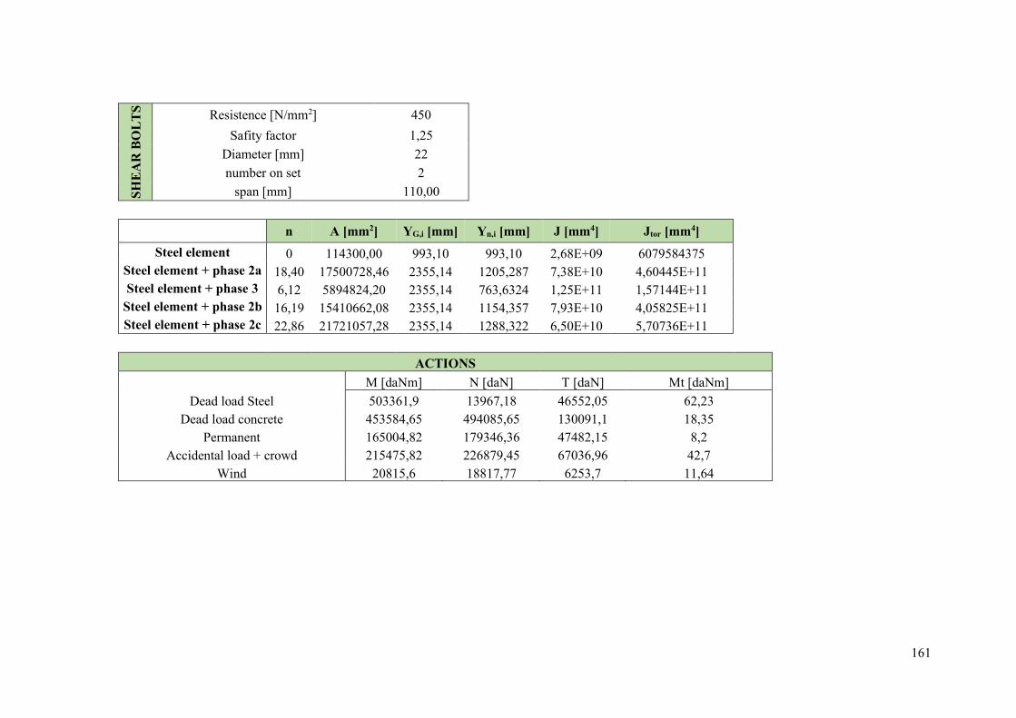
161
SHE
AR
BO
LT
S Resistence [N/mm2] 450
Safity factor 1,25
Diameter [mm] 22
number on set 2
span [mm] 110,00
n A [mm2] YG,i [mm] Yn,i [mm] J [mm4] Jtor [mm4]
Steel element 0 114300,00 993,10 993,10 2,68E+09 6079584375 Steel element + phase 2a 18,40 17500728,46 2355,14 1205,287 7,38E+10 4,60445E+11 Steel element + phase 3 6,12 5894824,20 2355,14 763,6324 1,25E+11 1,57144E+11
Steel element + phase 2b 16,19 15410662,08 2355,14 1154,357 7,93E+10 4,05825E+11 Steel element + phase 2c 22,86 21721057,28 2355,14 1288,322 6,50E+10 5,70736E+11
ACTIONS
M [daNm] N [daN] T [daN] Mt [daNm] Dead load Steel 503361,9 13967,18 46552,05 62,23
Dead load concrete 453584,65 494085,65 130091,1 18,35 Permanent 165004,82 179346,36 47482,15 8,2
Accidental load + crowd 215475,82 226879,45 67036,96 42,7 Wind 20815,6 18817,77 6253,7 11,64
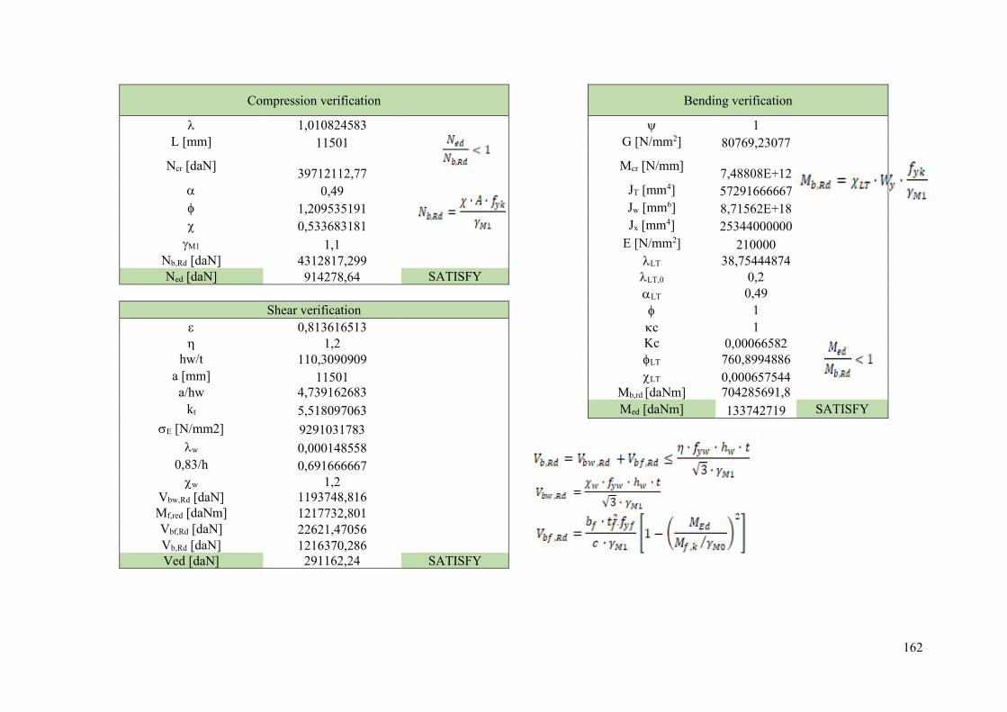
162
Compression verification
Bending verification
1,010824583 1 L [mm] 11501 G [N/mm2] 80769,23077
Ncr [daN] 39712112,77
Mcr [N/mm] 7,48808E+12
0,49 JT [mm4] 57291666667
1,209535191 Jw [mm6] 8,71562E+18
0,533683181 Jx [mm4] 25344000000
M1 1,1 E [N/mm2] 210000
Nb,Rd [daN] 4312817,299 LT 38,75444874 Ned [daN] 914278,64 SATISFY LT,0 0,2
LT 0,49 Shear verification 1
0,813616513 c 1 1,2 Kc 0,00066582
hw/t 110,3090909 LT 760,8994886 a [mm] 11501 LT 0,000657544 a/hw 4,739162683 Mb,rd [daNm] 704285691,8
kt 5,518097063 Med [daNm] 133742719 SATISFY E [N/mm2] 9291031783
w 0,000148558
0,83/h 0,691666667
w 1,2
Vbw,Rd [daN] 1193748,816
Mf,red [daNm] 1217732,801
Vbf,Rd [daN] 22621,47056
Vb,Rd [daN] 1216370,286 Ved [daN] 291162,24 SATISFY

163
PRO
FIL
E
Height [mm] 2500 Reference lenght [mm] 11002 C7 thickness upper flange [mm] 30 Number of beams 2
width upper flange [mm] 500
thickness added uuper flange [mm] 0 Type of steel S 355 JR width added upper flange [mm] 0
web thickness [mm] 16
thickness lower flange [mm] 35
width lower flange [mm] 900
thickness added lower flange [mm] 35
width added lower flange [mm] 400
As [mm2] 98900,00
Iy [mm4] 2,63E+09
Yg [mm] 848,39
CO
NC
RE
TE
Rck [N/mm2] 37
Thickness [mm] 280
Thickness predalles [mm] 60
Effective width [mm] 3375
CO
EFF
ICIE
NT
S Permanent loads 18,40
Accidental loads 6,12
Shrinkage 16,19
Seattlement 22,86
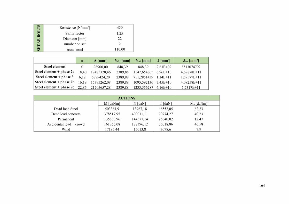
164
SHE
AR
BO
LT
S Resistence [N/mm2] 450
Safity factor 1,25
Diameter [mm] 22
number on set 2
span [mm] 110,00
n A [mm2] YG,i [mm] Yn,i [mm] J [mm4] Jtor [mm4]
Steel element 0 98900,00 848,39 848,39 2,63E+09 8513074792 Steel element + phase 2a 18,40 17485328,46 2389,88 1147,654865 6,96E+10 4,62878E+11 Steel element + phase 3 6,12 5879424,20 2389,88 711,2851439 1,14E+11 1,59577E+11
Steel element + phase 2b 16,19 15395262,08 2389,88 1095,592136 7,45E+10 4,08258E+11 Steel element + phase 2c 22,86 21705657,28 2389,88 1233,556287 6,16E+10 5,7317E+11
ACTIONS
M [daNm] N [daN] T [daN] Mt [daNm] Dead load Steel 503361,9 13967,18 46552,05 62,23
Dead load concrete 378517,95 400011,11 70774,27 40,23 Permanent 135830,96 144577,14 25640,02 12,47
Accidental load + crowd 161766,08 178396,12 35018,86 46,58 Wind 17185,44 15013,8 3078,6 7,9

165
Compression verification
Bending verification
1,054722503 1 L [mm] 11002 G [N/mm2] 80769,23077
Ncr [daN] 31560815,81
Mcr [N/mm] 5,57214E+12
0,49 JT [mm4] 41666666667
1,265626792 Jw [mm6] 5,54886E+18
0,508859808 Jx [mm4] 18432000000
M1 1,1 E [N/mm2] 210000
Nb,Rd [daN] 1624164,856 LT 38,31283632 Ned [daN] 736951,55 SATISFY LT,0 0,2
LT 0,49 Shear verification 1
0,813616513 c 1 1,2 Kc 0,000681258
hw/t 151,2152778 LT 743,7743584 a [mm] 11002 LT 0,000672693 a/hw 4,547324914 Mb,rd [daNm] 524008956
kt 5,533440773 Med [daNm] 117947689 SATISFY E [N/mm2] 6736633421
w 0,000174464
0,83/h 0,691666667
w 1,2
Vbw,Rd [daN] 865549,5272
Mf,red [daNm] 1082840,258
Vbf,Rd [daN] 16264,44725
Vb,Rd [daN] 881813,9745 Ved [daN] 177985,2 SATISFY

166
PRO
FIL
E
Height [mm] 2500 Reference lenght [mm] 12295 C8 thickness upper flange [mm] 30 Number of beams 1
width upper flange [mm] 600
thickness added uuper flange [mm] 0 Type of steel S 355 JR width added upper flange [mm] 0
web thickness [mm] 16
thickness lower flange [mm] 35
width lower flange [mm] 900
thickness added lower flange [mm] 35
width added lower flange [mm] 600
As [mm2] 108509,37
Iy [mm4] 3,27E+09
Yg [mm] 838,95
CO
NC
RE
TE
Rck [N/mm2] 37
Thickness [mm] 280
Thickness predalles [mm] 60
Effective width [mm] 3375
CO
EFF
ICIE
NT
S Permanent loads 18,40
Accidental loads 6,12
Shrinkage 16,19
Seattlement 22,86

167
SHE
AR
BO
LT
S Resistence [N/mm2] 450
Safity factor 1,25
Diameter [mm] 22
number on set 3
span [mm] 110,00
n A [mm2] YG,i [mm] Yn,i [mm] J [mm4] Jtor [mm4]
Steel element 0 108509,37 838,95 838,95 3,27E+09 8514503958 Steel element + phase 2a 18,40 17494937,82 2368,09 1184,761117 7,29E+10 4,6288E+11 Steel element + phase 3 6,12 5889033,56 2368,09 744,5235524 1,21E+11 1,59579E+11
Steel element + phase 2b 16,19 15404871,45 2368,09 1133,366734 7,82E+10 4,08259E+11 Steel element + phase 2c 22,86 21715266,64 2368,09 1268,909993 6,44E+10 5,73171E+11
ACTIONS
M [daNm] N [daN] T [daN] Mt [daNm] Dead load Steel 503361,9 13967,18 46552,05 62,23
Dead load concrete 417790,58 438275,87 24446,82 45,46 Permanent 150286,51 158492,4 8955,49 18,04
Accidental load + crowd 182466,02 197967,11 12947,18 29,01 Wind 18734,58 16434,71 1060,28 7,33

168
Compression verification
Bending verification
1,010824583 1 L [mm] 11501 G [N/mm2] 80769,23077
Ncr [daN] 39712112,77
Mcr [N/mm] 7,48808E+12
0,49 JT [mm4] 57291666667
1,209535191 Jw [mm6] 8,71562E+18
0,533683181 Jx [mm4] 25344000000
M1 1,1 E [N/mm2] 210000
Nb,Rd [daN] 1968635,962 LT 38,75444874 Ned [daN] 808702,56 SATISFY LT,0 0,2
LT 0,49 Shear verification 1
0,813616513 c 1 1,2 Kc 0,00066582
hw/t 110,3090909 LT 760,8994886 a [mm] 11501 LT 0,000657544 a/hw 4,739162683 Mb,rd [daNm] 704285691,8
kt 5,518097063 Med [daNm] 125390501 SATISFY E [N/mm2] 9291031783
w 0,000148558
0,83/h 0,691666667
w 1,2
Vbw,Rd [daN] 1193748,816
Mf,red [daNm] 1153678,369
Vbf,Rd [daN] 16285,7285
Vb,Rd [daN] 1210034,544 Ved [daN] 929015,4 SATISFY
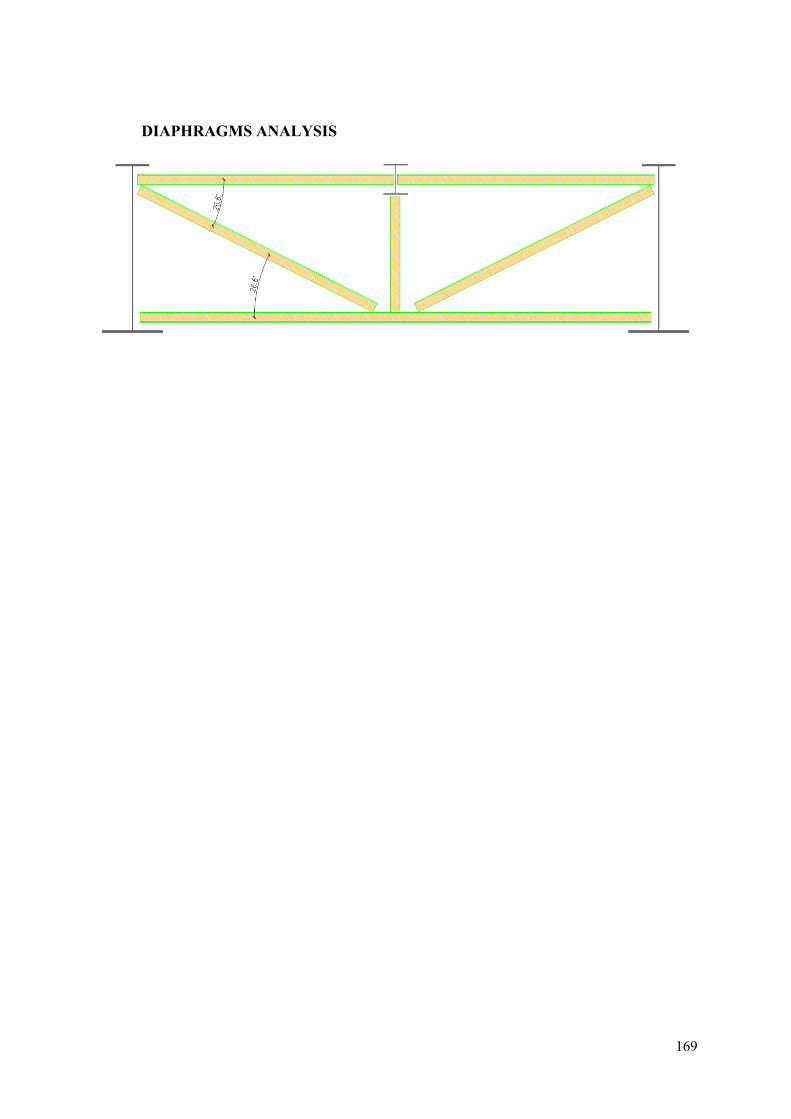
169
DIAPHRAGMS ANALYSIS
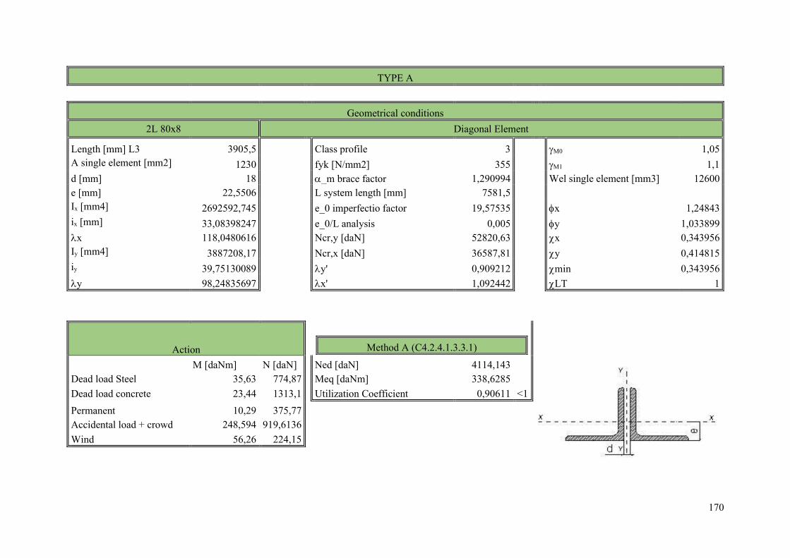
170
TYPE A
Geometrical conditions
2L 80x8 Diagonal Element
Length [mm] L3 3905,5 Class profile 3 M0 1,05 A single element [mm2] 1230 fyk [N/mm2] 355 M1 1,1 d [mm] 18 _m brace factor 1,290994 Wel single element [mm3] 12600 e [mm] 22,5506 L system length [mm] 7581,5 Ix [mm4] 2692592,745 e_0 imperfectio factor 19,57535 x 1,24843 ix [mm] 33,08398247 e_0/L analysis 0,005 y 1,033899 x 118,0480616 Ncr,y [daN] 52820,63 x 0,343956 Iy [mm4] 3887208,17 Ncr,x [daN] 36587,81 y 0,414815 iy 39,75130089 y' 0,909212 min 0,343956 y 98,24835697 x' 1,092442 LT 1
Action
Method A (C4.2.4.1.3.3.1)
M [daNm] N [daN] Ned [daN] 4114,143 Dead load Steel 35,63 774,87 Meq [daNm] 338,6285 Dead load concrete 23,44 1313,1 Utilization Coefficient 0,90611 <1 Permanent 10,29 375,77 Accidental load + crowd 248,594 919,6136 Wind 56,26 224,15
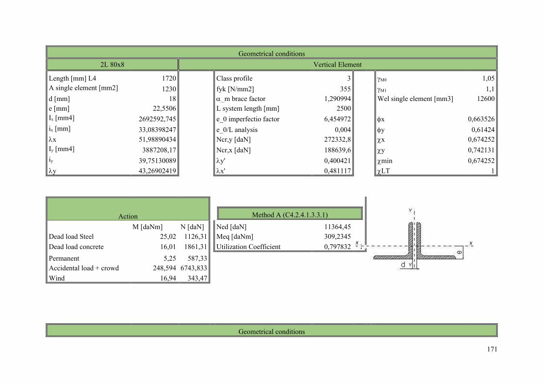
171
Geometrical conditions 2L 80x8 Vertical Element
Length [mm] L4 1720 Class profile 3 M0 1,05 A single element [mm2] 1230 fyk [N/mm2] 355 M1 1,1 d [mm] 18 _m brace factor 1,290994 Wel single element [mm3] 12600 e [mm] 22,5506 L system length [mm] 2500 Ix [mm4] 2692592,745 e_0 imperfectio factor 6,454972 x 0,663526 ix [mm] 33,08398247 e_0/L analysis 0,004 y 0,61424 x 51,98890434 Ncr,y [daN] 272332,8 x 0,674252 Iy [mm4] 3887208,17 Ncr,x [daN] 188639,6 y 0,742131 iy 39,75130089 y' 0,400421 min 0,674252 y 43,26902419 x' 0,481117 LT 1
Action
Method A (C4.2.4.1.3.3.1)
M [daNm] N [daN] Ned [daN] 11364,45 Dead load Steel 25,02 1126,31 Meq [daNm] 309,2345 Dead load concrete 16,01 1861,31 Utilization Coefficient 0,797832 <1 Permanent 5,25 587,33 Accidental load + crowd 248,594 6743,833 Wind 16,94 343,47
Geometrical conditions
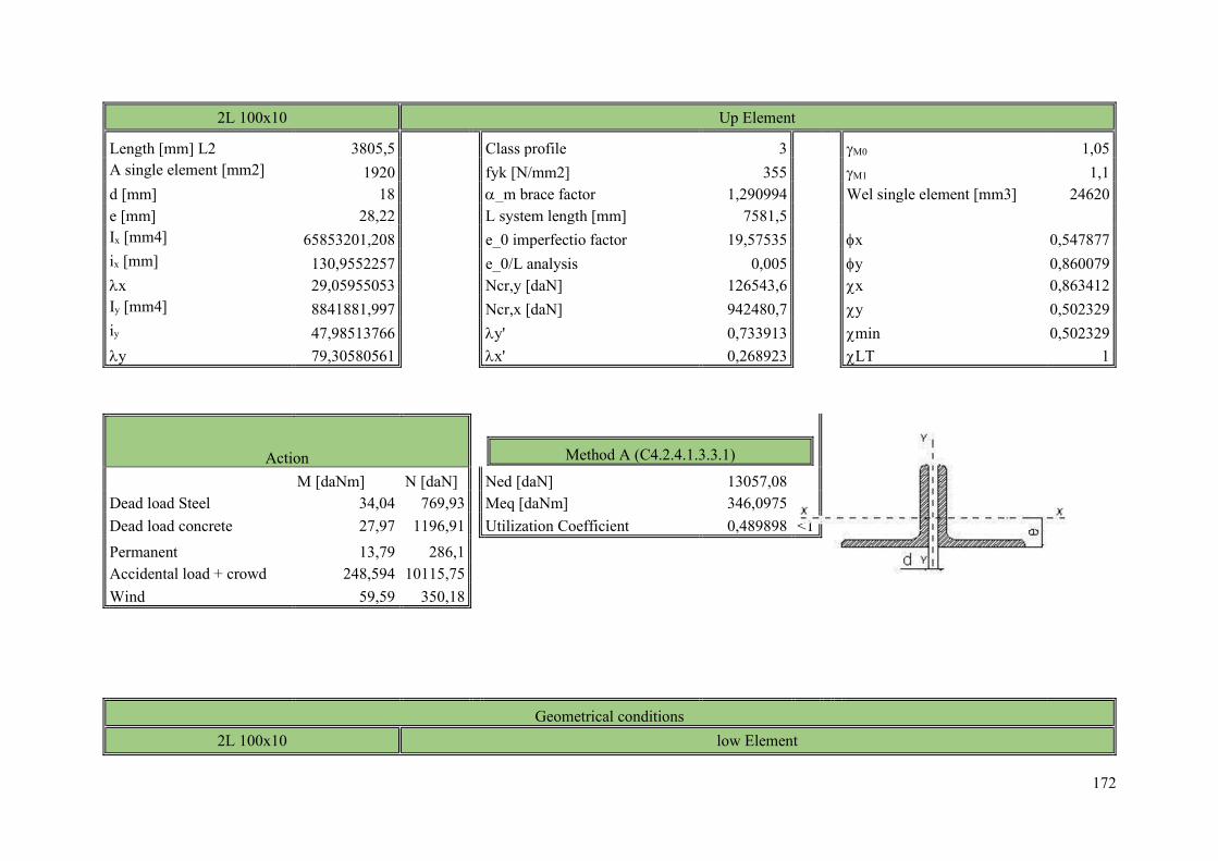
172
2L 100x10 Up Element
Length [mm] L2 3805,5 Class profile 3 M0 1,05 A single element [mm2] 1920 fyk [N/mm2] 355 M1 1,1 d [mm] 18 _m brace factor 1,290994 Wel single element [mm3] 24620 e [mm] 28,22 L system length [mm] 7581,5 Ix [mm4] 65853201,208 e_0 imperfectio factor 19,57535 x 0,547877 ix [mm] 130,9552257 e_0/L analysis 0,005 y 0,860079 x 29,05955053 Ncr,y [daN] 126543,6 x 0,863412 Iy [mm4] 8841881,997 Ncr,x [daN] 942480,7 y 0,502329 iy 47,98513766 y' 0,733913 min 0,502329 y 79,30580561 x' 0,268923 LT 1
Action
Method A (C4.2.4.1.3.3.1)
M [daNm] N [daN] Ned [daN] 13057,08 Dead load Steel 34,04 769,93 Meq [daNm] 346,0975 Dead load concrete 27,97 1196,91 Utilization Coefficient 0,489898 <1 Permanent 13,79 286,1 Accidental load + crowd 248,594 10115,75 Wind 59,59 350,18
Geometrical conditions 2L 100x10 low Element
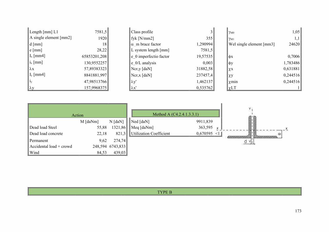
173
Length [mm] L1 7581,5 Class profile 3 M0 1,05 A single element [mm2] 1920 fyk [N/mm2] 355 M1 1,1 d [mm] 18 _m brace factor 1,290994 Wel single element [mm3] 24620 e [mm] 28,22 L system length [mm] 7581,5 Ix [mm4] 65853201,208 e_0 imperfectio factor 19,57535 x 0,7006 ix [mm] 130,9552257 e_0/L analysis 0,003 y 1,783486 x 57,89383323 Ncr,y [daN] 31882,58 x 0,631881 Iy [mm4] 8841881,997 Ncr,x [daN] 237457,4 y 0,244516 iy 47,98513766 y' 1,462137 min 0,244516 y 157,9968375 x' 0,535762 LT 1
Action
Method A (C4.2.4.1.3.3.1)
M [daNm] N [daN] Ned [daN] 9911,839 Dead load Steel 55,88 1321,86 Meq [daNm] 363,595 Dead load concrete 22,18 821,3 Utilization Coefficient 0,670595 <1 Permanent 9,62 274,74 Accidental load + crowd 248,594 6743,833 Wind 84,53 439,03
TYPE B
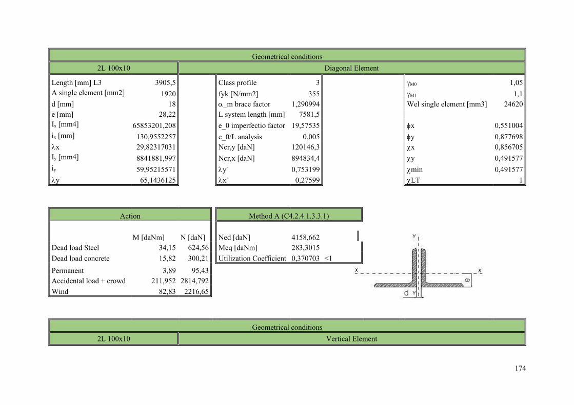
174
Geometrical conditions 2L 100x10 Diagonal Element
Length [mm] L3 3905,5 Class profile 3 M0 1,05 A single element [mm2] 1920 fyk [N/mm2] 355 M1 1,1 d [mm] 18 _m brace factor 1,290994 Wel single element [mm3] 24620 e [mm] 28,22 L system length [mm] 7581,5 Ix [mm4] 65853201,208 e_0 imperfectio factor 19,57535 x 0,551004 ix [mm] 130,9552257 e_0/L analysis 0,005 y 0,877698 x 29,82317031 Ncr,y [daN] 120146,3 x 0,856705 Iy [mm4] 8841881,997 Ncr,x [daN] 894834,4 y 0,491577 iy 59,95215571 y' 0,753199 min 0,491577 y 65,1436125 x' 0,27599 LT 1
Action Method A (C4.2.4.1.3.3.1)
M [daNm] N [daN] Ned [daN] 4158,662
Dead load Steel 34,15 624,56 Meq [daNm] 283,3015 Dead load concrete 15,82 300,21 Utilization Coefficient 0,370703 <1 Permanent 3,89 95,43 Accidental load + crowd 211,952 2814,792 Wind 82,83 2216,65
Geometrical conditions 2L 100x10 Vertical Element
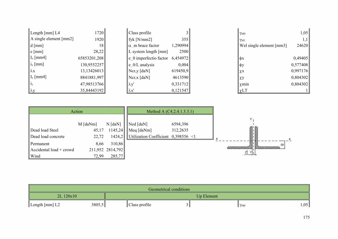
175
Length [mm] L4 1720 Class profile 3 M0 1,05 A single element [mm2] 1920 fyk [N/mm2] 355 M1 1,1 d [mm] 18 _m brace factor 1,290994 Wel single element [mm3] 24620 e [mm] 28,22 L system length [mm] 2500 Ix [mm4] 65853201,208 e_0 imperfectio factor 6,454972 x 0,49405 ix [mm] 130,9552257 e_0/L analysis 0,004 y 0,577408 x 13,13426013 Ncr,y [daN] 619450,9 x 0,997176 Iy [mm4] 8841881,997 Ncr,x [daN] 4613590 y 0,804302 iy 47,98513766 y' 0,331712 min 0,804302 y 35,84443192 x' 0,121547 LT 1
Action Method A (C4.2.4.1.3.3.1)
M [daNm] N [daN] Ned [daN] 6594,396
Dead load Steel 45,17 1145,24 Meq [daNm] 312,2635 Dead load concrete 22,72 1424,2 Utilization Coefficient 0,398556 <1 Permanent 8,66 310,86 Accidental load + crowd 211,952 2814,792 Wind 72,99 285,77
Geometrical conditions 2L 120x10 Up Element
Length [mm] L2 3805,5 Class profile 3 M0 1,05
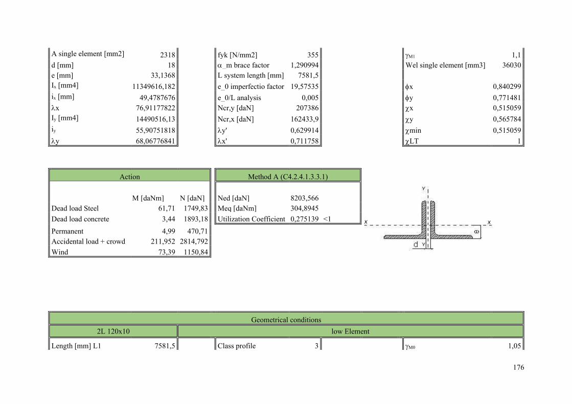
176
A single element [mm2] 2318 fyk [N/mm2] 355 M1 1,1 d [mm] 18 _m brace factor 1,290994 Wel single element [mm3] 36030 e [mm] 33,1368 L system length [mm] 7581,5 Ix [mm4] 11349616,182 e_0 imperfectio factor 19,57535 x 0,840299 ix [mm] 49,4787676 e_0/L analysis 0,005 y 0,771481 x 76,91177822 Ncr,y [daN] 207386 x 0,515059 Iy [mm4] 14490516,13 Ncr,x [daN] 162433,9 y 0,565784 iy 55,90751818 y' 0,629914 min 0,515059 y 68,06776841 x' 0,711758 LT 1
Action Method A (C4.2.4.1.3.3.1)
M [daNm] N [daN] Ned [daN] 8203,566
Dead load Steel 61,71 1749,83 Meq [daNm] 304,8945 Dead load concrete 3,44 1893,18 Utilization Coefficient 0,275139 <1 Permanent 4,99 470,71 Accidental load + crowd 211,952 2814,792 Wind 73,39 1150,84
Geometrical conditions 2L 120x10 low Element
Length [mm] L1 7581,5 Class profile 3 M0 1,05
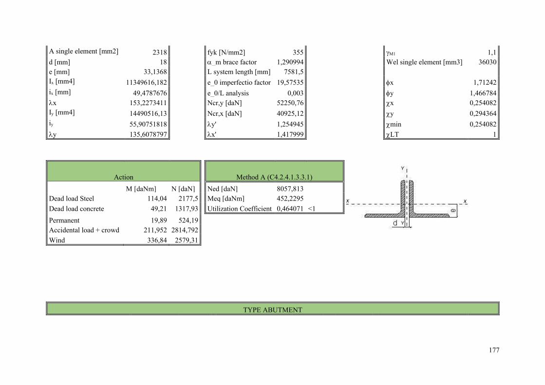
177
A single element [mm2] 2318 fyk [N/mm2] 355 M1 1,1 d [mm] 18 _m brace factor 1,290994 Wel single element [mm3] 36030 e [mm] 33,1368 L system length [mm] 7581,5 Ix [mm4] 11349616,182 e_0 imperfectio factor 19,57535 x 1,71242 ix [mm] 49,4787676 e_0/L analysis 0,003 y 1,466784 x 153,2273411 Ncr,y [daN] 52250,76 x 0,254082 Iy [mm4] 14490516,13 Ncr,x [daN] 40925,12 y 0,294364 iy 55,90751818 y' 1,254945 min 0,254082 y 135,6078797 x' 1,417999 LT 1
Action Method A (C4.2.4.1.3.3.1)
M [daNm] N [daN] Ned [daN] 8057,813 Dead load Steel 114,04 2177,5 Meq [daNm] 452,2295 Dead load concrete 49,21 1317,93 Utilization Coefficient 0,464071 <1 Permanent 19,89 524,19 Accidental load + crowd 211,952 2814,792 Wind 336,84 2579,31
TYPE ABUTMENT
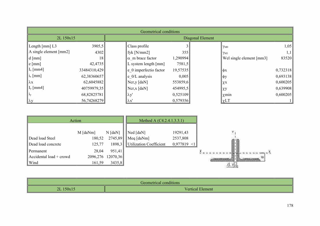
178
Geometrical conditions 2L 150x15 Diagonal Element
Length [mm] L3 3905,5 Class profile 3 M0 1,05 A single element [mm2] 4302 fyk [N/mm2] 355 M1 1,1 d [mm] 18 _m brace factor 1,290994 Wel single element [mm3] 83520 e [mm] 42,4735 L system length [mm] 7581,5 Ix [mm4] 33484310,429 e_0 imperfectio factor 19,57535 x 0,732318 ix [mm] 62,38360657 e_0/L analysis 0,005 y 0,693138 x 62,6045882 Ncr,y [daN] 553859,6 x 0,600205 Iy [mm4] 40759979,35 Ncr,x [daN] 454995,5 y 0,639908 iy 68,82825781 y' 0,525109 min 0,600205 y 56,74268279 x' 0,579356 LT 1
Action Method A (C4.2.4.1.3.3.1)
M [daNm] N [daN] Ned [daN] 19291,43
Dead load Steel 180,52 2745,89 Meq [daNm] 2537,808 Dead load concrete 125,77 1898,3 Utilization Coefficient 0,977819 <1 Permanent 28,04 951,41 Accidental load + crowd 2096,276 12070,36 Wind 161,59 3435,8
Geometrical conditions 2L 150x15 Vertical Element
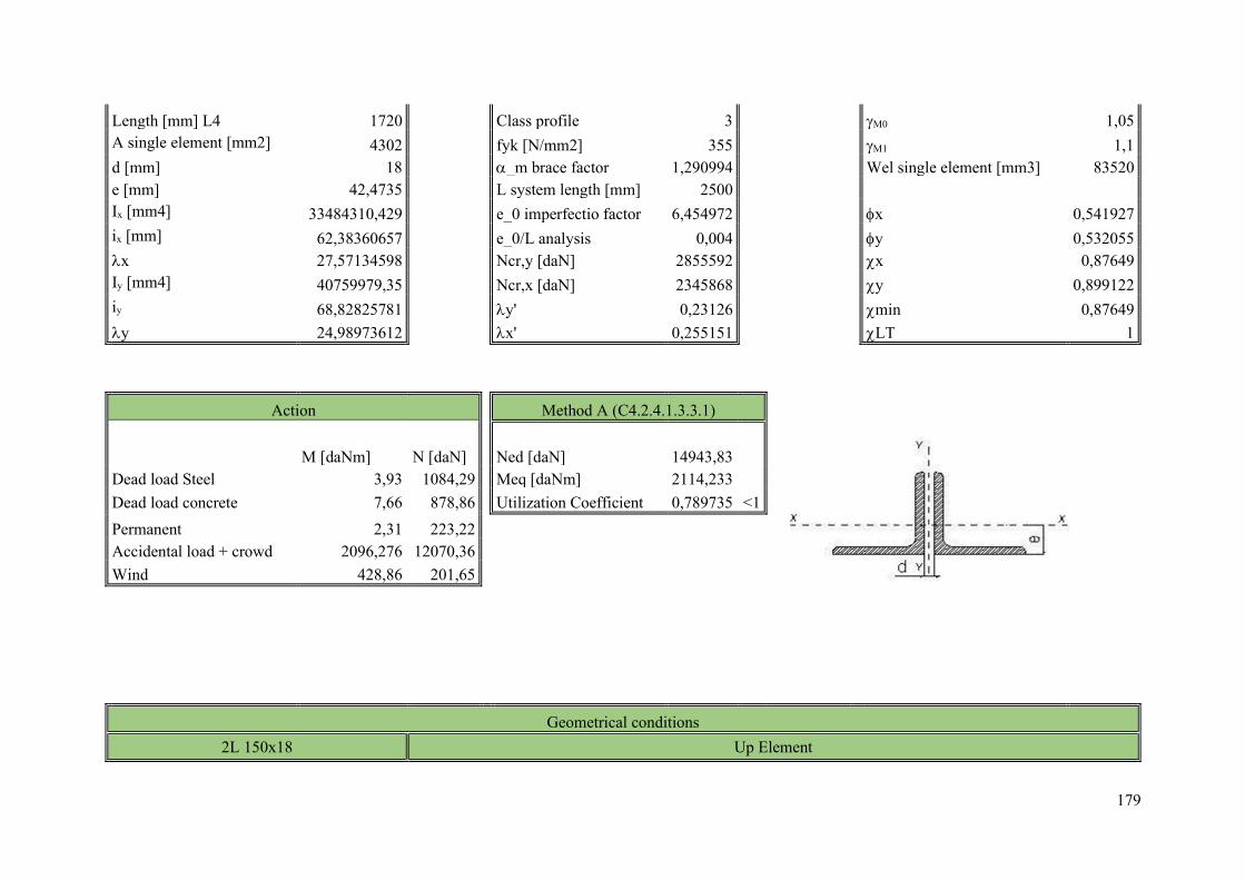
179
Length [mm] L4 1720 Class profile 3 M0 1,05 A single element [mm2] 4302 fyk [N/mm2] 355 M1 1,1 d [mm] 18 _m brace factor 1,290994 Wel single element [mm3] 83520 e [mm] 42,4735 L system length [mm] 2500 Ix [mm4] 33484310,429 e_0 imperfectio factor 6,454972 x 0,541927 ix [mm] 62,38360657 e_0/L analysis 0,004 y 0,532055 x 27,57134598 Ncr,y [daN] 2855592 x 0,87649 Iy [mm4] 40759979,35 Ncr,x [daN] 2345868 y 0,899122 iy 68,82825781 y' 0,23126 min 0,87649 y 24,98973612 x' 0,255151 LT 1
Action Method A (C4.2.4.1.3.3.1)
M [daNm] N [daN] Ned [daN] 14943,83
Dead load Steel 3,93 1084,29 Meq [daNm] 2114,233 Dead load concrete 7,66 878,86 Utilization Coefficient 0,789735 <1 Permanent 2,31 223,22 Accidental load + crowd 2096,276 12070,36 Wind 428,86 201,65
Geometrical conditions
2L 150x18 Up Element
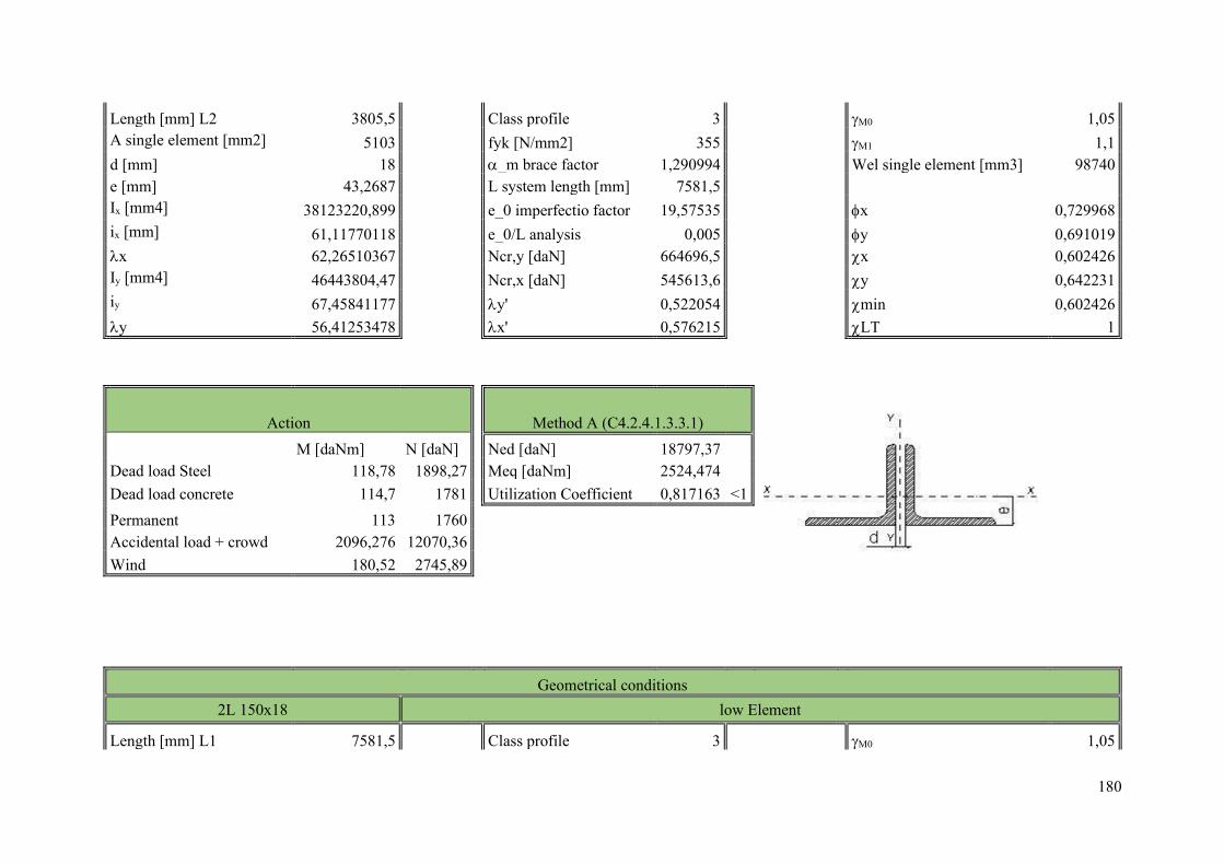
180
Length [mm] L2 3805,5 Class profile 3 M0 1,05 A single element [mm2] 5103 fyk [N/mm2] 355 M1 1,1 d [mm] 18 _m brace factor 1,290994 Wel single element [mm3] 98740 e [mm] 43,2687 L system length [mm] 7581,5 Ix [mm4] 38123220,899 e_0 imperfectio factor 19,57535 x 0,729968 ix [mm] 61,11770118 e_0/L analysis 0,005 y 0,691019 x 62,26510367 Ncr,y [daN] 664696,5 x 0,602426 Iy [mm4] 46443804,47 Ncr,x [daN] 545613,6 y 0,642231 iy 67,45841177 y' 0,522054 min 0,602426 y 56,41253478 x' 0,576215 LT 1
Action Method A (C4.2.4.1.3.3.1)
M [daNm] N [daN] Ned [daN] 18797,37 Dead load Steel 118,78 1898,27 Meq [daNm] 2524,474 Dead load concrete 114,7 1781 Utilization Coefficient 0,817163 <1 Permanent 113 1760 Accidental load + crowd 2096,276 12070,36 Wind 180,52 2745,89
Geometrical conditions 2L 150x18 low Element
Length [mm] L1 7581,5 Class profile 3 M0 1,05
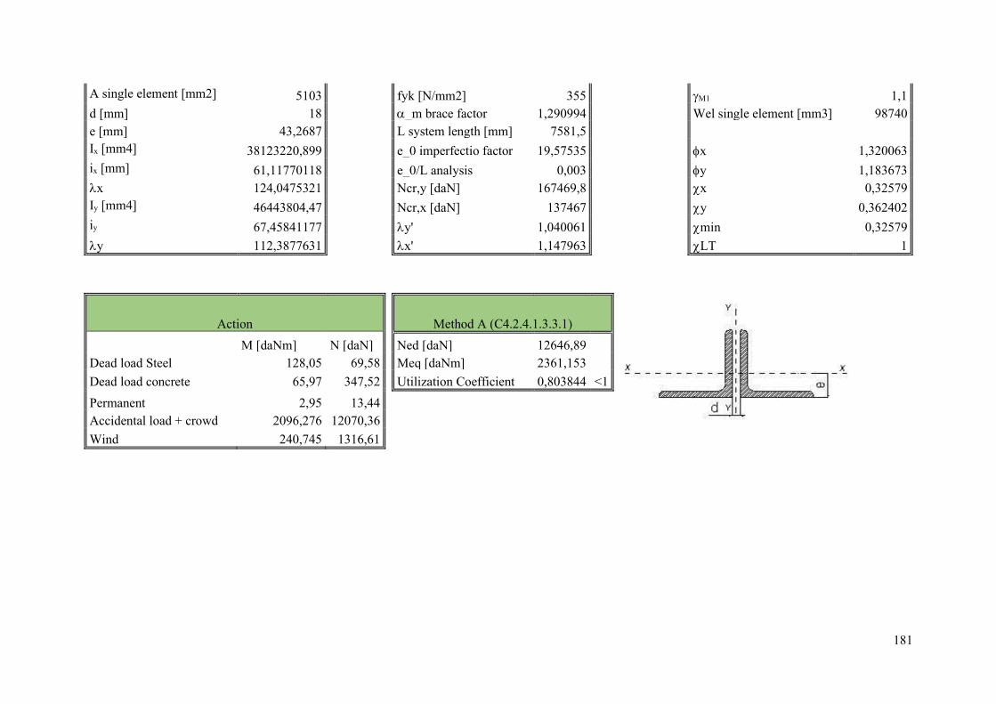
181
A single element [mm2] 5103 fyk [N/mm2] 355 M1 1,1 d [mm] 18 _m brace factor 1,290994 Wel single element [mm3] 98740 e [mm] 43,2687 L system length [mm] 7581,5 Ix [mm4] 38123220,899 e_0 imperfectio factor 19,57535 x 1,320063 ix [mm] 61,11770118 e_0/L analysis 0,003 y 1,183673 x 124,0475321 Ncr,y [daN] 167469,8 x 0,32579 Iy [mm4] 46443804,47 Ncr,x [daN] 137467 y 0,362402 iy 67,45841177 y' 1,040061 min 0,32579 y 112,3877631 x' 1,147963 LT 1
Action Method A (C4.2.4.1.3.3.1)
M [daNm] N [daN] Ned [daN] 12646,89 Dead load Steel 128,05 69,58 Meq [daNm] 2361,153 Dead load concrete 65,97 347,52 Utilization Coefficient 0,803844 <1 Permanent 2,95 13,44 Accidental load + crowd 2096,276 12070,36 Wind 240,745 1316,61
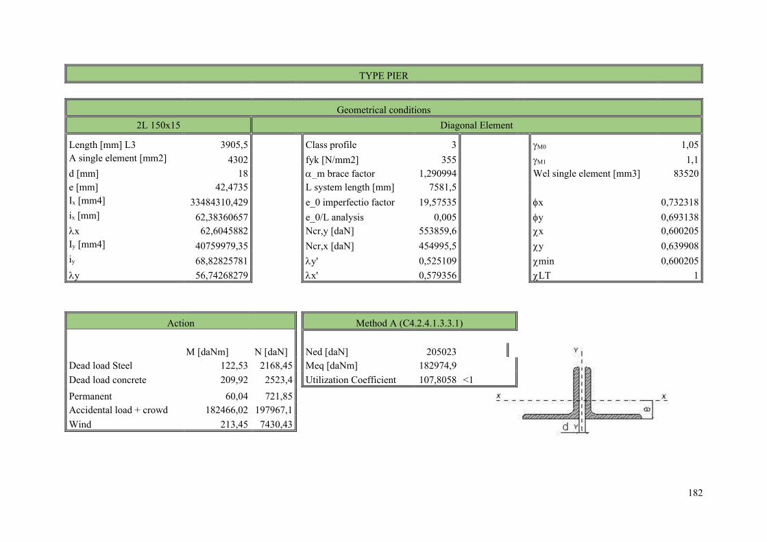
182
TYPE PIER
Geometrical conditions
2L 150x15 Diagonal Element
Length [mm] L3 3905,5 Class profile 3 M0 1,05 A single element [mm2] 4302 fyk [N/mm2] 355 M1 1,1 d [mm] 18 _m brace factor 1,290994 Wel single element [mm3] 83520 e [mm] 42,4735 L system length [mm] 7581,5 Ix [mm4] 33484310,429 e_0 imperfectio factor 19,57535 x 0,732318 ix [mm] 62,38360657 e_0/L analysis 0,005 y 0,693138 x 62,6045882 Ncr,y [daN] 553859,6 x 0,600205 Iy [mm4] 40759979,35 Ncr,x [daN] 454995,5 y 0,639908 iy 68,82825781 y' 0,525109 min 0,600205 y 56,74268279 x' 0,579356 LT 1
Action Method A (C4.2.4.1.3.3.1)
M [daNm] N [daN] Ned [daN] 205023
Dead load Steel 122,53 2168,45 Meq [daNm] 182974,9 Dead load concrete 209,92 2523,4 Utilization Coefficient 107,8058 <1 Permanent 60,04 721,85
Accidental load + crowd 182466,02 197967,1 Wind 213,45 7430,43

183
Geometrical conditions 2L 150x15 Vertical Element
Length [mm] L4 1720 Class profile 3 M0 1,05 A single element [mm2] 4302 fyk [N/mm2] 355 M1 1,1 d [mm] 18 _m brace factor 1,290994 Wel single element [mm3] 83520 e [mm] 42,4735 L system length [mm] 2500 Ix [mm4] 33484310,429 e_0 imperfectio factor 6,454972 x 0,541927 ix [mm] 62,38360657 e_0/L analysis 0,004 y 0,532055 x 27,57134598 Ncr,y [daN] 2855592 x 0,87649 Iy [mm4] 40759979,35 Ncr,x [daN] 2345868 y 0,899122 iy 68,82825781 y' 0,23126 min 0,87649 y 24,98973612 x' 0,255151 LT 1
Action Method A (C4.2.4.1.3.3.1)
M [daNm] N [daN] Ned [daN] 15183,06
Dead load Steel 6,55 1428,01 Meq [daNm] 1334,904 Dead load concrete 45,66 1918,08 Utilization Coefficient 0,499144 <1 Permanent 13,92 530,34
Accidental load + crowd 1250,5 10135,5 Wind 108,98 367,95
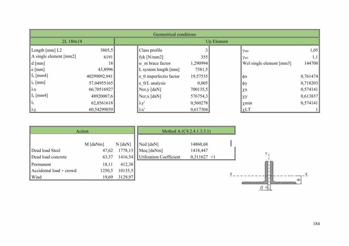
184
Geometrical conditions 2L 180x18 Up Element
Length [mm] L2 3805,5 Class profile 3 M0 1,05 A single element [mm2] 6191 fyk [N/mm2] 355 M1 1,1 d [mm] 18 _m brace factor 1,290994 Wel single element [mm3] 144700 e [mm] 43,8996 L system length [mm] 7581,5 Ix [mm4] 40299092,941 e_0 imperfectio factor 19,57535 x 0,761474 ix [mm] 57,04955165 e_0/L analysis 0,005 y 0,718203 x 66,70516927 Ncr,y [daN] 700135,5 x 0,574141 Iy [mm4] 48920007,6 Ncr,x [daN] 576754,3 y 0,613837 iy 62,8561618 y' 0,560278 min 0,574141 y 60,54299039 x' 0,617304 LT 1
Action Method A (C4.2.4.1.3.3.1)
M [daNm] N [daN] Ned [daN] 14860,68
Dead load Steel 47,62 1778,13 Meq [daNm] 1418,447 Dead load concrete 63,37 1416,54 Utilization Coefficient 0,311627 <1 Permanent 18,11 412,38 Accidental load + crowd 1250,5 10135,5 Wind 19,69 3129,97
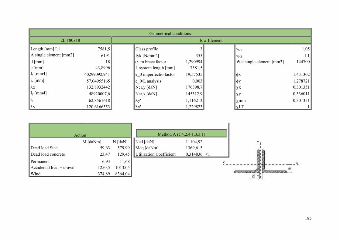
185
Geometrical conditions 2L 180x18 low Element
Length [mm] L1 7581,5 Class profile 3 M0 1,05 A single element [mm2] 6191 fyk [N/mm2] 355 M1 1,1 d [mm] 18 _m brace factor 1,290994 Wel single element [mm3] 144700 e [mm] 43,8996 L system length [mm] 7581,5 Ix [mm4] 40299092,941 e_0 imperfectio factor 19,57535 x 1,431302 ix [mm] 57,04955165 e_0/L analysis 0,003 y 1,278721 x 132,8932442 Ncr,y [daN] 176398,7 x 0,301351 Iy [mm4] 48920007,6 Ncr,x [daN] 145312,9 y 0,336011 iy 62,8561618 y' 1,116213 min 0,301351 y 120,6166553 x' 1,229823 LT 1
Action
Method A (C4.2.4.1.3.3.1)
M [daNm] N [daN] Ned [daN] 11104,92 Dead load Steel 59,63 579,99 Meq [daNm] 1369,615 Dead load concrete 23,47 129,45 Utilization Coefficient 0,314836 <1 Permanent 6,93 11,68 Accidental load + crowd 1250,5 10135,5 Wind 374,89 8364,04

186
BRACES RESULTS
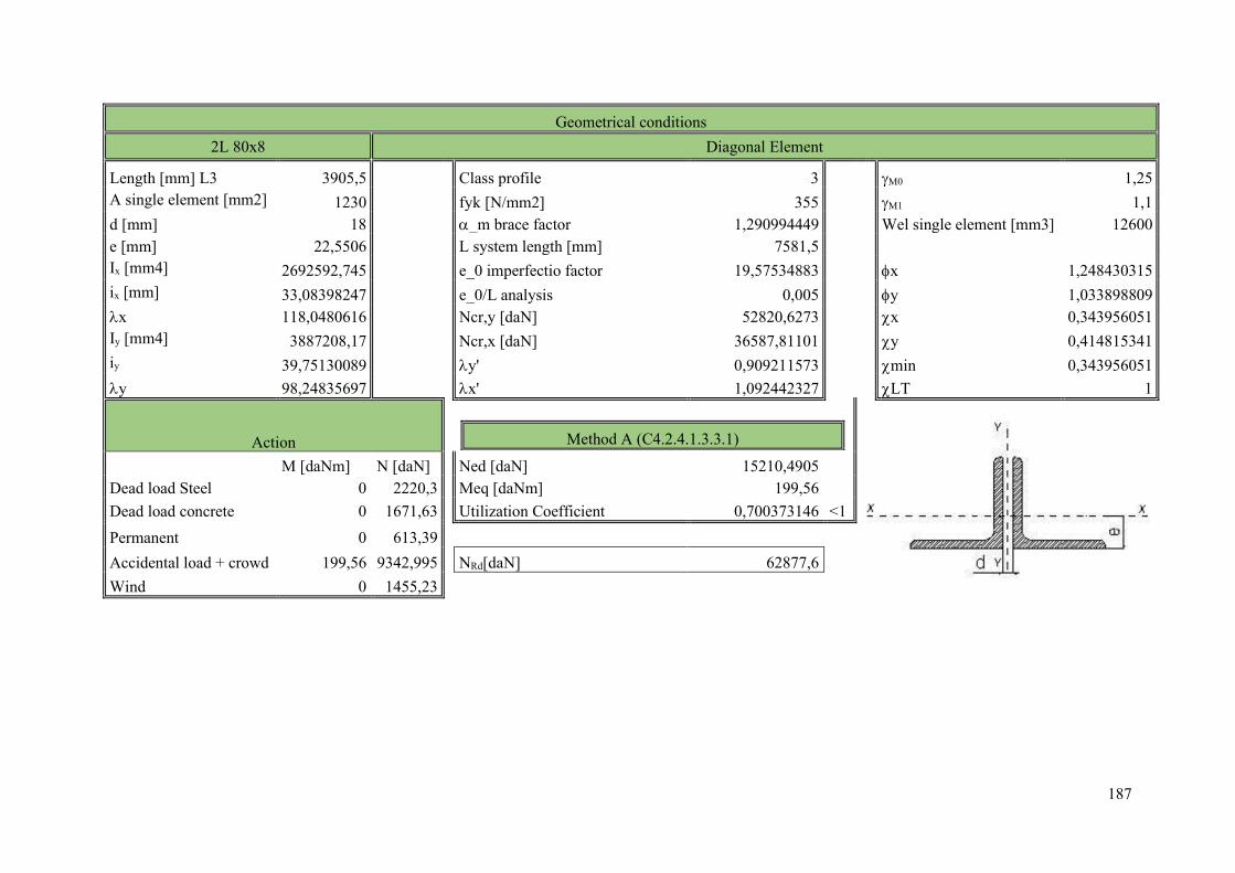
187
Geometrical conditions 2L 80x8 Diagonal Element
Length [mm] L3 3905,5 Class profile 3 M0 1,25 A single element [mm2] 1230 fyk [N/mm2] 355 M1 1,1 d [mm] 18 _m brace factor 1,290994449 Wel single element [mm3] 12600 e [mm] 22,5506 L system length [mm] 7581,5 Ix [mm4] 2692592,745 e_0 imperfectio factor 19,57534883 x 1,248430315 ix [mm] 33,08398247 e_0/L analysis 0,005 y 1,033898809 x 118,0480616 Ncr,y [daN] 52820,6273 x 0,343956051 Iy [mm4] 3887208,17 Ncr,x [daN] 36587,81101 y 0,414815341 iy 39,75130089 y' 0,909211573 min 0,343956051 y 98,24835697 x' 1,092442327 LT 1
Action
Method A (C4.2.4.1.3.3.1)
M [daNm] N [daN] Ned [daN] 15210,4905 Dead load Steel 0 2220,3 Meq [daNm] 199,56 Dead load concrete 0 1671,63 Utilization Coefficient 0,700373146 <1 Permanent 0 613,39
Accidental load + crowd 199,56 9342,995 NRd[daN] 62877,6 Wind 0 1455,23
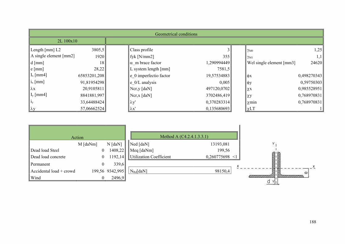
188
Geometrical conditions 2L 100x10
Length [mm] L2 3805,5 Class profile 3 M0 1,25 A single element [mm2] 1920 fyk [N/mm2] 355 M1 1,1 d [mm] 18 _m brace factor 1,290994449 Wel single element [mm3] 24620 e [mm] 28,22 L system length [mm] 7581,5 Ix [mm4] 65853201,208 e_0 imperfectio factor 19,57534883 x 0,498270343 ix [mm] 91,81954298 e_0/L analysis 0,005 y 0,59750303 x 20,9105811 Ncr,y [daN] 497120,0702 x 0,985528951 Iy [mm4] 8841881,997 Ncr,x [daN] 3702486,419 y 0,768970831 iy 33,64488424 y' 0,370283314 min 0,768970831 y 57,06662524 x' 0,135680693 LT 1
Action
Method A (C4.2.4.1.3.3.1)
M [daNm] N [daN] Ned [daN] 13193,081 Dead load Steel 0 1408,22 Meq [daNm] 199,56 Dead load concrete 0 1192,14 Utilization Coefficient 0,260775698 <1 Permanent 0 339,6
Accidental load + crowd 199,56 9342,995 NRd[daN] 98150,4 Wind 0 2496,9
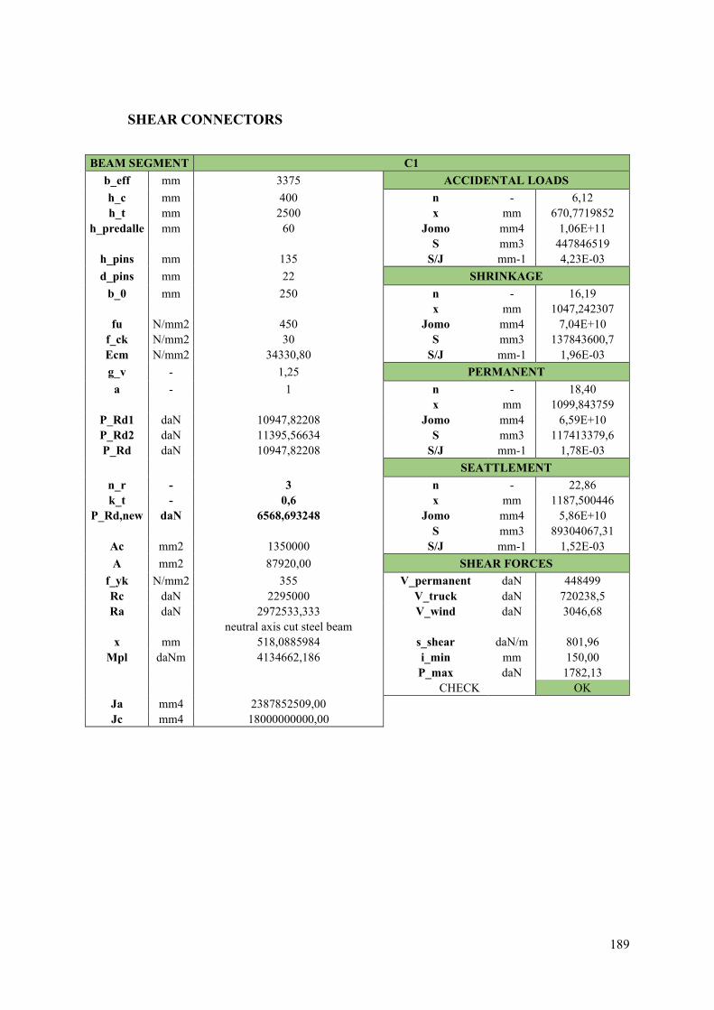
189
SHEAR CONNECTORS
BEAM SEGMENT C1 b_eff mm 3375 ACCIDENTAL LOADS h_c mm 400 n - 6,12 h_t mm 2500 x mm 670,7719852
h_predalle mm 60 Jomo mm4 1,06E+11 S mm3 447846519
h_pins mm 135 S/J mm-1 4,23E-03 d_pins mm 22 SHRINKAGE
b_0 mm 250 n - 16,19 x mm 1047,242307
fu N/mm2 450 Jomo mm4 7,04E+10 f_ck N/mm2 30 S mm3 137843600,7 Ecm N/mm2 34330,80 S/J mm-1 1,96E-03 g_v - 1,25 PERMANENT
a - 1 n - 18,40 x mm 1099,843759
P_Rd1 daN 10947,82208 Jomo mm4 6,59E+10 P_Rd2 daN 11395,56634 S mm3 117413379,6 P_Rd daN 10947,82208 S/J mm-1 1,78E-03
SEATTLEMENT n_r - 3 n - 22,86 k_t - 0,6 x mm 1187,500446
P_Rd,new daN 6568,693248 Jomo mm4 5,86E+10 S mm3 89304067,31
Ac mm2 1350000 S/J mm-1 1,52E-03 A mm2 87920,00 SHEAR FORCES
f_yk N/mm2 355 V_permanent daN 448499 Rc daN 2295000 V_truck daN 720238,5 Ra daN 2972533,333 V_wind daN 3046,68 neutral axis cut steel beam x mm 518,0885984 s_shear daN/m 801,96
Mpl daNm 4134662,186 i_min mm 150,00 P_max daN 1782,13 CHECK OK
Ja mm4 2387852509,00 Jc mm4 18000000000,00
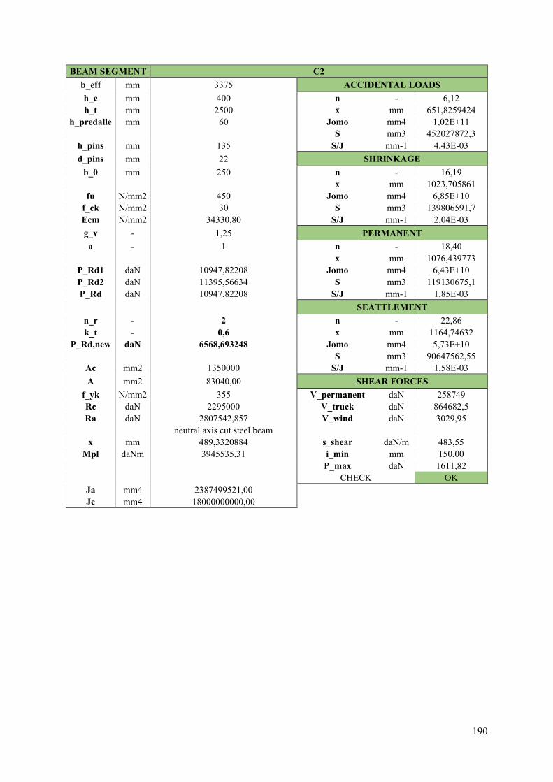
190
BEAM SEGMENT C2 b_eff mm 3375 ACCIDENTAL LOADS h_c mm 400 n - 6,12 h_t mm 2500 x mm 651,8259424
h_predalle mm 60 Jomo mm4 1,02E+11 S mm3 452027872,3
h_pins mm 135 S/J mm-1 4,43E-03 d_pins mm 22 SHRINKAGE
b_0 mm 250 n - 16,19 x mm 1023,705861
fu N/mm2 450 Jomo mm4 6,85E+10 f_ck N/mm2 30 S mm3 139806591,7 Ecm N/mm2 34330,80 S/J mm-1 2,04E-03 g_v - 1,25 PERMANENT a - 1 n - 18,40 x mm 1076,439773
P_Rd1 daN 10947,82208 Jomo mm4 6,43E+10 P_Rd2 daN 11395,56634 S mm3 119130675,1 P_Rd daN 10947,82208 S/J mm-1 1,85E-03
SEATTLEMENT n_r - 2 n - 22,86 k_t - 0,6 x mm 1164,74632
P_Rd,new daN 6568,693248 Jomo mm4 5,73E+10 S mm3 90647562,55
Ac mm2 1350000 S/J mm-1 1,58E-03 A mm2 83040,00 SHEAR FORCES
f_yk N/mm2 355 V_permanent daN 258749 Rc daN 2295000 V_truck daN 864682,5 Ra daN 2807542,857 V_wind daN 3029,95 neutral axis cut steel beam x mm 489,3320884 s_shear daN/m 483,55
Mpl daNm 3945535,31 i_min mm 150,00 P_max daN 1611,82 CHECK OK
Ja mm4 2387499521,00 Jc mm4 18000000000,00
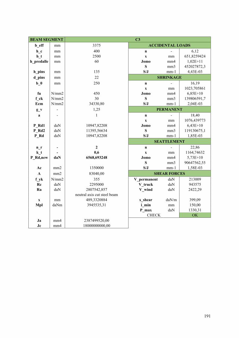
191
BEAM SEGMENT C3 b_eff mm 3375 ACCIDENTAL LOADS h_c mm 400 n - 6,12 h_t mm 2500 x mm 651,8259424
h_predalle mm 60 Jomo mm4 1,02E+11 S mm3 452027872,3
h_pins mm 135 S/J mm-1 4,43E-03 d_pins mm 22 SHRINKAGE
b_0 mm 250 n - 16,19 x mm 1023,705861
fu N/mm2 450 Jomo mm4 6,85E+10 f_ck N/mm2 30 S mm3 139806591,7 Ecm N/mm2 34330,80 S/J mm-1 2,04E-03 g_v - 1,25 PERMANENT a - 1 n - 18,40 x mm 1076,439773
P_Rd1 daN 10947,82208 Jomo mm4 6,43E+10 P_Rd2 daN 11395,56634 S mm3 119130675,1 P_Rd daN 10947,82208 S/J mm-1 1,85E-03
SEATTLEMENT n_r - 2 n - 22,86 k_t - 0,6 x mm 1164,74632
P_Rd,new daN 6568,693248 Jomo mm4 5,73E+10 S mm3 90647562,55
Ac mm2 1350000 S/J mm-1 1,58E-03 A mm2 83040,00 SHEAR FORCES
f_yk N/mm2 355 V_permanent daN 213009 Rc daN 2295000 V_truck daN 943575 Ra daN 2807542,857 V_wind daN 2422,29 neutral axis cut steel beam x mm 489,3320884 s_shear daN/m 399,09
Mpl daNm 3945535,31 i_min mm 150,00 P_max daN 1330,31 CHECK OK
Ja mm4 2387499520,00 Jc mm4 18000000000,00

192
BEAM SEGMENT C4 b_eff mm 3375 ACCIDENTAL LOADS h_c mm 400 n - 6,12 h_t mm 2500 x mm 741,5627364
h_predalle mm 60 Jomo mm4 1,20E+11 S mm3 432223143,3
h_pins mm 135 S/J mm-1 3,60E-03 d_pins mm 22 SHRINKAGE
b_0 mm 250 n - 16,19 x mm 1130,067901
fu N/mm2 450 Jomo mm4 7,72E+10 f_ck N/mm2 30 S mm3 130935765,3 Ecm N/mm2 34330,80 S/J mm-1 1,70E-03 g_v - 1,25 PERMANENT a - 1 n - 18,40 x mm 1181,529247
P_Rd1 daN 10947,82208 Jomo mm4 7,20E+10 P_Rd2 daN 11395,56634 S mm3 111419609,2 P_Rd daN 10947,82208 S/J mm-1 1,55E-03
SEATTLEMENT n_r - 2 n - 22,86 k_t - 0,6 x mm 1265,844183
P_Rd,new daN 6568,693248 Jomo mm4 6,35E+10 S mm3 84678337,47
Ac mm2 1350000 S/J mm-1 1,33E-03 A mm2 107630,00 SHEAR FORCES
f_yk N/mm2 355 V_permanent daN 370261 Rc daN 2295000 V_truck daN 1013082 Ra daN 3638919,048 V_wind daN 3637,62 neutral axis cut steel beam x mm 634,2342567 s_shear daN/m 576,92
Mpl daNm 4850252,87 i_min mm 150,00 P_max daN 1923,07 CHECK OK
Ja mm4 2547559577,00 Jc mm4 18000000000,00

193
BEAM SEGMENT C5 b_eff mm 3375 ACCIDENTAL LOADS h_c mm 400 n - 6,12 h_t mm 2500 x mm 863,5446831
h_predalle mm 60 Jomo mm4 1,50E+11 S mm3 405301974,4
h_pins mm 135 S/J mm-1 2,71E-03 d_pins mm 22 SHRINKAGE
b_0 mm 200 n - 16,19 x mm 1256,256079
fu N/mm2 450 Jomo mm4 9,29E+10 f_ck N/mm2 30 S mm3 120411395,7 Ecm N/mm2 34330,80 S/J mm-1 1,30E-03 g_v - 1,25 PERMANENT a - 1 n - 18,40 x mm 1303,998351
P_Rd1 daN 10947,82208 Jomo mm4 8,63E+10 P_Rd2 daN 11395,56634 S mm3 102433292 P_Rd daN 10947,82208 S/J mm-1 1,19E-03
SEATTLEMENT n_r - 3 n - 22,86 k_t - 0,6 x mm 1380,266266
P_Rd,new daN 6568,693248 Jomo mm4 7,60E+10 S mm3 77922396,68
Ac mm2 1350000 S/J mm-1 1,03E-03 A mm2 148230,00 SHEAR FORCES
f_yk N/mm2 355 V_permanent daN 558693 Rc daN 2295000 V_truck daN 1153569 Ra daN 5011585,714 V_wind daN 4852,94 neutral axis cut steel beam x mm 873,4789916 s_shear daN/m 665,93
Mpl daNm 6080359,011 i_min mm 150,00 P_max daN 1479,84 CHECK OK
Ja mm4 7656856608,00 Jc mm4 18000000000,00

194
BEAM SEGMENT C5a b_eff mm 3375 ACCIDENTAL LOADS h_c mm 400 n - 6,12 h_t mm 2500 x mm 968,8709124
h_predalle mm 60 Jomo mm4 1,74E+11 S mm3 382056688,6
h_pins mm 135 S/J mm-1 2,20E-03 d_pins mm 22 SHRINKAGE
b_0 mm 200 n - 16,19 x mm 1351,218178
fu N/mm2 450 Jomo mm4 1,04E+11 f_ck N/mm2 30 S mm3 112491349,3 Ecm N/mm2 34330,80 S/J mm-1 1,08E-03 g_v - 1,25 PERMANENT a - 1 n - 18,40 x mm 1394,619771
P_Rd1 daN 10947,82208 Jomo mm4 9,65E+10 P_Rd2 daN 11395,56634 S mm3 95783836,9 P_Rd daN 10947,82208 S/J mm-1 9,93E-04
SEATTLEMENT n_r - 3 n - 22,86 k_t - 0,6 x mm 1462,674372
P_Rd,new daN 6568,693248 Jomo mm4 8,46E+10 S mm3 73056690,08
Ac mm2 1350000 S/J mm-1 8,64E-04 A mm2 192330,00 SHEAR FORCES
f_yk N/mm2 355 V_permanent daN 563529 Rc daN 2295000 V_truck daN 1157524,5 Ra daN 6502585,714 V_wind daN 4869,67 neutral axis cut steel beam x mm 1133,348273 s_shear daN/m 562,01
Mpl daNm 7044419,285 i_min mm 150,00 P_max daN 1248,92 CHECK OK
Ja mm4 10369681812,00 Jc mm4 18000000000,00
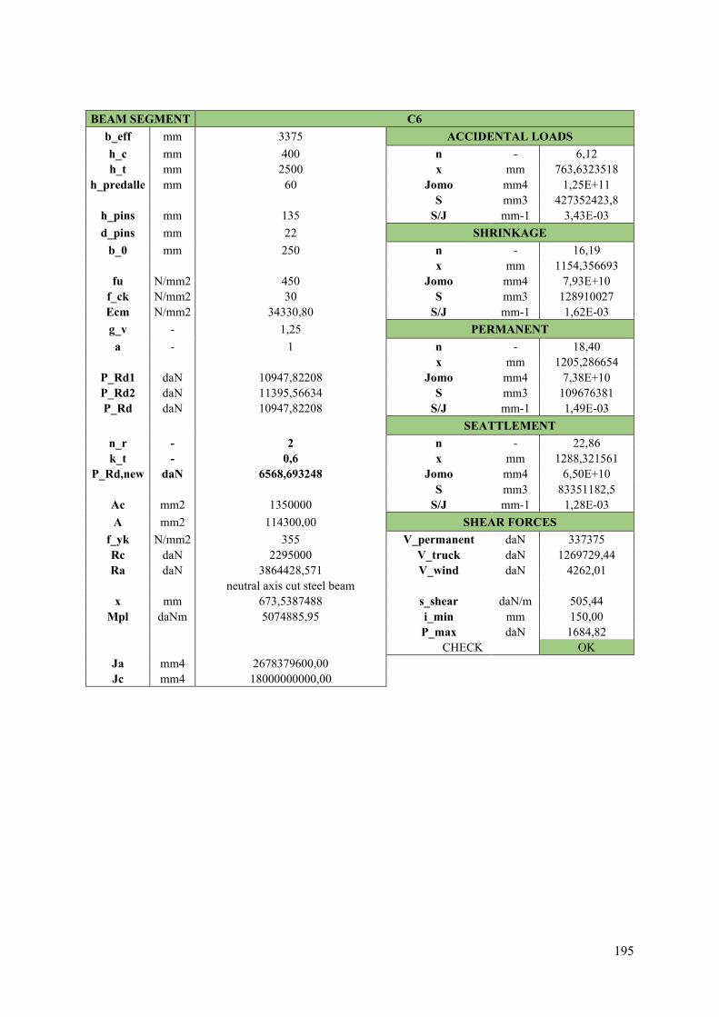
195
BEAM SEGMENT C6 b_eff mm 3375 ACCIDENTAL LOADS h_c mm 400 n - 6,12 h_t mm 2500 x mm 763,6323518
h_predalle mm 60 Jomo mm4 1,25E+11 S mm3 427352423,8
h_pins mm 135 S/J mm-1 3,43E-03 d_pins mm 22 SHRINKAGE
b_0 mm 250 n - 16,19 x mm 1154,356693
fu N/mm2 450 Jomo mm4 7,93E+10 f_ck N/mm2 30 S mm3 128910027 Ecm N/mm2 34330,80 S/J mm-1 1,62E-03 g_v - 1,25 PERMANENT a - 1 n - 18,40 x mm 1205,286654
P_Rd1 daN 10947,82208 Jomo mm4 7,38E+10 P_Rd2 daN 11395,56634 S mm3 109676381 P_Rd daN 10947,82208 S/J mm-1 1,49E-03
SEATTLEMENT n_r - 2 n - 22,86 k_t - 0,6 x mm 1288,321561
P_Rd,new daN 6568,693248 Jomo mm4 6,50E+10 S mm3 83351182,5
Ac mm2 1350000 S/J mm-1 1,28E-03 A mm2 114300,00 SHEAR FORCES
f_yk N/mm2 355 V_permanent daN 337375 Rc daN 2295000 V_truck daN 1269729,44 Ra daN 3864428,571 V_wind daN 4262,01 neutral axis cut steel beam x mm 673,5387488 s_shear daN/m 505,44
Mpl daNm 5074885,95 i_min mm 150,00 P_max daN 1684,82 CHECK OK
Ja mm4 2678379600,00 Jc mm4 18000000000,00

196
BEAM SEGMENT C7 b_eff mm 3375 ACCIDENTAL LOADS h_c mm 400 n - 6,12 h_t mm 2500 x mm 711,2851439
h_predalle mm 60 Jomo mm4 1,14E+11 S mm3 438905346,8
h_pins mm 135 S/J mm-1 3,85E-03 d_pins mm 22 SHRINKAGE
b_0 mm 250 n - 16,19 x mm 1095,592136
fu N/mm2 450 Jomo mm4 7,45E+10 f_ck N/mm2 30 S mm3 133811119,4 Ecm N/mm2 34330,80 S/J mm-1 1,80E-03 g_v - 1,25 PERMANENT a - 1 n - 18,40 x mm 1147,654865
P_Rd1 daN 10947,82208 Jomo mm4 6,96E+10 P_Rd2 daN 11395,56634 S mm3 113905182,5 P_Rd daN 10947,82208 S/J mm-1 1,64E-03
SEATTLEMENT n_r - 2 n - 22,86 k_t - 0,6 x mm 1233,556287
P_Rd,new daN 6568,693248 Jomo mm4 6,16E+10 S mm3 86584744,9
Ac mm2 1350000 S/J mm-1 1,41E-03 A mm2 98900,00 SHEAR FORCES
f_yk N/mm2 355 V_permanent daN 448499 Rc daN 2295000 V_truck daN 868638 Ra daN 3343761,905 V_wind daN 3654,34 neutral axis cut steel beam x mm 582,7907459 s_shear daN/m 737,58
Mpl daNm 4542850,396 i_min mm 150,00 P_max daN 2458,61 CHECK OK
Ja mm4 2626235869,00 Jc mm4 18000000000,00

197
BEAM SEGMENT C8 b_eff mm 3375 ACCIDENTAL LOADS h_c mm 600 n - 6,12 h_t mm 2500 x mm 757,4462012
h_predalle mm 60 Jomo mm4 1,51E+11 S mm3 676181238,8
h_pins mm 135 S/J mm-1 4,48E-03 d_pins mm 22 SHRINKAGE
b_0 mm 200 n - 16,19 x mm 1159,831169
fu N/mm2 450 Jomo mm4 9,79E+10 f_ck N/mm2 30 S mm3 205190493,2 Ecm N/mm2 34330,80 S/J mm-1 2,10E-03 g_v - 1,25 PERMANENT a - 1 n - 18,40 x mm 1218,923123
P_Rd1 daN 10947,82208 Jomo mm4 9,20E+10 P_Rd2 daN 11395,56634 S mm3 174020112,7 P_Rd daN 10947,82208 S/J mm-1 1,89E-03
SEATTLEMENT n_r - 3 n - 22,86 k_t - 0,6 x mm 1319,056077
P_Rd,new daN 6568,693248 Jomo mm4 8,23E+10 S mm3 131161343,6
Ac mm2 2025000 S/J mm-1 1,59E-03 A mm2 108509,37 SHEAR FORCES
f_yk N/mm2 355 V_permanent daN 494627 Rc daN 3442500 V_truck daN 724194 Ra daN 3668650,003 V_wind daN 4245,28 neutral axis cut steel beam x mm 639,4161226 s_shear daN/m 852,05
Mpl daNm 5614105,526 i_min mm 150,00 P_max daN 1893,45 CHECK OK
Ja mm4 3273457880,50 Jc mm4 60750000000,00
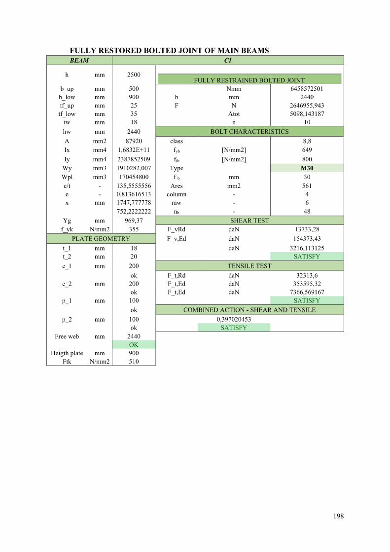
198
FULLY RESTORED BOLTED JOINT OF MAIN BEAMS BEAM C1
h mm 2500
FULLY RESTRAINED BOLTED JOINT
b_up mm 500 Nmm 6458572501 b_low mm 900 b mm 2440 tf_up mm 25 F N 2646955,943
tf_low mm 35 Atot 5098,143187 tw mm 18 n 10 hw mm 2440 BOLT CHARACTERISTICS A mm2 87920 class 8,8 Ix mm4 1,6832E+11 fyb [N/mm2] 649 Iy mm4 2387852509 ftb [N/mm2] 800
Wy mm3 1910282,007 Type M30 Wpl mm3 170454800 f b mm 30 c/t - 135,5555556 Ares mm2 561 e - 0,813616513 column - 4 x mm 1747,777778 raw - 6 752,2222222 nb - 48
Yg mm 969,37 SHEAR TEST f_yk N/mm2 355 F_vRd daN 13733,28
PLATE GEOMETRY F_v,Ed daN 154373,43 t_1 mm 18 daN 3216,113125 t_2 mm 20 SATISFY e_1 mm 200 TENSILE TEST
ok F_t,Rd daN 32313,6 e_2 mm 200 F_t,Ed daN 353595,32
ok F_t,Ed daN 7366,569167 p_1 mm 100 SATISFY
ok COMBINED ACTION - SHEAR AND TENSILE p_2 mm 100 0,397020453
ok SATISFY
Free web mm 2440 OK
Heigth plate mm 900 Ftk N/mm2 510

199
BEAM C2
h mm 2500
FULLY RESTRAINED BOLTED JOINT
b_up mm 500 Nmm 6457617752 b_low mm 900 b mm 2440 tf_up mm 25 F N 2646564,652
tf_low mm 35 Atot 5097,389546 tw mm 16 n 10 hw mm 2440 BOLT CHARACTERISTICS A mm2 83040 class 8,8 Ix mm4 1,5822E+11 fyb [N/mm2] 649 Iy mm4 2387499521 ftb [N/mm2] 800
Wy mm3 1909999,617 Type M30 Wpl mm3 158547600 f b mm 30 c/t - 152,5 Ares mm2 561 e - 0,813616513 column - 4 x mm 1813,75 raw - 6 686,25 nb - 48
Yg mm 954,65 SHEAR TEST f_yk N/mm2 355 F_vRd daN 13733,28
PLATE GEOMETRY F_v,Ed daN 154373,43 t_1 mm 16 daN 955,8845833 t_2 mm 20 SATISFY e_1 mm 200 TENSILE TEST
ok F_t,Rd daN 32313,6 e_2 mm 200 F_t,Ed daN 445758,43
ok F_t,Ed daN 9286,633958 p_1 mm 100 SATISFY
ok COMBINED ACTION - SHEAR AND TENSILE p_2 mm 100 0,274882717
ok SATISFY
Free web mm 2440 OK
Heigth plate mm 900 Ftk N/mm2 510

200
BEAM C3
h mm 2500
FULLY RESTRAINED BOLTED JOINT
b_up mm 500 Nmm 6457617749 b_low mm 900 b mm 2440 tf_up mm 25 F N 2646564,651
tf_low mm 35 Atot 5097,389544 tw mm 16 n 10 hw mm 2440 BOLT CHARACTERISTICS A mm2 83040 class 8,8 Ix mm4 1,5822E+11 fyb [N/mm2] 649 Iy mm4 2387499520 ftb [N/mm2] 800
Wy mm3 1909999,616 Type M30 Wpl mm3 158547600 f b mm 30 c/t - 152,5 Ares mm2 561 e - 0,813616513 column - 4 x mm 1813,75 raw - 6 686,25 nb - 48
Yg mm 954,65 SHEAR TEST f_yk N/mm2 355 F_vRd daN 13733,28
PLATE GEOMETRY F_v,Ed daN 154373,43 t_1 mm 16 daN 2821,059375 t_2 mm 20 SATISFY e_1 mm 200 TENSILE TEST
ok F_t,Rd daN 32313,6 e_2 mm 200 F_t,Ed daN 411790,24
ok F_t,Ed daN 8578,963333 p_1 mm 100 SATISFY
ok COMBINED ACTION - SHEAR AND TENSILE p_2 mm 100 0,395054024
ok SATISFY
Free web mm 2440 OK
Heigth plate mm 900 Ftk N/mm2 510

201
BEAM C4
h mm 2500
FULLY RESTRAINED BOLTED JOINT
b_up mm 500 Nmm 6890542094 b_low mm 900 b mm 2415 tf_up mm 30 F N 2853226,54
tf_low mm 55 Atot 5495,428621 tw mm 22 n 10 hw mm 2415 BOLT CHARACTERISTICS A mm2 107630 class 8,8 Ix mm4 2,0317E+11 fyb [N/mm2] 649 Iy mm4 2547559577 ftb [N/mm2] 800
Wy mm3 2038047,662 Type M30 Wpl mm3 203961450 f b mm 30 c/t - 110,2777778 Ares mm2 561 e - 0,813616513 column - 4 x mm 1764,318182 raw - 6 735,6818182 nb - 48
Yg mm 947,51 SHEAR TEST f_yk N/mm2 355 F_vRd daN 13733,28
PLATE GEOMETRY F_v,Ed daN 154373,43 t_1 mm 22 daN 5165,503542 t_2 mm 20 SATISFY e_1 mm 200 TENSILE TEST
ok F_t,Rd daN 32313,6 e_2 mm 200 F_t,Ed daN 886610,95
ok F_t,Ed daN 18471,06146 p_1 mm 100 SATISFY
ok COMBINED ACTION - SHEAR AND TENSILE p_2 mm 100 0,784429507
ok SATISFY
Free web mm 2415 OK
Heigth plate mm 900 Ftk N/mm2 510

202
BEAM C5
h mm 2500
FULLY RESTRAINED BOLTED JOINT
b_up mm 900 Nmm 20709974064 b_low mm 1250 b mm 2410 tf_up mm 30 F N 8593350,234
tf_low mm 60 Atot 16551,13681 tw mm 28 n 30 hw mm 2410 BOLT CHARACTERISTICS A mm2 148230 class 8,8 Ix mm4 3,0742E+11 fyb [N/mm2] 649 Iy mm4 7656856608 ftb [N/mm2] 800
Wy mm3 6125485,286 Type M30 Wpl mm3 298348050 f b mm 30 c/t - 86,67857143 Ares mm2 561 e - 0,813616513 column - 4 x mm 1682,678571 raw - 6 817,3214286 nb - 48
Yg mm 1006,37 SHEAR TEST f_yk N/mm2 355 F_vRd daN 13733,28
PLATE GEOMETRY F_v,Ed daN 154373,43 t_1 mm 28 daN 6135,905417 t_2 mm 20 SATISFY e_1 mm 200 TENSILE TEST
ok F_t,Rd daN 32313,6 e_2 mm 200 F_t,Ed daN 1129730,21
ok F_t,Ed daN 23536,04604 p_1 mm 100 SATISFY
ok COMBINED ACTION - SHEAR AND TENSILE p_2 mm 100 0,967050591
ok SATISFY
Free web mm 2410 OK
Heigth plate mm 900 Ftk N/mm2 510
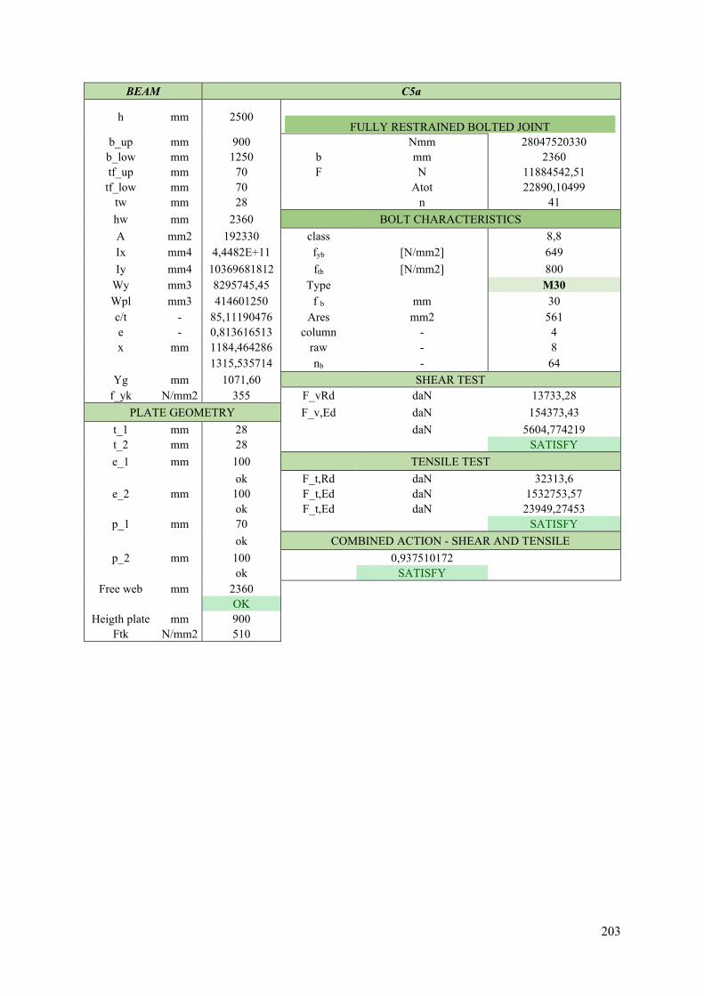
203
BEAM C5a
h mm 2500
FULLY RESTRAINED BOLTED JOINT
b_up mm 900 Nmm 28047520330 b_low mm 1250 b mm 2360 tf_up mm 70 F N 11884542,51
tf_low mm 70 Atot 22890,10499 tw mm 28 n 41 hw mm 2360 BOLT CHARACTERISTICS A mm2 192330 class 8,8 Ix mm4 4,4482E+11 fyb [N/mm2] 649 Iy mm4 10369681812 ftb [N/mm2] 800
Wy mm3 8295745,45 Type M30 Wpl mm3 414601250 f b mm 30 c/t - 85,11190476 Ares mm2 561 e - 0,813616513 column - 4 x mm 1184,464286 raw - 8 1315,535714 nb - 64
Yg mm 1071,60 SHEAR TEST f_yk N/mm2 355 F_vRd daN 13733,28
PLATE GEOMETRY F_v,Ed daN 154373,43 t_1 mm 28 daN 5604,774219 t_2 mm 28 SATISFY e_1 mm 100 TENSILE TEST
ok F_t,Rd daN 32313,6 e_2 mm 100 F_t,Ed daN 1532753,57
ok F_t,Ed daN 23949,27453 p_1 mm 70 SATISFY
ok COMBINED ACTION - SHEAR AND TENSILE p_2 mm 100 0,937510172
ok SATISFY
Free web mm 2360 OK
Heigth plate mm 900 Ftk N/mm2 510
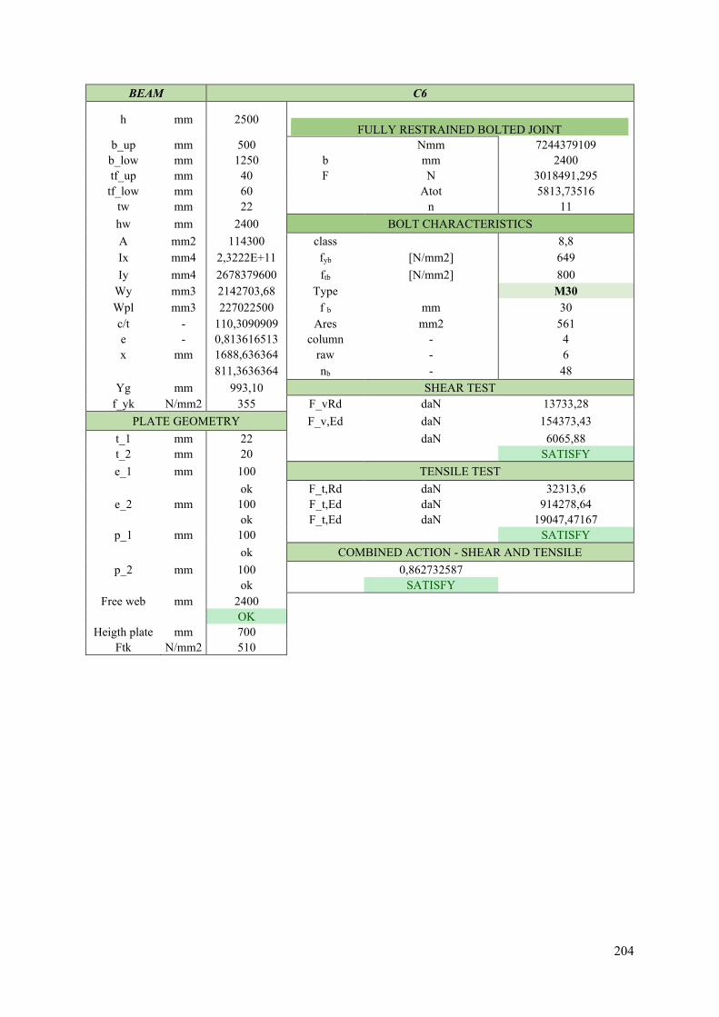
204
BEAM C6
h mm 2500
FULLY RESTRAINED BOLTED JOINT
b_up mm 500 Nmm 7244379109 b_low mm 1250 b mm 2400 tf_up mm 40 F N 3018491,295
tf_low mm 60 Atot 5813,73516 tw mm 22 n 11 hw mm 2400 BOLT CHARACTERISTICS A mm2 114300 class 8,8 Ix mm4 2,3222E+11 fyb [N/mm2] 649 Iy mm4 2678379600 ftb [N/mm2] 800
Wy mm3 2142703,68 Type M30 Wpl mm3 227022500 f b mm 30 c/t - 110,3090909 Ares mm2 561 e - 0,813616513 column - 4 x mm 1688,636364 raw - 6 811,3636364 nb - 48
Yg mm 993,10 SHEAR TEST f_yk N/mm2 355 F_vRd daN 13733,28
PLATE GEOMETRY F_v,Ed daN 154373,43 t_1 mm 22 daN 6065,88 t_2 mm 20 SATISFY e_1 mm 100 TENSILE TEST
ok F_t,Rd daN 32313,6 e_2 mm 100 F_t,Ed daN 914278,64
ok F_t,Ed daN 19047,47167 p_1 mm 100 SATISFY
ok COMBINED ACTION - SHEAR AND TENSILE p_2 mm 100 0,862732587
ok SATISFY
Free web mm 2400 OK
Heigth plate mm 700 Ftk N/mm2 510

205
BEAM C7
h mm 2500
FULLY RESTRAINED BOLTED JOINT
b_up mm 500 Nmm 7103342731 b_low mm 900 b mm 2400 tf_up mm 30 F N 2959726,138
tf_low mm 70 Atot 5700,551113 tw mm 16 n 11 hw mm 2400 BOLT CHARACTERISTICS A mm2 98900 class 8,8 Ix mm4 1,7305E+11 fyb [N/mm2] 649 Iy mm4 2626235869 ftb [N/mm2] 800
Wy mm3 2100988,695 Type M30 Wpl mm3 167812500 f b mm 30 c/t - 151,2152778 Ares mm2 561 e - 0,813616513 column - 4 x mm 2153,125 raw - 6 346,875 nb - 48
Yg mm 848,39 SHEAR TEST f_yk N/mm2 355 F_vRd daN 13733,28
PLATE GEOMETRY F_v,Ed daN 154373,43 t_1 mm 16 daN 3708,025 t_2 mm 20 SATISFY e_1 mm 100 TENSILE TEST
ok F_t,Rd daN 32313,6 e_2 mm 100 F_t,Ed daN 736951,55
ok F_t,Ed daN 15353,15729 p_1 mm 100 SATISFY
ok COMBINED ACTION - SHEAR AND TENSILE p_2 mm 100 0,609381364
ok SATISFY
Free web mm 2400 OK
Heigth plate mm 700 Ftk N/mm2 510
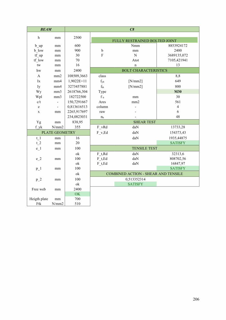
206
BEAM C8
h mm 2500
FULLY RESTRAINED BOLTED JOINT
b_up mm 600 Nmm 8853924172 b_low mm 900 b mm 2400 tf_up mm 30 F N 3689135,072
tf_low mm 70 Atot 7105,421941 tw mm 16 n 13 hw mm 2400 BOLT CHARACTERISTICS A mm2 108509,3663 class 8,8 Ix mm4 1,9022E+11 fyb [N/mm2] 649 Iy mm4 3273457881 ftb [N/mm2] 800
Wy mm3 2618766,304 Type M30 Wpl mm3 182722500 f b mm 30 c/t - 150,7291667 Ares mm2 561 e - 0,813616513 column - 4 x mm 2265,917697 raw - 6 234,0823031 nb - 48
Yg mm 838,95 SHEAR TEST f_yk N/mm2 355 F_vRd daN 13733,28
PLATE GEOMETRY F_v,Ed daN 154373,43 t_1 mm 16 daN 1935,44875 t_2 mm 20 SATISFY e_1 mm 100 TENSILE TEST
ok F_t,Rd daN 32313,6 e_2 mm 100 F_t,Ed daN 808702,56
ok F_t,Ed daN 16847,97 p_1 mm 100 SATISFY
ok COMBINED ACTION - SHEAR AND TENSILE p_2 mm 100 0,513352314
ok SATISFY
Free web mm 2400 OK
Heigth plate mm 700 Ftk N/mm2 510
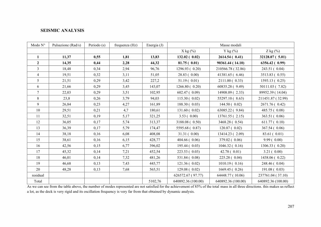
207
SEISMIC ANALYSIS
Modo N° Pulsazione (Rad/s) Periodo (s) frequenza (Hz) Energia (J) Masse modali X kg (%) Y kg (%) Z kg (%)
1 11,37 0,55 1,81 13,83 132.02 ( 0.02) 2614.54 ( 0.41) 32128.07 ( 5.01) 2 14,35 0,44 2,28 44,32 81.75 ( 0.01) 90361.44 ( 14.10) 6356.42 ( 0.99) 3 18,48 0,34 2,94 96,76 1296.93 ( 0.20) 210566.78 ( 32.86) 243.51 ( 0.04) 4 19,51 0,32 3,11 51,05 28.83 ( 0.00) 41381.65 ( 6.46) 3513.83 ( 0.55) 5 21,51 0,29 3,42 227,2 51.19 ( 0.01) 2111.00 ( 0.33) 1593.13 ( 0.25) 6 21,66 0,29 3,45 143,07 1266.80 ( 0.20) 60835.28 ( 9.49) 50111.03 ( 7.82) 7 22,03 0,29 3,51 102,95 602.47 ( 0.09) 14908.09 ( 2.33) 89952.39 ( 14.04) 8 23,8 0,26 3,79 94,03 115.30 ( 0.02) 55297.10 ( 8.63) 211451.87 ( 32.99) 9 26,84 0,23 4,27 161,89 188.30 ( 0.03) 144.50 ( 0.02) 2671.76 ( 0.42)
10 29,51 0,21 4,7 180,61 131.60 ( 0.02) 63085.22 ( 9.84) 485.75 ( 0.08) 11 32,51 0,19 5,17 321,25 3.53 ( 0.00) 13761.55 ( 2.15) 363.51 ( 0.06) 12 36,05 0,17 5,74 313,37 3188.08 ( 0.50) 3468.28 ( 0.54) 611.77 ( 0.10) 13 36,39 0,17 5,79 174,47 5595.68 ( 0.87) 120.87 ( 0.02) 367.54 ( 0.06) 14 38,18 0,16 6,08 408,08 31.31 ( 0.00) 13414.23 ( 2.09) 83.61 ( 0.01) 15 38,61 0,16 6,15 428,77 404.66 ( 0.06) 379.02 ( 0.06) 9.99 ( 0.00) 16 42,56 0,15 6,77 396,02 195.44 ( 0.03) 1046.32 ( 0.16) 1306.33 ( 0.20) 17 45,32 0,14 7,21 452,54 223.53 ( 0.03) 42.78 ( 0.01) 3.21 ( 0.00) 18 46,01 0,14 7,32 481,26 531.84 ( 0.08) 225.28 ( 0.04) 1438.06 ( 0.22) 19 46,68 0,13 7,43 445,77 121.36 ( 0.02) 1010.19 ( 0.16) 248.46 ( 0.04) 20 48,28 0,13 7,68 565,51 129.08 ( 0.02) 1669.45 ( 0.26) 191.08 ( 0.03)
residual 626572.67 ( 97.77) 64448.77 ( 10.06) 237761.04 ( 37.10) Total 5102,76 640892.36 (100.00) 640892.36 (100.00) 640892.36 (100.00)
As we can see from the table above, the number of modes represented are not satisfied for the achievement of 85% of the total mass in all three directions. this makes us reflect a lot, as the deck is very rigid and its oscillation frequency is very far from that obtained by dynamic analysis.
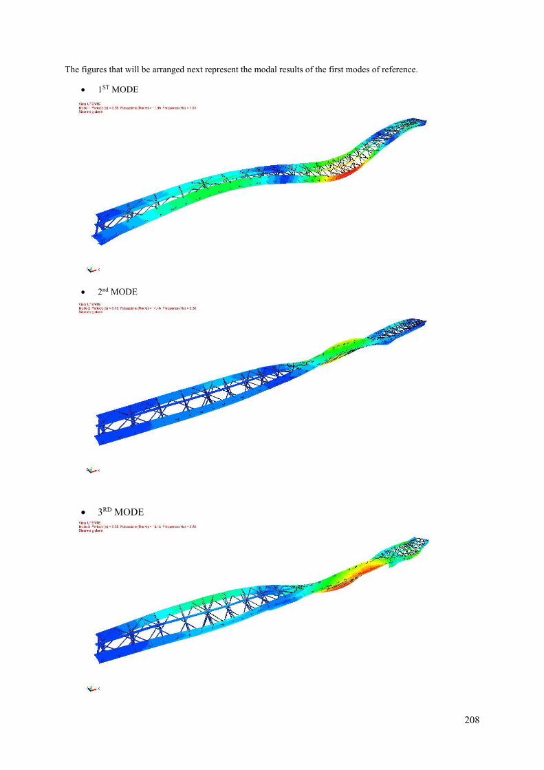
208
The figures that will be arranged next represent the modal results of the first modes of reference.
• 1ST MODE
• 2nd MODE
• 3RD MODE
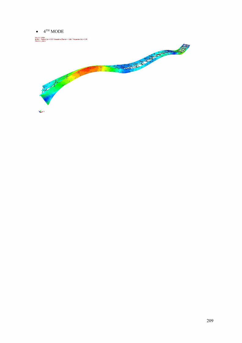
209
• 4TH MODE
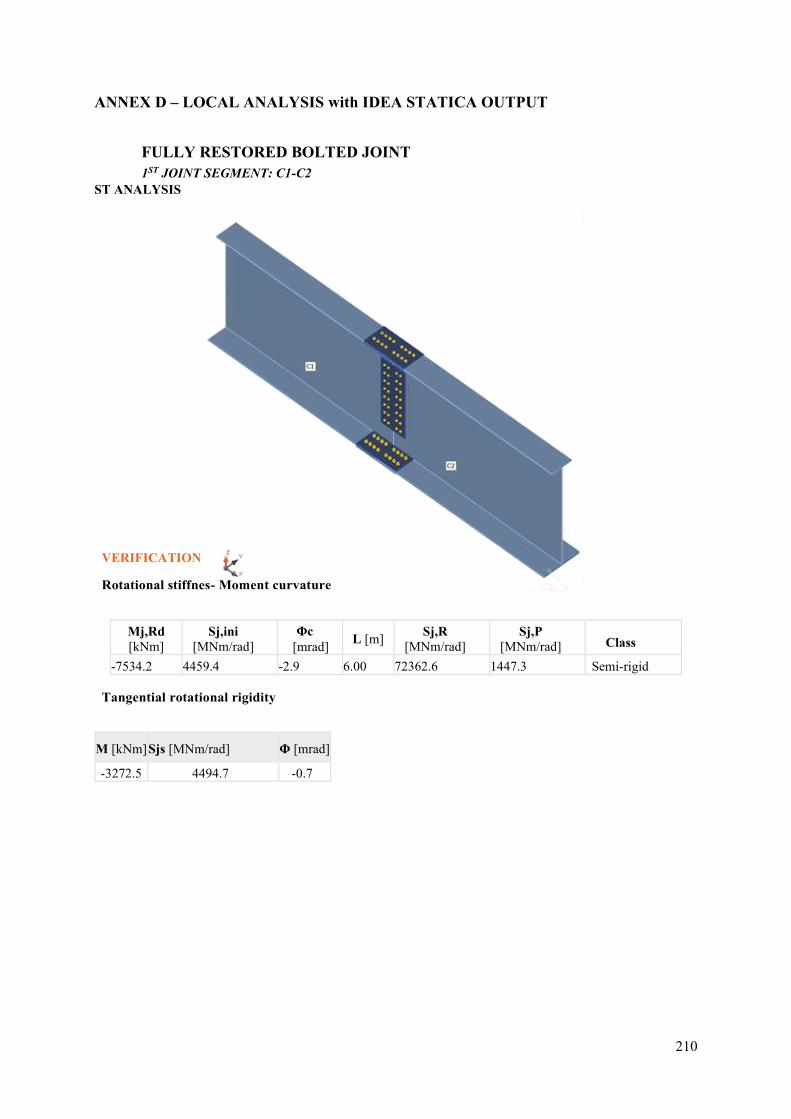
210
ANNEX D – LOCAL ANALYSIS with IDEA STATICA OUTPUT
FULLY RESTORED BOLTED JOINT 1ST JOINT SEGMENT: C1-C2
ST ANALYSIS
VERIFICATION
Rotational stiffnes- Moment curvature
Mj,Rd [kNm]
Sj,ini [MNm/rad]
Φc [mrad] L [m] Sj,R
[MNm/rad] Sj,P
[MNm/rad] Class
-7534.2 4459.4 -2.9 6.00 72362.6 1447.3 Semi-rigid
Tangential rotational rigidity
M [kNm] Sjs [MNm/rad] Φ [mrad]
-3272.5 4494.7 -0.7
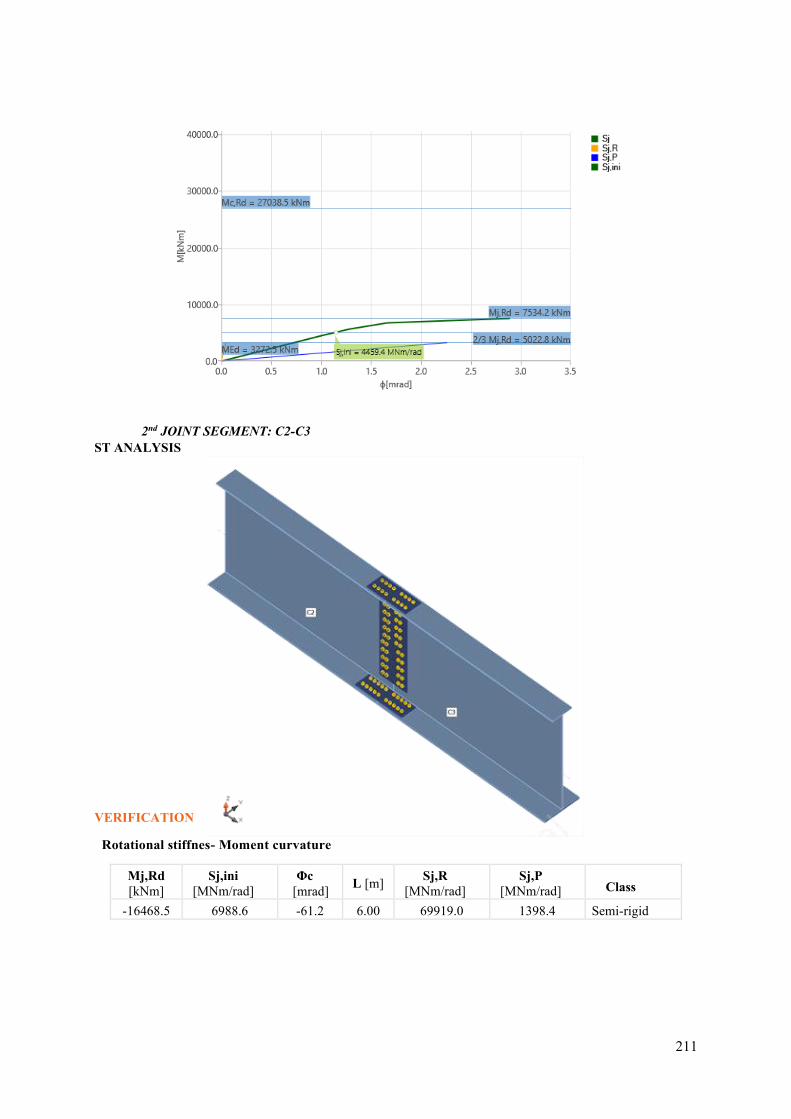
211
2nd JOINT SEGMENT: C2-C3 ST ANALYSIS
VERIFICATION
Rotational stiffnes- Moment curvature
Mj,Rd [kNm]
Sj,ini [MNm/rad]
Φc [mrad] L [m] Sj,R
[MNm/rad] Sj,P
[MNm/rad] Class
-16468.5 6988.6 -61.2 6.00 69919.0 1398.4 Semi-rigid
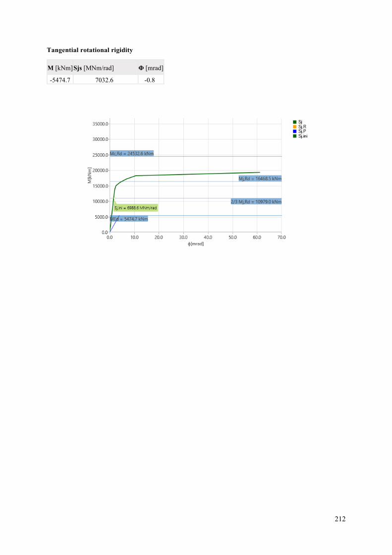
212
Tangential rotational rigidity
M [kNm] Sjs [MNm/rad] Φ [mrad]
-5474.7 7032.6 -0.8
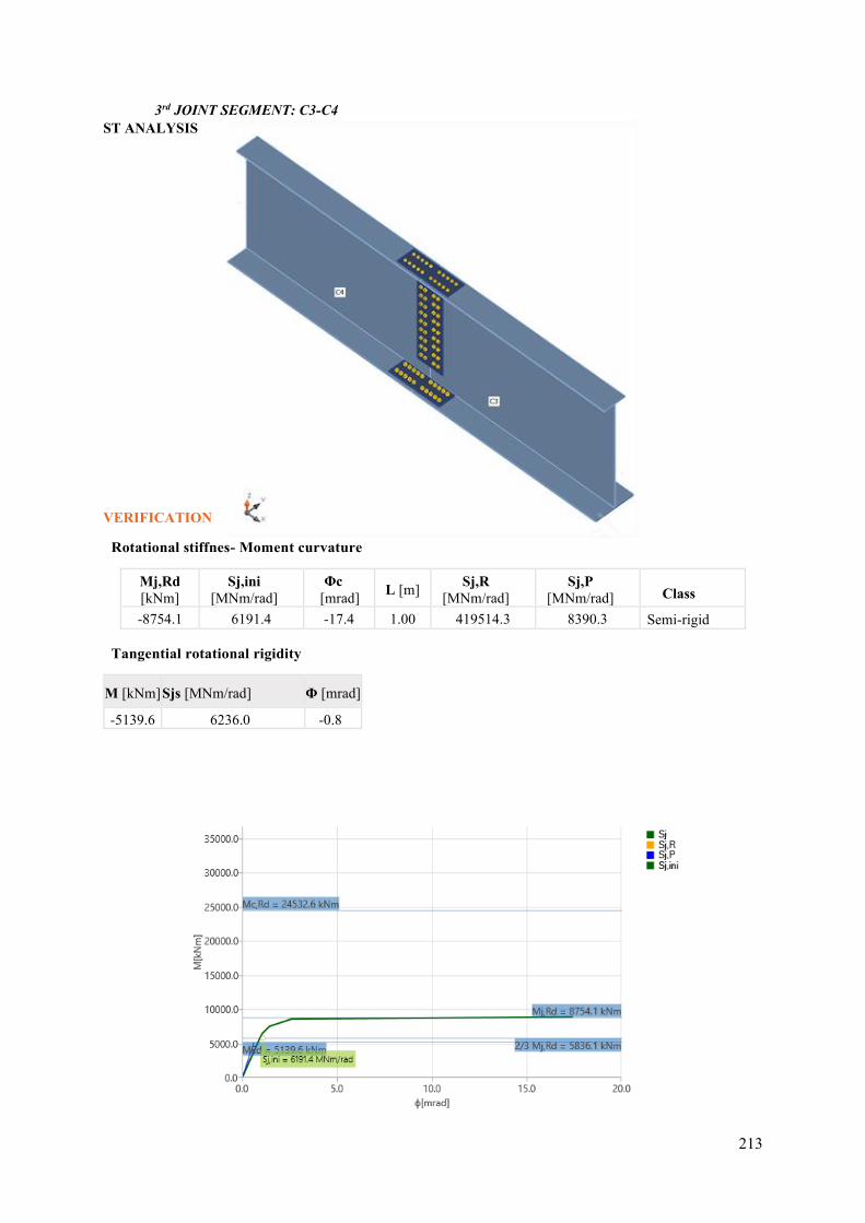
213
3rd JOINT SEGMENT: C3-C4 ST ANALYSIS
VERIFICATION
Rotational stiffnes- Moment curvature
Mj,Rd [kNm]
Sj,ini [MNm/rad]
Φc [mrad] L [m] Sj,R
[MNm/rad] Sj,P
[MNm/rad] Class
-8754.1 6191.4 -17.4 1.00 419514.3 8390.3 Semi-rigid
Tangential rotational rigidity
M [kNm] Sjs [MNm/rad] Φ [mrad]
-5139.6 6236.0 -0.8
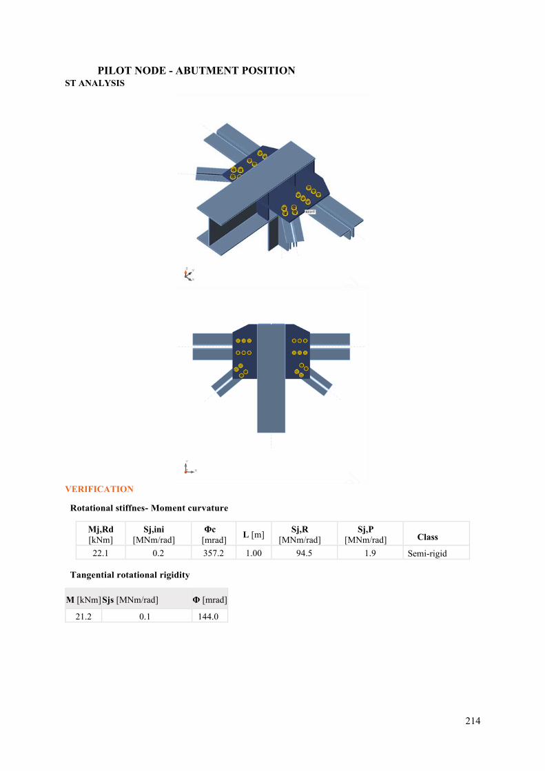
214
PILOT NODE - ABUTMENT POSITION ST ANALYSIS
VERIFICATION
Rotational stiffnes- Moment curvature
Mj,Rd [kNm]
Sj,ini [MNm/rad]
Φc [mrad] L [m] Sj,R
[MNm/rad] Sj,P
[MNm/rad] Class
22.1 0.2 357.2 1.00 94.5 1.9 Semi-rigid
Tangential rotational rigidity
M [kNm] Sjs [MNm/rad] Φ [mrad]
21.2 0.1 144.0
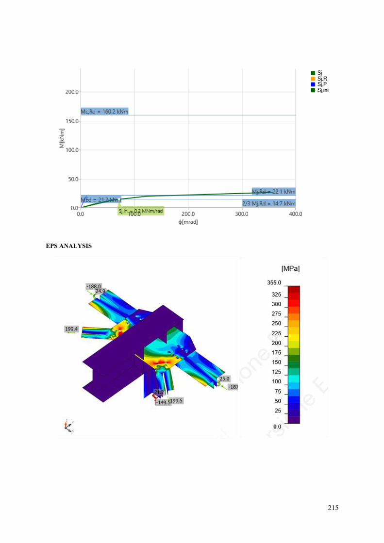
215
EPS ANALYSIS
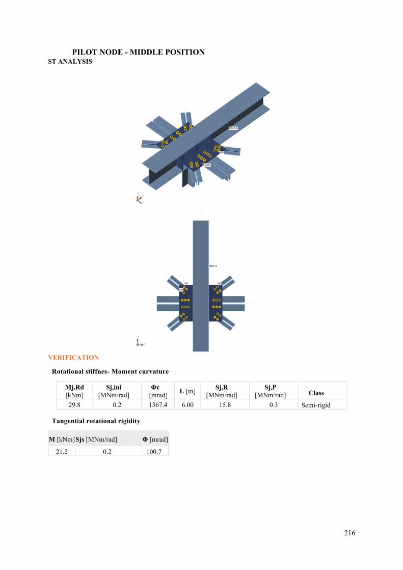
216
PILOT NODE - MIDDLE POSITION ST ANALYSIS
VERIFICATION
Rotational stiffnes- Moment curvature
Mj,Rd [kNm]
Sj,ini [MNm/rad]
Φc [mrad] L [m] Sj,R
[MNm/rad] Sj,P
[MNm/rad] Class
29.8 0.2 1367.4 6.00 15.8 0.3 Semi-rigid
Tangential rotational rigidity
M [kNm] Sjs [MNm/rad] Φ [mrad]
21.2 0.2 100.7
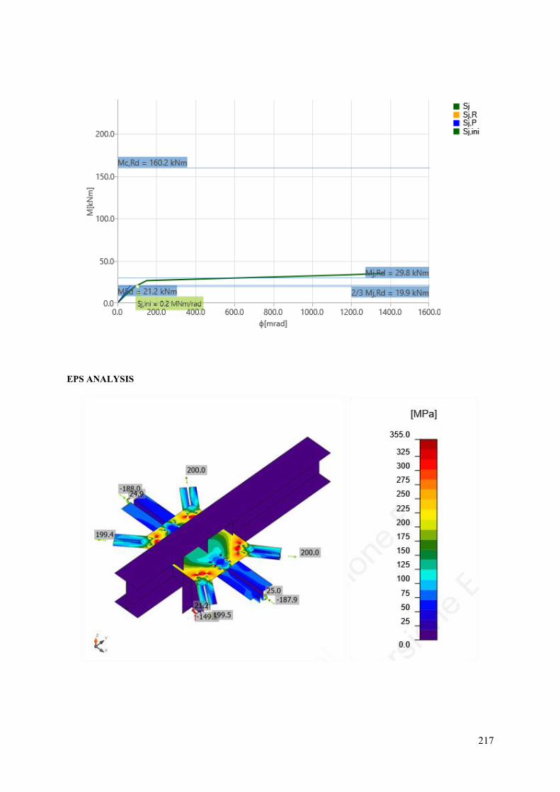
217
EPS ANALYSIS
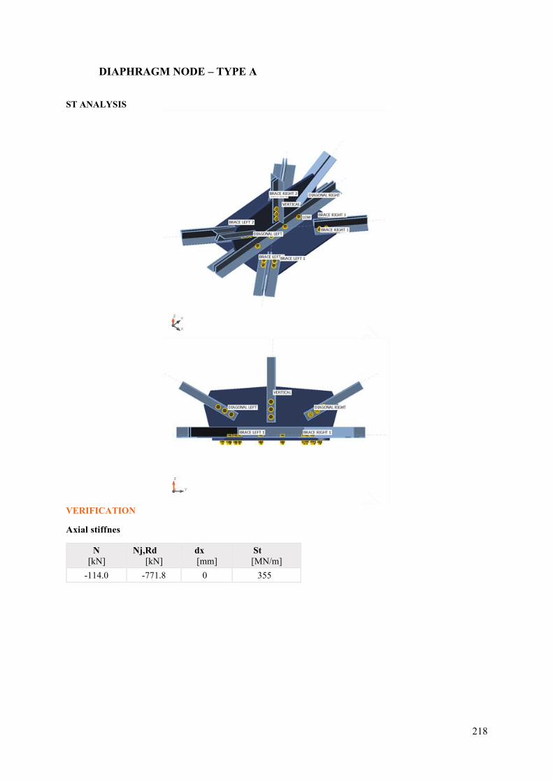
218
DIAPHRAGM NODE – TYPE A
ST ANALYSIS
VERIFICATION
Axial stiffnes
N [kN]
Nj,Rd [kN]
dx [mm]
St [MN/m]
-114.0 -771.8 0 355
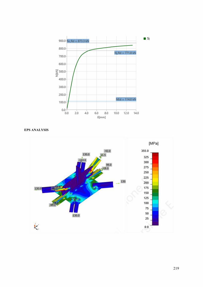
219
EPS ANALYSIS
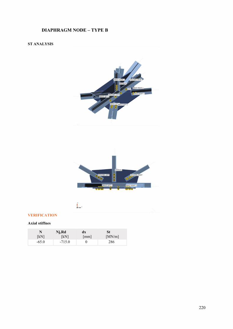
220
DIAPHRAGM NODE – TYPE B
ST ANALYSIS
VERIFICATION
Axial stiffnes
N [kN]
Nj,Rd [kN]
dx [mm]
St [MN/m]
-65.0 -715.0 0 286
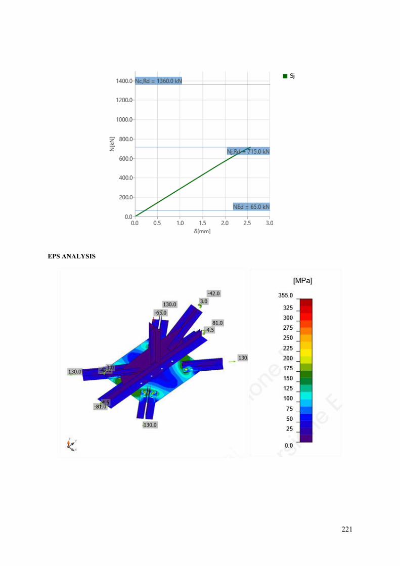
221
EPS ANALYSIS
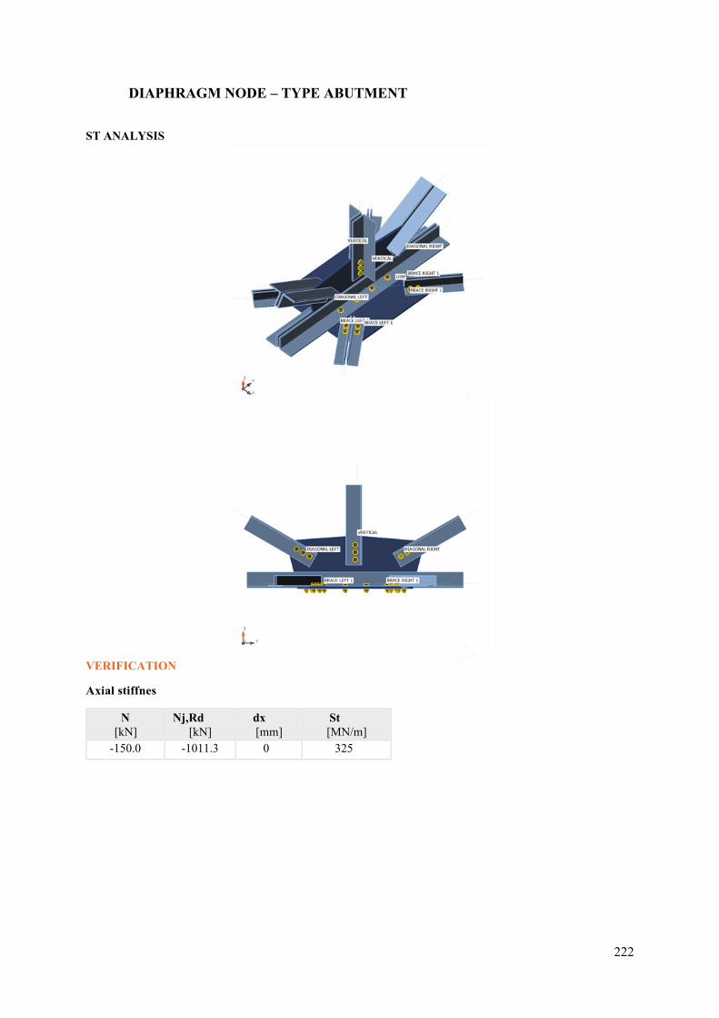
222
DIAPHRAGM NODE – TYPE ABUTMENT
ST ANALYSIS
VERIFICATION
Axial stiffnes
N [kN]
Nj,Rd [kN]
dx [mm]
St [MN/m]
-150.0 -1011.3 0 325
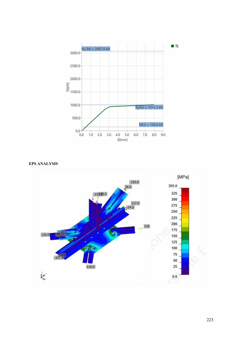
223
EPS ANALYSIS
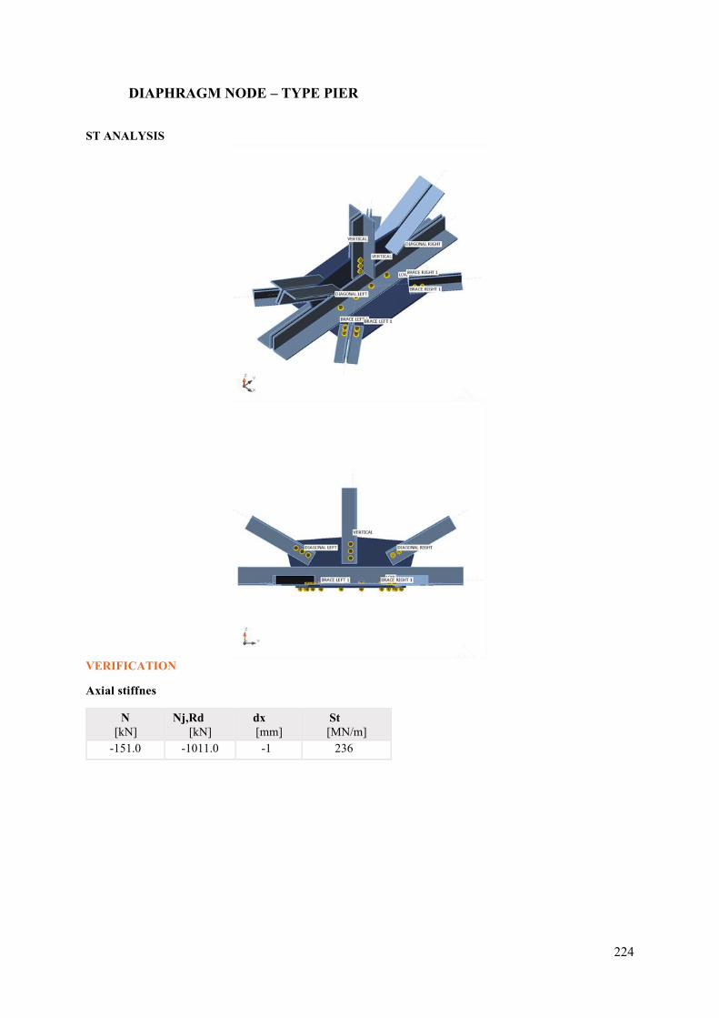
224
DIAPHRAGM NODE – TYPE PIER
ST ANALYSIS
VERIFICATION
Axial stiffnes
N [kN]
Nj,Rd [kN]
dx [mm]
St [MN/m]
-151.0 -1011.0 -1 236
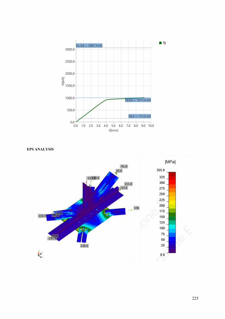
225
EPS ANALYSIS
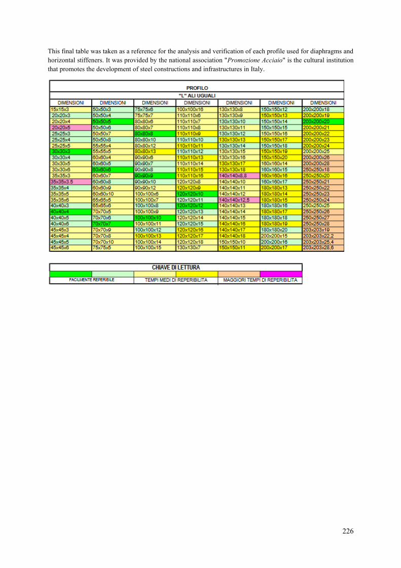
226
This final table was taken as a reference for the analysis and verification of each profile used for diaphragms and horizontal stiffeners. It was provided by the national association "Promozione Acciaio" is the cultural institution that promotes the development of steel constructions and infrastructures in Italy.
Related Documents