Life expectancy: managing the IT portfolio of a pension administrator

Life expectancy: managing the IT portfolio of a pension administrator

Drs. George Labrujere

Cordares Diensten (IT),

Basisweg 10, 1043 AP,

Amsterdam, The Netherlands

[email protected]

Drs. Hans de Weme

Cordares Pensioenen,

Basisweg 10, 1043 AP,

Amsterdam, The Netherlands

[email protected]

Dr. Adri van der Wurff

Cordares Holding,

Basisweg 10, 1043 AP,

Amsterdam, The Netherlands

[email protected]

Abstract

Cordares is a financial services firm specialized in

managing assets and liabilities (the corresponding

individual pension rights) for pension funds.

Traditionally IT-oriented, Cordares depends on IT to

ensure cost leadership in its business of pension

administration and IT currently accounts for 40% of

Cordares’ total expenses. IT governance and IT

portfolio management are therefore key issues, even

more so considering the extreme length of necessary

data consistency. The average life of an individual

pension scheme starts at about 25 years of age and will

probably end at around the age of 80.

Portfolio management at Cordares is characterized

by strict benchmarking of system development practice,

simple and effective measurement of costs (both

operational and software maintenance) and a

relentless system of kill management, replacing

systems that jeopardize the efficiency advantage. Of

each instrument of governance, real-life examples are

shown. We also relate our findings to mainstream

scientific results.

1. Introduction

A pension firm manages the assets and the liabilities

of pension funds. To do so, pension rights of thousands

of people have to be administrated, from the first day

that an employee enters the pension scheme until the

day he or she dies. This has to be done on a penny-

accurate, individual basis. The typical accrual period

covers 40 years, from 25 to 65, with a pension drawing

period of another 10 to 15 years.

Cordares is such a pension firm, providing financial

and administrative services to industry sector and

corporate pension funds. Our database of ‘participants’

(people participating in a scheme as an employee, a

pensioner, an insured relative or someone having

deferred rights) contains over one million persons. We

have an administrative relationship with more than

20,000 employers, who provide information on each of

their (about 250,000) employees and pay premium on a

monthly or a four-weekly basis. Payment of pensions

takes place on a monthly basis, to about 250,000

pensioners, with correct taxation and tax contribution

payments. This population is always changing, leading

to six million administrative change messages on an

annual basis. An annual pension benefit statement

provides every participant with an overview of the

accumulated pension rights and a forecast of pension

rights at the age of retirement.

This administrative task could not be performed

efficiently and effectively without extensive use of IT.

From the seventies on, Cordares has increasingly made

use of software to record pension rights, perform

calculations and produce pension bills, pension

statements and pension paychecks. In the international

CEM benchmark (by Cost Effectiveness Measurement

INC. from Canada), Cordares is a cost leader,

characterized by very high IT expenses and an

unsurpassed ratio of pension fund participants to

numbers of Cordares staff1

.

1

�The results of the international and annual CEM-benchmark are

constantly positive for Cordares. They show that, although the costs

of IT are high (for Cordares 40% of the costs is IT related, while the

peer group spends – on average – 21% on IT), the total costs for the

pension administration is 70% of the average costs of the peer group.

Also, the ratio of pension fund participants and Cordares staff is

more than double the same ratio for the peer group.

1-4244-2537-2/08/$20.00 ©2008 IEEE 9

One of the essential features of the administrative

process is that employers digitally send in information

on their employees. Starting as early as 1994 with 60%

digital messages (mostly from large employers and

accounting firms), at present there is a true 100%

digital inflow of information, most of which is

followed by digital straight-through processing.

This seems to be a real-life sound business case for

the use of IT in financial services. But how does

Cordares ensure that the almost 40% of total expenses

paid on IT is not too much – or too little, for that

matter. How do we know when it is time to modernize

systems? How do we build systems that guarantee data

consistency, so that today a 25-year-old carpenter does

not need to worry about his pension income in 2050?

Under such constraints, IT life is not easy, but it is

not difficult either. IT typically does attract

management attention when it constitutes 40% of total

expenses. And when assets under management amount

to 26 billion Euros, it is better not to record the

corresponding individual liabilities in an amateur

spreadsheet. In this overview of the Cordares IT

portfolio management, we subsequently focus on the

process of software development, the regular

measurement of IT costs associated with both

deployment and software maintenance and the process

of active ‘kill management’: selecting which systems

are to be radically rebuilt or changed to improve cost

efficiency.

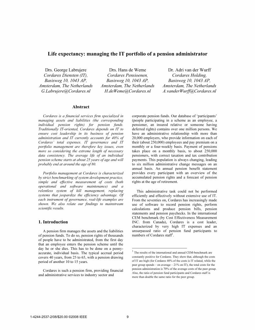
Assets under management 26 billion euros

Insured people > 1 million persons

Incoming premium > 2 billion euros

Benefits > 250,000 persons

Number of Payments > 3 million

Total amount of Payments > 2 billion euros

Incoming digital messages > 6 million

FTE 772

Net worth 331 million euros

Net result 22.5 million euros

Solvability 31.4%

Fig. 0. Cordares at a glance (2006)

2. Model Lifecycle Costs

Similar to corporate governance, IT governance

focuses on transparency and standardization. In

addition to compliance, these are key terms in assuring

high-quality and (nevertheless) cost effective

performance, especially when business is totally

dependent on an extensive use of IT. This does not

imply that we have to implement and conform to the

strict regime of top-heavy (and very expensive) all-in-

one solutions for the demand, portfolio, program

management and the like. When considering ERP, in

this case for the IT organization itself, the smart route

is to first get processes right and only then possibly

choose an implementation that is appropriate. Even

better, if you are in control a lot can be achieved with

relatively simple tools.

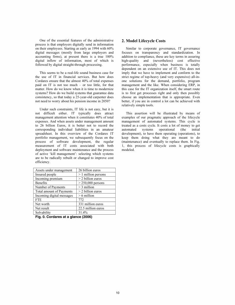
This assertion will be illustrated by means of

examples of our pragmatic approach of the lifecycle

management of automated systems. This cycle is

treated as a costs cycle. It costs a lot of money to get

automated systems operational (the initial

development), to have them operating (operations), to

keep them doing what they are meant to do

(maintenance) and eventually to replace them. In Fig.

1, this process of lifecycle costs is graphically

modeled.

10

Fig. 1. Model of Lifecycle costs

At Cordares, bulk processing has always been a

core competence. In the old days, outsourcing such

large-scale specialized financial applications was

simply not an option and even today, it would be

difficult. Also finding readymade, off-the-shelf

applications to do the job was not possible. So system

development at Cordares remained a tailor-made job

by a relatively large-scale in-house IT company, which

was also responsible for deployment and maintenance.

Today, it is still pretty much the same situation: as a

financial service provider, the pension administration

business unit delivers a chain of services to pension

funds as its clients, and in its turn is a client of the

internal IT business unit. Bound to both parties with

tariff contracts, it is vital to the pension firm to

maintain a grip on IT spending. The supply side – the

IT business unit – is therefore faced with a strong

demand management and an ISO certified process of

portfolio and program management.

Controllability depends, to a large extent, on the

standardization of operational processes and methods.

In each and every design for a computer system, the

non-redundant corporate data model is at issue: apart

from rare exceptions, the essential structure and

content of the central data stores have a semi-

permanent character in comparison with the

information systems that make use of these. For

example, the main integrated development

environment of Cordares IT forces the developer to

dissect his “problem” into small (and well-defined)

building blocks with relatively elementary

functionality. They have to describe these building

blocks in terms of the IDE’s metadata, and a highly

standardized language generator. The IDE then

generates most of the procedural coding and all of the

data handling.

Another example of standardization at Cordares IT

is the choice of a (single) method for project

management (PRINCE2) and system development

(SDM2). Indispensably also, besides a careful

management of resources, is a standardized manner of

estimating and planning projects in combination with a

system of activity-based management and the

obligation for everybody to record each hour spent in a

certain role for a certain project. Such methods and

tools are essential in order to control the projects

portfolio. Because of this standardized way of

developing, the probability for the existence of simple,

descriptive and predictive models is relatively high.

We believe that the following analysis supports the

existence of such models.

Systems for resource management and the

registration of working hours are relatively simple to

buy or develop and implement2

. Standardizing the

sizing, planning and budgeting of projects may prove

more cumbersome because of the dependency on the

specifics of the organization of system development.

Also the estimating of system development often is

2

Although, admittedly, enforcing general use will probably be more

problematic.

�

������� ��� ���������

���

���� �����������

���������

���������

�����������

���

������

������

���������

���������

�����������

����

�����������

���������

������

��� � ��� �

���

�������

������

11

considered ‘higher mathematics’, a form of art for

which one needs to be gifted with an exceptional

intellectual ability. However, even in this area, much

can be achieved, given a certain homogeneity in

projects and the availability of reliable figures.

The process of estimating on the basis of past

experience will be enhanced by objectifying that past

experience as much as possible. A standard method of

estimating and careful recording and analysis of results

can and will improve the process and make it less

dependent on those rare individuals with knowledge

and experience. This requires comparing project

planning data with the actual realization in order to

refine and broaden the process of sizing and

estimating.

Making this knowledge more readily accessible is

critical wherever controllable, systematic system

development is decisive. A first step to this end is

formalizing what mostly implicitly takes place. Both

functional and technical specialists use directives, rules

of thumb for the weighting of functions in terms of

scope and complexity. Given a method and a

development environment, indicative numbers of hours

are used for the design and the realization of a simple,

an average or a complex input/output function, or for

that matter, for the formal description of the

workflow3

.

3. Function points and Benchmarking

Systematic recording and analysis of planning and

realization data is crucial. In this analysis, the use of

function points is indispensable. The function point is

the commonly accepted unit for the measurement of

software, used also to measure the productivity of

developers and for (external) benchmarking. Function

points are counted on the basis of an inventory of input

and output functions, interactive functions and the

entities and interfaces in a logical data model. Thus

this can be undertaken at the same time as expert

estimates are made. A weight factor has to be stipulate

per function, entity and interface. A basis for budgeting

the needed effort can be found in multiplying function

points by productivity in terms of the average number

of hours per function point.

3

All disciplines involved in the process of system development more

or less consciously use rules of thumb for estimating the required

effort. The first, vital step to standardization is to make these implicit

rules of thumb explicit.

The status of the function point becomes apparent

from the fact that, in professional and academic

environments, function points are used as a criterion

when examining the productivity of system

development. Although it must be noted that frequently

a technique known as backfiring is used in which

statistics are used to infer function points from lines of

code. In this area, pioneering work has been done by

Boehm [1] and Capers Jones [2], who probably owns

the world’s largest database with project data. The

ISBSG4

also has assembled a large knowledge base.

Many rules of thumb have been distilled from this

collected project data.

Ways of estimating typically focus on different

project phases. Even if we do not have very detailed

figures on different phases, it is still possible to

calculate the required effort using proportional figures

of the different project phases and disciplines. That is

the advantage of a highly standardized manner of

system development. We can assume that, for instance,

a preliminary impact analysis takes up approximately

5% of the total costs. The functional design takes about

15%, so about 20% of the budget will be spent on the

design as a whole.

After many years of analysis of innumerable

projects, Capers Jones [2] has proposed a number of

rules of thumb that are still commonly used for project

estimating and benchmarking. Some of these rules of

thumb have been verified at Cordares with promising

results. First, we present the rules of thumb we have

put to a test.

1 fp = 100 (net) lines of code (3.1)

The relation function points – lines or code (LoC)

has been a subject of research for a long time.

Depending on the language used, approximately 100

LoCs count as 1 function point in 3GL5.

Research at

Cordares shows this rule is applicable for our COBOL

(generator) development environment. Third-party

auditing (KPMG, Sogeti/Nesma) has also established

that in our case the factor 100 gives a sound indication

of the number of function points.

fp1.15

= number of pages documentation (3.2)

fp1.20

= number of test cases needed (3.3)

4

The international institute of cooperating national function point

organizations, among them the Dutch NESMA.

5

See, for instance, http://www.spr.com/products/programming.shtm.

For the complete table, SPR nowadays charges a fee. However, the

original table by Capers Jones can still be found on the web.

12

fp1.25

= number of development problems, failures

etc. (3.4)

These rules are used as an indication of the

necessary efforts for documenting and testing.

fp0.4

= (optimum) project duration after design in

calendar months (3.5)

This is the most important rule so far. What we

have here, is the first half of the benchmark function of

these rules.

fp/150 = (optimum) number of FTE in development

(3.6)

This is the second half of the benchmark function:

Besides the optimum duration, it shows the number of

developers needed during that period.

1% “functionality creep” of at least per calendar

month (3.7)

The almost uncontrollable inclination of projects to

grow in functionality during design and development is

a well-known phenomenon. We consider this rule thus

as a warning.

Combining rules 3.5 and 3.6 gives us the SPR

benchmark for project duration and the number of full-

time employees needed. Combined with the number of

productive hours per month this yields the costs for the

required effort after functional design. Total effort

after design = calendar months * number of FTE *

hours-per-month (130). The forecast this benchmark

provides, dovetails strikingly with the actual realization

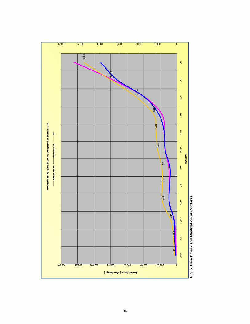
figures at Cordares. In Fig. 2, Fig. 4 and in Fig. 5, we

show the benchmark and compare it to the recent

development of pension systems at Cordares.

As mentioned above, we require everybody to

register every hour spent on a project. So it is not the

number of employees, whether full-time or part-time,

but the gross hours per discipline that count. Literally

every hour is counted and the result is then related to

the size of the final product: the system made available

for production. So things like ‘scaffolding’ code are

included in the hours, not in the measurement of

resulting function points.

Shown here is the complete portfolio of the pension

back-office systems at the time. So we did not pick

only those that fitted nicely in the curve. We did,

however, use one way of ‘curve smoothing’. The only

exception in the realization figures at Cordares as

compared to the benchmark concerns the actuarial

function. We found that the two actuarial systems in

practice were on average 200% (e.g. 150% vs. 250%)

more expensive (in hours) than, according to the

benchmark, could be expected on the basis of the size

in fp. This obliges us to use a correction factor for

actuarial complexity. Below the data used is shown in a

table.

13

Fig. 2. Data used in benchmarking pension systems

The benchmark clearly shows the non-linear

relation between project size and project costs. Put

differently: the productivity in terms of hours-per-fp

decreases as the number of fps increases. We all

‘know’ that in projects a doubling in scope results in a

disproportional increase of costs. Now, with the aid of

this benchmark, we can calculate and predict the

impact! Suppose that we have the choice to realize

2,000 fps in one large project or in two smaller projects

of 1,000 fps each. As shown below, the latter would be

far more efficient.

project split-up

fp hours fp hours

1,000 17,170 1,000 17,170

2,000 45,311 1,000 + 1,000 34,340

difference 10,971

Fig. 3. Productivity and size

Notice also that for really small projects, the

benchmark tends to slightly underestimate the effort at

Cordares, however, for really big projects, the

benchmark tends to overestimate. From this, one could

infer that we should concentrate on large-scale

projects. We just saw, however, that such an approach

would probably not be a smart one. The message

seems clear: do not size your projects too small (< 350

FPs) but certainly also not too big (> 2,500 FPs).

However, if you cannot avoid doing a large project,

Cordares appears to be able to reduce the common

exponential growth of costs.

system

gross hours

correction

com

plexity

corrected

hours

hours after

functional

design

LoC

FP

hours per FP

SPR

predicted

hours (a5 &

a6)

SPR

predicted

hours per FP

match

AVB 1,400 1,400 1,120 12,275 123 9.1 729 5.9 65%

AVR 3,100 3,100 2,480 16,809 168 14.8 1,131 6.7 46%

CBP 3,850 3,850 3,080 31,377 314 9.8 2,711 8.6 88%

ACP 28,057 2.5 11,223 8,978 73,302 733 12.2 8,892 12.1 99%

BPS 10,700 10,700 8,560 74,097 741 11.6 9,028 12.2 105%

IPN 10,075 10,075 8,060 76,612 766 10.5 9,457 12.3 117%

WOD 17,550 17,550 14,040 97,714 991 14.2 13,570 13.7 97%

STN 28,067 1.5 18,711 14,969 106,937 1,069 14.0 15,088 14.1 101%

VBA 26,579 26,579 21,263 118,520 1,185 17.9 17,425 14.7 82%

BEP 48,382 48,382 38,706 208,150 2,082 18.6 38,334 18.4 99%

VSP 90,505 90,505 72,404 344,154 3,442 21.0 77,501 22.5 107%

BPF 115,284 115,284 92,227 483,527 4,835 19.1 124,750 25.8 135%

14

Fig

. 4. S

PR

Ben

chm

ark

gross hours per function point(total project costs)

gross hours (total project costs)

fu

nc

tio

n p

oin

ts

p

er p

ro

je

ct

to

tal p

ro

ject h

ou

rs a

t a

g

ive

n n

um

be

r o

f fu

nctio

n p

oin

ts

SPR

Hours/FP

Lin

ear (SPR)

15

Fig

. 5. B

ench

mar

k an

d R

ealiz

atio

n a

t C

ord

ares

123

168

314

733

741

766

991

1,069

1,185

2,082

3,442

4,835

01,0002,0003,0004,0005,0006,000

020,00040,00060,00080,000100,000120,000140,000

AVB

AVR

CBP

ACP

BPS

IPN

WOD

STN

VBA

BEP

VSP

BPF

Sy

ste

ms

Project hours (after design )

Pro

du

ctiv

ity

P

en

sio

n Sy

ste

ms co

mpa

re

d to

B

en

ch

ma

rk

Be

nch

ma

rk

Re

aliza

tio

nFP

16

4. Quantifying models

In his paper “Quantifying the value of IT

investments” [5], Prof. dr. Chris Verhoef describes a

method to quantify the value of investments in

software systems. Of interest here are the heuristics

models he uses. The models are derived from simple

benchmark data concerning the relationship between

hours per function point (PDR [8])6

spent in building

an information system and the total amount of function

points (fp) of the information system:

PDR = 0.6141603 · fp0.4121902

(4.1)

The formula is derived by applying the least squares

approximation method to exponential functions and the

dataset of three pairs of benchmark data relating

function points and hours: (100, 4.33), (1000, 10.41)

and (10000, 27.39).

From (4.1) it is immediately clear that the total amount

of hours (th) spent on a project is given by the formula:

th(fp) = fp · PDR= 0.6141603 · fp1.4121902

(4.2)

Hence the formula gives a method to extract the

number of function points when only the total number

of hours for realizing the project is known. The number

of function points can be found by solving the equation

in fp. This also implies that the total cost for initially

realizing the software product is given by the following

expression:

tc(fp) = af · fp · PDR = af · 0.6141603 · fp1.4121902

(4.3)

Where af stands for the average fee per hour. This can

be estimated for outsourcers at €100 and for internal

employees at € 75. Hence, if the product is built by

internal staff only, the total cost for the internal

realization (tci) is:

tci(fp) = af

i · fp · PDR = € 46.06· fp

1.4121902

(4.4)

Therefore, the average cost per function point is given

by:

acpfi(fp) = af

i · fp · PDR/fp = €46.06· fp

0.4121902

(4.5)

Although the above considerations depend heavily

on the benchmark data (only three measurements!) and

6

See:

http://www.isbsg.org/isbsg.nsf/weben/Project%20Delivery%20Rate.

the exponential form of the formula goes without

justification7

, it is interesting to compare the results

with the SPR-formulas and the Cordares data of the

previous chapter. The SPR-formulas discussed above

give the total amount of hours as:

th(fp) = fp 0.4

· fp/150 · 130 =0.867 · fp 1.4

(4.6)

In this formula, the number of productive hours per

month is taken to be 130 as we have seen above.

Hence, we have two expressions for the total amount

of hours (th) for a given software product as a function

of the amount of function points (4.2), (4.6).

The basic form of the formulas is the same, only the

constant differs. This difference can be explained by

the fact that Verhoef’s parameters are based on a

higher number of working days per year, corrected for

outsourcing contracts, as compared to the Cordares

internal IT-department with a lesser number of

effective working days, while, on the other hand, there

might be a difference in definition of activities

(effective hours) included in the function point

calculation.

The same article also offers an interesting

relationship between the minimal costs of operation

(mco) and the total amount of function points (fp), by:

mco(fp) = wr · fp1.25

(4.7)

750

and the corresponding life expectancy of the system

(y), by:

y(fp) = fp0.25

(4.8)

Further explanation can be found in C. Verhoef:

Quantitative Aspects of Outsourcing Deals [7].

The parameter wr implies the yearly costs of an

employee, internal or external, and is estimated, in the

article, at € 200.000 (wr) for outsourced contracts. The

constant 750 is established experimentally.

At Cordares, the internal cost of an employee can be

estimated at € 111,000 (wri).

From (4.1) and (4.2) it is clear that:

mcoi(fp) / y(fp) = wr

i · fp = €148 · fp (4.9)

750

7

Software productivity research, without exception, uses this form

of regression.

17

That is: the cost per year per function point is a

constant and depends only on the parameter wri.

The Cordares situation differs in the sense that the

actual life expectancy is substantially higher than the

suggested life expectancy, probably double. If we

calculate a linear relation between the yearly costs and

the function points and use the same exponential

formulas, we must introduce the following

relationships:

y(f) = f0.36

(4.10)

and hence:

mco(f) = p · f1.36

(4.11)

where the parameter p in the Cordares context

amounts to € 110,000/750 = € 148. The difference is

thus explained completely by the dissimilarity in costs

between external and internal fees.

We conclude that the benchmarking approach of

Capers Jones [3] and the conclusions of Verhoef [5]

are consistent with the real life data at Cordares.

5. Costs of Operation & Maintenance

In this chapter, we will take a closer look at the

practice of managing operational costs at Cordares.

When the total costs of developing a system are

estimated, an indication can also be given of the

lifecycle costs for that system. Decisive, besides the

expected lifespan and the period of use, are the

expected costs of operation and maintenance costs. At

Cordares, we assembled and analyzed a lot of data

concerning both kinds of system costs. These research

data suggest that for our current pension systems, the

annual maintenance and deployment costs both amount

to a minimum of about 4.5% – 5% of the initial

investment.

In forecasting, average realization values provide a

good starting point. Nevertheless, for every new

system, things need to be assessed thoroughly. Costs

prognosis needs to evaluate different properties for

maintenance and operation. Costs of operation depend

mostly on the nature and frequency of processing, the

size and growth of the administrated population, the

degree in which history is built up and must be used,

etc. With respect to maintenance costs, the volatility of

the system’s functionality is especially important, e.g.

the degree of variety that the basic functionality in

itself permits and to what extent and with what

frequency influences from the system’s environment

will in fact cause change.

Of course, forecasting is only possible if reliable

figures are available concerning the actual costs of the

operational systems. At Cordares, this material was not

primarily collected and analyzed for the purpose of

forecasting the expected costs of newly built systems

but from a broader, more general concern with

lifecycle management. Below, we will zoom in on

some of the more important insights that our analysis

has produced.

First, a practical consideration: it is much easier to

translate absolute values like costs, hours worked, etc

into percentages of the corresponding initial values. In

this way comparing systems becomes simpler and

statistical analysis as well.

From research publications, it is well known that

the non-linear development in decreasing added value

and/or increasing costs with increasing difficulty can

be described statistically with polynomial curves. For

instance, the costs of drilling for oil at increasing

depths or those of air conditioners as temperatures rise.

The same holds true for the operational costs of

aging mechanical systems or, for that matter, for aging

software systems.

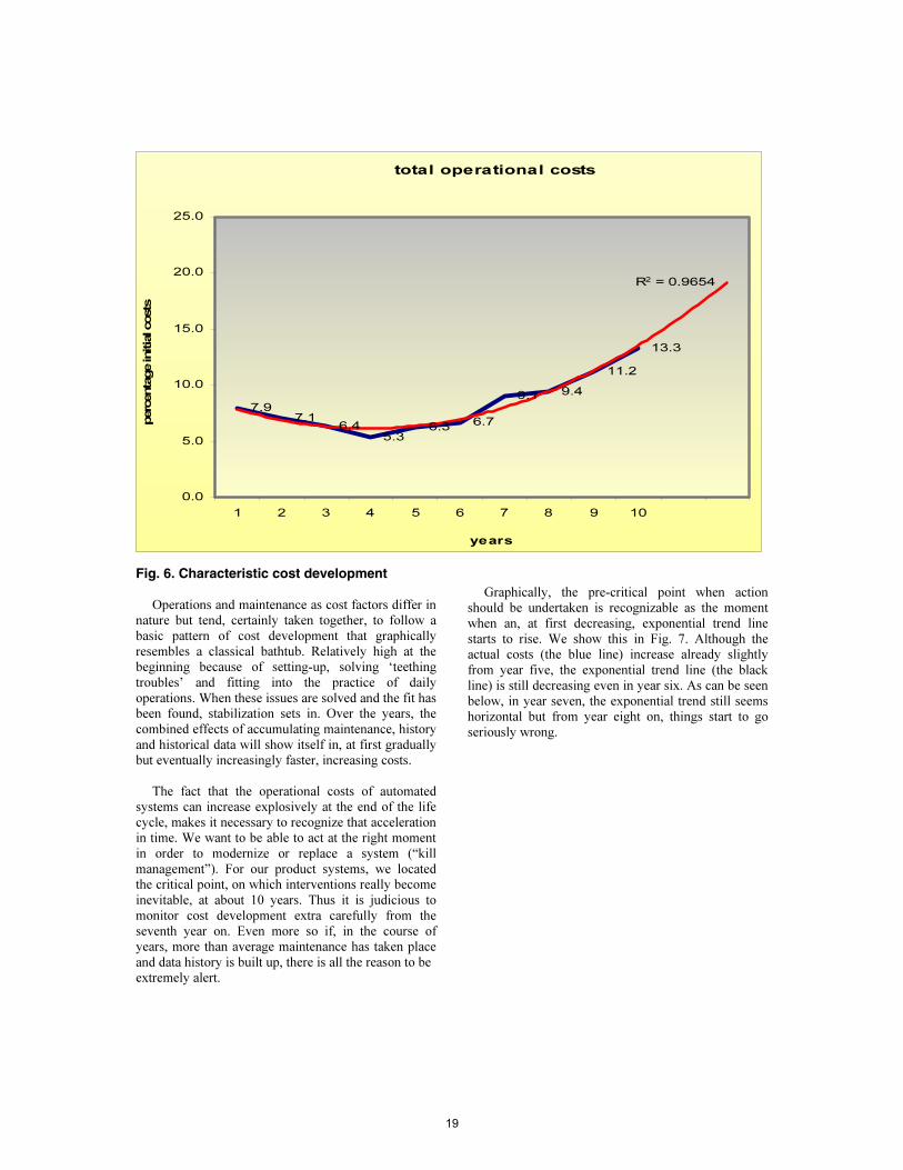
In Fig. 6, the characteristic cost development for an

average pension system is given over a period of 10

years. Data is used from several of the Cordares

pension systems at different age stages, but on the

whole they all tend to behave like this. Besides the

actual cost development (in blue), a trend line (in red)

is also given with a projection of two more years.

Notice the high correlation between the actual

development and the curvilinear trend line. We found

that it is the cost of operation, in particular, that makes

the total cost pattern tends so strongly to a theoretical

ideal model. Statisticians call this a J curve, less

prosaic, the pattern is also known as a bathtub curve8

.

8

Also used to describe component failure over time: “Common term

for the curve (resembling an end-to-end section of one of those claw-

footed antique bathtubs) that describes the expected failure rate of

electronics with time: initially high, dropping low for most of the

system's lifetime, then rising again as it `tires out'.”

18

total operational costs

7.9

7.1

6.4

5.3

6.3

6.7

9.19.4

11.2

13.3

R2

= 0.9654

0.0

5.0

10.0

15.0

20.0

25.0

1 2 3 4 5 6 7 8 9 10

years

percentage initial costs

Fig. 6. Characteristic cost development

Operations and maintenance as cost factors differ in

nature but tend, certainly taken together, to follow a

basic pattern of cost development that graphically

resembles a classical bathtub. Relatively high at the

beginning because of setting-up, solving ‘teething

troubles’ and fitting into the practice of daily

operations. When these issues are solved and the fit has

been found, stabilization sets in. Over the years, the

combined effects of accumulating maintenance, history

and historical data will show itself in, at first gradually

but eventually increasingly faster, increasing costs.

The fact that the operational costs of automated

systems can increase explosively at the end of the life

cycle, makes it necessary to recognize that acceleration

in time. We want to be able to act at the right moment

in order to modernize or replace a system (“kill

management”). For our product systems, we located

the critical point, on which interventions really become

inevitable, at about 10 years. Thus it is judicious to

monitor cost development extra carefully from the

seventh year on. Even more so if, in the course of

years, more than average maintenance has taken place

and data history is built up, there is all the reason to be

extremely alert.

Graphically, the pre-critical point when action

should be undertaken is recognizable as the moment

when an, at first decreasing, exponential trend line

starts to rise. We show this in Fig. 7. Although the

actual costs (the blue line) increase already slightly

from year five, the exponential trend line (the black

line) is still decreasing even in year six. As can be seen

below, in year seven, the exponential trend still seems

horizontal but from year eight on, things start to go

seriously wrong.

19

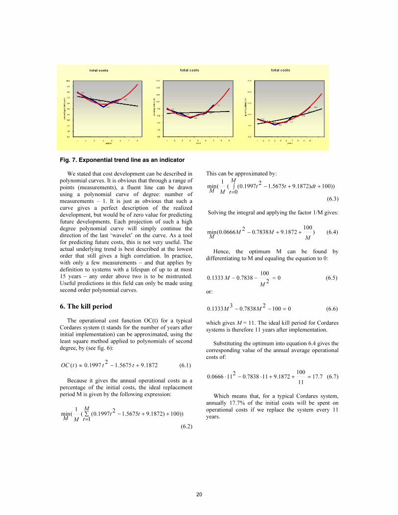
Fig. 7. Exponential trend line as an indicator

We stated that cost development can be described in

polynomial curves. It is obvious that through a range of

points (measurements), a fluent line can be drawn

using a polynomial curve of degree: number of

measurements – 1. It is just as obvious that such a

curve gives a perfect description of the realized

development, but would be of zero value for predicting

future developments. Each projection of such a high

degree polynomial curve will simply continue the

direction of the last ‘wavelet’ on the curve. As a tool

for predicting future costs, this is not very useful. The

actual underlying trend is best described at the lowest

order that still gives a high correlation. In practice,

with only a few measurements – and that applies by

definition to systems with a lifespan of up to at most

15 years – any order above two is to be mistrusted.

Useful predictions in this field can only be made using

second order polynomial curves.

6. The kill period

The operational cost function OC(t) for a typical

Cordares system (t stands for the number of years after

initial implementation) can be approximated, using the

least square method applied to polynomials of second

degree, by (see fig. 6):

1872.95675.12

1997.0)( +−≈ tttOC (6.1)

Because it gives the annual operational costs as a

percentage of the initial costs, the ideal replacement

period M is given by the following expression:

))100)

1

1872.95675.12

1997.0((

1

(min +∑

=

+−

M

t

tt

MM

(6.2)

This can be approximated by:

))100

0

)1872.95675.12

1997.0((

1

(min +∫

=

+−

M

t

dttt

MM

(6.3)

Solving the integral and applying the factor 1/M gives:

)

100

1872.97838.02

0.0666(min

M

MM

M

++− (6.4)

Hence, the optimum M can be found by

differentiating to M and equaling the equation to 0:

0

2

100

7838.0 0.1333 =−−

M

M (6.5)

or:

0100

2

7838.0

3

0.1333 =−− MM (6.6)

which gives M = 11. The ideal kill period for Cordares

systems is therefore 11 years after implementation.

Substituting the optimum into equation 6.4 gives the

corresponding value of the annual average operational

costs of:

7.17

11

100

1872.9117838.0

2

110.0666 =++⋅−⋅ (6.7)

Which means that, for a typical Cordares system,

annually 17.7% of the initial costs will be spent on

operational costs if we replace the system every 11

years.

20

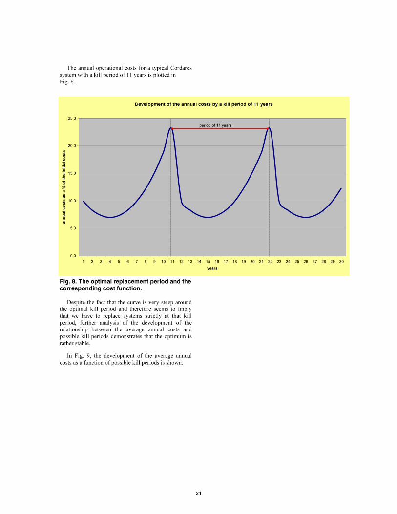
The annual operational costs for a typical Cordares

system with a kill period of 11 years is plotted in

Fig. 8.

Fig. 8. The optimal replacement period and the corresponding cost function.

Despite the fact that the curve is very steep around

the optimal kill period and therefore seems to imply

that we have to replace systems strictly at that kill

period, further analysis of the development of the

relationship between the average annual costs and

possible kill periods demonstrates that the optimum is

rather stable.

In Fig. 9, the development of the average annual

costs as a function of possible kill periods is shown.

Development of the annual costs by a kill period of 11 years

0.0

5.0

10.0

15.0

20.0

25.0

1 2 3 4 5 6 7 8 9 10 11 12 13 14 15 16 17 18 19 20 21 22 23 24 25 26 27 28 29 30

years

an

nu

al co

sts as a %

o

f th

e in

itial co

sts

period of 11 years

21

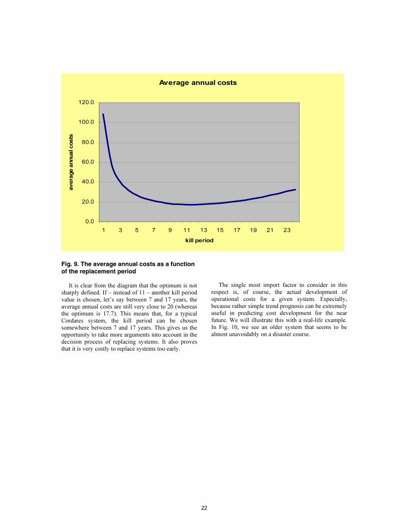
Fig. 9. The average annual costs as a function of the replacement period

It is clear from the diagram that the optimum is not

sharply defined. If – instead of 11 – another kill period

value is chosen, let’s say between 7 and 17 years, the

average annual costs are still very close to 20 (whereas

the optimum is 17.7). This means that, for a typical

Cordares system, the kill period can be chosen

somewhere between 7 and 17 years. This gives us the

opportunity to take more arguments into account in the

decision process of replacing systems. It also proves

that it is very costly to replace systems too early.

The single most import factor to consider in this

respect is, of course, the actual development of

operational costs for a given system. Especially,

because rather simple trend prognosis can be extremely

useful in predicting cost development for the near

future. We will illustrate this with a real-life example.

In Fig. 10, we see an older system that seems to be

almost unavoidably on a disaster course.

Average annual costs

0.0

20.0

40.0

60.0

80.0

100.0

120.0

1 3 5 7 9 11 13 15 17 19 21 23

kill period

average annual costs

22

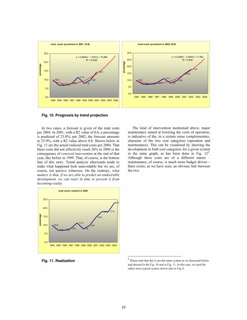
Fig. 10. Prognosis by trend projection

In two cases, a forecast is given of the total costs

per 2004. In 2001, with a R2 value of 0.6, a percentage

is predicted of 23.8%; per 2002, the forecast amounts

to 25.9%, with a R2 value above 0.8. Shown below in

Fig. 11 are the actual realized total costs per 2004. That

these costs did not effectively reach 26% in 2004 is the

consequence of renewed intervention at the end of that

year, like before in 1999. That, of course, is the bottom

line of this story. Trend analysis afterwards tends to

make what happened look unavoidable but we are, of

course, not passive witnesses. On the contrary, what

matters is that, if we are able to predict an undesirable

development, we can react in time to prevent it from

becoming reality.

Fig. 11. Realization

The kind of intervention mentioned above, major

maintenance aimed at lowering the costs of operation,

is indicative of the, in a certain sense complementary,

character of the two cost categories (operation and

maintenance). This can be visualized by showing the

development in both cost categories for a given system

in the same graph, as has been done in Fig. 129

.

Although these costs are of a different nature –

maintenance, of course, is much more budget driven –

there exists, as we have seen, an obvious link between

the two.

9

Please note that this is not the same system as we discussed before

and showed in the Fig. 10 and in Fig. 11. In this case, we used the

rather more typical system shown also in Fig. 6.

total costs (predicted in 2002: 25.9)

10.0

7.0 7.0

8.0

11.3

7.9

9.8

14.5

17.9

y = 0.3258x2

- 2.2642x + 11.383

R2

= 0.839

0.0

5.0

10.0

15.0

20.0

25.0

30.0

1994 1995 1996 1997 1998 1999 2000 2001 2002 2003 2004

percentage

total costs (predicted in 2001 23.8)

10.0

7.0 7.0

8.0

11.3

7.9

9.8

14.5

y = 0.2804x2

- 1.9101x + 10.884

R2

= 0.6322

0.0

5.0

10.0

15.0

20.0

25.0

1994 1995 1996 1997 1998 1999 2000 2001 2002 2003 2004

percentage

total costs realized in 2004

10.0

7.0 7.0

8.0

11.3

7.9

9.8

14.5

17.9

23.0

17.9

0.0

5.0

10.0

15.0

20.0

25.0

1994 1995 1996 1997 1998 1999 2000 2001 2002 2003 2004

percentage

23

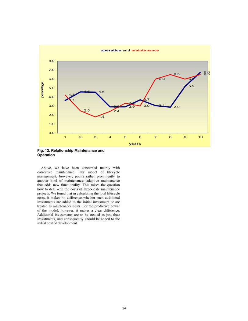
Fig. 12. Relationship Maintenance and Operation

Above, we have been concerned mainly with

corrective maintenance. Our model of lifecycle

management, however, points rather prominently to

another kind of maintenance: adaptive maintenance

that adds new functionality. This raises the question

how to deal with the costs of large-scale maintenance

projects. We found that in calculating the total lifecycle

costs, it makes no difference whether such additional

investments are added to the initial investment or are

treated as maintenance costs. For the predictive power

of the model, however, it makes a clear difference.

Additional investments are to be treated as just that:

investments, and consequently should be added to the

initial cost of development.

operation and maintenance

3.7

4.6 4.6

2.9 2.9

3.7

3.1

2.9

5.2

6.8

4.3

2.5

1.8

2.4

3.3

3.0

6.0

6.5

6.0

6.5

0.0

1.0

2.0

3.0

4.0

5.0

6.0

7.0

8.0

1 2 3 4 5 6 7 8 9 10

years

percentage

24

7. Conclusion

An attempt has been made to show that introducing

lifecycle management does not need to be a

particularly difficult undertaking and that the obvious

starting point is certainly not the implementation of an

all-embracing software suite for IT governance. When

discussing our model of lifecycle cost management at

the beginning of this article, we stated that there is no

need to adjust the way the company is run to the

structure that this type of suites imposes. It is rather the

other way around: one needs to be in control of the

process of software development before even

considering the use of these kinds of tools.

What concerns us here is the performance of the IT

organization; everyone must be convinced of the

importance of standardization in this field nowadays. If

processes and procedures are under control, it takes

only a relatively small effort to set up your own

method of gathering reliable material. For the analysis,

fairly simple tools like MS Excel and SPSS will

suffice. Therefore, setting up lifecycle management

need not cost a fortune. It is, as already observed

earlier, above all a question of discipline. If we succeed

in that, a pragmatic approach to lifecycle cost control

could bring about the next step towards a better

performance of IT in our organizations.

Throughout this article, we stressed the importance

of standardization and measuring. By standardization,

the applicability of simple models is strongly

increased; these models can be verified by measuring.

Using simple models makes it possible to achieve

higher levels of predictable processing. In this way, IT

governance is supported with cost control in general

and the ‘kill management’ of automated systems in

particular. Standardization for us at Cordares is the

only way to control the complexity of constantly

changing regulations and (pension) schemes, and thus

to ensure the necessary long life expectancy.

Threefold calibration of our models has been

undertaken. First, we established and confirmed that

backfiring lines of code for our 3GL systems yields a

sound indication of function points. On the other hand,

dividing total project costs by the average fee per hour

gives an indication of the total workload in hours. The

soundness of this result is assured by comparing the

estimated hours with the carefully registered hours.

Combining the two gives us a productivity factor in

terms of hours per function point. Second, we double

checked our findings by reconstructing amounts of

function points out of implemented systems as opposed

to functional design. Third, we related our productivity

figures to the benchmarking approach of Capers Jones

[3] and, as we demonstrated above, found them to be

consistent with conclusions of Verhoef [5].

We are convinced that the pragmatic approach to

lifecycle cost management will be instrumental in

ensuring that Cordares maintains cost leadership.

George Labrujere, Hans de Weme & Adri van der

Wurff

25

Acknowledgements

We would like to thank Prof. Dr Chris Verhoef

(Free University of Amsterdam, Department of

Mathematics and Computer Science) for his

encouragement to write this paper, and for his

invitation for the IEEE-conference.

We also thank the (anonymous) reviewers for their

useful and encouraging comments on the first version

of this paper. It helped us a lot in improving the clarity

and quality.

Bibliography

[1]

B. Boehm. Software Engineering Economics.

Prentice Hall, 1981.

[2]

C. Jones. Estimating Software Costs. McGraw-

Hill, 1998.

[3]

C. Jones. Software Assessments, Benchmarks,

and Best Practices. Information Technology

Series. Addison- Wesley, 2000.

[4]

L.H. Putnam and W. Myers. Measures for

Excellence – Reliable Software on Time, Within

Budget. Yourdon Press Computing Series, 1992.

[5]

C. Verhoef. Quantifying the Value of IT-

Investments. Science of Computer Programming,

2004.

[6]

C. Verhoef. Quantitative IT Portfolio

Management. Science of Computer Programming,

45(1):1-96, 2002.

[7]

C. Verhoef. Quantitative Aspects of Outsourcing

Deals. Science of Computer Programming,

56(2005):275-313, 2002

[8] http://www.isbsg.org/isbsg.nsf/weben/Project%20

Delivery%20Rate

26