LES OFWIND AND WAVEFORCED OCEANIC TURBULENT …congress.cimne.com/iacm-eccomas2014/admin/files/file... · 2014-04-06 · 9500 Gilman Drive MC0085 La Jolla, CA 92093, USA e-mail: [email protected]

11th World Congress on Computational Mechanics (WCCM XI)5th European Conference on Computational Mechanics (ECCM V)

6th European Conference on Computational Fluid Dynamics (ECFD VI)E. Onate, J. Oliver and A. Huerta (Eds)

LES OF WIND AND WAVE FORCED OCEANICTURBULENT BOUNDARY LAYERS USING THERESIDUAL-BASED VARIATIONAL MULTISCALE

METHOD AND NEAR-WALL MODELING

ANDRES E. TEJADA-MARTINEZ∗, ROOZBEH GOLSHAN∗, IDO

AKKERMAN† and YURI BAZILEVS††

∗Department of Civil and Environmental EngineeringUniversity of South Florida

4202 East Fowler Avenue ENB 118Tampa, FL 33620, USA

e-mail: [email protected], [email protected]

†School of Engineering and Computing SciencesDurham University

South Road, DH1 3LEDurham, UK

e-mail: [email protected]

††Department of Structural EngineeringUniversity of California, San Diego

9500 Gilman Drive MC0085La Jolla, CA 92093, USAe-mail: [email protected]

Key words: Langmuir Turbulence, Langmuir Circulation, Wall Modeling, Residual-based Variational Multiscale Method

Abstract. Large-eddy simulation (LES) of wind and wave forced oceanic turbulentboundary layers is performed using the residual-based variational multiscale method (RB-VMS) [1, 10] and near-wall modeling [2, 9]. Wind and surface gravity wave forcinggenerates Langmuir turbulence characterized by Langmuir circulation (LC) with largestscales consisting of streamwise vortices aligned in the direction of the wind, acting as asecondary flow structure to the primary wind-driven component of the flow. Our LES isrepresentative of a shallow water continental shelf flow (10 to 30 meters in depth) far fromlateral boundaries in which LC engulfs the full depth of the water column and disruptsthe bottom log layer. Field measurements indicate that occurrence of full-depth LC istypical during the passage of storms. The RBVMS method with quadratic NURBS (Non-Uniform Rational B-splines) with near-wall resolution has been shown to possess goodconvergence characteristics for this flow [10]. The use of near-wall modeling facilitates

1

Andres E. Tejada-Martınez, Roozbeh Golshan, Ido Akkerman and Yuri Bazilevs

simulations with expanded domains over horizontal directions. Thus, these simulationsare able to resolve multiple Langmuir cells permitting analysis of the interaction betweenthe cells. Results in terms of velocity statistics are presented from simulations performedwith various domain sizes and distinct near-wall treatments: (1) the classical treatmentreviewed in [9] based on prescription of the wall shear stress and (2) a recent treatmentpresented in [2] based on weak imposition of the no-slip bottom boundary condition.

1 INTRODUCTION

Wind speeds greater than 3 m s−1 can lead to the generation of Langmuir turbulence inthe upper ocean [11]. Interaction between surface gravity waves and the wind-driven shearcurrent in the upper ocean is well-known to produce Langmuir turbulence characterizedby Langmuir circulation or cells consisting of parallel counter-rotating vortices roughlyaligned in the direction of the wind. The longest Langmuir cells extend in the downwinddirection for tens of meters to kilometers. In the upper ocean mixed layer, the cells canextend to the base of the mixed layer which is tens of meters deep, depending on variousfactors such as winds, surface waves and surface buoyancy conditions. In shallow coastalshelf regions, the passage of storms leads to intense vertical mixing and an unstratifiedwater column. In these cases, Langmuir cells have been observed occupying the full-depthof the water column while serving as an important mechanism for sediment re-suspension[5, 6]. Full-depth Langmuir cells have been observed in water columns ranging from 10to 30 meters deep.

Over the past two decades LES has yielded fundamental knowledge on the structure ofLangmuir turbulence. These simulations have been based on the phase-averaged Navier-Stokes equations or Craik-Leibovich equations [7] in which the averaging filters out surfacegravity waves giving rise to the well-known Craik-Leibovich (C-L) vortex force [4]. TheC-L vortex force consists of the cross-product between the Stokes drift velocity induced bysurface gravity waves and the flow vorticity. The presence of this force in the momentumequations accounts for the generating mechanism of Langmuir turbulence without theneed to resolve surface gravity waves. Hence, simulations may be conducted with a flatsurface.

In [10] we have shown that the C-L vortex force in the Craik-Leibovich equations pos-sesses an advective structure given in terms of an advective matrix of velocities. Suchadvective structure led to the consistent definition of the intrinsic timescale parameterτM for the momentum equation in the RBVMS formulation of the C-L equations. Fur-thermore, in [10] we performed LES with near-wall resolution (LES-NWR) of Langmuirturbulence in shallow water characterized by full-depth Langmuir cells. Results fromthe simulations compared favorably with the field measurements of [5, 6] in terms of theturbulence structure resolved.

The LES of [10] was performed with relatively small domain dimensions in the stream-

2


wise (downwind) and spanwise (crosswind) directions and thus limited to resolution ofone full-depth Langmuir cell. In this paper, we make use of the formulation in [10] to-gether with near-wall modeling in order to perform simulations on bigger domains overdownwind and crosswind directions and thus investigate the impact of the domain size onthe resolved Langmuir turbulence structure and statistics. Such simulation approach isoften referred to as LES with near-wall modeling or LES-NWM and permits simulationswithout having to resolve the computationally expensive near-wall region.

2 COMPUTATIONAL SETUP

The computational domain is similar to that depicted in [10] and consists of a rect-angular box with dimensions L1 in the streamwise or downwind (x1) direction, L2 in thespanwise or crosswind (x2) direction and L3 in the vertical or wall-normal (x3) direction.

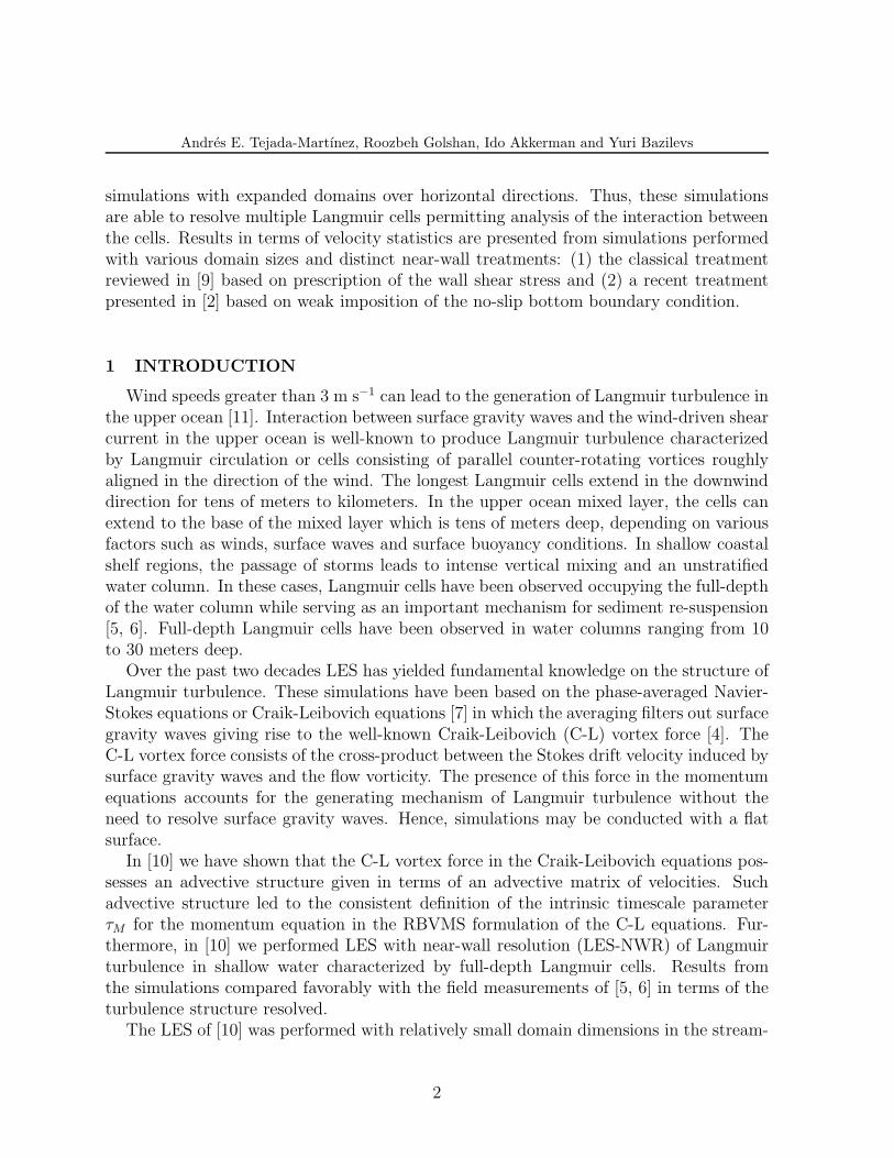
The half-depth of the domain (in the x3-direction) is δ and the domain extends from0 to 2δ over x3. Various domain lengths over x1 and x2 directions were utilized in orderto investigate their influence on turbulence structure and statistics. Domain sizes arelisted in Table 1. This table also shows mesh resolutions in terms of the numbers ofquadratic NURBS basis functions (N1, N2 and N3) used in each tensor product direction.Mesh resolution is uniform in all three directions. The coarse mesh resolution in thewall-normal (vertical) is such that viscous wall and buffer sublayers are not well-resolved,thereby requiring near-wall modeling.

L1 L2 L3 N1 N2 N3

4πδ 83πδ 2δ 32 64 34

28πδ 163πδ 2δ 256 128 34

40πδ 163πδ 2δ 320 128 34

Table 1: Summary of domain sizes and mesh resolutions used in LES-NWM.

The flow is driven by a constant wind stress τw = ρu2τ , where ρ is density and uτ is wind

stress friction velocity. This wind stress is applied in the x1 direction at the top surface(x3 = 2δ) of the rectangular box domain, where no-penetration boundary condition is alsoassumed to hold. A no-slip condition (enforced weakly) or a shear stress (a Neummanboundary condition) is applied at the bottom wall boundary (x3 = 0). In the streamwiseand spanwise directions, periodic boundary conditions are employed in order to representan unbounded domain in these directions, approximating a continental shelf wind andwave-driven flow far from (unaffected by) coastal boundaries.

Characteristic flow velocity, Stokes drift velocity and length are taken as wind stressfriction velocity uτ , Stokes drift at the surface us, and half-depth δ, respectively. Charac-teristic time scale is taken as δ/uτ . Using these scales to non-dimensionalize the Craik-Leibovich equations gives rise to the Reynolds number defined as Re = uτδ/ν (where νis kinematic viscosity) and the turbulent Langmuir number defined as Lat =

√

uτ/us,

3


the latter representative of wind forcing relative to wave forcing. Note that the C-Lvortex force in the momentum (Craik-Leibovich) equations requires input of the Stokesdrift velocity which is a depth-dependent (x3) function decaying with distance to the topsurface of the domain. The decay rate is inversely proportional to λ, the wavelength ofthe dominant surface gravity waves generating the Langmuir turbulence (thus the Stokesdrift velocity decays with depth more rapidly for shorter waves). The interested reader isdirected to [10] for the full Craik-Leibovich equations and corresponding RBVMS formu-lation. Results presented in upcoming sections were obtained from simulations performedwith Re = 395, Lat = 0.7 and λ = 12δ, the latter two parameters representative of thewave and wind forcing conditions during field measurements of full-depth Langmuir cellsin [5, 6]. In [12, 10], velocity fluctuations in the core region of the flow obtained fromLES-NWR at the laboratory-scale Re = 395 have been shown to scale-up favorably tofield-scale Re via comparisons with the field measurements in [5, 6]. However, futuresimulations should be conducted at higher Reynolds numbers to further verify this.

3 WALL MODELING

3.1 Classical wall model

LES-NWM is performed with two distinct wall modeling approaches. The first is theclassical approach in which a Neumann or natural boundary condition is imposed at thebottom wall (at x3 = 0) in the form of the wall shear stress. For example, in this case thedimensional wall shear stress in the x1-momentum equation is prescribed as

τwall = ρ u2∗

u1(x1, x2, xol3 , t)

Uol(1)

In the previous expression u∗ is the wall friction velocity, and xol3 denotes the distance from

the wall to the first grid point in the outer layer (ol) satisfying the classical logarithmicprofile

Uol+ =Uol

u∗

=1

κlog

xol3 u∗

ν+B (2)

Here ν is kinematic viscosity, κ = 0.41 is the von Karman constant and B ranges between5 and 8 for flows with full-depth Langmuir circulation depending on wind and wave forcingconditions (i.e. values of Lat and λ). The latter variation in B can be observed in theLES-NWR in [13] conducted using a high order hybrid finite difference/spectral numericalmethod. The wall friction velocity u∗ in (1) is solved iteratively from the log law in (2)with Uol obtained from the LES-computed velocity at x3 = xol

3 . Note that for the currentflow configuration, in the mean, wall friction velocity u∗ is equal to wind stress frictionvelocity uτ .

4


3.2 Weak imposition of the bottom no-slip condition

An alternate approach to wall modeling has been investigated consisting of weak im-position of the bottom no-slip (Dirichlet) boundary condition. Here the weak Dirichletboundary terms of the RBVMS formulation are taken as

Bwbc({w}, {u}) = (w,−2Re−1∇su · n)Γg

+(−2Re−1∇sw · n, (u− g))Γg

+(w, τB(u− g))Γg, (3)

weakly imposing the Dirichlet boundary condition u = g, with u = (u1, u2, u3) being theflow velocity, w the corresponding weighting function, and g = 0 the no-slip condition atthe bottom wall. In equation (3), Γg is the Dirichlet part of the problem domain boundary(i.e. the bottom wall) and n is the unit outward normal vector to this boundary (i.e.(0, 0,−1)). In the formulation we assume that the normal component of the flow velocityvector (i.e. the wall-normal velocity) is imposed strongly at the boundary (i.e. u3 = 0strongly at the bottom wall). To ensure numerical stability and optimal convergence, thepenalty parameter τB in equation (3) is chosen as

τB = CbRe−1√

niGijnj , (4)

where ni’s are the Cartesian component of the unit outward normal vector to Γg andCb is an element-wise constant emanating from a boundary inverse estimate [3]. Furtherdiscussion and computational results employing weakly-enforced Dirichlet conditions maybe found in [2].

4 RESULTS

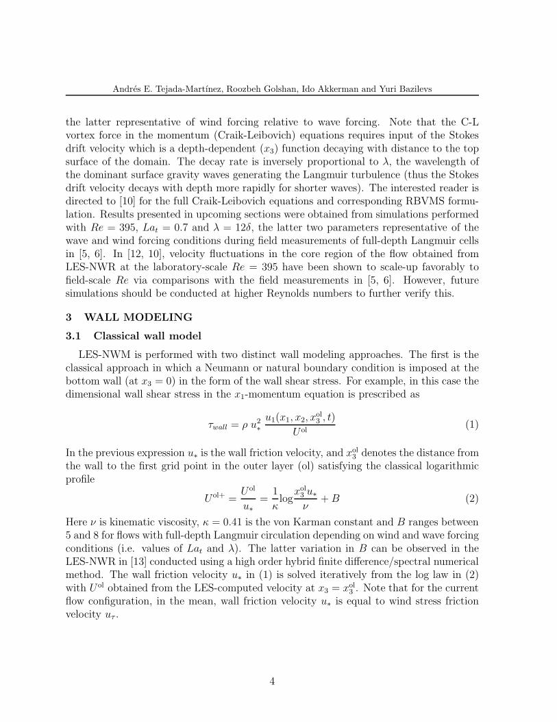
Figure (1) shows velocity fluctuations averaged over the streamwise (x1) direction andover time on the streamwise-wall-normal plane. These averaged fluctuations reveal thecellular structure captured by the LES. In this case, one Langmuir cell was resolvedwith spanwise length of the domain L2 = 8πδ/3. This spanwise length of the cell isconsistent with the field measurements in [5, 6]. In the upper panel of Figure (1), thebottom convergence of the resolved Langmuir cell is seen in terms of converging averagedspanwise velocity fluctuations near x2/δ = 4.2 in the lower half of the domain. This cellbottom convergence generates the full-depth upwelling limb of the cell, seen in the middlepanel of Figure (1) in terms of positive averaged wall-normal velocity fluctuation. Finally,the upwelling limb of the cell generally coincides with a full-depth region of negativeaveraged streamwise velocity fluctuation (lower panel) which is intensified in the lowerhalf of the domain and in the near-surface region. The previous characteristics are typicalof full-depth Langmuir cells as observed in the field measurements in [5, 6].

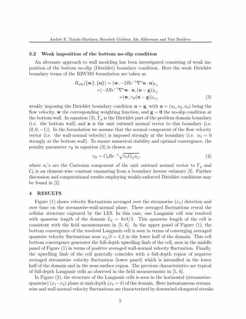
In Figure (2), the structure of the Langmuir cells is seen in the horizontal (streamwise-spanwise) (x1−x2) plane at mid-depth (x3 = δ) of the domain. Here instantaneous stream-wise and wall-normal velocity fluctuations are characterized by downwind-elongated streaks

5


x2/δ

x3/δ

streamwise

0 1 2 3 4 5 6 7 8

0

0.5

1

1.5

2

−2

0

2

x3/δ

spanwise

0 1 2 3 4 5 6 7 80

0.5

1

1.5

2

−2

−1

0

1

2

x3/δ

wall-normal

0 1 2 3 4 5 6 7 80

0.5

1

1.5

2

−2

−1

0

1

2

Figure 1: Streamwise-wall-normal plane of streamwise- and time-averaged spanwise (top), wall-normal(middle) and streamwise (bottom) velocity fluctuations scaled by uτ from LES-NWM in the domainL1/δ × L2/δ × L3/δ = 4π × 8

3π × 2. Results were obtained with classical wall model in sub-section 3.1

with B = 6.5 in (2). Streamwise direction (x1) is out of page.

alternating in sign in the spanwise direction. Note that the negative streamwise velocityfluctuation streak (upper panel) corresponds to the upwelling limb of the cell observed ear-lier in Figure (1). Furthermore in Figure (2), the positive wall-normal velocity fluctuationstreak (lower panel) generally coincides with the negative downwind velocity fluctuationstreak (upper panel), also consistent with Figure (1).

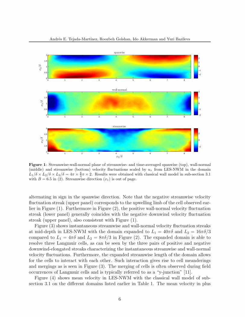
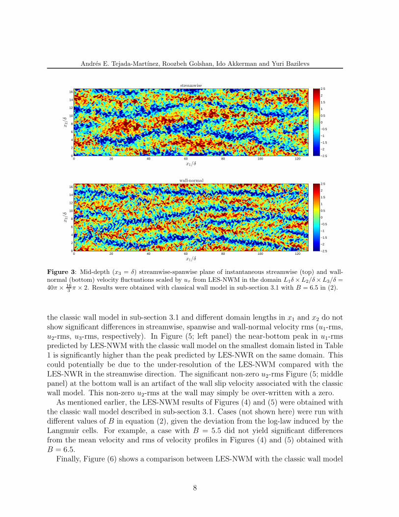
Figure (3) shows instantaneous streamwise and wall-normal velocity fluctuation streaksat mid-depth in LES-NWM with the domain expanded to L1 = 40πδ and L2 = 16πδ/3compared to L1 = 4πδ and L2 = 8πδ/3 in Figure (2). The expanded domain is able toresolve three Langmuir cells, as can be seen by the three pairs of positive and negativedownwind-elongated streaks characterizing the instantaneous streamwise and wall-normalvelocity fluctuations. Furthermore, the expanded streamwise length of the domain allowsfor the cells to interact with each other. Such interaction gives rise to cell meanderingsand mergings as is seen in Figure (3). The merging of cells is often observed during fieldoccurrences of Langmuir cells and is typically referred to as a “y-junction” [11].

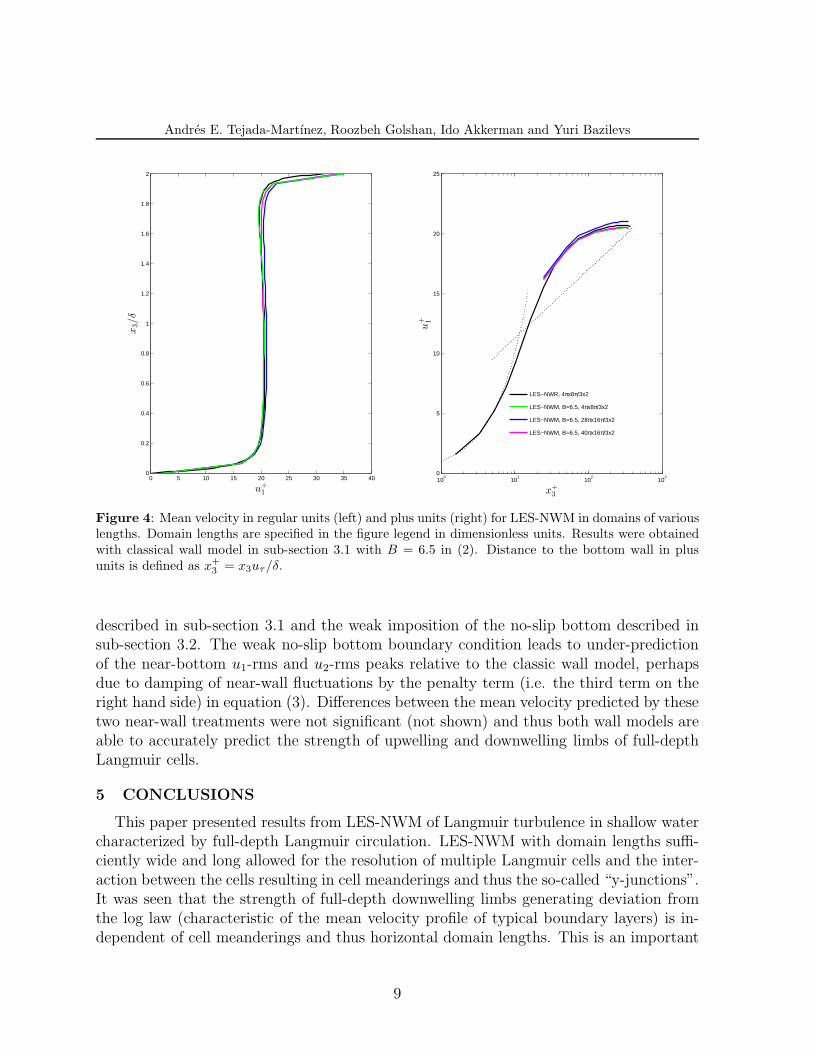
Figure (4) shows mean velocity in LES-NWM with the classical wall model of sub-section 3.1 on the different domains listed earlier in Table 1. The mean velocity in plus

6


x1/δ

x2/δ

streamwise

0 2 4 6 8 10 120

1

2

3

4

5

6

7

8

−2.5

−2

−1.5

−1

−0.5

0

0.5

1

1.5

2

2.5

x1/δ

x2/δ

wall-normal

0 2 4 6 8 10 120

1

2

3

4

5

6

7

8

−2.5

−2

−1.5

−1

−0.5

0

0.5

1

1.5

2

2.5

Figure 2: Mid-depth (x3 = δ) streamwise-spanwise plane of instantaneous streamwise (top) and wall-normal (bottom) velocity fluctuations scaled by uτ from LES-NWM in the domain L1/δ×L2/δ×L3/δ =4π × 8

3π × 2. Results were obtained with classical wall model in sub-section 3.1 with B = 6.5 in (2).

units is characterized by a deviation from the log-law. This deviation has been attributedto the high speed fluid brought down to the near-wall region by the downwelling limbsof the Langmuir cells [13]. Thus, the log-law deviation depends on the strength of theselimbs, which can be measured, for example, in terms of root mean square of wall-normalvelocity [8]. As can be seen in Figure (4), the deviation from the log law is robust acrossLES-NWM with different horizontal domain lengths. Furthermore, all LES-NWM casespredict a mean velocity in good agreement with the velocity calculated via LES-NWR(in [10]) on the smallest domain in Table 1. In [10] LES-NWR (i.e. LES with near-wallresolution) was performed with quadratic NURBS with N1 = N2 = 64 and N3 = 66. TheLES-NWR mesh was uniform in x1 and x2 and stretched in x3 so as to resolve viscousboundary layers at the bottom wall and top surface. These results imply that LES-NWM is able to perform well in capturing the strength of the full-depth upwelling anddownwelling limbs of the Langmuir cells. Furthermore, the strength of these limbs andresulting deviation of mean velocity from the log law is nearly independent of horizontaldomain length and cell meanderings.

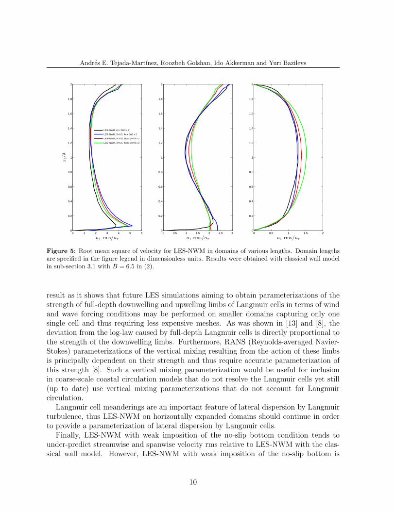
Figure (5) shows root mean square (rms) of velocity. Results from LES-NWM with

7


x1/δ

x2/δ

streamwise

0 20 40 60 80 100 1200

2

4

6

8

10

12

14

16

−2.5

−2

−1.5

−1

−0.5

0

0.5

1

1.5

2

2.5

x1/δ

x2/δ

wall-normal

0 20 40 60 80 100 1200

2

4

6

8

10

12

14

16

−2.5

−2

−1.5

−1

−0.5

0

0.5

1

1.5

2

2.5

Figure 3: Mid-depth (x3 = δ) streamwise-spanwise plane of instantaneous streamwise (top) and wall-normal (bottom) velocity fluctuations scaled by uτ from LES-NWM in the domain L1δ×L2/δ×L3/δ =40π × 16

3π × 2. Results were obtained with classical wall model in sub-section 3.1 with B = 6.5 in (2).

the classic wall model in sub-section 3.1 and different domain lengths in x1 and x2 do notshow significant differences in streamwise, spanwise and wall-normal velocity rms (u1-rms,u2-rms, u3-rms, respectively). In Figure (5; left panel) the near-bottom peak in u1-rmspredicted by LES-NWM with the classic wall model on the smallest domain listed in Table1 is significantly higher than the peak predicted by LES-NWR on the same domain. Thiscould potentially be due to the under-resolution of the LES-NWM compared with theLES-NWR in the streamwise direction. The significant non-zero u2-rms Figure (5; middlepanel) at the bottom wall is an artifact of the wall slip velocity associated with the classicwall model. This non-zero u2-rms at the wall may simply be over-written with a zero.

As mentioned earlier, the LES-NWM results of Figures (4) and (5) were obtained withthe classic wall model described in sub-section 3.1. Cases (not shown here) were run withdifferent values of B in equation (2), given the deviation from the log-law induced by theLangmuir cells. For example, a case with B = 5.5 did not yield significant differencesfrom the mean velocity and rms of velocity profiles in Figures (4) and (5) obtained withB = 6.5.

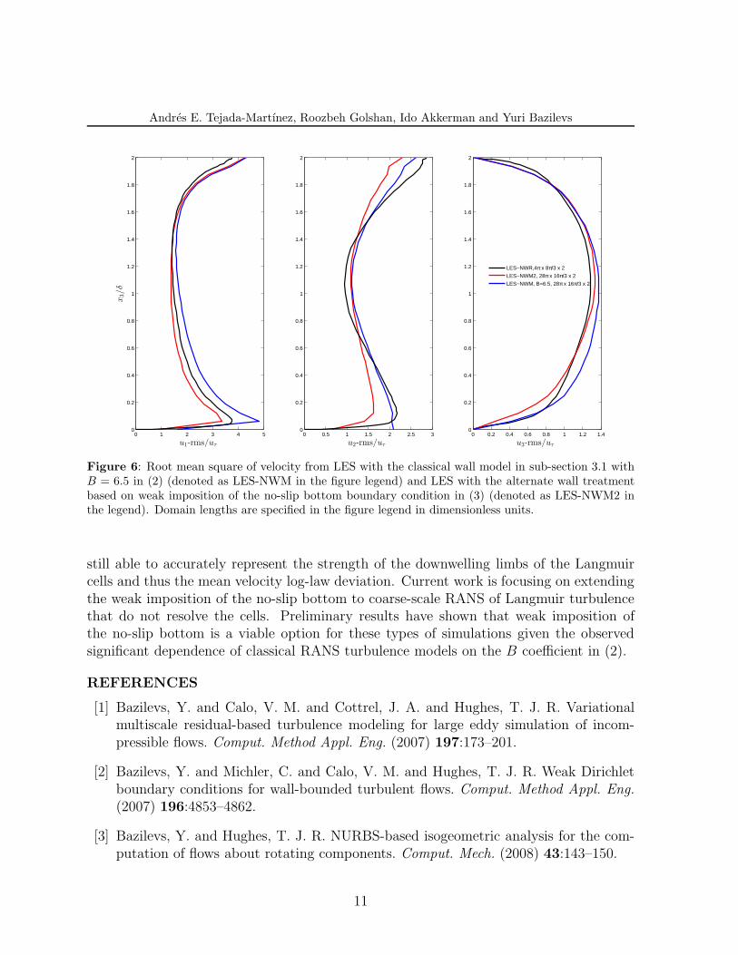
Finally, Figure (6) shows a comparison between LES-NWM with the classic wall model

8


0 5 10 15 20 25 30 35 400

0.2

0.4

0.6

0.8

1

1.2

1.4

1.6

1.8

2

x3/δ

u+1

100

101

102

103

0

5

10

15

20

25

x+3

u+ 1

LES−NWR, 4πx8π/3x2

LES−NWM, B=6.5, 4πx8π/3x2



Figure 4: Mean velocity in regular units (left) and plus units (right) for LES-NWM in domains of variouslengths. Domain lengths are specified in the figure legend in dimensionless units. Results were obtainedwith classical wall model in sub-section 3.1 with B = 6.5 in (2). Distance to the bottom wall in plusunits is defined as x+

3 = x3uτ/δ.

described in sub-section 3.1 and the weak imposition of the no-slip bottom described insub-section 3.2. The weak no-slip bottom boundary condition leads to under-predictionof the near-bottom u1-rms and u2-rms peaks relative to the classic wall model, perhapsdue to damping of near-wall fluctuations by the penalty term (i.e. the third term on theright hand side) in equation (3). Differences between the mean velocity predicted by thesetwo near-wall treatments were not significant (not shown) and thus both wall models areable to accurately predict the strength of upwelling and downwelling limbs of full-depthLangmuir cells.

5 CONCLUSIONS

This paper presented results from LES-NWM of Langmuir turbulence in shallow watercharacterized by full-depth Langmuir circulation. LES-NWM with domain lengths suffi-ciently wide and long allowed for the resolution of multiple Langmuir cells and the inter-action between the cells resulting in cell meanderings and thus the so-called “y-junctions”.It was seen that the strength of full-depth downwelling limbs generating deviation fromthe log law (characteristic of the mean velocity profile of typical boundary layers) is in-dependent of cell meanderings and thus horizontal domain lengths. This is an important

9


0 1 2 3 4 5 60

0.2

0.4

0.6

0.8

1

1.2

1.4

1.6

1.8

2

x3/δ

u1-rms/uτ

0 0.5 1 1.5 2 2.5 30

0.2

0.4

0.6

0.8

1

1.2

1.4

1.6

1.8

2

u1-rms/uτ

0 0.5 1 1.5 20

0.2

0.4

0.6

0.8

1

1.2

1.4

1.6

1.8

2

u1-rms/uτ

LES−NWR, 4π x 8π/3 x 2

LES−NWM, B=6.5, 4π x 8π/3 x 2

LES−NWM, B=6.5, 28π x 16π/3 x 2

LES−NWM, B=6.5, 40π x 16π/3 x 2

Figure 5: Root mean square of velocity for LES-NWM in domains of various lengths. Domain lengthsare specified in the figure legend in dimensionless units. Results were obtained with classical wall modelin sub-section 3.1 with B = 6.5 in (2).

result as it shows that future LES simulations aiming to obtain parameterizations of thestrength of full-depth downwelling and upwelling limbs of Langmuir cells in terms of windand wave forcing conditions may be performed on smaller domains capturing only onesingle cell and thus requiring less expensive meshes. As was shown in [13] and [8], thedeviation from the log-law caused by full-depth Langmuir cells is directly proportional tothe strength of the downwelling limbs. Furthermore, RANS (Reynolds-averaged Navier-Stokes) parameterizations of the vertical mixing resulting from the action of these limbsis principally dependent on their strength and thus require accurate parameterization ofthis strength [8]. Such a vertical mixing parameterization would be useful for inclusionin coarse-scale coastal circulation models that do not resolve the Langmuir cells yet still(up to date) use vertical mixing parameterizations that do not account for Langmuircirculation.

Langmuir cell meanderings are an important feature of lateral dispersion by Langmuirturbulence, thus LES-NWM on horizontally expanded domains should continue in orderto provide a parameterization of lateral dispersion by Langmuir cells.

Finally, LES-NWM with weak imposition of the no-slip bottom condition tends tounder-predict streamwise and spanwise velocity rms relative to LES-NWM with the clas-sical wall model. However, LES-NWM with weak imposition of the no-slip bottom is

10


0 1 2 3 4 50

0.2

0.4

0.6

0.8

1

1.2

1.4

1.6

1.8

2

x3/δ

u1-rms/uτ

0 0.5 1 1.5 2 2.5 30

0.2

0.4

0.6

0.8

1

1.2

1.4

1.6

1.8

2

u2-rms/uτ

0 0.2 0.4 0.6 0.8 1 1.2 1.40

0.2

0.4

0.6

0.8

1

1.2

1.4

1.6

1.8

2

u3-rms/uτ

LES−NWR,4π x 8π/3 x 2

LES−NWM2, 28π x 16π/3 x 2

LES−NWM, B=6.5, 28π x 16π/3 x 2

Figure 6: Root mean square of velocity from LES with the classical wall model in sub-section 3.1 withB = 6.5 in (2) (denoted as LES-NWM in the figure legend) and LES with the alternate wall treatmentbased on weak imposition of the no-slip bottom boundary condition in (3) (denoted as LES-NWM2 inthe legend). Domain lengths are specified in the figure legend in dimensionless units.

still able to accurately represent the strength of the downwelling limbs of the Langmuircells and thus the mean velocity log-law deviation. Current work is focusing on extendingthe weak imposition of the no-slip bottom to coarse-scale RANS of Langmuir turbulencethat do not resolve the cells. Preliminary results have shown that weak imposition ofthe no-slip bottom is a viable option for these types of simulations given the observedsignificant dependence of classical RANS turbulence models on the B coefficient in (2).

REFERENCES

[1] Bazilevs, Y. and Calo, V. M. and Cottrel, J. A. and Hughes, T. J. R. Variationalmultiscale residual-based turbulence modeling for large eddy simulation of incom-pressible flows. Comput. Method Appl. Eng. (2007) 197:173–201.

[2] Bazilevs, Y. and Michler, C. and Calo, V. M. and Hughes, T. J. R. Weak Dirichletboundary conditions for wall-bounded turbulent flows. Comput. Method Appl. Eng.

(2007) 196:4853–4862.

[3] Bazilevs, Y. and Hughes, T. J. R. NURBS-based isogeometric analysis for the com-putation of flows about rotating components. Comput. Mech. (2008) 43:143–150.

11


[4] Craik, A. D. D. and Leibovich, S. A rational model for Langmuir circulation. J.Fluid. Mech. (1976) 73:401–426.

[5] Gargett, A. E. and Wells, J. R. and Tejada-Martınez, A. E. and Grosch, C. E. Lang-muir supercells: A mechanism for sediment resuspension and transport in shallowseas. Science (2004) 306:1925–1928.

[6] Gargett, A. E. and Wells, J. R. Langmuir turbulence in shallow water. Part 1. Ob-servations J. Fluid. Mech. (2007) 576:27–61.

[7] McWilliams, J. C. and Sullivan, P. P. and Moeng C-H. Langmuir turbulence in theocean. J. Fluid. Mech. (1997) 334:31–58.

[8] Sinha, N. Towards RANS parameterization of Langmuir turbulence in shallow water.Ph.D. thesis, University of South Florida (2013).

[9] Piomelli, U. and Balaras, E. Wall-layer models for large-eddy simulations. Annu.Rev. Fluid. Mech. (2012) 34:349–374.

[10] Tejada-Martınez, A. E. and Akkerman, I. and Bazilevs, Y. Large-eddy simulationof shallow water Langmuir turbulence using isogeometric analysis and the residual-based variational multiscale method. J. Appl. Mech (2012) 34:349–374.

[11] Thorpe, S. A. Langmuir circulation. Annu. Rev. Fluid. Mech. (2012) 34:349–374.

[12] Tejada-Martınez, A. E. and Grosch, C. E. and Gargett, A. E. and Polton, J. A. andSmith, J. A. and MacKinnon, J. A. A hybrid spectral/finite-difference large-eddysimulator of turbulent processes in the upper ocean. Ocean Model. (2009) 39:115–142.

[13] A. E. Tejada-Martınez and Grosch, C.E. and Sinha, .N and Akan, C. and Martinat,G. Disruption of bottom log layer in large-eddy simulations of full-depth Langmuircirculation. J. Fluid. Mech. (2012) 699:79–93.

12

LES OFWIND AND WAVEFORCED OCEANIC TURBULENT …congress.cimne.com/iacm-eccomas2014/admin/files/file... · 2014-04-06 · 9500 Gilman Drive MC0085 La Jolla, CA 92093, USA e-mail: [email protected]

Documents