U NIVERSITY OF B ONN L EARNING AND I NFERENCE A LGORITHMS FOR M ONOCULAR P ERCEPTION WITH APPLICATIONS TO OBJECT DETECTION,LOCALIZATION AND TIME SERIES MODELS FOR 3D HUMAN MOTION UNDERSTANDING C RISTIAN S MINCHISESCU

Welcome message from author
This document is posted to help you gain knowledge. Please leave a comment to let me know what you think about it! Share it to your friends and learn new things together.
Transcript

UNIVERSITY OF BONN
LEARNING AND INFERENCE ALGORITHMS FOR
MONOCULAR PERCEPTION
WITH APPLICATIONS TO OBJECT DETECTION, LOCALIZATION AND TIME SERIESMODELS FOR 3D HUMAN MOTION UNDERSTANDING
CRISTIAN SMINCHISESCU
Contents
1 Contributions and Roadmap 31.1 Models for Monocular Perception . . . . . . . . . . . . . . . . . . . . . . . . . . . . . . . 31.2 The Application Context and its Challenges . . . . . . . . . . . . . . . . . . . . . . . . . . 5
1.2.1 Difficulties in the Visual Analysis of Articulated Biological Forms . . . . . . . . . . 61.3 Contributions . . . . . . . . . . . . . . . . . . . . . . . . . . . . . . . . . . . . . . . . . . 8
1.3.1 Optimization and Sampling Algorithms . . . . . . . . . . . . . . . . . . . . . . . . 81.3.2 Discriminative and Conditional Models . . . . . . . . . . . . . . . . . . . . . . . . 111.3.3 Non-linear Latent Variable Models . . . . . . . . . . . . . . . . . . . . . . . . . . . 20
PART I: OPTIMIZATION AND SAMPLING ALGORITHMS 23
2 Kinematic Jump Sampling 252.1 Sampling for Articulated Chains . . . . . . . . . . . . . . . . . . . . . . . . . . . . . . . . 25
2.1.1 Human Pose Reconstruction Algorithms . . . . . . . . . . . . . . . . . . . . . . . . 262.2 Modeling and Estimation . . . . . . . . . . . . . . . . . . . . . . . . . . . . . . . . . . . . 262.3 Kinematic Jump Processes . . . . . . . . . . . . . . . . . . . . . . . . . . . . . . . . . . . 27
2.3.1 Direct Inverse Kinematics . . . . . . . . . . . . . . . . . . . . . . . . . . . . . . . 282.3.2 Iterative Inverse Kinematics . . . . . . . . . . . . . . . . . . . . . . . . . . . . . . 29
2.4 The Algorithm . . . . . . . . . . . . . . . . . . . . . . . . . . . . . . . . . . . . . . . . . 302.5 Experiments . . . . . . . . . . . . . . . . . . . . . . . . . . . . . . . . . . . . . . . . . . . 31
2.5.1 Quantitative Evaluation . . . . . . . . . . . . . . . . . . . . . . . . . . . . . . . . . 312.5.2 Tracking . . . . . . . . . . . . . . . . . . . . . . . . . . . . . . . . . . . . . . . . 34
2.6 Conclusions . . . . . . . . . . . . . . . . . . . . . . . . . . . . . . . . . . . . . . . . . . . 34
3 Variational Mixture Smoothing for Non-Linear Dynamical Systems 363.1 Smoothing for Non-linear Systems . . . . . . . . . . . . . . . . . . . . . . . . . . . . . . . 363.2 Existing Smoothing Algorithms . . . . . . . . . . . . . . . . . . . . . . . . . . . . . . . . 373.3 Formulation . . . . . . . . . . . . . . . . . . . . . . . . . . . . . . . . . . . . . . . . . . . 383.4 Multiple Trajectory Optima using Dynamic Programming . . . . . . . . . . . . . . . . . . . 393.5 Continuous MAP Refinement . . . . . . . . . . . . . . . . . . . . . . . . . . . . . . . . . . 393.6 Variational Updates for Mixtures . . . . . . . . . . . . . . . . . . . . . . . . . . . . . . . . 403.7 Experiments . . . . . . . . . . . . . . . . . . . . . . . . . . . . . . . . . . . . . . . . . . . 413.8 Conclusions . . . . . . . . . . . . . . . . . . . . . . . . . . . . . . . . . . . . . . . . . . . 44
4 Generalized Darting Monte Carlo 464.1 Sampling and Mixing . . . . . . . . . . . . . . . . . . . . . . . . . . . . . . . . . . . . . . 464.2 Markov Chain Monte Carlo Sampling . . . . . . . . . . . . . . . . . . . . . . . . . . . . . 474.3 The Mode-Hopping MCMC Algorithm . . . . . . . . . . . . . . . . . . . . . . . . . . . . 47
4.3.1 Elliptical Regions with Deterministic Moves . . . . . . . . . . . . . . . . . . . . . 484.3.2 Mode-Hopping in Discrete State Spaces . . . . . . . . . . . . . . . . . . . . . . . . 504.3.3 A Further Generalization . . . . . . . . . . . . . . . . . . . . . . . . . . . . . . . . 51
ii
CONTENTS iii
4.4 Proof of Detailed Balance . . . . . . . . . . . . . . . . . . . . . . . . . . . . . . . . . . . . 514.5 Auxiliary Variable Formulation . . . . . . . . . . . . . . . . . . . . . . . . . . . . . . . . . 52
4.5.1 Uniform Sampling inside Regions . . . . . . . . . . . . . . . . . . . . . . . . . . . 534.5.2 Deterministic Moves between Regions . . . . . . . . . . . . . . . . . . . . . . . . . 53
4.6 Learning Random Fields . . . . . . . . . . . . . . . . . . . . . . . . . . . . . . . . . . . . 534.7 Monocular Human Pose Inference and Learning . . . . . . . . . . . . . . . . . . . . . . . . 54
4.7.1 Domain Modeling . . . . . . . . . . . . . . . . . . . . . . . . . . . . . . . . . . . 564.7.2 Experiments . . . . . . . . . . . . . . . . . . . . . . . . . . . . . . . . . . . . . . 56
4.8 Discussion . . . . . . . . . . . . . . . . . . . . . . . . . . . . . . . . . . . . . . . . . . . . 59
PART II: CONDITIONAL AND DISCRIMINATIVE MODELS 61
5 BM3E : Discriminative Density Propagation for Visual Tracking 635.1 Motivation . . . . . . . . . . . . . . . . . . . . . . . . . . . . . . . . . . . . . . . . . . . . 635.2 Formulation of the BM 3E Model . . . . . . . . . . . . . . . . . . . . . . . . . . . . . . . 66
5.2.1 Discriminative Density Propagation . . . . . . . . . . . . . . . . . . . . . . . . . . 665.2.2 Conditional Bayesian Mixture of Experts Model (BME) . . . . . . . . . . . . . . . 675.2.3 Mixture of Experts based on Random Regression and Joint Density . . . . . . . . . 715.2.4 Learning Bayesian Mixtures in Kernel Induced State Spaces (kBME) . . . . . . . . 74
5.3 Experiments . . . . . . . . . . . . . . . . . . . . . . . . . . . . . . . . . . . . . . . . . . . 755.3.1 High-dimensional Models . . . . . . . . . . . . . . . . . . . . . . . . . . . . . . . 785.3.2 Low-dimensional Models . . . . . . . . . . . . . . . . . . . . . . . . . . . . . . . 82
5.4 Conclusions . . . . . . . . . . . . . . . . . . . . . . . . . . . . . . . . . . . . . . . . . . . 84
6 Semi-supervised Hierarchical Models for 3D Reconstruction 876.1 Supervision and Flexible Image Encodings . . . . . . . . . . . . . . . . . . . . . . . . . . 87
6.1.1 Existing Features and Models . . . . . . . . . . . . . . . . . . . . . . . . . . . . . 886.2 Hierarchical Image Encodings . . . . . . . . . . . . . . . . . . . . . . . . . . . . . . . . . 896.3 Metric Learning and Correlation Analysis . . . . . . . . . . . . . . . . . . . . . . . . . . . 906.4 Manifold Regularization for Multivalued Prediction . . . . . . . . . . . . . . . . . . . . . . 916.5 Experiments . . . . . . . . . . . . . . . . . . . . . . . . . . . . . . . . . . . . . . . . . . . 926.6 Conclusions . . . . . . . . . . . . . . . . . . . . . . . . . . . . . . . . . . . . . . . . . . . 95
7 Learning Joint Top-Down and Bottom-up Processes for 3D Visual Inference 977.1 Models with Bidirectional Mappings . . . . . . . . . . . . . . . . . . . . . . . . . . . . . . 97
7.1.1 Existing Methods . . . . . . . . . . . . . . . . . . . . . . . . . . . . . . . . . . . . 987.2 Modeling and Learning . . . . . . . . . . . . . . . . . . . . . . . . . . . . . . . . . . . . . 99
7.2.1 Generative Model . . . . . . . . . . . . . . . . . . . . . . . . . . . . . . . . . . . . 997.2.2 Recognition Model . . . . . . . . . . . . . . . . . . . . . . . . . . . . . . . . . . . 997.2.3 Learning a Generative-Recognition Tandem . . . . . . . . . . . . . . . . . . . . . . 100
7.3 Experiments . . . . . . . . . . . . . . . . . . . . . . . . . . . . . . . . . . . . . . . . . . . 1027.4 Conclusions . . . . . . . . . . . . . . . . . . . . . . . . . . . . . . . . . . . . . . . . . . . 106
8 Conditional Models for Contextual Human Motion Recognition 1078.1 The Importance of Context . . . . . . . . . . . . . . . . . . . . . . . . . . . . . . . . . . . 107
8.1.1 Existing Recognition Methods . . . . . . . . . . . . . . . . . . . . . . . . . . . . . 1098.2 Conditional Models for Recognition . . . . . . . . . . . . . . . . . . . . . . . . . . . . . . 110
8.2.1 Undirected Models. Conditional Random Fields . . . . . . . . . . . . . . . . . . . 1118.2.2 Directed Conditional Models. Maximum Entropy Markov Models (MEMM) . . . . 112
8.3 Experiments . . . . . . . . . . . . . . . . . . . . . . . . . . . . . . . . . . . . . . . . . . . 1138.3.1 Recognition Experiments based on 2d features . . . . . . . . . . . . . . . . . . . . 1158.3.2 Recognition based on reconstructed 3d joint angle features . . . . . . . . . . . . . . 116
8.4 Conclusions . . . . . . . . . . . . . . . . . . . . . . . . . . . . . . . . . . . . . . . . . . . 117

iv CONTENTS
9 Conditional Part-Based Models for Spatial Localization 1209.1 Part-based Recognition Models . . . . . . . . . . . . . . . . . . . . . . . . . . . . . . . . . 1209.2 Existing Methods for Localization . . . . . . . . . . . . . . . . . . . . . . . . . . . . . . . 1219.3 Deformable Part Model . . . . . . . . . . . . . . . . . . . . . . . . . . . . . . . . . . . . . 1219.4 Maximizing the Conditional Likelihood . . . . . . . . . . . . . . . . . . . . . . . . . . . . 123
9.4.1 Computing the Expected Sufficient Statistics . . . . . . . . . . . . . . . . . . . . . 1249.4.2 Learning the Tree Structure . . . . . . . . . . . . . . . . . . . . . . . . . . . . . . 125
9.5 Articulated Models . . . . . . . . . . . . . . . . . . . . . . . . . . . . . . . . . . . . . . . 1259.6 Appearance Descriptor Im(li) . . . . . . . . . . . . . . . . . . . . . . . . . . . . . . . . . 1269.7 Results . . . . . . . . . . . . . . . . . . . . . . . . . . . . . . . . . . . . . . . . . . . . . . 126
9.7.1 Discussion . . . . . . . . . . . . . . . . . . . . . . . . . . . . . . . . . . . . . . . 129
10 Support Kernel Machines for Object Recognition 13110.1 Kernel Methods for Recognition . . . . . . . . . . . . . . . . . . . . . . . . . . . . . . . . 13110.2 Support Kernel Machines . . . . . . . . . . . . . . . . . . . . . . . . . . . . . . . . . . . . 132
10.2.1 Learning Multiple Linear Classifiers . . . . . . . . . . . . . . . . . . . . . . . . . . 13310.3 Multilevel Histogram Intersection Kernels . . . . . . . . . . . . . . . . . . . . . . . . . . . 13410.4 Experiments . . . . . . . . . . . . . . . . . . . . . . . . . . . . . . . . . . . . . . . . . . . 134
10.4.1 Caltech 101 . . . . . . . . . . . . . . . . . . . . . . . . . . . . . . . . . . . . . . . 13510.4.2 Caltech 256 . . . . . . . . . . . . . . . . . . . . . . . . . . . . . . . . . . . . . . . 13610.4.3 INRIA pedestrian . . . . . . . . . . . . . . . . . . . . . . . . . . . . . . . . . . . . 13710.4.4 Discussion . . . . . . . . . . . . . . . . . . . . . . . . . . . . . . . . . . . . . . . 13810.4.5 Conclusions . . . . . . . . . . . . . . . . . . . . . . . . . . . . . . . . . . . . . . . 139
PART III: LATENT VARIABLE MODELS 141
11 A Non-linear Generative Model for Low-dimensional Inference 14311.1 Desirable Properties of a Low-dimensional Model . . . . . . . . . . . . . . . . . . . . . . . 143
11.1.1 Existing Work . . . . . . . . . . . . . . . . . . . . . . . . . . . . . . . . . . . . . 14511.2 Learning a Low-dimensional Continuous Generative Model . . . . . . . . . . . . . . . . . . 145
11.2.1 Smooth Global Generative Mappings . . . . . . . . . . . . . . . . . . . . . . . . . 14611.2.2 Layered Generative Priors . . . . . . . . . . . . . . . . . . . . . . . . . . . . . . . 14711.2.3 Computing Geodesics . . . . . . . . . . . . . . . . . . . . . . . . . . . . . . . . . 147
11.3 Temporal Inference . . . . . . . . . . . . . . . . . . . . . . . . . . . . . . . . . . . . . . . 14811.4 Learning Human State Representations for Visual Tracking . . . . . . . . . . . . . . . . . . 148
11.4.1 Experiments . . . . . . . . . . . . . . . . . . . . . . . . . . . . . . . . . . . . . . 14911.5 Conclusion . . . . . . . . . . . . . . . . . . . . . . . . . . . . . . . . . . . . . . . . . . . 152
12 People Tracking with the Non-parametric Laplacian Eigenmaps Latent Variable Model 15412.1 Low-dimensional Models . . . . . . . . . . . . . . . . . . . . . . . . . . . . . . . . . . . . 15412.2 Priors for Articulated Human Pose . . . . . . . . . . . . . . . . . . . . . . . . . . . . . . . 15512.3 The Non-parametric Laplacian Eigenmaps Latent Variable Model (NLELVM) . . . . . . . . 15612.4 Tracking . . . . . . . . . . . . . . . . . . . . . . . . . . . . . . . . . . . . . . . . . . . . . 15712.5 Experiments . . . . . . . . . . . . . . . . . . . . . . . . . . . . . . . . . . . . . . . . . . . 158
12.5.1 Experiments with synthetic data . . . . . . . . . . . . . . . . . . . . . . . . . . . . 16212.5.2 Experiments with real images . . . . . . . . . . . . . . . . . . . . . . . . . . . . . 162
12.6 Conclusion and Extensions . . . . . . . . . . . . . . . . . . . . . . . . . . . . . . . . . . . 164

CONTENTS v
13 Sparse Spectral Latent Variable Models for Perceptual Inference 16513.1 Perceptual Models . . . . . . . . . . . . . . . . . . . . . . . . . . . . . . . . . . . . . . . 165
13.1.1 Prior Work on Latent Variable Models . . . . . . . . . . . . . . . . . . . . . . . . . 16613.2 Spectral Latent Variable Models (SLVM) . . . . . . . . . . . . . . . . . . . . . . . . . . . 16713.3 Feedforward 3D Pose Prediction . . . . . . . . . . . . . . . . . . . . . . . . . . . . . . . . 16913.4 Experiments . . . . . . . . . . . . . . . . . . . . . . . . . . . . . . . . . . . . . . . . . . . 169
13.4.1 The S-Sheet and Swiss Roll . . . . . . . . . . . . . . . . . . . . . . . . . . . . . . 16913.4.2 3D Human Pose Reconstruction . . . . . . . . . . . . . . . . . . . . . . . . . . . . 170
13.5 Conclusions . . . . . . . . . . . . . . . . . . . . . . . . . . . . . . . . . . . . . . . . . . . 174
14 Conclusions and Perspectives 175
Appendix 177
Bibliography 177
List of Figures
1.1 Reflective Ambiguities . . . . . . . . . . . . . . . . . . . . . . . . . . . . . . . . . . . . . 71.2 Illustrative example of ambiguities during dynamic inference . . . . . . . . . . . . . . . . . 71.3 Jump kinematics in action! Tracking results for a 4 s agile dancing sequence. . . . . . . . . 91.4 Multiple plausible trajectories computing by the smoothing algorithm. . . . . . . . . . . . . 111.5 Classical MCMC and darting comparisons. . . . . . . . . . . . . . . . . . . . . . . . . . . 121.6 Learning the body proportions and the variance of the observation likelihood. . . . . . . . . 121.7 Conditional graphical models for recognition. . . . . . . . . . . . . . . . . . . . . . . . . . 131.8 Ilustration of BME on a toy problem. . . . . . . . . . . . . . . . . . . . . . . . . . . . . . 141.9 BM3E tracking of a ‘picking sequence’ with variable background. . . . . . . . . . . . . . 151.10 3d embeddings of image descriptors before and after metric learning. . . . . . . . . . . . . . 161.11 Qualitative 3D reconstruction results obtained on images from the movie ‘Run Lola Run’ . . 161.12 Impact of context in the improvement of recognition accuracy. . . . . . . . . . . . . . . . . 171.13 Learning sparse linear combinations of kernels. . . . . . . . . . . . . . . . . . . . . . . . . 171.14 Comparison of star models learned with ML and CML. . . . . . . . . . . . . . . . . . . . . 181.15 Localization results for horses in the Weizmann database. . . . . . . . . . . . . . . . . . . . 191.16 Automatic human detection and 3d reconstruction using generative-recognition models. . . . 191.17 Inferential ambiguities in a low-dimensional perceptual space. . . . . . . . . . . . . . . . . 201.18 Tracking based on 2d markers available for a real sequence. . . . . . . . . . . . . . . . . . . 211.19 The trajectory of a gradient descent optimizer in a latent space of faces. . . . . . . . . . . . 22
2.1 A simple model of a kinematic chain consisting of ellipsoidal parts. . . . . . . . . . . . . . 272.2 Forwards/backwards ambiguity for a kinematic link under monocular perspective projection. 282.3 The ‘flipping’ ambiguities of the forearm and hand under monocular perspective. . . . . . . 292.4 A three-joint link modeling anthropometric limbs . . . . . . . . . . . . . . . . . . . . . . . 302.5 The steps of our mixture density propagation algorithm. . . . . . . . . . . . . . . . . . . . . 312.6 The components of our CSS diffusion plus kinematic jump sampling algorithm. . . . . . . . 322.7 Distribution of optimized parameter space distance and standard deviation for the KJS exper-
iment. . . . . . . . . . . . . . . . . . . . . . . . . . . . . . . . . . . . . . . . . . . . . . . 342.8 Jump kinematics in action! Tracking results for a 4 s agile dancing sequence. . . . . . . . . 35
3.1 The steps of our Variational Mixture Smoothing Algorithm. . . . . . . . . . . . . . . . . . . 413.2 Multimodal trajectory distribution in a video sequence. . . . . . . . . . . . . . . . . . . . . 433.3 MAP smooths trajectories but correctly preserves prior constraints. . . . . . . . . . . . . . . 433.4 Continuous optimization achieves low negative low-likelihood. . . . . . . . . . . . . . . . . 443.5 Optimizing the variational bound increases the data likelihood. . . . . . . . . . . . . . . . . 443.6 Multiple plausible trajectories computing by the smoothing algorithm. . . . . . . . . . . . . 45
4.1 The steps of our generalized darting sampler. . . . . . . . . . . . . . . . . . . . . . . . . . 494.2 Human pose estimation based on a single image of a person walking parallel to the image
plane. . . . . . . . . . . . . . . . . . . . . . . . . . . . . . . . . . . . . . . . . . . . . . . 584.3 Eigenvalues and ergodic measure plots. . . . . . . . . . . . . . . . . . . . . . . . . . . . . 59
vi
LIST OF FIGURES vii
4.4 Classical MCMC and darting comparisons. . . . . . . . . . . . . . . . . . . . . . . . . . . 594.5 Learning the body proportions and the variance of the observation likelihood. . . . . . . . . 60
5.1 Generative and conditional temporal chain models. . . . . . . . . . . . . . . . . . . . . . . 665.2 Graphical models for Conditional Bayesian Mixture of Experts. . . . . . . . . . . . . . . . 685.3 Ilustration of BME on a toy problem. . . . . . . . . . . . . . . . . . . . . . . . . . . . . . 695.4 The graphical model of a joint mixture based on random regression. . . . . . . . . . . . . . 725.5 The learned low-dimensional predictor, kBME. . . . . . . . . . . . . . . . . . . . . . . . . 745.6 3D inference ambiguities. . . . . . . . . . . . . . . . . . . . . . . . . . . . . . . . . . . . . 765.7 Analysis of a human motion capture database consisting of 8262 samples. . . . . . . . . . . 765.8 Affinity matrices for different image feature encodings. . . . . . . . . . . . . . . . . . . . . 775.9 Illustration of the BM 3E tracker in a dancing sequence. . . . . . . . . . . . . . . . . . . . 795.10 Reconstruction error in the ‘best k’ experts for a model trained globally. . . . . . . . . . . . 795.11 Reconstruction of walking. . . . . . . . . . . . . . . . . . . . . . . . . . . . . . . . . . . . 805.12 A single hypothesis Bayesian fails to reconstruct the ‘picking’ sequence. . . . . . . . . . . . 805.13 BM3E tracking of a ‘picking sequence’ with variable background. . . . . . . . . . . . . . 815.14 Quantitative 3d reconstruction results for a dancing sequence. . . . . . . . . . . . . . . . . . 825.15 Tracking and 3d reconstruction of a dancing sequence. . . . . . . . . . . . . . . . . . . . . 825.16 Evaluation of dimensionality reduction methods. . . . . . . . . . . . . . . . . . . . . . . . 835.17 Reconstruction of a jump. . . . . . . . . . . . . . . . . . . . . . . . . . . . . . . . . . . . . 845.18 Reconstruction of domestic activities (washing a windos and picking a box). . . . . . . . . . 84
6.1 3d embeddings of image descriptors before and after metric learning. . . . . . . . . . . . . . 936.2 Projection of the training set on canonical correlations. . . . . . . . . . . . . . . . . . . . . 936.3 Quantitative evaluation of image features and metric learning methods. . . . . . . . . . . . . 946.4 Effect of unlabeled data on model prediction performance. . . . . . . . . . . . . . . . . . . 956.5 Qualitative 3D reconstruction results obtained on images from the movie ‘Run Lola Run’ . . 96
7.1 Gating functions based on feedforward and feedback information. . . . . . . . . . . . . . . 1007.2 Variational EM algorithm for learning bidirectional models. . . . . . . . . . . . . . . . . . . 1017.3 A bidirectional model for learning and recognition. . . . . . . . . . . . . . . . . . . . . . . 1027.4 Affinity matrices for different feature types. . . . . . . . . . . . . . . . . . . . . . . . . . . 1037.5 Images from our training database. . . . . . . . . . . . . . . . . . . . . . . . . . . . . . . . 1047.6 3D reconstructions from a pedestrian dataset. . . . . . . . . . . . . . . . . . . . . . . . . . 1057.7 Reconstruction of two people moving in an office. . . . . . . . . . . . . . . . . . . . . . . . 106
8.1 Conditional graphical models for recognition. . . . . . . . . . . . . . . . . . . . . . . . . . 1108.2 Analysis of the degree of ambiguity in the motion class labeling in the training database. . . 1148.3 Sample images and features used for recognition. . . . . . . . . . . . . . . . . . . . . . . . 1148.4 Conditional model training statistics. . . . . . . . . . . . . . . . . . . . . . . . . . . . . . . 1158.5 Impact of context in the improvement of recognition accuracy. . . . . . . . . . . . . . . . . 1178.6 Class label distribution for recognition based on 3d features. . . . . . . . . . . . . . . . . . 1188.7 Style recognition improves with larger context. . . . . . . . . . . . . . . . . . . . . . . . . 118
9.1 Our approach to conditional model training. . . . . . . . . . . . . . . . . . . . . . . . . . . 1229.2 Differences between models trained using ML and CML. . . . . . . . . . . . . . . . . . . . 1279.3 Bar detectors used for image features. . . . . . . . . . . . . . . . . . . . . . . . . . . . . . 1279.4 Comparison of star models learned with ML and CML. . . . . . . . . . . . . . . . . . . . . 1279.5 Finding people in the USC dataset. . . . . . . . . . . . . . . . . . . . . . . . . . . . . . . . 1289.6 Localization results for horses in the Weizmann database. . . . . . . . . . . . . . . . . . . . 128
10.1 Sparsity for PMK (Caltech 101) for low and high regularization. . . . . . . . . . . . . . . . 13610.2 Mean recognition results on the Caltech 101. . . . . . . . . . . . . . . . . . . . . . . . . . 136
viii LIST OF FIGURES
10.3 Sparsity for SPK (Caltech 101) for low and high regularization. . . . . . . . . . . . . . . . . 13710.4 Sparsity for PMK + SPK (Caltech 101) for low and high regularization. . . . . . . . . . . . 13710.5 Sparsity for SPK (Caltech 256) for high and low regularization. . . . . . . . . . . . . . . . . 13810.6 Performance on all categories of Caltech 256. . . . . . . . . . . . . . . . . . . . . . . . . . 13910.7 DET plots for INRIA pedestrian. . . . . . . . . . . . . . . . . . . . . . . . . . . . . . . . . 139
11.1 Low-dimensional generative model and layered priors. . . . . . . . . . . . . . . . . . . . . 14611.2 Analysis of the walking manifold. . . . . . . . . . . . . . . . . . . . . . . . . . . . . . . . 14911.3 Tracking walking parallel to the image plane. . . . . . . . . . . . . . . . . . . . . . . . . . 15011.4 Quantitative comparisons of low and high-dimensional models. . . . . . . . . . . . . . . . . 15111.5 Analysis of a mixed walking, running, conversation manifold. . . . . . . . . . . . . . . . . 15111.6 Exploring system component failure modes. . . . . . . . . . . . . . . . . . . . . . . . . . . 15111.7 Tracking humans involved in conversations. . . . . . . . . . . . . . . . . . . . . . . . . . . 15211.8 Inferential ambiguities in a low-dimensional perceptual space. . . . . . . . . . . . . . . . . 153
12.1 Tracking using synthetic running data. . . . . . . . . . . . . . . . . . . . . . . . . . . . . . 15912.2 Tracking in a low-dimensional space. . . . . . . . . . . . . . . . . . . . . . . . . . . . . . 15912.3 RMSE error for each frame. . . . . . . . . . . . . . . . . . . . . . . . . . . . . . . . . . . 16012.4 Tracking based on 2d markers available for a real sequence (part 1). . . . . . . . . . . . . . 16012.5 Tracking based on 2d markers available for a real sequence (part 2). . . . . . . . . . . . . . 16112.6 Tracking of a person running straight towards the camera. . . . . . . . . . . . . . . . . . . . 16112.7 Comparison of PCA, GPLVM and LELVM . . . . . . . . . . . . . . . . . . . . . . . . . . 163
13.1 . . . . . . . . . . . . . . . . . . . . . . . . . . . . . . . . . . . . . . . . . . . . . . . . . 17013.2 Analysis of SLVM, GTM and GPLVM on the S-Sheet and the Swiss roll. . . . . . . . . . . 17113.3 Quantiative comparisons for different motions and latent variable models. . . . . . . . . . . 17213.4 Posterior plots showing the predicted distribution in latent space. . . . . . . . . . . . . . . . 17213.5 Training and test times for different LVMs. . . . . . . . . . . . . . . . . . . . . . . . . . . 17313.6 Low-dimensional 3D reconstruction results from the movie ‘Run Lola Run’. . . . . . . . . . 17413.7 The trajectory of a gradient descent optimizer in a latent space of faces. . . . . . . . . . . . 174

List of Tables
2.1 Quantitative results for sample distributions with different regimes. . . . . . . . . . . . . . . 33
4.1 Comparative results of different algorithms for models with different state dimensions. . . . 57
5.1 Comparisons of BME, regression, and neareast neighbor models. . . . . . . . . . . . . . . 785.2 Comparison of average joint angle prediction error for structured models. . . . . . . . . . . 83
7.1 Quantitative 3D reconstructions based on HSIFT features. . . . . . . . . . . . . . . . . . . 1057.2 Quantitative 3D reconstructions based on BSIFT features. . . . . . . . . . . . . . . . . . . . 105
8.1 Comparisons of recognition accuracy on synthetic data. . . . . . . . . . . . . . . . . . . . . 1158.2 Comparisons of recognition accuracy on real data. . . . . . . . . . . . . . . . . . . . . . . . 1168.3 Walking style recognition for a 45o viewpoint. . . . . . . . . . . . . . . . . . . . . . . . . . 1168.4 Walking style recognition for a side viewpoint. . . . . . . . . . . . . . . . . . . . . . . . . 1178.5 Walking style recognition for a frontal viewpoint. . . . . . . . . . . . . . . . . . . . . . . . 1178.6 Recognition accuracy based on 3d joint angle features. . . . . . . . . . . . . . . . . . . . . 118
9.1 Localization results for Calthech Motorbikes. . . . . . . . . . . . . . . . . . . . . . . . . . 1299.2 Localization results for USC People. . . . . . . . . . . . . . . . . . . . . . . . . . . . . . . 1299.3 Localization results for Weizmann Horses. . . . . . . . . . . . . . . . . . . . . . . . . . . . 129
1

Acknowledgements
I want to thank Martin Rumpf who had a crucial role in making my presence at the University of Bonnpossible and has been a wonderful host along the way. I want to thank the Director of the Institute forNumerical Simulation, Michael Griebel, for hosting my group and for his interest in my research topics. Iwant to thank the Dean of the Department of Computer Science at the University of Bonn, Armin B. Cremersfor his support and encouragement in writing this monograph. I want to also thank Daniel Cremers, ReinhardKlein and Michael Clausen, for their interest in the work.
This research wouldn’t have been possible without the support and contribution of my collaborators:Bill Triggs, with whom I have started the work in numerical optimization and human tracking, and sharedvaluable discussions, Allan Jepson who has been an insightful collaborator during several pleasant years Ispent at the University of Toronto, Max Welling and Geoffrey Hinton for thoughtful machine learning views,Dimitris Metaxas for pragmatic perspectives on visual modeling, Sven Dickinson for insights on objectrecognition, Deva Ramanan for ideas on building vision systems, Miguel Carreira Perpinan for discussionson dimensionality reduction. I am indebted to my students, Atul Kanaujia, with whom I have worked ondiscriminative models, Zhiguo Li for his initial participation in the human sensing project, Zhengdong Lu forwork on latent variable models, and Ankita Kumar for studies in object recognition.
This work benefited from discussions with other colleagues and friends: Michael Black, Andrew Blake,David Fleet, Alex Telea, Andrew Zisserman, Jitendra Malik, Cordelia Schmid, Roger Mohr, Richard Harltey,Fernando de la Torre, Joao Barreto, John Langford, Long Quan, Luc van Gool, Pascal Fua, David Forsyth,David McAllester, and Leonid Sigal.
2
Chapter 1
Contributions and Roadmap
This monograph studies the design and application of novel machine learning methods to computer vision.In this chapter, we review our contributions and give the main directions that we follow in order to design andtrain artificial visual perception systems for operation on monocular images. We argue in support of proba-bilistic graphical models that formally combine generative and discriminative components. In this context welearn hierarchical image descriptors with task specific similarity metrics and design representations that cap-ture the dominant factors of perceptual variation in visual scenes. The models are made sufficiently flexibleso they can be trained using the complete set of supervision signals available: supervised, semi-supervisedand unsupervised. For efficiency, we design inference algorithms based on tractable tree dependency struc-tures, and derive search strategies that take advantage of problem-dependent symmetries. In order to limitinferential ambiguities, we derive models that encode spatial context and use temporal contexts of obser-vations both forward and backward in time, for video processing. We review the application domain thatspans object detection and localization, 3D reconstruction and action recognition. Our demonstrators areprimarily designed at analyzing the articulated and deformable motion of biological forms, e.g. humans oranimals, based on monocular images or video, but most techniques are generally applicable to other objectsand temporal inference problems. We review the fundamental difficulties for analyzing biological motion:high-dimensional state spaces, irregular dynamics, complex data association, or depth and observation un-certainty. The final section reviews our contributions. These are illustrated with sample image results andcover three classes of methods, each one being devoted a separate section of the monograph: I) optimizationand sampling algorithms and applications for generative models, II) conditional and discriminative models,and III) latent variable models.
1.1 Models for Monocular Perception
Our goal is to design of learning and inference algorithms for monocular visual perception problems. Wedevelop methods for generic image understanding problems including object detection and localization, 3Dreconstruction and tracking, and action recognition, and show how these apply, specifically, to the analysisof articulated and deformable objects. Before discussing specific application difficulties, we review the basicmodels and the computational ideas that we pursue throughout this work.
Probabilistic models with spatial and temporal context: Computer vision is concerned with the recogni-tion of objects and actions from images. The imaged objects have spatial extent and their motion is temporallycoherent. The world contains multiple objects that interact and occlude each other.
To design artificial vision systems that can reliably understand images, one needs to model the spatialand temporal correlations that are present among, and within, the objects in the world. It is also important torepresent and propagate uncertainty that arises, inherently, due to complex scene interactions like occlusion,lighting, or perspective projection. Finally, the visual world is too complex to be modeled satisfactorily usingpreprogrammed artificial systems. Instead, the algorithms need to be trained flexibly and optimally, with
3
4 Chapter 1. Contributions and Roadmap
the goal of adequately representing the degree of variability in the task and the structural regularities of realscenes.
Probabilistic graphical models provide a generic framework for representation, inference and learningin intelligent systems. The dependencies among variables in a probability distribution are represented byedges and paths connecting corresponding nodes in a graph. Algorithm like the Bayes ball can be usedto answer dependency queries and algorithms like Belief Propagation or the Junction Tree can be used forprobabilistic inference based on partially observed data. Generative models represent the joint distributionover all the variables of interest, both observed and hidden, hence the models can be used to both synthesizedata and analyze it. This is, arguably a comprehensive approach to modeling. In this framework, visualinterpretation can be intuitively understood as ‘analysis-by-synthesis’. But because the visual world is oftentoo complicated to be synthesized accurately, generative models face the danger of being systematicallyinaccurate. From a principled point of view, the need for models that generate images in the visual analysismay also be questionable. Why would these be necessary if the goal of computer vision is strictly the inversecalculation, the estimation of the state of the world given images?
The practical and the conceptual difficulties regarding the use of generative models for visual inferencejustify the study of discriminative models – methods designed to directly predict, or recognize the state of avisual model given image evidence as input. The shift the emphasis from modeling the image to conditioningon it no longer requires a model of the observation process, nor does it require simplifying naïve Bayesassumptions like the independence of observations. Arbitrary spatial or temporal observation contexts,or overcomplete descriptors based on overlapping image features can be used at no significant penalty intractability. Not surprisingly, this has beneficial effects for the accuracy of inference: many ambiguitiesarising due to naïve Bayes assumptions or as a result of analysis based on limited spatial image contexts canbe eliminated.
Probabilistic generative and discriminative models that are flexible enough to represent complex spatialand temporal dependencies form an underlying theme of this work and are used to formalize it. Anotherrelated theme is the use of Bayesian models. In Bayesian modeling we make all prior assumptions explicit inthe form priors and hyperpriors over the parameters and model variables of interest. Learning and inferencerequires marginalizing over all distributions of interest and producing a distribution or a consolidated averagefor the target variables. To approximate the required high-dimensional integrals, one of our objectives is todesign efficient numerical optimization and sampling algorithms, as presented in Section I of this monograph.
Learning hierarchical, perceptual representations: Once a suitable model class has been selected, thechoice of representation follows: the state, the parameters, the observation descriptor. Because inferenceis exponential in the state space dimension, designing suitable representations can significantly impact per-formance. The representation needs to be dimensionally minimal and perceptually intuitive, with intrinsicdegrees of freedom that mirror the essential factors of scene variation. For example, the phase of the walkingcycle of a pedestrian is potentially more relevant than exact joint angles; a set of images of an object cap-tured under viewpoint and lighting changes is likely to be better modeled as function of these two factors,rather than the high-dimensional set of image pixel vectors. To meet the desiderata of being both intuitiveand sufficiently expressive in order to model complex variations in the measured image signals, perceptualrepresentations need to be highly non-linear. In order to tolerate intra-class variability, e.g. different phases ofwalking, different patterns of illumination, we need to conciliate two conflicting goals: exploit correlationsand dependencies that are typical, yet be capable to represent what is specific. A possible answer to this‘content-style’ dilemma, that we pursue, is the design of hierarchical representations with multiple levels ofselectivity and invariance.
A similar argument applies to the image representation. An encoding of images as vectors of local fea-tures extracted on regular spatial grids (e.g. histograms of gradients collected at regular locations on a fixedgrid) can be distinctive, yet it has no tolerance to variability due to image clutter or different object propor-tions, hence no invariance to a set of typical imagining nuisance factors. A 3D predictor or object recognizerbased on this image encoding may not generalize well. It is more appropriate to work with multilevel, hi-erarchical descriptors that progressively relax local rigid spatial or temporal encodings to weaker modelsof correlation, accumulated over increasingly larger spatial or temporal measurement contexts. But flexibleencodings introduce uncertainty. Insensitivity to spatial misalignment, may imply, for a 3D predictor, that
1.2. The Application Context and its Challenges 5
image changes due to motion in depth and variations due to different object shapes are confused. This isa typical selectivity vs. invariance trade-off. A certain degree of ambiguity may, nevertheless, be a mildpenalty for models that can reliably generalize across the set of nuisance factors typically encountered innatural scenes.
Efficient Computation: Designing adequate representations does not eliminate the need for efficient infer-ence algorithms. For predictable generalization and run time performance, it is necessary to estimate theoptimal level of selectivity and invariance, hence a subset of the entries in a potentially large feature vector.We use feature selection methods in a tightly coupled model learning procedure: the models will be trainedwith the objective of both good predictive performance and sparsity. A similar sparsity concept, albeit dif-ferently applied to the dependency structure of the models, is used to exploit tractable structure in intractablegraphical models. Instead of using models with large cliques and loopy dependencies among their variables,we rely on approximate models with tree dependency. For these we can infer globally optimal solutions inpolynomial time using dynamic programming, and we can learn their parameters using convex optimization.Finally, we take advantage of problem-dependent symmetries. E.g., for articulated 3D tracking problems theequivalent set of configurations of a human, say, kinematic tree, can be obtained from any given optimumusing a set of forward-backwards flips in depth, at each link. Because the flipped configurations of each linktend to project identically (pointwise) under perspective, they will have comparably high image likelihood.If the initial configuration of a kinematic tree is a local optimum (given the image evidence), each memberof its equivalence class is likely to be an optimum as well. By means of deterministic ‘kinematic jumps’, alarge set of plausible hypotheses can be generated and tested rapidly.
Another strategy to make inference efficient is to combine discriminative and generative models. Dis-criminative methods provide fast initialization for generative algorithms, which in turn, are useful for verify-ing hypotheses, i.e. reject outliers, and for generating typical data to re-train discriminative models, wheneverthese lack it.
Multiple, flexible levels of supervision: Both generative and discriminative methods have trainable parame-ters that range from tens to hundreds of thousands. Their reliable estimation often requires a large number oftraining examples, paired with ground truth labels (either continuous values for predictive models, or categor-ical values for classification models). Nevertheless, it is practically unrealistic and biologically implausibleto assume that large amounts of labeled data are available. In fact, model representations can be alreadyobtained from unlabeled data using unsupervised learning methods, in the form of dimensionality reduction,latent variable models, etc. Other components like 3D predictors, action or object recognizers, require atleast some degree of labeling, but unlabeled data can help. Semi-supervised learning methods provide aformal way to use unlabeled data by introducing additional smoothness assumptions designed to propagateinformation from those examples that are labeled to the ones that are not, but are close to them in some met-ric, e.g. the intrinsic geometry of the image manifold, as encoded by the Laplacian of the underlying graphdiscretization. To make label propagation reliable, learning image distance metrics that reflect perceptualsimilarity between different image encodings is necessary. Finally, subsets of the model parameters may betrained using only unlabeled data, in an unsupervised fashion, with no other constraint but to model the imagewell, by searching for parameters that maximize the image evidence under the particular model. This steprequires the marginalization of all unobserved (hidden) model state variables and is dependent, once again,on efficient inference algorithms.
1.2 The Application Context and its Challenges
The problem we study is the analysis of humans and similar articulated biological forms, at progressivelyfiner level of detail, based on visual information: we want to detect where in the image are the people, localizetheir body parts, recognize their action and finally, reconstruct their full-body 3D motion based on monocularvideo sequences. It is legitimate to question the emphasis on monocular images, as opposed to sequencesacquired with multiple video cameras, in order to attack an already difficult inference problem. The answeris both practical and philosophical. On the practical side, often only a single image sequence is available,when processing movie footage, or when cheap devices are used as interface tools devoted to gesture or
6 Chapter 1. Contributions and Roadmap
activity recognition. A more stringent practical argument is that, even when multiple cameras are available,general 3d reconstruction is complicated by occlusion from other people or scene objects. A robust humanmotion perception system has to necessarily deal with incomplete, ambiguous and noisy measurements. Forgeneral scenes, these fundamental difficulties persist irrespective of how many cameras are used. From aphilosophical viewpoint, reconstructing 3D structure using only one eye or a photograph is something thathumans can do. We conjecture that in the long run a computer system should be able to do it just as well.The use of monocular images emphasizes the need for strong priors as unavoidable elements for stable visualperceptions.
The inference of human or animal motion based on images has been already studied extensively. Onone hand, there exist commercial motion capture systems that represent the standard for the special effectsindustry, virtual and augmented reality, or medical applications and video games. These systems are veryaccurate1 but they need several calibrated and synchronized cameras, controlled illumination, and specialclothing with passive markers for simplifying the image correspondence problem. On the other hand, andit is the path this work takes, there exist studies that work with increasingly more natural images, obtainedwith uncalibrated, unsynchronized cameras, in natural uninstrumented environments, and filming subjectswearing their own clothing and no markers. We are interested in understanding human motion, reconstructingarticulated / kinematic models of characters in video, for instance cultural event like movies, ballet or opera,where no prior information about the characters or the environment is available.
Two classes of strategies can be used for modeling articulated and deformable objects:(i) Generative, ortop-down methods, optimize volumetric and appearance-based body models for good alignment with imagefeatures. The objective is encoded as an observation likelihood or cost function with optima (ideally) cen-tered at correct pose hypotheses; (ii) Conditional, or bottom-up methods, also referred as discriminative orrecognition-based, predict 2D / 3D state distributions directly from images, typically using training sets con-sisting of (pose, image) pairs. Difficulties exist in each case. Some of them, like data association are generic.Others are specific to the class of techniques used: optimizing generative models is expensive and manysolutions may exist, some of which spurious, because the image appearance of articulated and deformablebodies is difficult to model accurately and because the problem is non-linear; discriminative methods need torepresent multivalued, inverse, image-to-model (2D-to-3D) relations. This rules out techniques for standardfunction approximation and calls for more sophisticated models that can represent multivalued dependencies.
1.2.1 Difficulties in the Visual Analysis of Articulated Biological Forms
Detecting and localizing humans or other biological forms, reconstructing their 3D structure and motion, andunderstanding their actions, based on monocular images or video poses several scientific challenges. Somecome from the use of a monocular video camera; others are generic artificial vision difficulties that are typicalof any complex image understanding problem.
High Dimensional State Space: In order to represent complex moving biological forms like humans oranimals, articulated models with rotational joints, in the order of 35-60 d.o.f. are typical.2 Because high-dimensional optimization is computationally expensive, exhaustive or random search is practically infea-sible. To make progress, existing algorithms rely on approximations and problem-dependent heuristics:gradient descent and forms of search locality (e.g. temporal coherency implemented as noisy dynamics orautoregressive processes), problem-dependent symmetries, and so on. One question is whether the apparenthigh-dimensionality of the problem is indeed unavoidable. From a statistical perspective, it appears natural to
1Studies of the physiologists in the XIX-th century reflect these very two classes of techniques with remarkableclairvoyance: E. Muybridge used multiple cameras to study humans in motion, whereas E. J. Marrey analyzed themotion of biological forms by designing special costumes not dissimilar to the ones used by the nowadays marker-basedmotion capture systems.
2We are primarily interested in moderately accurate localization and reconstruction using explicit models based on2D or 3D kinematic chains, but a continuum of representations that range from accurate surface meshes to kinematictrees or compact blob centroid coordinates is just as natural. Apart from tractability, the choice is application dependent.A hierarchy with automatically selected complexity level, depending on task and imagining context, may be the mostrealistic in practice.
1.2. The Application Context and its Challenges 7
follow a data-driven approach – learn intrinsic, compact representations with optimal (minimal) dimension-ality, capable to synthesize the variability of shapes and poses in the observation domain. In Section III ofthis monograph, devoted to latent variable models, we introduce methods to learn compact low-dimensionalmodels and to estimate their intrinsic dimensionality.
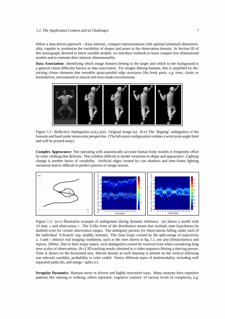
Data Association: Identifying which image features belong to the target and which to the background isa general vision difficulty known as data association. For images filming humans, this is amplified by dis-tracting clutter elements that resemble quasi-parallel edge structures like body parts, e.g. trees, chairs orbookshelves, encountered in natural and man-made environments.
Figure 1.1: Reflective Ambiguities (a,b,c,d,e). Original image (a). (b-e) The ‘flipping’ ambiguities of theforearm and hand under monocular perspective. (The left-most configuration violates a wrist joint-angle limitand will be pruned away).
Complex Appearance: Not operating with anatomically accurate human body models is frequently offsetby outer clothing that deforms. This exhibits difficult to model variations in shape and appearance. Lightingchange is another factor of variability. Artificial edges created by cast shadows and inter-frame lightingvariations lead to difficult to predict patterns of image texture.
Frame Number
Rig
ht
Th
igh
Jo
int
An
gle
aro
un
d X
−a
xis
20 40 60 80 100 120 140 160 180 200 220 240 260
140
100
60
20
−20
−60
−100
−140
−180 0
0.05
0.1
0.15
0.2
Frame Number
Rig
ht F
oo
t Jo
int A
ng
le a
rou
nd
Y−
axis
20 40 60 80 100 120 140 160 180 200 220 240 260
140
100
60
20
−20
−60
−100
−140
−180 0
0.02
0.04
0.06
0.08
0.1
0.12
0.14
0.16
0.18
Figure 1.2: (a-c) Illustrative example of ambiguities during dynamic inference. (a) shows a model with1d state x and observation r. The S-like form of the distribution means that multiple state hypotheses (indashed) exist for certain observation ranges. The ambiguity persists for observations falling under each ofthe individual ‘S-branch’ (up, middle, bottom). The close loops created by the split-merge of trajectoriesa, b and c abstract real imaging conditions, such as the ones shown in fig. 1.1, see also [Sminchisescu andJepson, 2004a]. Due to their loopy nature, such ambiguities cannot be resolved even when considering longtime-scales of observations. (b-c) 3D tracking results obtained in a video sequence filming a dancing person.Time is shown on the horizontal axis, filtered density at each timestep is plotted on the vertical (showingone selected variable), probability is color coded. Notice different types of multimodality, including wellseparated paths (b), and merge / splits (c).
Irregular Dynamics: Humans move in diverse and highly structured ways. Many motions have repetitivepatterns like running or walking, others represent ‘cognitive routines’ of various levels of complexity, e.g.
8 Chapter 1. Contributions and Roadmap
gestures during a discussion, or crossing the street by checking for cars to the left and to the right, or officeactivities centered around sitting, talking to the phone, typing and checking e-mail. It is natural to hopethat if such routines were identified in the image, they could provide strong constraints for tracking andreconstruction with image measurements serving merely to adjust and fine tune the estimate. However,human activities are not simply preprogrammed – they are parameterized by many cognitive and externalun-expected variables (goals, locations of objects or obstacles) that are challenging to recover from imagesand several activities or motions are often combined.
Depth Uncertainty: A fundamental computer vision difficulty is the loss of information due to image acqui-sition – projecting the 3D world into images suppresses depth. While depth parameters remain in principleobservable in perspective projection, they are difficult to estimate, even for close-up views. A quantitativemeasure of hardness is given by the ill-conditioning typical of the Jacobian matrix of the model-to-imagetransformation, where a range of singular values ≈ 103 is common. For point-and-link kinematic chainsviewed in perspective, the non-uniqueness of estimating 3D pose in monocular images is apparent in the‘forward-backward ambiguities’ produced when positioning the links, symmetrically, forwards or backwards,with respect to the camera ‘rays of sight’ (see fig. 1.1).
In generative models, ambiguities manifest as multiple peaks of somewhat comparable magnitude in theobservation likelihood. The distinction between a global and a local optimum becomes narrow and unreliabledue to modeling error – for predictable performance it is wiser to consider all optima that are sufficientlygood. For discriminative models, depth uncertainty leads to multivalued image-to-3D relations that defeatfunction approximation based on neural networks or regression. Perhaps surprisingly, the ambiguities aretemporally persistent not only for models with smooth dynamics [Sminchisescu and Jepson, 2004a] but alsofor constrained dynamical models learned from typical human motions [Sminchisescu and Jepson, 2004b],see figures 1.2, 1.4, 1.17 and 1.2. Often, the information critical to break-down ambiguity, e.g. fine bodyshape or shadows is unreliable due to modeling error (folding cloth) or unavailable, being eliminated as anuisance factor in the design of image features invariant to lighting. While more expressive features canbe considered, it remains delicate — and a good avenue for future work – to design encodings and featureselection schemes that are both repeatable and offer better selectivity-invariance trade-offs.
Incomplete Observability: Difficulties arise when a subset of the model state variables cannot be directlyinferred from image observations. This includes but is by no means limited to kinematic and depth ambi-guities. Observability depends on the design of the model and type of image features used and ultimatelyon the evidence available in the specific image inputs. In particular, given the flexible structure of an artic-ulated body, self-occlusion between different body parts occurs frequently in monocular views. Occlusionproduces observation ambiguities! Occlusion is also typical of real scenes containing people filmed in naturalor man-made environments. In order to avoid singularities or arbitrary default estimates, it is appropriate touse prior-knowledge acquired during model learning in order to constrain the uncertainty of occluded bodyparts, based on observations collected at visible parts. Missing states can be conditionally filled-in usingcorrelation models learned from a typical training set of natural human motions.
For generative models, occlusion raises the issue of constructing an observation likelihood that real-istically reflects the probability of different configurations under partial occlusion and viewpoint change.Independence assumptions are often used to fuse likelihoods from different measurements, but this is not anadequate model for occlusion, which is a coherent phenomenon. For realistic likelihoods, spatial correla-tions among measurements need to be incorporated, but this has non-trivial implications for the tractabilityof likelihood computation.
1.3 Contributions
1.3.1 Optimization and Sampling Algorithms
The first section of this monograph discusses inference algorithms and their application to the problem oftracking and reconstructing generative tree-structured kinematic models. The models are sufficiently flexibleto represent not only the human body but other articulated biological forms like animals. Fitting generative
1.3. Contributions 9
models requires a computationally intensive search-by-alignment loop where the appearance of a structural3D (or 2d) model is matched to the image evidence. The quality of fit is encoded in the observation likelihood(or model-image matching) function.
Kinematic Jump Sampling (KJS)
A major difficulty especially when tracking articulated chains from sequences of monocular images is thenear non-observability of kinematic degrees of freedom that generate motion in depth. For known link (bodysegment) lengths, the strict non-observabilities reduce to twofold ‘forwards/backwards flipping’ ambiguitiesfor each link. These imply 2# links formal inverse kinematics solutions for the full model, and hence linkedgroups ofO(2# links) local minima in the model-image matching cost function. Choosing the wrong minimumleads to rapid mistracking, so for reliable tracking, rapid methods of investigating alternative minima withina group are needed. Existing approaches to solving the problem, including our own prior work (cca. the year2002), have used generic search methods that do not exploit the specific problem structure.
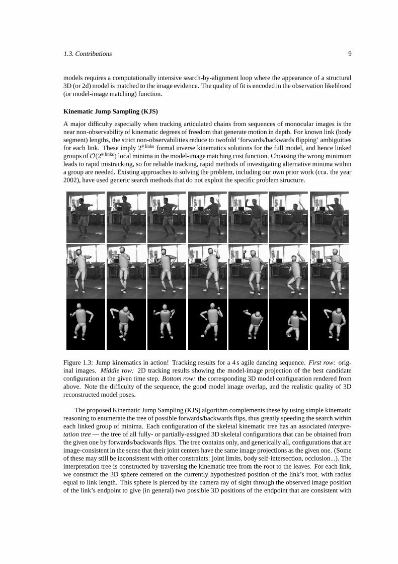
Figure 1.3: Jump kinematics in action! Tracking results for a 4 s agile dancing sequence. First row: orig-inal images. Middle row: 2D tracking results showing the model-image projection of the best candidateconfiguration at the given time step. Bottom row: the corresponding 3D model configuration rendered fromabove. Note the difficulty of the sequence, the good model image overlap, and the realistic quality of 3Dreconstructed model poses.
The proposed Kinematic Jump Sampling (KJS) algorithm complements these by using simple kinematicreasoning to enumerate the tree of possible forwards/backwards flips, thus greatly speeding the search withineach linked group of minima. Each configuration of the skeletal kinematic tree has an associated interpre-tation tree — the tree of all fully- or partially-assigned 3D skeletal configurations that can be obtained fromthe given one by forwards/backwards flips. The tree contains only, and generically all, configurations that areimage-consistent in the sense that their joint centers have the same image projections as the given one. (Someof these may still be inconsistent with other constraints: joint limits, body self-intersection, occlusion...). Theinterpretation tree is constructed by traversing the kinematic tree from the root to the leaves. For each link,we construct the 3D sphere centered on the currently hypothesized position of the link’s root, with radiusequal to link length. This sphere is pierced by the camera ray of sight through the observed image positionof the link’s endpoint to give (in general) two possible 3D positions of the endpoint that are consistent with
10 Chapter 1. Contributions and Roadmap
the image observation and the hypothesized parent position. Joint angles are then recovered for each positionusing simple inverse kinematics. If the ray misses the sphere, the parent hypothesis was inconsistent with theimage data and the branch can be pruned.
The method can be used either deterministically, or within stochastic ‘jump-diffusion’ style recursivetracking frameworks. Because the jumps only explore kinematic optima, a complementary search method(e.g. Covariance Scaled Sampling [Sminchisescu and Triggs, 2003b]) is necessary in order to handle imageassignment ambiguities. In practice, a KJS-based tracker turns out to be effective and can competentlyreconstruct difficult motions of dancing people. The work appeared at the IEEE International Conference onComputer Vision and Pattern Recognition (CVPR) [Sminchisescu and Triggs, 2003a].
Variational Mixture Smoothing (VMS)
The second inference method we propose, Variational Mixture Smoothing (VMS), is used to compute jointstate, smoothed, density estimates for non-linear dynamical systems in a Bayesian setting. Visual trackingproblems are frequently formulated as recursive probabilistic inference over time, but there are compara-tively few mixture smoothers adapted for weakly identifiable models that arise in applications with sustainedmultimodality, e.g. monocular 3D human tracking. In this case the model state distribution at each timestepis persistently rather than transiently multi-modal, hence the effect is not alleviated by smoothing – the ob-servation of an entire video sequence and the back-propagation of evidence that becomes available forwardin time w.r.t. to the particular timestep. The non-linear non-Gaussian setting we study excludes, in prin-ciple, the single-hypothesis iterated Kalman smoothers, whereas flexible MCMC methods or sample basedparticle smoothers, albeit applicable, encounter computational difficulties: accurately locating an exponen-tial number of probable high-dimensional trajectories, rapidly mixing between those or resampling probableconfigurations missed during filtering. VMS progressively refines a mixture approximation of the target jointdistribution at all timesteps by combining polynomial time search over the network of temporal model-imagematching cost optima, maximum a-posteriori continuous trajectory estimates, and variational Bayesian ad-justment. (The algorithm can use the results of a filtering method, e.g. KJS, or a static pose estimator runindependently on each image in a sequence.) An illustration of the algorithm in operation, where it estimatesmultiple 3D human pose trajectories from monocular video, is given in fig. 1.17. The method is useful eitherstand-alone, or within a Maximum Likelihood learning procedure, where the model parameters are trained tomake one of the trajectories, corresponding to the ground truth, significantly more probable than any compet-ing but perceptually ‘incorrect’ ones, see fig. 1.6 and the next section. The work was presented at the IEEEInternational Conference on Computer Vision and Pattern Recognition (CVPR) [Sminchisescu and Jepson,2004a].
Generalized Darting Monte Carlo (GD)
Many vision or machine learning problems are formulated as statistical calculations that require samplingfrom a complex multi-modal distribution. One flexible method to achieve this goal is Markov Chain MonteCarlo (MCMC). It is well known, however, that MCMC samplers have difficulty in mixing from one modeto the other because it typically takes many steps of very low probability to make the trip [Neal, 1993,Celeux et al., 2000]. Recent improvements designed to combat random walk behavior, like Hybrid MonteCarlo and over-relaxation [Duane et al., 1987, Neal, 1993] do not solve this problem when modes are sep-arated by high energy barriers. In a third algorithm, given in the inference section, we show how to exploitknowledge of the location of the modes (as computed e.g. by KJS or VMS) to design a MCMC samplerbased on mode-hopping moves that satisfy detailed balance, yet has significantly better mixing times thanless-informed samplers. The proposed Generalized Darting (GD) algorithm explores individual modal dis-tributions through local MCMC moves (e.g. diffusion or Hybrid Monte Carlo) but in addition also representsthe relative strengths of the different modes correctly using a set of global moves. This ‘mode-hopping’MCMC sampler can be viewed as a generalization of the darting method [Andricioaiei et al., 2001]. We an-alyze the method, prove detailed balance, give an auxiliary variable formulation, and compare performancewith independence samplers and spherical darting methods (see also fig. 1.5). We illustrate the algorithm forlearning Markov random fields that encode tree-structured spatial constraints (in this case, GD provides a
1.3. Contributions 11
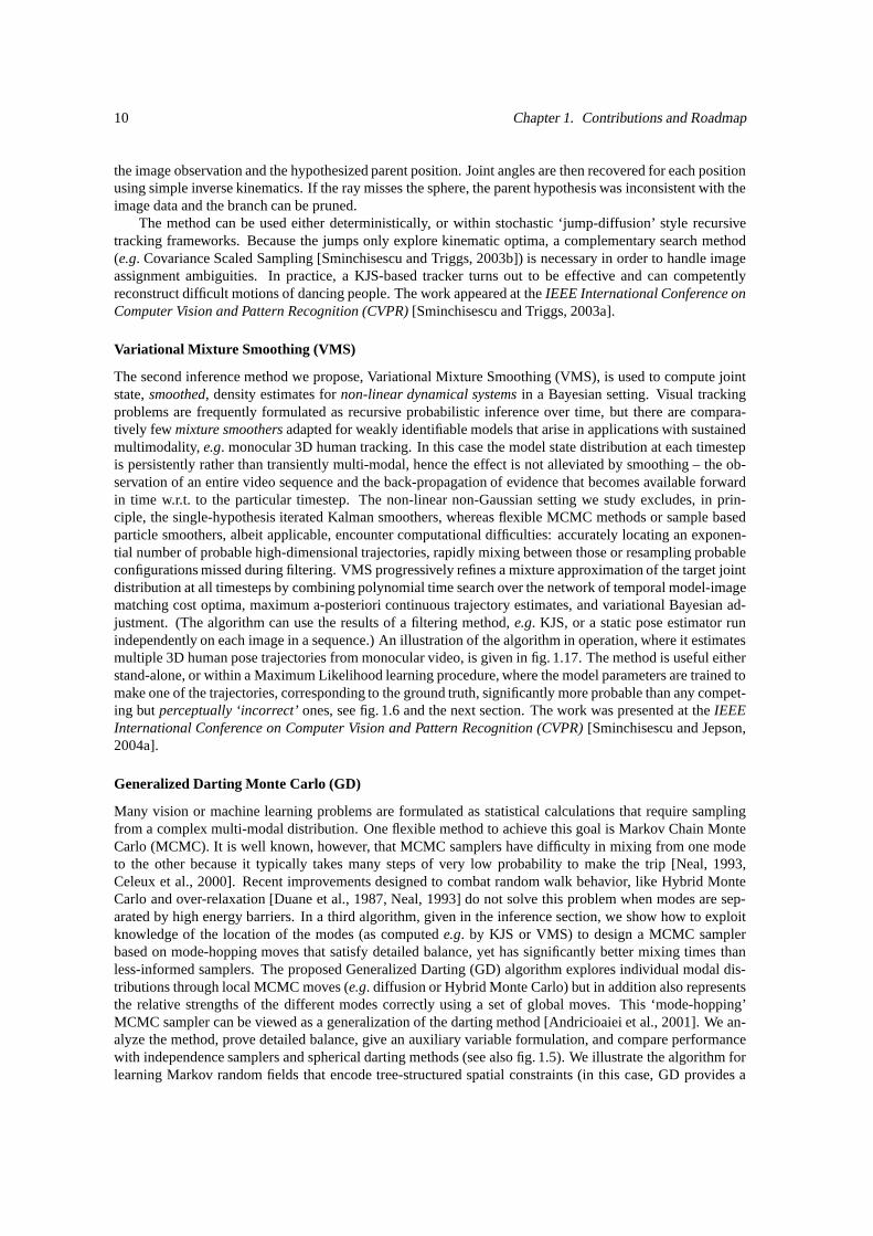
Figure 1.4: Variational smoothing computes multiple optimal trajectories given an entire image sequence (theestimates at each timespet are optimal w.r.t. both the past and the future measurements. 3D reconstructionresults based on a 2.5s video sequence. First row: original Sequence, Second row: one probable model statesequence projected onto image at selected time-steps. Third row: One smoothed reconstructed 3D trajectoryviewed from a synthetic viewpoint. Forth row: alternative 3D trajectory. Although in the beginning the twotrajectories are qualitatively similar, they diverge significantly during the second half of the sequence. Notethe different tilt of the torso and the significant difference in the left arm positioning that followed a smoothtrajectory corresponding to a reflective ambiguity w.r.t. the camera. Each trajectory is smooth and fits theimage sequence well, i.e. it is a local optimum in the model trajectory distribution, conditioned on the imagesequence. This behavior is typical for the problem and such consistent trajectories in the order of tens arecommon.
sample-based estimate to approximate the model partition function), and for inferring 3D human body posedistributions from 2D image information, fig. 1.6. The work appeared at the International Conference onArtificial Intelligence and Statistics (AISTATS) [Sminchisescu and Welling, 2007].
1.3.2 Discriminative and Conditional Models
This section of the monograph consists of chapters that describe both spatial and temporal conditional mod-els, with applications to 3D reconstruction and tracking, action recognition, object detection and localization.
12 Chapter 1. Contributions and Roadmap
4
5
6
7
8
9
10
11
100 200 300 400 500 600 700
Ener
gy
Iterations
Classical Hybrid MCMC
4
5
6
7
8
9
10
11
100 200 300 400 500 600 700
Ener
gy
Iterations
Spherical Darted Hybrid MCMC
4
5
6
7
8
9
10
11
100 200 300 400 500 600 700
Ener
gy
Iterations
Geralized Darted Hybrid MCMC
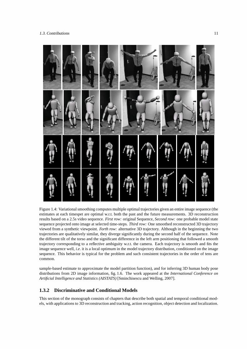
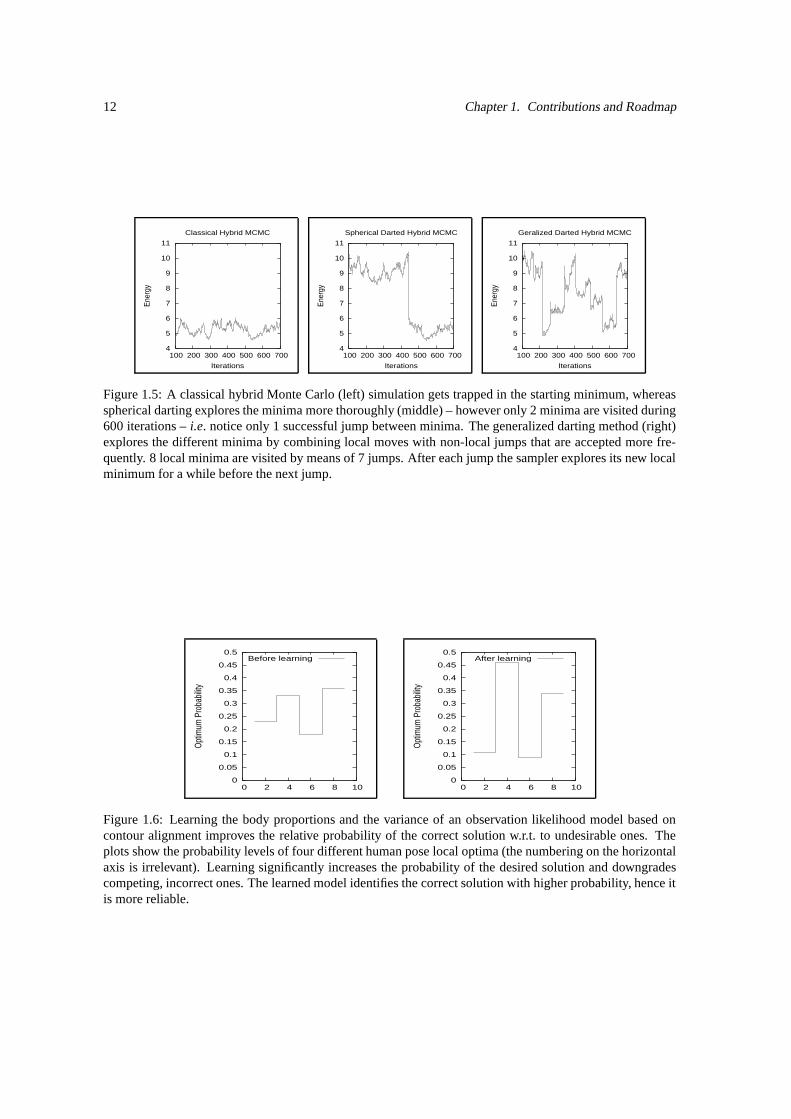
Figure 1.5: A classical hybrid Monte Carlo (left) simulation gets trapped in the starting minimum, whereasspherical darting explores the minima more thoroughly (middle) – however only 2 minima are visited during600 iterations – i.e. notice only 1 successful jump between minima. The generalized darting method (right)explores the different minima by combining local moves with non-local jumps that are accepted more fre-quently. 8 local minima are visited by means of 7 jumps. After each jump the sampler explores its new localminimum for a while before the next jump.
0
0.05
0.1
0.15
0.2
0.25
0.3
0.35
0.4
0.45
0.5
0 2 4 6 8 10
Opt
imum
Pro
babi
lity
Before learning
0
0.05
0.1
0.15
0.2
0.25
0.3
0.35
0.4
0.45
0.5
0 2 4 6 8 10
Opt
imum
Pro
babi
lity
After learning
Figure 1.6: Learning the body proportions and the variance of an observation likelihood model based oncontour alignment improves the relative probability of the correct solution w.r.t. to undesirable ones. Theplots show the probability levels of four different human pose local optima (the numbering on the horizontalaxis is irrelevant). Learning significantly increases the probability of the desired solution and downgradescompeting, incorrect ones. The learned model identifies the correct solution with higher probability, hence itis more reliable.
1.3. Contributions 13
In addition, we study hierarchical image representations and strategies for training models more flexibly:from supervised to semi-supervised and unsupervised learning methods.
BM3E: Discriminative Density Propagation for Continuous Time Series Models
The inferential difficulties encountered with generative models and high-dimensional state spaces asked forbetter ways to address the complexity of the problem, and occasionally challenged the approach entirely: Isthis the right problem to solve? Why should one focus on modeling the observation, when the ultimate goalis state prediction? This calculation appears to require models with the opposite directionality, that conditionon the observation rather than modeling it.
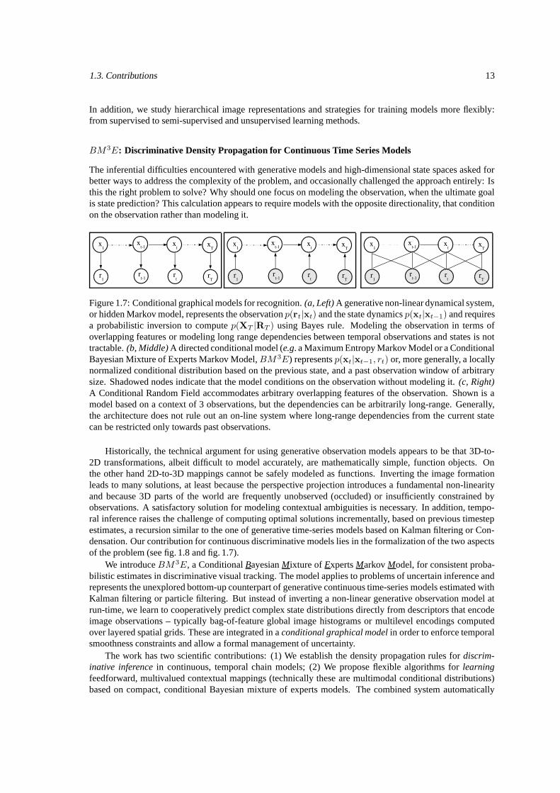
Figure 1.7: Conditional graphical models for recognition. (a, Left) A generative non-linear dynamical system,or hidden Markov model, represents the observation p(rt|xt) and the state dynamics p(xt|xt−1) and requiresa probabilistic inversion to compute p(XT |RT ) using Bayes rule. Modeling the observation in terms ofoverlapping features or modeling long range dependencies between temporal observations and states is nottractable. (b, Middle) A directed conditional model (e.g. a Maximum Entropy Markov Model or a ConditionalBayesian Mixture of Experts Markov Model,BM 3E) represents p(xt|xt−1, rt) or, more generally, a locallynormalized conditional distribution based on the previous state, and a past observation window of arbitrarysize. Shadowed nodes indicate that the model conditions on the observation without modeling it. (c, Right)A Conditional Random Field accommodates arbitrary overlapping features of the observation. Shown is amodel based on a context of 3 observations, but the dependencies can be arbitrarily long-range. Generally,the architecture does not rule out an on-line system where long-range dependencies from the current statecan be restricted only towards past observations.
Historically, the technical argument for using generative observation models appears to be that 3D-to-2D transformations, albeit difficult to model accurately, are mathematically simple, function objects. Onthe other hand 2D-to-3D mappings cannot be safely modeled as functions. Inverting the image formationleads to many solutions, at least because the perspective projection introduces a fundamental non-linearityand because 3D parts of the world are frequently unobserved (occluded) or insufficiently constrained byobservations. A satisfactory solution for modeling contextual ambiguities is necessary. In addition, tempo-ral inference raises the challenge of computing optimal solutions incrementally, based on previous timestepestimates, a recursion similar to the one of generative time-series models based on Kalman filtering or Con-densation. Our contribution for continuous discriminative models lies in the formalization of the two aspectsof the problem (see fig. 1.8 and fig. 1.7).
We introduce BM3E, a Conditional Bayesian Mixture of Experts Markov Model, for consistent proba-bilistic estimates in discriminative visual tracking. The model applies to problems of uncertain inference andrepresents the unexplored bottom-up counterpart of generative continuous time-series models estimated withKalman filtering or particle filtering. But instead of inverting a non-linear generative observation model atrun-time, we learn to cooperatively predict complex state distributions directly from descriptors that encodeimage observations – typically bag-of-feature global image histograms or multilevel encodings computedover layered spatial grids. These are integrated in a conditional graphical model in order to enforce temporalsmoothness constraints and allow a formal management of uncertainty.
The work has two scientific contributions: (1) We establish the density propagation rules for discrim-inative inference in continuous, temporal chain models; (2) We propose flexible algorithms for learningfeedforward, multivalued contextual mappings (technically these are multimodal conditional distributions)based on compact, conditional Bayesian mixture of experts models. The combined system automatically
14 Chapter 1. Contributions and Roadmap
0 0.5 1 1.50
0.2
0.4
0.6
0.8
1
1.2
1.4
Input r
Outp
ut x
Cluster 1Cluster 2Cluster 3Regr. 1Regr. 2Regr. 3
0 0.2 0.4 0.6 0.8 10
0.2
0.4
0.6
0.8
1
Input r
Pro
babili
ty
Cl. 1 DensityCl. 2 DensityCl. 3 DensityCl. 1 WeightCl. 2 WeightCl. 3 Weight
0 0.5 1 1.50
0.2
0.4
0.6
0.8
1
Input r
Outp
ut x
Cluster 1Cluster 2Cluster 3 Single Regressor
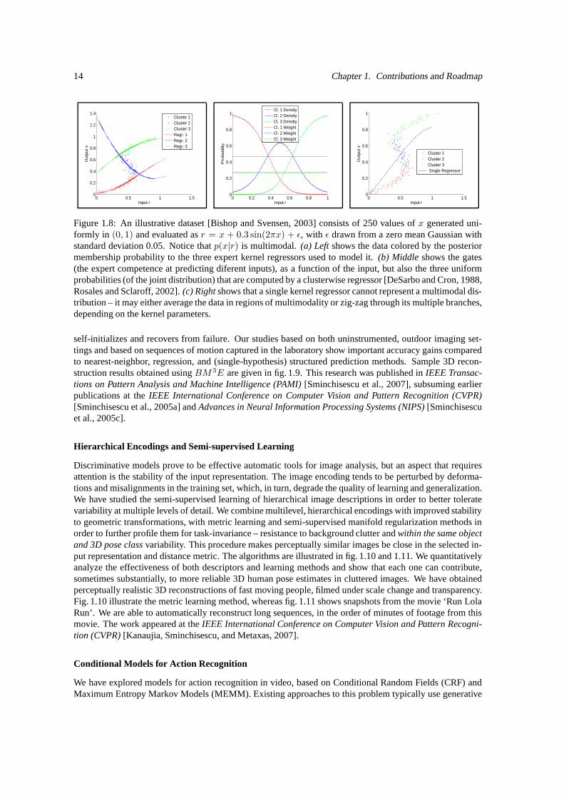
Figure 1.8: An illustrative dataset [Bishop and Svensen, 2003] consists of 250 values of x generated uni-formly in (0, 1) and evaluated as r = x + 0.3 sin(2πx) + ε, with ε drawn from a zero mean Gaussian withstandard deviation 0.05. Notice that p(x|r) is multimodal. (a) Left shows the data colored by the posteriormembership probability to the three expert kernel regressors used to model it. (b) Middle shows the gates(the expert competence at predicting diferent inputs), as a function of the input, but also the three uniformprobabilities (of the joint distribution) that are computed by a clusterwise regressor [DeSarbo and Cron, 1988,Rosales and Sclaroff, 2002]. (c) Right shows that a single kernel regressor cannot represent a multimodal dis-tribution – it may either average the data in regions of multimodality or zig-zag through its multiple branches,depending on the kernel parameters.
self-initializes and recovers from failure. Our studies based on both uninstrumented, outdoor imaging set-tings and based on sequences of motion captured in the laboratory show important accuracy gains comparedto nearest-neighbor, regression, and (single-hypothesis) structured prediction methods. Sample 3D recon-struction results obtained using BM 3E are given in fig. 1.9. This research was published in IEEE Transac-tions on Pattern Analysis and Machine Intelligence (PAMI) [Sminchisescu et al., 2007], subsuming earlierpublications at the IEEE International Conference on Computer Vision and Pattern Recognition (CVPR)[Sminchisescu et al., 2005a] and Advances in Neural Information Processing Systems (NIPS) [Sminchisescuet al., 2005c].
Hierarchical Encodings and Semi-supervised Learning
Discriminative models prove to be effective automatic tools for image analysis, but an aspect that requiresattention is the stability of the input representation. The image encoding tends to be perturbed by deforma-tions and misalignments in the training set, which, in turn, degrade the quality of learning and generalization.We have studied the semi-supervised learning of hierarchical image descriptions in order to better toleratevariability at multiple levels of detail. We combine multilevel, hierarchical encodings with improved stabilityto geometric transformations, with metric learning and semi-supervised manifold regularization methods inorder to further profile them for task-invariance – resistance to background clutter and within the same objectand 3D pose class variability. This procedure makes perceptually similar images be close in the selected in-put representation and distance metric. The algorithms are illustrated in fig. 1.10 and 1.11. We quantitativelyanalyze the effectiveness of both descriptors and learning methods and show that each one can contribute,sometimes substantially, to more reliable 3D human pose estimates in cluttered images. We have obtainedperceptually realistic 3D reconstructions of fast moving people, filmed under scale change and transparency.Fig. 1.10 illustrate the metric learning method, whereas fig. 1.11 shows snapshots from the movie ‘Run LolaRun’. We are able to automatically reconstruct long sequences, in the order of minutes of footage from thismovie. The work appeared at the IEEE International Conference on Computer Vision and Pattern Recogni-tion (CVPR) [Kanaujia, Sminchisescu, and Metaxas, 2007].
Conditional Models for Action Recognition
We have explored models for action recognition in video, based on Conditional Random Fields (CRF) andMaximum Entropy Markov Models (MEMM). Existing approaches to this problem typically use generative
1.3. Contributions 15
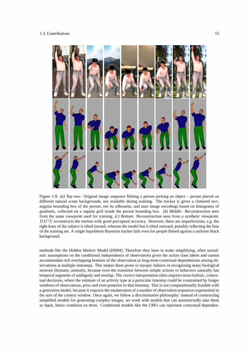
Figure 1.9: (a) Top row: Original image sequence filming a person picking an object – person placed ondifferent natural scene backgrounds, not available during training. The tracker is given a cluttered rect-angular bounding box of the person, not its silhouette, and uses image encodings based on histograms ofgradients, collected on a regular grid inside the person bounding box. (b) Middle: Reconstruction seenfrom the same viewpoint used for training, (c) Bottom: Reconstruction seen from a synthetic viewpoint.BM3E reconstructs the motion with good perceptual accuracy. However, there are imperfections, e.g. theright knee of the subject is tilted inward, whereas the model has it tilted outward, possibly reflecting the biasof the training set. A single hypothesis Bayesian tracker fails even for people filmed against a uniform blackbackground.
methods like the Hidden Markov Model (HMM). Therefore they have to make simplifying, often unreal-istic assumptions on the conditional independence of observations given the action class labels and cannotaccommodate rich overlapping features of the observation or long-term contextual dependencies among ob-servations at multiple timesteps. This makes them prone to myopic failures in recognizing many biologicalmotions (humans, animals), because even the transition between simple actions or behaviors naturally hastemporal segments of ambiguity and overlap. The correct interpretation often requires more holistic, contex-tual decisions, where the estimate of an activity type at a particular timestep could be constrained by longerwindows of observations, prior and even posterior to that timestep. This is not computationally feasible witha generative model, because it requires the enumeration of a number of observation sequences exponential inthe size of the context window. Once again, we follow a discriminative philosophy: instead of constructingsimplified models for generating complex images, we work with models that can unrestrictedly take themas input, hence condition on them. Conditional models like the CRFs can represent contextual dependen-
16 Chapter 1. Contributions and Roadmap
Before RCA
After RCA
CleanQRealReal
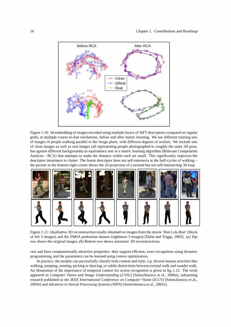
Figure 1.10: 3d embedding of images encoded using multiple layers of SIFT descriptors computed on regulargrids, at multiple coarse-to-fine resolutions, before and after metric learning. We use different training setsof images of people walking parallel to the image plane, with different degrees of realism. We include setsof clean images as well as real images (all representing people photographed in roughly the same 3D pose,but against different backgrounds) as equivalence sets in a metric learning algorithm (Relevant ComponentsAnalysis - RCA) that attempts to make the distance within each set small. This significantly improves thedescriptor invariance to clutter. The learnt descriptor does not self-intersects at the half-cycles of walking –the picture in the bottom-right corner shows the 2d projection of a twisted but not self-intersecting 3d loop.
Figure 1.11: Qualitative 3D reconstruction results obtained on images from the movie ‘Run Lola Run’ (blockof left 5 images) and the INRIA pedestrian dataset (rightmost 3 images) [Dalal and Triggs, 2005]. (a) Toprow shows the original images, (b) Bottom row shows automatic 3D reconstructions.
cies and have computationally attractive properties: they support efficient, exact recognition using dynamicprogramming, and the parameters can be learned using convex optimization.
In practice, the models can successfully classify both content and style, e.g. diverse human activities likewalking, jumping, running, picking or dancing, or subtle distinctions between normal walk and wander walk.An illustration of the importance of temporal context for action recognition is given in fig. 1.12. The workappeared in Computer Vision and Image Understanding (CVIU) [Sminchisescu et al., 2006a], subsumingresearch published at the IEEE International Conference on Computer Vision (ICCV) [Sminchisescu et al.,2005b] and Advances in Neural Processing Systems (NIPS) [Sminchisescu et al., 2005c].
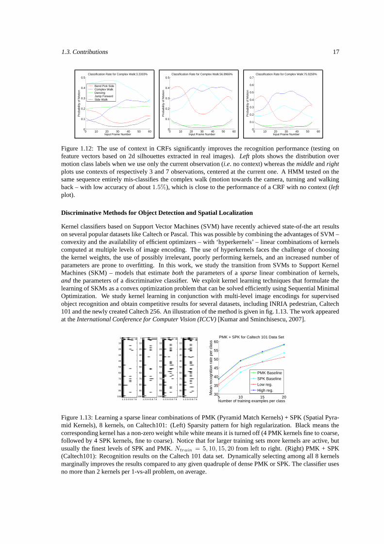
1.3. Contributions 17
0 10 20 30 40 50 600
0.1
0.2
0.3
0.4
0.5
Input Frame Number
Pro
babi
lity
of M
otio
n
Classification Rate for Complex Walk:3.3333%
Bend Pick SideComplex WalkDancingJump ForwardSide Walk
0 10 20 30 40 50 600
0.1
0.2
0.3
0.4
0.5
Input Frame Number
Pro
babi
lity
of M
otio
n
Classification Rate for Complex Walk:56.8966%
0 10 20 30 40 50 600
0.1
0.2
0.3
0.4
0.5
0.6
0.7
Input Frame Number
Pro
babi
lity
of M
otio
n
Classification Rate for Complex Walk:75.9259%
Figure 1.12: The use of context in CRFs significantly improves the recognition performance (testing onfeature vectors based on 2d silhouettes extracted in real images). Left plots shows the distribution overmotion class labels when we use only the current observation (i.e. no context) whereas the middle and rightplots use contexts of respectively 3 and 7 observations, centered at the current one. A HMM tested on thesame sequence entirely mis-classifies the complex walk (motion towards the camera, turning and walkingback – with low accuracy of about 1.5%), which is close to the performance of a CRF with no context (leftplot).
Discriminative Methods for Object Detection and Spatial Localization
Kernel classifiers based on Support Vector Machines (SVM) have recently achieved state-of-the art resultson several popular datasets like Caltech or Pascal. This was possible by combining the advantages of SVM –convexity and the availability of efficient optimizers – with ‘hyperkernels’ – linear combinations of kernelscomputed at multiple levels of image encoding. The use of hyperkernels faces the challenge of choosingthe kernel weights, the use of possibly irrelevant, poorly performing kernels, and an increased number ofparameters are prone to overfitting. In this work, we study the transition from SVMs to Support KernelMachines (SKM) – models that estimate both the parameters of a sparse linear combination of kernels,and the parameters of a discriminative classifier. We exploit kernel learning techniques that formulate thelearning of SKMs as a convex optimization problem that can be solved efficiently using Sequential MinimalOptimization. We study kernel learning in conjunction with multi-level image encodings for supervisedobject recognition and obtain competitive results for several datasets, including INRIA pedestrian, Caltech101 and the newly created Caltech 256. An illustration of the method is given in fig. 1.13. The work appearedat the International Conference for Computer Vision (ICCV) [Kumar and Sminchisescu, 2007].
1 2 3 4 5 6 7 8
1
10
20
30
40
50
60
70
80
90
1001 2 3 4 5 6 7 8
1
10
20
30
40
50
60
70
80
90
1001 2 3 4 5 6 7 8
1
10
20
30
40
50
60
70
80
90
1001 2 3 4 5 6 7 8
1
10
20
30
40
50
60
70
80
90
100 5 10 15 2030
35
40
45
50
55
60
Number of training examples per class
Mea
n re
cogn
ition
rat
e pe
r cl
ass
PMK + SPK for Caltech 101 Data Set
PMK Baseline
SPK Baseline
Low reg.
High reg.
Figure 1.13: Learning a sparse linear combinations of PMK (Pyramid Match Kernels) + SPK (Spatial Pyra-mid Kernels), 8 kernels, on Caltech101: (Left) Sparsity pattern for high regularization. Black means thecorresponding kernel has a non-zero weight while white means it is turned off (4 PMK kernels fine to coarse,followed by 4 SPK kernels, fine to coarse). Notice that for larger training sets more kernels are active, butusually the finest levels of SPK and PMK. Ntrain = 5, 10, 15, 20 from left to right. (Right) PMK + SPK(Caltech101): Recognition results on the Caltech 101 data set. Dynamically selecting among all 8 kernelsmarginally improves the results compared to any given quadruple of dense PMK or SPK. The classifier usesno more than 2 kernels per 1-vs-all problem, on average.
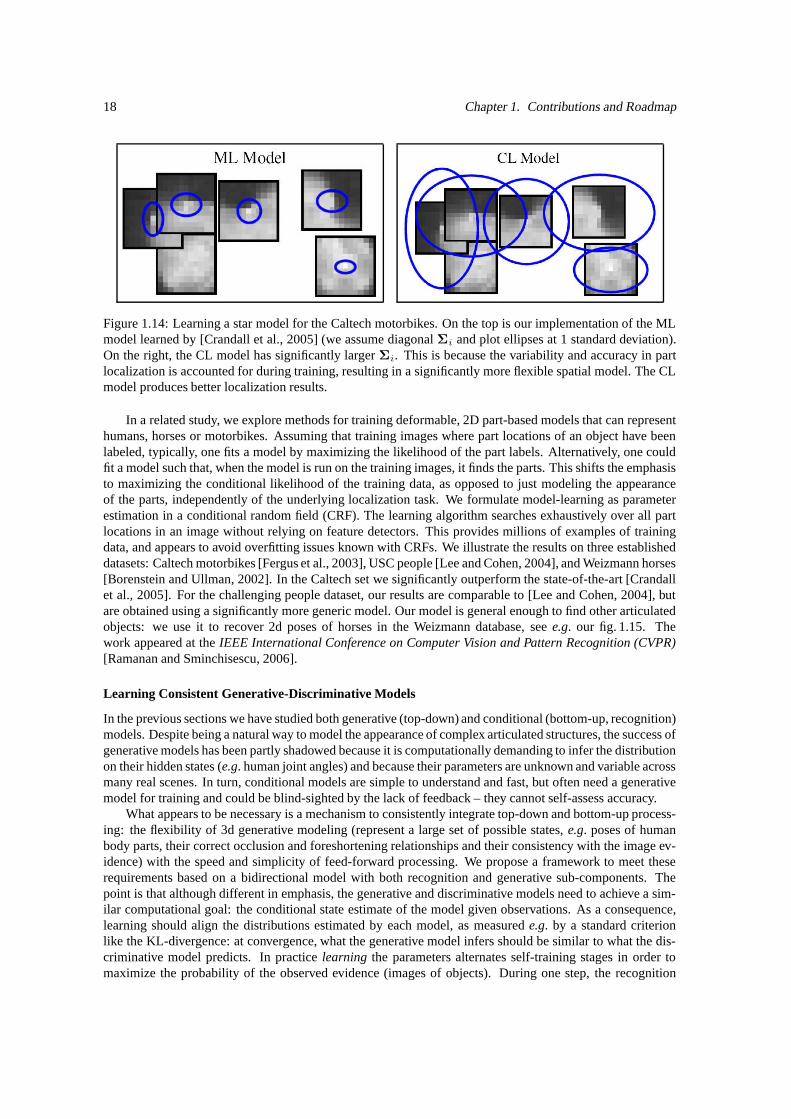
18 Chapter 1. Contributions and Roadmap
Figure 1.14: Learning a star model for the Caltech motorbikes. On the top is our implementation of the MLmodel learned by [Crandall et al., 2005] (we assume diagonal Σi and plot ellipses at 1 standard deviation).On the right, the CL model has significantly larger Σi. This is because the variability and accuracy in partlocalization is accounted for during training, resulting in a significantly more flexible spatial model. The CLmodel produces better localization results.
In a related study, we explore methods for training deformable, 2D part-based models that can representhumans, horses or motorbikes. Assuming that training images where part locations of an object have beenlabeled, typically, one fits a model by maximizing the likelihood of the part labels. Alternatively, one couldfit a model such that, when the model is run on the training images, it finds the parts. This shifts the emphasisto maximizing the conditional likelihood of the training data, as opposed to just modeling the appearanceof the parts, independently of the underlying localization task. We formulate model-learning as parameterestimation in a conditional random field (CRF). The learning algorithm searches exhaustively over all partlocations in an image without relying on feature detectors. This provides millions of examples of trainingdata, and appears to avoid overfitting issues known with CRFs. We illustrate the results on three establisheddatasets: Caltech motorbikes [Fergus et al., 2003], USC people [Lee and Cohen, 2004], and Weizmann horses[Borenstein and Ullman, 2002]. In the Caltech set we significantly outperform the state-of-the-art [Crandallet al., 2005]. For the challenging people dataset, our results are comparable to [Lee and Cohen, 2004], butare obtained using a significantly more generic model. Our model is general enough to find other articulatedobjects: we use it to recover 2d poses of horses in the Weizmann database, see e.g. our fig. 1.15. Thework appeared at the IEEE International Conference on Computer Vision and Pattern Recognition (CVPR)[Ramanan and Sminchisescu, 2006].
Learning Consistent Generative-Discriminative Models
In the previous sections we have studied both generative (top-down) and conditional (bottom-up, recognition)models. Despite being a natural way to model the appearance of complex articulated structures, the success ofgenerative models has been partly shadowed because it is computationally demanding to infer the distributionon their hidden states (e.g. human joint angles) and because their parameters are unknown and variable acrossmany real scenes. In turn, conditional models are simple to understand and fast, but often need a generativemodel for training and could be blind-sighted by the lack of feedback – they cannot self-assess accuracy.
What appears to be necessary is a mechanism to consistently integrate top-down and bottom-up process-ing: the flexibility of 3d generative modeling (represent a large set of possible states, e.g. poses of humanbody parts, their correct occlusion and foreshortening relationships and their consistency with the image ev-idence) with the speed and simplicity of feed-forward processing. We propose a framework to meet theserequirements based on a bidirectional model with both recognition and generative sub-components. Thepoint is that although different in emphasis, the generative and discriminative models need to achieve a sim-ilar computational goal: the conditional state estimate of the model given observations. As a consequence,learning should align the distributions estimated by each model, as measured e.g. by a standard criterionlike the KL-divergence: at convergence, what the generative model infers should be similar to what the dis-criminative model predicts. In practice learning the parameters alternates self-training stages in order tomaximize the probability of the observed evidence (images of objects). During one step, the recognition
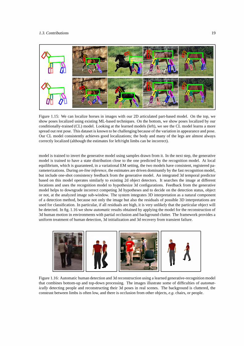
1.3. Contributions 19
Figure 1.15: We can localize horses in images with our 2D articulated part-based model. On the top, weshow poses localized using existing ML-based techniques. On the bottom, we show poses localized by ourconditionally-trained (CL) model. Looking at the learned models (left), we see the CL model learns a morespread out rest pose. This dataset is known to be challenging because of the variation in appearance and pose.Our CL model consistently achieves good localizations; the body and many of the legs are almost alwayscorrectly localized (although the estimates for left/right limbs can be incorrect).
model is trained to invert the generative model using samples drawn from it. In the next step, the generativemodel is trained to have a state distribution close to the one predicted by the recognition model. At localequilibrium, which is guaranteed, in a variational EM setting, the two models have consistent, registered pa-rameterizations. During on-line inference, the estimates are driven dominantly by the fast recognition model,but include one-shot consistency feedback from the generative model. An integrated 3d temporal predictorbased on this model operates similarly to existing 2d object detectors. It searches the image at differentlocations and uses the recognition model to hypothesize 3d configurations. Feedback from the generativemodel helps to downgrade incorrect competing 3d hypotheses and to decide on the detection status, objector not, at the analyzed image sub-window. The system integrates 3D interpretation as a natural componentof a detection method, because not only the image but also the residuals of possible 3D interpretations areused for classification. In particular, if all residuals are high, it is very unlikely that the particular object willbe detected. In fig. 1.16 we show automatic results obtained by applying the model for the reconstruction of3d human motion in environments with partial occlusion and background clutter. The framework provides auniform treatment of human detection, 3d initialization and 3d recovery from transient failure.
Figure 1.16: Automatic human detection and 3d reconstruction using a learned generative-recognition modelthat combines bottom-up and top-down processing. The images illustrate some of difficulties of automat-ically detecting people and reconstructing their 3d poses in real scenes. The background is cluttered, theconstrast between limbs is often low, and there is occlusion from other objects, e.g. chairs, or people.
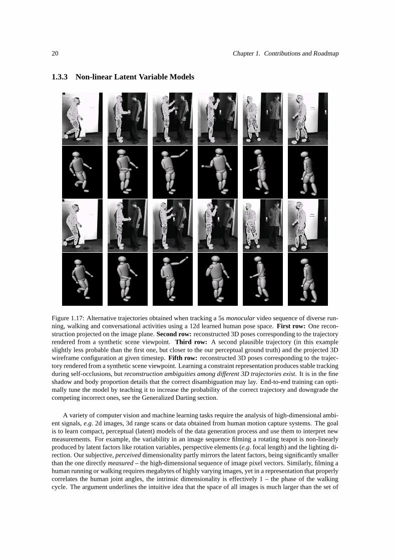
20 Chapter 1. Contributions and Roadmap
1.3.3 Non-linear Latent Variable Models
Figure 1.17: Alternative trajectories obtained when tracking a 5s monocular video sequence of diverse run-ning, walking and conversational activities using a 12d learned human pose space. First row: One recon-struction projected on the image plane. Second row: reconstructed 3D poses corresponding to the trajectoryrendered from a synthetic scene viewpoint. Third row: A second plausible trajectory (in this exampleslightly less probable than the first one, but closer to the our perceptual ground truth) and the projected 3Dwireframe configuration at given timestep. Fifth row: reconstructed 3D poses corresponding to the trajec-tory rendered from a synthetic scene viewpoint. Learning a constraint representation produces stable trackingduring self-occlusions, but reconstruction ambiguities among different 3D trajectories exist. It is in the fineshadow and body proportion details that the correct disambiguation may lay. End-to-end training can opti-mally tune the model by teaching it to increase the probability of the correct trajectory and downgrade thecompeting incorrect ones, see the Generalized Darting section.
A variety of computer vision and machine learning tasks require the analysis of high-dimensional ambi-ent signals, e.g. 2d images, 3d range scans or data obtained from human motion capture systems. The goalis to learn compact, perceptual (latent) models of the data generation process and use them to interpret newmeasurements. For example, the variability in an image sequence filming a rotating teapot is non-linearlyproduced by latent factors like rotation variables, perspective elements (e.g. focal length) and the lighting di-rection. Our subjective, perceived dimensionality partly mirrors the latent factors, being significantly smallerthan the one directly measured – the high-dimensional sequence of image pixel vectors. Similarly, filming ahuman running or walking requires megabytes of highly varying images, yet in a representation that properlycorrelates the human joint angles, the intrinsic dimensionality is effectively 1 – the phase of the walkingcycle. The argument underlines the intuitive idea that the space of all images is much larger than the set of
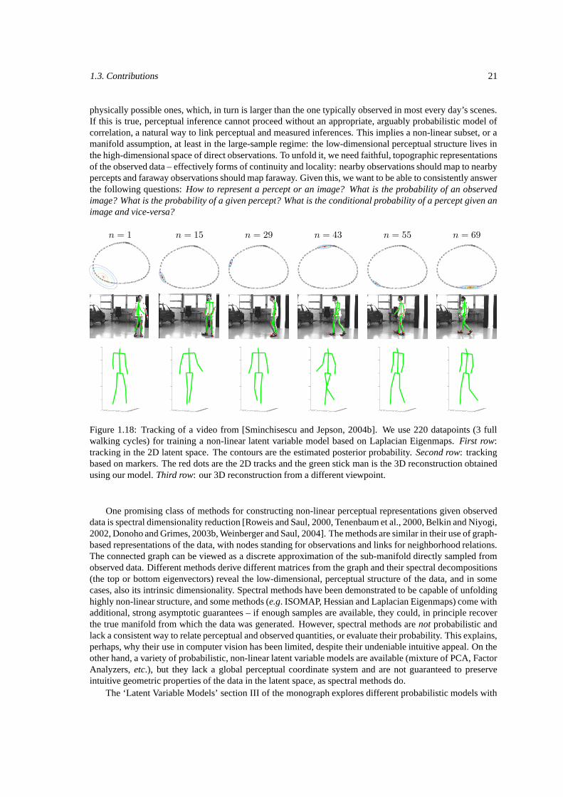
1.3. Contributions 21
physically possible ones, which, in turn is larger than the one typically observed in most every day’s scenes.If this is true, perceptual inference cannot proceed without an appropriate, arguably probabilistic model ofcorrelation, a natural way to link perceptual and measured inferences. This implies a non-linear subset, or amanifold assumption, at least in the large-sample regime: the low-dimensional perceptual structure lives inthe high-dimensional space of direct observations. To unfold it, we need faithful, topographic representationsof the observed data – effectively forms of continuity and locality: nearby observations should map to nearbypercepts and faraway observations should map faraway. Given this, we want to be able to consistently answerthe following questions: How to represent a percept or an image? What is the probability of an observedimage? What is the probability of a given percept? What is the conditional probability of a percept given animage and vice-versa?
n = 1 n = 15 n = 29 n = 43 n = 55 n = 69
−50−40
−30−20
−100
1020
3040
50
−50
−40
−30
−20
−10
0
10
20
30
40
50
−100
−50
0
50
100
−50−40
−30−20
−100
1020
3040
50
−50
−40
−30
−20
−10
0
10
20
30
40
50
−100
−50
0
50
100
−50−40
−30−20
−100
1020
3040
50
−50
−40
−30
−20
−10
0
10
20
30
40
50
−100
−50
0
50
100
−50−40
−30−20
−100
1020
3040
50
−50
−40
−30
−20
−10
0
10
20
30
40
50
−100
−50
0
50
100
−50−40
−30−20
−100
1020
3040
50
−50
−40
−30
−20
−10
0
10
20
30
40
50
−100
−50
0
50
100
−50−40
−30−20
−100
1020
3040
50
−50
−40
−30
−20
−10
0
10
20
30
40
50
−100
−50
0
50
100
Figure 1.18: Tracking of a video from [Sminchisescu and Jepson, 2004b]. We use 220 datapoints (3 fullwalking cycles) for training a non-linear latent variable model based on Laplacian Eigenmaps. First row:tracking in the 2D latent space. The contours are the estimated posterior probability. Second row: trackingbased on markers. The red dots are the 2D tracks and the green stick man is the 3D reconstruction obtainedusing our model. Third row: our 3D reconstruction from a different viewpoint.
One promising class of methods for constructing non-linear perceptual representations given observeddata is spectral dimensionality reduction [Roweis and Saul, 2000, Tenenbaum et al., 2000, Belkin and Niyogi,2002, Donoho and Grimes, 2003b, Weinberger and Saul, 2004]. The methods are similar in their use of graph-based representations of the data, with nodes standing for observations and links for neighborhood relations.The connected graph can be viewed as a discrete approximation of the sub-manifold directly sampled fromobserved data. Different methods derive different matrices from the graph and their spectral decompositions(the top or bottom eigenvectors) reveal the low-dimensional, perceptual structure of the data, and in somecases, also its intrinsic dimensionality. Spectral methods have been demonstrated to be capable of unfoldinghighly non-linear structure, and some methods (e.g. ISOMAP, Hessian and Laplacian Eigenmaps) come withadditional, strong asymptotic guarantees – if enough samples are available, they could, in principle recoverthe true manifold from which the data was generated. However, spectral methods are not probabilistic andlack a consistent way to relate perceptual and observed quantities, or evaluate their probability. This explains,perhaps, why their use in computer vision has been limited, despite their undeniable intuitive appeal. On theother hand, a variety of probabilistic, non-linear latent variable models are available (mixture of PCA, FactorAnalyzers, etc.), but they lack a global perceptual coordinate system and are not guaranteed to preserveintuitive geometric properties of the data in the latent space, as spectral methods do.
The ‘Latent Variable Models’ section III of the monograph explores different probabilistic models with
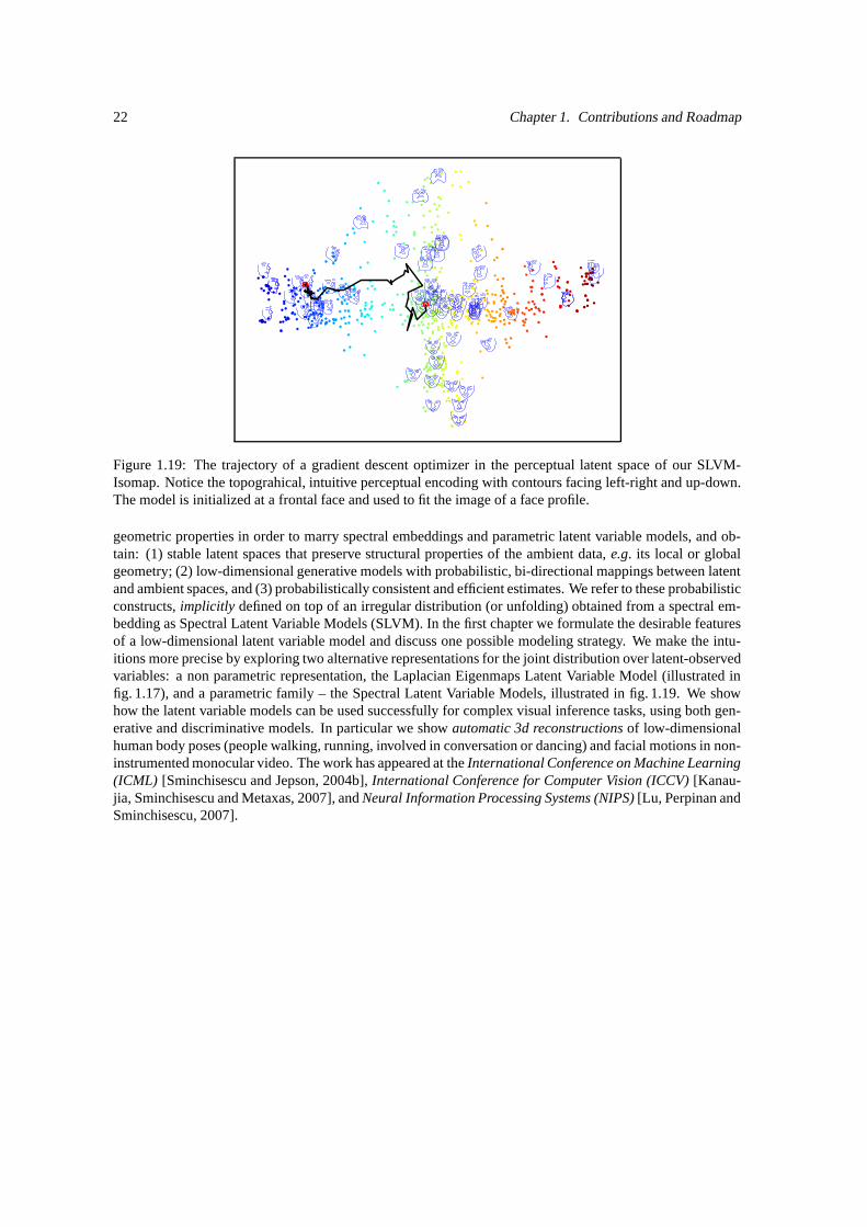
22 Chapter 1. Contributions and Roadmap
Figure 1.19: The trajectory of a gradient descent optimizer in the perceptual latent space of our SLVM-Isomap. Notice the topograhical, intuitive perceptual encoding with contours facing left-right and up-down.The model is initialized at a frontal face and used to fit the image of a face profile.
geometric properties in order to marry spectral embeddings and parametric latent variable models, and ob-tain: (1) stable latent spaces that preserve structural properties of the ambient data, e.g. its local or globalgeometry; (2) low-dimensional generative models with probabilistic, bi-directional mappings between latentand ambient spaces, and (3) probabilistically consistent and efficient estimates. We refer to these probabilisticconstructs, implicitly defined on top of an irregular distribution (or unfolding) obtained from a spectral em-bedding as Spectral Latent Variable Models (SLVM). In the first chapter we formulate the desirable featuresof a low-dimensional latent variable model and discuss one possible modeling strategy. We make the intu-itions more precise by exploring two alternative representations for the joint distribution over latent-observedvariables: a non parametric representation, the Laplacian Eigenmaps Latent Variable Model (illustrated infig. 1.17), and a parametric family – the Spectral Latent Variable Models, illustrated in fig. 1.19. We showhow the latent variable models can be used successfully for complex visual inference tasks, using both gen-erative and discriminative models. In particular we show automatic 3d reconstructions of low-dimensionalhuman body poses (people walking, running, involved in conversation or dancing) and facial motions in non-instrumented monocular video. The work has appeared at the International Conference on Machine Learning(ICML) [Sminchisescu and Jepson, 2004b], International Conference for Computer Vision (ICCV) [Kanau-jia, Sminchisescu and Metaxas, 2007], and Neural Information Processing Systems (NIPS) [Lu, Perpinan andSminchisescu, 2007].

PART I:OPTIMIZATION AND SAMPLINGALGORITHMS

Chapter 2
Kinematic Jump Sampling
A major difficulty for 3D human body tracking from monocular image sequences is the near non-observabilityof kinematic degrees of freedom that generate motion in depth. For known link (body segment) lengths, thestrict non-observabilities reduce to twofold ‘forwards/backwards flipping’ ambiguities for each link. Theseimply 2# links formal inverse kinematics solutions for the full model, and hence linked groups of O(2# links)local minima in the model-image matching cost function. Choosing the wrong minimum leads to rapidmistracking, so for reliable tracking, rapid methods of investigating alternative minima within a group areneeded. Previous approaches to this have used generic search methods that do not exploit the specific prob-lem structure. Here, we complement these by using simple kinematic reasoning to enumerate the tree ofpossible forwards/backwards flips, thus greatly speeding the search within each linked group of minima. Ourmethods can be used either deterministically, or within stochastic ‘jump-diffusion’ style search processes.We give experimental results on some challenging monocular human tracking sequences, showing how thenew kinematic-flipping based sampling method improves and complements existing ones. An earlier ver-sion of this chapter appeared in IEEE International Conference on Computer Vision and Pattern Recognition(CVPR) [Sminchisescu and Triggs, 2003a].
2.1 Sampling for Articulated Chains
A major difficulty for 3D human body tracking from monocular image sequences is the quasi-unobservabilityof kinematic degrees of freedom that generate motion in depth. For unknown limb (link) lengths this leadsto continuous nonrigid ‘affine folding’ ambiguities, but once lengths are known these reduce to twofold‘forwards/backwards flipping’ ambiguities for each link. The full model thus has 2# links formal inverse kine-matics solutions. Even with strong joint limits and no image correspondence ambiguities, the model-imagematching cost function typically still has O(2# links) local minima, so optimizing it is a difficult global searchproblem. But also a necessary one, as following the wrong local minimum rapidly leads to mistracking.
Several generic global search methods have already been applied to this problem [Deutscher et al., 2001,Sidenbladh et al., 2000, Sminchisescu and Triggs, 2001, 2002b], but they tend to be somewhat inefficient asthey make little use of the specific problem structure. Here, we develop a new method that speeds the searchfor local minima by using simple kinematic principles to construct ‘interpretation trees’ generating the pos-sible 3D body configurations associated with a given set of projected joint centres (§2.3). We give simpleclosed-form inverse kinematics solutions for constructing these trees for human limbs, and show how themethod can be used to produce an efficient deterministic ‘kinematic jump’ sampler for the different configu-rations. We use this sampler to construct a novel mixture density propagation based tracking algorithm (§2.4)that combines local covariance based diffusion, adaptive kinematic chain selection based on local uncertain-ties, quasi-global kinematic jumps and local continuous constrained optimization. We present quantitativeresults showing the effectiveness of the new samplers compared to existing methods (§2.5.1), and concludewith some challenging monocular experiments showing the final tracker’s ability to follow rapid, complexhuman motions in clutter.
25
26 Chapter 2. Kinematic Jump Sampling
2.1.1 Human Pose Reconstruction Algorithms
There is a large literature on human motion tracking but relatively little work on developing search methodsthat exploit both the local and global structure present in the 3D monocular articulated problem. Sidenbladhet al. [2000, 2002] use particle filtering with importance sampling based on either a learned walking model ora database of motion snippets, to focus search in the neighborhood of known trajectory pathways . Deutscheret al. [2000] propose an annealing framework in a multi-camera setting. During annealing, the search for pa-rameters is driven by noise proportional with their individual variances [Deutscher et al., 2001]. Consideredas an improved (implicit) search space decomposition mechanism, an early method of this type was proposedby Gavrila and Davis [1996] to efficiently sample partial kinematic chains. Adaptively identifying and sam-pling parameters with high variance is useful, but kinematic parameters usually have quite strong interactionsthat make simple axis-aligned sampling questionable. It is important to realize that the principal axes of thecovariance change drastically depending on the viewing direction, and that even if these are computed andused for sampling (as in [Sminchisescu and Triggs, 2001]), they are only local measures that capture littleinformation about the global minimum structure.
Sminchisescu and Triggs [2001] argue that an effective random sampler must combine all three of cost-surface-aware covariance scaling, a sampling distribution with widened tails for deeper search, and localoptimization (because deep samples usually have very high costs, and hence will not be resampled even ifthey lead to other minima). More recently, they have also constructed deterministic optimization methods[Sminchisescu and Triggs, 2002a] and cost-function-modifying MCMC samplers [Sminchisescu and Triggs,2002b], for finding ‘transition states’ (saddle points) leading to nearby minima.
Skeletal reconstruction methods recover an interpretation tree of possible 3D joint positions, based onuser-specified image joint positions [Lee and Chen, 1985, Taylor, 2000]. Lee and Chen [1985] attempt toprune their perspective interpretation tree using physical reasoning, while Taylor [2000] relies on additionaluser input to specify plausible relative joint-centre depths for his affine one. Although these methods doincorporate the forward-backward flipping ambiguity, they can not reconstruct skeletal joint angles, and thismakes them inappropriate for tracking applications.
Our approach can be seen as a marriage of locally optimized covariance based random sampling with adomain-specific deterministic sampler based on skeletal reconstruction using inverse kinematics. The localcovariance information obtained during optimization also provides a useful heuristic for which kinematicparameters to sample.
2.2 Modeling and Estimation
Representation A typical human body model is constructed from a ‘skeleton’ that has 30-35 rotationaljoints controlled by angular joint state variables x, which includes a global 6d translation of the body center.It also has ‘body flesh’ built from three-dimensional ellipsoids with deformation parameters θ, here 30–35variables for the head, torso, arms and legs. The surface model improves the image representation for the 3Dhuman pose estimates based on image features like edges. In one of the experiments we not only estimatethe model state, but also learn its parameters using maximum likelihood, c.f . §4.6.
Joint positions ui in local coordinate systems for each body limb are transformed into points pi(x,ui) ina global 3-D coordinate system, then into predicted image points ri(x,ui) using composite nonlinear trans-formations ri(x,ui) = P(pi(x,ui)) = P(K(x,ui)), where K represents a chain of rigid transformationsthat map different body links through the kinematic chain to their global 3-D position (see fig. 2.1), and P
represents perspective image projection.The complete model state is encoded in a single large parameter vector x. During tracking and static pose
estimation we usually estimate only joint parameters, but during initialization some parameters (length ratiosare also estimated). In use, the superquadric surfaces are discretized into 2D meshes and the mesh nodes aremapped to 3D points using the kinematic body chain then projected to predicted image points ri(x) usingperspective image projection.
Observation Likelihood: During tracking robust model-to-image matching cost metrics are evaluated foreach predicted image feature ri, and the results are summed over all observations to produce the image
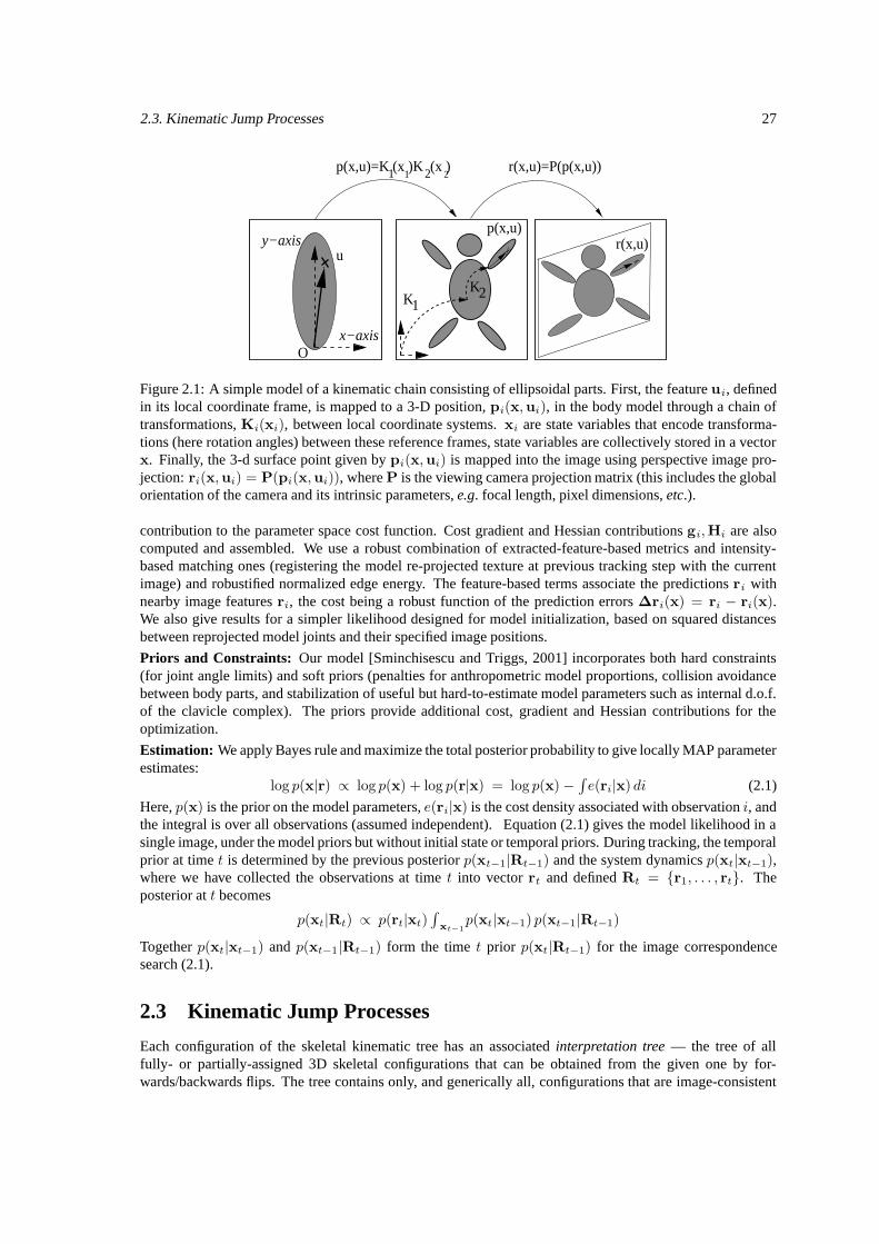
2.3. Kinematic Jump Processes 27
p(x,u)
O
ur(x,u)
K1K2
1 1 2p(x,u)=K (x )K (x ) r(x,u)=P(p(x,u))2
y−axis
x−axis
Figure 2.1: A simple model of a kinematic chain consisting of ellipsoidal parts. First, the feature ui, definedin its local coordinate frame, is mapped to a 3-D position, pi(x,ui), in the body model through a chain oftransformations, Ki(xi), between local coordinate systems. xi are state variables that encode transforma-tions (here rotation angles) between these reference frames, state variables are collectively stored in a vectorx. Finally, the 3-d surface point given by pi(x,ui) is mapped into the image using perspective image pro-jection: ri(x,ui) = P(pi(x,ui)), where P is the viewing camera projection matrix (this includes the globalorientation of the camera and its intrinsic parameters, e.g. focal length, pixel dimensions, etc.).
contribution to the parameter space cost function. Cost gradient and Hessian contributions gi,Hi are alsocomputed and assembled. We use a robust combination of extracted-feature-based metrics and intensity-based matching ones (registering the model re-projected texture at previous tracking step with the currentimage) and robustified normalized edge energy. The feature-based terms associate the predictions ri withnearby image features ri, the cost being a robust function of the prediction errors ∆ri(x) = ri − ri(x).We also give results for a simpler likelihood designed for model initialization, based on squared distancesbetween reprojected model joints and their specified image positions.
Priors and Constraints: Our model [Sminchisescu and Triggs, 2001] incorporates both hard constraints(for joint angle limits) and soft priors (penalties for anthropometric model proportions, collision avoidancebetween body parts, and stabilization of useful but hard-to-estimate model parameters such as internal d.o.f.of the clavicle complex). The priors provide additional cost, gradient and Hessian contributions for theoptimization.
Estimation: We apply Bayes rule and maximize the total posterior probability to give locally MAP parameterestimates:
log p(x|r) ∝ log p(x) + log p(r|x) = log p(x)−∫e(ri|x) di (2.1)
Here, p(x) is the prior on the model parameters, e(ri|x) is the cost density associated with observation i, andthe integral is over all observations (assumed independent). Equation (2.1) gives the model likelihood in asingle image, under the model priors but without initial state or temporal priors. During tracking, the temporalprior at time t is determined by the previous posterior p(xt−1|Rt−1) and the system dynamics p(xt|xt−1),where we have collected the observations at time t into vector rt and defined Rt = r1, . . . , rt. Theposterior at t becomes
p(xt|Rt) ∝ p(rt|xt)∫
xt−1p(xt|xt−1) p(xt−1|Rt−1)
Together p(xt|xt−1) and p(xt−1|Rt−1) form the time t prior p(xt|Rt−1) for the image correspondencesearch (2.1).
2.3 Kinematic Jump Processes
Each configuration of the skeletal kinematic tree has an associated interpretation tree — the tree of allfully- or partially-assigned 3D skeletal configurations that can be obtained from the given one by for-wards/backwards flips. The tree contains only, and generically all, configurations that are image-consistent
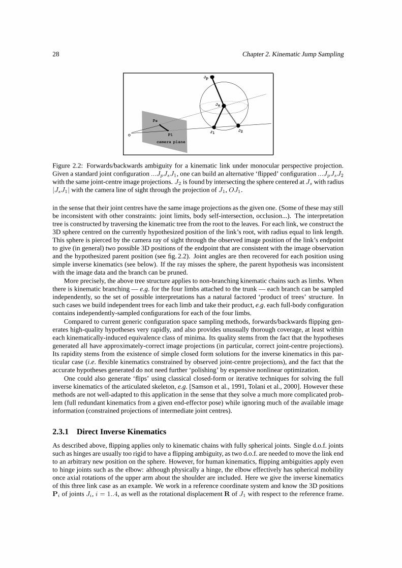
28 Chapter 2. Kinematic Jump Sampling
O
camera plane
Js
J1J2
Jp
p1
ps
Figure 2.2: Forwards/backwards ambiguity for a kinematic link under monocular perspective projection.Given a standard joint configuration ...JpJsJ1, one can build an alternative ‘flipped’ configuration ...JpJsJ2
with the same joint-centre image projections. J2 is found by intersecting the sphere centered at Js with radius|JsJ1| with the camera line of sight through the projection of J1, OJ1.
in the sense that their joint centres have the same image projections as the given one. (Some of these may stillbe inconsistent with other constraints: joint limits, body self-intersection, occlusion...). The interpretationtree is constructed by traversing the kinematic tree from the root to the leaves. For each link, we construct the3D sphere centred on the currently hypothesized position of the link’s root, with radius equal to link length.This sphere is pierced by the camera ray of sight through the observed image position of the link’s endpointto give (in general) two possible 3D positions of the endpoint that are consistent with the image observationand the hypothesized parent position (see fig. 2.2). Joint angles are then recovered for each position usingsimple inverse kinematics (see below). If the ray misses the sphere, the parent hypothesis was inconsistentwith the image data and the branch can be pruned.
More precisely, the above tree structure applies to non-branching kinematic chains such as limbs. Whenthere is kinematic branching — e.g. for the four limbs attached to the trunk — each branch can be sampledindependently, so the set of possible interpretations has a natural factored ‘product of trees’ structure. Insuch cases we build independent trees for each limb and take their product, e.g. each full-body configurationcontains independently-sampled configurations for each of the four limbs.
Compared to current generic configuration space sampling methods, forwards/backwards flipping gen-erates high-quality hypotheses very rapidly, and also provides unusually thorough coverage, at least withineach kinematically-induced equivalence class of minima. Its quality stems from the fact that the hypothesesgenerated all have approximately-correct image projections (in particular, correct joint-centre projections).Its rapidity stems from the existence of simple closed form solutions for the inverse kinematics in this par-ticular case (i.e. flexible kinematics constrained by observed joint-centre projections), and the fact that theaccurate hypotheses generated do not need further ‘polishing’ by expensive nonlinear optimization.
One could also generate ‘flips’ using classical closed-form or iterative techniques for solving the fullinverse kinematics of the articulated skeleton, e.g. [Samson et al., 1991, Tolani et al., 2000]. However thesemethods are not well-adapted to this application in the sense that they solve a much more complicated prob-lem (full redundant kinematics from a given end-effector pose) while ignoring much of the available imageinformation (constrained projections of intermediate joint centres).
2.3.1 Direct Inverse Kinematics
As described above, flipping applies only to kinematic chains with fully spherical joints. Single d.o.f. jointssuch as hinges are usually too rigid to have a flipping ambiguity, as two d.o.f. are needed to move the link endto an arbitrary new position on the sphere. However, for human kinematics, flipping ambiguities apply evento hinge joints such as the elbow: although physically a hinge, the elbow effectively has spherical mobilityonce axial rotations of the upper arm about the shoulder are included. Here we give the inverse kinematicsof this three link case as an example. We work in a reference coordinate system and know the 3D positionsPi of joints Ji, i = 1..4, as well as the rotational displacement R of J1 with respect to the reference frame.
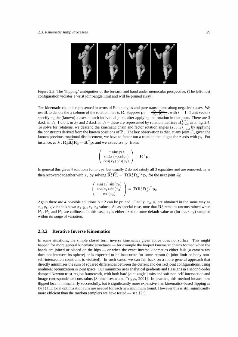
2.3. Kinematic Jump Processes 29
Figure 2.3: The ‘flipping’ ambiguities of the forearm and hand under monocular perspective. (The left-mostconfiguration violates a wrist joint-angle limit and will be pruned away).
The kinematic chain is represented in terms of Euler angles and pure translations along negative z axes. Weuse R to denote the z column of the rotation matrix R. Suppose pi = Pi−Pi+1
‖Pi−Pi+1‖, with i = 1..3 unit vectors
specifying the (known) z axes at each individual joint, after applying the rotation in that joint. There are 3d.o.f. in J1, 1 d.o.f. in J2 and 2 d.o.f. in J3 – these are represented by rotation matrices R1,2,3
x,y,z as in fig. 2.4.To solve for rotations, we descend the kinematic chain and factor rotation angles (x, y, z)1,2,3 by applyingthe constraints derived from the known positions of Pi. The key observation is that, at any joint Ji, given theknown previous rotational displacement, we have to factor out a rotation that aligns the z-axis with pi. For
instance, at J1, R1xR
1yR
1z = R>pi and we extract x1, y1 from:
− sin(y1)sin(x1) cos(y1)cos(x1) cos(y1)
= R>p1
In general this gives 4 solutions for x1, y1, but usually 2 do not satisfy all 3 equalities and are removed. z1 is
then recovered together with x2 by solving R1zR
2x = (RR1
xR1y)T p2 for the next joint J2:
sin(z1) sin(x2)cos(z1) sin(x2)
cos(x2)
= (RR1
xR1y)
>p2
Again there are 4 possible solutions but 2 can be pruned. Finally, x3, y3 are obtained in the same way asx1, y1, given the known x1, y1, z1, x2 values. As as special case, note that R1
z remains unconstrained whenP1, P2 and P3 are collinear. In this case, z1 is either fixed to some default value or (for tracking) sampledwithin its range of variation.
2.3.2 Iterative Inverse Kinematics
In some situations, the simple closed form inverse kinematics given above does not suffice. This mighthappen for more general kinematic structures — for example the looped kinematic chains formed when thehands are joined or placed on the hips — or when the exact inverse kinematics either fails (a camera raydoes not intersect its sphere) or is expected to be inaccurate for some reason (a joint limit or body non-self-intersection constraint is violated). In such cases, we can fall back on a more general approach thatdirectly minimizes the sum of squared differences between the current and desired joint configurations, usingnonlinear optimization in joint space. Our minimizer uses analytical gradients and Hessians in a second-orderdamped Newton trust-region framework, with both hard joint-angle limits and soft non-self-intersection andimage correspondence constraints [Sminchisescu and Triggs, 2001]. In practice, this method locates newflipped local minima fairly successfully, but is significantly more expensive than kinematics-based flipping asO(1) full local optimization runs are needed for each new minimum found. However this is still significantlymore efficient than the random samplers we have tested — see §2.5.

30 Chapter 2. Kinematic Jump Sampling
z
z
z
z
z
P1
P2
P3 P4
Rx1Ry1Rz
1
Rx2
Rx3Ry3
R
Figure 2.4: A three-joint link modeling anthropometric limbs. It has one spherical joint J1, one hinge jointJ2 and a 2 d.o.f. end effector J3. The representation is built in terms of Euler angles (with associated rotationmatrices R1,2,3
x,y,z with angles as sub-scripts and the joint rotation centers as superscripts) and pure translationsto the next joint along the negative z axis. The inverse kinematics solution factors rotation angles usingknowledge of successive z axes (computed from Pi −Pi+1) for limbs.
2.4 The Algorithm
In normal use, we embed our kinematic jump sampler within a cost-sensitive mixture density propagationframework [Sminchisescu and Triggs, 2001]. The jump sampler ensures rapid, consistent diffusion of sam-ples across the kinematic minima associated with any given set of image joint positions, while the randomsampler provides robustness against incorrect image correspondences. Here, we use a Covariance ScaledSampling [Sminchisescu and Triggs, 2001] tracker. This probabilistic method represents the posterior distri-bution of hypotheses in joint space as a mixture of long-tailed Gaussian-like distributions mi ∈ M, whoseweights, centres and scale matrices (‘covariances’) mi = (ci,µi,Σi) are obtained as follows. Randomsamples are generated, and each is optimized (by nonlinear local optimization, respecting any joint con-straints, etc.) to maximize the local posterior likelihood encoded by an image- and prior-knowledge basedcost function. The optimized likelihood value and position give the weight and centre of a new component,and the inverse Hessian of the log-likelihood gives a scale matrix that is well adapted to the contours ofthe cost function, even for very ill-conditioned problems like monocular human tracking. However, whensampling, particles are deliberately scattered more widely than a Gaussian of this scale matrix (covariance)would predict, in order to probe more deeply for alternative minima.
Fig. 2.5 gives the general form of the algorithm, and fig. 2.6 describes the novel KinematicDiffusion-JumpSampling routine that lies at its core. On entry, the user specifies a set C of kinematic sub-chainsthat may be sampled (this can be quite large, as the routine adaptively decides which to sample). At eachtime step, covariance scaled samples are generated from the prior. For each such sample an interpretationtree is created on-line by the BuildInterpretationTree routine, with kinematic solutions obtained using In-verseKinematics. The chain to be sampled is chosen adaptively using a voting process based on the localcovariance structure of that region of the parameter space, SelectSamplingChain in fig. 2.6. Local covari-ance scaled resampling is performed before the jump because we do not (yet) have the covariance informationneeded to perform it afterwards. Each element of the sampleable sub-chain set C is simply a list of parameternames to sample. For instance, for a sub-chain rooted at the left shoulder, this might include the rotationalparameters (xs, ys, zs, xe, xh, yh) where the (s, e, h) stand for (shoulder, elbow, hand) and x, y, z for therotation axes.
The proposed sampling strategy provides a balance between local and global search effort since samplesare generated around the prior modes, as well as around new peaks that are potentially emerging and havenot yet been explored. Re-weighting based on closest prior modes as in fig. 2.5, step 5, ensures the tracker isnot distracted by remote multi-modality when tracking the correct minima.
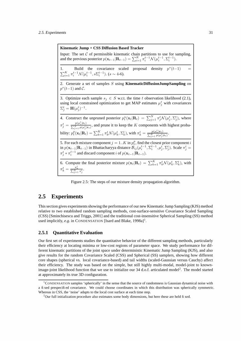
2.5. Experiments 31
Kinematic Jump + CSS Diffusion Based Tracker
Input: The set C of permissible kinematic chain partitions to use for sampling,and the previous posterior p(xt−1|Rt−1) =
∑Ki=1 π
t−1i N (µt−1
i ,Σt−1i ).
1. Build the covariance scaled proposal density p∗(t−1) =∑Ki=1 π
t−1i N (µt−1
i , sΣt−1i ). (s ∼ 4-6).
2. Generate a set of samples S using KinematicDiffusionJumpSampling onp∗(t−1) and C.
3. Optimize each sample sj ∈ S w.r.t. the time t observation likelihood (2.1),using local constrained optimization to get MAP estimates µt
j with covariancesΣt
j = H(µtj)
−1.
4. Construct the unpruned posterior put (xt|Rt) =
∑Nj=1 π
tjN (µt
j ,Σtj), where
πtj =
p(µtj |rt)
P
Nj=1 p(µt
j|rt)
, and prune it to keep the K components with highest proba-
bility: ppt (xt|Rt) =
∑Kk=1 π
tkN (µt
k ,Σtk), with πt
k =p(µt
k|rt)P
Kj=1 p(µt
j|rt)
.
5. For each mixture component j = 1..K in ppt , find the closest prior component i
in p(xt−1|Rt−1) in Bhattacharyya distance Bij(µt−1i ,Σt−1
i , µtj ,Σ
tj). Scale πt
j =
πtj ∗ πt−1
i and discard component i of p(xt−1|Rt−1).
6. Compute the final posterior mixture p(xt|Rt) =∑K
k=1 πtkN (µt
k,Σtk), with
πtk =
πtk
P
Kj=1 πt
j
.
Figure 2.5: The steps of our mixture density propagation algorithm.
2.5 Experiments
This section gives experiments showing the performance of our new Kinematic Jump Sampling (KJS) methodrelative to two established random sampling methods, cost-surface-sensitive Covariance Scaled Sampling(CSS) [Sminchisescu and Triggs, 2001] and the traditional cost-insensitive Spherical Sampling (SS) methodused implicitly, e.g. in CONDENSATION [Isard and Blake, 1998a]1.
2.5.1 Quantitative Evaluation
Our first set of experiments studies the quantitative behavior of the different sampling methods, particularlytheir efficiency at locating minima or low-cost regions of parameter space. We study performance for dif-ferent kinematic partitions of the joint space under deterministic Kinematic Jump Sampling (KJS), and alsogive results for the random Covariance Scaled (CSS) and Spherical (SS) samplers, showing how differentcore shapes (spherical vs. local covariance-based) and tail widths (scaled-Gaussian versus Cauchy) affecttheir efficiency. The study was based on the simple, but still highly multi-modal, model-joint to known-image-joint likelihood function that we use to initialize our 34 d.o.f. articulated model2. The model startedat approximately its true 3D configuration.
1CONDENSATION samples ‘spherically’ in the sense that the source of randomness is Gaussian dynamical noise witha fixed prespecified covariance. We could choose coordinates in which this distribution was spherically symmetric.Whereas in CSS, the ‘noise’ adapts to the local cost surface at each time step.
2Our full initialization procedure also estimates some body dimensions, but here these are held fixed.
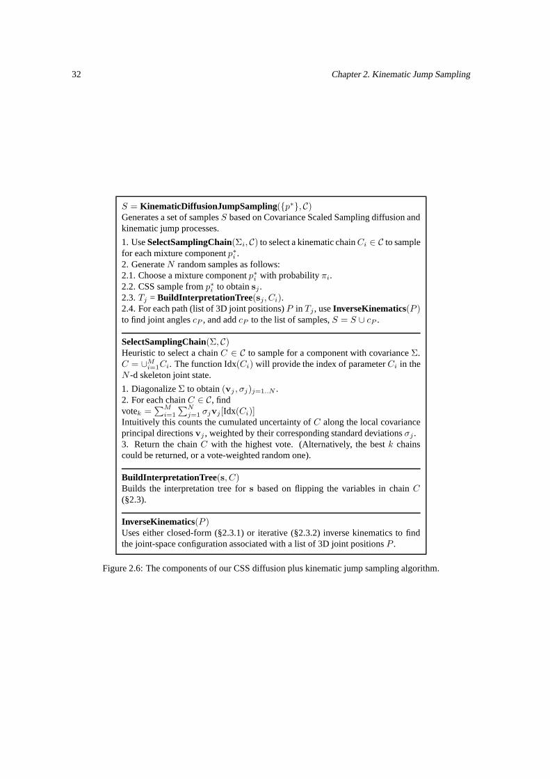
32 Chapter 2. Kinematic Jump Sampling
S = KinematicDiffusionJumpSampling(p∗, C)Generates a set of samples S based on Covariance Scaled Sampling diffusion andkinematic jump processes.
1. Use SelectSamplingChain(Σi, C) to select a kinematic chainCi ∈ C to samplefor each mixture component p∗i .2. Generate N random samples as follows:2.1. Choose a mixture component p∗i with probability πi.2.2. CSS sample from p∗i to obtain sj .2.3. Tj = BuildInterpretationTree(sj, Ci).2.4. For each path (list of 3D joint positions) P in Tj , use InverseKinematics(P )to find joint angles cP , and add cP to the list of samples, S = S ∪ cP .
SelectSamplingChain(Σ, C)Heuristic to select a chain C ∈ C to sample for a component with covariance Σ.C = ∪M
i=1Ci. The function Idx(Ci) will provide the index of parameter Ci in theN -d skeleton joint state.
1. Diagonalize Σ to obtain (vj , σj)j=1..N .2. For each chain C ∈ C, findvotek =
∑Mi=1
∑Nj=1 σjvj [Idx(Ci)]
Intuitively this counts the cumulated uncertainty of C along the local covarianceprincipal directions vj , weighted by their corresponding standard deviations σj .3. Return the chain C with the highest vote. (Alternatively, the best k chainscould be returned, or a vote-weighted random one).
BuildInterpretationTree(s, C)Builds the interpretation tree for s based on flipping the variables in chain C(§2.3).
InverseKinematics(P )Uses either closed-form (§2.3.1) or iterative (§2.3.2) inverse kinematics to findthe joint-space configuration associated with a list of 3D joint positions P .
Figure 2.6: The components of our CSS diffusion plus kinematic jump sampling algorithm.
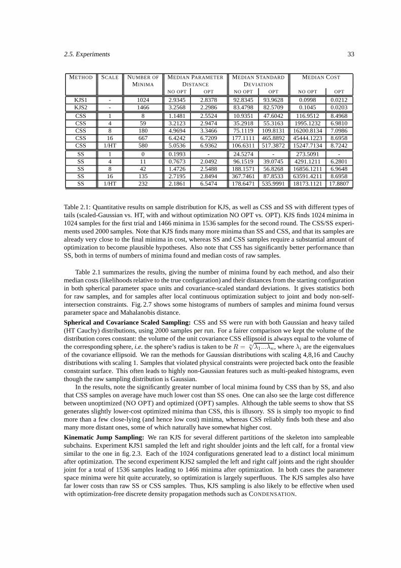
2.5. Experiments 33
METHOD SCALE NUMBER OF MEDIAN PARAMETER MEDIAN STANDARD MEDIAN COST
MINIMA DISTANCE DEVIATION
NO OPT OPT NO OPT OPT NO OPT OPT
KJS1 - 1024 2.9345 2.8378 92.8345 93.9628 0.0998 0.0212KJS2 - 1466 3.2568 2.2986 83.4798 82.5709 0.1045 0.0203
CSS 1 8 1.1481 2.5524 10.9351 47.6042 116.9512 8.4968CSS 4 59 3.2123 2.9474 35.2918 55.3163 1995.1232 6.9810CSS 8 180 4.9694 3.3466 75.1119 109.8131 16200.8134 7.0986CSS 16 667 6.4242 6.7209 177.1111 465.8892 45444.1223 8.6958CSS 1/HT 580 5.0536 6.9362 106.6311 517.3872 15247.7134 8.7242
SS 1 0 0.1993 - 24.5274 - 273.5091 -SS 4 11 0.7673 2.0492 96.1519 39.0745 4291.1211 6.2801SS 8 42 1.4726 2.5488 188.1571 56.8268 16856.1211 6.9648SS 16 135 2.7195 2.8494 367.7461 87.8533 63591.4211 8.6958SS 1/HT 232 2.1861 6.5474 178.6471 535.9991 18173.1121 17.8807
Table 2.1: Quantitative results on sample distribution for KJS, as well as CSS and SS with different types oftails (scaled-Gaussian vs. HT, with and without optimization NO OPT vs. OPT). KJS finds 1024 minima in1024 samples for the first trial and 1466 minima in 1536 samples for the second round. The CSS/SS experi-ments used 2000 samples. Note that KJS finds many more minima than SS and CSS, and that its samples arealready very close to the final minima in cost, whereas SS and CSS samples require a substantial amount ofoptimization to become plausible hypotheses. Also note that CSS has significantly better performance thanSS, both in terms of numbers of minima found and median costs of raw samples.
Table 2.1 summarizes the results, giving the number of minima found by each method, and also theirmedian costs (likelihoods relative to the true configuration) and their distances from the starting configurationin both spherical parameter space units and covariance-scaled standard deviations. It gives statistics bothfor raw samples, and for samples after local continuous optimization subject to joint and body non-self-intersection constraints. Fig. 2.7 shows some histograms of numbers of samples and minima found versusparameter space and Mahalanobis distance.
Spherical and Covariance Scaled Sampling: CSS and SS were run with both Gaussian and heavy tailed(HT Cauchy) distributions, using 2000 samples per run. For a fairer comparison we kept the volume of thedistribution cores constant: the volume of the unit covariance CSS ellipsoid is always equal to the volume ofthe corresponding sphere, i.e. the sphere’s radius is taken to be R = n
√λ1...λn, where λi are the eigenvalues
of the covariance ellipsoid. We ran the methods for Gaussian distributions with scaling 4,8,16 and Cauchydistributions with scaling 1. Samples that violated physical constraints were projected back onto the feasibleconstraint surface. This often leads to highly non-Gaussian features such as multi-peaked histograms, eventhough the raw sampling distribution is Gaussian.
In the results, note the significantly greater number of local minima found by CSS than by SS, and alsothat CSS samples on average have much lower cost than SS ones. One can also see the large cost differencebetween unoptimized (NO OPT) and optimized (OPT) samples. Although the table seems to show that SSgenerates slightly lower-cost optimized minima than CSS, this is illusory. SS is simply too myopic to findmore than a few close-lying (and hence low cost) minima, whereas CSS reliably finds both these and alsomany more distant ones, some of which naturally have somewhat higher cost.
Kinematic Jump Sampling: We ran KJS for several different partitions of the skeleton into sampleablesubchains. Experiment KJS1 sampled the left and right shoulder joints and the left calf, for a frontal viewsimilar to the one in fig. 2.3. Each of the 1024 configurations generated lead to a distinct local minimumafter optimization. The second experiment KJS2 sampled the left and right calf joints and the right shoulderjoint for a total of 1536 samples leading to 1466 minima after optimization. In both cases the parameterspace minima were hit quite accurately, so optimization is largely superfluous. The KJS samples also havefar lower costs than raw SS or CSS samples. Thus, KJS sampling is also likely to be effective when usedwith optimization-free discrete density propagation methods such as CONDENSATION.
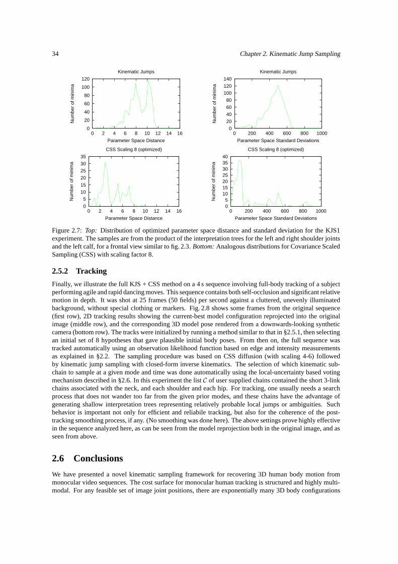
34 Chapter 2. Kinematic Jump Sampling
0
20
40
60
80
100
120
0 2 4 6 8 10 12 14 16
Num
ber
of m
inim
a
Parameter Space Distance
Kinematic Jumps
0
20
40
60
80
100
120
140
0 200 400 600 800 1000
Num
ber
of m
inim
a
Parameter Space Standard Deviations
Kinematic Jumps
0
5
10
15
20
25
30
35
0 2 4 6 8 10 12 14 16
Num
ber
of m
inim
a
Parameter Space Distance
CSS Scaling 8 (optimized)
05
10152025303540
0 200 400 600 800 1000N
umbe
r of
min
ima
Parameter Space Standard Deviations
CSS Scaling 8 (optimized)
Figure 2.7: Top: Distribution of optimized parameter space distance and standard deviation for the KJS1experiment. The samples are from the product of the interpretation trees for the left and right shoulder jointsand the left calf, for a frontal view similar to fig. 2.3. Bottom: Analogous distributions for Covariance ScaledSampling (CSS) with scaling factor 8.
2.5.2 Tracking
Finally, we illustrate the full KJS + CSS method on a 4 s sequence involving full-body tracking of a subjectperforming agile and rapid dancing moves. This sequence contains both self-occlusion and significant relativemotion in depth. It was shot at 25 frames (50 fields) per second against a cluttered, unevenly illuminatedbackground, without special clothing or markers. Fig. 2.8 shows some frames from the original sequence(first row), 2D tracking results showing the current-best model configuration reprojected into the originalimage (middle row), and the corresponding 3D model pose rendered from a downwards-looking syntheticcamera (bottom row). The tracks were initialized by running a method similar to that in §2.5.1, then selectingan initial set of 8 hypotheses that gave plausible initial body poses. From then on, the full sequence wastracked automatically using an observation likelihood function based on edge and intensity measurementsas explained in §2.2. The sampling procedure was based on CSS diffusion (with scaling 4-6) followedby kinematic jump sampling with closed-form inverse kinematics. The selection of which kinematic sub-chain to sample at a given mode and time was done automatically using the local-uncertainty based votingmechanism described in §2.6. In this experiment the list C of user supplied chains contained the short 3-linkchains associated with the neck, and each shoulder and each hip. For tracking, one usually needs a searchprocess that does not wander too far from the given prior modes, and these chains have the advantage ofgenerating shallow interpretation trees representing relatively probable local jumps or ambiguities. Suchbehavior is important not only for efficient and reliabile tracking, but also for the coherence of the post-tracking smoothing process, if any. (No smoothing was done here). The above settings prove highly effectivein the sequence analyzed here, as can be seen from the model reprojection both in the original image, and asseen from above.
2.6 Conclusions
We have presented a novel kinematic sampling framework for recovering 3D human body motion frommonocular video sequences. The cost surface for monocular human tracking is structured and highly multi-modal. For any feasible set of image joint positions, there are exponentially many 3D body configurations
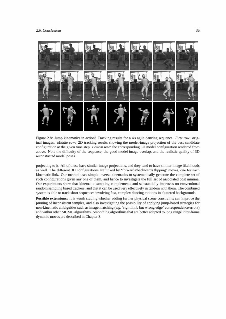
2.6. Conclusions 35
Figure 2.8: Jump kinematics in action! Tracking results for a 4 s agile dancing sequence. First row: orig-inal images. Middle row: 2D tracking results showing the model-image projection of the best candidateconfiguration at the given time step. Bottom row: the corresponding 3D model configuration rendered fromabove. Note the difficulty of the sequence, the good model image overlap, and the realistic quality of 3Dreconstucted model poses.
projecting to it. All of these have similar image projections, and they tend to have similar image likelihoodsas well. The different 3D configurations are linked by ‘forwards/backwards flipping’ moves, one for eachkinematic link. Our method uses simple inverse kinematics to systematically generate the complete set ofsuch configurations given any one of them, and hence to investigate the full set of associated cost minima.Our experiments show that kinematic sampling complements and substantially improves on conventionalrandom sampling based trackers, and that it can be used very effectively in tandem with them. The combinedsystem is able to track short sequences involving fast, complex dancing motions in cluttered backgrounds.
Possible extensions: It is worth studing whether adding further physical scene constraints can improve thepruning of inconsistent samples, and also investigating the possibility of applying jump-based strategies fornon-kinematic ambiguities such as image matching (e.g. ‘right limb but wrong edge’ correspondence errors)and within other MCMC algorithms. Smoothing algorithms that are better adapted to long range inter-framedynamic moves are described in Chapter 3.

Chapter 3
Variational Mixture Smoothing forNon-Linear Dynamical Systems
We present an algorithm for computing joint state, smoothed, density estimates for non-linear dynamicalsystems in a Bayesian setting. Many visual tracking problems can be formulated as probabilistic inferenceover time series, but we are not aware of mixture smoothers that would apply to weakly identifiable models,where multimodality is persistent rather than transient (e.g. monocular 3D human tracking). Such processes,in principle, exclude iterated Kalman smoothers, whereas flexible MCMC methods or sample based particlesmoothers encounter computational difficulties: accurately locating an exponential number of probable jointstate modes representing high-dimensional trajectories, rapidly mixing between those or resampling proba-ble configurations missed during filtering. In this paper we present an alternative, layered, mixture densitysmoothing algorithm that exploits the accuracy of efficient optimization within a Bayesian approximationframework. The distribution is progressively refined by combining polynomial time search over the embed-ded network of temporal observation likelihood peaks, MAP continuous trajectory estimates, and Bayesianvariational adjustment of the resulting joint mixture approximation. Our results demonstrate the effectivenessof the method on the problem of inferring multiple plausible 3D human motion trajectories from monocularvideo. An earlier version of this chapter appeared in IEEE International Conference on Computer Vision andPattern Recognition (CVPR) [Sminchisescu and Jepson, 2004a].
3.1 Smoothing for Non-linear Systems
Many visual tracking problems can be naturally formulated as probabilistic inference over the hidden statesof a dynamical system. In this framework, we work with time series of system state vectors linked by prob-abilistic dynamic transition rules, and for each state we also have observations and define an observationmodel. The parameter space consists of the joint state vectors at all times. This trajectory through statesis probabilistically constrained both by dynamics and by the observation model. To the extent that theseare realistic statistical models, Bayes-law propagation of a probability density for the true state is possible.Filtering computes the optimal distribution of states conditioned only by the past whereas smoothing findsthe optimal state estimate at each time given both past and future observations and dynamics. For non-lineardynamics and observation models under Gaussian noise, this can be computed using iterated Kalman filteringand smoothing. However, for many tracking problems involving clutter and complex models this methodol-ogy is not applicable. For general multimodal distributions under non-Gaussian dynamics and observationmodels, direct MCMC methods or particle filters/smoothers [Gordon et al., 1993, Isard and Blake, 1998a,Kitagawa, 1996, Isard and Blake, 1998b, Scott, 2002, Neal et al., 2003] result. These algorithms naturallyrepresent uncertainty, but are less efficient for weakly identifiable high-dimensional models where multi-
36
3.2. Existing Smoothing Algorithms 37
modality is persistent rather than transient.1 In such cases, there is, theoretically, an exponential number oftrajectories for any single observation sequence, and many of these may be probable. Accurately locatingthem, or sampling new trajectories through temporal states missed during filtering is a major computationalchallenge. An additional difficulty is that none of the methods give multiple MAP estimates or a similarcompact multimodal approximation. This may be useful in its own right for many applications (e.g. visual-ization, high-level analysis and recognition) where the mean state or other expectation calculations may beuninformative or, at least, not the only desired output.
We are not aware of prior work that computes a mixture approximation for smoothing general non-linearnon-Gaussian dynamical systems. In this chapter, we propose such an algorithm that exploits the accuracyof efficient discrete and continuous optimization within a variational approximation setting. Our methodestimates a compact mixture distribution over joint temporal states, and can be efficiently used in tandem withmixture filtering methods [Cham and Rehg, 1999, Sminchisescu and Triggs, 2003b,a, Vermaak et al., 2003].To sidestep the difficulties associated with random high-dimensional initialization, the algorithm cascadesseveral layers of computation. We use dynamic programming, sparse robust non-linear optimization, andvariational adjustment, in order to progressively refine a Kullback-Leibler approximation to the true jointstate posterior, given an entire observation sequence. The resulting density model is compact and principled,allowing accurate sampling of alternative trajectories, as well as general Bayesian expectation calculations.We finally demonstrate the algorithm on the difficult problem of inferring smooth trajectories that reconstructdifferent plausible 3D human motions in complex monocular video.
Many existing tracking or smoothing solutions attempt to limit multimodality using learned dynamicalmodels [Brand, 1999, Howe et al., 1999, Deutscher et al., 2000, Sidenbladh et al., 2000, 2002]. While thesemay stabilize the estimates, the distracting likelihood peaks are only down-weighted, but rarely disappear.The state space volume, and therefore the theoretical search complexity remains unchanged, and the gen-erality of the tracker may be significantly reduced. In subsequent chapters of this thesis (Ch. 11–13), wepropose different latent variable models that allow visual inference over low-dimensional manifolds learnedfrom motion data that is typical of the problem domain. It is likely, however, that under realistic imagingconditions, at least a mild degree of multimodality will still persist during visual inference, for any interesting(i.e. sufficiently flexible) motion model or low-dimensional state representation. The smoothing algorithmwe propose remains useful in such contexts. Another application is the accurate reconstruction of general 3Dbiological motion for computer graphics or animation.
3.2 Existing Smoothing Algorithms
There is a large literature on non-linear filtering and smoothing, using both Kalman [Gelb, 1974] and Monte-Carlo methods [Isard and Blake, 1998a, Kitagawa, 1996, Neal et al., 2003]. Kalman filtering and smoothing[Gelb, 1974] is not applicable for non-Gaussian systems. Particle smoothers [Isard and Blake, 1998a, Kita-gawa, 1996] are based on forward filtering, followed by smoothing that reweights existing particles, in orderto better reflect future evidence. Introduced mostly to tackle the erroneous mean state estimates under tran-sient multimodality [Isard and Blake, 1998a], the algorithms may not scale well under strong multimodality,where a large number of trajectories have high probability, or when probable temporal states have beenmissed or eliminated prematurely during filtering. Direct full sequence MCMC methods [Neal et al., 2003]iteratively generate particle smoother style proposals in their transition kernel. This makes the sampling ofnew states possible at the price of more expensive step updates, but the methods do not provide an explicitmulti-modal representation and fast mixing is difficult. A more compact and efficient approximation thatretains modeling generality would be useful.
Bayesian variational methods are one possible class of solutions [Jaakkola and Jordan, 1998, Gahramaniand Hinton, 2001, Pavlovic et al., 2001] that typically construct approximations that decouple some of thedependencies present in the original model (e.g. mean field). The switching state space model [Gahramani
1Consider e.g. 3D monocular human tracking where for known link (body segment) lengths, the strict non-observabilities reduce to twofold ‘forwards/backwards flipping’ ambiguities for each link, at each timestep [Sminchisescuand Triggs, 2003a].
38 Chapter 3. Variational Mixture Smoothing for Non-Linear Dynamical Systems
and Hinton, 2001, Pavlovic et al., 2001] is designed only for piece-wise linear, Gaussian dynamical systems.In general, the variational methods have to sidestep suboptimal modeling and high-dimensional initialization,both of which are problematic. The algorithm we propose is also formulated in a variational setting. Here weuse a fully coupled mixture approximation, initialized based on layered, time efficient processing: dynamicprogramming, polynomial time trajectory search over the network of temporal observation likelihood peaks(initialized from filtering), and local continuous MAP trajectory refinement. Our final approximation is amixture of Gaussians, and it can be also used to improve mixing in MCMC simulations [Sminchisescu et al.,2003].
Several multiple hypothesis methods exist for filtering 3D human motion [Deutscher et al., 2000, Siden-bladh et al., 2000, Sminchisescu and Triggs, 2003b, Sidenbladh et al., 2002, Sminchisescu and Triggs, 2003a]but less attention has been given to similar methods for smoothing. Most of the proposed methods computea single point estimate. Howe et al [Howe et al., 1999] use a dynamical prior obtained from motion capturedata and assume 2D joint tracks over an entire time series to compute a 3D joint position MAP estimate.Brand [1999] similarly learns a HMM representation from motion capture data and estimates MAP trajecto-ries, based on time series of human silhouette inputs. DiFranco et al. [2001] propose an interactive systembased on a batch optimizer of a Gaussian observation model consisting of 2D human joint correspondencesand 3D given human pose key-frames that help disambiguate multimodality resulting from monocular re-flective limb ambiguities. This is essentially an iterated Kalman smoother with a better second order stepupdate.
3.3 Formulation
Consider a non-linear, non-Gaussian, dynamical system having temporal state xt, t = 1...T , prior p(x1),observation model p(rt|xt) with observations rt, and dynamics p(xt|xt−1). Let Xt = (x1,x2, . . . ,xt)be the model joint state estimated over a time series 1...t, t ≤ T , based on observations encoded as Rt =(r1, . . . , rt). The joint probability of all observations and hidden states can be factored (assume for nowX = XT and R = RT for notational simplicity) as:
P(X,R) = p(x1)T∏
t=2
p(xt|xt−1)T∏
t=1
p(rt|xt) (3.1)
For smoothing and other sequence calculations, we are however interested in P(X|R) = P(X,R)/P(R).For multimodal temporal observation likelihood distributions p(rt|xt), the joint P(X,R) may contain anexponential number of modes. We seek a tractable approximating distribution qθ(X), parameterized by θ,that minimizes the relative entropy:
D(qθ||P) =
∫
X
qθ(X) logqθ(X)
P(X|R)(3.2)
We further consider the variational free energy F(qθ,P), which is a simple modification to D(qθ||P)that does not change its minimum structure:
F(qθ,P) = D(qθ||P)− logP(R) (3.3)
=
∫
X
qθ(X) logqθ(X)
P(X|R)−∫
X
qθ(X) logP(R) (3.4)
=
∫
X
qθ(X) logqθ(X)
P(X,R)(3.5)
In the above logP(R) does not depend on θ and does therefore not count for the optimization. Minimizingthe variational free energy w.r.t. θ is equivalent to refining the approximation qθ(X) to P(X|R). The ef-fectiveness of this procedure depends on a good design and initialization of qθ(X). We use a fully coupledmixture approximation qθ(X) =
∑i q
θi (X), with Gaussian components qθ
i (X). Methods to initialize itsparameters are given in §3.4 and §3.5.
3.4. Multiple Trajectory Optima using Dynamic Programming 39
3.4 Multiple Trajectory Optima using Dynamic Programming
Let the temporal observation likelihood density be approximated by mixtures:
p(rt|xt) =
Nt∑
i=1
πitm
it(xt,µ
it,Σ
it), t = 1...T (3.6)
where mit are observation likelihood modes (Gaussian or heavy tail distributions), πi
t are mixing propor-tions, Nt are the number of modes at time t. In practice, this representation can be efficiently computed intandem with a filtering method. For continuously optimized filters like [Cham and Rehg, 1999, Sminchisescuand Triggs, 2003b,a], a mixture for p(rt|xt) is estimated anyway, as a necessary substep during the compu-tation of p(xt|Rt) (we will use KJS [Sminchisescu and Triggs, 2003a] for this work). For discrete particlefilters [Isard and Blake, 1998a, Choo and Fleet, 2001, Vermaak et al., 2003] this may involve local optimiza-tion on samples from p(xt|Rt−1) or on the centers of its fitted mixture [Vermaak et al., 2003]. Regard theobservation likelihood modes as nodes of an embedded network that approximates P(X,R). Each mi
t is anode having value equal to its observation likelihood p(rt|mi
t). It connects with all the components j in theprevious and next timesteps through links that are the dynamic probabilities p(mi
t|mjt−1) and p(mj
t+1|mit).
The values for the inter-mode dynamics and mode observation likelihood can be obtained by integrating thepoint-wise dynamics and observation likelihood over the support of each mode:
p(mjt+1|mi
t) =
∫
xt+1
∫
xt
mjt+1(xt+1)m
it(xt)p(xt+1|xt) (3.7)
p(rt|mit) =
∫
xt
mit(xt)p(rt|xt) (3.8)
p(mi1) =
∫
x1
mi1(x1)p(x1) (3.9)
Given the parametric temporal mixture representation, this operation can be performed efficiently either bysampling or by using analytic approximations for particular functional forms of mi
t or p (e.g. a Bhattachayyadistance for Gaussians).2 Notice that the mixture weights πi
t are not necessary for the construction of theembedded network.
Each embedded trajectory is a sample from P(X,R) but we seek a reduced set that is representative ofP among exponentially many possible paths. We select a tractable intuitive approximation and consider theN1NT most probable trajectories between any possible pairs of observation likelihood modes in the initialand final timesteps. To compute these efficiently with dynamic programming (DP), we exploit the embeddednetwork sparsity (each mixture set at t only connects with the previous ones at timestep t − 1 and with thenext ones at timestep t+1) and use Johnson’s algorithm [Cormen et al., 1996]. This applies multiple Dijkstracomputations at each node in the network to compute single source most probable paths (each of these formsa tree rooted at the source node [Cormen et al., 1996]). The process has complexity O(V 2 logV + V E)for a network with V vertexes and E edges. For our problem this can be further reduced since only themost probable paths between nodes of the initial and final timesteps are desired. Given an upper boundM ≥ Ni, ∀i and T timesteps, the complexity of this computation is O(M 3(T − 1) +M2T logMT ) for aFibonacci heap implementation.
3.5 Continuous MAP Refinement
Trajectories obtained with DP are globally optimal only w.r.t. a fixed network of observation likelihood peaks(obtained using filtering or some importance proposal distribution). True optimal smoothing can be obtainedby re-estimating the joint hidden state X based on the full observation sequence R. Because the model is
2The embedded network is not a HMM. In a HMM, the number and the set of possible values for the states is thesame, temporally. Here, the number of modes at each timestep depends on the uncertainty of the observation likelihood,and their corresponding means can take different continuous values.
40 Chapter 3. Variational Mixture Smoothing for Non-Linear Dynamical Systems
non-linear and non-Gaussian, we have to follow a general approach and directly optimize P(X,R). The DPsolutions provide good quality, fast initialization to an otherwise difficult high-dimensional search problem.Based on these, trajectories are refined to obtain optimal modes (MAP) using efficient sparse second ordercontinuous methods [Fletcher, 1987, Toint and Tuyttens, 1990]. (While the DP results are also aposteriorimaxima w.r.t. the embedded network, for brevity we use the names DP and MAP to differentiate betweenthe discrete and the continuous optimization results) An ascent direction is chosen by solving the regularizedsubproblem:
(H + λW) δX = g subject to Cbl ·X < 0 (3.10)
with g = dPdX
, H = d2PdX2 , W is a symmetric positive definite damping matrix and λ is a dynamically chosen
weighting factor. Cbl are hard rectangular prior state constraints (e.g. joint angle limits, replicated at alltime-steps). For our problem, the joint state Hessian H is block tridiagonal. The observations couple to the
current time state, and fill the diagonal blocks Ht = d2p(rt|xt)dx2
t
, whereas the first-order Markovian dynamics
couples to the previous and next states, and fills the off-diagonal blocks Ht,t−1 = d2p(xt|xt−1)dx2
t
. The lower
and upper triangular factors are also block tridiagonal, the inverse is however dense. 3
To efficiently compute the state update, the Hessian is decomposed by recursive steps of reduction,where blocks of variables are progressively eliminated by partial factorization. At each linearization point,the forwards reduction gives filtering. It progressively computes, for each timestep, the optimal current stateestimate given all previous observations and dynamics. The corresponding recursion by back-substitutiongives smoothing [Gelb, 1974, Triggs et al., 2000]. Filtering is the first half-iteration of a general nonlinearoptimizer. For non-linear dynamics and non-Gaussian observation models, the local MAP state trajectory isestimated by successive passes of filtering, smoothing and relinearization of P(X,R).
3.6 Variational Updates for Mixtures
Given, MAP modes of P(X,R) (computed in §3.5) having mixing proportions, means and covariancesunfolded in parameter vector θi = (ρi, ξi = X
mapi ,Λi = (Hmap
i )−1), i = 1...N1NT , we construct anapproximating mixture distribution with augmented parameter space θ = (θ1, . . . ,θN1NT
), qθ =∑
i qθi ,
with qθi ∼ ρiN (X, ξi,Λi). (Each component qθ
i indexes in the global state θ for its parameters θi) Thevariational free energy is:
F(qθ,P) =
∫
X
qθ(X) logqθ(X)
P(X,R)(3.11)
=∑
i
∫
X
qθi (X) log
qθ(X)
P(X,R)(3.12)
=∑
i
< logqθ(X)
P(X,R)>qθ
i(3.13)
The mixture parameters can be optimized by computing the gradient of the variational free energy:
dFdθ
=∑
i
∫
X
qθi (X)gθ
i (X)
(1 + log
qθ(X)
P(X,R)
)(3.14)
=∑
i
< gθi (X)
(1 + log
qθ(X)
P(X,R)
)>qθ
i(3.15)
gθi (X) =
d log qθi (X)
dθ(3.16)
3For kinematic modeling, the Hessian has, in general, a secondary tridiagonal structure embedded in each block. Thisis produced by the simply coupled kinematic chains of the limbs, where each link couples with the previous and nextones. Body parts at the root of the hierarchy, e.g. the torso, however induce denser couplings.
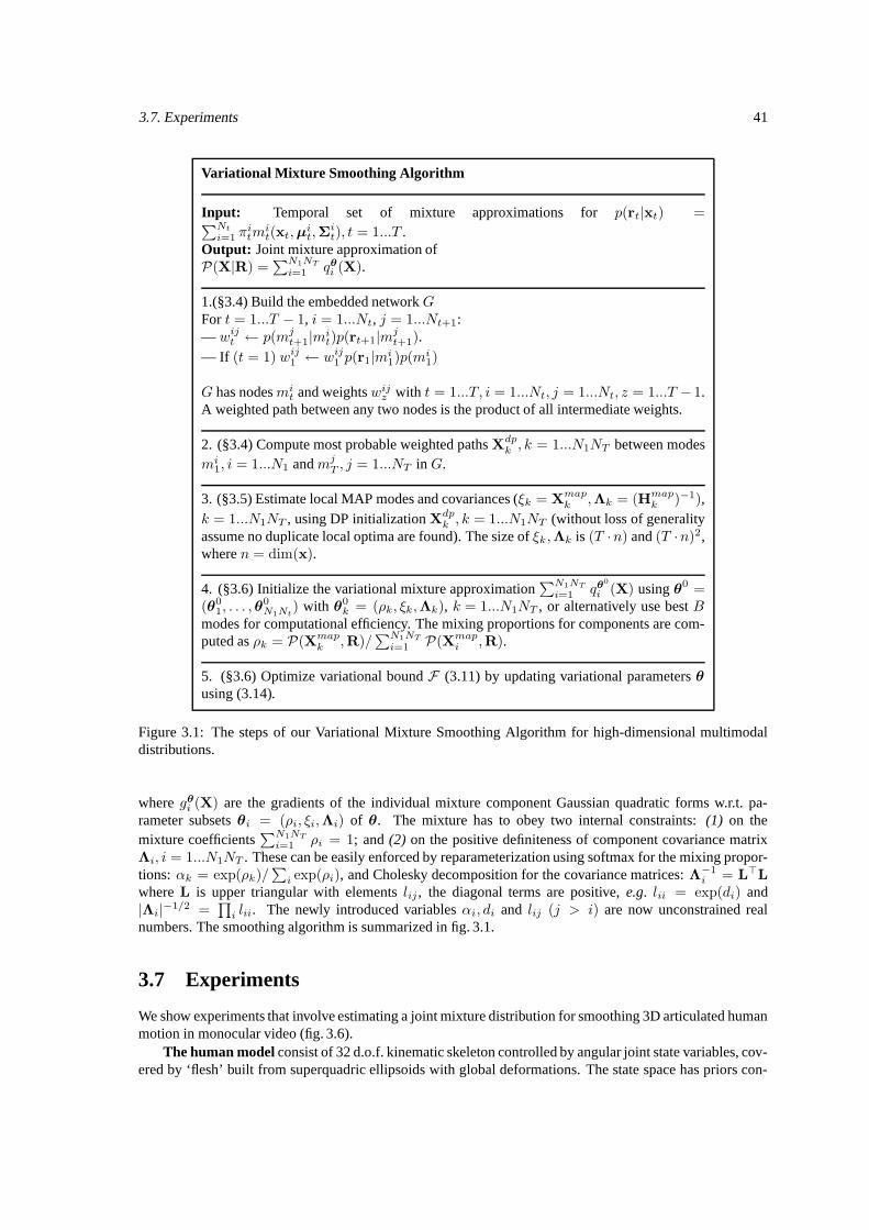
3.7. Experiments 41
Variational Mixture Smoothing Algorithm
Input: Temporal set of mixture approximations for p(rt|xt) =∑Nt
i=1 πitm
it(xt,µ
it,Σ
it), t = 1...T .
Output: Joint mixture approximation ofP(X|R) =
∑N1NT
i=1 qθi (X).
1.(§3.4) Build the embedded network GFor t = 1...T − 1, i = 1...Nt, j = 1...Nt+1:— wij
t ← p(mjt+1|mi
t)p(rt+1|mjt+1).
— If (t = 1) wij1 ← wij
1 p(r1|mi1)p(m
i1)
G has nodesmit and weights wij
z with t = 1...T, i = 1...Nt, j = 1...Nt, z = 1...T − 1.A weighted path between any two nodes is the product of all intermediate weights.
2. (§3.4) Compute most probable weighted paths Xdpk , k = 1...N1NT between modes
mi1, i = 1...N1 and mj
T , j = 1...NT in G.
3. (§3.5) Estimate local MAP modes and covariances (ξk = Xmapk ,Λk = (Hmap
k )−1),k = 1...N1NT , using DP initialization X
dpk , k = 1...N1NT (without loss of generality
assume no duplicate local optima are found). The size of ξk ,Λk is (T ·n) and (T ·n)2,where n = dim(x).
4. (§3.6) Initialize the variational mixture approximation∑N1NT
i=1 qθ0
i (X) using θ0 =(θ0
1, . . . ,θ0N1Nt
) with θ0k = (ρk, ξk,Λk), k = 1...N1NT , or alternatively use best B
modes for computational efficiency. The mixing proportions for components are com-puted as ρk = P(Xmap
k ,R)/∑N1NT
i=1 P(Xmapi ,R).
5. (§3.6) Optimize variational bound F (3.11) by updating variational parameters θ
using (3.14).
Figure 3.1: The steps of our Variational Mixture Smoothing Algorithm for high-dimensional multimodaldistributions.
where gθi (X) are the gradients of the individual mixture component Gaussian quadratic forms w.r.t. pa-
rameter subsets θi = (ρi, ξi,Λi) of θ. The mixture has to obey two internal constraints: (1) on themixture coefficients
∑N1NT
i=1 ρi = 1; and (2) on the positive definiteness of component covariance matrixΛi, i = 1...N1NT . These can be easily enforced by reparameterization using softmax for the mixing propor-tions: αk = exp(ρk)/
∑i exp(ρi), and Cholesky decomposition for the covariance matrices: Λ−1
i = L>L
where L is upper triangular with elements lij , the diagonal terms are positive, e.g. lii = exp(di) and|Λi|−1/2 =
∏i lii. The newly introduced variables αi, di and lij (j > i) are now unconstrained real
numbers. The smoothing algorithm is summarized in fig. 3.1.
3.7 Experiments
We show experiments that involve estimating a joint mixture distribution for smoothing 3D articulated humanmotion in monocular video (fig. 3.6).
The human model consist of 32 d.o.f. kinematic skeleton controlled by angular joint state variables, cov-ered by ‘flesh’ built from superquadric ellipsoids with global deformations. The state space has priors con-
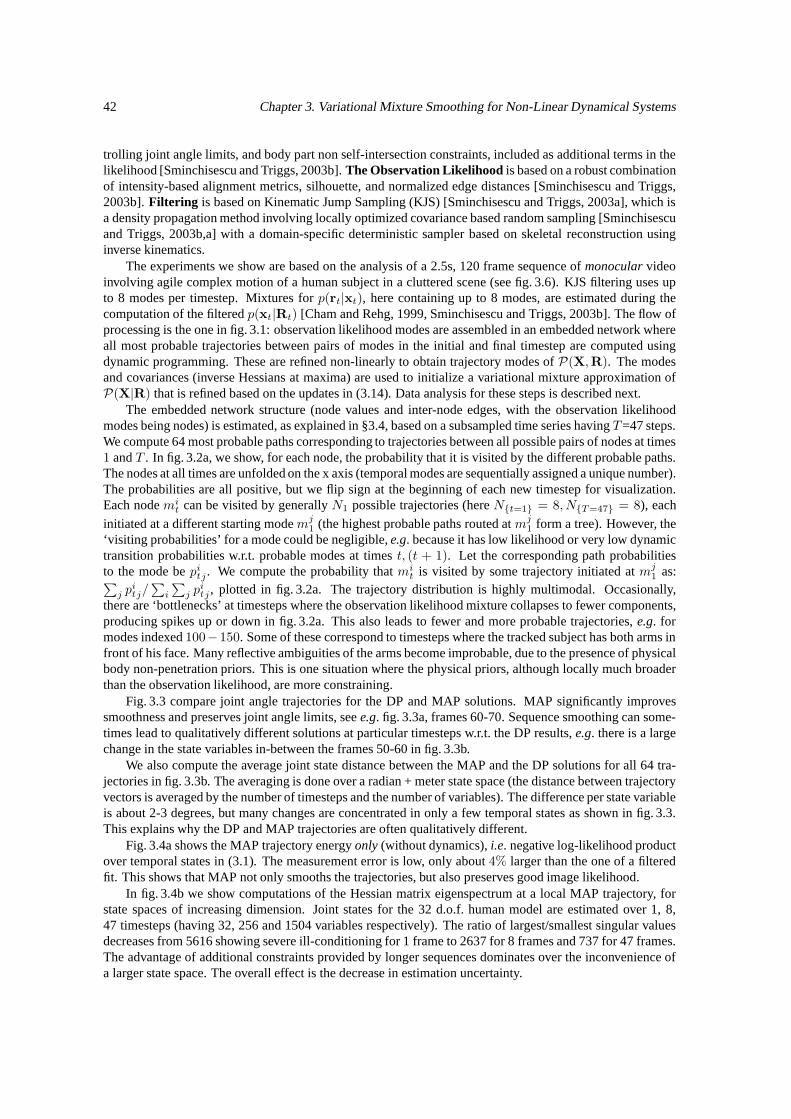
42 Chapter 3. Variational Mixture Smoothing for Non-Linear Dynamical Systems
trolling joint angle limits, and body part non self-intersection constraints, included as additional terms in thelikelihood [Sminchisescu and Triggs, 2003b]. The Observation Likelihood is based on a robust combinationof intensity-based alignment metrics, silhouette, and normalized edge distances [Sminchisescu and Triggs,2003b]. Filtering is based on Kinematic Jump Sampling (KJS) [Sminchisescu and Triggs, 2003a], which isa density propagation method involving locally optimized covariance based random sampling [Sminchisescuand Triggs, 2003b,a] with a domain-specific deterministic sampler based on skeletal reconstruction usinginverse kinematics.
The experiments we show are based on the analysis of a 2.5s, 120 frame sequence of monocular videoinvolving agile complex motion of a human subject in a cluttered scene (see fig. 3.6). KJS filtering uses upto 8 modes per timestep. Mixtures for p(rt|xt), here containing up to 8 modes, are estimated during thecomputation of the filtered p(xt|Rt) [Cham and Rehg, 1999, Sminchisescu and Triggs, 2003b]. The flow ofprocessing is the one in fig. 3.1: observation likelihood modes are assembled in an embedded network whereall most probable trajectories between pairs of modes in the initial and final timestep are computed usingdynamic programming. These are refined non-linearly to obtain trajectory modes of P(X,R). The modesand covariances (inverse Hessians at maxima) are used to initialize a variational mixture approximation ofP(X|R) that is refined based on the updates in (3.14). Data analysis for these steps is described next.
The embedded network structure (node values and inter-node edges, with the observation likelihoodmodes being nodes) is estimated, as explained in §3.4, based on a subsampled time series having T=47 steps.We compute 64 most probable paths corresponding to trajectories between all possible pairs of nodes at times1 and T . In fig. 3.2a, we show, for each node, the probability that it is visited by the different probable paths.The nodes at all times are unfolded on the x axis (temporal modes are sequentially assigned a unique number).The probabilities are all positive, but we flip sign at the beginning of each new timestep for visualization.Each node mi
t can be visited by generally N1 possible trajectories (here Nt=1 = 8, NT=47 = 8), each
initiated at a different starting mode mj1 (the highest probable paths routed at mj
1 form a tree). However, the‘visiting probabilities’ for a mode could be negligible, e.g. because it has low likelihood or very low dynamictransition probabilities w.r.t. probable modes at times t, (t + 1). Let the corresponding path probabilitiesto the mode be pi
tj . We compute the probability that mit is visited by some trajectory initiated at mj
1 as:∑j p
itj/∑
i
∑j p
itj , plotted in fig. 3.2a. The trajectory distribution is highly multimodal. Occasionally,
there are ‘bottlenecks’ at timesteps where the observation likelihood mixture collapses to fewer components,producing spikes up or down in fig. 3.2a. This also leads to fewer and more probable trajectories, e.g. formodes indexed 100−150. Some of these correspond to timesteps where the tracked subject has both arms infront of his face. Many reflective ambiguities of the arms become improbable, due to the presence of physicalbody non-penetration priors. This is one situation where the physical priors, although locally much broaderthan the observation likelihood, are more constraining.
Fig. 3.3 compare joint angle trajectories for the DP and MAP solutions. MAP significantly improvessmoothness and preserves joint angle limits, see e.g. fig. 3.3a, frames 60-70. Sequence smoothing can some-times lead to qualitatively different solutions at particular timesteps w.r.t. the DP results, e.g. there is a largechange in the state variables in-between the frames 50-60 in fig. 3.3b.
We also compute the average joint state distance between the MAP and the DP solutions for all 64 tra-jectories in fig. 3.3b. The averaging is done over a radian + meter state space (the distance between trajectoryvectors is averaged by the number of timesteps and the number of variables). The difference per state variableis about 2-3 degrees, but many changes are concentrated in only a few temporal states as shown in fig. 3.3.This explains why the DP and MAP trajectories are often qualitatively different.
Fig. 3.4a shows the MAP trajectory energy only (without dynamics), i.e. negative log-likelihood productover temporal states in (3.1). The measurement error is low, only about 4% larger than the one of a filteredfit. This shows that MAP not only smooths the trajectories, but also preserves good image likelihood.
In fig. 3.4b we show computations of the Hessian matrix eigenspectrum at a local MAP trajectory, forstate spaces of increasing dimension. Joint states for the 32 d.o.f. human model are estimated over 1, 8,47 timesteps (having 32, 256 and 1504 variables respectively). The ratio of largest/smallest singular valuesdecreases from 5616 showing severe ill-conditioning for 1 frame to 2637 for 8 frames and 737 for 47 frames.The advantage of additional constraints provided by longer sequences dominates over the inconvenience ofa larger state space. The overall effect is the decrease in estimation uncertainty.
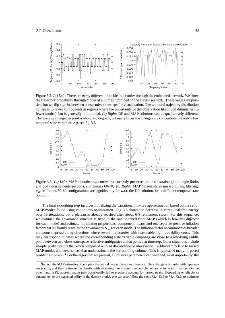
3.7. Experiments 43
-0.6
-0.4
-0.2
0
0.2
0.4
0.6
0 50 100 150 200 250 300
Tra
ject
ory
Pro
babi
lity
Thr
ough
Mod
e
Mode Index
0.02
0.022
0.024
0.026
0.028
0.03
0.032
0.034
0.036
0 10 20 30 40 50 60 70
Diff
eren
ce (
per
para
met
er)
Trajectory Index
Trajectory Parameter Space Difference (MAP vs. DP)
Figure 3.2: (a) Left: There are many different probable trajectories through the embedded network. We showthe trajectory probability through modes at all times, unfolded on the x axis (see text). These values are posi-tive, but we flip sign in-between consecutive timesteps for visualization. The temporal trajectory distributioncollapses to fewer components in regions where the uncertainty of the observation likelihood diminishes (tofewer modes), but is generally multimodal. (b) Right: DP and MAP solutions can be qualitatively different.The average change per joint is about 2-3 degrees, but many times the changes are concentrated in only a fewtemporal state variables, e.g. see fig. 3.3.
-2
-1.8
-1.6
-1.4
-1.2
-1
-0.8
-0.6
-0.4
-0.2
0 10 20 30 40 50 60 70 80 90 100
Join
t ang
le
Frame
DPMAP
0.4
0.6
0.8
1
1.2
1.4
1.6
1.8
2
2.2
2.4
0 10 20 30 40 50 60 70 80 90 100
Join
t ang
le
Frame
DPMAP
Figure 3.3: (a) Left: MAP smooths trajectories but correctly preserves prior constraints (joint angle limitsand body non self-intersection), e.g. frames 60-70. (b) Right: MAP fills-in states missed during filtering,e.g. in frames 50-60 configurations are significantly far w.r.t. the DP solution, i.e. a different temporal stateoptimum.
The final smoothing step involves initializing the variational mixture approximation based on the set ofMAP modes found using continuous optimization. Fig. 3.5 shows the decrease in variational free energyover 15 iterations, but a plateau is already reached after about 6-8 refinement steps. For this sequence,we assumed the covariance structure is fixed to the one obtained from MAP (which is however differentfor each mode) and estimate the mixing proportions, component means and one separate positive inflationfactor that uniformly rescales the covariances Λk, for each mode. The inflation factor accommodates broadercomponent spread along directions where several trajectories with reasonable high probability cross. Thismay correspond to cases where the corresponding state variable couplings are close to a low-lying saddlepoint between two close state space reflective ambiguities at that particular timestep. Other situations includesharply peaked priors that when composed with an ill-conditioned observation likelihood may lead to biasedMAP modes and covariances that underestimate the surrounding volume. This is typical of many ill-posedproblems in vision.4 For the algorithm we present, all mixture parameters can vary and, most importantly, the
4In fact, the MAP estimates do not play the central role in Bayesian inference. They change arbitrarily with reparam-eterization, and they optimize the density without taking into account the complementary volume information. On theother hand, a KL approximation may occasionally fail to precisely account for narrow peaks. Depending on efficiencyconstraints, or the expected utility of the density model, one can also follow the steps §3.4,§3.5 or §3.4,§3.6, or optimize
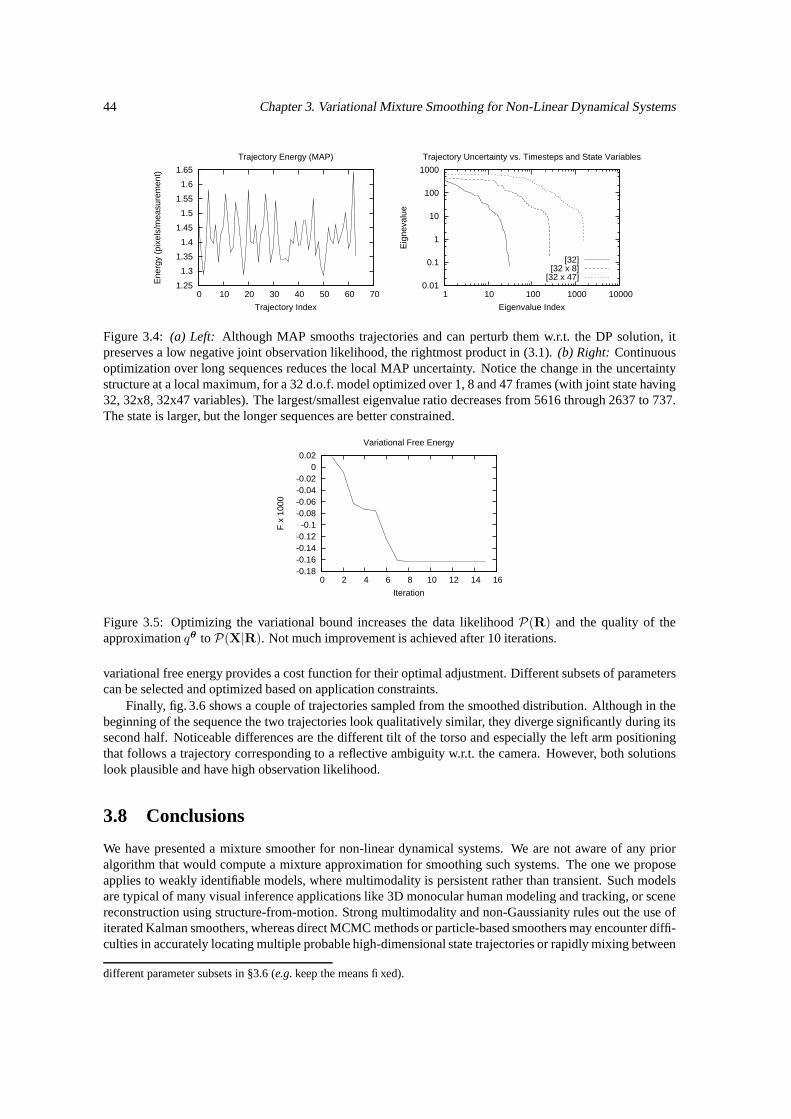
44 Chapter 3. Variational Mixture Smoothing for Non-Linear Dynamical Systems
1.25
1.3
1.35
1.4
1.45
1.5
1.55
1.6
1.65
0 10 20 30 40 50 60 70
Ene
rgy
(pix
els/
mea
sure
men
t)
Trajectory Index
Trajectory Energy (MAP)
0.01
0.1
1
10
100
1000
1 10 100 1000 10000
Eig
neva
lue
Eigenvalue Index
Trajectory Uncertainty vs. Timesteps and State Variables
[32][32 x 8]
[32 x 47]
Figure 3.4: (a) Left: Although MAP smooths trajectories and can perturb them w.r.t. the DP solution, itpreserves a low negative joint observation likelihood, the rightmost product in (3.1). (b) Right: Continuousoptimization over long sequences reduces the local MAP uncertainty. Notice the change in the uncertaintystructure at a local maximum, for a 32 d.o.f. model optimized over 1, 8 and 47 frames (with joint state having32, 32x8, 32x47 variables). The largest/smallest eigenvalue ratio decreases from 5616 through 2637 to 737.The state is larger, but the longer sequences are better constrained.
-0.18-0.16-0.14-0.12-0.1
-0.08-0.06-0.04-0.02
0 0.02
0 2 4 6 8 10 12 14 16
F x
100
0
Iteration
Variational Free Energy
Figure 3.5: Optimizing the variational bound increases the data likelihood P(R) and the quality of theapproximation qθ to P(X|R). Not much improvement is achieved after 10 iterations.
variational free energy provides a cost function for their optimal adjustment. Different subsets of parameterscan be selected and optimized based on application constraints.
Finally, fig. 3.6 shows a couple of trajectories sampled from the smoothed distribution. Although in thebeginning of the sequence the two trajectories look qualitatively similar, they diverge significantly during itssecond half. Noticeable differences are the different tilt of the torso and especially the left arm positioningthat follows a trajectory corresponding to a reflective ambiguity w.r.t. the camera. However, both solutionslook plausible and have high observation likelihood.
3.8 Conclusions
We have presented a mixture smoother for non-linear dynamical systems. We are not aware of any prioralgorithm that would compute a mixture approximation for smoothing such systems. The one we proposeapplies to weakly identifiable models, where multimodality is persistent rather than transient. Such modelsare typical of many visual inference applications like 3D monocular human modeling and tracking, or scenereconstruction using structure-from-motion. Strong multimodality and non-Gaussianity rules out the use ofiterated Kalman smoothers, whereas direct MCMC methods or particle-based smoothers may encounter diffi-culties in accurately locating multiple probable high-dimensional state trajectories or rapidly mixing between
different parameter subsets in §3.6 (e.g. keep the means fixed).

3.8. Conclusions 45
Figure 3.6: Variational smoothing generates multiple plausible trajectories. 3D reconstruction results basedon a 2.5s video sequence. First row: original Sequence, Second row: one probable model state sequenceprojected onto image at selected time-steps. Third row: One smoothed reconstructed 3D trajectory viewedfrom a synthetic viewpoint. Forth row: alternative 3D trajectory. Although in the beginning the two trajec-tories appear qualitatively similar, they diverge significantly during the second half of the sequence. Notethe different tilt of the torso and the significant difference in the left arm positioning that followed a smoothtrajectory corresponding to a reflective ambiguity w.r.t. the camera.
them. Our algorithm refines a compact approximation by combining polynomial time search over the net-work of observation likelihood peaks, local MAP continuous trajectory estimates and Bayesian variationaladjustment of the resulting joint mixture representation. We show results that demonstrate the method onthe estimation of multiple, smooth, high-quality trajectories that represent plausible articulated 3D humanmotions in difficult monocular video.Possible extensions: One can explore the design of multiresolution solvers for large dynamic programmingproblems, as well as tractable mixture approximations that automatically decouple the state variables. It is in-teresting to study the impact of learned motion models on the trajectory distribution, or derive reconstructionalgorithms robust to missing data (Chapters 11–13).

Chapter 4
Generalized Darting Monte Carlo
One of the main shortcomings of Markov chain Monte Carlo samplers is their inability to mix between modesof the target distribution. In this paper we show that advance knowledge of the location of these modes canbe incorporated into the MCMC sampler by introducing mode-hopping moves that satisfy detailed balance.The proposed sampling algorithm explores local mode structure through local MCMC moves (e.g. diffusionor Hybrid Monte Carlo) but in addition also represents the relative strengths of the different modes correctlyusing a set of global moves. This ‘mode-hopping’ MCMC sampler can be viewed as a generalization ofthe darting method [Andricioaiei et al., 2001]. We illustrate the method on learning Markov random fieldsand evaluate it against the spherical darting algorithm on a ‘real world’ vision application of inferring 3-Dhuman body pose distributions from 2-D image information. An earlier version of this chapter appearedin International Conference on Artificial Intelligence and Statistics (AISTATS) [Sminchisescu and Welling,2007].
4.1 Sampling and Mixing
It is well known that MCMC samplers have difficulty in mixing from one mode to the other because it typ-ically takes many steps of very low probability to make the trip [Neal, 1993, Celeux et al., 2000]. Recentimprovements designed to combat random walk behavior, like Hybrid Monte Carlo and over-relaxation [Du-ane et al., 1987, Neal, 1993] do not solve this problem when modes are separated by high energy barriers. Inthis paper we show how to exploit knowledge of the location of the modes to design a MCMC sampler thatmixes properly between them.
We consider two possible scenarios where this advance knowledge is present. In one example we haveactively searched for high probability regions using sophisticated optimization methods [Neal, 2001, Smin-chisescu and Triggs, 2002a]. Given these local maxima, we now desire to collect unbiased samples from theunderlying probability distribution. In another example we are given data-cases and aim at learning a modeldistribution to represent these data as accurately as possible. In this case, the data itself is representative ofthe low energy mode of a well fitted model.
This paper is organized as follows. In section 2 we review some popular Markov chain Monte Carlomethods. Then, in section 3 we introduce the new mode-hopping sampler and some extensions. An addi-tional proof of detailed balance and an auxiliary variable formulation of the method appear in the appendix.Section 4 explains and illustrates an application to learning Markov random fields, while in section 5 the gen-eralized darting method is evaluated against the spherical darting method on a ‘real world’ vision application– learning human models and estimating 3D human body poses from 2D image information.
46
4.2. Markov Chain Monte Carlo Sampling 47
4.2 Markov Chain Monte Carlo Sampling
Imagine we are given a probability distribution p(x) with x ∈ X ⊂ Rd a vector of continuous randomvariables. In the following we will focus on continuous variables, but the algorithm is easily extended todiscrete state spaces. A very general method to sample from this distribution is provided by Markov chainMonte Carlo (MCMC) sampling. The idea is to start with an initial distribution p0(x) and design a set oftransition probabilities that will eventually converge to the target distribution p(x).
The most commonly known transition scheme is the one proposed in the Metroplis-Hastings (M-H)algorithm, where a target point is sampled from a possibly asymmetric conditional distribution Q(xt+1|xt),where xt represents the current sample. To make sure that detailed balance holds, i.e. p(xt)Q(xt+1|xt) =p(xt+1)Q(xt|xt+1), which in turn guarantees that the target distribution remains invariant under Q, weshould only accept a certain fraction of the proposed targets:
Paccept = min
[1,p(xt+1)Q(xt|xt+1)
p(xt)Q(xt+1|xt)
](4.1)
In the most commonly used M-H algorithm, the transition distribution Q is symmetric and independentof the energy-surface at location x. This simplifies (4.1) (the Q factors cancel), but leads to slow mixingdue to random walk behavior. It is however not hard to incorporate local gradient information, dE(x)/dx toimprove mixing speed. One could for instance bias the proposal distribution Q(xt+1|xt) in the direction ofthe negative gradient−dE(x)/dx and accept using (4.1):
xτ+1 = xτ −∆τ2
2
dE(x)
dx
∣∣∣∣x=xτ
+ ∆τ n (4.2)
where n is a vector of independently chosen Gaussian variables with zero mean and unit variance, and ∆τis the stepsize. When the stepsize becomes infinitesimally small this is called the Langevin method and onecan show that the rejection rate vanishes in this limit.1
The Langevin method is a special case of a more general sampling technique called Hybrid Monte Carlo(HMC) sampling [Duane et al., 1987, Neal, 1993]. In HMC the particle is given a random initial momentumsampled from a unit-variance isotropic Gaussian density and its deterministic trajectory along the energysurface is then simulated for T time steps using Hamiltonian dynamics. If this simulation has no numericalerrors the increase, ∆E, in the combined potential and kinetic energy will be zero. If ∆E is positive, theparticle is returned to its initial position with a probability of 1− exp(−∆E). Numerical errors up to secondorder are eliminated by using a ‘leapfrog’ method which uses the potential energy gradient at time τ tocompute the velocity increment between time τ − 1
2 and τ + 12 and uses the velocity at time τ + 1
2 to computethe position increment between time τ and τ + 1. The Langevin method corresponds to precisely one step ofHMC (i.e. T = 1).
A host of clever MCMC samplers can be found in the literature. We refer to the excellent review [Neal,1993] for more information.
4.3 The Mode-Hopping MCMC Algorithm
We start with reviewing the closely related darting algorithm described in [Andricioaiei et al., 2001]. Indarting-MCMC we place spherical jump regions of equal volume at the location of the modes of the targetdistribution. The algorithm is based on a simple local MCMC sampler which is interrupted with a certainprobability to check if its current location is inside one of these spheres. If so, we initiate a jump to the cor-responding location in another sphere, chosen uniformly at random, where the usual Metropolis acceptancerule applies. To maintain detailed balance we decide not to move if we are located outside any of the balls. Itis not hard to check that this algorithm maintains detailed balance between any two points in sampling space.
1One can use more general biased proposal distributions, but the one defined in (4.2) was chosen because of itsvanishing rejection rate in the limit ∆ → 0.
48 Chapter 4. Generalized Darting Monte Carlo
In high dimensional spaces this procedure may still lead to unacceptably high rejection rates because themodes will likely decay sharply in at least a few directions. Since these ridges of probability are likely tobe uncorrelated across the modes, the proposed target location of the jump will have very low probability,resulting in almost certain rejection. In the following we will propose two important improvements over thedarting method. Firstly, we allow the jump regions to have arbitrary shapes and volumes and secondly theseregions may overlap. The first extension opens the possibility to align the jump regions precisely with theshape of the high probability regions of the target distribution. The second extension simplifies the design andplacement of the jump regions since we don’t have to worry about possible overlaps of the chosen regions.
First consider the case when the regions are non-overlapping but of different volumes. Like in thedarting method we could consider a one-to-one mapping between points in the different regions, or we couldchoose to sample the target point uniformly inside the new region. Because the latter is somewhat simplerconceptually, we’ll use uniform sampling in this section. The deterministic case will be treated in the nextsection. Also, to simplify the discussion we’ll first consider the case where the underlying target distributionis uniform, i.e. has equal probability everywhere. Due to the difference in volumes, particles are more likelyto be inside a large region than in small ones. Thus, there will be a larger flow of particles going from thebigger regions towards the smaller ones violating detailed balance. To correct for it we could reject a fractionof the proposed jumps from larger towards smaller regions. There is however a smarter solution, that picksthe target region proportional to its volume:
Pi =Vi∑j Vj
(4.3)
If we view the jumps between the various regions as a (separate) Markov chain, this method samples directlyfrom the equilibrium distribution while a rejection method would require a certain mixing time to reachequilibrium. Clearly, if the underlying distribution is not uniform, we need the Metropolis acceptance rulebetween the jump point and its image in the target region:
Paccept = min
[1,p(t)
p(x)
](4.4)
where t is the target point and x is the exit point.Now, let’s see what happens if two regions happen to overlap. Again, we first consider sampling the
target point uniformly in the new region, and consider a target distribution which is uniform. Consider tworegions which partly overlap. Due to the fact that we use the probability Pi (4.3), each volume element dx
inside the regions has equal probability of being chosen. However, points located in the intersection will bea target twice as often as points outside the intersection. To compensate, i.e. to maintain detailed balance, weneed to reject half of the proposed jumps into the intersection. In general, we check the number of regionsthat contain the exit point, n(x), and similarly for the target point, n(t). The appropriate fraction of movesthat is to be accepted in order to maintain detailed balance is min [1, n(x)/n(t)]. Combining this with theMetropolis acceptance probability 4.4 we find:
Paccept = min
[1,n(x)p(t)
n(t)p(x)
](4.5)
Putting everything together, we define the mode-hopping MCMC sampler explained in figure 4.1.
4.3.1 Elliptical Regions with Deterministic Moves
In the previous section we have uniformly sampled the proposed new location of the particle inside the targetregion. This is a very flexible method for which it is easy to prove detailed balance. However, a deterministictransformation can be tuned to map between points of roughly equal probability which is expected to im-prove the acceptance rate. Consider for instance the case that the energy surfaces near the regions is exactlyquadratic and have the same height (i.e. their centers have equal probability). We can now define a transfor-mation between ellipses that maps between points of equal probability resulting in a vanishing rejection rate.This is obviously not the case when we use uniform sampling.
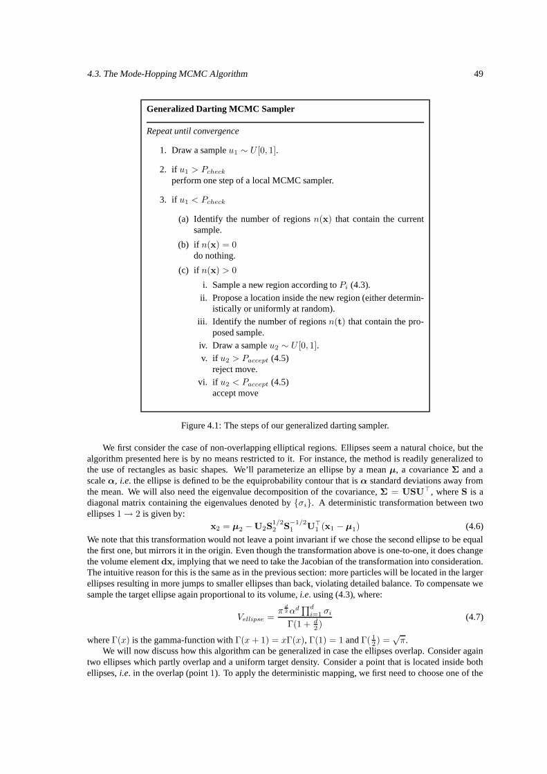
4.3. The Mode-Hopping MCMC Algorithm 49
Generalized Darting MCMC Sampler
Repeat until convergence
1. Draw a sample u1 ∼ U [0, 1].
2. if u1 > Pcheck
perform one step of a local MCMC sampler.
3. if u1 < Pcheck
(a) Identify the number of regions n(x) that contain the currentsample.
(b) if n(x) = 0do nothing.
(c) if n(x) > 0
i. Sample a new region according to Pi (4.3).
ii. Propose a location inside the new region (either determin-istically or uniformly at random).
iii. Identify the number of regions n(t) that contain the pro-posed sample.
iv. Draw a sample u2 ∼ U [0, 1].
v. if u2 > Paccept (4.5)reject move.
vi. if u2 < Paccept (4.5)accept move
Figure 4.1: The steps of our generalized darting sampler.
We first consider the case of non-overlapping elliptical regions. Ellipses seem a natural choice, but thealgorithm presented here is by no means restricted to it. For instance, the method is readily generalized tothe use of rectangles as basic shapes. We’ll parameterize an ellipse by a mean µ, a covariance Σ and ascale α, i.e. the ellipse is defined to be the equiprobability contour that is α standard deviations away fromthe mean. We will also need the eigenvalue decomposition of the covariance, Σ = USU>, where S is adiagonal matrix containing the eigenvalues denoted by σi. A deterministic transformation between twoellipses 1→ 2 is given by:
x2 = µ2 −U2S1/22 S
−1/21 U>
1 (x1 − µ1) (4.6)
We note that this transformation would not leave a point invariant if we chose the second ellipse to be equalthe first one, but mirrors it in the origin. Even though the transformation above is one-to-one, it does changethe volume element dx, implying that we need to take the Jacobian of the transformation into consideration.The intuitive reason for this is the same as in the previous section: more particles will be located in the largerellipses resulting in more jumps to smaller ellipses than back, violating detailed balance. To compensate wesample the target ellipse again proportional to its volume, i.e. using (4.3), where:
Vellipse =π
d2 αd
∏di=1 σi
Γ(1 + d2 )
(4.7)
where Γ(x) is the gamma-function with Γ(x+ 1) = xΓ(x), Γ(1) = 1 and Γ( 12 ) =
√π.
We will now discuss how this algorithm can be generalized in case the ellipses overlap. Consider againtwo ellipses which partly overlap and a uniform target density. Consider a point that is located inside bothellipses, i.e. in the overlap (point 1). To apply the deterministic mapping, we first need to choose one of the
50 Chapter 4. Generalized Darting Monte Carlo
two ellipses as a basis for the transformation. Unfortunately, an arbitrary rule such as the ellipse on top ofthe stack, or the one with the largest volume will result in a violation of detailed balance. Thus, we proposeto pick the ellipse at random with equal probability. Now consider the image point under the mapping (point2), choosing either the same ellipse (resulting in mirroring the point at the origin) or choosing the otherellipse. Assume point 2 is not located in the overlap. The probability of moving from 1 → 2 is 1
4 ; a factor12 coming from the fact that we first choose with equal probability which ellipse will be used to define thetransformation, and another factor 1
2 because we sample the target ellipse using (4.3). However, in the otherdirection 2 → 1 the probability is 1
2 . Note that unlike the case of uniformly sampling a target point (seeprevious section) the probability of going from 2 → 1 is not doubled2. Thus, to rescue detailed balancewe need to accept only half of the proposed moves from 2 → 1, or more generally min [1, n(x)/n(t)] withn(·) the number of ellipses containing a point. Combining this with the usual Metropolis acceptance ruleapplicable to general target densities, we arrive precisely at the rule in (4.5).
To summarize, the deterministic algorithm has precisely the same structure as algorithm in fig. 4.1, wherein the transformation (4.6) ellipse 1 is chosen uniformly at random from all ellipses containing point 1 andellipse 2 is chosen using (4.3) with Vi given by (4.7).
4.3.2 Mode-Hopping in Discrete State Spaces
Many practical problems are best described by probability distributions with discrete state spaces. It istherefore of importance to discuss this case as well. Fortunately, the extension is rather straightforward, themain difference being that ‘volumes’ are to be replaced by ‘number of states within a certain distance’.
In this section we consider the Manhattan distance, but the algorithm is by no means restricted to thatchoice. Consider a discrete state s in some D dimensional space, where every dimension can take one of Vvalues, e.g. s = [0, 3, 6, 1] for D = 4 and V = 6. The Manhattan distance between two states s1 and s2 isthe total number of changes we need to make to transform one state into the other, or:
D(s1, s2) =
D∑
i=1
|si1 − si
2| (4.8)
First consider the situation where no points are contained in two distinct regions and the regions have thesame shape. Again, we have a choice of using a deterministic transformation, mapping states one-to-one toeach other. For instance, if regions are defined to be the collection of all states that are at most a distance d
away from a reference state r, than we can use the offset s− r to define the mapping: s2 → r2 + (s1 − r1).Since all regions have the same number of states, we can simply pick a target region uniformly at random.
The situation is slightly more complicated if we allow for regions with different numbers of states. Itis clear that one-to-one mappings are now no longer possible. If one insists on a deterministic mappingmany-to-one mappings are possible, but intricate acceptance rules will need to be designed to retain detailedbalance. We will therefore proceed by using a random method, where the state in the target region is pickeduniformly at random from all possible states in that region. In analogy with the continuous case, in order tomaintain detailed balance, we need to pick the target region according to the distribution:
Pi = κi/∑
j
κj (4.9)
where κi is the number of states contained in region i.It is also easy to generalize this to overlapping regions. The same reasoning as in section 4.3 leads to
the conclusion that a fraction of samples min [1, n(x)/n(t)] should be accepted where n(·) is the number ofregions that contains a point. Finally, combining this with general target densities leads to the acceptance rule(4.5). The resulting MCMC algorithm is now very similar to the one in fig. 4.1, but with a different distancemeasure and a probability of picking a target region given by (4.9).
2The reason is that for every target ellipse the image of the point under the mapping (4.6) is different. However, thereare circumstances, e.g. when one ellipse is completely encircled by a larger one, that isolated points have the same imagefor two distinct target ellipses, resulting in violation of detailed balance. Since in the continuous case this set has measurezero, we will ignore it.

4.4. Proof of Detailed Balance 51
4.3.3 A Further Generalization
In the previous sections we have used distance measures to define regions between which the samples could‘jump’. This is geometrically appealing, but unnecessary for the algorithm to function properly. Moregenerally, we can use a set of conditions that must be satisfied in order to be able to jump between thesegeneralized regions. In order to maintain detailed balance we should however be able to determine the totalnumber of states which satisfy each set of conditions. The probability (4.9) can then be used to pick a targetregion and the acceptance rule (4.5) can be used to accept or reject a randomly picked point from that region.Overlaps are also allowed in this case.
4.4 Proof of Detailed Balance
The generalized darting Monte Carlo sampler can be viewed as a Hybrid Monte Carlo sampler that is in-terrupted with a certain probability to attempt a long range jump. Since Hybrid Monte Carlo sampling isergodic, a “mixture” of Hybrid Monte Carlo and any other (possibly non-ergodic) sampler is automaticallyergodic as well.
To prove detailed balance between any pair of points in the sample space, we consider the followingthree possibilities:
1. Both points are located outside any of the jump-regions.
2. One of the two points is located inside one or more jump-regions while the other one is located outsideany of the regions.
3. Both points are located in one or more of the regions.
1: When both points are located outside any of the jump-regions detailed balance follows because ofthe Markov chain for the local moves is assumed to respect detailed balance. With probability Pcheck thisMarkov chain is interrupted to check if the particle is located inside a jump-region. But since both pointsunder consideration are assumed to be located outside any jump-region this interruption will be symmetricand does not destroy detailed balance.
2: The particle located outside any jump-region follows its local dynamics (i.e. it is not interrupted) withprobability 1 − Pcheck. The particle inside one or more regions will also follow its local dynamics (i.e. itwill not attempt a jump) with probability 1−Pcheck. With probability Pcheck the sampler decides to performa check. But in that case the particle outside any region will stay put while the particle inside one or moreregions will attempt a jump and will therefore never end up outside the set of all regions. Thus detailedbalance again holds.
3: We will prove the case of two points in possibly overlapping regions, where the jump points are sam-pled uniformly at random inside a target region. The prove for the deterministic case goes along similar lines(see section 4.3.1).
With probability 1 − Pcheck we follow the local dynamics of the Markov chain which fulfills detailedbalance by assumption. With probability Pcheck we initiate a jump to some other point in some other region.Define A to be the set of regions that contain point 1 and B the set of regions that contain point 2. We nowhave:
52 Chapter 4. Generalized Darting Monte Carlo
p(x1) P (x1 → x2) = p(x1) Pcheck
∑
i⊂B
Pi
ViPaccept:1→2 (4.10)
= p(x1) Pcheckn(x2)∑
j Vjmin
[1,p(x2)n(x1)
p(x1)n(x2)
](4.11)
= Pcheck1∑j Vj
min [p(x1)n(x2), p(x2)n(x1)] (4.12)
= p(x2) Pcheckn(x1)∑
j Vjmin
[1,p(x1)n(x2)
p(x2)n(x1)
](4.13)
= p(x2) Pcheck
∑
i⊂A
Pi
ViPaccept:2→1 (4.14)
= p(x2) P (x2 → x1) (4.15)
where Pi (equation 4.3) is the probability of jumping to region i and the factor 1/Vi is included becausethe target point is sampled uniformly at random inside this region. Thus, once again establish detailedbalance.
4.5 Auxiliary Variable Formulation
The algorithm we presented in §4.3 can be formulated, more generally as an auxiliary variable method. Herethe index of the regions (wormholes) plays the role of the auxiliary variable and we sample from the jointdistribution over state space and region indexes using a mixture of Metropolis-Hastings transitions.
Consider x ∈ X the space and p the target distribution, and a covering with regions Ri (with volumesVi = |Ri|) of X such that:
X = ∪Ni=1Ri (4.16)
Define, for any x ∈ X , n(x) =∑N
i=1 I(x ∈ Ri), where I(x ∈ A) is the indicator function for the set A.We use the following identity:
p(dx) = p(dx)
N∑
i=1
I(x ∈ Ri)
n(x)= (4.17)
=
N∑
i=1
p(dx)/n(x)I(x ∈ Ri)∫Rip(dx)/n(x)
∫
Ri
p(dx)/n(x) (4.18)
We can now define a joint probability distribution over the space defined by the Cartesian product of theregion index set and the state space 1, . . . , N × X :
p(i,dx) ≡ p(dx)/n(x)I(x ∈ Ri)∫Rip(dx)/n(x)
∫
Ri
p(dx)/n(x) (4.19)
where, based on Bayes’ rule:
p(dx|i) =p(dx)/n(x)I(x ∈ Ri)∫
Rip(dx)/n(x)
(4.20)
p(i) =
∫
Ri
p(dx)/n(x) (4.21)
In this auxiliary variable setting, we will sample from the joint target distribution p(i,x)using a proposaldistribution Q(i,dx). The transition probability for the algorithm, excluding local moves and assuming theratio is well defined, is:

4.6. Learning Random Fields 53
P (i,x; j,dy = t− x) =N∑
k=1
min
(1,p(j,dy)Q(j,dy; i,dx)
p(i,dx)Q(i,dx; j,dy)
)Q(j,dy) (4.22)
+ δi,x(j,dy)r(i,x)
(4.23)
where in the above r(i,x) is the probability of not moving from (i,x), either because a proposed moveis rejected, or because no move is attempted [Green, 1995]. Choices of Q are given in the next sections.
4.5.1 Uniform Sampling inside Regions
For this case, we use:
Q(i) =Vi∑N
k=1 Vk
I(i ∈ 1, . . . , N) (4.24)
Q(dx|i) = 1/Vidx I(x ∈ Ri) (4.25)
and the acceptance probability simplifies to (4.5).
4.5.2 Deterministic Moves between Regions
The second choice of proposal Q correspond to deterministic moves [Tierney, 1998], given in §4.3.1:
Q(i,x; j,dy) = δF (i,x)(j,dy)Vi∑N
k=1 Vk
I(i ∈ 1, . . . , N) (4.26)
for a deterministic mapping F : X → X . This typically requires a change of variables, thus a Jacobianterm. We sample using (4.3), hence the need to consider the relative volume ratios in the equation.
4.6 Learning Random Fields
The proposed mode-hopping algorithm can only be successful if we have advance information3 about theexpected location of regions of high probability. In the following two sections we discuss examples wherethis is indeed the case.
In the first example we consider a situation where we want to train a Random Field (RF) model fromdata. The general form of a RF is given by:
p(x|r,θ) =1
Z(θ, r)e−E(x;r,θ) (4.27)
where θ is a set of parameters that we try to infer given the data, r = r1, ..., rn are image observations,E(x; r,θ) is the energy and Z(θ) the normalizing constant or partition function:
Z(θ, r) =
∫dθ e−E(x;r,θ) (4.28)
We use the maximum likelihood criterium to define a cost function for finding the optimal setting of theseparameters:
F = − 1
N
N∑
n=1
log p(xn|rn,θ) (4.29)
= 〈E(x; rn,θ)〉data + logZ(θ, r) (4.30)
3Adapting the Markov chain to include new regions on-line would violate the Markov assumption and is thereforenot guaranteed to converge to the desired probability distribution.
54 Chapter 4. Generalized Darting Monte Carlo
To minimize this ‘free energy’ (negative log-likelihood) we need to compute its gradients:
dFdθ
=
⟨dE(x; r,θ)
dθ
⟩
data
−⟨dE(x; r,θ)
dθ
⟩
model
(4.31)
where the second term is equal to the negative derivative of the log-partition function w.r.t. θ. Note thatthe only difference between the two terms in (4.31) is the distribution which is used to average the energyderivative. In the first term we use the empirical distribution, i.e. we simply average over the available data-set. In the second term however we average over the model distribution as defined by the current setting of theparameters. Computing this second average analytically is typically too complicated, so approximations areneeded instead. An unbiased estimate can be obtained by replacing the integral by a sample average, wherethe sample is to be drawn from the model p(x|r,θ). In many cases MCMC is the only method available thatcan generate this sample set.
Imagine the target distribution p(x|r,θ) has many modes and the Markov chain is initialized in one ofthem. Due to the energy barriers, we do not expect the chain to mix very well between the modes whichresults in very poor estimates of the second term in (4.31). Under the assumption that the modes of thedistribution are located close to clusters of data-points, a viable strategy is to start the Markov chains atvarious different data-points in order to have some representative samples in each mode. This strategy isused in contrastive divergence learning [Hinton, 2002] where a Markov chain is initiated at each data-pointand run for only a few steps (i.e. not to equilibrium) to generate distorted reconstructions of the data-point.Those reconstructions are subsequently used in the second term of (4.31) to compute an estimate of theenergy derivative.
Even though we have arranged to generate samples in most relevant modes of the distribution, the factthat the samples do not properly mix between the modes results in poor estimates of the relative probabilitymasses of the modes under the distribution defined by the model. The mode-hopping extension of the MCMCsampler proposed in this paper can help resolve this problem by defining regions around data clusters betweenwhich the sampler jumps. In one limit one could imagine defining a a small spherical region around every datapoint, or an appropriate subset of all data points. An alternative possibility is to run a clustering algorithm asa preprocessing step and to define regions corresponding to each cluster. For example, a mixture of Gaussianmodel could be trained using the Expectation Maximization algorithm with regions corresponding to theequiprobability contours α standard deviations away from the mean. Since these regions are elliptical, thedeterministic mode-hopping algorithm described in section 4.3.1 may be used.
4.7 Monocular Human Pose Inference and Learning
We explore the potential of the generalized darting method for monocular 3D human pose estimation. Thisproblem has applications for human-computer interaction and for actor reconstruction from movie footage –in this case only one camera viewpoint, the one presented in the movie, is usually available.
We run experiments based on correspondences between the articulated joints of a subject in the imageand the joints of a 3D articulated model (2D-3D correspondences). We also report experiments for learningthe model parameters in a maximum likelihood framework (§4.6), using a more sophisticated edge-basedobservation model. Monocular human pose estimation is well adapted to illustrate the algorithm because theresulting 3D pose posterior is both high-dimensional (≈35 human joint angle state variables) and highly mul-timodal. In any single monocular image, under point-wise 3D human joints and their image projections, eachlimb of the human is subject to a ‘reflective’ kinematic flip ambiguity. Two 3D human body configurationswith symmetrical slant in depth w.r.t. the camera (see fig. 4.2) produce identical point-wise image perspectiveprojections. The number of possible solutions multiples over the number of links of the human body. Forexample, a 3D human model with 10 links (torso, head, left/right forearm, upperarm, thigh and calf) mayhave 2#links local optima, although this is usually an overestimate. Some solutions may not be physicallyplausible and may violate joint angle limits or body non-self-intersection constraints. The question this workaddresses is not how to find the optima but how to efficiently sample from the 3D human pose equilibriumdistribution once these are known.
4.7. Monocular Human Pose Inference and Learning 55
Related Research. Many powerful approaches to image-based Bayesian inference use non-parametric,sampled-based representations for their target distributions and employ factored sampling schemes [Isardand Blake, 1998a] for computation. These allow working with non-Gaussian observation models and haveguaranteed asymptotic correctness. Practically however, sample-based representations are computationallyexpensive, a factor often limiting their practical usage to models with 6-8 dimensions. The number of parti-cles required for good accuracy grows exponentially when there are loosely coupled sub-systems, such as thelimbs of a body, that each create local minima separated by high energy barriers. To alleviate these problems,partitioned samplers [MacCormick and Isard, 2000] or layered, annealing-based methods have been proposed[Neal, 2001, Deutscher et al., 2000]. However these methods tend not to be well adapted for our problem,where there is often not a large margin between the desired global optimum and other competing ones. In-stead, we observe several competing local optima with comparable energy, see e.g. fig. 4.2 and fig. 4.5. Theserepresent plausible 3D human pose interpretations given our overly-simple human body model, the sparseset of image observations we consider and the intrinsic forward-backward depth ambiguities in the pose of3D articulated chains from monocular images. It is likely that the margin and volume ratio between thecorrect pose optimum and the incorrect ones may be increased with better modeling and with learning (as weshow in one of the experiments). It is likely, however, that at the early stages of learning the 3D human poseposterior will be highly multimodal and have high entropy. Effective ML learning requires efficient methodsfor sampling c.f . (4.31). The proposed generalized darting is one possible way of doing this.
Another approach is to approximate the pose posterior using a mixture model. The energy minima can belocated using non-linear continuous optimization and used to build an importance sampler based on a mixtureof simple densities (e.g. Gaussians). However, the sampler may be deficient in approximating the tails of themodal distributions and may have low correction weights. An alternative is to use gradient-based hybridMCMC schemes [Duane et al., 1987, Neal, 1993, Choo and Fleet, 2001, Sminchisescu and Triggs, 2002b].These can significantly improve acceptance rates for high-dimensional models, but broken ergodicity causedby trapping in local optima usually persists [Sminchisescu and Triggs, 2002b].
In this paper we assume that there is considerable prior knowledge about the shape of the energy surface(e.g. prior search to locate optima) and focus on using this information to accelerate fair sampling. Severalalgorithms for locating multiple pose optima can be used. Sminchisescu and Triggs [2003a] use problemdependent constraints about forward / backward pose ambiguities in order to explicitly enumerate an entireequivalence class of kinematic minima starting at any given one in the class. For more general second-orderdifferentiable energy functions without kinematic symmetries [Sminchisescu and Triggs, 2002a,b] presentmethods to systematically find new minima by locating first-order saddle points (transition states) surround-ing the basin of attraction of an initially chosen one, found e.g. by gradient descent. The search progresses ina local to global manner, in order to eventually locate a sufficiently large and representative minimum set.
In this paper we propose an algorithm that uses knowledge of local optima and gradient-based samplingmoves in order to greatly improve both local and non-local acceptance rates – both mixing withing a modeand mixing between different modes. The algorithm is not only general but also motivated by the structureof the studied visual inference problem. The modes of the 3D human pose probability distribution are theconfigurations of a 3D human body model that align well with image features, e.g. 2D projected modeledges align with the edges of the filmed human. The use of monocular image sequences makes the depthinformation difficult to infer because depth is lost in perspective projection. The combinations of modelvariables that produce motion in depth (towards or away from the camera) have the highest uncertainty. Thevariables that control the motions parallel with the image plane are better constrained by the image evidence.Hence the core of the maxima have highly anisotropic ellipsoidal structure – see fig. 4.3a for the spectralcovariance structure of a local minimum with ratio of most uncertain / most certain direction ≈ 103. Thecombinations of variables that lead to motion in depth change with 3D human pose and with camera viewingdirection. Hence the different optima do not share the same principal directions, nor the same scaling. Incontrast to classical darting, where the sampler uses spherical, mode-centered regions, generalized dartinguses oriented ellipsoids computed from the local uncertainty structure of the distribution, for more global andfaster sampling estimates with increased acceptance rates.
56 Chapter 4. Generalized Darting Monte Carlo
4.7.1 Domain Modeling
This experiments in this section use the humanoid visual model described in chapter 2. We use the classicalLangevin sampler (see section 2), in combination with long-range jumps using the spherical darting and thegeneralized darting methods. We also experiment using an independence sampler based on a mixture ofnormal distributions centered at the local pose optima.
Energy Function: Recall that model state estimates are obtained by optimizing a maximum a posteriori cri-terion, the total posterior probability according to Bayes rule. The energy function is defined as the negativelog-likelihood of the posterior:
E(x, r,θ) = − log p(r|x,θ)− log p(x) = (4.32)
=∑
ie(ri,x,θ) +Ep(x) (4.33)
where e(ri,x) is the cost density associated with observation i, the sum is over all observations r =r1, ..., rn, and p(x) is the model state prior.
Observation Likelihood: We used a simple product of Gaussian likelihoods for each model skeletal joint(assumed independent) with cost e(ri,x,θ) = ∆r2
i /2σ2. The negative log-likelihood for the observations
is the sum of squared model joint re-projection errors. For our study, it provides an interesting and difficultto handle degree of multi-modality owing to the kinematic complexity of the human model and the lack ofobservability of 1/3 of the model state variables (the depth related ones) in any single monocular image. Forlearning experiments, we use an observation model based on edge residuals. These are collected at modeloccluding contours predicted in the image. At each 3D model configuration, for each element on a image-predicted model contour, a line search along the normal direction is used to locate an image edge that matchesit. The distance between the location of the model contour and the image edge is used to construct a quadraticfunction of the residual, similar to the one based on skeletal joint residuals. This is summed over all contourpredictions and all the human body parts.
4.7.2 Experiments
Sampling Experiments: We have selected 4 local minima corresponding to the left forearm and left calf ina monocular side view of the body (see fig. 4.2). The local minima have relative volumes of (0.16,0.38,0.10,0.36) and energy levels (4.41, 6.31, 7.20, 8.29).
For local optimization we use a second-order damped Newton trust region method [Fletcher, 1987] wheregradient and Hessians of the energy functions are computed analytically and assembled using the chain rulewith back-propagation on individual kinematic chains, for efficiency. For generalized darting, we estimatelocal covariances as inverse Hessians at each local minimum. For MCMC simulations, we enforce joint limitconstraints using reflective boundary conditions, i.e. by reversing the sign of the normal momentum when ithits a joint limit. We found this gave an improved sampling acceptance rate compared to simply projectingthe proposed configuration back on the constraint surface, as the latter leads to cascades of rejected movesuntil the momentum direction gradually swings around.
We ran the simulation for ∆τ = 0.1, using the Langevin sampler (fig. 4.4a), the darting method withspherical covariances (fig. 4.4b) and the generalized darting method with deterministic moves (fig. 4.4c). Infig. 4.4 we show a fragment of a larger simulation that uses a small jump probability P = 0.03, in order todiminish the frequency of jumps for illustrative purposes. It is easily noticeable that the classical sampleris trapped in the starting mode, and wastes all of its samples exploring it repeatedly. The spherical dartingmethod explores only 2 minima based on one successful long-range jump during 600 iterations. The dartingmethod (right) explores more minima by combining local moves with non-local jumps that are accepted morefrequently. Different minima are visited using 7 jumps. This could be visually observed in fig. 4.4. Aftereach jump, the sampler equilibrates at a different energy level associated to the new local minimum.
We have also performed a large simulation (105 steps) with ∆τ = 0.1 and probability P = 0.25 forthe darting moves. The first 200 samples were discarded in order to let the chain reach equilibrium. Thecovariance volume scaling factor α was set to unity. For classical darting, we place spheres of unit radius
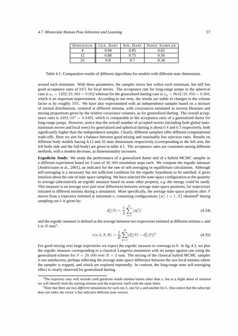
4.7. Monocular Human Pose Inference and Learning 57
DIMENSION GEN. DART SPH. DART INDEP. SAMPLER
4 0.94 0.85 0.6212 0.88 0.75 0.5635 0.8 0.7 0.34
Table 4.1: Comparative results of different algorithms for models with different state dimensions.
around each minimum. With these parameters, the sampler mixes fast within each minimum, but still hasgood acceptance rates of 94% for local moves. The acceptance rate for long-range jumps in the sphericalcase is as = 1292/24, 863 = 0.052 whereas for the generalized darting case is ag = 9642/25, 850 = 0.388,which is an important improvement. According to our tests, the results are stable to changes in the volumefactor α by roughly 10%. We have also experimented with an independence sampler based on a mixtureof normal distributions, centered at different minima, with covariances estimated as inverse Hessians andmixing proportions given by the relative covariance volumes, as for generalized darting. The overall accep-tance ratio is 3492/105 = 0.3492, which is comparable to the acceptance ratio of a generalized darter forlong-range jumps. However, notice that the overall number of accepted moves (including both global inter-minimum moves and local ones) for generalized and spherical darting is about 0.8 and 0.7 respectively, bothsignificantly higher than the independence sampler. Clearly, different samplers offer different computationaltrade-offs. Here we aim for a balance between good mixing and reasonably low rejection rates. Results ondifferent body models having 4,12 and 35 state dimensions respectively (corresponding to the left arm, theleft body side and the full-body) are given in table 4.1. The acceptance rates are consistent among differentmethods, with a modest decrease, as dimensionality increases.
Ergodicity Study: We study the performance of a generalized darter and of a hybrid MCMC sampler ina different experiment based on 3 runs of 20, 000 simulation steps each. We compute the ergodic measure[Andricioaiei et al., 2001], an indicator for the rate of self-averaging in equilibrium calculations. Althoughself-averaging is a necessary but not sufficient condition for the ergodic hypothesis to be satisfied, it givesintuition about the rate of state space sampling. We have selected the state-space configuration as the quantityto average (alternatively an ergodic measure based on some other property, e.g. the energy could be used).This measure is an average over pair-wise differences between average state-space positions, for trajectoriesinitiated in different minima during a simulation. More specifically, the average state space position after Smoves from a trajectory initiated at minimum a, containing configurations xa
i , i = 1..S obtained4 duringsampling run k is given by:
dak(S) =
1
S
S∑
i=1
||xai || (4.34)
and the ergodic measure is defined as the average between two trajectories initiated at different minima a andb in R runs5:
e(a, b, S,R) =1
R
R∑
k=1
[dak(S)− db
k(S)]2 (4.35)
For good mixing over large trajectories we expect the ergodic measure to converge to 0. In fig. 4.3, we plotthe ergodic measure corresponding to a classical Langevin simulation with no jumps against one using thegeneralized scheme for S = 20, 000 over R = 3 runs. The mixing of the classical hybrid MCMC sampleris not satisfactory, perhaps reflecting the average state-space difference between the two local minima wherethe sampler is trapped, and which are explored repeatedly. In contrast, the long-range state self-averagingeffect is clearly observed for generalized darting.
4The trajectory may well include configurations inside minima basins other than a, but in a slight abuse of notationwe will identify both the starting minima and the trajectory itself with the same letter.
5Note that there are two different simulations for each run k, one for a and another for b. Also notice that the subscriptdoes not index the vector x but indicates different state vectors.
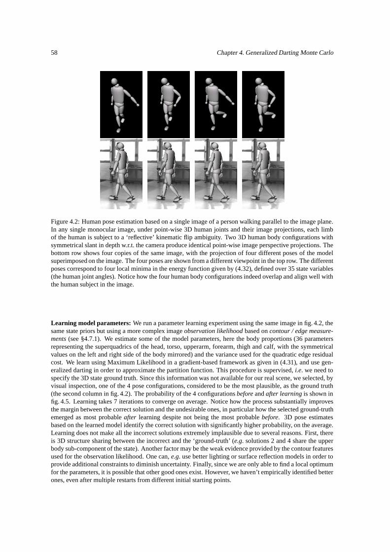
58 Chapter 4. Generalized Darting Monte Carlo
Figure 4.2: Human pose estimation based on a single image of a person walking parallel to the image plane.In any single monocular image, under point-wise 3D human joints and their image projections, each limbof the human is subject to a ‘reflective’ kinematic flip ambiguity. Two 3D human body configurations withsymmetrical slant in depth w.r.t. the camera produce identical point-wise image perspective projections. Thebottom row shows four copies of the same image, with the projection of four different poses of the modelsuperimposed on the image. The four poses are shown from a different viewpoint in the top row. The differentposes correspond to four local minima in the energy function given by (4.32), defined over 35 state variables(the human joint angles). Notice how the four human body configurations indeed overlap and align well withthe human subject in the image.
Learning model parameters: We run a parameter learning experiment using the same image in fig. 4.2, thesame state priors but using a more complex image observation likelihood based on contour / edge measure-ments (see §4.7.1). We estimate some of the model parameters, here the body proportions (36 parametersrepresenting the superquadrics of the head, torso, upperarm, forearm, thigh and calf, with the symmetricalvalues on the left and right side of the body mirrored) and the variance used for the quadratic edge residualcost. We learn using Maximum Likelihood in a gradient-based framework as given in (4.31), and use gen-eralized darting in order to approximate the partition function. This procedure is supervised, i.e. we need tospecify the 3D state ground truth. Since this information was not available for our real scene, we selected, byvisual inspection, one of the 4 pose configurations, considered to be the most plausible, as the ground truth(the second column in fig. 4.2). The probability of the 4 configurations before and after learning is shown infig. 4.5. Learning takes 7 iterations to converge on average. Notice how the process substantially improvesthe margin between the correct solution and the undesirable ones, in particular how the selected ground-truthemerged as most probable after learning despite not being the most probable before. 3D pose estimatesbased on the learned model identify the correct solution with significantly higher probability, on the average.Learning does not make all the incorrect solutions extremely implausible due to several reasons. First, thereis 3D structure sharing between the incorrect and the ‘ground-truth’ (e.g. solutions 2 and 4 share the upperbody sub-component of the state). Another factor may be the weak evidence provided by the contour featuresused for the observation likelihood. One can, e.g. use better lighting or surface reflection models in order toprovide additional constraints to diminish uncertainty. Finally, since we are only able to find a local optimumfor the parameters, it is possible that other good ones exist. However, we haven’t empirically identified betterones, even after multiple restarts from different initial starting points.
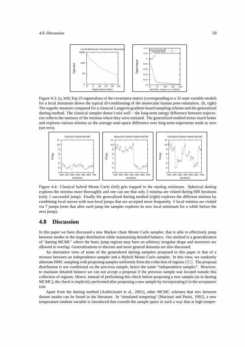
4.8. Discussion 59
1
10
100
1000
0 5 10 15 20 25
Eige
nval
ue
Eigenvalue Index
Local Minimum Covariance Structure
0
0.2
0.4
0.6
0.8
1
1.2
1.4
0 5 10 15 20
Ergo
dic m
easu
re
MCMC steps (x 1000)
GeneralizedHybrid MC
Figure 4.3: (a, left) Top 25 eigenvalues of the covariance matrix (corresponding to a 35 state variable model)for a local minimum shows the typical ill-conditioning of the monocular human pose estimation. (b, right)The ergodic measure compared for a classical Langevin gradient-based sampling scheme and the generalizeddarting method. The classical sampler doesn’t mix well – the long-term energy difference between trajecto-ries reflects the memory of the minima where they were initiated. The generalized method mixes much betterand explores various minima so the average state-space difference over long-term trajectories tends to zero(see text).
4
5
6
7
8
9
10
11
100 200 300 400 500 600 700
Ener
gy
Iterations
Classical Hybrid MCMC
4
5
6
7
8
9
10
11
100 200 300 400 500 600 700
Ener
gy
Iterations
Spherical Darted Hybrid MCMC
4
5
6
7
8
9
10
11
100 200 300 400 500 600 700
Ener
gy
Iterations
Geralized Darted Hybrid MCMC
Figure 4.4: Classical hybrid Monte Carlo (left) gets trapped in the starting minimum. Spherical dartingexplores the minima more thoroughly and one can see that only 2 minima are visited during 600 iterations(only 1 successful jump). Finally the generalized darting method (right) explores the different minima bycombining local moves with non-local jumps that are accepted more frequently. 8 local minima are visitedvia 7 jumps (note that after each jump the sampler explores its new local minimum for a while before thenext jump).
4.8 Discussion
In this paper we have discussed a new Markov chain Monte Carlo sampler, that is able to effectively jumpbetween modes in the target distribution while maintaining detailed balance. Our method is a generalizationof ‘darting MCMC’ where the basic jump regions may have an arbitrary irregular shape and moreover areallowed to overlap. Generalizations to discrete and more general domains are also discussed.
An alternative view of some of the generalized darting samplers proposed in this paper is that of amixture between an independence sampler and a Hybrid Monte Carlo sampler. In this view, we randomlyalternate HMC sampling with proposing samples uniformly from the collection of regions Vi. The proposaldistribution is not conditional on the previous sample, hence the name “independence sampler”. However,to maintain detailed balance we can not accept a proposal if the previous sample was located outside thiscollection of regions. Hence, instead of performing this check before proposing a new sample (as in dartingMCMC), the check is implicitly performed after proposing a new sample by incorporating it in the acceptancerule.
Apart from the darting method [Andricioaiei et al., 2001], other MCMC schemes that mix betweendistant modes can be found in the literature. In ‘simulated tempering’ [Marinari and Parisi, 1992], a newtemperature random variable is introduced that extends the sample space in such a way that at high temper-
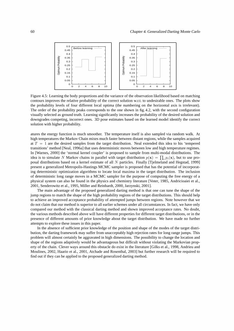
60 Chapter 4. Generalized Darting Monte Carlo
0
0.05
0.1
0.15
0.2
0.25
0.3
0.35
0.4
0.45
0.5
0 2 4 6 8 10
Opt
imum
Pro
babi
lity
Before learning
0
0.05
0.1
0.15
0.2
0.25
0.3
0.35
0.4
0.45
0.5
0 2 4 6 8 10
Opt
imum
Pro
babi
lity
After learning
Figure 4.5: Learning the body proportions and the variance of the observation likelihood based on matchingcontours improves the relative probability of the correct solution w.r.t. to undesirable ones. The plots showthe probability levels of four different local optima (the numbering on the horizontal axis is irrelevant).The order of the probability peaks corresponds to the one shown in fig. 4.2, with the second configurationvisually selected as ground truth. Learning significantly increases the probability of the desired solution anddowngrades competing, incorrect ones. 3D pose estimates based on the learned model identify the correctsolution with higher probability.
atures the energy function is much smoother. The temperature itself is also sampled via random walk. Athigh temperatures the Markov Chain mixes much faster between distant regions, while the samples acquiredat T = 1 are the desired samples from the target distribution. Neal extended this idea to his ‘temperedtransitions’ method [Neal, 1996a] that uses deterministic moves between low and high temperature regimes.In [Warnes, 2000] the ‘normal kernel coupler’ is proposed to sample from multi-modal distributions. Theidea is to simulate N Markov chains in parallel with target distribution p(x) =
∏i pi(x), but to use pro-
posal distributions based on a kernel estimate of all N particles. Finally [Tjelmeland and Hegstad, 1999]present a generalized Metropolis-Hastings MCMC sampler is proposed that has the potential of incorporat-ing deterministic optimization algorithms to locate local maxima in the target distribution. The inclusionof deterministic long range moves in a MCMC sampler for the purpose of computing the free energy of aphysical system can also be found in the physics and chemistry literature [Voter, 1985, Andricioaiei et al.,2001, Senderowitz et al., 1995, Miller and Reinhardt, 2000, Jarzynski, 2001].
The main advantage of the proposed generalized darting method is that one can tune the shape of thejump regions to match the shape of the high probability regions of the target distributions. This should helpto achieve an improved acceptance probability of attempted jumps between regions. Note however that wedo not claim that our method is superior to all earlier schemes under all circumstances. In fact, we have onlycompared our method with the classical darting method and shown improved acceptance rates. No doubt,the various methods described above will have different properties for different target distributions, or in thepresence of different amounts of prior knowledge about the target distribution. We have made no furtherattempts to explore these issues in this paper.
In the absence of sufficient prior knowledge of the position and shape of the modes of the target distri-bution, the darting framework may suffer from unacceptably high rejection rates for long range jumps. Thisproblem will almost certainly be aggravated in high dimensions. The possibility to change the location andshape of the regions adaptively would be advantageous but difficult without violating the Markovian prop-erty of the chain. Clever ways around this obstacle do exist in the literature [Gilks et al., 1998, Andrieu andMoulines, 2002, Haario et al., 2001, Atchade and Rosenthal, 2003] but further research will be required tofind out if they can be applied to the proposed generalized darting method.

PART II:CONDITIONAL ANDDISCRIMINATIVE MODELS

Chapter 5
BM3E : Discriminative Density
Propagation for Visual Tracking
We introduce BM3E, a Conditional Bayesian Mixture of Experts Markov Model, for consistent probabilis-tic estimates in discriminative visual tracking. The model applies to problems of temporal and uncertaininference and represents the unexplored bottom-up counterpart of pervasive generative models estimatedwith Kalman filtering or particle filtering. Instead of inverting a non-linear generative observation model atrun-time, we learn to cooperatively predict complex state distributions directly from descriptors that encodeimage observations – typically bag-of-feature global image histograms or descriptors computed over regularspatial grids. These are integrated in a conditional graphical model in order to enforce temporal smoothnessconstraints and allow a principled management of uncertainty. The algorithms combine sparsity, mixturemodeling, and non-linear dimensionality reduction for efficient computation in high-dimensional continuousstate spaces. The combined system automatically self-initializes and recovers from failure. The research hasthree contributions: (1) We establish the density propagation rules for discriminative inference in continuous,temporal chain models; (2) We propose flexible supervised and unsupervised algorithms for learning feed-forward, multivalued contextual mappings (multimodal state distributions) based on compact, conditionalBayesian mixture of experts models; (3) We validate the framework empirically for the reconstruction of 3dhuman motion in monocular video sequences. Our tests on both real and motion capture-based sequencesshow significant performance gains with respect to competing nearest-neighbor, regression, and structuredprediction methods. An earlier version of this chapter appeared in IEEE Transactions on Pattern Analysisand Machine Intelligence (PAMI) [Sminchisescu et al., 2007], based on research published in IEEE Inter-national Conference on Computer Vision and Pattern Recognition (CVPR) [Sminchisescu et al., 2005a] andAdvances in Neural Processing Systems (NIPS) [Sminchisescu et al., 2005c].
5.1 Motivation
We consider the problem of probabilistic state inference in feedforward, conditional chain models, based ontemporal observation sequences. For demonstration, we concentrate on the tracking and 3d reconstructionof articulated human motion in monocular video. This is a challenging research topic with a broad set ofapplications for scene understanding, but we emphasize that our framework applies generally, to continuousand uncertain temporal state estimation problems.
Two general classes of strategies exist for visual modeling and inference: (i) Generative (feedback) meth-ods optimize 3d kinematic and appearance models for good alignment with image features. The objective isencoded as an observation likelihood or cost function with optima (ideally!) centered at correct pose hypothe-ses; (ii) Conditional (feedforward) methods – also referred as discriminative, diagnostic, or recognition-based– predict human poses directly from images features. Both approaches require a state representation, x say,here a 3d human model with kinematics or shape (joint angles, surfaces or joint positions), and both use
63
64 Chapter 5. BM3E : Discriminative Density Propagation for Visual Tracking
a set of image feature observations, r, for state inference. A training set, T = (ri,xi) | i = 1 . . .N,sampled from the joint distribution is usually available. The computational goal is common: the conditionaldistribution, or a model state point estimate, given observations. The state and the observation descriptors areimportant components of modeling. The state needs dimensionality adequate for the variability in the task,and the observation descriptor needs to be specific enough to capture not only strong image dependencies butalso discriminative detail. Typically, these are obtained by combining a-priori design and off-line unsuper-vised learning. Once selected, the representation (model state & observation descriptor) is known for laterlearning and inference stages. This currently holds for both generative and discriminative models.
Generative algorithms model the joint distribution using a constructive form of the the observer: theobservation likelihood or cost function. Complex sampling or non-linear optimization methods are used toinfer the likelihood peaks, and Bayes’ rule is used to compute the state conditional from the observationconditional and the state prior. Both supervised and unsupervised procedures are used for model learning– either to obtain state priors [Brand, 1999, Howe et al., 1999, Deutscher et al., 2000, Sigal et al., 2004,Sminchisescu and Jepson, 2004b, Urtasun et al., 2005, Jaeggli et al., 2006] or to tune the parameters of theobservation model, e.g. texture, ridge or edge distributions, using problem-dependent, natural image statistics[Sidenbladh and Black, 2001, Roth et al., 2004, Sminchisescu and Welling, 2006]. Tracking is framed in aclear probabilistic and computational framework based on mixture filters or particle filters [Isard and Blake,1998a, Deutscher et al., 2000, Choo and Fleet, 2001, Sminchisescu and Triggs, 2003b,a, Sudderth et al.,2003, Sigal et al., 2004].
It has been argued that generative models can flexibly reconstruct complex unknown motions and cannaturally handle problem constraints. It has been counter-argued that both flexibility and modeling difficul-ties lead to expensive, uncertain inference [Deutscher et al., 2000, Sidenbladh and Black, 2001, Sminchisescuand Triggs, 2003a, Sminchisescu and Jepson, 2004a], and a constructive form of the observation (i.e. imageappearance) is both difficult to build and indirect with respect to the task – primarily conditional state esti-mation, not conditional observation modeling.
The generative counter-argument motivates the complementary study of discriminative algorithms[Rosales and Sclaroff, 2002, Mori and Malik, 2002, Shakhnarovich et al., 2003, Tomasi et al., 2003, Agarwaland Triggs, 2006c, Elgammal and Lee, 2004], that predict state distributions directly from image features.This approach is not without its own difficulties: background clutter, occlusion or depth ambiguities make theobservations-to-state mapping multi-valued and not amenable to simple functional prediction. Although, inprinciple, single hypothesis methods are not expected to be sufficient in this context, several authors demon-strated good practical performance [Shakhnarovich et al., 2003, Mori and Malik, 2002, Tomasi et al., 2003,Agarwal and Triggs, 2006c, Elgammal and Lee, 2004]. The methods differ in the organization of the trainingset and in the runtime hypothesis selection method: some construct data structures for fast nearest-neighborretrieval [Shakhnarovich et al., 2003, Tomasi et al., 2003, Mori and Malik, 2002], others learn regressionmodels [Agarwal and Triggs, 2006c, Elgammal and Lee, 2004]. Inference involves either indexing for thenearest-neighbors of the observation and using their state for locally weighted prediction, direct predictionusing the learned regression model [Agarwal and Triggs, 2006c, Elgammal and Lee, 2004], or affine recon-struction from joint centers [Mori and Malik, 2002].
Among (dominantly) discriminative methods, Rosales and Sclaroff [2002] take a notably different ap-proach, by accurately modeling the joint distribution using a mixture of perceptrons. Their system combinesmultiple image-based state prediction with hypothesis selection based on a rendering (feedback) model. Arelated method has been suggested by Grauman et al. [2003], who model the joint distribution of multi-viewsilhouettes-pose using a mixture of probabilistic PCA. The problem has been independently studied by Agar-wal and Triggs [2005] who use joint models based on random regression in a Condensation-based generativetracking framework. There is an important difference between working with the joint distribution [DeSarboand Cron, 1988, Rosales and Sclaroff, 2002] and working only with the conditional state distribution – evenwhen using mixture of feedforward state models (as opposed to generative observation models). In a jointmodel based on multiple components, the reliability of each state predictor has to be ranked at run-time –a non-trivial operation because the state is missing. The problem can be solved either by conditioning andmarginalization (the application of Bayes rule) in the joint model or by verification, using an ad-hoc, externalobservation model. Depending on the assumed modeling details, the computations can be difficult to per-

5.1. Motivation 65
form or may not be probabilistically consistent. An alternative is to use a conditionally parameterized model.Details on models and computations for both directly parameterized conditionals, and for models based onrandom regression and joint density appear in our earlier work [Sminchisescu et al., 2004].
To summarize, discriminative models provide fast inference, interpolate flexibly in the trained region,but can fail on non-typical inputs, especially if trained using small datasets. Large training set and complexmotions increase the image-to-pose ambiguity which manifests as multivalued image-to-pose relations or,probabilistically, as multimodal conditional state distributions. Learning multivalued models is inherentlydifficult. Moreover, existing discriminative methods lack a probabilistic temporal estimation framework thathas been so fruitful with generative models [Isard and Blake, 1998a, Deutscher et al., 2000, Sminchisescu andTriggs, 2003a]. Existing tracking algorithms [Tomasi et al., 2003, Agarwal and Triggs, 2006c, Elgammal andLee, 2004] involve per-frame state inference, often using estimates at previous timesteps [Tomasi et al., 2003,Agarwal and Triggs, 2006c, Elgammal and Lee, 2004], but do rely on an set of independence assumptions orpropagation rules. What distributions should be modeled, how should they be modeled, and how should theybe temporally combined for optimal solutions?
The research we present addresses these questions formally. We introduce BM 3E, a ConditionalBayesian Mixture of Experts Markov Model for consistent probabilistic estimates in discriminative visualtracking. This represents the unexplored, feedforward counterpart of temporal generative models estimatedwith Kalman filtering or particle filtering. Instead of inverting a generative observation model at run-time,we learn to cooperatively predict complex state distributions directly from image descriptors. These are in-tegrated in a conditional graphical model in order to enforce temporal smoothness constraints, and allow aprincipled management of uncertainty.1 The algorithm combines sparsity, mixture modeling, and non-lineardimensionality reduction for efficient computation in high-dimensional continuous state spaces [Sminchis-escu et al., 2005a,c, 2004, Sminchisescu and Jepson, 2004c]. The combined system automatically initializesand recovers from failure – it can be used either stand-alone, or as a component to bootstrap generativeinference algorithms. This research has three technical contributions:
(1) We establish the density propagation rules for discriminative inference in continuous, temporal chainmodels. The ingredients of the approach are: (a) the structure of the graphical model (see fig. 5.1 and §5.2.1);(b) the representation of local, per-node conditional state distributions (see (2) below and §5.2.2); (c) thebelief propagation (chain inference) procedure (§5.2.1). We work parametrically and analytically, to predictand propagate Gaussian mixtures [Sminchisescu and Jepson, 2004a], but non-parametric belief propagationmethods [Sudderth et al., 2003, Sigal et al., 2004] can also be used to solve (c).
(2) We propose flexible algorithms for learning to contextually predict feedforward multimodal statedistributions based on compact, conditional Bayesian mixture of experts. (An expert is any functional ap-proximator, e.g. a perceptron or regressor.) These are based on hierarchical mixtures of experts [Jordan andJacobs, 1994, Waterhouse et al., 1996, Ueda and Ghahramani, 2002, Bishop and Svensen, 2003], an elabo-rated version of clusterwise or switching regression [DeSarbo and Cron, 1988, Rosales and Sclaroff, 2002],where the expert mixture proportions, called gates, are themselves observation-sensitive predictors, synchro-nized across experts to give properly normalized conditional state distributions for any input observation. Ourlearning algorithm is different from the one of [Waterhouse et al., 1996] in that we use sparse greedy approx-imations, and differs from [Bishop and Svensen, 2003] in that we use type-II maximum likelihood Bayesianapproximations [Mackay, 1998, 1992, Tipping, 2001, Lawrence et al., 2003], not structured variational ones.
(3) We validate the framework empirically on the problem of reconstructing 3d human motion in monoc-ular video sequences. Our tests on both real and motion capture-based sequences show important robustnessand performance gains compared to nearest-neighbor, regression, and structured prediction methods.
Chapter Organization: We introduce the discriminative density propagation framework, referred asBM 3E ,in §5.2 as follows: §5.2.1 reviews the structure of the graphical model and the equations used for tempo-ral density propagation (precise derivations are given in the Appendix), §5.2.2 describes the ConditionalBayesian Mixture of Experts Model (BME) and explains its parameter learning algorithm; §5.2.3 discussesan alternative model based on random regression and joint density. §5.2.4 shows how to construct struc-
1This model should not be confused with a Maximum Entropy Markov Model, MEMM [McCallum et al., 2000], de-signed for discrete state variables, and based on a different, maximum entropy representation of conditional distributions.
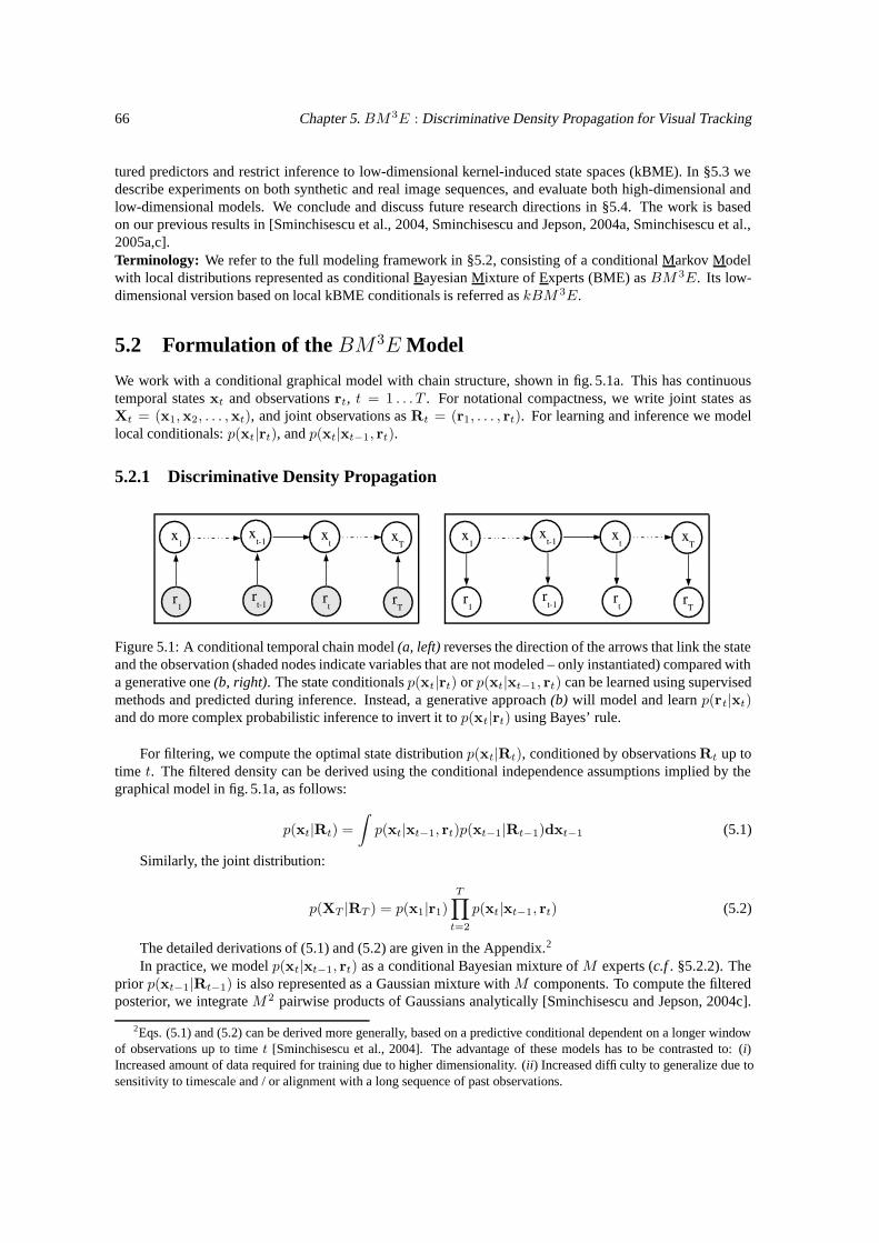
66 Chapter 5. BM3E : Discriminative Density Propagation for Visual Tracking
tured predictors and restrict inference to low-dimensional kernel-induced state spaces (kBME). In §5.3 wedescribe experiments on both synthetic and real image sequences, and evaluate both high-dimensional andlow-dimensional models. We conclude and discuss future research directions in §5.4. The work is basedon our previous results in [Sminchisescu et al., 2004, Sminchisescu and Jepson, 2004a, Sminchisescu et al.,2005a,c].Terminology: We refer to the full modeling framework in §5.2, consisting of a conditional Markov Modelwith local distributions represented as conditional Bayesian Mixture of Experts (BME) as BM 3E. Its low-dimensional version based on local kBME conditionals is referred as kBM 3E.
5.2 Formulation of the BM3E Model
We work with a conditional graphical model with chain structure, shown in fig. 5.1a. This has continuoustemporal states xt and observations rt, t = 1 . . . T . For notational compactness, we write joint states asXt = (x1,x2, . . . ,xt), and joint observations as Rt = (r1, . . . , rt). For learning and inference we modellocal conditionals: p(xt|rt), and p(xt|xt−1, rt).
5.2.1 Discriminative Density Propagation
Figure 5.1: A conditional temporal chain model (a, left) reverses the direction of the arrows that link the stateand the observation (shaded nodes indicate variables that are not modeled – only instantiated) compared witha generative one (b, right). The state conditionals p(xt|rt) or p(xt|xt−1, rt) can be learned using supervisedmethods and predicted during inference. Instead, a generative approach (b) will model and learn p(rt|xt)and do more complex probabilistic inference to invert it to p(xt|rt) using Bayes’ rule.
For filtering, we compute the optimal state distribution p(xt|Rt), conditioned by observations Rt up totime t. The filtered density can be derived using the conditional independence assumptions implied by thegraphical model in fig. 5.1a, as follows:
p(xt|Rt) =
∫p(xt|xt−1, rt)p(xt−1|Rt−1)dxt−1 (5.1)
Similarly, the joint distribution:
p(XT |RT ) = p(x1|r1)
T∏
t=2
p(xt|xt−1, rt) (5.2)
The detailed derivations of (5.1) and (5.2) are given in the Appendix.2
In practice, we model p(xt|xt−1, rt) as a conditional Bayesian mixture of M experts (c.f . §5.2.2). Theprior p(xt−1|Rt−1) is also represented as a Gaussian mixture with M components. To compute the filteredposterior, we integrate M 2 pairwise products of Gaussians analytically [Sminchisescu and Jepson, 2004c].
2Eqs. (5.1) and (5.2) can be derived more generally, based on a predictive conditional dependent on a longer windowof observations up to time t [Sminchisescu et al., 2004]. The advantage of these models has to be contrasted to: (i)Increased amount of data required for training due to higher dimensionality. (ii) Increased difficulty to generalize due tosensitivity to timescale and / or alignment with a long sequence of past observations.
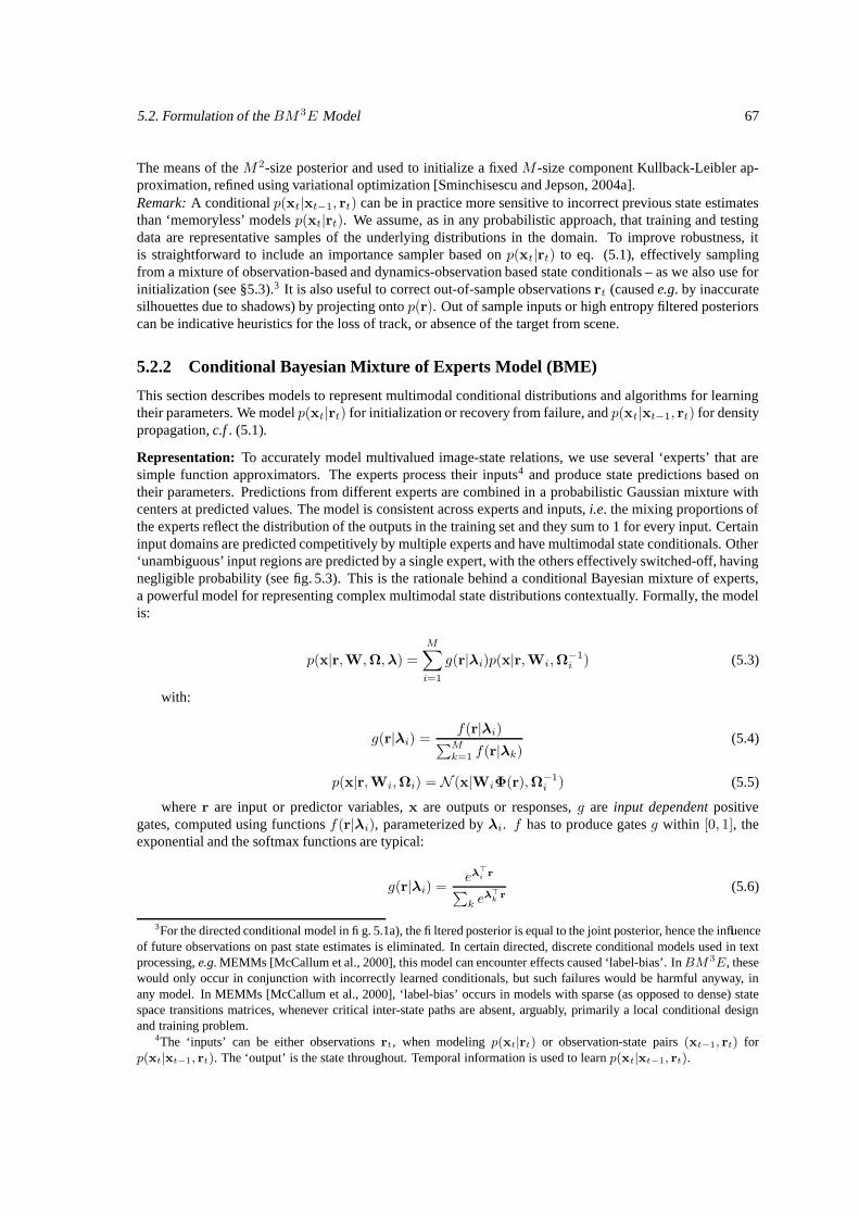
5.2. Formulation of the BM 3E Model 67
The means of the M2-size posterior and used to initialize a fixed M -size component Kullback-Leibler ap-proximation, refined using variational optimization [Sminchisescu and Jepson, 2004a].Remark: A conditional p(xt|xt−1, rt) can be in practice more sensitive to incorrect previous state estimatesthan ‘memoryless’ models p(xt|rt). We assume, as in any probabilistic approach, that training and testingdata are representative samples of the underlying distributions in the domain. To improve robustness, itis straightforward to include an importance sampler based on p(xt|rt) to eq. (5.1), effectively samplingfrom a mixture of observation-based and dynamics-observation based state conditionals – as we also use forinitialization (see §5.3).3 It is also useful to correct out-of-sample observations rt (caused e.g. by inaccuratesilhouettes due to shadows) by projecting onto p(r). Out of sample inputs or high entropy filtered posteriorscan be indicative heuristics for the loss of track, or absence of the target from scene.
5.2.2 Conditional Bayesian Mixture of Experts Model (BME)
This section describes models to represent multimodal conditional distributions and algorithms for learningtheir parameters. We model p(xt|rt) for initialization or recovery from failure, and p(xt|xt−1, rt) for densitypropagation, c.f . (5.1).
Representation: To accurately model multivalued image-state relations, we use several ‘experts’ that aresimple function approximators. The experts process their inputs4 and produce state predictions based ontheir parameters. Predictions from different experts are combined in a probabilistic Gaussian mixture withcenters at predicted values. The model is consistent across experts and inputs, i.e. the mixing proportions ofthe experts reflect the distribution of the outputs in the training set and they sum to 1 for every input. Certaininput domains are predicted competitively by multiple experts and have multimodal state conditionals. Other‘unambiguous’ input regions are predicted by a single expert, with the others effectively switched-off, havingnegligible probability (see fig. 5.3). This is the rationale behind a conditional Bayesian mixture of experts,a powerful model for representing complex multimodal state distributions contextually. Formally, the modelis:
p(x|r,W,Ω,λ) =
M∑
i=1
g(r|λi)p(x|r,Wi,Ω−1i ) (5.3)
with:
g(r|λi) =f(r|λi)∑M
k=1 f(r|λk)(5.4)
p(x|r,Wi,Ωi) = N (x|WiΦ(r),Ω−1i ) (5.5)
where r are input or predictor variables, x are outputs or responses, g are input dependent positivegates, computed using functions f(r|λi), parameterized by λi. f has to produce gates g within [0, 1], theexponential and the softmax functions are typical:
g(r|λi) =eλ>
i r
∑k e
λ>
kr
(5.6)
3For the directed conditional model in fig. 5.1a), the filtered posterior is equal to the joint posterior, hence the influenceof future observations on past state estimates is eliminated. In certain directed, discrete conditional models used in textprocessing, e.g. MEMMs [McCallum et al., 2000], this model can encounter effects caused ‘label-bias’. In BM 3E, thesewould only occur in conjunction with incorrectly learned conditionals, but such failures would be harmful anyway, inany model. In MEMMs [McCallum et al., 2000], ‘label-bias’ occurs in models with sparse (as opposed to dense) statespace transitions matrices, whenever critical inter-state paths are absent, arguably, primarily a local conditional designand training problem.
4The ‘inputs’ can be either observations rt, when modeling p(xt|rt) or observation-state pairs (xt−1, rt) forp(xt|xt−1, rt). The ‘output’ is the state throughout. Temporal information is used to learn p(xt|xt−1, rt).
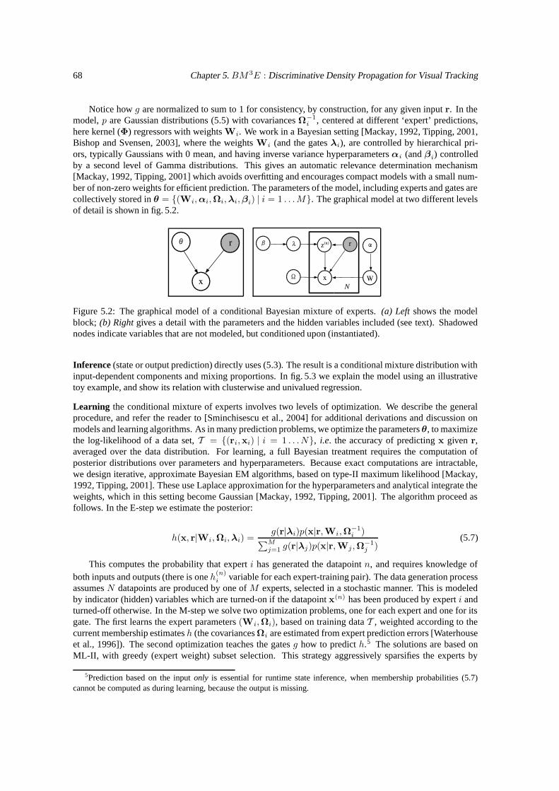
68 Chapter 5. BM3E : Discriminative Density Propagation for Visual Tracking
Notice how g are normalized to sum to 1 for consistency, by construction, for any given input r. In themodel, p are Gaussian distributions (5.5) with covariances Ω−1
i , centered at different ‘expert’ predictions,here kernel (Φ) regressors with weights Wi. We work in a Bayesian setting [Mackay, 1992, Tipping, 2001,Bishop and Svensen, 2003], where the weights Wi (and the gates λi), are controlled by hierarchical pri-ors, typically Gaussians with 0 mean, and having inverse variance hyperparameters αi (and βi) controlledby a second level of Gamma distributions. This gives an automatic relevance determination mechanism[Mackay, 1992, Tipping, 2001] which avoids overfitting and encourages compact models with a small num-ber of non-zero weights for efficient prediction. The parameters of the model, including experts and gates arecollectively stored in θ = (Wi,αi,Ωi,λi,βi) | i = 1 . . .M. The graphical model at two different levelsof detail is shown in fig. 5.2.
Figure 5.2: The graphical model of a conditional Bayesian mixture of experts. (a) Left shows the modelblock; (b) Right gives a detail with the parameters and the hidden variables included (see text). Shadowednodes indicate variables that are not modeled, but conditioned upon (instantiated).
Inference (state or output prediction) directly uses (5.3). The result is a conditional mixture distribution withinput-dependent components and mixing proportions. In fig. 5.3 we explain the model using an illustrativetoy example, and show its relation with clusterwise and univalued regression.
Learning the conditional mixture of experts involves two levels of optimization. We describe the generalprocedure, and refer the reader to [Sminchisescu et al., 2004] for additional derivations and discussion onmodels and learning algorithms. As in many prediction problems, we optimize the parameters θ, to maximizethe log-likelihood of a data set, T = (ri,xi) | i = 1 . . .N, i.e. the accuracy of predicting x given r,averaged over the data distribution. For learning, a full Bayesian treatment requires the computation ofposterior distributions over parameters and hyperparameters. Because exact computations are intractable,we design iterative, approximate Bayesian EM algorithms, based on type-II maximum likelihood [Mackay,1992, Tipping, 2001]. These use Laplace approximation for the hyperparameters and analytical integrate theweights, which in this setting become Gaussian [Mackay, 1992, Tipping, 2001]. The algorithm proceed asfollows. In the E-step we estimate the posterior:
h(x, r|Wi,Ωi,λi) =g(r|λi)p(x|r,Wi,Ω
−1i )
∑Mj=1 g(r|λj)p(x|r,Wj ,Ω
−1j )
(5.7)
This computes the probability that expert i has generated the datapoint n, and requires knowledge ofboth inputs and outputs (there is one h(n)
i variable for each expert-training pair). The data generation processassumes N datapoints are produced by one of M experts, selected in a stochastic manner. This is modeledby indicator (hidden) variables which are turned-on if the datapoint x(n) has been produced by expert i andturned-off otherwise. In the M-step we solve two optimization problems, one for each expert and one for itsgate. The first learns the expert parameters (Wi,Ωi), based on training data T , weighted according to thecurrent membership estimates h (the covariances Ωi are estimated from expert prediction errors [Waterhouseet al., 1996]). The second optimization teaches the gates g how to predict h.5 The solutions are based onML-II, with greedy (expert weight) subset selection. This strategy aggressively sparsifies the experts by
5Prediction based on the input only is essential for runtime state inference, when membership probabilities (5.7)cannot be computed as during learning, because the output is missing.
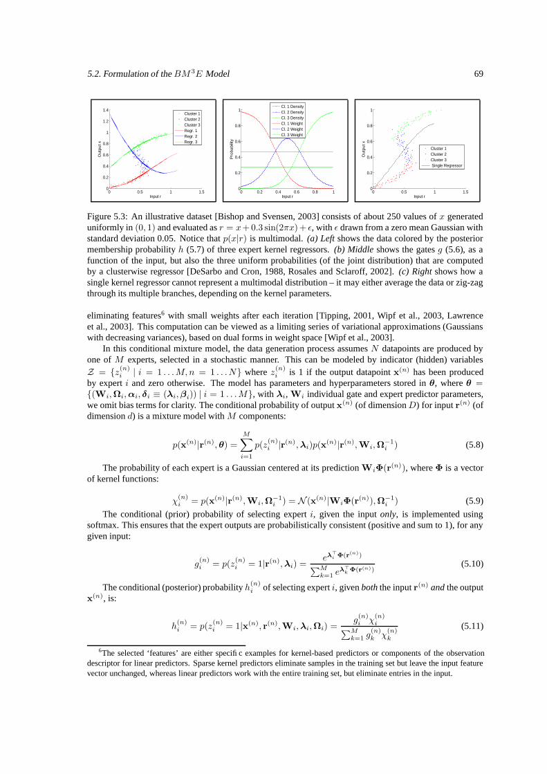
5.2. Formulation of the BM 3E Model 69
0 0.5 1 1.50
0.2
0.4
0.6
0.8
1
1.2
1.4
Input r
Outp
ut x
Cluster 1Cluster 2Cluster 3Regr. 1Regr. 2Regr. 3
0 0.2 0.4 0.6 0.8 10
0.2
0.4
0.6
0.8
1
Input r
Pro
babili
ty
Cl. 1 DensityCl. 2 DensityCl. 3 DensityCl. 1 WeightCl. 2 WeightCl. 3 Weight
0 0.5 1 1.50
0.2
0.4
0.6
0.8
1
Input r
Outp
ut x
Cluster 1Cluster 2Cluster 3 Single Regressor
Figure 5.3: An illustrative dataset [Bishop and Svensen, 2003] consists of about 250 values of x generateduniformly in (0, 1) and evaluated as r = x+0.3 sin(2πx)+ ε, with ε drawn from a zero mean Gaussian withstandard deviation 0.05. Notice that p(x|r) is multimodal. (a) Left shows the data colored by the posteriormembership probability h (5.7) of three expert kernel regressors. (b) Middle shows the gates g (5.6), as afunction of the input, but also the three uniform probabilities (of the joint distribution) that are computedby a clusterwise regressor [DeSarbo and Cron, 1988, Rosales and Sclaroff, 2002]. (c) Right shows how asingle kernel regressor cannot represent a multimodal distribution – it may either average the data or zig-zagthrough its multiple branches, depending on the kernel parameters.
eliminating features6 with small weights after each iteration [Tipping, 2001, Wipf et al., 2003, Lawrenceet al., 2003]. This computation can be viewed as a limiting series of variational approximations (Gaussianswith decreasing variances), based on dual forms in weight space [Wipf et al., 2003].
In this conditional mixture model, the data generation process assumes N datapoints are produced byone of M experts, selected in a stochastic manner. This can be modeled by indicator (hidden) variablesZ = z(n)
i | i = 1 . . .M, n = 1 . . .N where z(n)i is 1 if the output datapoint x(n) has been produced
by expert i and zero otherwise. The model has parameters and hyperparameters stored in θ, where θ =(Wi,Ωi,αi, δi ≡ (λi,βi)) | i = 1 . . .M, with λi, Wi individual gate and expert predictor parameters,we omit bias terms for clarity. The conditional probability of output x(n) (of dimensionD) for input r(n) (ofdimension d) is a mixture model with M components:
p(x(n)|r(n),θ) =
M∑
i=1
p(z(n)i |r(n),λi)p(x
(n)|r(n),Wi,Ω−1i ) (5.8)
The probability of each expert is a Gaussian centered at its prediction WiΦ(r(n)), where Φ is a vectorof kernel functions:
χ(n)i = p(x(n)|r(n),Wi,Ω
−1i ) = N (x(n)|WiΦ(r(n)),Ω−1
i ) (5.9)
The conditional (prior) probability of selecting expert i, given the input only, is implemented usingsoftmax. This ensures that the expert outputs are probabilistically consistent (positive and sum to 1), for anygiven input:
g(n)i = p(z
(n)i = 1|r(n),λi) =
eλ>
i Φ(r(n))
∑Mk=1 e
λ>
kΦ(r(n))
(5.10)
The conditional (posterior) probability h(n)i of selecting expert i, given both the input r(n) and the output
x(n), is:
h(n)i = p(z
(n)i = 1|x(n), r(n),Wi,λi,Ωi) =
g(n)i χ
(n)i∑M
k=1 g(n)k χ
(n)k
(5.11)
6The selected ‘features’ are either specific examples for kernel-based predictors or components of the observationdescriptor for linear predictors. Sparse kernel predictors eliminate samples in the training set but leave the input featurevector unchanged, whereas linear predictors work with the entire training set, but eliminate entries in the input.
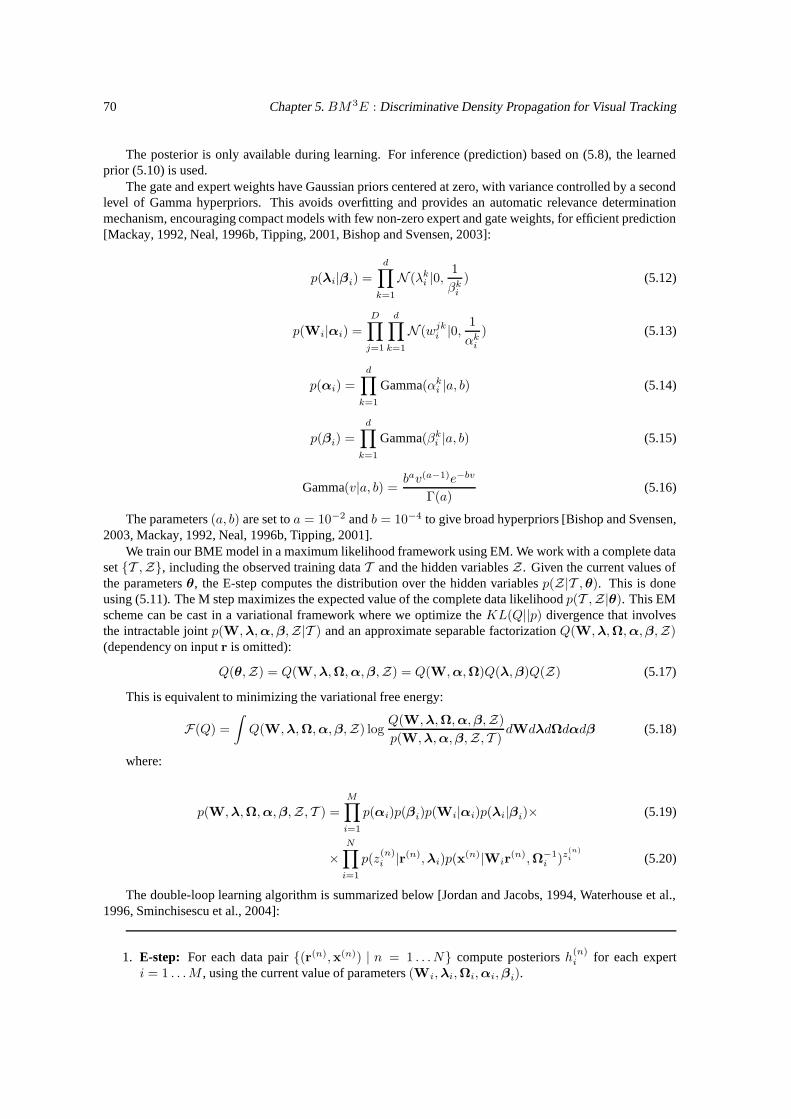
70 Chapter 5. BM3E : Discriminative Density Propagation for Visual Tracking
The posterior is only available during learning. For inference (prediction) based on (5.8), the learnedprior (5.10) is used.
The gate and expert weights have Gaussian priors centered at zero, with variance controlled by a secondlevel of Gamma hyperpriors. This avoids overfitting and provides an automatic relevance determinationmechanism, encouraging compact models with few non-zero expert and gate weights, for efficient prediction[Mackay, 1992, Neal, 1996b, Tipping, 2001, Bishop and Svensen, 2003]:
p(λi|βi) =
d∏
k=1
N (λki |0,
1
βki
) (5.12)
p(Wi|αi) =
D∏
j=1
d∏
k=1
N (wjki |0,
1
αki
) (5.13)
p(αi) =
d∏
k=1
Gamma(αki |a, b) (5.14)
p(βi) =
d∏
k=1
Gamma(βki |a, b) (5.15)
Gamma(v|a, b) =bav(a−1)e−bv
Γ(a)(5.16)
The parameters (a, b) are set to a = 10−2 and b = 10−4 to give broad hyperpriors [Bishop and Svensen,2003, Mackay, 1992, Neal, 1996b, Tipping, 2001].
We train our BME model in a maximum likelihood framework using EM. We work with a complete dataset T ,Z, including the observed training data T and the hidden variables Z . Given the current values ofthe parameters θ, the E-step computes the distribution over the hidden variables p(Z|T ,θ). This is doneusing (5.11). The M step maximizes the expected value of the complete data likelihood p(T ,Z|θ). This EMscheme can be cast in a variational framework where we optimize the KL(Q||p) divergence that involvesthe intractable joint p(W,λ,α,β,Z|T ) and an approximate separable factorization Q(W,λ,Ω,α,β,Z)(dependency on input r is omitted):
Q(θ,Z) = Q(W,λ,Ω,α,β,Z) = Q(W,α,Ω)Q(λ,β)Q(Z) (5.17)
This is equivalent to minimizing the variational free energy:
F(Q) =
∫Q(W,λ,Ω,α,β,Z) log
Q(W,λ,Ω,α,β,Z)
p(W,λ,α,β,Z , T )dWdλdΩdαdβ (5.18)
where:
p(W,λ,Ω,α,β,Z , T ) =M∏
i=1
p(αi)p(βi)p(Wi|αi)p(λi|βi)× (5.19)
×N∏
i=1
p(z(n)i |r(n),λi)p(x
(n)|Wir(n),Ω−1
i )z(n)i (5.20)
The double-loop learning algorithm is summarized below [Jordan and Jacobs, 1994, Waterhouse et al.,1996, Sminchisescu et al., 2004]:
1. E-step: For each data pair (r(n),x(n)) | n = 1 . . .N compute posteriors h(n)i for each expert
i = 1 . . .M , using the current value of parameters (Wi,λi,Ωi,αi,βi).
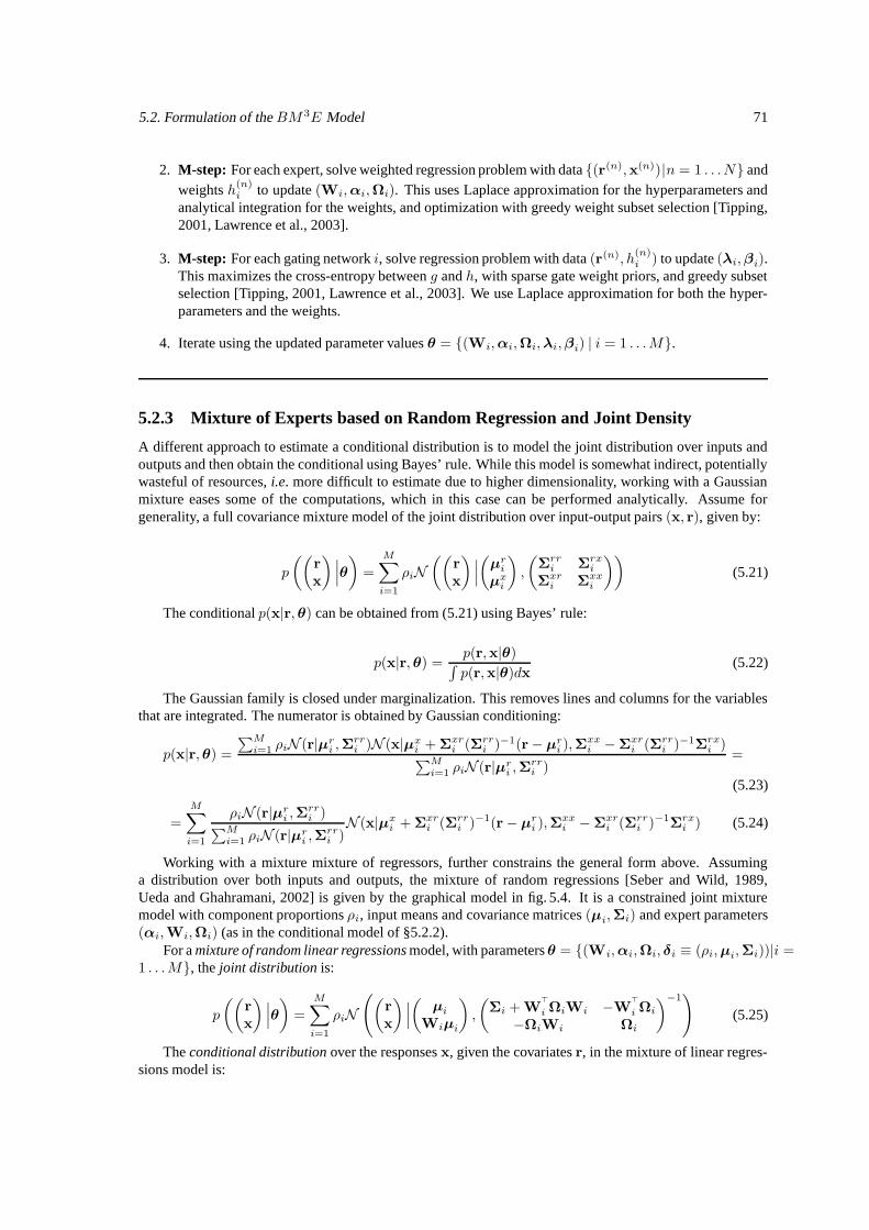
5.2. Formulation of the BM 3E Model 71
2. M-step: For each expert, solve weighted regression problem with data (r(n),x(n))|n = 1 . . .N andweights h(n)
i to update (Wi,αi,Ωi). This uses Laplace approximation for the hyperparameters andanalytical integration for the weights, and optimization with greedy weight subset selection [Tipping,2001, Lawrence et al., 2003].
3. M-step: For each gating network i, solve regression problem with data (r(n), h(n)i ) to update (λi,βi).
This maximizes the cross-entropy between g and h, with sparse gate weight priors, and greedy subsetselection [Tipping, 2001, Lawrence et al., 2003]. We use Laplace approximation for both the hyper-parameters and the weights.
4. Iterate using the updated parameter values θ = (Wi,αi,Ωi,λi,βi) | i = 1 . . .M.
5.2.3 Mixture of Experts based on Random Regression and Joint Density
A different approach to estimate a conditional distribution is to model the joint distribution over inputs andoutputs and then obtain the conditional using Bayes’ rule. While this model is somewhat indirect, potentiallywasteful of resources, i.e. more difficult to estimate due to higher dimensionality, working with a Gaussianmixture eases some of the computations, which in this case can be performed analytically. Assume forgenerality, a full covariance mixture model of the joint distribution over input-output pairs (x, r), given by:
p
((r
x
) ∣∣∣θ)
=
M∑
i=1
ρiN((
r
x
) ∣∣∣(
µri
µxi
),
(Σrr
i Σrxi
Σxri Σxx
i
))(5.21)
The conditional p(x|r,θ) can be obtained from (5.21) using Bayes’ rule:
p(x|r,θ) =p(r,x|θ)∫p(r,x|θ)dx
(5.22)
The Gaussian family is closed under marginalization. This removes lines and columns for the variablesthat are integrated. The numerator is obtained by Gaussian conditioning:
p(x|r,θ) =
∑Mi=1 ρiN (r|µr
i ,Σrri )N (x|µx
i + Σxri (Σrr
i )−1(r− µri ),Σ
xxi −Σxr
i (Σrri )−1Σrx
i )∑M
i=1 ρiN (r|µri ,Σ
rri )
=
(5.23)
=
M∑
i=1
ρiN (r|µri ,Σ
rri )
∑Mi=1 ρiN (r|µr
i ,Σrri )N (x|µx
i + Σxri (Σrr
i )−1(r− µri ),Σ
xxi −Σxr
i (Σrri )−1Σrx
i ) (5.24)
Working with a mixture mixture of regressors, further constrains the general form above. Assuminga distribution over both inputs and outputs, the mixture of random regressions [Seber and Wild, 1989,Ueda and Ghahramani, 2002] is given by the graphical model in fig. 5.4. It is a constrained joint mixturemodel with component proportions ρi, input means and covariance matrices (µi,Σi) and expert parameters(αi,Wi,Ωi) (as in the conditional model of §5.2.2).
For a mixture of random linear regressions model, with parameters θ = (Wi,αi,Ωi, δi ≡ (ρi,µi,Σi))|i =1 . . .M, the joint distribution is:
p
((r
x
) ∣∣∣θ)
=
M∑
i=1
ρiN((
r
x
) ∣∣∣(
µi
Wiµi
),
(Σi + W
>
i ΩiWi −W>
i Ωi
−ΩiWi Ωi
)−1)
(5.25)
The conditional distribution over the responses x, given the covariates r, in the mixture of linear regres-sions model is:
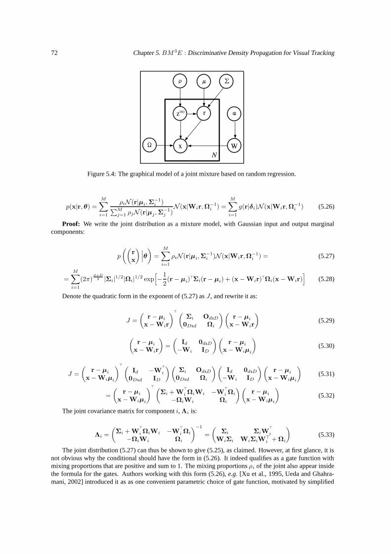
72 Chapter 5. BM3E : Discriminative Density Propagation for Visual Tracking
Figure 5.4: The graphical model of a joint mixture based on random regression.
p(x|r,θ) =
M∑
i=1
ρiN (r|µi,Σ−1i )
∑Mj=1 ρjN (r|µj ,Σ
−1j )N (x|Wir,Ω
−1i ) =
M∑
i=1
g(r|δi)N (x|Wir,Ω−1i ) (5.26)
Proof: We write the joint distribution as a mixture model, with Gaussian input and output marginalcomponents:
p
((r
x
) ∣∣∣θ)
=
M∑
i=1
ρiN (r|µi,Σ−1i )N (x|Wir,Ω
−1i ) = (5.27)
=
M∑
i=1
(2π)d+D
2 |Σi|1/2|Ωi|1/2 exp[−1
2(r− µi)
>Σi(r− µi) + (x−Wir)>Ωi(x−Wir)
](5.28)
Denote the quadratic form in the exponent of (5.27) as J , and rewrite it as:
J =
(r− µi
x−Wir
)>(Σi OdxD
0Dxd Ωi
)(r− µi
x−Wir
)(5.29)
(r− µi
x−Wir
)=
(Id 0dxD
−Wi ID
)(r− µi
x−Wiµi
)(5.30)
J =
(r− µi
x−Wiµi
)>(Id −W
>
i
0Dxd ID
)(Σi OdxD
0Dxd Ωi
)(Id 0dxD
−Wi ID
)(r− µi
x−Wiµi
)(5.31)
=
(r− µi
x−Wiµi
)>(Σi + W
>
i ΩiWi −W>
i Ωi
−ΩiWi Ωi
)(r− µi
x−Wiµi
)(5.32)
The joint covariance matrix for component i, Λi is:
Λi =
(Σi + W
>
i ΩiWi −W>
i Ωi
−ΩiWi Ωi
)−1
=
(Σi ΣiW
>
i
WiΣi WiΣiW>i + Ωi
)(5.33)
The joint distribution (5.27) can thus be shown to give (5.25), as claimed. However, at first glance, it isnot obvious why the conditional should have the form in (5.26). It indeed qualifies as a gate function withmixing proportions that are positive and sum to 1. The mixing proportions ρi of the joint also appear insidethe formula for the gates. Authors working with this form (5.26), e.g. [Xu et al., 1995, Ueda and Ghahra-mani, 2002] introduced it as as one convenient parametric choice of gate function, motivated by simplified
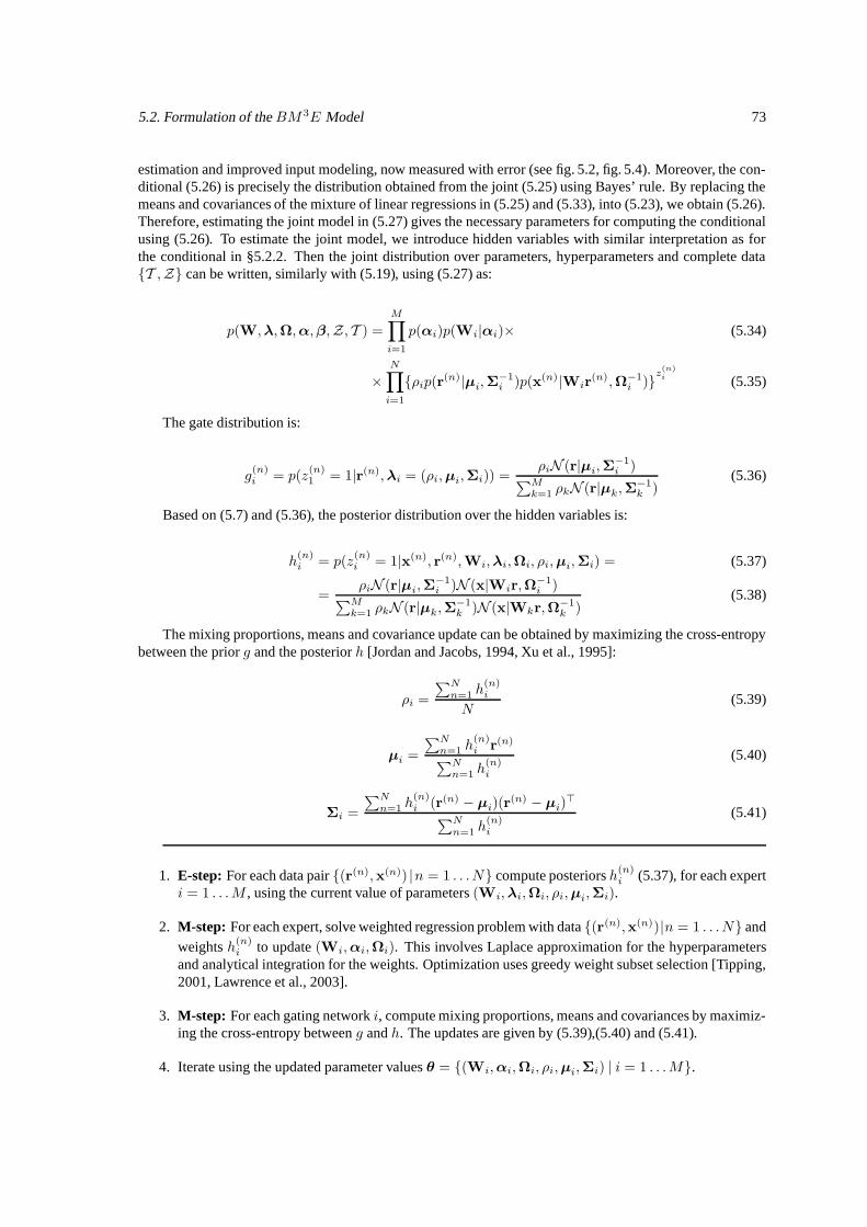
5.2. Formulation of the BM 3E Model 73
estimation and improved input modeling, now measured with error (see fig. 5.2, fig. 5.4). Moreover, the con-ditional (5.26) is precisely the distribution obtained from the joint (5.25) using Bayes’ rule. By replacing themeans and covariances of the mixture of linear regressions in (5.25) and (5.33), into (5.23), we obtain (5.26).Therefore, estimating the joint model in (5.27) gives the necessary parameters for computing the conditionalusing (5.26). To estimate the joint model, we introduce hidden variables with similar interpretation as forthe conditional in §5.2.2. Then the joint distribution over parameters, hyperparameters and complete dataT ,Z can be written, similarly with (5.19), using (5.27) as:
p(W,λ,Ω,α,β,Z , T ) =
M∏
i=1
p(αi)p(Wi|αi)× (5.34)
×N∏
i=1
ρip(r(n)|µi,Σ
−1i )p(x(n)|Wir
(n),Ω−1i )z
(n)i (5.35)
The gate distribution is:
g(n)i = p(z
(n)1 = 1|r(n),λi = (ρi,µi,Σi)) =
ρiN (r|µi,Σ−1i )
∑Mk=1 ρkN (r|µk,Σ
−1k )
(5.36)
Based on (5.7) and (5.36), the posterior distribution over the hidden variables is:
h(n)i = p(z
(n)i = 1|x(n), r(n),Wi,λi,Ωi, ρi,µi,Σi) = (5.37)
=ρiN (r|µi,Σ
−1i )N (x|Wir,Ω
−1i )
∑Mk=1 ρkN (r|µk,Σ
−1k )N (x|Wkr,Ω
−1k )
(5.38)
The mixing proportions, means and covariance update can be obtained by maximizing the cross-entropybetween the prior g and the posterior h [Jordan and Jacobs, 1994, Xu et al., 1995]:
ρi =
∑Nn=1 h
(n)i
N(5.39)
µi =
∑Nn=1 h
(n)i r(n)
∑Nn=1 h
(n)i
(5.40)
Σi =
∑Nn=1 h
(n)i (r(n) − µi)(r
(n) − µi)>
∑Nn=1 h
(n)i
(5.41)
1. E-step: For each data pair (r(n),x(n)) |n = 1 . . .N compute posteriors h(n)i (5.37), for each expert
i = 1 . . .M , using the current value of parameters (Wi,λi,Ωi, ρi,µi,Σi).
2. M-step: For each expert, solve weighted regression problem with data (r(n),x(n))|n = 1 . . .N andweights h(n)
i to update (Wi,αi,Ωi). This involves Laplace approximation for the hyperparametersand analytical integration for the weights. Optimization uses greedy weight subset selection [Tipping,2001, Lawrence et al., 2003].
3. M-step: For each gating network i, compute mixing proportions, means and covariances by maximiz-ing the cross-entropy between g and h. The updates are given by (5.39),(5.40) and (5.41).
4. Iterate using the updated parameter values θ = (Wi,αi,Ωi, ρi,µi,Σi) | i = 1 . . .M.
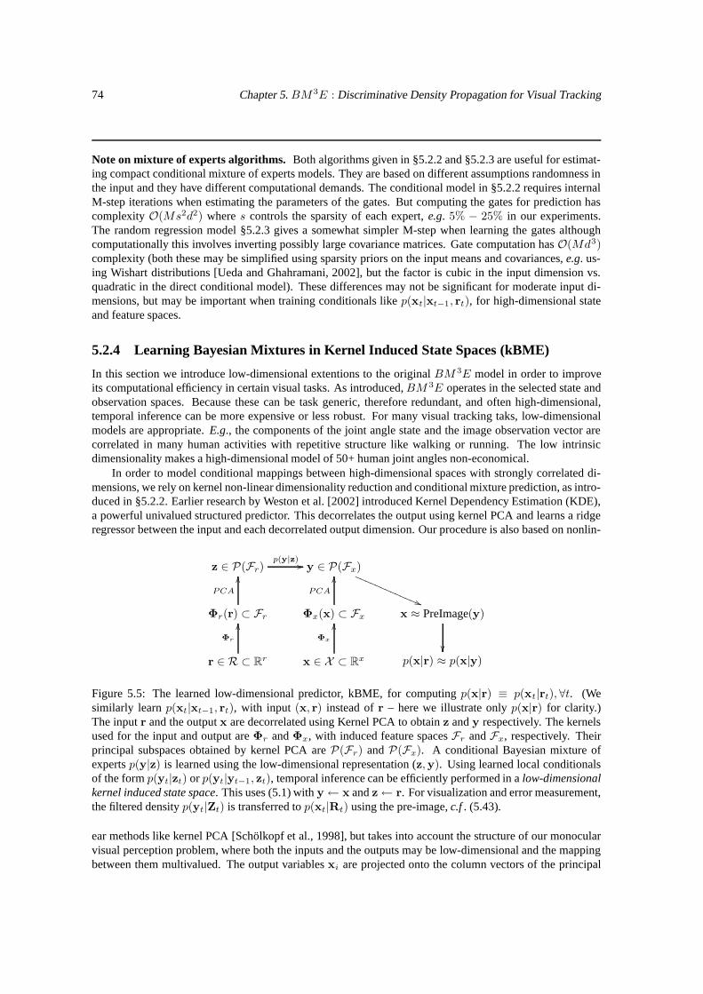
74 Chapter 5. BM3E : Discriminative Density Propagation for Visual Tracking
Note on mixture of experts algorithms. Both algorithms given in §5.2.2 and §5.2.3 are useful for estimat-ing compact conditional mixture of experts models. They are based on different assumptions randomness inthe input and they have different computational demands. The conditional model in §5.2.2 requires internalM-step iterations when estimating the parameters of the gates. But computing the gates for prediction hascomplexity O(Ms2d2) where s controls the sparsity of each expert, e.g. 5% − 25% in our experiments.The random regression model §5.2.3 gives a somewhat simpler M-step when learning the gates althoughcomputationally this involves inverting possibly large covariance matrices. Gate computation has O(Md3)complexity (both these may be simplified using sparsity priors on the input means and covariances, e.g. us-ing Wishart distributions [Ueda and Ghahramani, 2002], but the factor is cubic in the input dimension vs.quadratic in the direct conditional model). These differences may not be significant for moderate input di-mensions, but may be important when training conditionals like p(xt|xt−1, rt), for high-dimensional stateand feature spaces.
5.2.4 Learning Bayesian Mixtures in Kernel Induced State Spaces (kBME)
In this section we introduce low-dimensional extentions to the original BM 3E model in order to improveits computational efficiency in certain visual tasks. As introduced,BM 3E operates in the selected state andobservation spaces. Because these can be task generic, therefore redundant, and often high-dimensional,temporal inference can be more expensive or less robust. For many visual tracking taks, low-dimensionalmodels are appropriate. E.g., the components of the joint angle state and the image observation vector arecorrelated in many human activities with repetitive structure like walking or running. The low intrinsicdimensionality makes a high-dimensional model of 50+ human joint angles non-economical.
In order to model conditional mappings between high-dimensional spaces with strongly correlated di-mensions, we rely on kernel non-linear dimensionality reduction and conditional mixture prediction, as intro-duced in §5.2.2. Earlier research by Weston et al. [2002] introduced Kernel Dependency Estimation (KDE),a powerful univalued structured predictor. This decorrelates the output using kernel PCA and learns a ridgeregressor between the input and each decorrelated output dimension. Our procedure is also based on nonlin-
z ∈ P(Fr)p(y|z) // y ∈ P(Fx)
((Q
Q
Q
Q
Q
Q
Q
Q
Q
Q
Q
Q
Q
Φr(r) ⊂ Fr
PCA
OO
Φx(x) ⊂ Fx
PCA
OO
x ≈ PreImage(y)
r ∈ R ⊂ Rr
Φr
OO
x ∈ X ⊂ Rx
Φx
OO
p(x|r) ≈ p(x|y)
Figure 5.5: The learned low-dimensional predictor, kBME, for computing p(x|r) ≡ p(xt|rt), ∀t. (Wesimilarly learn p(xt|xt−1, rt), with input (x, r) instead of r – here we illustrate only p(x|r) for clarity.)The input r and the output x are decorrelated using Kernel PCA to obtain z and y respectively. The kernelsused for the input and output are Φr and Φx, with induced feature spaces Fr and Fx, respectively. Theirprincipal subspaces obtained by kernel PCA are P(Fr) and P(Fx). A conditional Bayesian mixture ofexperts p(y|z) is learned using the low-dimensional representation (z,y). Using learned local conditionalsof the form p(yt|zt) or p(yt|yt−1, zt), temporal inference can be efficiently performed in a low-dimensionalkernel induced state space. This uses (5.1) with y← x and z← r. For visualization and error measurement,the filtered density p(yt|Zt) is transferred to p(xt|Rt) using the pre-image, c.f . (5.43).
ear methods like kernel PCA [Schölkopf et al., 1998], but takes into account the structure of our monocularvisual perception problem, where both the inputs and the outputs may be low-dimensional and the mappingbetween them multivalued. The output variables xi are projected onto the column vectors of the principal
5.3. Experiments 75
space in order to obtain their principal coordinates yi. A similar procedure is performed on the inputs ri toobtain zi. In order to relate the reduced feature spaces of z and y (P(Fr) and P(Fx)), we estimate a prob-ability distribution over mappings from training pairs (zi,yi). As in §5.2.2, we use a conditional Bayesianmixture of experts (BME) in order to account for ambiguity when mapping similar, possibly identical re-duced feature inputs to distant feature outputs, as common in our problem. This gives a conditional Bayesianmixture of low-dimensional kernel-induced experts (kBME):
p(y|z) =
M∑
i=1
g(z|λi)N (y|WiΦ(z),Ω−1i ) (5.42)
where g(z|λi) is a softmax function parameterized by λi and (Wi,Ω−1i ) are the parameters and output
covariance of expert i, here a kernel regressor, as before (5.3).The kernel-induced kBME model requires the computation of pre-images in order to recover the state
distribution x from its image y ∈ P(Fx). This is a closed form computation for polynomial kernels ofodd degree. In general, for other kernels, optimization or learning (regression based) methods are necessary[Bakir et al., 2004]. Following [Bakir et al., 2004, Weston et al., 2002], we use a sparse Bayesian kernelregressor to learn the pre-image. This is based on training data (xi,yi):
p(x|y) = N (x|AΦy(y),Σ−1) (5.43)
with parameters and covariances (A,Σ−1). Since temporal inference is performed in the low-dimensionalkernel induced state space, the pre-image has to be calculated only for visualization or error reporting. Thesolution is transferred from the reduced feature space P(Fx) to the output X by covariance propagation.This gives a Gaussian mixture withM elements, coefficients g(z|λi) and componentsN (x|AΦy(WiΦ(z)),AJΦy
Ω−1i J>
ΦyA> + Σ−1), where JΦy
is the Jacobian of the mapping Φy.
5.3 Experiments
This section describes our experiments, as well as the training sets and the image features we use. Weshow results on real and artificially rendered motion capture-based test sequences, and compare with existingmethods: nearest neighbor, regression, KDE, both high-dimensional and low-dimensional. The predictionerror is reported in degrees (for mixture of experts, this is w.r.t. the most probable one – but see also fig. 5.10and fig. 5.16b) – and normalized per joint angle, per frame. We also report maximum average estimateswhich are static or temporal averages of the maximum error among all joint angles at particular timestep.The models are learned using standard cross-validation. For kBM 3E, pre-images are learned using kernelregressors with average error 1.7o.
Database and Model Representation: It is difficult to obtain ground truth for human motion and difficultto train using many viewpoints or lighting conditions. To gather data, we use, as others authors [Rosales andSclaroff, 2002, Shakhnarovich et al., 2003, Elgammal and Lee, 2004, Agarwal and Triggs, 2006c, Tomasiet al., 2003], packages like Maya (Alias Wavefront), with realistically rendered computer graphics humansurface models, animated using human motion capture [cmu, 2003]. Our human representation (x) is basedon an articulated skeleton with spherical joints, and has 56 d.o.f. including global translation (the same modelis shown in fig. 5.6 and used for all reconstructions). The database consists of 8262 individual pose samplesobtain from motion sequence clips of different human activities including walking, running, turns, jumps,gestures in conversations, quarreling and pantomime. The training set contains pairs of either states andobservations, when learning p(xt|rt), or states at two succesive timesteps and observations at one of them,when learning p(xt|xt−1, rt). Fig. 5.7 shows data analysis for the database. The data is whithened (this isthe format used to train models) and we cluster the input features – either rt or (xt−1, rt), and the jointangle vectors – xt, independently, using k-means. For every sample in the database, its input (either rt orxt−1, rt) is assigned to the closest input cluster, and its output is assigned to the closest joint angle cluster.Each input cluster stores the maxium number of different joint angle clusters selected by samples assigned toit, and we build histograms of the maximum values across all input clusters. The use of many clusters models
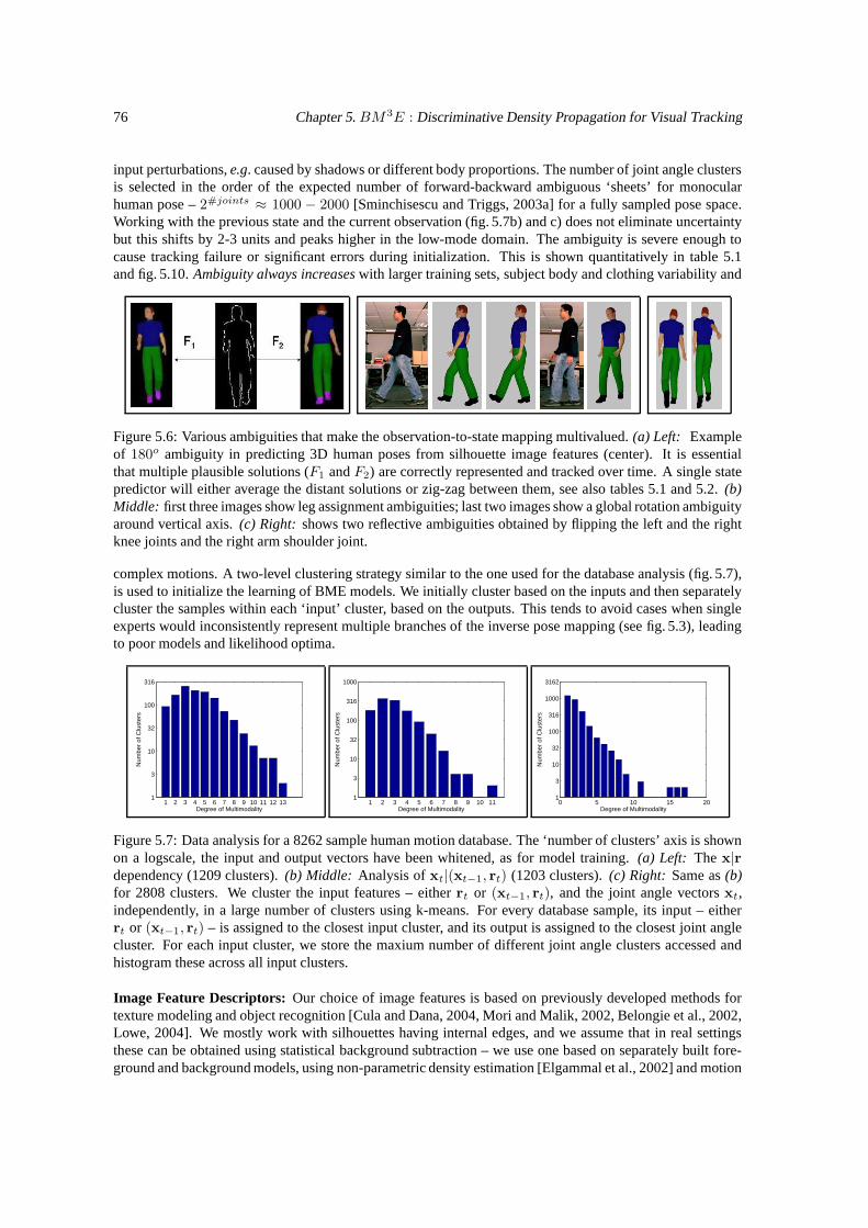
76 Chapter 5. BM3E : Discriminative Density Propagation for Visual Tracking
input perturbations, e.g. caused by shadows or different body proportions. The number of joint angle clustersis selected in the order of the expected number of forward-backward ambiguous ‘sheets’ for monocularhuman pose – 2#joints ≈ 1000 − 2000 [Sminchisescu and Triggs, 2003a] for a fully sampled pose space.Working with the previous state and the current observation (fig. 5.7b) and c) does not eliminate uncertaintybut this shifts by 2-3 units and peaks higher in the low-mode domain. The ambiguity is severe enough tocause tracking failure or significant errors during initialization. This is shown quantitatively in table 5.1and fig. 5.10. Ambiguity always increases with larger training sets, subject body and clothing variability and
Figure 5.6: Various ambiguities that make the observation-to-state mapping multivalued. (a) Left: Exampleof 180o ambiguity in predicting 3D human poses from silhouette image features (center). It is essentialthat multiple plausible solutions (F1 and F2) are correctly represented and tracked over time. A single statepredictor will either average the distant solutions or zig-zag between them, see also tables 5.1 and 5.2. (b)Middle: first three images show leg assignment ambiguities; last two images show a global rotation ambiguityaround vertical axis. (c) Right: shows two reflective ambiguities obtained by flipping the left and the rightknee joints and the right arm shoulder joint.
complex motions. A two-level clustering strategy similar to the one used for the database analysis (fig. 5.7),is used to initialize the learning of BME models. We initially cluster based on the inputs and then separatelycluster the samples within each ‘input’ cluster, based on the outputs. This tends to avoid cases when singleexperts would inconsistently represent multiple branches of the inverse pose mapping (see fig. 5.3), leadingto poor models and likelihood optima.
1 2 3 4 5 6 7 8 9 10 11 12 131
3
10
32
100
316
Degree of Multimodality
Num
ber
of C
lust
ers
1 2 3 4 5 6 7 8 9 10 111
3
10
32
100
316
1000
Degree of Multimodality
Num
ber
of C
lust
ers
0 5 10 15 201
3
10
32
100
316
1000
3162
Degree of Multimodality
Num
ber
of C
lust
ers
Figure 5.7: Data analysis for a 8262 sample human motion database. The ‘number of clusters’ axis is shownon a logscale, the input and output vectors have been whitened, as for model training. (a) Left: The x|rdependency (1209 clusters). (b) Middle: Analysis of xt|(xt−1, rt) (1203 clusters). (c) Right: Same as (b)for 2808 clusters. We cluster the input features – either rt or (xt−1, rt), and the joint angle vectors xt,independently, in a large number of clusters using k-means. For every database sample, its input – eitherrt or (xt−1, rt) – is assigned to the closest input cluster, and its output is assigned to the closest joint anglecluster. For each input cluster, we store the maxium number of different joint angle clusters accessed andhistogram these across all input clusters.
Image Feature Descriptors: Our choice of image features is based on previously developed methods fortexture modeling and object recognition [Cula and Dana, 2004, Mori and Malik, 2002, Belongie et al., 2002,Lowe, 2004]. We mostly work with silhouettes having internal edges, and we assume that in real settingsthese can be obtained using statistical background subtraction – we use one based on separately built fore-ground and background models, using non-parametric density estimation [Elgammal et al., 2002] and motion
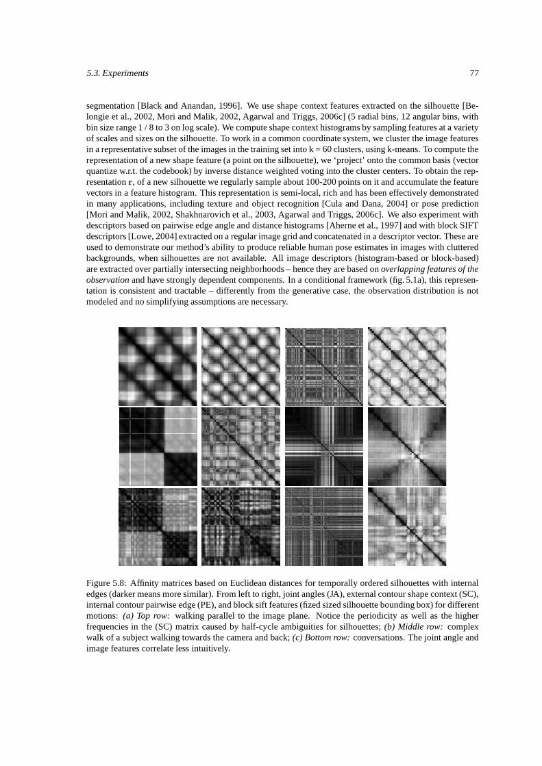
5.3. Experiments 77
segmentation [Black and Anandan, 1996]. We use shape context features extracted on the silhouette [Be-longie et al., 2002, Mori and Malik, 2002, Agarwal and Triggs, 2006c] (5 radial bins, 12 angular bins, withbin size range 1 / 8 to 3 on log scale). We compute shape context histograms by sampling features at a varietyof scales and sizes on the silhouette. To work in a common coordinate system, we cluster the image featuresin a representative subset of the images in the training set into k = 60 clusters, using k-means. To compute therepresentation of a new shape feature (a point on the silhouette), we ‘project’ onto the common basis (vectorquantize w.r.t. the codebook) by inverse distance weighted voting into the cluster centers. To obtain the rep-resentation r, of a new silhouette we regularly sample about 100-200 points on it and accumulate the featurevectors in a feature histogram. This representation is semi-local, rich and has been effectively demonstratedin many applications, including texture and object recognition [Cula and Dana, 2004] or pose prediction[Mori and Malik, 2002, Shakhnarovich et al., 2003, Agarwal and Triggs, 2006c]. We also experiment withdescriptors based on pairwise edge angle and distance histograms [Aherne et al., 1997] and with block SIFTdescriptors [Lowe, 2004] extracted on a regular image grid and concatenated in a descriptor vector. These areused to demonstrate our method’s ability to produce reliable human pose estimates in images with clutteredbackgrounds, when silhouettes are not available. All image descriptors (histogram-based or block-based)are extracted over partially intersecting neighborhoods – hence they are based on overlapping features of theobservation and have strongly dependent components. In a conditional framework (fig. 5.1a), this represen-tation is consistent and tractable – differently from the generative case, the observation distribution is notmodeled and no simplifying assumptions are necessary.
Figure 5.8: Affinity matrices based on Euclidean distances for temporally ordered silhouettes with internaledges (darker means more similar). From left to right, joint angles (JA), external contour shape context (SC),internal contour pairwise edge (PE), and block sift features (fized sized silhouette bounding box) for differentmotions: (a) Top row: walking parallel to the image plane. Notice the periodicity as well as the higherfrequencies in the (SC) matrix caused by half-cycle ambiguities for silhouettes; (b) Middle row: complexwalk of a subject walking towards the camera and back; (c) Bottom row: conversations. The joint angle andimage features correlate less intuitively.
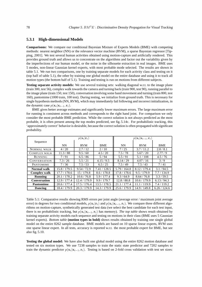
78 Chapter 5. BM3E : Discriminative Density Propagation for Visual Tracking
5.3.1 High-dimensional Models
Comparisons: We compare our conditional Bayesian Mixture of Experts Models (BME) with competingmethods: nearest neighbor (NN) or the relevance vector machine (RVM), a sparse Bayesian regressor [Tip-ping, 2001]. We test several human activities obtained using motion-capture and artificially rendered. Thisprovides ground truth and allows us to concentrate on the algorithms and factor out the variability given bythe imperfections of our human model, or the noise in the silhouette extraction in real images. BME uses5 modes, non-linear Gaussian kernel experts, with most probable mode selected. The results are shown intable 5.1. We run two comparisons, one by training separate models for each activity class and testing on it(top half of table 5.1), the other by training one global model on the entire database and using it to track allmotion types (the bottom half of 5.1). Training and testing is run on motions from different subjects.
Testing separate activity models: We use several training sets: walking diagonal w.r.t. to the image plane(train 300, test 56), complex walk towards the camera and turning back (train 900, test 90), running parallel tothe image plane (train 150, test 150), conversation involving some hand movement and turning (train 800, test160), pantomime (1000 train, 100 test). During testing, we initialize from ground truth. This is necessary forsingle hypothesis methods (NN, RVM), which may immediately fail following and incorrect initialization, inthe dynamic case p(xt|xt−1, rt).
BME gives better average estimates and significantly lower maximum errors. The large maximum errorfor running is consistent across methods and corresponds to the right hand joint. For comparison we onlyconsider the most probable BME prediction. While the correct solution is not always predicted as the mostprobable, it is often present among the top modes predicted, see fig. 5.14c. For probabilistic tracking, this‘approximately correct’ behavior is desirable, because the correct solution is often propagated with significantprobability.
p(xt|rt) p(xt|xt−1, rt)Sequence
NN RVM BME NN RVM BMENORMAL WALK 4 / 20 2.7 / 12 2 / 10 7 / 25 3.7 / 11.2 2.8 / 8.1COMPLEX WALK 11.3 / 88 9.5 / 60 4.5 / 20 7.5 / 78 5.67 / 20 2.77 / 9
RUNNING 7 / 91 6.5 / 86 5 / 94 5.5 / 91 5.1 / 108 4.5 / 76CONVERSATION 7.3 / 26 5.5 / 21 4.15 / 9.5 8.14 / 29 4.07 / 16 3 / 9
PANTOMIME 7 / 36 7.5 / 53 6.5 / 25 7.5 / 49 7.5 / 43 7 / 41
Normal walk 15.8 / 179.5 9.54 / 72.9 7.41 / 128.5 5.79 / 164.8 8.12 / 179.4 3.1 / 94.5Complex walk 17.7 / 178.6 15 / 179.8 8.6 / 178.8 17.8 / 178.6 9.5 / 179.9 7.7 / 134.9
Running 20.1 / 178.2 10.6 / 76.8 5.9 / 177.4 9.3 / 64.9 8.64 / 76.8 3.3 / 59.5Conversation 12.9 / 177.4 12.4 / 179.9 9.9 / 179.7 12.8 / 88.8 10.6 / 179.9 6.13 / 94.3Pantomime 20.6 / 177.4 17.5 / 176.4 13.5 / 178.5 21.1 / 177.4 11.1 / 119.9 7.4 / 119.2
Dancing 18.4 / 179.9 20.3 / 179.9 14.3 / 179.9 25.6 / 179.9 14.9 / 149.8 6.26 / 124.6
Table 5.1: Comparative results showing RMS errors per joint angle (average error / maximum joint averageerror) in degrees for two conditional models, p(xt|rt) and p(xt|xt−1, rt). We compare three different algo-rithms on motion-capture, synthetically generated test data (we select the best candidate for each test input,there is no probabilistic tracking, but p(xt|xt−1, rt) has memory). The top table shows result obtained bytraining separate activity models each sequence and testing on motions in their class (BME uses 5 Gaussiankernel experts). Bottom table (motion types in bold) shows results obtained by training one single globalmodel on the entire 8262 sample database. BME models are based on 10 sparse linear experts, RVM usesone sparse linear expert. In all tests, accuracy is reported w.r.t. the most probable expert for BME, but seealso fig. 5.10.
Testing the global model: We have also built one global model using the entire 8262 motion database andtested on six motion types. We use 7238 samples to train the static state predictor and 7202 samples totrain the dynamic predictor p(xt|xt−1, rt). Testing is based on 2-fold cross validation with test set sizes:
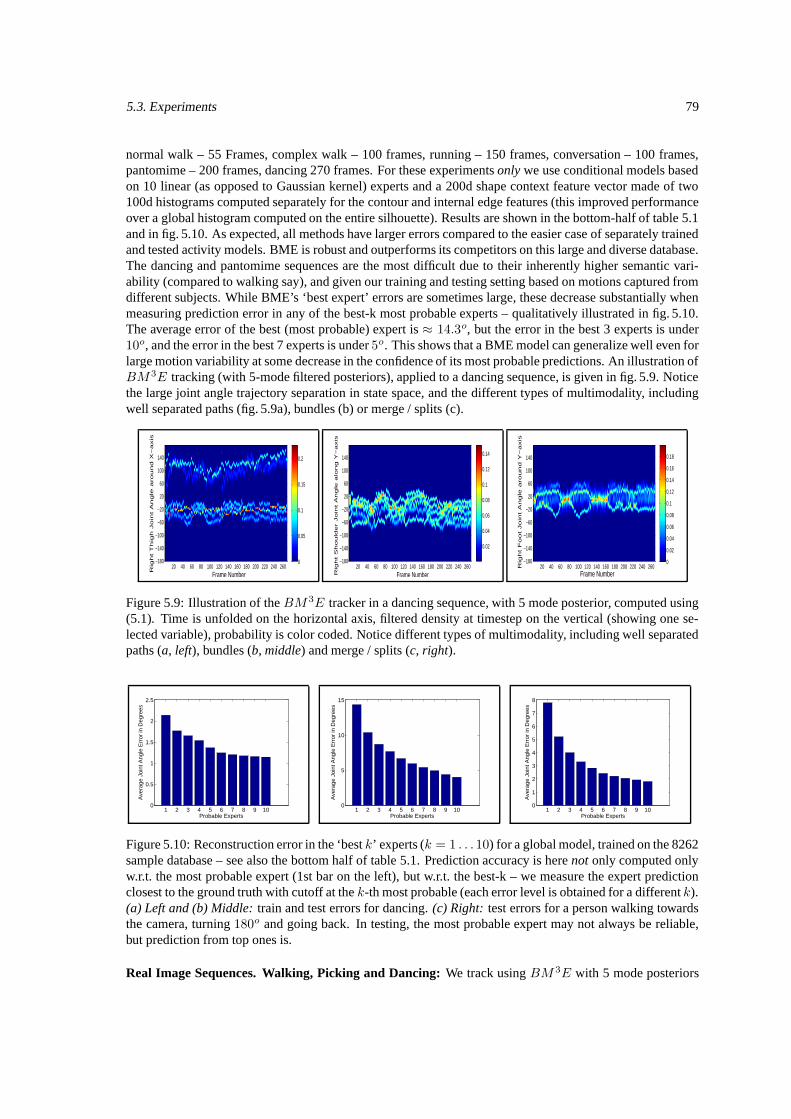
5.3. Experiments 79
normal walk – 55 Frames, complex walk – 100 frames, running – 150 frames, conversation – 100 frames,pantomime – 200 frames, dancing 270 frames. For these experiments only we use conditional models basedon 10 linear (as opposed to Gaussian kernel) experts and a 200d shape context feature vector made of two100d histograms computed separately for the contour and internal edge features (this improved performanceover a global histogram computed on the entire silhouette). Results are shown in the bottom-half of table 5.1and in fig. 5.10. As expected, all methods have larger errors compared to the easier case of separately trainedand tested activity models. BME is robust and outperforms its competitors on this large and diverse database.The dancing and pantomime sequences are the most difficult due to their inherently higher semantic vari-ability (compared to walking say), and given our training and testing setting based on motions captured fromdifferent subjects. While BME’s ‘best expert’ errors are sometimes large, these decrease substantially whenmeasuring prediction error in any of the best-k most probable experts – qualitatively illustrated in fig. 5.10.The average error of the best (most probable) expert is ≈ 14.3o, but the error in the best 3 experts is under10o, and the error in the best 7 experts is under 5o. This shows that a BME model can generalize well even forlarge motion variability at some decrease in the confidence of its most probable predictions. An illustration ofBM3E tracking (with 5-mode filtered posteriors), applied to a dancing sequence, is given in fig. 5.9. Noticethe large joint angle trajectory separation in state space, and the different types of multimodality, includingwell separated paths (fig. 5.9a), bundles (b) or merge / splits (c).
Frame Number
Rig
ht
Th
igh
Jo
int
An
gle
aro
un
d X
−a
xis
20 40 60 80 100 120 140 160 180 200 220 240 260
140
100
60
20
−20
−60
−100
−140
−180 0
0.05
0.1
0.15
0.2
Frame NumberRig
ht
Sh
ou
lde
r Jo
int
An
gle
alo
ng
Y−
axis
20 40 60 80 100 120 140 160 180 200 220 240 260
140
100
60
20
−20
−60
−100
−140
−180
0.02
0.04
0.06
0.08
0.1
0.12
0.14
Frame Number
Rig
ht F
oo
t Jo
int A
ng
le a
rou
nd
Y−
axis
20 40 60 80 100 120 140 160 180 200 220 240 260
140
100
60
20
−20
−60
−100
−140
−180 0
0.02
0.04
0.06
0.08
0.1
0.12
0.14
0.16
0.18
Figure 5.9: Illustration of the BM 3E tracker in a dancing sequence, with 5 mode posterior, computed using(5.1). Time is unfolded on the horizontal axis, filtered density at timestep on the vertical (showing one se-lected variable), probability is color coded. Notice different types of multimodality, including well separatedpaths (a, left), bundles (b, middle) and merge / splits (c, right).
1 2 3 4 5 6 7 8 9 100
0.5
1
1.5
2
2.5
Probable Experts
Ave
rage
Joi
nt A
ngle
Err
or in
Deg
rees
1 2 3 4 5 6 7 8 9 100
5
10
15
Probable Experts
Ave
rage
Joi
nt A
ngle
Err
or in
Deg
rees
1 2 3 4 5 6 7 8 9 100
1
2
3
4
5
6
7
8
Probable Experts
Ave
rage
Joi
nt A
ngle
Err
or in
Deg
rees
Figure 5.10: Reconstruction error in the ‘best k’ experts (k = 1 . . . 10) for a global model, trained on the 8262sample database – see also the bottom half of table 5.1. Prediction accuracy is here not only computed onlyw.r.t. the most probable expert (1st bar on the left), but w.r.t. the best-k – we measure the expert predictionclosest to the ground truth with cutoff at the k-th most probable (each error level is obtained for a different k).(a) Left and (b) Middle: train and test errors for dancing. (c) Right: test errors for a person walking towardsthe camera, turning 180o and going back. In testing, the most probable expert may not always be reliable,but prediction from top ones is.
Real Image Sequences. Walking, Picking and Dancing: We track using BM 3E with 5 mode posteriors
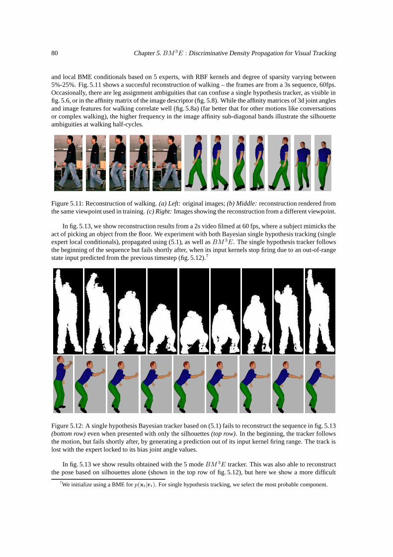
80 Chapter 5. BM3E : Discriminative Density Propagation for Visual Tracking
and local BME conditionals based on 5 experts, with RBF kernels and degree of sparsity varying between5%-25%. Fig. 5.11 shows a succesful reconstruction of walking – the frames are from a 3s sequence, 60fps.Occasionally, there are leg assignment ambiguities that can confuse a single hypothesis tracker, as visible infig. 5.6, or in the affinity matrix of the image descriptor (fig. 5.8). While the affinity matrices of 3d joint anglesand image features for walking correlate well (fig. 5.8a) (far better that for other motions like conversationsor complex walking), the higher frequency in the image affinity sub-diagonal bands illustrate the silhouetteambiguities at walking half-cycles.
Figure 5.11: Reconstruction of walking. (a) Left: original images; (b) Middle: reconstruction rendered fromthe same viewpoint used in training. (c) Right: Images showing the reconstruction from a different viewpoint.
In fig. 5.13, we show reconstruction results from a 2s video filmed at 60 fps, where a subject mimicks theact of picking an object from the floor. We experiment with both Bayesian single hypothesis tracking (singleexpert local conditionals), propagated using (5.1), as well as BM 3E. The single hypothesis tracker followsthe beginning of the sequence but fails shortly after, when its input kernels stop firing due to an out-of-rangestate input predicted from the previous timestep (fig. 5.12).7
Figure 5.12: A single hypothesis Bayesian tracker based on (5.1) fails to reconstruct the sequence in fig. 5.13(bottom row) even when presented with only the silhouettes (top row). In the beginning, the tracker followsthe motion, but fails shortly after, by generating a prediction out of its input kernel firing range. The track islost with the expert locked to its bias joint angle values.
In fig. 5.13 we show results obtained with the 5 mode BM 3E tracker. This was also able to reconstructthe pose based on silhouettes alone (shown in the top row of fig. 5.12), but here we show a more difficult
7We initialize using a BME for p(xt|rt). For single hypothesis tracking, we select the most probable component.
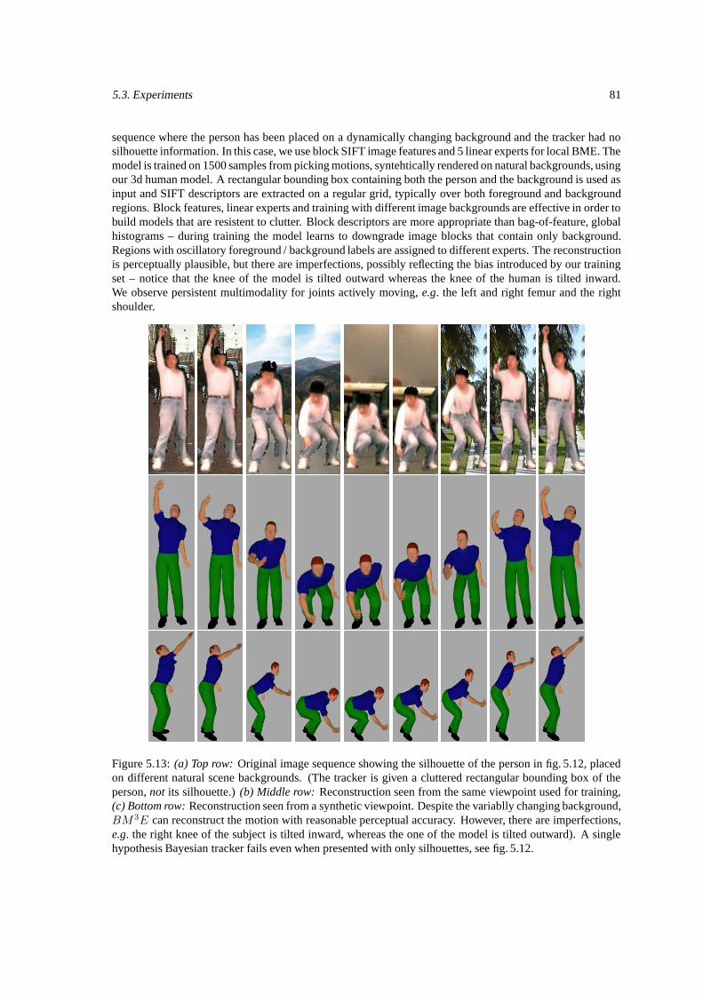
5.3. Experiments 81
sequence where the person has been placed on a dynamically changing background and the tracker had nosilhouette information. In this case, we use block SIFT image features and 5 linear experts for local BME. Themodel is trained on 1500 samples from picking motions, syntehtically rendered on natural backgrounds, usingour 3d human model. A rectangular bounding box containing both the person and the background is used asinput and SIFT descriptors are extracted on a regular grid, typically over both foreground and backgroundregions. Block features, linear experts and training with different image backgrounds are effective in order tobuild models that are resistent to clutter. Block descriptors are more appropriate than bag-of-feature, globalhistograms – during training the model learns to downgrade image blocks that contain only background.Regions with oscillatory foreground / background labels are assigned to different experts. The reconstructionis perceptually plausible, but there are imperfections, possibly reflecting the bias introduced by our trainingset – notice that the knee of the model is tilted outward whereas the knee of the human is tilted inward.We observe persistent multimodality for joints actively moving, e.g. the left and right femur and the rightshoulder.
Figure 5.13: (a) Top row: Original image sequence showing the silhouette of the person in fig. 5.12, placedon different natural scene backgrounds. (The tracker is given a cluttered rectangular bounding box of theperson, not its silhouette.) (b) Middle row: Reconstruction seen from the same viewpoint used for training,(c) Bottom row: Reconstruction seen from a synthetic viewpoint. Despite the variablly changing background,BM3E can reconstruct the motion with reasonable perceptual accuracy. However, there are imperfections,e.g. the right knee of the subject is tilted inward, whereas the one of the model is tilted outward). A singlehypothesis Bayesian tracker fails even when presented with only silhouettes, see fig. 5.12.
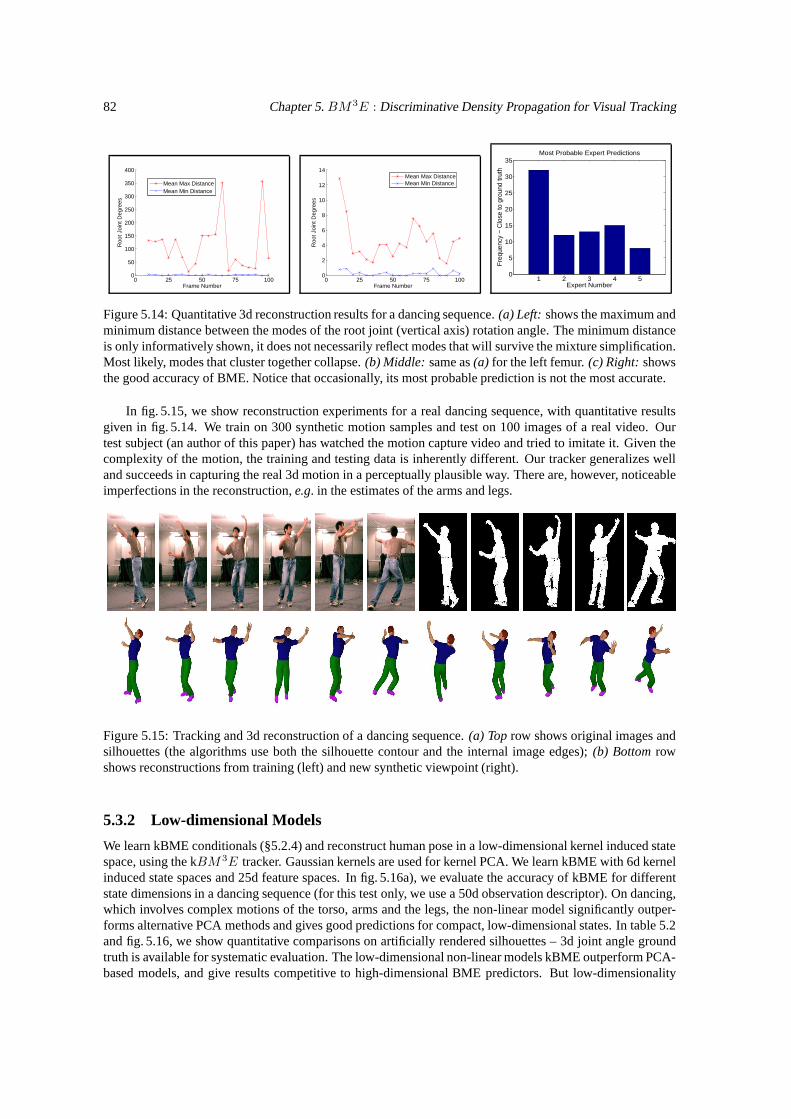
82 Chapter 5. BM3E : Discriminative Density Propagation for Visual Tracking
0 25 50 75 1000
50
100
150
200
250
300
350
400
Frame Number
Roo
t Joi
nt D
egre
es
Mean Max DistanceMean Min Distance
0 25 50 75 1000
2
4
6
8
10
12
14
Frame Number
Roo
t Joi
nt D
egre
es
Mean Max DistanceMean Min Distance
1 2 3 4 50
5
10
15
20
25
30
35Most Probable Expert Predictions
Expert Number
Fre
quen
cy −
Clo
se to
gro
und
trut
h
Figure 5.14: Quantitative 3d reconstruction results for a dancing sequence. (a) Left: shows the maximum andminimum distance between the modes of the root joint (vertical axis) rotation angle. The minimum distanceis only informatively shown, it does not necessarily reflect modes that will survive the mixture simplification.Most likely, modes that cluster together collapse. (b) Middle: same as (a) for the left femur. (c) Right: showsthe good accuracy of BME. Notice that occasionally, its most probable prediction is not the most accurate.
In fig. 5.15, we show reconstruction experiments for a real dancing sequence, with quantitative resultsgiven in fig. 5.14. We train on 300 synthetic motion samples and test on 100 images of a real video. Ourtest subject (an author of this paper) has watched the motion capture video and tried to imitate it. Given thecomplexity of the motion, the training and testing data is inherently different. Our tracker generalizes welland succeeds in capturing the real 3d motion in a perceptually plausible way. There are, however, noticeableimperfections in the reconstruction, e.g. in the estimates of the arms and legs.
Figure 5.15: Tracking and 3d reconstruction of a dancing sequence. (a) Top row shows original images andsilhouettes (the algorithms use both the silhouette contour and the internal image edges); (b) Bottom rowshows reconstructions from training (left) and new synthetic viewpoint (right).
5.3.2 Low-dimensional Models
We learn kBME conditionals (§5.2.4) and reconstruct human pose in a low-dimensional kernel induced statespace, using the kBM 3E tracker. Gaussian kernels are used for kernel PCA. We learn kBME with 6d kernelinduced state spaces and 25d feature spaces. In fig. 5.16a), we evaluate the accuracy of kBME for differentstate dimensions in a dancing sequence (for this test only, we use a 50d observation descriptor). On dancing,which involves complex motions of the torso, arms and the legs, the non-linear model significantly outper-forms alternative PCA methods and gives good predictions for compact, low-dimensional states. In table 5.2and fig. 5.16, we show quantitative comparisons on artificially rendered silhouettes – 3d joint angle groundtruth is available for systematic evaluation. The low-dimensional non-linear models kBME outperform PCA-based models, and give results competitive to high-dimensional BME predictors. But low-dimensionality
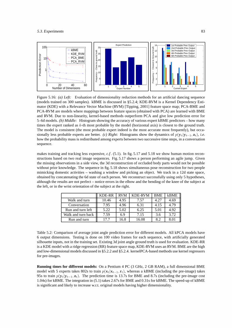
5.3. Experiments 83
0 20 40 60
1
10
100
Number of Dimensions
Pre
dic
tion E
rror
kBMEKDE_RVMPCA_BMEPCA_RVM
1 2 3 4 50
5
10
15
20
25
30Expert Prediction
Expert Number
Fre
quen
cy −
Clo
se to
gro
und
trut
h
1 2 3 4 50
2
4
6
8
10
12
14
Current Expert
Fre
qu
en
cy −
C
lose
st t
o G
rou
nd
tru
th
1st Probable Prev Output2nd Probable Prev Output3rd Probable Prev Output4th Probable Prev Output5th Probable Prev Output
Figure 5.16: (a) Left: Evaluation of dimensionality reduction methods for an artificial dancing sequence(models trained on 300 samples). kBME is discussed in §5.2.4; KDE-RVM is a Kernel Dependency Esti-mator (KDE) with a Relevance Vector Machine (RVM) [Tipping, 2001] feature space map; PCA-BME andPCA-RVM are models where mappings between feature spaces (obtained with PCA) are learned with BMEand RVM. Due to non-linearity, kernel-based methods outperform PCA and give low prediction error for5–6d models. (b) Middle: Histogram showing the accuracy of various expert kBME predictors – how manytimes the expert ranked as k-th most probable by the model (horizontal axis) is closest to the ground truth.The model is consistent (the most probable expert indeed is the most accurate most frequently), but occa-sionally less probable experts are better. (c) Right: Histograms show the dynamics of p(yt|yt−1, zt), i.e.how the probability mass is redistributed among experts between two successive time steps, in a conversationsequence.
makes training and tracking less expensive, c.f . (5.1). In fig. 5.17 and 5.18 we show human motion recon-structions based on two real image sequences. Fig. 5.17 shows a person performing an agile jump. Giventhe missing observations in a side view, the 3d reconstruction of occluded body parts would not be possiblewithout prior knowledge. The sequence in fig. 5.18 shows simultaneous pose reconstruction for two peoplemimicking domestic activities – washing a window and picking an object. We track in a 12d state space,obtained by concatenating the 6d state of each person. We reconstruct successfully using only 5 hypotheses,although the results are not perfect – notice errors in the elbow and the bending of the knee of the subject atthe left, or in the wrist orientation of the subject at the right.
KDE-RR RVM KDE-RVM BME kBMEWalk and turn 10.46 4.95 7.57 4.27 4.69Conversation 7.95 4.96 6.31 4.15 4.79
Run and turn left 5.22 5.02 6.25 5.01 4.92Walk and turn back 7.59 6.9 7.15 3.6 3.72
Run and turn 17.7 16.8 16.08 8.2 8.01
Table 5.2: Comparison of average joint angle prediction error for different models. All kPCA models have6 output dimensions. Testing is done on 100 video frames for each sequence, with artificially generatedsilhouette inputs, not in the training set. Existing 3d joint angle ground truth is used for evaluation. KDE-RRis a KDE model with a ridge regression (RR) feature space map, KDE-RVM uses an RVM. BME are the highand low-dimensional models discussed in §5.2.2 and §5.2.4. kernelPCA-based methods use kernel regressorsfor pre-images.
Running times for different models: On a Pentium 4 PC (3 GHz, 2 GB RAM), a full dimensional BMEmodel with 5 experts takes 802s to train p(xt|xt−1, rt), whereas a kBME (including the pre-image) takes95s to train p(yt|yt−1, zt). The prediction time is 13.7s for BME and 8.7s (including the pre-image cost1.04s) for kBME. The integration in (5.1) takes 2.67s for BME and 0.31s for kBME. The speed-up of kBMEis significant and likely to increase w.r.t. original models having higher dimensionality.
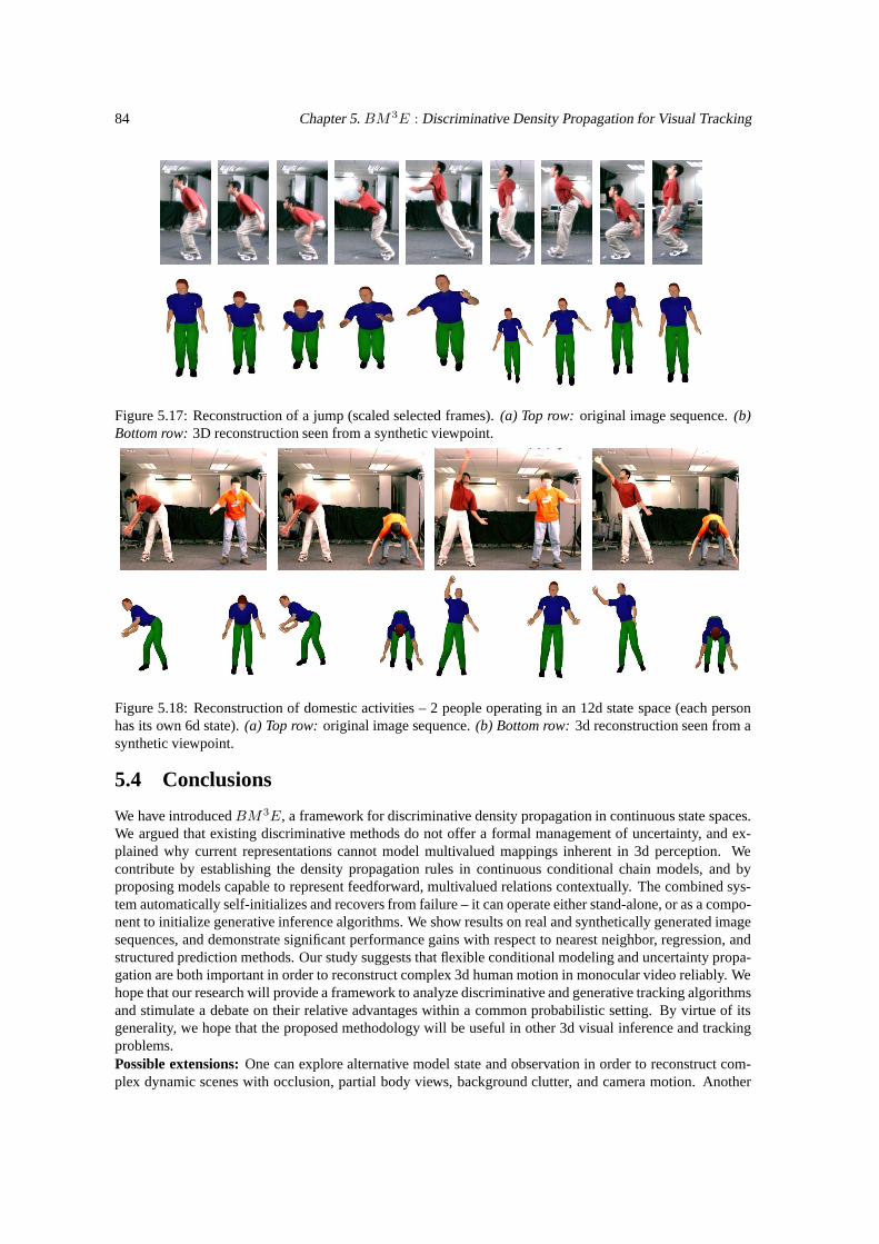
84 Chapter 5. BM3E : Discriminative Density Propagation for Visual Tracking
Figure 5.17: Reconstruction of a jump (scaled selected frames). (a) Top row: original image sequence. (b)Bottom row: 3D reconstruction seen from a synthetic viewpoint.
Figure 5.18: Reconstruction of domestic activities – 2 people operating in an 12d state space (each personhas its own 6d state). (a) Top row: original image sequence. (b) Bottom row: 3d reconstruction seen from asynthetic viewpoint.
5.4 Conclusions
We have introducedBM 3E, a framework for discriminative density propagation in continuous state spaces.We argued that existing discriminative methods do not offer a formal management of uncertainty, and ex-plained why current representations cannot model multivalued mappings inherent in 3d perception. Wecontribute by establishing the density propagation rules in continuous conditional chain models, and byproposing models capable to represent feedforward, multivalued relations contextually. The combined sys-tem automatically self-initializes and recovers from failure – it can operate either stand-alone, or as a compo-nent to initialize generative inference algorithms. We show results on real and synthetically generated imagesequences, and demonstrate significant performance gains with respect to nearest neighbor, regression, andstructured prediction methods. Our study suggests that flexible conditional modeling and uncertainty propa-gation are both important in order to reconstruct complex 3d human motion in monocular video reliably. Wehope that our research will provide a framework to analyze discriminative and generative tracking algorithmsand stimulate a debate on their relative advantages within a common probabilistic setting. By virtue of itsgenerality, we hope that the proposed methodology will be useful in other 3d visual inference and trackingproblems.Possible extensions: One can explore alternative model state and observation in order to reconstruct com-plex dynamic scenes with occlusion, partial body views, background clutter, and camera motion. Another
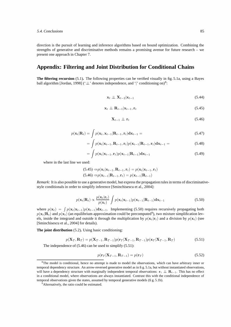
5.4. Conclusions 85
direction is the pursuit of learning and inference algorithms based on bound optimization. Combining thestrengths of generative and discriminative methods remains a promising avenue for future research – wepresent one approach in Chapter 7.
Appendix: Filtering and Joint Distribution for Conditional Chains
The filtering recursion (5.1). The following properties can be verified visually in fig. 5.1a, using a Bayesball algorithm [Jordan, 1998] (‘⊥⊥’ denotes independence, and ‘|’ conditioning on)8:
xt ⊥⊥ Xt−2|xt−1 (5.44)
xt ⊥⊥ Rt−1|xt−1, rt (5.45)
Xt−1 ⊥⊥ rt (5.46)
p(xt|Rt) =
∫p(xt,xt−1|Rt−1, rt)dxt−1 = (5.47)
=
∫p(xt|xt−1,Rt−1, rt)p(xt−1|Rt−1, rt)dxt−1 = (5.48)
=
∫p(xt|xt−1, rt)p(xt−1|Rt−1)dxt−1 (5.49)
where in the last line we used:
(5.45)⇒p(xt|xt−1,Rt−1, rt) = p(xt|xt−1, rt)
(5.46)⇒p(xt−1|Rt−1, rt) = p(xt−1|Rt−1)
Remark: It is also possible to use a generative model, but express the propagation rules in terms of discriminative-style conditionals in order to simplify inference [Sminchisescu et al., 2004]:
p(xt|Rt) ∝p(xt|rt)
p(xt)
∫p(xt|xt−1)p(xt−1|Rt−1)dxt−1 (5.50)
where p(xt) =∫p(xt|xt−1)p(xt−1)dxt−1. Implementing (5.50) requires recursively propagating both
p(xt|Rt) and p(xt) (an equilibrium approximation could be precomputed9), two mixture simplification lev-els, inside the integrand and outside it through the multiplication by p(xt|rt) and a division by p(xt) (see[Sminchisescu et al., 2004] for details).
The joint distribution (5.2). Using basic conditioning:
p(XT ,RT ) = p(XT−1,RT−1)p(rT |XT−1,RT−1)p(xT |XT−1,RT ) (5.51)
The independence of (5.46) can be used to simplify (5.51):
p(rT |XT−1,RT−1) = p(rT ) (5.52)
8The model is conditional, hence no attempt is made to model the observations, which can have arbitrary inner ortemporal dependency structure. An arrow-reversed generative model as in fig. 5.1a, but without instantiated observations,will have a dependency structure with marginally independent temporal observations: rt ⊥⊥ Rt−1. This has no effectin a conditional model, where observations are always instantiated. Contrast this with the conditional independence oftemporal observations given the states, assumed by temporal generative models (fig. 5.1b).
9Alternatively, the ratio could be estimated.

86 Chapter 5. BM3E : Discriminative Density Propagation for Visual Tracking
p(xT |xT−1,XT−2,RT−1, rT ) = p(xT |xT−1, rT ) (5.53)
Using (5.52) and (5.53) in (5.51), we obtain:
p(XT ,RT ) = p(XT−1,RT−1)p(rT )p(xT |xT−1, rT ) (5.54)
and (5.2) is verified given:
p(XT |RT ) =p(XT ,RT )∏T
t=1 rt
(5.55)
and p(x1|r1) = p(x1, r1)/p(r1).
Chapter 6
Semi-supervised Hierarchical Modelsfor 3D Reconstruction
In the previous chapter 5, we have shown that discriminatively trained image-based predictors can providefast, automatic qualitative 3D reconstructions of human body pose or scene structure in real-world environ-ments. However, the stability of existing image representations tends to be perturbed by deformations andmisalignments in the training set, which, in turn, degrade the quality of learning and generalization. In thischapter we advocate the semi-supervised learning of hierarchical image descriptions in order to better toleratevariability at multiple levels of detail. We combine multilevel encodings with improved stability to geometrictransformations, with metric learning and semi-supervised manifold regularization methods in order to fur-ther profile them for task-invariance – resistance to background clutter and within the same human pose classdifferences. We quantitatively analyze the effectiveness of both descriptors and learning methods and showthat each one can contribute, sometimes substantially, to more reliable 3D human pose estimates in clutteredimages. An earlier version of this chapter appeared in IEEE International Conference on Computer Visionand Pattern Recognition (CVPR) [Kanujia, Sminchisescu, and Metaxas, 2007].
6.1 Supervision and Flexible Image Encodings
One line of recent research in the area of monocular 3D human pose reconstruction has studied discrimina-tive, feedforward models that can be trained to automatically predict pose distributions directly from imagedescriptors. This is in contrast with generative algorithms that search the pose space for configurations withgood image alignment. Each class of methods has complementary trade-offs. Generative models are flex-ible at representing large classes of poses and useful for training and hypothesis verification, but inferenceis expensive and good observation models are difficult to construct without simplifying assumptions. Dis-criminative (feedforward) predictors offer the promise of speed, full automation and complete flexibility inselecting the image descriptor1, but have to model multivalued image-to-3D relations and their reliance ona training set makes generalization to very different poses, body proportions, or scenes where people arefilmed against background clutter, problematic. (N.B. Clearly, these remain hard problems for any method,be it generative or discriminative.)
The design of multi-valued feedforward pose predictors and the temporal density propagation in con-ditional chains is, at present, well understood, but the tradeoffs inherent in the acquisition of a sufficientlyrepresentative training set or the design of image descriptors with good resistance to clutter and intra-classvariations is less explored. The construction of realistic pose labeled human databases (images of humansand their 3D poses) is inherently difficult because no existing system can provide accurate 3D ground truth forhumans in real-world, non-instrumented scenes. Current solutions rely either on motion acquisition systems
1Overcomplete bases or overlapping features of the observation can be designed without simplifying independenceassumptions.
87

88 Chapter 6. Semi-supervised Hierarchical Models for 3D Reconstruction
like Vicon, but these operate in engineered environments, where subjects wear special costumes and markersand the background is simplified, or on quasi-synthetic databases, generated by CG characters, animated us-ing motion capture, and placed on real image backgrounds [Agarwal and Triggs, 2006b, Sminchisescu et al.,2006b]. In either case, there is a risk that models learned with these training sets may not generalize wellwhen confronted with the diversity of real world scenes. A more flexible and scalable solution for modelacquisition is necessary.
A second difficulty for reliable pose prediction is the design of image descriptors that are distinctiveenough to differentiate among different poses, yet invariant to within the same pose class differences – peoplein similar stances, but differently proportioned, or photographed on different backgrounds. Exiting methodshave successfully demonstrated that bag of features or regular-grid based representations of local descriptors(e.g. bag of shape context features, block of SIFT features [Agarwal and Triggs, 2006b, Sminchisescu et al.,2006b]) can be effective at predicting 3D human poses, but the representations tend to be too inflexible forreconstruction in general scenes. It is more appropriate to view them as two useful extremes of a multilevel,hierarchical representation of images – a family of descriptors that progressively relaxes block-wise, rigidlocal spatial image encodings to increasingly weaker spatial models of position / geometry accumulated overincreasingly larger image regions. Selecting the most competitive representation for an application – a typicalset of people, motions, backgrounds or scales – reduces to either directly or implicitly learning a metric inthe space of image descriptors, so that both good invariance and distinctiveness is achieved, e.g., for 3Dreconstruction, suppress noise by maximizing correlation within the desired pose invariance class, yet keepdifferent classes separated, and turn off components that are close to being statistical random for the task ofprediction, disregarding the class.
Our research brings together several innovations at the incidence of object recognition, metric learningand semi-supervised learning, as follows:
• We learn hierarchical, coarse to fine image descriptors that combine multilevel image encodings (in-spired from object recognition, but here in the different context of 3D reconstruction) and metric learn-ing algorithms. HMAX [Serre et al., 2005, Agarwal and Triggs, 2006a], spatial pyramids [Lazebniket al., 2006], and vocabulary trees [Nistér and Stévenius, 2006] are complemented with noise suppres-sion and metric learning algorithms based on Canonical Correlation Analysis and Relevant Compo-nent Analysis. These refine and further align the image descriptors within individual pose invarianceclasses in order to better tolerate deformation, misalignment and clutter in the training and test sets.
• We construct models based on both labeled and unlabeled data, in order to make training with diverse,real-world datasets possible. We generalize semi-supervised regression models [Chapelle et al., 2006]to the more general problem of learning multi-valued predictors. We follow a manifold regularizationapproach in order to construct smoothness priors that automatically propagate outputs (poses) fromlabeled image descriptors to those unlabeled ones close in their intrinsic geometry, as represented,e.g., by the graph Laplacian of a training set.
The two components are strongly dependent in practice. To make unlabeled data useful for generaliza-tion, perceptually similar descriptors have to be close in the selected input metric.2 Learning an appropriateone becomes a necessary preliminary step.
6.1.1 Existing Features and Models
Our research relates to work in areas like discriminative human pose reconstruction, feature design, cor-relation analysis and semi-supervised learning. Several methods exists for discriminative pose prediction[Rosales and Sclaroff, 2002, Sminchisescu et al., 2005a, 2006b, 2007, Agarwal and Triggs, 2006b, Sigal andBlack, 2006] but they primarily concentrate on its multi-valuedness [Rosales and Sclaroff, 2002, Sminchis-escu et al., 2005a, Sigal and Black, 2006], or on single levels of feature encodings [Sminchisescu et al., 2005a,2006b, 2007], based on global histograms or regular grids of SIFT blocks. Here we also study the general
2This holds broadly, for both supervised and unsupervised methods.
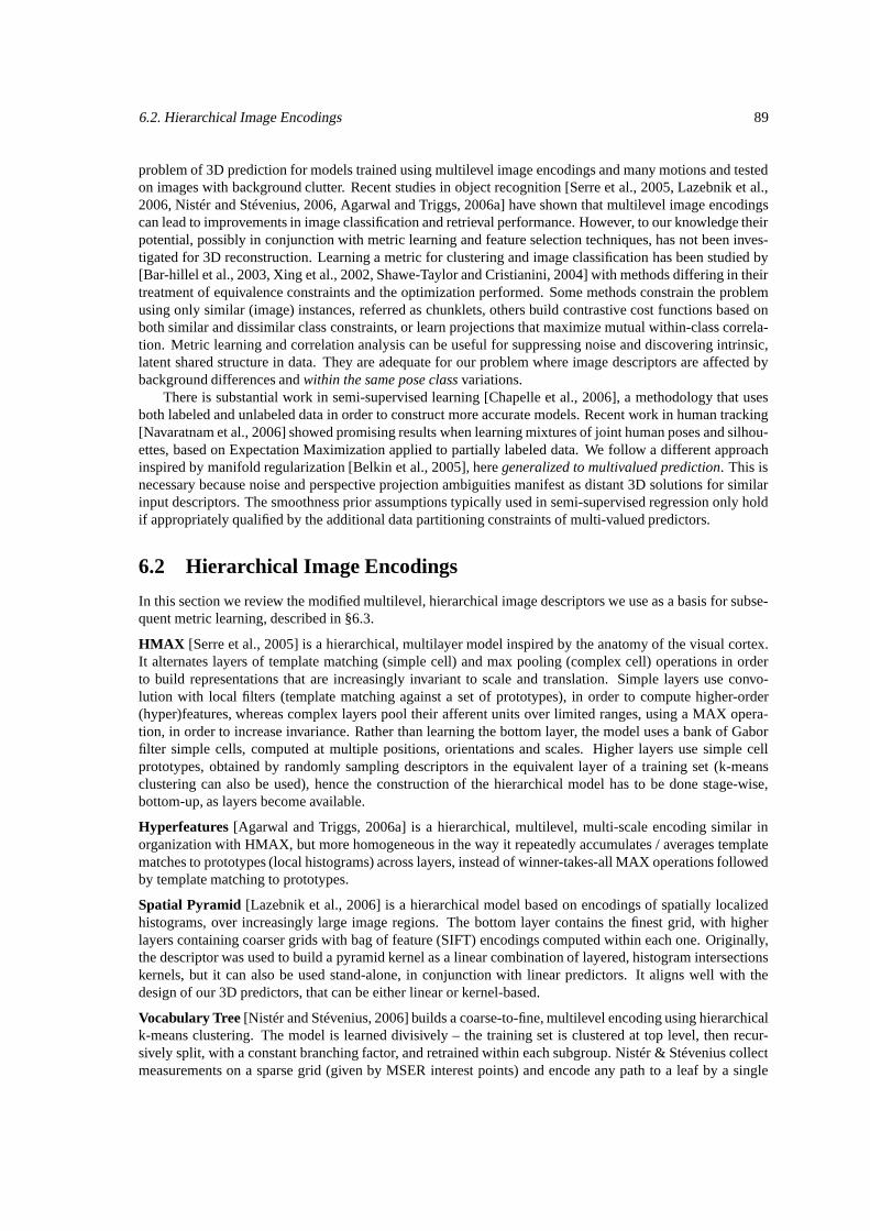
6.2. Hierarchical Image Encodings 89
problem of 3D prediction for models trained using multilevel image encodings and many motions and testedon images with background clutter. Recent studies in object recognition [Serre et al., 2005, Lazebnik et al.,2006, Nistér and Stévenius, 2006, Agarwal and Triggs, 2006a] have shown that multilevel image encodingscan lead to improvements in image classification and retrieval performance. However, to our knowledge theirpotential, possibly in conjunction with metric learning and feature selection techniques, has not been inves-tigated for 3D reconstruction. Learning a metric for clustering and image classification has been studied by[Bar-hillel et al., 2003, Xing et al., 2002, Shawe-Taylor and Cristianini, 2004] with methods differing in theirtreatment of equivalence constraints and the optimization performed. Some methods constrain the problemusing only similar (image) instances, referred as chunklets, others build contrastive cost functions based onboth similar and dissimilar class constraints, or learn projections that maximize mutual within-class correla-tion. Metric learning and correlation analysis can be useful for suppressing noise and discovering intrinsic,latent shared structure in data. They are adequate for our problem where image descriptors are affected bybackground differences and within the same pose class variations.
There is substantial work in semi-supervised learning [Chapelle et al., 2006], a methodology that usesboth labeled and unlabeled data in order to construct more accurate models. Recent work in human tracking[Navaratnam et al., 2006] showed promising results when learning mixtures of joint human poses and silhou-ettes, based on Expectation Maximization applied to partially labeled data. We follow a different approachinspired by manifold regularization [Belkin et al., 2005], here generalized to multivalued prediction. This isnecessary because noise and perspective projection ambiguities manifest as distant 3D solutions for similarinput descriptors. The smoothness prior assumptions typically used in semi-supervised regression only holdif appropriately qualified by the additional data partitioning constraints of multi-valued predictors.
6.2 Hierarchical Image Encodings
In this section we review the modified multilevel, hierarchical image descriptors we use as a basis for subse-quent metric learning, described in §6.3.
HMAX [Serre et al., 2005] is a hierarchical, multilayer model inspired by the anatomy of the visual cortex.It alternates layers of template matching (simple cell) and max pooling (complex cell) operations in orderto build representations that are increasingly invariant to scale and translation. Simple layers use convo-lution with local filters (template matching against a set of prototypes), in order to compute higher-order(hyper)features, whereas complex layers pool their afferent units over limited ranges, using a MAX opera-tion, in order to increase invariance. Rather than learning the bottom layer, the model uses a bank of Gaborfilter simple cells, computed at multiple positions, orientations and scales. Higher layers use simple cellprototypes, obtained by randomly sampling descriptors in the equivalent layer of a training set (k-meansclustering can also be used), hence the construction of the hierarchical model has to be done stage-wise,bottom-up, as layers become available.
Hyperfeatures [Agarwal and Triggs, 2006a] is a hierarchical, multilevel, multi-scale encoding similar inorganization with HMAX, but more homogeneous in the way it repeatedly accumulates / averages templatematches to prototypes (local histograms) across layers, instead of winner-takes-all MAX operations followedby template matching to prototypes.
Spatial Pyramid [Lazebnik et al., 2006] is a hierarchical model based on encodings of spatially localizedhistograms, over increasingly large image regions. The bottom layer contains the finest grid, with higherlayers containing coarser grids with bag of feature (SIFT) encodings computed within each one. Originally,the descriptor was used to build a pyramid kernel as a linear combination of layered, histogram intersectionskernels, but it can also be used stand-alone, in conjunction with linear predictors. It aligns well with thedesign of our 3D predictors, that can be either linear or kernel-based.
Vocabulary Tree [Nistér and Stévenius, 2006] builds a coarse-to-fine, multilevel encoding using hierarchicalk-means clustering. The model is learned divisively – the training set is clustered at top level, then recur-sively split, with a constant branching factor, and retrained within each subgroup. Nistér & Stévenius collectmeasurements on a sparse grid (given by MSER interest points) and encode any path to a leaf by a single
90 Chapter 6. Semi-supervised Hierarchical Models for 3D Reconstruction
integer. This is compact and gives good results for object retrieval, but is not sufficiently smooth for ourcontinuous pose prediction problem, where it collapses qualitatively different poses to identical encodings.We learn the same vocabulary tree, but construct stage-wise encodings by concatenating all levels. At eachlevel we store the continuous distances to prototypes and recursively descend in the closest sub-tree. Entriesin unvisited sub-trees are set to zero. For each image, we accumulate tree-based encodings of patches on aregular grid and normalize.
Multilevel Spatial Blocks (MSB) is an encoding we have derived and consists of a set of layers, each aregular grid of overlapping image blocks, with increasingly large (SIFT) descriptor cell size. We concatenatedescriptors within each layer and across layers, orderly, in order to obtain encodings of an entire image orsub-window.
6.3 Metric Learning and Correlation Analysis
Multilevel hierarchical encodings are necessary in order to obtain image descriptors with good resistance todeformations, clutter or misalignments in the training / test set. But they do not entirely eliminate the need forproblem dependent similarity measures for descriptor comparison. Albeit multilevel encodings are in generalmore stable at preserving invariance to geometric transformations, their components may still be perturbedby clutter or may not be relevant for the task.
Linear predictors implicitly assume a Euclidean metric in input space, whereas kernel methods use anexplicit metric induced by the selected kernel. In each case, there is no guarantee that an ad-hoc selectedmetric – a Euclidean distance or an RBF kernel with arbitrary covariance, would provide the best invariancew.r.t. the task e.g., for 3D prediction, the invariance within the same pose class. In this section we reviewlearning techniques to build a metric – or alternatively, to compute representations with implicit Euclideanmetric, for a desired level of invariance. The training set consists of image descriptor examples of the sameinvariance class, here different people in roughly the same pose, but with different body proportions or viewedon different backgrounds.3 In practice, each pose can define an invariance class but we will need to train withonly a few qualitatively different poses in order to learn a useful metric.
Relevant Component Analysis (RCA): [Bar-hillel et al., 2003] is a metric learning method that minimizesthe spread within each chunklet – a subset of examples obtained by applying a transitive closure on givenequivalence relations, e.g. pairwise constraints on examples, here image descriptors. We use RCA to optimizea Mahalanobis distance for the image descriptors, with a constraint on the covariance matrix, in order to avoidtrivial solutions that shrink the entire space. The cost function is:
minD
1
U
k∑
j=1
Uj∑
i=1
||rji −mj ||D, s.th. |D| ≥ 1 (6.1)
where U is the total of examples and Uj is the number of examples rji, i ∈ 1 . . . Uj in chunklet j, andmj its mean. The solution to (6.1) can be obtained in closed form in 3 steps, for details see [Bar-hillel et al.,2003]: (1) subtract the mean of each chunklet from all its points, (2) compute the covariance matrix of eachchunklet, and (3) sum the covariance matrices of all chunklets, scaled by the inverse number of examples1/U ) and use it as a Mahalanobis distance (the RCA matrix that needs to be inverted has dimension dim(r)).
Canonical Correlation Analysis (CCA): In its standard form, CCA [Shawe-Taylor and Cristianini, 2004]is a method to identify shared structure among two classes of variables: the algorithm estimates two basisvectors so that, after linear projection4, the correlation between the two classes is mutually maximized. Giventwo sets of vectors r and u, as samples: S = ((r1,u1), (r2,u2), . . . , (rn,un)), and their projection on twoarbitrary directions, wr and wu, with Sr = (〈wr, r1〉, . . . , 〈wr, rn〉), and Su = (〈wu,u1〉, . . . , 〈wu,un〉),CCA maximizes the cost:
3No explicit 3D pose information is necessary.4Non-linear extensions can be obtained in the usual way, using ‘kernelization’ [Shawe-Taylor and Cristianini, 2004].
6.4. Manifold Regularization for Multivalued Prediction 91
f = maxwr,wu
〈Srwr,Suwu〉||Srwr||||Suwu||
= (6.2)
maxwr,wu
wr>Cruwu√w>
r Crrwrw>u Cuuwu
(6.3)
with Crr and Cuu within-sets covariance matrices and Cru = C>ur between-sets covariances. A closed form
solution to (6.2) can be computed by solving a generalized eigenvalue problem of size dim(r) + dim(u).Large problems can be solved efficiently using predictive low-rank decomposition with partial Gram-Schmidtorthogonalization [Shawe-Taylor and Cristianini, 2004].
6.4 Manifold Regularization for Multivalued Prediction
In this section we introduce semi-supervised extensions to multivalued discriminative models. Existing mod-els are primarily designed for supervised problems and represent the solution space (e.g. for 3D human poseestimation, the joint angles) using a mixture of image-based predictors. Each expert is paired with an ob-servation dependent gate function that scores its competence in predicting states (3D) when presented withdifferent inputs / images. As the input changes, different experts are active and their rankings (relative prob-abilities) change. The model is a mixture of predictors with input-sensitive mixing proportions (see chapter5, §5.2.2). Recall:
p(x|r) =M∑
i=1
gi(r)pi(x|r) (6.4)
gi(r) =exp(λ>
i r)∑
k exp(λ>k r)
(6.5)
pi(x|r) = G(x|Wir,Ω−1i ) (6.6)
with r image descriptors, x state outputs, gi input dependent gates, computed using linear regressors c.f .(6.5), with weights λi. g are normalized to sum to 1 for any given input r and pi are Gaussian functions (6.6)with covariance Ω−1
i , centered at the expert predictions, here chosen to be linear regressors with weightsWi.
A semi-supervised extension of this model would combine both labeled and unlabeled data in order toconstrain the parameter estimates of each expert pi. A standard semi-supervised learning assumption can bestated as follows: if two inputs r in a high density region are close, so should be their corresponding outputsx. For our problem and predictor, this assumption is adapted as follows:
• Manifold assumption: If two points are close in the intrinsic geometry of p(r) (given by a manifold orgraph regularizer, see below), their conditional distributions p(x|r) should be similar.
• Expert responsibility assumption: If two inputs r are close (in the intrinsic geometry) and can bepredicted by expert i with confidence gi, their corresponding conditional distributions p(x|r) shouldbe smooth to the same extent (i.e. modulated by gi).
For the linear case, the semi-supervised manifold assumption manifests as a prior on the weights ofeach expert i, or equivalently, a (negative log-likelihood) regularization term (constants and scaling factorsdropped for simplicity):
Ri =
U∑
u,j=1
(Wiru −Wirj)Nuj(Wiru −Wirj)> (6.7)
= WiR>LRW>
i (6.8)
92 Chapter 6. Semi-supervised Hierarchical Models for 3D Reconstruction
where U is the size of the entire training set including the unlabeled points, R is a dim(r) × U matrixthat stores all the input vectors r in the training set (supervised and unsupervised), L is a graph Laplacianregularizer constructed over all the training set5: L = D−N with N a matrix of graph weights Nij and D
a diagonal matrix with elements Dii =∑U
j=1 Nij . The input geometry is not distorted because the manifoldregularization framework does not compute a low-dimensional embedding explicitly. The framework onlyimplicitly assumes that some intrinsic geometry, embedded in Rdim(r), exists.
Eq. (6.7) can be interpreted as a ridge-style regression prior on the expert weights, with a special co-variance matrix given by the graph Laplacian. The prior is computationally tractable – it contributes as yetanother matrix to the existing ones corresponding to the labeled data or the expert weight priors6 – whichare inverted in order to compute each expert. Learning is performed iteratively, using an EM algorithm thatcomputes soft assignments of each datapoint to experts and learns both the experts and their gates using adouble loop (expert-gate) estimation scheme.
6.5 Experiments
In this section we report experiments obtained using 5 different multilevel image encodings further profiledusing 2 different metric learning and noise suppression methods (RCA and CCA), and the semi-supervisedmanifold regularization framework based on both labeled and unlabeled data.
Multilevel Encodings: We use 5 different hierarchical encodings, calibrated to roughly similar dimension-ality: HMAX (1600, 4 levels with patch size 4-16 codebooks, obtained by sampling from 1600 real images- the same set was used to generate codebooks for all methods which need them), Spatial Pyramid (1400, 3levels, SIFT descriptors, 6x6 pixel cells, 4x4 cells per block, 4 angular bins of gradient orientations, 0−180o
unsigned,10 pixel grid overlap), Hyperfeatures (1400, SIFT descriptors, 4x4 blocks, 4x4 pixels per cell, 3levels having 200, 400, and 800 centers with scales 2, 4, 6), Vocabulary Tree (1365, 5 levels, branching factor4, SIFT descriptors computed at 5 different scales of a Gaussian pyramid, SIFT descriptors, 4x4 blocks, 4x4pixels per cell) and Multilevel Spatial Blocks (1344, 3 levels with 16, 4, 1 SIFT block, 4x4 cells per block,12x12 cell size).
Database and Multivalued Predictor: For qualitative experiments we use images from a movie (Run LolaRun) and the INRIA pedestrian database [Dalal and Triggs, 2005]. For quantitative experiments we use ourown database consisting of 3 × 3247 = 9741 quasi-real images, generated using a computer graphics hu-man model that was rendered on real image backgrounds. We have 3247 different 3D poses from the CMUmotion capture database [cmu, 2003], rendered to produce different viewing patterns of walks, either frontalor parallel to the image plane, dancing, conversation, bending and picking, running and pantomime (oneof the 3 sets of 3247 poses is placed on a clean background). We collect three test sets of 150 poses foreach of the five motion classes. The motions executed by different subject are not in the training set. Wealso render one test set on a clean background as baseline (Clean). The other two test sets are progressivelymore complicated: one has the model randomly placed at different locations, but on the same images as inthe training set (Clutter1), the other has the model placed on unseen backgrounds (Clutter2). In all cases, a320x240 bounding box of the model and the background is obtained, possibly using rescaling [Sminchisescuet al., 2006b]. There is significant variability and lack of centering in this dataset because certain poses arevertically (and horizontally) more symmetric than others (e.g. compare a person who picks an object withone who is standing, or pointing the arm in one direction). We train a multivalued predictor (a conditionalBayesian mixture of 5 experts) on the entire dataset, as opposed to training models for each motion / activityseparately. The model uses linear experts with sparsity priors, complementing the close-form pre-processingfrom RCA / CCA. Empirically, we observe sparsity patterns in the range 15% − 45%, with lower values
5This is (typically) a sparse graph construction, obtained by connecting each training point to its k-nearest neighborsand computing local Gaussian distances to them. A global regularizer based on geodesic distances can also be used.
6We also use a sparsity weight prior, but this does not appear explicitly in the sum that accumulates the matrix tobe inverted – for linear methods sparsity contributes by decreasing the effective input dimension, hence the size of thematrix.
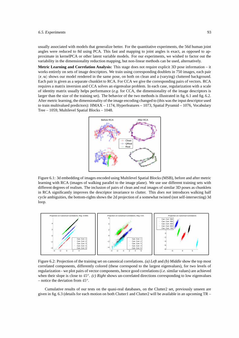
6.5. Experiments 93
usually associated with models that generalize better. For the quantitative experiments, the 56d human jointangles were reduced to 8d using PCA. This fast and mapping to joint angles is exact, as opposed to ap-proximate in kernelPCA or other latent variable models. For our experiments, we wished to factor out thevariability in the dimensionality reduction mapping, but non-linear methods can be used, alternatively.
Metric Learning and Correlation Analysis: This stage does not require explicit 3D pose information – itworks entirely on sets of image descriptors. We train using corresponding doublets in 750 images, each pair(r,u) shows our model rendered in the same pose, on both on clean and a (varying) cluttered background.Each pair is given as a separate chunklet to RCA. For CCA we give the corresponding pairs of vectors. RCArequires a matrix inversion and CCA solves an eigenvalue problem. In each case, regularization with a scaleof identity matrix usually helps performance (e.g. for CCA, the dimensionality of the image descriptors islarger than the size of the training set). The behavior of the two methods is illustrated in fig. 6.1 and fig. 6.2.After metric learning, the dimensionality of the image encoding changed to (this was the input descriptor usedto train multivalued predictors): HMAX – 1174, Hyperfeatures – 1073, Spatial Pyramid – 1076, VocabularyTree – 1059, Multilevel Spatial Blocks – 1048.
Before RCA
After RCA
CleanQRealReal
Figure 6.1: 3d embedding of images encoded using Multilevel Spatial Blocks (MSB), before and after metriclearning with RCA (images of walking parallel to the image plane). We use use different training sets withdifferent degrees of realism. The inclusion of pairs of clean and real images of similar 3D poses as chunkletsin RCA significantly improves the descriptor invariance to clutter. This does not introduces walking halfcycle ambiguities, the bottom-rights shows the 2d projection of a somewhat twisted (not self-intersecting) 3dloop.
−4 −2 0 2 4
−4
−2
0
2
4
Projection on Canonical Correlations, Reg. 0.0001
Can. Corr. 1Can. Corr. 2Can. Corr. 3Can. Corr. 4Can. Corr. 5
−4 −2 0 2 4 6
−4
−2
0
2
4
6Projection on Canonical Correlations, Reg. 0.01
Can. Corr. 1Can. Corr. 2Can. Corr. 3Can. Corr. 4Can. Corr. 5
−5 0 5−8
−6
−4
−2
0
2
4
6
Projection on Canonical Correlations
Can. Corr. 500Can. Corr. 550Can. Corr. 600Can. Corr. 650Can. Corr. 700
Figure 6.2: Projection of the training set on canonical correlations. (a) Left and (b) Middle show the top mostcorrelated components, differently colored (these correspond to the largest eigenvalues), for two levels ofregularization - we plot pairs of vector components, hence good correlations (i.e. similar values) are achievedwhen their slope is close to 45o. (c) Right shows un-correlated directions corresponding to low eigenvalues– notice the deviation from 45o.
Cumulative results of our tests on the quasi-real databases, on the Clutter2 set, previously unseen aregiven in fig. 6.3 (details for each motion on both Clutter1 and Clutter2 will be available in an upcoming TR –
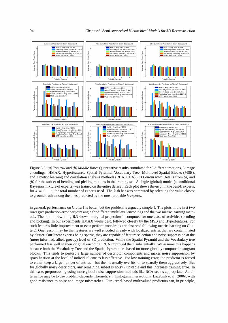
94 Chapter 6. Semi-supervised Hierarchical Models for 3D Reconstruction
1 2 3 4 50
5
10
15
20
Probable Experts
Ave
rage
Joi
nt A
ngle
Err
ors
Cumulative Prediction on Clean Background
HMAX− Avg. Error:8.2092Spatial Pyramid− Avg. Error:8.1526Hyperfeatures− Avg. Error:8.4874Vocabulary Tree− Avg. Error:7.4157MSB− Avg. Error:7.5933
1 2 3 4 50
5
10
15
20
Probable Experts
Ave
rage
Joi
nt A
ngle
Err
ors
RCA Cumulative Prediction on Clean Background
HMAX− Avg. Error:7.0575Spatial Pyramid− Avg. Error:6.727Hyperfeatures− Avg. Error:8.4325Vocabulary Tree− Avg. Error:7.6013MSB− Avg. Error:7.4812
1 2 3 4 50
5
10
15
20
Probable Experts
Ave
rage
Joi
nt A
ngle
Err
ors
CCA Cumulative Prediction on Clean Background
HMAX− Avg. Error:6.7935Spatial Pyramid− Avg. Error:7.9461Hyperfeatures− Avg. Error:8.4341Vocabulary Tree− Avg. Error:7.6307MSB− Avg. Error:7.3585
1 2 3 4 50
5
10
15
20
Probable Experts
Ave
rage
Joi
nt A
ngle
Err
ors
Cumulative Prediction on Clutter2 Background
HMAX− Avg. Error:8.5233Spatial Pyramid− Avg. Error:18.1754Hyperfeatures− Avg. Error:9.5695Vocabulary Tree− Avg. Error:11.8846MSB− Avg. Error:9.003
1 2 3 4 50
5
10
15
20
Probable Experts
Ave
rage
Joi
nt A
ngle
Err
ors
RCA Cumulative Prediction on Clutter2 Background
HMAX− Avg. Error:10.6414Spatial Pyramid− Avg. Error:13.5865Hyperfeatures− Avg. Error:10.2945Vocabulary Tree− Avg. Error:10.3374MSB− Avg. Error:10.5738
1 2 3 4 50
5
10
15
20
Probable Experts
Ave
rage
Joi
nt A
ngle
Err
ors
CCA Cumulative Prediction on Clutter2 Background
HMAX− Avg. Error:8.0185Spatial Pyramid− Avg. Error:16.9987Hyperfeatures− Avg. Error:10.7131Vocabulary Tree− Avg. Error:11.8748MSB− Avg. Error:8.6005
1 2 3 4 50
2
4
6
8
10
12
14
16
Probable Experts
Ave
rage
Joi
nt A
ngle
Err
ors
BendingPickup Prediction on Clean Background
HMAX− Avg. Error:7.3272Spatial Pyramid− Avg. Error:6.3989Hyperfeatures− Avg. Error:6.1906Vocabulary Tree− Avg. Error:5.6443MSB− Avg. Error:4.563
1 2 3 4 50
2
4
6
8
10
12
14
16
Probable Experts
Ave
rage
Joi
nt A
ngle
Err
ors
BendingPickup Prediction on Clutter2 Background
HMAX− Avg. Error:7.6329Spatial Pyramid− Avg. Error:15.4777Hyperfeatures− Avg. Error:8.143Vocabulary Tree− Avg. Error:11.8866MSB− Avg. Error:7.3335
1 2 3 4 50
2
4
6
8
10
12
14
16
Probable Experts
Ave
rage
Joi
nt A
ngle
Err
ors
RCA BendingPickup Prediction on Clutter2 Background
HMAX− Avg. Error:9.455Spatial Pyramid− Avg. Error:8.888Hyperfeatures− Avg. Error:9.2604Vocabulary Tree− Avg. Error:9.8158MSB− Avg. Error:8.581
Figure 6.3: (a) Top row and (b) Middle Row: Quantitative results cumulated for 5 different motions, 5 imageencodings: HMAX, Hyperfeatures, Spatial Pyramid, Vocabulary Tree, Multilevel Spatial Blocks (MSB),and 2 metric learning and correlation analysis methods (RCA, CCA). (c) Bottom row: Details from (a) and(b) for the subset of bending and picking motions in the training set. A single (global) model (a conditionalBayesian mixture of experts) was trained on the entire dataset. Each plot shows the error in the best-k experts,for k = 1 . . . 5, the total number of experts used. The k-th bar was computed by selecting the value closestto ground truth among the ones predicted by the most probable k experts.
in general, performance on Clutter1 is better, but the problem is arguably simpler). The plots in the first tworows give prediction error per joint angle for different multilevel encodings and the two metric learning meth-ods. The bottom row in fig. 6.3 shows ‘marginal projections’, computed for one class of activities (bendingand picking). In our experiments HMAX works best, followed closely by the MSB and Hyperfeatures. Forsuch features little improvement or even performance drops are observed following metric learning on Clut-ter2. One reason may be that features are well encoded already with localized entries that are contaminatedby clutter. Our linear experts being sparse, they are capable of feature selection and noise suppression at the(more informed, albeit greedy) level of 3D prediction. While the Spatial Pyramid and the Vocabulary treeperformed less well in their original encoding, RCA improved them substantially. We assume this happensbecause both the Vocabulary Tree and the Spatial Pyramid are based on more globally computed histogramblocks. This tends to perturb a large number of descriptor components and makes noise suppression bysparsification at the level of individual entries less effective. For low training error, the predictor is forcedto either keep a large number of entries – but then it usually overfits, or to sparsify them aggressively. Butfor globally noisy descriptors, any remaining subset is noisy / unstable and this increases training error. Inthis case, preprocessing using more global noise suppression methods like RCA seems appropriate. An al-ternative may be to use problem-dependent kernels, e.g. histogram intersections [Lazebnik et al., 2006], withgood resistance to noise and image mismatches. Our kernel-based multivalued predictors can, in principle,
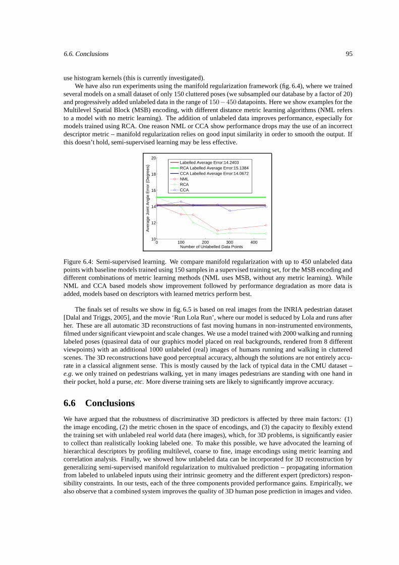
6.6. Conclusions 95
use histogram kernels (this is currently investigated).We have also run experiments using the manifold regularization framework (fig. 6.4), where we trained
several models on a small dataset of only 150 cluttered poses (we subsampled our database by a factor of 20)and progressively added unlabeled data in the range of 150−450 datapoints. Here we show examples for theMultilevel Spatial Block (MSB) encoding, with different distance metric learning algorithms (NML refersto a model with no metric learning). The addition of unlabeled data improves performance, especially formodels trained using RCA. One reason NML or CCA show performance drops may the use of an incorrectdescriptor metric – manifold regularization relies on good input similarity in order to smooth the output. Ifthis doesn’t hold, semi-supervised learning may be less effective.
0 100 200 300 40010
12
14
16
18
20
Number of Unlabelled Data Points
Ave
rage
Joi
nt A
ngle
Err
or (
Deg
rees
)
Labelled Average Error:14.2403RCA Labelled Average Error:15.1384CCA Labelled Average Error:14.0672NMLRCACCA
Figure 6.4: Semi-supervised learning. We compare manifold regularization with up to 450 unlabeled datapoints with baseline models trained using 150 samples in a supervised training set, for the MSB encoding anddifferent combinations of metric learning methods (NML uses MSB, without any metric learning). WhileNML and CCA based models show improvement followed by performance degradation as more data isadded, models based on descriptors with learned metrics perform best.
The finals set of results we show in fig. 6.5 is based on real images from the INRIA pedestrian dataset[Dalal and Triggs, 2005], and the movie ‘Run Lola Run’, where our model is seduced by Lola and runs afterher. These are all automatic 3D reconstructions of fast moving humans in non-instrumented environments,filmed under significant viewpoint and scale changes. We use a model trained with 2000 walking and runninglabeled poses (quasireal data of our graphics model placed on real backgrounds, rendered from 8 differentviewpoints) with an additional 1000 unlabeled (real) images of humans running and walking in clutteredscenes. The 3D reconstructions have good perceptual accuracy, although the solutions are not entirely accu-rate in a classical alignment sense. This is mostly caused by the lack of typical data in the CMU dataset –e.g. we only trained on pedestrians walking, yet in many images pedestrians are standing with one hand intheir pocket, hold a purse, etc. More diverse training sets are likely to significantly improve accuracy.
6.6 Conclusions
We have argued that the robustness of discriminative 3D predictors is affected by three main factors: (1)the image encoding, (2) the metric chosen in the space of encodings, and (3) the capacity to flexibly extendthe training set with unlabeled real world data (here images), which, for 3D problems, is significantly easierto collect than realistically looking labeled one. To make this possible, we have advocated the learning ofhierarchical descriptors by profiling multilevel, coarse to fine, image encodings using metric learning andcorrelation analysis. Finally, we showed how unlabeled data can be incorporated for 3D reconstruction bygeneralizing semi-supervised manifold regularization to multivalued prediction – propagating informationfrom labeled to unlabeled inputs using their intrinsic geometry and the different expert (predictors) respon-sibility constraints. In our tests, each of the three components provided performance gains. Empirically, wealso observe that a combined system improves the quality of 3D human pose prediction in images and video.
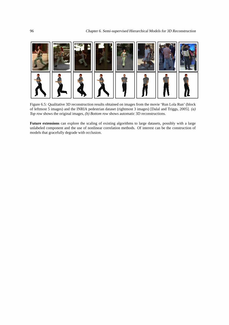
96 Chapter 6. Semi-supervised Hierarchical Models for 3D Reconstruction
Figure 6.5: Qualitative 3D reconstruction results obtained on images from the movie ‘Run Lola Run’ (blockof leftmost 5 images) and the INRIA pedestrian dataset (rightmost 3 images) [Dalal and Triggs, 2005]. (a)Top row shows the original images, (b) Bottom row shows automatic 3D reconstructions.
Future extensions can explore the scaling of existing algorithms to large datasets, possibly with a largeunlabeled component and the use of nonlinear correlation methods. Of interest can be the construction ofmodels that gracefully degrade with occlusion.

Chapter 7
Learning Joint Top-Down andBottom-up Processes for 3D VisualInference
In this chapter, we present an algorithm for jointly learning a consistent bidirectional generative-recognitionmodel that combines top-down and bottom-up processing for monocular 3d human motion reconstruction.Learning progresses in alternative stages of self-training that optimize the probability of the image evidence:the recognition model is tunned using samples from the generative model and the generative model is opti-mized to produce inferences close to the ones predicted by the current recognition model. At equilibrium,the two models are consistent. During on-line inference, we scan the image at multiple locations and predict3d human poses using the recognition model. But this implicitly includes one-shot generative consistencyfeedback. The framework provides a uniform treatment of human detection, 3d initialization and 3d recov-ery from transient failure. Our experimental results show that this procedure is promising for the automaticreconstruction of human motion in more natural scene settings with background clutter and occlusion. Anearlier version of this chapter appeared in IEEE International Conference on Computer Vision and PatternRecognition (CVPR) [Sminchisescu et al., 2006b].
7.1 Models with Bidirectional Mappings
Analyzing three-dimensional human motion in real world environments is an actively growing field with abroad scope of applications spanning video browsing and indexing, human-computer interaction and surveil-lance. The problem has been traditionally attacked using the powerful machinery of top-down, generativemodeling, with image-based feedback provided within an analysis-by-synthesis loop. Despite being a naturalway to model the appearance of complex articulated structures, the success of generative models has beenpartly shadowed because it is computational demanding to infer the distribution on their hidden states (herehuman joint angles) and because their parameters are unknown and variable across many real scenes.
The difficulty of generative modeling has motivated the advent of a complementary class of bottom-up, feed-forward, discriminative recognition methods which predict state distributions directly from imagefeatures. Despite being simple to understand and fast, recognition methods tend to assume that the objectof interest is segmented and could be blind-sighted by the lack of feedback – they cannot self-asses accu-racy. It may be possible to bootstrap them using powerful global or part-based 2d human detectors, but onechallenge is to make this approach scale to the range of poses needed for general 3d reconstruction with-out progressively modeling most of the 3d constraints. This is partly because the space of (even typical)human articulation is large, because self-occlusion and foreshortening are hard to model in 2d, and becausemost of the human body parts do not have the distinctiveness that allows their unambiguous detection andcombination.
97
98 Chapter 7. Learning Joint Top-Down and Bottom-up Processes for 3D Visual Inference
To summarize, what appears to be necessary is a mechanism to consistently integrate top-down andbottom-up processing: the flexibility of 3d generative modeling (represent a large set of possible poses ofhuman body parts, their correct occlusion and foreshortening relationships and their consistency with theimage evidence) with the speed and simplicity of feed-forward processing.
In this chapter we present one possible way to meet these requirements based on a bidirectional modelwith both recognition and generative sub-components. Learning the model parameters alternates self-trainingstages in order to maximize the probability of the observed evidence (images of humans). During one step, therecognition model is trained to invert the generative model using samples drawn from it. In the next step, thegenerative model is trained to have a state distribution close to the one predicted by the recognition model. Atlocal equilibrium, which is guaranteed, the two models have consistent, registered parameterizations. Duringon-line inference, the estimates are driven mostly by the fast recognition model, but implicitly include one-shot generative consistency feedback.
The resulting 3d temporal predictor operates similarly to existing 2d object detectors. It searches theimage at different locations and uses the recognition model to hypothesize 3d configurations. Feedback fromthe generative model helps to downgrade incorrect competing 3d hypotheses and to decide on the detectionstatus (human or not) at the analyzed image sub-window. Our results obtained in monocular video show thatthe proposed model is promising for the automatic reconstruction of 3d human motion in environments withbackground clutter. The framework provides a uniform treatment of human detection, 3d initialization and3d recovery from transient failure.
7.1.1 Existing Methods
The research we present relates to the growing body of work in the area of 2d human detection, 3d motionreconstruction, as well as learning and approximation. Due to space limitations, we only give a brief surveywithout aiming at a full literature review. Generative human models and efficient inference algorithms are de-scribed in [Deutscher et al., 2000, Sidenbladh and Black, 2001, Sigal et al., 2004, Sminchisescu and Jepson,2004b, Urtasun et al., 2005]. Discriminative 3d reconstruction methods, based on single or multiple hypothe-ses, in both static and temporal settings are proposed in [Rosales and Sclaroff, 2002, Shakhnarovich et al.,2003, Agarwal and Triggs, 2006a, Elgammal and Lee, 2004, Sminchisescu et al., 2005a]. Systems basedon global [Leibe et al., 2005, Dalal and Triggs, 2005, Viola et al., 2003, Leibe et al., 2005] or part-basedhuman detectors [Mori et al., 2004, Ramanan and Sminchisescu, 2006, Lan and Huttenlocher, 2005] havebeen demonstrated convincingly, and can be an alternative 2d front end to the integrated 3d reconstructionscheme proposed here.
Generative models and variational learning algorithms for extracting motion layers in video have beenexplored by [Jojic and Frey, 2001] and recently by [Kumar et al., 2005] with excellent results. Generativemodels based on variational techniques [Ghahramani and Hinton, 2000] have been investigated by [Pavlovicet al., 2001] in the context of switching linear dynamical models for human motion analysis. Learningflexible aspect graphs of 2d human exemplars is a goal in the work of [Toyama and Blake, 2001] wherespecific models and inference algorithms are given.
The combination of generative and discriminative 3d human models for the static case has been studiedby [Rosales and Sclaroff, 2002] who has employed a mixture of neural networks for the recognition modeland a neural network model for verification. This type of approach has been extended to the dynamic case[Demirdjian et al., 2005] in a multi-camera setting, in conjunction with Parameter Sensitive Hashing, a fastnearest neighbor method [Shakhnarovich et al., 2003] used to initialize model-based non-linear optimization.The combination of top-down and bottom-up information is considered in the work on generative modelsestimated using importance sampling [Isard and Blake, 1998c, Deutscher et al., 2000], although their proposaldistributions are typically predefined and not learned, being good starting points for inference rather thancompletely plausible solutions to it. Combining feed-forward and feed-back information is also a researchfocus in the biologically inspired machine learning community. The wake-sleep algorithm [Hinton et al.,1995] can be viewed as a notable precursor of the one we propose, although it is based on a significantlydifferent model architecture, cost function and optimization procedure for learning.
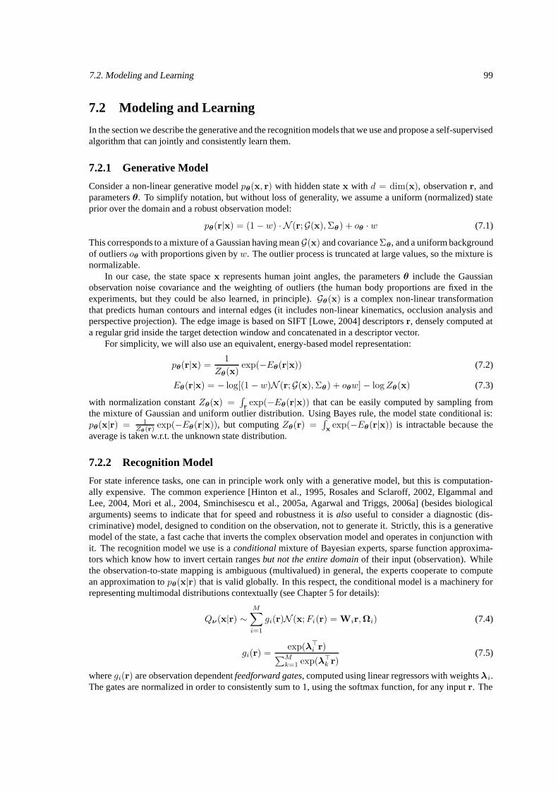
7.2. Modeling and Learning 99
7.2 Modeling and Learning
In the section we describe the generative and the recognition models that we use and propose a self-supervisedalgorithm that can jointly and consistently learn them.
7.2.1 Generative Model
Consider a non-linear generative model pθ(x, r) with hidden state x with d = dim(x), observation r, andparameters θ. To simplify notation, but without loss of generality, we assume a uniform (normalized) stateprior over the domain and a robust observation model:
pθ(r|x) = (1− w) · N (r;G(x),Σθ) + oθ · w (7.1)
This corresponds to a mixture of a Gaussian having mean G(x) and covariance Σθ, and a uniform backgroundof outliers oθ with proportions given by w. The outlier process is truncated at large values, so the mixture isnormalizable.
In our case, the state space x represents human joint angles, the parameters θ include the Gaussianobservation noise covariance and the weighting of outliers (the human body proportions are fixed in theexperiments, but they could be also learned, in principle). Gθ(x) is a complex non-linear transformationthat predicts human contours and internal edges (it includes non-linear kinematics, occlusion analysis andperspective projection). The edge image is based on SIFT [Lowe, 2004] descriptors r, densely computed ata regular grid inside the target detection window and concatenated in a descriptor vector.
For simplicity, we will also use an equivalent, energy-based model representation:
pθ(r|x) =1
Zθ(x)exp(−Eθ(r|x)) (7.2)
Eθ(r|x) = − log[(1− w)N (r;G(x),Σθ) + oθw]− logZθ(x) (7.3)
with normalization constant Zθ(x) =∫rexp(−Eθ(r|x)) that can be easily computed by sampling from
the mixture of Gaussian and uniform outlier distribution. Using Bayes rule, the model state conditional is:pθ(x|r) = 1
Zθ(r) exp(−Eθ(r|x)), but computing Zθ(r) =∫x
exp(−Eθ(r|x)) is intractable because theaverage is taken w.r.t. the unknown state distribution.
7.2.2 Recognition Model
For state inference tasks, one can in principle work only with a generative model, but this is computation-ally expensive. The common experience [Hinton et al., 1995, Rosales and Sclaroff, 2002, Elgammal andLee, 2004, Mori et al., 2004, Sminchisescu et al., 2005a, Agarwal and Triggs, 2006a] (besides biologicalarguments) seems to indicate that for speed and robustness it is also useful to consider a diagnostic (dis-criminative) model, designed to condition on the observation, not to generate it. Strictly, this is a generativemodel of the state, a fast cache that inverts the complex observation model and operates in conjunction withit. The recognition model we use is a conditional mixture of Bayesian experts, sparse function approxima-tors which know how to invert certain ranges but not the entire domain of their input (observation). Whilethe observation-to-state mapping is ambiguous (multivalued) in general, the experts cooperate to computean approximation to pθ(x|r) that is valid globally. In this respect, the conditional model is a machinery forrepresenting multimodal distributions contextually (see Chapter 5 for details):
Qν(x|r) ∼M∑
i=1
gi(r)N (x;Fi(r) = Wir,Ωi) (7.4)
gi(r) =exp(λ>
i r)∑M
k=1 exp(λ>k r)
(7.5)
where gi(r) are observation dependent feedforward gates, computed using linear regressors with weights λi.The gates are normalized in order to consistently sum to 1, using the softmax function, for any input r. The
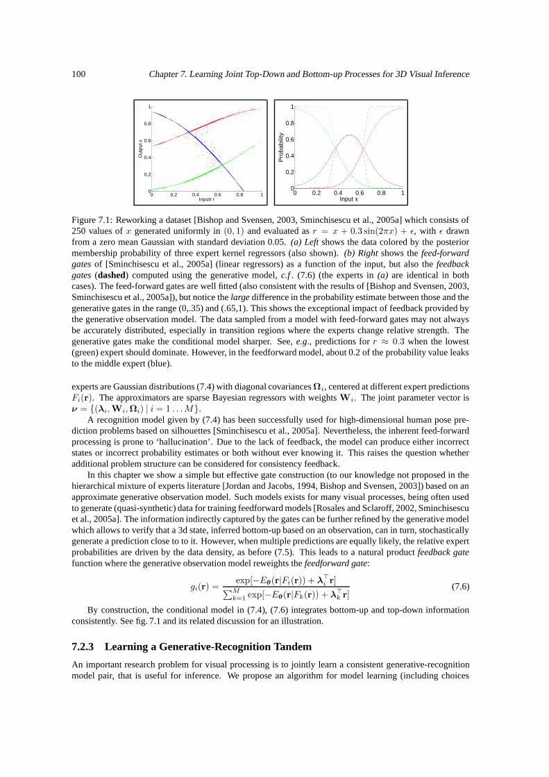
100 Chapter 7. Learning Joint Top-Down and Bottom-up Processes for 3D Visual Inference
0 0.2 0.4 0.6 0.8 10
0.2
0.4
0.6
0.8
1
Inputr r
Out
put x
0 0.2 0.4 0.6 0.8 10
0.2
0.4
0.6
0.8
1
Input x
Pro
ba
bili
ty
Figure 7.1: Reworking a dataset [Bishop and Svensen, 2003, Sminchisescu et al., 2005a] which consists of250 values of x generated uniformly in (0, 1) and evaluated as r = x + 0.3 sin(2πx) + ε, with ε drawnfrom a zero mean Gaussian with standard deviation 0.05. (a) Left shows the data colored by the posteriormembership probability of three expert kernel regressors (also shown). (b) Right shows the feed-forwardgates of [Sminchisescu et al., 2005a] (linear regressors) as a function of the input, but also the feedbackgates (dashed) computed using the generative model, c.f . (7.6) (the experts in (a) are identical in bothcases). The feed-forward gates are well fitted (also consistent with the results of [Bishop and Svensen, 2003,Sminchisescu et al., 2005a]), but notice the large difference in the probability estimate between those and thegenerative gates in the range (0,.35) and (.65,1). This shows the exceptional impact of feedback provided bythe generative observation model. The data sampled from a model with feed-forward gates may not alwaysbe accurately distributed, especially in transition regions where the experts change relative strength. Thegenerative gates make the conditional model sharper. See, e.g., predictions for r ≈ 0.3 when the lowest(green) expert should dominate. However, in the feedforward model, about 0.2 of the probability value leaksto the middle expert (blue).
experts are Gaussian distributions (7.4) with diagonal covariances Ωi, centered at different expert predictionsFi(r). The approximators are sparse Bayesian regressors with weights Wi. The joint parameter vector isν = (λi,Wi,Ωi) | i = 1 . . .M.
A recognition model given by (7.4) has been successfully used for high-dimensional human pose pre-diction problems based on silhouettes [Sminchisescu et al., 2005a]. Nevertheless, the inherent feed-forwardprocessing is prone to ‘hallucination’. Due to the lack of feedback, the model can produce either incorrectstates or incorrect probability estimates or both without ever knowing it. This raises the question whetheradditional problem structure can be considered for consistency feedback.
In this chapter we show a simple but effective gate construction (to our knowledge not proposed in thehierarchical mixture of experts literature [Jordan and Jacobs, 1994, Bishop and Svensen, 2003]) based on anapproximate generative observation model. Such models exists for many visual processes, being often usedto generate (quasi-synthetic) data for training feedforward models [Rosales and Sclaroff, 2002, Sminchisescuet al., 2005a]. The information indirectly captured by the gates can be further refined by the generative modelwhich allows to verify that a 3d state, inferred bottom-up based on an observation, can in turn, stochasticallygenerate a prediction close to to it. However, when multiple predictions are equally likely, the relative expertprobabilities are driven by the data density, as before (7.5). This leads to a natural product feedback gatefunction where the generative observation model reweights the feedforward gate:
gi(r) =exp[−Eθ(r|Fi(r)) + λ>
i r]∑M
k=1 exp[−Eθ(r|Fk(r)) + λ>k r]
(7.6)
By construction, the conditional model in (7.4), (7.6) integrates bottom-up and top-down informationconsistently. See fig. 7.1 and its related discussion for an illustration.
7.2.3 Learning a Generative-Recognition Tandem
An important research problem for visual processing is to jointly learn a consistent generative-recognitionmodel pair, that is useful for inference. We propose an algorithm for model learning (including choices
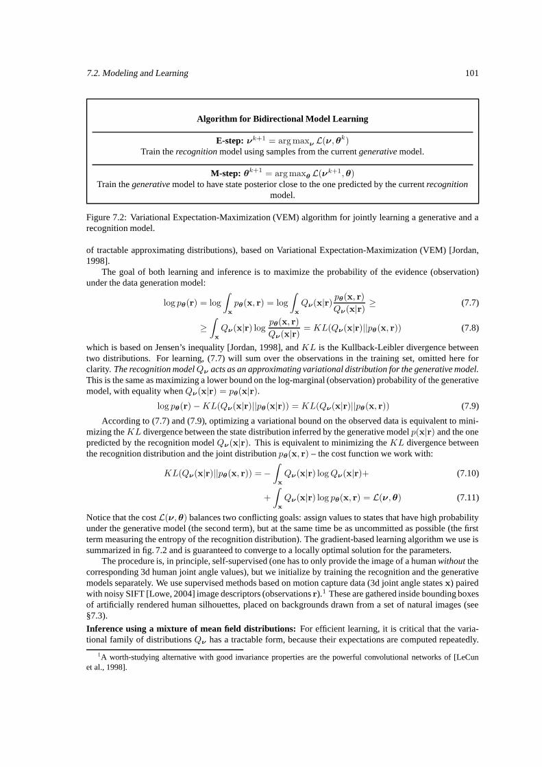
7.2. Modeling and Learning 101
Algorithm for Bidirectional Model Learning
E-step: νk+1 = argmaxν L(ν,θk)Train the recognition model using samples from the current generative model.
M-step: θk+1 = argmaxθ L(νk+1,θ)Train the generative model to have state posterior close to the one predicted by the current recognition
model.
Figure 7.2: Variational Expectation-Maximization (VEM) algorithm for jointly learning a generative and arecognition model.
of tractable approximating distributions), based on Variational Expectation-Maximization (VEM) [Jordan,1998].
The goal of both learning and inference is to maximize the probability of the evidence (observation)under the data generation model:
log pθ(r) = log
∫
x
pθ(x, r) = log
∫
x
Qν(x|r) pθ(x, r)
Qν(x|r) ≥ (7.7)
≥∫
x
Qν(x|r) logpθ(x, r)
Qν(x|r) = KL(Qν(x|r)||pθ(x, r)) (7.8)
which is based on Jensen’s inequality [Jordan, 1998], and KL is the Kullback-Leibler divergence betweentwo distributions. For learning, (7.7) will sum over the observations in the training set, omitted here forclarity. The recognition modelQν acts as an approximating variational distribution for the generative model.This is the same as maximizing a lower bound on the log-marginal (observation) probability of the generativemodel, with equality when Qν(x|r) = pθ(x|r).
log pθ(r)−KL(Qν(x|r)||pθ(x|r)) = KL(Qν(x|r)||pθ(x, r)) (7.9)
According to (7.7) and (7.9), optimizing a variational bound on the observed data is equivalent to mini-mizing theKL divergence between the state distribution inferred by the generative model p(x|r) and the onepredicted by the recognition model Qν(x|r). This is equivalent to minimizing the KL divergence betweenthe recognition distribution and the joint distribution pθ(x, r) – the cost function we work with:
KL(Qν(x|r)||pθ(x, r)) =−∫
x
Qν(x|r) logQν(x|r)+ (7.10)
+
∫
x
Qν(x|r) log pθ(x, r) = L(ν,θ) (7.11)
Notice that the cost L(ν,θ) balances two conflicting goals: assign values to states that have high probabilityunder the generative model (the second term), but at the same time be as uncommitted as possible (the firstterm measuring the entropy of the recognition distribution). The gradient-based learning algorithm we use issummarized in fig. 7.2 and is guaranteed to converge to a locally optimal solution for the parameters.
The procedure is, in principle, self-supervised (one has to only provide the image of a human without thecorresponding 3d human joint angle values), but we initialize by training the recognition and the generativemodels separately. We use supervised methods based on motion capture data (3d joint angle states x) pairedwith noisy SIFT [Lowe, 2004] image descriptors (observations r).1 These are gathered inside bounding boxesof artificially rendered human silhouettes, placed on backgrounds drawn from a set of natural images (see§7.3).
Inference using a mixture of mean field distributions: For efficient learning, it is critical that the varia-tional family of distributions Qν has a tractable form, because their expectations are computed repeatedly.
1A worth-studying alternative with good invariance properties are the powerful convolutional networks of [LeCunet al., 1998].
102 Chapter 7. Learning Joint Top-Down and Bottom-up Processes for 3D Visual Inference
We design the recognition model Qν (§7.2.2) as a conditional Gaussian mixture, with means and diagonalcovariances learned by training independent kernel regressors for each state dimension. Each mixture com-ponent thus factorizes as a product of univariate Gaussians: N (x;Fi(r),Ωi) =
∏dj=1N (xj ;F
ji (r), ωij),
where ωij is the expert i’s variance for state dimension j. This considerably simplifies the calculation ofexpectations needed for learning. The resulting variational approximation is a mixture of mean-field dis-tributions. See [Jordan, 1998] for a detailed derivation of the iterative parameter updates for this class ofapproximations.
The approximation accuracy may be of legitimate concern given the strong correlations among the hu-man state variables. This turns out to be effective because, even though different dimensions of the statespace are decoupled, they are strongly constrained by the observation r (through Fi(r)), by the Bayesianexpert parameters, and indirectly by feedback from the generative model.2 An alternative for strongly cou-pled models is to first decorrelate the state dependency using a non-linear dimensionality reduction method[Sminchisescu et al., 2005c], and then use weaker variational approximations on the latent representation(e.g. a mean field procedure based on factorized state distributions not constrained by the observation [Jor-dan, 1998]). This is computationally more attractive, but we found it was less accurate (≈ 3o higher averageerror per human joint angle in preliminary tests). It also comes at the price of operating with models havinga restricted capacity. Here we aim at a balance between specificity and speed (the recognition model) andrepresentation generality (the generative model).
Online inference (3d reconstruction and tracking) is straightforward using the E-step in fig. 7.2, but forefficiency we usually work only with the recognition model ((7.4) and (7.6)). More generally, it is possibleto iterate the mean field updates (do generative inference) when the recognition distribution has high entropy.The model then effectively switches between a discriminative density propagation rule [Sminchisescu et al.,2005a] but with generative gates c.f . (7.4) and (7.6), and a generative propagation rule [Isard and Blake,1998c, Deutscher et al., 2000, Sidenbladh and Black, 2001, Sminchisescu and Jepson, 2004b]. This offers anatural ‘exploitation-exploration’ or prediction-search tradeoff.
Figure 7.3: A bidirectional model for learning and recognition. During learning, the model is symmetricallydriven by both recognition (bottom-up) and generative (top-down) connections. It alternates by learningone directional component at a time. During online inference, the model is driven mostly by recognitionconnections, but includes one-shot (generative) consistency feedback.
7.3 Experiments
We describe 3d reconstruction experiments in both real image sequences and in quasi-synthetic ones (com-bination of real and synthetic images, with known 3d ground truth).
State representation and image descriptors: The state variables (x) are 56d human joint angles. The imagefeatures (r) are vectors of SIFT descriptors [Lowe, 2004], computed at a densely sampled grid of imagelocations [Viola et al., 2003, Dalal and Triggs, 2005], inside a putative detection window. (For training, thisis a scaled bounding box of the human silhouette.) Each descriptor consists of 9 blocks (3x3), 6x6 pixels,
2This factorial state construction is not exclusively driven by tractability constraints. Models based on experts learnedseparately for each state dimension have been shown to give jointly consistent predictions [Agarwal and Triggs, 2006a,Sminchisescu et al., 2005a].
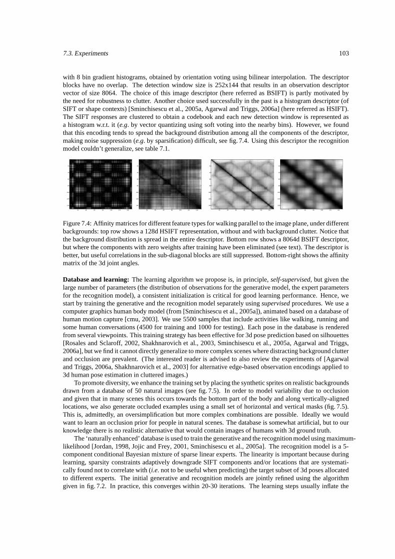
7.3. Experiments 103
with 8 bin gradient histograms, obtained by orientation voting using bilinear interpolation. The descriptorblocks have no overlap. The detection window size is 252x144 that results in an observation descriptorvector of size 8064. The choice of this image descriptor (here referred as BSIFT) is partly motivated bythe need for robustness to clutter. Another choice used successfully in the past is a histogram descriptor (ofSIFT or shape contexts) [Sminchisescu et al., 2005a, Agarwal and Triggs, 2006a] (here referred as HSIFT).The SIFT responses are clustered to obtain a codebook and each new detection window is represented asa histogram w.r.t. it (e.g. by vector quantizing using soft voting into the nearby bins). However, we foundthat this encoding tends to spread the background distribution among all the components of the descriptor,making noise suppression (e.g. by sparsification) difficult, see fig. 7.4. Using this descriptor the recognitionmodel couldn’t generalize, see table 7.1.
20 40 60 80 100 120 140
20
40
60
80
100
120
140
20 40 60 80 100 120 140
20
40
60
80
100
120
140
20 40 60 80 100 120 140
20
40
60
80
100
120
140
20 40 60 80 100 120 140
20
40
60
80
100
120
140
Figure 7.4: Affinity matrices for different feature types for walking parallel to the image plane, under differentbackgrounds: top row shows a 128d HSIFT representation, without and with background clutter. Notice thatthe background distribution is spread in the entire descriptor. Bottom row shows a 8064d BSIFT descriptor,but where the components with zero weights after training have been eliminated (see text). The descriptor isbetter, but useful correlations in the sub-diagonal blocks are still suppressed. Bottom-right shows the affinitymatrix of the 3d joint angles.
Database and learning: The learning algorithm we propose is, in principle, self-supervised, but given thelarge number of parameters (the distribution of observations for the generative model, the expert parametersfor the recognition model), a consistent initialization is critical for good learning performance. Hence, westart by training the generative and the recognition model separately using supervised procedures. We use acomputer graphics human body model (from [Sminchisescu et al., 2005a]), animated based on a database ofhuman motion capture [cmu, 2003]. We use 5500 samples that include activities like walking, running andsome human conversations (4500 for training and 1000 for testing). Each pose in the database is renderedfrom several viewpoints. This training strategy has been effective for 3d pose prediction based on silhouettes[Rosales and Sclaroff, 2002, Shakhnarovich et al., 2003, Sminchisescu et al., 2005a, Agarwal and Triggs,2006a], but we find it cannot directly generalize to more complex scenes where distracting background clutterand occlusion are prevalent. (The interested reader is advised to also review the experiments of [Agarwaland Triggs, 2006a, Shakhnarovich et al., 2003] for alternative edge-based observation encodings applied to3d human pose estimation in cluttered images.)
To promote diversity, we enhance the training set by placing the synthetic sprites on realistic backgroundsdrawn from a database of 50 natural images (see fig. 7.5). In order to model variability due to occlusionand given that in many scenes this occurs towards the bottom part of the body and along vertically-alignedlocations, we also generate occluded examples using a small set of horizontal and vertical masks (fig. 7.5).This is, admittedly, an oversimplification but more complex combinations are possible. Ideally we wouldwant to learn an occlusion prior for people in natural scenes. The database is somewhat artificial, but to ourknowledge there is no realistic alternative that would contain images of humans with 3d ground truth.
The ‘naturally enhanced’ database is used to train the generative and the recognition model using maximum-likelihood [Jordan, 1998, Jojic and Frey, 2001, Sminchisescu et al., 2005a]. The recognition model is a 5-component conditional Bayesian mixture of sparse linear experts. The linearity is important because duringlearning, sparsity constraints adaptively downgrade SIFT components and/or locations that are systemati-cally found not to correlate with (i.e. not to be useful when predicting) the target subset of 3d poses allocatedto different experts. The initial generative and recognition models are jointly refined using the algorithmgiven in fig. 7.2. In practice, this converges within 20-30 iterations. The learning steps usually inflate the
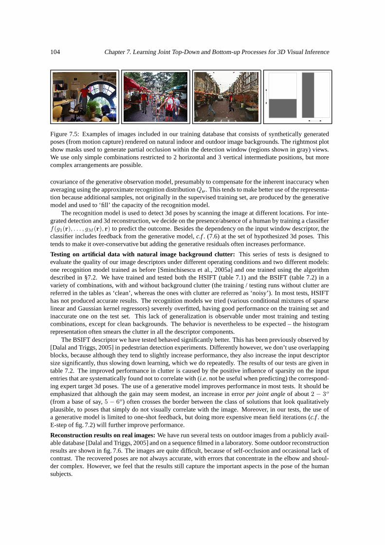
104 Chapter 7. Learning Joint Top-Down and Bottom-up Processes for 3D Visual Inference
Figure 7.5: Examples of images included in our training database that consists of synthetically generatedposes (from motion capture) rendered on natural indoor and outdoor image backgrounds. The rightmost plotshow masks used to generate partial occlusion within the detection window (regions shown in gray) views.We use only simple combinations restricted to 2 horizontal and 3 vertical intermediate positions, but morecomplex arrangements are possible.
covariance of the generative observation model, presumably to compensate for the inherent inaccuracy whenaveraging using the approximate recognition distributionQν . This tends to make better use of the representa-tion because additional samples, not originally in the supervised training set, are produced by the generativemodel and used to ‘fill’ the capacity of the recognition model.
The recognition model is used to detect 3d poses by scanning the image at different locations. For inte-grated detection and 3d reconstruction, we decide on the presence/absence of a human by training a classifierf(g1(r), . . . , gM (r), r) to predict the outcome. Besides the dependency on the input window descriptor, theclassifier includes feedback from the generative model, c.f . (7.6) at the set of hypothesized 3d poses. Thistends to make it over-conservative but adding the generative residuals often increases performance.
Testing on artificial data with natural image background clutter: This series of tests is designed toevaluate the quality of our image descriptors under different operating conditions and two different models:one recognition model trained as before [Sminchisescu et al., 2005a] and one trained using the algorithmdescribed in §7.2. We have trained and tested both the HSIFT (table 7.1) and the BSIFT (table 7.2) in avariety of combinations, with and without background clutter (the training / testing runs without clutter arereferred in the tables as ‘clean’, whereas the ones with clutter are referred as ‘noisy’). In most tests, HSIFThas not produced accurate results. The recognition models we tried (various conditional mixtures of sparselinear and Gaussian kernel regressors) severely overfitted, having good performance on the training set andinaccurate one on the test set. This lack of generalization is observable under most training and testingcombinations, except for clean backgrounds. The behavior is nevertheless to be expected – the histogramrepresentation often smears the clutter in all the descriptor components.
The BSIFT descriptor we have tested behaved significantly better. This has been previously observed by[Dalal and Triggs, 2005] in pedestrian detection experiments. Differently however, we don’t use overlappingblocks, because although they tend to slightly increase performance, they also increase the input descriptorsize significantly, thus slowing down learning, which we do repeatedly. The results of our tests are given intable 7.2. The improved performance in clutter is caused by the positive influence of sparsity on the inputentries that are systematically found not to correlate with (i.e. not be useful when predicting) the correspond-ing expert target 3d poses. The use of a generative model improves performance in most tests. It should beemphasized that although the gain may seem modest, an increase in error per joint angle of about 2 − 3o
(from a base of say, 5 − 6o) often crosses the border between the class of solutions that look qualitativelyplausible, to poses that simply do not visually correlate with the image. Moreover, in our tests, the use ofa generative model is limited to one-shot feedback, but doing more expensive mean field iterations (c.f . theE-step of fig. 7.2) will further improve performance.
Reconstruction results on real images: We have run several tests on outdoor images from a publicly avail-able database [Dalal and Triggs, 2005] and on a sequence filmed in a laboratory. Some outdoor reconstructionresults are shown in fig. 7.6. The images are quite difficult, because of self-occlusion and occasional lack ofcontrast. The recovered poses are not always accurate, with errors that concentrate in the elbow and shoul-der complex. However, we feel that the results still capture the important aspects in the pose of the humansubjects.
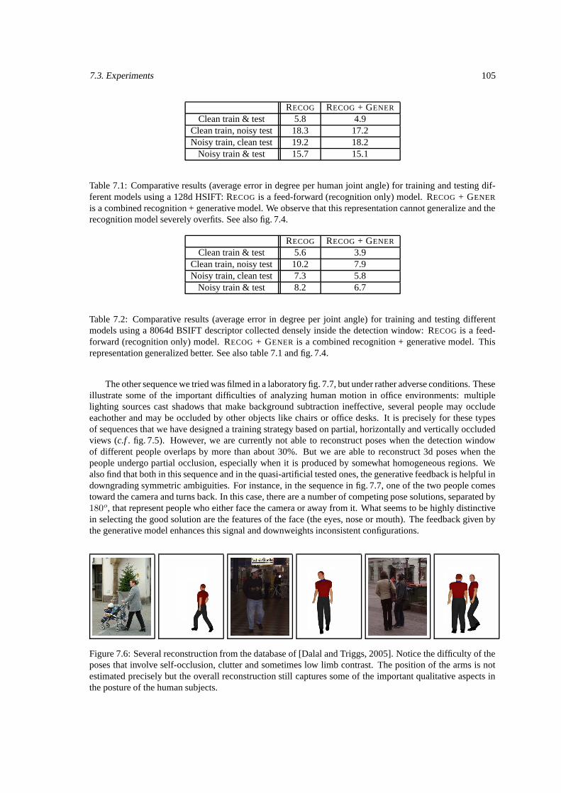
7.3. Experiments 105
RECOG RECOG + GENER
Clean train & test 5.8 4.9Clean train, noisy test 18.3 17.2Noisy train, clean test 19.2 18.2
Noisy train & test 15.7 15.1
Table 7.1: Comparative results (average error in degree per human joint angle) for training and testing dif-ferent models using a 128d HSIFT: RECOG is a feed-forward (recognition only) model. RECOG + GENER
is a combined recognition + generative model. We observe that this representation cannot generalize and therecognition model severely overfits. See also fig. 7.4.
RECOG RECOG + GENER
Clean train & test 5.6 3.9Clean train, noisy test 10.2 7.9Noisy train, clean test 7.3 5.8
Noisy train & test 8.2 6.7
Table 7.2: Comparative results (average error in degree per joint angle) for training and testing differentmodels using a 8064d BSIFT descriptor collected densely inside the detection window: RECOG is a feed-forward (recognition only) model. RECOG + GENER is a combined recognition + generative model. Thisrepresentation generalized better. See also table 7.1 and fig. 7.4.
The other sequence we tried was filmed in a laboratory fig. 7.7, but under rather adverse conditions. Theseillustrate some of the important difficulties of analyzing human motion in office environments: multiplelighting sources cast shadows that make background subtraction ineffective, several people may occludeeachother and may be occluded by other objects like chairs or office desks. It is precisely for these typesof sequences that we have designed a training strategy based on partial, horizontally and vertically occludedviews (c.f . fig. 7.5). However, we are currently not able to reconstruct poses when the detection windowof different people overlaps by more than about 30%. But we are able to reconstruct 3d poses when thepeople undergo partial occlusion, especially when it is produced by somewhat homogeneous regions. Wealso find that both in this sequence and in the quasi-artificial tested ones, the generative feedback is helpful indowngrading symmetric ambiguities. For instance, in the sequence in fig. 7.7, one of the two people comestoward the camera and turns back. In this case, there are a number of competing pose solutions, separated by180o, that represent people who either face the camera or away from it. What seems to be highly distinctivein selecting the good solution are the features of the face (the eyes, nose or mouth). The feedback given bythe generative model enhances this signal and downweights inconsistent configurations.
Figure 7.6: Several reconstruction from the database of [Dalal and Triggs, 2005]. Notice the difficulty of theposes that involve self-occlusion, clutter and sometimes low limb contrast. The position of the arms is notestimated precisely but the overall reconstruction still captures some of the important qualitative aspects inthe posture of the human subjects.
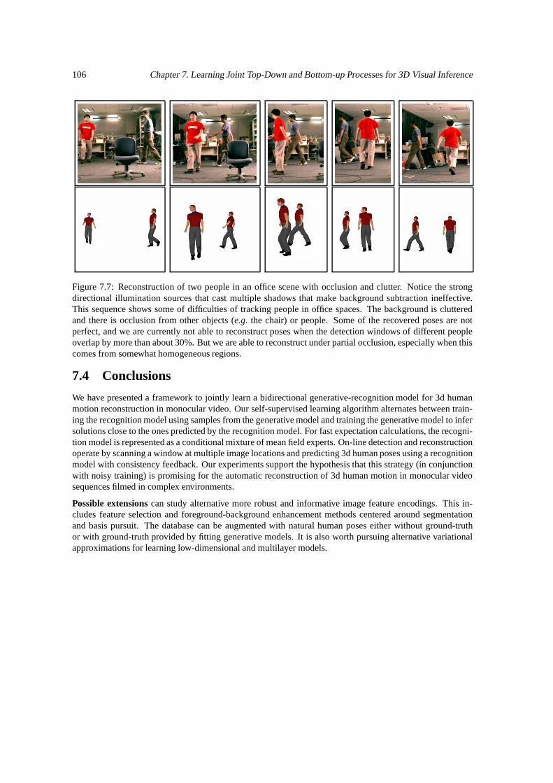
106 Chapter 7. Learning Joint Top-Down and Bottom-up Processes for 3D Visual Inference
Figure 7.7: Reconstruction of two people in an office scene with occlusion and clutter. Notice the strongdirectional illumination sources that cast multiple shadows that make background subtraction ineffective.This sequence shows some of difficulties of tracking people in office spaces. The background is clutteredand there is occlusion from other objects (e.g. the chair) or people. Some of the recovered poses are notperfect, and we are currently not able to reconstruct poses when the detection windows of different peopleoverlap by more than about 30%. But we are able to reconstruct under partial occlusion, especially when thiscomes from somewhat homogeneous regions.
7.4 Conclusions
We have presented a framework to jointly learn a bidirectional generative-recognition model for 3d humanmotion reconstruction in monocular video. Our self-supervised learning algorithm alternates between train-ing the recognition model using samples from the generative model and training the generative model to infersolutions close to the ones predicted by the recognition model. For fast expectation calculations, the recogni-tion model is represented as a conditional mixture of mean field experts. On-line detection and reconstructionoperate by scanning a window at multiple image locations and predicting 3d human poses using a recognitionmodel with consistency feedback. Our experiments support the hypothesis that this strategy (in conjunctionwith noisy training) is promising for the automatic reconstruction of 3d human motion in monocular videosequences filmed in complex environments.
Possible extensions can study alternative more robust and informative image feature encodings. This in-cludes feature selection and foreground-background enhancement methods centered around segmentationand basis pursuit. The database can be augmented with natural human poses either without ground-truthor with ground-truth provided by fitting generative models. It is also worth pursuing alternative variationalapproximations for learning low-dimensional and multilayer models.
Chapter 8
Conditional Models for ContextualHuman Motion Recognition
We describe algorithms for recognizing human motion in monocular video sequences, based on discrimi-native Conditional Random Fields (CRF) and Maximum Entropy Markov Models (MEMM). Existing ap-proaches to this problem typically use generative structures like the Hidden Markov Model (HMM). There-fore they have to make simplifying, often unrealistic assumptions on the conditional independence of obser-vations given the motion class labels and cannot accommodate rich overlapping features of the observationor long-term contextual dependencies among observations at multiple timesteps. This makes them proneto myopic failures in recognizing many human motions, because even the transition between simple humanactivities naturally has temporal segments of ambiguity and overlap. The correct interpretation of these se-quences requires more holistic, contextual decisions, where the estimate of an activity at a particular timestepcould be constrained by longer windows of observations, prior and even posterior to that timestep. This wouldnot be computationally feasible with a HMM which requires the enumeration of a number of observation se-quences exponential in the size of the context window. In this work we follow a different philosophy: insteadof restrictively modeling the complex image generation process – the observation, we work with models thatcan unrestrictedly take it as an input, hence condition on it. Conditional models like the proposed CRFsseamlessly represent contextual dependencies and have computationally attractive properties: they supportefficient, exact recognition using dynamic programming, and their parameters can be learned using convexoptimization. We introduce conditional graphical models as complementary tools for human motion recog-nition and present an extensive set of experiments that show not only how these can successfully classifydiverse human activities like walking, jumping, running, picking or dancing, but also how they can discrim-inate among subtle motion styles like normal walks and wander walks. An earlier version of this chapterappeared in Computer Vision and Image Understanding (CVIU) [Sminchisescu et al., 2006a], based on re-search published in IEEE International Conference on Computer Vision (ICCV) [Sminchisescu et al., 2005b]and Advances in Neural Processing Systems (NIPS) [Sminchisescu et al., 2005c].
8.1 The Importance of Context
Solutions for robustly tracking and recognizing human motion in natural environments are important becausethey can provide the basic infrastructure for the advancement of several technologies that enable adaptivevisual assistants for intelligent human-computer interfaces or systems for entertainment, surveillance andsecurity. Human tracking is complex due to the large variability in the shape and articulation of the humanbody, the presence of clothing or fast motions. Highly variable lighting conditions or occlusion from otherpeople or objects further complicate the problem.
Human activity and behavior recognition, on the other hand, is challenging because human motion lacksa clear categorical structure: the motion can be often classified into several categories simultaneously, be-
107
108 Chapter 8. Conditional Models for Contextual Human Motion Recognition
cause some activities have a natural compositional (or concurrent) structure in terms of basic action units(run and hand-wave, walk and shake hands while involved in a conversation with somebody known) andbecause even the transition between simple activities naturally has temporal segments of ambiguity and over-lap. The human motion often displays multiple levels of increasing complexity that range from action-unitsto activities and behaviors. The more complex the human behavior, the more difficult it becomes to performrecognition in isolation. Motions can happen at various timescales and because they often exhibit long-termdependencies, long contexts of observations may need to be considered for correct classification at particulartimesteps. For instance, the motion class at a current timestep may be hard to predict using only the previousstate and the current image observation alone, but may be less ambiguous if several neighboring states orobservations possibly both backward and forward in time are considered. However, this computation wouldbe hard to perform using a Hidden Markov Model (HMM) [Rabiner, 1989] where stringent independenceassumptions among observations are required in order to ensure computational tractability (notably, the con-ditional independence of observations given the hidden class labels).
For concreteness, consider a person doing a turn during dancing. After observing several image frames,the nature of this activity may become clear. However, initially, a turn followed by an ample arm movementmay be very similar to the beginning of a conversation. Making local decisions for the current state con-strained by a longer observation context, both prior and posterior in time can be critical for increasing theconfidence (hence accuracy) of the inferred activity percept. A clear illustration is given in our fig. 8.6. Amodel that myopically decides the current motion class based on the previous state and the current obser-vation only achieves 56% recognition accuracy for dancing. The remaining test instances are misclassifiedas conversation. In turn, a flexible conditional model that decides based on the previous state label and acontextual window of 7 observtions centered at the current state to be labeled achieves 100 % recognitionaccuracy and has a large recognition margin w.r.t. to the other activities in its repertoire. The importance ofcontext is also apparent whenever one has to make subtle distinctions between human activity styles, e.g.normal walking, wander walking or slow walking. These styles contain many similar 3d poses with similarimage appearance. Constraining the style estimate at each timestep based on a long-range context of priorobservations can significantly improve its recognition performance. See our fig. 8.5 and fig. 8.7 as well astables 8.4–8.5.
To summarize, HMMs and more generally the class of stochastic grammars, are generative models thatdefine a joint probability distribution p(X,R) over observations R and motion label sequences X and useBayes rule to compute p(X|R). In order to model the observation process and enumerate all possible se-quences of observations, generative models need to assume them atomic and independent. Therefore theycan’t accommodate multiple overlapping features of the observation or long-range dependencies betweenstate indexes and observation indexes at multiple time steps because the inference problem in this case be-comes intractable. Arguably, another inconvenient of using generative models like HMMs stems from theirindirection: they use a joint probabilistic model to solve a conditional inference problem thus focusing onmodeling the observations that at runtime are fixed. Even if the generative model were accurate, this ap-proach could be non-economical in cases where the underlying generative model may be quite complex butthe motion class conditioned on the observation (or the boundary between classes) is nevertheless simple.
In this chapter we advocate a complementary discriminative approach to human motion recognition basedon extensions to Conditional Random Fields (CRF) [Lafferty et al., 2001] and Maximum Entropy MarkovModels (MEMM) [McCallum et al., 2000]. A CRF conditions on the observation without modeling it, there-fore it avoids independence assumptions and can accommodate long range interactions between observationsand states at different timesteps. Our approach is based on non-locally defined, multiple features of theobservation, represented as log-linear models – it can be viewed as a generalization of logistic regression toaccount for correlations among successive class labels. Inference can be performed efficiently using dynamicprogramming, whereas training the parameters is based on a convex problem, with guaranteed global opti-mality. We demonstrate the algorithms on the task of both recognizing broader classes of human motions likewalking, running, jumping, conversation or dancing, but also for finely discriminating among motion styleslike slow walk or wander walk. We compare against HMMs and demonstrate that the conditional models cansignificantly improve recognition performance in tests that use both features extracted from 3d reconstructedjoint angles, but also in recognition experiments that use feature descriptors extracted directly from image
8.1. The Importance of Context 109
silhouettes. Combining the relative advantages of generative and conditional models for robust recognitionremains a promising avenue for future work.
Chapter Organization: §8.1.1 discusses related work, §8.2 introduces directed and undirected recognitionmodels and discusses their relative trade-offs, §8.3 describes experimental results on human motion recogni-tion. The proposed CRF and MEMM models are compared to HMMs in two series of examples, one using2d image features and the other using 3d joint angle features, on both real and artificial image sequences. Insection §8.4 we conclude and discuss perspectives for future work.
8.1.1 Existing Recognition Methods
The research devoted to human motion recognition is extensive, accounting for its clear social and techno-logical importance. We refer to the comprehensive reviews by Aggarwal and Cai [1999], Gavrila [1999],Pavlovic et al. [1997] or Hu et al. [2004], and here only aim at a limited literature overview. Approachesto human activity recognition can be both supervised [Fablet and Bouthemy, 2001, Rabiner, 1989, Starnerand Pentland, 1995, Brand et al., 1996, Bregler, 1997, Gong and Xing, 2003, Vogler and Metaxas, 2001]and unsupervised [Manor and Irani, 2001, Stauffer and Grimson, 2000, Vasilescu, 2002, Efros et al., 2003].The methods can be subdivided into: (i) Techniques based on spatiotemporal features extract templates foreach activity and match them to those of unseen events [Bobick and Wilson, 1995, Bobick and Davis, 2001,Efros et al., 2003, Manor and Irani, 2001]; (ii) Methods based on temporal logic represent critical orderingconstraints on activities [Pinhanez and Bobick, 1998, Hongeng et al., 2004], and (iii) Algorithms based onstochastic grammars or Hidden Markov Models (HMM) represent the observed data distribution and modelthe dynamic, temporal state constraints [Starner and Pentland, 1995, Brand et al., 1996, Bregler, 1997, Gongand Xing, 2003, Vogler and Metaxas, 2001, Olivier et al., 2002].
HMMs [Rabiner, 1989] and their various extensions have been successfully used for recognizing humanmotion based on both 2d observations [Starner and Pentland, 1995, Brand et al., 1996, Bregler, 1997, Gongand Xing, 2003] and 3d observations [Vogler and Metaxas, 2001, Ramanan and Forsyth, 2003]. More sophis-ticated recognition structures have been obtained by compositing the basic ones: (i) Layering [Olivier et al.,2002, Zhang et al.] composes recognition modules hierarchically by feeding the results of one recognitionlayer as observations for the next one; (ii) Left-right modeling allows certain transitions, but not all the possi-ble ones between different class labels: as time increases, the state index only increases or remains the same;(iii) Factorial methods [Ghahramani and Jordan, 1997] use variational inference to decouple dependencies inmodels with multivariate discrete states. To make state inference tractable, some of the correlations betweenthe different dimensions are relaxed. The computation is performed independently on the temporal chainscorresponding to each one of them. (iv) Parallel techniques [Vogler and Metaxas, 2001] recognize using abattery of models independently trained for each different action in a corpus. The most probable motion classis decided based on model selection procedures; (v) Coupling [Brand et al., 1996] operates using a number ofparallel HMMs where each individual state dimension depends on all the other ones. All these constructionscan be realized within the conditional modeling framework of introduced in this chapter.
Generative approaches to simultaneous (mixed) tracking and motion classification have been proposedby Blake et al. [1999] and Pavlovic and Rehg [2000]. In their algorithms, the variability within each motionclass is represented as an auto-regressive process, or a linear dynamical system, with learning and inferencebased on Condensation and variational techniques, respectively. Black and Jepson [1998] model motionas a trajectory through a state space spanned by optical flow fields and infer the activity class based onpropagating multiple hypotheses using a Condensation filter. Fablet and Bouthemy [2001] present a powerfulapproach to recognition using multiscale Gibbs models. Shi et al. [2004] employ a propagation networkand a discrete Condensation algorithm in order to better take into account sequential activities that includeparallel streams of action. Fanti et al. [2005] represent the human motion dependencies by a triangulatedgraph and exploit position, velocity and appearance cues within a recognition procedure based on beliefpropagation. Vasilescu [2002] represents human motion signatures w.r.t. as projection on a multilinear basisand classify using nearest neighbor. Hoey and Little [2000] recognize human motion using HMMs havingflow field observations represented w.r.t. to a Zernike basis. Yilmaz and Shah [2005] recognize human motionusing multiple uncalibrated cameras and a criteria based on the condition number of a matrix that stores 3d
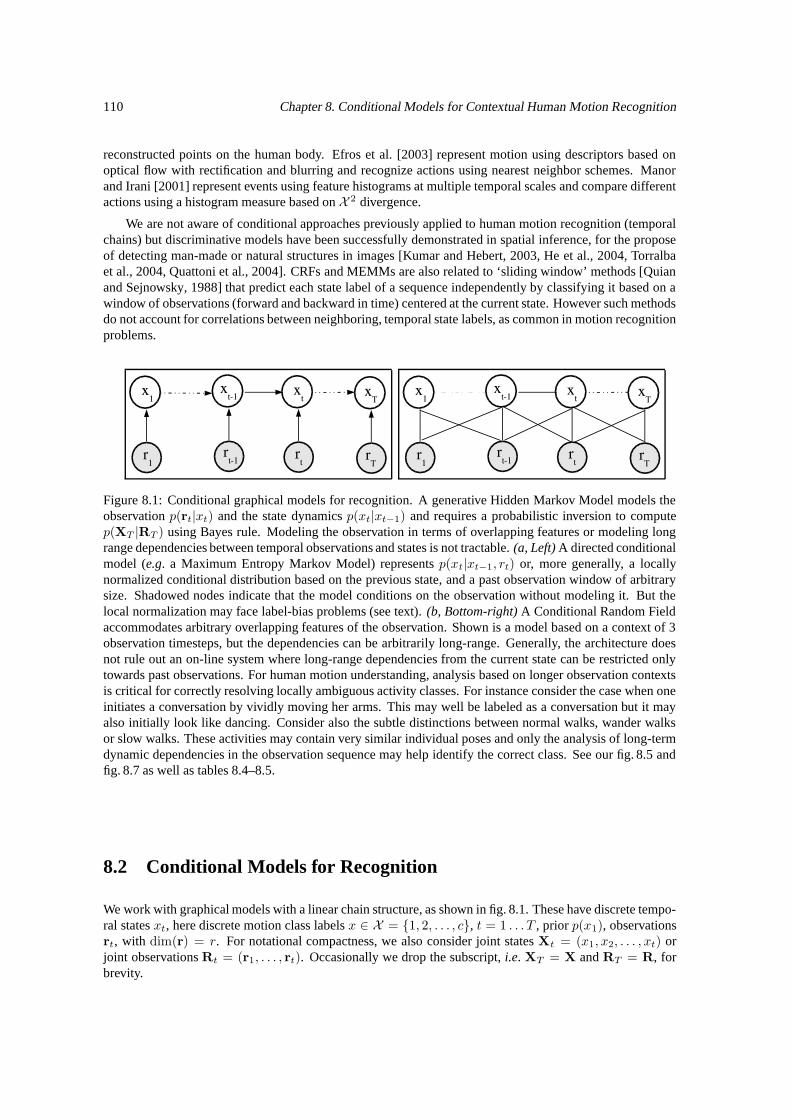
110 Chapter 8. Conditional Models for Contextual Human Motion Recognition
reconstructed points on the human body. Efros et al. [2003] represent motion using descriptors based onoptical flow with rectification and blurring and recognize actions using nearest neighbor schemes. Manorand Irani [2001] represent events using feature histograms at multiple temporal scales and compare differentactions using a histogram measure based on X 2 divergence.
We are not aware of conditional approaches previously applied to human motion recognition (temporalchains) but discriminative models have been successfully demonstrated in spatial inference, for the proposeof detecting man-made or natural structures in images [Kumar and Hebert, 2003, He et al., 2004, Torralbaet al., 2004, Quattoni et al., 2004]. CRFs and MEMMs are also related to ‘sliding window’ methods [Quianand Sejnowsky, 1988] that predict each state label of a sequence independently by classifying it based on awindow of observations (forward and backward in time) centered at the current state. However such methodsdo not account for correlations between neighboring, temporal state labels, as common in motion recognitionproblems.
Figure 8.1: Conditional graphical models for recognition. A generative Hidden Markov Model models theobservation p(rt|xt) and the state dynamics p(xt|xt−1) and requires a probabilistic inversion to computep(XT |RT ) using Bayes rule. Modeling the observation in terms of overlapping features or modeling longrange dependencies between temporal observations and states is not tractable. (a, Left) A directed conditionalmodel (e.g. a Maximum Entropy Markov Model) represents p(xt|xt−1, rt) or, more generally, a locallynormalized conditional distribution based on the previous state, and a past observation window of arbitrarysize. Shadowed nodes indicate that the model conditions on the observation without modeling it. But thelocal normalization may face label-bias problems (see text). (b, Bottom-right) A Conditional Random Fieldaccommodates arbitrary overlapping features of the observation. Shown is a model based on a context of 3observation timesteps, but the dependencies can be arbitrarily long-range. Generally, the architecture doesnot rule out an on-line system where long-range dependencies from the current state can be restricted onlytowards past observations. For human motion understanding, analysis based on longer observation contextsis critical for correctly resolving locally ambiguous activity classes. For instance consider the case when oneinitiates a conversation by vividly moving her arms. This may well be labeled as a conversation but it mayalso initially look like dancing. Consider also the subtle distinctions between normal walks, wander walksor slow walks. These activities may contain very similar individual poses and only the analysis of long-termdynamic dependencies in the observation sequence may help identify the correct class. See our fig. 8.5 andfig. 8.7 as well as tables 8.4–8.5.
8.2 Conditional Models for Recognition
We work with graphical models with a linear chain structure, as shown in fig. 8.1. These have discrete tempo-ral states xt, here discrete motion class labels x ∈ X = 1, 2, . . . , c, t = 1 . . . T , prior p(x1), observationsrt, with dim(r) = r. For notational compactness, we also consider joint states Xt = (x1, x2, . . . , xt) orjoint observations Rt = (r1, . . . , rt). Occasionally we drop the subscript, i.e. XT = X and RT = R, forbrevity.
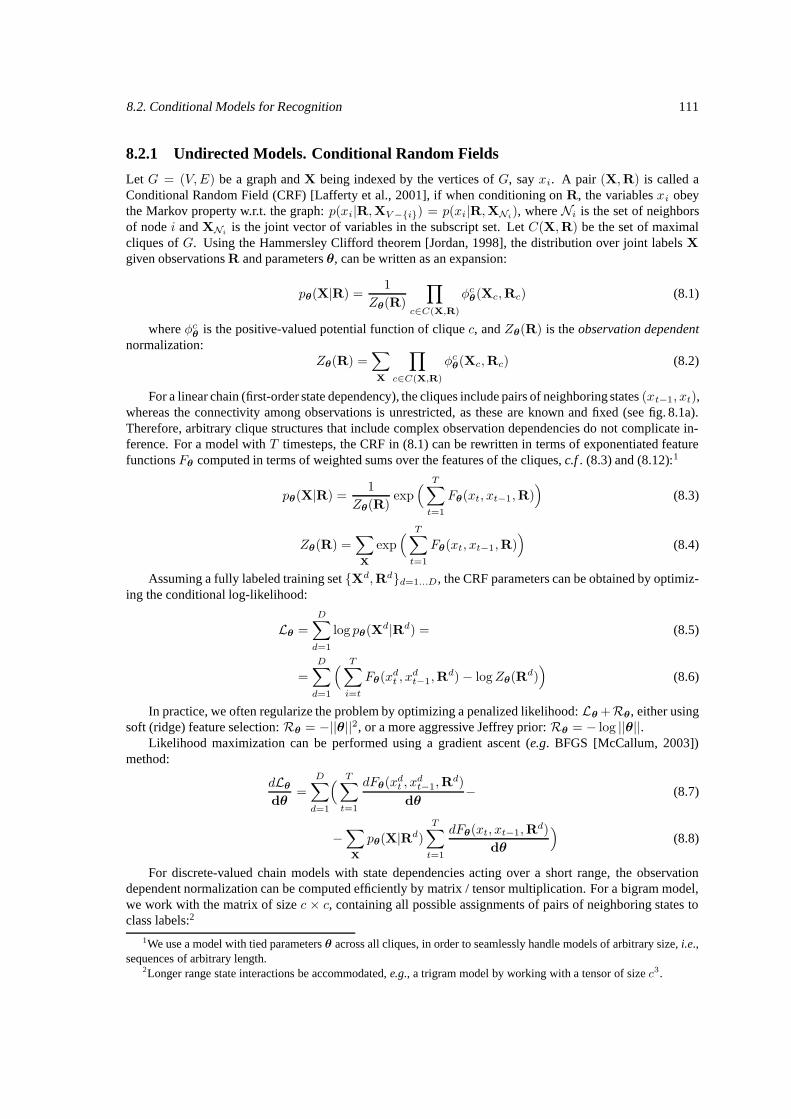
8.2. Conditional Models for Recognition 111
8.2.1 Undirected Models. Conditional Random Fields
Let G = (V,E) be a graph and X being indexed by the vertices of G, say xi. A pair (X,R) is called aConditional Random Field (CRF) [Lafferty et al., 2001], if when conditioning on R, the variables xi obeythe Markov property w.r.t. the graph: p(xi|R,XV −i) = p(xi|R,XNi
), where Ni is the set of neighborsof node i and XNi
is the joint vector of variables in the subscript set. Let C(X,R) be the set of maximalcliques of G. Using the Hammersley Clifford theorem [Jordan, 1998], the distribution over joint labels X
given observations R and parameters θ, can be written as an expansion:
pθ(X|R) =1
Zθ(R)
∏
c∈C(X,R)
φcθ(Xc,Rc) (8.1)
where φcθ is the positive-valued potential function of clique c, and Zθ(R) is the observation dependent
normalization:Zθ(R) =
∑
X
∏
c∈C(X,R)
φcθ(Xc,Rc) (8.2)
For a linear chain (first-order state dependency), the cliques include pairs of neighboring states (xt−1, xt),whereas the connectivity among observations is unrestricted, as these are known and fixed (see fig. 8.1a).Therefore, arbitrary clique structures that include complex observation dependencies do not complicate in-ference. For a model with T timesteps, the CRF in (8.1) can be rewritten in terms of exponentiated featurefunctions Fθ computed in terms of weighted sums over the features of the cliques, c.f . (8.3) and (8.12):1
pθ(X|R) =1
Zθ(R)exp
( T∑
t=1
Fθ(xt, xt−1,R))
(8.3)
Zθ(R) =∑
X
exp( T∑
t=1
Fθ(xt, xt−1,R))
(8.4)
Assuming a fully labeled training set Xd,Rdd=1...D, the CRF parameters can be obtained by optimiz-ing the conditional log-likelihood:
Lθ =
D∑
d=1
log pθ(Xd|Rd) = (8.5)
=
D∑
d=1
( T∑
i=t
Fθ(xdt , x
dt−1,R
d)− logZθ(Rd))
(8.6)
In practice, we often regularize the problem by optimizing a penalized likelihood: Lθ +Rθ, either usingsoft (ridge) feature selection: Rθ = −||θ||2, or a more aggressive Jeffrey prior: Rθ = − log ||θ||.
Likelihood maximization can be performed using a gradient ascent (e.g. BFGS [McCallum, 2003])method:
dLθ
dθ=
D∑
d=1
( T∑
t=1
dFθ(xdt , x
dt−1,R
d)
dθ− (8.7)
−∑
X
pθ(X|Rd)
T∑
t=1
dFθ(xt, xt−1,Rd)
dθ
)(8.8)
For discrete-valued chain models with state dependencies acting over a short range, the observationdependent normalization can be computed efficiently by matrix / tensor multiplication. For a bigram model,we work with the matrix of size c × c, containing all possible assignments of pairs of neighboring states toclass labels:2
1We use a model with tied parameters θ across all cliques, in order to seamlessly handle models of arbitrary size, i.e.,sequences of arbitrary length.
2Longer range state interactions be accommodated, e.g., a trigram model by working with a tensor of size c3.
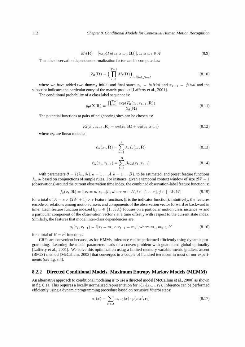
112 Chapter 8. Conditional Models for Contextual Human Motion Recognition
Mt(R) = [exp(Fθ(xt, xt−1,R))], xt, xt−1 ∈ X (8.9)
Then the observation dependent normalization factor can be computed as:
Zθ(R) =( T+1∏
t=1
Mt(R))
initial,final(8.10)
where we have added two dummy initial and final states x0 = initial and xT+1 = final and thesubscript indicates the particular entry of the matrix product [Lafferty et al., 2001].
The conditional probability of a class label sequence is:
pθ(X|R) =
∏T+1t=1 exp(Fθ(xt, xt−1,R))
Zθ(R)(8.11)
The potential functions at pairs of neighboring sites can be chosen as:
Fθ(xt, xt−1,R) = ψθ(xt,R) + ψθ(xt, xt−1) (8.12)
where ψθ are linear models:
ψθ(xt,R) =
A∑
a=1
λafa(xt,R) (8.13)
ψθ(xt, xt−1) =
B∑
b=1
βbgb(xt, xt−1) (8.14)
with parameters θ = (λa, βb), a = 1 . . . A, b = 1 . . . B, to be estimated, and preset feature functionsfa, gb based on conjunctions of simple rules. For instance, given a temporal context window of size 2W + 1(observations) around the current observation time index, the combined observation-label feature function is:
fa(xt,R) = I[xt = m]rt−j [i],where m ∈ X , i ∈ 1 . . . r, j ∈ [−W,W ] (8.15)
for a total of A = c × (2W + 1) × r feature functions (I is the indicator function). Intuitively, the featuresencode correlations among motion classes and components of the observation vector forward or backward intime. Each feature function indexed by a ∈ 1 . . .A focuses on a particular motion class instance m anda particular component of the observation vector i at a time offset j with respect to the current state index.Similarly, the features that model inter-class dependencies are:
gb(xt, xt−1) = I[xt = m1 ∧ xt−1 = m2],where m1,m2 ∈ X (8.16)
for a total of B = c2 functions.CRFs are convenient because, as for HMMs, inference can be performed efficiently using dynamic pro-
gramming. Learning the model parameters leads to a convex problem with guaranteed global optimality[Lafferty et al., 2001]. We solve this optimization using a limited-memory variable-metric gradient ascent(BFGS) method [McCallum, 2003] that converges in a couple of hundred iterations in most of our experi-ments (see fig. 8.4).
8.2.2 Directed Conditional Models. Maximum Entropy Markov Models (MEMM)
An alternative approach to conditional modeling is to use a directed model [McCallum et al., 2000] as shownin fig. 8.1a. This requires a locally normalized representation for p(xt|xt−1, rt). Inference can be performedefficiently using a dynamic programming procedure based on recursive Viterbi steps:
αt(x) =∑
x′∈X
αt−1(x) · p(x|x′, rt) (8.17)
8.3. Experiments 113
where αt(x) computes the probability of being in state x at time t, given the observation sequence up to timet. Similarly, the backward procedure computes βt as the probability of starting from state x at time t, giventhe observation sequence after time t as:
βt(x′) =
∑
x∈X
p(x|x′, rt) · βt+1(x) (8.18)
The conditional distribution p(xt|xt−1, rt) can be modeled as a log-linear model expressed in terms of featurefunctions Fθ as in (8.12), (8.13) and (8.14):
p(xt|xt−1, rt) =1
Z(xt−1, rt)exp(Fθ(xt, xt−1, rt)) (8.19)
whereZ(xt−1, rt) =
∑
xt
Fθ(xt, xt−1, rt) (8.20)
It is worth noticing that CRFs solve a problem that exists in MEMMs [McCallum et al., 2000, Laffertyet al., 2001], called the label-bias problem. This problem arises because such models are locally normalized.(MEMMs still have a non-linear decision surface because the local normalization depends on the state.) Theper-state normalization requirement implies that the current observation is only able to select what successorstate is selected, but not the probability mass transfered to it, causing biases towards states with low-entropytransitions. In the limit, the current observation is effectively ignored for states with single outgoing tran-sitions. In order to avoid this effect, a CRF employs an undirected graphical model that defines a singlelog-linear distribution over the joint vector of an entire class label sequence given a particular observationsequence (thus the model has a linear decision surface). By virtue of the global normalization, entire statesequences are interpreted jointly, and this allows individual states to boost or damp the probability masstransfered to their successive states.
8.3 Experiments
We run a variety of recognition experiments, where we compare the proposed MEMM and CRF models (withdifferent windows of observations encoding different degrees of context) with HMMs. We do two series oftests, one using 2d image features and the other using 3d human joint angle features. The recognition modelsand algorithms used are the same in both cases, the only difference is the type of information represented inthe observation vector (one series of tests use 2d information whereas the other uses 3d information). Wereport recognition accuracy as the percentage of input frames classified with the correct activity type.
Training Set: To gather image training data, we use Maya (Alias Wavefront), with realistically renderedcomputer graphics human surface models that we animate using human motion capture [cmu, 2003]. Thisdatabase is annotated by activity class (with each individual sequence supplementary sub-segmented by activ-ity type) and this information can be used to generate a labeled training set on which we perform segmentationand classification. Our 3d human state representation is based on an articulated skeleton with spherical joints,and has 56 d.o.f. including global translation. Our database consists of 8000 samples (individual image or3d joint angle observations, paired with their class labels) from 10 different human activities: conversation,dance, bending forward, bending sideways, washing windows, jumping, walking (normal and wander), turn-ing, running. For each action we acquired samples from 3 different subjects, 2 male and 1 female. We teston 3 different subjects. Some insight into the structure of the database is given in fig. 8.2, whereas imagesamples from our motion test sequences are shown in fig. 8.3.
2d Image Features: For the image-based experiments, we work with silhouettes that we obtain using acombination of statistical background subtraction and motion segmentation [Sminchisescu et al., 2005a]. Asimage descriptors, we use 50-dimensional histograms of combined shape context and pair-wise edge featuresextracted at a variety of scales on the silhouette [Sminchisescu et al., 2005a]. This representation is semi-local, rich and has been effectively demonstrated in many applications, including texture recognition or poseprediction. The representation is based on overlapping features of the observation. Therefore the elements
114 Chapter 8. Conditional Models for Contextual Human Motion Recognition
1 2 3 4 5 6 7 8 91
5
10
20
Degree of Multimodality
Num
ber
of C
lust
ers
Figure 8.2: Analysis of the degree of ambiguity in the motion class labeling for our database, under moderateinput (silhouette) perturbations. We cluster the input silhouette feature vectors into 80 clusters, count thenumber of different motion labels that fall within each, and histogram those.
Figure 8.3: Sample images (top row) and silhouettes (bottom row) of typical motions that are recognized:walking, running, bending and picking, dancing, etc. Notice that the silhouettes are of average quality andpotentially quite different from the ones we trained on and which were synthetically generated. Nevertheless,we observe that the recognition accuracy is usually robust to these factors.
of the silhouette feature vector are generally not independent. However, due to its conditional structure, aCRF flexibly accommodates this representation without modeling assumption violations.
3d joint angle features: For 3d recognition experiments, we work with observation vectors consisting of 56dimensional human joint angles obtained from a 3d human motion reconstruction system.
Models, parameters and training times: All our training and testing used a standard 2GHz desktop PC andrunning times are given for this system. We perform tests in order to compare the CRF model described in§8.2.1 with HMMs and MEMMs. The number of parameters in the models is determined by the number ofactivities c = 10, the dimension of the observation vector r, in our case dim(r) = 50 for 2d image featuresand dim(r) = 56 for 3d human joint angle features, and the window context (for CRFs): W = 0, 1, 3implying that 0, 1 or 3 observations forward and backward in time are used and the overall window size is2W + 1.
The HMM we use is a fully ergodic model based on Gaussian emission probabilities having diagonalcovariance matrix for each state. The parameters of the model (the emission probability density, the statetransition matrix) are learned from training data [Rabiner, 1989] using Maximum Likelihood (training takesabout 3s). The total number of HMM parameters is: 2× c × dim(r) + c2 for a total of 1100 parameters inthe 2d experiments and 1220 parameters for the 3d experiments. We also learn a variety of CRFs that modelvarious degrees of long-range dependencies between observations, i.e. windows W = 0, 1, 3, implyingthat we consider contexts of observations of size 0,3 and 7 centered at the current time index.3 The total
3For the experiments, we only consider baseline models, arguably, more complex HMMs or CRFs can be used.
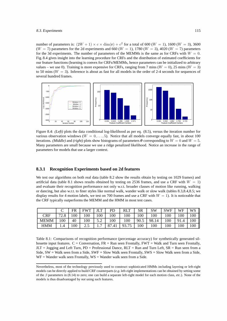
8.3. Experiments 115
number of parameters is: (2W + 1) × c × dim(r) + c2 for a total of 600 (W = 1), 1600 (W = 3), 3600(W = 7) parameters for the 2d experiments and 660 (W = 1), 1780 (W = 3), 4020 (W = 7) parametersfor the 3d experiments. The number of parameters of the MEMMs is the same as for CRFs with W = 0.Fig. 8.4 gives insight into the learning procedure for CRFs and the distribution of estimated coefficients forour feature functions (learning is convex for CRFs/MEMMs, hence parameters can be initialized to arbitraryvalues – we use 0). Training is more expensive for CRFs, ranging from 7 mins (W = 0), 25 mins (W = 3)to 50 mins (W = 3). Inference is about as fast for all models in the order of 2-4 seconds for sequences ofseveral hundred frames.
0 20 40 60 80 100 120−3000
−2500
−2000
−1500
−1000
−500
0
Iteration Number
Lo
g L
ike
liho
od
Window = 0 Window = 1Window = 3Window = 5
0.001 0.643 1.286 1.928 2.5710
10
100
Feature Coefficient Centers
Fre
quency
0.001 0.932 1.862 2.793 3.7230
10
100
1000
Feature Coefficient Centers
Fre
quency
Figure 8.4: (Left) plots the data conditional log-likelihood as per eq. (8.5), versus the iteration number forvarious observation windows (W = 0, . . . , 5). Notice that all models converge equally fast, in about 100iterations. (Middle) and (right) plots show histograms of parameters θ corresponding to W = 0 and W = 5.Many parameters are small because we use a ridge penalized likelihood. Notice an increase in the range ofparameters for models that use a larger context.
8.3.1 Recognition Experiments based on 2d features
We test our algorithms on both real data (table 8.2 show the results obtain by testing on 1029 frames) andartificial data (table 8.1 shows results obtained by testing on 2536 frames, and use a CRF with W = 1)and evaluate their recognition performance not only w.r.t. broader classes of motion like running, walkingor dancing, but also w.r.t. to finer styles like normal walk, wander walk or slow walk (tables 8.3,8.4,8.5; wedisplay results for 4 motion labels, we test on 700 frames and use a CRF with W = 1). It is noticeable thatthe CRF typically outperforms the MEMM and the HMM in most test cases.
C FR FWT JLT PD RLT SR SW SWF WF WSCRF 72.8 100 100 100 100 100 100 100 100 100 100
MEMM 100 40 100 5.2 100 100 90.5 98.14 100 91.4 100HMM 1.4 100 2.5 1.7 87.41 93.75 100 100 100 100 100
Table 8.1: Comparisons of recognition performance (percentage accuracy) for synthetically generated sil-houette input features. C = Conversation, FR = Run seen Frontally, FWT = Walk and Turn seen Frontally,JLT = Jogging and Left Turn, PD = Professional Dance, RLT = Run and Turn Left, SR = Run seen from aSide, SW = Walk seen from a Side, SWF = Slow Walk seen Frontally, SWS = Slow Walk seen from a Side,WF = Wander walk seen Frontally, WS = Wander walk seen from a Side.
Nevertheless, most of the technology previously used to construct sophisticated HMMs including layering or left-rightmodels can be directly applied to build CRF counterparts (e.g. left-right implementations can be obtained by setting someof the β parameters in (8.14) to zero; one can build a separate left-right model for each motion class, etc.). None of themodels is thus disadvantaged by not using such features.
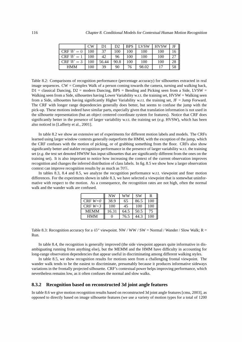
116 Chapter 8. Conditional Models for Contextual Human Motion Recognition
CW D1 D2 BPS LVSW HVSW JFCRF W = 0 100 37 100 100 100 100 16CRF W = 1 100 42 96 100 100 100 27CRF W = 3 100 56.44 90.8 100 100 100 28
HMM 100 39 90 76 98.02 17 58
Table 8.2: Comparisons of recognition performance (percentage accuracy) for silhouettes extracted in realimage sequences. CW = Complex Walk of a person coming towards the camera, turning and walking back,D1 = classical Dancing, D2 = modern Dancing, BPS = Bending and Picking seen from a Side, LVSW =Walking seen from a Side, silhouettes having Lower Variability w.r.t. the training set, HVSW = Walking seenfrom a Side, silhouettes having significantly Higher Variability w.r.t. the training set, JF = Jump Forward.The CRF with longer range dependencies generally does better, but seems to confuse the jump with thepick-up. These motions indeed have similar parts, especially given that translation information is not used inthe silhouette representation (but an object centered coordinate system for features). Notice that CRF doessignificantly better in the presence of larger variability w.r.t. the training set (e.g. HVSW), which has beenalso noticed in [Lafferty et al., 2001].
In table 8.2 we show an extensive set of experiments for different motion labels and models. The CRFslearned using larger window contexts generally outperform the HMM, with the exception of the jump, whichthe CRF confuses with the motion of picking, or of grabbing something from the floor. CRFs also showsignificantly better and stabler recognition performance in the presence of larger variability w.r.t. the trainingset (e.g. the test set denoted HWSW has input silhouettes that are significantly different from the ones on thetraining set). It is also important to notice how increasing the context of the current observation improvesrecognition and changes the inferred distribution of class labels. In fig. 8.5 we show how a larger observationcontext can improve recognition results by as much as 70%.
In tables 8.3, 8.4 and 8.5, we analyze the recognition performance w.r.t. viewpoint and finer motiondifferences. For the experiments shown in table 8.3, we have selected a viewpoint that is somewhat uninfor-mative with respect to the motion. As a consequence, the recognition rates are not high, often the normalwalk and the wander walk are confused.
NW WW SW RCRF W=0 38.9 65 86.5 100CRF W=3 100 45 100 100MEMM 16.31 64.5 50.5 75HMM 0 76.5 44.3 100
Table 8.3: Recognition accuracy for a 45o viewpoint. NW / WW / SW = Normal / Wander / Slow Walk; R =Run.
In table 8.4, the recognition is generally improved (the side viewpoint appears quite informative in dis-ambiguating running from anything else), but the MEMM and the HMM have difficulty in accounting forlong-range observation dependencies that appear useful in discriminating among different walking styles.
In table 8.5, we show recognition results for motions seen from a challenging frontal viewpoint. Thewander walk tends to be the easiest to discriminate, presumably because it produces informative sidewaysvariations in the frontally projected silhouette. CRF’s contextual power helps improving performance, whichnevertheless remains low, as it often confuses the normal and slow walks.
8.3.2 Recognition based on reconstructed 3d joint angle features
In table 8.6 we give motion recognition results based on reconstructed 3d joint angle features [cmu, 2003], asopposed to directly based on image silhouette features (we use a variety of motion types for a total of 1200
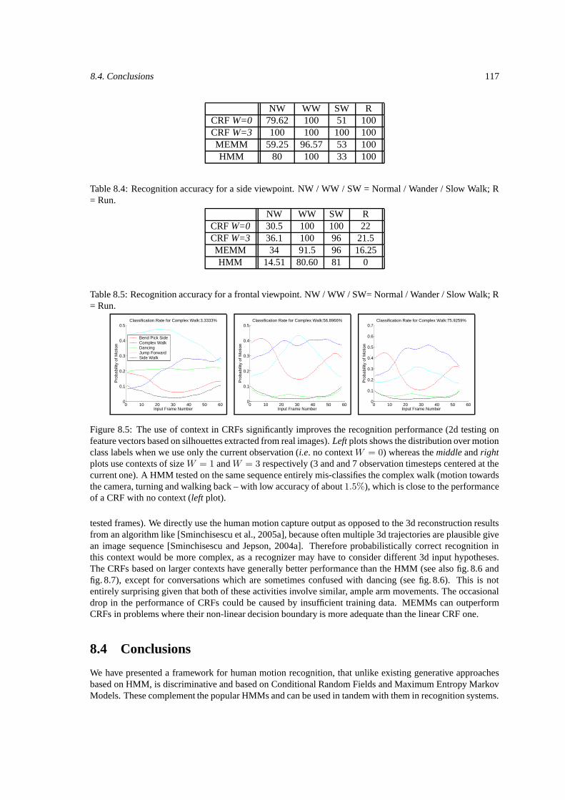
8.4. Conclusions 117
NW WW SW RCRF W=0 79.62 100 51 100CRF W=3 100 100 100 100MEMM 59.25 96.57 53 100HMM 80 100 33 100
Table 8.4: Recognition accuracy for a side viewpoint. NW / WW / SW = Normal / Wander / Slow Walk; R= Run.
NW WW SW RCRF W=0 30.5 100 100 22CRF W=3 36.1 100 96 21.5MEMM 34 91.5 96 16.25HMM 14.51 80.60 81 0
Table 8.5: Recognition accuracy for a frontal viewpoint. NW / WW / SW= Normal / Wander / Slow Walk; R= Run.
0 10 20 30 40 50 600
0.1
0.2
0.3
0.4
0.5
Input Frame Number
Pro
babi
lity
of M
otio
n
Classification Rate for Complex Walk:3.3333%
Bend Pick SideComplex WalkDancingJump ForwardSide Walk
0 10 20 30 40 50 600
0.1
0.2
0.3
0.4
0.5
Input Frame Number
Pro
babi
lity
of M
otio
n
Classification Rate for Complex Walk:56.8966%
0 10 20 30 40 50 600
0.1
0.2
0.3
0.4
0.5
0.6
0.7
Input Frame Number
Pro
babi
lity
of M
otio
n
Classification Rate for Complex Walk:75.9259%
Figure 8.5: The use of context in CRFs significantly improves the recognition performance (2d testing onfeature vectors based on silhouettes extracted from real images). Left plots shows the distribution over motionclass labels when we use only the current observation (i.e. no context W = 0) whereas the middle and rightplots use contexts of size W = 1 and W = 3 respectively (3 and and 7 observation timesteps centered at thecurrent one). A HMM tested on the same sequence entirely mis-classifies the complex walk (motion towardsthe camera, turning and walking back – with low accuracy of about 1.5%), which is close to the performanceof a CRF with no context (left plot).
tested frames). We directly use the human motion capture output as opposed to the 3d reconstruction resultsfrom an algorithm like [Sminchisescu et al., 2005a], because often multiple 3d trajectories are plausible givean image sequence [Sminchisescu and Jepson, 2004a]. Therefore probabilistically correct recognition inthis context would be more complex, as a recognizer may have to consider different 3d input hypotheses.The CRFs based on larger contexts have generally better performance than the HMM (see also fig. 8.6 andfig. 8.7), except for conversations which are sometimes confused with dancing (see fig. 8.6). This is notentirely surprising given that both of these activities involve similar, ample arm movements. The occasionaldrop in the performance of CRFs could be caused by insufficient training data. MEMMs can outperformCRFs in problems where their non-linear decision boundary is more adequate than the linear CRF one.
8.4 Conclusions
We have presented a framework for human motion recognition, that unlike existing generative approachesbased on HMM, is discriminative and based on Conditional Random Fields and Maximum Entropy MarkovModels. These complement the popular HMMs and can be used in tandem with them in recognition systems.
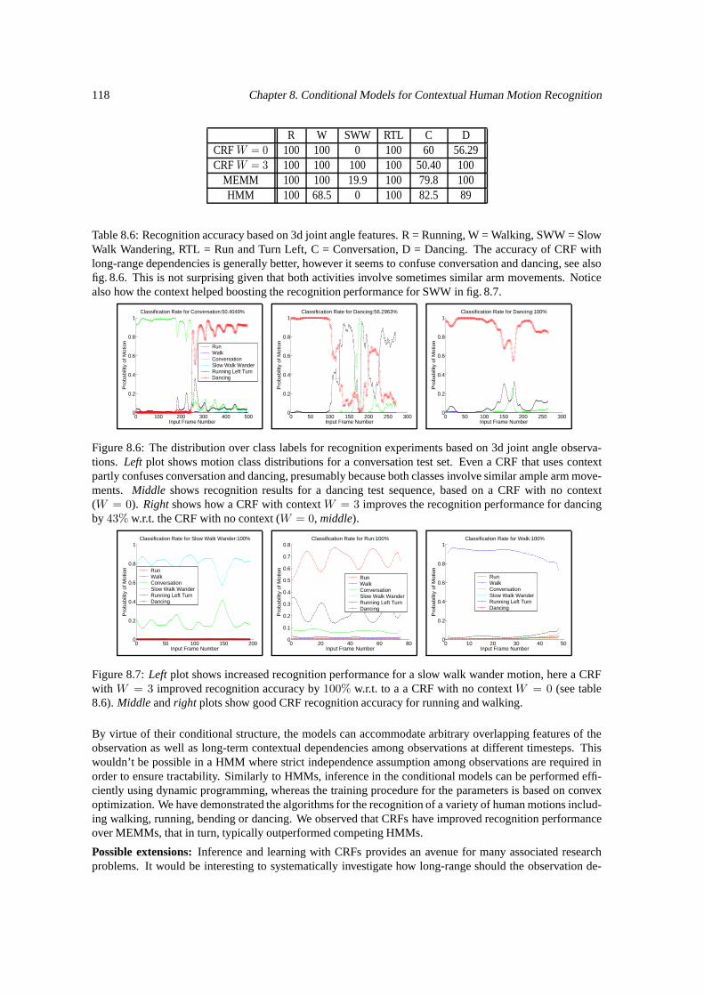
118 Chapter 8. Conditional Models for Contextual Human Motion Recognition
R W SWW RTL C DCRF W = 0 100 100 0 100 60 56.29CRF W = 3 100 100 100 100 50.40 100
MEMM 100 100 19.9 100 79.8 100HMM 100 68.5 0 100 82.5 89
Table 8.6: Recognition accuracy based on 3d joint angle features. R = Running, W = Walking, SWW = SlowWalk Wandering, RTL = Run and Turn Left, C = Conversation, D = Dancing. The accuracy of CRF withlong-range dependencies is generally better, however it seems to confuse conversation and dancing, see alsofig. 8.6. This is not surprising given that both activities involve sometimes similar arm movements. Noticealso how the context helped boosting the recognition performance for SWW in fig. 8.7.
0 100 200 300 400 5000
0.2
0.4
0.6
0.8
1
Input Frame Number
Pro
ba
bili
ty o
f M
otio
n
Classification Rate for Conversation:50.4049%
RunWalkConversationSlow Walk WanderRunning Left TurnDancing
0 50 100 150 200 250 3000
0.2
0.4
0.6
0.8
1
Input Frame Number
Pro
babi
lity
of M
otio
n
Classification Rate for Dancing:56.2963%
0 50 100 150 200 250 3000
0.2
0.4
0.6
0.8
1
Input Frame Number
Pro
babi
lity
of M
otio
n
Classification Rate for Dancing:100%
Figure 8.6: The distribution over class labels for recognition experiments based on 3d joint angle observa-tions. Left plot shows motion class distributions for a conversation test set. Even a CRF that uses contextpartly confuses conversation and dancing, presumably because both classes involve similar ample arm move-ments. Middle shows recognition results for a dancing test sequence, based on a CRF with no context(W = 0). Right shows how a CRF with context W = 3 improves the recognition performance for dancingby 43% w.r.t. the CRF with no context (W = 0, middle).
0 50 100 150 2000
0.2
0.4
0.6
0.8
1
Input Frame Number
Pro
babi
lity
of M
otio
n
Classification Rate for Slow Walk Wander:100%
RunWalkConversationSlow Walk WanderRunning Left TurnDancing
0 20 40 60 800
0.1
0.2
0.3
0.4
0.5
0.6
0.7
0.8
Input Frame Number
Pro
babi
lity
of M
otio
n
Classification Rate for Run:100%
RunWalkConversationSlow Walk WanderRunning Left TurnDancing
0 10 20 30 40 500
0.2
0.4
0.6
0.8
1
Input Frame Number
Pro
babi
lity
of M
otio
n
Classification Rate for Walk:100%
RunWalkConversationSlow Walk WanderRunning Left TurnDancing
Figure 8.7: Left plot shows increased recognition performance for a slow walk wander motion, here a CRFwith W = 3 improved recognition accuracy by 100% w.r.t. to a a CRF with no context W = 0 (see table8.6). Middle and right plots show good CRF recognition accuracy for running and walking.
By virtue of their conditional structure, the models can accommodate arbitrary overlapping features of theobservation as well as long-term contextual dependencies among observations at different timesteps. Thiswouldn’t be possible in a HMM where strict independence assumption among observations are required inorder to ensure tractability. Similarly to HMMs, inference in the conditional models can be performed effi-ciently using dynamic programming, whereas the training procedure for the parameters is based on convexoptimization. We have demonstrated the algorithms for the recognition of a variety of human motions includ-ing walking, running, bending or dancing. We observed that CRFs have improved recognition performanceover MEMMs, that in turn, typically outperformed competing HMMs.
Possible extensions: Inference and learning with CRFs provides an avenue for many associated researchproblems. It would be interesting to systematically investigate how long-range should the observation de-

8.4. Conclusions 119
pendency be for optimal recognition performance, as well as recognition based on different selections offeatures. The number of possible feature combinations can be large, so efficient methods for feature selec-tion or feature induction are necessary. In this work we use a model with first order state dependency (abigram) but it would be interesting to study longer range state dependencies, e.g. trigrams. All these exten-sions are straightforward to include in a CRF. More complex human motion recognition systems based onthe ideas described here may be constructed using advanced tools based on left-right models and multiplelayers. The design of models with conditional and generative subcomponents (CRF/MEMMs and HMMs)can be a promising avenue for future research [Sminchisescu et al., 2006b].
Chapter 9
Conditional Part-Based Models forSpatial Localization
We present a new method for training deformable models. Assume that we have training images where partlocations have been labeled. Typically, one fits a model by maximizing the likelihood of the part labels.Alternatively, one could fit a model such that, when the model is run on the training images, it finds the parts.We do this by maximizing the conditional likelihood of the training data. We formulate model-learningas parameter estimation in a conditional random field (CRF). Initializing parameters with their maximumlikelihood estimates, we reach the global optimum by gradient ascent. We present a learning algorithm thatsearches exhaustively over all part locations in an image without relying on feature detectors. This providesmillions of examples of training data, and seems to avoid overfitting issues known with CRFs. Results for partlocalization are relatively scarce in the community. We present results on three established datasets; Caltechmotorbikes [Fergus et al., 2003], USC people [Lee and Cohen, 2004], and Weizmann horses [Borenstein andUllman, 2002]. In the Caltech set we significantly outperform the state-of-the-art [Crandall et al., 2005].For the challenging people dataset, we present results that are comparable to [Lee and Cohen, 2004], but areobtained using a significantly more generic model (devoid of a face or skin detector). Our model is generalenough to find other articulated objects; we use it to recover 2d poses of horses in the challenging Weizmanndatabase. An earlier version of this chapter appeared in IEEE International Conference on Computer Visionand Pattern Recognition (CVPR) [Ramanan and Sminchisescu, 2006].
9.1 Part-based Recognition Models
Deformable models have a long-standing history in the vision community beginning with pictorial structures[Fischler and Elschlager, 1973] and deformable templates [Grenander et al., 1991], and also include therecent active appearance models [Sha and Pereira, 2003] and constellation models [Burl et al., 1998]. Thesemodels represent an object as a collection of parts, explicitly encoding both the appearance of a part and itsspatial arrangement. There have been numerous approaches that use these models for detection. They addressquestions of the form: given an image, is there a motorbike or not? Surprisingly, one can obtain state-of-the-art detection performance by ig- noring spatial constraints (the so-called "bag of feature" models). Webelieve this fact suggests that: (1) shape is hard to learn with current methods and (2) one should considermore difficult recognition tasks such as localization: where is the motorbike, which way is it facing? Ourwork focuses on methods for learning and evaluating deformable models, given the task of localization.A natural method of learning a deformable model is to fit the model to some observed instances. This isoften formulated as maximum likelihood (ML). Given a collection of images where part locations have beenlabeled, one computes sample means and variances (assuming gaussian models). Even non-probabilisticapproaches such as exem- plar matching implicitly do this; here the mean is encoded by the exemplar. Analternative is to tune parameters so that the model does well at a task (in our case, localization). Intuitively, we
120
9.2. Existing Methods for Localization 121
want to tune parameters so that the model, when run on a training image, recovers the labeled part locations.We show that by formulating our model as a conditional random field (CRF), we naturally optimize thiscriteria. We demonstrate the resulting models on three datasets; Caltech motorbikes [Fergus et al., 2003],USC people [Lee and Cohen, 2004], and Weizmann horses [Borenstein and Ullman, 2002]. The Caltech setis known to be easy for detection, but we use it to evaluate part localization. We surpass the best-reportedresults in [Crandall et al., 2005]. We present an articulated model for human 2d pose estimation that iscomparable to [Lee and Cohen, 2004] on their challenging set of people images. In contrast to [Lee andCohen, 2004], we use a generic articulated model devoid of a face detector or skin model. To demonstrate itsgenerality, we train it to localize deforming horses in the challenging Weizmann dataset.
9.2 Existing Methods for Localization
Approaches for learning parts-based models can loosely be divided into generative, semi-supervised, anddiscriminative. Given labeled training data, generative methods follow the ML framework described above[Cootes et al., 1998, Crandall et al., 2005, Felzenszwalb and Huttenlocher, 2005, Fergus et al., 2003, Grenan-der et al., 1991, Ioffe and Forsyth, 2002, Kumar et al., 2004, Leung et al., 1995]. Alternatively, Weber etal. and Fergus et al. use EM to learn models from partially-labeled data [Fergus et al., 2003, Weber et al.,2000]. Their approach required knowing an image contains a motorbike, but not where its parts are located.Although our work here learns in a supervised framework, there is a close connection between our CRF opti-mization and EM (we look at this in §9.4. Discriminative training of deformable models dates back to at leastdecision trees [Amit et al., 1997], convolutional neural nets [LeCun and Bengio, 1995], and include recentapproaches such as [Hillel et al., 2005, Holub and Perona, 2005, Quattoni et al., 2004]. In these cases, modelsare optimized for detection and not localization. Kumar and Hebert [2003] introduced CRFs for low-levelvision. They infer pixel labels from a loopy grid (and so require approximations for inference and learn-ing), while we infer part locations on a tree-structured model. There exist relatively few published resultsfor localization of deformable models [Crandall et al., 2005, Ramanan et al., 2005]. One notable exceptionis human 2d pose estimation. Most work involves tracking in video sequences, although approaches for 2dpose estimation in static images exist [Ioffe and Forsyth, 2002, Lee and Cohen, 2004, Mori et al., 2004, Renet al., 2005]. The unconstrained nature of the problem typically requires some limiting assumption such asuncluttered backgrounds, visible faces, and/or visible skin regions.
9.3 Deformable Part Model
We use a parts and structure model framework common in the previously mentioned approaches. Let us writethe location of part i as li = (xi, yi). We later extend li to encode part orientation for articulated models.We denote the configuration of a K part model as L = (l1 . . . lK). Given model parameters θ, the jointprobability of a configuration L in an image Im is:
p(Im,L|θ) =∏
(i,j )∈E
p(li |lj )K∏
i=1
p(Im(li )|li)∏
l∈bg
p(Im(l|bg)) (9.1)
The first term captures part geometry, while the second term models the local image patch at each part.The last term models the image patches in the background. We assume the local probability functions aregaussian:
p(li|lj) ∼ N (li − lj |µi,Σi) (9.2)
The geometric model in (9.2) has an intuitive interpretation as a "spring" that connects part i to part j.The spring has a rest position of µi and a stiffness encoded by Σi. We assume E is a known tree (see §9.4.2),and so each part i is connected to one parent j. We will often write the relative location of part i simply asri = li − lj .
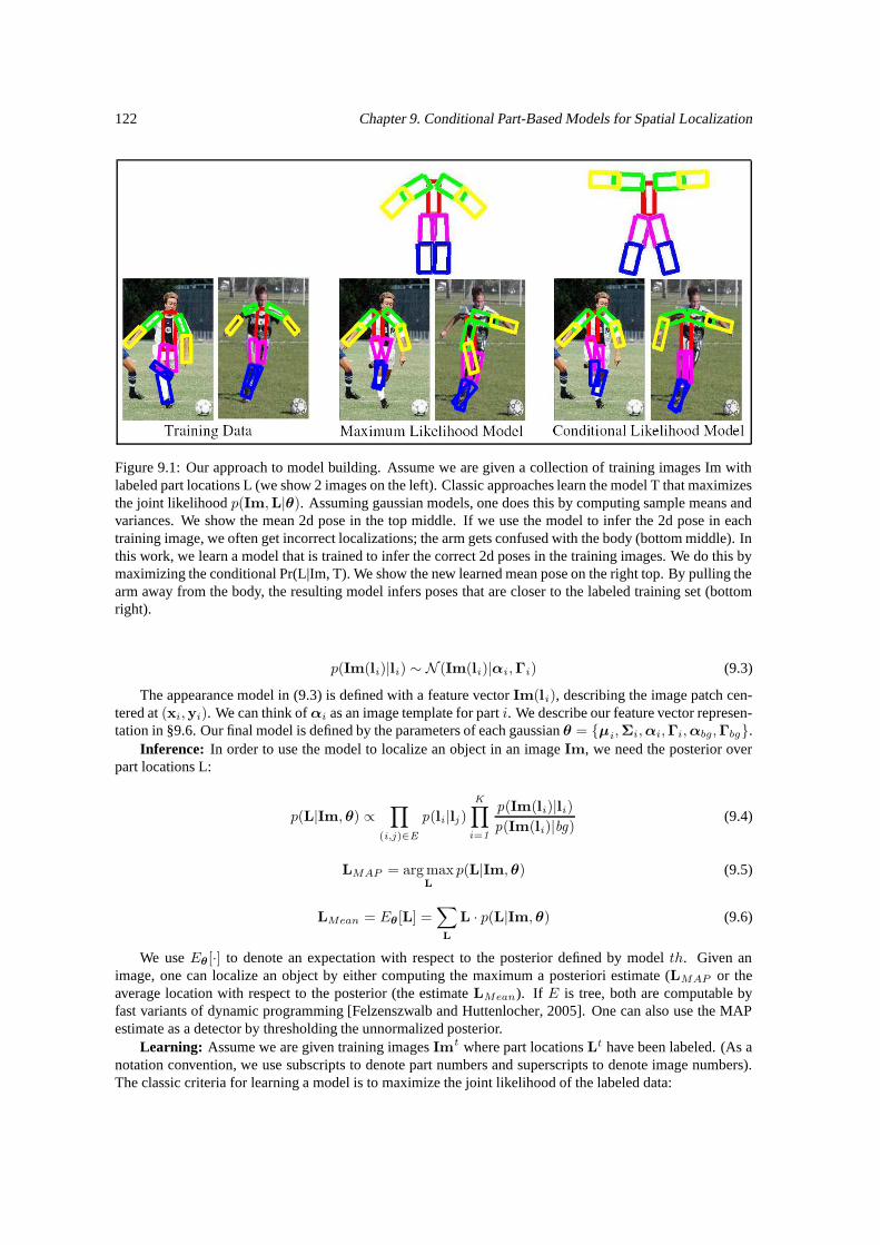
122 Chapter 9. Conditional Part-Based Models for Spatial Localization
Figure 9.1: Our approach to model building. Assume we are given a collection of training images Im withlabeled part locations L (we show 2 images on the left). Classic approaches learn the model T that maximizesthe joint likelihood p(Im,L|θ). Assuming gaussian models, one does this by computing sample means andvariances. We show the mean 2d pose in the top middle. If we use the model to infer the 2d pose in eachtraining image, we often get incorrect localizations; the arm gets confused with the body (bottom middle). Inthis work, we learn a model that is trained to infer the correct 2d poses in the training images. We do this bymaximizing the conditional Pr(L|Im, T). We show the new learned mean pose on the right top. By pulling thearm away from the body, the resulting model infers poses that are closer to the labeled training set (bottomright).
p(Im(li)|li ) ∼ N (Im(li )|αi ,Γi ) (9.3)
The appearance model in (9.3) is defined with a feature vector Im(li ), describing the image patch cen-tered at (xi,yi). We can think of αi as an image template for part i. We describe our feature vector represen-tation in §9.6. Our final model is defined by the parameters of each gaussian θ = µi,Σi,αi,Γi,αbg,Γbg.
Inference: In order to use the model to localize an object in an image Im, we need the posterior overpart locations L:
p(L|Im,θ) ∝∏
(i,j )∈E
p(li |lj )K∏
i=1
p(Im(li)|li )p(Im(li)|bg)
(9.4)
LMAP = arg maxL
p(L|Im,θ) (9.5)
LMean = Eθ[L] =∑
L
L · p(L|Im,θ) (9.6)
We use Eθ[·] to denote an expectation with respect to the posterior defined by model th. Given animage, one can localize an object by either computing the maximum a posteriori estimate (LMAP or theaverage location with respect to the posterior (the estimate LMean). If E is tree, both are computable byfast variants of dynamic programming [Felzenszwalb and Huttenlocher, 2005]. One can also use the MAPestimate as a detector by thresholding the unnormalized posterior.
Learning: Assume we are given training images Imt where part locations Lt have been labeled. (As anotation convention, we use subscripts to denote part numbers and superscripts to denote image numbers).The classic criteria for learning a model is to maximize the joint likelihood of the labeled data:
9.4. Maximizing the Conditional Likelihood 123
θML = maxθ
p(Imt ,Lt |θ) = (9.7)
= maxµ,Σ
∏
t
p(Lt|µ,Σ) maxα,Γ
∏
t
p(Imt |Lt ,α,Γ) (9.8)
In the literature, this is often called maximum likelihood (ML) learning. Since the likelihood factors in,it (9.1), it suffices to find the ML estimates of the individual gaussian terms. This is done by independentlycomputing sample means and variances. For example, we set µi to be the average position of part i with re-spect to part j. In some ways, this independence is unintuitive. Suppose we learn a very accurate appearancetemplate αi. This suggests we do not need a strong spatial prior Σi (since we can find the part simply bymatching the template αi).
What can be problematic with θML? Consider fig. 9.1. The mean 2d pose in a collection of labeledpeople images tends to have the arms lying alongside the body. This is because, on average, a person tendsto keep their arms there. However, such a pose may not be useful for localizing people because the estimatedarms will be confused with the body. We do not want the most likely pose, but rather the pose that producesthe best estimates when used for inference. We argue that ML may be inadequate because it is not directlytied to the inference problem to be solved.
The posterior in (9.4) is the precise quantity used for inference. We will show that learning a θ whichmaximizes p(L|Im,T ) produces a model well-suited for localization. We call such a model θCL, becauseit maximizes the conditional likelihood of labels given the image. Computing θCL is difficult because (9.4)is not normalized. The implicit normalization factor is actually a function of all the parameters θCL. Thismeans that, unlike ML learning, we cannot find each parameter independently. Our resulting model, however,is equivalent to a tree-structured Conditional Random Field (CRF) [Lafferty et al., 2001]. We apply standardalgorithms from that literature to learn θCL.
9.4 Maximizing the Conditional Likelihood
Since are working directly with (9.4), it will be convenient to simplify our appearance model by assumingboth parts and the background have the same covariance Γbg . In this case we can write:
p(Im(li )|li)p(Im(li )|bg)
∝ exp[w>i · Im(li )] (9.9)
where:
wi = Γ−1bg (αi −αbg) (9.10)
Given a set of labeled 2d poses Lt, let us write the (log) conditional likelihood:
L(θ) =∑
t
log p(Lt|Imt ,θ) (9.11)
We find the θCL, that maximizes (9.11) by gradient ascent. Decomposing Σ−1 = C>i Ci, we calculate
the gradient as follows:
dLdµi
= C>i Ci
∑
t
rti −∑
t
Eθ[rti ] (9.12)
dLdΣi
= Ci∑
t
(rti − µi)
2 −∑
t
Eθ[(rti − µi)
2] (9.13)
dLdwi
=∑
t
Imt (lti )−∑
t
Eθ[Imt(lti )] (9.14)
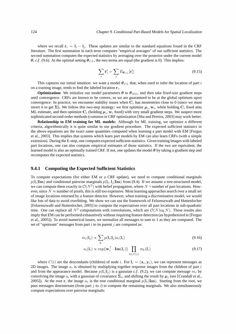
124 Chapter 9. Conditional Part-Based Models for Spatial Localization
where we recall ri = li − lj . These updates are similar to the standard equations found in the CRFliterature. The first summation in each term computes "empirical averages" of our sufficient statistics. Thesecond summation computes the expected statistics by averaging over the posterior under the current modelθ, c.f . (9.6). At the optimal setting θCL, the two terms are equal (the gradient is 0). This implies:
∑
t
rti =
∑
t
EθCL[rt
i] (9.15)
This captures our initial intuition: we want a model θCL that, when used to infer the location of part ion a training image, tends to find the labeled location ri.
Optimization: We initialize our model parameters θ to θML, and then take fixed-size gradient stepsuntil convergence. CRFs are known to be convex, so we are guaranteed to be at the global optimum uponconvergence. In practice, we encounter stability issues when Ci has mostentries close to 0 (since we mustinvert it to get Σ). We follow this two-step strategy: we first optimize µi,wi, while holding Ci fixed atitsML estimate, and then optimize Ci (holding µi,wi fixed) with very small gradient steps. We suspect moresophisticated second-order methods (common in CRF optimization [Sha and Pereira, 2003] may work better.
Relationship to EM training for ML models: Although for ML training, we optimize a differentcriteria, algorithmically it is quite similar to our gradient procedure. The expected sufficient statistics inthe above equations are the exact same quantities computed when learning a part model with EM [Ferguset al., 2003]. This implies that systems which learn part models by EM can also learn CRFs (with a simpleextension). During the E-step, one computes expected sufficient statistics. Given training images with labeledpart locations, one can also compute empirical estimates of those statistics. If the two are equivalent, thelearned model is also an optimally trained CRF. If not, one updates the model θ by taking a gradient step andrecomputes the expected statistics.
9.4.1 Computing the Expected Sufficient Statistics
To compute expectations (for either EM or a CRF update), we need to compute conditional marginalsp(li|Im) and conditional pairwise marginals p(li, lj |Im) from (9.4). If we assume a tree-structured model,we can compute them exactly inO(N 2) with belief propagation, where N = number of part locations. How-ever, sinceN ≈ number of pixels, this is still too expensive. Most learning approaches search over a small setof image locations returned by a feature detector. However, when training a discriminative model, we wouldlike lots of data to avoid overfitting. We show we can use the framework of Felzenszwalb and Huttenlocher[Felzenszwalb and Huttenlocher, 2005] to compute the expectations over all part locations in sub-quadratictime. One can replace all N 2 computations with convolutions, which are O(N logN). These results alsoimply that EM can be performed exhaustively without requiring feature detection (as hypothesized in [Ferguset al., 2005]). To avoid numerical issues, we normalize all messages to sum to 1 as they are computed. Theset of "upstream" messages from part i to its parent j are computed as:
mi(lj) ∝∑
li
p(li|lj)ai(li) (9.16)
ai(li) ∝ expw>i · Im(li )
∏
k∈C (i)
mk (li) (9.17)
where C(i) are the descendants (children) of node i. For li = (xi,yi), we can represent messages as2D images. The image ai is obtained by multiplying together response images from the children of part iand from the appearance model. Because p(li|lj) is a gaussian c.f . (9.2), we can compute message mi byconvolving the image ai with a gaussian of covariance Σi, and shifting the result by µi (see [Crandall et al.,2005]). At the root r, the image at is the true conditional marginal p(lr|Im). Starting from the root, wepass messages downstream (from part j to i) to compute the remaining marginals. We also simultaneouslycompute expectations over pairwise marginals:
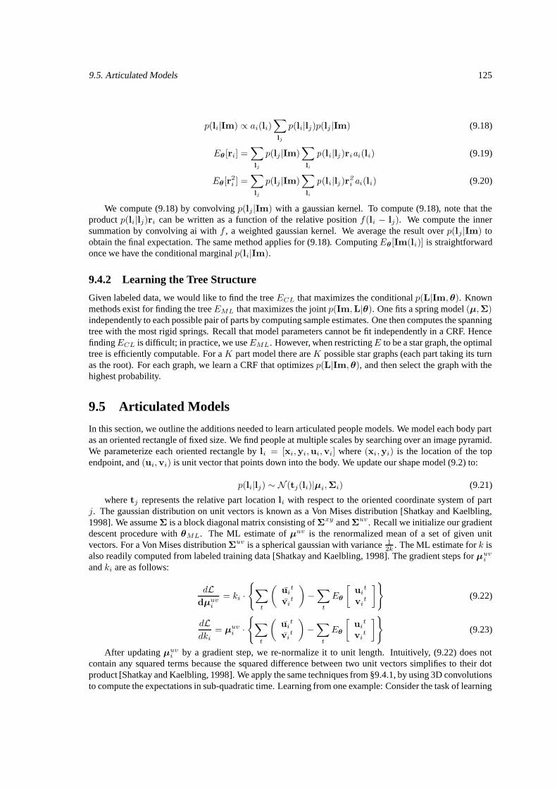
9.5. Articulated Models 125
p(li|Im) ∝ ai(li)∑
lj
p(li|lj)p(lj |Im) (9.18)
Eθ [ri] =∑
lj
p(lj |Im)∑
li
p(li |lj )riai (li ) (9.19)
Eθ[r2i ] =
∑
lj
p(lj |Im)∑
li
p(li |lj )r2i ai (li ) (9.20)
We compute (9.18) by convolving p(lj |Im) with a gaussian kernel. To compute (9.18), note that theproduct p(li|lj)ri can be written as a function of the relative position f(li − lj). We compute the innersummation by convolving ai with f , a weighted gaussian kernel. We average the result over p(lj |Im) toobtain the final expectation. The same method applies for (9.18). Computing Eθ[Im(li )] is straightforwardonce we have the conditional marginal p(li|Im).
9.4.2 Learning the Tree Structure
Given labeled data, we would like to find the tree ECL that maximizes the conditional p(L|Im,θ). Knownmethods exist for finding the tree EML that maximizes the joint p(Im,L|θ). One fits a spring model (µ,Σ)independently to each possible pair of parts by computing sample estimates. One then computes the spanningtree with the most rigid springs. Recall that model parameters cannot be fit independently in a CRF. HencefindingECL is difficult; in practice, we useEML. However, when restrictingE to be a star graph, the optimaltree is efficiently computable. For a K part model there are K possible star graphs (each part taking its turnas the root). For each graph, we learn a CRF that optimizes p(L|Im,θ), and then select the graph with thehighest probability.
9.5 Articulated Models
In this section, we outline the additions needed to learn articulated people models. We model each body partas an oriented rectangle of fixed size. We find people at multiple scales by searching over an image pyramid.We parameterize each oriented rectangle by li = [xi,yi,ui,vi] where (xi,yi) is the location of the topendpoint, and (ui,vi) is unit vector that points down into the body. We update our shape model (9.2) to:
p(li|lj) ∼ N (tj(li)|µi,Σi) (9.21)
where tj represents the relative part location li with respect to the oriented coordinate system of partj. The gaussian distribution on unit vectors is known as a Von Mises distribution [Shatkay and Kaelbling,1998]. We assume Σ is a block diagonal matrix consisting of Σxy and Σuv . Recall we initialize our gradientdescent procedure with θML. The ML estimate of µuv is the renormalized mean of a set of given unitvectors. For a Von Mises distribution Σuv is a spherical gaussian with variance 1
2k . The ML estimate for k isalso readily computed from labeled training data [Shatkay and Kaelbling, 1998]. The gradient steps for µuv
i
and ki are as follows:
dLdµuv
i
= ki ·∑
t
(ui
t
vit
)−∑
t
Eθ
[ui
t
vit
](9.22)
dLdki
= µuvi ·
∑
t
(ui
t
vit
)−∑
t
Eθ
[ui
t
vit
](9.23)
After updating µuvi by a gradient step, we re-normalize it to unit length. Intuitively, (9.22) does not
contain any squared terms because the squared difference between two unit vectors simplifies to their dotproduct [Shatkay and Kaelbling, 1998]. We apply the same techniques from §9.4.1, by using 3D convolutionsto compute the expectations in sub-quadratic time. Learning from one example: Consider the task of learning
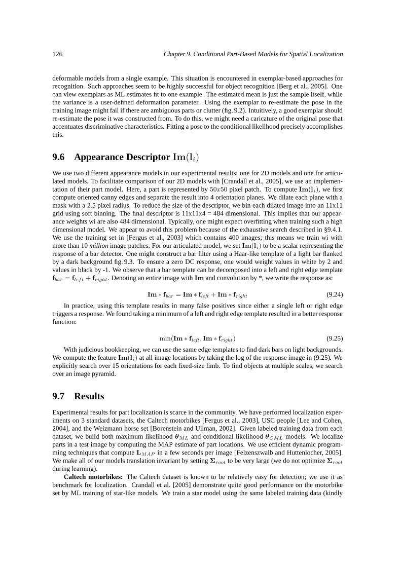
126 Chapter 9. Conditional Part-Based Models for Spatial Localization
deformable models from a single example. This situation is encountered in exemplar-based approaches forrecognition. Such approaches seem to be highly successful for object recognition [Berg et al., 2005]. Onecan view exemplars as ML estimates fit to one example. The estimated mean is just the sample itself, whilethe variance is a user-defined deformation parameter. Using the exemplar to re-estimate the pose in thetraining image might fail if there are ambiguous parts or clutter (fig. 9.2). Intuitively, a good exemplar shouldre-estimate the pose it was constructed from. To do this, we might need a caricature of the original pose thataccentuates discriminative characteristics. Fitting a pose to the conditional likelihood precisely accomplishesthis.
9.6 Appearance Descriptor Im(li)
We use two different appearance models in our experimental results; one for 2D models and one for articu-lated models. To facilitate comparison of our 2D models with [Crandall et al., 2005], we use an implemen-tation of their part model. Here, a part is represented by 50x50 pixel patch. To compute Im(li ), we firstcompute oriented canny edges and separate the result into 4 orientation planes. We dilate each plane with amask with a 2.5 pixel radius. To reduce the size of the descriptor, we bin each dilated image into an 11x11grid using soft binning. The final descriptor is 11x11x4 = 484 dimensional. This implies that our appear-ance weights wi are also 484 dimensional. Typically, one might expect overfitting when training such a highdimensional model. We appear to avoid this problem because of the exhaustive search described in §9.4.1.We use the training set in [Fergus et al., 2003] which contains 400 images; this means we train wi withmore than 10 million image patches. For our articulated model, we set Im(li) to be a scalar representing theresponse of a bar detector. One might construct a bar filter using a Haar-like template of a light bar flankedby a dark background fig. 9.3. To ensure a zero DC response, one would weight values in white by 2 andvalues in black by -1. We observe that a bar template can be decomposed into a left and right edge templatefbar = fleft + fright. Denoting an entire image with Im and convolution by *, we write the response as:
Im ∗ fbar = Im ∗ fleft + Im ∗ fright (9.24)
In practice, using this template results in many false positives since either a single left or right edgetriggers a response. We found taking a minimum of a left and right edge template resulted in a better responsefunction:
min(Im ∗ fleft , Im ∗ fright ) (9.25)
With judicious bookkeeping, we can use the same edge templates to find dark bars on light backgrounds.We compute the feature Im(li ) at all image locations by taking the log of the response image in (9.25). Weexplicitly search over 15 orientations for each fixed-size limb. To find objects at multiple scales, we searchover an image pyramid.
9.7 Results
Experimental results for part localization is scarce in the community. We have performed localization exper-iments on 3 standard datasets, the Caltech motorbikes [Fergus et al., 2003], USC people [Lee and Cohen,2004], and the Weizmann horse set [Borenstein and Ullman, 2002]. Given labeled training data from eachdataset, we build both maximum likelihood θML and conditional likelihood θCML models. We localizeparts in a test image by computing the MAP estimate of part locations. We use efficient dynamic program-ming techniques that compute LMAP in a few seconds per image [Felzenszwalb and Huttenlocher, 2005].We make all of our models translation invariant by setting Σroot to be very large (we do not optimize Σroot
during learning).Caltech motorbikes: The Caltech dataset is known to be relatively easy for detection; we use it as
benchmark for localization. Crandall et al. [2005] demonstrate quite good performance on the motorbikeset by ML training of star-like models. We train a star model using the same labeled training data (kindly
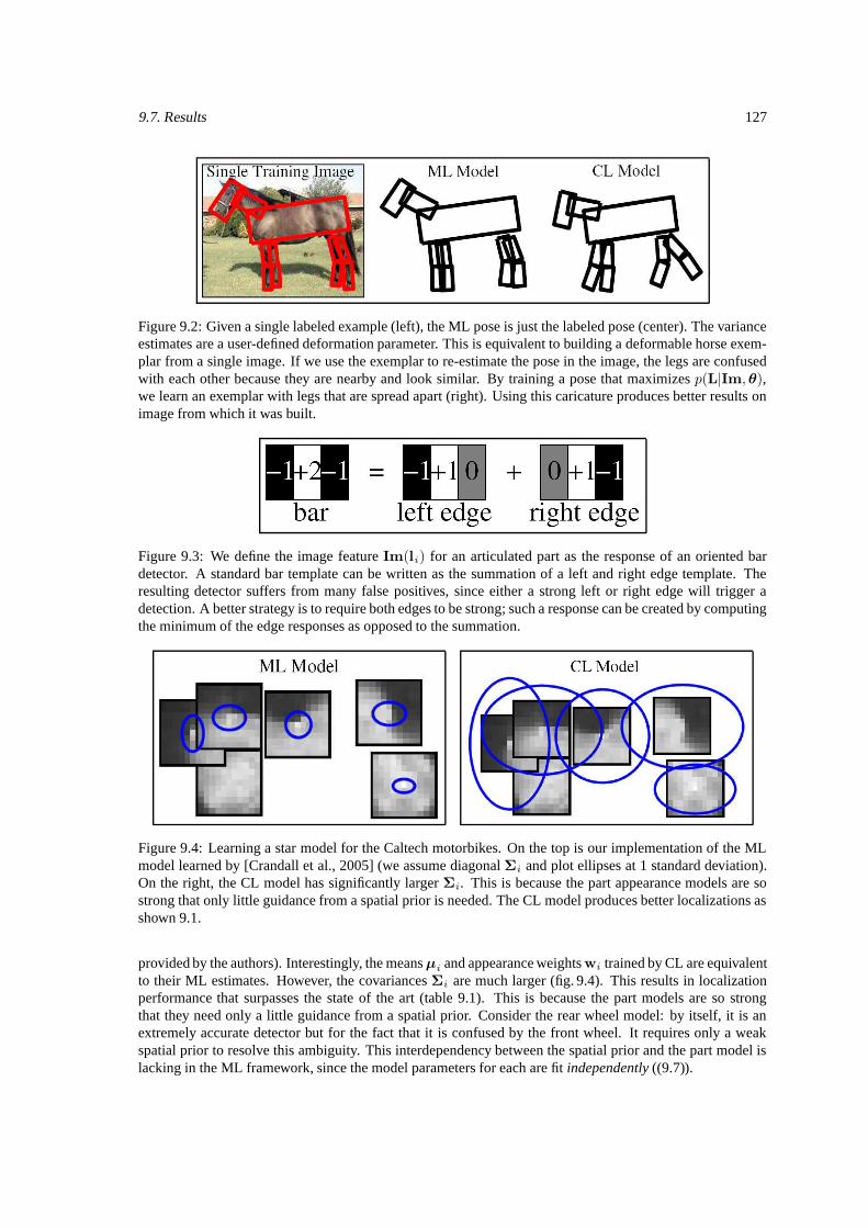
9.7. Results 127
Figure 9.2: Given a single labeled example (left), the ML pose is just the labeled pose (center). The varianceestimates are a user-defined deformation parameter. This is equivalent to building a deformable horse exem-plar from a single image. If we use the exemplar to re-estimate the pose in the image, the legs are confusedwith each other because they are nearby and look similar. By training a pose that maximizes p(L|Im,θ),we learn an exemplar with legs that are spread apart (right). Using this caricature produces better results onimage from which it was built.
Figure 9.3: We define the image feature Im(li ) for an articulated part as the response of an oriented bardetector. A standard bar template can be written as the summation of a left and right edge template. Theresulting detector suffers from many false positives, since either a strong left or right edge will trigger adetection. A better strategy is to require both edges to be strong; such a response can be created by computingthe minimum of the edge responses as opposed to the summation.
Figure 9.4: Learning a star model for the Caltech motorbikes. On the top is our implementation of the MLmodel learned by [Crandall et al., 2005] (we assume diagonal Σi and plot ellipses at 1 standard deviation).On the right, the CL model has significantly larger Σi. This is because the part appearance models are sostrong that only little guidance from a spatial prior is needed. The CL model produces better localizations asshown 9.1.
provided by the authors). Interestingly, the means µi and appearance weights wi trained by CL are equivalentto their ML estimates. However, the covariances Σi are much larger (fig. 9.4). This results in localizationperformance that surpasses the state of the art (table 9.1). This is because the part models are so strongthat they need only a little guidance from a spatial prior. Consider the rear wheel model: by itself, it is anextremely accurate detector but for the fact that it is confused by the front wheel. It requires only a weakspatial prior to resolve this ambiguity. This interdependency between the spatial prior and the part model islacking in the ML framework, since the model parameters for each are fit independently ((9.7)).
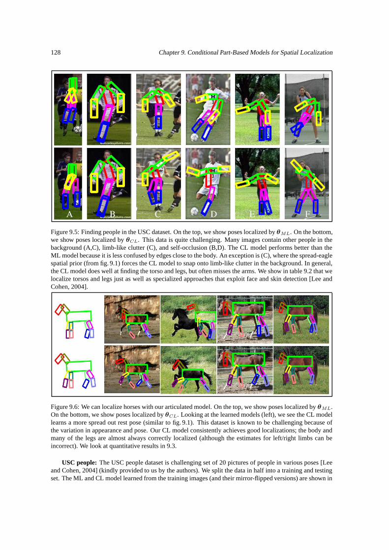
128 Chapter 9. Conditional Part-Based Models for Spatial Localization
Figure 9.5: Finding people in the USC dataset. On the top, we show poses localized by θML. On the bottom,we show poses localized by θCL. This data is quite challenging. Many images contain other people in thebackground (A,C), limb-like clutter (C), and self-occlusion (B,D). The CL model performs better than theML model because it is less confused by edges close to the body. An exception is (C), where the spread-eaglespatial prior (from fig. 9.1) forces the CL model to snap onto limb-like clutter in the background. In general,the CL model does well at finding the torso and legs, but often misses the arms. We show in table 9.2 that welocalize torsos and legs just as well as specialized approaches that exploit face and skin detection [Lee andCohen, 2004].
Figure 9.6: We can localize horses with our articulated model. On the top, we show poses localized by θML.On the bottom, we show poses localized by θCL. Looking at the learned models (left), we see the CL modellearns a more spread out rest pose (similar to fig. 9.1). This dataset is known to be challenging because ofthe variation in appearance and pose. Our CL model consistently achieves good localizations; the body andmany of the legs are almost always correctly localized (although the estimates for left/right limbs can beincorrect). We look at quantitative results in 9.3.
USC people: The USC people dataset is challenging set of 20 pictures of people in various poses [Leeand Cohen, 2004] (kindly provided to us by the authors). We split the data in half into a training and testingset. The ML and CL model learned from the training images (and their mirror-flipped versions) are shown in

9.7. Results 129
Rear Front Head Tail Seat Seatwheel wheel light light back Front
ML 4.19 3.22 13.97 11.58 13.17 9.46CL 2.88 2.44 12.49 7.95 10.39 6.77
Table 9.1: Localization results for Calthech Motorbikes. To evaluate localization, we look at the (90%alpha-trimmed) mean euclidean error of each part, measured with respect to a canonical car width of 200pixels (as in [Crandall et al., 2005]). Our average error across all parts for the CL model is 7.15. Thiscompares favorable with the best-reported error of 12.9 [Crandall et al., 2005]. This significant reductionseems to stem from the looser spatial model learned by the conditional likelihood model.
Sho Elbow Wrist Hip Knee AnkleML 21.2 21.4 38.3 11.2 15.3 21.5CL 17.9 21.9 39.7 7.8 12.3 17.2
Table 9.2: Localization results for USC People. Our error rates in (pixel) root mean squared error for theUSC dataset. Our models struggle to find arms, but the CL model localizes torsos and legs fairly well. Ourerror rates for those body parts are comparable to the average error of 14.9 reported in [Lee and Cohen, 2004](error for individual body parts were not given). Our results are impressive given that [Lee and Cohen, 2004]uses a face detector and a skin model. Our part appearance models are quite generic; we show they can alsobe used to find other articulated objects such as horses in fig. 9.6.
fig. 9.1. The CL model learns a rest pose where the arms and legs lie away from the body. This helps duringlocalization because the model will tend to be less confused by edges near the body. We show results for thetest set in fig. 9.5. We quantitatively evaluate results in table 9.3. The pose recovery algorithm used by Leeand Cohen is initialized by a face detector and is tuned to find skin pixels; hence it is designed for frontallyfacing people with uncovered limbs. Our articulated part model from §9.6 is quite generic (as we use it toalso find horses). We obtain error rates for certain body parts that are comparable to [Lee and Cohen, 2004](see table 9.2).
Weizmann horses: The Weizmann horse dataset is a well-known collection of images used to evaluatesegmentation. We are not aware of any results presented for part localization. We hand-labeled the first 40images with ground truth locations, and learned an articulated model from the first 20 images. We show thelearned models and test image results in fig. 9.6. The CL model almost always localizes the body and mostlegs correctly, though it often has difficulties with the head. These results are impressive given the variety inappearance and pose for this dataset.
9.7.1 Discussion
We specifically address the recognition task of localization. By focusing on that task, we have developed anew criteria for optimizing part-based models. Instead of learning a model that best matches some labeled
Nose Ear Sho. Knee Hoof RearML 50.9 38.6 24.4 24.7 27.13 25.7CL 45.9 34.2 19.1 19.8 22.72 20.0
Table 9.3: Localization results for Weizmann Horses. Our error rates in (pixel) root mean squared errorfor the Weizmann dataset. These are computed with respect to a canonical horse width of 300 pixels. Theaverage error for the ML model is 27.9, while the CL model is 23.1. Given the variety in appearance andpose in the dataset, we do quite well at localizing the main body and legs. The head proves difficult; wemight do better by learning a specific head model rather than using our generic limb model.

130 Chapter 9. Conditional Part-Based Models for Spatial Localization
2d poses, we learn the model that best localizes those 2d poses. This subtle difference often leads to verydifferent models because the objective is discriminative (rather than generative) and the model parameters arejointly learned (rather than independently). We demonstrate these models on challenging datasets, achievingor surpassing state of the art results.
Chapter 10
Support Kernel Machines for ObjectRecognition
Kernel classifiers based on Support Vector Machines (SVM) have recently achieved state-of-the art resultson several popular datasets like Caltech or Pascal. This was possible by combining the advantages of SVM– convexity and the availability of efficient optimizers, with ‘hyperkernels’ – linear combinations of kernelscomputed at multiple levels of image encoding. The use of hyperkernels faces the challenge of choosingthe kernel weights, the use of possibly irrelevant, poorly performing kernels, and an increased number ofparameters that can lead to overfitting. In this chapter we advocate the transition from SVMs to SupportKernel Machines (SKM) – models that estimate both the parameters of a sparse linear combination of kernels,and the parameters of a discriminative classifier. We explot recent kernel learning techniques, appreantly notknown and used in computer vision, that formulated the of learning SKMs as a convex optimization problemand solved it efficiently using Sequential Minimal Optimization. We study kernel learning for several multi-level image encodings for supervised object recognition and report competitive results on several datasets,including INRIA pedestrian, Caltech 101 and the newly created Caltech 256. The work appears at theInternational Conference for Computer Vision (ICCV) [Kumar and Sminchisescu, 2007].
10.1 Kernel Methods for Recognition
Recent work in object recognition and image classification has shown that significant performance gainscan be achieved by carefully combining multi-level, coarse-to-fine, layered feature encodings, and learningmethods. Top-scoring classifiers on image databases like Caltech or Pascal tend to be discriminative andkernel-based [Zhang et al., 2006, Lazebnik et al., 2006, Grauman and Darrell, 2005, Dalal and Triggs, 2005,Agarwal and Triggs, 2006a], but generative methods [Fei-Fei. et al., 2004, Sudderth et al., 2005] can alsobe used in order to build hybrid, even more sophisticated kernels (e.g. the Fisher kernel) [Holub and Perona,2005]. Monolithic kernels are by no means the only way to build successful classifiers. Several hierarchicalmethods like HMAX [Serre et al., 2005, Mutch and Lowe, 2006] or recent versions of convolutional neuralnetworks [Ranzato et al., 2007] use them more sparingly, at a final stage of a complex hierarchical compu-tation that involves successive convolution and rectification, but a straightforward monolithic kernel can bealternatively obtained by combining the representations across all layers. In any case, an underlying themeof current research is the use of kernel methods, in particular the Support Vector Machine (SVM) [Vapnik,1995, Schölkopf and Smola, 2002] – a methodology well-justified both theoretically and practically [Changand Lin, 2001]: the resulting program is convex with global optimality guarantees, and efficient algorithmslike Sequential Minimal Optimization (SMO) exist for solving large problems, with hundreds of thousandsof examples.
The successful proliferation of a variety of kernels has recently motivated several researchers to explorethe use of homogenous models obtained as linear combinations of histogram intersection kernels, computed
131
132 Chapter 10. Support Kernel Machines for Object Recognition
at each level of a multilevel image encoding [Grauman and Darrell, 2005, Lazebnik et al., 2006]. These moresophisticated classifiers have been demonstrated convincingly and state-of-the art results have been achieved,but their use raises a number of new research challenges:
(i) A weighting of kernels needs to be specified. In particular, for histogram intersection, very goodresults have been obtained using geometric approximate weightings to the optimal bipartite matching1 – butthis problem-dependent intuition may not be available for all kernels and problems, or may not be as effectivewhen combining heterogeneous kernels with different underlying metrics, or feature spaces (e.g. histogramintersections, polynomials and RBFs).
(ii) The kernel selection becomes important especially for small training sets, as the effective number ofmodel parameters increases with the number of kernels. This raises the question of which kernel is good,which one doesn’t matter and which one is likely to harm performance, a problem that requires a form ofcapacity control. Indeed, previous studies [Lazebnik et al., 2006, Agarwal and Triggs, 2006a] have shownthat for some problems, the best performance is achieved only for a subset of the kernels / levels of encoding –sometimes only a single one. The insights were gained by learning classifiers both for individual kernels andfor multiple ones, but as the number increases, an exhaustive exploration of the kernel power set becomesinfeasible. One is faced with the combinatorial problem of selecting a parsimonious kernel subset for adesired accuracy-computation trade-off - this is precisely the sparse, kernel subset selection problem weconsider.
To summarize, combining kernels is a promising research direction with an already very good perfor-mance record in image classification, but the problem of weighing the kernels or obtaining sparse optimalsolutions that are computationally efficient and don’t overfit falls beyond the machinery of a standard SVM.
The main emphasis of this work is to advocate the transition from Support Vector Machines – convexlearners that can be used to train one kernel efficiently using SMO, to Support Kernel Machines (SKM) –perhaps surprisingly, convex and sparse learners that can be used to train multiple kernels by jointly optimiz-ing both the coefficients of a conic combination of kernel matrices and the coefficients of a discriminativeclassifier. The research builds on recent algorithms [Lanckriet et al., 2004, Francis R. Bach and Jordan,2004, Bach et al., 2004a,b], where the objective of learning a sparse combination of kernels has been formu-lated as a convex, quadratically constrained quadratic problem, efficiently solved using sequential minimaloptimization (SMO) techniques.
The insights of this chapter are as follows: (i) We explore SKM for object recognition. This technique –to our knowledge not previously used in computer vision – provides a tractable solution to the combinatorialkernel selection problem and allows the design of new kernels and features and ways to systematically assestheir performance. (ii) We show that equivalent state-of-the art results (marginally better or worse) on largescale problems can be achieved with fewer, automatically selected kernels, compared to existing methodsbased on insightful problem-dependent selection of kernel combinations. We learn sparse kernel subsets forseveral datasets including Caltech 101 [Fei-Fei. et al., 2004], the newly created Caltech 256 [Griffin et al.,2007] and the pedestrian from INRIA [Dalal and Triggs, 2005] and report our experiences showing that SKMis a viable technology that improves and complements existing ones.
10.2 Support Kernel Machines
Although the fixed weighting of histogram intersections proposed in earlier work of [Grauman and Darrell,2005, Lazebnik et al., 2006] make sense intuitively and achieves good results, we consider the more scalableproblem of learning the weights instead. Ideally, we want to use several possibly inhomogeneous types ofkernels and select the ones most effective for the task. In this section, we review multiple kernel learningtechniques that makes it possible – for details see [Lanckriet et al., 2004, Francis R. Bach and Jordan, 2004,Bach et al., 2004a,b].
Lanckriet et al. [2004] considered SVMs based on conic combinations of kernel matrices (linear com-binations with non-negative coefficients) and showed that the optimization of the coefficients reduces to a
1These penalize matchings found in large histogram cells more than ones found in fine grained cells / layers.
10.2. Support Kernel Machines 133
convex optimization problem known as a quadratically-constrained quadratic program (QCQP). They pro-vided an initial solution based on Semi-Definite Programming, but that faced scalability problems for trainingsets larger that 2-3000 points. Bach et al. [2004a] proposed a dual formulation of the QCQP as a second-order cone programming, and showed how to exploit the technique of Moreau-Yosida regularization in orderto yield a formulation to which SMO techniques can be applied. Because this method uses sparse regular-izers to obtain a parsimonious conic combination of kernels, this methodology is referred to as the SupportKernel Machine (SKM) [Bach et al., 2004a]. More recent work by Bach et al. [2004b] has shown that anentire regularization path can be efficiently computed for the SKM using numerical continuation techniques.Unlike the regularization path of SVM which is piecewise linear, the one of SKM is piecewise smooth, eachkink in the path corresponding to places where the pattern of sparsity in the linear combination of kernelschanges. However, the main SKM optimization is performed using interior point (second-order) methodswhich again makes the use of this technique impractical for large problems. For our experiments, we follow[Bach et al., 2004a, Francis R. Bach and Jordan, 2004].The Problem: Assume we are given n data points (xi, yi), where xi is in the input space X = Rk, andyi ∈ −1, 1. Consider the input space X which will be mapped to m different feature spaces F1, . . . ,Fm
using feature maps Φ1(x), . . . ,Φm(x) and denote Φ(x) = (Φ1(x), . . . ,Φm(x)) as the joint feature space.Consider also variables wi, i ∈ 1 . . .m with joint vector w = (w1, . . . ,wm). To encourage sparsity at thelevel of blocks, the cost function is chosen to penalize the block L1-norm of w. The multiple kernel learningproblem can be formulated as follows:
minw∈F1...×Fm
n∑
i=1
L(yiw
>Φ(x))
+ λ
m∑
j=1
dj(‖wj‖2)2
(10.1)
where dj are positive weights associated with each kernel, λ is a regularization constant, and L can be anyloss function for classification, e.g. the hinge loss (see below). In the next subsection we give the basicprimal problems for the simpler and more readable case of multiple linear classifiers, but the kernelization isstraightforward [Schölkopf and Smola, 2002, Bach et al., 2004a, Francis R. Bach and Jordan, 2004].
10.2.1 Learning Multiple Linear Classifiers
To study the problem of learning a conic combination of linear classifiers, assume we are given a decom-position of Rk as a product of m blocks: Rk = Rk1 × · · · × Rkm , so that each data point xi can bedecomposed into m block components, i.e. xi = (x1i, · · · ,xmi), where each xji is a vector. The goalis to find a linear classifier of the form y = sign(w>x + b) where w has the same block decompositionw = (w1, . . . ,wm) ∈ Rk1+···+km . The primal for this problem is very similar to the one of a linear SVM,except for the cost used to penalize the coefficient, a block-weightedL1 norm, not an L2 norm, as usual:
(P) min1
2
m∑
j=1
dj‖wj‖2
2
+ C
n∑
i=1
ξi
w.r.t. w ∈ Rk1 × · · · × Rkm , ξ ∈ Rn+, b ∈ R
s.t. yi
m∑
j=1
w>j xji + b
≥ 1− ξi, ∀i ∈ 1, · · · , n
where a soft margin is used, with ξi slack variables.The cost defined by (P) gives a convex yet non-differentiable dual problem. However, an L2 norm
regularizer can be added to the cost in order to obtain a differentiable dual. This uses ‘bridge’ weightings aj
that are estimated during the optimization. Their role is to provide a dynamically adaptive cost that makesthe problem locally smooth. The technique is known as Moreau-Yoshida regularization [Bach et al., 2004a].The primal problem is:
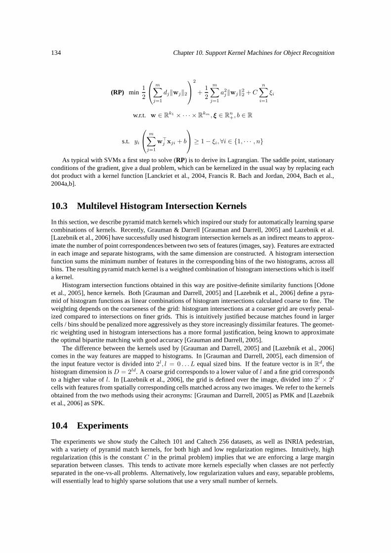
134 Chapter 10. Support Kernel Machines for Object Recognition
(RP) min1
2
m∑
j=1
dj‖wj‖2
2
+1
2
m∑
j=1
a2j‖wj‖22 + C
n∑
i=1
ξi
w.r.t. w ∈ Rk1 × · · · × Rkm , ξ ∈ Rn+, b ∈ R
s.t. yi
m∑
j=1
w>j xji + b
≥ 1− ξi, ∀i ∈ 1, · · · , n
As typical with SVMs a first step to solve (RP) is to derive its Lagrangian. The saddle point, stationaryconditions of the gradient, give a dual problem, which can be kernelized in the usual way by replacing eachdot product with a kernel function [Lanckriet et al., 2004, Francis R. Bach and Jordan, 2004, Bach et al.,2004a,b].
10.3 Multilevel Histogram Intersection Kernels
In this section, we describe pyramid match kernels which inspired our study for automatically learning sparsecombinations of kernels. Recently, Grauman & Darrell [Grauman and Darrell, 2005] and Lazebnik et al.[Lazebnik et al., 2006] have successfully used histogram intersection kernels as an indirect means to approx-imate the number of point correspondences between two sets of features (images, say). Features are extractedin each image and separate histograms, with the same dimension are constructed. A histogram intersectionfunction sums the minimum number of features in the corresponding bins of the two histograms, across allbins. The resulting pyramid match kernel is a weighted combination of histogram intersections which is itselfa kernel.
Histogram intersection functions obtained in this way are positive-definite similarity functions [Odoneet al., 2005], hence kernels. Both [Grauman and Darrell, 2005] and [Lazebnik et al., 2006] define a pyra-mid of histogram functions as linear combinations of histogram intersections calculated coarse to fine. Theweighting depends on the coarseness of the grid: histogram intersections at a coarser grid are overly penal-ized compared to intersections on finer grids. This is intuitively justified because matches found in largercells / bins should be penalized more aggressively as they store increasingly dissimilar features. The geomet-ric weighting used in histogram intersections has a more formal justification, being known to approximatethe optimal bipartite matching with good accuracy [Grauman and Darrell, 2005].
The difference between the kernels used by [Grauman and Darrell, 2005] and [Lazebnik et al., 2006]comes in the way features are mapped to histograms. In [Grauman and Darrell, 2005], each dimension ofthe input feature vector is divided into 2l, l = 0 . . . L equal sized bins. If the feature vector is in Rd, thehistogram dimension is D = 2ld. A coarse grid corresponds to a lower value of l and a fine grid correspondsto a higher value of l. In [Lazebnik et al., 2006], the grid is defined over the image, divided into 2l × 2l
cells with features from spatially corresponding cells matched across any two images. We refer to the kernelsobtained from the two methods using their acronyms: [Grauman and Darrell, 2005] as PMK and [Lazebniket al., 2006] as SPK.
10.4 Experiments
The experiments we show study the Caltech 101 and Caltech 256 datasets, as well as INRIA pedestrian,with a variety of pyramid match kernels, for both high and low regularization regimes. Intuitively, highregularization (this is the constant C in the primal problem) implies that we are enforcing a large marginseparation between classes. This tends to activate more kernels especially when classes are not perfectlyseparated in the one-vs-all problems. Alternatively, low regularization values and easy, separable problems,will essentially lead to highly sparse solutions that use a very small number of kernels.
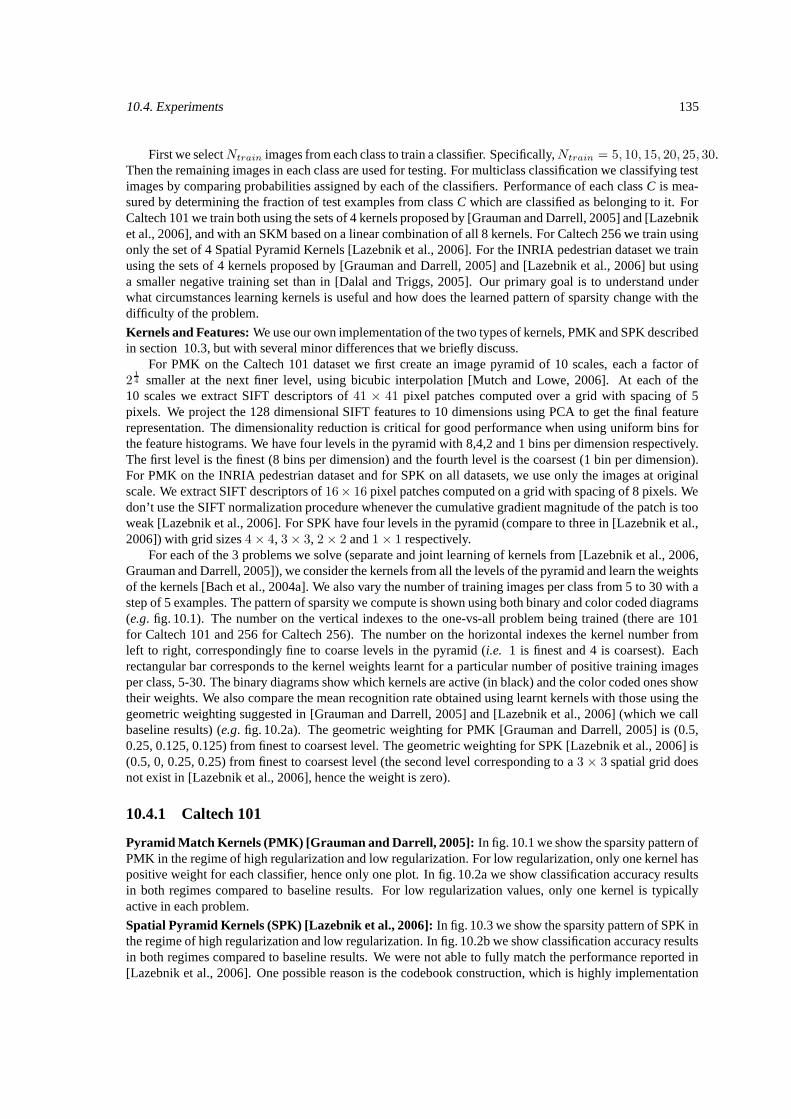
10.4. Experiments 135
First we selectNtrain images from each class to train a classifier. Specifically,Ntrain = 5, 10, 15, 20, 25, 30.Then the remaining images in each class are used for testing. For multiclass classification we classifying testimages by comparing probabilities assigned by each of the classifiers. Performance of each class C is mea-sured by determining the fraction of test examples from class C which are classified as belonging to it. ForCaltech 101 we train both using the sets of 4 kernels proposed by [Grauman and Darrell, 2005] and [Lazebniket al., 2006], and with an SKM based on a linear combination of all 8 kernels. For Caltech 256 we train usingonly the set of 4 Spatial Pyramid Kernels [Lazebnik et al., 2006]. For the INRIA pedestrian dataset we trainusing the sets of 4 kernels proposed by [Grauman and Darrell, 2005] and [Lazebnik et al., 2006] but usinga smaller negative training set than in [Dalal and Triggs, 2005]. Our primary goal is to understand underwhat circumstances learning kernels is useful and how does the learned pattern of sparsity change with thedifficulty of the problem.
Kernels and Features: We use our own implementation of the two types of kernels, PMK and SPK describedin section 10.3, but with several minor differences that we briefly discuss.
For PMK on the Caltech 101 dataset we first create an image pyramid of 10 scales, each a factor of2
14 smaller at the next finer level, using bicubic interpolation [Mutch and Lowe, 2006]. At each of the
10 scales we extract SIFT descriptors of 41 × 41 pixel patches computed over a grid with spacing of 5pixels. We project the 128 dimensional SIFT features to 10 dimensions using PCA to get the final featurerepresentation. The dimensionality reduction is critical for good performance when using uniform bins forthe feature histograms. We have four levels in the pyramid with 8,4,2 and 1 bins per dimension respectively.The first level is the finest (8 bins per dimension) and the fourth level is the coarsest (1 bin per dimension).For PMK on the INRIA pedestrian dataset and for SPK on all datasets, we use only the images at originalscale. We extract SIFT descriptors of 16× 16 pixel patches computed on a grid with spacing of 8 pixels. Wedon’t use the SIFT normalization procedure whenever the cumulative gradient magnitude of the patch is tooweak [Lazebnik et al., 2006]. For SPK have four levels in the pyramid (compare to three in [Lazebnik et al.,2006]) with grid sizes 4× 4, 3× 3, 2× 2 and 1× 1 respectively.
For each of the 3 problems we solve (separate and joint learning of kernels from [Lazebnik et al., 2006,Grauman and Darrell, 2005]), we consider the kernels from all the levels of the pyramid and learn the weightsof the kernels [Bach et al., 2004a]. We also vary the number of training images per class from 5 to 30 with astep of 5 examples. The pattern of sparsity we compute is shown using both binary and color coded diagrams(e.g. fig. 10.1). The number on the vertical indexes to the one-vs-all problem being trained (there are 101for Caltech 101 and 256 for Caltech 256). The number on the horizontal indexes the kernel number fromleft to right, correspondingly fine to coarse levels in the pyramid (i.e. 1 is finest and 4 is coarsest). Eachrectangular bar corresponds to the kernel weights learnt for a particular number of positive training imagesper class, 5-30. The binary diagrams show which kernels are active (in black) and the color coded ones showtheir weights. We also compare the mean recognition rate obtained using learnt kernels with those using thegeometric weighting suggested in [Grauman and Darrell, 2005] and [Lazebnik et al., 2006] (which we callbaseline results) (e.g. fig. 10.2a). The geometric weighting for PMK [Grauman and Darrell, 2005] is (0.5,0.25, 0.125, 0.125) from finest to coarsest level. The geometric weighting for SPK [Lazebnik et al., 2006] is(0.5, 0, 0.25, 0.25) from finest to coarsest level (the second level corresponding to a 3 × 3 spatial grid doesnot exist in [Lazebnik et al., 2006], hence the weight is zero).
10.4.1 Caltech 101
Pyramid Match Kernels (PMK) [Grauman and Darrell, 2005]: In fig. 10.1 we show the sparsity pattern ofPMK in the regime of high regularization and low regularization. For low regularization, only one kernel haspositive weight for each classifier, hence only one plot. In fig. 10.2a we show classification accuracy resultsin both regimes compared to baseline results. For low regularization values, only one kernel is typicallyactive in each problem.
Spatial Pyramid Kernels (SPK) [Lazebnik et al., 2006]: In fig. 10.3 we show the sparsity pattern of SPK inthe regime of high regularization and low regularization. In fig. 10.2b we show classification accuracy resultsin both regimes compared to baseline results. We were not able to fully match the performance reported in[Lazebnik et al., 2006]. One possible reason is the codebook construction, which is highly implementation
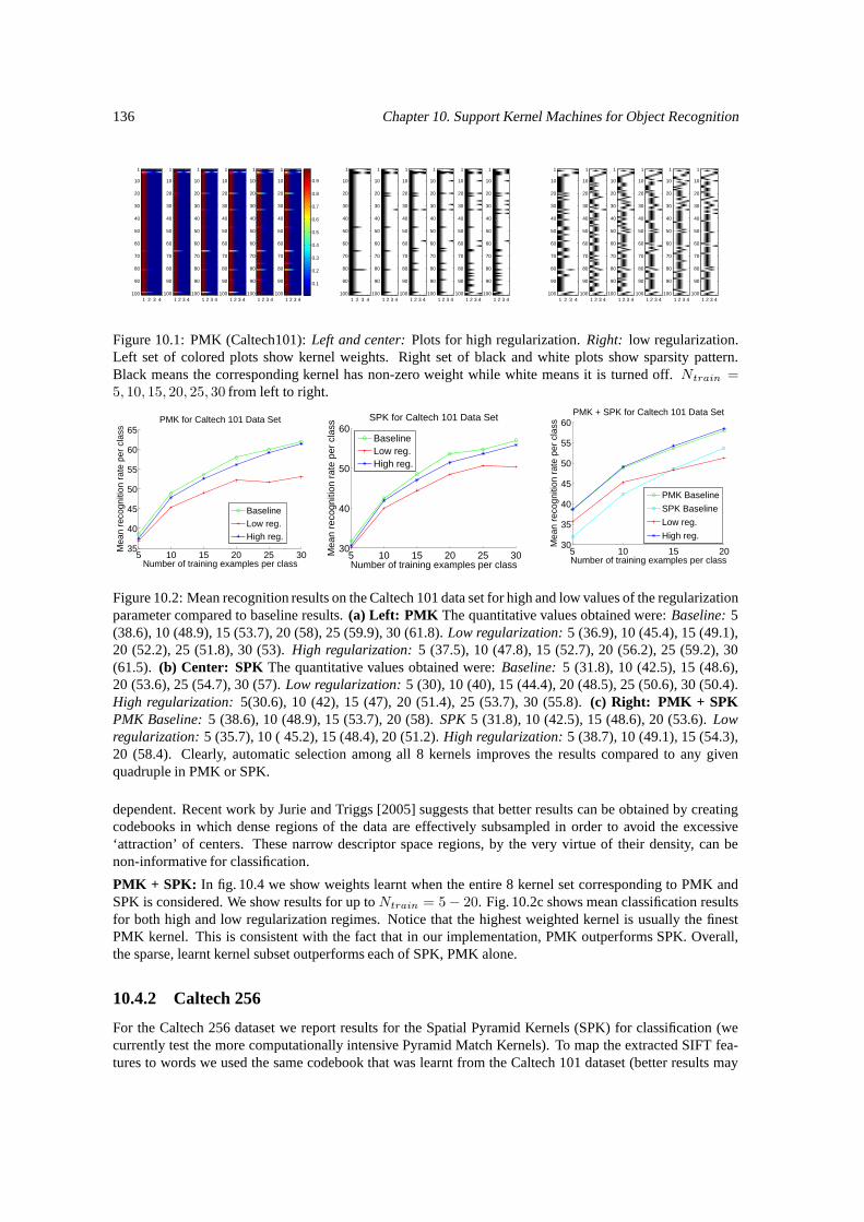
136 Chapter 10. Support Kernel Machines for Object Recognition
1 2 3 4
1
10
20
30
40
50
60
70
80
90
1001 2 3 4
1
10
20
30
40
50
60
70
80
90
1001 2 3 4
1
10
20
30
40
50
60
70
80
90
1001 2 3 4
1
10
20
30
40
50
60
70
80
90
1001 2 3 4
1
10
20
30
40
50
60
70
80
90
1001 2 3 4
1
10
20
30
40
50
60
70
80
90
100
0.1
0.2
0.3
0.4
0.5
0.6
0.7
0.8
0.9
1 2 3 4
1
10
20
30
40
50
60
70
80
90
1001 2 3 4
1
10
20
30
40
50
60
70
80
90
1001 2 3 4
1
10
20
30
40
50
60
70
80
90
1001 2 3 4
1
10
20
30
40
50
60
70
80
90
1001 2 3 4
1
10
20
30
40
50
60
70
80
90
1001 2 3 4
1
10
20
30
40
50
60
70
80
90
1001 2 3 4
1
10
20
30
40
50
60
70
80
90
1001 2 3 4
1
10
20
30
40
50
60
70
80
90
1001 2 3 4
1
10
20
30
40
50
60
70
80
90
1001 2 3 4
1
10
20
30
40
50
60
70
80
90
1001 2 3 4
1
10
20
30
40
50
60
70
80
90
1001 2 3 4
1
10
20
30
40
50
60
70
80
90
100
Figure 10.1: PMK (Caltech101): Left and center: Plots for high regularization. Right: low regularization.Left set of colored plots show kernel weights. Right set of black and white plots show sparsity pattern.Black means the corresponding kernel has non-zero weight while white means it is turned off. Ntrain =5, 10, 15, 20, 25, 30 from left to right.
5 10 15 20 25 3035
40
45
50
55
60
65
Number of training examples per class
Mea
n re
cogn
ition
rat
e pe
r cl
ass
PMK for Caltech 101 Data Set
BaselineLow reg.High reg.
5 10 15 20 25 3030
40
50
60
Number of training examples per class
Mea
n re
cogn
ition
rat
e pe
r cl
ass SPK for Caltech 101 Data Set
BaselineLow reg.High reg.
5 10 15 2030
35
40
45
50
55
60
Number of training examples per classM
ean
reco
gniti
on r
ate
per
clas
s
PMK + SPK for Caltech 101 Data Set
PMK Baseline
SPK Baseline
Low reg.
High reg.
Figure 10.2: Mean recognition results on the Caltech 101 data set for high and low values of the regularizationparameter compared to baseline results. (a) Left: PMK The quantitative values obtained were: Baseline: 5(38.6), 10 (48.9), 15 (53.7), 20 (58), 25 (59.9), 30 (61.8). Low regularization: 5 (36.9), 10 (45.4), 15 (49.1),20 (52.2), 25 (51.8), 30 (53). High regularization: 5 (37.5), 10 (47.8), 15 (52.7), 20 (56.2), 25 (59.2), 30(61.5). (b) Center: SPK The quantitative values obtained were: Baseline: 5 (31.8), 10 (42.5), 15 (48.6),20 (53.6), 25 (54.7), 30 (57). Low regularization: 5 (30), 10 (40), 15 (44.4), 20 (48.5), 25 (50.6), 30 (50.4).High regularization: 5(30.6), 10 (42), 15 (47), 20 (51.4), 25 (53.7), 30 (55.8). (c) Right: PMK + SPKPMK Baseline: 5 (38.6), 10 (48.9), 15 (53.7), 20 (58). SPK 5 (31.8), 10 (42.5), 15 (48.6), 20 (53.6). Lowregularization: 5 (35.7), 10 ( 45.2), 15 (48.4), 20 (51.2). High regularization: 5 (38.7), 10 (49.1), 15 (54.3),20 (58.4). Clearly, automatic selection among all 8 kernels improves the results compared to any givenquadruple in PMK or SPK.
dependent. Recent work by Jurie and Triggs [2005] suggests that better results can be obtained by creatingcodebooks in which dense regions of the data are effectively subsampled in order to avoid the excessive‘attraction’ of centers. These narrow descriptor space regions, by the very virtue of their density, can benon-informative for classification.
PMK + SPK: In fig. 10.4 we show weights learnt when the entire 8 kernel set corresponding to PMK andSPK is considered. We show results for up to Ntrain = 5− 20. Fig. 10.2c shows mean classification resultsfor both high and low regularization regimes. Notice that the highest weighted kernel is usually the finestPMK kernel. This is consistent with the fact that in our implementation, PMK outperforms SPK. Overall,the sparse, learnt kernel subset outperforms each of SPK, PMK alone.
10.4.2 Caltech 256
For the Caltech 256 dataset we report results for the Spatial Pyramid Kernels (SPK) for classification (wecurrently test the more computationally intensive Pyramid Match Kernels). To map the extracted SIFT fea-tures to words we used the same codebook that was learnt from the Caltech 101 dataset (better results may
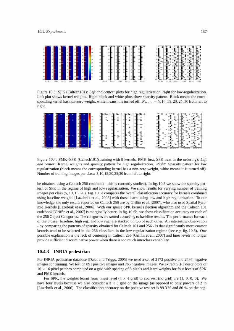
10.4. Experiments 137
1 2 3 4
1
10
20
30
40
50
60
70
80
90
1001 2 3 4
1
10
20
30
40
50
60
70
80
90
1001 2 3 4
1
10
20
30
40
50
60
70
80
90
1001 2 3 4
1
10
20
30
40
50
60
70
80
90
1001 2 3 4
1
10
20
30
40
50
60
70
80
90
1001 2 3 4
1
10
20
30
40
50
60
70
80
90
100
0.1
0.2
0.3
0.4
0.5
0.6
0.7
0.8
0.9
1 2 3 4
1
10
20
30
40
50
60
70
80
90
1001 2 3 4
1
10
20
30
40
50
60
70
80
90
1001 2 3 4
1
10
20
30
40
50
60
70
80
90
1001 2 3 4
1
10
20
30
40
50
60
70
80
90
1001 2 3 4
1
10
20
30
40
50
60
70
80
90
1001 2 3 4
1
10
20
30
40
50
60
70
80
90
1001 2 3 4
1
10
20
30
40
50
60
70
80
90
1001 2 3 4
1
10
20
30
40
50
60
70
80
90
1001 2 3 4
1
10
20
30
40
50
60
70
80
90
1001 2 3 4
1
10
20
30
40
50
60
70
80
90
1001 2 3 4
1
10
20
30
40
50
60
70
80
90
1001 2 3 4
1
10
20
30
40
50
60
70
80
90
100
Figure 10.3: SPK (Caltech101): Left and center: plots for high regularization, right for low-regularization.Left plot shows kernel weights. Right black and white plots show sparsity pattern. Black means the corre-sponding kernel has non-zero weight, white means it is turned off. Ntrain = 5, 10, 15, 20, 25, 30 from left toright.
1 2 3 4 5 6 7 8
1
10
20
30
40
50
60
70
80
90
1001 2 3 4 5 6 7 8
1
10
20
30
40
50
60
70
80
90
1001 2 3 4 5 6 7 8
1
10
20
30
40
50
60
70
80
90
1001 2 3 4 5 6 7 8
1
10
20
30
40
50
60
70
80
90
100
0.1
0.2
0.3
0.4
0.5
0.6
0.7
0.8
0.9
1 2 3 4 5 6 7 8
1
10
20
30
40
50
60
70
80
90
1001 2 3 4 5 6 7 8
1
10
20
30
40
50
60
70
80
90
1001 2 3 4 5 6 7 8
1
10
20
30
40
50
60
70
80
90
1001 2 3 4 5 6 7 8
1
10
20
30
40
50
60
70
80
90
1001 2 3 4 5 6 7 8
1
10
20
30
40
50
60
70
80
90
1001 2 3 4 5 6 7 8
1
10
20
30
40
50
60
70
80
90
1001 2 3 4 5 6 7 8
1
10
20
30
40
50
60
70
80
90
1001 2 3 4 5 6 7 8
1
10
20
30
40
50
60
70
80
90
100
Figure 10.4: PMK+SPK (Caltech101)(training with 8 kernels, PMK first, SPK next in the ordering): Leftand center: Kernel weights and sparsity pattern for high regularization. Right: Sparsity pattern for lowregularization (black means the corresponding kernel has a non-zero weight, white means it is turned off).Number of training images per class: 5,10,15,20,25,30 from left to right.
be obtained using a Caltech 256 codebook - this is currently studied). In fig. 10.5 we show the sparsity pat-tern of SPK in the regime of high and low regularization. We show results for varying number of trainingimages per class (5, 10, 15, 20). Fig. 10.6a compares the overall classification accuracy for kernels combinedusing baseline weights [Lazebnik et al., 2006] with those learnt using low and high regularization. To ourknowledge, the only results reported on Caltech 256 are by Griffin et al. [2007], who also used Spatial Pyra-mid Kernels [Lazebnik et al., 2006]. With our sparse SPK kernel selection algorithm and the Caltech 101codebook [Griffin et al., 2007] is marginally better. In fig. 10.6b, we show classification accuracy on each ofthe 256 Object Categories. The categories are sorted according to baseline results. The performance for eachof the 3 case: baseline, high reg. and low reg. are stacked on top of each other. An interesting observation- by comparing the patterns of sparsity obtained for Caltech 101 and 256 - is that significantly more coarserkernels tend to be selected in the 256 classifiers in the low-regularization regime (see e.g. fig. 10.5). Onepossible explanation is the lack of centering in Caltech 256 [Griffin et al., 2007] and finer levels no longerprovide sufficient discriminative power when there is too much intraclass variability.
10.4.3 INRIA pedestrian
For INRIA pedestrian database [Dalal and Triggs, 2005] we used a set of 2172 positive and 2436 negativeimages for training. We test on 891 positive images and 765 negative images. We extract SIFT descriptors of16× 16 pixel patches computed on a grid with spacing of 8 pixels and learn weights for four levels of SPKand PMK kernels.
For SPK, the weights learnt from finest level (4 × 4 grid) to coarsest (no grid) are (1, 0, 0, 0). Wehave four levels because we also consider a 3 × 3 grid on the image (as opposed to only powers of 2 in[Lazebnik et al., 2006]. The classification accuracy on the positive test set is 99.3 % and 80 % on the neg-
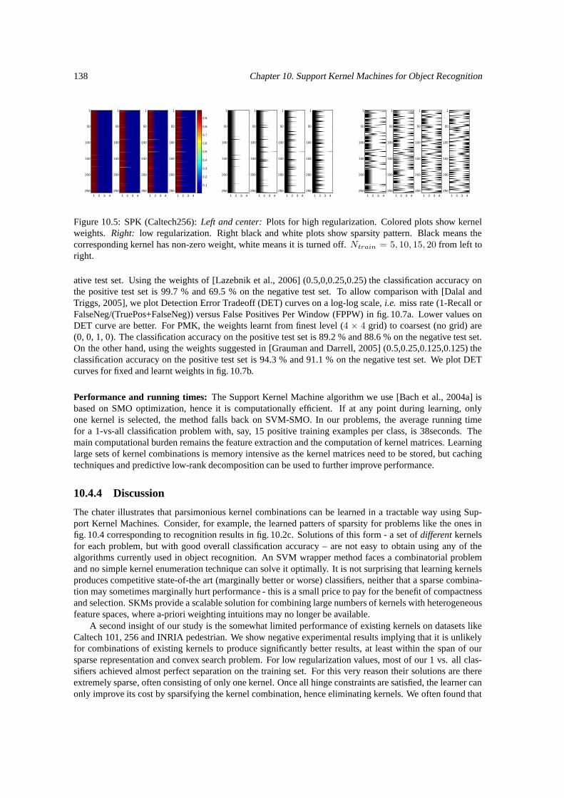
138 Chapter 10. Support Kernel Machines for Object Recognition
1 2 3 4
1
50
100
150
200
250
1 2 3 4
1
50
100
150
200
250
1 2 3 4
1
50
100
150
200
250
1 2 3 4
1
50
100
150
200
250
0.1
0.2
0.3
0.4
0.5
0.6
0.7
0.8
0.9
1 2 3 4
1
50
100
150
200
250
1 2 3 4
1
50
100
150
200
250
1 2 3 4
1
50
100
150
200
250
1 2 3 4
1
50
100
150
200
250
1 2 3 4
1
50
100
150
200
250
1 2 3 4
1
50
100
150
200
250
1 2 3 4
1
50
100
150
200
250
1 2 3 4
1
50
100
150
200
250
Figure 10.5: SPK (Caltech256): Left and center: Plots for high regularization. Colored plots show kernelweights. Right: low regularization. Right black and white plots show sparsity pattern. Black means thecorresponding kernel has non-zero weight, white means it is turned off. Ntrain = 5, 10, 15, 20 from left toright.
ative test set. Using the weights of [Lazebnik et al., 2006] (0.5,0,0.25,0.25) the classification accuracy onthe positive test set is 99.7 % and 69.5 % on the negative test set. To allow comparison with [Dalal andTriggs, 2005], we plot Detection Error Tradeoff (DET) curves on a log-log scale, i.e. miss rate (1-Recall orFalseNeg/(TruePos+FalseNeg)) versus False Positives Per Window (FPPW) in fig. 10.7a. Lower values onDET curve are better. For PMK, the weights learnt from finest level (4 × 4 grid) to coarsest (no grid) are(0, 0, 1, 0). The classification accuracy on the positive test set is 89.2 % and 88.6 % on the negative test set.On the other hand, using the weights suggested in [Grauman and Darrell, 2005] (0.5,0.25,0.125,0.125) theclassification accuracy on the positive test set is 94.3 % and 91.1 % on the negative test set. We plot DETcurves for fixed and learnt weights in fig. 10.7b.
Performance and running times: The Support Kernel Machine algorithm we use [Bach et al., 2004a] isbased on SMO optimization, hence it is computationally efficient. If at any point during learning, onlyone kernel is selected, the method falls back on SVM-SMO. In our problems, the average running timefor a 1-vs-all classification problem with, say, 15 positive training examples per class, is 38seconds. Themain computational burden remains the feature extraction and the computation of kernel matrices. Learninglarge sets of kernel combinations is memory intensive as the kernel matrices need to be stored, but cachingtechniques and predictive low-rank decomposition can be used to further improve performance.
10.4.4 Discussion
The chater illustrates that parsimonious kernel combinations can be learned in a tractable way using Sup-port Kernel Machines. Consider, for example, the learned patters of sparsity for problems like the ones infig. 10.4 corresponding to recognition results in fig. 10.2c. Solutions of this form - a set of different kernelsfor each problem, but with good overall classification accuracy – are not easy to obtain using any of thealgorithms currently used in object recognition. An SVM wrapper method faces a combinatorial problemand no simple kernel enumeration technique can solve it optimally. It is not surprising that learning kernelsproduces competitive state-of-the art (marginally better or worse) classifiers, neither that a sparse combina-tion may sometimes marginally hurt performance - this is a small price to pay for the benefit of compactnessand selection. SKMs provide a scalable solution for combining large numbers of kernels with heterogeneousfeature spaces, where a-priori weighting intuitions may no longer be available.
A second insight of our study is the somewhat limited performance of existing kernels on datasets likeCaltech 101, 256 and INRIA pedestrian. We show negative experimental results implying that it is unlikelyfor combinations of existing kernels to produce significantly better results, at least within the span of oursparse representation and convex search problem. For low regularization values, most of our 1 vs. all clas-sifiers achieved almost perfect separation on the training set. For this very reason their solutions are thereextremely sparse, often consisting of only one kernel. Once all hinge constraints are satisfied, the learner canonly improve its cost by sparsifying the kernel combination, hence eliminating kernels. We often found that
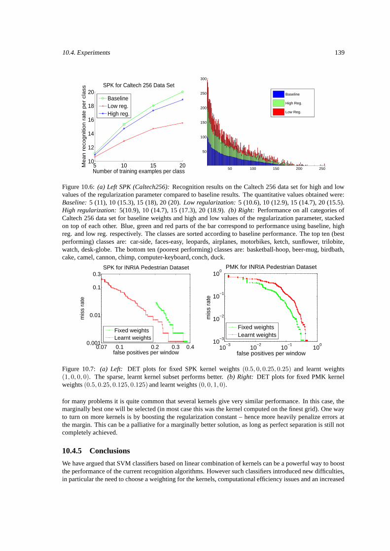
10.4. Experiments 139
5 10 15 2010
12
14
16
18
20
Number of training examples per class
Me
an
re
cog
niti
on
ra
te p
er
cla
ssSPK for Caltech 256 Data Set
BaselineLow reg.High reg.
50 100 150 200 250
50
100
150
200
250
300
Baseline
High Reg.
Low Reg.
Figure 10.6: (a) Left SPK (Caltech256): Recognition results on the Caltech 256 data set for high and lowvalues of the regularization parameter compared to baseline results. The quantitative values obtained were:Baseline: 5 (11), 10 (15.3), 15 (18), 20 (20). Low regularization: 5 (10.6), 10 (12.9), 15 (14.7), 20 (15.5).High regularization: 5(10.9), 10 (14.7), 15 (17.3), 20 (18.9). (b) Right: Performance on all categories ofCaltech 256 data set for baseline weights and high and low values of the regularization parameter, stackedon top of each other. Blue, green and red parts of the bar correspond to performance using baseline, highreg. and low reg. respectively. The classes are sorted according to baseline performance. The top ten (bestperforming) classes are: car-side, faces-easy, leopards, airplanes, motorbikes, ketch, sunflower, trilobite,watch, desk-globe. The bottom ten (poorest performing) classes are: basketball-hoop, beer-mug, birdbath,cake, camel, cannon, chimp, computer-keyboard, conch, duck.
0.07 0.1 0.2 0.3 0.40.001
0.01
0.1
0.3
false positives per window
mis
s ra
te
SPK for INRIA Pedestrian Dataset
Fixed weightsLearnt weights
10−3
10−2
10−1
100
10−3
10−2
10−1
100
false positives per window
mis
s ra
te
PMK for INRIA Pedestrian Dataset
Fixed weightsLearnt weights
Figure 10.7: (a) Left: DET plots for fixed SPK kernel weights (0.5, 0, 0.25, 0.25) and learnt weights(1, 0, 0, 0). The sparse, learnt kernel subset performs better. (b) Right: DET plots for fixed PMK kernelweights (0.5, 0.25, 0.125, 0.125) and learnt weights (0, 0, 1, 0).
for many problems it is quite common that several kernels give very similar performance. In this case, themarginally best one will be selected (in most case this was the kernel computed on the finest grid). One wayto turn on more kernels is by boosting the regularization constant – hence more heavily penalize errors atthe margin. This can be a palliative for a marginally better solution, as long as perfect separation is still notcompletely achieved.
10.4.5 Conclusions
We have argued that SVM classifiers based on linear combination of kernels can be a powerful way to boostthe performance of the current recognition algorithms. However such classifiers introduced new difficulties,in particular the need to choose a weighting for the kernels, computational efficiency issues and an increased

140 Chapter 10. Support Kernel Machines for Object Recognition
danger to overfit. Ultimately, the problem of learning a parsimonious set of kernels from a possibly largesubset, falls beyond the methodology of current SVM. In this chapter we advocate the transition from SVMsto Support Kernel Machines (SKM) – a technique previously not used in computer vision – in order to obtainmodels that estimate both the parameters of a sparse linear combination of kernels, and the parameters of adiscriminative classifier in one convex problem. Our large scale study of representative datasets like Caltech101, 256 or INRIA pedestrian show that state-of-the art results can be achieved using sparse learned kernelcombinations (see e.g. fig. 10.2c), but also underlines the limitations of current feature extraction and kerneldesign methods. In the long run, SKM appears to be a viable technique for designing new kernels andfeatures, systematically assessing their performance, and selecting the best performing kernel subset for agiven problem.

PART III:LATENT VARIABLE MODELS

Chapter 11
A Non-linear Generative Model forLow-dimensional Inference
Many difficult visual perception problems, like 3D human motion estimation, can be formulated in terms ofinference using complex generative models, defined over high-dimensional state spaces. Despite progress,optimizing such models is difficult because prior knowledge cannot be flexibly integrated in order to re-shape an initially designed representation space. Non-linearities, inherent sparsity of high-dimensional train-ing sets, and lack of global continuity makes dimensionality reduction challenging and low-dimensionalsearch inefficient. To address these problems, we present a learning and inference algorithm that restrictsvisual tracking to automatically extracted, non-linearly embedded, low-dimensional spaces. This formu-lation produces a layered generative model with reduced state representation, that can be estimated usingefficient continuous optimization methods. Our prior flattening method allows a simple analytic treatment oflow-dimensional intrinsic curvature constraints, and allows consistent interpolation operations. We analyzereduced manifolds for human interaction activities, and demonstrate that the algorithm learns continuousgenerative models that are useful for tracking and for the reconstruction of 3D human motion in monocularvideo. An earlier version of this chapter appeared in International Conference on Machine Learning (ICML)[Sminchisescu and Jepson, 2004b].
11.1 Desirable Properties of a Low-dimensional Model
Many successful visual tracking approaches are based on high-dimensional, physically inspired, non-lineargenerative models of shape, intensity or motion [Isard and Blake, 1998a, Deutscher et al., 2000, Sidenbladhet al., 2002, Sminchisescu and Triggs, 2003b]. Although usually hard to construct, such models offer intuitiverepresentations, counterpoint coherence to image clutter and offer the analytical advantage of a global coor-dinate system for continuous optimization or sampling. However, despite good progress, inference in theseframeworks remains difficult, mostly due to the lack of learning and representation adaption beyond the initialdesign choice. This inflexibility leads to either high-dimensional, ill-conditioned state spaces [Sminchisescuand Triggs, 2003b], or to a lack of representational power that restricts model usage to oversimplified sce-narios. The use of priors in the original state space may alleviate this problem [Howe et al., 1999, Deutscheret al., 2000, Sidenbladh et al., 2002] while conserving continuous representations, but still the state spacedimension (and search complexity) remains unchanged. Another approach is to use forms of non-linear di-mensionality reduction [Bregler and Omohundro, 1995, Toyama and Blake, 2001, Wang et al., 2003] butthen lose the global nature of the representation [Bregler and Omohundro, 1995, Toyama and Blake, 2001]or the continuity of the generative mapping [Wang et al., 2003] that makes efficient optimization possible. Inthis chapter, we propose an algorithm thatuses unsupervised learning methods in order to construct reducedgenerative models that are global, continuous and can be use for consistent inference.
Unsupervised methods have recently been used to learn state representations that are lower-dimensional,
143
144 Chapter 11. A Non-linear Generative Model for Low-dimensional Inference
hence better adapted for encoding the class of human motions in a particular domain, e.g. walking, running,conversations or jumps [Sminchisescu and Jepson, 2004b, Urtasun et al., 2005, Li et al., 2006]. We dis-cuss methods trained on sequences of high-dimensional joint angles obtained from human motion capture,but other representations, e.g. joint positions can be used. The goal is to reduce standard computations likevisual tracking in the human joint angle state space – referred here as ambient space, to better constrainedlow-dimensional spaces referred as perceptual (or latent). Learning couples otherwise independent variables,so changes in any of the perceptual coordinates change all the ambient high-dimensional variables (fig. 11.2).The advantage of perceptual representations is that image measurements collected at any of the human bodyparts constrain all the body parts. This is useful for inference during partial visibility or self-occlusion. Adisadvantage of perceptual representations is the loss of physical interpretation – joint angle limit constraintsare simple to express and easy to enforce as per-variable, localized inequalities in ambient space, but hard toseparate in a perceptual space, where they involve (potentially complex) relations among all variables. Thefollowing aspects are important when designing latent variable models:
(i) Global perceptual coordinate system: To make optimization efficient in a global coordinate systemis necessary. This can be obtained with any of several dimensionality reduction methods including Lapla-cian Eigenmaps, ISOMAP, LLE, etc [Belkin and Niyogi, 2002, Tenenbaum et al., 2000, Roweis and Saul,2000, Donoho and Grimes, 2003b]. The methods represent the training set as a graph with local connectionsbased on Euclidean distances between high-dimensional points. Local embeddings aim to preserve the localgeometry of the dataset whereas ISOMAP conserves the global geometry (the geodesics on the manifoldapproximated as shortest paths in the graph). Learning the perceptual representation involves embeddingthe graph with minimal distortion. Alternatively the perceptual space can be represented with a mixture oflow-dimensional local models with separate coordinate systems. In this case, one either has to manage thetransition between coordinate systems by stitching their boundaries, or to align, post-hoc, the local modelsin a global coordinate system. The procedure is more complex and the coordinates not used to estimate thealignment, or out of sample coordinates, may still not be unique. This makes global optimization based ongradient methods non-trivial.
(ii) Preservation of intrinsic curvature: The ambient space may be intrinsically curved due to the physi-cal constraints of the human body or occlusion [Donoho and Grimes, 2003a]. To preserve the structure of theambient space when embedding, one needs to use methods that preserve the local geometry. e.g. Laplacianeigenmaps, LLE or Hessian embeddings [Belkin and Niyogi, 2002, Roweis and Saul, 2000, Donoho andGrimes, 2003b]. ISOMAP would not be adequate, because geodesics running around a curved, inadmissibleambient region, will be mapped, at curvature loss, to straight lines in perceptual space.
(iii) Intrinsic Dimensionality: It is important to select the optimal number of dimensions of a perceptualmodel. Too few will lead to biased, restricted models that cannot capture the variability of the problem. Toomany dimensions will lead to high variance estimates during inference. A useful sample-based method toestimate the intrinsic dimensionality is based on the Hausdorff dimension, and measures the rate of growthin the number of neighbors of a point as the size of its neighborhood increases. At the well calibrated dimen-sionality, the increase should be exponential in the intrinsic dimension. Details are given in §11.4.1.
(iv) Continuous generative model: Continuous optimization in a low dimensional, perceptual spacebased on image observations requires not only a global coordinate system but also a global continuous map-ping between the perceptual and observation spaces. Assuming the high-dimensional ambient model iscontinuous, the one obtained by reducing its dimensionality should also be. For example, a smooth mappingbetween the perceptual and the ambient space can be estimated using function approximation (e.g. kernelregression, neural networks) based on high-dimensional points in both spaces (training pairs are availableonce the embedding is computed). A perceptual continuous generative model enables the use of continuousmethods for high-dimensional optimization [Choo and Fleet, 2001, Sminchisescu et al., 2003, Sminchisescuand Triggs, 2003b,a]. Working in perceptual spaces indeed targets dimensionality reduction but for manycomplex processes, even reduced representations would still have large dimensionality (e.g. 10d–15d) – effi-
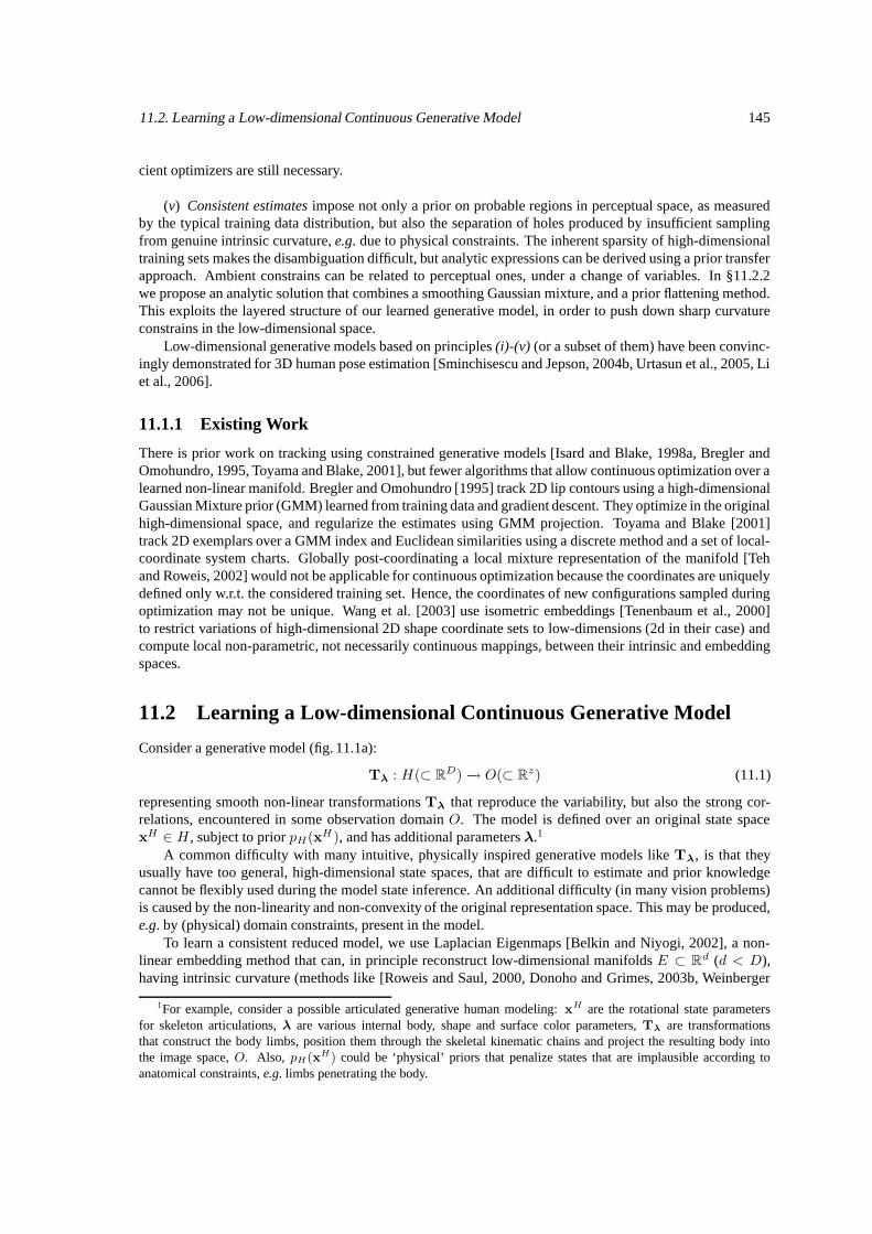
11.2. Learning a Low-dimensional Continuous Generative Model 145
cient optimizers are still necessary.
(v) Consistent estimates impose not only a prior on probable regions in perceptual space, as measuredby the typical training data distribution, but also the separation of holes produced by insufficient samplingfrom genuine intrinsic curvature, e.g. due to physical constraints. The inherent sparsity of high-dimensionaltraining sets makes the disambiguation difficult, but analytic expressions can be derived using a prior transferapproach. Ambient constrains can be related to perceptual ones, under a change of variables. In §11.2.2we propose an analytic solution that combines a smoothing Gaussian mixture, and a prior flattening method.This exploits the layered structure of our learned generative model, in order to push down sharp curvatureconstrains in the low-dimensional space.
Low-dimensional generative models based on principles (i)-(v) (or a subset of them) have been convinc-ingly demonstrated for 3D human pose estimation [Sminchisescu and Jepson, 2004b, Urtasun et al., 2005, Liet al., 2006].
11.1.1 Existing Work
There is prior work on tracking using constrained generative models [Isard and Blake, 1998a, Bregler andOmohundro, 1995, Toyama and Blake, 2001], but fewer algorithms that allow continuous optimization over alearned non-linear manifold. Bregler and Omohundro [1995] track 2D lip contours using a high-dimensionalGaussian Mixture prior (GMM) learned from training data and gradient descent. They optimize in the originalhigh-dimensional space, and regularize the estimates using GMM projection. Toyama and Blake [2001]track 2D exemplars over a GMM index and Euclidean similarities using a discrete method and a set of local-coordinate system charts. Globally post-coordinating a local mixture representation of the manifold [Tehand Roweis, 2002] would not be applicable for continuous optimization because the coordinates are uniquelydefined only w.r.t. the considered training set. Hence, the coordinates of new configurations sampled duringoptimization may not be unique. Wang et al. [2003] use isometric embeddings [Tenenbaum et al., 2000]to restrict variations of high-dimensional 2D shape coordinate sets to low-dimensions (2d in their case) andcompute local non-parametric, not necessarily continuous mappings, between their intrinsic and embeddingspaces.
11.2 Learning a Low-dimensional Continuous Generative Model
Consider a generative model (fig. 11.1a):
Tλ : H(⊂ RD) −→ O(⊂ Rz) (11.1)
representing smooth non-linear transformations Tλ that reproduce the variability, but also the strong cor-relations, encountered in some observation domain O. The model is defined over an original state spacexH ∈ H , subject to prior pH(xH ), and has additional parameters λ.1
A common difficulty with many intuitive, physically inspired generative models like Tλ, is that theyusually have too general, high-dimensional state spaces, that are difficult to estimate and prior knowledgecannot be flexibly used during the model state inference. An additional difficulty (in many vision problems)is caused by the non-linearity and non-convexity of the original representation space. This may be produced,e.g. by (physical) domain constraints, present in the model.
To learn a consistent reduced model, we use Laplacian Eigenmaps [Belkin and Niyogi, 2002], a non-linear embedding method that can, in principle reconstruct low-dimensional manifolds E ⊂ Rd (d < D),having intrinsic curvature (methods like [Roweis and Saul, 2000, Donoho and Grimes, 2003b, Weinberger
1For example, consider a possible articulated generative human modeling: xH are the rotational state parametersfor skeleton articulations, λ are various internal body, shape and surface color parameters, Tλ are transformationsthat construct the body limbs, position them through the skeletal kinematic chains and project the resulting body intothe image space, O. Also, pH(xH) could be ‘physical’ priors that penalize states that are implausible according toanatomical constraints, e.g. limbs penetrating the body.
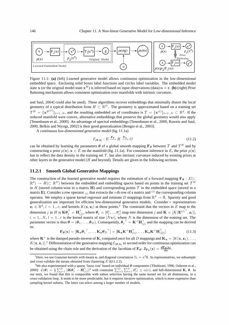
146 Chapter 11. A Non-linear Generative Model for Low-dimensional Inference
Figure 11.1: (a) (left) Learned generative model allows continuous optimization in the low-dimensionalembedded space. Enclosing solid boxes label functions and circles label variables. The embedded modelstate x (or the original model state xH ) is inferred based on input observations (data) o = r. (b) (right) Priorflattening mechanism allows consistent optimization over manifolds with intrinsic curvature.
and Saul, 2004] could also be used). These algorithms recover embeddings that minimally distort the localgeometry of a typical distribution from H ⊂ RD. The geometry is approximated based on a training set
T H = xH (t)t=1..N , and the resulting embedded set of coordinates is T = x(t)t=1..N ⊂ Rd. If thereduced manifold were convex, alternative embeddings that preserve the global geometry would also apply[Tenenbaum et al., 2000]. An advantage of spectral embeddings [Tenenbaum et al., 2000, Roweis and Saul,2000, Belkin and Niyogi, 2002] is their good generalization [Bengio et al., 2003].
A continuous low-dimensional generative model (fig. 11.1a)
E(θ,λ) : EFθ−−→ H
Tλ−−→ O (11.2)
can be obtained by learning the parameters θ of a global smooth mapping Fθ between T and T H and byconstructing a prior p(x),x ∈ E on the manifold (fig. 11.1a). For consistent inference in E, the prior p(x)has to reflect the data density in the training set T , but also intrinsic curvature induced by existing priors atother layers in the generative model (H and beyond). Details are given in the following sections.
11.2.1 Smooth Global Generative Mappings
The construction of the learned generative model requires the estimation of a forward mapping Fθ : E(⊂Rd) → H(⊂ RD) between the embedded and embedding spaces based on points in the training set T H
in H (stored column-wise in a matrix H) and corresponding points T in the embedded space (stored in amatrix E). Consider a row operator (i) that extracts the i-th row of a matrix and (i) the corresponding columnoperator. We employ a sparse kernel regressor and estimate D mappings from Rd → R. Sparsity and goodgeneralization are important for efficient low-dimensional generative models. Consider r representativeszl ∈ Rd, l = 1...r, and kernels K(x, zl) at these points.2 The constraint that the vectors in E map to the
dimension j in H is Kθ>j = H>
(j), where θj = [θ1j , ..., θrj ] map into dimension j and K = [K(E(i)>, zl)],
i = 1...N , l = 1...r is the kernel matrix of size [Nxr], where N is the dimension of the training set. Theparameter vector is thus θ = (θ1, . . . ,θD). Consequently, θj
> = K+H>(j) and the mapping can be derived
as:Fθ(x) = [Kxθ1
>, . . . ,KxθD>] = [KxK
+H>(1), . . . ,KxK
+H>(D)] (11.3)
where K+ is the damped pseudo-inverse of K, computed once for allD mappings and Kx = [K(x, z1), . . . ,K(x, zr)].3 Differentiation of the generative mapping E(θ,λ) to second order for continuous optimization can
be obtained using the chain rule and the derivation of the Jacobian of Fθ: JFθ(x) = dFθ(x)
dx.
2Here, we use Gaussian kernels with means zl and diagonal covariances Σl = σ2I. As representatives, we subsampleand cross-validate the means obtained from clustering E (§11.2.2).
3We also experimented with a sparse ‘lasso cost’ based on individual θ components [Tibshirani, 1996, Osborne et al.,2000]: L(θ) = 1
2
PD
j=1 ||Kθ>
j − H>
(j)||2 with constraint
PD
j=1
PN
l=1 |θlj | ≤ α(r), and full-dimensional K, θ. In
our tests, we found that this is comparable with subset selection having the same kernel set for all dimensions, in across-validation loop. It tends to be more predictable, but it requires iterative optimization, which is more expensive thansampling kernel subsets. The latter can select among a larger number of models.
11.2. Learning a Low-dimensional Continuous Generative Model 147
11.2.2 Layered Generative Priors
Consistent inference in the embedded space Rd requires a prior over the probable regions of the low-dimensional manifold E, determined by the training data density. Here we use a mixture prior pE(x) =∑K
k=1 πkKΣk(x,µk), where K are Gaussian kernels with parameters obtained by clustering the embedded
coordinates in the training set using k-means [Ng et al., 2001].4
Sampling artifacts and problem domain constraints may interact in a way that is difficult to separate inE. In particular, the constraints may generate unfeasible regions having intrinsic curvature. Geometricallythese will be holes, in both H and in E. For human kinematic representations based on joint angles xH , theintrinsic curvature is produced by the limits of articulations and by the body non-self intersection constraints.These exclude certain state variable combinations (see also §11.4). While for many domain models, analyticcharacterizations of unfeasible regions may be available (in H), directly separating sampling artifacts fromintrinsic curvature in E is nearly impossible, under general, unrestrictive, sampling assumptions. The reasonis that one cannot assume that e.g. the training data available in H has been sampled uniformly and / ordensely from the unknown E [Silva and Tenenbaum, 2002], and the prior pE is simply blind to such effects(i.e. it smooths them). In fact, it may assign unfeasible regions a moderately high probability, especially ifthese are surrounded by densely sampled zones.
Because the learned model E(θ,λ) is layered, sharper curvature constraints may be induced in the em-bedded space by existing priors in the original representation space, where these may be available in simpleanalytic form. For a layered continuous generative model E(θ,λ), one can exploit the modular structure ofits forward transformation chain. Since evaluation and differentiation of E(θ,λ) with respect to its state vari-ables is the main computational machinery of the model, analytic forms for intermediate function valuesand derivatives on the generative transformation chain are available. For a two-layer embedded-embedding
model slice EFθ−−→ H with x ∈ E, xH(= Fθ(x)) ∈ H and priors pE(x) and pH(xH ) respectively, we
combine the distribution over probable regions in E with flattened priors from the embedding space H :
p(x) ∝ pE(x) · pH(Fθ(x)) · |JFθ(x)>JFθ
(x)|1/2 (11.4)
(see fig. 11.1b). Notice that the resulting prior is not normalized and it requires a state-dependent Jacobianscaling factor. Analytically differentiating p(x) is possible, given pE, and the parametric form of the mappingFθ, from §11.2.1. The mechanism allows consistent inference in the embedded space E (see §11.3). Priorsat subsequent layers can be discarded, being already absorbed in p(x).
11.2.3 Computing Geodesics
The construction of geodesics can be framed as optimal inference where we synthesize a trajectory that issmooth and consistent with the prior p on the manifoldE. Assume a trajectory with endpoints x0,xT+1 ∈ E,and its discretization with T knots x = [x1, . . . ,xT ]. The energy function for geodesics can be writtenas: Vg(x) = −∑T
i=1 log p(xi) + xS>Sx>, where S is a first order difference operator square matrix ofdimension [Txd] consisting of T band-diagonal blocks of d-dimensional identity matrices [... − IdId...].Priors encoding higher degree of smoothness can be obtained by self-multiplication, e.g. for second order asS>S>SS, etc. The function Vg is differentiable and can be sampled or optimized for a local MAP solutionfrom a trivial initialization (e.g. points xi uniformly distributed on a straight line between x0 and xT+1).To avoid unrepresentative local optima, we initialize using Floyd’s dynamic programming algorithm (DP).This is run off-line to find all shortest paths on the set of mixture centers µi obtained from clustering E(see §11.2.2). This roadmap can be effectively used at geodesic query time: given known endpoints, linkto the closest mixture component at each end and use the precomputed road (see fig. 11.2(d) for an orientedbounded box decomposition used in nearest neighbor queries). The DP trajectory is then refined using theconsistent geodesic function Vg .
4The mixture centers will also be used in §11.2.3 for off-line estimation of a roadmap for initializing geodesic calcu-lations.
148 Chapter 11. A Non-linear Generative Model for Low-dimensional Inference
11.3 Temporal Inference
We apply Bayes rule to compute the ‘static’ total posterior probability over the learned manifold space Egiven (data) observation r: p(x|r) ∝ p(r|x) · p(x). Here, p(x) is the prior on the model state spaceand p(r|x) is the observation likelihood, that can be computed in terms of p(r|g(x) = Tλ(Fθ(x))),the probability of observation r as predicted by the generative model feature g at configuration x (seefig. 11.1a). For tracking using dynamic observations, the prior at time t combines the previous posteriorp(xt−1|Rt−1) and the dynamics p(xt|xt−1), where we have collected the observations at time t into vectorrt and defined Rt = r1, . . . , rt. The posterior at t becomes: p(xt|Rt) ∝ p(rt|xt) · p(xt|Rt−1), wherep(xt|Rt−1) =
∫xt−1
p(xt|xt−1) p(xt−1|Rt−1).5 Together, p(xt|xt−1) and p(xt−1|Rt−1) form the time tprior p(xt|Rt−1) for the static Bayes equation. To approximate the propagating density, we use CovarianceScaled Sampling (CSS) [Sminchisescu and Triggs, 2003b]. This probabilistic method represents the poste-rior distribution of hypotheses in state space p(xt|Rt), as a Gaussian mixture, whose weights, centers andcovariances are obtained as follows. Random samples are generated from the temporal prior p(xt|Rt−1),and each is optimized by nonlinear local optimization (respecting any prior constraints, etc.) to maximizethe local posterior likelihood encoded by p(rt|xt). The optimized likelihood value and position gives theweight and center of a new component, and the inverse Hessian of the log-likelihood gives a scale matrix thatis well adapted to the contours of the cost function, even for very ill-conditioned problems like monocularhuman tracking. The likelihood and temporal prior distributions are then composed and pruned to a max-imum number of mixture components, in order to produce the posterior p(xt|Rt) for the current timestep(see [Sminchisescu and Triggs, 2003b] for details).
11.4 Learning Human State Representations for Visual Tracking
Representation Learning is based on a physically inspired 3D body model that consists of a kinematic‘skeleton’ of articulated joints controlled by angular joint variables, covered by a ‘flesh’ built from su-perquadric ellipsoids with deformations. The model has internal proportions, shape and surface color pa-rameters λ. The state space consists of 29 joint angle variables (for shoulder, elbow, hip, knee joints, etc.)and 6d global rigid motion variables xR, encoded in the state xH . We learn a low-dimensional representa-tion x ∈ E for training vector slices of xH , that do not include the rigid components xR, using manifoldembedding on a set of body joint angle training data, obtained with a motion capture system (courtesy of themotion capture database at the CMU graphics laboratory [cmu, 2003]). We estimate a mixture model for Eby k-means clustering the embedded eigenvectors, to build the prior pE(x). We also learn the parameters θ
of a forward mapping Fθ into the original joint angle space using Gaussian kernel regression. In use, modelsuperquadric surfaces are discretized into 2D meshes and the mesh nodes (and their colors, updated aftereach tracked image, e.g. by texture mapping) are mapped to 3D points using knowledge of the kinematicstate variables predicted at configuration xH by Fθ(x). These map to each body kinematic chain and thenpredict image positions and pixel colors, using perspective image projection, transformations that are all en-coded in Tλ(xH ) 6. The Observation Model is based on sums of predicted-to-image matching likelihoods(and their gradient and Hessian metrics) evaluated for each model feature prediction g. As image features, weuse a robust combination of intensity-based alignment metrics, silhouettes and robustified normalized edgedistances [Sminchisescu and Triggs, 2003b]. Flattened Layered Priors consist of soft joint angle limits andbody non self-intersection constraints [Sminchisescu and Triggs, 2003b]. For the experiments here, we work
5Here p(xt|xt−1) ∝ ps(xt)pd(xt|xt−1) will encode both simple dynamic rules pd and a prior ps in order to ensurethe dynamics remains inside the feasible manifold region. We use the prior p on the manifold (§11.2.2) as ps.
6The 6d global rigid state representation xR is not learned using embedding because people can move in any di-rections and can be seen from any viewpoint, so it is restrictive to learn preferential subspaces for global translation orrotation. This implies that this slice of variables, although part of the inferred state, is mapped by Tλ, and not by E(θ,λ).This is simply a technicality and we avoided making it explicit for notational simplicity. In practice, we do inferenceover an augmented hidden state (x,xR) (embedded coordinate + global rigid motion) and therefore need to add a trivialidentity component to Fθ for the map g = Tλ(xH = (Fθ(x),xR)).
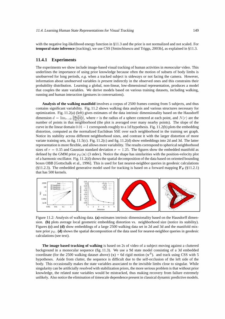
11.4. Learning Human State Representations for Visual Tracking 149
with the negative log-likelihood energy function in §11.3 and the prior is not normalized and not scaled. Fortemporal state inference (tracking), we use CSS [Sminchisescu and Triggs, 2003b], as explained in §11.3.
11.4.1 Experiments
The experiments we show include image-based visual tracking of human activities in monocular video. Thisunderlines the importance of using prior knowledge because often the motion of subsets of body limbs isunobserved for long periods, e.g. when a tracked subject is sideways or not facing the camera. However,information about unobserved variables is present indirectly in the observed ones and this constrains theirprobability distribution. Learning a global, non-linear, low-dimensional representation, produces a modelthat couples the state variables. We derive models based on various training datasets, including walking,running and human interaction (gestures in conversations).
Analysis of the walking manifold involves a corpus of 2500 frames coming from 5 subjects, and thuscontains significant variability. Fig. 11.2 shows walking data analysis and various structures necessary foroptimization. Fig. 11.2(a) (left) gives estimates of the data intrinsic dimensionality based on the Hausdorffdimension d = limr→0
log N(r)log(1/r) , where r is the radius of a sphere centered at each point, and N(r) are the
number of points in that neighborhood (the plot is averaged over many nearby points). The slope of thecurve in the linear domain 0.01−1 corresponds roughly to a 1d hypothesis. Fig. 11.2(b) plots the embeddingdistortion, computed as the normalized Euclidean SSE over each neighborhood in the training set graph.Notice its stability across different neighborhood sizes, and contrast it with the larger distortion of morevariate training sets, in fig. 11.5(c). Fig. 11.2(c) and fig. 11.2(d) show embeddings into 2d and 3d. The latterrepresentation is more flexible, and allows more variability. The results correspond to spherical neighborhoodsizes of r = 0.35 and Gaussian standard deviation σ = 1.25. The figures show the embedded manifold asdefined by the GMM prior pE(x) (3 stdev). Notice the shape has similarities with the position-velocity plotof a harmonic oscillator. Fig. 11.2(d) shows the spatial decomposition of the data based on oriented boundingboxes OBB [Gottschalk et al., 1996]. This is used for fast nearest-neighbor queries in geodesic calculations(§11.2.3). The embedded generative model used for tracking is based on a forward mapping Fθ (§11.2.1)that has 500 kernels.
1e-06
0.0001
0.01
1
100
10000
0.001 0.01 0.1 1
N(r
)
r
Data1D hypothesis2D hypothesis3D hypothesis
0 0.05 0.1
0.15 0.2
0.25 0.3
0.35 0.4
0.45 0.5
0.55
1 2 3 4 5 6
Dis
tance d
isto
rtio
n
Dimension
r=0.25r=0.3
r=0.35r=0.4
Figure 11.2: Analysis of walking data. (a) estimates intrinsic dimensionality based on the Hausdorff dimen-sion. (b) plots average local geometric embedding distortion vs. neighborhood size (notice its stability).Figures (c) and (d) show embeddings of a large 2500 walking data set in 2d and 3d and the manifold mix-ture prior pE . (d) shows the spatial decomposition of the data used for nearest-neighbor queries in geodesiccalculations (see text).
The image based tracking of walking is based on 2s of video of a subject moving against a clutteredbackground in a monocular sequence (fig. 11.3). We use a 9d state model consisting of a 3d embeddedcoordinate (for the 2500 walking dataset above) (x) + 6d rigid motion (xR). and track using CSS with 5hypotheses. Aside from clutter, the sequence is difficult due to the self-occlusion of the left side of thebody. This occasionally makes the state variables associated to the invisible limbs close to singular. Whilesingularity can be artificially resolved with stabilization priors, the more serious problem is that without priorknowledge, the related state variables would be mistracked, thus making recovery from failure extremelyunlikely. Also notice the elimination of timescale dependence present in classical dynamic predictive models.
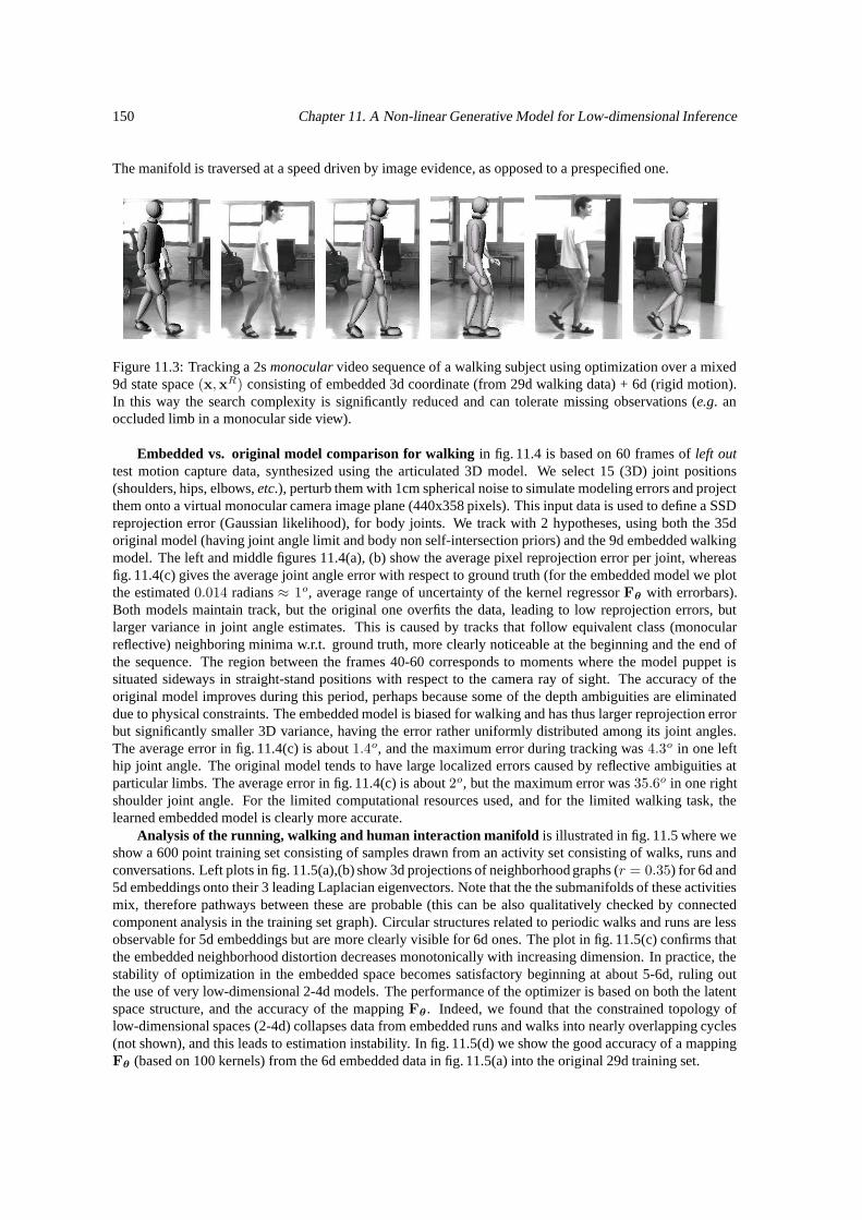
150 Chapter 11. A Non-linear Generative Model for Low-dimensional Inference
The manifold is traversed at a speed driven by image evidence, as opposed to a prespecified one.
Figure 11.3: Tracking a 2s monocular video sequence of a walking subject using optimization over a mixed9d state space (x,xR) consisting of embedded 3d coordinate (from 29d walking data) + 6d (rigid motion).In this way the search complexity is significantly reduced and can tolerate missing observations (e.g. anoccluded limb in a monocular side view).
Embedded vs. original model comparison for walking in fig. 11.4 is based on 60 frames of left outtest motion capture data, synthesized using the articulated 3D model. We select 15 (3D) joint positions(shoulders, hips, elbows, etc.), perturb them with 1cm spherical noise to simulate modeling errors and projectthem onto a virtual monocular camera image plane (440x358 pixels). This input data is used to define a SSDreprojection error (Gaussian likelihood), for body joints. We track with 2 hypotheses, using both the 35doriginal model (having joint angle limit and body non self-intersection priors) and the 9d embedded walkingmodel. The left and middle figures 11.4(a), (b) show the average pixel reprojection error per joint, whereasfig. 11.4(c) gives the average joint angle error with respect to ground truth (for the embedded model we plotthe estimated 0.014 radians ≈ 1o, average range of uncertainty of the kernel regressor Fθ with errorbars).Both models maintain track, but the original one overfits the data, leading to low reprojection errors, butlarger variance in joint angle estimates. This is caused by tracks that follow equivalent class (monocularreflective) neighboring minima w.r.t. ground truth, more clearly noticeable at the beginning and the end ofthe sequence. The region between the frames 40-60 corresponds to moments where the model puppet issituated sideways in straight-stand positions with respect to the camera ray of sight. The accuracy of theoriginal model improves during this period, perhaps because some of the depth ambiguities are eliminateddue to physical constraints. The embedded model is biased for walking and has thus larger reprojection errorbut significantly smaller 3D variance, having the error rather uniformly distributed among its joint angles.The average error in fig. 11.4(c) is about 1.4o, and the maximum error during tracking was 4.3o in one lefthip joint angle. The original model tends to have large localized errors caused by reflective ambiguities atparticular limbs. The average error in fig. 11.4(c) is about 2o, but the maximum error was 35.6o in one rightshoulder joint angle. For the limited computational resources used, and for the limited walking task, thelearned embedded model is clearly more accurate.
Analysis of the running, walking and human interaction manifold is illustrated in fig. 11.5 where weshow a 600 point training set consisting of samples drawn from an activity set consisting of walks, runs andconversations. Left plots in fig. 11.5(a),(b) show 3d projections of neighborhood graphs (r = 0.35) for 6d and5d embeddings onto their 3 leading Laplacian eigenvectors. Note that the the submanifolds of these activitiesmix, therefore pathways between these are probable (this can be also qualitatively checked by connectedcomponent analysis in the training set graph). Circular structures related to periodic walks and runs are lessobservable for 5d embeddings but are more clearly visible for 6d ones. The plot in fig. 11.5(c) confirms thatthe embedded neighborhood distortion decreases monotonically with increasing dimension. In practice, thestability of optimization in the embedded space becomes satisfactory beginning at about 5-6d, ruling outthe use of very low-dimensional 2-4d models. The performance of the optimizer is based on both the latentspace structure, and the accuracy of the mapping Fθ. Indeed, we found that the constrained topology oflow-dimensional spaces (2-4d) collapses data from embedded runs and walks into nearly overlapping cycles(not shown), and this leads to estimation instability. In fig. 11.5(d) we show the good accuracy of a mappingFθ (based on 100 kernels) from the 6d embedded data in fig. 11.5(a) into the original 29d training set.
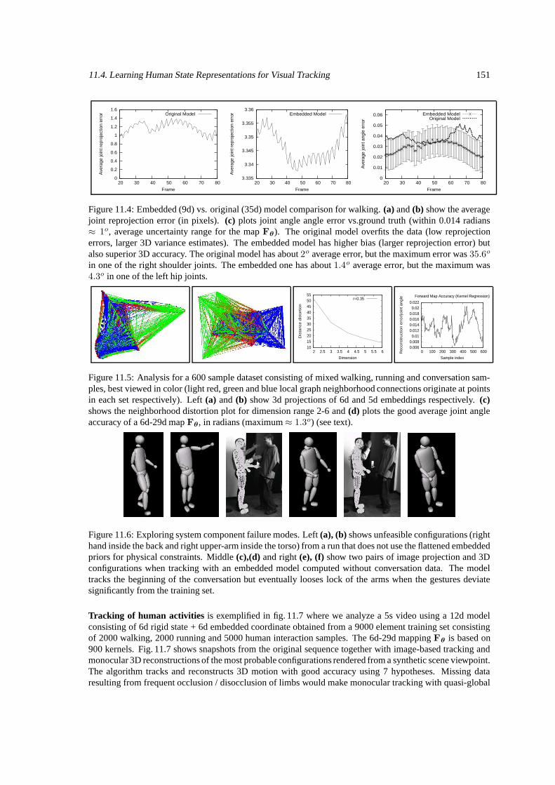
11.4. Learning Human State Representations for Visual Tracking 151
0
0.2
0.4
0.6
0.8
1
1.2
1.4
1.6
20 30 40 50 60 70 80
Ave
rage
join
t rep
roje
ctio
n er
ror
Frame
Original Model
3.335
3.34
3.345
3.35
3.355
3.36
20 30 40 50 60 70 80
Ave
rage
join
t rep
roje
ctio
n er
ror
Frame
Embedded Model
0
0.01
0.02
0.03
0.04
0.05
0.06
20 30 40 50 60 70 80
Ave
rage
join
t ang
le e
rror
Frame
Embedded ModelOriginal Model
Figure 11.4: Embedded (9d) vs. original (35d) model comparison for walking. (a) and (b) show the averagejoint reprojection error (in pixels). (c) plots joint angle angle error vs.ground truth (within 0.014 radians≈ 1o, average uncertainty range for the map Fθ). The original model overfits the data (low reprojectionerrors, larger 3D variance estimates). The embedded model has higher bias (larger reprojection error) butalso superior 3D accuracy. The original model has about 2o average error, but the maximum error was 35.6o
in one of the right shoulder joints. The embedded one has about 1.4o average error, but the maximum was4.3o in one of the left hip joints.
10 15 20 25 30 35 40 45 50 55
2 2.5 3 3.5 4 4.5 5 5.5 6
Dis
tan
ce d
isto
rtio
n
Dimension
r=0.35
0.006 0.008 0.01
0.012 0.014 0.016 0.018 0.02
0.022
0 100 200 300 400 500 600Re
con
stru
ctio
n e
rro
r/jo
int
an
gle
Sample index
Forward Map Accuracy (Kernel Regression)
Figure 11.5: Analysis for a 600 sample dataset consisting of mixed walking, running and conversation sam-ples, best viewed in color (light red, green and blue local graph neighborhood connections originate at pointsin each set respectively). Left (a) and (b) show 3d projections of 6d and 5d embeddings respectively. (c)shows the neighborhood distortion plot for dimension range 2-6 and (d) plots the good average joint angleaccuracy of a 6d-29d map Fθ, in radians (maximum≈ 1.3o) (see text).
Figure 11.6: Exploring system component failure modes. Left (a), (b) shows unfeasible configurations (righthand inside the back and right upper-arm inside the torso) from a run that does not use the flattened embeddedpriors for physical constraints. Middle (c),(d) and right (e), (f) show two pairs of image projection and 3Dconfigurations when tracking with an embedded model computed without conversation data. The modeltracks the beginning of the conversation but eventually looses lock of the arms when the gestures deviatesignificantly from the training set.
Tracking of human activities is exemplified in fig. 11.7 where we analyze a 5s video using a 12d modelconsisting of 6d rigid state + 6d embedded coordinate obtained from a 9000 element training set consistingof 2000 walking, 2000 running and 5000 human interaction samples. The 6d-29d mapping Fθ is based on900 kernels. Fig. 11.7 shows snapshots from the original sequence together with image-based tracking andmonocular 3D reconstructions of the most probable configurations rendered from a synthetic scene viewpoint.The algorithm tracks and reconstructs 3D motion with good accuracy using 7 hypotheses. Missing dataresulting from frequent occlusion / disocclusion of limbs would make monocular tracking with quasi-global
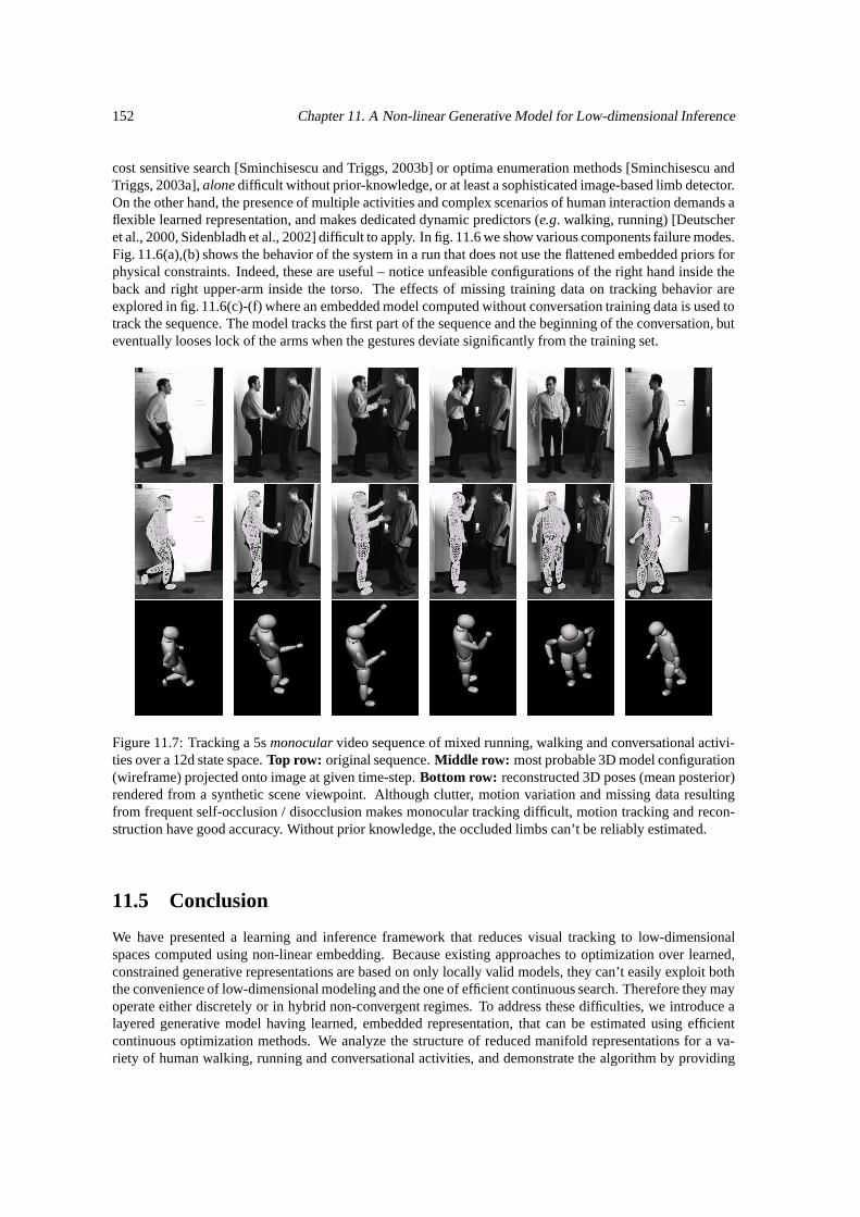
152 Chapter 11. A Non-linear Generative Model for Low-dimensional Inference
cost sensitive search [Sminchisescu and Triggs, 2003b] or optima enumeration methods [Sminchisescu andTriggs, 2003a], alone difficult without prior-knowledge, or at least a sophisticated image-based limb detector.On the other hand, the presence of multiple activities and complex scenarios of human interaction demands aflexible learned representation, and makes dedicated dynamic predictors (e.g. walking, running) [Deutscheret al., 2000, Sidenbladh et al., 2002] difficult to apply. In fig. 11.6 we show various components failure modes.Fig. 11.6(a),(b) shows the behavior of the system in a run that does not use the flattened embedded priors forphysical constraints. Indeed, these are useful – notice unfeasible configurations of the right hand inside theback and right upper-arm inside the torso. The effects of missing training data on tracking behavior areexplored in fig. 11.6(c)-(f) where an embedded model computed without conversation training data is used totrack the sequence. The model tracks the first part of the sequence and the beginning of the conversation, buteventually looses lock of the arms when the gestures deviate significantly from the training set.
Figure 11.7: Tracking a 5s monocular video sequence of mixed running, walking and conversational activi-ties over a 12d state space. Top row: original sequence. Middle row: most probable 3D model configuration(wireframe) projected onto image at given time-step. Bottom row: reconstructed 3D poses (mean posterior)rendered from a synthetic scene viewpoint. Although clutter, motion variation and missing data resultingfrom frequent self-occlusion / disocclusion makes monocular tracking difficult, motion tracking and recon-struction have good accuracy. Without prior knowledge, the occluded limbs can’t be reliably estimated.
11.5 Conclusion
We have presented a learning and inference framework that reduces visual tracking to low-dimensionalspaces computed using non-linear embedding. Because existing approaches to optimization over learned,constrained generative representations are based on only locally valid models, they can’t easily exploit boththe convenience of low-dimensional modeling and the one of efficient continuous search. Therefore they mayoperate either discretely or in hybrid non-convergent regimes. To address these difficulties, we introduce alayered generative model having learned, embedded representation, that can be estimated using efficientcontinuous optimization methods. We analyze the structure of reduced manifold representations for a va-riety of human walking, running and conversational activities, and demonstrate the algorithm by providing
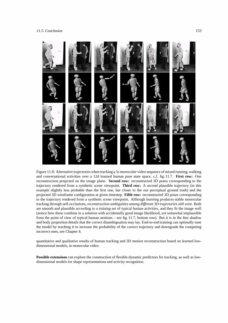
11.5. Conclusion 153
Figure 11.8: Alternative trajectories when tracking a 5s monocular video sequence of mixed running, walkingand conversational activities over a 12d learned human pose state space, c.f . fig. 11.7. First row: Onereconstruction projected on the image plane. Second row: reconstructed 3D poses corresponding to thetrajectory rendered from a synthetic scene viewpoint. Third row: A second plausible trajectory (in thisexample slightly less probable than the first one, but closer to the our perceptual ground truth) and theprojected 3D wireframe configuration at given timestep. Fifth row: reconstructed 3D poses correspondingto the trajectory rendered from a synthetic scene viewpoint. Although learning produces stable monoculartracking through self-occlusions, reconstruction ambiguities among different 3D trajectories still exist. Bothare smooth and plausible according to a training set of typical human activities, and they fit the image well(notice how these combine in a solution with accidentally good image likelihood, yet somewhat implausiblefrom the point of view of typical human motions – see fig. 11.7, bottom row). But it is in the fine shadowand body proportion details that the correct disambiguation may lay. End-to-end training can optimally tunethe model by teaching it to increase the probability of the correct trajectory and downgrade the competingincorrect ones, see Chapter 4.
quantitative and qualitative results of human tracking and 3D motion reconstruction based on learned low-dimensional models, in monocular video.
Possible extensions can explore the construction of flexible dynamic predictors for tracking, as well as low-dimensional models for shape representations and activity recognition.
Chapter 12
People Tracking with theNon-parametric Laplacian EigenmapsLatent Variable Model
Reliably recovering 3D human pose from monocular video requires constraints that bias the estimates to-wards typical human poses and motions. We define priors for people tracking using a Non-parametricLaplacian Eigenmaps Latent Variable Model (LELVM). LELVM is a probabilistic dimensionality reduc-tion model that combines the advantages of latent variable models—definining a multimodal probabilitydensity for latent and observed variables, and globally differentiable nonlinear mappings for reconstructionand dimensionality reduction—with those of spectral manifold learning methods—no local optima, abilityto unfold highly nonlinear manifolds, and good practical scaling to latent spaces of high dimension. LELVMis computationally efficient, simple to learn from sparse training data, and compatible with standard proba-bilistic trackers such as particle filters. We analyze the performance of a LELVM-based probabilistic sigmapoint mixture tracker in several real and synthetic human motion sequences and demonstrate that LELVMprovides sufficient constraints for robust operation in the presence of missing, noisy and ambiguous imagemeasurements. The works appearst at Neural Information Processing Systems (NIPS) [Lu, Perpinan andSminchisescu, 2007].
12.1 Low-dimensional Models
Recent research in reconstructing articulated human motion has focused on methods that can exploit avail-able prior knowledge on typical human poses or motions in an attempt to build more reliable algorithms. Thehigh-dimensionality of human ambient pose space—between 30-60 joint angles or joint positions dependingon the desired accuracy level, makes exhaustive search prohibitively expensive. This has negative impact onexisting trackers, which are often not sufficiently reliable at reconstructing human-like poses, self-initializingor recovering from failure. Such difficulties have stimulated research in algorithms and models that reducethe effective working space, either using generic search focusing methods (annealing, state space decompo-sition, covariance scaling) or by exploiting specific problem structure (e.g. kinematic jumps). Experiencewith these procedures has nevertheless shown that any search strategy, no matter how effective, can be madesignificantly more reliable if restricted to low-dimensional state spaces. This permits a more thorough ex-ploration of the typical solution space, for a given comparable computational effort as a high-dimensionalmethod. The argument correlates well with the belief that the human pose space, although high-dimensionalin its natural ambient parameterization, has a significantly lower perceptual (latent or intrinsic) dimensional-ity, at least in a practical sense—many poses that are possible are so improbable in many real-world situationsthat it pays-off to encode them with low accuracy.
A perceptual representation has to be sufficiently powerful to capture the diversity of human poses in a
154
12.2. Priors for Articulated Human Pose 155
sufficiently broad domain of applicability (the task domain), yet compact and analytically tractable for searchand optimization. This justifies the use of models that are non-linear and low-dimensional (capable at unfold-ing highly non-linear manifolds with low-distortion), yet probabilistically motivated and globally continuousfor efficient optimization. Reducing dimensionality is not the only goal: perceptual representations have topreserve critical properties of the ambient space. A necessary feature for reliable tracking is locality: nearbyregions in ambient space have to be mapped to nearby regions in latent space. If this doesn’t hold, the trackeris forced to make unrealistically large, and difficult to predict jumps in latent space in order to follow smoothtrajectories in the joint angle ambient space.
In this chapter we propose to model priors for articulated motion using a probabilistic dimensionalityreduction method, the Non-parametric Laplacian Eigenmaps Latent Variable Model (LELVM). Section 12.2discusses the requirements of priors for articulated motion in the context of probabilistic and spectral methodsfor manifold learning, and section 12.3 describes LELVM and shows how it combines both types of methodsin a principled way and shares the advantages of both. Section 12.4 describes our tracking framework (usinga particle filter) and section 12.5 shows experiments with synthetic and real human motion sequences usingLELVM priors learned from motion-capture data.
Related work: Deriving compact prior representations for tracking people—or more generally, articulatedobjects, is an active research field, steadily growing with the increased availability of human motion cap-ture data [cmu, 2003]. Howe et al. [1999] propose Gaussian mixture representations of short human motionfragments (snippets) and integrate them in a Bayesian MAP estimation framework that uses 2D human jointmeasurements, independently tracked by a scaled prismatic model [Cham and Rehg, 1999]. Brand [1999]models the human pose manifold using a Gaussian mixture and uses a Hidden Markov Model to infer themixture component index based on a temporal sequence of human silhouettes. Sidenbladh et al. [2002] usesimilar dynamic priors and exploit ideas in texture synthesis—efficient nearest-neighbor search for similarmotion fragments at runtime—in order to build a particle-filter tracker with observation model based oncontour and image intensity measurements. Sminchisescu and Jepson [2004b] propose a low-dimensionalprobabilistic model based on fitting a parametric reconstruction mapping (sparse radial basis function) and aparametric latent density (Gaussian mixture) to the embedding produced with the Laplacian eigenmaps – thisis essentially a parametric alternative to the the model described here and shares similar advantages. Theytrack humans walking and involved in conversations using a Bayesian multiple hypotheses framework thatfuses contour and intensity measurements. Urtasun et al. [2005] use a Gaussian Process Probabilistic PCALatent Variable model and a dynamic MAP estimation framework based on 2D human joint correspondencesobtained from an independent image-based tracker. Li et al. [2006] use a coordinated mixture of factor an-alyzers within a particle filtering framework, in order to reconstruct human motion in multiple views usingchamfer matching to score different configuration. Jaeggli et al. [2006] use a mixture of view-dependentmodels in order to represent the time-varying appearance of the human body pose and track based on silhou-ettes in a particle filtering framework. Our work complements and extends the existing studies: we introducea different model, analyze its ability to work with real or partially missing data and its competence at trackingmultiple activities.
12.2 Priors for Articulated Human Pose
We consider the problem of learning a probabilistic low-dimensional model of human articulated motion.Call y ∈ RD the representation in ambient space of the articulated pose of a person. In this chapter, y
contains the 3D locations of anywhere between 10 and 60 markers located on the person’s joints (otherrepresentations such as joint angles are also possible). The values of y have been normalised for translationand rotation in order to remove rigid motion and leave only the articulated motion (see section 12.4 for howwe track the rigid motion). While y is high-dimensional, the motion pattern lives in a low-dimensionalmanifold because most values of y yield poses that violate body constraints or are simply atypical for themotion type considered. Thus we want to model y in terms of a small number of latent variables x given acollection of poses ynNn=1 (recorded from a human with motion-capture technology). The model should
156 Chapter 12. People Tracking with the Non-parametric Laplacian Eigenmaps Latent Variable Model
satisfy the following: (1) It should define a probability density for x and y, to be able to deal with noise(in the image or marker measurements) and uncertainty (from missing data due to occlusion or markers thatdrop), and to allow integration in a sequential Bayesian estimation framework. The density model shouldalso be flexible enough to represent multimodal densities. (2) It should define mappings for dimensionalityreduction F : y → x and reconstruction f : x→ y that apply to any value of x and y (not just those in thetraining set), and such mappings should be defined on a global coordinate system, be continuous (to avoidphysically impossible discontinuities) and differentiable (to allow efficient optimisation when tracking), yetflexible enough to represent the highly nonlinear manifold of articulated poses. From a statistical machinelearning point of view, this is precisely what latent variable models (LVMs) do; for example, factor analysisdefines linear mappings and Gaussian densities, while the generative topographic mapping (GTM; [Bishopet al., 1998a]) defines nonlinear mappings and a Gaussian-mixture density in ambient space. However,factor analysis is too limited to be of practical use, and GTM—while flexible—has two important practicalproblems: (1) the latent space must be discretised to allow tractable learning and inference, which limits itto very low (2–3) latent dimensions; (2) the parameter estimation is prone to bad local optima that result inhighly distorted mappings.
Another dimensionality reduction method recently introduced, GPLVM [Lawrence, 2005], which uses aGaussian process mapping f(x), partly improves this situation by defining a tunable parameter xn for eachdata point yn. While still prone to local optima, this allows the use of a better initialisation for xnNn=1
(obtained from a spectral method, see later). This has prompted the application of GPLVM for trackinghuman motion [Urtasun et al., 2005]. However, GPLVM has some disadvantages: its training is very costly(each step of the gradient iteration is cubic on the number of training pointsN , though approximations basedon using few points exist); it defines neither a posterior distribution in latent space nor a dimensionalityreduction mapping; and the latent representation it obtains is not ideal. For example, for periodic motionssuch as running or walking, repeated periods (identical up to small noise) can be mapped apart from eachother in latent space because nothing constrains xn and xm to be close even when yn = ym (see fig. 3 and[Urtasun et al., 2006]).
There exists a different type of dimensionality reduction methods, spectral methods (such as Isomap[Tenenbaum et al., 2000], LLE [Roweis and Saul, 2000] or Laplacian eigenmaps [Belkin and Niyogi, 2002]),that have advantages and disadvantages complementary to those of LVMs. They define neither mappingsnor densities but just a correspondence (xn,yn) between points in latent space xn and ambient space yn.However, the training is efficient (a sparse eigenvalue problem) and has no local optima, and often yieldsa correspondence that successfully models highly nonlinear, convoluted manifolds such as the Swiss roll.While these attractive properties have spurred recent research in spectral methods, their lack of mappingsand densities has limited their applicability in people tracking. This chapter, as well as Ch. 11 and 13 explorevarious models that combine the advantages of LVMs and spectral methods in a principled way.
12.3 The Non-parametric Laplacian Eigenmaps Latent Variable Model(NLELVM)
NLELVM is based on a natural way of defining an out-of-sample mapping for Laplacian eigenmaps (LE)which, in addition, results in a density model. In LE, typically we first define a k-nearest-neighbour graphon the sample data ynNn=1 and weigh each edge yn ∼ ym by a Gaussian affinity function K(yn,ym) =wnm = exp (− 1
2 ||(yn − ym)/σ||2). Then the latent points xnNn=1 ⊂ RL result from:
minX∈RL×N
Trace(XLX>
)s.t. XDX> = I,XD1 = 0 (12.1)
where we define the matrix XL×N = (x1, . . . ,xN ), the symmetric affinity matrix WN×N , the degree matrixD = diag
∑Nn=1 wnm, the graph Laplacian matrix L = D −W, and 1 = (1, . . . , 1)>. The constraints
eliminate the two trivial solutions X = 0 (by setting an arbitrary scale) and x1 = · · · = xN (by removing1, which is an eigenvector of L associated with a zero eigenvalue). The solution is given by the leadingu2, . . . ,uL+1 eigenvectors of the normalised affinity matrix N = D− 1
2 WD− 12 , namely X = V>D− 1
2
with VN×L = (v2, . . . ,vL+1) (an a posteriori translated, rotated or uniformly scaled X is equally valid).
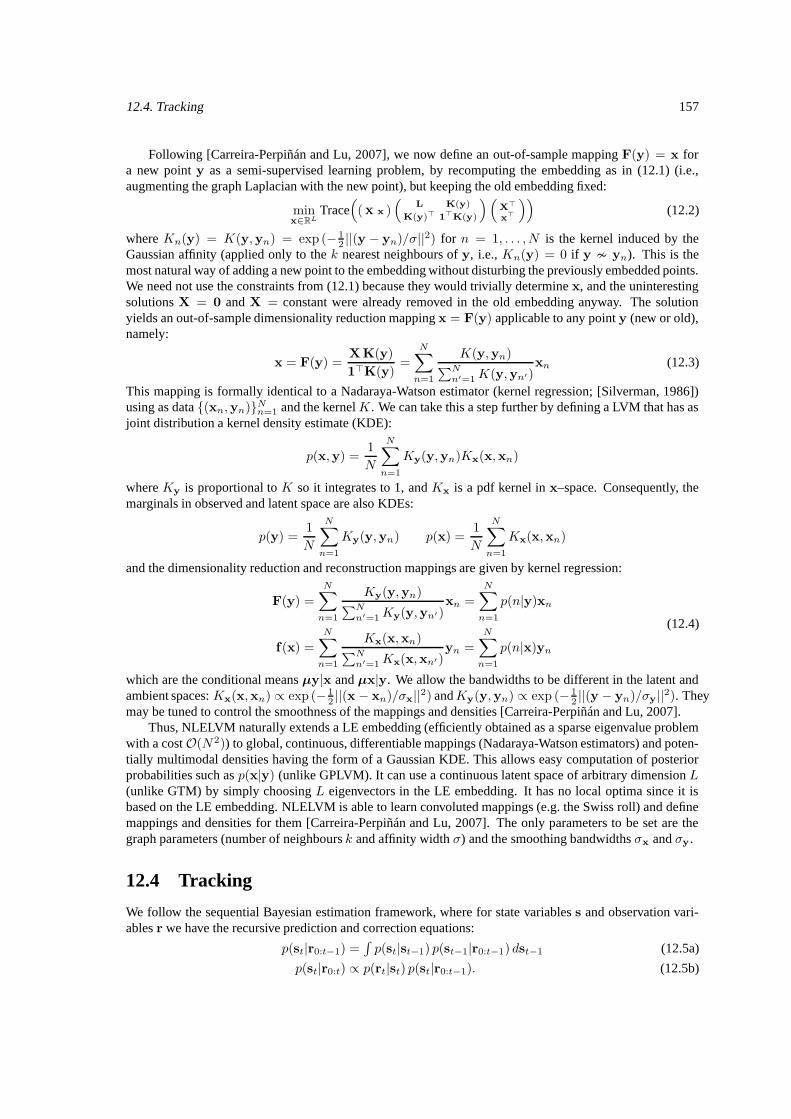
12.4. Tracking 157
Following [Carreira-Perpiñán and Lu, 2007], we now define an out-of-sample mapping F(y) = x fora new point y as a semi-supervised learning problem, by recomputing the embedding as in (12.1) (i.e.,augmenting the graph Laplacian with the new point), but keeping the old embedding fixed:
minx∈RL
Trace(( X x )
(L K(y)
K(y)> 1>K(y)
)(X>
x>
))(12.2)
where Kn(y) = K(y,yn) = exp (− 12 ||(y − yn)/σ||2) for n = 1, . . . , N is the kernel induced by the
Gaussian affinity (applied only to the k nearest neighbours of y, i.e., Kn(y) = 0 if y yn). This is themost natural way of adding a new point to the embedding without disturbing the previously embedded points.We need not use the constraints from (12.1) because they would trivially determine x, and the uninterestingsolutions X = 0 and X = constant were already removed in the old embedding anyway. The solutionyields an out-of-sample dimensionality reduction mapping x = F(y) applicable to any point y (new or old),namely:
x = F(y) =XK(y)
1>K(y)=
N∑
n=1
K(y,yn)∑N
n′=1 K(y,yn′)xn (12.3)
This mapping is formally identical to a Nadaraya-Watson estimator (kernel regression; [Silverman, 1986])using as data (xn,yn)Nn=1 and the kernelK. We can take this a step further by defining a LVM that has asjoint distribution a kernel density estimate (KDE):
p(x,y) =1
N
N∑
n=1
Ky(y,yn)Kx(x,xn)
where Ky is proportional to K so it integrates to 1, and Kx is a pdf kernel in x–space. Consequently, themarginals in observed and latent space are also KDEs:
p(y) =1
N
N∑
n=1
Ky(y,yn) p(x) =1
N
N∑
n=1
Kx(x,xn)
and the dimensionality reduction and reconstruction mappings are given by kernel regression:
F(y) =
N∑
n=1
Ky(y,yn)∑N
n′=1Ky(y,yn′ )xn =
N∑
n=1
p(n|y)xn
f(x) =
N∑
n=1
Kx(x,xn)∑N
n′=1Kx(x,xn′ )yn =
N∑
n=1
p(n|x)yn
(12.4)
which are the conditional means µy|x and µx|y. We allow the bandwidths to be different in the latent andambient spaces: Kx(x,xn) ∝ exp (− 1
2 ||(x − xn)/σx||2) andKy(y,yn) ∝ exp (− 12 ||(y − yn)/σy||2). They
may be tuned to control the smoothness of the mappings and densities [Carreira-Perpiñán and Lu, 2007].Thus, NLELVM naturally extends a LE embedding (efficiently obtained as a sparse eigenvalue problem
with a costO(N2)) to global, continuous, differentiable mappings (Nadaraya-Watson estimators) and poten-tially multimodal densities having the form of a Gaussian KDE. This allows easy computation of posteriorprobabilities such as p(x|y) (unlike GPLVM). It can use a continuous latent space of arbitrary dimension L(unlike GTM) by simply choosing L eigenvectors in the LE embedding. It has no local optima since it isbased on the LE embedding. NLELVM is able to learn convoluted mappings (e.g. the Swiss roll) and definemappings and densities for them [Carreira-Perpiñán and Lu, 2007]. The only parameters to be set are thegraph parameters (number of neighbours k and affinity width σ) and the smoothing bandwidths σx and σy.
12.4 Tracking
We follow the sequential Bayesian estimation framework, where for state variables s and observation vari-ables r we have the recursive prediction and correction equations:
p(st|r0:t−1) =∫p(st|st−1) p(st−1|r0:t−1) dst−1 (12.5a)
p(st|r0:t) ∝ p(rt|st) p(st|r0:t−1). (12.5b)
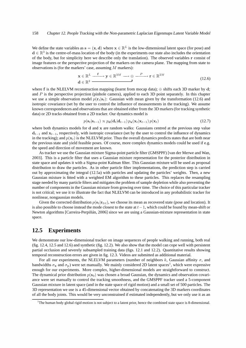
158 Chapter 12. People Tracking with the Non-parametric Laplacian Eigenmaps Latent Variable Model
We define the state variables as s = (x,d) where x ∈ RL is the low-dimensional latent space (for pose) andd ∈ R3 is the centre-of-mass location of the body (in the experiments our state also includes the orientationof the body, but for simplicity here we describe only the translation). The observed variables r consist ofimage features or the perspective projection of the markers on the camera plane. The mapping from state toobservations is (for the markers’ case, assuming M markers):
x ∈ RL f−−−−→ y ∈ R3M −−→ ⊕ P−−−−−→ r ∈ R2M
d ∈ R3(12.6)
where f is the NLELVM reconstruction mapping (learnt from mocap data); ⊕ shifts each 3D marker by d;and P is the perspective projection (pinhole camera), applied to each 3D point separately. In this chapterwe use a simple observation model p(rt|st): Gaussian with mean given by the transformation (12.6) andisotropic covariance (set by the user to control the influence of measurements in the tracking). We assumeknown correspondences and observations that are obtained either from the 3D markers (for tracking syntheticdata) or 2D tracks obtained from a 2D tracker. Our dynamics model is
p(st|st−1) ∝ pd(dt|dt−1) px(xt|xt−1) p(xt) (12.7)
where both dynamics models for d and x are random walks: Gaussians centred at the previous step valuedt−1 and xt−1, respectively, with isotropic covariance (set by the user to control the influence of dynamicsin the tracking); and p(xt) is the NLELVM prior. Thus the overall dynamics predicts states that are both nearthe previous state and yield feasible poses. Of course, more complex dynamics models could be used if e.g.the speed and direction of movement are known.
As tracker we use the Gaussian mixture Sigma-point particle filter (GMSPPF) [van der Merwe and Wan,2003]. This is a particle filter that uses a Gaussian mixture representation for the posterior distribution instate space and updates it with a Sigma-point Kalman filter. This Gaussian mixture will be used as proposaldistribution to draw the particles. As in other particle filter implementations, the prediction step is carriedout by approximating the integral (12.5a) with particles and updating the particles’ weights. Then, a newGaussian mixture is fitted with a weighted EM algorithm to these particles. This replaces the resamplingstage needed by many particle filters and mitigates the problem of sample depletion while also preventing thenumber of components in the Gaussian mixture from growing over time. The choice of this particular trackeris not critical; we use it to illustrate the fact that NLELVM can be introduced in any probabilistic tracker fornonlinear, nongaussian models.
Given the corrected distribution p(st|r0:t), we choose its mean as recovered state (pose and location). Itis also possible to choose instead the mode closest to the state at t−1, which could be found by mean-shift orNewton algorithms [Carreira-Perpiñán, 2006] since we are using a Gaussian-mixture representation in statespace.
12.5 Experiments
We demonstrate our low-dimensional tracker on image sequences of people walking and running, both real(fig. 12.4, 12.5 and 12.6) and synthetic (fig. 12.2). We also show that the model can cope well with persistentpartial occlusion and severely subsampled training data (figs. 12.1 and 12.2). Quantitative results showingtemporal reconstruction errors are given in fig. 12.3. Videos are submitted as additional material.
For all our experiments, the NLELVM parameters (number of neighbors k, Gaussian affinity σ, andbandwidths σx and σy) were set manually. We mainly considered 2D latent spaces1, which were expressiveenough for our experiments. More complex, higher-dimensional models are straightforward to construct.The dynamical prior distribution p(s0) was chosen a broad Gaussian, the dynamics and observation covari-ance were set manually to control the tracking smoothness, and the GMSPPF tracker used a 5-componentGaussian mixture in latent space (and in the state space of rigid motion) and a small set of 500 particles. The3D representation we use is a 45-dimensional vector obtained by concatenating the 3D markers coordinatesof all the body joints. This would be very unconstrained if estimated independently, but we only use it as an
1The human body global rigid motion is not subject to a latent prior, hence the combined state space is 8-dimensional.
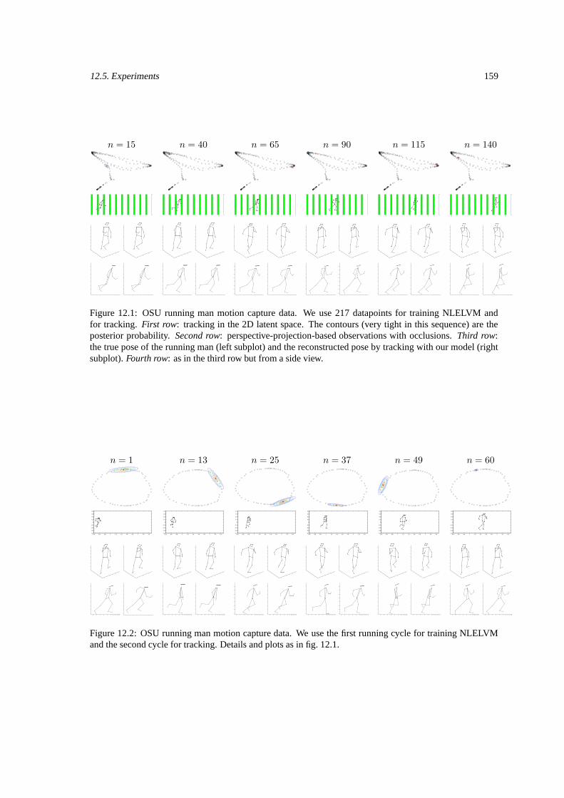
12.5. Experiments 159
n = 15 n = 40 n = 65 n = 90 n = 115 n = 140
−1.5
−1
−0.5
0
0.5
1
−1.5
−1
−0.5
0
0.5
1
−2
−1.5
−1
−0.5
0
0.5
1
1.5
−1.5
−1
−0.5
0
0.5
1
−1.5
−1
−0.5
0
0.5
1
−2
−1.5
−1
−0.5
0
0.5
1
1.5
−1.5
−1
−0.5
0
0.5
1
−1.5
−1
−0.5
0
0.5
1
−2
−1.5
−1
−0.5
0
0.5
1
1.5
−1.5
−1
−0.5
0
0.5
1
−1.5
−1
−0.5
0
0.5
1
−2
−1.5
−1
−0.5
0
0.5
1
1.5
−1.5
−1
−0.5
0
0.5
1
−1.5
−1
−0.5
0
0.5
1
−2
−1.5
−1
−0.5
0
0.5
1
1.5
−1.5
−1
−0.5
0
0.5
1
−1.5
−1
−0.5
0
0.5
1
−2
−1.5
−1
−0.5
0
0.5
1
1.5
−1.5
−1
−0.5
0
0.5
1
−1.5
−1
−0.5
0
0.5
1
−2
−1.5
−1
−0.5
0
0.5
1
1.5
−1.5
−1
−0.5
0
0.5
1
−1.5
−1
−0.5
0
0.5
1
−2
−1.5
−1
−0.5
0
0.5
1
1.5
−1.5
−1
−0.5
0
0.5
1
−1.5
−1
−0.5
0
0.5
1
−2
−1.5
−1
−0.5
0
0.5
1
1.5
−1.5
−1
−0.5
0
0.5
1
−1.5
−1
−0.5
0
0.5
1
−2
−1.5
−1
−0.5
0
0.5
1
1.5
−1.5
−1
−0.5
0
0.5
1
−1.5
−1
−0.5
0
0.5
1
−2
−1.5
−1
−0.5
0
0.5
1
1.5
−1.5
−1
−0.5
0
0.5
1
−1.5
−1
−0.5
0
0.5
1
−2
−1.5
−1
−0.5
0
0.5
1
1.5
−1.5 −1 −0.5 0 0.5 1 −1.5 −1 −0.5 0 0.5 1
−2
−1.5
−1
−0.5
0
0.5
1
1.5
−1.5 −1 −0.5 0 0.5 1 −1.5 −1 −0.5 0 0.5 1
−2
−1.5
−1
−0.5
0
0.5
1
1.5
−1.5 −1 −0.5 0 0.5 1 −1.5 −1 −0.5 0 0.5 1
−2
−1.5
−1
−0.5
0
0.5
1
1.5
−1.5 −1 −0.5 0 0.5 1 −1.5 −1 −0.5 0 0.5 1
−2
−1.5
−1
−0.5
0
0.5
1
1.5
−1.5 −1 −0.5 0 0.5 1 −1.5 −1 −0.5 0 0.5 1
−2
−1.5
−1
−0.5
0
0.5
1
1.5
−1.5 −1 −0.5 0 0.5 1 −1.5 −1 −0.5 0 0.5 1
−2
−1.5
−1
−0.5
0
0.5
1
1.5
−1.5 −1 −0.5 0 0.5 1 −1.5 −1 −0.5 0 0.5 1
−2
−1.5
−1
−0.5
0
0.5
1
1.5
−1.5 −1 −0.5 0 0.5 1 −1.5 −1 −0.5 0 0.5 1
−2
−1.5
−1
−0.5
0
0.5
1
1.5
−1.5 −1 −0.5 0 0.5 1 −1.5 −1 −0.5 0 0.5 1
−2
−1.5
−1
−0.5
0
0.5
1
1.5
−1.5 −1 −0.5 0 0.5 1 −1.5 −1 −0.5 0 0.5 1
−2
−1.5
−1
−0.5
0
0.5
1
1.5
−1.5 −1 −0.5 0 0.5 1 −1.5 −1 −0.5 0 0.5 1
−2
−1.5
−1
−0.5
0
0.5
1
1.5
−1.5 −1 −0.5 0 0.5 1 −1.5 −1 −0.5 0 0.5 1
−2
−1.5
−1
−0.5
0
0.5
1
1.5
Figure 12.1: OSU running man motion capture data. We use 217 datapoints for training NLELVM andfor tracking. First row: tracking in the 2D latent space. The contours (very tight in this sequence) are theposterior probability. Second row: perspective-projection-based observations with occlusions. Third row:the true pose of the running man (left subplot) and the reconstructed pose by tracking with our model (rightsubplot). Fourth row: as in the third row but from a side view.
n = 1 n = 13 n = 25 n = 37 n = 49 n = 60
0.4 0.6 0.8 1 1.2 1.4 1.6 1.8 2 2.2 2.4−0.4
−0.3
−0.2
−0.1
0
0.1
0.2
0.3
0.4
0.4 0.6 0.8 1 1.2 1.4 1.6 1.8 2 2.2 2.4−0.4
−0.3
−0.2
−0.1
0
0.1
0.2
0.3
0.4
0.4 0.6 0.8 1 1.2 1.4 1.6 1.8 2 2.2 2.4−0.4
−0.3
−0.2
−0.1
0
0.1
0.2
0.3
0.4
0.4 0.6 0.8 1 1.2 1.4 1.6 1.8 2 2.2 2.4−0.4
−0.3
−0.2
−0.1
0
0.1
0.2
0.3
0.4
0.4 0.6 0.8 1 1.2 1.4 1.6 1.8 2 2.2 2.4−0.4
−0.3
−0.2
−0.1
0
0.1
0.2
0.3
0.4
0.4 0.6 0.8 1 1.2 1.4 1.6 1.8 2 2.2 2.4−0.4
−0.3
−0.2
−0.1
0
0.1
0.2
0.3
0.4
−1.5
−1
−0.5
0
0.5
1
−1.5
−1
−0.5
0
0.5
1
−2
−1.5
−1
−0.5
0
0.5
1
1.5
−1.5
−1
−0.5
0
0.5
1
−1.5
−1
−0.5
0
0.5
1
−2
−1.5
−1
−0.5
0
0.5
1
1.5
−1.5
−1
−0.5
0
0.5
1
−1.5
−1
−0.5
0
0.5
1
−2
−1.5
−1
−0.5
0
0.5
1
1.5
−1.5
−1
−0.5
0
0.5
1
−1.5
−1
−0.5
0
0.5
1
−2
−1.5
−1
−0.5
0
0.5
1
1.5
−1.5
−1
−0.5
0
0.5
1
−1.5
−1
−0.5
0
0.5
1
−2
−1.5
−1
−0.5
0
0.5
1
1.5
−1.5
−1
−0.5
0
0.5
1
−1.5
−1
−0.5
0
0.5
1
−2
−1.5
−1
−0.5
0
0.5
1
1.5
−1.5
−1
−0.5
0
0.5
1
−1.5
−1
−0.5
0
0.5
1
−2
−1.5
−1
−0.5
0
0.5
1
1.5
−1.5
−1
−0.5
0
0.5
1
−1.5
−1
−0.5
0
0.5
1
−2
−1.5
−1
−0.5
0
0.5
1
1.5
−1.5
−1
−0.5
0
0.5
1
−1.5
−1
−0.5
0
0.5
1
−2
−1.5
−1
−0.5
0
0.5
1
1.5
−1.5
−1
−0.5
0
0.5
1
−1.5
−1
−0.5
0
0.5
1
−2
−1.5
−1
−0.5
0
0.5
1
1.5
−1.5
−1
−0.5
0
0.5
1
−1.5
−1
−0.5
0
0.5
1
−2
−1.5
−1
−0.5
0
0.5
1
1.5
−1.5
−1
−0.5
0
0.5
1
−1.5
−1
−0.5
0
0.5
1
−2
−1.5
−1
−0.5
0
0.5
1
1.5
−1.5 −1 −0.5 0 0.5 1 −1.5 −1 −0.5 0 0.5 1
−2
−1.5
−1
−0.5
0
0.5
1
1.5
−1.5 −1 −0.5 0 0.5 1 −1.5 −1 −0.5 0 0.5 1
−2
−1.5
−1
−0.5
0
0.5
1
1.5
−1.5 −1 −0.5 0 0.5 1 −1.5 −1 −0.5 0 0.5 1
−2
−1.5
−1
−0.5
0
0.5
1
1.5
−1.5 −1 −0.5 0 0.5 1 −1.5 −1 −0.5 0 0.5 1
−2
−1.5
−1
−0.5
0
0.5
1
1.5
−1.5 −1 −0.5 0 0.5 1 −1.5 −1 −0.5 0 0.5 1
−2
−1.5
−1
−0.5
0
0.5
1
1.5
−1.5 −1 −0.5 0 0.5 1 −1.5 −1 −0.5 0 0.5 1
−2
−1.5
−1
−0.5
0
0.5
1
1.5
−1.5 −1 −0.5 0 0.5 1 −1.5 −1 −0.5 0 0.5 1
−2
−1.5
−1
−0.5
0
0.5
1
1.5
−1.5 −1 −0.5 0 0.5 1 −1.5 −1 −0.5 0 0.5 1
−2
−1.5
−1
−0.5
0
0.5
1
1.5
−1.5 −1 −0.5 0 0.5 1 −1.5 −1 −0.5 0 0.5 1
−2
−1.5
−1
−0.5
0
0.5
1
1.5
−1.5 −1 −0.5 0 0.5 1 −1.5 −1 −0.5 0 0.5 1
−2
−1.5
−1
−0.5
0
0.5
1
1.5
−1.5 −1 −0.5 0 0.5 1 −1.5 −1 −0.5 0 0.5 1
−2
−1.5
−1
−0.5
0
0.5
1
1.5
−1.5 −1 −0.5 0 0.5 1 −1.5 −1 −0.5 0 0.5 1
−2
−1.5
−1
−0.5
0
0.5
1
1.5
Figure 12.2: OSU running man motion capture data. We use the first running cycle for training NLELVMand the second cycle for tracking. Details and plots as in fig. 12.1.
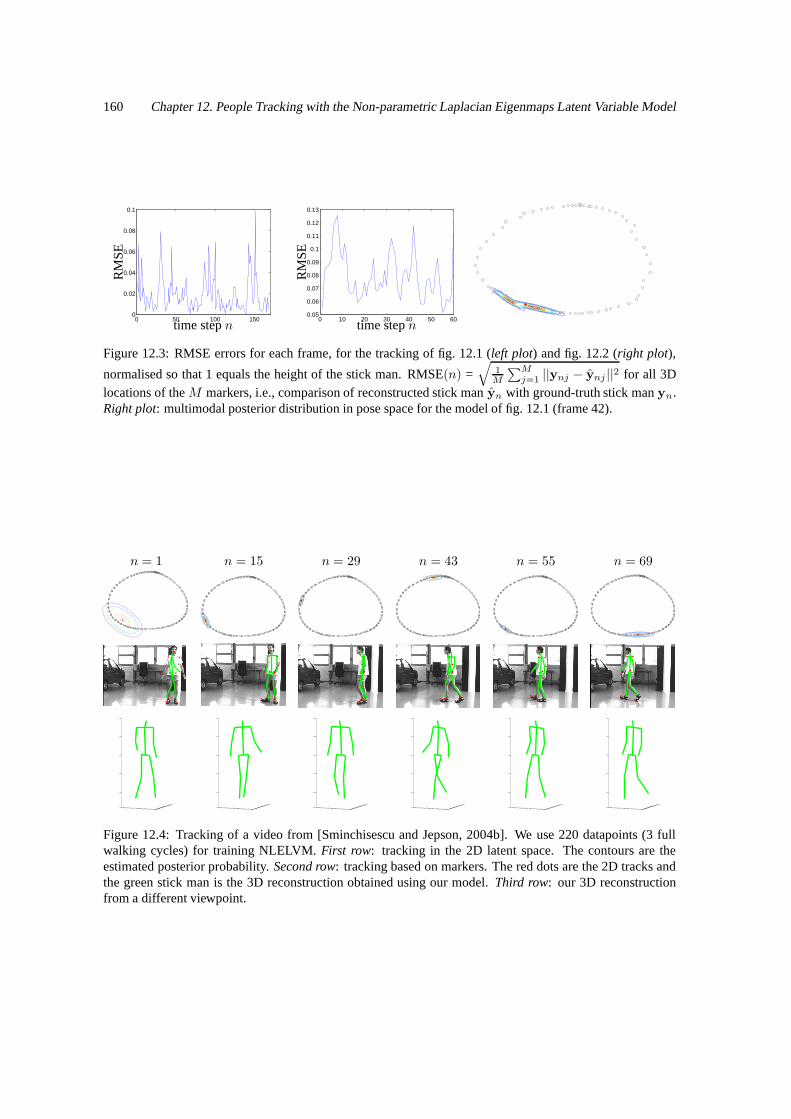
160 Chapter 12. People Tracking with the Non-parametric Laplacian Eigenmaps Latent Variable Model
0 50 100 1500
0.02
0.04
0.06
0.08
0.1
PSfrag replacements
time step n
RM
SE
0 10 20 30 40 50 600.05
0.06
0.07
0.08
0.09
0.1
0.11
0.12
0.13
PSfrag replacements
time step n
RM
SE
PSfrag replacementstime step n
RMSEtime step n
B
Figure 12.3: RMSE errors for each frame, for the tracking of fig. 12.1 (left plot) and fig. 12.2 (right plot),
normalised so that 1 equals the height of the stick man. RMSE(n) =√
1M
∑Mj=1 ||ynj − ynj ||2 for all 3D
locations of the M markers, i.e., comparison of reconstructed stick man yn with ground-truth stick man yn.Right plot: multimodal posterior distribution in pose space for the model of fig. 12.1 (frame 42).
n = 1 n = 15 n = 29 n = 43 n = 55 n = 69
−50−40
−30−20
−100
1020
3040
50
−50
−40
−30
−20
−10
0
10
20
30
40
50
−100
−50
0
50
100
−50−40
−30−20
−100
1020
3040
50
−50
−40
−30
−20
−10
0
10
20
30
40
50
−100
−50
0
50
100
−50−40
−30−20
−100
1020
3040
50
−50
−40
−30
−20
−10
0
10
20
30
40
50
−100
−50
0
50
100
−50−40
−30−20
−100
1020
3040
50
−50
−40
−30
−20
−10
0
10
20
30
40
50
−100
−50
0
50
100
−50−40
−30−20
−100
1020
3040
50
−50
−40
−30
−20
−10
0
10
20
30
40
50
−100
−50
0
50
100
−50−40
−30−20
−100
1020
3040
50
−50
−40
−30
−20
−10
0
10
20
30
40
50
−100
−50
0
50
100
Figure 12.4: Tracking of a video from [Sminchisescu and Jepson, 2004b]. We use 220 datapoints (3 fullwalking cycles) for training NLELVM. First row: tracking in the 2D latent space. The contours are theestimated posterior probability. Second row: tracking based on markers. The red dots are the 2D tracks andthe green stick man is the 3D reconstruction obtained using our model. Third row: our 3D reconstructionfrom a different viewpoint.
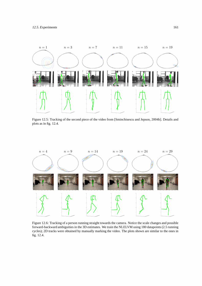
12.5. Experiments 161
n = 1 n = 3 n = 7 n = 11 n = 15 n = 19
−50−40
−30−20
−100
1020
3040
50
−50
−40
−30
−20
−10
0
10
20
30
40
50
−100
−50
0
50
100
−50−40
−30−20
−100
1020
3040
50
−50
−40
−30
−20
−10
0
10
20
30
40
50
−100
−50
0
50
100
−50−40
−30−20
−100
1020
3040
50
−50
−40
−30
−20
−10
0
10
20
30
40
50
−100
−50
0
50
100
−50−40
−30−20
−100
1020
3040
50
−50
−40
−30
−20
−10
0
10
20
30
40
50
−100
−50
0
50
100
−50−40
−30−20
−100
1020
3040
50
−50
−40
−30
−20
−10
0
10
20
30
40
50
−100
−50
0
50
100
−50−40
−30−20
−100
1020
3040
50
−50
−40
−30
−20
−10
0
10
20
30
40
50
−100
−50
0
50
100
Figure 12.5: Tracking of the second piece of the video from [Sminchisescu and Jepson, 2004b]. Details andplots as in fig. 12.4.
n = 4 n = 9 n = 14 n = 19 n = 24 n = 29
50 100 150 200 250 300 350
20
40
60
80
100
120
140
160
180
200
220
50 100 150 200 250 300 350
20
40
60
80
100
120
140
160
180
200
220
50 100 150 200 250 300 350
20
40
60
80
100
120
140
160
180
200
220
50 100 150 200 250 300 350
20
40
60
80
100
120
140
160
180
200
220
50 100 150 200 250 300 350
20
40
60
80
100
120
140
160
180
200
220
50 100 150 200 250 300 350
20
40
60
80
100
120
140
160
180
200
220
−50−40
−30−20
−100
1020
3040
50
−50
−40
−30
−20
−10
0
10
20
30
40
50
−100
−50
0
50
100
−50−40
−30−20
−100
1020
3040
50
−50
−40
−30
−20
−10
0
10
20
30
40
50
−100
−50
0
50
100
−50−40
−30−20
−100
1020
3040
50
−50
−40
−30
−20
−10
0
10
20
30
40
50
−100
−50
0
50
100
−50−40
−30−20
−100
1020
3040
50
−50
−40
−30
−20
−10
0
10
20
30
40
50
−100
−50
0
50
100
−50−40
−30−20
−100
1020
3040
50
−50
−40
−30
−20
−10
0
10
20
30
40
50
−100
−50
0
50
100
−50−40
−30−20
−100
1020
3040
50
−50
−40
−30
−20
−10
0
10
20
30
40
50
−100
−50
0
50
100
Figure 12.6: Tracking of a person running straight towards the camera. Notice the scale changes and possibleforward-backward ambiguities in the 3D estimates. We train the NLELVM using 180 datapoints (2.5 runningcycles); 2D tracks were obtained by manually marking the video. The plots shown are similar to the ones infig. 12.4.
162 Chapter 12. People Tracking with the Non-parametric Laplacian Eigenmaps Latent Variable Model
intermediary representation further constrained using the low-dimensional prior.2 For the synthetic experi-ments and some of the real experiments (figs. 12.4 and 12.5) the camera parameters and the body proportionswere known (for the latter, we used the 2D outputs of [Sminchisescu and Jepson, 2004b]). For the CMUmotion capture video (fig. 12.6) we roughly guessed. We used motion-capture data from several sourcesincluding [cmu, 2003, OSU Human Motion Capture Database]. As observations we always use 2D markerpositions, which, depending on the analyzed sequence were either known (the synthetic case), or providedby an existing tracker [Sminchisescu and Jepson, 2004b] or specified manually (fig. 12.6). Alternatively 2Dpoint trackers similar to the ones of [Urtasun et al., 2005] can be used. The forward generative model is ob-tained by combining the latent to ambient space mapping (this provides the position of the 3D markers) witha perspective projection transformation. The observation model is a product of Gaussians, each measuringthe probability of a particular marker position given its corresponding image point track.
12.5.1 Experiments with synthetic data
In this experiment we analyze the performance of our tracker in controlled conditions (noise perturbed syn-thetically generated image tracks) both under regular circumstances (reasonable sampling of training data)and more severe conditions with subsampled training points and persistent partial occlusion (the man run-ning behind an artificially created regular fence, with some of the 2D marker tracks obstructed). Figs. 12.1and 12.2 show both the posterior (filtered) latent space distribution obtained from our tracker, and its mean(we do not show the distribution of the global rigid body motion, which is unconstrained; in all experimentsthis is tracked with good accuracy). In the latent space plot shown in fig. 12.1 the onset of running (two cy-cles were used) appears as a separate region external to the main loop. It does not appear in the subsampledtraining set in fig. 12.2, where only one running cycle was used for training and the onset of running was re-moved. In each case, one can see that the model is able to track quite competently, with a modest decrease inits temporal accuracy, shown in fig. 12.3 left and middle plots where the averages are computed per 3D joint(normalised wrt body height). Subsampling causes some ambiguity in the estimate, e.g. see the bimodalityin the right plot in fig. 12.3. In another set of experiments (not shown) we also tracked using different subsetsof 3D markers. The estimates were accurate even when about 30% of the markers were dropped.
12.5.2 Experiments with real images
This set of experiments shows our tracker’s ability to work with real motions of different people, with dif-ferent body proportions, not in its latent variable model training set (figs. 12.4–12.5 and 12.6). We studywalking, running and turns. In all cases, tracking and 3D reconstruction are reasonably accurate. Please,have a look at the videos in our additional material.
It is important to note that errors in the pose estimates are primarily caused by mismatches between themotion capture data used to learn the NLELVM prior and the body proportions of the person in the video.For example, the body proportions of the OSU motion captured walker are quite different from those of theimage in fig. 12.4–12.5 (e.g. note how the legs of the stick man are shorter relative to the trunk). Likewise,the style of the runner from the OSU data (e.g. the swinging of the arms) is quite different from that of thevideo. Finally, the interest points tracked by the 2D tracker do not entirely correspond either in numberor location to the motion capture markers. In future work, we plan to include an optimization step to alsoestimate the body proportions. This would be complicated for a general, unconstrained model because thedimensions of the body couple with the pose, so either one or the other can be changed to improve thetracking error (the observation likelihood can also become singular). But for dedicated prior pose modelslike ours these difficulties should be significantly diminished. The model simply cannot assume highlyunlikely stances—these are either not representable at all, or have negligible probability—thus avoidingcompensatory, unrealistic body proportion estimates.
Comparison with PCA and GPLVM: (fig. 3): for these models, the tracker uses the same GMSPPF settingas for LELVM (number of particles, initialisation, random-walk dynamics, etc.) but with the mapping y =
2Only the latent coordinate is estimated explicitly, not the 3D set of markers.
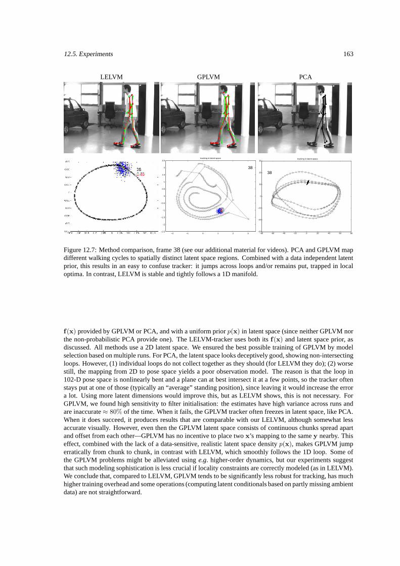
12.5. Experiments 163
LELVM GPLVM PCA
−2 −1 0 1 2 3−2.5
−2
−1.5
−1
−0.5
0
0.5
1
1.5
2
2.5
38
tracking in latent space
−80 −60 −40 −20 0 20 40 60 80−30
−20
−10
0
10
20
30
38
tracking in latent space
Figure 12.7: Method comparison, frame 38 (see our additional material for videos). PCA and GPLVM mapdifferent walking cycles to spatially distinct latent space regions. Combined with a data independent latentprior, this results in an easy to confuse tracker: it jumps across loops and/or remains put, trapped in localoptima. In contrast, LELVM is stable and tightly follows a 1D manifold.
f(x) provided by GPLVM or PCA, and with a uniform prior p(x) in latent space (since neither GPLVM northe non-probabilistic PCA provide one). The LELVM-tracker uses both its f(x) and latent space prior, asdiscussed. All methods use a 2D latent space. We ensured the best possible training of GPLVM by modelselection based on multiple runs. For PCA, the latent space looks deceptively good, showing non-intersectingloops. However, (1) individual loops do not collect together as they should (for LELVM they do); (2) worsestill, the mapping from 2D to pose space yields a poor observation model. The reason is that the loop in102-D pose space is nonlinearly bent and a plane can at best intersect it at a few points, so the tracker oftenstays put at one of those (typically an “average” standing position), since leaving it would increase the errora lot. Using more latent dimensions would improve this, but as LELVM shows, this is not necessary. ForGPLVM, we found high sensitivity to filter initialisation: the estimates have high variance across runs andare inaccurate≈ 80% of the time. When it fails, the GPLVM tracker often freezes in latent space, like PCA.When it does succeed, it produces results that are comparable with our LELVM, although somewhat lessaccurate visually. However, even then the GPLVM latent space consists of continuous chunks spread apartand offset from each other—GPLVM has no incentive to place two x’s mapping to the same y nearby. Thiseffect, combined with the lack of a data-sensitive, realistic latent space density p(x), makes GPLVM jumperratically from chunk to chunk, in contrast with LELVM, which smoothly follows the 1D loop. Some ofthe GPLVM problems might be alleviated using e.g. higher-order dynamics, but our experiments suggestthat such modeling sophistication is less crucial if locality constraints are correctly modeled (as in LELVM).We conclude that, compared to LELVM, GPLVM tends to be significantly less robust for tracking, has muchhigher training overhead and some operations (computing latent conditionals based on partly missing ambientdata) are not straightforward.

164 Chapter 12. People Tracking with the Non-parametric Laplacian Eigenmaps Latent Variable Model
12.6 Conclusion and Extensions
We have proposed the use of priors based on the Non-parametric Laplacian Eigenmaps Latent Variable Model(NLELVM) for people tracking. NLELVM is a probabilistic dimensionality reduction method that combinesthe advantages of latent variable models and spectral manifold learning algorithms: a multimodal probabilitydensity over latent and ambient variables, globally differentiable nonlinear mappings for reconstruction anddimensionality reduction, no local optima, ability to unfold highly nonlinear manifolds, and good practicalscaling to latent spaces of high dimension. NLELVM is computationally efficient, simple to learn from sparsetraining data, and compatible with standard probabilistic trackers such as particle filters. Our results usinga NLELVM-based probabilistic sigma point mixture tracker with several real and synthetic human motionsequences show that NLELVM provides sufficient constraints for robust operation in the presence of missing,noisy and ambiguous image measurements.
The objective of this chapter was to demonstrate the ability of the NLELVM prior in a simple set-ting using 2D tracks obtained automatically or manually, and single-type motions (running, walking). It isstraightforward to explore more complex observation models such as silhouettes, intensity or edges, as e.g.with the parametric Laplacian Eigenmaps generative model presented in Chapter 11 or the SLVMs describedin Chapter 13. One can also study models based on commbining different motion types in the same latentspace (with dimension>> 2) or explore the multimodal latent space posteriors caused by visual ambiguities.
Chapter 13
Sparse Spectral Latent Variable Modelsfor Perceptual Inference
In this chapter, we introduce non-linear generative models referred to as Sparse Spectral Latent VariableModels (SLVM), that combine the advantages of spectral embeddings with the ones of parametric latentvariable models: (1) provide stable latent spaces that preserve global or local geometric properties of themodeled data; (2) offer low-dimensional generative models with probabilistic, bi-directional mappings be-tween latent and ambient spaces, (3) are probabilistically consistent (i.e., reflect the data distribution, bothjointly and marginally) and efficient to learn and use. We show that SLVMs compare favorably with compet-ing methods based on PCA, GPLVM or GTM for the reconstruction of typical human motions like walking,running, pantomime or dancing in a benchmark dataset. Empirically, we observe that SLVMs are effectivefor the automatic 3d reconstruction of low-dimensional human motion in movies. This research apears at theInternational Conference for Computer Vision (ICCV) [Kanaujia, Sminchisescu and Metaxas, 2007].
13.1 Perceptual Models
A variety of computer vision and machine learning tasks require the analysis of high-dimensional ambientsignals, e.g. 2d images, 3d range scans or data obtained from human motion capture systems. The goalis to learn compact, perceptual (latent) models of the data generation process and use them to interpretnew measurements. For example, the variability in an image sequence filming a rotating teapot is non-linearly produced by latent factors like rotation variables and the lighting direction. Our subjective, perceiveddimensionality partly mirrors the latent factors, being significantly smaller than the one directly measured– the high-dimensional sequence of image pixel vectors. Similarly, filming a human running or walkingrequires megabytes of wildly varying images, yet in a representation that properly correlates the human jointangles, the intrinsic dimensionality is effectively 1 – the phase of the walking cycle. The argument can goon, but underlines the intuitive idea that the space of all images is much larger than the set of physicallypossible ones, which, in turn is larger than the one typically observed in most every day’s scenes. If this istrue, perceptual inference cannot proceed without an appropriate, arguably probabilistic model of correlation,a natural way to link perceptual and measured inferences. This implies a non-linear subset, or a manifoldassumption, at least in the large-sample regime: the low-dimensional perceptual structure lives in the high-dimensional space of direct observations. To unfold it, we need faithful, topographic representations ofthe observed data – effectively forms of continuity and locality: nearby observations should map to nearbypercepts and faraway observations should map faraway. Given this, we want to be able to consistently answerthe following questions: How to represent a percept or an image? What is the probability of an observedimage? What is the probability of a given percept? What is the conditional probability of a percept given animage and vice-versa?
One promising class of methods for constructing non-linear perceptual representations given observed
165
166 Chapter 13. Sparse Spectral Latent Variable Models for Perceptual Inference
data is spectral dimensionality reduction [Roweis and Saul, 2000, Tenenbaum et al., 2000, Belkin and Niyogi,2002, Donoho and Grimes, 2003b, Weinberger and Saul, 2004]. The methods are similar in their use of graph-based representations of the data, with nodes standing for observations and links for neighborhood relations.The connected graph can be viewed as a discrete approximation of the sub-manifold directly sampled fromobserved data. Different methods derive different matrices from the graph and their spectral decompositions(the top or bottom eigenvectors) reveal the low-dimensional, perceptual structure of the data, and in somecases, also its intrinsic dimensionality. Spectral methods have been demonstrated to be capable of unfoldinghighly non-linear structure, and some methods (e.g. ISOMAP, Hessian and Laplacian Eigenmaps) come withadditional, strong asymptotic guarantees – if enough samples are available, they could, in principle recoverthe true manifold from which the data was generated. However, spectral methods are not probabilistic andlack a consistent way to relate perceptual and observed quantities, or evaluate their probability. This explains,perhaps, why their use in computer vision has been limited, despite their undeniable intuitive appeal. On theother hand, a variety of probabilistic, non-linear latent variable models are available (mixture of PCA, FactorAnalyzers, etc.), but they lack a global perceptual coordinate system and are not guaranteed to preserveintuitive geometric properties of the data in the latent space, as spectral methods do.
In this paper we introduce probabilistic models with geometric properties in order to marry spectralembeddings and parametric latent variable models, and obtain: (1) stable latent spaces that preserve structuralproperties of the ambient data, e.g. its local or global geometry; (2) low-dimensional generative models withprobabilistic, bi-directional mappings between latent and ambient spaces, and (3) probabilistically consistentand efficient estimates. We refer to these probabilistic constructs, implicitly defined on top of an irregulardistribution (or unfolding) obtained from a spectral embedding as Sparse Spectral Latent Variable Models(SLVM). We show how SLVMs can be used successfully for complex visual inference tasks, in particular theautomatic discriminative 3d reconstruction of low-dimensional human poses in non-instrumented monocularvideo.
13.1.1 Prior Work on Latent Variable Models
Our research relates to work in spectral manifold learning, latent variable models and visual tracking. Spec-tral methods can model intuitive local or global geometric constraints [Roweis and Saul, 2000, Tenenbaumet al., 2000, Belkin and Niyogi, 2002, Donoho and Grimes, 2003b, Weinberger and Saul, 2004] and their,local-optima free, polynomial time calculations are amenable to efficient optimization – either sparse eigen-value problems, or dense problems that can be solved with algebraic multigrid methods [Bengio et al., 2003,Sminchisescu and Jepson, 2004b].
A variety of non-linear latent variable models exist e.g. mixtures of factor analyzers or PPCA [Tipping,1998]. These methods can model complicated non-linear structure but do not provide global latent coordinatesystems or latent spaces which provably preserve local or global geometric properties of the data. Regulargrid-based methods like the Generative Topographic Mapping GTM [Bishop et al., 1998a] do not scalebeyond latent spaces higher than 2-3d, or for structured problems, where the latent space distribution isunlikely to be uniform (in fact GTM’s latent prior is a mixture of nodal delta functions – non-zero only onthe grid). GTM is a useful non-linear method, yet it cannot unfold many convoluted manifolds (e.g. spirals,rolls) due to its data independent embedding grid, and local optima in training.1 The Gaussian Process LatentVariable Model (GPLVM) [Lawrence, 2005] is a non-linear PCA technique based on a Gaussian Processmapping to ambient (data) space with zero mean unit Gaussian regularizer in latent space. Strictly, GPLVMdefines a regularized conditional map to observed data, not a generative model. It is a competitive modelprimarily targeting data reconstruction error, but not designed to enforce the constraints we are after, e.g. thelatent regularizer is data independent and geometric properties of ambient data are not explicitly preserved.GPLVM’s lack of latent space prior makes it somewhat agnostic in visual inference applications, where itis useful to penalize drifts from the manifold of typical configurations. A discussion and comparisons with
1Our model can be viewed a spectral generalization of the notable GTM precursor [Bishop et al., 1998a,b], where weuse a data-dependent, geometry preserving (rather than regular) embedding grid, sparsity constraints for the data map, aGaussian mixture latent prior (as opposed to a delta sum) and MC sampling methods for training (as opposed to exactintegration in GTM).
13.2. Spectral Latent Variable Models (SLVM) 167
both GPLVM and GTM appear in the experimental section. Memisevic [Memisevic, 2006] models the jointlatent-ambient density using a separable product of non-parametric kernel density estimates and computesan embedding by optimizing a mutual information criterion over latent space coordinates – similar in spiritto GPLVM.
Recent work on visual tracking has identified the importance of low-dimensional models with intuitivegeometric properties and latent-ambient mappings. Elgammal & Lee [Elgammal and Lee, 2004] fit an RBFto the corresponding points of an LLE-embedding, but their model devoid of a latent space prior is notfully probabilistic and there are no mappings to the latent space. In independent work, Sminchisescu &Jepson [Sminchisescu and Jepson, 2004b] augment spectral embeddings (e.g. Laplacian Eigenmaps) withboth latent space priors and RBF mappings to ambient space. Their model is a latent variable one, butambient to latent mappings are more difficult to compute, and the model is trained piece-wise. The modelproposed here complements it. Urtasun et al [Urtasun et al., 2005] use GPLVM to track walking based onimage tracks of the human joints obtained using the WSL tracker of Jepson’s et al. For more expressivekinematic representations, and in order to compensate for GPLVM’s lack of latent space prior, the authors[Urtasun et al., 2005] use an augmented, constrained (latent, ambient) state for tracking. This is feasiblebut, once again, renders the state estimation problem high-dimensional.
13.2 Spectral Latent Variable Models (SLVM)
We work with two sets of vectors, X and Y , of equal size N (initially in correspondence), in two spacesreferred as latent (or perceptual) and ambient (or data). Both sets are un-ordered, hence there is no constraintto place either one on a regular grid (i.e. a matrix in 2d or the cells of cube in 3d). The latent space vectors aregenerically denoted x, with dim(x) = d, the ambient vectors are y with dim(y) = D, typically D >> d.
Spectral Embeddings: Assume that vector-valued points in ambient space Y = yi|i = 1 . . .N arecaptured from a high-dimensional process (images, sound, human motion capture systems), whereas cor-responding latent space points X = xi|i = 1 . . .N are initially obtained using any spectral, non-linearembedding method like ISOMAP, LLE, Hessian or Laplacian Eigenmaps, etc. The methods use graph-basedrepresentations of the observed data, with nodes that represent observations and links that stand for neighbor-hood relations. The connected graph can be viewed as a discrete approximation of the sub-manifold directlysampled from observed data. Different methods derive different matrices from the graph. Their spectraldecompositions (the top or bottom eigenvectors) reveal the low-dimensional, latent structure of the data. Wewill use the distribution of latent points and a mapping to the ambient space is order to construct a jointprobability distribution over latent and ambient variables.
Latent Variable Models: We model the joint distribution over latent and ambient variables using a construc-tive form: p(x,y) = p(x)p(y|x). Without loss of generality we select the latent space prior p(x) to be anon-parametric kernel density estimate, with kernels K and covariance θ, centered at embedded points xi,but more compact representations, e.g. Gaussian mixture models can be used instead:2
p(x) =1
K
K∑
i=1
Kθ(x,xi) (13.1)
In the model, we assume that ambient vectors are related to the latent ones using a nonlinear vector-valuedfunction F(x,W,α) with parameters W and output noise covariance σ. Otherwise said, the joint distribu-tion has a non-linear constraint between two blocks of its variables:
p(y|x,W,α,σ) ∼ N (y|F(x,W,α),σ) (13.2)
2This is one possible construction for the joint distribution, arguably not the only possible. Instead, one can ap-proximate as product of marginals in latent and ambient space p(x,y) =
PN
i=1 Kθ(x,xi)Kθ(y,yi), rely on indexcorrespondences in the embedding, and optimize the latent coordinates xi in order to account for correlations in the joint[Memisevic, 2006].
168 Chapter 13. Sparse Spectral Latent Variable Models for Perceptual Inference
where N is a Gaussian distribution with mean F and covariance σ. F is chosen to be a generalized (non-linear parametric) regression model:
F(x,W,α) = Wφ(x) (13.3)
with φ(x) = [Kδ(x,x1), . . . ,Kδ(x,xM )]>, having Gaussian kernels (other distributions can also be used)placed at an M-sized subset xi sampled from the prior p(x) (and selected automatically from a larger sampleusing a sparsity hyperprior, see below), with covariance δ, and W is a weight matrix of size DxM .
The model is made computationally efficient and more robust to overfitting by using hierarchical priorson the parameters W of the mapping F, in order to select a sparse subset for prediction [Tipping, 2001,Mackay, 1998]:
p(W|α) ∼D∏
j=1
N∏
k=1
N (wjk |0,1
αk) (13.4)
p(α) =
N∏
i=1
Gamma(αi|a, b) (13.5)
with Gamma(α|a, b) = Γ(a)−1baαa−1e−bα, and a = 10−2, b = 10−4 chosen to give broad hyperpriors.The ambient marginal is obtained by integrating the latent space:
p(y|W,α,σ) =
∫p(y|x,W,α,σ)p(x)dx (13.6)
The evidence, as well as derivatives w.r.t. model parameters, can be computed using a simple Monte Carlo(MC) estimate using, say K, samples from the prior.3 This gives the MC estimate of the ambient marginal:
p(y|W,α,σ) =1
K
K∑
i=1
p(y|xi,W,α,σ) (13.7)
The latent space conditional is obtained using Bayes’ rule:
p(x|y) =p(y|x)p(x)
p(y)= (13.8)
=p(y|x)
∑Ki=1Kθ(x,xi)∑K
i=1 p(y|xi,W,α,σ)(13.9)
For pairs of ambient data points j and MC latent samples i, we abbreviate p(i,j) = p(xi|yj). Notice how thechoice of prior p(x) influences the membership probabilities in (13.8) and (13.10). We can compute eitherthe conditional mean or the mode (better for multimodal distributions) in latent space, using the same MCintegration method used for (13.7):
Ex|yn,W,α,σ =
∫p(x|yn,W,α,σ)xdx (13.10)
=
K∑
i=1
p(i,n)xi (13.11)
imax = arg maxi
p(i,n) (13.12)
The model contains all the ingredients for efficient computation in both latent and ambient space: eq. (13.1)gives the prior in latent space, (13.7) the ambient marginal, (13.2) provides the conditional distribution (ormapping) from latent to ambient space, and (13.10) and (13.12) give the mean or mode of the mapping
3The number of samples and the number of prior components are chosen co-incidentally, as K, for notational con-venience, and so was the sample index xi to match the datapoint yi. In general, the latent MC samples are distributedaccording to the latent density, and may be different from the latent coordinates of datapoints obtained from the spectralembedding. Sampling from the kernel density estimate is efficient and can be done once for all – the same set can bereused used for all MC calculations, both training and testing.
13.3. Feedforward 3D Pose Prediction 169
from ambient to latent space (a more accurate but also more expensive mode-finding approximation than(13.12) can be obtained by direct gradient ascent on (13.8)). Latent conditionals given partially observed y
vectors are easy to compute, using (13.8). The y distribution is Gaussian and unobserved components canbe integrated analytically – this effectively removes them from the mean and the corresponding lines andcolumns of the covariance. The model can be trained by maximizing the log-likelihood of the data:
L = log
N∏
i=1
p(yn|W,α,σ) = (13.13)
=N∑
n=1
log 1
K
K∑
i=1
p(yn|xi,W,α,σ) (13.14)
Maximizing the likelihood provides estimates for W,α,σ (consider σ is diagonal with values σ):
Σ = (σΦ>GΦ + S)−1 (13.15)
W> = σΣΦ>RY (13.16)
where S = diag(α1, . . . , αM ) with α corresponding only to the active set, G = diag(G1, . . . , GK) withGi =
∑Nj=1 p(i,j), R is a KxN matrix with elements p(i,j), and Y is an NxD matrix that stores the output
vectors yi, i = 1 . . .N row-wise, and Φ is a KxM matrix with elements G(xi|xj ,θ). The inverse varianceis estimated from prediction error:
σ =1
ND
N∑
n=1
K∑
k=1
p(kn)||W∗φ(x)− yn||2 (13.17)
where a ‘∗′ superscript identifies an updated variable estimate. The hyperparameters are re-estimated usingthe relevance determination equations [Mackay, 1998]:
α∗i =
γi
||µi||2, γi = 1− αiΣ
∗ii (13.18)
where µi is the i-th column of W. The algorithm is summarized in fig. 13.1.
13.3 Feedforward 3D Pose Prediction
We estimate a distribution over solutions in latent space, given input descriptors derived from images obtainedby detecting the person using a bounding-box. We then map from latent states to 3d human joint angles (usinge.g. (13.2)) in order to recover body configurations for visualization or error reporting. To predict latent spacedistributions from image features, we use a conditional mixture of expert predictors, here sparse Bayesianlinear regressors. Each one is paired with an observation dependent gate (a softmax function with sparselinear regressor exponent) that scores its competence when presented with different images. As this change,different experts may be active and their rankings (relative probabilities) may change. The model is trainedusing a double-loop EM algorithm [Jordan and Jacobs, 1994, Sminchisescu et al., 2005a].
13.4 Experiments
We illustrate the SLVM on simple S-sheet and Swiss-roll toy datasets and experiment also with a computervision application: the reconstruction of low-dimensional representations of 3d human poses from monocularimages of people photographed against non-stationary backgrounds.
13.4.1 The S-Sheet and Swiss Roll
This set of experiments are illustrated in fig. 13.2. The original S-sheet data set (top)a) consists of 1000 pointssampled regularly on the surface of S-sheet and (in most plots) color coded to show their relative spatial
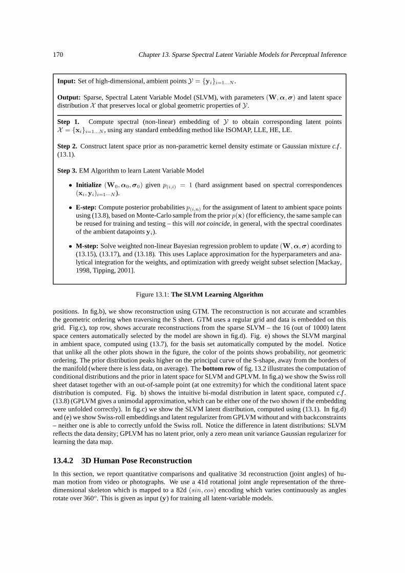
170 Chapter 13. Sparse Spectral Latent Variable Models for Perceptual Inference
Input: Set of high-dimensional, ambient points Y = yii=1...N .
Output: Sparse, Spectral Latent Variable Model (SLVM), with parameters (W,α,σ) and latent spacedistribution X that preserves local or global geometric properties of Y .
Step 1. Compute spectral (non-linear) embedding of Y to obtain corresponding latent pointsX = xii=1...N , using any standard embedding method like ISOMAP, LLE, HE, LE.
Step 2. Construct latent space prior as non-parametric kernel density estimate or Gaussian mixture c.f .(13.1).
Step 3. EM Algorithm to learn Latent Variable Model
• Initialize (W0,α0,σ0) given p(i,i) = 1 (hard assignment based on spectral correspondences(xi,yi)i=1···N ).
• E-step: Compute posterior probabilities p(i,n) for the assignment of latent to ambient space pointsusing (13.8), based on Monte-Carlo sample from the prior p(x) (for efficiency, the same sample canbe reused for training and testing – this will not coincide, in general, with the spectral coordinatesof the ambient datapoints yi).
• M-step: Solve weighted non-linear Bayesian regression problem to update (W,α,σ) acording to(13.15), (13.17), and (13.18). This uses Laplace approximation for the hyperparameters and ana-lytical integration for the weights, and optimization with greedy weight subset selection [Mackay,1998, Tipping, 2001].
Figure 13.1: The SLVM Learning Algorithm
positions. In fig.b), we show reconstruction using GTM. The reconstruction is not accurate and scramblesthe geometric ordering when traversing the S sheet. GTM uses a regular grid and data is embedded on thisgrid. Fig.c), top row, shows accurate reconstructions from the sparse SLVM – the 16 (out of 1000) latentspace centers automatically selected by the model are shown in fig.d). Fig. e) shows the SLVM marginalin ambient space, computed using (13.7), for the basis set automatically computed by the model. Noticethat unlike all the other plots shown in the figure, the color of the points shows probability, not geometricordering. The prior distribution peaks higher on the principal curve of the S-shape, away from the borders ofthe manifold (where there is less data, on average). The bottom row of fig. 13.2 illustrates the computation ofconditional distributions and the prior in latent space for SLVM and GPLVM. In fig.a) we show the Swiss rollsheet dataset together with an out-of-sample point (at one extremity) for which the conditional latent spacedistribution is computed. Fig. b) shows the intuitive bi-modal distribution in latent space, computed c.f .(13.8) (GPLVM gives a unimodal approximation, which can be either one of the two shown if the embeddingwere unfolded correctly). In fig.c) we show the SLVM latent distribution, computed using (13.1). In fig.d)and (e) we show Swiss-roll embeddings and latent regularizer from GPLVM without and with backconstraints– neither one is able to correctly unfold the Swiss roll. Notice the difference in latent distributions: SLVMreflects the data density; GPLVM has no latent prior, only a zero mean unit variance Gaussian regularizer forlearning the data map.
13.4.2 3D Human Pose Reconstruction
In this section, we report quantitative comparisons and qualitative 3d reconstruction (joint angles) of hu-man motion from video or photographs. We use a 41d rotational joint angle representation of the three-dimensional skeleton which is mapped to a 82d (sin, cos) encoding which varies continuously as anglesrotate over 360o. This is given as input (y) for training all latent-variable models.
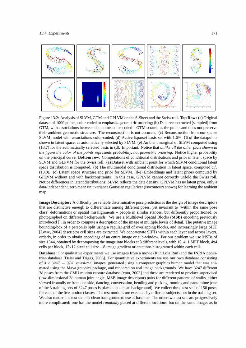
13.4. Experiments 171
0
0.5
1
1.5
2
2.5
3
3.5
4
4.5
5
x 10−3
−1.5 −1 −0.5 0 0.5 1 1.5−1.5
−1
−0.5
0
0.5
1
1.5
−1 −0.5 0 0.5 1 1.5−1.5
−1
−0.5
0
0.5
1
1.5
Figure 13.2: Analysis of SLVM, GTM and GPLVM on the S-Sheet and the Swiss roll. Top Row: (a) Originaldataset of 1000 points, color coded to emphasize geometric ordering; (b) Data reconstructed (sampled) fromGTM, with associations between datapoints color-coded – GTM scrambles the points and does not preservetheir ambient geometric structure. The reconstruction is not accurate. (c) Reconstruction from our sparseSLVM model with associations color-coded; (d) Active (sparse) basis set with 1.6%=16 of the datapointsshown in latent space, as automatically selected by SLVM. (e) Ambient marginal of SLVM computed using(13.7) for the automatically selected basis in (d). Important: Notice that unlike all the other plots shown inthe figure the color of the points represents probability, not geometric ordering. Notice higher probabilityon the principal curve. Bottom row: Computations of conditional distributions and prior in latent space bySLVM and GLPVM for the Swiss roll. (a) Dataset with ambient point for which SLVM conditional latentspace distribution is computed. (b) The multimodal conditional distribution in latent space, computed c.f .(13.8). (c) Latent space structure and prior for SLVM. (d-e) Embeddings and latent priors computed byGPLVM without and with backconstraints. In this case, GPLVM cannot correctly unfold the Swiss roll.Notice differences in latent distributions: SLVM reflects the data density; GPLVM has no latent prior, only adata-independent, zero mean unit variance Gaussian regularizer (isocontours shown) for learning the ambientmap.
Image Descriptor: A difficulty for reliable discriminative pose prediction is the design of image descriptorsthat are distinctive enough to differentiate among different poses, yet invariant to ‘within the same poseclass’ deformations or spatial misalignments – people in similar stances, but differently proportioned, orphotographed on different backgrounds. We use a Multilevel Spatial Blocks (MSB) encoding previouslyintroduced [], in order to compute a description of the image at multiple levels of detail. The putative imagebounding-box of a person is split using a regular grid of overlapping blocks, and increasingly large SIFT[Lowe, 2004] descriptor cell sizes are extracted. We concatenate SIFTs within each layer and across layers,orderly, in order to obtain encodings of an entire image or sub-window. For our problem we use MSBs ofsize 1344, obtained by decomposing the image into blocks at 3 different levels, with 16, 4, 1 SIFT block, 4x4cells per block, 12x12 pixel cell size – 8 image gradient orientations histogramed within each cell.
Database: For qualitative experiments we use images from a movie (Run Lola Run) and the INRIA pedes-trian database [Dalal and Triggs, 2005]. For quantitative experiments we use our own database consistingof 3 × 3247 = 9741 quasi-real images, generated using a computer graphics human model that was ani-mated using the Maya graphics package, and rendered on real image backgrounds. We have 3247 different3d poses from the CMU motion capture database [cmu, 2003] and these are rendered to produce supervised(low-dimensional 3d human joint angle, MSB image descriptor) pairs for different patterns of walks, eitherviewed frontally or from one side, dancing, conversation, bending and picking, running and pantomime (oneof the 3 training sets of 3247 poses is placed on a clean background). We collect three test sets of 150 posesfor each of the five motion classes. The test motions are executed by different subjects, not in the training set.We also render one test set on a clean background to use as baseline. The other two test sets are progressivelymore complicated: one has the model randomly placed at different locations, but on the same images as in
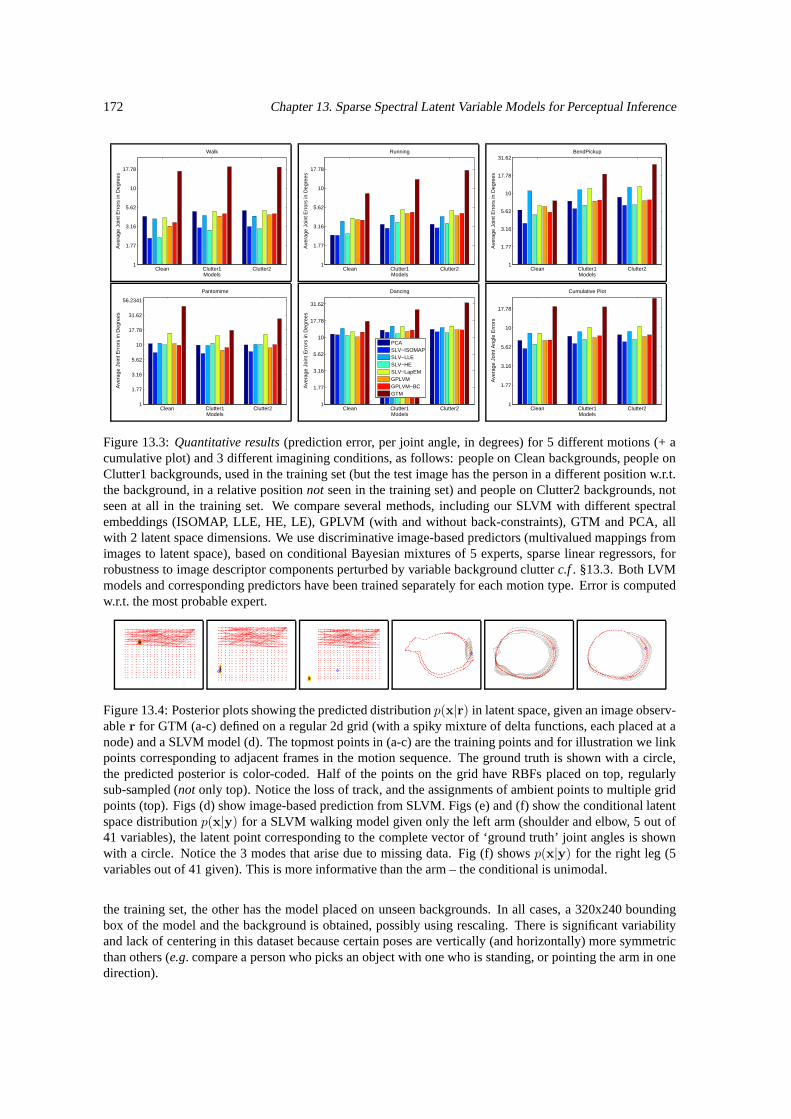
172 Chapter 13. Sparse Spectral Latent Variable Models for Perceptual Inference
Clean Clutter1 Clutter21
1.77
3.16
5.62
10
17.78
Models
Ave
rage
Joi
nt E
rror
s in
Deg
rees
Walk
Clean Clutter1 Clutter21
1.77
3.16
5.62
10
17.78
Models
Ave
rage
Joi
nt E
rror
s in
Deg
rees
Running
Clean Clutter1 Clutter21
1.77
3.16
5.62
10
17.78
31.62
Models
Ave
rage
Joi
nt E
rror
s in
Deg
rees
BendPickup
Clean Clutter1 Clutter21
1.77
3.16
5.62
10
17.78
31.62
56.2341
Models
Ave
rage
Joi
nt E
rror
s in
Deg
rees
Pantomime
Clean Clutter1 Clutter21
1.77
3.16
5.62
10
17.78
31.62
Models
Ave
rage
Joi
nt E
rror
s in
Deg
rees
Dancing
PCASLV−ISOMAPSLV−LLESLV−HESLV−LapEMGPLVMGPLVM−BCGTM
Clean Clutter1 Clutter21
1.77
3.16
5.62
10
17.78
Models
Ave
rage
Joi
nt A
ngle
Err
ors
Cumulative Plot
Figure 13.3: Quantitative results (prediction error, per joint angle, in degrees) for 5 different motions (+ acumulative plot) and 3 different imagining conditions, as follows: people on Clean backgrounds, people onClutter1 backgrounds, used in the training set (but the test image has the person in a different position w.r.t.the background, in a relative position not seen in the training set) and people on Clutter2 backgrounds, notseen at all in the training set. We compare several methods, including our SLVM with different spectralembeddings (ISOMAP, LLE, HE, LE), GPLVM (with and without back-constraints), GTM and PCA, allwith 2 latent space dimensions. We use discriminative image-based predictors (multivalued mappings fromimages to latent space), based on conditional Bayesian mixtures of 5 experts, sparse linear regressors, forrobustness to image descriptor components perturbed by variable background clutter c.f . §13.3. Both LVMmodels and corresponding predictors have been trained separately for each motion type. Error is computedw.r.t. the most probable expert.
Figure 13.4: Posterior plots showing the predicted distribution p(x|r) in latent space, given an image observ-able r for GTM (a-c) defined on a regular 2d grid (with a spiky mixture of delta functions, each placed at anode) and a SLVM model (d). The topmost points in (a-c) are the training points and for illustration we linkpoints corresponding to adjacent frames in the motion sequence. The ground truth is shown with a circle,the predicted posterior is color-coded. Half of the points on the grid have RBFs placed on top, regularlysub-sampled (not only top). Notice the loss of track, and the assignments of ambient points to multiple gridpoints (top). Figs (d) show image-based prediction from SLVM. Figs (e) and (f) show the conditional latentspace distribution p(x|y) for a SLVM walking model given only the left arm (shoulder and elbow, 5 out of41 variables), the latent point corresponding to the complete vector of ‘ground truth’ joint angles is shownwith a circle. Notice the 3 modes that arise due to missing data. Fig (f) shows p(x|y) for the right leg (5variables out of 41 given). This is more informative than the arm – the conditional is unimodal.
the training set, the other has the model placed on unseen backgrounds. In all cases, a 320x240 boundingbox of the model and the background is obtained, possibly using rescaling. There is significant variabilityand lack of centering in this dataset because certain poses are vertically (and horizontally) more symmetricthan others (e.g. compare a person who picks an object with one who is standing, or pointing the arm in onedirection).
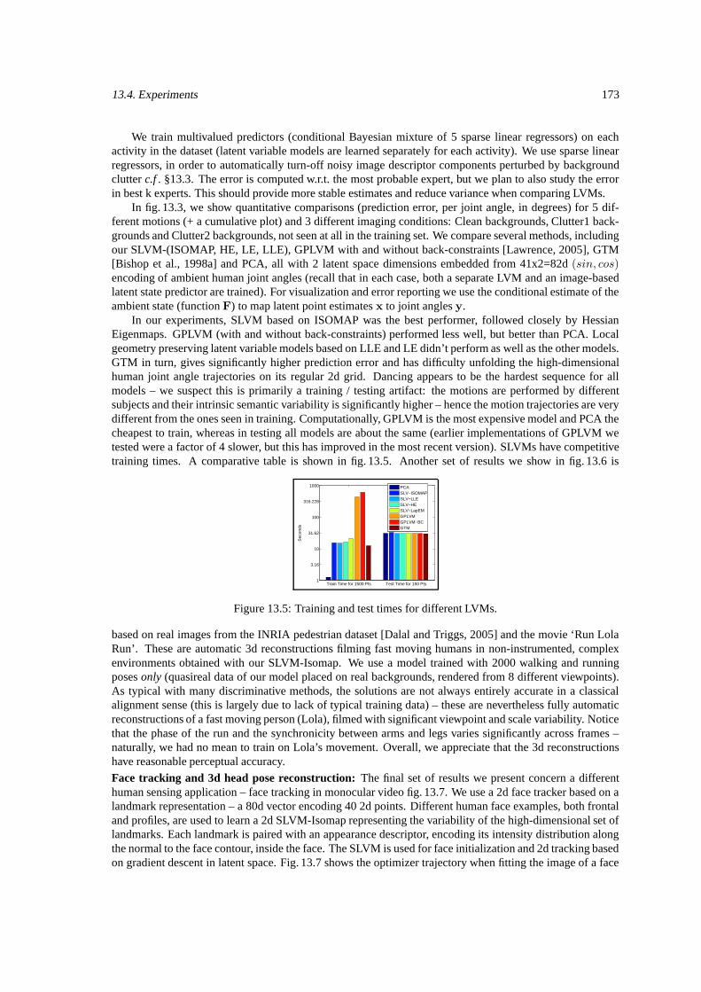
13.4. Experiments 173
We train multivalued predictors (conditional Bayesian mixture of 5 sparse linear regressors) on eachactivity in the dataset (latent variable models are learned separately for each activity). We use sparse linearregressors, in order to automatically turn-off noisy image descriptor components perturbed by backgroundclutter c.f . §13.3. The error is computed w.r.t. the most probable expert, but we plan to also study the errorin best k experts. This should provide more stable estimates and reduce variance when comparing LVMs.
In fig. 13.3, we show quantitative comparisons (prediction error, per joint angle, in degrees) for 5 dif-ferent motions (+ a cumulative plot) and 3 different imaging conditions: Clean backgrounds, Clutter1 back-grounds and Clutter2 backgrounds, not seen at all in the training set. We compare several methods, includingour SLVM-(ISOMAP, HE, LE, LLE), GPLVM with and without back-constraints [Lawrence, 2005], GTM[Bishop et al., 1998a] and PCA, all with 2 latent space dimensions embedded from 41x2=82d (sin, cos)encoding of ambient human joint angles (recall that in each case, both a separate LVM and an image-basedlatent state predictor are trained). For visualization and error reporting we use the conditional estimate of theambient state (function F) to map latent point estimates x to joint angles y.
In our experiments, SLVM based on ISOMAP was the best performer, followed closely by HessianEigenmaps. GPLVM (with and without back-constraints) performed less well, but better than PCA. Localgeometry preserving latent variable models based on LLE and LE didn’t perform as well as the other models.GTM in turn, gives significantly higher prediction error and has difficulty unfolding the high-dimensionalhuman joint angle trajectories on its regular 2d grid. Dancing appears to be the hardest sequence for allmodels – we suspect this is primarily a training / testing artifact: the motions are performed by differentsubjects and their intrinsic semantic variability is significantly higher – hence the motion trajectories are verydifferent from the ones seen in training. Computationally, GPLVM is the most expensive model and PCA thecheapest to train, whereas in testing all models are about the same (earlier implementations of GPLVM wetested were a factor of 4 slower, but this has improved in the most recent version). SLVMs have competitivetraining times. A comparative table is shown in fig. 13.5. Another set of results we show in fig. 13.6 is
Train Time for 1500 Pts Test Time for 150 Pts1
3.16
10
31.62
100
316.228
1000
Sec
onds
PCASLV−ISOMAPSLV−LLESLV−HESLV−LapEMGPLVMGPLVM−BCGTM
Figure 13.5: Training and test times for different LVMs.
based on real images from the INRIA pedestrian dataset [Dalal and Triggs, 2005] and the movie ‘Run LolaRun’. These are automatic 3d reconstructions filming fast moving humans in non-instrumented, complexenvironments obtained with our SLVM-Isomap. We use a model trained with 2000 walking and runningposes only (quasireal data of our model placed on real backgrounds, rendered from 8 different viewpoints).As typical with many discriminative methods, the solutions are not always entirely accurate in a classicalalignment sense (this is largely due to lack of typical training data) – these are nevertheless fully automaticreconstructions of a fast moving person (Lola), filmed with significant viewpoint and scale variability. Noticethat the phase of the run and the synchronicity between arms and legs varies significantly across frames –naturally, we had no mean to train on Lola’s movement. Overall, we appreciate that the 3d reconstructionshave reasonable perceptual accuracy.
Face tracking and 3d head pose reconstruction: The final set of results we present concern a differenthuman sensing application – face tracking in monocular video fig. 13.7. We use a 2d face tracker based on alandmark representation – a 80d vector encoding 40 2d points. Different human face examples, both frontaland profiles, are used to learn a 2d SLVM-Isomap representing the variability of the high-dimensional set oflandmarks. Each landmark is paired with an appearance descriptor, encoding its intensity distribution alongthe normal to the face contour, inside the face. The SLVM is used for face initialization and 2d tracking basedon gradient descent in latent space. Fig. 13.7 shows the optimizer trajectory when fitting the image of a face
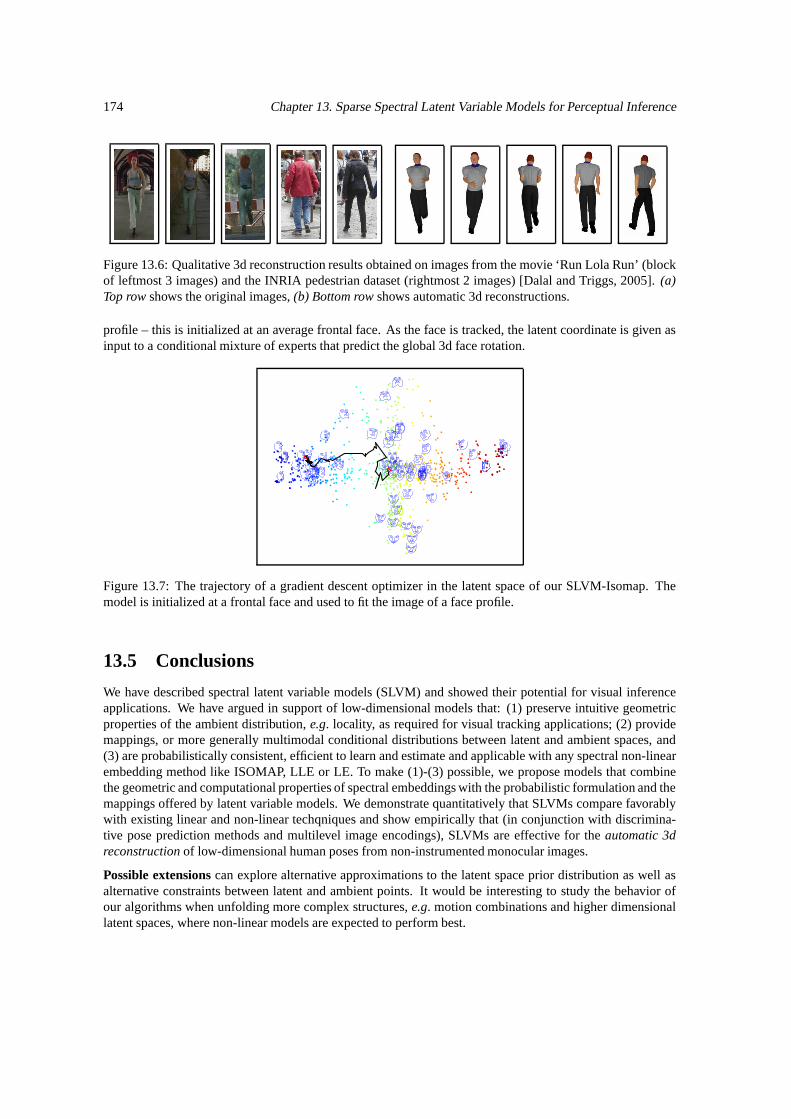
174 Chapter 13. Sparse Spectral Latent Variable Models for Perceptual Inference
Figure 13.6: Qualitative 3d reconstruction results obtained on images from the movie ‘Run Lola Run’ (blockof leftmost 3 images) and the INRIA pedestrian dataset (rightmost 2 images) [Dalal and Triggs, 2005]. (a)Top row shows the original images, (b) Bottom row shows automatic 3d reconstructions.
profile – this is initialized at an average frontal face. As the face is tracked, the latent coordinate is given asinput to a conditional mixture of experts that predict the global 3d face rotation.
Figure 13.7: The trajectory of a gradient descent optimizer in the latent space of our SLVM-Isomap. Themodel is initialized at a frontal face and used to fit the image of a face profile.
13.5 Conclusions
We have described spectral latent variable models (SLVM) and showed their potential for visual inferenceapplications. We have argued in support of low-dimensional models that: (1) preserve intuitive geometricproperties of the ambient distribution, e.g. locality, as required for visual tracking applications; (2) providemappings, or more generally multimodal conditional distributions between latent and ambient spaces, and(3) are probabilistically consistent, efficient to learn and estimate and applicable with any spectral non-linearembedding method like ISOMAP, LLE or LE. To make (1)-(3) possible, we propose models that combinethe geometric and computational properties of spectral embeddings with the probabilistic formulation and themappings offered by latent variable models. We demonstrate quantitatively that SLVMs compare favorablywith existing linear and non-linear techqniques and show empirically that (in conjunction with discrimina-tive pose prediction methods and multilevel image encodings), SLVMs are effective for the automatic 3dreconstruction of low-dimensional human poses from non-instrumented monocular images.
Possible extensions can explore alternative approximations to the latent space prior distribution as well asalternative constraints between latent and ambient points. It would be interesting to study the behavior ofour algorithms when unfolding more complex structures, e.g. motion combinations and higher dimensionallatent spaces, where non-linear models are expected to perform best.
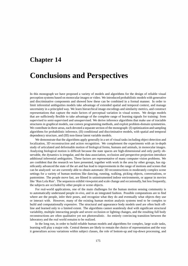
Chapter 14
Conclusions and Perspectives
In this monograph we have proposed a variety of models and algorithms for the design of reliable visualperception systems based on monocular images or video. We introduced probabilistic models with generativeand discriminative components and showed how these can be combined in a formal manner. In order tolimit inferential ambiguities models take advantage of extended spatial and temporal context, and manageuncertainty in a principled way. We learn hierarchical image encodings and similarity metrics, and constructrepresentations that capture the main factors of perceptual variation in visual scenes. We design modelsthat are sufficiently flexible to take advantage of the complete range of learning signals for training: fromsupervised to semi-supervised and unsupervised. We derive inference algorithms that make use of tractablestructures in graphical models, use convex programming methods, and exploit problem-domain symmetries.We contribute in three areas, each devoted a separate section of the monograph: (I) optimization and samplingalgorithms for probabilistic inference, (II) conditional and discriminative models, with spatial and temporaldependency structure, and (III) non-linear latent variable models.
We demonstrate that the algorithms apply generally in a set of visual tasks including object detection andlocalization, 3D reconstruction and action recognition. We complement the experiments with an in-depthstudy of articulated and deformable motion of biological forms, humans and animals, in monocular images.Analyzing biological motion is difficult because the state spaces are high-dimensional and only partly ob-servable, the dynamics is irregular, and the data association, occlusion and perspective projection introduceadditional inferential ambiguities. These factors are representative of many computer vision problems. Weare confident that the research we have presented, together with work in the area by other groups, has sig-nificantly advanced the state of the art and has lead to improvements in the range of motions and scenes thatcan be analyzed: we are currently able to obtain automatic 3D reconstructions in moderately complex scenesettings for a variety of human motions like dancing, running, walking, picking objects, conversations, orpantomime. The people move fast, are filmed in uninstrumented indoor environments, or appear in movieslike ‘Run Lola Run’. The sequences exhibit viewpoint and scale change and occasionally, but less frequently,the subjects are occluded by other people or scene objects.
For real-world applications, one of the main challenges for the human motion sensing community isto automatically understand people in-vivo, and in an integrated fashion. Possible computations are to findwhere are the people, infer their poses, and recognize what they do and eventually what objects they useor interact with. However, many of the existing human motion analysis systems tend to be complex tobuild and computationally expensive. The structural and appearance body models used are often built off-line and learned only to a limited extent. The algorithms cannot seamlessly deal with significant structuralvariability, multiple interacting people and severe occlusion or lighting changes, and the resulting full bodyreconstructions are often qualitative yet not photorealistic. An entirely convincing transition between thelaboratory and the real world remains to be realized.
In the long run, in order to build reliable human models and algorithms for complex, large scale tasks,learning will play a major role. Central themes are likely to remain the choice of representation and the wayit generalizes across variations within subject classes, the role of bottom-up and top-down processing, and
175

176 Chapter 14. Conclusions and Perspectives
the design of efficient search methods. Exploiting the problem structure and the scene context will be criticalin order to limit inferential ambiguities.
One shortcoming of the existing systems is that they do not provide a satisfactory solution to the problemof model selection and the management of the level of detail. Anyone who watches movies, TV or othersources of video can easily notice to what limited extent the people are visible in close-up full-body shots.The subjects are frequently occluded by other people, by scene elements, or simply clipped to obtain partialviews for artistic and practical reasons – the camera operator tends to focus on the relevant aspects of thegesture and pose rather than the entire body – and so should our algorithms. This suggests that existingglobal, monolithic models need to be replaced with a set of models that can flexibly represent partial viewsand multiple level of detail. Level of detail, albeit considered in the different sense of 2D, vs 2.5D vs. 3Dneeds to be also modeled. The extent of 2D–to–3D ‘lifting’, ranging from none, partial to full, should ideallybe calibrated to the task performed and correlated to the available degree of scene observability, or the imageresolution.
Working with multiple models raises inference questions: how to decide what model is appropriate, andhow to switch between different models in a tractable manner? How can we manage the trade-off betweenrun-time search and caching solutions? In order to make the process robust and be able to initialize andrecover from tracking failure, combining the advantages of bottom-up, conditional models and top-down,generative models will be necessary.
The availability of flexible models opens the path towards inference methods for scenes with multiplepeople and complex data association. The role of context cannot be further emphasized for resolving ambi-guities during inference. The interaction between recognition and reconstruction will probably emerge as anatural solution towards the goal of robust and coherent scene understanding.

Bibliography
CMU Human Motion DataBase. Online at http://mocap.cs.cmu.edu/search.html, 2003.
A. Agarwal and B. Triggs. Monocular human motion capture with a mixture of regressors. In Workshop onVision for Human Computer Interaction, 2005.
A. Agarwal and B. Triggs. Hyperfeatures – Multilevel Local Coding for Visual Recognition. In EuropeanConference on Computer Vision, 2006a.
A. Agarwal and B. Triggs. A local basis representation for estimating human pose from cluttered images. InAsian Conference on Computer Vision, 2006b.
A. Agarwal and B. Triggs. Recovering 3d human pose from monocular images. IEEE Transactions onPattern Analysis and Machine Intelligence, 2006c.
J. Aggarwal and Q. Cai. Human Motion Analysis: A Review. Computer Vision and Image Understanding,73(3):428–440, 1999.
F. Aherne, N. Thacker, and P. Rocket. Optimal pairwise geometric histograms. In British Machine VisionConference, 1997.
Y. Amit, D. Geman, and K. Wilder. Joint induction of shape features and tree classifiers. In IEEE Transactionson Pattern Analysis and Machine Intelligence, 1997.
I. Andricioaiei, J. Straub, and A. Voter. Smart Darting MonteCarlo. J. Chem. Phys., 114(16), 2001.
C. Andrieu and E. Moulines. On the ergodicity properties of some adaptive MCMC algorithms. Technicalreport, University of Bristol, 2002.
Y. Atchade and J. Rosenthal. An adaptive Markov Chain Monte Carlo algorithms. Technical report, Univer-sity of Montreal, 2003.
F. R. Bach, G. R. G. Lanckriet, and M. I. Jordan. Multiple kernel learning, conic duality, and the SMOalgorithm. In International Conference on Machine Learning, page 6, New York, NY, USA, 2004a. ACMPress.
F. R. Bach, R. Thibaux, and M. I. Jordan. Computing regularization paths for learning multiple kernels. InAdvances in Neural Information Processing Systems, 2004b.
G. Bakir, J. Weston, and B. Scholkopf. Learning to find pre-images. In Advances in Neural InformationProcessing Systems, 2004.
A. Bar-hillel, T. Hertz, N. Shental, and D. Weinshall. Learning distance functions using equivalence relations.In International Conference on Machine Learning, 2003.
M. Belkin and P. Niyogi. Laplacian Eigenmaps and Spectral Techniques for Embedding and Clustering. InAdvances in Neural Information Processing Systems, 2002.
177

178 BIBLIOGRAPHY
M. Belkin, P. Niyogi, and V. Sindhwani. On manifold regularization. In Artificial Intelligence and Statistics,2005.
S. Belongie, J. Malik, and J. Puzicha. Shape matching and object recognition using shape contexts. IEEETransactions on Pattern Analysis and Machine Intelligence, 24, 2002.
J. Bengio, J. Paiement, and P. Vincent. Out-of-Sample Extensions for LLE, Isomap, MDS, Eigenmaps andSpectral Clustering. In Advances in Neural Information Processing Systems, 2003.
A. C. Berg, T. L. Berg, and J. Malik. Shape matching and object recognition using low distortion correspon-dence. In IEEE International Conference on Computer Vision and Pattern Recognition, 2005.
C. Bishop and M. Svensen. Bayesian mixtures of experts. In Uncertainty in Artificial Intelligence, 2003.
C. Bishop, M. Svensen, and C. K. I. Williams. Gtm: The generative topographic mapping. Neural Compu-tation, (1):215–234, 1998a.
C. Bishop, M. Svensen, and C. K. I. Williams. Developments of the generative topographic mapping. Neu-rocomputing, (21):203–224, 1998b.
M. Black and P. Anandan. The Robust Estimation of Multiple Motions: Parametric and Piecewise SmoothFlow Fields. Computer Vision and Image Understanding, 6(1):57–92, 1996.
M. Black and A. Jepson. A probabilistic framework for matching temporal trajectories: Condensation-basedrecognition of gestures and expressions. In European Conference on Computer Vision, 1998.
A. Blake, B. North, and M. Isard. Learning Multi-Class Dynamics. Advances in Neural Information Pro-cessing Systems, 11:389–395, 1999.
A. Bobick and J. Davis. The recognition of human movement using temporal templates. In IEEE Transac-tions on Pattern Analysis and Machine Intelligence, 2001.
A. Bobick and A. Wilson. A state based technique for the summarization and recognition of gesture. In IEEEInternational Conference on Computer Vision, 1995.
E. Borenstein and S. Ullman. Class-specific, top-down segmentation. In European Conference on ComputerVision, 2002.
M. Brand. Shadow Puppetry. In IEEE International Conference on Computer Vision, pages 1237–44, 1999.
M. Brand, N. Oliver, and A. Pentland. Coupled Hidded Markov models for complex action recognition. InIEEE International Conference on Computer Vision and Pattern Recognition, 1996.
M. Bray, P. Kohli, and P. Torr. Posecut: Simultaneous segmentation and and 3d pose estimation of humansusing dynamic graph cuts. In European Conference on Computer Vision, 2006.
C. Bregler. Learning and recognizing human dynamics in video sequences. In IEEE International Conferenceon Computer Vision and Pattern Recognition, 1997.
C. Bregler and S. Omohundro. Non-linear Manifold Learning for Visual Speech Recogntion. In IEEEInternational Conference on Computer Vision, 1995.
M. Burl, M.Weber, and P. Perona. A probabilistic approach to object recognition using local photometry andglobal geometry. In European Conference on Computer Vision, 1998.
M. Carreira-Perpiñán and Z. Lu. The Laplacian Eigenmaps Latent Variable Model. In Artificial Intelligenceand Statistics, 2007.
BIBLIOGRAPHY 179
M. Á. Carreira-Perpiñán. Acceleration strategies for Gaussian mean-shift image segmentation. In IEEEInternational Conference on Computer Vision and Pattern Recognition, pages 1160–1167, 2006.
G. Celeux, M. Hurn, and C. Robert. Computational and inferential difficulties with mixture posterior distri-butions. J. Amer. Statist. Assoc, 95:957–979, 2000.
T. Cham and J. Rehg. A Multiple Hypothesis Approach to Figure Tracking. In IEEE International Conferenceon Computer Vision and Pattern Recognition, volume 2, pages 239–245, 1999.
C. Chang and C. Lin. LIBSVM: a library for support vector machines, 2001.
O. Chapelle, B. Scholkopf, and A. Smola. Semi-supervised Learning. MIT Press, 2006.
K. Choo and D. Fleet. People Tracking Using Hybrid Monte Carlo Filtering. In IEEE International Confer-ence on Computer Vision, 2001.
T. Cootes, G. Edwards, and C. Taylor. Active appearance models. In European Conference on ComputerVision, 1998.
T. Cormen, C. Leiserson, and R. Rivest. An Introduction to Algorithms. MIT Press, 1996.
D. Crandall, P. Felzenszwalb, and D. Huttenlocher. Spatial priors for part-based recognition using statisticalmodels. In IEEE International Conference on Computer Vision and Pattern Recognition, 2005.
O. Cula and K. Dana. 3D texture recognition using bidirectional feature histograms. International Journalof Computer Vision, 59(1):33–60, 2004.
N. Dalal and B. Triggs. Histograms of oriented gradients for human detection. In IEEE InternationalConference on Computer Vision and Pattern Recognition, 2005.
D. Demirdjian, L. Taycher, G. Shakhnarovich, K. Grauman, and T. Darrell. Avoiding the streetlight effect:tracking by exploring likelihood modes. In IEEE International Conference on Computer Vision, 2005.
W. DeSarbo and W. Cron. A maximum likelihood methodology for clusterwise linear regression. Journal ofClassification, (5):249–282, 1988.
J. Deutscher, A. Blake, and I. Reid. Articulated Body Motion Capture by Annealed Particle Filtering. InIEEE International Conference on Computer Vision and Pattern Recognition, 2000.
J. Deutscher, A. Davidson, and I. Reid. Articulated Partitioning of High Dimensional Search Spacs associatedwith Articulated Body Motion Capture. In IEEE International Conference on Computer Vision and PatternRecognition, 2001.
D. DiFranco, T. Cham, and J. Rehg. Reconstruction of 3-D Figure Motion from 2-D Correspondences. InIEEE International Conference on Computer Vision and Pattern Recognition, 2001.
D. Donoho and C. Grimes. When Does ISOMAP Recover the Natural Parameterization of Families ofArticulated Images? Technical report, Dept. of Statistics, Stanford University, 2003a.
D. Donoho and C. Grimes. Hessian Eigenmaps: Locally Linear Embedding Techniques for High-dimensional Data. Proc. Nat. Acad. Arts and Sciences, 2003b.
S. Duane, A. D. Kennedy, B. J. Pendleton, and D. Roweth. Hybrid Monte Carlo. Physics Letters B, 195(2):216–222, 1987.
A. Efros, A. Berg, G. Mori, and J. Malik. Recognizing action at a distance. In IEEE International Conferenceon Computer Vision, 2003.

180 BIBLIOGRAPHY
A. Elgammal and C. Lee. Inferring 3d body pose from silhouettes using activity manifold learning. In IEEEInternational Conference on Computer Vision and Pattern Recognition, 2004.
A. Elgammal, R. Duraiswami, D. Harwood, and L. Davis. Foreground and background modeling usingnon-parametric kernel density estimation for visual surveillance. Proc.IEEE, 2002.
R. Fablet and P. Bouthemy. Non-parametric motion recognition using temporal multiscale Gibbs models. InIEEE International Conference on Computer Vision and Pattern Recognition, 2001.
C. Fanti, L. Zelnik-Manor, and P. Perona. Hybrid models for human motion recognition. In IEEE Interna-tional Conference on Computer Vision, 2005.
L. Fei-Fei., R. Fergus, and P. Perona. Learning generative visual models from few training examples: anincremental bayesian approach tested on 101 object categories. In IEEE Proc. CVPR, Workshop onGenerative-Model Based Vision, 2004.
P. F. Felzenszwalb and D. P. Huttenlocher. Pictorial structures for object recognition. In International Journalof Computer Vision, 2005.
R. Fergus, P. Perona, and A. Zisserman. Object class recognition by unsupervised scale-invariant learning.In IEEE International Conference on Computer Vision and Pattern Recognition, 2003.
R. Fergus, P. Perona, and A. Zisserman. A sparse object category model for ef?cient learning and exhaustiverecognition. In IEEE International Conference on Computer Vision and Pattern Recognition, 2005.
M. A. Fischler and R. A. Elschlager. The representation and matching of pictorial structures. In IEEETransactions on Computer, 1973.
R. Fletcher. Practical Methods of Optimization. In John Wiley, 1987.
G. R. G. L. Francis R. Bach and M. I. Jordan. Fast kernel learning using sequential minimal optimization.Technical Report UCB/CSD-04-1307, EECS Department, University of California, Berkeley, 2004.
Z. Gahramani and G. Hinton. Variational learning for switching state space models. Neural Computation,2001.
D. Gavrila. The Visual Analysis of Human Movement: A Survey. Computer Vision and Image Understand-ing, 73(1):82–98, 1999.
D. Gavrila and L. Davis. 3-D Model Based Tracking of Humans in Action:A Multiview Approach. In IEEEInternational Conference on Computer Vision and Pattern Recognition, pages 73–80, 1996.
A. Gelb, editor. Applied Optimal Estimation. MIT Press, 1974.
Z. Ghahramani and G. Hinton. Variational learning for switching state-space models. Neural Computation,2000.
Z. Ghahramani and M. Jordan. Factorial Hidden Markov Models. Machine Learning, 1997.
W. R. Gilks, G. O. Roberts, and S. K. Sahu. Adaptive Markov Chain Monte Carlo Through Regeneration.Journal of the American Statistical Association, 93(443):1045–1054, 1998.
S. Gong and T. Xing. Recognition of group activities using dynamic probabilistic networks. In IEEE Inter-national Conference on Computer Vision, 2003.
N. Gordon, D. Salmond, and A. Smith. Novel Approach to Non-linear/Non-Gaussian State Estimation. IEEProc. F, 1993.
BIBLIOGRAPHY 181
S. Gottschalk, M. Lin, and D. Manocha. OBBTree: A Hierarchical Structure for Rapid Interference Detec-tion. In SIGGRAPH, 1996.
K. Grauman and T. Darrell. The pyramid match kernel: Discriminative classification with sets of imagefeatures. In IEEE International Conference on Computer Vision, pages 1458–1465, Washington, DC,USA, 2005. IEEE Computer Society. ISBN 0-7695-2334-X-02.
K. Grauman, G. Shakhnarovich, and T. Darell. Inferring 3D structure with a statistical image-based shapemodel. In IEEE International Conference on Computer Vision, 2003.
P. Green. Reversible Jump MCMC Computation and Bayesian Model Determination. Biometrika, 82:711–732, 1995.
U. Grenander, Y. Chow, and D. Keenan. Hands: a pattern theoretic study of biological shapes. In Springer-Verlag, 1991.
G. Griffin, A. Holub, and P. Perona. Caltech-256 object category dataset. Tech-nical Report UCB/CSD-04-1366, California Institute of Technology, 2007. URLhttp://www.vision.caltech.edu/Image_Datasets/Caltech256.
H. Haario, E. Saksman, and J.Tamminen. An adaptive Metropolis algorithm. Bernoulli, 7(2), 2001.
X. He, R. Zemel, and M. Carreira-Perpinan. Multiscale conditional random fields for image labeling. InIEEE International Conference on Computer Vision and Pattern Recognition, 2004.
A. B. Hillel, T. Hertz, and D. Weinshall. Efficient learning of relational object class models. In IEEEInternational Conference on Computer Vision, 2005.
G. Hinton. Training Products of Experts by Minimizing Contrastive Divergence. Neural Computation, 14:1771–1800, 2002.
G. Hinton, P. Dayan, B. Frey, and R. Neal. The wake-sleep algorithm for unsupervised neural networks.Science, 1995.
J. Hoey and J. Little. Representation and recognition of complex human motion. In IEEE InternationalConference on Computer Vision and Pattern Recognition, 2000.
A. Holub and P. Perona. A discriminative framework for modelling object classes. In IEEE InternationalConference on Computer Vision and Pattern Recognition, pages 664–671, Washington, DC, USA, 2005.IEEE Computer Society.
S. Hongeng, R. Nevatia, and F. Bremond. Video-based event recognition: activity representation and proba-bilistic recognition methods. Computer Vision and Image Understanding, 2004.
N. Howe, M. Leventon, and W. Freeman. Bayesian Reconstruction of 3D Human Motion from Single-Camera Video. Advances in Neural Information Processing Systems, 1999.
W. Hu, T. Tan, L. Wang, and S. Maybank. A survey on visual surveillance of object motion and behaviours.IEEE Transactions on Systems, Man and Cybernetics, 2004.
S. Ioffe and D. Forsyth. Probabilistic Models for Finding People. In International Journal of ComputerVision, 2002.
M. Isard and A. Blake. CONDENSATION – Conditional Density Propagation for Visual Tracking. Interna-tional Journal of Computer Vision, 1998a.

182 BIBLIOGRAPHY
M. Isard and A. Blake. A Smoothing Filter for CONDENSATION. In European Conference on ComputerVision, 1998b.
M. Isard and A. Blake. Icondensation: Unifying low-level and high-level tracking in a stochastic framework.In European Conference on Computer Vision, 1998c.
T. Jaakkola and M. Jordan. Improving the Mean Field Approximation via the use of Mixture Distributions.Learning in Graphical Models, 1998.
T. Jaeggli, E. Koller-Meier, and L. V. Gool. Monocular tracking with a mixture of view-dependent learnedmodels. In Conference on Articulated Motion and Deformable Objects, pages 494–503, 2006.
C. Jarzynski. Targeted Free Energy Perturbation. Technical Report LAUR-01-2157, Los Alamos NationalLaboratory, 2001.
T. Jebara and A. Pentland. On reversing Jensen’s inequality. In Advances in Neural Information ProcessingSystems, 2000.
N. Jojic and B. Frey. Learning flexible sprites in video layers. In IEEE International Conference on ComputerVision and Pattern Recognition, 2001.
M. Jordan. Learning in graphical models. MIT Press, 1998.
M. Jordan and R. Jacobs. Hierarchical mixtures of experts and the EM algorithm. Neural Computation, (6):181–214, 1994.
F. Jurie and B. Triggs. Creating efficient codebooks for visual recognition. In IEEE International Conferenceon Computer Vision, 2005.
I. Kakadiaris and D. Metaxas. Model-Based Estimation of 3D Human Motion with Occlusion PredictionBased on Active Multi-Viewpoint Selection. In IEEE International Conference on Computer Vision andPattern Recognition, pages 81–87, 1996.
A. Kanaujia, C. Sminchisescu, and D. Metaxas. Semi-supervised Hierarchical Models for 3D Human PoseReconstruction. In IEEE International Conference on Computer Vision and Pattern Recognition, 2007a.
A. Kanaujia, C. Sminchisescu, and D. Metaxas. Spectral latent variable models for perceptual inference. InIEEE International Conference on Computer Vision, 2007b.
G. Kitagawa. Monte Carlo Filter and Smoother for Non-Gaussian Nonlinear State Space Models. J. Comput.Graph. Statist., 1996.
A. Kumar and C. Sminchisescu. Support kernel machines for object recognition. In IEEE InternationalConference on Computer Vision, 2007.
M. Kumar, P. Torr, and A. Zisserman. Extending pictorial structures for object recognition. In BritishMachine Vision Conference, 2004.
P. Kumar, P. Torr, and A. Zisserman. Learning layered motion segmentation of video. In IEEE InternationalConference on Computer Vision, 2005.
S. Kumar and M. Hebert. Discriminative random fields: A discriminative framework for contextual interac-tion and classification. In IEEE International Conference on Computer Vision, 2003.
J. Lafferty, A. McCallum, and F. Pereira. Conditional random fields: probabilistic models for segmentingand labeling sequence data. In International Conference on Machine Learning, 2001.

BIBLIOGRAPHY 183
X. Lan and D. Huttenlocher. Beyond trees: common factor models for 2d human pose recovery. In IEEEInternational Conference on Computer Vision, 2005.
G. R. G. Lanckriet, N. Cristianini, P. Bartlett, L. E. Ghaoui, and M. I. Jordan. Learning the kernel matrix withsemidefinite programming. Journal of Machine Learning Research, 5:27–72, 2004. ISSN 1533-7928.
N. Lawrence. Probabilistic non-linear component analysis with gaussian process latent variable models.Journal of Machine Learning Research, (6):1783–1816, 2005.
N. Lawrence, M. Seeger, and R. Herbrich. Fast sparse Gaussian process methods: the informative vectormachine. In Advances in Neural Information Processing Systems, 2003.
S. Lazebnik, C. Schmid, and J. Ponce. Beyond bags of features: Spatial pyramid matching for recognizingnatural scene categories. In IEEE International Conference on Computer Vision and Pattern Recognition,2006.
Y. LeCun and Y. Bengio. Pattern recognition and neural networks. MIT Press, 1995.
Y. LeCun, L. Bottou, Y. Bengio, and P. Haffner. Gradient-based learning applied to document recognition.Proc. of IEEE, 1998.
H. J. Lee and Z. Chen. Determination of 3D Human Body Postures from a Single View. Computer Vision,Graphics and Image Processing, 30:148–168, 1985.
M. Lee and I. Cohen. Proposal maps driven mcmc for estimating human body pose in static images. In IEEEInternational Conference on Computer Vision and Pattern Recognition, 2004.
B. Leibe, E. Seeman, and B. Schiele. Pedestrian detection in crowded scenes. In IEEE International Confer-ence on Computer Vision and Pattern Recognition, 2005.
T. Leung, M. Burl, and P. Perona. Finding faces in cluttered scenes using random labelled graph matching.In IEEE International Conference on Computer Vision, 1995.
R. Li, M. Yang, S. Sclaroff, and T. Tian. Monocular Tracking of 3D Human Motion with a CoordiantedMixture of Factor Analyzers. In European Conference on Computer Vision, 2006.
D. Lowe. Distinctive image features from scale-invariant keypoints. International Journal of ComputerVision, 60(2), 2004.
Z. Lu, M. C. Perpinan, and C. Sminchisescu. People tracking with the laplacian eigenmaps latent variablemodel. In Advances in Neural Information Processing Systems, 2007.
J. MacCormick and M. Isard. Partitioned Sampling, Articulated Objects, and Interface-Quality Hand Tracker.In European Conference on Computer Vision, volume 2, pages 3–19, 2000.
D. Mackay. Bayesian interpolation. Neural Computation, 4(5):720–736, 1992.
D. Mackay. Comparison of Approximate Methods for Handling Hyperparameters. Neural Computation, 11(5), 1998.
Z. Manor and M. Irani. Event-based analysis of video. In IEEE International Conference on ComputerVision and Pattern Recognition, 2001.
E. Marinari and G. Parisi. Simulated Tampering: A New Monte Carlo Scheme. Europhysics Letters, 19(6),1992.
A. McCallum. Efficiently inducing features of conditional random fields. In Uncertainty in Artificial Intelli-gence, 2003.

184 BIBLIOGRAPHY
A. McCallum, D. Freitag, and F. Pereira. Maximum entropy Markov models for information extraction andsegmentation. In International Conference on Machine Learning, 2000.
R. Memisevic. Kernel Information Embeddings. In International Conference on Machine Learning, 2006.
M. Miller and W. Reinhardt. Efficient Free Energy Calculations by Variationally Optimized Metric Scaling.J. Chem. Phys., 113(17), 2000.
G. Mori and J. Malik. Estimating human body configurations using shape context matching. In EuropeanConference on Computer Vision, 2002.
G. Mori, X. Ren, A. Efros, and J. Malik. Recovering human body configurations: combining segmentationand recognition. In IEEE International Conference on Computer Vision and Pattern Recognition, 2004.
J. Mutch and D. G. Lowe. Multiclass object recognition with sparse, localized features. In IEEE InternationalConference on Computer Vision and Pattern Recognition, pages 11–18, Washington, DC, USA, 2006.IEEE Computer Society.
R. Navaratnam, A. W. Fitzgibbon, and R. Cipolla. Semi-supervised learning of joint density models forhuman pose estimation. In British Machine Vision Conference, 2006.
R. Neal. Annealed Importance Sampling. Statistics and Computing, 11:125–139, 2001.
R. Neal. Probabilistic Inference Using Markov Chain Monte Carlo. Technical Report CRG-TR-93-1, Uni-versity of Toronto, 1993.
R. Neal. Sampling from multimodal distributions using tempered transitions. Statistics and Computing, 6:353–366, 1996a.
R. Neal. Bayesian learning for neural networks. Springer-Verlag, 1996b.
R. Neal and G. Hinton. A View of EM that justifies Incremental, Sparse, and other Variants. In Learning inGraphical Models, 1998.
R. Neal, M. Beal, and S. Roweis. Inferring State Sequences for Non-Linear Systems with Embedded HiddenMarkov Models. In Advances in Neural Information Processing Systems, 2003.
A. Ng, M. Jordan, and Y. Weiss. On Spectral Clustering: Analysis and an Algorithm. In Advances in NeuralInformation Processing Systems, 2001.
D. Nistér and H. Stévenius. Scalable recognition with a vocabulary tree. In IEEE International Conferenceon Computer Vision and Pattern Recognition, 2006.
F. Odone, A. Barla, and A. Verri. Building kernels from binary strings for image matching. IEEE Trans. onImage Processing, 14(2):169–180, 2005.
N. Olivier, E. Horovitz, and A. Garg. Layered representations for human activity recognition. In IEEEInternational Conference on Multimodal Interfaces, 2002.
M. Osborne, B. Presnell, and B. Turlach. On the Lasso and its Dual. J.Comput.Graphical Statist, 9:319–337,2000.
OSU Human Motion Capture Database. Available online. http://accad.osu.edu/research/mocap/.
V. Pavlovic and J. Rehg. Imact of dynamic model learning on the classification of human motion. In IEEEInternational Conference on Computer Vision and Pattern Recognition, 2000.

BIBLIOGRAPHY 185
V. Pavlovic, R. Sharma, and T. Huang. Visual interpretation of hand gestures for human-computer interaction:a review. IEEE Transactions on Pattern Analysis and Machine Intelligence, 1997.
V. Pavlovic, J. Rehg, T. Cham, and K. Murphy. A Dynamic Bayesian Approach to Figure Tracking usingLearned Dynamical Models. In IEEE International Conference on Computer Vision, 2001.
C. Pinhanez and A. Bobick. Human action detection using pnf propagation of temporal constraints. In IEEEInternational Conference on Computer Vision and Pattern Recognition, 1998.
R. Pless. Using Isomap to Explore Video Sequences. In IEEE International Conference on Computer Vision,2003.
A. Quattoni, M. Collins, and T. Darrell. Conditional random fileds for object recognition. In Advances inNeural Information Processing Systems, 2004.
N. Quian and T. Sejnowsky. Predicting the secondary structure of globular proteins using neural networkmodels. J. Mol. Bio., 1988.
L. Rabiner. A tutorial on Hidden Markov Models and selected applications in speech recognition. Proc.IEEE, 77(2):257–286, 1989.
D. Ramanan and D. Forsyth. Automatic annotation of everyday movements. In Advances in Neural Infor-mation Processing Systems, 2003.
D. Ramanan and C. Sminchisescu. Training Deformable Models for Localization. In IEEE InternationalConference on Computer Vision and Pattern Recognition, 2006.
D. Ramanan, D. Forsyth, and K. Barnard. Detecting, localizing, and recovering kinematics of texturedanimals. In IEEE International Conference on Computer Vision and Pattern Recognition, 2005.
M. Ranzato, C. Poultney, S. Chopra, and Y. LeCun. Efficient learning of sparse representations with anenergy-based model. In B. Schölkopf, J. Platt, and T. Hoffman, editors, Advances in Neural InformationProcessing Systems. MIT Press, Cambridge, MA, 2007.
X. Ren, A. C. Berg, and J. Malik. Recovering human body configurations using pairwise constraints betweenparts. In IEEE International Conference on Computer Vision, 2005.
R. Rosales and S. Sclaroff. Learning Body Pose Via Specialized Maps. In Advances in Neural InformationProcessing Systems, 2002.
S. Roth, L. Sigal, and M. Black. Gibbs Likelihoods for Bayesian Tracking. In IEEE International Conferenceon Computer Vision and Pattern Recognition, 2004.
S. Roweis and L. Saul. Nonlinear Dimensionality Reduction by Locally Linear Embedding. Science, 2000.
C. Samson, M. Borgne, and B. Espiau. Robot Control. The Task Function Approach. Oxford SciencePublications, 1991.
B. Schölkopf and A. Smola. Learning with Kernels. MIT Press, Cambridge, MA, 2002.
B. Schölkopf, A. Smola, and K. Müller. Nonlinear component analysis as a kernel eigenvalue problem.Neural Computation, 10:1299–1319, 1998.
S. Scott. Bayesian Methods for Hidden Markov Models. Recursive Computing in the 21st Century. J. Amer.Stat. Association, 97, 2002.
G. Seber and C. Wild. Non-linear regression. Willey, 1989.

186 BIBLIOGRAPHY
H. Senderowitz, F. Guarnieri, and W. Still. A Smart Monte Carlo Technique for Free Energy Simulations ofMulticonformal Molecules. Direct Calculation of the Conformational Population of Organic Molecules.J. Am. Chem. Society, 117, 1995.
T. Serre, L. Wolf, and T. Poggion. Object recognition with features inspired by visual cortex. In IEEEInternational Conference on Computer Vision and Pattern Recognition, pages 994–1000, Washington,DC, USA, 2005.
F. Sha and F. Pereira. Shallow parsing with conditional random feilds. In HLT/NAACL, 2003.
G. Shakhnarovich, P. Viola, and T. Darrell. Fast Pose Estimation with Parameter Sensitive Hashing. In IEEEInternational Conference on Computer Vision, 2003.
H. Shatkay and L. P. Kaelbling. Heading in the right direction. In International Conference on MachineLearning, 1998.
J. Shawe-Taylor and N. Cristianini. Kernel Methods for Pattern Analysis. Cambridge University Press, 2004.
Y. Shi, Y. Huang, D. Minnen, A. Bobick, and I. Essa. Propagation networks for recognition of partiallyordered sequential action. In IEEE International Conference on Computer Vision and Pattern Recognition,2004.
H. Sidenbladh and M. Black. Learning Image Statistics for Bayesian Tracking. In IEEE InternationalConference on Computer Vision, 2001.
H. Sidenbladh, M. Black, and D. Fleet. Stochastic Tracking of 3D Human Figures Using 2D Image Motion.In European Conference on Computer Vision, 2000.
H. Sidenbladh, M. Black, and L. Sigal. Implicit Probabilistic Models of Human Motion for Synthesis andTracking. In European Conference on Computer Vision, 2002.
L. Sigal and M. Black. Predicting 3d people from 2d pictures. In Conference on Articulated Motion andDeformable Objects, 2006.
L. Sigal, S. Bhatia, S. Roth, M. Black, and M. Isard. Tracking Loose-limbed People. In IEEE InternationalConference on Computer Vision and Pattern Recognition, 2004.
V. Silva and G. Tenenbaum. Global versus Local Methods in Nonlinear Dimensionality Reduction. InAdvances in Neural Information Processing Systems, 2002.
B. W. Silverman. Density Estimation for Statistics and Data Analysis. Number 26 in Monographs onStatistics and Applied Probability. Chapman & Hall, London, New York, 1986.
C. Sminchisescu. Consistency and Coupling in Human Model Likelihoods. In IEEE International Confer-ence on Automatic Face and Gesture Recognition, pages 27–32, Washington D.C., 2002.
C. Sminchisescu and A. Jepson. Variational Mixture Smoothing for Non-Linear Dynamical Systems. InIEEE International Conference on Computer Vision and Pattern Recognition, volume 2, pages 608–615,Washington D.C., 2004a.
C. Sminchisescu and A. Jepson. Generative Modeling for Continuous Non-Linearly Embedded Visual Infer-ence. In International Conference on Machine Learning, pages 759–766, Banff, 2004b.
C. Sminchisescu and A. Jepson. Density propagation for continuous temporal chains. Generative and dis-criminative models. Technical Report CSRG-401, University of Toronto, October 2004c.

BIBLIOGRAPHY 187
C. Sminchisescu and B. Triggs. Covariance-Scaled Sampling for Monocular 3D Body Tracking. In IEEEInternational Conference on Computer Vision and Pattern Recognition, volume 1, pages 447–454, Hawaii,2001.
C. Sminchisescu and B. Triggs. Kinematic Jump Processes for Monocular 3D Human Tracking. In IEEEInternational Conference on Computer Vision and Pattern Recognition, volume 1, pages 69–76, Madison,2003a.
C. Sminchisescu and B. Triggs. Building Roadmaps of Local Minima of Visual Models. In EuropeanConference on Computer Vision, volume 1, pages 566–582, Copenhagen, 2002a.
C. Sminchisescu and B. Triggs. Hyperdynamics Importance Sampling. In European Conference on ComputerVision, volume 1, pages 769–783, Copenhagen, 2002b.
C. Sminchisescu and B. Triggs. Estimating Articulated Human Motion with Covariance Scaled Sampling.International Journal of Robotics Research, 22(6):371–393, 2003b.
C. Sminchisescu and M. Welling. Generalized Darting Monte-Carlo. In Artificial Intelligence and Statistics,volume 1, 2007.
C. Sminchisescu and M. Welling. Generalized darting Monte Carlo. Technical Report CSRG-543, Universityof Toronto, October 2006.
C. Sminchisescu, M. Welling, and G. Hinton. A Mode-Hopping MCMC Sampler. Technical Report CSRG-478, University of Toronto, September 2003.
C. Sminchisescu, A. Kanaujia, Z. Li, and D. Metaxas. Learning to reconstruct 3D human motion fromBayesian mixtures of experts. A probabilistic discriminative approach. Technical Report CSRG-502,University of Toronto, October 2004.
C. Sminchisescu, A. Kanaujia, Z. Li, and D. Metaxas. Discriminative Density Propagation for 3D HumanMotion Estimation. In IEEE International Conference on Computer Vision and Pattern Recognition,volume 1, pages 390–397, 2005a.
C. Sminchisescu, A. Kanaujia, Z. Li, and D. Metaxas. Conditional models for contextual human motionrecognition. In IEEE International Conference on Computer Vision, volume 2, pages 1808–1815, 2005b.
C. Sminchisescu, A. Kanaujia, Z. Li, and D. Metaxas. Conditional Visual Tracking in Kernel Space. InAdvances in Neural Information Processing Systems, 2005c.
C. Sminchisescu, , A. Kanaujia, and D. Metaxas. Conditional Models for Contextual Human Motion Recog-nition. Computer Vision and Image Understanding, 104(2-3):210–220, 2006a.
C. Sminchisescu, A. Kanaujia, and D. Metaxas. Learning Joint Top-down and Bottom-up Processes for 3DVisual Inference. In IEEE International Conference on Computer Vision and Pattern Recognition, 2006b.
C. Sminchisescu, A. Kanaujia, and D. Metaxas. BM 3E: Discriminative Density Propagation for VisualTracking. IEEE Transactions on Pattern Analysis and Machine Intelligence, 2007.
T. Starner and A. Pentland. Real-time ASL recognition from video using Hidden Markov Models. In ISCV,1995.
C. Stauffer and E. Grimson. Learning patterns of activity using real-time tracking. In IEEE Transactions onPattern Analysis and Machine Intelligence, 2000.
E. Sudderth, A. Ihler, W. Freeman, and A.Wilsky. Non-parametric belief propagation. In IEEE InternationalConference on Computer Vision and Pattern Recognition, 2003.
188 BIBLIOGRAPHY
E. B. Sudderth, A. Torralba, W. T. Freeman, and A. S. Willsky. Learning hierarchical models of scenes,objects, and parts. In IEEE International Conference on Computer Vision, pages 1331–1338, Washington,DC, USA, 2005. IEEE Computer Society.
C. J. Taylor. Reconstruction of Articulated Objects from Point Correspondences in a Single UncalibratedImage. In IEEE International Conference on Computer Vision and Pattern Recognition, pages 677–684,2000.
Y. Teh and S. Roweis. Automatic Alignment of Hidden Representations. In Advances in Neural InformationProcessing Systems, 2002.
J. Tenenbaum, V. Silva, and J. Langford. A Global Geometric Framewok for Nonlinear DimensionalityReduction. Science, 2000.
R. Tibshirani. Regression Shrinkage and Selection via the Lasso. J. Roy. Statist.Soc, B58(1):267–288, 1996.
L. Tierney. A note on Metropolis-Hastings kernel for general state spaces. The Annals of Applied Probability,8(1):1–9, 1998.
M. Tipping. Sparse Bayesian learning and the Relevance Vector Machine. Journal of Machine LearningResearch, 2001.
M. Tipping. Mixtures of probabilistic principal component analysers. Neural Computation, 1998.
H. Tjelmeland and B. K. Hegstad. Mode Jumping Proposals in MCMC. Technical report, Norwegian Uni-versity of Science and Technology, Trondheim, Norway, 1999. Preprint Statistics No.1/1999.
P. Toint and D. Tuyttens. On large-scale Nonlinear Network Optimization. Mathematical Programming,1990.
D. Tolani, A. Goswami, and N. Badler. Real-Time Inverse Kinematics Techniques for Anthropometric Limbs.Graphical Models, 62:353–388, 2000.
C. Tomasi, S. Petrov, and A. Sastry. 3d tracking = classification + interpolation. In IEEE InternationalConference on Computer Vision, 2003.
A. Torralba, K. Murphy, and W. Freeman. Contextual models for object detection using boosted randomfields. In Advances in Neural Information Processing Systems, 2004.
K. Toyama and A. Blake. Probabilistic Tracking in a Metric Space. In IEEE International Conference onComputer Vision, 2001.
B. Triggs, P. McLauchlan, R. Hartley, and A. Fitzgibbon. Bundle Adjustment - A Modern Synthesis. InSpringer-Verlag, editor, Vision Algorithms: Theory and Practice, 2000.
N. Ueda and Z. Ghahramani. Bayesian model search for mixture models based on optimizing variationalbounds. Neural Networks, 15:1223–1241, 2002.
R. Urtasun, D. Fleet, A. Hertzmann, and P. Fua. Priors for people tracking in small training sets. In IEEEInternational Conference on Computer Vision, 2005.
R. Urtasun, D. J. Fleet, and P. Fua. Gaussian process dynamical models for 3D people tracking. In IEEEInternational Conference on Computer Vision and Pattern Recognition, pages 238–245, 2006.
R. van der Merwe and E. A. Wan. Gaussian mixture sigma-point particle filters for sequential probabilisticinference in dynamic state-space models. In International Conference on Acoustics, Speech, and SignalProcessing, volume 6, pages 701–704, 2003.
BIBLIOGRAPHY 189
V. N. Vapnik. The nature of statistical learning theory. Springer-Verlag New York, Inc., New York, NY,USA, 1995.
A. Vasilescu. Human motion signatures: analysis, synthesis, recognition. In IEEE International Conferenceon Pattern Recognition, 2002.
J. Vermaak, A. Doucet, and P. Perez. Maintaining Multimodality through Mixture Tracking. In IEEE Inter-national Conference on Computer Vision, 2003.
P. Viola, M. Jones, and D. Snow. Detecting Pedestrians using Patterns of Motion and Appearance. In IEEEInternational Conference on Computer Vision, 2003.
C. Vogler and D. Metaxas. A framework for recognizing the simultaneous aspects of ASL. In ComputerVision and Image Understanding, 2001.
A. Voter. A Monte Carlo Method for Determining Free-Energy Differences and Transition State Theory RateConstants. J. Chem. Phys., 82(4), 1985.
Q. Wang, G. Xu, and H. Ai. Learning Object Intrinsic Structure for Robust Visual Tracking. In IEEEInternational Conference on Computer Vision and Pattern Recognition, 2003.
G. Warnes. The Normal Kernel Coupler: An adaptive Markov Chain Monte Carlo Method for EfficientlySampling from Multi-modal Distributions, 2000.
S. Waterhouse, D.Mackay, and T.Robinson. Bayesian methods for mixtures of experts. In Advances inNeural Information Processing Systems, 1996.
M. Weber, M. Welling, and P. Perona. Unsupervised learning of models for recognition. In EuropeanConference on Computer Vision, 2000.
K. Weinberger and L. Saul. Unsupervised Learning of Image Manifolds by Semidefinite Programming. InIEEE International Conference on Computer Vision and Pattern Recognition, 2004.
J. Weston, O. Chapelle, A. Elisseeff, B. Scholkopf, and V. Vapnik. Kernel dependency estimation. InAdvances in Neural Information Processing Systems, 2002.
D. Wipf, J. Palmer, and B. Rao. Perspectives on Sparse Bayesian Learning. In Advances in Neural Informa-tion Processing Systems, 2003.
E. P. Xing, A. Y. Ng, M. I. Jordan, and S. Russell. Distance metric learning, with application to clusteringwith side-information. In Advances in Neural Information Processing Systems, 2002.
L. Xu, M. Jordan, and G. Hinton. An alternative model for mixture of experts. In Advances in NeuralInformation Processing Systems, 1995.
A. Yilmaz and M. Shah. Recognizing human actions in videos acquired by uncalibrated moving cameras. InIEEE International Conference on Computer Vision, 2005.
D. Zhang, D. Gatica-Perez, S. Bengio, I. McCowan, and G. Lathoud. Modeling individual group actions inmeetings: a two-layer HMM framewok.
H. Zhang, A. C. Berg, M. Maire, and J. Malik. SVM-KNN: Discriminative nearest neighbor classifica-tion for visual category recognition. In IEEE International Conference on Computer Vision and PatternRecognition, pages 2126–2136, Washington, DC, USA, 2006. IEEE Computer Society.

Related Documents