Advances in Algorithms for Inference and Learning in Complex

Advances in Algorithms for Inference and Learningin Complex Probability Models

Brendan J. Frey and Nebojsa Jojic

Abstract

Computer vision is currently one of the most exciting areas of artificial intelligence research,

largely because it has recently become possible to record, store and process large amounts of

visual data. Impressive results have been obtained by applying discriminative techniques in an

ad hoc fashion to large amounts of data, e.g., using support vector machines for detecting face

patterns in images. However, it is even more exciting that researchers may be on the verge

of introducing computer vision systems that perform realistic scene analysis, decomposing a

video into its constituent objects, lighting conditions, motion patterns, and so on. In our view,

two of the main challenges in computer vision are finding efficient models of the physics of vi-

sual scenes and finding efficient algorithms for inference and learning in these models. In this

paper, we advocate the use of graph-based generative probability models and their associated

inference and learning algorithms for computer vision and scene analysis. We review exact

techniques and various approximate, computationally efficient techniques, including iterative

conditional modes, the expectation maximization algorithm, the mean field method, variational

techniques, structured variational techniques, Gibbs sampling, the sum-product algorithm and

“loopy” belief propagation. We describe how each technique can be applied to an illustrative

example of inference and learning in models of multiple, occluding objects, and compare the

performances of the techniques.

1

1 Introduction

Aristotle conjectured that natural vision is an active process, whereby the eyes are connected to invisible,

touch-sensitive tendrils that reach out and sense the visual scene [22]. Even though Aristotle did not

emphasize the importance of the brain as a computational tool for interpreting the scene, his conjecture

indicates an early appreciation of the importance of exploring and understanding the visual scene, so that

one can eliminate uncertainties about the environment and effectively act upon it. In the 18th century, a

computational approach to sorting out plausible explanations of data was pioneered by Thomas Bayes and

Pierre-Simon Laplace. They showed how probability models of data could be updated to account for new

observations, using Bayes rule. At the time, new techniques for efficiently computing sums and integrals

(in particular, calculus) vastly sped up computations, but the fact that computations were carried out by

hand restricted the size of the models under consideration. The research community would have to wait

two more centuries before applying Bayes rule to problems in vision.

Using the eye-ball of an ox, Rene Descartes demonstrated in the 17th century that the eye contains

a 2-dimensional retinal image of the 3-dimensional scene. By the 19th century, the physics of light and

color insofar as vision is concerned were well understood. This led 19th century scientists to question

how and where visual scene analysis takes place in the human nervous system. In the mid-19th century,

there was a controversy about whether vision was “nativist” – a consequence of the lower nervous system

and the optics of the eye – or “empiricist” – a consequence of learned models created from physical and

visual experiences [7]. Hermann von Helmholtz was one of the first researchers to define and support the

empiricist view. By 1867, Helmholtz had established a thesis that vision involves psychological inferences

in the higher nervous system, based on learned models gained from experience. He conjectured that the

brain learns models of how scenes are put together to explain the visual input (what we now call generative

models) and that vision is inverse inference in these models. He went so far as to conjecture that an

individual carries out physical experiments, such as moving an object in front of his eyes, in order to build

a better visual model of the object and its interactions with other objects in the environment.

The introduction of computers in the 20th century enabled researchers to formulate realistic models of

natural and artificial vision, and perform experiments to evaluate these models. In particular, the use of

Bayes rule and probabilistic inference in probability models of vision became computationally feasible.

The availability of computational power motivated researchers to tackle the problem of how to specify

complex, hierarchical probability models and perform probabilistic inference and learning in these models.

In practice there are two general types of probability model: generative probability models and dis-

1

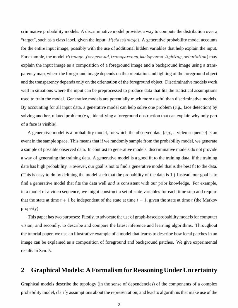
criminative probability models. A discriminative model provides a way to compute the distribution over a

“target”, such as a class label, given the input: P (class|image). A generative probability model accounts

for the entire input image, possibly with the use of additional hidden variables that help explain the input.

For example, the model P (image, foreground, transparency, background, lighting, orientation) may

explain the input image as a composition of a foreground image and a background image using a trans-

parency map, where the foreground image depends on the orientation and lighting of the foreground object

and the transparency depends only on the orientation of the foreground object. Discriminative models work

well in situations where the input can be preprocessed to produce data that fits the statistical assumptions

used to train the model. Generative models are potentially much more useful than discriminative models.

By accounting for all input data, a generative model can help solve one problem (e.g., face detection) by

solving another, related problem (e.g., identifying a foreground obstruction that can explain why only part

of a face is visible).

A generative model is a probability model, for which the observed data (e.g., a video sequence) is an

event in the sample space. This means that if we randomly sample from the probability model, we generate

a sample of possible observed data. In contrast to generative models, discriminative models do not provide

a way of generating the training data. A generative model is a good fit to the training data, if the training

data has high probability. However, our goal is not to find a generative model that is the best fit to the data.

(This is easy to do by defining the model such that the probability of the data is 1.) Instead, our goal is to

find a generative model that fits the data well and is consistent with our prior knowledge. For example,

in a model of a video sequence, we might construct a set of state variables for each time step and require

that the state at time t + 1 be independent of the state at time t − 1, given the state at time t (the Markov

property).

This paper has two purposes: Firstly, to advocate the use of graph-based probability models for computer

vision; and secondly, to describe and compare the latest inference and learning algorithms. Throughout

the tutorial paper, we use an illustrative example of a model that learns to describe how local patches in an

image can be explained as a composition of foreground and background patches. We give experimental

results in Scn. 5.

2 Graphical Models: A Formalism for Reasoning Under Uncertainty

Graphical models describe the topology (in the sense of dependencies) of the components of a complex

probability model, clarify assumptions about the representation, and lead to algorithms that make use of the

2

topology to increase speed and accuracy. When constructing a complex probability model, we are faced

with the following challenges: Ensuring that the model reflects our prior knowledge; Deriving efficient

algorithms for inference and learning; Translating the model to a different form; Communicating the model

to other researchers and users. Graphical models (graphical representations of probability models) offer a

way to overcome these challenges in a wide variety of situations. After briefly addressing each of these

issues, we review 3 kinds of graphical model: Bayesian networks, Markov random fields, and factor graphs.

Here, we briefly review graphical models. For a more extensive treatment, see [30, 35, 44].

Prior knowledge usually includes strong beliefs about the existence of hidden variables and the relation-

ships between variables in the system. This notion of “modularity” is a central aspect of graphical models.

For example, suppose we are constructing a model of motion fields for both the foreground object and the

background object in a video sequence. In a particular frame, the motion vector associated with a small

foreground patch is related to the corresponding patch in temporally proximal frames and also to nearby

motion vectors in the foreground. In contrast, the motion vector is neither directly related to the patches and

motion vectors in the background, nor directly related to foreground motion vectors from distant patches,

nor directly related to any of the patches and motion vectors from video frames that are temporally distant.

In a graphical model, the existence of a relationship is depicted by a path that connects the two variables.

Probabilistic inference in a probability model can, in principle, be carried out using Bayes rule. For

example, if U tx,y is a hidden random variable corresponding to the motion vector of the foreground patch

at position (x, y) in the frame from time t, and D is the video sequence, Bayes rule can be written

P (U tx,y = u|D) =

P (D|U tx,y = u)P (U t

x,y = u)∑u′ P (D|U t

x,y = u′)P (U tx,y = u′)

.

However, for the complex probability models that accurately describe a visual scene, direct application of

Bayes rule leads to an intractable number of computations. In this example, computing P (D|U tx,y = u)

requires marginalizing over a large number of other variables, including the motion vectors of all other

foreground patches at time t, U tx′,y′ , (x′, y′) �= (x, y), the motion vectors of all foreground patches in other

frames, and the motion vectors of all background patches for all frames.

Graphical models provide a framework for deriving efficient inference and learning algorithms. In the

above example, suppose we have somehow computed current estimates for all of the image patches and

motion vectors and would like to update the motion vector for a small foreground patch. The graphical

model indicates which other variables are directly relevant, in this case the corresponding patch in temporally

proximal frames and nearby motion vectors in the foreground. By examining these variables, we can update

the motion vector without regard to the other variables. Generally, the variables that are directly relevant

3

for updating a particular variable form the Markov blanket, which can be determined from the graph.

A Markov blanket for a variable is a set of variables such that when the variable is conditioned on the

Markov blanket, it becomes independent of all other variables. The Markov blanket is a useful concept when

deriving efficient inference algorithms, since it reveals which variables are directly relevant for computing

the distribution over a particular variable. Small Markov blankets are often preferred over large ones,

since the complexity of inference is usually exponentially related to the number of variables in the Markov

blanket.

In a complex probability model, computational inference and interpretation usually benefit from judi-

ciously groupings of variables and these clusters should take into account dependencies between variables.

Other types of useful transformation include splitting variables, eliminating (integrating over) variables,

and conditioning on variables. By examining the graph, we can often easily identify transformations steps

that will lead to simpler models or models that are better suited to our goals and in particular our choice of

inference algorithm. For example, we may be able to transform a graphical model that contains cycles to

a tree, and thus use an exact, but efficient, inference algorithm.

By examining a picture of the graph, a researcher or user can quickly identify the dependency rela-

tionships between variables in the system and understand how the influence of a variable flows through

the system to change the distributions over other variables. Whereas block diagrams enable us to effi-

ciently communicate how computations and signals flow through a system, graphical models enable us to

efficiently communicate the dependencies between components in a modular system.

2.1 Illustrative Example: A Model of Occluding Image Patches

The use of probability models in vision applications is, of course, extensive (c.f., [3, 5, 26, 47, 48] for a

sample of applications). Here, we introduce a model that is simple enough to study in this review paper,

but correctly accounts for an important effect in vision: occlusion. The model explains an input image with

pixel intensities z1, . . . , zK , as a composition of a foreground layer and a background layer [1]. Each patch

is explained as a composition of a foreground patch with a background patch, and each of these patches is

selected from a library of possible patches (a mixture model).

The generative process is illustrated in Fig. 1. To begin with, the class of the foreground, f ∈ {1, . . . , J},is randomly selected from distributionP (f). Then, depending on the class of the foreground, a binary mask

m = (m1, . . . ,mK), mi ∈ {0, 1} is randomly chosen. mi = 1 indicates that pixel zi is a foreground pixel,

whereasmi = 0 indicates that pixel zi is a background pixel. Given the foreground class, the mask elements

4

Figure 1: A generative process that explains an image as a composition of the image of a foreground object with

the image of the background, using a transparency map, or mask. The foreground, background and mask are each

selected stochastically from a library.

are chosen independently: P (m|f) =∏K

i=1 P (mi|f). Next, the class of the background, b ∈ {1, . . . , J}, is

randomly chosen fromP (b). Finally, the intensity of the pixels in the patch are selected independently, given

the mask, the class of the foreground, and the class of the background: P (z|m, f, b) =∏K

i=1 P (zi|mi, f, b).

The joint distribution is given by the following product of distributions:

P (z,m, f, b) = P (b)P (f)( K∏

i=1

P (mi|f))( K∏

i=1

P (zi|mi, f, b)). (2)

In fact, the above product of factors can be broken down further, by noting that if mi = 0 the class is

given by the variable b, and ifmi = 1 the class is given by the variable f . So, we can write P (zi|mi, f, b) =

P f (zi|f)miP b(zi|b)1−mi , where P f (zi|f) is the distribution over the ith pixel intensity for class f under

the foreground model, and P b(zi|b) is the same for the background model. These distributions account for

the dependence of the pixel intensity on the mixture index, as well as independent observation noise. The

joint distribution can thus be written:

P (z,m, f, b) = P (b)P (f)( K∏

i=1

P (mi|f))( K∏

i=1

P f (zi|f)mi

)( K∏i=1

P b(zi|b)1−mi

). (3)

Note that this factorization reduces the number of arguments in some of the factors.

For representational and computational efficiency, it is often useful to specify a model using parametric

distributions. We can parameterize P f (zi|f) and P b(zi|b) by assuming zi is Gaussian given its class. The

foreground and background models can have separate sets of means and variances, but here we assume

they share parameters: Let µki and ψki be the mean and variance of the ith pixel for class k. So, a particular

5

mean patch may act as a foreground patch in one instance, and a background patch in another instance.

If it is desirable that the foreground and background models have separate sets of means and variances,

the class variables f and b can be constrained, e.g., so that f ∈ {1, . . . , n}, b ∈ {n + 1, . . . , n + k}, and

µ1·, . . . , µn· are the n foreground means and µn+1·, . . . , µn+k· are the k background means.

Denote the probability of class k by πk, and let the probability that mi = 1 given that the foreground

class is f , be αfi. Since the probability that mi = 0 is 1 − αfi, we have P (mi|f) = αmifi (1 − αfi)1−mi .

Using these parametric forms, the joint distribution is

P (z,m, f, b) = πbπf

( K∏i=1

αmifi (1− αfi)1−miN (zi;µfi, ψfi)miN (zi;µbi, ψbi)1−mi

). (4)

where N (z;µ, ψ) is the normal density function on z with mean µ and variance ψ.

In the remainder of this review paper, the above patch model is used as an example when describing

graphical models, inference algorithms and learning algorithms. Although this model is quite simple and

perhaps not in need of the most advanced techniques, it is complex enough to be useful for shedding light

on the advantages and disadvantages of each type of graphical model, inference algorithm and learning

algorithm. In addition, one of the appeals of generative models is in their modularity - our simple model

can be extended in various ways to apply to more complex situations. For example, in our past research,

we have shown how transformations can be added to the mixture models [14,27,29], and how an occlusion

model such as the one above can be combined with transformation models to model layers of appearance

in a video [28].

2.2 Bayesian Network for the Patch Model

A Bayesian network [44] for variables s1, . . . , sN is a directed acyclic graph on the set of variables, along

with one conditional probability function for each variable given its parents, P (si|sAi), where Ai is the set

of indices of si’s parents. The joint distribution is given by the product of all the conditional probability

functions: P (s) =∏N

i=1 P (si|sAi). A directed acyclic graph is a directed graph that does not contain any

directed cycles.

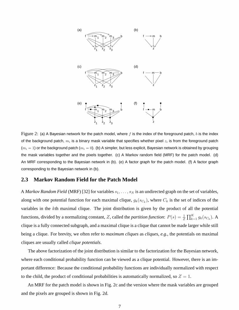
Fig. 2a shows the Bayesian network for the joint distribution given in (2) with K = 3 pixels. In this

Bayesian network, b and f don’t have any parents, because the distributions for b and f are not conditioned

on any other variables in (2), By group the mask variables together and the pixels together, we obtain the

Bayesian network shown in Fig. 2b. Although this graph is simpler than the graph in Fig. 2a, it is also less

explicit about conditional independencies.

6

bf

z

m

z1 z2 z3

m 1 m 3m 2f b

z2

m 1 m 3m 2

z3z1

f b bf

z

m

bf

z

mm 1

z3z1

m 3

z2

m 2f b

(b)(a)

(d)(c)

(f)(e)

Figure 2: (a) A Bayesian network for the patch model, where f is the index of the foreground patch, b is the index

of the background patch, mi is a binary mask variable that specifies whether pixel zi is from the foreground patch

(mi = 1) or the background patch (mi = 0). (b) A simpler, but less explicit, Bayesian network is obtained by grouping

the mask variables together and the pixels together. (c) A Markov random field (MRF) for the patch model. (d)

An MRF corresponding to the Bayesian network in (b). (e) A factor graph for the patch model. (f) A factor graph

corresponding to the Bayesian network in (b).

2.3 Markov Random Field for the Patch Model

A Markov Random Field (MRF) [32] for variables s1, . . . , sN is an undirected graph on the set of variables,

along with one potential function for each maximal clique, gk(sCk), where Ck is the set of indices of the

variables in the kth maximal clique. The joint distribution is given by the product of all the potential

functions, divided by a normalizing constant, Z, called the partition function: P (s) = 1Z

∏Kk=1 gk(sCk

). A

clique is a fully connected subgraph, and a maximal clique is a clique that cannot be made larger while still

being a clique. For brevity, we often refer to maximum cliques as cliques, e.g., the potentials on maximal

cliques are usually called clique potentials.

The above factorization of the joint distribution is similar to the factorization for the Bayesian network,

where each conditional probability function can be viewed as a clique potential. However, there is an im-

portant difference: Because the conditional probability functions are individually normalized with respect

to the child, the product of conditional probabilities is automatically normalized, so Z = 1.

An MRF for the patch model is shown in Fig. 2c and the version where the mask variables are grouped

and the pixels are grouped is shown in Fig. 2d.

7

2.4 Factor Graph for the Patch Model

Factor graphs [11, 30, 34] subsume Bayesian networks and MRFs. Any Bayesian network can be easily

converted to a factor graph, without loss of information. Any MRF can be easily converted to a factor graph,

without loss of information. Further, there exists models that have independence relationships that cannot

be expressed in a Bayesian network or an MRF, but that can be expressed in a factor graph [13]. Also,

belief propagation takes on a simple form in factor graphs, so that inference in both Bayesian networks and

MRFs can be simplified to a single, unified inference algorithm.

A factor graph for variables s1, . . . , sN and local functions g1(sf ), . . . , gK(sCK), is a bipartite graph

on the set of variables and a set of nodes corresponding to the functions, where each function node gk is

connected to the variables in its argument sCk. The joint distribution is given by the product of all the

functions: P (s) = 1Z

∏Kk=1 gk(sCk

). Z = 1 if the factor graph is a directed graph, as described below;

otherwiseZ ensures the distribution is normalized. Note that the local functions may be positive potentials,

as in MRFs, or conditional probability functions, as in Bayesian networks.

Fig. 2e shows a factor graph for the patch model and Fig. 2f shows a factor graph for the version where

the mask variables are grouped together and the pixels are grouped together.

3 Parameterized Models and Bayesian Learning

So far, we have studied graphical models as representations of structured probability models for computer

vision. We now turn to the general problem of how to learn these models from training data. For the purpose

of learning, it is often convenient to express the conditional distributions or potentials in a graphical model

as parameterized functions. Choosing the forms of the parameterized functions usually restricts the model

class, but often makes computations easier.

For example, Scn. 2.1 shows how we can parameterize the conditional probability functions in the patch

model. Recall that the joint distribution is

P (z,m, f, b) = πbπf

( K∏i=1


).

where the parameters are the π’s, α’s, µ’s and ψ’s.

8

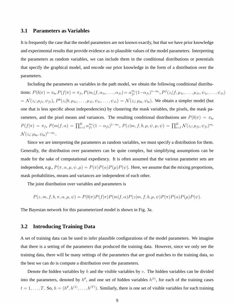
3.1 Parameters as Variables

It is frequently the case that the model parameters are not known exactly, but that we have prior knowledge

and experimental results that provide evidence as to plausible values of the model parameters. Interpreting

the parameters as random variables, we can include them in the conditional distributions or potentials

that specify the graphical model, and encode our prior knowledge in the form of a distribution over the

parameters.

Including the parameters as variables in the path model, we obtain the following conditional distribu-

tions: P (b|π) = πb,P (f |π) = πf ,P (mi|f, α1i, . . . , αJi)= αmifi (1−αfi)1−mi ,P f (zi|f, µ1i, . . . , µJi, ψ1i, . . . , ψJi)

= N (zi;µfi, ψfi), P b(zi|b, µ1i, . . . , µJi, ψ1i, . . . , ψJi) = N (zi;µbi, ψbi). We obtain a simpler model (but

one that is less specific about independencies) by clustering the mask variables, the pixels, the mask pa-

rameters, and the pixel means and variances. The resulting conditional distributions are P (b|π) = πb,

P (f |π) = πf , P (m|f, α) =∏K

i=1 αmifi (1 − αfi)1−mi , P (z|m, f, b, µ, ψ, µ, ψ) =

∏Ki=1N (zi;µfi, ψfi)mi

N (zi;µbi, ψbi)1−mi .

Since we are interpreting the parameters as random variables, we must specify a distribution for them.

Generally, the distribution over parameters can be quite complex, but simplifying assumptions can be

made for the sake of computational expediency. It is often assumed that the various parameter sets are

independent, e.g., P (π, α, µ, ψ, µ) = P (π)P (α)P (µ)P (ψ). Here, we assume that the mixing proportions,

mask probabilities, means and variances are independent of each other.

The joint distribution over variables and parameters is

P (z,m, f, b, π, α, µ, ψ) = P (b|π)P (f |π)P (m|f, α)P (z|m, f, b, µ, ψ)P (π)P (α)P (µ)P (ψ).

The Bayesian network for this parameterized model is shown in Fig. 3a.

3.2 Introducing Training Data

A set of training data can be used to infer plausible configurations of the model parameters. We imagine

that there is a setting of the parameters that produced the training data. However, since we only see the

training data, there will be many settings of the parameters that are good matches to the training data, so

the best we can do is compute a distribution over the parameters.

Denote the hidden variables by h and the visible variables by v. The hidden variables can be divided

into the parameters, denoted by hθ, and one set of hidden variables h(t), for each of the training cases

t = 1, . . . , T . So, h = (hθ, h(1), . . . , h(T )). Similarly, there is one set of visible variables for each training

9

f b f b f b f b

ψµ ψµ ψµ ψµ

t=Tt=3t=2t=1

(c)

z

m

π α

z

m

π α

z

m

π α

z

m

π α

f b f b f b

(b)

z

m

z

m

z

m

. . .t=Tt=2t=1

ψµ

π α

f b

(a)

z

m

π α

ψµ

. . .

Figure 3: (a) The parameter sets π, α, µ and ψ can be included in the Bayesian network as random variables. (b)

For a training set with T i.i.d. cases, these parameters are shared across all training cases. (c) If the training cases

are time-series data (e.g. a video sequence), we may create one parameter set for each time instance, but require

the parameters to change slowly over time.

case: v = (v(1), . . . , v(T )). Assuming the training cases are independent and identically drawn (i.i.d.), the

distribution over all visible variables and hidden variables (including parameters) can be written

P (h, v) = P (hθ)T∏

t=1

P (h(t), v(t)|hθ).

In this expression, P (hθ) is called the parameter prior and∏T

t=1 P (h(t), v(t)|hθ) is called the likelihood. In

the following two sections, we describe forms of the parameter prior that lead to computationally efficient

inference and learning algorithms.

In the patch model described above, we have hθ = (µ, ψ, µ, ψ, πf , πb, α), h(t) = (f (t), b(t),m(t)), and

v(t) = z(t). The Bayesian network for T i.i.d. training cases is shown in Fig. 3b.

When the training cases consist of time-series data (such as a video sequence), the parameters often

can be thought of as variables that change slowly over time. Fig. 3c shows the above model, where there

is a different set of parameters for each training case, but where we assume the parameters are coupled

across time. Using (t) to denote the training case at time t = 1, . . . , T , the following distributions couple

the parameters across time: P (π(t)|π(t−1)), P (α(t)|α(t−1)), P (µ(t)|µ(t−1)), P (ψ(t)|ψ(t−1)). The uncertainty

in these distributions specifies how quickly the parameters can change over time.

10

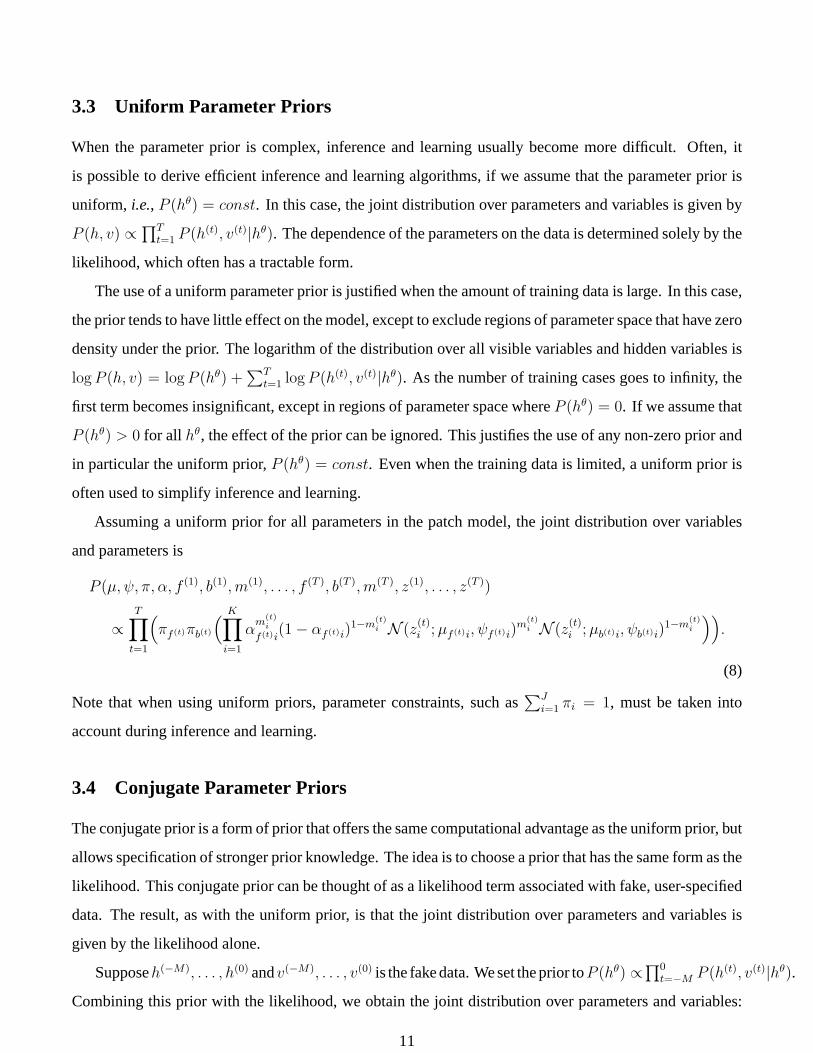
3.3 Uniform Parameter Priors

When the parameter prior is complex, inference and learning usually become more difficult. Often, it

is possible to derive efficient inference and learning algorithms, if we assume that the parameter prior is

uniform, i.e., P (hθ) = const. In this case, the joint distribution over parameters and variables is given by

P (h, v) ∝∏Tt=1 P (h(t), v(t)|hθ). The dependence of the parameters on the data is determined solely by the

likelihood, which often has a tractable form.

The use of a uniform parameter prior is justified when the amount of training data is large. In this case,

the prior tends to have little effect on the model, except to exclude regions of parameter space that have zero

density under the prior. The logarithm of the distribution over all visible variables and hidden variables is

logP (h, v) = logP (hθ) +∑T

t=1 logP (h(t), v(t)|hθ). As the number of training cases goes to infinity, the

first term becomes insignificant, except in regions of parameter space where P (hθ) = 0. If we assume that

P (hθ) > 0 for all hθ, the effect of the prior can be ignored. This justifies the use of any non-zero prior and

in particular the uniform prior, P (hθ) = const. Even when the training data is limited, a uniform prior is

often used to simplify inference and learning.

Assuming a uniform prior for all parameters in the patch model, the joint distribution over variables

and parameters is

P (µ, ψ, π, α, f (1), b(1),m(1), . . . , f (T ), b(T ),m(T ), z(1), . . . , z(T ))

∝T∏

t=1

(πf (t)πb(t)

( K∏i=1

αm

(t)i

f (t)i(1− αf (t)i)

1−m(t)i N (z(t)

i ;µf (t)i, ψf (t)i)m

(t)i N (z(t)

i ;µb(t)i, ψb(t)i)1−m

(t)i

)).

(8)

Note that when using uniform priors, parameter constraints, such as∑J

i=1 πi = 1, must be taken into

account during inference and learning.

3.4 Conjugate Parameter Priors

The conjugate prior is a form of prior that offers the same computational advantage as the uniform prior, but

allows specification of stronger prior knowledge. The idea is to choose a prior that has the same form as the

likelihood. This conjugate prior can be thought of as a likelihood term associated with fake, user-specified

data. The result, as with the uniform prior, is that the joint distribution over parameters and variables is

given by the likelihood alone.

Supposeh(−M), . . . , h(0) andv(−M), . . . , v(0) is the fake data. We set the prior toP (hθ) ∝∏0t=−M P (h(t), v(t)|hθ).

Combining this prior with the likelihood, we obtain the joint distribution over parameters and variables:

11

P (h, v) ∝ ∏Tt=−M P (h(t), v(t)|hθ). Computationally, inference and learning in this model is equivalent to

inference and learning using a uniform prior, but with extra, fake data.

In addition to specifying fake training cases, it is also useful to specify how many times each one occurs.

Let w(t) be the number of times the tth training case occurs. For each real training case (1 ≤ t ≤ T ), we

havew(t) = 1. The contribution of the tth case to the likelihood isP (h(t), v(t)|hθ)w(t). The joint distribution

is P (h, v) ∝∏Tt=−M P (h(t), v(t)|hθ)w(t)

. The values of the weights usually have very little influence on the

computational efficiency of inference and learning, but provide control over the impact of the fake data. In

fact, we can set each w (or, weight) to any real number, including fractional numbers.

In the patch model, we might imagine that before seeing any training data, we observe a total of λj

examples from patch class j = 1, . . . , J . It follows that the likelihood of the fake data for parameter πj is

πjλj . The conjugate prior for π1, . . . , πJ is thus

P (π1, . . . , πJ) ∝

∏Ji=1 πj

λj if∑J

i=1 πj = 1,

0 otherwise.

This is the Dirichlet distribution, so P (π1, . . . , πJ) is called a Dirichlet prior.

The conjugate prior for the mean of a Gaussian distribution is a Gaussian distribution, because the

random variable and its mean appear symmetrically in the density function for a Gaussian.

The conjugate prior for the inverse variance β of a Gaussian distribution is a Gamma distribution. To

see this, imagine fake data consisting of λ examples where the squared difference between the random

variable and its mean is δ. The likelihood for this fake data is proportional to βλ/2e−(λδ/2)β . Setting the prior

for β to be proportional to this likelihood, we see that the conjugate prior for β is the Gamma distribution,

with mean 1/δ + 2/λδ and variance 2(1/δ + 2/λδ)/λδ. Note that for large weight, λ→∞, the mean of

the inverse variance is 1/δ, the inverse of the fake squared difference between the random variable and its

mean. Also, the prior variance on the inverse variance decreases as the weight increases.

4 Algorithms for Inference and Learning

Once a generative model describing the image rendering process has been specified, vision consists of

inverse inference in the generative model. Exact inference is often intractable, so we turn to approximate

algorithms that try to find distributions that are close to the correct posterior distribution. This is accom-

plished by minimizing pseudo-distances on distributions, called “free energies”. It is interesting that in the

1800’s, Helmholtz was one of the first researchers to propose that vision is inverse inference in a generative

12

model, and that nature seeks correct probability distributions in physical systems by minimizing what is

now called the Helmholtz free energy. Although there is no record that Helmholtz saw that the brain might

perform vision by minimizing a free energy, one can’t help but wonder if he pondered this.

In a parameterized model, given the training data, vision consists of inferring the parameters used to

describe the entire training set, as well as the variables that explain each training case. In the model shown

in Fig. 3b, for training images z(1), . . . , z(T ), vision consists of inferring the set of model patches and

variance maps, µ, ψ, the mixing proportions of the model patches π, the set of binary mask probabilities

for every foreground class, α, and, for every training case, the class of the foreground patch, f , the class of

the background patch, b, and the binary mask used to combine these patches, m.

As presented in this tutorial paper, parameters and variables are both considered to be random variables.

One difference between parameters and variables is that the parameters are constant across all training cases

for i.i.d. data, or change slowly across time in time-series data, such as videos. This difference leads to the

terminology whereby we refer to inference of model parameters as machine learning, or just learning. It is

often important to treat parameters and variables differently during inference. Whereas each variable plays

a role in a single training case, the parameters are shared across many training cases. So, the parameters

are impacted by more evidence than variables and are often pinned down more tightly by the data. This

observation becomes relevant when we study approximate inference techniques that obtain point estimates

of the parameters, such as the expectation maximization algorithm [6].

We now turn to the general problem of inferring the values of unobserved (hidden) variables, given

the values of the observed (visible) variables. As above, denote the hidden variables by h and the visible

variables by v. The hidden variables can usually be divided into the parameters, denoted by hθ, and one set

of hidden variables h(t), for each of the training cases t = 1, . . . , T . So, h = (hθ, h(1), . . . , h(T )). Similarly,

there is one set of visible variables for each training case: v = (v(1), . . . , v(T )). Assuming the training

cases are i.i.d., the distribution over all hidden and visible variables can be written

P (h, v) = P (hθ)( T∏

t=1

P (h(t), v(t)|hθ)). (10)

In the patch model, we have hθ = (µ, ψ, π, α), h(t) = (f (t), b(t),m(t)), and v(t) = z(t).

Exact inference consists of computing estimates or making decisions based on the posterior distribution

over all hidden variables (including the parameters), P (h|v). From Bayes rule,

P (h|v) =P (h, v)∫hP (h, v)

,

where we use the notation∫

hto include summing over discrete hidden variables. The denominator serves

13

to normalize the distribution over h. For various types of inference and various inference algorithms, we

need only a function that is proportional to the posterior distribution. In these cases P (h, v) suffices, since

w.r.t. h,

P (h|v) ∝ P (h, v).

Note that in the case of a graphical model, P (h, v) is equal to the either the product of the conditional

distributions, or the product of the potential functions, divided by the partition function.

Exact inference in the patch model with known parameters

When the model parameters are known, the distribution over the foreground class, background class,

and mask variables is proportional to the joint distribution from (4):

P (m, f, b|z) ∝ πbπf

( K∏i=1


).

f and b each take on J values and there are K binary mask variables, so the total number of configurations

of f , b and m is J22K . For moderate model sizes, even if we can compute the posterior, we cannot store

the posterior probability of every configuration.

However, from the Bayesian network in Fig. 2, we see that mi is independent of mj, j �= i, given f , b

and zi (the Markov blanket of mi). Thus, we represent the posterior distribution as follows:

P (m, f, b|z) = P (f, b|z)P (m|f, b, z) = P (f, b|z)K∏

i=1

P (mi|f, b, z).

In this form, the posterior can be stored using order J2 numbers forP (f, b|z) and for each configuration of f

and b, orderK numbers for the probabilities P (mi|f, b, z), i = 1, . . . , K, giving a total storage requirement

of order KJ2 numbers.

P (f, b|z) can be computed as follows:

P (f, b|z) ∝ P (f, b, z) =∑m1

· · ·∑mK

P (m, f, b, z)

= πbπf

K∏i=1

(∑mi

(αmi

fi (1− αfi)1−miN (zi;µfi, ψfi)miN (zi;µbi, ψbi)1−mi

))

= πbπf

K∏i=1

(αfiN (zi;µfi, ψfi) + (1− αfi)N (zi;µbi, ψbi)

).

For each value of f and b, this can be computed using order K multiply-adds. Once it is computed for all

J2 combinations of f and b, the result is normalized to give P (f, b|z). The total number of multiply-adds

needed to compute P (f, b|z) is order KJ2.

14

For each mi, P (mi|f, b, z) can be rewritten thus:

P (mi|f, b, z) = P (mi|f, b, zi) ∝ P (mi|f, b, zi)P (zi|f, b) = P (zi,mi|f, b)= P (mi|f, b)P (zi|mi, f, b) = P (mi|f)P (zi|mi, f, b).

Substituting the definitions of these conditional distributions, we have

P (mi|f, b, z) ∝ αmifi (1− αfi)1−miN (zi;µfi, ψfi)miN (zi;µbi, ψbi)1−mi .

For each i = 1, . . . , K and each configuration of f and b, this can be computed and normalized using a

small number of multiply-adds. The total number of multiply-adds needed to compute P (mi|f, b, z) for

all i is order KJ2.

Using the above technique, when given the model parameters, the exact posterior over f , b and m can

be computed in order KJ2 multiply-adds and stored using order KJ2 numbers.

Exact inference of variables and parameters in the patch model

Assuming a uniform parameter prior, the joint distribution over parameters and variables in the patch

model of Fig. 3b is given in (8). The posterior distribution is proportional to this joint distribution:

P (µ, ψ, π, α, f (1), b(1),m(1), . . . , f (T ), b(T ),m(T )|z(1), . . . , z(T ))

∝T∏

t=1

(πf (t)πb(t)

( K∏i=1

αm

(t)i

f (t)i(1− αf (t)i)

1−m(t)i N (z(t)

i ;µf (t)i, ψf (t)i)m

(t)i N (z(t)

i ;µb(t)i, ψb(t)i)1−m

(t)i

)).

(16)

This posterior can be thought of as a very large mixture model. There are J2T 2KT discrete configurations

of the class variables and the mask variables and for each configuration, there is a distribution over the

real-valued parameters. In each mixture component, the class probabilities are Dirichlet-distributed and

the mask probabilities are Beta-distributed. The pixel means and variances are coupled in the posterior,

but given the variances, the means are normally distributed and given the means, the inverse variances are

Gamma-distributed.

Even for this quite simple example, the exact posterior is intractable, because the number of posterior

mixture components is exponential in the number of training cases, and the posterior distribution over

the pixel means and variances are coupled. In the remainder of this paper, we describe a variety of

approximate inference techniques and discuss advantages and disadvantages of each approach. Before

discussing approximations, we discuss practical ways of interpreting the results of inference.

15

4.1 Approximate Inference as Minimizing Helmholtzian Free Energies

Usually, the above techniques cannot be applied directly to P (h|v), because this distribution cannot be

computed in a tractable manner. So, we must turn to various approximations.

Many approximate inference techniques can be viewed as minimizing a cost function called “free

energy”, which measures the accuracy of an approximate probability distribution. These include iterative

conditional modes [2], the expectation maximization (EM) algorithm [6,41], mean field methods [45,46,52],

variational techniques [10,11,20,21,24,31,41], structured variational techniques [17,25,31,42,43], Gibbs

sampling [40], the sum-product algorithm (a.k.a. loopy belief propagation) [51] and the expectation

propagation algorithm [38].

The idea is to approximate the true posterior distribution P (h|v) by a simpler distribution Q(h), which

is then used for making decisions, computing estimates, summarizing the data, etc. Here, approximate

inference consists of searching for the distribution Q(h) that is closest to P (h|v). A natural choice for

a measure of similarity between the two distributions is the relative entropy (a.k.a. Kullback-Leibler

divergence) [4]:

D(Q,P ) =∫

h

Q(h) logQ(h)P (h|v) .

This is a divergence, not a distance, because it is not symmetric – in general, swapping Q and P will

give a different value for D(Q,P ). However, D(Q,P ) is similar to a distance in that D(Q,P ) ≥ 0, and

D(Q,P ) = 0 if and only if the approximating distribution exactly matches the true posterior, Q(h) =

P (h|v).Approximate inference techniques can be derived by examining ways of searching forQ(h), to minimize

D(Q,P ). In fact, directly computing D(Q,P ) is usually intractable, because it depends on P (h|v). If

we already have a tractable form for P (h|v) to insert into the expression for D(Q,P ), we probably don’t

have a need for approximate inference. Fortunately, D(Q,P ) can be modified in a way that does not alter

the structure of the search space of Q(h), but makes computations tractable. If we subtract logP (v) from

D(Q,P ), we obtain

F (Q,P ) = D(Q,P )− logP (v)

=∫

h

Q(h) logQ(h)P (h|v) −

∫h

Q(h) logP (v)

=∫

h

Q(h) logQ(h)

P (h|v)P (v)

=∫

h

Q(h) logQ(h)P (h, v)

. (18)

16

Notice that logP (v) does not depend on Q(h), so subtracting logP (v) will not influence the search for

Q(h). For Bayesian networks and directed factor graphs, we do have a tractable expression for P (h, v),

namely the product of conditional distributions.

F (Q,P ) is called the Helmholtz free energy or the Gibbs free energy, or just the free energy. If we

interpret− logP (h, v) as the energy function of a physical system andQ(h) as a distribution over the state

of the system, then the expression for F (Q,P ) is identical to the expression for the Helmholtz or Gibbs

free energy defined in physics textbooks. In this case minimizing the free energy corresponds to finding

the equilibrium distribution of the physical system (the Boltzmann distribution).

Another way to derive the free energy is by using Jensen’s inequality [4] to bound the log-probability

of the visible variables. Jensen’s inequality states that a concave function of a convex combination of

points in a vector space is greater than or equal to the convex combination of the concave function applied

to the points. The log-probability of the visible variables is logP (v) = log(∫

hP (h, v)). By introducing

an arbitrary distribution Q(h) (which provides a set of convex weights), we obtain a convex combination

inside the log() function, which can be bounded:

logP (v) = log(∫

h

P (h, v))

= log(∫

h

Q(h)P (h, v)Q(h)

)

≥∫

h

Q(h) log(P (h, v)Q(h)

)= −F (Q,P ). (19)

We see that the free energy is an upper bound on the negative log-probability of the visible variables:

F (Q,P ) ≥ − logP (v). This can also be seen by noting that D(Q,P ) ≥ 0 in (18).

Free energy for i.i.d. training cases

From (10), for a training set of T i.i.d. training cases with hidden variables h = (hθ, h(1), . . . , h(T )) and

visible variables v = (v(1), . . . , v(T )), we have P (h, v) = P (hθ)∏T

t=1 P (h(t), v(t)|hθ). The free energy is

F (Q,P ) =∫

h

Q(h) logQ(h)−∫

h

Q(h) logP (h, v)

=∫

h

Q(h) logQ(h)−∫

hθ

Q(hθ) logP (hθ)−T∑

t=1

∫h(t),hθ

Q(h(t), hθ) logP (h(t), v(t)|hθ). (20)

The decomposition of F into a sum of one term for each training case simplifies learning.

Exact inference revisited

The idea of approximate inference is to search for Q(h) in a space of models that are simpler than

the true posterior P (h|v). It is instructive to not assume Q(h) is simplified and derive the minimizer of

17

F (Q,P ). The only constraint we put on Q(h) is that it is normalized:∑

hQ(h) = 1. To account for this

constraint, we form a Lagrangian from F (Q,P ) with Lagrange multiplier λ and optimize F (Q,P ) w.r.t.

Q(h):∂(F (Q,P ) + λ

∫hQ(h))

∂Q(h)= logQ(h) + 1− logP (h, v) + λ.

Setting this derivative to 0 and solving for λ, we find

Q(h) =P (h, v)∫hP (h, v)

= P (h|v).

So, minimizing the free energy without any simplifying assumptions on Q(h) produces exact inference.

The minimum free energy is

minQ

F (Q,P ) =∫

h

P (h|v) logP (h|v)P (h, v)

= − logP (v).

The minimum free energy is equal to the negative log-probability of the data. This minimum is achieved

when Q(h) = P (h|v).Revisiting exact inference in the patch model

In the patch model, if we allow the approximating distribution Q(f, b,m) to be unconstrained, we find

that the minimum free energy is obtained when

Q(f, b,m) = P (f, b|z)K∏

i=1

P (mi|f, b, z).

Of course, nothing is gained computationally by using this Q-distribution. In the following sections, we

see how the use of various approximate forms for Q(f, b,m) lead to tremendous speed-ups.

4.2 Point Inference for Discrete Variables and Continuous Variables

Many standard techniques search for a single configuration h of the hidden variables. In particular, re-

searchers often formulate problems as searching over configurations of hidden variables, so as to minimize

a cost, or energy function.

For discrete hidden variables, we can understand this procedure as minimizingF (Q,P ) for a degenerate

Q-distribution. Using Iverson’s equality-indicator function, we define

Q(h) = [h = h] =

1 if h = h

0 otherwise.

18

In this case, the free energy in (18) simplifies to

F (Q,P ) =∑

h

[h = h] log[h = h]P (h, v)

= − logP (h, v).

So, minimizing F (Q,P ) corresponds to searching for values of h that maximize P (h, v). At the global

minimum, F (Q,P ) is equal to the global minimum of − logP (h, v).

For continuous hidden variables, theQ-distribution for a point estimate is a Dirac delta function centered

at the estimate:

Q(h) = δ(h− h),

which is an infinite spike of density at h. δ(h− h) has the following properties:∫

hδ(h− h)f(h) = f(h),

and∫

hδ(h− h) = 1. The free energy in (18) simplifies to

F (Q,P ) =∫

h

δ(h− h) logδ(h− h)P (h, v)

= − logP (h, v)−Hδ,

where Hδ is the entropy of the Dirac delta. This entropy does not depend on h, so minimizing F (Q,P )

corresponds to searching for values of h that maximize P (h, v).

Unfortunately, the entropy of the Dirac delta goes to negative infinity1,Hδ → −∞. So, even the optimal

value of h results in F (Q,P ) → ∞, which is clearly not equal to the global minimum of − logP (h, v).

The fact that F (Q,P ) → ∞ is an indication of the theoretical absurdity of making point inferences for

continuous variables. The probability that a continuous variable has any one value is zero, so inferring a

single value is probabilistic nonsense. Even so, point inference of continuous variables can lead to useful

results. In this paper, we review two popular techniques that use point inferences: Iterative condition

modes, and the expectation maximization algorithm.

4.3 Iterative Conditional Modes (ICM)

The main advantage of this technique is that it is usually very easy to implement. Its main disadvantage is

that it does not take into account uncertainties in the values of hidden variables, when inferring the values

of other hidden variables. This causes ICM to find poor local minima.

The algorithm works by searching for a configuration of h that maximizesP (h|v). The simplest version

of ICM proceeds as follows.

1To see this, let δ(x) have the value 1/ε in the interval 0 ≤ x ≤ ε and let ε→ 0. The entropy is log ε, which goes to −∞ as

ε→ 0.

19

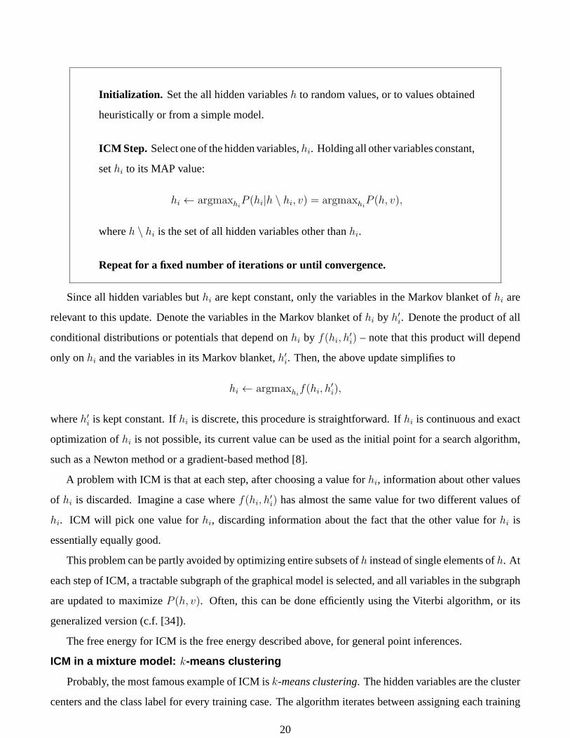
Initialization. Set the all hidden variables h to random values, or to values obtained

heuristically or from a simple model.

ICM Step. Select one of the hidden variables, hi. Holding all other variables constant,

set hi to its MAP value:

hi ← argmaxhiP (hi|h \ hi, v) = argmaxhi

P (h, v),

where h \ hi is the set of all hidden variables other than hi.

Repeat for a fixed number of iterations or until convergence.

Since all hidden variables but hi are kept constant, only the variables in the Markov blanket of hi are

relevant to this update. Denote the variables in the Markov blanket of hi by h′i. Denote the product of all

conditional distributions or potentials that depend on hi by f(hi, h′i) – note that this product will depend

only on hi and the variables in its Markov blanket, h′i. Then, the above update simplifies to

hi ← argmaxhif(hi, h

′i),

where h′i is kept constant. If hi is discrete, this procedure is straightforward. If hi is continuous and exact

optimization of hi is not possible, its current value can be used as the initial point for a search algorithm,

such as a Newton method or a gradient-based method [8].

A problem with ICM is that at each step, after choosing a value for hi, information about other values

of hi is discarded. Imagine a case where f(hi, h′i) has almost the same value for two different values of

hi. ICM will pick one value for hi, discarding information about the fact that the other value for hi is

essentially equally good.

This problem can be partly avoided by optimizing entire subsets of h instead of single elements of h. At

each step of ICM, a tractable subgraph of the graphical model is selected, and all variables in the subgraph

are updated to maximize P (h, v). Often, this can be done efficiently using the Viterbi algorithm, or its

generalized version (c.f. [34]).

The free energy for ICM is the free energy described above, for general point inferences.

ICM in a mixture model: k-means clustering

Probably, the most famous example of ICM is k-means clustering. The hidden variables are the cluster

centers and the class label for every training case. The algorithm iterates between assigning each training

20

case to the closest cluster center, and setting each cluster center equal to the average of the training cases

assigned to it.

ICM in the patch model

Even when the model parameters in the patch model are known, the computational cost of exact inference

can be rather high. When the number of clusters J is large (say, 200), examining all J2 configurations

of the foreground class and the background class is computationally burdensome. For ICM in the patch

model, the Q-distribution for the entire training set is

Q =(∏

k

δ(πk − πk))(∏

k,i

δ(µki − µki))(∏

k,i

δ(ψki − ψki))(∏

k,i

δ(αki − αki))

( ∏t

[b(t) = b(t)])( ∏

t

[f (t) = f (t)])( ∏

t

∏i

[m(t)i = m

(t)i ]

).

Substituting this Q-distribution and the P -distribution in (8) into the expression for the free energy in (20),

we obtain the following:

F = −∑

t

log πf (t) + log πb(t) +

−∑

t

∑i

m(t)i log αf (t)i + (1− m(t)

i ) log(1− αf (t)i)

+∑

t

∑i

m(t)i

((z(t)

i − µf (t)i)2/2ψf (t)i + log(2πψf (t)i)/2

)

+∑

t

∑i

(1− m(t)i )

((z(t)

i − µb(t)i)2/2ψb(t)i + log(2πψb(t)i)/2

)−H.

The last term, H , is the entropy of the δ-functions and is constant w.r.t. the optimization. Intuitively, this

cost measures the mismatch between the input image and the image obtained by combining the foreground

and background patches, using the mask.

In order to minimize the free energy with respect to all variables and parameters, we can iteratively

solve for each variable keeping others fixed, until convergence. This can be done in any order, but since the

model parameters depend on values of all hidden variables, we first optimize for all hidden variables, and

then optimize for model parameters. Furthermore, since for every observation, the class variables depend

on all pixels, when updating the hidden variables, we first visit the mask values for all pixels and then the

class variables.

After all parameters and variables are set to random values, the updates proceed as follows (the “”

notation is dropped for convenience):

• For t = 1, . . . , T

21

{ f (t) ← argmaxf (t)

[πf (t)

∏i:m(t)

i =1N (z(t)i ;µf (t)i, ψf (t)i)

]

{ b(t) ← argmaxb(t)

[πb(t)

∏i:m(t)

i =0N (z(t)i ;µb(t)i, ψb(t)i)

]

{ For i = 1, . . . , K: m(t)i ←

1 if αf (t)iN (z(t)i ;µf (t)i, ψf (t)i) > (1− αf (t)i)N (z(t)

i ;µb(t)i, ψb(t)i)

0 otherwise

• For j = 1, . . . , J

{ πj ← (∑T

t=1[f(t) = j] +

∑Tt=1[b

(t) = j])/2T

• For j = 1, . . . , J , for i = 1, . . . , K

{ αji ← (∑T

t=1[f(t) = j]m(t)

i )/(∑T

t=1[f(t) = j])

{ µji ← (∑T

t=1[f(t) = j or b(t) = j]z(t)

i )/(∑T

t=1[f(t) = j or b(t) = j])

{ ψji ← (∑T

t=1[f(t) = j or b(t) = j](z(t)

i − µji)2)/(∑T

t=1[f(t) = j or b(t) = j])

Here, the Iverson notation is used where [True] = 1 and [False] = 0.

4.4 The Expectation-Maximization Algorithm

As discussed above, one problem with ICM is that it does not account for uncertainty in the values of

hidden variables. The EM algorithm accounts for uncertainty in some variables, while performing ICM-

like updates for the other variables. In particular, for parameters hθ and remaining variables h(1), . . . , h(T ),

EM obtains point estimates for hθ and computes the exact posterior over the other variables, given hθ. The

Q-distribution is

Q(h) = δ(hθ − hθ)Q(h(1), . . . , h(T )).

Recall that for i.i.d. data, P (h, v) = P (hθ)(∏T

t=1 P (h(t), v(t)|hθ)). Given hθ, the variables associated with

different training cases are independent. So, we can use the following factorized form for Q:

Q(h) = δ(hθ − hθ)T∏

t=1

Q(h(t)).

In exact EM, no restrictions are placed on the distributions, Q(h(t)).

Substituting the expressions for P (h, v) and Q(h) into (18), we obtain the following free energy:

F (Q,P ) = − logP (hθ) +T∑

t=1

(∫h(t)

Q(h(t)) logQ(h(t))

P (h(t), v(t)|hθ)

).

22

EM is an iterative algorithm that alternates between minimizing F (Q,P ) with respect to the set of distri-

butions Q(h(1)), . . . , Q(h(T )) in the E step, and minimizing F (Q,P ) with respect to hθ in the M step.

When updating the distribution over the hidden variables for training case t, the only constraint on

Q(h(t)) is that∫

h(t) Q(h(t)) = 1. As described earlier, we account for this constraint by including a

Lagrange multiplier. Setting the derivative of F (Q,P ) to zero and solving for Q(h(t)), we obtain the

solution, Q(h(t)) = P (h(t)|v(t), hθ). Taking the derivative of F (Q,P ) w.r.t. hθ, we obtain

∂F (Q,P )

∂hθ= − ∂

∂hθlogP (hθ)−

T∑t=1

(∫h(t)

Q(h(t))∂

∂hθlogP (h(t), v(t)|hθ)

).

For M parameters, this is a set of M equations. These two solutions give the EM algorithm:

Initialization. Set the estimates of the parameters, hθ, to random values, or to values

obtained from a simple model.

E Step. Minimize F (Q,P ) w.r.t. Q by setting

Q(h(t))← P (h(t)|v(t), hθ),

for each training case, given the parameters hθ and the data v(t).

M Step. Minimize F (Q,P ) w.r.t. the model parameters hθ by solving

− ∂

∂hθlogP (hθ)−

T∑t=1

(∫h(t)

Q(h(t))∂

∂hθlogP (h(t), v(t)|hθ)

)= 0. (36)

ForM parameters, this is a system ofM equations. Often, the prior on the parameters

is assumed to be uniform, P (hθ) = const, in which case the first term in the above

expression vanishes.


In Scn. 4.1, we showed that when Q(h) = P (h|v), F (Q,P ) = − logP (v). So, the EM algorithm

alternates between obtaining a tight lower bound on logP (v) and then maximizing this bound w.r.t. the

model parameters. This means that with each iteration, the log-probability of the data, logP (v), must

increase or stay the same.

EM in the patch model

23

As with ICM we approximate the distribution over the parameters using Q(hθ) = δ(hθ − hθ). As

described above, in the E step we set Q(b, f,m)← P (b, f,m|z) for each training case. Because the mi’s

are independent given f and b, this Q-distribution can be expressed as

Q(b, f,m) = Q(b, f)∏

i

Q(mi|b, f).

This is the distribution used in the M step to minimize the free energy w.r.t. the model parameters,

hθ = {αk, µk, ψk, πk}Kk=1.

In the E step, the values in the probability tables Q(b, f) and Q(mi|b, f) are determined so as to

minimize the free energy subject to the normalization constraints∑

f,bQ(b, f) = 1 and Q(mi = 1|b, f) =

1 − Q(mi = 0|b, f), leading to the following updates of the variational distributions for a single training

case:

Q(mi = 1|b, f)← αfiN (zi;µfi, ψfi)αfiN (zi;µfi, ψfi) + (1− αfi)N (zi;µbi, ψbi)

,

Q(b, f)← cπbπf exp{−

∑i

(Q(mi = 1|b, f)

((zi − µfi)2

2ψfi

+log 2πψfi

2

)+

(1−Q(mi = 1|b, f))((zi − µbi)2

2ψbi

+log 2πψbi

2

))},

where c is computed to normalize the distribution. We also compute the following distributions, which

are needed in the M step: Q(b) ← ∑f Q(b, f), Q(f) ← ∑

bQ(b, f), Q(mi = 1, b) ← ∑f Q(mi =

1|b, f)Q(b, f), Q(mi = 1, f)←∑bQ(mi = 1|b, f)Q(b, f).

The derivatives of the free energy w.r.t. the model parameters in (36) give the following parameter

updates, where t indexes the training cases:

πk ←( ∑

t

Q(f (t) = k) +∑

t

Q(b(t) = k))/(2T ),

αki ←∑

tQ(m(t)i = 1, f (t) = k)∑

tQ(f (t) = k),

µki ←∑

t

(Q(m(t)

i = 1, f (t) = k) +Q(m(t)i = 0, b(t) = k)

)z

(t)i∑

t

(Q(m(t)

i = 1, f (t) = k) +Q(m(t)i = 0, b(t) = k)

) .

ψki ←∑

t

(Q(m(t)

i = 1, f (t) = k) +Q(m(t)i = 0, b(t) = k)

)(z(t)

i − µki)2

∑t

(Q(m(t)

i = 1, f (t) = k) +Q(m(t)i = 0, b(t) = k)

) .

24

The above updates can be iterated in a variety of ways. For example, each iteration may consist of

repeatedly updating the variational distributions until convergence and then updating the parameters. Or,

each iteration may consist of updating each variational distribution once, and then updating the parameters.

There are many possibilities and the update order is best at avoiding local minima depends on the problem.

This variety of ways of minimizing the free energy leads to a generalization of EM.

4.5 Generalized EM

The above derivation of the EM algorithm makes obvious several generalizations, all of which attempt to

decrease F (Q,P ) [41]. If F (Q,P ) is a complex function of the parameters hθ, it may not be possible to

exactly solve for the hθ that minimizes F (Q,P ) in the M step. Instead, hθ can be modified so as to decrease

F (Q,P ), e.g., by taking a step downhill in the gradient of F (Q,P ). Or, if hθ contains many parameters,

it may be that F (Q,P ) can be optimized with respect to one parameter while holding the others constant.

Although doing this does not solve the system of equations, it does decrease F (Q,P ).

Another generalization of EM arises when the posterior distribution over the hidden variables is too

complex to perform the exact update Q(h(t)) ← P (h(t)|v(t), hθ) that minimizes F (Q,P ) in the E step.

Instead, the distribution Q(h(t)) from the previous E step can be modified to decrease F (Q,P ). In fact,

ICM is a special case of EM where in the E step, F (Q,P ) is decreased by finding the value of h(t)) that

minimizes F (Q,P ) subject to Q(h(t)) = δ(h(t) − h(t)).

4.6 Variational Techniques and the Mean Field Method

A problem with ICM is that it does not account for uncertainty in any variables. Each variable is updated

using the current guesses for its neighbors. Clearly, a neighbor that is untrustworthy should count for

less when updating a variable. If exact EM can be applied, then at least the exact posterior distribution is

used for a subset of the variables. However, exact EM is often not possible because the exact posterior is

intractable. Also, exact EM does not account for uncertainty in the parameters.

Variational techniques assume thatQ(h) comes from a family of probability distributions parameterized

by φ: Q(h;φ). Substituting this expression into (18), we obtain the variational free energy:

F (Q,P ) =∫

h

Q(h;φ) logQ(h;φ)P (h, v)

. (43)

Note that F depends on the variational parameters, φ. Here, inference proceeds by minimizing F (Q,P )

with respect to the variational parameters. The term variational refers to the process of minimizing the

25

functional F (Q,P ) with respect to the function Q(h;φ). For notational simplicity, we often use Q(h) to

refer to the parameterized distribution, Q(h;φ).

The proximity of F (Q,P ) to its minimum possible value, − logP (v), will depend on the family of

distributions parameterized by φ. In practice, this family is usually chosen so that a closed form expression

for F (Q,P ) can be obtained and optimized. The “starting point” when deriving variational techniques is

the product form (a.k.a. fully-factorized, or mean-field)Q-distribution. If h consists ofM hidden variables

h = (h1, . . . , hM), the product form Q distribution is

Q(h) =M∏i=1

Q(hi), (44)

where there is one variational parameter or one set of variational parameters that specifies the marginal

Q(hi) for each hidden variable hi.

The advantage of the product form approximation is most readily seen when P (h, v) is described by

a Bayesian network. Suppose that the kth conditional probability function is a function of variables hCk

and vDk. Some conditional distributions may depend on hidden variables only, in which case Dk is empty.

Other conditional distributions may depend on visible variables only, in which case Ck is empty. Let

fk(hCk, vDk

) be the kth conditional probability function. Then,

P (h, v) =∏

k

fk(hCk, vDk

). (45)

Substituting (45) and (44) into (43), we obtain

F (Q,P ) =∑

i

(∫hi

Q(hi) logQ(hi))−

∑k

(∫hCk

(∏i∈Ck

Q(hi))

log fk(hCk, vDk

)).

The high-dimensional integral over all hidden variables simplifies into a sum over the conditional probability

functions, of low-dimensional integrals over small collections of hidden variables. The first term is the sum

of the negative entropies of the Q-distributions for individual hidden variables. For many scalar random

variables (e.g., Bernoulli, Gaussian, etc.) the entropy can be written in closed form quite easily.

The second term is the sum of the expected log-conditional distributions, where for each conditional

distribution, the expectation is taken with respect to the product of the Q-distributions for the hidden

variables. For appropriate forms of the conditional distributions, this term can also be written in closed

form.

For example, suppose P (h1|h2) = exp(− log(2πσ2)/2 − (h1 − ah2)2/2σ2) (i.e., h1 is Gaussian with

mean ah2), and Q(h1) and Q(h2) are Gaussian with means φ11 and φ21 and variances φ12 and φ22. Then,

26

the entropy terms for h1 and h2 are − log(2πeφ12)/2 and − log(2πeφ22)/2. The expected log-conditional

distribution is− log(2πσ2)/2− (φ11− aφ21)2/2σ2−φ12/2σ2− a2φ22/2σ2. These expressions are easily-

computed functions of the variational parameters. Their derivatives (needed for minimizing F (Q,P )) can

also be computed quite easily.

In general, variational inference consists of searching for the value of φ that minimizes F (Q,P ). For

convex problems, this optimization is easy. Usually, F (Q,P ) is not convex inQ and iterative optimization

is required:

Initialization. Set the variational parameters φ to random values, or to values

obtained from a simpler model.

Optimization Step. Decrease F (Q,P ) by adjusting the parameter vector φ, or a

subset of φ.


The above variational technique accounts for uncertainty in both the hidden variables and the hidden

model parameters. Often, variational techniques are used to approximate the distribution over the hidden

variables in the E step of the EM algorithm, but point estimates are used for the model parameters. In such

variational EM algorithms, the Q-distribution is

Q(h) = δ(hθ − hθ)T∏

t=1

Q(h(t);φ(t)).

Note that there is one set of variational parameters for each training case. In this case, we have the following

generalized EM steps:

27

Initialization. Set the variational parameters φ(1), . . . , φ(T ) and the model parameters

hθ to random values, or to values obtained from a simpler model.

Generalized E Step. Starting from the variational parameters from the previous

iteration, modify φ(1), . . . , φ(T ) so as to decrease F .

Generalized M Step. Starting from the model parameters from the previous

iteration, modify hθ so as to decrease F .


Variational inference and learning in the patch model

The fully-factorizedQ-distribution over the hidden variables for a single data sample in the patch model

is

Q(m, f, b) = Q(b)Q(f)K∏

i=1

Q(mi).

Defining qi = Q(mi = 1), we have Q(m, f, b) = Q(b)Q(f)∏K

i=1 qmii (1 − qi)1−mi . Substituting this

Q-distribution into the free energy for a single observed data sample in the patch model, we obtain

F =∑

b

Q(b) logQ(b)πb

+∑

f

Q(f) logQ(f)πf

+∑

i

(qi log qi + (1− qi) log(1− qi)

)−

∑i

(qi(

∑f

Q(f) logαfi) + (1− qi)(∑

f

Q(f) log(1− αfi)))

+∑

i

∑f

Q(f)qi

((zi − µfi)2

2ψfi

+log 2πψfi

2

)

+∑

i

∑b

Q(b)(1− qi)((zi − µbi)2

2ψbi

+log 2πψbi

2

).

Setting the derivatives of F to zero, we obtain the following updates for theQ-distributions (the variational

E step):

Q(b)← πb exp{−

∑i

((1− qi)

((zi − µbi)2

2ψbi

+log 2πψbi

2

))},

Q(f)← πf exp{∑

i

(qi logαfi + (1− qi) log(1− αfi)

)−

∑i

qi

((zi − µfi)2

2ψfi

+log 2πψfi

2

)},

qi ← 1/(

1 +1− αfi

αfi

exp{∑

f

Q(f)((zi − µfi)2

2ψfi

+log 2πψfi

2

)−

∑b

Q(b)((zi − µbi)2

2ψbi

+log 2πψbi

2

)}).

28

Following the update, each distribution is normalized. These updates can be computed in order KJ time,

which is a K-fold speed-up over the exact inference used for exact EM. Once the variational parameters

are computed for all observed images, the total free energy F =∑

t F(t) is optimized with respect to he

model parameters to obtain the variational M step

πk ←( ∑

t

Q(f (t) = k) +∑

t

Q(b(t) = k))/(2T ),

αki ←∑

tQ(f (t) = k)Q(m(t)i = 1)∑

tQ(f (t) = k),

µki ←∑

t

(Q(f (t) = k)Q(m(t)

i = 1) +Q(b(t) = k)Q(m(t)i = 0)

)z

(t)i∑

t

(Qf (t) = k)Q(m(t)

i = 1) +Q(b(t) = k)Q(m(t)i = 0)

) ,

ψki ←∑

t

(Q(f (t) = k)Q(m(t)

i = 1) +Q(b(t) = k)Q(m(t)i = 0)

)(z(t)

i − µki)2

∑tQ(f (t) = k)Q(m(t)

i = 1) +Q(b(t) = k)Q(m(t)i = 0)

.

These updates are very similar to the updates for exact EM, except that the exact posterior distributions are

replaced by their factorized surrogates.

4.7 Structured Variational Techniques

The product-form (mean-field) approximation does not describe the joint probabilities of hidden variables.

For example, if the posterior has two distinct modes, the variational technique for the product-form ap-

proximation will find only one mode. With a different initialization, the technique may find another mode,

but the exact form of the dependence is not revealed.

In structured variational techniques, the Q-distribution is itself specified by a graphical model, such

that F (Q,P ) can still be optimized. Fig. 4a shows the original Bayesian network for the patch model

and Fig. 4b shows the Bayesian network for the fully-factorized (mean field) Q-distribution. From this

network, we haveQ(m, f, b) = Q(f)Q(b)∏K

i=1Q(mi), which gives the variational inference and learning

technique described above. Fig. 4c shows a more complex Q-distribution, which leads to a variational

technique described in detail in the following section.

Previously, we saw that the exact posterior can be written P (m, f, b|z) = P (f, b|z) ∏Ki=1 P (mi|f, b, z).

It follows that a Q-distribution of the form, Q(m, f, b) = Q(f)Q(b|f)∏K

i=1Q(mi|f, b), is capable of

representing the posterior distribution exactly. The graph for this Q-distribution is shown in Fig. 4d.

Generally, increasing the number of dependencies in the Q-distribution leads to more exact inference

algorithms, but also increases the computational demands of variational inference. As shown above, the

29

z1 z2 z3

m 1 m 3m 2f b

(a)

z3z2z1

(b)

f m 1 m 2 m 3 b

z1 z2 z3

(c)

bf m 3m 2m 1

z1 z2 z3

(d)

m 1 m 2 bm 3f

Figure 4: Starting with the graph structure of the original patch model (a), variational techniques ranging from the

fully factorized approximation to exact inference can be derived. (b) shows the Bayesian network for the factorized

(mean field) Q-distribution. Note that for inference, z is observed, so it is not included in the graphical model for

the Q-distribution. (c) shows the network for a Q-distribution that infers the dependence of the mask variables on

the foreground class. (d) shows the network for a Q-distribution that is capable of exact inference. Each level of

structure increases the computational demands of inference, but it turns out that approximation (c) is almost as

computationally efficient as approximation (b), but accounts for more dependencies in the posterior.

fully-factorized approximation in Fig. 4b leads to an inference algorithm that takes order KJ time per

iteration. In contrast, the exact Q-distribution in Fig. 4d takes order KJ2 numbers to represent, so clearly

the inference algorithm will take at least order KJ2 time.

Although increasing the complexity of the Q-distribution usually leads to slower inference algorithms,

by carefully choosing the structure, it is often possible to obtain more accurate inference algorithms without

any significant increase in computation. For example, as shown below, the structured variational distribution

in Fig. 4c leads to an inference algorithm that is more exact than the fully-factorized (mean field) variational

technique, but takes the same order of time, KJ .

Structured variational inference in the patch model

The Q-distribution corresponding to the network in Fig. 4c is Q(m, f, b) = Q(b)Q(f)∏K

i=1Q(mi|f).

Defining qfi = Q(mi = 1|f), we have Q(m, f, b) = Q(b)Q(f)∏K

i=1 qmifi (1 − qfi)1−mi . Substituting this

30

Q-distribution into the free energy for the patch model, we obtain

F =∑

b

Q(b) logQ(b)πb

+∑

f

Q(f) logQ(f)πf

+∑

i

∑f

Q(f)(qfi log

qfi

αfi

+ (1− qfi) log1− qfi

1− αfi

)

+∑

i

∑f

Q(f)qfi

((zi − µfi)2

2ψfi

+log 2πψfi

2

)

+∑

i

((∑f

Q(f)(1− qfi)) ∑

b

Q(b)((zi − µbi)2

2ψbi

+log 2πψbi

2

)).

Setting the derivatives of F to zero, we obtain the following updates for the Q-distributions:

Q(b)← πb exp{−

∑i

((∑f

Q(f)(1− qfi))((zi − µbi)2

2ψbi

+log 2πψbi

2

))},

Q(f)← πf exp{−

∑i

(qfi log

qfi

αfi

+ (1− qfi) log1− qfi

1− αfi

)−

∑i

qfi

((zi − µfi)2

2ψfi

+log 2πψfi

2

)

−∑

i

(1− qfi)(∑

b

Q(b)((zi − µbi)2

2ψbi

+log 2πψbi

2

))},

qfi ← 1/(

1 +1− αfi

αfi

exp{((zi − µfi)2

2ψfi

+log 2πψfi

2

)−

∑b

Q(b)((zi − µbi)2

2ψbi

+log 2πψbi

2

)}).

With some care, these updates can be computed in order KJ time, which is a K-fold speed-up over

exact inference. Although the dependences of f and mi, i = 1, . . . , K on b are not accounted form, the

dependence of mi on f is accounted for by the qfi’s. The parameter updates in the M step have a similar

form as for exact EM, except that the exact posterior is replaced by the above, structured Q-distribution.

4.8 The Sum-Product Algorithm (Belief Propagation)

The sum-product algorithm (a.k.a. belief propagation, probability propagation) performs approximate

probabilistic inference (the generalized E step) by passing messages along the edges of the graphical

model [19, 44]. The message arriving at a variable is a probability distribution (or a function that is

proportional to a probability distribution), that represents the inference for the variable, as given by the part

of the graph that the message came from. Pearl [44] showed that the algorithm is exact if the graph is a

tree. If the graph contains loops, the algorithm is not exact and can even diverge. However, the use of the

sum-product algorithm in graphs with cycles (“loopy belief propagation”) recently became popular when

it was discovered that this algorithm can be used to decode error-correcting codes such as turbo-codes and

low-density parity check codes close to Shannon’s information-theoretic limit [16, 18, 36, 37, 50].

The sum-product algorithm can be thought of as a variational technique. Recall that in contrast to

product-form variational techniques, structured variational techniques account for more of the direct de-

31

pendencies (edges) in the original graphical model, by finding Q-distributions over disjoint substructures

(sub-graphs). However, one problem with structured variational techniques is that dependencies induced

by the edges that connect the sub-graphs are accounted for quite weakly through the variational parameters

in the Q-distributions for the sub-graphs. In contrast, the sum-product algorithm uses a set of sub-graphs

that cover all edges in the original graph and accounts for every direct dependence approximately, using

one or more Q-distributions [51].

The sum-product algorithm can be applied in both directed and undirected models, so we describe the

algorithm in factor graphs, which subsume Bayesian networks and MRFs. When it comes to probabilistic

inference in a factor graph, the observed variables, v, can be deleted from the graph. For every potential

that depends on one or more visible variables, the observed values of those variables can be thought of

as constants in the potential function. The modified factor graph is a graphical model for only the hidden

variables, h. Let the factorization be

P (h, v) =∏

j

fj(hCj),

where hCjis the set of variables in the jth local function. (For an MRF, there is a normalizing constant

1/Z, but since this constant does not depend on h, it can be disregarded for the purpose of probabilistic

inference.)

The message sent along an edge in a factor graph is a function of the neighboring variable. For discrete

variables, the messages can be stored as vectors; for continuous variables, parametric forms are desirable,

but discretization and Monte Carlo approximations can be used. Initially all messages are set to be uniform,

such that the sum over the elements equals 1. Then, the messages and marginals are updated as follows.

32

Sending Messages From Variable Nodes. The message sent out on an edge con-

nected to a variable is given by the product of the incoming message on the other

edges connected to the variable.

Sending Messages From Function Nodes. The message sent out on an edge con-

nected to a function is obtained by taking the product of the incoming messages on

the other edges and the function itself, and summing over all variables that should not

appear in the outgoing message. Recall that each message is a function only of its

neighboring variable.

Fusion Rule. To compute the current estimate of the posterior marginal distribution

over a variable hi, take the product of the incoming messages and normalize. To

compute the current estimate of the posterior marginal distribution over the variables

hCjin a local function, take the product of the local function with all messages arriving

from outside the local function, and normalize.


For numerical stability, it is a good idea to normalize each message, e.g., so the sum of its elements

equals 1.

If the graph is a tree, once messages have been flowed from every node to every other node, the estimates

of the posterior marginals are exact. So, if the graph has E edges, exact inference is accomplished by

propagating 2E messages, as follows. Select one node as the root and arrange the nodes in layers beneath

the root. Propagate messages from the leaves to the root (E messages) and then propagate messages from

the root to the leaves (another E messages). This procedure ensures that messages have been flowed from

every node to every other node.

If the graph is not a tree, the sum-product algorithm (“loopy belief propagation”) is not exact, but

computes approximate posterior marginals. When the sum-product algorithm converges, it tends to pro-

duce good results. It can be shown that when the “max-product” variant of the sum-product algorithm

converges, it converges to local maxima of the exact posterior distribution [49]. When applying loopy

belief propagation, messages can be passed in an iterative fashion for a fixed number of iterations, until

convergence is detected, or until divergence is detected.

The Bethe free energy is only an approximation to F . Minimizing the Bethe free energy sometimes

does not minimize F , so the sum-product algorithm can diverge (producing absurd results). However, it

33

P(f)

g (f,b,m )i

Ki

(a) P(b)

mm . . .. . .m 1 bf

ρ i(f)f

λ i(b)bλ i(f)f

ρ i(b)b

m( )iλmi

(b)

P(b)b

P(f)f mi

i

1

g (f,b,m )

Figure 5: (a) The factor graph for the patch model with K pixels, after the observations (z1, . . . , zK) are absorbed

into function nodes, gi(f, b,mi) = P (zi|mi, f, b)P (mi|f). (b) The sum-product algorithm (belief propagation) passes

messages along each edge of the graph. This graph fragment shows the different types of messages propagated in

the patch model.

has been shown to produce excellent results for some problems. In particular, it has been shown to give

the best known algorithms for decoding error-correcting codes [16,18,37] and for phase-unwrapping in 2-

dimensional images [15,33]. Initial results look very promising for applications in computer vision [9,12]

as well as other areas of artificial intelligence research [39].

The sum-product algorithm (belief propagation) in the patch model

For a patch model withK pixels, we assume the model parameters are known, and show how to compute

approximations toP (f |z),P (b|z) andP (mi|z), i = 1, . . . , K. As discussed above, exact inference requires

examining every possible combination of f and b, which takes order J2 time. In contrast, loopy belief

propagation takes order J time, assuming the number of iterations needed for convergence is constant.

Generally, the computational gain from using loopy belief propagation is exponential in the number of

variables that combine to explain the data.

After the pixels, z1, . . . , zK , are observed, we obtain the factor graph shown in Fig. 5a. The pixels are

deleted from the graph and for each pixel i, there is one local function gi, where

gi(f, b,mi) = P (zi|mi, f, b)P (mi|f) = N (zi;µfi, ψfi)miN (zi;µbi, ψbi)1−miαmifi (1− αfi)1−mi .

This factor graph has cycles, so belief propagation will not be exact. Note that for each mask variable,

P (mi|f) has been included in gi, which reduces the number of cycles and may improve the accuracy of

inference.

Fig. 5b shows how we have labeled the messages along the edges of the factor graph. During message

passing, some messages will always be the same. In particular, a message leaving a singly-connected

function node will always be equal to the function. So, the messages leaving the nodes corresponding to

P (a) andP (b) are equal to P (a) andP (b), as shown in Fig. 5b. Also, a message leaving a singly-connected

variable node will always be equal to the constant 1. So, the messages leaving the mask variables, mi are

34

1. Initially, all other messages are set to the value 1.

Before updating messages in the graph, we must specify in what order the messages should be updated.

This choice will influence how quickly the algorithm converges, and for graphs with cycles can influence

whether or not it converges at all. Messages can be passed until convergence, or for a fixed amount of time.

Here, we define one iteration to consist of passing messages from the g’s to f , from f to the g’s, from the

g’s to b, from b to the g’s, and from the g’s to the m’s. Each iteration ensures that each variable propagates

its influence to every other variable. Since the graph has cycles, this procedure should be repeated.

From the above recipe for belief propagation, we see that the message sent from gi to f should be

updated as follows:

λfi (f)←

∑b

∑mi

gi(f, b,mi) · 1 · ρbi(b).

Note that since the resulting message is a function of f alone, b andmi must be summed over. Substituting

gi(f, b,mi) from above and assuming that ρbi(b) is normalized, this update can be simplified:

λfi (f)← αfiN (zi;µfi, ψfi) + (1− αfi)

∑b

N (zi;µbi, ψbi)ρbi(b).

The last step in computing this message is to normalize it: λfi (f)← λf

i (f)/(∑

f λfi (f)).

The message sent from f to gi is given by the product of the other incoming messages:

ρfi (f)← P (f)

∏j �=i

λfi (f), (57)

and then normalized: ρfi (f)← ρf

i (f)/(∑

f ρfi (f).

The message sent from gi to b is given by λbi(b)←

∑f

∑migi(f, b,mi) · 1 · ρf

i (f), which simplifies to

λbi(b)←

(∑f

N (zi;µfi, ψfi)αfiρfi (f)

)+N (zi;µbi, ψbi)

(∑f

(1− αfi)ρfi (f)

).

Note that the terms in large parentheses don’t depend on b, So they need to be computed only once when

updating this message. Again, before proceeding, the message is normalized: λbi(b)← λb

i(b)/(∑

b λbi(b)).

The message sent from b to gi is given by

ρbi(b)← P (b)

∏j �=i

λbi(b),

and then normalized: ρbi(b)← ρb

i(b)/(∑

b ρbi(b).

35

Finally, the message sent from gi to mi is updated as follows: λmi (mi)←

∑f

∑b gi(f, b,mi) · ρf

i (f) ·ρb

i(b), which simplifies to

λmi (1)←

∑f

N (zi;µfi, ψfi)αfiρfi (f),

λmi (0)←

(∑b

N (zi;µbi, ψbi)ρbi(b)

)(∑f

(1− αfi)ρfi (f)

).

Normalization is performed by setting λmi (mi)← λm

i (mi)/(λmi (0) + λm

i (1)).

At any point during message-passing, the fusion rule can be used to estimate the posterior marginal

distribution for any unobserved variable. The resulting estimates are

P (f |z) ≈ P (f |z) =P (f)

∏i λ

fi (f)∑

f P (f)∏

i λfi (f)

,

P (b|z) ≈ P (b|z) =P (b)

∏i λ

bi(b)∑

b P (b)∏

i λbi(b)

,

P (mi|z) ≈ P (mi|z) = λmi (mi).

Often, we compute these during each iteration. In fact, computing the posterior marginals is often useful

as an intermediate step for more efficiently computing other messages. For example, ρfi (f) can be updated

using ρfi (f)← P (f |z)/λf

i (f), followed by normalization. For K pixels, P (f |z) is computed in order K

time and then all ρfi messages are computed in order K time. If the update in (57) is used, computing all

ρfi messages takes order K2 time.

The E step in a generalized EM algorithm may consist of updating some of these messages, all of them

once, all of them to convergence, or by following various other message-passing schedules.

4.9 Gibbs sampling

Another way to approximate an intractable distribution is to represent it as a collection of samples. For

example, whenever there is a need for computing expectations of a function under a probability distribution,

such an expectation can be approximated as an average function value computed over the samples from

the distribution. Sampling techniques are numerous and frequently used, but due to space constraints we

describe only one technique, Gibbs sampling. For an overview of sampling techniques see [40].

The premise of Gibbs sampling is that while the posterior over the hidden variables,P (h1, h2, . . . , hK |v),is not tractable for computing expectations and direct sampling, the conditional distributions for individual

variables, P (hi|h \ hi, v), where h \ hi is the set of all hidden variables other than hi, are tractable. By

36

iteratively sampling the conditional distributions,

h(n+1)1 ∼ P (h1|h(n)

2 , h(n)2 , . . . , h

(n)K , v),

h(n+1)2 ∼ P (h2|h(n+1)

1 , h(n)3 , . . . , h

(n)K , v),

h(n+1)3 ∼ P (h3|h(n+1)

1 , h(n+1)2 , . . . , h

(n)K , v), etc., (60)

we obtain the samples {h(n)1 , h

(n)2 , . . . , h

(n)K } which in the limit as n → ∞, follow the true distribution

P (h1, . . . , hK |v). Thus, the expectations under the exact posterior can be approximated by averaging over

these samples.

In contrast to the variational techniques described above and the sum-product algorithm, Gibbs sampling

accounts for uncertainty through the use of samples of hidden variables. When updating variable hi, Gibbs

sampling can be viewed as using a variational distribution,

Q(h1, . . . , hK) = Q(hi)∏j �=i

δ(hj − h(n)j ).

At each step, Q(hi) is computed so as to minimize the free energy using the above Q-distribution. The

result is Q(hi) = P (hi|h \ hi, v). Then, this distribution is represented using samples and in fact, a single

sample is usually used.

In this context ICM can be viewed as technique that picks hi so as to maximize Q(hi), whereas Gibbs

sampling draws hi from the distribution Q(hi). As evident from the experiments discussed later, ICM is

often inferior to using a mean-field variational posterior, which captures the uncertainty in each hidden

variable, rather than only focusing on the mode. In an interesting experiment, we show that in order to keep

the computational advantages of the ICM technique, which avoids averaging over different configurations

of a hidden variable, and yet incorporate some of the uncertainty in the posterior, it is possible to run a

grossly simplified version of a Gibbs sampler, where only a single sample of each hidden variable is used

to re-estimate the model parameters. However, as opposed to ICM, this sample is not the mode of the

distribution, but just a sample that follows the distribution Q(hi) described above. This technique, that we

named iterative conditional samples (ICS) is computationally of the same complexity as ICM and shares

almost all steps with ICM, except for sampling, rather than maximizing. Yet, it performs much better than

ICM, as it seems to suffer less from the local minima problem.

Gibbs sampling in the patch model

For the patch model, generalized EM works by first randomly selecting the parameters and the hidden

variables, and then iterating the following steps:

37

• For t = 1, . . . , T

{ For n = 1, . . . , N (N is the number of steps of Gibbs sampling)

∗ Compute Q(f (t)) that minimizes the free energy, sample f (t,n) from Q(f (t)) and set

Q(f (t))← δ(f (t) − f (t,n))

∗ ComputeQ(b(t)) that minimizes the new free energy (that depends on f (t,n)), take a sample

and set Q(b(t))← δ(b(t) − b(t,n))

∗ Do the same for the pixel mask variables in m to obtain a sample m(t,n)

• Adjust the model parameters {µ, ψ, α} so as to minimize the free energy,

F = −∑

t

∑n

logP (z(t), b(t,n), f (t,n),m(t,n)).

Note that the parameter updates will be similar to the ones for ICM, except that the single configuration

of the hidden variables is replaced by the sample of configurations.

Often, the Gibbs sampler is allowed to “burn in”, i.e., find equilibrium. This corresponds to discarding the

samples obtained early on, when updating the parameters.

5 Discussion of Inference and Learning Algorithms

We explored the following algorithms for learning the parameters of the patch model described in Scn. 2.1:

exact EM; variational EM with a fully-factorized posterior; iterative conditional modes (ICM); a form of

Gibbs sampling that we call iterative conditional samples (ICS); and the sum-product algorithm (loopy

belief propagation). Each technique can be tweaked in a variety of ways to improve performance, but our

goal is to provide the reader with a “peek under the hood” of each inference engine, so as to convey a

qualitative sense of the similarities and differences between the techniques. In all cases, each inference

variable or parameter is initialized to a random number drawn uniformly from the range of the variable or

parameter.

The training data is described and illustrated in Fig. 6. Techniques that we tested are at best guaranteed

to converge to a local minimum of the free energy, and they do not necessarily find the global maximum of

the log likelihood of the data, which is upper-bounded by the negative free energy. One of the typical local

minimums of the free energy is a set of clusters in which some of the true classes in the data are repeated

while the others are merged into blurry clusters. To avoid this type of a local minimum, we use 14 clusters

38

Figure 6: A subset of the 300 training images used to train the model from Scn. 2.1. Each image was created by

randomly selecting one of 7 different background images and one of 5 different foreground objects from the Yale face

database, combining them into a 2-layer image, and adding normal noise with std. dev. of 2% of the dynamic range.

Each foreground object always appears in the same location in the image, but different foreground objects appear

in different places so that each pixel in the background is seen in several training images.

in the model, 2 more than the total number of different foreground and background objects. Note that if

too many clusters are used, the model tends to overfit and learn specific combinations of foreground and

background.

Each learning algorithm is applied on the training data starting with five different random initializations

and the solution with the best total log likelihood is kept. As part of initialization, the pixels in the class

means are independently set to random intensities in [0, 1), the pixels variances are set to 1, and the mask

prior for each pixel is set to 0.5. All classes are allowed to be used in both foreground and background

layers.2 In order to avoid numerical problems, the model variances as well as the prior and posterior

probabilities on discrete variables f, b,mi were not allowed to drop below 10−6.

The learned parameters after convergence are shown in Fig. 7 and the computational costs and speed of

convergence associated with the algorithms are shown in Fig. 8. Although the computational requirements2Separating the foreground and background classes in the model speeds up the training, but introduces more local minima.

39

α µ ψ

0.04 0.11

0 0.04

0.20 0

0 0.14

0.19 0

0.17 0

0.19 0

0 0.13

0 0.13

0.21 0

0 0.12

0 0.17

0 0

0 0.16

α µ ψνf νb0.06 0.07

0.07 0.12

0.07 0.04

νf νb

0.07 0.06

0.07 0.15

0.09 0.07

0.10 0.03

0.03 0.08

0.09 0.06

0.02 0.03

0.10 0.04

0.04 0.06

0.07 0.15

0.12 0.04

Class

1

2

3

4

5

6

7

8

9

10

11

12

13

14

α µ ψ α µ ψ

Exact EM Variational EM ICM Belief propagation

Figure 7: Comparison of the learned parameters of the model in Section 2.1 using various learning techniques. For

all techniques we show the prior on the mask αk, mean µk, and variance ψk for each class k, where black indicates

a variance of 0. For exact and variational EM, we also show the total posterior probability that each class is used in

modeling the foreground (νf ) and background (νb): νfk = 1

T

∑tQ(f (t) = k), νb

k = 1T

∑tQ(b(t) = k). These indicate

when an approximate techniqe may end up accounting for too much data (high posterior probability). Note that there

is no reason for the same class index for two techniques to correspond to the same object (i.e., the same row of

pictures for different techniques don’t correspond).

varied by almost 2 orders of magnitude, most techniques eventually managed to find all classes of appear-

ance. The greediest technique, ICM, failed to find all classes3. The ability to disambiguate foreground and

background classes is indicated by the estimated mask priors α (see also the example in Fig. 10), as well

as the total posterior probability of a class being used as a background (νb), and foreground (νf ).

Exact EM for the most part correctly infers which of the classes are used as foreground or background.

The only error it made is evident in the first two learned classes, which are sometimes swapped to model

the combination of the background and foreground layers, shown in the last example from the training

set in Fig. 6. This particular combination (total of 12 images in the dataset) is modeled with class 2 in3however, for a different parameterization of the model, the ICM technique could work better. For example, if a real-valued

mask were used instead of a binary mask, the ICM technique would be estimating a real-valued mask making it closer to the

mean-field technique described in this paper.

40

103

104

105

-4

-3

-2

-1

0

1

x 105

flops/pixel

F

Exact EM

Variational EM

Belief propagation

ICM

Figure 8: Free energy as a function of computation time, for exact EM, variational EM, ICM and the sum-product

algorithm.

the background and class 1 in the foreground. This is a consequence of using 14, rather than the required

12 classes. Without class 2 which is a repeated version of class 6, class 6 would be correctly used as

a foreground class for these examples. The other redundancy is class 13, which ended up with a prior

probability of zero, indicating it is not used by the model.

On the other hand, the variational technique does not disambiguate foreground from background classes

as is evident from the computed total posterior probabilities of using a class in each layer νf , νb. For the

classes that exact EM always inferred as background classes, the variational technique learned masks

priors that allow cutting holes in various places in order to place the classes in the foreground and show

the faces behind them. The mask priors for these classes show outlines of faces and have values that are

between zero and one indicating that the corresponding pixels are not consistently used when the class is

picked to be in the foreground. Such mask values reduce the overall likelihood of the data, and increase

the variational free energy, as the mask distribution P (mi|f) = αmifi (1 − αfi)1−mi has the highest value

when αfi is either 0 or 1, and mi has the same value. Because of this, the variational free energy is always

somewhat above the negative likelihood of the data for any given parameters (see Fig. 9a). Similar behavior

is evident in the results of other approximate learning techniques that effectively decouple the posterior

over the foreground and background classes, such as loopy belief propagation (last column of Fig. 7), and

the structured variational technique (results not shown to conserve space).

One concern that is often raised about minimizing the free energy, which bounds the negative log-

41

1 10 30 -4

-3

-2

-11

0

1

2x 10

5

Iteration

F

Point estimate

Negative log-likelihood

Variational free energy

1 10 30 -4

-3

-2

-1

0

1

2x 10

5

Iteration

F

Point estimate


Variational free energy

(a) (b)

1 10 30 -4

-3

-2

-1

0

1

2x 10

5

Iteration

F

Free energy


1 10 30 -4

-3

-2

-1

0

1

2x 10

5

Iteration

F

Free energy


(c) (d)

Figure 9: How good are the free energy approximations to the negative log-likelihood? In (a) we compare the

variational free energy, the point estimate of the free energy and the negative log likelihood during variational EM. In

(b) we compare the same two approximations and the negative log likelihood during exact EM.To further illustrate the

advantage of modeling uncertainty in the posterior, in (c), we compare ICM that approximates each factored piece

of the posterior with its mode, and in (d), we compare a form of Gibbs sampling (what we call iterative conditional

samples, ICS), which instead of the mode, picks a random sample from the distribution.

likelihood, is that if the approximation to the posterior is too weak (e.g., fully-factorized), the bound may

be too lose to be useful for optimization. However, as discussed earlier and in [23], in theory, minimizing

the free energy will tend to select models where the approximation to the posterior is more exact. Here,

we see this effect experimentally in the plots in Fig. 9. In Fig. 9a we show the free energy estimated using

42

the variational method during 30 iterations of learning. In this case, a single iteration corresonds to the

shortest sequence of steps that update all variational parameters (Q(b), Q(f), Q(mi) for each training case)

and all model parameters. In the same plot, we show the negative of the true log-likelihood computed for

the model parameters after each iteration.

We also show the point estimate of the free energy, which is evaluated at the modes of the variational

posterior. Since the parameters are updated using the variational technique, the variational bound is the

only one of the curves that theoretically has to be monotonic. While the negative of the log-likelihood is

consistently better than the other estimates, the bound does appear to be relatively tight most of the time.

Note that early on in learning, the point estimate gives a poor bound, but after learning is essentially finished,

the point estimate gives a good bound. The fact that ICM performs poorly for learning, but performs well

for inference after learning using a better technique, indicates the importance of accounting for uncertainty

early on in the learning process.

If the same energies are plotted for the parameters after each iteration of exact EM, the curves converge

by the 5th iteration (Fig. 9b). The variational free energy in this plot is computed using the factorized

posteriorQ(f)Q(b)∏Q(mi|f, b) fitted by minimizing the KL distance to the exact posterior P (f, b,m|z),

while the point estimate is computed by further discarding everything but the peaks in the variational

posterior. While the posterior is still broad due to the high variances in the early iterations, the variational

posterior leads to a better approximation of the free energy than the point estimate. However, the point

estimate, catches up quickly as the EM algorithm converges and the true posterior becomes peaked itself.

In contrast, if the parameters are updated using the ICM technique (Fig. 9c), which uses point estimates

from the beginning of the learning to reestimate parameters in each iteration, the model parameters never

get close to the solution obtained by exact and variational EM. Also, the free energy stays substantially

higher than the energy to which the variational technique converges. In fact, even the log-likelihood of

the data computed using exact posterior for the parameters learned by ICM is still much worse than the

optimum.

These plots are meant to illustrate that while fairly severe approximations of the posterior often provide

a tight bound near the local optimum of the log likelihood, it is the behavior of the learning algorithm in

the early iterations that determines how close will an approximate technique get to a true local optimum

of the likelihood. In the early iterations, to give the model a chance to get to a good local optimum, the

model parameters are typically initialized to model broad distributions, allowing the learning techniques

to explore more broadly the space of possibilities through relatively flat posteriors (e.g., in our case we

initialize the variances to be equal to one, corresponding to a standard deviation of 100% of the dynamic

43

range of the image). If the approximate posterior makes greedy decisions early in the learning process, it

is often difficult to correct the errors in later iterations. The ICM technique, while very fast, is the most

greedy of all the techniques. Even if the model is initialized with high variances, the ICM technique makes

greedy decisions for the configuration of the hidden variables from the beginning and can never make much

progress.

Importantly, computational efficiency does not necessarily demand extreme greediness. To illustrate

this, in Fig. 9d, we show the free energy when the ICM technique is modified to take some uncertainty

into account by performing a Gibbs sampling step for each variable, instead of picking the most probable

value. This does not increase the computation cost. While doing this may seem counterintuitive, since by

sampling we make a suboptimal decision in terms of improving the free energy, the resulting algorithm

ends up with much better values of the free energy. The log-likelihood of the data is considerably better as

well. Taking a sample sometimes makes the free energy worse during the learning, but allows the algorithm

to account for uncertainty early on in learning, when the distributions for individual variables are broad.

Note, however, that this single-step Gibbs sampling technique does not achieve the same low free energy

as exact EM and variational EM.

The effect of approximate probabilistic inference on the progress of the learning algorithm, deserves

further illustration. In Fig. 10, we show how the model parameters change through several iterations of

the sum-product algorithm learning technique. In the same figure we illustrate the inference over hidden

variables (foreground class f , background class b and the maskm) for two cases (samples) from the training

set. After the very first iteration, while finding good guesses for the classes that took part in the formation

process, the foreground and background are incorrectly inverted in the posterior for the first sample, and

this situation persists even after convergence. However, by applying an additional two iterations of EM

learning, the inferred posterior leaves the local minimum, not only in the first training sample, but also

in the rest of the training data, as indicated by the erasure of holes in the estimated mask prior for the

background classes. The same improvement can be observed for the variational technique. In fact, adding

exact a small number of EM iterations to improve the results of variational learning can be seen as a part

of the same framework of optimizing the variational free energy, except that not only the parameters of the

variational posterior, but also its form can be varied to increase the bound in each step.

When the nature of the local minima to which a learning technique is susceptible is well understood,

it is often possible to change either the model or the form of the approximation to the posterior, to avoid

these minima without too much extra computation. In the patch model, the problem is the background-

foreground inversion, which can be avoided by simply testing the inversion hypothesis and switching the

44

Model parameters after each iteration (mask prior α , mean appearance µ and variance ψ for each class k) Posterior for two data samples

m

^µf

^µb

k=1 k=2 k=3 k=4 k=5 k=6 k=7 k=8 k=9 k=10 k=11 k=12 k=13 k=14

αk

0 µk

ψk

Two data samples

m

^µf

^µb

m

^µf

^µb

m

^µf

^µb

m

^µf

^µb

m

^µf

^µb

m

^µf

^µb

αk

2ΕΜ µk

ψk

αk

1 µk

ψk

αk

2 µk

ψk

αk

3 µk

ψk

αk

4 µk

ψk

αk

30 µk

ψk

Figure 10: An illustration of learning using loopy belief propagation (the sum-product algorithm). For each iteration,

we show: (a) model parameters, including mask priors, mean and variance parameters for each class, and (b)

inferred distribution over the mask and the most likely foreground and background class for two of the 300 training

images. Although the algorithm (Scn. 4.8) converges quickly, it cannot escape a local minimum caused by an overly-

greedy decision made in the very first iteration, in which the foreground object is placed into the background layer

for the first illustrated training case. An additional 2 iterations of exact EM (Scn. 4.4), which uses the exact posterior

Q(f, b)Q(m|f, b), allows the inference process to flip the foreground and background where needed, and escape the

local minimum.

inferred background and foreground classes to check if this lowers the free energy, rather than exploring all

possible combinations of classes in the exact posterior. An elegant way of doing this within the variational

framework is to add an additional switch variable to the model, which in the generative process can switch

45

the two classes. Then, the mean field posterior would have a component that models the uncertainty about

foreground-background inversion. While this would render the variational learning two times slower, it

would still be much faster than the exact EM.

6 Future Directions

In our view, the most interesting and potentially high-impact areas of current research include introducing

effective representations and models of visual data; inventing new inference and learning algorithms,

that can efficiently infer combinatorial explanations of visual scenes; developing real-time, or near-real-

time, modular software systems that enable researchers and developers to evaluate the effectiveness of

combinations of inference and learning algorithms for solving vision tasks; advancing techniques for

combining information from multiple sources, including multiple cameras, multiple spectral components,

multiple features, and other modalities, such as audio, textual and tactile information; developing inference

algorithms for active vision, that effectively account for uncertainties in the sensory inputs and the model

of the scene, when making decisions about investigating the environment. In our view, a core requirement

in all of these directions of research is that uncertainty should be properly accounted for, both in the

representations of problems and in adapting to new data. Large-scale, hierarchical probability models and

efficient inference and learning algorithms will play a large role in the successful implementation of these

systems.

References

[1] E. H. Adelson and P. Anandan. Ordinal characteristics of transparency. In Proceedings of AAAI

Workshop on Qualitative Vision, 1990.

[2] J. Besag. On the statistical analysis of dirty pictures. Journal of the Royal Statistical Society B,

48:259–302, 1986.

[3] M. J. Black and D. J. Fleet. Probabilistic detection and tracking of motion discontinuities. International

Journal on Computer Vision, 2000.

[4] T. M. Cover and J. A. Thomas. Elements of Information Theory. John Wiley & Sons, New York NY.,

1991.

46

[5] P. Dayan and R. S. Zemel. Competition and multiple cause models. Neural Computation, 7:565–579,

1995.

[6] A. P. Dempster, N. M. Laird, and D. B. Rubin. Maximum likelihood from incomplete data via the

EM algorithm. Proceedings of the Royal Statistical Society, B-39:1–38, 1977.

[7] D. Cahan (editor). Hermann von Helmholtz. University of California Press, Los Angeles CA., 1993.

[8] R. Fletcher. Practical methods of optimization. John Wiley & Sons, New York NY., 1987.

[9] W. Freeman and E. Pasztor. Learning low-level vision. In Proceedings of the International Conference

on Computer Vision, pages 1182–1189, 1999.

[10] B. J. Frey. Variational inference for continuous sigmoidal Bayesian networks. In Sixth International

Workshop on Artificial Intelligence and Statistics, January 1997.

[11] B. J. Frey. Graphical Models for Machine Learning and Digital Communication. MIT Press, Cam-

bridge MA., 1998.

[12] B. J. Frey. Filling in scenes by propagating probabilities through layers and into appearance models.

In Proceedings of the IEEE Conference on Computer Vision and Pattern Recognition, June 2000.

[13] B. J. Frey. Factor graphs and directed factor graphs. In preparation for Uncertainty in Artificial

Intelligence 2003, 2003.

[14] B. J. Frey and N. Jojic. Transformation-invariant clustering using the EM algorithm. IEEE Transac-

tions on Pattern Analysis and Machine Intelligence, 25(1), 2003.

[15] B. J. Frey, R. Koetter, and N. Petrovic. Very loopy belief propagation for unwrapping phase images.

In 2001 Conference on Advances in Neural Information Processing Systems, Volume 14. MIT Press,

2002.

[16] B. J. Frey and F. R. Kschischang. Probability propagation and iterative decoding. In Proceedings of

the 1996 Allerton Conference on Communication, Control and Computing, 1996.

[17] B. J. Frey, N. Lawrence, and C. M. Bishop. Markovian inference in belief networks. Presented at

Machines That Learn, April 1998.

47

[18] B. J. Frey and D. J. C. MacKay. A revolution: Belief propagation in graphs with cycles. In M. I.

Jordan, M. I. Kearns, and S. A. Solla, editors, Advances in Neural Information Processing Systems

1997, Volume 10, pages 479–485. MIT Press, 1998.

[19] R. G. Gallager. Low-Density Parity-Check Codes. MIT Press, Cambridge MA., 1963.

[20] Z. Ghahramani. Factorial learning and the EM algorithm. In G. Tesauro, D. Touretzky, and T. Leen,

editors, Advances in Neural Information Processing Systems 7, pages 617–624. MIT Press, 1995.

[21] Z. Ghahramani and M. I. Jordan. Factorial hidden Markov models. Machine Learning, 29:245–273,

1997.

[22] J. Gribbin. Schrodinger’s Kittens and the Search for Reality: Solving the Quantum Mysteries. Little

Brown & Co., 1996.

[23] G. E. Hinton, P. Dayan, B. J. Frey, and R. M. Neal. The wake-sleep algorithm for unsupervised neural

networks. Science, 268:1158–1161, 1995.

[24] T. Jaakkola, L. K. Saul, and M. I. Jordan. Fast learning by bounding likelihoods in sigmoid type

belief networks. In D. S. Touretzky, M. C. Mozer, and M. E. Hasselmo, editors, Advances in Neural

Information Processing Systems 8. MIT Press, 1996.

[25] T. S. Jaakkola and M. I. Jordan. Approximating posteriors via mixture models. In M. I. Jordan, editor,

Learning in Graphical Models. Kluwer Academic Publishers, Norwell MA., 1998.

[26] A. Jepson and M. J. Black. Mixture models for optical flow computation. In Proceedings of the IEEE

Conference on Computer Vision and Pattern Recognition, pages 760–761, June 1993.

[27] N. Jojic and B. J. Frey. Topographic transformation as a discrete latent variable. In S. A. Solla, T. K.

Leen, and K.-R. Muller, editors, Advances in Neural Information Processing Systems 12. MIT Press,

Cambridge MA., 2000.

[28] N. Jojic and B. J. Frey. Learning flexible sprites in video layers. In Proceedings of the IEEE Conference

on Computer Vision and Pattern Recognition, 2001.

[29] N. Jojic, P. Simard, B. J. Frey, and D. Heckerman. Separating appearance from deformation. In

Proceedings of the IEEE Conference on Computer Vision and Pattern Recognition, July 2001.

48

[30] M. I. Jordan. An Inroduction to Learning in Graphical Models. 2004. In preparation.

[31] M. I. Jordan, Z. Ghahramani, T. S. Jaakkola, and L. K. Saul. An introduction to variational methods

for graphical models. In M. I. Jordan, editor, Learning in Graphical Models. Kluwer Academic

Publishers, Norwell MA., 1998.

[32] R. Kinderman and J. L. Snell. Markov Random Fields and Their Applications. American Mathematical

Society, Providence USA, 1980.

[33] R. Koetter, B. J. Frey, N. Petrovic, and D. C. Munson, Jr. Unwrapping phase images by propagating

probabilities across graphs. In Proceedings of the International Conference on Acoustics, Speech and

Signal Processing. IEEE Press, 2001.

[34] F. R. Kschischang, B. J. Frey, and H.-A. Loeliger. Factor graphs and the sum-product algorithm. IEEE

Transactions on Information Theory, Special Issue on Codes on Graphs and Iterative Algorithms,

47(2):498–519, February 2001.

[35] S. L. Lauritzen. Graphical Models. Oxford University Press, New York NY., 1996.

[36] D. J. C. MacKay and R. M. Neal. Near Shannon limit performance of low density parity check codes.

Electronics Letters, 32(18):1645–1646, August 1996. Reprinted in Electronics Letters, vol. 33, March

1997, 457–458.

[37] R. J. McEliece. Coding theory and probability propagation in loopy Bayesian networks. Invited talk

at Thirteenth Conference on Uncertainty in Artificial Intelligence, 1997.

[38] T. P. Minka. Expectation propagation for approximate Bayesian inference. In Uncertainty in Artificial

Intelligence 2001. Seattle, Washington, 2001.

[39] Kevin P. Murphy, Yair Weiss, and Michael I. Jordan. Loopy belief propagation for approximate

inference: An empirical study. In Uncertainty in Artificial Intelligence 1999. Stockholm, Sweden,

1999.

[40] R. M. Neal. Probabilistic inference using Markov chain Monte Carlo

methods. Unpublished manuscript available over the internet by ftp at

ftp://ftp.cs.utoronto.ca/pub/radford/review.ps.Z, 1993.

49

[41] R. M. Neal and G. E. Hinton. A view of the EM algorithm that justifies incremental, sparse, and other

variants. In M. I. Jordan, editor, Learning in Graphical Models, pages 355–368. Kluwer Academic

Publishers, Norwell MA., 1998.

[42] V. Pavlovic, B. J. Frey, and T. S. Huang. Times series classification using mixed-state dynamic bayesian

networks. In Proceedings of the IEEE Conference on Computer Vision and Pattern Recognition, June

1999.

[43] V. Pavlovic, J. M. Rehg, and J. MacCormick. Learning switching linear models of human motion. In

Advances in Neural Information Processing Systems 13. MIT Press, Cambridge MA., 2001.

[44] J. Pearl. Probabilistic Reasoning in Intelligent Systems. Morgan Kaufmann, San Mateo CA., 1988.

[45] C. Peterson and J. R. Anderson. A mean field theory learning algorithm for neural networks. Complex

Systems, 1:995–1019, 1987.

[46] L. K. Saul, T. Jaakkola, and M. I. Jordan. Mean field theory for sigmoid belief networks. Journal of

Artificial Intelligence Research, 4:61–76, 1996.

[47] P. H. S. Torr, R. Szeliski, and P. Anandan. An integrated Bayesian approach to layer extraction from

image sequences. IEEE Transactions on Pattern Analysis and Machine Intelligence, 23(3):297–303,

2001.

[48] Y. Weiss. Smoothness in layers: Motion segmentation using nonparametric mixture estimation. In

Proceedings of the IEEE Conference on Computer Vision and Pattern Recognition, pages 520–527,

June 1997.

[49] Y. Weiss and W. Freeman. On the optimaility of solutions of the max-product belief propagation

algorithm in artbitrary graphs. IEEE Transactions on Information Theory, Special Issue on Codes on

Graphs and Iterative Algorithms, 47(2):736–744, February 2001.

[50] N. Wiberg, H.-A. Loeliger, and R. Koetter. Codes and iterative decoding on general graphs. European

Transactions on Telecommunications, 6:513–525, September/October 1995.

[51] J. Yedidia, W. T. Freeman, and Y. Weiss. Generalized belief propagation. In Advances in Neural

Information Processing Systems 13. MIT Press, Cambridge MA., 2001.

50

[52] J. Zhang. The mean field theory in EM procedures for blind Markov random field image restoration.

IEEE Transactions on Image Processing, 2:27–40, 1993.

51

Advances in Algorithms for Inference and Learning in Complex

Documents