Advances in Soft Computing Algorithms - Correo CIC-IPN

Advances in Soft Computing Algorithms

Research in Computing Science

Series Editorial Board Comité Editorial de la Serie

Editors-in-Chief: Editores en Jefe

Juan Humberto Sossa Azuela (Mexico) Gerhard Ritter (USA)

Jean Serra (France)

Ulises Cortés (Spain)

Associate Editors: Editores Asociados

Jesús Angulo (Frane)

Jihad El-Sana (Israel)

Jesús Figueroa (Mexico)

Alexander Gelbukh (Russia) Ioannis Kakadiaris (USA)

Serguei Levachkine (Russia)

Petros Maragos (Greece)

Julian Padget (UK)

Mateo Valero (Spain)

Editorial Coordination: Coordinación Editorial

Blanca Miranda Valencia

Research in Computing Science es una publicación trimestral, de circulación internacional, editada por el

Centro de Investigación en Computación del IPN, para dar a conocer los avances de investigación científica

y desarrollo tecnológico de la comunidad científica internacional. Volumen 54, noviembre, 2011. Tiraje:

500 ejemplares. Certificado de Reserva de Derechos al Uso Exclusivo del Título No. 04-2004-

062613250000-102, expedido por el Instituto Nacional de Derecho de Autor. Certificado de Licitud de

Título No. 12897, Certificado de licitud de Contenido No. 10470, expedidos por la Comisión Calificadora

de Publicaciones y Revistas Ilustradas. El contenido de los artículos es responsabilidad exclusiva de sus

respectivos autores. Queda prohibida la reproducción total o parcial, por cualquier medio, sin el permiso expreso del editor, excepto para uso personal o de estudio haciendo cita explícita en la primera página de

cada documento. Impreso en la Ciudad de México, en los Talleres Gráficos del IPN – Dirección de Publicaciones, Tres Guerras 27, Centro Histórico, México, D.F. Distribuida por el Centro de Investigación

en Computación, Av. Juan de Dios Bátiz S/N, Esq. Av. Miguel Othón de Mendizábal, Col. Nueva

Industrial Vallejo, C.P. 07738, México, D.F. Tel. 57 29 60 00, ext. 56571.

Editor Responsable: Juan Humberto Sossa Azuela, RFC SOAJ560723

Research in Computing Science is published by the Center for Computing Research of IPN. Volume 54,

November, 2011. Printing 500. The authors are responsible for the contents of their articles. All rights

reserved. No part of this publication may be reproduced, stored in a retrieval system, or transmitted, in any

form or by any means, electronic, mechanical, photocopying, recording or otherwise, without prior

permission of Centre for Computing Research. Printed in Mexico City, November, 2011, in the IPN

Graphic Workshop – Publication Office.

Volume 54 Volumen 54

Advances in Soft Computing Algorithms

Volume Editors: Editores del Volumen

Ildar Batyrshin

Grigori Sidorov

Instituto Politécnico Nacional

Centro de Investigación en Computación

México 2011

ISSN: 1870-4069 Copyright © Instituto Politécnico Nacional 2011

Copyright © by Instituto Politécnico Nacional

Instituto Politécnico Nacional (IPN)

Centro de Investigación en Computación (CIC)

Av. Juan de Dios Bátiz s/n esq. M. Othón de Mendizábal

Unidad Profesional “Adolfo López Mateos”, Zacatenco

07738, México D.F., México

http://www.ipn.mx

http://www.cic.ipn.mx

The editors and the Publisher of this journal have made their best effort in

preparing this special issue, but make no warranty of any kind, expressed or

implied, with regard to the information contained in this volume.

All rights reserved. No part of this publication may be reproduced, stored on a

retrieval system or transmitted, in any form or by any means, including electronic,

mechanical, photocopying, recording, or otherwise, without prior permission of

the Instituto Politécnico Nacional, except for personal or classroom use provided

that copies bear the full citation notice provided on the first page of each paper.

Indexed in LATINDEX and Periodica / Indexada en LATINDEX y Periódica

Printing: 500 / Tiraje: 500

Printed in Mexico / Impreso en México

Preface

The purpose of this volume is to reflect the new directions of investigation in the areas of

Computer Science related to Artificial Intelligence (AI), and more specifically, this issue

is focused on algorithms that are based on AI in different ways.

Papers for this volume were carefully selected by volume editors on the basis of the

blind reviewing process performed by editorial board members and additional reviewers.

The main criteria for selection were their originality and technical quality.

This issue of the journal Research in Computing Science can be interesting for

researchers and students in computer science, especially in areas related to artificial

intelligence, and also for persons who are interested in cutting edge themes of the

computer science. Each submission was reviewed by three independent members of the

editorial board of the volume or additional reviewers.

This volume contains revised versions of 25 accepted papers. The papers are structured

into the following six sections:

− Image Processing and Pattern Recognition (6 papers),

− Ontologies, Logic and Multi-agent Systems (3 papers),

− Natural Language Processing (3 papers),

− Evolutionary Algorithms and Process Optimization (4 papers),

− Bioinformatics and Medical Applications (4 papers),

− Robotics, Planning and Scheduling (5 papers).

As usual, the main topics of the papers reflect the tendencies in the current state of art

in Artificial Intelligence, or we can say that they represent the research lines that are “in

fashion” or have major demand in the area of practical applications.

This volume is a result of work of many people. In the first place, we thank the authors

of the papers included in this volume for the technical excellence of their papers that

assures the high quality of this publication. We also thank the members of the

International Editorial Board of the volume and the additional reviewers for their hard

work consisting in selection of the best papers out of many submissions that were

received.

The submission, reviewing, and selection process was performed on the basis of the

free system EasyChair, www.EasyChair.org.

November, 2011 Ildar Batyrshin

Grigori Sidorov

Table of Contents Índice

Page/Pág.

Image Processing and Pattern Recognition

Automatic Recognition of Human Activities under Variable Lighting ....................... 3 Jaime R. Ruiz, Leopoldo Altamirano, Eduardo F. Morales, Adrián León, and Jesús A. González

A Study on How the Training Data Monotonicity Affects the Performance

of Ordinal Classifiers ................................................................................................. 15 Carlos Milian, Rafael Bello, Carlos Morell, and Bernard de Baets

An Information Fusion Architecture for Situation Assessment

of Ground Battlefield ................................................................................................. 25 Huimin Chai and Baoshu Wang

Unsupervised Learning Objects Categories using Image Retrieval System .............. 39 Karina Ruby Perez Daniel, Enrique Escamilla Hernandez, Mariko Nakano Miyatake, and Hector Manuel Perez Meana

Video Processing on the DaVinci Platform ............................................................... 51 Alejandro A. Ramírez-Acosta, Mireya S. García-Vázquez, and Gustavo L. Vidal-González

Using Signal Processing Based on Wavelet Analysis

to Improve Automatic Speech Recognition on a Corpus of Digits ............................ 65 José Luis Oropeza Rodríguez, Mario Jiménez Hernández, and Alfonso Martínez Cruz

Ontologies, Logic and Multi-agent Systems

Methontology-based Ontology Representing a Service-based Architectural

Model for Collaborative Applications ...................................................................... 77 Mario Anzures-García, Luz A. Sánchez-Gálvez, Miguel J. Hornos, and Patricia Paderewski

Consistency and Soundness for a Defeasible Logic of Intention ............................... 91 José Martín Castro-Manzano, Axel Arturo Barceló-Aspeitia, and Alejandro Guerra-Hernández

Modeling an Agent for Intelligent Tutoring in 3D CSCL

based on Nonverbal Communication ....................................................................... 103

Adriana Peña Pérez Negrón, Raúl A. Aguilar Vera, and Elsa Estrada Guzmán

Natural Language Processing

New Textual Representation using Structure and Contents ..................................... 117 Damny Magdaleno, Juan M. Fernández, Juan Huete, Leticia Arco, Ivett E. Fuentes, Michel Artiles, and Rafael Bello

Native Speaker Dependent System for the Development

of a Multi-User ASR-Training System for the Mixtec Language ............................ 131 Santiago Omar Caballero Morales and Edgar De Los Santos Ramírez

Comparison of State-of-the-Art Methods and Commercial Tools

for Multi-Document Text Summarization ............................................................... 145 Yulia Ledeneva, René García Hernández, Grigori Sidorov, Griselda Mathias Mendoza, Selene Vargas Flores, and Abraham García Aguilar

Evolutionary Algorithms and Process Optimization

The Application of the Genetic Algorithm based on Abstract Data Type

(GAADT) Model for the Adaptation of Scenarios of MMORPGs .......................... 161 Leonardo F. B. S. Carvalho, Helio C. Silva Neto, Roberta V. V. Lopes, and Fábio Paraguaçu

Increasing the Performance of Differential Evolution

by Random Number Generation with the Feasibility Region Shape ....................... 173 Felix Calderon, Juan Flores, and Erick De la Vega

Determination of Optimal Cutting Condition for Desired Surface Finish

in Face Milling Process Using Non-Conventional Computational Methods .......... 185 Muthumari Chandrasekaran and Amit Kumar Singh

Dynamic Quadratic Assignment to Model Task Assignment Problem

to Processors in a 2D Mesh ..................................................................................... 199 A. Velarde M., E. Ponce de Leon S., E. Díaz D., and A. Padilla D.

Bioinformatics and Medical Applications

New Method for Comparing Somatotypes using

Logical-Combinatorial Approach ............................................................................ 221

Ignacio Acosta-Pineda and Martha R. Ortiz-Posadas

Modeling of 2D Protein Folding using Genetic Algorithms

and Distributed Computing ...................................................................................... 231 Andriy Sadovnychyy

Neural Network Based Model for Radioiodine (I-131) Dose Decision

in Patients with Well Differentiated Thyroid Cancer .............................................. 243 Dušan Teodorović, Milica Šelmić, and Ljiljana Mijatović-Teodorović

Evaluation of Hydrocephalic Ventricular in Brain Images

using Fuzzy Logic and Computer Vision Methods ................................................. 251 Miguel Ángel López Ramírez, Erika Consuelo Ayala Leal, Arnulfo Alanis Garza, and Carlos Francisco Romero Gaitán

Robotics, Planning and Scheduling

Ball Chasing Coordination in Robotic Soccer

using a Response Threshold Model with Multiple Stimuli ...................................... 261 Efren Carbajal and Leonardo Garrido

IOCA: An Interaction-Oriented Cognitive Architecture ......................................... 273 Luis A. Pineda, Ivan V. Meza, Héctor H. Avilés, Carlos Gershenson, Caleb Rascón, Montserrat Alvarado, and Lisset Salinas

Visual Data Combination for Object Detection and Localization

for Autonomous Robot Manipulation Tasks............................................................ 285 Luis A. Morgado-Ramirez, Sergio Hernandez-Mendez, Luis F. Marin-Urias, Antonio Marin-Hernandez, and Homero V. Rios-Figueroa

Mobile Robot SPLAM for Robust Navigation ........................................................ 295 Abraham Sánchez, Alfredo Toriz, Rene Zapata, and Maria Osorio

A Similitude Algorithm through the Web 2.0 to Compute

the Best Paths Movility in Urban Environments ..................................................... 307 Christian J. Abrajan, Fabian E. Carrasco, Adolfo Aguilar, Georgina Flores, Selene Hernández, and Paolo Bucciol

Author Index .......................................................................................................... 319 Índice de autores

Editorial Board of the Volume ............................................................................. 321 Comité editorial del volumen

Additional Reviewers............................................................................................. 324 Árbitros adicionales

Image Processing and Pattern Recognition

Automatic Recognition of Human Activitiesunder Variable Lighting

Jaime R. Ruiz1, Leopoldo Altamirano2, Eduardo F. Morales3, Adrian Leon4,and Jesus A. Gonzalez5

jrruiz1 ,robles2 ,emorales3 ,enthe4 ,jagonzalez5 @ccc.inaoep.mx

Department of Computer ScienceNational Institute of Astrophysics, Optics, and ElectronicsLuis Enrique Erro #1, Sta. Maria Tonantzintla,C.P. 72840

Puebla, Mexico.Tel.:+52 222 266 3100, ext, 8303; Fax: +52 222 266 3152.

Abstract. The recognition of activities plays an important role as partof the analysis of human behavior in video sequences. It is desirable thatmonitoring systems may accomplish their task in conditions different tothe training ones. A novel method is proposed for activity recognitionon variable lighting. The method starts with an automatic segmentationprocedure to locate the person. It takes the advantage of Harris andHarris-Laplace operators of capturing information in spite of extremechanging lighting to locate corners along the human body. Corners arefollowed through the images to generate a set of trajectories that rep-resent the behavior of the human. The method shows its effectivenessrecognizing behaviors by a comparison procedure based on dynamic timewarping, and also working well with examples of activities under differentlighting.

1 Introduction

The analysis of human behavior has taken great importance in modern surveil-lance systems, due to its application for video analysis, elderly care, video re-trieval, among others.

In the last decade, the demand for systems capable of interpret human behav-ior in video sequences and capable of operating correctly under variable lightingconditions has been an unsolved challenge.

This capability depends directly on the performance of an algorithm to de-termine the location of a person on the scene and to follow it through the nextimages in the video sequence. This tracking information is not enough for deter-mining what the person does at the place. If the algorithm can obtain consistentinformation, we need after that a learning phase that defines how the informa-tion will be represented, and how a model will be constructed to represent theindividuals’ activities, and in later steps to identify similar activities.

A big effort has been dedicated, and a lot of works have been proposed toaccomplish this work. Some of the methods involve to determine activities based

in the human body’s form, principally based on silhouettes, to determine whatthe person did at the place of analysis [15,8,1], or if the activity is normal ornot, [12,6]. These approaches do not work on scenes with variable lighting.

Other works like [16,2,5] are able to recognize activities according to the per-son’s movements and consider gradual changes in environment lighting. However,these approaches consider the tracked person as a whole region. As a consequenceof this simplification, they cannot distinguish activities where articulations asindividuals are involved. Considering both trends, our work can do the recogni-tion of activities based on the human body articulations taking into account ascene with variable illumination.

The method use local feature operators as a tool to segment and follow theperson inside a scene. From these operators, we calculate space-time informationderived from the tracking of interest points. After that the algorithm builds anactivity model using the tracked points in a compact form. We choose b-splines torepresent the trajectories over the scene. Once the models have been constructed,the activities are evaluated with a test set of activity sequences taken in differentlighting conditions. The results show that the method can be used to recognizeactivities in this kind of environments.

The organization of the paper is as follows. In the section 2, the methodof feature extraction and the segmentation used are described. In the section3, we detail the representation of the trajectories obtained based on b-splines.The generation of the model and how to recognize the activities are explainedin section 4. Experiments and results are presented in section 5, and conclusionsare exposed in section 6.

2 Feature extraction method

2.1 Features

Follow a person under changes of illumination in a scene represents a challengefor tracking algorithms. In spite of this, there are algorithms that can be usedfor this purpose. These approaches works by taking into account the spatialinformation of the object of interest in an initialization step. Then, in subsequentframes, the algorithms calculates the new object position in the scene using datafrom the previous frame.

Finding out the location in the scene of the tracked person is not a hardtask if we need only to know where the person is situated [16,2]. However, if weneed to make an analysis based on the human body parts is essential not onlyto know its position in the environment but also to determine the area that itoccupies in the scene with the purpose of obtaining information from differentparts of its body. With these data it is possible to make an analysis using thepose of the person.

Taking into account the idea explained above,and knowing the complexityinvolved to do this on variable lighting conditions. We perform an exhaustive

4 Jaime R. Ruiz, Leopoldo Altamirano, Eduardo F. Morales, Adrián León, and Jesús A. González

evaluation of some interest points algorithms reported in the literature. We eval-uate SIFT, Hessian-Laplace and Harris-Laplace algorithms under different de-grees of illumination; the results have been showed in the table 1. According withthe results, we have proposed the use of Harris-Laplace detector [11] to obtaina set of points located on several parts of the human body, and capture motioninformation of these. This can be seen in figure 1. An analysis about the detec-tor Harris-Laplace allows us to know that some corners have been removed bythe operator because they do not pass the selection criteria for multiples scales—[11]— therefore there is information not considered that may be helpful. Asa result, to compensate this loss, we propose to use the original Harris detector[7] for getting a greater number of points on the region of interest.

Five ActivitiesSIFT Harris-Laplace Hessian-Laplace

Morning 168.6 274.4 209.6

Evening 34.8 175.4 53.6

Night 12.4 109.2 16.2

Table 1: Points number average calculated for each detector under three lightingconditions.

Fig. 1: Example of Harris-Laplace points calculated with the proposed method.

2.2 Segmentation

For exploiting the robustness of the Harris points to extreme lighting, we usethem in the segmentation procedure to locate the person in scene. The methodstarts by applying the detectors of Harris and Harris-Laplace on the first frame,to obtain a set of points.

After that, we examine the behavior of this collection of points during thenext nine frames, with the purpose of finding regions with high movement.

Automatic Recognition of Human Activities under Variable Lighting 5

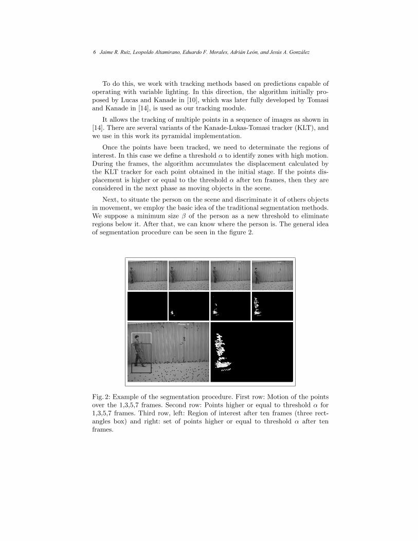
To do this, we work with tracking methods based on predictions capable ofoperating with variable lighting. In this direction, the algorithm initially pro-posed by Lucas and Kanade in [10], which was later fully developed by Tomasiand Kanade in [14], is used as our tracking module.

It allows the tracking of multiple points in a sequence of images as shown in[14]. There are several variants of the Kanade-Lukas-Tomasi tracker (KLT), andwe use in this work its pyramidal implementation.

Once the points have been tracked, we need to determinate the regions ofinterest. In this case we define a threshold α to identify zones with high motion.During the frames, the algorithm accumulates the displacement calculated bythe KLT tracker for each point obtained in the initial stage. If the points dis-placement is higher or equal to the threshold α after ten frames, then they areconsidered in the next phase as moving objects in the scene.

Next, to situate the person on the scene and discriminate it of others objectsin movement, we employ the basic idea of the traditional segmentation methods.We suppose a minimum size β of the person as a new threshold to eliminateregions below it. After that, we can know where the person is. The general ideaof segmentation procedure can be seen in the figure 2.

Fig. 2: Example of the segmentation procedure. First row: Motion of the pointsover the 1,3,5,7 frames. Second row: Points higher or equal to threshold α for1,3,5,7 frames. Third row, left: Region of interest after ten frames (three rect-angles box) and right: set of points higher or equal to threshold α after tenframes.


2.3 Tracking

Once the person position and size are determined, the next is to determine whichstrategy is useful to capture the motion of the body of the person being tested.

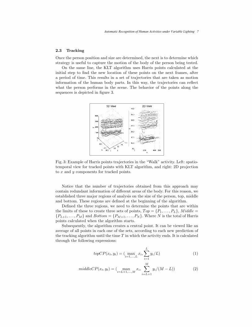
On the same line, the KLT algorithm uses Harris points calculated at theinitial step to find the new location of these points on the next frames, aftera period of time. This results in a set of trajectories that are taken as motioninformation of the human body parts. In this way, the trajectories can reflectwhat the person performs in the scene. The behavior of the points along thesequences is depicted in figure 3.

Fig. 3: Example of Harris points trajectories in the “Walk” activity. Left: spatio-temporal view for tracked points with KLT algorithm, and right: 2D projectionto x and y components for tracked points.

Notice that the number of trajectories obtained from this approach maycontain redundant information of different areas of the body. For this reason, weestablished three major regions of analysis on the size of the person, top, middleand bottom. These regions are defined at the beginning of the algorithm.

Defined the three regions, we need to determine the points that are withinthe limits of these to create three sets of points, Top = P1, . . . , PL, Middle =PL+1, . . . , PM and Bottom = PM+1, . . . , PN. Where N is the total of Harrispoints calculated when the algorithm starts.

Subsequently, the algorithm creates a central point. It can be viewed like anaverage of all points in each one of the sets, according to each new prediction ofthe tracking algorithm until the time T in which the activity ends. It is calculatedthrough the following expressions:

topCP (xt, yt) = ( maxi=1,...,L

xi,L∑

i=1

yi/L) (1)

middleCP (xt, yt) = ( maxi=L+1,...,M

xi,M∑

i=L+1

yi/(M − L)) (2)


bottomCP (xt, yt) = ( maxi=M+1,...,N

xi,N∑

i=M+1

yi/(N −M)) (3)

Note that in the expressions (1, 2, 3). t = 1, . . . , T , the position xt is thecoordinate farther in the x axis. This is the direction in which the person ismoving. This is done to preserve as much detail in the trajectory generation aspossible. The yt position is the simple average of the y-coordinates of the pointswithin each set.

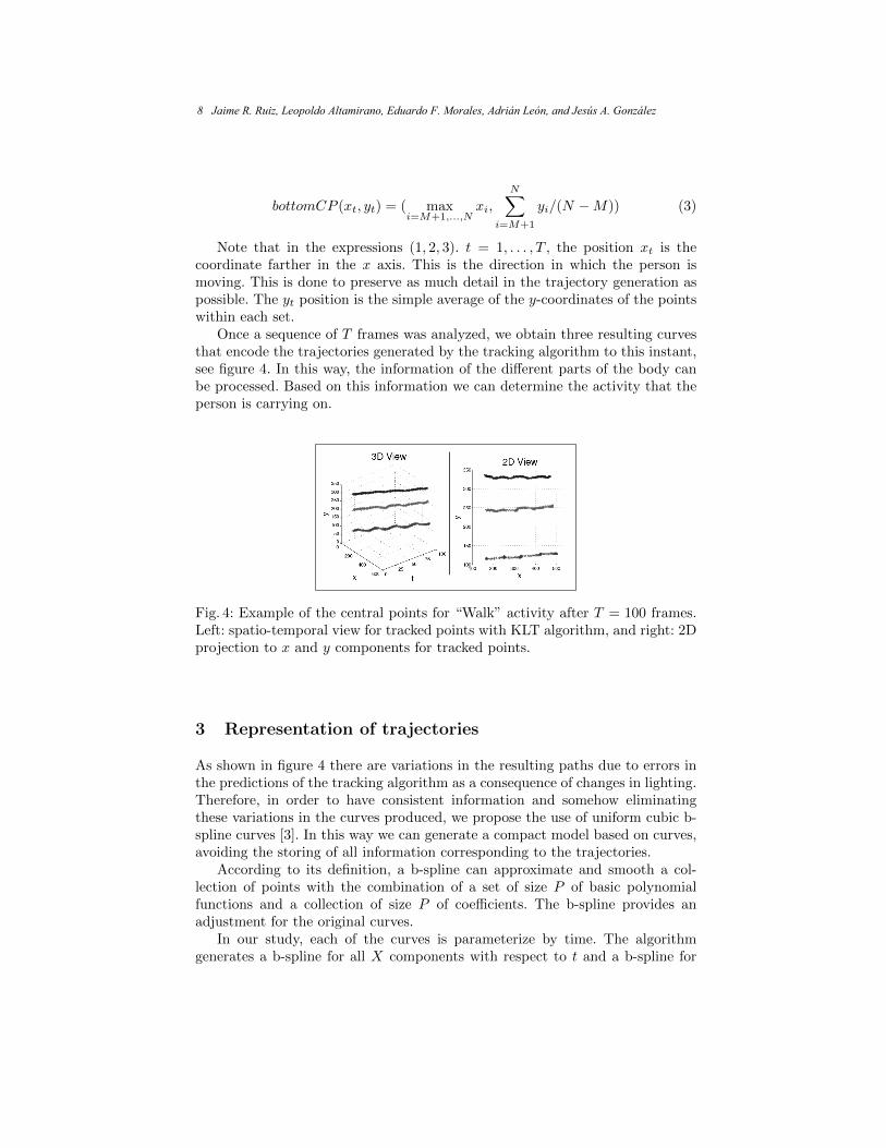
Once a sequence of T frames was analyzed, we obtain three resulting curvesthat encode the trajectories generated by the tracking algorithm to this instant,see figure 4. In this way, the information of the different parts of the body canbe processed. Based on this information we can determine the activity that theperson is carrying on.

Fig. 4: Example of the central points for “Walk” activity after T = 100 frames.Left: spatio-temporal view for tracked points with KLT algorithm, and right: 2Dprojection to x and y components for tracked points.

3 Representation of trajectories

As shown in figure 4 there are variations in the resulting paths due to errors inthe predictions of the tracking algorithm as a consequence of changes in lighting.Therefore, in order to have consistent information and somehow eliminatingthese variations in the curves produced, we propose the use of uniform cubic b-spline curves [3]. In this way we can generate a compact model based on curves,avoiding the storing of all information corresponding to the trajectories.

According to its definition, a b-spline can approximate and smooth a col-lection of points with the combination of a set of size P of basic polynomialfunctions and a collection of size P of coefficients. The b-spline provides anadjustment for the original curves.

In our study, each of the curves is parameterize by time. The algorithmgenerates a b-spline for all X components with respect to t and a b-spline for


Y with respect to t. At the end, the information is combined to generate theresulting curve that encodes the trajectory of each of the zones established forthe analysis. As an uniform b-spline is used, we need a knot vector -[3]- evenlydistributed to make the adjustment.

The procedure can be summarized as follows: The central points of eacharea identified -top, middle and lower- are stored in the curves TopCurve,MiddleCurve and BottomCurve, respectively.

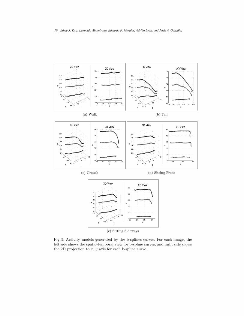
Each of these curves is then approximated and smoothed with b-spline, aspreviously established. In this way models are built for the top, middle andbottom zones of the person for each of the activities by eliminating the effectsof different lighting conditions on the scene. The resulting curves can be seen infigure 5a.

Once patterns of activity are generated and the effects of lighting changesare eliminated, see figure 5, we must define how a new activity will be identifiedwith respect to the activities stored.

4 Recognition of activities

Each activity consists of a set of three curves, resulting from the approximationto b-spline of the components X y Y of each curve. Due to the nature of thepeople’s activities, an activity can be re-executed at diverse speeds either bythe same person or by a different person. Therefore we must use a method thatallows us to compare the shape of two curves which have different proportions.It should determine a degree of similarity between them. In this case, we use thedynamic time warping algorithm (DTW) [13] to do this comparison.

The DTW was developed for comparing two time series of different lengthsand find out the similarity grade between them [13]. This technique is widely usedin mathematical field [4,9]. Using these algorithms is possible to find similaritiesbetween signatures and person activities based on sensors.

It is worth to mention that it is necessary to follow the same procedure thatwas used for the generation of the stored models in the moment of the comparisonof an unknown activity with the stored activities models. This means that weneed to generate a model with three curves that represents the new behavior.For a better adjustment in the comparison step, the models and the activitiesto be evaluated are moved to one common point that we will call origin.

Then, we compare one by one the curves corresponding to each zone of theperson. We compare the top curve of the activity that we attempt to recognizewith each of the top curves of the activities that were stored as models usingDTW. With this action, we obtain a degree of similarity between them. Theprocedure is the same for middle and lower curves.

At the end of comparison of the zones, the recognized activity will be theactivity with the highest fit, i.e., activity with the highest average measure ofsimilarity of the three zones. Thus the method can recognize activities throughDTW as a measure of similarity between the models.


(a) Walk (b) Fall

(c) Crouch (d) Sitting Front

(e) Sitting Sideways

Fig. 5: Activity models generated by the b-splines curves. For each image, theleft side shows the spatio-temporal view for b-spline curves, and right side showsthe 2D projection to x, y axis for each b-spline curve.


5 Experiments and results

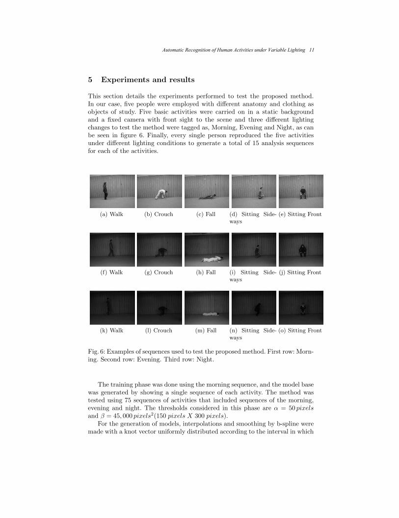
This section details the experiments performed to test the proposed method.In our case, five people were employed with different anatomy and clothing asobjects of study. Five basic activities were carried on in a static backgroundand a fixed camera with front sight to the scene and three different lightingchanges to test the method were tagged as, Morning, Evening and Night, as canbe seen in figure 6. Finally, every single person reproduced the five activitiesunder different lighting conditions to generate a total of 15 analysis sequencesfor each of the activities.

(a) Walk (b) Crouch (c) Fall (d) Sitting Side-ways

(e) Sitting Front

(f) Walk (g) Crouch (h) Fall (i) Sitting Side-ways

(j) Sitting Front

(k) Walk (l) Crouch (m) Fall (n) Sitting Side-ways

(o) Sitting Front

Fig. 6: Examples of sequences used to test the proposed method. First row: Morn-ing. Second row: Evening. Third row: Night.

The training phase was done using the morning sequence, and the model basewas generated by showing a single sequence of each activity. The method wastested using 75 sequences of activities that included sequences of the morning,evening and night. The thresholds considered in this phase are α = 50 pixelsand β = 45, 000 pixels2(150 pixels X 300 pixels).

For the generation of models, interpolations and smoothing by b-spline weremade with a knot vector uniformly distributed according to the interval in which


each curve was evaluated. We used 10 control points and therefore, 10 basicfunctions, and 10 coefficients were used to adjust the curves that were analyzed.

For the purpose of comparison we use other approach. A human operatorlocalize and establish the area of the person manually in the beginning of themethod.

The results of the proposed method are summarized in the confusion matrixin table 2. The results of the method assisted by a human operator are concen-trated in the confusion matrix in table 3, both results show the average score ofrepeating the experiment five times.

At the end a recognition rate of 88% in average was reached for all activitiesfor the proposed method in comparison with a recognition rate of 89.33% forthe manual method.

Walk Crouch Fall SF SS

Walk 15

Crouch 14 1

Fall 1 14

SF 14 1

SS 5 1 9

Table 2: Confusion matrix with the results from the recognition of activitiesusing the automatic proposed method.

Walk Crouch Fall SF SS

Walk 15

Crouch 14 1

Fall 1 14

SF 14 1

SS 3 2 10

Table 3: Confusion matrix with the results from the recognition of activitiesusing the method assisted by a human operator.

6 Discussion

The percentage of correct classification of the results presented in table 2 mayseem low compared with other approaches reported in the literature. However,the proposed method is evaluated in a scenario with different levels of illumi-nation. Furthermore, compared to other jobs with uncontrolled lighting, thisproject, in very similar activities such as “Crouch” and “Sit”, had good results.But, the activity “Sitting sideways” was confused with the activities of “Crouch”


and “Sitting front” because sometimes it was impossible to obtain a set of curvesto make a clearer distinction between activities. By contrast, in “Walk” activ-ity, the method has no problems extracting the curves to make the distinctionbetween “Walk” and other activities. Comparing the method proposed with themanual approach, even though we get a better percentage in the correct classifi-cation with the human assisted method, the results show that only one examplecorrectly classified in the “Sitting Sideways” activity makes the difference.

7 Conclusions

The proposed method is useful for recognition of activities under different light-ing conditions, using a simple technique for comparison.

The procedure in the same way, gives evidence that Harris operator canlocate important body parts for the analysis of behavior, in our case, the head,torso, legs and feet, and these features can be detected even though there is achange in lighting conditions. The algorithm is also able to recognize activitiesbased on the human body that are similar and can be easily confused betweenthem.

As future work, we plan to test the method performance with abrupt changesin lighting when the activities are performed in outdoor scenarios.

Acknowledgment

The research reported in this paper was supported by the National Council ofScience and Technology of Mexico (CONACYT) scholarship No. 40427.

References

1. Ali, S., Shah, M.: Human action recognition in videos using kinematic features andmultiple instance learning. IEEE Transactions on Pattern Analysis and MachineIntelligence 32, 288–303 (2010)

2. Arasanz, P.B.: Modeling Human Behavior for Image Sequence Understanding andGeneration. Ph.D. thesis, Universidad Autonoma de Barcelona, Espana (2009)

3. Deboor, C.: A Practical Guide to Splines. Springer-Verlag Berlin and HeidelbergGmbH & Co. K (dec 1978), http://www.worldcat.org/isbn/3540903569

4. Efrat, A., Fan, Q., Venkatasubramanian, S.: Curve matching, time warping, andlight fields: New algorithms for computing similarity between curves. J. Math.Imaging Vis. 27, 203–216 (April 2007), http://portal.acm.org/citation.cfm?id=1265122.1265128

5. Fernandez Tena, C., Baiget, P., Roca, X., Gonzalez, J.: Natural language descrip-tions of human behavior from video sequences. In: KI 2007: Advances in ArtificialIntelligence, pp. 279–292 (2007)

6. Goya, K., Zhang, X., Kitayama, K., Nagayama, I.: A method for automatic detec-tion of crimes for public security by using motion analysis. In: Proceedings of the2009 Fifth International Conference on Intelligent Information Hiding and Mul-timedia Signal Processing. pp. 736–741. IIH-MSP ’09, IEEE Computer Society,Washington, DC, USA (2009), http://dx.doi.org/10.1109/IIH-MSP.2009.264


http://www.worldcat.org/isbn/3540903569

http://portal.acm.org/citation.cfm?id=1265122.1265128

http://portal.acm.org/citation.cfm?id=1265122.1265128

http://dx.doi.org/10.1109/IIH-MSP.2009.264

7. Harris, C., Stephens, M.: A combined corner and edge detection. In: Proceedingsof The Fourth Alvey Vision Conference. pp. 147–151 (1988)

8. Lao, W., Han, J.: Flexible human behavior analysis framework for video surveil-lance applications. International Journal of Digital Multimedia Broadcasting 2010,1–10 (2010)

9. Liu, J., Wang, Z., Zhong, L., Wickramasuriya, J., Vasudevan, V.: uWave:Accelerometer-based personalized gesture recognition and its applications. Perva-sive Computing and Communications, IEEE International Conference on pp. 1–9(2009), http://dx.doi.org/10.1109/PERCOM.2009.4912759

10. Lucas, B.D., Kanade, T.: An iterative image registration technique with an appli-cation to stereo vision. In: IJCAI81. pp. 674–679 (1981), http://citeseerx.ist.psu.edu/viewdoc/summary?doi=10.1.1.49.2019

11. Mikolajczyk, K., Schmid, C.: An affine invariant interest point detector. In:Proceedings of the 7th European Conference on Computer Vision, Copen-hagen, Denmark. pp. 128–142. Springer (2002), http://perception.inrialpes.fr/Publications/2002/MS02, copenhagen

12. Nater, F., Grabner, H., Gool, L.V.: Exploiting simple hierarchies for unsupervisedhuman behavior analysis. Computer and Robot Vision (CRV2010) (2010)

13. Sakoe, H.: Dynamic programming algorithm optimization for spoken word recog-nition. IEEE Transactions on Acoustics, Speech, and Signal Processing 26, 43–49(1978)

14. Tomasi, C., Kanade, T.: Detection and tracking of point features. Tech. rep., In-ternational Journal of Computer Vision (1991)

15. Wang, Y., Mori, G.: Human action recognition by semilatent topic models. IEEETransactions on Pattern Analysis and Machine Intelligence 31(10), 1762–1774(2009), http://www.ncbi.nlm.nih.gov/pubmed/19696448

16. Zhou, Z., Chen, X., Chung, Y.C., He, Z., Han, T.X., Keller, J.M.: Activity anal-ysis, summarization, and visualization for indoor human activity monitoring. Cir-cuits and Systems for Video Technology, IEEE Transactions on 18(11), 1489–1498(2008), http://dx.doi.org/10.1109/TCSVT.2008.2005612


http://dx.doi.org/10.1109/PERCOM.2009.4912759

http://citeseerx.ist.psu.edu/viewdoc/summary?doi=10.1.1.49.2019

http://citeseerx.ist.psu.edu/viewdoc/summary?doi=10.1.1.49.2019

http://perception.inrialpes.fr/Publications/2002/MS02

http://perception.inrialpes.fr/Publications/2002/MS02

http://www.ncbi.nlm.nih.gov/pubmed/19696448

http://dx.doi.org/10.1109/TCSVT.2008.2005612

A Study on How the Training Data Monotonicity

Affects the Performance of Ordinal Classifiers

Carlos Milian1, Rafael Bello

2, Carlos Morell

2, and Bernard de Baets

3

1 Universidad de las Ciencias Informáticas, Cuba 2 Computer Science Department, Universidad Central "Marta Abreu" de Las Villas, Cuba 3 Department of Applied Mathematics, Biometrics and Process Control, Ghent University,

Coupure links 653, B-9000 Gent, Belgium

Abstract. Some classification problems are based on decision systems with ordinal-

valued attributes. Sometimes ordinal classification problems arise with monotone

datasets. One important characteristic of monotone decision systems is that objects

with better condition attribute values cannot be classified in a worse class.

Nevertheless, noise is often present in real-life data, and these noises could generate

partially non-monotone datasets. Several classifiers have been developed to deal

with this problem but its performance is affected when faced with real data that are

only partially monotone. In this paper are studied two monotonicity measures for

datasets and it is analyzed its correlation with several ordinal classifiers

performance. The results allow to a priori estimate the ordinal classifier behavior

when faced with partially monotone ordinal decision system.

Keyword:. Ordinal classification, monotonicity, data complexity.

1 Introduction

The problem of the ordinal classification, also called ordinal regression has attracted the

interest of the machine learning field due to the fact that many prediction problems or

decision taking have present the ordinal values on the decision features [1, 2, 3], and [4].

An ordinal dataset is one with an ordinal variable output. In this case, the classification

could be seen as a ranking, with a preference of the type ‘higher values are better’.

In the ordinal classification, there is a dataset , , … , , where each object

is described by a group of features , , … , ; each feature has a domain with

an order relation which establishes an order among the domain’s values; this kind of

feature is frequently called criterion. Also, each object has a decision feature , which

is also a criterion; therefore the decision values have also an order which defines a

preference degree. Two objects and can be compared on the basis of their feature

vectors , , … , and , , … , or their decision values and .

One important aspect in this topic is the data’s monotony. Because of this concept, it is

established the following relation:

⇒ . (1)

which means that if the object is selected over the therefore the class of the object must be as good as the one of the object This means that if only the value of one

feature increase (or decrease), while the rest is un-changed; the value of the decision

feature can only increase (decrease) or remain unchanged. An object is called monotone

if it does not make up a non-monotone couple with any other object, and a dataset

monotone if it contains no non-monotone objects. That is, monotone classification of

multi-criteria data simply means that for improving criterion scores, the rank assigned by

the ranking algorithm will never get worse. Non-monotonicity is present if there exist and in the dataset for which and , such instances are said to be ’non-monotone’. Monotone ordinal problems, in which monotonicity constraint is

imposed on the relationship between the input variables and the ordinal output is a special,

yet common, type of ordinal problem [5].

Nevertheless, noise is often present in real-life data, and these noises could generate

partially non-monotone datasets. Data can contain inaccurate rank or criterion values or

can be an amalgam of various sources ranked by different experts; this then leads to a

training set where a ‘better’ instance has received a lower rank than a ‘worse’ instance,

when training a ranking algorithm on such a training set, contradictory information will be

supplied to the ranking algorithm [6]. Non-monotonicity is in conflict with the domain

knowledge where not only two objects with identical feature scores should have identical

labels, but additionally, that increasing scores should not lead to a decrease in label; in

other words, an object should receive a label at least as good as the best label received by

any object that is worse than it [7].

There are many investigations about how monotony affects the way learning

algorithms work. Some of the already existent algorithms are unable to be trained by

using these partially non-monotone data sets. However, there are other algorithms that

select the examples suitable for learning the concepts needed, during the learning process,

eliminating those examples with monotonic inconsistencies.

One alternative to face this problem has been to drop the non-monotonicity grade by

means of a method for relabeling the datasets, authors in [6] and [8] studied the

consequences of a non-monotone training and test a set for a general monotone

classification algorithm, to discuss some ways of cleaning up a non-monotone training set

and determine whether it is useful in general to do such a thing. In [7], a single-pass

optimal ordinal relabeling algorithm is formulated; other algorithm was presented in [9].

Also, other method was formulated in [1].

Algorithms for this kind of classification have been developed, some of which require

monotone datasets. Because a monotone instance-based ranking algorithm will classify

any new instance in a way monotone w.r.t. the dataset, not all instances will be able to be

16 Carlos Milian, Rafael Bello, Carlos Morell, and Bernard de Baets

classified ‘correctly’ [6]; therefore the need of the methods for relabeling the datasets.

Some classifiers guarantee the monotonicity of subsequent predictions, while others do

not; ordinal classifiers also differ from each other by the way they handle non-monotone

datasets [5]. For a non-monotone classification algorithm, no such ‘handicap’ exists;

therefore, the accuracy might misleadingly be reported higher.

The method of construction of decision trees for ordinal classification in [10] also

requires monotone datasets. In other work, a method was formulated to construct

monotone ordinal decision trees [11] for the case of partially non-monotone datasets,

though it has to relabel some of the noisy objects during the construction of the trees. The

TOMASO algorithm [12] does not accept a (partially) non-monotone training set. There

are some other algorithms which are mentioned and used in other parts of this work.

In this work, has been studied the relation between the grade of non-monotonicity and

the performance of some classifiers. To establish this relation there are considered some

measures for measuring the non-monotonicity grade. The rest of the paper is organized as

follows. In section 2, we briefly describe a set of data complexity measures which will be

used to develop the experimental analysis. Section 3 presents the experiments carried out

over several training sets and discusses the relation between the measures and the

performance of the some ordinal classifiers. Finally, the conclusions are outlined.

2 Measures of Data Complexity

The monotonicity constraint is so important that some monotone classification algorithms

cannot be trained on datasets containing this kind of noise. Research on more flexible

algorithms is increasing, but the basic question that if non-monotonicity of a dataset

affects the learning process, remains valid. Authors in [6], showed the grade of non-

monotonicity present in two datasets, quantified by the number of nonmonotone instances,

and the maximum attainable accuracy for a monotone classification algorithm (OSDL);

also, the effect of relabeling the instances is presented.

The purpose of this work is showing by means of an experimental study and statistical

analysis the relation between monotonicity (non-monotonicity) and the performance of

the algorithm. In order to do that, some measures to measure the monotonicity of the

datasets are employed, and several classifiers are used.

The problem of characterizing data by means of different measures is present in

machine learning, the central idea is that high-quality data characteristics or meta-features

provide enough information to differentiate the performance of a set of given learning

algorithms. Different studies have been done on data complexity and meta-learning, such

as [13, 14, 15 and 16]. To address this problem it is necessary to use data describing the

characteristics of the datasets and the performance of the algorithms, which are called

meta-data. In this work, are used some measures to characterize the grade of monotonicity

A Study on How the Training Data Monotonicity Affects the Performance of Ordinal Classifiers 17

(or non-monotonicity) of the datasets, and two measures about the performance of the

classifiers.

Two measures are used in this study, DgrMon y OM. The first one was presented in [4]

and the second is proposed by us in this paper. The degree of monotonicity DgrMon of a

dataset D is defined by expression (2):

#!""#"$%&'()

#*"%&'&+,$%&'() . (2)

The pair ; is called comparable if or . , according to features in ; and if the relationship defined in (1) holds, it is also a monotone pair. If all comparable

pairs are monotone then 1 and the dataset is called monotone (non-decreasing

by assumption).

The other degree of monotonicity of a dataset is defined by expression (3):

#!""#"$0+$1#()

#0+$1#(). (3)

As it was stated before, an object is called monotone if it does not make up a non-

monotone couple with any other object.

It was studied the performance of the following classifiers: OLM, OSDL, B-OSDL,

2B-OSDL, and OCC. The ordinal learning model (OLM) is a simple algorithm that learns

ordinal concepts by eliminating non-monotonic pairwise inconsistencies [17]; the learning

process is based on a rule-based, which is generated during the learning. The Ordinal

Stochastic Dominance Learner (OSDL) is an instance-based monotone ranking algorithm

based on the concept of ordinal stochastic dominance of which several variants exist [2]

and [18]; according to [7], it (really some of its extensions such as B-OSDL, this

algorithm reduces to the OSDL when the stochastic training dataset is monotone) is able

to use non-monotone training sets to perform a monotone interpolation, without the need

of deletion or relabelling of non-monotone samples. The Ordinal class classifier (OCC) is

a meta-classifier, because it uses some other classifier, such as C4.5, k-nearest neighbor,

Naive bayes, etc., as a base classifier [19], in the experiments developed in this work was

used as a base classifier J48, although there were used others obtaining similar results as it

will be showed afterwards.; OCC does not guarantee monotonic classifications even when

it learns from monotonic data.

3 Experimental Results

In the experimental study were used nine datasets whose dimensions are described in

Table1.

In Tables 2-6 is described the measures’ value for each dataset and the performance

reached by the algorithms using the Weka platform, as measures, the Accuracy and

coefficient Kappa. Accuracy (often called Confidence) is the number of instances that it

predicts correctly, expressed as a proportion of all instances to which it applies.


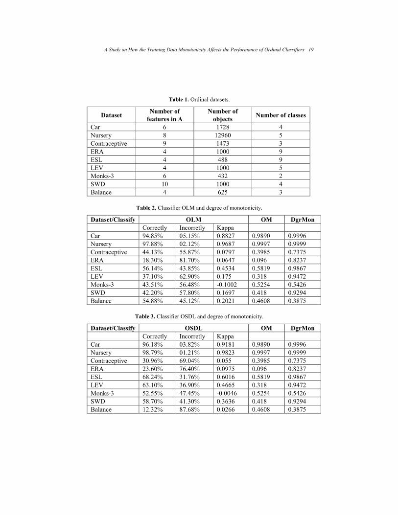
Table 1. Ordinal datasets.

Dataset Number of

features in A

Number of

objects Number of classes

Car 6 1728 4

Nursery 8 12960 5

Contraceptive 9 1473 3

ERA 4 1000 9

ESL 4 488 9

LEV 4 1000 5

Monks-3 6 432 2

SWD 10 1000 4

Balance 4 625 3

Table 2. Classifier OLM and degree of monotonicity.

Dataset/Classify OLM OM DgrMon

Correctly Incorretly Kappa

Car 94.85% 05.15% 0.8827 0.9890 0.9996

Nursery 97.88% 02.12% 0.9687 0.9997 0.9999

Contraceptive 44.13% 55.87% 0.0797 0.3985 0.7375

ERA 18.30% 81.70% 0.0647 0.096 0.8237

ESL 56.14% 43.85% 0.4534 0.5819 0.9867

LEV 37.10% 62.90% 0.175 0.318 0.9472

Monks-3 43.51% 56.48% -0.1002 0.5254 0.5426

SWD 42.20% 57.80% 0.1697 0.418 0.9294

Balance 54.88% 45.12% 0.2021 0.4608 0.3875

Table 3. Classifier OSDL and degree of monotonicity.

Dataset/Classify OSDL OM DgrMon


Car 96.18% 03.82% 0.9181 0.9890 0.9996

Nursery 98.79% 01.21% 0.9823 0.9997 0.9999

Contraceptive 30.96% 69.04% 0.055 0.3985 0.7375

ERA 23.60% 76.40% 0.0975 0.096 0.8237

ESL 68.24% 31.76% 0.6016 0.5819 0.9867

LEV 63.10% 36.90% 0.4665 0.318 0.9472

Monks-3 52.55% 47.45% -0.0046 0.5254 0.5426

SWD 58.70% 41.30% 0.3636 0.418 0.9294

Balance 12.32% 87.68% 0.0266 0.4608 0.3875


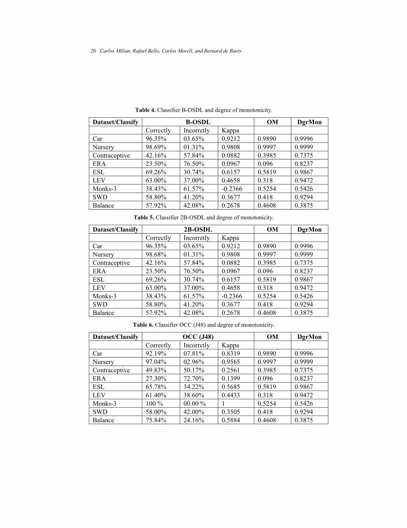
Table 4. Classifier B-OSDL and degree of monotonicity.

Dataset/Classify B-OSDL OM DgrMon


Car 96.35% 03.65% 0.9212 0.9890 0.9996

Nursery 98.69% 01.31% 0.9808 0.9997 0.9999

Contraceptive 42.16% 57.84% 0.0882 0.3985 0.7375

ERA 23.50% 76.50% 0.0967 0.096 0.8237

ESL 69.26% 30.74% 0.6157 0.5819 0.9867

LEV 63.00% 37.00% 0.4658 0.318 0.9472

Monks-3 38.43% 61.57% -0.2366 0.5254 0.5426

SWD 58.80% 41.20% 0.3677 0.418 0.9294

Balance 57.92% 42.08% 0.2678 0.4608 0.3875

Table 5. Classifier 2B-OSDL and degree of monotonicity.

Dataset/Classify 2B-OSDL OM DgrMon


Car 96.35% 03.65% 0.9212 0.9890 0.9996

Nursery 98.68% 01.31% 0.9808 0.9997 0.9999

Contraceptive 42.16% 57.84% 0.0882 0.3985 0.7375

ERA 23.50% 76.50% 0.0967 0.096 0.8237

ESL 69.26% 30.74% 0.6157 0.5819 0.9867

LEV 63.00% 37.00% 0.4658 0.318 0.9472

Monks-3 38.43% 61.57% -0.2366 0.5254 0.5426

SWD 58.80% 41.20% 0.3677 0.418 0.9294

Balance 57.92% 42.08% 0.2678 0.4608 0.3875

Table 6. Classifier OCC (J48) and degree of monotonicity.

Dataset/Classify OCC (J48) OM DgrMon


Car 92.19% 07.81% 0.8319 0.9890 0.9996

Nursery 97.04% 02.96% 0.9565 0.9997 0.9999

Contraceptive 49.83% 50.17% 0.2561 0.3985 0.7375

ERA 27.30% 72.70% 0.1399 0.096 0.8237

ESL 65.78% 34.22% 0.5685 0.5819 0.9867

LEV 61.40% 38.60% 0.4433 0.318 0.9472

Monks-3 100 % 00.00 % 1 0.5254 0.5426

SWD 58.00% 42.00% 0.3505 0.418 0.9294

Balance 75.84% 24.16% 0.5884 0.4608 0.3875


The Kappa statistic is used to measure the agreement between predicted and observed

categorizations of a dataset, while correcting for agreement that occurs by chance [20].

In the following Tables 7 and 8 is shown a review of the statistic correlation between

measures y , and the performance of the algorithms, measured, by using the

precision and the coefficient Kappa.

This statistical analysis was carried out using bivariate correlations in the Kendall´s

tau-b correlation coefficient that is used to analyze data not following a normal

distribution. This coefficient establishes that for values smaller than 0.05 the significance

between the data is high.

Fig. 1. Algorithms performance vs. Monotonicity measured by OM.

Table 7. Correlation between OM and the algorithms

Ordinal Classifiers Correlation OM and

precision

Correlation OM and

Kappa

OLM Significant 0.002 Significant 0.022

OSDL Significant 0.037 Not Significant 0.211

B-OSDL Significant 0.037 Not Significant 0.95

2B-OSDL Significant 0.037 Not Significant 0.95

OCC(J48) Significant 0.012 Significant 0.012

In the case of the OCC other experiments were performed using as a base classifier,

classification methods k-NN and Naive Bayes, obtaining a performance similar to that


obtained with the base classifier J48; Figures 1 and 2 show the performance of the

algorithms.

Table 8. Correlation between DgrMon and the algorithms.

Ordinal Classifiers Correlation DgrMon and

precision

Correlation DgrMon and

Kappa

OLM Not Significant 0.211 Significant 0.012

OSDL Significant 0.002 Significant 0.000

B-OSDL Significant 0.007 Significant 0.002

2B-OSDL Significant 0.007 Significant 0.002

OCC(J48) Not Significant 0.297 Not Significant 0.297

Fig. 2. Monotone and non-monotones algorithms performance vs. Monotonicity

As can be seen from the results shown in Tables 7 and 8 there is a significant statistical

correlation between the measures considered to calculate the degree of monotony of the

datasets and the performance of the algorithms, especially the monotony extent OM

proposed in this work and the performance measure Accuracy, which is also shown in

Figures 1 and 2.

The correct correlation existing between the proposed measure OM and the accuracy

shown by classifiers is due to the fact that this measure is more sensible to the degree of

monotony present in the datasets than the measure DgrMon because the former is more

rigorous in selecting the objects to be compared.


4 Conclusions

The study on the relationship between the degree of monotony of ordinal datasets and the

performance of some classifiers showed a significant correlation. The degree of monotony

of the datasets was calculated by using two measures, one of which is proposed in this

work and it showed a stronger relationship. This relationship allows that given a new

dataset, can be estimated, by using the measures, its degree of non-monotonicity and to

estimate the potential performance of the classifiers.

References

1. H. Daniels and M. Velikova.: Derivation of monotone decision models from noisy data, IEEE

Trans. Syst. Man Cybern. Part C Appl. Rev., pp. 705–710 (2006)

2. S. Lievens, S., De Baets, B., and Cao-Van, K.: A probabilistic framework for the design of

instance-based supervised ranking algorithms in an ordinal setting, Annals of Operations

Research. 163, pp. 115–142 (2008)

3. Ben-David, A., Sterling, L., Tran, T.: Adding monotonicity to learning algorithms may impair

their accuracy, Expert Systems with Applications 36, pp 667–66 (2009)

4. Velikova, M. and Daniels, H.: On Testing Monotonicity of Datasets. Ad Feelders and Rob

Potharst (eds) Proceedings of MoMo2009, ¨Learning monotone models from data¨, at ECML

PKDD 2009, pp. 11–22. September 7, Bled, Slovenia. (2009)

5. Potharst, R., Ben-David, A., and van Wezel, M.: Two algorithms for generating structured and

unstructured monotone ordinal datasets. Engineering Applications of Artificial Intelligence 22,

pp. 491–496 (2009)

6. Rademaker, M., De Baets, B., and De Meyer, H.: On the Role of Maximal Independent Sets in

Cleaning Data Sets for Supervised Ranking. In Proc. of IEEE International Conference on

Fuzzy Systems, Vancouver, BC, Canada. July 16-21 (2006)

7. Rademaker, M., De Baets, B., and De Meyer, H.: Optimal monotone relabelling of partially

non-monotone ordinal data. Optimization Methods and Software, iFirst, pp. 1–15 (2010)

8. Rademaker, M., De Baets, B., and De Meyer, H.: Loss optimal monotone relabeling of noisy

multi-criteria data sets. Information Sciences 179, pp. 4089–4096 (2009)

9. Rademaker, M., De Baets, B.: Optimal restoration of stochastic monotonicity with respect to

cumulative label frequency loss functions. Information Sciences 181, 747–757. (2011)

10. Potharst, R. and Bioch, JJ.C.: Decision trees for ordinal classification, Intell. Data Anal. 4 (2),

pp. 97–111 (2000)

11. Bioch, J. and Popova, V.: Monotone decision trees and noisy data, Tech. Rep. ERS-2002-53-

LIS, Department of Computer Science, Erasmus University Rotterdam (2002)

12. Marichal, J.-L., Meyer, P. and Roubens, M.M.: Sorting multi-attribute alternatives: The

TOMASO method, Computational Oper. Research. 32, pp. 861–877 (2005)

13. T. Ho, M. Basu.: Complexity measures of supervised classification problems, IEEE

Transactions on Pattern Analysis and Machine Intelligence 24, pp. 289–300 (2002)

14. S. Singh.: Multiresolution estimates of classification complexity, IEEE Transactions on Pattern

Analysis and Machine Intelligence 25 (12), pp. 1534–1539 (2003)

15. Brazdil, P. et al.: Metalearning: Applications to Data Mining. Springer, ISSN: 1611–2482,

ISBN: 978-3-540-73262-4 (2009)


16. Caballero, Y., Bello, R., Arco, L., and Garcia, M.: Knowledge Discovery using Rough Set

Theory, Capitulo en el libro Advances in Machine learning I Dedicated to the memory of

Professor Ryszard S. Michalski in Series: Studies in Computational Intelligence Vol 262;

Koronacki J., Ras Z.W., Wierzchon S.T.; Kacprzyk J (Eds), ISBN 978-3-642-05176-0 (2010)

17. Ben-David, A.: Automatic Generation of Symbolic Multiattribute Ordinal Knowledge-Based

DSSs: methodology and Applications. Decision Sciences. 23:1357–1372 (1992)

18. Lievens, S., De Baets, B.: Supervised ranking in the WEKA environment, Information

Sciences 180 (24), 4763–4771 (2010)

19. Frank, E. and Hall, M.: A Simple Approach to Ordinal Classification. In: 12th European

Conference on Machine Learning, 145–156 (2001)

20. Witten, I. H. and Frank E.: Data mining: practical machine learning tools and techniques-2nd

ed. Elsevier, ISBN: 0-12-088407-0 (2005)


An Information Fusion Architecture

for Situation Assessment of Ground Battlefield

Huimin Chai and Baoshu Wang

School of Computer Science and Technology, Xidain University, Xi’an, China

[email protected], [email protected]

Abstract. The information fusion architecture for situation assessment is designed

in the paper, which is divided into three stages: perception, comprehension and

projection. The process of force structure classification is an important part which

includes target aggregation region partition, command post recognition and force

structure classification. The algorithm of template matching is proposed for the

recognition of command post and force structure. Thus, the ground situation

assessment is made in terms of concepts that can be computed. Finally, the

simulation system of situation assessment is developed, a seaboard defense scenario

is simulated and the situation assessment for the seaboard is analyzed to illustrate

the functionality of the proposed model.

Keywords: Situation assessment, ground battlefield awareness, template matching.

1 Introduction

In recent years, decision-making in real-time dynamic battlefield is becoming increasingly

complex due to the nature and diversity of threats and tactics that may be encountered.

With enormous amounts of information available for command decisions, C4ISR system

is required of the capability for situation assessment, which can help commanders form

appropriate perception, timely and exactly understanding of battlefield situation. Situation

assessment (SA) is the process of inferring relevant information about forces of concern in

a battlefield, including location, movement and deployment of enemy forces, which is

needed by the campaign commanders or analysts to support decision-making [1, 2].

Situation assessment is belonging to high-level information fusion, which goals include

identifying the meaningful events and activities, deriving higher order relations among

objects and inferring the intension. Over the course of the last two decades there have

been several definitions of situation assessment proposed. The most widely accepted

definitions are Dr. Mica Endsley’s [3] and the Joint Development Laboratory (JDL)

fusion model [4, 5]. Endsley’s view is based on cognitive principles, which divides SA

into three levels: perceiving elements in the environment within a volume of space and

time; comprehending what they mean in context; and predicting their status in the near

future. On the other hand, the JDL model provides a function data centric approach, which

has 5 levels: Level 0-Sub-Object Identification; Level 1-Object Identification; Level 2-

Situation Assessment; Level 3-Threat Assessment; Level 4-Process Refinement. With the

JDL data fusion model, situation assessment falls in level 2 and accepts the results from

level 1.

Situation assessment is a complex domain, especially for ground battlefield. Today, the

modern battlefield is characterized by an overwhelming volume of information collected

from a vast networked array of increasingly more sophisticated sensors and

technologically equipped troops. There remains a significant need for higher levels of

information fusion such as those required for generic situation assessment, prediction of

enemy coursed of action (COA) and potential threat. For roughly 10 years, the research

community has been recognizing the need for significant progress in this domain. Some

researchers have proposed a few of methods and models for situation assessment, which

includes fuzzy reasoning and theory [6, 7], Bayesian networks [8, 9, 10], template

matching [11, 12], case-based reasoning [13, 14], ontology-based system [15, 16, 17], etc.

Some researchers [18, 19, 20] have advocated the considerations of the battlefield

intelligence in situation assessment, which provides some good illustrations of the

complexity of gathering and processing intelligence in the practical applications.

In this paper, the problem of ground battlefield awareness is discussed. The rest of the

paper is organized as follows. Section 2 provides an overview of the information fusion

architecture for ground battlefield. Section 3 presents the process of force structure and

deployment recognition, and the template matching algorithm is given. Section 4

illustrates a demonstration scenario of the coastal defense plan, and the results of situation

assessment are given. Section 5 concludes this paper and presents some prospects for

future work.

2 Overview of the Information Fusion Architecture

The process of situation assessment for ground battlefield is complex, nonlinear and

replete with human interpretation and judgment. Therefore, the construction of

computational models that infers the enemy courses of action (COA) and comprehends

what have happened in the context is an extremely challenging task. In this section, we

will provide an overview of the information fusion architecture for ground battlefield. The

architecture is based on Endsley’s model of SA with stages for perception, comprehension

and projection. In Fig.1, the fusion architecture of ground battlefield awareness is

presented.

(1) Event extraction: In the battlefield, there are various sensors deployed to scan an

area of stationary or moving targets. Based on the output of sensors, we can obtain the

different intelligence of ground battlefield. With the characteristics of the raw intelligence

data, we can identify meaningful events and activities, such as appearance of important

target, radio signal, fortification, force activity and so on. This is the first fusion level of

26 Huimin Chai and Baoshu Wang

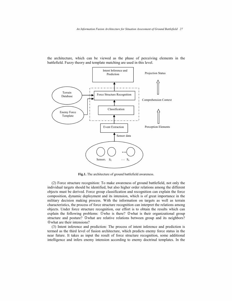
the architecture, which can be viewed as the phase of perceiving elements in the

battlefield. Fuzzy theory and template matching are used in this level.

Fig.1. The architecture of ground battlefield awareness.

(2) Force structure recognition: To make awareness of ground battlefield, not only the

individual targets should be identified, but also higher order relations among the different

objects must be derived. Force group classification and recognition can explain the force

composition, dynamic deployment and its intension, which is of great importance in the

military decision making process. With the information on targets as well as terrain

characteristics, the process of force structure recognition can interpret the relations among

objects. Under force structure recognition, our effort is to obtain the results which can

explain the following problems: who is there? what is their organizational group

structure and posture? what are relative relations between group and its neighbors?

what are their intensions?

(3) Intent inference and prediction: The process of intent inference and prediction is

termed as the third level of fusion architecture, which predicts enemy force status in the

near future. It takes as input the result of force structure recognition, some additional

intelligence and infers enemy intension according to enemy doctrinal templates. In the

…

Sensor1 S2 Sn

Event Extraction

Classification

Intent Inference and

Prediction

Force Structure Recognition

Enemy Force

Template

Terrain

Database

Comprehension Context

Projection Status

Perception Elements

Sensor data

…

An Information Fusion Architecture for Situation Assessment of Ground Battlefield 27

ground battlefield, the enemy intent inference is a very challenging problem, for the high

degree uncertainty of observations. Most computational approaches to the intent inference

are based on artificial intelligence, for example, D-S theory, dynamic Bayesian networks,

fuzzy reasoning, etc. In the paper, this part is not discussed in the following.

(4) Enemy structure template: An enemy structure template depicts the composition

and deployment of various types of sub-echelons or forces. For example, a brigade of

artillery consists of several battalions, artillery. The expert knowledge base should be

constructed for different level of force structure, which is used to recognize the enemy

force structure.

(5) Terrain database: The terrain data is stored in the terrain database, which represents

the terrain characteristics and traffic facilities: elevation, slopes, down-country,

vegetation, body of water, road, railway, etc. The terrain data, used by force structure

recognition, can make our analytical approach and methods available to the ground

battlefield. The format of terrain data is based on a sampling of every N meters of terrain

from a reference map, a rectangular mesh that includes significant information: elevation,

road, river, and so on. Terrain analysis is essential in the process of determining enemy

force group, including tactically important terrain characteristics, traffic ability patterns,

and key terrain.

3 Force Structure Recognition

3.1 Intelligence Report

One of the challenges at the heart of this paper is analyzing large volumes of battlefield

intelligence with the intention of figuring out what the enemy is doing and what type of

threat such activities might represent. The intelligence reports are derived from various

forms of physical sensors as well as by direct human observations. In the process of

intelligence report analysis, some questions can be explained, for example, “what the

enemy unit is doing?”, “where are the important fortification in the ground battlefield?”,

and so on.

As intelligence reports come from the battlefield, the information it contains needs to

be analyzed in the context, which is very important for situation assessment in ground

battlefield. After event extraction from intelligence reports, we can identify some

meaningful battlefield events. We now turn attention to the dimensions or attributes of the

event from intelligence data, which includes: (1)Object: the object described in

intelligence report, for example, command car, radio signal, fortification; (2)Size: the

number of observed vehicles, the level of enemy force which can be equated with echelon

level(e.g., squad, platoon, company); (3) Location: the location of the observed units in

terms of latitude/longitude; (4) Time: the time of the observation; (5) Features: the


features of target, such as a list of all the observed equipment the enemy is occupied,

activity which denotes what the enemy force is doing, parameters of radio signal.

For different type of intelligence report, it can be represented by the formulation:

,, ,( )ii i iiIntel K S T F= (1)

where iK represents the observed object in intelligence report, such as enemy force,

fortification, radio signal. iS denotes the size of enemy force or the number of vehicles,

and iT represents the time of intelligence. iF denotes the feature of the observed object.

For the different type of object, the representation of feature is different.

3.2 Processing of Force Classification

According to the characteristics of ground battlefield, we give the process of force

structure classification in the following:

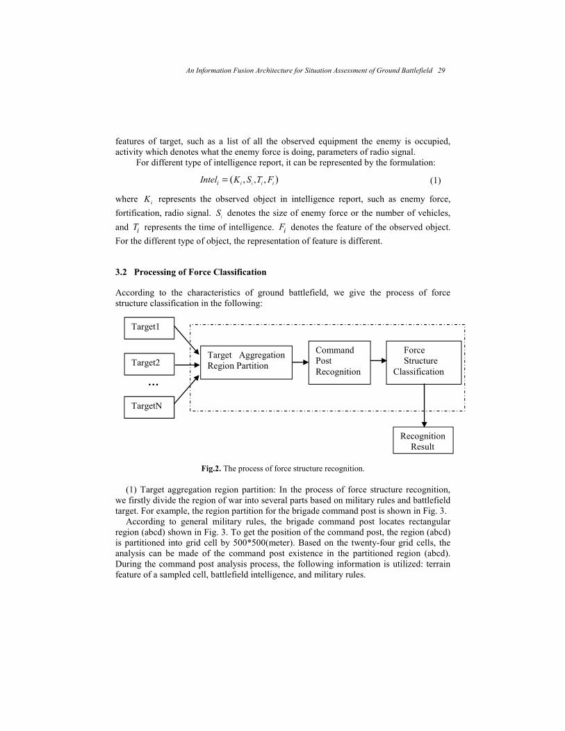
Fig.2. The process of force structure recognition.

(1) Target aggregation region partition: In the process of force structure recognition,

we firstly divide the region of war into several parts based on military rules and battlefield

target. For example, the region partition for the brigade command post is shown in Fig. 3.

According to general military rules, the brigade command post locates rectangular

region (abcd) shown in Fig. 3. To get the position of the command post, the region (abcd)

is partitioned into grid cell by 500*500(meter). Based on the twenty-four grid cells, the

analysis can be made of the command post existence in the partitioned region (abcd).

During the command post analysis process, the following information is utilized: terrain

feature of a sampled cell, battlefield intelligence, and military rules.

…

…

Target1

Target2

TargetN

Target Aggregation

Region Partition

Command

Post

Recognition

Force

Structure

Classification

Recognition

Result


(2) Command post recognition: After the partition of war region, we can analyze

whether there is command post based on the military rules in the region. If the analysis

shows the existence of command post, then the type of enemy force should be identified,

e.g. tank platoon, company. Otherwise, the recognition of enemy force will be not

performed in the partitioned region.

Fig.3. The region partition for the brigade command post.

On the process of recognizing the command post, the knowledge model is utilized to

identify the type of command post. The knowledge model is based on some military

knowledge, which is comprised of three parts: Position rule, Terrain characteristic,

Intelligence symptom. For illustrative purpose, the knowledge model of brigade command

post is described concisely in Fig.4.

0 .4 (w eigh t) 1 .0 from de fence fo rw ard position

Po sitio n 0 .5 lie s in the rear w ar reg ion

0 .5 n ea r th e m a in fo rce

0 .3 1 .0 d ow n -con try

B rig ade Terra in 1 .0 hyp sog raphy

C omm and 1 .0 e lev a tion

Po st 1 .0 R ad io s igna l(b rig ade)

0 .3 0 .5 A rm o red car(3~4 )

Sym p tom 0 .1 A ssis t car(2 )

0 .2 Fo rtif ica tion

0 .2 A ir d e fense w eapon

(4 -6 Km )

Fig.4. The knowledge model for the brigade command post.


According to the knowledge model, we can calculate the belief of the type of command

post, which is defined by

1 2 3Belief W Pbelief W Tbelief W Sbelief= × + × + ×

(2)

where Pbelief denotes the belief of position according to corresponding military rules,

Tbelief is the belief of terrain characteristic, Sbelief is the belief of intelligence report,

1 2 3, ,W W W are the weights that are standardized to sum to unity.

(3) Force structure classification: To make useful predictions about the enemy

intension, we should cluster the battlefield entities into higher level force aggregates based

on the result of command post recognition. Similarly, expert knowledge model for force

structure are used to match the various clusters so as to classify the aggregates into known

classes of force structure. In the paper, the template matching method is utilized to

classify the force structure.

3.3 Algorithm for Template Matching

A doctrinal template of force structure depicts the characteristic and deployment of

various types of sub-echelons or vehicles. For example, a brigade consists of several

battalions and some weapons. In general, a brigade should be deployed in the suitable

area. So the template of brigade is comprised of three parts: terrain characteristics, the

position of battalion, and intelligence reports for force, weapons and fortification, which is

similar to knowledge model shown in Fig.4. Then the template of brigade can be

represented as:

, , T Rule Terrain Intel= (3)

where Rule is the military rules for the brigade deployment, Terrain denotes the terrain

characteristics, and Intel is the intelligence reports for the brigade. For different levels of force, the constituent structure of each template is the same as

the template of brigade. We can identify the type of force structure based on the force

template matching. The algorithm of template matching includes: position rules matching,

terrain characteristic matching and the matching of intelligence report. The matching

process attempts to maximize the matching degree between a template and the enemy

force. The process returns the template with the maximum matching degree.

For the two parts in the template: terrain characteristics, rule for the position of force,

the matching algorithm is simple. We assume that for a given location L, there are enemy

forces, e.g., two platoons. If the given location L is correspondent with the i-th rule in the

template, the matching degree for part rule Rule is calculated as:

1.0R R RiBel Bel W= + × (4)


where RiW is the weight value of the i-th rule in the template and all the weights are

standardized to sum to unity. Similarly, the matching degree for terrain characteristic

TBel

can be calculated by (4). For example, the force deployment area contains the

features, such as a river, road, and elevation. And if the area terrain features is

correspondent with the terrain characteristic in the template, then 1.0

T T TiWBel Bel= + ×

.

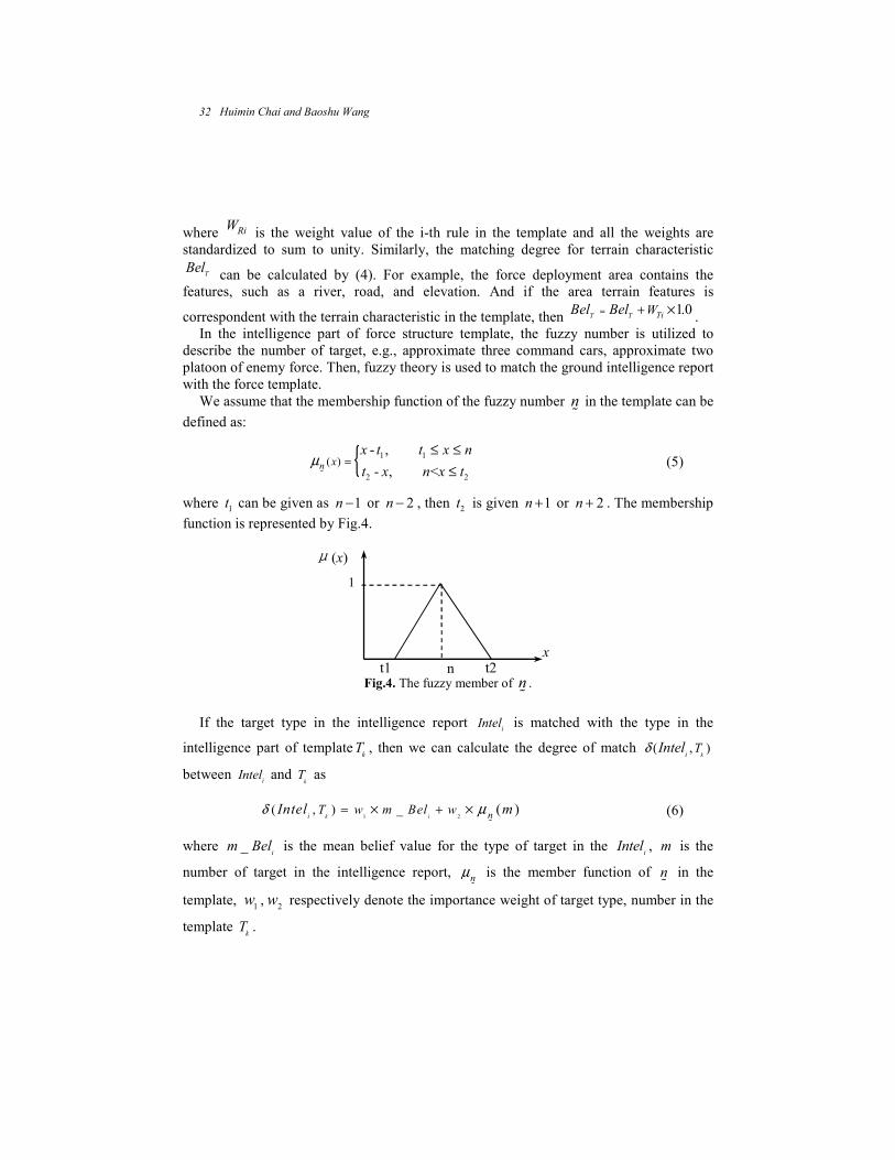
In the intelligence part of force structure template, the fuzzy number is utilized to

describe the number of target, e.g., approximate three command cars, approximate two

platoon of enemy force. Then, fuzzy theory is used to match the ground intelligence report

with the force template.

We assume that the membership function of the fuzzy number n% in the template can be

defined as:

1 1

2 2

( )- ,

- , <n x

x t t x n

t x n x tµ =

≤ ≤

≤%

(5)

where 1t can be given as 1n − or 2n − , then

2t is given 1n + or 2n + . The membership

function is represented by Fig.4.

Fig.4. The fuzzy member of n%.

If the target type in the intelligence report i

Intel is matched with the type in the

intelligence part of templatekT , then we can calculate the degree of match ( , )

kiTIntelδ

between i

Intel and kT as

1 2( , ) _ ( )

k ii nT w m Bel wIntel mδ µ= +× ×%

(6)

where _i

m Bel is the mean belief value for the type of target in the i

Intel , m is the

number of target in the intelligence report, nµ%

is the member function of n% in the

template, 1w ,

2w respectively denote the importance weight of target type, number in the

template kT .

x

μ(x)

1

t1 n t2


Algorithm1 describes the process of matching with force structure template, where the

matching degreeδ is initialized as ‘0’. The template with the maximum matching degree which is greater than the threshold valueσ is returned by the matching process. The

algorithm can also be used to match command post, e.g. a command post of brigade.

Algorithm 1. Template Matching Algorithm.

1: Initialize 0k

δ = , and the templates for matching: 1 2

, , ...,n

T T T

2: For rules of force deployment(position), the matching degree is calculated as:

( , ) 1.0i k Ri

Location T Wδ = ×

3: For terrain characteristic, ( , ) 1.0j k TjTerrain T Wδ = ×

4: For intelligence report: I1 I2

( , ) _ ( )k pp nT m BelIntel w w mδ µ= +× ×

%

5: Update the total matching degree as necessary:

( , )( , ) ( , )p kk R i k T j k I

Intel TW T W Terrain T WLocation δδ δ δ= + +∑ ∑ ∑

where 1R T I

W W W+ + = . If the value of ( , )p k

Intel Tδ∑ is greater than ‘1’, then

the value is set ‘1’.

6: Determine the k

δ is maximum matching degree and greater than the threshold

σ , then return template kT .

4 Simulation and Results

The simulation system, the essential part of information fusion project, is developed to

demonstrate the process of ground battlefield awareness, which is comprised of four parts:

intelligence editor, command post recognition, force structure analysis, template database

and terrain database. The relation of the different parts in the simulation system is shown

in Fig. 5.

We developed the intelligence editor in order to add the ground battlefield intelligence

report into the simulation system. The type of intelligence includes force activity,

fortification, vehicles, radio signal and so on. The intelligence data is comprised of the

type of object, the size or number of object, the position, the object feature and the

received time. The data of terrain characteristic is stored in the terrain database. The

corresponding database editor is also developed for terrain data maintenance. The results

of situation assessment are displayed on a traditional map.

For the purpose of showing the simulation process of situation assessment, let’s

consider the following scenario: there is a conflict in the sea, and the enemy attempt to

attack our domain. They deployed some force in the seaboard. To destroy their plan, we

should analyze the enemy force deployment and the force structure. According to the


terrain features, received intelligence report and other sensor data, the situation

assessment for the seaboard can be analyzed.

Fig.5. The structure of simulation system.

Fig.6. The result of intelligence edition for situation assessment.

4.1 Intelligence Editor

The intelligence editor is used to demonstrate the fusion of ground battlefield intelligence

report. It is a software tool that can edit the intelligence for ground battlefield awareness.

Intelligence

Editor Command Post

Recognition

Force Structure

Analysis

Result

Display

Terrain

DatabasTemplat

e


An example edition result of the tool is shown in Fig.6. We can add, delete, or update an

intelligence object which is shown by blue color on the map, such as command car,

fortification. Then the intelligence report can be generated according to the edition result,

and saved in a file by defined data format. While the simulation of battlefield situation

assessment, the intelligence report is read from the corresponding file and sent to the

module of command post recognition or force structure analysis by the order of the

received time.

Similarly, some intelligence reports are edited for the simulation scenario. Table 1

describes the object of each intelligence report and the number or size of the object.

Table 1. The intelligence reports in the simulation scenario.

Intelligence No. Target Size/number Position(x,y)

1

2

3

4

5

6

7

8

9

10

11

Armored car

Air defense rocket

Fortification

Assist car

Grenade launch base

Air defense rocket

Assist car

Fortification

Radio signal(battalion)

Air defense weapon

Fortification

3~4

2

3~5

2

4~5

(9233,5466)

(6366,2600)

(8933,5350)

(9033,5750)

(3833,5216)

(3933,4166)

(9450,2850)

(9283,3066)

(5450,5400)

(9150,2800)

(7200,3583)

Fig.7. The results of target aggregation region partition


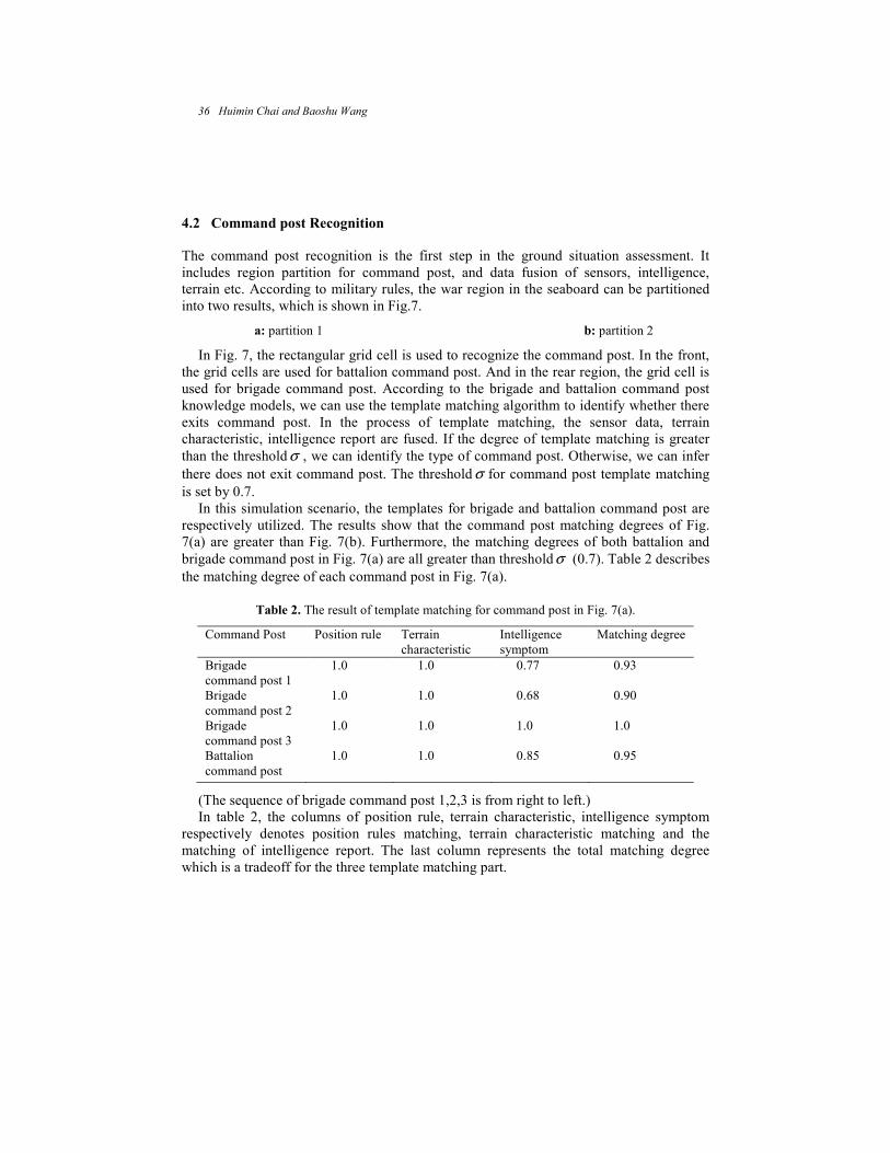
4.2 Command post Recognition

The command post recognition is the first step in the ground situation assessment. It

includes region partition for command post, and data fusion of sensors, intelligence,

terrain etc. According to military rules, the war region in the seaboard can be partitioned

into two results, which is shown in Fig.7.

a: partition 1 b: partition 2

In Fig. 7, the rectangular grid cell is used to recognize the command post. In the front,

the grid cells are used for battalion command post. And in the rear region, the grid cell is

used for brigade command post. According to the brigade and battalion command post

knowledge models, we can use the template matching algorithm to identify whether there

exits command post. In the process of template matching, the sensor data, terrain

characteristic, intelligence report are fused. If the degree of template matching is greater

than the thresholdσ , we can identify the type of command post. Otherwise, we can infer

there does not exit command post. The thresholdσ for command post template matching

is set by 0.7.

In this simulation scenario, the templates for brigade and battalion command post are

respectively utilized. The results show that the command post matching degrees of Fig.

7(a) are greater than Fig. 7(b). Furthermore, the matching degrees of both battalion and

brigade command post in Fig. 7(a) are all greater than thresholdσ (0.7). Table 2 describes

the matching degree of each command post in Fig. 7(a).

Table 2. The result of template matching for command post in Fig. 7(a).

Command Post Position rule Terrain

characteristic

Intelligence

symptom

Matching degree

Brigade

command post 1

Brigade

command post 2

Brigade

command post 3

Battalion

command post

1.0

1.0

1.0

1.0

1.0

1.0

1.0

1.0

0.77

0.68

1.0

0.85

0.93

0.90

1.0

0.95

(The sequence of brigade command post 1,2,3 is from right to left.)

In table 2, the columns of position rule, terrain characteristic, intelligence symptom

respectively denotes position rules matching, terrain characteristic matching and the

matching of intelligence report. The last column represents the total matching degree

which is a tradeoff for the three template matching part.


4.3 Force Structure Analysis

In the next step, we can analyze the force structure according to the results of command

post recognition. Thus, the analysis is made based on the result of Fig. 7(a). The force

structure templates are used in this step, and the template matching algorithm described as

section 4.3 is implemented. In this simulation example, the result of force structure

analysis is shown in Fig. 8.

Fig.8. The result of force structure analysis.

The deployment of enemy force is approximately illustrated in Fig.8, which template

matching degree is great than 0.60. There are three battalions in the forward position

which is represented by blue arc, and each battalion command post is located which is

shown by blue flag. In the rear area, the blue flag represents the brigade command post.

Furthermore, the analysis can give the detail features of the deployment, such as the

location of battalion or brigade, the width value and depth value.

5 Conclusion

We presented architecture and its implemented computational embodiment for situation

assessment of ground battlefield. The architecture can fuse intelligence from sensor data,

terrain characteristic, and military knowledge in a coherent system. The force structure is

analyzed and computed, which can be shown in the simulation system of situation

assessment.


In the future work, we plan to explore the model of tactical goal hypothesis generation

and inference. In addition, we will extend our architecture of situation assessment to

predict the future significant feature of battlefield.

Acknowledgement. The research is supported by the Fundamental Research Funds for

the Central Universities (No.KS0510030005).

References

1. Blasch, E., Plano, S.: DFIG Level 5 issues supporting Situation Assessment Reasoning,

Proceedings of Information Fusion. (2005)

2. Salerno, J.J.: Where’s Level 2/3 Fusion- a Look Back over the Past 10 Years. Proceedings of

Information Fusion, pp.1-4 (2007)

3. Endsley, M.R.: Toward a Theory of Situation Awareness in Dynamic Systems. Human Factors

Journal. 37(1), pp. 32-64 (1995)

4. Hall, D.L., Llinas, J.: Handbook of Multisensor Data Fusion. Washington DC, NY: CRC Press

(2001)

5. Linas, J., Bowman, C.,: Revisiting the JDL Data Fusion Model II. Proceedings of Information

Fusion, pp.1-13 (2004)

6. Stover, J. A., Hall, D.L., Gibson, R.E.: A Fuzzy-logic Architecture for Autonomous Multisensor

Data Fusion. IEEE Transaction on Industrial Electronics, 43(3), pp.403-410 (1996)

7. Huimin, C., Baoshu, W.: A Fuzzy Logic Approach for Force Aggregation and Classification in

Situation Assessment. Proceedings of the International Conference of Machine Learning and

Cybernetics, pp. 1220-1225 (2007)

8. Das, S., Grey, R., Gonsalves, P.: Situation Assessment via Bayesian Belief Networks.

Proceedings of the Fifth International Conference on Information Fusion, 1, pp. 664–671 (2002)

9. Das, S., Lawless, D.: Trustworthy Situation Assessment via Belief Networks. Proceedings of

Information Fusion, 1, pp. 543–549 (2002)

10.Qiang, J.: Information Fusion for High Level Situation Assessment and Prediction. Report:OMB

No. 3, pp. 074-0188 (2007)

11.Noble, D.F.: Schema-Based Knowledge Elicitation for Planning and Situation Assessment Aids.

IEEE Trans. on Systems, Man and Cybernetics, Part A, 19(3): pp. 473-482(1989)

12.Huimin, C., Baoshu, W.: A Template-based Method for Force Group Classification in Situation

Assessment. IEEE Symposium on Computation Intelligence in Security and Defense

Application, pp. 85-91 (2007)

13.Looney, C.G., Liang, L.R.: Cognitive situation and threat assessment of ground battlespaces,

Information Fusion, 4, pp. 297-308 (2003)


Unsupervised Learning Objects Categories usingImage Retrieval System

Karina Ruby Perez Daniel, Enrique Escamilla Hernandez,Mariko Nakano Miyatake, and Hector Manuel Perez Meana

National Polytechnic Institute IPN, ESIME Culhuacan, Av. Santa Ana No. 1000 Col.San, Francisco Culhuacan, Del. Coyoacan, Zip Code 04430, Mexico City

[email protected],[email protected],[email protected],

[email protected]

http://www.posgrados.esimecu.ipn.mx

Abstract. Since several years ago artificial intelligent systems have be-come in a big challenge and learning of object categories is one of themost important parts in this field. Unsupervised learning of object cat-egories provides the considerably high intelligence to apply several am-bitious tasks, such as robot vision and powerful image retrieval engine,etc. In the learning object categories, a fast and accurate unsupervisedlearning model is required. In this paper we propose an unsupervisedlearning method to categorize the objects using images retrieved by In-ternet, in which a keyword is introduced as input data. For this purpose,all retrieved images are described using the Pyramid of Histogram ofOriented Gradients (PHOG) algorithm and the resultant PHOG vectoris clustered to get a dataset for learning object categories. Two cluster-ing methods are used in the proposed method, which are K-means andChinese Restaurant Process (CRP), to make the learning method moreefficient and simple.

Key words: Unsupervised learning objects, PHOG, k-means, Chineserestaurant process.

1 Introduction

Learning Object Categories is a very important tool in computer vision systems,which has attracted the researchers’ attention during the last several years. Mostof currently learning object methods are based on the manually gathered andlabeled images [1–3]. However recently, with the fast developing of internet andfast growing users number, the requirement of more efficient methods have stim-ulated the developing of new learning methods to handle the images retrievedby internet [4–7]. Because of that it is a fast developing field in which many re-searchers around the world are concentrating their efforts, given as a result thedeveloping of learning objects methods to be used with internet connection basedon labels or word annotations [8], complex images training to classify them [9]or probabilistic methods using text and images. However, when used in internetsuch methods still retrieve several images unrelated with the keyword.

To reduce this problem, a learning object method in which the ChineseRestaurant Process CRP is used as a clustering method for learning object pur-poses is proposed since, as shown in [10–12], CRP is very simple and efficientfor clustering data making it possible the unsupervised learning of objects andthe image classification according to their vector features. Thus, the learningobject method proposed in this paper is based on a simple techniques that let usbuilding a visual model from a query (word) given by the user, where the mainthe aim is to construct a visual representation of any object without previousknowledge about it.

Is well known that is almost impossible to store an image database largeenough to represent all the existing objects related to a given keyword providedfor a given user, thus the web appears to be a desirable alternative and thenthe internet connection is fundamental for the proposed system. To search theimage associated to the given keyword avoids the construction of an extensivedatabase, however many images obtained from internet may have few relationwith the desired object and then these images must be filtered out. In orderto filter the image database obtained from internet to achieve the acquisition ofobjects concept, all images must be clustered according to the similarity existingamong their main features. This process, if it is possible, must be carried outin an unsupervised way. To this end several unsupervised and semi-supervisedclustering algorithms have been proposed in the literature. Among them, oneof the most widely used is the k-means algorithm. The K-means [13] is easyto implement, simple and efficient, however this method needs the number ofclusters as an input. To solve this problem, this paper proposes to use “ChineseRestaurant Process” (CRP) [12] as clustering method. CRP implements a model-based Bayesian clustering algorithm, in which the cluster assignment procedurecan be regarded as an iterative Chinese restaurant process. The CRP, unlike theK-means, is a probabilistic method and do not need the number of clusters asan input.

Taking in account the above mentioned issues, this paper proposes a learningobject algorithm in which, all gathered images from Internet are transformedinto vectors features which are clustered using CRP according to the similaritiesexisting among their main features. To this end, firstly the feature extractionis done using PHOG (Pyramid of Histogram of Oriented Gradients) [14, 15]method. Then the PHOG, CRP and color segmentations are combined to achievethe Learning Object Category. Here as first step the K-means algorithm is usedand next the CRP is used in order to get a successful method at learning fromGoogle images. Finally the “Ground Trut” test was used as evaluation criteria.The rest of this paper is organized as follows, in Section 2 a brief description ofPHOG, K-means, color segmentation and CRP is given, in Section 3 providesthe proposed algorithm. Section 4 provides the experimental results and finallyin section 5 the conclusion of this work is given.

40 Karina Ruby Perez Daniel, Enrique Escamilla Hernandez...

2 Basic Concepts used in the Proposed Algorithm

In the proposed algorithm, several important tools, such as Pyramid of His-togram of Oriented Gradient (PHOG), K-means clustering algorithm, objectsegmentation and Chinese Restaurant Process (CRP) are used. In this sectionwe describe basic concept of the before mentioned algorithms in general manner.

2.1 Pyramid of Histogram of Oriented Gradient (PHOG)

PHOG is a global feature descriptor based on distribution of the edge directionof the image, then using PHOG the global shape of each object in the image canbe extracted as a vector representation. Therefore recently PHOG is consideredas adequate tool for the image classification [4, 7, 9, 14]. PHOG extracts an imagedescription based on hierarchical representation which consists of several levelsof descriptions. In the first level, Histogram of Oriented Gradients (HOG) isapplied into the original whole image, while in the subsequent levels, the imageor sub-image is segmented into four non-overlapped sub-images and a HOG isapplied to each of them. Once the HOG vectors of sub-images of each level areobtained, the final PHOG vector is obtained concatenating each single HOGvector. The detail operation of PHOG is described below.

Firstly, the edge contours of the entry image must be extracted using theCanny edge detector. The resultant edge image is split into four non-overlappedsub-images called cell in the first level of pyramid, in the second level of pyramideach cell of first level of pyramid moreover is split into four non-overlapped cells.Consecutively this operation is done until L level of PHOG. The HOG operationis applied to each cell of each level of pyramid, getting histogram of the directionof existent edges in each cell. This operation is performed using Sobel operatorof 3 x 3 without Gaussian smoothing filter. The edges direction is divided intoN intervals, which forms N bins of a histogram of a single cell. The values of allbins of the histogram of a single cell form a vector of N elements, called HOGvector. Once HOG vectors of all cells are obtained, these are concatenated at eachpyramid level, which means the HOG vector of 0-level pyramid is concatenatedwith four HOG vectors of 1-level pyramid, and so on. The concatenated vectorsform the PHOG vector, which introduces the spatial information of the image,giving the ability of detection of global shape and also local features of theobject, which corresponds to human learning mechanism of objects [14, 15]. Thenumber of elements (vector size) of PHOG vector is determined by number ofbins of each cell, which is given by 1.

PHOG vector size = N∑l∈L

4l (1)

Where N is the number of bins, l is number of bins used in each cell and Lis total pyramid levels. If we use L = 0 (only original whole image is used) andN = 20, PHOG vector is a 20-dimentioanl vector. Thus if L = 1, and N = 20,PHOG vector has 100 elements, when L = 2 and N = 40, the size of PHOG

Unsupervised Learning Objects Categories using Image Retrieval System 41

vector is 840. Worth noting that if the HOG quantize 20 edge direction (N = 20),the range of orientation angle [0, 180] is divided by 20 and if N = 40, the anglerange is [0, 360], but the interval of each angle is same with N = 20.

2.2 K-means

The K-means clustering algorithm [13] is an unsupervised method to clusterinput feature vectors into some meaningful subclasses, i. e., the members of thesame cluster share similar features while the members from different clusters aresufficiently different each other. Considering that each input feature vector xi isd-dimension vector, the data set X is given by 2.

X = xi | xi ∈ Rd, i = 1, 2, . . .M (2)

where M is number of input vectors.The K-means clustering algorithm [16] is described as follows:

1. Initialization: k-centroids (c1, c2, . . . , ck) of k clusters C1, C2, . . . , Ck are ran-domly selected from data set X. These centroids are initial cluster centersof each cluster.

2. Assignment: Each elements xi(i = 1 . . .M) of the data set X is assigned toa cluster with closest centroid from xi which is determined taking account ofminimum distance between and all centroids. That is if d (xi, cj) < d (xi, cm)for all m = 1, . . . , k; j 6= m then xi is assigned to the cluster Cj .

3. Updating: Recalculate the centroids c∗1, c∗2, . . . , c

∗k of clusters, using members

of clusters.4. Iteration: Repeat steps 2 and 3 until the centroids no longer move. That is

if c∗i = ci for all i = 1, . . . , k then the current c∗1, c∗2, . . . , c

∗k are considered as

the final cluster centroids, otherwise assign ci = c∗i and then repeat steps 2and 3.

Finally all elements of data set X are classified into k clusters. A principalinconvenience of the K-means algorithm is that the number of cluster must bedetermined in advance. In the many applications, this number is unknown.

2.3 Object Segmentation

In almost all image processing techniques, complex background in image causesseveral difficulties an adequate process. Then the complex background must bediscarded using image segmentation method, before the principal processing.The image segmentation is typically used to locate objects and boundaries inthe images. A segmented region of an image should be uniform and homogeneouswith respect to some characteristic such as color, intensity or texture. Thereforethe image segmentation provides homogeneous regions.

Although according to Lucchese and Mitra [17], the object segmentation al-gorithms can be divided into feature-space, image-domain and physics based


techniques, all these techniques use a same assumption that color is a constantproperty of the surface of each object. The formal definition of the object seg-mentation is given as following way [18].

Let I denote an image and let H define a color homogeneity; then the imageI is segmented into N regions Rn, n = 1, 2, . . . ,N such that

1.⋃Nn=1Rn = I with Rn ∩ Rm 6= ∅, n 6= m, i.e., states that the union of all

region cover the whole image.2. H(Rn) = true ∀ n states that each region has to be color homogeneous, and3. H(Rn∪Rm) = false ∀ Rn and Rm adjacent, i.e., two adjacent region cannot

be merged into a single region that satisfies the color homogeneity H

Nowadays, there are several color-spaces used in different applications, al-though the RGB color-space is most commonly used color-space, it doesn’t rep-resent the color perception of human visual system. In this sense, the color-spaceHSV (Hue, Saturation and Value) is considered as better color-space than RGB[17–19], because HSV is more intuitive than RGB. For example, the variationof the saturation (S) presents the variation of perceptual color intensity and thevariation of value (V) presents the perceptual illumination intensity. Taking ac-count of the property of the HSV color-space , a circular histogram HSV colorsegmentation was proposed [19]. Then HSV color-space can be obtained fromthe RGB color-space, performing as follows.

H = tan−1(√

3(G−B), (2R−G−B))

S = 1−min (R,G,B)/IV = max(R,G,B)

2.4 Chinese Restaurant Process

Chinese Restaurant Process [11, 12] refers to an analogy with a real Chineserestaurant where the number of tables is infinite. The first customer sits downat a table. The ith customer sits down at a table with a probability that isproportional to the number of people already sitting at that table or if a newtable is opened up with a probability proportional to the hyperparameter α.Because of exchangeability, the order in which customers sit down is irrelevantand we can draw each customers table assignment zi by pretending they arethe last person to sit down. Let K be the number of tables and let nk be thenumber of people sitting at each table. For the ith customer, then is defined amultinomial distribution over table assignments conditioned on z−i, i.e. all othertable assignments except the ith:

p(zi = k | z−i, α) ∝nk if k ≤ Kα if k = K + 1

(3)

Given the cluster assignment each data point is conditionally independent ofthe other ones. The exchangeability assumption in this process holds for somedatasets but not in others. While several special models for spatial and temporal


dependencies have been proposed, the distance-dependent CRP offers an elegantgeneral method to modeling additional features and non-exchangeability. Forexample if 10 customers are clustered using the CRP method, the first customerchoosed the firts table with p = α

α = 1. The second customer chooses the firsttable with probability 1

1+α and the second table with probability α1+α . After

the second customer chooses the second table, the third customer chooses thefirst table with probability 1

2+α , the second table with probability 12+α , and the

third table with probability of α2+α . This process continues until all customers

have seats, defining a distribution over allocations of people to table or objectto classes.

This method employed as a clustering algorithm shows an advantage com-pared with K-means clustering algorithm. In the K-means algorithm, the numberof clusters must be determined in advance, while in the CRP algorithm, an ad-equate number of clusters can be determined though the process.

3 Proposed Algorithm

In the proposed algorithm, to cluster successfully the retrieved images from In-ternet, a PHOG, K-means clustering, object segmentation and CRP algorithmsare employed in the cascade structure with 4-stages. This proposed 4-stagesapproach is shown by figure 1. Firstly using keyword introduced by user, theGoogle image retrieval engine “Google Image SearchTM” extracts the corre-sponding images from Internet to generate a database, which becomes the inputof the proposed 4-stages clustering algorithm. The dataset consist of 64 imagesfor each keyword. The use of Internet is convenient, because it allows uploadingthe dataset for any object at any time. In this section process of each stage isdescribed.

3.1 Image Clustering using PHOG and K-means

The data set generated using any image search engine contains many junk imageswhich is not related to the introduced keyword. Firstly in the proposed algorithmjunk images are discarded using PHOG and K-means clustering algorithm. ThePHOG is applied to all images retrieved by a specific keyword to get M PHOGvectors, where M is number of retrieved images. Figure 2 shows some retrievedimage together with the PHOG vector (level 0) represented by histogram form.From the figure, the images which share similar object shape yield quite similarPHOG vector. For instance the PHOG vector shown in figure 2b is very similarto figure 2b. On the other hand, the representation of figures 2f and 2h aresignificantly different, indicating that two images 2e and 2g are different. Thepyramid levels of the PHOG used for this task is one, that is level-0 PHOGvectors is used. Thus, in order to get the most common group of the imagesretrieved by the same keyword, K-means clustering algorithm is used.

K-means algorithm requires the number of clusters as one of input data.After previous test, the clustering performance cannot be improved using more


Fig. 1: Outline of the proposed learning object method.

than three clusters, so adequate number of cluster is considered as three (k = 3).Actually using three clusters, 64 retrieved images using same query (keyword)can be clustered correctly according with image appearance.

When K-means algorithm is converged, we analyze the number of elements ofthree clusters. The cluster with largest number of elements (images) is consideredas winner and is kept for further process, while other two clusters are discarded,because images in these clusters are junk images whose relation with the queryis very low.

3.2 Object Segmentation

In this section, all images in the winner cluster obtained in the previous stagesare analyzed. When an image which contains a specific object is classified usingthis object, the background of the image can be interfered with the classificationprocess causing an error. As mentioned in section 2.3, to segment the objectfrom the background, we use color property of the surface of the object in HSVcolor-space.

The color reference is randomly selected from the center region of the image,which is defined as Region of Interest (ROI). The segmentation is done usinga HSV color filter inspired on the circular filter introduced in [19]. If extractedarea (object region) is less than the pre-established threshold, then the imageis considered as a junk image, in other words, the image does not contain theobject indicated by keyword, otherwise the image is considered as useful imageand it is analyzed furthermore. The junk images are discarded in this stage.


(a) (b)

(c) (d)

(e) (f)

(g) (h)

Fig. 2: Example of retrieved images and their PHOG representation (L=0).

The threshold value is established by a heuristic way, retrieving more than1000 images using 50 keywords indicating cartoon’s characters, animals andseveral objects. Fig. 3 shows an example of useful images and discarded imagesthrough the segmentation process, when a word “Pikachu” is given as keyword.

3.3 Chinese Restaurant Process (CRP)

Once the most of junk images were discarded, the most representative images(cluster of images) with the desired object indicated by keyword, can be selectedusing the CRP. CRP is implemented by a model-based Bayesian clustering al-gorithm with two input parameters n and α (see 2.4). The first parameter nis the maximum number of elements of each cluster and another parameter αdetermines the probability that a new table is opened up.

According with the total number of the retrieved images and the numberof the discarded images during the previous stages, we determine these two


Fig. 3: Segmentation results.

parameters as n = 5 and α = 0.2. These values guarantee that the highestprobability is assigned to the most popular cluster. The final cluster obtainedby this process is called as “Learning Object Category”


To evaluate the proposed algorithm, in this section some experimental resultsare shown. The evaluation criteria used here is “Ground truth”, which indicateif the elements of final cluster obtained through the proposed algorithm arecorresponded to the query (keyword) or not. The figure 4 shows the numberof well-classified objects after all four stages on the proposed algorithm. Worthnoting that for each keyword, 64 images are retrieved and finally only five imagesare allowed as the most popular cluster of the CRP algorithm.

The two graphs shown by Fig. 4 depict the level of well-classified objectsaccording to the Ground Truth test. Although the values of the Ground Truthtest of some objects such as teapot and chair are not sufficiently high comparedwith other objects, this situation can be improved if more specific keywordsare used. This refers to a semantic problem. When the user query implies anambiguous concept, for instance,“mouse”, in the 64 retrieved images, 52 imagescontains computer mouse, 10 of them are an animal mouse and only 2 imagesare Mickey Mouse. In this case, the most of the retrieved images regards toa “computer mouse”, therefore the learning object by the proposed algorithmis obviously a computer mouse. If a user desires to retrieve“animal mouse” inplace of “computer mouse”, he has to specify the query specifying his keyword as“animal mouse” or “mouse animal”. Figure 5 shows the PHOG vectors obtainedfrom given three images with the three different “mouse” object. From the figure,we can observed that three PHOG vectors are considerably different amongthem.

The learning objects obtained, are similar images to each other, i.e., thismethod can be used as similar-images retrieval system.


(a)

(b)

Fig. 4: Number of well-classified objects. a) Varied Objects. b) Animals.

5 Conclusions

In this paper, we proposed learning object category algorithm, which is com-posed by the following four stages: Pyramid of Histogram of Oriented Gradient(PHOG), K-means clustering algorithm, image segmentation on HSV color filterand Chinese Restaurant Process (CRP). From the experimental results, we con-clude that the rate of the wrong classified objects in the final cluster (learningobjects) is very low according to the figure 4. Due to the shape description ca-pacity of PHOG, K-means algorithm and moreover efficient CRP classifier allowimproving the learning methodology. Since CRP is a non parametric clusteringmethod, the proposed algorithm can be combined with other techniques for someapplications in which the learning of object category is important. Furthermore,since the proposed algorithm can use the huge image database of Internet, it canbe an alternative method to learn any object at any time without a prior storeddatabase. Even though the totally unsupervised learning object category task isstill far, we consider that this work contributes to achieve this goal.

Acknowledgements. This work was supported by CONACYT and IPN.


(a) (b)

(c) (d)

(e) (f)

Fig. 5: Example of retrieved images by the “mouse” querry and their PHOGrepresentation.

References

1. S. Agarwal, A. Awan, and D. Roth: Learning to detect objects in images via asparse, part-based representation. IEEE PAMI, Vol. 20, Number 11, pp. 1475–1490 (2004)

2. K. Barnard, P. Duygulu, N. de Freitas, D. Forsyth, D. Blei, and M. Jordan: Match-ing words and pictures. JMLR, Vol. 3, pp. 1107–1135 (2003)

3. A. Berg, T. Berg, and J. Malik: An improved cluster labeling method for supportvector clustering. Pattern Analysis and Machine Intelligence, IEEE Transactions,Vol. 27, pp. 461–464 (2005)

4. R. Fergus, L. Fei-Fei, P. Perona, and A. Zisserman: Learning Object Categoriesfrom Google’s Image Search. In Proc. of ICCV, Vol. 2, pp. 1816–1823 (2005)

5. F.Schroff, A.Criminisi, A.Zisserman: Harvesting Image Database from the Web. inProc. of International Conference on Computer Vision, pp. 1–8 (2007)

6. B. C. Russell, A. Torralba, K. P. Murphy, and W. T. Freeman: Labelme: a Databaseand Web Based Tool for Image Annotation. IJCV, Vol. 77, Number 1, pp.1453–1466 (2010)

7. R. Fergus, L. Fei-Fei, P. Perona, and A. Zisserman: Learning Object Categoriesfrom Internet Image Search. JPROC. of IEEE, Vol. 98, pp. 1453–1466 (2010)

8. J. Liu, R. Hu, M. Wang, Y. Wang and E. Chang: Web-Scale Image Annotation.Proceedings of the 9th Pacific Rim Conference on Multimedia, pp. 663–674 (2008)

9. F.Schroff, A.Criminisi, A.Zisserman: Harvesting Image Database from the Web. InProc. of International Conference on Computer Vision, pp. 1–8 (2007)


10. D. M. Blei and P. I. Frazier: Distance dependent Chinese restaurant processes. InICML 2010 (2010)

11. D. M. Blei, T. L. Griffiths, M. I. Jordan and J.B. Tenenbaum: Hierarchical TopicModels and the Nested Chinese Restaurant Process. In Neural Information Pro-cessing Systems(NIPS) (2003)

12. R. Socher, A. Maas and Christopher D. Manning: Spectral Chinese RestaurantProcesses: Nonparametric Clustering Based on Similarities. In Fourteenth Interna-tional Conference on Artificial Intelligence and Statistics (AISTATS) (2011)

13. K. Jain: Data clustering: 50 years beyond K-means. Pattern Recognition Letters.Elseiver Journal. Vol.31, pp. 651–666 (2010)

14. A. Bosch, A. Zisserman, and X. Munoz: Representing shape with a spatial pyramidkernel. In Proceedings of the International Conference on Computer Vision, pp.401–408 (2007)

15. A. Bosch, A. Zisserman, and X. Munoz: Image Classification using Random Forestsand Ferns. In Proceedings of the International Conference on Image and VideoRetrieval, pp. 1–8 (2007)

16. J. Meng, H. Shang and L. Bian: The Application on Intrusion Detection Based onK-means Cluster Algorithm. In Proceedings of the 2009 International Forum onInformation Technology and Applications, Vol.1, pp. 150–152 (2007)

17. L. Lucchese and S.K. Mitra: Image Segmentation A State-Of-Art Survey for Pre-diction. In Advanced Computer Control, 2009. ICACC ’09., pp. 420–424 (2009)

18. N.R. Pal and S.K. Pal: A Review on Image Segmentation Techniques. PatternRecognition, Vol. 26, Number 9, pp. 1277–1294 (1993)

19. Din-Chang Tseng, Yao-Fu Li, and Cheng-Tan Tung: Circular histogram threshold-ing for color image segmentation. Pattern Recognition, Vol. 2, pp. 673–676, (1995)Current version: 2002


Video Processing on the DaVinci Platform

Alejandro A. Ramírez-Acosta2, Mireya S. García-Vázquez

1,

and Gustavo L. Vidal-González1

1 Centro de Centro de Investigación y Desarrollo de Tecnología Digital (CITEDI),

Av. del Parque No. 1310, Mesa de Otay,

Tijuana, Baja California, C.P. 22510,

México 2 MIRAL R&D, Imperial Beach,

USA mgarcia, [email protected], [email protected]

Abstract. Nowadays, the complexity of embedded systems has increased

dramatically, making design process more complex and time consuming. This

situation has caused significant delays in introducing new products to market and

serious economic problems for several companies. Thus, the integrated circuit

manufacturers have revised; redesigned or abandoned the traditional paradigms of

the design of electronic circuits and systems. This effort allows the emergence of

applications based on design platforms (platform-based design, PBD). This paper

describes the implementation of a MPEG-4 Advanced Simple Profile video encoder

prototype based on Xvid software, which is ported to the ARM9 platform-based

architecture of the evaluation development DaVinci platform DVEVM355 of Texas

Instruments (TI). Our encoder implementation is under eXpressDSP Digital Media

(xDM) standard of TI. The importance of our work is that the implemented encoder

based on xDM standard can be integrated with other software to build a multimedia

system based on either DVEMs platform in a very short time. The experimental

evaluation of our MPEG-4 ASP-Xvid encoder’s performance demonstrate high

performance and efficiency compared to the MPEG-4 Simple Profile video encoder

of TI.

Keywords: Video, embedded system, DaVinci platform, platform-based design,

MPEG-4 codecs, DVEVMs.

1 Introduction

Thanks to the advent of microprocessor technology, the applications based on platform-

based design [1] and the emergence of standards bodies in the area of video coding such

as ISO/IEC [2] and ITU-T [3], the multimedia embedded systems are a reality. For

instance, recently, embedded multimedia system based on advanced digital media

processors (DMP) have been integrated into commercial products to implement coding

tools in MPEG-4 real time environment [4]. The MPEG-4 includes many standard coding

tools [5, 6].

Texas Instruments (TI) as an industry leader has generated DaVinci technology for

embedded application development [7]. This includes hardware, software and

development tools. DaVinci technology belongs to development applications platform-

based design [1]. The design platforms from TI, called Digital Video Evaluation Module

(DVEVM) under DaVinci technology [7], allow to create a SoC (System on Chip, [8]) for

video applications such as videophones, IP set-top-box, digital cameras, IP cameras,

DVRs, portable media players, media gateways, medical images, etc.

Nowadays, the complexity of embedded systems has increased dramatically, making

design process more complex and time consuming. Therefore the use of standardized

tools and methodologies such as DaVinci technology significantly help designers,

developers, integrators and researchers to develop complex embedded systems in shorter

times. In this paper we describe the use of standardized tools and DaVinci technology for

the implementation of a MPEG-4 Advanced Simple Profile video encoder prototype based

on Xvid software, which is ported to the ARM9 platform-based architecture of the

evaluation development DaVinci platform DVEVM355 of Texas Instruments (TI). Our

encoder implementation is under eXpressDSP Digital Media (xDM) standard of TI. The

importance of our work is that the implemented encoder based on xDM standard can be

integrated with other software to build a multimedia system based on either DVEMs

platform in a very short time.

The paper is organized as follows: In section 2 the main features of the MPEG-4

standard and ASP profile are presented. In section 3, DaVinci development environment

is described. The methodology for integrating a modular MPEG-4 ASP Xvid encoder in

DaVinci architecture DVEVM355 is given in section 4. The results of the performance of

MPEG-4 ASP-Xvid encoder ported to the ARM9 platform-based DaVinci architecture of

DM355 are set out in section 5. Conclusions are drawn in section 6.

2 MPEG-4 ASP

The MPEG-4 standard and the rapid proliferation of the existing IP (Internet Protocol)

networks present new opportunities and challenges to the scientific community. The

MPEG-4 standard provides standardized technological elements enabling the integration

of production, distribution and access to content. Examples of this are: digital television,

graphic interactive applications and interactive multimedia. In addition, the standard tries

to avoid a multitude of formats and owner players, which do not have interoperability

capability. The MPEG-4 standard is organized into multiple parts, two of these parts

define the video coding schemes: Part 2 (ISO/IEC 14496-2) [5] define the MPEG-4 visual

and Part-10 (ISO/IEC 14496-10) [6] define MPEG-4 AVC (Advanced Video Coding).

The MPEG-4 part-2, offers a variety of tools for visual coding. These tools are combined

in subgroups called Profiles. The most common profiles for video coding are: Simple

52 Alejandro A. Ramírez-Acosta, Mireya S. García-Vázquez, and Gustavo L. Vidal-González

Visual Profile (SP) and the Advanced Simple Visual Profile (ASP). These profiles are the

best choice for coding an entire image. The standard also defines Levels. These levels

subdivide the profiles in terms of complexity as the image resolution, bitrates or buffer

requirements. The Simple Visual Profile provides efficient, error resilient coding of

rectangular video objects, suitable for applications on mobile networks, such as IMT2000

[9]. The Advanced Simple Profile looks much like Simple in that it has only rectangular

objects, but it has a few extra tools that make it more efficient: B-frames, ¼ pel motion

compensation, extra quantization tables and global motion compensation.

3 DVEVM355 Evaluation Module

DaVinci technology [7] is a signal processing based solution tailored for digital video

applications that provides video equipment manufacturers with integrated processors,

software, tools and support to simplify the design process and accelerate innovation.

DaVinci technology refers to the DM platform of media processors with their associated

development tools, software components, and support infrastructure including third party

companies.

The DM3x generation, including DM355 processors [10], is ideal for applications

compliant to MPEG-4 standard (video-playback devices such as IP cameras, video

doorbells, video conferencing, digital signage, portable media players and more). This

processor, due to its parallelism, it can be used to process multiple blocks of an image

simultaneously. This improves system performance and overall performance compared to

the serial processors.

The DVEVM355 evaluation module [11] is based on the TI TMS320DM355 processor

[10]. DM355 is a multimedia processor with ARM9EJ processor and hardware video

accelerator (fixed function co-processor, MJCP) and a set of peripherals for multimedia

products. To harness the processing power of the DM355, we integrate MPEG-4 ASP

encoder for the DM355 ARM processor.

The following figure shows the software components used for application development

with the DVEVM kit.

In Figure 1, everything runs on the ARM. The application handles I/O and application

processing. To process video, image, speech, and audio signals, it uses the VISA APIs

provided by the Codec Engine. The Codec Engine, in turn, uses xDM-based codecs

(enCOders/DECoders).

xDM, which stands for xDAIS for Digital Medial [12] is a standard API (Application

Programmer Interface) that is wrapped around all signal processing functions, especially

encoders/decoders. In the figure, this is represented as a container that holds a codec in

VISA API. The container, which represents the code interconnections in the xDM

standard and the Codec Engine negotiate the execution stages and the resources required

by the encoder/decoder. VISA API (Video, Imaging, and Speech & Audio) abstracts the

details of signal processing functionality, and allows an application developer to leverage

Video Processing on the DaVinci Platform 53

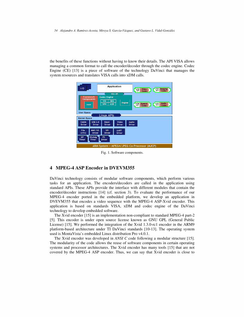
the benefits of these functions without having to know their details. The API VISA allows

managing a common format to call the encoder/decoder through the codec engine. Codec

Engine (CE) [13] is a piece of software of the technology DaVinci that manages the

system resources and translates VISA calls into xDM calls.

Fig. 1. Software components.

4 MPEG-4 ASP Encoder in DVEVM355

DaVinci technology consists of modular software components, which perform various

tasks for an application. The encoders/decoders are called in the application using

standard APIs. These APIs provide the interface with different modules that contain the

encoder/decoder instructions [14] (cf. section 3). To evaluate the performance of our

MPEG-4 encoder ported in the embedded platform, we develop an application in

DVEVM355 that encodes a video sequence with the MPEG-4 ASP-Xvid encoder. This

application is based on standards VISA, xDM and codec engine of the DaVinci

technology to develop embedded software.

The Xvid encoder [15] is an implementation non-compliant to standard MPEG-4 part-2

[5]. This encoder is under open source license known as GNU GPL (General Public

License) [15]. We performed the integration of the Xvid 1.3.0-rc1 encoder in the ARM9

platform-based architecture under TI DaVinci standards [10-13]. The operating system

used is MontaVista’s embedded Linux distribution Pro v4.0.1.

The Xvid encoder was developed in ANSI C code following a modular structure [15].

The modularity of the code allows the reuse of software components in certain operating

systems and processor architectures. The Xvid encoder has many tools [15] that are not

covered by the MPEG-4 ASP encoder. Thus, we can say that Xvid encoder is close to


compliant, but no really compliant. For this reason, one of our contributions in this work

is the Xvid encoder adaptation being compliant to the MPEG-4 ASP [5] standard. With

this, we only integrate the tools provided in the standard for MPEG-4 ASP encoder. The

coding tools of the Xvid encoder that satisfy the MPEG-4 ASP profile are: ASP@Level 1

(ASP@L1), ASP@L2, ASP@L3, ASP@L4, ASP@L5; I-Frames/Keyframes, P-

Frames/directional encoding, B-Frames/Bi-directional encoding, Quarter Pixel Motion

Estimation search precision (QPEL), Global Motion Compensation (GMC), Interlace

coding, and H.263/MPEG/Custom Quantization.

Another interesting contribution of our work is the porting of the Xvid encoder to the

ARM9 CPU; this porting takes advantage of the TI DaVinci standards and the DaVinci TI

DVEVM355 platform. The method to porting the Xvid encoder in the ARM9 platform-

based architecture of DM355 is divided in two parts:

− Xvid encoder configuration to the ARM9 platform-based architecture.

− Porting of Xvid encoder to the xDM TI standards.

4.1 Xvid Encoder Configuration to the ARM9 Platform-based Architecture

The Xvid encoder is configured to be executed on the ARM9 processor architecture into

the DM355 of TI. The parameters for the set up are: target platform “ARM generic”; type

of compiler “ARM_V5T_LE-GCC”, the company Montavista Linux; host platform

“x86_64-pc-linux”.

4.2 Porting of Xvid Encoder to the xDM TI Standards

Once that the Xvid encoder is integrated with the coding tools under the MPEG-4 ASP

profile and its configurations to be executed in the DM355 ARM processor, we develop

the MPEG-4 ASP-Xvid encoder implementation under DaVinci TI standards. The

methodology is based on the recommendations of R. Pawate [14]. We used the APIs

VISA, xDM and the Codec Engine for the management of MPEG-4 ASP-Xvid encoder

being compatible with the software components of the DVEVM355 platform. The

implementation is described in the following lines:

Figure 2 shows the outline to follow to implement an encoder/decoder under DaVinci

technology. The codec engine software basically translates these create, control, process

and delete APIs to their respective xDM APIs, while managing the system resources and

inter-processor communication.

The process and control API of VISA are a direct reflection of the low-level process

and control functions of the xDM algorithm (codec1). As a result, Texas Instruments

providing low-level control of codecs along with high level abstraction of the details. The

figure 3 shows the specific VISA and xDM APIs for the video encoder/decoder. For a


given class, say Video, the signature of these APIs is held constant. This enables an

integrator and developer to easily replace one encoder/decoder with another.

Fig. 2. Management of an encoder/decoder under DaVinci technology.

Fig. 3. VISA Abstracts details of xDM algorithms for video encoder/decoder.

To use the followings APIs: VISA, xDM and of the Codec Engine, the application is

divided into four logical blocks:

− Parameter setup,

− Algorithm instance creation and initialization,

− Process call – xDM 1.0,

− Algorithm instance deletion.


4.2.1 Parameter Setup The video encoder/decoder requires various configuration parameters to be set at

initialization. Our application obtains the required parameters from the encoder

configuration. The coding parameters are assigned to VIDENC1_XVID_PARAMS

structure, which is an extended version of the generic structure IVIDENC1_Params. The

generic structure is used by video codecs for the API VISA. We verify that the parameters

are within the ranges set by the MPEG-4 ASP standard. We also assign memory space

E/S for the data of the entry frame and for the data of the coded frame. The allocation of

contiguous memory space is done by the function: Memory_contigAlloc(). After

successful completion of the above steps, the application does the algorithm instance

creation and initialization.

4.2.2 Algorithm Instance Creation and Initialization

In this logical block, the application accepts the various initialization parameters and

returns an algorithm instance pointer. The VIDENC1_XVID_Create() API creates an

instance of xDM encoder MPEG-4 ASP-Xvid and allocates the required resources for the

encoder MPEG-4 ASP-Xvid to run. VIDENC1_XVID_Create() API, using the Codec

Engine, queries the xDM encoder for the resources that it needs, and based on the encoder

requirements, it allocates them. The following APIs are called in sequence:

− algAlloc() – to query the algorithm about the memory requirement to be filled in the

memory records.

− xvid_global(XVID_GBL_INIT) – to initialize the global variables of the algorithm.

− xvid_encore(XVID_ENC_CREATE) – to initialize the algorithm.

− algInit() – to initialize the algorithm with the memory structures provided by the

application.

4.2.3 Process Call – xDM 1.0

After algorithm instance creation and initialization, the application does the following:

− Sets the dynamic parameters (if they change during run time) by calling the

VIDENC1_XVID_control() function.

− Sets the input and output buffers descriptors required for the

VIDENC1_XVID_process() function call. The input and output buffer descriptors are

obtained by calling the VIDENC1_XVID_control() function.

− Call the VIDENC1_XVID_process() function to encode a single frame of data. In this

function, we call the function xvid_encore(XVID_ENC_ENCODE) which coding the

frame at the input buffer with MPEG-4 ASP-Xvid encoder. When the process

function ends, the output buffer is updated with the encoded picture.

The VIDENC1_XVID_control() and VIDENC1_XVID_process() functions should be

called only within the scope of the algActivate() and algDeactivate() xDAIS functions

which activate and deactivate the algorithm instance respectively. Once an algorithm is


activated, there could be any ordering of VIDENC1_XVID_control() and

VIDENC1_XVID_process() functions. The do-while loop encapsulates frame level

VIDENC1_XVID_process() call and updates the input buffer pointer every time before the

next call. The do-while loop breaks off either when an error condition occurs or when the

input buffer exhausts.

4.2.4 Algorithm Instance Deletion

Once encoding is complete, the application must release the resource for the encoder

MPEG-4 ASP-Xvid and delete the current algorithm instance.

5 Results

This section presents the evaluation of MPEG-4 ASP-Xvid encoder ported in the

embedded Linux operating system under ARM9 platform-based architecture of DM355.

In order to evaluate our MPEG-4 ASP-Xvid encoder porting, we develop an application in

DVEVM355 that encodes a video sequence with the MPEG-4 ASP-Xvid encoder. In

order to have a reference for comparing our encoder’s performance, we conducted the

evaluation of the MPEG-4 SP encoder of TI for DM355 [16] under the same conditions.

The test database consists of three video sequences (Bus, Foreman and News). These

sequences are used as reference by the integrators developers, and the scientific

community to evaluate the encoder’s performance. These sequences have great

information in texture, movements ranging from low to high level. Each video has the

following parameters: 10 seconds of video, CIF (Common Interface Format) resolutions

(352x288), YUV 4:2:0P, 30 fps. The coding scheme was tested with different constant

bitrates: CBR: 64kbps, 128Kbps, 384Kbps, 512Kbps and 1024Kbps. The GOP size for

both encoders is 12 (frames). The GOP structure for the MPEG-4 ASP-Xvid encoder is

IBBPBBPBBPBB, while for the MPEG-4 SP encoder of TI is IPPPPPPPPPPP. According

to the above parameters, the three sequences were coded for both encoders under DaVinci

platform. Then, the coded sequences were decoded in the host computer. To evaluate the

performance of our integration of MPEG-4 ASP-Xvid encoder in the DVEVM355

architecture, according to the standard xDM of TI, we consider Peak Signal to Noise

Ratio of the Y-plane of the frame (Y-PSNR) measure. Equation 1 describes Y-PSNR

mathematically.

, ′ = 10 ∙ 102 ∙ ∙

, − ′, 2−1

=0

−1

=0 (1)


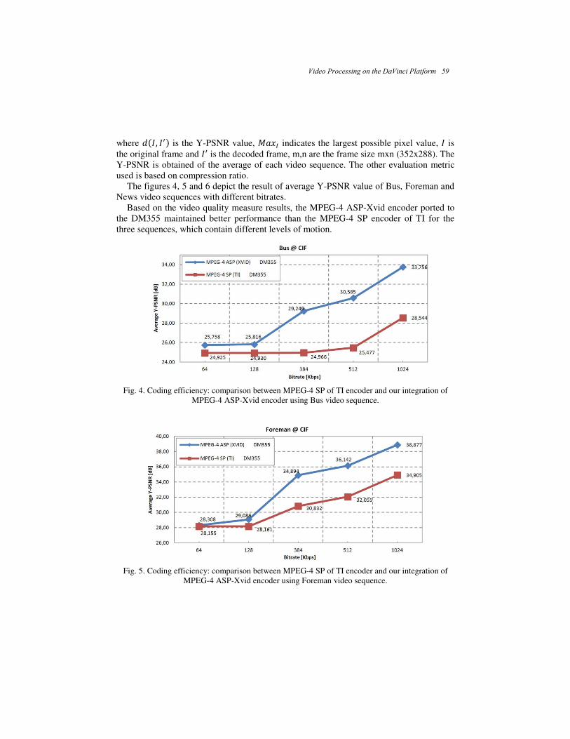
where , is the Y-PSNR value, indicates the largest possible pixel value, is

the original frame and is the decoded frame, m,n are the frame size mxn (352x288). The

Y-PSNR is obtained of the average of each video sequence. The other evaluation metric

used is based on compression ratio.

The figures 4, 5 and 6 depict the result of average Y-PSNR value of Bus, Foreman and

News video sequences with different bitrates.

Based on the video quality measure results, the MPEG-4 ASP-Xvid encoder ported to

the DM355 maintained better performance than the MPEG-4 SP encoder of TI for the

three sequences, which contain different levels of motion.

Fig. 4. Coding efficiency: comparison between MPEG-4 SP of TI encoder and our integration of

MPEG-4 ASP-Xvid encoder using Bus video sequence.


MPEG-4 ASP-Xvid encoder using Foreman video sequence.



MPEG-4 ASP-Xvid encoder using News video sequence.

Fig. 7. Compression efficiency: comparison between MPEG-4 SP of TI encoder and our integration

of MPEG-4 ASP-Xvid encoder using Bus video sequence.

With respect to overall performance on the three sequences for both encoders, we

observe that the best quality is obtained with the News sequence (Fig. 6) behaving with

low movement, followed by Foreman (Fig. 5) that presents a middle movement category.

Finally, the worst quality is obtained with the Bus sequence (Fig. 4), which presents a

high motion category. Based on the compression ratio, figures 7, 8 and 9 show the

encoder’s performance under different bitrates. The compression ratio represents the size

in Kbytes of coded video with respect to the size in Kbytes of the original sequence. The

rate of compression is presented as a percentage. With respect to the measure of

compression ratio, a value close to zero represents a better performance of the encoder.


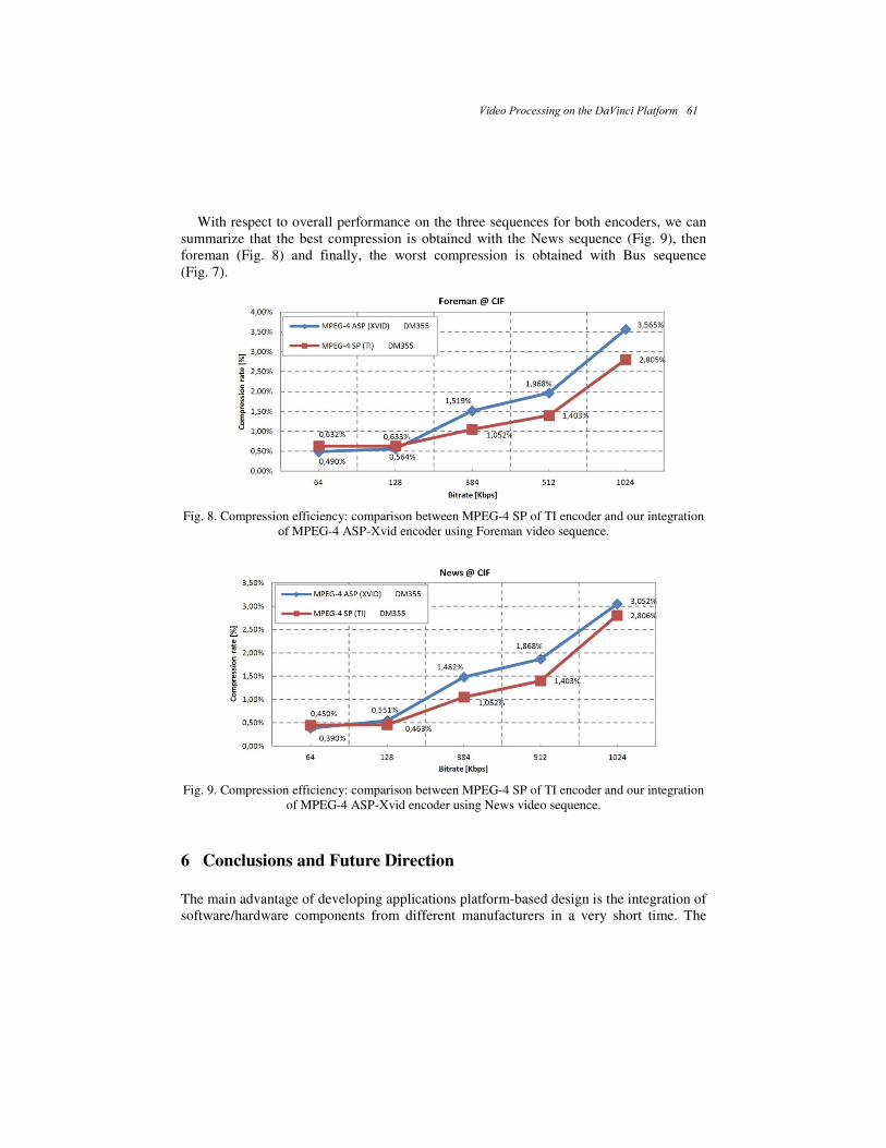
With respect to overall performance on the three sequences for both encoders, we can

summarize that the best compression is obtained with the News sequence (Fig. 9), then

foreman (Fig. 8) and finally, the worst compression is obtained with Bus sequence

(Fig. 7).


of MPEG-4 ASP-Xvid encoder using Foreman video sequence.


of MPEG-4 ASP-Xvid encoder using News video sequence.

6 Conclusions and Future Direction

The main advantage of developing applications platform-based design is the integration of

software/hardware components from different manufacturers in a very short time. The


development of a complete software application that constitutes a working embedded

system relies on many software components. For this reason, this work leverages the use

of an embedded Linux operating system tailored for the DaVinci platform. Based on the

analysis of the DaVinci technology, this paper presented a prototype of an MPEG-4

encoder video profile ASP based on Xvid software ported to the architecture ARM9

processor of the DaVinci Platform DVEVM355 of Texas Instruments. We developed an

application to evaluate the performance of our MPEG-4 ASP Xvid encoder. This

application is based on standards VISA, xDM and codec engine of the DaVinci

technology to develop embedded software. The encoder is then evaluated for performance

on the platform DVEVM355. Based on testing and performance, the MPEG-4 ASP Xvid

encoder ported to the ARM9 platform-based architecture of DM355 is a good candidate to

replace the MPEG-4 SP encoder of TI since it shows higher quality video. As future work,

we will migrate our algorithm in a fully-programmable DSP to leverage the power of the

DSP on the SoC (ARM+DSP) since the co-processor of the DM355 is not a DSP open for

programming.

Acknowledgements. This work was supported by IPN-SIP 20110032.

References

1 Sangiovanni-Vincentelli, A., Carloni, L., De Bernardinis, F., Sgroi, M.: Benefits and

challenges for platform-based design. In: Proc. DAC, pp. 409–414 (2004)

2 International Organization for Standardization (ISO/IEC). http://www.iso.org (2011)

3 International Telecommunication Union (ITU-T). http://www.itu.int/ITU-T (2011)

4 Chatterji, S., Narayanan, M., Duell, J., Oliker, L.: Performance evaluation of two emerging

media processors: Viram and imagine. In: International Parallel and Distributed Processing

Symposium, pp. 229–235 (2003)

5 ISO/IEC 14496-2:2004, Information technology – Coding of audio-visual objects – Part 2:

Visual (Approved in 05-24) (2004)

6 Wiegand, T., Sullivan, G. J., Bjontegaard, G., Luthra, A.: Overview of the H.264 / AVC Video

Coding Standard. IEEE transactions on circuits and systems for video technology (2003)

7 Texas Instruments, http://www.ti.com (2011)

8 Shin, D., Gerstlauer, A., Dömer, R., Gajski, D.: Automatic Network Generation for System-on-

Chip Communication Design. In: Proceedings of the International Conference on

Hardware/Software Codesign and System Synthesis. Jersey City, New Jersey (2005)

9 IMT-2000.: International Mobile Telecommunications, http://www.itu.int/osg/spu/imt-

2000/technology.html (2011)

10 TMS320DM355 Digital Media System-on-Chip (DMSoC) (Rev.G, 24 June). SPRS463G.

Texas Instruments (2010)

11 TMS320DM355 Evaluation Module Technical Reference. 509905-0001 Rev. E. Spectrum

Digital, Inc. (2008)

12 xDAIS-DM (Digital Media), User Guide. Literature Number: SPRUEC8B. Texas Instruments

(2007)


13 Codec Engine Application Developer User’s Guide. Literature Number: SPRUE67D,

September. Texas Instruments (2007)

14 Pawate, B.I. R.: Developing Embedded Software using DaVinci & OMAP Technology,

Synthesis Lectures on Digital Circuits and Systems. Morgan & Claypool Publishers (2009)

15 Xvid Codec. http://www.xvid.org (2011)

16 MPEG-4 Simple Profile Encoder Codec on DM355. User’s Guide. Literature Number:

SPRUFE4C. Texas Instruments (2008)


Using Signal Processing Based on Wavelet Analysis

to Improve Automatic Speech Recognition

on a Corpus of Digits

José Luis Oropeza Rodríguez, Mario Jiménez Hernández,

and Alfonso Martínez Cruz

Center for Computing Research, National Polytechnic Institute,

Av. Juan de Dios Batiz esq Miguel Othon de Mendizabal s/n, 07038, México DF, Mexico [email protected], [email protected], [email protected]

Abstract. This paper shows results when we used wavelets in a corpus of digits

pronounced by five speakers in Spanish language. One of the most important aspects

related to the ASR is to reduce the number of data used. Firstly, we show the results

when we used wavelet filters to the speech signal in order to obtain low frequencies

only. Secondly, we use the ability of wavelet analysis is to perform data

compression, to reduce by half the amount of voice data analyzed. For each of the

two previous experiments we obtained new corpus, after that each corpus was used

to train an Automatic Speech Recognition System using the technique vector

quantization (VQ), being more employed in these corpus, also at final we compare

the results obtained with DHMM technique. Finally, we compare our results with

respect to the original corpus and found a 3-5% reduction in Word Error Rate

(WER) when we use VQ and (1-3%) using CHMM. Daubechies wavelets were used

in the experiments, as well as Vector Quantization (VQ) with Linear Prediction

Coefficients (LPC) as features to represent the speech signal and DHMM.

Keywords: Wavelets, automatic speech recognition systems (ASRs), Daubechies

wavelet, wavelet filters, vector quantization (VQ), discrete hidden Markov models

(DHMM), data speech compression.

1 Introduction

Automatic Speech Recognition systems (ASRs) work reasonably well in quiet conditions

but work poorly under noisy conditions or distorted channels. For example, the accuracy

of a speech recognition system may be acceptable if you call from the phone in your quiet

office, yet its performance can be unacceptable if you try to use your cellular phone in a

shopping mall. The researchers in the speech group are working on algorithms to improve

the robustness of speech recognition system to high noise levels channel conditions not

present in the training data used to build the recognizer [Cole et al., 1996]. In this paper

we used wavelet filters to avoid high frequencies, where noisy signals regularly are

present. That is very important because of one of the most important aspects that have

been studied for the last years is that the important information of the speech signals is

contained within low frequencies more than high frequencies. “The schools of thought in

speech recognition” describe four different approach researched at today [6], we are going

to use template-based approach.

ASR has implemented one stage called “speech analysis”. The applications that need

voice processing (such as coding, synthesis, and recognition) require specific

representations of speech information. For instance, the main requirement for speech

recognition is the extraction of speech features, which may distinguish different phonemes

of a language. In the template-based approach, the units of speech (usually words, like in

this work), are represented by templates in the same form as the speech input itself.

Distance metrics are used to compare templates to find the best match, and dynamic

programming is used to resolve the problem of temporal variability. Tem-plate-based

approaches have been successful, particularly for simple applications requiring minimal

overhead. We used this approach in this paper. A variety of techniques have been

developed to efficiently represent to speech signals in digital form for either transmission

or storage. Since most of the speech energy is contained in the lower frequencies results

very important to encode the lower-frequency band with more bits than the high-

frequency band. In this paper we based our experiments in the last aspect, we use subband

coding which is a method where the speech signal is subdivided into several bands and

each band is digitally encoded separately. In subband coding a speech signal is sampled at

a rate Fs samples per second. The first frequency subdivision splits the signal spectrum

into two equal-width segments, a lowpass signal , and a highpass signal

. The second frequency subdivision splits the lowpass signal from the

first stage into two equal bands, a lowpass signal , and a highpass signal

. Finally, the third fre-quency division splits the lowpass signal from the

second stage into two equal band-width signals. Thus the signal is subdivided into four

frequency bands, covering three octaves. To perform subband coding we use wavelet

analysis as implemented in [7].

1.1 Phonetic and Frequency Analysis

One aspect related with propose mentioned above is that /s/ phoneme, that we can

consider as unvoiced fricative sound, contains representative frequencies lower than 3.5

kHz. For that, if the noise components integrated into speech signal were removed using a

filter and the response filter were used into Automatic Speech Recognition systems to try

to reduce the WER, we can obtain a methodology that can be used in ASR. Now, wavelet

filter is newest approach used in digital signal processing, their characteristics are better

(in some cases) than techniques employed in classical digital filter.

66 José Luis Oropeza Rodríguez, Mario Jiménez Hernández, and Alfonso Martínez Cruz

1.2 Wavelet Compression

Wavelet compression is a form of data compression well suited for image compression

(sometimes also video compression and audio compression). The goal is to store image

data in as little space as possible in a file. Wavelet compression can be either lossless or

lossy (JPEG 2000, for example, may use a 5/3 wavelet for lossless (reversible) transform

and a 9/7 wavelet for loss (irreversible transform) [Van Fleet, 2008]. Using a wavelet

transform, the wavelet compression methods are adequate for representing transients, such

as percussion sounds in audio, or high-frequency components in two-dimensional images,

for example an image of stars on a night sky. This means that the transient elements of a

data signal can be represented by a smaller amount of information than would be the case

if some other transform, such as the more widespread discrete cosine transform, had been

used.

1.3 Speech Recognition using Wavelets

Taking into account all that we mentioned above for researcher interested in speech

recognition is very interesting analyze how can we use compression properties related

with wavelet analysis into a corpus of speech signals that it will be used into Automatic

Speech Recognition tasks. The results obtained not only have impact over the task

mentioned above, but it could be used for a combination of data compression that it will

be used for transmission of information into digital networks, for example. Wavelets was

used for one important reason, its computational implementation as digital filter and in

compression signal is easy to make and, due to that multi-resolution analysis inherent

wavelet systems, a reduced number of coefficients are necessary to be implemented in

comparison with digital filters design traditional (FIR) or instability conditions (IIR) [Van

Fleet, 2008].

An important amount of works have been realized in this aspect, above all for robust

speech recognition task, it refers to the need to maintain good recognition accuracy even

when the quality of the input speech is degraded, or when the acoustical, articulatory, or

phonetic characteristics of speech in the training and testing environments differ.

Obstacles to robust recognition include acoustical degradations produced by additive

noise, the effects of linear filtering, nonlinearities in transduction or transmission, as well

as impulsive interfering sources, and diminished accuracy caused by changes in

articulation produced by the presence of high-intensity noise sources. Even systems, that

are designed to be speaker-independent, exhibit dramatic degradations in recognition

accuracy when training and testing conditions differ [2]. For these reasons, within others,

is necessary to find an alternative that can be used to reduce the conflicts presented here.

Using Signal Processing Based on Wavelet Analysis... 67

2 Wavelet Theory

Fourier analysis, using the Fourier transform, is a powerful tool for analyzing the

components of a stationary signal. For example, the Fourier transform is a powerful tool

for processing signals that are composed of some combination of sine and cosine signals.

The Fourier transform is less useful in analyzing non-stationary data, where there is no

repetition within the region sampled. Wavelet transforms (of which there are, at least

formally, an infinite number) allow the components of a non-stationary signal to be

analyzed. Wavelets also allow filters to be constructed for stationary and non-stationary

signals [3].

The statistics of many natural images are simplified when they are decomposed via

wavelet transform. Recently, many researchers have found that statistics of order greater

than two can be utilized in choosing a basis for images, has shown that the coefficients of

frequency subbands of natural scenes have much higher kurtosis than a Gaussian

distribution. Daubechies wavelets are a family of orthogonal wavelets defining a discrete

wavelet transform and characterized by a maximal number of vanishing moments for

some given support [3]. With each wavelet type of this class, there is a scaling function

(also called mother wavelet) which generates an orthogonal multiresolution analysis. The

selected sub-band was the 3 in all case, because the high level recognition was better for

this case. A signal or function f (t) can often be better analyzed, described, or processed if

expressed as a linear decomposition by [4].

∑∈

=Zk

kjkj tctf )()( ,, φ (1)

Where is an integer index for the sum, is the expansion coefficients and is the set of

real-valued functions of t called the expansion set. If the expansion is unique, the set is

called a basis for the functions that could be represented. If the basis is orthogonal, then

the coefficients can be calculated by the inner product. [Walnut, 2001]

dtttfttfc kjkjkj ∫∞

∞−== )()()(),( ,,, φφ (2)

A single coefficient is obtained by substituting (1) into (2) and therefore for the

wavelet expansion, a two-parameter system is constructed such that (1) becomes

∑∑ ∑∑+=k j k j

kjkj tdtctf )()()( ,, ψφ (3)

Where and is the wavelet expansion that usually forms an

orthogonal basis. The set of expansion coefficients are called the discrete wavelet

transform of f (t) and (3) is its inverse.

)(, tkjφ

)(, tkjφ

Zkjtkj ∈,|)(,ψ )(, tkjφ)(, tkjψ


All wavelet systems are generated from a single scaling function or wavelet by simple

scaling and translation. This two-dimensional representation is achieved from the function

, also called the mother wavelet, by

( ) Zkjktt j

j

kj ∈−= ,22)( 2, ψψ (4)

Wavelet systems also satisfy multi-resolution conditions. In effect, this means that a set

of scaling functions can be determined in terms of integer translates of the basic scaling

function by

Zkjktt j

j

kj ∈−= ,)2(2)( 2, φφ (5)

It can therefore be seen that if a set of signals can be represented by ; a larger

set can represented by , giving a better approximation of any signal.

Hence, due to the spanning of the space of by , it can be expressed in

terms of the weighted sum of the shifted as

( ) ( ) ( )ktnhtZk

−= ∑∈

22φφ (6)

Where the coefficients h(n) may be real or complex numbers called the scaling

function coefficients. However, the important features of a signal can better be described,

not by , but by defining a slightly different set of functions that span the

differences between the spaces spanned by the various scales of the scaling function.

These functions are the wavelets and, they can be represented by a weighted sum of

shifted scaling function defined in (6) by [Yuan Yan, 2009].

( ) ( )∑∈

−=Zk

ktnht 2)(2 φψ (7)

The function generated by (7) gives the prototype or mother wavelet for a class of

expansion functions of the form given by (4).

∑∑ ∑∑+=k j k j

kjkj tdtctf )()()( ,, ψφ (8)

The coefficients in this wavelet expansion are called the discrete wavelet transform

(DWT), of the signal f(t). For a large class of signals, the wavelet expansion coefficients

drop off rapidly as j and k increase. As a result, the DWT is efficient for image and audio

compression

)(, tkjψ

)( kt −φ)2( kt −φ

)(tφ )2( tφ

)2( tφ )(, tkjψ

)(, tkjφ

)(tψ


3 Template-Based Approach

The frequency bandwidth of a speech signal is about 16 KHz. However, most of speech

energy is under 7 KHz. Speech bandwidth is generally reduced in recording. A speech

signal is called orthophonic if all the spectral components over 16 KHz are discarded. A

telephonic lower quality signal is obtained whenever a signal does not have energy out of

the band 300-3400 Hz. Therefore, digital speech processing is usually performed by a

frequency sampling ranging between 8000 samples/sec and 32000 samples/sec. These

values correspond to a bandwidth of 4KHz and 16KHz respectively. In this work, we use

a frequency sampling 11025 samples/sec [1].

4 Experiments and Results

In the proposal developed in the experiments we used the methodology represented in

figure 6, this figure shows the experiment developed using wavelets theory to reduce the

amount of noise contained in the speech signal, it was obtained taking into account the

frequency allocation in a (conventional, decimated) DWT where we have A1 and D1

frequency allocation to represent such Approximations as Details obtained from wavelet

filter used, the actual shape depends of the wavelet filters. Also, figure 6 shows the

experiment developed using wavelet theory to applied data compression, DWT

decomposition were used with the difference that we token the speech signal from

different points.

Fig. 1. Analysis wavelet used in the experiments.

For experiments, a Spanish digits database (0-9) was used, it consists of 5 speakers

each one of them pronounced 200 sentences of digits, half of them were used to training

system and the rest for recognition. Speech signals were recorded at 11025 kHz with 16


bits by sample, using mono-channel with PCM format. As we mentioned before and after

to describe the proposal developed in this paper, we obtained a total of 600 sentences for

each speaker obtained of a great total of 3000 sentences processed during experiments

reported. As we mentioned before and after to describe the proposal developed in this

paper, we obtained a total of 600 sentences for each speaker obtained of a great total of

3000 sentences processed during experiments reported.

The signal flow diagram for a single-level conventional DWT is shown in figure 1. The

information used to eliminate the noise was taken after of the block denoted as L, while

the information used for compression was taken after of the first label cA1 as we shown in

the same figure, where down-sampling for 2 was reached. As we mentioned before and

after to describe the proposal developed in this paper, we obtained a total of 600 sentences

for each speaker obtained of a great total of 3000 sentences processed during experiments

reported. The signal flow diagram for a single-level conventional DWT is shown in figure

6. The information used to eliminate the noise was taken after of the block denoted as L,

while the information used for compression was taken after of the first label cA1 as we

shown in the same figure.

Table 1 shows results obtained using speech signals after to apply wavelet

compression, we can see that performance reached was superior using decomposition

level 1, for that in all experiments reported here this decomposition level was selected.

In rows we can see wavelet Daubechies order (form 1 to 3) and in the columns we can

see the 5 corpus analyzed, the performance reached also is showed. We can see clearly

that the best performance was obtained using decomposition level 1 in comparison with

decomposition level 2.

Table 1. Results using wavelet filters.

Another results obtained is illustrated in table 2 which reports obtained using speech

signals after to apply lowpass filter, again we can see that the best performance is

obtained when we used decomposition level 1.

As we can see, the results obtained using two aspects considered in this paper was

successful when we used decomposition level 1, but the best performance occurs and it is

most significant using wavelet compression.


Table 2. Results using wavelet filters.

Finally, we show, in table 3, the performance reached when we used the original

corpus for recognition task.

Comparing the results we can conclude that the recognition percentage was better using

the compression wavelet with the exception showed for the second corpus because of it

had noisy signal.

Table 3 Results using original corpus

The results previously presented were compared using Discrete Hidden Markov

Models (DHMM) with 6 states per model for each word into the corpus. The results

obtained demonstrated that DHMM results better than VQ technique in order 3% related

with the corpus used.

5 Conclusions and Future Works

Without loss of generality, such as has been demonstrated in ASRs based in VQ, we can

to say that the results obtained in these experiments can be extended to others ASRs that

employ Continuous Density Hidden Markov Model (CDHMM) and Mel Frequency

Cepstrum Coefficients (MFCC) without problem. The main purpose of this paper was to

integrate wavelet aspects such as digital filters and compression into ASRs. We showed

that the methodology proposed reached out an increase of the 3-5% of the WER for some

corpus created. For future works we are going to use the results obtained here to integrate

the Automatic Speech Recognition for a system that is focused to speaker and speech

recognition wheatear more synthesis in an application that is going to interactively it will

respond to anybody people. For that, we must to work in increase the number of the


speakers and programming another splitting algorithm. Though the results reported

demonstrated a good and better performance.

References

1. Bechetti, C., Ricoti L.P.: Speech Recognition Theory and C++ Implementation, Fundazione

Ugo Bordón. Rome, Italy. John Wiley and Sons, Ltd. (1999)

2. Cole, A.R., Mariani,J., Uszkoreit, H., Zaenen, A., Zue, V.:. Survey of the State of the Art in

Human Language Technology, National Science Foundation, CSLU, Oregon Institute.

3. Duran, D.I.: The Wavelet Transform, Time-Frequency Localization and Signal Analysis. IEEE

Transactions on Information Theory, Vol. 36, No. 5 (1990)

4. Faundez, P., Fuentes, A.: Procesamiento de señales acústicas utilizando wavelets. Instituto de

Matemáticas, UACH.

5. Farnetani, E.: Coarticulation and connected speech processes. In: The Handbook of Phonetic

Sciences. W. Hardcastle and J. Laver, 12 . Blackwell, pp. 371-404 (1997)

6. Kirschning, A.I.: Automatic Speech Recognition with the parallel Cascade Neural network,

PhD Thesis. Tokyo, Japan (1998)

7. Mallat, S.: A wavelet tour of signal processing. Academic Press, ISBN: 0-12-4666606-X

(1999)

8. Nicholas, G.R..: Fourier and wavelet representations of functions, Electronic Journal of

Undergraduate Mathematics. Furman University. Volume 6, 1-12 (2000)


Ontologies, Logic and Multi-agent Systems

Methontology-based Ontology

Representing a Service-based Architectural Model

for Collaborative Applications

Mario Anzures-García1, Luz A. Sánchez-Gálvez

2, Miguel J. Hornos

2,

and Patricia Paderewski2

1 Facultad de Ciencias de la Computación, Benemérita Universidad Autónoma de Puebla,

14 sur y avenida San Claudio. Ciudad Universitaria, San Manuel, 72570 Puebla, Mexico 2 Universidad de Granada, C/ Periodista Saucedo Aranda, s/n, 18071 Granada, Spain

mario.anzures, [email protected],

mhornos, [email protected]

Abstract. Nowadays, the usage of ontologies to model systems has been extended

to several domains, since ontology facilitates the modeling of complex systems and

presents axioms which can be used as rules, policies or constrains to govern the

system behavior. This paper presents ontology to represent a Service-based

Architectural Model for Collaborative Applications, such as a Conference

Management System (CMS), a simple social network, a chat, or a shared workspace.

The development process of this ontology is based on Methontology, which is a

well-structured methodology to build ontologies from scratch that includes a set of

activities, techniques to carry out each one, and deliverables to be produced after the

execution of such activities using its attached techniques. In order to show the

development of the ontology using Methontology, the concepts, relations, axioms

and instances of this ontology are specified for the collaborative application chosen

as a case study, which is a CMS.

Keywords: Ontology, ontology construction process, methontology, collaborative

application, architectural model.

1 Introduction

Recently, there has been an increase in the use of ontologies to model applications in any

domain. Ontology is presented as an organization resource and knowledge representation

through an abstract model. This representation model provides a common vocabulary of a

domain and defines the meaning of the terms and the relations amongst them.

In a collaborative domain, the ontology provides a well-defined common and shared

vocabulary, which supplies a set of concepts, relations and axioms to describe this domain

in a formal way. In this domain, the ontologies have mainly been used to model tasks or

sessions. Different concepts and terms, such as group, role, actor, task, etc., have been

used for the design of tasks and sessions. Moreover, semiformal methods (e.g. UML class

diagrams, use cases, activity graphs, transition graphs, etc.) and formal ones (such as

algebraic expressions) have also been applied to model the sessions. There is also a work

[1] for modeling cross-enterprise business processes from the perspective of a cooperative

system, which is a multi-level design scheme for the construction of cooperative system

ontologies. This last work is focused on business processes, and it describes a general

scheme for the construction of ontologies. In the literature, there are several papers on

ontologies to model collaborative work; however, ontologies to support architectural

modeling for developing collaborative applications have not been presented. In this work,

the ontology will be used to facilitate the service composition of the architectural

modeling by means of a Business Process Modeling (BPM), which is based on the

ontological approach. This is the main reason to build the ontology; however, the BPM

explanation is outside the scope of this article. Instead, this paper will focus on the

ontology construction process using Methontology, since this methodology presents tasks

set, which allow us to simplify this construction process and same time the development

of collaborative application. These tasks detail each concept, the relations between these,

as well as the rules and the axioms that govern its interaction, so it carries out the

correspondent tables to these activities facilitate the development of the collaborative

applications.

The ontology construction process must be based on methodologies, which specify

techniques and methods that drive the development of the corresponding ontology. This

allows us to define common and structured guidelines that establish a set of principles,

design criteria and phases for building the ontology. Methontology [2, 3] is a methodology

that supports the ontology construction process from scratch or the reuse of existing

ontologies. For this reason, this paper proposes a Methontology-based ontology to

represent a Service-based Architectural Model for Collaborative Applications (SAMCA).

As a collaborative application example, a Conference Management System (CMS) is

modeled by means of this ontology, to show how the CMS construction process is simple

when it elaborates the table of each activity of the Methontology.

In the following sections, this paper presents a brief introduction to ontologies (Section

2), a review of the methodologies used in the ontology construction process, and

particularly of Methontology, which is the one we applied to this work (Section 3), a

concise explanation of SAMCA (Section 4), an example taken from the collaborative

application CMS to show the use of Methontology (Section 5), and finally, the

conclusions and future work (Section 6).

2 Introduction to Ontologies

There are several definitions of ontology, which have different connotations depending on

the specific application domain. In this paper, we will refer to Gruber’s well-known

definition [4], where an ontology is an explicit specification of a conceptualization.

Conceptualization refers to an abstract model of some phenomenon in the world by

78 Mario Anzures-García, Luz A. Sánchez-Gálvez, Miguel J. Hornos, and Patricia Paderewski

identifying the relevant concepts of that phenomenon. Explicit specification means that

the type of concepts used, and the constraints on their use are explicitly defined.

The ontologies require of a logical and formal language to be expressed. In Artificial

Intelligence, different languages have been developed, including First-order Logic-based,

Frames-based, and Description Logic-based ones. The first ones provide powerful

modeling primitives; the second ones have more expressive power but less inference

capacity, while the third ones are more robust in the reasoning power.

Ontology is specified using the following components [4]:

− Classes: Set of classes (or concepts) that belong to the ontology. They may

contain individuals (or instances), other classes, or a combination of both with

their corresponding attributes.

− Relations: These define interrelations between two or more classes (object

properties) or a concept related to a data type (data type properties).

− Axioms: These are used to impose constraints on the values of classes or

instances. Axioms represent expressions in the ontology (logical statement) and

are always true if they are used inside the ontology.

− Instances: These represent the objects, elements or individuals of ontology.

Based on these components used to represent domain knowledge, the ontology

community distinguishes two types of ontologies: lightweight ontologies and heavyweight

ontologies [5]. On the one hand, lightweight ontologies include concepts, concept

taxonomies, relationships between concepts, and properties that describe concepts. On the

other hand, heavyweight ontologies add axioms and constraints to lightweight ontologies.

Axioms and constraints clarify the intended meaning of the terms gathered on the

ontology. Heavyweight and lightweight ontologies can be modeled with different

knowledge modeling techniques and they can be implemented in various kinds of

languages [6]. Ontologies can be highly informal, if they are expressed in natural

language; semi-informal, if they are expressed in a restricted and structured form of

natural language; formal, if they are expressed in an artificial and formally defined

language (i.e. Ontolingua [7], OWL -Web Ontology Language- [8]); and rigorously

formal, if they meticulously provide terms defined with formal semantics, theorems and

proofs of properties, such as soundness and completeness.

The ontology that models a Service-based Architectural Model for developing

Collaborative Applications is a heavy and formal ontology, which has been built using

Methontology, defined in OWL, which is a description logic-based language that can

define and instantiate Web ontologies using XML (eXtensible Markup Language) and

RDF (Resource Description Framework), and published, implemented, validated and

documented with the Protégé tool [9]. The ontology validation has been done with the

software RACER (Renamed Abox and Concept Expression Reasoner) [10], which can

work with Protégé. RACER can verify the consistency of the ontology (i.e. non-

contradictory knowledge in it) to infer taxonomy and classify knowledge. Finally, the

ontology was implemented with OWL, which allows generating a standalone application

in Java.

Methontology-based Ontology Representing a Service-based Architectural Model... 79

3 Brief Review of Methodologies for Ontology Construction Process:

Why We Use Methontology

The use of terms such as methodology, method, technique, process, activity, etc. on the

ontological field is made in accordance to IEEE definitions [11], where it is established

that a methodology is made up of methods and techniques, in such a way that the methods

include processes and are detailed with techniques, and the processes contain activities.

Finally, the activities are made up of a series of tasks.

The absence of common and structured guidelines has slowed the development of

ontologies within and between teams. This has led to each development team usually

follows their own set of principles, design criteria and phases for manually building the

ontology. However, in the last decades, a series of methods and methodologies have been

applied to the ontology construction process, such as: some general steps and some

interesting points about the Cyc development [12]; the first guidelines for developing

ontologies were proposed in the domain of enterprise modeling [5, 13]; a method to build

an ontology in the domain of electrical networks was presented in [14]; the Methontology

methodology appeared in [2, 3, 5]; a new method was proposed for building ontologies

based on the Sensus ontology [15]; and the On-To-Knowledge methodology appeared in

[16]. From all of them, only some methodologies were created for the ontology

construction process from scratch in any domain, which are: Methontology, Sensus and

On-To-Knowledge. In this paper, we use Methontology, since it is a well-structured

methodology used to build ontologies from scratch as well as the reuse of existing

ontologies. Moreover, this methodology defines different activities related to the ontology

development process and its lifecycle, allowing us to adapt these activities to the

knowledge representation needs in a domain. In this way, it is possible to modify the

knowledge representation in each activity by adding, removing or changing some of the

concepts, relations and instances previously presented. One more reason that has

influenced the choice of this methodology is that it organizes and converts an informally

perceived view of a domain into a semi-formal specification using a set of intermediate

representations based on tabular and graphical notations that can be understood by domain

experts and ontology developers. All this provides the necessary flexibility and simplicity

to the ontology construction process.

Methontology, which was developed within the Ontology group at the Technical

University of Madrid, enables the construction of ontologies at the knowledge level,

having its roots in the main activities identified by the software development process [17]

and in knowledge engineering methodologies [16]. This methodology includes: the

identification of the ontology development process, a life cycle based on evolving

prototypes (because it allows adding, changing, and removing terms in each new version)

and techniques to carry out each activity in the three categories of activities identified in

the ontology development process, which are [5]: ontology management, ontology

development and ontology support. This process refers to which activities are performed


when building ontologies. Methontology includes a set of tasks (described in Section 5)

for structuring knowledge within the conceptualization activity [5].

4 SAMCA

Our architectural model, namely SAMCA, is focused on solving a major problem in the

development of collaborative applications, which is their lack to adapt to the different

needs and collaborative scenarios that usually arise while these applications are running,

i.e. these applications have not enough capability to be reused and adapted to different and

dynamic collaborative scenarios. Therefore, a change in the group work objectives, the

participants involved, the group structure, etc. can make a previously successful

collaborative application unsuitable for the new situation. SAMCA allows us to develop

collaborative applications that are both adaptable (the adaptation process adjusts the

application functionality by the user’s direct intervention) and adaptive (the adaptation

process is automatically carried out). In order to achieve both kinds of adaptations,

SAMCA considers the adaptation processes are focused on adjusting the architectural

model and/or the group organizational structure. In the former case, the fact that the

architectural model is based on SOA (Service-Oriented Architecture) [18], allows us to

adapt it by replacing or even only modifying one or several application services in order

to change solely that part of the application that did not fit the characteristics of the new

scenario. In the latter case, such structure is modeled using other ontology (presented in

[19]), which supports and manages the necessary dynamic changes and the different

working styles of several groups to carry out the group work adequately.

SAMCA have a layered architectural style (see Fig. 1), containing the Data, Group,

Cooperation, Application and Adaption layers. Each of them abstracts the corresponding

concerns related to collaborative applications and allows a top-down development, in such

a way that the lower layer provides resources to the upper layer, which uses them in

accordance with its particular needs.

Data Layer contains different repositories with information, which will be used by the

different services of the rest of SAMCA layers. Application Layer has only services;

while the other layers are made up of modules, which contain services. Group Layer

supplies a series of modules and services which support the necessary activities for

carrying out the group work in a collaborative application. Cooperation Layer supports

mechanisms that allow users to establish a common context and to coordinate group

interactions. Application Layer contains the collaborative applications (e.g. CMS, chat, e-

mail, etc.) which will be used to carry out the group work. Adaption Layer controls how

the SAMCA services will be adapted when a state change requiring the modification of

the collaborative application takes place, so that the application functionality can be

preserved.


Fig. 1. General scheme of SAMCA

5 Methontology-based Ontology

This section shows how to apply Methontology to build an ontology-based CMS in

according to the eleven tasks of this methodology [5]. It presents the tasks and how they

are used to build a CMS.

Task 1: To build the glossary of terms: It identifies the concepts and relations to be

included in the ontology, as well as the concept instances. Therefore, Table 1

presents the concepts (which are SAMCA services and are represented by an

oval in Fig. 2), theirs relations (drawn by arrows joining the ovals in Fig. 2)

and theirs instances (for Group_ Organizational_Style service, only the

corresponding instances to the paper submission stage of the CMS and to the

author role are shown, by reason of space limitation).

Task 2: To build concept taxonomies: It builds the concepts that make up the

ontology taxonomy to develop the CMS, which is shown in Fig. 2. Note that

this hierarchy has its root in the Application concept.

Task 3: To build ad hoc binary relation diagrams: It establishes relationships

between concepts of different ontologies. Fig. 2 shows how two ontologies

(represented with solid and dashed lines respectively) are related.

Task 4: To build the concept dictionary: It specifies the relations that describe each

concept of the taxonomy in a concept dictionary (see Table 1).


Task 5: To define ad hoc binary relations in detail: Each binary relation is specified

in detail, expressing relation name, source and target concept, and inverse

relation, since all ontology relations are symmetrical, for example, the makes

up relationship that as can see in the first row of the Table 1, which describes

this relation and specifies that “it application is made up of Stages” and in the

third row it specifies that “Stage makes up an Application”.

Task 6: To define instance attributes in detail: This task describes in detail all the

instances included in each concept (see third column of the Table 1).

Task 7: To define class attributes in detail: This task describes in detail all the class

attributes included in the concept dictionary.

Task 8: To define constants in detail: This task describes in detail each of the

constants defined in the glossary of terms.

Task 9: To define formal axioms: This task identifies the formal axioms needed in the

ontology and describes them precisely (see Table 2). Methontology proposes

to specify: name, natural language description, logical expression that

formally describes the axiom using first order logic, concepts, attributes and

ad hoc relations to which the axiom refers and variables used. For example,

the first expression in Table 2 shows a formal axiom of our ontology that

states that “every application sets up a configuration”. The variables used are

?X for Application and ?Y for Configuration.

Task 10: To define rules: This task identifies which rules are needed in the ontology,

and describes them.

Task 11: To define instances: This task defines relevant instances that appear in the

concept dictionary.

The definition of these tasks allows us to establish the interactions of the SAMCA

services and deduce the phases that make up this interaction. The first phase is Services

Preparation (see Fig. 3), in which the responsible user to develop the collaborative

application must define it and configure it. In this case, the responsible user is the PCC

(see Table 1) and the collaborative application to build is a CMS. The services that must

be configured are: Application, Stage, GOS, and User Interface. This configuration is

carried out in accordance with data shown in Table 1 for the corresponding concepts (i.e.

services).

The second phase corresponds to Service Binding (see Fig. 3), where the main services

are binding to allows the user to use the CMS, e.g. when PCC invokes the CMS.

Therefore, when a user invokes the Application Service (the CMS, in this case) to

organize and/or participate in a conference, its user interface is displayed (using the User

Interface Service). On the one hand, the CMS is established by means of a session (which

defines a set of geographically distributed individuals who share the interest to achieve a

common aim), which is established with the Session Management Service.


Fig. 2

. Onto

log

y d

evelo

ped

with

Meth

onto

log

y.

needs

requires

administers

perfo

rms

execu

tes

modifies

disp

lays

sets u

p

supplies

contro

ls

provides

defin

es

CM

S_

GO

S

CM

S_

R

eg

CM

S_A

ut

allows

manages

CM

S_S

M

establish

es

CM

CM

S_

GM

CM

S_

N

CM

S_G

A

CM

S_

CM

S_

C

y

MU

I, R

UI,

AU

I, SU

I

CM

S_

E

supervises

CM

S_

Ag

CM

S_R

ep

CM

S_

A

F

CM

S_

VT

access

makes u

p

CM

S_

C

CM

S

_S

CM

S

_D

CM

S_

P

Polic

y

U1

,U

2, U

3,

User

is_governed_by

is_member_of

Au

thor,

PC

M, P

CC

Role

Paper,

MU

I,

RU

I, A

UI,

Shared Reso

urces

defin

es

uses

facilita

tes

does

makess

plays

TIA

, T

UR

, T

UA

, T

CT

,

Task

carries o

ut

disp

oses

RO

IA,

RO

UR

,

RO

UA

, R

OC

T,

RO

SP

, RO

MD

Rigth/O

blig

atio

n

provides

CM

S_

S

Status

contains

BA

IA,

BA

FR

, B

AS

R,

BA

FA

, B

AS

A,

BA

FS

,

Basic A

ctiv

ity

comprises

supports


Table 1. A

n ex

cerpt o

f the C

oncep

t Dictio

nary o

f an o

nto

log

y to

represen

t SA

MC

A.

Concep

t Name

Rela

tions

Insta

nces

Applica

tion

It sets up

a C

onfig

ura

tion

; it is made u

p o

f Stages; it d

isplays U

ser In

terface

; it esta

blish

es

Sessio

n M

anagem

ent

Co

nfe

rence M

anag

ement S

yste

m (C

MS

)

Configuration (C

) It is se

t up b

y A

pplica

tion

CM

S_

C

User In

terfa

ce (U

I) It is d

isplayed

at A

pplica

tion

; it is modified

by th

e Enviro

nmen

t M

ain U

ser In

terfa

ce (MU

I), Registratio

n U

ser Inte

rface

(RU

I), Au

then

tication

User In

terfa

ce (AU

I), Su

bm

ission U

ser In

terfac

e (SU

I)

Stage (S

) It m

akes u

p an

Applica

tion

CM

S_

S

Sessio

n M

anagem

ent (S

M)

It is esta

blish

ed b

y A

pplica

tion

; it is supervise

d by D

etec

tion

; it administers N

otifica

tion

; it

manages a

Gro

up; it d

efines a G

roup O

rganiza

tional S

tyle (G

OS)

CM

S_

SM

Detec

tion (D

) It su

pervise

s a SM

; it needs A

gre

emen

t; it perfo

rms A

dapta

tion F

low

C

MS

_D

Agreem

ent (A

g)

It is needed by S

M; it ex

ecutes V

ote T

ool

CM

S_

Ag

Adaptation Flow (A

F)

It perfo

rms b

y SM

; it require

s Repara

tion

C

MS

_A

F

Reparation (R

ep)

It is requires b

y A

dapta

tion F

low

C

MS

_R

ep

Notific

ation (N

) It is a

dministered

by S

M; it p

rovides G

roup A

waren

ess; it su

pplies G

roup M

emory; it

contro

ls Concu

rrency

CM

S_

N

Group Awareness (G

A)

It is provid

ed by N

otifica

tion

CM

S_

GA

Group M

emory (G

M)

It is supplied by N

otific

atio

n

CM

S_

GM

Concurren

cy (C

y) It is co

ntro

lled by N

otifica

tion; it is fa

cilita

ted by G

OS

CM

S_

Cy

Group

It is managed by a S

M; it is su

pported

by G

OS

; it is accessed

by A

uth

entic

atio

n

CM

G_G

Group_Organiza

tional_Style

(GOS)

It is defin

ed by S

M; it su

pports a

Gro

up

; it is govern

ed by a P

olic

y; it has U

sers; it facilita

tes

Concu

rrency

CM

G_G

OS

Authentication

It give

s acce

ss to G

roup; it is a

llowed by R

egistra

tion

; it is done b

y Use

r C

MS

_A

ut

Registra

tion

it allows R

egistra

tion, it is m

ade b

y User

CM

S_

Reg

Policy

It governs a

GOS

; it defin

es Roles

CM

S_

P

User (U

) It is m

ember o

f a GOS

; it plays R

oles; it d

oes A

uthen

ticatio

n; it m

akes R

egistra

tion; it

carrie

s out T

asks; it u

ses Share

d R

esourc

es

U1

U2

, U3, U

4

Shared Reso

urce

s It is u

sed by U

ser P

aper, M

UI, R

UI, A

UI, S

UI

Role

It is played by U

sers; it is defin

ed by a

Polic

y; it contains a

Sta

tus; it p

rovid

es

Rights/O

blig

atio

ns; it d

isposes T

ask

s

Au

tho

r; Pro

gra

m C

om

mittee

Mem

bers (P

CM

) and

Pro

gra

m C

om

mittee

Ch

airs

(PC

C)

Status (S

t) It is co

ntained in

Role

Au

tho

rs_S

t (U1

, U2, U

4), P

CM

_S

t (U2

, U3

), PC

C_

St (U

1, U

3)

Right/O

bligation (R

O)

It is provided

by R

ole

RO

Invo

kin

g A

pp

licatio

n (R

OIA

), RO

Use

r Registratio

n (R

OU

R), R

O U

ser

Au

thentica

tion (R

OU

A), R

O C

ho

osin

g c

onfe

rence T

op

ics (RO

CT

), RO

Su

bm

iting P

aper (R

OS

P), R

O M

od

ifyin

g D

ata (R

OM

D)

Task (T

) It is ca

rried out by U

ser;it it is disp

osed

by R

ole; it is co

mp

rised

by B

asic

Activ

ities T

Inv

okin

g A

pp

licatio

n (T

IA), T

User R

egistratio

n (T

UR

), T U

ser

Au

thentic

ation

(TU

A), T

cho

osin

g C

onfere

nce

To

pic

s (TC

T), T

Sub

missio

n

Papers (T

SP

), T M

od

ifyin

g D

ata (T

MD

)

Basic A

ctivity

It form

s part o

f a T

ask

BA

Invo

kin

g A

pp

licatio

n (B

AIA

), BA

Fillin

g R

egistra

tion fo

rm (B

AF

R), B

A

Send

ing R

egistratio

n fo

rm (B

AS

R), B

A F

illing A

uth

entica

tion fo

rm (B

AF

A),

BA

Sen

din

g A

uth

entica

tion fo

rm (B

AS

A), B

A F

illing S

ub

missio

n fo

rm

(BA

FS

), BA

Sen

din

g S

ub

missio

n fo

rm (B

AS

S)


Table 2. A

n ex

cerpt o

f the fo

rmal a

xioms o

f an o

nto

log

y to

represen

t SA

MC

A.

Axiom Name

Descrip

tion

Expressio

n

Concep

ts Binary

Rela

tions

Varia

bles

App

licatio

n C

on

figu

ration

E

very

app

licatio

n sets u

p

a con

figu

ration

Fo

r all(?X, ?Y

)

([App

lication

](?X) a

nd

([Con

figu

ratio

n](?Y

) and

[App

licatio

n](?X

)

[sets up

Config

uratio

n](?Y

) )

Ap

plicatio

n

Con

figu

ration

sets up

?X,

?Y

Estab

lishin

g o

f Sessio

n

Every

app

licatio

n

establish

es at least o

ne

man

agem

ent sessio

n

Fo

r all(?X, ?Y

)

([App

lication

](?X) a

nd

([Man

agem

ent S

ession

](?Y) an

d

[App

licatio

n](?X

)

[establish

es Man

agem

ent S

ession

](?Y) )

Ap

plicatio

n M

anagem

ent

Sessio

n

establish

es ?X

,

?Y

Ad

min

isterin

g N

otificatio

n

Every

app

licatio

n

adm

inisters n

otificatio

ns

Fo

r all(?X, ?Y

)

([App

lication

](?X) a

nd

([Notific

ation

](?Y) an

d

[App

licatio

n](?X

)

[adm

iniste

rs Notifica

tion

](?Y) )

Ap

plicatio

n N

otific

ation

ad

min

isters ?X

,

?Y

Mak

ing u

p A

pp

lication

Every

app

licatio

n m

akes

up o

f stages

Fo

r all(?X, ?Y

) ([A

pp

lication

](?X) a

nd

([Stag

e](?Y) a

nd

[App

licatio

n](?X

)

[mak

es up

Stag

e](?Y) )

Ap

plicatio

n S

tage

mak

es up

?X,

?Y

Su

perv

ising D

etectio

n

Every

app

licatio

n

superv

ises the d

etectio

n

mech

anism

Fo

r all(?X, ?Y

)

([App

lication

](?X) a

nd

([Detec

tion

](?Y) an

d

[App

licatio

n](?X

)

[sup

ervises D

etection

](?Y) )

Ap

plicatio

n D

etection

su

perv

ises ?X

,

?Y

Defin

ing G

roup

Org

aniza

tion

al S

tyle (G

OS

)

Every

app

licatio

n d

efines

Gro

up

Org

anizatio

nal

Sty

le

Fo

r all(?X, ?Y

)

([App

lication

](?X) a

nd

([GO

S](?Y

) and

[App

licatio

n](?X

)

[defin

es GO

S](?Y

) )

Ap

plicatio

n G

OS

d

efines

?X,

?Y


Fig. 3. Interaction phases into SAMCA.

On the other hand, User Interface Service is related to tasks to be carried out by a user

playing a role according to the defined organizational style (with the Group

Organizational Style Service). A session represents an execution environment, where the

Notification Service and the Detection Service are always active. The former notifies each

event which happens in this environment in order to provide group awareness (Group

Awareness Service) and memory (Group Memory Service), as well as control the

concurrency (Concurrency Service). The latter is triggered each time that a shared event

has occurred, so that it can capture when an adaptation process must be carried out (this is

defined by the group). When this process is performed, the Adaptation Flow Service is

invoked. In case adaptation pre-conditions or pos-conditions are not met, the Reparation

Service is required. If during the Services Binding phase a failure arises, such as

unavailability of a requested service, errors in the composition of the collaborative

application, missing data or parameters in an execution flow, etc., reconfiguration actions


are carried out, such as duplication (or replication) of services, or substitution of a faulty

service. The first case involves addition of services representing similar functionalities;

this aims at improving load balancing between services in order to achieve a better

adaptation. The second case encompasses redirection between two services; applying this

action means the first one is deactivated and replaced by the second one.

The third phase is related with Services Operation (see Fig. 3). For example, when an

Author wants to send a paper to a conference, s/he has to invoke the CMS, then the

registration or authentication user interface (RUI or AUI, see Table 1) is displayed.

Supposing that author U4 uses the CMS by first time, s/he must register in it. Once done

this, the services Group (to add a new user), Group_Organizational_Style to assign the

Author role, its tasks, its status, etc. – see Fig. 2), Concurrency (to manage the new user’s

permissions), Group Awareness (to inform existing users that a new user is in the CMS),

Group Memory (to the shared resources modified by U4 to the other users or services),

User Interface (to present the MUI – see Table 1) and Detection (to carry out the

adaptation process corresponding to having a new user) are notified (Notification Service).

If these services meet the adaptation pre-conditions and post-conditions, the adaptive

process will successfully finish. This is an adaptive process, because it is automatically

carried out by the CMS. Methontology facilitates the ontology construction process, since

it supplies a set of activities determining its elements (with concepts), the interactions

between them (by relations, axioms and rules) and the instances represented. In addition,

if different set of instances are specified, different collaborative applications are got.

Although a comparison between ontologies and architecture would be interesting, it is

outside the scope of this paper.

6 Conclusions and Future Work

This paper has presented an ontology that allows carrying out the development of

collaborative applications; a CMS has been used as an example. The ontology

construction process is based on Methontology, which allows specifying ontologies from

scratch as well as reusing some existent ones. The resultant ontology allows us to specify

the services and the relations between them, facilitating the construction of our

architectural model in a flexible way. Hence, it allows us to deduce the interactions

between the different SAMCA services.

Our future work is orientated to specify a Business Process Management (BPM) based

on the ontology proposed in this paper. Its main aim is to control the service composition

of SAMCA, facilitating their adaptation in runtime.


References

1. Noguera, M., Hurtado, V, Garrido, J.L.: An Ontology-Based Scheme Enabling the Modeling

of Cooperation in Business Processes. In: Meersman, R., Tari, Z., Herrero, P. et al. (eds.)

OTM Workshops 2006. LNCS, vol. 4277, pp. 863--872. Springer, Berlin (2006)

2. Fernández-López, M, Gómez-Pérez, A, Pazos, A, Pazos, J.: Building a Chemical Ontology

Using Methontology and the Ontology Design Environment. IEEE Intelligent Systems & their

Applications. 4(1), 37--46 (1999)

3. Fernández-López, M, Gómez-Pérez, A, Juristo, N.: Methontology: From Ontological Art

Towards Ontological Engineering. In: Spring Symposium on Ontological Engineering of

AAAI. Stanford University, California, pp 33--40 (1997)

4. Gruber, T.R.: Toward Principles for the Design of Ontologies Used for Knowledge Sharing.

In: Guarino, N., Poli, R. (eds.) IWFOCAKR. Padova, Italy. Kluwer Academic Publishers,

Deventer (1993)

5. Gómez-Pérez, A., Fernández-López, M, Corcho, O.: Ontological Engineering with Examples

from the Areas of Knowledge Management, e-Commerce and the Semantic Web. Springer

(2004)

6. Uschold, M., Grüninger, M.: Ontologies: Principles, Methods and Applications. Knowledge

Engineering Review 11(2), pp. 93--155 (1996)

7. Farquhar, A., Fikes, R, Rice, J.: The Ontolingua Server: A Tool for Collaborative Ontology

Construction. I. J. Human Computer Studies 46(6), pp. 707--727 (1997)

8. Dean, M., Schreiber, G.: OWL Web Ontology Language Reference. W3C Working Draft,

http://www.w3.org/TR/owl-ref/ (2003)

9. Protégé Ontology Editor and Knowledge Acquisition System, http://protege.stanford.edu

10. RACER, http://www.sts.tu-harburg.de/~r.f.moeller/racer/

11. IEEE Standard Glossary of Software Engineering Terminology: IEEE Std 610-12. IEEE

Computer Society, New York (1990)

12. Lenat, D.B., Guha, R.V.: Building Large Knowledge-based Systems: Representation and

Inference in the Cyc Project. Addison-Wesley, Boston, Massachusetts (1990)

13. Uschold, M., King, M.: Towards a Methodology for Building Ontologies. In: Skuce, D. (ed.)

IJCAI’95 Workshop on Basic Ontological Issues in Knowledge Sharing. Montreal, Canada,

pp. 6.1--6.10 (1995)

14. Bernaras, A., Laresgoiti, I., Corera. J.: Building and Reusing Ontologies for Electrical

Network Applications. In: Wahlster W (ed.) European Conference on Artificial Intelligence.

John Wiley and Sons, Chichester, United Kingdom, pp. 298--302 (1996)

15. Swartout, B., Ramesh, P., Knight, K., Russ. T.: Toward Distributed Use of Large-Scale

Ontologies. In: Farquhar, A., Gruninger, M., Gómez-Pérez, A., Uschold, M., van der Vet, P.

(eds.) AAAI’97. Stanford University, California, pp. 138--148 (1997)

16. Staab, S., Schnurr, H.P., Studer, R., Sure, Y.: Knowledge Processes and Ontologies. IEEE

Intelligent Systems 16(1) pp. 26--34 (2001)

17. IEEE Standard for Developing Software Life Cycle Processes: IEEE Std 1074. IEEE

Computer Society, New York (1995)

18. Erl, T.: Service Oriented Architecture (SOA): Concepts, Technology and Design. Prentice-

Hall, Englewood Cliffs (2005)

19. Anzures-García, M., Sánchez-Gálvez, L.A., Hornos, M.J., Paderewski-Rodríguez, P.

Ontology-Based Modelling of Session Management Policies for Groupware Applications.

LNCS, vol. 4739, pp. 57--64. Springer-Verlag, Berlin (2007)


Consistency and Soundness for a DefeasibleLogic of Intention

Jose Martın Castro-Manzano1, Axel Arturo Barcelo-Aspeitia1, andAlejandro Guerra-Hernandez2

1 Instituto de Investigaciones Filosoficas, Universidad Nacional Autonoma de MexicoCircuito Mario de la Cueva s/n Ciudad Universitaria, 04510, Mexico, D.F., Mexico

[email protected], [email protected] Departamento de Inteligencia Artificial, Universidad Veracruzana,

Sebastian Camacho No. 5, 91000, Xalapa, Ver., [email protected]

Abstract. Defeasible logics have been mainly developed to reason aboutbeliefs but have been barely used to reason about temporal structures;meanwhile, intentional logics have been mostly used to reason about in-tentional states and temporal behavior but most of them are monotonic.So, a defeasible temporal logic for intentional reasoning has not beendeveloped yet. In this work we propose a defeasible temporal logic withthe help of some temporal semantics and a non-monotonic framework inorder to model intentional reasoning. We also show the consistency andsoundness of the system.

Keywords: Defeasible logic, temporal logic, BDI logic.

1 Introduction

Intentional reasoning is a form of logical reasoning that uses beliefs and intentionsduring time. It has been mainly modeled via BDI logics, for instance [21,23,25];however, there are two fundamental problems with such approaches: in firstplace, human reasoning is not and should not be monotonic [17], and thus, thelogical models should be non-monotonic; and in second place, intentional statesshould respect temporal norms, and so, the logical models need to be temporalas well. Thus, the proof process of intentional reasoning has to have some sort ofcontrol over time and has to take into account a form of non-monotonic reasoningusing beliefs and intentions.

In the state of the art defeasible logics have been mainly developed to reasonabout beliefs [19] but have been barely used to reason about temporal struc-tures [11]; on the other hand, intentional logics have been mostly used to reasonabout intentional states and temporal behavior but most of them are monotonic.In order to solve the double problem mentioned above, our main contribution isthe adaptation and extension for CTLAgentSpeak(L) [13] semantics with a non-monotonic framework. So, a defeasible temporal logic for intentional reasoningis proposed. We also show its consistency and soundness.

The relevance of this work becomes clear once we notice that, althoughintentions have received a lot of attention, their dynamic features have notbeen studied completely [24]. There are formal theories of intentional reason-ing [6,14,21,23,25] but very few of them consider the revision of intentions [24]or the non-monotonicity of intentions [10] as legitimate research topics, whichwe find odd since the foundational theory guarantees that such research is le-gitimate and necessary [4]. Recent works confirm the status of this emergingarea [10,24,18].

In Section 2 we discuss the case of intentional reasoning as a case of non-monotonic reasoning and we expose a non-monotonic framework for intentionalreasoning. In Section 3 we display the system, its consistency and soundness.Finally, in Section 4 we discuss the results and we mention future work.

2 Non-monotonicity of Intentional Reasoning

The BDI models based upon Bratman’s theory [4] tend to interpret intentionsas a unique fragment [21,23,25] while Bratman’s richer framework distinguishedthree classes of intentions: deliverative, non-deliverative and policy-based. Inparticular, policy-based intentions are of great importance given their structureand behavior: they have the form of rules and behave like plans. These remarksare relevant because the existing formalisms, despite of recognizing the intimaterelationship between plans and intentions, seem to forget that intentions behavelike plans.

As Bratman has argued, plans are intentions as well [4]. In this way we canset policy-based intentions to be structures te : ctx ← body [2] (see Table 1).Now, consider the next example for sake of argument: on(X,Y ) ← put(X,Y ).This intention tells us that, for an agent to achieve on(a, b), it typically has toput a on b. If we imagine such an agent is immersed in a dynamic environment,of course the agent will try to put, typically, a on b; nevertheless, a rationalagent would only do it as long as it is possible.

Thus, it results quite natural to talk about some intentions that are main-tained typically but not absolutely. And so, it is reasonable to conclude thatintentions, and particularly policy-based, allow defeasible intentional reason-ing [10]. However, the current BDI models are monotonic and non-monotoniclogics are barely used to reason about time [11] or intentional states. Thus, a de-feasible temporal logic for intentional reasoning has not been developed yet. So,for example, standard First Order Logic is an instance of monotonic atemporalreasoning; default logic [22] is an instance of non-monotonic atemporal reasoning.In turn, BDI logic [21,23,25] is an example of temporal but monotonic reasoning.Our proposal is a case of temporal and non-monotonic reasoning.

Traditional BDI models formalize intentional reasoning in a monotonic way[6,14,21,23,25], while our proposal aims to do it non-monotonically. As a workingexample consider the following scenario under the traditional approach: an agentintends to acquire its PhD, INT(phd), and there is a rule phd ⇒ exam, then itfollows that INT(exam). It is not hard to notice that this reasoning schema

92 José Martín Castro-Manzano, Axel Arturo Barceló-Aspeitia, and Alejandro Guerra-Hernández

looks familiar. In knowledge bases it is known as the problem of logical omni-science [15]. Around intentions is it called the problem of collateral effect [4,16].The schema above, INT(φ) ∧ φ⇒ ψ ` INT(ψ), is an example of collateral effectthat does not allow us to distinguish between intentions that are maintainedtypically but not absolutely.

Despite great avances in this area, if we take into account the philosophicalfoundations of rational agency [4], it is not hard to see that most BDI logicsfail to grasp all the properties of intentions: functional properties like proactiv-ity, admissibility and inertia; descriptive properties like partiality, hierarchy anddynamism; and of course, the normative properties: internal consistency, strongconsistency and means-end coherence. The explanation of these properties canbe found in [4]. Following these ideas we propose the next framework:

Definition 1 (Non-monotonic intentional framework) A non-monotonic inten-tional framework is a tuple 〈B, I, FB , FI ,`, |∼ ,a, ∼| ,〉 where:

– B denotes the belief base.

– I denotes the set of intentions.

– FB ⊆ B denotes the basic beliefs.

– FI ⊆ I denotes the basic intentions.

– ` and a are strong consequence relations.

– |∼ and ∼| are weak consequence relations.

– ⊆ I2 s.t. is acyclic.

With the help of this framework we can represent the non-monotonic natureof intentional reasoning. We assume a commitment strategy embedded in theagent architecture, i.e, we assume the inertia of intentions by a fixed mechanismthat is single-minded [20], because if there is no commitment or the agent isblindly-committed, there is no sense in talking about inertia [12,13], i.e., inreconsidering intentions.

As usual, B denotes the beliefs base, which are literals. FB stands for thebeliefs that are considered basic; and similarly FI stands for intentions consideredas basic. Each intention φ ∈ I is a structure te : ctx← body where te representsthe goal of the intention –so we preserve proactivity–, ctx a context and the restdenotes the body. When ctx or body are empty we write te : > ← > or just te.

We also preserve internal consistency by allowing the context of an intention,ctx(φ), ctx(φ) ∈ B and by letting te be the head of the intention. So, strongconsistency is implied by internal consistency (given that strong consistency isctx(φ) ∈ B). Means-end coherence is implied by admissibility and the hierarchyof intentions is represented by the order relation, which we require to be acyclicin order to solve conflicts between intentions. Again, all these features can befound in [4]. And with this framework we can arrange a notion of inference wherewe say that φ is strongly (weakly) derivable from a sequence ∆ iff there is a proofof ∆ ` φ (∆ |∼ φ). And also, that φ is not strongly (weakly) provable iff thereis a proof of ∆ a φ (∆ ∼| φ), where ∆ = 〈B, I〉.

Consistency and Soundness for a Defeasible Logic of Intention 93

3 Formal Model

In this work we adopt AgentSpeak(L) [21] because it has a well defined op-erational semantics. The problem, however, is that these particular semanticsexclude modalities which are important to represent intentional states. To avoidthis problem we use CTLAgentSpeak(L) [13] as a logical tool for the formal spec-ification. Of course, initially, the approach is similar to a BDICTL system de-fined after BKD45DKDIKD with the temporal operators: next (©), eventually(♦), always (), until (U), optional (E), inevitable (A), and so on, defined afterCTL∗ [7,9]. In this section we are going to expose the syntax and semantics ofCTLAgentSpeak(L).

3.1 Syntax of AgentSpeak(L)

An agent ag is formed by a set of plans ps and beliefs bs (grounded literals).Each plan has the form te : ctx ← h. The context ctx of a plan is a literal ora conjunction of them. A non empty plan body h is a finite sequence of actionsA(t1, . . . , tn), goals g (achieve ! or test ? an atomic formula P (t1, . . . , tn)), orbeliefs updates u (addition + or deletion −). > denotes empty elements, e.g.,plan bodies, contexts, intentions. The trigger events te are updates (addition ordeletion) of beliefs or goals. The syntax is shown in Table 1.

ag ::= bs ps h ::= h1;> | >bs ::= b1 . . . bn (n ≥ 0) h1 ::= a | g | u | h1;h1

ps ::= p1 . . . pn (n ≥ 1) at ::= P (t1, . . . , tn) (n ≥ 0)p ::= te : ctx← h a ::= A(t1, . . . , tn) (n ≥ 0)te ::= +at | − at | + g | − g g ::= !at | ?atctx ::= ctx1 | > u ::= +b | − bctx1 ::= at | ¬at | ctx1 ∧ ctx1

Table 1. Sintax of AgentSpeak(L) adapted from [2].

3.2 Semantics of AgentSpeak(L)

The operational semantics of AgentSpeak(L) are defined by a transition system,as showed in Figure 1, between configurations 〈ag, C,M, T, s〉, where:

– ag is an agent program formed by beliefs bs and plans ps.– An agent circumstance C is a tuple 〈I, E,A〉 where I is the set of intentionsi, i′, . . . , n s.t. i ∈ I is a stack of partially instantiated plans p ∈ ps; E is aset of events 〈te, i〉 , 〈te′, i′〉 , . . . , n, s.t. te is a triggerEvent and each i isan intention (internal event) or an empty intention > (external event); andA is a set of actions to be performed by the agent in the environment.


ProcMsg

SelEv RelPl ApplPl

SelAppl

AddIM

SelInt

ExecInt

ClrInt

SelEv2

SelEv1 Rel1

Rel2

Appl1Appl2

SelApplExtEvIntEv

SelInt1

SelInt2

Action

AchvGl

TestGl1TestGl2

AddBelDelBel

ClrInt2

ClrInt1ClrInt3

Fig. 1. The interpreter for AgentSpeak(L) as a transition system.

– M is a tuple 〈In,Out, SI〉 that works as a mailbox, where In is the mailboxof the agent, Out is a list of messages to be delivered by the agent andSI is a register of suspended intentions (intentions that wait for an answermessage).

– T is a tuple 〈R,Ap, ι, ε, ρ〉 that registers temporal information: R is the set ofrelevant plans given certain triggerEvent; Ap is the set of applicable plans(the subset of R s.t. bs |= ctx); ι, ε and ρ register, respectively, the intention,the event and the current plan during an agent execution.

– The label s ∈ SelEv,RelP l, AppP l, SelAppl, SelInt, AddIM,ExecInt,ClrInt, ProcMsg indicates the current step in the reasoning cycle of theagent.

Under such semantics a run is a set Run = (σi, σj)|Γ ` σi → σj where Γis the transition system defined by AgentSpeak(L) operational semantics and σi,σj are agent configurations.

3.3 Syntax of BDICTLAS(L)

CTLAgentSpeak(L) may be seen as an instance of BDICTL. Similar approacheshave been accomplished for other programming languages [8]. The idea is todefine some BDICTL semantics in terms of AgentSpeak(L) structures. So, weneed a language able to express temporal and intentional states. Thus, we requirein first place some way to express these features.

Definition 2 (Syntax of BDICTLAS(L)) If φ is an AgentSpeak(L) atomic formula,

then BEL(φ), DES(φ) and INT(φ) are well formed formulas of BDICTLAS(L).

To specify the temporal behavior we use CTL∗ in the next way.


Definition 3 (BDICTLAS(L) temporal syntax) Every BDICTLAS(L) formula is a stateformula s:

– s ::= φ|s ∧ s|¬s– p ::= s|¬p|p ∧ p|Ep|Ap| © p|♦p|p|p U p

3.4 Semantics of BDICTLAS(L)

Initially the semantics of BEL, DES and INT is adopted from [3]. So, we use thenext function:

agoals(>) = ,

agoals(i[p]) =

at ∪ agoals(i) if p = +!at : ct← h,agoals(i) otherwise

which gives us the set of atomic formulas (at) attached to an achievement goal(+!) and i[p] denotes the stack of intentions with p at the top.

Definition 4 (BDICTLAS(L) semantics) The operators BEL, DES and INT are de-

fined in terms of an agent ag and its configuration 〈ag, C,M, T, s〉:

BEL〈ag,C,M,T,s〉(φ) ≡ φ ∈ bs

INT〈ag,C,M,T,s〉(φ) ≡ φ ∈⋃i∈CI

agoals(i) ∨⋃

〈te,i〉∈CE

agoals(i)

DES〈ag,C,M,T,s〉(φ) ≡ 〈+!φ, i〉 ∈ CE ∨ INT(φ)

where CI denotes current intentions and CE suspended intentions.

We have a defeasible framework for intentions that lacks temporal repre-sentation; while the BDI temporal model described before grasps the temporalrepresentation but lacks non-monotonicity. The next step is a system denoted byNBDI because it has a non-monotonic behavior. An intention φ in NBDICTLAS(L)

is a structure 〈g : ctx← body〉 where g is the head, ctx is the context and body isthe body of the rule. We will denote an intention φ with head g by φ[g]. Also, anegative intention is denoted by φ[gc], i.e., the intention φ with ¬g as the head.

The semantics of this theory requires a Kripke structure K = 〈S,R, V 〉 whereS is the set of agent configurations, R is an access relation defined after the tran-sition system Γ and V is a valuation function that goes from agent configurationsto true propositions in those states.


Definition 5 Let K = 〈S, Γ, V 〉, then:

– S is a set of agent configurations c = 〈ag, C,M, T, s〉.– Γ ⊆ S2 is a total relation s.t. for all c ∈ Γ there is a c′ ∈ Γ s.t. (c, c′) ∈ Γ .– V is valuation s.t.:

- VBEL(c, φ) = BELc(φ) where c = 〈ag, C,M, T, s〉.- VDES(c, φ) = DESc(φ) where c = 〈ag, C,M, T, s〉.- VINT(c, φ) = INTc(φ) where c = 〈ag, C,M, T, s〉.

– Paths are sequences of configurations c0, . . . , cn s.t. ∀i(ci, ci+1) ∈ R. We usexi to indicate the i-th state of path x. Then:

S1 K, c |= BEL(φ)⇔ φ ∈ VBEL(c)S2 K, c |= DES(φ)⇔ φ ∈ VDES(c)S3 K, c |= INT(φ)⇔ φ ∈ VINT(c)S4 K, c |= Eφ⇔ ∃x = c1, . . . ∈ K|K,x |= φS5 K, c |= Aφ⇔ ∀x = c1, . . . ∈ K|K,x |= φP1 K, c |= φ⇔ K,x0 |= φ where φ is a state formula.P2 K, c |=©φ⇔ K,x1 |= φ.P3 K, c |= ♦φ⇔ K,xn |= φ for n ≥ 0P4 K, c |= φ⇔ K,xn |= φ for all nP5 K, c |= φ U ψ ⇔ ∃k ≥ 0 s.t. K,xk |= ψ and for all j, k, 0 ≤ j < k|K, cj |= φ

or ∀j ≥ 0 : K,xj |= φ

We have four cases of proof: if the sequence is ∆ ` φ, we say φ is stronglyprovable; if it is ∆ a φ we say φ is not strongly provable. If is ∆ |∼ φ we say φis weakly provable and if it is ∆ ∼| φ, then φ is not weakly provable.

Definition 6 (Proof) A proof of φ from ∆ is a finite sequence of beliefs andintentions satisfying:

1. ∆ ` φ iff1.1. A(INT(φ)) or1.2. A(∃φ[g] ∈ FI : BEL(ctx(φ)) ∧ ∀ψ[g′] ∈ body(φ) ` ψ[g′])

2. ∆ |∼ φ iff2.1. ∆ ` φ or2.2. ∆ a ¬φ and

2.2.1. ♦E(INT(φ) U ¬BEL(ctx(φ))) or2.2.2. ♦E(∃φ[g] ∈ I : BEL(ctx(φ)) ∧ ∀ψ[g′] ∈ body(φ) |∼ ψ[g′]) and

2.2.2.1. ∀γ[gc] ∈ I, γ[gc] fails at ∆ or2.2.2.2. ψ[g′] γ[gc]

3. ∆ a φ iff3.1. ♦E(INT(¬φ)) and3.2. ♦E(∀φ[g] ∈ FI : ¬BEL(ctx(φ)) ∨ ∃ψ[g′] ∈ body(φ) a ψ)

4. ∆ ∼| φ iff4.1. ∆ a φ and4.2. ∆ ` ¬φ or

4.2.1. A¬(INT(φ) U ¬BEL(ctx(φ))) and4.2.2. A(∀φ[gc] ∈ I : ¬BEL(ctx(φ)) ∨ ∃ψ[g′] ∈ body(φ) ∼| ψ[g′]) or

4.2.2.1. ∃γ[gc] ∈ I s.t. γ[gc] succeds at ∆ and4.2.2.2. ψ[g′] 6 γ[gc]


3.5 Consistency

The next statements are quite straightforward.

Proposition 1 (Subalterns1) If ` φ then |∼ φ.

Proof. Let us assume that ` φ but not |∼ φ, i.e., ∼| φ. Then, given ` φ we havetwo general cases. Case 1: given the initial assumption that ` φ, by Definition 6item 1.1, we have that A(INT(φ)). Now, given the second assumption, i.e., that∼| φ, by Definition 6 item 4.1, we have a φ. And so, ♦E(INT(¬φ)), and thus, bythe temporal semantics, we get ¬φ; however, given the initial assumption, wealso obtain φ, which is a contradiction.

Case 2: given the assumption that ` φ, by Definition 6 item 1.2, we havethat ∃φ[g] ∈ FI : BEL(ctx(φ)) ∧ ∀ψ[g′] ∈ body(φ) ` ψ[g′]. Now, given the secondassumption, that ∼| φ, we also have a φ and so we obtain ♦E(∀φ[g] ∈ FI :¬BEL(ctx(φ)) ∨ ∃ψ[g′] ∈ body(φ) a ψ), and thus we can obtain ∀φ[g] ∈ FI :¬BEL(ctx(φ)) ∨ ∃ψ[g′] ∈ body(φ) a ψ) which is ¬(∃φ[g] ∈ FI : BEL(ctx(φ)) ∧∀ψ[g′] ∈ body(φ) ` ψ[g′]).

Corollary 1 (Subalterns2) If ∼| φ then a φ.

Proposition 2 (Contradictories1) There is no φ s.t. ` φ and a φ.

Proof. Assume that there is a φ s.t. ` φ and a φ. If a φ then, by Definition 6item 3.1, ♦E(INT(¬φ)). Thus, by proper semantics, we can obtain ¬φ. However,given that ` φ it also follows that φ, which is a contradiction.

Corollary 2 (Contradictories2) There is no φ s.t. |∼ φ and ∼| φ.

Proposition 3 (Contraries) There is no φ s.t. ` φ and ∼| φ.

Proof. Assume there is a φ such that ` φ and ∼| φ. By Proposition 1, it followsthat |∼ φ, but that contradicts the assumption that ∼| φ by Corollary 2.

Proposition 4 (Subcontraries) For all φ either |∼ φ or a φ.

Proof. Assume it is not the case that for all φ either |∼ φ or a φ. Then thereis φ s.t. ∼| φ and ` φ. Taking ∼| φ it follows from Corollary 1 that a φ. ByProposition 2 we get a contradiction with ` φ.

Considering these results, we get the next square of opposition where c de-notes contradictories, s subalterns, k contraries and r subcontraries.

` φ < k > ∼| φ

s∨

c

><

s∨

|∼ φ∨

<<

r > a φ∨>


These results represent the following properties: Proposition 1 and Corol-lary 1 represent supraclassicality; Proposition 2 and Corollary 2 stand for con-sistency while the remaining statements specify the coherence of the square, andthus, the overall coherence of the system.

If we recover our working example, the scenario in which an agent intends toacquire its PhD, and we set the next configuration ∆ of beliefs and intentions:FB = >, B = scolarship, FI = research : > ← >, I = phd : > ←thesis, exam; thesis : scolarship← research; exam : > ← research. And sup-pose we send the query: phd? The search of intentions with head phd in FI fails,thus the alternative ` φ[phd] does not hold. Thus, we can infer, by contradictionrule (Proposition 2), that it is not strongly provable that phd, i.e., that eventu-ally in some state the intention phd does not hold. Thus, the result of the queryshould be that the agent will get its PhD defeasibly under the ∆ configuration.On the contrary, the query research? will succedd as ` φ[research], and thus,we would say research is both strongly and weakly provable (Proposition 1).

3.6 Soundness

The idea is to show the framework is sound with respect to its semantics. Thus,as usual, we will need some notions of satisfaction and validity.

Definition 7 (Satisfaction) A formula φ is true in K iff φ is true in all config-urations σ in K. This is to say, K |= φ⇔ K,σ |= φ for all σ ∈ S.

Definition 8 (Run of an agent in a model) Given an initial configuration β, a

transition system Γ and a valuation V , KβΓ =

⟨SβΓ , R

βΓ , V

⟩denotes a run of an

agent in a model.

Definition 9 (Validity) A formula φ ∈ BDICTLAS(L) is true for any agent run in

Γ iff ∀KβΓ |= φ

Further, we will denote (∃KβΓ |= φ U ¬BEL(ctx(φ)))∨ |= φ by |≈ φ. We

can observe, moreover, that |= φ ≥ |≈ φ and ≈| φ ≥=| φ. With these remarks

we should find a series of translations s.t.: ` φ −→ ∀KβΓ |= φ −→|= φ and

|= φ −→|≈ φ.

Proposition 5 If ` φ then |= φ.

Proof. Base case. Taking ∆i as a sequence with i = 1. If we assume ` φ, wehave two subcases. First subcase is given by Definition 6 item 1.1. Thus we haveA(INT(φ)). This means, by Definition 5 items P4 and S5 and Definition 4, thatfor all paths and all states φ ∈ CI ∨ CE . We can represent this expression, byway of a translation, in terms of runs. Since paths and states are sequences ofagent configurations we have that ∀Kβ

Γ |= φ, which implies |= φ. Second subcaseis given by Definition 6 item 1.2, which in terms of runs means that for all runs∃φ[g] ∈ FI : BEL(ctx(φ)) ∧ ∀ψ[g′] ∈ body(φ) ` ψ[g′]. Since ∆1 is a single step,


body(φ) = > and for all runs BEL(ctx(φ))), ctx(φ) ∈ FB . Then ∀KβΓ |= φ which,

same as above, implies |= φ.Inductive case. Let us assume that for n ≤ k, if ∆n ` φ then ∆ |= φ. And

suppose ∆n+1. Further, suppose ∆n ` φ, then we have two alternatives. Firstone being, by Definition 6 item 1.1, that we have an intention φ s.t. ctx(φ) =body(φ) = >. Since body(φ) is empty, it trivially holds at n, and by the inductionhypothesis, body(φ) ⊆ ∆n+1, and thus |= φ. Secondly, by Definition 6 item 1.2,for all runs ∃φ[g] ∈ I : BEL(ctx(φ))∧∀ψ[g′] ∈ body(φ) ` ψ[g′]. Thus, for all runsn, ∀ψ[g′] ∈ body(φ) ` ψ[g′], and so by the induction hypothesis, body(φ) ⊆ ∆n+1,i.e., ∆ ` ψ[g′]. Therefore, |= φ.

Proposition 6 If |∼ φ then |≈ φ.

Base case. Taking ∆i as a sequence with i = 1. Let us suppose |∼ φ. Thenwe have two subcases. The first one is given by Definition 6 item 2.1. So, wehave that ` φ which, as we showed above, already implies |= φ. On the otherhand, by item 2.2, we have a ¬φ and two alternatives. The first alternative, item2.2.1, is ♦E(INT(φ) U ¬BEL(ctx(φ))). Thus, we can reduce this expression by

way of Definition 5 items P3 and S4, to a translation in terms of runs: ∃KβΓ |=

φ U ¬BEL(ctx(φ)), which implies |≈ φ. The second alternative comes from item2.2.2, ♦E(∃φ[g] ∈ I : BEL(ctx(φ))∧ ∀ψ[g′] ∈ body(φ) |∼ ψ[g′]) which in terms ofruns means that for some run ∃φ[g] ∈ I : BEL(ctx(φ))∧∀ψ[g′] ∈ body(φ) |∼ ψ[g′],but ∆1 is a single step, and thus body(φ) = >. Thus, there is a run in which

∃φ[g] ∈ I : BEL(ctx(φ)), i.e., (∃KβΓ |= (φ U ¬BEL(ctx(φ))) by using the weak

case of Definition 6 P5. Thus, by addition, (∃KβΓ |= (φ U ¬BEL(ctx(φ)))∨ |= φ,

and therefore, |≈ φ.Inductive case. Let us assume that for n ≤ k, if ∆n |∼ φ then ∆ |≈ φ. And

suppose ∆n+1. Assume ∆n |∼ φ. We have two alternatives. The first one is givenby Definition 6 item 2.1, i.e., ` φ, which already implies |= φ. The second alterna-tive is given by item 2.2, ∆ a ¬φ and two subcases: ♦E(INT(φ) U ¬BEL(ctx(φ)))or ♦E(∃φ[g] ∈ I : BEL(ctx(φ)) ∧ ∀ψ[g′] ∈ body(φ) |∼ ψ[g′]). If we consider thefirst subcase there are runs n which comply with the definition of |≈ φ. In theremaining subcase we have ∀ψ[g′] ∈ body(φ) |∼ ψ[g′], since body(φ) ⊆ ∆n, bythe induction hypothesis ∆ |∼ ψ[g′], and thus, ∆n+1 |∼ φ, i.e., |≈ φ.

Also, we can find a series of translations for the remaining fragments:

Corollary 3 If a φ then =| φ; and if ∼| φ then ≈| φ

4 Conclusion

The formal model described above attempts to represent temporal and non-monotonic features of intentional reasoning. We observed the model preservessupraclassicality, consistency and soundness.

Currently we are trying to find relations between the notion of inference ofthis system and a notion of intention revision [5]. For example, is it the case


that intentions strongly proved cannot be contracted? And is it the case thatintentions weakly proved can be revised? Conversely, revised intentions are defea-sible? And so on. Plus, since the model of revision is related to AgentSpeak(L),we foresee implementations that may follow organically.

Acknowledgements. The authors would like to thank the anonymous review-ers for all the useful comments and precise corrections. First author is supportedby the CONACyT scholarship 214783.

References

1. Alchourron, C. E., Gardenfors, P., Makinson, D.: On the logic of theory change:Partial meet contraction and revision functions. Journal of Symbolic Logic, 50,510–530 (1985)

2. Bordini, R.H., Wooldridge, M., Hubner, J.F.: Programming Multi-Agent Systemsin AgentSpeak using Jason (Wiley Series in Agent Technology). John Wiley & Sons(2007)

3. Bordini, R.H., Moreira, A.F.: Proving BDI Properties of Agent-Oriented Program-ming Languages. Annals of Mathematics and Artificial Intelligence, 42, 197–226(2004)

4. Bratman, M.E.: Intention, Plans, and Practical Reason. Cambridge University Press(1999)

5. Castro-Manzano, J.M., Barcelo-Aspeitia, A.A., Guerra-Hernandez, A.: Intentionallearning procedures as intention revision mechanisms. Mexican International Con-ference on Artificial Intelligence, 51–56 (2010)

6. Cohen, P., Levesque, H.: Intention is choice with commitment. Artificial Intelligence,42(3), 213–261 (1990)

7. Clarke, E.M. Jr., Grumberg, O.,Peled. D.A.: Model Checking. MIT Press (1999)

8. Dastani, M., van Riemsdijk, M.B., Meyer, J.C.: A grounded specification languagefor agent programs. Proceedings of the 6th international joint conference on Au-tonomous agents and multiagent systems ’07 AAMAS ’07, 1–8 (2007)

9. Emerson, A.: Temporal and modal logic. Handbook of Theoretical Computer Sci-ence, Elsevier Science Publishers, 995–1072 (1995)

10. Governatori, G., Padmanabhan, V. and Sattar, A.: A Defeasible Logic of Policy-based Intentions. Proceedings of the 15th Australian Joint Conference on ArtificialIntelligence: Advances in Artificial Intelligence. LNAI-2557, Springer Verlag (2002)

11. Governatori, G., Terenziani, P.: Temporal Extensions to Defeasible Logic. Proceed-ings of the 20th Australian joint conference on Advances in artificial intelligence,476–485 (2007)

12. Guerra-Hernandez, A., Castro-Manzano, J.M., El-Fallah-Seghrouchni, A.: Towardan AgentSpeak(L) Theory of Commitment and Intentional Learning. Proceedingsof the 7th Mexican International Conference on Artificial Intelligence: Advancesin Artificial Intelligence MICAI 2008, LNCS, vol. 5317, 848–858, Springer-Verlag,Berlin Heidelberg, (2008)

13. Guerra-Hernandez, A., Castro-Manzano, J.M., El-Fallah-Seghrouchni, A.: CTLAgentSpeak(L): a Specification Language for Agent Programs. J. Algorithms, 64(1),31–40 (2009)


14. Konolige, K., Pollack, M. E.: A representationalist theory of intentions. Proceed-ings of International Joint Conference on Artificial Intelligence (IJCAI-93), 390–395(1993)

15. K. M. Sim: Epistemic Logic and Logical Omniscience: A Survey. InternationalJournal of Intelligent Systems, vol. 12, 57–81, John Wiley and Sons Inc. (1997)

16. Linder, B. Van: Modal Logic for Rational Agents. PhD thesis, Department ofComputer Science, Utrecht University, 19th June (1996)

17. Nute, D.: Defeasible logic. INAP 2001, LNAI 2543M, Springer-Verlag, 151–169(2003)

18. Icard, Th., Pacuit. E., Shoham, Y.: Joint revision of belief and intention. Pro-ceedings of the Twelfth International Conference on the Principles of KnowledgeRepresentation and Reasoning, (2010)

19. Prakken, H., Vreeswijk, G.: Logics for defeasible argumentation. In D. Gabbayand F. Guenthner (eds.), Handbook of Philosophical Logic, second edition, Vol 4,Kluwer Academic Publishers, 219–318 (2002)

20. Rao, A.S., Georgeff, M.P.: Modelling Rational Agents within a BDI Architecture.In: Huhns, M.N., Singh, M.P., (eds.) Readings in Agents, Morgan Kaufmann, 42–55(1998)

21. Rao, A.S.: AgentSpeak(L): BDI agents speak out in a logical computable language.In: de Velde, W.V., Perram, J.W. (eds.) MAAMAW. LNCS, vol. 1038, Springer,Heidelberg, 42–55 (1996)

22. Reiter, R.: A logic for default reasoning. Artificial Intelligence, 13, 81–132, (1980)23. Singh, M.P., Rao, A.S., Georgeff, M.P.: Formal Methods in DAI: Logic-Based Rep-

resentation and Reasoning. In: Multiagent Systems: A Modern Approach to Dis-tributed Artificial Intelligence, MIT Press, Cambridge, 331–376 (1999)

24. van der Hoek, W., Jamroga, W., Wooldridge, M.: Towards a theory of intentionrevision. Synthese, 155(2), 265–290 (2007)

25. Wooldridge, M.: Reasoning about Rational Agents. MIT Press (2000).


Modeling an Agent for Intelligent Tutoring in 3D CSCL

based on Nonverbal Communication

Adriana Peña Pérez Negrón1, Raúl A. Aguilar Vera2, and Elsa Estrada Guzmán1

1 CUCEI - Universidad de Guadalajara,

Blvd. Marcelino García Barragán #1421,

44430 Guadalajara, Mexico [email protected]; [email protected]

2 Mathematics School - Universidad Autónoma de Yucatán,

Periférico Norte Tablaje 13615, 97110, Mérida, Mexico [email protected]

Abstract. During collaboration, people’s nonverbal involvement mainly intention is

the achievement of the task at hand. While in 3D Collaborative Virtual

Environments (CVE) the users’ graphical representation −their avatars, are usually

able to display some nonverbal communication (NVC) like gazing or pointing, in

such a way that their NVC cues could be the means to understand their collaborative

interaction; its automatic interpretation in turn may provide a virtual tutor with the

tools to support collaboration within a learning scenario. In order to model a virtual

tutor for 3D collaborative learning environments, based on literature review, the

NVC cues to be collected; how to relate them to indicators of collaborative learning

as participation or involvement; and to task stages (i.e. planning, implementing an

evaluating) are here discussed. On this context, results from collecting NVC cues in

an experimental application during the accomplishment of a task are then analyzed.

Keywords: CSCL, collaborative virtual environments, collaborative interaction,

nonverbal communication, intelligent tutoring.

1 Introduction

There seems to be a general agreement on the motivational impact of virtual reality (VR)

in the students, but there are other important reasons to use it for learning purposes. VR is

a powerful context, in which time, scale, and physics can be controlled; where participants

can have entirely new capabilities, such as the ability to have any object as a virtual body

or to observe the environment from different perspectives; in virtual environments (VE)

materials do not break, are dangerous or wear out. Also, VR allows safe experiences of

distant or dangerous locations and processes [2, 18, 20].

Socio-constructivism is the fundamental theory that motivates educational uses for

Collaborative Virtual Environments (CVE) [4]. Because group work improves cognitive

development as well as social and management skills, CVE have the potentials to enable

innovative and effective education, involving debate, simulation, role-play, discussion

groups, problem solving and decision-making in a group content.

In the joint effort to solve a problem or to take care of a task, the students will interact

with each other; interaction takes place when an action or its effects are perceived by at

least one member of the group other than the one who carried out the action [12]. The

analysis of collaboration thus can be conducted through the observation of the interaction

that affects the collaborative process. However, its automatic analysis is not trivial; a main

challenge consists on computationally understanding and assessing it [11]. By addition,

even that computers can record every student intervention, the completely understanding

of unstructured dialogue has not being accomplished in Computer Supported

Collaborative Learning (CSCL) yet [17].

A number of approaches have been proposed to monitor collaboration [17] mainly

applicable to conventional interfaces less naturals than expected for a CVE and not easy

to adapt. For example, with menus that in a VE will cover part of the view and may be

difficult to operate considering that the user has to operate his graphical representation

and very probably some objects too. Or based on text communication analysis, while oral

communication is substituting text in VR applications, plus VEs allow other

communication channels. As a result, these approaches may not appropriately fit CVEs.

CVEs bring remote people and remote objects together into a spatial and social

proximity [21], providing a technology that supports interaction through auditory and

visual allowing. In such a way that, this VEs visual characteristic, guided us to explore the

users’ avatar nonverbal communication (NVC). There are three different approaches to

transmit NVC to a VE:

1) Directly controlled –with sensors attached to the user;

2) User-guided –when the user guides the avatar by defining its tasks and movements,

and;

3) Autonomous –where the avatar has an internal state that depends on its goals and its

environment, the state is directly or indirectly modified by the user and the NVC is

automatically generated according to the new state [3].

As far as NVC features are automatically digitized from the user, they should be more

revealing and spontaneous; but, succinct metaphors to display nonverbal cues also support

the users’ communication.

Now then effective collaborative learning includes both learning to collaborate and

collaborating to learn, the students may require guidance in both collaboration and task

oriented issues [10], while facilitating only collaboration is not particularly attached to the

task at hand.

The modeled virtual agent intends is to guide collaboration for effective collaborative

learning; its modeling assumes a CVE for learning in which the users’ avatars interact to

take care of a spatial task. The agent will not comprehend the students’ dialogue; in doing

so, generic analysis can be conducted and it can be mixed with other tutoring approaches

like task oriented or dialogue analysis.

104 Adriana Peña Pérez Negrón, Raúl A. Aguilar Vera, and Elsa Estrada Guzmán

2 Nonverbal Communication in Collaborative Interaction

Broadly defined, nonverbal behavior might include most of what we do with our bodies; it

includes also certain characteristics of verbal behavior by distinguishing the content, or

meaning, of speech from paralinguistic cues such as loudness, tempo, pitch or intonation

[13]. The use of certain objects like our decided outfit, or the physical environment when

used to communicate something, without saying it, has also traditionally being considered

as NVC.

Although NVC changes from person to person and from one culture to other, it is also

functional, which means that different functional uses will lead to different arousal,

cognitive and behavioral patterns of interchange [13]. Therefore, for its analysis it is

particularly important taking into account its purpose.

Following Miles L. Patterson [13], the nonverbal involvement which purpose is to

facilitate service or a task goal is essentially impersonal and usually constrained by the

norms of the setting. NVC during collaborative interaction is more likely to have a

routinely nature for interactants; gazes, pointing gestures or proximity to others will be

mainly aimed to the achievement of the task.

2.1 Collaborative Learning

In the accomplishment of a task, a desired situation for an effective learning session

should be a starting planning period that will help to create a shared ground or common

ground [5] and to define how thinks are going to be done; followed by the

implementation, that is, the task accomplishment on itself; and from time to time an

evaluation episode where the students re-analyze their plans or the implementation, and

change what is not appropriately working; whereas all the students have a significant

participation in the three stages: i.e. planning, implementing and evaluating.

Group learning possibilities grow with its members’ participation [16]. While the

students participation in dialogue allows them to create a shared ground, which implies

that they share knowledge, beliefs and assumptions of the task at hand in order to be able

to work on it together [5]; an active student’s participation corroborates that she/he is

interested and understands the group activity. For collaborative learning students’

participation is expected to have symmetry in both decisions making and implementing.

Jermann [10] suggested that by contrasting the students’ participation in dialogue and

implementation different types of division of labor can be inferred as follows:

− In sessions with symmetric in both dialogue and implementation: the absence of

division of labor.

− The students’ symmetric participation in dialogue and their asymmetric participation

in implementation: a role based on division of labor without status differences, where

subjects discuss plans for action together but only part of them does the

implementation.

− The asymmetric participation in both dialogue and implementation: a hierarchic role

Modeling an Agent for Intelligent Tutoring in 3D CSCL based on Nonverbal Communication 105

organization where some give orders and others execute them.

And the problem-solving strategies:

− Dialogue and implementation alternation could reflect a systematic problem

solving approach which follows the plan-implement-evaluate phases.

− While almost null participation in dialogue and continuous implementation could

reflect a brute force trial and error strategy.

Since the final purpose for the analysis of NVC cues is to model a virtual agent, the

NVC cues retrieved from the environment have to be totally recognizable by a computer

system.

In [14] has been argued that the collaborative interaction analysis based on NVC can

be conducted with the cues available at the environment. On the other hand in a study

conducted in a real life situation results showed that group member’ participation rates in

two NVC cues: i.e. amount of talking time and time of manipulation in the workspace,

corresponded to their contribution to the accomplishment of the task; and that certain

NVC cues: frequency of vocalizations, object manipulation, pointing gestures and gazes

to peers can be the means to differentiate when the participants were planning,

implementing or evaluating [15]. The rationalizations for the automation of these NVC

cues during a collaborative learning session are next discussed:

Discussion period. During discussion episodes, planes, evaluation and agreements are

settled. Then they should be distinguished from situations like a simple question-answer

interchange, or the statements people working in a group produce alongside their action

directed to no one in particular [8]; for that, a number of talk-turns involving most of the

group members might be an appropriate method.

A talking turn, as defined by Jaffe and Feldstein [9]: begins when the student starts to

speak alone and is kept while nobody else interrupts him/her. For practical effects, in a

computer environment with written text communication, the talking turn can be

understand as a posted message, and in oral communication to a vocalization placed by

the user. Based only in talking turns, discussion periods could be inferred as in (1).

Discussion period ⇒ (number of talking turns > threshold A) ∧ (number of

group members involved > threshold B)

(1)

Artifact manipulation. When the task at hand involves objects, their manipulation is

necessarily part of the interaction; e.g. it can be the answer to an expression. The artifacts

or objects related to the learning session also represent the students’ shared workspace.

During the planning and reviewing phases scarce implementation should be expected,

the objects will be probably more just touched than moved, while in the implementation

phase there has to be significant activity in the shared workspace. The initiation of the

implementation phase can be established, like with discussion periods and based only in

the workspace activity, through a degree of manipulation and a number of students

involved (2).


Implementation phase ⟹ (number of objects manipulated > threshold C) ∧

(number of group members involved > threshold D)

(2)

When implementation is made by division of labor, this activity will probably appear in

different locations at the same time. Considering, for example a group of five people, if at

least two students are working in different area(s) than the other three, then division of

labor could be assumed as in (3).

Division of labor ⇒ number of students working in different areas of the

workspace > threshold E

(3)

As mentioned, a combination of amount of talk and amount of manipulation can be

used to understand division of labor and the followed problem solving strategy [10].

Deictic gestures. Deictic gestures are used for pointing, they can be performed in a VE

through the user’s avatar body movements such as a gaze or a hand movement, but they

can also be the mouse pointing.

When a group is working with objects, the communication by reference serves to get a

common focus in a quick and secure form [5], [7]. Thus, the directed deictic gestures to

the workspace are useful to determine whether students are talking about the task. An

isolated deictic gesture could be just an instruction given or a gesture to make clear a

statement about an entity, while turns of deictic gestures can be related to creating shared

ground, which in turn could be related to the planning phase. In such a way that during the

planning stage the students’ alternation of deictic gestures and talking turn can be

expected as in (4).

Planning phase ⟹ (1) ∧ (alternated deictic gestures to the workspace >

threshold F)

(4)

Gazes. Gazes usually have a target; this target indicates the students’ focus of attention.

By observing the students’ gazes it can be overseen if the group maintains focus on the

task, and they could also be helpful to measure the students’ involvement degree on it.

In order to establish if a student is involved in the task, his/her gazes should be

congruent with what is going on in the environment, that is, usually gazing to the speaker

or to what he/she is pointing at during a discussion period then (5), and usually to the

workspace during implementation as showed in (6).

A range from 70 to 75 per cent of the time for the student to maintain this congruence is

suggested as an acceptable rate in gaze behavior [1]. In that same way, it can be overseen

if the group as a whole maintains focus on the task.

Gaze target congruence in (1) ⟹ % of the gazes directed to the speaker ∨ to

the object pointed by the speaker

(5)

Gaze target congruence in (2) ⇒ % of gazing directed to the workspace (6)


Including gazes to the analysis may provide accuracy to the distinction of a discussion

period, the implementation phase and when division of labor. Where the gazing behavior

expected in discussion periods could be the student’s field of view directed to the peers

with short shifts to the workspace and going back to peers, then (7); during the

implementation stage, the student’s field of view directed to the workspace with shifts to

peers then (8); and in division of labor, the students working in different areas and gazing

most of the time only to what they are doing as in (9).

Discussion period ⇒ (number of talking turns > threshold A) ∧ (number of

group members involved > threshold B) ∧ (5)

(7)

Implementation phase ⟹ (number of objects manipulated > threshold C)

∧(number of group members involved > threshold D) ∧ (6)

(8)

Division of labor ⇒ number of students working in different areas of the

workspace > threshold E ∧ (6)

(9)

Now then the reviewing phases are expected to interrupt or to appear at the end of an

implementation phase, the end or interruption of the implementation phase in the

environment will be manifested as in (10). The end of the implementation phase can

represent also the end of the accomplishment of the task. The reviewing phase should

convey discussion periods and in some cases some workspace activity as a result of that

review.

Implementation phase pause ⟹ ∃ (2) ∧ (number of objects manipulated <

threshold C) ∧ (number of group members involved < threshold D)

(10)

Reviewing phase ⟹ ∃ (10) ∧ (7) (11)

Adding gazes to the analysis should provide accuracy to the distinction of the

reviewing phase, where the task results have to be observed in a more extended area than

just an object as when implementing, the gazes will be spread in the area under review.

The statistical dispersion formula can be applied to identify the spread of gazes. Data

of the gaze targets of the students collected during the implementation phase will provide

their standard deviation. To quantify “nearly all” and “close to”, it can be used the

Chebyshev's inequality that states that no more than 1/k2 of the values are more than k

standard deviations away from the mean to understand the spread of gazes (12). For

example, for 2 standard deviations it is 1/4 = .25, then if more than 25% of the gazes are

out of the range of 2 standard deviation then gazes have been spread over the workspace.

Gaze target spread in the workspace ⟹ threshold F σ of gaze targets during

an implementation ≥ 1/(threshold F) 2

(12)

Reviewing phase ⟹ ∃ (10) ∧ (7) (13)


Some of these assumptions were observed in an experimental application, which results

are showed in the next section.

3 Preliminary Study

A preliminary study was conducted with the purpose to understand the group process

phases: planning, implementation, and evaluation, identifying patterns derived from

certain NVC cues extracted from the group behavior during the session.

Fig. 1. Experimental application.

Fig. 2. Seeing down to the workspace.


The experimental application allows three users net-connected people to work in a

collaborative task; the three users’ avatars are placed around a table, the workspace.

The NVC cues in the environment and the students’ actions available in the CVE are

narrowed to those wanted to be observed and measured, avoiding other possibilities like

navigation. These NVC cues are: talking turns, objects manipulation, gazes to the

workspace and to peers, and pointing to objects. The avatars do not have a ‘natural

behavior’; they are just seated representations of the user that need a metaphorical

representation of their actions in the environment. The user does not see his/her own

avatar (see Figure 1).

The NVC cues are user-guided transmitted to the CVE through the keyboard and the

mouse. The significant entities associated to the avatars actions are:

− Colored arrows coupled to their hair color (yellow, red, or brown) that take the place

of their hands, and can be used to point the objects and/or grab them to move them;

− The avatars’ head is another entity that can take four positions to change the user

field of view –the change of view is controlled with the four keyboard arrows. To the

front where the other two peers can be seen, to the right or left to see directly one of

the peers, or down to see the workspace (see Figure 2); and,

− When the user is speaking a dialogue globe appears near his/her right hand –the user

has to press the spacebar for the others to hear his/her voice.

3.1 Method

Subjects. Fifteen undergraduate students, 14 males and 1 female from the Informatics

School at the Universidad of Guadalajara were invited to participate. Five groups were

voluntarily formed of triads.

Materials and Task. The task consisted on the re-arrange of furniture on an apartment

sketch to make room for a billiard or a ping-pong table; they decided which one of them.

Sessions were audio recorder.

Procedure. A number of rules with punctuation were given regarding on how to place

furniture such as the required space for the playing table, spaces between furniture and

restriction on the number of times they could move furniture. Participants were allowed to

try the application for a while before starting the task in order to get comfortable with its

functionality. The time to accomplish the task was restricted to 15 minutes.

Data. Every student intervention within the environment was recorded in a logs file. The

logs content is the user identification; the type of contribution he/she makes: i.e. move

furniture, point furniture, a change in the point of view of the environment, when speaking

to others; and the time the contribution was made with minutes and seconds.


3.2 Results

At a first glance to the data it could be overseen that the pointing mechanism was barely

used; the speech content revealed that the users’ had to make oral references to areas

where there were no furniture because they could not point them.

Other identified problem related to gazes was that when the user was viewing the

workspace area, he/she did not receive enough awareness about other users’ gazes (see

Figure 2); users had to verbally specify who they were addressing to if not to both

members. We were particularly interested in observing if this unnatural gaze behavior was

going to be accepted and used by the students.

Unfortunately, due to these misconceptions in the design of the environment gazes and

pointing gestures had to be left out.

Discussion periods were defined as when the three group members had at least one

talking turn. In order to determine the end of a discussion period, pauses of silences were

considered in the range of three seconds; for automatic speech recognition, the end of an

utterance is usually measured when a silence pause occurs in the range of 500 and 2000

ms [6], also the answer to a question usually goes in a smaller range, around 500 ms [19].

Fig. 3. The team stages during the sessions.

An external person was asked to determine through audio recorders, for each talking

turn interchange whether the students were having an episode in which they were taking

decisions, making plans or reviewing those; only two interchanges involving two of the

three members had one of these characteristics, therefore most of the talking turn

interchanges with the three members involved were discussion periods.

The stages were established as follows:

1. Planning stage – when discussion periods occur at the beginning of the session.

2. Implementation period – when at least one piece of furniture was moved.


3. Reviewing phase – discussion periods within the implementation period or at the

end of it.

In Figure 3, graphics for each team session stages are presented, discussion periods are

marked with an ‘X’. A number of analyses can be derived from the distinction of these

stages in the collaborative session such as stages times versus task effectiveness, of other

related to group personality like cohesiveness.

Regarding a collaborative intelligent tutor, a clear opportunity to intervene is the fourth

team which started with the implementation and then they had a discussion period while

they kept the implementing, and continue working it seems that almost in silence. In the

audio tape at some point they commented – “remember that we are not supposed to talk”

with apparently no reason, and work to the end of the task in silence. However they fake

talking, that is, they press the talking turn key probably to bring the others attention.

4 Discussion and Future Work

Nonverbal communication in a CVE could be the means to understand to a certain point

what takes place during a learning session, its automatic analysis is proposed here as a

tool for a virtual tutor to guide students to enhanced collaboration, as when the students

are expected to start with a planning stage in which they create a common ground, and

with an implementation that includes reviewing periods.

In order to understand these assumptions an experimental application was used to

conduct a preliminary study. Unfortunately two misconceptions on its design invalidate

the gazes and pointing mechanisms. Although, results showed that planning,

implementing and reviewing stages can be distinguished through the retrieval from the

logs of the talking turns and the manipulation of objects, also discussion periods can be

determine.

There is no doubt of the importance of awareness; the lack of awareness for the other

users invalidates the visual advantages in CVEs. An obvious next step is to adapt the

application to give feedback for gazes when users have the view towards the workspace;

along with a more free pointing facilitation to the entire workspace.

In this paper assessment rules for the automatic analysis of NVC cues were presented,

using these methods a virtual tutor to facilitate collaborative interaction in a learning

scenario can be modeled.

References

1. Argyle, M., & Cook, M.: Gaze and mutual gaze. Cambridge University Press, Cambridge

(1976)


2. Bricken, M.: Virtual Reality Learning Environments: Potentials and Challenges. Computer

Graphics, 25, 178–184 (1991)

3. Capin, T. K., Pandzic, I. S., Thalmann, N. M. et al.: Realistic Avatars and Autonomous Virtual

Humans in VLNET Networked Virtual Environments (1997)

4. Chittaro, L., & Ranon, R.: Web3D Technologies in Learning, Education and Training:

Motivations, Issues, Opportunities. Computers & Education Journal, 49, 3-18 (2007)

5. Clark, H. H., & Brennan, S. E.: Grounding in communication. In: Resnick, L.B., Levine, J.M.

and Teasley, S.D. (eds.) Perspectives on socially shared cognition, pp. 127–149. American

Psychological Association, Hyattsville, MD (1991)

6. Edlund, J., Heldner, M., Gustafson, J.: Utterance Segmentation and Turn-Taking in Spoken

Dialogue Systems. Computer Studies in Language and Speech, 8, 576–587 (2005)

7. Gergle, D., Kraut, R. E., Fussell, S. R.: Language Efficiency and Visual Technology:

Minimizing Collaborative Effort with Visual Information. Journal of Language and Social

Psychology, 491–517 (2004)

8. Heath, C., Jirotka, M., Luff, P. et al.: Unpacking Collaboration: The Interactional Organisation

of Trading in a City Dealing Room. Computer Supported Cooperative Work, 3, 147–165

(1995)

9. Jaffe, J., & Feldstein, S.: Rhythms of dialogue. Academic, New York, NY (1970)

10. Jermann, P.: Computer Support for Interaction Regulation in Collaborative Problem-Solving

(2004)

11. Jermann, P., Soller, A., Lesgold, A.: Computer Software Support for Collaborative Learning.

In: Anonymous What We Know About CSCL in Higher Education, Kluwer, Amsterdam pp.

141–166 (2004)

12. Martínez, A., Dimitriadis, Y., de la Fuente, P.: An XML-Based Model for the Representation

of Collaborative Action (2002)

13. Patterson, M. L.: Nonverbal Behavior: A Functional Perspective. Springer-Verlag, New York

(1983)

14. Peña, A., & de Antonio, A.: Inferring Interaction to Support Collaborative Learning in 3D

Virtual Environments through the User’s Avatar Nonverbal Communication. IJTEL, 2, 75–90

(2010)

15. Peña, A., & de Antonio, A.: Nonverbal Communication as a means to support collaborative

interaction assessment in 3D Virtual Environments for learning. In: Juan, A.A., Daradoumis,

T., Xhafa, F., et al (eds.) Monitoring and Assessment in Online Collaborative Environments:

Emergent Computational Technologies for E-learning Support,IGI-Global, Hershey, PA, pp.

172–197 (2009)

16. Scrimshaw, P.: Cooperative writing with computers. In: Scrimshaw, P. (ed.) Language,

classrooms & computers, pp. 100-110. Routledge, London-UK (1993)

17. Soller, A., Jermann, P., Muehlenbrock, M. et al.: Designing Computational Models of

Collaborative Learning Interaction: Introduction to the Workshop Proceeding (2004)

18. Sonnet, H., Carpendale, S., Strothotte, T.: Integrating Expanding Annotations with a 3D

Explosion Probe, 63–70 (2004)

19. Stivers, T., Enfield, N. J., Brown, P. et al.: Universals and Cultural Variation in Turn-Taking in

Conversation. PNAS, 106, 10587–10592 (2009)

20. Winn, W. D.: Current Trends in Educational Technology Research: The Study of Learning

Environments. Educational Psychology Review, 14, 331–351 (2002)

21. Wolff, R., Roberts, D., Steed, A. et al.: A Review of Tele-Collaboration Technologies with

Respect to Closely Coupled Collaboration. IJCAT (2005)


Natural Language Processing

New Textual Representation

using Structure and Contents

Damny Magdaleno1, Juan M. Fernández

2, Juan Huete

2, Leticia Arco

1,

Ivett E. Fuentes1, Michel Artiles

1, and Rafael Bello

1

1 Computer Science Department, Central University “Marta Abreu” from Las Villas,

Camajuaní Road km 5½, Santa Clara, Villa Clara, Cuba 2 Computer Science and Artificial Intelligence Department

University of Granada, Granada, Spain

dmg, leticiaa, ifuentes, [email protected]

jmfluna, [email protected]

Abstract. The effectiveness of documents representation is directly related with

how well can be compared their contents with another. When representing XML

documents it is important not only its content, the structure can be exploited in tasks

of text mining. Unfortunately, most XML documents representations do not

consider both components. In this paper is presented a new form of textual XML

documents representation using their structure and contents. The main results are:

the new form of textual representation, following the criterion that depending on the

location in which is presented a term within a document will have more or less

importance in deciding how relevant this is in the document; it was joined to

GARLucene software, increasing its potential for handling XML documents; the

clustering, based on differential Betweenness of 25 textual collections represented

with the new proposal, yielded better results than when they were represented with

classic VSM.

Keywords: Textual representation, XML, clustering and document management.

1 Introduction

The increase of information in digital format, facilitated by storage technologies, poses

new challenges to information processing tasks, among which may include: information

retrieval, clustering and classification [1].

In performing these tasks, one of the steps is the Textual Representation (TR), which

aims to transform textual document into a format that is suitable for input to algorithms

application (e.g. machine learning, clustering and classification) in order to do Text

Mining (TM) [2].

The effectiveness of a document representation is directly related to the accuracy with

which the selected set of terms represents the document’s contents and how well can be

compared that document’s contents with another, that is, given two documents d1 and d2

and its representations r1 and r2, respectively, if r1 equals r2, this means that the content

of d1 is equal to the contents of d2 with a level of abstraction [1]. So the TR have a key

role in manipulating text documents, then a textual representation leads to good results in

tasks such as clustering.

Among the different techniques of TR in the literature may be mentioned the Vector

Space Model (VSM) [3], which is widely recognized as an effective representation for

documents in the TM community, especially in the areas of information retrieval,

clustering and classification. This representation sees the documents as a set of vectors

where each dimension represents the weight of a term in the contents, which can be

calculated, rather easily based on the number of term occurrences in the document, for

example using inverse document frequency, or if exits information on the categories of

documents using the Shannon entropy on all documents class set, for which is used the

classification information [4]. In [5] the representation used is based on phrases rather

than words to form the vector representation, using such phrases as input units for the

functions of traditional weighting: Binary, TF and TF-IDF. In [6] are proposed the

CONSOM model using two vectors instead of one to represent both the input documents

with the aim of combining the vector space with what they call a conceptual space. The

use of self-organizing maps with fuzzy logic for the RT content of Web pages was

proposed in [4].

Some authors state that the documents are indivisible and independent units. Reflecting

briefly on the concept of a document, can be found multiple types where it is more natural

to treat them as a set of parts, these include scientific papers, which usually consist of title,

abstract, keywords, a series of sections (can be divided into several subsections and so

on), conclusions, among others. Therefore, given a set of documents D = d1, …, dm,

these correspond to a set of structural units U = u1, ..., un. In this way the concept of

document as indivisible unit disappears. Such is the case of XML format documents

(Extensible Markup Language), which is a meta-language developed by the W3C1 that

arose from the need that the company had to store large amounts of information. An XML

document is a self-descriptive hierarchical structure of information, which consists of a set

of atoms, compound elements and attributes [7]. Added to this XML documents contain

information on a semi-structured form [8], incorporating data and structure in the same

entity. XML are extensible, with easy analysis and processing structure. The labels in

XML documents allowing semantic content description of the elements. Thus, the

structure of documents can be exploited for retrieval of relevant documents [9]. For all the

above, XML documents are undoubtedly the standard data exchange format between Web

applications and everyday more electronic data are presented on the web in this format

[7]. For efficient organization and retrieval of relevant documents, a possible solution is to

clustering XML documents based on their structure and / or its content [10]. A clustering

algorithm attempts to find natural clusters of data based mainly on the similarity and

relationships of objects, so as to obtain the internal distribution of the data set by its

1 http://www.w3c.org.

118 Damny Magdaleno, Juan M. Fernández, Juan Huete...

partitioning into clusters. When the clustering is based on the similarity of the objects, it is

intended that objects belonging to the same cluster are as similar as possible and the

objects belonging to different clusters are as different as possible [11].

Therefore a proposal for TR for XML documents is presented in this paper, using the

existing structure and contents therein, specifically dealing with the content in terms of

the document’s structure, following the criterion that depending on the location

(Structural Unit, SU) in that a term (word) is present inside a document, it will have more

or less importance in deciding how relevant this is in the paper. This representation will

be used in a document clustering algorithm. The clustering algorithm applied in this paper

is based on Differential Betweenness (DB) [12], which has shown good performance in

textual domains. The organization of the paper is as follows: Section 2 shall treat forms of

XML documents representation and related work; section 3 presents a new form of

representation that weighs textual content based on the structure; in 4, application of the

technique implemented in a system for managing documents is shown; section 5 will

discuss the experimental results and finally; Section 6 presents conclusions.

2 XML Document Representation Forms

When the XML semi-structured documents, there are three ways to make textual

representation: (1) representation that considers only the contents of the documents, (2)

representation which considers only the structure, and (3) representation that considers

these two dimensions of XML documents (structure and content).

2.1 Only Content Representation

This type of representation is often presented in the literature, but in the case of XML

documents it ignores the advantage they offer, its structure. Thus, this approach focuses

on treating the documents only by their content, either by performing a lexical analysis

only, or including syntactic or semantic elements in the study. Those algorithms that

perform lexical analysis, generally considered the documents as a bag of words, therefore,

removed all the labels and lose the structural information provided by the documents [13].

Following this approach several authors rely on the traditional VSM representation.

2.2 Only Structure Representation

Making a TR of XML documents considering only its hierarchical structure is vitally

important in tasks such as clustering, information extraction and integration of

heterogeneous data, among others [9]. Several works represent XML documents in tree

using its hierarchical structure, an example of this is made by [7, 14] using the tree view

New Textual Representation using Structure and Contents 119

to calculate the tree-edit distance or some variant to compare documents, this is just the

number of operations (insertion, remove and replacement of nodes) to perform in a tree so

that its structure is equal to the other tree with which it is compared. The smaller the

number of operations is, the greater the similarity between the trees for XML documents.

In [7] is proposed the Structural Summaries calculation for reducing trees to compare,

given their nests and repetitions that may exist. Thus, representations are obtained as low

as possible to maintain the relationships between elements of the tree and facilitate later

comparisons. Other forms of document representation considering structure are based on

the use of Edit Graph [15].

2.3 Representation using Structure and Content

Most existing approaches do not use these two dimensions (structure and content) because

of its complexity. However, for best results in the later stages of the TR (e.g. clustering,

classification), it is essential to use both [16]. Here are some works in the literature. A first

and easy option is to mix in a VSM representation [17] the content and document tags. In

[16] are used Close Frequent Sub-trees in charge of processing the document structure and

then perform a preprocessing to the contents of documents. Other work carried out

extensions to the VSM representation, called C-VSM and SLVM [17, 18]. In both forms

for each document a matrix Mext where e is the number of labels and t the number of terms

is implemented, each cell will contain the frequency of each term ti in the label ej. C-VSM

presented the "low contribution" problem to ignore the semantic relationship between

different elements and SLVM not taking into account the relationship between common

elements can present the "over contribution" problem. In order to eliminate these

difficulties [13] proposed the Proportional Transportation Similarity, working with

weighted comparisons according to the similarity of the items to compare in two

documents.

3 New Textual Representation Weighting Content as related to

Structure Position

Information in XML documents are in semi-structured format, so that the textual

representation is essential for further processing. In this work we have selected the VSM

representation [3], which will change the way of calculating the frequency of terms in

each document. The modification proposed in this paper follow the criterion that a term

has more or less important for comparing two documents, depending on the place it

occupies within them.

That is, given three documents d1, d2, d3 and the words w1, w2, ..., wn, where w1, ..., wk,

k<n, are common to d1 and d2 and are present in important parts of documents (e.g.

abstract, keywords), and wk+1, ..., wn are common to d1 and d3, but are present in less


important sections of these, the relationship between the documents d1 and d2 is stronger

than there between d1 and d3, because since their common words belong to key parts of

the document, the information from these two documents is common significantly

compared to the documents d1 and d3.

The Textual Representation referred to in this paper has four main modules: documents

corpus transformation, term extraction, dimensionality reduction, matrix normalization

and weighting, the next subsections will describe these.

3.1 Corpus Transformation

To do the TR, the input is a set of tokens of words obtained in a process of Information

Retrieval, these tokens will be used to generate significant features (index terms). The first

step in the corpus transformation can process XML documents, identifying in which SU is

present a given content. Second, the resulting sequence of tokens is transformed

converting all letters to capital letter, removing punctuation marks at the end of tokens,

ignoring tokens containing alphanumeric characters, and substituting contractions by their

full expressions [19].

3.2 Term Extraction

This submodule starts from a tokens sequence and produce an index terms sequence based

on these tokens. This paper performs a lexical analysis of texts, identifying simple words

like features. Thus, the statistical plane of the texts is basically exploited and the sequence

of appearance of words in a document is not considered (bag-of-words model) [20], but

take into account in which SU is present the word.

In the original VSM representation each document dj is a vector of term frequencies dtf

= (tfd(t1), ..., tfd(tm))T, where tfd(t) denotes the term t appearing frequency in the document

d. In this proposal, as mentioned above, is takes into account documents’ structure, so that

the frequency (tfd(t)) will be weighted, depending on what SU the analyzed token

occupies, being defined for a token ti in a document dj as shown in Equation 1, where n is

the number of SU present in d, tftk is the frequency of t in the SU k, and wkd is the weight

the SU k in document d

∗

1 (1)

In Equation 2 in shown how to perform the calculation of the each SU k in each

document d; here Lk is the length of k, Ld is the length of the document d and p is a

parameter that gives a degree of freedom to estimate weight.


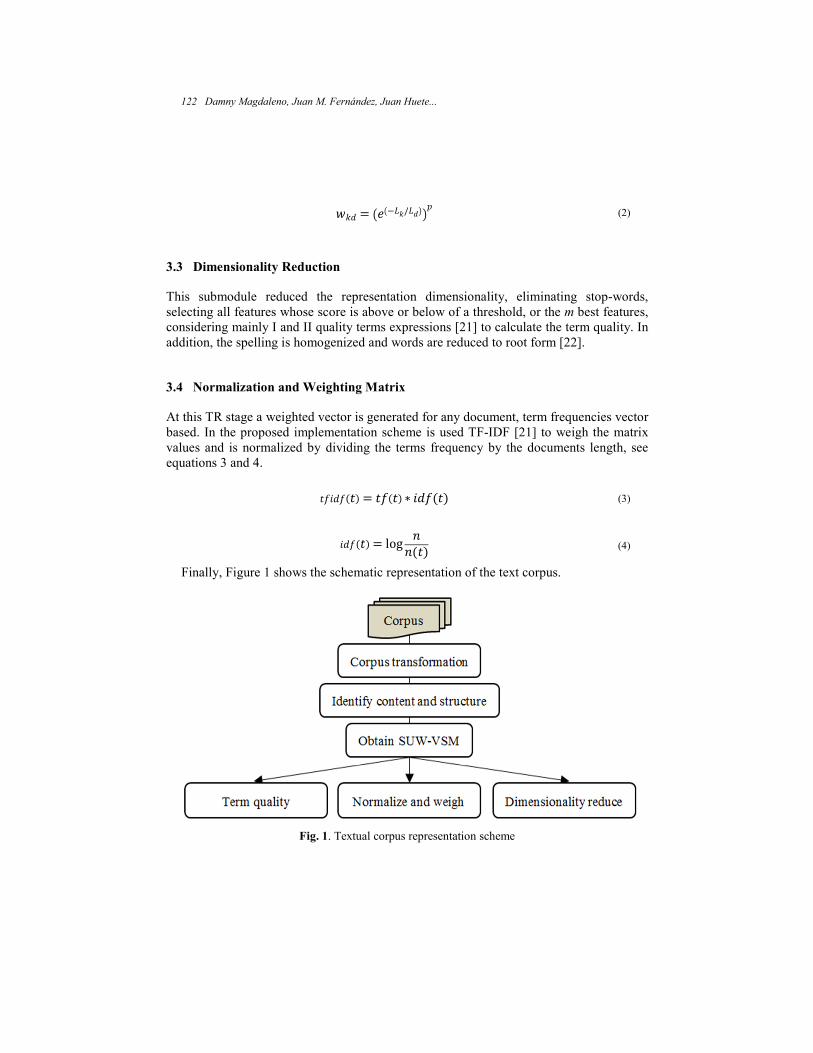
/ (2)

3.3 Dimensionality Reduction

This submodule reduced the representation dimensionality, eliminating stop-words,

selecting all features whose score is above or below of a threshold, or the m best features,

considering mainly I and II quality terms expressions [21] to calculate the term quality. In

addition, the spelling is homogenized and words are reduced to root form [22].

3.4 Normalization and Weighting Matrix

At this TR stage a weighted vector is generated for any document, term frequencies vector

based. In the proposed implementation scheme is used TF-IDF [21] to weigh the matrix

values and is normalized by dividing the terms frequency by the documents length, see

equations 3 and 4.

∗ (3)

log (4)

Finally, Figure 1 shows the schematic representation of the text corpus.

Fig. 1. Textual corpus representation scheme


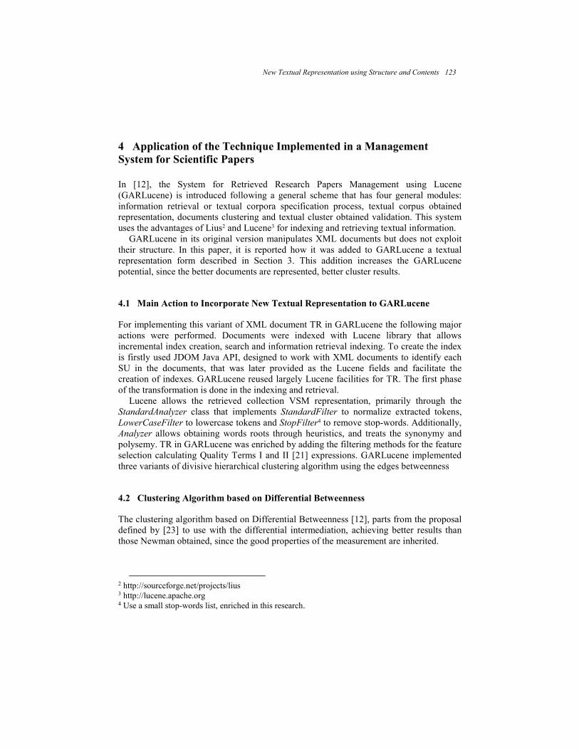
4 Application of the Technique Implemented in a Management

System for Scientific Papers

In [12], the System for Retrieved Research Papers Management using Lucene

(GARLucene) is introduced following a general scheme that has four general modules:

information retrieval or textual corpora specification process, textual corpus obtained

representation, documents clustering and textual cluster obtained validation. This system

uses the advantages of Lius2 and Lucene3 for indexing and retrieving textual information.

GARLucene in its original version manipulates XML documents but does not exploit

their structure. In this paper, it is reported how it was added to GARLucene a textual

representation form described in Section 3. This addition increases the GARLucene

potential, since the better documents are represented, better cluster results.

4.1 Main Action to Incorporate New Textual Representation to GARLucene

For implementing this variant of XML document TR in GARLucene the following major

actions were performed. Documents were indexed with Lucene library that allows

incremental index creation, search and information retrieval indexing. To create the index

is firstly used JDOM Java API, designed to work with XML documents to identify each

SU in the documents, that was later provided as the Lucene fields and facilitate the

creation of indexes. GARLucene reused largely Lucene facilities for TR. The first phase

of the transformation is done in the indexing and retrieval.

Lucene allows the retrieved collection VSM representation, primarily through the

StandardAnalyzer class that implements StandardFilter to normalize extracted tokens,

LowerCaseFilter to lowercase tokens and StopFilter4 to remove stop-words. Additionally,

Analyzer allows obtaining words roots through heuristics, and treats the synonymy and

polysemy. TR in GARLucene was enriched by adding the filtering methods for the feature

selection calculating Quality Terms I and II [21] expressions. GARLucene implemented

three variants of divisive hierarchical clustering algorithm using the edges betweenness

4.2 Clustering Algorithm based on Differential Betweenness

The clustering algorithm based on Differential Betweenness [12], parts from the proposal

defined by [23] to use with the differential intermediation, achieving better results than

those Newman obtained, since the good properties of the measurement are inherited.

2 http://sourceforge.net/projects/lius 3 http://lucene.apache.org 4 Use a small stop-words list, enriched in this research.


Differential Betweenness and Cosine Similarity

When applying DB to textual domains a graph representation can be used where the

interaction between two documents (edges’ weight) is expressed in terms of how similar

they are. Areas of high similarity values involve highly interconnected nodes. Generally,

documents in the same cluster are more similar than documents in different cluster.

In [12] is illustrated the utility of the DB in the bridges detection between clusters, to

cluster documents where Cosine similarity expresses the interrelationships between them.

This way of calculating the edges centralities discover the bridges between clusters

because, unlike the cosine similarity, it is able to exploit the graph topological properties.

Clustering Algorithm Based on the Similarity Matrix

This section show the clustering algorithm based on the concept of DB proposed by [12],

see Figure 2. In [12] is described step by step this algorithm.

Fig. 2. Clustering algorithm based in Differential Betweenness.


This section aims to illustrate how much are improved the results of clustering based on

DB when using the textual representation proposed, with respect to the results obtained

when using the classical VSM representation.

5.1 Definition of Case Studies and Tools used

For achieve the experiments two case studies were defined, the first consists of 15 corpora

formed as subsets of documents in the Biomed5 collection, the second case study has 10

corpora of XML documents from papers recovered from the ICT6 site of the Centro de

Estudios de Informática (Centre of Studies of Informatics), in the Universidad Central

5 Bioinformatics and Medical papers http://www.biomedcentral.com/info/about/datamining/ 6 http://ict.cei.uclv.edu.cu

1. Obtaiment of the similarity graph. 2. Calculation of the weighted differential

betweenness matrix. 3. Estimation of the edges to be eliminated. 4. Determination of the kernels of clustering by means

of the extraction of the connected components. 5. Classification of the nodes not belonging to the

kernels.


"Marta Abreu" de Las Villas (Central University of Las Villas). Table 1 describes these

corpora (case study 1, corpus 1 to corpus 15; case study 2, corpus 16 to corpus 25).

5.2 Experiments Design and Implementation

Since we had the reference classification of textual collections considered in the

experiment, we selected Overall F-measure (OFM) measurement for the comparative

study of the clustering results with both TR. Equation 5 shows the general expression of

OFM; equation 6 shows the F-measure calculation, that combines both expressions

Precision (Pr) and Recall (Re) (see Equation 7), considering the real threshold α∈[0.1].

Here nij is the number of objects that are in both class i and cluster j, nj is number of

objects in the cluster j, ni is the number of objects in the class i, n is the count of clustered

objects and k is the count of reference classes.

Table 1. The description of case studies.

Corpus Document

count Class count Reference classification

1 54 2 Cystic Fibrosis, Diabetes Mellitus

2 31 2 Cystic Fibrosis, Lung Cancer

3 26 2 Cystic Fibrosis, Microarray

4 28 2 Cystic Fibrosis, Genetic Therapy

5 42 2 Cystic Fibrosis, HIV

6 53 2 Diabetes Mellitus, Lung Cancer

7 48 2 Diabetes Mellitus, Microarray

8 50 2 Diabetes Mellitus, Genetic Therapy

9 64 2 Diabetes Mellitus, HIV

10 25 2 Lung Cancer, Microarray

11 27 2 Lung Cancer, Genetic Therapy

12 41 2 Lung Cancer, HIV

13 22 2 Microarray, Genetic Therapy

14 36 2 Microarray, HIV

15 38 2 Genetic Therapy, HIV

16 37 2 Clustering, Fuzzy Logic

17 37 2 Clustering, Association Rules

18 37 2 Clustering, Rough Set

19 41 2 Clustering, SVM

20 30 2 Fuzzy Logic, Association Rules

21 30 2 Fuzzy Logic, Rough Set

22 34 2 Fuzzy Logic, SVM

23 30 2 Association Rules, Rough Set

24 34 2 Association Rules, SVM

25 34 2 Rough Set, SVM


! "#$ !, &'

1 (5)

!, & 1(1/Pr, & + 1(1/,, & (6)

Pr, & &/ & Re, & &/ (7)

Table 2 shows the results of applying OFM to the results of clustering based on the DB

when the selected collections were represented with classic VSM and the variant propose

in this paper.

Table 2. The comparison of the new and original TR by OFM applied to clustering.

Corpus OFM, classic

representation OFM, new representation

1 0,710 0,710

2 0,660 0,659

3 0,670 0,670

4 0,681 0,629

5 0,676 0,676

6 0,716 0,716

7 0,762 0,851

8 0,757 0,741

9 0,675 0,675

10 0,660 0,668

11 0,678 0,660

12 0,663 0,680

13 0,675 0,754

14 0,715 0,715

15 0,606 0,688

16 0,684 0,870

17 0,674 0,946

18 0,674 0,973

19 0,959 0,976

20 0,674 0,967

21 0,665 0,659

22 0,736 1,000

23 0,864 1,000

24 0,703 0,971

25 0,858 1,000


After obtaining the results of the OFM for the algorithm applied to each collection,

statistical tests were performed to compare and analyze the significance level and

behavior of the two variants of TR analyzed. In this sense, were performed to compare the

algorithms non parametric tests for two related samples, using the Wilcoxon test, see

Table 3 and Table 4.

For interpreting the results was considered:

Highly significant, a significance less than 0.01,

Significant, a result of significance less than 0.05 and greater than 0.01,

Moderately significant, a result less than 0.1 and greater than 0.05,

Not significant, a result greater than 0.1.

Table 3. Ranks of results.

N Mean Rank Sum of Ranks

Classic-New Negative Ranks 14ª 12,00 168,00

Positive Ranks 5b 4,40 22,00

Ties 6c

Total 25 aClassic < New bClassic > New cClassic = New

Table 4. Wilcoxon test statistics of results.

Classic-New

Z 2.938ª

Aymp. Sig

(2-tailed) 0,003

aBase on positive ranks.

In analyzing the results of the statistical test can be seen that there are highly

significant differences between the two variants of textual representation, with the textual

representation proposal presented in this paper that yielded the best results of clustering,

considering the OFM validation measure

6 Conclusions

This paper presented a new form of textual representation of XML documents, using their

structure and content. The new form of textual representation is the content based on the

structure of the document, following the criterion that depending on the location

(structural unit) in the presence of a term (word) within a document, you will have greater

or lesser importance to decide how relevant this is in the document. The incorporation of

the new form of textual representation in GARLucene has increased significantly the

potential of the software for handling XML documents and extracting knowledge from


them. This new form of textual representation yields better clustering results considering

the algorithm based on the Differential Betweenness, than using classical VSM

representation.

References

1. Carrillo, R.M., A.L.L.: Una Representación Vectorial para Contenido de Textos en Tratamiento

de Información, In: CCC-08-004. Coordinación de Ciencias Computacionales INAOE (2008)

2. Lewis, D.D.: Representation and Learning in Information Retrieval, in Department of Computer

and Information Science. University of Massachusetts (1992)

3. Salton, G., Wong, A., and Yang C.S.: A Vector Space Model for Information Retrieval. Journal

of the ASIS, 18(11): pp. 613-620 (1975)

4. García-Plaza A.P., Víctor Fresno, R.M.: Una Representación Basada en Lógica Borrosa para el

Clustering de páginas web con Mapas Auto-Organizativos, In: Procesamiento del Lenguaje

Natural. 79-86 (2009)

5. Bakus, J.H., M.F.; Kamel, M.: A SOM-based document clustering using phrases, In: 9th

International Conference on Neural Information Processing ICONIP 2002. pp. 2212-2216 (2002)

6. Liu, Y., Wang, X., Wu, C.: ConSOM: A conceptional self-organizing map model for text

clustering. Neurocomputing. 71(4-6): pp. 857-862. (2008)

7. Theodore Dalamagas, T.C., Klaas-Jan Winkel, Timos Sellis: A Methodology for Clustering

XML Documents by Structure. Information Systems (2006)

8. Abiteboul, S., Querying semi-structured data. Proceedings of the ICDT Conference, Delphi,

Greece (1997)

9. Guerrini, G.M.M., Sanz, I.: An Overview of Similarity Measures for Clustering XML

Documents. (2006)

10. Tien T., R.N.: Evaluating the Performance of XML Document Clustering by Structure only.

11. Kruse, R., Döring C., Lesor M.J.: Fundamentals of Fuzzy Clustering, in Advances in Fuzzy

Clustering and its Applications. Oliveira, J.V.D., Pedrycz, W. Editors. John Wiley and Sons:

East Sussex, England. pp. 3-27 (2007)

12. Arco, L.: Agrupamiento basado en la intermediación diferencial y su valoración utilizando la

teoría de los conjuntos aproximados, In: Ciencias de la Computación. Universidad Central

"Marta Abreu" de Las Villas: Santa Clara, Villa Clara. pp. 187. (2009)

13. Wan, X., Yang, J.: Using Proportional Transportation Similarity with Learned Element

Semantics for XML Document Clustering. International World Wide Web Conference

Committee (2006).

14. Flesca, S., et al.: Fast detection of XML structural similarities. IEEE Trans. Knowl. Data Engin.

7(2): pp. 160-175 (2005)

15. Chawathe, S.S.: Comparing Hierarchical Data in External Memory. In: In Proceedings of

International Conference on Very Large Databases (1999)

16. Kutty, S., et al.: Combining the structure and content of XML documents for clustering using

frequent subtrees. INEX, pp. 391-401 (2008)

17. Doucet, A., AhonenMyka, H.: Naive clustering of a large XML document collection. INEX. pp.

84-89 (2002)

18. Yang, W., Chen, X.O.: A semi-structured document model for text mining. Journal of Computer

Science and Technology, 17(5): pp. 603-610 (2002)


19. Lanquillon, C.: Enhancing Text Classification to Improve Information Filtering, in Research

Group Neural Networks and Fuzzy Systems. 2001, University of Magdeburg "Otto von

Guericke": Magdeburg. pp. 231. (2001)

20. Lewis, D.D., Ringuette M.:. A comparison of two learning algorithms for text classification. In:

Third Annual Symposium on Document Analysis and Information Retrieval. University of

Nevada, Las Vegas. (1994)

21. Berry, M.W.: Survey of Text mining: Clustering, Classification, and Retrieval. New York, NY,

USA: Springer Verlag. (2004)

22. Frakes, W.B., Baeza-Yates, R.: Information Retrieval. Data Structure & Algorithms. New York:

Prentice Hall. (1992)

23. Newman, M.E.J.: Analysis of weighted networks. Physical Review E. 70(52): pp. 056131.

(2004)


Native Speaker Dependent System for the Development

of a Multi-User ASR-Training System

for the Mixtec Language

Santiago Omar Caballero Morales and Edgar De Los Santos Ramírez

Technological University of the Mixtec Region, Postgraduate Division, Highway to Acatlima K.m.

2.5, Huajuapan de Leon, Oaxaca, 69000, Mexico [email protected], [email protected]

Abstract. The Mixtec Language is one of the main native languages in Mexico, and

is present mainly in the regions of Oaxaca and Guerrero. Due to urbanization,

discrimination, and limited attempts to promote the culture, the native languages are

disappearing. Most of the information available about these languages (and their

variations) is in written form, and while there is speech data available for listening

and pronunciation practicing, a multimedia tool that incorporates both, speech and

written representation, could improve the learning of the languages for non-native

speakers, thus contributing to their preservation. In this paper we present some

advances towards the development of a Multi-User Automatic Speech Recognition

(ASR) Training system for one variation of the Mixtec Language that could be used

for the design of speech communication, translation, and learning interfaces for

both, native and non-native speakers. The methodology and proposed

implementation, which consisted of a native Speaker - Dependent (SD) ASR system

integrated with an adaptation technique, showed recognition accuracies over 90%

and 85% when tested by a male and a female non-native speakers respectively.

Keywords: Speech recognition, native languages, learning interfaces.

1 Introduction

Research on spoken language technology has led to the development of Automatic Speech

Recognition (ASR), Text-To-Speech (TTS) synthesis, and dialogue systems. These

systems are now used for different applications such as in mobile telephones for voice

dialing, GPS navigation, information retrieval, dictation [1, 2, 3], translation [4, 5], and

assistance for handicapped people [6, 7].

ASR technology has been used also for language learning, and examples of these can

be found in [8, 9, 10] for English, [11] for Spanish and French among others, and [12] for

“sign” languages. These interfaces allow the user to practice their pronunciation at home

or work without the limitations of a schedule. They also have the advantage of mobility as

some of them can be installed in different computer platforms, or even mobile telephones

for basic practicing. However, although there are applications for the most common

foreign languages, there are limited (if any) applications for native or ancient languages.

In Mexico there are around 89 native languages still spoken by 6.6 millions of native

speakers. Although the number of speakers may be significant (considering the total

number of inhabitants in Mexico) this number is decreasing, especially in the Mixtec

region.

The population of native speakers of the Mixtec language is decreasing given urban

migration and development, culture rejection and limited attempts to preserve the

language. This has been expressed by people living in communities in the Mixtec region

of Mexico, and this can be corroborated by national statistics that show that the number of

people who spoke any native language, 6.3 millions in 2000 (7.1% of the total population)

decreased to 6.0 millions in 2005 (6.6% of the total population), and this amount was even

higher in 1990 (7.5% of the total population) [13]. This increases the possibility of native

languages being lost, as some dialects or variations had less than 10 known speakers (i.e.,

Ayapaneco, 4 speakers; Chinanteco of Sochiapan, 2 speakers; Mixtec of the Mazateca

Region, 6 speakers [13]). In this case, historic antecedents or information about the

language is not recorded, making very difficult to recover or save some part of the

language. This may happen to other languages with more speakers. The Mixtec Language,

with approximately 480,000 speakers, has been reported to lose annually 200 speakers.

To preserve a language is not an easy task, because all characteristics such as grammar

rules, written expression, speech articulation, and phonetics must be documented and

recorded. Although there are books and dictionaries that among the word definitions

include examples about how to pronounce them, this is not as complete as listening the

correct pronunciation from a native speaker

We consider that this goal can be accomplished by the use of modern technology such

as that used for foreign language learning [10, 11] to promote the language among non-

native speakers and thus, to contribute to its preservation. In this work we focus on the

development of an ASR-Training system to allow a speaker to practice his or her

pronunciation. The methodology and proposed implementation, which consisted of a

native Speaker - Dependent (SD) ASR system integrated with a speaker adapting

technique, achieved accuracies over 90% and 85% for a male and a female non-native

users respectively.

The development of the native ASR-Training system is presented as follows: in Section

2 the details about the phonetics of the reference Mixtec language variation, and the

speech corpus developed to build the native ASR system, are shown; in Section 3 the

design of the SD native ASR system, which includes the supervised training of the

system’s acoustic models, and the adaptation technique for its use by non-native users, are

shown; in Section 4 the details of the testing methodology by two non-native speakers and

the performance of the system in real time are presented and analyzed; finally in Section

5 we discuss about our findings and future work.

132 Santiago Omar Caballero Morales and Edgar De Los Santos Ramírez

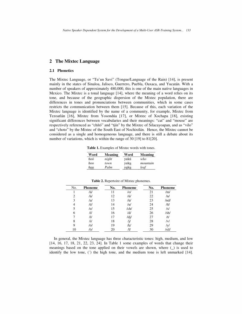
2 The Mixtec Language

2.1 Phonetics

The Mixtec Language, or “Tu’un Savi” (Tongue/Language of the Rain) [14], is present

mainly in the states of Sinaloa, Jalisco, Guerrero, Puebla, Oaxaca, and Yucatán. With a

number of speakers of approximately 480,000, this is one of the main native languages in

Mexico. The Mixtec is a tonal language [14], where the meaning of a word relies on its

tone, and because of the geographic dispersion of the Mixtec population, there are

differences in tones and pronunciations between communities, which in some cases

restricts the communication between them [15]. Because of this, each variation of the

Mixtec language is identified by the name of a community, for example, Mixtec from

Tezoatlán [16], Mixtec from Yosondúa [17], or Mixtec of Xochapa [18], existing

significant differences between vocabularies and their meanings: “cat” and “mouse” are

respectively referenced as “chító” and “tiín” by the Mixtec of Silacayoapan, and as “vilo”

and “choto” by the Mixtec of the South East of Nochixtlán. Hence, the Mixtec cannot be

considered as a single and homogeneous language, and there is still a debate about its

number of variations, which is within the range of 30 [19] to 81[20].

Table 1. Examples of Mixtec words with tones.

Word Meaning Word Meaning

ñoó night yukú who

ñoo town yuku mountain

ñoo Palm yuku leaf

Table 2. Repertoire of Mixtec phonemes.

No. Phoneme No. Phoneme No. Phoneme

1 /á/ 11 /o/ 21 /m/

2 /à/ 12 /ú/ 22 /n/

3 /a/ 13 /ù/ 23 /nd/

4 /é/ 14 /u/ 24 /ñ/

5 /e/ 15 /ch/ 25 /s/

6 /í/ 16 /d/ 26 /sh/

7 /ì/ 17 /dj/ 27 /t/

8 /i/ 18 /j/ 28 /v/

9 /ó/ 19 /k/ 29 /y/

10 /ò/ 20 /l/ 30 /sil/

In general, the Mixtec language has three characteristic tones: high, medium, and low

[14, 16, 17, 18, 21, 22, 23, 24]. In Table 1 some examples of words that change their

meanings based on the tone applied on their vowels are shown, where (_) is used to

identify the low tone, (´) the high tone, and the medium tone is left unmarked [14].

Native Speaker Dependent System for the Development of a Multi-User ASR-Training System... 133

Although there are other tone representations, where the low tone also is represented with

a horizontal line over the vowel [24], usually the high tone is represented with the

diacritical (´).

Based on the phonemes identified in [14, 21-24] and by integrating the different tones

in the vowels, the repertoire shown in Table 2 was defined. The low tone is represented by

the diacritical (`) while the high tone is represented by (´), the medium tone is unmarked

to keep consistency.

The phonetics of the Mixtec has some differences when compared with the Mexican

Spanish language. For example, from Table 2:

− The Mixtec phoneme /dj/ represents a sound similar to the Spaniard Spanish z

(phoneme /z/), which is stronger than s (/s/) in both languages. In the phonetics of the

Mexican Spanish from the center region both sounds, z and s, are represented by the

phoneme /s/ [25];

− The Mixtec phonemes /sh/ and /ch/ are pronounced in Mexican Spanish as the

consonant X in the word “Xicoténcatl” and CH in the word “chicle” respectively;

− There are short pauses, uttered as a glottal closure between vowels within a word,

which are represented by (’) such as in “tu’un” or “ndá’a” ;

− The Mixtec phoneme /n/ sounds as n in the Mexican Spanish (associated with the

consonant N) if it is placed before a vowel, but is mute if placed after the vowel.

2.2 Vocabulary

Because the purpose of the system is to be used for speech training and practicing of the

Mixtec language, a vocabulary used for learning was chosen. For this, we established

contact with a native speaker who teaches the Mixtec language at the local Cultural

Center. The place of origin of this speaker is the community of San Juan Dikiyú in

Oaxaca. Since this variation shares similarities with other variations in Oaxaca, we were

confident about using it as the reference variation.

With support from the Mixtec teacher we selected 7 traditional Mixtec narratives from

a total of 15 that he uses in his lessons for teaching, where the first were used for

beginners and the last for more advanced students. The 7 narratives were read twice by

the teacher in a recording studio, where the speech samples were recorded in WAV format

with a sampling rate of 44,100 Hz and one audio channel (monaural). These recordings

were transcribed at the phonetic and word levels (TIMIT standard) using the list of

phonemes defined in Table 2 using the software WaveSurfer. All this material formed the

Training Speech Corpus for the native ASR system which had a total of 192 different

words.

Based on the frequency of phonemes of the corpus, which is shown in Figure 1, it was

considered that the Training Corpus was phonetically balanced as there were enough

samples from each phoneme for the supervised training of the acoustic models of the ASR

system.


Fig. 1. Frequency distribution of the Mixtec phonemes in the Training Speech Corpus.

3 Mixtec Speaker-Dependent ASR System

The elements of the native ASR that were built with the Training Speech Corpus are

shown in Figure 2.

Fig. 2. Structure of the native ASR system.

These were implemented with the software HTK Toolkit [26], and each one was built

as follows:

− Acoustic Models: Hidden Markov Models (HMMs) [27, 28] were used for the

acoustic modeling of each phoneme in the Training Corpus. These were standard

three-state left-to-right HMMs with 10 Gaussian components per state. The front-end

used 12 MFCCs plus energy, delta, and acceleration coefficients [26]. The supervised

training of the HMMs with the Training Corpus (labeled at the phonetic level) was

performed with the Baum-Welch and Viterbi algorithms.

− Lexicon: the phonetic dictionary was made at the same time as the phonetic labeling

of the Training Corpus. The phoneme sequences that formed each word in the

vocabulary were defined by perceptual analysis considering the pronouncing rules

presented in Section 2.1.

218

271

335

636

167

49

209

82

32

201

4118

318

3157

40

2

281

17 14

197

72

121 131

38

228

105 101

30

á à a é e í ì i ó ò o ú ù u ch d dj j k l m n nd ñ s sh t v y sil


− Language Model: Word-bigram language models were estimated from the word

transcriptions of the corpus. Speech recognition was performed with a scale grammar

factor of 10.

− Search Algorithm: Speech recognition was performed with the Viterbi algorithm

implemented with the module HVite of the HTK Toolkit.

3.1 Adaptation for Non-native Speakers

As presented in Section 2.2 the Speech Training Corpus of the native ASR was built with

the speech samples from a single native speaker. Thus, the system described above is

Speaker Dependent (SD) and it will show good performance only when used by the same

speaker. For practicing and learning purposes this is a disadvantage.

Commercial ASR systems are trained with hundreds or thousands of speech samples

from different speakers, which leads to Speaker-Independent (SI) systems. When a new

user wants to use such system, it is common to ask the user to read some words or

narratives to provide speech samples that will be used by the system to adapt the SI

acoustic models to the patterns of the user’s voice. SI ASR systems are robust enough to

get benefits by the implementation of adaptation techniques such as MAP or MLLR [26,

28].

In the case of the development of a SI ASR system for the Mixtec language there are

challenges given by the wide range of variations in tones and pronunciations, and the

limited availability of native speakers to obtain training corpora. Because of this situation,

the use of a speaker adaptation technique on this SD system was studied.

Maximum Likelihood Linear Regression (MLLR) was the adaptation technique used

for the native SD ASR system in order to make it usable for non-native speakers. MLLR

is based on the assumption that a set of linear transformations can be used to reduce the

mismatch between an initial HMM model set and the adaptation data. In this work, these

transformations were applied to the mean and variance parameters of the Gaussian

mixtures of the SD HMMs, and it was performed in two steps:

− Global Adaptation. A global base class was used to specify the set of HMM

components that share the same transform. Then a global transform was generated

and applied to every Gaussian component of the SD HMMs.

− Dynamic Adaptation. The global transformation was used as an input

transformation to adapt the model set, producing better frame/state alignments which

were then used to estimate a set of more specific transforms by using a regression

class tree. For this work, the regression class tree had 32 terminal nodes, and was

constructed to cluster together components that were close in acoustic space, and thus

could be transformed in similar way. These transforms become more specific to

certain groupings of Gaussian components, and are estimated according to the

“amount" and “type" of available adaptation data (see Table 3). Because each

Gaussian component of an HMM belongs to one particular base class, the tying of


each transformation across a number of mixture components can be used to adapt

distributions for which there are no observations at all (hence, all models can be

adapted). The adaptation process is dynamically refined when more adaptation data

becomes available [26].

−

Fig.3. Binary regression class tree with four terminal nodes.

Table 3. Selection of words for supervised non-native speaker adaptation.

No. Selected Word Phonemes No. Selected Word Phonemes

1 ÀNE’ECHOOS à n e e ch o o s 14 KOÚNI k o ú n i

2 ÁTOKÓ á t o k ó 15 KUALÍ k u a l í

3 DIKIYÚ d i k i y ú 16 KÙTAKU k ù t a k u

4 DJAMA d j a m a 17 KUTÓ k u t ó

5 DJÀVÌ z à v ì 18 LAA l a a

6 CHÁNÍ ch á n í 19 LULI l u l i

7 CHI ch i 20 NDAKONÓ nd a k o n ó

8 ÍDJONA í z o n a 21 NDEEYÉ nd e y é

9 ÍÑÒ í ñ ò 22 NÍKÉE n í k é e

10 KAMA k a m a 23 ÑA ñ a

11 KÌVÌ k ì v ì 24 ÑUU ñ u u

12 KOKUMI k o k u m i 25 SÁXI s á sh i

13 KÒÒÍÚN k ò í ú 26 ÙXÌ ù sh ì

As an example of how MLLR works, in Figure 3 a regression class tree is presented

with four terminal nodes (or base classes) denoted as C4, C5, C6 and C7. Solid nodes and

arrows indicate that there is enough data in that class to generate a transformation matrix,

and dotted lines and circles indicate that there is insufficient data. During the “dynamic"

adaptation, the mixture components of the models that belong to the nodes 2, 3 and 4 are

1

2 3

4 5 6 7

C4 C5 C6 C7

W3W2

W4


used to construct a set of transforms denoted by W2, W3 and W4. When the transformed

model set is required, the transformation matrices (mean and variance) are applied in the

following fashion to the Gaussian components in each base class: W2C5; W3 C6, C7;

and W4C4, thus adapting the distributions of the classes with insufficient data (nodes 5,

6, and 7) as well as the classes with enough data.

For the native SD system, a selection of words from the Training Corpus was defined

to allow the user to provide enough speech samples (adaptation data) from each phoneme

listed in Table 2. These words are shown in Table 3 and have the frequency distribution of

phonemes shown in Figure 4, which has a correlation coefficient of 0.69 with the

distribution of the Training Corpus (Figure 1). Hence it was considered that the

adaptation samples were representative of the Training Corpus and sufficient for MLLR

adaptation.

Fig. 4. Frequency distribution of the phonemes in the selection of words for non-native speaker

adaptation.

3.2 Non-native Speakers

Two non-native speakers, a female and a male, were recruited to test the performance of

the native SD ASR with the adaptation technique. Their background details are shown in

Figure 5.

Fig. 5. Non-native speakers for evaluation of the native SD ASR system.

Prior to use the system, both received 6 hours of informative sessions which were

distributed over three days. In these sessions, information about the pronunciation of the

Mixtec words from the ASR system’s vocabulary and the 7 narratives, which included the

audios from the native speaker, were reviewed.

32

14

2

4

7

4

7

3 3

7

4

2

7

32 2

1

15

5

3

6

2

4

2 23

2 2

á à a é e í ì i ó ò o ú ù u ch d dj j k l m n nd ñ s sh t v y


Fig. 6. Graphical User Interface for the native SD ASR-Training system.

3.3 Graphical User Interface

As shown in Figure 6, the native SD ASR system was integrated with a Graphical User

Interface (GUI) for the adaptation and recognition tasks which were conducted as follows:

− Adaptation (1). As shown in Figure 6, there is a “New User” field (1A) where the

user can write his/her name, for example, “Juan”. When the user does this, the

interface builds the respective directories and files to perform adaptation. On the right

side there are buttons with the names of the adaptation words from Table 3 (1B), and

with the label “Record” (1C). When the 1B buttons are pressed the audio file

corresponding to that word (from the native speaker) is played, so the user can hear

the correct pronunciation of that word before providing any speech sample for

adaptation. When pressed the respective 1C button (the one next to that word) the

interface records the user’s pronunciation of that word. When the recording task is

finished an “OK” is shown next to 1C. After all adaptation words are recorded the

user can press the “Perform Adaptation” button (1D), which starts the MLLR

adaptation with the audio samples from the user.


− Recognition (2). Once that the user got registered and performed adaptation,

his/her data (i.e., MLLR transformations) is stored in directories identified by his/her

name. After re-starting the interface, the new user’s name is shown in the list of

“Registered Users” (2A). At this point the user selects his/her name and the interface

automatically loads the corresponding MLLR transformations and acoustic models,

enabling the button “Speech Recognition” (2B) to perform ASR in real time when

pressed. The user pronounces any phrase from the narratives (when pressing 2B) and

the interface displays two outputs: in the field 2C the non-adapted response of the SD

ASR is shown, while in 2D the MLLR adapted response is shown.

4 Performance of the Mixtec SD ASR-Training System

The measure of performance for the Mixtec ASR-Training system was the Word

Recognition Accuracy (WAcc), which is analogous to the Word Error Rate (WER) [26].

For convenience we used both measures, which are defined as:

WAcc = (N-D-S-I)/N . (1)

WER = 1 – WAcc . (2)

where N is the total number of elements (words) in the reference (correct) transcription of

the spoken words, D and I are the number of elements deleted and inserted in the decoded

sequence of words (word output from the ASR system), and S the number of elements

from the correct transcription substituted by a different word in the decoded sequence.

The Mixtec ASR was tested initially with the Training Corpus, and the performance

results are shown in Table 4.

Table 4. Performance of the Mixtec ASR system when tested with the Training Corpus.

N D S I %WAcc %WER

911 0 18 29 94.84 5.16

By replacing the word-bigram language model with a phoneme-based language model,

a response at the phonetic level was obtained from the recognizer. A phoneme confusion-

matrix, shown in Figure 7, was estimated from this response in order to identify patterns

of errors at the low level of the baseline ASR. As it can be observed, there were a few confusions between phonemes, for example:

between vowels /á/, /à/, /a/, and /í/, /ì/, /i/; and a significant confusion between /nd/ and

/d/. Analogous to Table 4, and as presented in Figure 7, the performance of the Mixtec

ASR at the phonetic level is shown in Table 5.

As shown in Figure 7 and Table 5, the deletions and substitutions rates were

approximately 10% of N (most of the deleted phonemes were vowels), while insertions

represented approximately 5%. A %WAcc of 78% is normal based on the fact that there


was no restriction from the phonetic dictionary (Lexicon) to form valid sequences of

phonemes (which lead to a %WAcc of 94.84%). These results show that the acoustic

modeling of the tonal phonemes of the SD ASR system with the Training Corpus was

performed satisfactorily. This is normal in most cases unless there were many variations

or inconsistencies in the training speech.

Table 5. Performance of the phoneme-based Mixtec ASR system

when tested with the Training Corpus.

N D S I %WAcc %WER

3846 340 338 144 78.63 21.37

Fig. 7. Pattern of errors at the phonetic level of the Mixtec ASR system when tested with the

Training Corpus.

The system was tested by the non-native speakers using three narratives (NTVs) with

different levels of difficulty: 1 (easy level), 3 (medium level), and 6 (hard level). Each

user was allowed to try up to 10 times the system in case that his/her uttered phrase wasn’t

recognized. If after those trials the phrase was not recognized, then the last result was

recorded as the final response of the ASR system.

The performance results for the non-native speakers are shown in Table 6. The

accuracy for the male user was -4.46% when no adaptation was performed. After the

adaptation session, the performance increased to 92.57%. With the female user the non-

adapted system performed with an accuracy of 9.90%, however after the adaptation

session this increased to 88.12%.

Sti

mu

lus

Response

á à a é e í ì i ó ò o ú ù u ch d dj j k l m n nd ñ s sh sp t v y sil Del

áàaéeíìi

óòoúùu

chddjjkl

mn

ndñs

shsp

tvy

silIns


Table 6. Performance of the Non-adapted and Adapted Mixtec ASR system

when tested by two non-native speakers.

User GCV User SCB

Non-adapted SD ASR-Training System Non-adapted SD ASR-Training System

NTV N D S I %WAcc %WER NTV N D S I %WAcc %WER

1 53 4 32 13 7.55 92.45 1 53 8 30 7 15.09 84.91

3 53 2 32 20 -1.89 101.89 3 53 6 25 18 7.55 92.45 6 96 1 59 48 -12.50 112.50 6 96 4 66 18 8.33 91.67

Total 202 7 123 81 -4.46 104.46 Total 202 18 121 43 9.90 90.10

MLLR-adapted SD ASR-Training System MLLR-adapted SD ASR-Training System

NTV N D S I %WAcc %WER NTV N D S I %WAcc %WER

1 53 0 1 0 98.11 1.89 1 53 0 2 0 96.23 3.77

3 53 0 3 2 90.57 9.43 3 53 0 5 3 84.91 15.09

6 96 0 8 1 90.63 9.38 6 96 0 10 4 85.42 14.58

Total 202 0 12 3 92.57 7.43 Total 202 0 17 7 88.12 11.88

While performing the testing sessions there were recorded the number of trials before

the adapted system could recognize correctly the test phrase. For the male user (GCV), in

7 out of 49 phrases after the 10 trials the exact phrase was not obtained. A mean of 2.97

with a standard deviation of 3.17 was obtained for the number of trials before the

recognizer could decode the correct phrase. In contrast, for the female user, in 17 phrases

the correct phrase was not obtained after the 10 trials. This was reflected in a mean of 5.10

trials with a standard deviation of 4.08 for this user.

These differences in performances could be caused by the acoustic differences between

the female’s voice and the male’s voice. Also, variations in the level of knowledge or

ability to utter the Mixtec phonemes, which are user dependent, can be attributable

factors. A matched pairs test [29] was used to test for statistical significant differences

between both performances, obtaining a p-value of 0.21 (< 0.10) for the results presented

in Table 6. Because of this, it was concluded that there was no statistical difference

between both performances.


In this paper we presented our advances towards the development of a Multi-user Mixtec

ASR system for language learning purposes. The Mixtec language is a complex language

given the diversity of tones and vocabulary, and so there are challenges to accomplish

such system, especially with limited availability of native speakers for speech corpora.

Nevertheless a native SD ASR system was developed for purposes of pronunciation

training of a tonal language. This system, when integrated with a speaker adaptation

technique, performed with levels of recognition accuracy of 92.57% (male user) and

88.12% (female user) for two non-native speakers, thus making it a multi-user system.


As presented in Table 6, MLLR is a very reliable adaptation technique when applied on

a tonal SD ASR system, being able to accomplish with few speech samples (in this case,

26 words) improvements in recognition accuracy of around 90%. For non-native users,

most of the word recognition errors were substitutions (12 for male user, 17 for female

user) and insertions (3 and 7 respectively). As starting point, the results presented in this

paper are encouraging, however we do realize that much more research is needed, and

here we present our future work:

− Develop a technique to increase the performance of the native ASR system.

− Increase the Training Speech Corpus: add more vocabulary words and increase the

complexity of the narratives; recruit more native speakers (both genders) in order to

develop a native SI ASR system. Currently we are in talks to recruit three additional

native speakers.

− Test the system with more users with different levels of expertise in the Mixtec

language (group tests are being planned).

− Improve the GUI to increase usability: incorporate learning methodologies to extend

the use of the ASR system for users that don’t have previous knowledge of the

language (with no informative sessions); integrate a measure of performance for the

level of knowledge or practicing that the user gets by using the ASR system.

References

1. Philips: SpeechExec Pro Transcribe. http://www.dictation.philips.com/index.php?id=1440

&CC=VV

2. Nuance: Dragon Speech Recognition Software. http://www.nuance.com/dragon/index.htm

3. IBM: Embedded ViaVoice.http://www-01.ibm.com/software/pervasive/embedded_viavoice/

4. Carnegie Mellon University (The Interactive Systems Laboratories): JANUS Speech

Translation System. http://www.is.cs.cmu.edu/mie/janus.html

5. The German Research Center for Artificial Intelligence: Verbmobil - Translation of

Spontaneous Speech. http://www.dfki.de/lt/project.php?id=Project_382&l=en

6. Green, P.D., Hawley, M.S., Enderby, P., Cunningham, S.P., Parker,M.: Automatic speech

recognition and training for severely dysarthric users of assistive technology: The STARDUST

project. Clinical Linguistics and Phonetics, 20:149–156 (2006)

7. Hawley, M., Cunningham, S., Cardinaux, F., Coy, A., O’Neill, P., Seghal, S., Enderby, P.:

Challenges in developing a voice input voice output communication aid for people with severe

dysarthria. In: Proc. European Conference for the Advancement of Assistive Technology in

Europe (2007)

8. English Computerized Learning Inc.: Pronunciation Power Speech Test.

http://www.englishlearning.com/products/pronunciation-power-speech-test/

9. Dalby, J., Kewley-Port, D.: Explicit Pronunciation Training Using Automatic Speech

Recognition Technology. Computer-Assisted Language Instruction Consortium (CALICO)

Journal, vol. 16 (1999)

10. Lesson Nine GmbH: Babbel. http://es.babbel.com/#Reconocimiento-de-voz


1. Rosetta Stone: Rosetta Stone Version 4 TOTALe. http://www.rosettastone.com

/content/rosettastonecom/en.html

2. Cox, S., Lincoln, M., Tryggvason, J., Nakisa, M., Wells, M., Tutt, M., Abbott, S.: The

Development and Evaluation of a Speech-to-Sign Translation System to Assist Transactions. Int.

J. Hum. Comput. Interaction, 16(2):141–161 (2003)

3. Instituto Nacional de Estadística y Geografía (INEGI): Hablantes de Lengua Indígena en

México. http://cuentame.inegi.org.mx/poblacion/lindigena.aspx?tema=P

4. Academia de la Lengua Mixteca: Bases para la Escritura de tu’un savi. Colección Diálogos:

Pueblos Originarios de Oaxaca, México (2007)

5. Mindek, D.: Mixtecos: Pueblos Indígenas del México Contemporáneo. Comisión Nacional para

el Desarrollo de los Pueblos Indígenas (2003)

6. Ferguson de Williams, J.: Gramática Popular del Mixteco del Municipio de Tezoatlán, San

Andrés Yutatío, Oaxaca. Instituto Lingüístico de Verano, A.C. , México D.F. (2007)

7. Beaty de Farris, K., García, P., García, R., Ojeda, J., García, A., Santiago, A.: Diccionario Básico

del Mixteco de Yosondúa, Oaxaca. Instituto Lingüístico de Verano, A.C., México, D.F. (2004)

8. Stark, S., Johnson, A., González de Guzmán, B.: Diccionario Básico del Mixteco de Xochapa,

Guerrero. Instituto Lingüístico de Verano, A.C., México, D.F. (2003)

9. Instituto Lingüístico de Verano en México: Familia Mixteca. http://www.sil.org/

mexico/mixteca/00e-mixteca.htm.

10. Instituto Nacional de Lenguas Indígenas: Catálogo de las Lenguas Indígenas Nacionales:

Variantes Lingüísticas de México con sus autodenominaciones y referencias geoestadísticas.

http://www.inali.gob.mx/pdf/CLIN_completo.pdf (2008)

11. Anderson, L. Alejandro, R.: Vocabulario de los verbos de movimiento y de carga: Mixteco de

Alacatlatzala, Guerrero. Instituto Lingüístico de Verano, A.C.

http://www.sil.org/americas/mexico/mixteca/alacatlatzala/P001-Vocab-MIM.pdf (1999)

12. García, A., Miguel, R.: Nadakua’a Ndo Tee Ndo Tu’un Ndo: Aprendamos a escribir nuestro

idioma. Instituto Lingüístico de Verano, A.C., México, D.F. (1998)

13. Morales, M. North, J.: Ná Cahví Tuhun Ndáhv Ta Ná Cahyí Ña: Vamos a leer y escribir en

mixteco (Mixteco de Silacayoapan, Oaxaca). Instituto Lingüístico de Verano, A.C., México, D.F.

(2000).

14. Alexander, R.M.: Mixteco de Atatlahuca. Instituto Lingüístico de Verano. México, D.F. (1980)

15. Pineda, L.A., Castellanos, H., Cuétara, J., Galescu, L., Juárez, J., Llisterri, J., Pérez, P.,

Villaseñor, L.: The Corpus DIMEx100: Transcription and Evaluation. Language Resources and

Evaluation. 44: 4, 347-370 (2010)

16. Young, S., Woodland, P.: The HTK Book (for HTK Version 3.4). Cambridge University

Engineering Department, Great Britain (2006)

17. Rabiner, L.: A tutorial on hidden markov models and selected applications in speech recognition.

Proc. of IEEE, 37, 257-286 (1989)

18. Jurafsky, D., Martin, J.H.: Speech and Language Processing. Pearson: Prentice Hall (2009)

19. Gillick, L., Cox, S.J.: Some statistical issues in the comparison of speech recognition algorithms.

In Proc. IEEE Conf. on Acoustics, Speech and Signal Processing, 532-535 (1989)


Comparison of State-of-the-Art Methods

and Commercial Tools

for Multi-Document Text Summarization

Yulia Ledeneva1, René García Hernández1, Grigori Sidorov2, Griselda Mathias Mendoza1, Selene Vargas Flores1, and Abraham García Aguilar1

1 Universidad Autónoma del Estado de México, Unidad Académica Profesional Tianguistenco,

Paraje el Tejocote San Pedro Tlantizapan, 52600, Estado de México, Mexico 2 Natural Language and Text Processing Laboratory,

Center for Computing Research (CIC), National Polytechnic Institute (IPN),

Av. Juan Dios Batiz, s/n, Zacatenco, 07738, Mexico City, Mexico

[email protected], [email protected], www.g-sidorov.org

Abstract. The final goal of Automatic Text Summarization (ATS) is to obtain tools that produce the most human-similar summary. Almost all the papers on ATS research area present a review of the state-of-the-art of one side of the issue, since only is reviewed the-state-of-the-art of the tools reported in papers. However, we found a great number of developed commercial tools which are not reported in papers (which is understandable by competitive reasons), but also have not been evaluated. The question is what commercial tools are good in comparison to paper-published tools. This paper gives a survey for 18 commercial tools and state-of-the-art methods for multi-document summarization task testing on a standard collection of documents which contains 59 collections of documents.

Keywords: Automatic multi-document summarization, Copernic summarizer, Microsoft office word summarizer, Svhoong summarizer, pertinence summarizer, Tool4noobs summarizer.

1 Introduction

According to recent researches the volume of information on the public Web are estimated at 167 terabytes, while the deep web to be 400 to 450 times larger, thus between 66,800 and 91,850 terabytes [1]. Such amount of information cannot be revised by a normal human, only with the help of computer by means of intelligent algorithms and tools. Such types of algorithms and methods have a big necessity and urgency to be

developed, for example, automatic generation of text summaries for multi-document collection. Humans tend to create summaries by generating and fusion of ideas, changing words and

rephrasing long sentences. This manner of composing summaries is called abstractive summarization, contrary to the extracted summarization, where different text units (words, phrases, sentences, etc.) are extracted from the original collection of documents. The generation of extractive summaries does not require the understanding of the text. Test summary is a short text transmitting the main ideas of the collections of

documents without redundancy describing these ideas. In this paper, we take into account some important parameters to compare tools, which some of the tools permit to be changed depending of the resulted summary. These parameters are the size and format of the summary. The size of the summary depends on the user needs and can depend from the size of the original document. Therefore, the size of the summary must be the most flexible parameter. Another parameter is the format in which the summary is presented to the user, the most important key phrases or sentences can be highlighted within the summary or original document, without deleting the context in which such phrases occur. It is also desirable that the tools can work independently of domain and language of a given document, indeed it is not necessary that the original document is grammatically well written. We consider that to achieve a good summary, the tool should work mostly with text content and to a less degree with the document format. Also, a good tool to generate summaries should have a friendly interface. We consider that a good summary also must have coherence. We consider two types of methods for generating multi-document summaries. There

are commercial tools and the state-of-art methods. The differences are the prices for the commercial tools and lack of their description. For commercial tools, we consider two groups: installed and online tools (see the section 3). Currently, there are commercial tools that automatically generate summaries

compressing main ideas of a collection of documents. The first objective of the paper is to know which of the commercial tools produces summaries most similar to a human. The second objective is to compare the commercial tools to the state-of-the-art methods.

The paper is organized as follows. Section 2 summarizes the state-of-the-art of multi-document summarization methods. In Section 3, commercial tools are introduced. Section 4 presents the experimental settings and results. Sections 5 discuss obtained experimental results and give some conclusions of the paper.

2 State-of-the-Art Methods for Multi-Document Summarization

The following state-of-the-art methods are obtained promising results but not yet commercialized.

Maximal Frequent Sequences (MFSs): This work presents a method to generate extractive summaries from a multi-document based on statistics, which is independent of

146 Yulia Ledeneva, René García Hernández...

the domain and language. Ledeneva et al. [2, 3] experimentally shows that the words which are parts of bigrams (2-word sequences) which are repeated more than once in the text are good terms to describe the content of that text, so also called the maximal frequent sequences (sequences of words that are repeated a number of times and also are not contained in other frequent sequences). This work also shows that the frequency of the term as ranking of terms gives good results (while only count the occurrences of a term in repeated bigrams). Ledeneva et al. applies a method which has 4 stages for generating the summary. These steps are term selection, term weighting, sentence weighting and sentence selection. In term selection step, SFMs, repetitive bigrams (must appear at least twice in the text), and unigrams (simply words) are extracted. In term weighting step, the frequency of the term is used, which is the number of times the term occurs in the text. In sentence weighting, only the weight of all the terms contained in that sentence is calculated. Finally, sentence selection that composes the summary is performed by two criteria. First, the k sentences with bigger weight are selected. Second, k sentences with bigger weight are selected and completed with the first sentences (similar to baseline heuristic) that appear in the document (combined version). The best result is obtained with combined version when k=1, reaching 47% of similarity with the summaries made by a human.

MFS 1st method: In [4] are shown that MFSs are good descriptors if the lengths of the descriptors are considered, and words that derived from MFSs are good descriptors if the frequency is considered. For term selection option W, the term weighting option f showed best performance in all experiments.

MFS 2nd method: MFSs with higher threshold generate better summaries than MFSs with lower threshold [5]. It can be explained on reason that there exist in the language multiword expressions that can express the same content in the more compact way which can be detected more precisely using higher. Then, we observed that, in contrast to MFSs, FSs is important if are extracted with

lower threshold. It can be explained because there exist in the language a lot of single word or at least an abbreviation to express an important meaning. Such single words or abbreviations should be considered as bearing the more important

meaning with lower threshold because we need to extract more single words or abbreviations for knowing if they can be used for composing a summary. The third hypotheses we explore in this work, is that MFSs represent in a better way

the summarized content of collection of documents than FSs because their (MFSs) probability to bear important meaning is higher. It can happen because there are too many non-maximal FSs in comparison to MFSs.

MFSs using clustering sentence algorithms: In the previous method, sentences which have bigger weight are selected for composing the summary. However, if the sentences that are chosen in that order may include very similar sentences and do not provide new information in the summary. The work [6] uses a clustering algorithm based on MFSs to

Comparison of State-of-the-Art Methods and Commercial Tools for Multi-Document Text Summarization 147

make some groups of sentences, from which the most representative sentence from each group are selected to compose the summary.

TextRank graph based algorithm: Mihalcea [7, 8] constructs the graph to represent the text, so the nodes are words or other text sequences interconnected by vertices with meaningful relationships and the vertices are added to the graph for each sentence in the text. A relation of similarity is defined to establish the connections between sentences, where the relationship between two sentences can be seen as a process of "recommendation". For the sentences extraction task, the goal is to qualify whole sentences and order them

from most to least importance. A sentence that points to a certain concept in the text gives to the reader a "recommendation" to refer to other sentences in the text that point to the same concepts, and then a link can be established between any two sentences that share a common content. Since this method can determine the importance of each of the sentences, it was used to generate multi-documents summaries.

Baseline configuration: The baseline configuration consists of taken the first n sentences of the document to complete the summary to required size. This configuration supposes that the most important information of a collection of documents is in the first sections of the document. This simple heuristic has been shown to generate very good summaries in the field of news documents [9].

Baseline random configuration: This heuristic far from seeking to obtain best summaries attempts to determine the quality of the summaries when only a set of sentences are taken randomly as a summary. The idea is to determine if obtained results are significant comparing to other “intelligent” methods [3].

Best DUC systems: The best top 5 systems from 17 systems in DUC 2002 for multi-document summarization task are described in [9], see Figure 6 for more details.

3 Commercial Tools for Multi-Document Summarization

Currently, there are several commercial tools that help us in generating automatic summaries, among the most popular are the following tools. In this paper, the tools considered to analyze and compare are: Svhoong Summarizer, Pertinence Summarizer, Tool4noobs Summarizer, Copernic Summarizer, Microsoft Office Word Summarizer 2003 and Microsoft Office Word Summarizer 2007, and Microsoft Office Word Summarizer 7.

Svhoong Summarizer: This summarizer is available online. The text should be copied to the web page [11]. The final summary are the text underlined in the same page. The usage of this summarizer it is very tedious because the final summary should be saved sentence by sentence. It offers some options to generate summaries of different size, with the


following percentages 10, 20, 30, 40, 50, 60, 70, 80, 90 of the original text. In this work, the percentages were calculated and approximated according to available option of the tool. This step was made manually and took long time. It is available for 21 languages.

Pertinence Summarizer: This summarizer is available online [12]. With each document, Pertinence calculated percentages automatically depending on the number of word in the document. For example, 1% (34 words), 5% (171 words), 10% (342 words), etc. There are 3 forms to introduce text: copy to the web page, examine the document (this option was utilized in this work), or introduce the address of the web page. The tool does not have an option for 100 words, thus the percentage were automatically calculated for the given collection. It is available for 12 languages.

Tool4noobs Summarizer: This summarizer is available online [13]. It all integer percentages from 1 to 100 of the original text can be introduced. The original text should be copied to the web page. A least one sentence should be introduced. It permits to introduce 50 lines of text. The percentages were re-calculated, because the difference to 100 should be calculated.

This tool uses three steps to generate summaries: extraction of text; identification of the key-words in the text and its relevance; identification of sentences with key-words and generation of summary.

Copernic Summarizer. This software was developed exclusively for the generation of automatic summaries. It is a flexible and suitable tool. In this paper, we use version 2.1 which was installed on the Microsoft Windows operating system. It offers different options to generate summaries from multiples documents:

– 5%, 10%, 25% and 50% of words of the original collection of documents; – 100, 250 and 1000 words.

According to [10], Copernic Summarizer uses the following methods:

1. Statistical model (S-Model). This model is used in order to find the vocabulary of the text.

2. Knowledge Intensive Processes (K-Process). Consider the way in which human make summary texts by taking into account the following steps:

3. Language detection. It detects the language (English, German, French or Spanish) of the document for applying specific processes.

4. The limits of sentence recognition. 5. Concept extraction. Copernic Summarizer uses machine learning techniques to extract

keywords. 6. Document Segmentation. Copernic Summarizer organizes the information that it can

be divided into larger related segments. 7. Sentence Selection. Sentences are selected according to their importance (weight)

discarding those that decrease readability and coherence.


Table 1. Parameters of Commercial Tools.

Tool Language Price Characteristic

Copernic Summarizer Franch, English, Dutch, Spanish

$59 US Installed

Microsoft Word 2003 Multilingual $830.78 Installed

Microsoft Word 2007 Multilingual $1400.00 Installed

OTS Multilingual Free software Installed

Pertinence Multilingual Free software Online

Tool4noobs Multilingual Free software Online

Shvoong Multilingual Free software Online

Microsoft Office Word Summarizer. This tool can be found in versions of Microsoft Office Word 2003 and Microsoft Office Word 2007. This tool can generate summaries of 10 or 20 sentences, 100 or 500 words (or less) or in percentages of 10%, 25%, 50% and 75% of words of the original document. If some of the percentages are not appropriate, the user can change as needed. This tool offers various ways of visualizing summaries. One is highlighting the color of important sentences in the original document.

The summary created by this tool is the result of an analysis of key words; the selection of these is done by assigning a score to each word. The most frequent words in the document will have highest scores which will be considered as important. The sentences containing these words will be included in the summary.


For comparing the above mentioned applications the collection Document Understanding Conference (DUC) 2002 [9] was used, which was created by the National Institute of Standards and Technology (NIST) for the usage by researchers in the area of automatic text summarization. This collection has the data set of 60 document collections which consist of 567 news articles of different length about technology, food, politics, finance, etc. For each document in the collection was created two summaries by two human experts with a minimum length of 100 words.

ROUGE 1.5.5 evaluation toolkit, proposed by Lin [14, 15], is the tool used for the automatic comparison of summaries. In particular, we use n-gram statistics (where n = 1), which has the ability to measure similarity and determine the quality of an automatic summary compared to the both summaries created by a human. We use this tool, to compare quality of the generated summaries by commercial tools and the state-of-the-state methods.


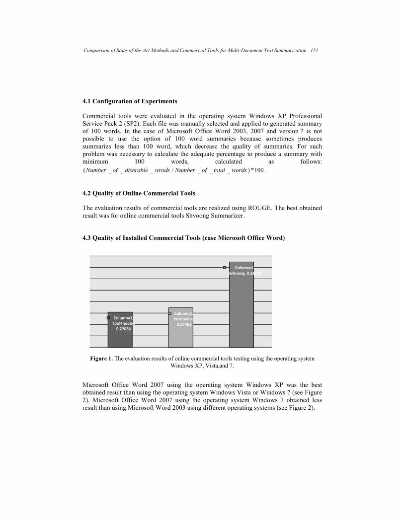
4.1 Configuration of Experiments

Commercial tools were evaluated in the operating system Windows XP Professional Service Pack 2 (SP2). Each file was manually selected and applied to generated summary of 100 words. In the case of Microsoft Office Word 2003, 2007 and version 7 is not possible to use the option of 100 word summaries because sometimes produces summaries less than 100 word, which decrease the quality of summaries. For such problem was necessary to calculate the adequate percentage to produce a summary with minimum 100 words, calculated as follows:

100*)___/___( wordstotalofNumberwrodsdiserableofNumber .

4.2 Quality of Online Commercial Tools

The evaluation results of commercial tools are realized using ROUGE. The best obtained result was for online commercial tools Shvoong Summarizer.

4.3 Quality of Installed Commercial Tools (case Microsoft Office Word)

Figure 1. The evaluation results of online commercial tools testing using the operating system

Windows XP, Vista,and 7.

Microsoft Office Word 2007 using the operating system Windows XP was the best obtained result than using the operating system Windows Vista or Windows 7 (see Figure 2). Microsoft Office Word 2007 using the operating system Windows 7 obtained less result than using Microsoft Word 2003 using different operating systems (see Figure 2).

Columna1,

Tool4noobs,

0.27084

Columna1,

Pertinence,

0.27461

Columna1,

Svhoong, 0.31478


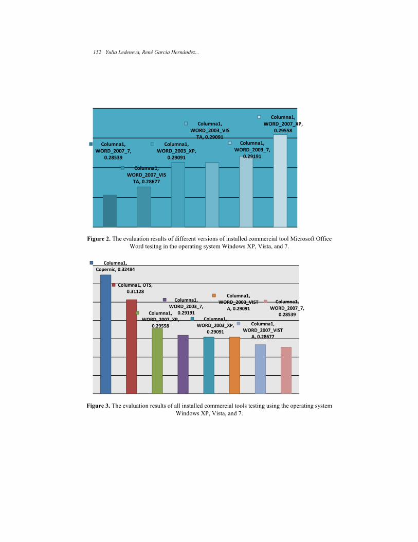
Figure 2. The evaluation results of different versions of installed commercial tool Microsoft Office

Word tesitng in the operating system Windows XP, Vista, and 7.

Figure 3. The evaluation results of all installed commercial tools testing using the operating system

Windows XP, Vista, and 7.

Columna1,

WORD_2007_7,

0.28539

Columna1,

WORD_2007_VIS

TA, 0.28677

Columna1,

WORD_2003_XP,

0.29091

Columna1,

WORD_2003_VIS

TA, 0.29091Columna1,

WORD_2003_7,

0.29191

Columna1,

WORD_2007_XP,

0.29558

Columna1,

Copernic, 0.32484

Columna1, OTS,

0.31128

Columna1,

WORD_2007_XP,

0.29558

Columna1,

WORD_2003_7,

0.29191

Columna1,

WORD_2003_XP,

0.29091

Columna1,

WORD_2003_VIST

A, 0.29091

Columna1,

WORD_2007_VIST

A, 0.28677

Columna1,

WORD_2007_7,

0.28539


Figure 4. The evaluation results of all installed and online commercial tools testing using the

operating system Windows XP, Vista, and 7.

4.4 Quality of all commercial tools

Copernic Summarizer obtained the best results of all installed commercial tools (see Figure 3). Microsoft Office Word 2007 y Microsoft Office Word 2003 obtained less quality then online tools Copernic, OTS y a Shvoong. The installed commercial tools are marked with orange color (see Figure 4).

4.5 Quality of Commercial Tools and State-of-the-Art Methods

In order to see the quality of previous results compared to those obtained with the state-of-the-art methods, in Figure 5 are shown the best results obtained by commercial tools and the results reported by the state-of-the-art methods. Figure 5 shows clearly that the results of Copernic Summarizer is the highest score, just

below the proposed method MFSs (1Best+First) and below of Sentence Clustering with MFSs, which confirms this software is one of the best of its kind.

Resúmenes de

Colecciones ,

Tool4noobs, 0.27084

Resúmenes de

Colecciones , Pertinence,

0.27461

Resúmenes de

Colecciones , Svhoong,

0.31478

Resúmenes de

Colecciones , Copernic,

0.32484

Resúmenes de

Colecciones , OTS,

0.31128

Resúmenes de

Colecciones ,

WORD_2007_XP,

0.29558

Resúmenes de

Colecciones ,

WORD_2003_7, 0.29191

Resúmenes de

Colecciones ,

WORD_2003_XP,

0.29091

Resúmenes de

Colecciones ,

WORD_2003_VISTA,

0.29091

Resúmenes de

Colecciones ,

WORD_2007_VISTA,

0.28677

Resúmenes de

Colecciones ,

WORD_2007_7, 0.28539


Figure 5. Results for the collection of documents obtained for commercial tools and the state-of-

the-art methods.

Table 2. The results of Commercial Tools are ordered by the quality of Text Summaries.

Commercial Tools F-measure Characteristic

Copernic 0.32484 Installed

Svhoong 0.31478 Online

OTS 0.31128 Installed

WORD_2007_XP 0.29558 Installed

WORD_2003_7 0.29191 Installed


WORD_2003_VISTA 0.29091 Installed



Pertinence 0.27461 Online

Tool4noobs 0.27084 Online


According to Figure 1 Copernic Summarizer outperforms the two versions of Microsoft OfficeWord, although Microsoft Office Word 2003 was slightly better than its 2007 version. However, during the experimentation an inconsistency in Microsoft Office Word was observed because the generated summaries change depending on the operating system. In order to verify this fact the same setup package of Microsoft Office Word 2003 was installed on Windows XP Professional SP2, which also was done with Microsoft Office Word 2007. The resulting abstracts were assessed with the same version of ROUGE and obtained the results shown in Figure 2. In Figure 2, we can observe the slight difference between the tools of auto summary of

Microsoft Office Word. In contrast, Copernic Summarizer tool show the same results in both operating systems. We can conclude that Copernic Summarizer is independent of the operating system).

Table 3. The results of the State-of-the-Art Methods (SAMs) and Commercial Tools are ordered by

the quality of Text Summaries.

Commercial Tools and

State-of-the-Art Methods

F-measure Characteristic

1st Best Method 0.3578 SAMs

2nd Best Method 0.3447 SAMs

3rd Best Method 0.3264 SAMs

Copernic 0.32484 Installed

MFS 0.3219 SAMs

Svhoong 0.31478 Online

OTS 0.31128 Installed

4th Best Method 0.3056 SAMs

5th Best Method 0.3047 SAMs


Baseline 0.2932 SAMs






Pertinence 0.27461 Online

Tool4noobs 0.27084 Online

Also, it is important to mention that Microsoft Office Word 2007 with Windows XP

Professional SP2 obtained the worst result, among the versions of Microsoft Office Word.


Nevertheless, the best result, among the versions of Microsoft Office Word, was obtained with Microsoft Word 2003 with Windows Vista Home Premium SP1. This shows the dependence of these tools with respect to the operating system they are using.

5 Discussion and Conclusions

Only four commercial tools are better than baseline configuration: Svhoong, Copernic, OTS, WORD_2007_XP. Other six evaluated commercial tools are worst than the baseline configuration. All the state-of-the-art methods overcome the baseline configuration and quality of the commercial tools (see Figure 6).

Figure 6. Results for the collection of documents obtained for commercial tools and the state-of-

the-art methods.

In this paper, the evaluation of the automatic summaries generated by commercial tools (Copernic Summarizer, Microsoft Office Word Summarizer 2003 and Microsoft Office Word Summarizer 2007) was realized. The summaries were evaluated using the ROUGE system. The following conclusions can be given based on obtained results:

– 18 different automatic multi-document summarization state-of-the art methods and commercial tools were compared


– In most cases, the state-of-the-art methods are better that commercial tools – Copernic Summarizer gets the best results of commercial tools. – Copernic Summarizer is the best commercial tool – Shvoong is the best online tool – Microsoft Office Word is inconsistent because it generates different summaries

depending on the operating system. – The results obtained with Microsoft Office Word 2003 and Microsoft Office Word

2007 with Windows Vista were better than with Windows XP. – Microsoft Office Word 2003 gets a better result than Microsoft Office Word 2007

with Windows Vista operating system.

We consider that computer methods can perform better and quicker than human the task of multi-document text summarization, in particular, reducing the contents of a big collection of documents to a single short text, so that the user can judge about the contents of the whole collection upon reading only this short text. However, it is still a challenge for computer methods to improve the quality for multi-document text summarization and even bigger challenge coherence. Good news is that the state-of the-art methods perform better than commercial tools.

Acknowledgments. Work done under partial support of Mexican Government (CONACyT, SNI, SEP-PROMEP, UAEM, SIP-IPN 20111146, 20113267) and Mexico City Government (project ICYT-DF PICCO10-120). The authors thank Autonomous University of the State of Mexico for their assistance.

References

1. Lyman, Peter and Hal R. Varian. How Much Information. Retrieved from http://www.sims.berkeley.edu/how-much-info-2003 (2003)

2. Yulia Ledeneva, Alexander Gelbukh, René A. García-Hernández. Terms Derived from Frequent Sequences for Extractive Text Summarization, 9th Conference on Intelligent Text Processing and Computational Linguistics (CICLing 2008), Lecture Notes in Computer Science, Springer-Verlag, Vol. 4919. pp. 593-604 (2008)

3. Yulia Ledeneva. Automatic Language-Independent Detection of Multiword Descriptions for Text Summarization, National Polytechnic Institute, PhD. Thesis, Mexico (2009)

4. Yulia Ledeneva, René García Hernández, Alexander Gelbukh. Multi-document Summarization using Maximal Frequent Sequences. Research in Computer Science, pp.15-24, vol. 47, ISSN 1870-4069 (2010)

5. Yulia Ledeneva, René García Hernández, Anabel Vazquez Ferreyra, Nayely Osorio de Jesus. Experimenting with Maximal Frequent Sequences for Multi-Document Summarization. Research in Computing Science, pp.233-244, vol. 45, ISSN 1870-4069 (2010)

6. René Arnulfo García-Hernández, Romyna Montiel, Yulia Ledeneva, Eréndira Rendón, Alexander Gelbukh, Rafael Cruz. Text Summarization by Sentence Extraction Using Unsupervised Learning, 7th Mexican International Conference on Artificial Intelligence


(MICAI08), Lecture Notes in Artificial Intelligence, Springer-Verlag, Vol. 5317 pp. 133-143 (2008)

7. Rada Mihalcea; Graph-based Ranking Algorithms for Sentence Extraction, Applied to Text Summarization; Department of Computer Science; University of North Texas; Texas; EUA (2004)

8. Rada Mihalcea, Paul Tarau. A language independent algorithm for single and multiple document summarization. In Proceedings of IJCNLP’2005 (2005)

9. DUC. Document Understanding Conference, www-nlpir.nist.gov/projects/duc. 10. Copernic Summarizer, Technologies White Paper (2003)

http://www.copernic.com/data/pdf/summarization-whitepaper-eng.pdf 11. Online Tool Noobs Summarizer. http://www.tools4noobs.com/summarize/ 12. Pertinence Summarizer. http://www.pertinence.net/index_en.html 13. Shvoong Summarizer. http://www.shvoong.com/summarizer/ 14. Lin, C., y E. Hovy: Automatic evaluation of summaries using N-gram co-occurrence statistics.

Proceedings of the 2003 Conference of the North American Chapter of the Association for Computational Linguistics on Human Language Technology. Vol. 1, pp. 71-78 (2003)

15. Lin, C.: ROUGE: A package for automatic evaluation of summaries. Proceedings of the Association for Computational Linguistics 2004 Workshop, pp. 74-81. Spain (2004)

16. Garcia, R., F. Martinez, A. Carrasco, Finding maximal sequential patterns in text document collections and single documents, Informatica, International Journal of Computing and Informatics, ISSN: 1854-3871, No. 34, pp. 93-101 (2010)

17. Sidorov, G. Lemmatization in automatized system for compilation of personal style dictionaries of literary writers. In: “Word of Dostoyevsky”, Russian Academy of Sciences, pp. 266-300 (1996)

18. Gelbukh, A. and Sidorov, G. Approach to construction of automatic morphological analysis systems for inflective languages with little effort. Lecture Notes in Computer Science, N 2588, Springer-Verlag, pp. 215–220 (2003)

19. Sidorov, G., Barrón-Cedeño, A., and Rosso, P. English-Spanish Large Statistical Dictionary of Inflectional Forms. In: Proceedings of the Seventh International Conference on Language Resources and Evaluation (LREC'10), Valletta, Malta. European Language Resources Association (ELRA), pp. 277-281 (2010)

20. Esaú Villatoro-Tello, Luis Villaseñor-Pineda, Manuel Montes-y-Gómez, and David Pinto-Avendaño. Multi-Document Summarization Based on Locally Relevant Sentences. Mexican International Conference on Artificial Intelligence MICAI 2009. Guanajuato, Mexico, November 09-13, pp. 87-91, IEEE Computer Society (2009)


Evolutionary Algorithms and Process Optimization

The Application of the Genetic Algorithmbased on Abstract Data Type (GAADT) Modelfor the Adaptation of Scenarios of MMORPGs

Leonardo F. B. S. Carvalho, Helio C. Silva Neto,Roberta V. V. Lopes, and Fabio Paraguacu

Federal University of Alagoas (UFAL - Universidade Federal de Alagoas),Institute of Computing (IC - Instituto de Computacao),

Campus A. C. Simoes, 57072-970 Maceio, Alagoas, Brazillfilipebsc,helio.hx,[email protected],

[email protected]

Abstract. The importance of using Artificial Intelligence in video gameshas grow in response to a need in showing behaviors and other gameelements in a closer accuracy to what is seen at the real world. In or-der to assist this need, this paper takes advantage of the context ofMMORPGs (game worlds with rich and interactive environments whereimportant events occur simultaneously) to demonstrate the applicationof the artificial intelligence technique of the Genetic Algorithm based onAbstract Data Type (GAADT) in changing the features of game mapsof MMORPGs due to the passage of time, in an attempt to reproducewhat is seen in the real world.

Keywords: Artificial Intelligence, genetic algorithms, GAADT, games,MMORPG.

1 Introduction

The Genetic Algorithms (GA) [6] are Artificial Intelligence (AI) algorithms thatemploy the evolutionary principle of the survival of the fittest to solve algorithmicproblems using an heuristic search based on metaphors combining principles ofsearch algorithms and biology.

In videogames, GAs are often used when the implementation of AI involvesmust deal with problems that have many possible outcomes or lots of variablesthat ought to be accounted to achieve proper results [4]. In this respect, thispaper presents an instantiation of a GA known as GAADT (Genetic Algorithmbased on Abstract Data Type) to solve a problem that fits both these charac-teristics, which is: “to change the features of pre-existing MMORPG (MassivelyOnline Role-Playing Game) game maps in order to create new maps”.

The problem above has a great level of abstraction. Thus, it must be statedthat the aim of this research is not to create new maps from scratch. In fact,the instance of GAADT that will be presented by this paper uses existing game

maps as input and manipulates them to create new maps. Game maps mayhouse various types of objects; however, only the type capable of representingthe different geographical images that make up its scenario (known as tile) willbe referred here.

After a game map is given as input to GAADT, the algorithm will startto create game maps that have some geographical features that are differentfrom the ones of the input map, meaning that they have one or more groupof cells whose tiles do not match the ones that are found in the input mapfor those specific locations. These differences occur in respect to the beginningof a season (spring, summer, autumn or winter) and to the unique geographyoriginally depicted by each cell. However, it is not mandatory for a game mapor its regions to have four properly defined seasons. Moreover, it is also unlikelythat the transitional period from one season to another will ever repeat itself,which is a response to the fact that the values defining the extent of a season, itsrainfall and even the time taken for switch between seasons are randomly chosenfor each execution of GAADT.

The use of GAADT to change the topology/geographical features of scenariosof game maps - which was first shown in [3] - contrasts with other algorithmsemployed for this purpose due the fact that GAADT is an AI algorithm, whileother identified approaches have a common link to computer graphics. Some ofthese approaches are listed in Table 1.

Paper Technique Limitations

[1] Visualizations of dynamic terrains usinga multiresolution algorithm with struc-tural changes.

The algorithm is restrict to create asingle kind of alteration in the gamemap (craters).

[7] Multiresolution algorithm coupled withreal-time optimally adapting meshes [5].

The model seems to apply only to real-time car driving in game maps simu-lating an off-road type of environment.

[10] Use of multiresolution meshes to rep-resent geometric objects. Each set ofmeshes corresponds to a different rep-resentation of a same object.

Unfit to systems requiring online up-dates.

Table 1: Different approaches for changing the geography of game maps

Now, this paper will be divided into different sections that better clarify theuse of GAADT as solution to the problem of changing the geographical featuresof a game map. Following this section, Sec. 2 will detail the concepts of theadopted game maps. Next, Sec. 3 will present the concepts of GAADT and theinstantiation used here. Last, Sec. 4 will show the results and conclusions drawnfrom this research.

162 Leonardo F. B. S. Carvalho, Helio C. Silva Neto, Roberta V. V. Lopes, and Fábio Paraguaçu

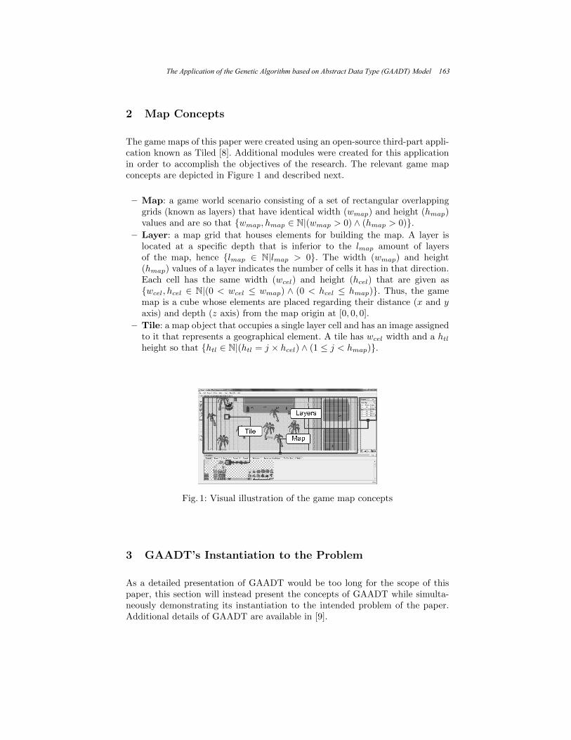
2 Map Concepts

The game maps of this paper were created using an open-source third-part appli-cation known as Tiled [8]. Additional modules were created for this applicationin order to accomplish the objectives of the research. The relevant game mapconcepts are depicted in Figure 1 and described next.

– Map: a game world scenario consisting of a set of rectangular overlappinggrids (known as layers) that have identical width (wmap) and height (hmap)values and are so that wmap, hmap ∈ N|(wmap > 0) ∧ (hmap > 0).

– Layer: a map grid that houses elements for building the map. A layer islocated at a specific depth that is inferior to the lmap amount of layersof the map, hence lmap ∈ N|lmap > 0. The width (wmap) and height(hmap) values of a layer indicates the number of cells it has in that direction.Each cell has the same width (wcel) and height (hcel) that are given aswcel, hcel ∈ N|(0 < wcel ≤ wmap) ∧ (0 < hcel ≤ hmap). Thus, the gamemap is a cube whose elements are placed regarding their distance (x and yaxis) and depth (z axis) from the map origin at [0, 0, 0].

– Tile: a map object that occupies a single layer cell and has an image assignedto it that represents a geographical element. A tile has wcel width and a htlheight so that htl ∈ N|(htl = j × hcel) ∧ (1 ≤ j < hmap).

Fig. 1: Visual illustration of the game map concepts

3 GAADT’s Instantiation to the Problem

As a detailed presentation of GAADT would be too long for the scope of thispaper, this section will instead present the concepts of GAADT while simulta-neously demonstrating its instantiation to the intended problem of the paper.Additional details of GAADT are available in [9].

The Application of the Genetic Algorithm based on Abstract Data Type (GAADT) Model 163

3.1 Basic Types

Def. 1. Basis: the elementary genetic unit of chromosomes. Here, a basis is ab = (x, y, z, tl, tp, in, fl) element that corresponds to a map cell at the x, y, zlocation that has the tl tile assigned to it, which is additionally identified by thetp description of its type of geography, by the unique index in of this descriptionand by the fl flag that indicates if the tile of this cell requires a collision.

The bases of GAADT are part of a B set that is defined here accordingto a DC = (x, y, z, tl, tp, in, fl)|(0 ≤ x < wmap) ∧ (0 ≤ y < hmap) ∧ (0 ≤ z <

lmap)∧(tl ∈ Tile)∧(in ∈ N)∧(fl ∈ Boolean) set that has the lmap value of thedomain of the z coordinate as the amount of map layers intended exclusively forthe allocation of tiles. The Tile set of DC defines the domain of the tl tile objectsand is so that Tile = (wcel, htl, gId, Img)|(Img ∈ Image) ∧ ((wcel, htl, gId) ∈N). The gId value is the unique index that identifies a tile.

Hence, the set of bases for this instance of GAADT is B = DC∪Bλ. The Bλset accords to GAADT’s assumption that exists a bλ innocuous basis whose datadoes not influence the identity of the gene that contains it. In turn, as this paperassumes that bases at different x, y, z coordinates are in fact different bases, thealgorithm requires a Bλ = b = (x, y, z, tl, tp, in, fl)|(tp = tpλ) set of innocuousbases, whose elements have the same tp value that marks them as cell with noinformation.

The bases are arranged in groups in order to create genes. Each gene is aparticular characteristic and thus, requires that its bases are connected in someway. For this reason, the creation of genes accords to a set of “formation rules”called Axioms for Formation of Genes (AFG).

Def. 2. Gene: a g = 〈b1, . . . , bn〉 “micro region” of the game map that meetsthe requirements of the AFG set of rules.

AFG1 = ∀g = 〈b1, . . . , bn〉 ∈ G ∀ (bα = (xα, yα, zα, tlα, tpα, inα, f lα),bβ = (xβ , yβ , zβ , tlβ , tpβ , inβ , f lβ)) ∈ b1, . . . , bn | zα = zβ

(1)

AFG2 = ∀g = 〈b1, . . . , bn〉 ∈ G ∀ (bα = (xα, yα, zα, tlα, tpα, inα, f lα),bβ = (xβ , yβ , zβ , tlβ , tpβ , inβ , f lβ)) ∈ b1, . . . , bn |(tpα = tpβ) ∧ (inα = inβ)

(2)

AFG3 = ∀g = 〈b1, . . . , bn〉 ∈ G∃1 (bx+ = (xx+ , yx+ , zx+ , tlx+ , tpx+ , inx+ , f lx+),bx− = (xx− , yx− , zx− , tlx− , tpx− , inx− , f lx−)) ∈ b1, . . . , bn∀b = (x, y, z, tl, tp, in, fl) ∈ b1, . . . , bn | ((x ≤ xx+)∧(xx− ≤ x)) ∧ (0 < (xx+ − xx− + 1) < (2× wmapa/3))

(3)


AFG4 = ∀g = 〈b1, . . . , bn〉 ∈ G∃1(by+ = (xy+ , yy+ , zy+ , tly+ , tpy+ , iny+ , f ly+),

by− = (xy− , yy− , zy− , tly− , tpy− , iny− , f ly−))∈ b1, . . . , bn

∀b = (x, y, z, tl, tp, in, fl) ∈ b1, . . . , bn |((y ≤ yy+

)∧(

yy− ≤ y))∧(0 <

(yy+ − yy− + 1

)< (2× hmapa/3)

) (4)

The genes are arranged in groups in order to create chromosomes. Thus,each chromosome is an aggregation of characteristics and is a unique elementthat does not repeat itself within any present or future population of GAADT.The creation of chromosomes obeys its own set of “formation rules” known asAxioms for Formation of Chromosomes (AFC) that validates their sequences ofgenes. Figure 2 shows some examples of bases, genes and chromosomes that wereobtained according to the defined B set and the stated AFG and AFC rules.

Def. 3. Chromosome: a c = g1, . . . , gn “macro region” of the game mapthat obeys the AFC set of rules.

AFC1 = ∀ c = g1, g2, . . . , gm ∈ C∀(gα =

⟨bα1 , . . . , b

αn1

⟩, gβ =

⟨bβ1 , . . . , b

βn2

⟩)∈ g1, g2, . . . , gm

∀bi = (xi, yi, zi, tli, tpi, ini, f li) ∈bα1 , . . . , b

αn1

∀bj = (xj , yj , zj , tlj , tpj , inj , f lj) ∈

bβ1 , . . . , b

βn2

|

(xi 6= xj) ∨ (yi 6= yj) ∨ (zi 6= zj)

(5)

AFC2 = ∀c = g1, g2, . . . , gm ∈ C ∀ (g = 〈b1, . . . , bn〉) ∈ g1, g2, . . . ,gm ∃b = (x, y, z, tl, tp, in, fl) ∈ b1, . . . , bn | z = 0 (6)

AFC3 = ∀ c = g1, g2, . . . , gm ∈ C ∀(gα =

⟨bα1 , . . . , b

αn1

⟩,

gβ =⟨bβ1 , . . . , b

βn2

⟩)∈ g1, g2, . . . , gm ∀bi = (xi, yi, zi, tli,

tpi, ini, f li) ∈bα1 , . . . , b

αn1

∀bj = (xj , yj , zj , tlj , tpj , inj , f lj)

∈bβ1 , . . . , b

βn2

| (zi ≥ zj) ∧ (∀z ∈ 0, 1, . . . , zi

∃(gγ =

⟨bγ1 , . . . , b

γnγ

⟩)∈ (g1, g2, . . . , gm − gβ)

)∧

(∀b = (xb, yb, zb, tlb, tpb, inb, f lb) ∈bγ1 , . . . , b

γnγ

(zb = z))

(7)

GAADT performs its operations according to cycle of evolutionary and stag-nant periods that assumes that environmental changes mark the beginning ofnew evolutionary periods and arranges its chromosomes in groups known aspopulations. Every chromosome is a potential result for the problem that thealgorithm is aiming to solve and, as a consequence, it assumes that the creationof an empty population reflects an incorrect assumption of the problem, as itwould mean that the intended problem does not have a solution.


(a) Chromosome (b) Gene at the z = 0layer and its x, y lo-cations

(c) Genes at the z =1 layer and their x, ylocations

(d) Gene at the z = 2layer and its x, y lo-cations

(e) Gene at the z = 3layer and its x, y lo-cations

(f) A chromosome ofa single gene (at z =0) and a single basis

Fig. 2: Example of chromosomes with their genes along the x, y and z axes andwith the bases standing as the genes’ individual cells

Each loop of the cycle is known as a generation and spawns new chromosomesto GAADT’s current population at the same time that removes from it the chro-mosomes it considers “unfit”. In time, GAADT will start to converge and createpopulations that are increasingly similar to the one of the previous generation,until they become indistinguishable. This indicates that GAADT has reacheda stagnant period, which will come to an end whenever a new environmentalchange occurs, forcing the evolutionary-stagnant process to repeat itself.

3.2 Genetic Operators

The genetic operators are responsible for creating new chromosomes for GAADT’spopulations. There are two operators that perform this task: the reproductionoperator and the mutation operator.

The reproduction operator used here is a crossover operation that combinesgenes of two different chromosomes (parent-chromosomes) in order to createnew chromosomes (child-chromosomes), while the mutation operator receives aninput chromosome and switch some of its genes by new ones, thus, creating newchromosomes (mutant-chromosomes). The value that indicates the suitabilityof a chromosome to its environment is known as adaptation value (or fitness),which depends of the degree value of its genes that indicates the suitability of agene to its environment.

Def. 4. Degree: the degree of a gene is a degree : G → Q+ function mappinga gene to a k value known as degree(g) that is so that k ∈ Q+. The degree(g)


function reflects a comparative stratification of the g gene suitability to its en-vironment in respect to GAADT’s intended problem.

Due the level of abstraction of the problem intended here, the degree functionshown in (8) uses the distri(g) function to exam how the micro-region of thegame map corresponding to the g input gene match its surroundings. Equation(9) shows the distri(g) function.

The distri(g) function uses the whiteInGene(g) function that combines allimages within the tiles of the bases of its input gene into a single image andsubject it to Canny’s edge detection algorithm [2], creating a black and whiteimage that outlines its geography (black background and white contours) andreturning its amount of white pixels, which is used by (9) as an indicator of thecorrect placement of its geographic elements.

degree(g = 〈b1, . . . , bn〉) =

distri(g)#g if (pass > 1) ∧ (∃1tppass ∈ INT ∀b =

(x, y, z, tl, tp, in, fl) ∈ b1, . . . , bn |tp = tppass)

1− distri(g)#g if (pass = 1) ∧ (∃1tppass ∈ INT ∀b =

(x, y, z, tl, tp, in, fl) ∈ b1, . . . , bn |tp = tppass)

0 if g ∈ Gλ1× 10−10 otherwise

(8)

distri (g) =

1−(

1#g×wcel×hcel

)if whiteInGene(g) = 0

1−(whiteInGene(g)#g×wcel×hcel

)otherwise

(9)

In addition to distri(g), (8) uses the INT = 〈tp1, . . . , tpn〉 sequence whose tptypes of geography are mapped accordingly to the predominant type of environ-ment of GAADT’s input map and to its randomly chosen season. The tp valuesof INT are the same elements presented in Def. 1 and their position withinINT denotes their level of importance to the geography that GAADT expectsto achieve for the game map. Therefore, tp1 is the most important type of geog-raphy for the intended game map while tpn is the least important one. Each callto distri(g) will randomly choose a pass value, pass ∈ N∗| pass ≤ #INT,that will indicate the type of geography that will be taken into account (tppass).The Gλ set is the set of innocuous-genes, a subset of GAADT’s G set of geneswhose elements have no influence for the identity of a chromosome and that, forthis instance of GAADT, corresponds to (10).

Gλ = gλ = 〈bgλ1 , . . . , bgλn 〉 | ∀ i ∈ 1, 2, . . . , n (bgλi ∈ Bλ) (10)

Def. 5. Adaptation: the adaptation of a chromosome (or fitness) is a func-tion adapt : C → Q+ that sums the degree of its genes and is defined here asadapt(c = g1, . . . , gn) =

∑ni=1 (Θ (c, gi)× degree(gi)).


The Θ function above is a weight function that maps a gene into a rationalvalue by identifying how much of a gene’s degree contributes to the chromo-some’s adaptation. Here, the weight function merely accounts if the tp valuewithin the bases of a gene is also an element of the INT sequence, resultingin 1 if tp ∈ INT and 0 otherwise. The adapt function also makes possible tocalculate the average adaptation of a population of chromosomes, which is sothat adaptm(P = c1, . . . , cn) = (

∑ni=1 adapt(ci))/#P .

The value of adaptation of a chromosome makes possible to select chromo-somes for specific purposes from any of GAADT’s populations. One such case isthe selection of chromosomes better fitted to create new chromosomes by sub-jection to genetic operators. The first of these operators that will be shown hereis the reproduction operator by crossover of chromosomes, which heavily relayson the selection operator.

Def. 6. Selection: an operator that chooses from a population the chromo-somes better satisfying an r predicate from GAADT’s Rq set of requirements.Hence, sel(P1, r) = P1 ∩ r.

The r predicate used here is shown in (11), which has P2 as the popula-tion of parents-chromosomes that suit r and INTr as a subsequence of INTset at running time so that INTr = 〈tpr1, . . . , tprn〉 |∀i ∈ 1, 2, . . . , n ∀j ∈1, 2, . . . ,m ∃tpj ∈ INT (i ≤ j) ∧ (j = i+ (m− n)) ∧ (tpri = tpj).

r = P2| (P2 ⊆ C) ∧ (c = g1, . . . , gn ∈ P2)↔ (∀b =(x, y, z, tl, tp, in, fl) ∈ g1, . . . , gn ∃tpr ∈ INTr(tp = tpr)) (11)

The P2 resulting set of chromosomes of (11) may be further split into distinctMALE and FEMALE by applying their equivalent predicates over P2. There-fore, assuming the predicates M,F ∈ Rq, follows that MALE = sel(P2;M) andFEMALE = sel(P2;F ). These two new sets of chromosomes are used by thefecundation operation of (12).

fec(cM , cF ) = g1, . . . , gm | (cM = gM1 , . . . , gMl ∈MALE)∧(cF = gF1 , . . . , gFn ∈ FEMALE)∧(g ⊆

gM1 , . . . , gMl

∪gF1 , . . . , g

Fn

)↔(

∀gM ∈gM1 , . . . , gMl

∀gF ∈

gF1 , . . . , g

Fn

(domi(gM , gF ) = g)

)

(12)The domi function of (12) receives two input genes and returns their domi-

nant one. A g1 gene is dominant over a g2 gene if both express the same char-acteristic and degree(g1) ≥ degree(g2). Therefore, if degree(g2) > degree(g1)the domi function returns g2. Additionally, if g1 and g2 do not express thesame characteristic domi returns a gλ innocuous-gene. Here, g1 and g2 ex-press the same characteristic if ∃1tp ∈ INT | ∀g1, g2 ∈ G ∀i, j ∈ N∗ ∀bi =(xi, yi, zi, tli, tpi, ini, f li) ∈ g1 ∀bj = (xj , yj , zj , tlj , tpj , inj , f lj) ∈ g2((i ≤ #g1)∧(j ≤ #g2) ∧ (tpi = tpj = tp)).


Def. 7. Crossover: the crossover is a reproduction operation defined by across : MALE × FEMALE → P function, which is so that cross(c1, c2) =c = g1, . . . , gn| c ⊆ fec(c1, c2).

The other genetic operator for creating new chromosomes is the mutationoperator. It acts as a safeguard that prevents the removal of chromosomes havingsome characteristics suitable to GAADT’s current environment, but that do notmeet the minimal adaptation value required to be kept in the current population.Once a chromosome is mutated its adaptation value is calculated again.

Def. 8. Mutation: an operator that replaces some of the genes of its inputchromosome. It is defined by a mut ⊆ ℘(P ) predicate corresponding to the func-tion mut(c) = c′|(∃G1, G2 ⊂ G)→ (c′ = change(c,G1, G2)) ∧ (c′ ∈ cut(P )).

The change function of the definition above is of type change : C × ℘(G)×℘(G) → C and is defined here as (13). Additionally, the cut function of mut isan acceptance criterion of the Rq set of requirements, cut ∈ Rq, that is imposedto every chromosome subject to mutation and that is defined here as cut(P ) =C∆| ∀c ∈ C((c ∈ C∆)↔ (adapt(c) ≥ adaptm(P ))).

change(c,G1, G2) =

(c ∪G1)−G2 if (c ∪G1 ∈ AFC) ∧ (c−G2 ∈ AFC)c ∪G1 if (c ∪G1 ∈ AFC) ∧ (c−G2 /∈ AFC)c−G2 if (c ∪G1 /∈ AFC) ∧ (c−G2 ∈ AFC)c if (c ∪G1 /∈ AFC) ∧ (c−G2 /∈ AFC)

(13)

3.3 The Algorithm

The populations of GAADT are part of an environment defined by the 8-tupleE = 〈P, ℘(P ), Rq,AFG,AFC, Tx,Σ, P0〉. The P value is the current populationof GAADT and #P ∈ N∗. Simultaneously, ℘(P ) is the power set of P ; Rq isthe set of environmental requirements guiding the evolution of chromosomes;AFG and AFC are, respectively, the sets of Axioms for Formation of Genes andof Chromosomes; Tx is the taxonomic classification of the chromosomes of P ,which prevents them from occurring multiple times within a population and ofresurging on any future population; Σ is the set of genetic operator; and P0 isthe initial population.

GAADT itself is established as the function GAADT : E → E shown at(14) and that assumes Pt ⊆ C as its input population and Pt+1 ⊆ C as thenext population of the algorithm, which contains the chromosomes that wereproduced from Pt as result of the environmental requirements imposed by the Rqset and the genetic operators of Σ. Consequently, Pt+1 = cross(a, b)∪mut(c)∪pcut(Pt) and a, b, c ∈ Pt.

GAADT (Pt) =

Poptm if Poptm = c| ∀c ∈ Pt(adapt(c) ≥ k) 6= ∅;Pt+1 if t+ 2 = T ;GAADT (Pt+1) otherwise

(14)


The Rq set of requirements of GAADT also contains two stopping criteriato halt its execution. The first of these criteria is defined in respect to what theinstantiation of GAADT is considering as an optimal solution to its intendedproblem and is presented in (14) as definition of the minimal adaptation valuek that must be met by the chromosomes of the Poptm optimal population. Thelast criterion establishes a maximum number of interactions (generations) thatGAADT can perform before returning a result. In (14) this corresponds to thedefined T value that is so that T ∈ N. This last criterion ensures that GAADT’sevolutionary process will eventually stop and therefore, is computable.

4 Results and Conclusions

Figure 3 shows a map provided as input to GAADT (Fig. 3a) and the mapthat results of its evolutionary process (Fig. 3b). The map area of Fig. 3b thatdiverges from Fig. 3a corresponds to the chromosome of greatest adaptationvalue that exists within the last population created by GAADT before the halt ofits process. In this particular example, a forest input map (Fig. 3a) was subjectto a period of drought that was caused by an extend summer and began toacquire geographic features commonly seen in deserts (Fig. 3b).

(a) Input map (forest) (b) Output map (desert)

Fig. 3: An input map and the output map created from it by GAADT

The number of interactions performed by GAADT to create the map of Fig.3b is shown in Table 2, along with the chromosomes of greater and lower adap-tation value and the average adaptation of the population of each generation.Table 2 also makes possible to identify stagnant periods of GAADT’s evolution-ary process, which correspond to the generations presenting identical values for


the greatest, lowest and average adaptation of its chromosomes (generations 3to 5 and 6 to 7). After seven generations with no changes in any of these threevalues, the evolutionary process of this instance of GAADT is halted.

Results

generation greatest adaptation lowest adaptation average adaptation

1 0,924541016 0,00302477 0,572786602

2 0,946289063 0,00302477 0,611779318

3 0,9921875 0,00302477 0,63175816

4 0,9921875 0,00302477 0,63175816

5 0,9921875 0,00302477 0,63175816

6 0,993339978 0,00302477 0,672413871

7 0,993339978 0,00302477 0,672413871

8 0,996235983 0,01467041 0,713797671

9 0,996235983 0,01467041 0,713797671

10 0,996235983 0,01467041 0,713797671

11 0,996235983 0,01467041 0,713797671

12 0,996235983 0,01467041 0,713797671

13 0,996235983 0,01467041 0,713797671

14 0,996235983 0,01467041 0,713797671

Table 2: Adaptation values for the chromosomes of GAADT in creating the mapof Fig. 3b

The result seen in Fig.3b and achieved by the process detailed in Table 2shows that even thought the use of GAADT contrasts with the traditional use ofcomputer graphics to modify the geography of game maps, it is a valid approachthat provides resulting maps suitable to MMORPGs and that add an extraelement of dynamic that players can explore.

However, it is the authors’ believe that such results can be further improvedby refining the parameters of the instance of the algorithm in order to achievean even better distribution of the geographic elements of the resulting maps.

An identified drawback is the time required by the algorithm to obtain aresulting map. In this respect, the map shown in Fig. 3b took roughly 10 hoursto be created from the map of Fig. 3a. This is a consequence of GAADT usingits Σ set of genetic operators to create all possible variations of the input mapthat obey the restrictions imposed by the Rq set of requirements.

To solve this drawback, future approaches to this problem will focus on eitherimplementing the GAADT instance seen here in hardware in order to reducethe processing time by taking advantage of its higher processing speeds; or,refactoring the instance of GAADT as to improve its execution in addition togeneralize it so it become applicable for game maps whose structure is differentfrom that of the game maps used here.


References

1. Cai, X., Li, F., Sun, H., Zhan, S.: Research of Dynamic Terrain in Complex Bat-tlefield Environments. In: Technologies for E-Learning and Digital Entertainment,Lecture Notes in Computer Science, vol. 3942. Springer Berlin / Heidelberg (2006)

2. Canny, J.: A Computational Approach to Edge Detection. IEEE Transactions onPattern Analysis and Machine Intelligence PAMI-8(6) (1986)

3. Carvalho, L.F.B.S., Neto, H.C.S., Lopes, R.V.V., Paraguau, F.: Application of agenetic algorithm based on abstract data type in electronic games. In: Proceedingsof the 9th Mexican International Conference on Artificial Intelligence - SpecialSession - (MICAI 2010). pp. 28–33. IEEE Computer Society Press (2010)

4. Carvalho, L.F.B.S.: An Evolutive game of Checkers. End of course work, Instituteof Computation, Federal University of Alagoas, Brazil (2008)

5. Duchaineau, M., Wolinsky, M., Sigeti, D., Miller, M., Aldrich, C., Mineev-Weinstein, M.: Roaming terrain: Real-time optimally adapting meshes. In: Pro-ceedings of the conference on Visualization ’97 (1997)

6. GOLDBERG, D.E., HOLLAND, J.H.: Genetic algorithms and machine learning.Machine Learning 3(2-3), 95–99 (1988)

7. He, Y., Cremer, J., Papelis, Y.: Real-time extendible-resolution display of on-linedynamic terrain. In: Proceedings of The 2002 Conference on Graphics Interface(2002)

8. Lindeijer, T., Turk, A.: Tiled Map Editor. Available at: http://www.mapeditor.org/ (2006-2011), last accessed on December 19 2010

9. Lopes, R.V.V.: A Genetic Algorithm Based on Abstract Data Type and its Spec-ification in Z. Ph.D. thesis, Computer Center, Federal University of Pernambuco(2003)

10. Shamir, A., Pascucci, V., Bajaj, C.L.: Multiresolution dynamic meshes with arbi-trary deformations. In: Proceedings of IEEE Visualization 2000 (2000)


Increasing the Performance of Differential

Evolution by Random Number Generation withthe Feasibility Region Shape

Felix Calderon, Juan Flores, and Erick De la Vega

Universidad Michoacana de San Nicolas de Hidalgo,Division de Estudios de Posgrado, Facultad de Ingenierıa Electrica,Santiago Tapia 403 Centro, Morelia, Michoacan, CP 58000, Mexico

[email protected], [email protected], [email protected]

Abstract. Global optimization based on evolutionary algorithms can beused for many engineering optimization problems and these algorithmshave yielded promising results for solving nonlinear, non-differentiable,and multi-modal optimization problems. In general, evolutionary algo-rithms require a set of random initial values; in the case of constrainedoptimization problems, the challenge is to generate random values insidethe feasible region. Differential evolution (DE) is a simple and efficientevolutionary algorithm for function optimization over continuous spaces.It outperforms search heuristics when tested over both benchmark andreal world problems. DE with Penalty Cost Functions is the most usedtechnique to deal with constraints, but the solution is moved by thepenalty factor, losing accuracy. Additionally, the probability to reachthe optimal value is near zero for some constrained optimization prob-lems, because the optima of the objective function are located out of thefeasible region, therefore the optimal solutions of the problem lie at theborder of the feasible region. In this paper we propose an improved DEalgorithm for linearly constrained optimization problem. This approachchanges the restricted problem to a non-restricted one, since all individu-als are generated inside the feasible region. The proposed modification toDE increases the accuracy of the results, compared to DE with penaltyFunctions; this is accomplished by the generation of random numberswhose convex hull is shaped by the feasible region. We tested our ap-proach with several benchmark and real problems, in particular withproblems of economic dispatch of electrical energy.

Keywords: Differential evolution, feasible region, optimization.

1 Introduction

For a differentiable function f(x) : RD → R, computing the minimum x∗ =[x∗

0, x∗1, · · · , x∗

D−1, ], can be done using gradient-based methods [1]. Neverthe-less, these techniques fail for non-differentiable and discontinuous functions. Analternative is to solve the problem using evolutionary computation; these meta-heuristics compute an initial set of prospect solutions, called initial population.

The most common way to generate a random initial population within afeasible reagion R, is computing a random number with uniform distributionusing Equation (1). The population generated this way is uniformly distributedinside a hyper-cube, therefore, when minimizing the function f(x) restricted byconstraints of the form xmin

j <= x <= xmaxj it is very easy to compute the

solution using Genetic Algorithms.

xj = xminj + α ∗ (xmax

j − xminj ) ∀j ∈ [0, D] (1)

Nevertheless, the problem contains a set of linear constraints that limit theregion, turning it into a line, a plane, or a hyper-plane (depending on the numberof dimensions of the problem). In general, the problem we are to solve usingDifferential Evolution has the form given by Equation (2)

f(x) s.a aTi x+ bi >= 0 ∀i ∈ [0,M1 − 1] (2)

aTk x+ bk = 0 ∀k ∈ [0,M2 − 1]

An example of this kind of constrained problem is Economic Dispatch (ED)[2]; ED consists of supplying electrical energy to a load using a set of generationunits. Electrical generators have constraints that limit the amount of energy itcan provide, and a linear constraint associated with energy conservation. San-tos [3] proposes a solution to this problem using Differential Evolution withpenalty functions. The problem includes linear constraints and forbidden gener-ation zones.

In this paper, we propose to model the feasible region by a set of points form-ing the convex hull of the feasible area. Calderon et al. [4] presents a GA-basedsolution using a set of vectors delimiting the feasibility region. Lara et al [5]propose an algorithm to compute the convex hull corresponding to an ED prob-lem with a set of inequalities limiting the generation hyper-cube, and one linearconstraint – a hyper-plane – where feasible solutions dwell. Based on that set ofpoints, an initial population living inside the feasible region can be computed vialinear combinations of points in that convex hull. Nevertheless, Differential Evo-lution has proven to be more precise than GA [6]. An algorithm for computinga convex hull has exponential time nevertheless given the characteristics for thisproblem Lara et al present an linear algorithm with respect to the intersectionpoints between the hyper plane and the hyper cube (for details see [5]).

To solve a problem like the one pose in Equation (2) using Differential Evo-lution, we need to guarantee an initial population within the feasible area. Ad-ditionally, when the DE operators are applied there is no guarantee for thepopulation to remain within the feasibility region. Our proposal does guaranteeboth, that the initial population is generated inside and fills uniformly the fea-sibility region, and that the DE evolution operators keep the population insidethat region.

It is very common for evolutionary algorithms to use penalty functions tomaintain the population within the feasibility space. The penalty function is

174 Felix Calderon, Juan Flores, and Erick De la Vega

charged a cost λ each time a constraint is violated. A problem with penaltyfunctions is that their associated cost moves the solution; besides, if the proba-bility to generate a solution is near zero, the accuracy of the result, in general,is very poor. The basic form of Equation (2) using a penalty function, can bewritten as in Equation (3).

F (x) = f(x) + λ

M−1∑i=0

C(−aTi x− bi) (3)

where C(y) = 1 if y > τ and 0 otherwise; τ is a threshold.Figure 1(a) shows a rectangle described by the limits [xmin

0 , xmax0 ] and [xmin

1 ,xmax1 ] in two dimensions. That rectangle will contain the initial population if

their individuals are generated from Equations (1). Nevertheless, where linearconstraints like those in Equation (2) are included in the problem formulation,the feasibility space does not fill that rectangle. Figure 1(b) shows how the areaof Figure 1(a) divides in two regions. Let us call R1 to the unfeasible region andR2 the feasible region (marked in the figure by numbers 1 and 2, respectively). Ifwe generate a random individual using (1), the probability to generate it withinthe feasible region is P (X) = Area(R2)/Area(R). The probability to generatean individual in the feasible region can decrease for a certain set of constraints; inthat case, it is more likely to generate individuals outside the feasible region, oreven worse, the probability to generate individuals in the feasible region may benull. A case where the feasible region has zero probability is when we minimizef(x) subject to xmin

0 ≤ x0 ≤ xmax0 , xmin

1 ≤ x1 ≤ xmax1 , and ax0 + bx1 = c.

The rest of the paper is organized as follows. Section 2 describes how to gen-erate a population with the same shape as the feasible region, and proves thatthe population is indeed inside it. This scheme allows us to change a constrainedoptimization problem to an unconstrained one. Section 3 presents the details ofthe DE algorithm and proposes a modification for it to generate all individualswithin the feasible region. Section 4 compares solutions obtained by DE withpenalty functions with Differential Evolution with Number Generation based onthe Feasible Region Shape (DE-NGFRS), as well as the solutions using Mathe-matica (in some cases), and solutions to problems of economic dispatch. Finally,Section 5 presents the conclusions.

2 Generation of a Random Population with the Shape ofthe Feasible Region

Number Generation with Feasible Region Shape (NGFRS) is described in thissection; NGFRS produces a random population with the shape of the feasibleregion. We will assume we have a set of vertices q = q0, q1, · · · , qi, · · · , qN−1,located on a hyper-plane on D dimensions, which define the convex hull of thefeasible region. One way to generate an individual x inside the feasible region isby a linear combination of the vertices, given by Equation (4), as proposed inCalderon et al. [4].

Increasing the Performance of Differential Evolution by Random Number Generation... 175

(a) (b) (c)

Fig. 1. Feasible Regions generated by a) eq. (1) , b) eq. (2) and c) algorithm 1

x =

N−1∑i=0

qiαi s.t.

N−1∑i=0

αi = 1 (4)

where αi is a random weight, such that αi ∼ U(0, 1).This constraint on the weights generates individuals distributed around the

center of the feasible area, reducing the probabilities to generate a random in-dividual at the vertices of the feasible region. This is due to the fact that thesum of random numbers follows a Gaussian distribution, according the centrallimit theorem [7]. Our proposal consists basically on the generation of randomindividuals with a normal distribution, covering the feasible area (described byits set of vertices). The mean of the generated population, μ, lies at the center ofthe feasible region, and the covariance matrix Σ is shaped as an ellipsoid aroundthe feasible region (see Figure 1(c)). The sample mean and covariance of thethat distribution is computed from the set of vertices q, using Equations (5),and (6).

μ =1

N

N−1∑i=0

qi (5)

Σ =1

N

N−1∑i=0

(qi − μ)(qi − μ)T (6)

Generating random numbers with zero mean and unity variance such thatz ∼ N(0, 1) is an easy task. The problem is to generate random numbers withnonzero mean and a covariance different to 1. The expected value of numbersz is E[z] = 0 and E[zzT ] = I (I is the identity matrix), given that their meanis zero and their variance is unity. A property of the expected value that willbe used to modify the mean and covariance of the randomly generated numbersis given by Equations (7) and (8). To modify the mean of the distribution, wesimply add a value μ to numbers z, according to (7). The procedure to modifythe covariance is not as straightforward, though.


E[z + μ] = E[z] + μ = μ (7)

E[zΣzT ] = ΣE[zzT ] = Σ (8)

If we represent the covariance matrix in Equation (8) by a singular val-ues decomposition given by Σ = RΛRT , where R is a rotation matrix andΛ = diag[λ0, λ1, · · · , λD−1], we can generate numbers that follow a normal dis-tribution x ∼ N(μ,Σ), from a random number z ∼ N(0, 1), those numbers canbe generated by making

E[zΣzT ] = E[zRLLTRT zT ] = E[xxT ] = Σ

x = RLz + μ (9)

where L = diag[√λ0,

√λ1, · · · ,

√λD−1].

This Equation guarantees to produce a random number inside an ellipsoidfrom the normal distribution. This number is not necessarily within the feasibleregion, though. To verify that the number is inside the polygon, we take Equa-tions (4) and take them to a matrix form (see Equation 10). The solution byminimum squared can be computed using Equation 11.

[x1

]=

[q0 q1 q2 · · · qN−1

1 1 1 · · · 1

]⎡⎢⎢⎢⎢⎢⎣

α0

α1

α2

...αN−1

⎤⎥⎥⎥⎥⎥⎦ (10)

X = Qα

α = [QT ∗Q]−1QTX (11)

So, point x is inside the polygon iff the values of α follow 0 ≤ αi ≤ 1. Thisprocedure is known as computation of the varicentric coordinates [8]. Algorithm1 summarizes all step described above for Generating Random Numbers insidethe Feasible Region. In our test we take advantages of generating the randomnumber with Gaussian distribution instead of uniform distribution because thefirsts generate a elliptical shape over the feasible region and the uniform producea shaped region quite different to the feasible region and in some cases do notcover all the feasible region.

3 Differential Evolution

Differential Evolution (DE) was developed by Storn and Price [9, 6] around 1995as an efficient and robust meta-heuristic to optimize functions of arbitrary com-plexity. Like most algorithms in Evolutionary Computation, DE is a population–based optimizer. Most of these methods produce new individuals, by different


Algorithm 1 Algorithm NGFRS

Input: q = q0, q1, · · · , qN−1Output: A set of random numbers x

Compute mean μ and an covariance matrix Σ by eq (5) and (6)Compute eigenvalue decomposition Σ = RΛRT

Compute L = diag[√λ0,

√λ1, · · · ,√λN−1]

For i = 0, 1, 2, · · ·Generate z ∼ N(0, 1)Compute x = RLz + μCompute the α values solving eq (11)If αi < 0 and αi > 1 for one value, reject the number and generate a new value

heuristic techniques, as perturbations of old ones (e.g. crossover, mutation, etc.).DE produces new individuals adding the scaled difference of two randomly se-lected individuals to a third one.

DE maintains two vector populations, containing Npop × Npar real-valuedparameters. Population x(g) contains Npop vectors for each generation g, wherethe kth individual in x(g,k) has Npar parameters. Population v(g) are mutantvectors produced from x(g). Each vector in the current population is recombinedwith a mutant to produce a trial population, u(g). The trial population is storedin the same array as the mutant population, so only two arrays are needed.

The initial population is generated on a searching space R by random num-bers following a uniform probability distribution, with a (possibly) differentrange for each dimension. Discrete and integral variables are represented byreal numbers and then interpreted in the right way. In order to have a Initialpopulation inside the feasible region, instead of the initial population generatedby Equation (1), we propose to use Algorithm 1.

Differential mutation adds a scaled randomly chosen, vector difference to athird vector, as you can see in Equation (12)

v(g,k) = x(g,r0) + F (x(g,r1) − x(g,r2)) (12)

∀k ∈ [1, Npop]

where F is a positive real number that control the rate at which the populationevolves. The difference vector indices, r1 and r2, and the index r0 are chosenrandomly from [1, Npop].

To complement the differential mutation strategy, DE uses uniform crossover,also known as discrete recombination. Crossover takes place according to Equa-tion (13)

u(g,k)j =

v(g,k)j if rand(0, 1) ≤ Cr or j = jrand

x(g,k)j otherwise

∀ < j, k >∈ [1, Npar]× [1, Npop]

(13)


where Cr ∈ [0, 1] is a user defined parameter that controls the proportion of com-

ponents copied from the mutant onto the trial vector. v(g,k)j is the jth component

of the ith individual of the gth generation of population v(g).If the trial vector u(g,k) has an equal or lower fitness value than its target

vector x(g,k)j , it replaces the target vector in the next generation (Equation 14).

x(g+1,k) =

u(g,k) if f(u(g,k)) ≤ f(x(g,k))

x(g,k) otherwisek ∈ [1, Npop]

(14)

Differential Evolution may create a new vector outside of the feasibility re-gion. If so, then reject it and set x(g+1,i) = x(g,i). The complete algorithm forminimizing f(x) inside a feasible region, given by q, is presented in Algorithm2, which additionally to the DE operation, randomly generates a new randomnumber if a probability γ ≤ 0.5. With this condition it is more likely for thepopulation to reach the global minimum inside the feasible region.

Algorithm 2 DE-NGFRS

Input: q, Npop, Ngen, F , Cr and f(x)

Output: x(∗,∗)

Compute a initial population x(g) by algorithm 1, with mean q and computethe fitness fuction f(x) with out restriction, for each population memberFor g = 0, 1, 2, · · · , Ngen

For k = 0, 1, 2, · · · , Npop Generate γ ∼ U(0, 1)if γ < 0.5 Compute v(g,k) by Equation (12)

Compute the crossover u(g,k) by Equation (13)

Select x(g+1,k) by (14)

If x(g+1,k) is out of the feasible region set x(g+1,k) = x(g,k)

else compute x(g+1,k) by algorithm 1 with mean x(g,k)

4 Results

To show our algorithm’s performance, we test it with five functions. The firstone is a sixth degree two-dimensional function; the second one is the Rosenbrockfunction, and the remaining three functions are the objective functions belongingto the Economic Dispatch problems known as IEEE14 [10], Wong [12] and Wood[11]. The following subsections present the details of these experiments.


4.1 Sixth Degree Function

This first experiment aims to solve the function f1(x) (15). The convex hull ofthe feasible region was determined computing the intersection of the search spacewith the linear constraint of the optimization problem. The set of vertices of theconvex hull is q = [−23,−95], [−24,−94], [−20,−50], [19, 1], [20,−2], [10,−40].To solve this problem using DE with a penalty function (3) the cost associatedto violating a constraint was λ = 1 × 1010. Table 1 presents the best, mean,and worst case of 100 independent runs of Algorithm DE-NGFRS. The sameproblem was presented to Mathematica, which failed to compute a solution. DEwith a penalty function converges in some cases and it does not in others.

f1(x) = −3x6 + 2x5 − x+ 2y3 + 45y + 23 (15)

s.a

x+ y + 118 ≥ 0, 11x− y + 170 ≥ 0, 17x− 13y − 310 ≥ 0

−3x− y + 58 ≥ 0,−19x+ 5y + 39 ≥ 0,−5x+ 170 + 3y ≥ 0

Table 1. Sixth Degree Function results for one hundred independent runs

Algorithm values time (sec) x f1(x)

DE-NGFRSMin 0.0203 [-24.0000,-94.0000] −5.90900 × 108

Mean 0.0203 [-24.0000,-94.0000 ] −5.90900 × 108

Max 0.0203 [-23.9983,-93.9818] −5.90900 × 108

Mathematica Always 10.73650 [ 1.5250, 0.0000] 0.234956

Pelnalty FunctionMin 0.046 [-24.0000,-94.0000] −5.9090 × 108

Mean 0.049 [−1.58× 1022,−1.12× 1047] −2.8228 × 10145

Max 0.048, [−1.48× 1024,−1.11× 1049] −2.82282 × 10147

4.2 Rosenbrock Function

This experiment solves a problem using the Rosenbrock function constrained toa thin band described by Equation f2(x) (16). The vertices of the convex hullof the feasible region are q = [2, 4], [−39, 101], [−40, 100], [1, 3] and the costfor the penalty function was λ = 100 (3). Table 2 shows the results; our pro-posal outperforms the other schemes in every case. DE with a penalty functionconverges only in some cases, and Mathematica presents similar results withexecutions times greater than those taken by Algorithm DE-NGFRS.

f2(x) = (1− x0)2 + 100(x0 − x2

1)2 (16)

s.a


−97.0x0 − 41.0x1 + 358 ≥ 0, x0 − x1 + 140.0 ≥ 0

97.0x0 + 41.0x1 − 220 ≥ 0,−x0 + x1 − 2.0 ≥ 0

Table 2. Results for Rosenbrock Funcion, for one hundred independent runs

Algorithm values time (sec) x f2(x)

DE-NGFRSmin 0.484 [1.99889, 3.99889] 0.998889mean 0.484 [1.99889, 3.99889] 0.998889max 0.484 [1.99880, 3.99889] 0.998889

Mathematica Always 8.07094 [1.99888, 3.99888] 0.998889

Penaltymin 2.089 [1.99889, 3.99889] 0.998889mean 2.151 [-3.76033, 17.30290] 48.9379Max 2.156 [-7.58911, 57.60030] 173.776

4.3 Economic Dispatch

This subsection presents the results obtained by solving the economic dispatchproblem with three electrical networks corresponding to IEEE14 (see [10]), Wood(see [11]), and Wong (see [12]). The cost (objective) functions for each of thenetworks are given by Equations (17), (18), and (19), respectively. The sets ofvertices of the convex hulls of the corresponding feasible regions were computedusing the algorithm proposed by Lara et al. [5]; those vectores are shown onTable 3. The set of convex hull vectors is computed and then we proceed tosolve the unconstrained version of the optimization problem using Algorihm 2.The average time to compute those vectors was 20 ms.

Table 4 shows the comparative results for these networks. The table showsthat we solve the economic dispatch in a time much lower than those reported in[4] producing results with better accuracy. See the results for the Wong problemusing Algorithm DE-NGFRS.

fIEEE14(x) = 2× 10−5 + 0.003x0 + 0.01x20 + 2× 10−5 + 0.003x1 + 0.01x2

1(17)

+2× 10−5 + 0.003x2 + 0.01x22 + 2× 10−5 + 0.003x3 + 0.01x2

3

+2× 10−5 + 0.003x4 + 0.01x24

s.a.

10 ≤ x0 ≤ 80, 10 ≤ x1 ≤ 60, 10 ≤ x2 ≤ 60, 10 ≤ x3 ≤ 60,

10 ≤ x4 ≤ 80, and x0 + x1 + x2 + x3 + x4 = 300.5576

fWood(x) = 749.55 + 6.950x0 + 9.680× 10−4x20 + 1.270× 10−7x3

0 (18)


+1285.00+ 7.051x1 + 7.375× 10−4x21 + 6.453× 10−8x3

1

+1531.00+ 6.531x2 + 1.040× 10−3x22 + 9.980× 10−8x3

2

s.a

320 ≤ x0 ≤ 800, 300 ≤ x1 ≤ 1200, 275 ≤ x2 ≤ 1100

and x0 + x1 + x2 = 2500

fWong(x) = 11.20 + 5.10238x0 − 2.64290× 10−3x20 + 3.3333× 10−6x3

0 (19)

−632.00 + 13.01x1 − 3.05714× 10−2x21 + 3.3333× 10−5x3

1

+147.144 + 4.28997x2 + 3.08450× 10−4x22 − 1.7677× 10−7x3

2

s.a

100 ≤ x0 ≤ 500, 100 ≤ x1 ≤ 500, 200 ≤ x2 ≤ 1000

and x0 + x1 + x2 = 1443.4

Table 5 shows the parameters used to perform these tests, the average andstandard deviation of the error function of 100 independent runs for the fivetest problems. Table 5 includes the name, population size Npop, the number ofgenerations Ngen, the mutation parameter F , the crossover parameter Cr, and

the mean f(x) and standard deviation EstDev(f(x)) of the error function f(x).Note that the mean of the error function is consistent in all experiments, with avery low standard deviation. The population size and generation number dependof the number of variables and this parameter is hand picked for the best resultsin general we can use the biggest for this parameters with the same results,obviously the execution time will be quite different.

5 Conclusions

Evolutionary computation has proven to be a good tool to solve non-linear op-timization problems, exhibiting an advantage over traditional gradient-basedmethods, specially for discontinuous and non-differentiable objective functions.These difficult problems become even harder when constraints are added to theproblem. Those constraints often represent relations that have to be preservedamong the problem variables, energy or flow conservation, etc. One way of deal-ing with constrained optimization problems is to add penalties to the objectivefunction when an individual lies outside the feasible region. Unfortunately, thisapproach leads to time wasted in generating and discarding individuals outsidethe feasible regions. There are situations where the proportion of the size of thefeasible region, with respect to the search space is zero. This fact affects an evo-lutionary search from the moment of generating the initial population, and lateron the individuals produced by evolutionary operations; in those cases most timeis wasted in discarding individuals violating the constraints, and the populationgets to an impasse.


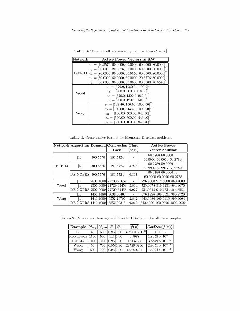
Table 3. Convex Hull Vectors computed by Lara et al. [5]

Network Active Power Vectors in KW

IEEE 14

v1 = [40.5576, 60.0000, 60.0000, 60.0000, 80.0000]T

v2 = [80.0000, 20.5576, 60.0000, 60.0000, 80.0000]T

v3 = [80.0000, 60.0000, 20.5576, 60.0000, 80.0000]T

v4 = [80.0000, 60.0000, 60.0000, 20.5576, 80.0000]T

v5 = [80.0000, 60.0000, 60.0000, 60.0000, 40.5576]T

Wood

v1 = [320.0, 1080.0, 1100.0]T

v2 = [800.0, 600.0, 1100.0]T

v3 = [320.0, 1200.0, 980.0]T

v4 = [800.0, 1200.0, 500.0]T

Wong

v1 = [343.40, 100.00, 1000.00]T

v2 = [100.00, 343.40, 1000.00]T

v3 = [100.00, 500.00, 843.40]T

v4 = [500.00, 500.00, 443.40]T

v5 = [500.00, 100.00, 843.40]T

Table 4. Comparative Results for Economic Dispatch problems.

Network Algorithm Demand Generation Time Active PowerCost (seg.) Vector Solution

IEEE 14

[10] 300.5576 181.5724 -[60.2788 60.0000 . . .

60.0000 60.0000 60.2788]

[4] 300.5576 181.5724 4.276[60.2789 59.9999 . . .

59.9999 59.9997 60.2789]

DE-NGFRS 300.5576 181.5724 0.811[60.2788 60.0000 . . .

60.0000 60.0000 60.2788

Wood[11] 2500.1000 22730.21669 - [726.9000 912.8000 860.4000][4] 2500.0000 22729.32458 2.814 [725.0078 910.1251 864.8670]

DE-NGFRS 2500.0000 22729.32458 0.027 [724.9915 910.1534 864.8551]

Wong[12] 1462.4480 6639.50400 - [376.1226 100.0521 986.2728][4] 1443.4000 6552.23790 2.842 [343.3980 100.0415 999.9604]

DE-NGFRS 1443.4000 6552.09315 0.260 [343.4000 100.0000 1000.0000]

Table 5. Parameters, Average and Standard Deviation for all the examples

Example Npop Ngen F Cr f(x) EstDev(f(x))

G6 50 500 0.95 0.90 −5.9090 × 108 0.01118

Rosenbrock 1500 500 1.2 0.90 0.9988 1.8058 × 10−15

IEEE14 1000 1000 0.95 0.90 181.5724 3.8849 × 10−12

Wood 50 700 0.95 0.90 22729.3246 2.9451 × 10−11

Wong 500 700 0.95 0.90 6552.0931 1.6024 × 10−11


In this paper we present an algorithm called NGFRS, which allows us togenerate a population of individuals that fills a convex area delimited by linearconstraints. The same ideas of NGFRS have been applied to solve non-linear,linearly constrained optimization problems; the resulting algorithm is called DE-NGFRS. It has been empirically shown that NGFRS exhibits a performance waysuperior to DE with a penalty function. The results obtained in the solution ofeconomic dispatch problems using DE-NGFRS was compared with the resultspresented for those problems in previous work; DE-NGFRS proved to improvethose results. Additionally, DE-NGFRS proves to be better than Algorithm GA-V, which is based on Genetic Algorithms.

References

1. Jorge, N., Wright, S.J.: Numerical Optimization. Springer (2000)2. Stevenson, W.D.: Elements of Power System Analysis. Mc Graw Hill (1982)3. dos Santos Coelhoa, L., Marianib, V.C.: Improved differential evolution algorithms

for handling economic dispatch optimization with generator constraints. EnergyConversion and Management, 48, 1631–1639 (2007)

4. Calderon Felix, Fuerte-Esquivel Claudio R, S.J., J., F.J.: A constraint-handlinggenetic algorithm to power economic dispatch. MICAI 2008: Advances in ArtificialIntelligence Lecture Notes in Computer Science, 371–381 (2008)

5. Lara, C., Flores, J.J., Calderon, F.: On the hyperbox hyperplane intersectionproblem. Infocomp Computer Journal Computer Science, 8, 21–27 (2009)

6. Storn, R., Price, K., Lampinen, J.: Differential Evolution. A Practical Approachto Global Optimization. Springer–Verlag, Berlin, Germany (2005)

7. Fischer, H.: A History of the Central Limit Theorem: From Classical to ModernProbability Theory. Springer (2010)

8. Lawson, C.L.: Properties of n-dimensional triangulations. Computer-Aided Geo-metric Design, 3, 231–246 (1986)

9. Storn, R., Price, K.: Differential evolution – a simple and efficient adaptive schemefor global optimization over continuous spaces. Technical Report 95-012, ICSI(1995)

10. Ongsakul, W., Ruangpayoongsak, N.: Constrained dynamic economic dispatchby simulatedannealing/genetic algorithms. In: Power Industry Computer Applica-tions, 2001. PICA 2001. Innovative Computing for Power - Electric Energy Meetsthe Market. 22nd IEEE Power Engineering Society International Conference, 207–212 (2001)

11. Wood, A., Wollenberg, B.: Power Generation, Operation, and Control. John Wileyand Sons Inc (1984)

12. Wong, K., Fung, C.: Simulated annealing based economic dispatch algorithm.In: Generation, Transmission and Distribution, IEE Proceedings C. Volume 140,509–515 (1993)


Determination of Optimal Cutting Condition

for Desired Surface Finish in Face Milling Process

Using Non-Conventional Computational Methods

Muthumari Chandrasekaran and Amit Kumar Singh

North Eastern Regional Institute of Science and Technology (NERIST), India [email protected]

Abstract. CNC (Computer Numerical Control) milling process is one of the

common metal removal operation used in industries because of its ability to remove

material faster with reasonably good surface quality. Surface roughness is the most

important attributes of the manufactured component in finish machining process. To

obtain required surface finish the selection of optimal cutting condition so as to

minimize the total production time is aimed in this work. In contrast to structured

conventional/traditional algorithm, this paper discusses the use of three non-

conventional optimization methods viz., Particle Swarm Optimization (PSO),

Teaching Learning Based Optimization (TLBO), and Fuzzy set based optimization

to solve optimization problem. To demonstrate the procedure and performance of

the approach illustrative examples are discussed. The algorithms are coded in

Matlab® and computational efforts, accuracy of result, effectiveness of algorithm are

compared.

Keywords: Finish milling, fuzzy set, optimization, PSO, TLBO.

1 Introduction

Optimization of machining parameters is an important step for the selection of cutting

conditions in CNC machining being used in today’s automated manufacturing system.

Among several CNC machining process, face milling is one of the commonly used metal

removal operations for machining casted components due to its ability to remove material

faster with reasonable good surface quality. For optimizing the process, number of

researchers used various conventional and non-conventional optimization techniques both

for single or multi pass machining problems. The conventional methods of optimization

such as graphical techniques, constrained optimization strategy, dynamic programming,

branch and bound algorithm, etc., have been used for the optimization of cutting

parameters [1,2]. These techniques are found to be ineffective since they either result in

local minima, or take long time to converge on a reasonable result. Mukherjee and Ray [3]

mentioned that the determination of optimal cutting conditions through cost–effective

mathematical models is a complex research for long time and the techniques for process

modeling and optimization have undergone substantial development and expansion. In

recent past, the researchers have used soft computing techniques as they are being

preferred to physics-based models for predicting the performance of machining processes.

Chandrasekaran et al. [4] have reviewed nearly 20 years of research work in the area of

metal cutting processes with the application of soft computing methods. The use of major

soft computing tools such as neural networks, fuzzy sets, genetic algorithms, simulated

annealing, ant colony optimization, and particle swarm optimization in performance

prediction and optimization of four common machining process viz., turning, milling,

drilling, and grinding is aimed in their work.

Wang [5] employed an optimization strategy for single pass end milling on CNC

machine tools considering many practical constraints for optimization of minimum

production time per component. Shunmugam et al. [6] used GA for optimization of multi

pass face milling process to minimize minimum production cost. The machining

parameters such as cutting speed, feed per tooth, depth of cut, and number of passes are

optimized. Baek et al. [7] developed a method for optimization of a face milling process

using a surface roughness model. Rao et al. [8] carried out the optimization of multi pass

milling using three non-conventional optimization algorithms namely artificial bee colony

(ABC), particle swarm optimization (PSO) and simulated annealing (SA). From the

review of literatures, most of the researchers used soft computing based optimization

methods and found good results over conventional optimization approach. The literature

related to milling optimization is mainly concerned with single objective only, mostly of

minimization of production time or cost. Also the fuzzy set based optimization, teaching

learning based optimization is not attempted earlier in optimizing milling process.

In the present work, the determination of optimal cutting condition to achieve desired

surface finish in a face milling process for minimizing the total production time is

attempted. Three non-conventional optimization methods, viz., PSO, TLBO and Fuzzy set

based optimization are employed to solve the problem. The accuracy of the results,

computational effort, and efficiency of algorithm are found advantageous in comparison

with conventional optimization techniques.

2 Mathematical Formulation

In CNC milling, the desired surface roughness is aimed in finish pass during which the

depth of cut remains constant. The surface roughness mainly depends on selected cutting

conditions viz., cutting velocity and feed per tooth. In this work, an optimization model

proposed by Singh et al. [9] to minimize the total production time is used. The total

production time composed of: (i) Actual machining time (Tm), (ii) Work piece loading

and unloading time (Tl/u), (iii) Cutter change time (Ttc) and (iv) Machine preparation

time (Tp) to produce batch of components. Thus the total production time being sum of all

above is expressed as:

186 Muthumari Chandrasekaran and Amit Kumar Singh

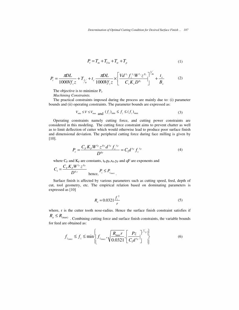
/t m l u tc pP T T T T= + + +

(1)

s

s

m

q

vv

pty

z

x

z

cu

l

z

tB

t

DKC

zWfVd

zVf

DLtT

zVf

DLP

v

vvzv

+

×++=

1

10001000

ππ (2)

The objective is to minimize Pt.

Machining Constraints.

The practical constraints imposed during the process are mainly due to: (i) parameter

bounds and (ii) operating constraints. The parameter bounds are expressed as:

min maxV V V≤ ≤ and min max( ) ( )z z zf f f≤ ≤

(3)

Operating constraints namely cutting force, and cutting power constraints are

considered in this modeling. The cutting force constraint aims to prevent chatter as well

as to limit deflection of cutter which would otherwise lead to produce poor surface finish

and dimensional deviation. The peripheral cutting force during face milling is given by

[10].

1

F F F F

F F

F

t p x y

x yF F zz zq

C K W z d fP C d f

D= =

(4)

where CF and KF are constants, tF,pF,xF,yF and qF are exponents and

1

F F

F

t p

F F

q

C K W zC

D=

hence, (max)z zP P≤.

Surface finish is affected by various parameters such as cutting speed, feed, depth of

cut, tool geometry, etc. The empirical relation based on dominating parameters is

expressed as [10]

2

0.0321 za

fR

r=

(5)

where, r is the cutter tooth nose-radius. Hence the surface finish constraint satisfies if

(max)aR R≤ . Combining cutting force and surface finish constraints, the variable bounds

for feed are obtained as:

1

(min) (max)

max

1

min , ,0.0321

yF

Fz z z x

R r Pzf f f

C d

≤ ≤

(6)

Determination of Optimal Cutting Condition for Desired Surface Finish ... 187

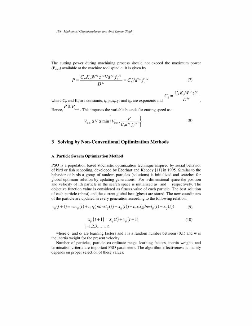
The cutting power during machining process should not exceed the maximum power

(Pmax) available at the machine tool spindle. It is given by

2 P P P P

P P

P

t p x y

x yP P zzq

C K W z Vd fP C Vd f

D= =

(7)

where CP and KP are constants, tP,pP,xP,yP and qP are exponents and 2

P P

P

t p

P P

q

C K W zC

D=

.

Hence, (max)P P≤

. This imposes the variable bounds for cutting speed as:

min max

2

min , ,P Px y

z

PV V V

C d f

≤ ≤

(8)

3 Solving by Non-Conventional Optimization Methods

A. Particle Swarm Optimization Method

PSO is a population based stochastic optimization technique inspired by social behavior

of bird or fish schooling, developed by Eberhart and Kenedy [11] in 1995. Similar to the

behavior of birds a group of random particles (solutions) is initialized and searches for

global optimum solution by updating generations. For n-dimensional space the position

and velocity of ith particle in the search space is initialized as and respectively. The

objective function value is considered as fitness value of each particle. The best solution

of each particle (pbest) and the current global best (gbest) are stored. The new coordinates

of the particle are updated in every generation according to the following relation:

( ) ))()(())()(()(.1 2211 txtgbestrctxtpbestrctvwtv ijijijijijij −+−+=+

(9)

( )1 ( ) ( 1)ij ij ijx t x t v t+ = + +

(10)

j=1,2,3,…….n

where c1 and c2 are learning factors and r is a random number between (0,1) and w is

the inertia weight for the present velocity.

Number of particles, particle co-ordinate range, learning factors, inertia weights and

termination criteria are important PSO parameters. The algorithm effectiveness is mainly

depends on proper selection of these values.


An Example.

Consider a finish pass milling process at a constant depth of cut of 1.5 mm to obtain

desired surface finish of 2.0 µm. The length (l) and width (w) of the work piece is 300 mm

and 150 mm respectively. The cutter size (D) is 160 mm. The length of travel by the cutter

(L) is considered as (L + D) and is 460 mm. A work material of grey cast iron is machined

with cutter made of cemented carbide. The other parameters remain constant as shown in

Table 1.

Table 1. Numerical data of the example problem.

Process : Face Milling

Cutting speed range (V)

Table feed range ( fz)

Number of teeth (z)

Tool change time ( tc)

M/c preparation time ( ts)

Loading and unloading time ( Tl/u )

Batch size ( Bs)

50 – 300 m/min

0.1 – 0.6 mm/tooth

16 Nos

5 min

15 min

1.5 min

150 Nos.

Constants and exponents

Tool life: Cv = 445, Kv = 1.0, m = 0.32, xv =0.15, yv = 0.35, pv = 0, qv = 0.2, tv = 0.2

Cutting Force: CF =534.6, KF = 1.0, tF = 1, pF = 1.0, xF =0.9, yF = 0.74, qF = 1.0

Cutting Power: CP = 0.5346, KP = 1.0, tP = 1.0, pP = 0, xP =0.9, yP = 0.74, qP = 1.0

PSO was performed for desired surface roughness value of 2.0 µm. Ten particles are

considered as initial population and the particle’s co-ordinates are randomized in the

solution space. In subsequent iterations all swarms move towards optimum and it is

reached in 8th iterations. The optimum parameters are 180.9 m/min and 0.137 mm/tooth

for V and fz respectively. The total production time obtained is 2.2061 min. The algorithm

was coded in Matlab® and run on a Pentium 4 PC.

B. Teaching-Learning-Based Optimization (TLBO) Method

In solving machining optimization problems ‘nature-inspired’ heuristic optimization

techniques are becoming popular and proven to be better than conventional optimization

methods. However, the applications of these algorithms are effective for specific kind of

problem and the selection of optimal controlling parameters found to be difficult. Rao et

al. [12] proposed a new optimization technique known as “Teaching-Learning-Based-

Optimization (TLBO)” based on philosophy of the teaching-learning process. TLBO

being population based method has a ‘group of learners’ learns both from the teacher in

‘Teacher phase’ as well as through interaction between them in ‘Learner phase’. They

have applied this technique for different benchmark design optimization problems and


shows better performance with less computational effort. This technique is applied here

for obtaining optimal cutting parameters for finish milling process in which ‘initial

randomized solution’ considered as ‘number of learners’, ‘best solution of the iteration’ as

‘teacher of the iteration’ and ‘decision variables’ as ‘courses or subjects offered’ by them

in the process of learning.

Steps in the TLBO.

The optimization methodology based on TLBO [12] consists of following steps:

Step 1: Randomize initial population (n=number of learners) and the termination criteria

(i.e., number of generation).

Step 2: In teacher phase, first calculate mean of each decision variables (V & fz) of the

optimization problem and identify mean row vector (i.e., MD = [V,fz]). The new mean

(M_new,D) is the best solution of the iteration and will act as a teacher.

Step 3: Now update the current solution by adding the ‘difference of the means’ to it. The

difference between the means is given by Eq. 11.

( _ )D D f D

Diff r M new t M= − ×

(11)

where r is a random number in the range [0,1] and tf is teacher factor which is either 1 or

2. The new solution is accepted if it gives better function value otherwise not.

Step 4: In learner phase, select any two learners (data sets) and evaluate its function

values. Based on their function values the new data set (Xnew) is calculated. If 1tP

and

2tP

are the two function values,

1 2

2 1

1 2

2 1

( )

( )

new old t t

new old t t

X X r X X if P P

and X X r X X if P P

= + − <

= + − <

(12)

Accept Xnew if it gives better function value otherwise not.

Step 5: Continue from Step 2 till the termination criteria is met.

An Example.

For the illustrated problem stated in previous section the optimum cutting condition

obtained by TLBO is (180.9, 0.137) and the total production time at optimal cutting

condition is 2.2061 min and the solution is converged in three iterations. Table 2 shows

iteration wise result of the problem. Number of problems having depth of cut from 1.5

mm to 2.5 mm for different values of surface roughness are tested and results are better

than PSO.


Table 2. Iteration wise result.

Input data (d,Ra): 1.5 mm, 2.0 µm

Iteration

No.

Optimum cutting parameters

(V (m/min) and fz (mm/tooth))

Pt

(min)

1 177.9, 0.137 2.2172

2 180.7, 0.137 2.2073

3 180.9, 0.137 2.2061

C. Fuzzy Set Based Optimization Method

Prof. Zadeh introduced fuzzy set theory in 1965 and it has been applied to a number of

engineering problems. Its applications include: (i) use of fuzzy set operations in decision

making, (ii) use of fuzzy arithmetic wherein physical variables are considered as fuzzy

numbers and (iii) use of fuzzy logic in modeling and control problems. Recently,

Chandrasekaran et al. [13] have developed a fuzzy rule based optimization procedure for

solving general optimization problems, which can provide an approximate and multiple

solutions. They used fuzzy set theory as a general optimization tool for optimizing multi

pass turning process and the method is applied here to obtain optimum cutting condition.

Steps in the Fuzzy Set Optimization.

The proposed optimization strategy using fuzzy logic consists of the following steps:

Step 1: The search domain is divided into a number of cells with the decision variables

fuzzified into a number of fuzzy sub-sets. Membership grade 1 is allotted to centroids of

the cell and 0 to the boundaries of the cell. A linear membership function is considered for

the fuzzy subset.

Step 2: Machining is performed at each cell centroids and evaluate the function values

at cell centroids. Now, decide the minimum ( minPt ) and maximum ( max

Pt ) values.

Fuzzyify them into n number of overlapping fuzzy sets as shown in Figure 5. If minPt

and maxPt are the variable bounds then for i-th fuzzy subset of the fuzzified variable, the

value at the vertex corresponding to the membership grade 1 is given by:

( )min min

min

P Pvalue at the vertex = P 1

1

t t

t in

−+ −

−

(13)

The right and left limits of the fuzzy subset (vertices corresponding to 0 membership

grades) are given by


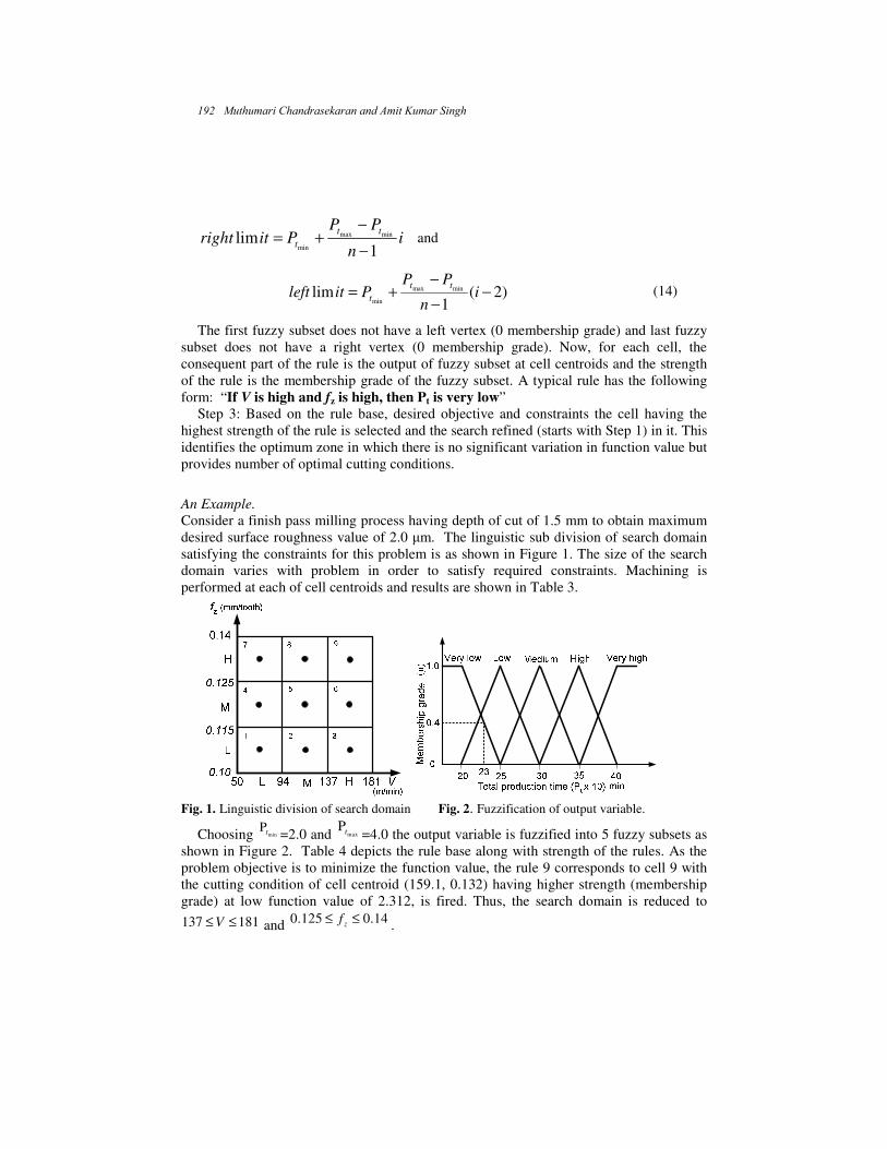
in

PPPitright

tt

t1

lim minmax

min −

−+= and

)2(1

lim minmax

min−

−

−+= i

n

PPPitleft

tt

t (14)

The first fuzzy subset does not have a left vertex (0 membership grade) and last fuzzy

subset does not have a right vertex (0 membership grade). Now, for each cell, the

consequent part of the rule is the output of fuzzy subset at cell centroids and the strength

of the rule is the membership grade of the fuzzy subset. A typical rule has the following

form: “If V is high and fz is high, then Pt is very low”

Step 3: Based on the rule base, desired objective and constraints the cell having the

highest strength of the rule is selected and the search refined (starts with Step 1) in it. This

identifies the optimum zone in which there is no significant variation in function value but

provides number of optimal cutting conditions.

An Example.

Consider a finish pass milling process having depth of cut of 1.5 mm to obtain maximum

desired surface roughness value of 2.0 µm. The linguistic sub division of search domain

satisfying the constraints for this problem is as shown in Figure 1. The size of the search

domain varies with problem in order to satisfy required constraints. Machining is

performed at each of cell centroids and results are shown in Table 3.

Fig. 1. Linguistic division of search domain Fig. 2. Fuzzification of output variable.

Choosing minPt =2.0 and max

Pt =4.0 the output variable is fuzzified into 5 fuzzy subsets as

shown in Figure 2. Table 4 depicts the rule base along with strength of the rules. As the

problem objective is to minimize the function value, the rule 9 corresponds to cell 9 with

the cutting condition of cell centroid (159.1, 0.132) having higher strength (membership

grade) at low function value of 2.312, is fired. Thus, the search domain is reduced to

137 181V≤ ≤ and 0.125 0.14zf≤ ≤

.


Table 3. Function values at centroids of each cell.

Input data (d,Ra): 1.5 mm, 2.0 µm

Cell

No.

Cell centroids

V (m/min), fz (mm/tooth)

Total

Production time

(Pt) (min)

1 (71.8,0.106) (low-low) 3.498

2 (115.5,0.106) (medium-low) 2.788

3 (159.1,0.106) (high-low) 2.473

4 (71.8,0.119) (low-medium) 3.301

5 (115.5, 0.119) (medium-medium) 2.670

6 (159.1,0.119) (high-medium) 2.384

7 (71.8, 0.132) (low-high) 3.141

8 (115.5,0.132) (medium-high) 2.570

9 (159.1,0.132) (high-high) 2.312

Table 4. Fuzzy rule base with membership strength.

Cell

No

Cutting

speed (V)

Feed

(fz)

Total

production

time (Pt)

Membership

grade

1 Low Low High 1.0

2 Medium Low Low 0.4

3 High Low Low 1.0

4 Low Medium Medium 0.4

5 Medium Medium Low 0.6

6 High Medium Very Low 0.2

7 Low High Medium 0.8

8 Medium High Low 0.8

9 High High Very Low 0.4

The new search is now initiated in the identified search domain, dividing it into 4 cells

with the fuzzy sub-set being ‘low’ and ‘high’. This provides new domain:159.1 180.9V≤ ≤

and0.13 0.14z

f≤ ≤ . The function value has no significant variation which is in the range

between 2.2 and 2.3. Thus, with the given range of cutting speed and feed rate, the fuzzy

set based optimization provides the following solution.

159.1 180.9, 0.13 0.14zV f≤ ≤ ≤ ≤

(15)

With small variation in time the fuzzy set based optimization provides multiple

numbers of solutions.

A number of other problems having depth of cut varying from 1.5 mm to 2.5 mm for

different values of desired surface roughness are tested. The optimum zone provides

multiple solutions to the problem. The function value and surface roughness produced in

optimum fuzzy domain do not vary significantly.


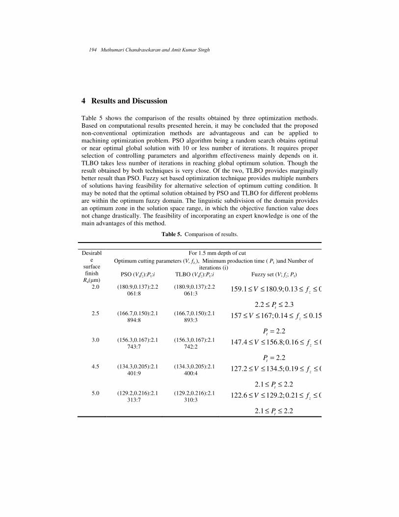
4 Results and Discussion

Table 5 shows the comparison of the results obtained by three optimization methods.

Based on computational results presented herein, it may be concluded that the proposed

non-conventional optimization methods are advantageous and can be applied to

machining optimization problem. PSO algorithm being a random search obtains optimal

or near optimal global solution with 10 or less number of iterations. It requires proper

selection of controlling parameters and algorithm effectiveness mainly depends on it.

TLBO takes less number of iterations in reaching global optimum solution. Though the

result obtained by both techniques is very close. Of the two, TLBO provides marginally

better result than PSO. Fuzzy set based optimization technique provides multiple numbers

of solutions having feasibility for alternative selection of optimum cutting condition. It

may be noted that the optimal solution obtained by PSO and TLBO for different problems

are within the optimum fuzzy domain. The linguistic subdivision of the domain provides

an optimum zone in the solution space range, in which the objective function value does

not change drastically. The feasibility of incorporating an expert knowledge is one of the

main advantages of this method.

Table 5. Comparison of results.

Desirabl

e

surface

finish

Ra(µm)

For 1.5 mm depth of cut

Optimum cutting parameters (V, fz,), Minimum production time ( Pt )and Number of

iterations (i)

PSO (V,fz):Pt:i TLBO (V,fz):Pt:i Fuzzy set (V; fz; Pt)

2.0 (180.9,0.137):2.2

061:8

(180.9,0.137):2.2

061:3 159.1 180.9;0.13 0.14zV f≤ ≤ ≤ ≤

2.2 2.3tP≤ ≤

2.5 (166.7,0.150):2.1

894:8

(166.7,0.150):2.1

893:3 157 167;0.14 0.15zV f≤ ≤ ≤ ≤

2.2tP =

3.0 (156.3,0.167):2.1

743:7

(156.3,0.167):2.1

742:2 147.4 156.8;0.16 0.17zV f≤ ≤ ≤ ≤

2.2tP =

4.5 (134.3,0.205):2.1

401:9

(134.3,0.205):2.1

400:4 127.2 134.5;0.19 0.21zV f≤ ≤ ≤ ≤

2.1 2.2tP≤ ≤

5.0 (129.2,0.216):2.1

313:7

(129.2,0.216):2.1

310:3 122.6 129.2;0.21 0.22zV f≤ ≤ ≤ ≤

2.1 2.2tP≤ ≤


In general the result shows that the total production time per component reduces as the

maximum allowable surface finish increases. Figure 3 shows the result of total production

time Vs desired surface roughness for different values depth of cut. From the graph it is

evident that the production time decreases as depth of cut decreases. However in finish

machining process depth of cut remains constant. Among the other two influencing

parameters i.e., feed and cutting velocity, feed is constrained mainly due to desired

surface roughness value while cutting velocity by cutting power. Since the cutting power

is the function feed, depth of cut and cutting velocity, the increased depth of cut

proportionately decreases optimum cutting velocity while feed remains fixed due to

surface roughness criterion.

Fig. 3. Variation of ‘Ra’ Vs ‘Pt’.

5 Conclusions

In this work, CNC milling process is optimized to minimize total production time and so

as to obtain desired surface finish value of the components produced. Cutting speed and

feed per tooth as decision variables and practical constraints such as cutting force, cutting

power, surface roughness, and variable bounds of the decision variables are considered in

model formulation. Three non-conventional optimization methods viz., PSO, TLBO, and

Fuzzy set based optimization are employed to solve the problem. The solution

methodology is presented with an illustrated example and numbers of problems are

solved.

Both PSO and TLBO provide better solution accuracy with less computational effort

compared with conventional optimization techniques. Of the two, TLBO provides

marginally better result than PSO with less number of iterations. PSO need proper


selection of controlling parameters and effectiveness of algorithm is mainly depends on it.

While TLBO is free from such algorithm parameters and found easy to implement it.

Fuzzy set optimization is based on linguistic subdivision of the domain providing a ‘range

of optimal solution’ in which the objective function value does not change drastically.

Thus the procedure provides multiple numbers of optimal solutions having feasibility for

alternative selection. Source codes for all three methods are written in MATLAB 7.2 and

computational time takes less than a second in Pentium-IV with RAM 512. The code can

be used for other finish machining process as well as for multi pass machining with

necessary modification

Acknowledgements. The authors acknowledges The Director, NERIST (DU), Govt. of

India for providing necessary financial assistance required for presenting the paper in 10th

MCAI conference held in Mexico.

References

1. Armarego, E.J.A., Smith, A.J.R., Wang, J.: Constrained optimization strategies and CAM

software for single-pass peripheral milling. Int. J. Prod. Res. vol. 31, no. 9, pp. 2139–2160

(1993)

2. Wang, J., Armarego, J.A.: Computer-aided optimization of multiple constraint single pass face

milling operations. Mach. Sci. Technol., vol. 5, no. 1, pp. 77–99 (2001)

3. Mukherjee, I., Ray, P.K.: A review of optimization techniques in metal cutting processes.

Computers & Industrial Engineering, vol. 50, no. 1–2, pp. 15–34 (2006)

4. M. Chandrasekaran, M., Muralidhar, C., Krishna, M., Dixit, U.S.: Application of soft computing

techniques in machining performance prediction and optimization: a literature review. Int. J. of

Adv. Manuf. Technol, vol. 46, no. 5–8, pp. 445–464 (2010)

5. Wang, J.: Computer aided economic optimisation of end milling operations. Int. J. Prod. Econ.,

vol. 54, pp. 307–320 (1998)

6. Shunmugam, M.S., Bhaskara Reddy, S.V., Narendran, T.T., Selection of optimal conditions in

multi-pass face-milling using a genetic algorithm. Int. J. Mach. Tools Manuf., vol. 40, pp. 401–

414 (2000)

7. Baek, D.K., Ko, T.J., Kim, H.S.: Optimization of feed rate in a face milling operation using a

surface roughness model. Int. J. of Mach. Tools & Manuf., vol. 41, pp. 451–462 (2001)

8. Rao, P.V., Pawar, P.J.: Parameter optimization of a multi-pass milling process using non-

traditional optimization algorithms. Applied soft computing, Vol. 10, 2010, pp. 445–456 (2010)

9. Singh, A.K., Chandrasekaran, M., Murali Krishna, C.: Optimization of finish-pass milling process

with practical constraints using particle swarm intelligence. Proc. 3rd Intl. & 24th AIMTDR

conference, Visakhapatnam, India. pp. 519–524 (2010)

10. Nefedov, N., Osipov, K.: Typical examples and problems in metal cutting and tool design. MIR

Publishers, Moscow (1987)

11. Kennedy, J., Eberhart, R.: Particle swarm optimization. In: Proc. IEEE Intl. Conf. on Neural

Networks (ICNN’95) Perth, Australia (1995)


12. Rao, P.V., Sasani, V.J., Vakharia, D.P.: Teaching-learning-based optimization: A novel method

for constrained mechanical design optimization problems. Computer-Aided Design, vol. 34, pp.

303-315 (2011)

13. Chandrasekaran, M., Muralidhar, M., Dixit, U.S.: Optimization of engineering problems by

Fuzzy set theory: An Application to Multipass Turning process. In: Proc. IISN-2010 Conf. ISTK,

Yamuna Nagar, Haryana, INDIA. pp. 539–542 (2010)


Dynamic Quadratic Assignment to Model Task

Assignment Problem to Processors in a 2D Mesh

A. Velarde M.1, E. Ponce de Leon S.2, E. Díaz D.2 and A. Padilla D.2

1 NSS Softtek, Unix Developer2 Universidad Autónoma de Aguascalientes, Mexico

Abstract. Mesh multicomputers systems are a viable option for par-allel computing. The process of executing a task in such systems is toassign a set of n+1 mesh-free processors to the task at the head of thequeue consisting of n subtasks. We assume that a task has a parent pro-cess and child processes that are called subtasks. These allocations arebased on methods that seek to maintain the execution of the task in ad-jacent processors, and methods that avoid maintaining free sub-meshesin the mesh caused by tasks that have completed their execution. AssignN facilities to a number N of sites or locations where it is considered acost associated with each of the assignments can be seen as a quadraticassignment problem whose solution combinations grow exponentially, anNP-complete problem. This paper describes a method for modelling dy-namic quadratic assignment problem of assigning tasks to processors in2D mesh multicomputers system, using the simplest class of the Esti-mation of Distribution Algorithm (EDA), the Univariate Marginal Dis-tribution Algorithm (UMDA) which aims to enable calculation of a dis-tribution joint probability from the selected tasks in the queue that aresusceptible to initiate enforcement in the mesh. Experiments are basedon a comparison the proposed method with two more methods of allo-cation of tasks to processors: Hilbert curves and linear assignment. Theresults show better time allocation, and better utilization of free proces-sors but more times during the process of full recognition of the mesh.The denser workload down to 256 with 256 subtasks tasks each, 16× 16mesh size, that correspond to 256 processors.

Keywords: Parallel computing, mesh multicomputer, estimation of dis-tribution algorithm, univariate marginal distribution algorithm.

1 Introduction

Distributed computing has been considered as the future of high performancecomputing [1]. The study of partitioning of dierent distributed computing sys-tems such as multiprocessor systems shared memory multicomputers systemswith transfer messages and wide-area distributed systems have been extensivelystudied in order to get more computing power, and thus permit tasks that areinherently parallel [2], run on shorter time. Examples of these tasks that requiremore computing power than a single node can provide are: access to distributed

data in dierent groups of computers [3], the graphics processing tasks [2] andin elds of science and engineering.

Parallel computing consists of a set of processors which cooperate with eachother to nd a solution to a given problem [4]. The processor communication canbe based on shared memory or distributed memory model. In shared memoryarchitectures also known as multiprocessor systems, processors communicate viashared memory. However, in parallel computers with distributed memory alsoknown as multicomputers the processors communicate is by exchanging messagesthrough interconnection network [5].

To solve a problem using parallel computing should break down probleminto smaller subproblems that can be solved in parallel. The results should beeciently combined to obtain the end result of the main problem, but is not easyto break a problem due to data dependency that exists in it and then. Due to datadependency that exists in a problem, it is not easy to divide it into subproblemsbecause the load of communication when the problem is running in parallelis very high. The important point here is the time taken for communicationbetween two processors compared to the processing time. Due to this factorcommunication scheme should be well planned to get a good parallel algorithm[4].

There are several approaches to implement parallel computing: through meshes[6], squares (grids) [3], and heterogeneous platforms [2], using certain perfor-mance metrics, heuristics such as simulated annealing [1] or the greedy algorithm[3], and alternative methods such as measuring the workload, where the work-load is generated not by discovery but dynamically by user models that interactwith the system and whose behaviour in simulation is similar to the behaviourof users in reality [8].

The vast majority of research converge on the approach that two structuresare to be developed in software for coexistence of multiple processors executingtasks in parallel: the allocation Processor and Task Scheduler [9].

Some of the objective functions that is desirable to minimizing or maximizingin the research work are: reduce the starvation of jobs, decrease internal frag-mentation, reduce external fragmentation, reduce costs communication withinlocal networks to reduce communication costs in wide area networks, reduce thenumber of jobs in the queue, maximize the number of jobs running in paral-lel, maximizing the time response to users to maintain their satisfaction andmotivate them to bring more jobs to the system [8].

The optimization problems that model a physical system which involves oneobjective function perform the task of nding an optimal solution is calleda single objective optimization, and when the problem optimization involvesmore than one objective function, the task of nding one or more optimal solu-tions is known as multi-objective optimization, also known as Multiple CriterionDecision-Making (MCDM) [10].

In evolutionary computation have emerged parallel multi-objective evolu-tionary algorithms their application to solve problems with long performance,excessive memory requirements to solve complex problems, decrease the like-

200 A. Velarde M., E. Ponce de Leon S., E. Díaz D., and A. Padilla D.

lihood of falling into local optima, nd solutions domains simultaneously andwork with multi-objective [11].

The objective of this paper is to describe a method for modelling dynamicquadratic assignment problem of assigning tasks to processors in 2D mesh mul-ticomputers system, using the simplest class of the estimation of distributionalgorithm (EDA), the univariate marginal distribution algorithm (UMDA)whichaims to enable calculation of a distribution joint probability from the selectedtasks in the queue that are susceptible to initiate enforcement in the mesh,considering two structures that are necessary to execute tasks in parallel: theAllocation Processor and Task Scheduler.

2 Allocation Algorithms

Ecient allocation of processors and scheduling tasks are two critical processesif the computational power of large-scale multicomputers want to eectively use[12]. Allocation Processor is responsible for nding, selecting and assigning allprocessors on which a parallel job will run, while the Task Scheduler is respon-sible for determining the order in which the jobs are selected for execution usinga scheduling policy [13].

If a job arrives and can not be immediately executed within the system dueto lack of free processors, or the existence of other jobs running, it is sent tothe queue. Once the processors are assigned to a task, they remain allocatedexclusively to it until the task ends. When the task ends and leaves the system,processors are released and made available to Allocation Processor. One of themain goals of parallel execution is to minimize the time that a job waits a setof free processors in the mesh are assigned to it, so it is important to developalgorithms with ecient allocation strategies processors, that minimize waitingtime of tasks within the mesh.

Is necessary to consider the following denitions:

Denition 1. An n-dimensional mesh has k0 × k1 × ... × kn−2 × kn−1 nodes,where ki is the number of nodes along the ith dimension and ki ≥ 2.Each node isidentied by n coordinates, ρ0(a), ρ1(a), ... , ρn−2(a), ρn−1(a), where 0 ≤ ρi(a)< ki for 0 ≤ i < n. Two nodes a and b are neighbours if and only if ρi(a) = ρi(b)for all dimensions except for one dimension j, where ρj(b) = ρj(a) ± 1. Eachnode in a mesh refers to a processor and two neighbours are connected by a directcommunication link.

Denition 2. A 2D mesh, which is referenced as M(W,L) consists of W ×Lprocessors, where W is the width of the mesh and L is the length. Each processoris denoted by a pair of coordinates (x, y), where 0 ≤ x < W y 0 ≤ y < L.A processor is connected by a bidirectional communication link to each of itsneighbours.

Dynamic Quadratic Assignment to Model Task Assignment Problem to Processors in a 2D Mesh 201

Denition 3. In a 2D mesh, M(W,L), a sub-mesh S(w, l) is a sub-two-dimensional mesh nodes belonging to M(W,L) with width w and length l, where0 < w ≤ W y 0 < l ≤ L. S(w, l) is represented by the coordinates (x, y, x′, y′),where (x, y) is the lower left corner of the sub-mesh and (x′, y′) is the upper rightcorner. The node of the lower left corner is called the base node of the sub-meshnode and the upper right corner is the end node. In this case w = x′−x+1 andl = y′ − y + 1. The size of S(w, l) is w × l processors.

Denition 4. In a 2D mesh M(W,L), an available sub-mesh S(w, l) is afree sub-mesh that satises the conditions: w ≥ α y w ≥ β assuming that theassignment of S(α, β) requested, where the assignment refers to selecting a setof processors for a task arrival.

2.1 Processor Allocation Strategies

Two strategies have been developed for the allocation of processors [12], andtheir classication reects the type of recognition is performed on the mesh ofprocessors: contiguous processor allocation strategies and non contiguous proces-sor allocation strategies. In this section we briey summarize processor allocationresearch, paying special attention to request partitioning based strategies usedin our study.

Strategies contiguous processor allocation, appears when you have a partialrecognition of the system and can be assigned for the execution of work, onlycontiguous sub-mesh of processors to jobs that request. The gure 1 shows acontiguous allocation strategy of 4 processors in a mesh of size 4× 4.

Fig. 1. Contiguous allocation of 4 processors in a mesh of size 4× 4.

Such a strategy implies that even with the number of free processors in thesystem, it is not possible to assign if the sub-meshes are not contiguous. Supposea task T that requests a sub-mesh 2×2 as shown in gure 1, there is still a numberof free processors containing the sub-meshes that are not contiguous, so the taskshould be put into the queue system where it remains until a sub-mesh sizerequested is available. This causes a 4-processor external fragmentation.


The fragmentation of processors can be of two types: internal and external[14]. Internal fragmentation occurs when more processors are assigned to a jobthat really requires, while external fragmentation occurs when there are enoughfree processors to satisfy outstanding allocation requests but can not be assignedbecause it is not contiguous, gure 1 exemplies this kind of fragmentation.

Contiguous processor allocation strategies have been developed by dierentresearch for 2D mesh connected multicomputers, examples of these are the TwoDimensional Buddy System (2DBS) [15], Frame Sliding (FS) [16], Adaptive Scan[17] , First Fit (FF) and Best Fit (BF) [18]. 2DBS strategy only applies tosquare mesh systems by leading to external processor fragmentation. The FSstrategy is applicable to a mesh of any size and shape but made âânoacknowledgement of all sub-nets free, so it produces external fragmentation. TheFS technique applies an operation that allows a frame to slide across the screen.AS strategy improves system performance by applying an exchange procedureorientation of the application when it can not be accommodated in the originalorientation, for example if a job requests a sub-grid is α×β not available, can beassigned to a sub-mesh β×α however, the allocation time is high compared withFS because the search of processors in the mesh is at a distance of a processorin a vertical direction. FF and BF strategies detected all free sub-mesh bigenough, but lack the ability to complete detection of sub-nets because they donot exchange the orientation of the applications.

To reduce the fragmentation of contiguous processor allocation produced,non-contiguous processor allocations strategies have been proposed [19]. In thenon-contiguous allocation techniques jobs can run on multiple disjoint sub-meshes,avoiding a wait of one sub-mesh size and shape required. Figure 1 when a jobrequests allocation of a sub-grid of size 2×2) contiguous allocation fails becausea sub-mesh the number of processors available is not contiguous. However, thefour free processors (drawn with white circles into the gure 1) can be assignedto work when we adopt a non-contiguous allocation. Although non-contiguousallocation can increase the transfer of messages on the network, improving thecontiguity to reduce external processor fragmentation and increase usefulness.

The widespread adoption of wormhole routing [19], whose main characteris-tic is the latency of messages, less sensitive to the distance and have the abilityto moderate heavy trac conditions in practical systems, has consider non-contiguous allocation for multicomputers that use long distance communication.The method used to respond to requests for partitioned allocation has a signi-cant impact on the performance of non-contiguous allocations, so you should goto maintain a high degree of contiguity among processors assigned to a paral-lel to the overhead of communication reduced without aecting overall systemperformance [19].

The non-contiguous allocation strategies have been developed are: Random[14], Paging [14], Multiple Buddy Strategy MBS [14], Adaptive Scan MultipleBuddy and ANCA [19], Adaptive Multiple Scan Buddy and AS & MB [21], andvariants of page Recent [24]. At Random [14], internal and external fragmen-tation is eliminated but there is a high interference of communication between


jobs. In the Paging method [14], there is a degree of contiguity among processorsassigned to a parallel, which increases if you use more pages size. However theremay be internal fragmentation of the processor when pages are allocated to largejobs do not require complete. MBS [14], improves the performance compared toprevious strategies but it presents problems when assigning a sub-mesh contigu-ous free processors, so you can increase the communication overhead. ANCA [19]divide the application in 2i equal parts in the ith iteration and requires parti-tioning and assignment occur in the same iteration, which causes in a previousiteration are not allocated sub-meshes to a large part of the application, whichcan increase the communication overhead. The performance of AS & MB [21],the response time and service are identical the MBS [14], however AS & MB hashigh overhead allocation for large meshes. In the variants paging unit allocationis a single processor, which requires more time to make a decision allocation inlarge mesh, while in MBS [14] and ANCA [19], allocation unit increases so ittakes a long time to make an assignment in large systems.

3 Task Assignment Problems in a Computer Environment

Distributed

The problems of assignment, have evolved along with the architecture of dis-tributed and parallel systems, this evolution has brought some problems withperformance, on which is:

All resources reside under a single domain. The resource set is invariant. Applications and data reside on the same site or the data collection is ahighly predictable.

The scheduling in multicomputers Systems (Job Scheduling Task Scheduler) isthe selection and assignment of a partition of processors to a parallel task, withthe inherent objective of maximizing the performance of a running workow[6].The task and its subtasks that are distributed among the processors to beexecuted communicate with each other to synchronize or to exchange any partialor nal result [5].

In multicomputers system once a task or process has assigned to a multiplenodes, can be use any scheduling local algorithm. However, precisely because ithas very little control when assigns a process to a node, it is important to the de-cision of which process should be in which node. Therefore worth considering howto allocate eectively processes to nodes. The algorithms and heuristics used tomake such assignment is called processor allocation algorithms [7] performed theschedule Job [7]. There are processor allocation algorithms have been proposedover the years, considering the local assignment in which the task is assignedon one processor and those that allow assignment to a subset of multicomput-ers system processor, which will be explained in detail in the following sections.Both types of algorithms seek to maximize the clock cycles [7] to avoid and thewaste of CPU due to the lack of local labour, minimize the total bandwidth of


communication and ensure equity for users and processes.The dierences lie inwhat is known and what is to be achieved. Among the properties of a processthat could be known are: the needs CPU time, memory consumption and theamount of communication with all other processes.

4 Metaheuristics Applied to the Problem of Scheduling

Tasks

As dened above, the allocation of tasks is a scheduling problem of tasks thatshould be assigned to a set of machines. Considering the variation of the jobshop (JS) applicable to this research project, then describe some metaheuristicsapplied to this particular planning problem, in the knowledge that for everyaspect of the problem of planning there are dierent uses of heuristics.

In [25] used branch and bound techniques and present the known graph-directed search method, with which proceeds to traverse a tree, whose nodes aresequences of operations manufacturing in line. They do not consider lines withpenalties for delays or for the steps of the tasks from one machine to another,hence the direct applicability of a method sweep of trees in the instrumentselection process and trajectories.

In [26] is incorporated two new concepts in the development of an algorithmGRASP (Greedy Randomized Adaptive Search Procedures) for the JSP stan-dard: a strategic escalation procedure (another form of probability distribution)to create candidates for technical solution and a POP (its acronym in EnglishProximate Optimality Principle) also in the construction phase. Both conceptshave already been applied to solve quadratic assignment problem. Genetic algo-rithms are applied in [27]. In this paper, the representation of chromosomes isbased on random charges of elitism, the authors seek to mimic the behaviour ofa variable work environment in a exible production line. On the other hand in[28], is the division of tasks in very small chromosomes so that the populationsgenerated are as varied as possible. Tabu Search is used in [29], in this work areas neighbourhoods for the implementation of the tabu list to the movement ofa candidate operation i-ésima task to program a machine to another machine,with the Tabu list that matrix of operations and machines which run, other in-teresting works can be found in [30] considers a exible route, which is denedas one where there are machines that can run more than one type of opera-tion, extending the denition of the JSP, in [31] apply the concepts of JSP ondistributed computing techniques in programming tasks.

5 The Quadratic Assignment Problem

In Quadratic Assignment Problem (QAP), we have a set of n places and n tasks,and assign to each place a task, so there n! possible assignments. To measurethe cost of each possible allocation, multiply the ow between each pair of tasksby the distance between the assigned locations and all pairs are added. Our goal


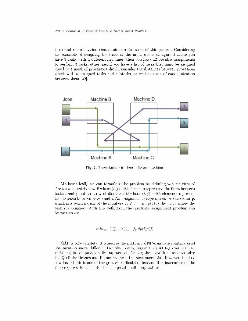
is to nd the allocation that minimizes the costs of this process. Consideringthe example of assigning the tasks of the input queue of gure 2,where youhave 3 tasks with 4 dierent machines, then you have 12 possible assignmentsto perform 3 tasks, otherwise, if you have a list of tasks that must be assignedglued to a mesh of processors should consider the distances between processorswhich will be assigned tasks and subtasks, as well as costs of communicationbetween them [29].

Fig. 2. Three tasks with four dierent machines

Mathematically we can formulate the problem by dening two matrices ofsize n×n: a matrix ow F whose (i, j)−ith elements represents the ows betweentasks i and j and an array of distances D whose (i, j) − ith elements representthe distance between sites i and j. An assignment is represented by the vector p,which is a permutation of the numbers 1, 2, ... , n . p(j) is the place where thetask j is assigned. With this denition, the quadratic assignment problem canbe written as:

minp∈∑ni=1

∑ni=1 fijdp(i)p(j)

QAP is NP-complete. It is seen as the problem of NP-complete combinatorialoptimization more dicult. Troubleshooting larger than 30 (eg over 900 0-1variables) is computationally impractical. Among the algorithms used to solvethe QAP the Branch and Bound has been the most successful. However, the lossof a lower limit is one of the greatest diculties, because it is inaccurate or thetime required to calculate it is computationally impractical.


6 Statement of Dynamic Quadratic Assignment Problem

to model the assignment of tasks to processors in a 2D

mesh multicomputers System

Given the gaps in the mesh, the chance to swap tasks at time t is given by theminimization function:

min e(πt) = (dij)(mij) + ...+ (dik,jk)(mik,jk)

Looking for the smallest value found in the set of all possible assignments attime t whose domain is the possible permutations of tasks within a sub-grid.

6.1 Description of the Modelling Problem

The assumption that we have a priori in the Modelling Problem is the knowledgeof the degree of communication between the main task and subtasks of all tasksthat are in the queue, and the relationship between those subtasks, for exampleif you have a task T1 with three subtasks S11, S12 and S13 the interactionthat can occur between them is illustrated in gure 3 through lines showing themessage transfer.

Fig. 3. Message passing between tasks, a task with 3 subtasks.

There is also a symmetric matrix of distances between processors that spec-ies the hops that a message must be made between a processor and another.Given this process of allocation of processors is based on carrying out a calcula-tion of allocation of processors based on their availability in the Grid and Tasksin the queue.

6.2 Example

Consider the following example. At a time t we have a mesh processor array ofsize 4×4 whose status is shown in Table 6.2, where 1 represents a processor busywhich was assigned to a task at time t-1, and 0 is not a free processor has beenassigned to a task or subtask, the symmetrical distance between processors aregiven by a the distance matrix where every value is calculated for each pair of


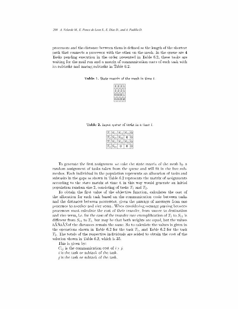
processors and the distance between them is dened as the length of the shortestpath that connects a processor with the other on the mesh. In the queue are 4Tasks pending execution in the order presented in Table 6.2, these tasks arewaiting for the mail run and a matrix of communication costs of each task withits subtasks and among subtasks in Table 6.2.

Table 1. State matrix of the mesh in time t.

1 1 1 1

1 1 1 1

0 0 0 1

0 0 0 0

Table 2. Input queue of tasks in a time t.

T1 S11 S12 S13 0

T2 S21 S22 0 0

T3 S31 S32 S33 0

T4 S41 0 0 0

To generate the rst assignment we take the state matrix of the mesh by arandom assignment of tasks taken from the queue and will t in the free sub-meshes. Each individual in the population represents an allocation of tasks andsubtasks in the gaps as shown in Table 6.2 represents the matrix of assignmentsaccording to the state matrix at time t, in this way would generate an initialpopulation random size 2, consisting of tasks T1 and T2.

To obtain the rst value of the objective function, calculates the cost ofthe allocation for each task based on the communication costs between tasksand the distances between processors, given the passage of messages from oneprocessor to another and vice versa . When considering message passing betweenprocessors must calculate the cost of their transfer, from source to destinationand vice versa, i.e. for the case of the transfer rate exemplication of T1 to S11 isdierent from S11 to T1, but may be that both weights are equal, but the valuesââof the distances remain the same. So to calculate the values is given inthe operations shown in Table 6.2 for the task T1, and Table 6.2 for the taskT2. The totals of the respective individuals are added to obtain the cost of thesolution shown in Table 6.2, which is 35.

This is given by:Cij is the communication cost of i y j.i is the task or subtask of the task.j is the task or subtask of the task.


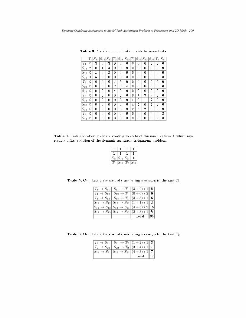
Table 3. Matrix communication costs between tasks.

T1 S11 S12 S13 T2 S21 S22 T3 S31 S32 S33 T4 S41

T1 0 3 0 3 0 0 0 0 0 0 0 0 0

S11 2 0 1 4 0 0 0 0 0 0 0 0 0

S12 0 1 0 2 0 0 0 0 0 0 0 0 0

S13 3 5 3 0 0 0 0 0 0 0 0 0 0

T2 0 0 0 0 1 3 0 0 0 0 0 0 0

S21 0 0 0 0 2 0 4 0 0 0 0 0 0

S22 0 0 0 0 4 3 0 0 0 0 0 0 0

T3 0 0 0 0 0 0 0 0 1 3 2 0 0

S31 0 0 0 0 0 0 0 1 0 1 2 0 0

S32 0 0 0 0 0 0 0 4 5 0 1 0 0

S33 0 0 0 0 0 0 0 2 5 2 0 0 0

T4 0 0 0 0 0 0 0 0 0 0 0 0 3

S41 0 0 0 0 0 0 0 0 0 0 0 2 0

Table 4. Task allocation matrix according to state of the mesh at time t, which rep-resents a rst solution of the dynamic quadratic assignment problem.

1 1 1 1

1 1 1 1

S11 S12 S21 1

T1 S13 T2 S22

Table 5. Calculating the cost of transferring messages to the task T1.

T1 → S11 S11 → T1 (3 + 2) ∗ 1 5

T1 → S12 S12 → T1 (0 + 0) ∗ 2 0

T1 → S13 S13 → T1 (3 + 3) ∗ 1 6

S11 → S12 S12 → S11 (1 + 1) ∗ 1 2

S11 → S13 S13 → S11 (4 + 5) ∗ 2 18

S12 → S13 S13 → S12 (2 + 3) ∗ 1 5

Total 35

Table 6. Calculating the cost of transferring messages to the task T2.

T2 → S21 S21 → T2 (1 + 2) ∗ 1 3

T2 → S22 S22 → T2 (3 + 4) ∗ 1 7

S21 → S21 S22 → S21 (4 + 3) ∗ 1 7

Total 17


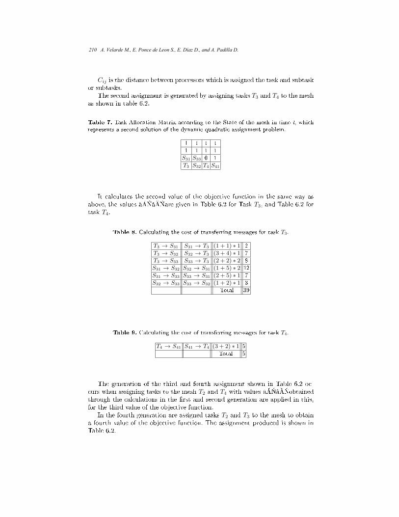
Cij is the distance between processors which is assigned the task and subtaskor subtasks.

The second assignment is generated by assigning tasks T3 and T4 to the meshas shown in table 6.2.

Table 7. Task Allocation Matrix according to the State of the mesh in time t, whichrepresents a second solution of the dynamic quadratic assignment problem.

1 1 1 1

1 1 1 1

S31 S33 0 1

T3 S32 T4 S41

It calculates the second value of the objective function in the same way asabove, the values ââare given in Table 6.2 for Task T3, and Table 6.2 fortask T4.

Table 8. Calculating the cost of transferring messages for task T3.

T3 → S31 S31 → T3 (1 + 1) ∗ 1 2

T3 → S32 S32 → T3 (3 + 4) ∗ 1 7

T3 → S33 S33 → T3 (2 + 2) ∗ 2 8

S31 → S32 S32 → S31 (1 + 5) ∗ 2 12

S31 → S33 S33 → S31 (2 + 5) ∗ 1 7

S32 → S33 S33 → S32 (1 + 2) ∗ 1 3

Total 39

Table 9. Calculating the cost of transferring messages for task T4.

T4 → S41 S41 → T4 (3 + 2) ∗ 1 5

Total 5

The generation of the third and fourth assignment shown in Table 6.2 oc-curs when assigning tasks to the mesh T2 and T4 with values ââobtainedthrough the calculations in the rst and second generation are applied in this,for the third value of the objective function.

In the fourth generation are assigned tasks T2 and T3 to the mesh to obtaina fourth value of the objective function. The assignment produced is shown inTable 6.2.


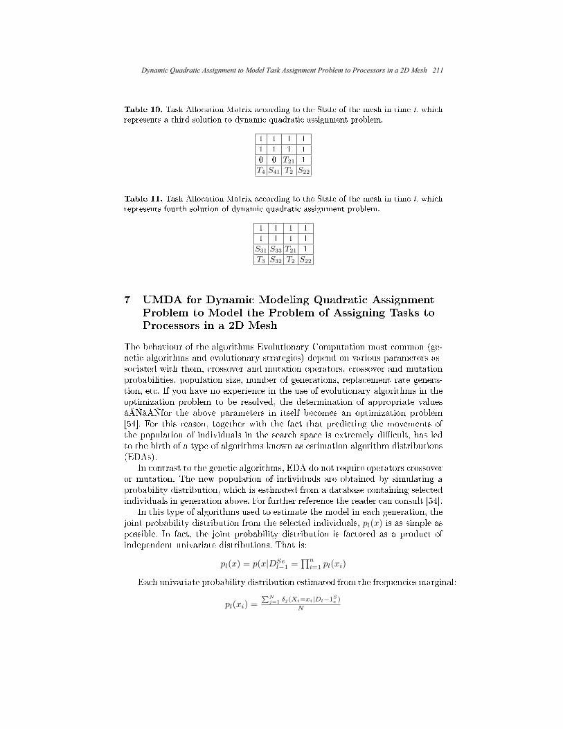
Table 10. Task Allocation Matrix according to the State of the mesh in time t, whichrepresents a third solution to dynamic quadratic assignment problem.

1 1 1 1

1 1 1 1

0 0 T21 1

T4 S41 T2 S22

Table 11. Task Allocation Matrix according to the State of the mesh in time t, whichrepresents fourth solution of dynamic quadratic assignment problem.

1 1 1 1

1 1 1 1

S31 S33 T21 1

T3 S32 T2 S22

7 UMDA for Dynamic Modeling Quadratic Assignment

Problem to Model the Problem of Assigning Tasks to

Processors in a 2D Mesh

The behaviour of the algorithms Evolutionary Computation most common (ge-netic algorithms and evolutionary strategies) depend on various parameters as-sociated with them, crossover and mutation operators, crossover and mutationprobabilities, population size, number of generations, replacement rate genera-tion, etc. If you have no experience in the use of evolutionary algorithms in theoptimization problem to be resolved, the determination of appropriate valuesââfor the above parameters in itself becomes an optimization problem[54]. For this reason, together with the fact that predicting the movements ofthe population of individuals in the search space is extremely dicult, has ledto the birth of a type of algorithms known as estimation algorithm distributions(EDAs).

In contrast to the genetic algorithms, EDA do not require operators crossoveror mutation. The new population of individuals are obtained by simulating aprobability distribution, which is estimated from a database containing selectedindividuals in generation above. For further reference the reader can consult [54].

In this type of algorithms used to estimate the model in each generation, thejoint probability distribution from the selected individuals, pl(x) is as simple aspossible. In fact, the joint probability distribution is factored as a product ofindependent univariate distributions. That is:

pl(x) = p(x|DSel−1 =

∏ni=1 pl(xi)

Each univariate probability distribution estimated from the frequencies marginal:

pl(xi) =∑N

j=1 δj(Xi=xi|Dl−1Se )

N


where:

δj(Xi = xi|DSe

l−1)=

1 if in the j − th event of DSe

l−1, Xi = xi0 in another case.

The pseudo code for the UMDA, see Table 12.

Table 12. Pseudo code for the UMDA.

UMDAD0 ← Generate M individuals (initial population) randomly

Repeat for l = 1, 2, ... until the stopping criterion check

DSel−1 ← Select N ≤M individuals

of Dl−1 according to a selection method

pl(x) = p(x|DSel−1 =

∏ni=1 pl(xi) =∏n

i=1

∑Nj=1 δj(Xi=xi|Dl−1Se )

N←

To estimate the joint probability distribution

Dl ← Sample M Sample m individuals, the new population from pl(x))

Reading Parameters: Once you have completed the rst assignment of tasksto the grid of processors, tasks start their execution so that at time t begin tovacate the sub-meshes. producing sets of processors that wait for tasks to beperformed, as shown in Table 6.2. Based on the queue of tasks (see section), theplanner performs a search of the tasks that can t in such sub-meshes unoccu-pied. Once this selection is necessary to generate the initial population.

Initial population generation. Generating the initial population to generateeach individual (allocation). The pseudo code for the generation of initial pop-ulation is shown in Table 13.

Evaluate Population. As explained in Section 6.2, we obtain the total gen-erated in Tables 6.2, 6.2, 6.2 y 6.2. The totals obtained are added to theassessment of an individual by the value obtained by the same objective func-tion. The pseudo code for the evaluation of the population shown in Table 14.

Estimating the Probabilistic Model. In this part we will use the simplestprobabilistic model, in which all the variables describing the problem are inde-pendent, so we calculate the frequency of apparition of a task in each emptycell of the mesh at time t of a part of the population who are the best individ-uals through a selection by truncation and the percentage of truncation. In thiscase the frequency of occurrence can be shown in Table 7, the pseudo code forestimating the probabilistic model shown in Table 16.

Generate the population from the Probabilistic Model. Pseudo code for gen-eration the population from the probabilistic model is shown in Table 17, where


Table 13. Pseudo code for the generation of initial population.

Initial Population

Repeat for Tasks = 1, 2, ... until the end of the queue of tasks

if TasksNumber in the position Tasks =Number of free processors in the submeshes

Storage Allocation

if not

Consider the following sub-mesh emptyend if

Report the number of tasks and identication

Table 14. pseudo code for the evaluation of the population.

Evaluate Population

Repeat for Tasks = 1, 2, ... until the end of the queue of tasksthat can be admitted to free submeshes.

Make the sum of the amounts obtained in eachcalculation of the cost of transferring messages for tasks

Report the total value of the objective function

if you generate a random number between 0 and 4 and if it is between 0 and 1the task T1 is assigned.

Save the best individual. This process is accomplished by taking each popula-tion generated the best individual at the time of ordering the current population.The process of ordering from low to high is because the search is performed isminimized.

8 Experimental Design and Results

Experiments are based on a comparison the proposed method with two moremethods of allocation of tasks to processors: linear assignment andHilbert curves.Linear assignment is the most used method in the allocation of processors, theease of implementation allows tasks to be quickly placed into the free mesh butpresents diculties when they begin to release sub-meshes and these are not con-tiguous. The nature of the method allows assignments of the bottom left of themesh to the right. The recognition that the algorithm makes is based on a linearpath of the mesh. The problems with this method are that we can not assign


Table 15. Frequencies of occurrence of each task in each cell.

P(0,0) P(0,1) P(0,2) P(0,3) P(1,0) P(1,1) P(1,2)

T1 1 0 0 0 0 0 0

S11 0 0 0 0 1 0 0

S12 0 0 0 0 0 1 0

S13 0 1 0 0 0 0 0

T2 0 0 3 0 0 0 0

S21 0 0 0 0 0 0 3

S22 0 0 0 3 0 0 0

T3 2 0 0 0 0 0 0

S31 0 0 0 0 2 0 0

S32 0 2 0 0 0 0 0

S33 0 0 0 0 0 2 0

T4 1 0 1 0 0 0 0

S41 0 1 0 1 0 0 0∑4 4 4 4 3 3 3

Table 16. Pseudo code to Estimate the probabilistic model.

Estimating probabilistic model

Repeat for AssignedTasks = 1, 2, ... until the end of the tables thatcontain the tasks that can be allocated to submeshes Free.

Verify that the net position of each task is assigned, 1 posted on eachassignment and stored in the matrix of the estimatedprobabilistic model

Report the values obtained in the frequency allocation

free sub-meshes in a dierent order, and presents diculties when attemptingto take free sub-meshes assignment by the linearity of procedure, this producesa high segmentation in the tasks and increasing the transfer of messages on themesh.

Hilbert curves method is a very interesting method for assign tasks into themesh. The Hilbert curve is a space lling curve that visits every point in asquare grid with a size of 2 × 2, 4 × 4, 8 × 8, 16 × 16, or any other power of2. It was rst described by David Hilbert in 1892. Applications of the Hilbertcurve are in image processing: especially image compression and dithering. Ithas advantages in those operations where the coherence between neighbouringpixels is important. The Hilbert curve is also a special version of a quad tree;any image processing function that benets from the use of quad trees may alsouse a Hilbert curve.

The results obtained in tests arise in three important ways:The waiting time processes in the input row. Both methods of assignment

Gilbert curves and linear allocation establish a philosophy based on FIFO, both


Table 17. Pseudo code to generate the population from the probabilistic model.

Generation the population from the probabilistic model

if (random ≤ Dif [0]) then P(0,0)=Sym[0]else

if (random ≤ Dif [1]) then P(0,0)=Sym[1]else

if (random ≤ Dif [2]) then P(0,0)=Sym[2]

do not compete for the assignment early into the mesh of processors so that anull starvation guaranteed, but the waiting times in the row are proportionalto the times of the processes. Both methods ensure the allocation of tasks withsubtasks in free submeshes close but as shown in the chart when the number oftasks, subtasks and their sizes increase, the waiting times are increased by thesame proportionality.Gilbert curves during the process of free submeshes showscontiguous allocation, but due to allocation method used does not allow usethem, but shows a tendency to use cluster of processors, which ensures that asthe tasks increase also increases the processor usage across the grid, avoidingleaving idle processors.

The proposed method allows for competition on the waiting list. Every time apart of the mesh is indicated as free processor allocator is responsible to performa search for tasks that can t in the sub-grid. There is a greater tendency to-wards starvation of processes, when small submeshes are unoccupied small tasksare arranged, when small submeshes are unoccupied small tasks are arranged,when large tasks release large number of processors there are occupation by asmall tasks too, tasks that require lots of processes waiting indenitely until therequirements of small tasks are handled so that the waiting time for certain taskstends to be higher.

The number of occupied meshes. In the two methods that use a FIFO allo-cation free submeshes processors can remain idle, even if there are jobs in thequeue that require equal or lesser number of processors, these tasks wait untilthe shift assignment will be valid. In the proposed method dispatcher will searchtasks that required number of processors is equal to or less than the numberof processors in the sub-grid free. As shown in Figure 2, the proposed methodallows greater utilization of processors in the allocation of tasks, reducing theidleness of processors.

9 Future Works

The works are planned to develop in the future are: Hardware implementationmulticomputers system. Hardware implementation multicomputers system con-sisting of a number n of dedicated computers interconnected through a mediumthat allows message passing. Operate within the hardware structure with evo-lutionary algorithms to enable an evaluation of allocation of processors time,


processes starvations and percentage of idle processors vs percentage of proces-sors used. Allow a real evaluation of evolutionary algorithms in a real scenario.Perform the evaluation with other evolutionary algorithms that include the threeaspects that are being evaluated.

Acknowledgements The work was nanced by Instituto para el Desarrollo dela Sociedad del Conocimiento del Estado de Aguascalientes México and underthe proyect PIINF10-2 of the UAA.

References

1. Jian Chen and Valerie E. Taylor: Mesh Partitioning for Ecient Use of DistributedSystems. IEEE Transactions on Parallel and Distributed Systems, Vol. 13, No. 1,January (2002)

2. Pierre-Francois Dutot, Tchimou N.Takpe, Frederic Suter: Scheduling Parallel TaskGraphs on (Almost) Homogeneous Multicluster Platforms. IEEE Transactions onParallel and Distributed Systems, Vol. 20, No. 7, July (2009)

3. Alessandro Amoroso, Keith Marzullo: Multiple Job Scheduling in a Connection-Limited Data Parallel System. IEEE Transactions on Parallel and DistributedSystems, Vol. 17, No. 2, February (2006)

4. C. Xavier and S. S. Iyengar: Introduction to Parallel Algorithms. Editorial: Wiley-Interscience, New York USA (1998)

5. A. Yassin Al-Dubai, M. Ould-Khaoua, L. M. Mackenzie: An Ecient Path-BasedMulticast Algorithm for Mesh Networks, ipdps, pp.283, International Parallel andDistributed Processing Symposium (IPDPS'03) (2003)

6. Debendra Das Sharma and Dhiraj K. Pradhan: Job Scheduling in Mesh Multi-computers. IEEE Transactions on Parallel and Distributed Systems, Vol. 9, No. 1,January (1998)

7. T. Srinivasan, Jayesh Seshadri, Arvind Chandrasekhat and J. B. SiddharthJonathana: Minimal Fragmentation Algorithm for Task Allocation in Mesh-Connected Multicomputers Proceedings. IEEE International Conference on Ad-vances in Intelligent Systems Theory and Applications AISTA 2004 in conjunctionwith IEEE Computer Society, IEEE Press (2004)

8. Edi Shmueli and Dror G. Feitelson. On Simulation of Parallel-Systems Schedulers:Are We Doing the Right Thing? IEEE Transactions on Parallel and DistributedSystems, Vol. 20, No. 7, July (2009)

9. A. Velarde M., E. E. Ponce de Leon S., E. Diaz, A. Padilla: Planning and Allo-cation of processors in 2D meshes. Doctoral Consortium. Mexican InternacionalConference on Articial Intelligence MICAI 2010 Pachuca Hidalgo, México (2010)

10. Kalyanmoy Deb: Multi-Objective Optimization using Evolutionary Algorithms.John Wiley & Sons, LTD. New York USA (2001)

11. Metaheuristics in Combinatorial Optimization: Overview and Conceptual Com-parison CHRISTIAN BLUM Université Libre de Bruxelles AND ANDREA ROLIUniversitá degli Studi di Bologna

12. Saad O. Bani Mohammad: Ecient Processor Allocation Strategies for Mesh-Connected Multicomputers. Tesis Doctoral. Faculty of Information and Mathe-matical Sciences University of Glasgow UK (2008)


13. B.S. Yoo and C.-R. Das: A Fast and Ecient Processor Allocation Scheme forMesh-Connected Multicomputers, IEEE Transactions on Parallel & DistributedSystems, vol. 51, no. 1, pp. 46-60 (2002)

14. V. Lo, K. Windisch, W. Liu, and B. Nitzberg: Non-contiguous processor allocationalgorithms for mesh-connected multicomputers, IEEE Transactions on Parallel andDistributed Systems, vol. 8, no. 7, pp. 712-726 (1997)

15. K. Li and K.H. Cheng: A Two-Dimensional Buddy System for Dynamic ResourceAllocation in a Partitionable Mesh Connected System, Journal of Parallel andDistributed Computing, vol. 12, no. 1, pp. 79-83 (1991)

16. P.J. Chuang and N.F. Tzeng: Allocating precise submeshes in mesh connectedsystems, IEEE Transactions on Parallel and Distributed Systems, vol. 5, no. 2, pp.211-217 (1994)

17. J. Ding and L.-N. Bhuyan: An Adaptive Submesh Allocation Strategy for Two-Dimensional Mesh Connected Systems, Proceedings of the 1993 International Con-ference on Parallel Processing, vol. 2, pp. 193-200 1(993)

18. Y. Zhu: Ecient processor allocation strategies for mesh-connected parallel com-puters, Journal of Parallel and Distributed Computing, vol. 16, no. 4, pp. 328-337(1992)

19. C.Y. Chang and P. Mohapatra: Performance improvement of allocation schemesfor mesh-connected computers, Journal of Parallel and Distributed Computing,vol. 52, no. 1, pp. 40-68 (1998)

20. J. Mache, V. Lo, and K. Windisch: Minimizing Message-Passing Contention inFragmentation-Free Processor Allocation, Proceedings of the 10th InternationalConference on Parallel and Distributed Computing Systems, pp. 120-124 (1997)

21. K. Suzaki, H. Tanuma, S. Hirano, Y. Ichisugi, C. Connelly, and M. Tsukamoto:Multi-tasking Method on Parallel Computers which Combines a Contiguous andNon-contiguous Processor Partitioning Algorithm. Proceedings of the 3rd Inter-national Workshop on Applied Parallel Computing, Industrial Computation andOptimization, Lecture Notes in Computer Science, Springer, London, pp. 641- 650(1996)

22. S. Bani-Mohammad, M. Ould-Khaoua, and I. Ababneh: A New Processor Alloca-tion Strategy with a High Degree of Contiguity in Mesh-Connected Multicomput-ers, Journal of Simulation Modelling, Practice & Theory, vol. 15, no. 4, pp. 465-480(2007)

23. P.Liu, Ch. Ch. Hsu and J. J. Wu: I/O Processor Allocation for Mesh Cluster Com-puters, IEEE Proceedings of the 2005 11th International Conference on Paralleland Distributed Systems ICPADS-05 (2005)

24. D. P. Bunde, V. J. Leung and J. Mache: Communication Patterns and AllocationStrategies, Sandia Technical Report SAND2003-4522 (2004)

25. P. Brucker, B. Jurisch, and B. Sievers: A branch and bound algorithm for thejob-shop scheduling problem. Journal of Discrete Applied Mathematics. No. 49,pp.105-127 (1994)

26. S. Binato, W. Hery, D. Loewenstern, and M. Resende: A GRASP for Job Schedul-ing. Technical Report No. 00.6.1 AT& T Labs Research (2000)

27. J. Goncalves, J. Magalhaes, M. Resende: A Hibrid Genetic algorith for the JobShop Scheduling. AT& T Labs Research Technical Report TD-5EAL6J (2002)

28. L. Davis: Job shop scheduling with genetic algorithms. First International Confer-ence on Genetic Algorithms and their Applications, pp. 136-140 (1985)

29. E. Taillard: Parallel Taboo Search Technique for the Job shop Scheduling Problem.Journal on Computing Science, No. 6 pp. 108-117 (1994)


30. J. Chambers, W. Barnes: Taboo Search for the Flexible-Routing Job Shop Prob-lem. Department of Computer Sciences, University of Texas-USA, Reporte Técnico(1997)

31. V. Subramani, R. Kettimuthu, S. Srinivasan, P. Sadayappan: Distributed JobScheduling on Computational Grids using Multiple Simultaneous Requests. De-partment of Computer and Information Science of Ohio State University, USA.Disponible http://www.gridforum.org (2003)


Bioinformatics and Medical Applications

New Method for Comparing Somatotypes

using Logical-Combinatorial Approach

Ignacio Acosta-Pineda1 and Martha R. Ortiz-Posadas

2

1 Master in Biomedical Engineering 2 Department of Electrical Engineering,

Universidad Autónoma Metropolitana Iztapalapa, Mexico [email protected], [email protected]

Abstract. This paper proposes a new method for comparing somatotypes using the

logical-combinatorial approach of pattern recognition theory, through the

mathematical modeling of a function to evaluate the similarity between

somatotypes, considering the 10 anthropometric dimensions defined in the Heath-

Carter method. This similarity function was applied to a sample of different

individual somatotypes and the results were compared with the ones obtained by the

two methods most commonly used: the somatotype dispersion distance and the

somatotype attitudinal distance. We obtained correct results with the method

presented in this work and it offers a new perspective for comparison between

somatotypes.

Keywords: Somatotype comparison, somatotype similarity, Heath-Carter method,

logical-combinatorial approach, pattern recognition.

1 Introduction

The term somatotype corresponds in such a way with the biotype term, and is one of the

most frequent tasks of Kineanthropometry, the discipline that studies the human body

through the measures and assessments of their size, shape, proportionality, composition,

biological maturation and body functions. The technique of somatotyping is used to

appraise body shape and composition. Somatotype concept is very useful in different

areas of healthcare, such as diet monitoring, effect of ergogenic aids, eating disorders

and/or sport sciences, in order to compare an athlete somatotype with his/her team, or

with a standard reference, or with a normal population, or itself at different stages of the

training [1].

The somatotype is defined as the quantification of the present shape and composition

of the human body. It is expressed in a three-number rating representing endomorphy,

mesomorphy and ectomorphy components respectively, always in the same order.

Endomorphy is the relative fatness, mesomorphy is the relative muscle-skeletal

robustness, and ectomorphy is the relative linearity or slenderness of a physique. To

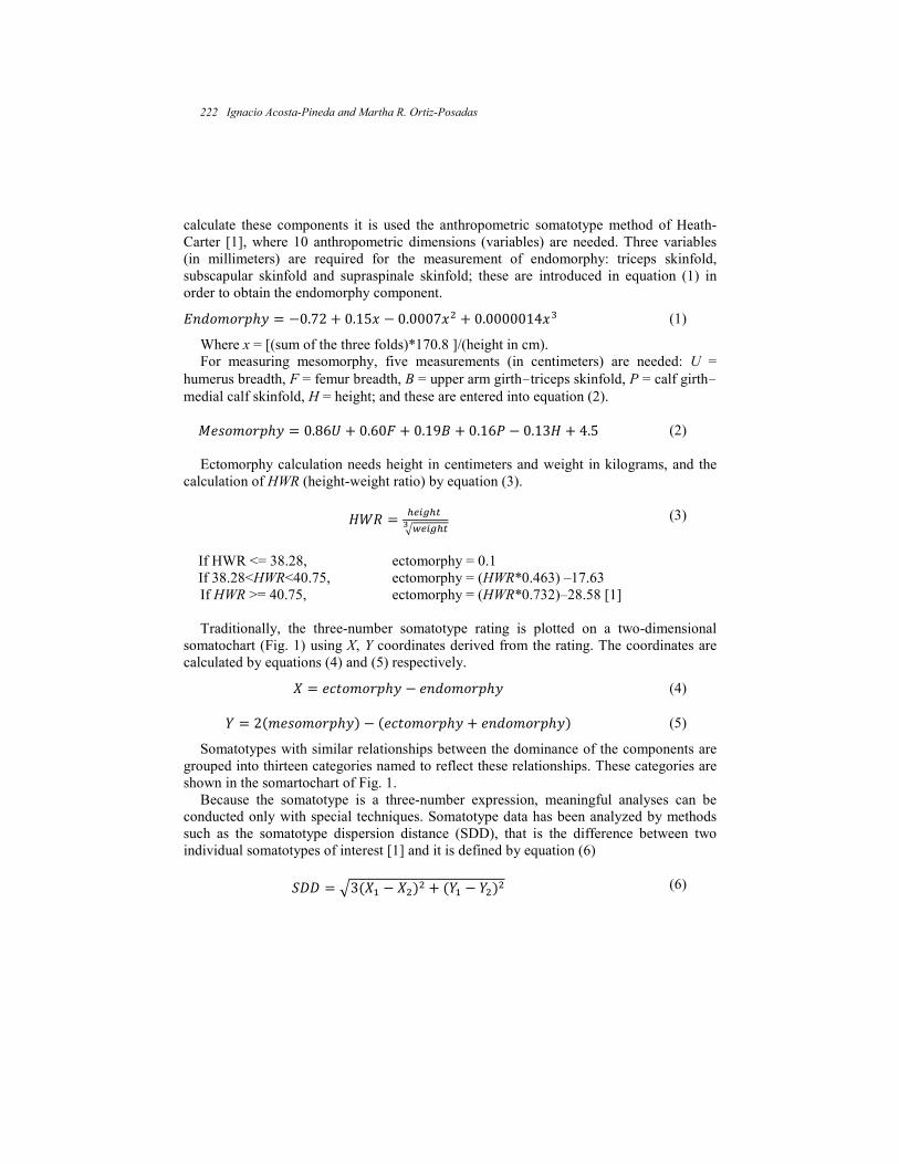
calculate these components it is used the anthropometric somatotype method of Heath-

Carter [1], where 10 anthropometric dimensions (variables) are needed. Three variables

(in millimeters) are required for the measurement of endomorphy: triceps skinfold,

subscapular skinfold and supraspinale skinfold; these are introduced in equation (1) in

order to obtain the endomorphy component.

0.72 0.15 0.0007 0.0000014 (1)

Where x = [(sum of the three folds)*170.8 ]/(height in cm).

For measuring mesomorphy, five measurements (in centimeters) are needed: U =

humerus breadth, F = femur breadth, B = upper arm girth-triceps skinfold, P = calf girth-

medial calf skinfold, H = height; and these are entered into equation (2).

0.86 0.60 0.19 0.16 0.13" 4.5

(2)

Ectomorphy calculation needs height in centimeters and weight in kilograms, and the

calculation of HWR (height-weight ratio) by equation (3).

"#$ %&'(%)+,&'(%)-

(3)

If HWR <= 38.28, ectomorphy = 0.1

If 38.28<HWR<40.75, ectomorphy = (HWR*0.463) –17.63

If HWR >= 40.75, ectomorphy = (HWR*0.732)–28.58 [1]

Traditionally, the three-number somatotype rating is plotted on a two-dimensional

somatochart (Fig. 1) using X, Y coordinates derived from the rating. The coordinates are

calculated by equations (4) and (5) respectively.

. /0 (4)

1 223 2/0 3 (5)

Somatotypes with similar relationships between the dominance of the components are

grouped into thirteen categories named to reflect these relationships. These categories are

shown in the somartochart of Fig. 1.

Because the somatotype is a three-number expression, meaningful analyses can be

conducted only with special techniques. Somatotype data has been analyzed by methods

such as the somatotype dispersion distance (SDD), that is the difference between two

individual somatotypes of interest [1] and it is defined by equation (6)

455 +32.6 .3 216 13

(6)

222 Ignacio Acosta-Pineda and Martha R. Ortiz-Posadas

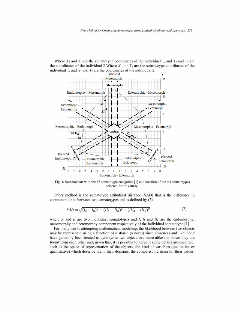
Where X1 and Y1 are the somatotype coordinates of the individual 1, and X2 and Y2 are

the coordinates of the individual 2 Where X1 and Y1 are the somatotype coordinates of the

individual 1, and X2 and Y2 are the coordinates of the individual 2.

Fig. 1. Somatochart with the 13 somatotype categories [1] and location of the six somatotypes

selected for this study.

Other method is the somatotype attitudinal distance (SAD) that is the difference in

component units between two somatotypes and is defined by (7).

475 +289 8:3 2889 88:3 28889 888:3

(7)

where A and B are two individual somatotypes and I, II and III are the endomorphy,

mesomorphy and ectomorphy component respectively of the individual somatotype [1].

For many works attempting mathematical modeling, the likelihood between two objects

may be represented using a function of distance (a norm) since closeness and likelihood

have generally been treated as synonyms: two objects are more alike the closer they are

found from each other and, given this, it is possible to agree if some details are specified,

such as the space of representation of the objects, the kind of variables (qualitative or

quantitative) which describe them, their domains, the comparison criteria for their values,

New Method for Comparing Somatotypes using Logical-Combinatorial Approach 223

etc. Likewise, it is important to consider the way in which full object descriptions are

attempted. In this sense, it is important to distinguish between likelihood and closeness in

those cases where these terms are not synonyms.

This paper proposes a new method for comparing somatotypes, using the logical-

combinatorial approach of pattern recognition theory [2], through the mathematical

modeling of a function to evaluate the similarity between two somatotypes, considering

the 10 anthropometric dimensions defined in the Heath-Carter method [1], and defining

differential comparison criteria for each variable. The similarity function was applied to 6

different individual somatotypes, and these results were compared with the results

obtained by both methods SDD and SAD.

2 Methodology

2.1 Mathematical Model [3]

Let O = O1, . . ., Om be a finite set of m objects, each object is described in terms of the

finite set of variables X= x1, . . ., xn, where each variable xi, i=1, . . ., n is defined on

its domain Mi = mi1, mi2, . . ..

Definition 1. Let the initial space representation (ISR) be the object space

representation defined by the Cartesian product of Mi sets

I(O) = (x1(O), . . . , xn(O)) ∈ (M1 × ... ×Mn)

Where I(O) is the object description of O in terms of the variables xi, i=1, ..., n. xi(O) is

the value taken by the variable xi in the object O.

Definition 2. Let C = C1, ..., Cn be a set of functions called comparison criteria for

each variable xi∈X such as: Ci: Mi×Mi→∆i; i=1, . . ., n where ∆i can be of any nature, it is

an ordered set and can be finite or infinite.

Definition 3. Let ω⊆X be a support set, where ω ≠ ∅. A system of support sets is

defined as Ω = ω1, ..., ωs. By ωO we denote the ω-part of O formed by the variables xj ∈

ωm, m=1, ..., s.

The system of support sets Ω will allow analysis of the objects to be classified, done by

paying attention to different parts or sub-descriptions of the objects, and not analyzing the

complete descriptions. Examples of systems of support sets are combinations with a fixed

cardinality, combinations with variable cardinality, the power set of features, etc.

The analogy between two objects is formalized by the concept of similarity function.

This function is based on the comparison criterion Ci generated for each variable xi. It is

important to mention that the similarity function can evaluate the similarity or difference

between two objects, i.e., between their descriptions.


Definition 4. Let β:(Mi ×Mi)2→∆ be the similarity function, where ∆ (as in the

comparison criterion function) can be of any nature; it is an ordered set and can be finite

or infinite. For I(Oi) and I(O) being two object descriptions in the domain (M1 ×. . .×Mn),

β(I(Oi), I(O)) is defined by:

• β((C1(x1(Oi), x1(O)), . . . , Cn(xn(Oi), xn(O)))), if Ci denotes similarity

• 1 − β((C1(x1(Oi), x1(O)), . . . , Cn(xn(Oi), xn(O)))), if Ci denotes difference

Definition 5. Let βω be a partial similarity function defined by: >? @82A'3, 8CADEF 1 ∑ H'C'2A'3, '2A3EIJ∈?

(8)

where ω represents a support set.

2.2 Somatotype Mathematical Model

We used the 10 anthropometric dimensions (variables) proposed in the Heath-Carter

method [1], described in the introduction. It was defined their domain by previously

classifying 38 subjects [4], and the difference comparison criteria (Definition 2), shown in

Table 1. The 0 means there is no difference and 1 represents the greatest difference

between the two values compared.

Table 1. Somatotype variables, domain and comparison criteria.

Variable Domain Comparison criteria

x1: Supraspinale skinfold

[6, 55]

HC2A'3, CADEE K1LM N2A'3 CADEN490L0/O P 0.1

x2: Subscapular skinfold

[8, 41]


x3: Triceps skinfold

[4, 25] HC2A'3, CADEE K1LM N2A'3 CADEN210L0/O P 0.1

x4: Medial calf skinfold

[0.5, 3.0]

HC2A'3, CADEE K1LM N2A'3 CADEN2.50L0/O P 0.1

x5: Calf girth, right

[30.0, 43.0]


x6: Upper arm girth,

elbow flexed and tensed

[29.0, 41.0]



x7: Biepicondylar breadth

of the femur

[8.0, 12.0]


x8: Biepicondylar breadth of the humerus

[5.0, 8.0]


x9: Body mass (weight)

[51.0, 120.0]


x10: Stature (height).

[157.0, 190.0]


We defined three support sets (Definition 3), one for each somatotype component: Ωendo

= x1, x2, x3, x10; Ωmeso = x3, x4, x5, x6, x7, x8; Ωecto = x9, x10. Likewise using Definition

5, we defined three partial similarity functions described below:

βRSTU @ΩI2OY3, ΩICOZEF 1- ∑ \]@^]2_`3,^]C_aEFbcd6,,,6e (9)

>f&gh @Ω82A'3, Ω8CADEF 1 ∑ ij@Ij2kJ3,IjCklEFmncd (10)

>&o)h @Ω82A'3, Ω8CADEF 1 ∑ ij@Ij2kJ3,IjCklEF6ecdp (11)

Finally, the total similarity function was composed by the three partial similarities as

follows.

>)h)qr282A'3, 82AD33 stuvwxsytzwxstjw (12)

All similarity functions were bounded in the interval [0, 1], where 0 means there are no

similarity (greatest difference) and 1 corresponds to identical somatotypes.

The procedure to calculate the similarity between two somatotypes using the similarity

function is described as follows: First, calculate the partial similarity of the three

components (βendo, βmeso, βecto) between of somatotypes using the equations (9), (10) and

(11) respectively; second, calculate the overall similarity between somatotypes using the

equation (12).


3 Results

From the sample of 38 subjects previously classified [4] we selected six: A1, A2 with a

rating of endomorphic-mesomorph; B1, B2 with a rating of mesomorphic-endomorph and

C1, C2 with a rating of mesomorphic-ectomorph. These somatotypes were placed in the

somatochart (Fig. 1). We calculated the similarity between these six somatotypes

described in terms of the 10 variables defined by Heath-Carter (Table 2); using three

methods: 1) Similarity Function, proposed in this work; 2) Somatotype Dispersion

Distance (SDD); and 3) Somatotype Attitudinal Distance (SAD).

First, we calculated the pairwise similarity between somatotypes belonged to the same

class in order to show similarity between these somatotypes should be high, and then we

calculated the similarity between somatotypes belonged to different classes, whose

likeness should be low. As follows it is shown the application of each method in the

calculation of the similarity between two different somatotypes.

Table 2. Description of 6 subjects with Heath-Carter 10 variables.

Variable A1 A2 B1 B2 C1 C2

x1 10 15 30 32 6 6

x2 10 11 25 27 7 8

x3 5 8 23 20 4 4

x4 0.8 0.8 1.6 1.7 0.8 0.5

x5 35.5 34.5 33 34 29 30

x6 37.5 36 33 32 28 29.5

x9 65 60 80 82 52 51

x7 8.8 9.2 9 8.8 8.4 8.5

x8 6 6.5 6.2 6 5.5 5.8

x10 162 165 172 170 167 169

3.1 Similarity Function β β β β (Proposed Method

To illustrate the application of partial and total similarity functions, we calculated the

similarity between somatotypes A1 and B1. We calculated the partial similarity between

endomorphy components of both somatotypes using (9):

>&|hCΩ82A963, Ω82A:63E 1 ~ |10 30|49 |10 25|33 |5 23|21 |162 172|33 4cd6,,,6e

0.49


Using (10) and (11), partial similarity between mesomorphy and ectomorphy

components respectively was calculated.

>f&ghCΩ82A963, Ω82A:63E 1 ∑ ij@Ij2kJ3,IjCklEFmncd 0.73

>&o)hCΩ82A963, Ω82A:63E 1 ∑ ij@Ij2kJ3,IjCklEF6ecdp 0.74

Using (12) the overall similarity between the two somatotypes was calculated:

>)h)qr282A963, 82A:633 2e.bp3x2e.3x2e.b3 0.65

3.2 Somatotype dispersion distance (SDD) and Somatotype attitudinal distance

(SAD)

For calculating SDD between both somatotypes A1 and B1 it was necessary to calculate the

three components (endomorphy, mesomorphy, ectomorphy) for each somatotype and

then, the X, Y coordinates. This is illustrated following the next procedure:

1. Calculate parameter x:

xA1 = [(10+10+5)170.18]/162 = 26.26, (xA1)2 = 689.58, (xA1)

3 = 18108.57

2. Calculate endomorphy component using (1):

EndomorphyA1= -0.72 + 0.15(26.26) - 0.0007(689.57) + 0.0000014(18108.57)

EndomorphyA1= 15.68

EndomorphyB1= 7.32

3. For calculating mesomorphy component, we identify the equivalence among the

parameters used in equation (2) and variables in Table 2. So the equivalence is: U=x8,

F=x7, B=x6-x5, P=x4 and H=x10, then:

MesomorphyA1= 0.86(6) + 0.6(8.8) + 0.19(2) + 0.16(0.8) - 0.13(162) + 4.5

MesomorphyA1= -5.77

MesomorphyB1= -10.34

4. Ectomorphy component needs to calculate the HWR (height-weight ratio) by

equation (3). For both somatotypes: "#$96 6m√m- = 40.5, "#$:6 6

√ne- = 40

If 38.28<HWR<40.75, then ectomorphy = (HWR*0.463) –17.63, then:

EctomorphyA1 = [40.5(0.463)] –17.63 = 1.12


EctomorphyB1 = 0.89

5. Calculate coordinates X and Y using equations (4) and (5) respectively:

XA1 = 1.12-2.77 = -1.65, XB1 = -6.43

YA1 = 2(-5.77) – (2.77-1.12) = -15.43, YB1 = -28.89

6. Calculate SDD using (6):

45596:6 +321.65 26.4333 215.43 228.8933 ≃ 15.7

7. Calculate SAD using equation (7):

47596:6 22.7796 7.32:63 25.7796 210.343:63 21.1296 0.89:63 ≃ 6.8

The similarity result for all cases is shown in Table 3. Clearly it is showed that between

somatotypes belong to the same class, the similarity is high (β ≥0.9), and in the case of

somatotypes belonging to different classes there is a low similarity (β≤0.85). However

observe that somatotypes A1-C1 obtained a similarity β = 0.84, this is because even both

somatotypes are different in their muscular proportions, both have a thin physique.

On the other hand, the distances SDD and SAD between somatotypes belonged to the

same class are short and in the case of somatotypes belonged to different classes the

distances are large. Observe that distance between subjects A1-B1 and subjects A1-C1 have

almost the same value; this means that A1 is far different from B1 as from C1, and this is

why their distance is large in both cases. By the other hand, observe pair A1-A2 (belong to

the same class): both SDD and SAD are shorter, but SAD is 40% shorter than SDD.

Moreover, distances are also shorter for both pairs B1-B2 and C1-C2; but interpretation

about these distances is not clear enough.

Related with function β, observe the similarity between these same pairs of

somatotypes (A1-B1), A1 is more different than B1 because of their similarity (β = 0.654) is

lower than similarity between A1-C1 (β = 0.84); meaning the pair (A1-C1) have a 20%

higher similarity.

Table 3. Results of similarity and both distances SDD and SAD.

A1-A2 B1-B2 C1-C2 A1-B1 B1-C1 A1-C1

Similarity β 0.91 0.94 0.96 0.65 0.62 0.84

SDD 2.68 0.87 0.96 15.7 15.2 12.7

SAD 1.58 0.38 0.82 6.80 6.55 5.30


5 Conclusion

Calculate the somatotype by the anthropometry method, needs to enter the 10 body

measures into the three component rating (endo, meso and ecto-morphy). This rating is

plotted on a two-dimensional somatochart, previously calculating coordinates X, Y by

using the three components. These component ratings are used also in the equations for

two and three-dimensional distances between somatotypes, called the somatotype

dispersion distance (SDD) and somatotype attitudinal distance (SAD) respectively.

Analysis of the three-number somatotype rating presents the problem of how should such

a rating be analyzed. How far (near) most be the distance between somatotypes, in order

to decide which class the somatotype belongs to.

In this sense, the similarity function proposed in this work, offers a new perspective for

comparing somatotypes, it does not need the three component rating neither the

somatochart. It just uses the 10 body measurements from the individual somatotype

description and the similarity function, in order to compare somatotypes. Furthermore,

sometimes in biotypological research or sport sciences, it is necessary to analyze one of

the three components in a separately way. Our method allows comparing (analyzing) each

component in an individual manner by defining the support sets and the partial similarity

function. Finally we shown that our method is effective for comparing somatotypes and

estimates the similarity between them, and all these characteristics make it simpler than

the traditional methods.

5 References

1. Carter, J.E.L.: The Heath-Carter Anthropometric Somatotype Instruction Manual. Department

of Exercise and Nutritional Sciences. San Diego State University. USA (2002)

2. Martínez-Trinidad, J.F., Guzmán-Arenas A.: The Logical Combinatorial Approach to Pattern

Recognition, An Overview Through Selected Works. Pattern Recogn. 34(4), 741-751 (2001)

3. Ortiz-Posadas, M.R., Vega-Alvarado, L, Toni B,: A Mathematical Function to Evaluate

Surgical Complexity of Cleft Lip and Palate. Comput. Meth. Prog. Bio. 94, 232-238 (2009)

4. Acosta-Pineda, I., Ortiz-Posadas, M.R.: Somatotype Classification Using the Logical-

Combinatorial Approach (in Spanish). In: V Latin-American Biomedical Engineering

Congress, vol. 3, pp.1-4. IFMBE Press, La Habana, Cuba (2011)


Modeling of 2D Protein Folding

using Genetic Algorithms and Distributed Computing

Andriy Sadovnychyy

DMAS, DCNI, UAM Cuajimalpa,

Artificios 40, col. Hidalgo, Delegación Álvaro Obregón,

México D. F., C.P. 01120, Mexico [email protected]

Abstract. In this work, it is presented an application of parallel programming for

studying of a scalable problem in the area of bioinformatics (Protein Folding) using

a genetic algorithm. The properties of proteins depend on its configuration in space.

Calculation of its configuration is a hard problem so we used some approximations

models like 2D square lattice. For finding an optimal configuration of the protein in

the space (configuration with minimal energy) genetic algorithm is used. It makes it

possible to find an optimal configuration several times faster than a full calculation

of interaction between atoms. Disadvantage of genetic algorithms is computation

load. Therefore the parallel genetic algorithms are applied in this work. Parallel

genetic algorithms operations (like mutation, crossover and fitness) are realized in

parallel mode. For this the multi-agent system are useful. They make it possible to

realize many independent functions in parallel mode.

Keywords: Protein folding, PH model of protein, genetic algorithm, parallel

computing.

1 Introduction

There are many problems of bioinformatics, such as folding, docking and molecular

design can be classified as "difficult problem of optimization". This family of problems is

those for which not guaranteed to find the best solution in a reasonable time. Therefore

the term NP-hard problem is used in the context of the complexity of algorithms.

Recently, several studies have shown that hybrid algorithms, metaheuristics and parallel

patterns have improved the search optimization methods, resulting in quite acceptable

solutions, and even robust, which solved many increasingly large and complex problems

with tolerable computing time [1, 2]. Examples of such problems are the problems which

we deal with. This work proposes the development of a conceptual and computational

infrastructure that allows integration through metaheuristics and hybrid algorithms, key

models, heuristics and algorithms for the study of biologically interesting problems. In

this work we postulate that many of these problems can be effectively modeled through a

conceptual and computational infrastructure based on multi-agent systems (MAS) that

supports the work of algorithms based on metaheuristics.

Using techniques for developing parallel models allows solving large and complex

problems in tolerable computing times. But to use all their advantages, parallel genetic

algorithms must submit all data structures into a specific model. We have to develop

computational algorithms using parallelization techniques. All tools can be heterogeneous

and distributed. It means that the simulation system can use the advantages of each of its

elements assigning the task to more suitable block. Using metaheuristic implemented

through the interaction of agents in the computing infrastructure allows interrelate the

properties of all molecules with the activity or function to be optimized, generating a

functional mathematical approach to describe such relationship. The simulations of

protein folding have the benefits of using heterogeneous systems. Applying this kind of

processing power changes the whole dynamic of the simulation and could significantly

reduce the time required to conduct research. In this work we develop the methods,

algorithms and computational model structures that allow, through metaheuristics and

hybrid algorithms, undertaking the study of biologically interesting problems mentioned

above.

2 Methods

The modeling of physics and chemistry processes is very complex. This problem can be

studied through alternative strategies, such as methods, techniques and models of

intelligence artificial (IA), science and computer engineering, and sciences information,

among other disciplines. It is noteworthy that such strategies have left aside those

traditional approaches in physics and chemical commonly biological science researchers

have used as study models [3]. Depending on empirical knowledge engaged in theoretical

model, this relationship will be more successful to reproduce and predict the properties of

a complex system of this nature. In this sense, we will mention some of the problems of

biological interest that we intend to address in this work and specify why this complexity

and strategies have been employed to get a solution.

The folding or folding of a protein is the physical process by which these biomolecules

are rearranged in three-dimensional structure. The prediction of protein folding has been

commonly addressed through combination of a model for the random generation of

conformations proteins in a 2D or 3D space (hydrophobic-hydrophilic model), and an

approximation algorithm for finding the closest conformation native state protein model.

Both algorithms were used a criterion of minimizing some function of free energy.

Genetic algorithm is one of the most commonly used techniques for approximation [4].

When this technique is used, the prediction of three-dimensional structure of a protein can

be formulated as a search through its conformation space to find a global minimum of the

energy state.

232 Andriy Sadovnychyy

The multi-agent systems paradigm is very effective in designing a methodology for

cover the entire spectrum of construction of a simulation, from design to development,

implementation and control (dynamic) runtime [5, 6]. Critical points of biological systems

- concerned with structures, activities and interactions - can be captured directly by

abstractions that are "Kept alive" design at run time, supported by appropriate

infrastructure. The simulation and modeling can then be framed as an experiment in

online or in simulation system, where researchers can observe and interact dynamically

with the system and its environment through changes in their structures, or directly

modifying the global biological process.

Agent-based systems and multi-agent systems (MAS) are considered strategies to

manage the correct level of abstraction modeling and building complex systems. In fact,

biological systems exhibit all the characteristics of complex systems. However, as noted

in [1], a biological system is much more than a complex system, it is a system consistent,

as it implies levels of functionality, localization, individualization and therefore

specialization, dimensionality (micro and macro levels) and other scenarios for these

levels of operation.

Fig. 1. Principal structure of simulation system.

Interaction among agents is realized indirectly through a blackboard,

which represents the communication coordination abstraction.

Modeling of 2D Protein Folding using Genetic Algorithms and Distributed Computing 233

In this work we will use an infrastructure for modeling MAS biological systems

strongly based on location, distribution and interaction (communication) of the

components of the system and therefore provide for better solutions compared to

generating strategies traditionally used. We will also make an analysis from a viewpoint

theory to explain the reasons why the infrastructure is better and which of its properties

can be used in other evolutionary systems.

3 Multi-agent System

The principal structure of simulation system can be seen in Figure 1. There its main

components, the agents and the blackboard, are presented. As can be seen in this figure,

the architecture provides three types of agents: model agents, algorithm agents and

interface agents [8]. According to this Multi-Agent System architecture, the interaction

among agents is realized by indirect communication, through a communication-

coordination abstraction, represented in this figure by the blackboard.

Fig. 2. Semantics assigned to the different blackboard levels and types of agents.

Figure 2 shows the semantics assigned to the different blackboard levels and types of

agents when protein folding is modeled. Evolution, the bioinformatics framework, allows

inducing folding of molecular-chain representations with the aim to explore both the

behavior and efficiency of EA by following the most relevant variables of chain folding.

Regarding the software development, our work will progress by using the bioinformatics

framework as a scaffold or mainframe devoted to the development and testing of


gradually more complex and robust EA and their associated parameters, with more

realistic representations of the problem and with improved fitness functions. This

framework would also allow adding functionalities for the user to tract results and

algorithm efficiency, to interactively bias the conformational search with biological sense,

or to perform graphical and numerical analysis.


The goal of experiments is to compare the performance of our simulation system with

similar simulations and others previously published. Also to see if our simulation system

can shed some light in the study of how proteins tend to fold and if there is some

phenomena that could be identified and explained.

The HP-48 problem. This problem is defined by the sequence HP-48 = P2H(P2H2)2P5H10P6(H2P2)2HP2H5 =

PPHPPHHPPHHPPPPPHHHHHHHHHH

In this problem the optimal sequences have a square shape in the H beads with several

options for the P beads. This problem was reported in [9] as very difficult.

According to the results in previous sections, this problem is likely to be difficult

simply because of this square shape. Any algorithm should have problems here.

Fig. 3. A near optimal configuration for HP-48.

Figure 3 shows one nearly optimal configuration found. One can see that the shape of

the H beads is more or less close to a rounded square. This is the kind of shapes that are

more easily found by our algorithm and we think that this is also the one that is more

likely to be present in nature. The 2D square model induces a bias that makes it difficult


to find square shaped optima. So we think that it is not good to try and solve this kind of

problems. It should suffice with the use of more rounded shapes to be able to study the

traits present in real life protein folding.

The genetic algorithm for find the optimal configuration was used. Each of gen

presents the direction of connection in the protein structure. The gen shows three

directions: straight, left and right. On basis of this information we construct the model

protein. We start construct the model from the first amino acid and first direction to

straight, then we continue construct in concordance with the chromosome.

Figure 4 shows the principal structure of genetic algorithm. On phases “Initial

population”, “Crossover and mutation”, “Selection” and “Termination” the algorithm

works with whole population. On these stages the processing of each chromosome is

depended of others.

On phase “Fitness” the algorithm calculates the level (fitness function) of each

chromosome. On this stage the processing of chromosome is independent. And we calc

the fitness function for each chromosome simultaneously, en parallel.

Fig. 4. Principal structure of genetic algorithm.

The main algorithm waits for termination of all parallel calculations, receives all results

(values of each fitness functions) and makes “selection”.

During the phase “selection”, the algorithm assigns the rank for each genome and

selects pairs for “Crossover” stage.

Figure 5 shows cluster’s structure that we are used for realize computing. The cluster

has Server, which controls and distributes tasks for nodes. Each node has 2 CPUs with 8

Initial population

Crossover and mutation

Fitness

Selection

Termination

Section of

parallel computing

Achieve the

necessary conditions


cores (16 cores for node) and work like SMP machine. We consider that each core like a

separate CPU.

We use Open MPI [10, 11] library and Open MP API [11, 12] for computing

parallelization.

Fig. 5. The cluster’s structure

The Open MPI library provides tools for communication between the nodes. It uses

sockets for sends and receives data. Open MPI automatically analyses the topology of

distributed system (cluster) and then chooses the best (fastest) way for send data,

messages.

The open MPI model uses distribute memory, so all processes have own local memory

and have not access to memory of others. They can communicates by the send/receive

function (send/receive massages).

The main program (in the server) has whole generation of population. Divides one for

parts and send them for each node. The nodes from 1 to P-1 receive N/P genomes, where:

N – number of genome in the population and P – number of node. And node P receives

the rest −

∗ ( − 1) of genome.

Then in the node we use Open MP API. Open MP realize shared memory paradigm. So

each thread has access to global memory.

Main Server

Main program.

Task’s distribution.

NODE 1

Calculation.

Fitness function.

Switch

1000 Mbit/s ethernet

NODE 1

Calculation.

Fitness function.

NODE 1

Calculation.

Fitness function.

NODE 1

Calculation.

Fitness function.


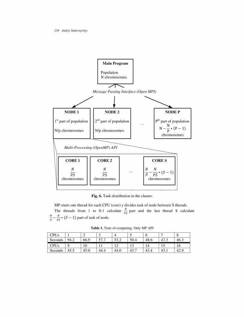
Fig. 6. Task distribution in the cluster.

MP starts one thread for each CPU (core) y divides task of node between S threads.

The threads from 1 to S-1 calculate

part and the last thread S calculate

−

∗ ( − 1) part of task of node.

Table 1. Time of computing. Only MP API

CPUs 1 2 3 4 5 6 7 8

Seconds 94.2 66.9 57.7 53.2 50.4 48.6 47.3 46.3

CPUs 9 10 11 12 13 14 15 16

Seconds 45.5 45.0 44.4 44.0 43.7 43.4 43.1 42.9

Main Program

Population

N chromosomes

NODE 1

1st part of population

N/p chromosomes

NODE 2

2nd

part of population

N/p chromosomes N −

N

P∗ (P − 1)

NODE P

Pth

part of population

chromosomes

…

CORE 1

chromosomes

CORE 2

chromosomes

−

∗ ( − 1)

CORE S

chromosomes

…

Message Passing Interface (Open MPI)

Multi-Processing (OpenMP) API


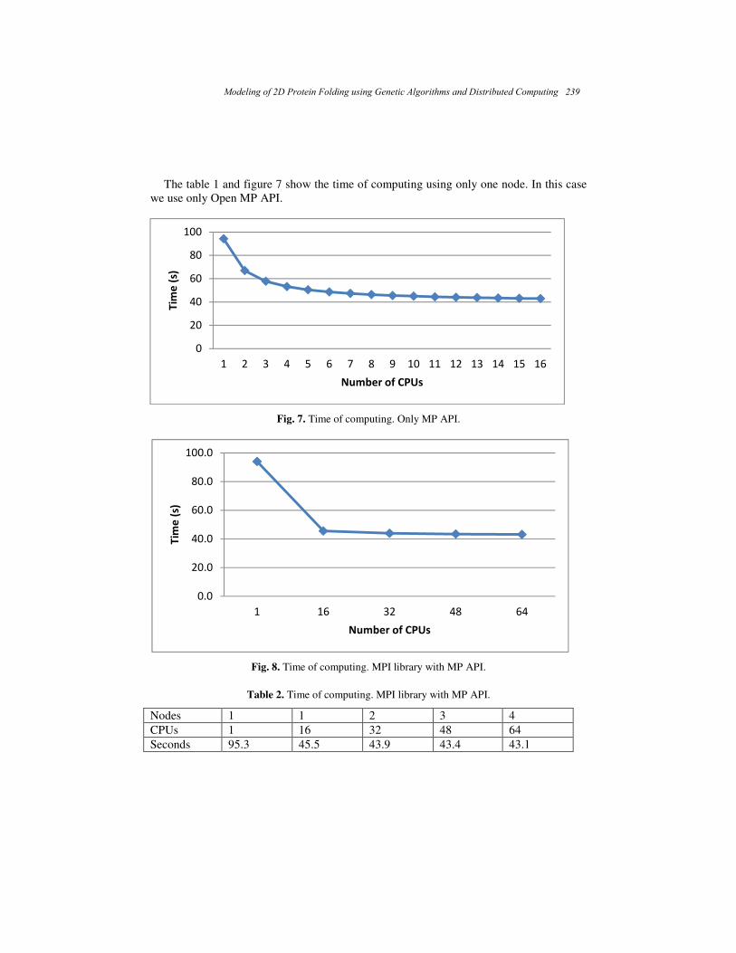
The table 1 and figure 7 show the time of computing using only one node. In this case

we use only Open MP API.

Fig. 7. Time of computing. Only MP API.

Fig. 8. Time of computing. MPI library with MP API.

Table 2. Time of computing. MPI library with MP API.

Nodes 1 1 2 3 4

CPUs 1 16 32 48 64

Seconds 95.3 45.5 43.9 43.4 43.1

0

20

40

60

80

100

1 2 3 4 5 6 7 8 9 10 11 12 13 14 15 16

Tim

e (

s)

Number of CPUs

0.0

20.0

40.0

60.0

80.0

100.0

1 16 32 48 64

Tim

e (

s)

Number of CPUs


The table 2 and figure 8 show the time of computing using Open MPI for distribute the

tasks between the nodes, and Open MP API for calculate the part of task in parallel mode.

In this case we use mixed mode Open MPI library+ Open MP API.

5 Conclusions

The methods of genetic algorithms allow finding optimal configurations of the proteins in

space. That makes it possible to model proteins properties. Using parallel genetic

algorithms, it is possible to analyze the whole of population in multiprocessors system.

All of these methods together decrease, by several times, time of modeling.

In the experiment we used different techniques for parallelize computing. The

experiment shows that than we incise number of CPU (processing units) the time of

computing is decreased. But there is limit of number of processing unit in our experiment.

According to Amdahl's law

()

where S is a number of processing unit and P is a

parallel part of the algorithm, this limit depends on the parallel part of algorithm.

The directions for future research are to change the algorithm for increasing the parallel

part and to design methods and models for simulation of protein folding with parallel

genetic algorithms in distributed system like clusters or grid.

References

1 Kitano, H.: Computational System Biology. Nature, Vol. 420, pp. 206-210 (2002)

2 Oliveto, P.S., Lehre P.K., Neumann, F.: Theoretical Analysis of Rank Based Mutation –

Combining Exploration and Exploitation. Proceedings of the Eleventh Congress on Evolutionary

Computation (2009)

3 C. Clementi: Coarse-grained models of protein folding: toy models or predictive tools?, Current

Opinion in Structural Biology. 18, 10-15 (2008)

4 Cervantes, J., Stephens, C.R.: Rank Based Variation Operators for Genetic Algorithms.

Proceedings of the 2008 international Genetic and Evolutionary Computation Conference

(GECCO08) pp. 905-912 (2008)

5 Zambonelli, F. and A. Omicini: Challenges and research directions in agent-oriented software

engineering. Autonomous Agents and Multi-Agent Systems, 9(3):253–283 (2004)

6 Parunak, V.D., R. Savit, and R. L. Riolo: Agent-based modelling vs. equation based modelling:

A case study and users’ guide. In J. S. Sichman, N. Gilbert, and Conte, R., editors, Multi-Agent

Systems and Agent-Based Simulation, pages 10–26, Springer-Verlag (1998)

7 Omicini, A., A. Ricci, M. Viroli, C. Castelfranchi, and L. Tummolini. 2004. Coordination

artifacts: Environment-based coordination for intelligent agents. In N. R. Jennings, C. Sierra, L.

Sonenberg, and M. Tambe, editors, 3rd international Joint Conference on Autonomous Agents

and Multiagent Systems (AAMAS 2004), volume 1, pages 286–293, New York, USA, 19–23

ACM (2004)


8 Cervantes, J., Sánchez, M., González, P.P.: Emerging traits in the application of an evolutionary

algorithm to a scalable bioinformatics problem, Evolutionary Computation (CEC), 2010 IEEE

Congress. Barcelona, pp 1–8 (2010)

9 Cox, G.A., Mortimer-Jones, T.V., Taylor, R.P. Johnston R.L.: Development and Optimization of

a novel Genetic Algorithm for Studying Model Protein Folding. Theor Chem Acc (2004) 112:

163–178 DOI 10.1007/s00214-004-0601-4 (2004)

10 Open MPI v1.4.3 documentation, http://www.open-mpi.org/doc/v1.4/

11 Michael Jay Quinn: Parallel programming in C with MPI and OpenMP, McGraw-Hill Higher

Education, 529 p. (2004)

12 Barbara Chapman, Gabriele Jost and Ruud van der Pas: Using OpenMP. Portable Shared

Memory Parallel Programming. Massachusetts Institute of Technology, 353 p. (2008)

13 Andriy Sadovnychyy, Pedro Pablo Gonzales Pérez and Jorge Cervantes: Design parallel genetic

algorithms for multi-agent systems. GESTS International Transactions on Computer Science and

Engineering. Volume 64, Number 1, pp 67-72 (2011)


*Corresponding author. Tel.: +381 -11-3091-210; fax: +381-11-2638-912. E-mail address: [email protected]

Neural Network Based Model

for Radioiodine (I-131) Dose Decision

in Patients with Well Differentiated Thyroid Cancer

Dušan Teodorović1,2, *, Milica Šelmić1, and Ljiljana Mijatović-Teodorović3, 4

1 University of Belgrade, Faculty of Transport and Traffic Engineering, Serbia [email protected], [email protected]

2 Serbian Academy of Sciences and Arts, Belgrade, Serbia 3 University of Kragujevac, Medical Faculty, Kragujevac, Serbia

4 Clinical Center Kragujevac, Serbia [email protected]

Abstract. A classifier system based on Artificial Neural Network is developed to suggest I-131 iodine dose in radioactive iodine therapy. The inputs to the system consist of patient’s diagnosis based on histopathologic findings, patient’s age, and TNM classification. The output of the neural network is proposed I-131 iodine dose that should be given to the patient. The training group was composed of 72 patients with well differentiated thyroid cancer. The test group consisted of 20 patients. An artificial neural network was trained using Levenberg-Marquardt back-propagation algorithm. By comparing the results obtained through the model with those resulting from the physician's decision, it has been found that the developed model is highly compatible with reality. The accuracy of the developed neural network has been exceptional. The developed classifier system could be used in educational purposes.

Keywords: Neural networks, radioactive iodine therapy, thyroid cancer.

1 Introduction

Although thyroid cancers represent less than 1% of all malignances, they are most common endocrine carcinomas, and ones of the ten most common cancers in women [6]. Between these, more than 95% are well differentiated thyroid cancers (WDTC) of follicular cell origin, papillary and follicular carcinomas. After the Chernobyl nuclear disaster the incidence of WDTC has increased in many European countries. Age, female sex, radiation exposure of neck region (particularly in children), and the positive familiar anamnesis of other malignances are the most important risk factors that increase the probability of WDTC.

Although WDTC have a very good prognosis in the vast majority of patients, there are still patients with high risk factors, who need, after total or near total thyroidectomy, the

radioactive iodine therapy [7, 11]. Ability of the thyroid follicular cells to take up iodine via sodium iodide symporter at the basolateral cell membrane, enable the use of radioiodine for the therapy of WDTC.

Experienced physician relatively easily determines the dose of I-131 iodine in WDTC treatment. On the other hand, this task is very complex for beginners and/or computers. Choice of dose proposed by a physician cannot be easily described by precise rules and/or mathematical algorithms. Artificial Neural Networks (ANN) that are information-processing systems are able to learn from experience, and to apply to new cases generalizations derived from previous instances [3, 12]. They are also capable to abstract essential characteristics of input data that often contain irrelevant information. ANN have been applied to various biomedical problems during last few decades [4, 5, 8, 9, 10]. The most important ANN applications in medicine are in the areas of image analysis, diagnostic systems, and drug development.

In this paper, we developed simple neural network for prescription of the I-131 iodine dose in WDTC treatment. We used a great number of medical records. All medical records that we used contain information on patient’s diagnosis, age, TNM classification (T - Tumor size, N - metastases in lymph nodes, M - distant metastases), as well as I-131 dose proposed by a physician. We trained artificial neural network by presenting to the network set of patient’s characteristics (histopathologic diagnosis, age, TNM classification of tumor), and applied therapy (doses). In other words, we created many (patient, therapy) pairs and presented them to the network. Trained network has been capable to propose the best therapy for every new case.

The main objective of this paper is to research the possibility of developing a classifier system that could improve the quality of decisions of young physicians that treat WDTC. In other words, our intention is to use the classifier system mainly in educational purposes. Since neural networks are well known for being a black box, the medicine student won’t learn how to reach an appropriate decision. On the other hand, our main attention is to help students in testing of their acquired knowledge.

To the best of our knowledge, this research represents first attempt to apply neural network concepts in WDTC therapy. The paper is organized as follows. Neural networks fundamentals are given in Section 2. Section 3 describes proposed neural network for prescription of the I-131 iodine dose in WDTC therapy. Results and discussion are given in Section 4. Section 5 contains conclusion.

2 Neural Networks Fundamentals

The Artificial Neural Network (ANN) is a mathematical model that is based on a simplified model of the brain, the processing task being distributed over numerous neurons (nodes, units, or processing elements). The power of a neural network is obtained as the result of the connectivity and collective behavior of these simple nodes. Artificial neural networks demonstrate a notable number of the brain’s properties. For example,

244 Dušan Teodorović, Milica Šelmić, and Ljiljana Mijatović-Teodorović

they are able to learn from experience, to apply to new cases generalizations derived from previous instances, and to abstract essential characteristics of input data that often contain irrelevant information.

Neural networks have been applied in medicine during the last few decades. There are a lot of various clinical and laboratory data related to every patient. The basic idea of using ANN in medicine is to have better diagnoses, predictions, decision making, and medical image analysis based on clinical and laboratory data. The pioneers of using ANN in medicine were Anderson [1], and Specht [9]. Donald Specht [9] used neural network to detect heart abnormalities. The inputs were EKG data. The possible outputs were “normal”, or “abnormal” [2, 9]. Anderson [1] developed “Instant Physician”. The main idea was to develop neural network capable to make diagnosis and recommend patient’s treatment based on a set of symptoms. The network developed performed well and was capable to give the same diagnosis and treatment as proposed by physician. We follow this idea in our paper.

3 Neural Network for Prescription of the I-131 Iodine Dose in WDTC

Treatment

The problem considered in this paper belongs to the pattern classification problems. In pattern classification problems, every input vector belongs to a specific category. In our case, input vectors (patterns) are patient’s characteristics (age, histopathologic diagnosis, TNM classification of tumor). Various doses of I-131 iodine given by a physician represent categories. In the numerical example that we consider we have three categories (doses of 1.85 GBq, 3.7 GBq, 5.5 GBq respectively).

We set a two-layered neural network (Figure 1). Between input and hidden layers there is a full connectivity. We use the proposed network to determine the dose of I-131 iodine. The dose is determined according to patient’s histopathologic diagnosis, age, as well as TNM classification. The input layer has 5 nodes, as well as hidden layer. The output layer contains one node. The following are inputs to the network:

PD - patient’s diagnosis PA - patient’s age T - tumor size N - metastases in lymph nodes M - distant metastases

Neural Network Based Model for Radioiodine (I-131) Dose Decision ... 245

Fig. 1. Neural network for choice of the I-131 iodine dose.

The output of the network D represents the dose received by a patient. We described patients’ diagnosis by the following integer numbers:

1 – Microcarcinoma papillare glandulae thyreoideae, 2 - Ca papillare glandulae thyreoideae multifocale, 3 - Ca papillare glandulae thyreoideae, 4 - Hurtle cell carcinoma glandulae thyreoideae, 5 - Ca folliculare gl. thyreoideae (multifocale), 6 - Ca folliculare gl. thyreoideae, 7 - Ca folliculare gl. thyreoideae (atypicum), 8 - Microcarcinoma papillare multicentricum.

The proposed neural network for choice of the I-131 iodine dose is shown in Fig. 1.


The proposed neural network is trained on 72 examples of physician’s decisions, and after that tested on 20 examples. Patients used in this research were patients from the University Clinical Center in Kragujevac, Serbia. They had undergone I-131 iodine therapy between 2005 and 2011. The physician whose decisions were used to train the neural network has 23 years of experience in nuclear medicine.

During network preparation there were three kinds of sets. All of these sets were generated by random splitting. First set was presented to the network during training, and

Age

Dose

Tumor size

Diagnosis

lymph nodesMetastases in

Distant metastases


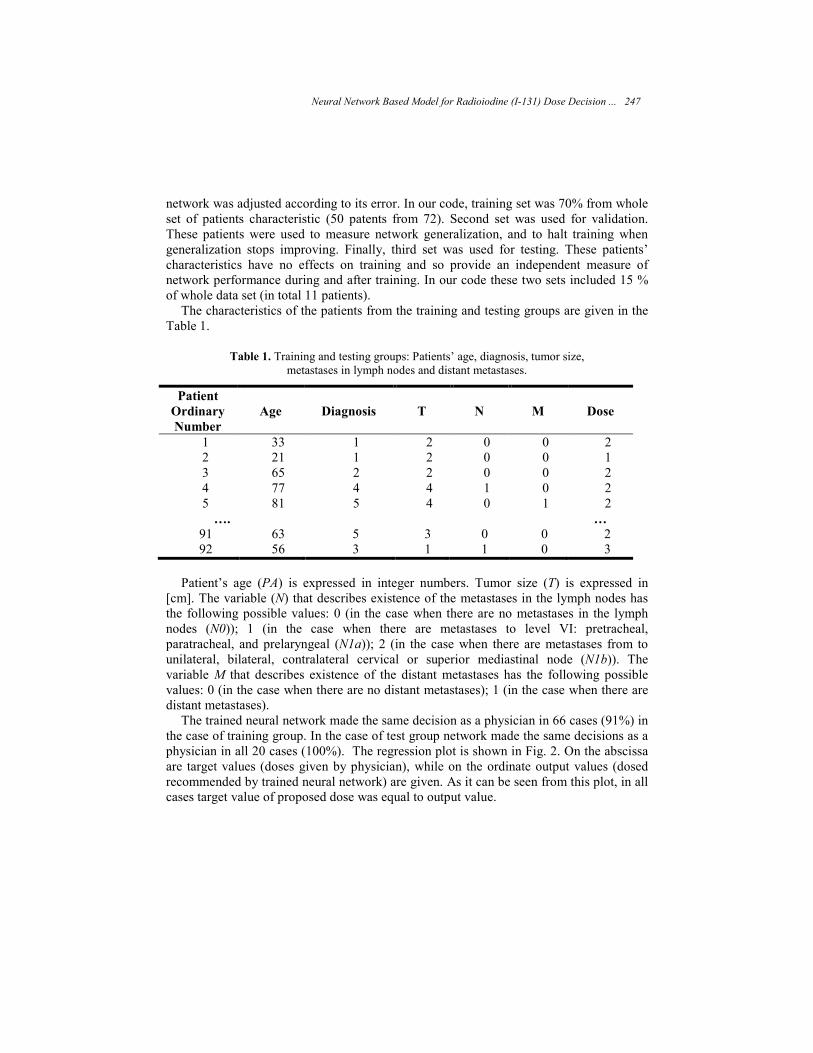
network was adjusted according to its error. In our code, training set was 70% from whole set of patients characteristic (50 patents from 72). Second set was used for validation. These patients were used to measure network generalization, and to halt training when generalization stops improving. Finally, third set was used for testing. These patients’ characteristics have no effects on training and so provide an independent measure of network performance during and after training. In our code these two sets included 15 % of whole data set (in total 11 patients).

The characteristics of the patients from the training and testing groups are given in the Table 1.

Table 1. Training and testing groups: Patients’ age, diagnosis, tumor size, metastases in lymph nodes and distant metastases.

Patient

Ordinary

Number

Age Diagnosis T N M Dose

1 33 1 2 0 0 2 2 21 1 2 0 0 1 3 65 2 2 0 0 2 4 77 4 4 1 0 2 5 81 5 4 0 1 2 …. …

91 63 5 3 0 0 2 92 56 3 1 1 0 3

Patient’s age (PA) is expressed in integer numbers. Tumor size (T) is expressed in

[cm]. The variable (N) that describes existence of the metastases in the lymph nodes has the following possible values: 0 (in the case when there are no metastases in the lymph nodes (N0)); 1 (in the case when there are metastases to level VI: pretracheal, paratracheal, and prelaryngeal (N1a)); 2 (in the case when there are metastases from to unilateral, bilateral, contralateral cervical or superior mediastinal node (N1b)). The variable M that describes existence of the distant metastases has the following possible values: 0 (in the case when there are no distant metastases); 1 (in the case when there are distant metastases).

The trained neural network made the same decision as a physician in 66 cases (91%) in the case of training group. In the case of test group network made the same decisions as a physician in all 20 cases (100%). The regression plot is shown in Fig. 2. On the abscissa are target values (doses given by physician), while on the ordinate output values (dosed recommended by trained neural network) are given. As it can be seen from this plot, in all cases target value of proposed dose was equal to output value.


5 Conclusion

The physician needs to be very knowledgeable, experienced and trained properly to adequately perform the studied task. In order to imitate physician’s decisions we developed a simple neural network that has the ability to adapt and learn. Training of the proposed neural network involves use of a data base of collected physician's decisions that are values for the input and the output of the neural network. The neural network learns by adjusting the connection strengths to minimize the error of the outputs.

Fig. 2. Regression plot.

The experience gained during this research indicated the importance of getting enough representative training and testing data. However, due to the nature of the information and all the difficulties of obtaining them, the number of available data was limited.

The purpose of the study in this phase of work was to develop a simple judgment system. Our aim was to create artificial neural network that would assist medical students to test their knowledge. We proposed neural network, which in the simplest form, is able to describe the actual judgment process. In other words, we showed that the proposed feedforward neural network has capability to imitate the actual decisions of the experienced physician. The developed classifier system could be used in educational purposes. It could assist and guide young physicians. The system developed can make the appropriate decision without knowing the functional relationships between individual variables.


References

1. Anderson, J.A: A Memory Storage Model Utilizing Spatial Correlation Functions. Kybernetics 5, 113−119 (1968)

2. Caudill, M., Butler, C.: Naturally Intelligent Systems, MIT Press, Cambridge, MA. 3. Fausett, L., Fundamentals of Neural Networks, Prentice Hall, Saddle River, New Jersey (1990) 4. Holst, H, Åström, K., Järund, A.: Automated interpretation of ventilation-perfusion lung

scintigrams for the diagnosis of pulmonary embolism using artificial neural networks. European Journal of Nuclear Medicine 27, 400−406 (2000)

5. Patil, S., Henry, J.W., Rubenfire, M., Stein, P.D.: Neural network in the clinical diagnosis of acute pulmonary embolism. Chest 104,1685−1689 (1993)

6. Riesco-Eizaguirre, G., Santisteban, P.: New insights in thyroid follicular cell biology and its impact in thyroid cancer therapy. Endocrine-Related Cancer 14, 957–77 (2007)

7. Savin, S., Cvejic, D., Mijatovic, Lj., Zivancevic Simonovic, S.: Measuring thyroglobulin concentrations in patients with differentiated thyroid carcinoma. Journal of Medical Biochemistry 29, 1−5 (2010)

8. Scott, J.A., Palmer, E.L.: Neural network analysis of ventilation perfusion lung scans. Radiology 186, 661−664 (1993)

9. Specht, D.F.: Vectorcardiographic Diagnosis Using the Polynomial Discriminant Method of Pattern Recognition, IEEE Transactions on Bio-Medical Engineering, BME-14, 90−95 (1967)

10. Tourassi, G.D., Floyd, C.E., Sostman, H.D., Coleman, R.E.: Acute pulmonary embolism: artificial neural network approach for diagnosis. Radiology 189, 555–558 (1993)

11. Vrndic, O.B., Savin, S.B., Mijatovic, Lj., Djukic, A., Jeftic, I.D., Zivancevic Simonovic S.T.: Concentration of thyroglobulin and thyroglobulin-specific autoantibodies in patients with differentiated thyroid cancer after treatment with radioactive Iodine 131. Labmedicine 42, 27−31 (2011)

12. Wasserrnan, P.D.: Neural Computing: Theory and Practice, Van Nostrand Reinhold, New York (1989)


Evaluation of Hydrocephalic Ventricular in Brain Images

using Fuzzy Logic and Computer Vision Methods

Miguel Ángel López Ramírez1, Erika Consuelo Ayala Leal1, Arnulfo Alanis Garza1,

and Carlos Francisco Romero Gaitán2

1 Division de Posgrado Instituto Tecnologico de Tijuana, Fraccionamiento Tomas Aquino S/N, Tijuana, Baja California, C.P. 22414, Mexico

2 Facultad de Medicina Universidad Autonoma de Baja California, Calzada Tecnologico No. 14418, Mesa de Otay, Tijuana Baja California, C.P. 22390, Mexico

Abstract. The purpose of this paper is classify cases of hydrocephalic ventricular of human brain images using fuzzy logic, based on the size of the ventricles of the human brain, using intelligent techniques combined with computer vision, the analysis of the ventricles size was based databases using magnetic resonance cases of normal ventricles, the criterion based of the fuzzy logic inference system and vision using the height, and volume of the ventricles to classify the hydrocephalic cases. The height, area and volume of the ventricles of the left and right brain were measured in 13 individuals, 10 normal and 3 cases of hydrocephalus. We expect that the symptoms of hydrocephalus using the proposed method are classified by the size of the ventricles with a significantly higher percentage when considering a large number of cases of hydrocephalus.

Keywords: Computer vision and image processing, bioinformatics and medical applications, fuzzy logic.

1 Introduction

The Hydrocephalus can be defined as a disturbance of the formation of flow, or absorption of cerebrospinal fluid (CSF) that leads to an increase in the volume occupied by the fluid in the central nervous system.

This condition could be termed as a disorder of CSF hydrodynamics. Acute hydrocephalus occurs in days, sub acute hydrocephalus occurs within weeks, and chronic hydrocephalus occurs over months or years. Conditions such as brain atrophy and focal destructive lesions also lead to an abnormal increase of cerebrospinal fluid in the central nervous system. In these cases, brain tissue loss leaves a void that is filled passively with CSF. These are not the result of a hydrodynamic disorder and therefore are not classified as hydrocephalus. A major misnomer used to describe these conditions was hydrocephalus ex vacuo.

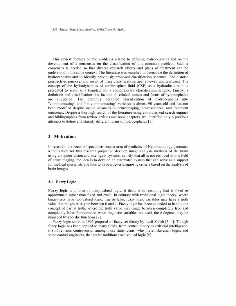
This review focuses on the problems related to defining hydrocephalus and on the development of a consensus on the classification of this common problem. Such a consensus is needed so that diverse research efforts and plans of treatment can be understood in the same context. The literature was searched to determine the definition of hydrocephalus and to identify previously proposed classification schemes. The historic perspective, purpose, and result of these classifications are reviewed and analyzed. The concept of the hydrodynamics of cerebrospinal fluid (CSF) as a hydraulic circuit is presented to serve as a template for a contemporary classification scheme. Finally, a definition and classification that include all clinical causes and forms of hydrocephalus are suggested. The currently accepted classification of hydrocephalus into "communicating" and "no communicating" varieties is almost 90 years old and has not been modified despite major advances in neuroimaging, neurosciences, and treatment outcomes. Despite a thorough search of the literature using computerized search engines and bibliographies from review articles and book chapters, we identified only 6 previous attempts to define and classify different forms of hydrocephalus [1].

2 Motivation

In research, the needs of specialists impact area of medicine of Neuroradiology generates a motivation for this research project to develop image analysis methods of the brain using computer vision and intelligent systems, namely that all is not resolved in this field of neuroimaging, the idea is to develop an automated system that can serve as a support for medical specialists and thus to have a better diagnostic criteria based on the analysis of brain images.

2.1 Fuzzy Logic

Fuzzy logic is a form of many-valued logic; it deals with reasoning that is fixed or approximate rather than fixed and exact. In contrast with traditional logic theory, where binary sets have two-valued logic: true or false, fuzzy logic variables may have a truth value that ranges in degree between 0 and 1. Fuzzy logic has been extended to handle the concept of partial truth, where the truth value may range between completely true and completely false. Furthermore, when linguistic variables are used, these degrees may be managed by specific functions [2].

Fuzzy logic starts in 1965 proposal of fuzzy set theory by Lotfi Zadeh [3, 4]. Though fuzzy logic has been applied to many fields, from control theory to artificial intelligence, it still remains controversial among most statisticians, who prefer Bayesian logic, and some control engineers, that prefer traditional two-valued logic [5].

252 Miguel Ángel López Ramírez, Erika Consuelo Ayala...

In this paper we use fuzzy logic to determine if the person has hydrocephalus or not, using two fuzzy systems that use height, area and volume of the left and right ventricles, which were obtained from a database of CT images Excel Medical Center.

3 The Ventricles of the Brain Metric Height, Area and Volume

We utilized a database of 13 individuals with 45 scans each for a total of 585 sample images to obtain the necessary metrics and to test the fuzzy inference system, 10 are normal people with hydrocephalus and 3 if then shown as obtained measures of height, area and volume of right and left ventricles [6].

Fig. 1a) Computerized axial tomography, height of the ventricles, 1b) Measurement Tools.

Fig. 2a) Computerized axial tomography, Area of the ventricles, 2b) Measurement Tools.

It was used to support development of specialized software from Philips with which we read the CT images and look at different angles of the image. Figures 1a and 1b show an example of how to calculate the height of the right and left ventricles in the image by

Evaluation of Hydrocephalic Ventricular in Brain Images... 253

drawing a line that covers each Ventricle, measures are in units of millimeters, the height within the brain image of the left ventricle are shown in red and yellow ventricle right.

The height is obtained by drawing a straight line from end to end for each left and right ventricle, for example, in this case we have the height: Right ventricle size: 59.2mm, Left ventricular measures: 56.1mm

The calculation of the area of the ventricles using the height of each ventricle and its base, forming a rectangle, take the base and the height and divide by two to calculate the area for each of the ventricles multiplying the base times height, it is in figures 2a) and 2b).

The following shows how to calculate the area of each ventricle for example:

Area = (base) x (Height Right ventricle height 59.2mm and 38.5mm base of the right ventricle. Area = (59.2mm) x (38.5mm) = 2279.2 mm2

The following is an example of the calculation of the volume using the area and height of the ventricles:

Volume = (Area) x (Height) Right ventricular volume: Area = 2279.2mm2, Height = 59.2mm from the right ventricle to obtain the volume of the right ventricle. Volume = (2279.2mm2) x (59.2mm), Volume = 134928.64 mm3

The calculation of Left ventricular volume, area = 2159.85mm2, height = 56.1mm, obtaining the right ventricular volume, Volume = (2159.85mm2) x (56.1mm), Volume = 121167.58 mm3

The following tables show the results of measurements of each of the test images which specify the measures normal and Hydrocephalus cases:

Table 1. Measurements (part 1).

Measures Brain Normal Hydrocephalus

Height(mm) Ventricle Right 50.7 68.0 70.0 90.0

Left 48.9 72.1 73.0 90.0 Area(mm2) Ventricle Right 870.94 1350.60 1270 2396

Left 875.94 1355.57 1273 2386 Volume(mm3) Ventricle Right 100 50 190 420 x million Left 89 215 180 410

Table 2 shows measures of 10 normal individuals. VBH is the height of the ventricle of the brain, VBA is the area of the brain ventricle and VBV is the volume of the ventricle of the brain.



Person VBH VBA VBV

Right Left Right Left Right Left

1 60.0 54.8 1093.47 1093.47 131216.4 119844.312 2 56.2 56.4 1187.93 1187.93 133760.918 133998.504 3 66.2 70.9 1355.57 1355.57 179478.262 192220.676 4 62.9 60.8 1237 1237 155614.6 150919.2

Normal 5 64.6 72.1 1467.81 1467.81 189641.859 211658.923 6 50.7 51.9 875.94 875.94 88821.076 90923.35 7 68.6 53.4 1242.87 1242.87 170522.45 132739.05 8 50.7 48.9 991.02 991.02 100489.420 96921.756 9 62.3 54.2 958.21 958.21 119393.277 103870.235 10 66.3 65.3 1112.04 1112.04 147453.852 145229.812

Table 3 shows the measures of height, area and volume of the ventricles of the individual cases of hydrocephalus.


Person VBH VBA VBV Right Left Right Left Right Left 1 75 73.7 1273.243 1273.243 190986.562 187676.091

Hydrocephalus

2 86.5 84.6 2386.84 2386.84 412924.185 403854.174

3 83.4 77 1888.71 1888.71 315036.828 290861.34

4 Evaluation of Fuzzy Inference System for Hydrocephalus

The proposed inference system uses three input variables, which are the height, area and volume of the ventricles, and one output variable, which is the staging evaluation hydrocephalus or normal membership functions are type triangular system is Mamdani type inference, the ranges established for the input variables and output based on the results tables 1, 2 and 3 is similar for right and left ventricle.

Figure 4 shows the inference system of evaluation cases of hydrocephalus to the right ventricle.

This fuzzy system is to the right ventricle of the brain has three input variables and output variable, and each input variable has three membership functions and the output variable has two membership functions. It is noted that the lowest height of the ventricles according to our tests was 48 mm and the highest was the 90 mm. as shown in Figure 5.

Figure 6 shows that the range area of the ventricles is a normal measure that would be 875.94 mm 2 and a case of hydrocephalus which would be 2386.84 mm2.

Figure 7 shows that the lowest volume is 98 mm 3and the highest volume was 420 mm3

(it is necessary to multiply the range by one million).


Fig. 4. Fuzzy system with three input variables and output.

Fig. 5. Each variable has three membership functions are low, medium and high.

Fig. 6. Membership Functions of right ventricular Area.

Figure 8 shows the output of the fuzzy system that evaluates which cases of normal ventricles and those with a problem of hydrocephalus.

We can see that the output range consider the criterion of height. In the case of individuals who have longer ventricle of 90mm height are be considered cases of hydrocephalus, the criterion of the rules of fuzzy inference system considers its area and volume.


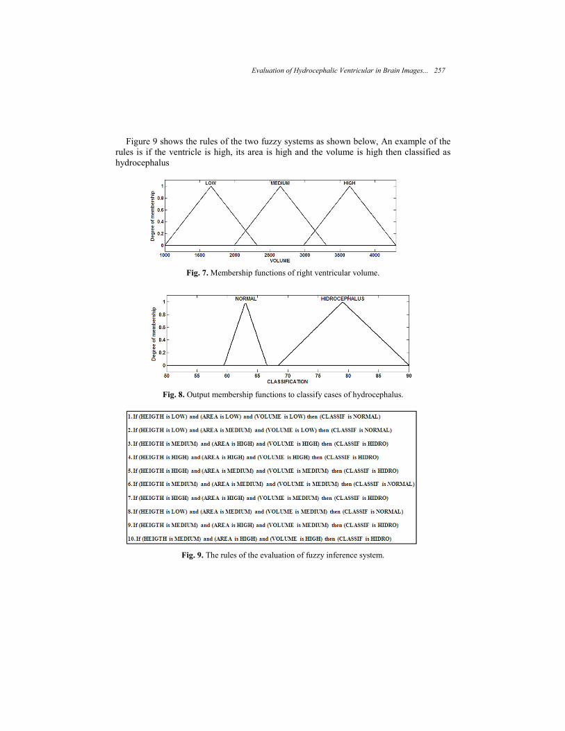
Figure 9 shows the rules of the two fuzzy systems as shown below, An example of the rules is if the ventricle is high, its area is high and the volume is high then classified as hydrocephalus

Fig. 7. Membership functions of right ventricular volume.

Fig. 8. Output membership functions to classify cases of hydrocephalus.

Fig. 9. The rules of the evaluation of fuzzy inference system.


5 Results and Conclusions

We utilized a database of 13 individuals with 45 scans each for a total of 585 sample images, To have a more diverse enough valid requires a larger database, and establishes contact with a neuroradiological center to get information, The results provide a criterion to classify cases of hydrocephalus based on the action of the ventricles height, area and volume, is one of the criteria that can be used to classify hydrocephalus and information required to relate the patient's clinical history. The tests were performed using a fuzzy inference system with a triangular membership function; it is necessary to experiment with other types of membership functions to see which provides better results and be able to use genetic algorithms for optimization of membership functions. Average measures were used the database, and statistical methods that allow us to validate the results.

We conclude that proposed method is a good approach, the proposed method is intended to be automated, and using methods of vision obtained measurements of the image and enter the evaluation system of fuzzy inference.

Acknowledgements. Excel medical center for providing the database of computerized axial tomography.

References

1. Espay, A.J., Crystal, A., Howard: http://emedicine.medscape.com/article/1135286-overview, (2010)

2. Novák, V., Perfilieva, I., Močkoř, J.: Mathematical principles of fuzzy logic Dodrecht: Kluwer Academic (1999)

3. Fuzzy Logic. Stanford Encyclopedia of Philosophy. Stanford University (2006) http://plato.stanford.edu/entries/logic-fuzzy/ Retrieved (2008)

4. Zadeh, L.A.: Fuzzy sets, Information and Control 8 (3): 8–353 (1965) 5. Zadeh, L.A. et al.: Fuzzy Sets, Fuzzy Logic, Fuzzy Systems, World Scientific Press (1996) 6. Jung-Woo, N., Chi-Bong, C., Dong-Cheol, W., Kyung-Nam R., Eun-Hee, K., Hwa-Seok, C.:

Evaluation of Hidrocephalic Ventricular Alterations in Maltese Dogs Using Low Field MRI. Vol.9, Num 1, International Journal Applications Veterinary Medical (2011)

7. Merge Efilm Helathcare Workstation Version 3.4, Philips, Software. 8. Francis, J.Y., Hahn, K.R.: Iowa City, Iowa: Frontal Ventricular Dimensions On Normal

Computed Tomography. Vol. 126, No. 3. 9. Jamous, M., Sood, S., Kumar, R., Ham, S.: Frontal and Occipital Horn Width Ratio for the

Evaluation of Small and Asymmetrical Ventricles Pediatry Neurosurgery. 39, 17–21 (2003) 10. Sullivan, E.V., Pfefferbaum, A., Adalsteinsson, E., Swam, G.E., Carmelli, D.: Differenctial

Rates of Regional Brain Change in Collosal and Ventricular Size 4 Year Longitudinal MRI Study of Elder Men. Cerebral Cortex, 12:438-445;1047-3211/02 (2002)


Robotics, Planning, and Scheduling

Ball Chasing Coordination in Robotic Soccerusing a Response Threshold Model with

Multiple Stimuli

Efren Carbajal and Leonardo Garrido

Intelligent Autonomous Agents Research Group,Department of Computer Science, ITESM, Monterrey, Mexico

A00937789,[email protected]

Abstract. In any system made of several robots task allocation is anindispensable component in order to achieve coordination. We presenttwo different approaches commonly found in literature to solve the dy-namic assignment of the ball chasing task, i.e. multi robot task allocationand division of labour. In particular, we explore both approaches in a3D simulation robotic soccer domain called Robotstadium. Moreover,we evaluate and compare four controllers representing different coordi-nation implementations belonging to either of the two approaches. Weshow that by formulating the problem as one of division labour andthen employing a response threshold model with multiple stimulus asarbitration mechanism, we provide an efficient algorithm with respect toa proven benchmark solution. We also present evidence indicating thatthis communication-less algorithm result in an emergent team behaviorwhich indirectly also address the positioning problem of robots withinthe soccer field, keeping physical interference low.

Keywords: Task allocation, response threshold, division of labour, roboticsoccer.

1 Introduction

In the last two decades, researchers have given more and more attention toMulti-Robot Systems (MRS). Besides an important reduction in hardware prices,there are some other advantages of MRS like performance benefits, and theaccomplishment of inherently complex tasks, which explain its growing use bythe scientific community. An example of this can be found in RoboCup, a roboticsoccer competition which foster research in robotics and Artificial Intelligence(AI) [1].

Task allocation, the process of assigning individual robots to sub-tasks ofa given system-level task, is a very important component of any MRS [13]. Inrobotic soccer a team of robots have to work together in order to win a matchagainst other team of robots. This entails that robots have to cooperate andcoordinate with each other. Where the global task of playing soccer require

different roles or sub-tasks like defense, goalkeeper, passing, and shooting becarried out in order to achieve a team behavior.

Robotic soccer researchers have labeled this problem also as dynamic assign-ing roles or role allocation [10, 14]. Solutions found in literature often involvethe construction of a model of the environment and the use of explicit commu-nication to assign roles. A intuitive idea to solve this problem it is to followinga centralized approach, however, the environment is only partial observable toeach robot, and no single individual has enough information to make correctdecisions [14]. Another attempt is to follow a well known approach in Multi-Agent Systems (MAS): negotiation. But, there are some issues concerning tocommunication in real time environments which make this technique unsuitable[15].

To overcome those issues some researchers had combined local and globalinformation about ball, using global information only when more reliable localinformation is not available [14].

Given the difficulties experienced and the importance of local information,it seems suitable the use of a Swarm Intelligence (SI) approach to this prob-lem. SI gives special importance to self-organization, local information, implicitcommunication to achieve emergent coordination. According to Lerman at al.[13]:

“Emergent coordination algorithms for task allocation that use only lo-cal sensing and no direct communication between robots are attractivebecause they are robust and scalable”

In this paper we propose the use of a response threshold model as a SI taskallocation mechanism for the ball chasing task in Robotstadium, a robot soccersimulation based on the Standard Platform League (SPL) of RoboCup and itsrules [2].

Section 2 introduce the response threshold model and how this is extendedin order to cover some issues present in the domain.

Section 3 shows the arquitecture of the generic controller (i.e. the controllerused as base for all the coordination strategies). Section 4 describes the coor-dination strategies. Section 5 describes the experimental setup. Section 6 showsthe results and offers an interpretation. Section 7 concludes.

2 Response Threshold

There are different classes of mathematical models which try to explain divisionof labour in social insects. According to Beshers et al. [5] response thresholdmodels is one them, and in their work they described this class of model. In thismodel every individual has its own internal response threshold for every task,andengaging in this when the level of the stimulus related to such task exceedstheir threshold [6]. This kind of models have been successfully implemented byresearchers in MAS and robotics. Examples of these applications are: artificialmail retrieval system [8] in MAS domain, and clustering objects [3] and foraging[11] in MRS.

262 Efren Carbajal and Leonardo Garrido

2.1 Fixed Threshold Model with One Task and OneStimuli

Bonabeau et al. [7] have developed a simple model of division of labour in insectsocieties. This model is describe by the authors as following. Suppose X is thestate of an individual (where X= 0 indicate that the task is not been performed,and X = 1 indicates the task is been performed ), and θi the response thresholdof individual i (i = 1, 2... ... n). Then the probability that an inactive individuali starts performing the task Pi per unit time is:

Pi(X = 0→ X = 1) =s2

s2 + θ2i. (1)

From the eq. 1 we know that the probability that an individual will perform atask depends on s which is the magnitude of the stimulus related task. Similarity,an individual will become inactive with a probability p as describe in eq. 2. Where1p is the average time spend by an individual before stops performing the task,therefore, p can be found experimentally.

Pi(X = 1→ X = 0) = p . (2)

2.2 Fixed Threshold Model with One Task andMultiple Stimuli

In this paper, we propose a slightly different model a little less stochastic. Inthis model, the probability Pi(X = 1→ X = 0) is not independent of stimulus,so it is not a constant p. Instead, we model this probability as the inverse ofPi(X = 0 → X = 1) as it is describe in eq. 3. However, this can’t be donewithout some sort of mechanism which allows to decrease the stimulus whileperforming the task independently of the execution’s duration. Here is wherethe reference to multiple stimuli comes into play. Basically, we employ differenttypes of stimuli that can be classify either as a excitatory or inhibitory, thusthe intensity and direction of the stimulus can be calculated as the differencebetween the sum of excitatory and the sum of inhibitory stimulus as shown ineq. 4.

Pi(X = 1→ X = 0) = 1− s2

s2 + θ2i. (3)

s =∑

sexcitatory −∑

sinhibitory . (4)

Ball Chasing Coordination in Robotic Soccer using a Response Threshold Model with Multiple Stimuli 263

2.3 Stimulus

Table 1. List of stimuli names and types

Stimulus Type

Distance to the ball Excitatory

Number of teammates Inhibitorycloser to the ball

Presence of obstacles Inhibitory(sonar)

This model differs from the original in two aspects: the number of differentstimuli related to the task, and how the probability to stop performing the taskis computed. Generally in literature the stimulus is only one straightforwardmeasurement of the environment. However, we believe there are several factorsinvolved in the decision making of whether or not approaching to the ball couldderive in a good output, specially when there is not direct communication amongthe individuals. Those factors and their nature are shown in table 1. Takinginto account both type of stimulus: excitatory and inhibitory, make possiblefor the individual to engage in performing the task when excitatory stimuluspredominates, or stop performing the task when inhibitory stimulus outweighexcitatory one. The result is a less stochastic response which adapts more quicklyto dynamic environment, making the controller better suited for a real-time,coarse-grained MRS competition.

3 Controller

The control algorithm is based on a simple finite state machine (FSM) as it isdepicted in figure 1. Different states represent the different phases of the soccergame, that is, the subtasks in which the overall game is decomposed. Thesesub-tasks are as follows:

Search The robot look for the ball just by moving its head. If ball has alreadybeen seen and there is no perception gained about a teammate robot, thenthe controller change Chase state. Otherwise, If ball is seen but a teammateperception is received then, it makes a transition to Wait state.

Chase Robot moves toward the ball and remains in this state until ball is closeenough, that is when the Shoot state takes place. While going after the ball,this may gets outs of sight, in that case the controller returns to the Searchstate.

Wait In this state robot is stand up tracking the ball until no perception ofother robot is received, alternatively switch to Chase state. Other possibilityis to lose out the ball, in which case the controller is forced to return tosearch state.


Search

Chase

Wait

Shoot

¬ see_ball

¬ see_ball

(see_ball) and

(¬ perceive_teammate)

(see_ball) and

(perceive_teammate)

(see_ball) and


(see_ball) and


ball_close

Fig. 1. Finite State Machine diagram.

Shoot Robot hit the ball in goal direction, then as ball moves along, roboteither lose it and return to Search state, or start to chase it again, switchingback to Chase state.

Transitions between states occur on the base of events that are external (e.g.Perception of another robot) to the robot. The edge labels between states (asshown in figure 1 represent the conditions (also called predicates) that mustbe true for the transition to occur. The complete list of the predicates, theirmeanings and how they are evaluated is given in table 2. Their truth values areevaluated from sensor readings at every control cycle.

Table 2. Definition of constants and predicates used by the control algorithm

B D Maximum distance between robot andball to try to kick the ball

see ball Ball is detected using visual informationobtained from the camera

perceive teammate A teammate is communicating that it iscloser to the ball

ball close Distance to ball < B D

4 Coordinations Strategies and Evaluation Metrics

In order to coordinate robots, allocation strategies addressed in this work employtwo types of communication mechanisms. The first refers as “public” emphasizesin the existence of an explicit collaborative information flow between teammatesthrough a emitter/receiver device. Whereas in the latter, which we are call “pri-vate”, there is no explicit information sharing but intead robot recognition al-gorithms are employed to communicate indirectly by sensing the presence of


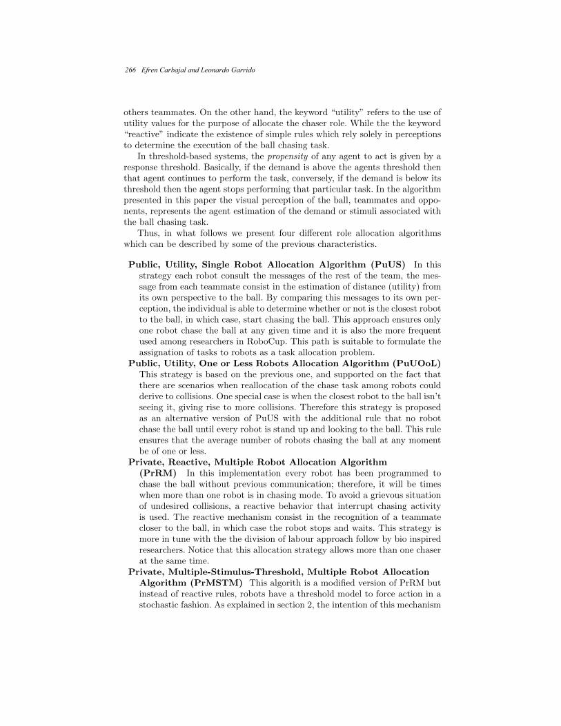
others teammates. On the other hand, the keyword “utility” refers to the use ofutility values for the purpose of allocate the chaser role. While the the keyword“reactive” indicate the existence of simple rules which rely solely in perceptionsto determine the execution of the ball chasing task.

In threshold-based systems, the propensity of any agent to act is given by aresponse threshold. Basically, if the demand is above the agents threshold thenthat agent continues to perform the task, conversely, if the demand is below itsthreshold then the agent stops performing that particular task. In the algorithmpresented in this paper the visual perception of the ball, teammates and oppo-nents, represents the agent estimation of the demand or stimuli associated withthe ball chasing task.

Thus, in what follows we present four different role allocation algorithmswhich can be described by some of the previous characteristics.

Public, Utility, Single Robot Allocation Algorithm (PuUS) In thisstrategy each robot consult the messages of the rest of the team, the mes-sage from each teammate consist in the estimation of distance (utility) fromits own perspective to the ball. By comparing this messages to its own per-ception, the individual is able to determine whether or not is the closest robotto the ball, in which case, start chasing the ball. This approach ensures onlyone robot chase the ball at any given time and it is also the more frequentused among researchers in RoboCup. This path is suitable to formulate theassignation of tasks to robots as a task allocation problem.

Public, Utility, One or Less Robots Allocation Algorithm (PuUOoL)This strategy is based on the previous one, and supported on the fact thatthere are scenarios when reallocation of the chase task among robots couldderive to collisions. One special case is when the closest robot to the ball isn’tseeing it, giving rise to more collisions. Therefore this strategy is proposedas an alternative version of PuUS with the additional rule that no robotchase the ball until every robot is stand up and looking to the ball. This ruleensures that the average number of robots chasing the ball at any momentbe of one or less.

Private, Reactive, Multiple Robot Allocation Algorithm(PrRM) In this implementation every robot has been programmed tochase the ball without previous communication; therefore, it will be timeswhen more than one robot is in chasing mode. To avoid a grievous situationof undesired collisions, a reactive behavior that interrupt chasing activityis used. The reactive mechanism consist in the recognition of a teammatecloser to the ball, in which case the robot stops and waits. This strategy ismore in tune with the the division of labour approach follow by bio inspiredresearchers. Notice that this allocation strategy allows more than one chaserat the same time.

Private, Multiple-Stimulus-Threshold, Multiple Robot AllocationAlgorithm (PrMSTM) This algorith is a modified version of PrRM butinstead of reactive rules, robots have a threshold model to force action in astochastic fashion. As explained in section 2, the intention of this mechanism


is to ponder several key aspects (i.e. multiple stimulus) of the environmentin order to assess the demand to execute the ball chasing task.

In order to evaluate the performance of such implementations, we make useof the direct output of every soccer robotic controller: goals (i.e. goals scored aswell as goal conceded). But we also propose the use of complementary metricsmaking emphasis in the intention we have in this work to produce results thatare interesting to continue with and validate beyond simulation level. Additionalmetrics proposed in this work are physical interference and efficiency. Both ofthem been of much interest in MRS [12, 9].

Performance The main indicator of performance in soccer is the goal difference(i.e. goals scored minus goals conceded). Because depending the team youchoose as reference team lose of win the match, this number can take nega-tive values (when reference team lose). To avoid confusion we are going to useas reference the team running implementations of strategies to test. In ad-dition, those results were normalized in order to ensure only zero or positivenumbers. The reason behind applying normalization to the data is becausepositive numbers are required to estimate the efficiency as it is discussedfurther in efficiency description. To summarize, for performance we meanthe output of a normalization process that employs the goal differenceas theonly input to generate zero or positive numbers. The normalization consist inadding all numbers with the absolute of the most negative (minimum valueof goal difference) such that the most negative one will become zero and allother number become positive.

Efficiency Lets start by defining efficiency, we refer to efficiency as the capa-bility to convert some valuable resource into another new valuable resource.In the context of robotic soccer, we define as the input resource the energyspent by the robot moving around, and as output resource,the total numberof goals scored and conceded. However, the energy spent by a robot dependson too many factors, known and unknown, and a precise measurement it isfar beyond the reach of this work. Conveniently, we know that the displace-ment of a robot is proportional to the energy it uses. Thus, we decide to usethe displacement as an approximation of the energy spent. This way we endup with equation 5.

ηi =∆i

εi. (5)

Where:

ηi = Team’s efficiency during match i∆i = Normalized goal difference during match iεi = Displacement in meters during match i

Interference Another important issue related to the performance of a genericMRS are collisions, also known as physical interference [4, 9]. According toGoldberg at al. [9] physical interference arises in competition for space. They


show with experiments that the measurement of it can be an effective tool forsystem design and evaluation. In Robotstadium’s case, space competition arepresent mostly in a particular task: chasing the ball. The number of collisionsby members of the tested team was tracked down with help of an emulatedGPS device in the supervisor’s code (i.e. referee code that along with codeof controllers and world complete the simulation).

5 Experimental Setup

The main objetive of this study is to challenge two ideas widely established inpractice. The first is related to the number of robots which should be chasingthe ball at any given time during the match. So far this number has remainedfix to one by roboCup researchers. As a consequence, two out of the four im-plementations evaluated in this section represent a division of labour approachwhich inherently allocate tasks without restrictions in the number of individualsthat engage in them. The second idea is about the need of make use of a spa-tial model, autolocalization and explicit commmunication in order to distributerobots, improve performance and reduce collisions among robots. A way to chal-lenge this idea is by contrasting it with bio inspired implementations, whichproduce an emergent team behavior that result in a self-organized distributionof robots in the field without direct communication or a concrete spatial modelof the environment.

Fig. 2. Robotstadium field measures in millimeters taken from the top orthographicprojection of the simulation in Webots


2 3 4 5

6

8

10

12

Goal diffe

rence

Robots

PuUS

PuUOoL

PrRM

PrMSTM

Fig. 3. Comparison of performance as group size increases

An experimental trial consist in running complete match divided in two halfperiods of 10 minutes, where in one side of the field there is a team representingone of the four strategies, while in the other side, there is a single robot. In thismanner, experimental trials have been performed with each of the four strategies:PuUOoL, PuUS, PrRM and PrMSTM; and for each strategy forty trials wereperformed with two, three, and four robots. An extra run of experiments withfive robots for the two better performed strategies were added as an attempt toshed light to further conclusions. As a result, a total of 560 experiments werecarried out.


Data obtaining from all the experiments have been analyzed with a two-wayANOVA statistic test. Where performance, interference and efficiency were ex-plained using coordination strategy as a categorical variable and team size (num-ber of robots) as numerical variable. In all three tests both variables, strategyand team size, were found to be statistically significant with p-values < 0.05.

Beforehand we hypothesized that PrRM would produce the higher number ofinterferences among all strategies, thus, its performance would be outperformedby that of strategies PuUS and PuUOoL. Surprisingly, this was not the resultas shown in fig. 3, despite the high level of interference. We believed this is duea higher chance to get first to the ball and to handicap the other team’s robot.However, when looking to interference, as fig. 4 shows it, the performance gainsof PrRM become overshadow by exponential growth in interferences.

On another hand, performance of PuUOoL was lower among all implementa-tions. And performance of PuUS and PrMSTM was similar between them withno statistically significant difference observed. A slightly better performance was


presented in the threshold strategy when the team size is 4, but with virtuallythe same performance when the team size reach 5 robots. Besides the fact ofboth implementations achieved almost the exact performance when team sizewas fixed to five, it is worth to note as well that PrMSTM strategy tendencyto improve along the team size increases, ends abruptly when arrives to the fiverobots per team, resulting in both strategies performance curves crossing eachother.

2 3 4 5

0

10

20

30

40

Inte

rfere

nce

Robots

PuUS

PuUOoL

PrRM

PrMSTM

Fig. 4. Comparison of interference level as group size increases

Could these two seemingly independent issues be related?, we suspect theyare indeed, we believe the performance of both strategies is bound by the fieldsize, which may happens to be too small to allow an equal and active partici-pation from all the robots. Outcome from efficiency, seems confirm this. Evenwhen there was no apparent gain in performance in PrMSTM when passing fromfour to five robots, there was a gain in efficiency, and since efficiency is affectedeither by performance or energy spent, this gain must come mostly from a re-duction in the latter. This reduction in energy spent is more pronounced thanin others team size configurations, which can be explain by a good coverage ofwhole field by the five robots. Note that if this hypothesis were correct, mayimply that PrMSTM strategy is also good at adapting or showing robustness toenvironmental changes. However, more evidence is needed to support this. Sofar we can only conclude that both controllers performed at a similar level.

As mentioned before, we hypothesize that the presence of interference ofPrRM would be greater than found in PuUO, and the latter greater than foundin PuUOoL. As figure 4 shows it, the guess was correct. However, we didn’tknow what to expect about the magnitude of those difference, neither of thelevel of interference in PrMSTM. The outcome is that the amount of collisionsin strategy PrRM is, to a large extent, bigger than the rest of implementations.


2 3 4 5

0.05

0.10

0.15

0.20

0.25

0.30

Effic

iency

Robots

PuUS

PuUOoL

PrRM

PrMSTM

Fig. 5. Comparison of efficiency results as group size increases

Unlike PrRM, in PrMSTM the interference level is not a grievous problem, infact, this is comparable to those in PuUOoL and PuUS when four or five robotsare set per team.

Another hypothesis we were interested to proved is related to the efficiency.Due to the restriction of one at most, we were expecting a more efficient use ofenergy in PuUS and PuUOoL. But as shown in figure 5 this was not exactly thecase. For three robots per controller PuUS is the most efficient, however, as thenumber of robots increase to four and up to five, PrMSTM takes the credit asthe most efficient.

Is interesting how PrMSTM and PrRM both representing a division of labourapproach are at the same time the most efficient and inefficient. This indicatethe influence of the threshold model in regulating the number of active chasers.A exception of PrMSTM, what happened with the rest of implementations wasthat efficiency holds almost steadily from the start only gaining a little withevery increase in team size. From the scalability perspective, we can observe infigure 5 that efficiency curves for all strategies, except for PrMSTM, resembledlogarithmic functions, this fact indicate marginal returns while adding morerobots.

7 Conclusions

In this paper, we have presented a comparative study of four distributed, multirobot allocation mechanisms that allow a team of autonomous, embodied agentsto dynamically allocate the fittest individual(s) to a given task. These coor-dination algortihms can be classified in two approaches, task allocation withPuUS and PuUOoL as representatives, and division of labour with PrRM and


PrMSTM as representatives. We compared their performance and efficiency ina robotic soccer case study concerned with a ball chasing task.

We showed that framing the ball chasing task assignment as a division oflabour problem and using a multiple stimulus threshold model to address it,the system performs as well as the benchmark solution (i.e.PuUS for been themost widely used among researchers) while at the same time arrive to additionalbenefits as a significant increment in efficiency when the team size is set to fouror five robots without any sort of direct communication.

References

1. Robocup objective: Pushing the state of art. http://www.robocup.org/

about-robocup/objective/

2. Robotstadium: online robot soccer competition. http://robotstadium.org

3. W Agassounon and A Martinoli. Efficiency and robustness of threshold-baseddistributed allocation algorithms in multi-agent systems. Proceedings of the firstinternational joint conference on Autonomous agents and multiagent systems part3 AAMAS 02, pp. 1090–1097 (2002)

4. R C Arkin and T Balch. Cooperative multiagent robotic systems. Artificial Intel-ligence and Mobile Robots, pp 277–296 (1998)

5. S N Beshers and J H Fewell. Models of division of labor in social insects. AnnualReview of Entomology, 46(413-440):413–440 (2001)

6. E Bonabeau, M Dorigo, and G Theraulaz. Swarm Intelligence: From Natural toArtificial Systems, Oxford University Press (1999)

7. E Bonabeau, G Theraulaz, and J L Deneubourg. Quantitative study of the fixedthreshold model for the regulation of division of labour in insect societies. Pro-ceedings Biological Sciences, 263(1376):1565–1569 (1996)

8. Eric Bonabeau, Andrej Sobkowski, Guy Theraulaz, and J L Deneubourg. Adaptivetask allocation inspired by a model of division of labor in social insects. BioComputation and Emergent Computing, pp. 36–45 (1997)

9. D Goldberg and M J Mataric. Interference as a Tool for Designing and EvaluatingMulti-Robot Controllers. AAAIIAAI, 8:637–642 (1997)

10. Eric Henry Work, Chown, Tucker Hermans, and Jesse Butterfield. Robust Team-Play in Highly Uncertain Environments ( Short Paper ). (Aamas) (2008)

11. M J B Krieger and J B Billeter. The call of duty: Self-organised task allocationin a population of up to twelve mobile robots. Robotics and Autonomous Systems,30(1-2):65–84 (2000)

12. Thomas H. Labella, Marco Dorigo, and Jean-Louis Deneubourg. Division of laborin a group of robots inspired by ants’ foraging behavior. PhD thesis (2006)

13. Kristina Lerman, Chris Jones, Aram Galstyan, and Maja J Mataric. Analysis ofDynamic Task Allocation in Multi-Robot Systems. The International Journal ofRobotics Research, 25(3):225–241 (2006)

14. Michael J Quinlan, Steven P Nicklin, Stephen R Young, Timothy G Moore,Stephan K Chalup, and Richard H Middleton. The 2005 NUbots Team Report.Electrical Engineering (2006)

15. Thomas Rofer, Michael Weber, Hans dieter Burkhard, J Matthias, G Daniel, JanHoffmann, and Bastian Schmitz. German Team: RoboCup 2005 (2005)


IOCA: An Interaction-Oriented Cognitive Architecture

Luis A. Pineda, Ivan V. Meza, Héctor H. Avilés, Carlos Gershenson, Caleb Rascón,

Montserrat Alvarado, and Lisset Salinas

Instituto de Investigaciones en Matemáticas Aplicadas y en Sistemas (IIMAS),

Universidad Nacional Autónoma de México (UNAM), México D. F., Mexico [email protected]

Abstract. In this paper an interaction-oriented cognitive architecture for the

specification and construction of situated systems and service robots is presented.

The architecture is centered on an interaction model, called dialogue model, with its

corresponding program interpreter or Dialogue Manager. A dialogue model

represents the task structure of a specific application, and coordinates interpretations

produced by the system’s perceptual devices with the system’s intentional actions.

The architecture also supports reactive behavior, which relates context independent

input information with the system’s rendering devices directly. The present

architecture has been used for the specification and implementation of fixed

multimodal applications, and also of service robots with spoken language, vision

and motor behavior, in a simple, integrated and modular fashion, where the

cognitive architecture’s modules and processes are generic, but each task is

represented with a specific dialogue model and its associated knowledge structures.

Keywords: Dactylogical alphabet, contour chains, ALVOT algorithms,

differentiated weighting diagram.

1 An Interaction-oriented Cognitive Architecture

Autonomous systems capable of interacting with the world through language, vision and

motor behavior need to be able to perform reactive and representational behaviors.

Reactive behavior involves responding to world’s stimuli directly in a context

independent manner, while representational or “intentional” behavior involves assigning

interpretations to the world’s stimuli, mostly in a context dependent manner, and acting

upon those interpretations. Detecting and avoiding an obstacle and turning towards a

source of sound are better thought of as reactive behaviors, while reasoning, planning and

problem-solving are representational processes. Reactive and representational behaviors

can also be distinguished in terms of the time elapsed from the stimulus to the response:

while the reactive loop is performed instantaneously, the latter can take several seconds,

minutes or even longer periods of time. Consequently, several reactive behaviors can be

embedded within one representational loop. Another distinctive feature between these two

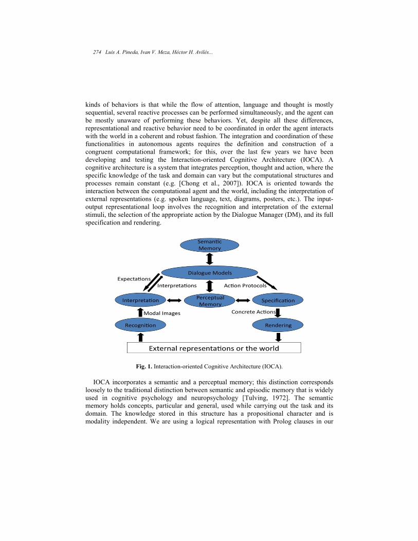
kinds of behaviors is that while the flow of attention, language and thought is mostly

sequential, several reactive processes can be performed simultaneously, and the agent can

be mostly unaware of performing these behaviors. Yet, despite all these differences,

representational and reactive behavior need to be coordinated in order the agent interacts

with the world in a coherent and robust fashion. The integration and coordination of these

functionalities in autonomous agents requires the definition and construction of a

congruent computational framework; for this, over the last few years we have been

developing and testing the Interaction-oriented Cognitive Architecture (IOCA). A

cognitive architecture is a system that integrates perception, thought and action, where the

specific knowledge of the task and domain can vary but the computational structures and

processes remain constant (e.g. [Chong et al., 2007]). IOCA is oriented towards the

interaction between the computational agent and the world, including the interpretation of

external representations (e.g. spoken language, text, diagrams, posters, etc.). The input-

output representational loop involves the recognition and interpretation of the external

stimuli, the selection of the appropriate action by the Dialogue Manager (DM), and its full

specification and rendering.

Fig. 1. Interaction-oriented Cognitive Architecture (IOCA).

IOCA incorporates a semantic and a perceptual memory; this distinction corresponds

loosely to the traditional distinction between semantic and episodic memory that is widely

used in cognitive psychology and neuropsychology [Tulving, 1972]. The semantic

memory holds concepts, particular and general, used while carrying out the task and its

domain. The knowledge stored in this structure has a propositional character and is

modality independent. We are using a logical representation with Prolog clauses in our

274 Luis A. Pineda, Ivan V. Meza, Héctor H. Avilés...

current implementations, but alternative schemes, like semantic networks or description

logics, could also be used.

The perceptual memory, in turn, stores associations between modality specific internal

images or “percepts” and their corresponding interpretations or meanings. Internal

images, on the one hand, represent the sensitive characteristics of the external stimuli and

are associated to a perception modality. However, these images also capture the way the

sensed information is structured (i.e. the external pattern). For instance, an object in the

world, such as a diagram, a map, a text, etc., can all be perceived through the visual

channel. The image, however, is “seen” differently in each case, and stored in a particular

format or code, that corresponds to that particular “way of seeing”. In the present

framework each of these codes corresponds to a modality; thus, there is a modality for

each “way of seeing”, and each may involve one or more recognition devices (e.g. an

Automatic Speech Recognition (ASR) System or a vision recognition machine). In

addition, an internal image codifies the corresponding external pattern independently of

its meaning. For instance, the product of an ASR system is an uninterpreted text; a SIFT

vector is the product of codifying a visual image independent of its interpretation. Internal

images are minimal information structures aimed to distinguish the particular concept in

the input from the set of particular or general concepts in the interpretation context.

Consequently, internal images do not have to be fully fleshed out representations of

external objects (e.g., 2-D or 3-D geometric constructions with color or texture). The

patterns represented through internal images can be dynamic and evolve in space and

time. For instance, the visual pattern of a physical gesture, like “halt”, that can be codified

as a Hidden-Markov Model [Avilés et al., 2010a]. Regular expressions and specialized

natural language grammars are also considered as internal images in the perceptual

memory. In this view, particular or general concepts are associated to the regular

expressions or grammars that “select” these concepts.

The meanings of internal images, on the other hand, are represented in a propositional

format, which is modality-independent, and the expressions representing these meanings

can be thought of as “tags” of the corresponding percepts. In this way, internal images can

be interpreted as expressing particular or general concepts. This structure also permits to

access concepts or interpretations via their percepts and vice versa. The associations

between internal images and their interpretations can be established beforehand when the

application is developed, or dynamically when the concept associated with the image is

provided by the human user at the time the image is recognized by the system in the

interactive task.

We turn now to the description of the main representational loop. The recognition

modules translate external patterns sensed by the recognition devices into the

corresponding internal images in the corresponding modal code, mainly in context

independent way and in a bottom-up fashion.

The interpretation module is responsible of assigning interpretations or meanings to

such internal images. This is a context dependent process that takes into account the

expectations of the system that are present in the interpretation situation, as will be

elaborated in Section 2. This process uses the perceptual memory and performs a

IOCA: An Interaction-Oriented Cognitive Architecture 275

qualitative match between the images recovered by the recognition devices and the

images in the perceptual memory, which are stored in the same modal code. The result of

the interpretation process is the “meaning” (i.e. the interpretation) associated to the

external image in the interpretation context. As the number of associations in the

perceptual memory can be quite large, the expectations of the current situations are also

used as the indexes of the associations to be considered in specific interpretation situation.

By this account, the expectations not only set up the interpretation context but also select

the relevant memories to be used for the particular interpretation act. The recognition and

interpretation levels of the architecture correspond to the overall perceptual process whose

purpose is to assign interpretations to the external patterns conveying linguistic messages

or events in the world that are attended to and acted upon “intentionally” by the

computational agent.

The central module in the interaction loop is the dialogue model with its associated

program interpreter or Dialogue Manager (DM). This contains the specification of the

task’s structure and relates expectations and interpretations with the corresponding

intentional actions. Interpretations and actions at this level are specified in a propositional

format that is independent of the input and output modalities.

In the output side, actions are performed as a response to interpretations; these can be

external, like displaying an image, synthesizing a text or moving a robot, but also

internal, like performing a reasoning or a planning task, involving only the

representational structures of the system. In this sense, we distinguish linguistic and

interaction protocols, which are stated through the dialogue models, from the “thought”

processes, which are internal actions that are called upon by the dialogue model when

required. Actions can be composite and involve a number of basic actions, more than one

output device, and an internal and external part. Dialogue models have also access to the

interaction history, and expectations and actions can be stated dynamically in terms of the

events that happened before in the current task. Dialogue models can also access the

knowledge stored in the semantic and perceptual memory (e.g. for heterogeneous

reasoning). Finally, the action protocols specified in dialogue models are fully specified

before they are sent to the specific rendering devices of the system.

IOCA differs from other cognitive architecture in that it is focused on the

communication channel, and on the inclusion of a perceptual memory for the explicit

recollection of sensory information. IOCA also aims to distinguish the main

communication loop involving interpretations from the cognitive processes proper, and

also to understand the relation between representational and reactive behavior. In doing

so, IOCA focuses on the questions related to the interaction between language, perception

and thought.


2 Specification and Interpretation of Dialogue Models

The central component of the cognitive architecture is the dialogue model –or interaction model– through which the task structure and the communication protocols between the computational agent and the human user are specified. Dialogue models are defined in relation to a basic notion: the situation. A situation is an “intentional state” of the agent, which is defined in relation to the expectations of the agent in the situation (either possible messages with communicative intent produced by the human interlocutor or natural event in the world), the actions the agent should perform in case a specific expectation is met, and the situations into which the agent moves after performing such action. In this way, situations are contextualized in terms of generic interaction protocols. These protocols represent the structure of the task, and traveling from the initial to the final situation corresponds to performing the task successfully.

Expectations are the set of potential speech acts types (e.g. [Levinson, 1983]) that can

be expressed by the interlocutor in the situation, in addition to the potential natural events

that can occur in the world in the situation, that are also handled intentionally.

Expectations are expressed through statements involving the system S and the human user

U like, for instance, “S expects that U commands S to make p” or “S expects that U ask S

to provide information q”. However, as the expectations are embedded in the protocols

and the corresponding actions assume this intentional interpretation (i.e., S makes p and S

provides information q), the intentional statements are implicit in the interpretation

process and only the conceptual content in the expectations is stated explicitly in the

dialogue models (e.g. the propositions p and q in the examples above). The central

component of the cognitive architecture is the dialogue model –or interaction model–

through which the task structure and the communication protocols between the

computational agent and the human user are specified. Dialogue models are defined in

relation to a basic notion: the situation. A situation is an “intentional state” of the agent,

which is defined in relation to the expectations of the agent in the situation (either possible

messages with communicative intent produced by the human interlocutor or natural event

in the world), the actions the agent should perform in case a specific expectation is met,

and the situations into which the agent moves after performing such action. In this way,

situations are contextualized in terms of generic interaction protocols. These protocols

represent the structure of the task, and traveling from the initial to the final situation

corresponds to performing the task successfully.

Expectations are the set of potential speech acts types (e.g. [Levinson, 1983]) that can be

expressed by the interlocutor in the situation, in addition to the potential natural events

that can occur in the world in the situation, that are also handled intentionally.

Expectations are expressed through statements involving the system S and the human user

U like, for instance, “S expects that U commands S to make p” or “S expects that U ask S

to provide information q”. However, as the expectations are embedded in the protocols

and the corresponding actions assume this intentional interpretation (i.e., S makes p and S

provides information q), the intentional statements are implicit in the interpretation


process and only the conceptual content in the expectations is stated explicitly in the

dialogue models (e.g. the propositions p and q in the examples above).

Speech acts are normally direct, in the sense that declarative statements are used for

communicating facts or beliefs, interrogative for making questions, and imperatives for

commands, etc., where each of these modalities of expression has a characteristic

intonation. However, the basic relation between the type of intention and the modality of

expression is often changed, as when a command is expressed through a polite question

(e.g., ''Could you show me poster A?''), producing the so-called indirect speech acts,

which pose great challenges to the interpretation process. In order to interpret speech acts,

either direct or indirect, we take advantage of the context present at the interpretation

situation, and the interpretation problem is seen as what is the most likely intention among

the expectations of the situation that is intended by the interlocutor. In this sense,

expectations are conceived as a priori knowledge, while the input information (the actual

external stimuli) is taken as evidence (i.e. likelihood) in favor of a particular expectation.

The actual interpretation of the input message is the “grounded” expectation that is best

met by the input information in the interpretation situation. This makes the interpretation

process as a whole have a strong Bayesian flavor. However, a priori knowledge and

likelihoods need not be numerical probabilities, as the “product operator” between these

two is the interpreter, that collects the output of the recognition devices, looks up the

relevant percepts in the perceptual memory, and produces the actual interpretation,

expressed as a grounded speech act in the dialogue model.

Natural states and events in the world that are expected by the computational agent are

also treated intentionally, and are defined as expectations of the situations in which they

are likely to occur. For instance, if a robot is standing in front of a door it may have the

expectation that the door is open or that it is closed. In this case, the actual image

recognized visually has no communicational intent, but nevertheless it is an expectation

that has to be acted upon intentionally in the context (e.g. crossing the door if it is opened

or asking for the door to be opened otherwise). In this case, although the stimulus is

visual, it is subject to interpretation and the behavior has a representational character.

Speech acts can express propositional or conceptual content (e.g. ''Please, explain me

poster A.''); can assert that the message has been understood as intended (e.g. ''Do you

want me to explain poster A?''); and can maintain the communication channel so the

interlocutors can establish and preserve a “common ground” (e.g. ''I didn’t hear you, can

you say it again?'') [Clark and Schaefer, 1989]. The structure of practical dialogues [Allen

et al., 2001] oriented to solve specific tasks has been analyzed with tagging schemes that

consider these three levels of speech acts (i.e. conceptual content, agreement, and

communication) and the relations between a speech act and the preceding and following

acts, which establishes a strong restriction in the structure of intentional transactions

[Allen and Core, 1997; Pineda et al., 2007]. These intuitions are also used in the

specification of dialogue models: agreement and communications protocols can be stated

to make sure the system and the user have a common ground. Also, whenever no

expectation in a situation is satisfied, the system is out of context (i.e. the common ground

has been lost) and invokes recovery protocols, stated also as dialogue models, with the


purpose to set itself in context again. These protocols can also be used to restore the

context when an expected natural event does not occur when it should.

The actions performed by the system in response to an interpretation are also thought

of as speech acts. For the specification of these actions we follow loosely Rhetorical

Structure Theory (RST) [Mann and Thompson, 1988], where an action predicate stands

for a “rhetorical structure” with one or more basic actions. Each basic predicate in the

structure stands for a particular action, either internal or external. For instance, an

explanation may involve a presentation, an elaboration, a generalization expressed

through spoken language, and even an exemplification expressed through a picture or a

video. Motor actions are also stated through rhetorical structures (e.g. move(a, b)). Action

predicates have to be fully specified, possibly using information in the perceptual

memory, before the corresponding actions are rendered in an output modality.

Dialogue models have a graphical representation where situations are represented

through nodes and situation relations are represented through directed links. Every link

has a label of the form α:β, where α stands for an expectation and β stands for the action

that is performed by the system when the expectation α is satisfied in the current situation si. As a result of performing such action, the system moves to the situation sj at the end of

the link, as illustrated in Figure 2. Situations can be basic, in the sense that a particular

interpretation act takes place at the situation (e.g., through language or vision, or both).

Situations are typed, and there is one type of situation for each modality defined in the

perceptual memory, so the DM considers the situations type in order to select the

appropriate recognition devices, with the particular modality code, to perform each basic

interpretation act. There is also a special type of situation that we refer to as recursive,

which embeds a full dialogue model. This expressive power permits to model complex

applications in a simple and modular way, where composite tasks have a stack structure.

The formalism corresponds to recursive transition networks (RTN), augmented with

functions that permit the dynamic specification of expectations, actions and next

situations. We refer to this formalism as Functional-RTN or F-RTN [Pineda, 2008; Pineda

et al., 2010].

Fig. 2. Graphical Representation of Dialogue Models.

The conceptual content in expectations can be of three kinds, which are as follows:

(1) Propositional: These are concrete expectations represented with constants or saturated propositions (e.g. a, p(a, b)) in the dialogue models.

(2) Predicative: These are expectations involving a limited form of abstraction, represented as open predicates or predicative functions (e.g. p(x), q(a, y)) in the dialogue models. To meet expectations of this kind, one or more parameter needs to be extracted from the world, and these become the arguments in the


expression representing the interpretation. For instance, if the robot asks the users for his or her name, the expectation is represented as name(x), and the interpretation of the user’s reply, in case the expectation is met. For instance, ''I’m Peter'', is represented as name(peter). These predicates are interpreted indexically in relation to the agents involved in the transaction and in relation to the local spatial and temporal context.

(3) Functional: These depend of the interaction history at the level of the interpretations, actions and situations, which is collected by the system along the interaction. In the present framework, this “working memory” structure is called the anaphoric context. Although the task protocols are specified in advance through the dialogue models, expectations and actions can change along the task, and need to be determined dynamically in relation to the context. These kinds of expectations are represented through explicit functions in the dialogue models. These functions have the anaphoric context as one of their argument, and their values are propositional or predicative expressions representing expectations. Functional expectations are evaluated first, and their values are passed top-down to the interpreter in the current interpretation act.

The next situation in a dialogue model’s transition can also depend on the anaphoric

context. In this case, the situation to which the agent has to move is represented through a

function h whose argument is again the anaphoric context but its value is the actual next

situation. In Figure 3, the function h is represented by a small dot, and its possible values

by dashed-links.

Fig. 3. Functional representation of expectations, actions and transitions.

Situations are also parametric objects, and their arguments can be bound with the

interpretation and action predicates’ arguments, allowing the establishment of co-

reference relations between terms in the interaction structure.

The system’s intentional actions can also be propositional, predicative and functional,

and can be determined dynamically. Predicative actions can be defined through open

predicates where the free variables are bound to the situation’s or expectation’s arguments

in the corresponding transition. Functional actions can be defined through explicit

functions, as it is with expectations and next situations.

Finally, the functions that define the described functional objects can access

information stored in the semantic memory, which can be considered as an additional

argument. Thus, functional expectations, actions, and next situations are dynamic objects


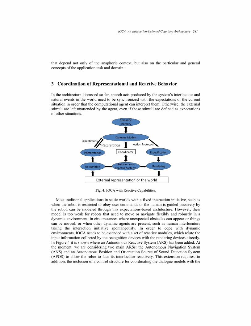
that depend not only of the anaphoric context, but also on the particular and general

concepts of the application task and domain.

3 Coordination of Representational and Reactive Behavior

In the architecture discussed so far, speech acts produced by the system’s interlocutor and

natural events in the world need to be synchronized with the expectations of the current

situation in order that the computational agent can interpret them. Otherwise, the external

stimuli are left unattended by the agent, even if those stimuli are defined as expectations

of other situations.

Fig. 4. IOCA with Reactive Capabilities.

Most traditional applications in static worlds with a fixed interaction initiative, such as

when the robot is restricted to obey user commands or the human is guided passively by

the robot, can be modeled through this expectations-based architecture. However, their

model is too weak for robots that need to move or navigate flexibly and robustly in a

dynamic environment; in circumstances where unexpected obstacles can appear or things

can be moved; or when other dynamic agents are present, such as human interlocutors

taking the interaction initiative spontaneously. In order to cope with dynamic

environments, IOCA needs to be extended with a set of reactive modules, which relate the

input information collected by the recognition devices with the rendering devices directly.

In Figure 4 it is shown where an Autonomous Reactive System (ARS) has been added. At

the moment, we are considering two main ARSs: the Autonomous Navigation System

(ANS) and an Autonomous Position and Orientation Source of Sound Detection System

(APOS) to allow the robot to face its interlocutor reactively. This extension requires, in

addition, the inclusion of a control structure for coordinating the dialogue models with the


ARSs that we called The Coordinator, also shown in Figure 4. This figure illustrates that

the main representational loop may embed a number, possible large, of reactive loops. In

this respect, IOCA loosely resembles a subsumption architecture [Chong et al., 2007].

The coordination between representational and reactive behavior is not trivial, as

reactive actions can change the spatial and temporal context expected by the dialogue

models, and the system needs to relocate itself in the context dynamically. In order to

address this problem, we are studying three basic coordination behaviors, which are as

follows:

(1) The interpretation process of the current dialogue model inside the DM and the

ARSs can proceed concurrently without interfering with each other.

(2) The DM can put on hold and reactivate the ARSs, and vice versa.

(3) An ARS can load and execute a recovery dialogue model directly.

For the ARSs we are considering a basic navigation function such that given a metric

map, the robot’s position and orientation in this map, and a target position and orientation,

the system produces and executes a plan (i.e., a sequence of moving commands) to reach

the target. During this process, the system avoids obstacles reactively and adjusts its

estimated position and orientation continuously in the metric map. In the present project

we are focusing on the definition of the coordinator, and for the actual navigation we are

exploring the use of available tools (e.g. [Vaughan et al., 2003]). This basic navigation

functionality is called upon intentionally by an action directive stated and performed by a

dialogue model; in this mode the reactive behavior is subsumed into the representational

main loop in a natural way.

The APOS, in turn, monitors the acoustic environment continuously. Whenever a

human voice is detected: it suspends the navigation system; turns to the interlocutor;

executes a dialogue model to attend the interruption; and resumes the navigation task

maintaining the original target, starting from the position and orientation that it was left

after the interruption.

The coordination involves conditions in which the reactive behavior takes precedence

over the representational one. For instance, imagine the robot is moving from position A

to B as a result of an action request, and is carrying out a conversation with the user

concurrently. In this scenario the robot has to notify the user that the navigation task has

been completed when it reaches position B. To do this, the ANS has to put on hold the

interpretation of the current dialogue model, make the notification, and resume the DM.

Another instance in which reactive behavior takes precedence is when the APOS handles

an spontaneous information request produced by the user in the middle of a moving

action, which involves the interruption of both the interpretation of the current dialogue

model, and perhaps of the ANS. Then, both the DM and the ANS have to be resumed

when the spontaneous request has been attended, but from the context that was left after

the interruption was handled.

Conversely, the coordination also involves conditions in which the representational

behavior takes precedence over the reactive one. For instance, if the robot is engaged in an

explanation task it may need to put on hold the APOS to avoid spontaneous distractions,


and restore it when the explanation task has been accomplished. Another condition is

when none of the expectations of the current situation are met, and the system has to load

and execute a recovery dialogue model. For this, the system may need to suspend both the

ANS and the APOS, direct all of its attention towards placing itself in context, and resume

both of these when the context has been restored. Here again, the ANS has to resume the

navigation task that was performing before the interruption, but from the context (i.e.

position and orientation) that was left after the contingency was handled.

Finally, these generic protocols are defined in the coordinator, which controls their

execution independently of the dialogue models representing the application task.

4 The robots Golem and Golem-II+

Over the last few years we have been developing the basic structure of IOCA: its dialogue

model specification, interpretation theory, and programming environment. We first

produced the Golem robot that was able to guide a poster session about our research

projects through a spoken Spanish conversation. We also produced several applications to

illustrate the integration of language, vision and navigation with Golem (e.g., [Aguilar and

Pineda, 2010]). Next, we produced the application “Guess the card: Golem in

Universum”. It is a multimodal application in a fixed platform in a permanent stand of

UNAM’s science museum Universum in which the user plays a game with the system

through a spoken Spanish conversation supported with computer vision and the display of

images [Meza et al., 2010]. Next, we presented the robot Golem-II+ which is also able to

guide a poster session, but in addition to the original system, it is capable of interpreting

pointing gestures expressed by the user during the interaction, illustrating the coordination

between language, vision and motor behavior [Avilés et al., 2010]. All of these

applications have been developed using the basic representational loop only. We have also

developed and tested the basic APOS algorithms with very promising results [Rascón et

al., 2010]. Videos of these systems are available at http://leibniz.iimas.unam.mx/~luis/. At

the moment, we are incorporating and testing the extension of IOCA with reactive

behaviors in the robot Golem-II+, to model the different test scenarios of the

RoboCup@home competition.

Acknowledgements. We acknowledge the support of the members of the DIME and

Golem group at IIMAS, UNAM. We also gratefully thank the support of grants

CONACyT 81965 and PAPPIT-UNAM IN-121206, IN-104408 and IN-115710.

References

1. Allen, J.F., Core, M.G.: Draft of DAMSL: Dialog Act Markup in Several Layers Annotation

Scheme. Department of Computer Science. Rochester University (1997)

2. Allen, J.F., Byron, D.K., Dzikovska, M., Ferguson, G., Galescu, L., Stent, A.: Toward

Conversational Human-Computer Interaction. AI Magazine, 22(4):27–38. Winter (2001)


3. Aguilar, W., Pineda, L.A.: Integrating Graph-Based Vision Perception to Spoken Conversation in

Human-Robot Interaction. J. Cabestany et al. (Eds.): IWANN 2009, Part I. LNCS 5517, pp. 789–

796. Springer-Verlag Berlin Heidelberg (2009)

4. Avilés, H., Alvarado, M., Venegas, E., Rascón. C., Meza, I., Pineda, L.: Development of a Tour-

Guide Robot Using Dialog Models and a Cognitive Architecture. IBERAMIA 2010, LNAI, Vol.

6433, Springer-Verlag. Berlin Heidelberg, pp. 512 – 521 (2010)

5. Avilés, H., Sucar, E., Pineda, L., Mendoza, C.: A comparison of dynamic naïve Bayesian

classifiers and Hidden Markov Models for gesture recognition, Journal of Applied Research and

Technology (to appear). 6. Chong, H.Q., Tan, A.H., Ng, G.W.: Integrated cognitive architectures: a survey. Artificial

Intelligence Review, 28:103—130 (2007)

7. Clark, H., Schaefer, E.F.: Contributing to Discourse. Cognitive Science, 13:259–294 (1989)

8. Levinson, S.C.: Pragmatics. Cambridge University Press, Cambridge, UK (1983)

9. Mann, W.C., Thompson, S.: Rhetorical Structure Theory: Towards a functional theory of text

organization, Text 8(3), pp. 243—281 (1988)

10. Meza, I., Salinas, L., Venegas, E., Castellanos, H., Chavarria, A., Pineda, L.: Specification and

Evaluation of a Spanish Conversational System Using Dialogue Models. IBERAMIA 2010,

LNAI, Vol. 6433, Springer-Verlag, Berlin Heidelberg, pp. 346 – 355 (2010)

11. Pineda, L., Estrada, V., Coria, S., Allen, J.: The obligations and common ground structure of

practical dialogues, Inteligencia Artificial, Revista Iberoamericana de Inteligencia Artificial.

Vol. 11 (36), pp. 9-17 (2007)

12. Pineda, L.A.: Specification and Interpretation of Multimodal Dialogue Models for Human-

Robot Interaction, in Artificial Intelligence for Humans: Service Robots and Social Modeling, G.

Sidorov (Ed.), SMIA, México, pp. 33–50 (2008)

13. Pineda, L., Meza, I, Salinas, L.: Dialogue Model Specification and Interpretation for Intelligent

Multimodal HCI. A. Kuri-Morales and G. Simari (Eds.): IBERAMIA 2010, LNAI, Vol. 6433,

Springer-Verlag. Berlin Heidelberg, pp. 20–29 (2010)

14. Rascón, C., Avilés, H., Pineda, L.: Robotic Orientation towards Speaker in Human-Robot

Interaction. IBERAMIA 2010, LNAI, Vol. 6433, Springer-Verlag, Berlin Heidelberg, pp. 10–19

(2010)

15. Tulving, E.: Memory systems: episodic and semantic memory. In: E. Tulving and W. Donaldson

(Eds.), Organization of Memory. New York: Academic Press. pp. 381-403 (1972)

16. Richard, T., Vaughan, B., Gerkey, P., Howard, A.: On device abstractions for portable, reusable

robot code. In Proc. of the IEEE/RSJ Intl. Conf. on Intelligent Robots and Systems (IROS),

pages 2121-2427. Las Vegas, Nevada (2003)


Visual Data Combination for Object Detection and

Localization for Autonomous Robot Manipulation Tasks

Luis A. Morgado-Ramirez, Sergio Hernandez-Mendez, Luis F. Marin-Urias,

Antonio Marin-Hernandez, and Homero V. Rios-Figueroa

Department of Artificial Intelligence, Universidad Veracruzana, Sebastian Camacho No. 5,

91000, Xalapa, Ver., Mexico

[email protected], [email protected], [email protected],

anmarin,[email protected]

Abstract. For mobile robot manipulation, autonomous object detection and

localization is at the present still an open issue. In this paper is presented a

method for detection and localization of simple colored geometric objects like

cubes, prisms and cylinders, located over a table. The method proposed uses a

passive stereovision system and consists in two steps. The first is colored object

detection, where it is used a combination of a color segmentation procedure

with an edge detection method, to restrict colored regions. Second step consists

on pose recovery; where the merge of the colored objects detection mask is

combined with the disparity map coming from stereo camera. Later step is very

important to avoid noise inherent to the stereo correlation process. Filtered 3D

data is then used to determine the main plane where the objects are posed, the

table, and then the footprint is used to localize them in the stereo camera

reference frame and then to the world reference frame.

1 Introduction

Automatic and robust detection and spatial localization of objects under no specific or

controlled conditions, i.e. unlike of assembly lines or structured environments, is one

of the most challenging tasks for computer vision. There are many problems where

the use of these sort of solutions can improve the performance of automatic systems,

e.g. in autonomous mobile robot manipulators or unknown scene analysis. On this

work we focus mainly on mobile robot manipulation scenarios but the approach

presented can be adapted to other complex environments.

For autonomous mobile robot manipulators is really a challenge to locate and

detect objects on scenes. The applications for these kinds of task vary from folding

clothes to environment mapping and so on. Typically the problem of mobile

manipulators is decomposed on three stages: a) object detection and localization, b)

approach planning and c) finally correct grasping. On this work we focus on the first

of the three mentioned stages.

Commonly to detect and localize objects in such scenarios active sensors are used,

e.g. active stereovision systems or time of flight (TOF) sensors. In active stereovision

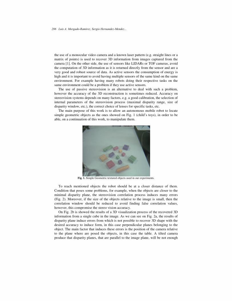
the use of a monocular video camera and a known laser pattern (e.g. straight lines or a

matrix of points) is used to recover 3D information from images captured from the

camera [1]. On the other side, the use of sensors like LIDARs or TOF cameras, avoid

the computation of 3D information as it is returned directly from the sensor and are a

very good and robust source of data. As active sensors the consumption of energy is

high and it is important to avoid having multiple sensors of the same kind on the same

environment. For example having many robots doing their respective tasks on the

same environment could be a problem if they use active sensors.

The use of passive stereovision is an alternative to deal with such a problem,

however the accuracy of the 3D reconstruction is sometimes reduced. Accuracy on

stereovision systems depends on many factors, e.g. a good calibration, the selection of

internal parameters of the stereovision process (maximal disparity range, size of

disparity window, etc.), the correct choice of lenses for specific tasks, etc.

The main purpose of this work is to allow an autonomous mobile robot to locate

simple geometric objects as the ones showed on Fig. 1 (child’s toys), in order to be

able, on a continuation of this work, to manipulate them.

Fig. 1. Simple Geometric textured objects used in our experiments.

To reach mentioned objects the robot should be at a closer distance of them.

Condition that poses some problems, for example, when the objects are closer to the

minimal disparity plane, the stereovision correlation process induces many errors

(Fig. 2). Moreover, if the size of the objects relative to the image is small, then the

correlation window should be reduced to avoid finding false correlation values,

however, this compromise the stereo vision accuracy.

On Fig. 2b is showed the results of a 3D visualization process of the recovered 3D

information from a single cube in the image. As we can see on Fig. 2a, the results of

disparity plane induce errors from which is not possible to recover 3D shape with the

desired accuracy to induce form, in this case perpendicular planes belonging to the

object. The main factor that induces these errors is the position of the camera relative

to the plane where are posed the objects, in this case the table. A tilted camera

produce that disparity planes, that are parallel to the image plane, will be not enough

286 Luis A. Morgado-Ramirez, Sergio Hernandez-Mendez...

to describe the planes of objects that are not parallel to these planes. Then errors are

induced creating larger deformations.

On Fig. 2b are showed some segmented objects where it is possible to see the

problem relative to correlation process, as we can see many wrongly matching pixels

on the neighborhood of the objects are considered as part of them.

When the objects in the scene are bigger these errors can be neglected, however

when it is desired that mobile robots could manipulate commonly humans objects this

is not the case. Bigger objects will be more difficult to manipulate by only one

anthropomorphous arm.

(a) (b)

Fig. 2. Stereovision common problems, a) form induced from the correlated data does not match the form

of the real object, b) some mismatched pixels create false data, which interpreted with truthful data deforms

the objects.

This paper is organized as follow; on next section we analyze some recent related

works. On section three and four we present the proposed approach, beginning with

the object detection, followed by the object localization method, respectively. On

section five we present the results, and finally on section six our conclusions and

future work.

2 Related Work

The problem of object detection and localization for autonomous mobile robot is

an active research field. As a direct result there are many approaches to deal with such

a problem. As it has been exposed previously, many of these works use active

sensors, together with CAD models in order to detect known objects and localization.

For example in [2] CAD models are used in combination with an efficient hierarchical

search computed offline to guide the exhaustive pose estimation.

In [3] it is presented a method for object detection using GPU computation in order

to accelerate commonly object detection algorithms usually very slow and

impractically to be used on mobile robot manipulation. There are some other

approaches that use shapes descriptors, as for example in [4] where these descriptors

are used in combination with a TOF sensor in order to recover 3D localization of the

Visual Data Combination for Object Detection and Localization... 287

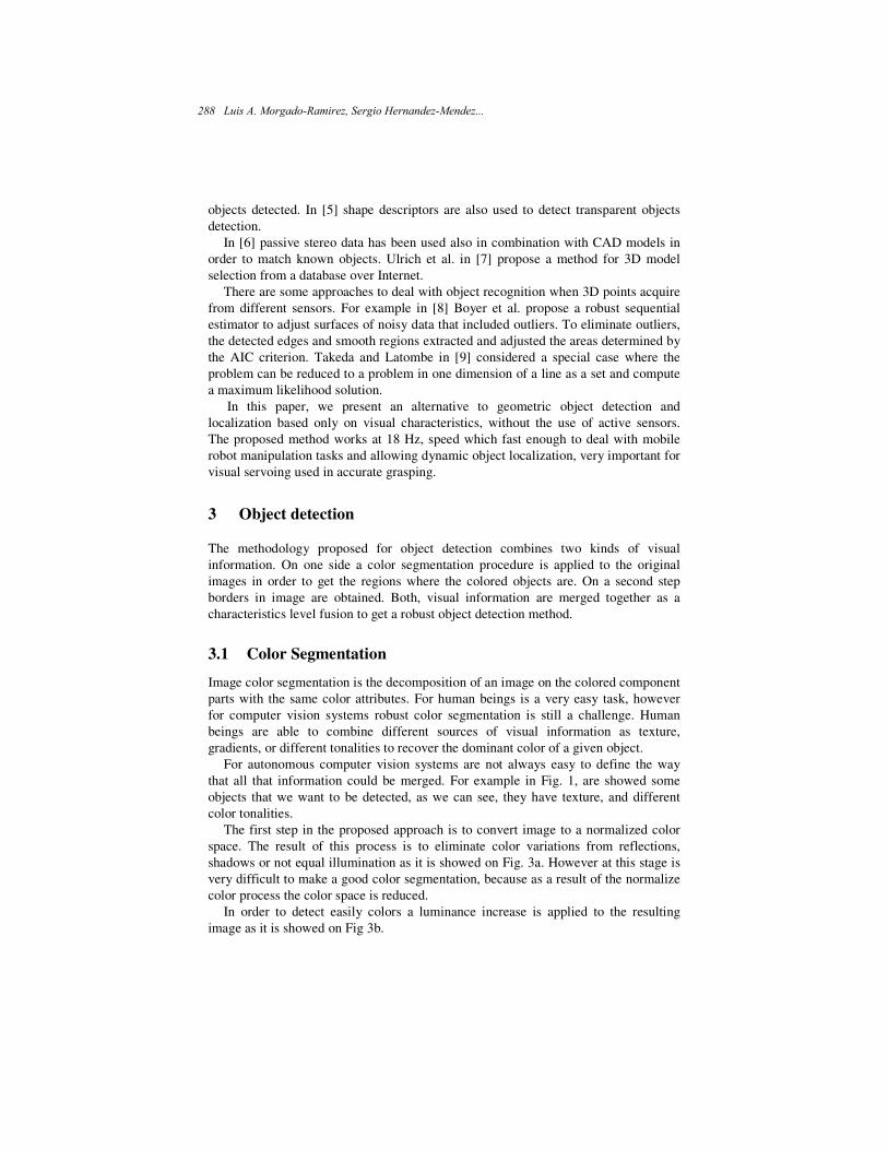
objects detected. In [5] shape descriptors are also used to detect transparent objects

detection.

In [6] passive stereo data has been used also in combination with CAD models in

order to match known objects. Ulrich et al. in [7] propose a method for 3D model

selection from a database over Internet.

There are some approaches to deal with object recognition when 3D points acquire

from different sensors. For example in [8] Boyer et al. propose a robust sequential

estimator to adjust surfaces of noisy data that included outliers. To eliminate outliers,

the detected edges and smooth regions extracted and adjusted the areas determined by

the AIC criterion. Takeda and Latombe in [9] considered a special case where the

problem can be reduced to a problem in one dimension of a line as a set and compute

a maximum likelihood solution.

In this paper, we present an alternative to geometric object detection and

localization based only on visual characteristics, without the use of active sensors.

The proposed method works at 18 Hz, speed which fast enough to deal with mobile

robot manipulation tasks and allowing dynamic object localization, very important for

visual servoing used in accurate grasping.

3 Object detection

The methodology proposed for object detection combines two kinds of visual

information. On one side a color segmentation procedure is applied to the original

images in order to get the regions where the colored objects are. On a second step

borders in image are obtained. Both, visual information are merged together as a

characteristics level fusion to get a robust object detection method.

3.1 Color Segmentation

Image color segmentation is the decomposition of an image on the colored component

parts with the same color attributes. For human beings is a very easy task, however

for computer vision systems robust color segmentation is still a challenge. Human

beings are able to combine different sources of visual information as texture,

gradients, or different tonalities to recover the dominant color of a given object.

For autonomous computer vision systems are not always easy to define the way

that all that information could be merged. For example in Fig. 1, are showed some

objects that we want to be detected, as we can see, they have texture, and different

color tonalities.

The first step in the proposed approach is to convert image to a normalized color

space. The result of this process is to eliminate color variations from reflections,

shadows or not equal illumination as it is showed on Fig. 3a. However at this stage is

very difficult to make a good color segmentation, because as a result of the normalize

color process the color space is reduced.

In order to detect easily colors a luminance increase is applied to the resulting

image as it is showed on Fig 3b.


A color space reduction is then applied to the processed image in order to cluster

similar colors as humans do easily, that is, many green tonalities are grouped together

as only green color (Fig 4).

Image color space reduction is obtained applying the following formula:

RSc =C

Dv

2 , with C ∈ R,G,B (1)

with RSc the new color component and Dv the reduction factor for the cubic color

space.

(a) (b)

Fig. 3. a) Normalized color space and b) luminance adjustment to separate colors.

In figure Fig. 4a are shown the results for the color space reduction where it is

applied a color labeling in order to distinguish more easily the colors. As we can see

in this figure, there are still some holes in the objects as well as some colors that do

not belong correctly to the segmented object.

(a) (b)

Fig. 4. Two images where reduce space color segmentation is applied.

3.2 Edge Detection

Combination of color segmentation with edge detection allow us to delimit object as

well as assign colors to the regions where color has not been detected or it has been

wrongly detected.


We use a simple canny edge detector that was the one that gives us best results as it

is showed on figure 5. Even so, edge detectors can be used isolated to delimited

objects, mainly edge detectors because edge detectors are sensible to illumination

conditions given different edges in a sequence of images which correspond most of

the time to shadows that are more or less perceive by the camera.

(a) (b) Fig. 5. Canny edge detector applied to the original images.

3.3 Object Detection Data Fusion

Data fusion at this stage is done with the following procedure.

Be C the color label of a given pixel and P the percentage of similar colored

neighbor pixels, then:

Add all the edges to a list L.

While L is not empty do

If the pixel u in L belongs to a given color label C then

Add u to a region C

For each neighbor pixel v of u do

If v belong to the same region C insert v in L

If not, label as visited pixel.

(a) (b)

Fig. 6. a) Binary mask obtained by the fusion of color segmentation and edge detection, and

in b) Color object labeled.


With this procedure we obtain a binary mask that determines the colored objects as

the images showed on Fig. 6a. Finally, dominant label on the object is assigned to the

entire segmented region as it is showed on Fig. 6b.

At this stage we have detected colored objects in the scene, now is necessary to

localize these objects on the camera reference frame.

4 Object Localization

In order to avoid the problems with the noise produced by the stereovision correlation

process as is has been showed on Fig. 2b, we use the object segmentation mask fig. 6

to recover 3D information only on the regions where the objects has been detected

Fig. 7a. However, as the objects are small, a very near the minimal disparity plane the

shape of the 3D form does not correspond to the real object form as has been

described in Fig. 2a.

In order localize objects; we assume that all objects are over a table and as it has

been said, all these objects are very simple geometric forms. So, the shape of the

footprint in the surface of the table, give us information about the position and

orientation of a given object. The problem here is the to find the plane equation

corresponding to the table in order to project all the 3D segmented points on this

surface to recover their footprint and then their position in the camera reference

frame, and then to the world or manipulator reference frame.

As we have seen on Fig. 2a, disparity data has a lot of noise, so is not possible to

recover flat surfaces belonging to the up side plane of the objects. In order to deal

with this problem we have applied a RANSAC algorithm to find the best plane that

fits to our objects and then with the bounding box of the 3D points belonging to the

objects in the recently calculated plane, we have move the plane to the bottom of this

bounding box.

Then the 3D points belonging to the objects are projected over this plane that

correspond to the table plane Fig. 7b.

(a) (b)

Fig. 7. Projection of 3D seemed points over a fitting plane that correspond to the table plane.


5 Results

In order to get a confidence measure we have compared the results of the proposed

methodology for color image segmentation with the ground truth (Fig. 8) of the coor

segmented objects and we have obtained a rate of 90% of matched pixels with an

average of 2% of false positives and a 8% of true negatives matches.

(a) (b)

(c) (d)

Fig. 8. a) and c) examples of color object segmentation mask and b) and d) corresponding ground truth.

We have estimated a maximal error of 1 cm on the projection of 3D footprint

center considered as the location of the objects. Many tests under different light

conditions were evaluated to validate the results of the proposed methodology without

varying the described accuracy.

6 Conclusions

We have presented a method for simple geometric colored object detection based on

the fusion of different visual characteristics. The proposed works at a frame rate of 18

hz, making it ideal for robotics applications where computing time is crucial. The

mask obtained by the color segmentation process is used as a noise filter in order to

avoid errors on the stereo correlation process that produces bad objects localization

estimations. The method can be applied continuously in order to give to a

manipulation robot the active state of the world.

Fusion data structure will be used in future works in order to match edges from

both images coming from the stereo camera in order to get a more robust object

detection and localization.


References

1. Quigley M., Batra S., Gould S., Klingbeil E., Le Q. V., Wellman A., Ng A. Y.: High-accuracy

3d sensing for mobile manipulation: Improving object detection and door opening, in

IEEE International Conference on Robotics and Automation (2009)

2. Ulrich M., Wiedemann C., Steger C.: Cad-based recognition of 3D objects in monocular

images. In International Conference on Robotics and Automation 1191–1198 (2009)

3. Coates A., Baumstarck P., Le Q. V., Ng A. Y.: Scalable learning for object detection with

gpu hardware. In IROS 4287–4293 (2009)

4. Marton, Z.; Pangercic, D.; Blodow, N.; Kleinehellefort, J.; Beetz, M.: General 3D modeling

of novel objects from a single view. Intelligent Robots and Systems (IROS), 2010

IEEE/RSJ International Conference, 3700–3705 (2010)

5. Fritz M., Darrell M., Black M., Bradski G., Karayev S.: An additive latent feature model for

transparent object recognition,” in NIPS, S. for Oral Presentation (2009)

6. Hillenbrand U.: Pose clustering from stereo data. In Proceedings VISAPP International

Workshop on Robotic Perception – RoboPerc (2008)

7. Klank, U.; Zia, M. Z., Beetz, M.: 3D model selection from an internet database for robotic

vision. Robotics and Automation. ICRA '09. IEEE International Conference, 2406–2411

(2009)

8. K.L Boyer, M.J. Mirza, and G. Ganguly, The robust sequential estimator: a general

approach and its application to surface organization in range data, IEEE Trans. Pattern

Anal. Machine Intell., vol. 16, no.10, 987-1001 (1994)

9. H. Takeda and J-C. Latombe, Maximum likelihood fitting of a straight line to perspective

range data. IEICE Trans., vol.J77-D-II, no.6, 1096-1103 (1994)


Mobile Robot SPLAM for Robust Navigation

Abraham Sanchez1, Alfredo Toriz2, Rene Zapata2, and Maria Osorio1

1 Benemerita Universidad Autonoma de Puebla, Computer Science Department,Puebla, Mexico

2 Montpellier Laboratory of Informatics, Robotics, and Microelectronics (LIRMM),UMR 5506 - CC 477

161 rue Ada, Montpellier, [email protected], [email protected], asanchez,

[email protected]

Abstract. This paper describes a simultaneous planning localizationand mapping (SPLAM) methodology, where a mobile robot explores theenvironment efficiently and also considers the requisites of the simulta-neous localization and mapping algorithm. The method is based on therandomized incremental generation of a data structure called Sensor-based Random Tree, which represents a roadmap of the explored areawith an associated safe region. A continuous localization procedure basedon B-Splines features of the safe region is integrated in the scheme.

1 Introduction

SLAM (Simultaneous Localization And Mapping) is a challenging problem inmobile robotics. SLAM approaches are used simultaneously with classic explo-ration algorithms [1]; however, results obtained with SLAM algorithms stronglydepend on the trajectories performed by the robots, while classic exploration al-gorithms do not take into account the uncertainty about the localization of therobot when it travels through unknown environments, making harder the con-struction of the map, when the robot’s position is unknown, generating uselessand inaccurate maps. With the integrated exploration or SPLAM (simultane-ous planning localization and mapping), the robot explores the environmentefficiently and also considers the requisites of the SLAM algorithm [2], [3].

An integrated exploration method is introduced in [3] to achieve the balanceof speed of exploration and accuracy of the map using a single robot [3]. Freda etal. [2] use a sensor-based random tree (SRT). Recently, a novel laser data basedSLAM algorithm using B-Spline as features has been developed in [4]. ExtendedKalman filter (EKF) is used in the proposed BS-SLAM algorithm and the statevector contains the current robot pose together with the control points of thesplines. The observation model used for the EKF update is the intersections ofthe laser beams with the splines contained in the map. In our proposal, we didnot use the EKF but and integrated exploration based approach, called SRT-B-Splines. In this method, the tree is expanded, while the configurations for thecoverage near the frontiers of the robot, that is a new candidate, are selected.

These configurations belonging to the new candidates are evaluated consideringthe reliability of the expected observable features in those points.

The basics of the B-splines are briefly presented in Section II. The proposedapproach to solve the simultaneous planning localization and mapping problemis detailed in Section III. Simulation results are discussed in Section IV. Finally,conclusion and future work are detailed in Section V.

2 B-Splines

Most shapes are simply too complicated to define using a single Bezier curve. Aspline curve is a sequence of curve segments that are connected together to forma single continuous curve. A knot vector is a list of parameter values, or knots,that specify the parameter intervals for the individual Bezier curves that makeup a B-spline. The purpose of the knot vector is to describe the range of influencefor each of the control points [6]. Let a list t0 ≤ t1 ≤ t2 ≤ . . . ≤ tm−1 ≤ tmof m + 1 non-decreasing numbers, such that the same value should not appearmore than k times, k = order of the B-spline. We define the i-th B-spline functionNik(t) of order k(= k − 1 degree) as:

Ni1(t) =

1 if ti ≤ t ≤ ti+1,

0 otherwise., k = 1 (1)

Nik(t) =t− ti

ti+k−1 − tiNi,k−1(t) +

ti+k − t

ti+k − ti+1Ni+1,k−1(t), k > 1 (2)

Let the next properties:

1. Nik(t) > 0 for ti < t < ti+k

2. Nik(t) = 0 for t0 ≤ t ≤ ti, ti+k ≤ t ≤ tn+k

3.∑n

i=0 Nik(t) = 1 t ∈ [tk−1, tn+1] normalizing property

Given a set of n + 1 control points di(i = 0, ..., n) and a knot vector T =[t0, t1, ..., tm−1, tm] one can define a B-spline X(t) of order k as:

X(t) =

n∑i=0

diNik(t) (3)

where Nik(t) describes the blending B-spline function of degree k− 1 associatedwith the knot vector T .

The simplest method of fitting a set of data points with a B-splines curveis the global interpolation method [6]. The spline fitting problem is, given a setof data points D0, D1, . . . , Dn which correspond to an unknown curve, find theB-spline function to approximate the data points.

296 Abraham Sánchez, Alfredo Toriz, Rene Zapata, and Maria Osorio

3 The SPLAM Approach

Several techniques have been proposed so far to tackle the SLAM problem. Themain difference between them concerns basically with the environment repre-sentation and the uncertainty description [5]. A wide variety of localization andmapping techniques relies on environment representations consisting of a set ofcharacteristics elements detectable by the robot’s sensory system (feature-basedmaps). Lines and segments are commonly used as features. They can be ef-fectively extracted from range scans and then exploited for localization and/ormapping purposes.

In the integrated exploration approach, the robot simultaneously creates amap of its environment and finds a location in such environment (i.e., the robottakes local decisions on how to move in order to minimize the error of its esti-mated positions and the positions of the marks). The strategy adopted for theexploration process is called SRT (Sensor Based Random Tree) [5], [8], and isbased on the construction of a data structure that represents the roadmap of theexplored area with an associated security region (SR); each node tree (T ) con-sists of a robot’s position and its associated local security region (LSR) that isconstructed through the perception of the robot system. It carries out a continu-ous localization process based on the extraction of environmental characteristics(curves or lines), these features are compared with the new curves that are ex-tracted from the LSR of the current position. The algorithm implemented forthe integrated exploration is described in [9].

The exploration of unknown environments requires an additional functional-ity because the odometric information reported by the robot, in most cases isnot accurate, resulting in inaccurate maps useless for future navigations. Thelocalization function implemented, uses B-spline curves to represent the fron-tier between the free regions and the obstacles in a complex environment. Theproposed algorithm assumes that the robot’s initial position is well located and,consequently, the first observation of the environment has a perfect location.Once the robot has moved from a position qlast to a position qcurr, the newposition of the robot is obtained by adding to the last located position, the in-crement x,y and θ reported by the robot’s odometric system. After thisposition is estimated, the robot will collect the information of the surroundingenvironment for the localization process.

The raw data collected by the sensor can not be directly used in the local-ization process, due to errors inherent to the measurement system used (lasersensor). In our case, we got an equivalent error of ±1% of the measured dis-tance, that will be optimized using the method of least median square (LMSLeast Median Square). The decision to use this method is based on a compar-ative study of different methods proposed in the literature, including RANSACand its variants (MSAC and NAPSAC), and Least Squares. The minimum isdefined as minM = med(r2i ), where ri(i = 1, ..., n) are the residuals of the con-trol points di and their corresponding points on the curve: ri = |di− diNi,p(tk)|.The treatment of the laser readings will be described in the data segmentation

Mobile Robot SPLAM for Robust Navigation 297

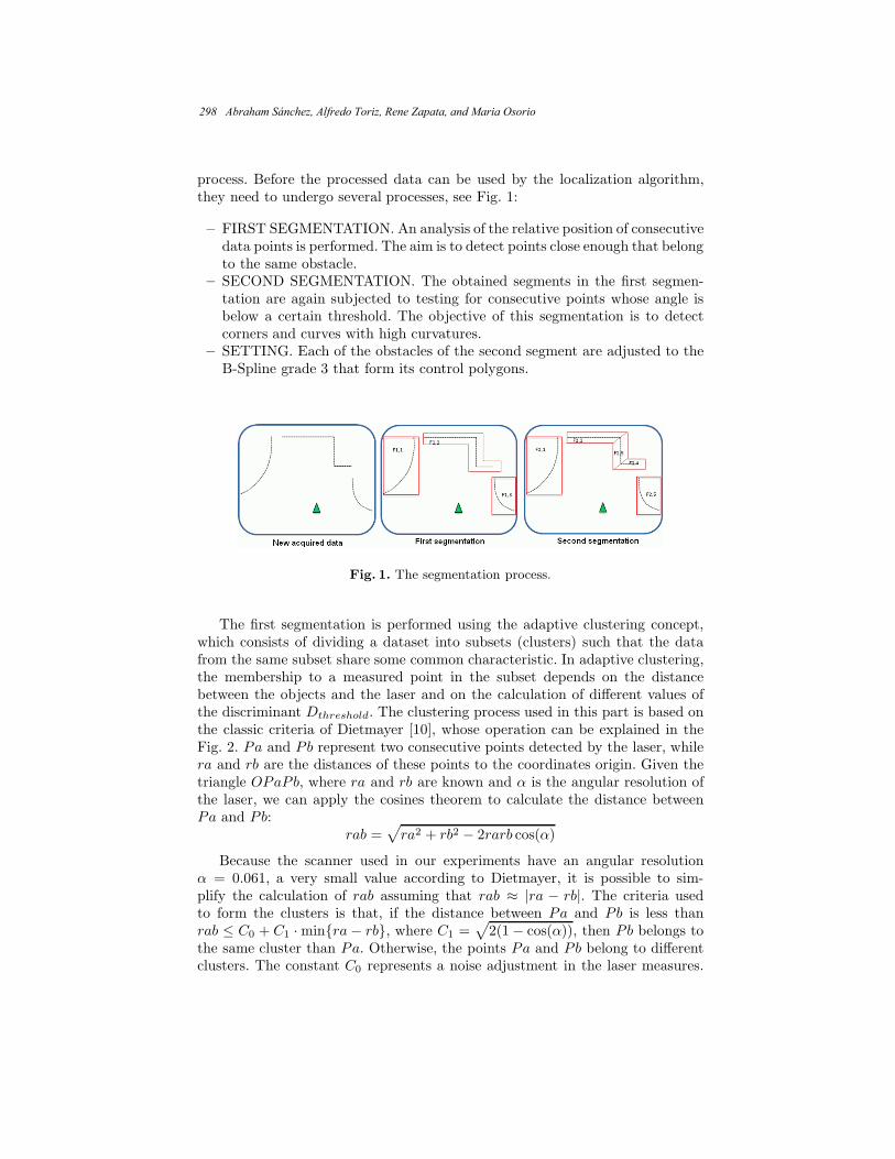
process. Before the processed data can be used by the localization algorithm,they need to undergo several processes, see Fig. 1:

– FIRST SEGMENTATION. An analysis of the relative position of consecutivedata points is performed. The aim is to detect points close enough that belongto the same obstacle.

– SECOND SEGMENTATION. The obtained segments in the first segmen-tation are again subjected to testing for consecutive points whose angle isbelow a certain threshold. The objective of this segmentation is to detectcorners and curves with high curvatures.

– SETTING. Each of the obstacles of the second segment are adjusted to theB-Spline grade 3 that form its control polygons.

Fig. 1. The segmentation process.

The first segmentation is performed using the adaptive clustering concept,which consists of dividing a dataset into subsets (clusters) such that the datafrom the same subset share some common characteristic. In adaptive clustering,the membership to a measured point in the subset depends on the distancebetween the objects and the laser and on the calculation of different values ofthe discriminant Dthreshold. The clustering process used in this part is based onthe classic criteria of Dietmayer [10], whose operation can be explained in theFig. 2. Pa and Pb represent two consecutive points detected by the laser, whilera and rb are the distances of these points to the coordinates origin. Given thetriangle OPaPb, where ra and rb are known and α is the angular resolution ofthe laser, we can apply the cosines theorem to calculate the distance betweenPa and Pb:

rab =√

ra2 + rb2 − 2rarb cos(α)

Because the scanner used in our experiments have an angular resolutionα = 0.061, a very small value according to Dietmayer, it is possible to sim-plify the calculation of rab assuming that rab ≈ |ra − rb|. The criteria usedto form the clusters is that, if the distance between Pa and Pb is less thanrab ≤ C0 + C1 ·minra− rb, where C1 =

√2(1− cos(α)), then Pb belongs to

the same cluster than Pa. Otherwise, the points Pa and Pb belong to differentclusters. The constant C0 represents a noise adjustment in the laser measures.


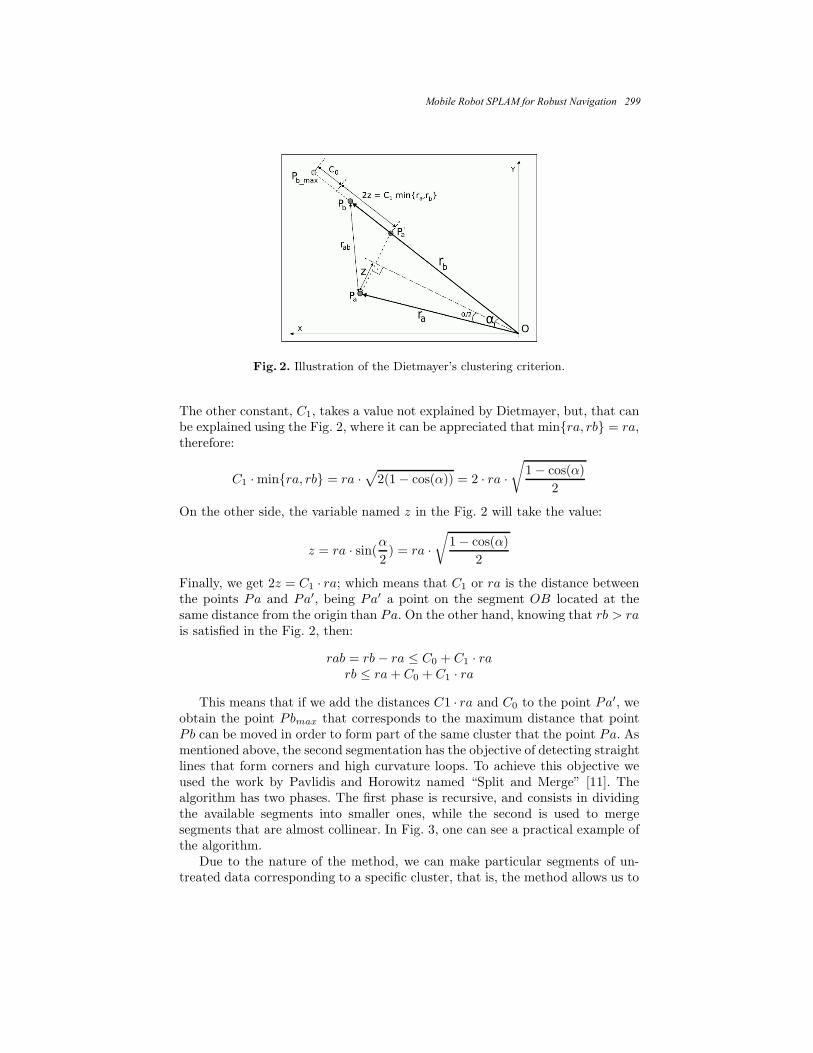
Fig. 2. Illustration of the Dietmayer’s clustering criterion.

The other constant, C1, takes a value not explained by Dietmayer, but, that canbe explained using the Fig. 2, where it can be appreciated that minra, rb = ra,therefore:

C1 ·minra, rb = ra ·√2(1− cos(α)) = 2 · ra ·

√1− cos(α)

2

On the other side, the variable named z in the Fig. 2 will take the value:

z = ra · sin(α2) = ra ·

√1− cos(α)

2

Finally, we get 2z = C1 · ra; which means that C1 or ra is the distance betweenthe points Pa and Pa′, being Pa′ a point on the segment OB located at thesame distance from the origin than Pa. On the other hand, knowing that rb > rais satisfied in the Fig. 2, then:

rab = rb − ra ≤ C0 + C1 · rarb ≤ ra+ C0 + C1 · ra

This means that if we add the distances C1 · ra and C0 to the point Pa′, weobtain the point Pbmax that corresponds to the maximum distance that pointPb can be moved in order to form part of the same cluster that the point Pa. Asmentioned above, the second segmentation has the objective of detecting straightlines that form corners and high curvature loops. To achieve this objective weused the work by Pavlidis and Horowitz named “Split and Merge” [11]. Thealgorithm has two phases. The first phase is recursive, and consists in dividingthe available segments into smaller ones, while the second is used to mergesegments that are almost collinear. In Fig. 3, one can see a practical example ofthe algorithm.

Due to the nature of the method, we can make particular segments of un-treated data corresponding to a specific cluster, that is, the method allows us to


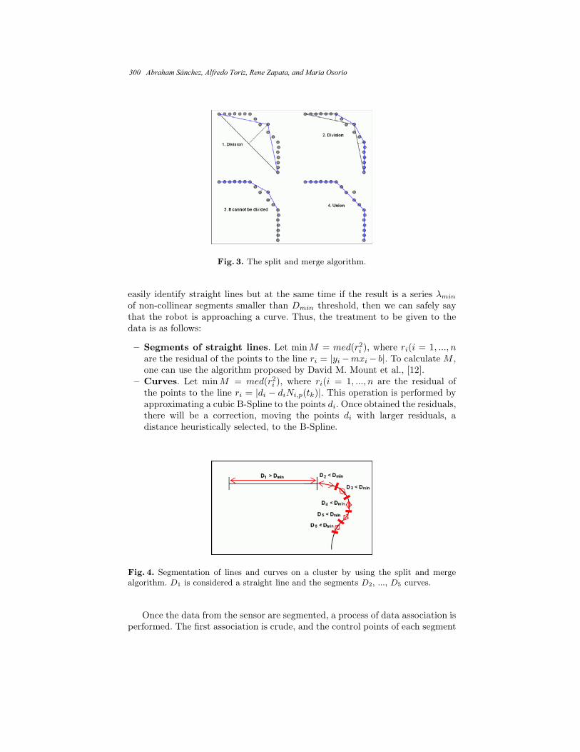
Fig. 3. The split and merge algorithm.

easily identify straight lines but at the same time if the result is a series λmin

of non-collinear segments smaller than Dmin threshold, then we can safely saythat the robot is approaching a curve. Thus, the treatment to be given to thedata is as follows:

– Segments of straight lines. Let minM = med(r2i ), where ri(i = 1, ..., nare the residual of the points to the line ri = |yi−mxi− b|. To calculate M ,one can use the algorithm proposed by David M. Mount et al., [12].

– Curves. Let minM = med(r2i ), where ri(i = 1, ..., n are the residual ofthe points to the line ri = |di − diNi,p(tk)|. This operation is performed byapproximating a cubic B-Spline to the points di. Once obtained the residuals,there will be a correction, moving the points di with larger residuals, adistance heuristically selected, to the B-Spline.

Fig. 4. Segmentation of lines and curves on a cluster by using the split and mergealgorithm. D1 is considered a straight line and the segments D2, ..., D5 curves.

Once the data from the sensor are segmented, a process of data association isperformed. The first association is crude, and the control points of each segment


obtained in the segmentation process are compared with the control points inthe map, using the following criteria:

min(dist(Xm,i, Xo,j)) < dmin, i = 1, ..., nm, j = 1, ..., n0

Where Xm,i and Xo,j are the control points of the splines, on the map andobserved, respectively, nm and n0 are the number of control points of the splineson the map and observed, dist(Xm,i, Xo,j) represents the Euclidean distancebetween the control points, and finally dmin is the parameter that will regulateif the points are or not related. If no spline in the map is close enough to adetected spline in order to be related, then this new object is added to the map,once the robot’s position has been located. By contrast, if a spline is associatedwith a map’s feature, it is necessary to obtain a concordance between its points,as follows:

Fig. 5. Concordance between curves.

– One of the ends of the curve is considered point a.– The closest point between the spline on the map and the point a is calculated

(point b).– If b is one of the endpoints of the spline on the map, then, the point nearest

to b in the spline is calculated and named point c, if not, point a is associatedwith point b.

– The process is repeated starting in the other end of the spline (point d inthe Fig. 5, that is associated with the point e on the spline in the map.

– Due to the B-splines property, the length of the curves can be known, andsegments e-b and d-c can be adjusted to have the same length. If the differ-ence of the lengths is greater than threshold lmax, the extreme elements ofthe larger curve are eliminated to adjust its size.

Once the curves of the estimated position and the curves of the environment areassociated, it is necessary to conduct a final verification of the association bygetting the distance from each end of each curve to the other as shown in theFig. 6:


A simulated robot and the real Pioneer P3DX robot equipped with front andrear bumper arrays, a ring of eight forward ultrasonic transducer sensors (range-finding sonar) and a Hokuyo URG-04Lx laser range finder were used in the ex-periment. The Pioneer P3DX robot is an unicycle robot. The LIRMM laboratory


Fig. 6. Two association forms: a) association crude, b) association fine.

environment was used in the experimental and simulation tests (the environmenthad several corridors). Figure 7 shows the two final maps: in the leftside, themap obtained without a localization process and only with odometric estimates;in the rightside, the map obtained with the proposed approach. Comparing thetwo final maps, it can be said that the robot did not use the localization pro-cess, and collided frequently with the obstacles, as can be appreciated in the leftimage. Figure 8 shows the odometry errors versus the errors obtained with theproposed approach.

Fig. 7. Final map obtained only with odometric estimates and final map obtained withthe SPLAM approach.

For the association process, the basic procedure proposed in [4] was retaken,but with a new functionality derived from the properties of the B-splines, i.e., weensure that these new curves and those belonging to the environment have thesame lengths. This new feature enabled better and more accurate association ofthe data collected with the sensor than the association obtained with the basicmethod originally proposed. The geometric properties of the final regions of thecurves was considered to make a final association checking with the distances ofthe points a the end of the curves of the environment and the estimated posi-tion in order to verify their similitude. This exhaustive verification is necessarybecause the nature of the proposed localization method. It can be said that the


Fig. 8. X, θ errors for the odometry and the proposed approach.

approach presented in this paper, makes a good use of the parametric represen-tation of the environment characteristics at the time of the data association.

The localization capability of a mobile robot is central to basic navigation andmap building tasks. The two main instances of mobile robot localization problemare the continuous pose maintenance problem and the global localization alsoknown as ‘robot kidnapping’ problem. Global position estimation is the abilityto determine the robot’s position in an a priori or previously learned map, givenno information other than that the robot is somewhere in the region representedby the map. Fulfilling all these properties, our method can solve the kidnappingproblem in a robust form, as can be seen in Fig. 9.

Fig. 9. Snapshot showing the execution of the proposed kidnapping strategy.



Most of the early SLAM work was point-feature based. The main drawback withpoint-feature based SLAM is that measurements acquired from typical sensorsdid not correspond to the feature points in the environment. After the rawsensor data is acquired, post processing is required to extract point features.This process may potentially introduce information loss and data associationerror. Furthermore, in some situation, the environment does not have enoughsignificant structure to enable point features to be robustly extracted from them.

As a conclusion, we can mention that we have developed a robust SPLAMtool that is not limited to environments with linear features. The localizationmethod is perfectly suited to the new curves that can be increasingly seen ineveryday’s life. The theory and implementation of the B-splines was a powerfultool in our approach, and can be adapted to environments where the previousmethods considered only simple descriptions.

As future work, we have considered the challenge of working with an exten-sion of our proposal to the case of integrated exploration with multiple robots,which will take to us to the search of a solution to the multi-robot localizationproblem.

References

1. S. Thrun, W. Burgard and D. Fox, “Probabilistic robotics”, The MIT Press,(2005)

2. L. Freda, F. Loiudice and G. Oriolo., “A randomized method for integrated ex-ploration”, IEEE Int. Conf. on Intelligent Robots and Systems, (2006) 2457–2464

3. A. A. Makarenko, S. B. Williams, F. Bourgante and H. F. Durrant-Whyte., “Anexperiment in integrated exploration”, IEEE Int. Conf. on Intelligent Robots andSystems, (2002) 534–539

4. L. Pedraza, G. Dissanayake, J. Valls Miro, D. Rodriguez-Losada, and F. Matia,“Extending the limits of feature-based SLAMwith B-Splines”, IEEE Transactionson Robotics, Vol. 25, (2009) 353–366

5. A. Garulli, A. Giannitrapani, A. Rossi and A. Vicino, “Mobile robot SLAMfor line-based environment representation”, IEEE European Control Conference.CDC-ECC, (2005) 2041–2046

6. F. Yamaguchi, “Curves and surfaces in computer aided geometric design”,Springer-Verlag, (1988)

7. G. Oriolo, M. Vendittelli, L. Freda and G. Troso, “The SRT method: Randomizedstrategies for exploration”, IEEE Int. Conf. on Robotics and Automation, (2004)4688–4694

8. J. Espinoza L., A. Sanchez L. and M. Osorio L., “Exploring unknown environ-ments with mobile robots using SRT Radial”, IEEE Int. Conf. on IntelligentRobots and Systems, (2007) 2089–209

9. A. Toriz P., A. Sanchez L., R. Zapata and M. Osorio L., “Building feature-basedmaps with B-splines for integrated exploration”. LNAI 6433, (2010) 562–571

10. K. C. Dietmayer, J. Sparbert and D. Streller, “Model based object classificationand object tracking in traffic scenes from range images”, Proc. of the IV IEEEIntelligent Vehicles Symposium, (2001) 25–30


11. T. Pavlidis and S. L. Horowitz, “Segmentation of plane curves”, IEEE Transac-tions on Computers, Vol. C-23, No. 8, (1974) 860–870

12. D. M. Mount, N. S. Netanyahu, K. Romanik, R. Silverman and A. Y. Wu, “Apractical approximation algorithm for the LMS line estimator”, Journal Compu-tational Statistics & Data Analysis, Vol. 51, Issue 5, (2007)


A Similitude Algorithm through the Web 2.0 to

Compute the Best Paths Movility in Urban

Environments

Christian J. Abrajan1, Fabian E. Carrasco1, Adolfo Aguilar1, Georgina Flores1,Selene Hernández1, and Paolo Bucciol2

1 DSC, Instituto Tecnológico de Puebla,Av. Tecnológico 420, Maravillas 72220, Puebla, Mexico

2 French-Mexican Laboratory of Informatics and Automatic Control,Ex Hacienda Sta. Catarina Mártir s/n, 72820 S. Andrés Cholula, Pue., Mexico

christian.abrajanf,node.fecc,adolforico2,kremhilda,

[email protected]

[email protected]

Resumen In this paper we present a similitude algorithm based onfuzzy relations to support the movement of a user of the Urban Pub-lic Transportation System (UPTS) in the Puebla City. The algorithmcomputes the best paths in order to support and to optimize the usermobility within urban environments based on three QoS metrics: spatialdistance, security and number of transfers. The algorithm feedback usesthe knowledge gained through the Web 2.0 to allow the user to queryand to exchange experiences. This virtual system incorporates: a deci-sion algorithm of the best paths, search algorithms and fuzzy relationsalgorithms of the UPTS, in order to benets local and foreign travelersof the Puebla City or cities with similar characteristics.

Key words: Fuzzy Classication, Similarity Relations, Public Trans-portation, Shortest Path Algorithms, Shortest Path Optimization, Per-sonal Safety, Web 2.0.

1. Introduction

In this paper a set of algorithms to nd the best mobility paths using theUrban Public Transportation System (UPTS) in the City of Puebla is proposed.The objective of our approach is to support the UPTS user in order to providethe best transfer options with respect to: the shortest distance, the lowest cost(number of transfer) and the higher level of security. Our approach is supportedon Web 2.0, enabling users to access and exchange knowledge taking advantage ofinteroperable standards. Our work is based on a novel approach to nd the bestpath between starting and destination points of UPTS users. The path searchand selection algorithm choose the best path based on road safety constraintsand on a fuzzy classication algorithm, with the ultimate goal to improve thesafety of the UPTS users. In Puebla, as happens in major cities, personal safety

is of utmost importance to visitors and residents. Helping them to choose thesafest mobility path is therefore one of the primary goals that a modern publictransportation system has to achieve. However, path selection algorithms forpublic transportation systems are actually based on only two types of metrics:temporal (time to reach the destination) and spatial metrics (distance to reachthe destination). The case of the Puebla city is even worse. Information on thepublic transportation system is provided by means of leaets sold in newspapersstores. Moreover, such information is generally inconsistent and vague. For thisreason, UPTS users take decisions on their mobility paths based on intuition andincomplete information, often wasting more resources than needed (such as timeand money) and putting into risk their physical safety. The proposed frameworkhas the objective of providing information on the possible mobility paths betweenvarious locations in the city, taking into consideration the urban bus routes andsafe transfer points. The remainder of this paper is organized as follows: Section2 presents the state of the art. The theoretical framework is discussed in Section3. Section 4 describes the architecture of the virtual web platform. Section 5presents the path search and classication algorithms. Section 6 presents thesimulation testbed and the results of the simulation. Finally, Section 7 concludesthe paper.

2. State of the Art

2.1. Other Similar Applications of Fuzzy Classications Algorithms

Fuzzy classication is used in several applications like medicine [3][4], urbanremoting sensing [5], intrusion detection systems [6], among other. Some classi-ers are based on several approaches, some of them are: fuzzy rules [7][8], evo-lutionary algorithms [6], maximumlikehood classication [5] and neurofuzzymodels [9]. In this paper, a fuzzy classier based on similarity relations is usedto select from a set of paths that meet desired characteristics (spatial distanceand number of transfers) those which meet certain restrictions (such as securitylevel).

2.2. Similar Works

Páginas Amarillas:3 Páginas amarillas is a Spanish site that has a sectioncalled Callejero that focuses on helping visitor and citizens of Spain. It providesinformation on trac and allows real-time viewing of trac webcams.ViaDF:4 ViaDF is a route planning web site for the public transportation systemin México City, Distrito Federal. The system minimizes the path cost betweentwo points based on the information of the whole public transportation network(Metro, Metrobus, bus) in the city.

3 http://callejero.paginasamarillas.es4 http://www.viadf.com.mx/

308 Christian J. Abrajan, Fabian E. Carrasco...

EL UNIVERSAL:5 El Universal is a national newspaper that has developeda software tool for anonymous complaint via Internet when threats to personalsafety, such as assaults, occur. The site of EL UNIVERSAL uses the GoogleMaps API [10] to show the place where the threat occurred, with the long-termgoal of raising public awareness and preventing more threats in dangerous loca-tions.

3. Theoretical Framework

3.1. K Shortest Path

The K shortest paths"means K loopless paths from the origin to the sinkthat have the shortest lengths, and the K th shortest path"means the last ofthe K shortest paths.[2]

The K -th Shortest Path Problem consists on the determination of a setp1, . . . pk of paths between a given pair of nodes when the objective functionof the shortest path problem. That is, not only the shortest path is to be deter-mined, but also the second shortest, the third shortest, and so up to the K -thshortest path.

3.2. Fuzzy Classication

The fuzzy classication could be based on Fuzzy Equivalence Relations. Afuzzy relation, R˜ , on a single universe X, maps elements of X to X through theCartesian product, where the strength of the relation between (x1,x2) orderedpairs of X is measured with a membership function µR˜(x1, x2) ∈ [0, 1]. The

Cosine Amplitude [1] is a useful similarity method to assing values to a fuzzyrelation when a set of m data samples, X = x1, x2, ..., xm, should be comparedwith each other. If each of the m data samples, xi, is characterized by a set of nattributes, xi = xi1 , xi2 , ..., xin, the Cosine Amplitud method computes rij as

rij =‖∑nk=1 xikxjk‖√

(∑nk=1 x

2ik)(∑n

k=1 x2jk

) , (1)

where i, j = 1, 2, ...,m and 0 ≤ rij ≤ 1; the resulting fuzzy relation R˜ is reexive(µR˜(xi, xi)=1) and symmetric µR˜(xi, xj) = µR˜(xj , xi)). In order to ensure that

R˜ is an equivalence relation, the transitivity, given by

µR˜(xi, xj) = λ1 and µR˜(xj , xk) = λ2, then µR˜(xi, xk) ≥ minλ1, λ2, (2)

is achieved by at most m− 1 fuzzy maxmin composition of R˜ , where the fuzzymaxmin composition of two fuzzy relations R˜ and S˜, T˜ = R˜ S˜, is computingby µT (x1, x3) = maxx2∈X(min(µR(x1, x2), µR(x2, x3))).

5 http://www.eluniversal.com.mx/gracos/gracosanimados10/EU_mapa/mapa.html

A Similitude Algorithm through the Web 2.0 to Compute the Best Paths Movility... 309

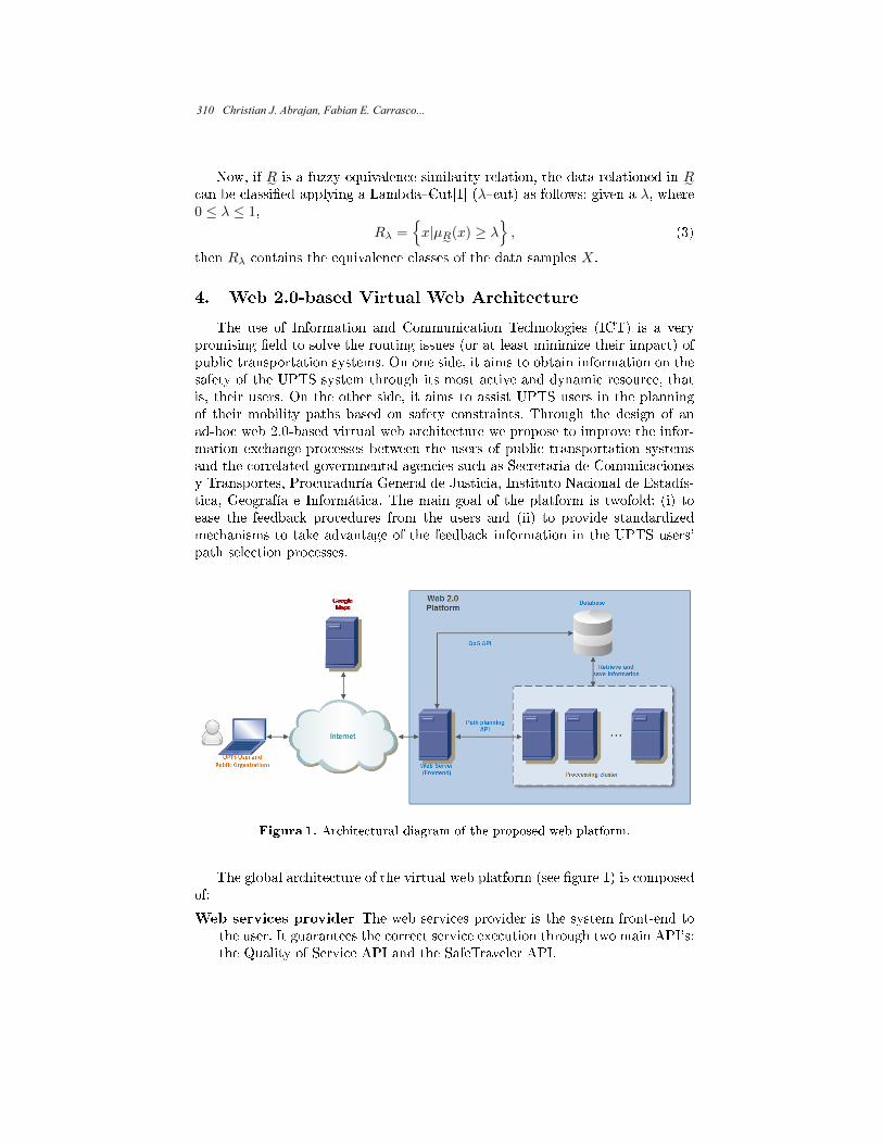
Now, if R˜ is a fuzzy equivalence similarity relation, the data relationed in R˜can be classied applying a LambdaCut[1] (λcut) as follows: given a λ, where0 ≤ λ ≤ 1,

Rλ =x|µR˜(x) ≥ λ

, (3)

then Rλ contains the equivalence classes of the data samples X.

4. Web 2.0-based Virtual Web Architecture

The use of Information and Communication Technologies (ICT) is a verypromising eld to solve the routing issues (or at least minimize their impact) ofpublic transportation systems. On one side, it aims to obtain information on thesafety of the UPTS system through its most active and dynamic resource, thatis, their users. On the other side, it aims to assist UPTS users in the planningof their mobility paths based on safety constraints. Through the design of anad-hoc web 2.0-based virtual web architecture we propose to improve the infor-mation exchange processes between the users of public transportation systemsand the correlated governmental agencies such as Secretaria de Comunicacionesy Transportes, Procuraduría General de Justicia, Instituto Nacional de Estadís-tica, Geografía e Informática. The main goal of the platform is twofold: (i) toease the feedback procedures from the users and (ii) to provide standardizedmechanisms to take advantage of the feedback information in the UPTS users'path selection processes.

Figura 1. Architectural diagram of the proposed web platform.

The global architecture of the virtual web platform (see gure 1) is composedof:

Web services provider The web services provider is the system front-end tothe user. It guarantees the correct service execution through two main API's:the Quality of Service API and the SafeTraveler API.


Algorithm 1 Yen's Algorithm that generates all shortest paths.

Input: s source, t target, P adjacency matrix.Output: Q paths.

1: For every arc u− v on P :2: Remove u− v and all nodes preceding u in P from graph.3: P ′

1 ← subpath from s to u in P .4: P ′

2 ← shortest path from u to t in modied graph.5: P ′ ← append P ′

2 to P ′1

6: Add P ′ to Q.7: Restore graph.

Processing cluster The processing cluster performs the system processing tasks.In particular, it pre-processes the user queries and executes the real-timepath selection algorithms.

Database Within the database the pre-processed information on the most queriedpaths is stored. This information is constantly updated with the results ofthe new queries.

Traveler This is the user that will (i) query and (ii) share information with thesystem.

The platform also includes web 2.0-based mechanisms such as polls and fora(not shown in the gure) to easily obtain feedback from the UPTS users on thequality of the public transportation systems, and interfaces (Web Services) topublic organizations to share information related with the UPTS system.

5. Search and Classication Algorithms of Public

Transport Path

5.1. Yen's Algorithm

Algorithm of Y. Yen [2] was used to nd the shortest routes to reach a des-tination.

Yen's algorithm calculates new paths from start node s to target node t basedon a path P as follows in algorithm 1.

The algorithm of Yen has a time complexity of: O(kn(m + nlogn)) with nthe number of nodes and m the number of arcs. [11]

5.2. Transfer Algorithm

The general complexity of the algorithm 2 is: O(∏Nti=0(2Nr ∗ (Nn/2i))

where:Nt: Number of transfers Nr: Number of routes Nn: Númber of nodes to goFor the case study, we have Nt = 2O(Nn3 ∗Nr3)where Nr is a small value.


Algorithm 2 Algorithm that generates the possible transfer options at UPTSfor a road and number of transfers given.

Globals: Rutas, m lists of nodes of the UPTS paths,Path, list of n nodes with the path from source A to destination B

Input: indice, current index of Path listresults, array of k triplets that contain Rutasx, Pathabordo,Pathdescensotransbordos, transfer number allowed

Output: R, l type-results arrays that contain the possible transfersBase Case If indice = PathB add results to R and returnPruning Case If transbordos = 0 returnSearch Recursive Case For each r ∈ Rutasidentify those containing a (Rutasr,i, ..., Rutasr,i+n)list equals to (Pathindice, ..., Pathindice+n),where n ≥ 1, it means, selecting all lists with more than one element,creating for each list a triplet Rutasr, Pathindice, Pathindice+n in results.Finally, the TransferAlgorithm(indice+ n, results, transbordos− 1) is called.

Algorithm 3 Algorithm that computes the equivalence classes of a data sample.

Input: X, m× n sample data matrix of m paths from A to B,each one of n attributesλ, the restriction of classication of m paths

Output: Rλ, m×m equivalence classes matrix of the m paths1. Compute the similarity matrix R˜ using (1)2. Verify if R˜ is transitive in accordance with (2)3. If R˜ is not an equivalence relationthen compute R˜ = R˜ R˜ at most m− 1 times4. Compute the equivalence class matrix Rλ using (3)

5.3. Fuzzy Classication Algorithm

In order to compute equivalence classes of the paths resulting from the trans-fer algorithm 2, the algorithm 3 is presented. This algorithm applies the CosineAmplitude method (step 1) to compute the similarity among the paths givenby algorithm 2. In steps 2 and 3 the similarity matrix obtained is transformedinto an equivalence relation matrix applying the maxmin composition. Finally,in accordance with a restriction level (λ) with respect to safety, distance andtransfer numbers given by user, in the step 4 a defuzzication process (λcut) isapplyed to equivalence relation matrix, obtaining the classication of paths thatallow a user to move from point A to point B in Puebla City using UPTS.

Since the complexity of steps 1, 2, 3 and 4 of the Algorithm 1 is O(mn2),O(m3), O(m4) and O(m2), respectively, the time complexity of algorithm 1 isO(m4), where m is the paths number from A to B.


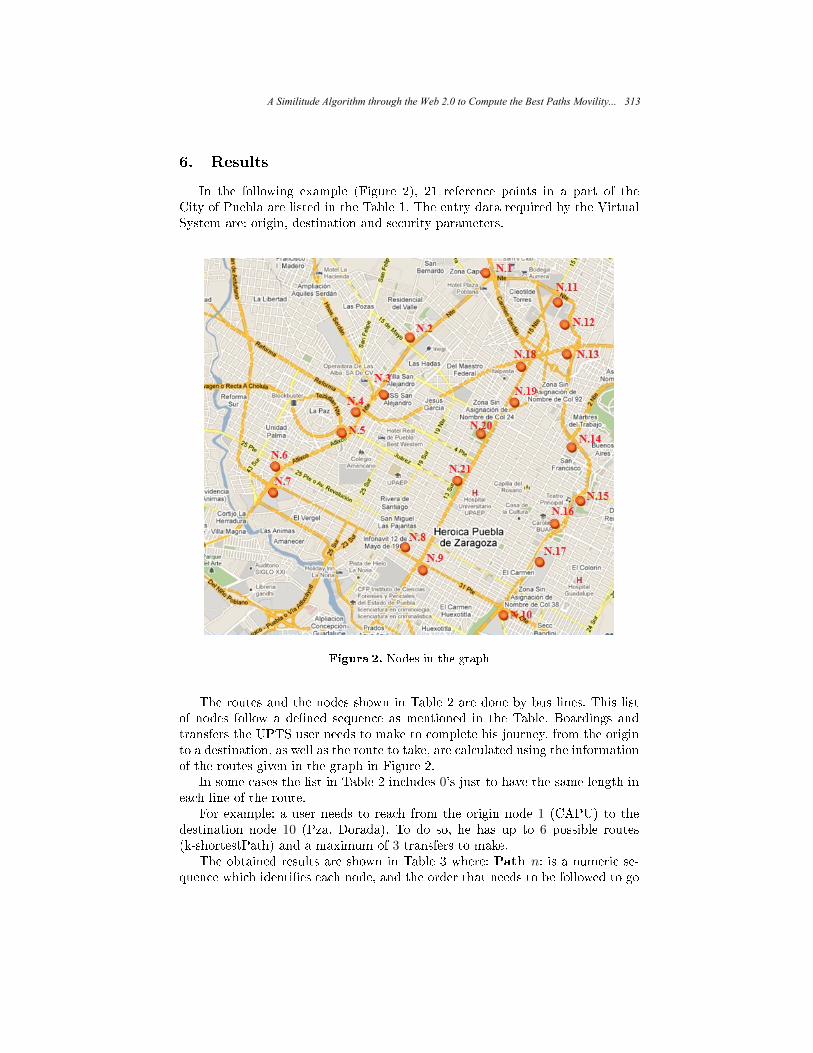
6. Results

In the following example (Figure 2), 21 reference points in a part of theCity of Puebla are listed in the Table 1. The entry data required by the VirtualSystem are: origin, destination and security parameters.

Figura 2. Nodes in the graph

The routes and the nodes shown in Table 2 are done by bus lines. This listof nodes follow a dened sequence as mentioned in the Table. Boardings andtransfers the UPTS user needs to make to complete his journey, from the originto a destination, as well as the route to take, are calculated using the informationof the routes given in the graph in Figure 2.

In some cases the list in Table 2 includes 0's just to have the same length ineach line of the route.

For example: a user needs to reach from the origin node 1 (CAPU) to thedestination node 10 (Pza. Dorada). To do so, he has up to 6 possible routes(k-shortestPath) and a maximum of 3 transfers to make.

The obtained results are shown in Table 3 where: Path n: is a numeric se-quence which identies each node, and the order that needs to be followed to go


Cuadro 1. List of Nodes in the graph.

Nodo Nombre Nodo Nombre1 CAPU 12 Karts2 Pza. San Pedro 13 China Poblana3 H. San Alejandro 14 H. San José4 Reforma 15 Centro Convenciones5 Fuente Los Frailes 16 Reforma y Blvrd. 5 Mayo6 25 pte y TELMEX 17 CENCH7 31 pte Marriot 18 Diagonal y 11 Nte8 Hosp. Universitario 19 Casa del Abue9 31 pte y 11 sur 20 Museo Ferrocarril10 Pza. Dorada 21 Paseo Bravo11 Soriana

Cuadro 2. List of Routes.

Route Way

R1 1 - 2 - 3 - 4 - 5 - 6 - 7 - 8 - 9 - 10 - 0 - 0 - 0 - 0 - 0 - 0R2 10 - 9 - 8 - 7 - 6 - 5 - 4 - 3 - 2 - 1 - 0 - 0 - 0 - 0 - 0 - 0R3 1 - 11 - 12 - 13 - 14 - 15 - 16 - 17 - 10 - 0 - 0 - 0 - 0 - 0 - 0- 0R4 10 - 17 - 16 - 15 - 14 - 13 - 12 - 11 - 1 - 0 - 0 - 0 - 0 - 0 - 0 - 0R5 8 - 7 - 6 - 5 - 4 - 3 - 2 - 1 - 11 - 12 - 13 - 14 - 15 - 16 - 17 - 10R6 1 - 11 - 18 - 19 - 20 - 21 - 9 - 0 - 0 - 0 - 0 - 0 - 0 - 0 - 0 - 0R7 9 - 21 - 20 - 19 - 18 - 11 - 1 - 0 - 0 - 0 - 0 - 0 - 0 - 0 - 0 - 0R7 15 - 20 - 21 - 0 - 0 - 0 - 0 - 0 - 0 - 0 - 0 - 0 - 0 - 0 - 0 - 0R8 21 - 20 - 15 - 0 - 0 - 0 - 0 - 0 - 0 - 0 - 0 - 0 - 0 - 0 - 0 - 0R9 20 - 21 - 4 - 5 - 6 - 0 - 0 - 0 - 0 - 0 - 0 - 0 - 0 - 0 - 0 - 0R10 6 - 5 - 4 - 21 - 20 - 0 - 0 - 0 - 0 - 0 - 0 - 0 - 0 - 0 - 0 - 0


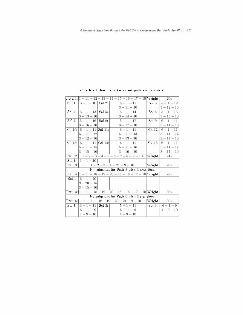
Cuadro 3. Results of k-shortest path and transfers.

Path 1: 1− 11− 12− 13− 14− 15− 16− 17− 10 Weight: 20u

Sol 1: 3− 1− 10 Sol 2: 5− 1− 11 Sol 3: 5− 1− 123− 11− 10 3− 12− 10

Sol 4: 5− 1− 13 Sol 5: 5− 1− 14 Sol 6: 5− 1− 153− 13− 10 3− 14− 10 3− 15− 10

Sol 7: 5− 1− 16 Sol 8: 5− 1− 17 Sol 9: 6− 1− 113− 16− 10 3− 17− 10 3− 11− 10

Sol 10: 6− 1− 11 Sol 11: 6− 1− 11 Sol 12: 6− 1− 115− 11− 12 5− 11− 13 5− 11− 143− 12− 10 3− 13− 10 3− 14− 10

Sol 13: 6− 1− 11 Sol 14: 6− 1− 11 Sol 15: 6− 1− 115− 11− 15 5− 11− 16 5− 11− 173− 15− 10 3− 16− 10 3− 17− 10

Path 2: 1− 2− 3− 4− 5− 6− 7− 8− 9− 10 Weight: 24u

Sol 1: 1− 1− 10

Path 3: 1− 2− 3− 4− 21− 9− 10 Weight: 26u

No solutions for Path 3 with 3 transfers.Path 4: 1− 11− 18− 19− 20− 15− 16− 17− 10 Weight: 28u

Sol 1 6− 1− 209− 20− 153− 15− 10

Path 3: 1− 11− 18− 19− 20− 15− 16− 17− 10 Weight: 30u

No solutions for Path 6 with 3 transfers.Path 6: 1− 11− 18− 19− 20− 21− 9− 10 Weight: 30u

Sol 1: 3− 1− 11 Sol 2: 5− 1− 11 Sol 3: 6− 1− 96− 11− 9 6− 11− 9 1− 9− 101− 9− 10 1− 9− 10


from the origin node to the destination node in each of the routes.Weight: is the path weight given in u units.Sol n: contains a group of (R,O,D) triplets, where R indicates the route toboard, O is the bus stop R, and D is either a bus stop to transfer or the desti-nation. It is worth mentioning that the order of the triplets in the result list isthe sequence in which the buses need to be boarded.The 20 found solutions are mapped obtaining a m× n matrix.

Given the following m×n matrix X = [X1 X2], of m = 20 (columns) pathsfrom A (CAPU) to B (Pza. Dorada), each one of n = 5 security levels: total,high, medium, low and poor (rows):

X1 =

0 0,33 0 0 0 0 0 0 0,33 0,250 0 0 0 0 0 0 0 0 00,50 0,33 0,67 0,67 0,67 0,33 0,33 0,33 0,33 0,500 0 0 0 0 0,33 0,33 0,33 0 00,50 0,33 0,33 0,33 0,33 0,33 0,33 0,33 0,33 0,25

,

X2 =

0,25 0,25 0,25 0,25 0,25 0 0 0,25 0,25 00 0 0 0 0 0 0 0 0 00,50 0,50 0,25 0,25 0,25 0,50 0,50 0,50 0,50 0,670 0 0,25 0,25 0,25 0 0,25 0 0 00,25 0,25 0,25 0,25 0,25 0,50 0,25 0,25 0,25 0,33

,the Algorithm 3 computes the equivalence classes of Table 4. When λ = 0,9, 0,91the method computes two equivalence classes, grouping the 1-12 and 16-20 pathsin the equivalence class 1: the paths with more unsafe transfers at a higher rate;and groupint the 13-15 paths in the equivalence class 2: the paths with a smallerproportion of unsafe transfers. In accordance with these results, the paths of theequivalence class 2 are preferable to the paths of the equivalence class 1.

Cuadro 4. Equivalence Classes Obtained by Fuzzy Classication Algorithm

λ Class 1 Class 2 Class 3 Class 4 Class 5 Class 6 Class 70.90,0.91 1-12, 13-15

16200.92,0.93, 1,3-5, 2,9-12, 6-8, 17, 0.94 16,20 18,19 13150.95,0.96, 1,16 2,9 3-5, 6-8 10-12, 13-15 170.97,0.98,0.99 20 18,19

Doing a similar analysis as above, in Table 4, when λ = 0,92, 0,93, 0,94,the Algorithm 3 computes three equivalence classes: the rst class comprises thepaths with medium security transfers at most; the second class comprises thepaths with safe, fairly safe and unsafe transfers at the same rate; most of thethird class paths have a balance of medium security, low security and unsafe


transfers. View of these results, the paths of the second equivalence class arepreferable.

Finally, when λ = 0,95, 0,96, 0,97, 0,98, 0,99, there are seven equivalenceclasses and the most recommended are rst the fth class and second the thirdclass, because in the fth class paths most of their transfers have medium securi-ty, and the third class paths have medium security transfers in greater proportionthan unsafe transfers. All other classes are less desirable because the transferswith low security and unsafe are signicant.

7. Conclusions

One of the main characteristics of the cities in developing countries is insecu-rity in certain urban areas. This Web platform designed to improve the integrityof UPTS traveler.

Mexico City and developing countries with similar characteristics, using anetwork of public disorderly public transport, which requires the traveler a pre-cise knowledge of the public transport routes, safe areas for transfers and poten-tial career options to ensure their integrity during their trip.

The creation of a social network based on the concepts of Web 2.0 providegreater speed in the exchange of experiences among travelers, with these prefer-ences stored to support future travelers.

The connection of this site via Web Services, provides mechanisms for theexchange of knowledge among end users (travelers) and the opportunity thatother sites use this service, incorporating the platform into the cloud computing.

Tackling a complex problem with a fuzzy classication algorithm providesa new approach to research to automatically nd the path between two points,considering fuzzy parameters and the integrity of travelers.

Despite being a cubic algorithm, the pre-processing routes, helps to reducethe dimension of the problem. The use of robust computational architecture andparallelization of these, improves performance.

Acknowledgments. Thanks to CONACyT, LAFMIA and the Instituto Tec-nológico de Puebla for their support, without which this research would havebeen possible.

Referencias

1. Ross, J.: Fuzzy Logic with Engineering Applications. John Wiley & Sons (2004)2. Yen J.:Finding the K shortest loopless paths in a network. Management Science

(1977)3. Sun, R., Wang, Y.; Atrial Arrhythmias Detection Based on Neural Network Com-

bining Fuzzy Classiers. Advances in Neural Networks 4492, 284292 (2007)4. Keles,A., Hasiloglu, A.S., Keles, A., Aksoy, Y.: Neuro-fuzzy classication of prostate

cancer using NEFCLASS-J. Computers in Biology and Medicine, vol. 37, issue 11,16171628 (2007)


5. Shackelford, A.K., Davis, C.H.: A hierarchical fuzzy classication approach for high-resolution multispectral data over urban areas. IEEE Transactions on Geoscienceand Remote Sensing, vol. 41, issue 9, 19201932 (2003)

6. Özyer, T., Alhajj, R., Barker, K.: Intrusion detection by integrating boosting geneticfuzzy classier and data mining criteria for rule pre-screening. Journal of Networkand Computer Applications 30(1), 99113 (2007)

7. Sánchez, L., Couso, I., Corrales, J.A.: Combining GP operators with SA search toevolve fuzzy rule based classiers. Information Sciences 136, 175191 (2001)

8. Evsuko, A.G., Costa, M.C.A, Ebecken, N.F.F.: High Performance Computing forComputational ScienceVECPAR 2004. LNCS 3402, 6396 (2004)

9. Ozturk, A., Arslan, A., Hardalac, F.: Comparison of neuro-fuzzy systems for classi-cation of transcranial Doppler signals with their chaotic invariant measures. ExpertSystems with Applications 32(2), 10441055 (2008)

10. API Google MAPS.: Google Maps API Family., available at http://code.google.com/apis/maps/index.html

11. Vanhove, S., Fack, V.: Fast Generation of Many Shortest Path Alternatives, Bel-gium


Author Index Índice de autores

Abrajan, Christian J. 307

Acosta-Pineda, Ignacio 221

Aguilar Vera, Raúl A. 103

Aguilar, Adolfo 307

Alanis Garza, Arnulfo 251

Altamirano, Leopoldo 3

Alvarado, Montserrat 273

Anzures-García, Mario 77

Arco, Leticia 117

Artiles, Michel 117

Avilés, Héctor H. 273

Ayala Leal, Erika Consuelo 251

Barceló-Aspeitia, Axel Arturo 91

Bello, Rafael 15, 117

Bucciol, Paolo 307

Caballero Morales, Santiago Omar

131

Calderon, Felix 173

Carbajal, Efren 261

Carrasco, Fabian E. 307

Carvalho, Leonardo F. B. S. 161

Castro-Manzano, José Martín 91

Chai, Huimin 25

Chandrasekaran, Muthumari 185

de Baets, Bernard 15

De la Vega, Erick 173

De Los Santos Ramírez, Edgar 131

Díaz D., E. 199

Escamilla Hernandez, Enrique 39

Estrada Guzmán, Elsa 103

Fernández, Juan M. 117

Flores, Juan 173

Flores, Georgina 307

Fuentes, Ivett E. 117

García Aguilar, Abraham 145

García Hernández, René 145

García-Vázquez, Mireya S. 51

Garrido , Leonardo 261

Gershenson, Carlos 273

González, Jesús A. 3

Guerra-Hernández, Alejandro 91

Hernández, Selene 307

Hernandez-Mendez, Sergio 285

Hornos, Miguel J. 77

Huete, Juan 117

Jiménez Hernández, Mario 65

Kumar Singh, Amit 185

Ledeneva, Yulia 145

León, Adrián 3

Lopes, Roberta V. V. 161

López Ramírez, Miguel Ángel 251

Magdaleno, Damny 117

Marin-Hernandez, Antonio 285

Marin-Urias, Luis F. 285

Martínez Cruz, Alfonso 65

Mathias Mendoza, Griselda 145

Meza, Ivan V. 273

Mijatović-Teodorović, Ljiljana

243

Milian, Carlos 15

Morales, Eduardo F. 3

Morell, Carlos 15

Morgado-Ramirez, Luis A. 285

Nakano Miyatake, Mariko 39

Oropeza Rodríguez, José Luis 65

Ortiz-Posadas, Martha R. 221

Osorio, Maria 295

Paderewski, Patricia 77

Padilla D., A. 199

Paraguaçu, Fábio 161

Peña Pérez Negrón, Adriana 103

Perez Daniel, Karina Ruby 39

Perez Meana, Hector Manuel 39

Pineda, Luis A. 273

Ponce de Leon S., E. 199

Ramírez-Acosta, Alejandro A. 51

Rascón, Caleb 273

Rios-Figueroa, Homero V. 285

Romero Gaitán, Carlos Francisco

251

Ruiz, Jaime R. 3

Sadovnychyy, Andriy 231

Salinas, Lisset 273

Sánchez, Abraham 295

Sánchez-Gálvez, Luz A. 77

Šelmić, Milica 243

Sidorov, Grigori 145

Silva Neto, Helio C. 161

Teodorović, Dušan 243

Toriz, Alfredo 295

Vargas Flores, Selene 145

Velarde M., A. 199

Vidal-González, Gustavo L. 51

Wang, Baoshu 25

Zapata, Rene 295

Editorial Board of the Volume

Comité editorial de volumen

Carlos Acosta Hector-Gabriel Acosta-Mesa

Luis Aguilar

Ruth Aguilar

Esma Aimeur

Teresa Alarcón

Alfonso Alba Rafik Aliev

Adel Alimi

Leopoldo Altamirano

Matias Alvarado

Gustavo Arechavaleta

Gustavo Arroyo Serge Autexier

Juan Gabriel Aviña Cervantes

Victor Ayala-Ramirez

Andrew Bagdanov

Javier Bajo

Helen Balinsky

Sivaji Bandyopadhyay

Maria Lucia Barrón-Estrada

Roman Barták

Ildar Batyrshin

Salem Benferhat Tibebe Beshah

Albert Bifet

Igor Bolshakov

Bert Bredeweg

Ramon Brena

Paul Brna Peter Brusilovsky

Pedro Cabalar

Abdiel Emilio Caceres Gonzalez

Felix Calderon

Nicoletta Calzolari

Gustavo Carneiro

Jesus Ariel Carrasco-Ochoa

Andre Carvalho

Mario Castelán

Oscar Castillo

Juan Castro Félix Agustín Castro Espinoza

Gustavo Cerda Villafana

Mario Chacon

Lee Chang-Yong

Niladri Chatterjee

Zhe Chen

Carlos Coello

Ulises Cortes Stefania Costantini

Raúl Cruz-Barbosa

Nareli Cruz-Cortés

Nicandro Cruz-Ramirez

Oscar Dalmau

Ashraf Darwish Justin Dauwels

Radu-Codrut David

Jorge De La Calleja

Carlos Delgado-Mata

Louise Dennis

Bernabe Dorronsoro Benedict Du Boulay

Hector Duran-Limon

Beatrice Duval

Asif Ekbal

Boris Escalante Ramírez

Jorge Escamilla Ambrosio

Susana C. Esquivel

Claudia Esteves

Julio Cesar Estrada Rico

Gibran Etcheverry

Eugene C. Ezin Jesus Favela

Claudia Feregrino

Robert Fisher

Juan J. Flores

Claude Frasson

Juan Frausto-Solis Olac Fuentes

Sofia Galicia-Haro

Ma.de Guadalupe Garcia-Hernandez

Eduardo Garea

Leonardo Garrido

Alexander Gelbukh

Onofrio Gigliotta

Duncan Gillies

Fernando Gomez

Pilar Gomez-Gil

Eduardo Gomez-Ramirez Felix Gonzales

Jesus Gonzales

Arturo Gonzalez

Jesus A. Gonzalez

Miguel Gonzalez

José-Joel Gonzalez-Barbosa

Miguel Gonzalez-Mendoza

Felix F. Gonzalez-Navarro

Rafael Guzman Cabrera

Hartmut Haehnel

Jin-Kao Hao

Yasunari Harada

Pitoyo Hartono

Rogelio Hasimoto

Jean-Bernard Hayet

Donato Hernandez Fusilier

Oscar Herrera Ignacio Herrera Aguilar

Joel Huegel

Michael Huhns

Dieter Hutter

Pablo H. Ibarguengoytia

Mario Alberto Ibarra-Manzano Héctor Jiménez Salazar

Moa Johansson

W. Lewis Johnson

Leo Joskowicz

Chia-Feng Juang

Hiroharu Kawanaka

Shubhalaxmi Kher

Ryszard Klempous

Mario Koeppen

Vladik Kreinovich

Sergei Kuznetsov

Jean-Marc Labat Susanne Lajoie

Ricardo Landa Becerra

H. Chad Lane

Reinhard Langmann

Bruno Lara

Yulia Ledeneva

Ronald Leder

Sergio Ledesma-Orozco

Yoel Ledo Mezquita

Eugene Levner

Derong Liu Weiru Liu

Giovanni Lizarraga

Aurelio Lopez

Omar Lopez

Virgilio Lopez

Gabriel Luque Sriram Madurai

Tanja Magoc

Luis Ernesto Mancilla

Claudia Manfredi

J. Raymundo Marcial-Romero

Antonio Marin Hernandez

Luis Felipe Marin Urias

Urszula Markowska-Kaczmar

Ricardo Martinez

Edgar Martinez-Garcia

Jerzy Martyna

Oscar Mayora

Gordon Mccalla

Patricia Melin

Luis Mena

Carlos Merida-Campos

Efrén Mezura-Montes Gabriela Minetti

Tanja Mitrovic

Dieter Mitsche

Maria-Carolina Monard

Luís Moniz Pereira

Raul Monroy Fernando Martin Montes-Gonzalez

Manuel Montes-Y-Gómez

Oscar Montiel

Jaime Mora-Vargas

Eduardo Morales

Guillermo Morales-Luna

Enrique Munoz de Cote

Angel E. Munoz Zavala

Angelica Munoz-Melendez

Masaki Murata

Rafael Murrieta

Tomoharu Nakashima Atul Negi

Juan Carlos Nieves

Sergey Nikolenko

Juan Arturo Nolazco Flores

Paulo Novais

Leszek Nowak

Alberto Ochoa O.Zezzatti

Iván Olier

Ivan Olmos

Constantin Orasan

Fernando Orduña Cabrera Felipe Orihuela-Espina

Daniel Ortiz-Arroyo

Mauricio Osorio

Elvia Palacios

David Pearce

Ted Pedersen Yoseba Penya

Thierry Peynot

Luis Pineda

David Pinto

Jan Platos

Silvia Poles

Eunice E. Ponce-De-Leon

Volodimir Ponomaryov

Edgar Alfredo Portilla-Flores

Zinovi Rabinovich

Jorge Adolfo Ramirez Uresti

Alonso Ramirez-Manzanares

Jose de Jesus Rangel Magdaleno

Francisco Reinaldo

Carolina Reta

Carlos A Reyes-Garcia

María Cristina Riff Homero Vladimir Rios

Arles Rodriguez

Horacio Rodriguez

Marcela Rodriguez

Katia Rodriguez Vazquez

Paolo Rosso Jianhua Ruan

Imre J. Rudas

Jose Ruiz Pinales

Leszek Rutkowski

Andriy Sadovnychyy

Carolina Salto

Gildardo Sanchez

Guillermo Sanchez

Eric Sanjuan

Jose Santos

Nikolay Semenov

Pinar Senkul Roberto Sepulveda

Leonid Sheremetov

Grigori Sidorov

Gerardo Sierra

Lia Susana Silva-López

Akin Sisbot

Aureli Soria Frisch

Peter Sosnin

Humberto Sossa Azuela

Luis Enrique Sucar

Sarina Sulaiman

Abraham Sánchez

Javier Tejada

Miguel Torres Cisneros Juan-Manuel Torres-Moreno

Leonardo Trujillo Reyes

Alexander Tulupyev

Fevrier Valdez

Berend Jan Van Der Zwaag

Genoveva Vargas-Solar Maria Vargas-Vera

Wamberto Vasconcelos

Francois Vialatte

Javier Vigueras

Manuel Vilares Ferro

Andrea Villagra

Miguel Gabriel Villarreal-Cervantes

Toby Walsh

Zhanshan Wang

Beverly Park Woolf

Michal Wozniak

Nadezhda Yarushkina Ramon Zatarain

Laura Zavala

Qiangfu Zhao

Additional Reviewers

Árbitros adicionales

Aboura, Khalid

Acosta-Guadarrama, Juan-Carlos

Aguilar Leal, Omar Alejandro

Aguilar, Ruth Arce-Santana, Edgar

Bankevich, Anton

Baroni, Pietro

Bhaskar, Pinaki

Bolshakov, Igor

Braga, Igor Cerda-Villafana, Gustavo

Chaczko, Zenon

Chakraborty, Susmita

Chavez-Echeagaray, Maria-Elena

Cintra, Marcos

Confalonieri, Roberto

Darriba, Victor

Das, Amitava

Das, Dipankar

Diaz, Elva

Ezin, Eugene C. Figueroa, Ivan

Fitch, Robert

Flores, Marisol

Gallardo-Hernández, Ana Gabriela

Garcia, Ariel

Giacomin, Massimiliano Ibarra Esquer, Jorge Eduardo

Joskowicz, Leo

Juárez, Antonio

Kawanaka, Hiroharu

Kolesnikova, Olga Li, Hongliang

Lopez-Juarez, Ismael

Montes Gonzalez, Fernando

Murrieta, Rafael

Navarro-Perez, Juan-Antonio

Nikodem, Jan Nurk, Sergey

Ochoa, Carlos Alberto

Orozco, Eber

Pakray, Partha

Pele, Ofir

Peynot, Thierry

Piccoli, Maria Fabiana

Ponomareva, Natalia

Pontelli, Enrico

Ribadas Pena, Francisco Jose

Rodriguez Vazquez, Katya Sánchez López, Abraham

Sirotkin, Alexander

Suárez-Araujo, Carmen Paz

Villatoro-Tello, Esaú

Wang, Ding

Yaniv, Ziv Zepeda, Claudia

Impreso en los Talleres Gráficos

de la Dirección de Publicaciones

del Instituto Politécnico Nacional

Tresguerras 27, Centro Histórico, México, D.F.

Noviembre de 2011

Printing 500 / Edición 500 ejemplares