LARGE SCALE SIMULATION OF WAVE PROPAGATION IN SOILS INTERACTING WITH STRUCTURES USING FEM AND SBFEM

April 14, 2011 16:8 WSPC/S0218-396X 130-JCA S0218396X11004316

Journal of Computational Acoustics, Vol. 19, No. 1 (2011) 75–93c© IMACSDOI: 10.1142/S0218396X11004316

LARGE SCALE SIMULATION OF WAVE PROPAGATIONIN SOILS INTERACTING WITH STRUCTURES

USING FEM AND SBFEM

MARCO SCHAUER∗ and SABINE LANGER†

Institut fur Angewandte MechanikTechnische Universitat Carolo-Wilhelmina zu Braunschweig

Spielmannstraße 11, 38106 Braunschweig, Germany∗[email protected]†[email protected]

http://www.infam.tu-braunschweig.de

JOSE E. ROMAN

D. Sistemas Informaticos y ComputacionUniversidad Politecnica de Valencia

Camino de Vera s/n, E-46022 Valencia, [email protected]

ENRIQUE S. QUINTANA-ORTI

Departamento de Ingenierıa y Ciencia de ComputadoresUniversidad Jaume I, Avda. Sos Baynat s/n

E-12071 Castellon, [email protected]

Received 4 February 2011Revised 14 February 2011

This paper applies a parallel algorithm for a coupled Finite Element/Scaled Boundary Element(FEM/SBFEM)-approach to study soil-structure-interaction problems. The application code isdesigned to run on clusters of computers, and it enables the analysis of large-scale problems. Acrucial point of the approach is that the SBFEM fulfills the radiation condition. Hence, the hybridnumerical approach is well suited for such problems where wave propagation to infinity in anunbounded domain must be considered. The main focus of the paper is to show the applicability ofthe numerical implementation on large scale problems. First the coupled FEM/SBFEM approachis validated by comparing the numerical results with a semi-analytical solution for a settlementproblem. Then the implemented algorithm is applied to study the dynamical behavior of foundedwind energy plants under time dependent loading.

Keywords: Scaled boundary finite element method; soil-structure interaction.

75

http://dx.doi.org/10.1142/S0218396X11004316


76 M. Schauer et al.

1. Introduction

The present work focuses on the analysis of soil-structure interaction (SSI). There aretwo major motivations: in active seismic areas it is necessary to construct reliableearthquake-resistant structures, and in our urban society it is an increasingly importantand challenging task to isolate a building from the surrounding emissions to enhance itscomfort. In both cases it is essential not only to analyze the structure itself but also to takethe surrounding soil into account.1,17,19 Whenever vibrations or impulses are emitted tosoil, they induce waves propagating through the ground that can result in vibration or evenfailure of structures. Traffic, blasting operations and earthquakes are some of the sourcesfor such kind of emissions.

For those types of complex analysis, two very different mechanical problems have tobe solved: the structure itself and the infinite half-space, which surrounds the domain ofinterest. Hence, the engineers have to deal with complex geometries or materials as well. Ingeneral, it is not possible to formulate an analytical or even semi-analytical solution, so theonly viable alternative is to use computational models. Nowadays, the finite element methodis a standard tool to discretize structures. Furthermore, finite differences are also applicablefor the computational analysis of structures. In contrast, the infinite half-space cannot beanalyzed with those standard methods as they do not fulfill the radiation condition.

Several methods have been developed during the last years which approximate the radia-tion condition. The viscous boundary condition is one of the simplest transmitting boundaryconditions, acting like a dashpot.16 Other local, absorbing boundary conditions8,15 and sev-eral other types of transmitting boundaries (e.g. infinite elements2,6) have been proposed,but none of them is able to fulfill the radiation condition exactly.

A more precise alternative is the discretization of the far-field by the boundary elementmethod (BEM)3 or a scaled boundary finite element method (SBFEM).22,23 The BEMis a well-known discretization method based on the boundary integral representation ofthe physical problem and fulfills the radiation condition exactly. It requires a fundamentalsolution of the problem. Here, the SBFEM is used in the following because it combines theadvantages of both FEM and BEM.12 In particular, alike FEM, the SBFEM does not requirea fundamental solution and the coefficient matrices are symmetric and can be added to theFEM matrices without changing their dimension. On the other hand, at the boundary thespatial dimension is reduced by one and the radiation conditions are satisfied exactly, as inthe BEM.13,14

The main goal of the paper is to apply a coupled FEM/SBFEM-approach to largescale problems. When a basic SSI problem consisting of a geometrically simple foundationand the surrounding space is discretized, the number of degrees of freedom is small. Suchproblems can generally be analyzed using a standard desktop computer. As the size ofthe foundation, the structure itself, and their complexity grows, the number of degreesof freedom increases conformally to maintain a similar level of accuracy in the results.Increasingly large problem sizes imply a growing cost of the matrix computations that soonmake the analysis unfeasible on standard computers. More often, this is even impossible


Large Scale Simulation of Wave Propagation in Soils Interacting with Structures 77

due to the lack of sufficient memory. Hence, the options for analyzing large SSI problemsare either to simplify the model, at the expense of losing accuracy, or to keep the detailedmodel and use parallel computing techniques. Publications on the practical applicationof SBFEM to large scale or larger scaled problems in time-domain, where the far-field isdiscretized by only one sub-domain, are not known to the authors. This paper describes theuse of a coupled FEM/SBFEM approach for large scale problems without sub-structuringthe interface Γ. The approach itself and its implementation is described in detail in Ref. 21.

In Sec. 2, the FEM/SBFEM coupling approach is introduced briefly. Some remarks onthe algorithm to solve the SBFEM part and its implementation for time domain simulationsare discussed in Sec. 3. In Sec. 4, a validation of the code is done using a settlement problem.That section also includes results of large scale simulations of soil-structure interaction. Weconclude with a brief discussion in Sec. 5.

2. Coupled FEM/SBFEM Approach

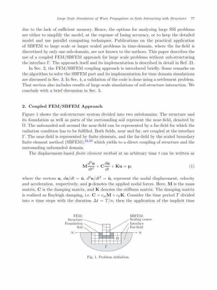
Figure 1 shows the soil-structure system divided into two subdomains. The structure andits foundation as well as parts of the surrounding soil represent the near-field, denoted byΩ. The unbounded soil around the near-field can be represented by a far-field for which theradiation condition has to be fulfilled. Both fields, near and far, are coupled at the interfaceΓ. The near-field is represented by finite elements, and the far-field by the scaled boundaryfinite element method (SBFEM),22,23 which yields to a direct coupling of structure and thesurrounding unbounded domain.

The displacement-based finite element method at an arbitrary time t can be written as

Md2udt2

+ Cdudt

+ Ku = p, (1)

where the vectors u, du/dt = u, d2u/dt2 = u, represent the nodal displacement, velocityand acceleration, respectively, and p denotes the applied nodal forces. Here, M is the massmatrix, C is the damping matrix, and K denotes the stiffness matrix. The damping matrixis realized as Rayleigh damping, i.e. C = cmM + ckK. Consider the time period T dividedinto n time steps with the duration ∆t = T/n; then the application of the implicit time

Fig. 1. Problem definition.



integration scheme Hilbert–Hughes–Taylor-α (HHT-α)10 results in

Mutn+1 + (1 + α)Cutn+1 − αCutn + (1 + α)Kutn+1 − αKutn = ptn+1+α∆t, (2)

utn+1 = utn + ∆tutn + ∆t212− βutn + β∆t2utn+1 , (3)

utn+1 = utn + (1 − γ)∆tutn + γ∆tutn+1 . (4)

Thus, for α = 0, the HHT-α scheme equals the Newmark integration method.18

In the next step we split the entries of the matrices in (1) into the near- and far-fields,which results in the following FEM equation:[

Mnn Mnf

Mfn Mff

]u +

[Cnn Cnf

Cfn Cff

]u +

[Knn Knf

Kfn Kff

]u =

[pnn

pff

]−

[0

pb

]. (5)

In this expression, blocks with subscript “nn” contain nodes at the near-field while blockswith subscript “ff ” comprise nodes at the far-field. The coupling of near-field nodes andfar-field nodes is reflected in those blocks labelled with the subscripts “nf” and “fn”.

The influence of the far-field on the near-field can be applied to the FEM subdomain asa load and is denoted by the vector pb. These forces pb at the near-field/far-field interfaceare computed by the SBFEM and given by the convolution integral

pb(t) =∫ t

0M∞(t − τ)u(τ)dτ, (6)

where M∞(t) is the acceleration unit-impulse response matrix, also known as the influencematrix. In order to solve the convolution integral equation (6) in time domain, a piecewiseconstant acceleration unit impulse response matrix is assumed, i.e.

M∞(t) =

M∞0 t ∈ [0;∆t],

M∞1 t ∈ [∆t; 2∆t],

......

M∞n t ∈ [(n − 1)∆t;n∆t],

(7)

so that Eq. (6) can be rewritten in discrete form as

pb(tn) =n∑

j=1

M∞n−j

∫ j∆t

(j−1)∆tu(τ)d(τ). (8)

This equation is then transformed using HHT-α (with γ parameter of HHT-α scheme) into

pb(tn) = γ∆tM∞0 un +

n−1∑j=1

M∞n−j(uj − uj−1). (9)



The coupling of FEM and SBFEM is done at the common interface of both subdomainswith the SBFEM part (9) being simply added to the sorted FEM part (5):[

Mnn Mnf

Mfn Mff + γ∆tM∞0

]u +

[Cnn Cnf

Cfn Cff

]u +

[Knn Knf

Kfn Kff

]u

=

pnn

pff −n−1∑j=1

M∞n−j (uj − uj−1)

.

(10)

The scaled boundary finite elements are described by a local coordinate system, η andζ, on the boundary and the radial coordinate ξ; see Fig. 2. This system (ξ, η, ζ) is related tothe Cartesian coordinate system xi as follows: ξ represents the distance between the scalingcenter (ξ = 0), boundary (ξ = 1) and infinity.

The geometry of a finite element at the boundary is represented by interpolating itsnodal coordinates xi with the shape functions N(η, ζ) using the local coordinates η andζ. An arbitrary point x(ξ, η, ζ) can be described by scaling its corresponding point at theboundary with the radial coordinate ξ. Since the displacements, stresses and strains aredefined in Cartesian coordinates, the differential operator D has to be modified so thatthe governing equation of elastodynamics is transformed to the scaled boundary coordinatesystem. For details, see Refs. 13, 22 and 23.

The SBFEM is the analog of the FEM formulated in a nodal force-displacement rela-tionship. At all surfaces Γξ the displacement u(ξ) can be determined by applying the shapefunction N(η, ζ) using the mapping equation

u(ξ, ηζ) = N(η, ζ)u(ξ). (11)

Using these functions to discretize the dynamic equilibrium in frequency domain leads tocoefficient matrices C1,C2,C3 whose expressions are not given here in detail (see Ref. 21).

Fig. 2. Scaled boundary transformation for three-dimensional problems: finite element and coordinatesystems.



The acceleration unit impulse response matrix M∞(t) can be derived from

M∞(t) = LM∞(t)LT . (12)

where L results from a Cholesky decomposition of the coefficient matrix C1. The timedependent matrix M∞(t) can be approximated for each time step applying the Fouriertransformation to the weak form of the differential equation of motion in frequency domain.The latter equation is formulated for this purpose using the frequency dependent dynamicstiffness matrix S∞(ω) for the unbounded medium

(S∞(ω) + C2)C−11 (S∞(ω) + CT

2 ) − S∞(ω) − ωS∞(ω),ω − C3 + ω2M = 0. (13)

This is a nonlinear first order differential equation, which represents the scaled boundaryfinite element equation in frequency domain for three dimensional elastodynamics.23 Theunknown dynamic stiffness matrix for the unbounded medium S∞(ω) with the independentfrequency ω is related to M∞(ω) by

M∞(ω) =S∞(ω)(iω)2

. (14)

The calculation of the time dependent matrix M∞(t) needs special care: a convolutionintegral appears in the Fourier transform of (13). Solving this convolution integral leads toa quadratic equation in the unknown matrix M∞ at the first time step that is analogousto an algebraic Riccati equation in the general form

FX + XFT − XBBT X + Q = 0, M∞ = X. (15)

This quadratic equation appears in the first time step only, so this time step requires aspecialized procedure. All subsequent time steps require solving a Lyapunov equation inthe unknown matrix M∞ in the general form

AX + XAT = C, M∞ = X, (16)

where the coefficient matrix changes at every step as A = A + (t/2)I.

3. Algorithm and its Implementation

In this section, we discuss practical aspects related with the computation of the accelerationunit impulse response matrices M∞

n and the solvers that are employed for the Riccatiand Lyapunov matrix equations. Hereby, we assume that the dimension of these numericalproblems ranges from moderate to large, thus calling for parallel computing capabilities.

The overall computation is depicted in Fig. 3, showing the main operations required toobtain the M∞

n matrices. As shown there, the frequency domain coefficient matrices mustbe calculated as well as the time domain coefficient matrices. The former are sparse, thelatter are unfortunately dense. The consequence is that we need to develop a hybrid sparse-dense code that operates in parallel. This adds a lot of complexity to programming as itrequires the integration of numerical libraries of different nature, using appropriate data



Fig. 3. Flowchart to compute the acceleration unit impulse response matrix M∞.

structures in each case. Fortunately, the resulting matrices M∞n are again sparse, enabling

their conversion to sparse format thus reducing the complexity of subsequent computationsrelated to the coupling of near-field and far-field. For a detailed description see Ref. 21.

The Riccati matrix equation appearing in the first time-step is solved employing New-ton’s root-finding iteration.11 It converges under mild conditions to the desired stabilizingsolution. The basic idea of the method is to improve the current approximate solution Xk bya correction X obtained by solving a c-stable Lyapunov equation. The rate of convergenceof Newton’s method strongly depends on the distance between the initial guess X0 and theexact solution. In our case, as F is stable (i.e. all its eigenvalues have negative real part),X0 = ‖F‖1 · I, with I the identity matrix, is a feasible initial guess and Newton’s method(with line search) becomes a competitive alternative as a solver for the algebraic Riccatiequation; see Refs. 4 and 5.

In terms of operations, Newton’s method for the Riccati equation is based on two mainkernels: a number of highly-parallel matrix-matrix products, and the resolution of one Lya-punov equation in each iteration, which represents the highest computational cost. Fortu-nately, the coefficient matrix of this equation, Ak, is c-stable so that it can be efficientlysolved via the matrix-sign function.20 The algorithm basically consists of matrix inver-sion and matrix-matrix products which can be efficiently implemented in current parallelplatforms.

For the next time steps, we can derive a quasi-triangular form of the Lyapunov equa-tion (16) by using the (real) Schur form. In this particular case, this transformation yields



a huge computational saving, because the Schur decomposition needs to be computed onlyonce since the Schur form of a shifted matrix, A = A + σI, is trivially related to the Schurform of A. The same does not hold for the Lyapunov equation that has to be solved ateach step of Newton iteration for the Riccati equation in the first time step as, there, thecoefficient matrix Ak changes at every iteration.

In our implementation we make use of specialized libraries to tackle the high complexityof the application. Modern numerical libraries are designed to provide enough flexibilityto enable software reuse in many different contexts, but also with other goals in mindsuch as numerical robustness, computational efficiency, portability to different computingplatforms, interoperability with other software, etc. For example, PETSc (parallel com-putation with sparse matrices), LAPACK (sequential computation with dense matrices),ScaLAPACK (parallel computation with dense matrices) and some related libraries areused in our implementation. It must be mentioned that the developed codes are written inC++, whereas PETSc is programmed in C, and ScaLAPACK and most of the rest of denselibraries are encoded in Fortran. Combining the three programming languages in a portableway requires a careful design of the interfaces. PETSc offers interfaces for C++ and Fortranprogrammers, as well as portable wrappers to LAPACK subroutines. We have extended thisto also wrap subroutines from ScaLAPACK and the other libraries. A detailed descriptionof the implementation can be found in Ref. 21.

4. Numerical Results

This section starts with the verification of the implemented algorithm. The verification isdone by comparing numerical results with a semi-analytic solution of a settlement problem.The intention is to show the ability of the implemented algorithm for analyzing large-scale problems. After that, we study an engineering problem of practical relevance within-situ scaling: The interaction of wind-induced vibrations of a wind energy plant with itsfoundation in the soil.

All calculations have been carried out on a cluster using 12 nodes (for the settlementproblem) and 20 nodes (for the wind power plant), each of them with 2 Opteron 246processors at 2 GHz and 4GB RAM, linked with a Myrinet-2000 interconnect. A total of2 h are needed for the calculation of 500 time steps for the most complex situation of a groupof wind power plants discretized approximately with 20 000 degrees of freedom. Detailedremarks on the parallel performance of the presented algorithm are given in Ref. 21.

4.1. Verification of the implemented algorithm — Settlement problem

In order to verify the coupled FEM/SBFEM approach, a settlement problem is chosen.The setup is shown in Fig. 4. Using an infinite half space, the flexible foundation and itssurrounding soil can be modeled easily. As discussed in Sec. 1, the problem has to be splitinto two separate domains, where the near-field is represented by finite elements and the far-field by scaled boundary finite elements. A semi-analytical solution is available for isotropic,homogeneous and fully linear elastic material.9 This can be described by only three material



Fig. 4. Infinite half space under constant area load q.

parameters: Young’s modulus E, Poisson ratio ν and density ρ. This solution is valid forconstant loads in time and space, so that the determined displacement is constant and timeindependent, which yields to a static solution.

The numerical model is implemented for time domain analysis so that the displacementsare time-dependent. Whenever constant loads are applied, the nodal displacements becomeconstant after a certain time, due to the fact that the coupled FEM/SBFEM approachfulfills the radiation condition. This means that the numerical results approximate thestatic semi-analytical solution.

An area load of q = 70[kN/m2] is applied on a square region of 152.4 × 152.4[m2].Locating the SBFEM scaling center in the middle of the load area causes that the distancebetween this center and all interface nodes at the boundary Γ is exactly r = 190.5[m]. Themesh was refined several times, to demonstrate the accuracy of the method. This leads toan increasing number of degrees of freedom, as shown in table of Fig. 5.

The material parameters are chosen as follows: E = 37150.0[kN/m2], ν = 0.48[−] andρ = 1800.0[kg/m3]. This results in a speed of cp = 425.779[m/s] for the longitudinal waveor p-wave, so that an adequate time step can be determined to ∆t = r/30cp = 0.0149[s] asit is suggested in Ref. 7. Performing the simulation of the settlement problem for a period

Fig. 5. Comparison of different FEM/SBFEM approaches (DOF) with semi-analytical approach(normalized).



of 6.25[s] the HHT-α parameters are set to α = −(1/4), β = (1−α)2/4, γ = (1− 2α)/2, thetime step ∆t is chosen to 0.0125[s], and the number of time steps is 500.

Figure 5 shows the time-dependent displacement of the settlement problem, which isnormalized by the settlement d(z) = 0.24800447[m] acquired from semi-analytic approach.The diagram shows obviously that the numerical solution meets the analytical solution.

4.2. Application: Wind energy plant

In the following, the vibrations of a wind energy plant due to time-dependent loadingare studied. On one hand, this is an application of high practical relevance, since energygeneration considering sustainable aspects is becoming more and more important nowadays.On the other hand, from the mechanical point of view it represents a complex soil-structure-interaction problem that is well suited to show the applicability of the presented coupledFEM/SBFEM approach.

We compare two models. The first one is a simple modeling of the plant as a clampedbeam with a conical decrease of its cross-section with the height, neglecting the foundationin the soil. Hence, a pure finite element model is used. In the second case, the structure, itsfoundation and the soil is modeled. So, the coupled FEM/SBFEM approach is applied toconsider the wave propagation in the half space.

In addition a study on the interaction of a group of four wind energy plants with thesoil is shown.

In all cases we do not study vibrations and the influence of the blades. The wind energyplant is loaded in situ by nonlinear wind profiles over its height as it is exemplary depictedin Fig. 7. In our numerical example we use an artificial loading: a time dependent pointforce exiting the cone end of the pillar. This artificial loading is a superposition of harmonicfunctions, as depicted in Fig. 6.

Performing the simulation of the wind power plants for a period of 6.25[s], thesame parameters are used as for the settlement problem: HHT-α parameters are set to

Fig. 6. Artificial wind load at the cone point of the pillar.



Fig. 7. Wind power power plant of 80 m height: Geometry of the pillar and wind profile.

α = −1/4, β = (1−α)2/4, γ = (1− 2α)/2, the time step ∆t is chosen to 0.0125[s], and thenumber of time steps is 500.

4.2.1. Simplified modeling of the wind power plant

First, only the wind power plant is modeled with finite elements. The foundation and thesoil are not part of the model in this analysis. The pillar of the wind power plant is clamped.A sketch of the problem is depicted in Fig. 7.

We assume a conic pillar so that the cross section area and the moment of inertiadecreases with the height of the pillar. The geometry data are given in the table of Fig. 7.Please note that in this subsection, the model of the wind power plant only consists of thepillar. The foundation in the ground (last line of the table) is only relevant in the nextsubsection where the founded wind power turbine is studied.

The geometry is discretized using beam elements with totally 486 FEM degrees offreedom (DOF). The material parameters of the pillar are chosen as follows: E =210 000 000.0[kN/m2], ν = 0.3[−] and ρ = 7850.0[kg/m3].

4.2.2. Modelling of founded wind power plant with coupled FEM/SBFEM

A coupled FEM/SBFEM model is used in the following to study the influence of the soilon the vibrations of the wind power plant. A sketch of the problem is given in Fig. 8.

As described in Sec. 2, the structure as well as the soil is discretized with finite elementswhen using a coupled FEM/SBFEM approach. In addition, the infinite half space is dis-cretized with Scaled Boundary DOF. For the FEM mesh 20315 finite elements are used, forthe SBFEM part 1827 DOF.

For this study the same type of soil has been chosen as for the settlement problem. Hence,the material parameters are E = 37150.0[kN/m2], ν = 0.48[−] and ρ = 1800.0[kg/m3] and atime step of ∆t = 0.0125[s] is used. The material parameters of the pillar are chosen constant



Fig. 8. Founded wind energy plant on infinite half space.

over height as before: E = 210000000.0[kN/m2], ν = 0.3[−] and ρ = 7850.0[kg/m3]. Thegeometry over the height of the pillar is the same as for the simplified model. It differs onlyin the foundation: the pillar is embedded 38 m into the ground as described in the last lineof the table in Fig. 7.

4.2.3. Group of four founded wind power plants with coupled FEM/SBFEM

The third application example is a group of four wind power plants. They are positionedin the corners of a square whose center is aligned with that of the infinite half space ofthe model of the previous example. The horizontal distance between the pillars is 152 m(see Fig. 9). The geometry and foundation of the four pillars are the same as before. Thegeometry data are given in Fig. 7. The material data are given in the previous section.

4.2.4. Discussion of results

First we compare the results for the simplified model (no soil influence) with the cou-pled FEM/SBFEM model (soil influence) for a single wind energy plant. We focus on the

Fig. 9. Plan view on the group of wind energy plants. Pillar 1 is loaded.



(a) Simplified model (b) Coupled FEM/SBFEM approach

(c) Simplified model (d) Coupled FEM/SBFEM approach

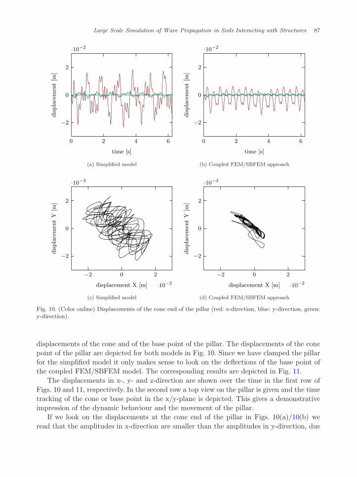
Fig. 10. (Color online) Displacements of the cone end of the pillar (red: x-direction, blue: y-direction, green:y-direction).

displacements of the cone and of the base point of the pillar. The displacements of the conepoint of the pillar are depicted for both models in Fig. 10. Since we have clamped the pillarfor the simplified model it only makes sense to look on the deflections of the base point ofthe coupled FEM/SBFEM model. The corresponding results are depicted in Fig. 11.

The displacements in x-, y- and z-direction are shown over the time in the first row ofFigs. 10 and 11, respectively. In the second row a top view on the pillar is given and the timetracking of the cone or base point in the x/y-plane is depicted. This gives a demonstrativeimpression of the dynamic behaviour and the movement of the pillar.

If we look on the displacements at the cone end of the pillar in Figs. 10(a)/10(b) weread that the amplitudes in x-direction are smaller than the amplitudes in y-direction, due



(a) Coupled FEM/SBFEM approach (b) Zoom of figure (a)

(c) Coupled FEM/SBFEM approach

Fig. 11. (Color online) Displacements of the base end of the pillar (red: x-direction, blue: y-direction, green:z-direction).

to the assumption of grazing wind excitation of the cone end of the pillar. The amplitudescalculated with the FEM/SBEFM (soil) approach are much smaller than those of the sim-plified model (no soil), because the infinite half space attenuates vibrations of the pillarsignificantly. Especially the overtones are attenuated by the infinite half space of the cou-pled FEM/SBFEM model, this is in great accordance with the real damping behavior ofsoil. The damping character of soil can be seen clearly in the time tracking plots in thesecond column of Figs. 10(c)/10(d). We assume a pure periodical loading, the response isapproximately periodic in all cases. The period length of the response is larger than that ofthe excitation.



The deformations of the base end of the pillar are depicted in Fig. 11 for the coupledFEM/SBFEM approach. The deflections of the pillar base are equal to zero for the simplifiedmodel, because the pillar is modeled as a clamped beam. The displacements of the coupledapproach are small (see Figs. 11(a) and 11(c)), due to the compact foundation of the pillarbase in the ground. The character of the vibrations of the base end of the pillar are similarto the cone end, as can be seen in Fig. 11(b). This plot is a zoom of Fig. 11(a).

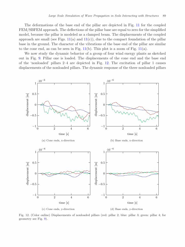
We now study the dynamic behavior of a group of four wind energy plants as sketchedout in Fig. 9. Pillar one is loaded. The displacements of the cone end and the base endof the ‘nonloaded’ pillars 2–4 are depicted in Fig. 12. The excitation of pillar 1 causesdisplacements of the nonloaded pillars. The dynamic response of the three nonloaded pillars

(a) Cone ends, x-direction (b) Base ends, x-direction

(c) Cone ends, y-direction (d) Base ends, y-direction

Fig. 12. (Color online) Displacements of nonloaded pillars (red: pillar 2; blue: pillar 3; green: pillar 4; forgeometry see Fig. 9).



differ concerning their frequency content due to their position in a square. The green curve(pillar 4) contains higher frequent amounts than the curves for pillar 3 and 2 in x-direction,because it is the closest pillar to the excited pillar 1 in this direction. Pillar 2 (red curve) isthe closest pillar to the excited pillar 1 in y-direction and therefore the red curve containshigher frequent amounts than the other curves. The deformation response of the nonloadedpillars with exceeded distance to the excited pillar are damped in all cases. This is in goodaccordance to real soil damping behavior.

A comparison of the displacements of the cone end and base end of the four pillars (seeFig. 13 for the x- and Fig. 14 for the y-direction) shows that the main characteristics andthe range of the amplitudes are similar for the cone and for the base end for each of thenonloaded pillars.

(a) Non-loaded pillar 4 (b) Excited pillar 1

(c) Non-loaded pillar 3 (d) Non-loaded pillar 2

Fig. 13. (Color online) Displacements in x-direction of the four pillars (red: cone end; blue: base end).



(a) Non-loaded pillar 4 (b) Excited pillar 1

(c) Non-loaded pillar 3 (d) Non-loaded pillar 2

Fig. 14. (Color online) Displacements in y-direction of the four pillars. (Red: cone end; blue: base end).

5. Concluding Remark

The presented paper demonstrates that the SBFEM method can yield the solution not onlyto academic benchmarks, but also to real problems when run on a moderately-sized cluster.All presented calculations have been carried out in no more than 2 hours, thanks to ourparallel implementation of the algorithm. These results demonstrate that this method canbe an appealing choice to analyze complex and large scaled engineering applications. Thedesigned parallel coupled FEM/SBFEM approach will be applicable even for much morecomplex and very large scaled engineering problems.



Acknowledgments

Jose E. Roman and Enrique S. Quintana-Ortı were partially supported by the SpanishMinisterio de Ciencia e Innovacion under grants TIN2009-07519, and TIN2008-06570-C04-01, respectively.

References

1. H. Antes and C. Spyrakos, Soil-structure interaction, eds. D. E. Beskos and S. A. Anagno-topoulos, Computer Analysis and Design of Earthquake Resistant Structures (ComputationalMechanics Publications, Southampton, 1997), pp. 271.

2. R. J. Astley, Infinite elements for wave problems: A review of current formulations and a assess-ment of accuracy, International Journal for Numerical Methods in Engineering 49(7) (2000)951–976.

3. G. Beer, The Boundary Element Method with Programming: For Engineers and Scientists(Springer, Wien, 2008).

4. P. Benner, Numerical solution of special algebraic Riccati equations via an exact line searchmethod, in Proc. European Control Conf. ECC 97, Waterloo (B) (1997) pp..

5. P. Benner, R. Byers, E. S. Quintana-Ortı and G. Quintana-Ortı, Solving algebraic Riccati equa-tions on parallel computers using Newton’s method with exact line search, Parallel Comput.26(10) (2000) 1345–1368.

6. P. Bettess, Infinite Elements (Penshaw Press, Sunderland, U.K., 1992).7. Robert Borsutzky, Braunschweiger Schriften zur Mechanik — Seismic Risk Analysis of Buried

Lifelines, Vol. 63. Mechanik-Zentrum Technische Universitat Braunschweig (2008).8. B. Engquist and A. Majda, Absorbing boundary conditions for the numerical simulation of

waves, Mathematics of Computation 31(139) (1977) 629–651.9. M. E. Harr, Foundations of Theoretical Soil Mechanics (McGraw-Hill Book Company, New York,

1966).10. H. Hilbert, T. Hughes and R. Taylor, Improved numerical dissipation for time integration algo-

rithms in structural dynamics, Earthquake Engineering & Structural Dynamics 5 (1977) 283.11. D. L. Kleinman, On an iterative technique for Riccati equation computations, IEEE Trans.

Automat. Control 13 (1968) 114–115.12. S. Langer and H. Antes, Analyses of sound transmission through windows by coupled finite and

boundary element methods, Acta Acustica United with Acustica, 89 (2003) 78–85.13. L. Lehmann, Wave Propagation in Infinite Domains (Springer, Berlin/Heidelberg, 2006).14. L. Lehmann, S. Langer and D. Clasen, Scaled boundary finite element method for acoustics,

Journal of Computational Acoustics 14(4) (2006) 489–506.15. Z. P. Liao and H. L. Wong, A transmitting boundary for the numerical simulation of elastic

wave propagation, Soil Dynamics and Earthquake Engineering 3(4) (1984) 174–183.16. J. Lysmer and R. L. Kuhlmeyer, Finite dynamic model for infinite media, Journal of Engineering

Mechanics 95 (1969) 859–875.17. K. Meskouris, K.-G. Hinzen, Ch. Butenweg and M. Mistler, Bauwerke und Erdbeben — Grund-

lagen — Anwendung — Beispiele (Vieweg+Teubner Verlag, Wiesbaden, 2007).18. N. Newmark, A method of computation for structural dynamics, Journal of Engineering

Mechanics Division 85 (1959) 67.19. Ch. Petersen, Dynamik der Baukonstruktionen (Vieweg & Sohn Verlagsgesellschaft mbH, Braun-

schweig/Wiesbaden, 2000).



20. J. D. Roberts, Linear model reduction and solution of the algebraic Riccati equation by use ofthe sign function, Internat. J. Control 32 (1980) 677–687.

21. M. Schauer, J. E. Roman, E. S. Quintana-Ortı and S. Langer, Parallel computation of 3-Dsoil-structure interaction in time domain with a coupled FEM/SBFEM approach, Journal ofScientific Computing, submitted, 2011.

22. J. Wolf, The Scaled Boundary Finite Element Method (John Wiley & Sons, Chichester, 2003).23. J. Wolf and C. Song, Finite-Element Modelling of Unbounded Media (John Wiley & Sons, Chich-

ester, 1996).

LARGE SCALE SIMULATION OF WAVE PROPAGATION IN SOILS INTERACTING WITH STRUCTURES USING FEM AND SBFEM

Documents