JPEG

JPEG

Vaidyanathan A,ECE, Final yr.

Agenda

• Recap• What is JPEG• Typical Usage• JPEG Characteristics• How it is done???• Advantages

Image coding

Objective: To find a way to represent the original image without (?) distortion with the minimum number of bits possible

Coder

Bit stream

....

Lossless image coding Lossy image coding

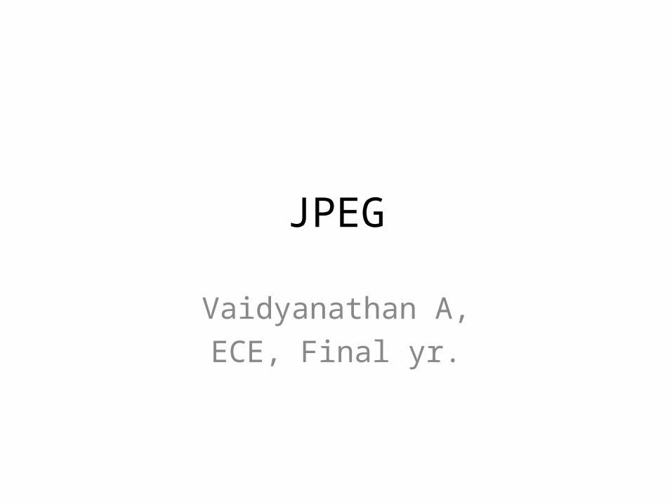
Lossless and lossy image coding Lossless image coding : The decoded image is pixel by pixel identical to the original

Lossy image coding : The decoded image is NOT pixel by pixel identical to the original

Coder

Original

Visually indistinguishable

Visually distinguishable

Agenda


What is JPEG

• The name "JPEG" stands for Joint Photographic Experts Group, the name of the committee that created the standard.

• The JPEG standard specifies both the codec, which defines how an image is compressed into a stream of bytes and decompressed back into an image, and the file format used to contain that stream.

Agenda


Typical Usage• The JPEG compression algorithm is at its best on

photographs and paintings of realistic scenes with smooth variations of tone and color.

• For web usage, where the bandwidth used by an image is important, JPEG is very popular. JPEG/Exif is also the most common format saved by digital cameras.

• On the other hand, JPEG is not as well suited for line drawings and other textual or iconic graphics, where the sharp contrasts between adjacent pixels cause noticeable artifacts. Such images are better saved in a lossless graphics format such as TIFF, GIF, PNG, or a raw image format.

Typical Usage• JPEG is also not well suited to files that will undergo

multiple edits, as some image quality will usually be lost each time the image is decompressed and recompressed, particularly if the image is cropped or shifted, or if encoding parameters are changed. To avoid this, an image that is being modified or may be modified in the future can be saved in a lossless format such as PNG, and a copy exported as JPEG for distribution.

• As JPEG is a lossy compression method, which removes information from the image, it must not be used in astronomical or medical imaging or other purposes where the exact reproduction of the data is required. Lossless formats such as PNG must be used instead.

Agenda


JPEG Characteristics

• Always Lossy Compression • True 24-bit color (16 million colors)• Compression ration of 2-100 : 1• Good performance for pictures that are smooth with

a lot of colors.• Bad performance for pictures with sharp edges.

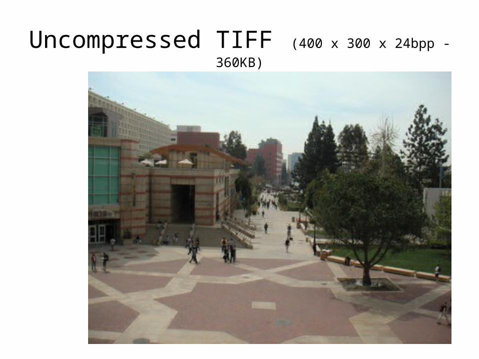
Uncompressed TIFF (400 x 300 x 24bpp - 360KB)

JPEG (19 KB – 5.28% of original image)

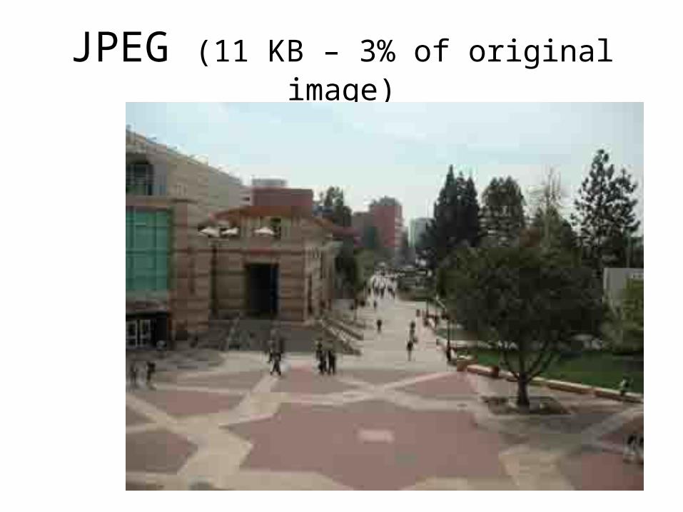
JPEG (11 KB – 3% of original image)

Agenda


General scheme of image coding (compression)

QuantizerQ

• Quantizer• Scalar or vectorial• This an optional block.

Although almost always exists

Entropic coder

• Entropic coder• This block always exists

Bit stream

Do something

• To prepare the image• To remove redundancy• This an optional block.

Although almost always exists

• DCT, wavelets, hybrid

Original image

Lossy scheme Lossless scheme

Reversible Non-reversible

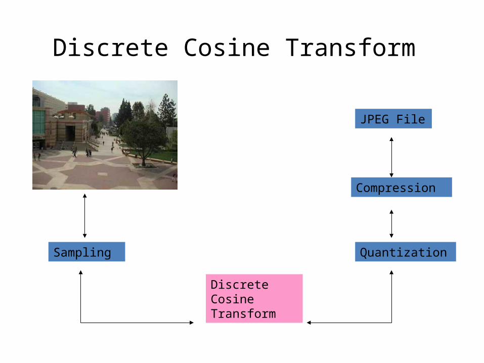
Dataflow of JPEG Compression Algorithm

Sampling

Discrete Cosine Transform

JPEG File

Compression

Quantization

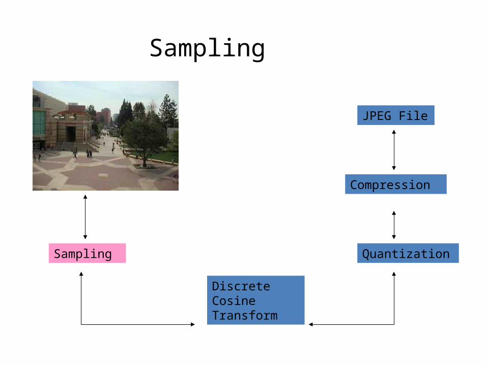
Sampling

Sampling


Quantization

JPEG File

Compression

Sampling: RGB Color System

• Three component representation of the color of a pixel

• Represents the intensities of the red, green, and blue components

• 24 bit “True Color”• Each component represented with 8 bits of precision• The components each contain roughly the same

amount of information

Human Visual System

• The human eye has a tendency to notice variations of brightness intensity much more than variations of the color in an image

• The human eye is not as sensitive to high-frequency chrominance (color) components as it is to luminance (intensity) components

• We can take advantage of this by transforming the color space of RGB to another representation

Human Visual System

• Here is an image represented with 8-bits per pixel

Human Visual System

• Here is the same image at 7-bits per pixel

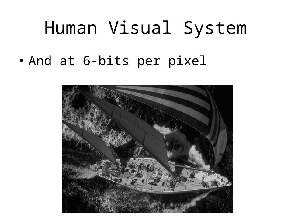
Human Visual System

• And at 6-bits per pixel

Human Visual System


Human Visual System


2D FFT transform

Man-made Scene

Can change spectrum, then reconstruct

Most information in at low frequencies!

Campbell-Robson contrast sensitivity curveCampbell-Robson contrast sensitivity curve

We don’t resolve high frequencies too well…

… let’s use this to compress images… JPEG!

Frequency sensitivity of Human Visual System

YUV (YCrCb) Color Space• An ideal format for JPEG compression• The brightness and color information in an image are

separated• Concentrates the most important info into one component,

allowing for greater compression• Y component represents the color intensity of the image

(equivalent to a black and white television signal)• U and V represent the relative redness and blueness of the

image

YUV Transformation

• A linear transformation from RGB to YUV and from YUV to RGB

Y = 0.299R + 0.587G + 0.114BU = -0.1687R -0.3313G + 0.5B + 128V = 0.5R – 0.4187G – 0.0813B + 128

R = Y + 1.402VG = Y – 0.34414(U – 128) – 0.71414(V – 128)B = Y + 1.722(U – 128)

128 = 2Sample Prescision/2

Y u v FormatsY u v Format

Y

U V

RGB 24 bits/pixel YUV 4:2:0 (12 bits/pixel)


Sampling


Quantization

JPEG File

Compression

Jean Baptiste Joseph Fourier (1768-1830)

had crazy idea (1807):Any periodic function can be rewritten as a weighted sum of sines and cosines of different frequencies.

Don’t believe it? • Neither did Lagrange,

Laplace, Poisson and other big wigs

• Not translated into English until 1878!

But it’s true!• called Fourier Series

Image compression using DCT

• DCT enables image compression by concentrating most image information in the low frequencies

• Loose unimportant image info (high frequencies) by cutting B(u,v) at bottom right

DCT on 8x8 blocks

64 pixels

64 pixels

8 pixels

8 pixels

•We will break the image into non-overlapping 8x8 blocks.

•For each block u(m,n), we will take an 8x8 DCT

Why 8x8 blocks?

222

22

2 1log2

1)1(log

2

1)( p

ND

pDR

R(D)

Block Size NxN

D

p 22

2

)1(log

2

1

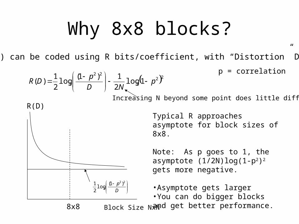
V(k) can be coded using R bits/coefficient, with “Distortion” D

8x8

Increasing N beyond some point does little difference

Typical R approaches asymptote for block sizes of 8x8.

Note: As p goes to 1, the asymptote (1/2N)log(1-p2)2 gets more negative.

•Asymptote gets larger•You can do bigger blocks and get better performance.

p = correlation

Unitary 2D-DCT

N

ln

N

kmlkVlknmu

N

l

N

k 2

)12(cos

2

)12(cos),()()(),(

1

0

1

0

N

ln

N

kmnmulklkV

N

n

N

m 2

)12(cos

2

)12(cos),()()(),(

1

0

1

0

Backward DCT

Not surprisingly, it turns out that you can get better compression using the DCT if you take into account the horizontal and vertical correlation between pixels simultaneously.

N

1)0(

Nk

2)(

Forward DCT

• Basis functions for the 8×8 DCT (courtesy Wikipedia)

Block-based Discrete Cosine Transform (DCT)

A nice set of basisTeases away fast vs. slow changes in the image.

Other Tranforms used in Image Processing

• KL Transform– Very important theoretically, but not used because no fast

algorithm exists and depends on statistics of the image.– KL Transform is optimal in producing transform

coefficients that are uncorrelated– Has best average energy compaction for an ensemble of

images• Singular Value Decomposition (SVD)

– Best energy compaction for a given image.

Quantization

Sampling


Quantization

JPEG File

Compression

Quantization

• Quantized Value = Round (coefficient / Quantum Value)

),(

),(),('

lkq

lkvroundlkv

Choosing a quantum value as small as 20 would convert over half of the coefficients to zeros.

The JPEG standard does not specify the quantization values to be used. This is left up to the application. However it does provide some quantization tables that have been tested empirically and found to generate good results

Quantization

Entropiccoder

Code2

42

64

6

Do something

Q

Quantization (1)Input digital levels Output levels

Output

levels

Input levels0 1 2 3 4 5 6 7 8 9

1

3

5

7

Entropiccoder

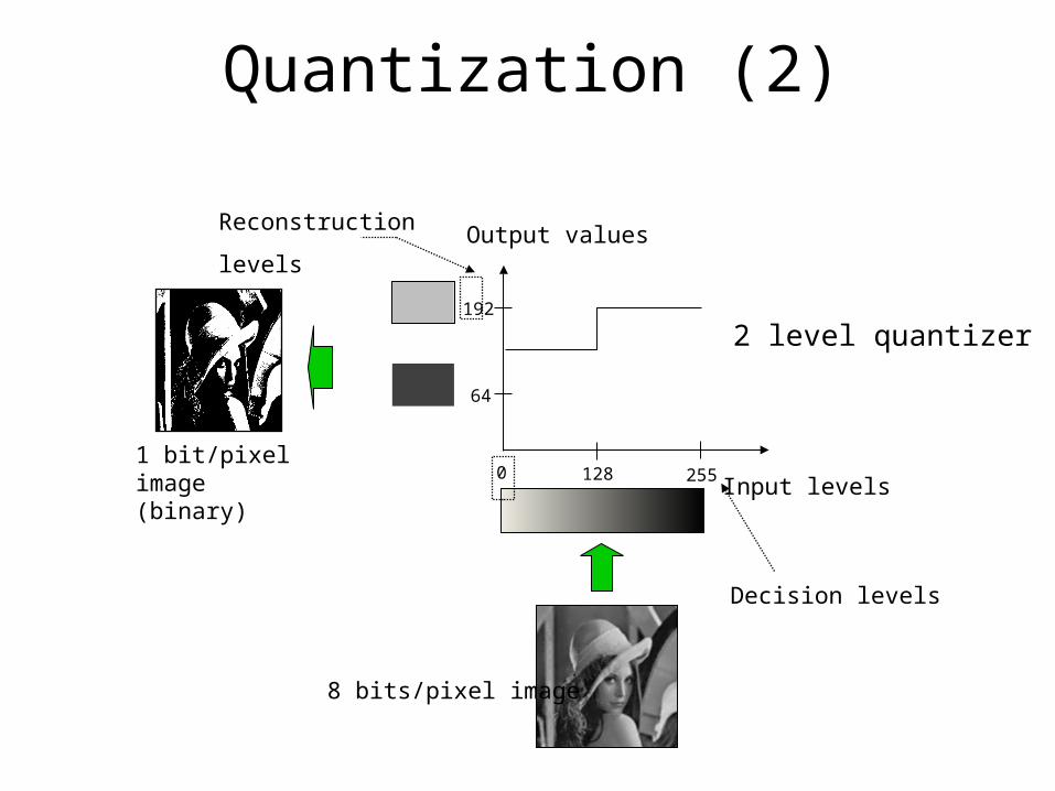
Quantization (2)

1 bit/pixel image(binary) Input levels

Output values

2 level quantizer

128 255

64

192

0

Reconstruction

levels

Decision levels

8 bits/pixel image

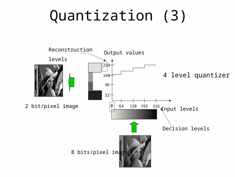
Quantization (3)

2 bit/pixel image Input levels

Output values

4 level quantizer

64 128 192 255

32

96

160

224

0

Reconstruction

levels

Decision levels

8 bits/pixel image

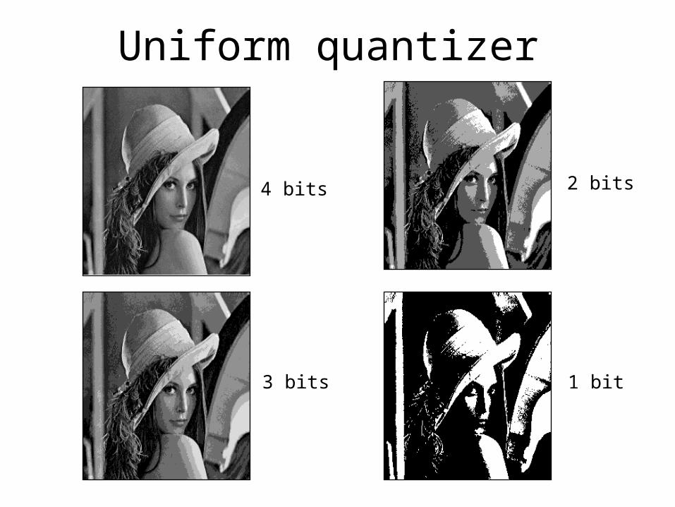
4 bits

1 bit

2 bits

3 bits

Uniform quantizer

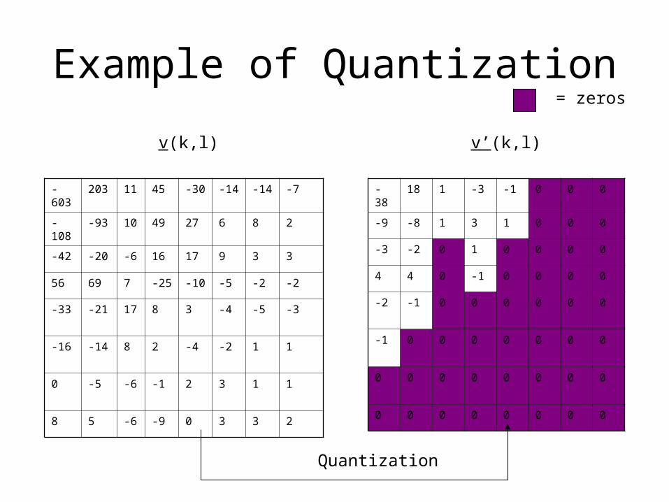
Example of Quantization

-38 18 1 -3 -1 0 0 0

-9 -8 1 3 1 0 0 0

-3 -2 0 1 0 0 0 0

4 4 0 -1 0 0 0 0

-2 -1 0 0 0 0 0 0

-1 0 0 0 0 0 0 0

0 0 0 0 0 0 0 0

0 0 0 0 0 0 0 0

-603

203 11 45 -30 -14 -14 -7

-108

-93 10 49 27 6 8 2

-42 -20 -6 16 17 9 3 3

56 69 7 -25 -10 -5 -2 -2

-33 -21 17 8 3 -4 -5 -3

-16 -14 8 2 -4 -2 1 1

0 -5 -6 -1 2 3 1 1

8 5 -6 -9 0 3 3 2

v(k,l) v’(k,l)

Quantization

= zeros

Quantization Table

16 11 10 16 24 40 51 61

12 12 14 19 26 58 60 55

14 13 16 24 40 57 69 56

14 17 22 29 51 87 80 62

18 22 37 56 58 109

103

77

24 35 55 64 81 104

113

92

49 64 78 87 103

121

120

101

72 92 95 98 112

100

103

99

17 18 24 47 99 99 99 99

18 21 26 66 99 99 99 99

24 26 56 99 99 99 99 99

47 66 99 99 99 99 99 99

99 99 99 99 99 99 99 99

99 99 99 99 99 99 99 99

99 99 99 99 99 99 99 99

99 99 99 99 99 99 99 99

Y Component U and V Components

Zig-Zag Ordering0 1 5 6 14 15 27 28

2 4 7 13 16 26 29 42

3 8 12 17 25 30 41 43

9 11 18 24 31 40 44 53

10 19 23 32 39 45 52 54

20 22 33 38 46 51 55 60

21 34 37 47 50 56 59 61

35 36 48 49 57 58 62 63

•The goal is to group all the zeros together, to allow compression18 -9 -3 -8 1 -3 1 -2 4 -2 4 0 3 -1 0 1 1 0 -1 -1 0 0 0 -1 0 0 0 0 0 0 0 0 0 0 0 0 0 0 0 0 0 0 0 0 0 0 0 0 0 0 0 0 0 0 0 0 0 0 0 0 0 0 0

= zeros

= DC

Compression

Sampling


Quantization

JPEG File

Compression

Compression/Source Coding

• Represent the information produced by a random source (random variable/process) with a different symbol alphabet to reduce the size

• Entropy – description of the amount of uncertainty of a random source. A quantitative measure that describes the number of bits on average required to represent a source

• Lossless compression schemes used

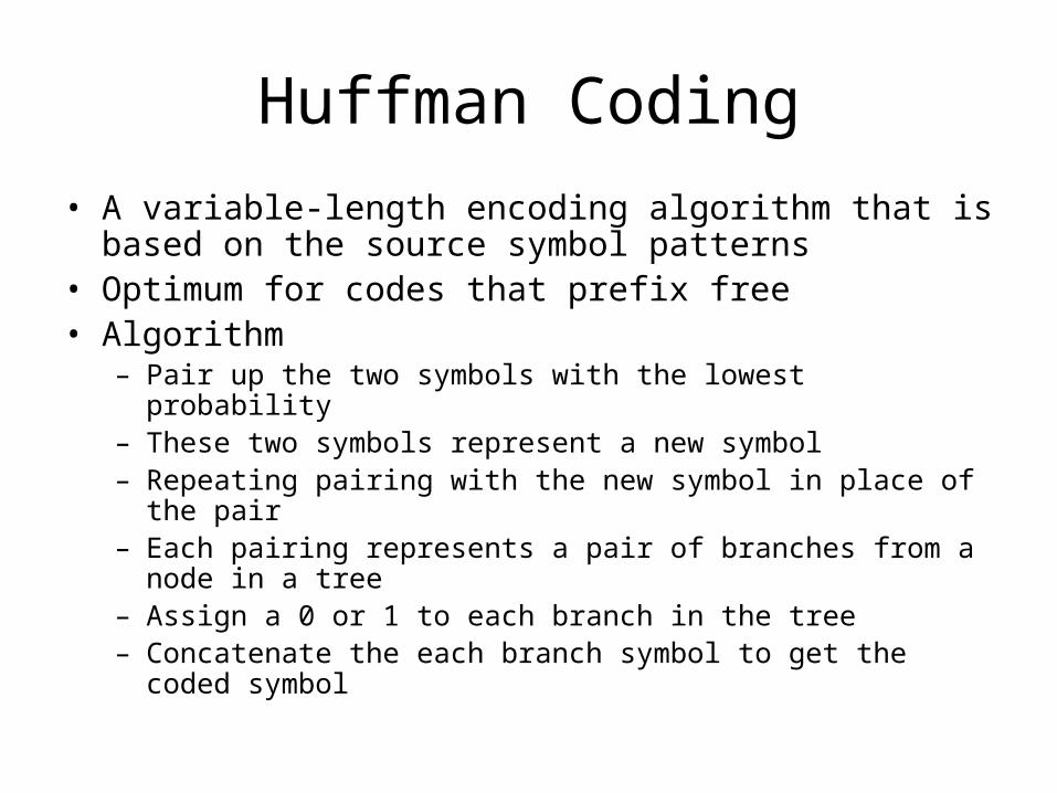
Huffman Coding• A variable-length encoding algorithm that is based on the

source symbol patterns• Optimum for codes that prefix free• Algorithm

– Pair up the two symbols with the lowest probability– These two symbols represent a new symbol– Repeating pairing with the new symbol in place of the pair– Each pairing represents a pair of branches from a node in a tree– Assign a 0 or 1 to each branch in the tree– Concatenate the each branch symbol to get the coded symbol

A Simple Example

• Alphabet = {1,2,3,4,5}• Probabilities = {.35, .3, .2, .1, .05}• Uncoded = 3 bits per symbol• Entropy = 2.06 bits per symbol• Huffman average code length = 2.15 bits

.35

.30

.20

.10

.05.15

.35

.65

1.0

0

1 0

1

1

1

00

00

01

10

110

111

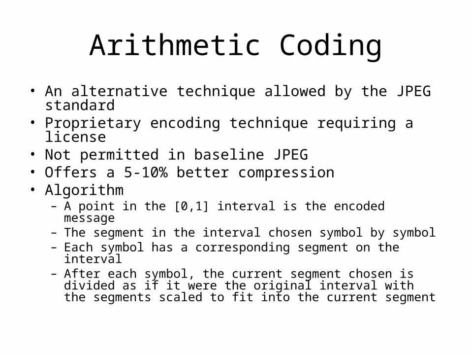
Arithmetic Coding• An alternative technique allowed by the JPEG standard• Proprietary encoding technique requiring a license• Not permitted in baseline JPEG• Offers a 5-10% better compression• Algorithm

– A point in the [0,1] interval is the encoded message – The segment in the interval chosen symbol by symbol– Each symbol has a corresponding segment on the interval– After each symbol, the current segment chosen is divided as if it were

the original interval with the segments scaled to fit into the current segment

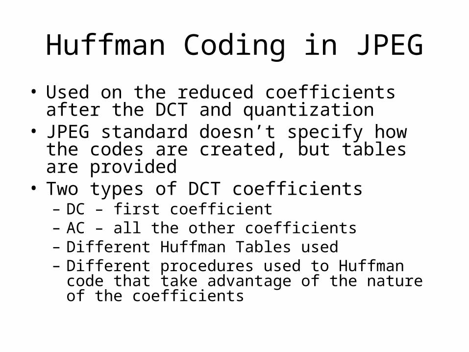
Huffman Coding in JPEG• Used on the reduced coefficients after the DCT and

quantization• JPEG standard doesn’t specify how the codes are

created, but tables are provided• Two types of DCT coefficients

– DC – first coefficient– AC – all the other coefficients– Different Huffman Tables used– Different procedures used to Huffman code that take

advantage of the nature of the coefficients

AC/DC0 1 5 6 14 15 27 28

2 4 7 13 16 26 29 42

3 8 12 17 25 30 41 43

9 11 18 24 31 40 44 53

10 19 23 32 39 45 52 54

20 22 33 38 46 51 55 60

21 34 37 47 50 56 59 61

35 36 48 49 57 58 62 63

= AC Coefficients

= DC Coefficients

Huffman Tables

• Difference in the nature of the AC and DC coefficients leads to different methods of coding for more optimal compression– Different tables for DC and AC coding

• Also differentiate between Luminance (Y) and Chrominance (U,V) information– Baseline however only allows two tables, so the DC code

uses same table for Luminance and Chrominance (same for AC)

Huffman Coding of the DC Coefficients

• Use a differential prediction model– Idea is that the DC coefficient itself is unpredictable, but

we expect to have little change between neighbors (Very high correlation)

• Increase the probability that the value that we encode will be small by taking the difference between the coefficient and the DC value from the previous block


Range (SSSS)

Difference Additional Bits

0 0

1 -1 , 1 0 , 1

2 -3,-2 , 2,3 00,01 , 10,11

3 -7,…,-4 , 4,…,7 000,…,011 , 100,111

4 -15,…,-8 , 8,…,15 0000,…,0111 , 1000,1111

5 -31,…,-16 , 16,…,31 00000,…,01111 , 10000,11111

6 -63,…,-32 , 32,…,63 000000,…,011111 , 100000…,111111

7 -127,…,-64 , 64,…,127 …

8 -255,…,-128 , 128,…,255 …

9 -511,…,-256 , 256,…,511 …

10 -1023,…,-512 , 512,…,1023 …

11 -2047,…,-1024 , 1024,…,2047

…


• Baseline JPEG only allows for 12 bit difference values for 8 bit input sample

• SSSS is only a range for absolute values• Code is completed when additional bits are

appended to the SSSS• Huffman code tables for SSSS can be different

depending on whether looking at luminance or chrominance

• Additional bits are always the same whether looking at luminance or chrominance values

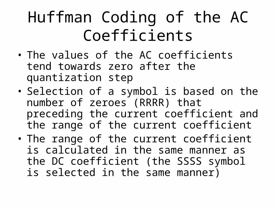
Huffman Coding of the AC Coefficients

• The values of the AC coefficients tend towards zero after the quantization step

• Selection of a symbol is based on the number of zeroes (RRRR) that preceding the current coefficient and the range of the current coefficient

• The range of the current coefficient is calculated in the same manner as the DC coefficient (the SSSS symbol is selected in the same manner)

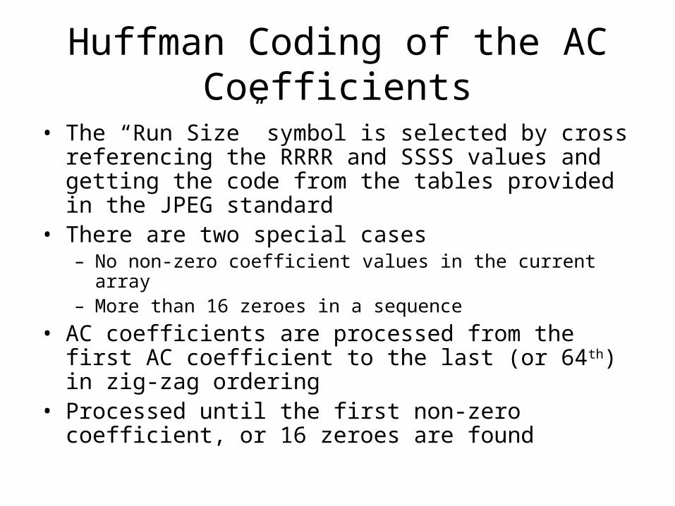
Huffman Coding of the AC Coefficients

• The “Run Size” symbol is selected by cross referencing the RRRR and SSSS values and getting the code from the tables provided in the JPEG standard

• There are two special cases– No non-zero coefficient values in the current array– More than 16 zeroes in a sequence

• AC coefficients are processed from the first AC coefficient to the last (or 64th) in zig-zag ordering

• Processed until the first non-zero coefficient, or 16 zeroes are found

JPEG File format (JFIF)

Sampling


Quantization

JPEG File

Compression

JFIF• JPEG File Interchange Format• No file format in the standard• Image orientation is top-down: first encoded image

samples are in the upper left hand corner, follows from left to right

• Defines header fields and sections to provide the necessary information for an image to be decoded

• Compression parameters include Quantization tables, Huffman tables, etc.

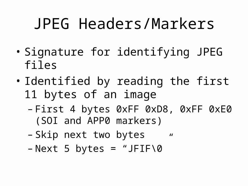
JPEG Headers/Markers

• Signature for identifying JPEG files• Identified by reading the first 11 bytes of an

image– First 4 bytes 0xFF 0xD8, 0xFF 0xE0 (SOI and APP0

markers)– Skip next two bytes– Next 5 bytes = “JFIF\0”

JPEG Headers/Markers (cont)

• http://www.w3.org/Graphics/JPEG/jfif3.pdf • Compressed Image File Formats by John Miano• SOI – Start of Image • APP0 – Allows for JFIF Extensions (the extensions to

JPEG are not used for baseline image formats) and specifies a few parameters– i.e. Aspect Ratio: 800x6004x3, 256x2561x1

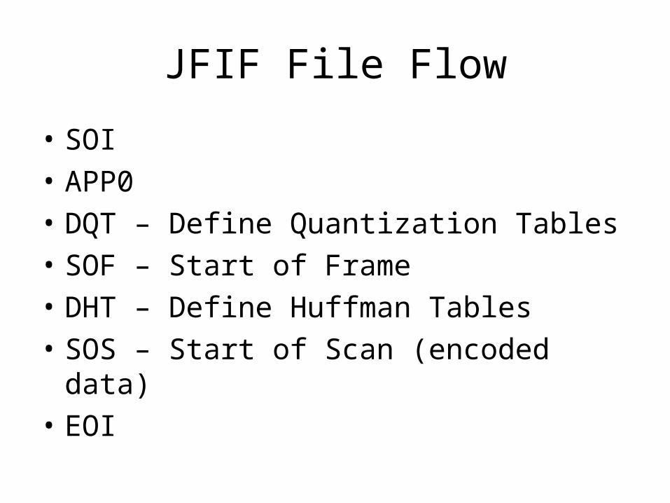
http://www.w3.org/Graphics/JPEG/jfif3.pdf

JFIF File Flow

• SOI• APP0• DQT – Define Quantization Tables• SOF – Start of Frame• DHT – Define Huffman Tables• SOS – Start of Scan (encoded data)• EOI

Agenda


Advantage !!!

89k 12k

Advantages

• “very good” or “excellent” compression rate, reconstructed image quality, transmission rate

• applicable to practically any kind of continuous-tone digital source image

• good complexity

Other Operation Modes

JPEG Progressive Model

• Why progressive model?– Quick transmission– Image built up in a coarse-to-fine passes

• First stage: encode a rough but recognizable version of the image• Later stage(s): the image refined by successive scans till get the final

image• Two ways to do this:

– Spectral selection – send DC, AC coefficients separately– Successive approximation – send the most significant bits first and

then the least significant bits

JPEG Lossless Model

DPCMSample values Descriptors

Differential pulse code modulation

C B

A X

selection value prediction strategy

7

0123

(A+B)/2

no predictionABC

Predictors for lossless coding

B+(A-C)/2

A+B-CA+(B-C)/2

456

JPEG Hierarchical Model

• Hierarchical model is an alternative of progressive model (pyramid)

• Steps:– filter and down-sample the original images by the desired number

of multiplies of 2 in each dimension– Encode the reduced-size image using one of the above coding

model– Use the up-sampled image as a prediction of the origin at this

resolution, encode the difference– Repeat till the full resolution image has been encode

Thank You

JPEG

Documents

decoded image

image quality

raw image format

original lossy image

jpeg standard

lossless graphics format

pixel identical

lossy compression method