Semi Annual Report (January 1 — June 30, 2000) Contract Number NAS5—31363 OCEAN OBSERVATIONS WITH EOS/MODIS: Algorithm Development and Post Launch Studies Howard R. Gordon University of Miami Department of Physics Coral Gables, FL 33124 (Submitted July 14, 2000)

Welcome message from author
This document is posted to help you gain knowledge. Please leave a comment to let me know what you think about it! Share it to your friends and learn new things together.
Transcript
Semi Annual Report
(January 1 — June 30, 2000)
Contract Number NAS5—31363
OCEAN OBSERVATIONS WITH EOS/MODIS:
Algorithm Development and Post Launch Studies
Howard R. GordonUniversity of Miami
Department of PhysicsCoral Gables, FL 33124
(Submitted July 14, 2000)
Preamble
This document describes our progress thus far toward completion of our research plansregarding two MODIS Ocean-related algorithms.
A. Retrieval of the Normalized Water-Leaving Radiance (AtmosphericCorrection).
B. Retrieval of the Detached Coccolith/Calcite Concentration
Our plans for Fiscal Year 2000 are included in this report as Appendix I. Fiscal Year2000 was to be heavily focused on validation of MODIS-derived products.Unfortunately, the delay of the launch of Terra required some modification of out initialplan. Our approach was to use SeaWiFS for validating MODIS algorithms in theabsence of MODIS itself, and when MODIS data became available, to perform therequired initialization exercise and validate the MODIS products directly. However, aswe already know (from theoretical studies and from SeaWiFS), that there are certainsituations in which the algorithms are unable to perform properly, or that there are itemsthat have not been included in the initial implementation, a portion of our effort will bedirected toward algorithm improvement. Thus, we break our effort into two broadcomponents for each algorithm:
• Algorithm Improvement/Enhancement;
• Validation of MODIS Algorithms and Products.
Of course, these components will overlap in some instances.
RETREIVAL OF NORMALIZED WATER-LEAVING RADIANCE(ATMOSPHERIC CORRECTION)
Algorithm Improvement/Enhancement
1. Evaluation/Tuning of Algorithm Performance
Task Progress:
With the launch of Terra, the availability of MODIS imagery, and the processing of theimagery by SDST (MODAPS) and the Goddard DAAC, we were in a position to beginan initial evaluation of the performance of MODIS and the algorithms. We started thisby looking in detail at MODIS Granual 2000102.2215, starting just south of the Equatorand progressing to 20 degrees South in the vicinity of 160 degrees West. Our evaluationis described in detail in Appendix II. Based on what is presented in Appendix II for thissingle granual, we can conclude the following:
(1) The overall the retrieved water-leaving radiances on the average are in thecorrect ranges, suggesting that the overall system calibration and theatmospheric correction are in the nominal ranges; however, when theimagery is evaluated at full resolution many artifacts are apparent.
(2) The normalized water-leaving radiance at 551 nm, nLw(551), shows severestriping (a maximum of about 10% over the 10 detectors in the spectralband) normal to the subsatellite track, and the average value is ~ 50% toohigh.
(3) After correcting errors and omissions in the processing codes, andreprocessing the granual at Miami, this error in the average nLw(551) wasreduced to ~ +10%; however, the striping in nLw(551) remained.
(4) After an initial attempt by R. Evans and co-workers at flat fielding theimagery, the strongly periodic nature of the striping was removed, butthere was still some striping.
(5) The retrieved nLw(551) across a scan line showed some limb brighteningthat could be due to overall calibration errors or to the influence of anunaccounted variability in the system response as a function of scan angle.
(6) Bands 15 or 16, or both, (used for atmospheric correction) appear todisplay excessive noise. This may require averaging the atmosphericcorrection parameter ε(15,16) over several pixels.
(7) Sun glint will likely render the eastern half of the scan useless in thetropics unless a correction scheme is developed.
(8) The striping in nLw(551) is not due to atmospheric correction, as ε(15,16)does not show significant banding.
(9) A significant amount of work will be required to removing the stripingfrom the MODIS derived products, as its root cause is probably spread

over several processes, e.g., instrument polarization sensitivity, variabilityin system response with scan angle, etc. Thus the improvement processwill require an incremental resolution and balancing of the individualeffects.
(10) Plans should be made to reprocess MODIS imagery as incrementalprogress is made.
In addition to evaluation of the initial performance of MODIS and the algorithms, wehave implemented two enhancements: (1) a wind-speed dependent computation of theRayleigh scattering contribution to the radiance at the sensor, and (2) correction softwarefor removing some of the influence of the MODIS polarization sensitivity. Thepolarization software can become fully operational only after MSCT and SBRS agree onthe validity of the analysis of the pre-launch polarization sensitivity characterization data.We consider resolving the polarization characterization issue to be of the highest priorityfor MCST in terms of MODIS ocean processing.
Anticipated Future Actions:
We will continue the evaluation of MODIS imagery, and work closely with R. Evans onremoving the artifacts from the imagery. We will also try to evaluate the ramifications ofaveraging the atmospheric correction parameter over several pixels. One obviousproblem with this approach is that a small cloud in any one pixel used in the averagingwill influence several pixels, reducing the amount of usable data.
2. Implement the Initial Algorithm Enhancements
The most important enhancement we have been considering focussed on absorbingaerosols. These constitute an important unsolved atmospheric correction issue for case 1waters, and these aerosols have a significant impact in many geographical areas. Twoimportant situations in which absorbing aerosols make an impact are desert dust andurban pollution carried over the oceans by the winds. In the case of urban pollution theaerosol contains black carbon and usually exhibits absorption that is nonselective, i.e., theimaginary part of the refractive index (the absorption index) is independent ofwavelength. In contrast, desert dust absorbs more in the blue than the red, i.e., theabsorption index decreases with wavelength.
Task Progress:
We are in the process of extensively examining two enhancements: (1) the spectralmatching algorithm (SMA) [Gordon, Du, and Zhang, “Remote sensing ocean color andaerosol properties: resolving the issue of aerosol absorption,” Applied Optics, 36, 8670-8684 (1997)]; and (2) the spectral optimization algorithm SOA [Chomko and Gordon,“Atmospheric correction of ocean color imagery: Use of the Junge power-law aerosolsize distribution with variable refractive index to handle aerosol absorption,” AppliedOptics , 37, 5560-5572 (1998)]. Simulations reveal that both algorithms have thepotential to perform well in the presence of strongly absorbing aerosols.

Our progress to date toward algorithm enhancements for these aerosols are provided inAppendices III and IV. Appendix III is a paper (submitted to Geophysical ResearchLetters) describing a successful processing of SeaWiFS imagery in the Saharan dust zoneusing the SMA. Appendix IV is a paper (submitted to Applied Optics) that describesapplication of the SOA to SeaWiFS imagery off the U.S. East Coast using the SOA. Theperformance of the algorithms (compared to the standard SeaWiFS/MODIS algorithm) isvery encouraging.
Anticipated Future Actions:
We will continue to evaluate the performance of these algorithms for possible inclusionin the MODIS processing software.
3. Study Future Enhancements
There are three additional issues that we are examining for inclusion into the MODISalgorithm: modeling the subsurface upwelling BRDF, understanding the influence ofcolored dissolve organic matter (CDOM) on the operation of the SOA and SMA, andremoving the influence of whitecaps on the sea surface.
Task progress:
The subsurface upwelling BRDF
We have reduced the RADS BRDF data acquired during the MOCE-5 validation cruisein the Gulf of California. This is an excellent data set in that it spans a wide range ofcholorophyll a concentrations. To study the influence of self-shading by the RADSinstrument, we participated in Dennis Clark’s February cruise and compared themeasurements from RADS with those from a new smaller instrument Dennis Clark hasdeveloped for MOBY that will essentially eliminate the self-shading problem. Thesedata are still being reduced. Similar measurements were made during a one-weekMODIS initialization cruise in April.
The influence of CDOM on the SOA and SMA
We have replaced the Gordon et al. semianalytic radiance model [A semianalyticradiance model of ocean color, Jour. Geophys. Res., 93(D9), 10909—10924, 1988] witha version of the Garver and Siegel reflectance model [Inherent optical property inversionof ocean color spectra and its biogeochemical interpretation: 1 time series from theSargasso Sea, Geophys. Res., 102C, 18607—18625, 1997] in our SOA algorithm. TheGarver and Siegel model has been tuned to the SeaBASS data set. This model includesabsorption by CDOM, detritus, and phytoplankton, as well as particle backscattering. Incontrast, the Gordon et al. model includes only chlorophyll absorption and particlebackscattering. The principal difficulty incorporating CDOM is that this model requires
that seven (instead of six) parameters must be determined by eight spectral bands. Asecond difficulty is that the optical effect of CDOM on the water-leaving reflectance issimilar to the effect of absorbing aerosols on the aerosol component of the reflectance. Inour initial trial we processed the same imagery as processed in Appendix IV. The resultssuggest that the influence of CDOM is much more significant than expected.
Influence of whitecaps on the sea surface
A paper describing our determination of the whitecap-augmented reflectance waspublished in JGR [K.D. Moore, K.J. Voss, and H.R. Gordon, Spectral reflectance ofwhitecaps: Their contribution to water-leaving radiance, Jour. Geophys. Res., 105(C3),6493—6499, 2000].
Anticipated Future Actions:
The subsurface upwelling BRDF
We will compare the newly reduced BRDF data with our model, and estimate the RADSself-shading effects using the data from the February and April experiments.
The influence of CDOM on the SOA and SMA
We have acquired AOL measurements of CDOM from Frank Hoge on a flight linethrough one of the SeaWiFS images we processed. This track will be compared toCDOM retrievals by the SOA. We are also studying the optimization algorithm in detailto try to understand how best to avoid the spurious results that sometimes occur atisolated pixels. In addition, we are studying the scaling of the various optimizedvariables to try to improve the performance over a wider range of parameter values.
Influence of whitecaps on the sea surface
This work is now essentially complete. We will now operate the whitecapinstrumentation only during MODIS validation cruises.
Validation of MODIS Algorithms and Products
4. Participate in MODIS Initialization/Validation Campaigns
This task refers to our participation in actual Terra/MODIS validation/initializationexercises.

Task Progress:
During the last six months we participated in a shortened MODIS initialization cruise(MOCE-6). The longer cruise was delayed until more favorable sun glint conditionscould be obtained. This longer cruise will occur later this year or early next yeardepending on ship schedules and the Aqua launch schedule. We are now in the processof reducing the data obtained on MOCE-6.
In addition, we continued to maintain our CIMEL station in the Dry Tortugas during thisperiod. This station will be used to help validate the MODIS derived aerosol opticaldepth (AOD), and aid in investigating the calibration of the near infrared (NIR) spectralbands of MODIS.
Anticipated future efforts:
We will complete analysis of the MOCE-6 data to provide an initial vicarious calibrationfor MODIS ocean bands. We will participate on the next MODIS initialization campaignwhen it occurs. We will make measurements of the sky radiance distribution (large angleand aureole), the in-water radiance distribution, AOD, and whitecap radiance. TheMicro-Pulse LIDAR (MPL) system has been repaired by the manufacturer and will beoperational for providing the aerosol’s vertical distribution during this campaign. We arecurrently testing the MPL. To ensure success with the MPL in this effort, we obtained aspare detector to try to avoid the long delay experienced in the last repair cycle (difficult,because they are no longer being manufactured).
5. Participate in Validation Campaign (SeaWiFS)
As part of our effort to validate the MODIS normalized water-leaving radiance algorithmusing SeaWiFS data, we participated in three long cruises, Aerosols99, INDOEX, andMOCE-5. This section describes those efforts.
Task Progress:
The Aerosols99 cruise took place between January 14 to February 8, 1999 betweenNorfolk, VA. and Cape Town, S.A. This was a multidisciplinary cruise with extensivemeasurements of the boundary layer aerosol (chemical, physical, and opticalmeasurements), chemistry, and vertical sounding (radio-sondes, ozone-sondes, and ourMPL), as well as in-water optics. It was very interesting as we encountered severalaerosol types: North American continental aerosols, North Atlantic clean maritimeaerosols, a Saharan dust event, biomass burning aerosols from the African continent, andSouth Atlantic maritime aerosols. The first regime (continental aerosols) occurred duringa cloudy period so our optical measurements were limited. We found that the NorthAtlantic and South Atlantic maritime aerosols were similar, with optical depths in therange of 0.10±0.03, with small angstrom exponents (0.30±0.3). These aerosols werecapped at approximately 1 km by a strong temperature inversion so most of theattenuation occurred below this. We calculated the level at which 90% of the AOD was
accounted for (from the surface up). In this area the 90% level for the attenuation was at1-2 km. The Saharan dust event changed the optical properties of the columnsignificantly. The AOD increased to 0.29±0.05, but the angstrom exponent remained low(0.36±0.13). The temperature inversion went to 1.5 km. The surface layer of theaerosols was capped by this inversion; however, another layer of aerosol was above thisinversion and extended to 3 km or so. The 90% level for attenuation was at 2 km, withexcursions up to 3 km at times. The biomass burning episode also had a high AOD(0.36±0.13) and was associated with the highest angstrom exponent experienced duringthe cruise (0.88±0.3), typical of smaller particles. The temperature structure in theatmosphere was more confusing with inversions occurring at many levels starting at 1km. The aerosol extended very high into the atmosphere with the 90% level ofattenuation at >3 km. At the end of this period the surface cleared before the upperatmosphere. Surface conditions indicated a very clean marine atmosphere, yet columnproperties showed a fairly turbid aerosol above this. As we continued south the entirecolumn cleared and the aerosol structure reverted to the clean maritime case (AODaround 0.1, capped at 1 km). These results are described in detail in the attachedAppendices V and VI.
The results from the INDOEX data set are still in the process of being prepared forpublication. Thus far, one important result we participated in was the observation thatabsorbing aerosols tend to reduce cloud fraction [Ackerman, et al., Reduction of tropicalcloudiness by soot, Science, 288, 1042-1047, 2000].
Anticipated future efforts:
We will complete our analysis of the INDOEX atmospheric data, and have manuscriptsready for submission within the next reporting period. We will use the INDOEX resultsto study the performance of our SOA and SMA algorithms with SeaWiFS imagery.
For MOCE-5 we are working extensively with the Sky and Aureole radiance distributiondata to investigate the aerosol phase function retrieval methods.
We will complete analysis of the in-water radiance distribution data obtained during theMOCE-5 cruise, as well as those obtained during Aerosols99 and INDOEX. This dataset provides an extensive body of upwelling radiance distributions with varying opticalproperties (Chlorophyll concentration, solar zenith angle). We will present results fromthis radiance distribution data set at the “Oceans from Space, Venice 2000” meeting inVenice, Italy in October.
RETRIEVAL OF DETACHED COCCOLITH/CALCITECONCENTRATION
This last half year of work has focussed on several areas: 1) submitting a manuscript ofpublication on coccolithophore distributions from the Indian Ocean, 2) participating inthe development of a new 3-band coccolithophore algorithm, 3) planning of a large-scalemanipulative experiment for testing the MODIS suspended calcite algorithm, 4) finishingcoccolith counts from 1999, evaluating the early MODIS coccolith products, and 5)monitoring bio-optical properties of a coccolithophore bloom in the Gulf of Maine,
Algorithm Evaluation/Improvement
Task Progress:
A second manuscript on our Arabian Sea has been submitted for publication [Balch, W.M., D. Drapeau, B. Bowler, and J. Fritz. Continuous measurements of calcite-dependentlight scattering in the Arabian Sea. Submitted to. Deep Sea Res. I]. The results aresummarized in the abstract provided below.
Continuous surface measurements of temperature, salinity, fluorescenceand optical backscattering were made during R/V Thompson cruise#TN053 in the northern Arabian Sea (“Bio-Optical cruise”; October-November, 1995). The cruise covered the early NE monsoon period.Optical measurements involved estimates of total backscattering and“acidified backscattering” (measured after addition of a weak acid todissolve calcium carbonate). Acid-labile backscattering was calculated asthe difference between total- and acidified backscattering. Total and acid-labile backscattering were converted to the concentration of particulateorganic carbon (POC) and particulate inorganic carbon (PIC; calciumcarbonate), respectively, utilizing discrete samples taken along the cruisetrack for calibration. Backscattering data were frequently coherent withtemperature, salinity, and density variability. Acid-labile backscatteringvalues revealed that calcium carbonate accounted for 10-40% of the totaloptical backscattering in the region and the continuous recordsdemonstrated distinct patches of coccolith-rich water. The northernregion of the Arabian Sea had the highest acid-labile backscattering.Results suggest that PIC:POC ratios can vary over about four orders ofmagnitude. Highest surface values of PIC:POC approached 1 in severalplaces. We also report qualitative observations of phytoplanktoncommunity structure made aboard ship, on fresh samples.

The observation that calcium carbonate accounted for 10-40% of the total opticalbackscattering, is particularly significant in oceanic optics, as the particles responsible forthe observed backscattering in the sea are still a mystery.
We have also developed a new algorithm for retrieval of coccolith calcium carbonatefrom MODIS imagery. This algorithm utilizes only red and near infrared bands and doesnot require knowledge of the chlorophyll concentration, which is very difficult toestimate remotely in coccolithophore blooms. This algorithm is described in detail inAppendix VII.
Anticipated future efforts:
We will incorporate the new coccolithophore calcite algorithm into the MODISprocessing code. We shall continue validating the new coccolithophore algorithm withboth MODIS and SeaWiFS data. The principal difficulty in validation being that ofsimultaneous acquisition of coccolithophore data and satellite imagery because of theephemeral nature of coccolithophore blooms. A novel approach toward remedying this isdescribed below.
Validation of MODIS Algorithms and Products
Task Progress:
Chalk-Ex
Given our interest in monitoring coccolithophores and their suspended calcite, plus themajor difficulty in predicting coccolithophore blooms in space and time, W.M. Balch hadthe idea to make a bloom, rather than hunt a bloom. The concept is relatively straight-forward. Bloom concentrations of calcium carbonate are ~10 g C as CaCO3 m
-2 of oceanwater (integrated over the top 50m of the sea). Concentrations of coccoliths are thus~200 mg C as CaCO3 m
-3. Thus, in one km2 of sea, there are ~10 metric tons of CaCO3
(or ~ 10 cubic yards). We have performed two initial experiments, testing the feasibilityof this approach. The first involved spreading 25 kg of chalk, the second, 0.9 tons. Ourfirst large-scale “Chalk-Ex” experiment is designed to sea-truth the MODIS coccolithalgorithm at slightly lower concentrations than found in a bloom, but still high enough tobe easily visible to MODIS. We will make an elongated chalk patch with an area of ~3km2 (requiring ~ 26 cubic yards, or ~26 metric tonnes), which will be visible even at the1km pixel resolution. We propose to make this patch in continental slope waters SW ofGeorges Bank, which is the main, ultimate, repository for coccolithophore bloomsoriginating in the Gulf of Maine. Most of these blooms are ~100,000 km2 features whichform either in the Jordan Basin or Wilkinson Basin, and ultimately are advected aroundthe northern flank of Georges Bank into slope waters. Note, previous blooms containedas much as ~8.3 million metric tonnes of CaCO3 in the form of coccoliths, hence ourexperiment is quite innocuous compared to the real thing.
We will lay this patch by diluting ground Cretaceous chalk (from the same coccolithdeposits which produced the White Cliffs of Dover) in surface sea water, and adding it tothe wake of a steaming vessel in order to further mix it as the ship steams a “radiator”pattern. We will have optical instrumentation available aboard the same vessel, tovalidate the satellite optical measurements inside and outside the patch. The fate of thisinert chalk will be to sink onto the continental slope. It is well known that the sedimentsof the continental slope consist of mostly CaCO3 coccolith ooze [Milliman, J.D., Pilkey,O.H. and Ross, D.A., Sediments of the continental margin off the eastern United States.Geological Society of America Bulletin 83, 1315-1334, 1972.].
Chalk is commercially available, and ground so that it all passes a 10 µm sieve, with 50%of the particles having diameter <1.9 µm. The chalk is ~98% pure, and is used foreverything from agricultural liming of soils, to absorbing polluting oils. It is likely thatabout 50% of the chalk will sink from surface waters on a time scale of hours, as thelarger calcite particles will settle quite rapidly. Coccolith blooms of 100,000 km2
typically are visible from satellite for 1-2 weeks. This time is determined by the rate ofcoccolithophore calcification and loss to zooplankton grazing. Field evidence shows,coccoliths are quickly consumed where they dissolve in the zooplankton guts or areincorporated into fast-sinking fecal pellets. Our laboratory evidence on sinking rates ofthis ground chalk suggests that it will be visible in surface waters for a few days afterdispersal.
The timing of this experiment is fairly flexible. Our biggest constraint is that the weatherbe clear, so that NASA’s satellite-borne ocean color sensors (SeaWiFS andTerra/MODIS) can see the experimental area. The experiment is planned for earlyAugust 2000, aboard the r/v Cape Hatteras. This is an optimal period for the firstexperiment due to the favorable cloud climatology at this time. We would like to repeatthis experiment in the summer of 2001, but utilizing a larger research vessel, so that wecould deploy sediment traps, and drifting arrays to monitor temperature, salinity andoptics. Both of these features will allow better documentation of the sinking flux andbio-transformations of the CaCO3. The Office of Naval Research requested a proposalfrom W. Balch, C. Pilskaln, and A. Plueddemann (already submitted) to use a patch ofsuspended chalk to monitor mixed layer dynamics, and the processes responsible for theloss of chalk particles from the mixed layer. If funded, the ONR experiment wouldprovide another Chalk-Ex cruise in November, 2001, at no cost to NASA.
Coccolith and Coccolithophore Counts
Discrete samples for the 1999 field season were all processed, including coccolithconcentration (microscopy, which was by far the most laborious). The 1999 field datasets have a wealth of information on coccolith concentrations in non-bloom conditions.All the atomic absorption samples have been sent to Scripps Inst. Of Oceanography forprocessing. We are awaiting the last numbers back to complete our spread sheets andwrite the papers.
2000 Coccolithophore Bloom in the Gulf of Maine
This year has seen a coccolithophore bloom directly along our SIMBIOS ferry track,which provided us with an unprecedented oppurtunity to monitor 1) pre-bloomconditions, 2) bloom growth, and 3) bloom demise. Coccolith concentrations werehighest around Jordan Basin (on east and west sides). Perhaps the most impressiveaspect was that MODIS was able to detect the bloom at concentrations lower than weoriginally imagined. This bodes well for the MODIS calcite algorithm. As of thiswriting, the bloom is decreasing in concentration. In terms of algorithm development,this bloom will provide us with the most sea-truth data, in concentration ranges muchmore commonly found in nature.
Anticipated future efforts:
As stated above, the implementation of “Chalk-Ex” will be done in August, 2000. Theexperiment, plus processing of the data, will occupy most of our MODIS effort for thenext few months. In preparation for this experiment, we have purchased a free-fallSatlantic radiometer for acquiring vertical radiance data, and calculation of diffuseattenuation coefficients. We also will spend time processing samples and data from therecent Gulf of Maine coccolithophore bloom.

PUBLICATIONS
E. J. Welton, K. J. Voss, H. R. Gordon, H. Maring, A. Smirnov, B. Holben, B. Schmid, J.M. Livingston, P. B. Russell, P. A. Durkee, P. Formenti, M. O. Andreae, "Ground-basedlidar measurements of aerosols during ACE-2: instrument description, results, andcomparisons with other ground-based and airborne measurements", Tellus, 52B, 568—593, 2000.
B. Schmid, J. M. Livingston, P. B. Russell, P. A. Durkee, H. H. Jonsson, D. R. Collins,R. C. Flagan, J. H. Seinfeld, S. Gassó, D. A. Hegg, E. Öström, K. J. Noone, E. J. Welton,K. J. Voss, H. R. Gordon, P. Formenti, and M. O. Andreae, "Clear sky closure studies oflower tropospheric aerosol and water vapor during ACE 2 using airborne sunphotometer,airborne in-situ, space-borne, and ground-based measurements", Tellus, 52B, 636—651,2000.
K.D. Moore, K. J. Voss, and H. R. Gordon, "Spectral reflectance of whitecaps: Theircontribution to water leaving radiance", Journal of Geophysical Research, 105(C3),6493—6499, 2000.
Ackerman, A. S., O. B. Toon, D. E. Stevens, A. J. Heymsfield, V. Ramanathan, and E. J.Welton, Reduction of tropical cloudiness by soot, Science, 288, 1042—1047, 2000.
J. M. Ritter and K. J. Voss, A new instrument to measure the solar aureole from anunstable platform, Journal of Atmospheric and Oceanic Technology (In Press).
Vaillancourt, R. D. and W. M. Balch, Size distribution of coastal sub-micron particlesdetermined by flow, field flow fractionation, Limnology and Oceanography, 45, 485—492, 2000.
Graziano, L., W. Balch, D. Drapeau, B.Bowler, and S. Dunford, Organic and inorganiccarbon production in the Gulf of Maine, Continental Shelf Research, 20, 685—705, 2000.
Balch, W.M., D. Drapeau, and J. Fritz, Monsoonal forcing of calcification in the ArabianSea, Deep Sea Research II, 47, 1301—1333, 2000.
Balch, W.M., J. Vaughn, J. Novotny, D.T. Drapeau, R.D. Vaillancourt, J. Lapierre, andA. Ashe, Light scattering by viral suspensions, Limnology and Oceanography, 45, 492—498, 2000.
Balch, W.M., D. Drapeau, B. Bowler and J. Fritz, Continuous measurements of calcite-dependent light scattering in the Arabian Sea, Deep Sea Research I (Submitted).
Gordon, H.R., G.C. Boynton, W.M. Balch, S.B. Groom, D.S. Harbour, and T.J. Smyth,Retrieval of Coccolithophore Calcite Concentration from SeaWiFS Imagery, GeophysicalResearch Letters (Submitted).

Moulin, C., H.R. Gordon, V.F. Banzon, and R.H. Evans, Assessment of Saharan dustabsorption in the visible to improve ocean color retrievals and dust radiative forcingestimates from SeaWiFS, Journal of Geophysical Research (Submitted).
Moulin, C., H.R. Gordon, R.M. Chomko, V.F. Banzon, and R.H. Evans, Atmosphericcorrection of ocean color imagery through thick layers of Saharan dust, GeophysicalResearch Letters (Submitted).
Chomko, R.M. and H.R. Gordon, Atmospheric correction of ocean color imagery: Test ofthe spectral optimization algorithm with SeaWiFS, Applied Optics, (Submitted).
Voss, K. J., E. J. Welton, J. Johnson, A. Thompson, P. K. Quinn, and H. R. Gordon,Lidar Measurements During Aerosols99, Journal of Geophysical Research (Submitted).
Voss, K. J., E. J. Welton, P. K. Quinn, R. Frouin, M. Reynolds, and M. Miller, AerosolOptical Depth Measurements During the Aerosols99 Experiment, Journal of GeophysicalResearch (Submitted).
Quinn, P. K., D. J. Coffman, T. S. Bates, T. L. Miller, J. E. Johnson, K. J. Voss, E. J.Welton, C. Neusüss, Dominant Aerosol Chemical Components and Their Contribution toExtinction During the Aerosols99 Cruise Across the Atlantic, Journal of GeophysicalResearch (Submitted).
Welton, E. J., P. J. Flatau, K. J. Voss, H. R. Gordon, K. Markowicz, J. R. Campbell, andJ. D. Spinhirne, Micro-pulse Lidar Measurements of Aerosols and Clouds DuringINDOEX 1999, Journal of Geophysical Research (Submitted).
Collins, W. D., P. J. Rasch, B. E. Eaton, E. J. Welton, and J. D. Spinhirne, Improvementsin aerosol forecasts from assimilation of in situ and remotely sensed aerosol properties,Journal of Geophysical Research (Submitted).

PRESENTATIONS
W. M. Balch, Drapeau, D. T., Bowler, B., Ashe, A., Vaillancourt, R., Dunford, S., andGraziano, L, Backscattering probability and calcite-dependent backscattering in the Gulfof Maine. Proceedings of the ASLO Meeting, Santa Fe, NM. ASLO Santa Fe, 1-5February, 1999, p. 18.
H.R. Gordon, MODIS Atmospheric Correction Performance: Initial Evaluation, MODISScience Team Meeting, Greenbelt, MD, June 7-9, 2000.
W.M. Balch, Chalk-Ex, MODIS Science Team Meeting, Greenbelt, MD, June 7-9, 2000.

ATTACHMENTS
Appendix I: Plans for FY 2000
Appendix II: MODIS Atmospheric Correction Performance: Initial Evaluation
Appendix III: Atmospheric correction of ocean color imagery through thick layers ofSaharan dust
Appendix IV: Atmospheric correction of ocean color imagery: Test of the spectraloptimization algorithm with SeaWiFS
Appendix V: Aerosol Optical Depth Measurements During the Aerosols99Experiment
Appendix VI: Lidar Measurements During Aerosols99
Appendix VII: Retrieval of Coccolithophore Calcite Concentration from SeaWiFSImagery
Appendix I
NASA/GSFC Contract No. NAS5-31363
OCEAN OBSERVATIONS WITH EOS/MODISAlgorithm Development and Post Launch Studies
Howard R. GordonUniversity of Miami
Department of PhysicsCoral Gables, FL 33124
Plans for FY 00

Preamble
This document describes plans for Fiscal Year 2000 regarding two MODIS Ocean-relatedalgorithms.
A. Retrieval of the Normalized Water-Leaving Radiance (AtmosphericCorrection).
B. Retrieval of the Detached Coccolith/Calcite Concentration
Fiscal Year 2000 will be heavily focused on validation of MODIS-derived products.Unfortunately, the delay of the launch of Terra requires some modification of out initialplan. Our approach for the coming year will be to use SeaWiFS for validating MODISalgorithms in the absence of MODIS itself, and when MODIS data become available, toperform the required initialization exercise and validate the MODIS products directly.However, as we already know (from theoretical studies and from SeaWiFS) that there arecertain situations in which the algorithms are unable to perform properly or that there areitems that have not been included in the initial implementation, a portion of our effortwill be directed toward algorithm improvement. Thus, we break our effort into two broadcomponents for each algorithm:
• Algorithm Improvement/Enhancement;
• Validation of MODIS Algorithms and Products.
These components will overlap in some instances.
RETREIVAL OF NORMALIZED WATER-LEAVING RADIANCE(ATMOSPHERIC CORRECTION)
Algorithm Evaluation/Improvement
1. Evaluation/Tuning of Algorithm Performance
Once MODIS imagery becomes available, there are several aspects of the data that mustbe examined. After the initialization procedure, with a ship-borne campaign, theimagery must be examined on a regular basis to ensure that the algorithms and theinstrument are operating properly. Specifically, the sensor-algorithms should provide theexpected “clear water radiances” [Gordon and Clark, “Clear water radiances foratmospheric correction of coastal zone color scanner imagery,” Applied Optics, 20, 4175-4180, 1981] in the blue-green region of the spectrum, and should retrieve water-leavingradiances that agree with measurements at the MOBY site [Clark et al., “Validation ofAtmospheric Correction over the Oceans,” Jour. Geophys. Res., 102D, 17209-17217,1997]. Any deviation from expectation or measurement must be reconciled. Deviationscould be due to time dependence of the sensor calibration coefficients (i.e., instability inthe sensor’s radiometric response), improper initialization, improper correction for thesensor’s polarization sensitivity, etc. Such analysis of necessity involves a statisticalstudy of the derived water-leaving radiances with sufficient observations to unravelpossible effects due to viewing angle, solar zenith angle, and other factors that couldinfluence the retrievals. In addition, the performance of the atmospheric correctionalgorithm needs to be carefully studied. For example, does the algorithm choosecandidate aerosol models that do not vary significantly from pixel to pixel? Suchvariation could indicate poor performance of the sensor in the NIR. Do the models thatare chosen suggest that ε(749,869) is undergoing a systematic variation with time? Such avariation would indicate that the radiometric response of the sensor is varying in time.
These studies will enable the algorithms to be tuned to the sensor and, in the event of anexpected degradation in the sensor response, provide the necessary corrections to theresponse.
2. Implement the Initial Algorithm Enhancements
Several algorithm enhancements are planned for implementation into the processingstream in the immediate post-lanch era. Most of the enhancements focus on dealing withabsorbing aerosols, which we consider to be the most important of the unsolvedatmospheric correction issues because it has such a significant impact in manygeographical areas. They are under intense development now. Among the enhancementswe are studying are the spectral matching algorithm (SMA) [Gordon, Du, and Zhang,
“Remote sensing ocean color and aerosol properties: resolving the issue of aerosolabsorption,” Applied Optics, 36, 8670-8684 (1997)], the spectral optimization algorithmSOA [Chomko and Gordon, “Atmospheric correction of ocean color imagery: Use ofthe Junge power-law aerosol size distribution with variable refractive index to handleaerosol absorption,” Applied Optics , 37, 5560-5572 (1998)], and application of a modelof Saharan dust transported over the ocean by the winds that is currently in the testingphase (Moulin et al., in preparation).
The SMA is now being studied extensively because it can be added to the presentMODIS algorithm with minor impact, as it uses the same look-up-tables (LUTs) as theexisting algorithm. Another attractive feature is that it is completely compatible with ourpresent plans for dealing with wind-blown desert dust. We plan to implement thisalgorithm in phases. In the first phase, the algorithm will be used to provide a flag thatsignals the presence of absorbing aerosols. In the second phase, the SMA will actuallyperform the atmospheric correction and retrieve the ocean products. In the third phase, itwill be applied to wind-blown dust. Our goal is to implement all three phases duringFY00. A question that needs to be resolved is whether or not the SMA, which employs asemi-analytic model of ocean color [Gordon et al., “A Semi-Analytic Radiance Model ofOcean Color,” Jour. Geophys. Res., 93D, 10909-10924, 1988], is compatible with moresophisticated ocean color models, e.g., Lee et al., “Method to derive ocean absorptioncoefficients from remote sensing reflectance,” Applied Optics, 35, 453—462, 1996.
The SOA is attractive in that it does not require detailed aerosol models to effectatmospheric correction; however, it is unclear as to its efficacy in dealing with wind-blown desert dust which displays absorption that varies strongly with wavelength. Theperformance of this algorithm will be studied in parallel with the SMA development.
We have implemented in principle our correction for the polarization sensitivity ofMODIS [Gordon, Du, and Zhang, “Atmospheric correction of ocean color sensors:analysis of the effects of residual instrument polarization sensitivity,” Applied Optics, 36,6938-6948]. All that is required now is the analysis of the SBRS polarizationcharacterization measurements by MCST. When these become avaliable, they will beadded to the code.
Finally, rather than assuming the sea surface is flat for computing the Rayleigh scatteringcontribution to the top-of-atmosphere reflectance, we have computed it as a function ofwind speed. This addition will improve the performance of the algorithm as described inGordon, “Atmospheric Correction of Ocean Color Imagery in the Earth ObservingSystem Era,” Jour. Geophys. Res., 102D, 17081-17106, 1997.
3. Study Future Enhancements
There are several enhancements that are now in the research phase. The study of thesewill continue during FY 2000. The two that we consider most important are (1)developing an accurate model of the subsurface upwelling radiance distribution as afunction of view angle, sun angle, and pigment concentration, and (2) evaluating the

performance of the SMA and SOA algorithms in the presence of high concentrations ofcolored dissolved organic matter (CDOM).
Most validation measurements of upwelled spectral radiance (BRDF) in the water aremade viewing in the nadir direction. In contrast, ocean color sensors are usually non-nadir viewing. Thus, an important question is how does one validate the sensorperformance when the quantity being measured differs from the quantity being sensed?Obviously, one must either correct the validation measurement to the correct viewingangle of the sensor, or correct the sensor observation to what it would be if the view werenadir. Either strategy requires a model of the subsurface radiance distribution. We areusing measurements made near the MOBY site to develop such a model. We startedusing the model of Morel and Gentili [“Diffuse reflectance of oceanic waters. II.Bidirectional aspects,” Applied Optics, 32, 6864—6879 (1993)]; however, that modeldid not agree well with the experimental results. We are now trying to understand thesource of the disagreement by examining processes left out of the computation of theradiance distribution, such as instrument self-shadowing and polarization.
The SMA and the SOA identify the presence of absorbing aerosols by using the fullspectrum of radiance at the top of the atmosphere (TOA). Typically, absorbing aerosolscause a depression of the TOA radiance in the blue portion of the spectrum.Unfortunately, CDOM in the water leads to a depression in the blue. We are examiningthe interference of these two effects. Strong interference could limit the usefulness ofocean color sensors in coastal waters where CDOM is high and absorbing aerosols (fromurban pollution) are likely to be present.
Once a model of the BRDF is available, we will use it to correct the diffuse transmittancefor BRDF effects as described by Yang and Gordon [“Remote sensing of ocean color:Assessment of the water-leaving radiance bidirectional effects on the atmospheric diffusetransmittance,” Applied Optics, 36, 7887-7897 (1997)].
We had originally planned to use MODIS Band 26 (1.38 µm) to correct the imagery forthe presence of thin cirrus clouds [Gordon, et al., “Effects of stratospheric aerosols andthin cirrus clouds on atmospheric correction of ocean color imagery: Simulations,”Applied Optics, 36, 682-697 (1997)]; however, the modification to the algorithmrequired to deal with strongly absorbing aerosol appear to be incompatible with ouroriginal ideas. For the time being we will use Band 26 only to screen for the presence ofthin cirrus.
A difficulty that we have noticed with SeaWiFS imagery is poor performance of theatmospheric correction algorithm at large viewing angles (much larger than will beencountered with MODIS). Presumably this is due to the neglect of the curvature of theearth. We will examine the algorithm to see if the curvature needs to be considered forMODIS.

Validation of MODIS Algorithms and Products
Our participation in validation and initialization exercises requires that an array ofinstrumentation be maintained and fully operational at all times. Furthermore, dataanalysis skills need to be maintained as well. Personnel for such maintenance areincluded in our cost estimates.
4. Participate in MODIS Initialization Campaign
Present plans are to have an initialization field campaign within approximately 90 days ofthe launch of Terra. We will participate in this campaign by providing several data sets:(1) we shall use our whitecap radiometer [K.D. Moore, K.J. Voss, and H.R. Gordon,“Spectral reflectance of whitecaps: Instrumentation, calibration, and performance incoastal waters,” Jour. Atmos. Ocean. Tech., 15, 496-509 (1998)] to measure theaugmented reflectance of the water due to the presence of whitecaps; (2) we shall use ourradiance distribution camera system (RADS) to measure the BRDF of the subsurfacereflectance; (3) we shall employ our micro pulse lidar (MPL) to measure the verticaldistribution of the aerosol (of critical importance when absorbing aerosols are present);(4) we shall use our solar aureole cameras and all-sky radiance camera (SkyRADS) tomeasure the sky radiance distribution to provide the aerosol scattering phase function;and (5) we will measure the aerosol optical depth (AOD). All measurements will becarried out at the station locations with the exception of the MPL which will operatecontinuously during the campaign. This data will be combined with the data fromMOBY to fine tune the sensor and algorithms.
In addition, we will continue to operate our CIMEL station in the Dry Tortugas as part ofthe Aeronet Network [Holben, et al., “AERONET--A federated instrument network anddata archive for aerosol characterization,” Remote Sensing of Environment, 66. 1-16].Data from this site will be used to validate MODIS-derived AOD and possibly provide ameans to examine the calibration of the near infrared (NIR) spectral bands.
5. Participate in Validation Campaign (SeaWiFS)
We also plan to participate in the pre-launch validation campaign scheduled for October1999. This campaign will utilize SeaWiFS imagery to validate the MODIS algorithmsand processing software. The measurements what we will make are identical to thosedescribed above in reference to the MODIS initialization campaign.
RETRIEVAL OF DETACHED COCCOLITH/CALCITECONCENTRATION
Algorithm Evaluation/Improvement
We are currently putting effort into evaluating the MODIS coccolith algorithmusing historical SeaWiFS observations, converted to synthetic MODIS products.Unfortunately, there have been very few observations of major coccolithophore bloomsthat were adequately sea-truthed, since the launch of SeaWiFS. The most striking of thefeatures has been the Bering Sea coccolithophore bloom of 1997 and 1998. Weenumerated field samples at two sites within the feature, and are comparing these to thederived quantities using the synthetic MODIS product. Our aim over the next year willbe to examine other such features that have corresponding sea-truth data. For example,there have been numerous coccolithophore blooms off of the European continental shelf,which were sampled by personnel from the Plymouth Marine Laboratory, (Plymouth,U.K.). We will request coccolith concentration data from these investigators, forcomparison with the satellite-derived coccolith concentrations. Moreover, we routinelyhave been working in the Gulf of Maine, measuring optical properties, enumeratingcoccolith concentrations, and measuring suspended calcite. These cruises have traversedsome relatively coccolith-rich areas (while still considered “non-bloom” theynevertheless should be above the noise threshold of the algorithm).
We have had to change analytical facilities for processing our calcite samples dueto non-availability of the previous graphite furnace atomic absorption spectrometer thatwe were using. We are now working with the Scripps Institution Of OceanographyAnalytical Facility, which has an Inductively Coupled Plasma Optical EmissionSpectrometer (ICPOES). This instrument is more sensitive than a graphite furnaceatomic absorption spectrometer for an equally sized sample. Before they can process ourcomplete set of samples, however, they must first run blanks, and verify proper signal tonoise for test samples (happening now). In late September, we will be sending them allunprocessed samples from the Gulf of Maine. Following receipt of the data, we willthen collate all data sets that we have for the Gulf of Maine, from 1996 to present, aswell as other data that we have collected from the North Atlantic, Caribbean, and ArabianSea, for revision of the “mean” backscattering versus suspended calcite relationship.This data set would be the largest of its kind available, and the validated relationship willallow significant improvement in the MODIS algorithm code.
Validation of MODIS Algorithms and Products
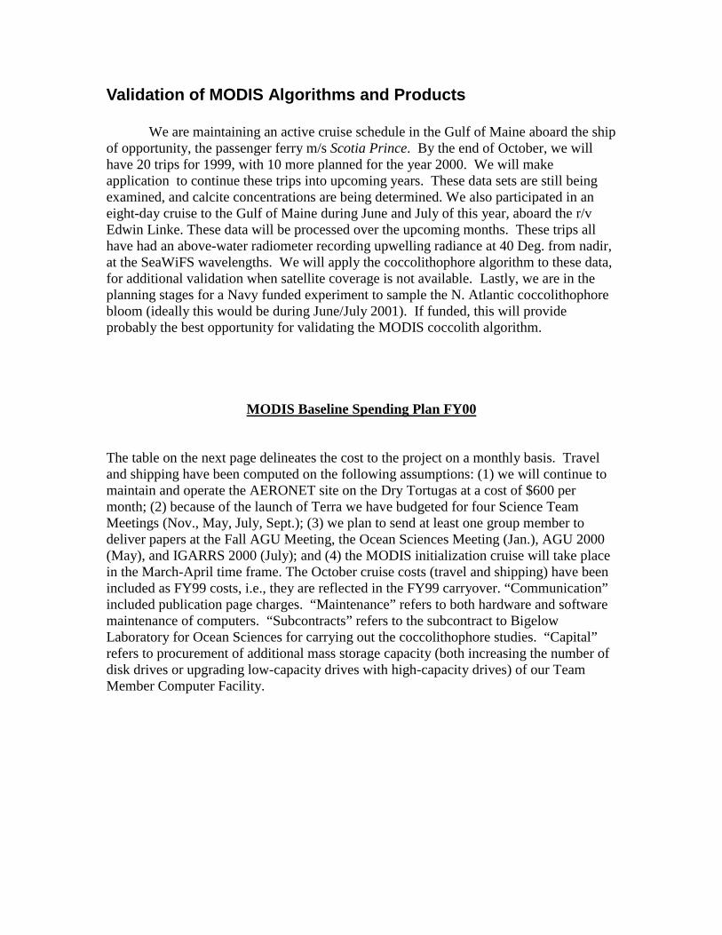
We are maintaining an active cruise schedule in the Gulf of Maine aboard the shipof opportunity, the passenger ferry m/s Scotia Prince. By the end of October, we willhave 20 trips for 1999, with 10 more planned for the year 2000. We will makeapplication to continue these trips into upcoming years. These data sets are still beingexamined, and calcite concentrations are being determined. We also participated in aneight-day cruise to the Gulf of Maine during June and July of this year, aboard the r/vEdwin Linke. These data will be processed over the upcoming months. These trips allhave had an above-water radiometer recording upwelling radiance at 40 Deg. from nadir,at the SeaWiFS wavelengths. We will apply the coccolithophore algorithm to these data,for additional validation when satellite coverage is not available. Lastly, we are in theplanning stages for a Navy funded experiment to sample the N. Atlantic coccolithophorebloom (ideally this would be during June/July 2001). If funded, this will provideprobably the best opportunity for validating the MODIS coccolith algorithm.
MODIS Baseline Spending Plan FY00
The table on the next page delineates the cost to the project on a monthly basis. Traveland shipping have been computed on the following assumptions: (1) we will continue tomaintain and operate the AERONET site on the Dry Tortugas at a cost of $600 permonth; (2) because of the launch of Terra we have budgeted for four Science TeamMeetings (Nov., May, July, Sept.); (3) we plan to send at least one group member todeliver papers at the Fall AGU Meeting, the Ocean Sciences Meeting (Jan.), AGU 2000(May), and IGARRS 2000 (July); and (4) the MODIS initialization cruise will take placein the March-April time frame. The October cruise costs (travel and shipping) have beenincluded as FY99 costs, i.e., they are reflected in the FY99 carryover. “Communication”included publication page charges. “Maintenance” refers to both hardware and softwaremaintenance of computers. “Subcontracts” refers to the subcontract to BigelowLaboratory for Ocean Sciences for carrying out the coccolithophore studies. “Capital”refers to procurement of additional mass storage capacity (both increasing the number ofdisk drives or upgrading low-capacity drives with high-capacity drives) of our TeamMember Computer Facility.
APPENDIX II
MODIS Atmospheric Correction Performance:Initial Evaluation
Howard R. GordonUniversity of Miami
With significant help from K. Turpie, R. Vogel, B. Franz,R. Evans, J. Brown, W. Esaias, MODIS SDST and MCST.

Preamble
In this appendix we describe an initial evaluation of the performance of MODIS and theatmospheric correction algorithm based on a single MODIS granual (2000102.2215) thatcovers an area in the Central Pacific from approximately 0−20 Deg. South and 147−172Deg. West. First, a simplified version of the atmospheric correction algorithm ispresented. Next, the retrieved normalized water-leaving radiance at 551 nm is evaluated.Then, the performance of the MODIS atmospheric correction bands is examined.Finally, preliminary conclusions are presented.
Atmospheric correction review
The atmospheric correction algorithm for MODIS is based on the work of Gordon andWang (1994). Improvements and unresolved problems concerning the MODIS algorithmhave been described in detail by Gordon (1997). The algorithm uses the MODIS nearinfrared bands (15 and 16 at 749 and 869 nm, respectively) to assess the aerosolcontribution in the visible. To understand the analysis that follows, a brief and simplifieddescription of the correction algorithm is provided below.
We convert all radiances to reflectance defined by
0cos0 θπρ
F
L= ,
where L is radiance, F0 is the extraterrestrial solar irradiance, and θ0 is the solar zenithangle. Then the reflectance measured at the top of the atmosphere (TOA), ρt, is given by
)()()(0
)(
)()()()( λρλλλρ
λρλρλρλρ wnvtt
A
raart +++=!! "!! #$
,
where ρr is the contribution from molecular (Rayleigh) scattering in the absence ofaerosols, ρa the contribution from the aerosol in the absence of air, ρra the contributionfrom interactive Rayleigh and aerosol scattering, and nρw is the normalized water-leaving reflectance. The quantities t0 and tv are the diffuse transmittances in directionsfrom sea surface toward the sun and from the sea surface toward the sensor, respectively.The Rayleigh contribution can be computed from an estimate of the surface atmosphericpressure (provided in the ancillary data from NOAA). In the NIR nρw ≈ 0, which allowsdetermination of ρA there. The atmospheric correction parameter ε(λ,λ0) isapproximately given by

)0(
)()0,(
λρλρλλε
A
A≈
(see Gordon 1997 for a more precise definition), so in the NIR ε(λ,λ0), can be determinedfor λ and λ0 representative of Bands 15 and 16, i.e.,
)16(
)15()16,15(
A
Aρρε ≈ .
For the other bands, we estimate ε(λ,16) from ε(15,16) using a set of candidate aerosolmodels. Then the water-leaving reflectance in any band can be estimated from
)]}16()16()[16,()()(){(1)(10)( rtrtvttwn ρρλελρλρλλλρ −−−−−= ,
with the diffuse transmittances being determined from the chosen candidate aerosolmodel and the aerosol concentration (found from ρA(16)).
To look at the performance of the atmospheric correction algorithm we examined theretrieved normalized water-leaving radiance at 551 nm nLw(551) and the retrievedε(15,16) from MODIS granual 2000102.2115. We chose to look at nLw(λ) at 551 nmbecause the value of nLw(551) is almost independent of the chlorophyll concentration if itis less than about 0.25 mg/m3, and has a nominal value of approximately 2.8 W/m2 µmSr, and (Gordon and Clark, 1981). Also, in typical maritime atmospheres, nLw(551)comprises only about 5% of Lt(551). We discuss nLw(551) first.
Retrieved nLw(551) evaluation
Figure 1 is an image of nLw(551) produced at Goddard using the MODIS Oceanprocessing code and the post-launch radiometric calibration (March 17) that was based onobservations of the solar diffuser. Periodic banding is evident in the imagery, and iscaused by the fact that the ten detectors that individually record a scan are not properlycalibrated in a relative sense. (Such a calibration is usually referred to as “flat fielding.”)In this figure the line numbers are arranged from 1 at the bottom (southern edge) of theimage to ~ 2000 at the top (northern edge), and the pixel numbers range from 1 (western)at the left edge to 1354 at the right (eastern) edge. Lines of constant pixel numbercorrespond to a constant scan angle and a constant angle of incidence (AOI) on the scanmirror, but employ all 10 detectors. In contrast, along a single scan line, only onedetector is employed, but all (earth scan) angles of incidence on the scan mirror are used.Figures 2 provide the actual values of nLw(551) extracted from the L2 product along aline of constant pixel number (Figure 2(a) from the vertical line in Figure 1(a)) andconstant line number (Figure 2(b) from the horizontal line in Figure 1(a)). The largeexcursions of nLw(551) from the background ~ 4.2 W/m2 µm Sr mean are due to data thathave been corrupted by clouds. The small excursions are the result of a systematicchange in the radiometric characteristics of the individual detectors in the track direction,

which we refer to as “banding” or “striping.” The banding evident in Figure 1(a) isfurther quantified in the Figure 3, and very evident in an expanded version of the image(Figure 1(b)). Figure 3, shows that the banding appears to be due primarily to a singledetector. The general level of nLw(551) is ~4.0-4.5 W/m2 µm Sr, i.e., about 50% toohigh. Figure 2(b) shows that there appears to be a regular variation of nLw(551) with scanangle, i.e., nLw(551) is larger at the edges of the scan than at the center. This is likely duein part to an overall system calibration error in this band, but it could also result from anuncorrected variation of the MODIS system response as a function of the scan angle.
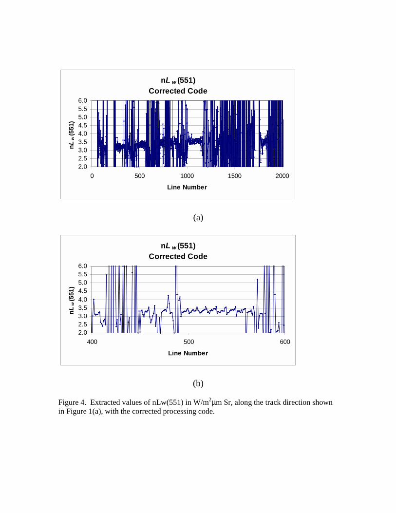
A new version of the processing code was produced in which errors in the original codewere corrected, and ε(15,16) was estimated using a 3×3 pixel average rather thanindividually to reduce noise (see ε(15,16) discussion below). Imagery processed at theUniversity of Miami using this new code version with the L1B data still showedsignificant banding (Figure 4), but the overall level of nLw(551) was reduced to ~ 3.0-3.5W/m2µm Sr, closer to the expected 2.8 W/m2µm Sr. Figure 4(b) also shows that thebanding now appears to be more of a ramp or linear trend (linear increase in radiancewith detector number) rather than a higher radiance from a single detector (Figure 3).Comparison of Figure 4(a) with Figure 2(a) shows that the ε(15,16)-averaging proceduremagnifies the influence of clouds. This is because a small cloud anywhere in the 3×3pixel box will corrupt the results. The variation of nLw(551) across the scan using thecorrected code still exhibits some variation; however, because of the increased cloudcorruption (compare Figures 2(a) and 4(a)) it is difficult to assess with this image.
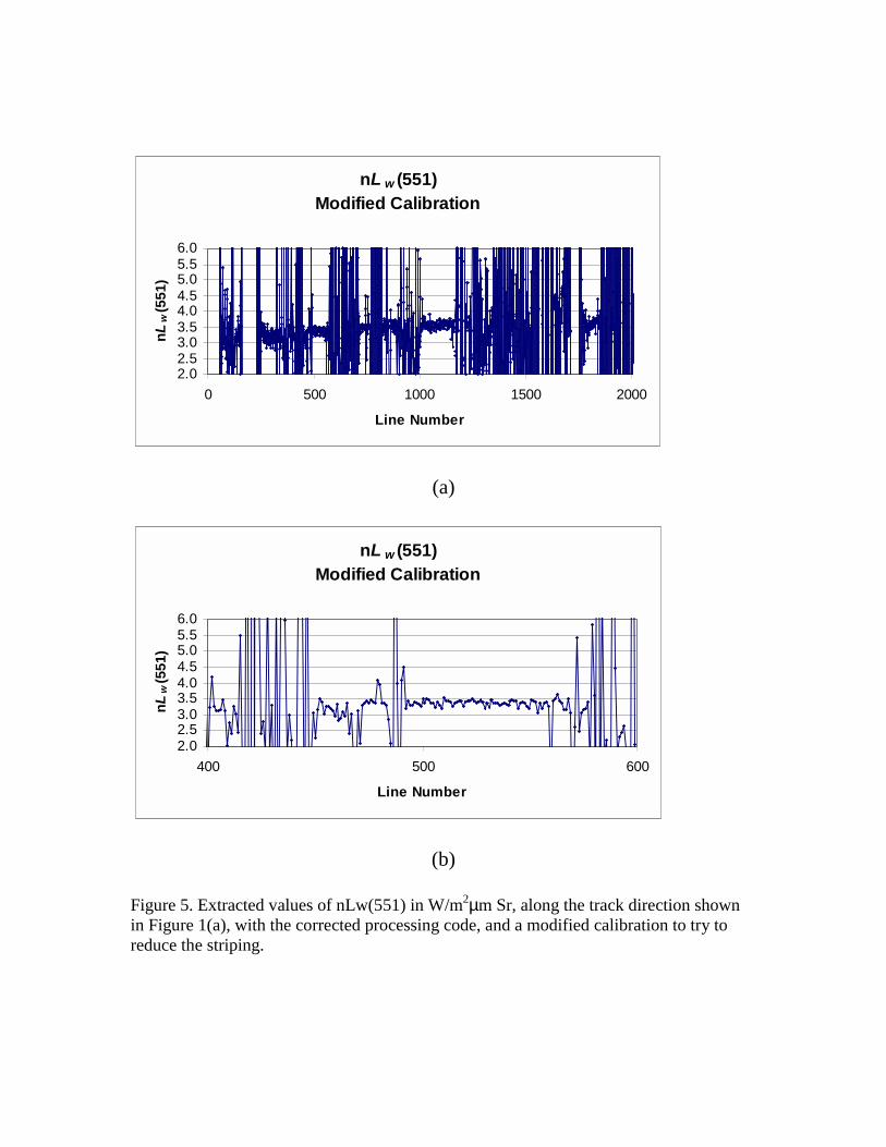
Finally, Figure 5 shows along track retrieval of nLw(551) using the University of Miamiempirical calibration adjustments. With this calibration the overall level is now ~3.3-3.5W/m2µm Sr, but the periodic banding is not as evident.
Retrieved εεεε(15,16) evaluation
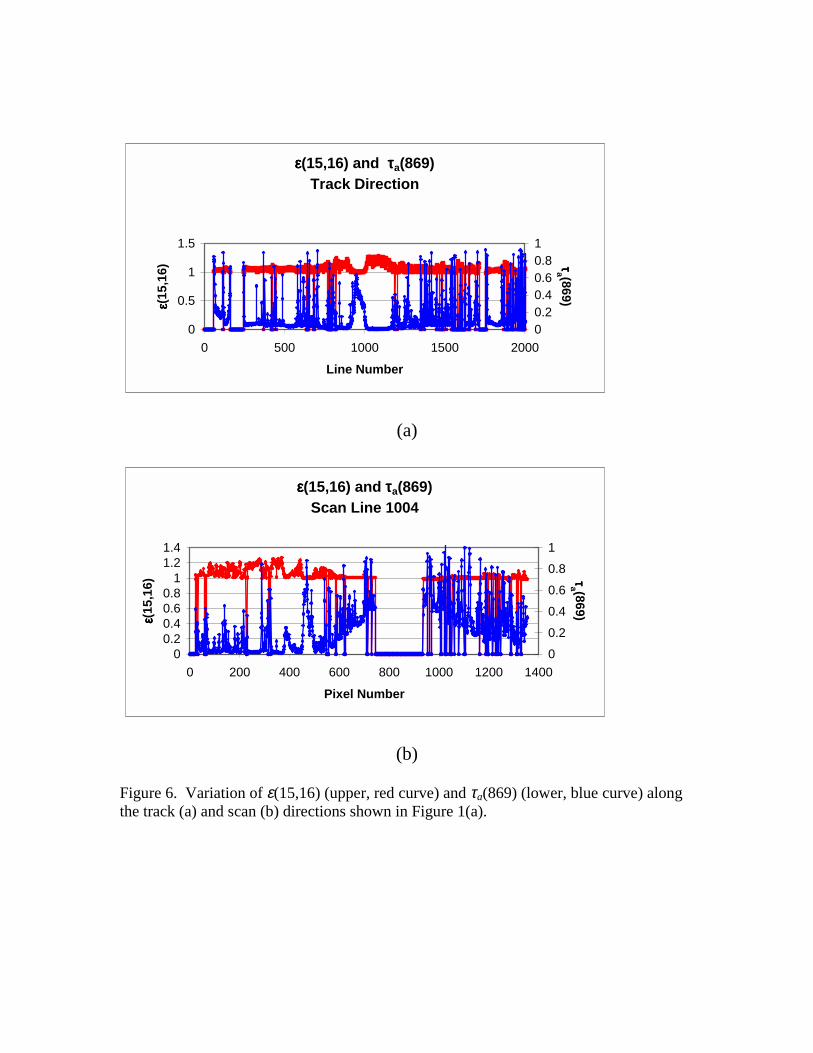
Much of the striping seen in nLw(551) is evident in the L1B data, i.e., Lt(551). However,we need to know how much, if any, of the banding is due to the atmospheric correctionprocess. For this we examined the behavior of ε(15,16) for this image. Figure 6 providesthe observed values of ε(15,16) and the retrieved aerosol optical thickness at 869nm,τa(869), for the along track (Figure 6(a)) and along scan (Figure 6(b)) directions ofthe image in Figure 1. The most obvious observation to be made from these figures isthat the observed values of ε(15,16) are quite noisy, and in the scan direction (Figure6(b)) the behavior of τa(869) shows that the sun glint centered near pixel 900 extendssignificantly beyond the area that has been masked as sun glint (pixels 745—935).Clearly, the sun glint is being interpreted as aerosol by the algorithm. This shows that alarge portion of the scan is unusable (pixels 600—1354) for this scan line that is atapproximately 10 degrees south of the Equator.
Figure 7 shows ε(15,16) for a small section of the track-direction line from lines 250 to600 that is relatively free of clouds. As mentioned earlier, this indicates that ε(15,16) isnoisy, but the noise does not appear to be systematic. One expects that, since ε(15,16)

depends mostly on the aerosol size distribution and should be independent of the aerosolconcentration, it would be essentially constant, at least over distances ~ few hundred kmin this region of the ocean (far from terrestrial and anthropogenic sources). The noise weobserve must be sensor generated. The red line on the figure provides the value ofε(15,16) for the same detector, i.e., it is the value for every 10th line. In addition each datapoint applies to the same AOI on the scan mirror. Thus, the noise does not appear to berelated to calibration. We tried to understand the source of this noise in the followingmanner. Figure 6(a) shows that in this region, τa(869)≈0.1. For this value of τa(869) anda typical marine aerosol (the Shettle and Fenn (1979) maritime aerosol model with arelative humidity of 80%, and referred to as M80) the characteristic values of thereflectances in the NIR are provided in Table 1.
Table 1: Characteristic Values (M80)(θ0=0, θv=45°)Band ρt ρr ρa + ρra
15 0.017759 0.010964 0.00679516 0.013219 0.006648 0.006574
For these values, the expected value of ε(15,16) ≈ 0.006795/0.006574 = 1.0336. Usingthe measured SNR’s we can compute the expected noise in ρt. This is provided in Table2.
Table 2: Expected noise in ρt
Band SNR ∆(ρt)15 800 2.22 × 10⁻⁵
16 700 1.88 × 10⁻⁵
Thus, we can compute a worst-case estimate of the expected noise in ε(15,16) byassuming maximum excursions of ∆(ρt) in the two bands, but with opposite sign, i.e., theupper excursion of ε(15,16) would be
0398.1)16()16()16(
)15()15()15()16,15( =
∆−+∆++=+
traa
traaρρρρρρε ,
while the lower excursion is
0274.1)16()16()16(
)15()15()15()16,15( =
∆++∆−+=−
traa
traaρρρρρρε .
The maximum amount of expected noise (peak-to-peak) should not exceed ∆ε(15,16) =ε(15,16)+ − ε(15,16)− ≈ 0.012. Halving the value of τa(869) would approximately double∆ε(15,16). The actual noise appears to be significantly in excess of these computedvalues of ∆ε(15,16). We do not know the source of this additional noise. To reduce theimportance of this noise, we have modified the processing code so that the value of

ε(15,16) is estimated by averaging the values of ρt in the NIR over a 3×3 pixel boxaround the pixel being processed. However, the value of ρt(16) at the actual pixel is usedin computing nρw(λ). Unfortunately this averaging procedure will increase the number ofpixels that are corrupted by clouds.
Conclusions
Based on the above analysis of granual 2000102.2215, we make the followingconclusions:
• The overall the retrieved water-leaving radiances on the average are in thecorrect ranges, suggesting that the overall system calibration and theatmospheric correction are in the nominal ranges; however, when theimagery is evaluated at full resolution many artifacts are apparent.
• The initial normalized water-leaving radiance at 551 nm, nLw(551),showed severe striping (a maximum of about 10% over the 10 detectors inthe spectral band) normal to the subsatellite track, and the average value is~ 50% too high.
• After correcting errors and omissions in the processing codes, andreprocessing the granual at Miami, this error in the average nLw(551) wasreduced to ~ +10%; however, the striping in nLw(551) remained.
• After an initial attempt by R. Evans and co-workers at flat fielding theimagery, the strongly periodic nature of the striping was removed, butthere was still some striping.
• The retrieved nLw(551) across a scan line showed some limb brighteningthat could be due to overall calibration errors or to the influence of anunaccounted variability in the system response as a function of scan angle.
• Bands 15 or 16, or both, (used for atmospheric correction) appear todisplay excessive noise. This may require averaging the atmosphericcorrection parameter ε(15,16) over several pixels.
• Sun glint will likely render the eastern half of the scan useless in thetropics unless a correction scheme can be developed.
• The striping in nLw(551) is not due to atmospheric correction, as ε(15,16)does not show significant striping.
In addition, it seems reasonable to conclude that

• a significant amount of work will be required to removing the stripingfrom the MODIS derived products, as its root cause is probably spreadover several processes, e.g., instrument polarization sensitivity, variabilityin system response with scan angle, etc. Thus the improvement processwill require an incremental resolution and balancing of the individualeffects, and
• plans should be made to reprocess MODIS imagery as incrementalprogress is made.
References
H.R. Gordon and D.K. Clark, Clear water radiances for atmospheric correction of CoastalZone Color Scanner imagery, Applied Optics, 20, 4175-4180 (1981).
H.R. Gordon and M. Wang, Retrieval of water-leaving radiance and aerosol opticalthickness over the oceans with SeaWiFS: A preliminary algorithm, Applied Optics, 33,443-452 (1994).
H.R. Gordon, Atmospheric Correction of Ocean Color Imagery in the Earth ObservingSystem Era, Jour. Geophys. Res., 102D, 17081-17106 (1997).
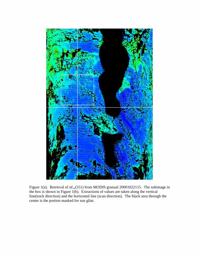
Figure 1(a). Retrieval of nLw(551) from MODIS granual 20001022115. The subimage inthe box is shown in Figure 1(b). Extractions of values are taken along the verticalline(track direction) and the horizontal line (scan direction). The black area through thecenter is the portion masked for sun glint.
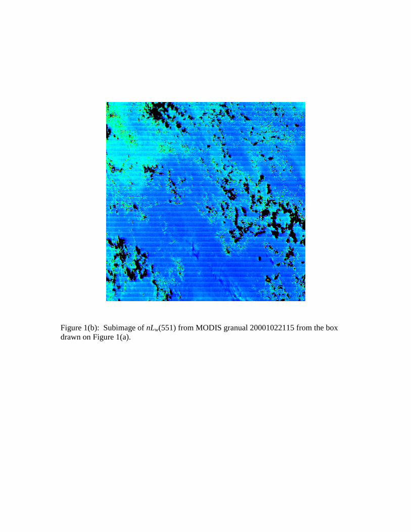
Figure 1(b): Subimage of nLw(551) from MODIS granual 20001022115 from the boxdrawn on Figure 1(a).

(a)
(b)
Figure 2. Extracted values of nLw(551) in W/m2µm Sr, along the track (a) and scan (b)directions on the lines shown in Figure 1(a).
nL w (551)Track Direction
2.02.5
3.03.54.0
4.55.0
5.56.0
0 200 400 600 800 1000 1200 1400 1600 1800 2000
Line Number
nL
w(5
51)
nLw(551)
Scan Line 1004
2.02.53.03.54.04.55.05.56.0
0 200 400 600 800 1000 1200 1400
Pixel Number
nL
w(5
51)

Figure 3. Expanded version of Figure 2(a) from line 400 to line 600.
nL w (551)Track Direction
22.5
3
3.54
4.55
5.56
400 500 600
Line Number
nL
w(5
51)
(a)
(b)
Figure 4. Extracted values of nLw(551) in W/m2µm Sr, along the track direction shownin Figure 1(a), with the corrected processing code.
nL w (551)Corrected Code
2.02.53.03.54.04.55.05.56.0
0 500 1000 1500 2000
Line Number
nL
w(5
51)
nL w (551)Corrected Code
2.02.53.03.54.0
4.55.05.56.0
400 500 600
Line Number
nL
w(5
51)
(a)
(b)
Figure 5. Extracted values of nLw(551) in W/m2µm Sr, along the track direction shownin Figure 1(a), with the corrected processing code, and a modified calibration to try toreduce the striping.
nL w (551) Modified Calibration
2.02.53.03.54.04.55.05.56.0
0 500 1000 1500 2000
Line Number
nL
w(5
51)
nL w (551) Modified Calibration
2.02.53.03.54.04.55.05.56.0
400 500 600
Line Number
nL
w(5
51)
(a)
(b)
Figure 6. Variation of ε(15,16) (upper, red curve) and τa(869) (lower, blue curve) alongthe track (a) and scan (b) directions shown in Figure 1(a).
εεεε(15,16) and ττττa(869)
Track Direction
0
0.5
1
1.5
0 500 1000 1500 2000
Line Number
ε εεε(15
,16)
00.20.40.60.81
τττ τa (869)
εεεε(15,16) and ττττa(869)
Scan Line 1004
00.20.40.60.8
11.21.4
0 200 400 600 800 1000 1200 1400
Pixel Number
ε εεε(15
,16)
0
0.2
0.4
0.6
0.8
1
τττ τa (869)

Figure 7. Expanded portion of Figure 6(a). The red line connects every tenth line andtherefore corresponds to a single detector and a single AOI on the scan mirror.
εεεε (15,16)Track Direction
1.00
1.02
1.04
1.06
1.08
1.10
250 300 350 400 450 500 550 600
Line Number
ε εεε(15
,16)

Appendix III
Atmospheric correction of ocean colorimagery through thick layers of Saharan dust
(Submitted to Geophysical Research Letters)
ATMOSPHERIC CORRECTION OF OCEAN COLOR IMAGERY
THROUGH THICK LAYERS OF SAHARAN DUST
C. Moulin1,2, H. R. Gordon1, R. M. Chomko1, V. F. Banzon1,3, and R. H. Evans3
1Physics Department, UM, Coral Gables, Florida, USA
2Lab. des Sciences du Climat et de l'Environnement, CEA-CNRS, Gif-Sur-Yvette, France
3Rosenstiel School of Marine and Atmospheric Science, UM, Miami, Florida, USA
ABSTRACT
Airborne plumes of desert dust from North Africa are observable all year on satellite images over
the Tropical Atlantic. In addition to its radiative impact, it has been suggested that this mineral
dust has a substantial influence on the marine productivity. This effect is however difficult to
gauge because present atmospheric correction algorithms for ocean color sensors are not capable
of handling absorbing mineral dust. We apply a new approach to atmospheric correction in
which the atmosphere is removed and the case 1 water properties are derived simultaneously.
Analysis of SeaWiFS images acquired off Western Africa during a dust storm demonstrates the
efficacy of this approach in terms of increased coverage and more reliable pigment retrievals.
INTRODUCTION
Phytoplankton, the first link in the marine food chain, can be detected from above the sea
surface through the change in water color brought about by virtue of the photosynthetic pigment
chlorophyll a and various accessory pigments they contain that absorb strongly in the blue
portion of the spectrum. The seminal CZCS mission demonstrated that these color variations
2
could be measured from satellite altitudes [Gordon et al. 1980] and led to the launching of
several new ocean color sensors, SeaWiFS, MODIS, POLDER, etc.
Of the radiance measured by an in-orbit ocean color sensor (Lt) only a small portion (Lw)
exited the ocean, typically < 10% in the blue, less at longer wavelengths, and negligible in the
near infrared (NIR). The rest is radiance backscattered from the atmosphere and reflected by the
sea surface. This radiance must be removed from Lt (atmospheric correction) in order to retrieve
Lw, the only part that contains information regarding marine productivity. The principal difficulty
in atmospheric correction lies in removing the effects of aerosols.
Assessment of the aerosol is now effected in a similar manner for all present ocean color
sensors (e.g., Gordon and Wang [1994] for SeaWiFS). Aerosol is detected in two NIR bands and
the observed spectral variation is compared to that of a set of aerosol models. The most
appropriate are then used to remove the aerosol’s contribution from Lt in the visible. Such
algorithms are presently being successfully applied, except when the aerosol is strongly
absorbing, because the aerosol’s absorption is not detectable from the observed spectral variation
in the NIR [Gordon 1997]. Standard atmospheric correction in the presence of absorbing
particles thus underestimates Lw in the blue leading to too-high pigment concentrations.
The predominant absorbing aerosol in the marine atmosphere is the mineral dust coming
from the Sahara [Herman et al. 1997]. This dust is strongly absorbing in the blue because it
contains ferrous minerals [Patterson 1981]. In addition, the impact of this absorption is very
dependent on the vertical distribution of the aerosol [Gordon 1997]. This is of primary
importance for Saharan dust [Moulin et al. 2000]. Because of these difficulties, the present
algorithms do not process pixels when high Lt are detected in the NIR. The quasi-permanent
presence of dust degrades satellite ocean color products in the Tropical Atlantic where large
3
areas are not sampled, sometimes for as long as an entire month. This failure of the atmospheric
correction also prevents observation of the potential fertilization effect due to the supply of
nutrients contained in dust to the surface water [Young et al. 1991].
RETRIEVAL ALGORITHM
Our approach to atmospheric correction in the dust zone is the spectral matching algorithm
(SMA) proposed by Gordon et al. [1997]. Briefly, a set of N candidate aerosol models is used
along with a model of the water-leaving radiance as a function of the pigment concentration C
and a marine particle-scattering parameter b0 [Gordon et al. 1988]. In this context, an aerosol
model is comprised of a particle size distribution and index of refraction, with the radiative
properties computed using Mie theory, and a vertical distribution of aerosol concentration. C is
defined to be the sum of the concentrations of chlorophyll a and its degradation product
phaeophytin a. It is the bio-optical quantity that was estimated by the CZCS. The Gordon et al.
[1988] radiance model was tuned to C using in-situ measurements in case 1 waters in the Eastern
Pacific, Gulf of California, Western Atlantic, and Gulf of Mexico.
The aerosol optical depth (AOD) for each aerosol model is adjusted so that the computed
top-of-atmosphere (TOA) radiance for the given model exactly reproduces the measured value in
the NIR. This allows the contribution of the atmosphere to the TOA radiance to be computed
throughout the visible for each aerosol model. The marine contribution for a given C and b0 is
then added to the atmospheric contribution for each of the N models to provide the modeled
TOA radiance throughout the visible. For each aerosol model, we then systematically varied C
(17 values, from 0.03 to 3 mg/m3) and b0 (12 values, from 0.12 to 0.45) over the range
characteristic of Case 1 waters to obtain the best agreement, in an root-mean square (RMS)
sense, between the modeled and measured TOA radiances at all wavelengths.

4
Realistic aerosol models are crucial for obtaining accurate estimates for the ocean
properties using this approach. We used the set of mineral dust models of Moulin et al. [2000]
which is based on earlier work with Meteosat [Moulin et al. 1997]. Comparisons between in-situ
and Meteosat-retrieved AOD showed that the Shettle [1984] “Background Desert” model was
superior to a wide range of other models. The real part of the aerosol’s refractive index was set to
1.53 and its imaginary part was set after Patterson [1981]. This provided the basic model from
which a set of 18 candidate dust models was developed by using three contributions of the coarse
mode to the size distribution, two spectral variations of the absorption index (Patterson’s and a
lower limit set by examination of several SeaWiFS images), and three thicknesses of the dust
layer [Moulin et al. 2000].
We applied the SMA to SeaWiFS on a pixel-by-pixel basis. Since the cloud screening of
the standard algorithm removed most of the bright "dusty" pixels, we decided to replace it by a
threshold on the standard deviation of the TOA radiance at 865 nm computed on 3x3 pixels
[Moulin et al. 1997]. This threshold was set by trial and error to 0.5 mW/cm2µmSr. It produces a
more conservative, and we believe better, cloud screen than that of the standard algorithm. For
the non-cloudy pixels that were then processed using the SMA, we do not report the retrieved
pigment concentration when the retrieved AOD is greater than 0.8.
SAMPLE RESULTS
We applied the SMA along with the University of Miami implementation of the standard
SeaWiFS algorithm to an 8-day period acquired off the West Coast of Africa between September
30th and October 7th, 1997. This time period was chosen because it enables comparison with the
standard SeaWiFS 8-day product. During this period, 5 SeaWiFS orbits (October 1st, 3rd, 4th, 5th
and 7th) crossed our region of interest (10-30°N; 10-25°W). An intense dust event, shown in

5
Figure 1, is observable between 10°N and 20°N on all orbits during this period, obscuring the
signal from the sea surface. The most interesting region to test our improved atmospheric
correction is between 15°N and 20°N where the mean AOD ranges mainly from 0.2 to 0.8 since
we expect the standard atmospheric correction to be degraded even for relatively low AOD.
North of the dust zone, between 20°N and 30°N, AOD remain low (≤ 0.1) during the period.
Figure 2 provides a comparison of the retrieved pigment concentrations from the SMA and
the standard SeaWiFS (STD) chlorophyll product of single orbit retrievals for the nearest "non-
dusty" day (September 29th) outside of the dust event. During this clear day, the AOD was about
0.1 over the whole region, so that the retrieved pigment concentrations can be used as a reference
to describe the actual marine productivity of this entire region. The STD chlorophyll product
uses the algorithms of Gordon and Wang [1994] for atmospheric correction and of O’Reilly et al.
[1997] (OC2) for retrieving the chlorophyll concentration from Lw. In contrast to the Gordon et
al. [1988] model that was tuned to pigment concentration, the O’Reilly et al. [1997] algorithm is
an empirical fit to chlorophyll a. C is approximately 35% greater than the concentration of
chlorophyll a [O’Reilly et al., 1997]; however, for the same water-leaving radiances the Gordon
et al. [1988] pigment concentration and the O’Reilly et al. [1997] chlorophyll a can differ as
much as a factor of two, with C even lower than chlorophyll a over some of the range. Rather
than trying to reconcile the existing differences between these two bio-optical algorithms, we
decided that for atmospheric correction purposes it is sufficient to compare the pigment
concentration from the SMA to the chlorophyll a concentration from the STD processing.
At the regional scale, it is obvious that both algorithms lead to very similar results for
oligotrophic waters as well as for the very productive Mauritanian upwelling. Indeed, even
though the aerosol models used to perform the atmospheric correction are completely different

6
(i.e., weakly- or non-absorbing for STD and absorbing for SMA), the aerosol contribution to the
TOA radiance is small enough so that it does not significantly influence the pigment retrievals. A
more detailed analysis however reveals some discrepancies between the two results that are
likely due to the difference in the derived product (chlorophyll a for STD and pigment for SMA),
as well as the bio-optical models used to estimate the pigment concentration from Lw. For
instance, there is an overestimate of the pigment concentration compared to chlorophyll a in
areas between 25°W and 23°W at about 20°N, and between 19°W and 16°W at about 17°N. In
the case 2 waters along the African coast at about 20°N, the SMA retrieves very low pigment
concentrations because it is based on the case 1 water model of Gordon et al. [1988]. Also, one
should note that the maximum pigment concentration that can be reached within our SMA for
case 1 waters is 3 mg/m3, whereas the O'Reilly et al. [1997] empirical algorithm is designed to
retrieve chlorophyll a concentrations as high as 30 mg/m3. Despite these differences, the general
agreement between the two results is satisfactory for this dust-free image.
Figure 3 shows single orbit retrievals of the pigment concentration for two "dusty" days
(October 3rd and 5th). Contrary to what was shown in Figure 2, the two algorithms lead to very
different results. The continuity of the SMA algorithm between the two dusty days and the clear
day in Figure 2 suggests that it has been successful in removing much of the influence of the dust
from the October 3rd and 5th images. In contrast, the standard algorithm shows very high
chlorophyll concentrations in the edge of the dust plume, but it retrieves reasonable
concentrations away from the plume, although comparison with Figure 2 shows that the STD
algorithm returns higher values north of 25°N. This cannot be due to a difference of bio-optical
algorithm, but rather to low concentrations of dust. In contrast, the SMA retrieves essentially the
same pigment concentration in this region on all three days.

7
We computed the corresponding concentration means of non-cloudy pixels for the 8-day
period from September 30th to October 7th. Both the SMA pigment and the SeaWiFS standard
chlorophyll a product (acquired from the NASA/GSFC web site) are shown on Figure 4. It is
evident that the SMA yields significantly more coverage in the dust region between13°N and
18°N. Furthermore, in the region between 10°N and 13°N, the STD algorithm actually processes
the imagery, but yields concentrations that are much too high (compare Figure 4 with Figure 2).
Above 25°N, the STD concentrations are also slightly too high, presumably because of a
background of dust. In contrast, over most of the area studied, the SMA retrieves approximately
the same pigment concentrations over the eight days as it did in the absence of dust (see Figure
2). This suggests that the SMA provides significantly better pigment retrievals and spatial
coverage than the STD does in producing the standard SeaWiFS chlorophyll product.
CONCLUDING REMARKS
We have applied an algorithm, developed for atmospheric correction of ocean color
imagery in strongly absorbing atmospheres, to SeaWiFS imagery acquired in the region of
Saharan dust transport off the coast of Africa. Application required a set of candidate aerosol
models, developed by studying SeaWiFS imagery in intense dust storms in the same region. The
results indicate that the methodology shows considerable promise for processing ocean color
imagery in the presence of mineral dust, and immediately suggests the possibility of estimating
other important consequences of the presence of dust, e.g., short-wave radiative forcing,
radiative heating and its vertical distribution in the troposphere, etc. The methodology, i.e.,
developing and tuning candidate aerosol models using SeaWiFS imagery, can be applied to other
regions and to other ocean color sensors in the same straightforward manner. The present dust
models permit processing close to the African coast. The models need to be validated, or new
8
models developed, for regions in the dust zone farther off shore, as significant changes in the size
distribution and particle characteristics may occur as the dust progresses across the Atlantic.
ACKNOWLEDGEMENTS
The authors are grateful for support for this work under the following grants and contracts:
NASA NAS5-31363 (HRG, CM), NASA NAS5-31734 (HRG, VFB), NASA NAS5-31362
(RHE). CM is grateful for the additional support provided by the French Commissariat à
l’Energie Atomique (CEA) and Centre National de la Recherche Scientifique (CNRS). This is
contribution XXX from LSCE.
REFERENCES
Gordon, H.R., D.K. Clark, J.L. Mueller, and W.A. Hovis, Phytoplankton pigments derived from
the Nimbus-7 CZCS: Initial comparisons with surface measurements, Science, 210, 63-66,
1980.
Gordon, H.R., O.B. Brown, R.E. Evans, J.W. Brown, R.C. Smith, K.S. Baker, and D.K. Clark, A
Semi-Analytic Radiance Model of Ocean Color, J. Geophys. Res., 93D, 10909-10924, 1988.
Gordon, H.R., and M. Wang, Retrieval of water-leaving radiance and aerosol optical thickness
over the oceans with SeaWiFS: A preliminary algorithm, Appl. Optics, 33, 443-452, 1994.
Gordon, H.R., Atmospheric Correction of Ocean Color Imagery in the Earth Observing System
Era, J. Geophys. Res., 102D, 17081-17106, 1997.
Gordon, H.R, T. Du, and T. Zhang, Remote sensing ocean color and aerosol properties:
Resolving the issue of aerosol absorption, Applied Optics, 36, 8670-8684, 1997.
Herman, J.R., P.K. Bhartia, O. Torres, C. Hsu, C. Seftor, and E. Celarier, Global distributions of
UV-absorbing aerosols from Nimbus 7/TOMS data, J. Geophys. Res., 102D, 16889-16909,
1997.

9
Moulin, C., F. Dulac, C.E. Lambert, P. Chazette, I. Jankowiak, B. Chatenet, and F. Lavenu,
Long-term daily monitoring of Saharan dust load over ocean using Meteosat ISCCP-B2 data,
2, Accuracy of the method and validation using sunphotometer measurements., J. Geophys.
Res., 102, 16959-16969, 1997.
Moulin, C., H.R. Gordon, R.H. Evans, and V.F. Banzon, Assessment of Saharan dust absorption
in the visible to improve ocean color retrievals and dust radiative forcing estimates from
SeaWiFS imagery. J. Geophys. Res., 2000 (Submitted).
O'Reilly, J.E., S. Maritorena, B.G. Mitchell, D.A. Siegel, K.L. Carder, S.A. Garver, M. Kahru, C.
McClain, Ocean color chlorophyll algorithms for SeaWiFS, J. Geophys. Res. 103C, 24937-
24953, 1998.
Patterson, E.M., Optical Properties of Crustal Aerosol: Relation to Chemical and Physical
Characteristics, J. Geophys. Res., 86C, 3236-3246, 1981.
Shettle, E. P. Optical and radiative properties of a desert aerosol model, In Proc. Symposium on
Radiation in the Atmosphere, ed. G. Fiocco, Hampton, Va.: A. Deepak, 1984.
Young, R.W., K.L. Carder, P.R. Betzer, D.K. Costello, R.A. Duce, G.R. Ditullio, N.W. Tindale,
E.A. Laws, M. Uematsu, J.T. Merrill, and R.A. Feeley, Atmospheric Iron Inputs and Primary
Productivity: Phytoplankton Responses in the North Pacific, Global Biogeochem. Cycles, 5,
119-134, 1991.

10
Figure 1. 8-day mean (30 Sept.–7 Oct., 1997) of the AOD as retrieved using the SMA.
Figure 2. Pigment concentrations for the clear day using the STD and the SMA processings.
10°N
15°N
20°N
25°N
30°N
Sept. 29thSTD
Sept. 29thSMA
0.03 0.1 0.3 1 3 10
mg/m3
25°W 20°W 15°W 10°W 25°W 20°W 15°W 10°W
10°N
15°N
20°N
25°N
30°N
25°W 20°W 15°W 10°W
0 0.25 0.5 0.75 1

11
Figure 3. Pigment concentrations for the two “dusty” days using STD and SMA processings.
10°N
15°N
20°N
25°N
30°N
25°W 20°W 15°W 10°W 25°W 20°W 15°W 10°W10°N
15°N
20°N
25°N
30°N
Oct. 3rdSTD
Oct. 3rdSMA
Oct. 5thSTD
Oct. 5thSMA
0.03 0.1 0.3 1 3 10
mg/m3
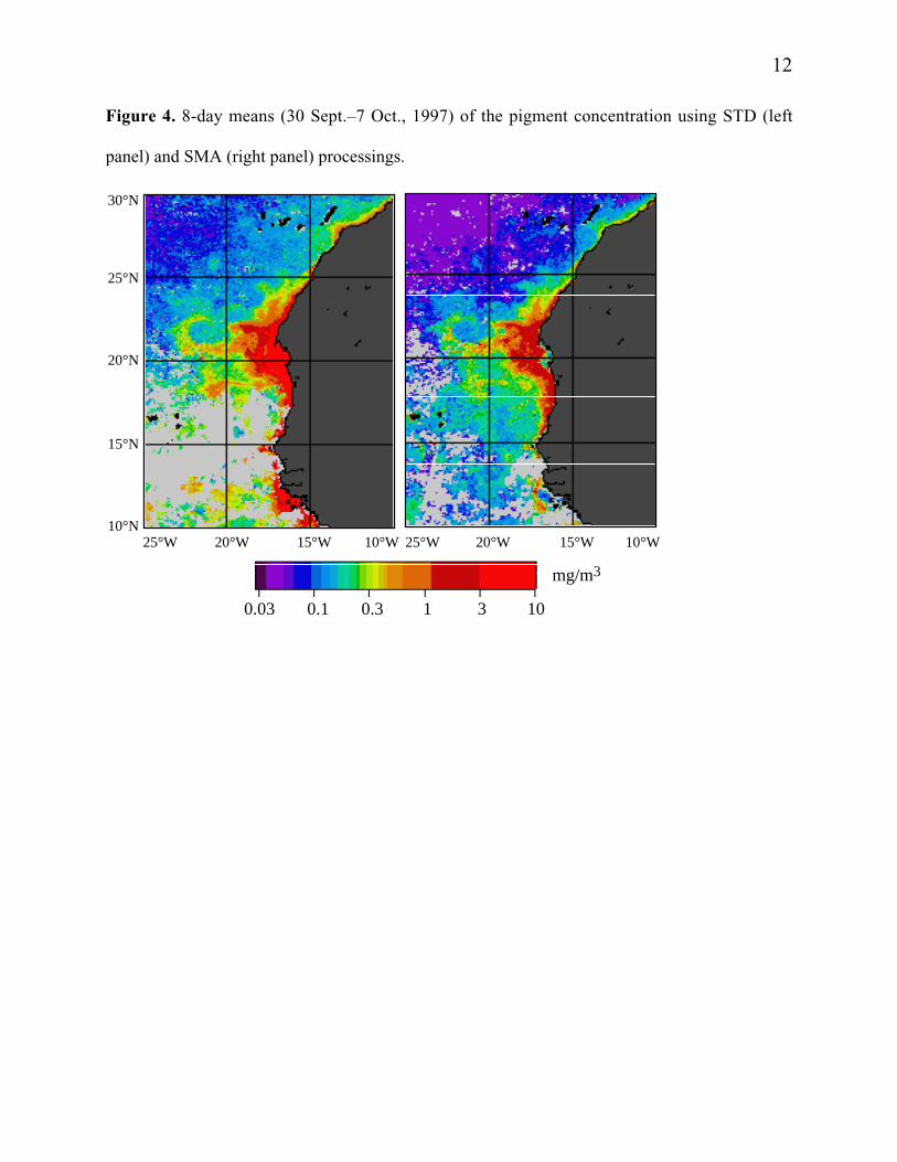
12
Figure 4. 8-day means (30 Sept.–7 Oct., 1997) of the pigment concentration using STD (left
panel) and SMA (right panel) processings.
0.03 0.1 0.3 1 3 10
mg/m3
10°N
15°N
20°N
25°N
30°N
25°W 20°W 15°W 10°W 25°W 20°W 15°W 10°W
Appendix IV
Atmospheric correction of ocean colorimagery: Test of the spectral optimization
algorithm with SeaWiFS
Atmospheric correction of ocean color imagery:
Test of the spectral optimization algorithm with SeaWiFS
Roman M. Chomko and Howard R. Gordon
Department of Physics
University of Miami
Coral Gables, FL 33124
Submitted to Applied Optics
1
Abstract
We implemented the spectral optimization algorithm [Chomko and Gordon, Applied
Optics, 37, 5560-5572 (1998)] (SOA) in an image processing environment and tested it with
SeaWiFS imagery from the Middle Atlantic Bight and the Sargasso Sea. We compared the
SOA and standard SeaWiFS algorithms (STD) on two days that had signi�cantly di�erent
atmospheric turbidities but, because of their location and time of the year, nearly the same
water properties. The SOA-derived pigment concentration showed excellent continuity
over the two days, with the relative di�erence in pigments exceeding 10% only in regions
characteristic of high advection. The derived water-leaving radiances at 443 and 555 nm
were also within � 10% and at 555 nm were close to clear water values in the Sargasso
Sea. There was no obvious correlation between the relative di�erences in pigments and the
aerosol concentration. In contrast, the standard processing (STD) showed poor continuity
in derived pigments over the two days, with the relative di�erences correlating strongly
with atmospheric turbidity. Additionally, the STD-derived pigment concentration showed
considerably more noise than the SOA pigments. SOA-derived atmospheric parameters
suggested that the retrieved ocean and atmospheric re ectances were decoupled on the
more turbid day, but not on the clearer day, where the aerosol concentration was so low
that relatively large changes in aerosol properties resulted in only small changes in aerosol
re ectance. This implies that SOA-derived atmospheric parameters cannot be accurate in
very clear atmospheres.
2
1. Introduction
Since the proof-of-concept ocean color mission, the Coastal Zone Color Scanner (CZCS),1{3
monitoring the concentration of phytoplankton pigments (C), the sum of the concentra-
tions of chlorophyll a and phaeophytin a, in the ocean from space-borne sensors has become
well established. Such sensors employ a set of discrete spectral bands throughout the visible
and into the near infrared region of the spectrum, and scan the earth producing a two-
dimensional image of the ocean. Optically, phytoplankton reveal their presence through
their in uence on the absorption of light by the water body by virtue of the strong ab-
sorption in the blue by the photosynthetic pigment chlorophyll a and by various accessory
pigments. Thus, in contrast to waters with low concentrations of phytoplankton, that are
bright in the blue, waters with high concentration of phytoplankton are usually dark in the
blue. The ocean color is a term that generally refers to the spectrum of light backscattered
out of the ocean | the \water-leaving radiance." The concentration of chlorophyll a is a
proxy for the phytoplankton concentration.
To improve the accuracy of the space-borne estimates, sensors with higher radiometric
sensitivity than CZCS have been developed. These include SeaWiFS,4 which was launched
August 1, 1997, and MODIS,5 launched December 18, 1999. The improvement in radio-
metric sensitivity necessitated the development of more sophisticated algorithms for both
atmospheric correction, to retrieve the water-leaving radiance from the total radiance mea-
sured at the top of the atmosphere (TOA), and bio-optical interpretation, for relating the
water-leaving radiance to the phytoplankton concentration.
The principal problem in atmospheric correction is to estimate the aerosol contribu-
tion to the measured TOA radiance. Aerosols are highly variable in space and time as well
as composition, thus their physical-chemical characteristics need to be estimated for each
pixel in an image. In contrast to the CZCS single-scattering atmospheric correction,6,7 the
3
algorithm developed for SeaWiFS and MODIS8,9 incorporates the full e�ects of multiple
scattering. This algorithm uses the fact that the water-leaving radiance is negligible in the
near infrared (NIR) region of the spectrum to assess the amount and the spectral varia-
tion of the aerosol contribution to the TOA radiance in the visible. This is e�ected by
comparing the spectral variation of the aerosol component in the NIR with that of several
candidate aerosol physical-chemical models. The most appropriate models are then used
to estimate the aerosol contribution in the visible. This technique appears to work well
when the aerosol is nonabsorbing; however, it fails completely when the aerosol is strongly
absorbing because it is generally impossible to infer the presence of the aerosol's absorption
using only measurements in the NIR.9 Because strongly absorbing aerosol are often trans-
ported over the oceans by the winds, e.g., urban pollution transported o� the U.S. East
Coast, and wind-blown dust from Africa, it is important to be able to make atmospheric
corrections in the presence of such aerosols. This can only be e�ected by incorporating
measurements from the visible into the correction process. The di�culty with this is that
the water-leaving radiance in the visible depends on the phytoplankton concentration and
therefore is unknown a priori. Two methods of proceeding have been proposed, and both
perform very well with simulated pseudo data. In the �rst, Gordon et al.10 proposed (1)
expanding the candidate aerosol model set to include strongly absorbing aerosols, (2) mod-
eling the ocean re ectance throughout the visible using the semi-analytic model of Gordon
et al.,11 that relates the water-leaving radiance to the pigment concentration and a particle
backscattering scattering coe�cient, and (3) systematically varying all the parameters of
the water model and the aerosol concentration of each aerosol model until a best �t (in an
rms sense) to the measured TOA radiance is determined. This provides both the water
properties and the aerosol properties simultaneously. In the second method12 a very simple
one-parameter model is assumed for the aerosol size distribution, a set of aerosol refractive
indices that represent a range of absorption properties is used in conjunction with Mie
theory to derive the aerosol optical properties, and these models are combined with the
4
semi-analytic radiance model to determine both the aerosol and water properties through
a nonlinear optimization procedure. The drawback for the �rst method is the requirement
that the aerosol models be representative (the closer one of the models is to reality, the
better will be the retrieval of aerosol and water properties). In the second method, no
attempt is made to use realistic models and this is a de�nite advantage | if it actually
works.
In this paper, we report a series of tests made with the spectral optimization algorithm
(SOA), second method in the last paragraph, using SeaWiFS imagery. These tests suggest
that the SOA is a viable approach to atmospheric correction, and can retrieve realistic
water parameters in cases in which the standard Gordon and Wang8 algorithm (henceforth
referred to as the \STD," i.e., \standard," algorithm) fails.
We begin with a brief review of radiative transfer in the ocean-atmosphere system.
Next, we describe the SOA and STD algorithms. Finally, we examine the performance of
both algorithms under clear and turbid atmospheric conditions o� the U.S. East Coast.
2. Radiative Transfer and Radiative Properties Review
To provide a framework for the discussion in Section 3 below, we brie y review radia-
tive transfer in the atmosphere-ocean system, the size distributions used to derive aerosol
models for atmospheric correction, and the water-leaving re ectance in terms of the con-
centration of phytoplankton pigments.
A. Radiative Transfer
We prefer to use re ectance � in place of radiance L. The re ectance is de�ned by
� = �L=F0 cos �0, where F0 is the extraterrestrial solar irradiance and �0 is the solar zenith
5

angle. Eliminating sun-glint contaminated pixels, and correcting for whitecaps, yields the
re ectance at the top of the atmosphere �t(�). It includes the following components:9
the pure Rayleigh (molecular) scattering contribution �r(�), the pure aerosol scattering
contribution �a(�), the contribution due to the interaction between air molecules and
aerosols �ra(�), and the desired water-leaving contribution t(�)�w(�), i.e.,
�t(�) = �r(�) + �a(�) + �ra(�) + t(�)�w(�); (1)
where t(�) is the di�use transmittance of the atmosphere. Since �r(�) can be computed
precisely from an estimate of the surface atmospheric pressure,13,14 it can be subtracted
from �t(�) to form
�t(�) � �r(�) = �A(�) + t(�)�w(�); (2)
where �A(�) � �a(�)+�ra(�). Both SeaWiFS and MODIS have spectral bands in the NIR
for which �w is nearly negligible in Case 1 waters,3 which comprise most of the oceans.
Calling �s and �` the shorter and longer wavelengths of the NIR bands, respectively, we
can form
"0(�s; �`) ��A(�s)
�A(�`): (3)
For SeaWiFS, �s = 765 nm and �` = 865 nm. If the aerosol optical thickness �a(�) were
su�ciently small, single scattering could be employed in the radiative transfer process. In
this case Eq. (1) can be written �t = �r + �as + t�w, where �as is the \single-scattered
aerosol re ectance." A quantity "(�s; �`) similar to "0(�s; �`) can be formed using the
single scattered aerosol re ectances:
"(�s; �`) ��as(�s)
�as(�`): (4)
"(�s; �`) depends only on the physical-chemical characteristics of the aerosol but not on
its concentration. In contrast, "0(�s; �`) includes the e�ects of multiple scattering and
therefore does depend on the aerosol concentration. The virtue of "(�s; �`) and "0(�s; �`)
6

is that they both depend mostly on the particle size distribution and very little on the
aerosol refractive index. Unfortunately, this means that these quantities are not helpful in
assessing the presence or absence of aerosol absorption.
B. Aerosol Models
Two types of aerosol size distributions have been considered: log-normal distributions
and power-law distributions. The multicomponent log-normal distribution given by
dNi
dD=
Ni
loge(10)p2��iD
exp
"�1
2
�log10(D=Di)
�i
�2#; (5)
where, dNi is the number of particles per unit volume per with diameter between D and
D + dD of the ith species or component, Di, and �i are the modal diameter and the
standard deviation, respectively, and Ni is the total number density of the ith component.
Summing over the components provides the actual size distribution:
dN
dD=
MXi=1
dNi
dD: (6)
For the models developed by Shettle and Fenn,15 M = 2, i.e., there are two components.
Each component had its own refractive index and the radiative properties were determined
using Mie theory.
The Junge power-law size distribution16 is of the form
dN
dD= K;
= K�D1
D
��+1;
= 0;
D0 <D � D1;
D1 <D � D2;
D > D2;
where dN is the number of particles per unit volume with diameters between D and
D+ dD. In contrast to the log-normal size distribution, given D0, D1 and D2, the power-
law distribution is characterized by a single parameter, �. Chomko and Gordon12 chose
7
D0 = 0:06 �m, D1 = 0:20 �m, and D2 = 20 �m, and assigned a single refractive index to
the entire distribution to compute the radiative properties using Mie theory.
C. Water-leaving Reflectance
In the CZCS era, the water re ectance was related to the pigment concentration
through empirical �ts of log-transformed re ectance ratios [�w(�1)=�w(�2)] to C.7,17 The
form of these ratios were later explained quantitatively by Gordon and Morel.3 When
individual re ectances are examined as a function of C, they are found to be noisy. This
noise is in part due to the natural variation of particle scattering with C.3 Gordon et
al.,11 developed a model for �w as a function of C and a scattering parameter b0, that
was successful in explaining the variation of �w with water constituents, and in accurately
reproducing the empirical re ectance ratio versus C relationships. In preparation for the
SeaWiFS launch, a complete review of the empirical algorithms was e�ected by O'Reilly et
al.,18 leading to new empirical algorithms for SeaWiFS. These algorithms were formulated
in terms of chlorophyll a (Chl) as opposed to C, and a C-Chl relationship was determined.
8

3. The STD and SOA Algorithms
A. The STD Algorithm
The STD algorithm8 is presently being used to process SeaWiFS imagery. It employs a
set of candidate aerosol models, from which it selects two, to extrapolate the NIR behavior
of �A into the visible. The basic form of the algorithm is as follows. For each model, the
re ectance �A(�) is related to the single scattering re ectance �as through a set of look up
tables (LUTs) that in essence contain the coe�cients a, b, etc., in
�A(�) = a(�)�as(�) + b(�)�as(�)2 + c(�)�as(�)
3 + d(�)�as(�)4; (7)
where a, b, etc., are also dependent on the viewing-solar geometry, and the particular
aerosol model. They contain all of the multiple scattering e�ects in �A(�). Given the
measured �A in the NIR, Eq. (7) is inverted to give an estimate of �as, and thus an
estimate of what each model would predict for "(�s; �`). Fortunately, these predictions
are all nearly the same, i.e., although "(�s; �`) and "0(�s; �`) may di�er considerably, the
multiple scattering e�ects on "(�s; �`) are only weakly dependent on the aerosol model.
(Note, however, that this is only true in the NIR, in the visible, the e�ects of multiple
scattering are strongly model-dependent.8,9) The resulting "(�s; �`)'s derived using the
individual models are then averaged, the mean is compared to the actual "'s for each
aerosol model, and the two models that are closest to, and bracket, the mean " are used
to the e�ect the atmospheric correction. For each of the two chosen models, the model "
value, referred to as "(M), is used to compute �as in the visible through
�(M)as (�) = "(M)(�; �`)�
(M)as (�`);
where �(M)as (�`) is the value of �as(�`) inverted from the measured �A(�`) with Eq. (7)
using the given model. Equation (7) is then used to compute �(M)
A(�) from �
(M)as (�). The
9
�nal value of �A(�) is a linear combination of the �(M)
A(�)'s for the two models, weighted
in relation to the closeness of the individual "(M)(�s; �`)'s to the mean ". Given �A(�),
we immediately �nd t(�)�w(�). The value of t for each model is found from a separate set
of LUTs19 and the �nal value of t is also a linear combination of those for the two models
weighted in the same manner as for �A(�). The ocean chlorophyll concentration, Chl, is
then estimated using the two-band (490 and 555 nm) OC2 algorithm from O'Reilly et al.18
The pigment concentration is derived from the chlorophyll concentration using
C = 1:34Chl0:983; (8)
also from O'Reilly et al.
The STD algorithm uses the Shettle and Fenn15 aerosol models as modi�ed by Gordon
and Wang.8 These are the Maritime, Coastal, and Tropospheric models at 50, 70, 90, and
99% relative humidity, for a total of 12 candidate aerosol models. The Maritime and
Coastal models are essentially nonabsorbing, and the Tropospheric models are weakly
absorbing. As expected, the algorithm fails when strongly absorbing aerosols are present.
B. The SOA
The SOA12 attempts to simultaneously retrieve the water and aerosol parameters. It
uses the Junge power-law size distribution for the aerosol. The quantity �A(�)+ t(�)�w(�)
is computed at each pixel using Eq. (2). The aerosol re ectance �A must be a function
of mr, mi, �, and �a, the real and imaginary parts of the aerosol's refractive index, the
Junge size parameter, and the aerosol optical depth at 865 nm, respectively, i.e., �A(�) =
�A(�;mr ;mi; �; �a). In a similar manner, t(�) = t(�;mr ;mi; �; �a). The water-leaving
re ectance �w is modeled using the Gordon et al.,11 semi-analytic model that employs the
two parameters C and b0, so �w(�) = �w(�;C; b0). Thus,
�A(�) + t(�)�w(�) = �A(�;mr;mi; �; �a) + t(�;mr;mi; �; �a)�w(�;C; b0);
10
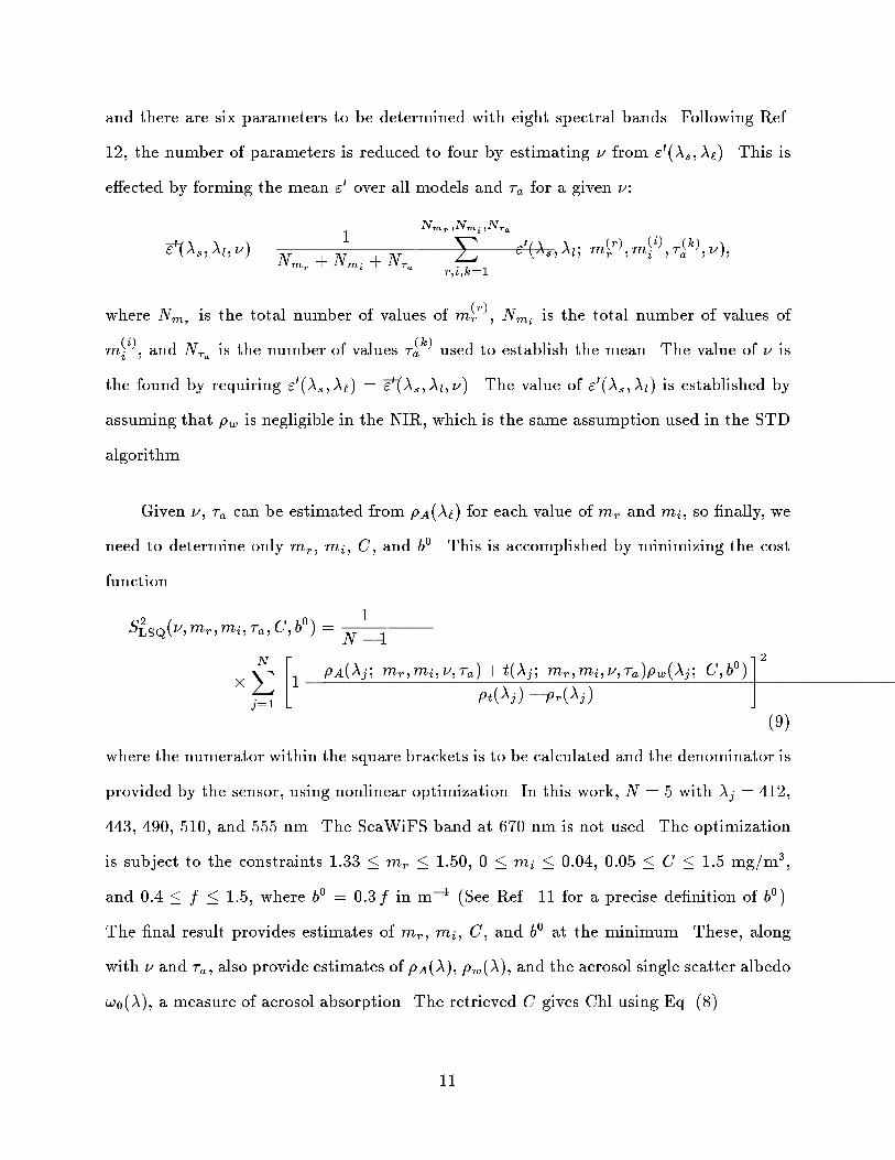
and there are six parameters to be determined with eight spectral bands. Following Ref.
12, the number of parameters is reduced to four by estimating � from "0(�s; �`). This is
e�ected by forming the mean "0 over all models and �a for a given �:
"0(�s; �l; �) =1
Nmr+Nmi
+N�a
Nmr;Nm
i;N�aX
r;i;k=1
"0(�s; �l; m(r)r ;m
(i)
i ; � (k)a ; �);
where Nmris the total number of values of m
(r)r , Nmi
is the total number of values of
m(i)
i , and N�a is the number of values �(k)a used to establish the mean. The value of � is
the found by requiring "0(�s; �`) = "0(�s; �l; �). The value of "0(�s; �l) is established by
assuming that �w is negligible in the NIR, which is the same assumption used in the STD
algorithm.
Given �, �a can be estimated from �A(�`) for each value of mr and mi, so �nally, we
need to determine only mr, mi, C, and b0. This is accomplished by minimizing the cost
function
S2LSQ(�;mr;mi; �a; C; b0) =
1
N � 1
�NXj=1
"1�
�A(�j ; mr;mi; �; �a) + t(�j ; mr;mi; �; �a)�w(�j ; C; b0)
�t(�j) � �r(�j )
#2
(9)
where the numerator within the square brackets is to be calculated and the denominator is
provided by the sensor, using nonlinear optimization. In this work, N = 5 with �j = 412,
443, 490, 510, and 555 nm. The SeaWiFS band at 670 nm is not used. The optimization
is subject to the constraints 1:33 � mr � 1:50, 0 � mi � 0:04, 0:05 � C � 1:5 mg/m3,
and 0:4 � f � 1:5, where b0 = 0:3 f in m�1 (See Ref. 11 for a precise de�nition of b0).
The �nal result provides estimates of mr, mi, C, and b0 at the minimum. These, along
with � and �a, also provide estimates of �A(�), �w(�), and the aerosol single scatter albedo
!0(�), a measure of aerosol absorption. The retrieved C gives Chl using Eq. (8).
11
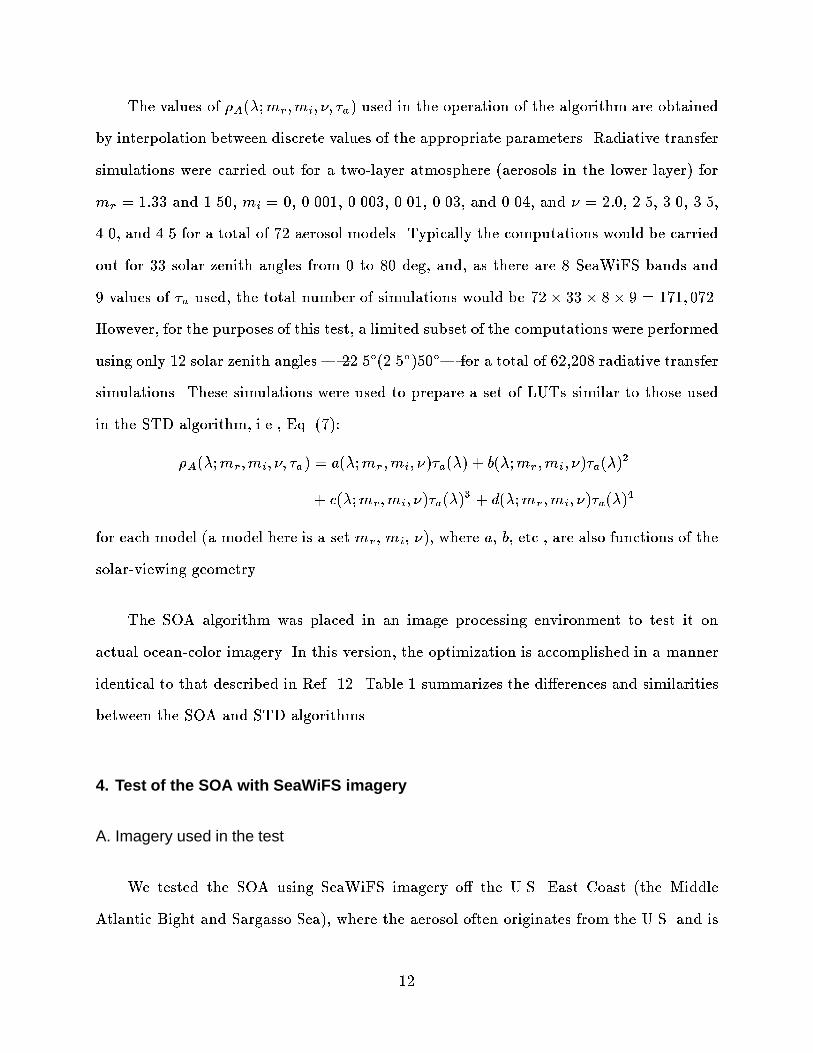
The values of �A(�;mr;mi; �; �a) used in the operation of the algorithm are obtained
by interpolation between discrete values of the appropriate parameters. Radiative transfer
simulations were carried out for a two-layer atmosphere (aerosols in the lower layer) for
mr = 1:33 and 1.50, mi = 0, 0.001, 0.003, 0.01, 0.03, and 0.04, and � = 2:0, 2.5, 3.0, 3.5,
4.0, and 4.5 for a total of 72 aerosol models. Typically the computations would be carried
out for 33 solar zenith angles from 0 to 80 deg, and, as there are 8 SeaWiFS bands and
9 values of �a used, the total number of simulations would be 72� 33 � 8� 9 = 171; 072.
However, for the purposes of this test, a limited subset of the computations were performed
using only 12 solar zenith angles | 22.5�(2.5�)50�| for a total of 62,208 radiative transfer
simulations. These simulations were used to prepare a set of LUTs similar to those used
in the STD algorithm, i.e., Eq. (7):
�A(�;mr;mi; �; �a) = a(�;mr ;mi; �)�a(�) + b(�;mr ;mi; �)�a(�)2
+ c(�;mr;mi; �)�a(�)3 + d(�;mr ;mi; �)�a(�)
4
for each model (a model here is a set mr, mi, �), where a, b, etc., are also functions of the
solar-viewing geometry.
The SOA algorithm was placed in an image processing environment to test it on
actual ocean-color imagery. In this version, the optimization is accomplished in a manner
identical to that described in Ref. 12. Table 1 summarizes the di�erences and similarities
between the SOA and STD algorithms.
4. Test of the SOA with SeaWiFS imagery
A. Imagery used in the test
We tested the SOA using SeaWiFS imagery o� the U.S. East Coast (the Middle
Atlantic Bight and Sargasso Sea), where the aerosol often originates from the U.S. and is
12
sometimes absorbing. In this study, we examined two SeaWiFS images from October 1997:
days-of-the-year 279 and 281 (October 6 and 8). True color renditions of these images are
presented in Figure 1. Images of �A(865), which is roughly proportional to the aerosol
optical thickness �a(865), remapped to a standard (Mercator) grid, are provided in Figure
2 for the areas shown in Figure 1. For Day 279, the atmosphere over the area examined is
turbid, e.g., along Track 2 �A(865) reaches 0.02. In contrast, Day 281 is characterized by a
clear atmosphere, with �A(865) more than a factor of 4{5 lower near the northern portion
of Track 2. The Day-281 values of �A(865) are more characteristic of the open ocean far
from land, i.e., a pure marine atmosphere. Although we have no surface truth for these
images, atmospheric correction in a clear atmosphere is not di�cult, and we expect that
both the SOA and the Gordon and Wang algorithm (STD) will perform well on Day 281.
However, because of the turbid atmosphere, this may not be the on case Day 279.
13

B. SOA-STD comparison
Here we judge the e�cacy of the algorithms under two criteria.
First, both STD and SOA should provide similar pigment concentrations
and water-leaving radiances on Day 281. In the Sargasso Sea (southern
portion of Tracks 2 and 3), the water-leaving radiances should be char-
acteristic of those in clear ocean water,20 particularly in the green (555
nm).
Second, the retrieved pigment concentrations and water-leaving radiances
for Days 279 and 281 should be very similar, because we do not expect large
changes in water properties over this large area at this time of the year
over a time period of 48 hours. (However, note that such changes would
be possible in the spring.) Local changes are possible through advection,
and these should be easily recognized in the imagery, but the gross values
of these parameters should not change.
Figure 3 provides remapped imagery of the retrieved phytoplankton pigment concen-
tration for this two days processed with the SOA and the STD algorithms. The color scale
is the same for STD and SOA. Black in the image is either clouds or land. [The cover of
this issue shows scan coordinate versions of the SOA algorithm enhanced to show the eddy
structure in the Sargasso Sea (lower panels), and the �nger-like patterns near the north
wall of the Gulf Stream (upper panels).]
It is obvious from Figure 3 that the SOA-retrieved pigment concentrations are very
similar in all areas for the two days. In contrast, the STD-derived concentrations di�er
signi�cantly from 279 to 281, especially in the vicinity of the higher aerosol concentrations
(Figure 2).
14

In the SOA, recognizable eddies (see cover) in the Sargasso Sea appear to retain their
pigment concentrations over the two days, while in the STD processing it is di�cult to
even recognize eddies there. (STD-processed imagery with the same enhancement as the
SOA on the cover is not shown.)
Figure 4 provides the pigment concentrations for Days 279 and 281 and for the SOA
and STD algorithms along the three tracks shown on Figures 2 and 3. It shows that
the SOA pigment concentrations are very consistent for the two days except in the re-
gions of high advection (Track 1 and the northern portions of Tracks 2 and 3). In the
turbid-atmosphere region (Track 2) the STD algorithm shows approximately a factor of
2 di�erence in pigment concentration between the two days, while the SOA pigments are
consistent over the two days. In contrast, along Track 3, for which the atmosphere is clear
over most of the Track (Figure 2) on both days, the SOA and STD algorithms are both
consistent over the two days; however, the STD pigments are approximately a factor of
two higher than the SOA pigments for low pigment concentrations. This is to be expected
because the SOA uses the Gordon et al. radiance model.11 Given the same spectrum of
water-leaving radiances, the radiance model will yield a lower pigment concentration than
the OC2 algorithm18 that is used in the standard processing, when the concentration is
low (Figure 5). This di�erence decreases as the pigment concentration increases. Thus, we
believe that the di�erences in the overall pigment concentrations in the Sargasso Sea are
not the result of atmospheric correction, but result from di�erent interpretations of the
water-leaving re ectance.
It is interesting that there appears to be muchmore detail and less noise in the imagery
processed with the SOA than the STD algorithm. There are two reasons for this. First, the
SOA employs all of the bands to estimate the pigment concentration (and simultaneously
perform atmospheric correction) as opposed to only the 490 and 555 nm bands in the
standard processing. Using more bands, and wider spacing between bands, results in a
15
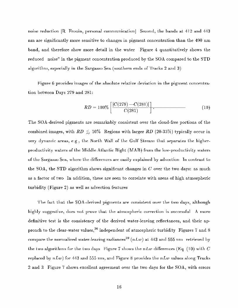
noise reduction [R. Frouin, personal communication]. Second, the bands at 412 and 443
nm are signi�cantly more sensitive to changes in pigment concentration than the 490 nm
band, and therefore show more detail in the water. Figure 4 quantitatively shows the
reduced \noise" in the pigment concentration produced by the SOA compared to the STD
algorithm, especially in the Sargasso Sea (southern ends of Tracks 2 and 3).
Figure 6 provides images of the absolute relative deviation in the pigment concentra-
tion between Days 279 and 281:
RD = 100%
�jC(279)� C(281)j
C(281)
�: (10)
The SOA-derived pigments are remarkably consistent over the cloud-free portions of the
combined images, with RD <� 10%. Regions with larger RD (20-35%) typically occur in
very dynamic areas, e.g., the North Wall of the Gulf Stream that separates the higher-
productivity waters of the Middle Atlantic Bight (MAB) from the low-productivity waters
of the Sargasso Sea, where the di�erences are easily explained by advection. In contrast to
the SOA, the STD algorithm shows signi�cant changes in C over the two days: as much
as a factor of two. In addition, these are seen to correlate with areas of high atmospheric
turbidity (Figure 2) as well as advection features.
The fact that the SOA-derived pigments are consistent over the two days, although
highly suggestive, does not prove that the atmospheric correction is successful. A more
de�nitive test is the consistency of the derived water-leaving re ectances, and their ap-
proach to the clear-water values,20 independent of atmospheric turbidity. Figures 7 and 8
compare the normalized water-leaving radiances20 (nLw) at 443 and 555 nm. retrieved by
the two algorithms for the two days. Figure 7 shows the nLw di�erences (Eq. (10) with C
replaced by nLw) for 443 and 555 nm, and Figure 8 provides the nLw values along Tracks
2 and 3. Figure 7 shows excellent agreement over the two days for the SOA, with errors
16
<� 10% except in the regions of high advection. The STD algorithm again shows large
errors that mimic the pattern of atmospheric turbidity (especially at 555 nm).
Figure 8 shows that the SOA algorithm provides values of nLw at 555 nm in the
Sargasso Sea that are independent of the atmospheric turbidity and close to the clear-
water value20 � 0:28 mW/cm2�mSr. The two algorithms retrieve similar values in low
turbidity regions, but not high-turbidity areas.
The comparisons in this subsection show that the SOA out performs the STD al-
gorithm in recovering C and nLw in the more turbid atmosphere (279). In the following
subsection we examine the retrieval of parameters unique to the SOA| aerosol absorption,
�, b0, and SLSQ.
17
C. Additional parameters estimated with the SOA
For a given value of C, which largely determines the spectral shape of the water-
leaving radiance, b0 controls the actual magnitude of the water-leaving radiance at each
wavelength. Figure 9 provides the retrieved values of b0 (actually f) for the two days.
The values are realistic in the sense that b0 is somewhat lower in the Sargasso Sea than
in the MAB. This was also observed in Ref. 11. They are usually within the range set
within the program (0:4 � f � 1:5) and only occasionally at the boundaries of the range
(an exception being in the vicinity of the coast where b0 would be expected to be outside
the range). Gross consistency in b0 is evident for the two days, although di�erences are
apparent in some regions. In particular, in the vicinity of Track 1 (Figures 2 and 3) the
values of b0 appear to be somewhat lower on Day 279 compared to Day 281. This is
paradoxical in the sense that the retrieved pigment concentrations are consistent here for
the two days (Figures 4 and 6), and the most turbid region of Day 279 is over the western
portion of the track, while on Day 281 its over the eastern portion. As one expects that
the better values of b0 are obtained in the clear atmosphere, the conclusion must be that
the b0 is higher along the western part of the slope waters in the MAB and smaller in the
eastern part. If this is true, the error in b0 in the turbid regions is � 0:2 to 0.3 in f .
Figure 10 provides the retrieved aerosol Junge power-law parameter � and the aerosol
single scattering albedo (!0) | the ratio of aerosol scattering to aerosol scattering plus
aerosol absorption | at 865 nm. !0 = 1 for a nonabsorbing aerosol and zero for a
nonscattering aerosol. We consider the aerosol to be strongly absorbing if !0 <� 0:9. The
values of !0 used in the STD algorithm were in the range 0.92 to 1.0.
For the turbid day � > 3 almost everywhere, suggesting a size distribution favoring
small particles. South of the cloud front at the bottom of the image � <� 2:5 suggesting a
maritime aerosol. On the clearer Day 281, the value of � is seen to decrease from >� 3 in
18

the MAB to maritime values far o� shore. Note that � is determined solely from the bands
at �s and �`, which are not in uenced by water properties (except close to the coast), and
therefore do not correlate with features clearly in the water.
Concerning !0, in the case of the more turbid atmosphere, !0 � 1 throughout the
image, which implies a weakly absorbing aerosol. Some water features appear in !0, but
only close to the coasts where the assumption that �w(�) = 0 at 765 and 865 nm may
not be valid. The fact that the aerosol is nearly nonabsorbing, along with � > 3, suggests
that it is composed of mostly sulfate21 and may originate in the mid-western U.S. (Figure
1). In contrast, on Day 281 water features are clearly evident in !0. The unrealistically
low values north of the Gulf Stream suggest that !0 is not correctly obtained there. This
problem occurs because the aerosol concentration is extremely low. In such cases, the
algorithm in e�ect focuses in on the correct water properties and then tries to minimize
SLSQ by varying the aerosol properties (mr and mi), which varies !0. Because the aerosol
concentration is so low, large variations in properties can take place with only modest
variations in �(c)
A(�). (Note that �a(865) is chosen so that �
(c)
A(865) is correct.) The result
is a very imprecise estimate of the aerosol's absorption properties. Thus, the retrieved
aerosol absorption can only be trusted at su�ciently large aerosol concentrations. Similar
conclusions were reached using simulated data.12
Figure 11 shows the retrieved images of �a(865) along with the parameter SLSQ that
determines the quality of the �nal solution. As discussed by Chomko and Gordon12 �a(865)
can be in error by as much as �50% because the scattering phase functions derived from
Junge power-law distributions may not be adequate in the backward directions (however,
this is irrelevant for atmospheric correction). We provide �a(865) for completeness. Note
that for Day 281 some water features are observed in �a(865). This is consistent with
similar features in !0.
19

The SLSQ images are almost almost mirror images of �A(865). This is to be expected
as SLSQ is the rms relative error in �A(�)+t(�)�w(�). For a similar absolute error in �w(�)
(Figure 7), SLSQ will be inversely related to the aerosol concentration. If the atmosphere
is very clear, i.e., �A(�)� t(�)�w(�), SLSQ should indicate the ability of the semi-analytic
ocean color model to represent �w(�). Figure 11 suggests that the rms error in this ability
is � 10% (near 38�N and 72�W).
20
5. Discussion
In this paper, we have tested the performance of an implementation of our SOA in an
image processing environment with SeaWiFS imagery. We consider this to be a proof-of-
concept exercise, in that our goal was the evaluation of the performance of the algorithm,
not the advocacy of its use in its present form for routine SeaWiFS processing.
We compared the SOA and STD algorithms on two days that had signi�cantly di�erent
aerosol concentrations but, because of their location, nearly the same water properties. The
SOA showed excellent continuity over the two days in the derived pigment concentrations,
with the relative di�erence in pigments exceeding 10% only in regions expected to have
high advection. The derived water-leaving radiances (nLw) at 443 and 555 nm were also
within � 10% and at 555 nm were close to clear water values20 in the Sargasso Sea. There
was no obvious correlation between the relative di�erences in pigments (and nLw) and the
aerosol concentration (as delineated by �A(865)).
In contrast, the standard processing (STD) showed poor continuity in derived quan-
tities (C and nLw) over the two days, with the relative di�erences correlating strongly
with the atmospheric turbidity. This implies a poor atmospheric correction. Furthermore,
the STD derived pigment concentration showed considerably more noise than the SOA
pigments.
The other SOA-derived water quantity b0 (with some exceptions) showed good con-
sistency over the two days; however, the atmospheric parameters !0 and �a(865) did not.
The atmospheric parameters showed little or no correlation with C and b0 for the turbid
day (279), suggesting that the atmospheric correction was excellent. Both !0 and �a(865)
showed obvious water patterns for the clear day indicating that the ocean and atmosphere
were not totally decoupled on Day 281. The reason suggested for this is that the aerosol
21
concentration was so low that relatively large changes were possible in !0 with only small
changes in �A(�). Thus SOA-derived atmospheric parameters are only to be trusted when
�A(865) is su�ciently large. We have not studied the minimum magnitude of �A(865) for
which the SOA can yield adequate atmospheric parameters.
Based on the above, we believe we have demonstrated the e�cacy of the SOA for
processing ocean color imagery in Case 1 waters. However, it is important to recognize
the SOA limitations. In the version used here, the pigment concentration is limited to the
range 0 to 1.5 mg/m3 and to Case 1 waters. These limitations are based on the fact that
the semi-analytic model of ocean color11 employed here has been validated only over this
range. (As an aside, it should be pointed out that a signi�cant fraction of the data used
develop and validate the semi-analytic model were collected in 1979 in the area discussed
in this paper.) Colored dissolved organic matter (CDOM) is only implicitly included11 in
the SOA and therefore cannot be explicitly retrieved. The algorithm in its present version
is too slow to use in routine processing. We are presently studying approaches for reducing
the SOA processing time.
We believe that the simultaneous retrieval of ocean and atmospheric properties, that
forms the heart of the SOA, is the preferred approach for processing ocean color imagery.
Although it requires a model of the ocean re ectance as a function of constituents, this
should not be considered a blemish. The STD algorithm already requires models of the
atmospheric re ectance, and ocean re ectance models are arguably as well developed as
atmospheric models. Improvements in both ocean and aerosol models will yield a con-
comitant improvement in ocean color retrievals.
Acknowledgment
22

The authors are grateful for support from the National Aeronautics and Space Admin-
istration, Goddard Space Flight Center, under Contracts NAS5-31363 and NAS5-31734.
23

References
1. H. R. Gordon, D. K. Clark, J. L. Mueller and W. A. Hovis, \Phytoplankton pigments
derived from the Nimbus{7 CZCS: initial comparisons with surface measurements,"
Science 210, 63{66 (1980).
2. W. A. Hovis, D. K. Clark, F. Anderson, R. W. Austin, W. H. Wilson, E. T. Baker,
D. Ball, H. R. Gordon, J. L. Mueller, S. Y. E. Sayed, B. Strum, R. C. Wrigley and
C. S. Yentsch, \Nimbus 7 coastal zone color scanner: system description and initial
imagery," Science 210, 60{63 (1980).
3. H. R. Gordon and A. Y. Morel, Remote Assessment of Ocean Color for Interpretation
of Satellite Visible Imagery: A Review (Springer-Verlag, New York, 1983), 114 pp.
4. S. B. Hooker, W. E. Esaias, G. C. Feldman, W. W. Gregg and C. R. McClain,
SeaWiFS Technical Report Series: Volume 1, An Overview of SeaWiFS and Ocean
Color (NASA, Greenbelt, MD, Technical Memorandum 104566, July 1992).
5. V. V. Salomonson, W. L. Barnes, P. W. Maymon, H. E. Montgomery and H. Ostrow,
\MODIS: Advanced Facility Instrument for Studies of the Earth as a System," IEEE
Geosci. Rem. Sens. 27, 145{152 (1989).
6. H. R. Gordon, \Removal of Atmospheric E�ects from Satellite Imagery of the Oceans,"
Applied Optics 17, 1631{1636 (1978).
24
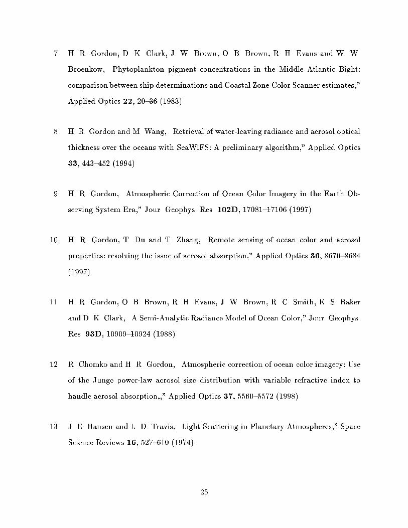
7. H. R. Gordon, D. K. Clark, J. W. Brown, O. B. Brown, R. H. Evans and W. W.
Broenkow, \Phytoplankton pigment concentrations in the Middle Atlantic Bight:
comparison between ship determinations and Coastal Zone Color Scanner estimates,"
Applied Optics 22, 20{36 (1983).
8. H. R. Gordon and M. Wang, \Retrieval of water-leaving radiance and aerosol optical
thickness over the oceans with SeaWiFS: A preliminary algorithm," Applied Optics
33, 443{452 (1994).
9. H. R. Gordon, \Atmospheric Correction of Ocean Color Imagery in the Earth Ob-
serving System Era," Jour. Geophys. Res. 102D, 17081{17106 (1997).
10. H. R. Gordon, T. Du and T. Zhang, \Remote sensing of ocean color and aerosol
properties: resolving the issue of aerosol absorption," Applied Optics 36, 8670{8684
(1997).
11. H. R. Gordon, O. B. Brown, R. H. Evans, J. W. Brown, R. C. Smith, K. S. Baker
and D. K. Clark, \A Semi-Analytic Radiance Model of Ocean Color," Jour. Geophys.
Res. 93D, 10909{10924 (1988).
12. R. Chomko and H. R. Gordon, \Atmospheric correction of ocean color imagery: Use
of the Junge power-law aerosol size distribution with variable refractive index to
handle aerosol absorption,," Applied Optics 37, 5560{5572 (1998).
13. J. E. Hansen and L. D. Travis, \Light Scattering in Planetary Atmospheres," Space
Science Reviews 16, 527{610 (1974).
25
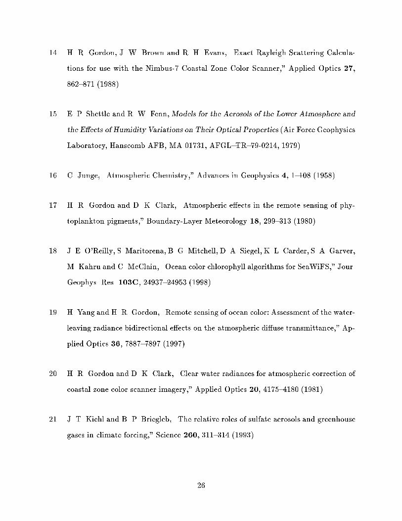
14. H. R. Gordon, J. W. Brown and R. H. Evans, \Exact Rayleigh Scattering Calcula-
tions for use with the Nimbus-7 Coastal Zone Color Scanner," Applied Optics 27,
862{871 (1988).
15. E. P. Shettle and R. W. Fenn,Models for the Aerosols of the Lower Atmosphere and
the E�ects of Humidity Variations on Their Optical Properties (Air Force Geophysics
Laboratory, Hanscomb AFB, MA 01731, AFGL{TR{79-0214, 1979).
16. C. Junge, \Atmospheric Chemistry," Advances in Geophysics 4, 1{108 (1958).
17. H. R. Gordon and D. K. Clark, \Atmospheric e�ects in the remote sensing of phy-
toplankton pigments," Boundary-Layer Meteorology 18, 299{313 (1980).
18. J. E. O'Reilly, S. Maritorena, B. G. Mitchell, D. A. Siegel, K. L. Carder, S. A. Garver,
M. Kahru and C. McClain, \Ocean color chlorophyll algorithms for SeaWiFS," Jour.
Geophys. Res. 103C, 24937{24953 (1998).
19. H. Yang and H. R. Gordon, \Remote sensing of ocean color: Assessment of the water-
leaving radiance bidirectional e�ects on the atmospheric di�use transmittance," Ap-
plied Optics 36, 7887{7897 (1997).
20. H. R. Gordon and D. K. Clark, \Clear water radiances for atmospheric correction of
coastal zone color scanner imagery," Applied Optics 20, 4175{4180 (1981).
21. J. T. Kiehl and B. P. Briegleb, \The relative roles of sulfate aerosols and greenhouse
gases in climate forcing," Science 260, 311{314 (1993).
26

Table 1: Comparative Methodology of the SOA and STD algorithms.
Method or Structure
Function STD Algorithm SOA
Aerosol 12 models: M,C,T at 72 Junge Power-Law models:
Assumptions�
4 relative humidities 6 values of �, 2 of mr, 6 of mi
Vertical Two-layer Two-layer
Structure Aerosol in lower layer Aerosol in lower layer
NIR Water �w(765) = 0 �w(765) = 0
Properties �w(865) = 0 �w(865) = 0
Data Storage LUT for �A(�as) and t(�a) LUT for �A(�a) and t(�a)
Aerosol Bands 7 and 8 are used to determine Bands 7 and 8 are used to determine
Properties: "(765; 865): �
LUTs are used to bracket the best given �0
(765; 865). �a(865) is
2 models. Further interpolation determined for each mr;mi set.
provides an \average" model.
Aerosol Based on extrapolation of the Non-linear optimization using
Re ect. �A(�) \average" model into the visible Bands 1 through 5 (Band 6 is optional)
Water-Leaving Computed directly Non-linear optimization using
Re ect. �w(�) Bands 1 through 5 (Band 6 is optional)
Di�use Bidirectional e�ects not included Bidirectional e�ects not included
Transmit. t(�)
�
M, C, T, stand for Maritime, Coastal, and Tropospheric models.
27

Figure Captions
Figure 1. \True" color rendition of the SeaWiFS imagery from October 6 and October 8,
1997.
Figure 2. The aerosol re ectance at 865 nm (�A(865)) along with three tracks from which
processed data will be extracted. Note the signi�cant di�erence in �A(865) between the
two days.
Figure 3. Pigment concentration retrieved for Days 279 and 281 using the SOA (left panels)
and the STD (right panels). The image has been remapped to a Mercator grid. The color
scale is linear and runs from 0 to 1.5 mg/m3.
Figure 4. The retrieved pigment concentrations along the three tracks on Figures 2 and 3:
(a) Track 1; (b) Track 2; (c) Track 3.
Figure 5. Comparison of the normalized water-leaving re ectance ratio (490 to 555 nm)
between the model used in the SOA (\Semi-analytic model") and the model used in the
STD (\OC2"). Note that for given water re ectances, the Semi-analytic model predicts a
smaller pigment concentration than OC2 for C <� 1 mg/m3.
Figure 6. Relative di�erence (in %) between the pigment concentrations computed for the
two days, e.g., Eq. (10). The left panel is for the SOA and the right panel for the STD.
Figure 7. Same as Figure 6 for nLw: top panels 443 nm; bottom panels 555 nm.
Figure 8. The retrieved nLw's for two of the three tracks on Figures 2 and 3: (a) Track 2;
(b) Track 3.
28

Figure 9. SOA-retrieved b0 (actually f). The color scale is linear and runs from f = 0:4
to f = 1:5.
Figure 10. SOA-retrieved � (upper panels) and !0 at 865 nm (lower panels). Both color
scales are linear and run from � = 2:0 to 4.5 and !0 = 0:6 to 1.0.
Figure 11. SOA-retrieved �a(865) (upper panels) and the SOA cost function SLSQ (lower
panels). Both color scales are linear and run from �a = 0 to 1 and SLSQ = 0 to 40%.
29
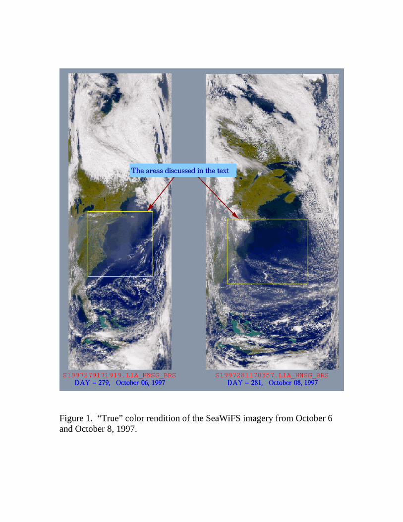
Figure 1. “True” color rendition of the SeaWiFS imagery from October 6and October 8, 1997.
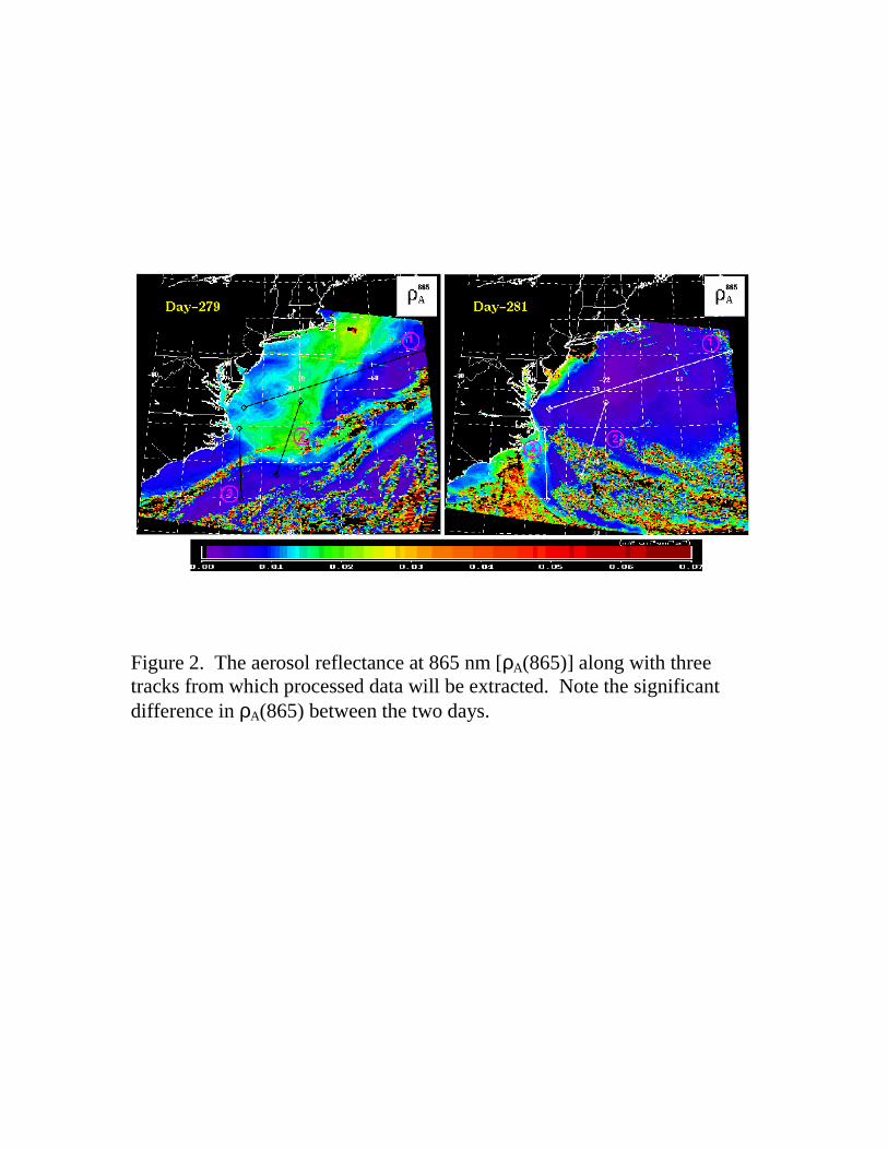
Figure 2. The aerosol reflectance at 865 nm [ρA(865)] along with threetracks from which processed data will be extracted. Note the significantdifference in ρA(865) between the two days.

Figure 3. Pigment concentration retrieved for Days 279 and 281 using theSOA (left panels) and STD (right panels). The image has been remapped toa Mercator grid. The color scale is linear and runs from 0 to 1.5 mg/m3.
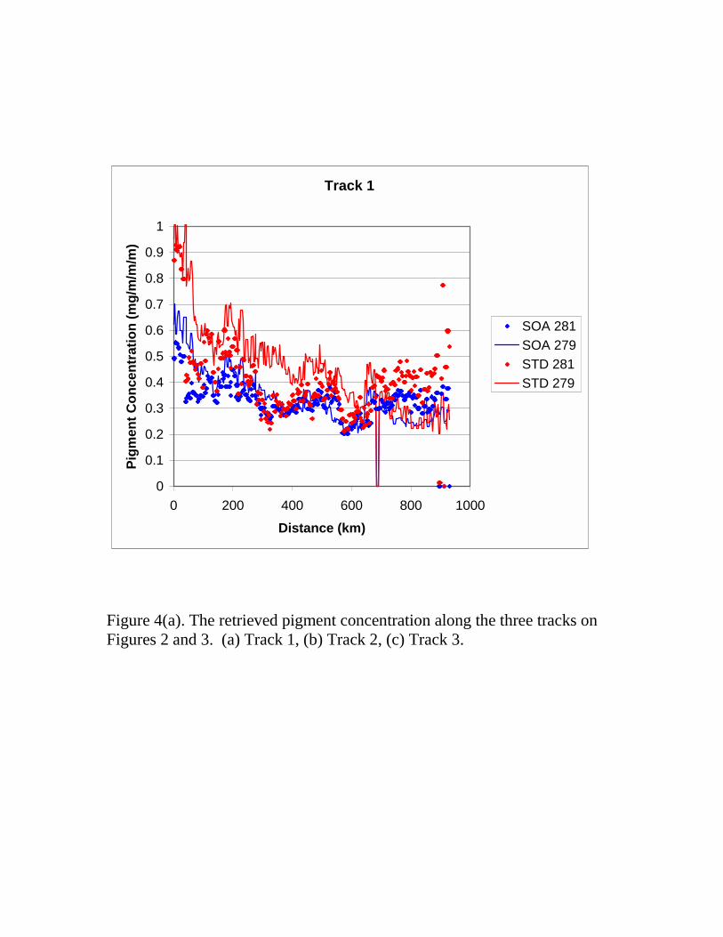
Figure 4(a). The retrieved pigment concentration along the three tracks onFigures 2 and 3. (a) Track 1, (b) Track 2, (c) Track 3.
Track 1
0
0.1
0.2
0.3
0.4
0.5
0.6
0.7
0.8
0.9
1
0 200 400 600 800 1000
Distance (km)
Pig
men
t C
on
cen
trat
ion
(m
g/m
/m/m
)
SOA 281
SOA 279
STD 281
STD 279
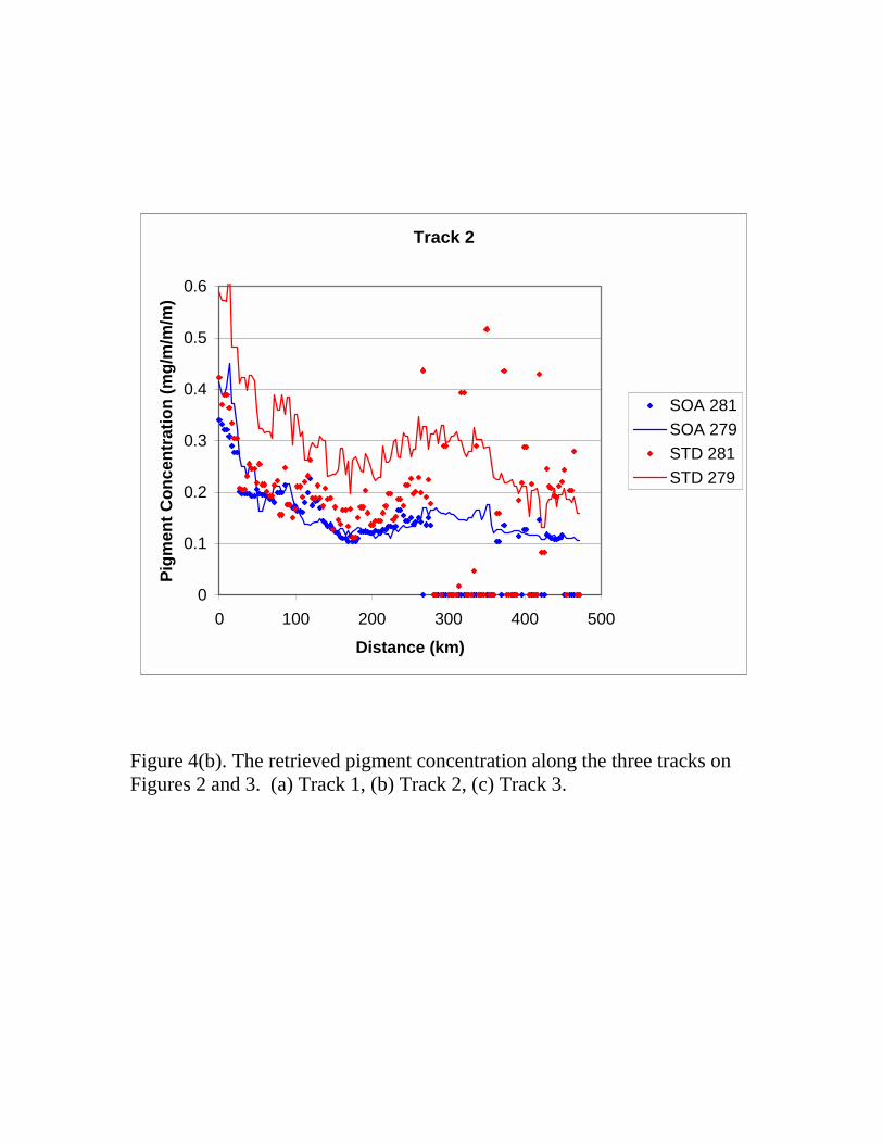
Figure 4(b). The retrieved pigment concentration along the three tracks onFigures 2 and 3. (a) Track 1, (b) Track 2, (c) Track 3.
Track 2
0
0.1
0.2
0.3
0.4
0.5
0.6
0 100 200 300 400 500
Distance (km)
Pig
men
t C
on
cen
trat
ion
(m
g/m
/m/m
)
SOA 281
SOA 279
STD 281
STD 279
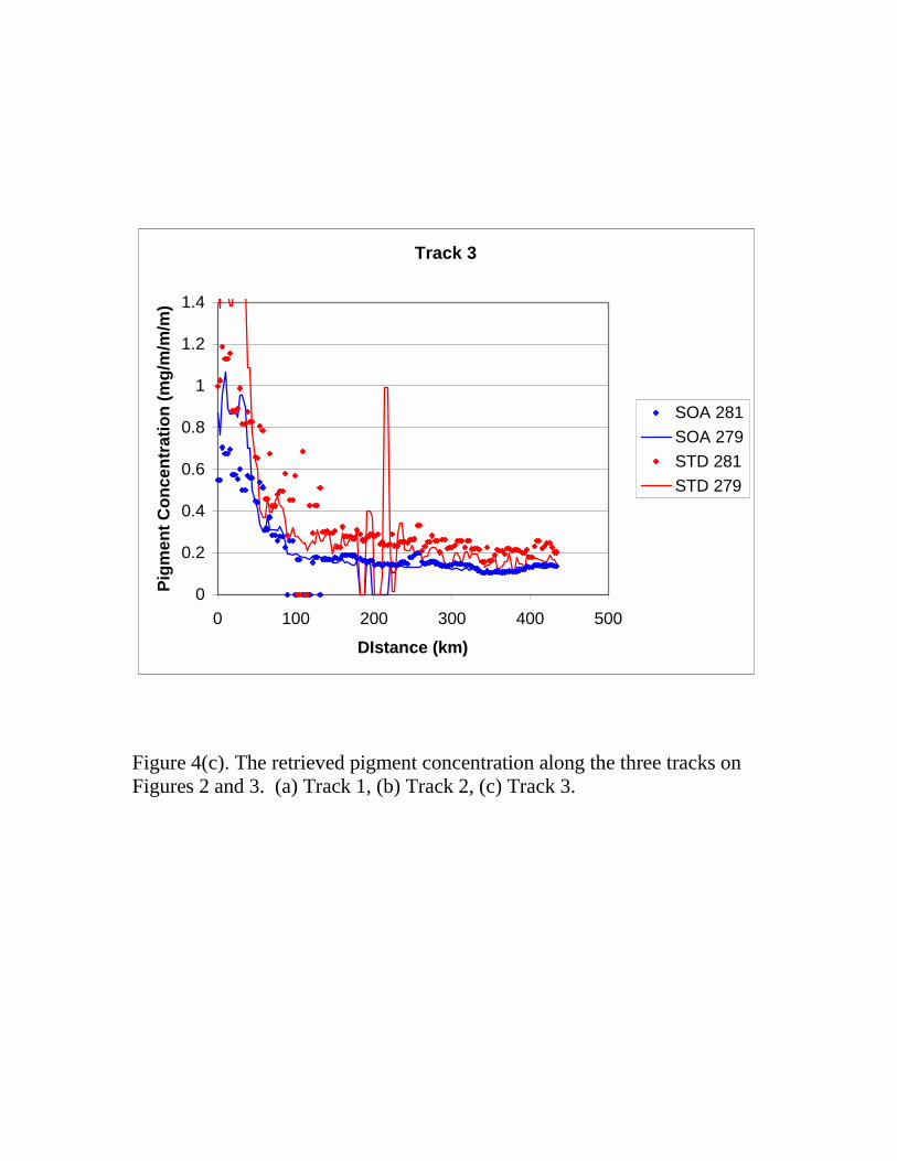
Figure 4(c). The retrieved pigment concentration along the three tracks onFigures 2 and 3. (a) Track 1, (b) Track 2, (c) Track 3.
Track 3
0
0.2
0.4
0.6
0.8
1
1.2
1.4
0 100 200 300 400 500
DIstance (km)
Pig
men
t C
on
cen
trat
ion
(m
g/m
/m/m
)
SOA 281
SOA 279
STD 281
STD 279
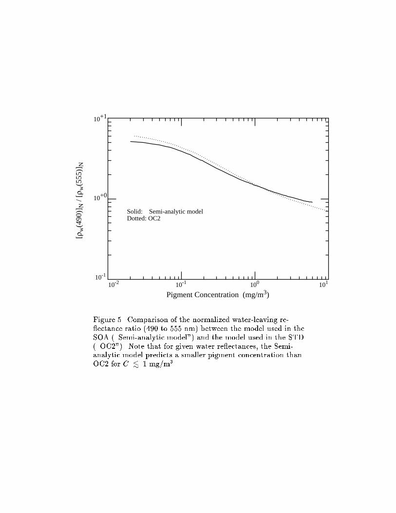
10-2 10-1 100 10110-1
10+0
10+1
Pigment Concentration (mg/m3)
[ρw
(490
)]N
/ [ρ
w(5
55)]
N
Solid: Semi-analytic modelDotted: OC2
Figure 5. Comparison of the normalized water-leaving re- ectance ratio (490 to 555 nm) between the model used in theSOA (\Semi-analytic model") and the model used in the STD(\OC2"). Note that for given water re ectances, the Semi-analytic model predicts a smaller pigment concentration thanOC2 for C <
�
1 mg/m3.

Figure 6. Relative difference (in %) between the pigment concentrationcomputed for the two days, i.e., Eq. (10). The left panel is for the SOA andthe right panel for the STD.
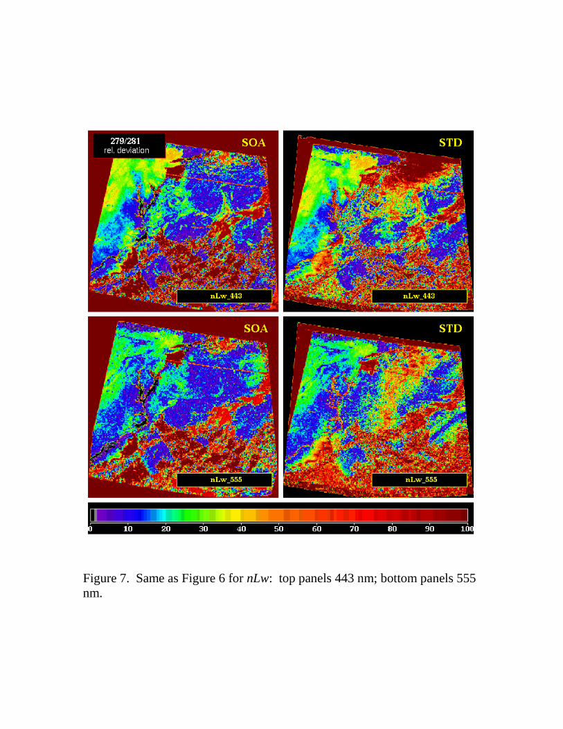
Figure 7. Same as Figure 6 for nLw: top panels 443 nm; bottom panels 555nm.
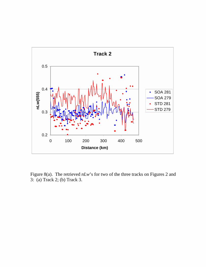
Figure 8(a). The retrieved nLw’s for two of the three tracks on Figures 2 and3: (a) Track 2; (b) Track 3.
Track 2
0.2
0.3
0.4
0.5
0 100 200 300 400 500
Distance (km)
nL
w(5
55
) SOA 281
SOA 279
STD 281
STD 279

Figure 8(b). The retrieved nLw’s for two of the three tracks on Figures 2and 3: (a) Track 2; (b) Track 3.
Track 3
0.1
0.2
0.3
0.4
0.5
0.6
0 100 200 300 400 500
Distance (km)
nL
w(5
55
) SOA 281
SOA 279
STD 281
STD 279

Figure 9. SOA-retrieved b0 (actually f). The color scale is linear and runsfrom f = 0.4 to 1.5.

Figure 10. SOA-retrieved ν (upper panels) and ω0 (lower panels). Bothcolor scales are linear and run from ν = 2.0 to 4.5 and ω0 = 0.6 to 1.0.

Figure 11. SOA-retrieved τa(865) (upper panels) and the SOA cost functionSLSQ (lower panels). Both color scales are linear and run from τa(865) = 0 to1, and SLSQ = 0 to 40%.

Appendix V
Aerosol Optical Depth Measurements Duringthe Aerosols99 Experiment
(Submitted to Journal of Geophysical Research)
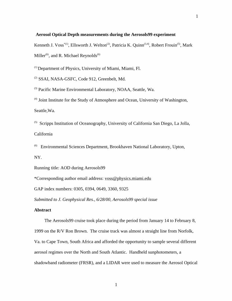
1
1
Aerosol Optical Depth measurements during the Aerosols99 experiment
Kenneth J. Voss*(1), Ellsworth J. Welton(2), Patricia K. Quinn(3,4), Robert Frouin(5), Mark
Miller(6), and R. Michael Reynolds(6)
(1) Department of Physics, University of Miami, Miami, Fl.
(2) SSAI, NASA-GSFC, Code 912, Greenbelt, Md.
(3) Pacific Marine Environmental Laboratory, NOAA, Seattle, Wa.
(4) Joint Institute for the Study of Atmosphere and Ocean, University of Washington,
Seattle,Wa.
(5) Scripps Institution of Oceanography, University of California San Diego, La Jolla,
California
(6) Environmental Sciences Department, Brookhaven National Laboratory, Upton,
NY.
Running title: AOD during Aerosols99
*Corresponding author email address: [email protected]
GAP index numbers: 0305, 0394, 0649, 3360, 9325
Submitted to J. Geophysical Res., 6/28/00, Aerosols99 special issue
Abstract
The Aerosols99 cruise took place during the period from January 14 to February 8,
1999 on the R/V Ron Brown. The cruise track was almost a straight line from Norfolk,
Va. to Cape Town, South Africa and afforded the opportunity to sample several different
aerosol regimes over the North and South Atlantic. Handheld sunphotometers, a
shadowband radiometer (FRSR), and a LIDAR were used to measure the Aerosol Optical

2
2
Depth (AOD) during the cruise. The AOD and angstrom exponent (spectral dependence
of the AOD) varied strongly between regimes. Maritime regions typically had AOD
(500nm) of approximately 0.10+ 0.03, with angstrom exponents around 0.3+ 0.3. An
African dust event was encountered in which the AOD(500nm) averaged 0.29+ 0.05 with
an angstrom exponent of 0.36+ 0.13. At the ITCZ, no measurements were obtained
because of cloudiness, however after the ITCZ we encountered a biomass burning aerosol
with high average AOD(500nm) of 0.36+ 0.13, and a high angstrom exponent (0.88+
0.30). Further south the aerosol went back to the low levels of a typical marine aerosol.
1. Introduction
The Aerosols99 cruise took place during the period from January 14, to February 8
1999 on the R/V Ron Brown, and on a cruise track from Norfolk, Va. to Cape Town,
South Africa. This track afforded the opportunity to sample several different aerosol
regimes over the North and South Atlantic. A suite of chemical and optical
instrumentation was used during this cruise to measure the physical, chemical, and
optical properties of the aerosols over this region. This paper will concentrate on the
Aerosol Optical Depth (AOD) measurements obtained during the cruise.
There were many different instruments making measurements of the spectral AOD
during this cruise. Three groups used Microtops Sunphotometers (Solar Light Co.,
Philadelphia, PA): the Brookhaven National Laboratory[BNL], Pacific Marine
Environmental Laboratory [PMEL], and the University of Miami group used a Microtops
on this leg supplied by the SIMBIOS [Mueller et al., 1998] instrument pool. The
Microtops sunphotometers are hand held instruments which, when manually aimed at the
sun, make measurements of the direct solar irradiance to derive the AOD. There was
3
3
another combination sunphotometer and radiometer, the Simbad instrument operated by a
group from Scripps which was also was manually operated and, for the AOD
measurements, operated in the same way as the Microtops instruments. BNL also had a
FRSR shadowband radiometer on board [Reynolds et al., 2000]. This instrument
operates automatically throughout the day making measurements of the indirect and
direct solar irradiance which are individually averaged at 2-minute intervals. Finally
there was a Micropulse LIDAR operating continuously throughout this cruise making
vertical profiles of the backscattering/attenuation profile at 1 minute intervals. Each of
these instruments has distinct advantages and disadvantages.
To measure the AOD with a radiometer, there must be a cloudfree line of site to the
sun. Since the handheld instruments (Microtops and Simbad radiometer) are manually
operated, the operator can select cloudfree periods to perform the measurements, visually
avoiding cloud contamination. However the need for an operator results in fewer
measurements than is possible with an automated instrument. The FRSR takes
measurements throughout the day automatically, thus any cloud free periods during the
day will be sampled. However since there is no operator continually monitoring the
measurements, algorithms must be developed to screen the processed data for cloudy
periods. A calibrated Micropulse LIDAR (MPL) allows measurements of the boundary
layer AOD even during periods of cirrus clouds. In addition, since this is an active
measurement, the AOD can also be measured during the night, while all the other
methods require the sun. However this method also requires an algorithm to avoid
periods of lower level clouds and requires a clean, aerosol free layer be defined above the
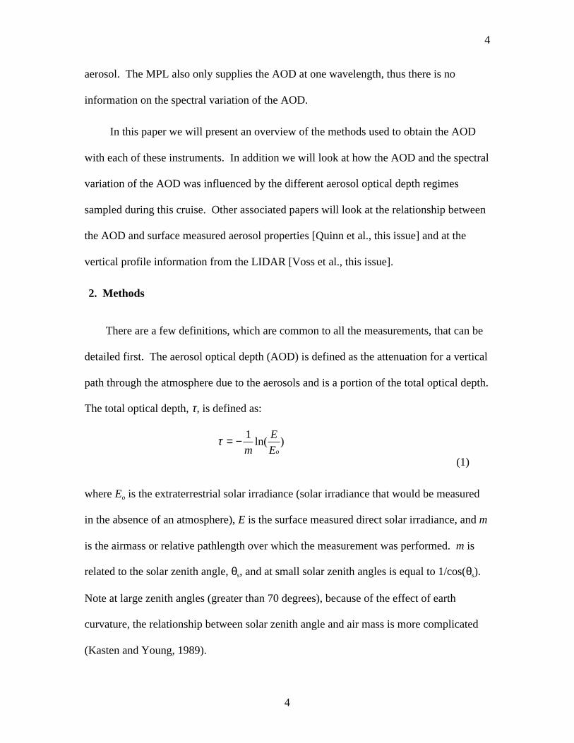
4
4
aerosol. The MPL also only supplies the AOD at one wavelength, thus there is no
information on the spectral variation of the AOD.
In this paper we will present an overview of the methods used to obtain the AOD
with each of these instruments. In addition we will look at how the AOD and the spectral
variation of the AOD was influenced by the different aerosol optical depth regimes
sampled during this cruise. Other associated papers will look at the relationship between
the AOD and surface measured aerosol properties [Quinn et al., this issue] and at the
vertical profile information from the LIDAR [Voss et al., this issue].
2. Methods
There are a few definitions, which are common to all the measurements, that can be
detailed first. The aerosol optical depth (AOD) is defined as the attenuation for a vertical
path through the atmosphere due to the aerosols and is a portion of the total optical depth.
The total optical depth, τ, is defined as:
(1)
where Eo is the extraterrestrial solar irradiance (solar irradiance that would be measured
in the absence of an atmosphere), E is the surface measured direct solar irradiance, and m
is the airmass or relative pathlength over which the measurement was performed. m is
related to the solar zenith angle, θs, and at small solar zenith angles is equal to 1/cos(θs).
Note at large zenith angles (greater than 70 degrees), because of the effect of earth
curvature, the relationship between solar zenith angle and air mass is more complicated
(Kasten and Young, 1989).
τ = − 1m
E
Eoln( )
5
5
Once τ is determined, the AOD can be determined by subtracting the contributions
to τ from molecular scattering (Rayleigh scattering, τR) [Penndorf, 1957] and molecular
absorption. The spectral regions measured are usually chosen to avoid regions of strong
molecular absorption, but the broad Chappius band absorption of O3 requires that
corrections be made for O3 absorption [Shaw, 1979]. Once O3 absorption, τO3, is
determined the AOD can be found by:
AOD = τ - τR - τO3. (2)
These parameters vary with the wavelength of light, hence the measurement wavelength
must be taken into account. The spectral variation of the AOD can be characterized by
the angstrom exponent, α, defined as:
(3)
λ1 and λ2 are two measurement wavelengths. The angstrom exponent is related to the
size distribution of the aerosol, small values imply a low spectral variation and large
particles, large α implies high spectral variation and more smaller particles.
Measurement of the AOD is a column averaged measurement, thus α derived from the
AOD is determined by the column averaged aerosol size distribution.
Details of the specific instrumentation and the methods used to calibrate and reduce
the data from these instruments will now be described.
α
λλ
λλ
= −ln(
( )( )
ln( )
AOD
AOD
1
2
1
2

6
6
2.1 Microtops
The 5-channel handheld Microtops sunphotometer (Solar Light Co.) used by NOAA
PMEL operated at 380, 440, 500, 675, and 870 nm. The full angular field of view is 2.5
deg. The instrument has built in pressure and temperature sensors and was operated with
a GPS connection to obtain position and time of the measurements. A MATLAB routine,
also used by the NASA SIMBIOS program and Brookhaven National Laboratory, was
used to convert the raw signal voltages from the Microtops to aerosol optical depths.
Included in the conversion is a correction for Rayleigh scattering [Penndorf, 1957], ozone
optical depth, and an air mass that accounts for the Earth’s curvature [Kasten and Young,
1989]. Ozone column amounts used to calculate the ozone optical depth were based on
ozonesonde measurements made during the cruise [Thompson et al., 2000] and, to fill in
data gaps, TOMS level 3 data. The instrument was calculated using a Langley plot
approach [Shaw, 1983] by the manufacturer prior to the cruise and again at Mauna Loa 5
months after the cruise. Calibration constants for the 5 wavelengths differed by less than
0.9% between the two calibrations, which corresponds to approximately 0.01 in optical
depth.
2.2 Simbad
The Simbad radiometer was designed to collect data on aerosol optical depth and
water-leaving radiance, the basic satellite ocean-color variables [Schwindling et al.,
1998]. Radiance is measured in five spectral bands centered at 443, 490, 560, 670, and
870 nm, total field-of-view is 3 degrees, and frequency of measurements is 10 Hz. In
sun-viewing mode, the instrument functions like a standard sun photometer, the only
difference being that the optics are fitted with a vertical polarizer. This polarizer reduces
7
7
reflected skylight and sunglint in the field-of-view when the instrument is operated in
sea-viewing mode. The polarizer is not an issue for sun intensity measurements, because
direct sunlight is not polarized. It takes 10 seconds to acquire a data set in sun-viewing
mode. Only the highest intensity during one-second (i.e., out of 10 measurements) is
stored automatically, to avoid pointing errors on a moving platform. Measurements were
made systematically from the bow of R/V Ron Brown when the solar path was free of
clouds, and repeated three times to reduce experimental errors.
Radiometric calibration was performed four times before and twice after the
experiment at Stevenson Peak (1,896 m), California using the Bouguer-Langley method.
No significant trend was detected in the calibration coefficients. The average log-
transformed numerical counts and standard errors after correction for Earth-Sun distance
are 12.656 ± 0.008, 13.014 ± 0.021, 12.906 ± 0.007, 12.920 ± 0.005, and 12.596 ± 0.008
at 443, 490, 560, 670, and 870 nm, respectively. The standard error is a measure of the
expected error on aerosol optical thickness due to calibration for an air mass of unity.
This error is inversely proportional to air mass. Except for the 490 nm spectral band, the
standard error is below 0.01 in optical depth.
Errors in molecular optical depth and ozone absorption will reduce the accuracy of
aerosol optical depth retrievals. Also, some scattered light may reach the detectors
because of the relatively large field-of-view (3 degrees), artificially increasing
atmospheric transmittance and, thus, decreasing aerosol optical depth. A 1% error on the
molecular optical depth at standard pressure and a 10hPa error on surface pressure would
give, for an air mass of 1, a 0.005 error in aerosol optical depth at 443 nm, decreasing to
practically zero at 870 nm. To compute ozone absorption, vertical ozone amount was

8
8
taken from ozone sondes deployed during the cruise [Thompson et al., 2000]. A 10%
error in ozone amount would translate into optical depth errors of 0.003 at 560 nm and
0.001 at 670 nm, and negligible (or nil) in the other spectral bands. These errors,
computed for an air mass of unity, increase with air mass. Regarding scattered light,
contamination is small in the presence of continental aerosols (i.e., <0.001 and 0.003 at
443 nm for an optical thickness of 0.05 and 0.2, respectively), but may be five to ten
times larger in the presence of maritime aerosols, due to the more pronounced forward
peak of the phase function. Although some errors may compensate, the absolute error
on aerosol optical depth is probably of the order of 0.02 (0.03 at 490 nm). Since the
absolute error is independent of optical depth, the relative error is inversely proportional
to optical depth, and becomes very large at low optical depth (e.g., about 50% at 443 nm
for an optical depth of 0.04).
2.3 Fast-Rotating Shadowband Radiometer
A shadowband radiometer measures the diffuse and global (upper hemispheric)
irradiance and computes E as the difference between the two. The device gets its name
from the hemispherical metal strip that rotates around the detector (the shadowband) and
blocks the direct solar beam to yield a signal that is from the sky only (after the effect of
the arm is included).
The multiple wavelength rotating shadow-band radiometer [Harrison et al.,1994]
uses independent interference-filter-photodiode detectors and an automated rotating
shadow-band technique to make spatially resolved measurements at seven wavelength
pass-bands. A marine version of the multiple wavelength rotating shadow-band
radiometer has been developed at the Brookhaven National Laboratory (BNL). The BNL

9
9
marine version uses a slightly modified version of the detector used for continental
applications. It has seven channels: one broadband silicon detector and six ten-nm-wide
channels at 415, 500, 610, 660, 870, and 940 nm. Modifications to the detector circuitry
used for continental applications are necessary because the response time of the original
circuitry is too slow for use on a moving ship. If the response time of the detector is too
slow, wave action may cause the orientation of the radiometer to change appreciably
during the time the shadow-band is occulting the sun. The rotation of the shadow-band
itself must be sufficiently fast for the same reason. The marine version of the shadow-
band radiometer is hereafter referred to as the BNL Fast-Rotating, Shadow-band
Radiometer (FRSR).
The shadow-band radiometer must properly measure the global and diffuse
irradiances from which the direct-beam irradiance is derived by the subtraction
EH= EG – ED (4)
where EH is the direct-beam irradiance projected onto a horizontal plane, EG is the global
irradiance on the horizontal plane, and ED is the diffuse irradiance from non-forward
scattering. The global irradiance, EG, is measured when the band is out of the field of
view and the sensor is exposed to full sunlight while ED is measured with the sensor
shadowed by the band. The irradiance normal to the incident beam, E in Eq. 1 is
computed by
E= EH /cos (θs). (5)
Corrections for the sky blocked by the occulting band and for roll and pitch of the sensor
head are made and discussed in detail in Reynolds et al. [2000]. The instrument
10
10
calibration coefficients for Aerosols99 were determined using the Langley technique at
Mauna Loa. Additional calibrations were performed during the cruise that showed good
agreement with the Mauna Loa data. The accuracy of the calibration coefficients is
thought to be about 5% and the accuracy of the irradiance measurements about 6%.
While the uncertainty in the AOD measurement also depends on the air mass, for typical
conditions, measurements of the AOD of sea-salt aerosol (due to its low AOD) are the
most uncertain.
Cloud filtering is the most important challenge for FRSR data processing. Because
the FRSR operates autonomously, cloud observations are naturally part of the signal that
must be processed to obtain τ. The cloud filter that is currently used is based on two
steps: computing signal statistics over windows of periods of less than two hours and
using these statistics to judge the quality of the observation under consideration. If the
standard deviation of the observations in a two-hour moving window is less than 0.05, a
subjectively defined threshold, and the observation at the center of the window is also
less than 0.05, the central observation is accepted. The underpinning of this cloud
filtering technique is that τ is relatively constant over a period of two hours, while the
cloud signal is highly variable. This approach has proven relatively successful, although
improvements in the filter are expected in the future.
2.4 Micropulse LIDAR
The Micropulse LIDAR (SESI, Burtonsville, MD) is a small compact LIDAR
system which averages high repetition, low energy pulses to obtain a profile of
attenuation/backscattering in the atmosphere [Spinhirne et al.,1995]. The Micropulse

11
11
LIDAR used during the cruise operated at 523 nm, with a pulse repetition rate of 2500
Hz, the vertical resolution was 75m, and data was collected to 30km. During the day the
signal above 10km became increasingly noisy due to a combination of attenuation in the
boundary layer and background sunlight at 523 nm, but during the night low noise data
could be obtained to 20km in the absence of clouds. The details of the algorithm to
derive the AOD from the micropulse LIDAR are detailed elsewhere [Welton, 1998,
Welton et al., 2000]. However an overview of the technique will be presented here.
The basic equation governing LIDAR propagation, when the LIDAR is vertically
oriented is:
(6)
Where Er is the received energy, Eo is the outgoing pulse energy, βr(180,z) is the
Rayleigh (molecular) backscattering, βa(180,z) is the aerosol backscattering, cr is the
Rayleigh attenuation, ca is the aerosol attenuation, and C is an instrument calibration
constant. The time the signal is received is related to the altitude, z, by the time it takes
for the LIDAR pulse to travel up to that altitude and back (z = tc/2, where c is the speed
of light). By using time resolved return signals, profiles of the backscattering and
attenuation can be obtained. C contains information on system parameters such as
throughput, solid angle acceptance of the receiver, divergence of the laser beam and other
parameters. While in principal this could be calculated [Spinhirne et al., 1980] in
practice it is much simpler and accurate to derive this parameter from measurements in
the field, as will be discussed below. For a practical LIDAR system such as the MPL,
Er t CEo z z c z c z dz zr a r a
z
( ) ( ( , ) ( , ))exp( [ ( ' ) ( ' )] ' ) /= + − ∗ +∫β β180 180 20
2

12
12
there are other important affects which must be taken into account, namely the overlap
function and afterpulse function. The overlap function describes the loss in signal
strength at close range. Signal loss is due to poor focusing to the detector by the MPL
telescope and optical design at close range (less than 4 km). Signals greater than the
overlap range are not effected by this problem. The afterpulse function is a result of
cross-talk between the laser pulse and detector, as well as dark noise in the system. Both
of these effects were corrected for in this data set in the manner described by Welton et
al.[2000].
If the calibration coefficient is known, and a clean layer above the aerosol layer can
be found where the backscattering and attenuation is dominated by Rayleigh scattering
then the returned energy from that altitude is simply:
(7)
Or
(8)
The later integral can be calculated, thus:
(9)
Er t CEo z c z c z dz zr r a
z
( ) ( , )exp( [ ( ' ) ( ' )] ' ) /= − ∗ +∫β 180 20
2
Er t CEo z AOD c z dz zr r
z
( ) ( , )exp( * )exp( ( ' ) ' ) /= − − ∗ ∫β 180 2 20
2
AODEr t z
CEo zc z dz
rr
z
= − − ∗ ∫12 180
22
0
ln[( )( , )
] ( ' ) ' )β
13
13
The measurement of the AOD with the LIDAR only requires finding a clean layer
above the aerosols and accurate calculation of the system calibration constant C. It is
important to note that this product does not depend on any assumption of the
extinction/backscatter ratio (S).
When the AOD is known from independent measurements (such as with a handheld
sunphotometer), the above equations can be turned around to determine the system
calibration constant C. During this cruise, during cloud free periods during the day,
episodic measurements of the AOD were made with an independent Microtops
sunphotometer (the data from this instrument are not included in this paper). Thus the
calibration coefficient was determined at intervals throughout the cruise. The calibration
coefficient was fit to a linear equation and varied during the cruise by 20%. The
accuracy of our calibration procedure is estimated to be +-6%, while the accuracy of the
AOD calculation is effected by this calibration coefficient, and the accuracy with which
the overlap and afterpulse corrections were made. The accuracy of the AOD determined
from the LIDAR is estimated to be + -0.05 in optical depth. The LIDAR AOD
calculation has the advantage that for boundary layer aerosols, it is the only method that
can determine the AOD during the night and in the presence of high cirrus. Care must be
taken in determining the level chosen to represent a clean atmosphere above the aerosol
[Welton et al., 2000]. This is usually obvious from the range corrected LIDAR signal by
looking for a region for which ln[Er(t)*z2] is decaying at the rate appropriate for Rayleigh
scattering.

14
14
2.5 Derivation of the angstrom exponent
Other than the LIDAR, all of the instruments measure the AOD at multiple
wavelengths close to simultaneously. For each of these instruments the angstrom
exponent was calculated using all the usable channels for that instrument (some channels
in specific instruments were not calibrated well, and were not included). The angstrom
exponent was calculated by determining the least squares fit to the line:
ln(AOD(λ)) = B – α ln(λ ),
(10)
for each measurement set (a set being the available wavelengths for a single instrument at
a given time). This was done throughout the data set, for each instruments AOD
measurement.
2.6 Compilation to averages for the days.
All the independent measurements of the AOD were compiled into a single data set
as shown in Figure 1, choosing the AOD at the wavelength of each instrument closest to
500nm. No effort was made to correct for the small wavelength differences between the
instruments. The largest wavelength difference was from 490nm to 523 nm, and with the
highest average angstrom exponent (1.2) this is only a 5% effect. As can be seen the
AOD varied strongly throughout the cruise depending on the atmospheric influences.
The divisions into regions were determined by the meterological data, calculated back
trajectories, trace gas distributions, and surface aerosol chemical and physical data [Bates
et al, this issue]. These regions will be discussed in more detail in the next section. For
comparison with the other data sets obtained, an average AOD and α for 1/4 day intervals
during the cruise had to be determined. For Region 4 and 1/28/99, because of almost
15
15
constant cloud cover, there was virtually no opportunity to measure the AOD with any
technique. For the rest of the cruise the average AOD and angstrom exponent were
calculated at 1/4 day intervals centered on Midnight, 0600, 1200, and 1800 UTC.
To determine the average AOD for a period, a 3rd order polynomial was fit to 1.5
days of data centered on the desired time. This polynomial was then used to interpolate
the AOD for the desired 1/4 day interval in increments of 1/200 day. For each period this
interpolated function was averaged to determine the AOD and is shown in Figure 1. For
noon and midnight (even and 0.5 day increments) the AOD is listed in Table 1. This
method was chosen to provide a true time average during that period and to avoid biasing
the average towards periods of many measurements. To get an estimate of the accuracy
of these averages, the standard deviation of the difference between this average and the
original data was determined. This standard deviation is shown in the figure as the error
bars on the average AOD data, and in Table 1.
The Angstrom exponent, α, was determined by simply averaging the data during
the relevant period, and is shown in Fig. 2. We chose to do this, rather than the method
chosen for AOD because the differences between separate measurements of α appeared
random. The errors bars on these graphs are determined by the standard deviation
between this average and the original data. The angstrom exponents and standard
deviation are also shown in Table 1. There are more periods without α data than for the
AOD since there were times when only the LIDAR obtained AOD measurements (for
example at night), and the LIDAR does not obtain α.
16
16
3. Results and discussion
We will first look at a comparison of the different instruments, then look at specific
regions of the cruise.
3.1 Instrument comparison
To investigate the variation in measurements between the different instruments, we
looked at three different days when the AOD appeared stable throughout the day. We
chose to do this so that we could get representative samples of each instrument. It was
difficult to find a time when all the instruments were working at exactly the same time,
because the handheld sunphotometers were most active at noon when the LIDAR was
turned off because of the low solar zenith angle. The three periods chosen were Day-of-
Year (DOY) 25, 30, and 37 (this corresponds to latitude ranges of 9.8° Ν – 6.9° N, 5.6° S
– 8.9° S, and 27.8° S – 30.4° S respectively).
Figure 3 shows the comparison between the instruments. In this figure the
AOD(500nm) is displayed for each instrument along with the standard deviation for the
individual instrument. We also show the average of the measurements during each day.
The averages, and standard deviations for each day are: 0.31 +0.03, 0.13+0.02, and 0.10
+ 0.02. It is interesting that the more standard handheld sunphotometers (the Scripps
Simbad, and the BNL and PMEL Microtops) had a constant difference (to within +0.01)
between them, as would be expected with small calibration offsets. The relationship
between these instruments and the non-traditional LIDAR and FRSR varied between the
days chosen however. It should be pointed out that the LIDAR and FRSR were averages
17
17
over longer periods (throughout the day for the LIDAR, and during daylight with the
FRSR). But overall the instruments agreed fairly well.
This uncertainty may affect the predictions of radiative forcing. In cloud-free
regions, the direct radiative forcing due to aerosols can be expressed as [e.g., Iacobellis et
al., 1999]:
F = µ0 E0 Ta2 G
(11)
with
G = R + T2As/(1 – AsR) - As (12)
R = ωοβ[1 – exp(-AOD/µ0)] (13)
T = exp(-AOD/µ0) + ωο (1 – β)[1 – exp(-AOD/µ0)] (14)
where µ0 is the sun zenith angle, E0 is the extraterrestrial solar flux, Ta is the
transmittance of the atmosphere above the aerosols, As is the albedo of the underlying
surface, R and T are the fraction of sunlight scattered and transmitted by the aerosol
layer, respectively, ωο is the single scattering albedo of aerosols, and β is the fraction of
scattering by aerosols which goes upwards.
The relative error on F, ∆F/F, due to error on AOD, ∆AOD, can be estimated from
Eq. (11) as:
∆F/F ≈ (1/G)(∂G/∂AOD)∆AOD (15)
Figure 4 displays ∆F/F as a function of AOD for µ0 = 0.8, β = 0.3, As = 0.1, ∆AOD=0.03,
and three values of ωο, from 1 (non-absorbing aerosol) to 0.6 (absorbing aerosol). Also

18
18
in Fig. 4 we show the ratio of ∆G/(G+As), which is effectively the error in
reflectance/(total reflectance), as a function of AOD and ωο. At small AOD (0.1) ∆F/F is
practically equal to ∆AOD/AOD. ∆F/F is only weakly dependent on ωο. If one looks at
∆G/(G+ As) (the error in surface +aerosol reflectance), because the aerosol adds little at
low AOD, the error in the combined surface/aerosol reflectance is less than 6% in all
cases.
3.2 Specific Regional Analysis
Bates et al. [this issue] separated the aerosol regions sampled on this cruise into 7
areas based on surface chemical and optical data and meteorological data. These regions
are shown in Figures 1 and 2 as Regions 2-7. The AOD and angstrom exponents with
their associated standard deviations are detailed in Table 2. In Region 1 there were very
few AOD measurements because of clouds and rain. The other Regions will now be
discussed.
3.2.1 Region 2: North Atlantic Marine airmass (31° N – 15.5° N)
In this Region the calculated 6 day back trajectories [Bates et al, this issue] were
mostly over the open ocean. This area was characterized by a very clean atmosphere
(AOD = 0.09 +0.02). The angstrom exponent was also low (0.27+0.27) indicating a
dominance by large particles. While the AOD measured by all instruments were fairly
consistent, the angstrom exponent had large variation. To some extent this is because at
low AOD, the angstrom exponent is difficult to determine and very dependent on the
accuracy of the individual instruments absolute calibration.

19
19
3.2.2 Region 3, African dust air mass (15.5° N – 8° N)
In this Region the chemical signature of the surface aerosols and the back
trajectories indicated that the major source of the aerosols was Northwest African dust.
Aerosol optical depth increased, with a lot of variability in the AOD. Average AOD was
0.29 (+ 0.05). The angstrom exponent remained low (0.36 + 0.13), as seen previously in
dust aerosols [Welton, 1998: Smirnov et al., 1998]. The variability in the angstrom
exponent between instruments was much lower with the increased AOD, indicating that
much of the earlier variability was probably caused by small calibration errors in the
individual instruments Eo.
3.2.3 Region 4, Mixed African dust and biomass burning (8° N – 3° N)
This Region was the beginning of the ITCZ. In this region we experienced almost
continuous boundary layer clouds, thus there were virtually no AOD measurements in
this region.
3.2.4 Region 5, Biomass burning in the ITCZ (3° N – 5° S)
This Region had the largest values and range of AOD. The AOD was 0.36 + 0.13.
Figure 1 shows the large excursions in the AOD experienced in this region. The
angstrom exponent was much larger (0.88 + 0.30) indicating a dominance by small
particles. The calculated back trajectories indicated that the source of the aerosol was
burning regions in southwestern North Africa [Bates et al., this issue]. After a peak at the
equator, the AOD slowly decreased as we moved south.

20
20
3.2.5 Region 6, South Atlantic Tropical Marine airmass ( 5°S – 24.5°S)
In this Region the surface concentrations of ozone and CO reached clean Southern
Hemisphere levels [Thompson et al. 2000]. However the column averaged measurement
of the AOD indicated that there was still an elevated signature of aerosols. The presence
of upper layer aerosols was confirmed in the LIDAR profile data [Voss et al., this issue].
The average AOD in this region was low (0.10 + 0.03), however there was definite
structure to the AOD with change in latitude. The angstrom exponent decreased from its
high in region 5 to 0.45 +0.20, however it had not decreased all the way to the values
seen in the Northern hemisphere marine airmass of region 2.
3.2.6 Region 7, South Atlantic temperate marine air mass (24.5°S – 33°S)
At this point the airmass trajectories indicated that the aerosols were dominantly
coming over the South Atlantic. Average AOD values were similar to the Northern
Hemisphere clean values (region 2) (0.10 +0.01), with angstrom exponents also similar to
Region 2 (0.35 + 0.07).
4.0 Conclusion
This cruise afforded the opportunity to sample a variety of aerosol regions with an
extensive set of chemical, physical, and optical instrumentation. The AOD and angstrom
exponent measured with the variety of instruments and techniques agreed fairly well and
afforded an opportunity to compare the various techniques. The handheld
sunphotometers and the FFRSR allowed the AOD and angstrom exponent to be measured
during completely cloudfree periods. The FFRSR, with the automatic sampling, could
measure the AOD during any daytime cloudfree period, but then depended on post-
21
21
processing to select valid measurements. The operators of the handheld instruments
could select cloudfree periods to measure, but obviously would not make measurements
continuously throughout the day. The LIDAR could obtain boundary layer AOD during
the night and in periods of high cirrus, however since it was only at one wavelength it
could not provide any measure of the angstrom exponent. However the
extinction/backscattering parameter, derived from the LIDAR inversion is related to the
size distribution, see Voss et al., [this issue]). Each instrument has it’s own advantages
and disadvantages and the combination of the techniques allows a more complete data set
to be obtained.
5. Acknowledgements
We thank the officers and crew of the NOAA Research Vessel Ron Brown. We
would like to acknowledge the support of NASA under contract #NAS5-31363 (KJV and
EW), NAS5-97135 (RF) and SIMBIOS # 52-210.91 (MM and RJR). Part of this work
(PKQ) was funded by the Aerosol Program of the NOAA Climate and Global Change
Program.
6. Reference
Angstrom, A., The parameters of atmosphere turbidity, Tellus, 16, 64 – 75, 1964.
Bates, T. S., P. K. Quinn, D. J. Coffman, J. E. Johnson, T. L. Miller, D. S. Covert,
A. Wiedensohler, S. Leinert, A. Nowak, and C. Neus, Regional Physical and Chemical
properties of the Marine Boundary Layer Aerosol across the Atlantic during Aerosols99:
An overview, submitted to J. Geophysical Research, this issue.

22
22
Harrison, L., J. Michalsky, and J. Berndt, Automated multi-filter rotating shadow-
band radiometer: an instrument for optical depth and radiation measurements, Applied
Optics, 33, 5126—5132, 1994.
Iacobellis, S. F., R. Frouin, and R. C. J. Somerville, 1999: Direct radiative forcing
by biomass-burning aerosols: impact of correlations between controlling variables. J.
Geophys. Res., 104, 12,031-12,045.
Kasten, F. and A. T. Young, Revised optical air mass tables and approximation
formula, Applied Optics, 28, 4735 – 4738, 1989.
Mueller J., C. McClain, R. Caffrey, and G. Feldman, The NASA SIMBIOS
Program, Backscatter, May, 29 – 32, 1998.
Penndorf, R. , Tables of refractive index for standard air and the Rayleigh scattering
coefficient for the spectral region between 0.2 and 20 um and their application to
atmospheric optics, J. Opt. Soc. America, 47, 176 - 182, 1957.
Quinn, P. K., D. J. Coffman, T. S. Bates, T. L. Miller, J. E. Johnson, K. J. Voss, E.
J. Welton, C. Neususs, Dominant Aerosol Chemical Components and their contribution
to extinction during the Aerosols99 Cruise across the Atlantic, submitted to J. Geophys.
Res., this issue.
Reynolds, R. M., M. A. Miller, and M. J. Bartholomew, Design, Operation, and
Calibration of a Shipboard Fast-Rotating Shadow-band Spectral Radiometer, Jour.
Atmos. Oceanic. Technology (accepted), 2000.
Schwindling, M., P.-Y. Deschamps, and R. Frouin, Verification of aerosol models
for satellite ocean color remote sensing. J. Geophys. Res., 103, 24,919-24,935, 1998.

23
23
Shaw, G. E., Atmospheric Ozone: Determination by Chappuis Band Absorption, J.
Appl. Met., 18, 1335 – 1339, 1979.
Shaw, G. E., Sun Photometry, Bull. Am. Met. Soc., 64, 4-9, 1983.
Smirnov, A., Holben, B. N., Slutsker, I., Welton, E. J. and Formenti, P., Optical
properties of Saharan dust during ACE-2, J. Geophys. Res. 103, 28079 – 28092, 1998.
Spinhirne, J. D., Rall, J., and V. S. Scott, Compact eye-safe LIDAR systems, Rev.
Laser Eng., 23, 26 – 32, 1995.
Spinhirne, J. D., J. A. Reagan, and B.M. Herman, Vertical Distribution of Aerosol
Extinction Cross Section and Inference of Aerosol Imaginary Index in the Troposphere
by LIDAR Technique, J. Appl. Meteorol., 19, 426-438, 1980.
Thompson, A. M., B. G. Doddridge, J. C. Witte, R. D. Hudson, W. T. Luke, J. E.
Johnson, B. J. Johnson, S. J. Oltmans, R. Weller, Shipboard and Satellite views of a
tropical Atlantic tropospheric ozone maximum and wave-one in January-February 1999,
Geophysical Res. Letters, submitted 2000.
Voss, K. J., E. J. Welton, J. Johnson, A. Thompson, P. Quinn, and H. Gordon,
LIDAR measurements during Aerosols99. Submitted, J. Geophys. Res. this issue.
Welton, E. J. Measurements of Aerosol Optical Properties over the Ocean using
Sunphotometry and LIDAR, Ph. D. Dissertation. University of Miami, Coral Gables, 1-
150, 1998.
Welton, E. J., J. R. Campbell, J. D. Spinhirne, and V. S. Scott, Aerosol and Cloud
measurements using micropulse LIDAR systems, J. Atmos. Oceanic Tech. Submitted,
2000.
24
24
Figure Captions
Figure 1) Aerosol optical depth at approximately 500nm for each instrument and the
average values. Error bars are displayed on the average values, derived from the
standard deviation between the average and the measurements. Regions 2-7 are
displayed on graph as discussed in section 3.2.
Figure 2) The variation in angstrom exponent throughout the cruise. Regions are
displayed as in Figure 1. Average angstrom exponent and standard deviation
between this average and the data are displayed.
Figure 3) Comparison between instruments for three days, DOY 25, 30, and 37.
Each instruments average measurement for the period is displayed, along with the
standard deviation. The line in each segment is the average of all the instruments
for that day.
Figure 4) Error in calculated forcing with ∆AOD = 0.03 vs. AOD. Also displayed is
the fractional error in the total (surface +aerosol) reflectance due to this 0.03 error
in AOD. In the calculation µ0 = 0.8, β = 0.3, and As = 0.1.
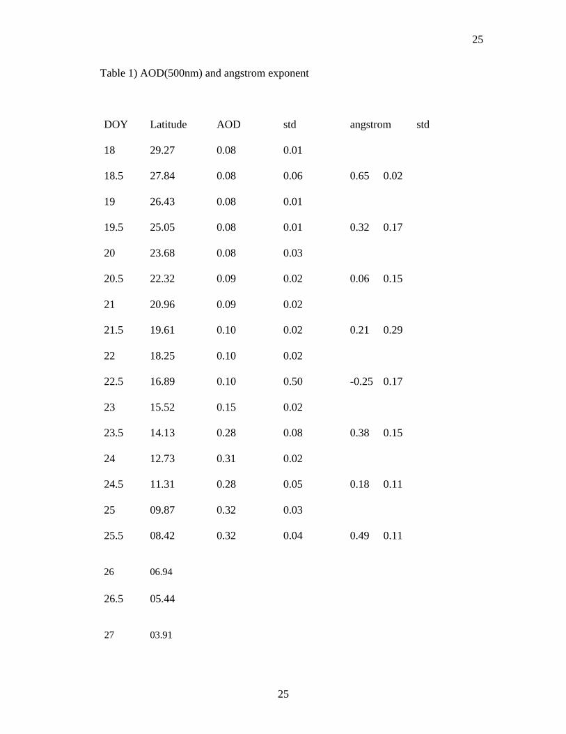
25
25
Table 1) AOD(500nm) and angstrom exponent
DOY Latitude AOD std angstrom std
18 29.27 0.08 0.01
18.5 27.84 0.08 0.06 0.65 0.02
19 26.43 0.08 0.01
19.5 25.05 0.08 0.01 0.32 0.17
20 23.68 0.08 0.03
20.5 22.32 0.09 0.02 0.06 0.15
21 20.96 0.09 0.02
21.5 19.61 0.10 0.02 0.21 0.29
22 18.25 0.10 0.02
22.5 16.89 0.10 0.50 -0.25 0.17
23 15.52 0.15 0.02
23.5 14.13 0.28 0.08 0.38 0.15
24 12.73 0.31 0.02
24.5 11.31 0.28 0.05 0.18 0.11
25 09.87 0.32 0.03
25.5 08.42 0.32 0.04 0.49 0.11
26 06.94
26.5 05.44
27 03.91

26
26
27.5 2.37 0.42 0.03 1.21 0.12
28 0.80 0.37 0.04
28.5
29 -02.38 0.41 0.04
29.5 -04.01 0.22 0.02 0.74 0.12
30 -05.64 0.17 0.02
30.5 -07.28 0.13 0.02 0.70 0.31
31 -08.94 0.10 0.01
31.5 -10.60 0.08 0.02
32 -12.26 0.07 0.02
32.5 -13.92 0.09 0.02
33 -15.57 0.15 0.02
33.5 -17.21 0.10 0.01
34 -18.83 0.07 0.02
34.5 -20.42 0.07 0.05 0.46 0.28
35 -21.99 0.08 0.02
35.5 -23.52 0.11 0.02 0.32 0.20
36 -25.01 0.11 0.03
36.5 -26.44 0.10 0.03
37 -27.82 0.10 0.03
37.5 -29.13 0.10 0.02 0.44 0.13
38 -30.37 0.09 0.02
38.5 -31.52 0.07 0.02 0.28 0.08

27
27
Table 2 AOD and Angstrom exponent broken down by region
Region AOD std Angstrom exponent std
2 0.09 0.02 0.27 0.28
3 0.29 0.05 0.36 0.13
4 0.41 0.16 0.52
5 0.36 0.13 0.88 0.30
6 0.10 0.03 0.45 0.20
7 0.10 0.01 0.35 0.07

4
4
Figure 1) Aerosol optical depth at approximately 500nm for each instrument and the
average values. Error bars are displayed on the average values, derived from the
standard deviation between the average and the measurements. Regions 2-7 are
displayed on graph as discussed in section 3.2.
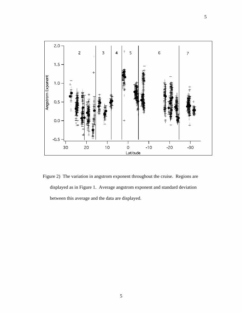
5
5
Figure 2) The variation in angstrom exponent throughout the cruise. Regions are
displayed as in Figure 1. Average angstrom exponent and standard deviation
between this average and the data are displayed.

6
6
Figure 3) Comparison between instruments for three days, DOY 25, 30, and 37.
Each instruments average measurement for the period is displayed, along with the
standard deviation. The line in each segment is the average of all the instruments
for that day.
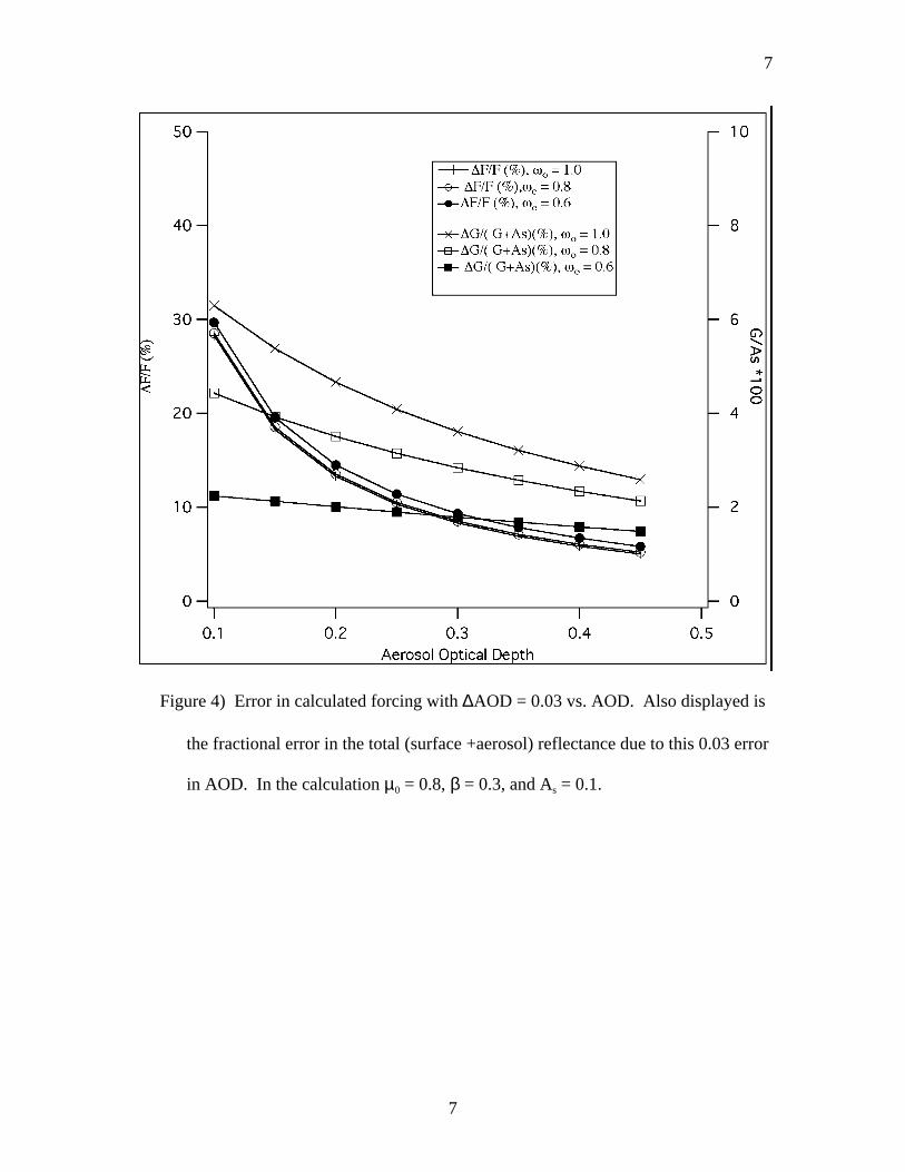
7
7
Figure 4) Error in calculated forcing with ∆AOD = 0.03 vs. AOD. Also displayed is
the fractional error in the total (surface +aerosol) reflectance due to this 0.03 error
in AOD. In the calculation µ0 = 0.8, β = 0.3, and As = 0.1.

Appendix VI
Lidar Measurements During Aerosols99
(Submitted to Journal of Geophysical Research)

1
1
LIDAR measurements during Aerosols99
Kenneth J. Voss(1), Ellsworth J. Welton(2), Patricia K. Quinn(3,4), James Johnson(3,4), Anne
Thompson(5), and Howard R. Gordon(1)
(1) Department of Physics, University of Miami, Miami, Fl.
(2) SSAI, NASA-GSFC, Code 912, Greenbelt, Md.
(3) Pacific Marine Environmental Laboratory, NOAA, Seattle, Wa.
(4) Joint Institute for the Study of Atmosphere and Ocean, University of Washington,
Seattle,Wa.
(5) Atmospheric Chemistry and Dynamics Branch, NASA/Goddard Space Flight Center,
Greenbelt, Md.
Running title: LIDAR during Aerosols99
*Corresponding author email address: [email protected]
GAP index numbers: 0305, 0649, 0315, 3360, 9325
Submitted J. Geophysical Res., 6/29/00, Aerosols99 Special Section
2
2
Abstract
The Aerosols99 cruise took place during the period from January 14, to February 8
1999 on the R/V Ron Brown. The cruise track was almost a straight line from Norfolk,
Va. to Cape Town, South Africa and afforded the opportunity to sample several different
aerosol regimes over the North and South Atlantic. A Micro Pulse LIDAR system was
used continually during this cruise to profile the aerosol vertical structure. Inversions of
this data illustrated a varying vertical structure depending on the dominant air mass. In
clean maritime aerosols in the Northern and Southern Hemispheres the aerosols were
capped at 1 km. When a Dust event from Africa was encountered the aerosol extinction
increased its maximum height to above 2 km. During a period in which the air mass was
dominated by biomass burning from Southern Africa, the aerosol layer extended to 4
km. Comparisons of the aerosol optical depth derived from LIDAR inversion and
surface sunphotometers showed an agreement within +0.05 RMS. Similar comparisons
between the extinction measured with a nephelometer and particle soot absorption
photometer (at 19 m altitude) and the lowest LIDAR measurement (75 m) showed good
agreement (+0.014 km-1). The LIDAR underestimated surface extinction during periods
when an elevated aerosol layer was present over a relatively clean surface layer, but
otherwise gave accurate results.

3
3
1. Introduction
The Aerosols99 cruise took place during the period from January 14, to February 8
1999 on the R/V Ron Brown. The cruise track was almost a straight line from Norfolk,
Va. to Cape Town, South Africa and afforded the opportunity to sample several different
aerosol regimes over the North and South Atlantic. A multidisciplinary group
participated on this cruise allowing for the measurement of an extensive suite of
chemical, physical, and optical properties of the surface aerosol [Bates et al. this issue].
Along with these surface measurements a Micropulse LIDAR system [SESI,
Burtonsville, MD] [Spinhirne et al., 1995] was operated continually to provide vertical
profile information on the aerosol distribution. Ozonesondes and Radiosondes provided
profiles of the temperature, humidity, and ozone distribution, which gave additional
information on the structure of the atmosphere. Finally 5-day meteorological back
trajectories provided information on the sources of the sampled aerosols. All of this
information, when combined, gives a more complete picture of the aerosol structure over
the Atlantic.
The cruise track presented a chance to look at many of the aerosol regimes over the
Atlantic. This cruise track was impacted by aerosols from the North American
continent, by Saharan Dust, by biomass burning on the African continent, and by clean
maritime air in the regions between. There is very little information on the vertical
distribution of the aerosols over the ocean, yet the vertical distribution of these aerosols
can impact the accuracy of climate models and atmospheric corrections needed for
retrieving ocean color. The Saharan Dust and biomass burning aerosols typically absorb
4
4
light. While atmospheric correction of ocean color imaging can be done for non-
absorbing aerosols without knowledge of the aerosol vertical structure [Gordon, 1997)]
the optical effect of absorbing aerosols is very dependent on the vertical structure
[Gordon et al., 1997]. Aerosol models for atmospheric correction of ocean color
imagery must account for this vertical structure when dealing with absorbing aerosols,
yet there is little data available on this problem. This cruise offered an excellent
opportunity to measure the aerosol vertical structure and have an extensive set of
correlated measurements of the boundary layer aerosol.
In addition to atmospheric correction, it is important to have information on the
vertical structure to understand how the surface measurements of the aerosol properties
are related to the aerosols in the rest of the atmospheric column. A LIDAR gives direct
information on the vertical distribution of aerosols. At times the surface measurements
can be very different from the column above [Welton et al., 2000]. The LIDAR
provides additional information that can be used to extend the surface measurements or
show the presence of other layers above the surface.
During this cruise a micro pulse LIDAR [Spinhirne et al., 1995] was used to provide
the vertical structure information. This LIDAR is a very compact system and was
operated continuously during the cruise. With careful calibration and data reduction,
accurate information on the aerosol vertical structure of the atmosphere can be obtained.
This cruise allowed us to look at the relationship between the vertical structure of the
aerosols, relative humidity (RH), temperature, surface physical and chemical aerosol
properties, and back trajectories.
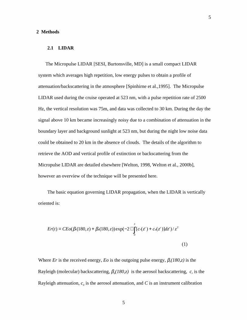
5
5
2 Methods
2.1 LIDAR
The Micropulse LIDAR [SESI, Burtonsville, MD] is a small compact LIDAR
system which averages high repetition, low energy pulses to obtain a profile of
attenuation/backscattering in the atmosphere [Spinhirne et al.,1995]. The Micropulse
LIDAR used during the cruise operated at 523 nm, with a pulse repetition rate of 2500
Hz, the vertical resolution was 75m, and data was collected to 30 km. During the day the
signal above 10 km became increasingly noisy due to a combination of attenuation in the
boundary layer and background sunlight at 523 nm, but during the night low noise data
could be obtained to 20 km in the absence of clouds. The details of the algorithm to
retrieve the AOD and vertical profile of extinction or backscattering from the
Micropulse LIDAR are detailed elsewhere [Welton, 1998, Welton et al., 2000b],
however an overview of the technique will be presented here.
The basic equation governing LIDAR propagation, when the LIDAR is vertically
oriented is:
(1)
Where Er is the received energy, Eo is the outgoing pulse energy, βr(180,z) is the
Rayleigh (molecular) backscattering, βa(180,z) is the aerosol backscattering, cr is the
Rayleigh attenuation, ca is the aerosol attenuation, and C is an instrument calibration
Er t CEo z z c z c z dz zr a r a
z
( ) ( ( , ) ( , ))exp( [ ( ' ) ( ' )] ' ) /= + − ∗ +∫β β180 180 20
2
6
6
constant. The time the signal is received is related to the altitude, z, by the time it takes
for the LIDAR pulse to travel up to that altitude and back (z = tc/2, where c is the speed
of light). By using time resolved return signals, profiles of the backscattering and
attenuation can be obtained. C contains information on system parameters such as
throughput, solid angle acceptance of the receiver, divergence of the laser beam and
other parameters. While in principal this could be calculated [Spinhirne et al., 1980], in
practice it is much simpler and more accurate to derive this parameter from
measurements in the field, as will be discussed below. For a practical LIDAR system
such as the MPL, there are other important effects which must be taken into account,
namely the overlap and afterpulse functions. The overlap function describes the loss in
signal strength at close range. Signal loss is due to optical design and to poor focusing
to the detector by the MPL telescope at close range (less than 4 km). Signals at ranges
greater than the overlap range are not effected by this problem. The afterpulse function
is a result of cross-talk between the laser pulse and detector, as well as dark noise in the
system. Both of these effects were corrected for in this data set in the manner described
by Welton et al.[2000b].
When the AOD is known from independent measurements (such as with a handheld
sunphotometer) the system calibration constant C can be determined [Welton et al.,
2000b]. During cloud free periods during the cruise, episodic measurements of the AOD
were made with a Microtops sunphotometer (Solar Light Co., Philadelphia, PA). For the
LIDAR profile corresponding to the AOD measurement, a clean aerosol free layer above
the boundary layer is found (for this cruise this was typically 6-7 km). This is usually
obvious from the range corrected LIDAR signal by looking for a region for which
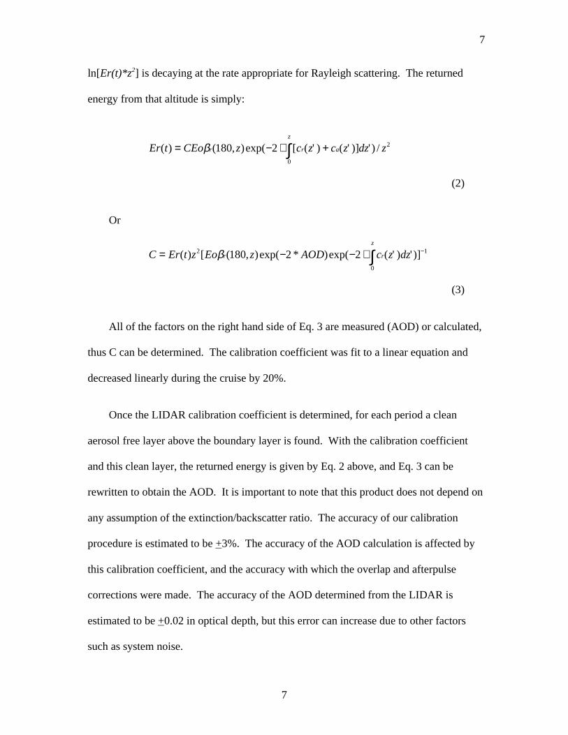
7
7
ln[Er(t)*z2] is decaying at the rate appropriate for Rayleigh scattering. The returned
energy from that altitude is simply:
(2)
Or
(3)
All of the factors on the right hand side of Eq. 3 are measured (AOD) or calculated,
thus C can be determined. The calibration coefficient was fit to a linear equation and
decreased linearly during the cruise by 20%.
Once the LIDAR calibration coefficient is determined, for each period a clean
aerosol free layer above the boundary layer is found. With the calibration coefficient
and this clean layer, the returned energy is given by Eq. 2 above, and Eq. 3 can be
rewritten to obtain the AOD. It is important to note that this product does not depend on
any assumption of the extinction/backscatter ratio. The accuracy of our calibration
procedure is estimated to be +3%. The accuracy of the AOD calculation is affected by
this calibration coefficient, and the accuracy with which the overlap and afterpulse
corrections were made. The accuracy of the AOD determined from the LIDAR is
estimated to be +0.02 in optical depth, but this error can increase due to other factors
such as system noise.
Er t CEo z c z c z dz zr r a
z
( ) ( , )exp( [ ( ' ) ( ' )] ' ) /= − ∗ +∫β 180 20
2
C Er t z Eo z AOD c z dzr r
z
= − − ∗ ∫ −( ) [ ( , )exp( * )exp( ( ' ) ' )]2
0
1180 2 2β

8
8
With the AOD determined, an inversion must be made of the LIDAR return signal
to obtain the extinction or backscattering profile. Since the LIDAR return depends on
both the backscattering and extinction of the aerosols and molecules this leads to 4
variables to find from one input. The molecular ( Rayleigh) backscatter and extinction
coefficients can be calculated, reducing the unknowns. To reduce the number of free
variables an assumption is made about the ratio between the extinction and backscatter
coefficient, otherwise known as S (units are sr). We use a top-down inversion with a
constant S for aerosols [Fernald et al., 1972, Fernald, 1984, Welton et al., 2000b], our
exact method is described in detail in Welton [1998] and Welton et al.[2000b]. In this
method the LIDAR equation is re-written in the form:
(4)
Where Sa is S for aerosols. An inversion of the LIDAR return signal is performed, with
an initial guess for Sa, to determine the profile of ca(z). This profile is then integrated and
compared with the AOD obtained from Eq.. 3. Sa is adjusted with this result, and the
procedure is iterated. This process is continued until the AOD and the integrated profile
of ca(z) agree within 0.5%. Since Sa is assumed to be constant, βa(180,z) is just ca(z)/ Sa.
The final accuracy of this inversion depends on the assumption of a constant Sa
through the aerosol layer. With additional information this constraint could be removed,
but without this errors are introduced. Even without changes in aerosol composition,
changes in RH can effect Sa by changing the size distribution and index of refraction of
Er t CEo z c z S c z c z dz zr a a r a
z
( ) ( ( , ) ( ) / )exp( [ ( ' ) ( ' )] ' ) /= + − ∗ +∫β 180 20
2
9
9
the aerosols [Ackermann, 1998]. The radiosonde data (discussed below) indicated that
the variation in RH through the aerosol layer changed between the different regions along
the cruise track(defined below). The constant Sa that is determined from the LIDAR
inversion is a column averaged Sa. The errors introduced by this assumption will be
discussed in more detail in the discussions of the individual regions and a comparison
with the surface extinction measured with a nephelometer and a PSAP.
2.2 Radiosonde
Radiosondes, [Vaisala, RS80-15GH] were launched from the deck of the ship at
10:45 and 22:45 UTC each day. This launch time ensured that each radiosonde would be
in the middle of its profile during the synoptic times of 0000 and 1200 UTC. The
radiosondes measured vertical profiles of temperature, relative humidity, and horizontal
winds. The winds were calculated from GPS measurements of the sonde horizontal
position. Most radiosonde profiles extended to at least 15 km altitude. The sondes
transmitted one data point every 10 seconds so that the raw data from the sondes (used
here) had a vertical resolution of 20 to 40 meters.
To help define the variation of temperature with altitude, the rate of change of the
temperature with altitude, ∆T/∆z, was derived from the temperature data. ∆T/∆z (°C/km)
was calculated by using a sliding five point least-squares-fit to the temperature data (+ 2
points around the specific altitude). This altitude interval is approximately 100-200 m.
2.3 Back-trajectories
Five day back-trajectories were made using the isentropic trajectory model at
Goddard Space Flight Center/NASA [Schoeberl et al., 1992]. These trajectories were
10
10
initialized from the position of the ozonesonde launches along the cruise track. Clusters
of back-trajectories were run from each launch to capture the uncertainties associated
with analyzed winds (Numerical Center for Environmental Prediction (NCEP) 2.5 X 2.5
deg).
3 Results
The first discussion will compare LIDAR-derived AOD and extinction to AOD and
extinction derived from independent measurements. We will then look at the overall
LIDAR cruise data and investigate the results of the LIDAR and other vertical profile
information for specific cruise regions.
3.1 AOD comparison
Voss et al. [this issue] shows the complete data set of AOD measurements obtained
during the cruise, including the LIDAR measurements. This data set included a set of 3
Microtops Sunphotometers [Solar Light Co., Philadelphia, PA] independent of the one
used to calibrate the LIDAR. To investigate the agreement between the LIDAR derived
AOD and the sunphotometer AOD we grouped the LIDAR data and Sunphotometer data
into common 72-minute measurement periods. In Fig. 1 the comparison between the two
data sets are shown for all periods which have measurements with both techniques. The
error bars for the sunphotometer measurement is the standard deviation of the distribution
of sunphotometer measurements during the specific interval. The LIDAR error bars are
due to the uncertainty in the LIDAR calibration constant, and signal noise (including
afterpulse and overlap noise). The line in the figure is the 1:1 line. The agreement
between the two methods is good, the RMS difference is 0.05 (optical depth). For larger

11
11
AOD the LIDAR AOD appears slightly higher than the sunphotometer AOD. The
difference could be due to the LIDAR technique, to different measurement volumes (the
LIDAR is vertical, the sunphotometer measures along the solar path), or differences in
the specific measurement time in the 72 minute period. In general though the LIDAR
derived AOD agrees with the standard sunphotometer technique to within the stated
errors.
3.2 Surface extinction comparison
We did not have simultaneous measurements of the vertical extinction profile from
an independent source (such as an aircraft) during this cruise, however we have done this
in the past and compared this data with the LIDAR inversion with good results (Welton
et al., 2000). During this cruise we had surface scattering and absorption measurements
[Quinn et al., this issue] with which to compare the lowest altitude bin of the LIDAR.
The aerosol was sampled at 19 m altitude with an integrating nephelometer (TSI Model
3563) and a particle soot absorption photometer (PSAP, Radiance Research). The
scattering coefficient (measured at 55% RH and 550nm) was adjusted to ambient RH
using the RH measured on the ship and previously measured f(RH) relationships. For the
marine air mass regions, f(RH) for the light scattering coefficient was based on
measurements during onshore flow at Cape Grim, Tasmania [Carrico et al., 1998]. In
continentally-influenced regions f(RH) from continental air masses at Sable Island, Nova
Scotia [McInnes et al., 1998] was used. For the light absorption coefficient (measured at
55% RH and 565 nm), f(RH) was assumed to equal one.
12
12
These surface extinction measurements were compared with the extinction retrieved
from the LIDAR inversion at the lowest altitude bin (75 m). The comparison through the
cruise is shown in Fig. 2. The agreement is generally very good, but there are specific
regions for which the agreement is not as good. Figure 3 shows the comparison of the
two measurements more quantitatively. The RMS difference between the two
measurements was 0.014 km-1. In this figure the measurements are broken into regions as
defined later in the text (section 3.4). The most pronounced bias between the two
measurements occurs during portions of Region 5 and at the beginning of Region 6 (to
approximately 13° S). The extreme of this is near 5°-10° S when the surface values of
the LIDAR are set to zero. During this period we had an elevated aerosol above a clean
marine boundary layer (MBL) (MBL properties were determined from the surface
chemistry measurements [Quinn et al., this issue]). In the portions of Region 5 (the lower
surface extinction areas) and in Region 6a, the total column AOD did not decrease as
much as the surface extinction did. When there is an elevated aerosol layer above a clean
(or relatively clean) lower layer, the lidar inversion underestimates the extinction in the
lower layer. It could also be that this difference is simply due to the different sampling
altitudes and this effect is most important in this region. In general the LIDAR inversion
worked well even in the near field, which has the most difficulties due to calibration
difficulties. However, this analysis shows a case where the surface LIDAR data may be
suspect because of the presence of an elevated aerosol layer over the relatively clean
surface layer
3.3 LIDAR data through cruise
13
13
Figure 4 shows the contour plot of the extinction profile during the cruise. The
contour plot is built from the LIDAR data, with 75m vertical resolution and at the data
points marked at the bottom of the graph. Gaps in data were predominately due to
clouds; however, during periods of high sun angle (solar noon) the LIDAR was turned
off to avoid direct sunlight entering the detector (this also had to take into account
possible ship roll, as direct sunlight would cause a complete failure of the system). Also
delineated in the figure is the division into regions, discussed in detail below. As can be
seen there was a large variation in both vertical structure and magnitude of the extinction,
which was dependent on both location and recent meteorological transport.
While the aerosol obviously reached higher levels near the equator, it is also
interesting to see how the aerosol is distributed, proportionately, for a given profile.
Figure 5 shows a contour of the integrated extinction coefficient. This was calculated as:
IntegratedExtinction z
c z dz
c z dz
a
z
a
km( )
( ' ) '
( ' ) '
*=∫
∫0
0
6 100
(5)
Once again the data points on which the contours were produced are shown at the bottom
of the graph. Before 8 N and after 15 S, 25% and 50% lines (the altitude at which 25 and
50% of the AOD has been accounted for already) are fairly constant at 0.5 km and 0.8
km. The 75% and 90% lines, during this time, show periods for which more aerosol
(relative to the rest of the column) was added at 1-1.5km (approximately 14 N and 20S).
Between 8 N and 15S the surface layer is cleaner than the elevated layers. Thus all the
contours rise during this period. In particular at the beginning of region 6 the 90% level
14
14
was the highest of the cruise. At this time there was a very clean lower level, and an
elevated aerosol. While the optical depth [Voss et al, this issue] and extinction (Figure 4)
were not maximum here, the clean lower level had the effect of making the upper
aerosols a more important contribution to the column properties.
Figure 6 shows Sa derived from the LIDAR inversions through the cruise, also
shown are the error bars on this derived parameter [method described in Welton et al.,
2000b]. These will also be discussed in the specific regional discussions below, but the
main feature is that during the periods of low total column extinction and low AOD, in
regions 2 and late 6, Sa tended to have low values characteristic of maritime aerosols.
During the periods of high AOD and high total column extinction, Sa was higher, typical
of smaller particles and continental aerosols.
3.4 Specific regional vertical structure features
We will now discuss the differences in vertical structure of the lower atmosphere
(<7 km) defined for the different regions. These regions were defined by surface trace gas
concentrations, aerosol chemical and physical properties, and trajectories at the 500 m
arrival height, [Bates et al., this issue], and may be somewhat different than those defined
by other information with vertical profiles such as LIDAR or ozonesondes [Thompson et
al. 2000]. The five day back-trajectories are shown in Fig. 7 and 8. The trajectories
shown correspond to the weighted central point in each cluster at 1km and 4km levels.
Time of trajectory initiation is 12Z with crosses marking every 24hr. For each region a
typical radiosonde/LIDAR profile is shown. In each case the figure shows the radiosonde
data (RH and ∆T/∆z) along with the average of three LIDAR extinction coefficient

15
15
profiles obtained within 1 hour of the radiosonde profile. Because of intense clouds there
are no LIDAR data for Region 1, so we begin our discussion with Region 2.
3.4.1 Region 2: Northern Hemisphere clean (31° N – 15.5° N)
In this region back trajectories at 1km and 4 km indicated that the airmass origin
was over the North Atlantic (Figs. 7 and 8). Surface measurements of the aerosol
chemistry indicated that the aerosol was clean maritime aerosol [Bates et al., this issue].
Example radiosonde and LIDAR profiles from this region (for DOY 18.5, N 27.7°) are
shown in Figure 9.
In the example shown there is a strong temperature inversion at 1 km, and another
at 2 and 4.5 km. The RH, in this example, stayed relatively constant at 80+10% up to 3
km. The aerosol was capped by the 1 km inversion, as witnessed by the LIDAR
extinction coefficient. In general the extinction coefficient was low throughout this
region (less than 0.2 km-1 peak), and the peak extinction coefficient was below 1 km, with
very little extinction above 1 km (this example had the largest extinction above 1 km).
The extinction profiles indicated that 90% of the AOD occurred below 2-3 km. The
temperature structure seemed to vary, with strong inversions often occurring between 1-
1.5 km. These temperature inversions were typically associated with the top of the
aerosol layer. Relative humidity was generally above 80% throughout the aerosol layer.
Since the surface chemistry and back trajectories all indicated that this was a
maritime atmosphere, there is no indications that there were drastic changes in aerosol
composition in the aerosol layer. With the RH limited between 80 and 100%,
Ackermann’s model [Ackermann, 1998] for Sa for a maritime atmosphere, indicates that
16
16
the value should be approximately 25, with RH effects only indicating a range from 23-
27. Thus our assumption of a constant Sa is a reasonable approximation in this region.
We found that the Sa average for this region was 32+6 sr, which is near the values derived
above. As discussed elsewhere [Voss et al, this issue] the AOD was low in this region
(around 0.09+0.02) with a low angstrom exponent (0.27+0.27). The low angstrom
exponent correlated with the low Sa indicating that the aerosol size distribution was
weighted towards larger particles.
One final feature in this region was that initially the RH stayed high (>60%)
throughout the column below 7 km. At 25° N the structure changed, becoming dryer
above 3 km. By 23.7° N the humidity was less than 10% between 3 and 6 km, with some
excursions above 10% occurring between 6 and 7 km. Since this was above the aerosol
layer, there was no visible effect on the aerosol vertical structure. A more complete
picture of the vertical profile of RH through the cruise is shown in Bates et al. [this
issue].
3.4.2 Region 3: Dust (15.5° N – 8° N)
During the next portion of the cruise we had a significant dust event that changed
the surface and vertical aerosol structure. Back trajectories at 1 km showed the aerosol
source switching to the coast of Africa, with 4 km trajectories still coming from the North
Atlantic.
A typical example of the vertical structure is shown in Fig. 10 for Day 24.5, N
11.2°. The radiosonde data throughout this period indicated a strong temperature
inversion at 1.5 km and another temperature feature at 4-5 km. The RH was relatively

17
17
constant at 80-100% in the lower layer, below the 1.5 km temperature inversion.
However at this inversion the RH decreased rapidly to 20-40%. The RH stayed constant
at this level to the upper temperature feature (4-5 km) where it seemed to decrease to near
0%RH for a 1 km layer, after which it would increase back to 20-40%.
The LIDAR profile data showed two distinct layers, with a sharp minimum in
extinction between them. The lower layer was capped by the temperature inversion at 1.5
km. The upper layer peaked at 2 km, with a subsequent gradual decrease with altitude.
By 4 km the aerosol extinction was very low (<0.02 km-1). The peak extinction in the
lower layer was approximately 0.3 km-1, while the peak extinction in the next layer was
approximately 0.1 km-1, so most of the AOD occurred in the lower layer. During this
period, 90% of the AOD occurred below 2-3 km.
The column averaged Sa during this period was 41+8 sr. This is significantly higher
than the Sa predicted by Ackermann (1998) for desert aerosols. Ackermann’s work
assumed spherical particles, however dust particles are often non-spherical which
increases Sa by decreasing the backscattering at 180 degrees. This value for Sa agrees
with earlier measurements by Welton et al. [2000]. In this region while the RH in each
layer was relatively constant, the RH changed significantly between the upper and lower
layer (80-100% to 40%). However because desert aerosol responds only weakly to RH,
this change effects Sa very weakly (less than 10% change in Sa [Ackermann, 1998]).
Thus changes in the Sa due to humidity are not expected. With the upper layer being very
distinct, it is possible that a different aerosol was in the upper layer, however we have no
in-situ chemical information on this layer to say what the layer might be. We also note
that the earlier comparison in Fig. 3 showed no definite bias for this region. Thus the
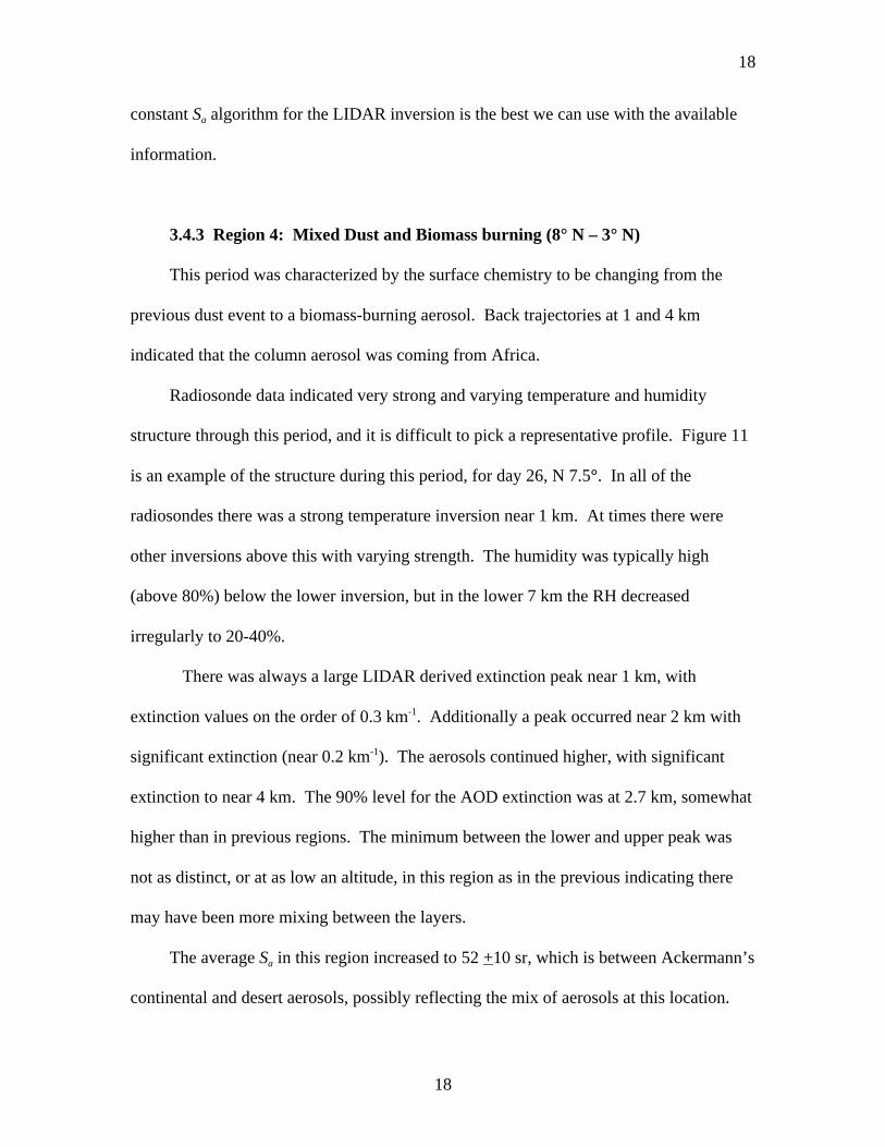
18
18
constant Sa algorithm for the LIDAR inversion is the best we can use with the available
information.
3.4.3 Region 4: Mixed Dust and Biomass burning (8° N – 3° N)
This period was characterized by the surface chemistry to be changing from the
previous dust event to a biomass-burning aerosol. Back trajectories at 1 and 4 km
indicated that the column aerosol was coming from Africa.
Radiosonde data indicated very strong and varying temperature and humidity
structure through this period, and it is difficult to pick a representative profile. Figure 11
is an example of the structure during this period, for day 26, N 7.5°. In all of the
radiosondes there was a strong temperature inversion near 1 km. At times there were
other inversions above this with varying strength. The humidity was typically high
(above 80%) below the lower inversion, but in the lower 7 km the RH decreased
irregularly to 20-40%.
There was always a large LIDAR derived extinction peak near 1 km, with
extinction values on the order of 0.3 km-1. Additionally a peak occurred near 2 km with
significant extinction (near 0.2 km-1). The aerosols continued higher, with significant
extinction to near 4 km. The 90% level for the AOD extinction was at 2.7 km, somewhat
higher than in previous regions. The minimum between the lower and upper peak was
not as distinct, or at as low an altitude, in this region as in the previous indicating there
may have been more mixing between the layers.
The average Sa in this region increased to 52 +10 sr, which is between Ackermann’s
continental and desert aerosols, possibly reflecting the mix of aerosols at this location.
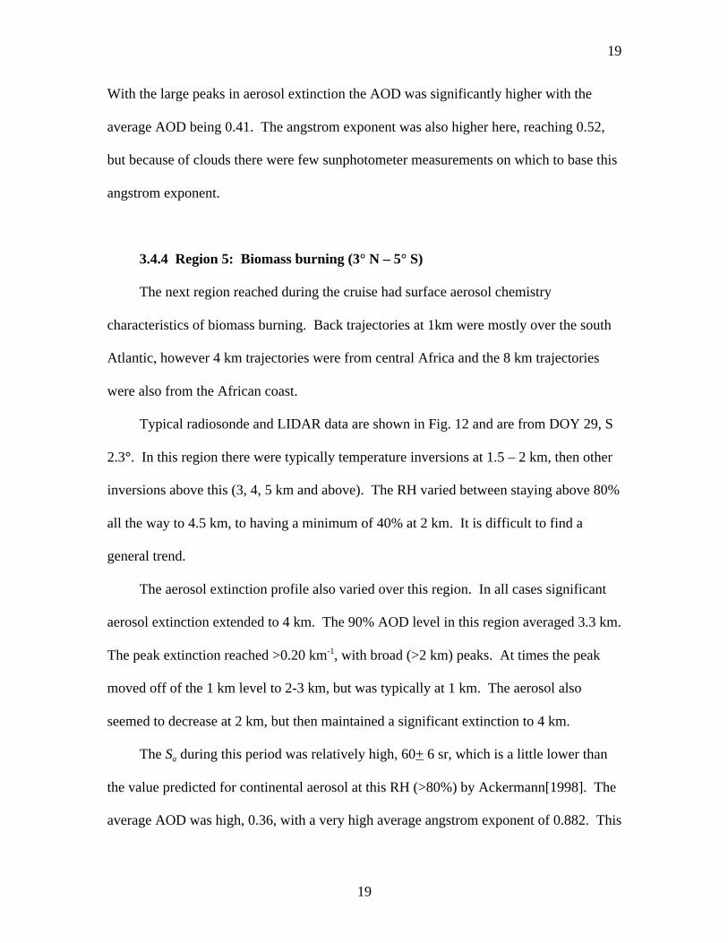
19
19
With the large peaks in aerosol extinction the AOD was significantly higher with the
average AOD being 0.41. The angstrom exponent was also higher here, reaching 0.52,
but because of clouds there were few sunphotometer measurements on which to base this
angstrom exponent.
3.4.4 Region 5: Biomass burning (3° N – 5° S)
The next region reached during the cruise had surface aerosol chemistry
characteristics of biomass burning. Back trajectories at 1km were mostly over the south
Atlantic, however 4 km trajectories were from central Africa and the 8 km trajectories
were also from the African coast.
Typical radiosonde and LIDAR data are shown in Fig. 12 and are from DOY 29, S
2.3°. In this region there were typically temperature inversions at 1.5 – 2 km, then other
inversions above this (3, 4, 5 km and above). The RH varied between staying above 80%
all the way to 4.5 km, to having a minimum of 40% at 2 km. It is difficult to find a
general trend.
The aerosol extinction profile also varied over this region. In all cases significant
aerosol extinction extended to 4 km. The 90% AOD level in this region averaged 3.3 km.
The peak extinction reached >0.20 km-1, with broad (>2 km) peaks. At times the peak
moved off of the 1 km level to 2-3 km, but was typically at 1 km. The aerosol also
seemed to decrease at 2 km, but then maintained a significant extinction to 4 km.
The Sa during this period was relatively high, 60+ 6 sr, which is a little lower than
the value predicted for continental aerosol at this RH (>80%) by Ackermann[1998]. The
average AOD was high, 0.36, with a very high average angstrom exponent of 0.882. This

20
20
indicates that the aerosol particles were probably relatively small, which agrees with the
high measured Sa.
3.4.5 Region 6: Southern hemisphere clean (5° S – 24.5° S) and Region 7:
South Atlantic temperate marine air mass (24.5° S – 33° S)
After going through these intense aerosol events, the surface chemistry again
indicated a clean maritime situation [Bates et al., this issue]. Interestingly, while the
surface measurements indicated a change at 5° S, the back trajectories did not switch as
rapidly. The 1km trajectories were over the south Atlantic, however early in the Region
(between 5° S and 12° S) 4 km trajectories were still over southern Africa and only
switched to the south Atlantic after 12° S. An example of the earlier period is shown in
Fig. 13, while an example of the later period is shown in Figure 14. Figure 13 is for Day
30.5, S 7.4°, while Fig. 14 is for Day 35.5, S 23.6°. We have grouped these two regions
together, because the vertical structure of the late part of region 6 was basically the same
as that of region 7.
The radiosonde data for the earlier period shows a strong temperature inversion at
1.5 km. The RH is typically very high (>80%) below this inversion, but decreases at the
inversion to 50-60%. The aerosol extinction profile shows why the surface chemistry
appeared clean, yet column AOD was not small. One can see that the surface extinction
is below 0.01 km-1, while the column extinction reaches >0.1 km-1 at 1 km or greater.
During this early period, significant aerosol extended to 4 km, with the average 90%
AOD level at 3.2 km, showing how high the aerosol was in the atmospheric column. The
Sa in the early period was 63 +12 sr, much higher than the values determined for the N.
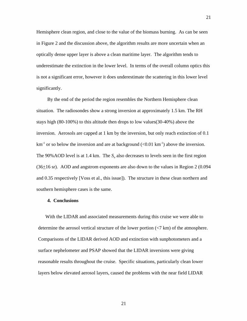
21
21
Hemisphere clean region, and close to the value of the biomass burning. As can be seen
in Figure 2 and the discussion above, the algorithm results are more uncertain when an
optically dense upper layer is above a clean maritime layer. The algorithm tends to
underestimate the extinction in the lower level. In terms of the overall column optics this
is not a significant error, however it does underestimate the scattering in this lower level
significantly.
By the end of the period the region resembles the Northern Hemisphere clean
situation. The radiosondes show a strong inversion at approximately 1.5 km. The RH
stays high (80-100%) to this altitude then drops to low values(30-40%) above the
inversion. Aerosols are capped at 1 km by the inversion, but only reach extinction of 0.1
km-1 or so below the inversion and are at background (<0.01 km-1) above the inversion.
The 90%AOD level is at 1.4 km. The Sa also decreases to levels seen in the first region
(36+16 sr). AOD and angstrom exponents are also down to the values in Region 2 (0.094
and 0.35 respectively [Voss et al., this issue]). The structure in these clean northern and
southern hemisphere cases is the same.
4. Conclusions
With the LIDAR and associated measurements during this cruise we were able to
determine the aerosol vertical structure of the lower portion (<7 km) of the atmosphere.
Comparisons of the LIDAR derived AOD and extinction with sunphotometers and a
surface nephelometer and PSAP showed that the LIDAR inversions were giving
reasonable results throughout the cruise. Specific situations, particularly clean lower
layers below elevated aerosol layers, caused the problems with the near field LIDAR
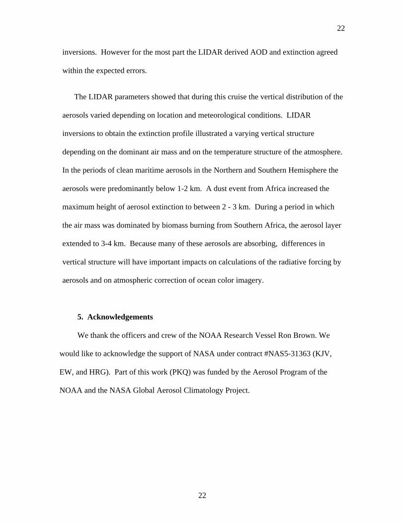
22
22
inversions. However for the most part the LIDAR derived AOD and extinction agreed
within the expected errors.
The LIDAR parameters showed that during this cruise the vertical distribution of the
aerosols varied depending on location and meteorological conditions. LIDAR
inversions to obtain the extinction profile illustrated a varying vertical structure
depending on the dominant air mass and on the temperature structure of the atmosphere.
In the periods of clean maritime aerosols in the Northern and Southern Hemisphere the
aerosols were predominantly below 1-2 km. A dust event from Africa increased the
maximum height of aerosol extinction to between 2 - 3 km. During a period in which
the air mass was dominated by biomass burning from Southern Africa, the aerosol layer
extended to 3-4 km. Because many of these aerosols are absorbing, differences in
vertical structure will have important impacts on calculations of the radiative forcing by
aerosols and on atmospheric correction of ocean color imagery.
5. Acknowledgements
We thank the officers and crew of the NOAA Research Vessel Ron Brown. We
would like to acknowledge the support of NASA under contract #NAS5-31363 (KJV,
EW, and HRG). Part of this work (PKQ) was funded by the Aerosol Program of the
NOAA and the NASA Global Aerosol Climatology Project.
23
23
6. References
Ackermann, The extinction-to-backscatter ratio of troposphere aerosol: A numerical
study, J. Atmosph. and Ocean. Techn., 15, 1043 – 1050 (1998).
Bates, T.S., P.K. Quinn, D.J. Coffman, J.E. Johnson, T.L. Miller, D.S. Covert, A.
Wiedensohler, S. Leinert, A. Nowak, and C. Neususs, Regional physical and chemical
properties of the marine boundary layer aerosol across the Atlantic during Aerosols99, J.
Geophys. Res., submitted, 2000.
Carrico, C.M, M.J. Rood, and J.A. Ogren, Aerosol light scattering properties at
Cape Grim, Tasmania, during the first Aerosol Characterization Experiment (ACE 1), J.
Geophys. Res., 103, 16,565 – 16,574 (1998).
Fernald, F.G., B. M. Herman, and J. A. Reagan, Determination of aerosol height
distributions by lidar. J. Appl. Meteorol., 11, 482-489 (1972).
Fernald, F.G., Analysis of atmospheric lidar observations: some comments. Appl. Opt.,
23, 652-653(1984).
Gordon, H. G., Atmospheric Correction of Ocean Color Imagery in the Earth
Observing System Era, Jour. Geophys. Res., 102D, 17081-17106 (1997).
Gordon, H. G., T. Du, and T. Zhang, Remote sensing ocean color and aerosol
properties: resolving the issue of aerosol absorption, Applied Optics, 36, 8670-8684
(1997).
McInnes, L., M Bergin, J. Ogren, and S. Schwartz, Apportionment of light
scattering and hygroscopic growth to aerosol composition, Geophys. Res. Lett., 25, 513
516 (1998).
24
24
Quinn, P.K., D.J. Coffman, T.S. Bates, T.L. Miller, J.E. Johnson, K. Voss, E.J.
Welton, and C. Neususs, Dominant aerosol chemical components and their contribution
to extinction during the Aerosols99 cruise across the Atlantic, J. Geophys. Res.,
submitted, 2000.
Schoeberl, M. R., Lait, L.R., Newman, P. A., Rosenfield, J. E., The Structure of the
Polar Vortex , J. Geophys. Res., 97, 7859-7882 (1992).
Spinhirne, J.D., J.A. Reagan, and B.M. Herman, Vertical Distribution of Aerosol
Extinction Cross Section and Inference of Aerosol Imaginary Index in the Troposphere
by LIDAR Technique, J. Appl. Meteorol., 19, 426-438 (1980).
Spinhirne, J. D., Rall, J., and V. S. Scott, Compact eye-safe LIDAR systems, Rev.
Laser Eng., 23, 26 – 32 (1995).
Welton, E. J. Measurements of Aerosol Optical Properties over the Ocean using
Sunphotometry and LIDAR, Ph. D. Dissertation. University of Miami, Coral Gables, 1-
150 (1998).
Welton, E. J., K. J. Voss, H. R. Gordon, H Maring, A. Smirnov, B. Holben, B.
Schmid, J. M. Livingston, P. B. Russell, P. A. Durkee, P. Formenti, M. O. Andreae,
Ground-based LIDAR Measurements of Aerosols During ACE-2: Instrument
Description, Results, and Comparisons with other Ground-based and Airborne
Measurements, Tellus, 52: 635 – 651 (2000a).
Welton, E. J., J. R. Campbell, J. D. Spinhirne, and V. S. Scott, Aerosol and Cloud
measurements using micropulse LIDAR systems, J. Atmos. Oceanic Tech. Submitted,
(2000b).
25
25
7. Figure Captions
Figure 1) LIDAR derived AOD vs Sunphotometer derived AOD for common
measurement periods during the cruise. Line is 1:1 fit. LIDAR AOD is at 523nm,
sunphotometer AOD ranges from 490 – 500 nm. Error bars on x-axis are from the
standard deviation of sunphotometer samples common with LIDAR measurements.
Error bars on y-axis are from the estimate of the error of the calibration coefficient, and
signal noise (including afterpulse and overlap noise)..
Figure 2) LIDAR derived surface (75m) extinction (displayed as +) and nephelometer
surface(19 m) extinction (displayed as the line) throughout the cruise.
Figure 3) LIDAR and Nephelometer extinctions during common measurements periods.
Measurements are broken into Regions as discussed in text. Note the definite regional
bias (LIDAR low) in Region 5 and 6a. Line is 1:1 line for reference.
Figure 4) Contour plot of LIDAR derived extinction coefficients along the cruise track.
Regions as defined by Bates et al. [this issue] are delineated by the lines. The data
positions on which the contours are based are shown as lines at the bottom of the graph.
Figure 5) Contour of integrated extinction from the surface to z. Vertical lines delineate
regions as defined in Bates et al.[this issue]. The data positions on which the contours are
based are shown as lines at the bottom of the graph.
26
26
Figure 6) Sa (extinction/backscattering) derived throughout the cruise. Vertical lines
delineate regions as defined in Bates et al.[this issue]. Sa was lower in clean maritime
airmasses then in those impacted by dust or biomass burning.
Figure 7) 1 km back-trajectories, Regions as discussed in text are shown divided by lines
on the graph.
Figure 8) 4 km trajectories, Regions as discussed in text are shown divided by lines on
the graph.
Figure 9) Radiosonde and LIDAR derived profiles typical for Region 2, Northern
Hemisphere clean (31° N – 15.5° N). This specific case was for DOY 18.5, N 27.7°.
LIDAR extinction is shown as the fine line with no symbols. This is an average of the
nearest three profiles (each of which is a 10 minute cloudfree average) around the
Radiosonde launch. Relative Humidity is displayed as the line marked with filled circles,
while ∆T/∆z is displayed as the line marked with filled squares. Note overall extinction
is low and capped by the first temperature inversion (positive ∆T/∆z).
Figure 10) Radiosonde and LIDAR derived profiles typical for Region 3, Dust (15.5° N
– 8° N). This specific case was for DOY 14.5, N 11.2°. Symbols are as in Figure 9.
Extinction has increased from Region 2 and there is another aerosol layer above the first
temperature inversion (positive ∆T/∆z).
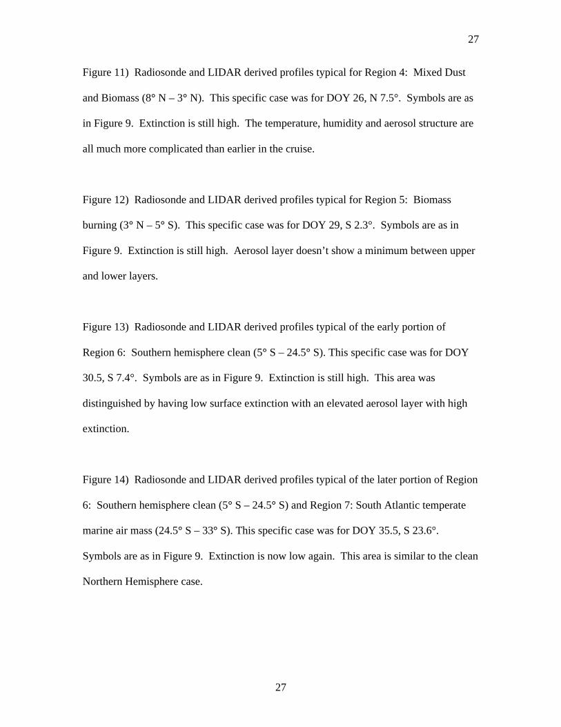
27
27
Figure 11) Radiosonde and LIDAR derived profiles typical for Region 4: Mixed Dust
and Biomass (8° N – 3° N). This specific case was for DOY 26, N 7.5°. Symbols are as
in Figure 9. Extinction is still high. The temperature, humidity and aerosol structure are
all much more complicated than earlier in the cruise.
Figure 12) Radiosonde and LIDAR derived profiles typical for Region 5: Biomass
burning (3° N – 5° S). This specific case was for DOY 29, S 2.3°. Symbols are as in
Figure 9. Extinction is still high. Aerosol layer doesn’t show a minimum between upper
and lower layers.
Figure 13) Radiosonde and LIDAR derived profiles typical of the early portion of
Region 6: Southern hemisphere clean (5° S – 24.5° S). This specific case was for DOY
30.5, S 7.4°. Symbols are as in Figure 9. Extinction is still high. This area was
distinguished by having low surface extinction with an elevated aerosol layer with high
extinction.
Figure 14) Radiosonde and LIDAR derived profiles typical of the later portion of Region
6: Southern hemisphere clean (5° S – 24.5° S) and Region 7: South Atlantic temperate
marine air mass (24.5° S – 33° S). This specific case was for DOY 35.5, S 23.6°.
Symbols are as in Figure 9. Extinction is now low again. This area is similar to the clean
Northern Hemisphere case.

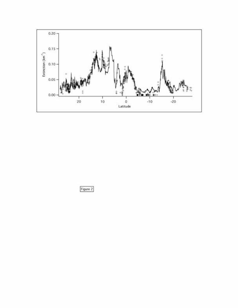
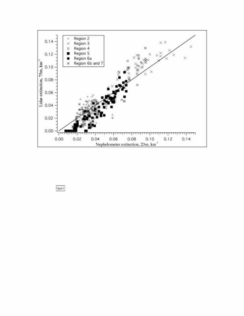
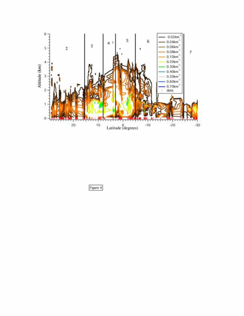
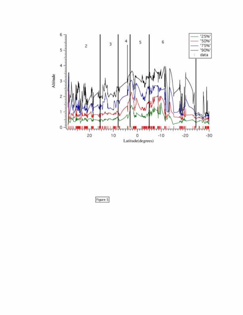
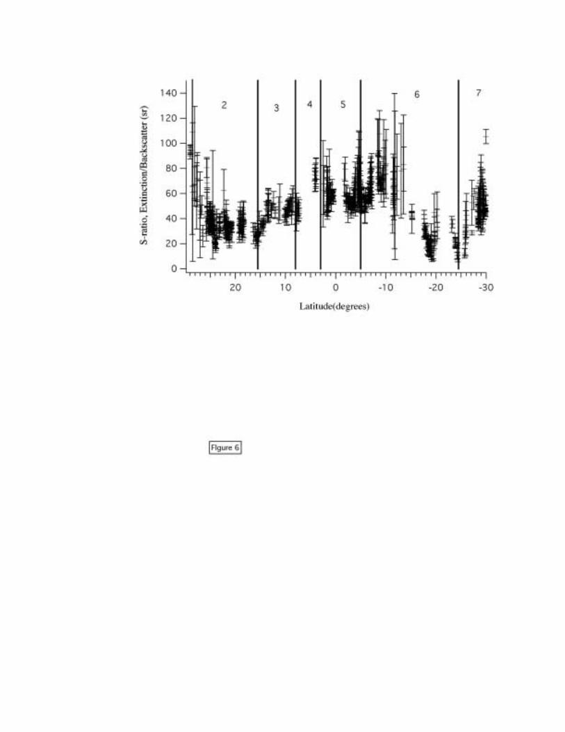

5-Day Back-trajectories: R/B Atlantic 1999 Cruise, Alt = 001 km
Back traj., NMC data, starttime 12Z
-150 -100 -50 0 50Degrees Longitude
-60
-40
-20
0
20
40
60
Deg
rees
Lat
itu
de
Unknown
Unknown
Unknown
Unknown
Unknown
Unknown
2
Unknown
3
Unknown
5
Unknown
4
Unknown
6
Unknown
7

5-Day Back-trajectories: R/B Atlantic 1999 Cruise, Alt = 004 km
Back traj., NMC data, starttime 12Z
-150 -100 -50 0 50Degrees Longitude
-60
-40
-20
0
20
40
60
Deg
rees
Lat
itu
de
Unknown
Unknown
Unknown
Unknown
Unknown
Unknown
2
Unknown
3
Unknown
4
Unknown
5
Unknown
6
Unknown
7

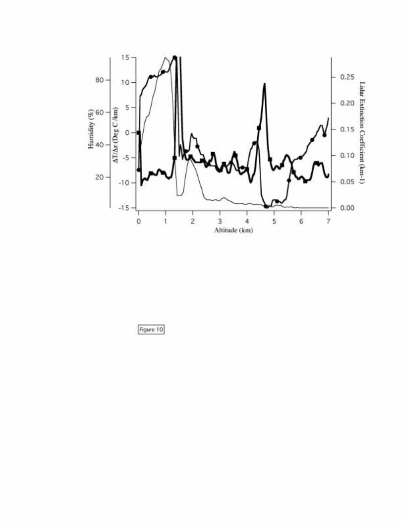

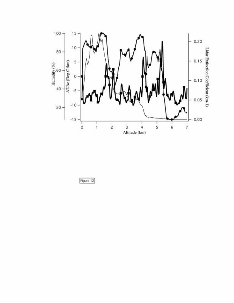

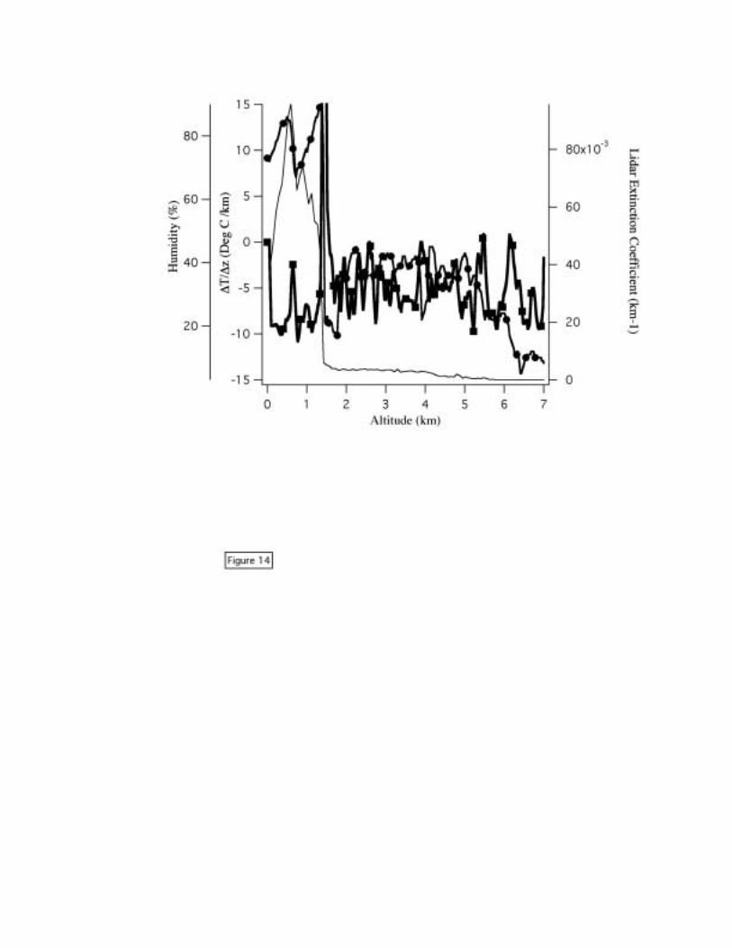
Appendix VII
Retrieval of Coccolithophore CalciteConcentration from SeaWiFS Imagery
(Submitted to Geophysical Research Letters)

Retrieval of Coccolithophore Calcite Concentration from SeaWiFS Imagery
Howard R. Gordon,1 G. Chris Boynton,1 William M. Balch,2 Stephen B. Groom,3
Derek S. Harbour4, and Tim J. Smyth3
1Department of Physics, University of Miami, Coral Gables, FL 331242Bigelow Laboratory for Ocean Sciences, West Booth Bay Harbor, ME 04575
3Centre for Coastal and Marine Sciences, Plymouth Marine Laboratory, Plymouth,Devon, PL1 3DH, UK
4 Sir Alastair Hardy Foundation for Ocean Science, 1 Walker Terrace, Plymouth PL13BN, UK
Abstract
We examined blooms of the coccolithophorid E. huxleyi, observed in SeaWiFS
imagery, with a new algorithm for the retrieval of detached coccolith concentration. The
algorithm uses only SeaWiFS bands in the red and near infrared (NIR) bands to minimize
the influence of the chlorophyll and dissolved organic absorption. We used published
experimental determinations of the calcite specific backscattering and its spectral
dependence, and assumed that the absorption coefficient of the medium was that of pure
water, to estimate the marine contribution to the SeaWiFS radiance. The aerosol (and
Rayleigh-aerosol interaction) contribution to the radiance was modeled as an exponential
function of wavelength. These allow derivation of the coccolith concentration on a pixel-
by-pixel basis from SeaWiFS imagery. Application to a July 30, 1999 SeaWiFS image of
a bloom south of Plymouth, England indicates that the SeaWiFS estimates are in good
agreement with surface measurements of coccolith concentration.
Introduction
Coccolithophores are small marine Prymnesiophyte phytoplankton which form
external CaCO2 scales (diameter ~ 2 µm and thickness 250 to 750 nm) called coccoliths.
The coccoliths can form multiple layers and eventually detach. Coccolithophores are the

2
largest source of calcium carbonate on earth [Westbroek et al. 1985]. Of the
coccolithophore species, Emiliania huxleyi is the most abundant, and its coccoliths can
often be found from tropical to sub-arctic regions and further north into regions with
water temperatures 0°C [Heimdal 1983]. The distribution of E. huxleyi coccoliths in
sediments generally matches the distribution of the overlying species in the water column
[McIntyre and Be 1967]. It can also be affected by biological processes such as grazing
by marine zooplankton [Harris 1994], or microzones of bacterial decomposition which
locally decrease the pH (see recent review by Milliman et al.[1999]). Dissolution of
calcite depends on the depth of the calcite compensation depth. Approximately 20% of
the biogenic carbonate is lost before accumulation in the sediments in regions such as the
Sargasso Sea [Fabry and Deuser 1990], while 97% is lost in the Arabian Sea [Nair et al.
1989]. Even so, globally, calcium carbonate is responsible for about 75% of the
deposition of carbon on the sea floor having a marine origin [Groom and Holligan 1987,
Honjo 1986, Honjo 1990], it exceeds organic burial by a factor of seven. Thus, coccolith
production is an important part of the biogenic carbon cycle.
The importance of coccolithophores to the overall particulate pool of
phytoplankton had not been realized until the advent of remote sensing. Upwelling
radiance measurements from the CZCS frequently showed large, mesoscale features in
the temperate waters of both hemispheres. These features were sometimes characterized
by complete saturation of band 3 (550 nm wavelength) of the CZCS. They were later
attributed to intense light scattering by coccolithophores and associated coccoliths
[Holligan et al. 1983]. Perhaps the most intriguing aspect of coccolithophores concerns
the frequency of their blooms. Analysis of CZCS imagery showed 100-200 km diameter

3
coccolithophore blooms within temperate waters on an annual basis [Brown and Yoder
1994]. Apart from the inherent ecological interest in the development and fate of large-
scale monospecific populations of phytoplankton, recent attention on the
coccolithophores has focused on their role in global biogeochemical cycles [Holligan et
al. 1993].
The Algorithm
Analysis of the influence of coccoliths on the water-leaving radiance [Gordon et
al. 1988] suggests that determination of the coccolith concentration using spectral bands
in the blue and green region of the spectrum requires the chlorophyll concentration (Chl).
Unfortunately, estimation of Chl is difficult in such blooms. A second difficulty is that at
high coccolith concentration the blue-green ocean color bands often saturate and must be
abandoned. These problems can be circumvented by using the red and near infrared
(NIR) spectral bands for two reasons. First, at these long wave-bands the absorption
coefficient of sea water alone is so high that the additional absorption by phytoplankton
and dissolved organic material is almost irrelevant. Second, because of the high water
absorption, the water-leaving radiance in these bands is unlikely to become large enough
to saturate the sensor.
The top-of-atmosphere (TOA) spectral reflectance ρt(λ) can be written
ρt(λ) =ρr(λ) + ρA(λ) + tp(λ)ts(λ)ρw(λ), where ρr(λ) is the contribution due to Rayleigh
scattering in the atmosphere in the absence of the aerosol, ρA(λ) is the contribution from
scattering by the aerosol in the absence of the air (but including the Rayleigh –aerosol
interaction), and ρw(λ) is the contribution from the water-leaving radiance. The
quantities ts(λ) and tp(λ) are the diffuse transmittances of the atmosphere, along a path
4
from the sea surface to the sun (ts) and the sea surface to the sensor (tp), at the wavelength
λ.
Our algorithm uses SeaWiFS Bands 6, 7, and 8 (670, 765, and 865 nm). In these
bands the water-leaving reflectance can be written approximately )(6 bwbw bab +≅ρ ,
where aw is the absorption coefficient of pure sea water, and bb is the backscattering
coefficient of the medium, e.g., see Gordon et al. [1988]. In coccolithophore blooms bb
results mostly from scattering by the coccolithophores and the detached coccoliths. For
the 1991 coccolithophore bloom in the central North Atlantic, Balch et al. [1996] found
empirically that the backscattering coefficient at 546 nm [bb(546) in m-1] could be related
statistically to the detached coccolith concentration [NCocco in ml-1] through
bb(546)=1.35×10⁻⁷ NCocco + 3.06×10⁻³, and to the concentration of calcite [C in moles/m3]
through bb(546)=1.6C − 0.0036. In addition, the spectral variation of bb could be
approximated by bb(λ)≈bb(546)×(546/λ)1.35, where λ is the wavelength in nm [Balch et al.
1996, Voss et al. 1998]. These relationships are used to relate ρw(λ) to either NCocco or C.
For ρA(λ) we use the Wang and Gordon [1994] approximation that
)](exp[)()( 00 λλλρλρ −≈ aAA , where a is a constant and λ0 is taken to be 865 nm.
Because this algorithm cannot estimate aerosol properties, the diffuse transmittances of
the atmosphere are modeled assuming that there is only Rayleigh scattering and, in the
case of band 7, O2 absorption.
Applying these observations and assumptions to the sensor-measured ρt(λ) −
ρr(λ) allows derivation of the three unknowns bb(546), ρA(865), and a on a pixel-by-pixel
basis using the SeaWiFS bands at 670, 765, and 865 nm, however, a correction using the
visible bands is required to address the significant out-of-band response in bands 6 and 8
5
prior to application of the algorithm. This correction was developed using by applying
the SeaWiFS spectral response functions to ρt(λ) − ρr(λ) in the visible as described by
Gordon [1995].
Results
We processed several images of coccolithophore blooms and found that spatial
patterns in bb(546) and a showed distinct similarities in regions of intense blooms even
though there is no obvious bloom structure evident in the sensor-measured reflectance at
865 nm. Assuming that a should be the same inside and outside the bloom, we believe
that these similarities are due to small errors in the sensor calibration; however, we found
that reducing the out-of-band contributions by a factor of two removed much of this
covariation. (Note, if this procedure were not applied, the change in bb(546) due to
incomplete correction for the atmosphere would be typically ~ 0.005 m-1or less,
corresponding to a detached coccolith concentration of ~ 70,000 ml-1.) Figures 1 and 2
provide bb(546) and a, respectively, for a coccolithophore bloom off Plymouth, England
acquired on July 30, 1999. Figure 1 shows that the maximum value of bb(546) is
approximately 0.08 m-1, and the minimum values are ~0.005 m-1 (near the upper left
corner of the image). Figure 2 indicated that a shows only a hint of the bloom,
suggesting that the procedure has successfully separated the water and atmospheric
signals.
For the image shown in Figure 1, surface measurements of the concentration of
detached coccoliths were made coincident with the satellite overpass, at the points
marked with an “X.” Samples for coccolithophore cell and detached coccolith
concentration were taken in buffered formalin, and the concentrations estimated with an

6
inverted microscope. Using the relationship between bb(546) and NCocco, we estimated
the detached coccolith concentration for the image. Figure 3(a) compares the coccolith
estimated concentration, along a track joining the measurement locations, with the
measured values. The error bars are an assumed 10% error in coccolith counts and a 12%
standard deviation in the bb(546)-NCocco relationship. The agreement is excellent. It
should be noted that no attempt has been made to tune the algorithm to the
measurements, other than to reduce the out-of-band correction by a factor of 2 to remove
the similarity in the initial bb(546) and a patterns. For example, assuming Chl was
nominally 1 mg/m3 rather than zero, the retrieved bb(546) would increase by ~5%
improving the agreement in Figure 3a. The analysis has been carried out completely
using only previously published relationships between the variables. Figure 3(b)
provides an estimate of the calcite concentration along the same track as in Figure 3(a).
Concluding Remarks
We have demonstrated the efficacy of a simple algorithm for retrieval of calcite
concentration from coccolithophore blooms using SeaWiFS imagery. We used the
detached coccolith concentration as an intermediate product (Figure 3a) only because it,
rather than the calcite concentration, was measured coincident with the imagery. In
application of the algorithm, normally one would proceed directly to calcite concentration
from bb(546). Calcite concentration is preferable to detached coccolith concentration
because (1) it includes coccoliths on plated cells, (2) the bb(546)-C relationship shows
less variability across coccolithophore species than the bb(546)-NCocco relationship [Balch
et al. 1998], and (3) calcite concentration is more relevant to ocean biogeochemistry than
NCocco. Although no attempt here has been made to do so, we believe that given sufficient

7
surface truth the algorithm could be tuned to provide better retrievals. We encourage
investigators observing coccolithophore blooms to sample them for microscopic counting
in the event that they are also imaged by SeaWiFS.
The algorithm in its present form is capable of processing one orbit of a complete
GAC image (North Pole to South Pole) in approximately five minutes, and is thus fast
enough to be included in routine SeaWiFS processing. Although the algorithm is not
capable of distinguishing between coccolithophore blooms features with similar high red-
NIR reflectance, it can be combined with the Brown and Yoder [1994] classification
algorithm to provide calcite concentration when the classification algorithm indicates the
presence of a coccolithophore bloom.
Acknowledgments
The authors are grateful for support for this work from the U.S. Office of Naval Research
(HRG) under grant number N00014-99-1-0007, NASA (HRG, WMB) under contract
numbers NAS5-31363 and NAS5-31734. This research forms part of the Core Strategic
Research Project on the Dynamics of Marine Ecosystems (DYME) of the Centre for
Coastal and Marine Sciences, Plymouth Marine Laboratory, UK.
References
Balch, W.M., K. Kilpatrick, P.M. Holligan, D. Harbour, and E. Fernandez, The 1991
coccolithophore bloom in the central north Atlantic II: Relating optics to
coccolith concentration, Limnology and Oeanography, 41, 1684—1696, 1996.
Balch, W.M., D.T. Drapeau, T.L. Cucci, and R.D. Vaillancourt, Optical backscattering by
calcifying algae: Separating the contribution of particulate inorganic and organic
carbon fractions, J. Geophys. Res., 104C, 1541—1558, 1999.
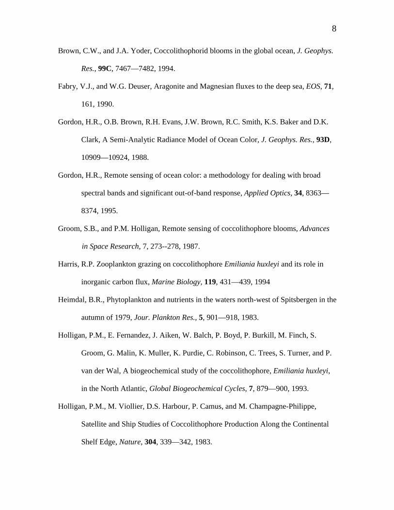
8
Brown, C.W., and J.A. Yoder, Coccolithophorid blooms in the global ocean, J. Geophys.
Res., 99C, 7467—7482, 1994.
Fabry, V.J., and W.G. Deuser, Aragonite and Magnesian fluxes to the deep sea, EOS, 71,
161, 1990.
Gordon, H.R., O.B. Brown, R.H. Evans, J.W. Brown, R.C. Smith, K.S. Baker and D.K.
Clark, A Semi-Analytic Radiance Model of Ocean Color, J. Geophys. Res., 93D,
10909—10924, 1988.
Gordon, H.R., Remote sensing of ocean color: a methodology for dealing with broad
spectral bands and significant out-of-band response, Applied Optics, 34, 8363—
8374, 1995.
Groom, S.B., and P.M. Holligan, Remote sensing of coccolithophore blooms, Advances
in Space Research, 7, 273--278, 1987.
Harris, R.P. Zooplankton grazing on coccolithophore Emiliania huxleyi and its role in
inorganic carbon flux, Marine Biology, 119, 431—439, 1994
Heimdal, B.R., Phytoplankton and nutrients in the waters north-west of Spitsbergen in the
autumn of 1979, Jour. Plankton Res., 5, 901—918, 1983.
Holligan, P.M., E. Fernandez, J. Aiken, W. Balch, P. Boyd, P. Burkill, M. Finch, S.
Groom, G. Malin, K. Muller, K. Purdie, C. Robinson, C. Trees, S. Turner, and P.
van der Wal, A biogeochemical study of the coccolithophore, Emiliania huxleyi,
in the North Atlantic, Global Biogeochemical Cycles, 7, 879—900, 1993.
Holligan, P.M., M. Viollier, D.S. Harbour, P. Camus, and M. Champagne-Philippe,
Satellite and Ship Studies of Coccolithophore Production Along the Continental
Shelf Edge, Nature, 304, 339—342, 1983.

9
Honjo, S., Oceanic particles and pelagic sedimentation in the western North Atlantic
Ocean, The Geology of North America Vol. M, The Western North Atlantic
Region, Geological Society of America, Ed. P.R. Vogt and B.E. Tucholke, 469—
478, 1986.
Honjo, S., Particle fluxes at 47° N and 34° N 20° W stations between April 3 to
September 26, 1989, EOS, 71, 81, 1990.
McIntyre, A., A.W.H. Be, Modern Coccolithophorideae of the Atlantic Ocean --
I.Placoliths and cyrtoliths, Deep Sea Res., 14, 561—597, 1967.
Milliman, J., P.J. Troy, W. Balch, A.K. Adams, Y.-H. Li, and F.T. MacKenzie,
Biologically-mediated dissolution of calcium carbonate above the chemical
lysocline?, Deep Sea Research, 46, 1653—1669, 1999.
Nair, R.R., V. Ittekkot, S.J. Monganini, V. Ramaswamy, B. Haake, E.T. Degens. B.N.
Desai, S. Honjo, Increased particle flux to the deep ocean related to monsoons,
Nature, 338, 749—751, 1989.
Wang, M., and H.R. Gordon, A Simple, Moderately Accurate, Atmospheric Correction
Algorithm for SeaWiFS, Remote Sensing of Environment, 50, 231—239, 1994.
Westbroek, P., E.W. De Vrind-De Jong, P. Van der Wal, A. H. Borman, and J. P. M. De
Vrind, Biopolymer-mediatedcalcium and manganese accumulation and
biomineralization, Geol. Mijnbouw, 64, 5—15, 1985.
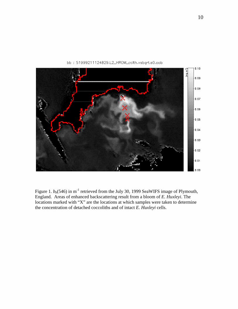
10
Figure 1. bb(546) in m-1 retrieved from the July 30, 1999 SeaWIFS image of Plymouth,England. Areas of enhanced backscattering result from a bloom of E. Huxleyi. Thelocations marked with “X” are the locations at which samples were taken to determinethe concentration of detached coccoliths and of intact E. Huxleyi cells.
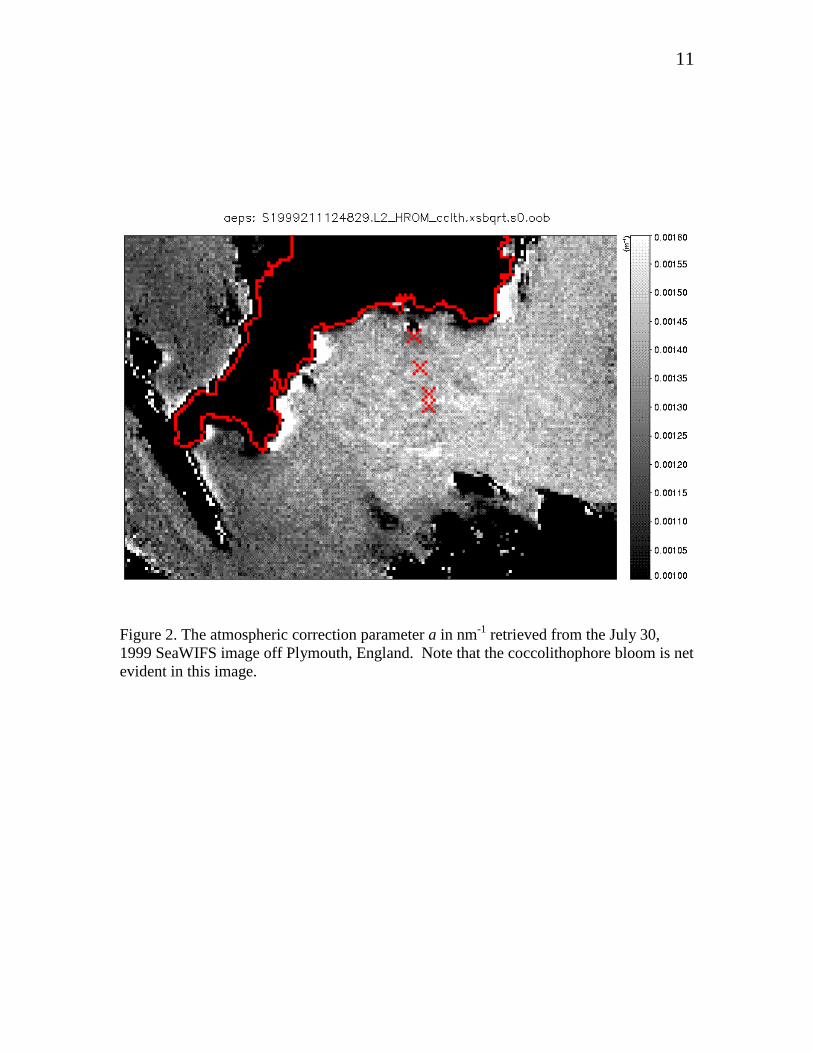
11
Figure 2. The atmospheric correction parameter a in nm-1 retrieved from the July 30,1999 SeaWIFS image off Plymouth, England. Note that the coccolithophore bloom is netevident in this image.
12
(a)
(b)
Figure 3. (a) comparison between retrieved and measured detached coccolithconcentration (a), and (b) estimated calcite concentration along the same track as in (a).
Plymouth Bloom
0
200,000
400,000
600,000
800,000
1,000,000
0 5 10 15 20 25 30
Distance (km)
Co
cco
lith
Co
nce
ntr
atio
n (
ml− −−−1
)
Retrieved
Measured
Plymouth Bloom
0
0.01
0.02
0.03
0.04
0.05
0.06
0.07
0 5 10 15 20 25 30
Distance (km)
Cal
cite
(m
ole
s/m
3 )
Related Documents