Instrumentation and measurement platform aeronautics ...

Studienarbeit January 15.2020

Instrumentation and measurement platform

aeronautics inspired, based on LabView

from

Nadège Prévost

Matriculation number 4617370

The project contains

Pages: 61

Figures: 46

Charts: 11

Institut für Flugführung

Technische Universität Braunschweig ·

Tutor & advisor: Dr. Astrid Lampert

MCIA center Innovation Electronics

Universitat Politècnica de Catalunya

Assistant professor: Miguel Delgado Prieto

January 2020

II

Student Thesis

for

Nadège Prévost

Matriculation Number: 4617370

Instrumentation and measurement platform, aeronautics inspired, based on

LabView

Background Instrumentation and measurement systems are constantly gaining in importance. Especially in the aeronautic sector they are essential in order to assure a secure process in which not every step has to be controlled manually. The data is converted from analogue to digital and then processed and visualized on monitors or panels. Currently the MCIA center Innovation Electronics of the Universitat Politècnica de Catalunya started a new series of practical sessions for an aeronautic subject related to instrumentation. Sensors of all type are being connected to LabView through an acquisition system of National Instruments in order to analyze and visualize the data on a panel. The aim is to provide a system that allows gaining rapidly insight in the functionality of LabView and acquiring knowledge about the processing of data within a professional acquisition and instrumentation environment. Choosing different sensors (with different output, digital, analogue, modular etc.) and connecting them to LabView gives the possibility to later on connect every other sensor of the same outcome type to the environment. With little changes every sensor will be able to be visualized on the panel.

Objective of the work The main goal of the project is the design and development of an instrumentation and measurement platform to visualize data of a set of sensors through an acquisition system and a virtual panel. The following tasks have to be accomplished:

• Familiarization with the LabView environment

• Selection and integration of different sensors in LabView

• Implementation of digital processing procedures for sensors adaption

• Design of a panel for displaying measurement parameters

• System validation

• Documentation of the thesis

III

Recommended Literature:

[1] Armando Péreza, Gisela Monterob, Rogelio Ramos Irigoyenb, Conrado Garciab, Marcos Coronadob, Jose Rodrigueza: Development and implementation of virtual instrumentation based on LabView applied to compression ignition engines operated with diesel-biodiesel blends, Method Article, 2019

[2] Amit Kumar Rohit, Amit Tomar, Anurag Kumar, Saroj Rangnekar: Virtual lab based real-time

data acquisition, measurement and monitoring platform for solar photovoltaic module, Resource-Efficient Technologies Journal, 2017

[3] Kunliang Xu: The Design Concept of a Virtual Experiment Teaching Platform for Digital Logic

Based on LabVIEW, International Journal of Hybrid Information Technology, 2015

[4] Nan Su, XiaoWei Tu, QingHua Yang, XuHui Li, Yan Tong: Design of Data Communication and Monitoring System Based on Aviation ARINC825 Bus, International Conference on Communication Software and Networks, 2019

[5] José Roberto Quezada Peña, Jefferson Oliveira, Manuel Leonel da Costa Neto, Luis Henrique

Neves Rodrigues: ACTIVE METHODOLOGIES IN EDUCATION OF ELECTRONIC INSTRUMENTATION USING VIRTUAL INSTRUMENTATION PLATFORM BASED ON LABVIEW AND ELVIS II, Global Engineering Education Conference (EDUCON), 2018

Duration: The duration of the student thesis is 3 months according to the current valid version of examination regulation (PO). Upon accepting the task description, the student confirms that he/she is familiar with the current valid PO that applies for his/her degree programme.

Further arrangements:

1 The thesis shall be written in coordination with the advisor. The thesis or parts of it must not be published or passed on to third parties without consulting the Institute.

2 Compliance with the „Richtlinien und Hinweise für die Anfertigung von Studien-, Diplom-, Bachelor- und Masterarbeiten“ (Recommended Practices and Guidelines for Student, Diploma, Bachelor and Master Theses) of the Institute for Flight Guidance of the TU Braunschweig shall be assured.

3 As far as use of equipment and facilities at the Institute of Flight Guidance is necessary, their use is limited to normal working hours of the Institute; beyond that only after consulting the advisor. In any case, at least one other person must be in visual or hearing range due to safety reasons. Safety instructions of the responsible employees must be obeyed.

Advisors: Dr. Astrid Lampert / Miguel Delgado Prieto (Dr. habil. A. Lampert) (Miguel Delgado Prieto) Date of issue: 15.01.2020 Due date: 15.01.2020

V

2 Abstract

Within the framework of this thesis a graphical interface in the programming environment of LabView

is to be developed. LabView is a software system of National Instruments which facilitates data

acquisition and data control.

The main goal of the project is to visualise outgoings of several sensors related to aeronautics on a

panel which analyses the signals and eventually permits to use them for further employments. This

implies a selection of sensors which are important in the aeronautic area within previously settled

criteria and connecting them to the programming environment. This accomplished a software is to be

developed in order to acquire the data of the connected sensors, process and allocate them to further

employment. The interface between user and software will be the panel on which the analysed data

of the sensors will be represented.

Considering all mentioned above, this project provides students the possibility to gain an inside in the

concepts of instrumentation and in the handling of data within a programming environment as

LabView.

VI

3 Table of contents 1 Affidavit .......................................................................................................................................... IV

2 Abstract ........................................................................................................................................... V

4 Table of figures .............................................................................................................................. VII

5 Table of charts ................................................................................................................................ IX

6 Table of formula .............................................................................................................................. X

7 Nomenclature ................................................................................................................................. XI

7.1 Latin symbols .......................................................................................................................... XI

7.2 Indices .................................................................................................................................... XII

7.3 Greek symbols ....................................................................................................................... XII

7.4 Acronyms ............................................................................................................................... XII

1. Introduction ..................................................................................................................................... 1

2. Background and trends ................................................................................................................... 2

3. Theoretical background and materials ............................................................................................ 5

3.1. National Instruments and their software LabView ................................................................. 5

3.2. Sensors and their categorizations ........................................................................................... 7

3.3. Standard Atmosphere ............................................................................................................. 8

3.4. Velocity, acceleration and their correlation .......................................................................... 10

4. Instrumentation and measurement platform design ................................................................... 12

4.1. Selection of the type and quantity of sensors ....................................................................... 12

4.2. Selection of the sensors ........................................................................................................ 15

4.3. Connecting port ..................................................................................................................... 21

5. Design of required processing procedures for selected sensors .................................................. 22

5.1. Temperature sensor .............................................................................................................. 22

5.2. Acceleration sensor ............................................................................................................... 22

5.3. Pressure sensor ..................................................................................................................... 25

5.4. Compass sensor ..................................................................................................................... 27

6. Testing of the sensor’s functionality ............................................................................................. 29

7. Programming the software and the visualization panel ............................................................... 31

8. Testing the software’s functionality .............................................................................................. 36

8.1. Testing of the software functionality by synthetic signals .................................................... 36

8.2. Testing of the software functionality by connecting sensors ............................................... 39

8.3. Testing of the whole system.................................................................................................. 44

9. Summary and outlook ................................................................................................................... 46

8 References ..................................................................................................................................... 47

VII

4 Table of figures

Figure 1 Example of front panel view ...................................................................................................... 6

Figure 2 Example of block diagram panel view ....................................................................................... 6

Figure 3 Tool palette ............................................................................................................................... 6

Figure 4 Control palette .......................................................................................................................... 6

Figure 5 Function palette ........................................................................................................................ 6

Figure 6 Formula node ............................................................................................................................ 7

Figure 7 ISO standard atmosphere – characteristic variables [23] ......................................................... 9

Figure 8 Primary flight display [8] ......................................................................................................... 12

Figure 9 General aviation instrument panel [43] .................................................................................. 12

Figure 10 Compass [7] ........................................................................................................................... 14

Figure 11 Difference between magnetic poles and geographical poles (excessive eccentricity), [6]... 14

Figure 12 Earth magnetic field vector and its components cf. [17] ...................................................... 14

Figure 13 Pressure sensor [40] .............................................................................................................. 20

Figure 14 Acceleration sensor [30] ........................................................................................................ 20

Figure 15 Temperature sensor [2] ......................................................................................................... 20

Figure 16 Compass sensor [19] ............................................................................................................. 20

Figure 17 NI PCI 6014 [28] ..................................................................................................................... 21

Figure 18 External acquisition card CB-68LP [15] .................................................................................. 21

Figure 19 Output PWM signal of the acceleration sensor cf. [31] ........................................................ 23

Figure 20 Schematic sketch of the pressure sensor cf. [11] .................................................................. 25

Figure 21 Output PWM signal of the electronic compass cf. [15] ......................................................... 27

Figure 22 Breadboard with the temperature sensor (left) and the pressure sensor (right) ................. 29

Figure 23 Breadboard with the acceleration sensor ............................................................................. 29

Figure 24 Schematic drawing of the installation – left: supply source, right: oscilloscope .................. 30

Figure 25 View of the designed front panel (first part) – 1. General aviation instrument panel, 2.

Control button, 3. Temperature indicator box, 4. Control indicator box, 5. Velocity indicator box, 6.

Pressure and altitude indicator box, 7. Compass indicator box ............................................................ 32

Figure 26 View of the designed front panel (second part) – from left to right: compass graphical

indicator, acceleration graphical indicator, vertical acceleration graphical indicator, acceleration

indicator box .......................................................................................................................................... 32

Figure 27 View of the designed block diagram panel (first part) .......................................................... 33

Figure 28 View of the designed Block diagram panel (second part) ..................................................... 33

Figure 29 View of the designed Block diagram panel (third part) ........................................................ 33

Figure 30 Compass panel – synthetic signal .......................................................................................... 37

Figure 31 Temperature panel – synthetic signal ................................................................................... 37

Figure 32 Pressure panel – synthetic signal .......................................................................................... 38

Figure 33 Acceleration panel – synthetical signal ................................................................................. 38

Figure 34 Vertical acceleration panel – synthetical signal .................................................................... 38

Figure 35 Compass panel – slow sensor signal ...................................................................................... 39

Figure 36 Compass panel – fast sensor signal ....................................................................................... 39

Figure 37 Compass – block diagram ...................................................................................................... 39

Figure 38 Offset – explained using the example of the temperature ................................................... 40

Figure 39 Temperature panel – room temperature .............................................................................. 41

Figure 40 Temperature – block diagram ............................................................................................... 41

Figure 41 Pressure panel – sensor signal .............................................................................................. 42

Figure 42 Pressure – block diagram ...................................................................................................... 43

VIII

Figure 43 Acceleration panel – sensor signal ........................................................................................ 43

Figure 44 Acceleration panel – block diagram ...................................................................................... 44

Figure 45 Front panel (1) – final testing ................................................................................................ 45

Figure 46 Front panel (2) – final testing ................................................................................................ 45

IX

5 Table of charts

Table 1 Value at sea level according to the standard atmosphere ......................................................... 9

Table 2 Standard Atmosphere [9] ......................................................................................................... 16

Table 3 Pressure changes according to altitude differences ................................................................. 16

Table 4 Ordered Weighted Average - Pressure sensor ......................................................................... 18

Table 5 Ordered Weighted Average - Acceleration sensor ................................................................... 19

Table 6 Ordered Weighted Average - Compass .................................................................................... 19

Table 7 Ordered Weighted Average – Temperature sensor ................................................................. 20

Table 8 Software settings ...................................................................................................................... 34

Table 9 Acquisition card connections .................................................................................................... 34

Table 10 Settings for the synthetic signals ............................................................................................ 36

Table 11 Acquisition card – dark grey: ground pin, light grey: supply pin ............................................ 44

X

6 Table of formula

(1) Polytropic equation .......................................................................................................................... 10

(2) Polytropic exponent ......................................................................................................................... 10

(3) Ideal gas law ..................................................................................................................................... 10

(4) Velocity............................................................................................................................................. 10

(5) Velocity norm ................................................................................................................................... 10

(6) Acceleration ..................................................................................................................................... 10

(7) Acceleration norm ............................................................................................................................ 11

(8) Acceleration norm for the sensor .................................................................................................... 11

(9) Integration of acceleration .............................................................................................................. 11

(10) Integration of the acceleration components ................................................................................. 11

(11) Pressure difference ........................................................................................................................ 16

(12) Calculation of OAW ........................................................................................................................ 18

(13) Temperature conversion from the sensor’s data .......................................................................... 22

(14) Temperature conversion from °C to K ........................................................................................... 22

(15) Conversion of the pulse duration to the acceleration ................................................................... 24

(16) Conversion duty cycle to acceleration ........................................................................................... 24

(17) Acceleration m s-2 ........................................................................................................................... 24

(18) Velocity in kn .................................................................................................................................. 24

(19) Mach number ................................................................................................................................. 24

(20) Vertical speed................................................................................................................................. 25

(21) Ground speed ................................................................................................................................. 25

(22) Pressure conversion from the sensor’s data ................................................................................. 26

(23) Conversion from Pa to bar ............................................................................................................. 26

(24) Pressure altitude equation ............................................................................................................. 26

(25) Height in dependency of the pressure ........................................................................................... 26

(26) Conversion from Meters to Feet .................................................................................................... 27

(27) Position in degree .......................................................................................................................... 28

(28) Sampling rate ................................................................................................................................. 36

XI

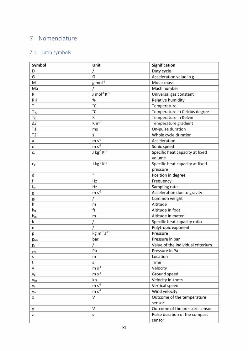
7 Nomenclature

7.1 Latin symbols

Symbol Unit Signification

D / Duty cycle

G G Acceleration value in g

M g mol-1 Molar mass

Ma / Mach number

R J mol-1 K-1 Universal gas constant

RH % Relative humidity

T °C Temperature

T°C °C Temperature in Celcius degree

TK K Temperature in Kelvin

∆𝑇 K m-1 Temperature gradient

T1 ms On-pulse duration

T2 s Whole cycle duration

a m s-2 Acceleration

c m s-1 Sonic speed

cv J kg-1 K-1 Specific heat capacity at fixed volume

cp J kg-1 K-1 Specific heat capacity at fixed pressure

d ° Position in degree

f Hz Frequency

fsr Hz Sampling rate

g m s-2 Acceleration due to gravity

gi / Common weight

h m Altitude

hft ft Altitude in foot

hm m Altitude in meter

k / Specific heat capacity ratio

n / Polytropic exponent

p kg m-1 s-2 Pressure

pbar bar Pressure in bar

pi / Value of the individual criterium

pPa Pa Pressure in Pa

s m Location

t s Time

v m s-1 Velocity

vg m s-1 Ground speed

vkn kn Velocity in knots

vv m s-1 Vertical speed

vw m s-1 Wind velocity

x V Outcome of the temperature sensor

y V Outcome of the pressure sensor

z s

Pulse duration of the compass sensor

XII

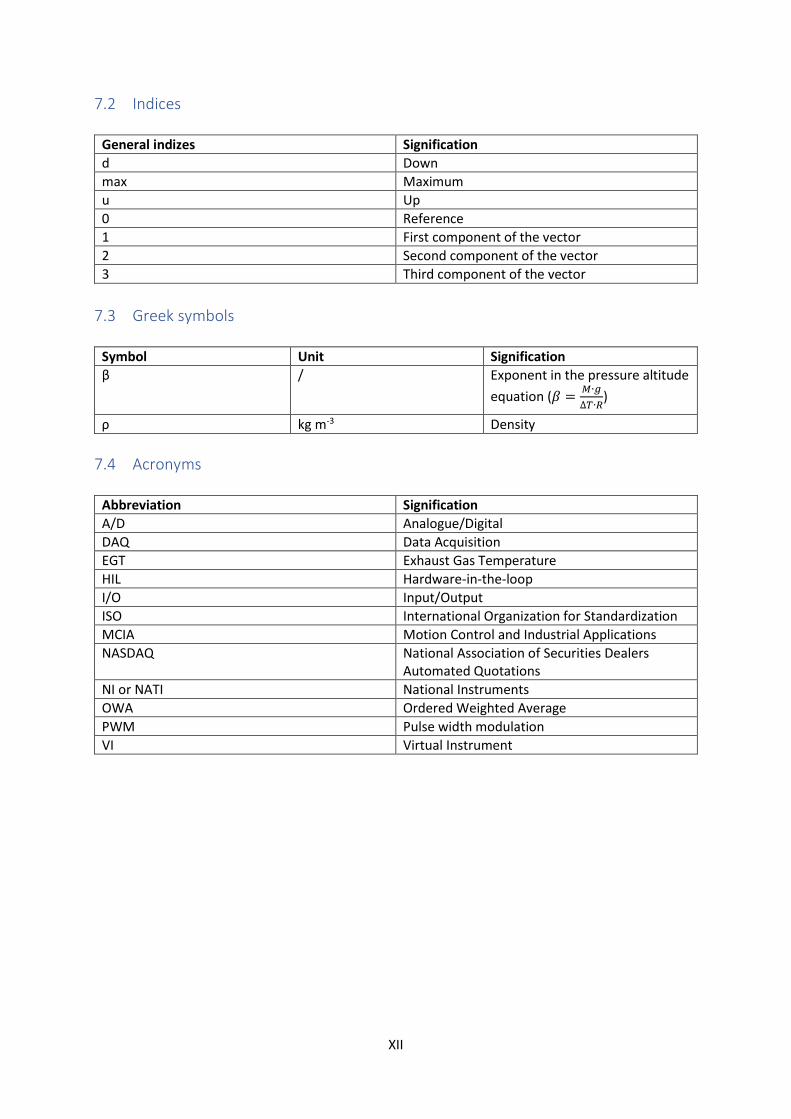
7.2 Indices

General indizes Signification

d Down

max Maximum

u Up

0 Reference

1 First component of the vector

2 Second component of the vector

3 Third component of the vector

7.3 Greek symbols

Symbol Unit Signification

β / Exponent in the pressure altitude

equation (𝛽 =𝑀∙𝑔

∆𝑇∙𝑅)

ρ kg m-3 Density

7.4 Acronyms

Abbreviation Signification

A/D Analogue/Digital

DAQ Data Acquisition

EGT Exhaust Gas Temperature

HIL Hardware-in-the-loop

I/O Input/Output

ISO International Organization for Standardization

MCIA Motion Control and Industrial Applications

NASDAQ National Association of Securities Dealers Automated Quotations

NI or NATI National Instruments

OWA Ordered Weighted Average

PWM Pulse width modulation

VI Virtual Instrument

1

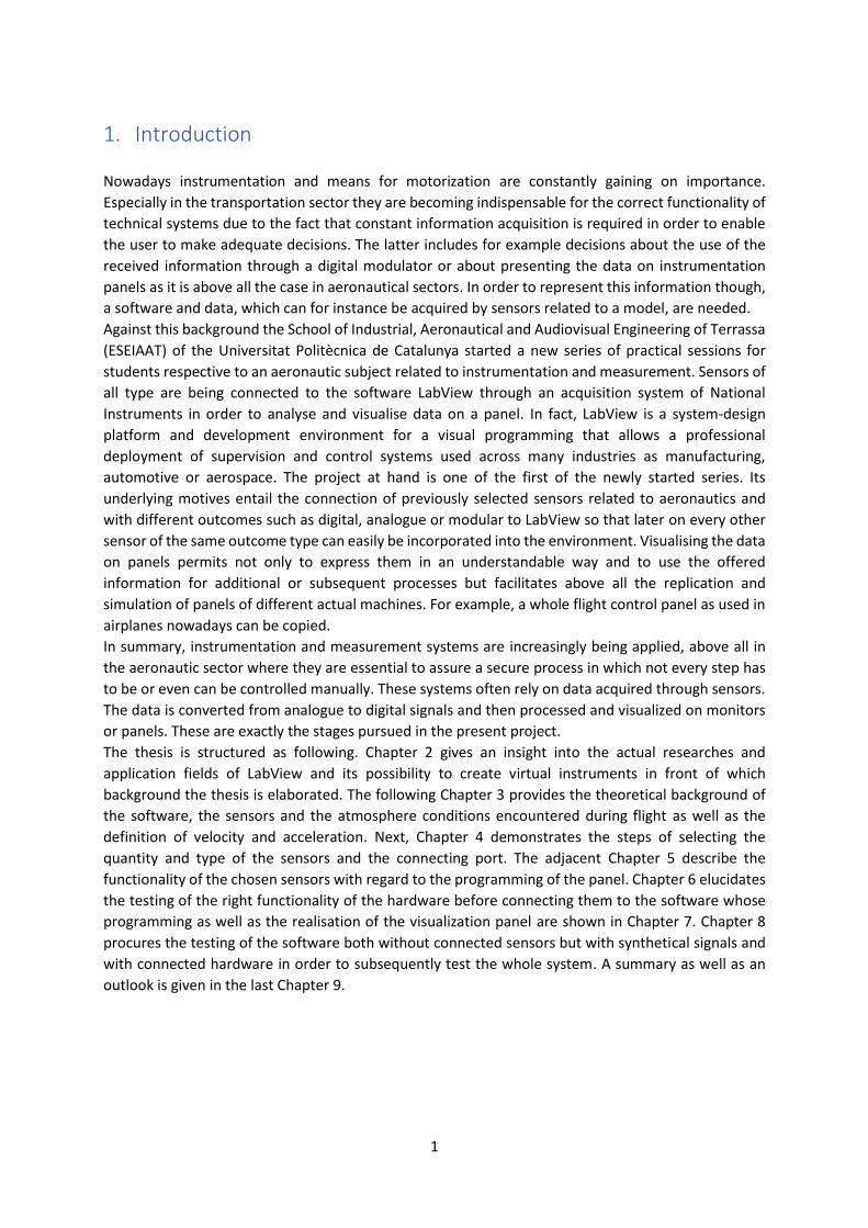
1. Introduction

Nowadays instrumentation and means for motorization are constantly gaining on importance.

Especially in the transportation sector they are becoming indispensable for the correct functionality of

technical systems due to the fact that constant information acquisition is required in order to enable

the user to make adequate decisions. The latter includes for example decisions about the use of the

received information through a digital modulator or about presenting the data on instrumentation

panels as it is above all the case in aeronautical sectors. In order to represent this information though,

a software and data, which can for instance be acquired by sensors related to a model, are needed.

Against this background the School of Industrial, Aeronautical and Audiovisual Engineering of Terrassa

(ESEIAAT) of the Universitat Politècnica de Catalunya started a new series of practical sessions for

students respective to an aeronautic subject related to instrumentation and measurement. Sensors of

all type are being connected to the software LabView through an acquisition system of National

Instruments in order to analyse and visualise data on a panel. In fact, LabView is a system-design

platform and development environment for a visual programming that allows a professional

deployment of supervision and control systems used across many industries as manufacturing,

automotive or aerospace. The project at hand is one of the first of the newly started series. Its

underlying motives entail the connection of previously selected sensors related to aeronautics and

with different outcomes such as digital, analogue or modular to LabView so that later on every other

sensor of the same outcome type can easily be incorporated into the environment. Visualising the data

on panels permits not only to express them in an understandable way and to use the offered

information for additional or subsequent processes but facilitates above all the replication and

simulation of panels of different actual machines. For example, a whole flight control panel as used in

airplanes nowadays can be copied.

In summary, instrumentation and measurement systems are increasingly being applied, above all in

the aeronautic sector where they are essential to assure a secure process in which not every step has

to be or even can be controlled manually. These systems often rely on data acquired through sensors.

The data is converted from analogue to digital signals and then processed and visualized on monitors

or panels. These are exactly the stages pursued in the present project.

The thesis is structured as following. Chapter 2 gives an insight into the actual researches and

application fields of LabView and its possibility to create virtual instruments in front of which

background the thesis is elaborated. The following Chapter 3 provides the theoretical background of

the software, the sensors and the atmosphere conditions encountered during flight as well as the

definition of velocity and acceleration. Next, Chapter 4 demonstrates the steps of selecting the

quantity and type of the sensors and the connecting port. The adjacent Chapter 5 describe the

functionality of the chosen sensors with regard to the programming of the panel. Chapter 6 elucidates

the testing of the right functionality of the hardware before connecting them to the software whose

programming as well as the realisation of the visualization panel are shown in Chapter 7. Chapter 8

procures the testing of the software both without connected sensors but with synthetical signals and

with connected hardware in order to subsequently test the whole system. A summary as well as an

outlook is given in the last Chapter 9.

2

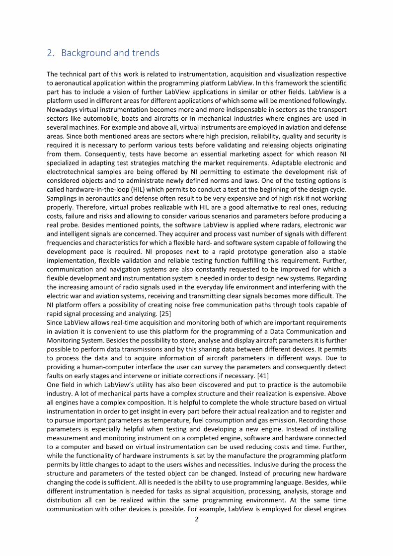
2. Background and trends

The technical part of this work is related to instrumentation, acquisition and visualization respective to aeronautical application within the programming platform LabView. In this framework the scientific part has to include a vision of further LabView applications in similar or other fields. LabView is a platform used in different areas for different applications of which some will be mentioned followingly. Nowadays virtual instrumentation becomes more and more indispensable in sectors as the transport sectors like automobile, boats and aircrafts or in mechanical industries where engines are used in several machines. For example and above all, virtual instruments are employed in aviation and defense areas. Since both mentioned areas are sectors where high precision, reliability, quality and security is required it is necessary to perform various tests before validating and releasing objects originating from them. Consequently, tests have become an essential marketing aspect for which reason NI specialized in adapting test strategies matching the market requirements. Adaptable electronic and electrotechnical samples are being offered by NI permitting to estimate the development risk of considered objects and to administrate newly defined norms and laws. One of the testing options is called hardware-in-the-loop (HIL) which permits to conduct a test at the beginning of the design cycle. Samplings in aeronautics and defense often result to be very expensive and of high risk if not working properly. Therefore, virtual probes realizable with HIL are a good alternative to real ones, reducing costs, failure and risks and allowing to consider various scenarios and parameters before producing a real probe. Besides mentioned points, the software LabView is applied where radars, electronic war and intelligent signals are concerned. They acquirer and process vast number of signals with different frequencies and characteristics for which a flexible hard- and software system capable of following the development pace is required. NI proposes next to a rapid prototype generation also a stable implementation, flexible validation and reliable testing function fulfilling this requirement. Further, communication and navigation systems are also constantly requested to be improved for which a flexible development and instrumentation system is needed in order to design new systems. Regarding the increasing amount of radio signals used in the everyday life environment and interfering with the electric war and aviation systems, receiving and transmitting clear signals becomes more difficult. The NI platform offers a possibility of creating noise free communication paths through tools capable of rapid signal processing and analyzing. [25] Since LabView allows real-time acquisition and monitoring both of which are important requirements in aviation it is convenient to use this platform for the programming of a Data Communication and Monitoring System. Besides the possibility to store, analyse and display aircraft parameters it is further possible to perform data transmissions and by this sharing data between different devices. It permits to process the data and to acquire information of aircraft parameters in different ways. Due to providing a human-computer interface the user can survey the parameters and consequently detect faults on early stages and intervene or initiate corrections if necessary. [41] One field in which LabView’s utility has also been discovered and put to practice is the automobile industry. A lot of mechanical parts have a complex structure and their realization is expensive. Above all engines have a complex composition. It is helpful to complete the whole structure based on virtual instrumentation in order to get insight in every part before their actual realization and to register and to pursue important parameters as temperature, fuel consumption and gas emission. Recording those parameters is especially helpful when testing and developing a new engine. Instead of installing measurement and monitoring instrument on a completed engine, software and hardware connected to a computer and based on virtual instrumentation can be used reducing costs and time. Further, while the functionality of hardware instruments is set by the manufacture the programming platform permits by little changes to adapt to the users wishes and necessities. Inclusive during the process the structure and parameters of the tested object can be changed. Instead of procuring new hardware changing the code is sufficient. All is needed is the ability to use programming language. Besides, while different instrumentation is needed for tasks as signal acquisition, processing, analysis, storage and distribution all can be realized within the same programming environment. At the same time communication with other devices is possible. For example, LabView is employed for diesel engines

3

which are operated with diesel-biodiesel blends in order to verify their functioning and characterize them. Since an engine needs several sensors and actuators differing in their communication protocol and signal acquisition a virtual instrumentation seems only logical. Mechanical, electronical as well as computing knowledge all are united in one single program enabling to combine measurement, analysis and control in one software. [33] A further application field for virtual instruments and the software LabView is the solar photovoltaic module. Nowadays more and more attention is being dedicated to sustainable energy supply. Employing photovoltaic systems, solar energy represents one possibility of producing sustainable energy. Thanks to their low costs, their simple maintenance and installation they have become one of the main emerging technology among the sustainable ones. In order to verify the efficiency and fill factor of these kind of module, a front panel within LabView is programmed to display real-time information about solar radiation, ambient temperature, humidity as well as current, voltage and other kind of data creating a virtual laboratory. Displaying the information on a graphical program facilitates the understanding of the module and its functionality and enables the monitoring of real-time performance as well as making the data accessible. Experiments and studies can easily be fulfilled through this platform besides the fact that the experiments can be performed under less controlled conditions. All this can be used as a tool for the user enabling him to unite theory and practice on real-time instruments. Besides the user can follow the data stream through the program starting by the sensor acquired data, to the collecting and displaying on the front panel in form of graphical indicators or tables. Once the basic program installed the virtual platform system can be adapted to the needs of the user – it can be extended to monitor lager solar modules or to fulfill educational purposes. [39] Behind this background the LabView environment represents a professional development tool with an essential academic potential. Technologies in both information and electronics keep constantly developing and improving while the digital system of which they are composed and which are running in the background are becoming more complex and larger. Students striving to become engineers or researchers need to confront themselves with the changing technologies. In order to achieve the former, they need to understand the complex coherencies as well as the logical relations assembling the digital systems. For this reason, new teaching or education methods in the classroom are requested. Here is where the programming platform Lab View as well as its application possibility of virtual instruments are gaining on importance. In order to improve the teaching quality in class and learning process of students it has been discovered that active participation in class and active integration of the students during the lecture are of much use. The professor should no longer stand before his students and explaining the new lessons talking in monologue about the themes but the students should interact directly with the new subject matter by putting instantly into practice the newly acquired knowledge. LabView permits a new teaching method based on high technologies where theory and practice can be executed at the same time by applying the theory instantly. The simple and easy structure of the programming platform thanks to the use of familiar icons and thanks to restricted code writing as well as to the numerous available libraries allows student to complete exercises in class as well as to keep practicing on their own after class. Followingly two examples of instrumental related LabView application respective to didactic and educational purposes are presented. First, the class Digital Logic form the School of Computer Science and Engineering of Qujing Normal University in QuJing (China) which is dedicated to computer and computer related subjects makes use of the programming platform LabView as a virtual teaching platform. A part from applying the learned theory the platform allows students to amplify their knowledge of planning and establishing a systematic concept, designing user interfaces and analyzing the background running system. They learn how to transition from the details to the bigger part and finally to the whole structure. Usually the class would take place in laboratories, where actual hardware equipment would be used for demonstrations. Besides their high acquisition and maintenance costs this equipment also is easily lost and broken. Consequently, the hardware is limited but needed in order to permit students to practice and retrace the learned theory to solve problems in real life. Using LabView as a virtual teaching platform reduce the costs especially respective to maintenance since it is less sensitive to mis-operation, and permits the consolidation of the newly

4

acquired knowledge with the help of experiments both for class demonstration as for self-learning. [47] The second example is the class Electronic instrumentation from the Department of Electrical Engineering of the Federal University of Maranhão (UFMA) in Brazil which is also proving to become more challenging due to the need to integrate innovative teaching methodologies. Learning methods have to be adapted to the learning objective. In order to increase the students learning retention by giving them the opportunity to participate actively instead of passively in class virtual instrumentation platform are proving themselves useful. The students get an insight in the functionalities of data acquisition and analysis, of virtual instrumentation and system control all in one single platform. Using technologies in order to accomplish informing and communicating between different devices or between computers and users as well as appropriate themselves with ID techniques is made possible. Usually the teacher holds a class by its own while the students listen passively and memorated the heard information in order to later on use the knowledge for projects to be solved after class. Since some students have trouble retaining information through passive listening, they can be discouraged to pursue the class. Using LabView tutorials by for example connecting and testing temperature sensors through which the students can retrace the application on data acquisition create a laboratory environment and motivates the students to apply and reinforce the learned theory. Additionally, tasks can be given to be accomplished at home on their own while an online forum including the teacher assures assistance if help is needed. Further, engineers as well as researchers work with software in order to create and design applications and projects. For this reason, it is useful to familiarize students on an early stage with the functionality of common software and programming platforms. [37] In this thesis the educational and aeronautic related part is exerted. Thanks to the tutorials and the application of the task students can rapidly gain insight in the functionality of LabView and acquire knowledge about the processing of data within a professional acquisition and instrumentation environment. Further the practical sessions relate to an aeronautic subject about instrumentation with the aim to analyse and visualise the data of different sensors on a panel with the possibility to later on connect every other sensor of the same outcome type to the environment. With little changes every sensor will be able to be visualized on the panel.

5

3. Theoretical background and materials

This chapter briefly introduces part of the National Instruments technology due to the fact that it is at

the origin of the here used programming platform LabView in which environment the final panel is

realized. Further, after presenting the programming environment itself it gives a general overview of

the definition and different types of sensors in order to better classify the sensors used for this project.

Finally, the Standard Atmosphere as well as a definition of velocity and acceleration are introduced

since they will be necessary for the calculations and interpretations of the sensor data.

3.1. National Instruments and their software LabView

National Instruments is a stock company specialized in automation and measurement systems related

to computers. Its shares can be acquired under the name NATI at the American electronic bourse

National Association of Securities Dealers Automated Quotations (NASDAQ). The company was

founded in 1976 in Austin, a city in Texas (USA), where its headquarters remain until today. Nowadays

the company has communities located all over the world as in France, Italy, Portugal, Turkey, Korea,

Japan, China and Spain – the latter one with community quarters situated in Madrid and Barcelona.

In order to allow Scientifics and engineers to easily develop, prototype and implement environments

respective to measurement, testing and control through an open platform a great number of different

products both in hardware and in software for data acquisition, processing and visualization which can

be connected and used by every standard computer is offered. The objective is to promote innovation

and discovery in the automation and measurement sectors. [27]

LabView is a software developed by National Instruments which offers a graphical programming

environment within the programming language G. The software can be adapted to the user’s needs

and can be deployed on every common computer. The main difference and advantage to usually

employed text-based programming softwares is the additional graphical environment within the same

development system specialized for applications in data acquisition, control, analysis and presentation.

It allows engineers to create every type of user interface without having to develop a whole new

program. Besides, systems written in other programming languages can be incorporated and

actualizations for both software and hardware exist.

LabView works with programs called Virtual Instruments (VI) due to the fact that they only represent

real instruments without being ones. Those VIs are the user interface between the outside world and

the developed program and divide themselves into a front panel, block diagrams and palettes.

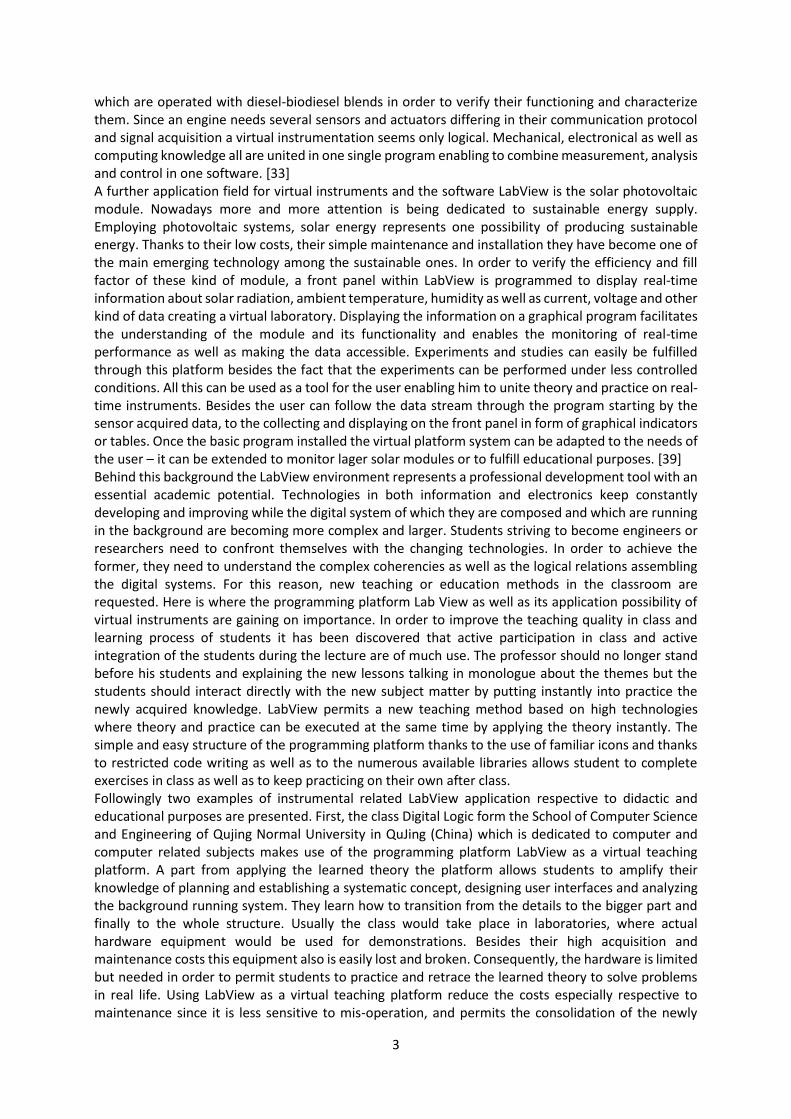
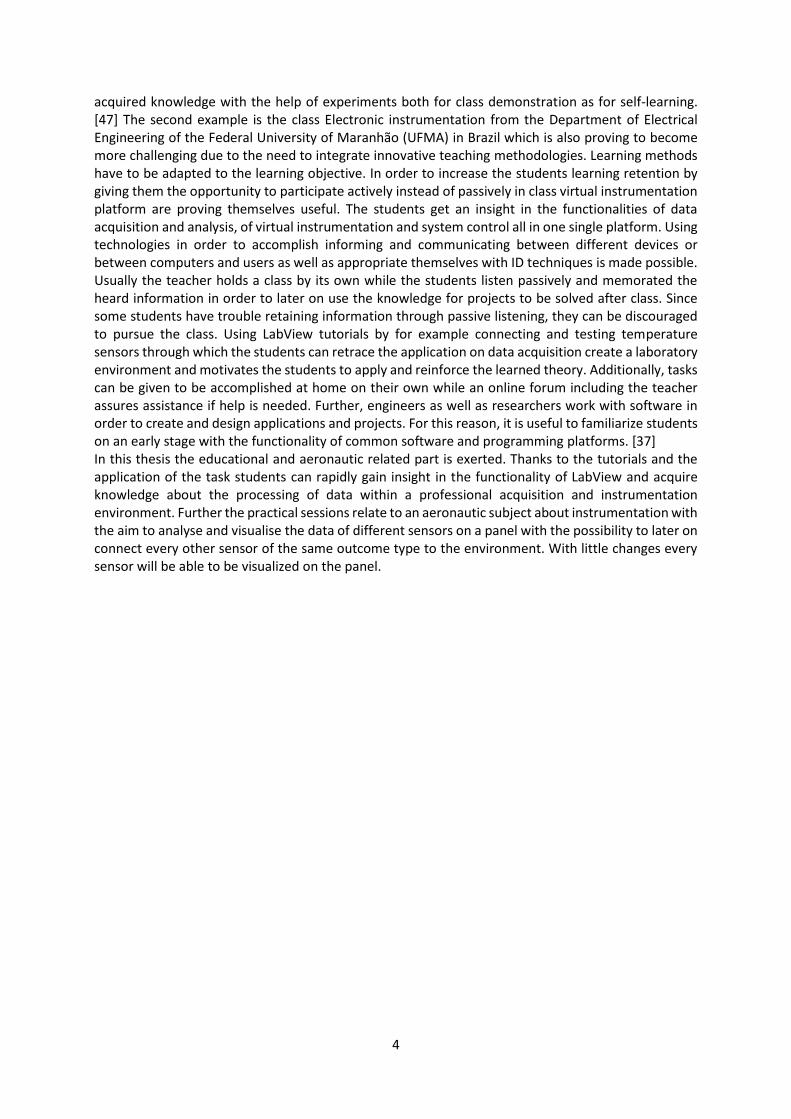
The front panel as shown in Figure 1 combines the outputs of the program and the inputs of the user

and represents the graphical interface of the VI. It is composed of controls in order to introduce

parameters and of indicators in order to display the obtained results. The controls and indicators can

adopt different forms such as buttons, graphics, displays etc..

6

Figure 1 Example of front panel view

Figure 2 Example of block diagram panel view

Figure 2 shows the block diagram panel, which represents the source code of the VI. The functions and

structures used within this part provide from the included program libraries specialized for data

acquisition, analyse, control, communication and presentation. Contrary to the usual way of creating

a source code by writing down text lines, the source code is created by arranging icons, symbols and

other objects and connecting them through cables. The latter represents the trajectory of the data and

consist of different colors and styles depending on the data type flowing through them. The objects or

structures meanwhile execute the code. The corresponding items appear automatically on the front

panel while the block diagrams are arranged and the other way around.

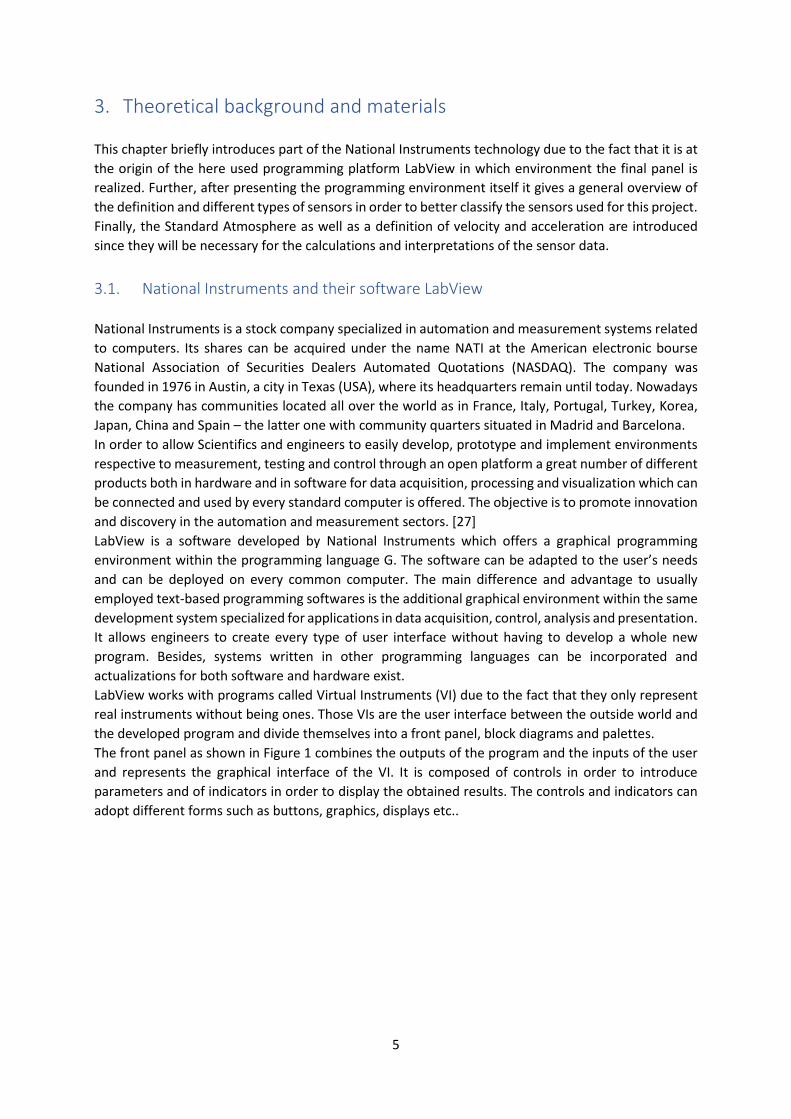
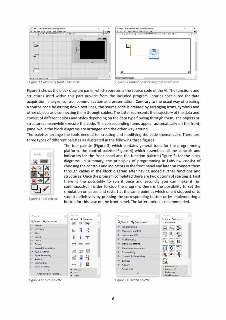
The palettes arrange the tools needed for creating and modifying the code thematically. There are

three types of different palettes as illustrated in the following three figures:

Figure 3 Tool palette

The tool palette (Figure 3) which contains general tools for the programming platform, the control palette (Figure 4) which assembles all the controls and indicators for the front panel and the function palette (Figure 5) for the block diagrams. In summary, the principles of programming in LabView consist of choosing the controls and indicators in the front panel and later on connect them through cables in the block diagram after having added further functions and structures. Once the program completed there are two options of starting it. First there is the possibility to run it once and secondly you can make it run continuously. In order to stop the program, there is the possibility to set the simulation on pause and restart at the same point at which one it stopped or to stop it definitively by pressing the corresponding button or by implementing a button for this case on the front panel. The latter option is recommended.

Figure 4 Control palette

Figure 5 Function palette

7

The program itself is organized in different rectangular structures which control the flow of information

and data. These structures are divided in sub diagrams which contain various cables and terminals.

Typical structures are the case structure, the sequence structure, the For Loop, the While Loop and

the formula node. The case structure consists of several overlapping sub diagrams. Only one of them

is visible and only one is executed at the time depending on the value the selector receives. The most

common example is the case structure true or false. Similarly, the sequence structure is arranged in

overlapping sub diagrams of which only one is visible at the time. When this structure is used all the

sub diagrams are run through respective to their chronological order, starting at number zero and

following the growing numbers. The data can be exchanged between the sub diagrams.

The For Loop serves to repeat its contents a defined number of times. There is the option shift register

which permits to save the values obtained by several previous interactions. A shift register always

shows the previous value on the left side and the actual value on the right side. The While Loop is

similar to the For Loop. Both are buckles and both have the option shift register proposes. Whereas

the For Loop is executed a defined number of times, the While Loop works after the principle “do…

while… is true”. Since the value is checked only after the buckle, it is always executed at least once.

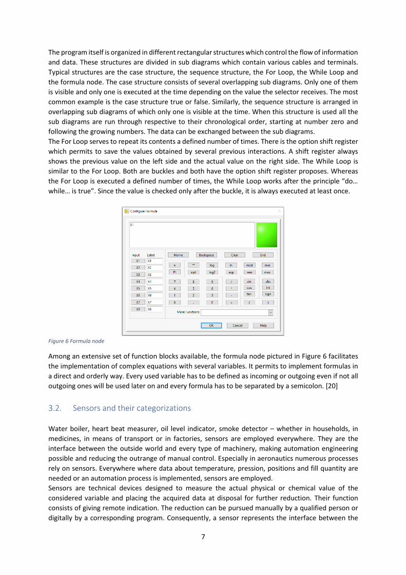
Figure 6 Formula node

Among an extensive set of function blocks available, the formula node pictured in Figure 6 facilitates

the implementation of complex equations with several variables. It permits to implement formulas in

a direct and orderly way. Every used variable has to be defined as incoming or outgoing even if not all

outgoing ones will be used later on and every formula has to be separated by a semicolon. [20]

3.2. Sensors and their categorizations

Water boiler, heart beat measurer, oil level indicator, smoke detector – whether in households, in

medicines, in means of transport or in factories, sensors are employed everywhere. They are the

interface between the outside world and every type of machinery, making automation engineering

possible and reducing the outrange of manual control. Especially in aeronautics numerous processes

rely on sensors. Everywhere where data about temperature, pression, positions and fill quantity are

needed or an automation process is implemented, sensors are employed.

Sensors are technical devices designed to measure the actual physical or chemical value of the

considered variable and placing the acquired data at disposal for further reduction. Their function

consists of giving remote indication. The reduction can be pursued manually by a qualified person or

digitally by a corresponding program. Consequently, a sensor represents the interface between the

8

outside world and the reduction system. Its application in order to measure these physical or chemical

values is called sensor system. An example for sensor-based systems are feedback control systems.

The measured value is constantly being compared to the desired value and according to the

discrepancy between the two, correcting actions are being initiated. First, an equalization process

starts in order to rearrange the desired value. Secondly, an alarm can be transmitted should the

discrepancy be too important to be corrected by the system itself or should an obvious trend be

illustrated. Lastly, the system can shut down automatically in order to prevent further damages or

destructions should the alarm keep being unattended for too long. [16]

Sensors can be classified respective to different categories. A common differentiation which refers to

the distinctive way of sensors of using or producing electrical power is the distinction between passive

and active sensors. Active sensors emit electrical signals according to the measured incoming signal

for which they do not need auxiliary energy but produce their own tension. Since a static state does

not provide any energy active sensors usually measure state changes. Passive sensors in contrary

capture and measure incoming signals, transform them into electrical ones and transfer them to a

processing system. In order to accomplish this, they need an external auxiliary energy supply which

also permit them to measure static states. Light sensors, temperature sensors as well as pressure

sensors are typical examples for the former while capacitive and inductive sensors as well as magnetic

sensors are examples for the latter. [46]

Another option of categorizing sensors is to differentiate between digital and analogue sensors. The

formers are used for switching outgoings and often detect final positions since they only contain

information coded into ones and zeros. Analogue sensors can edit various outgoings besides ones and

zeros wherefore they can be used for measuring distances and positions. Their outputs can be both a

current or a tension output. Usually the tension output reaches values between 0 and 10 V while

current outputs differ between 0 and 20 mA. If the outputs are digital, the signals are transferred by

busses or synchronous serial interfaces. [13]

In order to better clarify how sensors actually work, two examples of common operation modes will be described followingly. The first usual operation mode is the electromagnetic one. An inductor is exposed to a magnetic field under a determined tension. Every disturbance or deformation of the magnetic field results into a change of tension which is captured by the sensor and translated into a signal. Acceleration and force sensors are examples for sensors working under the electromagnetic mode. A different functionality is used for temperature sensors relying on the bimetallic operation mode. According to a change in the temperature the bimetal will deform in a specific way. If connected to a voltage source the deformation leads to different resistances from which again the importance of the change of the observed value can be deduced and finally be indicated. [16] In the aeronautic sector sensors need to master high reliability and steadiness as well as resilience respective to a harsh environment. Also, they may be exposed to a wide range of temperature due to altitude changes. Sensors are used for the dynamic of the structure, the flight tests, the chassis, the flume, the engines, the combustor etc.. With them acceleration, pression, vibrations, sounds, strains, turning moments and forces can be captured and surveyed. [32]

3.3. Standard Atmosphere

The Earth’s atmosphere is divided into several different layers of which the lowest one reaches up to

11 km and is called troposphere. Due to the weather influence the atmosphere experiences constant

changings dependent on time and on the geographical location which are noticeable in the different

variables that characterize the atmosphere. The temperature, the wind, the sonic speed, the pressure,

the humidity and the density are the most typical variables defining the atmosphere’s air state. They

are all dependent one from each other in such way as to influence themselves mutually. In order to

allow a comparison of atmospheric data independent from the geographical location and the actual

9

weather, a common basis called the standard atmosphere has been introduced by the International

Organization for Standardization (IOS). Especially in the aviation sector it is of high importance to

calibrate all the aviation instruments according to the standard atmosphere to avoid

misunderstandings between the ground team and the airplanes or the airplanes among each other.

The calibration according to the standard atmosphere ensures that all flight instruments of airplanes

flying at a similar geographical location and a similar height succumb the same deviation such as to

display identic information. Above all for the barometric height after which the airplane’s staggering

is oriented the comparison is obligatory.

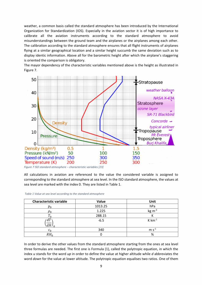
The mayor dependency of the characteristic variables mentioned above is the height as illustrated in

Figure 7.

Figure 7 ISO standard atmosphere – characteristic variables [23]

All calculations in aviation are referenced to the value the considered variable is assigned to

corresponding to the standard atmosphere at sea level. In the ISO standard atmosphere, the values at

sea level are marked with the index 0. They are listed in Table 1.

Table 1 Value at sea level according to the standard atmosphere

Characteristic variable Value Unit

𝑝0 1013.25 hPa

𝜌0 1.225 kg m-3

𝑇0 288.15 K

(𝑑𝑇

𝑑𝐻)

0

-6.5 K km-1

𝑐0 340 m s-1

𝑅𝐻0 0 %

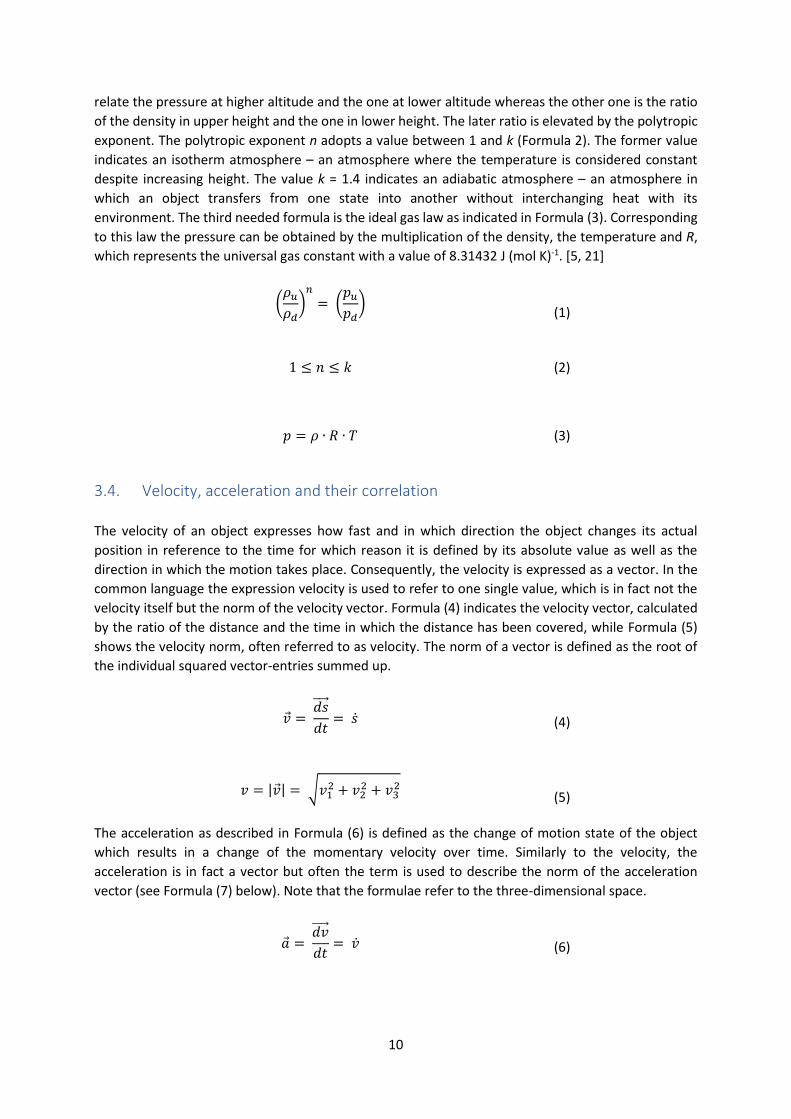
In order to derive the other values from the standard atmosphere starting from the ones at sea level

three formulas are needed. The first one is Formula (1), called the polytropic equation, in which the

index u stands for the word up in order to define the value at higher altitude while d abbreviates the

word down for the value at lower altitude. The polytropic equation equalises two ratios. One of them

10

relate the pressure at higher altitude and the one at lower altitude whereas the other one is the ratio

of the density in upper height and the one in lower height. The later ratio is elevated by the polytropic

exponent. The polytropic exponent n adopts a value between 1 and k (Formula 2). The former value

indicates an isotherm atmosphere – an atmosphere where the temperature is considered constant

despite increasing height. The value k = 1.4 indicates an adiabatic atmosphere – an atmosphere in

which an object transfers from one state into another without interchanging heat with its

environment. The third needed formula is the ideal gas law as indicated in Formula (3). Corresponding

to this law the pressure can be obtained by the multiplication of the density, the temperature and R,

which represents the universal gas constant with a value of 8.31432 J (mol K)-1. [5, 21]

(𝜌𝑢

𝜌𝑑)

𝑛

= (𝑝𝑢

𝑝𝑑)

(1) Polytropic equation

1 ≤ 𝑛 ≤ 𝑘

(2) Polytropic exponent

𝑝 = 𝜌 ∙ 𝑅 ∙ 𝑇 (3) Ideal gas law

3.4. Velocity, acceleration and their correlation

The velocity of an object expresses how fast and in which direction the object changes its actual

position in reference to the time for which reason it is defined by its absolute value as well as the

direction in which the motion takes place. Consequently, the velocity is expressed as a vector. In the

common language the expression velocity is used to refer to one single value, which is in fact not the

velocity itself but the norm of the velocity vector. Formula (4) indicates the velocity vector, calculated

by the ratio of the distance and the time in which the distance has been covered, while Formula (5)

shows the velocity norm, often referred to as velocity. The norm of a vector is defined as the root of

the individual squared vector-entries summed up.

�⃗� = 𝑑𝑠⃗⃗⃗⃗⃗

𝑑𝑡= �̇�

(4) Velocity

𝑣 = |�⃗�| = √𝑣12 + 𝑣2

2 + 𝑣32

(5) Velocity norm

The acceleration as described in Formula (6) is defined as the change of motion state of the object

which results in a change of the momentary velocity over time. Similarly to the velocity, the

acceleration is in fact a vector but often the term is used to describe the norm of the acceleration

vector (see Formula (7) below). Note that the formulae refer to the three-dimensional space.

�⃗� = 𝑑𝑣⃗⃗ ⃗⃗⃗

𝑑𝑡= �̇�

(6) Acceleration

11

𝑎 = |�⃗�| = √𝑎12 + 𝑎2

2 + 𝑎32

(7) Acceleration norm

Since the later on chosen acceleration sensor refer to two and not three directions, the actual

acceleration norm will be calculated with Formula (8).

𝑎 = |�⃗�| = √𝑎12 + 𝑎2

2

(8) Acceleration norm for the sensor

As demonstrated in Formula (9) the velocity can be obtained by integrating the measured acceleration

over time.

𝑣 = ∫ 𝑎 𝑑𝑡

𝑡1

𝑡0

(9) Integration of acceleration

If the velocity in each direction is required, instead of integrating the acceleration norm, the discrete

components of the vector can be integrated separately. As for this, the variables in Formula (10)

receive the index 1 or 2 depending on the actual axis.

𝑣1 = ∫ 𝑎1 𝑑𝑡

𝑡1

𝑡0

𝑣2 = ∫ 𝑎2 𝑑𝑡

𝑡1

𝑡0

(10) Integration of the acceleration components

12

4. Instrumentation and measurement platform design

As it has been aforementioned, the main goal of this project is to create an interface in order to

visualize data and used them for further actions (e.g. control, monitoring, maintenances, etc.).

Therefore, at first point some sensors have to be selected. The following chapters will give an insight

into the requirements the sensors have to fulfill, into the process of choosing the type of sensors and

finally into the selection of the hardware to buy for both sensors and the connecting port.

4.1. Selection of the type and quantity of sensors

Considering the available acquisition modules and the academic purpose of the platform, some initial

consideration was taken into account to face the selection of the sensors:

1 They have to be related to aeronautics, as for example to the flight control or to the maintenance.

2 Different physical magnitudes have to be considered to emulate an instrumentation panel.

3 The entrance can only be analogue (i.e. no digital protocols can be considered).

4 The sensors should differentiate in their outputs to consider diversity in their acquisition and

adaption procedures (i.e. analogue, digital or modulated outcomes).

5 Sensors should include necessary electronic to deliver electric outputs.

6 Low cost sensors are preferred.

In order to select sensors related to the aeronautic sector the first question to answer is: Which sensors

are used in airplanes? Like explained in the previous chapter there are numerous sensors of every type

and kind used in every area of a plane for which reason there is a wide palette of choices.

Figure 8 Primary flight display [8]

Figure 9 General aviation instrument panel [43]

One of the most common and indispensable flight control support for pilots is the primary flight

display, nowadays arranged in a glass panel (Figure 8). It indicates the position of the airplane in space

respective to the horizon and displays the rolling motion. Further, it informs the pilot about the speed

of the airplane and its flight altitude.

At the time the primary flight panel was introduced it was not as a glass panel but as a general aviation

instrument panel. Where now the digital screens are located there were analog circular indicators as

can be seen in Figure 9. Though the design and technology may have been adapted over time the basic

13

Primary Flight Instruments stay unchanged. There are six different types of them for which reason their

entity is referred to as Six Pack. The six instruments are the following:

1. Airspeed Indicator

2. Attitude Indicator

3. Altimeter

4. Vertical Speed Indicator

5. Heading Indicator

6. Turn Coordinator

The information that can be deduced from the displays are essential for the pilot in order to be able to

fly safely and keep the control over the airplane. [12] Adequate to its name the Airspeed Indicator

displays information about the airplane’s velocity measured in knots, a unit defined as following: 1 kn

equals 1,852 km·h-1 which again equals 0,514 m·s-1. There is to make a difference between the

indicated velocity and the actual velocity over ground. In fact, the Airspeed Indicator measures the

speed of the airplane relative to the surrounding air. In order to obtain the true air speed, the wind’s

influence needs to be subducted. Initially the position and the acceleration were measured with

gyroscopes but nowadays electrical acceleration sensors mostly replace the gyroscopes. In order to

define the position in three-dimensional space three piezo sensors are orthogonally arranged – one

for each coordinate axis. The speed can be deduced from these acceleration sensors by integrating the

value once the data is acquired. It is important to differ between the actual true air speed of the plane

and the ground speed. For the latter the wind and the rotation of the Earth have to be considered

additionally.

The Attitude Indicator is an artificial horizon indicating the airplane’s orientation respective to the

actual horizon. It facilitates the location of the airplane’s position in space and give the possibility to

identify if the airplane is flying upward or down and if the wings are inclined or level.

Third is listed the Altimeter. It depicts the airplane’s height respective to the sea level. If the altitude

over ground is wanted, the ground level of the momentary over-flown area has to be identified and

subducted from the indicated altitude. In order to measure the altitude a barometric pressure system

is employed. Thus, the altitude respective to the height above sea-level is deduced from the air

pressure outside the airplane and the actual measured data is the pressure – not the height. As the

pressure is constantly changing due to the distribution of low- and high-pressure-systems the system

has to be adjusted before and during the flight. How to derive the altitude from the pressure is

explained later on in Chapter 5.3.

Next comes the Vertical Speed Indicator illustrating the airplane’s vertical velocity in Feet Per Minute

to give information about the climb and the descend rate.

Another flight support indicator is the Heading Indicator, used to display the main direction the

airplane is heading to respective to the horizon system of coordinates or rather the earth fixed

coordinate systems. [10] It is a completely gimballed suspended gyroscope whose rotation axis is held

perpendicular to the airplane vertical axis by an additional mechanism. Consequently, the rotation axis

is constantly located in the level spanned by the airplane longitudinal and lateral axis. In order to avoid

important drifts resulting from the Earth rotation or from unbalanced gyroscope parts the Heading

Indicator is calibrated with a magnetic compass. During flight the calibration needs to be renewed

every quarter hour. The functionality of the gyroscope is based on electricity or on air flow which is

bled off a pump connected and operated by the airplane engine.

14

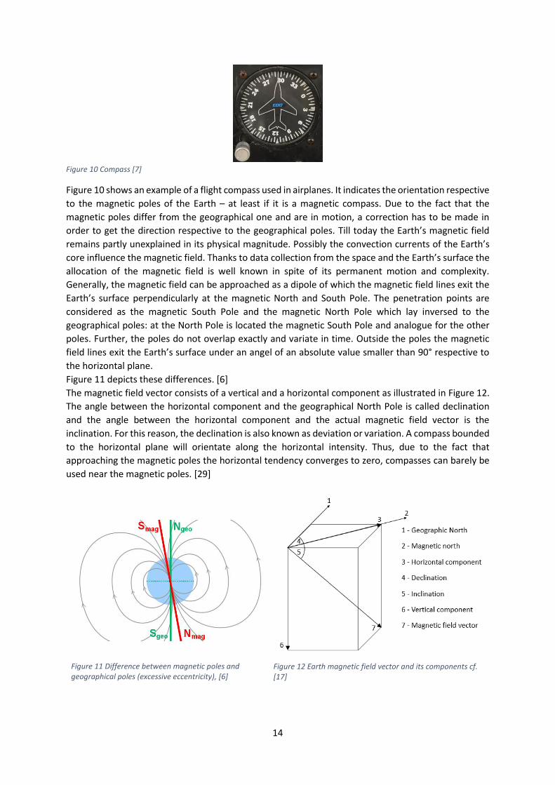
Figure 10 Compass [7]

Figure 10 shows an example of a flight compass used in airplanes. It indicates the orientation respective

to the magnetic poles of the Earth – at least if it is a magnetic compass. Due to the fact that the

magnetic poles differ from the geographical one and are in motion, a correction has to be made in

order to get the direction respective to the geographical poles. Till today the Earth’s magnetic field

remains partly unexplained in its physical magnitude. Possibly the convection currents of the Earth’s

core influence the magnetic field. Thanks to data collection from the space and the Earth’s surface the

allocation of the magnetic field is well known in spite of its permanent motion and complexity.

Generally, the magnetic field can be approached as a dipole of which the magnetic field lines exit the

Earth’s surface perpendicularly at the magnetic North and South Pole. The penetration points are

considered as the magnetic South Pole and the magnetic North Pole which lay inversed to the

geographical poles: at the North Pole is located the magnetic South Pole and analogue for the other

poles. Further, the poles do not overlap exactly and variate in time. Outside the poles the magnetic

field lines exit the Earth’s surface under an angel of an absolute value smaller than 90° respective to

the horizontal plane.

Figure 11 depicts these differences. [6]

The magnetic field vector consists of a vertical and a horizontal component as illustrated in Figure 12.

The angle between the horizontal component and the geographical North Pole is called declination

and the angle between the horizontal component and the actual magnetic field vector is the

inclination. For this reason, the declination is also known as deviation or variation. A compass bounded

to the horizontal plane will orientate along the horizontal intensity. Thus, due to the fact that

approaching the magnetic poles the horizontal tendency converges to zero, compasses can barely be

used near the magnetic poles. [29]

Figure 11 Difference between magnetic poles and geographical poles (excessive eccentricity), [6]

Figure 12 Earth magnetic field vector and its components cf. [17]

15

Lastly listed above is the Turn Coordinator. This instrument’s purpose is to help to fly coordinated

turns. It depicts the turn rate, the turn amount and the direction in which corrections have to be

applied if necessary, in order to fly coordinatively.

Besides the Primary Flight Display and the compass which are essential for the adequate navigation of

airplanes, another important value is the temperature. Not only is the latter necessary to control the

passenger’s cabin temperature in order to ensure health and comfort but it is also indispensable to

keep an overview of the different temperatures in the machinery. Whether the combustor, the engines

or simply the lubricating oils – to ensure their right functionality and to enable a secure flight the

temperature is a common indicator for the maintenance. In order to give an example for a typical

indicator the Exhaust Gas Temperature Margin by which the engine’s condition is monitored will

shortly be introduced. Exhaust Gas Temperature whose acronym is EGT represents the gas

temperature after the turbine. The EGT-Margin is the margin between the actual EGT and the maximal

tolerable EGT. An increasing EGT results in a decreasing EGT-Margin and indicates a degradation of the

engine’s condition. With the ageing of the engine’s components the degree of efficiency declines and

achieves less thrust with the same amount of fuel. Subsequently, in order to maintain the thrust level

more fuel needs to be consumed which results in a higher combustor exhaust temperature and

therefore also in a higher EGT. A maximal tolerable EGT has to be defined in order to prevent a thermal

overload of the engine. Recapitulatory, the EGT is a measure of efficiency deterioration. [14] This

example of the EGT-Margin illustrates clearly that generally measuring the temperature inside the

machinery of an airplane is of great importance.

For the reasons mentioned above the following four sensors will be used and connected to LabView:

A sensor for acceleration, one for temperature, one for air pression and a compass.

4.2. Selection of the sensors

Once the types of sensors chosen the next task consists in making a choice out of the different supplies

accessible at the market.

The temperature sensors differ mainly in the measured medium and temperature range they are

designed for. There are different sensors for outside air, cabin air, oil, water, gas, exhaust temperature

etc.. The measured medium also implicates certain supplementary properties. If the sensor is in

contact with water for example the threat of corrosion or oxidation is higher than if it only measures

cabin air for which reason a supplementary protection has to be installed. Further, depending on the

sensors’ location and functionality they need to withstand a larger or smaller range of temperatures.

Sensors inside engines can be exposed to temperatures up to 1200 °C while sensors for oil normally

will not exceed 400 °C. Especially after the combustor and the turbine the gas temperature reaches

high values. Sensors on the outer surface of the plane have to withstand low temperatures since at a

height of 10 km the air temperature is usually around -55 °C. At the same time outer sensors can be

exposed to temperatures up to 40 °C for example when the airport is situated in the desert. Should

the sensor be located inside a passenger cabin the standard temperature is 20 °C. Consequently, the

needed measuring range depends on the area the sensor is used within and has to be considered to

assure the sensor is properly working at any time.

Similarly to the temperature sensors, the needed measuring range for the pressure depends on the

concerned medium. The pressure of oil, water and air can reach different values. Since the objective

is to measure the outside air in order to derive the altitude from the acquired data a small range is

sufficient but it needs to be very precise. Considering the standard cruising altitude of approximately

10 km at which the air pressure reaches 0.262 bar and counting on an air pressure of 1 bar at ground

level, the range may be small but 0.1 bar of deviation already results in a significate difference of height

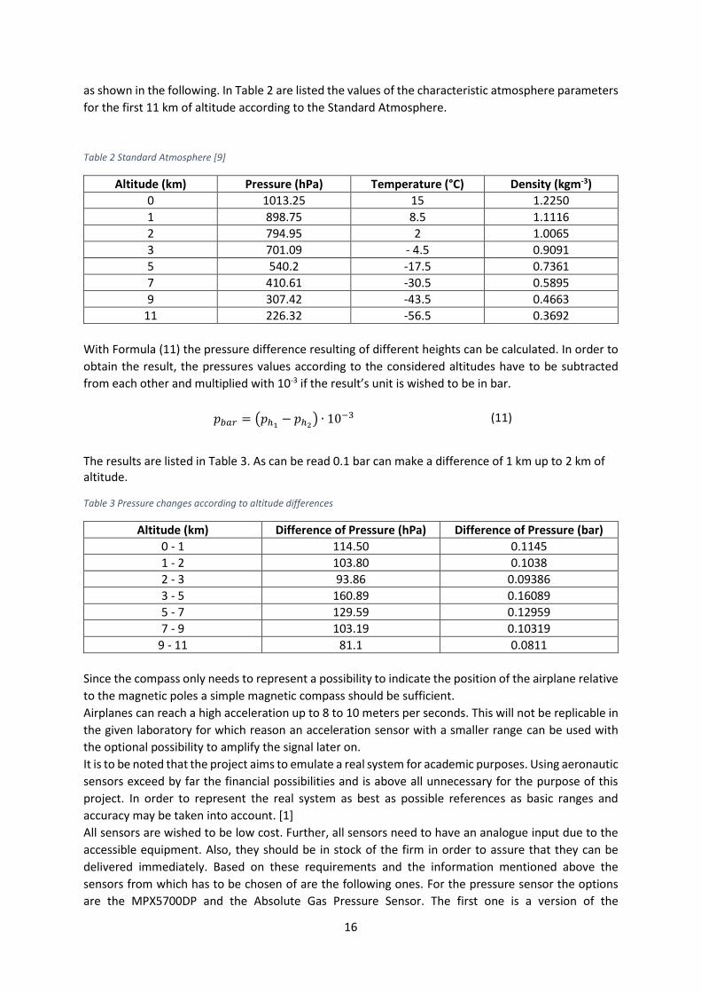
16

as shown in the following. In Table 2 are listed the values of the characteristic atmosphere parameters

for the first 11 km of altitude according to the Standard Atmosphere.

Table 2 Standard Atmosphere [9]

Altitude (km) Pressure (hPa) Temperature (°C) Density (kgm-3)

0 1013.25 15 1.2250

1 898.75 8.5 1.1116

2 794.95 2 1.0065

3 701.09 - 4.5 0.9091

5 540.2 -17.5 0.7361

7 410.61 -30.5 0.5895

9 307.42 -43.5 0.4663

11 226.32 -56.5 0.3692

With Formula (11) the pressure difference resulting of different heights can be calculated. In order to

obtain the result, the pressures values according to the considered altitudes have to be subtracted

from each other and multiplied with 10-3 if the result’s unit is wished to be in bar.

𝑝𝑏𝑎𝑟 = (𝑝ℎ1− 𝑝ℎ2

) ∙ 10−3 (11) Pressure difference

The results are listed in Table 3. As can be read 0.1 bar can make a difference of 1 km up to 2 km of altitude.

Table 3 Pressure changes according to altitude differences

Altitude (km) Difference of Pressure (hPa) Difference of Pressure (bar)

0 - 1 114.50 0.1145

1 - 2 103.80 0.1038

2 - 3 93.86 0.09386

3 - 5 160.89 0.16089

5 - 7 129.59 0.12959

7 - 9 103.19 0.10319

9 - 11 81.1 0.0811

Since the compass only needs to represent a possibility to indicate the position of the airplane relative

to the magnetic poles a simple magnetic compass should be sufficient.

Airplanes can reach a high acceleration up to 8 to 10 meters per seconds. This will not be replicable in

the given laboratory for which reason an acceleration sensor with a smaller range can be used with

the optional possibility to amplify the signal later on.

It is to be noted that the project aims to emulate a real system for academic purposes. Using aeronautic

sensors exceed by far the financial possibilities and is above all unnecessary for the purpose of this

project. In order to represent the real system as best as possible references as basic ranges and

accuracy may be taken into account. [1]

All sensors are wished to be low cost. Further, all sensors need to have an analogue input due to the

accessible equipment. Also, they should be in stock of the firm in order to assure that they can be

delivered immediately. Based on these requirements and the information mentioned above the

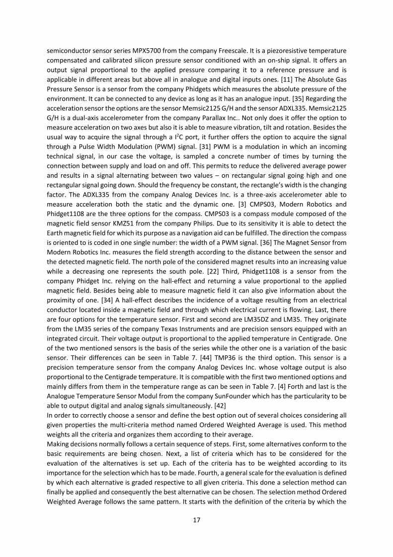
sensors from which has to be chosen of are the following ones. For the pressure sensor the options

are the MPX5700DP and the Absolute Gas Pressure Sensor. The first one is a version of the

17

semiconductor sensor series MPX5700 from the company Freescale. It is a piezoresistive temperature

compensated and calibrated silicon pressure sensor conditioned with an on-ship signal. It offers an

output signal proportional to the applied pressure comparing it to a reference pressure and is

applicable in different areas but above all in analogue and digital inputs ones. [11] The Absolute Gas

Pressure Sensor is a sensor from the company Phidgets which measures the absolute pressure of the

environment. It can be connected to any device as long as it has an analogue input. [35] Regarding the

acceleration sensor the options are the sensor Memsic2125 G/H and the sensor ADXL335. Memsic2125

G/H is a dual-axis accelerometer from the company Parallax Inc.. Not only does it offer the option to

measure acceleration on two axes but also it is able to measure vibration, tilt and rotation. Besides the

usual way to acquire the signal through a I2C port, it further offers the option to acquire the signal

through a Pulse Width Modulation (PWM) signal. [31] PWM is a modulation in which an incoming

technical signal, in our case the voltage, is sampled a concrete number of times by turning the

connection between supply and load on and off. This permits to reduce the delivered average power

and results in a signal alternating between two values – on rectangular signal going high and one

rectangular signal going down. Should the frequency be constant, the rectangle’s width is the changing

factor. The ADXL335 from the company Analog Devices Inc. is a three-axis accelerometer able to

measure acceleration both the static and the dynamic one. [3] CMPS03, Modern Robotics and

Phidget1108 are the three options for the compass. CMPS03 is a compass module composed of the

magnetic field sensor KMZ51 from the company Philips. Due to its sensitivity it is able to detect the

Earth magnetic field for which its purpose as a navigation aid can be fulfilled. The direction the compass

is oriented to is coded in one single number: the width of a PWM signal. [36] The Magnet Sensor from

Modern Robotics Inc. measures the field strength according to the distance between the sensor and

the detected magnetic field. The north pole of the considered magnet results into an increasing value

while a decreasing one represents the south pole. [22] Third, Phidget1108 is a sensor from the

company Phidget Inc. relying on the hall-effect and returning a value proportional to the applied

magnetic field. Besides being able to measure magnetic field it can also give information about the

proximity of one. [34] A hall-effect describes the incidence of a voltage resulting from an electrical

conductor located inside a magnetic field and through which electrical current is flowing. Last, there

are four options for the temperature sensor. First and second are LM35DZ and LM35. They originate

from the LM35 series of the company Texas Instruments and are precision sensors equipped with an

integrated circuit. Their voltage output is proportional to the applied temperature in Centigrade. One

of the two mentioned sensors is the basis of the series while the other one is a variation of the basic

sensor. Their differences can be seen in Table 7. [44] TMP36 is the third option. This sensor is a

precision temperature sensor from the company Analog Devices Inc. whose voltage output is also

proportional to the Centigrade temperature. It is compatible with the first two mentioned options and

mainly differs from them in the temperature range as can be seen in Table 7. [4] Forth and last is the

Analogue Temperature Sensor Modul from the company SunFounder which has the particularity to be

able to output digital and analog signals simultaneously. [42]

In order to correctly choose a sensor and define the best option out of several choices considering all

given properties the multi-criteria method named Ordered Weighted Average is used. This method

weights all the criteria and organizes them according to their average.

Making decisions normally follows a certain sequence of steps. First, some alternatives conform to the

basic requirements are being chosen. Next, a list of criteria which has to be considered for the

evaluation of the alternatives is set up. Each of the criteria has to be weighted according to its

importance for the selection which has to be made. Fourth, a general scale for the evaluation is defined

by which each alternative is graded respective to all given criteria. This done a selection method can

finally be applied and consequently the best alternative can be chosen. The selection method Ordered

Weighted Average follows the same pattern. It starts with the definition of the criteria by which the

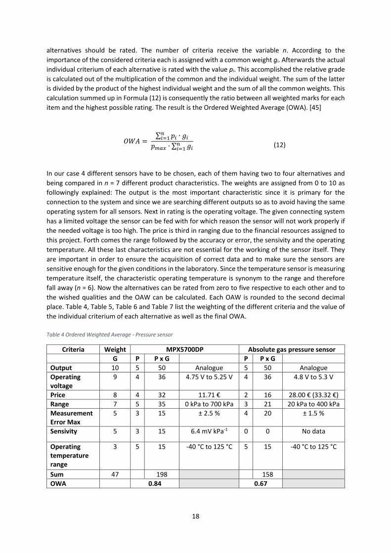
18

alternatives should be rated. The number of criteria receive the variable n. According to the

importance of the considered criteria each is assigned with a common weight gi. Afterwards the actual

individual criterium of each alternative is rated with the value pi. This accomplished the relative grade

is calculated out of the multiplication of the common and the individual weight. The sum of the latter

is divided by the product of the highest individual weight and the sum of all the common weights. This

calculation summed up in Formula (12) is consequently the ratio between all weighted marks for each

item and the highest possible rating. The result is the Ordered Weighted Average (OWA). [45]

𝑂𝑊𝐴 = ∑ 𝑝𝑖 ∙ 𝑔𝑖

𝑛𝑖=1

𝑝𝑚𝑎𝑥 ∙ ∑ 𝑔𝑖𝑛𝑖=1

(12) Calculation of OAW

In our case 4 different sensors have to be chosen, each of them having two to four alternatives and

being compared in n = 7 different product characteristics. The weights are assigned from 0 to 10 as

followingly explained: The output is the most important characteristic since it is primary for the

connection to the system and since we are searching different outputs so as to avoid having the same

operating system for all sensors. Next in rating is the operating voltage. The given connecting system

has a limited voltage the sensor can be fed with for which reason the sensor will not work properly if

the needed voltage is too high. The price is third in ranging due to the financial resources assigned to

this project. Forth comes the range followed by the accuracy or error, the sensivity and the operating

temperature. All these last characteristics are not essential for the working of the sensor itself. They

are important in order to ensure the acquisition of correct data and to make sure the sensors are

sensitive enough for the given conditions in the laboratory. Since the temperature sensor is measuring

temperature itself, the characteristic operating temperature is synonym to the range and therefore

fall away (n = 6). Now the alternatives can be rated from zero to five respective to each other and to

the wished qualities and the OAW can be calculated. Each OAW is rounded to the second decimal

place. Table 4, Table 5, Table 6 and Table 7 list the weighting of the different criteria and the value of

the individual criterium of each alternative as well as the final OWA.

Table 4 Ordered Weighted Average - Pressure sensor

Criteria Weight MPX5700DP Absolute gas pressure sensor

G P P x G P P x G

Output 10 5 50 Analogue 5 50 Analogue

Operating voltage

9 4 36 4.75 V to 5.25 V 4 36 4.8 V to 5.3 V

Price 8 4 32 11.71 € 2 16 28.00 € (33.32 €)

Range 7 5 35 0 kPa to 700 kPa 3 21 20 kPa to 400 kPa

Measurement Error Max

5 3 15 ± 2.5 % 4 20 ± 1.5 %

Sensivity 5 3 15 6.4 mV kPa-1 0 0 No data

Operating temperature range

3 5 15 -40 °C to 125 °C 5 15 -40 °C to 125 °C

Sum 47 198 158

OWA 0.84 0.67

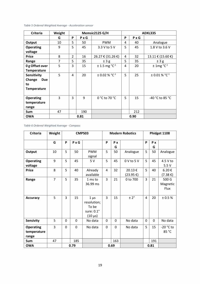
19

Table 5 Ordered Weighted Average - Acceleration sensor

Criteria Weight Memsic2125 G/H ADXL335

G P P x G P P x G

Output 10 5 50 PWM 4 40 Analogue

Operating voltage

9 5 45 3.3 V to 5 V 5 45 1.8 V to 3.6 V

Price 8 2 16 26.27 € (31.26 €) 4 32 13.11 € (15.60 €)

Range 7 5 35 ± 3 g 5 35 ± 3 g

0 g Offset over Temperature

5 3 15 ± 1.5 mg °C-1 4 20 ± 1mg °C-1

Sensitivity Change Due to Temperature

5 4 20 ± 0.02 % °C-1 5 25 ± 0.01 % °C-1

Operating temperature range

3 3 9 0 °C to 70 °C 5 15 -40 °C to 85 °C

Sum 47 190 212

OWA 0.81 0.90

Table 6 Ordered Weighted Average - Compass

Criteria Weight CMPS03

Modern Robotics Phidget 1108

G P P x G P P x G

P P x G

Output 10 5 50 PWM signal

5 50 Analogue 5 50 Analogue

Operating voltage

9 5 45 5 V 5 45 0 V to 5 V 5 45 4.5 V to 5.5 V

Price 8 5 40 Already available

4 32 20.13 € (23.95 €)

5 40 6.20 € (7.38 €)

Range 7 5 35 1 ms to 36.99 ms

3 21 0 to 700 3 21 500 G Magnetic

Flux

Accuracy 5 3 15 1 µs resolution;

To be sure: 0.1°

(10 µs)

3 15 ± 2° 4 20 ± 0.5 %

Sensivity 5 0 0 No data 0 0 No data 0 0 No data

Operating temperature range

3 0 0 No data 0 0 No data 5 15 -20 °C to 85 °C

Sum 47 185 163 191

OWA 0.79 0.69 0.81

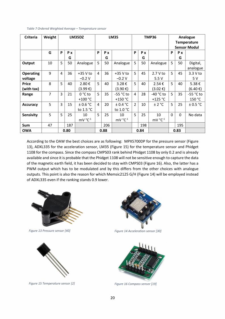
20

Table 7 Ordered Weighted Average – Temperature sensor

Criteria Weight LM35DZ LM35 TMP36 Analogue Temperature Sensor Modul

G P P x G

P P x G

P P x G

P P x G

Output 10 5 50 Analogue 5 50 Analogue 5 50 Analogue 5 50 Digital, analogue

Operating voltage

9 4 36 +35 V to −0.2 V

4 36 +35 V to −0.2 V

5 45 2.7 V to 5.5 V

5 45 3.3 V to 5 V

Price (with tax)

8 5 40 2.80 € (3.99 €)

5 40 3.28 € (3.90 €)

5 40 2.54 € (3.02 €)

5 40 5.38 € (6.40 €)

Range 7 3 21 0 °C to +100 °C

5 35 -55 °C to +150 °C

4 28 -40 °C to +125 °C

5 35 -55 °C to 150 °C

Accuracy 5 3 15 ± 0.6 °C to 1.5 °C

4 20 ± 0.4 °C to 1.0 °C

2 10 ± 2 °C 5 25 ± 0.5 °C

Sensivity 5 5 25 10 mV °C-1

5 25 10 mV °C-1

5 25 10 mV °C-1

0 0 No data

Sum 47 187 206 198 195

OWA 0.80 0.88 0.84 0.83

According to the OAW the best choices are as following: MPX5700DP for the pressure sensor (Figure

13), ADXL335 for the acceleration sensor, LM35 (Figure 15) for the temperature sensor and Phidget

1108 for the compass. Since the compass CMPS03 rank behind Phidget 1108 by only 0.2 and is already

available and since it is probable that the Phidget 1108 will not be sensitive enough to capture the data

of the magnetic earth field, it has been decided to stay with CMPS03 (Figure 16). Also, the latter has a

PWM output which has to be modulated and by this differs from the other choices with analogue

outputs. This point is also the reason for which Memsic2125 G/H (Figure 14) will be employed instead

of ADXL335 even if the ranking stands 0.9 lower.

Figure 13 Pressure sensor [40]

Figure 14 Acceleration sensor [30]

Figure 15 Temperature sensor [2]

Figure 16 Compass sensor [19]

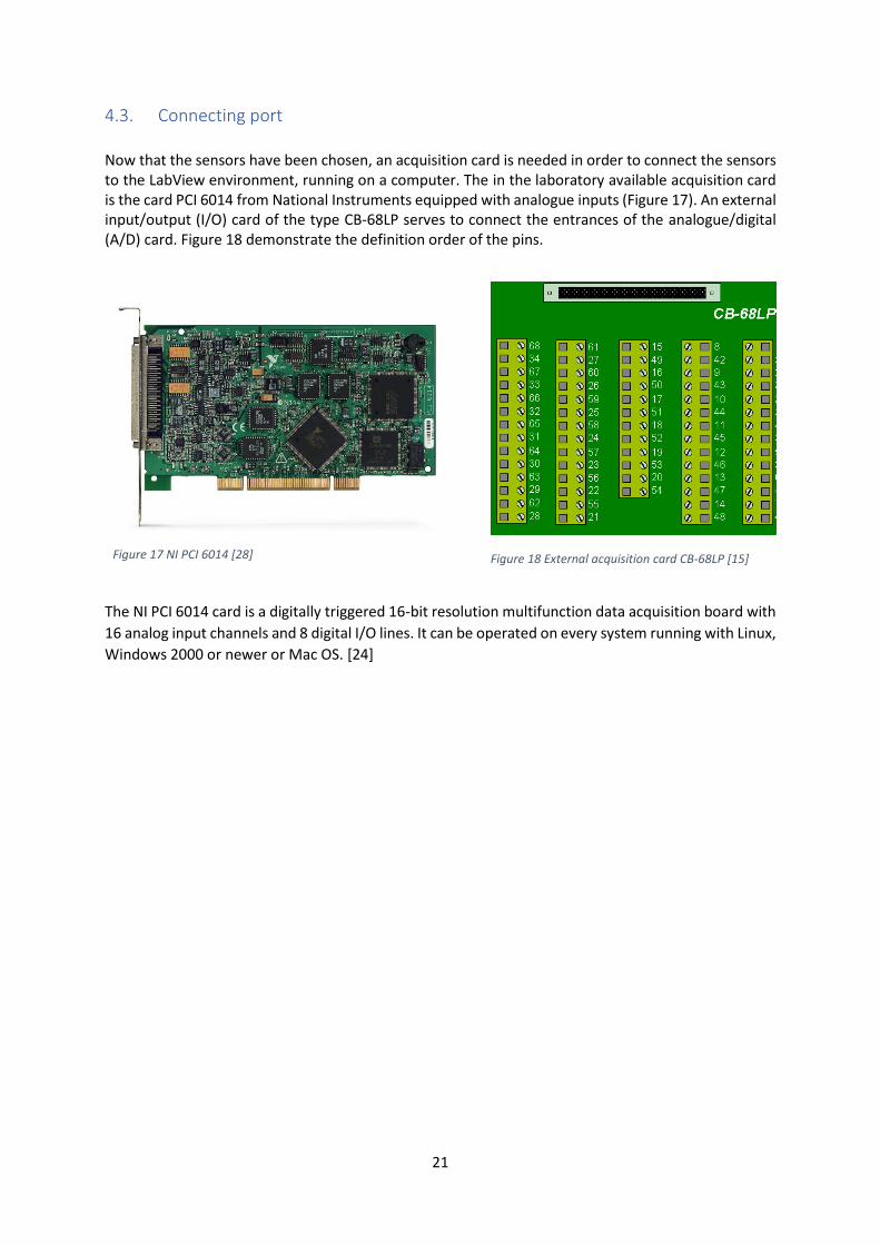
21

4.3. Connecting port

Now that the sensors have been chosen, an acquisition card is needed in order to connect the sensors to the LabView environment, running on a computer. The in the laboratory available acquisition card is the card PCI 6014 from National Instruments equipped with analogue inputs (Figure 17). An external input/output (I/O) card of the type CB-68LP serves to connect the entrances of the analogue/digital (A/D) card. Figure 18 demonstrate the definition order of the pins.

Figure 17 NI PCI 6014 [28]

Figure 18 External acquisition card CB-68LP [15]

The NI PCI 6014 card is a digitally triggered 16-bit resolution multifunction data acquisition board with

16 analog input channels and 8 digital I/O lines. It can be operated on every system running with Linux,

Windows 2000 or newer or Mac OS. [24]

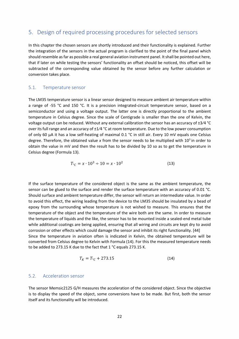
22

5. Design of required processing procedures for selected sensors

In this chapter the chosen sensors are shortly introduced and their functionality is explained. Further

the integration of the sensors in the actual program is clarified to the point of the final panel which

should resemble as far as possible a real general aviation instrument panel. It shall be pointed out here,

that if later on while testing the sensors’ functionality an offset should be noticed, this offset will be

subtracted of the corresponding value obtained by the sensor before any further calculation or

conversion takes place.

5.1. Temperature sensor

The LM35 temperature sensor is a linear sensor designed to measure ambient air temperature within

a range of -55 °C and 150 °C. It is a precision integrated-circuit temperature sensor, based on a

semiconductor and using a voltage output. The latter one is directly proportional to the ambient

temperature in Celsius degree. Since the scale of Centigrade is smaller than the one of Kelvin, the

voltage output can be reduced. Without any external calibration the sensor has an accuracy of ±3⁄4 °C

over its full range and an accuracy of ±1⁄4 °C at room temperature. Due to the low power consumption

of only 60 μA it has a low self-heating of maximal 0.1 °C in still air. Every 10 mV equals one Celsius

degree. Therefore, the obtained value x from the sensor needs to be multiplied with 103 in order to

obtain the value in mV and then the result has to be divided by 10 so as to get the temperature in

Celsius degree (Formula 13).

𝑇°𝐶 = 𝑥 ∙ 103 ÷ 10 = 𝑥 ∙ 102 (13) Temperature

conversion from the sensor’s data

If the surface temperature of the considered object is the same as the ambient temperature, the

sensor can be glued to the surface and render the surface temperature with an accuracy of 0.01 °C.

Should surface and ambient temperature differ, the sensor will return an intermediate value. In order

to avoid this effect, the wiring leading from the device to the LM35 should be insulated by a bead of

epoxy from the surrounding whose temperature is not wished to measure. This ensures that the

temperature of the object and the temperature of the wire both are the same. In order to measure

the temperature of liquids and the like, the sensor has to be mounted inside a sealed-end metal tube

while additional coatings are being applied, ensuring that all wiring and circuits are kept dry to avoid

corrosion or other effects which could damage the sensor and inhibit its right functionality. [44]

Since the temperature in aviation often is indicated in Kelvin, the obtained temperature will be converted from Celsius degree to Kelvin with Formula (14). For this the measured temperature needs to be added to 273.15 K due to the fact that 1 °C equals 273.15 K.

𝑇𝐾 = 𝑇°𝐶 + 273.15 (14) Temperature conversion from °C to K

5.2. Acceleration sensor

The sensor Memsic2125 G/H measures the acceleration of the considered object. Since the objective

is to display the speed of the object, some conversions have to be made. But first, both the sensor

itself and its functionality will be introduced.

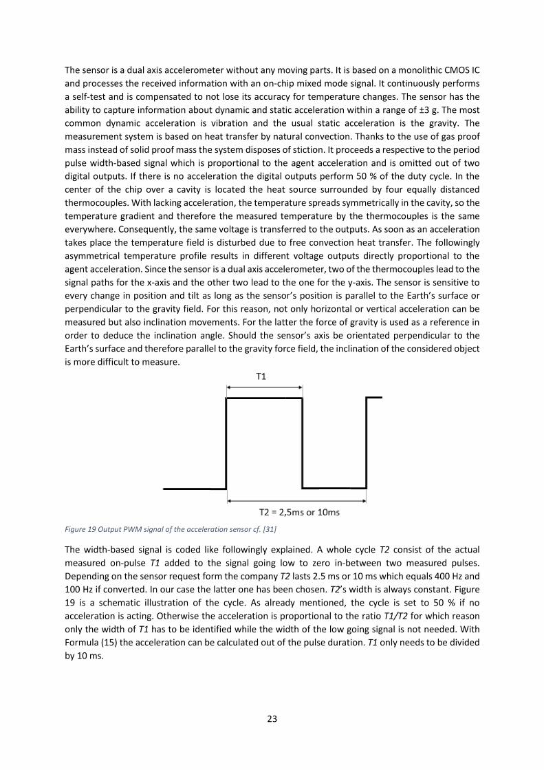
23

The sensor is a dual axis accelerometer without any moving parts. It is based on a monolithic CMOS IC

and processes the received information with an on-chip mixed mode signal. It continuously performs

a self-test and is compensated to not lose its accuracy for temperature changes. The sensor has the

ability to capture information about dynamic and static acceleration within a range of ±3 g. The most

common dynamic acceleration is vibration and the usual static acceleration is the gravity. The

measurement system is based on heat transfer by natural convection. Thanks to the use of gas proof

mass instead of solid proof mass the system disposes of stiction. It proceeds a respective to the period

pulse width-based signal which is proportional to the agent acceleration and is omitted out of two

digital outputs. If there is no acceleration the digital outputs perform 50 % of the duty cycle. In the

center of the chip over a cavity is located the heat source surrounded by four equally distanced

thermocouples. With lacking acceleration, the temperature spreads symmetrically in the cavity, so the

temperature gradient and therefore the measured temperature by the thermocouples is the same

everywhere. Consequently, the same voltage is transferred to the outputs. As soon as an acceleration

takes place the temperature field is disturbed due to free convection heat transfer. The followingly

asymmetrical temperature profile results in different voltage outputs directly proportional to the

agent acceleration. Since the sensor is a dual axis accelerometer, two of the thermocouples lead to the

signal paths for the x-axis and the other two lead to the one for the y-axis. The sensor is sensitive to

every change in position and tilt as long as the sensor’s position is parallel to the Earth’s surface or

perpendicular to the gravity field. For this reason, not only horizontal or vertical acceleration can be

measured but also inclination movements. For the latter the force of gravity is used as a reference in

order to deduce the inclination angle. Should the sensor’s axis be orientated perpendicular to the

Earth’s surface and therefore parallel to the gravity force field, the inclination of the considered object

is more difficult to measure.

Figure 19 Output PWM signal of the acceleration sensor cf. [31]

The width-based signal is coded like followingly explained. A whole cycle T2 consist of the actual

measured on-pulse T1 added to the signal going low to zero in-between two measured pulses.

Depending on the sensor request form the company T2 lasts 2.5 ms or 10 ms which equals 400 Hz and

100 Hz if converted. In our case the latter one has been chosen. T2’s width is always constant. Figure

19 is a schematic illustration of the cycle. As already mentioned, the cycle is set to 50 % if no

acceleration is acting. Otherwise the acceleration is proportional to the ratio T1/T2 for which reason

only the width of T1 has to be identified while the width of the low going signal is not needed. With

Formula (15) the acceleration can be calculated out of the pulse duration. T1 only needs to be divided

by 10 ms.

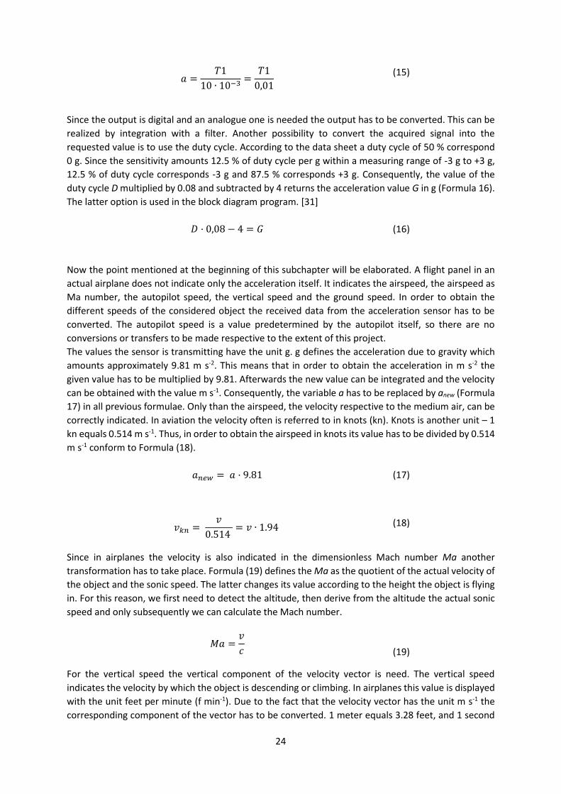
24

𝑎 =𝑇1

10 ∙ 10−3=

𝑇1

0,01

(15) Conversion of the pulse duration to the acceleration

Since the output is digital and an analogue one is needed the output has to be converted. This can be

realized by integration with a filter. Another possibility to convert the acquired signal into the

requested value is to use the duty cycle. According to the data sheet a duty cycle of 50 % correspond

0 g. Since the sensitivity amounts 12.5 % of duty cycle per g within a measuring range of -3 g to +3 g,

12.5 % of duty cycle corresponds -3 g and 87.5 % corresponds +3 g. Consequently, the value of the

duty cycle D multiplied by 0.08 and subtracted by 4 returns the acceleration value G in g (Formula 16).

The latter option is used in the block diagram program. [31]

𝐷 · 0,08 − 4 = 𝐺 (16) Conversion duty cycle to acceleration

Now the point mentioned at the beginning of this subchapter will be elaborated. A flight panel in an

actual airplane does not indicate only the acceleration itself. It indicates the airspeed, the airspeed as

Ma number, the autopilot speed, the vertical speed and the ground speed. In order to obtain the

different speeds of the considered object the received data from the acceleration sensor has to be

converted. The autopilot speed is a value predetermined by the autopilot itself, so there are no

conversions or transfers to be made respective to the extent of this project.

The values the sensor is transmitting have the unit g. g defines the acceleration due to gravity which

amounts approximately 9.81 m s-2. This means that in order to obtain the acceleration in m s-2 the

given value has to be multiplied by 9.81. Afterwards the new value can be integrated and the velocity

can be obtained with the value m s-1. Consequently, the variable a has to be replaced by anew (Formula

17) in all previous formulae. Only than the airspeed, the velocity respective to the medium air, can be

correctly indicated. In aviation the velocity often is referred to in knots (kn). Knots is another unit – 1

kn equals 0.514 m s-1. Thus, in order to obtain the airspeed in knots its value has to be divided by 0.514

m s-1 conform to Formula (18).

𝑎𝑛𝑒𝑤 = 𝑎 · 9.81 (17) Acceleration m s-2

𝑣𝑘𝑛 = 𝑣

0.514 = 𝑣 ∙ 1.94 (18) Velocity in kn

Since in airplanes the velocity is also indicated in the dimensionless Mach number Ma another

transformation has to take place. Formula (19) defines the Ma as the quotient of the actual velocity of

the object and the sonic speed. The latter changes its value according to the height the object is flying

in. For this reason, we first need to detect the altitude, then derive from the altitude the actual sonic

speed and only subsequently we can calculate the Mach number.

𝑀𝑎 =𝑣

𝑐

(19) Mach number

For the vertical speed the vertical component of the velocity vector is need. The vertical speed

indicates the velocity by which the object is descending or climbing. In airplanes this value is displayed

with the unit feet per minute (f min-1). Due to the fact that the velocity vector has the unit m s-1 the

corresponding component of the vector has to be converted. 1 meter equals 3.28 feet, and 1 second

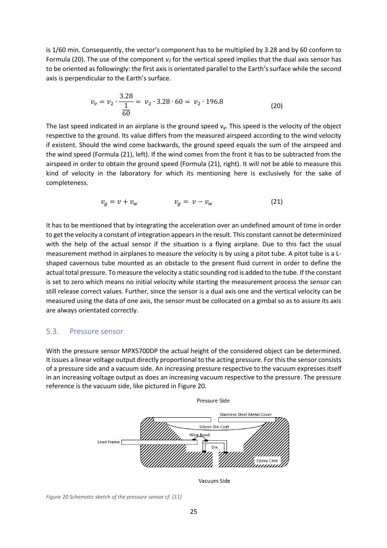
25

is 1/60 min. Consequently, the vector’s component has to be multiplied by 3.28 and by 60 conform to

Formula (20). The use of the component v2 for the vertical speed implies that the dual axis sensor has

to be oriented as followingly: the first axis is orientated parallel to the Earth’s surface while the second

axis is perpendicular to the Earth’s surface.

𝑣𝑣 = 𝑣2 ∙3.28

160

= 𝑣2 ∙ 3.28 ∙ 60 = 𝑣2 ∙ 196.8 (20) Vertical speed

The last speed indicated in an airplane is the ground speed vg. This speed is the velocity of the object

respective to the ground. Its value differs from the measured airspeed according to the wind velocity

if existent. Should the wind come backwards, the ground speed equals the sum of the airspeed and

the wind speed (Formula (21), left). If the wind comes from the front it has to be subtracted from the

airspeed in order to obtain the ground speed (Formula (21), right). It will not be able to measure this

kind of velocity in the laboratory for which its mentioning here is exclusively for the sake of

completeness.

𝑣𝑔 = 𝑣 + 𝑣𝑤 𝑣𝑔 = 𝑣 − 𝑣𝑤 (21) Ground speed

It has to be mentioned that by integrating the acceleration over an undefined amount of time in order

to get the velocity a constant of integration appears in the result. This constant cannot be determinized

with the help of the actual sensor if the situation is a flying airplane. Due to this fact the usual

measurement method in airplanes to measure the velocity is by using a pitot tube. A pitot tube is a L-

shaped cavernous tube mounted as an obstacle to the present fluid current in order to define the

actual total pressure. To measure the velocity a static sounding rod is added to the tube. If the constant

is set to zero which means no initial velocity while starting the measurement process the sensor can

still release correct values. Further, since the sensor is a dual axis one and the vertical velocity can be

measured using the data of one axis, the sensor must be collocated on a gimbal so as to assure its axis

are always orientated correctly.

5.3. Pressure sensor

With the pressure sensor MPX5700DP the actual height of the considered object can be determined. It issues a linear voltage output directly proportional to the acting pressure. For this the sensor consists of a pressure side and a vacuum side. An increasing pressure respective to the vacuum expresses itself in an increasing voltage output as does an increasing vacuum respective to the pressure. The pressure reference is the vacuum side, like pictured in Figure 20.

Figure 20 Schematic sketch of the pressure sensor cf. [11]

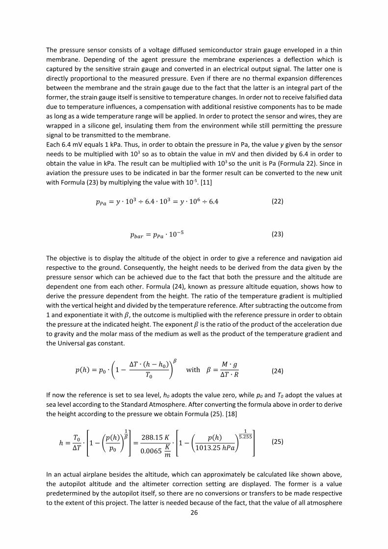
26

The pressure sensor consists of a voltage diffused semiconductor strain gauge enveloped in a thin

membrane. Depending of the agent pressure the membrane experiences a deflection which is

captured by the sensitive strain gauge and converted in an electrical output signal. The latter one is

directly proportional to the measured pressure. Even if there are no thermal expansion differences

between the membrane and the strain gauge due to the fact that the latter is an integral part of the

former, the strain gauge itself is sensitive to temperature changes. In order not to receive falsified data

due to temperature influences, a compensation with additional resistive components has to be made

as long as a wide temperature range will be applied. In order to protect the sensor and wires, they are

wrapped in a silicone gel, insulating them from the environment while still permitting the pressure

signal to be transmitted to the membrane.

Each 6.4 mV equals 1 kPa. Thus, in order to obtain the pressure in Pa, the value y given by the sensor

needs to be multiplied with 103 so as to obtain the value in mV and then divided by 6.4 in order to

obtain the value in kPa. The result can be multiplied with 103 so the unit is Pa (Formula 22). Since in

aviation the pressure uses to be indicated in bar the former result can be converted to the new unit

with Formula (23) by multiplying the value with 10-5. [11]

𝑝𝑃𝑎 = 𝑦 ∙ 103 ÷ 6.4 ∙ 103 = 𝑦 ∙ 106 ÷ 6.4 (22) Pressure conversion from the sensor’s data

𝑝𝑏𝑎𝑟 = 𝑝𝑃𝑎 ∙ 10−5 (23) Conversion from Pa to bar

The objective is to display the altitude of the object in order to give a reference and navigation aid

respective to the ground. Consequently, the height needs to be derived from the data given by the

pressure sensor which can be achieved due to the fact that both the pressure and the altitude are

dependent one from each other. Formula (24), known as pressure altitude equation, shows how to

derive the pressure dependent from the height. The ratio of the temperature gradient is multiplied

with the vertical height and divided by the temperature reference. After subtracting the outcome from

1 and exponentiate it with 𝛽, the outcome is multiplied with the reference pressure in order to obtain

the pressure at the indicated height. The exponent 𝛽 is the ratio of the product of the acceleration due

to gravity and the molar mass of the medium as well as the product of the temperature gradient and

the Universal gas constant.

𝑝(ℎ) = 𝑝0 ∙ (1 − ∆𝑇 ∙ (ℎ − ℎ0)

𝑇0)

𝛽

with 𝛽 =𝑀 ∙ 𝑔

∆𝑇 ∙ 𝑅

(24) Pressure altitude equation

If now the reference is set to sea level, h0 adopts the value zero, while p0 and T0 adopt the values at

sea level according to the Standard Atmosphere. After converting the formula above in order to derive

the height according to the pressure we obtain Formula (25). [18]

ℎ =𝑇0

∆𝑇∙ [1 − (

𝑝(ℎ)

𝑝0)

1𝛽

] =288.15 𝐾

0.0065 𝐾𝑚

∙ [1 − (𝑝(ℎ)

1013.25 ℎ𝑃𝑎)

15.255

]

(25) Height in dependency of the pressure

In an actual airplane besides the altitude, which can approximately be calculated like shown above,

the autopilot altitude and the altimeter correction setting are displayed. The former is a value

predetermined by the autopilot itself, so there are no conversions or transfers to be made respective

to the extent of this project. The latter is needed because of the fact, that the value of all atmosphere

27

variables and data are constantly changing and depend on several not influenceable factors, so that in

order to calculate the wished value some simplifications have to be made. The Standard Atmosphere

itself for example is already a simplification. Therefore, the calculated values always differ even if only

slightly from the veritable ones. In order to eliminate the most important deviations some calculative

corrections can be made and the outcome is the altimeter correction setting. Since the tools for these

corrections are not available and since they would outreach the extent of this project the altimeter

correction setting will not be considered.

Feet is a common unit used in aviation for which the altitude will also be indicated in Feet. With

Formula (26) the height can be converted from Meters to Feet by multiplying the value with

approximately 3.28 due to the fact that 1 Meter equals 3.28 Feet.

ℎ𝑓𝑡 = ℎ𝑚 ∙ 3.28 (26) Conversion from Meters to Feet

5.4. Compass sensor

The compass CMPS03 is a digital and manual compass module with a sensitivity high enough to

measure the magnetic field of the Earth. This characteristic is possible due to the magnetic field sensors

of Philips KMZ51 the CMPS03 is composed of. In order to detect the horizontal component of the Earth

magnetic field and thereby indicating the navigation course of the object, two of these magnetic field

sensors outputs are oriented at right angles respective to each other.

The compass has the particularity to offer two different ways of getting the data: a PWM signal and an

I2C interface. Since an analogue input is needed the PWM signal will be used and only this one will be

explained in the following. The PWM signal is a pulse generated by a 16-bit timer ranging from 1 ms to

36.99 ms. The lowest value represents 0° while the highest values represents 359.9°. For consequence

each degree is coded by 100 μs additional to 1 ms of offset. Between the pulses the width modulated

signal goes down to zero for 65 ms. Consequently, a cycle time is formed by the 65 ms added to the

pulse width. That means that contrary to the acceleration sensor where the cycle time’s width is always

constant, the compass sensor’s constant is the width of the low going signal not of the cycle time.

Figure 21 demonstrate the codification of the direction. Only the positive values of the PWM signal

emitted by the sensor output indicate an actual angle of the compass. Though the processor offers a

1 μs resolution, it is recommended to measure at the maximum up to 10 μs, which represents 0.1°.

Even if not used each signal is converted due to the lack of synchronization between the output and

the conversion. To conclude this compass module design is a simple aid to navigation since it codes

the direction the object is facing in a unique number. [38]

Figure 21 Output PWM signal of the electronic compass cf. [15]

28

In order to calculate the position d of the considered object in degrees after obtaining the pulse

duration in seconds, Formula (27) has to be applied. 0.001 is subtracted from the pulse duration z and

the result is multiplied with 10000.

𝑑 = (𝑧 − 0.001) ∙ 10000

(27) Position in degree

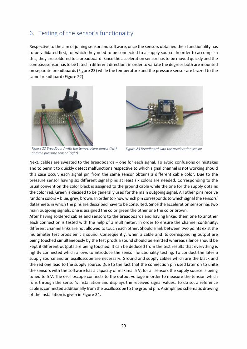
29

6. Testing of the sensor’s functionality

Respective to the aim of joining sensor and software, once the sensors obtained their functionality has

to be validated first, for which they need to be connected to a supply source. In order to accomplish

this, they are soldered to a breadboard. Since the acceleration sensor has to be moved quickly and the

compass sensor has to be tilted in different directions in order to variate the degrees both are mounted

on separate breadboards (Figure 23) while the temperature and the pressure sensor are brazed to the

same breadboard (Figure 22).

Figure 22 Breadboard with the temperature sensor (left) and the pressure sensor (right)

Figure 23 Breadboard with the acceleration sensor

Next, cables are sweated to the breadboards – one for each signal. To avoid confusions or mistakes

and to permit to quickly detect malfunctions respective to which signal channel is not working should

this case occur, each signal pin from the same sensor obtains a different cable color. Due to the

pressure sensor having six different signal pins at least six colors are needed. Corresponding to the

usual convention the color black is assigned to the ground cable while the one for the supply obtains

the color red. Green is decided to be generally used for the main outgoing signal. All other pins receive

random colors – blue, grey, brown. In order to know which pin corresponds to which signal the sensors’

datasheets in which the pins are described have to be consulted. Since the acceleration sensor has two

main outgoing signals, one is assigned the color green the other one the color brown.

After having soldered cables and sensors to the breadboards and having linked them one to another

each connection is tested with the help of a multimeter. In order to ensure the channel continuity,

different channel links are not allowed to touch each other. Should a link between two points exist the

multimeter test prods emit a sound. Consequently, when a cable and its corresponding output are

being touched simultaneously by the test prods a sound should be emitted whereas silence should be

kept if different outputs are being touched. It can be deduced from the test results that everything is

rightly connected which allows to introduce the sensor functionality testing. To conduct the later a

supply source and an oscilloscope are necessary. Ground and supply cables which are the black and

the red one lead to the supply source. Due to the fact that the connection pin used later on to unite

the sensors with the software has a capacity of maximal 5 V, for all sensors the supply source is being

tuned to 5 V. The oscilloscope connects to the output voltage in order to measure the tension which

runs through the sensor’s installation and displays the received signal values. To do so, a reference

cable is connected additionally from the oscilloscope to the ground pin. A simplified schematic drawing

of the installation is given in Figure 24.

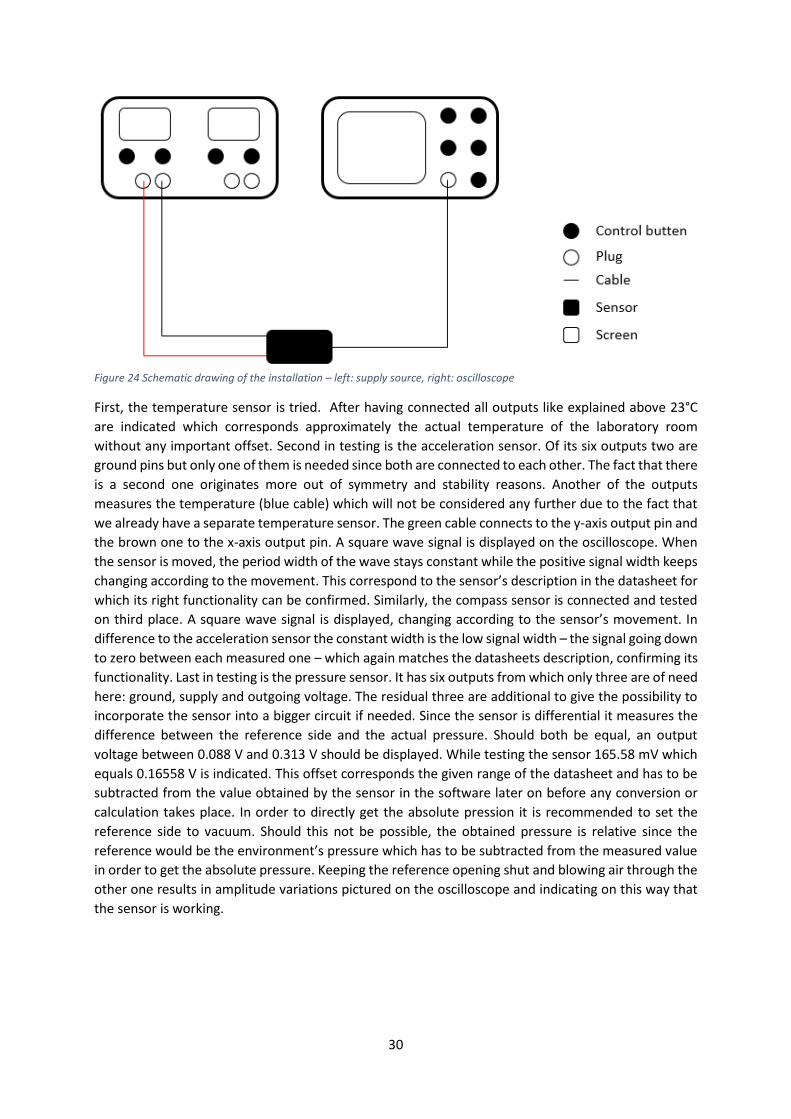
30

Figure 24 Schematic drawing of the installation – left: supply source, right: oscilloscope

First, the temperature sensor is tried. After having connected all outputs like explained above 23°C

are indicated which corresponds approximately the actual temperature of the laboratory room

without any important offset. Second in testing is the acceleration sensor. Of its six outputs two are

ground pins but only one of them is needed since both are connected to each other. The fact that there

is a second one originates more out of symmetry and stability reasons. Another of the outputs

measures the temperature (blue cable) which will not be considered any further due to the fact that

we already have a separate temperature sensor. The green cable connects to the y-axis output pin and

the brown one to the x-axis output pin. A square wave signal is displayed on the oscilloscope. When

the sensor is moved, the period width of the wave stays constant while the positive signal width keeps

changing according to the movement. This correspond to the sensor’s description in the datasheet for

which its right functionality can be confirmed. Similarly, the compass sensor is connected and tested

on third place. A square wave signal is displayed, changing according to the sensor’s movement. In

difference to the acceleration sensor the constant width is the low signal width – the signal going down

to zero between each measured one – which again matches the datasheets description, confirming its

functionality. Last in testing is the pressure sensor. It has six outputs from which only three are of need

here: ground, supply and outgoing voltage. The residual three are additional to give the possibility to

incorporate the sensor into a bigger circuit if needed. Since the sensor is differential it measures the

difference between the reference side and the actual pressure. Should both be equal, an output

voltage between 0.088 V and 0.313 V should be displayed. While testing the sensor 165.58 mV which

equals 0.16558 V is indicated. This offset corresponds the given range of the datasheet and has to be

subtracted from the value obtained by the sensor in the software later on before any conversion or

calculation takes place. In order to directly get the absolute pression it is recommended to set the

reference side to vacuum. Should this not be possible, the obtained pressure is relative since the

reference would be the environment’s pressure which has to be subtracted from the measured value

in order to get the absolute pressure. Keeping the reference opening shut and blowing air through the

other one results in amplitude variations pictured on the oscilloscope and indicating on this way that

the sensor is working.

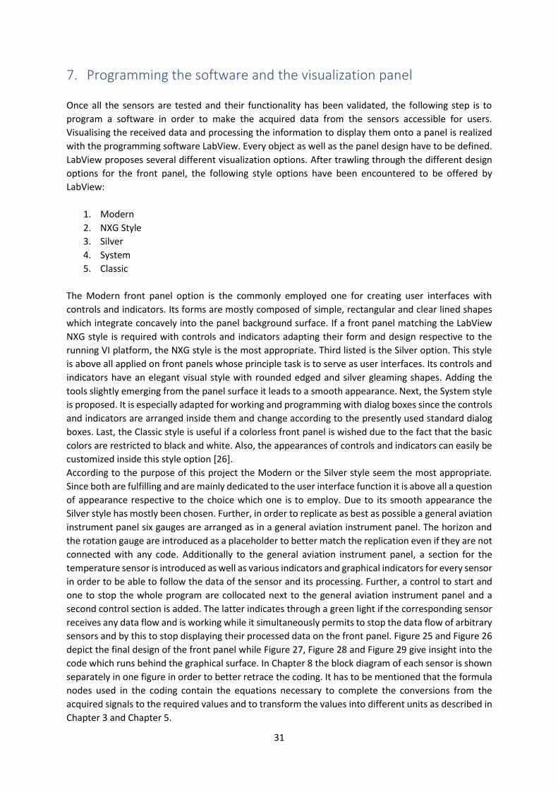
31

7. Programming the software and the visualization panel

Once all the sensors are tested and their functionality has been validated, the following step is to

program a software in order to make the acquired data from the sensors accessible for users.

Visualising the received data and processing the information to display them onto a panel is realized

with the programming software LabView. Every object as well as the panel design have to be defined.

LabView proposes several different visualization options. After trawling through the different design

options for the front panel, the following style options have been encountered to be offered by

LabView:

1. Modern

2. NXG Style

3. Silver

4. System

5. Classic

The Modern front panel option is the commonly employed one for creating user interfaces with

controls and indicators. Its forms are mostly composed of simple, rectangular and clear lined shapes

which integrate concavely into the panel background surface. If a front panel matching the LabView

NXG style is required with controls and indicators adapting their form and design respective to the

running VI platform, the NXG style is the most appropriate. Third listed is the Silver option. This style

is above all applied on front panels whose principle task is to serve as user interfaces. Its controls and

indicators have an elegant visual style with rounded edged and silver gleaming shapes. Adding the

tools slightly emerging from the panel surface it leads to a smooth appearance. Next, the System style

is proposed. It is especially adapted for working and programming with dialog boxes since the controls

and indicators are arranged inside them and change according to the presently used standard dialog

boxes. Last, the Classic style is useful if a colorless front panel is wished due to the fact that the basic

colors are restricted to black and white. Also, the appearances of controls and indicators can easily be

customized inside this style option [26].

According to the purpose of this project the Modern or the Silver style seem the most appropriate.

Since both are fulfilling and are mainly dedicated to the user interface function it is above all a question

of appearance respective to the choice which one is to employ. Due to its smooth appearance the

Silver style has mostly been chosen. Further, in order to replicate as best as possible a general aviation

instrument panel six gauges are arranged as in a general aviation instrument panel. The horizon and

the rotation gauge are introduced as a placeholder to better match the replication even if they are not

connected with any code. Additionally to the general aviation instrument panel, a section for the

temperature sensor is introduced as well as various indicators and graphical indicators for every sensor

in order to be able to follow the data of the sensor and its processing. Further, a control to start and

one to stop the whole program are collocated next to the general aviation instrument panel and a

second control section is added. The latter indicates through a green light if the corresponding sensor

receives any data flow and is working while it simultaneously permits to stop the data flow of arbitrary

sensors and by this to stop displaying their processed data on the front panel. Figure 25 and Figure 26

depict the final design of the front panel while Figure 27, Figure 28 and Figure 29 give insight into the

code which runs behind the graphical surface. In Chapter 8 the block diagram of each sensor is shown

separately in one figure in order to better retrace the coding. It has to be mentioned that the formula

nodes used in the coding contain the equations necessary to complete the conversions from the

acquired signals to the required values and to transform the values into different units as described in

Chapter 3 and Chapter 5.

32

Figure 25 View of the designed front panel (first part) – 1. General aviation instrument panel, 2. Control button, 3. Temperature indicator box, 4. Control indicator box, 5. Velocity indicator box, 6. Pressure and altitude indicator box, 7. Compass indicator box

Figure 26 View of the designed front panel (second part) – from left to right: compass graphical indicator, acceleration graphical indicator, vertical acceleration graphical indicator, acceleration indicator box

Followingly, the used items and objects in the front panel will shortly be introduced according to where

they are sorted inside the control palette. The Modern and the Silver programming library have been

employed. Respective to the Silver programming library every introduced gauge and numeric indicator

as well as the thermometer are to be found in the sub library Numeric. The stop buttons and the round

LED originate from the sub library Boolean while all the rounded boxes belong to the sub library

Decorations. Regarding the Modern programming library, both the vertical toggle switchs and the

square LED correspond to the sub library Boolean. Every employed waveform graph can be found in

the sub library Graph.

1 3

7

6 5

4

2

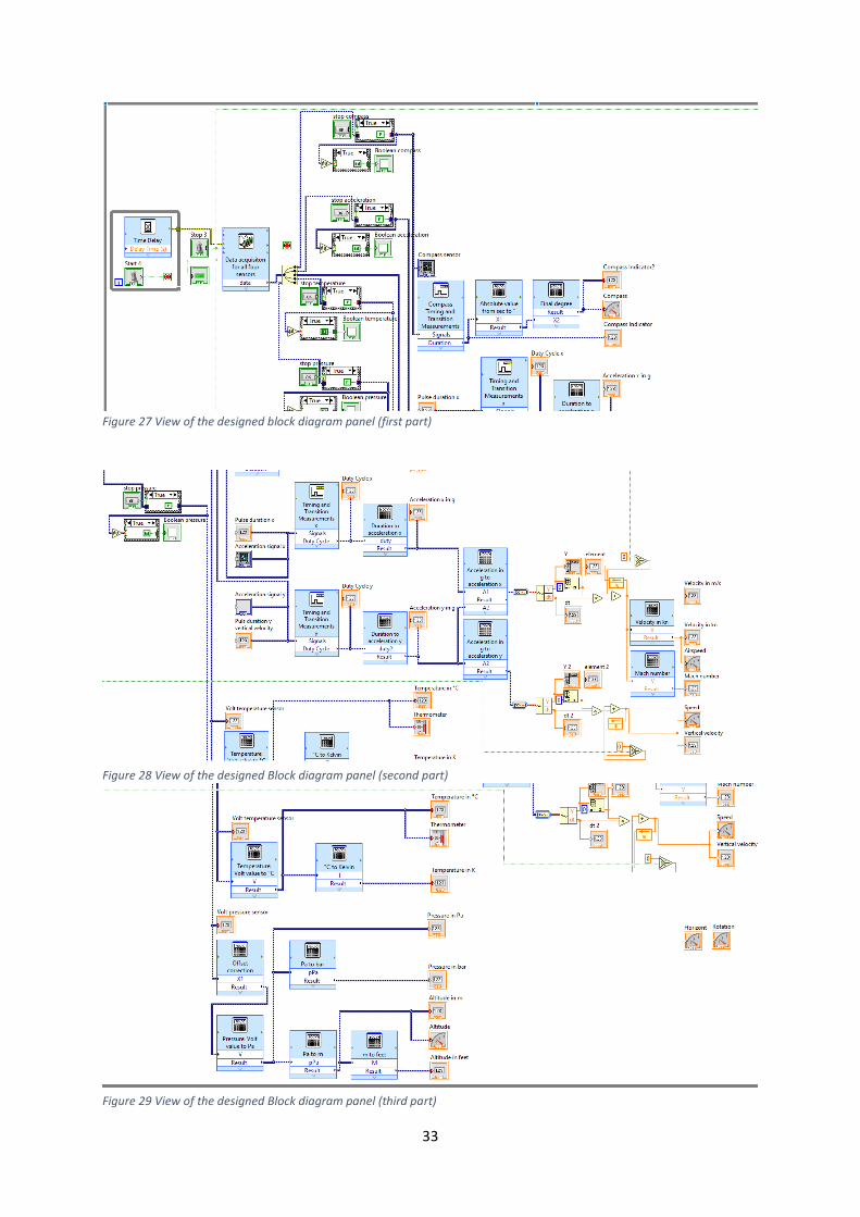
33

Figure 27 View of the designed block diagram panel (first part)

Figure 28 View of the designed Block diagram panel (second part)

Figure 29 View of the designed Block diagram panel (third part)

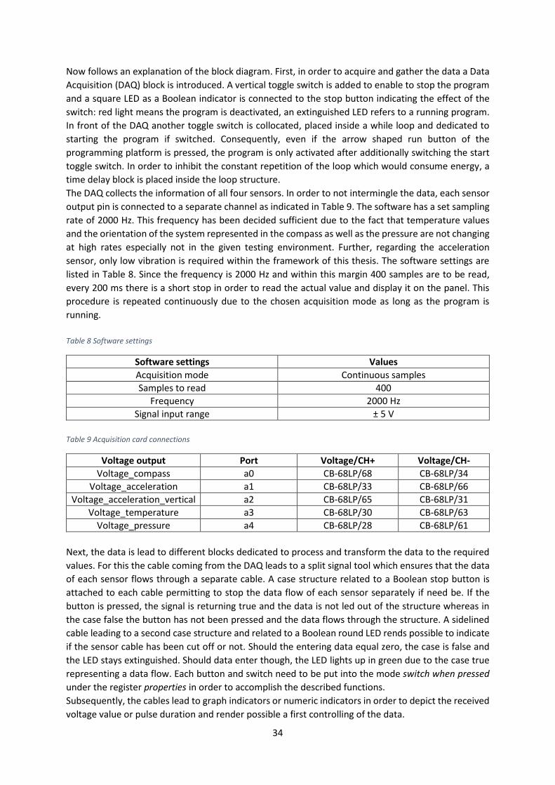
34

Now follows an explanation of the block diagram. First, in order to acquire and gather the data a Data

Acquisition (DAQ) block is introduced. A vertical toggle switch is added to enable to stop the program

and a square LED as a Boolean indicator is connected to the stop button indicating the effect of the

switch: red light means the program is deactivated, an extinguished LED refers to a running program.

In front of the DAQ another toggle switch is collocated, placed inside a while loop and dedicated to

starting the program if switched. Consequently, even if the arrow shaped run button of the

programming platform is pressed, the program is only activated after additionally switching the start

toggle switch. In order to inhibit the constant repetition of the loop which would consume energy, a

time delay block is placed inside the loop structure.

The DAQ collects the information of all four sensors. In order to not intermingle the data, each sensor

output pin is connected to a separate channel as indicated in Table 9. The software has a set sampling

rate of 2000 Hz. This frequency has been decided sufficient due to the fact that temperature values

and the orientation of the system represented in the compass as well as the pressure are not changing

at high rates especially not in the given testing environment. Further, regarding the acceleration

sensor, only low vibration is required within the framework of this thesis. The software settings are

listed in Table 8. Since the frequency is 2000 Hz and within this margin 400 samples are to be read,

every 200 ms there is a short stop in order to read the actual value and display it on the panel. This

procedure is repeated continuously due to the chosen acquisition mode as long as the program is

running.

Table 8 Software settings

Software settings Values

Acquisition mode Continuous samples

Samples to read 400

Frequency 2000 Hz

Signal input range ± 5 V

Table 9 Acquisition card connections

Voltage output Port Voltage/CH+ Voltage/CH-

Voltage_compass a0 CB-68LP/68 CB-68LP/34

Voltage_acceleration a1 CB-68LP/33 CB-68LP/66

Voltage_acceleration_vertical a2 CB-68LP/65 CB-68LP/31

Voltage_temperature a3 CB-68LP/30 CB-68LP/63

Voltage_pressure a4 CB-68LP/28 CB-68LP/61

Next, the data is lead to different blocks dedicated to process and transform the data to the required

values. For this the cable coming from the DAQ leads to a split signal tool which ensures that the data

of each sensor flows through a separate cable. A case structure related to a Boolean stop button is

attached to each cable permitting to stop the data flow of each sensor separately if need be. If the

button is pressed, the signal is returning true and the data is not led out of the structure whereas in

the case false the button has not been pressed and the data flows through the structure. A sidelined

cable leading to a second case structure and related to a Boolean round LED rends possible to indicate

if the sensor cable has been cut off or not. Should the entering data equal zero, the case is false and

the LED stays extinguished. Should data enter though, the LED lights up in green due to the case true

representing a data flow. Each button and switch need to be put into the mode switch when pressed

under the register properties in order to accomplish the described functions.

Subsequently, the cables lead to graph indicators or numeric indicators in order to depict the received

voltage value or pulse duration and render possible a first controlling of the data.

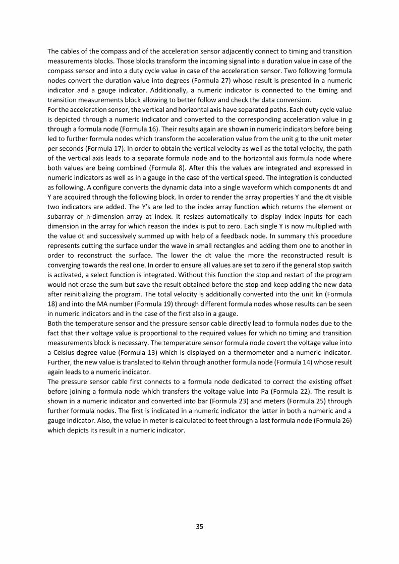
35

The cables of the compass and of the acceleration sensor adjacently connect to timing and transition

measurements blocks. Those blocks transform the incoming signal into a duration value in case of the

compass sensor and into a duty cycle value in case of the acceleration sensor. Two following formula

nodes convert the duration value into degrees (Formula 27) whose result is presented in a numeric

indicator and a gauge indicator. Additionally, a numeric indicator is connected to the timing and

transition measurements block allowing to better follow and check the data conversion.

For the acceleration sensor, the vertical and horizontal axis have separated paths. Each duty cycle value

is depicted through a numeric indicator and converted to the corresponding acceleration value in g

through a formula node (Formula 16). Their results again are shown in numeric indicators before being

led to further formula nodes which transform the acceleration value from the unit g to the unit meter

per seconds (Formula 17). In order to obtain the vertical velocity as well as the total velocity, the path

of the vertical axis leads to a separate formula node and to the horizontal axis formula node where

both values are being combined (Formula 8). After this the values are integrated and expressed in

numeric indicators as well as in a gauge in the case of the vertical speed. The integration is conducted

as following. A configure converts the dynamic data into a single waveform which components dt and

Y are acquired through the following block. In order to render the array properties Y and the dt visible

two indicators are added. The Y’s are led to the index array function which returns the element or

subarray of n-dimension array at index. It resizes automatically to display index inputs for each

dimension in the array for which reason the index is put to zero. Each single Y is now multiplied with

the value dt and successively summed up with help of a feedback node. In summary this procedure

represents cutting the surface under the wave in small rectangles and adding them one to another in

order to reconstruct the surface. The lower the dt value the more the reconstructed result is

converging towards the real one. In order to ensure all values are set to zero if the general stop switch

is activated, a select function is integrated. Without this function the stop and restart of the program

would not erase the sum but save the result obtained before the stop and keep adding the new data

after reinitializing the program. The total velocity is additionally converted into the unit kn (Formula

18) and into the MA number (Formula 19) through different formula nodes whose results can be seen

in numeric indicators and in the case of the first also in a gauge.

Both the temperature sensor and the pressure sensor cable directly lead to formula nodes due to the

fact that their voltage value is proportional to the required values for which no timing and transition

measurements block is necessary. The temperature sensor formula node covert the voltage value into

a Celsius degree value (Formula 13) which is displayed on a thermometer and a numeric indicator.

Further, the new value is translated to Kelvin through another formula node (Formula 14) whose result

again leads to a numeric indicator.

The pressure sensor cable first connects to a formula node dedicated to correct the existing offset

before joining a formula node which transfers the voltage value into Pa (Formula 22). The result is

shown in a numeric indicator and converted into bar (Formula 23) and meters (Formula 25) through

further formula nodes. The first is indicated in a numeric indicator the latter in both a numeric and a

gauge indicator. Also, the value in meter is calculated to feet through a last formula node (Formula 26)

which depicts its result in a numeric indicator.

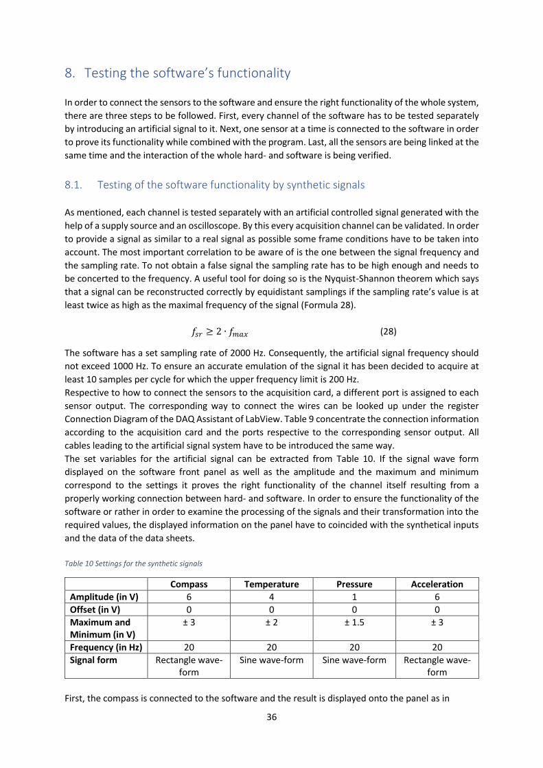
36

8. Testing the software’s functionality

In order to connect the sensors to the software and ensure the right functionality of the whole system,

there are three steps to be followed. First, every channel of the software has to be tested separately

by introducing an artificial signal to it. Next, one sensor at a time is connected to the software in order

to prove its functionality while combined with the program. Last, all the sensors are being linked at the

same time and the interaction of the whole hard- and software is being verified.

8.1. Testing of the software functionality by synthetic signals

As mentioned, each channel is tested separately with an artificial controlled signal generated with the

help of a supply source and an oscilloscope. By this every acquisition channel can be validated. In order

to provide a signal as similar to a real signal as possible some frame conditions have to be taken into

account. The most important correlation to be aware of is the one between the signal frequency and

the sampling rate. To not obtain a false signal the sampling rate has to be high enough and needs to

be concerted to the frequency. A useful tool for doing so is the Nyquist-Shannon theorem which says

that a signal can be reconstructed correctly by equidistant samplings if the sampling rate’s value is at

least twice as high as the maximal frequency of the signal (Formula 28).

𝑓𝑠𝑟 ≥ 2 ∙ 𝑓𝑚𝑎𝑥 (28) Sampling rate

The software has a set sampling rate of 2000 Hz. Consequently, the artificial signal frequency should

not exceed 1000 Hz. To ensure an accurate emulation of the signal it has been decided to acquire at

least 10 samples per cycle for which the upper frequency limit is 200 Hz.

Respective to how to connect the sensors to the acquisition card, a different port is assigned to each

sensor output. The corresponding way to connect the wires can be looked up under the register

Connection Diagram of the DAQ Assistant of LabView. Table 9 concentrate the connection information

according to the acquisition card and the ports respective to the corresponding sensor output. All

cables leading to the artificial signal system have to be introduced the same way.

The set variables for the artificial signal can be extracted from Table 10. If the signal wave form

displayed on the software front panel as well as the amplitude and the maximum and minimum

correspond to the settings it proves the right functionality of the channel itself resulting from a

properly working connection between hard- and software. In order to ensure the functionality of the

software or rather in order to examine the processing of the signals and their transformation into the

required values, the displayed information on the panel have to coincided with the synthetical inputs

and the data of the data sheets.

Table 10 Settings for the synthetic signals

Compass Temperature Pressure Acceleration

Amplitude (in V) 6 4 1 6

Offset (in V) 0 0 0 0

Maximum and Minimum (in V)

± 3 ± 2 ± 1.5 ± 3

Frequency (in Hz) 20 20 20 20

Signal form Rectangle wave-form

Sine wave-form Sine wave-form Rectangle wave-form

First, the compass is connected to the software and the result is displayed onto the panel as in

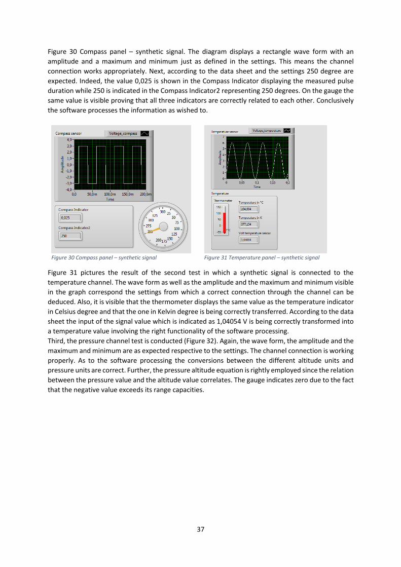
37

Figure 30 Compass panel – synthetic signal. The diagram displays a rectangle wave form with an

amplitude and a maximum and minimum just as defined in the settings. This means the channel

connection works appropriately. Next, according to the data sheet and the settings 250 degree are

expected. Indeed, the value 0,025 is shown in the Compass Indicator displaying the measured pulse

duration while 250 is indicated in the Compass Indicator2 representing 250 degrees. On the gauge the

same value is visible proving that all three indicators are correctly related to each other. Conclusively

the software processes the information as wished to.

Figure 30 Compass panel – synthetic signal

Figure 31 Temperature panel – synthetic signal

Figure 31 pictures the result of the second test in which a synthetic signal is connected to the

temperature channel. The wave form as well as the amplitude and the maximum and minimum visible

in the graph correspond the settings from which a correct connection through the channel can be

deduced. Also, it is visible that the thermometer displays the same value as the temperature indicator

in Celsius degree and that the one in Kelvin degree is being correctly transferred. According to the data

sheet the input of the signal value which is indicated as 1,04054 V is being correctly transformed into

a temperature value involving the right functionality of the software processing.

Third, the pressure channel test is conducted (Figure 32). Again, the wave form, the amplitude and the

maximum and minimum are as expected respective to the settings. The channel connection is working

properly. As to the software processing the conversions between the different altitude units and

pressure units are correct. Further, the pressure altitude equation is rightly employed since the relation

between the pressure value and the altitude value correlates. The gauge indicates zero due to the fact

that the negative value exceeds its range capacities.

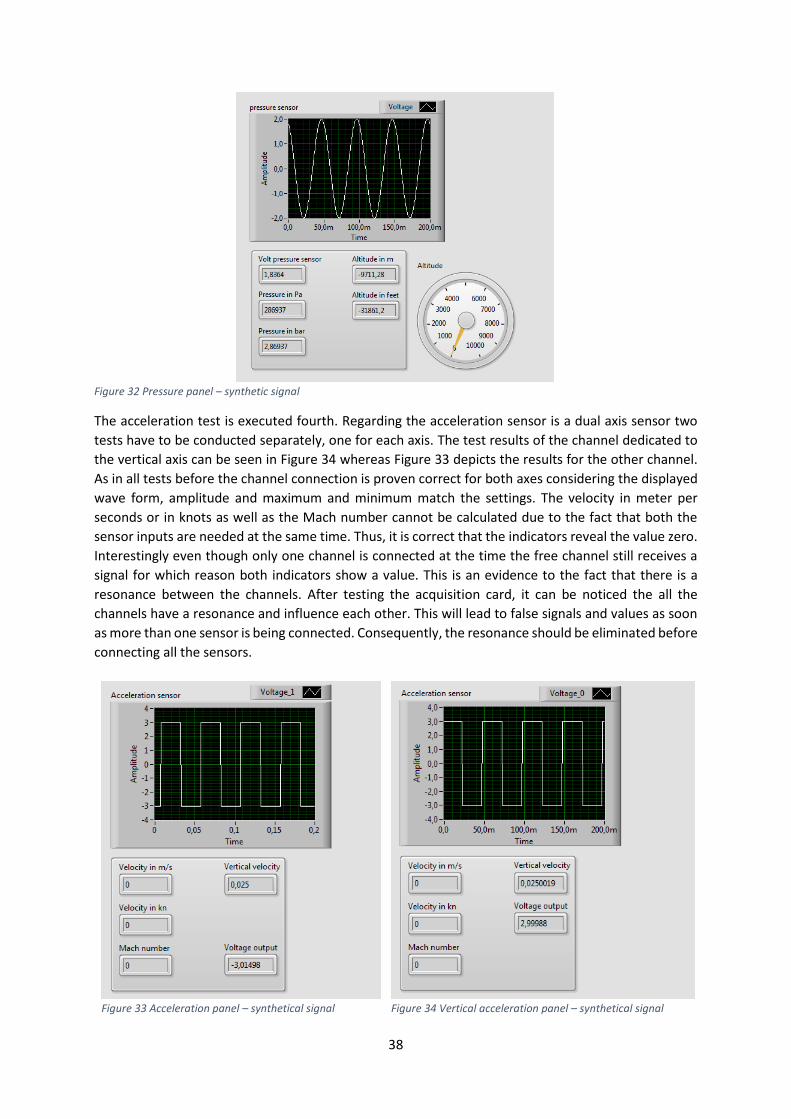
38

Figure 32 Pressure panel – synthetic signal

The acceleration test is executed fourth. Regarding the acceleration sensor is a dual axis sensor two

tests have to be conducted separately, one for each axis. The test results of the channel dedicated to

the vertical axis can be seen in Figure 34 whereas Figure 33 depicts the results for the other channel.

As in all tests before the channel connection is proven correct for both axes considering the displayed

wave form, amplitude and maximum and minimum match the settings. The velocity in meter per

seconds or in knots as well as the Mach number cannot be calculated due to the fact that both the

sensor inputs are needed at the same time. Thus, it is correct that the indicators reveal the value zero.

Interestingly even though only one channel is connected at the time the free channel still receives a

signal for which reason both indicators show a value. This is an evidence to the fact that there is a

resonance between the channels. After testing the acquisition card, it can be noticed the all the

channels have a resonance and influence each other. This will lead to false signals and values as soon

as more than one sensor is being connected. Consequently, the resonance should be eliminated before

connecting all the sensors.

Figure 33 Acceleration panel – synthetical signal

Figure 34 Vertical acceleration panel – synthetical signal

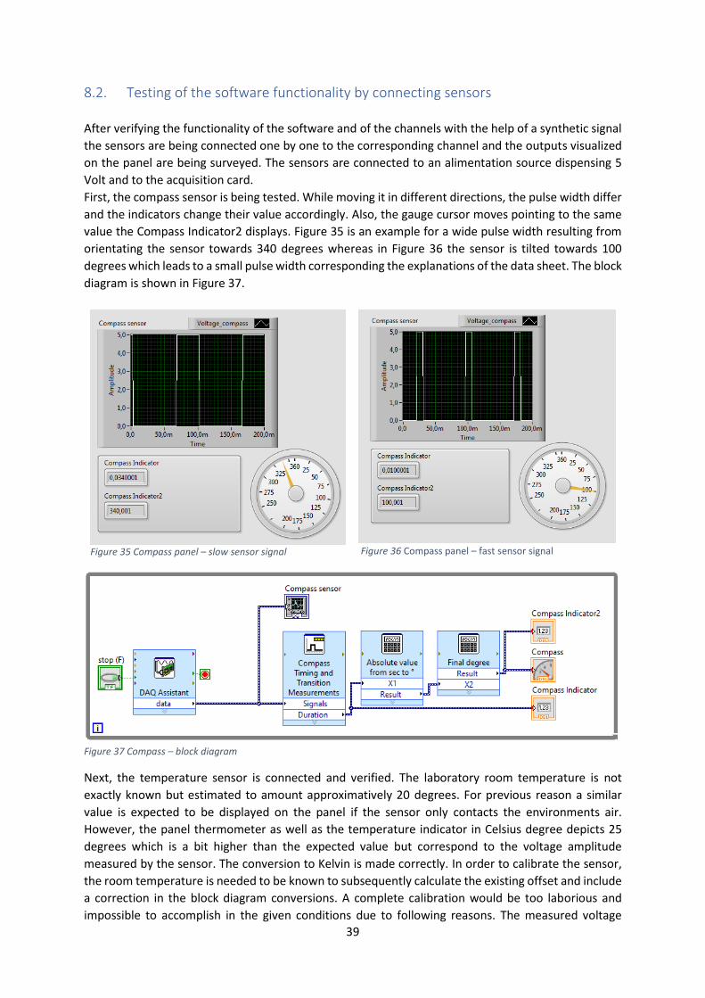
39

8.2. Testing of the software functionality by connecting sensors

After verifying the functionality of the software and of the channels with the help of a synthetic signal

the sensors are being connected one by one to the corresponding channel and the outputs visualized

on the panel are being surveyed. The sensors are connected to an alimentation source dispensing 5

Volt and to the acquisition card.

First, the compass sensor is being tested. While moving it in different directions, the pulse width differ

and the indicators change their value accordingly. Also, the gauge cursor moves pointing to the same

value the Compass Indicator2 displays. Figure 35 is an example for a wide pulse width resulting from

orientating the sensor towards 340 degrees whereas in Figure 36 the sensor is tilted towards 100

degrees which leads to a small pulse width corresponding the explanations of the data sheet. The block

diagram is shown in Figure 37.

Figure 35 Compass panel – slow sensor signal

Figure 36 Compass panel – fast sensor signal

Figure 37 Compass – block diagram

Next, the temperature sensor is connected and verified. The laboratory room temperature is not

exactly known but estimated to amount approximatively 20 degrees. For previous reason a similar

value is expected to be displayed on the panel if the sensor only contacts the environments air.

However, the panel thermometer as well as the temperature indicator in Celsius degree depicts 25

degrees which is a bit higher than the expected value but correspond to the voltage amplitude

measured by the sensor. The conversion to Kelvin is made correctly. In order to calibrate the sensor,

the room temperature is needed to be known to subsequently calculate the existing offset and include

a correction in the block diagram conversions. A complete calibration would be too laborious and

impossible to accomplish in the given conditions due to following reasons. The measured voltage

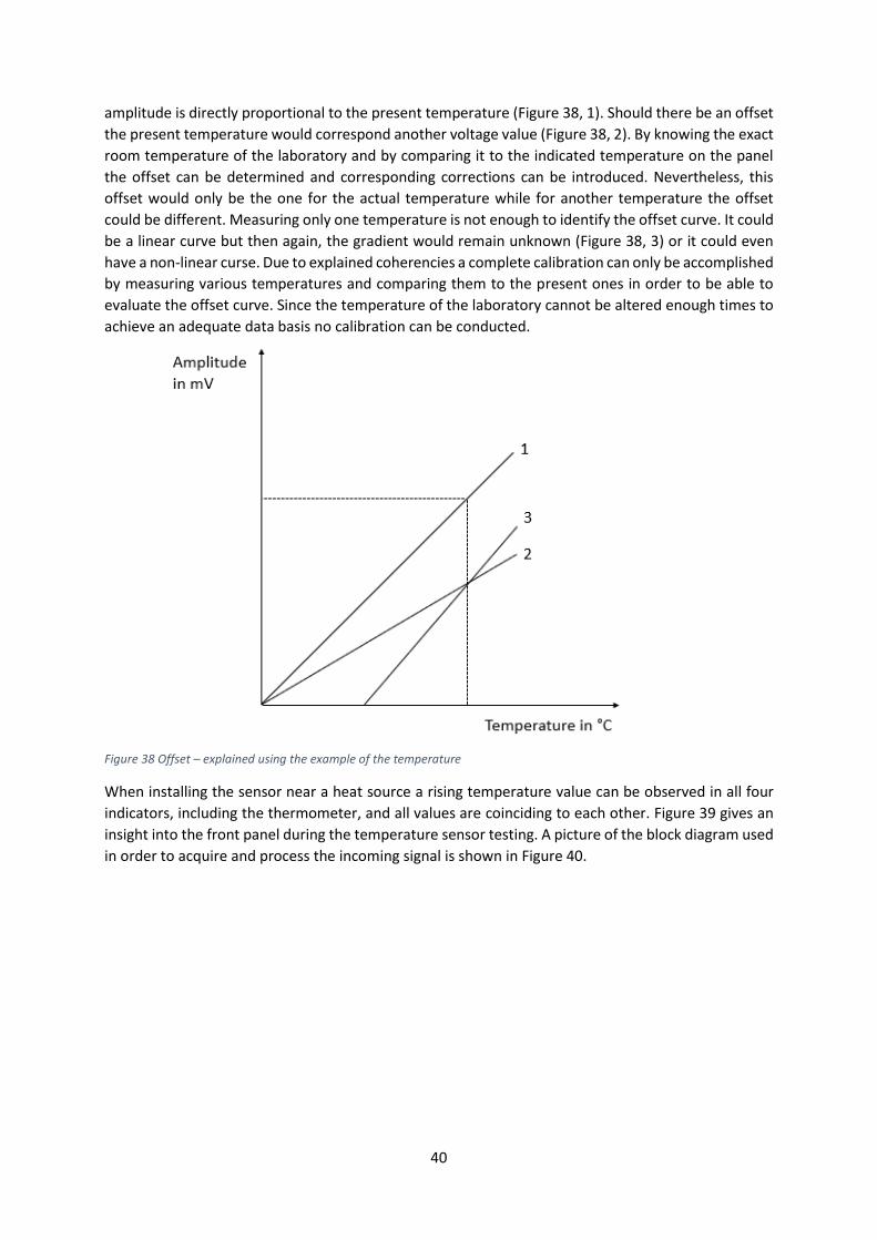
40

amplitude is directly proportional to the present temperature (Figure 38, 1). Should there be an offset

the present temperature would correspond another voltage value (Figure 38, 2). By knowing the exact

room temperature of the laboratory and by comparing it to the indicated temperature on the panel

the offset can be determined and corresponding corrections can be introduced. Nevertheless, this

offset would only be the one for the actual temperature while for another temperature the offset

could be different. Measuring only one temperature is not enough to identify the offset curve. It could

be a linear curve but then again, the gradient would remain unknown (Figure 38, 3) or it could even

have a non-linear curse. Due to explained coherencies a complete calibration can only be accomplished

by measuring various temperatures and comparing them to the present ones in order to be able to

evaluate the offset curve. Since the temperature of the laboratory cannot be altered enough times to

achieve an adequate data basis no calibration can be conducted.

Figure 38 Offset – explained using the example of the temperature

When installing the sensor near a heat source a rising temperature value can be observed in all four

indicators, including the thermometer, and all values are coinciding to each other. Figure 39 gives an

insight into the front panel during the temperature sensor testing. A picture of the block diagram used

in order to acquire and process the incoming signal is shown in Figure 40.

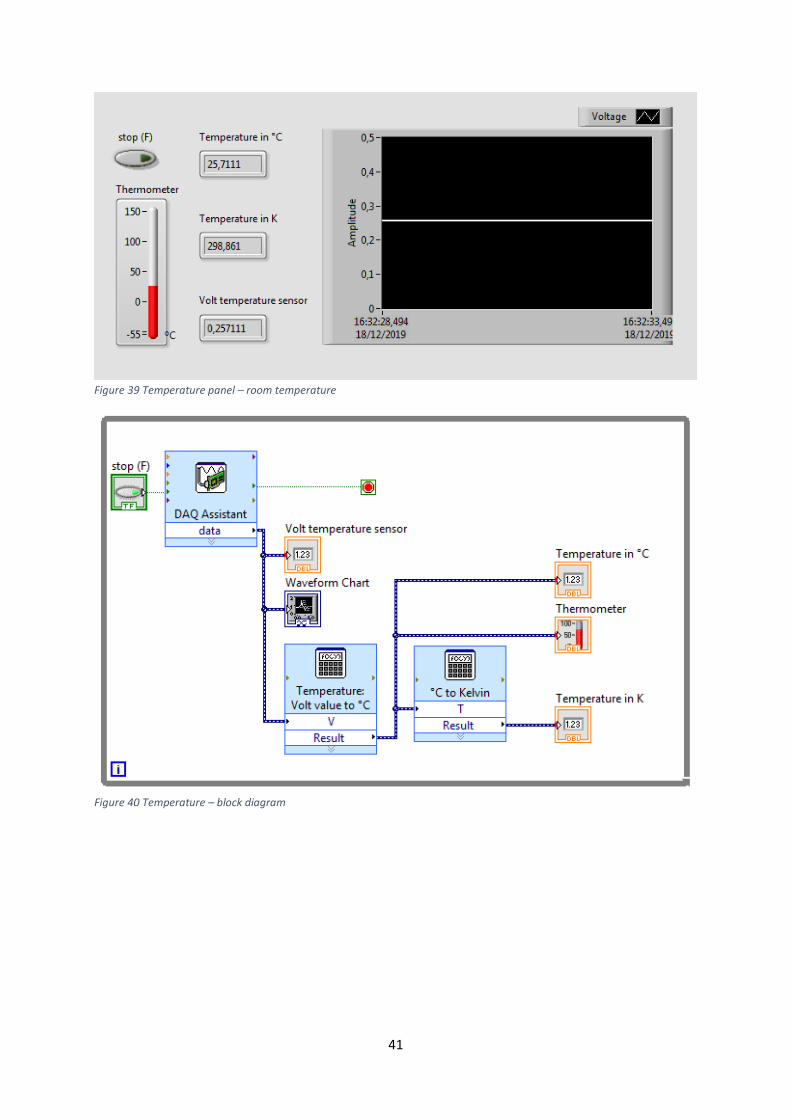
41

Figure 39 Temperature panel – room temperature

Figure 40 Temperature – block diagram

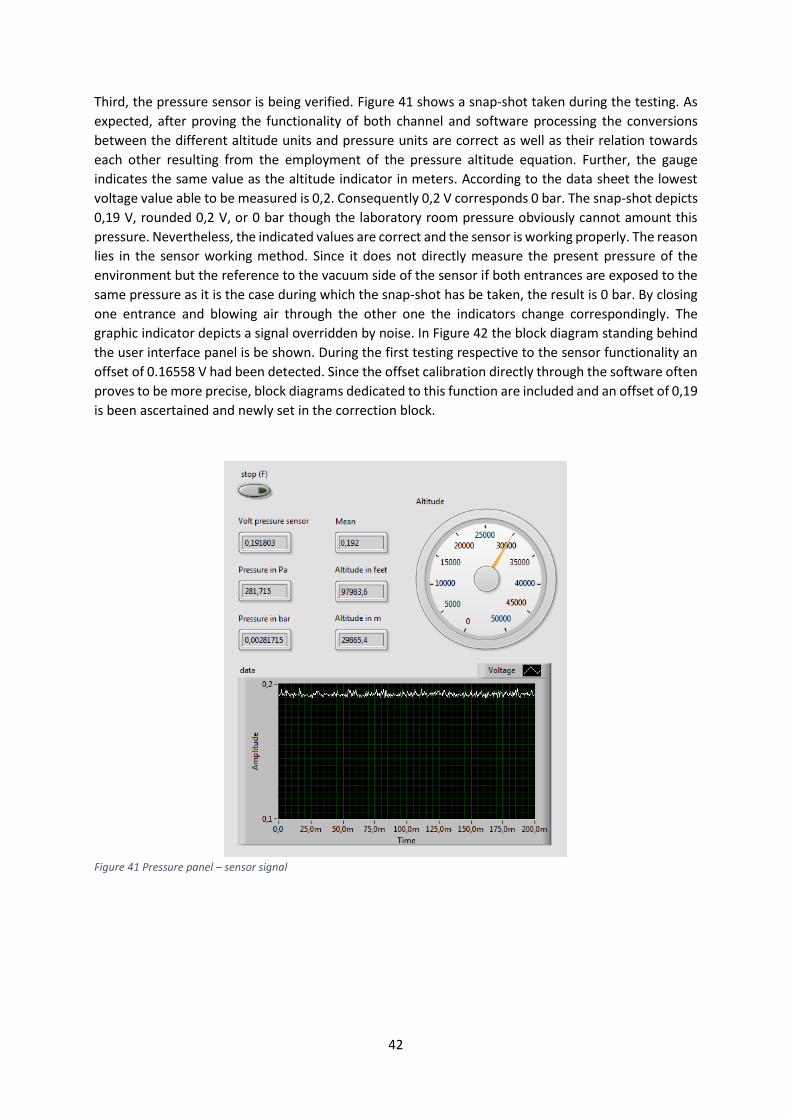
42

Third, the pressure sensor is being verified. Figure 41 shows a snap-shot taken during the testing. As

expected, after proving the functionality of both channel and software processing the conversions

between the different altitude units and pressure units are correct as well as their relation towards

each other resulting from the employment of the pressure altitude equation. Further, the gauge

indicates the same value as the altitude indicator in meters. According to the data sheet the lowest

voltage value able to be measured is 0,2. Consequently 0,2 V corresponds 0 bar. The snap-shot depicts

0,19 V, rounded 0,2 V, or 0 bar though the laboratory room pressure obviously cannot amount this

pressure. Nevertheless, the indicated values are correct and the sensor is working properly. The reason

lies in the sensor working method. Since it does not directly measure the present pressure of the

environment but the reference to the vacuum side of the sensor if both entrances are exposed to the

same pressure as it is the case during which the snap-shot has be taken, the result is 0 bar. By closing

one entrance and blowing air through the other one the indicators change correspondingly. The

graphic indicator depicts a signal overridden by noise. In Figure 42 the block diagram standing behind

the user interface panel is be shown. During the first testing respective to the sensor functionality an

offset of 0.16558 V had been detected. Since the offset calibration directly through the software often

proves to be more precise, block diagrams dedicated to this function are included and an offset of 0,19

is been ascertained and newly set in the correction block.

Figure 41 Pressure panel – sensor signal

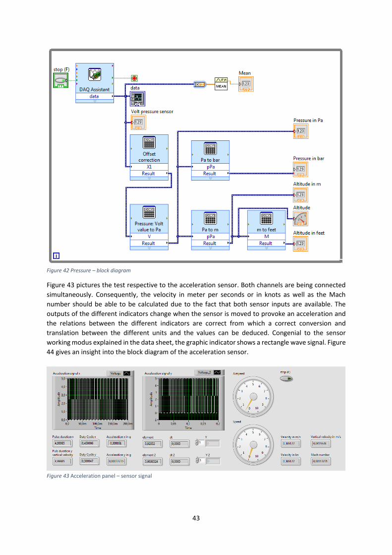
43

Figure 42 Pressure – block diagram

Figure 43 pictures the test respective to the acceleration sensor. Both channels are being connected

simultaneously. Consequently, the velocity in meter per seconds or in knots as well as the Mach

number should be able to be calculated due to the fact that both sensor inputs are available. The

outputs of the different indicators change when the sensor is moved to provoke an acceleration and

the relations between the different indicators are correct from which a correct conversion and

translation between the different units and the values can be deduced. Congenial to the sensor

working modus explained in the data sheet, the graphic indicator shows a rectangle wave signal. Figure

44 gives an insight into the block diagram of the acceleration sensor.

Figure 43 Acceleration panel – sensor signal

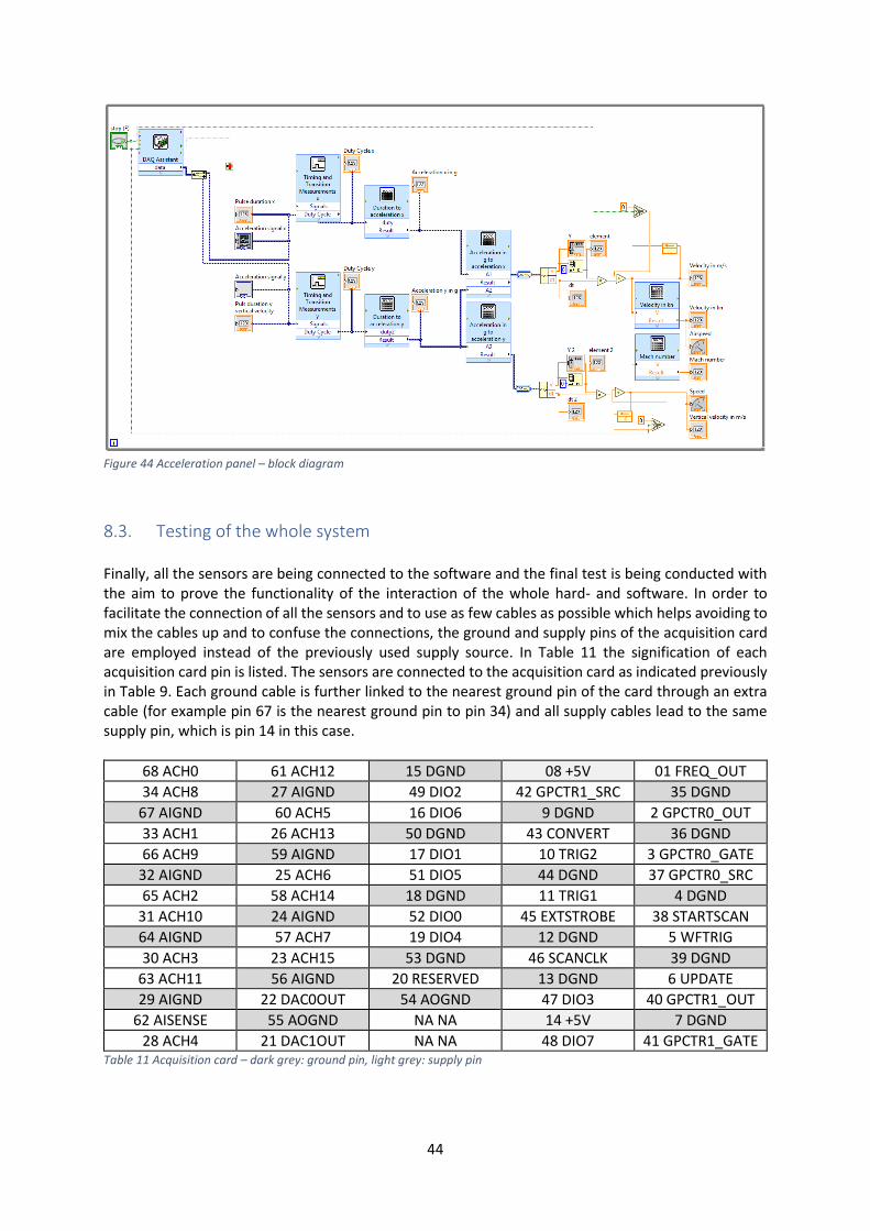
44

Figure 44 Acceleration panel – block diagram

8.3. Testing of the whole system Finally, all the sensors are being connected to the software and the final test is being conducted with the aim to prove the functionality of the interaction of the whole hard- and software. In order to facilitate the connection of all the sensors and to use as few cables as possible which helps avoiding to mix the cables up and to confuse the connections, the ground and supply pins of the acquisition card are employed instead of the previously used supply source. In Table 11 the signification of each acquisition card pin is listed. The sensors are connected to the acquisition card as indicated previously in Table 9. Each ground cable is further linked to the nearest ground pin of the card through an extra cable (for example pin 67 is the nearest ground pin to pin 34) and all supply cables lead to the same supply pin, which is pin 14 in this case.

68 ACH0 61 ACH12 15 DGND 08 +5V 01 FREQ_OUT

34 ACH8 27 AIGND 49 DIO2 42 GPCTR1_SRC 35 DGND

67 AIGND 60 ACH5 16 DIO6 9 DGND 2 GPCTR0_OUT

33 ACH1 26 ACH13 50 DGND 43 CONVERT 36 DGND

66 ACH9 59 AIGND 17 DIO1 10 TRIG2 3 GPCTR0_GATE

32 AIGND 25 ACH6 51 DIO5 44 DGND 37 GPCTR0_SRC

65 ACH2 58 ACH14 18 DGND 11 TRIG1 4 DGND

31 ACH10 24 AIGND 52 DIO0 45 EXTSTROBE 38 STARTSCAN

64 AIGND 57 ACH7 19 DIO4 12 DGND 5 WFTRIG

30 ACH3 23 ACH15 53 DGND 46 SCANCLK 39 DGND

63 ACH11 56 AIGND 20 RESERVED 13 DGND 6 UPDATE

29 AIGND 22 DAC0OUT 54 AOGND 47 DIO3 40 GPCTR1_OUT

62 AISENSE 55 AOGND NA NA 14 +5V 7 DGND

28 ACH4 21 DAC1OUT NA NA 48 DIO7 41 GPCTR1_GATE Table 11 Acquisition card – dark grey: ground pin, light grey: supply pin

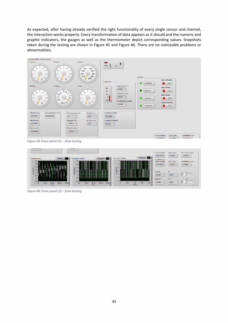
45

As expected, after having already verified the right functionality of every single sensor and channel, the interaction works properly. Every transformation of data appears as it should and the numeric and graphic indicators, the gauges as well as the thermometer depict corresponding values. Snapshots taken during the testing are shown in Figure 45 and Figure 46. There are no noticeable problems or abnormalities.

Figure 45 Front panel (1) – final testing

Figure 46 Front panel (2) – final testing

46

9. Summary and outlook

In this thesis the programming platform LabView has been used in order to connect four different

sensors to the software and visualise their data on a graphical surface. Since the aim was to choose

aeronautic related sensors, a temperature sensor, a pressure sensor, a compass sensor and an

acceleration sensor have been chosen to copy as close as possible a general aviation instrument panel.

The data of each sensor is successfully being processed and visualized through the acquisition system

of National Instruments LabView. A virtual general aviation instrument panel has been created as far

as possible with the given materials and under the given conditions.

As continuative steps different sensors of the same outcome type can be incorporated into the

environment in order to verify if their connection to the system is realizable with only little changes

which was one of the expectations set at the beginning.

Further, the general aviation instrument panel can be extended and completed in order to better

represent the functionality of a real one. Especially the horizon and the rotation gauge which are

missing in the simulation and only appears in this version as placeholder on the front panel can be

programmed and added to the existing software.

In addition, the sensors can be attached to some testing object and be collocated in an adequate

testing and simulation environment. This would permit to use and test the full capacity of the sensors

measuring ranges. For example, cooling or heating chambers can be used in order to expose the

temperature sensor to different temperatures and simulate an uprising of an airplane, knowing that

the temperature cools down with increasing high. Also, the acceleration sensor can be replaced by a

pitot tube in order to measure the velocity as it is usually measured in airplanes. This done a wind

tunnel or a similar environment can be used in order to change the pressure and the velocity of flow

and by this simulate a flying airplane.

Besides, in order to obtain more exact data about the surrounding environment an exact calibration

needs to be conducted. Above all the temperature sensor has an offset which still is unknown and

should be determined if a more realistic simulation is wished.

This practical session dedicated and created for students studying in the aeronautic field had further

the educational aim to give the student the possibility to approach the principle of operation of

instrumentation and data. Effectively the principles of converting analogue signals to digital data and

visualize this data on a panel after acquiring, processing and converting it have become very clear.

Thanks to the manageable and comprehensibly structured programming platform LabView laypersons

quickly get an impression of the stages to pursue in order to process and visualize data on monitors or

panels. It accentuates that in order to express data in an understandable way visualizing it on panels

is helpful and capacitate the students to replicate and simulate panels of other machines in a similar

way. The educational aim was met.

In order to consolidate the newly acquired ability students could as continuative steps transfer their

knowledge onto other machinery panels and replicate those ones or change the design of the existing

one. This would permit them to deepen their understanding of the software and to widen their horizon

respective to the different functions and design options as well as to the large variety of tools LabView

is offering.

47

8 References [1] AERO EXPO. 2019. barometrischer Drucksensor / Vdc / in mA / für Flugzeuge MLH Series

(2019). Retrieved October 17, 2019 from https://www.aeroexpo.online/de/prod/honeywell-

safety-and-productivity-solutions/product-186046-37363.html.

[2] AliExpress. 2019. LM35 Precision Centigrade Temperature Sensors (2019). Retrieved January 6,

2020 from

es.aliexpress.com/wholesale?catId=0&initiative_id=SB_20200106062727&SearchText=LM35+

Precision+Centigrade+Temperature+Sensors.

[3] Inc. Analog Devices. 2009. Small, Low Power, 3-Axis ±3 g Accelerometer ADXL335 (2009).

Retrieved December 11, 2019 from https://www.sparkfun.com/datasheets/Components/

SMD/adxl335.pdf.

[4] Analog Devices Inc. 2015. Low Voltage Temperature Sensors. Data Sheet

TMP35/TMP36/TMP37 (2015). Retrieved December 12, 2019 from https://www.analog.com/

media/en/technical-documentation/data-sheets/TMP35_36_37.pdf.

[5] Astrid Lampert, Martin Schachtebeck, Rudolf Hankers, Kjell zum Berge. 2019.

Flugmeteorologie. Wetter, sein Einfluss auf die Luftfahrt und Messmethoden. Institut für

Flugführung. Technische Universität Braunschweig, Braunschweig.

[6] Christopher S. Baird. 2013. Why does a magnetic compass point to the Geographic North Pole?

(2013). Retrieved December 28, 2019 from https://wtamu.edu/~cbaird/sq/2013/11/15/why-

does-a-magnetic-compass-point-to-the-geographic-north-pole/.

[7] Clint Budd. 2016. Heading 295 Magnetic. (2016). Retrieved December 4, 2019 from https://

www.flickr.com/photos/58827557@N06/29181693970.

[8] Denelson83. 2009. Datei:Primary Flight Display.svg (2009). Retrieved December 4, 2019 from

https://de.wikipedia.org/wiki/Datei:Primary_Flight_Display.svg.

[9] Deutscher Wetterdienst. 2019. ICAO-Standardatmosphäre (ISA) (2019). Retrieved December 4,

2019 from https://www.dwd.de/DE/service/lexikon/begriffe/S/

Standardatmosphaere_pdf.pdf?__blob=publicationFile&v=3.

[10] Edgar von Hinüber. 2002. Inertiale Messsysteme mit faseroptischen Kreiseln für Fahrdynamik

und Topologiedaten-Erfassung. ENTWICKLUNG Fahrdynamik (2002). Retrieved December 11,

2019 from imar-navigation.de/downloads/papers/atz_6_2002_printoff_de.pdf.

[11] Freescale_Semiconductor_Inc., Ed. 2012. Integrated Silicon Pressure Sensor On-Chip Signal

Conditioned, Temperature Compensated and Calibrated. Data Sheet: Technical Data.

[12] Geoff McKay. 2010. Six Pack – The Primary Flight Instruments (2010). Retrieved November 6,

2019 from https://learntofly.ca/six-pack-primary-flight-instruments/.

[13] induux Wiki. 2019. Sensoren (2019). Retrieved October 16, 2019 from https://wiki.induux.de/

Sensoren.

[14] Jens Friedrichs. 2017. Airline Operation. Übung 2: Triebwerks-Crash-Kurs. Institut für

Flugantriebe und Strömungsmaschinen. Technische Universität Braunschweig, Braunschweig.

48

[15] José Luis Romeral Martínez. 2018. PRÁCTICA 1: Sistemas de Instrumentación: Lab View.

Aplicación: Lectura y procesado de señales analógicas. Departament d'enginyeria electrònica.

UPC BarcelonaTECH, Barcelona.

[16] Katharina Juschkat. 2019. Sensor. Wie Sensoren funktionieren und wo sie eingesetzt werden

(2019). Retrieved October 16, 2019 from https://www.elektrotechnik.vogel.de/wie-sensoren-

funktionieren-und-wo-sie-eingesetzt-werden-a-713477/.

[17] Krzysztof Tokarz. 2019. Earth's magnetic field vector in three dimensions (2019). Retrieved

December 28, 2019 from https://www.researchgate.net/figure/Earths-magnetic-field-vector-

in-three-dimensions_fig3_262176296.

[18] Maria Budweiser. 2011. Die Barometrische Höhenformel. Vortrag von Maria Budweiser im

Rahmen der "Übungen im Vortragen mit Demonstrationen - Physikalische Chemie", WS 11/12.

Didaktik der Chemie (2011). Retrieved November 4, 2019 from daten.didaktikchemie.uni-

bayreuth.de/umat/hoehenformel_barometrisch/hoehenf_barometrisch.html.

[19] MercadoLibre. 2019. cmps03 compass module brujla digital (2019). Retrieved January 6, 2020

from https://listado.mercadolibre.com.mx/cmps03-compass-module-brujla-digital.

[20] Miguel Delgado. 2018. Tutorial de LabView. Departament d'enginyeria electrònica. UPC

BarcelonaTECH, Barcelona.

[21] Mirko Ribow. 2009. Ausbildungsseminar Klima und Wetter im WS 09/10. Druck und

Temperaturschichtung in der Atmosphäre.

[22] Modern Robotics Inc. 2016. Modern Robotics Inc. Sensor Documentation (2016). Retrieved

December 11, 2019 from https://docplayer.net/26385945-Modern-robotics-inc-sensor-

documentation.html.

[23] mSparks43. 2018. Temperature above ISA tropopause (2018). Retrieved December 28, 2019

from https://forums.x-plane.org/index.php?/forums/topic/157579-temperature-above-isa-

tropopause/.

[24] National Instruments Corporation, Ed. 2005. B Series Multifunction DAQ, 16-Bit, 200 kS/s, 16

Analog Inputs. Datasheet.

[25] National Instruments Corporation. 2019. Aeroespacial y Defensa (2019). Retrieved January 6,

2020 from https://www.ni.com/es-es/innovations/aerospace-defense.html.

[26] National Instruments Corporation. 2019. Controls Palette. Styles of Controls and Indicators

(2019). Retrieved December 27, 2019 from https://zone.ni.com/reference/en-XX/help/

371361R-01/glang/controlspalette/.

[27] National Instruments Corporation. 2019. National Instruments (2019). Retrieved October 14,

2019 from http://www.ni.com/es-es.html.

[28] National Instruments Corporation. 2019. PCI-6014 Dispositivo de E/S Multifunción (2019).

Retrieved November 11, 2019 from https://www.ni.com/es-es/support/model.pci-6014.html.

[29] Natural Resources Canada. 2019. Magnetic components (2019). Retrieved December 28, 1019

from https://www.geomag.nrcan.gc.ca/mag_fld/comp-en.php.

[30] OpenCircuit. 2019. MEMSIC 2125 Dual-axis Accelerometer (2019). Retrieved January 6, 2020

from https://opencircuit.shop/Product/MEMSIC-2125-Dual-axis-Accelerometer.

49

[31] Parallax_Inc., Ed. 2012. Memsic 2125 Dual-Axis Accelerometer (#28017).

[32] PCB Synotech GmbH, Ed. 2019. Sensoren für Luft- und Raumfahrt, Porschestr. 20 – 30 n 41836

Hückelhoven.

[33] Armando Péreza, Rogelio R. Irigoyenb, Gisela Monterob, Conrado Garciab, Jose Rodrigueza,

and Marcos Coronadob. 2019. Development and implementation of virtual instrumentation

based on LabView applied to compression ignition engines operated with diesel-biodiesel

blends. MethodsX Article, 6, 2782–2792.

[34] Phidgets Inc. 2016. Magnetic Sensor (2016). Retrieved December 11, 2019 from https://

www.phidgets.com/?tier=3&catid=5&pcid=3&prodid=78.

[35] Phidgets Inc. 2019. Absolute Gas Pressure Sensor 20 - 400 kPa (2019). Retrieved December 11,

2019 from https://www.robotshop.com/en/absolute-gas-pressure-sensor-20-400-kpa.html.

[36] Philips. 2007. CMPS03 - Compass Module. KMZ51 magnetic field sensor (2007). Retrieved from.

[37] José R. Quezada Peña, Luis H. Neves Rodrigues, Manuel L. da Costa Neto, and Jefferson

Oliveira. 2018. ACTIVE METHODOLOGIES IN EDUCATION OF ELECTRONIC INSTRUMENTATION

USING VIRTUAL INSTRUMENTATION PLATFORM BASED ON LABVIEW AND ELVIS II. Global

Engineering Education Conference (EDUCON), 1696–1705.

[38] Robot Electronics, Ed. 2007. CMPS03 - Robot Compass Module.

[39] Amit K. Rohit, Saroj Rangnekar, Anurag Kumar, and Amit Tomar. 2017. Virtual lab based real-

time data acquisition, measurement and monitoring platform for solar photovoltaic module.

Resource-Efficient Technologies, 3, 446–451.

[40] RS Components. 2019. Pressure Sensor MPX5700DP, 6 pines (2019). Retrieved January 6, 2020

from https://es.rs-online.com/web/p/circuitos-integrados-de-sensor-de-presion-diferencial/

7191119/.

[41] Nan Su, XiaoWei Tu, Yan Tong, XuHui Li, and QingHua Yang. 2019. Design of Data

Communication and Monitoring System Based on Aviation ARINC825 Bus. International

Conference on Communication Software and Networks, 286-290.

[42] Sunfounder. 2018. Analog Temperature Sensor Module (2018). Retrieved December 12, 2019

from https://www.robotshop.com/en/analog-temperature-sensor-module.html.

[43] Tal Ronaldinho King. 2019. File: BASIC Flight instruments Improved.svg (2019). Retrieved

December 4, 2019 from https://commons.wikimedia.org/wiki/

File:BASIC_Flight_instruments_Improved.svg.

[44] Texas_Instruments, Ed. 2017. LM35 Precision Centigrade Temperature Sensors.

[45] UPC BarcelonaTECH. 2018. Aerospace Engineering ProjectsM02-S06. DECISIONMAKING.

Aerospace Engineering Projects Degrees on Aerospace Engineering Technologies and

Aerospace Engineering Vehicles ESEIAAT. Department of Project and Construction Engineering.

UPC BarcelonaTECH, Barcelona.

[46] xplore-dna – Didactically Networked Automation. 2019. Sensorik - Sensorarten (2019).

Retrieved October 16, 2019 from https://www.xplore-dna.net/mod/page/view.php?id=81.

[47] Kunliang Xu. 2015. The Design Concept of a Virtual Experiment Teaching Platform for Digital

Logic Based on LabVIEW. International Journal of Hybrid Information Technology, 8, 229–236.