Welcome message from author
This document is posted to help you gain knowledge. Please leave a comment to let me know what you think about it! Share it to your friends and learn new things together.
Transcript
Measurement andInstrumentation Principles

To Jane, Nicola and Julia
Measurement andInstrumentation
Principles
Alan S. Morris
OXFORD AUCKLAND BOSTON JOHANNESBURG MELBOURNE NEW DELHI

Butterworth-HeinemannLinacre House, Jordan Hill, Oxford OX2 8DP225 Wildwood Avenue, Woburn, MA 01801-2041A division of Reed Educational and Professional Publishing Ltd
A member of the Reed Elsevier plc group
First published 2001
© Alan S. Morris 2001
All rights reserved. No part of this publicationmay be reproduced in any material form (includingphotocopying or storing in any medium by electronicmeans and whether or not transiently or incidentallyto some other use of this publication) without thewritten permission of the copyright holder exceptin accordance with the provisions of the Copyright,Designs and Patents Act 1988 or under the terms of alicence issued by the Copyright Licensing Agency Ltd,90 Tottenham Court Road, London, England W1P 9HE.Applications for the copyright holder’s written permissionto reproduce any part of this publication should be addressedto the publishers
British Library Cataloguing in Publication DataA catalogue record for this book is available from the British Library
ISBN 0 7506 5081 8
Typeset in 10/12pt Times Roman by Laser Words, Madras, IndiaPrinted and bound in Great Britain
Contents
Preface xviiAcknowledgements xx
Part 1: Principles of Measurement 1
1 INTRODUCTION TO MEASUREMENT 31.1 Measurement units 31.2 Measurement system applications 61.3 Elements of a measurement system 81.4 Choosing appropriate measuring instruments 9
2 INSTRUMENT TYPES AND PERFORMANCECHARACTERISTICS 122.1 Review of instrument types 12
2.1.1 Active and passive instruments 122.1.2 Null-type and deflection-type instruments 132.1.3 Analogue and digital instruments 142.1.4 Indicating instruments and instruments with a
signal output 152.1.5 Smart and non-smart instruments 16
2.2 Static characteristics of instruments 162.2.1 Accuracy and inaccuracy (measurement uncertainty) 162.2.2 Precision/repeatability/reproducibility 172.2.3 Tolerance 172.2.4 Range or span 182.2.5 Linearity 192.2.6 Sensitivity of measurement 192.2.7 Threshold 202.2.8 Resolution 202.2.9 Sensitivity to disturbance 202.2.10 Hysteresis effects 222.2.11 Dead space 23
2.3 Dynamic characteristics of instruments 23
vi Contents
2.3.1 Zero order instrument 252.3.2 First order instrument 252.3.3 Second order instrument 28
2.4 Necessity for calibration 292.5 Self-test questions 30
3 ERRORS DURING THE MEASUREMENT PROCESS 323.1 Introduction 323.2 Sources of systematic error 33
3.2.1 System disturbance due to measurement 333.2.2 Errors due to environmental inputs 373.2.3 Wear in instrument components 383.2.4 Connecting leads 38
3.3 Reduction of systematic errors 393.3.1 Careful instrument design 393.3.2 Method of opposing inputs 393.3.3 High-gain feedback 393.3.4 Calibration 413.3.5 Manual correction of output reading 423.3.6 Intelligent instruments 42
3.4 Quantification of systematic errors 423.5 Random errors 42
3.5.1 Statistical analysis of measurements subject torandom errors 43
3.5.2 Graphical data analysis techniques – frequencydistributions 46
3.6 Aggregation of measurement system errors 563.6.1 Combined effect of systematic and random errors 563.6.2 Aggregation of errors from separate measurement
system components 563.6.3 Total error when combining multiple measurements 59
3.7 Self-test questions 60References and further reading 63
4 CALIBRATION OF MEASURING SENSORS ANDINSTRUMENTS 644.1 Principles of calibration 644.2 Control of calibration environment 664.3 Calibration chain and traceability 674.4 Calibration records 71References and further reading 72
5 MEASUREMENT NOISE AND SIGNAL PROCESSING 735.1 Sources of measurement noise 73
5.1.1 Inductive coupling 745.1.2 Capacitive (electrostatic) coupling 745.1.3 Noise due to multiple earths 74
Contents vii
5.1.4 Noise in the form of voltage transients 755.1.5 Thermoelectric potentials 755.1.6 Shot noise 765.1.7 Electrochemical potentials 76
5.2 Techniques for reducing measurement noise 765.2.1 Location and design of signal wires 765.2.2 Earthing 775.2.3 Shielding 775.2.4 Other techniques 77
5.3 Introduction to signal processing 785.4 Analogue signal filtering 78
5.4.1 Passive analogue filters 815.4.2 Active analogue filters 85
5.5 Other analogue signal processing operations 865.5.1 Signal amplification 875.5.2 Signal attenuation 885.5.3 Differential amplification 895.5.4 Signal linearization 905.5.5 Bias (zero drift) removal 915.5.6 Signal integration 925.5.7 Voltage follower (pre-amplifier) 925.5.8 Voltage comparator 925.5.9 Phase-sensitive detector 935.5.10 Lock-in amplifier 945.5.11 Signal addition 945.5.12 Signal multiplication 95
5.6 Digital signal processing 955.6.1 Signal sampling 955.6.2 Sample and hold circuit 975.6.3 Analogue-to-digital converters 975.6.4 Digital-to-analogue (D/A) conversion 995.6.5 Digital filtering 1005.6.6 Autocorrelation 1005.6.7 Other digital signal processing operations 101
References and further reading 101
6 ELECTRICAL INDICATING AND TEST INSTRUMENTS 1026.1 Digital meters 102
6.1.1 Voltage-to-time conversion digital voltmeter 1036.1.2 Potentiometric digital voltmeter 1036.1.3 Dual-slope integration digital voltmeter 1036.1.4 Voltage-to-frequency conversion digital voltmeter 1046.1.5 Digital multimeter 104
6.2 Analogue meters 1046.2.1 Moving-coil meters 1056.2.2 Moving-iron meter 1066.2.3 Electrodynamic meters 107
viii Contents
6.2.4 Clamp-on meters 1086.2.5 Analogue multimeter 1086.2.6 Measuring high-frequency signals 1096.2.7 Thermocouple meter 1106.2.8 Electronic analogue voltmeters 1116.2.9 Calculation of meter outputs for non-standard
waveforms 1126.3 Cathode ray oscilloscope 114
6.3.1 Cathode ray tube 1156.3.2 Channel 1166.3.3 Single-ended input 1176.3.4 Differential input 1176.3.5 Timebase circuit 1176.3.6 Vertical sensitivity control 1176.3.7 Display position control 118
6.4 Digital storage oscilloscopes 118References and further reading 118
7 VARIABLE CONVERSION ELEMENTS 1197.1 Bridge circuits 119
7.1.1 Null-type, d.c. bridge (Wheatstone bridge) 1207.1.2 Deflection-type d.c. bridge 1217.1.3 Error analysis 1287.1.4 A.c. bridges 130
7.2 Resistance measurement 1347.2.1 D.c. bridge circuit 1357.2.2 Voltmeter–ammeter method 1357.2.3 Resistance-substitution method 1357.2.4 Use of the digital voltmeter to measure resistance 1367.2.5 The ohmmeter 1367.2.6 Codes for resistor values 137
7.3 Inductance measurement 1387.4 Capacitance measurement 138
7.4.1 Alphanumeric codes for capacitor values 1397.5 Current measurement 1407.6 Frequency measurement 141
7.6.1 Digital counter-timers 1427.6.2 Phase-locked loop 1427.6.3 Cathode ray oscilloscope 1437.6.4 The Wien bridge 144
7.7 Phase measurement 1457.7.1 Electronic counter-timer 1457.7.2 X–Y plotter 1457.7.3 Oscilloscope 1477.7.4 Phase-sensitive detector 147
7.8 Self-test questions 147References and further reading 150
Contents ix
8 SIGNAL TRANSMISSION 1518.1 Electrical transmission 151
8.1.1 Transmission as varying voltages 1518.1.2 Current loop transmission 1528.1.3 Transmission using an a.c. carrier 153
8.2 Pneumatic transmission 1548.3 Fibre-optic transmission 155
8.3.1 Principles of fibre optics 1568.3.2 Transmission characteristics 1588.3.3 Multiplexing schemes 160
8.4 Optical wireless telemetry 1608.5 Radio telemetry (radio wireless transmission) 1618.6 Digital transmission protocols 163References and further reading 164
9 DIGITAL COMPUTATION AND INTELLIGENT DEVICES 1659.1 Principles of digital computation 165
9.1.1 Elements of a computer 1659.1.2 Computer operation 1689.1.3 Interfacing 1749.1.4 Practical considerations in adding computers to
measurement systems 1769.2 Intelligent devices 177
9.2.1 Intelligent instruments 1779.2.2 Smart sensors 1799.2.3 Smart transmitters 1809.2.4 Communication with intelligent devices 1839.2.5 Computation in intelligent devices 1849.2.6 Future trends in intelligent devices 185
9.3 Self-test questions 185References and further reading 186
10 INSTRUMENTATION/COMPUTER NETWORKS 18710.1 Introduction 18710.2 Serial communication lines 188
10.2.1 Asynchronous transmission 18910.3 Parallel data bus 19010.4 Local area networks (LANs) 192
10.4.1 Star networks 19310.4.2 Ring and bus networks 194
10.5 Gateways 19510.6 HART 19510.7 Digital fieldbuses 19610.8 Communication protocols for very large systems 198
10.8.1 Protocol standardization 19810.9 Future development of networks 199References and further reading 199
x Contents
11 DISPLAY, RECORDING AND PRESENTATION OFMEASUREMENT DATA 20011.1 Display of measurement signals 200
11.1.1 Electronic output displays 20011.1.2 Computer monitor displays 201
11.2 Recording of measurement data 20211.2.1 Mechanical chart recorders 20211.2.2 Ultra-violet recorders 20811.2.3 Fibre-optic recorders (recording oscilloscopes) 20911.2.4 Hybrid chart recorders 20911.2.5 Magnetic tape recorders 20911.2.6 Digital recorders 21011.2.7 Storage oscilloscopes 211
11.3 Presentation of data 21211.3.1 Tabular data presentation 21211.3.2 Graphical presentation of data 213
11.4 Self-test questions 222References and further reading 223
12 MEASUREMENT RELIABILITY AND SAFETY SYSTEMS 22412.1 Reliability 224
12.1.1 Principles of reliability 22412.1.2 Laws of reliability in complex systems 22812.1.3 Improving measurement system reliability 22912.1.4 Software reliability 232
12.2 Safety systems 23612.2.1 Introduction to safety systems 23612.2.2 Operation of safety systems 23712.2.3 Design of a safety system 238
12.3 Self-test questions 241References and further reading 242
Part 2: Measurement Sensors and Instruments 245
13 SENSOR TECHNOLOGIES 24713.1 Capacitive and resistive sensors 24713.2 Magnetic sensors 24713.3 Hall-effect sensors 24913.4 Piezoelectric transducers 25013.5 Strain gauges 25113.6 Piezoresistive sensors 25213.7 Optical sensors (air path) 25213.8 Optical sensors (fibre-optic) 253
13.8.1 Intrinsic sensors 25413.8.2 Extrinsic sensors 25813.8.3 Distributed sensors 259
Contents xi
13.9 Ultrasonic transducers 25913.9.1 Transmission speed 26013.9.2 Direction of travel of ultrasound waves 26113.9.3 Directionality of ultrasound waves 26113.9.4 Relationship between wavelength, frequency and
directionality of ultrasound waves 26213.9.5 Attenuation of ultrasound waves 26213.9.6 Ultrasound as a range sensor 26313.9.7 Use of ultrasound in tracking 3D object motion 26413.9.8 Effect of noise in ultrasonic measurement systems 26513.9.9 Exploiting Doppler shift in ultrasound transmission 26513.9.10 Ultrasonic imaging 267
13.10 Nuclear sensors 26713.11 Microsensors 268References and further reading 270
14 TEMPERATURE MEASUREMENT 27114.1 Principles of temperature measurement 27114.2 Thermoelectric effect sensors (thermocouples) 272
14.2.1 Thermocouple tables 27614.2.2 Non-zero reference junction temperature 27714.2.3 Thermocouple types 27914.2.4 Thermocouple protection 28014.2.5 Thermocouple manufacture 28114.2.6 The thermopile 28214.2.7 Digital thermometer 28214.2.8 The continuous thermocouple 282
14.3 Varying resistance devices 28314.3.1 Resistance thermometers (resistance temperature
devices) 28414.3.2 Thermistors 285
14.4 Semiconductor devices 28614.5 Radiation thermometers 287
14.5.1 Optical pyrometers 28914.5.2 Radiation pyrometers 290
14.6 Thermography (thermal imaging) 29314.7 Thermal expansion methods 294
14.7.1 Liquid-in-glass thermometers 29514.7.2 Bimetallic thermometer 29614.7.3 Pressure thermometers 296
14.8 Quartz thermometers 29714.9 Fibre-optic temperature sensors 29714.10 Acoustic thermometers 29814.11 Colour indicators 29914.12 Change of state of materials 29914.13 Intelligent temperature-measuring instruments 30014.14 Choice between temperature transducers 300
xii Contents
14.15 Self-test questions 302References and further reading 303
15 PRESSURE MEASUREMENT 30415.1 Diaphragms 30515.2 Capacitive pressure sensor 30615.3 Fibre-optic pressure sensors 30615.4 Bellows 30715.5 Bourdon tube 30815.6 Manometers 31015.7 Resonant-wire devices 31115.8 Dead-weight gauge 31215.9 Special measurement devices for low pressures 31215.10 High-pressure measurement (greater than 7000 bar) 31515.11 Intelligent pressure transducers 31615.12 Selection of pressure sensors 316
16 FLOW MEASUREMENT 31916.1 Mass flow rate 319
16.1.1 Conveyor-based methods 31916.1.2 Coriolis flowmeter 32016.1.3 Thermal mass flow measurement 32016.1.4 Joint measurement of volume flow rate and fluid
density 32116.2 Volume flow rate 321
16.2.1 Differential pressure (obstruction-type) meters 32216.2.2 Variable area flowmeters (Rotameters) 32716.2.3 Positive displacement flowmeters 32816.2.4 Turbine meters 32916.2.5 Electromagnetic flowmeters 33016.2.6 Vortex-shedding flowmeters 33216.2.7 Ultrasonic flowmeters 33216.2.8 Other types of flowmeter for measuring volume
flow rate 33616.3 Intelligent flowmeters 33816.4 Choice between flowmeters for particular applications 338References and further reading 339
17 LEVEL MEASUREMENT 34017.1 Dipsticks 34017.2 Float systems 34017.3 Pressure-measuring devices (hydrostatic systems) 34117.4 Capacitive devices 34317.5 Ultrasonic level gauge 34417.6 Radar (microwave) methods 346
Contents xiii
17.7 Radiation methods 34617.8 Other techniques 348
17.8.1 Vibrating level sensor 34817.8.2 Hot-wire elements/carbon resistor elements 34817.8.3 Laser methods 34917.8.4 Fibre-optic level sensors 34917.8.5 Thermography 349
17.9 Intelligent level-measuring instruments 35117.10 Choice between different level sensors 351References and further reading 351
18 MASS, FORCE AND TORQUE MEASUREMENT 35218.1 Mass (weight) measurement 352
18.1.1 Electronic load cell (electronic balance) 35218.1.2 Pneumatic/hydraulic load cells 35418.1.3 Intelligent load cells 35518.1.4 Mass-balance (weighing) instruments 35618.1.5 Spring balance 359
18.2 Force measurement 35918.2.1 Use of accelerometers 36018.2.2 Vibrating wire sensor 360
18.3 Torque measurement 36118.3.1 Reaction forces in shaft bearings 36118.3.2 Prony brake 36118.3.3 Measurement of induced strain 36218.3.4 Optical torque measurement 364
19 TRANSLATIONAL MOTION TRANSDUCERS 36519.1 Displacement 365
19.1.1 The resistive potentiometer 36519.1.2 Linear variable differential transformer (LVDT) 36819.1.3 Variable capacitance transducers 37019.1.4 Variable inductance transducers 37119.1.5 Strain gauges 37119.1.6 Piezoelectric transducers 37319.1.7 Nozzle flapper 37319.1.8 Other methods of measuring small displacements 37419.1.9 Measurement of large displacements (range sensors) 37819.1.10 Proximity sensors 38119.1.11 Selection of translational measurement transducers 382
19.2 Velocity 38219.2.1 Differentiation of displacement measurements 38219.2.2 Integration of the output of an accelerometer 38319.2.3 Conversion to rotational velocity 383
19.3 Acceleration 38319.3.1 Selection of accelerometers 385
xiv Contents
19.4 Vibration 38619.4.1 Nature of vibration 38619.4.2 Vibration measurement 386
19.5 Shock 388
20 ROTATIONAL MOTION TRANSDUCERS 39020.1 Rotational displacement 390
20.1.1 Circular and helical potentiometers 39020.1.2 Rotational differential transformer 39120.1.3 Incremental shaft encoders 39220.1.4 Coded-disc shaft encoders 39420.1.5 The resolver 39820.1.6 The synchro 39920.1.7 The induction potentiometer 40220.1.8 The rotary inductosyn 40220.1.9 Gyroscopes 40220.1.10 Choice between rotational displacement transducers 406
20.2 Rotational velocity 40720.2.1 Digital tachometers 40720.2.2 Stroboscopic methods 41020.2.3 Analogue tachometers 41120.2.4 Mechanical flyball 41320.2.5 The rate gyroscope 41520.2.6 Fibre-optic gyroscope 41620.2.7 Differentiation of angular displacement measurements 41720.2.8 Integration of the output from an accelerometer 41720.2.9 Choice between rotational velocity transducers 417
20.3 Measurement of rotational acceleration 417References and further reading 418
21 SUMMARY OF OTHER MEASUREMENTS 41921.1 Dimension measurement 419
21.1.1 Rules and tapes 41921.1.2 Callipers 42121.1.3 Micrometers 42221.1.4 Gauge blocks (slip gauges) and length bars 42321.1.5 Height and depth measurement 425
21.2 Angle measurement 42621.3 Flatness measurement 42821.4 Volume measurement 42821.5 Viscosity measurement 429
21.5.1 Capillary and tube viscometers 43021.5.2 Falling body viscometer 43121.5.3 Rotational viscometers 431
21.6 Moisture measurement 43221.6.1 Industrial moisture measurement techniques 43221.6.2 Laboratory techniques for moisture measurement 434
Contents xv
21.6.3 Humidity measurement 43521.7 Sound measurement 43621.8 pH measurement 437
21.8.1 The glass electrode 43821.8.2 Other methods of pH measurement 439
21.9 Gas sensing and analysis 43921.9.1 Catalytic (calorimetric) sensors 44021.9.2 Paper tape sensors 44121.9.3 Liquid electrolyte electrochemical cells 44121.9.4 Solid-state electrochemical cells (zirconia sensor) 44221.9.5 Catalytic gate FETs 44221.9.6 Semiconductor (metal oxide) sensors 44221.9.7 Organic sensors 44221.9.8 Piezoelectric devices 44321.9.9 Infra-red absorption 44321.9.10 Mass spectrometers 44321.9.11 Gas chromatography 443
References and further reading 444
APPENDIX 1 Imperial–metric–SI conversion tables 445
APPENDIX 2 Thevenin’s theorem 452
APPENDIX 3 Thermocouple tables 458
APPENDIX 4 Solutions to self-test questions 464
INDEX 469
Preface
The foundations of this book lie in the highly successful text Principles of Measurementand Instrumentation by the same author. The first edition of this was published in 1988,and a second, revised and extended edition appeared in 1993. Since that time, a numberof new developments have occurred in the field of measurement. In particular, therehave been significant advances in smart sensors, intelligent instruments, microsensors,digital signal processing, digital recorders, digital fieldbuses and new methods of signaltransmission. The rapid growth of digital components within measurement systems hasalso created a need to establish procedures for measuring and improving the reliabilityof the software that is used within such components. Formal standards governing instru-ment calibration procedures and measurement system performance have also extendedbeyond the traditional area of quality assurance systems (BS 5781, BS 5750 and morerecently ISO 9000) into new areas such as environmental protection systems (BS 7750and ISO 14000). Thus, an up-to-date book incorporating all of the latest developmentsin measurement is strongly needed. With so much new material to include, the oppor-tunity has been taken to substantially revise the order and content of material presentedpreviously in Principles of Measurement and Instrumentation, and several new chaptershave been written to cover the many new developments in measurement and instru-mentation that have occurred over the past few years. To emphasize the substantialrevision that has taken place, a decision has been made to publish the book under anew title rather than as a third edition of the previous book. Hence, Measurement andInstrumentation Principles has been born.
The overall aim of the book is to present the topics of sensors and instrumentation,and their use within measurement systems, as an integrated and coherent subject.Measurement systems, and the instruments and sensors used within them, are ofimmense importance in a wide variety of domestic and industrial activities. The growthin the sophistication of instruments used in industry has been particularly significant asadvanced automation schemes have been developed. Similar developments have alsobeen evident in military and medical applications.
Unfortunately, the crucial part that measurement plays in all of these systems tendsto get overlooked, and measurement is therefore rarely given the importance that itdeserves. For example, much effort goes into designing sophisticated automatic controlsystems, but little regard is given to the accuracy and quality of the raw measurementdata that such systems use as their inputs. This disregard of measurement systemquality and performance means that such control systems will never achieve their full
xviii Preface
potential, as it is very difficult to increase their performance beyond the quality of theraw measurement data on which they depend.
Ideally, the principles of good measurement and instrumentation practice should betaught throughout the duration of engineering courses, starting at an elementary leveland moving on to more advanced topics as the course progresses. With this in mind,the material contained in this book is designed both to support introductory courses inmeasurement and instrumentation, and also to provide in-depth coverage of advancedtopics for higher-level courses. In addition, besides its role as a student course text, itis also anticipated that the book will be useful to practising engineers, both to updatetheir knowledge of the latest developments in measurement theory and practice, andalso to serve as a guide to the typical characteristics and capabilities of the range ofsensors and instruments that are currently in use.
The text is divided into two parts. The principles and theory of measurement arecovered first in Part 1 and then the ranges of instruments and sensors that are availablefor measuring various physical quantities are covered in Part 2. This order of coveragehas been chosen so that the general characteristics of measuring instruments, and theirbehaviour in different operating environments, are well established before the reader isintroduced to the procedures involved in choosing a measurement device for a particularapplication. This ensures that the reader will be properly equipped to appreciate andcritically appraise the various merits and characteristics of different instruments whenfaced with the task of choosing a suitable instrument.
It should be noted that, whilst measurement theory inevitably involves some mathe-matics, the mathematical content of the book has deliberately been kept to the minimumnecessary for the reader to be able to design and build measurement systems thatperform to a level commensurate with the needs of the automatic control scheme orother system that they support. Where mathematical procedures are necessary, workedexamples are provided as necessary throughout the book to illustrate the principlesinvolved. Self-assessment questions are also provided in critical chapters to enablereaders to test their level of understanding, with answers being provided in Appendix 4.
Part 1 is organized such that all of the elements in a typical measurement systemare presented in a logical order, starting with the capture of a measurement signal bya sensor and then proceeding through the stages of signal processing, sensor outputtransducing, signal transmission and signal display or recording. Ancillary issues, suchas calibration and measurement system reliability, are also covered. Discussion startswith a review of the different classes of instrument and sensor available, and thesort of applications in which these different types are typically used. This openingdiscussion includes analysis of the static and dynamic characteristics of instrumentsand exploration of how these affect instrument usage. A comprehensive discussion ofmeasurement system errors then follows, with appropriate procedures for quantifyingand reducing errors being presented. The importance of calibration procedures in allaspects of measurement systems, and particularly to satisfy the requirements of stan-dards such as ISO 9000 and ISO 14000, is recognized by devoting a full chapter tothe issues involved. This is followed by an analysis of measurement noise sources,and discussion on the various analogue and digital signal-processing procedures thatare used to attenuate noise and improve the quality of signals. After coverage of therange of electrical indicating and test instruments that are used to monitor electrical
Preface xix
measurement signals, a chapter is devoted to presenting the range of variable conver-sion elements (transducers) and techniques that are used to convert non-electrical sensoroutputs into electrical signals, with particular emphasis on electrical bridge circuits. Theproblems of signal transmission are considered next, and various means of improvingthe quality of transmitted signals are presented. This is followed by an introduction todigital computation techniques, and then a description of their use within intelligentmeasurement devices. The methods used to combine a number of intelligent devicesinto a large measurement network, and the current status of development of digitalfieldbuses, are also explained. Then, the final element in a measurement system, ofdisplaying, recording and presenting measurement data, is covered. To conclude Part 1,the issues of measurement system reliability, and the effect of unreliability on plantsafety systems, are discussed. This discussion also includes the subject of softwarereliability, since computational elements are now embedded in many measurementsystems.
Part 2 commences in the opening chapter with a review of the various technologiesused in measurement sensors. The chapters that follow then provide comprehensivecoverage of the main types of sensor and instrument that exist for measuring all thephysical quantities that a practising engineer is likely to meet in normal situations.However, whilst the coverage is as comprehensive as possible, the distinction is empha-sized between (a) instruments that are current and in common use, (b) instruments thatare current but not widely used except in special applications, for reasons of cost orlimited capabilities, and (c) instruments that are largely obsolete as regards new indus-trial implementations, but are still encountered on older plant that was installed someyears ago. As well as emphasizing this distinction, some guidance is given about howto go about choosing an instrument for a particular measurement application.

Acknowledgements
The author gratefully acknowledges permission by John Wiley and Sons Ltd to repro-duce some material that was previously published in Measurement and CalibrationRequirements for Quality Assurance to ISO 9000 by A. S. Morris (published 1997).The material involved are Tables 1.1, 1.2 and 3.1, Figures 3.1, 4.2 and 4.3, parts ofsections 2.1, 2.2, 2.3, 3.1, 3.2, 3.6, 4.3 and 4.4, and Appendix 1.
Part 1 Principles ofMeasurement
1
Introduction tomeasurement
Measurement techniques have been of immense importance ever since the start ofhuman civilization, when measurements were first needed to regulate the transfer ofgoods in barter trade to ensure that exchanges were fair. The industrial revolutionduring the nineteenth century brought about a rapid development of new instrumentsand measurement techniques to satisfy the needs of industrialized production tech-niques. Since that time, there has been a large and rapid growth in new industrialtechnology. This has been particularly evident during the last part of the twentiethcentury, encouraged by developments in electronics in general and computers in partic-ular. This, in turn, has required a parallel growth in new instruments and measurementtechniques.
The massive growth in the application of computers to industrial process controland monitoring tasks has spawned a parallel growth in the requirement for instrumentsto measure, record and control process variables. As modern production techniquesdictate working to tighter and tighter accuracy limits, and as economic forces limitingproduction costs become more severe, so the requirement for instruments to be bothaccurate and cheap becomes ever harder to satisfy. This latter problem is at the focalpoint of the research and development efforts of all instrument manufacturers. In thepast few years, the most cost-effective means of improving instrument accuracy hasbeen found in many cases to be the inclusion of digital computing power withininstruments themselves. These intelligent instruments therefore feature prominently incurrent instrument manufacturers’ catalogues.
1.1 Measurement units
The very first measurement units were those used in barter trade to quantify the amountsbeing exchanged and to establish clear rules about the relative values of differentcommodities. Such early systems of measurement were based on whatever was avail-able as a measuring unit. For purposes of measuring length, the human torso was aconvenient tool, and gave us units of the hand, the foot and the cubit. Although gener-ally adequate for barter trade systems, such measurement units are of course imprecise,varying as they do from one person to the next. Therefore, there has been a progressivemovement towards measurement units that are defined much more accurately.
4 Introduction to measurement
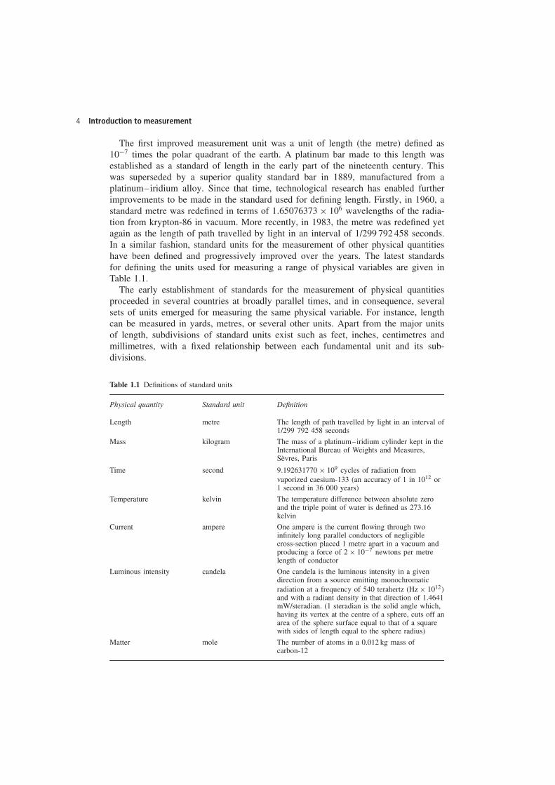
The first improved measurement unit was a unit of length (the metre) defined as10�7 times the polar quadrant of the earth. A platinum bar made to this length wasestablished as a standard of length in the early part of the nineteenth century. Thiswas superseded by a superior quality standard bar in 1889, manufactured from aplatinum–iridium alloy. Since that time, technological research has enabled furtherimprovements to be made in the standard used for defining length. Firstly, in 1960, astandard metre was redefined in terms of 1.65076373 ð 106 wavelengths of the radia-tion from krypton-86 in vacuum. More recently, in 1983, the metre was redefined yetagain as the length of path travelled by light in an interval of 1/299 792 458 seconds.In a similar fashion, standard units for the measurement of other physical quantitieshave been defined and progressively improved over the years. The latest standardsfor defining the units used for measuring a range of physical variables are given inTable 1.1.
The early establishment of standards for the measurement of physical quantitiesproceeded in several countries at broadly parallel times, and in consequence, severalsets of units emerged for measuring the same physical variable. For instance, lengthcan be measured in yards, metres, or several other units. Apart from the major unitsof length, subdivisions of standard units exist such as feet, inches, centimetres andmillimetres, with a fixed relationship between each fundamental unit and its sub-divisions.
Table 1.1 Definitions of standard units
Physical quantity Standard unit Definition
Length metre The length of path travelled by light in an interval of1/299 792 458 seconds
Mass kilogram The mass of a platinum–iridium cylinder kept in theInternational Bureau of Weights and Measures,Sevres, Paris
Time second 9.192631770 ð 109 cycles of radiation fromvaporized caesium-133 (an accuracy of 1 in 1012 or1 second in 36 000 years)
Temperature kelvin The temperature difference between absolute zeroand the triple point of water is defined as 273.16kelvin
Current ampere One ampere is the current flowing through twoinfinitely long parallel conductors of negligiblecross-section placed 1 metre apart in a vacuum andproducing a force of 2 ð 10�7 newtons per metrelength of conductor
Luminous intensity candela One candela is the luminous intensity in a givendirection from a source emitting monochromaticradiation at a frequency of 540 terahertz (Hz ð 1012)and with a radiant density in that direction of 1.4641mW/steradian. (1 steradian is the solid angle which,having its vertex at the centre of a sphere, cuts off anarea of the sphere surface equal to that of a squarewith sides of length equal to the sphere radius)
Matter mole The number of atoms in a 0.012 kg mass ofcarbon-12

Measurement and Instrumentation Principles 5
Table 1.2 Fundamental and derived SI units
(a) Fundamental units
Quantity Standard unit Symbol
Length metre mMass kilogram kgTime second sElectric current ampere ATemperature kelvin KLuminous intensity candela cdMatter mole mol
(b) Supplementary fundamental units
Quantity Standard unit Symbol
Plane angle radian radSolid angle steradian sr
(c) Derived units
DerivationQuantity Standard unit Symbol formula
Area square metre m2
Volume cubic metre m3
Velocity metre per second m/sAcceleration metre per second squared m/s2
Angular velocity radian per second rad/sAngular acceleration radian per second squared rad/s2
Density kilogram per cubic metre kg/m3
Specific volume cubic metre per kilogram m3/kgMass flow rate kilogram per second kg/sVolume flow rate cubic metre per second m3/sForce newton N kg m/s2
Pressure newton per square metre N/m2
Torque newton metre N mMomentum kilogram metre per second kg m/sMoment of inertia kilogram metre squared kg m2
Kinematic viscosity square metre per second m2/sDynamic viscosity newton second per square metre N s/m2
Work, energy, heat joule J NmSpecific energy joule per cubic metre J/m3
Power watt W J/sThermal conductivity watt per metre kelvin W/m KElectric charge coulomb C A sVoltage, e.m.f., pot. diff. volt V W/AElectric field strength volt per metre V/mElectric resistance ohm � V/AElectric capacitance farad F A s/VElectric inductance henry H V s/AElectric conductance siemen S A/VResistivity ohm metre �mPermittivity farad per metre F/mPermeability henry per metre H/mCurrent density ampere per square metre A/m2
(continued overleaf )
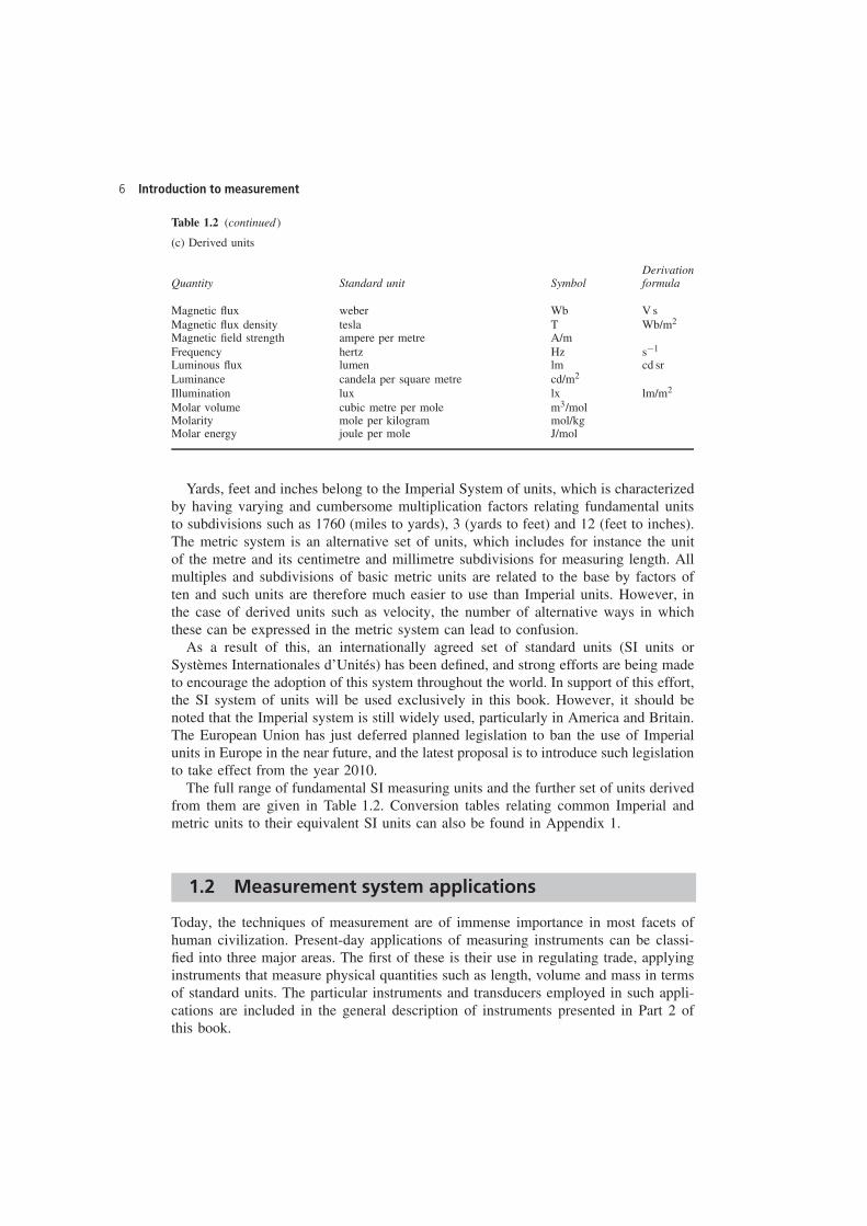
6 Introduction to measurement
Table 1.2 (continued)
(c) Derived units
DerivationQuantity Standard unit Symbol formula
Magnetic flux weber Wb V sMagnetic flux density tesla T Wb/m2
Magnetic field strength ampere per metre A/mFrequency hertz Hz s�1
Luminous flux lumen lm cd srLuminance candela per square metre cd/m2
Illumination lux lx lm/m2
Molar volume cubic metre per mole m3/molMolarity mole per kilogram mol/kgMolar energy joule per mole J/mol
Yards, feet and inches belong to the Imperial System of units, which is characterizedby having varying and cumbersome multiplication factors relating fundamental unitsto subdivisions such as 1760 (miles to yards), 3 (yards to feet) and 12 (feet to inches).The metric system is an alternative set of units, which includes for instance the unitof the metre and its centimetre and millimetre subdivisions for measuring length. Allmultiples and subdivisions of basic metric units are related to the base by factors often and such units are therefore much easier to use than Imperial units. However, inthe case of derived units such as velocity, the number of alternative ways in whichthese can be expressed in the metric system can lead to confusion.
As a result of this, an internationally agreed set of standard units (SI units orSystemes Internationales d’Unites) has been defined, and strong efforts are being madeto encourage the adoption of this system throughout the world. In support of this effort,the SI system of units will be used exclusively in this book. However, it should benoted that the Imperial system is still widely used, particularly in America and Britain.The European Union has just deferred planned legislation to ban the use of Imperialunits in Europe in the near future, and the latest proposal is to introduce such legislationto take effect from the year 2010.
The full range of fundamental SI measuring units and the further set of units derivedfrom them are given in Table 1.2. Conversion tables relating common Imperial andmetric units to their equivalent SI units can also be found in Appendix 1.
1.2 Measurement system applications
Today, the techniques of measurement are of immense importance in most facets ofhuman civilization. Present-day applications of measuring instruments can be classi-fied into three major areas. The first of these is their use in regulating trade, applyinginstruments that measure physical quantities such as length, volume and mass in termsof standard units. The particular instruments and transducers employed in such appli-cations are included in the general description of instruments presented in Part 2 ofthis book.
Measurement and Instrumentation Principles 7
The second application area of measuring instruments is in monitoring functions.These provide information that enables human beings to take some prescribed actionaccordingly. The gardener uses a thermometer to determine whether he should turnthe heat on in his greenhouse or open the windows if it is too hot. Regular studyof a barometer allows us to decide whether we should take our umbrellas if we areplanning to go out for a few hours. Whilst there are thus many uses of instrumentationin our normal domestic lives, the majority of monitoring functions exist to providethe information necessary to allow a human being to control some industrial operationor process. In a chemical process for instance, the progress of chemical reactions isindicated by the measurement of temperatures and pressures at various points, andsuch measurements allow the operator to take correct decisions regarding the electricalsupply to heaters, cooling water flows, valve positions etc. One other important use ofmonitoring instruments is in calibrating the instruments used in the automatic processcontrol systems described below.
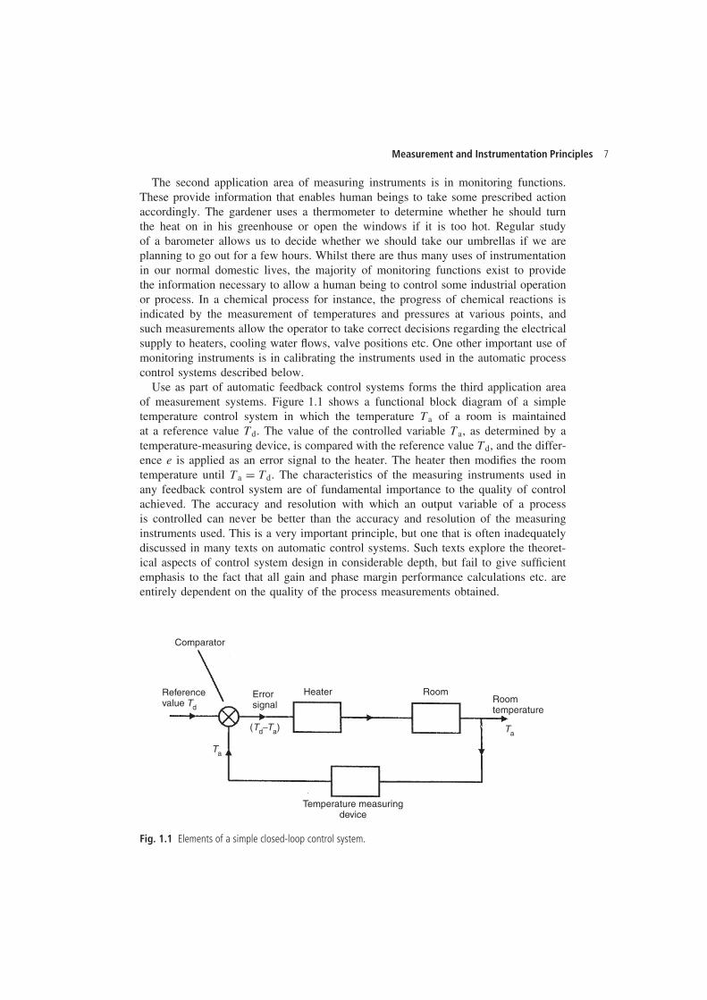
Use as part of automatic feedback control systems forms the third application areaof measurement systems. Figure 1.1 shows a functional block diagram of a simpletemperature control system in which the temperature Ta of a room is maintainedat a reference value Td. The value of the controlled variable Ta, as determined by atemperature-measuring device, is compared with the reference value Td, and the differ-ence e is applied as an error signal to the heater. The heater then modifies the roomtemperature until Ta D Td. The characteristics of the measuring instruments used inany feedback control system are of fundamental importance to the quality of controlachieved. The accuracy and resolution with which an output variable of a processis controlled can never be better than the accuracy and resolution of the measuringinstruments used. This is a very important principle, but one that is often inadequatelydiscussed in many texts on automatic control systems. Such texts explore the theoret-ical aspects of control system design in considerable depth, but fail to give sufficientemphasis to the fact that all gain and phase margin performance calculations etc. areentirely dependent on the quality of the process measurements obtained.
Comparator
Referencevalue Td
Errorsignal
Heater RoomRoomtemperature
Temperature measuringdevice
Ta
Ta(Td−Ta)
Fig. 1.1 Elements of a simple closed-loop control system.
8 Introduction to measurement
1.3 Elements of a measurement system
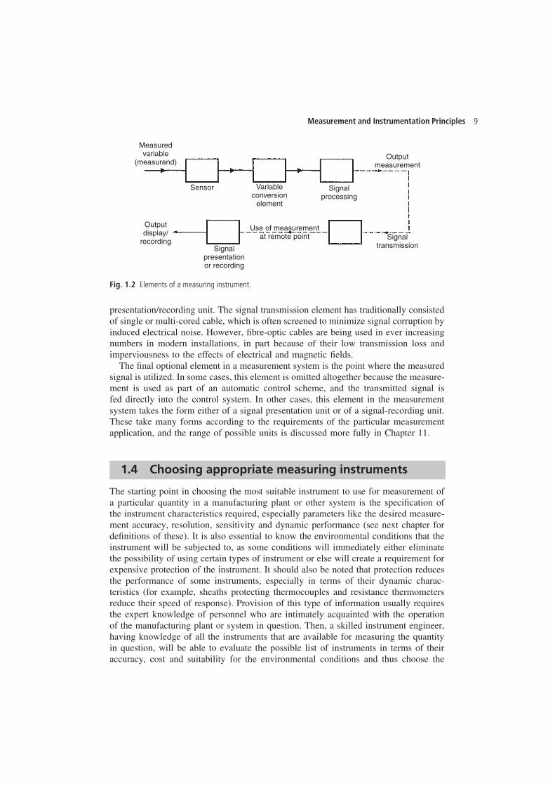
A measuring system exists to provide information about the physical value of somevariable being measured. In simple cases, the system can consist of only a single unitthat gives an output reading or signal according to the magnitude of the unknownvariable applied to it. However, in more complex measurement situations, a measuringsystem consists of several separate elements as shown in Figure 1.2. These compo-nents might be contained within one or more boxes, and the boxes holding individualmeasurement elements might be either close together or physically separate. The termmeasuring instrument is commonly used to describe a measurement system, whetherit contains only one or many elements, and this term will be widely used throughoutthis text.
The first element in any measuring system is the primary sensor: this gives anoutput that is a function of the measurand (the input applied to it). For most but notall sensors, this function is at least approximately linear. Some examples of primarysensors are a liquid-in-glass thermometer, a thermocouple and a strain gauge. In thecase of the mercury-in-glass thermometer, the output reading is given in terms ofthe level of the mercury, and so this particular primary sensor is also a completemeasurement system in itself. However, in general, the primary sensor is only part ofa measurement system. The types of primary sensors available for measuring a widerange of physical quantities are presented in Part 2 of this book.
Variable conversion elements are needed where the output variable of a primarytransducer is in an inconvenient form and has to be converted to a more convenientform. For instance, the displacement-measuring strain gauge has an output in the formof a varying resistance. The resistance change cannot be easily measured and so it isconverted to a change in voltage by a bridge circuit, which is a typical example of avariable conversion element. In some cases, the primary sensor and variable conversionelement are combined, and the combination is known as a transducer.Ł
Signal processing elements exist to improve the quality of the output of a measure-ment system in some way. A very common type of signal processing element is theelectronic amplifier, which amplifies the output of the primary transducer or variableconversion element, thus improving the sensitivity and resolution of measurement. Thiselement of a measuring system is particularly important where the primary transducerhas a low output. For example, thermocouples have a typical output of only a fewmillivolts. Other types of signal processing element are those that filter out inducednoise and remove mean levels etc. In some devices, signal processing is incorporatedinto a transducer, which is then known as a transmitter.Ł
In addition to these three components just mentioned, some measurement systemshave one or two other components, firstly to transmit the signal to some remote pointand secondly to display or record the signal if it is not fed automatically into a feed-back control system. Signal transmission is needed when the observation or applicationpoint of the output of a measurement system is some distance away from the siteof the primary transducer. Sometimes, this separation is made solely for purposesof convenience, but more often it follows from the physical inaccessibility or envi-ronmental unsuitability of the site of the primary transducer for mounting the signal
Ł In some cases, the word ‘sensor’ is used generically to refer to both transducers and transmitters.
Measurement and Instrumentation Principles 9
Measuredvariable
(measurand)
Sensor Variableconversion
element
Signalprocessing
Outputmeasurement
Outputdisplay/
recordingSignal
presentationor recording
Use of measurementat remote point Signal
transmission
Fig. 1.2 Elements of a measuring instrument.
presentation/recording unit. The signal transmission element has traditionally consistedof single or multi-cored cable, which is often screened to minimize signal corruption byinduced electrical noise. However, fibre-optic cables are being used in ever increasingnumbers in modern installations, in part because of their low transmission loss andimperviousness to the effects of electrical and magnetic fields.
The final optional element in a measurement system is the point where the measuredsignal is utilized. In some cases, this element is omitted altogether because the measure-ment is used as part of an automatic control scheme, and the transmitted signal isfed directly into the control system. In other cases, this element in the measurementsystem takes the form either of a signal presentation unit or of a signal-recording unit.These take many forms according to the requirements of the particular measurementapplication, and the range of possible units is discussed more fully in Chapter 11.
1.4 Choosing appropriate measuring instruments
The starting point in choosing the most suitable instrument to use for measurement ofa particular quantity in a manufacturing plant or other system is the specification ofthe instrument characteristics required, especially parameters like the desired measure-ment accuracy, resolution, sensitivity and dynamic performance (see next chapter fordefinitions of these). It is also essential to know the environmental conditions that theinstrument will be subjected to, as some conditions will immediately either eliminatethe possibility of using certain types of instrument or else will create a requirement forexpensive protection of the instrument. It should also be noted that protection reducesthe performance of some instruments, especially in terms of their dynamic charac-teristics (for example, sheaths protecting thermocouples and resistance thermometersreduce their speed of response). Provision of this type of information usually requiresthe expert knowledge of personnel who are intimately acquainted with the operationof the manufacturing plant or system in question. Then, a skilled instrument engineer,having knowledge of all the instruments that are available for measuring the quantityin question, will be able to evaluate the possible list of instruments in terms of theiraccuracy, cost and suitability for the environmental conditions and thus choose the
10 Introduction to measurement
most appropriate instrument. As far as possible, measurement systems and instrumentsshould be chosen that are as insensitive as possible to the operating environment,although this requirement is often difficult to meet because of cost and other perfor-mance considerations. The extent to which the measured system will be disturbedduring the measuring process is another important factor in instrument choice. Forexample, significant pressure loss can be caused to the measured system in sometechniques of flow measurement.
Published literature is of considerable help in the choice of a suitable instrumentfor a particular measurement situation. Many books are available that give valuableassistance in the necessary evaluation by providing lists and data about all the instru-ments available for measuring a range of physical quantities (e.g. Part 2 of this text).However, new techniques and instruments are being developed all the time, and there-fore a good instrumentation engineer must keep abreast of the latest developments byreading the appropriate technical journals regularly.
The instrument characteristics discussed in the next chapter are the features that formthe technical basis for a comparison between the relative merits of different instruments.Generally, the better the characteristics, the higher the cost. However, in comparingthe cost and relative suitability of different instruments for a particular measurementsituation, considerations of durability, maintainability and constancy of performanceare also very important because the instrument chosen will often have to be capableof operating for long periods without performance degradation and a requirement forcostly maintenance. In consequence of this, the initial cost of an instrument often hasa low weighting in the evaluation exercise.
Cost is very strongly correlated with the performance of an instrument, as measuredby its static characteristics. Increasing the accuracy or resolution of an instrument, forexample, can only be done at a penalty of increasing its manufacturing cost. Instru-ment choice therefore proceeds by specifying the minimum characteristics requiredby a measurement situation and then searching manufacturers’ catalogues to find aninstrument whose characteristics match those required. To select an instrument withcharacteristics superior to those required would only mean paying more than necessaryfor a level of performance greater than that needed.
As well as purchase cost, other important factors in the assessment exercise areinstrument durability and the maintenance requirements. Assuming that one had £10 000to spend, one would not spend £8000 on a new motor car whose projected life wasfive years if a car of equivalent specification with a projected life of ten years wasavailable for £10 000. Likewise, durability is an important consideration in the choiceof instruments. The projected life of instruments often depends on the conditions inwhich the instrument will have to operate. Maintenance requirements must also betaken into account, as they also have cost implications.
As a general rule, a good assessment criterion is obtained if the total purchase costand estimated maintenance costs of an instrument over its life are divided by theperiod of its expected life. The figure obtained is thus a cost per year. However, thisrule becomes modified where instruments are being installed on a process whose life isexpected to be limited, perhaps in the manufacture of a particular model of car. Then,the total costs can only be divided by the period of time that an instrument is expectedto be used for, unless an alternative use for the instrument is envisaged at the end ofthis period.

Measurement and Instrumentation Principles 11
To summarize therefore, instrument choice is a compromise between performancecharacteristics, ruggedness and durability, maintenance requirements and purchase cost.To carry out such an evaluation properly, the instrument engineer must have a wideknowledge of the range of instruments available for measuring particular physical quan-tities, and he/she must also have a deep understanding of how instrument characteristicsare affected by particular measurement situations and operating conditions.
2
Instrument types andperformance characteristics
2.1 Review of instrument types
Instruments can be subdivided into separate classes according to several criteria. Thesesubclassifications are useful in broadly establishing several attributes of particularinstruments such as accuracy, cost, and general applicability to different applications.
2.1.1 Active and passive instruments
Instruments are divided into active or passive ones according to whether the instrumentoutput is entirely produced by the quantity being measured or whether the quantitybeing measured simply modulates the magnitude of some external power source. Thisis illustrated by examples.
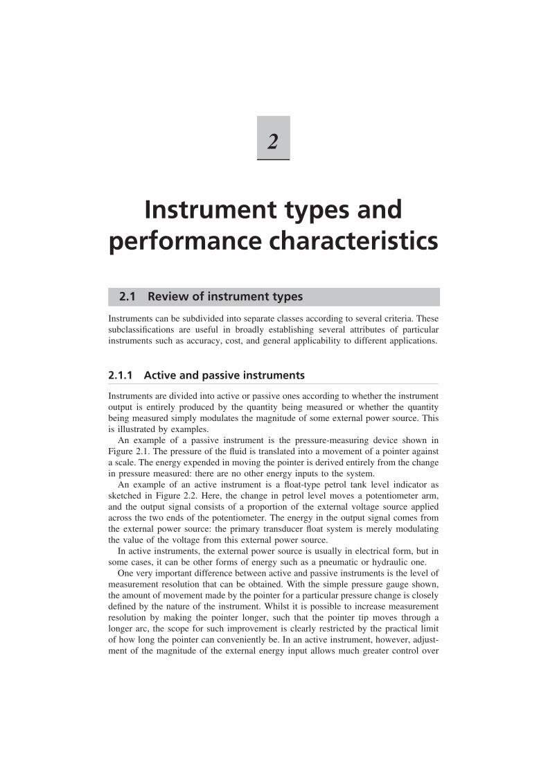
An example of a passive instrument is the pressure-measuring device shown inFigure 2.1. The pressure of the fluid is translated into a movement of a pointer againsta scale. The energy expended in moving the pointer is derived entirely from the changein pressure measured: there are no other energy inputs to the system.
An example of an active instrument is a float-type petrol tank level indicator assketched in Figure 2.2. Here, the change in petrol level moves a potentiometer arm,and the output signal consists of a proportion of the external voltage source appliedacross the two ends of the potentiometer. The energy in the output signal comes fromthe external power source: the primary transducer float system is merely modulatingthe value of the voltage from this external power source.
In active instruments, the external power source is usually in electrical form, but insome cases, it can be other forms of energy such as a pneumatic or hydraulic one.
One very important difference between active and passive instruments is the level ofmeasurement resolution that can be obtained. With the simple pressure gauge shown,the amount of movement made by the pointer for a particular pressure change is closelydefined by the nature of the instrument. Whilst it is possible to increase measurementresolution by making the pointer longer, such that the pointer tip moves through alonger arc, the scope for such improvement is clearly restricted by the practical limitof how long the pointer can conveniently be. In an active instrument, however, adjust-ment of the magnitude of the external energy input allows much greater control over
Measurement and Instrumentation Principles 13
Spring
Piston
Fluid
Pointer
Scale
Pivot
Fig. 2.1 Passive pressure gauge.
Float
Pivot
Outputvoltage
Fig. 2.2 Petrol-tank level indicator.
measurement resolution. Whilst the scope for improving measurement resolution ismuch greater incidentally, it is not infinite because of limitations placed on the magni-tude of the external energy input, in consideration of heating effects and for safetyreasons.
In terms of cost, passive instruments are normally of a more simple constructionthan active ones and are therefore cheaper to manufacture. Therefore, choice betweenactive and passive instruments for a particular application involves carefully balancingthe measurement resolution requirements against cost.
2.1.2 Null-type and deflection-type instruments
The pressure gauge just mentioned is a good example of a deflection type of instrument,where the value of the quantity being measured is displayed in terms of the amount of
14 Instrument types and performance characteristics
Weights
Piston Datum level
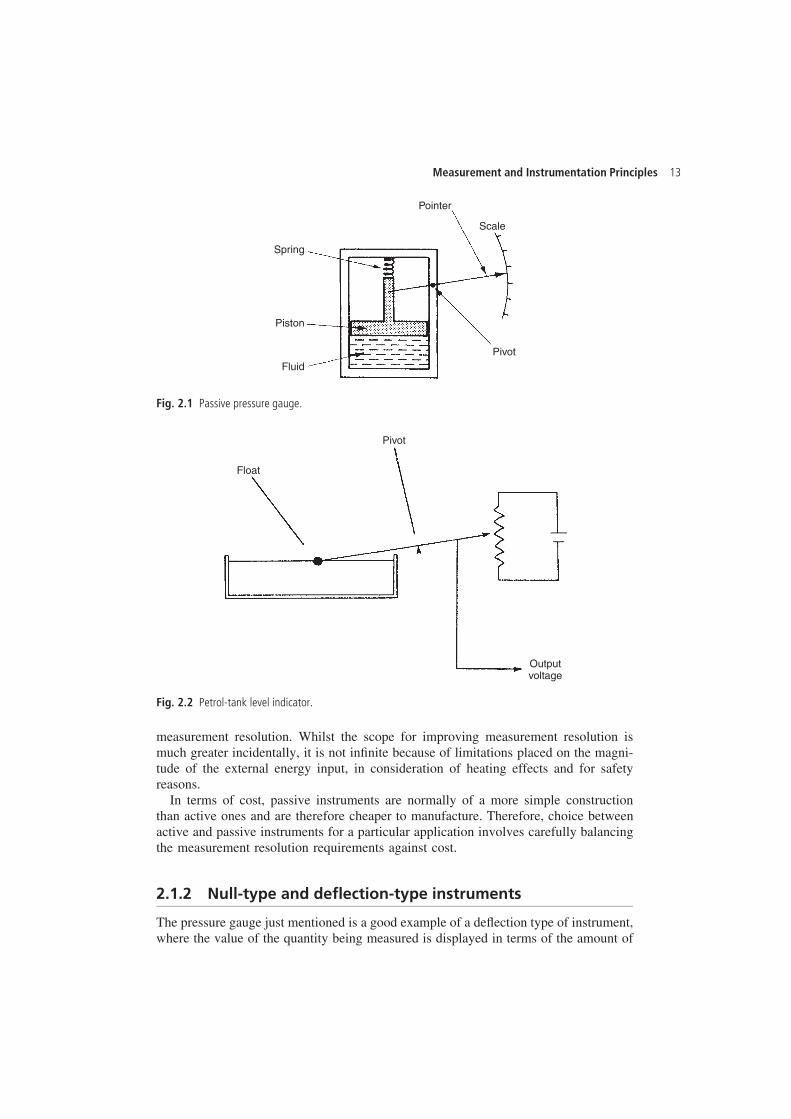
Fig. 2.3 Deadweight pressure gauge.
movement of a pointer. An alternative type of pressure gauge is the deadweight gaugeshown in Figure 2.3, which is a null-type instrument. Here, weights are put on topof the piston until the downward force balances the fluid pressure. Weights are addeduntil the piston reaches a datum level, known as the null point. Pressure measurementis made in terms of the value of the weights needed to reach this null position.
The accuracy of these two instruments depends on different things. For the first oneit depends on the linearity and calibration of the spring, whilst for the second it relieson the calibration of the weights. As calibration of weights is much easier than carefulchoice and calibration of a linear-characteristic spring, this means that the second typeof instrument will normally be the more accurate. This is in accordance with the generalrule that null-type instruments are more accurate than deflection types.
In terms of usage, the deflection type instrument is clearly more convenient. It isfar simpler to read the position of a pointer against a scale than to add and subtractweights until a null point is reached. A deflection-type instrument is therefore the onethat would normally be used in the workplace. However, for calibration duties, thenull-type instrument is preferable because of its superior accuracy. The extra effortrequired to use such an instrument is perfectly acceptable in this case because of theinfrequent nature of calibration operations.
2.1.3 Analogue and digital instruments
An analogue instrument gives an output that varies continuously as the quantity beingmeasured changes. The output can have an infinite number of values within the rangethat the instrument is designed to measure. The deflection-type of pressure gaugedescribed earlier in this chapter (Figure 2.1) is a good example of an analogue instru-ment. As the input value changes, the pointer moves with a smooth continuous motion.Whilst the pointer can therefore be in an infinite number of positions within its rangeof movement, the number of different positions that the eye can discriminate betweenis strictly limited, this discrimination being dependent upon how large the scale is andhow finely it is divided.
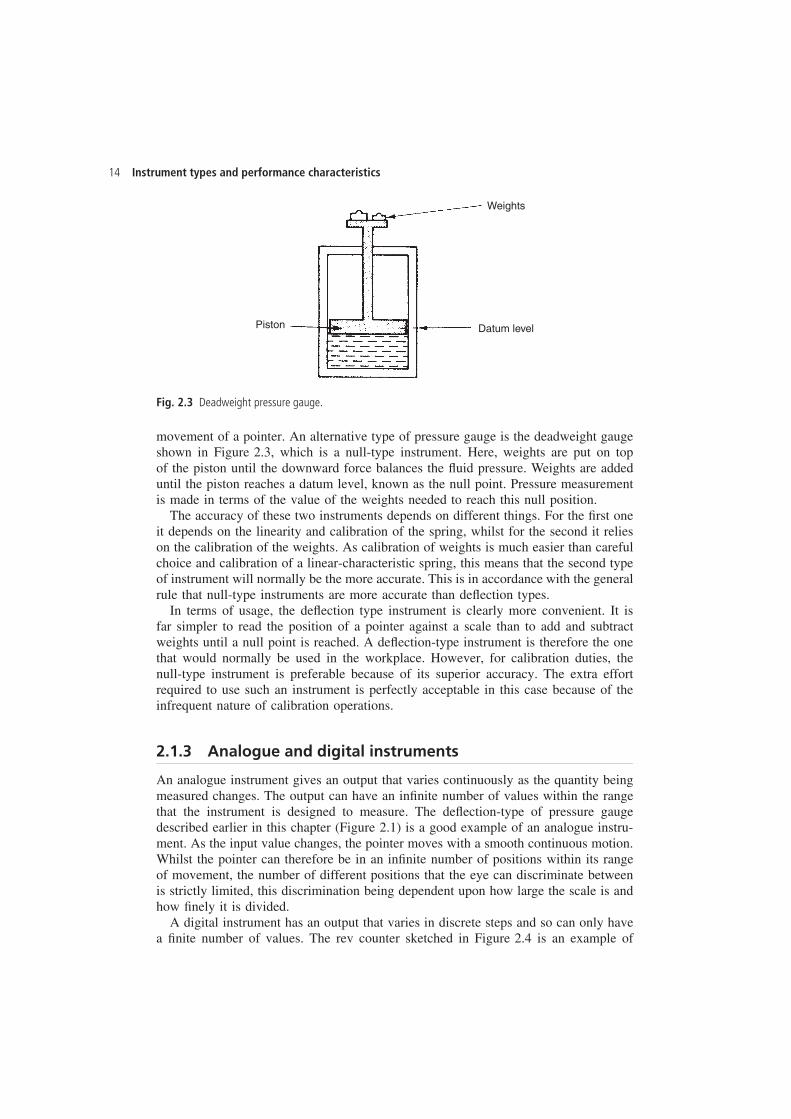
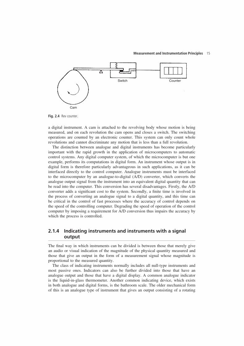
A digital instrument has an output that varies in discrete steps and so can only havea finite number of values. The rev counter sketched in Figure 2.4 is an example of
Measurement and Instrumentation Principles 15
Cam
Switch Counter
Fig. 2.4 Rev counter.
a digital instrument. A cam is attached to the revolving body whose motion is beingmeasured, and on each revolution the cam opens and closes a switch. The switchingoperations are counted by an electronic counter. This system can only count wholerevolutions and cannot discriminate any motion that is less than a full revolution.
The distinction between analogue and digital instruments has become particularlyimportant with the rapid growth in the application of microcomputers to automaticcontrol systems. Any digital computer system, of which the microcomputer is but oneexample, performs its computations in digital form. An instrument whose output is indigital form is therefore particularly advantageous in such applications, as it can beinterfaced directly to the control computer. Analogue instruments must be interfacedto the microcomputer by an analogue-to-digital (A/D) converter, which converts theanalogue output signal from the instrument into an equivalent digital quantity that canbe read into the computer. This conversion has several disadvantages. Firstly, the A/Dconverter adds a significant cost to the system. Secondly, a finite time is involved inthe process of converting an analogue signal to a digital quantity, and this time canbe critical in the control of fast processes where the accuracy of control depends onthe speed of the controlling computer. Degrading the speed of operation of the controlcomputer by imposing a requirement for A/D conversion thus impairs the accuracy bywhich the process is controlled.
2.1.4 Indicating instruments and instruments with a signaloutput
The final way in which instruments can be divided is between those that merely givean audio or visual indication of the magnitude of the physical quantity measured andthose that give an output in the form of a measurement signal whose magnitude isproportional to the measured quantity.
The class of indicating instruments normally includes all null-type instruments andmost passive ones. Indicators can also be further divided into those that have ananalogue output and those that have a digital display. A common analogue indicatoris the liquid-in-glass thermometer. Another common indicating device, which existsin both analogue and digital forms, is the bathroom scale. The older mechanical formof this is an analogue type of instrument that gives an output consisting of a rotating
16 Instrument types and performance characteristics
pointer moving against a scale (or sometimes a rotating scale moving against a pointer).More recent electronic forms of bathroom scale have a digital output consisting ofnumbers presented on an electronic display. One major drawback with indicatingdevices is that human intervention is required to read and record a measurement. Thisprocess is particularly prone to error in the case of analogue output displays, althoughdigital displays are not very prone to error unless the human reader is careless.
Instruments that have a signal-type output are commonly used as part of automaticcontrol systems. In other circumstances, they can also be found in measurement systemswhere the output measurement signal is recorded in some way for later use. This subjectis covered in later chapters. Usually, the measurement signal involved is an electricalvoltage, but it can take other forms in some systems such as an electrical current, anoptical signal or a pneumatic signal.
2.1.5 Smart and non-smart instruments
The advent of the microprocessor has created a new division in instruments betweenthose that do incorporate a microprocessor (smart) and those that don’t. Smart devicesare considered in detail in Chapter 9.
2.2 Static characteristics of instruments
If we have a thermometer in a room and its reading shows a temperature of 20°C, thenit does not really matter whether the true temperature of the room is 19.5°C or 20.5°C.Such small variations around 20°C are too small to affect whether we feel warm enoughor not. Our bodies cannot discriminate between such close levels of temperature andtherefore a thermometer with an inaccuracy of š0.5°C is perfectly adequate. If we hadto measure the temperature of certain chemical processes, however, a variation of 0.5°Cmight have a significant effect on the rate of reaction or even the products of a process.A measurement inaccuracy much less than š0.5°C is therefore clearly required.
Accuracy of measurement is thus one consideration in the choice of instrumentfor a particular application. Other parameters such as sensitivity, linearity and thereaction to ambient temperature changes are further considerations. These attributesare collectively known as the static characteristics of instruments, and are given in thedata sheet for a particular instrument. It is important to note that the values quotedfor instrument characteristics in such a data sheet only apply when the instrument isused under specified standard calibration conditions. Due allowance must be made forvariations in the characteristics when the instrument is used in other conditions.
The various static characteristics are defined in the following paragraphs.
2.2.1 Accuracy and inaccuracy (measurement uncertainty)
The accuracy of an instrument is a measure of how close the output reading of theinstrument is to the correct value. In practice, it is more usual to quote the inaccuracyfigure rather than the accuracy figure for an instrument. Inaccuracy is the extent to
Measurement and Instrumentation Principles 17
which a reading might be wrong, and is often quoted as a percentage of the full-scale(f.s.) reading of an instrument. If, for example, a pressure gauge of range 0–10 barhas a quoted inaccuracy of š1.0% f.s. (š1% of full-scale reading), then the maximumerror to be expected in any reading is 0.1 bar. This means that when the instrument isreading 1.0 bar, the possible error is 10% of this value. For this reason, it is an importantsystem design rule that instruments are chosen such that their range is appropriate to thespread of values being measured, in order that the best possible accuracy is maintainedin instrument readings. Thus, if we were measuring pressures with expected valuesbetween 0 and 1 bar, we would not use an instrument with a range of 0–10 bar. Theterm measurement uncertainty is frequently used in place of inaccuracy.
2.2.2 Precision/repeatability/reproducibility
Precision is a term that describes an instrument’s degree of freedom from randomerrors. If a large number of readings are taken of the same quantity by a high precisioninstrument, then the spread of readings will be very small. Precision is often, thoughincorrectly, confused with accuracy. High precision does not imply anything aboutmeasurement accuracy. A high precision instrument may have a low accuracy. Lowaccuracy measurements from a high precision instrument are normally caused by abias in the measurements, which is removable by recalibration.
The terms repeatability and reproducibility mean approximately the same but areapplied in different contexts as given below. Repeatability describes the closenessof output readings when the same input is applied repetitively over a short periodof time, with the same measurement conditions, same instrument and observer, samelocation and same conditions of use maintained throughout. Reproducibility describesthe closeness of output readings for the same input when there are changes in themethod of measurement, observer, measuring instrument, location, conditions of useand time of measurement. Both terms thus describe the spread of output readings forthe same input. This spread is referred to as repeatability if the measurement conditionsare constant and as reproducibility if the measurement conditions vary.
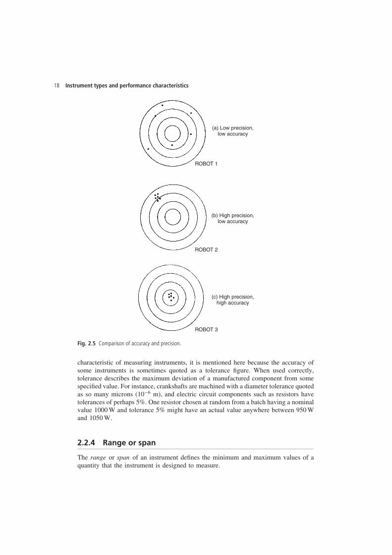
The degree of repeatability or reproducibility in measurements from an instrument isan alternative way of expressing its precision. Figure 2.5 illustrates this more clearly.The figure shows the results of tests on three industrial robots that were programmedto place components at a particular point on a table. The target point was at the centreof the concentric circles shown, and the black dots represent the points where eachrobot actually deposited components at each attempt. Both the accuracy and precisionof Robot 1 are shown to be low in this trial. Robot 2 consistently puts the componentdown at approximately the same place but this is the wrong point. Therefore, it hashigh precision but low accuracy. Finally, Robot 3 has both high precision and highaccuracy, because it consistently places the component at the correct target position.
2.2.3 Tolerance
Tolerance is a term that is closely related to accuracy and defines the maximumerror that is to be expected in some value. Whilst it is not, strictly speaking, a static
18 Instrument types and performance characteristics
(a) Low precision,low accuracy
(b) High precision,low accuracy
(c) High precision,high accuracy
ROBOT 1
ROBOT 2
ROBOT 3
Fig. 2.5 Comparison of accuracy and precision.
characteristic of measuring instruments, it is mentioned here because the accuracy ofsome instruments is sometimes quoted as a tolerance figure. When used correctly,tolerance describes the maximum deviation of a manufactured component from somespecified value. For instance, crankshafts are machined with a diameter tolerance quotedas so many microns (10�6 m), and electric circuit components such as resistors havetolerances of perhaps 5%. One resistor chosen at random from a batch having a nominalvalue 1000 W and tolerance 5% might have an actual value anywhere between 950 Wand 1050 W.
2.2.4 Range or span
The range or span of an instrument defines the minimum and maximum values of aquantity that the instrument is designed to measure.
Measurement and Instrumentation Principles 19
2.2.5 Linearity
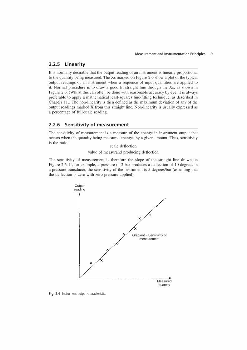
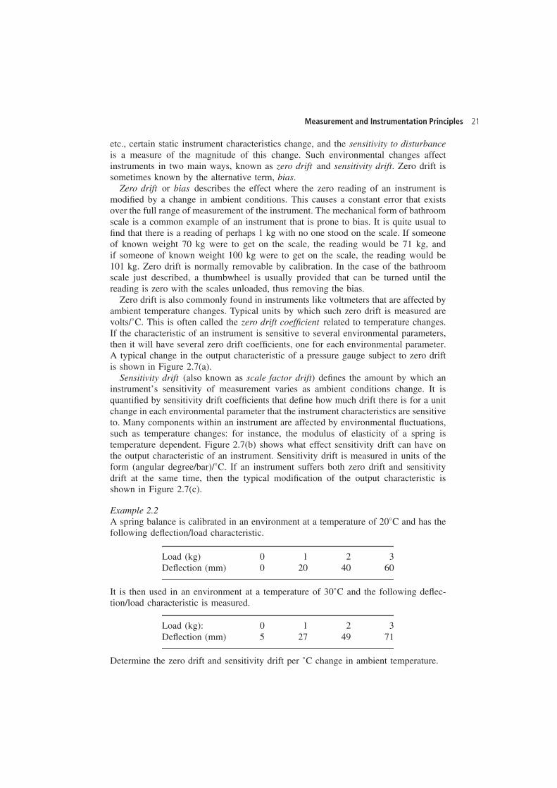
It is normally desirable that the output reading of an instrument is linearly proportionalto the quantity being measured. The Xs marked on Figure 2.6 show a plot of the typicaloutput readings of an instrument when a sequence of input quantities are applied toit. Normal procedure is to draw a good fit straight line through the Xs, as shown inFigure 2.6. (Whilst this can often be done with reasonable accuracy by eye, it is alwayspreferable to apply a mathematical least-squares line-fitting technique, as described inChapter 11.) The non-linearity is then defined as the maximum deviation of any of theoutput readings marked X from this straight line. Non-linearity is usually expressed asa percentage of full-scale reading.
2.2.6 Sensitivity of measurement
The sensitivity of measurement is a measure of the change in instrument output thatoccurs when the quantity being measured changes by a given amount. Thus, sensitivityis the ratio:
scale deflection
value of measurand producing deflection
The sensitivity of measurement is therefore the slope of the straight line drawn onFigure 2.6. If, for example, a pressure of 2 bar produces a deflection of 10 degrees ina pressure transducer, the sensitivity of the instrument is 5 degrees/bar (assuming thatthe deflection is zero with zero pressure applied).
Outputreading
Gradient = Sensitivity ofmeasurement
Measuredquantity
Fig. 2.6 Instrument output characteristic.
20 Instrument types and performance characteristics
Example 2.1The following resistance values of a platinum resistance thermometer were measuredat a range of temperatures. Determine the measurement sensitivity of the instrumentin ohms/°C.
Resistance (�) Temperature (°C)
307 200314 230321 260328 290
SolutionIf these values are plotted on a graph, the straight-line relationship between resistancechange and temperature change is obvious.
For a change in temperature of 30°C, the change in resistance is 7 �. Hence themeasurement sensitivity D 7/30 D 0.233 �/°C.
2.2.7 Threshold
If the input to an instrument is gradually increased from zero, the input will have toreach a certain minimum level before the change in the instrument output reading isof a large enough magnitude to be detectable. This minimum level of input is knownas the threshold of the instrument. Manufacturers vary in the way that they specifythreshold for instruments. Some quote absolute values, whereas others quote thresholdas a percentage of full-scale readings. As an illustration, a car speedometer typically hasa threshold of about 15 km/h. This means that, if the vehicle starts from rest and acceler-ates, no output reading is observed on the speedometer until the speed reaches 15 km/h.
2.2.8 Resolution
When an instrument is showing a particular output reading, there is a lower limit on themagnitude of the change in the input measured quantity that produces an observablechange in the instrument output. Like threshold, resolution is sometimes specified as anabsolute value and sometimes as a percentage of f.s. deflection. One of the major factorsinfluencing the resolution of an instrument is how finely its output scale is divided intosubdivisions. Using a car speedometer as an example again, this has subdivisions oftypically 20 km/h. This means that when the needle is between the scale markings,we cannot estimate speed more accurately than to the nearest 5 km/h. This figure of5 km/h thus represents the resolution of the instrument.
2.2.9 Sensitivity to disturbance
All calibrations and specifications of an instrument are only valid under controlledconditions of temperature, pressure etc. These standard ambient conditions are usuallydefined in the instrument specification. As variations occur in the ambient temperature
Measurement and Instrumentation Principles 21
etc., certain static instrument characteristics change, and the sensitivity to disturbanceis a measure of the magnitude of this change. Such environmental changes affectinstruments in two main ways, known as zero drift and sensitivity drift. Zero drift issometimes known by the alternative term, bias.
Zero drift or bias describes the effect where the zero reading of an instrument ismodified by a change in ambient conditions. This causes a constant error that existsover the full range of measurement of the instrument. The mechanical form of bathroomscale is a common example of an instrument that is prone to bias. It is quite usual tofind that there is a reading of perhaps 1 kg with no one stood on the scale. If someoneof known weight 70 kg were to get on the scale, the reading would be 71 kg, andif someone of known weight 100 kg were to get on the scale, the reading would be101 kg. Zero drift is normally removable by calibration. In the case of the bathroomscale just described, a thumbwheel is usually provided that can be turned until thereading is zero with the scales unloaded, thus removing the bias.
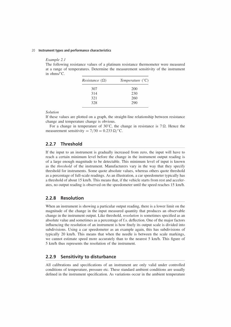
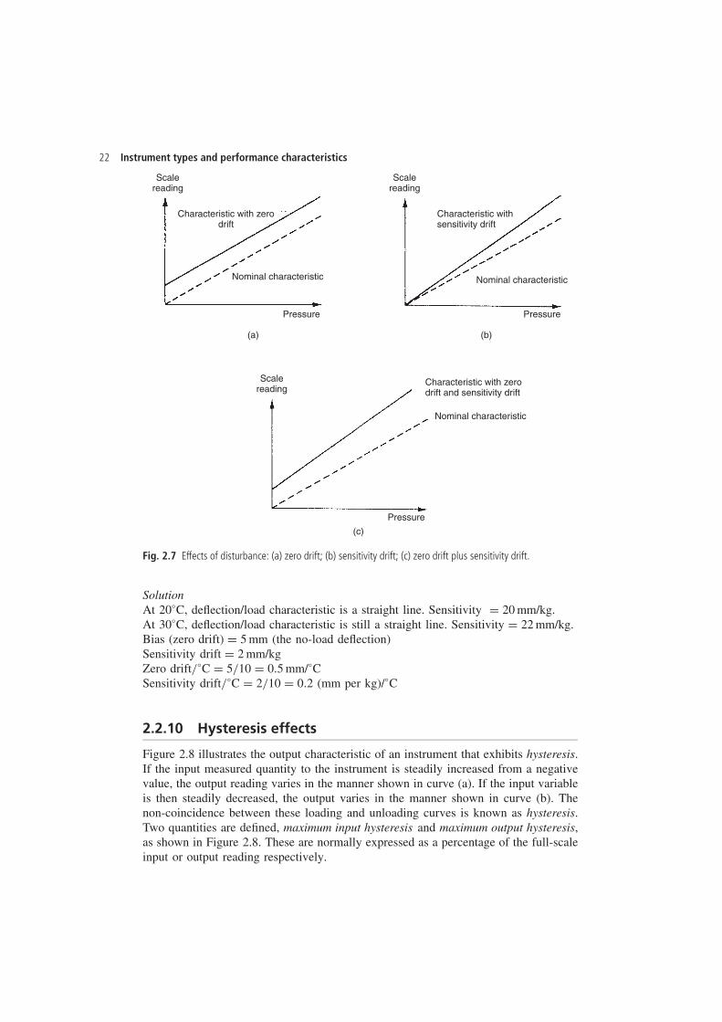
Zero drift is also commonly found in instruments like voltmeters that are affected byambient temperature changes. Typical units by which such zero drift is measured arevolts/°C. This is often called the zero drift coefficient related to temperature changes.If the characteristic of an instrument is sensitive to several environmental parameters,then it will have several zero drift coefficients, one for each environmental parameter.A typical change in the output characteristic of a pressure gauge subject to zero driftis shown in Figure 2.7(a).
Sensitivity drift (also known as scale factor drift) defines the amount by which aninstrument’s sensitivity of measurement varies as ambient conditions change. It isquantified by sensitivity drift coefficients that define how much drift there is for a unitchange in each environmental parameter that the instrument characteristics are sensitiveto. Many components within an instrument are affected by environmental fluctuations,such as temperature changes: for instance, the modulus of elasticity of a spring istemperature dependent. Figure 2.7(b) shows what effect sensitivity drift can have onthe output characteristic of an instrument. Sensitivity drift is measured in units of theform (angular degree/bar)/°C. If an instrument suffers both zero drift and sensitivitydrift at the same time, then the typical modification of the output characteristic isshown in Figure 2.7(c).
Example 2.2A spring balance is calibrated in an environment at a temperature of 20°C and has thefollowing deflection/load characteristic.
Load (kg) 0 1 2 3Deflection (mm) 0 20 40 60
It is then used in an environment at a temperature of 30°C and the following deflec-tion/load characteristic is measured.
Load (kg): 0 1 2 3Deflection (mm) 5 27 49 71
Determine the zero drift and sensitivity drift per °C change in ambient temperature.
22 Instrument types and performance characteristics
Scalereading
Scalereading
Scalereading
Characteristic with zerodrift
Characteristic withsensitivity drift
Characteristic with zerodrift and sensitivity drift
Nominal characteristic Nominal characteristic
Nominal characteristic
Pressure Pressure
Pressure
(a) (b)
(c)
Fig. 2.7 Effects of disturbance: (a) zero drift; (b) sensitivity drift; (c) zero drift plus sensitivity drift.
SolutionAt 20°C, deflection/load characteristic is a straight line. Sensitivity D 20 mm/kg.At 30°C, deflection/load characteristic is still a straight line. Sensitivity D 22 mm/kg.Bias (zero drift) D 5 mm (the no-load deflection)Sensitivity drift D 2 mm/kgZero drift/°C D 5/10 D 0.5 mm/°CSensitivity drift/°C D 2/10 D 0.2 (mm per kg)/°C
2.2.10 Hysteresis effects
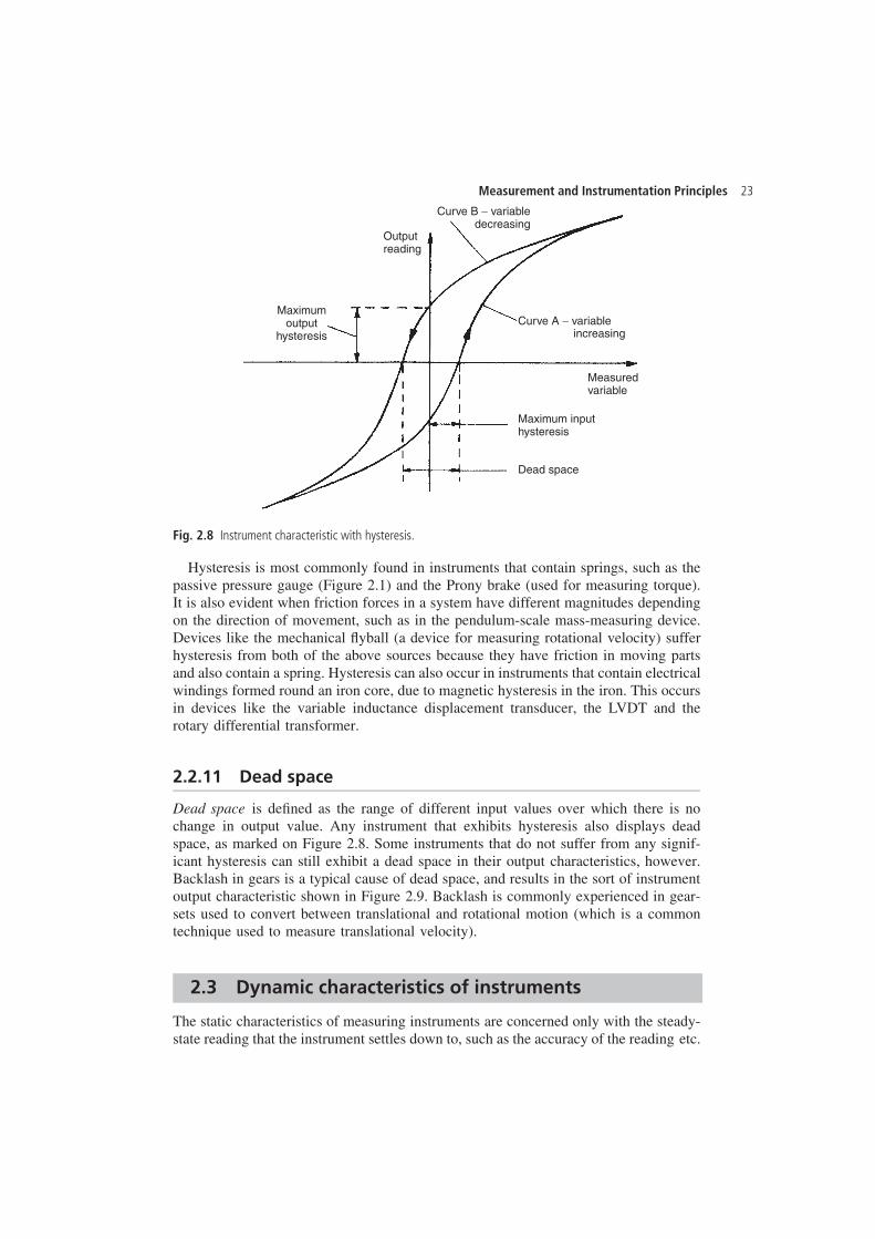
Figure 2.8 illustrates the output characteristic of an instrument that exhibits hysteresis.If the input measured quantity to the instrument is steadily increased from a negativevalue, the output reading varies in the manner shown in curve (a). If the input variableis then steadily decreased, the output varies in the manner shown in curve (b). Thenon-coincidence between these loading and unloading curves is known as hysteresis.Two quantities are defined, maximum input hysteresis and maximum output hysteresis,as shown in Figure 2.8. These are normally expressed as a percentage of the full-scaleinput or output reading respectively.
Measurement and Instrumentation Principles 23
Outputreading
Maximumoutput
hysteresis
Maximum inputhysteresis
Curve B − variabledecreasing
Curve A − variable
Dead space
increasing
Measuredvariable
Fig. 2.8 Instrument characteristic with hysteresis.
Hysteresis is most commonly found in instruments that contain springs, such as thepassive pressure gauge (Figure 2.1) and the Prony brake (used for measuring torque).It is also evident when friction forces in a system have different magnitudes dependingon the direction of movement, such as in the pendulum-scale mass-measuring device.Devices like the mechanical flyball (a device for measuring rotational velocity) sufferhysteresis from both of the above sources because they have friction in moving partsand also contain a spring. Hysteresis can also occur in instruments that contain electricalwindings formed round an iron core, due to magnetic hysteresis in the iron. This occursin devices like the variable inductance displacement transducer, the LVDT and therotary differential transformer.
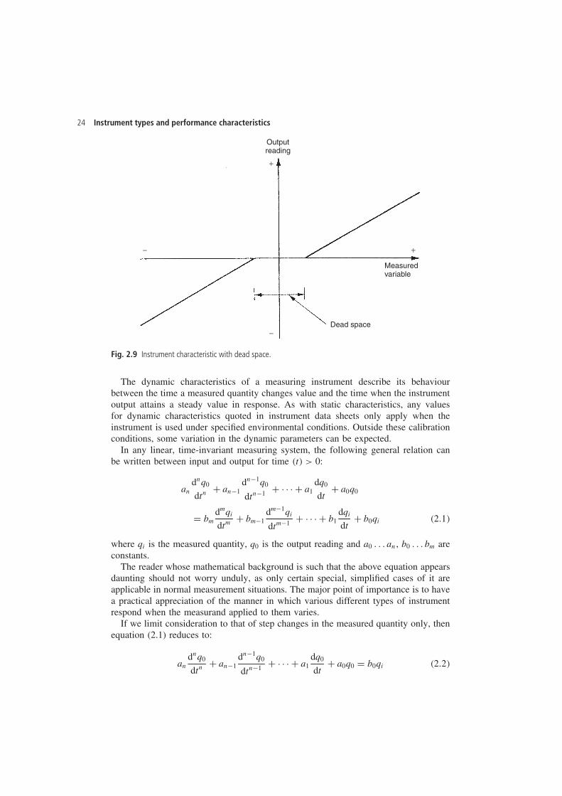
2.2.11 Dead space
Dead space is defined as the range of different input values over which there is nochange in output value. Any instrument that exhibits hysteresis also displays deadspace, as marked on Figure 2.8. Some instruments that do not suffer from any signif-icant hysteresis can still exhibit a dead space in their output characteristics, however.Backlash in gears is a typical cause of dead space, and results in the sort of instrumentoutput characteristic shown in Figure 2.9. Backlash is commonly experienced in gear-sets used to convert between translational and rotational motion (which is a commontechnique used to measure translational velocity).
2.3 Dynamic characteristics of instruments
The static characteristics of measuring instruments are concerned only with the steady-state reading that the instrument settles down to, such as the accuracy of the reading etc.
24 Instrument types and performance characteristics
Outputreading
Dead space
Measuredvariable
+
+
−
−
Fig. 2.9 Instrument characteristic with dead space.
The dynamic characteristics of a measuring instrument describe its behaviourbetween the time a measured quantity changes value and the time when the instrumentoutput attains a steady value in response. As with static characteristics, any valuesfor dynamic characteristics quoted in instrument data sheets only apply when theinstrument is used under specified environmental conditions. Outside these calibrationconditions, some variation in the dynamic parameters can be expected.
In any linear, time-invariant measuring system, the following general relation canbe written between input and output for time �t� > 0:
andnq0
dtn C an�1dn�1q0
dtn�1 C Ð Ð Ð C a1dq0
dtC a0q0
D bmdmqi
dtm C bm�1dm�1qi
dtm�1 C Ð Ð Ð C b1dqi
dtC b0qi �2.1�
where qi is the measured quantity, q0 is the output reading and a0 . . . an, b0 . . . bm areconstants.
The reader whose mathematical background is such that the above equation appearsdaunting should not worry unduly, as only certain special, simplified cases of it areapplicable in normal measurement situations. The major point of importance is to havea practical appreciation of the manner in which various different types of instrumentrespond when the measurand applied to them varies.
If we limit consideration to that of step changes in the measured quantity only, thenequation (2.1) reduces to:
andnq0
dtn C an�1dn�1q0
dtn�1 C Ð Ð Ð C a1dq0
dtC a0q0 D b0qi �2.2�
Measurement and Instrumentation Principles 25
Further simplification can be made by taking certain special cases of equation (2.2),which collectively apply to nearly all measurement systems.
2.3.1 Zero order instrument
If all the coefficients a1 . . . an other than a0 in equation (2.2) are assumed zero, then:
a0q0 D b0qi or q0 D b0qi/a0 D Kqi �2.3�
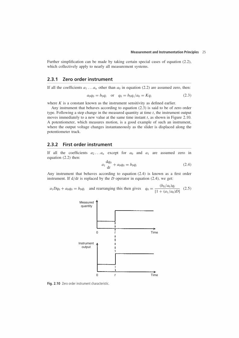
where K is a constant known as the instrument sensitivity as defined earlier.Any instrument that behaves according to equation (2.3) is said to be of zero order
type. Following a step change in the measured quantity at time t, the instrument outputmoves immediately to a new value at the same time instant t, as shown in Figure 2.10.A potentiometer, which measures motion, is a good example of such an instrument,where the output voltage changes instantaneously as the slider is displaced along thepotentiometer track.
2.3.2 First order instrument
If all the coefficients a2 . . . an except for a0 and a1 are assumed zero inequation (2.2) then:
a1dq0
dtC a0q0 D b0qi �2.4�
Any instrument that behaves according to equation (2.4) is known as a first orderinstrument. If d/dt is replaced by the D operator in equation (2.4), we get:
a1Dq0 C a0q0 D b0qi and rearranging this then gives q0 D �b0/a0�qi
[1 C �a1/a0�D]�2.5�
Measuredquantity
Instrumentoutput
0 t
0 t
Time
Time
Fig. 2.10 Zero order instrument characteristic.
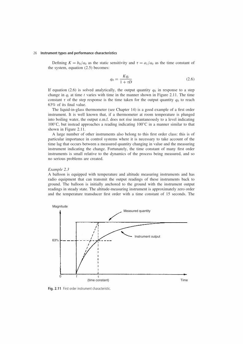
26 Instrument types and performance characteristics
Defining K D b0/a0 as the static sensitivity and � D a1/a0 as the time constant ofthe system, equation (2.5) becomes:
q0 D Kqi
1 C �D�2.6�
If equation (2.6) is solved analytically, the output quantity q0 in response to a stepchange in qi at time t varies with time in the manner shown in Figure 2.11. The timeconstant � of the step response is the time taken for the output quantity q0 to reach63% of its final value.
The liquid-in-glass thermometer (see Chapter 14) is a good example of a first orderinstrument. It is well known that, if a thermometer at room temperature is plungedinto boiling water, the output e.m.f. does not rise instantaneously to a level indicating100°C, but instead approaches a reading indicating 100°C in a manner similar to thatshown in Figure 2.11.
A large number of other instruments also belong to this first order class: this is ofparticular importance in control systems where it is necessary to take account of thetime lag that occurs between a measured quantity changing in value and the measuringinstrument indicating the change. Fortunately, the time constant of many first orderinstruments is small relative to the dynamics of the process being measured, and sono serious problems are created.
Example 2.3A balloon is equipped with temperature and altitude measuring instruments and hasradio equipment that can transmit the output readings of these instruments back toground. The balloon is initially anchored to the ground with the instrument outputreadings in steady state. The altitude-measuring instrument is approximately zero orderand the temperature transducer first order with a time constant of 15 seconds. The
MagnitudeMeasured quantity
Instrument output63%
0 t τ(time constant) Time
Fig. 2.11 First order instrument characteristic.
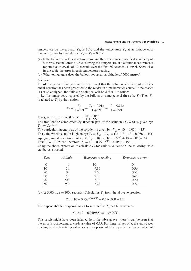
Measurement and Instrumentation Principles 27
temperature on the ground, T0, is 10°C and the temperature Tx at an altitude of xmetres is given by the relation: Tx D T0 � 0.01x
(a) If the balloon is released at time zero, and thereafter rises upwards at a velocity of5 metres/second, draw a table showing the temperature and altitude measurementsreported at intervals of 10 seconds over the first 50 seconds of travel. Show alsoin the table the error in each temperature reading.
(b) What temperature does the balloon report at an altitude of 5000 metres?
SolutionIn order to answer this question, it is assumed that the solution of a first order differ-ential equation has been presented to the reader in a mathematics course. If the readeris not so equipped, the following solution will be difficult to follow.
Let the temperature reported by the balloon at some general time t be Tr. Then Tx
is related to Tr by the relation:
Tr D Tx
1 C �DD T0 � 0.01x
1 C �DD 10 � 0.01x
1 C 15D
It is given that x D 5t, thus: Tr D 10 � 0.05t1 C 15D
The transient or complementary function part of the solution (Tx D 0) is given by:Trcf D Ce�t/15
The particular integral part of the solution is given by: Trpi D 10 � 0.05�t � 15�Thus, the whole solution is given by: Tr D Trcf C Trpi D Ce�t/15 C 10 � 0.05�t � 15�Applying initial conditions: At t D 0, Tr D 10, i.e. 10 D Ce�0 C 10 � 0.05��15�Thus C D �0.75 and therefore: Tr D 10 � 0.75e�t/15 � 0.05�t � 15�Using the above expression to calculate Tr for various values of t, the following tablecan be constructed:
Time Altitude Temperature reading Temperature error
0 0 10 010 50 9.86 0.3620 100 9.55 0.5530 150 9.15 0.6540 200 8.70 0.7050 250 8.22 0.72
(b) At 5000 m, t D 1000 seconds. Calculating Tr from the above expression:
Tr D 10 � 0.75e�1000/15 � 0.05�1000 � 15�
The exponential term approximates to zero and so Tr can be written as:
Tr ³ 10 � 0.05�985� D �39.25°C
This result might have been inferred from the table above where it can be seen thatthe error is converging towards a value of 0.75. For large values of t, the transducerreading lags the true temperature value by a period of time equal to the time constant of
28 Instrument types and performance characteristics
15 seconds. In this time, the balloon travels a distance of 75 metres and the temperaturefalls by 0.75°. Thus for large values of t, the output reading is always 0.75° less thanit should be.
2.3.3 Second order instrument
If all coefficients a3 . . . an other than a0, a1 and a2 in equation (2.2) are assumed zero,then we get:
a2d2q0
dt2 C a1dq0
dtC a0q0 D b0qi �2.7�
Applying the D operator again: a2D2q0 C a1Dq0 C a0q0 D b0qi, and rearranging:
q0 D b0qi
a0 C a1D C a2D2 �2.8�
It is convenient to re-express the variables a0, a1, a2 and b0 in equation (2.8) in terms ofthree parameters K (static sensitivity), ω (undamped natural frequency) and � (dampingratio), where:
K D b0/a0; ω D a0/a2; � D a1/2a0a2
Re-expressing equation (2.8) in terms of K, ω and � we get:
q0
qiD K
D2/ω2 C 2�D/ω C 1�2.9�
This is the standard equation for a second order system and any instrument whoseresponse can be described by it is known as a second order instrument. If equation (2.9)is solved analytically, the shape of the step response obtained depends on the valueof the damping ratio parameter �. The output responses of a second order instrumentfor various values of � following a step change in the value of the measured quantityat time t are shown in Figure 2.12. For case (A) where � D 0, there is no dampingand the instrument output exhibits constant amplitude oscillations when disturbed byany change in the physical quantity measured. For light damping of � D 0.2, repre-sented by case (B), the response to a step change in input is still oscillatory but theoscillations gradually die down. Further increase in the value of � reduces oscillationsand overshoot still more, as shown by curves (C) and (D), and finally the responsebecomes very overdamped as shown by curve (E) where the output reading creepsup slowly towards the correct reading. Clearly, the extreme response curves (A) and(E) are grossly unsuitable for any measuring instrument. If an instrument were to beonly ever subjected to step inputs, then the design strategy would be to aim towards adamping ratio of 0.707, which gives the critically damped response (C). Unfortunately,most of the physical quantities that instruments are required to measure do not changein the mathematically convenient form of steps, but rather in the form of ramps ofvarying slopes. As the form of the input variable changes, so the best value for �varies, and choice of � becomes one of compromise between those values that arebest for each type of input variable behaviour anticipated. Commercial second orderinstruments, of which the accelerometer is a common example, are generally designedto have a damping ratio (�) somewhere in the range of 0.6–0.8.
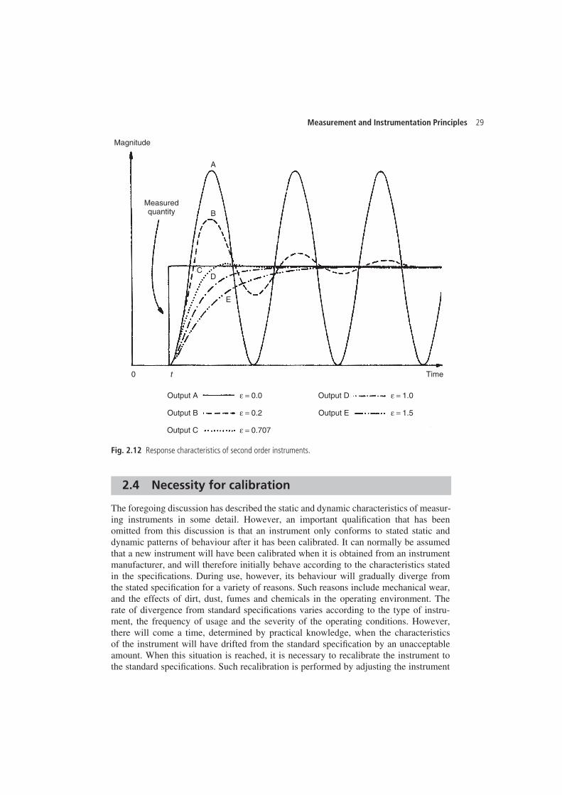
Measurement and Instrumentation Principles 29
Magnitude
Measuredquantity
A
B
CD
E
0 t
Output A ε = 0.0
ε = 0.2
ε = 0.707
Output B
Output D ε = 1.0
ε = 1.5Output E
Output C
Time
Fig. 2.12 Response characteristics of second order instruments.
2.4 Necessity for calibration
The foregoing discussion has described the static and dynamic characteristics of measur-ing instruments in some detail. However, an important qualification that has beenomitted from this discussion is that an instrument only conforms to stated static anddynamic patterns of behaviour after it has been calibrated. It can normally be assumedthat a new instrument will have been calibrated when it is obtained from an instrumentmanufacturer, and will therefore initially behave according to the characteristics statedin the specifications. During use, however, its behaviour will gradually diverge fromthe stated specification for a variety of reasons. Such reasons include mechanical wear,and the effects of dirt, dust, fumes and chemicals in the operating environment. Therate of divergence from standard specifications varies according to the type of instru-ment, the frequency of usage and the severity of the operating conditions. However,there will come a time, determined by practical knowledge, when the characteristicsof the instrument will have drifted from the standard specification by an unacceptableamount. When this situation is reached, it is necessary to recalibrate the instrument tothe standard specifications. Such recalibration is performed by adjusting the instrument
30 Instrument types and performance characteristics
at each point in its output range until its output readings are the same as those of asecond standard instrument to which the same inputs are applied. This second instru-ment is one kept solely for calibration purposes whose specifications are accuratelyknown. Calibration procedures are discussed more fully in Chapter 4.
2.5 Self-test questions
2.1 Explain what is meant by:(a) active instruments(b) passive instruments.Give examples of each and discuss the relative merits of these two classes ofinstruments.
2.2 Discuss the advantages and disadvantages of null and deflection types ofmeasuring instrument. What are null types of instrument mainly used for andwhy?
2.3 Briefly define and explain all the static characteristics of measuring instruments.2.4 Explain the difference between accuracy and precision in an instrument.2.5 A tungsten/5% rhenium–tungsten/26% rhenium thermocouple has an output
e.m.f. as shown in the following table when its hot (measuring) junction isat the temperatures shown. Determine the sensitivity of measurement for thethermocouple in mV/°C.
mV 4.37 8.74 13.11 17.48°C 250 500 750 1000
2.6 Define sensitivity drift and zero drift. What factors can cause sensitivity drift andzero drift in instrument characteristics?
2.7 (a) An instrument is calibrated in an environment at a temperature of 20°C andthe following output readings y are obtained for various input values x:
y 13.1 26.2 39.3 52.4 65.5 78.6x 5 10 15 20 25 30
Determine the measurement sensitivity, expressed as the ratio y/x.(b) When the instrument is subsequently used in an environment at a temperature
of 50°C, the input/output characteristic changes to the following:
y 14.7 29.4 44.1 58.8 73.5 88.2x 5 10 15 20 25 30
Determine the new measurement sensitivity. Hence determine the sensitivitydrift due to the change in ambient temperature of 30°C.
Measurement and Instrumentation Principles 31
2.8 A load cell is calibrated in an environment at a temperature of 21°C and has thefollowing deflection/load characteristic:
Load (kg) 0 50 100 150 200Deflection (mm) 0.0 1.0 2.0 3.0 4.0
When used in an environment at 35°C, its characteristic changes to the following:
Load (kg) 0 50 100 150 200Deflection (mm) 0.2 1.3 2.4 3.5 4.6
(a) Determine the sensitivity at 21°C and 35°C.(b) Calculate the total zero drift and sensitivity drift at 35°C.(c) Hence determine the zero drift and sensitivity drift coefficients (in units of
μm/°C and (μm per kg)/(°C)).2.9 An unmanned submarine is equipped with temperature and depth measuring
instruments and has radio equipment that can transmit the output readings ofthese instruments back to the surface. The submarine is initially floating on thesurface of the sea with the instrument output readings in steady state. The depth-measuring instrument is approximately zero order and the temperature transducerfirst order with a time constant of 50 seconds. The water temperature on the seasurface, T0, is 20°C and the temperature Tx at a depth of x metres is given bythe relation:
Tx D T0 � 0.01x
(a) If the submarine starts diving at time zero, and thereafter goes down at avelocity of 0.5 metres/second, draw a table showing the temperature anddepth measurements reported at intervals of 100 seconds over the first 500seconds of travel. Show also in the table the error in each temperature reading.
(b) What temperature does the submarine report at a depth of 1000 metres?2.10 Write down the general differential equation describing the dynamic response of
a second order measuring instrument and state the expressions relating the staticsensitivity, undamped natural frequency and damping ratio to the parameters inthis differential equation. Sketch the instrument response for the cases of heavydamping, critical damping and light damping, and state which of these is theusual target when a second order instrument is being designed.
3
Errors during themeasurement process
3.1 Introduction
Errors in measurement systems can be divided into those that arise during the measure-ment process and those that arise due to later corruption of the measurement signalby induced noise during transfer of the signal from the point of measurement to someother point. This chapter considers only the first of these, with discussion on inducednoise being deferred to Chapter 5.
It is extremely important in any measurement system to reduce errors to the minimumpossible level and then to quantify the maximum remaining error that may exist in anyinstrument output reading. However, in many cases, there is a further complicationthat the final output from a measurement system is calculated by combining togethertwo or more measurements of separate physical variables. In this case, special consid-eration must also be given to determining how the calculated error levels in eachseparate measurement should be combined together to give the best estimate of themost likely error magnitude in the calculated output quantity. This subject is consideredin section 3.6.
The starting point in the quest to reduce the incidence of errors arising during themeasurement process is to carry out a detailed analysis of all error sources in thesystem. Each of these error sources can then be considered in turn, looking for waysof eliminating or at least reducing the magnitude of errors. Errors arising during themeasurement process can be divided into two groups, known as systematic errors andrandom errors.
Systematic errors describe errors in the output readings of a measurement system thatare consistently on one side of the correct reading, i.e. either all the errors are positiveor they are all negative. Two major sources of systematic errors are system disturbanceduring measurement and the effect of environmental changes (modifying inputs), asdiscussed in sections 3.2.1 and 3.2.2. Other sources of systematic error include bentmeter needles, the use of uncalibrated instruments, drift in instrument characteristicsand poor cabling practices. Even when systematic errors due to the above factors havebeen reduced or eliminated, some errors remain that are inherent in the manufactureof an instrument. These are quantified by the accuracy figure quoted in the publishedspecifications contained in the instrument data sheet.
Measurement and Instrumentation Principles 33
Random errors are perturbations of the measurement either side of the true valuecaused by random and unpredictable effects, such that positive errors and negativeerrors occur in approximately equal numbers for a series of measurements made ofthe same quantity. Such perturbations are mainly small, but large perturbations occurfrom time to time, again unpredictably. Random errors often arise when measure-ments are taken by human observation of an analogue meter, especially where thisinvolves interpolation between scale points. Electrical noise can also be a source ofrandom errors. To a large extent, random errors can be overcome by taking the samemeasurement a number of times and extracting a value by averaging or other statisticaltechniques, as discussed in section 3.5. However, any quantification of the measure-ment value and statement of error bounds remains a statistical quantity. Because ofthe nature of random errors and the fact that large perturbations in the measured quan-tity occur from time to time, the best that we can do is to express measurementsin probabilistic terms: we may be able to assign a 95% or even 99% confidencelevel that the measurement is a certain value within error bounds of, say, š1%, butwe can never attach a 100% probability to measurement values that are subject torandom errors.
Finally, a word must be said about the distinction between systematic and randomerrors. Error sources in the measurement system must be examined carefully to deter-mine what type of error is present, systematic or random, and to apply the appropriatetreatment. In the case of manual data measurements, a human observer may makea different observation at each attempt, but it is often reasonable to assume that theerrors are random and that the mean of these readings is likely to be close to thecorrect value. However, this is only true as long as the human observer is not intro-ducing a parallax-induced systematic error as well by persistently reading the positionof a needle against the scale of an analogue meter from one side rather than fromdirectly above. In that case, correction would have to be made for this systematic error(bias) in the measurements before statistical techniques were applied to reduce theeffect of random errors.
3.2 Sources of systematic error
Systematic errors in the output of many instruments are due to factors inherent inthe manufacture of the instrument arising out of tolerances in the components of theinstrument. They can also arise due to wear in instrument components over a periodof time. In other cases, systematic errors are introduced either by the effect of envi-ronmental disturbances or through the disturbance of the measured system by the actof measurement. These various sources of systematic error, and ways in which themagnitude of the errors can be reduced, are discussed below.
3.2.1 System disturbance due to measurement
Disturbance of the measured system by the act of measurement is a common sourceof systematic error. If we were to start with a beaker of hot water and wished tomeasure its temperature with a mercury-in-glass thermometer, then we would take the
34 Errors during the measurement process
thermometer, which would initially be at room temperature, and plunge it into thewater. In so doing, we would be introducing a relatively cold mass (the thermometer)into the hot water and a heat transfer would take place between the water and thethermometer. This heat transfer would lower the temperature of the water. Whilstthe reduction in temperature in this case would be so small as to be undetectableby the limited measurement resolution of such a thermometer, the effect is finite andclearly establishes the principle that, in nearly all measurement situations, the processof measurement disturbs the system and alters the values of the physical quantitiesbeing measured.
A particularly important example of this occurs with the orifice plate. This is placedinto a fluid-carrying pipe to measure the flow rate, which is a function of the pressurethat is measured either side of the orifice plate. This measurement procedure causes apermanent pressure loss in the flowing fluid. The disturbance of the measured systemcan often be very significant.
Thus, as a general rule, the process of measurement always disturbs the system beingmeasured. The magnitude of the disturbance varies from one measurement system tothe next and is affected particularly by the type of instrument used for measurement.Ways of minimizing disturbance of measured systems is an important consideration ininstrument design. However, an accurate understanding of the mechanisms of systemdisturbance is a prerequisite for this.
Measurements in electric circuitsIn analysing system disturbance during measurements in electric circuits, Thevenin’stheorem (see Appendix 3) is often of great assistance. For instance, consider the circuitshown in Figure 3.1(a) in which the voltage across resistor R5 is to be measured by avoltmeter with resistance Rm. Here, Rm acts as a shunt resistance across R5, decreasingthe resistance between points AB and so disturbing the circuit. Therefore, the voltageEm measured by the meter is not the value of the voltage E0 that existed prior tomeasurement. The extent of the disturbance can be assessed by calculating the open-circuit voltage E0 and comparing it with Em.
Thevenin’s theorem allows the circuit of Figure 3.1(a) comprising two voltagesources and five resistors to be replaced by an equivalent circuit containing a singleresistance and one voltage source, as shown in Figure 3.1(b). For the purpose ofdefining the equivalent single resistance of a circuit by Thevenin’s theorem, all voltagesources are represented just by their internal resistance, which can be approximatedto zero, as shown in Figure 3.1(c). Analysis proceeds by calculating the equivalentresistances of sections of the circuit and building these up until the required equivalentresistance of the whole of the circuit is obtained. Starting at C and D, the circuit tothe left of C and D consists of a series pair of resistances (R1 and R2) in parallel withR3, and the equivalent resistance can be written as:
1
RCDD 1
R1 C R2C 1
R3or RCD D �R1 C R2�R3
R1 C R2 C R3
Moving now to A and B, the circuit to the left consists of a pair of series resistances(RCD and R4) in parallel with R5. The equivalent circuit resistance RAB can thus be
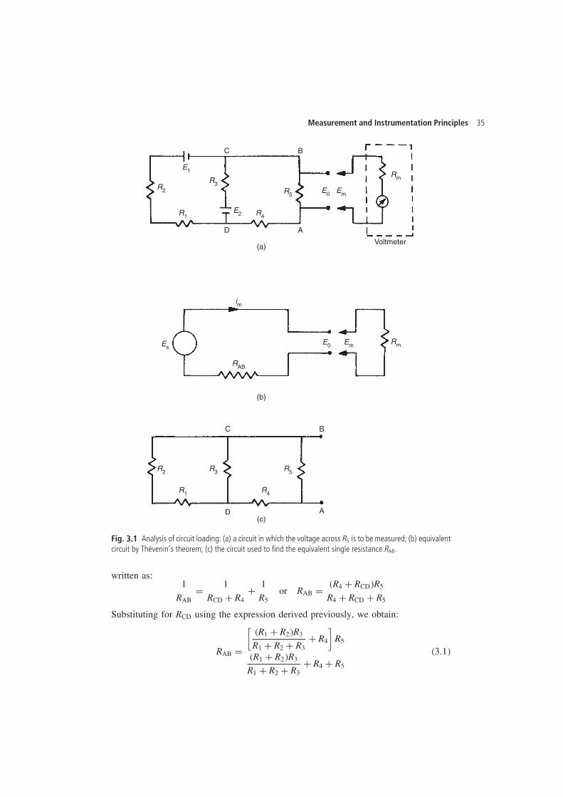
Measurement and Instrumentation Principles 35
R2
R2
R3
R3
R5
R5
Rm
Rm
EmE0
EmE0
R4
R4
R1
R1
RAB
E1
Es
im
E2
C B
A
C
D
D
B
A
Voltmeter(a)
(b)
(c)
Fig. 3.1 Analysis of circuit loading: (a) a circuit in which the voltage across R5 is to be measured; (b) equivalentcircuit by Thevenin’s theorem; (c) the circuit used to find the equivalent single resistance RAB.
written as:1
RABD 1
RCD C R4C 1
R5or RAB D �R4 C RCD�R5
R4 C RCD C R5
Substituting for RCD using the expression derived previously, we obtain:
RAB D
[�R1 C R2�R3
R1 C R2 C R3C R4
]R5
�R1 C R2�R3
R1 C R2 C R3C R4 C R5
�3.1�
36 Errors during the measurement process
Defining I as the current flowing in the circuit when the measuring instrument isconnected to it, we can write:
I D E0
RAB C Rm,
and the voltage measured by the meter is then given by:
Em D RmE0
RAB C Rm.
In the absence of the measuring instrument and its resistance Rm, the voltage acrossAB would be the equivalent circuit voltage source whose value is E0. The effect ofmeasurement is therefore to reduce the voltage across AB by the ratio given by:
Em
E0D Rm
RAB C Rm�3.2�
It is thus obvious that as Rm gets larger, the ratio Em/E0 gets closer to unity,showing that the design strategy should be to make Rm as high as possible to minimizedisturbance of the measured system. (Note that we did not calculate the value of E0,since this is not required in quantifying the effect of Rm.)
Example 3.1Suppose that the components of the circuit shown in Figure 3.1(a) have the followingvalues:
R1 D 400 �; R2 D 600 �; R3 D 1000 �, R4 D 500 �; R5 D 1000 �
The voltage across AB is measured by a voltmeter whose internal resistance is 9500 �.What is the measurement error caused by the resistance of the measuring instrument?
SolutionProceeding by applying Thevenin’s theorem to find an equivalent circuit to that ofFigure 3.1(a) of the form shown in Figure 3.1(b), and substituting the given componentvalues into the equation for RAB (3.1), we obtain:
RAB D [�10002/2000� C 500]1000
�10002/2000� C 500 C 1000D 10002
2000D 500 �
From equation (3.2), we have:Em
E0D Rm
RAB C Rm
The measurement error is given by �E0 � Em�:
E0 � Em D E0
(1 � Rm
RAB C Rm
)
Substituting in values:
E0 � Em D E0
(1 � 9500
10 000
)D 0.95E0
Thus, the error in the measured value is 5%.
Measurement and Instrumentation Principles 37
At this point, it is interesting to note the constraints that exist when practical attemptsare made to achieve a high internal resistance in the design of a moving-coil voltmeter.Such an instrument consists of a coil carrying a pointer mounted in a fixed magneticfield. As current flows through the coil, the interaction between the field generatedand the fixed field causes the pointer it carries to turn in proportion to the appliedcurrent (see Chapter 6 for further details). The simplest way of increasing the inputimpedance (the resistance) of the meter is either to increase the number of turns in thecoil or to construct the same number of coil turns with a higher-resistance material.However, either of these solutions decreases the current flowing in the coil, giving lessmagnetic torque and thus decreasing the measurement sensitivity of the instrument (i.e.for a given applied voltage, we get less deflection of the pointer). This problem can beovercome by changing the spring constant of the restraining springs of the instrument,such that less torque is required to turn the pointer by a given amount. However, thisreduces the ruggedness of the instrument and also demands better pivot design to reducefriction. This highlights a very important but tiresome principle in instrument design:any attempt to improve the performance of an instrument in one respect generallydecreases the performance in some other aspect. This is an inescapable fact of lifewith passive instruments such as the type of voltmeter mentioned, and is often thereason for the use of alternative active instruments such as digital voltmeters, wherethe inclusion of auxiliary power greatly improves performance.
Bridge circuits for measuring resistance values are a further example of the need forcareful design of the measurement system. The impedance of the instrument measuringthe bridge output voltage must be very large in comparison with the component resist-ances in the bridge circuit. Otherwise, the measuring instrument will load the circuitand draw current from it. This is discussed more fully in Chapter 7.
3.2.2 Errors due to environmental inputs
An environmental input is defined as an apparently real input to a measurement systemthat is actually caused by a change in the environmental conditions surrounding themeasurement system. The fact that the static and dynamic characteristics specifiedfor measuring instruments are only valid for particular environmental conditions (e.g.of temperature and pressure) has already been discussed at considerable length inChapter 2. These specified conditions must be reproduced as closely as possible duringcalibration exercises because, away from the specified calibration conditions, the char-acteristics of measuring instruments vary to some extent and cause measurement errors.The magnitude of this environment-induced variation is quantified by the two constantsknown as sensitivity drift and zero drift, both of which are generally included in thepublished specifications for an instrument. Such variations of environmental conditionsaway from the calibration conditions are sometimes described as modifying inputs tothe measurement system because they modify the output of the system. When suchmodifying inputs are present, it is often difficult to determine how much of the outputchange in a measurement system is due to a change in the measured variable andhow much is due to a change in environmental conditions. This is illustrated by thefollowing example. Suppose we are given a small closed box and told that it maycontain either a mouse or a rat. We are also told that the box weighs 0.1 kg when
38 Errors during the measurement process
empty. If we put the box onto bathroom scales and observe a reading of 1.0 kg, thisdoes not immediately tell us what is in the box because the reading may be due to oneof three things:
(a) a 0.9 kg rat in the box (real input)(b) an empty box with a 0.9 kg bias on the scales due to a temperature change (envi-
ronmental input)(c) a 0.4 kg mouse in the box together with a 0.5 kg bias (real + environmental inputs).
Thus, the magnitude of any environmental input must be measured before the valueof the measured quantity (the real input) can be determined from the output readingof an instrument.
In any general measurement situation, it is very difficult to avoid environmentalinputs, because it is either impractical or impossible to control the environmental condi-tions surrounding the measurement system. System designers are therefore charged withthe task of either reducing the susceptibility of measuring instruments to environmentalinputs or, alternatively, quantifying the effect of environmental inputs and correctingfor them in the instrument output reading. The techniques used to deal with envi-ronmental inputs and minimize their effect on the final output measurement follow anumber of routes as discussed below.
3.2.3 Wear in instrument components
Systematic errors can frequently develop over a period of time because of wear ininstrument components. Recalibration often provides a full solution to this problem.
3.2.4 Connecting leads
In connecting together the components of a measurement system, a common sourceof error is the failure to take proper account of the resistance of connecting leads (orpipes in the case of pneumatically or hydraulically actuated measurement systems). Forinstance, in typical applications of a resistance thermometer, it is common to find thatthe thermometer is separated from other parts of the measurement system by perhaps100 metres. The resistance of such a length of 20 gauge copper wire is 7 �, and thereis a further complication that such wire has a temperature coefficient of 1 m�/°C.
Therefore, careful consideration needs to be given to the choice of connecting leads.Not only should they be of adequate cross-section so that their resistance is minimized,but they should be adequately screened if they are thought likely to be subject toelectrical or magnetic fields that could otherwise cause induced noise. Where screeningis thought essential, then the routing of cables also needs careful planning. In oneapplication in the author’s personal experience involving instrumentation of an electric-arc steel making furnace, screened signal-carrying cables between transducers on thearc furnace and a control room at the side of the furnace were initially corrupted byhigh amplitude 50 Hz noise. However, by changing the route of the cables between thetransducers and the control room, the magnitude of this induced noise was reduced bya factor of about ten.
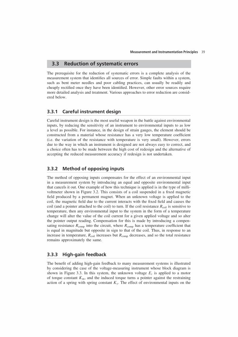
Measurement and Instrumentation Principles 39
3.3 Reduction of systematic errors
The prerequisite for the reduction of systematic errors is a complete analysis of themeasurement system that identifies all sources of error. Simple faults within a system,such as bent meter needles and poor cabling practices, can usually be readily andcheaply rectified once they have been identified. However, other error sources requiremore detailed analysis and treatment. Various approaches to error reduction are consid-ered below.
3.3.1 Careful instrument design
Careful instrument design is the most useful weapon in the battle against environmentalinputs, by reducing the sensitivity of an instrument to environmental inputs to as lowa level as possible. For instance, in the design of strain gauges, the element should beconstructed from a material whose resistance has a very low temperature coefficient(i.e. the variation of the resistance with temperature is very small). However, errorsdue to the way in which an instrument is designed are not always easy to correct, anda choice often has to be made between the high cost of redesign and the alternative ofaccepting the reduced measurement accuracy if redesign is not undertaken.
3.3.2 Method of opposing inputs
The method of opposing inputs compensates for the effect of an environmental inputin a measurement system by introducing an equal and opposite environmental inputthat cancels it out. One example of how this technique is applied is in the type of milli-voltmeter shown in Figure 3.2. This consists of a coil suspended in a fixed magneticfield produced by a permanent magnet. When an unknown voltage is applied to thecoil, the magnetic field due to the current interacts with the fixed field and causes thecoil (and a pointer attached to the coil) to turn. If the coil resistance Rcoil is sensitive totemperature, then any environmental input to the system in the form of a temperaturechange will alter the value of the coil current for a given applied voltage and so alterthe pointer output reading. Compensation for this is made by introducing a compen-sating resistance Rcomp into the circuit, where Rcomp has a temperature coefficient thatis equal in magnitude but opposite in sign to that of the coil. Thus, in response to anincrease in temperature, Rcoil increases but Rcomp decreases, and so the total resistanceremains approximately the same.
3.3.3 High-gain feedback
The benefit of adding high-gain feedback to many measurement systems is illustratedby considering the case of the voltage-measuring instrument whose block diagram isshown in Figure 3.3. In this system, the unknown voltage Ei is applied to a motorof torque constant Km, and the induced torque turns a pointer against the restrainingaction of a spring with spring constant Ks. The effect of environmental inputs on the
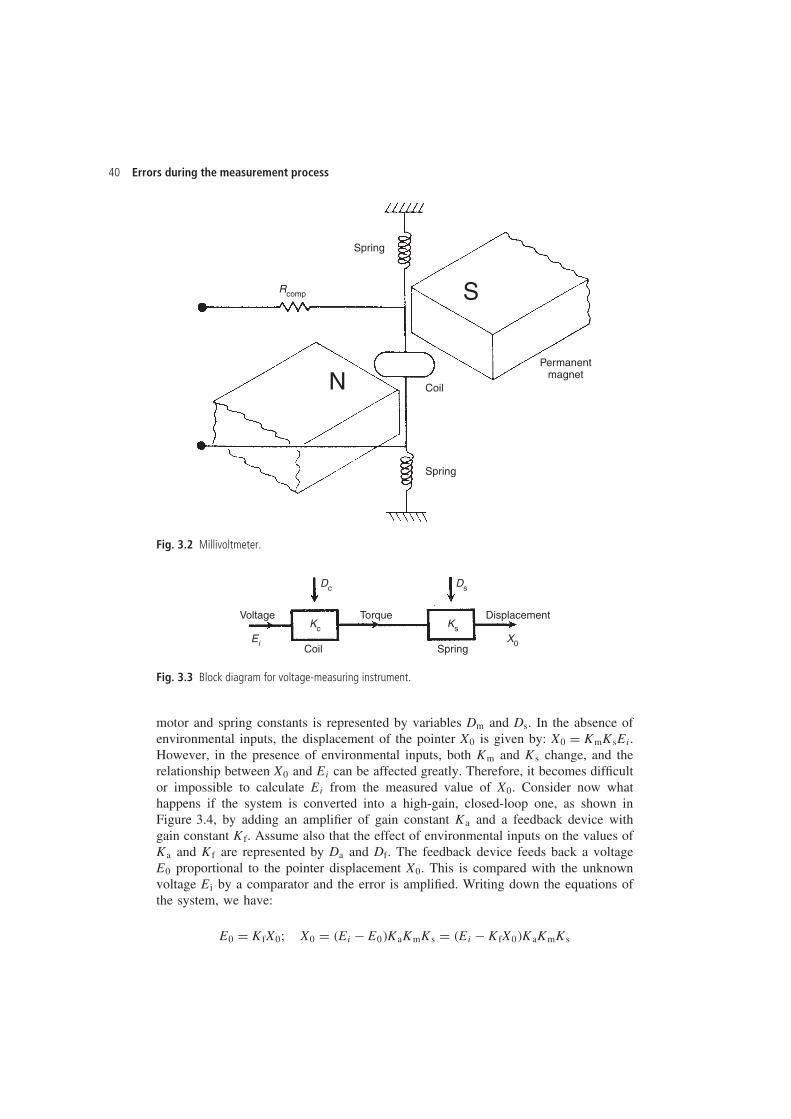
40 Errors during the measurement process
Rcomp
Spring
Spring
CoilN
S
Permanentmagnet
Fig. 3.2 Millivoltmeter.
Voltage Torque
Coil Spring
Displacement
Ei X0
Kc Ks
Dc Ds
Fig. 3.3 Block diagram for voltage-measuring instrument.
motor and spring constants is represented by variables Dm and Ds. In the absence ofenvironmental inputs, the displacement of the pointer X0 is given by: X0 D KmKsEi.However, in the presence of environmental inputs, both Km and Ks change, and therelationship between X0 and Ei can be affected greatly. Therefore, it becomes difficultor impossible to calculate Ei from the measured value of X0. Consider now whathappens if the system is converted into a high-gain, closed-loop one, as shown inFigure 3.4, by adding an amplifier of gain constant Ka and a feedback device withgain constant Kf. Assume also that the effect of environmental inputs on the values ofKa and Kf are represented by Da and Df. The feedback device feeds back a voltageE0 proportional to the pointer displacement X0. This is compared with the unknownvoltage Ei by a comparator and the error is amplified. Writing down the equations ofthe system, we have:
E0 D KfX0; X0 D �Ei � E0�KaKmKs D �Ei � KfX0�KaKmKs
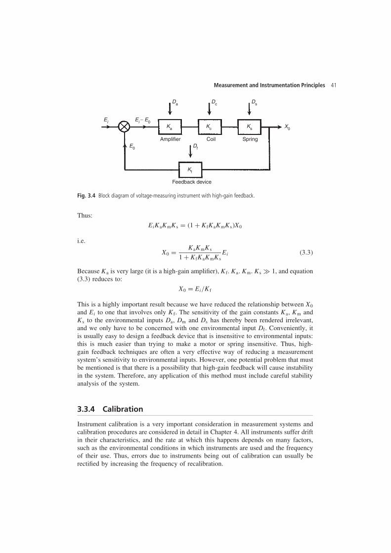
Measurement and Instrumentation Principles 41
Amplifier Coil Spring
Feedback device
Ei Ei − E0X0Ka Kc Ks
Kf
Da Dc Ds
DfE0
Fig. 3.4 Block diagram of voltage-measuring instrument with high-gain feedback.
Thus:
EiKaKmKs D �1 C KfKaKmKs�X0
i.e.
X0 D KaKmKs
1 C KfKaKmKsEi �3.3�
Because Ka is very large (it is a high-gain amplifier), Kf. Ka. Km. Ks × 1, and equation(3.3) reduces to:
X0 D Ei/Kf
This is a highly important result because we have reduced the relationship between X0
and Ei to one that involves only Kf. The sensitivity of the gain constants Ka, Km andKs to the environmental inputs Da, Dm and Ds has thereby been rendered irrelevant,and we only have to be concerned with one environmental input Df. Conveniently, itis usually easy to design a feedback device that is insensitive to environmental inputs:this is much easier than trying to make a motor or spring insensitive. Thus, high-gain feedback techniques are often a very effective way of reducing a measurementsystem’s sensitivity to environmental inputs. However, one potential problem that mustbe mentioned is that there is a possibility that high-gain feedback will cause instabilityin the system. Therefore, any application of this method must include careful stabilityanalysis of the system.
3.3.4 Calibration
Instrument calibration is a very important consideration in measurement systems andcalibration procedures are considered in detail in Chapter 4. All instruments suffer driftin their characteristics, and the rate at which this happens depends on many factors,such as the environmental conditions in which instruments are used and the frequencyof their use. Thus, errors due to instruments being out of calibration can usually berectified by increasing the frequency of recalibration.
42 Errors during the measurement process
3.3.5 Manual correction of output reading
In the case of errors that are due either to system disturbance during the act of measure-ment or due to environmental changes, a good measurement technician can substantiallyreduce errors at the output of a measurement system by calculating the effect of suchsystematic errors and making appropriate correction to the instrument readings. This isnot necessarily an easy task, and requires all disturbances in the measurement systemto be quantified. This procedure is carried out automatically by intelligent instruments.
3.3.6 Intelligent instruments
Intelligent instruments contain extra sensors that measure the value of environmentalinputs and automatically compensate the value of the output reading. They have theability to deal very effectively with systematic errors in measurement systems, anderrors can be attenuated to very low levels in many cases. A more detailed analysis ofintelligent instruments can be found in Chapter 9.
3.4 Quantification of systematic errors
Once all practical steps have been taken to eliminate or reduce the magnitude of system-atic errors, the final action required is to estimate the maximum remaining error thatmay exist in a measurement due to systematic errors. Unfortunately, it is not alwayspossible to quantify exact values of a systematic error, particularly if measurementsare subject to unpredictable environmental conditions. The usual course of action isto assume mid-point environmental conditions and specify the maximum measurementerror as šx% of the output reading to allow for the maximum expected deviation inenvironmental conditions away from this mid-point. Data sheets supplied by instru-ment manufacturers usually quantify systematic errors in this way, and such figurestake account of all systematic errors that may be present in output readings from theinstrument.
3.5 Random errors
Random errors in measurements are caused by unpredictable variations in the measure-ment system. They are usually observed as small perturbations of the measurementeither side of the correct value, i.e. positive errors and negative errors occur in approx-imately equal numbers for a series of measurements made of the same constant quantity.Therefore, random errors can largely be eliminated by calculating the average ofa number of repeated measurements, provided that the measured quantity remainsconstant during the process of taking the repeated measurements. This averagingprocess of repeated measurements can be done automatically by intelligent instruments,as discussed in Chapter 9. The degree of confidence in the calculated mean/medianvalues can be quantified by calculating the standard deviation or variance of the data,
Measurement and Instrumentation Principles 43
these being parameters that describe how the measurements are distributed about themean value/median. All of these terms are explained more fully in section 3.5.1.
3.5.1 Statistical analysis of measurements subject to randomerrors
Mean and median valuesThe average value of a set of measurements of a constant quantity can be expressedas either the mean value or the median value. As the number of measurementsincreases, the difference between the mean value and median values becomes verysmall. However, for any set of n measurements x1, x2 Ð Ð Ð xn of a constant quantity, themost likely true value is the mean given by:
xmean D x1 C x2 C Ð Ð Ð xn
n�3.4�
This is valid for all data sets where the measurement errors are distributed equallyabout the zero error value, i.e. where the positive errors are balanced in quantity andmagnitude by the negative errors.
The median is an approximation to the mean that can be written down without havingto sum the measurements. The median is the middle value when the measurementsin the data set are written down in ascending order of magnitude. For a set of nmeasurements x1, x2 Ð Ð Ð xn of a constant quantity, written down in ascending order ofmagnitude, the median value is given by:
xmedian D xnC1/2 �3.5�
Thus, for a set of 9 measurements x1, x2 Ð Ð Ð x9 arranged in order of magnitude, themedian value is x5. For an even number of measurements, the median value is mid-way between the two centre values, i.e. for 10 measurements x1 Ð Ð Ð x10, the medianvalue is given by: �x5 C x6�/2.
Suppose that the length of a steel bar is measured by a number of different observersand the following set of 11 measurements are recorded (units mm). We will call thismeasurement set A.
398 420 394 416 404 408 400 420 396 413 430 �Measurement set A�
Using (3.4) and (3.5), mean D 409.0 and median D 408. Suppose now that the measure-ments are taken again using a better measuring rule, and with the observers taking morecare, to produce the following measurement set B:
409 406 402 407 405 404 407 404 407 407 408 �Measurement set B�
For these measurements, mean D 406.0 and median D 407. Which of the two measure-ment sets A and B, and the corresponding mean and median values, should we havemost confidence in? Intuitively, we can regard measurement set B as being more reli-able since the measurements are much closer together. In set A, the spread betweenthe smallest (396) and largest (430) value is 34, whilst in set B, the spread is only 6.
44 Errors during the measurement process
ž Thus, the smaller the spread of the measurements, the more confidence we have inthe mean or median value calculated.
Let us now see what happens if we increase the number of measurements by extendingmeasurement set B to 23 measurements. We will call this measurement set C.
409 406 402 407 405 404 407 404 407 407 408 406 410 406 405 408
406 409 406 405 409 406 407 �Measurement set C�
Now, mean D 406.5 and median D 406.
ž This confirms our earlier statement that the median value tends towards the meanvalue as the number of measurements increases.
Standard deviation and varianceExpressing the spread of measurements simply as the range between the largest andsmallest value is not in fact a very good way of examining how the measurementvalues are distributed about the mean value. A much better way of expressing thedistribution is to calculate the variance or standard deviation of the measurements. Thestarting point for calculating these parameters is to calculate the deviation (error) di ofeach measurement xi from the mean value xmean:
di D xi � xmean �3.6�
The variance (V) is then given by:Ł
V D d21 C d2
2 Ð Ð Ð d2n
n � 1�3.7�
The standard deviation ��� is simply the square root of the variance. ThusŁ:
� D pV D
√d2
1 C d22 Ð Ð Ð d2
n
n � 1�3.8�
Example 3.2Calculate � and V for measurement sets A, B and C above.
Ł Mathematically minded readers may have observed that the expressions for V and � differ from theformal mathematical definitions, which have �n� instead of �n � 1� in the denominator. This differencearises because the mathematical definition is for an infinite data set, whereas, in the case of measurements,we are concerned only with finite data sets. For a finite set of measurements �xi� i D 1, n, the mean xmwill differ from the true mean μ of the infinite data set that the finite set is part of. If somehow we knewthe true mean μ of a set of measurements, then the deviations di could be calculated as the deviation ofeach data value from the true mean and it would then be correct to calculate V and � using �n� insteadof �n � 1�. However, in normal situations, using �n � 1� in the denominator of equations (3.7) and (3.8)produces a value that is statistically closer to the correct value.
Measurement and Instrumentation Principles 45
SolutionFirst, draw a table of measurements and deviations for set A (mean D 409 as calculatedearlier):
Measurement 398 420 394 416 404 408 400 420 396 413 430Deviation from mean �11 C11 �15 C7 �5 �1 �9 C11 �13 C4 C21(deviations)2 121 121 225 49 25 1 81 121 169 16 441
∑�deviations2� D 1370; n D number of measurements D 11.
Then, from (3.7), V D ∑�deviations2�/n � 1; D 1370/10 D 137; � D p
V D 11.7.The measurements and deviations for set B are (mean D 406 as calculated earlier):
Measurement 409 406 402 407 405 404 407 404 407 407 408Deviation from mean C3 0 �4 C1 �1 �2 C1 �2 C1 C1 C2(deviations)2 9 0 16 1 1 4 1 4 1 1 4
From this data, using (3.7) and (3.8), V D 4.2 and � D 2.05.The measurements and deviations for set C are (mean D 406.5 as calculated earlier):
Measurement 409 406 402 407 405 404 407 404Deviation from mean C2.5 �0.5 �4.5 C0.5 �1.5 �2.5 C0.5 �2.5(deviations)2 6.25 0.25 20.25 0.25 2.25 6.25 0.25 6.25
Measurement 407 407 408 406 410 406 405 408Deviation from mean C0.5 C0.5 C1.5 �0.5 C3.5 �0.5 �1.5 C1.5(deviations)2 0.25 0.25 2.25 0.25 12.25 0.25 2.25 2.25
Measurement 406 409 406 405 409 406 407Deviation from mean �0.5 C2.5 �0.5 �1.5 C2.5 �0.5 C0.5(deviations)2 0.25 6.25 0.25 2.25 6.25 0.25 0.25
From this data, using (3.7) and (3.8), V D 3.53 and � D 1.88.
Note that the smaller values of V and � for measurement set B compared with Acorrespond with the respective size of the spread in the range between maximum andminimum values for the two sets.
ž Thus, as V and � decrease for a measurement set, we are able to express greaterconfidence that the calculated mean or median value is close to the true value, i.e.that the averaging process has reduced the random error value close to zero.
ž Comparing V and � for measurement sets B and C, V and � get smaller as the numberof measurements increases, confirming that confidence in the mean value increasesas the number of measurements increases.
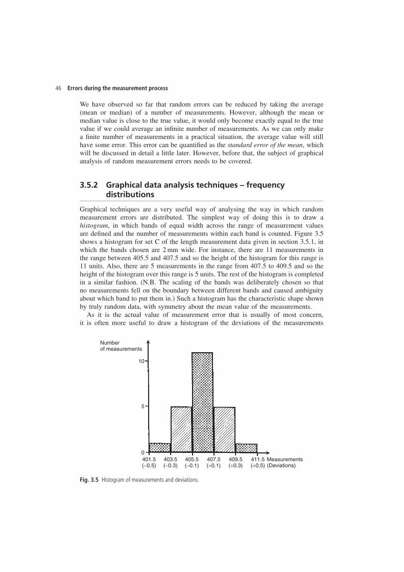
46 Errors during the measurement process
We have observed so far that random errors can be reduced by taking the average(mean or median) of a number of measurements. However, although the mean ormedian value is close to the true value, it would only become exactly equal to the truevalue if we could average an infinite number of measurements. As we can only makea finite number of measurements in a practical situation, the average value will stillhave some error. This error can be quantified as the standard error of the mean, whichwill be discussed in detail a little later. However, before that, the subject of graphicalanalysis of random measurement errors needs to be covered.
3.5.2 Graphical data analysis techniques – frequencydistributions
Graphical techniques are a very useful way of analysing the way in which randommeasurement errors are distributed. The simplest way of doing this is to draw ahistogram, in which bands of equal width across the range of measurement valuesare defined and the number of measurements within each band is counted. Figure 3.5shows a histogram for set C of the length measurement data given in section 3.5.1, inwhich the bands chosen are 2 mm wide. For instance, there are 11 measurements inthe range between 405.5 and 407.5 and so the height of the histogram for this range is11 units. Also, there are 5 measurements in the range from 407.5 to 409.5 and so theheight of the histogram over this range is 5 units. The rest of the histogram is completedin a similar fashion. (N.B. The scaling of the bands was deliberately chosen so thatno measurements fell on the boundary between different bands and caused ambiguityabout which band to put them in.) Such a histogram has the characteristic shape shownby truly random data, with symmetry about the mean value of the measurements.
As it is the actual value of measurement error that is usually of most concern,it is often more useful to draw a histogram of the deviations of the measurements
Numberof measurements
Measurements(Deviations)
10
5
0401.5(−0.5)
403.5(−0.3)
405.5(−0.1)
407.5(+0.1)
409.5(+0.3)
411.5(+0.5)
Fig. 3.5 Histogram of measurements and deviations.
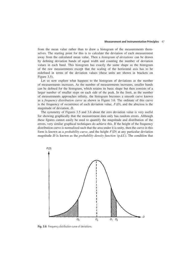
Measurement and Instrumentation Principles 47
from the mean value rather than to draw a histogram of the measurements them-selves. The starting point for this is to calculate the deviation of each measurementaway from the calculated mean value. Then a histogram of deviations can be drawnby defining deviation bands of equal width and counting the number of deviationvalues in each band. This histogram has exactly the same shape as the histogramof the raw measurements except that the scaling of the horizontal axis has to beredefined in terms of the deviation values (these units are shown in brackets onFigure 3.5).
Let us now explore what happens to the histogram of deviations as the numberof measurements increases. As the number of measurements increases, smaller bandscan be defined for the histogram, which retains its basic shape but then consists of alarger number of smaller steps on each side of the peak. In the limit, as the numberof measurements approaches infinity, the histogram becomes a smooth curve knownas a frequency distribution curve as shown in Figure 3.6. The ordinate of this curveis the frequency of occurrence of each deviation value, F�D�, and the abscissa is themagnitude of deviation, D.
The symmetry of Figures 3.5 and 3.6 about the zero deviation value is very usefulfor showing graphically that the measurement data only has random errors. Althoughthese figures cannot easily be used to quantify the magnitude and distribution of theerrors, very similar graphical techniques do achieve this. If the height of the frequencydistribution curve is normalized such that the area under it is unity, then the curve in thisform is known as a probability curve, and the height F�D� at any particular deviationmagnitude D is known as the probability density function (p.d.f.). The condition that
F(D)
DD2D1DpD0
Fig. 3.6 Frequency distribution curve of deviations.
48 Errors during the measurement process
the area under the curve is unity can be expressed mathematically as:∫ 1
�1F�D� dD D 1
The probability that the error in any one particular measurement lies between two levelsD1 and D2 can be calculated by measuring the area under the curve contained betweentwo vertical lines drawn through D1 and D2, as shown by the right-hand hatched areain Figure 3.6. This can be expressed mathematically as:
P�D1 � D � D2� D∫ D2
D1
F�D� dD �3.9�
Of particular importance for assessing the maximum error likely in any one measure-ment is the cumulative distribution function (c.d.f.). This is defined as the probabilityof observing a value less than or equal to D0, and is expressed mathematically as:
P�D � D0� D∫ D0
�1F�D� dD �3.10�
Thus, the c.d.f. is the area under the curve to the left of a vertical line drawn throughD0, as shown by the left-hand hatched area on Figure 3.6.
The deviation magnitude Dp corresponding with the peak of the frequency distri-bution curve (Figure 3.6) is the value of deviation that has the greatest probability. Ifthe errors are entirely random in nature, then the value of Dp will equal zero. Anynon-zero value of Dp indicates systematic errors in the data, in the form of a bias thatis often removable by recalibration.
Gaussian distributionMeasurement sets that only contain random errors usually conform to a distributionwith a particular shape that is called Gaussian, although this conformance must alwaysbe tested (see the later section headed ‘Goodness of fit’). The shape of a Gaussian curveis such that the frequency of small deviations from the mean value is much greater thanthe frequency of large deviations. This coincides with the usual expectation in measure-ments subject to random errors that the number of measurements with a small error ismuch larger than the number of measurements with a large error. Alternative namesfor the Gaussian distribution are the Normal distribution or Bell-shaped distribution.A Gaussian curve is formally defined as a normalized frequency distribution that issymmetrical about the line of zero error and in which the frequency and magnitude ofquantities are related by the expression:
F�x� D 1
�p
2e[��x�m�2/2�2] �3.11�
where m is the mean value of the data set x and the other quantities are as defined before.Equation (3.11) is particularly useful for analysing a Gaussian set of measurements andpredicting how many measurements lie within some particular defined range. If themeasurement deviations D are calculated for all measurements such that D D x � m,then the curve of deviation frequency F�D� plotted against deviation magnitude D is
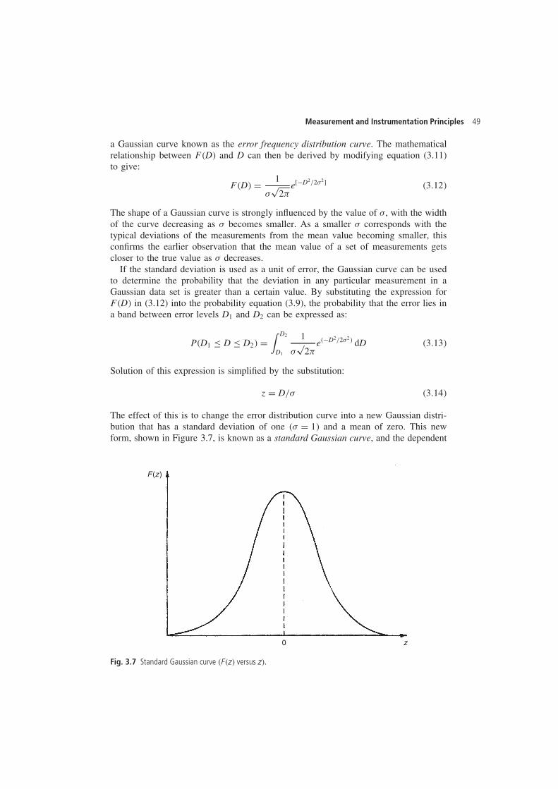
Measurement and Instrumentation Principles 49
a Gaussian curve known as the error frequency distribution curve. The mathematicalrelationship between F�D� and D can then be derived by modifying equation (3.11)to give:
F�D� D 1
�p
2e[�D2/2�2] �3.12�
The shape of a Gaussian curve is strongly influenced by the value of �, with the widthof the curve decreasing as � becomes smaller. As a smaller � corresponds with thetypical deviations of the measurements from the mean value becoming smaller, thisconfirms the earlier observation that the mean value of a set of measurements getscloser to the true value as � decreases.
If the standard deviation is used as a unit of error, the Gaussian curve can be usedto determine the probability that the deviation in any particular measurement in aGaussian data set is greater than a certain value. By substituting the expression forF�D� in (3.12) into the probability equation (3.9), the probability that the error lies ina band between error levels D1 and D2 can be expressed as:
P�D1 � D � D2� D∫ D2
D1
1
�p
2e��D2/2�2� dD �3.13�
Solution of this expression is simplified by the substitution:
z D D/� �3.14�
The effect of this is to change the error distribution curve into a new Gaussian distri-bution that has a standard deviation of one �� D 1� and a mean of zero. This newform, shown in Figure 3.7, is known as a standard Gaussian curve, and the dependent
0
F(z)
z
Fig. 3.7 Standard Gaussian curve �F�z� versus z�.
50 Errors during the measurement process
variable is now z instead of D. Equation (3.13) can now be re-expressed as:
P�D1 � D � D2� D P�z1 � z � z2� D∫ z2
z1
1
�p
2e��z2/2� dz �3.15�
Unfortunately, neither equation (3.13) nor (3.15) can be solved analytically using tablesof standard integrals, and numerical integration provides the only method of solu-tion. However, in practice, the tedium of numerical integration can be avoided whenanalysing data because the standard form of equation (3.15), and its independencefrom the particular values of the mean and standard deviation of the data, means thatstandard Gaussian tables that tabulate F�z� for various values of z can be used.
Standard Gaussian tablesA standard Gaussian table, such as that shown in Table 3.1, tabulates F�z� for variousvalues of z, where F�z� is given by:
F�z� D∫ z
�1
1
�p
2e��z2/2� dz �3.16�
Thus, F�z� gives the proportion of data values that are less than or equal to z. Thisproportion is the area under the curve of F�z� against z that is to the left of z. There-fore, the expression given in (3.15) has to be evaluated as [F�z2� � F�z1�]. Study ofTable 3.1 shows that F�z� D 0.5 for z D 0. This confirms that, as expected, the numberof data values � 0 is 50% of the total. This must be so if the data only has randomerrors. It will also be observed that Table 3.1, in common with most published standardGaussian tables, only gives F�z� for positive values of z. For negative values of z, wecan make use of the following relationship because the frequency distribution curve isnormalized:
F��z� D 1 � F�z� �3.17�
(F��z� is the area under the curve to the left of (�z), i.e. it represents the proportionof data values � �z.)
Example 3.3How many measurements in a data set subject to random errors lie outside deviationboundaries of C� and ��, i.e. how many measurements have a deviation greaterthan j�j?SolutionThe required number is represented by the sum of the two shaded areas in Figure 3.8.This can be expressed mathematically as:
P�E < �� or E > C�� D P�E < ��� C P�E > C��
For E D ��, z D �1.0 (from equation 3.12).Using Table 3.1:
P�E < ��� D F��1� D 1 � F�1� D 1 � 0.8413 D 0.1587
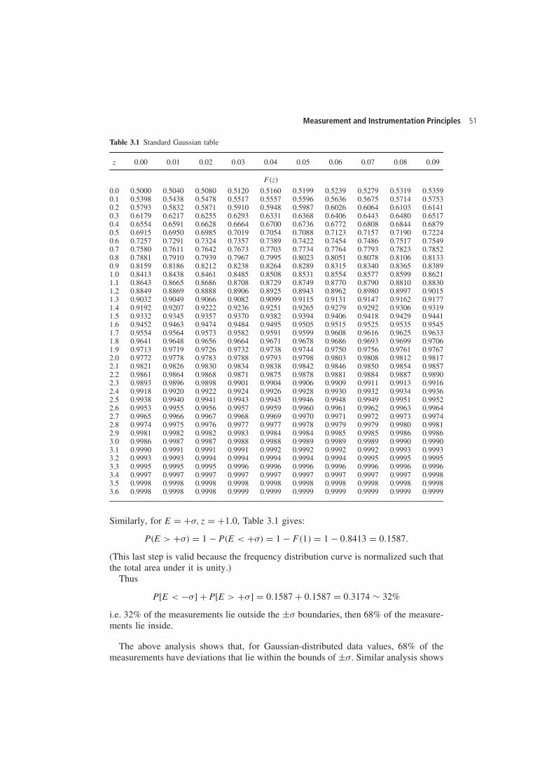
Measurement and Instrumentation Principles 51
Table 3.1 Standard Gaussian table
z 0.00 0.01 0.02 0.03 0.04 0.05 0.06 0.07 0.08 0.09
F�z�
0.0 0.5000 0.5040 0.5080 0.5120 0.5160 0.5199 0.5239 0.5279 0.5319 0.53590.1 0.5398 0.5438 0.5478 0.5517 0.5557 0.5596 0.5636 0.5675 0.5714 0.57530.2 0.5793 0.5832 0.5871 0.5910 0.5948 0.5987 0.6026 0.6064 0.6103 0.61410.3 0.6179 0.6217 0.6255 0.6293 0.6331 0.6368 0.6406 0.6443 0.6480 0.65170.4 0.6554 0.6591 0.6628 0.6664 0.6700 0.6736 0.6772 0.6808 0.6844 0.68790.5 0.6915 0.6950 0.6985 0.7019 0.7054 0.7088 0.7123 0.7157 0.7190 0.72240.6 0.7257 0.7291 0.7324 0.7357 0.7389 0.7422 0.7454 0.7486 0.7517 0.75490.7 0.7580 0.7611 0.7642 0.7673 0.7703 0.7734 0.7764 0.7793 0.7823 0.78520.8 0.7881 0.7910 0.7939 0.7967 0.7995 0.8023 0.8051 0.8078 0.8106 0.81330.9 0.8159 0.8186 0.8212 0.8238 0.8264 0.8289 0.8315 0.8340 0.8365 0.83891.0 0.8413 0.8438 0.8461 0.8485 0.8508 0.8531 0.8554 0.8577 0.8599 0.86211.1 0.8643 0.8665 0.8686 0.8708 0.8729 0.8749 0.8770 0.8790 0.8810 0.88301.2 0.8849 0.8869 0.8888 0.8906 0.8925 0.8943 0.8962 0.8980 0.8997 0.90151.3 0.9032 0.9049 0.9066 0.9082 0.9099 0.9115 0.9131 0.9147 0.9162 0.91771.4 0.9192 0.9207 0.9222 0.9236 0.9251 0.9265 0.9279 0.9292 0.9306 0.93191.5 0.9332 0.9345 0.9357 0.9370 0.9382 0.9394 0.9406 0.9418 0.9429 0.94411.6 0.9452 0.9463 0.9474 0.9484 0.9495 0.9505 0.9515 0.9525 0.9535 0.95451.7 0.9554 0.9564 0.9573 0.9582 0.9591 0.9599 0.9608 0.9616 0.9625 0.96331.8 0.9641 0.9648 0.9656 0.9664 0.9671 0.9678 0.9686 0.9693 0.9699 0.97061.9 0.9713 0.9719 0.9726 0.9732 0.9738 0.9744 0.9750 0.9756 0.9761 0.97672.0 0.9772 0.9778 0.9783 0.9788 0.9793 0.9798 0.9803 0.9808 0.9812 0.98172.1 0.9821 0.9826 0.9830 0.9834 0.9838 0.9842 0.9846 0.9850 0.9854 0.98572.2 0.9861 0.9864 0.9868 0.9871 0.9875 0.9878 0.9881 0.9884 0.9887 0.98902.3 0.9893 0.9896 0.9898 0.9901 0.9904 0.9906 0.9909 0.9911 0.9913 0.99162.4 0.9918 0.9920 0.9922 0.9924 0.9926 0.9928 0.9930 0.9932 0.9934 0.99362.5 0.9938 0.9940 0.9941 0.9943 0.9945 0.9946 0.9948 0.9949 0.9951 0.99522.6 0.9953 0.9955 0.9956 0.9957 0.9959 0.9960 0.9961 0.9962 0.9963 0.99642.7 0.9965 0.9966 0.9967 0.9968 0.9969 0.9970 0.9971 0.9972 0.9973 0.99742.8 0.9974 0.9975 0.9976 0.9977 0.9977 0.9978 0.9979 0.9979 0.9980 0.99812.9 0.9981 0.9982 0.9982 0.9983 0.9984 0.9984 0.9985 0.9985 0.9986 0.99863.0 0.9986 0.9987 0.9987 0.9988 0.9988 0.9989 0.9989 0.9989 0.9990 0.99903.1 0.9990 0.9991 0.9991 0.9991 0.9992 0.9992 0.9992 0.9992 0.9993 0.99933.2 0.9993 0.9993 0.9994 0.9994 0.9994 0.9994 0.9994 0.9995 0.9995 0.99953.3 0.9995 0.9995 0.9995 0.9996 0.9996 0.9996 0.9996 0.9996 0.9996 0.99963.4 0.9997 0.9997 0.9997 0.9997 0.9997 0.9997 0.9997 0.9997 0.9997 0.99983.5 0.9998 0.9998 0.9998 0.9998 0.9998 0.9998 0.9998 0.9998 0.9998 0.99983.6 0.9998 0.9998 0.9998 0.9999 0.9999 0.9999 0.9999 0.9999 0.9999 0.9999
Similarly, for E D C�, z D C1.0, Table 3.1 gives:
P�E > C�� D 1 � P�E < C�� D 1 � F�1� D 1 � 0.8413 D 0.1587.
(This last step is valid because the frequency distribution curve is normalized such thatthe total area under it is unity.)
Thus
P[E < ��] C P[E > C�] D 0.1587 C 0.1587 D 0.3174 ¾ 32%
i.e. 32% of the measurements lie outside the š� boundaries, then 68% of the measure-ments lie inside.
The above analysis shows that, for Gaussian-distributed data values, 68% of themeasurements have deviations that lie within the bounds of š�. Similar analysis shows
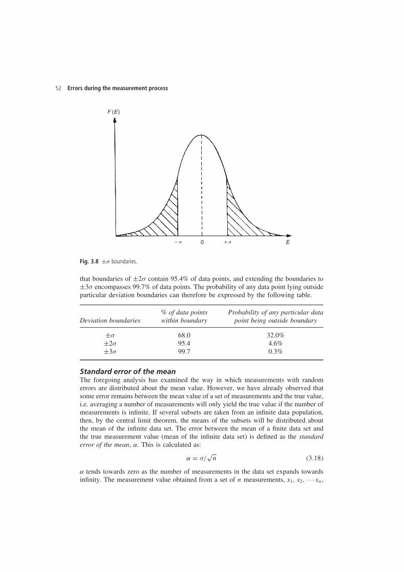
52 Errors during the measurement process
E
F (E)
− s + s0
Fig. 3.8 š� boundaries.
that boundaries of š2� contain 95.4% of data points, and extending the boundaries toš3� encompasses 99.7% of data points. The probability of any data point lying outsideparticular deviation boundaries can therefore be expressed by the following table.
% of data points Probability of any particular dataDeviation boundaries within boundary point being outside boundary
š� 68.0 32.0%š2� 95.4 4.6%š3� 99.7 0.3%
Standard error of the meanThe foregoing analysis has examined the way in which measurements with randomerrors are distributed about the mean value. However, we have already observed thatsome error remains between the mean value of a set of measurements and the true value,i.e. averaging a number of measurements will only yield the true value if the number ofmeasurements is infinite. If several subsets are taken from an infinite data population,then, by the central limit theorem, the means of the subsets will be distributed aboutthe mean of the infinite data set. The error between the mean of a finite data set andthe true measurement value (mean of the infinite data set) is defined as the standarderror of the mean, ˛. This is calculated as:
˛ D �/p
n �3.18�
˛ tends towards zero as the number of measurements in the data set expands towardsinfinity. The measurement value obtained from a set of n measurements, x1, x2, Ð Ð Ð xn,
Measurement and Instrumentation Principles 53
can then be expressed as:x D xmean š ˛
For the data set C of length measurements used earlier, n D 23, � D 1.88 and ˛ D 0.39.The length can therefore be expressed as 406.5 š 0.4 (68% confidence limit). However,it is more usual to express measurements with 95% confidence limits (š2� boundaries).In this case, 2� D 3.76, 2˛ D 0.78 and the length can be expressed as 406.5 š 0.8 (95%confidence limits).
Estimation of random error in a single measurementIn many situations where measurements are subject to random errors, it is not practicalto take repeated measurements and find the average value. Also, the averaging processbecomes invalid if the measured quantity does not remain at a constant value, asis usually the case when process variables are being measured. Thus, if only onemeasurement can be made, some means of estimating the likely magnitude of error in itis required. The normal approach to this is to calculate the error within 95% confidencelimits, i.e. to calculate the value of the deviation D such that 95% of the area underthe probability curve lies within limits of šD. These limits correspond to a deviationof š1.96�. Thus, it is necessary to maintain the measured quantity at a constant valuewhilst a number of measurements are taken in order to create a reference measurementset from which � can be calculated. Subsequently, the maximum likely deviation ina single measurement can be expressed as: Deviation D š1.96�. However, this onlyexpresses the maximum likely deviation of the measurement from the calculated meanof the reference measurement set, which is not the true value as observed earlier. Thusthe calculated value for the standard error of the mean has to be added to the likelymaximum deviation value. Thus, the maximum likely error in a single measurementcan be expressed as:
Error D š�1.96� C ˛� �3.19�
Example 3.4Suppose that a standard mass is measured 30 times with the same instrument to createa reference data set, and the calculated values of � and ˛ are � D 0.43 and ˛ D 0.08. Ifthe instrument is then used to measure an unknown mass and the reading is 105.6 kg,how should the mass value be expressed?
SolutionUsing (3.19), 1.96� C ˛ D 0.92. The mass value should therefore be expressed as:105.6 š 0.9 kg.
Before leaving this matter, it must be emphasized that the maximum error specifiedfor a measurement is only specified for the confidence limits defined. Thus, if themaximum error is specified as š1% with 95% confidence limits, this means that thereis still 1 chance in 20 that the error will exceed š1%.
Distribution of manufacturing tolerancesMany aspects of manufacturing processes are subject to random variations caused byfactors that are similar to those that cause random errors in measurements. In mostcases, these random variations in manufacturing, which are known as tolerances, fit a
54 Errors during the measurement process
Gaussian distribution, and the previous analysis of random measurement errors can beapplied to analyse the distribution of these variations in manufacturing parameters.
Example 3.5An integrated circuit chip contains 105 transistors. The transistors have a mean currentgain of 20 and a standard deviation of 2. Calculate the following:
(a) the number of transistors with a current gain between 19.8 and 20.2(b) the number of transistors with a current gain greater than 17.
Solution(a) The proportion of transistors where 19.8 < gain < 20.2 is:
P[X < 20] � P[X < 19.8] D P[z < 0.2] � P[z < �0.2] �for z D �X � �/��
For X D 20.2; z D 0.1 and for X D 19.8; z D �0.1From tables, P[z < 0.1] D 0.5398 and thus P[z < �0.1] D 1 � P[z < 0.1] D 1 �0.5398 D 0.4602Hence, P[z < 0.1] � P[z < �0.1] D 0.5398 � 0.4602 D 0.0796Thus 0.0796 ð 105 D 7960 transistors have a current gain in the range from 19.8to 20.2.(b) The number of transistors with gain >17 is given by:
P[x > 17] D 1 � P[x < 17] D 1 � P[z < �1.5] D P[z < C1.5] D 0.9332
Thus, 93.32%, i.e. 93 320 transistors have a gain >17.
Goodness of fit to a Gaussian distributionAll of the analysis of random deviations presented so far only applies when the databeing analysed belongs to a Gaussian distribution. Hence, the degree to which a set ofdata fits a Gaussian distribution should always be tested before any analysis is carriedout. This test can be carried out in one of three ways:
(a) Simple test: The simplest way to test for Gaussian distribution of data is to plota histogram and look for a ‘Bell-shape’ of the form shown earlier in Figure 3.5.Deciding whether or not the histogram confirms a Gaussian distribution is a matterof judgement. For a Gaussian distribution, there must always be approximatesymmetry about the line through the centre of the histogram, the highest point ofthe histogram must always coincide with this line of symmetry, and the histogrammust get progressively smaller either side of this point. However, because thehistogram can only be drawn with a finite set of measurements, some deviationfrom the perfect shape of the histogram as described above is to be expected evenif the data really is Gaussian.
(b) Using a normal probability plot: A normal probability plot involves dividing thedata values into a number of ranges and plotting the cumulative probability ofsummed data frequencies against the data values on special graph paper.Ł Thisline should be a straight line if the data distribution is Gaussian. However, carefuljudgement is required since only a finite number of data values can be used and
Ł This is available from specialist stationery suppliers.
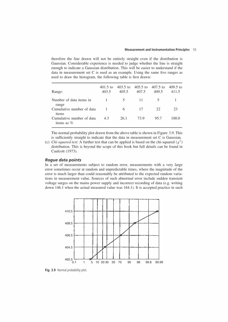
Measurement and Instrumentation Principles 55
therefore the line drawn will not be entirely straight even if the distribution isGaussian. Considerable experience is needed to judge whether the line is straightenough to indicate a Gaussian distribution. This will be easier to understand if thedata in measurement set C is used as an example. Using the same five ranges asused to draw the histogram, the following table is first drawn:
401.5 to 403.5 to 405.5 to 407.5 to 409.5 toRange: 403.5 405.5 407.5 409.5 411.5
Number of data items inrange
1 5 11 5 1
Cumulative number of dataitems
1 6 17 22 23
Cumulative number of dataitems as %
4.3 26.1 73.9 95.7 100.0
The normal probability plot drawn from the above table is shown in Figure 3.9. Thisis sufficiently straight to indicate that the data in measurement set C is Gaussian.
(c) Chi-squared test: A further test that can be applied is based on the chi-squared ��2�distribution. This is beyond the scope of this book but full details can be found inCaulcott (1973).
Rogue data pointsIn a set of measurements subject to random error, measurements with a very largeerror sometimes occur at random and unpredictable times, where the magnitude of theerror is much larger than could reasonably be attributed to the expected random varia-tions in measurement value. Sources of such abnormal error include sudden transientvoltage surges on the mains power supply and incorrect recording of data (e.g. writingdown 146.1 when the actual measured value was 164.1). It is accepted practice in such
0.1402.5
2010 70 9850 90 99.9999.851 30
404.5
406.5
408.5
410.5
Fig. 3.9 Normal probability plot.
56 Errors during the measurement process
cases to discard these rogue measurements, and a threshold level of a š3� deviationis often used to determine what should be discarded. It is extremely rare for measure-ment errors to exceed š3� limits when only normal random effects are affecting themeasured value.
Special case when the number of measurements is smallWhen the number of measurements of a quantity is particularly small and statisticalanalysis of the distribution of error values is required, problems can arise when usingstandard Gaussian tables in terms of z as defined in equation (3.16) because the mean ofonly a small number of measurements may deviate significantly from the true measure-ment value. In response to this, an alternative distribution function called the Student-tdistribution can be used which gives a more accurate prediction of the error distributionwhen the number of samples is small. This is discussed more fully in Miller (1990).
3.6 Aggregation of measurement system errors
Errors in measurement systems often arise from two or more different sources, andthese must be aggregated in the correct way in order to obtain a prediction of thetotal likely error in output readings from the measurement system. Two different formsof aggregation are required. Firstly, a single measurement component may have bothsystematic and random errors and, secondly, a measurement system may consist ofseveral measurement components that each have separate errors.
3.6.1 Combined effect of systematic and random errors
If a measurement is affected by both systematic and random errors that are quantifiedas šx (systematic errors) and šy (random errors), some means of expressing thecombined effect of both types of error is needed. One way of expressing the combinederror would be to sum the two separate components of error, i.e. to say that the totalpossible error is e D š�x C y�. However, a more usual course of action is to expressthe likely maximum error as follows:
e D√
�x2 C y2� �3.20�
It can be shown (ANSI/ASME, 1985) that this is the best expression for the errorstatistically, since it takes account of the reasonable assumption that the systematicand random errors are independent and so are unlikely to both be at their maximumor minimum value at the same time.
3.6.2 Aggregation of errors from separate measurementsystem components
A measurement system often consists of several separate components, each of which issubject to errors. Therefore, what remains to be investigated is how the errors associated
Measurement and Instrumentation Principles 57
with each measurement system component combine together, so that a total errorcalculation can be made for the complete measurement system. All four mathematicaloperations of addition, subtraction, multiplication and division may be performed onmeasurements derived from different instruments/transducers in a measurement system.Appropriate techniques for the various situations that arise are covered below.
Error in a sumIf the two outputs y and z of separate measurement system components are to be addedtogether, we can write the sum as S D y C z. If the maximum errors in y and z are šayand šbz respectively, we can express the maximum and minimum possible values ofS as:
Smax D �y C ay� C �z C bz�; Smin D �y � ay� C �z � bz�; or S D y C z š �ay C bz�
This relationship for S is not convenient because in this form the error term cannotbe expressed as a fraction or percentage of the calculated value for S. Fortunately,statistical analysis can be applied (see Topping, 1962) that expresses S in an alternativeform such that the most probable maximum error in S is represented by a quantity e,where e is calculated in terms of the absolute errors as:
e D√
�ay�2 C �bz�2 �3.21�
Thus S D �y C z� š e. This can be expressed in the alternative form:
S D �y C z��1 š f� where f D e/�y C z� �3.22�
It should be noted that equations (3.21) and (3.22) are only valid provided that themeasurements are uncorrelated (i.e. each measurement is entirely independent of theothers).
Example 3.6A circuit requirement for a resistance of 550 � is satisfied by connecting together tworesistors of nominal values 220 � and 330 � in series. If each resistor has a toleranceof š2%, the error in the sum calculated according to equations (3.21) and (3.22) isgiven by:
e D√
�0.02 ð 220�2 C �0.02 ð 330�2 D 7.93; f D 7.93/50 D 0.0144
Thus the total resistance S can be expressed as
S D 550 � š 7.93 � or S D 550 �1 š 0.0144� �, i.e. S D 550 � š 1.4%
Error in a differenceIf the two outputs y and z of separate measurement systems are to be subtracted fromone another, and the possible errors are šay and šbz, then the difference S can beexpressed (using statistical analysis as for calculating the error in a sum and assumingthat the measurements are uncorrelated) as:
S D �y � z� š e or S D �y � z��1 š f�
where e is calculated as above (equation 3.21), and f D e/�y � z�
58 Errors during the measurement process
Example 3.7A fluid flow rate is calculated from the difference in pressure measured on both sidesof an orifice plate. If the pressure measurements are 10.0 bar and 9.5 bar and the errorin the pressure measuring instruments is specified as š0.1%, then values for e and fcan be calculated as:
e D√
�0.001 ð 10�2 C �0.001 ð 9.5�2 D 0.0138; f D 0.0138/0.5 D 0.0276
ž This example illustrates very poignantly the relatively large error that can arise whencalculations are made based on the difference between two measurements.
Error in a productIf the outputs y and z of two measurement system components are multiplied together,the product can be written as P D yz. If the possible error in y is šay and in z is šbz,then the maximum and minimum values possible in P can be written as:
Pmax D �y C ay��z C bz� D yz C ayz C byz C aybz;
Pmin D �y � ay��z � bz� D yz � ayz � byz C aybz
For typical measurement system components with output errors of up to one or twoper cent in magnitude, both a and b are very much less than one in magnitude andthus terms in aybz are negligible compared with other terms. Therefore, we havePmax D yz�1 C a C b�; Pmin D yz�1 � a � b�. Thus the maximum error in the productP is š�a C b�. Whilst this expresses the maximum possible error in P, it tends tooverestimate the likely maximum error since it is very unlikely that the errors in yand z will both be at the maximum or minimum value at the same time. A statisticallybetter estimate of the likely maximum error e in the product P, provided that themeasurements are uncorrelated, is given by Topping (1962):
e D√
a2 C b2 �3.23�
Note that in the case of multiplicative errors, e is calculated in terms of the fractionalerrors in y and z (as opposed to the absolute error values used in calculating additiveerrors).
Example 3.8If the power in a circuit is calculated from measurements of voltage and currentin which the calculated maximum errors are respectively š1% and š2%, thenthe maximum likely error in the calculated power value, calculated using (3.23) isšp
0.012 C 0.022 D š0.022 or š2.2%.
Error in a quotientIf the output measurement y of one system component with possible error šay isdivided by the output measurement z of another system component with possibleerror šbz, then the maximum and minimum possible values for the quotient can be
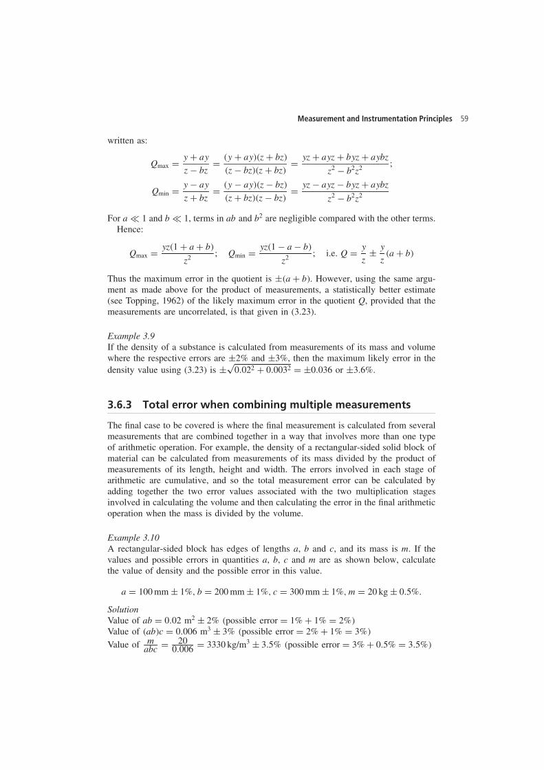
Measurement and Instrumentation Principles 59
written as:
Qmax D y C ay
z � bzD �y C ay��z C bz�
�z � bz��z C bz�D yz C ayz C byz C aybz
z2 � b2z2 ;
Qmin D y � ay
z C bzD �y � ay��z � bz�
�z C bz��z � bz�D yz � ayz � byz C aybz
z2 � b2z2
For a − 1 and b − 1, terms in ab and b2 are negligible compared with the other terms.Hence:
Qmax D yz�1 C a C b�
z2 ; Qmin D yz�1 � a � b�
z2 ; i.e. Q D y
zš y
z�a C b�
Thus the maximum error in the quotient is š�a C b�. However, using the same argu-ment as made above for the product of measurements, a statistically better estimate(see Topping, 1962) of the likely maximum error in the quotient Q, provided that themeasurements are uncorrelated, is that given in (3.23).
Example 3.9If the density of a substance is calculated from measurements of its mass and volumewhere the respective errors are š2% and š3%, then the maximum likely error in thedensity value using (3.23) is šp
0.022 C 0.0032 D š0.036 or š3.6%.
3.6.3 Total error when combining multiple measurements
The final case to be covered is where the final measurement is calculated from severalmeasurements that are combined together in a way that involves more than one typeof arithmetic operation. For example, the density of a rectangular-sided solid block ofmaterial can be calculated from measurements of its mass divided by the product ofmeasurements of its length, height and width. The errors involved in each stage ofarithmetic are cumulative, and so the total measurement error can be calculated byadding together the two error values associated with the two multiplication stagesinvolved in calculating the volume and then calculating the error in the final arithmeticoperation when the mass is divided by the volume.
Example 3.10A rectangular-sided block has edges of lengths a, b and c, and its mass is m. If thevalues and possible errors in quantities a, b, c and m are as shown below, calculatethe value of density and the possible error in this value.
a D 100 mm š 1%, b D 200 mm š 1%, c D 300 mm š 1%, m D 20 kg š 0.5%.
SolutionValue of ab D 0.02 m2 š 2% �possible error D 1% C 1% D 2%�Value of �ab�c D 0.006 m3 š 3% �possible error D 2% C 1% D 3%�
Value of mabc D 20
0.006 D 3330 kg/m3 š 3.5% �possible error D 3% C 0.5% D 3.5%�
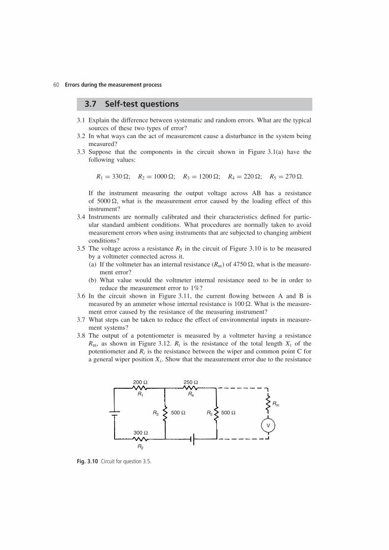
60 Errors during the measurement process
3.7 Self-test questions
3.1 Explain the difference between systematic and random errors. What are the typicalsources of these two types of error?
3.2 In what ways can the act of measurement cause a disturbance in the system beingmeasured?
3.3 Suppose that the components in the circuit shown in Figure 3.1(a) have thefollowing values:
R1 D 330 �; R2 D 1000 �; R3 D 1200 �; R4 D 220 �; R5 D 270 �.
If the instrument measuring the output voltage across AB has a resistanceof 5000 �, what is the measurement error caused by the loading effect of thisinstrument?
3.4 Instruments are normally calibrated and their characteristics defined for partic-ular standard ambient conditions. What procedures are normally taken to avoidmeasurement errors when using instruments that are subjected to changing ambientconditions?
3.5 The voltage across a resistance R5 in the circuit of Figure 3.10 is to be measuredby a voltmeter connected across it.(a) If the voltmeter has an internal resistance (Rm) of 4750 �, what is the measure-
ment error?(b) What value would the voltmeter internal resistance need to be in order to
reduce the measurement error to 1%?3.6 In the circuit shown in Figure 3.11, the current flowing between A and B is
measured by an ammeter whose internal resistance is 100 �. What is the measure-ment error caused by the resistance of the measuring instrument?
3.7 What steps can be taken to reduce the effect of environmental inputs in measure-ment systems?
3.8 The output of a potentiometer is measured by a voltmeter having a resistanceRm, as shown in Figure 3.12. Rt is the resistance of the total length Xt of thepotentiometer and Ri is the resistance between the wiper and common point C fora general wiper position Xi. Show that the measurement error due to the resistance
200 Ω
300 Ω
500 Ω
V
R1
R2
R3 500 ΩR5
Rm
R4
250 Ω
Fig. 3.10 Circuit for question 3.5.
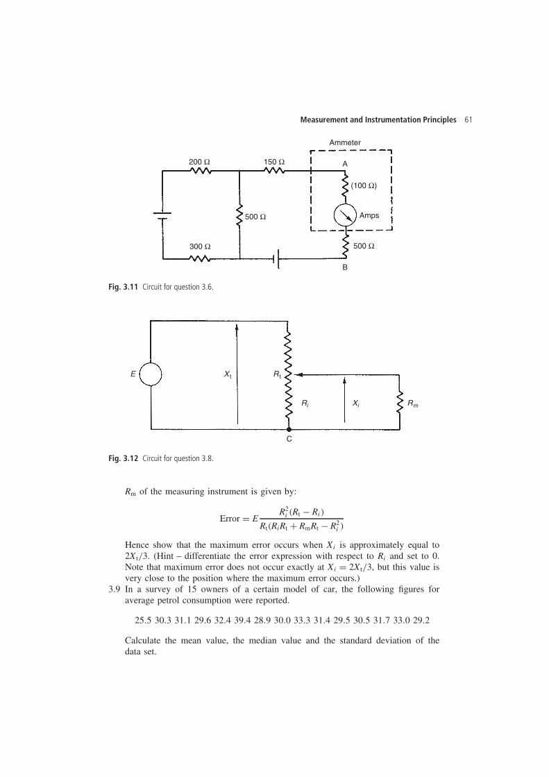
Measurement and Instrumentation Principles 61
200 Ω
300 Ω
500 Ω
A
Ammeter
B
Amps
500 Ω
(100 Ω)
150 Ω
Fig. 3.11 Circuit for question 3.6.
E Xt Rt
RmRi Xi
C
Fig. 3.12 Circuit for question 3.8.
Rm of the measuring instrument is given by:
Error D ER2
i �Rt � Ri�
Rt�RiRt C RmRt � R2i �
Hence show that the maximum error occurs when Xi is approximately equal to2Xt/3. (Hint – differentiate the error expression with respect to Ri and set to 0.Note that maximum error does not occur exactly at Xi D 2Xt/3, but this value isvery close to the position where the maximum error occurs.)
3.9 In a survey of 15 owners of a certain model of car, the following figures foraverage petrol consumption were reported.
25.5 30.3 31.1 29.6 32.4 39.4 28.9 30.0 33.3 31.4 29.5 30.5 31.7 33.0 29.2
Calculate the mean value, the median value and the standard deviation of thedata set.
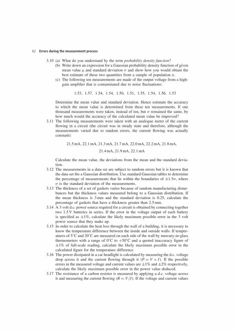
62 Errors during the measurement process
3.10 (a) What do you understand by the term probability density function?(b) Write down an expression for a Gaussian probability density function of given
mean value μ and standard deviation � and show how you would obtain thebest estimate of these two quantities from a sample of population n.
(c) The following ten measurements are made of the output voltage from a high-gain amplifier that is contaminated due to noise fluctuations:
1.53, 1.57, 1.54, 1.54, 1.50, 1.51, 1.55, 1.54, 1.56, 1.53
Determine the mean value and standard deviation. Hence estimate the accuracyto which the mean value is determined from these ten measurements. If onethousand measurements were taken, instead of ten, but � remained the same, byhow much would the accuracy of the calculated mean value be improved?
3.11 The following measurements were taken with an analogue meter of the currentflowing in a circuit (the circuit was in steady state and therefore, although themeasurements varied due to random errors, the current flowing was actuallyconstant):
21.5 mA, 22.1 mA, 21.3 mA, 21.7 mA, 22.0 mA, 22.2 mA, 21.8 mA,
21.4 mA, 21.9 mA, 22.1 mA
Calculate the mean value, the deviations from the mean and the standard devia-tion.
3.12 The measurements in a data set are subject to random errors but it is known thatthe data set fits a Gaussian distribution. Use standard Gaussian tables to determinethe percentage of measurements that lie within the boundaries of š1.5�, where� is the standard deviation of the measurements.
3.13 The thickness of a set of gaskets varies because of random manufacturing distur-bances but the thickness values measured belong to a Gaussian distribution. Ifthe mean thickness is 3 mm and the standard deviation is 0.25, calculate thepercentage of gaskets that have a thickness greater than 2.5 mm.
3.14 A 3 volt d.c. power source required for a circuit is obtained by connecting togethertwo 1.5 V batteries in series. If the error in the voltage output of each batteryis specified as š1%, calculate the likely maximum possible error in the 3 voltpower source that they make up.
3.15 In order to calculate the heat loss through the wall of a building, it is necessary toknow the temperature difference between the inside and outside walls. If temper-atures of 5°C and 20°C are measured on each side of the wall by mercury-in-glassthermometers with a range of 0°C to C50°C and a quoted inaccuracy figure ofš1% of full-scale reading, calculate the likely maximum possible error in thecalculated figure for the temperature difference.
3.16 The power dissipated in a car headlight is calculated by measuring the d.c. voltagedrop across it and the current flowing through it �P D V ð I�. If the possibleerrors in the measured voltage and current values are š1% and š2% respectively,calculate the likely maximum possible error in the power value deduced.
3.17 The resistance of a carbon resistor is measured by applying a d.c. voltage acrossit and measuring the current flowing �R D V/I�. If the voltage and current values
Measurement and Instrumentation Principles 63
are measured as 10 š 0.1 V and 214 š 5 mA respectively, express the value ofthe carbon resistor.
3.18 The density (d) of a liquid is calculated by measuring its depth (c) in a calibratedrectangular tank and then emptying it into a mass measuring system. The lengthand width of the tank are (a) and (b) respectively and thus the density is given by:
d D m/�a ð b ð c�
where m is the measured mass of the liquid emptied out.If the possible errors in the measurements of a, b, c and m are 1%, 1%, 2% and0.5% respectively, determine the likely maximum possible error in the calculatedvalue of the density (d).
3.19 The volume flow rate of a liquid is calculated by allowing the liquid to flowinto a cylindrical tank (stood on its flat end) and measuring the height of theliquid surface before and after the liquid has flowed for 10 minutes. The volumecollected after 10 minutes is given by:
Volume D �h2 � h1��d/2�2
where h1 and h2 are the starting and finishing surface heights and d is themeasured diameter of the tank.
(a) If h1 D 2 m, h2 D 3 m and d D 2 m, calculate the volume flow rate in m3/min.(b) If the possible error in each measurement h1, h2 and d is š1%, determine the
likely maximum possible error in the calculated value of volume flow rate.
References and further reading
ANSI/ASME standards (1985) ASME performance test codes, supplement on instruments andapparatus, part 1: measurement uncertainty, American Society of Mechanical Engineers, NewYork.
Bennington, P.R. and Robinson, D.K. (1992) Data Reduction and Error Analysis for the PhysicalSciences, McGraw-Hill.
Caulcott, E. (1973) Significance Tests, Routledge and Kegan Paul.Miller, I.R., Freung, J.E. and Johnson, R. (1990) Probability and Statistics for Engineers, Prentice-
Hall.Topping, J. (1962) Errors of Observation and Their Treatment, Chapman and Hall.
4
Calibration of measuringsensors and instruments
4.1 Principles of calibration
Calibration consists of comparing the output of the instrument or sensor under testagainst the output of an instrument of known accuracy when the same input (themeasured quantity) is applied to both instruments. This procedure is carried out for arange of inputs covering the whole measurement range of the instrument or sensor.Calibration ensures that the measuring accuracy of all instruments and sensors used ina measurement system is known over the whole measurement range, provided that thecalibrated instruments and sensors are used in environmental conditions that are thesame as those under which they were calibrated. For use of instruments and sensorsunder different environmental conditions, appropriate correction has to be made for theensuing modifying inputs, as described in Chapter 3. Whether applied to instrumentsor sensors, calibration procedures are identical, and hence only the term instrumentwill be used for the rest of this chapter, with the understanding that whatever is saidfor instruments applies equally well to single measurement sensors.
Instruments used as a standard in calibration procedures are usually chosen to be ofgreater inherent accuracy than the process instruments that they are used to calibrate.Because such instruments are only used for calibration purposes, greater accuracycan often be achieved by specifying a type of instrument that would be unsuitablefor normal process measurements. For instance, ruggedness is not a requirement, andfreedom from this constraint opens up a much wider range of possible instruments. Inpractice, high-accuracy, null-type instruments are very commonly used for calibrationduties, because the need for a human operator is not a problem in these circumstances.
Instrument calibration has to be repeated at prescribed intervals because the charac-teristics of any instrument change over a period. Changes in instrument characteristicsare brought about by such factors as mechanical wear, and the effects of dirt, dust,fumes, chemicals and temperature changes in the operating environment. To a greatextent, the magnitude of the drift in characteristics depends on the amount of use aninstrument receives and hence on the amount of wear and the length of time that itis subjected to the operating environment. However, some drift also occurs even instorage, as a result of ageing effects in components within the instrument.
Measurement and Instrumentation Principles 65
Determination of the frequency at which instruments should be calibrated is depen-dent upon several factors that require specialist knowledge. If an instrument is requiredto measure some quantity and an inaccuracy of š2% is acceptable, then a certainamount of performance degradation can be allowed if its inaccuracy immediately afterrecalibration is š1%. What is important is that the pattern of performance degrada-tion be quantified, such that the instrument can be recalibrated before its accuracy hasreduced to the limit defined by the application.
Susceptibility to the various factors that can cause changes in instrument character-istics varies according to the type of instrument involved. Possession of an in-depthknowledge of the mechanical construction and other features involved in the instru-ment is necessary in order to be able to quantify the effect of these quantities onthe accuracy and other characteristics of an instrument. The type of instrument, itsfrequency of use and the prevailing environmental conditions all strongly influence thecalibration frequency necessary, and because so many factors are involved, it is diffi-cult or even impossible to determine the required frequency of instrument recalibrationfrom theoretical considerations. Instead, practical experimentation has to be applied todetermine the rate of such changes. Once the maximum permissible measurement errorhas been defined, knowledge of the rate at which the characteristics of an instrumentchange allows a time interval to be calculated that represents the moment in time whenan instrument will have reached the bounds of its acceptable performance level. Theinstrument must be recalibrated either at this time or earlier. This measurement errorlevel that an instrument reaches just before recalibration is the error bound that mustbe quoted in the documented specifications for the instrument.
A proper course of action must be defined that describes the procedures to befollowed when an instrument is found to be out of calibration, i.e. when its outputis different to that of the calibration instrument when the same input is applied. Therequired action depends very much upon the nature of the discrepancy and the type ofinstrument involved. In many cases, deviations in the form of a simple output bias canbe corrected by a small adjustment to the instrument (following which the adjustmentscrews must be sealed to prevent tampering). In other cases, the output scale of theinstrument may have to be redrawn, or scaling factors altered where the instrumentoutput is part of some automatic control or inspection system. In extreme cases, wherethe calibration procedure shows up signs of instrument damage, it may be necessaryto send the instrument for repair or even scrap it.
Whatever system and frequency of calibration is established, it is important to reviewthis from time to time to ensure that the system remains effective and efficient. It mayhappen that a cheaper (but equally effective) method of calibration becomes availablewith the passage of time, and such an alternative system must clearly be adopted inthe interests of cost efficiency. However, the main item under scrutiny in this review isnormally whether the calibration interval is still appropriate. Records of the calibrationhistory of the instrument will be the primary basis on which this review is made. It mayhappen that an instrument starts to go out of calibration more quickly after a period oftime, either because of ageing factors within the instrument or because of changes inthe operating environment. The conditions or mode of usage of the instrument may alsobe subject to change. As the environmental and usage conditions of an instrument maychange beneficially as well as adversely, there is the possibility that the recommendedcalibration interval may decrease as well as increase.
66 Calibration of measuring sensors and instruments
4.2 Control of calibration environment
Any instrument that is used as a standard in calibration procedures must be kept solelyfor calibration duties and must never be used for other purposes. Most particularly, itmust not be regarded as a spare instrument that can be used for process measurementsif the instrument normally used for that purpose breaks down. Proper provision forprocess instrument failures must be made by keeping a spare set of process instruments.Standard calibration instruments must be totally separate.
To ensure that these conditions are met, the calibration function must be managedand executed in a professional manner. This will normally mean setting aside a partic-ular place within the instrumentation department of a company where all calibrationoperations take place and where all instruments used for calibration are kept. As faras possible this should take the form of a separate room, rather than a sectioned-offarea in a room used for other purposes as well. This will enable better environmentalcontrol to be applied in the calibration area and will also offer better protection againstunauthorized handling or use of the calibration instruments. The level of environmentalcontrol required during calibration should be considered carefully with due regard towhat level of accuracy is required in the calibration procedure, but should not beoverspecified as this will lead to unnecessary expense. Full air conditioning is notnormally required for calibration at this level, as it is very expensive, but sensibleprecautions should be taken to guard the area from extremes of heat or cold, and alsogood standards of cleanliness should be maintained. Useful guidance on the operationof standards facilities can be found elsewhere (British Standards Society, 1979).
Whilst it is desirable that all calibration functions are performed in this carefullycontrolled environment, it is not always practical to achieve this. Sometimes, it is notconvenient or possible to remove instruments from process plant, and in these cases,it is standard practice to calibrate them in situ. In these circumstances, appropriatecorrections must be made for the deviation in the calibration environmental conditionsaway from those specified. This practice does not obviate the need to protect calibrationinstruments and maintain them in constant conditions in a calibration laboratory at alltimes other than when they are involved in such calibration duties on plant.
As far as management of calibration procedures is concerned, it is important that theperformance of all calibration operations is assigned as the clear responsibility of justone person. That person should have total control over the calibration function, andbe able to limit access to the calibration laboratory to designated, approved personnelonly. Only by giving this appointed person total control over the calibration functioncan the function be expected to operate efficiently and effectively. Lack of such definitemanagement can only lead to unintentional neglect of the calibration system, resultingin the use of equipment in an out-of-date state of calibration and subsequent loss oftraceability to reference standards. Professional management is essential so that thecustomer can be assured that an efficient calibration system is in operation and thatthe accuracy of measurements is guaranteed.
Calibration procedures that relate in any way to measurements that are used forquality control functions are controlled by the international standard ISO 9000 (thissubsumes the old British quality standard BS 5750). One of the clauses in ISO9000 requires that all persons using calibration equipment be adequately trained. Themanager in charge of the calibration function is clearly responsible for ensuring that
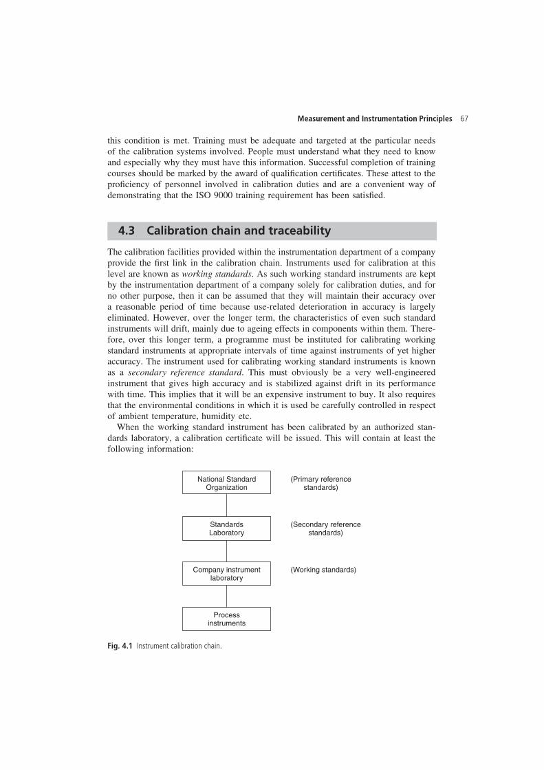
Measurement and Instrumentation Principles 67
this condition is met. Training must be adequate and targeted at the particular needsof the calibration systems involved. People must understand what they need to knowand especially why they must have this information. Successful completion of trainingcourses should be marked by the award of qualification certificates. These attest to theproficiency of personnel involved in calibration duties and are a convenient way ofdemonstrating that the ISO 9000 training requirement has been satisfied.
4.3 Calibration chain and traceability
The calibration facilities provided within the instrumentation department of a companyprovide the first link in the calibration chain. Instruments used for calibration at thislevel are known as working standards. As such working standard instruments are keptby the instrumentation department of a company solely for calibration duties, and forno other purpose, then it can be assumed that they will maintain their accuracy overa reasonable period of time because use-related deterioration in accuracy is largelyeliminated. However, over the longer term, the characteristics of even such standardinstruments will drift, mainly due to ageing effects in components within them. There-fore, over this longer term, a programme must be instituted for calibrating workingstandard instruments at appropriate intervals of time against instruments of yet higheraccuracy. The instrument used for calibrating working standard instruments is knownas a secondary reference standard. This must obviously be a very well-engineeredinstrument that gives high accuracy and is stabilized against drift in its performancewith time. This implies that it will be an expensive instrument to buy. It also requiresthat the environmental conditions in which it is used be carefully controlled in respectof ambient temperature, humidity etc.
When the working standard instrument has been calibrated by an authorized stan-dards laboratory, a calibration certificate will be issued. This will contain at least thefollowing information:
National StandardOrganization
(Primary referencestandards)
StandardsLaboratory
(Secondary referencestandards)
Company instrumentlaboratory
(Working standards)
Processinstruments
Fig. 4.1 Instrument calibration chain.
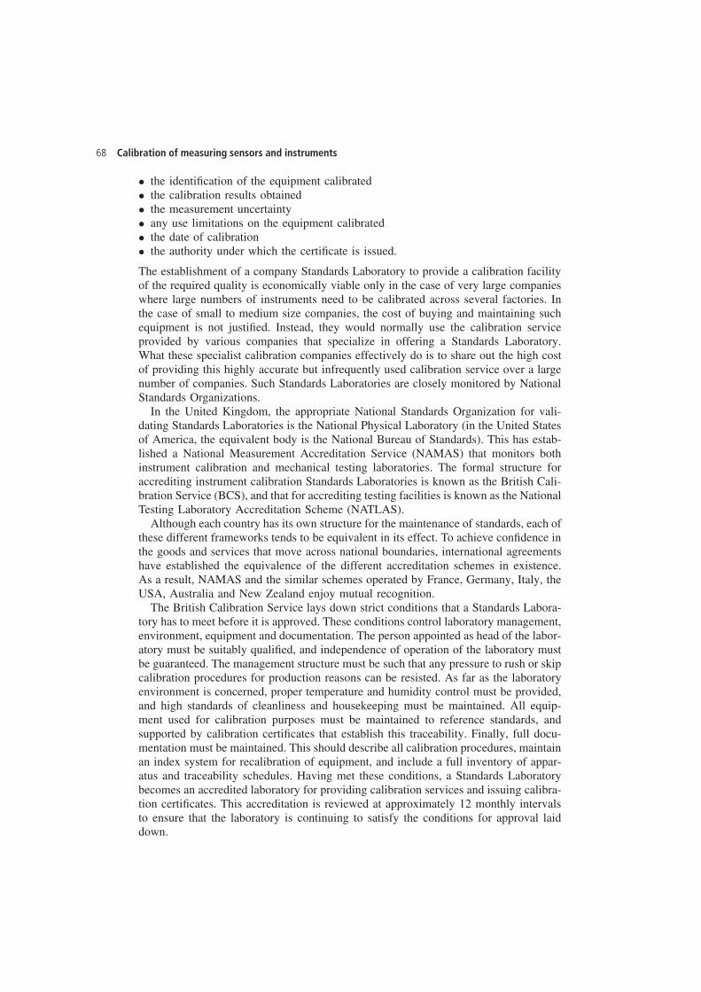
68 Calibration of measuring sensors and instruments
ž the identification of the equipment calibratedž the calibration results obtainedž the measurement uncertaintyž any use limitations on the equipment calibratedž the date of calibrationž the authority under which the certificate is issued.
The establishment of a company Standards Laboratory to provide a calibration facilityof the required quality is economically viable only in the case of very large companieswhere large numbers of instruments need to be calibrated across several factories. Inthe case of small to medium size companies, the cost of buying and maintaining suchequipment is not justified. Instead, they would normally use the calibration serviceprovided by various companies that specialize in offering a Standards Laboratory.What these specialist calibration companies effectively do is to share out the high costof providing this highly accurate but infrequently used calibration service over a largenumber of companies. Such Standards Laboratories are closely monitored by NationalStandards Organizations.
In the United Kingdom, the appropriate National Standards Organization for vali-dating Standards Laboratories is the National Physical Laboratory (in the United Statesof America, the equivalent body is the National Bureau of Standards). This has estab-lished a National Measurement Accreditation Service (NAMAS) that monitors bothinstrument calibration and mechanical testing laboratories. The formal structure foraccrediting instrument calibration Standards Laboratories is known as the British Cali-bration Service (BCS), and that for accrediting testing facilities is known as the NationalTesting Laboratory Accreditation Scheme (NATLAS).
Although each country has its own structure for the maintenance of standards, each ofthese different frameworks tends to be equivalent in its effect. To achieve confidence inthe goods and services that move across national boundaries, international agreementshave established the equivalence of the different accreditation schemes in existence.As a result, NAMAS and the similar schemes operated by France, Germany, Italy, theUSA, Australia and New Zealand enjoy mutual recognition.
The British Calibration Service lays down strict conditions that a Standards Labora-tory has to meet before it is approved. These conditions control laboratory management,environment, equipment and documentation. The person appointed as head of the labor-atory must be suitably qualified, and independence of operation of the laboratory mustbe guaranteed. The management structure must be such that any pressure to rush or skipcalibration procedures for production reasons can be resisted. As far as the laboratoryenvironment is concerned, proper temperature and humidity control must be provided,and high standards of cleanliness and housekeeping must be maintained. All equip-ment used for calibration purposes must be maintained to reference standards, andsupported by calibration certificates that establish this traceability. Finally, full docu-mentation must be maintained. This should describe all calibration procedures, maintainan index system for recalibration of equipment, and include a full inventory of appar-atus and traceability schedules. Having met these conditions, a Standards Laboratorybecomes an accredited laboratory for providing calibration services and issuing calibra-tion certificates. This accreditation is reviewed at approximately 12 monthly intervalsto ensure that the laboratory is continuing to satisfy the conditions for approval laiddown.
Measurement and Instrumentation Principles 69
Primary reference standards, as listed in Table 2.1, describe the highest level ofaccuracy that is achievable in the measurement of any particular physical quantity. Allitems of equipment used in Standards Laboratories as secondary reference standardshave to be calibrated themselves against primary reference standards at appropriateintervals of time. This procedure is acknowledged by the issue of a calibration certifi-cate in the standard way. National Standards Organizations maintain suitable facilitiesfor this calibration, which in the case of the United Kingdom are at the National Phys-ical Laboratory. The equivalent National Standards Organization in the United States ofAmerica is the National Bureau of Standards. In certain cases, such primary referencestandards can be located outside National Standards Organizations. For instance, theprimary reference standard for dimension measurement is defined by the wavelength ofthe orange–red line of krypton light, and it can therefore be realized in any laboratoryequipped with an interferometer. In certain cases (e.g. the measurement of viscosity),such primary reference standards are not available and reference standards for calibra-tion are achieved by collaboration between several National Standards Organizationswho perform measurements on identical samples under controlled conditions (ISO5725, 1998).
What has emerged from the foregoing discussion is that calibration has a chain-like structure in which every instrument in the chain is calibrated against a moreaccurate instrument immediately above it in the chain, as shown in Figure 4.1. All ofthe elements in the calibration chain must be known so that the calibration of processinstruments at the bottom of the chain is traceable to the fundamental measurementstandards. This knowledge of the full chain of instruments involved in the calibrationprocedure is known as traceability, and is specified as a mandatory requirement insatisfying the BS EN ISO 9000 standard. Documentation must exist that shows that
Iodine-stabilizedhelium–neon laser
Inaccuracy1 in 109
Spectrallamp
Inaccuracy1 in 107
Reference gradegauge blocks
Inaccuracy1 in 106
Standardgauge blocks
Inaccuracy1 in 105
Shop-floormicrometer
Inaccuracy1 in 104
Fig. 4.2 Typical calibration chain for micrometers.
70 Calibration of measuring sensors and instruments
process instruments are calibrated by standard instruments that are linked by a chain ofincreasing accuracy back to national reference standards. There must be clear evidenceto show that there is no break in this chain.
To illustrate a typical calibration chain, consider the calibration of micrometers(Figure 4.2). A typical shop floor micrometer has an uncertainty (inaccuracy) of lessthan 1 in 104. These would normally be calibrated in the instrumentation departmentor Standards Laboratory of a company against laboratory standard gauge blocks witha typical uncertainty of less than 1 in 105. A specialist calibration service companywould provide facilities for calibrating these laboratory standard gauge blocks againstreference-grade gauge blocks with a typical uncertainty of less than 1 in 106. Moreaccurate calibration equipment still is provided by National Standards Organizations.The National Physical Laboratory maintains two sets of standards for this type ofcalibration, a working standard and a primary standard. Spectral lamps are used toprovide a working reference standard with an uncertainty of less than 1 in 107. Theprimary standard is provided by an iodine-stabilized Helium–Neon laser that has aspecified uncertainty of less than 1 in 109. All of the links in this calibration chainmust be shown in any documentation that describes the use of micrometers in makingquality-related measurements.
4.4 Calibration records
An essential element in the maintenance of measurement systems and the operationof calibration procedures is the provision of full documentation. This must give a fulldescription of the measurement requirements throughout the workplace, the instrumentsused, and the calibration system and procedures operated. Individual calibration recordsfor each instrument must be included within this. This documentation is a necessarypart of the quality manual, although it may physically exist as a separate volume if thisis more convenient. An overriding constraint on the style in which the documentationis presented is that it should be simple and easy to read. This is often greatly facilitatedby a copious use of appendices.
The starting point in the documentation must be a statement of what measurementlimits have been defined for each measurement system documented. Such limits areestablished by balancing the costs of improved accuracy against customer require-ments, and also with regard to what overall quality level has been specified in thequality manual. The technical procedures required for this, which involve assessingthe type and magnitude of relevant measurement errors, are described in Chapter 3. Itis customary to express the final measurement limit calculated as š2 standard devi-ations, i.e. within 95% confidence limits (see Chapter 3 for an explanation of theseterms).
The instruments specified for each measurement situation must be listed next. Thislist must be accompanied by full instructions about the proper use of the instrumentsconcerned. These instructions will include details about any environmental control orother special precautions that must be taken to ensure that the instruments providemeasurements of sufficient accuracy to meet the measurement limits defined. Theproper training courses appropriate to plant personnel who will use the instrumentsmust be specified.
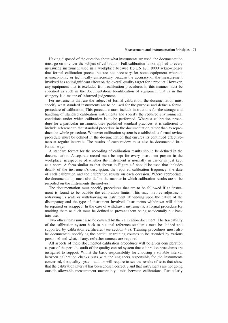
Measurement and Instrumentation Principles 71
Having disposed of the question about what instruments are used, the documentationmust go on to cover the subject of calibration. Full calibration is not applied to everymeasuring instrument used in a workplace because BS EN ISO 9000 acknowledgesthat formal calibration procedures are not necessary for some equipment where itis uneconomic or technically unnecessary because the accuracy of the measurementinvolved has an insignificant effect on the overall quality target for a product. However,any equipment that is excluded from calibration procedures in this manner must bespecified as such in the documentation. Identification of equipment that is in thiscategory is a matter of informed judgement.
For instruments that are the subject of formal calibration, the documentation mustspecify what standard instruments are to be used for the purpose and define a formalprocedure of calibration. This procedure must include instructions for the storage andhandling of standard calibration instruments and specify the required environmentalconditions under which calibration is to be performed. Where a calibration proce-dure for a particular instrument uses published standard practices, it is sufficient toinclude reference to that standard procedure in the documentation rather than to repro-duce the whole procedure. Whatever calibration system is established, a formal reviewprocedure must be defined in the documentation that ensures its continued effective-ness at regular intervals. The results of each review must also be documented in aformal way.
A standard format for the recording of calibration results should be defined in thedocumentation. A separate record must be kept for every instrument present in theworkplace, irrespective of whether the instrument is normally in use or is just keptas a spare. A form similar to that shown in Figure 4.3 should be used that includesdetails of the instrument’s description, the required calibration frequency, the dateof each calibration and the calibration results on each occasion. Where appropriate,the documentation must also define the manner in which calibration results are to berecorded on the instruments themselves.
The documentation must specify procedures that are to be followed if an instru-ment is found to be outside the calibration limits. This may involve adjustment,redrawing its scale or withdrawing an instrument, depending upon the nature of thediscrepancy and the type of instrument involved. Instruments withdrawn will eitherbe repaired or scrapped. In the case of withdrawn instruments, a formal procedure formarking them as such must be defined to prevent them being accidentally put backinto use.
Two other items must also be covered by the calibration document. The traceabilityof the calibration system back to national reference standards must be defined andsupported by calibration certificates (see section 4.3). Training procedures must alsobe documented, specifying the particular training courses to be attended by variouspersonnel and what, if any, refresher courses are required.
All aspects of these documented calibration procedures will be given considerationas part of the periodic audit of the quality control system that calibration procedures areinstigated to support. Whilst the basic responsibility for choosing a suitable intervalbetween calibration checks rests with the engineers responsible for the instrumentsconcerned, the quality system auditor will require to see the results of tests that showthat the calibration interval has been chosen correctly and that instruments are not goingoutside allowable measurement uncertainty limits between calibrations. Particularly
72 Calibration of measuring sensors and instruments
Type of instrument:
Manufacturer's part number:
Measurement limit:
Location:
Instructions for use:
Calibration frequency:
Company serial number:
Manufacturer's serial number:
Date introduced:
Signature of person responsiblefor calibration:
CALIBRATION RECORD
Calibration date: Calibration results Calibrated by
Fig. 4.3 Typical format for instrument record sheets.
important in such audits will be the existence of procedures that are instigated inresponse to instruments found to be out of calibration. Evidence that such proceduresare effective in avoiding degradation in the quality assurance function will also berequired.
References and further reading
British Standards Society (1979) The operation of a company standards department, BritishStandards Society, London.
ISO 5725 (1998) Precision of test methods – determination of repeatability and reproducibilityby inter-laboratory tests, International Organization for Standards, Geneva.
ISO 9000 (2000): Quality Management and Quality Assurance Standards, International Organi-zation for Standards, Geneva (individual parts published as ISO 9001, ISO 9002, ISO 9003and ISO 9004).
5
Measurement noise andsignal processing
5.1 Sources of measurement noise
Chapter 3 has already provided a detailed analysis of error sources that arise duringthe measurement process of sensing the value of a physical variable and generatingan output signal. However, further errors are often created in measurement systemswhen electrical signals from measurement sensors and transducers are corrupted byinduced noise. This induced noise arises both within the measurement circuit itself andalso during the transmission of measurement signals to remote points. The aim whendesigning measurement systems is always to reduce such induced noise voltage levelsas far as possible. However, it is usually not possible to eliminate all such noise, andsignal processing has to be applied to deal with any noise that remains.
Noise voltages can exist either in serial mode or common mode forms. Serial modenoise voltages act in series with the output voltage from a measurement sensor ortransducer, which can cause very significant errors in the output measurement signal.The extent to which series mode noise corrupts measurement signals is measured bya quantity known as the signal-to-noise ratio. This is defined as:
Signal-to-noise ratio D 20 log10
(Vs
Vn
)
where Vs is the mean voltage level of the signal and Vn is the mean voltage level ofthe noise. In the case of a.c. noise voltages, the root-mean squared value is used as themean.
Common mode noise voltages are less serious, because they cause the potential ofboth sides of a signal circuit to be raised by the same level, and thus the level of theoutput measurement signal is unchanged. However, common mode voltages do haveto be considered carefully, since they can be converted into series mode voltages incertain circumstances.
Noise can be generated from sources both external and internal to the measure-ment system. Induced noise from external sources arises in measurement systemsfor a number of reasons that include their proximity to mains-powered equipmentand cables (causing noise at the mains frequency), proximity to fluorescent lighting
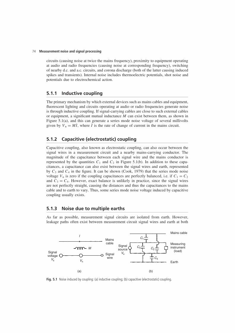
74 Measurement noise and signal processing
circuits (causing noise at twice the mains frequency), proximity to equipment operatingat audio and radio frequencies (causing noise at corresponding frequency), switchingof nearby d.c. and a.c. circuits, and corona discharge (both of the latter causing inducedspikes and transients). Internal noise includes thermoelectric potentials, shot noise andpotentials due to electrochemical action.
5.1.1 Inductive coupling
The primary mechanism by which external devices such as mains cables and equipment,fluorescent lighting and circuits operating at audio or radio frequencies generate noiseis through inductive coupling. If signal-carrying cables are close to such external cablesor equipment, a significant mutual inductance M can exist between them, as shown inFigure 5.1(a), and this can generate a series mode noise voltage of several millivoltsgiven by Vn D MPI, where PI is the rate of change of current in the mains circuit.
5.1.2 Capacitive (electrostatic) coupling
Capacitive coupling, also known as electrostatic coupling, can also occur between thesignal wires in a measurement circuit and a nearby mains-carrying conductor. Themagnitude of the capacitance between each signal wire and the mains conductor isrepresented by the quantities C1 and C2 in Figure 5.1(b). In addition to these capa-citances, a capacitance can also exist between the signal wires and earth, representedby C3 and C4 in the figure. It can be shown (Cook, 1979) that the series mode noisevoltage Vn is zero if the coupling capacitances are perfectly balanced, i.e. if C1 D C2
and C3 D C4. However, exact balance is unlikely in practice, since the signal wiresare not perfectly straight, causing the distances and thus the capacitances to the mainscable and to earth to vary. Thus, some series mode noise voltage induced by capacitivecoupling usually exists.
5.1.3 Noise due to multiple earths
As far as possible, measurement signal circuits are isolated from earth. However,leakage paths often exist between measurement circuit signal wires and earth at both
Signalvoltage
Vs
Signalsource
VsSignalwire
(a) (b)
Mainscable
Mains cable
Earth
Measuringinstrument
(load)
I
M
Vn
C1
C3 C2
C4
Fig. 5.1 Noise induced by coupling: (a) inductive coupling; (b) capacitive (electrostatic) coupling.
Measurement and Instrumentation Principles 75
the source (sensor) end of the circuit and also the load (measuring instrument) end.This does not cause a problem as long as the earth potential at both ends is the same.However, it is common to find that other machinery and equipment carrying largecurrents is connected to the same earth plane. This can cause the potential to varybetween different points on the earth plane. This situation, which is known as multipleearths, can cause a series mode noise voltage in the measurement circuit.
5.1.4 Noise in the form of voltage transients
When motors and other electrical equipment (both a.c. and d.c.) are switched on and off,large changes of power consumption suddenly occur in the electricity supply system.This can cause voltage transients (‘spikes’) in measurement circuits connected to thesame power supply. Such noise voltages are of large magnitude but short time duration.Corona discharge can also cause voltage transients on the mains power supply. Thisoccurs when the air in the vicinity of high voltage d.c. circuits becomes ionized anddischarges to earth at random times.
5.1.5 Thermoelectric potentials
Whenever metals of two different types are connected together, a thermoelectric poten-tial (sometimes called a thermal e.m.f.) is generated according to the temperature of thejoint. This is known as the thermoelectric effect and is the physical principle on whichtemperature-measuring thermocouples operate (see Chapter 14). Such thermoelectricpotentials are only a few millivolts in magnitude and so the effect is only significantwhen typical voltage output signals of a measurement system are of a similar lowmagnitude.
One such situation is where one e.m.f.-measuring instrument is used to monitor theoutput of several thermocouples measuring the temperatures at different points in aprocess control system. This requires a means of automatically switching the outputof each thermocouple to the measuring instrument in turn. Nickel–iron reed-relayswith copper connecting leads are commonly used to provide this switching function.This introduces a thermocouple effect of magnitude 40 μV/°C between the reed-relayand the copper connecting leads. There is no problem if both ends of the reed relayare at the same temperature because then the thermoelectric potentials will be equaland opposite and so cancel out. However, there are several recorded instances where,because of lack of awareness of the problem, poor design has resulted in the twoends of a reed-relay being at different temperatures and causing a net thermoelectricpotential. The serious error that this introduces is clear. For a temperature differencebetween the two ends of only 2°C, the thermoelectric potential is 80 μV, which is verylarge compared with a typical thermocouple output level of 400 μV.
Another example of the difficulties that thermoelectric potentials can create becomesapparent in considering the following problem that was reported in a current-measuringsystem. This system had been designed such that the current flowing in a particularpart of a circuit was calculated by applying it to an accurately calibrated wire-woundresistance of value 100 � and measuring the voltage drop across the resistance. In
76 Measurement noise and signal processing
calibration of the system, a known current of 20 μA was applied to the resistance and avoltage of 2.20 mV was measured by an accurate high-impedance instrument. Simpleapplication of Ohm’s law reveals that such a voltage reading indicates a current valueof 22 μA. What then was the explanation for this discrepancy? The answer once againis a thermoelectric potential. Because the designer was not aware of thermoelectricpotentials, the circuit had been constructed such that one side of the standard resistancewas close to a power transistor, creating a difference in temperature between the twoends of the resistor of 2°C. The thermoelectric potential associated with this wassufficient to account for the 10% measurement error found.
5.1.6 Shot noise
Shot noise occurs in transistors, integrated circuits and other semiconductor devices.It consists of random fluctuations in the rate of transfer of carriers across junctionswithin such devices.
5.1.7 Electrochemical potentials
These are potentials that arise within measurement systems due to electrochemicalaction. Poorly soldered joints are a common source.
5.2 Techniques for reducing measurement noise
Prevention is always better than cure, and much can be done to reduce the levelof measurement noise by taking appropriate steps when designing the measurementsystem.
5.2.1 Location and design of signal wires
Both the mutual inductance and capacitance between signal wires and other cables areinversely proportional to the square of the distance between the wires and the cable.Thus, noise due to inductive and capacitive coupling can be minimized by ensuringthat signal wires are positioned as far away as possible from such noise sources. Aminimum separation of 0.3 m is essential, and a separation of at least 1 m is preferable.Noise due to inductive coupling is also substantially reduced if each pair of signalwires is twisted together along its length. This design is known as a twisted pair, andis illustrated in Figure 5.2. In the first loop, wire A is closest to the noise source andhas a voltage V1 induced in it, whilst wire B has an induced noise voltage V2. Forloop 2, wire B is closest to the noise source and has an induced voltage V1 whilst wireA has an induced voltage V2. Thus the total voltage induced in wire A is V1 C V2 andin wire B it is V2 C V1 over these two loops. This pattern continues for all the loopsand hence the two wires have an identical voltage induced in them.
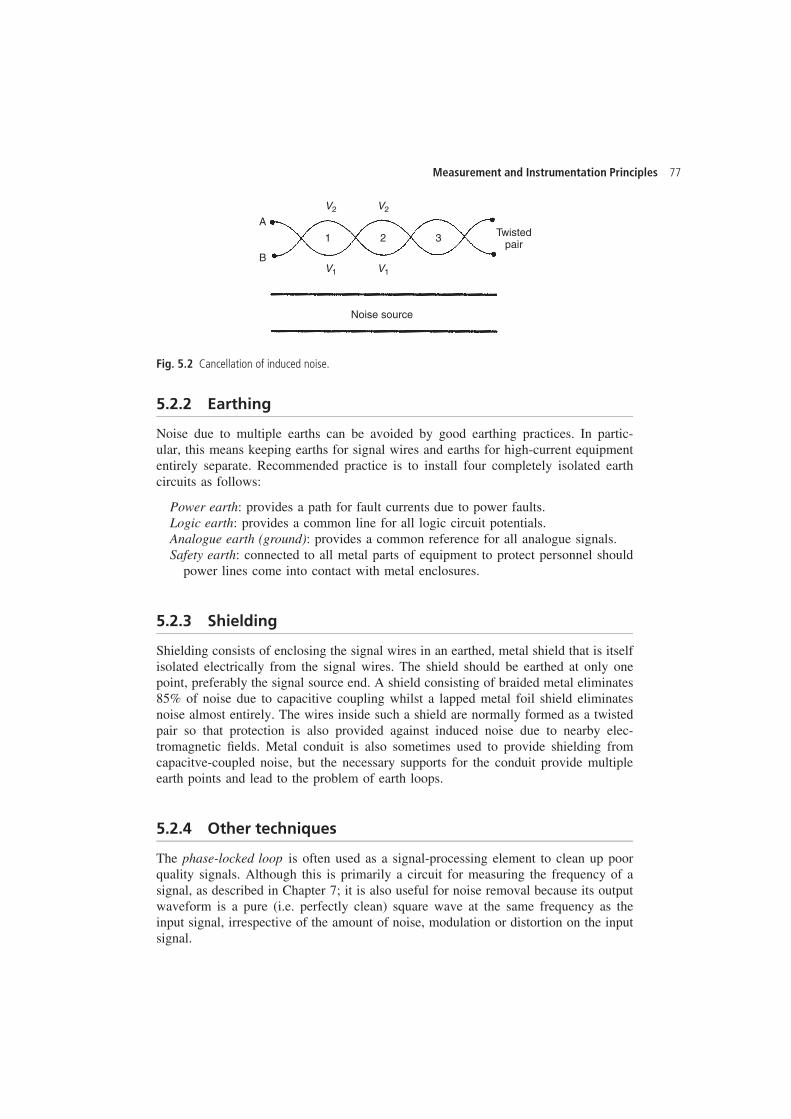
Measurement and Instrumentation Principles 77
A
1 2
V1
3
BV1
V2V2
Noise source
Twistedpair
Fig. 5.2 Cancellation of induced noise.
5.2.2 Earthing
Noise due to multiple earths can be avoided by good earthing practices. In partic-ular, this means keeping earths for signal wires and earths for high-current equipmententirely separate. Recommended practice is to install four completely isolated earthcircuits as follows:
Power earth: provides a path for fault currents due to power faults.Logic earth: provides a common line for all logic circuit potentials.Analogue earth (ground): provides a common reference for all analogue signals.Safety earth: connected to all metal parts of equipment to protect personnel should
power lines come into contact with metal enclosures.
5.2.3 Shielding
Shielding consists of enclosing the signal wires in an earthed, metal shield that is itselfisolated electrically from the signal wires. The shield should be earthed at only onepoint, preferably the signal source end. A shield consisting of braided metal eliminates85% of noise due to capacitive coupling whilst a lapped metal foil shield eliminatesnoise almost entirely. The wires inside such a shield are normally formed as a twistedpair so that protection is also provided against induced noise due to nearby elec-tromagnetic fields. Metal conduit is also sometimes used to provide shielding fromcapacitve-coupled noise, but the necessary supports for the conduit provide multipleearth points and lead to the problem of earth loops.
5.2.4 Other techniques
The phase-locked loop is often used as a signal-processing element to clean up poorquality signals. Although this is primarily a circuit for measuring the frequency of asignal, as described in Chapter 7; it is also useful for noise removal because its outputwaveform is a pure (i.e. perfectly clean) square wave at the same frequency as theinput signal, irrespective of the amount of noise, modulation or distortion on the inputsignal.
78 Measurement noise and signal processing
Lock-in amplifiers (see section 5.5.10) are also commonly used to extract d.c. orslowly varying measurement signals from noise. The input measurement signal ismodulated into a square-wave a.c. signal whose amplitude varies with the level of theinput signal. This is normally achieved by either a relay or a field effect transistor.As a relay is subject to wear; the transistor is better. An alternative method is to usean analogue multiplier. Also, in the case of optical signals, the square wave can beproduced by chopping the measurement signals using a set of windows in a rotatingdisc. This technique is frequently used with transducers like photodiodes that oftengenerate large quantities of noise.
5.3 Introduction to signal processing
Signal processing is concerned with improving the quality of the reading or signal at theoutput of a measurement system, and one particular aim is to attenuate any noise in themeasurement signal that has not been eliminated by careful design of the measurementsystem as discussed above. However, signal processing performs many other functionsapart from dealing with noise, and the exact procedures that are applied depend on thenature of the raw output signal from a measurement transducer. Procedures of signalfiltering, signal amplification, signal attenuation, signal linearization and bias removalare applied according to the form of correction required in the raw signal.
Traditionally, signal processing has been carried out by analogue techniques in thepast, using various types of electronic circuit. However, the ready availability of digitalcomputers in recent years has meant that signal processing has increasingly been carriedout digitally, using software modules to condition the input measurement data.
Digital signal processing is inherently more accurate than analogue techniques, butthis advantage is greatly reduced in the case of measurements coming from analoguesensors and transducers, because an analogue-to-digital conversion stage is necessarybefore the digital processing can be applied, thereby introducing conversion errors.Also, analogue processing remains the faster of the two alternatives in spite of recentadvances in the speed of digital signal processing. Hence, both analogue and digitalprocessing are considered in this chapter, with analogue processing being consideredfirst because some preliminary analogue processing is often carried out even when themajor part of the processing is carried out digitally.
5.4 Analogue signal filtering
Signal filtering consists of processing a signal to remove a certain band of frequencieswithin it. The band of frequencies removed can be either at the low-frequency end ofthe frequency spectrum, at the high-frequency end, at both ends, or in the middle ofthe spectrum. Filters to perform each of these operations are known respectively aslow-pass filters, high-pass filters, band-pass filters and band-stop filters (also knownas notch filters). All such filtering operations can be carried out by either analogue ordigital methods.
The result of filtering can be readily understood if the analogy with a proceduresuch as sieving soil particles is considered. Suppose that a sample of soil A is passed
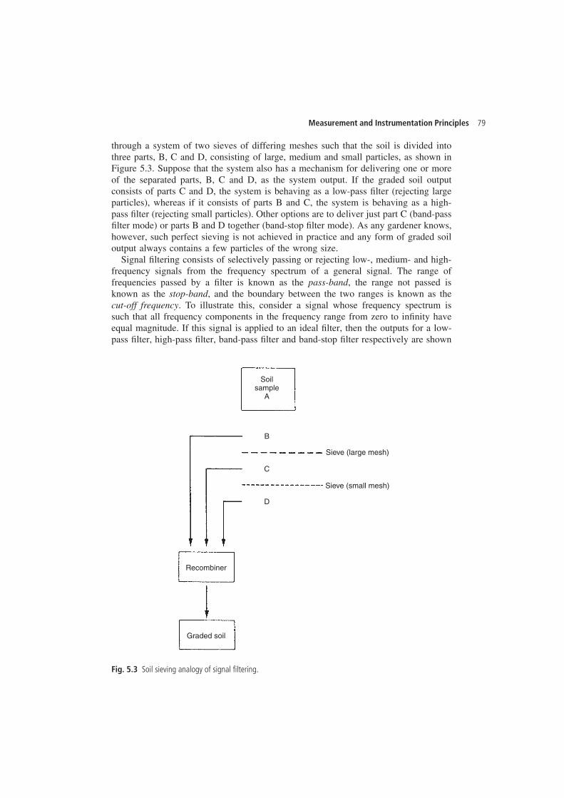
Measurement and Instrumentation Principles 79
through a system of two sieves of differing meshes such that the soil is divided intothree parts, B, C and D, consisting of large, medium and small particles, as shown inFigure 5.3. Suppose that the system also has a mechanism for delivering one or moreof the separated parts, B, C and D, as the system output. If the graded soil outputconsists of parts C and D, the system is behaving as a low-pass filter (rejecting largeparticles), whereas if it consists of parts B and C, the system is behaving as a high-pass filter (rejecting small particles). Other options are to deliver just part C (band-passfilter mode) or parts B and D together (band-stop filter mode). As any gardener knows,however, such perfect sieving is not achieved in practice and any form of graded soiloutput always contains a few particles of the wrong size.
Signal filtering consists of selectively passing or rejecting low-, medium- and high-frequency signals from the frequency spectrum of a general signal. The range offrequencies passed by a filter is known as the pass-band, the range not passed isknown as the stop-band, and the boundary between the two ranges is known as thecut-off frequency. To illustrate this, consider a signal whose frequency spectrum issuch that all frequency components in the frequency range from zero to infinity haveequal magnitude. If this signal is applied to an ideal filter, then the outputs for a low-pass filter, high-pass filter, band-pass filter and band-stop filter respectively are shown
Soilsample
A
B
C
D
Recombiner
Graded soil
Sieve (small mesh)
Sieve (large mesh)
Fig. 5.3 Soil sieving analogy of signal filtering.
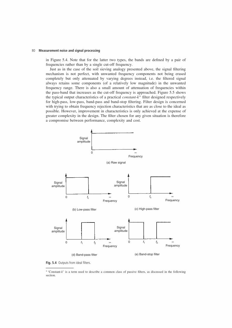
80 Measurement noise and signal processing
in Figure 5.4. Note that for the latter two types, the bands are defined by a pair offrequencies rather than by a single cut-off frequency.
Just as in the case of the soil sieving analogy presented above, the signal filteringmechanism is not perfect, with unwanted frequency components not being erasedcompletely but only attenuated by varying degrees instead, i.e. the filtered signalalways retains some components (of a relatively low magnitude) in the unwantedfrequency range. There is also a small amount of attenuation of frequencies withinthe pass-band that increases as the cut-off frequency is approached. Figure 5.5 showsthe typical output characteristics of a practical constant-kŁ filter designed respectivelyfor high-pass, low-pass, band-pass and band-stop filtering. Filter design is concernedwith trying to obtain frequency rejection characteristics that are as close to the ideal aspossible. However, improvement in characteristics is only achieved at the expense ofgreater complexity in the design. The filter chosen for any given situation is thereforea compromise between performance, complexity and cost.
Signalamplitude
Frequency0 ∞
Signalamplitude
Frequency
(b) Low-pass filter
(a) Raw signal
0 fc ∞
Signalamplitude
Frequency
(c) High-pass filter
0 fc ∞
Signalamplitude
Frequency
(d) Band-pass filter
0 f1 f2 ∞
Signalamplitude
Frequency
(e) Band-stop filter
0 f1 f2 ∞
Fig. 5.4 Outputs from ideal filters.
Ł ‘Constant-k’ is a term used to describe a common class of passive filters, as discussed in the followingsection.
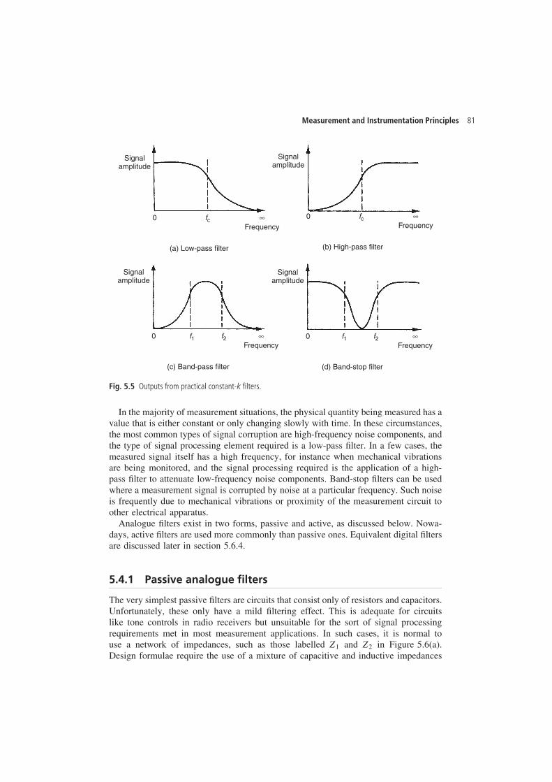
Measurement and Instrumentation Principles 81
Signalamplitude
Frequency
(a) Low-pass filter
0 fc ∞
Signalamplitude
Frequency
(b) High-pass filter
0 fc ∞
Signalamplitude
Frequency
(c) Band-pass filter
0 f1 f2 ∞
Signalamplitude
Frequency
(d) Band-stop filter
0 f1 f2 ∞
Fig. 5.5 Outputs from practical constant-k filters.
In the majority of measurement situations, the physical quantity being measured has avalue that is either constant or only changing slowly with time. In these circumstances,the most common types of signal corruption are high-frequency noise components, andthe type of signal processing element required is a low-pass filter. In a few cases, themeasured signal itself has a high frequency, for instance when mechanical vibrationsare being monitored, and the signal processing required is the application of a high-pass filter to attenuate low-frequency noise components. Band-stop filters can be usedwhere a measurement signal is corrupted by noise at a particular frequency. Such noiseis frequently due to mechanical vibrations or proximity of the measurement circuit toother electrical apparatus.
Analogue filters exist in two forms, passive and active, as discussed below. Nowa-days, active filters are used more commonly than passive ones. Equivalent digital filtersare discussed later in section 5.6.4.
5.4.1 Passive analogue filters
The very simplest passive filters are circuits that consist only of resistors and capacitors.Unfortunately, these only have a mild filtering effect. This is adequate for circuitslike tone controls in radio receivers but unsuitable for the sort of signal processingrequirements met in most measurement applications. In such cases, it is normal touse a network of impedances, such as those labelled Z1 and Z2 in Figure 5.6(a).Design formulae require the use of a mixture of capacitive and inductive impedances
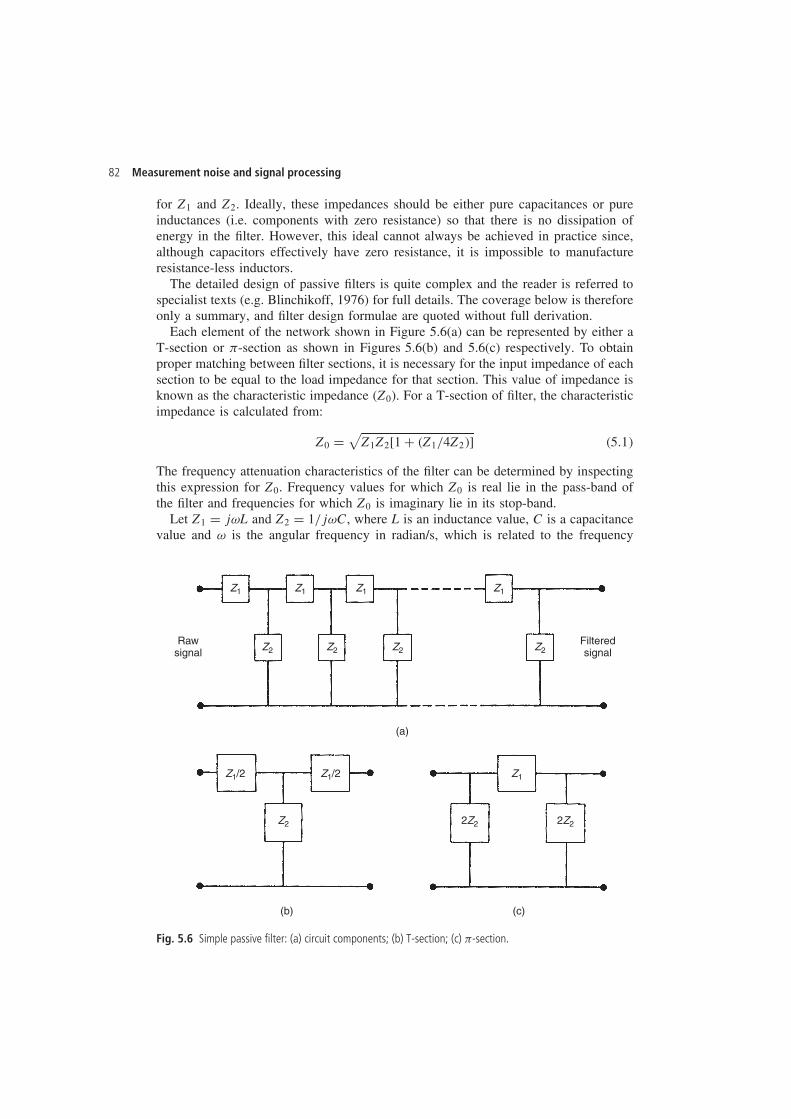
82 Measurement noise and signal processing
for Z1 and Z2. Ideally, these impedances should be either pure capacitances or pureinductances (i.e. components with zero resistance) so that there is no dissipation ofenergy in the filter. However, this ideal cannot always be achieved in practice since,although capacitors effectively have zero resistance, it is impossible to manufactureresistance-less inductors.
The detailed design of passive filters is quite complex and the reader is referred tospecialist texts (e.g. Blinchikoff, 1976) for full details. The coverage below is thereforeonly a summary, and filter design formulae are quoted without full derivation.
Each element of the network shown in Figure 5.6(a) can be represented by either aT-section or -section as shown in Figures 5.6(b) and 5.6(c) respectively. To obtainproper matching between filter sections, it is necessary for the input impedance of eachsection to be equal to the load impedance for that section. This value of impedance isknown as the characteristic impedance (Z0). For a T-section of filter, the characteristicimpedance is calculated from:
Z0 D√
Z1Z2[1 C �Z1/4Z2�] �5.1�
The frequency attenuation characteristics of the filter can be determined by inspectingthis expression for Z0. Frequency values for which Z0 is real lie in the pass-band ofthe filter and frequencies for which Z0 is imaginary lie in its stop-band.
Let Z1 D jωL and Z2 D 1/jωC, where L is an inductance value, C is a capacitancevalue and ω is the angular frequency in radian/s, which is related to the frequency
Z2
Z2 2Z2 2Z2
Z2 Z2 Z2
Z1Z1 Z1 Z1
Z1Z1/2 Z1/2
Rawsignal
Filteredsignal
(a)
(b) (c)
Fig. 5.6 Simple passive filter: (a) circuit components; (b) T-section; (c) -section.
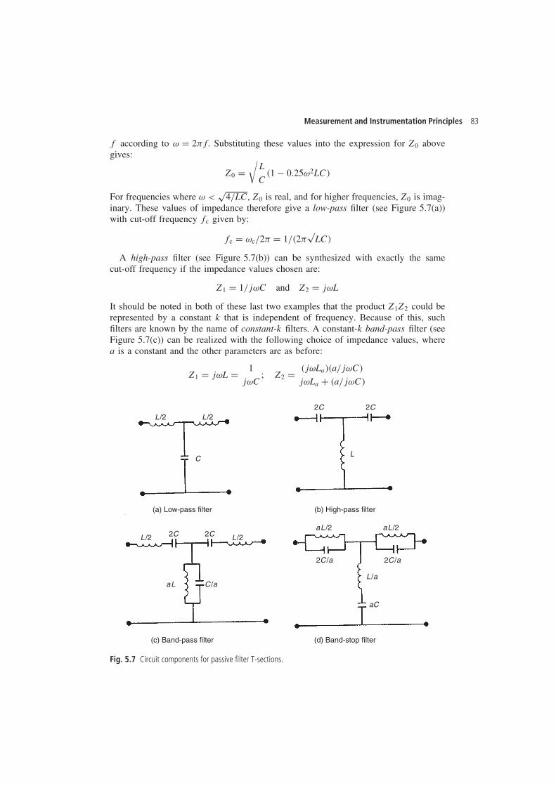
Measurement and Instrumentation Principles 83
f according to ω D 2f. Substituting these values into the expression for Z0 abovegives:
Z0 D√
L
C�1 � 0.25ω2LC�
For frequencies where ω <p
4/LC, Z0 is real, and for higher frequencies, Z0 is imag-inary. These values of impedance therefore give a low-pass filter (see Figure 5.7(a))with cut-off frequency fc given by:
fc D ωc/2 D 1/�2p
LC�
A high-pass filter (see Figure 5.7(b)) can be synthesized with exactly the samecut-off frequency if the impedance values chosen are:
Z1 D 1/jωC and Z2 D jωL
It should be noted in both of these last two examples that the product Z1Z2 could berepresented by a constant k that is independent of frequency. Because of this, suchfilters are known by the name of constant-k filters. A constant-k band-pass filter (seeFigure 5.7(c)) can be realized with the following choice of impedance values, wherea is a constant and the other parameters are as before:
Z1 D jωL D 1
jωC; Z2 D �jωLa��a/jωC�
jωLa C �a/jωC�
L/2 L/2
L/2
aL
aC
L/aC/a
L/2aL/2 aL/2
C
(a) Low-pass filter
(c) Band-pass filter
2C
2C 2C
2C
L
(b) High-pass filter
(d) Band-stop filter
2C/a 2C/a
Fig. 5.7 Circuit components for passive filter T-sections.
84 Measurement noise and signal processing
The frequencies f1 and f2 defining the end of the pass-band are most easily expressedin terms of a frequency f0 in the centre of the pass-band. The corresponding equationsare:
f0 D 1
2p
LC; f1 D f0[
p1 C a � p
a]; f2 D f0[p
1 C a C pa]
For a constant-k band-stop filter (see Figure 5.7(d)), the appropriate impedancevalues are:
Z1 D �jωLa��a/jωC�
jωLa C �a/jωC�; Z2 D 1
a
(jωL C 1
jωC
)
The frequencies defining the ends of the stop-band are again normally defined in termsof the frequency f0 in the centre of the stop-band:
f0 D 1
2p
LC; f1 D f0
(1 � a
4
); f2 D f0
(1 C a
4
)
As has already been mentioned, a practical filter does not eliminate frequencies in thestop-band but merely attenuates them by a certain amount. The attenuation coefficient,˛, at a frequency in the stop band, f, for a single T-section of a low-pass filter isgiven by:
˛ D 2 cosh�1�f/fc� �5.2�
The relatively poor attenuation characteristics are obvious if we evaluate this expres-sion for a value of frequency close to the cut-off frequency given by f D 2fc. Then˛ D 2 cosh�1�2� D 2.64. Further away from the cut-off frequency, for f D 20fc, ˛ D2 cosh�1�20� D 7.38.
Improved attenuation characteristics can be obtained by putting several T-sections incascade. If perfect matching is assumed, then two T-sections give twice the attenuationof one section, i.e. at frequencies of 2fc and 20fc, ˛ for two sections would have avalue of 5.28 and 14.76 respectively.
The discussion so far has assumed that the inductances are resistance-less and thatthere is perfect matching between filter sections. However, it has already been noted thatsuch ideal conditions cannot be achieved in practice, and this has several consequences.Inspection of the expression for the characteristic impedance (5.1) reveals frequency-dependent terms. Thus, the condition that the load impedance is equal to the inputimpedance for a section is only satisfied at one particular frequency. It is usual to matchthe impedances at zero frequency for a low-pass filter and at infinite frequency for ahigh-pass filter. This ensures that the frequency where the input and load impedancesare matched is comfortably within the pass-band of the filter. Frequency dependency isone of the reasons for the degree of attenuation in the pass-band shown in the practicalfilter characteristics of Figure 5.5, the other reason being the presence of resistivecomponents in the inductors of the filter. The effect of this in a practical filter is thatthe value of ˛ at the cut-off frequency is 1.414 whereas the value predicted theoreticallyfor an ideal filter (equation 5.2) is zero. Cascading filter sections together increasesthis attenuation in the pass-band as well as increasing attenuation of frequencies in thestop-band.
Measurement and Instrumentation Principles 85
This problem of matching successive sections in a cascaded filter seriously degradesthe performance of constant-k filters and this has resulted in the development of othertypes such as m-derived and n-derived composite filters. These produce less attenuationwithin the pass-band and greater attenuation outside it than constant-k filters, althoughthis is only achieved at the expense of greater filter complexity and cost. The readerinterested in further consideration of these is directed to consult one of the specialisttexts recommended in the Further Reading section at the end of this chapter.
5.4.2 Active analogue filters
In the foregoing discussion on passive filters, the two main difficulties noted were thoseof obtaining resistance-less inductors and achieving proper matching between signalsource and load through the filter sections. A further problem is that the inductorsrequired by passive filters are bulky and relatively expensive. Active filters overcomeall of these problems and so they are now used more commonly than passive filters.
The major component in an active filter is an electronic amplifier. The filter char-acteristics are defined by amplifier input and feedback components that consist ofresistors and capacitors but not inductors. The fact that the necessary characteristicscan be obtained using only resistors and capacitors, without requiring inductors, is aparticular advantage of this class of filters. The circuits shown in Figure 5.8 producethe four types of filter characteristics discussed earlier. These are all known as secondorder filters, because the input–output relationship across each filter is described by asecond order differential equation.
The characteristics of each filter in terms of attenuation behaviour in the pass- andstop-bands is determined by the choice of circuit components in Figure 5.8. A commonset of design formulae is given below, although detailed derivation is not given. Furtherinformation on the derivation of these formulae can be found in specialist texts (e.g.Stephenson, 1985):
(a) Low-pass filter (b) High-pass filter
ω0 D√
1R1R2C1C2
ω0 D√
1R1R2C1C2
G D 1 C �R4/R3� G D 1 C �R4/R3�where ω0 is the cut-off frequencyand G is the filter gain (at d.c.).
where ω0 is the cut-off frequency and Gis the filter gain (at infinite frequency).
(c) Band-pass filter (d) Band-stop filter
ω0 Dp
2R1C ω0 D
√1
R4C2
(1R1
C 1R2
)ω1 D ω0 � 4 � G
2R1C ω1 D ω0 � 1R4C
ω2 D ω0 C 4 � G2R1C ω2 D ω0 C 1
R4CG D filter gain �at frequency ω0�
D 1 C R3/R2 where ω1 and ω2
are frequencies at ends of thepass-band, and ω0 is centrefrequency of the pass-band.
G D filter gain (at d.c. and also highfrequency� D �R6/R3 where ω1 and ω2
are frequencies at ends of thestop-band, and ω0 is centre frequencyof the stop-band.
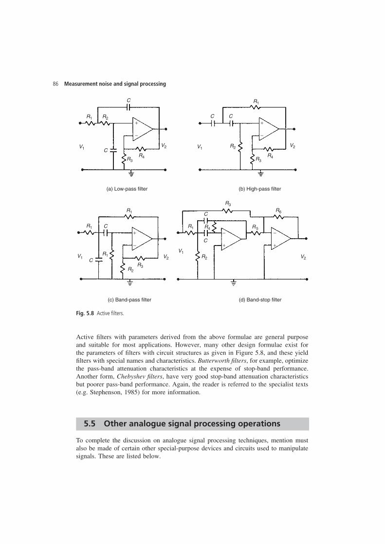
86 Measurement noise and signal processing
C
C
R1
V1V2
R2
R2
R3R4
R4 R5
R6
+
−
C C
R1
V1V2
R3R4
+
−
C
C
C
C
R1
R1
R1
R1
V1 V2
V1V2
R2
R2
R3
R3
+
−
−
+
−
+
(a) Low-pass filter (b) High-pass filter
(d) Band-stop filter(c) Band-pass filter
Fig. 5.8 Active filters.
Active filters with parameters derived from the above formulae are general purposeand suitable for most applications. However, many other design formulae exist forthe parameters of filters with circuit structures as given in Figure 5.8, and these yieldfilters with special names and characteristics. Butterworth filters, for example, optimizethe pass-band attenuation characteristics at the expense of stop-band performance.Another form, Chebyshev filters, have very good stop-band attenuation characteristicsbut poorer pass-band performance. Again, the reader is referred to the specialist texts(e.g. Stephenson, 1985) for more information.
5.5 Other analogue signal processing operations
To complete the discussion on analogue signal processing techniques, mention mustalso be made of certain other special-purpose devices and circuits used to manipulatesignals. These are listed below.
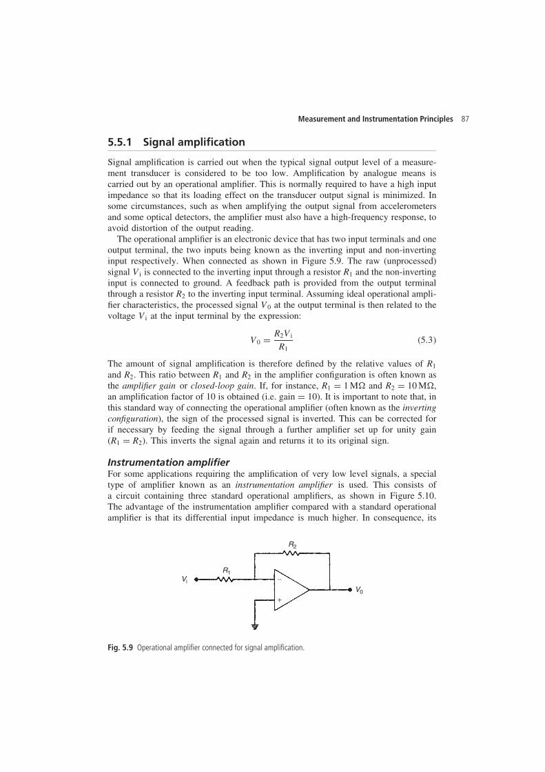
Measurement and Instrumentation Principles 87
5.5.1 Signal amplification
Signal amplification is carried out when the typical signal output level of a measure-ment transducer is considered to be too low. Amplification by analogue means iscarried out by an operational amplifier. This is normally required to have a high inputimpedance so that its loading effect on the transducer output signal is minimized. Insome circumstances, such as when amplifying the output signal from accelerometersand some optical detectors, the amplifier must also have a high-frequency response, toavoid distortion of the output reading.
The operational amplifier is an electronic device that has two input terminals and oneoutput terminal, the two inputs being known as the inverting input and non-invertinginput respectively. When connected as shown in Figure 5.9. The raw (unprocessed)signal Vi is connected to the inverting input through a resistor R1 and the non-invertinginput is connected to ground. A feedback path is provided from the output terminalthrough a resistor R2 to the inverting input terminal. Assuming ideal operational ampli-fier characteristics, the processed signal V0 at the output terminal is then related to thevoltage Vi at the input terminal by the expression:
V0 D R2Vi
R1�5.3�
The amount of signal amplification is therefore defined by the relative values of R1
and R2. This ratio between R1 and R2 in the amplifier configuration is often known asthe amplifier gain or closed-loop gain. If, for instance, R1 D 1 M� and R2 D 10 M�,an amplification factor of 10 is obtained (i.e. gain D 10). It is important to note that, inthis standard way of connecting the operational amplifier (often known as the invertingconfiguration), the sign of the processed signal is inverted. This can be corrected forif necessary by feeding the signal through a further amplifier set up for unity gain(R1 D R2). This inverts the signal again and returns it to its original sign.
Instrumentation amplifierFor some applications requiring the amplification of very low level signals, a specialtype of amplifier known as an instrumentation amplifier is used. This consists ofa circuit containing three standard operational amplifiers, as shown in Figure 5.10.The advantage of the instrumentation amplifier compared with a standard operationalamplifier is that its differential input impedance is much higher. In consequence, its
R1
R2
Vi
V0
+
−
Fig. 5.9 Operational amplifier connected for signal amplification.
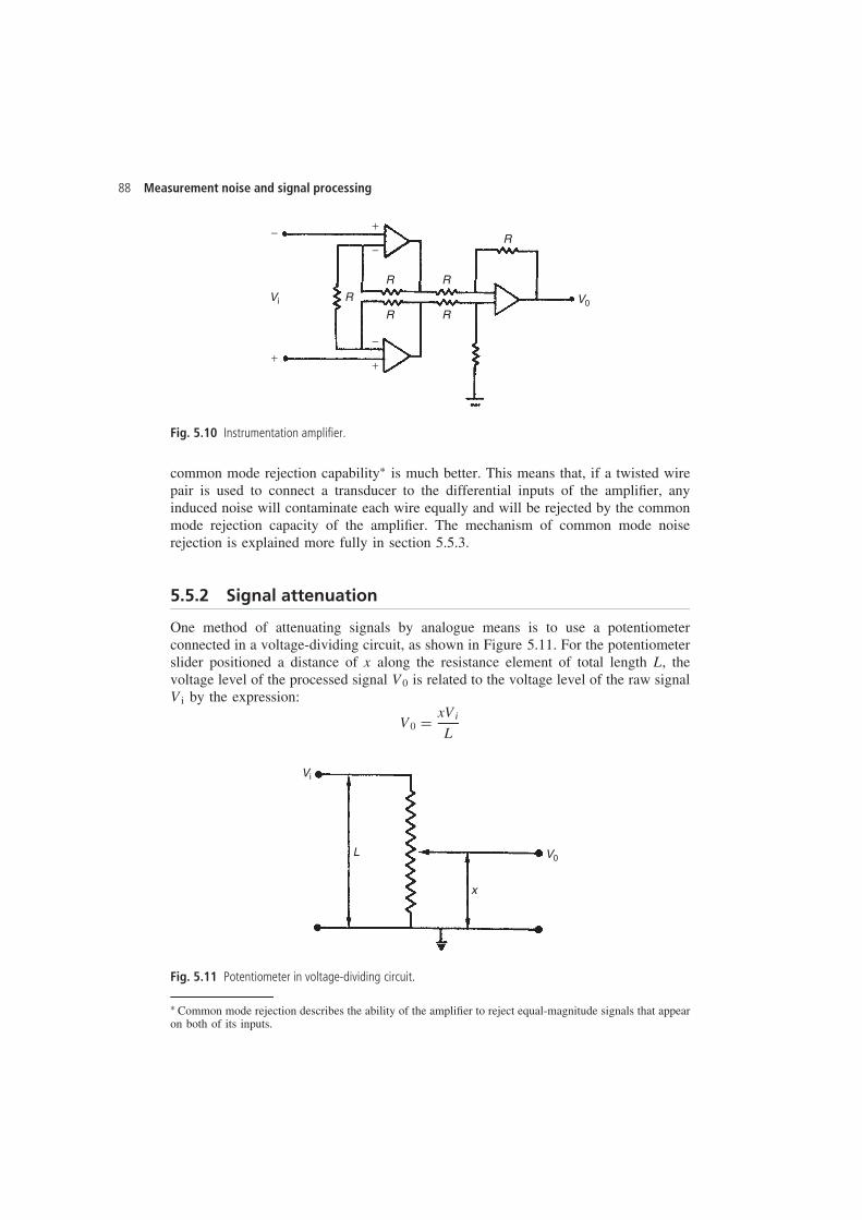
88 Measurement noise and signal processing
Vi V0R
R
R
R
R
R
−−
+
+
+
−
Fig. 5.10 Instrumentation amplifier.
common mode rejection capabilityŁ is much better. This means that, if a twisted wirepair is used to connect a transducer to the differential inputs of the amplifier, anyinduced noise will contaminate each wire equally and will be rejected by the commonmode rejection capacity of the amplifier. The mechanism of common mode noiserejection is explained more fully in section 5.5.3.
5.5.2 Signal attenuation
One method of attenuating signals by analogue means is to use a potentiometerconnected in a voltage-dividing circuit, as shown in Figure 5.11. For the potentiometerslider positioned a distance of x along the resistance element of total length L, thevoltage level of the processed signal V0 is related to the voltage level of the raw signalVi by the expression:
V0 D xVi
L
Vi
V0L
x
Fig. 5.11 Potentiometer in voltage-dividing circuit.
Ł Common mode rejection describes the ability of the amplifier to reject equal-magnitude signals that appearon both of its inputs.
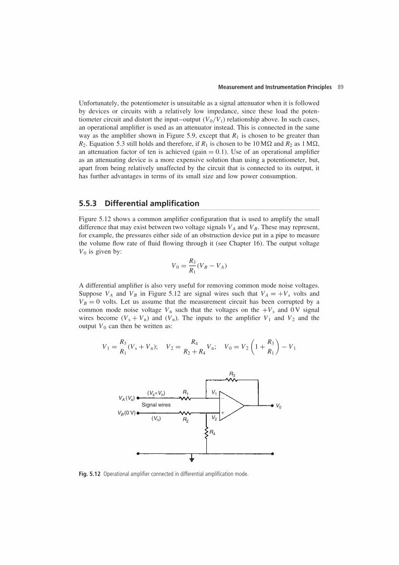
Measurement and Instrumentation Principles 89
Unfortunately, the potentiometer is unsuitable as a signal attenuator when it is followedby devices or circuits with a relatively low impedance, since these load the poten-tiometer circuit and distort the input–output �V0/Vi� relationship above. In such cases,an operational amplifier is used as an attenuator instead. This is connected in the sameway as the amplifier shown in Figure 5.9, except that R1 is chosen to be greater thanR2. Equation 5.3 still holds and therefore, if R1 is chosen to be 10 M� and R2 as 1 M�,an attenuation factor of ten is achieved (gain D 0.1). Use of an operational amplifieras an attenuating device is a more expensive solution than using a potentiometer, but,apart from being relatively unaffected by the circuit that is connected to its output, ithas further advantages in terms of its small size and low power consumption.
5.5.3 Differential amplification
Figure 5.12 shows a common amplifier configuration that is used to amplify the smalldifference that may exist between two voltage signals VA and VB. These may represent,for example, the pressures either side of an obstruction device put in a pipe to measurethe volume flow rate of fluid flowing through it (see Chapter 16). The output voltageV0 is given by:
V0 D R3
R1�VB � VA�
A differential amplifier is also very useful for removing common mode noise voltages.Suppose VA and VB in Figure 5.12 are signal wires such that VA D CVs volts andVB D 0 volts. Let us assume that the measurement circuit has been corrupted by acommon mode noise voltage Vn such that the voltages on the CVs and 0 V signalwires become (Vs C Vn) and (Vn). The inputs to the amplifier V1 and V2 and theoutput V0 can then be written as:
V1 D R3
R1�Vs C Vn�; V2 D R4
R2 C R4Vn; V0 D V2
(1 C R3
R1
)� V1
VB (0 V)
(Vs+Vn)
(Vn)
R1 V1
R4
R3
V0
V2R2
Signal wiresVA (Vs)
+
−
Fig. 5.12 Operational amplifier connected in differential amplification mode.
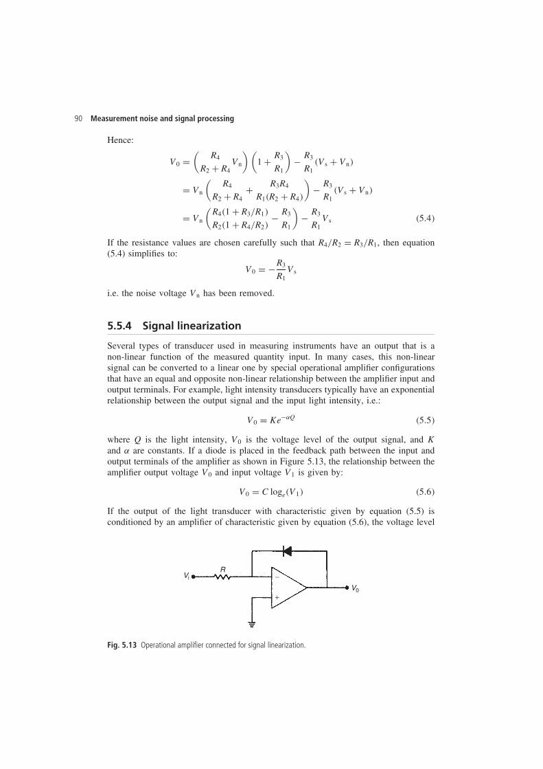
90 Measurement noise and signal processing
Hence:
V0 D(
R4
R2 C R4Vn
)(1 C R3
R1
)� R3
R1�Vs C Vn�
D Vn
(R4
R2 C R4C R3R4
R1�R2 C R4�
)� R3
R1�Vs C Vn�
D Vn
(R4�1 C R3/R1�
R2�1 C R4/R2�� R3
R1
)� R3
R1Vs �5.4�
If the resistance values are chosen carefully such that R4/R2 D R3/R1, then equation(5.4) simplifies to:
V0 D �R3
R1Vs
i.e. the noise voltage Vn has been removed.
5.5.4 Signal linearization
Several types of transducer used in measuring instruments have an output that is anon-linear function of the measured quantity input. In many cases, this non-linearsignal can be converted to a linear one by special operational amplifier configurationsthat have an equal and opposite non-linear relationship between the amplifier input andoutput terminals. For example, light intensity transducers typically have an exponentialrelationship between the output signal and the input light intensity, i.e.:
V0 D Ke�˛Q �5.5�
where Q is the light intensity, V0 is the voltage level of the output signal, and Kand ˛ are constants. If a diode is placed in the feedback path between the input andoutput terminals of the amplifier as shown in Figure 5.13, the relationship between theamplifier output voltage V0 and input voltage V1 is given by:
V0 D C loge�V1� �5.6�
If the output of the light transducer with characteristic given by equation (5.5) isconditioned by an amplifier of characteristic given by equation (5.6), the voltage level
Vi
V0
R−
+
Fig. 5.13 Operational amplifier connected for signal linearization.
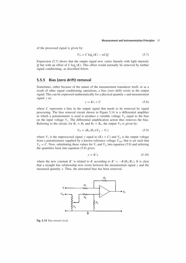
Measurement and Instrumentation Principles 91
of the processed signal is given by:
V0 D C loge�K� � ˛CQ �5.7�
Expression (5.7) shows that the output signal now varies linearly with light intensityQ but with an offset of C loge�K�. This offset would normally be removed by furthersignal conditioning, as described below.
5.5.5 Bias (zero drift) removal
Sometimes, either because of the nature of the measurement transducer itself, or as aresult of other signal conditioning operations, a bias (zero drift) exists in the outputsignal. This can be expressed mathematically for a physical quantity x and measurementsignal y as:
y D Kx C C �5.8�
where C represents a bias in the output signal that needs to be removed by signalprocessing. The bias removal circuit shown in Figure 5.14 is a differential amplifierin which a potentiometer is used to produce a variable voltage Vp equal to the biason the input voltage Vi. The differential amplification action thus removes the bias.Referring to the circuit, for R1 D R2 and R3 D R4, the output V0 is given by:
V0 D �R3/R1��Vp � Vi� �5.9�
where Vi is the unprocessed signal y equal to (Kx C C) and Vp is the output voltagefrom a potentiometer supplied by a known reference voltage Vref, that is set such thatVp D C. Now, substituting these values for Vi and Vp into equation (5.9) and referringthe quantities back into equation (5.8) gives:
y D K0x �5.10�
where the new constant K0 is related to K according to K0 D �K�R3/R1�. It is clearthat a straight line relationship now exists between the measurement signal y and themeasured quantity x. Thus, the unwanted bias has been removed.
Vi −
+V0Vref
Vp
R2
R4
R3
R1
Fig. 5.14 Bias removal circuit.
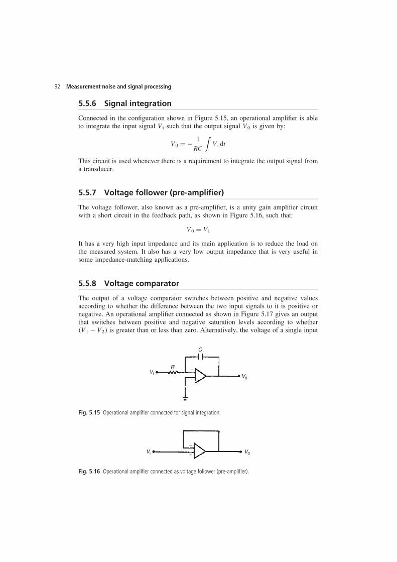
92 Measurement noise and signal processing
5.5.6 Signal integration
Connected in the configuration shown in Figure 5.15, an operational amplifier is ableto integrate the input signal Vi such that the output signal V0 is given by:
V0 D � 1
RC
∫Vi dt
This circuit is used whenever there is a requirement to integrate the output signal froma transducer.
5.5.7 Voltage follower (pre-amplifier)
The voltage follower, also known as a pre-amplifier, is a unity gain amplifier circuitwith a short circuit in the feedback path, as shown in Figure 5.16, such that:
V0 D Vi
It has a very high input impedance and its main application is to reduce the load onthe measured system. It also has a very low output impedance that is very useful insome impedance-matching applications.
5.5.8 Voltage comparator
The output of a voltage comparator switches between positive and negative valuesaccording to whether the difference between the two input signals to it is positive ornegative. An operational amplifier connected as shown in Figure 5.17 gives an outputthat switches between positive and negative saturation levels according to whether�V1 � V2� is greater than or less than zero. Alternatively, the voltage of a single input
Vi
+
−V0
R
C
Fig. 5.15 Operational amplifier connected for signal integration.
Vi
−
+ V0
Fig. 5.16 Operational amplifier connected as voltage follower (pre-amplifier).
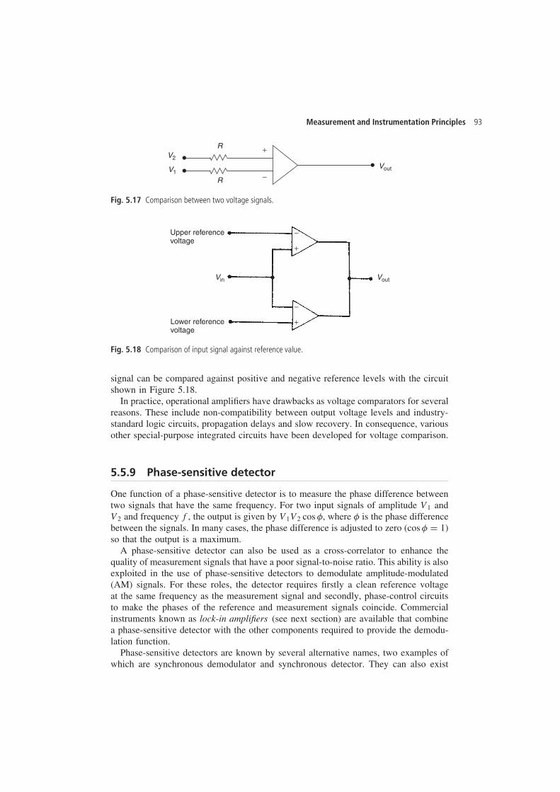
Measurement and Instrumentation Principles 93
V2
VoutV1
R
−
+
R
Fig. 5.17 Comparison between two voltage signals.
Upper referencevoltage
Lower referencevoltage
Vin Vout
−
+
−
+
Fig. 5.18 Comparison of input signal against reference value.
signal can be compared against positive and negative reference levels with the circuitshown in Figure 5.18.
In practice, operational amplifiers have drawbacks as voltage comparators for severalreasons. These include non-compatibility between output voltage levels and industry-standard logic circuits, propagation delays and slow recovery. In consequence, variousother special-purpose integrated circuits have been developed for voltage comparison.
5.5.9 Phase-sensitive detector
One function of a phase-sensitive detector is to measure the phase difference betweentwo signals that have the same frequency. For two input signals of amplitude V1 andV2 and frequency f, the output is given by V1V2 cos �, where � is the phase differencebetween the signals. In many cases, the phase difference is adjusted to zero (cos � D 1)so that the output is a maximum.
A phase-sensitive detector can also be used as a cross-correlator to enhance thequality of measurement signals that have a poor signal-to-noise ratio. This ability is alsoexploited in the use of phase-sensitive detectors to demodulate amplitude-modulated(AM) signals. For these roles, the detector requires firstly a clean reference voltageat the same frequency as the measurement signal and secondly, phase-control circuitsto make the phases of the reference and measurement signals coincide. Commercialinstruments known as lock-in amplifiers (see next section) are available that combinea phase-sensitive detector with the other components required to provide the demodu-lation function.
Phase-sensitive detectors are known by several alternative names, two examples ofwhich are synchronous demodulator and synchronous detector. They can also exist
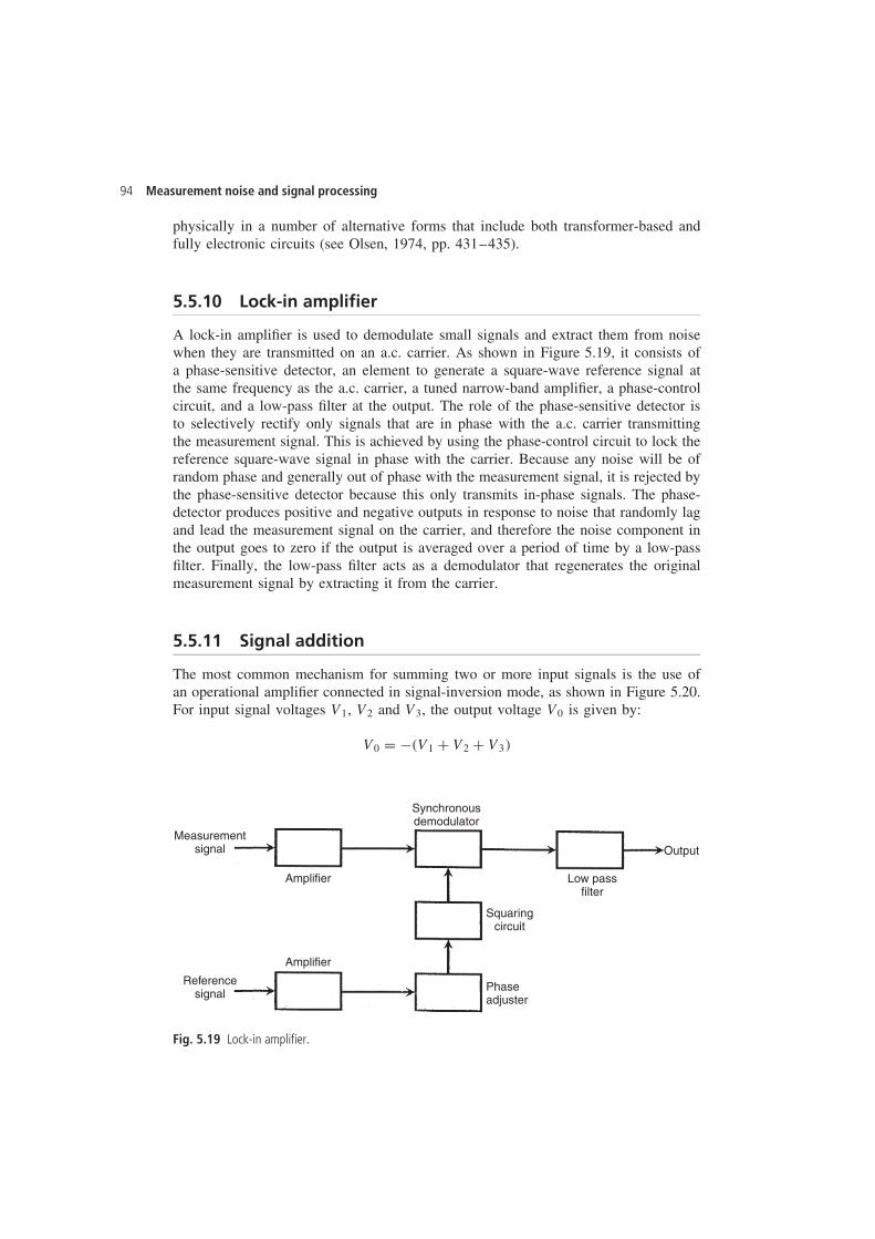
94 Measurement noise and signal processing
physically in a number of alternative forms that include both transformer-based andfully electronic circuits (see Olsen, 1974, pp. 431–435).
5.5.10 Lock-in amplifier
A lock-in amplifier is used to demodulate small signals and extract them from noisewhen they are transmitted on an a.c. carrier. As shown in Figure 5.19, it consists ofa phase-sensitive detector, an element to generate a square-wave reference signal atthe same frequency as the a.c. carrier, a tuned narrow-band amplifier, a phase-controlcircuit, and a low-pass filter at the output. The role of the phase-sensitive detector isto selectively rectify only signals that are in phase with the a.c. carrier transmittingthe measurement signal. This is achieved by using the phase-control circuit to lock thereference square-wave signal in phase with the carrier. Because any noise will be ofrandom phase and generally out of phase with the measurement signal, it is rejected bythe phase-sensitive detector because this only transmits in-phase signals. The phase-detector produces positive and negative outputs in response to noise that randomly lagand lead the measurement signal on the carrier, and therefore the noise component inthe output goes to zero if the output is averaged over a period of time by a low-passfilter. Finally, the low-pass filter acts as a demodulator that regenerates the originalmeasurement signal by extracting it from the carrier.
5.5.11 Signal addition
The most common mechanism for summing two or more input signals is the use ofan operational amplifier connected in signal-inversion mode, as shown in Figure 5.20.For input signal voltages V1, V2 and V3, the output voltage V0 is given by:
V0 D ��V1 C V2 C V3�
Measurementsignal
Referencesignal
Squaringcircuit
Phaseadjuster
Synchronousdemodulator
Low passfilter
Amplifier
Amplifier
Output
Fig. 5.19 Lock-in amplifier.
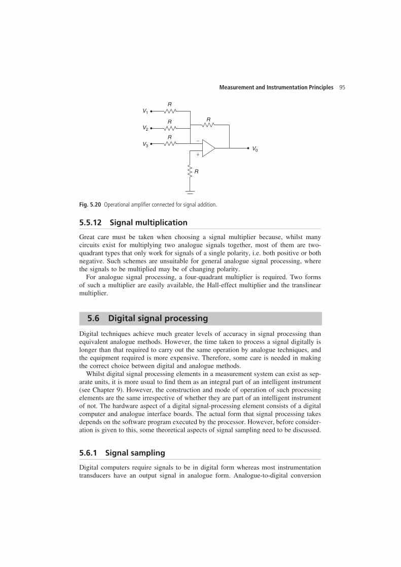
Measurement and Instrumentation Principles 95
V1
R
R
R
−
+
R
R
V2
V3 V0
Fig. 5.20 Operational amplifier connected for signal addition.
5.5.12 Signal multiplication
Great care must be taken when choosing a signal multiplier because, whilst manycircuits exist for multiplying two analogue signals together, most of them are two-quadrant types that only work for signals of a single polarity, i.e. both positive or bothnegative. Such schemes are unsuitable for general analogue signal processing, wherethe signals to be multiplied may be of changing polarity.
For analogue signal processing, a four-quadrant multiplier is required. Two formsof such a multiplier are easily available, the Hall-effect multiplier and the translinearmultiplier.
5.6 Digital signal processing
Digital techniques achieve much greater levels of accuracy in signal processing thanequivalent analogue methods. However, the time taken to process a signal digitally islonger than that required to carry out the same operation by analogue techniques, andthe equipment required is more expensive. Therefore, some care is needed in makingthe correct choice between digital and analogue methods.
Whilst digital signal processing elements in a measurement system can exist as sep-arate units, it is more usual to find them as an integral part of an intelligent instrument(see Chapter 9). However, the construction and mode of operation of such processingelements are the same irrespective of whether they are part of an intelligent instrumentof not. The hardware aspect of a digital signal-processing element consists of a digitalcomputer and analogue interface boards. The actual form that signal processing takesdepends on the software program executed by the processor. However, before consider-ation is given to this, some theoretical aspects of signal sampling need to be discussed.
5.6.1 Signal sampling
Digital computers require signals to be in digital form whereas most instrumentationtransducers have an output signal in analogue form. Analogue-to-digital conversion
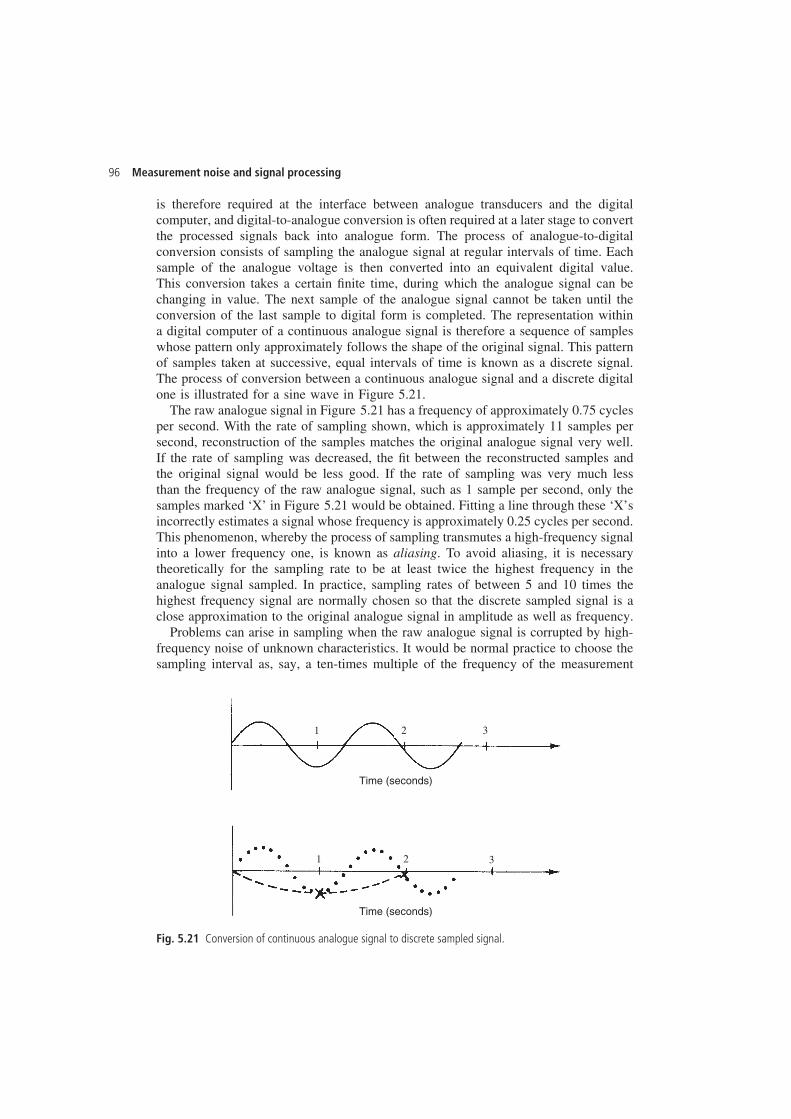
96 Measurement noise and signal processing
is therefore required at the interface between analogue transducers and the digitalcomputer, and digital-to-analogue conversion is often required at a later stage to convertthe processed signals back into analogue form. The process of analogue-to-digitalconversion consists of sampling the analogue signal at regular intervals of time. Eachsample of the analogue voltage is then converted into an equivalent digital value.This conversion takes a certain finite time, during which the analogue signal can bechanging in value. The next sample of the analogue signal cannot be taken until theconversion of the last sample to digital form is completed. The representation withina digital computer of a continuous analogue signal is therefore a sequence of sampleswhose pattern only approximately follows the shape of the original signal. This patternof samples taken at successive, equal intervals of time is known as a discrete signal.The process of conversion between a continuous analogue signal and a discrete digitalone is illustrated for a sine wave in Figure 5.21.
The raw analogue signal in Figure 5.21 has a frequency of approximately 0.75 cyclesper second. With the rate of sampling shown, which is approximately 11 samples persecond, reconstruction of the samples matches the original analogue signal very well.If the rate of sampling was decreased, the fit between the reconstructed samples andthe original signal would be less good. If the rate of sampling was very much lessthan the frequency of the raw analogue signal, such as 1 sample per second, only thesamples marked ‘X’ in Figure 5.21 would be obtained. Fitting a line through these ‘X’sincorrectly estimates a signal whose frequency is approximately 0.25 cycles per second.This phenomenon, whereby the process of sampling transmutes a high-frequency signalinto a lower frequency one, is known as aliasing. To avoid aliasing, it is necessarytheoretically for the sampling rate to be at least twice the highest frequency in theanalogue signal sampled. In practice, sampling rates of between 5 and 10 times thehighest frequency signal are normally chosen so that the discrete sampled signal is aclose approximation to the original analogue signal in amplitude as well as frequency.
Problems can arise in sampling when the raw analogue signal is corrupted by high-frequency noise of unknown characteristics. It would be normal practice to choose thesampling interval as, say, a ten-times multiple of the frequency of the measurement
1 2 3
1 2 3
Time (seconds)
Time (seconds)
Fig. 5.21 Conversion of continuous analogue signal to discrete sampled signal.
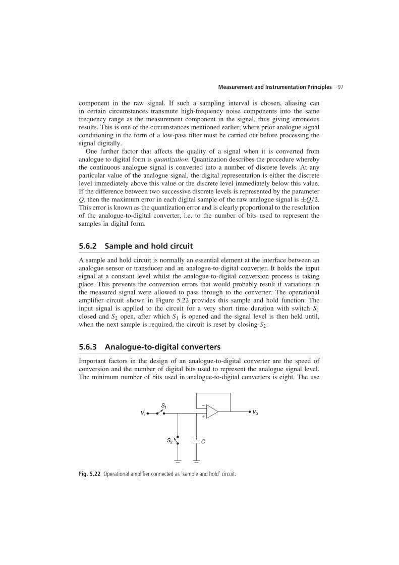
Measurement and Instrumentation Principles 97
component in the raw signal. If such a sampling interval is chosen, aliasing canin certain circumstances transmute high-frequency noise components into the samefrequency range as the measurement component in the signal, thus giving erroneousresults. This is one of the circumstances mentioned earlier, where prior analogue signalconditioning in the form of a low-pass filter must be carried out before processing thesignal digitally.
One further factor that affects the quality of a signal when it is converted fromanalogue to digital form is quantization. Quantization describes the procedure wherebythe continuous analogue signal is converted into a number of discrete levels. At anyparticular value of the analogue signal, the digital representation is either the discretelevel immediately above this value or the discrete level immediately below this value.If the difference between two successive discrete levels is represented by the parameterQ, then the maximum error in each digital sample of the raw analogue signal is šQ/2.This error is known as the quantization error and is clearly proportional to the resolutionof the analogue-to-digital converter, i.e. to the number of bits used to represent thesamples in digital form.
5.6.2 Sample and hold circuit
A sample and hold circuit is normally an essential element at the interface between ananalogue sensor or transducer and an analogue-to-digital converter. It holds the inputsignal at a constant level whilst the analogue-to-digital conversion process is takingplace. This prevents the conversion errors that would probably result if variations inthe measured signal were allowed to pass through to the converter. The operationalamplifier circuit shown in Figure 5.22 provides this sample and hold function. Theinput signal is applied to the circuit for a very short time duration with switch S1
closed and S2 open, after which S1 is opened and the signal level is then held until,when the next sample is required, the circuit is reset by closing S2.
5.6.3 Analogue-to-digital converters
Important factors in the design of an analogue-to-digital converter are the speed ofconversion and the number of digital bits used to represent the analogue signal level.The minimum number of bits used in analogue-to-digital converters is eight. The use
−
+Vi
S1
S2
V0
C
Fig. 5.22 Operational amplifier connected as ’sample and hold’ circuit.
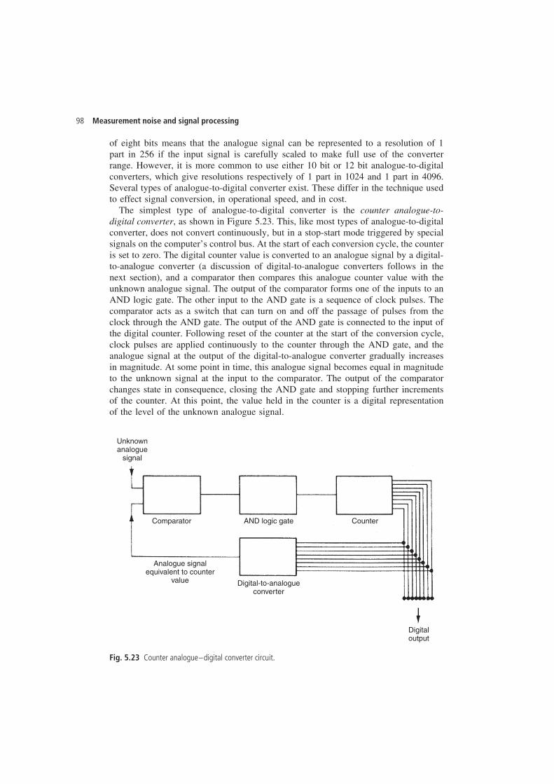
98 Measurement noise and signal processing
of eight bits means that the analogue signal can be represented to a resolution of 1part in 256 if the input signal is carefully scaled to make full use of the converterrange. However, it is more common to use either 10 bit or 12 bit analogue-to-digitalconverters, which give resolutions respectively of 1 part in 1024 and 1 part in 4096.Several types of analogue-to-digital converter exist. These differ in the technique usedto effect signal conversion, in operational speed, and in cost.
The simplest type of analogue-to-digital converter is the counter analogue-to-digital converter, as shown in Figure 5.23. This, like most types of analogue-to-digitalconverter, does not convert continuously, but in a stop-start mode triggered by specialsignals on the computer’s control bus. At the start of each conversion cycle, the counteris set to zero. The digital counter value is converted to an analogue signal by a digital-to-analogue converter (a discussion of digital-to-analogue converters follows in thenext section), and a comparator then compares this analogue counter value with theunknown analogue signal. The output of the comparator forms one of the inputs to anAND logic gate. The other input to the AND gate is a sequence of clock pulses. Thecomparator acts as a switch that can turn on and off the passage of pulses from theclock through the AND gate. The output of the AND gate is connected to the input ofthe digital counter. Following reset of the counter at the start of the conversion cycle,clock pulses are applied continuously to the counter through the AND gate, and theanalogue signal at the output of the digital-to-analogue converter gradually increasesin magnitude. At some point in time, this analogue signal becomes equal in magnitudeto the unknown signal at the input to the comparator. The output of the comparatorchanges state in consequence, closing the AND gate and stopping further incrementsof the counter. At this point, the value held in the counter is a digital representationof the level of the unknown analogue signal.
Unknownanalogue
signal
Analogue signalequivalent to counter
value
Comparator AND logic gate
Digital-to-analogueconverter
Counter
Digitaloutput
Fig. 5.23 Counter analogue–digital converter circuit.
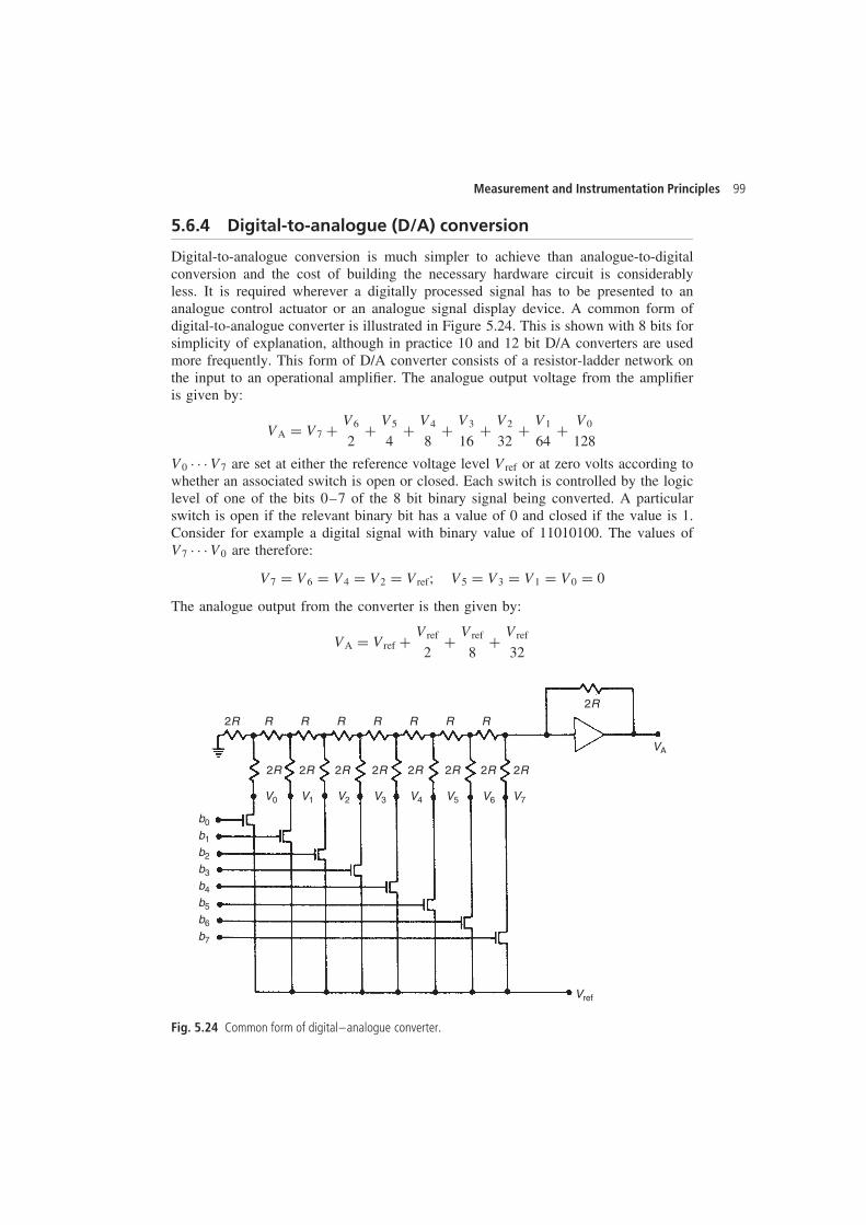
Measurement and Instrumentation Principles 99
5.6.4 Digital-to-analogue (D/A) conversion
Digital-to-analogue conversion is much simpler to achieve than analogue-to-digitalconversion and the cost of building the necessary hardware circuit is considerablyless. It is required wherever a digitally processed signal has to be presented to ananalogue control actuator or an analogue signal display device. A common form ofdigital-to-analogue converter is illustrated in Figure 5.24. This is shown with 8 bits forsimplicity of explanation, although in practice 10 and 12 bit D/A converters are usedmore frequently. This form of D/A converter consists of a resistor-ladder network onthe input to an operational amplifier. The analogue output voltage from the amplifieris given by:
VA D V7 C V6
2C V5
4C V4
8C V3
16C V2
32C V1
64C V0
128
V0 Ð Ð Ð V7 are set at either the reference voltage level Vref or at zero volts according towhether an associated switch is open or closed. Each switch is controlled by the logiclevel of one of the bits 0–7 of the 8 bit binary signal being converted. A particularswitch is open if the relevant binary bit has a value of 0 and closed if the value is 1.Consider for example a digital signal with binary value of 11010100. The values ofV7 Ð Ð Ð V0 are therefore:
V7 D V6 D V4 D V2 D Vref; V5 D V3 D V1 D V0 D 0
The analogue output from the converter is then given by:
VA D Vref C Vref
2C Vref
8C Vref
32
b0
V0 V1 V2 V3 V4 V5
VA
Vref
V6 V7
2R
2R R R R R R R R
2R 2R 2R 2R 2R 2R 2R
2R
b1
b2
b3
b4
b5
b6
b7
Fig. 5.24 Common form of digital–analogue converter.
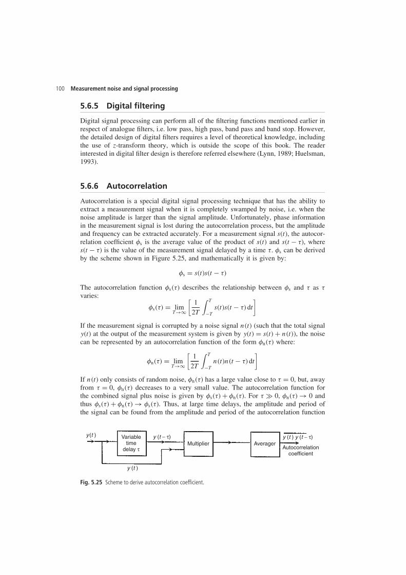
100 Measurement noise and signal processing
5.6.5 Digital filtering
Digital signal processing can perform all of the filtering functions mentioned earlier inrespect of analogue filters, i.e. low pass, high pass, band pass and band stop. However,the detailed design of digital filters requires a level of theoretical knowledge, includingthe use of z-transform theory, which is outside the scope of this book. The readerinterested in digital filter design is therefore referred elsewhere (Lynn, 1989; Huelsman,1993).
5.6.6 Autocorrelation
Autocorrelation is a special digital signal processing technique that has the ability toextract a measurement signal when it is completely swamped by noise, i.e. when thenoise amplitude is larger than the signal amplitude. Unfortunately, phase informationin the measurement signal is lost during the autocorrelation process, but the amplitudeand frequency can be extracted accurately. For a measurement signal s�t�, the autocor-relation coefficient �s is the average value of the product of s�t� and s�t � ��, wheres�t � �� is the value of the measurement signal delayed by a time �. �s can be derivedby the scheme shown in Figure 5.25, and mathematically it is given by:
�s D s�t�s�t � ��
The autocorrelation function �s��� describes the relationship between �s and � as �varies:
�s��� D limT!1
[1
2T
∫ T
�Ts�t�s�t � �� dt
]
If the measurement signal is corrupted by a noise signal n�t� (such that the total signaly�t� at the output of the measurement system is given by y�t� D s�t� C n�t��, the noisecan be represented by an autocorrelation function of the form �n��� where:
�n��� D limT!1
[1
2T
∫ T
�Tn�t�n�t � �� dt
]
If n�t� only consists of random noise, �n��� has a large value close to � D 0, but, awayfrom � D 0, �n��� decreases to a very small value. The autocorrelation function forthe combined signal plus noise is given by �s��� C �n���. For � × 0, �n��� ! 0 andthus �s��� C �n��� ! �s���. Thus, at large time delays, the amplitude and period ofthe signal can be found from the amplitude and period of the autocorrelation function
y(t )
y (t )
y (t − τ) y (t ) y (t − τ)Variabletime
delay τMultiplier Averager
Autocorrelationcoefficient
Fig. 5.25 Scheme to derive autocorrelation coefficient.
Measurement and Instrumentation Principles 101
of the signal at the output of the measurement system. Further details can be found inHealey, (1975).
5.6.7 Other digital signal processing operations
Once a satisfactory digital representation in discrete form of an analogue signal has beenobtained, many signal processing operations become trivial. For signal amplificationand attenuation, all samples have to be multiplied or divided by a fixed constant. Biasremoval involves simply adding or subtracting a fixed constant from each sample ofthe signal. Signal linearization requires a priori knowledge of the type of non-linearityinvolved, in the form of a mathematical equation that expresses the relationship betweenthe output measurements from an instrument and the value of the physical quantitybeing measured. This can be obtained either theoretically through knowledge of thephysical laws governing the system or empirically using input–output data obtainedfrom the measurement system under controlled conditions. Once this relationship hasbeen obtained, it is used to calculate the value of the measured physical quantitycorresponding to each discrete sample of the measurement signal. Whilst the amountof computation involved in this is greater than for the trivial cases of signal amplifica-tion etc. already mentioned, the computational burden is still relatively small in mostmeasurement situations.
References and further reading
Blinchikoff, H.J. (1976) Filtering in the Time and Frequency Domains, Wiley, New York.Cook, B.J. (1979) Journal of Measurement and Control, 12(8), 1979, pp. 326–335.Healey, M. (1975) Principles of Automatic Control, Hodder and Stoughton.Huelsman, L.P. (1993) Active and Passive Analog Filter Design, McGraw-Hill, New York.Lynn, P.A. (1989) The Analysis and Processing of Signals, Macmillan, London.Olsen, G.H. (1974) A Handbook for Engineers and Scientists, Butterworth, London.Stephenson, F.W. (1985) RC Active Filter Design Handbook, Wiley, New York.
6
Electrical indicating andtest instruments
The magnitude of voltage signals can be measured by various electrical indicating andtest instruments, such as meters (both analogue and digital), the cathode ray oscillo-scope and the digital storage oscilloscope. As well as signal-level voltages, many ofthese instruments can also measure higher-magnitude voltages, and this is indicatedwhere appropriate.
6.1 Digital meters
All types of digital meter are basically modified forms of the digital voltmeter (DVM),irrespective of the quantity that they are designed to measure. Digital meters designedto measure quantities other than voltage are in fact digital voltmeters that containappropriate electrical circuits to convert current or resistance measurement signals intovoltage signals. Digital multimeters are also essentially digital voltmeters that containseveral conversion circuits, thus allowing the measurement of voltage, current andresistance within one instrument.
Digital meters have been developed to satisfy a need for higher measurement accur-acies and a faster speed of response to voltage changes than can be achieved withanalogue instruments. They are technically superior to analogue meters in almostevery respect. However, they have a greater cost due to the higher manufacturingcosts compared with analogue meters. The binary nature of the output reading froma digital instrument can be readily applied to a display that is in the form of discretenumerals. Where human operators are required to measure and record signal voltagelevels, this form of output makes an important contribution to measurement reliabilityand accuracy, since the problem of analogue meter parallax error is eliminated andthe possibility of gross error through misreading the meter output is greatly reduced.The availability in many instruments of a direct output in digital form is also veryuseful in the rapidly expanding range of computer control applications. Quoted inac-curacy figures are between š0.005% (measuring d.c. voltages) and š2%. Additionaladvantages of digital meters are their very high input impedance (10 M� comparedwith 1–20 k� for analogue meters), the ability to measure signals of frequency upto 1 MHz and the common inclusion of features such as automatic ranging, whichprevents overload and reverse polarity connection etc.
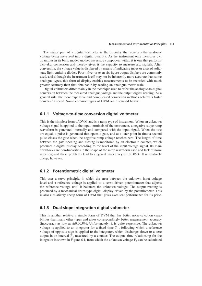
Measurement and Instrumentation Principles 103
The major part of a digital voltmeter is the circuitry that converts the analoguevoltage being measured into a digital quantity. As the instrument only measures d.c.quantities in its basic mode, another necessary component within it is one that performsa.c.–d.c. conversion and thereby gives it the capacity to measure a.c. signals. Afterconversion, the voltage value is displayed by means of indicating tubes or a set of solid-state light-emitting diodes. Four-, five- or even six-figure output displays are commonlyused, and although the instrument itself may not be inherently more accurate than someanalogue types, this form of display enables measurements to be recorded with muchgreater accuracy than that obtainable by reading an analogue meter scale.
Digital voltmeters differ mainly in the technique used to effect the analogue-to-digitalconversion between the measured analogue voltage and the output digital reading. As ageneral rule, the more expensive and complicated conversion methods achieve a fasterconversion speed. Some common types of DVM are discussed below.
6.1.1 Voltage-to-time conversion digital voltmeter
This is the simplest form of DVM and is a ramp type of instrument. When an unknownvoltage signal is applied to the input terminals of the instrument, a negative-slope rampwaveform is generated internally and compared with the input signal. When the twoare equal, a pulse is generated that opens a gate, and at a later point in time a secondpulse closes the gate when the negative ramp voltage reaches zero. The length of timebetween the gate opening and closing is monitored by an electronic counter, whichproduces a digital display according to the level of the input voltage signal. Its maindrawbacks are non-linearities in the shape of the ramp waveform used and lack of noiserejection, and these problems lead to a typical inaccuracy of š0.05%. It is relativelycheap, however.
6.1.2 Potentiometric digital voltmeter
This uses a servo principle, in which the error between the unknown input voltagelevel and a reference voltage is applied to a servo-driven potentiometer that adjuststhe reference voltage until it balances the unknown voltage. The output reading isproduced by a mechanical drum-type digital display driven by the potentiometer. Thisis also a relatively cheap form of DVM that gives excellent performance for its price.
6.1.3 Dual-slope integration digital voltmeter
This is another relatively simple form of DVM that has better noise-rejection capa-bilities than many other types and gives correspondingly better measurement accuracy(inaccuracy as low as š0.005%). Unfortunately, it is quite expensive. The unknownvoltage is applied to an integrator for a fixed time T1, following which a referencevoltage of opposite sign is applied to the integrator, which discharges down to a zerooutput in an interval T2 measured by a counter. The output–time relationship for theintegrator is shown in Figure 6.1, from which the unknown voltage Vi can be calculated
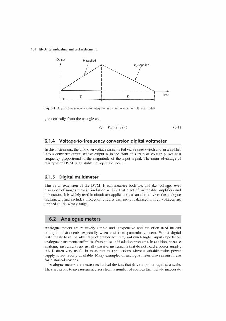
104 Electrical indicating and test instruments
Output
Time
Vi applied
T1 T2
Vref applied
Fig. 6.1 Output–time relationship for integrator in a dual-slope digital voltmeter (DVM).
geometrically from the triangle as:
Vi D Vref �T1/T2� �6.1�
6.1.4 Voltage-to-frequency conversion digital voltmeter
In this instrument, the unknown voltage signal is fed via a range switch and an amplifierinto a converter circuit whose output is in the form of a train of voltage pulses at afrequency proportional to the magnitude of the input signal. The main advantage ofthis type of DVM is its ability to reject a.c. noise.
6.1.5 Digital multimeter
This is an extension of the DVM. It can measure both a.c. and d.c. voltages overa number of ranges through inclusion within it of a set of switchable amplifiers andattenuators. It is widely used in circuit test applications as an alternative to the analoguemultimeter, and includes protection circuits that prevent damage if high voltages areapplied to the wrong range.
6.2 Analogue meters
Analogue meters are relatively simple and inexpensive and are often used insteadof digital instruments, especially when cost is of particular concern. Whilst digitalinstruments have the advantage of greater accuracy and much higher input impedance,analogue instruments suffer less from noise and isolation problems. In addition, becauseanalogue instruments are usually passive instruments that do not need a power supply,this is often very useful in measurement applications where a suitable mains powersupply is not readily available. Many examples of analogue meter also remain in usefor historical reasons.
Analogue meters are electromechanical devices that drive a pointer against a scale.They are prone to measurement errors from a number of sources that include inaccurate
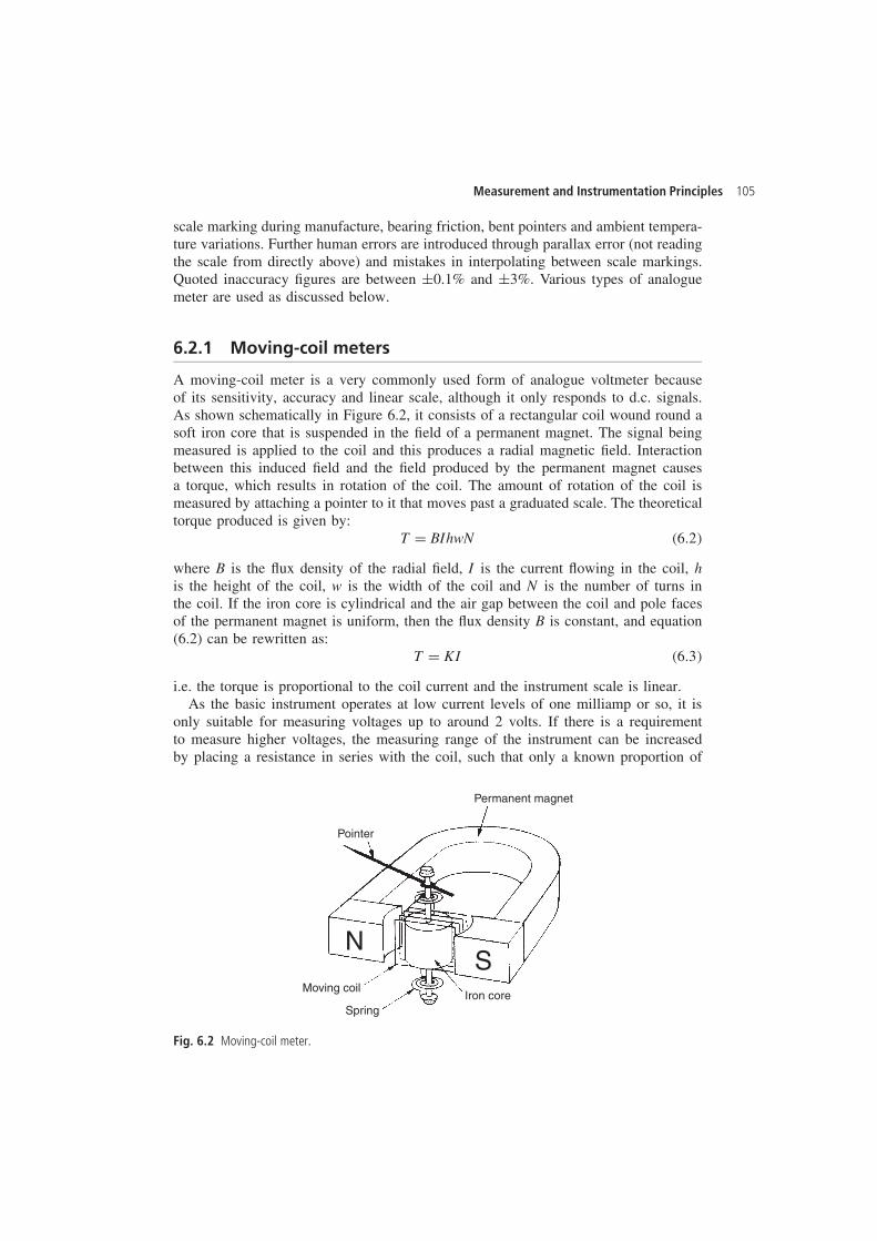
Measurement and Instrumentation Principles 105
scale marking during manufacture, bearing friction, bent pointers and ambient tempera-ture variations. Further human errors are introduced through parallax error (not readingthe scale from directly above) and mistakes in interpolating between scale markings.Quoted inaccuracy figures are between š0.1% and š3%. Various types of analoguemeter are used as discussed below.
6.2.1 Moving-coil meters
A moving-coil meter is a very commonly used form of analogue voltmeter becauseof its sensitivity, accuracy and linear scale, although it only responds to d.c. signals.As shown schematically in Figure 6.2, it consists of a rectangular coil wound round asoft iron core that is suspended in the field of a permanent magnet. The signal beingmeasured is applied to the coil and this produces a radial magnetic field. Interactionbetween this induced field and the field produced by the permanent magnet causesa torque, which results in rotation of the coil. The amount of rotation of the coil ismeasured by attaching a pointer to it that moves past a graduated scale. The theoreticaltorque produced is given by:
T D BIhwN �6.2�
where B is the flux density of the radial field, I is the current flowing in the coil, his the height of the coil, w is the width of the coil and N is the number of turns inthe coil. If the iron core is cylindrical and the air gap between the coil and pole facesof the permanent magnet is uniform, then the flux density B is constant, and equation(6.2) can be rewritten as:
T D KI �6.3�
i.e. the torque is proportional to the coil current and the instrument scale is linear.As the basic instrument operates at low current levels of one milliamp or so, it is
only suitable for measuring voltages up to around 2 volts. If there is a requirementto measure higher voltages, the measuring range of the instrument can be increasedby placing a resistance in series with the coil, such that only a known proportion of
Pointer
NS
Moving coil
SpringIron core
Permanent magnet
Fig. 6.2 Moving-coil meter.
106 Electrical indicating and test instruments
the applied voltage is measured by the meter. In this situation the added resistance isknown as a shunting resistor.
Whilst Figure 6.2 shows the traditional moving-coil instrument with a long U-shapedpermanent magnet, many newer instruments employ much shorter magnets made fromrecently developed magnetic materials such as Alnico and Alcomax. These materialsproduce a substantially greater flux density, which, besides allowing the magnet to besmaller, has additional advantages in allowing reductions to be made in the size of thecoil and in increasing the usable range of deflection of the coil to about 120°. Someversions of the instrument also have either a specially shaped core or specially shapedmagnet pole faces to cater for special situations where a non-linear scale such as alogarithmic one is required.
6.2.2 Moving-iron meter
As well as measuring d.c. signals, the moving-iron meter can also measure a.c. signalsat frequencies up to 125 Hz. It is the cheapest form of meter available and, conse-quently, this type of meter is also commonly used for measuring voltage signals. Thesignal to be measured is applied to a stationary coil, and the associated field produced isoften amplified by the presence of an iron structure associated with the fixed coil. Themoving element in the instrument consists of an iron vane that is suspended within thefield of the fixed coil. When the fixed coil is excited, the iron vane turns in a directionthat increases the flux through it.
The majority of moving-iron instruments are either of the attraction type or of therepulsion type. A few instruments belong to a third combination type. The attractiontype, where the iron vane is drawn into the field of the coil as the current is increased,is shown schematically in Figure 6.3(a). The alternative repulsion type is sketched inFigure 6.3(b). For an excitation current I, the torque produced that causes the vane to
Stationarycoil Pointer
(a) (b)
Spring
Coil
Pointer
SpringIron vane
Iron vane
Fig. 6.3 Moving-iron meter: (a) attraction type; (b) repulsion type.
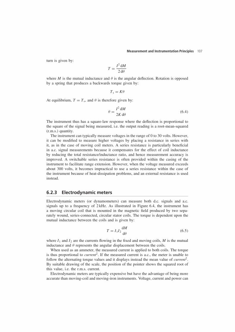
Measurement and Instrumentation Principles 107
turn is given by:
T D I2 dM
2 d
where M is the mutual inductance and is the angular deflection. Rotation is opposedby a spring that produces a backwards torque given by:
Ts D K
At equilibrium, T D Ts, and is therefore given by:
D I2 dM
2K d �6.4�
The instrument thus has a square-law response where the deflection is proportional tothe square of the signal being measured, i.e. the output reading is a root-mean-squared(r.m.s.) quantity.
The instrument can typically measure voltages in the range of 0 to 30 volts. However,it can be modified to measure higher voltages by placing a resistance in series withit, as in the case of moving coil meters. A series resistance is particularly beneficialin a.c. signal measurements because it compensates for the effect of coil inductanceby reducing the total resistance/inductance ratio, and hence measurement accuracy isimproved. A switchable series resistance is often provided within the casing of theinstrument to facilitate range extension. However, when the voltage measured exceedsabout 300 volts, it becomes impractical to use a series resistance within the case ofthe instrument because of heat-dissipation problems, and an external resistance is usedinstead.
6.2.3 Electrodynamic meters
Electrodynamic meters (or dynamometers) can measure both d.c. signals and a.c.signals up to a frequency of 2 kHz. As illustrated in Figure 6.4, the instrument hasa moving circular coil that is mounted in the magnetic field produced by two sepa-rately wound, series-connected, circular stator coils. The torque is dependent upon themutual inductance between the coils and is given by:
T D I1I2dM
d �6.5�
where I1 and I2 are the currents flowing in the fixed and moving coils, M is the mutualinductance and represents the angular displacement between the coils.
When used as an ammeter, the measured current is applied to both coils. The torqueis thus proportional to current2. If the measured current is a.c., the meter is unable tofollow the alternating torque values and it displays instead the mean value of current2.By suitable drawing of the scale, the position of the pointer shows the squared root ofthis value, i.e. the r.m.s. current.
Electrodynamic meters are typically expensive but have the advantage of being moreaccurate than moving-coil and moving-iron instruments. Voltage, current and power can
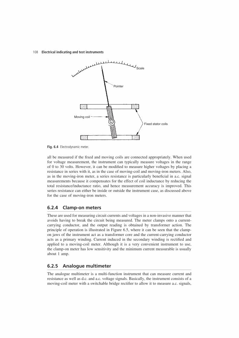
108 Electrical indicating and test instruments
Scale
Pointer
Moving coil
Fixed stator coils
Fig. 6.4 Electrodynamic meter.
all be measured if the fixed and moving coils are connected appropriately. When usedfor voltage measurement, the instrument can typically measure voltages in the rangeof 0 to 30 volts. However, it can be modified to measure higher voltages by placing aresistance in series with it, as in the case of moving-coil and moving-iron meters. Also,as in the moving-iron meter, a series resistance is particularly beneficial in a.c. signalmeasurements because it compensates for the effect of coil inductance by reducing thetotal resistance/inductance ratio, and hence measurement accuracy is improved. Thisseries resistance can either be inside or outside the instrument case, as discussed abovefor the case of moving-iron meters.
6.2.4 Clamp-on meters
These are used for measuring circuit currents and voltages in a non-invasive manner thatavoids having to break the circuit being measured. The meter clamps onto a current-carrying conductor, and the output reading is obtained by transformer action. Theprinciple of operation is illustrated in Figure 6.5, where it can be seen that the clamp-on jaws of the instrument act as a transformer core and the current-carrying conductoracts as a primary winding. Current induced in the secondary winding is rectified andapplied to a moving-coil meter. Although it is a very convenient instrument to use,the clamp-on meter has low sensitivity and the minimum current measurable is usuallyabout 1 amp.
6.2.5 Analogue multimeter
The analogue multimeter is a multi-function instrument that can measure current andresistance as well as d.c. and a.c. voltage signals. Basically, the instrument consists of amoving-coil meter with a switchable bridge rectifier to allow it to measure a.c. signals,
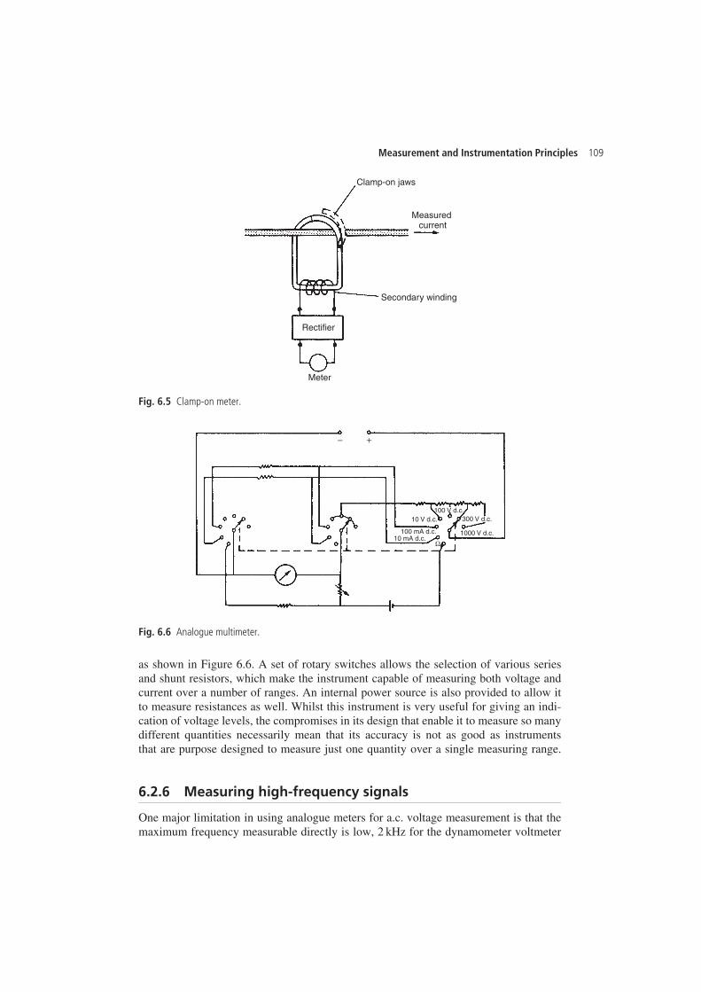
Measurement and Instrumentation Principles 109
Clamp-on jaws
Measured current
Secondary winding
Rectifier
Meter
Fig. 6.5 Clamp-on meter.
− +
10 V d.c.
100 mA d.c.10 mA d.c.
100 V d.c.300 V d.c.
1000 V d.c.
Ω
Fig. 6.6 Analogue multimeter.
as shown in Figure 6.6. A set of rotary switches allows the selection of various seriesand shunt resistors, which make the instrument capable of measuring both voltage andcurrent over a number of ranges. An internal power source is also provided to allow itto measure resistances as well. Whilst this instrument is very useful for giving an indi-cation of voltage levels, the compromises in its design that enable it to measure so manydifferent quantities necessarily mean that its accuracy is not as good as instrumentsthat are purpose designed to measure just one quantity over a single measuring range.
6.2.6 Measuring high-frequency signals
One major limitation in using analogue meters for a.c. voltage measurement is that themaximum frequency measurable directly is low, 2 kHz for the dynamometer voltmeter
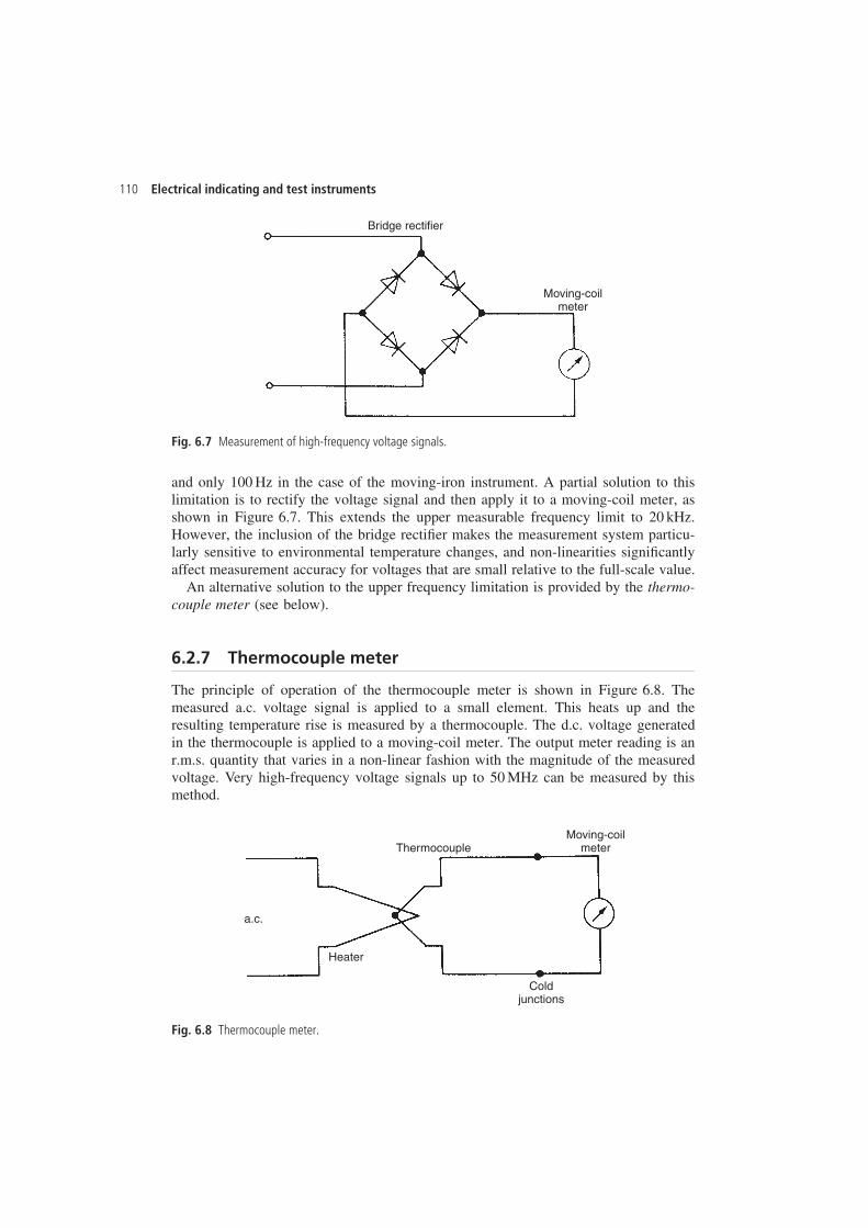
110 Electrical indicating and test instruments
Bridge rectifier
Moving-coilmeter
Fig. 6.7 Measurement of high-frequency voltage signals.
and only 100 Hz in the case of the moving-iron instrument. A partial solution to thislimitation is to rectify the voltage signal and then apply it to a moving-coil meter, asshown in Figure 6.7. This extends the upper measurable frequency limit to 20 kHz.However, the inclusion of the bridge rectifier makes the measurement system particu-larly sensitive to environmental temperature changes, and non-linearities significantlyaffect measurement accuracy for voltages that are small relative to the full-scale value.
An alternative solution to the upper frequency limitation is provided by the thermo-couple meter (see below).
6.2.7 Thermocouple meter
The principle of operation of the thermocouple meter is shown in Figure 6.8. Themeasured a.c. voltage signal is applied to a small element. This heats up and theresulting temperature rise is measured by a thermocouple. The d.c. voltage generatedin the thermocouple is applied to a moving-coil meter. The output meter reading is anr.m.s. quantity that varies in a non-linear fashion with the magnitude of the measuredvoltage. Very high-frequency voltage signals up to 50 MHz can be measured by thismethod.
a.c.
Heater
ThermocoupleMoving-coil
meter
Coldjunctions
Fig. 6.8 Thermocouple meter.
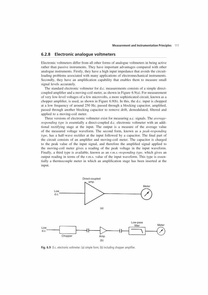
Measurement and Instrumentation Principles 111
6.2.8 Electronic analogue voltmeters
Electronic voltmeters differ from all other forms of analogue voltmeters in being activerather than passive instruments. They have important advantages compared with otheranalogue instruments. Firstly, they have a high input impedance that avoids the circuit-loading problems associated with many applications of electromechanical instruments.Secondly, they have an amplification capability that enables them to measure smallsignal levels accurately.
The standard electronic voltmeter for d.c. measurements consists of a simple direct-coupled amplifier and a moving-coil meter, as shown in Figure 6.9(a). For measurementof very low-level voltages of a few microvolts, a more sophisticated circuit, known as achopper amplifier, is used, as shown in Figure 6.9(b). In this, the d.c. input is choppedat a low frequency of around 250 Hz, passed through a blocking capacitor, amplified,passed through another blocking capacitor to remove drift, demodulated, filtered andapplied to a moving-coil meter.
Three versions of electronic voltmeter exist for measuring a.c. signals. The average-responding type is essentially a direct-coupled d.c. electronic voltmeter with an addi-tional rectifying stage at the input. The output is a measure of the average valueof the measured voltage waveform. The second form, known as a peak-respondingtype, has a half-wave rectifier at the input followed by a capacitor. The final part ofthe circuit consists of an amplifier and moving-coil meter. The capacitor is chargedto the peak value of the input signal, and therefore the amplified signal applied tothe moving-coil meter gives a reading of the peak voltage in the input waveform.Finally, a third type is available, known as an r.m.s.-responding type, which gives anoutput reading in terms of the r.m.s. value of the input waveform. This type is essen-tially a thermocouple meter in which an amplification stage has been inserted at theinput.
Lowd.c.
Lowd.c.
Direct-coupledamp.
Meter
MeterLow-pass
filter
(a)
(b)
Amp.Chopper
Fig. 6.9 D.c. electronic voltmeter: (a) simple form; (b) including chopper amplifier.
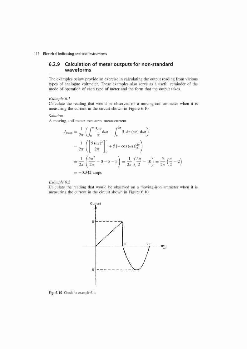
112 Electrical indicating and test instruments
6.2.9 Calculation of meter outputs for non-standardwaveforms
The examples below provide an exercise in calculating the output reading from varioustypes of analogue voltmeter. These examples also serve as a useful reminder of themode of operation of each type of meter and the form that the output takes.
Example 6.1Calculate the reading that would be observed on a moving-coil ammeter when it ismeasuring the current in the circuit shown in Figure 6.10.
SolutionA moving-coil meter measures mean current.
Imean D 1
2
(∫
0
5ωt
dωt C
∫ 2
5 sin �ωt� dωt
)
D 1
2
([5 �ωt�2
2
]
0
C 5 [� cos �ωt�]2
)
D 1
2
(52
2� 0 � 5 � 5
)D 1
2
(5
2� 10
)D 5
2
(
2� 2
)
D �0.342 amps
Example 6.2Calculate the reading that would be observed on a moving-iron ammeter when it ismeasuring the current in the circuit shown in Figure 6.10.
Current
5
−5
p 2p
wt
Fig. 6.10 Circuit for example 6.1.
Measurement and Instrumentation Principles 113
SolutionA moving-iron meter measures r.m.s. current.
I2r.m.s. D 1
2
(∫
0
25 �ωt�2
2 dωt C∫ 2
25 sin2 �ωt� dωt
)
D 1
2
(∫
0
25 �ωt�2
2 dωt C∫ 2
25 �1 � cos 2ωt�
2dωt
)
D 25
2
([�ωt�3
32
]
0
C[
ωt
2� sin 2ωt
4
]2
)D 25
2
(
3C 2
2�
2
)
D 25
2
(
3C
2
)D 25
2
(1
3C 1
2
)D 10.416
Thus, Ir.m.s. D√(
I2r.m.s.
) D 3.23 amps
Example 6.3A dynamometer ammeter is connected in series with a 500 � resistor, a rectifyingdevice and a 240 V r.m.s. alternating sinusoidal power supply. The rectifier behaves asa resistance of 200 � to current flowing in one direction and as a resistance of 2 k�to current in the opposite direction. Calculate the reading on the meter.
SolutionVpeak D
√Vr.m.s. �2� D 339.4 V
For 0 < wt < , R D 700 � and for < wt < 2, R D 2500 �. Thus:
I2r.m.s. D 1
2
(∫
0
�339.4 sin ωt�2
7002 dωt C∫ 2
�339.4 sin ωt�2
25002 dωt
)
D 339.42
2104
(∫
0
sin2 ωt
49dωt C
∫ 2
sin2 ωt
625dωt
)
D 339.42
4104
(∫
0
�1 � cos 2ωt�
49dωt C
∫ 2
�1 � cos 2ωt�
625dωt
)
D 339.42
4104
([ωt
49� sin 2ωt
98
]
0C
[ωt
625� sin 2ωt
1250
]2
)
D 339.42
4104
(
49C
625
)D 0.0634
Hence, Ir.m.s. D p0.0634 = 0.25 amp.
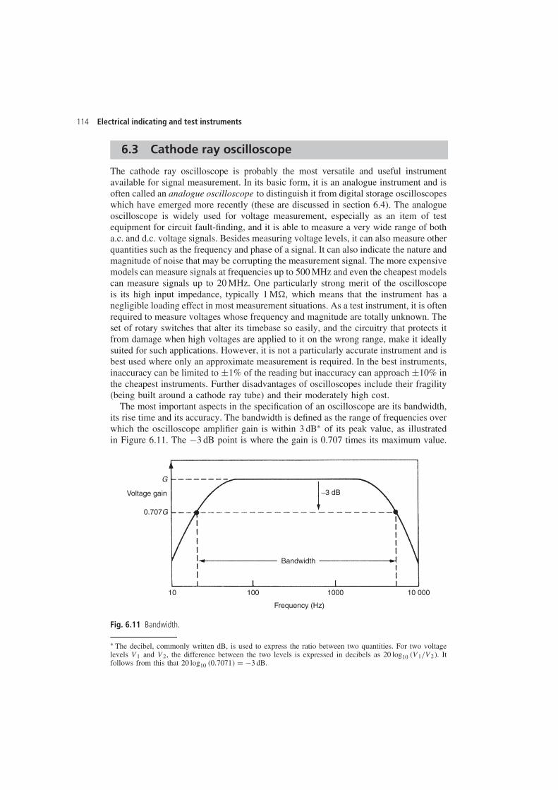
114 Electrical indicating and test instruments
6.3 Cathode ray oscilloscope
The cathode ray oscilloscope is probably the most versatile and useful instrumentavailable for signal measurement. In its basic form, it is an analogue instrument and isoften called an analogue oscilloscope to distinguish it from digital storage oscilloscopeswhich have emerged more recently (these are discussed in section 6.4). The analogueoscilloscope is widely used for voltage measurement, especially as an item of testequipment for circuit fault-finding, and it is able to measure a very wide range of botha.c. and d.c. voltage signals. Besides measuring voltage levels, it can also measure otherquantities such as the frequency and phase of a signal. It can also indicate the nature andmagnitude of noise that may be corrupting the measurement signal. The more expensivemodels can measure signals at frequencies up to 500 MHz and even the cheapest modelscan measure signals up to 20 MHz. One particularly strong merit of the oscilloscopeis its high input impedance, typically 1 M�, which means that the instrument has anegligible loading effect in most measurement situations. As a test instrument, it is oftenrequired to measure voltages whose frequency and magnitude are totally unknown. Theset of rotary switches that alter its timebase so easily, and the circuitry that protects itfrom damage when high voltages are applied to it on the wrong range, make it ideallysuited for such applications. However, it is not a particularly accurate instrument and isbest used where only an approximate measurement is required. In the best instruments,inaccuracy can be limited to š1% of the reading but inaccuracy can approach š10% inthe cheapest instruments. Further disadvantages of oscilloscopes include their fragility(being built around a cathode ray tube) and their moderately high cost.
The most important aspects in the specification of an oscilloscope are its bandwidth,its rise time and its accuracy. The bandwidth is defined as the range of frequencies overwhich the oscilloscope amplifier gain is within 3 dBŁ of its peak value, as illustratedin Figure 6.11. The �3 dB point is where the gain is 0.707 times its maximum value.
−3 dB
Bandwidth
G
Voltage gain
0.707G
10 100 1000 10 000
Frequency (Hz)
Fig. 6.11 Bandwidth.
Ł The decibel, commonly written dB, is used to express the ratio between two quantities. For two voltagelevels V1 and V2, the difference between the two levels is expressed in decibels as 20 log10 �V1/V2�. Itfollows from this that 20 log10 �0.7071� D �3 dB.
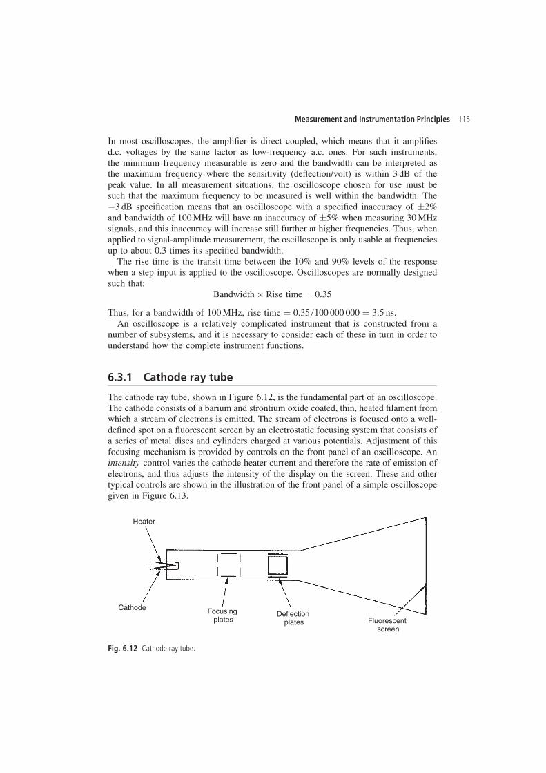
Measurement and Instrumentation Principles 115
In most oscilloscopes, the amplifier is direct coupled, which means that it amplifiesd.c. voltages by the same factor as low-frequency a.c. ones. For such instruments,the minimum frequency measurable is zero and the bandwidth can be interpreted asthe maximum frequency where the sensitivity (deflection/volt) is within 3 dB of thepeak value. In all measurement situations, the oscilloscope chosen for use must besuch that the maximum frequency to be measured is well within the bandwidth. The�3 dB specification means that an oscilloscope with a specified inaccuracy of š2%and bandwidth of 100 MHz will have an inaccuracy of š5% when measuring 30 MHzsignals, and this inaccuracy will increase still further at higher frequencies. Thus, whenapplied to signal-amplitude measurement, the oscilloscope is only usable at frequenciesup to about 0.3 times its specified bandwidth.
The rise time is the transit time between the 10% and 90% levels of the responsewhen a step input is applied to the oscilloscope. Oscilloscopes are normally designedsuch that:
Bandwidth ð Rise time D 0.35
Thus, for a bandwidth of 100 MHz, rise time D 0.35/100 000 000 D 3.5 ns.An oscilloscope is a relatively complicated instrument that is constructed from a
number of subsystems, and it is necessary to consider each of these in turn in order tounderstand how the complete instrument functions.
6.3.1 Cathode ray tube
The cathode ray tube, shown in Figure 6.12, is the fundamental part of an oscilloscope.The cathode consists of a barium and strontium oxide coated, thin, heated filament fromwhich a stream of electrons is emitted. The stream of electrons is focused onto a well-defined spot on a fluorescent screen by an electrostatic focusing system that consists ofa series of metal discs and cylinders charged at various potentials. Adjustment of thisfocusing mechanism is provided by controls on the front panel of an oscilloscope. Anintensity control varies the cathode heater current and therefore the rate of emission ofelectrons, and thus adjusts the intensity of the display on the screen. These and othertypical controls are shown in the illustration of the front panel of a simple oscilloscopegiven in Figure 6.13.
Heater
Cathode Focusing plates
Deflection plates Fluorescent
screen
Fig. 6.12 Cathode ray tube.
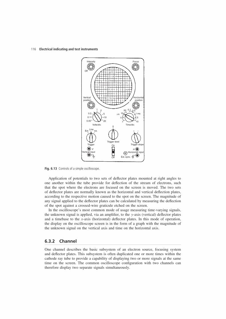
116 Electrical indicating and test instruments
Intensity
Off
Focus
Horizontal position
Vertical position
1 2
5
10
20
0.2
0.1
0.05
Volts/div. Time/div.
Ext.Line
Int.
0
Trigger levelTrigger Trigger slopeOn
Off
HVHorizontal inputVertical input
Ext. sync.
−+
0.1 0.51 mss
5
10
1050
1
5
m
Fig. 6.13 Controls of a simple oscilloscope.
Application of potentials to two sets of deflector plates mounted at right angles toone another within the tube provide for deflection of the stream of electrons, suchthat the spot where the electrons are focused on the screen is moved. The two setsof deflector plates are normally known as the horizontal and vertical deflection plates,according to the respective motion caused to the spot on the screen. The magnitude ofany signal applied to the deflector plates can be calculated by measuring the deflectionof the spot against a crossed-wire graticule etched on the screen.
In the oscilloscope’s most common mode of usage measuring time-varying signals,the unknown signal is applied, via an amplifier, to the y-axis (vertical) deflector platesand a timebase to the x-axis (horizontal) deflector plates. In this mode of operation,the display on the oscilloscope screen is in the form of a graph with the magnitude ofthe unknown signal on the vertical axis and time on the horizontal axis.
6.3.2 Channel
One channel describes the basic subsystem of an electron source, focusing systemand deflector plates. This subsystem is often duplicated one or more times within thecathode ray tube to provide a capability of displaying two or more signals at the sametime on the screen. The common oscilloscope configuration with two channels cantherefore display two separate signals simultaneously.
Measurement and Instrumentation Principles 117
6.3.3 Single-ended inputThis type of input only has one input terminal plus a ground terminal per oscilloscopechannel and, consequently, only allows signal voltages to be measured relative toground. It is normally only used in simple oscilloscopes.
6.3.4 Differential inputThis type of input is provided on more expensive oscilloscopes. Two input terminalsplus a ground terminal are provided for each channel, which allows the potentials attwo non-grounded points in a circuit to be compared. This type of input can also beused in single-ended mode to measure a signal relative to ground by using just one ofthe input terminals plus ground.
6.3.5 Timebase circuit
The purpose of a timebase is to apply a voltage to the horizontal deflector plates suchthat the horizontal position of the spot is proportional to time. This voltage, in theform of a ramp known as a sweep waveform, must be applied repetitively, such thatthe motion of the spot across the screen appears as a straight line when a d.c. level isapplied to the input channel. Furthermore, this timebase voltage must be synchronizedwith the input signal in the general case of a time-varying signal, such that a steadypicture is obtained on the oscilloscope screen. The length of time taken for the spotto traverse the screen is controlled by a time/div switch, which sets the length oftime taken by the spot to travel between two marked divisions on the screen, therebyallowing signals at a wide range of frequencies to be measured.
Each cycle of the sweep waveform is initiated by a pulse from a pulse generator. Theinput to the pulse generator is a sinusoidal signal known as a triggering signal, witha pulse being generated every time the triggering signal crosses a preselected slopeand voltage level condition. This condition is defined by the trigger level and triggerslope switches. The former selects the voltage level on the trigger signal, commonlyzero, at which a pulse is generated, whilst the latter selects whether pulsing occurs ona positive- or negative-going part of the triggering waveform.
Synchronization of the sweep waveform with the measured signal is most easilyachieved by deriving the trigger signal from the measured signal, a procedure that isknown as internal triggering. Alternatively, external triggering can be applied if thefrequencies of the triggering signal and measured signals are related by an integerconstant such that the display is stationary. External triggering is necessary when theamplitude of the measured signal is too small to drive the pulse generator, and it isalso used in applications where there is a requirement to measure the phase differencebetween two sinusoidal signals of the same frequency. It is very convenient to use the50 Hz line voltage for external triggering when measuring signals at mains frequency,and this is often given the name line triggering.
6.3.6 Vertical sensitivity control
This consists of a series of attenuators and pre-amplifiers at the input to the oscilloscope.These condition the measured signal to the optimum magnitude for input to the main
118 Electrical indicating and test instruments
amplifier and vertical deflection plates, thus enabling the instrument to measure a verywide range of different signal magnitudes. Selection of the appropriate input ampli-fier/attenuator is made by setting a volts/div control associated with each oscilloscopechannel. This defines the magnitude of the input signal that will cause a deflection ofone division on the screen.
6.3.7 Display position control
This allows the position at which a signal is displayed on the screen to be controlledin two ways. The horizontal position is adjusted by a horizontal position knob on theoscilloscope front panel and similarly a vertical position knob controls the verticalposition. These controls adjust the position of the display by biasing the measuredsignal with d.c. voltage levels.
6.4 Digital storage oscilloscopes
Digital storage oscilloscopes consist of a conventional analogue cathode ray oscillo-scope with the added facility that the measured analogue signal can be converted todigital format and stored in computer memory within the instrument. This stored datacan then be reconverted to analogue form at the frequency necessary to refresh theanalogue display on the screen. This produces a non-fading display of the signal onthe screen.
The signal displayed by a digital oscilloscope consists of a sequence of individualdots rather than a continuous line as displayed by an analogue oscilloscope. However,as the density of dots increases, the display becomes closer and closer to a continuousline, and the best instruments have displays that look very much like continuous traces.The density of the dots is entirely dependent upon the sampling rate at which theanalogue signal is digitized and the rate at which the memory contents are read toreconstruct the original signal. Inevitably, the speed of sampling etc. is a function ofcost, and the most expensive instruments give the best performance in terms of dotdensity and the accuracy with which the analogue signal is recorded and represented.
Besides their ability to display the magnitude of voltage signals and other parameterssuch as signal phase and frequency, some digital oscilloscopes can also compute signalparameters such as peak values, mean values and r.m.s. values. They are also ideallysuited to capturing transient signals when set to single-sweep mode. This avoids theproblem of the very careful synchronization that is necessary to capture such signalson an analogue oscilloscope. In addition, digital oscilloscopes often have facilities tooutput analogue signals to devices like chart recorders and output digital signals in aform that is compatible with standard interfaces like IEEE488 and RS232. Some noweven have floppy disk drives to extend their storage ability. Fuller details on digitaloscilloscopes can be found elsewhere Hickman, (1997).
References and further reading
Hickman, I. (1997) Digital Storage Oscilloscopes, Newnes.
7
Variable conversionelements
Outputs from measurement sensors that take the form of voltage signals can bemeasured using the voltage indicating and test instruments discussed in the last chapter.However, in many cases, the sensor output does not take the form of an electricalvoltage. Examples of these other forms of sensor output include translational displace-ments and changes in various electrical parameters such as resistance, inductance,capacitance and current. In some cases, the output may alternatively take the form ofvariations in the phase or frequency of an a.c. signal.
For sensor outputs that are initially in some non-voltage form, conversion to ameasurement signal that is in a more convenient form can be achieved by varioustypes of variable conversion element in the measurement system. Bridge circuits are aparticularly important type of variable conversion element, and these will be coveredin some detail. Following this, the various alternative techniques for transducing theoutputs of a measurement sensor will be covered.
7.1 Bridge circuits
Bridge circuits are used very commonly as a variable conversion element in measure-ment systems and produce an output in the form of a voltage level that changes as themeasured physical quantity changes. They provide an accurate method of measuringresistance, inductance and capacitance values, and enable the detection of very smallchanges in these quantities about a nominal value. They are of immense importancein measurement system technology because so many transducers measuring physicalquantities have an output that is expressed as a change in resistance, inductance orcapacitance. The displacement-measuring strain gauge, which has a varying resistanceoutput, is but one example of this class of transducers. Normally, excitation of thebridge is by a d.c. voltage for resistance measurement and by an a.c. voltage forinductance or capacitance measurement. Both null and deflection types of bridge exist,and, in a like manner to instruments in general, null types are mainly employed forcalibration purposes and deflection types are used within closed-loop automatic controlschemes.
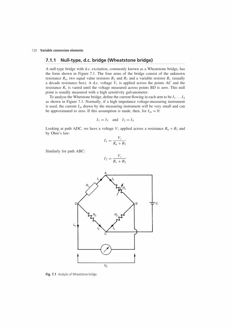
120 Variable conversion elements
7.1.1 Null-type, d.c. bridge (Wheatstone bridge)
A null-type bridge with d.c. excitation, commonly known as a Wheatstone bridge, hasthe form shown in Figure 7.1. The four arms of the bridge consist of the unknownresistance Ru, two equal value resistors R2 and R3 and a variable resistor Rv (usuallya decade resistance box). A d.c. voltage Vi is applied across the points AC and theresistance Rv is varied until the voltage measured across points BD is zero. This nullpoint is usually measured with a high sensitivity galvanometer.
To analyse the Whetstone bridge, define the current flowing in each arm to be I1 . . . I4
as shown in Figure 7.1. Normally, if a high impedance voltage-measuring instrumentis used, the current Im drawn by the measuring instrument will be very small and canbe approximated to zero. If this assumption is made, then, for Im D 0:
I1 D I3 and I2 D I4
Looking at path ADC, we have a voltage Vi applied across a resistance Ru C R3 andby Ohm’s law:
I1 D Vi
Ru C R3
Similarly for path ABC:
I2 D Vi
Rv C R2
A
B
C
D
I1
R3 R2
Ru
Vi
Rv
I2
ImI3 I4
V0
Fig. 7.1 Analysis of Wheatstone bridge.
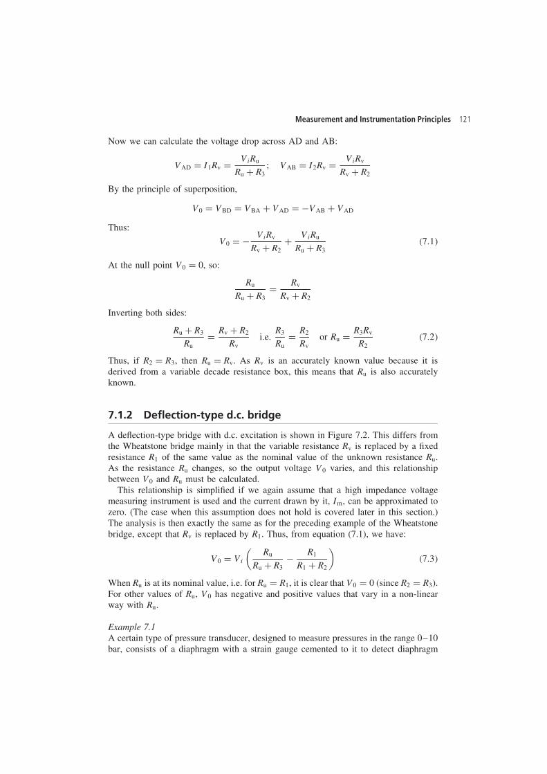
Measurement and Instrumentation Principles 121
Now we can calculate the voltage drop across AD and AB:
VAD D I1Rv D ViRu
Ru C R3; VAB D I2Rv D ViRv
Rv C R2
By the principle of superposition,
V0 D VBD D VBA C VAD D �VAB C VAD
Thus:
V0 D � ViRv
Rv C R2C ViRu
Ru C R3�7.1�
At the null point V0 D 0, so:
Ru
Ru C R3D Rv
Rv C R2
Inverting both sides:
Ru C R3
RuD Rv C R2
Rvi.e.
R3
RuD R2
Rvor Ru D R3Rv
R2�7.2�
Thus, if R2 D R3, then Ru D Rv. As Rv is an accurately known value because it isderived from a variable decade resistance box, this means that Ru is also accuratelyknown.
7.1.2 Deflection-type d.c. bridge
A deflection-type bridge with d.c. excitation is shown in Figure 7.2. This differs fromthe Wheatstone bridge mainly in that the variable resistance Rv is replaced by a fixedresistance R1 of the same value as the nominal value of the unknown resistance Ru.As the resistance Ru changes, so the output voltage V0 varies, and this relationshipbetween V0 and Ru must be calculated.
This relationship is simplified if we again assume that a high impedance voltagemeasuring instrument is used and the current drawn by it, Im, can be approximated tozero. (The case when this assumption does not hold is covered later in this section.)The analysis is then exactly the same as for the preceding example of the Wheatstonebridge, except that Rv is replaced by R1. Thus, from equation (7.1), we have:
V0 D Vi
(Ru
Ru C R3� R1
R1 C R2
)�7.3�
When Ru is at its nominal value, i.e. for Ru D R1, it is clear that V0 D 0 (since R2 D R3).For other values of Ru, V0 has negative and positive values that vary in a non-linearway with Ru.
Example 7.1A certain type of pressure transducer, designed to measure pressures in the range 0–10bar, consists of a diaphragm with a strain gauge cemented to it to detect diaphragm
122 Variable conversion elements
A
B
C
D
R3 R2
Ru
Vi
R1
V0
Fig. 7.2 Deflection-type d.c. bridge.
deflections. The strain gauge has a nominal resistance of 120 � and forms one armof a Wheatstone bridge circuit, with the other three arms each having a resistance of120 �. The bridge output is measured by an instrument whose input impedance canbe assumed infinite. If, in order to limit heating effects, the maximum permissiblegauge current is 30 mA, calculate the maximum permissible bridge excitation voltage.If the sensitivity of the strain gauge is 338 m�/bar and the maximum bridge excitationvoltage is used, calculate the bridge output voltage when measuring a pressure of 10bar.
SolutionThis is the type of bridge circuit shown in Figure 7.2 in which the components havethe following values:
R1 D R2 D R3 D 120 �
Defining I1 to be the current flowing in path ADC of the bridge, we can write:
Vi D I1�Ru C R3�
At balance, Ru D 120 and the maximum value allowable for I1 is 0.03 A.Hence:
Vi D 0.03�120 C 120� D 7.2 V
Thus, the maximum bridge excitation voltage allowable is 7.2 volts.For a pressure of 10 bar applied, the resistance change is 3.38 �, i.e. Ru is then
equal to 123.38 �.
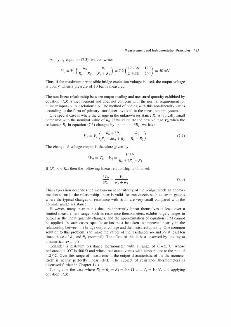
Measurement and Instrumentation Principles 123
Applying equation (7.3), we can write:
V0 D Vi
(Ru
Ru C R3� R1
R1 C R2
)D 7.2
(123.38
243.38� 120
240
)D 50 mV
Thus, if the maximum permissible bridge excitation voltage is used, the output voltageis 50 mV when a pressure of 10 bar is measured.
The non-linear relationship between output reading and measured quantity exhibited byequation (7.3) is inconvenient and does not conform with the normal requirement fora linear input–output relationship. The method of coping with this non-linearity variesaccording to the form of primary transducer involved in the measurement system.
One special case is where the change in the unknown resistance Ru is typically smallcompared with the nominal value of Ru. If we calculate the new voltage V0
0 when theresistance Ru in equation (7.3) changes by an amount υRu, we have:
V00 D Vi
(Ru C υRu
Ru C υRu C R3� R1
R1 C R2
)�7.4�
The change of voltage output is therefore given by:
υV0 D V00 � V0 D ViυRu
Ru C υRu C R3
If υRu << Ru, then the following linear relationship is obtained:
υV0
υRuD Vi
Ru C R3�7.5�
This expression describes the measurement sensitivity of the bridge. Such an approx-imation to make the relationship linear is valid for transducers such as strain gaugeswhere the typical changes of resistance with strain are very small compared with thenominal gauge resistance.
However, many instruments that are inherently linear themselves at least over alimited measurement range, such as resistance thermometers, exhibit large changes inoutput as the input quantity changes, and the approximation of equation (7.5) cannotbe applied. In such cases, specific action must be taken to improve linearity in therelationship between the bridge output voltage and the measured quantity. One commonsolution to this problem is to make the values of the resistances R2 and R3 at least tentimes those of R1 and Ru (nominal). The effect of this is best observed by looking ata numerical example.
Consider a platinum resistance thermometer with a range of 0° –50°C, whoseresistance at 0°C is 500 � and whose resistance varies with temperature at the rate of4 �/°C. Over this range of measurement, the output characteristic of the thermometeritself is nearly perfectly linear. (N.B. The subject of resistance thermometers isdiscussed further in Chapter 14.)
Taking first the case where R1 D R2 D R3 D 500 � and Vi D 10 V, and applyingequation (7.3):
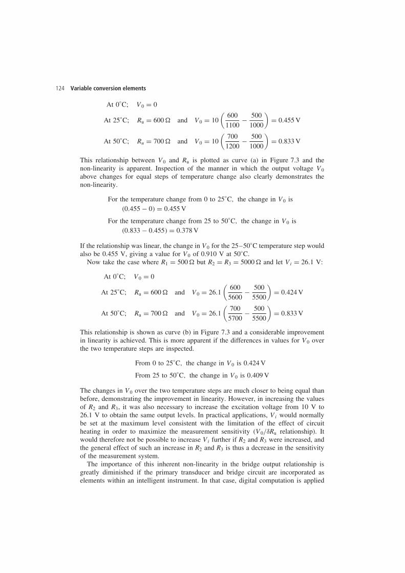
124 Variable conversion elements
At 0°C; V0 D 0
At 25°C; Ru D 600 � and V0 D 10(
600
1100� 500
1000
)D 0.455 V
At 50°C; Ru D 700 � and V0 D 10(
700
1200� 500
1000
)D 0.833 V
This relationship between V0 and Ru is plotted as curve (a) in Figure 7.3 and thenon-linearity is apparent. Inspection of the manner in which the output voltage V0
above changes for equal steps of temperature change also clearly demonstrates thenon-linearity.
For the temperature change from 0 to 25°C, the change in V0 is�0.455 � 0� D 0.455 V
For the temperature change from 25 to 50°C, the change in V0 is�0.833 � 0.455� D 0.378 V
If the relationship was linear, the change in V0 for the 25–50°C temperature step wouldalso be 0.455 V, giving a value for V0 of 0.910 V at 50°C.
Now take the case where R1 D 500 � but R2 D R3 D 5000 � and let Vi D 26.1 V:
At 0°C; V0 D 0
At 25°C; Ru D 600 � and V0 D 26.1(
600
5600� 500
5500
)D 0.424 V
At 50°C; Ru D 700 � and V0 D 26.1(
700
5700� 500
5500
)D 0.833 V
This relationship is shown as curve (b) in Figure 7.3 and a considerable improvementin linearity is achieved. This is more apparent if the differences in values for V0 overthe two temperature steps are inspected.
From 0 to 25°C, the change in V0 is 0.424 V
From 25 to 50°C, the change in V0 is 0.409 V
The changes in V0 over the two temperature steps are much closer to being equal thanbefore, demonstrating the improvement in linearity. However, in increasing the valuesof R2 and R3, it was also necessary to increase the excitation voltage from 10 V to26.1 V to obtain the same output levels. In practical applications, Vi would normallybe set at the maximum level consistent with the limitation of the effect of circuitheating in order to maximize the measurement sensitivity (V0/υRu relationship). Itwould therefore not be possible to increase Vi further if R2 and R3 were increased, andthe general effect of such an increase in R2 and R3 is thus a decrease in the sensitivityof the measurement system.
The importance of this inherent non-linearity in the bridge output relationship isgreatly diminished if the primary transducer and bridge circuit are incorporated aselements within an intelligent instrument. In that case, digital computation is applied
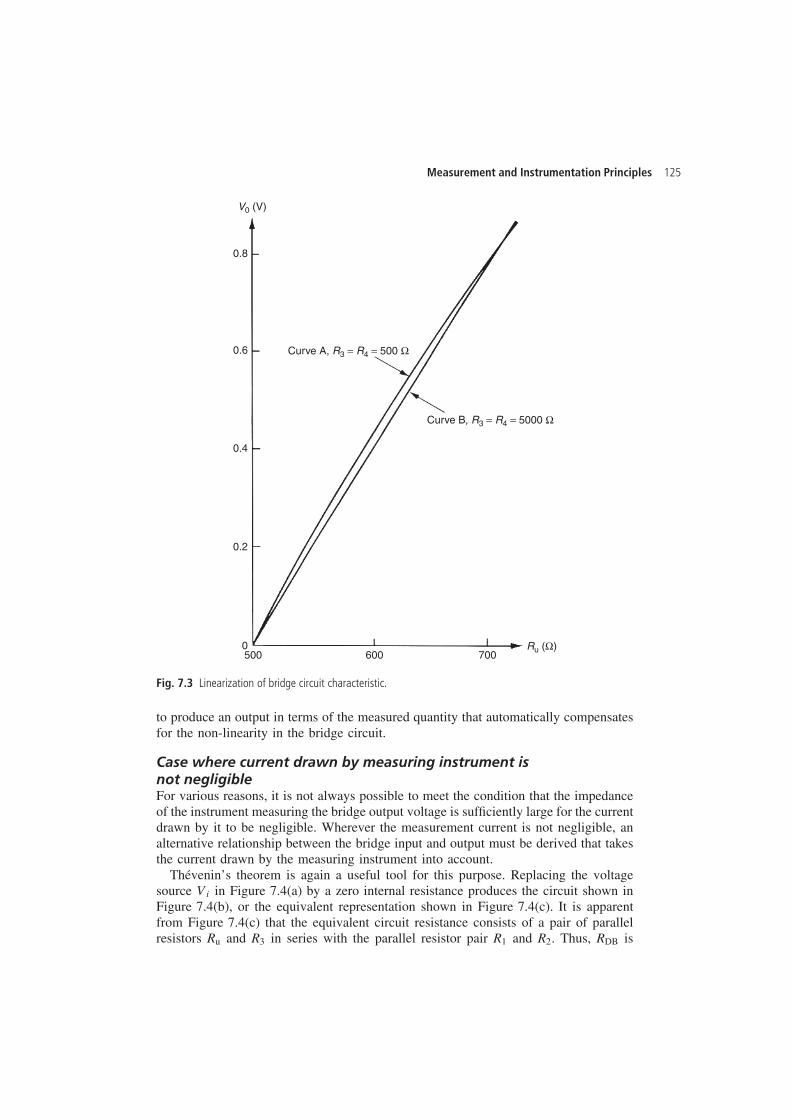
Measurement and Instrumentation Principles 125
500 600 700Ru (Ω)
V0 (V)
0
0.2
0.4
0.6
0.8
Curve B, R3 = R4 = 5000 Ω
Curve A, R3 = R4 = 500 Ω
Fig. 7.3 Linearization of bridge circuit characteristic.
to produce an output in terms of the measured quantity that automatically compensatesfor the non-linearity in the bridge circuit.
Case where current drawn by measuring instrument isnot negligibleFor various reasons, it is not always possible to meet the condition that the impedanceof the instrument measuring the bridge output voltage is sufficiently large for the currentdrawn by it to be negligible. Wherever the measurement current is not negligible, analternative relationship between the bridge input and output must be derived that takesthe current drawn by the measuring instrument into account.
Thevenin’s theorem is again a useful tool for this purpose. Replacing the voltagesource Vi in Figure 7.4(a) by a zero internal resistance produces the circuit shown inFigure 7.4(b), or the equivalent representation shown in Figure 7.4(c). It is apparentfrom Figure 7.4(c) that the equivalent circuit resistance consists of a pair of parallelresistors Ru and R3 in series with the parallel resistor pair R1 and R2. Thus, RDB is
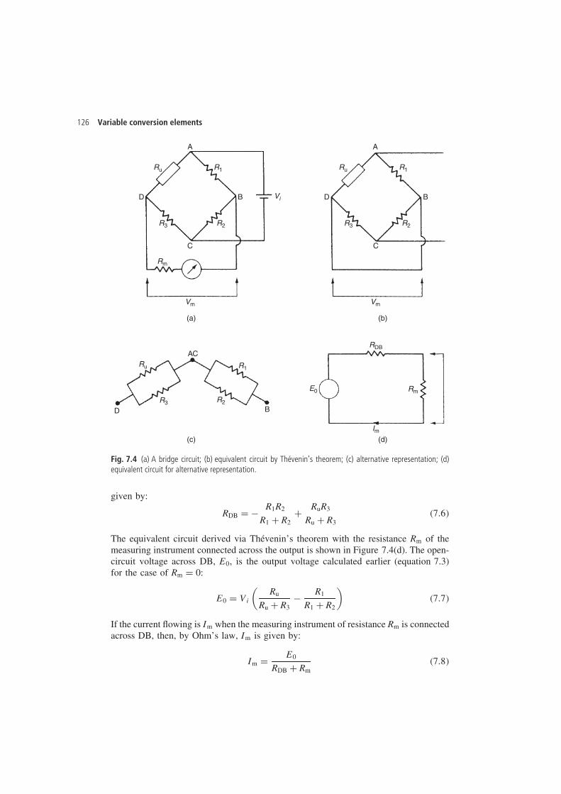
126 Variable conversion elements
A
B
B
C
AC
C
D
D
R3 R2
R3 R2
Ru
Vm
Im
E0
Rm
Rm
Vi
R1
Ru R1
A
BD
R3
RDB
R2
Ru
Vm
R1
(a) (b)
(c) (d)
Fig. 7.4 (a) A bridge circuit; (b) equivalent circuit by Thevenin’s theorem; (c) alternative representation; (d)equivalent circuit for alternative representation.
given by:
RDB D � R1R2
R1 C R2C RuR3
Ru C R3�7.6�
The equivalent circuit derived via Thevenin’s theorem with the resistance Rm of themeasuring instrument connected across the output is shown in Figure 7.4(d). The open-circuit voltage across DB, E0, is the output voltage calculated earlier (equation 7.3)for the case of Rm D 0:
E0 D Vi
(Ru
Ru C R3� R1
R1 C R2
)�7.7�
If the current flowing is Im when the measuring instrument of resistance Rm is connectedacross DB, then, by Ohm’s law, Im is given by:
Im D E0
RDB C Rm�7.8�
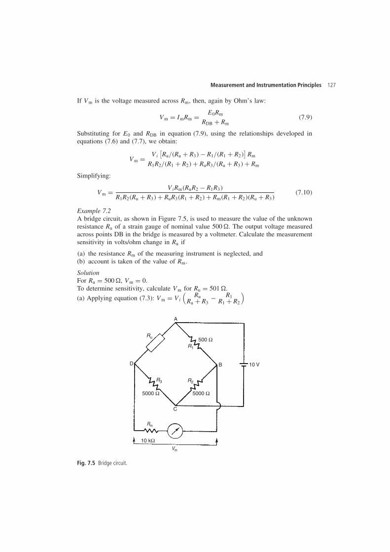
Measurement and Instrumentation Principles 127
If Vm is the voltage measured across Rm, then, again by Ohm’s law:
Vm D ImRm D E0Rm
RDB C Rm�7.9�
Substituting for E0 and RDB in equation (7.9), using the relationships developed inequations (7.6) and (7.7), we obtain:
Vm D Vi[Ru/�Ru C R3� � R1/�R1 C R2�
]Rm
R1R2/�R1 C R2� C RuR3/�Ru C R3� C Rm
Simplifying:
Vm D ViRm�RuR2 � R1R3�
R1R2�Ru C R3� C RuR3�R1 C R2� C Rm�R1 C R2��Ru C R3��7.10�
Example 7.2A bridge circuit, as shown in Figure 7.5, is used to measure the value of the unknownresistance Ru of a strain gauge of nominal value 500 �. The output voltage measuredacross points DB in the bridge is measured by a voltmeter. Calculate the measurementsensitivity in volts/ohm change in Ru if
(a) the resistance Rm of the measuring instrument is neglected, and(b) account is taken of the value of Rm.
SolutionFor Ru D 500 �, Vm D 0.To determine sensitivity, calculate Vm for Ru D 501 �.
(a) Applying equation (7.3): Vm D Vi
(Ru
Ru C R3� R1
R1 C R2
)
A
B
C
D
R3 R2
Ru
10 V
R1
Vm
Rm
500 Ω
5000 Ω5000 Ω
10 kΩ
Fig. 7.5 Bridge circuit.
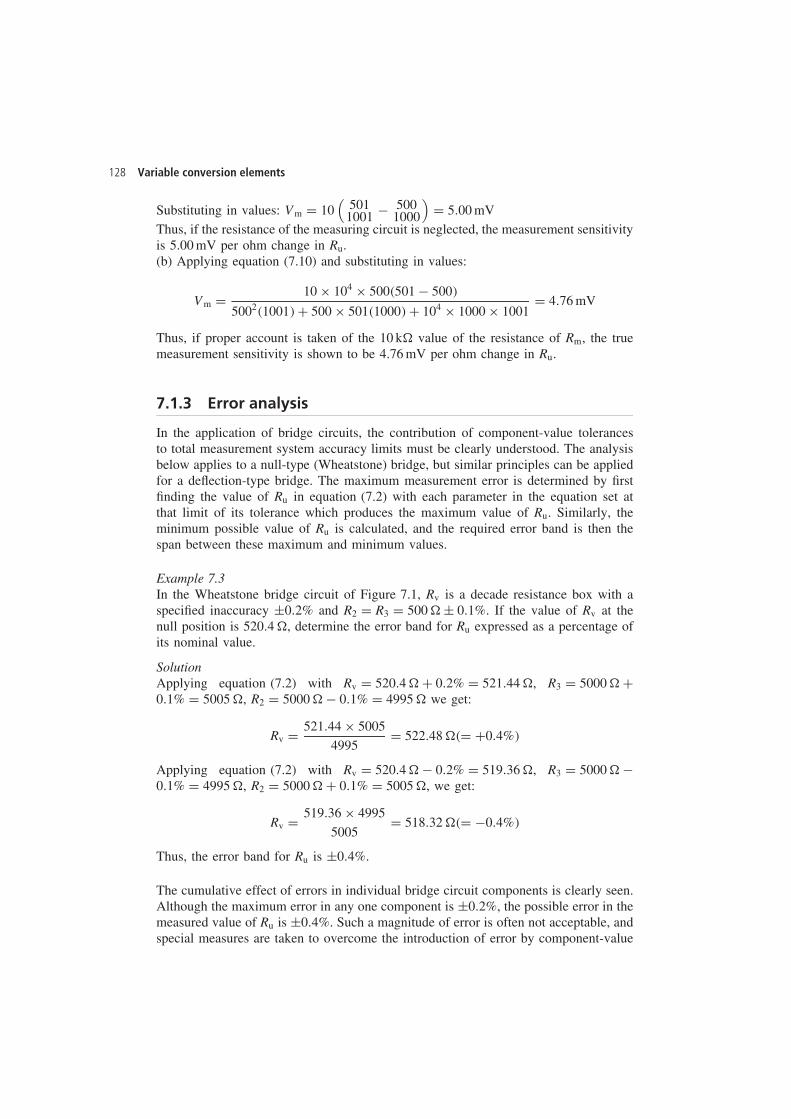
128 Variable conversion elements
Substituting in values: Vm D 10(
5011001 � 500
1000
)D 5.00 mV
Thus, if the resistance of the measuring circuit is neglected, the measurement sensitivityis 5.00 mV per ohm change in Ru.(b) Applying equation (7.10) and substituting in values:
Vm D 10 ð 104 ð 500�501 � 500�
5002�1001� C 500 ð 501�1000� C 104 ð 1000 ð 1001D 4.76 mV
Thus, if proper account is taken of the 10 k� value of the resistance of Rm, the truemeasurement sensitivity is shown to be 4.76 mV per ohm change in Ru.
7.1.3 Error analysis
In the application of bridge circuits, the contribution of component-value tolerancesto total measurement system accuracy limits must be clearly understood. The analysisbelow applies to a null-type (Wheatstone) bridge, but similar principles can be appliedfor a deflection-type bridge. The maximum measurement error is determined by firstfinding the value of Ru in equation (7.2) with each parameter in the equation set atthat limit of its tolerance which produces the maximum value of Ru. Similarly, theminimum possible value of Ru is calculated, and the required error band is then thespan between these maximum and minimum values.
Example 7.3In the Wheatstone bridge circuit of Figure 7.1, Rv is a decade resistance box with aspecified inaccuracy š0.2% and R2 D R3 D 500 � š 0.1%. If the value of Rv at thenull position is 520.4 �, determine the error band for Ru expressed as a percentage ofits nominal value.
SolutionApplying equation (7.2) with Rv D 520.4 � C 0.2% D 521.44 �, R3 D 5000 � C0.1% D 5005 �, R2 D 5000 � � 0.1% D 4995 � we get:
Rv D 521.44 ð 5005
4995D 522.48 ��D C0.4%�
Applying equation (7.2) with Rv D 520.4 � � 0.2% D 519.36 �, R3 D 5000 � �0.1% D 4995 �, R2 D 5000 � C 0.1% D 5005 �, we get:
Rv D 519.36 ð 4995
5005D 518.32 ��D �0.4%�
Thus, the error band for Ru is š0.4%.
The cumulative effect of errors in individual bridge circuit components is clearly seen.Although the maximum error in any one component is š0.2%, the possible error in themeasured value of Ru is š0.4%. Such a magnitude of error is often not acceptable, andspecial measures are taken to overcome the introduction of error by component-value
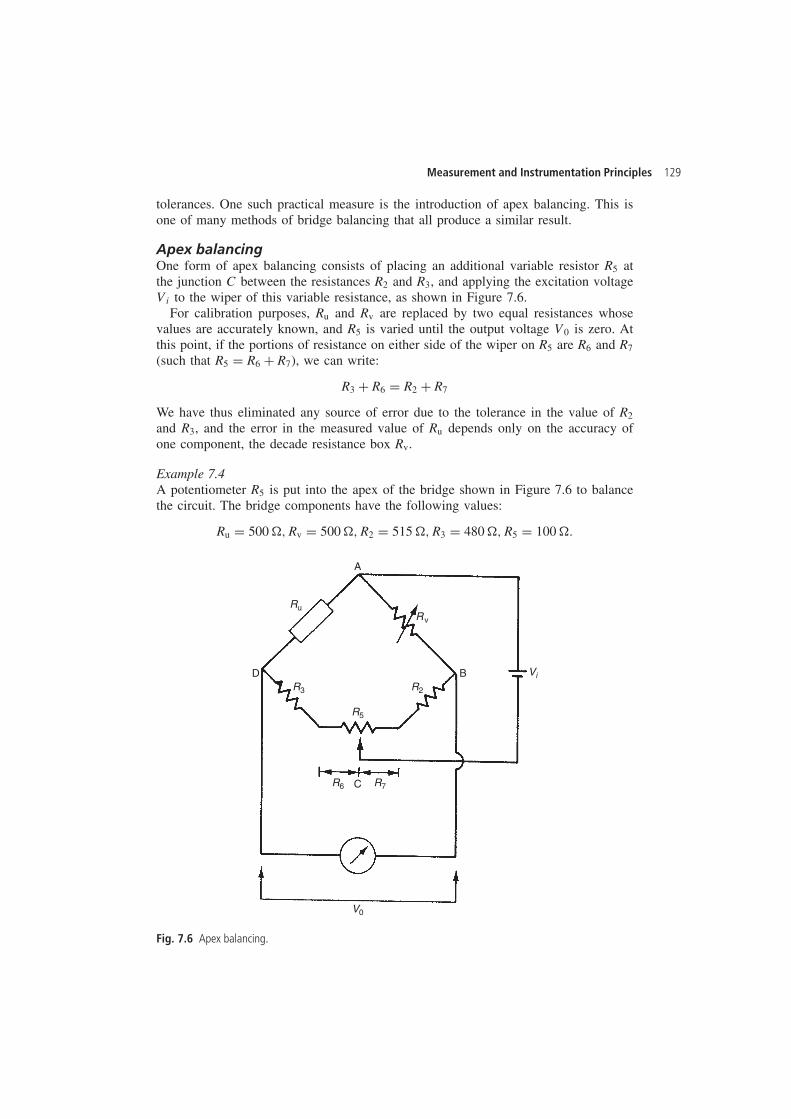
Measurement and Instrumentation Principles 129
tolerances. One such practical measure is the introduction of apex balancing. This isone of many methods of bridge balancing that all produce a similar result.
Apex balancingOne form of apex balancing consists of placing an additional variable resistor R5 atthe junction C between the resistances R2 and R3, and applying the excitation voltageVi to the wiper of this variable resistance, as shown in Figure 7.6.
For calibration purposes, Ru and Rv are replaced by two equal resistances whosevalues are accurately known, and R5 is varied until the output voltage V0 is zero. Atthis point, if the portions of resistance on either side of the wiper on R5 are R6 and R7
(such that R5 D R6 C R7), we can write:
R3 C R6 D R2 C R7
We have thus eliminated any source of error due to the tolerance in the value of R2
and R3, and the error in the measured value of Ru depends only on the accuracy ofone component, the decade resistance box Rv.
Example 7.4A potentiometer R5 is put into the apex of the bridge shown in Figure 7.6 to balancethe circuit. The bridge components have the following values:
Ru D 500 �, Rv D 500 �, R2 D 515 �, R3 D 480 �, R5 D 100 �.
A
B
C
DR3 R2
R5
R6 R7
Ru
Vi
Rv
V0
Fig. 7.6 Apex balancing.
130 Variable conversion elements
Determine the required value of the resistances R6 and R7 of the parts of the poten-tiometer track either side of the slider in order to balance the bridge and compensatefor the unequal values of R2 and R3.
SolutionFor balance, R2 C R7 D R3 C R6; hence, 515 C R7 D 480 C R6
Also, because R6 and R7 are the two parts of the potentiometer track R5 whose resistanceis 100 �:
R6 C R7 D 100; thus 515 C R7 D 480 C �100 � R7�; i.e. 2R7 D 580 � 515 D 65Thus, R7 D 32.5; hence, R6 D 100 � 32.5 D 67.5 �.
7.1.4 A.c. bridges
Bridges with a.c. excitation are used to measure unknown impedances. As for d.c.bridges, both null and deflection types exist, with null types being generally reservedfor calibration duties.
Null-type impedance bridgeA typical null-type impedance bridge is shown in Figure 7.7. The null point can beconveniently detected by monitoring the output with a pair of headphones connectedvia an operational amplifier across the points BD. This is a much cheaper method ofnull detection than the application of an expensive galvanometer that is required for ad.c. Wheatstone bridge.
Referring to Figure 7.7, at the null point,
I1R1 D I2R2; I1Zu D I2Zv
Thus:
Zu D ZvR1
R2�7.11�
A
B
C
D
I1R2 R1
I2
ZuZv
Fig. 7.7 Null-type impedance bridge.
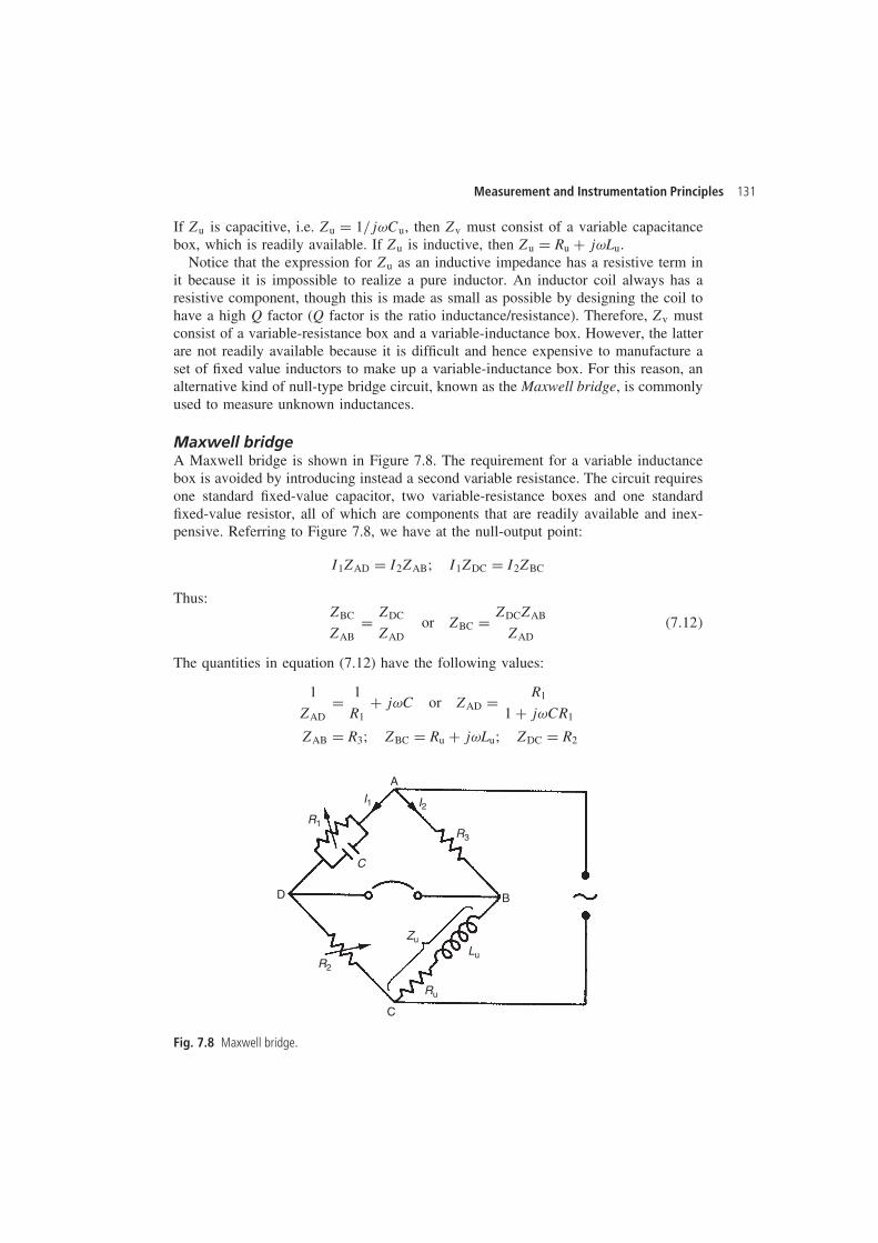
Measurement and Instrumentation Principles 131
If Zu is capacitive, i.e. Zu D 1/jωCu, then Zv must consist of a variable capacitancebox, which is readily available. If Zu is inductive, then Zu D Ru C jωLu.
Notice that the expression for Zu as an inductive impedance has a resistive term init because it is impossible to realize a pure inductor. An inductor coil always has aresistive component, though this is made as small as possible by designing the coil tohave a high Q factor (Q factor is the ratio inductance/resistance). Therefore, Zv mustconsist of a variable-resistance box and a variable-inductance box. However, the latterare not readily available because it is difficult and hence expensive to manufacture aset of fixed value inductors to make up a variable-inductance box. For this reason, analternative kind of null-type bridge circuit, known as the Maxwell bridge, is commonlyused to measure unknown inductances.
Maxwell bridgeA Maxwell bridge is shown in Figure 7.8. The requirement for a variable inductancebox is avoided by introducing instead a second variable resistance. The circuit requiresone standard fixed-value capacitor, two variable-resistance boxes and one standardfixed-value resistor, all of which are components that are readily available and inex-pensive. Referring to Figure 7.8, we have at the null-output point:
I1ZAD D I2ZAB; I1ZDC D I2ZBC
Thus:ZBC
ZABD ZDC
ZADor ZBC D ZDCZAB
ZAD�7.12�
The quantities in equation (7.12) have the following values:
1
ZADD 1
R1C jωC or ZAD D R1
1 C jωCR1
ZAB D R3; ZBC D Ru C jωLu; ZDC D R2
A
B
C
C
D
I1
R3
R1
R2
Ru
Lu
Zu
I2
Fig. 7.8 Maxwell bridge.
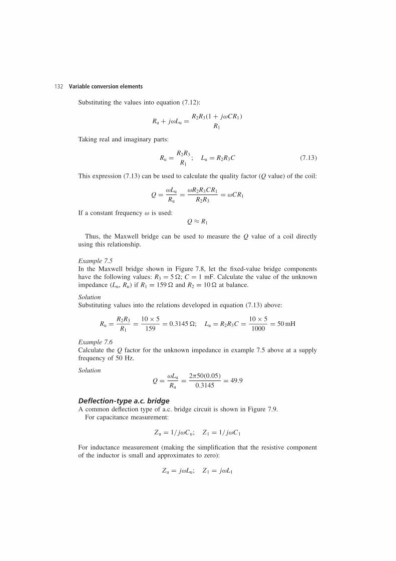
132 Variable conversion elements
Substituting the values into equation (7.12):
Ru C jωLu D R2R3�1 C jωCR1�
R1
Taking real and imaginary parts:
Ru D R2R3
R1; Lu D R2R3C �7.13�
This expression (7.13) can be used to calculate the quality factor (Q value) of the coil:
Q D ωLu
RuD ωR2R3CR1
R2R3D ωCR1
If a constant frequency ω is used:Q ³ R1
Thus, the Maxwell bridge can be used to measure the Q value of a coil directlyusing this relationship.
Example 7.5In the Maxwell bridge shown in Figure 7.8, let the fixed-value bridge componentshave the following values: R3 D 5 �; C D 1 mF. Calculate the value of the unknownimpedance (Lu, Ru) if R1 D 159 � and R2 D 10 � at balance.
SolutionSubstituting values into the relations developed in equation (7.13) above:
Ru D R2R3
R1D 10 ð 5
159D 0.3145 �; Lu D R2R3C D 10 ð 5
1000D 50 mH
Example 7.6Calculate the Q factor for the unknown impedance in example 7.5 above at a supplyfrequency of 50 Hz.
Solution
Q D ωLu
RuD 250�0.05�
0.3145D 49.9
Deflection-type a.c. bridgeA common deflection type of a.c. bridge circuit is shown in Figure 7.9.
For capacitance measurement:
Zu D 1/jωCu; Z1 D 1/jωC1
For inductance measurement (making the simplification that the resistive componentof the inductor is small and approximates to zero):
Zu D jωLu; Z1 D jωL1
Measurement and Instrumentation Principles 133
A
B
C
D
I1
Z1R2
Zu
Vs
R3
I2
Im
V0
Fig. 7.9 Deflection-type a.c. bridge.
Analysis of the circuit to find the relationship between V0 and Zu is greatly simplifiedif one assumes that Im is negligible. This is valid provided that the instrument measuringV0 has a high impedance. For Im D 0, currents in the two branches of the bridge, asdefined in Figure 7.9, are given by:
I1 D Vs
Z1 C Zu; I2 D Vs
R2 C R3
Also
VAD D I1Zu and VAB D I2R3
Hence:
V0 D VBD D VAD � VAB D Vs
(Zu
Z1 C Zu� R3
R2 C R3
)
Thus, for capacitances:
V0 D Vs
(1/Cu
1/C1 C 1/Cu� R3
R2 C R3
)D Vs
(C1
C1 C Cu� R3
R2 C R3
)�7.14�
and for inductances:
V0 D Vs
(Lu
L1 C Lu� R3
R2 C R3
)�7.15�
134 Variable conversion elements
This latter relationship (7.15) is in practice only approximate since inductiveimpedances are never pure inductances as assumed but always contain a finite resistance(i.e. Zu D jωLu C R). However, the approximation is valid in many circumstances.
Example 7.7A deflection bridge as shown in Figure 7.9 is used to measure an unknown capacitance,Cu. The components in the bridge have the following values:
Vs D 20 Vr.m.s., C1 D 100 μF, R2 D 60 �, R3 D 40 �
If Cu D 100 μF, calculate the output voltage V0.
SolutionFrom equation (7.14):
V0 D Vs
(C1
C1 C Cu� R3
R2 C R3
)D 20�0.5 � 0.4� D 2Vr.m.s.
Example 7.8An unknown inductance Lu is measured using a deflection type of bridge as shown inFigure 7.9. The components in the bridge have the following values:
Vs D 10 Vr.m.s., L1 D 20 mH, R2 D 100 �, R3 D 100 �
If the output voltage V0 is 1 Vr.m.s., calculate the value of Lu.
SolutionFrom equation (7.15):
Lu
L1 C LuD V0
VsC R3
R2 C R3D 0.1 C 0.5 D 0.6
Thus
Lu D 0.6�L1 C Lu�; 0.4Lu D 0.6L1; Lu D 0.6L1
0.4D 30 mH
7.2 Resistance measurement
Devices that convert the measured quantity into a change in resistance include theresistance thermometer, the thermistor, the wire-coil pressure gauge and the straingauge. The standard devices and methods available for measuring change in resist-ance, which is measured in units of ohms (�), include the d.c. bridge circuit, thevoltmeter–ammeter method, the resistance-substitution method, the digital voltmeterand the ohmmeter. Apart from the ohmmeter, these instruments are normally onlyused to measure medium values of resistance in the range of 1 � to 1 M�. Specialinstruments are available for obtaining high-accuracy resistance measurements outsidethis range (see Baldwin (1973)).
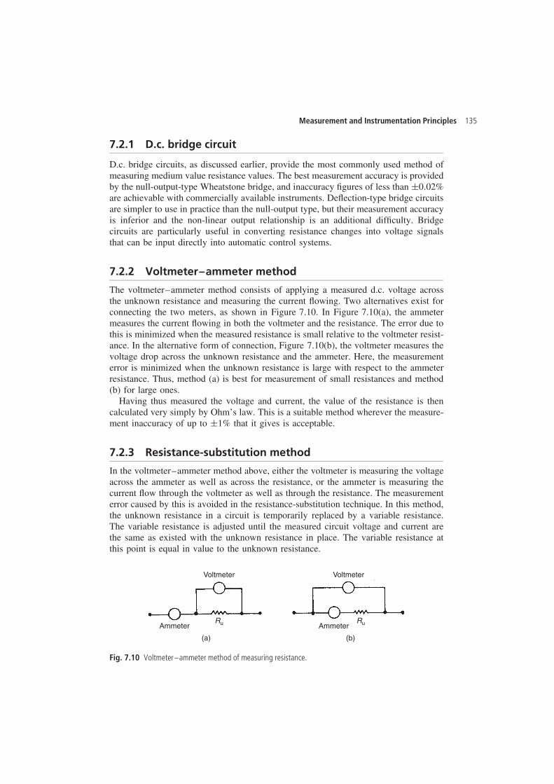
Measurement and Instrumentation Principles 135
7.2.1 D.c. bridge circuit
D.c. bridge circuits, as discussed earlier, provide the most commonly used method ofmeasuring medium value resistance values. The best measurement accuracy is providedby the null-output-type Wheatstone bridge, and inaccuracy figures of less than š0.02%are achievable with commercially available instruments. Deflection-type bridge circuitsare simpler to use in practice than the null-output type, but their measurement accuracyis inferior and the non-linear output relationship is an additional difficulty. Bridgecircuits are particularly useful in converting resistance changes into voltage signalsthat can be input directly into automatic control systems.
7.2.2 Voltmeter–ammeter method
The voltmeter–ammeter method consists of applying a measured d.c. voltage acrossthe unknown resistance and measuring the current flowing. Two alternatives exist forconnecting the two meters, as shown in Figure 7.10. In Figure 7.10(a), the ammetermeasures the current flowing in both the voltmeter and the resistance. The error due tothis is minimized when the measured resistance is small relative to the voltmeter resist-ance. In the alternative form of connection, Figure 7.10(b), the voltmeter measures thevoltage drop across the unknown resistance and the ammeter. Here, the measurementerror is minimized when the unknown resistance is large with respect to the ammeterresistance. Thus, method (a) is best for measurement of small resistances and method(b) for large ones.
Having thus measured the voltage and current, the value of the resistance is thencalculated very simply by Ohm’s law. This is a suitable method wherever the measure-ment inaccuracy of up to š1% that it gives is acceptable.
7.2.3 Resistance-substitution method
In the voltmeter–ammeter method above, either the voltmeter is measuring the voltageacross the ammeter as well as across the resistance, or the ammeter is measuring thecurrent flow through the voltmeter as well as through the resistance. The measurementerror caused by this is avoided in the resistance-substitution technique. In this method,the unknown resistance in a circuit is temporarily replaced by a variable resistance.The variable resistance is adjusted until the measured circuit voltage and current arethe same as existed with the unknown resistance in place. The variable resistance atthis point is equal in value to the unknown resistance.
Voltmeter
(a)
AmmeterRu
Voltmeter
(b)
AmmeterRu
Fig. 7.10 Voltmeter–ammeter method of measuring resistance.
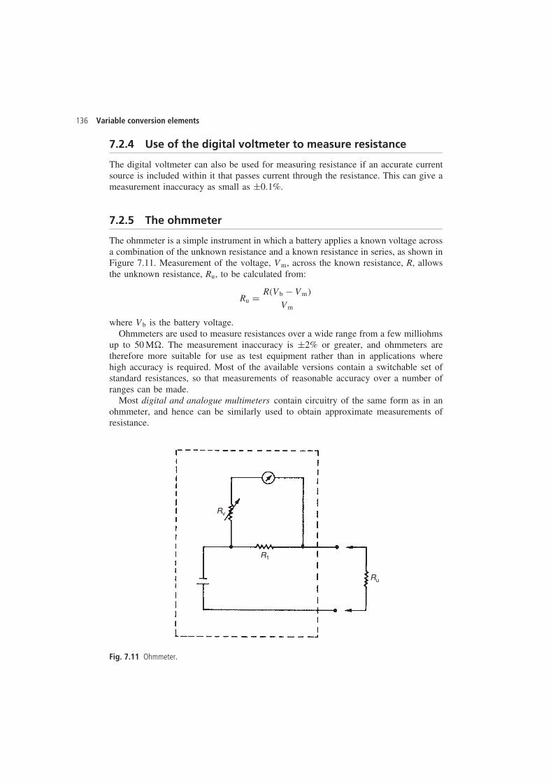
136 Variable conversion elements
7.2.4 Use of the digital voltmeter to measure resistance
The digital voltmeter can also be used for measuring resistance if an accurate currentsource is included within it that passes current through the resistance. This can give ameasurement inaccuracy as small as š0.1%.
7.2.5 The ohmmeter
The ohmmeter is a simple instrument in which a battery applies a known voltage acrossa combination of the unknown resistance and a known resistance in series, as shown inFigure 7.11. Measurement of the voltage, Vm, across the known resistance, R, allowsthe unknown resistance, Ru, to be calculated from:
Ru D R�Vb � Vm�
Vm
where Vb is the battery voltage.Ohmmeters are used to measure resistances over a wide range from a few milliohms
up to 50 M�. The measurement inaccuracy is š2% or greater, and ohmmeters aretherefore more suitable for use as test equipment rather than in applications wherehigh accuracy is required. Most of the available versions contain a switchable set ofstandard resistances, so that measurements of reasonable accuracy over a number ofranges can be made.
Most digital and analogue multimeters contain circuitry of the same form as in anohmmeter, and hence can be similarly used to obtain approximate measurements ofresistance.
Rv
R1
Ru
Fig. 7.11 Ohmmeter.
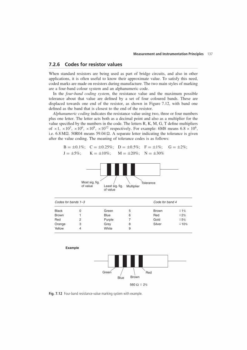
Measurement and Instrumentation Principles 137
7.2.6 Codes for resistor values
When standard resistors are being used as part of bridge circuits, and also in otherapplications, it is often useful to know their approximate value. To satisfy this need,coded marks are made on resistors during manufacture. The two main styles of markingare a four-band colour system and an alphanumeric code.
In the four-band coding system, the resistance value and the maximum possibletolerance about that value are defined by a set of four coloured bands. These aredisplaced towards one end of the resistor, as shown in Figure 7.12, with band onedefined as the band that is closest to the end of the resistor.
Alphanumeric coding indicates the resistance value using two, three or four numbersplus one letter. The letter acts both as a decimal point and also as a multiplier for thevalue specified by the numbers in the code. The letters R, K, M, G, T define multipliersof ð1, ð103, ð106, ð109, ð1012 respectively. For example: 6M8 means 6.8 ð 106,i.e. 6.8 M�. 50R04 means 59.04 �. A separate letter indicating the tolerance is givenafter the value coding. The meaning of tolerance codes is as follows:
B D š0.1%; C D š0.25%; D D š0.5%; F D š1%; G D š2%;
J D š5%; K D š10%; M D š20%; N D š30%
Most sig. fig.of value Least sig. fig.
of valueMultiplier
Tolerance
BlackBrownRedOrangeYellow
GreenBluePurpleGreyWhite
Brown
Codes for bands 1–3 Code for band 4
RedGoldSilver
�1%�2%�5%�10%
01234
56789
Green
Blue BrownRed
560 Ω � 2%
Example
Fig. 7.12 Four-band resistance-value marking system with example.
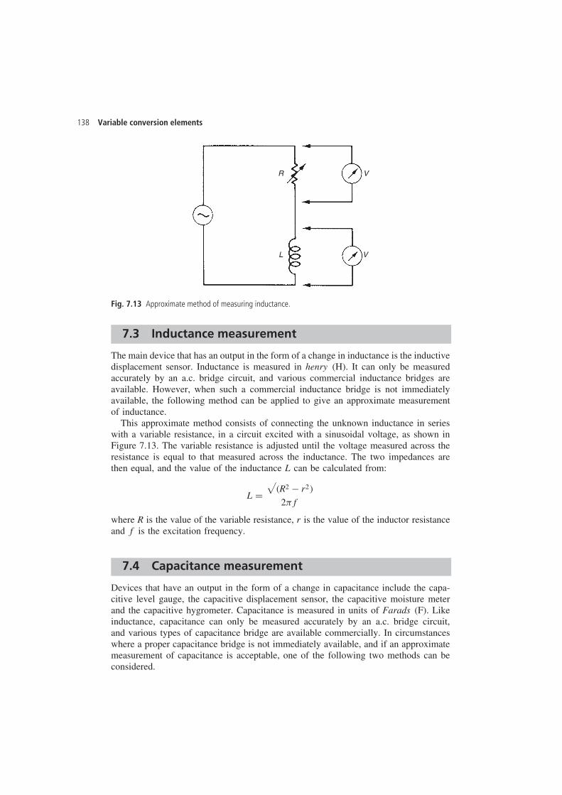
138 Variable conversion elements
R
L
V
V
Fig. 7.13 Approximate method of measuring inductance.
7.3 Inductance measurement
The main device that has an output in the form of a change in inductance is the inductivedisplacement sensor. Inductance is measured in henry (H). It can only be measuredaccurately by an a.c. bridge circuit, and various commercial inductance bridges areavailable. However, when such a commercial inductance bridge is not immediatelyavailable, the following method can be applied to give an approximate measurementof inductance.
This approximate method consists of connecting the unknown inductance in serieswith a variable resistance, in a circuit excited with a sinusoidal voltage, as shown inFigure 7.13. The variable resistance is adjusted until the voltage measured across theresistance is equal to that measured across the inductance. The two impedances arethen equal, and the value of the inductance L can be calculated from:
L D√
�R2 � r2�
2f
where R is the value of the variable resistance, r is the value of the inductor resistanceand f is the excitation frequency.
7.4 Capacitance measurement
Devices that have an output in the form of a change in capacitance include the capa-citive level gauge, the capacitive displacement sensor, the capacitive moisture meterand the capacitive hygrometer. Capacitance is measured in units of Farads (F). Likeinductance, capacitance can only be measured accurately by an a.c. bridge circuit,and various types of capacitance bridge are available commercially. In circumstanceswhere a proper capacitance bridge is not immediately available, and if an approximatemeasurement of capacitance is acceptable, one of the following two methods can beconsidered.
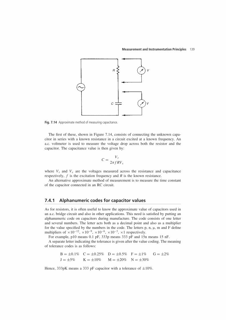
Measurement and Instrumentation Principles 139
R
C
V
V
Fig. 7.14 Approximate method of measuring capacitance.
The first of these, shown in Figure 7.14, consists of connecting the unknown capa-citor in series with a known resistance in a circuit excited at a known frequency. Ana.c. voltmeter is used to measure the voltage drop across both the resistor and thecapacitor. The capacitance value is then given by:
C D Vr
2fRVc
where Vr and Vc are the voltages measured across the resistance and capacitancerespectively, f is the excitation frequency and R is the known resistance.
An alternative approximate method of measurement is to measure the time constantof the capacitor connected in an RC circuit.
7.4.1 Alphanumeric codes for capacitor values
As for resistors, it is often useful to know the approximate value of capacitors used inan a.c. bridge circuit and also in other applications. This need is satisfied by putting analphanumeric code on capacitors during manufacture. The code consists of one letterand several numbers. The letter acts both as a decimal point and also as a multiplierfor the value specified by the numbers in the code. The letters p, n, μ, m and F definemultipliers of ð10�12, ð10�9, ð10�6, ð10�3, ð1 respectively.
For example, p10 means 0.1 pF, 333p means 333 pF and 15n means 15 nF.A separate letter indicating the tolerance is given after the value coding. The meaning
of tolerance codes is as follows:
B D š0.1% C D š0.25% D D š0.5% F D š1% G D š2%
J D š5% K D š10% M D š20% N D š30%
Hence, 333pK means a 333 pF capacitor with a tolerance of š10%.
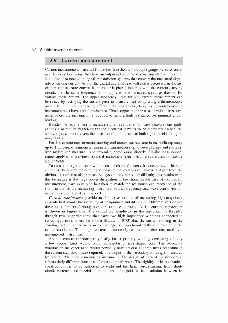
140 Variable conversion elements
7.5 Current measurement
Current measurement is needed for devices like the thermocouple-gauge pressure sensorand the ionization gauge that have an output in the form of a varying electrical current.It is often also needed in signal transmission systems that convert the measured signalinto a varying current. Any of the digital and analogue voltmeters discussed in the lastchapter can measure current if the meter is placed in series with the current-carryingcircuit, and the same frequency limits apply for the measured signal as they do forvoltage measurement. The upper frequency limit for a.c. current measurement canbe raised by rectifying the current prior to measurement or by using a thermocouplemeter. To minimize the loading effect on the measured system, any current-measuringinstrument must have a small resistance. This is opposite to the case of voltage measure-ment where the instrument is required to have a high resistance for minimal circuitloading.
Besides the requirement to measure signal-level currents, many measurement appli-cations also require higher-magnitude electrical currents to be measured. Hence, thefollowing discussion covers the measurement of currents at both signal level and highermagnitudes.
For d.c. current measurement, moving-coil meters can measure in the milliamp rangeup to 1 ampere, dynamometer ammeters can measure up to several amps and moving-iron meters can measure up to several hundred amps directly. Similar measurementranges apply when moving-iron and dynamometer-type instruments are used to measurea.c. currents.
To measure larger currents with electromechanical meters, it is necessary to insert ashunt resistance into the circuit and measure the voltage drop across it. Apart from theobvious disturbance of the measured system, one particular difficulty that results fromthis technique is the large power dissipation in the shunt. In the case of a.c. currentmeasurement, care must also be taken to match the resistance and reactance of theshunt to that of the measuring instrument so that frequency and waveform distortionin the measured signal are avoided.
Current transformers provide an alternative method of measuring high-magnitudecurrents that avoids the difficulty of designing a suitable shunt. Different versions ofthese exist for transforming both d.c. and a.c. currents. A d.c. current transformeris shown in Figure 7.15. The central d.c. conductor in the instrument is threadedthrough two magnetic cores that carry two high impedance windings connected inseries opposition. It can be shown (Baldwin, 1973) that the current flowing in thewindings when excited with an a.c. voltage is proportional to the d.c. current in thecentral conductor. This output current is commonly rectified and then measured by amoving-coil instrument.
An a.c. current transformer typically has a primary winding consisting of onlya few copper turns wound on a rectangular or ring-shaped core. The secondarywinding on the other hand would normally have several hundred turns according tothe current step-down ratio required. The output of the secondary winding is measuredby any suitable current-measuring instrument. The design of current transformers issubstantially different from that of voltage transformers. The rigidity of its mechanicalconstruction has to be sufficient to withstand the large forces arising from short-circuit currents, and special attention has to be paid to the insulation between its
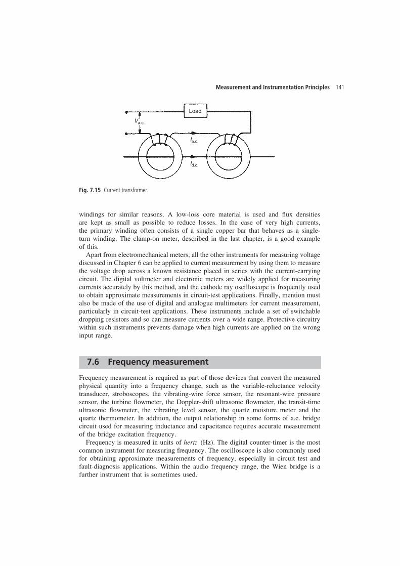
Measurement and Instrumentation Principles 141
Load
Va.c.
Ia.c.
Id.c.
Fig. 7.15 Current transformer.
windings for similar reasons. A low-loss core material is used and flux densitiesare kept as small as possible to reduce losses. In the case of very high currents,the primary winding often consists of a single copper bar that behaves as a single-turn winding. The clamp-on meter, described in the last chapter, is a good exampleof this.
Apart from electromechanical meters, all the other instruments for measuring voltagediscussed in Chapter 6 can be applied to current measurement by using them to measurethe voltage drop across a known resistance placed in series with the current-carryingcircuit. The digital voltmeter and electronic meters are widely applied for measuringcurrents accurately by this method, and the cathode ray oscilloscope is frequently usedto obtain approximate measurements in circuit-test applications. Finally, mention mustalso be made of the use of digital and analogue multimeters for current measurement,particularly in circuit-test applications. These instruments include a set of switchabledropping resistors and so can measure currents over a wide range. Protective circuitrywithin such instruments prevents damage when high currents are applied on the wronginput range.
7.6 Frequency measurement
Frequency measurement is required as part of those devices that convert the measuredphysical quantity into a frequency change, such as the variable-reluctance velocitytransducer, stroboscopes, the vibrating-wire force sensor, the resonant-wire pressuresensor, the turbine flowmeter, the Doppler-shift ultrasonic flowmeter, the transit-timeultrasonic flowmeter, the vibrating level sensor, the quartz moisture meter and thequartz thermometer. In addition, the output relationship in some forms of a.c. bridgecircuit used for measuring inductance and capacitance requires accurate measurementof the bridge excitation frequency.
Frequency is measured in units of hertz (Hz). The digital counter-timer is the mostcommon instrument for measuring frequency. The oscilloscope is also commonly usedfor obtaining approximate measurements of frequency, especially in circuit test andfault-diagnosis applications. Within the audio frequency range, the Wien bridge is afurther instrument that is sometimes used.
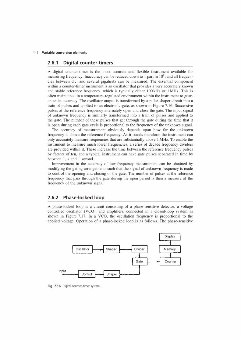
142 Variable conversion elements
7.6.1 Digital counter-timers
A digital counter-timer is the most accurate and flexible instrument available formeasuring frequency. Inaccuracy can be reduced down to 1 part in 108, and all frequen-cies between d.c. and several gigahertz can be measured. The essential componentwithin a counter-timer instrument is an oscillator that provides a very accurately knownand stable reference frequency, which is typically either 100 kHz or 1 MHz. This isoften maintained in a temperature-regulated environment within the instrument to guar-antee its accuracy. The oscillator output is transformed by a pulse-shaper circuit into atrain of pulses and applied to an electronic gate, as shown in Figure 7.16. Successivepulses at the reference frequency alternately open and close the gate. The input signalof unknown frequency is similarly transformed into a train of pulses and applied tothe gate. The number of these pulses that get through the gate during the time that itis open during each gate cycle is proportional to the frequency of the unknown signal.
The accuracy of measurement obviously depends upon how far the unknownfrequency is above the reference frequency. As it stands therefore, the instrument canonly accurately measure frequencies that are substantially above 1 MHz. To enable theinstrument to measure much lower frequencies, a series of decade frequency dividersare provided within it. These increase the time between the reference frequency pulsesby factors of ten, and a typical instrument can have gate pulses separated in time bybetween 1 μs and 1 second.
Improvement in the accuracy of low-frequency measurement can be obtained bymodifying the gating arrangements such that the signal of unknown frequency is madeto control the opening and closing of the gate. The number of pulses at the referencefrequency that pass through the gate during the open period is then a measure of thefrequency of the unknown signal.
7.6.2 Phase-locked loop
A phase-locked loop is a circuit consisting of a phase-sensitive detector, a voltagecontrolled oscillator (VCO), and amplifiers, connected in a closed-loop system asshown in Figure 7.17. In a VCO, the oscillation frequency is proportional to theapplied voltage. Operation of a phase-locked loop is as follows. The phase-sensitive
Oscillator
ControlInput
Shaper
Shaper Divider Memory
Display
Gate Counter
Fig. 7.16 Digital counter-timer system.
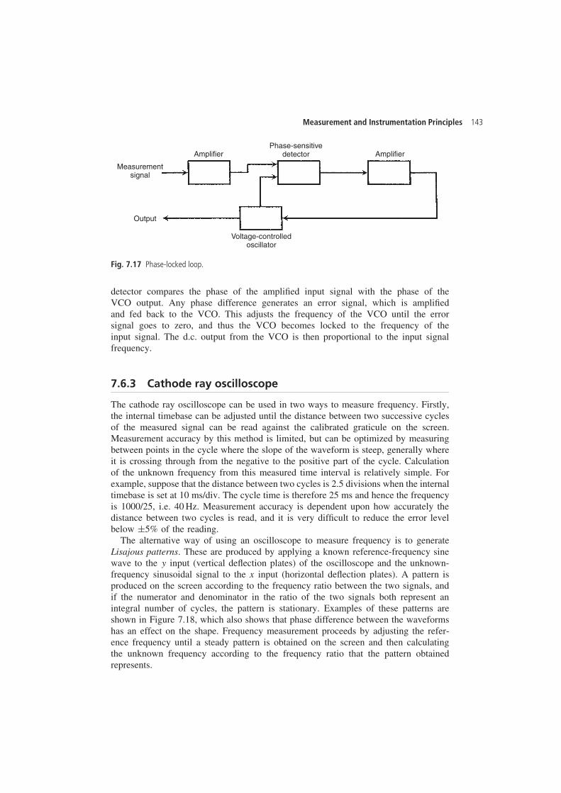
Measurement and Instrumentation Principles 143
Measurementsignal
Voltage-controlledoscillator
Output
Amplifier AmplifierPhase-sensitive
detector
Fig. 7.17 Phase-locked loop.
detector compares the phase of the amplified input signal with the phase of theVCO output. Any phase difference generates an error signal, which is amplifiedand fed back to the VCO. This adjusts the frequency of the VCO until the errorsignal goes to zero, and thus the VCO becomes locked to the frequency of theinput signal. The d.c. output from the VCO is then proportional to the input signalfrequency.
7.6.3 Cathode ray oscilloscope
The cathode ray oscilloscope can be used in two ways to measure frequency. Firstly,the internal timebase can be adjusted until the distance between two successive cyclesof the measured signal can be read against the calibrated graticule on the screen.Measurement accuracy by this method is limited, but can be optimized by measuringbetween points in the cycle where the slope of the waveform is steep, generally whereit is crossing through from the negative to the positive part of the cycle. Calculationof the unknown frequency from this measured time interval is relatively simple. Forexample, suppose that the distance between two cycles is 2.5 divisions when the internaltimebase is set at 10 ms/div. The cycle time is therefore 25 ms and hence the frequencyis 1000/25, i.e. 40 Hz. Measurement accuracy is dependent upon how accurately thedistance between two cycles is read, and it is very difficult to reduce the error levelbelow š5% of the reading.
The alternative way of using an oscilloscope to measure frequency is to generateLisajous patterns. These are produced by applying a known reference-frequency sinewave to the y input (vertical deflection plates) of the oscilloscope and the unknown-frequency sinusoidal signal to the x input (horizontal deflection plates). A pattern isproduced on the screen according to the frequency ratio between the two signals, andif the numerator and denominator in the ratio of the two signals both represent anintegral number of cycles, the pattern is stationary. Examples of these patterns areshown in Figure 7.18, which also shows that phase difference between the waveformshas an effect on the shape. Frequency measurement proceeds by adjusting the refer-ence frequency until a steady pattern is obtained on the screen and then calculatingthe unknown frequency according to the frequency ratio that the pattern obtainedrepresents.
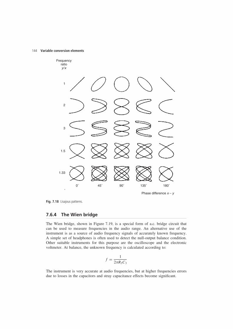
144 Variable conversion elements
Frequencyratioy/x
1
2
3
1.5
1.33
0˚ 45˚ 90˚ 135˚ 180˚
Phase difference x – y˚
Fig. 7.18 Lisajous patterns.
7.6.4 The Wien bridge
The Wien bridge, shown in Figure 7.19, is a special form of a.c. bridge circuit thatcan be used to measure frequencies in the audio range. An alternative use of theinstrument is as a source of audio frequency signals of accurately known frequency.A simple set of headphones is often used to detect the null-output balance condition.Other suitable instruments for this purpose are the oscilloscope and the electronicvoltmeter. At balance, the unknown frequency is calculated according to:
f D 1
2R3C3
The instrument is very accurate at audio frequencies, but at higher frequencies errorsdue to losses in the capacitors and stray capacitance effects become significant.
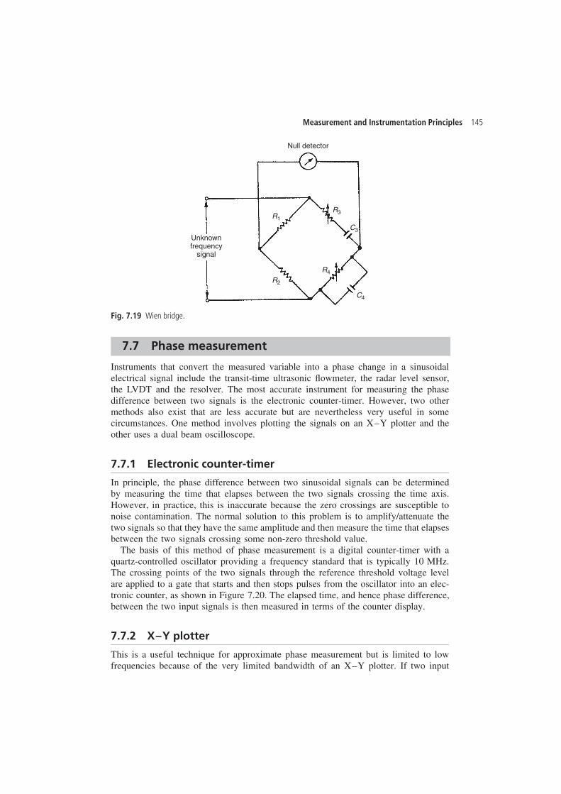
Measurement and Instrumentation Principles 145
Unknownfrequency
signal
R1
R2
R4
C4
R3
C3
Null detector
Fig. 7.19 Wien bridge.
7.7 Phase measurement
Instruments that convert the measured variable into a phase change in a sinusoidalelectrical signal include the transit-time ultrasonic flowmeter, the radar level sensor,the LVDT and the resolver. The most accurate instrument for measuring the phasedifference between two signals is the electronic counter-timer. However, two othermethods also exist that are less accurate but are nevertheless very useful in somecircumstances. One method involves plotting the signals on an X–Y plotter and theother uses a dual beam oscilloscope.
7.7.1 Electronic counter-timer
In principle, the phase difference between two sinusoidal signals can be determinedby measuring the time that elapses between the two signals crossing the time axis.However, in practice, this is inaccurate because the zero crossings are susceptible tonoise contamination. The normal solution to this problem is to amplify/attenuate thetwo signals so that they have the same amplitude and then measure the time that elapsesbetween the two signals crossing some non-zero threshold value.
The basis of this method of phase measurement is a digital counter-timer with aquartz-controlled oscillator providing a frequency standard that is typically 10 MHz.The crossing points of the two signals through the reference threshold voltage levelare applied to a gate that starts and then stops pulses from the oscillator into an elec-tronic counter, as shown in Figure 7.20. The elapsed time, and hence phase difference,between the two input signals is then measured in terms of the counter display.
7.7.2 X–Y plotter
This is a useful technique for approximate phase measurement but is limited to lowfrequencies because of the very limited bandwidth of an X–Y plotter. If two input
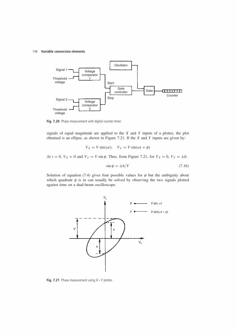
146 Variable conversion elements
Signal 1
Thresholdvoltage
Signal 2
Thresholdvoltage
Voltagecomparator
1
Voltagecomparator
2
Start
Stop
Gate
Counter
Gatecontroller
Oscillator
Fig. 7.20 Phase measurement with digital counter-timer.
signals of equal magnitude are applied to the X and Y inputs of a plotter, the plotobtained is an ellipse, as shown in Figure 7.21. If the X and Y inputs are given by:
VX D V sin�ωt�; VY D V sin�ωt C ��
At t D 0, VX D 0 and VY D V sin �. Thus, from Figure 7.21, for VX D 0, VY D šh:
sin � D šh/V �7.16�
Solution of equation (7.4) gives four possible values for � but the ambiguity aboutwhich quadrant � is in can usually be solved by observing the two signals plottedagainst time on a dual-beam oscilloscope.
V
Vx
Vy
h
h
X
Y
V sin wt
V sin(wt + f)
Fig. 7.21 Phase measurement using X–Y plotter.
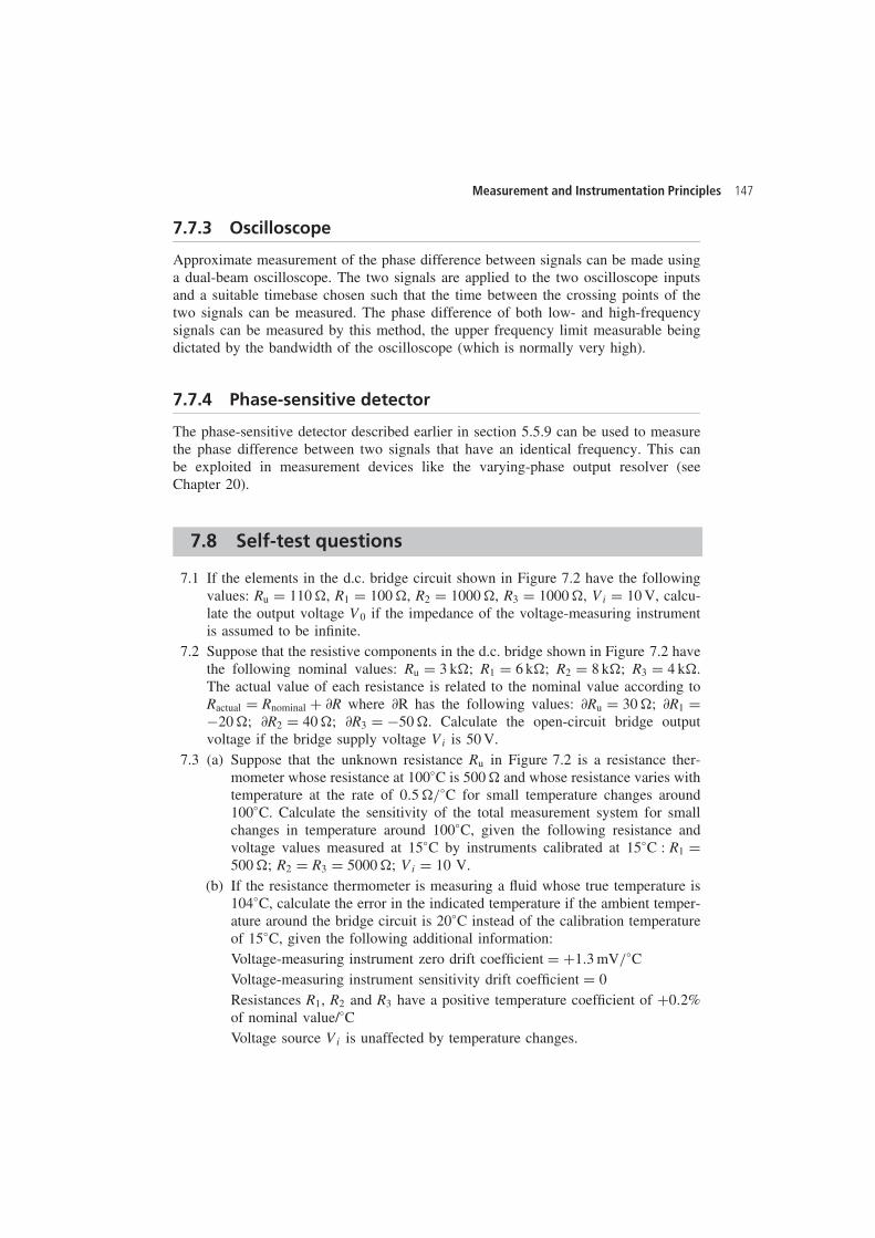
Measurement and Instrumentation Principles 147
7.7.3 Oscilloscope
Approximate measurement of the phase difference between signals can be made usinga dual-beam oscilloscope. The two signals are applied to the two oscilloscope inputsand a suitable timebase chosen such that the time between the crossing points of thetwo signals can be measured. The phase difference of both low- and high-frequencysignals can be measured by this method, the upper frequency limit measurable beingdictated by the bandwidth of the oscilloscope (which is normally very high).
7.7.4 Phase-sensitive detector
The phase-sensitive detector described earlier in section 5.5.9 can be used to measurethe phase difference between two signals that have an identical frequency. This canbe exploited in measurement devices like the varying-phase output resolver (seeChapter 20).
7.8 Self-test questions
7.1 If the elements in the d.c. bridge circuit shown in Figure 7.2 have the followingvalues: Ru D 110 �, R1 D 100 �, R2 D 1000 �, R3 D 1000 �, Vi D 10 V, calcu-late the output voltage V0 if the impedance of the voltage-measuring instrumentis assumed to be infinite.
7.2 Suppose that the resistive components in the d.c. bridge shown in Figure 7.2 havethe following nominal values: Ru D 3 k�; R1 D 6 k�; R2 D 8 k�; R3 D 4 k�.The actual value of each resistance is related to the nominal value according toRactual D Rnominal C ∂R where ∂R has the following values: ∂Ru D 30 �; ∂R1 D�20 �; ∂R2 D 40 �; ∂R3 D �50 �. Calculate the open-circuit bridge outputvoltage if the bridge supply voltage Vi is 50 V.
7.3 (a) Suppose that the unknown resistance Ru in Figure 7.2 is a resistance ther-mometer whose resistance at 100°C is 500 � and whose resistance varies withtemperature at the rate of 0.5 �/°C for small temperature changes around100°C. Calculate the sensitivity of the total measurement system for smallchanges in temperature around 100°C, given the following resistance andvoltage values measured at 15°C by instruments calibrated at 15°C : R1 D500 �; R2 D R3 D 5000 �; Vi D 10 V.
(b) If the resistance thermometer is measuring a fluid whose true temperature is104°C, calculate the error in the indicated temperature if the ambient temper-ature around the bridge circuit is 20°C instead of the calibration temperatureof 15°C, given the following additional information:Voltage-measuring instrument zero drift coefficient D C1.3 mV/°CVoltage-measuring instrument sensitivity drift coefficient D 0Resistances R1, R2 and R3 have a positive temperature coefficient of C0.2%of nominal value/°CVoltage source Vi is unaffected by temperature changes.
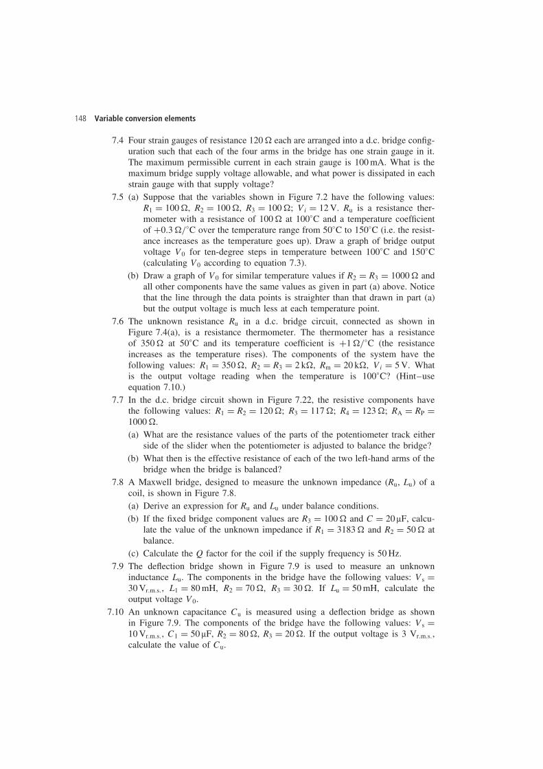
148 Variable conversion elements
7.4 Four strain gauges of resistance 120 � each are arranged into a d.c. bridge config-uration such that each of the four arms in the bridge has one strain gauge in it.The maximum permissible current in each strain gauge is 100 mA. What is themaximum bridge supply voltage allowable, and what power is dissipated in eachstrain gauge with that supply voltage?
7.5 (a) Suppose that the variables shown in Figure 7.2 have the following values:R1 D 100 �, R2 D 100 �, R3 D 100 �; Vi D 12 V. Ru is a resistance ther-mometer with a resistance of 100 � at 100°C and a temperature coefficientof C0.3 �/°C over the temperature range from 50°C to 150°C (i.e. the resist-ance increases as the temperature goes up). Draw a graph of bridge outputvoltage V0 for ten-degree steps in temperature between 100°C and 150°C(calculating V0 according to equation 7.3).
(b) Draw a graph of V0 for similar temperature values if R2 D R3 D 1000 � andall other components have the same values as given in part (a) above. Noticethat the line through the data points is straighter than that drawn in part (a)but the output voltage is much less at each temperature point.
7.6 The unknown resistance Ru in a d.c. bridge circuit, connected as shown inFigure 7.4(a), is a resistance thermometer. The thermometer has a resistanceof 350 � at 50°C and its temperature coefficient is C1 �/°C (the resistanceincreases as the temperature rises). The components of the system have thefollowing values: R1 D 350 �, R2 D R3 D 2 k�, Rm D 20 k�, Vi D 5 V. Whatis the output voltage reading when the temperature is 100°C? (Hint–useequation 7.10.)
7.7 In the d.c. bridge circuit shown in Figure 7.22, the resistive components havethe following values: R1 D R2 D 120 �; R3 D 117 �; R4 D 123 �; RA D RP D1000 �.(a) What are the resistance values of the parts of the potentiometer track either
side of the slider when the potentiometer is adjusted to balance the bridge?(b) What then is the effective resistance of each of the two left-hand arms of the
bridge when the bridge is balanced?7.8 A Maxwell bridge, designed to measure the unknown impedance (Ru, Lu) of a
coil, is shown in Figure 7.8.(a) Derive an expression for Ru and Lu under balance conditions.(b) If the fixed bridge component values are R3 D 100 � and C D 20 μF, calcu-
late the value of the unknown impedance if R1 D 3183 � and R2 D 50 � atbalance.
(c) Calculate the Q factor for the coil if the supply frequency is 50 Hz.7.9 The deflection bridge shown in Figure 7.9 is used to measure an unknown
inductance Lu. The components in the bridge have the following values: Vs D30 Vr.m.s., L1 D 80 mH, R2 D 70 �, R3 D 30 �. If Lu D 50 mH, calculate theoutput voltage V0.
7.10 An unknown capacitance Cu is measured using a deflection bridge as shownin Figure 7.9. The components of the bridge have the following values: Vs D10 Vr.m.s., C1 D 50 μF, R2 D 80 �, R3 D 20 �. If the output voltage is 3 Vr.m.s.,calculate the value of Cu.
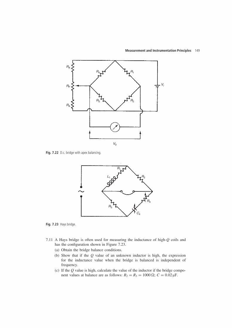
Measurement and Instrumentation Principles 149
RA
R4 R1
R3 R2
RP
RA
V0
Vi
Fig. 7.22 D.c. bridge with apex balancing.
L1
R1
R2
R3
R4
C4
Fig. 7.23 Hays bridge.
7.11 A Hays bridge is often used for measuring the inductance of high-Q coils andhas the configuration shown in Figure 7.23.(a) Obtain the bridge balance conditions.(b) Show that if the Q value of an unknown inductor is high, the expression
for the inductance value when the bridge is balanced is independent offrequency.
(c) If the Q value is high, calculate the value of the inductor if the bridge compo-nent values at balance are as follows: R2 D R3 D 1000 �; C D 0.02 μF.

150 Variable conversion elements
References and further reading
Baldwin, C.T. (1973) Fundamentals of Electrical Measurements, Prentice-Hall, London.Buckingham, H. and Price, E.M. (1966) Principles of Electrical Measurements, English Univer-
sities Press, London.Smith, R.J. and Dorf, R.C. (1992) Circuits, Devices and Systems, Wiley, New York.
8
Signal transmission
There is a necessity in many measurement systems to transmit measurement signalsover quite large distances from the point of measurement to the place where the signalsare recorded and/or used in a process control system. This creates several problemsfor which a solution must be found. Of the many difficulties associated with longdistance signal transmission, contamination of the measurement signal by noise isthe most serious. Many sources of noise exist in industrial environments, such asradiated electromagnetic fields from electrical machinery and power cables, inducedfields through wiring loops, and spikes (large transient voltages) on the a.c. powersupply. Signals can be transmitted electrically, pneumatically, optically, or by radio-telemetry, in either analogue or digital format. Optical data transmission can be furtherdivided into fibre-optic transmission and optical wireless transmission, according towhether a fibre-optic cable or just a plain air path is used as the transmission medium.These various options are explored in the following sections.
8.1 Electrical transmission
The simplest method of electrical transmission is to transmit the measurement signal asa varying analogue voltage. However, this can cause the measurement signal to becomecorrupted by noise. If noise causes a problem, the signal can either be transmitted inthe form of a varying current, or else it can be superimposed on an a.c. carrier system.
8.1.1 Transmission as varying voltages
As most signals already exist in an electrical form as varying analogue voltages, thesimplest mode of transmission is to maintain the signals in the same form. However,electrical transmission suffers problems of signal attenuation, and also exposes signalsto corruption through induced noise. Therefore, special measures have to be taken toovercome these problems.
Because the output signal levels from many types of measurement transducer arevery low, signal amplification prior to transmission is essential if a reasonable signal-to-noise ratio is to be obtained after transmission. Amplification at the input to the
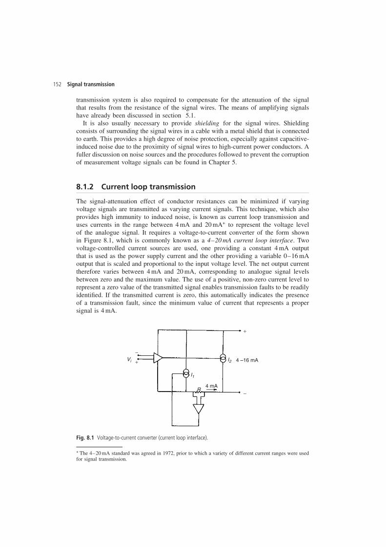
152 Signal transmission
transmission system is also required to compensate for the attenuation of the signalthat results from the resistance of the signal wires. The means of amplifying signalshave already been discussed in section 5.1.
It is also usually necessary to provide shielding for the signal wires. Shieldingconsists of surrounding the signal wires in a cable with a metal shield that is connectedto earth. This provides a high degree of noise protection, especially against capacitive-induced noise due to the proximity of signal wires to high-current power conductors. Afuller discussion on noise sources and the procedures followed to prevent the corruptionof measurement voltage signals can be found in Chapter 5.
8.1.2 Current loop transmission
The signal-attenuation effect of conductor resistances can be minimized if varyingvoltage signals are transmitted as varying current signals. This technique, which alsoprovides high immunity to induced noise, is known as current loop transmission anduses currents in the range between 4 mA and 20 mAŁ to represent the voltage levelof the analogue signal. It requires a voltage-to-current converter of the form shownin Figure 8.1, which is commonly known as a 4–20 mA current loop interface. Twovoltage-controlled current sources are used, one providing a constant 4 mA outputthat is used as the power supply current and the other providing a variable 0–16 mAoutput that is scaled and proportional to the input voltage level. The net output currenttherefore varies between 4 mA and 20 mA, corresponding to analogue signal levelsbetween zero and the maximum value. The use of a positive, non-zero current level torepresent a zero value of the transmitted signal enables transmission faults to be readilyidentified. If the transmitted current is zero, this automatically indicates the presenceof a transmission fault, since the minimum value of current that represents a propersignal is 4 mA.
Vi
I1
I2
R
−
+
+
−4 mA
4 –16 mA
Fig. 8.1 Voltage-to-current converter (current loop interface).
Ł The 4–20 mA standard was agreed in 1972, prior to which a variety of different current ranges were usedfor signal transmission.
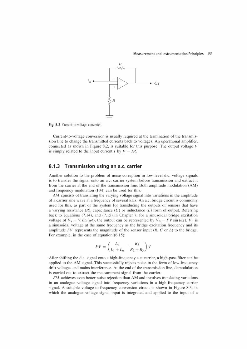
Measurement and Instrumentation Principles 153
R
R
VoutI in
−
+
Fig. 8.2 Current-to-voltage converter.
Current-to-voltage conversion is usually required at the termination of the transmis-sion line to change the transmitted currents back to voltages. An operational amplifier,connected as shown in Figure 8.2, is suitable for this purpose. The output voltage Vis simply related to the input current I by V D IR.
8.1.3 Transmission using an a.c. carrier
Another solution to the problem of noise corruption in low level d.c. voltage signalsis to transfer the signal onto an a.c. carrier system before transmission and extract itfrom the carrier at the end of the transmission line. Both amplitude modulation (AM)and frequency modulation (FM) can be used for this.
AM consists of translating the varying voltage signal into variations in the amplitudeof a carrier sine wave at a frequency of several kHz. An a.c. bridge circuit is commonlyused for this, as part of the system for transducing the outputs of sensors that havea varying resistance (R), capacitance (C) or inductance (L) form of output. Referringback to equations (7.14), and (7.15) in Chapter 7, for a sinusoidal bridge excitationvoltage of Vs D V sin �ωt�, the output can be represented by V0 D FV sin �ωt�. V0 isa sinusoidal voltage at the same frequency as the bridge excitation frequency and itsamplitude FV represents the magnitude of the sensor input (R, C or L) to the bridge.For example, in the case of equation (6.15):
FV D(
Lu
L1 C Lu� R3
R2 C R3
)V
After shifting the d.c. signal onto a high-frequency a.c. carrier, a high-pass filter can beapplied to the AM signal. This successfully rejects noise in the form of low-frequencydrift voltages and mains interference. At the end of the transmission line, demodulationis carried out to extract the measurement signal from the carrier.
FM achieves even better noise rejection than AM and involves translating variationsin an analogue voltage signal into frequency variations in a high-frequency carriersignal. A suitable voltage-to-frequency conversion circuit is shown in Figure 8.3, inwhich the analogue voltage signal input is integrated and applied to the input of a
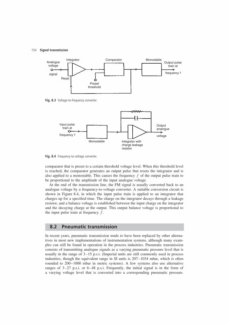
154 Signal transmission
Analoguevoltage
signal
Presetthreshold
Comparator MonostableOutput pulse
train at
frequency f
Integrator
Reset
Fig. 8.3 Voltage-to-frequency converter.
Input pulsetrain at
frequency f
Monostable Integrator withcharge leakageresistor
Outputanalogue
voltage
Fig. 8.4 Frequency-to-voltage converter.
comparator that is preset to a certain threshold voltage level. When this threshold levelis reached, the comparator generates an output pulse that resets the integrator and isalso applied to a monostable. This causes the frequency f of the output pulse train tobe proportional to the amplitude of the input analogue voltage.
At the end of the transmission line, the FM signal is usually converted back to ananalogue voltage by a frequency-to-voltage converter. A suitable conversion circuit isshown in Figure 8.4, in which the input pulse train is applied to an integrator thatcharges up for a specified time. The charge on the integrator decays through a leakageresistor, and a balance voltage is established between the input charge on the integratorand the decaying charge at the output. This output balance voltage is proportional tothe input pulse train at frequency f.
8.2 Pneumatic transmission
In recent years, pneumatic transmission tends to have been replaced by other alterna-tives in most new implementations of instrumentation systems, although many exam-ples can still be found in operation in the process industries. Pneumatic transmissionconsists of transmitting analogue signals as a varying pneumatic pressure level that isusually in the range of 3–15 p.s.i. (Imperial units are still commonly used in processindustries, though the equivalent range in SI units is 207–1034 mbar, which is oftenrounded to 200–1000 mbar in metric systems). A few systems also use alternativeranges of 3–27 p.s.i. or 6–48 p.s.i. Frequently, the initial signal is in the form ofa varying voltage level that is converted into a corresponding pneumatic pressure.
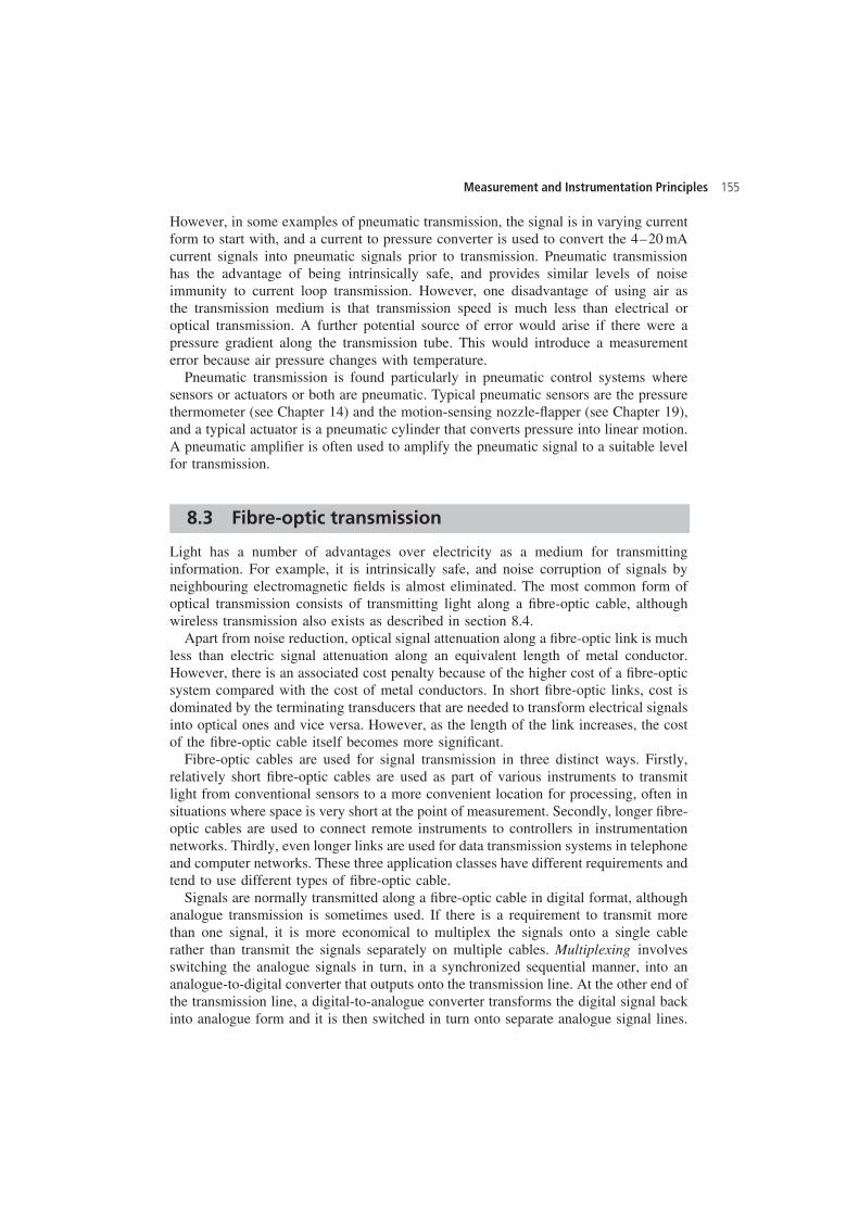
Measurement and Instrumentation Principles 155
However, in some examples of pneumatic transmission, the signal is in varying currentform to start with, and a current to pressure converter is used to convert the 4–20 mAcurrent signals into pneumatic signals prior to transmission. Pneumatic transmissionhas the advantage of being intrinsically safe, and provides similar levels of noiseimmunity to current loop transmission. However, one disadvantage of using air asthe transmission medium is that transmission speed is much less than electrical oroptical transmission. A further potential source of error would arise if there were apressure gradient along the transmission tube. This would introduce a measurementerror because air pressure changes with temperature.
Pneumatic transmission is found particularly in pneumatic control systems wheresensors or actuators or both are pneumatic. Typical pneumatic sensors are the pressurethermometer (see Chapter 14) and the motion-sensing nozzle-flapper (see Chapter 19),and a typical actuator is a pneumatic cylinder that converts pressure into linear motion.A pneumatic amplifier is often used to amplify the pneumatic signal to a suitable levelfor transmission.
8.3 Fibre-optic transmission
Light has a number of advantages over electricity as a medium for transmittinginformation. For example, it is intrinsically safe, and noise corruption of signals byneighbouring electromagnetic fields is almost eliminated. The most common form ofoptical transmission consists of transmitting light along a fibre-optic cable, althoughwireless transmission also exists as described in section 8.4.
Apart from noise reduction, optical signal attenuation along a fibre-optic link is muchless than electric signal attenuation along an equivalent length of metal conductor.However, there is an associated cost penalty because of the higher cost of a fibre-opticsystem compared with the cost of metal conductors. In short fibre-optic links, cost isdominated by the terminating transducers that are needed to transform electrical signalsinto optical ones and vice versa. However, as the length of the link increases, the costof the fibre-optic cable itself becomes more significant.
Fibre-optic cables are used for signal transmission in three distinct ways. Firstly,relatively short fibre-optic cables are used as part of various instruments to transmitlight from conventional sensors to a more convenient location for processing, often insituations where space is very short at the point of measurement. Secondly, longer fibre-optic cables are used to connect remote instruments to controllers in instrumentationnetworks. Thirdly, even longer links are used for data transmission systems in telephoneand computer networks. These three application classes have different requirements andtend to use different types of fibre-optic cable.
Signals are normally transmitted along a fibre-optic cable in digital format, althoughanalogue transmission is sometimes used. If there is a requirement to transmit morethan one signal, it is more economical to multiplex the signals onto a single cablerather than transmit the signals separately on multiple cables. Multiplexing involvesswitching the analogue signals in turn, in a synchronized sequential manner, into ananalogue-to-digital converter that outputs onto the transmission line. At the other end ofthe transmission line, a digital-to-analogue converter transforms the digital signal backinto analogue form and it is then switched in turn onto separate analogue signal lines.
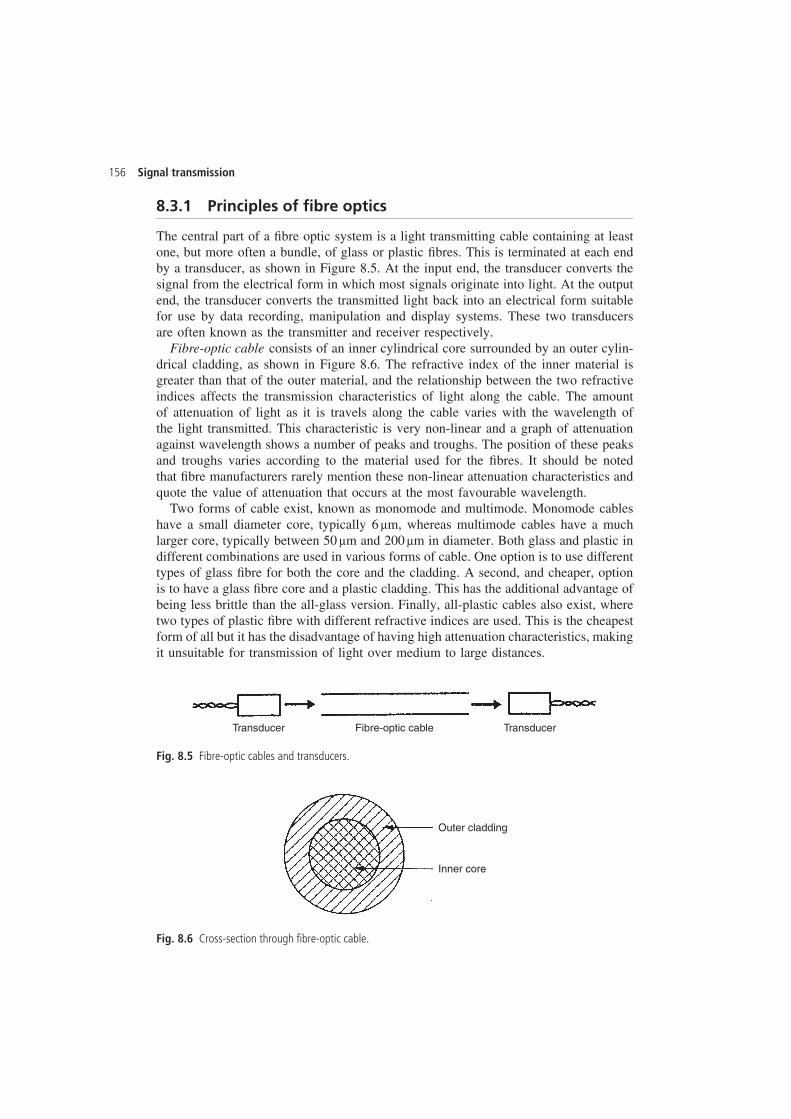
156 Signal transmission
8.3.1 Principles of fibre optics
The central part of a fibre optic system is a light transmitting cable containing at leastone, but more often a bundle, of glass or plastic fibres. This is terminated at each endby a transducer, as shown in Figure 8.5. At the input end, the transducer converts thesignal from the electrical form in which most signals originate into light. At the outputend, the transducer converts the transmitted light back into an electrical form suitablefor use by data recording, manipulation and display systems. These two transducersare often known as the transmitter and receiver respectively.
Fibre-optic cable consists of an inner cylindrical core surrounded by an outer cylin-drical cladding, as shown in Figure 8.6. The refractive index of the inner material isgreater than that of the outer material, and the relationship between the two refractiveindices affects the transmission characteristics of light along the cable. The amountof attenuation of light as it is travels along the cable varies with the wavelength ofthe light transmitted. This characteristic is very non-linear and a graph of attenuationagainst wavelength shows a number of peaks and troughs. The position of these peaksand troughs varies according to the material used for the fibres. It should be notedthat fibre manufacturers rarely mention these non-linear attenuation characteristics andquote the value of attenuation that occurs at the most favourable wavelength.
Two forms of cable exist, known as monomode and multimode. Monomode cableshave a small diameter core, typically 6 μm, whereas multimode cables have a muchlarger core, typically between 50 μm and 200 μm in diameter. Both glass and plastic indifferent combinations are used in various forms of cable. One option is to use differenttypes of glass fibre for both the core and the cladding. A second, and cheaper, optionis to have a glass fibre core and a plastic cladding. This has the additional advantage ofbeing less brittle than the all-glass version. Finally, all-plastic cables also exist, wheretwo types of plastic fibre with different refractive indices are used. This is the cheapestform of all but it has the disadvantage of having high attenuation characteristics, makingit unsuitable for transmission of light over medium to large distances.
Transducer TransducerFibre-optic cable
Fig. 8.5 Fibre-optic cables and transducers.
Outer cladding
Inner core
Fig. 8.6 Cross-section through fibre-optic cable.
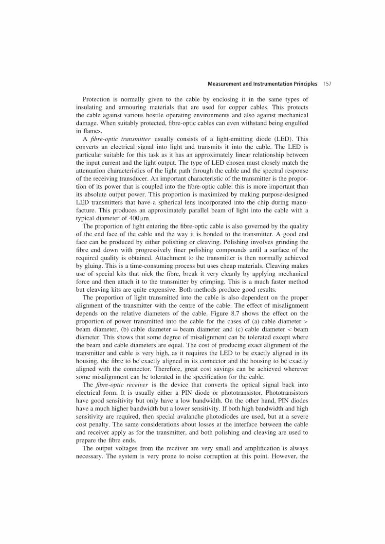
Measurement and Instrumentation Principles 157
Protection is normally given to the cable by enclosing it in the same types ofinsulating and armouring materials that are used for copper cables. This protectsthe cable against various hostile operating environments and also against mechanicaldamage. When suitably protected, fibre-optic cables can even withstand being engulfedin flames.
A fibre-optic transmitter usually consists of a light-emitting diode (LED). Thisconverts an electrical signal into light and transmits it into the cable. The LED isparticular suitable for this task as it has an approximately linear relationship betweenthe input current and the light output. The type of LED chosen must closely match theattenuation characteristics of the light path through the cable and the spectral responseof the receiving transducer. An important characteristic of the transmitter is the propor-tion of its power that is coupled into the fibre-optic cable: this is more important thanits absolute output power. This proportion is maximized by making purpose-designedLED transmitters that have a spherical lens incorporated into the chip during manu-facture. This produces an approximately parallel beam of light into the cable with atypical diameter of 400 μm.
The proportion of light entering the fibre-optic cable is also governed by the qualityof the end face of the cable and the way it is bonded to the transmitter. A good endface can be produced by either polishing or cleaving. Polishing involves grinding thefibre end down with progressively finer polishing compounds until a surface of therequired quality is obtained. Attachment to the transmitter is then normally achievedby gluing. This is a time-consuming process but uses cheap materials. Cleaving makesuse of special kits that nick the fibre, break it very cleanly by applying mechanicalforce and then attach it to the transmitter by crimping. This is a much faster methodbut cleaving kits are quite expensive. Both methods produce good results.
The proportion of light transmitted into the cable is also dependent on the properalignment of the transmitter with the centre of the cable. The effect of misalignmentdepends on the relative diameters of the cable. Figure 8.7 shows the effect on theproportion of power transmitted into the cable for the cases of (a) cable diameter >beam diameter, (b) cable diameter D beam diameter and (c) cable diameter < beamdiameter. This shows that some degree of misalignment can be tolerated except wherethe beam and cable diameters are equal. The cost of producing exact alignment of thetransmitter and cable is very high, as it requires the LED to be exactly aligned in itshousing, the fibre to be exactly aligned in its connector and the housing to be exactlyaligned with the connector. Therefore, great cost savings can be achieved whereversome misalignment can be tolerated in the specification for the cable.
The fibre-optic receiver is the device that converts the optical signal back intoelectrical form. It is usually either a PIN diode or phototransistor. Phototransistorshave good sensitivity but only have a low bandwidth. On the other hand, PIN diodeshave a much higher bandwidth but a lower sensitivity. If both high bandwidth and highsensitivity are required, then special avalanche photodiodes are used, but at a severecost penalty. The same considerations about losses at the interface between the cableand receiver apply as for the transmitter, and both polishing and cleaving are used toprepare the fibre ends.
The output voltages from the receiver are very small and amplification is alwaysnecessary. The system is very prone to noise corruption at this point. However, the
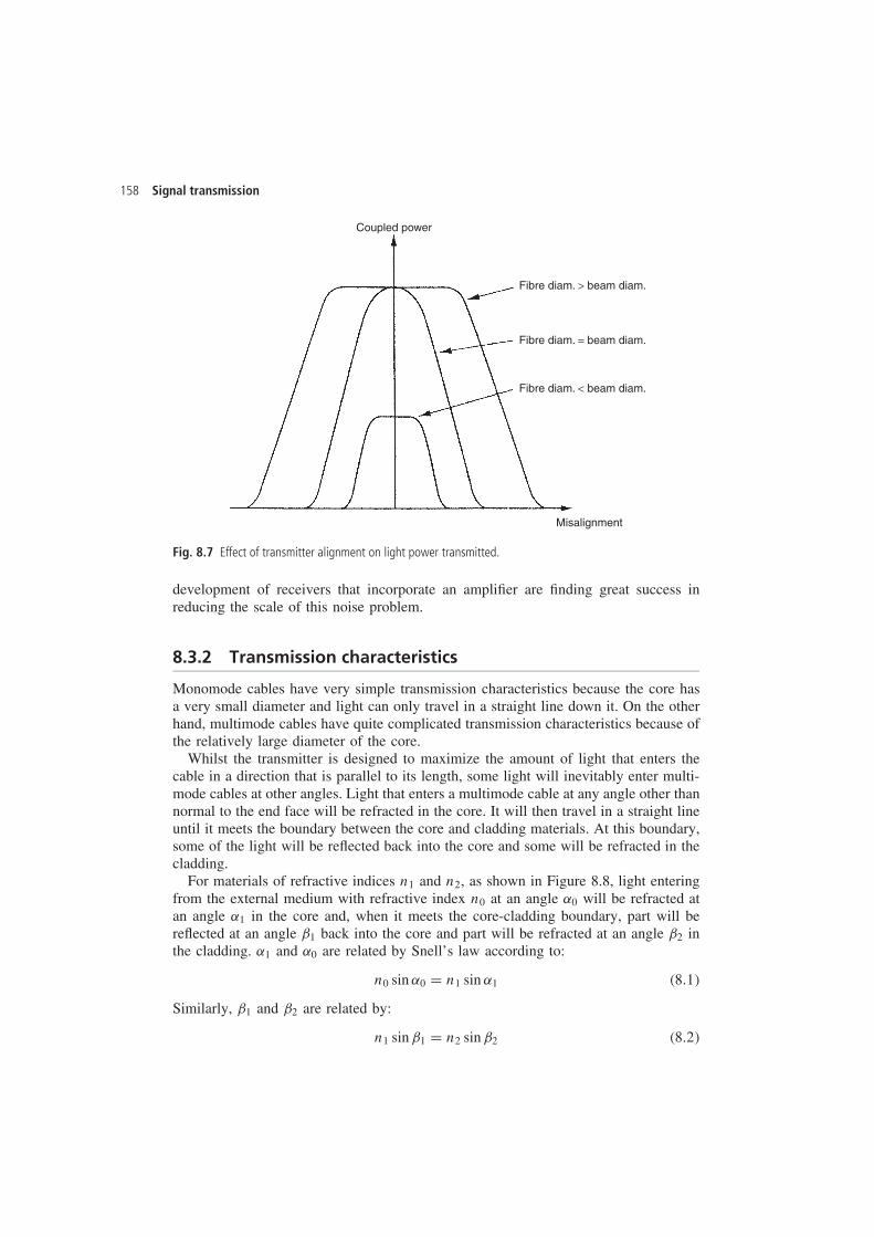
158 Signal transmission
Coupled power
Fibre diam. > beam diam.
Fibre diam. = beam diam.
Fibre diam. < beam diam.
Misalignment
Fig. 8.7 Effect of transmitter alignment on light power transmitted.
development of receivers that incorporate an amplifier are finding great success inreducing the scale of this noise problem.
8.3.2 Transmission characteristics
Monomode cables have very simple transmission characteristics because the core hasa very small diameter and light can only travel in a straight line down it. On the otherhand, multimode cables have quite complicated transmission characteristics because ofthe relatively large diameter of the core.
Whilst the transmitter is designed to maximize the amount of light that enters thecable in a direction that is parallel to its length, some light will inevitably enter multi-mode cables at other angles. Light that enters a multimode cable at any angle other thannormal to the end face will be refracted in the core. It will then travel in a straight lineuntil it meets the boundary between the core and cladding materials. At this boundary,some of the light will be reflected back into the core and some will be refracted in thecladding.
For materials of refractive indices n1 and n2, as shown in Figure 8.8, light enteringfrom the external medium with refractive index n0 at an angle ˛0 will be refracted atan angle ˛1 in the core and, when it meets the core-cladding boundary, part will bereflected at an angle ˇ1 back into the core and part will be refracted at an angle ˇ2 inthe cladding. ˛1 and ˛0 are related by Snell’s law according to:
n0 sin ˛0 D n1 sin ˛1 �8.1�
Similarly, ˇ1 and ˇ2 are related by:
n1 sin ˇ1 D n2 sin ˇ2 �8.2�
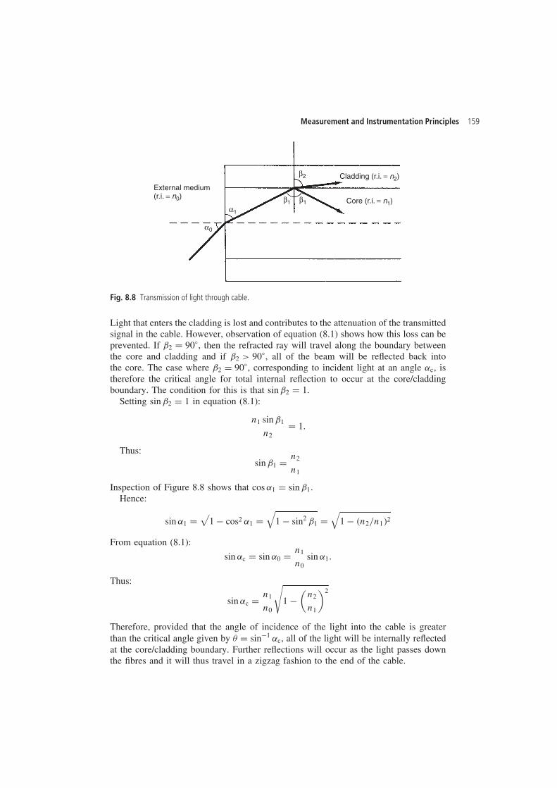
Measurement and Instrumentation Principles 159
External medium(r.i. = n0)
α0
α1
β1 β1
β2 Cladding (r.i. = n2)
Core (r.i. = n1)
Fig. 8.8 Transmission of light through cable.
Light that enters the cladding is lost and contributes to the attenuation of the transmittedsignal in the cable. However, observation of equation (8.1) shows how this loss can beprevented. If ˇ2 D 90°, then the refracted ray will travel along the boundary betweenthe core and cladding and if ˇ2 > 90°, all of the beam will be reflected back intothe core. The case where ˇ2 D 90°, corresponding to incident light at an angle ˛c, istherefore the critical angle for total internal reflection to occur at the core/claddingboundary. The condition for this is that sin ˇ2 D 1.
Setting sin ˇ2 D 1 in equation (8.1):
n1 sin ˇ1
n2D 1.
Thus:sin ˇ1 D n2
n1
Inspection of Figure 8.8 shows that cos ˛1 D sin ˇ1.Hence:
sin ˛1 D√
1 � cos2 ˛1 D√
1 � sin2 ˇ1 D√
1 � �n2/n1�2
From equation (8.1):
sin ˛c D sin ˛0 D n1
n0sin ˛1.
Thus:
sin ˛c D n1
n0
√1 �
(n2
n1
)2
Therefore, provided that the angle of incidence of the light into the cable is greaterthan the critical angle given by D sin�1 ˛c, all of the light will be internally reflectedat the core/cladding boundary. Further reflections will occur as the light passes downthe fibres and it will thus travel in a zigzag fashion to the end of the cable.
160 Signal transmission
Whilst attenuation has been minimized, there is a remaining problem that the trans-mission time of the parts of the beam which travel in this zigzag manner will be greaterthan light which enters the fibre at 90° to the face and so travels in a straight line tothe other end. In practice, the incident light rays to the cable will be spread over therange given by sin�1 ˛c < < 90° and so the transmission times of these separate partsof the beam will be distributed over a corresponding range. These differential delaycharacteristics of the light beam are known as modal dispersion. The practical effectis that a step change in light intensity at the input end of the cable will be receivedover a finite period of time at the output.
It is possible to largely overcome this latter problem in multimode cables by usingcables made solely from glass fibres in which the refractive index changes graduallyover the cross-section of the core rather than abruptly at the core/cladding interface asin the step index cable discussed so far. This special type of cable is known as gradedindex cable and it progressively bends light incident at less than 90° to its end facerather than reflecting it off the core/cladding boundary. Although the parts of the beamaway from the centre of the cable travel further, they also travel faster than the beampassing straight down the centre of the cable because the refractive index is loweraway from the centre. Hence, all parts of the beam are subject to approximately thesame propagation delay. In consequence, a step change in light intensity at the inputproduces an approximately step change of light intensity at the output. The alternativesolution is to use a monomode cable. This propagates light in a single mode only,which means that time dispersion of the signal is almost eliminated.
8.3.3 Multiplexing schemes
Various types of branching network and multiplexing schemes have been proposed,some of which have been implemented as described in Grattan (1989). Wavelengthdivision multiplexing is particularly well suited to fibre-optic applications, and thetechnique is now becoming well established. A single fibre is capable of propagatinga large number of different wavelengths without cross-interference, and multiplexingthus allows a large number of distributed sensors to be addressed. A single opticallight source is often sufficient for this, particularly if the modulated parameter is notlight intensity.
8.4 Optical wireless telemetry
Wireless telemetry allows signal transmission to take place without laying down aphysical link in the form of electrical or fibre-optic cable. This can be achieved usingeither radio or light waves to carry the transmitted signal across a plain air path betweena transmitter and a receiver.
Optical wireless transmission was first developed in the early 1980s. It consists ofa light source (usually infrared) transmitting encoded data information across an open,unprotected air path to a light detector. Three distinct modes of optical telemetry arepossible, known as point-to-point, directed and diffuse:
Measurement and Instrumentation Principles 161
ž Point-to-point telemetry uses a narrowly focused, fine beam of light, which iscommonly used for transmission between adjacent buildings. A data transmissionspeed of 5 Mbit/s is possible at the maximum transmission distance of 1000 m.However, if the transmission distance is limited to 200 m, a transmission speed of20 Mbit/s is possible. Point-to-point telemetry is commonly used to connect electricalor fibre-optic ethernet networks in adjacent buildings.
ž Directed telemetry transmits a slightly divergent beam of light that is directedtowards reflective surfaces, such as the walls and ceilings in a room. This producesa wide area of coverage and means that the transmitted signal can be received at anumber of points. However, the maximum transmission rate possible is only 1 Mbit/sat the maximum transmission distance of 70 m. If the transmission distance is limitedto 20 m, a transmission speed of 10 Mbit/s is possible.
ž Diffuse telemetry is similar to directed telemetry but the beam is even more divergent.This increases the area of coverage but reduces transmission speed and range. At themaximum range of 20 m, the maximum speed of transmission is 500 kbit/s, thoughthis increases to 2 Mbit/s at a reduced range of 10 m.
In practice, implementations of optical wireless telemetry are relatively uncommon.Where optical transmission is favoured because of its immunity to electromagneticnoise, fibre-optic transmission is usually preferred since optical wireless transmission issusceptible to random interruption when data is transmitted across an open, unprotectedair path. This preference for fibre-optic transmission exists despite its much greater costthan optical wireless transmission. Similarly, when the difficulty of laying a physicalcable link determines that wireless transmission is used, it is normal to use radiorather than optical transmission. This preference arises because radio transmission ismuch less prone to interference than optical transmission, since radio waves can passthrough most materials. However, there are a few instances where radio transmissionis subject to interference from neighbouring radio frequency systems operating at asimilar wavelength and, in such circumstances, optical transmission is sometimes abetter option.
8.5 Radio telemetry (radio wireless transmission)
Radio telemetry is normally used over transmission distances up to 400 miles, thoughthis can be extended by special techniques to provide communication through spaceover millions of miles. However, radio telemetry is also commonly used over quiteshort distances to transmit signals where physical electrical or fibre-optic links aredifficult to install or maintain. This occurs particularly when the source of the signals ismobile. The great advantage that radio telemetry has over optical wireless transmissionthrough an air medium is that radio waves are attenuated much less by obstaclesbetween the energy transmitter and receiver. Hence, as noted above, radio telemetryusually performs better than optical wireless telemetry and is therefore used much morecommonly.
In radio telemetry, data are usually transmitted in a frequency modulated (FM)format according to the scheme shown in Figure 8.9. This scheme actually involvestwo separate stages of frequency modulation, and the system is consequently known
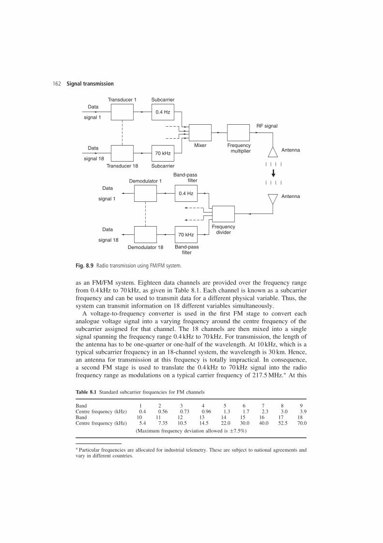
162 Signal transmission
Data
signal 1
Data
signal 18
Transducer 1
Transducer 18
Subcarrier
Subcarrier
0.4 Hz
70 kHz
Data
signal 1
Data
signal 18
Demodulator 1
Demodulator 18
Band-passfilter
Band-passfilter
0.4 Hz
70 kHz
Mixer Frequencymultiplier
RF signal
Antenna
Antenna
Frequencydivider
Fig. 8.9 Radio transmission using FM/FM system.
as an FM/FM system. Eighteen data channels are provided over the frequency rangefrom 0.4 kHz to 70 kHz, as given in Table 8.1. Each channel is known as a subcarrierfrequency and can be used to transmit data for a different physical variable. Thus, thesystem can transmit information on 18 different variables simultaneously.
A voltage-to-frequency converter is used in the first FM stage to convert eachanalogue voltage signal into a varying frequency around the centre frequency of thesubcarrier assigned for that channel. The 18 channels are then mixed into a singlesignal spanning the frequency range 0.4 kHz to 70 kHz. For transmission, the length ofthe antenna has to be one-quarter or one-half of the wavelength. At 10 kHz, which is atypical subcarrier frequency in an 18-channel system, the wavelength is 30 km. Hence,an antenna for transmission at this frequency is totally impractical. In consequence,a second FM stage is used to translate the 0.4 kHz to 70 kHz signal into the radiofrequency range as modulations on a typical carrier frequency of 217.5 MHz.Ł At this
Table 8.1 Standard subcarrier frequencies for FM channels
Band 1 2 3 4 5 6 7 8 9Centre frequency (kHz) 0.4 0.56 0.73 0.96 1.3 1.7 2.3 3.0 3.9Band 10 11 12 13 14 15 16 17 18Centre frequency (kHz) 5.4 7.35 10.5 14.5 22.0 30.0 40.0 52.5 70.0
(Maximum frequency deviation allowed is š7.5%)
Ł Particular frequencies are allocated for industrial telemetry. These are subject to national agreements andvary in different countries.
Measurement and Instrumentation Principles 163
frequency, the wavelength is 1.38 m, and so a transmission antenna of length 0.69 mor 0.345 m would be suitable. The signal is received by an antenna of identical lengthsome distance away. A frequency divider is then used to convert the signal back to oneacross the 0.4 kHz to 70 kHz subcarrier frequency spectrum, following which a seriesof band-pass filters are applied to extract the 18 separate frequency bands containingthe measurement data. Finally, a demodulator is applied to each channel to return eachsignal into varying voltage form.
The inaccuracy of radio telemetry is typically š1%. Thus, measurement uncertaintyin transmitting a temperature measurement signal with a range of 0–100°C over onechannel would be š1%, i.e. š1°C. However, if there are unused transmission channelsavailable, the signal could be divided into two ranges (0–50°C and 50–100°C) andtransmitted over two channels, reducing the measurement uncertainty to š0.5°C. Byusing ten channels for one variable, a maximum measurement uncertainty of š0.1°Ccould be achieved.
In theory, radio telemetry is very reliable because, although the radio frequencywaveband is relatively crowded, specific frequencies within it are allocated to specificusages under national agreements that are normally backed by legislation. Interferenceis avoided by licensing each frequency to only one user in a particular area, and limitingthe transmission range through limits on the power level of transmitted signals, suchthat there is no interference to other licensed users of the same frequency in other areas.Unfortunately, interference can still occur in practice, due both to adverse atmosphericconditions extending the transmission range beyond that expected into adjoining areas,and also due to unauthorized transmissions by other parties at the wavelengths licensedto registered users. There is a legal solution to this latter problem, although some timemay elapse before the offending transmission is successfully stopped.
8.6 Digital transmission protocols
Digital transmission has very significant advantages compared with analogue trans-mission because the possibility of signal corruption during transmission is greatlyreduced. Many different protocols exist for digital signal transmission, and these areconsidered in detail in Chapter 10. However, the protocol that is normally used forthe transmission of data from a measurement sensor or circuit is asynchronous serialtransmission, with other forms of transmission being reserved for use in instrumen-tation and computer networks. Asynchronous transmission involves converting ananalogue voltage signal into a binary equivalent, using an analogue-to-digital converteras discussed in section 6.4.3. This is then transmitted as a sequence of voltage pulsesof equal width that represent binary ‘1’ and ‘0’ digits. Commonly, a voltage level ofC6 V is used to represent binary ‘1’ and zero volts represents binary ‘0’. Thus, thetransmitted signal takes the form of a sequence of 6 V pulses separated by zero voltpulses. This is often known by the name of pulse code modulation. Such transmissionin digital format provides very high immunity to noise because noise is typically muchsmaller than the amplitude of a pulse representing binary 1. At the receiving end ofa transmitted signal, any pulse level between 0 and 3 volts can be interpreted as abinary ‘0’ and anything greater than 3 V can be interpreted as a binary ‘1’. A furtheradvantage of digital transmission is that other information, such as about plant status,
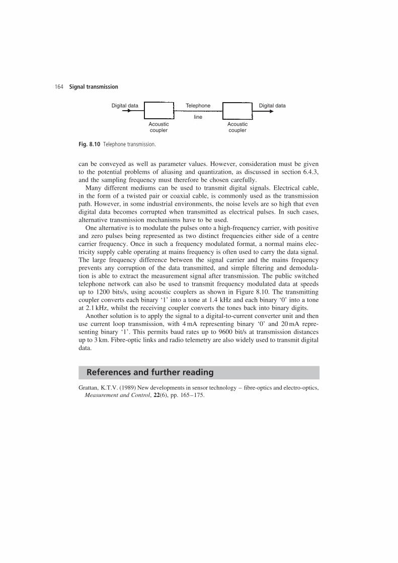
164 Signal transmission
Digital data Digital dataTelephone
lineAcousticcoupler
Acousticcoupler
Fig. 8.10 Telephone transmission.
can be conveyed as well as parameter values. However, consideration must be givento the potential problems of aliasing and quantization, as discussed in section 6.4.3,and the sampling frequency must therefore be chosen carefully.
Many different mediums can be used to transmit digital signals. Electrical cable,in the form of a twisted pair or coaxial cable, is commonly used as the transmissionpath. However, in some industrial environments, the noise levels are so high that evendigital data becomes corrupted when transmitted as electrical pulses. In such cases,alternative transmission mechanisms have to be used.
One alternative is to modulate the pulses onto a high-frequency carrier, with positiveand zero pulses being represented as two distinct frequencies either side of a centrecarrier frequency. Once in such a frequency modulated format, a normal mains elec-tricity supply cable operating at mains frequency is often used to carry the data signal.The large frequency difference between the signal carrier and the mains frequencyprevents any corruption of the data transmitted, and simple filtering and demodula-tion is able to extract the measurement signal after transmission. The public switchedtelephone network can also be used to transmit frequency modulated data at speedsup to 1200 bits/s, using acoustic couplers as shown in Figure 8.10. The transmittingcoupler converts each binary ‘1’ into a tone at 1.4 kHz and each binary ‘0’ into a toneat 2.1 kHz, whilst the receiving coupler converts the tones back into binary digits.
Another solution is to apply the signal to a digital-to-current converter unit and thenuse current loop transmission, with 4 mA representing binary ‘0’ and 20 mA repre-senting binary ‘1’. This permits baud rates up to 9600 bit/s at transmission distancesup to 3 km. Fibre-optic links and radio telemetry are also widely used to transmit digitaldata.
References and further reading
Grattan, K.T.V. (1989) New developments in sensor technology – fibre-optics and electro-optics,Measurement and Control, 22(6), pp. 165–175.
9
Digital computation andintelligent devices
This chapter is concerned with introducing the principles of digital computation andits application in measurement systems. Digital computers have been used in conjunc-tion with measurement systems for many years in the typical control system scenariowhere a computer uses data on process variables supplied by a measurement systemto compute a control signal that is then applied to an actuator in order to modifysome aspect of the controlled process. In this case, the computer is not actually partof the measurement system but merely works with it by taking data from the system.However, the rapid fall in the cost of computers has led to their widespread inclusionactually within measurement systems, performing various signal processing operationsdigitally that were previously carried out by analogue electronic circuits.
In early applications of digital signal processing, the computer remained as adistinctly separate component within the measurement system. However, the past fewyears have seen the development of measurement systems in the form of intelligentdevices in which the computational element (usually called a microcomputer ormicroprocessor) is much more closely integrated into the measurement system. Thesedevices are known by various names such as intelligent instruments, smart sensors andsmart transmitters. However, before discussing these in detail, the basic principles ofdigital computation need to be covered first.
9.1 Principles of digital computation
9.1.1 Elements of a computer
The primary function of a digital computer is the manipulation of data. The threeelements that are essential to the fulfilment of this task are the central processing unit,the memory and the input–output interface, as shown in Figure 9.1. These elementsare collectively known as the computer hardware, and each element exists physicallyas one or more integrated circuit chips mounted on a printed circuit board. Wherethe central processing unit (CPU) consists of a single microprocessor, it is usual toregard the system as a microcomputer. The distinction between the terms ‘micro-computer’, ‘minicomputer’ and ‘mainframe computer’ is a very arbitrary divisionmade according to relative computer power. However, this classification has become
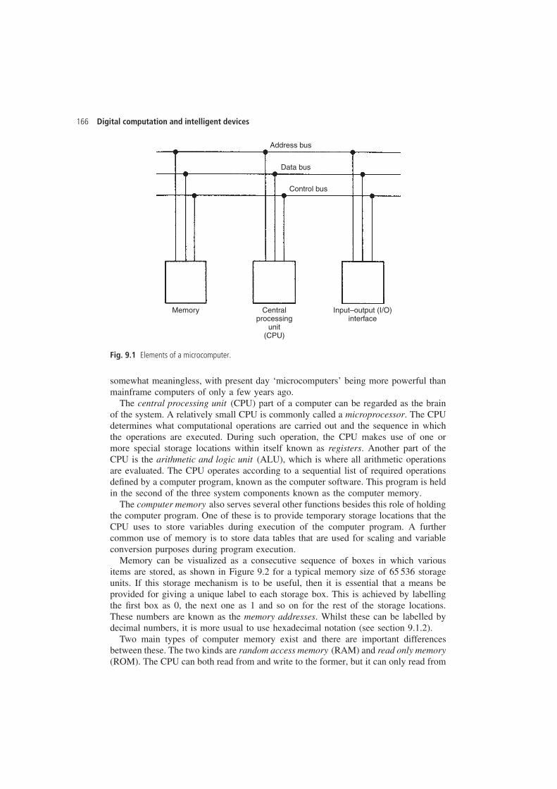
166 Digital computation and intelligent devices
Address bus
Data bus
Control bus
Memory Centralprocessing
unit(CPU)
Input–output (I/O)interface
Fig. 9.1 Elements of a microcomputer.
somewhat meaningless, with present day ‘microcomputers’ being more powerful thanmainframe computers of only a few years ago.
The central processing unit (CPU) part of a computer can be regarded as the brainof the system. A relatively small CPU is commonly called a microprocessor. The CPUdetermines what computational operations are carried out and the sequence in whichthe operations are executed. During such operation, the CPU makes use of one ormore special storage locations within itself known as registers. Another part of theCPU is the arithmetic and logic unit (ALU), which is where all arithmetic operationsare evaluated. The CPU operates according to a sequential list of required operationsdefined by a computer program, known as the computer software. This program is heldin the second of the three system components known as the computer memory.
The computer memory also serves several other functions besides this role of holdingthe computer program. One of these is to provide temporary storage locations that theCPU uses to store variables during execution of the computer program. A furthercommon use of memory is to store data tables that are used for scaling and variableconversion purposes during program execution.
Memory can be visualized as a consecutive sequence of boxes in which variousitems are stored, as shown in Figure 9.2 for a typical memory size of 65 536 storageunits. If this storage mechanism is to be useful, then it is essential that a means beprovided for giving a unique label to each storage box. This is achieved by labellingthe first box as 0, the next one as 1 and so on for the rest of the storage locations.These numbers are known as the memory addresses. Whilst these can be labelled bydecimal numbers, it is more usual to use hexadecimal notation (see section 9.1.2).
Two main types of computer memory exist and there are important differencesbetween these. The two kinds are random access memory (RAM) and read only memory(ROM). The CPU can both read from and write to the former, but it can only read from
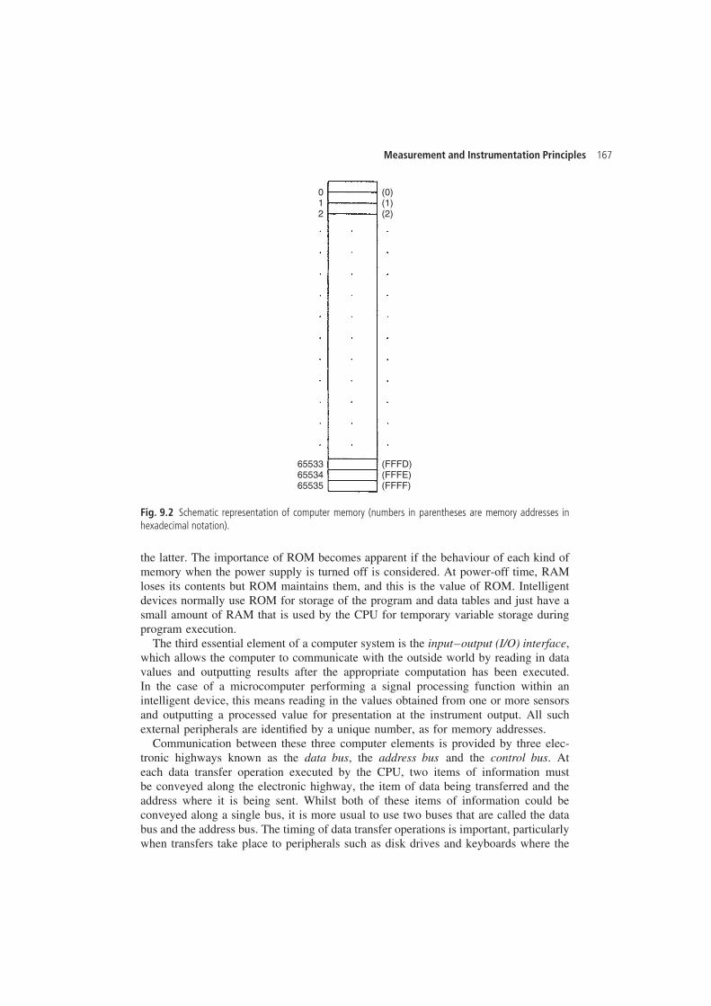
Measurement and Instrumentation Principles 167
012
655336553465535
(0)(1)(2)
(FFFD)(FFFE)(FFFF)
Fig. 9.2 Schematic representation of computer memory (numbers in parentheses are memory addresses inhexadecimal notation).
the latter. The importance of ROM becomes apparent if the behaviour of each kind ofmemory when the power supply is turned off is considered. At power-off time, RAMloses its contents but ROM maintains them, and this is the value of ROM. Intelligentdevices normally use ROM for storage of the program and data tables and just have asmall amount of RAM that is used by the CPU for temporary variable storage duringprogram execution.
The third essential element of a computer system is the input–output (I/O) interface,which allows the computer to communicate with the outside world by reading in datavalues and outputting results after the appropriate computation has been executed.In the case of a microcomputer performing a signal processing function within anintelligent device, this means reading in the values obtained from one or more sensorsand outputting a processed value for presentation at the instrument output. All suchexternal peripherals are identified by a unique number, as for memory addresses.
Communication between these three computer elements is provided by three elec-tronic highways known as the data bus, the address bus and the control bus. Ateach data transfer operation executed by the CPU, two items of information mustbe conveyed along the electronic highway, the item of data being transferred and theaddress where it is being sent. Whilst both of these items of information could beconveyed along a single bus, it is more usual to use two buses that are called the databus and the address bus. The timing of data transfer operations is important, particularlywhen transfers take place to peripherals such as disk drives and keyboards where the
168 Digital computation and intelligent devices
CPU often has to wait until the peripheral is free before it can initialize a data transfer.This timing information is carried by a third highway known as the control bus.
The latest trend made possible by advances in very large-scale integration (VLSI)technology is to incorporate all three functions of central processor unit, memory andI/O within a single chip (known as a computer on a chip or microcomputer). The term‘microprocessor’ is often used to describe such an integrated unit, but this is strictlyincorrect since the device contains more than just processing power.
9.1.2 Computer operation
As has already been mentioned, the fundamental role of a computer is the manipulationof data. Numbers are used both in quantifying items of data and also in the form ofcodes that define the computational operations that are to be executed. All numbersthat are used for these two purposes must be stored within the computer memoryand also transported along the communication buses. A detailed consideration of theconventions used for representing numbers within the computer is therefore required.
Number systemsThe decimal system is the best known number system, but it is not very suitable foruse by digital computers. It uses a base of ten, such that each digit in a number canhave any one of ten values within the range 0–9. Items of electronic equipment suchas the digital counter, which are often used as computer peripherals, have liquid crystaldisplay elements that can each display any of the ten decimal digits, and therefore afour element display can directly represent decimal numbers in the range 0–9999. Thedecimal system is therefore perfectly suitable for use with such output devices.
The fundamental unit of data storage within a digital computer is a memory elementknown as a bit. This holds information by switching between one of two possiblestates. Each storage unit can therefore only represent two possible values and alldata to be entered into memory must be organized into a format that recognizes thisrestriction. This means that numbers must be entered in binary format, where eachdigit in the number can only have one of two values, 0 or 1. The binary representationis particularly convenient for computers because bits can be represented very simplyelectronically as either zero or non-zero voltages. However, the conversion is tediousfor humans. Starting from the right-hand side of a binary number, where the firstdigit represents 20 (i.e. 1), each successive binary digit represents progressively higherpowers of 2. For example, in the binary number 1111, the first digit (starting fromthe right-hand side) represents 1, the next 2, the next 4 and the final, leftmost digitrepresents 8, Thus the decimal equivalent is 1 C 2 C 4 C 8 D 15.
Example 9.1Convert the following 8-bit binary number to its decimal equivalent: 10110011
SolutionStarting at the right-hand side, we have:
�1 ð 20� C �1 ð 21� C �0 ð 22� C �0 ð 23� C �1 ð 24� C �1 ð 25�
C �0 ð 26� C �1 ð 27�
D 1 C 2 C 0 C 0 C 16 C 32 C 0 C 128 D 179
Measurement and Instrumentation Principles 169
For data storage purposes, memory elements are combined into larger units known asbytes, which are usually considered to consist of 8 bits each. Each bit holds one binarydigit, and therefore a memory unit consisting of 8 bits can store 8-digit binary numbersin the range 00000000 to 11111111 (equivalent to decimal numbers in the range 0 to255). A binary number in this system of 10010011 for instance would correspond withthe decimal number 147.
This range is clearly inadequate for most purposes, including measurement systems,because even if all data could be conveniently scaled the maximum resolution obtain-able is only 1 part in 128. Numbers are therefore normally stored in units of either 2or 4 bytes, which allow the storage of integer (whole) numbers in the range 0–65 535or 0–4 294 967 296.
No means have been suggested so far for expressing the sign of numbers, whichis clearly necessary in the real world where negative as well as positive numbersoccur. A simple way to do this is to reserve the most significant (left-hand bit) in astorage unit to define the sign of a number, with ‘0’ representing a positive numberand ‘1’ a negative number. This alters the ranges of numbers representable in a 1-byte storage unit to �127 to C127, as only 7 bits are left to express the magnitudeof the number, and also means that there are two representations of the value 0. Inthis system the binary number 10010011 translates to the decimal number �19 and00010011 translates to C19. For reasons dictated by the mode of operation of theCPU, however, most computers use an alternative representation known as the two’scomplement form.
The two’s complement of a number is most easily formed by going via an interme-diate stage of the one’s complement. The one’s complement of a number is formed byreversing all digits in the binary representation of the magnitude of a number, changing1s to 0s and 0s to 1s, and then changing the left-hand bit to a 1 if the original numberwas negative. The two’s complement is then formed by adding 1 at the least signif-icant (right-hand) end of the one’s complement. As before for a 1-byte storage unit,only 7 bits are available for representing the magnitude of a number, but, becausethere is now only one representation of zero, the decimal range representable is �128to C127.
Example 9.2Find the one’s and two’s complement 8-bit binary representation of the followingdecimal numbers: 56 �56 73 119 27 �47
Method of SolutionTake first the decimal value of 56Form 7-bit binary representation: 0111000Reverse digits in this: 1000111Add sign bit to left-hand end to form one’s complement: 01000111Form two’s complement by adding one to one’s complement: 01000111C1D01001000Take next the decimal value of �56Form 7-bit binary representation: 0111000Reverse digits in this: 1000111Add sign bit to left-hand end to form one’s complement: 11000111Form two’s complement by adding one to one’s complement: 11000111C1D11001000
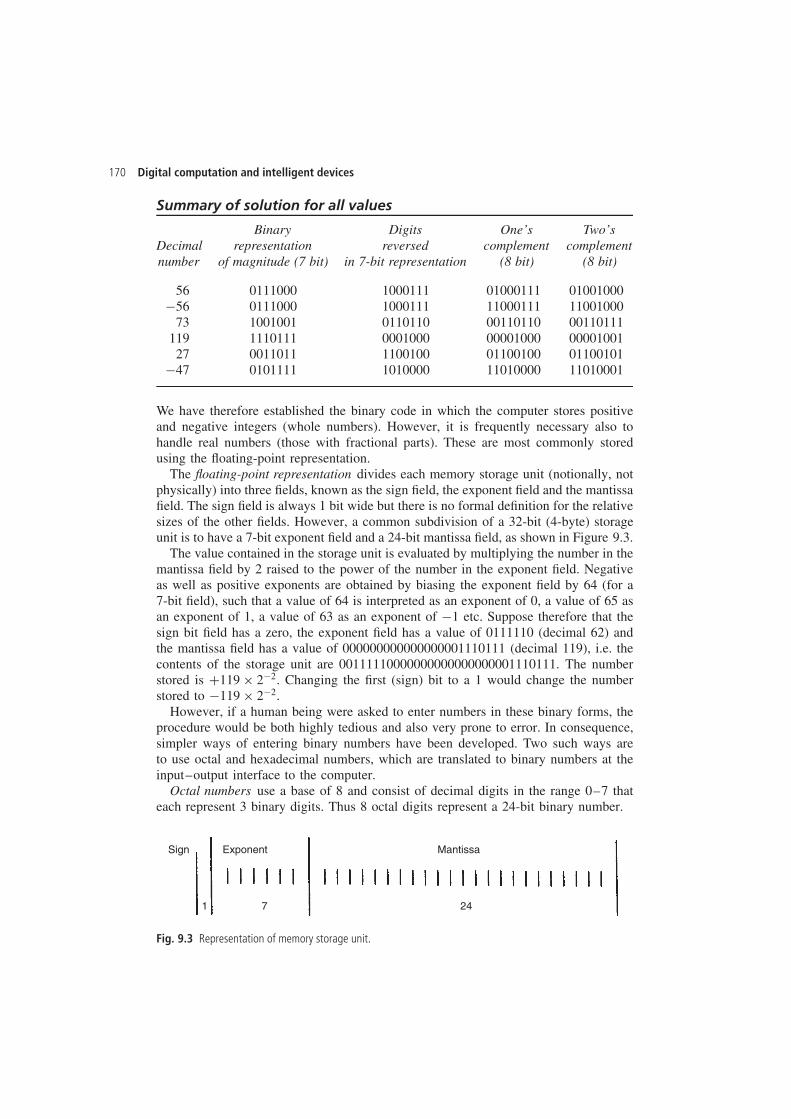
170 Digital computation and intelligent devices
Summary of solution for all values
Binary Digits One’s Two’sDecimal representation reversed complement complementnumber of magnitude (7 bit) in 7-bit representation (8 bit) (8 bit)
56 0111000 1000111 01000111 01001000�56 0111000 1000111 11000111 11001000
73 1001001 0110110 00110110 00110111119 1110111 0001000 00001000 0000100127 0011011 1100100 01100100 01100101
�47 0101111 1010000 11010000 11010001
We have therefore established the binary code in which the computer stores positiveand negative integers (whole numbers). However, it is frequently necessary also tohandle real numbers (those with fractional parts). These are most commonly storedusing the floating-point representation.
The floating-point representation divides each memory storage unit (notionally, notphysically) into three fields, known as the sign field, the exponent field and the mantissafield. The sign field is always 1 bit wide but there is no formal definition for the relativesizes of the other fields. However, a common subdivision of a 32-bit (4-byte) storageunit is to have a 7-bit exponent field and a 24-bit mantissa field, as shown in Figure 9.3.
The value contained in the storage unit is evaluated by multiplying the number in themantissa field by 2 raised to the power of the number in the exponent field. Negativeas well as positive exponents are obtained by biasing the exponent field by 64 (for a7-bit field), such that a value of 64 is interpreted as an exponent of 0, a value of 65 asan exponent of 1, a value of 63 as an exponent of �1 etc. Suppose therefore that thesign bit field has a zero, the exponent field has a value of 0111110 (decimal 62) andthe mantissa field has a value of 000000000000000001110111 (decimal 119), i.e. thecontents of the storage unit are 00111110000000000000000001110111. The numberstored is C119 ð 2�2. Changing the first (sign) bit to a 1 would change the numberstored to �119 ð 2�2.
However, if a human being were asked to enter numbers in these binary forms, theprocedure would be both highly tedious and also very prone to error. In consequence,simpler ways of entering binary numbers have been developed. Two such ways areto use octal and hexadecimal numbers, which are translated to binary numbers at theinput–output interface to the computer.
Octal numbers use a base of 8 and consist of decimal digits in the range 0–7 thateach represent 3 binary digits. Thus 8 octal digits represent a 24-bit binary number.
Sign Exponent Mantissa
1 7 24
Fig. 9.3 Representation of memory storage unit.
Measurement and Instrumentation Principles 171
Hexadecimal numbers have a base of 16 and are used much more commonly thanoctal numbers. They use decimal digits in the range 0–9 and letters in the rangeA–F that each represent 4 binary digits. The decimal digits 0–9 translate directlyto the decimal values 0–9 and the letters A–F translate respectively to the decimalvalues 10–15. A 24-bit binary number requires 6 hexadecimal digits to represent it.The following table shows the octal, hexadecimal and binary equivalents of decimalnumbers in the range 0–15.
Decimal Octal Hexadecimal Binary
0 0 0 01 1 1 12 2 2 103 3 3 114 4 4 1005 5 5 1016 6 6 1107 7 7 1118 10 8 10009 11 9 1001
10 12 A 101011 13 B 101112 14 C 110013 15 D 110114 16 E 111015 17 F 1111
Octal/hexadecimal to binary conversionOctal and hexadecimal conversion is very simple. Each octal/hexadecimal digit is takenin turn and converted to its binary representation according to the table above.
Example 9.3Convert the octal number 7654 to binary.
SolutionUsing the table above, write down the binary equivalent of each octal digit:
j 7 j 6 j 5 j 4 jj 111 j 110 j 101 j 100 j
Thus, the binary code is 111110101100.
Example 9.4Convert the hexadecimal number ABCD to binary.
SolutionUsing the table above, write down the binary equivalent of each hexadecimal digit:
j A j B j C j D jj 1010 j 1011 j 1100 j 1101 j
Thus, the binary code is 1010101111001101.
172 Digital computation and intelligent devices
Binary to octal/hexadecimal conversionConversion from binary to octal or hexadecimal is also simple. The binary digits aretaken in groups of three at a time (for octal) or four at a time (for hexadecimal),starting at the least significant end of the number (right-hand side) and writing downthe appropriate octal or hexadecimal digit for each group.
Example 9.5Convert the binary number 010111011001 into octal and hexadecimal.
Solution j 010 j 111 j 011 j 001 jj 2 j 7 j 3 j 1 j
= 2731 octal
j 0101 j 1101 j 1001 jj 5 j D j 9 j
= 5D9 hexadecimal
Example 9.6The 24-bit binary number 011111001001001101011010 is to be entered into acomputer. How would it be entered using (a) octal code and (b) hexadecimal code?
Solution
(a) Divide the 24-bit number into groups of three, starting at the right-hand side:
011 j 111 j 001 j 001 j 001 j 101 j 011 j 010 j D 37111532 octal
Thus, the number would be entered as 37111532 using octal code.(b) Divide the 24-bit number into groups of four, starting at the right-hand side:
j 0111 j 1100 j 1001 j 0011 j 0101 j 1010 j D 7C935A hexadecimal
In carrying out such conversions, it is essential that the groupings of binary digitsstart from the right-hand side. Groupings starting at the left-hand side give completelywrong values unless the number of binary digits happens to be an integer multiple ofthe grouping size. Consider a 10-digit binary number: 1011100011.
Grouping digits starting at the right-hand side gives the values 1343 octal and 2E3hexadecimal.
Grouping digits starting at the left gives the (incorrect) values of 5611 octal andB83 hexadecimal.
When converting a binary number to octal or hexadecimal representation, a checkmust also be made that all of the binary digits represent data. In some systems, thefirst (left-hand) digit is used as a sign bit and the last (right-hand) digit is used as aparity bit.
Example 9.7In a system that uses the first bit as a sign bit and the last bit as a parity bit, what isthe octal and hexadecimal representation of the binary code: 110111000111?
Measurement and Instrumentation Principles 173
SolutionThe ten data bits are 1011100011. This converts to 1343 octal and 2E3 hexadecimal.
Programming and program executionIn most modes of usage, including use as part of intelligent devices, computersare involved in manipulating data. This requires data values to be input, processedand output according to a sequence of operations defined by the computer program.However, in practice, programming the microprocessor within an intelligent device isnot normally the province of the instrument user, indeed, there is rarely any provisionfor the user to create or modify operating programs even if he/she wished to doso. There are several reasons for this. Firstly, the signal processing needed withinan intelligent device is usually well defined, and therefore it is more efficient fora manufacturer to produce this rather than to have each individual user producenear identical programs separately. Secondly, better program integrity and instrumentoperation is achieved if a standard program produced by the instrument manufactureris used. Finally, use of a standard program allows it to be burnt into ROM, therebyprotecting it from any failure of the instrument power supply. This also facilitatessoftware maintenance and updates, by the mechanism of the manufacturer providing anew ROM that simply plugs into the slot previously occupied by the old ROM.
However, even though it is not normally a task undertaken by the user, some appre-ciation of microprocessor programming for an intelligent device is useful backgroundknowledge. To illustrate the techniques involved in programming, consider a verysimple program that reads in a value from a sensor, adds a pre-stored value to it tocompensate for a bias in the sensor measurement, and outputs a corrected reading toa display device.
Let us assume that the addresses of the sensor and output display device are 00C0and 00C1 respectively, and that the required scaling value has already been stored inmemory address 0100. The instructions below are formed from the instruction set fora Z80Ł microprocessor and make use of CPU registers A and B.
IN A,C0
IN B,100
ADD A,B
OUT C1,A
This list of four instructions constitutes the computer program that is necessary toexecute the required task. The CPU normally executes the instructions one at a time,starting at the top of the list and working downwards (though jump and branch instruc-tions change this order). The first instruction (IN A,C0) reads in a value from the sensorat address C0 and places the value in CPU register A (often called the accumulator).The mechanics of the execution of this instruction consist of the CPU putting therequired address C0 on the address bus and then putting a command on the controlbus that causes the contents of the target address (C0) to be copied onto the data bus
Ł The Z80 is now an obsolete 8-bit processor but its simplicity is well suited to illustrating programmingtechniques. Similar, but necessarily more complex, programming instructions are used with current 16- and32-bit processors.
174 Digital computation and intelligent devices
and subsequently transferred into the A register. The next instruction (IN B,100) readsin a value from address 100 (the pre-stored biasing value) and stores it in register B.The following instruction (ADD A,B) adds together the contents of registers A andB and stores the result in register A. Register A now contains the measurement readfrom the sensor but corrected for bias. The final instruction (OUT C1,A) transfers thecontents of register A to the output device on address C1.
9.1.3 Interfacing
The input–output interface connects the computer to the outside world, and is thereforean essential part of the computer system. When the CPU puts the address of a peripheralonto the address bus, the input–output interface decodes the address and identifies theunique computer peripheral with which a data transfer operation is to be executed. Theinterface also has to interpret the command on the control bus so that the timing ofthe data transfer is correct. One further very important function of the input–outputinterface is to provide a physical electronic highway for the flow of data betweenthe computer data bus and the external peripheral. In many computer applications,including their use within intelligent devices, the external peripheral requires signals tobe in analogue form. Therefore the input–output interface must provide for conversionbetween these analogue signals and the digital signals required by a digital computer.This is satisfied by analogue-to-digital and digital-to-analogue conversion elementswithin the input–output interface.
A standard form of interface used to connect a computer to its peripheral devicesis the UART (Universal Asynchronous Receiver/Transmitter). This has been used foraround 30 years. A newer interface protocol that is particularly suitable for connecting alarge number of devices and providing for communication between different computersis the PCI (Peripheral Component Interconnect) interface. Very recently, an alternativeprotocol called the Universal Serial Bus (USB) has been developed that is rapidlygaining in popularity.
The rest of this section presents some elementary concepts of interfacing in simpleterms. A more detailed discussion follows later in Chapter 10, where the combinationof intelligent devices into larger networks is discussed.
Address decodingA typical address bus in a microcomputer is 16 bits wideŁ, allowing 65 536 separateaddresses to be accessed in the range 0000–FFFF (in hexadecimal representation).Special commands on some computers are reserved for accessing the bottom end 256of these addresses in the range 0000–00FF, and, if these commands are used, only 8bits are needed to specify the required address. For the purpose of explaining address-decoding techniques, the scheme below shows how the lower 8 bits of the 16-bitaddress line are decoded to identify the unique address referenced by one of thesespecial commands. Decoding of all 16 address lines follows a similar procedure butrequires a substantially greater number of integrated circuit chips.
Address decoding is performed by a suitable combination of logic gates. Figure 9.4shows a very simple hardware scheme for decoding 8 address lines. This consists
Ł Recently, 32-bit address fields have also become available in some devices.
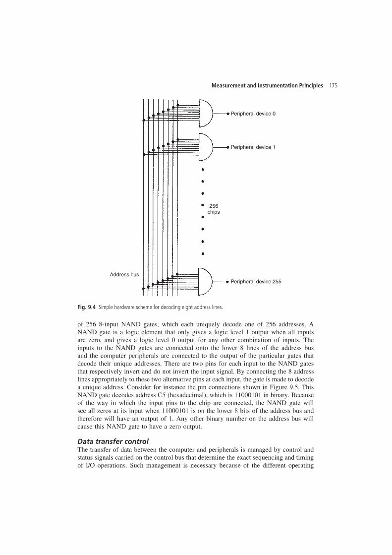
Measurement and Instrumentation Principles 175
Address busPeripheral device 255
Peripheral device 1
Peripheral device 0
256chips
Fig. 9.4 Simple hardware scheme for decoding eight address lines.
of 256 8-input NAND gates, which each uniquely decode one of 256 addresses. ANAND gate is a logic element that only gives a logic level 1 output when all inputsare zero, and gives a logic level 0 output for any other combination of inputs. Theinputs to the NAND gates are connected onto the lower 8 lines of the address busand the computer peripherals are connected to the output of the particular gates thatdecode their unique addresses. There are two pins for each input to the NAND gatesthat respectively invert and do not invert the input signal. By connecting the 8 addresslines appropriately to these two alternative pins at each input, the gate is made to decodea unique address. Consider for instance the pin connections shown in Figure 9.5. ThisNAND gate decodes address C5 (hexadecimal), which is 11000101 in binary. Becauseof the way in which the input pins to the chip are connected, the NAND gate willsee all zeros at its input when 11000101 is on the lower 8 bits of the address bus andtherefore will have an output of 1. Any other binary number on the address bus willcause this NAND gate to have a zero output.
Data transfer controlThe transfer of data between the computer and peripherals is managed by control andstatus signals carried on the control bus that determine the exact sequencing and timingof I/O operations. Such management is necessary because of the different operating
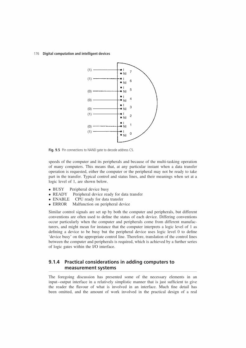
176 Digital computation and intelligent devices
(0)
(0)
(0)
(1)
(0)
(1)
(1)
(1) INI
INI
INI
INIINI
INI
INI
INI
7
6
5
4
3
2
1
0
Fig. 9.5 Pin connections to NAND gate to decode address C5.
speeds of the computer and its peripherals and because of the multi-tasking operationof many computers. This means that, at any particular instant when a data transferoperation is requested, either the computer or the peripheral may not be ready to takepart in the transfer. Typical control and status lines, and their meanings when set at alogic level of 1, are shown below.
ž BUSY Peripheral device busyž READY Peripheral device ready for data transferž ENABLE CPU ready for data transferž ERROR Malfunction on peripheral device
Similar control signals are set up by both the computer and peripherals, but differentconventions are often used to define the status of each device. Differing conventionsoccur particularly when the computer and peripherals come from different manufac-turers, and might mean for instance that the computer interprets a logic level of 1 asdefining a device to be busy but the peripheral device uses logic level 0 to define‘device busy’ on the appropriate control line. Therefore, translation of the control linesbetween the computer and peripherals is required, which is achieved by a further seriesof logic gates within the I/O interface.
9.1.4 Practical considerations in adding computers tomeasurement systems
The foregoing discussion has presented some of the necessary elements in aninput–output interface in a relatively simplistic manner that is just sufficient to givethe reader the flavour of what is involved in an interface. Much fine detail hasbeen omitted, and the amount of work involved in the practical design of a real
Measurement and Instrumentation Principles 177
interface should not be underestimated. One significant omission so far is discussionof the scaling that is generally required within the analogue–digital interface of acomputer. The raw analogue input and output signals are generally either too largeor too small for compatibility with the operating voltage levels of a digital computerand they have to be scaled upwards or downwards. This is normally achieved byoperational amplifiers and/or potentiometers. The main features of an operationalamplifier are its high gain (typically ð 1 000 000) and its large bandwidth (typically1 MHz or better). However, when one is used at very high frequencies, the bandwidthbecomes significant. The quality of an amplifier is often measured by a criterioncalled the gain–bandwidth product, which is the product of its gain and bandwidth.Other important attributes of the operational amplifier, particularly when used in acomputer input–output interface or within intelligent devices, are its distortion level,overload recovery capacity and offset level. Special instrumentation amplifiers thatare particularly good in these attributes have been developed for instrumentationapplications, as described in section 5.5.1.
Suitable care must always be taken when introducing a computer into a measurementsystem to avoid creating sources of measurement noise. This applies particularly whereone computer is used to process the output of several transducers and is connected tothem by signal wires. In such circumstances, the connections and connecting wirescan create noise through electrochemical potentials, thermoelectric potentials, offsetvoltages introduced by common mode impedances, and a.c. noise at power, audio andradio frequencies. Recognition of all these possible noise sources allows them to beeliminated in most cases by employing good practice when designing and constructingthe measurement system.
9.2 Intelligent devices
The term ‘intelligent device’ is used to describe a package containing either a completemeasurement system, or else a component within a measurement system, which incor-porates a digital processor. Processing of the output of measurement sensors to correctfor errors inherent in the measurement process brings about large improvements inmeasurement accuracy. Such intelligent devices are known by various names such asintelligent instrument, smart sensor and smart transmitter. There is no formal definitionfor any of these names, and there is considerable overlap between the characteristicsof particular devices and the name given to them. The discussion below tries to layout the historical development of intelligent devices, and it summarizes the generalunderstanding of the sort of characteristics possessed by the various forms of intelli-gent device. Details of their application to measure particular physical variables willbe covered in appropriate chapters in Part 2 of this book.
9.2.1 Intelligent instruments
The first intelligent instrument appeared over 20 years ago, although high prices whensuch devices first became available meant that their use within measurement systemsgrew very slowly initially. The processor within an intelligent instrument allows it to
178 Digital computation and intelligent devices
apply pre-programmed signal processing and data manipulation algorithms to measure-ments. One of the main functions performed by the first intelligent instruments tobecome available was compensation for environmental disturbances to measurementsthat cause systematic errors. Thus, apart from a primary sensor to measure the vari-able of interest, intelligent instruments usually have one or more secondary sensorsto monitor the value of environmental disturbances. These extra measurements allowthe output reading to be corrected for the effects of environmentally induced errors,subject to the following pre-conditions being satisfied:
(a) The physical mechanism by which a measurement sensor is affected by ambientcondition changes must be fully understood and all physical quantities that affectthe output must be identified.
(b) The effect of each ambient variable on the output characteristic of the primarysensor must be quantified.
(c) Suitable secondary sensors for monitoring the value of all relevant environmentalvariables must be available that will operate satisfactorily in the prevailing envi-ronmental conditions.
Condition (a) above means that the thermal expansion and contraction of all elementswithin a sensor must be considered in order to evaluate how it will respond to ambienttemperature changes. Similarly, the sensor response, if any, to changes in ambientpressure, humidity, gravitational force or power supply level (active instruments) mustbe examined.
Quantification of the effect of each ambient variable on the characteristics of themeasurement sensor is then necessary, as stated in condition (b). Analytic quantificationof ambient condition changes from purely theoretical consideration of the constructionof a sensor is usually extremely complex and so is normally avoided. Instead, theeffect is quantified empirically in laboratory tests where the output characteristic of thesensor is observed as the ambient environmental conditions are changed in a controlledmanner.
One early application of intelligent instruments was in volume flow rate measure-ment, where the flow rate is inferred by measuring the differential pressure across anorifice plate placed in a fluid-carrying pipe (see Chapter 16). The flow rate is propor-tional to the square root of the difference in pressure across the orifice plate. Fora given flow rate, this relationship is affected both by the temperature and by themean pressure in the pipe, and changes in the ambient value of either of these causemeasurement errors. A typical intelligent flowmeter therefore contains three sensors, aprimary one measuring pressure difference across the orifice plate and secondary onesmeasuring absolute pressure and temperature. The instrument is programmed to correctthe output of the primary differential-pressure sensor according to the values measuredby the secondary sensors, using appropriate physical laws that quantify the effect ofambient temperature and pressure changes on the fundamental relationship betweenflow and differential pressure. Even 20 years ago, such intelligent flow measuringinstruments achieved typical inaccuracy levels of š0.1%, compared with š0.5% fortheir non-intelligent equivalents.
Although automatic compensation for environmental disturbances is a very importantattribute of intelligent instruments, many versions of such devices perform additionalfunctions, and this was so even in the early days of their development. For example,
Measurement and Instrumentation Principles 179
the orifice-plate flowmeter just discussed usually converts the square root relation-ship between flow and signal output into a linear one, thus making the output mucheasier to interpret. Other examples of the sort of functions performed by intelligentinstruments are:
ž correction for the loading effect of measurement on the measured systemž signal damping with selectable time constantsž switchable ranges (using several primary sensors within the instrument that each
measure over a different range)ž switchable output units (e.g. display in Imperial or SI units)ž linearization of the outputž self-diagnosis of faultsž remote adjustment and control of instrument parameters from up to 1500 metres
away via 4-way, 20 mA signal lines.
These features will be discussed in greater detail under the later headings of smartsensors and smart transmitters.
Over the intervening years since their first introduction, the size of intelligent instru-ments has gradually reduced and the functions performed have steadily increased. Oneparticular development has been the inclusion of a microprocessor within the sensoritself, in devices that are usually known as smart sensors. As further size reductionand device integration has taken place, such smart sensors have been incorporated intopackages with other sensors and signal processing circuits etc. Whilst such a packageconforms to the definition of an intelligent instrument given previously, most manu-facturers now tend to call the package a smart transmitter rather than an intelligentinstrument, although the latter term has continued in use in some cases.
9.2.2 Smart sensors
A smart sensor is a sensor with local processing power that enables it to react tolocal conditions without having to refer back to a central controller. Smart sensorsare usually at least twice as accurate as non-smart devices, have reduced maintenancecosts and require less wiring to the site where they are used. In addition, long-termstability is improved, reducing the required calibration frequency.
The functions possessed by smart sensors vary widely, but consist of at least someof the following:
ž Remote calibration capabilityž Self-diagnosis of faultsž Automatic calculation of measurement accuracy and compensation for random errorsž Adjustment for measurement of non-linearities to produce a linear outputž Compensation for the loading effect of the measuring process on the measured
system.
Calibration capabilitySelf-calibration is very simple in some cases. Sensors with an electrical output can usea known reference voltage level to carry out self-calibration. Also, load-cell types ofsensor, which are used in weighing systems, can adjust the output reading to zero whenthere is no applied mass. In the case of other sensors, two methods of self-calibration
180 Digital computation and intelligent devices
are possible, use of a look-up table and an interpolation technique. Unfortunately, alook-up table requires a large memory capacity to store correction points. Also, a largeamount of data has to be gathered from the sensor during calibration. In consequence,the interpolation calibration technique is preferable. This uses an interpolation methodto calculate the correction required to any particular measurement and only requires asmall matrix of calibration points (van der Horn, 1996).
Self-diagnosis of faultsSmart sensors perform self-diagnosis by monitoring internal signals for evidence offaults. Whilst it is difficult to achieve a sensor that can carry out self-diagnosis ofall possible faults that might arise, it is often possible to make simple checks thatdetect many of the more common faults. One example of self-diagnosis in a sensor ismeasuring the sheath capacitance and resistance in insulated thermocouples to detectbreakdown of the insulation. Usually, a specific code is generated to indicate each typeof possible fault (e.g. a failing of insulation in a device).
One difficulty that often arises in self-diagnosis is in differentiating between normalmeasurement deviations and sensor faults. Some smart sensors overcome this by storingmultiple measured values around a set-point, calculating minimum and maximumexpected values for the measured quantity.
Uncertainty techniques can be applied to measure the impact of a sensor fault onmeasurement quality. This makes it possible in certain circumstances to continue touse a sensor after it has developed a fault. A scheme for generating a validity index hasbeen proposed that indicates the validity and quality of a measurement from a sensor(Henry, 1995).
Automatic calculation of measurement accuracy and compensationfor random errorsMany smart sensors can calculate measurement accuracy on-line by computing themean over a number of measurements and analysing all factors affecting accuracy. Thisaveraging process also serves to greatly reduce the magnitude of random measurementerrors.
Adjustment for measurement non-linearitiesIn the case of sensors that have a non-linear relationship between the measured quantityand the sensor output, digital processing can convert the output to a linear form,providing that the nature of the non-linearity is known so that an equation describingit can be programmed into the sensor.
9.2.3 Smart transmitters
In concept, a smart transmitter is almost identical to the intelligent instruments describedearlier. The change in name has occurred over a number of years as intelligent instru-ments have become smaller and assumed a greater range of functions. Usage of theterm ‘smart transmitter’ rather than ‘intelligent instrument’ is therefore mainly one offashion. In some instances, smart transmitters are known alternatively as intelligenttransmitters. The term multivariable transmitter is also sometimes used, particularlyfor a device like a smart flow-measuring instrument. This measures absolute pressure,

Measurement and Instrumentation Principles 181
differential pressure and process temperature, and computes both the mass flow rateand volume flow rate of the measured fluid.
There has been a dramatic reduction in the price of intelligent devices over thepast few years and the cost differential between smart and conventional transmittersis now very small. Indeed, in a few cases, a smart transmitter is now cheaper than itsnon-smart equivalent because of the greater sales volume for the smart version. Thus,smart transmitters are now routinely bought instead of non-smart versions. However, inmany cases, smart transmitters are only used at present in a conventional (non-smart)fashion to give a 4–20 mA analogue measurement signal on the two output wires.Where smart features are used at all, they are often only used during the commissioningphase of measurement systems. This is largely due to the past investment in analoguemeasurement systems, and the time and effort necessary to convert to measurementsystems that can make proper use of intelligent features.
Almost all of the smart sensors that are presently available have an analogue output,because of the continuing popularity and investment in 4–20 mA current transmissionsystems. Whilst a small number of devices are now available with digital output, mostusers have to convert this to analogue form to maintain compatibility with existinginstrumentation systems.
The capabilities of smart transmitters are perhaps best emphasized by comparingthe attributes of the alternative forms of transmitter available. There are three types oftransmitter, analogue, programmable and smart.
(a) Analogue transmitters:ž require one transmitter for every sensor type and every sensor rangež require additional transmitters to correct for environmental changesž require frequent calibration.
(b) Programmable transmitters:ž include a microprocessor but do not have bi-directional communication (hence
are not truly intelligent)ž require field calibration.
(c) Smart transmitters:ž include a microprocessor and have bi-directional communicationž include secondary sensors that can measure, and so compensate for, environ-
mental disturbancesž usually incorporate signal conditioning and a–d conversionž often incorporate multiple sensors covering different measurement ranges and
allow automatic selection of the required range. The range can be readily alteredif initially estimated incorrectly
ž have a self-calibration capability that allows removal of zero drift and sensitivitydrift errors
ž have a self-diagnostic capability that allows them to report problems or require-ments for maintenance
ž can adjust for non-linearities to produce a linear output.
Smart transmitters are usually a little larger and heavier than non-smart equivalents.However, their advantages can be summarized as:
ž Improved accuracy and repeatabilityž Long-term stability is improved and required recalibration frequency is reduced
182 Digital computation and intelligent devices
ž Reduced maintenance costsž Large range coverage, allowing interoperability and giving increased flexibilityž Remote adjustment of output range, on command from a portable keyboard or from a
PC. This saves on technician time compared with carrying out adjustment manuallyž Reduction in number of spare instruments required, since one spare transmitter can
be configured to cover any range and so replace any faulty transmitterž Possibility of including redundant sensors, which can be used to replace failed
sensors and so improve device reliabilityž Allowing remote recalibration or re-ranging by sending a digital signal to themž Ability to store last calibration date and indicate when next calibration is requiredž Single penetration into the measured process rather than the multiple penetration
required by discrete devices, making installation easier and cheaperž Ability to store data so that plant and instrument performance can be analysed. For
example, data relating to the effects of environmental variations can be stored andused to correct output measurements over a large range.
Summary of smart transmitter featuresMany of the features of smart transmitters are common with those of smart sensors,and the comments made earlier about smart sensors therefore apply equally. However,the use of multiple primary sensors and secondary sensors to measure environmentalparameters mean that additional comments are necessary in respect of their self-calibration and self-diagnosis capabilities.
Self-calibrationCalibration techniques are very similar to those already described for smart sensors andthe general principle is always to use simple calibration methods if these are available.Look-up tables in a smart transmitter have a particularly large memory requirementif correction for cross-sensitivity to another parameter (e.g. temperature) is requiredbecause a matrix of correction values has to be stored. Hence, interpolation calibrationis even more preferable to look-up tables than it is in the case of calibrating smartsensors.
Self-diagnosis and fault detectionFault diagnosis in sensors is often difficult because it is not easy to distinguish betweenmeasurement deviation due to a sensor fault and deviation due to a plant fault. The besttheoretical approach to this difficulty is to apply mathematical modelling techniques tothe sensor and plant in which it is working, with the aim of detecting inconsistenciesin data from the sensor. However, there are very few industrial applications of thisapproach to fault detection in practice, firstly, because of the cost of implementationand, secondly, because of the difficulty of obtaining plant models that are robust toplant disturbances. Thus, it is usually necessary to resort to having multiple sensorsand using a scheme such as two-out-of-three voting. Further advice on self-checkingprocedures can be found elsewhere (Brignell, 1996).
Effect of sensor errorsThe effect of a sensor error on the quality of measurement varies according to thenature of the fault and the type of sensor. For example, a smart pressure sensor that
Measurement and Instrumentation Principles 183
loses temperature measurement will still give valid measurements but the uncertaintyincreases.
9.2.4 Communication with intelligent devices
The subject of instrumentation networks and digital communication with instrumentsis covered in detail in the next chapter. The aim over many years has been to useintelligent devices to their full potential by making all communications, including themeasurement signal, entirely digital. A number of digital fieldbuses are now usedfor instrumentation systems, with protocols such as Profibus and WorldFIP being inwidespread use. However, to date, despite international efforts over many years, nostandard protocol for digital fieldbus communications has yet been established.
Partly because of this delay in developing an international digital fieldbus stan-dard, and partly because of the need to maintain compatibility with the vast currentinvestment in analogue instrumentation systems, a number of part analogue/part digitalcommunication protocols have been developed as an interim measure. Prominentamongst these is a protocol called HART (Highway Addressable Remote Transducer).This is a manufacturer-independent protocol that provides for analogue measurementsignal transmission as well as sending command/status information digitally. Thenormal requirement for such dual analogue/digital communication with an intelli-gent device is six wires, two to convey the measurement signal, two to conveycommand/device status information and two to provide a power supply to the device.However, in order to economize on wiring and installation costs, HART allows thisrequirement to be reduced to four or even two wires by using the signal wires to conveydevice status/command signals or the power supply or both of these. HART has nowachieved widespread use, even though it is not backed by an international standard.
Extended 4–20 mA current interface protocolThe 4–20 mA protocol is the most-used analogue transmission mechanism because ofthe protection against noise that it offers to the measurement values transmitted. Thisprotocol has been extended for communication with intelligent devices to allow for thetransmission, where necessary, of command/status information and the device powersupply in analogue form on the signal wires. In this extended protocol, signals in therange 3.8 mA to 20.5 mA are regarded as ‘normal’ measurement signals, thus allowingfor under- and over-range from the 4–20 mA measurement signal standard. The currentbands immediately outside this in the range 3.6 mA to 3.8 mA and 20.5 mA to 21.0 mAare used for the conveyance of commands to the sensor/transmitter and the receipt ofstatus information from it. This means that, if the signal wires are also used to carrythe power supply to the sensor/transmitter, the power supply current must be limited to3.5 mA or less to avoid the possibility of it being interpreted as a measurement signalor fault indicator. Signals greater than 21 mA (and less than 3.6 mA if the signal wiresare not carrying a power supply) are normally taken to indicate either a short circuitor open circuit in the signal wiring.
Sending commands to sensor/transmitterCommands can either be sent from a handheld keyboard or else communicated froma remote PC. Whilst a handheld keyboard is the cheaper option in terms of equipment
184 Digital computation and intelligent devices
requirement, it cannot store calibration data because it does not usually have anymemory. It is therefore time consuming for a technician to enter the necessary cali-bration data manually. A PC makes communication easier because it can readily storecalibration data. Also, its large screen allows more information to be viewed at onetime. A PC is also able to receive status data from the sensor and store it for later use(e.g. to disclose trends in sensor status).
For hazardous environments, versions of smart transmitters are available that aremade intrinsically safe by using reed-relay switches to alter transmitter parameters. Insuch cases, an LCD programming display is usually used to give commands to thetransmitter, as this is also intrinsically safe.
9.2.5 Computation in intelligent devices
In the past, most computation in intelligent devices has been performed by softwareroutines executed on a general-purpose microcomputer. However, there has been atrend in the last few years towards implementing digital signal processing, data conver-sion and communication interface functions in specially designed hardware elements.This achieves a large improvement in processing speed compared with the executionof software routines. The first implementations of this (Brignell, 1996) used ASICs(Application Specific Integrated Circuits). An ASIC is a gate array that is programmedby designing a mask that creates connections between elements in the device. Unfor-tunately, the mask design is a very costly process and therefore such devices are onlycost effective in high-volume applications such as automobile systems.
More recently, alternative programming devices such as FPGAs (Field ProgrammableGate Arrays) and CPLDs (Complex Programmable Logic Devices) have become avail-able that offer a means of implementing digital signal processing and other functionsthat are cost effective in low-volume applications. Implementation cost is reducedbecause these devices are user-programmable and avoid the very expensive mask-design process required by ASICs. In fact, these alternative programming devices arenow routinely used to build prototypes of designs before going into production ofASICs (which are still more cost effective than FPGAs and CPLDs in high-volumeapplications).
A typical programmable device consists of an array of configurable logic blocks,programmable input–output blocks and memory. However, FPGAs and CPLDs differsubstantially in the way that elements are connected within the device, with the connec-tions used in a CPLD allowing faster operation of the device. These differences meanthat, in general, the CPLD is preferred for applications where there is a requirementfor high processing speed and the FPGA is preferred where there is a need for highcapacity (number of logic gates) in the device.
Some programmable devices contain both soft and hard cores, in which a hardcore performing specific functions such as a PCI (Peripheral Component Interconnect)interface is embedded in a programmable soft core. In this hard-core/soft-core approach,the inclusion of hard-core elements increases computational speed and reduces size, butthe increased specialization of the device reduces the number of potential applicationsand therefore increases unit cost.
Further information on these modern programmable devices can be found elsewhere(Amos, 1995; Brown, 1996).
Measurement and Instrumentation Principles 185
9.2.6 Future trends in intelligent devices
The extent of application of smart transmitters is currently limited by:
ž Lack of sufficient varieties of transmitter due to manufacturers’ reluctance to investin producing them ahead of agreement on an international fieldbus standard
ž Limitations on the power of microprocessors availablež The large investment in conventional 4–20 mA signal transmission systems and
cabling, thus inhibiting the use of transmitters to their full potential in fully digitaltransmission mode
ž Limitations in the speed of bi-directional communication capabilities. If a commonbus is used to transmit signals for several different transmitters, data transfer speedis slow because the bus can only service one transmitter at a time. This means thatthe time interval between measurements from a particular transmitter being readand responded to can become excessively large. In consequence, it is possible fordangerous conditions to develop in the controlled plant, such as high pressures.
Current research and international discussions are currently directed at solving all ofthese problems. Hence, a rapid growth in the application of intelligent devices, and theiruse in fully digital mode, is expected over the next few years. Size reductions will alsocontinue, and indeed the first smart microsensors are now available. These are coveredin greater detail in Chapter 13. The establishment of an international fieldbus standard(see Chapter 10) will also encourage greater use of intelligent devices in all-digitalinstrumentation and control schemes for industrial plant.
The use of programmable devices to perform signal processing functions withinintelligent devices is likely to expand rapidly in the future. As well as further improve-ments to the processing capacity and computational speed of these devices, currentresearch (Tempesti, 1999) is directed towards developing self-repairing capabilities insuch devices.
Also, now that both sensors, processing elements and microcontrollers can all beconstructed on silicon wafers, the next logical step is to extend the process of inte-gration still further and include all of these elements on a single silicon chip. Apartfrom the reduction in system cost due to the reduction in the number of components,the requirement for fewer connections between components will lead to substantiallyimproved system reliability, since most system faults can be traced to connection faults.However, whether, or how soon, this further integration will happen will depend onthe relevant economics of separate and combined implementation of these systemcomponents.
9.3 Self-test questions
9.1 Describe briefly the three essential elements of a microcomputer system.9.2 Write down the one’s complement and two’s complement 8-bit representations of
the following decimal numbers: (a) 47 (b) �119 (c) �101 (d) 86 (e) 1089.3 Write down the binary, octal and hexadecimal representations of the following
decimal numbers: (a) 57 (b) 101 (c) 175 (d) 259 (e) 999 (f) 1234
186 Digital computation and intelligent devices
9.4 The binary code representation of a number is 111101001101. If all 12 digitsare data bits, what are (a) the octal and (b) the hexadecimal equivalents of thisnumber?
9.5 The binary code representation of a number is 1011000110100101. If all 16 digitsare data bits, what are (a) the octal and (b) the hexadecimal equivalents of thisnumber?
9.6 The binary code representation of a number is 110100011000. The first and lastbinary digits are sign and parity bits respectively, so only the middle ten digitsare data bits. What are (a) the octal, (b) the hexadecimal and (c) the decimal datavalues?
References and further reading
Amos, D. (1995) Interconnect trade-offs: CPLD versus FPGA, Electronic Engineering, Marchpp. 81–84.
Barney, G.C. (1988) Intelligent Instruments, Prentice-Hall, London.Brignell, J. and White, N. (1996) Intelligent Sensor Systems, Institute of Physics Publishing.Brown, S. and Rose, J. (1996) Architecture of FPGAs and CPLDs: A Tutorial, IEEE Design
and Test of Computers, 13, pp. 42–57.Henry, M. (1995) Self-validation improves Coriolis flowmeter, Control Engineering, May
pp. 81–86.Tempesti, G. (1999) A biologically-inspired self-repairing FPGA, Electronic Engineering,
August pp. 45–46.Van der Horn, G et al. (1996) Calibration and linearisation method for microcontroller-based
sensor systems, Measurement and Control, 29, pp. 270–273.
10
Instrumentation/computernetworks
10.1 Introduction
The inclusion of computer processing power in intelligent instruments and intelligentactuators creates the possibility of building an instrumentation system where severalintelligent devices collaborate together, transmit information to one another and executeprocess control functions. Such an arrangement is often known as a distributed controlsystem. Additional computer processors can also be added to the system as neces-sary to provide the necessary computational power when the computation of complexcontrol algorithms is required. Such an instrumentation system is far more fault tolerantand reliable than older control schemes where data from several discrete instrumentsis carried to a centralized computer controller via long instrumentation cables. Thisimproved reliability arises from the fact that the presence of computer processors inevery unit injects a degree of redundancy into the system. Therefore, measurement andcontrol action can still continue, albeit in a degraded form, if one unit fails.
In order to effect the necessary communication when two or more intelligent devicesare to be connected together as nodes in a distributed system, some form of electronichighway must be provided between them that permits the exchange of information.Apart from data transfer, a certain amount of control information also has to be trans-ferred. The main purpose of this control information is to make sure that the targetdevice is ready to receive information before data transmission starts. This controlinformation also prevents more than one device trying to send information at the sametime.
In modern installations, all communication and data transmission between processingnodes in a distributed instrumentation and control system is carried out digitally alongsome form of electronic highway, although analogue data transmission (mainly currentloop) is still widely used to transmit data from field devices into the processing nodes.If analogue transmission is used for measurement data, an analogue-to-digital convertermust be provided at the interfaces between the measurement signal transmission cablesand the processing nodes.
The electronic highway can either be a serial communication line, a parallel databus, or a local area network. Serial data lines are very slow and are only used where a
188 Instrumentation/computer networks
low data transmission speed is acceptable. Parallel data buses are limited to connectinga modest number of devices spread over a small geographical area, typically a singleroom, but provide reasonably fast data transmission. Local area networks are used toconnect larger numbers of devices spread over larger geographical distances, typicallya single building or site. They transmit data in digital format at high speed. Instrumen-tation networks that are geographically larger than a single building or site can also bebuilt, but these generally require transmission systems that include telephone lines aswell as local networks at particular sites within the large system.
The input/output interface of an intelligent device provides the necessary connectionbetween the device and the electronic highway. The interface can be either serial orparallel.
A serial interface is used to connect a device onto a serial communication line. Theconnection is effected physically by a multi-pin plug that fits into a multi-pin socket onthe casing of the device. The pins in this plug/socket match the signal lines used in theserial communication line exactly in number and function. Effectively, there is only onestandard format for serial data transmission that enjoys international recognition. Whilstthis is advantageous in avoiding compatibility problems when connecting togetherdevices coming from different manufacturers, serial transmission is relatively slow.
A parallel interface is used to connect devices onto parallel instrument buses andalso into all other types of network systems. Like the serial interface, the parallelinterface exists physically as a multi-pin plug that fits into a multi-pin socket on thecasing of the device. The pins in the plug/socket are matched exactly in number andfunction with the data and control lines used by a particular parallel instrument bus.Unfortunately, there are a number of different parallel instrument buses in use and thusa corresponding number of different parallel interface protocols, with little compati-bility between them. Hence, whilst parallel data transmission is much faster than serialtransmission, there are serious compatibility problems to be overcome when connectingtogether devices coming from different manufacturers because of the different parallelinterface protocols used.
10.2 Serial communication lines
Serial communication only allows relatively slow data transfer rates, but it can operateover much larger distances than parallel communication. Transmission distances up to3 km are possible with standard copper-wire links, and much greater distances can beachieved using either telephone lines or radio telemetry. Data are transferred down asingle line on the electronic highway one bit at a time, and the start and finish of eachitem of data are denoted by special sequences of control characters that precede andfollow the data bits.
Three alternative forms of serial communication exist, known as simplex, half-duplexand full-duplex. Simplex mode only allows transmission of data in one direction. Forthis reason, it is not widely used, since, although it permits a remote sensor to transmitinformation, the receiving station cannot send a message back to acknowledge receiptor request retransmission if the received data has been corrupted. In half-duplex mode,the same data wire is used by a device to both send and receive data, and thus thereceiving station is able to acknowledge receipt of data from a sensor. However, sending
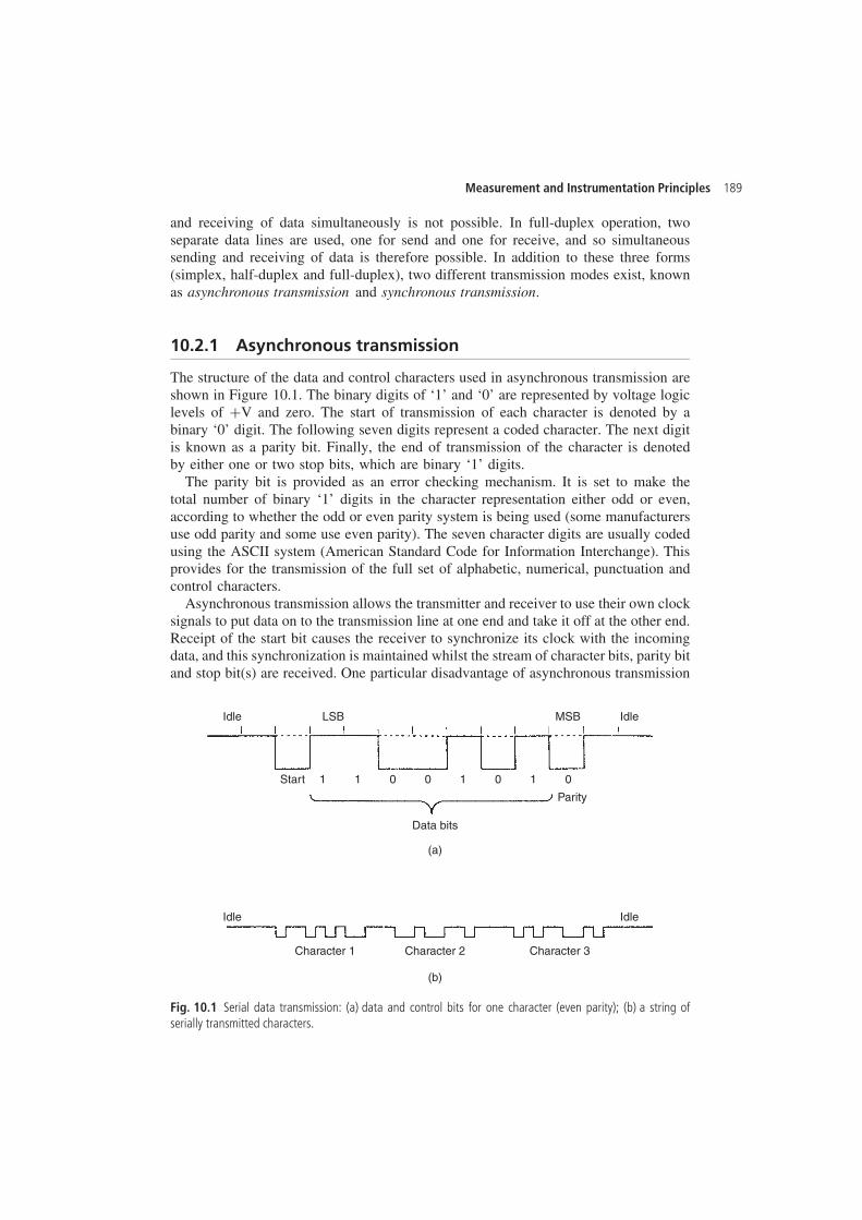
Measurement and Instrumentation Principles 189
and receiving of data simultaneously is not possible. In full-duplex operation, twoseparate data lines are used, one for send and one for receive, and so simultaneoussending and receiving of data is therefore possible. In addition to these three forms(simplex, half-duplex and full-duplex), two different transmission modes exist, knownas asynchronous transmission and synchronous transmission.
10.2.1 Asynchronous transmission
The structure of the data and control characters used in asynchronous transmission areshown in Figure 10.1. The binary digits of ‘1’ and ‘0’ are represented by voltage logiclevels of CV and zero. The start of transmission of each character is denoted by abinary ‘0’ digit. The following seven digits represent a coded character. The next digitis known as a parity bit. Finally, the end of transmission of the character is denotedby either one or two stop bits, which are binary ‘1’ digits.
The parity bit is provided as an error checking mechanism. It is set to make thetotal number of binary ‘1’ digits in the character representation either odd or even,according to whether the odd or even parity system is being used (some manufacturersuse odd parity and some use even parity). The seven character digits are usually codedusing the ASCII system (American Standard Code for Information Interchange). Thisprovides for the transmission of the full set of alphabetic, numerical, punctuation andcontrol characters.
Asynchronous transmission allows the transmitter and receiver to use their own clocksignals to put data on to the transmission line at one end and take it off at the other end.Receipt of the start bit causes the receiver to synchronize its clock with the incomingdata, and this synchronization is maintained whilst the stream of character bits, parity bitand stop bit(s) are received. One particular disadvantage of asynchronous transmission
Idle
Idle
Character 1 Character 2 Character 3
Idle
Idle
LSB MSB
Start 1 1 0 0 1 0 1 0
(a)
(b)
Data bits
Parity
Fig. 10.1 Serial data transmission: (a) data and control bits for one character (even parity); (b) a string ofserially transmitted characters.
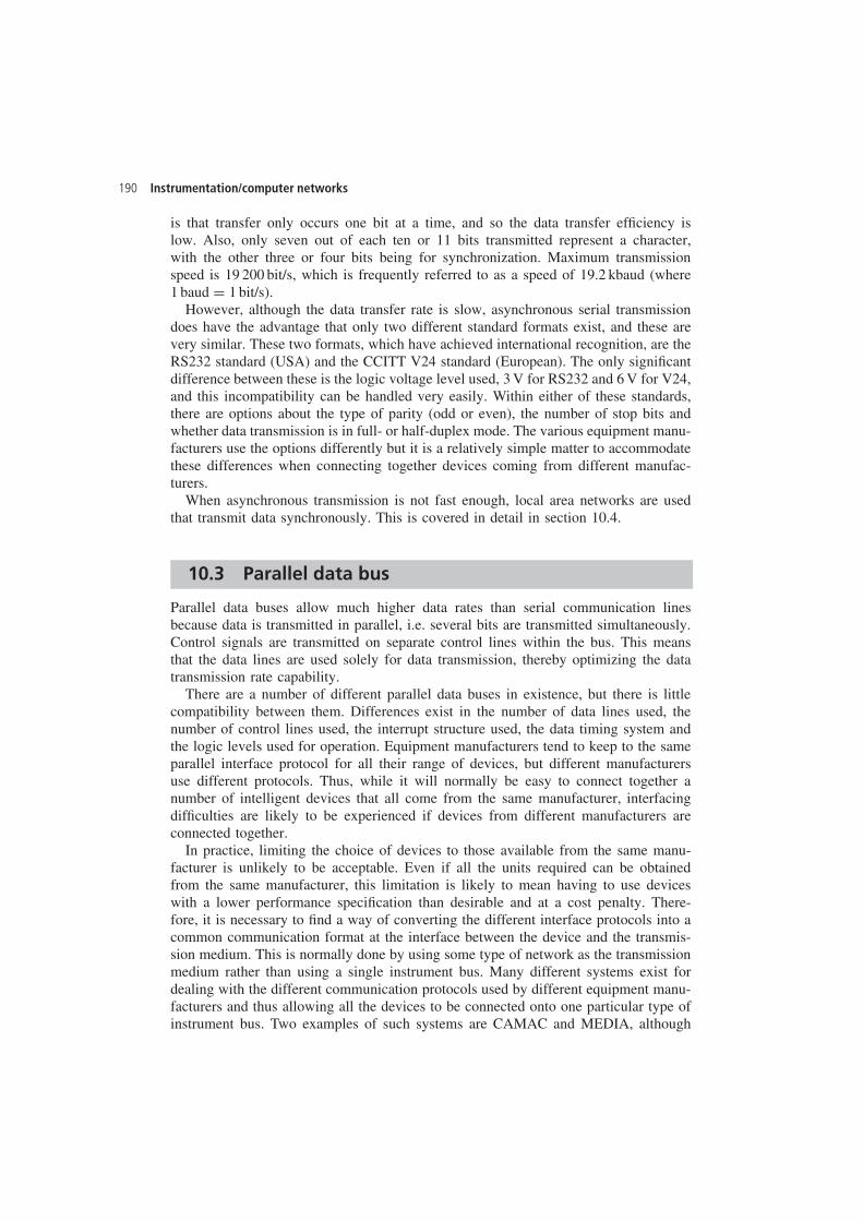
190 Instrumentation/computer networks
is that transfer only occurs one bit at a time, and so the data transfer efficiency islow. Also, only seven out of each ten or 11 bits transmitted represent a character,with the other three or four bits being for synchronization. Maximum transmissionspeed is 19 200 bit/s, which is frequently referred to as a speed of 19.2 kbaud (where1 baud D 1 bit/s).
However, although the data transfer rate is slow, asynchronous serial transmissiondoes have the advantage that only two different standard formats exist, and these arevery similar. These two formats, which have achieved international recognition, are theRS232 standard (USA) and the CCITT V24 standard (European). The only significantdifference between these is the logic voltage level used, 3 V for RS232 and 6 V for V24,and this incompatibility can be handled very easily. Within either of these standards,there are options about the type of parity (odd or even), the number of stop bits andwhether data transmission is in full- or half-duplex mode. The various equipment manu-facturers use the options differently but it is a relatively simple matter to accommodatethese differences when connecting together devices coming from different manufac-turers.
When asynchronous transmission is not fast enough, local area networks are usedthat transmit data synchronously. This is covered in detail in section 10.4.
10.3 Parallel data bus
Parallel data buses allow much higher data rates than serial communication linesbecause data is transmitted in parallel, i.e. several bits are transmitted simultaneously.Control signals are transmitted on separate control lines within the bus. This meansthat the data lines are used solely for data transmission, thereby optimizing the datatransmission rate capability.
There are a number of different parallel data buses in existence, but there is littlecompatibility between them. Differences exist in the number of data lines used, thenumber of control lines used, the interrupt structure used, the data timing system andthe logic levels used for operation. Equipment manufacturers tend to keep to the sameparallel interface protocol for all their range of devices, but different manufacturersuse different protocols. Thus, while it will normally be easy to connect together anumber of intelligent devices that all come from the same manufacturer, interfacingdifficulties are likely to be experienced if devices from different manufacturers areconnected together.
In practice, limiting the choice of devices to those available from the same manu-facturer is unlikely to be acceptable. Even if all the units required can be obtainedfrom the same manufacturer, this limitation is likely to mean having to use deviceswith a lower performance specification than desirable and at a cost penalty. There-fore, it is necessary to find a way of converting the different interface protocols into acommon communication format at the interface between the device and the transmis-sion medium. This is normally done by using some type of network as the transmissionmedium rather than using a single instrument bus. Many different systems exist fordealing with the different communication protocols used by different equipment manu-facturers and thus allowing all the devices to be connected onto one particular type ofinstrument bus. Two examples of such systems are CAMAC and MEDIA, although
Measurement and Instrumentation Principles 191
these are rarely used nowadays as it is more common to solve the problem by usinglocal area networks.
Some examples of parallel interface buses are Multibus, the S100 Bus and the IEEE488 bus (also known by the alternative names of HP-IB bus, GBIB bus, Plus busand ANSI standard MC1-1 bus). The IEEE 488 bus has now gained prominence forinstrumentation networks, and it has been adopted by the International ElectrotechnicalCommission (IEC) as a standard, IEC625. It provides a parallel interface that facilitatesthe connection of intelligent instruments, actuators and controllers within a single room.The maximum length of bus allowable is about 20 m, and no more than 15 instrumentsshould be distributed along its length. The maximum distance between two particularunits on the bus should not exceed about 2 m. The maximum data transfer rate permittedby the bus is 1 Mbit/s in theory, though the maximum data rate achieved in practiceover a full 20 m length of bus is more likely to be in the range 250–500 Kbit/s.
Physically, the bus consists of a shielded, 24-conductor cable. Sixteen of the conduc-tors are used as signal lines, eight carrying data and eight carrying control signals. Theremaining eight conductors are used as ground wires for the control signals, eachcontrol wire being twisted together along its full length with one of the ground wires.This minimizes cross-talk between the control wires. Normal practice is to route theeight twisted pairs carrying control signals in the centre of the cable and place theeight data wires round the periphery. This bundle of wires is surrounded by shieldingand an outer insulated coating. Each end of the cable is connected to a standard24-pin metal connector, with generally a female connector at one end and a maleconnector at the other. This facilitates several cables being chained from one deviceto another.
Figure 10.2 shows three devices connected onto an IEEE 488 bus. The bus canonly carry one lot of information at a time, and which unit is sending data and whichis receiving it is controlled by a supervisory computer connected to the bus. Thissupervisor ensures that only one unit can put data on the bus at a time, and thus preventsthe corruption of data that would occur if several instruments had simultaneous access.
Having eight data lines means that the bus can transmit 8 bits of data in parallelat the same time. This was originally designed so that 8-bit computer words could betransmitted as whole words. This does not prevent the bus being used with computersof a different wordlength, for example 16 or 32 bits. However, if the wordlength islonger than 8 bits, whole words cannot be transmitted in one go: they have to betransmitted 8 bits at a time. The eight status lines provide the necessary control toensure that when data transmission takes place between two units, three conditions aresatisfied simultaneously. These three conditions are (a) that the sender unit is ready totransmit data, (b) that the receiver unit is ready to receive data and (c) that the busdoes not currently have any data on it. The functioning of the eight status lines is asfollows:
ž DAV (Data valid) This goes to a logic zero when the data on theeight data lines is valid.
ž NFRD (Not ready for data) This goes to logic zero when the receiver unit isready to accept data.
ž NDAC (Not data accepted) This goes to logic zero when the receiver unithas finished receiving data.
192 Instrumentation/computer networks
01234567DAV (data valid)NRFD (not ready for data)NDAC (not data accepted)ATN (attenuation)IFC (interface clear)SRQ (service request)REN (remote enable)EOI (end or identify)
Data lines
Device1
Device2
Device3
Fig. 10.2 IEEE 488 bus.
ž ATN (Attention) This is a general control signal that is used forvarious purposes to control the use of data linesand specify the send and receive devices to beused.
ž IFC (Interface clear) The controller uses this status line to put theinterface into a wait state.
ž SRQ (Service request) This is an interrupt status line that allows highpriority devices such as alarms to interruptcurrent bus traffic and get immediate access tothe bus.
ž REN (Remote enable) This status line is used to specify which of twoalternative sets of device programming data areto be used.
ž EOI (End of output or identify) This status line is used by the sending unit toindicate that it has finished transmitting data.
The IEEE 488 bus protocol uses a logic level of less than 0.8 V to represent a logic 0signal and a voltage level greater than 2.0 V to represent a logic 1 signal.
10.4 Local area networks (LANs)
Local area networks transmit data in digital format along serial transmission lines.Synchronous transmission is normally used because this allows relatively high trans-mission speeds by transmitting blocks of characters at a time. A typical data blockconsists of 80 characters: this is preceded by a synchronization sequence and followedby a stop sequence. The synchronization sequence causes the receiver to synchronize
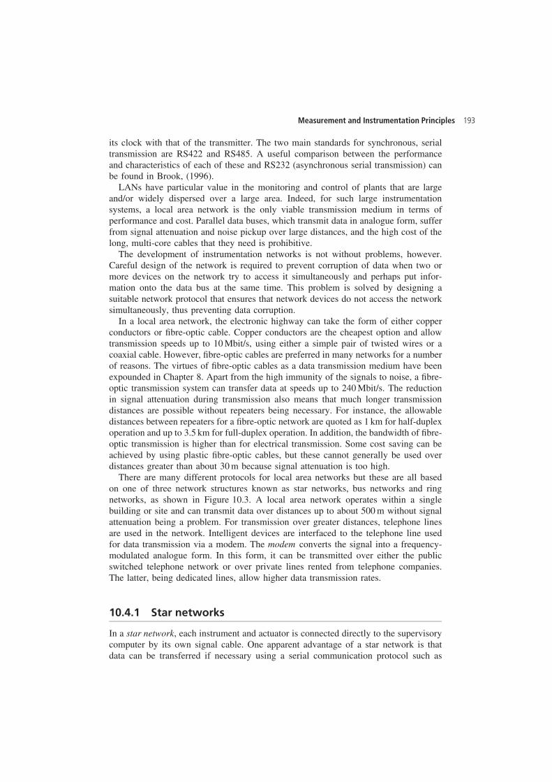
Measurement and Instrumentation Principles 193
its clock with that of the transmitter. The two main standards for synchronous, serialtransmission are RS422 and RS485. A useful comparison between the performanceand characteristics of each of these and RS232 (asynchronous serial transmission) canbe found in Brook, (1996).
LANs have particular value in the monitoring and control of plants that are largeand/or widely dispersed over a large area. Indeed, for such large instrumentationsystems, a local area network is the only viable transmission medium in terms ofperformance and cost. Parallel data buses, which transmit data in analogue form, sufferfrom signal attenuation and noise pickup over large distances, and the high cost of thelong, multi-core cables that they need is prohibitive.
The development of instrumentation networks is not without problems, however.Careful design of the network is required to prevent corruption of data when two ormore devices on the network try to access it simultaneously and perhaps put infor-mation onto the data bus at the same time. This problem is solved by designing asuitable network protocol that ensures that network devices do not access the networksimultaneously, thus preventing data corruption.
In a local area network, the electronic highway can take the form of either copperconductors or fibre-optic cable. Copper conductors are the cheapest option and allowtransmission speeds up to 10 Mbit/s, using either a simple pair of twisted wires or acoaxial cable. However, fibre-optic cables are preferred in many networks for a numberof reasons. The virtues of fibre-optic cables as a data transmission medium have beenexpounded in Chapter 8. Apart from the high immunity of the signals to noise, a fibre-optic transmission system can transfer data at speeds up to 240 Mbit/s. The reductionin signal attenuation during transmission also means that much longer transmissiondistances are possible without repeaters being necessary. For instance, the allowabledistances between repeaters for a fibre-optic network are quoted as 1 km for half-duplexoperation and up to 3.5 km for full-duplex operation. In addition, the bandwidth of fibre-optic transmission is higher than for electrical transmission. Some cost saving can beachieved by using plastic fibre-optic cables, but these cannot generally be used overdistances greater than about 30 m because signal attenuation is too high.
There are many different protocols for local area networks but these are all basedon one of three network structures known as star networks, bus networks and ringnetworks, as shown in Figure 10.3. A local area network operates within a singlebuilding or site and can transmit data over distances up to about 500 m without signalattenuation being a problem. For transmission over greater distances, telephone linesare used in the network. Intelligent devices are interfaced to the telephone line usedfor data transmission via a modem. The modem converts the signal into a frequency-modulated analogue form. In this form, it can be transmitted over either the publicswitched telephone network or over private lines rented from telephone companies.The latter, being dedicated lines, allow higher data transmission rates.
10.4.1 Star networks
In a star network, each instrument and actuator is connected directly to the supervisorycomputer by its own signal cable. One apparent advantage of a star network is thatdata can be transferred if necessary using a serial communication protocol such as
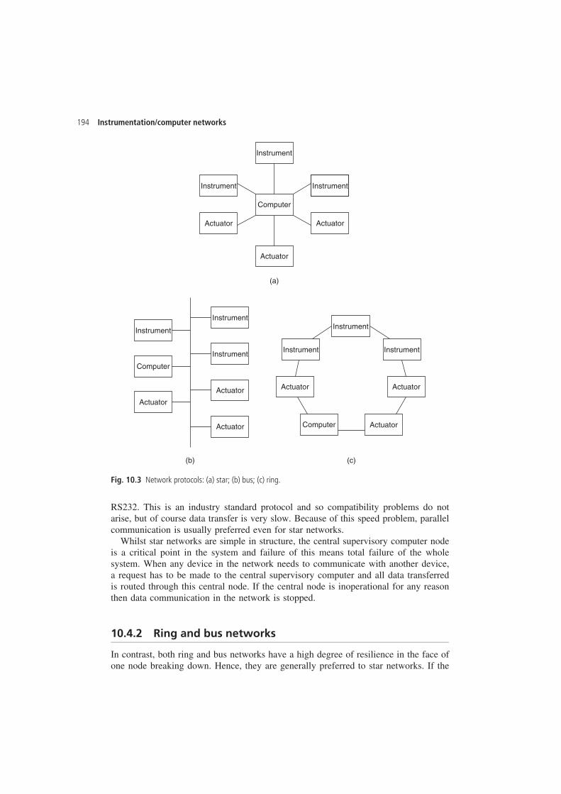
194 Instrumentation/computer networks
Instrument
Instrument
Computer
Actuator
Actuator
Instrument
Actuator
Instrument Instrument
Instrument Instrument
Actuator
Instrument
Instrument
Actuator Actuator
Actuator
Actuator
Actuator
Computer
Computer
(a)
(b) (c)
Fig. 10.3 Network protocols: (a) star; (b) bus; (c) ring.
RS232. This is an industry standard protocol and so compatibility problems do notarise, but of course data transfer is very slow. Because of this speed problem, parallelcommunication is usually preferred even for star networks.
Whilst star networks are simple in structure, the central supervisory computer nodeis a critical point in the system and failure of this means total failure of the wholesystem. When any device in the network needs to communicate with another device,a request has to be made to the central supervisory computer and all data transferredis routed through this central node. If the central node is inoperational for any reasonthen data communication in the network is stopped.
10.4.2 Ring and bus networks
In contrast, both ring and bus networks have a high degree of resilience in the face ofone node breaking down. Hence, they are generally preferred to star networks. If the
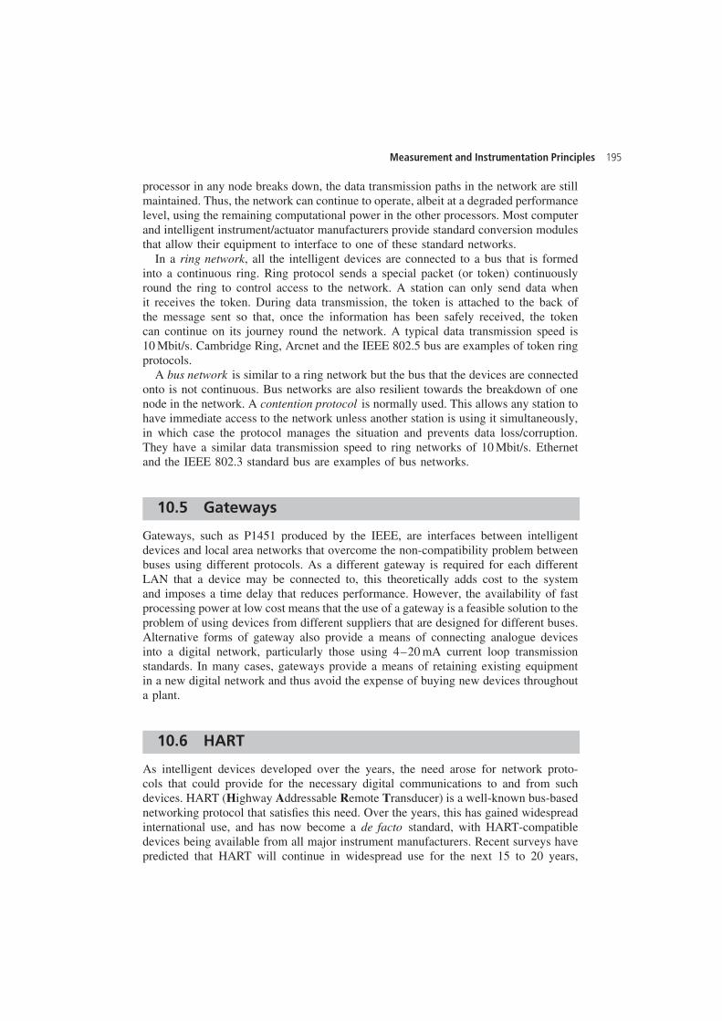
Measurement and Instrumentation Principles 195
processor in any node breaks down, the data transmission paths in the network are stillmaintained. Thus, the network can continue to operate, albeit at a degraded performancelevel, using the remaining computational power in the other processors. Most computerand intelligent instrument/actuator manufacturers provide standard conversion modulesthat allow their equipment to interface to one of these standard networks.
In a ring network, all the intelligent devices are connected to a bus that is formedinto a continuous ring. Ring protocol sends a special packet (or token) continuouslyround the ring to control access to the network. A station can only send data whenit receives the token. During data transmission, the token is attached to the back ofthe message sent so that, once the information has been safely received, the tokencan continue on its journey round the network. A typical data transmission speed is10 Mbit/s. Cambridge Ring, Arcnet and the IEEE 802.5 bus are examples of token ringprotocols.
A bus network is similar to a ring network but the bus that the devices are connectedonto is not continuous. Bus networks are also resilient towards the breakdown of onenode in the network. A contention protocol is normally used. This allows any station tohave immediate access to the network unless another station is using it simultaneously,in which case the protocol manages the situation and prevents data loss/corruption.They have a similar data transmission speed to ring networks of 10 Mbit/s. Ethernetand the IEEE 802.3 standard bus are examples of bus networks.
10.5 Gateways
Gateways, such as P1451 produced by the IEEE, are interfaces between intelligentdevices and local area networks that overcome the non-compatibility problem betweenbuses using different protocols. As a different gateway is required for each differentLAN that a device may be connected to, this theoretically adds cost to the systemand imposes a time delay that reduces performance. However, the availability of fastprocessing power at low cost means that the use of a gateway is a feasible solution to theproblem of using devices from different suppliers that are designed for different buses.Alternative forms of gateway also provide a means of connecting analogue devicesinto a digital network, particularly those using 4–20 mA current loop transmissionstandards. In many cases, gateways provide a means of retaining existing equipmentin a new digital network and thus avoid the expense of buying new devices throughouta plant.
10.6 HART
As intelligent devices developed over the years, the need arose for network proto-cols that could provide for the necessary digital communications to and from suchdevices. HART (Highway Addressable Remote Transducer) is a well-known bus-basednetworking protocol that satisfies this need. Over the years, this has gained widespreadinternational use, and has now become a de facto standard, with HART-compatibledevices being available from all major instrument manufacturers. Recent surveys havepredicted that HART will continue in widespread use for the next 15 to 20 years,
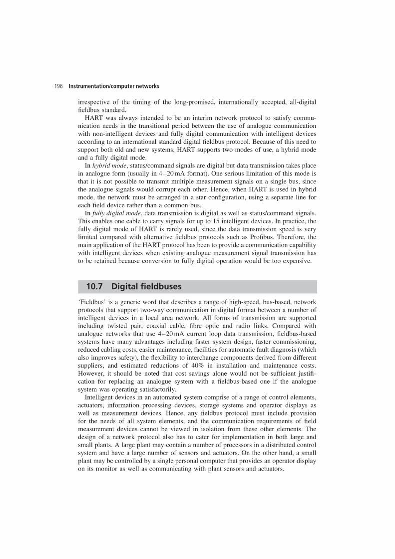
196 Instrumentation/computer networks
irrespective of the timing of the long-promised, internationally accepted, all-digitalfieldbus standard.
HART was always intended to be an interim network protocol to satisfy commu-nication needs in the transitional period between the use of analogue communicationwith non-intelligent devices and fully digital communication with intelligent devicesaccording to an international standard digital fieldbus protocol. Because of this need tosupport both old and new systems, HART supports two modes of use, a hybrid modeand a fully digital mode.
In hybrid mode, status/command signals are digital but data transmission takes placein analogue form (usually in 4–20 mA format). One serious limitation of this mode isthat it is not possible to transmit multiple measurement signals on a single bus, sincethe analogue signals would corrupt each other. Hence, when HART is used in hybridmode, the network must be arranged in a star configuration, using a separate line foreach field device rather than a common bus.
In fully digital mode, data transmission is digital as well as status/command signals.This enables one cable to carry signals for up to 15 intelligent devices. In practice, thefully digital mode of HART is rarely used, since the data transmission speed is verylimited compared with alternative fieldbus protocols such as Profibus. Therefore, themain application of the HART protocol has been to provide a communication capabilitywith intelligent devices when existing analogue measurement signal transmission hasto be retained because conversion to fully digital operation would be too expensive.
10.7 Digital fieldbuses
‘Fieldbus’ is a generic word that describes a range of high-speed, bus-based, networkprotocols that support two-way communication in digital format between a number ofintelligent devices in a local area network. All forms of transmission are supportedincluding twisted pair, coaxial cable, fibre optic and radio links. Compared withanalogue networks that use 4–20 mA current loop data transmission, fieldbus-basedsystems have many advantages including faster system design, faster commissioning,reduced cabling costs, easier maintenance, facilities for automatic fault diagnosis (whichalso improves safety), the flexibility to interchange components derived from differentsuppliers, and estimated reductions of 40% in installation and maintenance costs.However, it should be noted that cost savings alone would not be sufficient justifi-cation for replacing an analogue system with a fieldbus-based one if the analoguesystem was operating satisfactorily.
Intelligent devices in an automated system comprise of a range of control elements,actuators, information processing devices, storage systems and operator displays aswell as measurement devices. Hence, any fieldbus protocol must include provisionfor the needs of all system elements, and the communication requirements of fieldmeasurement devices cannot be viewed in isolation from these other elements. Thedesign of a network protocol also has to cater for implementation in both large andsmall plants. A large plant may contain a number of processors in a distributed controlsystem and have a large number of sensors and actuators. On the other hand, a smallplant may be controlled by a single personal computer that provides an operator displayon its monitor as well as communicating with plant sensors and actuators.
Measurement and Instrumentation Principles 197
Many different digital fieldbus protocols now exist, and names of some of the moreprominent ones include Profibus (Germany), WorldFIP (France), P-net (Denmark),Lonworks (USA), Devicenet (USA), IEEE 1118 (USA), Milbus (UK), Canbus,Interbus-S and SDS. These differ in many major respects such as message format,access protocols and rules for performance prediction. In recognition of the difficultiesinherent in attempting to connect devices from different manufacturers that use avariety of incompatible interface standards and network protocols, the InternationalElectrotechnical Commission (IEC) set up a working part in 1985 that was chargedwith defining a standard interface protocol, which was to be called the IEC Fieldbus.However, at the time of the IEC initiative, a number of companies were alreadydeveloping their own fieldbus standards, and commercial interests have continuallyblocked agreement on a common, internationally recognized standard. In the meantime,some countries have adopted their own national fieldbus standard. Also, the EuropeanUnion established a European standard (EN50170) in 1996 as an interim measureuntil the appearance of the promised IEC standard. EN50170 has adopted Profibus,WorldFIP and P-net as the three standards authorized for use, and the intention is toallow their use until six years after the IEC standard has been published. The inclusionof three protocols rather than one in EN50170 is unfortunate, but three protocols aremuch better than the 50 protocols that were in use prior to the adoption of EN50170.
In the meantime, efforts to achieve a single fieldbus standard have continued, withdevelopment now being carried out by a body called the Fieldbus Foundation, which isa consortium of instrument system manufacturers and users supported by the IEC. Thepresent approach is to define a protocol whose basic architecture is in two levels, knownas upper and lower. The lower level provides for communication between field devicesand field input–output devices whilst the upper level enables field input–output devicesto communicate with controllers. These two levels have quite different characteristics.The lower level generally requires few connections, only needs a slow data-transferrate and must support intrinsically safe working. On the other hand, the upper levelrequires numerous connections and fast data transfer, but does not have to satisfyintrinsic safety requirements. In the fieldbus standard proposed, the lower level willconform with the specifications for the Application Layer in ISO-7Ł and the upper layerwill satisfy the specifications for the Physical and Data Link Layers in ISO-7. Threestandard bus speeds are currently specified for the Foundation Fieldbus lower levelof 31.25 kbit/s, 1 Mbit/s and 2.5 Mbit/s. Maximum cable lengths allowed are 1900 mat 31.25 kbit/s, 750 m at 1 Mbit/s and 500 m at 2.5 Mbit/s. For the upper FoundationFieldbus layer, a high-speed ethernet is currently being developed that will provide adata transfer rate up to 100 Mbit/s.
At the time of writing, it appears that we may now be very close to achieving aninternational fieldbus standard. The Fieldbus Foundation published a draft standardin 1998 known as IEC61158. This was agreed by a majority vote, but with dissentfrom a number of major instrument manufacturers. In the confirmed standard, which isexpected in 2000, there are likely to be supplements that will allow devices operatingunder other protocols such as Profibus to be interfaced with the IEC61158 system.
Ł ISO-7 is an abbreviation for the International Standards Organization Open System Interconnection seven-layer model which covers all aspects of connections between computers and intelligent devices. It isdiscussed further in section 10.8.
198 Instrumentation/computer networks
10.8 Communication protocols for very large systems
Once a system gets too large to be covered by a local area network, it is generally neces-sary to use telephone lines. These provide communication over large distances withina protocol that is often called a wide area network. Public telephone lines are readilyavailable, but there is a fundamental problem about their use for a wide area network.Whilst instrumentation networks need high bandwidths, public networks operate at thelow bandwidth required to satisfy speech-based telephony. High bandwidths can beobtained by leasing private telephone lines but this solution is expensive and oftenuneconomic.
The solution that is emerging is to extend LAN technology into public telephonenetworks. A LAN extended in this way is renamed a metropolitan area network (MAN).An IEEE standard for MAN (IEEE 802.6) was first published in 1990. Messagesbetween nodes are organized in packets. MANs cover areas that are typically up to50 km in diameter, but in some cases links can be several hundred kilometres long. Useof the public switched telephone network for transmission is most common althoughprivate lines are sometimes used.
Both ring and bus networks lose efficiency as the number of nodes increases andare unsuitable for adoption by MAN. Instead, a protocol known as distributed queuedual bus (DQDB) is used. DQDB is a hybrid bus that carries isochronous data forthe public switched telephone network as well as providing the data bus for a MAN.For handling data on a MAN, DQDB has a pair of buses on which data, preceded bythe target address, circulates in fixed size packets in opposite directions, i.e. there isa clockwise bus and an anticlockwise bus. All stations have access to both buses andthe protocol establishes a distributed queue. This ensures that all stations have accessto the bus on a fair basis. Thus, the stations have their access demands satisfied in theorder in which they arise (i.e. a first-come, first-served basis) but commensurate withensuring that the bus is used efficiently. Fibre-optic cables are commonly used for thebuses, allowing data transmission at speeds up to 140 Mbit/s.
10.8.1 Protocol standardization
Many years ago, the International Standards Organization recognized the enormousproblems that would ensue, as the size of networks increased, if a diversity of commu-nication protocols developed. In response, it published the Open Systems Intercon-nection seven-layer model (ISO-7) in 1978. This provides standard protocols for allaspects of computer communications required in a large-scale system, that is, manage-ment and stock control information etc. as well as instrumentation/process controlnetworks.
The ISO seven-layer model defines a set of standard message formats, and rules fortheir interchange. The model can be applied both within local area networks and inmuch larger global networks that involve data transmission via telephone lines. Whilstthe standards and protocols involved in ISO-7 are highly complex, the network builderdoes not need to have a detailed understanding of them as long as all devices usedin the network are certified by their manufacturer as conforming to the standard. Themain functions of each of the seven layers are summarized below:
Measurement and Instrumentation Principles 199
Layer 1: Physical protocol: Defines how data are physically transported betweentwo devices, including specification of cabling, connectors, I/O ports, modems,voltage levels, signal format and transfer speed.
Layer 2: Data protocol: Establishes paths to ensure data can be exchanged betweentwo devices, and provides error detection and correction (by retransmittingcorrupted data).
Layer 3: Network protocol: Controls the flow of data in packets between all devicesin a network.
Layer 4: Transport protocol: Allows a user-task on one computer to commu-nicate with another user-task on a different computer transparently of networkcharacteristics, thus ensuring high reliability in data exchange.
Layer 5: Session protocol: Synchronizes communication activities during a session,and maintains a communication path between active user-tasks (a session isdefined as the period of time during which two user-tasks remain connected).
Layer 6: Presentation protocol: Provides for code conversion as necessary, so thatuser-tasks using different data formats can communicate with each other.
Layer 7: Application protocol: Controls functions specific to user-tasks, such asresource sharing, file transfer and remote file access.
It should be noted that only layers 1, 2 and 7 are usually relevant to instrumentationand plant control systems.
The Manufacturing Automation Protocol (MAP) was conceived by General Motorsin 1980 in order to support computer integrated manufacturing. It conforms with ISO-7, and is a similar attempt at providing a standard computer communications protocolfor large systems.
10.9 Future development of networks
Network design and protocol are changing at a similar rapid rate to that of computersystems as a whole. Hence, it would be impossible in a text of this nature to cover allcurrent developments, and, in any case, any such coverage would rapidly become outof date. The past few pages have covered some aspects of the general concepts anddesign of networks, and this will prove useful in helping the reader to understand themode of operation of existing networks. However, network specialists should alwaysbe consulted to obtain up-to-date information about the current situation whenever anew network is being planned.
References and further reading
Brook, N. and Herklot, T. (1996) Choosing and implementing a serial interface, ElectronicEngineering, June pp. 46–54.
11
Display, recording andpresentation of
measurement dataThe earlier chapters in this book have been essentially concerned with describingways of producing high-quality, error-free data at the output of a measurement system.Having got the data, the next consideration is how to present it in a form where it canbe readily used and analysed. This chapter therefore starts by covering the techniquesavailable to either display measurement data for current use or record it for futureuse. Following this, standards of good practice for presenting data in either graphicalor tabular form are covered, using either paper or a computer monitor screen as thedisplay medium. This leads on to a discussion of mathematical regression techniquesfor fitting the best lines through data points on a graph. Confidence tests to assess thecorrectness of the line fitted are also described. Finally, correlation tests are describedthat determine the degree of association between two sets of data when they are bothsubject to random fluctuations.
11.1 Display of measurement signals
Measurement signals in the form of a varying electrical voltage can be displayedeither by an oscilloscope or else by any of the electrical meters described earlier inChapter 6. However, if signals are converted to digital form, other display options apartfrom meters become possible, such as electronic output displays or using a computermonitor.
11.1.1 Electronic output displays
Electronic displays enable a parameter value to be read immediately, thus allowing forany necessary response to be made immediately. The main requirement for displaysis that they should be clear and unambiguous. Two common types of character formatused in displays, seven-segment and 7 ð 5 dot matrix, are shown in Figure 11.1. Bothtypes of display have the advantage of being able to display alphabetic as well asnumeric information, although the seven-segment format can only display a limitednine-letter subset of the full 26-letter alphabet. This allows added meaning to be givento the number displayed by including a word or letter code. It also allows a single
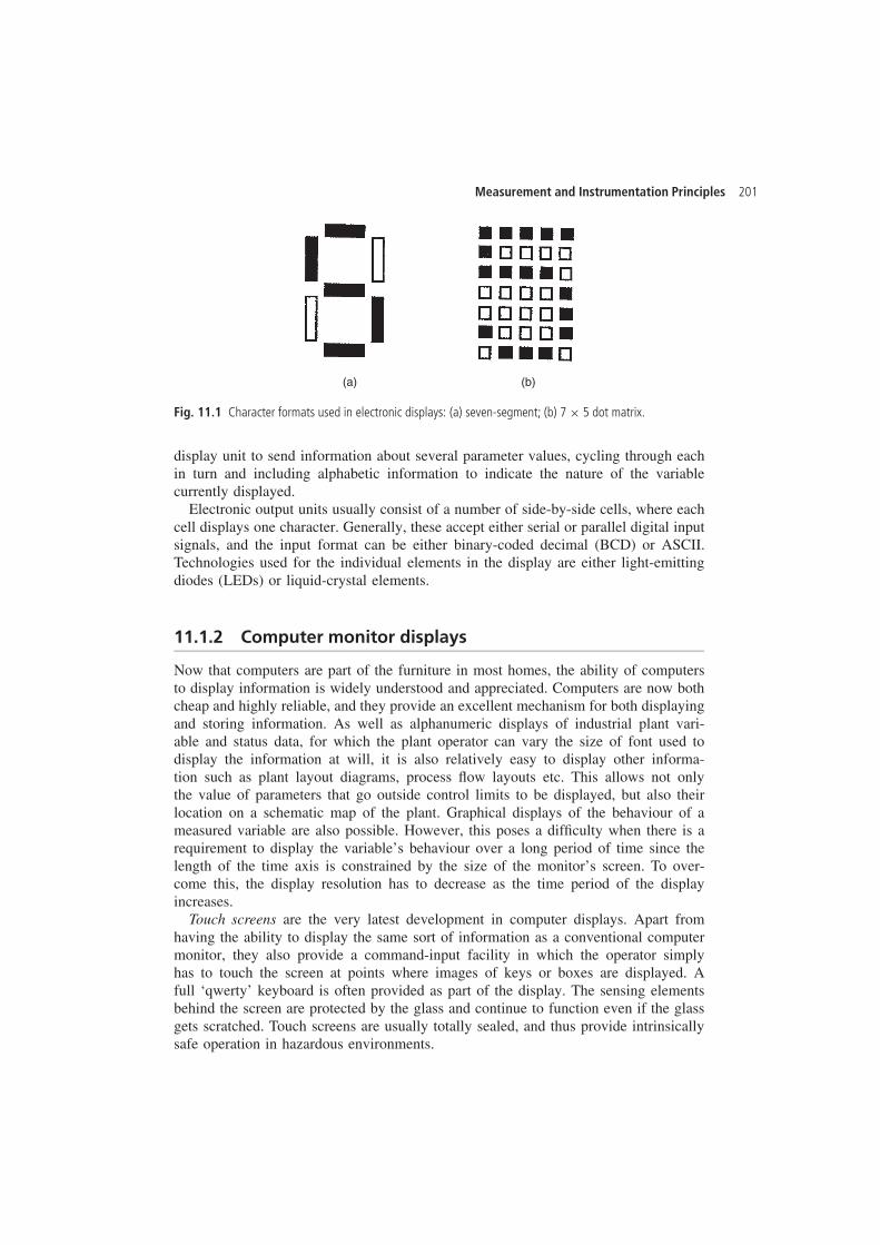
Measurement and Instrumentation Principles 201
(a) (b)
Fig. 11.1 Character formats used in electronic displays: (a) seven-segment; (b) 7 ð 5 dot matrix.
display unit to send information about several parameter values, cycling through eachin turn and including alphabetic information to indicate the nature of the variablecurrently displayed.
Electronic output units usually consist of a number of side-by-side cells, where eachcell displays one character. Generally, these accept either serial or parallel digital inputsignals, and the input format can be either binary-coded decimal (BCD) or ASCII.Technologies used for the individual elements in the display are either light-emittingdiodes (LEDs) or liquid-crystal elements.
11.1.2 Computer monitor displays
Now that computers are part of the furniture in most homes, the ability of computersto display information is widely understood and appreciated. Computers are now bothcheap and highly reliable, and they provide an excellent mechanism for both displayingand storing information. As well as alphanumeric displays of industrial plant vari-able and status data, for which the plant operator can vary the size of font used todisplay the information at will, it is also relatively easy to display other informa-tion such as plant layout diagrams, process flow layouts etc. This allows not onlythe value of parameters that go outside control limits to be displayed, but also theirlocation on a schematic map of the plant. Graphical displays of the behaviour of ameasured variable are also possible. However, this poses a difficulty when there is arequirement to display the variable’s behaviour over a long period of time since thelength of the time axis is constrained by the size of the monitor’s screen. To over-come this, the display resolution has to decrease as the time period of the displayincreases.
Touch screens are the very latest development in computer displays. Apart fromhaving the ability to display the same sort of information as a conventional computermonitor, they also provide a command-input facility in which the operator simplyhas to touch the screen at points where images of keys or boxes are displayed. Afull ‘qwerty’ keyboard is often provided as part of the display. The sensing elementsbehind the screen are protected by the glass and continue to function even if the glassgets scratched. Touch screens are usually totally sealed, and thus provide intrinsicallysafe operation in hazardous environments.
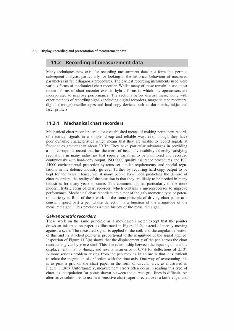
202 Display, recording and presentation of measurement data
11.2 Recording of measurement data
Many techniques now exist for recording measurement data in a form that permitssubsequent analysis, particularly for looking at the historical behaviour of measuredparameters in fault diagnosis procedures. The earliest recording instruments used werevarious forms of mechanical chart recorder. Whilst many of these remain in use, mostmodern forms of chart recorder exist in hybrid forms in which microprocessors areincorporated to improve performance. The sections below discuss these, along withother methods of recording signals including digital recorders, magnetic tape recorders,digital (storage) oscilloscopes and hard-copy devices such as dot-matrix, inkjet andlaser printers.
11.2.1 Mechanical chart recorders
Mechanical chart recorders are a long-established means of making permanent recordsof electrical signals in a simple, cheap and reliable way, even though they havepoor dynamic characteristics which means that they are unable to record signals atfrequencies greater than about 30 Hz. They have particular advantages in providinga non-corruptible record that has the merit of instant ‘viewability’, thereby satisfyingregulations in many industries that require variables to be monitored and recordedcontinuously with hard-copy output. ISO 9000 quality assurance procedures and ISO14000 environmental protection systems set similar requirements, and special regu-lations in the defence industry go even further by requiring hard-copy output to bekept for ten years. Hence, whilst many people have been predicting the demise ofchart recorders, the reality of the situation is that they are likely to be needed in manyindustries for many years to come. This comment applies particularly to the moremodern, hybrid form of chart recorder, which contains a microprocessor to improveperformance. Mechanical chart recorders are either of the galvanometric type or poten-tiometric type. Both of these work on the same principle of driving chart paper at aconstant speed past a pen whose deflection is a function of the magnitude of themeasured signal. This produces a time history of the measured signal.
Galvanometric recordersThese work on the same principle as a moving-coil meter except that the pointerdraws an ink trace on paper, as illustrated in Figure 11.2, instead of merely movingagainst a scale. The measured signal is applied to the coil, and the angular deflectionof this and its attached pointer is proportional to the magnitude of the signal applied.Inspection of Figure 11.3(a) shows that the displacement y of the pen across the chartrecorder is given by y D R sin . This sine relationship between the input signal and thedisplacement y is non-linear, and results in an error of 0.7% for deflections of š10°.A more serious problem arising from the pen moving in an arc is that it is difficultto relate the magnitude of deflection with the time axis. One way of overcoming thisis to print a grid on the chart paper in the form of circular arcs, as illustrated inFigure 11.3(b). Unfortunately, measurement errors often occur in reading this type ofchart, as interpolation for points drawn between the curved grid lines is difficult. Analternative solution is to use heat-sensitive chart paper directed over a knife-edge, and
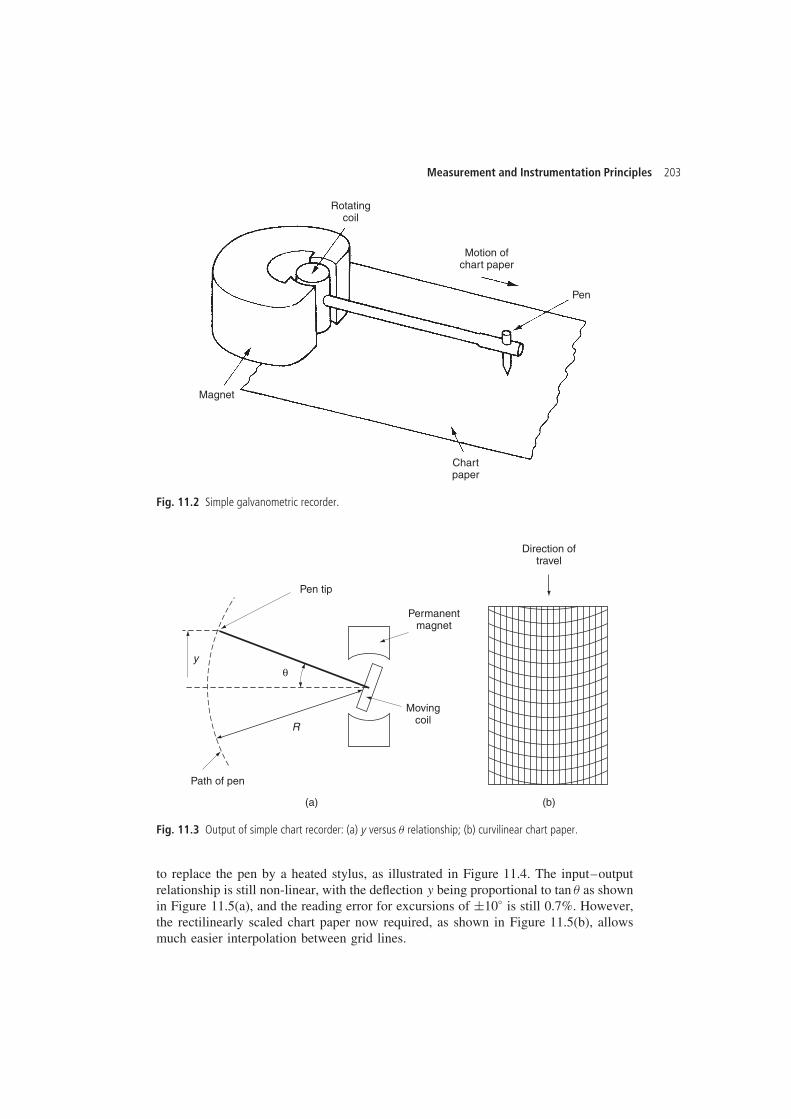
Measurement and Instrumentation Principles 203
Rotatingcoil
Magnet
Chartpaper
Pen
Motion ofchart paper
Fig. 11.2 Simple galvanometric recorder.
(b)(a)
Direction oftravel
Permanentmagnet
Movingcoil
Pen tip
R
Path of pen
yθ
Fig. 11.3 Output of simple chart recorder: (a) y versus relationship; (b) curvilinear chart paper.
to replace the pen by a heated stylus, as illustrated in Figure 11.4. The input–outputrelationship is still non-linear, with the deflection y being proportional to tan as shownin Figure 11.5(a), and the reading error for excursions of š10° is still 0.7%. However,the rectilinearly scaled chart paper now required, as shown in Figure 11.5(b), allowsmuch easier interpolation between grid lines.
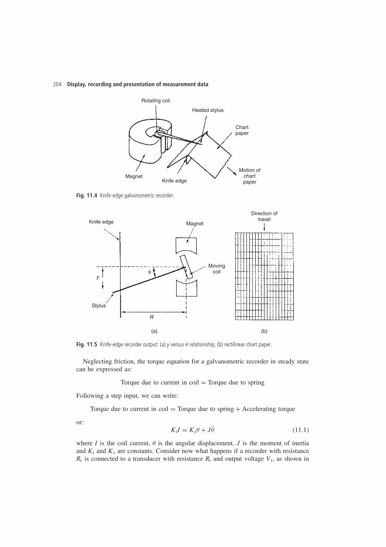
204 Display, recording and presentation of measurement data
Rotating coil
MagnetKnife edge
Motion ofchartpaper
Chartpaper
Heated stylus
Fig. 11.4 Knife-edge galvanometric recorder.
(b)(a)
Direction oftravel
Magnet
Movingcoil
Knife edge
Stylus
y
R
θ
Fig. 11.5 Knife-edge recorder output: (a) y versus relationship; (b) rectilinear chart paper.
Neglecting friction, the torque equation for a galvanometric recorder in steady statecan be expressed as:
Torque due to current in coil D Torque due to spring
Following a step input, we can write:
Torque due to current in coil D Torque due to spring C Accelerating torque
or:KiI D Ks C JR �11.1�
where I is the coil current, is the angular displacement, J is the moment of inertiaand Ki and Ks are constants. Consider now what happens if a recorder with resistanceRr is connected to a transducer with resistance Rt and output voltage Vt, as shown in
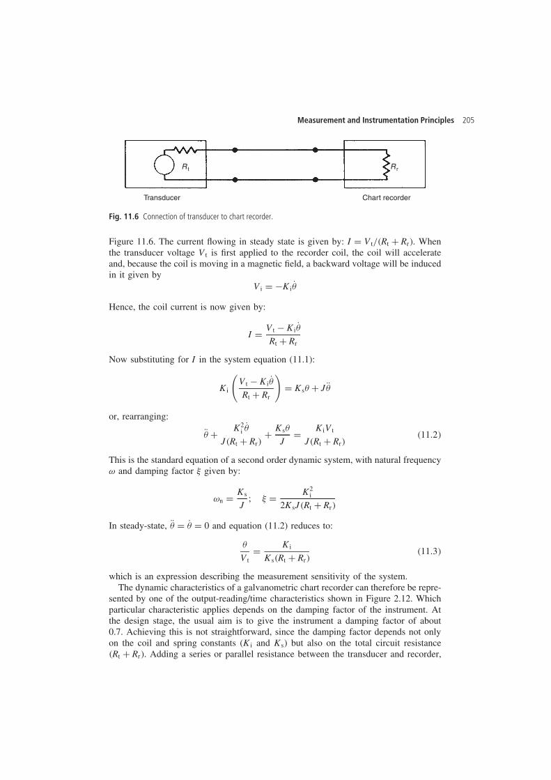
Measurement and Instrumentation Principles 205
Rt Rr
Transducer Chart recorder
Fig. 11.6 Connection of transducer to chart recorder.
Figure 11.6. The current flowing in steady state is given by: I D Vt/�Rt C Rr�. Whenthe transducer voltage Vt is first applied to the recorder coil, the coil will accelerateand, because the coil is moving in a magnetic field, a backward voltage will be inducedin it given by
Vi D �Ki P Hence, the coil current is now given by:
I D Vt � Ki P Rt C Rr
Now substituting for I in the system equation (11.1):
Ki
(Vt � Ki P Rt C Rr
)D Ks C JR
or, rearranging:
R C K2iP
J�Rt C Rr�C Ks
JD KiVt
J�Rt C Rr��11.2�
This is the standard equation of a second order dynamic system, with natural frequencyω and damping factor � given by:
ωn D Ks
J; � D K2
i
2KsJ�Rt C Rr�
In steady-state, R D P D 0 and equation (11.2) reduces to:
VtD Ki
Ks�Rt C Rr��11.3�
which is an expression describing the measurement sensitivity of the system.The dynamic characteristics of a galvanometric chart recorder can therefore be repre-
sented by one of the output-reading/time characteristics shown in Figure 2.12. Whichparticular characteristic applies depends on the damping factor of the instrument. Atthe design stage, the usual aim is to give the instrument a damping factor of about0.7. Achieving this is not straightforward, since the damping factor depends not onlyon the coil and spring constants (Ki and Ks) but also on the total circuit resistance�Rt C Rr�. Adding a series or parallel resistance between the transducer and recorder,
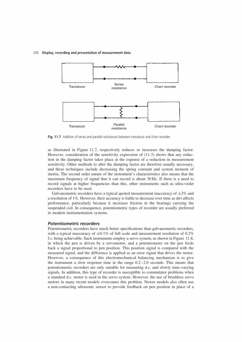
206 Display, recording and presentation of measurement data
TransducerSeries
resistance
Parallelresistance
Chart recorder
Chart recorderTransducer
Fig. 11.7 Addition of series and parallel resistances between transducer and chart recorder.
as illustrated in Figure 11.7, respectively reduces or increases the damping factor.However, consideration of the sensitivity expression of (11.3) shows that any reduc-tion in the damping factor takes place at the expense of a reduction in measurementsensitivity. Other methods to alter the damping factor are therefore usually necessary,and these techniques include decreasing the spring constant and system moment ofinertia. The second order nature of the instrument’s characteristics also means that themaximum frequency of signal that it can record is about 30 Hz. If there is a need torecord signals at higher frequencies than this, other instruments such as ultra-violetrecorders have to be used.
Galvanometric recorders have a typical quoted measurement inaccuracy of š2% anda resolution of 1%. However, their accuracy is liable to decrease over time as dirt affectsperformance, particularly because it increases friction in the bearings carrying thesuspended coil. In consequence, potentiometric types of recorder are usually preferredin modern instrumentation systems.
Potentiometric recordersPotentiometric recorders have much better specifications than galvanometric recorders,with a typical inaccuracy of š0.1% of full scale and measurement resolution of 0.2%f.s. being achievable. Such instruments employ a servo system, as shown in Figure 11.8,in which the pen is driven by a servomotor, and a potentiometer on the pen feedsback a signal proportional to pen position. This position signal is compared with themeasured signal, and the difference is applied as an error signal that drives the motor.However, a consequence of this electromechanical balancing mechanism is to givethe instrument a slow response time in the range 0.2–2.0 seconds. This means thatpotentiometric recorders are only suitable for measuring d.c. and slowly time-varyingsignals. In addition, this type of recorder is susceptible to commutator problems whena standard d.c. motor is used in the servo system. However, the use of brushless servomotors in many recent models overcomes this problem. Newer models also often usea non-contacting ultrasonic sensor to provide feedback on pen position in place of a
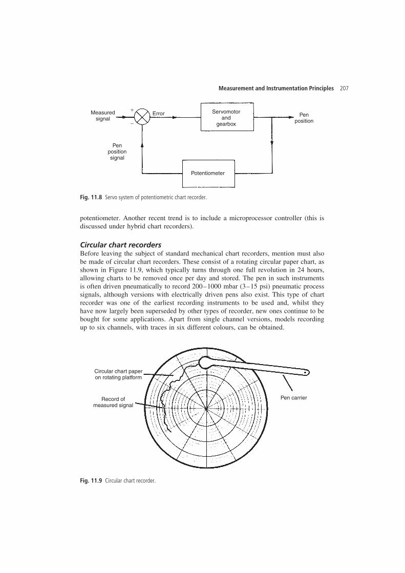
Measurement and Instrumentation Principles 207
Servomotorand
gearbox
ErrorMeasuredsignal
Penpositionsignal
Potentiometer
Penposition
+
−
Fig. 11.8 Servo system of potentiometric chart recorder.
potentiometer. Another recent trend is to include a microprocessor controller (this isdiscussed under hybrid chart recorders).
Circular chart recordersBefore leaving the subject of standard mechanical chart recorders, mention must alsobe made of circular chart recorders. These consist of a rotating circular paper chart, asshown in Figure 11.9, which typically turns through one full revolution in 24 hours,allowing charts to be removed once per day and stored. The pen in such instrumentsis often driven pneumatically to record 200–1000 mbar (3–15 psi) pneumatic processsignals, although versions with electrically driven pens also exist. This type of chartrecorder was one of the earliest recording instruments to be used and, whilst theyhave now largely been superseded by other types of recorder, new ones continue to bebought for some applications. Apart from single channel versions, models recordingup to six channels, with traces in six different colours, can be obtained.
Circular chart paperon rotating platform
Record ofmeasured signal
Pen carrier
Fig. 11.9 Circular chart recorder.
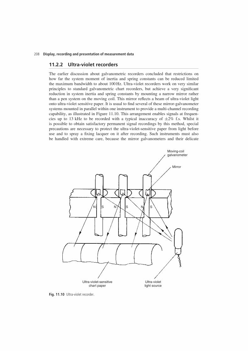
208 Display, recording and presentation of measurement data
11.2.2 Ultra-violet recorders
The earlier discussion about galvanometric recorders concluded that restrictions onhow far the system moment of inertia and spring constants can be reduced limitedthe maximum bandwidth to about 100 Hz. Ultra-violet recorders work on very similarprinciples to standard galvanometric chart recorders, but achieve a very significantreduction in system inertia and spring constants by mounting a narrow mirror ratherthan a pen system on the moving coil. This mirror reflects a beam of ultra-violet lightonto ultra-violet sensitive paper. It is usual to find several of these mirror-galvanometersystems mounted in parallel within one instrument to provide a multi-channel recordingcapability, as illustrated in Figure 11.10. This arrangement enables signals at frequen-cies up to 13 kHz to be recorded with a typical inaccuracy of š2% f.s. Whilst itis possible to obtain satisfactory permanent signal recordings by this method, specialprecautions are necessary to protect the ultra-violet-sensitive paper from light beforeuse and to spray a fixing lacquer on it after recording. Such instruments must alsobe handled with extreme care, because the mirror galvanometers and their delicate
Moving-coilgalvanometer
Mirror
N
Ultra-violet-sensitivechart paper
Ultra-violetlight source
S N S N S
Fig. 11.10 Ultra-violet recorder.
Measurement and Instrumentation Principles 209
mounting systems are easily damaged by relatively small shocks. In addition, ultra-violet recorders are significantly more expensive than standard chart recorders.
11.2.3 Fibre-optic recorders (recording oscilloscopes)
The fibre optic recorder uses a fibre-optic system to direct light onto light-sensitivepaper. Fibre-optic recorders are similar to oscilloscopes in construction, insofar asthey have an electron gun and focusing system that directs a stream of electrons ontoone point on a fluorescent screen, and for this reason they are alternatively known asrecording oscilloscopes. The screen is usually a long thin one instead of the square typefound in an oscilloscope and only one set of deflection plates is provided. The signalto be recorded is applied to the deflection plates and the movement of the focused spotof electrons on the screen is proportional to the signal amplitude. A narrow strip offibre optics in contact with the fluorescent screen transmits the motion of the spot tophotosensitive paper held in close proximity to the other end of the fibre-optic strip.By driving the photosensitive paper at a constant speed past the fibre-optic strip, a timehistory of the measured signal is obtained. Such recorders are much more expensivethan ultra-violet recorders but have an even higher bandwidth up to 1 MHz.
Whilst the construction above is the more common in fibre-optic recorders, a secondtype also exists that uses a conventional square screen instead of a long thin one. Thishas a square faceplate attached to the screen housing a square array of fibre-optics.The other side of the fibre-optic system is in contact with chart paper. The effect ofthis is to provide a hard copy of the typical form of display obtainable on a cathoderay oscilloscope.
11.2.4 Hybrid chart recorders
Hybrid chart recorders represent the latest generation of chart recorder and basicallyconsist of a potentiometric chart recorder with an added microprocessor. The micro-processor provides for selection of range and chart speed, and also allows specificationof alarm modes and levels to detect when measured variables go outside acceptablelimits. Additional information can also be printed on charts, such as names, times anddates of variables recorded. Microprocessor-based, hybrid versions of circular chartrecorders also now exist.
11.2.5 Magnetic tape recorders
Magnetic tape recorders can record analogue signals up to 80 kHz in frequency. Asthe speed of the tape transport can be switched between several values, signals can berecorded at high speed and replayed at a lower speed. Such time scaling of the recordedinformation allows a hard copy of the signal behaviour to be obtained from instrumentssuch as ultra-violet and galvanometric recorders whose bandwidth is insufficient toallow direct signal recording. A 200 Hz signal cannot be recorded directly on a chartrecorder, but if it is recorded on a magnetic tape recorder running at high speed andthen replayed at a speed ten times lower, its frequency will be time scaled to 20 Hz
210 Display, recording and presentation of measurement data
which can be recorded on a chart recorder. Instrumentation tape recorders typically havebetween four and ten channels, allowing many signals to be recorded simultaneously.
The two basic types of analogue tape recording technique are direct recording andfrequency-modulated recording. Direct recording offers the best data bandwidth butthe accuracy of signal amplitude recording is quite poor, and this seriously limits theusefulness of this technique in most applications. The frequency-modulated techniqueoffers better amplitude-recording accuracy, with a typical inaccuracy of š5% at signalfrequencies of 80 kHz. In consequence, this technique is very much more common thandirect recording.
11.2.6 Digital recorders
For some time, the only technique available for recording signals at frequencies higherthan 80 kHz has been to use a digital processor. As the signals to be recorded are usuallyin analogue form, a prerequisite for this is an analogue-to-digital (A–D) converter boardto sample the analogue signals and convert them to digital form. The relevant aspectsof computer hardware necessary to achieve this were covered in Chapter 9. Correctchoice of the sampling interval is always necessary to ensure that an accurate digitalrecord of the signal is obtained and problems of aliasing etc. are not encountered, asexplained in Chapter 5. Some prior analogue signal conditioning may also be requiredin some circumstances, again as mentioned in Chapter 5.
Until a few years ago, the process of recording data digitally was carried out by stan-dard computer equipment equipped with the necessary analogue interface boards etc.,and the process was known as data-logging. More recently, purpose-designed digitalrecorders have become available for this purpose. These are usually multi-channel, andare available from many suppliers. Typically, a 10-bit A–D converter is used, whichgives a 0.1% measurement resolution. Alternatively, a 12-bit converter gives 0.025%resolution. Specifications typically quoted for digital recorders are frequency responseof 25 kHz, maximum sampling frequency of 200 MHz and data storage up to 4000data points per channel.
When there is a requirement to view recorded data, for instance to look at thebehaviour of parameters in a production process immediately before a fault has occurredin the process, it is usually necessary to use the digital recorder in conjunction witha chart recorderŁ, applying speed scaling as appropriate to allow for the difference infrequency-response capability between a digital recorder and a chart recorder. However,in these circumstances, it is only necessary to use the chart recorder to display theprocess parameters for the time period of interest. This saves a large amount of papercompared with the alternative of running the chart recorder continuously if a digitalrecorder is not used as the main data-capture mechanism.
As an alternative to chart recorders when hard-copy records are required, numericaldata can be readily output from digital recorders onto alphanumeric digital printersin the form of dot-matrix, inkjet or laser printing devices. However, when there aretrends in data, the graphical display of the time history of a variable provided by achart recorder shows up the trends much more readily.
Ł Note that some digital recorders actually incorporate a recording oscilloscope to provide a hard copy ofrecorded data, thus obviating the need for a chart recorder.
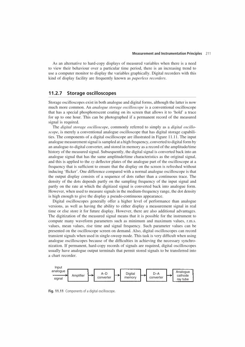
Measurement and Instrumentation Principles 211
As an alternative to hard-copy displays of measured variables when there is a needto view their behaviour over a particular time period, there is an increasing trend touse a computer monitor to display the variables graphically. Digital recorders with thiskind of display facility are frequently known as paperless recorders.
11.2.7 Storage oscilloscopes
Storage oscilloscopes exist in both analogue and digital forms, although the latter is nowmuch more common. An analogue storage oscilloscope is a conventional oscilloscopethat has a special phosphorescent coating on its screen that allows it to ‘hold’ a tracefor up to one hour. This can be photographed if a permanent record of the measuredsignal is required.
The digital storage oscilloscope, commonly referred to simply as a digital oscillo-scope, is merely a conventional analogue oscilloscope that has digital storage capabili-ties. The components of a digital oscilloscope are illustrated in Figure 11.11. The inputanalogue measurement signal is sampled at a high frequency, converted to digital form byan analogue-to-digital converter, and stored in memory as a record of the amplitude/timehistory of the measured signal. Subsequently, the digital signal is converted back into ananalogue signal that has the same amplitude/time characteristics as the original signal,and this is applied to the xy deflector plates of the analogue part of the oscilloscope at afrequency that is sufficient to ensure that the display on the screen is refreshed withoutinducing ‘flicker’. One difference compared with a normal analogue oscilloscope is thatthe output display consists of a sequence of dots rather than a continuous trace. Thedensity of the dots depends partly on the sampling frequency of the input signal andpartly on the rate at which the digitized signal is converted back into analogue form.However, when used to measure signals in the medium-frequency range, the dot densityis high enough to give the display a pseudo-continuous appearance.
Digital oscilloscopes generally offer a higher level of performance than analogueversions, as well as having the ability to either display a measurement signal in realtime or else store it for future display. However, there are also additional advantages.The digitization of the measured signal means that it is possible for the instrument tocompute many waveform parameters such as minimum and maximum values, r.m.s.values, mean values, rise time and signal frequency. Such parameter values can bepresented on the oscilloscope screen on demand. Also, digital oscilloscopes can recordtransient signals when used in single-sweep mode. This task is very difficult when usinganalogue oscilloscopes because of the difficulties in achieving the necessary synchro-nization. If permanent, hard-copy records of signals are required, digital oscilloscopesusually have analogue output terminals that permit stored signals to be transferred intoa chart recorder.
Inputanalogue
signalAmplifier A–D
converterDigital
memoryD–A
converter
Analoguecathoderay tube
Fig. 11.11 Components of a digital oscilloscope.
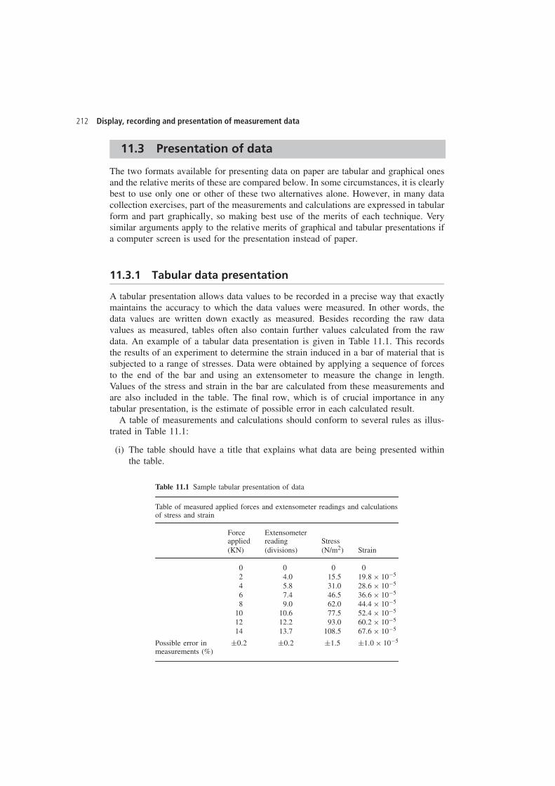
212 Display, recording and presentation of measurement data
11.3 Presentation of data
The two formats available for presenting data on paper are tabular and graphical onesand the relative merits of these are compared below. In some circumstances, it is clearlybest to use only one or other of these two alternatives alone. However, in many datacollection exercises, part of the measurements and calculations are expressed in tabularform and part graphically, so making best use of the merits of each technique. Verysimilar arguments apply to the relative merits of graphical and tabular presentations ifa computer screen is used for the presentation instead of paper.
11.3.1 Tabular data presentation
A tabular presentation allows data values to be recorded in a precise way that exactlymaintains the accuracy to which the data values were measured. In other words, thedata values are written down exactly as measured. Besides recording the raw datavalues as measured, tables often also contain further values calculated from the rawdata. An example of a tabular data presentation is given in Table 11.1. This recordsthe results of an experiment to determine the strain induced in a bar of material that issubjected to a range of stresses. Data were obtained by applying a sequence of forcesto the end of the bar and using an extensometer to measure the change in length.Values of the stress and strain in the bar are calculated from these measurements andare also included in the table. The final row, which is of crucial importance in anytabular presentation, is the estimate of possible error in each calculated result.
A table of measurements and calculations should conform to several rules as illus-trated in Table 11.1:
(i) The table should have a title that explains what data are being presented withinthe table.
Table 11.1 Sample tabular presentation of data
Table of measured applied forces and extensometer readings and calculationsof stress and strain
Force Extensometerapplied reading Stress(KN) (divisions) (N/m2) Strain
0 0 0 02 4.0 15.5 19.8 ð 10�5
4 5.8 31.0 28.6 ð 10�5
6 7.4 46.5 36.6 ð 10�5
8 9.0 62.0 44.4 ð 10�5
10 10.6 77.5 52.4 ð 10�5
12 12.2 93.0 60.2 ð 10�5
14 13.7 108.5 67.6 ð 10�5
Possible error inmeasurements (%)
š0.2 š0.2 š1.5 š1.0 ð 10�5
Measurement and Instrumentation Principles 213
(ii) Each column of figures in the table should refer to the measurements or calcula-tions associated with one quantity only.
(iii) Each column of figures should be headed by a title that identifies the data valuescontained in the column.
(iv) The units in which quantities in each column are measured should be stated atthe top of the column.
(v) All headings and columns should be separated by bold horizontal (and sometimesvertical) lines.
(vi) The errors associated with each data value quoted in the table should be given.The form shown in Table 11.1 is a suitable way to do this when the error levelis the same for all data values in a particular column. However, if error levelsvary, then it is preferable to write the error boundaries alongside each entry inthe table.
11.3.2 Graphical presentation of data
Presentation of data in graphical form involves some compromise in the accuracy towhich the data are recorded, as the exact values of measurements are lost. However,graphical presentation has important advantages over tabular presentation.
(i) Graphs provide a pictorial representation of results that is more readily compre-hended than a set of tabular results.
(ii) Graphs are particularly useful for expressing the quantitative significance ofresults and showing whether a linear relationship exists between two variables.Figure 11.12 shows a graph drawn from the stress and strain values given inthe Table 11.1. Construction of the graph involves first of all marking the pointscorresponding to the stress and strain values. The next step is to draw some linesthrough these data points that best represents the relationship between the twovariables. This line will normally be either a straight one or a smooth curve. Thedata points will not usually lie exactly on this line but instead will lie on eitherside of it. The magnitude of the excursions of the data points from the line drawnwill depend on the magnitude of the random measurement errors associated withthe data.
(iii) Graphs can sometimes show up a data point that is clearly outside the straight lineor curve that seems to fit the rest of the data points. Such a data point is probablydue either to a human mistake in reading an instrument or else to a momentarymalfunction in the measuring instrument itself. If the graph shows such a datapoint where a human mistake or instrument malfunction is suspected, the propercourse of action is to repeat that particular measurement and then discard theoriginal data point if the mistake or malfunction is confirmed.
Like tables, the proper representation of data in graphical form has to conform tocertain rules:
(i) The graph should have a title or caption that explains what data are being presentedin the graph.
(ii) Both axes of the graph should be labelled to express clearly what variable is asso-ciated with each axis and to define the units in which the variables are expressed.
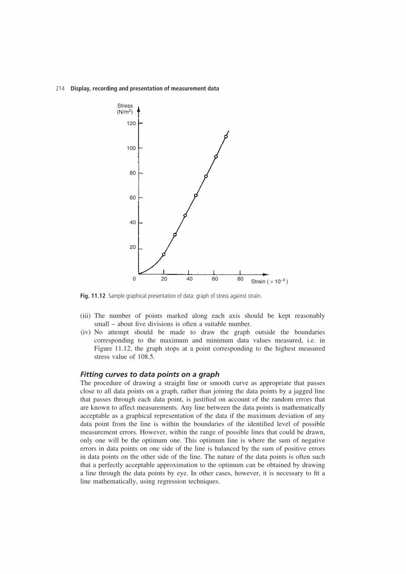
214 Display, recording and presentation of measurement data
Stress(N/m2)
120
100
80
60
40
20
0 20 40 60 80 Strain ( × 10−5 )
Fig. 11.12 Sample graphical presentation of data: graph of stress against strain.
(iii) The number of points marked along each axis should be kept reasonablysmall – about five divisions is often a suitable number.
(iv) No attempt should be made to draw the graph outside the boundariescorresponding to the maximum and minimum data values measured, i.e. inFigure 11.12, the graph stops at a point corresponding to the highest measuredstress value of 108.5.
Fitting curves to data points on a graphThe procedure of drawing a straight line or smooth curve as appropriate that passesclose to all data points on a graph, rather than joining the data points by a jagged linethat passes through each data point, is justified on account of the random errors thatare known to affect measurements. Any line between the data points is mathematicallyacceptable as a graphical representation of the data if the maximum deviation of anydata point from the line is within the boundaries of the identified level of possiblemeasurement errors. However, within the range of possible lines that could be drawn,only one will be the optimum one. This optimum line is where the sum of negativeerrors in data points on one side of the line is balanced by the sum of positive errorsin data points on the other side of the line. The nature of the data points is often suchthat a perfectly acceptable approximation to the optimum can be obtained by drawinga line through the data points by eye. In other cases, however, it is necessary to fit aline mathematically, using regression techniques.
Measurement and Instrumentation Principles 215
Regression techniquesRegression techniques consist of finding a mathematical relationship between measure-ments of two variables y and x, such that the value of variable y can be predicted froma measurement of the other variable x. However, regression techniques should not beregarded as a magic formula that can fit a good relationship to measurement data inall circumstances, as the characteristics of the data must satisfy certain conditions.In determining the suitability of measurement data for the application of regressiontechniques, it is recommended practice to draw an approximate graph of the measureddata points, as this is often the best means of detecting aspects of the data that makeit unsuitable for regression analysis. Drawing a graph of the data will indicate, forexample, whether there are any data points that appear to be erroneous. This may indi-cate that human mistakes or instrument malfunctions have affected the erroneous datapoints, and it is assumed that any such data points will be checked for correctness.
Regression techniques cannot be successfully applied if the deviation of any partic-ular data point from the line to be fitted is greater than the maximum possible errorthat is calculated for the measured variable (i.e. the predicted sum of all systematicand random errors). The nature of some measurement data sets is such that this criter-ion cannot be satisfied, and any attempt to apply regression techniques is doomed tofailure. In that event, the only valid course of action is to express the measurements intabular form. This can then be used as a x–y look-up table, from which values of thevariable y corresponding to particular values of x can be read off. In many cases, thisproblem of large errors in some data points only becomes apparent during the processof attempting to fit a relationship by regression.
A further check that must be made before attempting to fit a line or curve to measure-ments of two variables x and y is to examine the data and look for any evidence thatboth variables are subject to random errors. It is a clear condition for the validity ofregression techniques that only one of the measured variables is subject to randomerrors, with no error in the other variable. If random errors do exist in both measuredvariables, regression techniques cannot be applied and recourse must be made insteadto correlation analysis (covered later in this chapter). A simple example of a situa-tion where both variables in a measurement data set are subject to random errors aremeasurements of human height and weight, and no attempt should be made to fit arelationship between them by regression.
Having determined that the technique is valid, the regression procedure is simplest ifa straight-line relationship exists between the variables, which allows a relationship ofthe form y D a C bx to be estimated by linear least squares regression. Unfortunately,in many cases, a straight-line relationship between the points does not exist, which isreadily shown by plotting the raw data points on a graph. However, knowledge of phys-ical laws governing the data can often suggest a suitable alternative form of relationshipbetween the two sets of variable measurements, such as a quadratic relationship or ahigher order polynomial relationship. Also, in some cases, the measured variables canbe transformed into a form where a linear relationship exists. For example, supposethat two variables y and x are related according to y D axc. A linear relationship fromthis can be derived, using a logarithmic transformation, as log�y� D log�a� C c log�x�.
Thus, if a graph is constructed of log�y� plotted against log�x�, the parameters of astraight-line relationship can be estimated by linear least squares regression.
216 Display, recording and presentation of measurement data
All quadratic and higher order relationships relating one variable y to another vari-able x can be represented by a power series of the form:
y D a0 C a1x C a2x2 C Ð Ð Ð C apxp
Estimation of the parameters a0 . . . ap is very difficult if p has a large value. Fortunately,a relationship where p only has a small value can be fitted to most data sets. Quadraticleast squares regression is used to estimate parameters where p has a value of two,and for larger values of p, polynomial least squares regression is used for parameterestimation.
Where the appropriate form of relationship between variables in measurement datasets is not obvious either from visual inspection or from consideration of physical laws,a method that is effectively a trial and error one has to be applied. This consists ofestimating the parameters of successively higher order relationships between y and xuntil a curve is found that fits the data sufficiently closely. What level of closeness isacceptable is considered in the later section on confidence tests.
Linear least squares regressionIf a linear relationship between y and x exists for a set of n measurements y1 . . . yn,x1 . . . xn, then this relationship can be expressed as y D a C bx, where the coefficientsa and b are constants. The purpose of least squares regression is to select the optimumvalues for a and b such that the line gives the best fit to the measurement data.
The deviation of each point �xi, yi� from the line can be expressed as di, wheredi D yi � �a C bxi�.
The best-fit line is obtained when the sum of the squared deviations, S, is a minimum,i.e. when
S Dn∑
iD1
�d2i � D
n∑iD1
�yi � a � bxi�2
is a minimum.The minimum can be found by setting the partial derivatives ∂S/∂a and ∂S/∂b to
zero and solving the resulting two simultaneous (normal) equations:
∂S/∂a D∑
2�yi � a � bxi���1� D 0 �11.4�
∂S/∂b D∑
2�yi � a � bxi���xi� D 0 �11.5�
The values of the coefficients a and b at the minimum point can be represented byOa and Ob, which are known as the least squares estimates of a and b. These can becalculated as follows:
From (11.4),
∑yi D
∑Oa C Ob
∑xi D nOa C Ob
∑xi and thus, Oa D
∑yi � Ob
∑xi
n�11.6�
From (11.5),∑�xiyi� D Oa
∑xi C Ob
∑x2
i �11.7�
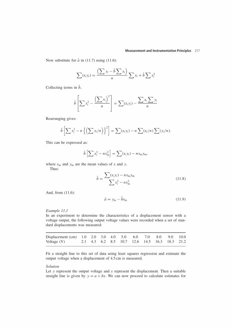
Measurement and Instrumentation Principles 217
Now substitute for Oa in (11.7) using (11.6):
∑�xiyi� D
(∑yi � Ob
∑xi
)n
∑xi C Ob
∑x2
i
Collecting terms in Ob,
Ob
⎡⎢⎣∑ x2
i �(∑
xi
)2
n
⎤⎥⎦ D
∑�xiyi� �
∑xi
∑yi
n
Rearranging gives:
Ob[∑
x2i � n
{(∑xi/n
)}2]
D∑
�xiyi� � n∑
�xi/n�∑
�yi/n�.
This can be expressed as:
Ob[∑
x2i � nx2
m
]D
∑�xiyi� � nxmym,
where xm and ym are the mean values of x and y.Thus:
Ob D∑
�xiyi� � nxmym∑x2
i � nx2m
�11.8�
And, from (11.6):
Oa D ym � Obxm �11.9�
Example 11.1In an experiment to determine the characteristics of a displacement sensor with avoltage output, the following output voltage values were recorded when a set of stan-dard displacements was measured:
Displacement (cm) 1.0 2.0 3.0 4.0 5.0 6.0 7.0 8.0 9.0 10.0Voltage (V) 2.1 4.3 6.2 8.5 10.7 12.6 14.5 16.3 18.3 21.2
Fit a straight line to this set of data using least squares regression and estimate theoutput voltage when a displacement of 4.5 cm is measured.
SolutionLet y represent the output voltage and x represent the displacement. Then a suitablestraight line is given by y D a C bx. We can now proceed to calculate estimates for
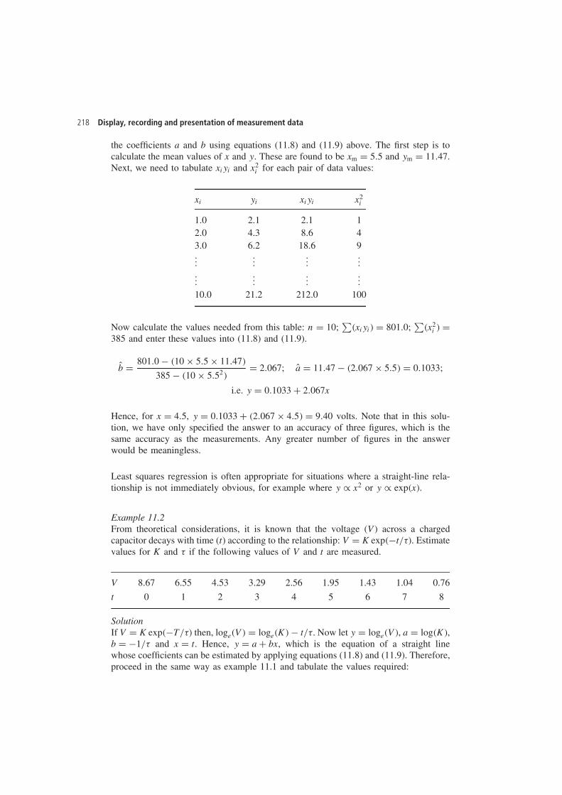
218 Display, recording and presentation of measurement data
the coefficients a and b using equations (11.8) and (11.9) above. The first step is tocalculate the mean values of x and y. These are found to be xm D 5.5 and ym D 11.47.Next, we need to tabulate xiyi and x2
i for each pair of data values:
xi yi xiyi x2i
1.0 2.1 2.1 12.0 4.3 8.6 43.0 6.2 18.6 9...
......
......
......
...10.0 21.2 212.0 100
Now calculate the values needed from this table: n D 10;∑
�xiyi� D 801.0;∑
�x2i � D
385 and enter these values into (11.8) and (11.9).
Ob D 801.0 � �10 ð 5.5 ð 11.47�
385 � �10 ð 5.52�D 2.067; Oa D 11.47 � �2.067 ð 5.5� D 0.1033;
i.e. y D 0.1033 C 2.067x
Hence, for x D 4.5, y D 0.1033 C �2.067 ð 4.5� D 9.40 volts. Note that in this solu-tion, we have only specified the answer to an accuracy of three figures, which is thesame accuracy as the measurements. Any greater number of figures in the answerwould be meaningless.
Least squares regression is often appropriate for situations where a straight-line rela-tionship is not immediately obvious, for example where y / x2 or y / exp�x�.
Example 11.2From theoretical considerations, it is known that the voltage (V) across a chargedcapacitor decays with time (t) according to the relationship: V D K exp��t/��. Estimatevalues for K and � if the following values of V and t are measured.
V 8.67 6.55 4.53 3.29 2.56 1.95 1.43 1.04 0.76
t 0 1 2 3 4 5 6 7 8
SolutionIf V D K exp��T/�� then, loge�V� D loge�K� � t/�. Now let y D loge�V�, a D log�K�,b D �1/� and x D t. Hence, y D a C bx, which is the equation of a straight linewhose coefficients can be estimated by applying equations (11.8) and (11.9). Therefore,proceed in the same way as example 11.1 and tabulate the values required:
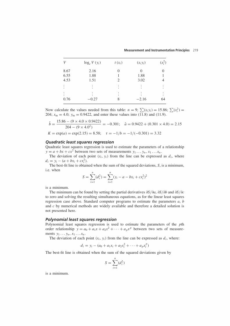
Measurement and Instrumentation Principles 219
V loge V �yi� t �xi� (xiyi) (x2i )
8.67 2.16 0 0 06.55 1.88 1 1.88 14.53 1.51 2 3.02 4...
......
......
......
......
...0.76 �0.27 8 �2.16 64
Now calculate the values needed from this table: n D 9;∑
�xiyi� D 15.86;∑
�x2i � D
204; xm D 4.0; ym D 0.9422, and enter these values into (11.8) and (11.9).
Ob D 15.86 � �9 ð 4.0 ð 0.9422�
204 � �9 ð 4.02�D �0.301; Oa D 0.9422 C �0.301 ð 4.0� D 2.15
K D exp�a� D exp�2.15� D 8.58; � D �1/b D �1/��0.301� D 3.32
Quadratic least squares regressionQuadratic least squares regression is used to estimate the parameters of a relationshipy D a C bx C cx2 between two sets of measurements y1 . . . yn, x1 . . . xn.
The deviation of each point �xi, yi� from the line can be expressed as di, wheredi D yi � �a C bxi C cx2
i �.The best-fit line is obtained when the sum of the squared deviations, S, is a minimum,
i.e. when
S Dn∑
iD1
�d2i � D
n∑iD1
�yi � a � bxi C cx2i �2
is a minimum.The minimum can be found by setting the partial derivatives ∂S/∂a, ∂S/∂b and ∂S/∂c
to zero and solving the resulting simultaneous equations, as for the linear least squaresregression case above. Standard computer programs to estimate the parameters a, band c by numerical methods are widely available and therefore a detailed solution isnot presented here.
Polynomial least squares regressionPolynomial least squares regression is used to estimate the parameters of the pthorder relationship y D a0 C a1x C a2x2 C Ð Ð Ð C apxp between two sets of measure-ments y1 . . . yn, x1 . . . xn.
The deviation of each point �xi, yi� from the line can be expressed as di, where:
di D yi � �a0 C a1xi C a2x2i C Ð Ð Ð C apxp
i �
The best-fit line is obtained when the sum of the squared deviations given by
S Dn∑
iD1
�d2i �
is a minimum.
220 Display, recording and presentation of measurement data
The minimum can be found as before by setting the p partial derivatives∂S/∂a0 . . . ∂S/∂ap to zero and solving the resulting simultaneous equations. Again, asfor the quadratic least squares regression case, standard computer programs to estimatethe parameters a0 . . . ap by numerical methods are widely available and therefore adetailed solution is not presented here.
Confidence tests in curve fitting by least squares regressionOnce data has been collected and a mathematical relationship that fits the data pointshas been determined by regression, the level of confidence that the mathematical rela-tionship fitted is correct must be expressed in some way. The first check that must bemade is whether the fundamental requirement for the validity of regression techniquesis satisfied, i.e. whether the deviations of data points from the fitted line are all lessthan the maximum error level predicted for the measured variable. If this conditionis violated by any data point that a line or curve has been fitted to, then use of thefitted relationship is unsafe and recourse must be made to tabular data presentation, asdescribed earlier.
The second check concerns whether or not random errors affect both measuredvariables. If attempts are made to fit relationships by regression to data where bothmeasured variables contain random errors, any relationship fitted will only be approx-imate and it is likely that one or more data points will have a deviation from the fittedline or curve that is greater than the maximum error level predicted for the measuredvariable. This will show up when the appropriate checks are made.
Having carried out the above checks to show that there are no aspects of the datawhich suggest that regression analysis is not appropriate, the next step is to applyleast squares regression to estimate the parameters of the chosen relationship (linear,quadratic etc.). After this, some form of follow-up procedure is clearly required toassess how well the estimated relationship fits the data points. A simple curve-fittingconfidence test is to calculate the sum of squared deviations S for the chosen y/xrelationship and compare it with the value of S calculated for the next higher orderregression curve that could be fitted to the data. Thus if a straight-line relationship ischosen, the value of S calculated should be of a similar magnitude to that obtained byfitting a quadratic relationship. If the value of S were substantially lower for a quadraticrelationship, this would indicate that a quadratic relationship was a better fit to the datathan a straight-line one and further tests would be needed to examine whether a cubicor higher order relationship was a better fit still.
Other more sophisticated confidence tests exist such as the F-ratio test. However,these are outside the scope of this book.
Correlation testsWhere both variables in a measurement data set are subject to random fluctuations,correlation analysis is applied to determine the degree of association between thevariables. For example, in the case already quoted of a data set containing measure-ments of human height and weight, we certainly expect some relationship betweenthe variables of height and weight because a tall person is heavier on average than ashort person. Correlation tests determine the strength of the relationship (or interdepen-dence) between the measured variables, which is expressed in the form of a correlationcoefficient.
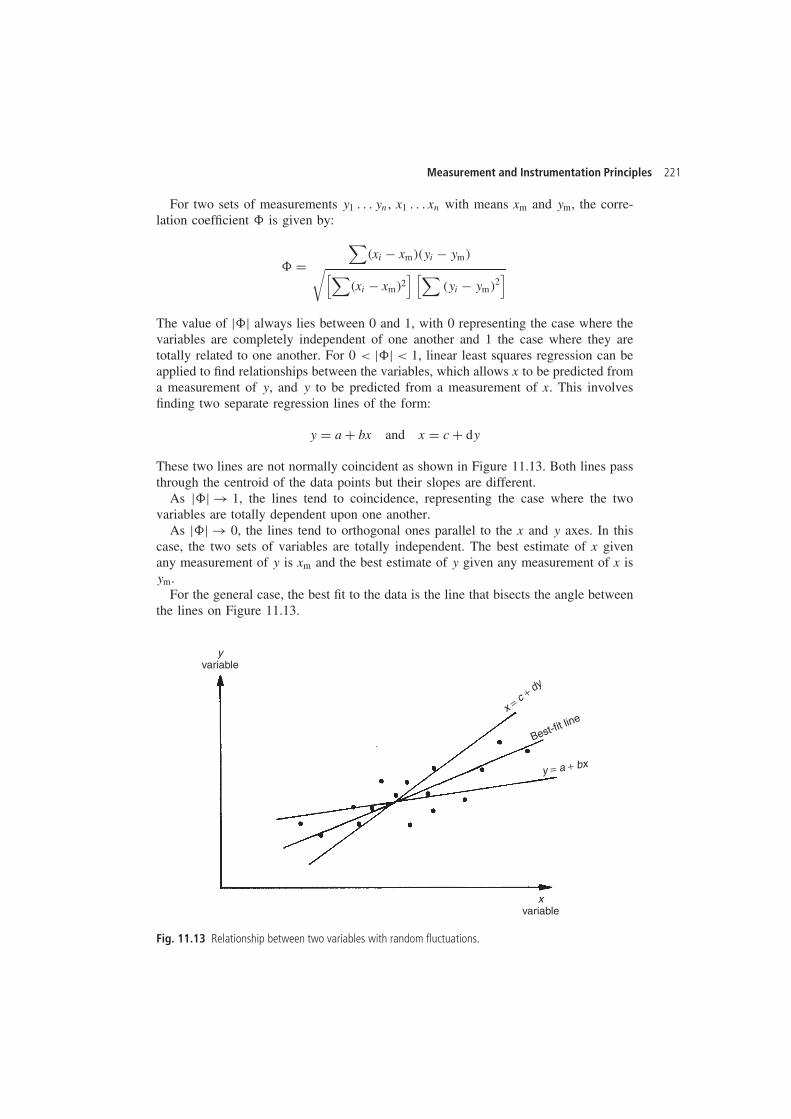
Measurement and Instrumentation Principles 221
For two sets of measurements y1 . . . yn, x1 . . . xn with means xm and ym, the corre-lation coefficient 8 is given by:
8 D∑
�xi � xm��yi � ym�√[∑�xi � xm�2
] [∑�yi � ym�2
]
The value of j8j always lies between 0 and 1, with 0 representing the case where thevariables are completely independent of one another and 1 the case where they aretotally related to one another. For 0 < j8j < 1, linear least squares regression can beapplied to find relationships between the variables, which allows x to be predicted froma measurement of y, and y to be predicted from a measurement of x. This involvesfinding two separate regression lines of the form:
y D a C bx and x D c C dy
These two lines are not normally coincident as shown in Figure 11.13. Both lines passthrough the centroid of the data points but their slopes are different.
As j8j ! 1, the lines tend to coincidence, representing the case where the twovariables are totally dependent upon one another.
As j8j ! 0, the lines tend to orthogonal ones parallel to the x and y axes. In thiscase, the two sets of variables are totally independent. The best estimate of x givenany measurement of y is xm and the best estimate of y given any measurement of x isym.
For the general case, the best fit to the data is the line that bisects the angle betweenthe lines on Figure 11.13.
yvariable
xvariable
Best-fit line
x = c
+ dy
y = a + bx
Fig. 11.13 Relationship between two variables with random fluctuations.
222 Display, recording and presentation of measurement data
11.4 Self-test questions
11.1 (a) Explain the derivation of the expression R C K2iP
JR C Ks J D KiVt
JR describingthe dynamic response of a chart recorder following a step change in theelectrical voltage output of a transducer connected to its input. Explain alsowhat all the terms in the expression stand for. (Assume that the impedancesof both the transducer and recorder have a resistive component only and thatthere is negligible friction in the system.)
(b) Derive expressions for the measuring system natural frequency, ωn, thedamping factor, �, and the steady-state sensitivity.
(c) Explain simple ways of increasing and decreasing the damping factor anddescribe the corresponding effect on measurement sensitivity.
(d) What damping factor gives the best system bandwidth?(e) What aspects of the design of a chart recorder would you modify in order to
improve the system bandwidth? What is the maximum bandwidth typicallyattainable in chart recorders, and if such a maximum-bandwidth instrument isavailable, what is the highest-frequency signal that such an instrument wouldbe generally regarded as being suitable for measuring if the accuracy of thesignal amplitude measurement is important?
11.2 Theoretical considerations show that quantities x and y are related in a linearfashion such that y D ax C b. Show that the best estimate of the constants a andb are given by:
Oa D∑
�xiyi� � nxmym∑x2
i � nx2m
; Ob D ym � Oaxm
Explain carefully the meaning of all the terms in the above two equations.11.3 The characteristics of a chromel-constantan thermocouple is known to be approx-
imately linear over the temperature range 300°C–800°C. The output e.m.f. wasmeasured practically at a range of temperatures and the following table of resultsobtained. Using least squares regression, calculate the coefficients a and b for therelationship T D aE C b that best describes the temperature–e.m.f. characteristic.
Temp (°C) 300 325 350 375 400 425 450 475 500 525 550e.m.f. (mV) 21.0 23.2 25.0 26.9 28.6 31.3 32.8 35.0 37.2 38.5 40.7
Temp (°C) 575 600 625 650 675 700 725 750 775 800e.m.f. (mV) 43.0 45.2 47.6 49.5 51.1 53.0 55.5 57.2 59.0 61.0
11.4 Measurements of the current (I) flowing through a resistor and the correspondingvoltage drop (V) are shown below:
I 1 2 3 4 5V 10.8 20.4 30.7 40.5 50.0
Measurement and Instrumentation Principles 223
The instruments used to measure voltage and current were accurate in all respectsexcept that they each had a zero error that the observer failed to take accountof or to correct at the time of measurement. Determine the value of the resistorfrom the data measured.
11.5 A measured quantity y is known from theoretical considerations to depend ona variable x according to the relationship y D a C bx2. For the following set ofmeasurements of x and y, use linear least squares regression to determine theestimates of the parameters a and b that fit the data best.
x 0 1 2 3 4 5y 0.9 9.2 33.4 72.5 130.1 200.8
11.6 The mean-time-to-failure (MTTF ) of an integrated circuit is known to obey a lawof the following form: MTTF D C exp T0/T, where T is the operating temper-ature and C and T0 are constants.The following values of MTTF at various temperatures were obtained fromaccelerated-life tests.
MTTF (hours) 54 105 206 411 941 2145Temperature (K) 600 580 560 540 520 500
(a) Estimate the values of C and T0. (Hint – loge�MTTF� D loge�C� C T0/T.This equation is now a straight-line relationship between log�MTTF� and1/T, where log�C� and T0 are constants.)
(b) For a MTTF of 10 years, calculate the maximum allowable temperature.
References and further reading
Chatfield, C. (1983) Statistics for Technology, Chapman and Hall, London.Topping, J. (1972) Errors of Observation and their Treatment, Chapman and Hall, London.
12
Measurement reliabilityand safety systems
12.1 Reliability
The reliability of measurement systems can be quantified as the mean time betweenfaults occurring in the system. In this context, a fault means the occurrence of anunexpected condition in the system that causes the measurement output to either beincorrect or not to exist at all. The following sections summarize the principles ofreliability theory that are relevant to measurement systems. A fuller account of relia-bility theory, and particularly its application in manufacturing systems, can be foundelsewhere (Morris, 1997).
12.1.1 Principles of reliability
The reliability of a measurement system is defined as the ability of the system toperform its required function within specified working conditions for a stated periodof time. Unfortunately, factors such as manufacturing tolerances in an instrument andvarying operating conditions conspire to make the faultless operating life of a systemimpossible to predict. Such factors are subject to random variation and chance, andtherefore reliability cannot be defined in absolute terms. The nearest one can get toan absolute quantification of reliability are quasi-absolute terms like the mean-time-between-failures, which expresses the average time that the measurement system workswithout failure. Otherwise, reliability has to be expressed as a statistical parameter thatdefines the probability that no faults will develop over a specified interval of time.
In quantifying reliability for a measurement system, an immediate difficulty thatarises is defining what counts as a fault. Total loss of a measurement output is anobvious fault but a fault that causes a finite but incorrect measurement is more difficultto identify. The usual approach is to identify such faults by applying statistical processcontrol techniques (Morris, 1997).
Reliability quantification in quasi-absolute termsWhilst reliability is essentially probabilistic in nature, it can be quantified in quasi-absoluteterms by the mean-time-between-failures and the mean-time-to-failure parameters. It
Measurement and Instrumentation Principles 225
must be emphasized that these two quantities are usually average values calculated overa number of identical instruments, and therefore the actual values for any particularinstrument may vary substantially from the average value.
The mean-time-between-failures (MTBF) is a parameter that expresses the averagetime between faults occurring in an instrument, calculated over a given period of time.For example, suppose that the history of an instrument is logged over a 360 day periodand the time intervals in days between faults occurring was as follows:
11 23 27 16 19 32 6 24 13 21 26 15 14 33 29 12 17 22
The mean interval is 20 days, which is therefore the mean-time-between-failures. Analternative way of calculating MTBF is simply to count the number of faults occurringover a given period. In the above example, there were 18 faults recorded over a periodof 360 days and so the MTBF can be calculated as:
MTBF D 360/18 D 20 days
Unfortunately, in the case of instruments that have a high reliability, such in-servicecalculation of reliability in terms of the number of faults occurring over a given periodof time becomes grossly inaccurate because faults occur too infrequently. In this case,MTBF predictions provided by the instrument manufacturer can be used, since manu-facturers have the opportunity to monitor the performance of a number of identicalinstruments installed in different companies. If there are a total of F faults recordedfor N identical instruments in time T, the MTBF can be calculated as MTBF D TN/F.One drawback of this approach is that it does not take the conditions of use, such asthe operating environment, into account.
The mean-time-to-failure (MTTF) is an alternative way of quantifying reliabilitythat is normally used for devices like thermocouples that are discarded when they fail.MTTF expresses the average time before failure occurs, calculated over a number ofidentical devices.
The final reliability-associated term of importance in measurement systems is themean-time-to-repair (MTTR). This expresses the average time needed for repair of aninstrument. MTTR can also be interpreted as the mean-time-to-replace, since replace-ment of a faulty instrument by a spare one is usually preferable in manufacturingsystems to losing production whilst an instrument is repaired.
The MTBF and MTTR parameters are often expressed in terms of a combinedquantity known as the availability figure. This measures the proportion of the totaltime that an instrument is working, i.e. the proportion of the total time that it is in anunfailed state. The availability is defined as the ratio:
Availability D MTBF
MTBF C MTTR
In measurement systems, the aim must always be to maximize the MTBF figure andminimize the MTTR figure, thereby maximizing the availability. As far as the MTBFand MTTF figures are concerned, good design and high-quality control standards duringmanufacture are the appropriate means of maximizing these figures. Design proceduresthat mean that faults are easy to repair are also an important factor in reducing theMTTR figure.
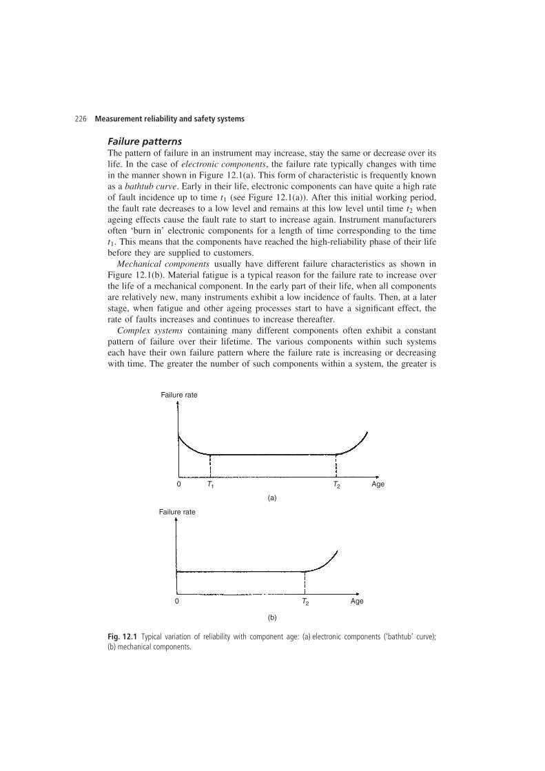
226 Measurement reliability and safety systems
Failure patternsThe pattern of failure in an instrument may increase, stay the same or decrease over itslife. In the case of electronic components, the failure rate typically changes with timein the manner shown in Figure 12.1(a). This form of characteristic is frequently knownas a bathtub curve. Early in their life, electronic components can have quite a high rateof fault incidence up to time t1 (see Figure 12.1(a)). After this initial working period,the fault rate decreases to a low level and remains at this low level until time t2 whenageing effects cause the fault rate to start to increase again. Instrument manufacturersoften ‘burn in’ electronic components for a length of time corresponding to the timet1. This means that the components have reached the high-reliability phase of their lifebefore they are supplied to customers.
Mechanical components usually have different failure characteristics as shown inFigure 12.1(b). Material fatigue is a typical reason for the failure rate to increase overthe life of a mechanical component. In the early part of their life, when all componentsare relatively new, many instruments exhibit a low incidence of faults. Then, at a laterstage, when fatigue and other ageing processes start to have a significant effect, therate of faults increases and continues to increase thereafter.
Complex systems containing many different components often exhibit a constantpattern of failure over their lifetime. The various components within such systemseach have their own failure pattern where the failure rate is increasing or decreasingwith time. The greater the number of such components within a system, the greater is
Failure rate
Age0
(a)
T1 T2
Failure rate
Age0
(b)
T2
Fig. 12.1 Typical variation of reliability with component age: (a) electronic components (‘bathtub’ curve);(b) mechanical components.
Measurement and Instrumentation Principles 227
the tendency for the failure patterns in the individual components to cancel out andfor the rate of fault-incidence to assume a constant value.
Reliability quantification in probabilistic termsIn probabilistic terms, the reliability R�T� of an instrument X is defined as the proba-bility that the instrument will not fail within a certain period of time T. The unreliabilityor likelihood of failure F�T� is a corresponding term which expresses the probabilitythat the instrument will fail within the specified time interval. R�T� and F�T� arerelated by the expression:
F�T� D 1 � R�T� �12.1�
To calculate R�T�, accelerated lifetime testingŁ is carried out for a number (N) ofidentical instruments. Providing all instruments have similar conditions of use, thetimes of failure, t1, t2 . . . tn will be distributed about the mean time to failure tm. Ifthe probability density of the time-to-failure is represented by f�t�, the probabilitythat a particular instrument will fail in a time interval υt is given by f�t� υt, and theprobability that the instrument will fail before a time T is given by:
F�T� D∫ T
0f�t� dt
The probability that the instrument will fail in a time interval 1T following T, assumingthat it has survived to time T, is given by:
F�T C 1T� � F�T�
R�T�
where R�T� is the probability that the instrument will survive to time T. Dividing thisexpression by 1T gives the average failure rate in the interval from T to T C 1T as:
F�T C 1T� � F�T�
1TR�T�
In the limit as 1T ! 0, the instantaneous failure rate at time T is given by:
f D d[F�T�]
dt
1
R�T�D F0�T�
R�T��12.2�
If it is assumed that the instrument is in the constant-failure-rate phase of its life,denoted by the interval between times t1 and t2 in Figure 12.1, then the instantaneousfailure rate at T is also the mean failure rate which can be expressed as the reciprocalof the MTBF, i.e. mean failure rate D f D 1/tm.
Differentiating (12.1) with respect to time gives F0�T� D �R0�T�. Hence, substitutingfor F0�T� in (12.2) gives:
f D �R0�T�
R�T�
Ł Accelerated lifetime testing means subjecting an instrument to a much greater frequency of use than wouldnormally be expected. If an instrument is normally used ten times per day, then one hundred days of normaluse can be simulated by using it one thousand times in a single day.
228 Measurement reliability and safety systems
This can be solved (Miller, 1990) to give the following expression:
R�T� D exp�� fT� �12.3�
Examination of equation (12.3) shows that, at time t D 0, the unreliability is zero.Also, as t tends to 1, the unreliability tends to a value of 1. This agrees with intuitiveexpectations that the value of unreliability should lie between values of 0 and 1. Anotherpoint of interest in equation (12.3) is to consider the unreliability when T D MTBF,i.e. when T D tm. Then: F�T� D 1 � exp��1� D 0.63, i.e. the probability of a productfailing after it has been operating for a length of time equal to the MTBF is 63%.
Further analysis of equation (12.3) shows that, for T/tm � 0.1:
F�T� ³ T/tm �12.4�
This is a useful formula for calculating (approximately) the reliability of a criticalproduct which is only used for a time that is a small proportion of its MTBF.
Example 12.1If the mean-time-to-failure of an instrument is 50 000 hours, calculate the probabilitythat it will not fail during the first 10 000 hours of operation.
SolutionFrom (12.3), R�T� D exp�� fT� D exp��10 000/50 000� D 0.8187
Example 12.2If the mean-time-to-failure of an instrument is 80 000 hours, calculate the probabilitythat it will not fail during the first 8000 hours of operation.
SolutionIn this case, T/tm D 80 000/8000 D 0.1 and so equation (12.4) can be applied,giving R�T� D 1 � F�T� ³ 1 � T/tm ³ 0.9. To illustrate the small level of inaccuracyinvolved in using the approximate expression (12.4), if we calculate the probabilityaccording to (12.3) we get R�T� D exp��0.1� D 0.905. Thus, there is a small but finiteerror in applying (12.4) instead of (12.3).
12.1.2 Laws of reliability in complex systems
Measurement systems usually comprise a number of components that are connectedtogether in series, and hence it is necessary to know how the reliabilities of individualcomponents are aggregated into a reliability figure for the whole system. In some cases,identical measurement components are put in parallel to improve reliability, becausethe measurement system then only fails if all of the parallel components fail. Thesetwo cases are covered by particular laws of reliability.
Reliability of components in seriesA measurement system consisting of several components in series fails when any oneof the separate components develops a fault. The reliability of such a system canbe quantified as the probability that none of the components will fail within a given
Measurement and Instrumentation Principles 229
interval of time. For a system of n series components, the reliability RS is the product ofthe separate reliabilities of the individual components according to the joint probabilityrule (Morris, 1997):
RS D R1R2 . . . Rn �12.5�
Example 12.3A measurement system consists of a sensor, a variable conversion element and a signalprocessing circuit, for which the reliability figures are 0.9, 0.95 and 0.99 respectively.Calculate the reliability of the whole measurement system.
SolutionApplying (12.5), RS D 0.9 ð 0.95 ð 0.99 D 0.85.
Reliability of components in parallelOne way of improving the reliability of a measurement system is to connect two ormore instruments in parallel. This means that the system only fails if every parallelinstrument fails. For such systems, the system reliability RS is given by:
RS D 1 � FS �12.6�
where FS is the unreliability of the system. The equation for calculating FS is similarto (12.5). Thus, for n instruments in parallel, the unreliability is given by:
FS D F1F2 . . . Fn �12.7�
If all the instruments in parallel are identical then (12.7) can be written in the simplerform:
FS D �FX�n �12.8�
where FX is the unreliability of each instrument.
Example 12.4In a particular safety critical measurement system, three identical instruments areconnected in parallel. If the reliability of each instrument is 0.95, calculate the reliabilityof the measurement system.
SolutionFrom (12.1), the unreliability of each instrument FX is given by FX D 1 � RX D 1 �0.95 D 0.05.Applying (12.8), FS D �FX�3 D �0.05�3 D 0.000125.Thus, from (12.6), RS D 1 � FS D 1 � 0.000125 D 0.999875.
12.1.3 Improving measurement system reliability
When designing a measurement system, the aim is always to reduce the probability ofthe system failing to as low a level as possible. An essential requirement in achievingthis is to ensure that the system is replaced at or before the time t2 in its life shown inFigure 12.1 when the statistical frequency of failures starts to increase. Therefore, theinitial aim should be to set the lifetime T equal to t2 and minimize the probability F�T�
230 Measurement reliability and safety systems
of the system failing within this specified lifetime. Once all measures to reduce F�T�have been applied, the acceptability of the reliability R�T� has to be assessed againstthe requirements of the measurement system. Inevitably, cost enters into this, as effortsto increase R�T� usually increase the cost of buying and maintaining the system. Lowerreliability is acceptable in some measurement systems where the cost of failure is low,such as in manufacturing systems where the cost of lost production, or the loss dueto making out-of-specification products, is not serious. However, in other applications,such as where failure of the measurement system incurs high costs or causes safetyproblems, high reliability is essential. Some special applications where human accessis very difficult or impossible, such as measurements in unmanned spacecraft, satellitesand nuclear power plants, demand especially high reliability because repair of faultymeasurement systems is impossible.
The various means of increasing R�T� are considered below. However, once allefforts to increase R�T� have been exhausted, the only solution available if the relia-bility specified for a working period T is still not high enough is to reduce the periodT over which the reliability is calculated by replacing the measurement system earlierthan time t2.
Choice of instrumentThe type of components and instruments used within measuring systems has a largeeffect on the system reliability. Of particular importance in choosing instruments is tohave regard to the type of operating environment in which they will be used. In parallelwith this, appropriate protection must be given (for example, enclosing thermocouplesin sheaths) if it is anticipated that the environment may cause premature failure of aninstrument. Some instruments are more affected than others, and thus more likely tofail, in certain environments. The necessary knowledge to make informed choices aboutthe suitability of instruments for particular environments, and the correct protection togive them, requires many years of experience, although instrument manufacturers cangive useful advice in most cases.
Instrument protectionAdequate protection of instruments and sensors from the effects of the operating envi-ronment is necessary. For example, thermocouples and resistance thermometers shouldbe protected by a sheath in adverse operating conditions.
Regular calibrationThe most common reason for faults occurring in a measurement system, whereby theerror in the measurement goes outside acceptable limits, is drift in the performanceof the instrument away from its specified characteristics. Such faults can usually beavoided by ensuring that the instrument is recalibrated at the recommended intervalsof time. Types of intelligent instrument and sensor that perform self-calibration haveclear advantages in this respect.
RedundancyRedundancy means the use of two or more measuring instruments or measurementsystem components in parallel such that any one can provide the required measurement.
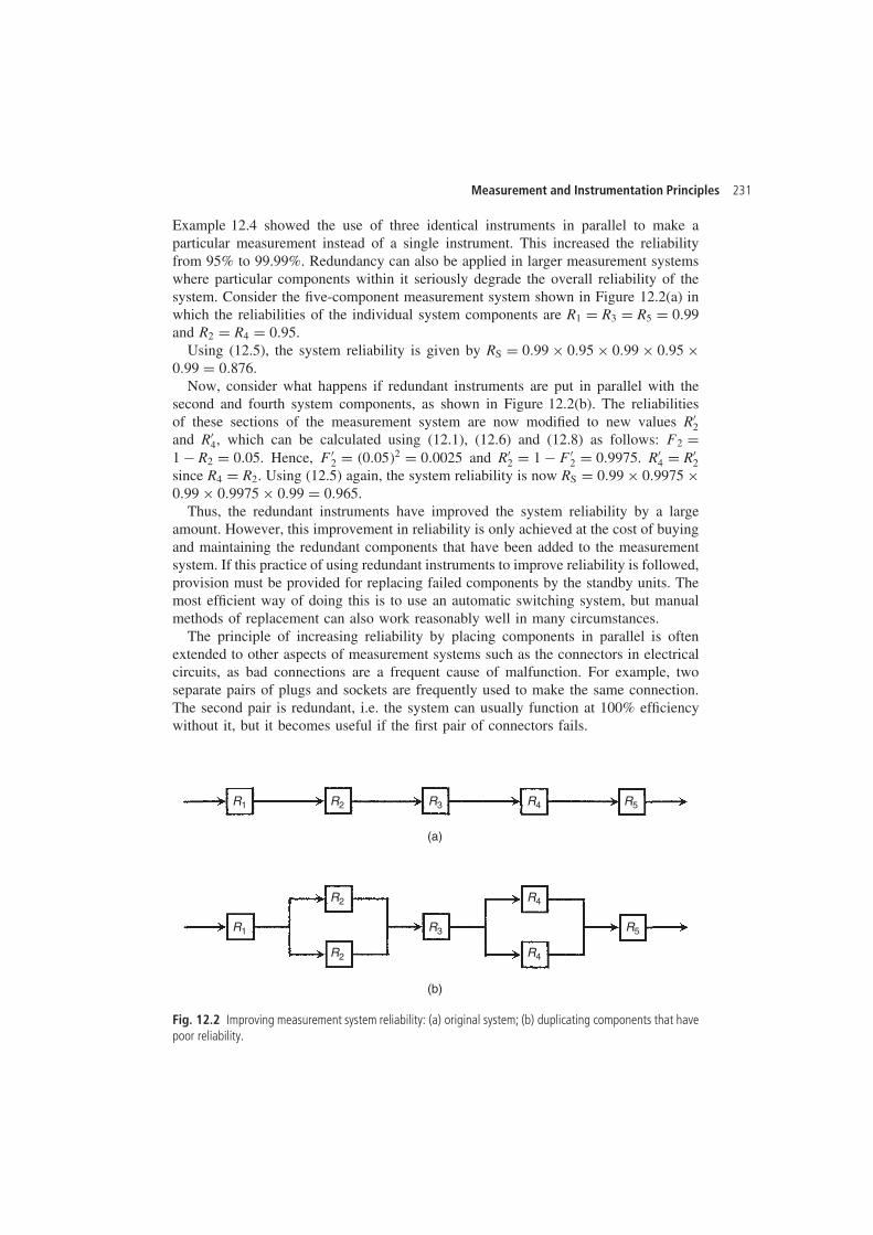
Measurement and Instrumentation Principles 231
Example 12.4 showed the use of three identical instruments in parallel to make aparticular measurement instead of a single instrument. This increased the reliabilityfrom 95% to 99.99%. Redundancy can also be applied in larger measurement systemswhere particular components within it seriously degrade the overall reliability of thesystem. Consider the five-component measurement system shown in Figure 12.2(a) inwhich the reliabilities of the individual system components are R1 D R3 D R5 D 0.99and R2 D R4 D 0.95.
Using (12.5), the system reliability is given by RS D 0.99 ð 0.95 ð 0.99 ð 0.95 ð0.99 D 0.876.
Now, consider what happens if redundant instruments are put in parallel with thesecond and fourth system components, as shown in Figure 12.2(b). The reliabilitiesof these sections of the measurement system are now modified to new values R0
2and R0
4, which can be calculated using (12.1), (12.6) and (12.8) as follows: F2 D1 � R2 D 0.05. Hence, F0
2 D �0.05�2 D 0.0025 and R02 D 1 � F0
2 D 0.9975. R04 D R0
2since R4 D R2. Using (12.5) again, the system reliability is now RS D 0.99 ð 0.9975 ð0.99 ð 0.9975 ð 0.99 D 0.965.
Thus, the redundant instruments have improved the system reliability by a largeamount. However, this improvement in reliability is only achieved at the cost of buyingand maintaining the redundant components that have been added to the measurementsystem. If this practice of using redundant instruments to improve reliability is followed,provision must be provided for replacing failed components by the standby units. Themost efficient way of doing this is to use an automatic switching system, but manualmethods of replacement can also work reasonably well in many circumstances.
The principle of increasing reliability by placing components in parallel is oftenextended to other aspects of measurement systems such as the connectors in electricalcircuits, as bad connections are a frequent cause of malfunction. For example, twoseparate pairs of plugs and sockets are frequently used to make the same connection.The second pair is redundant, i.e. the system can usually function at 100% efficiencywithout it, but it becomes useful if the first pair of connectors fails.
R1 R2 R3 R4 R5
R1
R2
(a)
(b)
R2
R3
R4
R4
R5
Fig. 12.2 Improving measurement system reliability: (a) original system; (b) duplicating components that havepoor reliability.
232 Measurement reliability and safety systems
12.1.4 Software reliability
As computer processors, and the software within them, are increasingly found in mostmeasurement systems, the issue of the reliability of such components has becomevery important. Computer hardware behaves very much like electronic components ingeneral, and the rules for calculating reliability given earlier can be applied. However,the factors affecting reliability in software are fundamentally different. Application ofthe general engineering definition of reliability to software is not appropriate becausethe characteristics of the error mechanisms in software and in engineering hardware arefundamentally different. Hardware systems that work correctly when first introducedcan develop faults at any time in the future, and so the MTBF is a sensible measureof reliability. However, software does not change with time: if it starts off being errorfree, then it will remain so. Therefore, what we need to know, in advance of its use,is whether or not faults are going to be found in the software after it has been put intouse. Thus, for software, a MTBF reliability figure is of little value. Instead, we mustsomehow express the probability that errors will not occur in it.
Quantifying software reliabilityA fundamental problem in predicting that errors will not occur in software is that,however exhaustive the testing, it is impossible to say with certainty that all errorshave been found and eliminated. Errors can be quantified by three parameters, D, Uand T, where D is the number of errors detected by testing the software, U is thenumber of undetected errors and T is the total number of errors (both detected andundetected).
Hence:U D T � D �12.9�
Good program testing can detect most errors and so make D approach T so that Utends towards zero. However, as the value of T can never be predicted with certainty,it is very difficult to predict that software is error free, whatever degree of diligenceis applied during testing procedures.
Whatever approach is taken to quantifying reliability, software testing is an essentialprerequisite to the quantification methods available. Whilst it is never possible to detectall the errors that might exist, the aim must always be to find and correct as many errorsas possible by applying a rigorous testing procedure. Software testing is a particularlyimportant aspect of the wider field of software engineering. However, as it is a subjectof considerable complexity, the detailed procedures available are outside the scope ofthis book. A large number of books now cover good software engineering in general andsoftware testing procedures in particular, and the reader requiring further informationis referred to the referenced texts such as Pfleeger (1987) and Shooman (1983).
One approach to quantifying software reliability (Fenton, 1991) is to monitor therate of error discovery during testing and then extrapolate this into an estimate of themean-time-between-failures for the software once it has been put into use. Testing canthen be extended until the predicted MTBF is greater than the projected time-horizonof usage of the software. This approach is rather unsatisfactory because it acceptsthat errors in the software exist and only predicts that errors will not emerge veryfrequently.
Measurement and Instrumentation Principles 233
Confidence in the measurement system is much greater if we can say, ‘There is ahigh probability that there are zero errors in the software’ rather than ‘There are a finitenumber of errors in the software but they are unlikely to emerge within the expectedlifetime of its usage.’ One way of achieving this is to estimate the value of T (totalnumber of errors) from initial testing and then carry out further software testing untilthe predicted value of T is zero, in a procedure known as error seeding (Mills, 1972).In this method, the programmer responsible for producing the software deliberatelyputs a number of errors E into the program, such that the total number of errors inthe program increases from T to T0, where T0 D T C E. Testing is then carried outby a different programmer who will identify a number of errors given by D0, whereD0 D D C E0 and E0 is the number of deliberately inserted errors that are detected bythis second programmer. Normally, the real errors detected (D) will be less than Tand the seeded errors detected (E0) will be less than E. However, on the assumptionthat the ratio of seeded errors detected to the total number of seeded errors will bethe same as the ratio of the real errors detected to the total number of real errors, thefollowing expression can be written:
D
TD E0
E�12.10�
As E0 is measured, E is known and D can be calculated from the number of errorsD0 detected by the second programmer according to D D D0 � E0, the value of T canthen be calculated as:
T D DE/E0 �12.11�
Example 12.5The author of a digital signal-processing algorithm that forms a software componentwithin a measurement system adds 12 deliberate faults to the program. The programis then tested by a second programmer, who finds 34 errors. Of these detected errors,the program author recognizes 10 of them as being seeded errors. Estimate the originalnumber of errors present in the software (i.e. excluding the seeded errors).
SolutionThe total number of errors detected (D0) is 34 and the program author confirms thatthe number of seeded errors (E0) within these is 10 and that the total number of seedederrors (E) was 12. Because D0 D D C E0 (see earlier), D D D0 � E0 D 24. Hence, from(12.11), T D DE/E0 D 24 ð 12/10 D 28.8.
One flaw in expression (12.11) is the assumption that the seeded errors are representa-tive of all the real (unseeded) errors in the software, both in proportion and character.This assumption is never entirely valid in practice because, if errors are unknown, thentheir characteristics are also unknown. Thus, whilst this approach may be able to givean approximate indication of the value of T, it can never predict its actual value withcertainty.
An alternative to error seeding is the double-testing approach, where two independentprogrammers test the same program (Pfleeger, 1987). Suppose that the number of errorsdetected by each programmer is D1 and D2 respectively. Normally, the errors detectedby the two programmers will be in part common and in part different. Let C be the
234 Measurement reliability and safety systems
number of common errors that both programmers find. The error-detection success ofeach programmer can be quantified as:
S1 D D1/T; S2 D D2/T �12.12�
It is reasonable to assume that the proportion of errors D1 that programmer 1 finds outof the total number of errors T is the same proportion as the number of errors C thathe/she finds out of the number D2 found by programmer 2, i.e.:
D1
TD C
D2D S1, and hence D2 D C
S1�12.13�
From (12.12), T D D2/S2, and substituting in the value of D2 obtained from (12.13),the following expression for T is obtained:
T D C/S1S2 �12.14�
From (12.13), S1 D C/D2 and from (12.12), S2 D D2S1/D1 D C/D1. Thus, substitutingfor S1 and S2 in (12.14):
T D D1D2/C �12.15�
Example 12.6A piece of software is tested independently by two programmers, and the number oferrors found is 24 and 26 respectively. Of the errors found by programmer 1, 21 arethe same as errors found by programmer 2.
SolutionD1 D 24, D2 D 26 and C D 21. Hence, applying (12.15), T D D1D2/C D 24 ð26/21 D 29.7.
Program testing should continue until the number of errors that have been found isequal to the predicted total number of errors T. In the case of example 12.6, this meanscontinuing testing until 30 errors have been found. However, the problem with doingthis is that T is only an estimated quantity and there may actually be only 28 or 29 errorsin the program. Thus, to continue testing until 30 errors have been found would meantesting forever! Hence, once 28 or 29 errors have been found and continued testing fora significant time after this has detected no more errors, the testing procedure shouldbe terminated, even though the program could still contain one or two errors. Theapproximate nature of the calculated value of T also means that its true value could be31 or 32, and therefore the software may still contain errors if testing is stopped once30 errors have been found. Thus, the fact that T is only an estimated value means thestatement that a program is error free once the number of errors detected is equal toT can only be expressed in probabilistic terms.
To quantify this probability, further testing of the program is necessary (Pfleeger,1987). The starting point for this further testing is the stage when the total number oferrors T that are predicted have been found (or when the number found is slightly lessthan T but further testing does not seem to be finding any more errors). The next stepis to seed the program with W new errors and then test it until all W seeded errors have
Measurement and Instrumentation Principles 235
been found. Provided that no new errors have been found during this further testingphase, the probability that the program is error free can then be expressed as:
P D W/�W C 1� �12.16�
However, if any new error is found during this further testing phase, the error must becorrected and then the seeding and testing procedure must be repeated. Assumingthat no new errors are detected, a value of W D 10 gives P D 0.91 (probability91% that program is error free). To get to 99% error-free probability, W has tobe 99.
Improving software reliabilityThe a priori requirement in achieving high reliability in software is to ensure thatit is produced according to sound software engineering principles. Formal standardsfor achieving high quality in software are set out in BS 7165 (1991) and ISO 9000-3(1991). Libraries and bookshops, especially academic ones, offer a number of texts ongood software design procedures. These differ significantly in their style of approach,but all have the common aim of encouraging the production of error-free software thatconforms to the design specification. It is not within the scope of this book to enterinto arguments about which software design approach is best, as choice between thedifferent software design techniques largely depends on personal preferences. However,it is essential that software contributing to a measurement system is produced accordingto good software engineering principles.
The second stage of reliability enhancement is the application of a rigorous testingprocedure as described in the last section. This is a very time-consuming and henceexpensive business, and so testing should only continue until the calculated level ofreliability is the minimum needed for the requirements of the measurement system.However, if a very high level of reliability is demanded, such rigorous testing becomesextremely expensive and an alternative approach known as N-version programming isoften used. N-version programming requires N different programmers to produce Ndifferent versions of the same software according to a common specification. Then,assuming that there are no errors in the specification itself, any difference in the outputof one program compared with the others indicates an error in that program. Commonly,N D 3 is used, that is, three different versions of the program are produced, but N D 5is used for measurement systems that are very critical. In this latter case, a ‘voting’system is used, which means that up to two out of the five versions can be faultywithout incorrect outputs being generated.
Unfortunately, whilst this approach reduces the chance of software errors in measure-ment systems, it is not foolproof because the degree of independence between programscannot be guaranteed. Different programmers, who may be trained in the same placeand use the same design techniques, may generate different programs that have thesame errors. Thus, this method has the best chance of success if the programmers aretrained independently and use different design techniques.
Languages such as ADA also improve the safety of software because they containspecial features that are designed to detect the kind of programming errors that arecommonly made. Such languages have been specifically developed with safety criticalapplications in mind.

236 Measurement reliability and safety systems
12.2 Safety systems
12.2.1 Introduction to safety systems
Measurement system reliability is usually inexorably linked with safety issues, sincemeasuring instruments to detect the onset of dangerous situations that may potentiallycompromise safety are a necessary part of all safety systems implemented. Statutorysafety legislation now exists in all countries around the world. Whilst the exact contentof legislation varies from country to country, a common theme is to set out responsi-bilities for all personnel whose actions may affect the safety of themselves or others.Penalties are prescribed for contravention of the legislation, which can include finesor custodial sentences or both. Legislation normally sets out duties for both employersand employees.
Duties of employers include:
ž To ensure that process plant is operated and maintained in a safe way so that thehealth and safety of all employees is protected
ž To provide such training and supervision as is necessary to ensure the health andsafety of all employees
ž To provide a monitoring and shutdown system (safety system) for any process plantor other equipment that may cause danger if certain conditions arise
ž To ensure the health and safety, as far as is reasonably practical, of all persons whoare not employees but who may reasonably be expected to be at risk from operationscarried out by a company.
Duties of employees include:
ž To take reasonable care for their own safetyž To take reasonable care for the safety of othersž To avoid misusing or damaging any equipment or system that is designed to protect
people’s safety.
The primary concern of measurement and instrumentation technologists with regard tosafety legislation is, firstly, to ensure that all measurement systems are installed andoperated in a safe way and, secondly, to ensure that instruments and alarms installedas part of safety protection systems operate reliably and effectively.
Intrinsic safetyIntrinsic safety describes the ability of measuring instruments and other systems tooperate in explosive or flammable environments without any risk of sparks or arcscausing an explosion or fire. The detailed design of systems to make them intrinsicallysafe is outside the scope of this book. However, the general principles are either todesign electrical systems in a way that avoids any possibility of parts that may sparkcoming into contact with the operating environment or else to avoid using electricalcomponents altogether. The latter point means that pneumatic sensors and actuatorscontinue to find favour in some applications despite the advantages of electrical devicesin most other respects.
Measurement and Instrumentation Principles 237
Installation practiceGood installation practice is necessary to prevent any possibility of people gettingelectrical shocks from measurement systems. Instruments that have a mains powersupply must be subject to the normal rules about the condition of supply cables,clamping of wires and earthing of all metal parts. However, most measurement systemsoperate at low voltages and so pose no direct threat unless parts of the system come intocontact with mains conductors. This should be prevented by applying codes of practicethat require that all cabling for measurement systems be kept physically separate tothat used for carrying mains voltages to equipment. Normally, this prohibits the use ofthe same trunking to house both signal wires and mains cables, although some specialforms of trunking are available that have two separate channels separated by a metalbarrier, thus allowing them to be used for both mains cables and signal wires. Thissubject is covered in depth in the many texts on electrical installation practice.
12.2.2 Operation of safety systems
The purpose of safety systems is to monitor parameter values in manufacturing plantand other systems and to make an effective response when plant parameters vary awayfrom normal operating values and cause a potentially dangerous situation to develop.The response can either be to generate an alarm for the plant operator to take actionor else to take more direct action to shut down the plant automatically. The designand operation of safety systems is now subject to guidelines set by the internationalstandard IEC61508.
IEC61508IEC61508 (1999) sets out a code of practice that is designed to ensure that safetysystems work effectively and reliably. Although primarily concerned with electrical,electronic and programmable-electronic safety systems, the principles embodied by thestandard can be applied as well to systems with other technologies, such as mechanical,pneumatic and hydraulic devices.
The IEC61508 standard is subdivided into three sets of requirements:
ž Proper management of design, implementation and maintenance of safety systemsž Competence and training of personnel involved in designing, implementing or main-
taining safety systemsž Technical requirements for the safety system itself.
A full analysis of these various requirements can be found elsewhere (Dean, 1999).A key feature of IEC61508 is the safety integrity level (SIL), which is expressed as
the degree of confidence that a safety system will operate correctly and ensure thatthere is an adequate response to any malfunctions in manufacturing plant etc. that maycause a hazard and put human beings at risk. The SIL value is set according to what thetolerable risk is in terms of the rate of failure for a process. The procedure for definingthe required SIL value is known as risk analysis. What is ‘tolerable’ depends on whatthe consequences of a dangerous failure are in terms of injury to one or more people ordeath to one or more people. The acceptable level of tolerance for particular industries
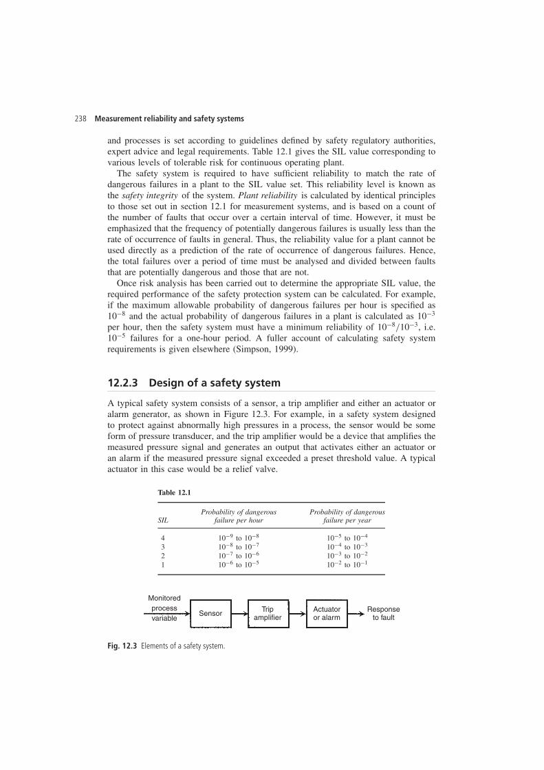
238 Measurement reliability and safety systems
and processes is set according to guidelines defined by safety regulatory authorities,expert advice and legal requirements. Table 12.1 gives the SIL value corresponding tovarious levels of tolerable risk for continuous operating plant.
The safety system is required to have sufficient reliability to match the rate ofdangerous failures in a plant to the SIL value set. This reliability level is known asthe safety integrity of the system. Plant reliability is calculated by identical principlesto those set out in section 12.1 for measurement systems, and is based on a count ofthe number of faults that occur over a certain interval of time. However, it must beemphasized that the frequency of potentially dangerous failures is usually less than therate of occurrence of faults in general. Thus, the reliability value for a plant cannot beused directly as a prediction of the rate of occurrence of dangerous failures. Hence,the total failures over a period of time must be analysed and divided between faultsthat are potentially dangerous and those that are not.
Once risk analysis has been carried out to determine the appropriate SIL value, therequired performance of the safety protection system can be calculated. For example,if the maximum allowable probability of dangerous failures per hour is specified as10�8 and the actual probability of dangerous failures in a plant is calculated as 10�3
per hour, then the safety system must have a minimum reliability of 10�8/10�3, i.e.10�5 failures for a one-hour period. A fuller account of calculating safety systemrequirements is given elsewhere (Simpson, 1999).
12.2.3 Design of a safety system
A typical safety system consists of a sensor, a trip amplifier and either an actuator oralarm generator, as shown in Figure 12.3. For example, in a safety system designedto protect against abnormally high pressures in a process, the sensor would be someform of pressure transducer, and the trip amplifier would be a device that amplifies themeasured pressure signal and generates an output that activates either an actuator oran alarm if the measured pressure signal exceeded a preset threshold value. A typicalactuator in this case would be a relief valve.
Table 12.1
Probability of dangerous Probability of dangerousSIL failure per hour failure per year
4 10�9 to 10�8 10�5 to 10�4
3 10�8 to 10�7 10�4 to 10�3
2 10�7 to 10�6 10�3 to 10�2
1 10�6 to 10�5 10�2 to 10�1
Monitoredprocessvariable
Sensor Tripamplifier
Actuatoror alarm
Responseto fault
Fig. 12.3 Elements of a safety system.
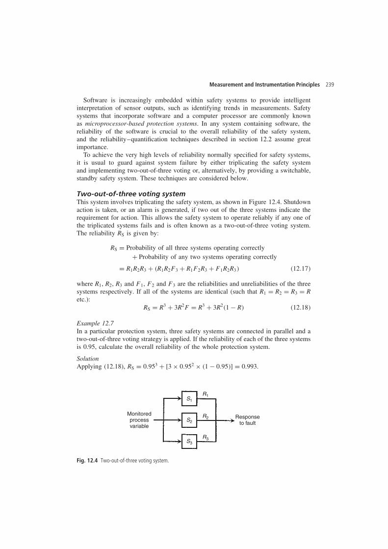
Measurement and Instrumentation Principles 239
Software is increasingly embedded within safety systems to provide intelligentinterpretation of sensor outputs, such as identifying trends in measurements. Safetysystems that incorporate software and a computer processor are commonly knownas microprocessor-based protection systems. In any system containing software, thereliability of the software is crucial to the overall reliability of the safety system,and the reliability–quantification techniques described in section 12.2 assume greatimportance.
To achieve the very high levels of reliability normally specified for safety systems,it is usual to guard against system failure by either triplicating the safety systemand implementing two-out-of-three voting or, alternatively, by providing a switchable,standby safety system. These techniques are considered below.
Two-out-of-three voting systemThis system involves triplicating the safety system, as shown in Figure 12.4. Shutdownaction is taken, or an alarm is generated, if two out of the three systems indicate therequirement for action. This allows the safety system to operate reliably if any one ofthe triplicated systems fails and is often known as a two-out-of-three voting system.The reliability RS is given by:
RS D Probability of all three systems operating correctlyC Probability of any two systems operating correctly
D R1R2R3 C �R1R2F3 C R1F2R3 C F1R2R3� �12.17�
where R1, R2, R3 and F1, F2 and F3 are the reliabilities and unreliabilities of the threesystems respectively. If all of the systems are identical (such that R1 D R2 D R3 D Retc.):
RS D R3 C 3R2F D R3 C 3R2�1 � R� �12.18�
Example 12.7In a particular protection system, three safety systems are connected in parallel and atwo-out-of-three voting strategy is applied. If the reliability of each of the three systemsis 0.95, calculate the overall reliability of the whole protection system.
SolutionApplying (12.18), RS D 0.953 C [3 ð 0.952 ð �1 � 0.95�] D 0.993.
Monitoredprocessvariable
Responseto fault
R1
R2
R3
S1
S2
S3
Fig. 12.4 Two-out-of-three voting system.
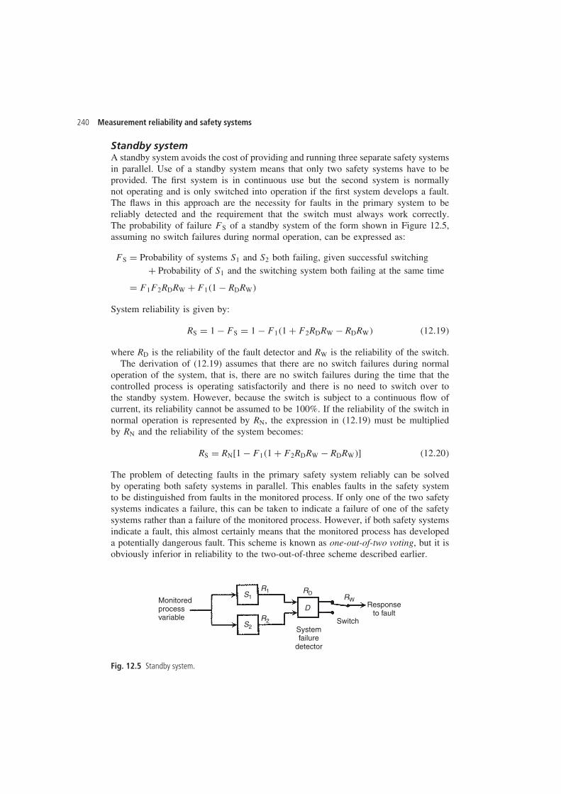
240 Measurement reliability and safety systems
Standby systemA standby system avoids the cost of providing and running three separate safety systemsin parallel. Use of a standby system means that only two safety systems have to beprovided. The first system is in continuous use but the second system is normallynot operating and is only switched into operation if the first system develops a fault.The flaws in this approach are the necessity for faults in the primary system to bereliably detected and the requirement that the switch must always work correctly.The probability of failure FS of a standby system of the form shown in Figure 12.5,assuming no switch failures during normal operation, can be expressed as:
FS D Probability of systems S1 and S2 both failing, given successful switchingC Probability of S1 and the switching system both failing at the same time
D F1F2RDRW C F1�1 � RDRW�
System reliability is given by:
RS D 1 � FS D 1 � F1�1 C F2RDRW � RDRW� �12.19�
where RD is the reliability of the fault detector and RW is the reliability of the switch.The derivation of (12.19) assumes that there are no switch failures during normal
operation of the system, that is, there are no switch failures during the time that thecontrolled process is operating satisfactorily and there is no need to switch over tothe standby system. However, because the switch is subject to a continuous flow ofcurrent, its reliability cannot be assumed to be 100%. If the reliability of the switch innormal operation is represented by RN, the expression in (12.19) must be multipliedby RN and the reliability of the system becomes:
RS D RN[1 � F1�1 C F2RDRW � RDRW�] �12.20�
The problem of detecting faults in the primary safety system reliably can be solvedby operating both safety systems in parallel. This enables faults in the safety systemto be distinguished from faults in the monitored process. If only one of the two safetysystems indicates a failure, this can be taken to indicate a failure of one of the safetysystems rather than a failure of the monitored process. However, if both safety systemsindicate a fault, this almost certainly means that the monitored process has developeda potentially dangerous fault. This scheme is known as one-out-of-two voting, but it isobviously inferior in reliability to the two-out-of-three scheme described earlier.
Monitoredprocessvariable
Systemfailure
detector
Switch
Responseto fault
S1
S2
R1 RDRW
R2
D
Fig. 12.5 Standby system.
Measurement and Instrumentation Principles 241
Example 12.8In a particular protection system, a switchable standby safety system is used to increasereliability. If the reliability of the main system is 0.95, that of the standby system is0.96Ł, that of the switching system is 0.95 and the reliability of the switch in normaloperation is 0.98, calculate the reliability of the protection system.
SolutionApplying (12.19), the parameter values are F1 D 0.05, F2 D 0.04, RDRW D 0.95.Hence:
RS D 0.98[1 � 0.05�1 C f0.04 ð 0.95g � 0.95�] D 0.976
Actuators and alarmsThe final element in a safety system is either an automatic actuator or an alarm thatrequires a human response. The reliability of the actuator can be calculated in thesame way as all other elements in the system and incorporated into the calculation ofthe overall system reliability as expressed in equations (12.17)–(12.20). However, thereliability of alarms cannot be quantified in the same manner. Therefore, safety systemreliability calculations have to exclude the alarm element. In consequence, the systemdesigner needs to take steps to maximize the probability that the human operator willtake the necessary response to alarms that indicate a dangerous plant condition.
Some useful guidelines for measurement technologists involved in designing alarmsystems are provided in a paper by Bransby (1999). A very important criterion insystem design is that alarms about dangerous conditions in plant must be much moreprominent than alarms about conditions that are not dangerous. Care should also betaken to ensure that the operator of a plant is not bombarded by too many alarms,as this leads the operator to get into the habit of ignoring alarms. Ignoring an alarmindicating that a fault is starting to occur may cause dangerous conditions in the plantto develop. Thus, alarms should be uncommon rather than routine, so that they attractthe attention of the plant operator. This ensures, as far as possible, that the operator willtake the proper action in response to an alarm about a potentially dangerous situation.
12.3 Self-test questions
1. The performance of a measuring instrument is monitored over a one-year (365-day)period and the intervals between faults being recorded are as follows:
27 6 18 41 54 29 46 14 49 38 17 26
Calculate the mean-time-between-failures.2. The days on which an instrument failed were recorded over a 12-month period as
follows (such that day 1 D 1 Jan, day 32 D 1 Feb etc.):
Day number of faults: 18 72 111 173 184 227 286 309 356
Calculate the mean-time-between-failures.
Ł Because the standby system is not subject to normal use, its reliability tends to be higher than the primarysystem even if the two systems consist of nominally identical components.
242 Measurement reliability and safety systems
3. A manufacturer monitors the performance of a new type of instrument that isinstalled at 20 different locations. If a total of nine faults are recorded over a100-day period, calculate the mean-time-between-failure that should be specifiedfor any one instrument.
4. If the mean-time-between-failure for an instrument is 247 days and the mean-time-to-repair is 3 days, calculate its availability.
5. If the mean-time-to-failure of an instrument is 100 000 hours, calculate the prob-ability that it will not fail in the first 50 000 hours.
6. If the mean-time-to-failure of an instrument is 100 000 hours, calculate the prob-ability that it will not fail in the first 5000 hours.
7. Four measurement components connected in series have the following reliabilities:0.98 0.93 0.95 0.99. Calculate the reliability of the whole measurement system.
8. In a particular measurement system, two instruments with individual reliability of0.95 are connected together in parallel. Calculate the reliability of the measurementsystem if it can continue to function as long as both of the instruments do not failat the same time.
9. Calculate the reliability of the measurement system shown in Figure 12.2(b) if the reli-abilities of the individual components are R1 D R3 D R5 D 0.98; R2 D R4 D 0.90.
10. In order to estimate the number of errors in a new piece of software by applyingthe error-seeding approach, a programmer puts ten deliberate (seeded) faults intothe program. A second programmer then tests the program and finds 27 errors, ofwhich eight are confirmed by the first programmer to be seeded errors. Estimatethe original number of faults in the program (i.e. excluding the seeded errors).
11. The double-testing approach is applied to test a new computer program and thetwo programmers who do the testing find 31 and 34 errors respectively. If 27 ofthe errors found by programmer 1 are the same as errors in the list produced byprogrammer 2, estimate the actual number of errors in the program.
12. A program is tested and the total number of errors is estimated as 16. The programis then seeded with 20 deliberate errors and further testing is then carried out untilall 20 seeded errors have been found.(a) If no new (previously undetected) errors are found during this further testing
to find all the seeded errors, calculate the probability that the program is errorfree after this further testing.
(b) How many seeded errors would have to be put into the program and thendetected to achieve a 98% probability that the program is error free?
13. Three safety systems are connected in parallel in a protection system and a two-out-of-three voting strategy is applied. If the reliability of each of the three systemsis 0.90, calculate the overall reliability of the whole protection system.
14. A switchable standby safety system is used to increase reliability in a protectionsystem. If the reliability of the main system is 0.90, that of the standby systemis 0.91, that of the switching system is 0.90 and the reliability of the switch innormal operation is 0.96, calculate the reliability of the protection system.
References and further reading
Bahr, M.J. (1997) System Safety: A Practical Approach, Taylor and Francis.Barnand, M.J. (1998) Health and Safety for Engineers, Thomas Telford.

Measurement and Instrumentation Principles 243
Bransby, M. (1999) The human contribution to safety – designing alarm systems, Measurementand Control, 32, pp. 209–213.
BS 7165 (1991) Recommendations for the achievement of quality in software, British StandardsInstitute.
Cluley, J.C. (1993) Reliability in Instrumentation and Control, Butterworth-Heinemann.Dean, S. (1999) IEC61508 – understanding functional safety assessment, Measurement and
Control, 32, pp. 201–204.Dhillon, B.S. and Singh, C. (1981) Engineering Reliability: New Techniques and Applications,
Wiley.Fenton, N.E. (1991) Software Metrics: A Rigorous Approach, Chapman and Hall.IEC61508 (1991) Functional safety of electrical, electronic and programmable-electronic safety
related systems, International Electrotechnical Commission, Geneva.ISO 9000-3 (1991) International Organization for Standards, Geneva.Mather, R.N. (1987) Methodology for business system development, IEEE Trans Software Eng.,
13(5), pp. 593–601.Miller, I.R., Freund, J.E. and Johnson, R. (1990) Probability and Statistics for Engineers, Pren-
tice Hall.Mills, H.D. (1972) On the Statistical Validation of Computer Programs, IBM Federal Systems
Division, Maryland.Morris, A.S. (1997) Measurement and Calibration Requirements for Quality Assurance to
ISO9000, John Wiley.Pfleeger, S.L. (1987) Software Engineering: The Production of Quality Software, Macmillan.Shooman, M.L. (1983) Software Engineering: Design, Reliability and Management, McGraw-
Hill.Simpson, K. and Smith, D.J. (1999) Assessing safety related systems and architectures,
Measurement and Control, 32, pp. 205–208.Thomson, J.R. (1987) Engineering Safety Assessment – An Introduction, Longman.
Related Documents