“Resource Sharing between Centre and States and Allocation across States: Some Issues in Balancing Equity and Efficiency” INSTITUTE OF ECONOMIC GROWTH, DELHI DRAFT REPORT July, 2019 A Study prepared for The Fifteenth Finance Commission of India

Welcome message from author
This document is posted to help you gain knowledge. Please leave a comment to let me know what you think about it! Share it to your friends and learn new things together.
Transcript

“Resource Sharing between Centre and States and Allocation across States:
Some Issues in Balancing Equity and Efficiency”
INSTITUTE OF ECONOMIC GROWTH, DELHI
DRAFT REPORT
July, 2019
A Study prepared for
The Fifteenth Finance Commission of India


Study Team:
Principal Investigator: Manoj Panda
Email: [email protected]
Co-PI: Purnamita Dasgupta, William Joe
Senior Consultant: M N Murty
Research Analysts: Kavitha Srikanth, Abhay Kumar

Draft Report of Study for 15th Finance Commission Institute of Economic Growth, July 2019
1
Resource Sharing between Centre and States and Allocation across States:
Some Issues in Balancing Equity and Efficiency
Chapter 1: Rationale and Review of devolution by Finance Commissions
1.1. Introduction: The Rationale for Devolution of Resources in India
The constitution of India provides for decentralization of revenue and expenditure at two levels
of the Federation, the Union and the States. It specifies the revenue raising power and areas of
expenditure broadly on considerations of efficiency based on comparative advantage of the
governments at the two levels. An imbalance arises in this process since the Union (Central)
government is assigned most of revenue raising power while the State governments are expected
to carry out most of the development and welfare oriented expenditure. Hence, the constitution
provides for devolution of part of the union revenue to the states.
Fiscal imbalance at different level of government is a common feature in many federal
countries1, the lower level of governments are generally confronted with inadequate resources
for meeting their expenditure needs. In the Indian case, the Centre has the authority2 to decide on
broad based and buoyant taxes such as income tax, corporation tax and excise duties while the
states have the authority on items like sales tax, stamp duties, entertainment tax, and land
revenue most of which are not as buoyant. In terms of expenditure decentralization, the central
government is entrusted with the responsibilities of provision of nationally important areas like
defence, foreign affairs, foreign trade and exchange management, money and banking, cross-
state transport and communication. The state governments are given the responsibility of
facilitating agriculture and industry, providing social sector services such as health and
education, police protection, state roads and infrastructure. The third level local self-governments
1 See Boadway & Shah. Edited (2007) for detailed discussion about theory and practice of fiscal federalism.
2 The Seventh Schedule of the constitution of India spells out the details of the areas of power and responsibilities
under Central, State and Concurrent lists.
Draft Report of Study for 15th Finance Commission Institute of Economic Growth, July 2019
2
– municipalities and panchayats3 -provide public utility services such as water supply and
sanitation, local roads, electricity etc. In addition, both central and state governments are
responsible for provisioning services in the concurrent list. The resultant vertical fiscal gap,
which also occurs in India, necessitates intergovernmental revenue transfer. The observed
imbalance is not entirely due to revenue instruments and functions assigned in the constitution,
but it is partly an outcome of fiscal choices exercised by different levels of government in
practice.
Revenue decentralization results in the sharing of revenue raising powers and the use of
instruments, especially various types of taxes, by different levels of government. The Indian
government has been undertaking tax reforms on continuous basis aimed at increasing the tax
base of both direct and indirect taxes, reduction in tax evasion and a resultant increase in the
revenues of both state and central governments. The Central government has greater revenue
raising powers in India, keeping in view considerations such as administrative efficiency in
collecting taxes with a nationwide base. However, expenditure decentralization gives freedom to
states to spend according to state specific needs given the huge diversity in preferences of
citizens in different states and in levels of their economic and social development.
The possibility of fiscal imbalance is well recognised in the Indian Constitution which provides
for an institutional mechanism to tackle the imbalance in the form of the Finance Commission
(FC) which makes recommendations on the magnitude of transfer of resources from the Centre
to the states for a period of 5 years. The Constitution stipulates the primary terms of reference
(ToR) of the FCs: (a) distribution of net proceeds of Union divisible taxes between Union and
States and among states inter-se, (article 280) (b) grants in aid from Union revenue to be given to
states. A third ToR, has been added later after the 73rd
and 74th
Constitutional Amendments in
1992 which relates to recommendation of measures needed to augment the consolidated funds of
States to supplement resources for rural and urban local governments in the States based on
recommendations of the State Finance Commissions. Besides, the President may include
additional ToR for the FC on any other matter in the interest of sound finance of the
3 The third level of local self-government bodies receive grants from their respective state governments. The 13
th
and 14th
Finance Commissions have provision for earmarked grants for the local bodies apart from tax devolution to
states.

Draft Report of Study for 15th Finance Commission Institute of Economic Growth, July 2019
3
governments. These additional matters are normally context specific and vary from one FC to
another. While the tax devolution and grants recommended by FC forms bulk of Central
transfers to states, it may also be noted that transfers from Union to States are not limited to FC
recommendations. Other channels include specific purpose transfers by Central Ministries and
grants transferred earlier by the erstwhile Planning Commission.
The FC has been recommending transfers under two heads for a period of 5 years. First, it
recommends tax devolutions which are general purpose transfer without being earmarked for
expenditure in any specific area and are specified as a percentage of sharable tax revenue.
Second, it states the principles governing grants in aid and recommends amount of specific
purpose grants. The Centre has generally accepted the recommendations of the FCs4.
It may be noted that the FC interacts with Central Ministries, state governments, industrial and
business bodies, academicians and several other stakeholders during the course of its
deliberations. Individual states and several central ministries provide their opinion and
suggestions to the Finance Commission. In making transfers, the FCs consider issues related to
vertical equity (deciding about the share of all states in the revenue collected by centre) and
horizontal equity (allocation among states their share of central revenue). The horizontal
transfers, distribution of funds meant for states, depends on criteria adopted by specific FCs and
has varied over time. These have been discussed in more details in later sections of the report.
This study relates to some issues in resource sharing between Centre and states and allocation
across states. The specific Terms of Reference of the study are:
1. Review of the approach and recommendations of the various Finance Commissions with
respect to vertical and horizontal devolution of resources
2. Describe the trends and changing patterns in vertical devolution by focusing on the
revenue and expenditure of the Union and the States
3. Summarize the trends and patterns in horizontal fiscal devolutions across states along
with states’ own effort to raise resources and maintain fiscal discipline
4 One exception is noted in the following section.

Draft Report of Study for 15th Finance Commission Institute of Economic Growth, July 2019
4
4. Analysis of major factors affecting the horizontal and vertical devolution trends
5. Understand the current status on key fiscal parameters related to the resource allocation
between Centre and states and further across states
6. Highlight the major emerging concerns in resource devolution with specific reference to
merits and demerits of criteria used for vertical and horizontal balances
In keeping with the overall objective of the report to examine alternative approaches to
understand vertical fiscal imbalances and degree of equalization in the light of current status and
recent trends the report is organised as follows. The rest of Chapter 1 provides a review of the
recommendations by various FCs, especially the last four with respect to vertical and horizontal
devolution in India. Chapters 2 and 3 discuss trends and changing patterns in vertical devolution
and horizontal devolution respectively. Chapter 4 provides an analysis of factors affecting the
vertical and horizontal devolution. Chapter 5 describes the current status on key fiscal parameters
related to resource allocation. Chapter 6 relates to some emerging concerns about vertical and
horizontal devolution. Chapter 7 provides summary and recommendations.
Besides analysis of issues and trends in revenue and expenditure of centre and states, we
highlight some specific focus points of investigation in this study as follows:
1) Population stabilization: The recommendations of the FCs for horizontal distribution
across states generally use the size of the population in deciding the magnitude of
transfers to states. The ToR of the 15th
FC mandates the Commission to use 2011
population for this purpose. At the same time, the ToR 4(ii) refers to a measurable
performance based incentives for States in respect of efforts and progress made in
moving towards replacement rate of population growth. In Chapter 6, we propose an
indicator of population stabilisation to devise a performance based incentive structure for
the states. Such indicators could either be used as a component of considerations of
horizontal equity to offset any disadvantage faced by states which have moved towards
population stabilization or could be part of the transfer through a grant mechanism.
2) Environment: The 14 FC brought in dense forest cover as a criteria determining
horizontal devolution. A re-look is taken at the formulation, in keeping with the TOR of
the 15 FC. The TOR mentions in 3(ii) resource demands for climate change, among other

Draft Report of Study for 15th Finance Commission Institute of Economic Growth, July 2019
5
factors and in ToR 4(iii), sustainable development goals. In this context, data based
analysis is done to examine the implications for states under varying scenarios, both for
inclusion in the formula or as a conditional grant. There is a need to expand the coverage
beyond dense cover in order to address the intent to compensate for fiscal disability while
performance based indicators can incentivize states and contribute towards the
international environmental commitments
3) Inequality: The rising inter-state inequality in recent decades might require some
consideration of non-linearity in the income distance formula to give more weight to
states at the bottom end of the income scale. One way of doing it is to introduce an
inequality aversion parameter. We show alternative weights for horizontal devolution
based on linear and non-linear considerations.
4) Social sector expenditure: Another questions we examine is whether social sector
expenditure is responsive to increase in both NSDP and general purpose devolution. Our
findings show that specific central transfers may not be required to meet the social sector
expenditures. Specific transfers can be designed for meeting specific national objectives
other than those covered under existing social sector expenditure or where there are
major inter-state implications.
.

Draft Report of Study for 15th Finance Commission Institute of Economic Growth, July 2019
6
1.2: Review of the approach and recommendations of the various Finance Commissions
with respect to vertical and horizontal devolution of resources (TOR I)
1.2.1 Vertical Equity and Approaches of Recent Finances Commissions of India
As stated above, origin of vertical imbalance lies in assignment of revenue generating powers
and functional responsibilities to Union and States on the basis of comparative advantage. The
Union government generally collects 60-68% of combined revenue receipts due to buoyant and
broad based taxes assigned to it and the states together collect the balance. The revenue
expenditure of the states, on the other hand, has been in the range 50-60% of the combined
revenue expenditure. The approaches followed by various FCs to bridge the above imbalance
have been evolutionary drawing upon those of the previous ones.
Different FCs have approached the issue of providing vertical balance taking into considerations
various factors that include assessment of fiscal balances of Centre and States, merits of
devolution and transfer, possible laxity on gap filling approach, types of expenditure,
constitutional amendments carried out by the Parliament, and the overall need to maintain
stability in the fiscal system. We discuss below under a few heads how these issues have been
approached by the FCs, particularly the recent ones.
Assessment of Need
The 1st FC set the tone of general procedure of seeking information and views of Centre and the
states, industry bodies, academics and other stakeholders and this procedure has been followed
by successive commissions. It assessed the needs of the states and Centre’s capacity to
accommodate assistance even as it meets its own need. In this process, the Commission’s
assessment regarding priority for expenditure need of the Centre and States finally gets reflected
in its recommendations. While states needed more resources for meeting their expanded
responsibilities for welfare and development of the citizens, the Centre was responsible for
services important at the national level. Thus, ability of the Centre to assist was an important
factor to be considered.

Draft Report of Study for 15th Finance Commission Institute of Economic Growth, July 2019
7
The 6th
FC (award period 1976-79) observation that “when the emphasis is on social justice,
there is no escape from the realignment of resources in favour of the states because services and
programmes which are at the core of a more equitable social order come within the purview of
the states in the Constitution.
The 14 FC stated that two main issues to assessing the vertical imbalance were “a realistic
estimation of revenue accruing solely to the Union as well as its expenditure needs and the
resources required to meet its obligations under the Constitution” and “a realistic assessment of
the revenue capacities of the States and the expenditures required to meet obligations mandated
under the Constitution.” It mentioned that the States had argued that “functional overlap has led
to an increase in the Union Government’s expenditure and a concomitant reduction in the
revenues available for vertical devolution.”
Given that the need for vertical transfers arise from the asymmetric assignment of revenue
collection and expenditure responsibility, Finance Commissions have used their own normative
assessment of vertical imbalance. Exact quantification of the imbalance is not only difficult,
there has been no attempt to do so. In the final analysis, magnitude of vertical imbalance depends
on subjective judgement of the Commission and the feedback it receives from the stakeholders.
Nevertheless, successive commissions have attempted to strike a balance between the demands
of Centre and States with a great degree of success
Tax Effort and Buoyancy
The 3rd
FC noted increasing dependence of states on Centre and laxity in raising resources on the
belief that gaps will be filled by the Centre. The 9th
FC advocated for phasing out of revenue
deficit and tried to promote fiscal responsibility for both Centre and States. In this context, we
may note the view of Reddy and Reddy (2019) who state that while norms proposed by the FCs
are not so difficult to impose on the States, there is no agency to impose such norms on the
Centre.
Several FCs have noted the differential tax buoyancy of the Centre and the states. This was an
important consideration for the 12th
FC which argued for increasing the share of states without
directly stating what portion of the change may be attributed to this factor. Srivastava (2010)

Draft Report of Study for 15th Finance Commission Institute of Economic Growth, July 2019
8
estimated that the Central tax buoyancy was 1.559 compared to 1.212 for combined own taxes of
the states during the 2004-05 to 2008-09. He justified a 1.5 percentage point increase in the share
of the states by the 12th
FC on the basis of the product of GDP growth rate and difference in
central tax buoyancy over that of states.
The 13th
FC felt that “vertical devolution must be informed by the revenue-raising capacity of the
Centre and states as well as emerging pressures on their expenditure commitments.” The 13th
FC
also observed that the “buoyancy of central taxes at 1.49 was higher than states (1.18) during the
period 2000-08 and that there are reasons to believe that the Centre’s revenue buoyancy will
continue to remain higher than that of States”. In addition, the 13th
FC noted that “the share of
states after transfers will be constant only if their share in central taxes is increased by a margin
by which the buoyancy of central taxes exceeds the buoyancy of combined tax revenue.” The
13th
FC recommended 32% as the share of tax devolution as against 30.5% by 12th
FC (Table
1.1).
Plan and Non-Plan Expenditure
There was also a debate on the authority to decide the quantum of plan expenditure. The 3rd
FC
made recommendation by majority opinion on part the plan expenditure of states leaving the
balance to Planning Commission. The Government of India rejected the majority view5 and
accepted the minority view of the Member-Secretary that entire plan expenditure should be
assessed by the Planning Commission. Thereafter, the ToR of 4th
to 13th
(except the 11th
) FCs
was restricted to non-plan expenditure requirement only. The 14th
FC assessed the total revenue
expenditure need due to abolition of plan and non-plan expenditure categorization.
Kelkar (2019) states that Finance Commission was given the task of allocating resources for
dealing with provision of different levels per capita consumption of basic public goods and
services across states, while the erstwhile Planning Commission was supposed to allocate
resources for meeting physical and social infrastructure crucial for growth. It was recognized at
times that resource availability for basic public goods and economic growth was interlinked. For
5 This is one exception in recommendations of the FCs that has not been accepted by the government.
Draft Report of Study for 15th Finance Commission Institute of Economic Growth, July 2019
9
instance, 10th
FC ToR included generation of surplus on revenue account for capital investment.
But, FCs generally confined themselves to revenue resources and revenue expenditure.
Devolution and Grants
Devolution or general purpose transfer are “given to enable states to provide comparable levels
of public services at comparable tax effort and specific purpose transfers are given to ensure a
minimum standard of public services” (Rao, 2019).
The 1st FC was of the view that tax devolution should be the primary means of transfer and that
grants in aid should be only residual form of assistance for considerations not reflected in the
devolution. While the above approach has generally been adopted by other FCs, there have also
been several important differences. The 2nd
FC, for example, observed that grants in aid should
be general and unconditional, but several other commissions have not viewed grants as
unconditional.
The 12th FC said that “if the share of states is increased, the redistributive content in the inter se
distribution will have to be increased significantly by altering the weights among the distribution
criteria so as to be consistent with the equalization objective.” It agreed that grants were a better
mechanism for this purpose and hence mentioned that they had used grants to a larger extent as
an instrument for these transfers. Srivastava (2010) too states: “The higher the vertical share of
the states, the lower the weight to the equalizing component of tax revenue sharing, as with
distance formula for horizontal distribution.” This implies that horizontal distribution is not
independent of the vertical distribution.
The 14th
FC, like its predecessors, was also of the view that tax devolution should be the primary
route of transfer of resources to States “since it is formula based and hence conducive to sound
fiscal federalism.” Additionally, the 14th
FC stated that where the formula-based transfers did not
meet the States’ needs, grants-in-aids must be given on an assured basis and in a fair manner.
The 14th
FC also believed that a compositional shift in transfers from grants to tax devolution
was desirable for two reasons: (a) it did not impose an additional fiscal burden on the Union
Draft Report of Study for 15th Finance Commission Institute of Economic Growth, July 2019
10
Government, and (b) an increase in tax devolution would enhance the share of unconditional
transfers to the States.
Constitutional Amendments
The approaches of FCs have also been influenced by amendments regarding sharable pool of
taxes. The first ten FCs based their recommendations on the mandatary provision of Article 270
regarding sharing net proceeds of income tax and the enabling provision of Article 272 regarding
permissible sharing of Union excise duties, ‘if Parliament by law so provided’. The first FC
recommended 40% of Union excise duties collected from 3 commodities of common and
widespread consumption (tobacco, matches and vegetable products). Subsequent three FCs
found states resources to be inadequate to meet expenditures and expanded the list of items of
Union excise duties for sharable revenue. The 4th
FC felt the need to share all Union excise
duties with the states. The proportions of revenue from income tax and Union excise duties to be
shared varied from time to time. For example, the 1st FC recommended 55% of income tax to be
shared and the percentage rose to 85% by the 7th
FC (see, Table 1.1). Finally, 10th
FC
recommended that states should have the benefit of buoyancy of all Central taxes and greater
certainty in resource flow. Consequently, 80th
amendment was introduced in the constitution in
2000 to include Central taxes on all goods and services, except cesses and surcharges, in the
divisible pool.
States, however, have been demanding to include cesses and surcharges in the divisible pool.
The 14th
FC also noted that it was not appropriate to amend the constitution to include the non-
divisible pool of resources (cesses and surcharges) given the experience so far and said the
alternate option to addressing this concern of the states of including cesses and surcharges as part
of the devolution was to compensate States by increasing the share of the divisible pool.
Continuity with Change
FCs attempt to make an overall fiscal assessment of the Union and States examining trends in
revenues and expenditure through a series of interactions. While important changes on scope and

Draft Report of Study for 15th Finance Commission Institute of Economic Growth, July 2019
11
design as noted above have occurred over time, there have also been medium run stability on the
quantum of transfers relative to total revenue or size of the economy. The 11th
FC, for example,
noted that the share of States in the net proceeds of all Union Taxes and duties fluctuated
between 26.3% and 31.59% and it recommended that States get 29.5% of the gross revenue.
The 14th
FC stated that they considered four considerations and then decided to increase the
share of tax devolution to 42% which they believed would “serve the twin objectives of
increasing the flow of unconditional transfers to the States and yet leave appropriate fiscal space
for the Union to carry out specific-purpose transfers to the States.” The considerations were: (i)
States not being entitled to the growing share of cesses and surcharges in the revenues of the
Union Government; (ii) the importance of increasing the share of tax devolution in total
transfers; (iii) an aggregate view of the revenue expenditure needs of States without plan and
non-plan distinction; and (iv) the space available with the Union Government. In view of these
considerations, it increased the share of tax devolution to 42% as against 32% recommended by
13th
FC. This big jump is, however, not comparable since the ToR of the 14th
FC did not
distinguish plan and non-plan components of revenue expenditure. The increase on a comparable
basis was only 3% from 39% to 42% (Rao, 2017).
Overall, FCs have not attempted to change the prevailing shares substantially and have used
recommendations of previous 2 or 3 FCs as a benchmark to begin with. The changes brought in
by a commission over its predecessors may well be described as incremental based on
considerations of intervening macroeconomic developments and demand of the states and the
Centre. Like the 14th
FC, some of them have also introduced substantial compositional changes.
The broad approach has been to maintain overall stability in share of centre and states in the
combined revenue receipt. The 13th
FC explicitly stated this as a desirable factor. Yet, as we
discuss in the following chapter, the cumulative effect of incremental changes by various
commissions do sum up to a substantial shift in favour of the states resulting in doubling of the
devolution as a percentage of gross tax revenue of the centre.

Draft Report of Study for 15th Finance Commission Institute of Economic Growth, July 2019
12
Table 1.1 Vertical Distribution: States Share in Divisible Pool of Central taxes
Finance Commission
States Share in the Net Proceeds of
Income Tax
(%)
Union Excise
Duties (%)
All Shareable
Union Taxes
(%)
FC-1 (1952-57) 55 40
FC-2(1957-62) 60 25
FC-3(1962-66) 66.66 20
FC-4(1966-69) 75 20
FC-5(1969-74) 75 20
FC-6(1974-79) 80 20
FC-7(1979-84) 85 40
FC-8(1984-89) 85 45
FC-9-I(1989-90) 85 40
FC-9-II(1990-95) 85 45
FC-10(1995-00) 77.5 47.5
FC-11(2000-05) 29.5
FC-12(2005-10)
30.5
FC-13(2010-15)
32
FC-14(2015-20) 42 Source: Gupta and Sarma (2019)
1.2.2 Horizontal Equity and Approaches of Recent Finance Commissions in India
Population has been the dominant factor in determining horizontal devolution, i.e. share of each
state in the total amount to be distributed amongst all states. In a sense, the need of a state for
comparable level of welfare oriented government service gets determined by the size of the
state’s population. The weight assigned to population has, however, varied from one commission
to another. Other factors considered by the FCs included backwardness, income, area,
infrastructure, contribution to central pool, tax effort, fiscal discipline and so on. A detailed
description of the factors considered and weights used by all the FCs is available in Reddy and
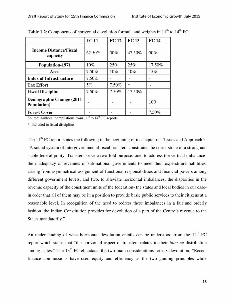
Reddy (2019). Table 1.2 below gives the criteria and weights for the last four FCs.
Draft Report of Study for 15th Finance Commission Institute of Economic Growth, July 2019
13
Table 1.2: Components of horizontal devolution formula and weights in 11th
to 14th
FC
FC 11 FC 12 FC 13 FC 14
Income Distance/Fiscal
capacity 62.50% 50% 47.50% 50%
Population-1971 10% 25% 25% 17.50%
Area 7.50% 10% 10% 15%
Index of Infrastructure 7.50% - - -
Tax Effort 5% 7.50% * -
Fiscal Discipline 7.50% 7.50% 17.50% -
Demographic Change (2011
Population) - - - 10%
Forest Cover - - - 7.50%
Source: Authors’ compilations from 11th
to 14th
FC reports
*: Included in fiscal discipline
The 11th
FC report states the following in the beginning of its chapter on “Issues and Approach’:
“A sound system of intergovernmental fiscal transfers constitutes the cornerstone of a strong and
stable federal polity. Transfers serve a two-fold purpose: one, to address the vertical imbalance-
the inadequacy of revenues of sub-national governments to meet their expenditure liabilities,
arising from asymmetrical assignment of functional responsibilities and financial powers among
different government levels, and two, to alleviate horizontal imbalances, the disparities in the
revenue capacity of the constituent units of the federation- the states and local bodies in our case-
in order that all of them may be in a position to provide basic public services to their citizens at a
reasonable level. In recognition of the need to redress these imbalances in a fair and orderly
fashion, the Indian Constitution provides for devolution of a part of the Centre’s revenue to the
States mandatorily.”
An understanding of what horizontal devolution entails can be understood from the 12th
FC
report which states that “the horizontal aspect of transfers relates to their inter se distribution
among states.” The 13th
FC elucidates the two main considerations for tax devolution: “Recent
finance commissions have used equity and efficiency as the two guiding principles while

Draft Report of Study for 15th Finance Commission Institute of Economic Growth, July 2019
14
recommending inter se shares of states in tax devolution”. The 11th
FC, 12th
FC and 14th
FC have
also considered equity and efficiency as the principles guiding devolution.
The 11th
FC mentions that “the principle of horizontal equity is guided by the consideration that,
as a result of revenue sharing, the resource deficiencies across States arising out of systemic and
identifiable factors are evened out”. The 11th
FC observed that since the principle of equity
makes up for resource deficiencies, it would tend to create a vested interest in continuing with
such deficiencies. Hence, the 11th
FC believed and mentioned that the principle of efficiency was
intended to neutralize the adverse incentive by rewarding of efforts to improve the resource bases
and to deliver services at minimum (efficient) costs.
In terms of decisions regarding balancing of equity with efficiency considerations, the 12th
FC
specifically expressed the view that although they had tried to balance equity with fiscal
efficiency in the construction of the formula, they were of the belief that equity considerations
should dominate in any scheme of fiscal transfers trying to implement the principle of
equalization.
The principle of equity according to and mentioned in the 13th
FC was to “address problems of
differences in revenue raising capacity and cost disabilities across states”. The principle of
efficiency according to and mentioned in the 13th
FC was intended to address the possible risk of
moral hazard arising due to assessing capacity on the basis of observed revenue collected. The
principle of efficiency according to and mentioned in the 13th
FC was to “motivate the states to
exploit their resource base and manage their fiscal operations in a cost-effective manner.”
While the 14th
FC did not seem to explicitly mention an exact definition for equity and
efficiency, it mentioned that “the devolution formula must be defined in such a way that it
attempts to mitigate the impact of the differences in fiscal capacity and cost disability among
states.”
The objective of horizontal equity according to and mentioned in the 11th
FC was to “help states
iron out resource deficiencies that arise due to systemic and identifiable factors.” The 13th
FC
Draft Report of Study for 15th Finance Commission Institute of Economic Growth, July 2019
15
expressed a more specific intent of the equity component that it should “ensure that all states
have the fiscal potential to provide comparable levels of public services to their residents, at
reasonably comparable levels of taxation.” The equity component was considered justified for
the 13th
FC not merely just for ensuring equal treatment of citizens by governments, but also for
reasons of economic efficiency so as to minimize fiscally-induced migration. The 13th
FC further
noted that the equity component by itself does not ensure the achievement of common standards
in quality or outcomes in public services and that for common standards to be achieved, the
comparable level of tax effort assumed to hold across states must actually prevail in each state
and the efficiency in delivery should be considerably uniform.
Both the 11th
FC and the 13th
FC brought up the issue relating to the design of incentive-based
criteria. The 11th
FC asked whether the incentive-based criteria should be dynamically related to
future achievements or related only to achievements which were already accomplished. The 13th
FC mentioned the same issue of choosing between criteria that was forward looking or criteria
based on past trends. Although dynamic incentives help modify future behavior according to the
11th
FC, it mentioned that if relevant data would become available only over a passage of time,
the FC would be unable to determine the actual shares of states. The 13th
FC also claimed that
forward looking indicators were better, but it noted that the FC would be unable to determine the
actual shares of states since it was not a permanent body. The 11th
FC stated that “Because of
operational difficulties and in the interest of certainty of the relative shares of States in the tax
devolution during the period of our recommendation, we do not consider it feasible or desirable
to build any incentives that may change from the quantum of devolution for a State from year to
year.”
Draft Report of Study for 15th Finance Commission Institute of Economic Growth, July 2019
16
Draft Report of Study for 15th Finance Commission Institute of Economic Growth, July 2019
17
Chapter 2: Trends and Patterns in Vertical Devolution
(TOR 2: Describe the trends and changing patterns in vertical devolution by focusing on
the revenue and expenditure of the Union and the States)
2.1 Revenue shares of Centre and States
We begin with a look at the long term trend in tax-GDP ratio in India during 1952-20186. In the
early 1950s, the combined tax collection by the Centre and the States was as low as 6% of GDP
reflecting very low level of average standard of living prevailing then. As industry and service
sectors expanded, the taxes in relation to GDP rose steadily and doubled by mid-1970s. As
Figure 2.1 shows the tax-GDP ratio fluctuated in a close interval of 14-15% for 25 long years till
2004-05, and rose slowly thereafter to reach 17.8% in 2014-15 and 18.2% in 2018-19 (RE). It is
recognized in several quarters that India’s tax-GDP ratio is low in comparison to its peer group7
and needs to be raised by 3-4 percentage points to meet increasing demand for public services.
The near stagnancy in tax-GDP ratio at a low level for several decades means that the Union and
State governments in India have limited fiscal space.
The Central government collected about 60-65% of the total revenue during the 1950s. Its share
rose to 70% during mid-1960s, but fell later to reach 60% in 2001-02. It again rose reaching 68%
in 2007-08 and dropped to 65% in 2018-19 (Figure 2.2). The remaining 30-40% of taxes relate to
states’ own taxes collected by them together. The share of states’ own taxes in combined tax
revenue of Centre and states was above 35% during mid-1950s, came down to remain between
30 and 35% till early 1990s, but rose subsequently reaching 39% in 2014-15 but coming down
again to 35% in 2018-19. Thus, there have been periods when the states have made more efforts
6 We use data for the period 1952 to 2014 from Indian Public Finance Statistics (IPFS) published by Ministry of
Finance supplanted by Economic Survey 2018-19 and Union Budget 2019-20 for later years. One difficulty is that
data on the share of the states in Central revenue in ES differ somewhat from that of IPFS presumably due to
coverage differences. For example, the share of states in IPFS is 2.0 to 3.9% higher than those in ES during 2010-11
and 2014-15. Hence, we have taken the annual growth rates since 2015-16 from ES and applied them on 2014-15
IPFS data so that the entire data series is on a comparable footing to the extent possible. 7 Tax-GDP ratio varies widely across countries depending on other sources of revenue available and functional
responsibilities expected from the government regarding welfare measures. It is, for example, about 20% for China
and Russia, 28% for Australia and South Africa, 32-34% for Brazil, Canada, Korea, US and UK.

Draft Report of Study for 15th Finance Commission Institute of Economic Growth, July 2019
18
to raise their own taxes as during 2007 and 2014. More recently, the tax revenue of the Centre
rose from 10.9% of GDP in 2014-15 to 11.8% in 2018-19 (RE), while states’ own tax revenue
dropped by 0.5% to 6.4% during the same period.
Figure 2.1. Tax-GDP Ratios of Centre and States 1952-2018 (%)
Sources: Based on Data from Indian Public Finance Statistics till 2014-15, Economic Survey and Union Budget for
later years.
Of the tax revenue collected by it, the Centre has been passing on a substantial portion to the
states based on recommendations of the Finance Commissions. The share of states in Central
taxes would differ from the FC recommendations since the latter applies to ‘divisible pool’
comprising of total central taxes excluding revenue from cesses and surcharges, cost of
collection, and certain earmarked taxes. This share rose from around 15% in mid-1950s to above
25% by late 1970s and mostly fluctuated between 26% and 29% later till 2014-15, but rose to
34-37% more recently (Figure 2.3). Looking at another way as a percentage of GDP, states’
share in Central taxes jumped from 3% of GDP in 2014-15 to 3.7% in 2015-16, rose further to
4% in 2016-17and remain around this level in the following 2 years. Thus, the recommendations
of the 14th
FC has meant an additional devolution of close to 1% of GDP in the first 4 years of
the award period.
0.0
2.0
4.0
6.0
8.0
10.0
12.0
14.0
16.0
18.0
20.0
19
52
-53
19
54
-55
19
56
-57
19
58
-59
19
60
-61
19
62
-63
19
64
-65
19
66
-67
19
68
-69
19
70
-71
19
72
-73
19
74
-75
19
76
-77
19
78
-79
19
80
-81
19
82
-83
19
84
-85
19
86
-87
19
88
-89
19
90
-91
19
92
-93
19
94
-95
19
96
-97
19
98
-99
20
00
-01
20
02
-03
20
04
-05
20
06
-07
20
08
-09
20
10
-11
20
12
-13
20
14
-15
20
16
-17
20
18
-19
(RE
)
Centre taxes (pre-devolution) States' own taxes Combined taxes

Draft Report of Study for 15th Finance Commission Institute of Economic Growth, July 2019
19
Figure 2.2. Central and States’ Share in Combined Tax Revenue 1952-2018 (before transfer to
States)
Source: Based on Data from Indian Public Finance Statistics
Figure 2.3. Share of States in Central Tax Revenue 1952-2018 (%)
Source: Based on Data from Indian Public Finance Statistics
Impact of Devolution
Now, in order to understand the quantitative dimension of the role of the FC recommendations in
vertical equity in recent years, revenue shares of centre and states can be compared under two
alternative scenarios: a scenario without central transfers (as in Figure 2.2 above) and another
scenario with central transfers (Figure 2.4 below). Given that the states have a constitutional
20.0
30.0
40.0
50.0
60.0
70.0
80.0
19
52
-53
19
54
-55
19
56
-57
19
58
-59
19
60
-61
19
62
-63
19
64
-65
19
66
-67
19
68
-69
19
70
-71
19
72
-73
19
74
-75
19
76
-77
19
78
-79
19
80
-81
19
82
-83
19
84
-85
19
86
-87
19
88
-89
19
90
-91
19
92
-93
19
94
-95
19
96
-97
19
98
-99
20
00
-01
20
02
-03
20
04
-05
20
06
-07
20
08
-09
20
10
-11
20
12
-13
20
14
-15
20
16
-17
20
18
-19
(RE
)
Central and States Share before Transfer in Tax Revenue
Centre State
0.0
5.0
10.0
15.0
20.0
25.0
30.0
35.0
40.0
19
52
-53
19
54
-55
19
56
-57
19
58
-59
19
60
-61
19
62
-63
19
64
-65
19
66
-67
19
68
-69
19
70
-71
19
72
-73
19
74
-75
19
76
-77
19
78
-79
19
80
-81
19
82
-83
19
84
-85
19
86
-87
19
88
-89
19
90
-91
19
92
-93
19
94
-95
19
96
-97
19
98
-99
20
00
-01
20
02
-03
20
04
-05
20
06
-07
20
08
-09
20
10
-11
20
12
-13
20
14
-15
20
16
-17
20
18
-19
(RE
)
States' share in Central taxes (% of Central Taxes)

Draft Report of Study for 15th Finance Commission Institute of Economic Growth, July 2019
20
right to use the revenue they collect, a comparison of these scenarios can reveal the impact of
vertical devolution from centre to states. An examination of these two scenarios shows that on
average, the Centre’s share in the combined revenue before transfer was between 61 and 64%
and that of the states between 36 and 39% respectively. The proportion going to the Centre in
combined revenue receipt after devolution reduces to vary between 44 and 47% while that of
states increases to stay between 53 and 61%. The pre-devolution dominant position of the Centre
in relation to the states thus clearly gets reversed. As Figure 2.4 reveals the Centre’s dominance
got weakened particularly after 1990-91 when states’ share have consistently been higher than
that of the Centre.
Figure 2.4 Central and States Share after Transfer in Tax Revenue 1952-2018
Source: Based on Data from Indian Public Finance Statistics
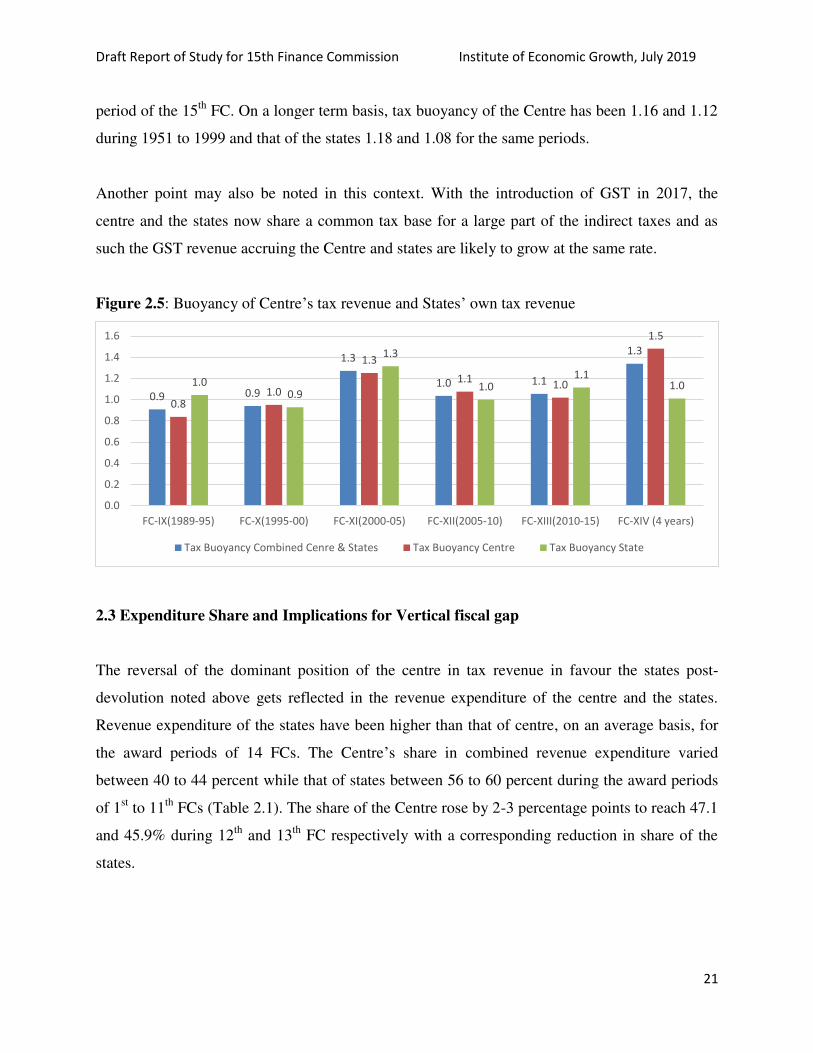
2.2 Tax Buoyancy and State Own Tax Revenue
In addition to trends in taxes, relative tax buoyancy of the Centre and the states has been a factor
considered by some FCs in decision regarding extent of devolution. The 12th
FC, for example,
explicitly states the buoyancy consideration. Figure 2.5 shows the tax buoyancy of central taxes,
states’ own taxes, and combined tax revenue. The central taxes have been more buoyant than the
states during 1995-2000, 2005-10 and 2015-18, but it has not always been so. The state taxes
were more buoyant than the Centre during 2000-2005 and 2010-15. Given this relative behavior,
it is difficult to judge the tax buoyancy of the states vis-à-vis that of Centre during the award
30.0
35.0
40.0
45.0
50.0
55.0
60.0
65.0
19
52
-53
19
54
-55
19
56
-57
19
58
-59
19
60
-61
19
62
-63
19
64
-65
19
66
-67
19
68
-69
19
70
-71
19
72
-73
19
74
-75
19
76
-77
19
78
-79
19
80
-81
19
82
-83
19
84
-85
19
86
-87
19
88
-89
19
90
-91
19
92
-93
19
94
-95
19
96
-97
19
98
-99
20
00
-01
20
02
-03
20
04
-05
20
06
-07
20
08
-09
20
10
-11
20
12
-13
20
14
-15
20
16
-17
20
18
-19
(RE
)
Centre State
Draft Report of Study for 15th Finance Commission Institute of Economic Growth, July 2019
21
period of the 15th
FC. On a longer term basis, tax buoyancy of the Centre has been 1.16 and 1.12
during 1951 to 1999 and that of the states 1.18 and 1.08 for the same periods.
Another point may also be noted in this context. With the introduction of GST in 2017, the
centre and the states now share a common tax base for a large part of the indirect taxes and as
such the GST revenue accruing the Centre and states are likely to grow at the same rate.
Figure 2.5: Buoyancy of Centre’s tax revenue and States’ own tax revenue
2.3 Expenditure Share and Implications for Vertical fiscal gap
The reversal of the dominant position of the centre in tax revenue in favour the states post-
devolution noted above gets reflected in the revenue expenditure of the centre and the states.
Revenue expenditure of the states have been higher than that of centre, on an average basis, for
the award periods of 14 FCs. The Centre’s share in combined revenue expenditure varied
between 40 to 44 percent while that of states between 56 to 60 percent during the award periods
of 1st to 11
th FCs (Table 2.1). The share of the Centre rose by 2-3 percentage points to reach 47.1
and 45.9% during 12th
and 13th
FC respectively with a corresponding reduction in share of the
states.
0.9 0.9
1.3
1.0 1.1
1.3
0.8 1.0
1.3
1.1 1.0
1.5
1.0 0.9
1.3
1.0 1.1
1.0
0.0
0.2
0.4
0.6
0.8
1.0
1.2
1.4
1.6
FC-IX(1989-95) FC-X(1995-00) FC-XI(2000-05) FC-XII(2005-10) FC-XIII(2010-15) FC-XIV (4 years)
Tax Buoyancy Combined Cenre & States Tax Buoyancy Centre Tax Buoyancy State

Draft Report of Study for 15th Finance Commission Institute of Economic Growth, July 2019
22
Table 2.1 Share of union and the States in the Combined Revenue Expenditure (%)
Table 2.1 Share of union and the States in the
Combined Revenue Expenditure (%)
Finance
Commission/Year State Centre
FC-1 (1952-57) 59.2 40.8
FC-2(1957-62) 58.2 41.8
FC-3(1962-66) 53.9 46.1
FC-4(1966-69) 58.2 41.8
FC-5(1969-74) 60.0 40.0
FC-6(1974-79) 55.8 44.2
FC-7(1979-84) 58.0 42.0
FC-8(1984-89) 55.8 44.2
FC-9 (1989-95) 56.5 43.5
FC-10 (1995-00) 56.8 43.2
FC-11 (2000-05) 56.0 44.0
FC-12 (2005-10) 52.9 47.1
FC-13 (2010-15) 54.1 45.9
FC-14 (First Four Years) 61.8 38.2 Source: Handbook of statistics on Indian Economy, RBI
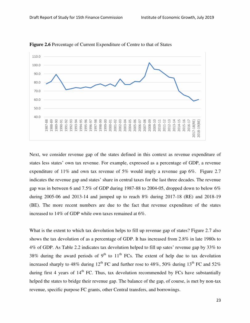
During the last decade, the share of Centre in combined revenue expenditure has fallen from
47.1% during 2005-10 to 38.2% during 2015-18 with a corresponding rise in expenditure of the
states. These figures represent a change of about 9 percentage points as compared to the 12th
FC
award period. Looked at another way, the ratio of Centre’s current expenditure to that of the
states was close to 1 in late-1990s and has been declining steadily since 2010-11. It dropped
down to 0.70 in 2014-15 and further to around 0.60 during last two years. This has considerably
changed the balance in revenue expenditure in favour of the states in recent years.
Draft Report of Study for 15th Finance Commission Institute of Economic Growth, July 2019
23
Figure 2.6 Percentage of Current Expenditure of Centre to that of States
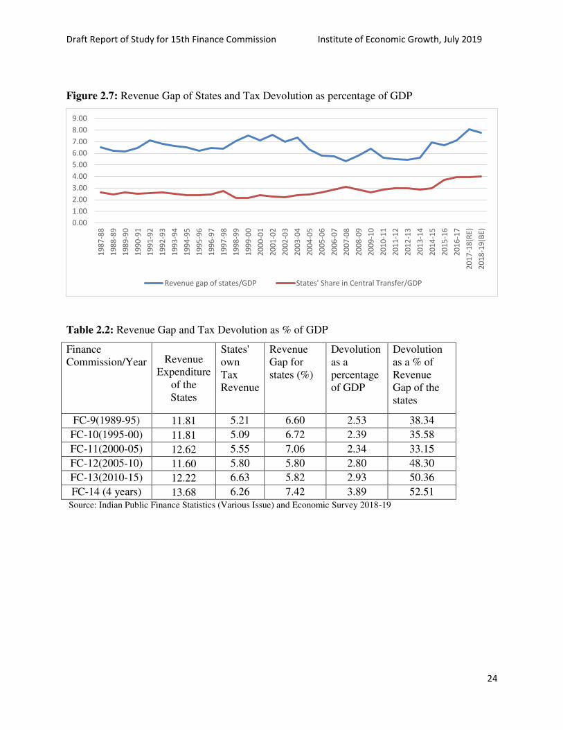
Next, we consider revenue gap of the states defined in this context as revenue expenditure of
states less states’ own tax revenue. For example, expressed as a percentage of GDP, a revenue
expenditure of 11% and own tax revenue of 5% would imply a revenue gap 6%. Figure 2.7
indicates the revenue gap and states’ share in central taxes for the last three decades. The revenue
gap was in between 6 and 7.5% of GDP during 1987-88 to 2004-05, dropped down to below 6%
during 2005-06 and 2013-14 and jumped up to reach 8% during 2017-18 (RE) and 2018-19
(BE). The more recent numbers are due to the fact that revenue expenditure of the states
increased to 14% of GDP while own taxes remained at 6%.
What is the extent to which tax devolution helps to fill up revenue gap of states? Figure 2.7 also
shows the tax devolution of as a percentage of GDP. It has increased from 2.8% in late 1980s to
4% of GDP. As Table 2.2 indicates tax devolution helped to fill up sates’ revenue gap by 33% to
38% during the award periods of 9th
to 11th
FCs. The extent of help due to tax devolution
increased sharply to 48% during 12th
FC and further rose to 48%, 50% during 13th
FC and 52%
during first 4 years of 14th
FC. Thus, tax devolution recommended by FCs have substantially
helped the states to bridge their revenue gap. The balance of the gap, of course, is met by non-tax
revenue, specific purpose FC grants, other Central transfers, and borrowings.
40.0
50.0
60.0
70.0
80.0
90.0
100.0
110.0
19
87
-88
19
88
-89
19
89
-90
19
90
-91
19
91
-92
19
92
-93
19
93
-94
19
94
-95
19
95
-96
19
96
-97
19
97
-98
19
98
-99
19
99
-00
20
00
-01
20
01
-02
20
02
-03
20
03
-04
20
04
-05
20
05
-06
20
06
-07
20
07
-08
20
08
-09
20
09
-10
20
10
-11
20
11
-12
20
12
-13
20
13
-14
20
14
-15
20
15
-16
20
16
-17
20
17
-18
(RE
)
20
18
-19
(BE
)
Draft Report of Study for 15th Finance Commission Institute of Economic Growth, July 2019
24
Figure 2.7: Revenue Gap of States and Tax Devolution as percentage of GDP
Table 2.2: Revenue Gap and Tax Devolution as % of GDP
Finance
Commission/Year Revenue
Expenditure
of the
States
States'
own
Tax
Revenue
Revenue
Gap for
states (%)
Devolution
as a
percentage
of GDP
Devolution
as a % of
Revenue
Gap of the
states
FC-9(1989-95) 11.81 5.21 6.60 2.53 38.34
FC-10(1995-00) 11.81 5.09 6.72 2.39 35.58
FC-11(2000-05) 12.62 5.55 7.06 2.34 33.15
FC-12(2005-10) 11.60 5.80 5.80 2.80 48.30
FC-13(2010-15) 12.22 6.63 5.82 2.93 50.36
FC-14 (4 years) 13.68 6.26 7.42 3.89 52.51
Source: Indian Public Finance Statistics (Various Issue) and Economic Survey 2018-19
0.00
1.00
2.00
3.00
4.00
5.00
6.00
7.00
8.00
9.00
19
87
-88
19
88
-89
19
89
-90
19
90
-91
19
91
-92
19
92
-93
19
93
-94
19
94
-95
19
95
-96
19
96
-97
19
97
-98
19
98
-99
19
99
-00
20
00
-01
20
01
-02
20
02
-03
20
03
-04
20
04
-05
20
05
-06
20
06
-07
20
07
-08
20
08
-09
20
09
-10
20
10
-11
20
11
-12
20
12
-13
20
13
-14
20
14
-15
20
15
-16
20
16
-17
20
17
-18
(RE
)
20
18
-19
(BE
)
Revenue gap of states/GDP States' Share in Central Transfer/GDP

Draft Report of Study for 15th Finance Commission Institute of Economic Growth, July 2019
25
Chapter 3: Trends and Patterns in Horizontal Fiscal Devolution
(TOR 3: Summarize the trends and patterns in horizontal fiscal devolutions across states
along with states’ own effort to raise resources and maintain fiscal discipline
3.1 Criteria for Horizontal Equity
As mentioned in Chapter 1, the past FCs have used various criteria for achieving horizontal
equity, focused primarily on economic, geographic and demographic characteristics of Indian
states. While interstate differences are a key consideration, decision making on allocations for
intrastate differences in equity or budgetary allocations across social sectors within the state are
upto the individual states. Summarized below are the criteria that have been used by the past 4
FCs in making devolutions.
3.1.1 Factors reflecting needs:
a. Population (1971):
The 11th
FC stated that “population reflects public requirement of public goods and services” and
the 13th
FC mentioned that “population is an indicator for the expenditure needs of a state”. The
13th
FC clarified that the criterion ensures equal per capita transfers to all states, without taking
into account cost disabilities across states because of differences in the geographical spread of
population.
Population figures given in the 1971 census forms the basis as is mandated by the Terms of
Reference for the last four FCs. The importance of the indicator moved from 10% in the 11th
FC
to 25% in the 12th
FC and 13th
FC, but reduced to 17.5% in the 14th
FC due to additional
consideration of 2011 population data separately.
b. Demographic changes- Population (2011)
The 14th
Commission deliberated on inclusion of demographic changes that had taken place
since 1971, especially changes in the composition of population and migration. This was to
address the concerns of differences in fertility rate amongst states. In addition, the 14th
FC
mentioned that it considered migration as an important factor which affected the population of
the State other than fertility and mortality. In regard to whether net-migration should be taken as

Draft Report of Study for 15th Finance Commission Institute of Economic Growth, July 2019
26
an indicator, the 14th
FC mentioned that it would “place a double burden on States from where
out-migration is taking place.”
The 14th
FC assigned a 10 per cent weight to the 2011 population.
c. Income distance:
The 12th
FC mentioned that the income distance criteria ensured that there was progressivity in
distribution. The 11th
FC stated that the core criteria used in the previous FCs for providing
higher per capita devolution to lower per capita income states are distance and inverse-income
formulae, whereas the inverse income formulae had been discarded in the 10th
FC.
The inverse income formula was discarded by the 10th
FC stating that “due to the implicit
convexity in the formula the middle-income states would have to bear a relatively higher
burden.”
Prior to the 11th
FC, NSDP was used to calculate distances, but taking into consideration the state
of collection and processing of income related data in the states, GSDP was considered to give a
better inter-state comparability of domestic economic activity thereafter. The distance was
calculated between the per capita income of a state and the weighted average of the states with
the three highest per capita income (11th
FC); between the average per capita GSDP of each of
the 28 states for the last 3 years and the weighted average of the states with the three highest per
capita income (12th
FC); between the average per capita GSDP of each of the 29 states for the
last 3 years and the state with the highest per capita income (14th
FC). .
Income distance index was assigned a weight of 62.5% in the 11th
FC, 50 percent in the 12th
FC
and 50% in the 14th
FC.
d. Fiscal capacity Distance
The 13th
FC claimed that the income distance criterion used by FC 12 (measured through per
capita GSDP) was a proxy for the distance between states in tax capacity. The 13th
FC went on to
state that “When so proxied, the procedure implicitly applies a single average tax-to-GSDP ratio
to determine fiscal capacity distance between states.” In addition, the 13th
FC recommended the
use of separate averages for measuring tax capacity- one for general category states and another
for special category states. The 13th
FC mentioned that “The use of average tax-to-GSDP ratios
specific to each category neutralizes to an extent the fiscal disadvantage of special category
states in terms of tax capacity.”
Draft Report of Study for 15th Finance Commission Institute of Economic Growth, July 2019
27
The 13th
FC justified the distinction of two categories of states by stating that “a single average
applied (implicitly) to GSDP does not accurately capture the fiscal distance between the two
groups.” The 13th
FC stated that this was because “GSDP did not accurately capture the taxable
base.”
13th
FC assigned a weight of 47.5 per cent to the fiscal capacity distance criterion.
The 14th
FC rejected the 13th
FC’s fiscal capacity distance and reverted to income distance
because it observed that “the relationship between income and tax is non-linear, as the
consumption basket differed between high, middle and low income States.”
3.1.2 Cost disability Indicators
a. Area
It was mentioned in the 11th
FC that “states with larger area and low density of population would
have to incur heavy expenditure for providing basic administrative infrastructure.” The 13th
FC
noted that the 10th
FC introduced area on the grounds that states with larger area incur more costs
to provide comparable services but believed that the cost of provision of services increases at a
decreasing rate with the size of states with the incremental costs becoming negligible after a
point. In addition, the 12th
FC noted that smaller states also had to spend some minimum amount
to establish required frameworks of governmental machinery.” Area shares have a floor of 2%
and a ceiling of 10% in the 11th
FC. The 12th
FC, 13th
FC and 14th
FC retained the floor but
removed the ceiling after realizing that only Rajasthan marginally exceeds 10%. As mentioned in
the 12th
FC, states with less than 2 per cent share in total area, were assigned a minimum share of
2 per cent.
b. Index of Infrastructure
The 12th
FC states that the Index of infrastructure refers to “the relative availability of economic
and social infrastructure in the state” and additionally mentions that the index is inversely
proportional to the share of the state. The argument in support for the index of infrastructure was
put forth by the 11th
FC which stated that infrastructure was critical in order to attract investment
which made a case for assisting states with low index of infrastructure. The 12th
FC found the
infrastructure criterion to be correlated with income distance and concluded that it was better to
use the index in an ordinal way and hence dropped the criterion.
c. Forest Cover
Draft Report of Study for 15th Finance Commission Institute of Economic Growth, July 2019
28
Forest cover was introduced into the horizontal devolution formula in the 14th
FC, though there
has been mention of forest cover in the reports of the previous commissions.
The 14th
FC argued that “Forests and the externalities arising from them impact both the revenue
capacities and the expenditure needs of the States” and believed that there needs to be a
compensation for the cost disability and encouragement to the states regarding the maintenance
and additions to green cover. The 14th
FC hence concluded that “A large forest cover provides
huge ecological benefits, but there is also an opportunity cost in terms of area not available for
other economic activities and this also serves as an important indicator of fiscal disability.” and
hence assigned 7.5 per cent weight to the forest cover.
3.1.3 Fiscal efficiency indicators
a. Tax effort
The 11th
FC report mentioned that the ToR of the 11th
FC explicitly mentioned consideration of
incentives to encourage better utilization of tax and non-tax revenue and proposed the tax effort
indicator as a solution. As mentioned in the 11th
FC, “Tax effort was to be measured by the ratio
of a state’s per capita own tax revenue to its per capita income and weighed by the inverse of the
per capita income.” [(Per capita OTR/Per capita GSDP of state i)* (1/Per capita GSDP of state
i)]. Hence the 11th
FC noted that, a poorer state utilizing its tax base as much as a rich state
would get additional consideration in the formula.
The 12th
FC modified the formula by taking a three-year average of the ratio of own tax revenue
to comparable GSDP (not per capita) and weighted it by the square root of the inverse of per
capita GSDP. [(Sum of three year OTR: GSDP ratios/3)* √ (1/per capita GSDP)] which would
ensure that a poorer state would get even higher weightage under this case.
The 11th
FC reduced the weight of inverse of income from 1 to 0.5. The weightage given to the
entire tax effort component was 5% in the 11th
FC and increased to 7.5% in the 12th
FC due to
the commission perceiving and stating an urgent need for fiscal consolidation.
b. Fiscal Discipline
The 11th
FC mentioned that fiscal discipline was an indicator that had come out of the
requirement for a further incentive for better fiscal management after taking into account the
fiscal situation of the states and the need for restructuring.

Draft Report of Study for 15th Finance Commission Institute of Economic Growth, July 2019
29
The 11th
FC explained that “The index of fiscal discipline considers an improvement in the ratio
of own revenue receipts to total revenue expenditure in comparison to a similar ratio for all
states.” The 12th
FC added that “If all the revenue performances of states are increasing, the state
where improvement is relatively more than average is rewarded more.” The 13th
FC thought
there was “a strong case to incentivize states to follow fiscal prudence, particularly in relation to
fiscal correction” and increased the weight from 7.5% in the 11th
and 12th
FC to 17.5% in the 13th
FC. To the 14th
FC, states argued that “this criterion places an extra burden on states with
revenue deficits” and its weight should therefore be reduced” and the indicator was removed in
the 14th
FC.
Other criteria suggested by states over the years
Some of the other criteria suggested by states to the previous commissions can be summarized as
follows: (refer Table 3.1)
Table 3.1 Criteria suggested by states, 11th
to 14th
FC
Source: Authors’ Compilation from various Finance Commission Reports, 11, 12, 13, 14
Note: The 12th
FC has not been included in this table since the report does not provide information on additional
criterion suggested by states for horizontal devolution. The 12th
FC document only contains information on the
11th
FC 13th
FC 14th
FC
Population control
Population BPL
Composite index of
backwardness
Contribution to central
taxes
Expenditure on HR
Development
Administration and social
services expenditure
Expenditure on
maintenance of social
structures and
infrastructure
Central Investment
Employment rate
Population of SC/ST
Proportion of people
above 60 years of age
Density of population
Population BPL
Length of international
border
Levels of backwardness
HDI
Share of primary sector in
GSDP
Contribution to central taxes
Expenditure on social
structures and infrastructure
Short and long term
Migration
SC/ST population
Incentive indicator for
reducing fiscal capacity
distance (using Gini)
HDI
Poverty ratio

Draft Report of Study for 15th Finance Commission Institute of Economic Growth, July 2019
30
states' preferences on the components of population, income distance, area, tax effort, fiscal discipline which have
already been covered in detail in this section.
3.2 Review of the trend and pattern of criteria
A review of the criteria adopted by successive FCs in India for tax devolution presented in Table
3.2 reveals that income or indirectly the tax capacity of the state is the major criteria accounting
for distribution of more than 50 percent of sharable tax revenue of centre among states in
successive FCs starting from the 8th
FC. Demographic factors accounted for a share ranging
between 10-25 percent. Among earlier FCs, income distance was given 25 percent weight by 6th
FC while 7th
FC gave a weight of 25 percent in the name of revenue equalization. Therefore, the
criteria of income distance have been alternatively considered as fiscal capacity (13th
FC) and
revenue equalization (7th
FC). Incentive based criteria of index of infrastructure was considered
by 10th
and 11th
FCs, tax effort by 10th
, 11th
and 12th
FCs and, fiscal discipline by 11th
, 12th
and
13th
FCs.
An analysis of the shares (in %) of different states over the 14th
FC periods, reveals that there
was not much variation in shares of each state in the net proceeds of all sharable central taxes. It
can be considered as an expected result given that the dominating criteria for distribution of
central revenue across states are population and income distance. Almost 75 per cent of
devolution has been distributed based on these two criteria. The problem of inequity of incomes
among different states was directly addressed by 4th
, 5th
and 9th
FCs by considering an index of
backwardness of sates as a criterion while the 7th
FC addressed this problem by considering the
poverty ratio as a criterion for distributing sharable central tax revenue among states.
The successive FCs have mostly been guided by performance and need based criteria for
devolution. Per capita income (income distance) or fiscal capacity (13th
FC) of the state is
considered for capturing the state`s capacity for raising taxes and the criteria of population and
area are considered as need based.

Draft Report of Study for 15th Finance Commission Institute of Economic Growth, July 2019
31

Draft Report of Study for 15th Finance Commission Institute of Economic Growth, July 2019
32
Table 3.2: Criteria Adopted for Devolution of Sharable Tax Revenue by FCs in India
Criteria
1st FC 2nd FC 3rd FC 4th FC 5th FC 6th FC
Income
Tax
Union
Excise
Income
Tax
Union
Excise
Income
Tax
Union
Excise
Income
Tax
Union
Excise
Income
Tax
Union
Excise
Income
Tax
Union
Excise
Population 80 100 90 90 80 80 80 90 80 90 75
Demographic
Change
Income
(Distance) 13.34
25
Area
Index of
Infrastructure
Tax Effort
Fiscal
Discipline
Forest cover
Inverse of
Income
Index of
Backwardness 20 6.66
Poverty Ratio
Revenue
Equalization
Discretionary
Adjustment 10 100
(Continued…)

Draft Report of Study for 15th Finance Commission Institute of Economic Growth, July 2019
33
Criteria
7th FC 8th FC 9th FC 10th FC 11th
FC
12th
FC
13th
FC 14th FC
Income
Tax
Union
Excise
Income
Tax
Union
Excise
Income
Tax
Union
Excise
Income
Tax
Union
Excise
Population 90 25 22.5 25 22.5 25 20 20 10 25 25
17.5
(1971
population)
Demographic
Change
10 (2011
population)
Income
(Distance) 45 50 45 33.5 60 60 62.5 50 47.5* 50
Area 5 5 7.5 10 10 15
Index of
Infrastructure 5 5 7.5
Tax Effort 10 10 5 7.5
Fiscal
Discipline 7.5 7.5 17.5
Forest cover 7.5
Inverse of
Income 25 22.5 25 11.25 12.5
Index of
Backwardness 11.25 12.5
Poverty Ratio 25
Revenue
Equalization 25
Discretionary
Adjustment
*Income distance is measured as fiscal capacity
Source: Reddy and Reddy (2019)

Draft Report of Study for 15th Finance Commission Institute of Economic Growth, July 2019
34
Chapter 4: Factors affecting devolution trends
(TOR 4: Analysis of major factors affecting the horizontal and vertical devolution trends)
4.1 Equity and Budgetary Policies of Centre and States
Budgetary policies of government are guided by the objectives of efficiency in resource
allocation and equity. To achieve the equity objective, government has to resort to progressive
taxes and redistributive public expenditures at the cost of foregoing some degree of efficiency in
resource allocation. Studies which have used normative approaches for studying welfare effects
of taxes have shown that personal income and corporate profit taxes in India are moderately
progressive while commodity taxes (levied through VAT until recently) are regressive. A
research project done by Institute of Economic Growth for NITI Aayog, Government of India in
20188 provides estimates of incidence of commodity taxes and GST in India by fractile groups of
monthly per capita expenditure (MPCE) classes and 15 commodity groups for both rural and
urban sectors. These estimates are obtained using National Sample Survey (NSS) consumer
expenditure data of 68th
round(2011-2012), the information about state VAT rates and
MODVAT rates for the year 2013-14, and income tax data for the assessment year 2014-15. The
estimates of marginal tax rates reveal that commodity taxes (central excise plus state vat or even
hypothetical GST considered) are not consistently progressive as the MPCE increases up to
median level and become regressive afterward (see Appendix Table 4.A.1, 4.A.2).Marginal tax
rates for income taxes show significant progressivity. (Table 4.A.3 in Appendix)
An evaluation of tax policies in the same study through a normative welfare function provides
insights on inequality aversion parameter estimates (e) or elasticity of social marginal utility
implicit in the commodity and income tax policies. The estimates of e for commodity taxes is
less than 1 showing that the Indian government has shown less aversion to income inequalities in
designing commodity taxes. In the case of income taxes this parameter takes value more than 1.5
implying that it shows moderate concern for inequality in income distribution. These details are
given in Table 4.1 as below.
8Source Murty et al., (2018) for details.

Draft Report of Study for 15th Finance Commission Institute of Economic Growth, July 2019
35
Table 4.1 Estimates of Inequality Aversion Parameter (e) Implicit in Commodity and Income
Taxes in India
Type of Tax Rural Urban All India
VAT -0.754 -0.703 -0.916
GST -0.833 -0.814
Income Tax -1.590
Source: Murty et al. 2018
4.2 Equalizing Effects of Central Transfers to States
Resource transfers from centre to states in India could be broadly classified as general purpose
and specific purpose grants. Until recently, all general purpose grants and some specific purpose
grants were made on the recommendations of FCs while most specific purpose grants were made
as plan grants by the Planning Commission. Grants for specific projects and centrally sponsored
schemes were made by different government departments and ministries. With the abolition of
the Planning Commission in August 2014, most of the transfers are now made as per the
recommendations of FC. All general purpose grants are now made as per the recommendations
of FC while the specific purpose grants are given by central ministries. The 14th
FC’s increase in
share of states in the divisible pool of resources to 42 percent was done both for compensating
plan expenditure grants foregone and for giving more flexibility to states in resource allocation
through untied grants.
To judge the merits of general transfer vis a vis specific transfer, it is important to analyse the
revenue and expenditure equalization properties of these transfers. The information about the
estimates of elasticities of state per capita revenue and per capita expenditure with respect to per
capita SDP could be helpful in this regard. Elasticity estimates of state own tax revenue (1.08)
were found to be higher than that of the state post transfer or total revenue (0.58). It indicates that
transfers from Centre to states have some equalizing effects on per capita total revenue available
to states. In addition, analysis reveals that there was no significant difference between the
elasticity of total expenditure (0.58) and the elasticity of revenue expenditure (0.59) (refer table
4.2).
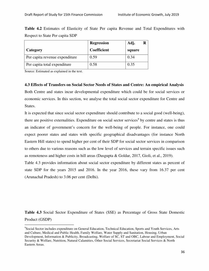
Draft Report of Study for 15th Finance Commission Institute of Economic Growth, July 2019
36
Table 4.2 Estimates of Elasticity of State Per capita Revenue and Total Expenditures with
Respect to State Per capita SDP
Category
Regression
Coefficient
Adj. R
square
Per capita revenue expenditure 0.59 0.34
Per capita total expenditure 0.58 0.35
Source: Estimated as explained in the text.
4.3 Effects of Transfers on Social Sector Needs of States and Centre: An empirical Analysis
Both Centre and states incur developmental expenditure which could be for social services or
economic services. In this section, we analyse the total social sector expenditure for Centre and
States.
It is expected that since social sector expenditure should contribute to a social good (well-being),
there are positive externalities. Expenditure on social sector services9 by centre and states is thus
an indicator of government’s concern for the well-being of people. For instance, one could
expect poorer states and states with specific geographical disadvantages (for instance North
Eastern Hill states) to spend higher per cent of their SDP for social sector services in comparison
to others due to various reasons such as the low level of services and terrain specific issues such
as remoteness and higher costs in hill areas (Dasgupta & Goldar, 2017, Gioli, et al., 2019).
Table 4.3 provides information about social sector expenditure by different states as percent of
state SDP for the years 2015 and 2016. In the year 2016, these vary from 16.37 per cent
(Arunachal Pradesh) to 3.06 per cent (Delhi).
Table 4.3 Social Sector Expenditure of States (SSE) as Percentage of Gross State Domestic
Product (GSDP)
9Social Sector includes expenditure on General Education, Technical Education, Sports and Youth Services, Arts
and Culture, Medical and Public Health, Family Welfare, Water Supply and Sanitation, Housing, Urban
Development, Information & Publicity, Broadcasting, Welfare of SC, ST and OBC, Labour and Employment, Social
Security & Welfare, Nutrition, Natural Calamities, Other Social Services, Secretariat Social Services & North
Eastern Areas.
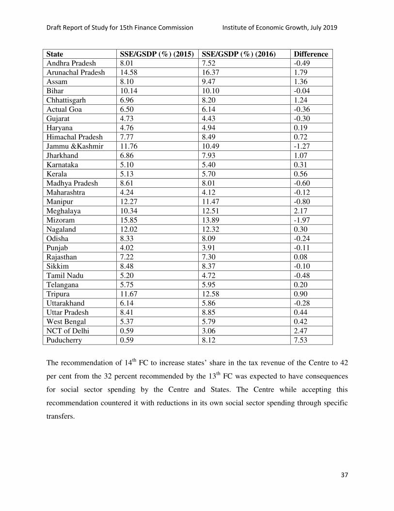
Draft Report of Study for 15th Finance Commission Institute of Economic Growth, July 2019
37
State SSE/GSDP (%) (2015) SSE/GSDP (%) (2016) Difference
Andhra Pradesh 8.01 7.52 -0.49
Arunachal Pradesh 14.58 16.37 1.79
Assam 8.10 9.47 1.36
Bihar 10.14 10.10 -0.04
Chhattisgarh 6.96 8.20 1.24
Actual Goa 6.50 6.14 -0.36
Gujarat 4.73 4.43 -0.30
Haryana 4.76 4.94 0.19
Himachal Pradesh 7.77 8.49 0.72
Jammu &Kashmir 11.76 10.49 -1.27
Jharkhand 6.86 7.93 1.07
Karnataka 5.10 5.40 0.31
Kerala 5.13 5.70 0.56
Madhya Pradesh 8.61 8.01 -0.60
Maharashtra 4.24 4.12 -0.12
Manipur 12.27 11.47 -0.80
Meghalaya 10.34 12.51 2.17
Mizoram 15.85 13.89 -1.97
Nagaland 12.02 12.32 0.30
Odisha 8.33 8.09 -0.24
Punjab 4.02 3.91 -0.11
Rajasthan 7.22 7.30 0.08
Sikkim 8.48 8.37 -0.10
Tamil Nadu 5.20 4.72 -0.48
Telangana 5.75 5.95 0.20
Tripura 11.67 12.58 0.90
Uttarakhand 6.14 5.86 -0.28
Uttar Pradesh 8.41 8.85 0.44
West Bengal 5.37 5.79 0.42
NCT of Delhi 0.59 3.06 2.47
Puducherry 0.59 8.12 7.53
The recommendation of 14th
FC to increase states’ share in the tax revenue of the Centre to 42
per cent from the 32 percent recommended by the 13th
FC was expected to have consequences
for social sector spending by the Centre and States. The Centre while accepting this
recommendation countered it with reductions in its own social sector spending through specific
transfers.
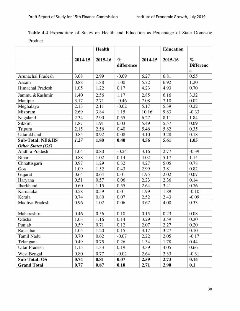
Draft Report of Study for 15th Finance Commission Institute of Economic Growth, July 2019
38
Table 4.4 Expenditure of States on Health and Education as Percentage of State Domestic
Product
Health
Education
2014-15 2015-16 %
difference
2014-15 2015-16 %
Differenc
e
Arunachal Pradesh 3.08 2.99 -0.09 6.27 6.81 0.55
Assam 0.88 1.88 1.00 5.72 6.92 1.20
Himachal Pradesh 1.05 1.22 0.17 4.23 4.93 0.70
Jammu &Kashmir 1.40 2.56 1.17 2.85 6.16 3.32
Manipur 3.17 2.71 -0.46 7.08 7.10 0.02
Meghalaya 2.13 2.11 -0.02 5.17 5.39 0.22
Mizoram 2.69 3.84 1.15 10.16 9.83 -0.33
Nagaland 2.34 2.90 0.55 6.27 8.11 1.84
Sikkim 1.87 1.91 0.03 5.49 5.57 0.09
Tripura 2.15 2.56 0.40 5.46 5.82 0.35
Uttarakhand 0.85 0.92 0.08 3.10 3.28 0.18
Sub-Total: NE&HS 1.27 1.80 0.40 4.56 5.61 1.05
Other States (GS)
Andhra Pradesh 1.04 0.80 -0.24 3.16 2.77 -0.39
Bihar 0.88 1.02 0.14 4.02 5.17 1.14
Chhattisgarh 0.97 1.29 0.32 4.27 5.05 0.78
Goa 1.09 1.52 0.43 2.99 3.81 0.82
Gujarat 0.64 0.64 0.01 1.95 2.02 0.07
Haryana 0.51 0.57 0.06 2.23 2.36 0.14
Jharkhand 0.60 1.15 0.55 2.64 3.41 0.76
Karnataka 0.58 0.59 0.01 1.99 1.89 -0.10
Kerala 0.74 0.80 0.07 2.52 2.43 -0.09
Madhya Pradesh 0.96 1.02 0.06 3.67 4.00 0.33
Maharashtra 0.46 0.56 0.10 0.15 0.23 0.08
Odisha 1.03 1.16 0.14 3.29 3.59 0.30
Punjab 0.59 0.71 0.12 2.07 2.27 0.20
Rajasthan 1.05 1.20 0.15 3.17 3.27 0.10
Tamil Nadu 0.70 0.62 -0.07 2.22 2.05 -0.17
Telangana 0.49 0.75 0.26 1.34 1.78 0.44
Uttar Pradesh 1.15 1.33 0.19 3.39 4.05 0.66
West Bengal 0.80 0.77 -0.02 2.64 2.33 -0.31
Sub-Total: OS 0.74 0.81 0.07 2.59 2.73 0.14
Grand Total 0.77 0.87 0.10 2.71 2.90 0.1
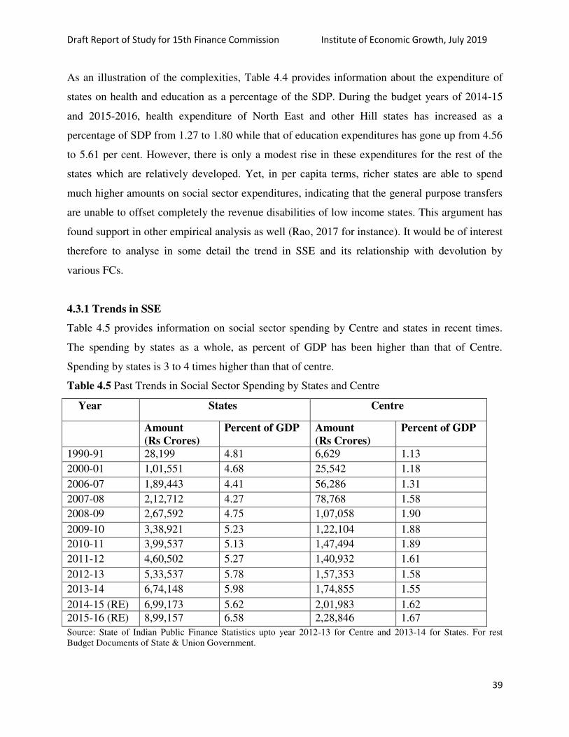
Draft Report of Study for 15th Finance Commission Institute of Economic Growth, July 2019
39
As an illustration of the complexities, Table 4.4 provides information about the expenditure of
states on health and education as a percentage of the SDP. During the budget years of 2014-15
and 2015-2016, health expenditure of North East and other Hill states has increased as a
percentage of SDP from 1.27 to 1.80 while that of education expenditures has gone up from 4.56
to 5.61 per cent. However, there is only a modest rise in these expenditures for the rest of the
states which are relatively developed. Yet, in per capita terms, richer states are able to spend
much higher amounts on social sector expenditures, indicating that the general purpose transfers
are unable to offset completely the revenue disabilities of low income states. This argument has
found support in other empirical analysis as well (Rao, 2017 for instance). It would be of interest
therefore to analyse in some detail the trend in SSE and its relationship with devolution by
various FCs.
4.3.1 Trends in SSE
Table 4.5 provides information on social sector spending by Centre and states in recent times.
The spending by states as a whole, as percent of GDP has been higher than that of Centre.
Spending by states is 3 to 4 times higher than that of centre.
Table 4.5 Past Trends in Social Sector Spending by States and Centre
Year States Centre
Amount
(Rs Crores)
Percent of GDP Amount
(Rs Crores)
Percent of GDP
1990-91 28,199 4.81 6,629 1.13
2000-01 1,01,551 4.68 25,542 1.18
2006-07 1,89,443 4.41 56,286 1.31
2007-08 2,12,712 4.27 78,768 1.58
2008-09 2,67,592 4.75 1,07,058 1.90
2009-10 3,38,921 5.23 1,22,104 1.88
2010-11 3,99,537 5.13 1,47,494 1.89
2011-12 4,60,502 5.27 1,40,932 1.61
2012-13 5,33,537 5.78 1,57,353 1.58
2013-14 6,74,148 5.98 1,74,855 1.55
2014-15 (RE) 6,99,173 5.62 2,01,983 1.62
2015-16 (RE) 8,99,157 6.58 2,28,846 1.67
Source: State of Indian Public Finance Statistics upto year 2012-13 for Centre and 2013-14 for States. For rest
Budget Documents of State & Union Government.
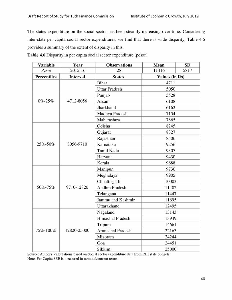
Draft Report of Study for 15th Finance Commission Institute of Economic Growth, July 2019
40
The states expenditure on the social sector has been steadily increasing over time. Considering
inter-state per capita social sector expenditures, we find that there is wide disparity. Table 4.6
provides a summary of the extent of disparity in this.
Table 4.6 Disparity in per capita social sector expenditure (pcsse)
Variable Year Observations Mean SD
Pcsse 2015-16 28 11416 5817
Percentiles Interval States Values (in Rs)
0%-25% 4712-8056
Bihar 4711
Uttar Pradesh 5050
Punjab 5528
Assam 6108
Jharkhand 6162
Madhya Pradesh 7154
Maharashtra 7865
25%-50% 8056-9710
Odisha 8245
Gujarat 8327
Rajasthan 8506
Karnataka 9256
Tamil Nadu 9307
Haryana 9430
Kerala 9688
50%-75% 9710-12820
Manipur 9730
Meghalaya 9905
Chhattisgarh 10003
Andhra Pradesh 11402
Telangana 11447
Jammu and Kashmir 11695
Uttarakhand 12495
75%-100% 12820-25000
Nagaland 13143
Himachal Pradesh 13949
Tripura 14661
Arunachal Pradesh 22163
Mizoram 24244
Goa 24451
Sikkim 25000 Source: Authors’ calculations based on Social sector expenditure data from RBI state budgets.
Note: Per Capita SSE is measured in nominal/current terms.

Draft Report of Study for 15th Finance Commission Institute of Economic Growth, July 2019
41
It is immediately apparent that there is a lot of variation across states. Similar disparity is found
for other years as well. For 2015, the median is smaller than the mean and the skewness is 1.31.
The data might have a slight positive skew implying that most of the per capita social sector
expenditure is concentrated towards the left (corresponding to below 50%). It can also be
observed that many north eastern states have higher than median per capita social sector
expenditure.
4.3.2 Results from an Econometric Analysis: SSE, NSDP and Devolution from FCs
A fixed effects regression model was run on a panel data set, comprising of annual data from 28
states, covering the period of three FCs, namely, the 12th
, 13th
and 14th
FC (first 3 years).
The elasticity of social sector expenditure to net devolution (in nominal prices, absolute values)
was found to be expectedly positive and statistically significant, though it is less than one,
indicating that a rise in net devolution leads to a less than proportionate increase in social sector
expenditure. The net devolution amount (in absolute values) is defined as gross devolution and
transfers minus repayments of loans to Centre and interest payments on loans from Centre. On
the other hand, the elasticity of social sector expenditure is higher (and positively significant)
with regard to per capita NSDP than it is with regard to net devolution. While an increase in per
capita NSDP leads to an increase in SSE, the share of social sector expenditure in NSDP is also
positively and significantly impacted by the share of devolution that a state receives. Upon
introducing dummies for capturing effects specific to each FC period, we find that the 12th
FC
dummy is negative, while the 14th
FC dummy is positive, indicating that the SSE were positively
associated with the period of the 14th
FC. The 13th
FC dummy changes signs depending on the
specification and hence does not lend itself to a uniform conclusion, while for the other two FCs,
the signs and significance remains robust across specifications. Details have been given in Table
4.7 below.

Draft Report of Study for 15th Finance Commission Institute of Economic Growth, July 2019
42
Table 4.7: Regression estimates
Specification
(All are run as panel fixed
effect models)
Per capita
NSDP
Ln(Per
capita
NSDP)
Devoluti
on share
(Net)
Devolutio
n values
(absolute)
Ln(Net
Devoluti
on)
Dummy
-12th
FC
Dummy-
14th
FC
Ln SSE(nominal)= f(ln Net
Devolution) - - - - 0.90*** - -
Ln SSE(nominal)= f(ln Per
Capita NSDP (current)) - 1.26*** - - - - -
SSE(nominal)= f(Per Capita
NSDP (current)) 0.002*** - - - - - -
SSE(nominal)/
NSDP(current) = f( Per
Capita NSDP (constant) ,
devolution share)
3.40e-07*** - 0.01** - - - -
SSE(nominal) = f(Per Capita
NSDP (current) , Devolution
Share, 12th
FC Dummy, 14th
FC Dummy)
0.002*** - (-) 20.86 - - (-)
34.91*** 45.4***
Legend: ***- p<0.01,**- p<0.05, *- p<0.1, If p>0.1- insignificant. All outliers beyond Mean+/-2SD were removed.
Source: Authors’ estimations based on data from RBI state budgets
Our findings seem to indicate that the social sector expenditure is responsive to increase in both
NSDP and devolution, the latter being more effective when routed through the general purpose
transfer. One could potentially argue that specific central transfers may not be required therefore
to meet these expenditures, rather such specific transfers can be designed for meeting specific
national objectives other than those covered under existing social sector expenditure or where
there are major inter-state implications. Such objectives could for instance include performance
enhancing grants to support specific targets (e.g. meeting SDGs - creation of a carbon sink for
SDG 13, tackling pollution, increasing clean energy access, disaster resilience, etc.) or inter-state
concerns (e.g. efforts on GST and public finance management, ease of doing business, grants to
local bodies, solid waste management, etc.)
4.4 Choice between Tax Devolution and Grants in Aid
One of the challenges for future FCs in India is about choosing between tax devolution and
grants in aid in deciding about central transfers to states. In their representations to recent FCs
states and centre have divergent views on this issue. A majority of states have been expressing
Draft Report of Study for 15th Finance Commission Institute of Economic Growth, July 2019
43
preferences for tax devolution while various ministries and departments of centre advocating for
sector specific grants-in-aid to states. The past FCs have recommended grants-in-aid to states for
five purposes – revenue deficit, disaster relief, local bodies, sector-specific schemes and state-
specific schemes. These grants through FCs as non-plan grants are found to overlap with central
assistance to states as plan grants. It is also found that state specific grants recommended by
recent FCs are found to duplicate central sector schemes. Several concerns have been raised
regarding the design of specific purpose grants, whether routed through Central ministries or
through the FCs.
Taking these things in to consideration, 14th
FC in its recommendation noted that grants for both
sector-specific and state-specific schemes by the FC are not necessary. In compensation, it has
increased states’ share of sharable tax revenue of centre to 42 per cent from 32 percent
recommended by 13th
FC. This recommendation is expected to facilitate the substitution of
general purpose transfers to sector and state specific transfers and thus reducing centre’s share in
sector specific expenditures in the states. Also, this approach is expected to provide more
leverage to states to plan their spending according to their specific sector needs. Table 4.8
provides information about grants- in- aid to different states recommended by 14th
FC.
We find that in the context of social sector expenditures, the expenditures are hugely divergent
across states. As some other scholars have also pointed out sometimes even richer states suffer
from social and economic infrastructural deficits, which tend to argue in favor of having specific
purpose grants (for instance, See Rao, 2017). Further, large variations in fiscal capacities among
states that are not offset by general purpose transfers (tax devolution), raises concerns in favor of
achieving equalization through specific transfers targeted at social sectors. If richer states end up
with higher spending on major social and economic services while the tax devolution is unable to
counter the fiscal disability of poorer states, it could lead to enhanced inequality. The persistence
of such inequities is troubling. However, it is also argued that there is evidence that, when grants
are routed through the FC, it achieves more equalization, preserves incentive properties and
ensures achievement of ultimate developmental goals, than when it comes through the Central
ministries (Rao, 2017, Rajaraman & Gupta, 2016 for local governments).

Draft Report of Study for 15th Finance Commission Institute of Economic Growth, July 2019
44
Table 4.8: Grants-in-aid to States Recommended by 14th
Finance Commission (Rs. Crores)
Sector Amount (Rs Crores)
Local Government 287436
Disaster Management 55097
Post-devolution Revenue
Deficit
194821
Total 537354
Source: Report of 14th
Finance Commission, Government of India

Draft Report of Study for 15th Finance Commission Institute of Economic Growth, July 2019
45
Appendix: Chapter 4
Table 4.A.1: Incidence of Indirect Taxes by Expenditure Groups in India (Rural and Urban)
Rural Urban
Fractile
Class
MPCE:
Y
Commodity
tax liability:
T(Y)
Marginal
tax rates:
T'(Y) F(Y)
MPCE:
Y
Commodity
tax liability:
T(Y)
Marginal
tax rates:
T'(Y)
0-5% 446.18 57.48
0.03 617.69 78.52
5-10% 563.69 72.41 0.13 0.04 795.78 101.34 0.13
10-20% 663.47 85.87 0.13 0.07 978.50 121.29 0.11
20-30% 773.81 100.11 0.13 0.08 1192.04 146.21 0.12
30-40% 876.19 114.11 0.14 0.08 1400.87 167.39 0.10
40-50% 976.58 127.26 0.13 0.09 1632.16 190.93 0.10
50-60% 1099.82 144.37 0.14 0.09 1907.49 219.85 0.11
60-70% 1248.53 162.06 0.12 0.10 2245.74 253.59 0.10
70-80% 1451.73 187.01 0.12 0.12 2729.81 300.55 0.10
80-90% 1785.61 224.55 0.11 0.14 3562.57 370.58 0.08
90-95% 2291.90 274.95 0.1 0.08 4994.43 475.75 0.07
95-100% 4525.64 383.47 0.05 0.09 10279.41 722.78 0.05
All
Classes 1278.94 153.95 0.07 1 2399.24 245.95 0.06 Source: Authors’ calculations as part of report NITI Aayog, 2018 using NSSO 68
th round data
Table 4.A.2: Incidence of GST by Expenditure Groups in India (Rural and Urban)
Rural Urban
Fractile Y F(Y) T(Y) T'(Y) Y F(Y) T(Y) T'(Y)
0-5% 446.18 0.03 40.19 - 617.69 0.07 55.66
5-10% 563.69 0.04 50.69 0.09 795.78 0.06 71.73 0.09
10-20% 663.47 0.07 60.71 0.10 978.50 0.12 88.41 0.09
20-30% 773.81 0.08 71.01 0.09 1192.04 0.10 108.27 0.09
30-40% 876.19 0.08 81.38 0.10 1400.87 0.10 126.05 0.09
40-50% 976.58 0.09 91.61 0.10 1632.16 0.09 145.18 0.08
50-60% 1099.82 0.09 103.94 0.10 1907.49 0.09 169.87 0.09
60-70% 1248.53 0.10 117.16 0.09 2245.74 0.09 197.92 0.08
70-80% 1451.73 0.12 136.71 0.10 2729.81 0.09 240.99 0.09
80-90% 1785.61 0.14 166.96 0.09 3562.57 0.10 302.96 0.07
90-95% 2291.90 0.08 208.55 0.08 4994.43 0.05 409.12 0.07
95-100% 4525.64 0.09 313.42 0.05 10279.41 0.04 669.61 0.05
All Classes 1278.94 1.00 113.59 0.06 2399.24 1.00 198.27 0.06 Source: Authors’ calculations as part of report NITI Aayog, 2018

Draft Report of Study for 15th Finance Commission Institute of Economic Growth, July 2019
46
Table 4.A.3: Incidence of Income Taxes in India (Assessment Year 2014-15)
Average Gross Total Income( in INR) F(Y) T(Y) T'(Y)
75000 0.08 0 0
184000 0.08 400 0.004
224000 0.22 4400 0.1
296000 0.21 11600 0.1
373000 0.06 19300 0.1
424000 0.05 24400 0.1
475000 0.04 29500 0.1
524000 0.04 34400 0.1
696000 0.13 53200 0.11
974000 0.01 108800 0.2
1204000 0.03 159200 0.22
1718000 0.01 313400 0.3
2224000 0.01 465200 0.3
3382000 0.01 812600 0.3
6888000 0.01 1864400 0.3
19234000 0.002 5568200 0.3
69078000 0.0002 20521400 0.3
151922000 0.0001 45374600 0.3
346746000 3.75943E-05 103821800 0.3 Source: Authors’ calculations as part of report NITI Aayog, 2018

Draft Report of Study for 15th Finance Commission Institute of Economic Growth, July 2019
47

Draft Report of Study for 15th Finance Commission Institute of Economic Growth, July 2019
48
Chapter 5: Status of Key Fiscal Parameters on Resource Allocation
(TOR 5: Understand the current status on key fiscal parameters related to the resource
allocation between Centre and states and further across states)
5.1 Fiscal Efficiency
One of important considerations for future FCs of India is to make use of incentive based fiscal
efficiency criteria for tax devolution which were ignored by many past FCs. As explained in
Chapter II, out 14 FCs that were there in India so far, only four of them have considered these
criteria. Surprisingly, the last FC (14th
FC) has totally ignored fiscal efficiency considerations.
Fiscal efficiency indicators are normally identified as tax effort and fiscal discipline by FCs. Tax
effort is measured by the ratio of a state’s own tax revenue to state’s income (GSDP), the higher
being the tax effort of a state the higher is the ratio, given income. However, the interpretation of
the tax performance has to be made in the specific context of a state. For instance, sectoral
composition of GDP can influence the state’s tax potential. States that have non-tax generating
sectors like agriculture as major contributors to GSDP would show up as poorer performers. The
relative position of states in terms of tax effort would be affected thereby. A poorer state with
lower GSDP could have the same tax effort as a richer state where income is derived mostly
from non-tax generating sectors. Therefore past FCs of India which considered tax effort as a
criterion for tax devolution have suggested to multiply this ratio either by the inverse of per
capita GSDP or the square root of inverse of per capita SDP. In this case, the poorer state with
higher tax performance will get higher weight in comparison with a richer state with identical tax
performance. Only the 10th, 11th and 12th
FC had considered tax effort as one of the criteria for
tax devolution while the 13th
and 14th
FCs did not use it as a criterion for horizontal devolution.
Columns 2 and 3 of Table 5.1 provide estimates of tax effort (ratio of own tax revenue to GSDP)
of Indian states for the financial years 2015-16 and 2016-17. For instance the tax effort varies
from 2.3 per cent (Mizoram and Nagaland) to 8.7 per cent (Puducherry) among the states in the
year 2016-2017. Poorer states Odisha and Bihar have comparable tax effort estimates to richer
states of Goa and Maharashtra. However, in reality, the poorer states have performed better in
terms of tax effort, given their lower income base. As per the rationale of past FCs, and for
distributive justice towards rewarding efficiency, these states could lay claim to be given higher
weightage for tax devolution. Only three FCs of India in the past (11th
, 12th
, and 13th
) have
Draft Report of Study for 15th Finance Commission Institute of Economic Growth, July 2019
49
considered fiscal discipline as one of the criteria for tax devolution. Fiscal discipline of a state is
measured as the ratio of its own tax revenue to its revenue expenditure and it is a measure of its
improvement or change over time as a criterion for tax devolution. As already noted in Chapter
2, this change is measured by comparing this ratio of a past reference period (average of 3 to 4
years) to the average of 3 or 4 of most recent years. Columns 4 and 5 in Table 5.1 provide
estimates of fiscal discipline (ratio of own revenue to revenue expenditure) for different states of
India for the years 2015-2016 and 2016-2017. Comparison of estimates for two recent
consecutive years given in Table 5.1 reveals a fall in the fiscal discipline ratio for many states
with the exception of a few states. Moving ahead, the effect of tax reforms through the
introduction of the GST, on the fiscal discipline of states will become evident over the next few
years. There is a possibility that GST implementation could have a reducing effect on state’s own
tax revenue at least during the initial years.
The status of different states with respect to budgetary deficits (revenue and fiscal) is also an
important indicator of fiscal discipline of states. The post devolution revenue and expenditure
position of states is such that majority of states have resorted to debt financing of expenditures.
Fiscal deficit level is higher in some states in the recent past as shown in Table 5.2.
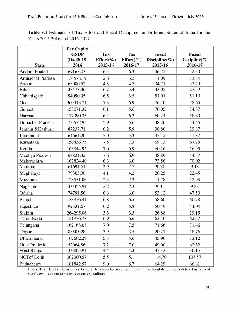
Draft Report of Study for 15th Finance Commission Institute of Economic Growth, July 2019
50
Table 5.1 Estimates of Tax Effort and Fiscal Discipline for Different States of India for the
Years 2015-2016 and 2016-2017
State
Per Capita
GSDP
(Rs.)2015-
2016
Tax
Effort(%)
2015-16
Tax
Effort(%)
2016-17
Fiscal
Discipline(%)
2015-16
Fiscal
Discipline(%)
2016-17
Andhra Pradesh 69168.03 6.5 6.3 46.72 42.50
Arunachal Pradesh 134578.19 2.6 3.2 11.09 13.34
Assam 68080.52 4.5 4.7 34.71 33.29
Bihar 33473.36 6.7 5.4 33.05 27.59
Chhattisgarh 94090.95 6.5 6.5 51.01 51.10
Goa 360413.71 7.3 6.9 76.10 78.65
Gujarat 158071.32 6.1 5.6 76.05 74.87
Haryana 177990.33 6.4 6.2 60.24 58.80
Himachal Pradesh 156572.95 5.9 5.6 38.26 34.55
Jammu &Kashmir 87237.71 6.2 5.9 30.86 29.87
Jharkhand 64664.20 5.0 5.3 47.42 41.37
Karnataka 156436.75 7.5 7.3 69.13 67.28
Kerala 163844.92 7.0 6.9 60.26 56.95
Madhya Pradesh 67821.32 7.6 6.9 48.89 44.57
Maharashtra 167824.40 6.3 6.0 73.56 70.02
Manipur 61691.61 2.9 2.7 9.50 9.18
Meghalaya 79305.36 4.1 4.2 20.25 22.45
Mizoram 128551.06 2.3 2.3 11.78 12.95
Nagaland 100355.94 2.2 2.3 9.01 9.88
Odisha 74791.56 6.8 6.0 53.12 47.50
Punjab 133976.41 6.8 6.5 58.60 60.78
Rajasthan 92331.67 6.2 5.8 50.49 44.04
Sikkim 264295.06 3.3 3.5 26.88 29.15
Tamil Nadu 151976.78 6.9 6.6 63.40 62.57
Telangana 162168.08 7.0 7.5 71.66 71.46
Tripura 88505.28 3.9 3.5 20.27 18.76
Uttarakhand 162662.29 5.3 5.6 45.90 73.12
Uttar Pradesh 52064.86 7.2 7.0 49.00 62.32
West Bengal 100805.94 4.4 4.3 37.33 36.15
NCTof Delhi 302300.57 5.5 5.1 116.70 107.57
Puducherry 181842.57 9.0 8.7 64.29 66.81 Notes: Tax Effort is defined as ratio of state’s own tax revenue to GSDP and fiscal discipline is defined as ratio of
state’s own revenue to states revenue expenditure

Draft Report of Study for 15th Finance Commission Institute of Economic Growth, July 2019
51
Table 5.2 Revenue Deficit/Surplus and Fiscal Deficit/Surplus as Percent of State’s GSDP during
the Years 2015-2016 and 2016-2017
2015-16 2016-17 2015-16 2016-17
State
Revenue
Surplus (-)/
Deficit (+)as a
percentage of
GSDP (in %)
Revenue
Surplus (-)/
Deficit (+) as a
percentage of
GSDP (in %)
Gross Fiscal
Surplus (-)/
Deficit (+) as a
percentage of
GSDP (in %)
Gross Fiscal
Surplus (-)/
Deficit (+) as a
percentage of
GSDP (in %)
Andhra Pradesh 1.20 0.66 3.58 2.74
Bihar -3.28 -1.88 3.16 5.14
Chhattisgarh -0.91 -1.66 2.09 2.62
Goa -0.24 - 2.73 -
Gujarat -0.17 -0.30 2.25 1.75
Haryana 2.41 2.23 6.49 4.27
Jharkhand -1.77 -2.32 4.98 2.69
Karnataka -0.18 -0.09 1.89 2.13
Kerala 1.73 2.26 3.19 3.80
Madhya Pradesh -1.08 -0.24 2.65 4.68
Maharashtra 0.27 0.63 1.42 2.22
Odisha -3.06 -1.92 2.13 3.22
Punjab 2.18 2.66 4.43 13.89
Rajasthan 0.87 2.35 9.22 6.28
Tamil Nadu 1.03 1.19 2.81 4.72
Telangana -0.04 -0.03 3.26 3.39
Uttar Pradesh -1.28 -1.99 5.22 4.46
Arunachal Pradesh -10.72 -10.56 -0.93 0.41
Assam -2.41 - -1.33 -
Himachal Pradesh -1.01 0.75 1.91 4.21
Jammu and Kashmir 0.54 - 6.77 -
Manipur -4.68 - 1.77 -
Meghalaya -2.70 -1.37 2.12 3.48
Mizoram -7.24 - -2.67 -
Nagaland -2.32 - 3.03 -
Sikkim -0.83 -3.50 3.07 2.92
Tripura -4.54 - 4.80 -
Uttarakhand 1.05 0.02 3.49 2.31 Source: Authors’ calculations based on data from RBI state budgets which has been sourced from State Government
Budgets and CAG for Jammu and Kashmir
Note: Revenue deficit and gross fiscal deficit data for 2015-16 are based on actuals (accounts), while data for 2016-
17 are based on revised estimates. GSDP is Gross State Domestic Product at Factor Cost measured in current prices
and is from the Base 2011-12 series.

Draft Report of Study for 15th Finance Commission Institute of Economic Growth, July 2019
52
5.2 Tax Effort of States: An empirical analysis
In this section, we analyse data from 2004-2005 till date to better understand the relationships
between tax effort and state GSDP. A three step approach is adopted: a literature review, a
descriptive data based analysis and estimates from an econometric model.
5.2.1 Key Insights from a desk review
We present below findings on some key aspects that have implications for the fiscal positions of
states, and are intertwined with scholarly arguments presented in response to the
recommendations of the past two FCs.
Revenue Deficit, Direct Transfers, Plan and Non-Plan expenditure, and Grants
The 14th
FC’s recommendations constituted a substantial change over prior FCs. A substantially
enhanced tax devolution implied an increase in general purpose transfers (Rao, 2017). A
highlight of the 14th
FC’s recommendations was the removal of the element of direct transfers.
The consideration of the entire pool of revenue as against the earlier consideration of plan and
non-plan elements separately, suggests that a sufficient size should have been received by the
states (Dholakia, 2015). However, the reduction in specific purpose FC grant offsets the increase
in general transfers (Chakraborty and Gupta, 2016), and it is assessed that a one percentage point
increase in general purpose transfer was countered by an equivalent reduction in allocation to
Central Schemes (Rao, 2017). The 14th
FC also provided revenue deficit grants to support the
states with low-per capita expenditure, while it made sure (by normalizing the expenditure) that
only states in need are benefitted (Bhaskar, 2015). While some state budgets in fact show
similarity in need of revenue deficit grants as projected by 14th
FC, for some other states it
implied an overly pessimistic outlook (Bhaskar, 2015).
After doing away with special and non-special category of states in 14th
Finance Commission,
the FC in fact considered specific disabilities and requirements, and hence decided to give post-
devolution revenue deficit grants (Dholakia, 2015). Additionally, the 14th
FC also estimated the
revenue and expenditure of each state to estimate pre- and post-devolution deficits. This
approach has been criticized because it gives rise to perverse incentives on the part of states.
Draft Report of Study for 15th Finance Commission Institute of Economic Growth, July 2019
53
Also, by removing certain specific grants and replacing them by unconditional grants on the
pretext of underutilization of resources, it is argued that the approach has restricted the flow of
resources in a desired direction, specifically in education, health or maintenance purposes. It is
further argued that states might even become apathetic to the idea of being penalized by not
meeting the specific conditions of expenditure on a specific sector.
On the other hand, enhancing transfers made within the formula based transfers has been
advocated by researchers. (Reddy and Reddy, 2019). It is also been felt that experience from the
past indicates that placing stringent conditions in order to be eligible for state-specific grants as
in the 13th
FC, has impinged upon the states’ fiscal autonomy(Chakraborty, 2010). For instance,
the grant for elementary education was based on the condition that the states should be
experiencing 8% growth in education spending, whereas actual all-states growth was about 14%.
This it is argued can create perverse incentives to decrease the expenditure on the education.
Impact of GST
The earlier FCs had been of the opinion that there was a lack of details available on GST, which
had not been adopted or finalized at the time, and hence felt unable to check its impact on
finances of the Centre or states. However, despite the ambiguity surrounding it, some scholars
had been studying the issue. There has been a broad consensus built around the positive pay-off
of GST (Dholakia, 2015). Plausible assumptions and trust in the gradual realization of its
benefits lead to this conclusion. Having said that, post introduction of the GST, GST revenues
are not reaching the expectations and opinions were expressed on possible reforms, including the
need for estimating its impact on revenue generations and other factors (for instance, Bhaskar,
2018). A further apprehension is about the provision of compensation that exists for the states
which are not able to meet the revenue target of 14%, and whether this can consequently reduce
the incentives for such states to deepen or widen the tax base.
Fiscal Discipline
It had been earlier argued that the horizontal devolution formula designed by the 13th
FC had two
components with contrary implications. These were the components of fiscal capacity distance
(which increases spending incentives by the states) and fiscal discipline (limits the expenditure),
which were deemed to be in conflict and penalized states twice on the same basis (Chakraborty,

Draft Report of Study for 15th Finance Commission Institute of Economic Growth, July 2019
54
2010). The 14th
FC did away with giving a weight to fiscal discipline in the devolution formula,
arguing that there has to be trust between the states and the Centre, and that states should be able
to manage their fiscal problems on their own. However, an alternative view that has been
expressed to this approach is that it may cause incentives to drive in the opposite direction,
leading states to practice fiscal profligacy (Dholakia, 2015).
Fiscal Federalism
The idea of fiscal federalism is much broader than that of encouraging fiscal prudence. True
federalism implies ensuring vertical and horizontal balance between the Centre and States, such
that the fiscal autonomy of states is promoted. The states and the Centre should also be equal
partners in the affair of development (Chakraborty, 2010). It was broadly agreed that earlier FC
recommendations limited the fiscal autonomy of the states while the 14th
FC made substantial
efforts to address some of the concerns in this regard. As pointed out by Bhaskar (2018), despite
following the fiscal consolidation path as suggested, at no point in time have all the states
simultaneously reported zero revenue deficits. Scholars also point out that the condition that
states have to meet a particular condition in order to be able to borrow the money persists due to
various reasons (Bhaskar, 2018; Reddy, 2018). The transfers from the FC have also been
considered to be more equalizing in their impact than the transfers through the Central schemes,
although the FC transfers it is felt only partially offset the revenue disabilities of low income
states (Rao 2017).
Other issues linked to TORs:
The TOR of the 15th
FC suggests reviewing the enhanced tax devolution given to states under
14th
FC10.The terms of reference (ToR) for the 15th
FC states that commission would take into
account the potential and fiscal capacity of state and central government for tax and non-tax
revenues. In this context, two aspects have been noted in recent papers.
Performance based incentives
In the context of fiscal federalism, the provision for performance based incentives, as proposed
in the ToR of 15th
FC need to be well thought out. On one hand these have been considered to
being biased towards the Centre, challenging thereby the idea of fiscal federalism, along with
similarly articulated needs of the Centre for resources. On the other hand, there are practical
aspects such as induction of appropriate funds in the prioritized fields, developing the
10
https://fincomindia.nic.in/writereaddata/html_en_files/fincom15/TermsofReference_XVFC.pdf

Draft Report of Study for 15th Finance Commission Institute of Economic Growth, July 2019
55
performance measure and ensuring that it allows for comparability across space and time. It may
logically also lead to change in the behavior of spending by states (Reddy, 2018) .
New India 2022
The “New India 2022” program has been initiated by the central government to impact welfare
through various means and sectors such as agriculture, health, education, poverty, gender, caste,
terrorism, corruption, sanitation, infrastructure, among others. The New India 2022 program
would require setting up of various state and central government schemes, and also delegating
the supervision of such schemes which will have to be carried out through state governments.
The program would have implications for state finances and at the same time implies a need for
funds if these are to be implemented through Central government schemes. The latter could
imply a decline in the vertical devolution to states while the former could impact horizontal
devolution in terms of criteria used.
5.2.2: Trends in States Own tax Revenue and Fiscal Deficit
To further understand the tax performance of states, we look at the historical trends in own tax
revenue (OTR) and its relationship with the devolution made across FCs. Theoretically, the own
tax revenue can be a reflection of the state’s ability to raise revenue through taxation, which in
turn depends on several factors such as the state’s NSDP, the structure of taxes, and the sectoral
composition of NSDP. The NSDP in general is taken as a major determinant. . It has been argued
in the literature that there may be a tendency towards fiscal profligacy, either in terms of
expenditures or in terms of lower tax efforts, if states receive higher proceeds from the Centre.
This line of thinking promotes the inclusion of an indicator to reflect tax performance in
balancing resource allocation across states. However, others argue that there is not much
empirical evidence to support this.
While 19 out of the 29 states studied display an overall upward trend in the fiscal deficit, even
these states do not consistently have a deficit during the entire period studied from 2004-05 to
2016-17 (Figure 5.1). For most states, there is an increase post 2013-14, however, for some of
them it reduces later. There is no clear correlation across states which would indicate higher
deficits corresponding to a particular FC award period. As a percentage of NSDP, there is no

Draft Report of Study for 15th Finance Commission Institute of Economic Growth, July 2019
56
observable increase in fiscal deficit in general. In majority of the states it is currently at 3% or
less as a percentage share of NSDP (Figure 5.2). In about half of the remaining states it
fluctuates around 4%.
However, since states have some discretion for raising public debt within certain limits for
public spending, budgetary deficits of states need not be related to states per capita GSDP.
Therefore, it could be useful from fiscal discipline point of view if future FCs could consider the
fiscal deficit as one of the criteria for ensuring that states make efforts to contain fiscal deficits
and exercise prudency in use of their discretionary power for debt financing of their budget.

Draft Report of Study for 15th Finance Commission Institute of Economic Growth, July 2019
57
Figure 5.1 Gross fiscal deficit- absolute values
Source: Authors’ compilations based on RBI State Finances which was taken from State Budgets and CAG in the case of Jammu and
Kashmir
Notes: Gross fiscal deficit/ surplus- deficit measured as positive, surplus measured as negative. These are absolute values measured in
nominal terms. Data for the year 2004-05 to 2015-16 are Accounts (or actuals as recorded in accounts) while data for 2016-17 are revised
estimates and data for 2017-18 are budget estimates. They are all measured in Rs. Crore.
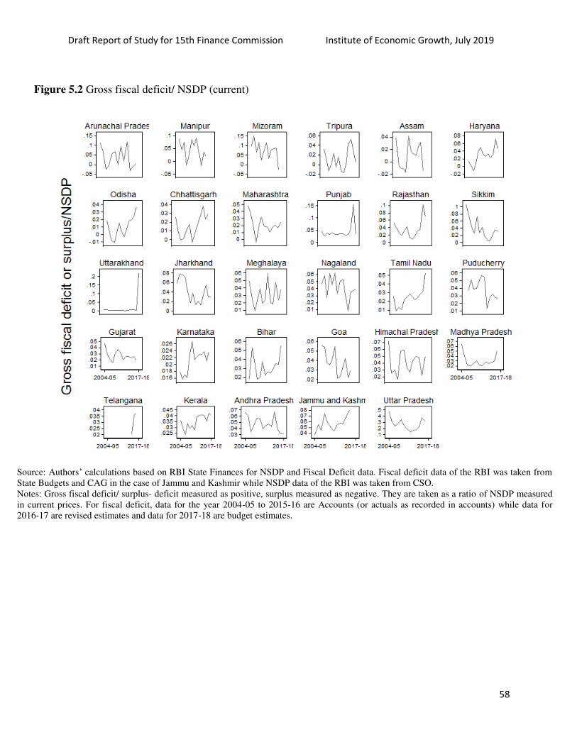
Draft Report of Study for 15th Finance Commission Institute of Economic Growth, July 2019
58
Figure 5.2 Gross fiscal deficit/ NSDP (current)
Source: Authors’ calculations based on RBI State Finances for NSDP and Fiscal Deficit data. Fiscal deficit data of the RBI was taken from
State Budgets and CAG in the case of Jammu and Kashmir while NSDP data of the RBI was taken from CSO.
Notes: Gross fiscal deficit/ surplus- deficit measured as positive, surplus measured as negative. They are taken as a ratio of NSDP measured
in current prices. For fiscal deficit, data for the year 2004-05 to 2015-16 are Accounts (or actuals as recorded in accounts) while data for
2016-17 are revised estimates and data for 2017-18 are budget estimates.

Draft Report of Study for 15th Finance Commission Institute of Economic Growth, July 2019
59
Figure 5.3 Own Tax Revenue (OTR)/NSDP across states from 2004-05 to 2016-17
Source: Authors’ calculations based on data from RBI state finances
Note: Both Own Tax Revenue (OTR) and NSDP are measured in nominal/current terms and in Rs. Billion.
Own Tax Revenue (OTR)/NSDP across states from 2004-05 to 2016-17
Trend analysis of data on OTR as a proportion of NSDP from Figure 5.3 reveals that for most
states during the study period there is a clear upward trend, although there have been years in
between when the ratio has dropped. In some of the states in South and West (Gujarat,
Maharashtra, Madhya Pradesh, Goa, Tamil Nadu , Andhra Pradesh) and in the North East,
significant declines are seen post 2014-2015. A rather mixed picture emerges, both across states
and time. Hence, we attempt an econometric analysis to further examine the data.
Draft Report of Study for 15th Finance Commission Institute of Economic Growth, July 2019
60
5.2.3 Results from econometric analysis: Tax Performance, NSDP and Devolution from
FCs
A set of panel fixed effects regression models were estimated to explore the relationships
between tax performance and devolution to the States. The period of analysis includes data for
three devolution periods – from 12th
to 14th
FC, from 2004-05 till 2016-2017. We present the
findings below.
Own tax revenue (in nominal and absolute terms) is inelastic with respect to changes in the net
devolution11. If the devolution increases the OTR increases less than proportionately. The
coefficient is positive, less than 1 and is statistically significant. However, higher share in the
devolution has been negatively associated with OTR collections during the period studied.
Further, adding dummies for the three FC periods reveals that the 13th
and 14th
FC periods were
associated with a positive impact on OTR irrespective of whether one controls for an impact of
increase in the per capita NSDP or not. There is a positive and significant correlation between
per capita NSDP and the FC period dummies which could be responsible for the dummies not
being significant when per capita NSDP is included in the estimation. Per capita incomes in
states are correlated positively with per capita OTR.
Thus, though higher devolutions are not associated with higher fiscal effort, there does not seem
to be sufficient evidence to establish that the introduction of fiscal discipline in the earlier FCs,
led to higher OTR as compared to the later FC period. We also note that in per capita terms,
OTR is positive and elastic with respect to per capita NSDP, indicating that a change in NSDP
leads to more than proportionate increase in tax collections. One explanation for this could be
that income inequality is increasing with increase in (per capita) income in the states, leading to a
more than proportionate increase in OTR per capita, with higher earnings among people who
were already existing tax payers, or those moving up across tax brackets. Details have been
given in Table 5.3.
11
The net devolution amount (in absolute values) is defined as gross devolution and transfers minus repayments of
loans to Centre and interest payments on loans from Centre.
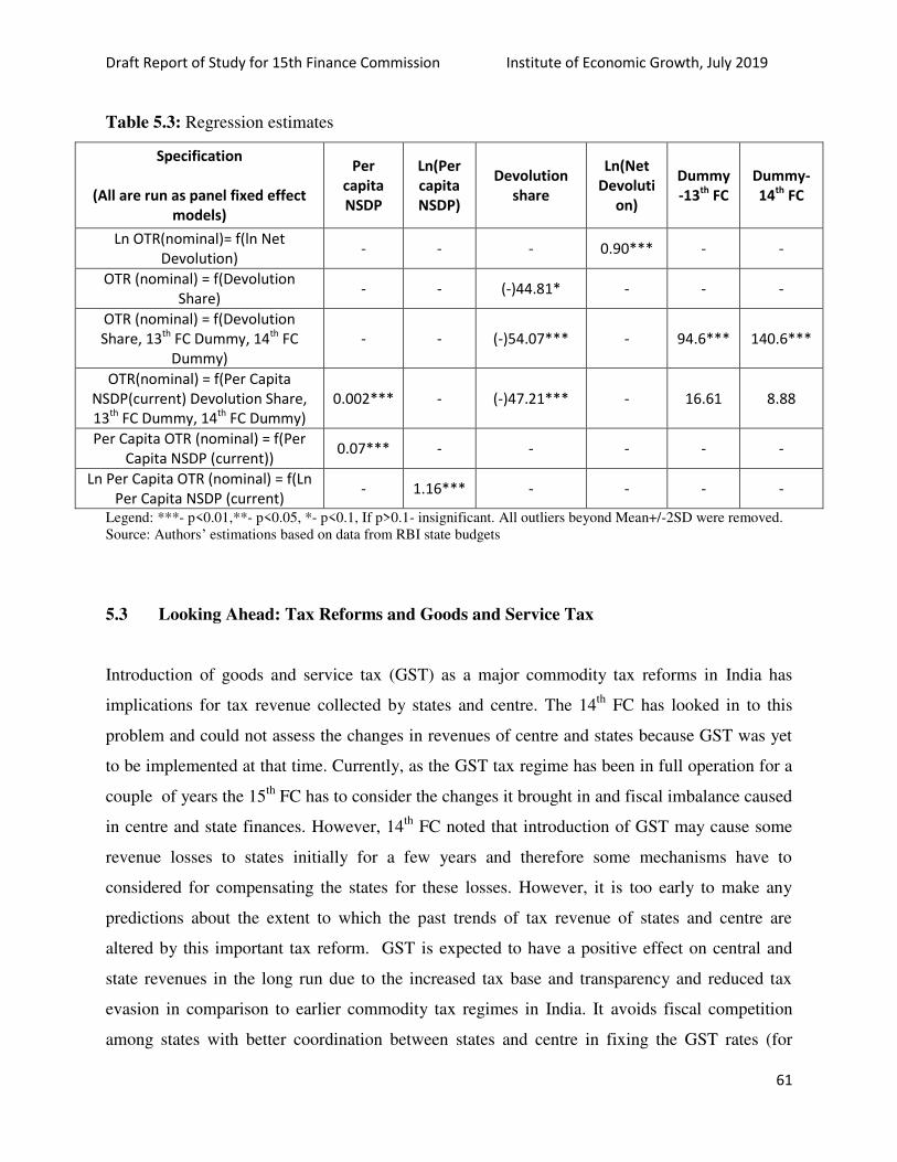
Draft Report of Study for 15th Finance Commission Institute of Economic Growth, July 2019
61
Table 5.3: Regression estimates
Specification
(All are run as panel fixed effect
models)
Per
capita
NSDP
Ln(Per
capita
NSDP)
Devolution
share
Ln(Net
Devoluti
on)
Dummy
-13th
FC
Dummy-
14th
FC
Ln OTR(nominal)= f(ln Net
Devolution) - - - 0.90*** - -
OTR (nominal) = f(Devolution
Share) - - (-)44.81* - - -
OTR (nominal) = f(Devolution
Share, 13th
FC Dummy, 14th
FC
Dummy)
- - (-)54.07*** - 94.6*** 140.6***
OTR(nominal) = f(Per Capita
NSDP(current) Devolution Share,
13th
FC Dummy, 14th
FC Dummy)
0.002*** - (-)47.21*** - 16.61 8.88
Per Capita OTR (nominal) = f(Per
Capita NSDP (current)) 0.07*** - - - - -
Ln Per Capita OTR (nominal) = f(Ln
Per Capita NSDP (current) - 1.16*** - - - -
Legend: ***- p<0.01,**- p<0.05, *- p<0.1, If p>0.1- insignificant. All outliers beyond Mean+/-2SD were removed.
Source: Authors’ estimations based on data from RBI state budgets
5.3 Looking Ahead: Tax Reforms and Goods and Service Tax
Introduction of goods and service tax (GST) as a major commodity tax reforms in India has
implications for tax revenue collected by states and centre. The 14th
FC has looked in to this
problem and could not assess the changes in revenues of centre and states because GST was yet
to be implemented at that time. Currently, as the GST tax regime has been in full operation for a
couple of years the 15th
FC has to consider the changes it brought in and fiscal imbalance caused
in centre and state finances. However, 14th
FC noted that introduction of GST may cause some
revenue losses to states initially for a few years and therefore some mechanisms have to
considered for compensating the states for these losses. However, it is too early to make any
predictions about the extent to which the past trends of tax revenue of states and centre are
altered by this important tax reform. GST is expected to have a positive effect on central and
state revenues in the long run due to the increased tax base and transparency and reduced tax
evasion in comparison to earlier commodity tax regimes in India. It avoids fiscal competition
among states with better coordination between states and centre in fixing the GST rates (for

Draft Report of Study for 15th Finance Commission Institute of Economic Growth, July 2019
62
example the current GST Council in India). The more pertinent problem of concern to states
arises because GST is a destination based tax. It is a worry to more industrialized states like
Gujarat, Maharashtra, Tamil Nadu etc because goods produced in these states are consumed
elsewhere in the country yielding tax revenue to jurisdictions in which they are purchased and
used. Therefore, FCs have to assess the effects of GST regime on revenue collection by states
and the centre before making the recommendations for tax devolution for correcting vertical
fiscal imbalance between centre and states and horizontal imbalances among states.

Draft Report of Study for 15th Finance Commission Institute of Economic Growth, July 2019
63
Draft Report of Study for 15th Finance Commission Institute of Economic Growth, July 2019
64
Chapter 6: Emerging concerns in horizontal and vertical devolution
(TOR 6: Highlight the major emerging concerns in resource devolution with specific
reference to merits and demerits of criteria used for vertical and horizontal balances)
Reducing inequality and poverty eradication are two major goals for the Indian government.
These are also two of the important Sustainable Development Goals, among many others which
India is committed to achieve by 2030. Studies indicate that absolute poverty has substantially
gone down aided by various policies, while inequality in terms of the distribution of
consumption in the economy has increased.
While it might be debatable whether Finance Commission should get involved in consideration
of inter-personal or intra-state inequality, consideration of inter-state inequality may be a natural
concern of the Commission. There is wide difference in average level of living across states in
India. For example, per capita income of Goa at Rs. 375500 is 11 times that of Bihar at Rs.
34400 in the year 2016-17. The difference between the highest per capita income and the lowest
has risen from 6.5 in 1993-94 to 11 in 2016-17.
The Gini coefficient captures the inequality among various subgroups (states in our case) in a
society considering the per capita income and the proportion of population of different
subgroups. The higher the coefficient, the higher the inequality across subgroups. The Gini
coefficient in per capita GSDP of the states in India has shown an increasing trend over time. As
Figure 6.1 shows it was in a small range of 20 to 22 during 1993-94 to 1999-2000, but has
increased thereafter to about 27 in 2016-17.
In view of the rise in inter-state inequality, one could consider using a normative welfare
approach for resource transfers which takes into account the preferences for income
redistribution in favour of the poorer states12
. This implies computing distributional weights for
the income of people belonging to different states in India incorporating an inequality aversion
parameter (e) (see, Note 6.A.1 in Appendix for a theoretical formulation).
12
See, Murty and Nayak (1994) for detailed methodology.
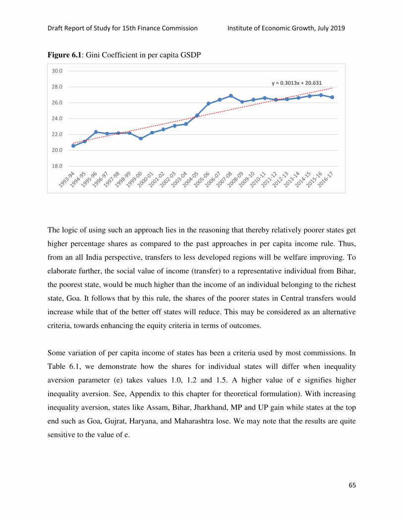
Draft Report of Study for 15th Finance Commission Institute of Economic Growth, July 2019
65
Figure 6.1: Gini Coefficient in per capita GSDP
The logic of using such an approach lies in the reasoning that thereby relatively poorer states get
higher percentage shares as compared to the past approaches in per capita income rule. Thus,
from an all India perspective, transfers to less developed regions will be welfare improving. To
elaborate further, the social value of income (transfer) to a representative individual from Bihar,
the poorest state, would be much higher than the income of an individual belonging to the richest
state, Goa. It follows that by this rule, the shares of the poorer states in Central transfers would
increase while that of the better off states will reduce. This may be considered as an alternative
criteria, towards enhancing the equity criteria in terms of outcomes.
Some variation of per capita income of states has been a criteria used by most commissions. In
Table 6.1, we demonstrate how the shares for individual states will differ when inequality
aversion parameter (e) takes values 1.0, 1.2 and 1.5. A higher value of e signifies higher
inequality aversion. See, Appendix to this chapter for theoretical formulation). With increasing
inequality aversion, states like Assam, Bihar, Jharkhand, MP and UP gain while states at the top
end such as Goa, Gujrat, Haryana, and Maharashtra lose. We may note that the results are quite
sensitive to the value of e.
y = 0.3013x + 20.631
18.0
20.0
22.0
24.0
26.0
28.0
30.0
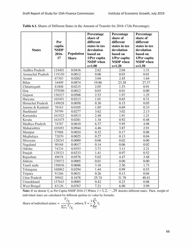
Draft Report of Study for 15th Finance Commission Institute of Economic Growth, July 2019
66
Table 6.1. Shares of Different States in the Amount of Transfer for 2016-17(In Percentage).
States
Per
capita
NSDP
2016-
17
Population
Share
Percentage
share of
different
states in tax
devolution
based on
1/Per capita
NSDP when
e=1.00
Percentage
share of
different
states in tax
devolution
based on
1/Per capita
NSDP when
e=1.20
Percentage
share of
different
states in tax
devolution
based on
1/Per capita
NSDP when
e=1.50
Andhra Pradesh 124401 0.0416 2.62 2.04 1.31
Arunachal Pradesh 119150 0.0012 0.08 0.03 0.01
Assam 67303 0.0262 3.04 2.45 1.64
Bihar 34409 0.0874 19.86 23.28 27.37
Chhattisgarh 81808 0.0215 2.05 1.53 0.91
Goa 375550 0.0012 0.03 0.01 0.00
Gujarat 156527 0.0508 2.53 1.97 1.25
Haryana 165491 0.0213 1.01 0.65 0.31
Himachal Pradesh 149028 0.0058 0.30 0.15 0.05
Jammu & Kashmir 78163 0.0105 1.05 0.69 0.33
Jharkhand 59799 0.0277 3.62 3.02 2.13
Karnataka 161922 0.0513 2.48 1.91 1.21
Kerala 163475 0.0281 1.34 0.92 0.48
Madhya Pradesh 74787 0.0610 6.37 5.95 4.98
Maharashtra 165491 0.0944 4.46 3.87 2.91
Manipur 57888 0.0024 0.32 0.17 0.06
Meghalaya 72870 0.0025 0.27 0.13 0.04
Mizoram 128241 0.0009 0.06 0.02 0.00
Nagaland 90168 0.0017 0.14 0.06 0.02
Odisha 74234 0.0353 3.71 3.11 2.21
Punjab 129321 0.0233 1.41 0.97 0.52
Rajasthan 89678 0.0576 5.02 4.47 3.48
Sikkim 270572 0.0005 0.01 0.00 0.00
Tamil nadu 150036 0.0606 3.16 2.56 1.73
Telangana 160062 0.0294 1.44 0.99 0.53
Tripura 91266 0.0031 0.26 0.13 0.04
Uttar Pradesh 50942 0.1678 25.74 31.78 40.41
Uttarakhand 157643 0.0085 0.42 0.23 0.08
West Bengal 83126 0.0767 7.21 6.90 5.99
Note: If we denote 𝑌𝑖 as Per Capita NSDP 2016-17.Where 1,2, , 29i denotes different states. Then, weight of
individual states are calculated for different epsilon (e) value by formula: Share of individual states = �̅� 𝑌𝑖⁄∑ �̅� 𝑌𝑖⁄29i=1 , where, Y̅ = 1n ∑ Yi29i=1

Draft Report of Study for 15th Finance Commission Institute of Economic Growth, July 2019
67
6.2. Integrating Population Stabilization Indicator in Finance Commission Transfers
Among other considerations, the Terms of Reference (TOR) of the 15th
Finance Commission
(15th
FC) calls for proposing measurable performance-based incentives for the States based on
their efforts and progress in moving towards replacement rate of population growth. Presumably,
this implies rewarding States for progressing towards a stationary population which in
demographic parlance refers to an indefinite continuation of a constant number of births, a
constant life table and zero migration at all ages (Preston et al, 2001). In spirit, the concerned
TOR reflects the overwhelming concern associated with increasing population and emphasises
on the urgency to a constant population in near future. The process - also referred to as
population stabilization – is consistent with development policymaking and has been a prime
focus of several national and international organizations (Srinivasan, 1998, Zodgekar, 1996).
It is critical to view this TOR along with the mandate for the 15th
FC using the population data of
2011. It may be noted that some of the states lagging in population stabilization are also the ones
with high share of population. In other words, states that have performed well in reducing natural
increase (net births) in population are likely to be disadvantaged if the formulae for horizontal
resource sharing is governed by 2011 population instead of 1971 base. Importantly, population
shares are used to weigh all the constituents of the horizontal transfer formulae. Consequently,
this particular TOR has generated considerable debates and disagreements, particularly among
the South India states who are almost set to be the net losers (Bhaskar, 2018, Reddy, 2018).
While the mandate of 15th
FC is to use 2011 population, it has considerable scope to decide upon
the net impact of the population criteria on horizontal transfers. In fact, the 14th
FC had used
2011 population in conjunction with 1971 population to arrive at a formulae for population based
transfers.
Nevertheless, the 15th
FC can conceive an indicator of population stabilization that can be used
to build in incentives (disincentives) for states that have (have not) achieved significant
reductions in population growth. Incentivizing good performance in population stabilization
would be viewed as an additional move that rewards progress and motivates states to move
towards stable population. Given the backdrop, this section is concerned with devising an
indicator and weighing mechanism based on state level performance in population stabilization.

Draft Report of Study for 15th Finance Commission Institute of Economic Growth, July 2019
68
Population Stabilization
At the outset, we briefly outline the concept of population stabilization. Essentially, it refers to
constant birth rates and constant death rates in the specific age structure of a population over a
period of time (Preston et al, 2001). More specifically, a population will be termed to attain
stability if it achieves replacement level of fertility which is 2.1. However, it is difficult to
determine the time period over which the population might stabilize because of variability in
age-specific birth and death rates. The process is dependent upon a number of factors and
assumptions. The key characteristic which could decide the course of stabilization is the age
structure of the population which in turn is determined by the demographic transition taking
place in the society. As such, demographic transition refers to transition from high birth and
death rates to lower birth and death rates. Overtime it is expected that both birth and death rates
decrease with socioeconomic progress.
Notably, population stabilization is a special case of zero population growth. There is a
difference when the population grows at a zero rate and when the population growth is constant.
Also, the effect of migration cannot be ignored which also influences the rate of growth of
population (Bhagat & Mohanty, 2009). To elaborate, if immigration is high in a region, then
population will grow even though the birth and death rates are constant. Another factor is the
sex ratio. In patriarchal societies the preference for son might make a couple opt for a larger
number of children to ensure at least one male child which could contribute to higher population
growth (Johnson, 1994).
The concept of population stabilization should receive more attention in case of India given the
challenging situation with respect to population growth and development (James, 2011). In the
past, the focus in case of India has always been on reducing birth rate to control the population.
The final draft of first five year plan had advocated the need to reduce the birth rate. The Third
Five Year Plan focused on the provision of sterilization services in health care facilities to
control population. In 1976, the government of India came up with its first National Population
Policy and assigned topmost priority to bring down fertility to control the growing population
(Donaldson, 2002). Prior to the first policy it was believed that education and development will
lead to a decline in population growth. However, the first policy noted that this was not a feasible
option. Coercive means were used to achieve lower population growth but the new government
formed in 1978 steered clear of these practices.
Draft Report of Study for 15th Finance Commission Institute of Economic Growth, July 2019
69
The issue of population stabilization did not resurface formally till the government came up with
the second population policy in 2000. The mid-term objective of the second population policy
was to bring total fertility rate (TFR) to 2.1 children per women, which is considered as the
replacement level. TFR is defined as the mean number of births to a woman who completes her
reproductive life and undergoes the same current age-specific fertility patterns over her lifetime.
The long term objective in second population policy was to achieve population stabilization by
the year 2045. Use of fertility rate as a policy indicator is desirable because fertility determines
the overall birth rate in the society and it is not the other way around because the latter is also
influenced by population changes due to migration and survival patterns. Also, the trends and
patterns in fertility outcomes could be monitored. In other words, it is easier to calculate fertility
and observe the change in trends and patterns as compared to other indicators such as migration,
crude birth rate and crude death rate. The Population (Stabilization) Bill 2017 introduced in the
Rajya Sabha also focuses on schemes which encourage two-child norm. Therefore, TFR seems
to be an ideal indicator to proxy the efforts and outcomes associated with population
stabilization.
Deriving TFR-based Weights
We estimate the share that could be allotted to different States based on the TFR. Data for TFR is
sourced from the National Family Health Survey 2015-16 which is conducted by the
International Institute for Population Sciences, Mumbai under the Ministry of Health and Family
Welfare. The idea is to incentivize the States with low TFR. For this purpose, we suggest a
method involving the following 4 steps:
1) The inverse of the TFR value (1/TFR) for each State has been computed.
2) This proportion is now divided by the sum of all the inverse values to arrive at
normalized figures.
3) The normalized values are weighted by using the population shares from Census 2011,
and
4) Values in step (3) is re-normalized to derive the TFR based weights for horizontal
transfers across states (Table 6.2).

Draft Report of Study for 15th Finance Commission Institute of Economic Growth, July 2019
70
Table 6.2 TFR-based weights for Indian states for population stabilization component based on
normalized population weighted inverse TFR analysis
States TFR 2015-16 Population Share
2011
Normalized
(1/TFR) TFR-based Weights (%)
Andhra Pradesh 1.83 0.041 0.038 4.80
Arunachal Pradesh 2.10 0.001 0.033 0.10
Assam 2.21 0.026 0.031 2.48
Bihar 3.41 0.087 0.020 5.36
Chhattisgarh 2.23 0.021 0.031 2.00
Goa 1.66 0.001 0.042 0.13
Gujarat 2.03 0.051 0.034 5.34
Haryana 2.05 0.021 0.034 2.20
Himachal Pradesh 1.88 0.006 0.037 0.68 Jammu and
Kashmir 2.01 0.011 0.034
1.15
Jharkhand 2.55 0.028 0.027 2.33
Karnataka 1.80 0.051 0.038 5.97
Kerala 1.56 0.028 0.044 3.79
Madhya Pradesh 2.32 0.061 0.030 5.64
Maharashtra 1.87 0.094 0.037 10.71
Manipur 2.61 0.002 0.027 0.17
Meghalaya 3.04 0.002 0.023 0.14
Mizoram 2.27 0.001 0.031 0.10
Nagaland 2.74 0.002 0.025 0.15
Odisha 2.05 0.035 0.034 3.66
Punjab 1.62 0.023 0.043 3.05
Rajasthan 2.40 0.058 0.029 5.18
Sikkim 1.17 0.001 0.059 0.18
Tamil Nadu 1.70 0.061 0.041 7.70
Telangana 1.78 0.030 0.039 3.60
Tripura 1.68 0.003 0.041 0.38
Uttar Pradesh 2.74 0.168 0.025 12.94
Uttarakhand 2.07 0.008 0.033 0.81
West Bengal 1.77 0.077 0.039 9.25
All India 2.18 1.000 1.000 100.0 Source: Authors computation based on NFHS 2015-16 and Census of India 2011
Draft Report of Study for 15th Finance Commission Institute of Economic Growth, July 2019
71

Draft Report of Study for 15th Finance Commission Institute of Economic Growth, July 2019
72
Table 6.2 presents the distribution of TFR across the 29 States as reported in NFHS-4. There is a
wide variation in TFR figures with the highest value being 3.41 in case of Bihar and lowest being
1.17 in Sikkim. As many as 11 out of 29 States have a TFR which is greater than 2.1. This means
a majority of the States have been able to bring TFR below the replacement level of 2.1. The
highest TFR is observed in Bihar (3.41) followed by Meghalaya (3.04), Nagaland (2.74) and
Uttar Pradesh (2.74), while the lowest TFR levels are observed in Sikkim (1.17), Kerala (1.56)
and Punjab (1.62).
Table 6.2 also presents the population share of India’s States. These figures are based on data
from Census of India (2011) and does not include the population of Union Territories while
estimating the population shares. The highest population share among states population is of
Uttar Pradesh (16.8 per cent), followed by Maharashtra (9.4 per cent) and Bihar (8.7 per cent).
Bulk of the population is concentrated in only few States. Interestingly, more than 50 per cent of
India’s population reside in Uttar Pradesh, Maharashtra, Bihar, West Bengal, Tamil Nadu and
Madhya Pradesh. The population share of most of the North-eastern States such as Arunachal
Pradesh, Sikkim, Manipur, Meghalaya, Mizoram, Nagaland and Goa is quite low. The combined
population share of these States is even less than 1 per cent. The wide variation in population of
the regions is influenced by a number of factors such as area, TFR levels in the past, birth rate,
death rate and migration to name a few.
The Pearson’s Correlation coefficient between TFR and population share was computed to
measure the strength and direction of linear association between the two variables. The limits for
the correlation coefficient are from +1 (perfect positive correlation) to -1 (perfect negative
correlation). A value of 0.238 was obtained which indicates almost no correlation between the
two variables. The estimate make a lot of sense since it is observed from the data that even
though the population share of UP is high but its TFR is 2.74 which is lower than Bihar’s TFR
(3.41). Similarly, the TFR of Meghalaya (3.04) and Nagaland (2.74) are high but the combined
share of population of these States is not even 1 per cent.
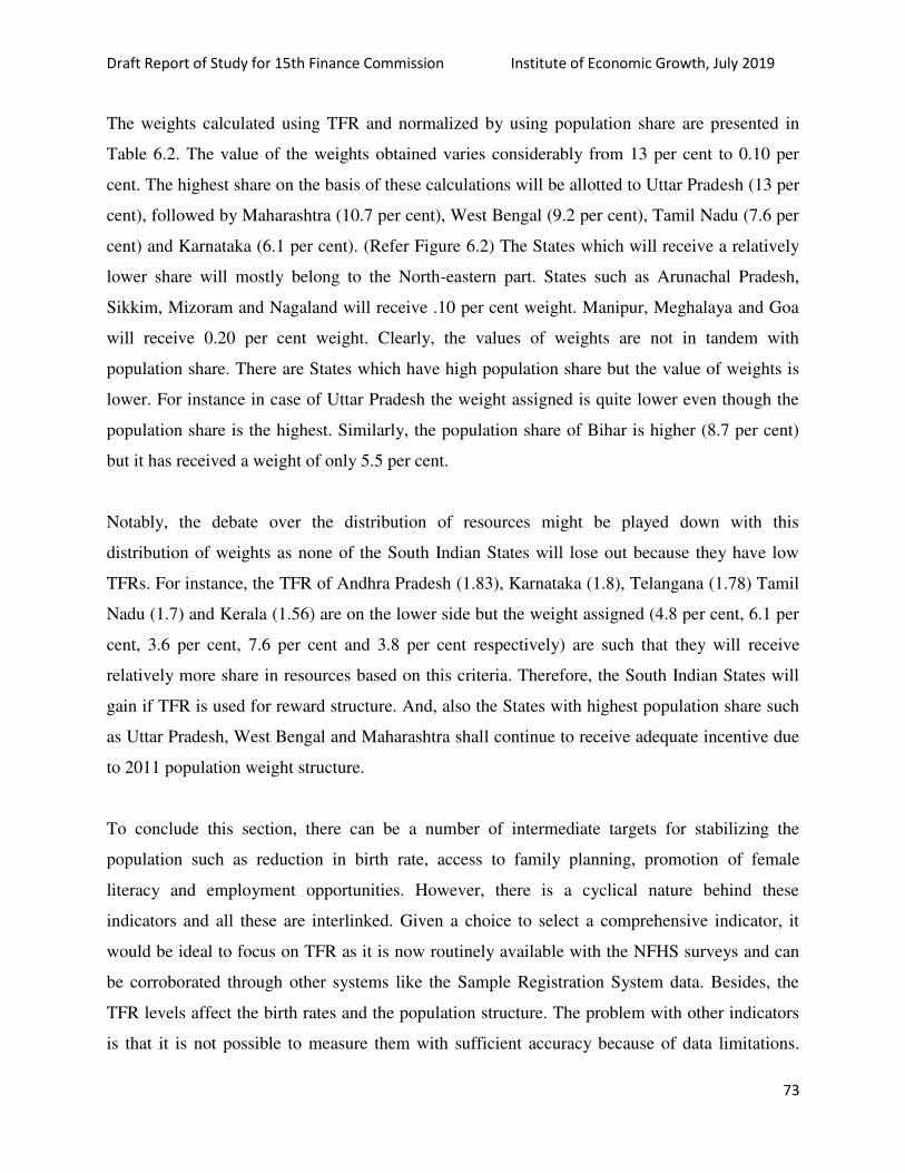
Draft Report of Study for 15th Finance Commission Institute of Economic Growth, July 2019
73
The weights calculated using TFR and normalized by using population share are presented in
Table 6.2. The value of the weights obtained varies considerably from 13 per cent to 0.10 per
cent. The highest share on the basis of these calculations will be allotted to Uttar Pradesh (13 per
cent), followed by Maharashtra (10.7 per cent), West Bengal (9.2 per cent), Tamil Nadu (7.6 per
cent) and Karnataka (6.1 per cent). (Refer Figure 6.2) The States which will receive a relatively
lower share will mostly belong to the North-eastern part. States such as Arunachal Pradesh,
Sikkim, Mizoram and Nagaland will receive .10 per cent weight. Manipur, Meghalaya and Goa
will receive 0.20 per cent weight. Clearly, the values of weights are not in tandem with
population share. There are States which have high population share but the value of weights is
lower. For instance in case of Uttar Pradesh the weight assigned is quite lower even though the
population share is the highest. Similarly, the population share of Bihar is higher (8.7 per cent)
but it has received a weight of only 5.5 per cent.
Notably, the debate over the distribution of resources might be played down with this
distribution of weights as none of the South Indian States will lose out because they have low
TFRs. For instance, the TFR of Andhra Pradesh (1.83), Karnataka (1.8), Telangana (1.78) Tamil
Nadu (1.7) and Kerala (1.56) are on the lower side but the weight assigned (4.8 per cent, 6.1 per
cent, 3.6 per cent, 7.6 per cent and 3.8 per cent respectively) are such that they will receive
relatively more share in resources based on this criteria. Therefore, the South Indian States will
gain if TFR is used for reward structure. And, also the States with highest population share such
as Uttar Pradesh, West Bengal and Maharashtra shall continue to receive adequate incentive due
to 2011 population weight structure.
To conclude this section, there can be a number of intermediate targets for stabilizing the
population such as reduction in birth rate, access to family planning, promotion of female
literacy and employment opportunities. However, there is a cyclical nature behind these
indicators and all these are interlinked. Given a choice to select a comprehensive indicator, it
would be ideal to focus on TFR as it is now routinely available with the NFHS surveys and can
be corroborated through other systems like the Sample Registration System data. Besides, the
TFR levels affect the birth rates and the population structure. The problem with other indicators
is that it is not possible to measure them with sufficient accuracy because of data limitations.
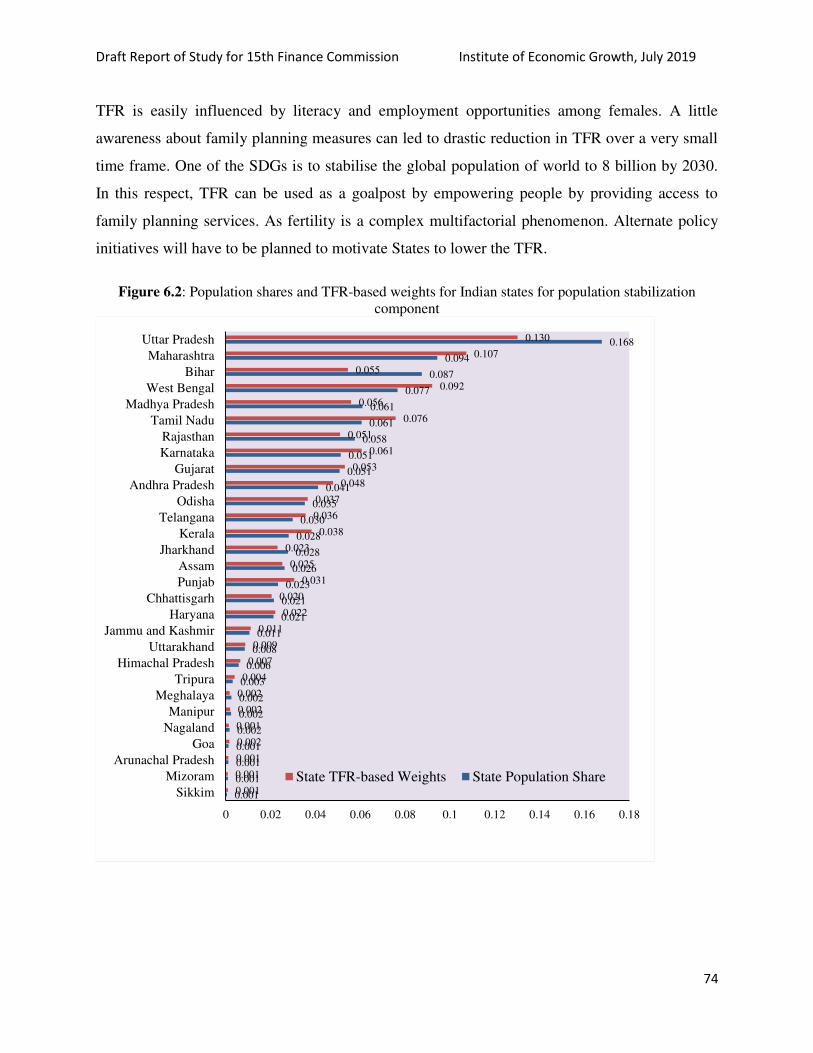
Draft Report of Study for 15th Finance Commission Institute of Economic Growth, July 2019
74
TFR is easily influenced by literacy and employment opportunities among females. A little
awareness about family planning measures can led to drastic reduction in TFR over a very small
time frame. One of the SDGs is to stabilise the global population of world to 8 billion by 2030.
In this respect, TFR can be used as a goalpost by empowering people by providing access to
family planning services. As fertility is a complex multifactorial phenomenon. Alternate policy
initiatives will have to be planned to motivate States to lower the TFR.
Figure 6.2: Population shares and TFR-based weights for Indian states for population stabilization
component
0.001
0.001
0.001
0.001
0.002
0.002
0.002
0.003
0.006
0.008
0.011
0.021
0.021
0.023
0.026
0.028
0.028
0.030
0.035
0.041
0.051
0.051
0.058
0.061
0.061
0.077
0.087
0.094
0.168
0.001
0.001
0.001
0.002
0.001
0.002
0.002
0.004
0.007
0.009
0.011
0.022
0.020
0.031
0.025
0.023
0.038
0.036
0.037
0.048
0.053
0.061
0.051
0.076
0.056
0.092
0.055
0.107
0.130
0 0.02 0.04 0.06 0.08 0.1 0.12 0.14 0.16 0.18
Sikkim
Mizoram
Arunachal Pradesh
Goa
Nagaland
Manipur
Meghalaya
Tripura
Himachal Pradesh
Uttarakhand
Jammu and Kashmir
Haryana
Chhattisgarh
Punjab
Assam
Jharkhand
Kerala
Telangana
Odisha
Andhra Pradesh
Gujarat
Karnataka
Rajasthan
Tamil Nadu
Madhya Pradesh
West Bengal
Bihar
Maharashtra
Uttar Pradesh
State TFR-based Weights State Population Share

Draft Report of Study for 15th Finance Commission Institute of Economic Growth, July 2019
75
6.3 Environment and NDC commitments
In India, environmental regulation is constitutionally mandated under various Acts, such as the
air and water pollution acts, the forest conservation act, the wildlife protection act, and the
environment protection act. Environmental regulation requires states to comply with
scientifically determined standards for air and water quality, and to maintain area under protected
ecosystems (forest cover, coastal zones, mangroves, etc.). While environmental regulation is
extremely important for sustainable development, it imposes costs on the states. These range
from maintenance and operating costs, to opportunity costs for those that have substantial part of
their land areas protected for their forest cover and/or for protecting wildlife, to those that are
impacted by severe air and water pollution and incur clean up or abatement costs. Thus, Indian
states would differ with respect to the costs incurred both by type and level of costs. The latter
would depend on two factors: the extent of environmental compliance and the type and extent of
natural resource stocks available with the state.
However, the positive externalities of environmental regulation lead to benefits across scales.
There are benefits to the people living in the state itself, for instance, in the case of abatement of
air pollution in cities. There are benefits at a regional level since multiple ecosystem services
flow across borders, for instance, in the case of abatement of air and water pollution across air
sheds and watersheds in Northern India. At the international level, India has caught global
attention for its forward-looking commitments towards the Paris Agreement, through its
Nationally Determined Contributions (NDCs). Two major thrust areas are targets set for
renewable energy and sinks for carbon. The TOR of the 15th
Finance Commission mentions in
3(ii), that in making its recommendations, the Commission shall consider the demands on the
resources of the Central Government on account of climate change, among other factors. In the
context of proposing measurable performance-based incentives for States, at the appropriate
level of government, in TOR 4 (iii) sustainable development goals have been mentioned. For
both the climate change implications and SDGs (e.g. Climate action, Life on land, etc.) forestry
sector has an important role to play. In particular, it deserves special mention in the context of
allocations made by previous FCs for forests. As mentioned earlier (chapter 3), the 14th
FC
brought in the dense forest cover in a state as a factor determining interstate devolution whereas
Draft Report of Study for 15th Finance Commission Institute of Economic Growth, July 2019
76
earlier provision for grants had been made. The primary argument in the FC award has been in
terms of the economic disability posed to states which are mandated to maintain forest cover and
the need to compensate them for the losses thereof in fiscal capacity.
The NDC target is to create an additional carbon sink of 2.5 to 3 billion tons Carbon dioxide
equivalent through forest and tree cover by 2030. Data on state wise forest cover from the recent
SFR (FSI, 2017) indicates that there has not been appreciable increase in forest cover across
most states over the period of the last decade. While the existing formula may have
compensated for fiscal capacity, the 14th
FC also acknowledged the role of forests in meeting
international obligations. As the devolution is an untied allocation by its very nature, it is
expected that it may not provide any incentive to increase forest cover in line with the NDC
target, on one hand. On the other hand, historically, grants have been limited in size and probably
will require a substantial boost in order to help meet even part of the costs of creating a carbon
sink of this magnitude. The formula seems well-positioned to address compensation for the
purpose of fiscal disability and is consistent with the intention of horizontal devolution which is
to ensure devolutions to states to meet their developmental needs.
Apart from the issue of the NDC target, an important concern with incentivizing dense forest
cover alone is that it fails to take note of the valuable ecological resources outside such forests in
many states. Some of these are also mandated to protect the environment and ecosystems (for
instance, preservation of species outside dense forests as in grasslands for Asiatic lions in Gir,
enriching soil carbon and enhancing tree cover outside dense forests, and so on). Under the
circumstances, a re-look at the devolution criteria may be considered to capture forward looking
aspects as well as to enhance the equity aspect of compensating for fiscal capacity.
An analysis of the data and interactions with forest department officials suggests that the current
formulation in which untied funds are devolved to states, is unlikely to help India achieve its
target for creation of additional CO2 sink through forest and tree cover. Implicitly it also creates
a wedge in the distribution across states with dense forest cover and those with other significant
environmental constraints. Nor, does it seem to have provided incentives for states to increase

Draft Report of Study for 15th Finance Commission Institute of Economic Growth, July 2019
77
tree cover outside forests. Some motivational alternatives alongside illustrative data are
presented below.
Forest Cover in Previous FC awards
The conversation around forest cover has been present from the 11th
FC itself. The 11th
FC found
that forest cover was below the desirable level and states were encouraged to prepare working
plans for management of forests. Obstacles in maintaining forests with respect to the working
plans was highlighted by the states in the 12th
FC when they claimed that the restrictions placed
by the Supreme Court on exploitation of forest wealth led to financial constraints regarding
maintenance and the forest becoming a net liability rather than a source of revenue. They put
forth a demand for separate grants for maintenance of forests which the 12th
FC conceded to,
stating that the forests were a national responsibility and recommended a grant of Rs.1000 crore
to be distributed amongst states based on their forest area for the period 2005-10 over and above
states’ forest department spending. The 13th
FC recommended an amount of Rs. 5000 crore as
forest grant for the award period with untied grants for the first two years and a conditional
release of grant for the last three years depending on the number of approved working plans. The
13th
FC grant formula took into consideration share of the states’ forest area in total forest area
which was weighted by forest density, in order to address both concerns of economic disability
and quality of forests. Under quality of forests, progressively higher weights were given to area
under moderately dense and dense forest cover. The 14th
FC argued that forests and their
externalities have impacts both on the provision of services to people living in forest areas
(hence, state expenditure) and also decline in revenue due to restriction on exploitation and
hence needed to be compensated. In addition, the 14th
FC acknowledged importance of
preserving forests in order to enable the nation to meet its international obligations on
environment related measures. The 14th
FC assigned 7.5 per cent weight to the forest cover and
took into consideration moderately dense forest and very dense forest (from here on, collectively
referred to as dense forest) as part of the formula.
Data Source
Data for the purpose of analysis was collected from the Indian State of Forests report published
by the Forest survey of India. The data was compiled from ISFR 2009, 2015 and 2017 and
Draft Report of Study for 15th Finance Commission Institute of Economic Growth, July 2019
78
correspond to the periods October 2006 to February 2007 (referred to as 2007), October 2013 to
February 2014(referred to as 2013) and October 2015 to December 2015 (referred to as 2015)
respectively.
Box 6.2: Forest Component -Relevant Definitions
Forest cover:
According to ISFR 2015, “the term forest cover as used in ISFR refers to all lands more than one
hectare in area with a tree canopy of more than 10% irrespective of land use, ownership and legal
status. It may include even orchards, palm, bamboo etc.”
Recorded Forest Area:
The definition of recorded forest area according to ISFR 2015, RFA refers to “All the geographic
areas recorded as forests in government records.” ISFR 2015 and ISFR 2017 state that
“Recorded Forest Areas largely consist of Reserved Forests (RF) and Protected Forests (PF),
which have been constituted under the provisions of Indian Forest Act 1927 or its counterpart
State Acts.”
Classification of forest in terms of canopy density classes:
According to ISFR 2017,
Very Dense Forest: “All lands with tree canopy density of 70% and above.”
Moderately Dense Forest: “All lands with tree canopy density of 40% and more but less than
70%.”
Open Forest: “All lands with tree canopy density of 10% and more but less than 40%”
Scrub: “Degraded forest lands with canopy density less than 10%”
Non-forest: “Lands not included in any of the above classes (includes water)”
Tree Cover: According to ISFR 2017,“tree cover is “an estimated area comprising of tree patches, which are
less than one hectare and isolated trees outside the recorded forest.” “Trees included in tree cover
constitute only a part of Trees Outside Forest.”
Trees Outside Forest: According to ISFR 2015, “TOF are trees outside the recorded forests”. ISFR 2017 also
additionally states that “Trees existing outside the recorded forest area mainly in the form of
block, linear and scattered size of patches are called TOF”.
Green wash area: According to ISFR 2017, “The area shown by green color, which is referred to as a green wash
area represents the forested areas at the time of survey carried out to prepare topographic sheets.”
“The green wash has been used as a substitute to RFA in respect of those states and UTs from
where the digitized boundary of recorded forest area is unavailable.”
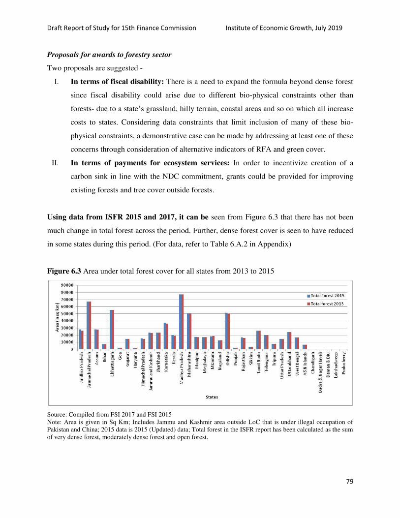
Draft Report of Study for 15th Finance Commission Institute of Economic Growth, July 2019
79
Proposals for awards to forestry sector
Two proposals are suggested -
I. In terms of fiscal disability: There is a need to expand the formula beyond dense forest
since fiscal disability could arise due to different bio-physical constraints other than
forests- due to a state’s grassland, hilly terrain, coastal areas and so on which all increase
costs to states. Considering data constraints that limit inclusion of many of these bio-
physical constraints, a demonstrative case can be made by addressing at least one of these
concerns through consideration of alternative indicators of RFA and green cover.
II. In terms of payments for ecosystem services: In order to incentivize creation of a
carbon sink in line with the NDC commitment, grants could be provided for improving
existing forests and tree cover outside forests.
Using data from ISFR 2015 and 2017, it can be seen from Figure 6.3 that there has not been
much change in total forest across the period. Further, dense forest cover is seen to have reduced
in some states during this period. (For data, refer to Table 6.A.2 in Appendix)
Figure 6.3 Area under total forest cover for all states from 2013 to 2015
Source: Compiled from FSI 2017 and FSI 2015
Note: Area is given in Sq Km; Includes Jammu and Kashmir area outside LoC that is under illegal occupation of
Pakistan and China; 2015 data is 2015 (Updated) data; Total forest in the ISFR report has been calculated as the sum
of very dense forest, moderately dense forest and open forest.
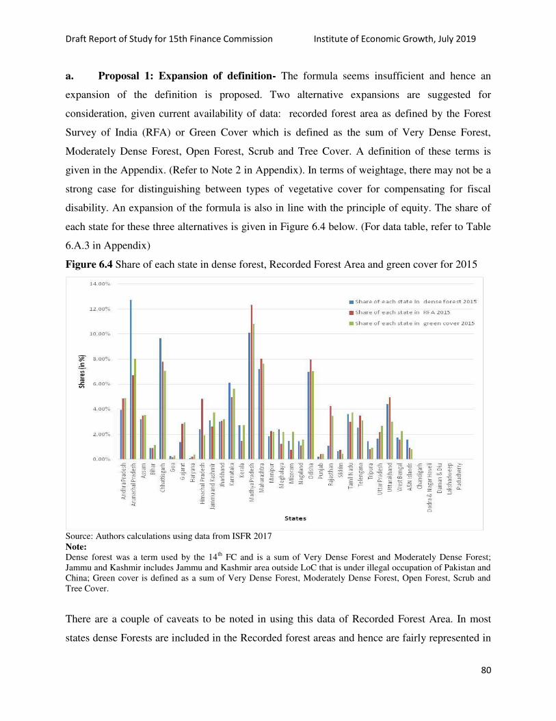
Draft Report of Study for 15th Finance Commission Institute of Economic Growth, July 2019
80
a. Proposal 1: Expansion of definition- The formula seems insufficient and hence an
expansion of the definition is proposed. Two alternative expansions are suggested for
consideration, given current availability of data: recorded forest area as defined by the Forest
Survey of India (RFA) or Green Cover which is defined as the sum of Very Dense Forest,
Moderately Dense Forest, Open Forest, Scrub and Tree Cover. A definition of these terms is
given in the Appendix. (Refer to Note 2 in Appendix). In terms of weightage, there may not be a
strong case for distinguishing between types of vegetative cover for compensating for fiscal
disability. An expansion of the formula is also in line with the principle of equity. The share of
each state for these three alternatives is given in Figure 6.4 below. (For data table, refer to Table
6.A.3 in Appendix)
Figure 6.4 Share of each state in dense forest, Recorded Forest Area and green cover for 2015
Source: Authors calculations using data from ISFR 2017
Note:
Dense forest was a term used by the 14th
FC and is a sum of Very Dense Forest and Moderately Dense Forest;
Jammu and Kashmir includes Jammu and Kashmir area outside LoC that is under illegal occupation of Pakistan and
China; Green cover is defined as a sum of Very Dense Forest, Moderately Dense Forest, Open Forest, Scrub and
Tree Cover.
There are a couple of caveats to be noted in using this data of Recorded Forest Area. In most
states dense Forests are included in the Recorded forest areas and hence are fairly represented in
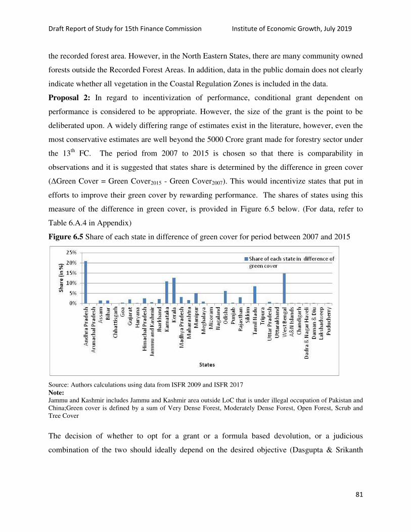
Draft Report of Study for 15th Finance Commission Institute of Economic Growth, July 2019
81
the recorded forest area. However, in the North Eastern States, there are many community owned
forests outside the Recorded Forest Areas. In addition, data in the public domain does not clearly
indicate whether all vegetation in the Coastal Regulation Zones is included in the data.
Proposal 2: In regard to incentivization of performance, conditional grant dependent on
performance is considered to be appropriate. However, the size of the grant is the point to be
deliberated upon. A widely differing range of estimates exist in the literature, however, even the
most conservative estimates are well beyond the 5000 Crore grant made for forestry sector under
the 13th
FC. The period from 2007 to 2015 is chosen so that there is comparability in
observations and it is suggested that states share is determined by the difference in green cover
(ΔGreen Cover = Green Cover2015 - Green Cover2007). This would incentivize states that put in
efforts to improve their green cover by rewarding performance. The shares of states using this
measure of the difference in green cover, is provided in Figure 6.5 below. (For data, refer to
Table 6.A.4 in Appendix)
Figure 6.5 Share of each state in difference of green cover for period between 2007 and 2015
Source: Authors calculations using data from ISFR 2009 and ISFR 2017
Note:
Jammu and Kashmir includes Jammu and Kashmir area outside LoC that is under illegal occupation of Pakistan and
China;Green cover is defined by a sum of Very Dense Forest, Moderately Dense Forest, Open Forest, Scrub and
Tree Cover
The decision of whether to opt for a grant or a formula based devolution, or a judicious
combination of the two should ideally depend on the desired objective (Dasgupta & Srikanth

Draft Report of Study for 15th Finance Commission Institute of Economic Growth, July 2019
82
2019)13
. In the case of a formula based, untied devolution to compensate for fiscal disability, it
can be argued that states can face fiscal disability from various biophysical characteristics and
forests constitute an important, but only one of these. Another prominent characteristic, apart
from forests, are mountains. Mountains impose constraints on states while taking forward their
commitments for provision of public services in the form of increased costs (Dasgupta & Goldar,
2017) and arise on the expenditure side, unlike forests where fiscal disability arises from the
limitations for raising revenues through alternative land use on the revenue side. Many
mountainous states also have significant overlaps with forested states. Yet, a case can be made
for privileging forests because of their multiple ecosystem services and the fact that they
represent a planetary boundary (Rockstrom et al., 2009; IPBES, 2018), essential for human
existence. In which case, the formula based devolution may be continued with some
modifications as suggested above in the computation of state shares, and an overall weightage of
5%.
Alternatively, grants maybe considered. Grants make it possible to ensure that fund allocation
serves stated targets for forest conservation. It also make it easier to build in social and
environmental safeguards to ensure that multiple goals are served, such as improving forest
condition alongside the achievement of relevant SDGs through scientifically planned livelihood
and income generation activities. The principal argument against grants seems to have been the
fact that conventionally the amount of grant has been relatively smaller than the magnitudes
devolved through the formula. We would recommend a straightforward doubling of the grant
amount from the 13th
Finance Commission, along with measures to monitor the utilization of the
grant mid-way through the award period, and ensuring safeguards for its implementation on the
ground in keeping with the achievement of the SDG commitments. The argument thus, is framed
not so much in terms of the NDC, but in terms of achieving SDGs as well. Also, India seems
well set on the path of achieving the NDC target, as defined on a baseline of 2005 (akin to the
commitment on reduction in emissions intensity of the economy).
Recent experience seems to suggest that if the desired objective is to encourage the achievement
of specific targets, then grant based allocation where funds are tied is likely to work better. Else,
13
Under review
Draft Report of Study for 15th Finance Commission Institute of Economic Growth, July 2019
83
if the primary intent is to compensate the state for fiscal disability, the untied allocation through
the formula provides the desired flexibility to states to help overcome the disability, and meet
their expenditure needs. However, the implications of going with one or the other vary from state
to state as our results clearly indicate. .
Some other considerations:
6.4 Disaster Management
Earmarking funds for disaster management and distributing them to different levels of
jurisdictions in a federal country like India are some of the challenges for finance commissions.
There is a need for considering adaptation or response strategies and mitigation strategies and the
cost implication of disasters.. Response strategies for disaster management require finances to
attend to the problems arising in the short run, probably the immediate mandatory five year
period of FC award. In contrast, mitigation strategies require funds for very long run planning
which makes it difficult for FC to assess the cost and make recommendations.
The Indian Parliament had enacted the Disaster Management Act, 2005 for constituting two
types of funds as expected: one for disaster response and the other for mitigation.14Subsequently,
disaster management authorities were introduced at national, state and district levels for
channelizing funds earmarked by Union FC, state FCs and the respective governments for
disaster management. The 13th
FC was of the view that the mitigation strategies have to be a part
of planning process and that direct transfers from respective ministries of centre, states and Niti
Aayog could help meet this objective. The 14th
FC recommended an aggregate amount of Rs.
61219 crores towards State Disaster Relief Fund (SDRF) with centre and states contributing to it
in the ratio of 90:10 percent respectively. It is a challenge to assess the costs of both adaptation
and mitigation in disaster management, and to make recommendations for different levels of
government in sharing the cost. Currently, only the cost of response strategies is considered by
the FCs given the problems in assessment of mitigation strategies. For making reliable
assessments of finances for disaster management, it is important to have some reliable scientific
information in advance about the possible number of events and their intensity. Some earlier FCs
14
The list of recorded disasters considered by various FCs after this act include cyclones, droughts, earth quakes, fires, floods, tsunamis,
hailstorms, landslides, avalanches, cloud bursts , pest attacks, cold waves and frost.

Draft Report of Study for 15th Finance Commission Institute of Economic Growth, July 2019
84
have noted the need for developing indices which reflect a state’s or district’s vulnerability to
disasters. The central and various state governments have now realized the need for developing
the Hazard Vulnerability Risk Profiles of States and considering them as a basis for determining
state disaster response fund (SDRF) and central allocations for this purpose. It is recommended
that these profiles are made available to the FCs by the concerned authorities, so that it is taken
into account in making the recommendations for SDRF. Availability of this scientific
information could also help in designing and assessing costs of mitigation strategies for disaster
management.
Information about consolidated yearly revenue grants of centre to states during the period 2000-
2001 to 2015-2016 at current prices reveals the following. (Refer to Table 6.3). There is a sharp
increase in these grants after the award of 14th
FC and has more than doubled (Rs. 57560.4 to.
Rs. 129100.0 million) between the financial years 2014 and 2015. One also finds very significant
variation in grants received by various states reflecting that states differ substantially in respect
to vulnerability to natural disasters. In the year 2016 the bigger states of UP, Maharashtra and
Tamil Nadu got relief of Rs. 77019.6, 28121.2, and 18386.2 million respectively. However, one
of the smaller states of Uttarakhand got the relief amounting to Rs. 62342.7 million which was
much higher than the relief given to Maharashtra. These reliefs granted ex post are indicate that
logically there are significant underlying differences in the disaster vulnerability index among
states.
Table 6.3: Consolidated Revenue Grants of Centre to States on Account of Natural Calamities
Year Grants (Rs. Million)
2000 4997.2
2001 5948.9
2002 32345.8
2003 17741.6
2004 21665.5
2005 32716.7
2006 36038.5
2007 26392.3
2008 29141.9
2009 34957.1
2010 52180.5
2011 32138.6
2012 55593.8

Draft Report of Study for 15th Finance Commission Institute of Economic Growth, July 2019
85
2013 61590.3
2014 57560.4
2015 129100
2016 110600 Source: State Finances, Reserve Bank of India
6.5 Air and Water Pollution
Indian states could differ with respect to sustainable use of environmental resources such as air
quality and water quality. There is an opportunity cost to the sates to keep the environmental
resource stocks at sustainable or natural regenerative levels. Environmental regulation to make
the states comply with the scientifically fixed environmental standards (say WHO standards for
air and water quality and forest cover) ensures that the environmental resource stocks in a state
are maintained at their natural regenerative levels. The cost to the states to comply with these
standards is called the cost of its environmentally sustainable development. It could be
empirically observed that Indian states differ with respect to level of environmental compliance
and abatements costs incurred.
Positive externalities of sustainable use of environmental resources by a state confer benefits to
the people belonging to it and also benefits for the people in the rest of states and in some cases
rest of the world. The amount of benefits each state generates in this context depends upon the
level of its compliance to environmental regulation and the amount of stocks of environmental
resources it possesses. The instruments of fiscal transfers from centre to states pertaining to
environmental performance of states could be therefore either cost based or benefit based. The
transfers are meant for compensating states for the cost they incur or benefits they confer by
efficient environmental management.
6.5.1 Air Pollution
Environmentally sustainable development requires that the atmospheric quality, one of the
important environmental resources has to be maintained at its natural regenerative level or at safe
air quality standards fixed by WHO and other national and international institutions. The local
air quality is affected by emissions of Particulate Matter (PM10), Sculpture Dioxide (SO2),
Nitrogenous Oxide (NOx) and other air pollutants while the emissions of greenhouse gases like
Draft Report of Study for 15th Finance Commission Institute of Economic Growth, July 2019
86
Carbon Dioxide (CO2) have effects on global atmosphere quality and climate change. The
environmental regulations of centre and states in India require that emissions from all
anthropogenic activities in an Indian state have to be such that the air quality standards are met.
Regulation entails an additional cost to the state’s economy in the form of air pollution
abatement costs incurred by polluting activities in the state. Equally it provides health benefits
of reduced air pollution to people living in the state and the benefits of reducing climate change
problem for the world community in the case of reduction of greenhouse gases. Scientifically
developed air quality index for each state accounting for effects of different types of emissions
on air quality if possible could be helpful to gauge each states performance in air pollution
reduction.
The instruments of resource transfers from centre to states designed to compensate states for the
emissions reduction could be again either benefit based or cost based. The weights to be assigned
for different pollutants to compute an air quality index could be either benefit based or cost
based. Hypothetically if all the emissions in the state are contained to WHO emission standards,
the computed air quality is index 100 percent. In the case of some or more of air pollutants
exceeding the standards, the air quality index will be below100 percent. The cost based weights
could be objectively estimated using the estimated abatement cost function for each pollutant.
However, the estimation of benefit based weights requires the use of valuation methods
involving lot of assumptions and subjectivity. There are number studies recently done in India
for estimating health benefits to urban households in cities like Delhi, Kolkata and Hyderabad
from particulate matter reductions using environmental valuation methods. It is empirically
observed in India that normally only Particulate Matter (P10) emissions exceed the prescribed
standards in major urban areas while the emissions of Sculpture Dioxide (SO2) and Nitrogenous
Oxide (NOx) do not violate the standards. Therefore the 15th
FC could be guided simply by
Particulate Matter (PM10) emission levels in each state instead of hypothetical air quality index
for each state in deciding about the relative shares of states in the resources ear marked for
maintaining air quality in the states.
Meta-analysis of environmental valuation studies in India related to effects of urban air pollution
(PM10) on household health could provide information about household marginal willingness pay
or demand function for urban air quality in India. Using this demand function and data about

Draft Report of Study for 15th Finance Commission Institute of Economic Growth, July 2019
87
annual average PM10 level for each state for a recent year, health damages from PM10 emissions
for a typical household in the state could be estimated. The total health damages to the state from
PM10 emissions could be estimated by extrapolating the damages to a typical household to the
entire population of urban households in the state. Estimates of health damages obtained in this
way for all the states in India could be used to calculate the relatives shares of states in the
central transfer ear marked for air quality in the states. Appendix 6 describes a method of
determining state specific air pollution standards for India with implications for tax devolution.
6.5.2 Water Pollution
The case of water pollution or pollution levels of rivers and water bodies in the states, it is
difficult to objectively measure ambient water quality specific to a state. Pollution of water
bodies is normally measured by parameters like Dissolved Oxygen (DO), Biological Oxygen
Demand (BOD), Chemical Oxygen Demand (COD) and Suspended Solids (SS). Given that all
the major rivers in India are interstate rivers, it is not possible to attribute the ambient river
pollution in a state entirely to that particular state. Environmental performance in reducing river
pollution is the result of efforts of all states in its basin. For example Ganga Action Plan to clean
Ganges is a project involving central government and governments of all states in the Ganga
basin. Therefore, water pollution could not be considered as one of the environmental indicators
specific to each to state and it could not be used as one of the environmental criteria for tax
devolution.
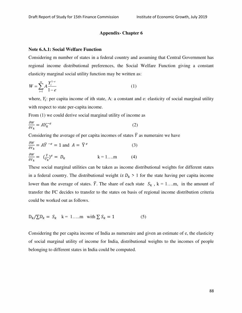
Draft Report of Study for 15th Finance Commission Institute of Economic Growth, July 2019
88
Appendix- Chapter 6
Note 6.A.1: Social Welfare Function
Considering m number of states in a federal country and assuming that Central Government has
regional income distributional preferences, the Social Welfare Function giving a constant
elasticity marginal social utility function may be written as:
m
i
e
i
e
YAW
1
1
1 (1)
where, 𝑌𝑖: per capita income of ith state, A: a constant and e: elasticity of social marginal utility
with respect to state per-capita income.
From (1) we could derive social marginal utility of income as 𝜕𝑊𝜕𝑌𝑘 = 𝐴𝑌𝑘−𝑒 (2)
Considering the average of per capita incomes of states �̅� as numeraire we have 𝜕𝑊𝜕𝑌𝑘 = 𝐴�̅� −𝑒 = 1 and 𝐴 = Y̅ 𝑒 (3) 𝜕𝑊𝜕𝑌𝑘 = ( �̅�𝑌𝑘)𝑒 = 𝐷𝑘 k = 1….m (4)
These social marginal utilities can be taken as income distributional weights for different states
in a federal country. The distributional weight 𝑖𝑠 𝐷𝑘 > 1 for the state having per capita income
lower than the average of states. �̅�. The share of each state 𝑆𝑘 , k = 1….m, in the amount of
transfer the FC decides to transfer to the states on basis of regional income distribution criteria
could be worked out as follows.
Dk/∑𝐷𝑘 = 𝑆𝑘 k = 1…..m with ∑ 𝑆𝑘 = 1 (5)
Considering the per capita income of India as numeraire and given an estimate of e, the elasticity
of social marginal utility of income for India, distributional weights to the incomes of people
belonging to different states in India could be computed.

Draft Report of Study for 15th Finance Commission Institute of Economic Growth, July 2019
89
Table 6.A.2: Table showing change in total forest cover from 2013 to 2015 for all states
State Total
forest 2015
Total
forest 2013
Difference in
total forest State
Total forest
2015
Total
forest
2013
Difference
in total
forest
Andhra Pradesh 28147 26006 2141 Nagaland 12489 12939 -450
Arunachal
Pradesh 66964 67154 -190 Odisha 51345 50460 885
Assam 28105 27538 567 Punjab 1837 1771 66
Bihar 7299 7254 45 Rajasthan 16572 16106 466
Chhattisgarh 55547 55559 -12 Sikkim 3344 3353 -9
Goa 2229 2210 19 Tamil Nadu 26281 26208 73
Gujarat 14757 14710 47 Telengana 20419 19854 565
Haryana 1588 1580 8 Tripura 7726 7890 -164
Himachal
Pradesh 15100 14707 393 Uttar Pradesh 14679 14401 278
Jammu and
Kashmir 23241 22988 253 Uttarakhand 24295 24272 23
Jharkhand 23553 23524 29 West Bengal 16847 16826 21
Karnataka 37550 36449 1101 A&N Islands 6742 6751 -9
Kerala 20321 19278 1043 Chandigarh 21.56 21.66 -0.1
Madhya Pradesh 77414 77426 -12 Dadra & Nagar
Haveli 207 206 1
Maharashtra 50682 50699 -17 Daman & Diu 20.49 19.61 0.88
Manipur 17346 17083 263 Lakshadweep 27.1 27.06 0.04
Meghalaya 17146 17262 -116 Puducherry 53.67 56.95 -3.28
Mizoram 18186 18717 -531 TOTAL 708080.8 701306.3 6774.54
Source: Compiled from FSI, 2015 and FSI, 2017
Note:
Area in sq km; Dense forest was a term used by the 14th
FC and is a sum of Very Dense Forest and Moderately
Dense Forest; Jammu and Kashmir includes Jammu and Kashmir area outside LoC that is under illegal occupation
of Pakistan and China; 2015 data is 2015 (Updated) data; Total forest in the ISFR report has been calculated as the
sum of very dense forest, moderately dense forest and open forest.

Draft Report of Study for 15th Finance Commission Institute of Economic Growth, July 2019
90
Table 6.A.3: Table showing share of each state in dense forest, RFA and green cover for 2015
State
Share of
each state
in dense
forest
2015
Share of
each state
in RFA
2015
Share of
each state
in green
cover
2015
State
Share of
each state
in dense
forest
2015
Share of
each
state in
RFA
2015
Share of
each
state in
green
cover
2015
(in %) (in %) (in %) (in %) (in %) (in %)
Andhra
Pradesh 3.94% 4.86% 4.89% Nagaland 1.44% 1.12% 1.58%
Arunachal
Pradesh 12.72% 6.70% 8.02% Odisha 6.97% 7.98% 7.04%
Assam 3.20% 3.50% 3.52% Punjab 0.20% 0.40% 0.41%
Bihar 0.88% 0.90% 1.15% Rajasthan 1.09% 4.27% 3.47%
Chhattisgarh 9.66% 7.79% 7.07% Sikkim 0.65% 0.76% 0.43%
Goa 0.27% 0.16% 0.30% Tamil Nadu 3.60% 2.98% 3.73%
Gujarat 1.37% 2.82% 2.95% Telengana 2.54% 3.51% 3.11%
Haryana 0.12% 0.20% 0.37% Tripura 1.45% 0.82% 0.94%
Himachal
Pradesh 2.42% 4.83% 1.91% Uttar Pradesh 1.65% 2.16% 2.67%
Jammu and
Kashmir 3.11% 2.64% 3.73% Uttarakhand 4.39% 4.95% 3.00%
Jharkhand 3.02% 3.08% 3.20% West Bengal 1.76% 1.55% 2.26%
Karnataka 6.14% 4.99% 5.63% A&N Islands 1.57% 0.93% 0.80%
Kerala 2.72% 1.47% 2.75% Chandigarh 0.00% 0.00% 0.00%
Madhya
Pradesh 10.12% 12.34% 10.82%
Dadra &
Nagar Haveli 0.02% 0.03% 0.03%
Maharashtra 7.23% 8.03% 7.63% Daman &
Diu 0.00% 0.00% 0.00%
Manipur 1.83% 2.27% 2.20% Lakshadweep 0.00% 0.00% 0.00%
Meghalaya 2.42% 1.24% 2.16% Puducherry 0.00% 0.00% 0.01%
Mizoram 1.47% 0.74% 2.20%
Source: Authors calculations using data from FSI 2017
Note: Columns total to 100; Dense forest was a term used by the 14th
FC and is a sum of Very Dense Forest and
Moderately Dense Forest; Jammu and Kashmir includes Jammu and Kashmir area outside LoC that is under illegal
occupation of Pakistan and China; Green cover is defined by a sum of Very Dense Forest, Moderately Dense Forest,
Open Forest, Scrub and Tree Cover.
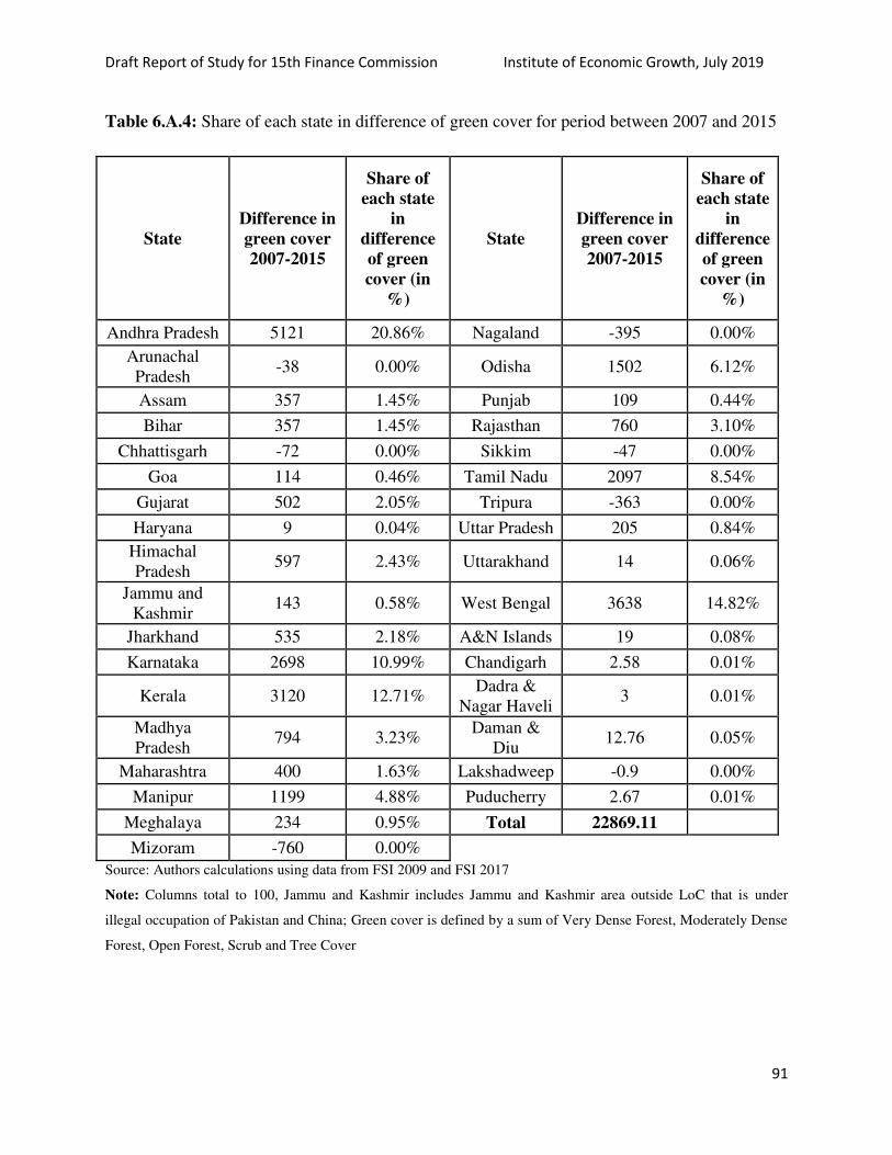
Draft Report of Study for 15th Finance Commission Institute of Economic Growth, July 2019
91
Table 6.A.4: Share of each state in difference of green cover for period between 2007 and 2015
State
Difference in
green cover
2007-2015
Share of
each state
in
difference
of green
cover (in
%)
State
Difference in
green cover
2007-2015
Share of
each state
in
difference
of green
cover (in
%)
Andhra Pradesh 5121 20.86% Nagaland -395 0.00%
Arunachal
Pradesh -38 0.00% Odisha 1502 6.12%
Assam 357 1.45% Punjab 109 0.44%
Bihar 357 1.45% Rajasthan 760 3.10%
Chhattisgarh -72 0.00% Sikkim -47 0.00%
Goa 114 0.46% Tamil Nadu 2097 8.54%
Gujarat 502 2.05% Tripura -363 0.00%
Haryana 9 0.04% Uttar Pradesh 205 0.84%
Himachal
Pradesh 597 2.43% Uttarakhand 14 0.06%
Jammu and
Kashmir 143 0.58% West Bengal 3638 14.82%
Jharkhand 535 2.18% A&N Islands 19 0.08%
Karnataka 2698 10.99% Chandigarh 2.58 0.01%
Kerala 3120 12.71% Dadra &
Nagar Haveli 3 0.01%
Madhya
Pradesh 794 3.23%
Daman &
Diu 12.76 0.05%
Maharashtra 400 1.63% Lakshadweep -0.9 0.00%
Manipur 1199 4.88% Puducherry 2.67 0.01%
Meghalaya 234 0.95% Total 22869.11
Mizoram -760 0.00%
Source: Authors calculations using data from FSI 2009 and FSI 2017
Note: Columns total to 100, Jammu and Kashmir includes Jammu and Kashmir area outside LoC that is under
illegal occupation of Pakistan and China; Green cover is defined by a sum of Very Dense Forest, Moderately Dense
Forest, Open Forest, Scrub and Tree Cover

Draft Report of Study for 15th Finance Commission Institute of Economic Growth, July 2019
92
Draft Report of Study for 15th Finance Commission Institute of Economic Growth, July 2019
93
Chapter 7: Summary and Recommendations
7.1 Summary of Findings from the study
This report has looked into various aspects of the vertical and horizontal devolution adopted
under different Finance Commissions, in view of trends and patterns in the fiscal space and the
socio-economic developmental needs of the country. We present below a summary of the
findings presented in the report.
Chapter 1 provides a review of the recommendations by various FCs, especially the last four
with respect to vertical and horizontal devolution in India. It points out that FCs have been
guided by the constitutional provisions and additional terms of reference provided by the
President. It discusses the various criteria used by the FCs such as assessment of needs of the
states, accommodative capacity of the centre, trends in revenue and expenditure of states and
centre, tax efforts and tax buoyancy. The chapter also discusses how some recent commissions
have attempted to balance equity and efficiency dimensions in horizontal devolution by
considering factors such as population, income, area, fiscal capacity and cost disability. The
chapter concludes that FCs have preferred continuity with change in the fiscal system.
Chapter 2 examines the trends and pattern in variables related to vertical devolution. It points
out that the central government collects about two-thirds of the combined revenue and the states
the rest in the form of their own taxes. The Centre and the states positions in the revenue
collection gets reversed after the transfers enabling the states to support more revenue
expenditure than the centre. The chapter concludes that while FCs have not substantially
deviated from their immediate predecessor in terms of share of states in central divisible pool,
yet the cumulative effect of the incremental changes during 1st to 14
th commissions have been
large enough to double the transfers as a percentage of central revenue. The fiscal balance has
shifted in favour of states over the years. An important factor neglected in deciding federal
transfer is the efficiency in service delivery. Developing a verifiable objective criteria for judging
relative efficiency in delivery of public services will be very useful to future commissions.

Draft Report of Study for 15th Finance Commission Institute of Economic Growth, July 2019
94
Chapter 3 concerns itself with the trends and patterns in horizontal fiscal devolutions and
summarizes key indicators that have been considered for devolution over the years. The
indicators include- population, income distance, fiscal capacity distance, area, index of
infrastructure, forest cover, tax effort and fiscal discipline. It notes that there has not been much
variation in shares of states in the net proceeds, since income and population are the dominating
criteria across most FCs carrying almost 75% of the weight. It notes that inequity was addressed
by a few FCs which considered an index of backwardness or through poverty ratio. In the recent
past, FCs were said to be mostly guided by performance based criteria in addition to the need
based criterions.
Chapter 4 undertakes analyses of various factors that affected the trends in devolution. The
matters of concern broadly comprised of whether there was an equalizing effect of Central
transfers on states and understanding the effects of transfers on social sector needs of the centre
and state. The question of whether there was an equalizing effect of central transfers was
examined by considering the revenue and equalization factors, and the transfers are observed to
have an equalizing effect on per capita total revenue that was available to states. States spent 3 to
4 times higher on social sector expenditure (as a percentage of state domestic product) in
comparison to the centre, with high interstate variation in both social sector expenditure (as a
percentage of state domestic product) and per capita social sector expenditures. Post the
increased devolution in 14 FC where the centre reduced its scope for its own social sector
spending through specific transfers; expenditure on health and education in per capita terms for
richer states still increased, indicating that general purpose transfers were unable to offset the
revenue disabilities of low income states completely. Social sector expenditure was found to be
responsive to increase in both NSDP and devolution, the latter being more effective when routed
through the general purpose transfer which could imply that specific central transfers might not
be required to meet these kind of expenditures. Specific transfers for social sector expenditure
may be required when richer states suffer from some unique social and economic infrastructural
deficits, or when there are large variations in fiscal capabilities among states that are not offset
by general purpose transfers.
Draft Report of Study for 15th Finance Commission Institute of Economic Growth, July 2019
95
Chapter 5 focused on the status of key fiscal parameters on resource allocation. It concerns itself
with the fiscal efficiency indicators of tax effort and fiscal discipline and makes remarks on GST.
Though some poorer states (in terms of per capita NSDP) have comparable tax efforts as
compared to some richer states, in reality the poorer states have done better given their lower
income base. Additionally, it is noted that there is a fall in fiscal discipline for some states over
time. Evidence suggests that the introduction of fiscal discipline as a criteria, does not
necessarily lead to higher own tax revenues if compared to the own tax revenue in the later FC
period. Most states displayed an upward trend in fiscal deficit for most years. It was less than 3%
as a percentage share of NSDP for majority of the states while in the rest it is about 4%.
However, it was noted that state budgetary deficits needs not be related to states per capita GSDP
since states have some discretion in raising public debt within certain limits. In this case, fiscal
deficit could be considered as an indicator for fiscal discipline. In regard to GST, it is too early to
be able to present evidence based analytical insights. However, it is noted that there is a broad
consensus of a positive pay-off from this tax reform in the literature, though it may be premature
to make rigorous predictions on how much impact it will have on tax revenues.
7.2: Some Specific Recommendations
1. Centre-States allocation of resources: The balance in Indian fiscal system has steadily but
significantly shifted in favour of states over the years. Attempts should be made in future
to examine questions regarding relative efficiency in delivery of public services amongst
states.
2. Inter-state inequality: In view of the rising inter-state inequality in per capita income, we
have presented a normative welfare approach for resource transfers which takes into
account the preferences for income redistribution in favour of the poorer states. This
involves incorporation of an inequality aversion parameter in the income criteria for
horizontal devolution so that relatively poorer states could get a higher share.
3. Population Stabilization: One of the SDGs is to stabilise the global population of world to
8 billion by 2030. The TOR of the 15th Finance Commission (15th
FC) on measurable
performance-based incentives for the States based on their efforts and progress in moving
towards replacement rate of population growth is considered in conjunction with the
Draft Report of Study for 15th Finance Commission Institute of Economic Growth, July 2019
96
mandate for the 15th
FC for using the population data of 2011. It is noted that some of the
states lagging in population stabilization are also the ones with high share of population
and, further, that population shares are used to weigh all the constituents of the horizontal
transfer formulae. An attempt is therefore made to devise an indicator based on state level
performance in population stabilization based on the TFR criteria, with replacement level
of fertility at 2.1. State shares are accordingly computed. TFR can be used as a goalpost
by empowering people by providing access to family planning services. As fertility is a
complex multifactorial phenomenon, policy initiatives will have to be planned to
motivate states to lower the TFR.
4. Forest Cover: The NDC target is to create an additional carbon sink of 2.5 to 3 billion
tons carbon dioxide equivalent through forest and tree cover by 2030. In the context of
proposing measurable performance-based incentives for States, at the appropriate level of
government, in TOR 4 (iii) sustainable development goals have been mentioned while as
in 3(ii), in making its recommendations, the Commission shall consider the demands on
the resources of the Central Government on account of climate change, among other
factors. For both the climate change implications and SDGs the forestry sector has an
important role to play. In particular, it deserves special mention in the context of
allocations made by previous FCs for forests, in particular the 14 FC incorporated dense
forest cover as a criteria for horizontal devolution. In this context the study presents a
data based analysis for comparing transfers based on horizontal devolution with those
through a grant. Also, scenarios incentivizing states for maintaining forests and other
valuable ecological resources (for instance, preservation of species outside dense forests
as in grasslands for Asiatic lions in Gir, enriching soil carbon and enhancing tree cover
outside dense forests) are compared with those based on accommodating the concern for
fiscal disability. Based on the analysis, two proposals are made for expanding the
definition of area to be considered for fiscal disability and for providing incentive based
grants to improve forest cover. Further, a grant seems to be more in keeping with the
achievement of specific objectives.

Draft Report of Study for 15th Finance Commission Institute of Economic Growth, July 2019
97

Draft Report of Study for 15th Finance Commission Institute of Economic Growth, July 2019
98
References
Bhagat, R. B., & Mohanty, S. (2009). Emerging pattern of urbanization and the contribution of
migration in urban growth in India. Asian Population Studies, 5(1), 5-20.
Bhaskar, V. (2015). Stance on Devolution and Grants. Economic and Political Weekly. 50(21),
36-
40.
Bhaskar, V. (2018). Challenges before Fifteenth Finance Commission. Economic and Political
Weekly. 53(10), 39-46.
Boadway, R., & Shah, A. (Eds). (2007). Intergovernmental Fiscal Transfers: Principles and
Practice. World Bank, 1818 H Street, NW Washington, DC 20433
Chakraborty, P. (2010). Deficit Fundamentalism vs Fiscal Federalism: Implications of 13th
Finance Commission's Recommendations. Economic and Political Weekly. 56-63.
Chakraborty, P. and Gupta, M. (2016). Evolving Centre-State Financial Relations. Economic and
Political Weekly. 1(16)
Dasgupta. P., & Goldar, B. (2017). Costing for Elevation in Development Expenditure:
Illustrative
Evidence from India. Journal of Quantitative Economics. 16(3), 811-830
Dholakia, A. R. (2015). Some Hits and Misses. Economic and Political Weekly. 50(21), 41-44
Donaldson, P. J. (2002). The elimination of contraceptive acceptor targets and the evolution of
population policy in India. Population Studies, 56(1), 97-110.
FSI(Forest Survey of India). (2009). State of Forest report.
FSI(Forest Survey of India). (2015). State of Forest report.
FSI(Forest Survey of India). (2017). State of Forest report.
Gioli, G., Thapa, G., Khan, F., Dasgupta, P., Nathan. D., Chhetri, N., Adhikari, L., Mohanty,
S.K.,
Aurino, E., & Scott, L.M. (2019) Poverty and Vulnerability in Mountain Livelihoods.
HIMAP Assessment. ICIMOD.
Gupta, Manish & Sarma, Atul (2019). Role of finance Commission Constituitionally aAssigned
and Beyond in National conference on Growth and Regional Development in India:
Recent experiences and emerging perspectives. Institute for Human Development, Delhi
IPBES (Intergovernmental Science-Policy Platform on Biodiversity and Ecosystem Services).
(2018). The IPBES regional assessment report on biodiversity and ecosystem services for
Asia and the Pacific. Bonn, Germany: Secretariat of the Intergovernmental Science-
Policy Platform on Biodiversity and Ecosystem Services. Retrieved from
https://www.ipbes.net/system/tdf/2018_asia_pacific_full_report_book_v3_pages.pdf?file
=1&type=node&id=29507
James, K. S. (2011). India’s demographic change: opportunities and challenges. Science,
333(6042), 576-580.

Draft Report of Study for 15th Finance Commission Institute of Economic Growth, July 2019
99
Johnson, S. D. (1994). Sex ratio and population stability. Oikos, 172-176.
Kelkar, Vijay (2019). Towards India’s New Fiscal Federalism, Sukhamoy Chakravarty
Memorial
Lecture, Indian Econometric Conference; also Working Paper No. 252, NIPFP, New
Delhi.
Murty, M.N & Nayak, P.B. (1994). A Normative Approach for Resource Transfers in a Federal
State In Tax Policy and Planning in Developing Countries. Amresh Bagchi & Nicholas
Stern (eds.). Oxford University Press, New Delhi.
Murty, M.N, Panda, M., & Joe, W. (2018). Reassessment of National Parameters for Project
Appraisal in India. Report of the Research Project Funded by NITI Aayog, Government
of India. Institute of Economic Growth Delhi University Enclave, Delhi 110007
Preston, S., Heuveline, P., & Guillot, M. (2001). Demography: Measuring and Modeling
Population Processes. Blackwell Publishers, Oxford, UK.
Rao, M.G. (2017). Central Transfers to States in India: Rewarding performance while ensuring
equity (Final Report of a Study Submitted to NITI Aayog.) NITI Aayog.
Rao, M. Govind (2019).Reforming the fiscal transfer system in India in National conference on
Growth and Regional Development in India:Recent experiences and emerging
perspectives. Institute for Human Development, Delhi
Rajaraman, I. and Gupta, M. (2016). Preserving the incentive properties of statutory grants.
Economic and Political Weekly. 51(9).
Reddy, G. R. (2018). Upholding Fiscal Federalism Terms of reference of the Fifteenth
commission. Economic and Political Weekly, 53(10), 19-21.
Reddy, Y.V., & Reddy, G.R. (2019). Indian Fiscal Federalism. Oxford University Press.
Rockström, J., Steffen, W., Noone, K., Persson, A., Chapin, F.S.III., Lambin, E., Lenton, T.M.,
Scheffer, M., Folke, C., Schellnhuber, H.J., Nykvist, B., de Wit, C.A., Hughes, T., van
der Leeuw,S., Rodhe, H., Sörlin, S., Snyder, P.K., Costanza, R., Svedin, U., Falkenmark ,
M., Karlberg, L., Corell, R.W., Fabry, V.J., Hansen, J., Walker, B., Liverman, D.,
Richardson, K., Crutzen, P., & Foley, J. (2009). Planetary boundaries: exploring the safe
operating space for humanity. Ecology and Society, 14(2). Retrieved from
http://www.ecologyandsociety.org/vol14/iss2/art32/
Srinivasan, K. (1998). Population policies and programmes since independence (a saga of great
expectations and poor performance). Demography India, 27(1), 1-22.
Srivastava, D.K. (2010). Vertical sharing and horizontal distribution of resources: The equity and
Efficiency trade-off. Economic and Political Weekly, 45(48)
Zodgekar, A. V. (1996). Family welfare programme and population stabilization strategies in
India. Asia-Pacific population Journal, 11(1), 3
Related Documents


