Incentives to Motivate

Incentives to Motivate�

Ola Kvaløyy and Anja Schöttnerz

July 6, 2012

Abstract

We present a model in which a motivator can take costly actions -

or what we call motivational e¤ort - in order to reduce the e¤ort costs

of a worker, and analyze the optimal combination of motivational ef-

fort and monetary incentives. We distinguish two cases. First, the �rm

owner chooses the intensity of motivation and bears the motivational

costs. Second, another agent of the �rm chooses the motivational ac-

tions and incurs the associated costs. In the latter case, the �rm must

not only incentivize the worker to work hard, but also the motivator

to motivate the worker. We characterize and discuss the conditions

under which monetary incentives and motivational e¤ort are substi-

tutes or complements, and show that motivational e¤ort may exceed

the e¢ cient level.

�We would like to thank Fabian Frank, Hideshi Itoh, Frauke Lammers, Trond Olsen,Gaute Torsvik, and seminar and conference participants in Bergen, Berlin, Bern, Frank-furt, Magdeburg, Vienna, and Zurich for helpful comments. Financial support from theNorwegian Research Council (Grant # 196873) is gratefully acknowledged.

yUniversity of Stavanger, 4036 Stavanger, Norway. [email protected] of Bonn, 53113 Bonn, Germany. [email protected]

1

�Leadership is based on a spiritual quality � the power to inspire, the

power to inspire others to follow.�

Vincent T. Lombardi

1 Introduction

The legendary football coach Vincent Thomas Lombardi was celebrated for

his ability to motivate and inspire his players. Even though he achieved an

amazing record of victories in a game where tactics and strategy matter,

he is not so famous for his tactical skills. Lombardi is legendary for his

coaching philosophy and motivational skills. He emphasized hard work and

dedication, and players were wholeheartedly devoted to him.

Anyone who follows sports has a sense that it is not only the coach�s

knowledge of the game that matters, but also his or her ability to motivate

and inspire the players with words and actions. This also applies to work life

in general. Leaders continuously emphasize the importance of motivation

in terms of "energizing people" or "challenging them to take those actions

that will realize results" (Filson, 2004). If one googles "leadership and mo-

tivation" one �nds an endless list of managerial words of wisdom such as

"Great leaders motivate through inspiration", or "Leadership is Motivation,

the Leader is a Motivator".1

From an economist�s point of view, this looks more like a technologi-

cal approach to motivation than an incentive approach. Indeed, economic

theories of motivation have primarily focused on incentives, and have not

considered motivation to be a kind of technology that helps workers perform

better. But when a coach motivates her players or a leader motivates her

workers, she may trigger the workers�e¤ort without increasing their mone-

tary incentives to exert e¤ort. This is emphasized by two contemporary lead-

ership theories in the �eld of organizational behavior: charismatic leadership

and transformational leadership. According to these closely related theories,

1The quotes are from CEO Dov Seidman and leadership consultant James Chapman,respectively.

2

leaders inspire followers through their words, ideas, and behavior.2 Several

studies �nd a positive relationship between charismatic/transformational

leadership, high performance, and job satisfaction, see Wang (2011) and

Robbins and Judge (2013) for recent surveys and overviews.

But even though leadership has an impact on �rm performance, a certain

leadership style typically does not change a �rm�s production technology, i.e.,

how inputs and particularly work e¤ort transform into output. The channel

through which charismatic/transformational leadership a¤ects productivity

appears to be its e¤ect on employees� (dis)utility of work. E¤ective lead-

ership makes employees like their job better and, as a consequence, they

work harder and perform in ways that bene�t the organization. As Robbins

and Judge (2013, p. 415) put it, "People working for charismatic leaders

are motivated to exert extra e¤ort and, because they like and respect their

leader, express greater satisfaction." In a similar spirit, Harter et al. (2010)

conclude, "Improving employee work perceptions can improve business com-

petitiveness while positively impacting the well-being of employees."

Therefore, a natural way to model charismatic/transformational leader-

ship in a principal-agent framework is to say that the leader or motivator

reduces workers�e¤ort costs. In this paper we make this plausible assump-

tion. We assume that a motivator can take costly actions - or what we call

motivational e¤ort - to reduce the e¤ort costs of a worker and analyze the

optimal combination of motivational e¤ort and monetary incentives. We

distinguish two situations. First, the �rm owner chooses the intensity of

motivation and bears the motivational costs. Second, another agent of the

�rm chooses the motivational actions and incurs the associated costs. In

the latter case, the �rm must then not only incentivize the worker to work

hard, but also the motivator to motivate the worker.

2Max Weber introduced the term �charismatic leadership� in his famous theory ofauthority (originally published posthumously in 1922). Robert House (1977) further de-veloped Weber�s concept in articulating a theory of charismatic leadership. Bernard Bass(1985) introduced the term �transformational leadership�, contrasting it with transac-tional leadership: while transactional leaders emphasize rewards in exchange for satisfy-ing performance, transformational leaders inspire their followers by articulating visionsand challenging goals. Charismatic and transformational leadership are now often usedsynonymously.

3

Our model allows for a broader interpretation of motivational actions

than what is typically emphasized in the literature on charismatic and trans-

formational leadership. We are interested in any action that the leader can

take in order to reduce the e¤ort costs of the worker, and we sometimes refer

to this as "motivational leadership".3 The costs of motivational e¤ort can

also take many forms and our model allows for various interpretations. For

example, the �rm can invest in developing its managers�leadership qualities.

Studies suggest that charismatic leaders are not only born but can also be

made. Barling et al. (1996) conduct a �eld experiment with Canadian bank

managers and �nd that branches whose managers underwent transforma-

tional leadership training performed better than branches whose managers

did not receive such training. With appropriate forms of training, managers

can also learn, e.g., how to better evaluate critical situations or improve

their interpersonal skills. Large �rms like BHP Billiton, Nokia, and Adobe

hire personal coaches for their top executives to improve their leadership

skills (Robbins and Judge, 2013, p. 430). According to the Harvard Busi-

ness Review, US companies are spending more than $1.5 billion a year on

coaching. Renton (2009) reports that about 40% of Britain�s CEOs undergo

coaching, as well as an increasing number of senior managers.

Motivational e¤ort costs are also in�icted through communication, at-

tention, or goal setting. Specifying goals that are in line with a worker�s am-

bitions for personal development requires time-consuming and thus costly

communication. Giving sound feedback and appraisals requires careful eval-

uation of employee performance. And importantly, motivational actions are

often at the discretion of the worker�s immediate superior, who is not the

residual claimant of the production process but has to bear the costs of mo-

tivation. The �rm owner then has to incentivize the motivator to motivate

the worker, which is also costly.

The main insights of our analysis are as follows:

First, we show that higher-powered monetary incentives to the worker

can reduce or enhance his responsiveness to motivational e¤ort. The �rst

3The term "motivational leadership" is often used by consultants. "Charismatic lead-ership" and in particular "transformational leadership" are narrower academic terms.

4

case implies that incentives make motivational e¤ort less e¤ective and thus

re�ects a "hidden cost of reward". Because our motivational e¤ort can

be interpreted as an attempt to increase the worker�s intrinsic motivation,

this result is related to the well-known crowding-out argument for intrinsic

motivation (Lepper and Green, 1978). Monetary incentives, however, can

also complement and enhance the e¤ect of motivational e¤ort. We thus also

identify a potential "hidden bene�t of reward".

Second, we analyze the optimal motivation-incentive mix from the �rm�s

point of view. Under unlimited liability of the worker, the �rm provides �rst-

best incentives that are equal to the marginal productivity of e¤ort. The

worker�s bonus is then independent of motivation, because the latter only

a¤ects the worker�s disutility of e¤ort. If the worker is subject to limited

liability, however, the �rm can use incentives and motivation as substitutes

as well as complements. The latter case occurs if the worker�s motivation

responsiveness increases with the strength of incentives. For example, this

is possible when a harder working employee interacts with his superior more

frequently and is therefore easier to inspire by charismatic leadership. We

show that, in such a situation, motivational e¤ort may even exceed the

e¢ cient level and occur in the second-best solution even when it is �rst-best

not optimal to motivate. The reason is that motivational e¤ort can reduce

the worker�s rent for each �xed e¤ort level. In this respect, we provide a

rather intuitive rationale for motivational e¤ort.

Third, if we make a broader interpretation of motivational e¤ort as any

activity that lowers the worker�s e¤ort costs, e.g., a nice o¢ ce, a car, or an

iPad for that matter, the model can also illuminate the practice of using

perks as a part of the worker�s compensation. At �rst sight perks appear

as rewards that increase the worker�s rent. We show that perks can also be

seen as a device that makes the worker work harder on lower rents.

Fourth, we �nd that a negative equilibrium relationship may occur be-

tween the motivator�s bonus and her e¤ort level. If the worker�s e¤ort be-

comes more productive (for exogenous reasons), the motivator�s e¤ort level

will increase. Cet. par. it may in fact exceed the �rst-best level of moti-

vation. The �rm may then mitigate the motivational e¤ort by lowering the

5

motivator�s incentives to motivate.

Finally, we identify a notable con�ict of interest between motivator and

worker. When the worker�s rent is decreasing in motivational e¤ort, he

clearly prefers a higher bonus rather than more non-monetary motivation.

But for a given level of worker e¤ort, the lower-powered the worker�s mon-

etary incentives, the higher often is the motivator�s bonus. Under limited

liability, a low bonus to the worker may thus imply a higher rent to the moti-

vator. Consequently, low-powered monetary incentives to the worker may be

in the motivator�s interest. Interestingly, we often see negative assessments

of monetary incentives in the leadership and coaching literature.4

The rest of the paper is organized as follows. In Section 2 we discuss

related literature. In Section 3 we present the basic model and characterize

the �rst-best solution. In Section 4 we analyze the trade-o¤ between mo-

tivational e¤ort and monetary incentives in a setting where the �rm owner

is the motivator. We derive the optimal contract with limited and unlim-

ited liability. The case where the �rm needs to hire a motivator to induce

motivation is analyzed in Section 5. Section 6 concludes.

2 Relationship to the Literature

In his celebrated book "The Modern Firm", John Roberts (2004) states that

"Management (. . . ) is vitally important, but it is not enough. Leadership is

needed too (...). Leaders o¤er direction and then motivate others to believe

and to follow." After the black box of the �rm was opened in the 1970�s,

management has been intensively studied. But leadership has almost been

ignored by economists, even though it is a signi�cant subject in the less

formal literature on organizational behavior (see e.g. House and Aditya,

1997, for an overview). Recently, however, a small economics literature on

leadership has emerged, focusing on the leader as one who has followers

because of superior skills or information, see Hermalin (1998, 2007), Komai

et al. (2007), Komai and Stegman (2010) and Lazear (2010). But the

4See for instance the best seller "Drive - the surprising truth about what motivatesus", by Daniel H. Pink (2009).

6

motivational part of leadership has been scantly treated in this literature.

Notable exceptions are Van den Steen (2005), who shows how a manager

with strong beliefs about the right course of action can attract employees

with similar beliefs, and the works by Rotemberg and Saloner (1993, 1994,

2000), who consider the e¤ect of visions and leadership style on employees�

motivation to generate proposals for innovation adoption.

Closer to our approach, however, is the important work on identity by

Akerlof and Kranton (2000, 2005). They assume that e¤ort costs are a

function of identity, and that the �rm can take actions that a¤ect the work-

ers�identity. In particular they di¤erentiate between insiders and outsiders,

where only insiders identify with the �rm/employer�s values. Like them,

we assume that the �rm can a¤ect the workers�e¤ort costs, but we do not

allow for discrete preference changes, and the trade-o¤s and interpretations

we present are more in line with standard principal-agent terminology (dis-

cussing, e.g., marginal e¤ects on motivation responsiveness). In this respect

our paper is more related to Dur et al. (2010), who analyze a situation

where the agent�s marginal costs of e¤ort are decreasing and the worker�s

well-being is increasing in the attention paid by the principal. In contrast to

them, we allow for a more general e¤ort cost function, which is crucial for

deriving our main results. As another important di¤erence, Dur et al. focus

on a commitment problem on the side of the principal, which is not an issue

in our setup. Neither Dur et al. nor Akerlof and Kranton study how the

motivator should be incentivized. Moreover, Akerlof and Kranton do not

consider limited liability and the rent extraction aspect, which is important

in our paper.

When the �rm needs to incentivize both a worker and a motivator, it

faces a team incentive problem. Our paper is thus related to Itoh (1991a)

who analyzes the incentives for workers to help each other, and in particular

Itoh (1991b) who analyzes a situation where workers can socialize with each

other and thereby a¤ect each other�s utility functions. Dur and Sol (2010)

also study social interaction between workers and how it is a¤ected by the

�nancial incentive systems. But the literature on team incentives does not

relate to the kind of motivational e¤ort we discuss. In contrast to the stan-

7

dard team literature, we analyze a team incentive problem where the agents

have very di¤erent roles: The team consists of an agent - the worker - who is

essential for production, and another agent - the motivator - who can help

the worker but cannot produce anything without him.

Finally, our paper is related to a recent literature on perks and bene�ts,

in particular Oyer (2008) and Marino and Zabojnik (2008). Oyer studies

how �rm and worker characteristics may a¤ect the trade-o¤ between salaries

and bene�ts, and models a situation where workplace bene�ts such as enter-

tainment options and errand services lower the workers�e¤ort costs. Bene�t

in his model could be reinterpreted as motivational e¤ort, but Oyer does not

consider the trade-o¤ between bene�ts and monetary incentive provision, as

he analyzes a full information model with no moral hazard problem. Marino

and Zabojnik study the trade-o¤ between work-related perks and incentive

provision. In their model perks improve the worker�s e¤ort productivity,

and the bene�t from perks is positively related to the worker�s e¤ort level.

We do not make such an assumption, which gives rise to di¤erent results

concerning the interaction of perks and monetary incentives. In contrast to

Marino and Zabojnik, we show that perks and monetary incentives can be

substitutes as well as complements.

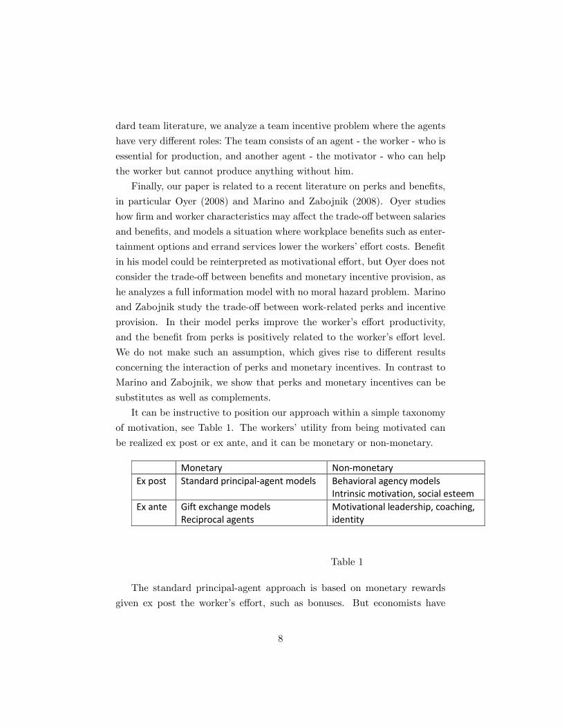
It can be instructive to position our approach within a simple taxonomy

of motivation, see Table 1. The workers�utility from being motivated can

be realized ex post or ex ante, and it can be monetary or non-monetary.

Monetary Non­monetaryEx post Standard principal­agent models Behavioral agency models

Intrinsic motivation, social esteemEx ante Gift exchange models

Reciprocal agentsMotivational leadership, coaching,identity

Table 1

The standard principal-agent approach is based on monetary rewards

given ex post the worker�s e¤ort, such as bonuses. But economists have

8

increasingly recognized the importance of non-material incentives, such as

the intrinsic pleasure of doing a good job (see Benabou and Tirole, 2003;

Besley and Ghatak, 2005), or the social esteem or respect that follows from

good performance (see Ellingsen and Johannesson, 2008). Like the standard

principal-agent models, the worker�s utility from motivation is also here

realized ex post. In contrast, the gift-exchange literature and its emphasis

on reciprocal preferences has shown both theoretically and experimentally

that workers can be motivated by ex ante material rewards. A worker that

receives a higher �xed wage responds by exerting higher e¤ort (see Falk and

Fehr, 2000, for an overview).

Finally, the huge literature on organizational behavior and motivational

leadership focuses to a large extent on ex ante non-material realization of

motivational utility. The immediate payo¤ from being motivated by a leader

is a reduction in non-material costs of exerting a given e¤ort level. This ef-

fort cost reduction can of course then materialize in ex post rewards from

higher e¤ort. The novelty of our approach is to formalize motivational ef-

fort/motivational leadership, and to combine it with a standard principal-

agent model with ex post material rewards.

3 The Model

We consider a model where a worker produces an output q for a �rm. The

output can be either high or low, i.e., q 2 fqL; qHg with qL < qH . The

probability of producing high output qH is given by the worker�s e¤ort

level e 2 [0; 1], i.e., Pr[q = qH je] = e: By exerting e¤ort, the worker thus

chooses the probability of high output. The worker�s e¤ort is non-observable,

whereas output is observable and veri�able. The �rm pays the worker a non-

contingent �xed wage s and can provide him with monetary incentives by

granting him a bonus b if output is high.

In addition, the worker can be motivated by motivational e¤ort a �0. We assume that, if the worker is exposed to motivational e¤ort, he

enjoys working more and also �nds it less troublesome to increase his e¤ort.

Hence, the worker�s private e¤ort costs C(e; a) are a¤ected by the level of

9

motivation that he experiences.5 The function C(e; a) is strictly increasing

and strictly convex in e, i.e., Ce(e; a) > 0 and Cee(e; a) > 0 for e > 0 and all

a. Motivation reduces both the worker�s absolute and marginal e¤ort costs

for all positive e¤ort levels, i.e., Ca(e; a) < 0 and Cea(e; a) < 0 for all e > 0

and all a: For e = 0, however, we assume that the worker�s absolute and

marginal e¤ort costs are zero (i.e., C(0; a) = Ce(0; a) = 0 for all a), and thus

cannot be further reduced by motivation, i.e., Ca(0; a) = Cea(0; a) = 0 for

all a:6

The costs of motivation are denoted by K(a). They are strictly increas-

ing and convex in the level of motivation, Ka > 0; Kaa � 0 for all a > 0.

Zero motivational e¤ort, a = 0, corresponds to a situation without moti-

vation and, therefore, K(0) = 0. However, the marginal motivational costs

at zero may be positive, i.e., Ka(0) � 0, which will imply that inducing

motivation may be too costly to implement.7 Both motivational e¤ort and

motivational costs are non-contractible.

We �rst consider a situation where the �rm chooses a itself and bears

the motivational costs. We can think of this as the �rm owner being the

motivator, or as motivation being delegated to a third party whose motiva-

tional actions are not subject to an incentive problem.8 Alternatively, we

can also allow for a broader interpretation of motivational actions such as

the provision of perks or bene�ts by the �rm.

5Even though monetary incentives are a source of motivation, we mainly reserve theterm �motivation� when talking about motivational e¤ort. We also use �motivationale¤ort�and �non-monetary motivation�synonymously.

6An alternative modelling approach would be to say that work e¤ort is costless up toa certain extent, and that motivation shifts the worker�s cost function to the right. Then,the maximal costless e¤ort level increases and the marginal costs for each costly e¤ortlevel strictly decrease. This would lead to similar results as those we will present here.

7The reason could be that the motivator has high opportunity costs or, when the �rmwants to hire a particularly charismatic manager, search costs are large.

8 In the latter case, the �rm owner could hire a particularly charismatic CEO, whonaturally motivates other top executives just by interacting with them. However, the�rm must o¤er higher compensation to a manager with extraordinary leadership qualitiesthan to a less gifted manager because the latter has less attractive outside options on thelabor market. The compensation di¤erential then re�ects the �rm�s motivational cost. Asanother example, the �rm can invest in developing its managers�leadership qualities.

10

We denote the sum of work e¤ort costs and motivational costs by

�(e; a) := C(e; a) +K(a) (1)

and de�ne H as the Hessian of �(e; a);

H :=

Cee Cea

Cea Caa +Kaa

!: (2)

To ensure strict convexity of the total cost function �(e; a), we assume that

H is positive de�nite, i.e., detH = Cee(Caa +Kaa)�Cea2 > 0 for all e anda. Note that the latter inequality implies that Caa +Kaa > 0.

The worker has a reservation utility of zero and is risk neutral. He may,

however, be protected by limited liability, meaning that all payments to him

must be non-negative. We will analyze the �rm�s contracting problem in the

case of both unlimited and limited liability of the worker.

Timing is as follows. First, the �rm o¤ers the worker a contract (s; b)

and announces to exert motivational e¤ort a. The worker can accept or

reject the contract o¤er. If he accepts the contract, he enters the �rm and

the �rm chooses the motivational e¤ort a at cost K(a). The worker observes

a and can decide whether to stay with the �rm or quit.9 If the worker stays

with the �rm, he exerts e¤ort e at cost C(e; a). Finally, q is realized and

the �rm pays the worker.

3.1 First-Best Work E¤ort and Motivational E¤ort

Before we proceed to the contracting game, it is useful to consider the �rst-

best e¤ort levels as a benchmark. The �rst-best work e¤ort eFB and the9Under unlimited liability, this interim participation decision will ensure that the �rm

can induce the �rst-best solution. Thus, allowing the worker to quit after observingthe motivational level is in the interest of the �rm. It serves as a self-commitment device.Under limited liability (or if the motivator is an agent of the �rm), the interim participationdecision will not be relevant for the results. In contrast to our model, Dur et al. (2010)assume that the worker cannot quit after observing the principal�s action.

11

�rst-best motivational e¤ort aFB maximize the social surplus, i.e.,

(eFB; aFB) = arg maxe2[0;1]a�0

qL + e ��q � �(e; a), (3)

where �q := qH � qL. The assumption C(0; a) = Ce(0; a) = 0 implies

that the e¢ cient work e¤ort is strictly positive, i.e., eFB > 0. Whether the

worker should be motivated (aFB > 0) or not (aFB = 0) depends on how

work e¤ort and motivational e¤ort interact in the total cost function �(e; a).

We now derive su¢ cient conditions for either aFB > 0 or aFB = 0, which

we will use later to compare �rst-best and second-best e¤ort levels.

A su¢ cient condition to obtain aFB > 0 is that, for each positive work

e¤ort, total costs are initially decreasing in a, i.e.,

�a(e; 0) < 0 for all e > 0: (4)

Because eFB > 0, we must then also have aFB > 0. More precisely, for

aFB > 0 it is already su¢ cient that �a(e; 0) < 0 holds at the work e¤ort

level that is optimal given that a = 0, which is

eFB0 := arg maxe2[0;1]

e ��q � C(e; 0): (5)

Hence, a su¢ cient condition for aFB > 0 is that

�a(eFB0 ; 0) < 0: (6)

The conditions (4) and (6) hold, e.g., if Ka(0) = 0.

By contrast, a su¢ cient condition to obtain aFB = 0 is that an in�ni-

tesimal amount of motivation always increases total costs, i.e.,

�a(e; 0) � 0 for all e: (7)

Then, from �aa = Caa +Kaa > 0 it follows that �a(e; a) > 0 for all e and

a > 0: Hence, total costs are always increasing in a. Consequently, letting

12

a�(e) denote the optimal motivational e¤ort for given work e¤ort e,

a�(e) = argmina�0

�(e; a); (8)

we obtain a�(e) = 0 for all e.

Thus, even though motivation always reduces the worker�s e¤ort costs, it

is not necessarily e¢ cient to induce motivation. The reason is that motiva-

tion might be too costly. Motivational e¤ort can be positive in the �rst-best

solution only if it initially reduces total costs for some work e¤ort levels.

Assuming that problem (3) has an interior solution, i.e., aFB > 0 and

eFB < 1, �rst-best e¤ort levels are characterized by the �rst-order conditions

�e(eFB; aFB) = Ce(e

FB; aFB) = �q; (9)

�a(eFB; aFB) = Ca(e

FB; aFB) +Ka(aFB) = 0: (10)

In this case, we can determine how eFB and aFB respond if the marginal

productivity of work e¤ort, �q, increases:

deFB

d�q= �det

�1 Cea

0 Caa +Kaa

!=detH = (Caa +Kaa)=detH > 0

(11)

daFB

d�q= �det

Cee �1Cea 0

!=detH = �Cea=detH > 0 (12)

Thus, because Caa +Kaa > 0, both work e¤ort eFB and motivational e¤ort

aFB are increasing in �q.

The following proposition summarizes the results of this section.

Proposition 1 First-best work e¤ort eFB is always positive. By contrast,�rst-best motivational e¤ort aFB may be zero. A su¢ cient condition for

aFB = 0 is that introducing an in�nitesimal amount of motivation increases

total cost, i.e., �a(e; 0) � 0 for all e. First-best work e¤ort eFB is strictly

increasing in �q if eFB < 1. First-best motivational e¤ort aFB is also

strictly increasing in �q if aFB > 0.

13

4 Monetary Incentives versus Motivational E¤ort

We now proceed to the contracting game where the �rm�s objective is to im-

plement the pro�t-maximizing combination of work e¤ort and motivational

actions. We solve the game by backward induction and thus �rst analyze

the worker�s e¤ort choice.

4.1 The Worker�s Optimal E¤ort Choice

The worker chooses his e¤ort given his bonus contract (s; b) and motivational

e¤ort a. The worker�s optimal e¤ort choice e(a; b) maximizes his expected

net payment, i.e.,

e(a; b) = arg maxe2[0;1]

s+ eb� C(e; a). (13)

The �rst-order condition of this optimization problem yields the worker�s

incentive constraint,

b = Ce(e; a); (IC)

which implicitly de�nes e(a; b).10 Equation (IC) describes the bonus that

the �rm has to o¤er to induce e¤ort level e given motivation a. It also tells us

how changes in monetary incentives or motivation a¤ect the worker�s e¤ort

choice. First, from (IC) we can derive the worker�s incentive responsiveness

eb and his "motivation responsiveness" ea, where

eb =1

Cee> 0 and ea = �

CeaCee

> 0. (14)

Accordingly, the worker exerts more e¤ort the higher his bonus and the

higher the motivational e¤ort. The latter observation follows from our as-

sumption Cea < 0 and is in line with the empirical studies indicating that

10 It is easy to see that the �rst-order condition holds at the worker�s optimal e¤ortchoice even if the �rm wishes to induce the minimum or maximum e¤ort, e = 0 or e = 1,respectively. To make the worker choose e = 0; the �rm optimally sets a = b = 0. If the�rm wants the worker to exert e = 1; it is not optimal to choose a and b such that theworker�s expected net payment is still increasing at e = 1; i.e., it cannot be the case thatb� Ce(1; a) > 0.

14

motivational leadership increases productivity, which we referred to in the

introduction. The higher the incentive responsiveness (the lower Cee), the

higher is also the motivation responsiveness. Furthermore, the worker is

more responsive to motivation than to incentives if Cea < �1, i.e., if mar-ginal e¤ort costs are relatively elastic to motivational e¤ort.

Next, we are interested in how the worker�s motivation responsiveness

changes when incentives increase, which is re�ected by eab. From (14) we

obtain

eab = �Ceae + Ceeeea

C2ee: (15)

Intuitively, with a higher bonus, the worker increases his e¤ort for each

given level of motivation, which changes the impact of motivation on his

marginal e¤ort costs (re�ected by Ceae) and the di¢ culty of raising e¤ort

further (re�ected by Ceee). Both e¤ects jointly determine the sign of eab.

Since Cee(e; a) denotes the worker�s marginal bonus, the third derivatives

Ceae = Ceea and Ceee also indicate how the marginal bonus changes with

higher motivation and higher e¤ort, respectively. It seems reasonable to

assume that Ceee � 0, i.e., to elicit marginally higher e¤ort, the �rm has to

increase the bonus more strongly the harder the worker works.

However, motivation can a¤ect the marginal bonus in di¤erent ways,

making the sign of eab ambiguous. If Ceae < 0 and the �rm increases moti-

vational e¤ort, it can achieve a marginal increase in work e¤ort by a smaller

bonus increase. If, in addition, Ceee is small, we obtain eab > 0, i.e., the

worker�s motivation responsiveness is increasing in the bonus. Such a case

occurs for example if a harder working agent interacts with his motivator

(e.g., superior) more frequently and is therefore more responsive to moti-

vational e¤ort. Alternatively, a worker who is more occupied with his job

could also be more eager for his motivator�s attention or feedback, which

then also has a stronger e¤ect on the worker�s job satisfaction and, conse-

quently, marginal disutility of e¤ort. By contrast, if Ceae > 0, we are in a

situation where eab < 0, i.e., motivation responsiveness is decreasing in mon-

etary incentives. This case occurs if, after a bonus increase, the agent works

15

at an intensity that makes it extremely di¢ cult to further raise e¤ort. Or,

from a certain point on, the agent�s opportunities to a¤ect the realization of

output are strongly limited (recall that e¤ort is measured as the probability

of high output in our model). Consequently, the agent is less responsive to

motivational e¤ort. Note that, because Cea(0; a) = 0 and Cea(e; a) < 0 for

e > 0, Ceae must initially be negative. Thus, Ceae > 0 can indeed occur

only if the worker�s e¤ort already is su¢ ciently high. Finally, the worker�s

motivation responsiveness could be independent of monetary incentives, i.e.,

eab = 0. For example, to increase the worker�s job satisfaction, he may be

allowed to occasionally work from home. This may increase the worker�s ef-

fort because he voluntarily uses part of the saved commuting time to work.

This e¤ort increase could be independent of his previous e¤ort intensity, at

least within a certain range.11

Thus, whether a higher bonus makes motivation more or less e¤ective

depends on the type of motivation and the worker�s scope to increase ef-

fort or, equivalently, a¤ect output. The strength of our model is that it

can capture this multi-faceted interaction in a simple way by considering

a general function C(e; a) that maps e¤ort and motivation to (dis)utility

from work. We thus provide a framework for thinking about the interaction

between monetary incentives and motivational e¤ort, where this framework

allow us to apply standard economic analysis. To make speci�c predictions

for individual employment relationships, empirical research is needed.

The next proposition summarizes the main results of this subsection.

Proposition 2 The worker is more responsive to motivational e¤ort thanto monetary incentives if Cea < �1. Furthermore, the worker�s motivationresponsiveness may be increasing, decreasing, or independent of his mone-

tary incentives, i.e., the sign of eab is ambiguous.

11 It is straightforward to specify speci�c cost functions for the di¤erent situations. Firstconsider a cost function of the type C(e; a) = c(e)g(a). Our initial assumptions on C implythat ce; cee > 0 and ga < 0: We thus obtain Ceae < 0. Consequently, we have eab > 0whenever ceee = 0, which is the case for a quadratic function c(e). In contrast, we obtainCeae > 0 and eab < 0, e.g., for the cost function C(e; a) = e2

2(t+a=e2)whenever te2 > a:

Finally, an example for Ceae = 0 and eab = 0 is C(e; a) = e2 + e(1� a) with a � 1:

16

Our result on the ambiguity of eab is related to the current controver-

sial discussion on the e¤ect of monetary incentives on intrinsic motivation.

On the one hand, there is the well-known crowding out argument saying

that higher-powered monetary incentives crowd out intrinsic motivation,

also termed as the "hidden cost of reward" by Lepper and Greene (1978).

Agency theory provides several versions of the argument: Monetary rewards

may change the worker�s preferences (Frey, 1997), undermine incentives for

social esteem (Benabou and Tirole, 2006, and Ellingsen and Johannesson,

2008), or a¤ect workers� perceptions of their tasks or own abilities (Ben-

abou and Tirole, 2003). On the other hand, several organizational behavior

papers �nd that more incentive pay leads to higher levels of intrinsic mo-

tivation for salespeople, see Babakus et al. (1996), Baldauf et al. (2002),

Miao and Evans (2007), and DelVecchio and Wagner (2011). DelVecchio and

Wagner argue that these results can be explained by the informative value

of �nancial rewards. All forms of feedback, both verbal evaluation and �-

nancial rewards, gives the recipient knowledge about his or her competence

and autonomy. Financial rewards may boost self-image and enhance the

credibility and e¤ect of non-monetary motivation.

In our model, motivational e¤ort a can be interpreted as measures aimed

at increasing the worker�s intrinsic motivation (e.g., through organizational

changes in job design). Even though a is not the level of intrinsic motiva-

tion, the assumption that higher a lowers e¤ort costs may re�ect a mapping

between a and intrinsic motivation. The above literature shows that, de-

pending on the speci�c characteristics of the employment relationship, mon-

etary incentives can increase or decrease intrinsic motivation. Thus, e¤ort

aimed at enhancing intrinsic motivation should also be more or less e¤ective

in combination with monetary incentives.

As another relation to the literature on motivational crowding out, our

model points out a new "hidden cost of reward": Monetary incentives may

make an employer�s attempts to increase intrinsic motivation or, more gen-

erally, utility from work, less fruitful (eab < 0). This conclusion also has

a natural counterpart. Since eab = eba, it also says that if a worker is

highly motivated by non-monetary motivational e¤ort, he may respond less

17

to monetary incentives. By contrast, if the worker�s cost function is such that

eab > 0, we have a "hidden bene�t of reward" that has not been addressed

in the economics literature so far. Monetary incentives then complement

and enhance the e¤ect of motivational e¤ort and vice versa.

The organizational behavior literature provides further evidence for the

existence of hidden bene�ts of rewards. One way to exert motivational e¤ort

is to formulate goals, either for each employee, for groups of employees

or for the whole �rm. Empirical evidence (see Locke and Latham, 2002)

suggests that demanding but achievable goals have a motivating e¤ect on

workers. Locke and Latham (1984) show that goal-setting works even better

when it is accompanied by �nancial incentives. This can be captured by

Ceae < 0, meaning the impact of motivation on marginal e¤ort costs is

more pronounced when the worker exerts more e¤ort, e.g., due to monetary

incentives. As a consequence, eab > 0 becomes more likely.

Furthermore, the leadership literature contrasts charismatic-transformational

leadership with transactional leadership. While transformational leaders

inspire their followers by o¤ering "a purpose that transcends short-term

goals and focuses on higher order intrinsic needs" (Judge and Piccolo, 2004,

p. 755), transactional leaders emphasize the exchange of resources such as

(monetary) rewards or praise in return for satisfying performance. Recent

work by organizational psychologists suggests that both leadership styles co-

exist, complement, and reinforce each other (see Gürerk et al. 2009, p. 594,

and further references therein). In our model, we can interpret monetary

incentives as a form of transactional leadership, whereas our motivational

e¤ort may correspond to transformational actions. The complementarity of

the two leadership styles is then re�ected in our model by eab > 0.

4.2 The Firm�s Contracting Problem

4.2.1 Optimal Contracting Under Unlimited Liability

We �rst solve the �rm�s contracting problem under unlimited liability, i.e.,

when there are no exogenously imposed lower bounds on the worker�s wage

payments. The solution proceeds in two steps: In a �rst step, we solve the

18

�rm�s �rst-stage optimization problem, assuming that the �rm can commit

to the motivational e¤ort a that it announces. In a second step, we show

that, under the previously derived contract, the �rm will indeed choose the

motivational level announced at the �rst stage, i.e., a = a.

The �rm�s �rst-stage optimization problem is:

maxe;a;b;s

qL + e�q � (eb+ s)�K(a) (16)

s.t. s+ eb� C(e; a) � 0; (PC)

b = Ce(e; a) (IC)

Accordingly, the �rm maximizes expected output net of wage costs and

motivational costs, taking into account the worker�s participation constraint

(PC) and incentive constraint (IC).

Solving the �rm�s problem is straightforward. For any given bonus and

level of motivation, the �rm optimally chooses the �xed wage s such that

(PC) is just binding. The �rm�s wage costs are thus equal to the worker�s

e¤ort costs C(e; a) and, consequently, the �rm�s total costs are equal to

�(e; a). It therefore implements the �rst-best motivational action aFB and

induces the worker to choose the �rst-best e¤ort level eFB: By equations (9)

and (IC), the corresponding bonus for the worker is

bFB = Ce(eFB; aFB) = �q. (17)

Intuitively, the worker�s incentives are e¢ cient when they make him inter-

nalize the impact of his e¤ort on output. Therefore, his bonus bFB is equal

to the marginal productivity of work e¤ort, �q. In particular, this implies

that bFB is independent of the speci�c "motivation technology", i.e., how

motivation a¤ects the worker�s e¤ort cost function, the motivational cost

function, and also the �rst-best motivational e¤ort aFB. The reason is that

the motivation technology has no direct impact on the productivity of work

e¤ort.

It remains to verify that the �rm indeed �nds it optimal to exert a = aFB

after the worker has signed the contract and entered the �rm. At this stage,

19

the �rm faces the following optimization problem:

max~aqL + e(~a; b

FB)(�q � bFB)� s�K(~a) (18)

s.t. s+ e(~a; bFB)bFB � C(e; ~a) � 0 (19)

Since the contract (s; bFB) is designed such that (19) is binding for ~a = aFB,

the �rm can ensure that the worker stays with the �rm only by implementing

a � aFB. Consequently, because the �rm�s motivational costs are lowest fora = aFB, it indeed exerts �rst-best motivational e¤ort.12

4.2.2 Optimal Contracting Under Limited Liability

The contracting problem becomes more complex when the �rm is not able

to implement �rst-best e¤ort levels. To consider such a situation, we use the

work-horse model of limited liability where the �rm cannot impose negative

wages.13 The central questions we want to answer in this section are: How

does motivation a¤ect the �rm�s wage costs under limited liability? Will

there be too much or too little motivational e¤ort in the second-best solution

compared to the �rst-best solution?

As under unlimited liability, we �rst solve the �rm�s problem assuming

that it will adhere to the motivational e¤ort announced at stage 1. Then,

we will check that this is indeed true. At the �rst stage, the �rm thus solves

the problem:

maxe;a;b;s

qL + e�q � (eb+ s)�K(a) (20)

s.t. s+ eb� C(e; a) � 0; (PC)

b = Ce(e; a); (IC)

s; s+ b � 0 (LL)

12Note that, if the worker is not allowed or able to leave the �rm after he observes thelevel of motivation, the �rm would not invest in motivation at all given that the bonus isb = bFB : Such a situation is analyzed by Dur et al. (2010).13Limited liability may arise from liquidity constraints or from laws that prohibit �rms

from extracting payments from workers.

20

The last line of the optimization problem contains the limited liability con-

straints, which ensure that the payment to the worker is non-negative for

both output realizations. From the worker�s incentive constraint (IC), we

see that the bonus b is always non-negative. Given an arbitrary non-negative

bonus and the worker�s optimal e¤ort response, the worker�s expected bonus

payment net of e¤ort costs, eb � C(e; a); must be at least zero.14 Thus, tosatisfy the participation constraint (PC) and the limited liability constraints

(LL), the �rm optimally sets the �xed wage s equal to zero. As a result, the

�rm�s wage costs for inducing a �xed e¤ort level e are equal to the expected

bonus payment to the worker, eb = eCe(e; a). Because eCe(e; a) > C(e; a)

for all a � 0 and e > 0, the expected bonus payment exceeds the worker�s ef-fort costs for all strictly positive e¤ort levels, implying that the worker earns

a rent. By the foregoing explanations, the �rm�s optimization problem can

be simpli�ed to

maxe;a

qL + e(�q � Ce(e; a))�K(a): (21)

We assume that the objective function in (21) is strictly concave15 and

denote the solution of (21) by (eSB; aSB). The bonus is bSB = Ce(eSB; aSB).

It remains to check that the �rm will indeed exert motivation a = aSB. At

the corresponding stage, the �rm solves

max~aqL + e(~a; b

SB)(�q � bSB)�K(~a) (22)

s.t. e(~a; bSB)bSB � C(e; ~a) � 0 (23)

The worker�s interim participation constraint is satis�ed for all ~a. Thus, the

�rm chooses a such that

ea(a; bSB)(�q � bSB)�K 0(a) = 0. (24)

14The worker can always ensure himself a payo¤ of zero by exerting zero e¤ort.15This is the case if the Hessian of eCe(e; a)+K(a) is positive de�nite, i.e., 2Cee+eCeee >

0 and (2Cee + eCeee)(eCeaa +Kaa)� (Cea + eCeea)2 > 0.

21

However, the �rm�s �rst-stage optimization problem can also be written as

maxa;b

qL + e(a; b)(�q � b)�K(a), (25)

implying that ea(aSB; bSB)(�q � bSB)�K 0(aSB) = 0 and thus a = aSB.

To characterize the solution (eSB; aSB), we can �rst observe that, as

under unlimited liability, the �rm always induces positive work e¤ort, eSB >

0. The reason is that both the expected bonus and the marginal expected

bonus16 are zero for e = 0. In contrast to unlimited liability, however,

when deciding whether the worker should be motivated or not, the �rm now

considers the e¤ect of motivation on the worker�s expected bonus eCe(e; a)

rather than his e¤ort costs C(e; a). By assumption, the worker�s marginal

e¤ort costs are decreasing in motivation, Cea < 0. Consequently, the bonus

Ce(e; a) that is necessary to induce a �xed e¤ort level e becomes smaller if

there is more motivation. Thus, as under unlimited liability, engaging in

motivation always lowers the �rm�s wage costs for inducing a given e¤ort

level. To determine whether this e¤ect is more or less pronounced compared

to the case of unlimited liability, we rewrite the expected bonus as

eCe(e; a) = R(e; a) + C(e; a). (26)

Here, R(e; a) = eCe(e; a)�C(e; a) denotes the worker�s rent when he exertse¤ort e given that the level of motivation is a. By assumption, motiva-

tion decreases the worker�s e¤ort costs C(e; a). Motivation also lowers the

worker�s rent if

Ra(e; a) = eCea(e; a)� Ca(e; a) < 0. (27)

Hence, if this condition is satis�ed, motivation has a stronger impact on

the �rm�s wage costs under limited liability than under unlimited liability

because is does not only lower the worker�s e¤ort costs but also his rent.

Condition (27) holds for all levels of e¤ort and motivation if Ca(e; a) is a

16We have @(eCe)@e

(0; a) = Ce(0; a) + 0 � Cee(0; a) = 0.

22

concave function of e, i.e., Caee(e; a) < 0 for all e and a. As explained in Sec-

tion 4.1, Caee = Ceae < 0 means that the impact of motivation on marginal

e¤ort costs is stronger when the worker exerts more e¤ort or, equivalently,

the worker�s marginal bonus Cee(e; a) is decreasing in motivation. In other

words, a worker who experiences more motivation reacts more strongly to

a bonus increase. Therefore, the rent he earns for exerting a given e¤ort

level decreases in motivation. As argued in Section 4.1, whether more mo-

tivation makes a higher bonus more or less e¤ective (Ceea < 0 or Ceea > 0,

respectively), should depend on the speci�c situation. If, however, the for-

mer holds, motivation has an additional bene�t for the �rm under limited

liability.

As the next proposition shows, this additional bene�t may make the

�rm invest more heavily in motivation than is e¢ cient. Analogous to (6), a

su¢ cient condition for aSB > 0 is that the �rm�s expected costs decrease in

motivation at the e¤ort level eSB0 that is optimal if a = 0, i.e.,

eSB0 Cea(eSB0 ; 0) +Ka(0) < 0; (28)

where eSB0 = argmaxe e(�q � Ce(e; 0)):

Proposition 3 It is possible that the �rm motivates under limited liability

even though motivation is ine¢ cient, i.e., aSB > 0 and aFB = 0:

The proof is given in the Appendix. It shows by example that total

costs �(e; a) may always be increasing in a and, yet, the �rm engages

in motivation because condition (28) is satis�ed. Comparing (28) with

(7), the condition for �(e; a) being increasing in motivation, yields that

eSB0 Cea(eSB0 ; 0) < Ca(e

SB0 ; 0) must hold in such a situation. The last in-

equality implies that the worker�s rent is decreasing in motivation at e = eSB0(compare (27)).

Now assume for the remainder of this section that the �rm motivates

the worker, i.e., aSB > 0. The optimal e¤ort levels (eSB; aSB) are then

23

characterized by the �rst-order conditions

�q � Ce(eSB; aSB)� eSBCee(eSB; aSB) = 0; (29)

eSBCea(eSB; aSB) +Ka(a

SB) = 0: (30)

From these conditions, we can learn more about the characteristics of the

second-best solution. Given that the worker exerts e¤ort e, the conditional

e¢ cient level of motivation a�(e) is the one that minimizes total costs, i.e.,

a�(e) = argminaC(e; a) +K(a). (31)

If a�(e) > 0, this is equivalent to Ca(e; a�) + Ka(a�) = 0: Comparing the

latter equation with (30), second-best motivation aSB is ine¢ ciently high

conditional on e = eSB (i.e., aSB > a�(eSB)) if and only if

eSBCea(eSB; aSB) < Ca(e

SB; aSB). (32)

This condition is equivalent to the worker�s rent being decreasing in moti-

vation at e = eSB (compare (27)). The �rm thus has an additional bene�t

from increasing a besides lowering the worker�s e¤ort costs. It therefore

chooses a motivational e¤ort-level exceeding the e¢ cient level. By contrast,

if the worker�s rent is increasing at e = eSB, the motivational action is below

the e¢ cient level a�(eSB).

On the other hand, given the motivational level a, the conditional e¢ -

cient work e¤ort is

e�(a) = argmaxee�q � C(e; a); (33)

which is equivalent to �q � Ce(e�; a) = 0. This implies together with (29)that eSB < e�(aSB): Intuitively, holding the motivational e¤ort �xed, the

�rm induces an ine¢ ciently small e¤ort level by choosing an ine¢ ciently

low bonus to keep the rent payment to the worker low.17 These results are

summarized in the following proposition.

17Note that the worker�s rent is increasing in e¤ort, Re = eCee > 0 for all e > 0.

24

Proposition 4 Conditional on work e¤ort being e = eSB, the �rm�s mo-

tivational e¤ort aSB is ine¢ ciently high if and only if the worker�s rent is

decreasing in motivation at e = eSB. Conditional on the motivational level

being a = aSB, the �rm induces an ine¢ ciently low work e¤ort eSB:

Building on our discussion in Section 4.1, the �rm invests too much in

motivation if the worker is more responsive to, e.g., charismatic leadership,

feedback, or attention the harder he works. By contrast, in a situation

where the worker �nds it especially hard to increase e¤ort or to a¤ect the

probability of high output, the �rm motivates too little.

It is worthwhile to note that, even if the worker�s rent is decreasing in

motivation for each �xed e¤ort level, this does not mean that the worker does

not bene�t from motivation. When we compare the setting (eSB0 ; 0); where

the �rm does not motivate, with the second-best setting (eSB; aSB), the

worker�s rent will usually be larger in the latter. When the �rm motivates

the worker, it typically also pays a (weakly) higher bonus18 and induces a

higher e¤ort level than without motivation (eSB > eSB0 ). The reason is that

motivation makes monetary incentives more e¤ective and less costly to the

�rm. The worker�s rent thus increases because he has lower e¤ort costs and

obtains a higher bonus.

4.3 Optimal Interaction of Motivation and Incentives

In this section, we analyze the optimal interaction of motivation and mon-

etary incentives and, in particular, whether the �rm employs these two in-

struments as complements or substitutes. Furthermore, we discuss another

application of our model, namely, the optimal provision of perks.

We have shown in Section 4.2.1 that, in the case of unlimited liability,

the worker�s optimal bonus does not depend on the motivation technology.

The �rm thus sets incentives independent of its motivational e¤ort. To in-

vestigate the more complex case of limited liability, we now assume that

motivational costs have the speci�c form K(a) = k(a), with > 0. Our

18For example, if C(e; a) = ce2

2(1+a)and K(a) = k

2a2 + ta, t > 0; as in the proof of

Proposition 3, the bonus is b = �q=2 both in the setting with and without motivation.

25

purpose is to analyze how a decrease in the parameter , re�ecting that im-

plementing motivation becomes less costly to the �rm, a¤ects the optimal

level of motivation and the worker�s bonus. Motivation gets less costly, e.g.,

when the motivator is less occupied with other tasks and thus his opportu-

nity costs of time fall, or when costs of leadership training decrease, or when

technological or organizational changes make it easier to implement more at-

tractive job characteristics such as more task variety, �exible working hours,

or work from home.

We �rst rewrite the �rm�s problem (21) in terms of b and a,

maxb;a

e(a; b)(�q � b)� k(a): (34)

Using the �rst-order conditions of (34), it is straightforward to verify that a

decrease in entails a rise in the intensity of motivation, i.e., daSB=d < 0.

For the e¤ect on the bonus bSB, we obtain

sign�dbSB

d

�= �sign

�eba[�q � bSB]� ea

�: (35)

Intuitively, increasing motivation has two e¤ects on the optimal bonus: First,

the worker�s incentive responsiveness eb changes, making a bonus increase

more or less e¤ective (eba 7 0).19 Second, the worker�s e¤ort increases

(ea > 0). Consequently, any bonus has to be paid more often, which favors

a smaller bonus. Thus, the overall e¤ect on bSB is ambiguous, which leads

to the following result.

Proposition 5 Assume that K(a) = k(a) and decreases, i.e., motiva-

tion becomes less costly. Then, the �rm increases the intensity of motiva-

tion. If the worker�s incentive responsiveness is decreasing in motivation

(eba � 0), higher motivation is accompanied by lower monetary incentives.If, however, the worker�s incentive responsiveness increases in motivation

(eba > 0), the worker may obtain stronger monetary incentives.

19Note that �q > bSB . Because the worker�s e¤ort is ine¢ ciently low given that a =aSB , his monetary incentives must also be ine¢ ciently small.

26

Thus, motivation and monetary incentives are substitutes whenever eba <

0. However, if eba > 0, motivation and incentives may also be comple-

ments.20

As discussed in the introduction, we can make a broader interpretation

of a as any actions or investments the �rm can undertake to lower the e¤ort

costs of the worker. A particularly interesting interpretation is to let a

stand for perks or work place bene�ts. Oyer (2008) convincingly argues that

perks and bene�ts such as free meals, free parking, electronic equipment,

or the provision of "concierge services" may be seen as an e¤ort to lower

employees�e¤ort costs. Perks and bene�ts are obviously an important part

of compensation, but formal analyses of the relationship between perks and

monetary incentives are scarce. To our knowledge Marino and Zabojnik

(2008) are the �rst to incorporate perks in an otherwise standard principal-

agent model. They show, among other things, that the �rm can use perks to

reduce the worker�s monetary incentives. Unlike us, they focus on a situation

in which perks increase the productivity and the utility of a risk-averse agent

without a¤ecting his e¤ort costs. They �nd that o¤ering perks then allows

the �rm to decrease the agent�s bonus and, consequently, his risk premium.

Similarly, our Propositions 3 and 4 show that, under limited liability,

the �rm can use perks to reduce the worker�s rent. A crucial assumption in

Marino and Zabojnik (2008) is that the bene�t from perks increases in the

worker�s e¤ort. We do not make this assumption, instead we characterize the

conditions for when perks reduce worker�s rent. In particular we show that

the �rm�s optimal mix of perks and monetary incentives depends crucially

on how perks a¤ect the worker�s incentive responsiveness eb. In Marino and

Zábojnik (2008), the �rm always uses perks to lower the worker�s monetary

incentives. Therefore, perks and incentives are substitutes. By contrast, our

model shows that, when perks increase the incentive responsive of the worker

(eba > 0), the �rm may also employ the two instruments as complements.

Analogous to our argumentation in Section 4.1, eba = eab > 0 is more

likely to occur when higher e¤ort (due to a higher bonus) enhances the cost-

20 It is also possible that the optimal bonus is independent of motivation. For example,if C(e; a) = e2

2(1+a)the optimal bonus is bSB = �q=2.

27

reducing e¤ect of perks on the worker�s marginal e¤ort cost even further.

For example, the worker could realize higher bene�ts from an innovative

electronic device when he spends more time using it, thereby learning about

additional features that facilitate work.

To summarize, the previous analysis has shown that a �rm may over-

invest in motivation or perks to decrease the worker�s rent. Nevertheless,

given the motivation the worker receives, he always works too little. How-

ever, this is optimal from the �rm�s point of view because it thereby also

avoids excessive rent payments to the worker. Furthermore, we contribute

to the literature on perks by showing that perks may not only be used as

an alternative to monetary incentives.

5 The Motivator as an Agent of the Firm

We now consider a situation where the motivational actions are not chosen

by the �rm owner but by another agent of the �rm, who also bears the costs

of motivation. We can think of the motivator as a leader or someone above

the worker in the hierarchy.21 The motivator�s e¤ort level is not observable to

the �rm, so that the �rm must contract on the worker�s output to incentivize

the motivator. It pays the motivator a bonus bM if the worker�s output is

high. In addition, the motivator receives a non-contingent �xed payment

sM . Like the worker, the motivator is risk neutral, has a reservation utility

of zero, and may be protected by limited liability.

Timing of the contracting game is now as follows: First, the �rm o¤ers the

motivator a contract (sM ; bM ) and the worker a contract (s; b). The parties

observe each other�s contracts and decide whether to accept or reject. If both

parties accept, the motivator chooses her motivational e¤ort a at cost K(a).

Afterwards, the worker chooses his e¤ort at cost C(e; a). Next, output is

realized and the �rm pays the motivator and the worker.

We again solve the model by backward induction. We have already

analyzed the last stage of the game where the worker chooses e¤ort (Section

21 If the motivator performs other tasks besides motivation within the �rm, we neglectthose tasks and the corresponding compensation schemes in our analysis.

28

4.1). We can therefore proceed to analyze how the motivator responds to

given contracts (s; b) and (sM ; bM ).

5.1 The Motivator�s Optimal E¤ort Choice

The motivator chooses her motivational e¤ort given the contracts (s; b),

(sM ; bM ) and anticipating the worker�s e¤ort choice e(a; b) as implicitly given

by (IC). The motivator�s optimal e¤ort a(b; bM ) is thus determined by

a(b; bM ) = argmaxasM + e(a; b)bM �K(a): (36)

We assume that the motivator�s problem is concave in a, i.e.,

eaa(a; b)bM �Kaa < 0 for all a � 0: (37)

Thus, the optimal motivational e¤ort a(b; bM ) is implicitly de�ned by

ea(a; b)bM = Ka(a). (IC-M)

We can observe that the motivator�s responsiveness to her own monetary

incentives, abM , is always positive,

abM = � eaeaa(a; b)bM �Kaa

> 0: (38)

Furthermore, the worker�s bonus b also a¤ects the motivator�s e¤ort level,

ab = �eabbM

eaa(a; b)bM �Kaa: (39)

The relationship between the worker�s incentives and the motivator�s e¤ort

is ambiguous because sign(ab) = sign(eab). By equation (15), sign(eab) can

be positive or negative. If eab > 0, i.e., the worker�s motivation responsive-

ness increases in his monetary incentives, the motivator will choose higher

motivational e¤ort when the worker receives a larger bonus. If, however,

eab < 0, the motivator exerts less e¤ort when the worker is provided with

higher-powered incentives. In other words, when the worker�s motivation

29

responsiveness decreases in his bonus, the provision of stronger incentives to

the worker reduces the motivational e¤ort.

Proposition 6 The motivator�s e¤ort is increasing in his bonus bM . More-over, his e¤ort is increasing in the worker�s bonus b if and only if eab > 0,

i.e., if the worker�s motivation responsiveness increases in b. Otherwise, the

motivator�s e¤ort decreases in the worker�s bonus.

We see that when monetary incentives to the worker amplify the e¤ect

of motivational e¤ort (i.e., eab > 0 as discussed in Section 4.1), it also in-

creases the motivator�s e¤ort level. In contrast, if there is a hidden cost

of reward (i.e., eab < 0), then higher monetary incentives to the worker

do not only crowd out the e¤ect of motivational e¤ort. It also crowds out

motivational e¤ort. The interaction between non-monetary motivation and

incentives thus transmits to the e¤ort-level chosen by the motivator - which

is illuminating, but not surprising. By equation (15) and the subsequent

discussion, we obtain eab < 0 whenever Ceae > 0, i.e., when the worker al-

ready exerts su¢ ciently high e¤ort and/or �nds it particularly hard to a¤ect

output. Our model thus predicts that motivators of such agents should exert

less motivational e¤ort when monetary incentives to the worker increase.

5.2 The Firm�s Contracting Problem with a Motivator

5.2.1 Optimal Contracting Under Unlimited Liability

We �rst analyze the �rm�s contracting problem under unlimited liability. In

this case, the �rm�s optimization problem is:

maxe;a;�;bs;sM

qL + e�q � [e(b+ bM ) + s+ sM ] (40)

s.t. s+ eb� C(e; a) � 0; (PC)

sM + ebM �K(a) � 0; (PC-M)

(IC),(IC-M)

30

Accordingly, the �rm maximizes expected output net of wage costs. Thereby,

it has to take into account the worker�s and motivator�s participation con-

straint (PC) and (PC-M), respectively, and each party�s optimal e¤ort choice

for given bonuses, (IC) and (IC-M), respectively.

Solving this problem is straightforward. The �rm optimally chooses

the �xed wages s and sM such that (PC) and (PC-M) are just binding.

Consequently, the �rm�s wage costs are equal to the total costs �(e; a). The

�rm therefore induces the worker and the motivator to exert �rst-best e¤ort

levels (eFB; aFB): As in the case where the �rm motivates the worker itself,

the worker�s optimal bonus is bFB = �q (compare equation (17) in Section

4.2.1): By (IC-M), if aFB > 0, the motivator�s optimal bonus is given by

bFBM =Ka(a

FB)

ea(aFB;�q). (41)

The motivator�s bonus is thus determined by the ratio of marginal motiva-

tional costs and the agent�s motivation responsiveness ea at a = aFB and

b = bFB = �q. Consequently, the motivator�s bonus crucially depends on

the characteristics of the worker�s e¤ort cost function C(e; a).

We can conclude from Proposition 1 that, when the �rst-best motiva-

tional e¤ort is positive and the marginal productivity of work e¤ort, �q,

increases, both the worker and the motivator exert more e¤ort. We now

investigate how, in such a situation, the �rm optimally adopts the contracts

to induce higher e¤ort levels. Obviously, the worker�s bonus bFB = �q will

increase when his e¤ort becomes more valuable to the �rm: The e¤ect on

the motivator�s bonus, however, is ambiguous. From (41), we obtain

dbFBMd�q

=Kaa

daFB

d�q ea

e2a�Ka

�eab + eaa

daFB

d�q

�e2a

: (42)

There are two e¤ects on bFBM . First, the motivator needs to be incentivized

to incur higher marginal e¤ort costs, which favors a higher bonus. This is

re�ected by the �rst, positive term on the right-hand side of (42). Second,

the higher worker bonus and the increased level of motivation changes the

31

worker�s motivation responsiveness (ea) and, thereby, the e¤ectiveness of

motivation. This e¤ect is given by the second term on the right-hand side of

(42), whose sign is undetermined because both eab and eaa can be negative

or positive.22 Consequently, if eab and/or eaa are positive, implying that the

worker responds more strongly to motivation if his bonus and/or motivation

increases, the overall e¤ect on bFBM may be negative. Thus, even though the

motivator works harder as �q increases, she may obtain a lower bonus. In

such a situation, the motivator increases her e¤ort because she anticipates

that the worker will respond more intensely to motivation.

Proposition 7 Assume that the marginal productivity of work e¤ort, �q,increases. Then, both the worker�s bonus and the motivator�s e¤ort increase.

However, the motivator may receive a lower bonus. This is the case if and

only ifKaaa

FBq ea

e2a�Ka�eab + eaaa

FBq

�e2a

< 0. (43)

We may thus have a negative equilibrium relationship between the mo-

tivator�s e¤ort and the bonus she receives. One way to express the intuition

is as follows: If the worker�s responsiveness to monetary incentives and/or

motivation increases in the level of motivation, then a higher productivity,

cet. par, may lead to an ine¢ ciently high level of motivation (a > aFB).

The �rm will then reduce the motivator�s incentives to motivate.

5.2.2 Optimal Contracting Under Limited Liability

In this section we assume that both the motivator and the worker are pro-

tected by limited liability. When we analyzed the limited liability case with-

out a motivator (Section 4.2.2), we found that the �rm, under certain condi-

tions, chooses an ine¢ ciently high motivational e¤ort level in order to reduce

the worker�s rent. A question now is whether this result continues to hold

when the �rm hires a motivator. Inducing motivation now entails a rent

payment to the motivator and, therefore, becomes more costly to the �rm.

22From (14) we obtain eaa = � (Ceaa+Ceaeea)Cee�(Ceea+Ceeeea)CeaC2ee

.

32

Our main questions are: Will limited liability make it less likely that the

�rm induces motivation? Can we still have excessive motivational e¤ort in

the second-best solution when the �rm must leave a rent to the motivator?

And how is the motivator�s and worker�s rent a¤ected by the bonuses they

receive?

The �rm�s optimization problem now reads as

maxe;a;b;bMs;sM

qL + e�q � [e(b+ bM ) + s+ sM ] (44)

s.t. s+ eb� C(e; a) � 0; (PC)

sM + ebM �K(a) � 0; (PC-M)

(IC),(IC-M);

s; sM ,s+ b; sM + bM � 0: (45)

The last line ensures that the payments to both the worker and the moti-

vator are always non-negative. From the worker�s and motivator�s incentive

constraint (IC) and (IC-M), respectively, we see that the bonuses b and

bM must be non-negative. Furthermore, given arbitrary bonuses and their

optimal e¤ort response, the worker�s and the motivator�s expected bonus

payment net of e¤ort costs, eb�C(e; a) and ebM �K(a), respectively, mustbe at least zero.23 Thus, to satisfy the participation constraints (PC), (PC-

M) and the limited liability constraints (45), the �rm optimally sets the �xed

wages s and sM equal to zero. As a result, the �rm�s wage costs are equal

to the expected bonus payments and its optimization problem can thus be

simpli�ed to

maxe;a;b;bM

e(�q � � � b) (46)

s.t. b = Ce(e; a), bM =Ka(a)

ea(a; b): (47)

De�ning(e; a) as the bonus o¤ered to the motivator, (e; a) := Ka(a)ea(a;Ce(e;a))

,

23Each party can ensure itself such a payo¤ by exerting zero e¤ort.

33

we can further rewrite the �rm�s problem as

maxe;a

e (�q � Ce(e; a)�(e; a)) : (48)

We again assume that the objective function is strictly concave24 and denote

the solution to (48) by (eSBM ; aSBM ). First, we can observe that the �rm still

induces a positive work e¤ort, eSBM > 0. When deciding whether the worker

should be motivated or not, the �rm trades o¤ the bene�t of lowering the

worker�s expected bonus payment against the costs of motivation. These

costs are now equal to the motivator�s expected bonus payment. Because

worker and motivator earn a rent when they exert positive e¤ort, the �rm�s

wage costs always exceed the total costs �(e; a). A su¢ cient condition for

aSBM > 0 is that the �rm�s expected costs decrease in a for each positive

e¤ort level:

e(Cea(e; 0) + a(e; 0)) < 0 for all e > 0 (49)

, Cea(e; 0) + a(e; 0) < 0 for all e > 0 (50)

The second inequality shows that the expected wage costs are decreasing in a

whenever the sum of the bonuses decreases in motivation. More speci�cally,

recalling that eSB0 denotes the work e¤ort that is optimal given that a = 0,

for aSBM > 0 it is su¢ cient that the sum of the bonuses is decreasing in

motivation at eSB0 , i.e.,

Cea(eSB0 ; 0) + a(e

SB0 ; 0) < 0: (51)

As the next proposition shows, even though motivation now entails a

rent payment to the motivator, the �rm may still induce more motivation

than is e¢ cient.

24This is the case if the Hessian L of e(Ce +) is positive de�nite, i.e., 2Cee + eCeee +e +ee > 0 and detL > 0 with

L =

�2Cee + eCeee +e +ee Cea + eCeea +a +eaCea + eCeea +a +ea e(Ceaa +aa)

�:

34

Proposition 8 When having to incentivize a motivator, it is possible that(i) the �rm induces motivation only under unlimited liability, i.e., aFB > 0

and aSBM = 0. However, it is also possible that (ii) motivation occurs only

under limited liability, i.e., aFB = 0 and aSBM > 0.

The proof is given in the Appendix. For case (i), it shows that, even if

exerting an in�nitesimal amount of motivation is costless for the motivator

(Ka(0) = 0), the �rm may decide against motivation. If the �rm could

motivate the worker itself, it would do so. However, incentivizing a motivator

is too costly because of the rent she earns. As the proof shows, such a case

can occur if marginal motivational e¤ort costs are large relative to the impact

that motivation has on the worker�s costs. Then, the motivator�s bonus

increases more sharply in motivation than the worker�s bonus decreases.

However, as case (ii) shows, there may also be situations where the �rm

hires a motivator even though motivation is ine¢ cient. Then, motivation

has a stronger advantageous e¤ect on the wage paid to the worker than it

increases the wage paid to the motivator.

Finally, it is interesting to analyze the relationship between the worker�s

and the motivator�s rent. To do so, we consider a situation where the �rm

wishes to induce a �xed work e¤ort e. This work e¤ort can be implemented

by all combinations of a and b satisfying the worker�s incentive constraint

(IC). The question we want to answer is: How do the worker�s and the

motivator�s rent change under the di¤erent feasible combinations and, con-

sequently, what combination does each party prefer? Assume that, starting

from a certain combination a = a1 and b = b1 that induces e, the �rm de-

cides to marginally increase motivation. This requires to adjust the bonuses

bM and b such that the motivator is willing to exert more e¤ort, while the

worker�s e¤ort level remains constant. The motivator�s initial bonus is

bM =Ka(e; a1)

ea(a1; Ce(e; a1)): (52)

If the �rm wishes to increase a, holding e constant (by decreasing b =

35

Ce(e; a1)), the motivator�s bonus changes as follows:

@bM@a

=Kaaea � (eaa + eabCea)Ka

e2a=Kaaea � eaaKa � eabCeaKa

e2a(53)

The term Kaaea � eaaKa is positive because, by the second-order conditionfor the motivator�s problem, (37), we have Kaa

eaa> b = Ka

ea. The sign of

the term eabCeaKa, however, depends on eab. If eab � 0, a lower bonus forthe worker leads to lower motivation responsiveness, which in turn has a

negative e¤ect on the motivator�s incentive to motivate (see Proposition 6).

Thus, it is clear that the motivator�s bonus must increase. Consequently,

the motivator�s rent,

RM (e; a) = e(a;Ce(e; a))Ka(e; a)

ea(a;Ce(e; a))�K(a); (54)

also gets larger. The reason is that, with the higher bonus, the motivator

would earn a higher rent than before if she still chose a = a1. However,

she prefers to exert higher motivational e¤ort. Consequently, this higher

e¤ort must entail an even larger rent. If, however, eab < 0, the worker

is more responsive to motivation after a bonus decrease. When this e¤ect

dominates in (53), the motivator�s bonus actually decreases in motivation.

Because motivational costs increase, the motivator�s rent is also lower. Thus,

the motivator prefers a lower bonus for the worker and more motivation if

eab � 0, but may favor a higher worker bonus and less motivation if eab < 0:From the analysis in Section 4.2.2, we can infer the interests of the

worker: He prefers a higher bonus and less motivation if and only if his rent

R(e; a) is decreasing in motivation, i.e., if Ceea < 0. This is always the case

if eab > 0. Consequently, we obtain the following result.

Proposition 9 If eab > 0, there always is a con�ict of interest between

worker and motivator: To be incentivized to exert a given e¤ort level, the

worker prefers stronger monetary incentives and less motivation, whereas

the motivator prefers lower monetary incentives and more motivation for

the worker. If eab < 0, there is a con�ict of interest between the two parties

36

if and only if Kaaea � (eaa + eabCea)Ka > 0 and Ceea < 0 (the motivator

prefers more motivation and the worker less) or Kaaea�(eaa + eabCea)Ka <0 and Ceea > 0 (the motivator prefers less motivation and the worker more).

If the worker�s motivation responsiveness is increasing in incentives (eab >

0), motivator and worker would never agree on a motivation-incentive mix:

The motivator then always advocates relatively more motivation and the

worker less. However, if eab < 0 ; the interests of the two parties may be

aligned. Interestingly, the motivator may then even favor lower motivation

and higher incentives for the worker. This is the case when a small bonus

makes the worker highly responsive to motivation. A high bonus to the

worker then acts as a self-commitment device for the motivator not to in-

crease motivational e¤ort even if her own bonus decreases. The worker does

not like a higher bonus when Ceea > 0. As argued in Section 4.1, such a

case can occur only if the worker already works quite hard. Motivation then

lowers his e¤ort costs so strongly that he is willing to accept a lower bonus

in return.

6 Concluding Remarks

In this paper we take a technological approach to motivation by modeling

"motivational e¤ort" as something that reduces other workers�e¤ort costs.

A worker can get motivated by visionary talks, pats on the back, or just

mere attention, making e¤ort more enjoyable and less costly.

Our simple framework makes it possible to study important details on

the interaction between monetary incentives and non-monetary motivation.

We can distinguish between incentive responsiveness and motivation respon-

siveness, and we can characterize the conditions under which monetary in-

centives and motivational e¤ort are substitutes or complements in the �rm�s

optimal motivation-incentive mix. Under unlimited liability of the worker,

the �rm provides �rst-best incentives. Since those are equal to the marginal

productivity of e¤ort, the optimal bonus is independent of the optimal level

of motivation. Things are di¤erent, however, when the worker is protected

37

by limited liability. The reason is that, in this case, the �rm induces moti-

vational e¤ort not just in order to reduce the worker�s e¤ort costs but also

to a¤ect the worker�s rent and thus his bonus. Under limited liability, mo-

tivation and incentives are substitutes if higher-powered incentives to the

worker reduce his responsiveness to motivational e¤ort, which constitutes a

new "hidden cost of reward". Since motivational e¤ort can be interpreted

as an attempt to increase the worker�s intrinsic motivation, this result is

related to the well-known crowding out argument for intrinsic motivation.

But motivation and incentives can also be complements because bonus pay-

ments may enhance the e¤ect of motivational e¤ort. We thus demonstrate

that there can be a "hidden bene�t of reward", which �nds empirical sup-

port in the organizational behavior literature. In such a situation, we can

equivalently speak of a "hidden bene�t of motivation" because higher mo-

tivation also makes bonus payments more e¤ective in increasing e¤ort and,

consequently, motivation decreases the worker�s rent. We show that the �rm

may then even implement excessive motivation.

Thus, a practical implication of our model is that �rms have to pay par-

ticular attention to the motivation-incentive mix when workers earn rents.

Rents cannot only occur when employees are protected by limited liability,

but also when they are wealth-constrained or receive a minimum wage as a

�xed wage. We �nd that, under a binding wage �oor constraint, monetary

incentives cannot be chosen independently of motivation. By contrast, if

an employee�s participation constraint is binding, the optimal bonus does

not change with motivation. Participation constraints can also be binding

when wage �oors such as liability limits or minimum wages exist, but the

worker�s reservation utility is high. More able or better quali�ed workers

typically have higher reservation utilities because they can easily �nd an-

other well-paid job outside their current �rm. Our model suggests that,

ceteris paribus, such workers tend to obtain stronger monetary incentives

than colleagues with less attractive outside options. Moreover, these high-

powered incentives do not vary with the �rm�s motivational e¤ort (as long

as e¤ort costs do not decrease so strongly with higher motivation that the

participation constraint is no longer binding). Our model also implies that

38

the �rm is more likely to overinvest in motivation for workers who have less

attractive outside options, e.g., workers on lower hierarchy levels who obtain

minimum wages as �xed compensation.

When another agent of the �rm motivates the worker, we show that

high-productive workers may trigger the motivator�s e¤ort to such an extent

that the �rm may want to mitigate motivation by lowering the motivator�s

bonus. This may create a negative equilibrium relationship between the

motivator�s bonus and her e¤ort level. We also identify a potential con�ict

of interest between motivator and worker. Motivators may have an interest

in low-powered incentives (and low rents) to the workers they motivate,

because this raises the need for higher bonuses (and thus higher rent) to

the motivator. This can contribute to explain why motivators and authors

of popular management books so often emphasize the importance of non-

monetary motivation, and why leaders often have higher-powered incentives

than lower-level employees. The latter can also be explained by the fact that

the ability to motivate is a scarce resource. If the motivator cannot herself

be motivated by a motivator, she has to be motivated by money. However,

if the worker responds much more strongly to motivation when his bonus

is low, the motivator can also prefer a high bonus for the worker to avoid

being driven to provide high motivational e¤ort. Moreover, the worker may

prefer motivation to monetary incentives if he already works quite hard.

Our model shows that di¤erent (con�icting) insights gained in �elds such

as management, leadership and organizational behavior can be understood

and analyzed within a simple microeconomic framework. Jobs di¤er in their

characteristics and employees have di¤erent preferences for leadership styles

and work environments. Thus, motivation has a di¤erent impact in di¤er-

ent employment relationships. For example, studies show that charismatic

leadership is more e¤ective if the subordinate�s task has an ideological com-

ponent, the work environment is subject to stress and uncertainty, or the

�rm is small (Robbins and Judge 2013, p. 415 and 419). According to the

GLOBE study by House et al. (2004), employees from di¤erent cultures

have distinct preferences for leadership styles. Our model not only suggests

that multinational �rms should adapt their motivational e¤ort to individual

39

tastes for leadership. They should also o¤er di¤erent compensation pack-

ages when �rst-best monetary incentives are not feasible, e.g., due to wage

�oors. Even if motivational e¤ort cannot be perfectly tailored to individual

employees, individually adapted incentive pay can mitigate this problem.

Companies have already realized that it is important to learn what moti-

vates an individual employee. Large �rms such as Kraft Foods or Deutsche

Telekom use the so-called "Reiss Motivation Pro�le" to �nd out more about

their employees�preferences.25

The model captures di¤erences in the e¤ectiveness of motivation and

its optimal interaction with monetary incentives by the worker�s e¤ort cost

function C(e; a):We show that, to assess the usefulness of motivation and to

determine the optimal motivation-incentive mix, it is essential for a �rm to

know whether motivational e¤ort becomes more or less e¤ective in increas-

ing work e¤ort with stronger monetary incentives (i.e., whether Ceae < 0

or Ceae > 0 holds, respectively). Our analysis thus illuminates potential

empirical strategies to better understand the interaction of motivation and

incentives. The main challenge for empirical and/or experimental work is

to determine the situation-speci�c interaction of monetary incentives and

motivation. So far, empirical studies have shown that di¤erent leadership

styles or leadership training have an impact on �rm performance. Our model

highlights that it is also crucial to determine whether and how this impact

depends on the strength of monetary incentives provided to those a¤ected

by motivation. If performance responds less to motivational e¤ort under

higher-powered incentives, then the �rm should use motivation and incen-

tives as substitutes. Otherwise, it may be optimal to use incentive and

motivation as complementary devices, and the �rm may bene�t from imple-

menting excessive motivation.

We have incorporated motivational e¤ort as a device to reduce a worker�s

e¤ort cost in a simple principal-agent model of (un)limited liability. One

could argue that our motivational e¤ort is hard to distinguish from many

25See "Gesucht: Der perfekte Kollege", Die Zeit, 21.06.2012, p. 75. The Reiss Pro�lewas developed and publicised by Prof. Steven Reiss, Emeritus Professor of Psychologyand Psychiatry at Ohio State University (USA), see, e.g., Reiss (2002).

40

other production inputs since there are many kinds of inputs that may lower

the worker�s e¤ort costs. Still, we believe our modeling approach and in-

terpretation is worthwhile. First, it clari�es how "technological motivation"

in terms of, e.g., inspiration or visions relates to standard incentive models

of motivation. Second, it opens for a new incentive problem that is not

relevant for other kinds of production inputs, namely how to incentivize the

motivator. The model can of course be extended in various ways, to include

incomplete (relational) contracting, multitasking and/or imperfect perfor-

mance measures. Motivational e¤ort may in fact be an important response

to incentive problems when good performance measures are not available.

To get a fuller understanding of leadership one should also study the re-

lationship between two distinct aspects of it; namely the ability to make

decisions (as in Lazear 2010), and the ability to motivate, as introduced

here.

7 Appendix

Proof of Proposition 3. The proof is by example. Assume that C(e; a) =ce2

2(1+a) and K(a) =k2a2 + ta, t > 0.26 By (7), a su¢ cient condition for

aFB = 0 is that

Ca(e; 0) +Ka(0) = �ce2

2(1 + 0)2+ k � 0 + t � 0 for all e. (55)

Since e � 1, this condition is satis�ed if t � c2 : Now consider the case of

limited liability. We have

eSB0 = arg maxe2[0;1]

e�q � ce2. (56)

26 In the motivational cost function, we need the a2-term to ensure convexity of the totalcost function and the ta-term to ensure that Ka(0) > 0 and, hence, aFB = 0 is possible.

41

Assuming that this problem has an interior solution, we obtain eSB0 = �q2c

for �q < 2c. By (28), it holds that aSB > 0 if

eSB0 Cea(eSB0 ; 0)+Ka(e

SB0 ; 0) = �

��q

2c

�2 c

(1 + 0)2+t < 0, t <

1

c

��q

2

�2:

(57)

Furthermore, we have

t =c

2<1

c

��q

2

�2,p2c < �q: (58)

It follows that aSB > 0 for, e.g., t = c=2 and �q 2�p2c; 2c

�. �

Proof of Proposition 8. The proof is by example. An example for case(i) is C(e; a) = e2

2(1+ca) and K(a) = ka2

2 . From (4) and Ka(0) = 0, we obtain

aFB > 0: Next, we verify that the sum of the bonuses, Ce(e; a) + (e; a),

is increasing in a for all e and, consequently, aSBM = 0. We have e(a; b) =

(1+ ca)b. Thus, recalling that (e; a) = Ka(a)ea(a;Ce(e;a))

, the sum of the bonuses

ise

1 + ca+

ka

c e(1+ca)

=e

1 + ca+k

cea(1 + ca). (59)

This sum is increasing in a if

� ce

(1 + ca)2+k

ce(1 + 2ca) > 0, (1 + 2ca)(1 + ca)2 >

c2

ke2: (60)

The last inequality holds for all a � 0 and e 2 [0; 1] if k > c2.As an example for case (ii), consider C(e; a) = ce2

2(1+a) and K(a) =k2a2+

ta, as in the proof of Proposition 3. We thus already know that aFB = 0

if t � c2 . Furthermore, for the limited liability case, we have e

SB0 = �q

2c if

�q < 2c. Since e(a; b) = 1c (1 + a)b, the motivator�s bonus and marginal

bonus is (e; a) = ka+t1c

ce(1+a)

= (1+a)(ka+t)e and a =

ka+t+k(1+a)e = t+k(1+2a)

e ,

42

respectively. By (51), we obtain aSBM > 0 if

Cea(eSB0 ; 0) + a(e

SB0 ; 0) = ��q

2c

c

(1 + 0)2+t+ k�q2c

< 0 (61)

, t < c

��q

2c

�2� k: (62)

Furthermore,

t =c

2< c

��q

2c

�2� k , 2c

�1

2+k

c

�1=2< �q (63)

It follows that aSBM > 0 for, e.g., t = c=2 and �q 2�2c�12 +

kc

�1=2; 2c�,

which is possible if 12 +kc < 1. �

References

[1] Akerlof, George and Rachel Kranton. 2000. "Economics and Identity."

Quarterly Journal of Economics, CVX: 715-753.

[2] Akerlof, George and Rachel Kranton. 2005. "Identity and the Eco-

nomics of Organizations." Journal of Economic Perspectives, 19: 9-32.

[3] Babakus, Emin, David W. Cravens, Mark Johnston and William C.

Moncrief. 1996. "Examining the Role of Organizational Variables in

The Salesperson Job Satisfaction Model." Journal of Personal Selling

& Sales Management, 16: 33-46.

[4] Baldauf, Artur, David W. Cravens and Kegn Grant. 2002. "Conse-

quences of Sales Management Control in Field Sales Organizations: A

Cross-National Perspective." International Business Review, 11: 577-

609.

[5] Barling, Julian, Tom Weber, and E. Kevin Kelloway. 1996. "E¤ects of

transformational leadership training on attitudinal and �nancial out-

43

comes: A �eld experiment." Journal of Applied Psychology, 81: 827-

832.

[6] Bass, B. M. 1985. Leadership and Performance, N.Y. Free Press.

[7] Bénabou, Roland, and Jean Tirole. 2003. �Intrinsic and Extrinsic Mo-

tivation.�Review of Economic Studies, 70(3): 489�520.

[8] Besley, Timothy and Maitreesh Ghatak. 2005. "Competition and In-

centives with Motivated Agents." American Economic Review, 95: 616-

636.

[9] Delvecchio, Susan and Judy Wagner. 2011. Motivation and monetary

incentives : A closer look. Journal of Management and Marketing Re-

search, 7: 1-13

[10] Dur, Robert, Arjan Non, and Hein Roelfsema. 2010. "Reciprocity and

incentive pay in the workplace." Journal of Economic Psychology, 31:

676-686.

[11] Dur, Robert and Joeri Sol. 2010. "Social interaction, co-worker altru-

ism, and incentives." Games and Economic Behavior, 69: 293-301.

[12] Ellingsen, Tore and Magnus Johannesson. 2008. "Pride and Prejudice:

The Human Side of Incentive Theory." American Economic Review, 98:

990-1008.

[13] Falk, Armin and Ernst Fehr. 2002. "Psychological Foundations of In-

centives." European Economic Review, 46: 687-724.

[14] Filson, Brent. 2004. Three Factors of Leadership - The Filson Leader-

ship Group.

[15] Frey, Bruno S., and Felix Oberholzer-Gee. 1997. �The Cost of Price In-

centives: An Empirical Analysis of Motivation Crowding-Out.�Amer-

ican Economic Review, 87: 746�55.

[16] Frey, Bruno S., and Reto Jegen. 2001. Motivation crowding out. Journal

of Economic Surveys, 15: 589-611.

44

[17] Gürerk, Özgür, Bernd Irlenbusch, and Bettina Rockenbach. 2009. �Mo-

tivating Teammates: The Leader�s Choice Between Positive and Nega-

tive Incentives.�Journal of Economic Psychology, 30: 591-607.

[18] Harter, James K., Frank L. Schmidt, James W. Asplund, Emily A.

Killham, and Sangeeta Agrawal. 2010. �Causal Impact of Employee

Work Perceptions on the Bottom Line of Organizations.�Perspectives

on Psychological Science, 5: 378�389.

[19] Hermalin, Benjamin. E. 2007. �Leading for the Long Term.�Journal of

Economic Behavior and Organization, 62: 1-19.

[20] � � � . 1998. �Toward an Economic Theory of Leadership: Leading by

Example.�American Economic Review, 88: 1188-206.

[21] House, R. J. 1977. "A 1976 theory of charismatic leadership", in J.G.

Hunt and L.L. Larson (eds.), Leadership: the Cutting Edge. Carbondale,

IL: Southern Illinois University Press.

[22] House, R. J., and R. N. Aditya. 1997. �The Social Scienti�c Study of

Leadership: Quo Vadis?�Journal of Management, 23: 409-473.

[23] House, Robert J., Paul J. Hanges, and Mansour Javidan. 2004. Culture,

Leadership, and Organizations: The Globe Study of 62 Societies, Sage

Publications.

[24] Itoh, Hideshi. 1991a. �Incentives to Help in Multi-Agent Situations.�

Econometrica, 59: 611-36.

[25] Itoh, Hideshi, 1991b. �Social relations and incentive contracts.�Kyoto

Univ. Econ. Rev. 41, 35�55.

[26] Judge, T. A., and R. F. Piccolo. 2004. �Transformational and Trans-

actional Leadership: A Meta-Analytic Test of Their Relative Validity.�

Journal of Applied Psychology, 89: 755-768.

[27] Komai, M., and M. Stegeman. 2010. �Leadership Based on Asymmetric

Information.�Rand Journal of Economics, 41: 35-63.

45

[28] Komai, M., M. Stegeman, and B. E. Hermalin. 2007. �Leadership and

Information.� American Economic Review, 97: 944-7.

[29] Lazear, Edward. 2010. "Leadership: A personnel economics approach".

NBER Working Paper, 15918.

[30] Lepper, M. R. and D. Greene. The hidden costs of reward: New Per-

spective on Psychology of Human Motivation. Hillsdale. NY Erlbaum.

[31] Locke, E. A., & Latham, G. P. 1984. Goal setting: A motivational

technique that works. Englewood Cli¤s, NJ: Prentice Hall.

[32] Locke, E. A., & Latham, G. P. 2002. "Building a practically useful the-

ory of goal setting and task motivation: A 35-year odyssey." American

Psychologist 57: 705-717.

[33] Marino, Anthony M., and Ján Zábojnik. 2008. �Work-related Perks,

Agency Problems, and Optimal Incentive Contracts.�RAND Journal

of Economics, 39: 565-585.

[34] Miao, C. Fred and Kenneth R. Evans. 2007. "The Impact of Salesper-

son Motivation on Role Perceptions and Job Performance - A Cognitive

and A¤ective Perspective," Journal of Personal Selling & Sales Man-

agement, 27 (1), 89-101.

[35] Oyer, Paul. 2008. �Salary or Bene�ts?�Research in Labor Economics,

28: 429-467.

[36] Pink, Daniel H. 2009. Drive - The surprising truth about what motivates

us. Riverhead Trade

[37] Reiss, Steven. 2002. Who am I? Berkley Trade.

[38] Renton, Jane. 2009. Coaching and Mentoring. The Economist Newspa-

per Ltd.

[39] Robbins, Stephen P. and Timothy A. Judge. 2013. Organizational Be-

havior. Global Edition, Pearson Education Limited, Harlow.

46

[40] Roberts, John. 2004. The Modern Firm: Organizational Design for Per-

formance and Growth. Oxford University Press, Oxford.

[41] Rotemberg, J. J., and G. Saloner. 1993. �Leadership Style and Incen-

tives.�Management Science, 39: 1299-318.

[42] � � � .1994 "Bene�ts of Narrow Business Strategies." American Eco-

nomic Review 84: 1330-1149.

[43] � � � . 2000. "Visionaries, Managers, and Strategic Direction." RAND

Journal of Economics, 31: 693-716.

[44] Van den Steen, Eric J. 2005. "Organizational Beliefs and Managerial

Vision" Journal of Law, Economics, and Organization 21: 256-283.

[45] Weber, Max. Theory of Social and Economic Organization. Chapter:

"The Nature of Charismatic Authority and its Routinization" trans-

lated by A. R. Anderson and Talcott Parsons, 1947. Originally pub-

lished in 1922 in German under the title Wirtschaft und Gesellschaft

chapter III, § 10.

[46] Wang Gang, In-Sue Oh, Stephen H. Courtright, and Amy E. Colbert.

2011. �Transformational Leadership and Performance Across Criteria

and Levels: A Meta-Analytic Review of 25 Years of Research.�Group

and Organization Management, 36: 223-270.

47