Improving the Computational Performance of an ... - MDPI

water

Article

Improving the Computational Performance of anOperational Two-Dimensional Real-Time FloodingForecasting System by Active-Cell and Multi-GridMethods in Taichung City, Taiwan

Che-Hao Chang 1, Ming-Ko Chung 1, Song-Yue Yang 2,* ID , Chih-Tsung Hsu 3 andShiang-Jen Wu 3

1 Department of Civil Engineering, National Taipei University of Technology, 10608 Taipei, Taiwan;[email protected] (C.-H.C.); [email protected] (M.-K.C.)

2 Water Resources Planning Institute, Water Resources Agency, Ministry of Economic Affairs,41350 Taichung, Taiwan

3 National Center for High-Performance Computing, National Applied Research Laboratories, 30076 Hsinchu,Taiwan; [email protected] (C.-T.H.); [email protected] (S.-J.W.)

* Correspondence: [email protected]; Tel.: +886-4-2330-1466

Received: 2 February 2018; Accepted: 12 March 2018; Published: 14 March 2018

Abstract: An operational two-dimensional real-time flood forecasting system has been developedin Taiwan to prevent urban inundation. This system takes an hour to come up with forecasts forthe next three hours, and the resolution of the forecasts is 40 × 40 m. This study used a large urbanarea of 126 km2 in downtown Taichung City for the case study and adopted the active-cell andmulti-grid methods to meet the target by computing from data of a 12-h rainfall within one hour at20 m × 20 m spatial resolution to provide faster forecasting and more hours for flood preparation.With the active-cell method, the Central Processing Unit (CPU) time was reduced by 65.04% from659 m 29 s to 230 m 33 s under the 200-year return period storm. Further, with multi-grid methods,the CUP time was reduced by 73.98% from 230 m 33 s to 60 m 0 s. In general, the computing timeof this model has been reduced 11-fold. The error validation coefficients of inundation areas werebetween 89.39~97.45% with an average error of depth between 1.06~3.22 cm.

Keywords: real-time flooding forecasting system; urban area; active-cell; multi-grid; Delft-FEWS;SOBEK

1. Introduction

Many countries have developed flood forecasting systems for flood prevention, such as theUK [1], Finland [2], Australia [3], Sweden [4], United States [5], Mekong River Commission [6],and so on. In Taiwan, the Water Resources Agency has developed flood forecasting systems usingthe structure of the Delft-FEWS (Flood Early Warning System) platform. The meteorology, radar,rainfall, water level, and other hydrological information have been integrated with the hydrologicaland hydrodynamic models into the platform. In 2013, the flood forecasting system forecasted theriver stages for 26 main rivers in the next three to 24 h during the flooding period [7,8]. Most of theflood forecasting systems, using a one-dimensional model for the computation, cannot accuratelysimulate flow in urban areas [9]. In 2016, a two-dimensional real-time flood forecasting system wasdeveloped to prevent urban inundation in Taiwan. This system adopts the Delft-FEWS platform tointegrate the quantitative precipitation forecasts form the Central Weather Bureau and the SOBEKmodel. This system takes only an hour to come up with forecasts for the next three hours in TaichungCity [10], and the resolution of the forecasts is 40 × 40 m. The river terrains in Taiwan are quite steep,

Water 2018, 10, 319; doi:10.3390/w10030319 www.mdpi.com/journal/water

Water 2018, 10, 319 2 of 13

and the time of concentration usually lasts only several hours. The time of concentration in urban areasusually lasts less than 1 h. Most of the buildings in Taiwan are concrete buildings over two stories.As the Central Weather Bureau issues a sea or land warning for typhoons, the authorities and peopleare able to prepare. Therefore, when a flood forecast is issued, people in the flood-prone areas set upflood gates for the buildings to prevent flooding, and evacuate to the second floor of the building orneighboring shelter. The important items in the house are moved to higher places. The authoritiesdispatch mobile pumps to the flood-prone areas.

Many researches have tried to analyze the effects of different spatial Digital Elevation Model(DEM) data resolution for model calculations [11–13]. In general, using high-resolution elevation dataleads to better inundation results than using low-resolution elevation data; however, the computationaltime increases with the increase of the DEM resolution. A variety of approaches has been developed forimproving model performance. First, the hydraulic governing equations have been simplified to makethe calculation more efficient [14,15]. Bates et al. presented a 1-D kinematic wave approximation forchannel flow solved using an explicit finite difference scheme, and a two-dimensional diffusion waverepresentation of floodplain flow [16]. The floodplain routing was conducted by solving a continuityequation with flow rates between each cell, and each cell is to be calculated using some uniform flowformulae. Bates presented a reasonable cellular automaton (CA) approach which considered only theinertial term, requiring low computational cost [16]. Liu et al. also developed a CA model, in whichonly gravitational terms were used to count for flux exchanges between cells, to simulate the floodinundation process for urban areas during extreme storm events [17].

Secondly, grid resolution reduction is commonly adopted to reduce the number of grid cells andfurther accelerate the calculation, such as coarser grid resampling methods [18], multi-layered coarsegrid methods [19], adaptive grid-based methods [20,21], unstructured grid [22–24], and sub-gridtreatment methods [25–27]. Besides, the combination of 1D and 2D flood modelling also has theadvantage of reducing grid numbers. In a pure 2D model, the minimum cell size is defined by thewidth of the stream channel. But, the requirement is not necessary if the coupled 1D/2D model isused [28]. On one hand, all open channel conveyance areas are modeled by the 1D model separatelyfrom the 2D model. Theoretically, the grid cells located inside the river width can be deleted. On theother hand, without the limitation of very fine 2D resolution for better representation of narrowchannels, a larger grid resolution can be used for simulating flood propagation overland. SOBEK,a model developed by WL/Delft Hydraulics in the Netherlands, couples with the 1D Rural, 1D Urban,and 2D overland flow modules to deal with open channel flow, sewer pipe flow, and flood propagationon land, respectively.

For large-scale spatial problems where fine resolution data is required, it is often not possiblenor practical to run the model on a single computer in a reasonable timeframe [26]. Therefore, thethird approach, the parallelization approach [23,29], has been used to accelerate the computationalefficiency of hydraulic models. Parallel computing can be classified into two types: numerical codeparallelization and domain decomposition. As for the numerical code parallelization, despite theefforts needed to implement code parallelization, it still considers whether the numerical schemesare suitable for parallelization or not [29], and whether the code is accessible (usually not accessiblefor commercial code). By using the computation resources built in the graphic processing unit, thenumerical scheme could be sped up efficiently. Kalyanapu et al. [30] used Flood2D-GPU to simulatethe Taum Sauk pump storage hydroelectric power plant dam break flood event with the results of a30-min event simulated in 2 mins. Teng et al. [31] listed and well organized most of the inundationmodels and pointed out that adopting a GPU to accelerate the computation power was 10–100 timesfaster than the CPU version. However, the source codes and the algorithms of the models mustbe modified when the GPU methodology is adopted, and it is not suitable for most commercialmodels. As for domain decomposition, model computations are applied respectively to each spatiallyindependent unit for parallelization without any code modification. Additional codes are required todeal with cross-boundary communications in the case that the discharge flow through units. However,

Water 2018, 10, 319 3 of 13

the improvement of efficiency by domain decomposition is still limited to enormous high-resolutionDEMs when the technology is applied to large study areas However, the improvement of efficiencyby domain decomposition is still limited to enormous high-resolution DEMs when the technology isapplied to large study areas [32].

Domain decomposition is a common algorithm for parallelization computation; however, thealgorithm is limited to simulation areas with enormous high-resolution DEMs, especially in urbanareas. There are very complex water networks in the city, such as rivers, drainage, sewers, andhydrological infrastructure. The terrain in urban areas is mostly flat. Even though it can be dividedinto many subcatchments, the flow usually crosses over between subcatchment and its neighboringsubcatchments during storms and typhoons. Therefore, the subcatchments in flat areas must besimulated together to avoid the block of flow continuity between subcatchments. The model simulationof the entire urban area results in the increase of computation time when using higher DEMs resolution,or a decrease in the computation time when using lower DEMs resolution. The two-dimensionalreal-time flood forecasting system in Taichung City has been developed, and the resolution of theforecasts is 40 × 40 m. This study used a large urban area in downtown Taichung City for this casestudy and adopted the active-cell and multi-grid methods, first introduced in this paper, to increasethe grid resolution without increasing the computational time. The aim of this study is to computethe model from a 12-h rainfall within one hour at 20 m × 20 m spatial resolution to provide fasterforecasting and more hours for flood preparation.

2. Materials and Methods

2.1. Study Area

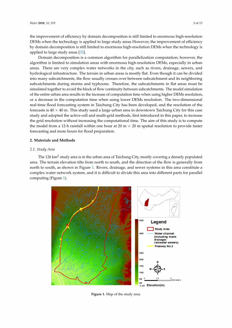
The 126 km2 study area is in the urban area of Taichung City, mostly covering a densely populatedarea. The terrain elevation tilts from north to south, and the direction of the flow is generally fromnorth to south, as shown in Figure 1. Rivers, drainage, and sewer systems in this area constitute acomplex water network system, and it is difficult to divide this area into different parts for parallelcomputing (Figure 1).

Water 2018, 10, x FOR PEER REVIEW 3 of 13

high-resolution DEMs when the technology is applied to large study areas However, the improvement of efficiency by domain decomposition is still limited to enormous high-resolution DEMs when the technology is applied to large study areas [30].

Domain decomposition is a common algorithm for parallelization computation; however, the algorithm is limited to simulation areas with enormous high-resolution DEMs, especially in urban areas. There are very complex water networks in the city, such as rivers, drainage, sewers, and hydrological infrastructure. The terrain in urban areas is mostly flat. Even though it can be divided into many subcatchments, the flow usually crosses over between subcatchment and its neighboring subcatchments during storms and typhoons. Therefore, the subcatchments in flat areas must be simulated together to avoid the block of flow continuity between subcatchments. The model simulation of the entire urban area results in the increase of computation time when using higher DEMs resolution, or a decrease in the computation time when using lower DEMs resolution. The two-dimensional real-time flood forecasting system in Taichung City has been developed, and the resolution of the forecasts is 40 × 40 m. This study used a large urban area in downtown Taichung City for this case study and adopted the active-cell and multi-grid methods, first introduced in this paper, to increase the grid resolution without increasing the computational time. The aim of this study is to compute the model from a 12-h rainfall within one hour at 20 m × 20 m spatial resolution to provide faster forecasting and more hours for flood preparation.

2. Materials and Methods

2.1. Study Area

The 126 km2 study area is in the urban area of Taichung City, mostly covering a densely populated area. The terrain elevation tilts from north to south, and the direction of the flow is generally from north to south, as shown in Figure 1. Rivers, drainage, and sewer systems in this area constitute a complex water network system, and it is difficult to divide this area into different parts for parallel computing (Figure 1).

Figure 1. Map of the study area. Figure 1. Map of the study area.

Water 2018, 10, 319 4 of 13

2.2. Delft-FEWS

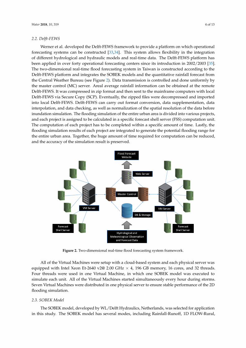
Werner et al. developed the Delft-FEWS framework to provide a platform on which operationalforecasting systems can be constructed [33,34]. This system allows flexibility in the integrationof different hydrological and hydraulic models and real-time data. The Delft-FEWS platform hasbeen applied in over forty operational forecasting centers since its introduction in 2002/2003 [35].The two-dimensional real-time flood forecasting system in Taiwan is constructed according to theDelft-FEWS platform and integrates the SOBEK models and the quantitative rainfall forecast fromthe Central Weather Bureau (see Figure 2). Data transmission is controlled and done uniformly bythe master control (MC) server. Areal average rainfall information can be obtained at the remoteDelft-FEWS. It was compressed in zip format and then sent to the mainframe computers with localDelft-FEWS via Secure Copy (SCP). Eventually, the zipped files were decompressed and importedinto local Delft-FEWS. Delft-FEWS can carry out format conversion, data supplementation, datainterpolation, and data checking, as well as normalization of the spatial resolution of the data beforeinundation simulation. The flooding simulation of the entire urban area is divided into various projects,and each project is assigned to be calculated in a specific forecast shell server (FSS) computation unit.The computation of each project has to be completed within a specific amount of time. Lastly, theflooding simulation results of each project are integrated to generate the potential flooding range forthe entire urban area. Together, the huge amount of time required for computation can be reduced,and the accuracy of the simulation result is preserved.

Water 2018, 10, x FOR PEER REVIEW 4 of 13

2.2. Delft-FEWS

Werner et al. developed the Delft-FEWS framework to provide a platform on which operational forecasting systems can be constructed [31,32]. This system allows flexibility in the integration of different hydrological and hydraulic models and real-time data. The Delft-FEWS platform has been applied in over forty operational forecasting centers since its introduction in 2002/2003 [33]. The two-dimensional real-time flood forecasting system in Taiwan is constructed according to the Delft-FEWS platform and integrates the SOBEK models and the quantitative rainfall forecast from the Central Weather Bureau (see Figure 2). Data transmission is controlled and done uniformly by the master control (MC) server. Areal average rainfall information can be obtained at the remote Delft-FEWS. It was compressed in zip format and then sent to the mainframe computers with local Delft-FEWS via Secure Copy (SCP). Eventually, the zipped files were decompressed and imported into local Delft-FEWS. Delft-FEWS can carry out format conversion, data supplementation, data interpolation, and data checking, as well as normalization of the spatial resolution of the data before inundation simulation. The flooding simulation of the entire urban area is divided into various projects, and each project is assigned to be calculated in a specific forecast shell server (FSS) computation unit. The computation of each project has to be completed within a specific amount of time. Lastly, the flooding simulation results of each project are integrated to generate the potential flooding range for the entire urban area. Together, the huge amount of time required for computation can be reduced, and the accuracy of the simulation result is preserved.

All of the Virtual Machines were setup with a cloud-based system and each physical server was equipped with Intel Xeon Et-2640 v2@ 2.00 GHz × 4, 196 GB memory, 16 cores, and 32 threads. Four threads were used in one Virtual Machine, in which one SOBEK model was executed to simulate each unit. All of the Virtual Machines started simultaneously every hour during storms. Seven Virtual Machines were distributed in one physical server to ensure stable performance of the 2D flooding simulation.

Figure 2. Two-dimensional real-time flood forecasting system framework.

2.3. SOBEK Model

The SOBEK model, developed by WL/Delft Hydraulics, Netherlands, was selected for application in this study. The SOBEK model has several modes, including Rainfall-Runoff, 1D

Figure 2. Two-dimensional real-time flood forecasting system framework.

All of the Virtual Machines were setup with a cloud-based system and each physical server wasequipped with Intel Xeon Et-2640 v2@ 2.00 GHz × 4, 196 GB memory, 16 cores, and 32 threads.Four threads were used in one Virtual Machine, in which one SOBEK model was executed tosimulate each unit. All of the Virtual Machines started simultaneously every hour during storms.Seven Virtual Machines were distributed in one physical server to ensure stable performance of the 2Dflooding simulation.

2.3. SOBEK Model

The SOBEK model, developed by WL/Delft Hydraulics, Netherlands, was selected for applicationin this study. The SOBEK model has several modes, including Rainfall-Runoff, 1D FLOW-Rural,

Water 2018, 10, 319 5 of 13

1D FLOW-Urban, Overland Flow-2D, and so on [36]. In this study, the rivers, regional drainage,rainwater sewers, and various hydraulic structures, including bridges, culverts, orifices, weirs, gates,pumping stations, and detention basins, etc., were set up in SOBEK. The SOBEK version used in thisstudy was version 2.13, and the processor model used was Intel® Core ™ i7-3770K CPU @ 3.50 GHz.

2.4. Grid Methods

2.4.1. Active-Cell

The flow of rainfall can be divided into two phases. The first phase is the process of converginginto drainages and river channels after the rainwater falls to the ground and then flows down theterrain through streams, ditches, and other flow routes. At this stage, SOBEK uses the Rainfall-Runoffmodule to convert rainfall into runoff and then directly into the downstream channels of catchment.This method is based on 1D-2D coupling modules, and the computational efficiency is much faster thanthat of 2D distributed streamflow model. The second phase is when the flow process after the runoff isintroduced into the channel. The SOBEK uses the 1D-2D coupling modules to perform the calculation.When the 1D channel encounters the bottleneck of conveyance or the embankment protection standardis insufficient, flooding will occur over the bank and then, the 2D overland flood module simulates thedynamic changes of water flooding.

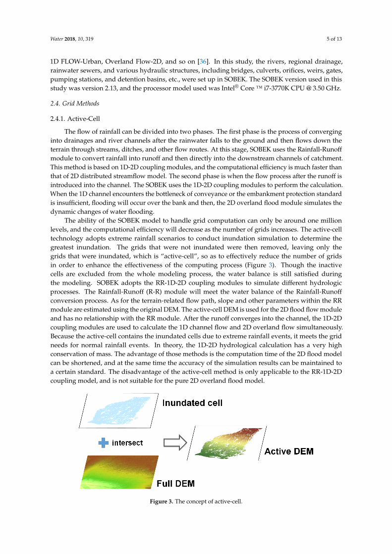
The ability of the SOBEK model to handle grid computation can only be around one millionlevels, and the computational efficiency will decrease as the number of grids increases. The active-celltechnology adopts extreme rainfall scenarios to conduct inundation simulation to determine thegreatest inundation. The grids that were not inundated were then removed, leaving only thegrids that were inundated, which is “active-cell”, so as to effectively reduce the number of gridsin order to enhance the effectiveness of the computing process (Figure 3). Though the inactivecells are excluded from the whole modeling process, the water balance is still satisfied duringthe modeling. SOBEK adopts the RR-1D-2D coupling modules to simulate different hydrologicprocesses. The Rainfall-Runoff (R-R) module will meet the water balance of the Rainfall-Runoffconversion process. As for the terrain-related flow path, slope and other parameters within the RRmodule are estimated using the original DEM. The active-cell DEM is used for the 2D flood flow moduleand has no relationship with the RR module. After the runoff converges into the channel, the 1D-2Dcoupling modules are used to calculate the 1D channel flow and 2D overland flow simultaneously.Because the active-cell contains the inundated cells due to extreme rainfall events, it meets the gridneeds for normal rainfall events. In theory, the 1D-2D hydrological calculation has a very highconservation of mass. The advantage of those methods is the computation time of the 2D flood modelcan be shortened, and at the same time the accuracy of the simulation results can be maintained toa certain standard. The disadvantage of the active-cell method is only applicable to the RR-1D-2Dcoupling model, and is not suitable for the pure 2D overland flood model.

Water 2018, 10, x FOR PEER REVIEW 5 of 13

FLOW-Rural, 1D FLOW-Urban, Overland Flow-2D, and so on [34]. In this study, the rivers, regional drainage, rainwater sewers, and various hydraulic structures, including bridges, culverts, orifices, weirs, gates, pumping stations, and detention basins, etc., were set up in SOBEK. The SOBEK version used in this study was version 2.13, and the processor model used was Intel® Core ™ i7-3770K CPU @ 3.50GHz.

2.4. Grid Methods

2.4.1. Active-Cell

The flow of rainfall can be divided into two phases. The first phase is the process of converging into drainages and river channels after the rainwater falls to the ground and then flows down the terrain through streams, ditches, and other flow routes. At this stage, SOBEK uses the Rainfall-Runoff module to convert rainfall into runoff and then directly into the downstream channels of catchment. This method is based on 1D-2D coupling modules, and the computational efficiency is much faster than that of 2D distributed streamflow model. The second phase is when the flow process after the runoff is introduced into the channel. The SOBEK uses the 1D-2D coupling modules to perform the calculation. When the 1D channel encounters the bottleneck of conveyance or the embankment protection standard is insufficient, flooding will occur over the bank and then, the 2D overland flood module simulates the dynamic changes of water flooding.

The ability of the SOBEK model to handle grid computation can only be around one million levels, and the computational efficiency will decrease as the number of grids increases. The active-cell technology adopts extreme rainfall scenarios to conduct inundation simulation to determine the greatest inundation. The grids that were not inundated were then removed, leaving only the grids that were inundated, which is “active-cell”, so as to effectively reduce the number of grids in order to enhance the effectiveness of the computing process (Figure 3). Though the inactive cells are excluded from the whole modeling process, the water balance is still satisfied during the modeling. SOBEK adopts the RR-1D-2D coupling modules to simulate different hydrologic processes. The Rainfall-Runoff (R-R) module will meet the water balance of the Rainfall-Runoff conversion process. As for the terrain-related flow path, slope and other parameters within the RR module are estimated using the original DEM. The active-cell DEM is used for the 2D flood flow module and has no relationship with the RR module. After the runoff converges into the channel, the 1D-2D coupling modules are used to calculate the 1D channel flow and 2D overland flow simultaneously. Because the active-cell contains the inundated cells due to extreme rainfall events, it meets the grid needs for normal rainfall events. In theory, the 1D-2D hydrological calculation has a very high conservation of mass. The advantage of those methods is the computation time of the 2D flood model can be shortened, and at the same time the accuracy of the simulation results can be maintained to a certain standard. The disadvantage of the active-cell method is only applicable to the RR-1D-2D coupling model, and is not suitable for the pure 2D overland flood model.

Figure 3. The concept of active-cell. Figure 3. The concept of active-cell.

Water 2018, 10, 319 6 of 13

2.4.2. Multi-Grid

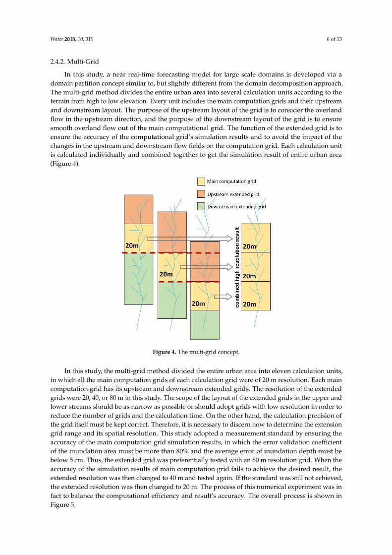
In this study, a near real-time forecasting model for large scale domains is developed via adomain partition concept similar to, but slightly different from the domain decomposition approach.The multi-grid method divides the entire urban area into several calculation units according to theterrain from high to low elevation. Every unit includes the main computation grids and their upstreamand downstream layout. The purpose of the upstream layout of the grid is to consider the overlandflow in the upstream direction, and the purpose of the downstream layout of the grid is to ensuresmooth overland flow out of the main computational grid. The function of the extended grid is toensure the accuracy of the computational grid’s simulation results and to avoid the impact of thechanges in the upstream and downstream flow fields on the computation grid. Each calculation unitis calculated individually and combined together to get the simulation result of entire urban area(Figure 4).

Water 2018, 10, x FOR PEER REVIEW 6 of 13

2.4.2. Multi-Grid

In this study, a near real-time forecasting model for large scale domains is developed via a domain partition concept similar to, but slightly different from the domain decomposition approach. The multi-grid method divides the entire urban area into several calculation units according to the terrain from high to low elevation. Every unit includes the main computation grids and their upstream and downstream layout. The purpose of the upstream layout of the grid is to consider the overland flow in the upstream direction, and the purpose of the downstream layout of the grid is to ensure smooth overland flow out of the main computational grid. The function of the extended grid is to ensure the accuracy of the computational grid’s simulation results and to avoid the impact of the changes in the upstream and downstream flow fields on the computation grid. Each calculation unit is calculated individually and combined together to get the simulation result of entire urban area (Figure 4).

Figure 4. The multi-grid concept.

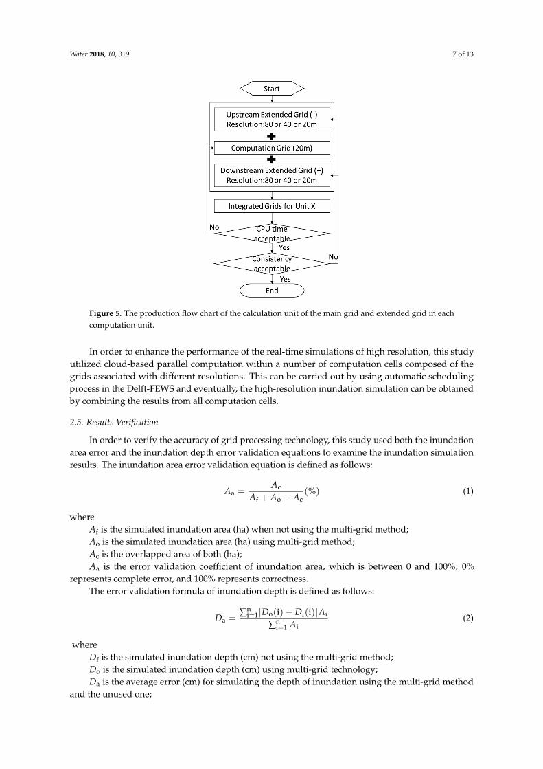
In this study, the multi-grid method divided the entire urban area into eleven calculation units, in which all the main computation grids of each calculation grid were of 20 m resolution. Each main computation grid has its upstream and downstream extended grids. The resolution of the extended grids were 20, 40, or 80 m in this study. The scope of the layout of the extended grids in the upper and lower streams should be as narrow as possible or should adopt grids with low resolution in order to reduce the number of grids and the calculation time. On the other hand, the calculation precision of the grid itself must be kept correct. Therefore, it is necessary to discern how to determine the extension grid range and its spatial resolution. This study adopted a measurement standard by ensuring the accuracy of the main computation grid simulation results, in which the error validation coefficient of the inundation area must be more than 80% and the average error of inundation depth must be below 5 cm. Thus, the extended grid was preferentially tested with an 80 m resolution grid. When the accuracy of the simulation results of main computation grid fails to achieve the desired result, the extended resolution was then changed to 40 m and tested again. If the standard was still not achieved, the extended resolution was then changed to 20 m. The process of this numerical experiment was in fact to balance the computational efficiency and result’s accuracy. The overall process is shown in Figure 5.

In order to enhance the performance of the real-time simulations of high resolution, this study utilized cloud-based parallel computation within a number of computation cells composed of the grids associated with different resolutions. This can be carried out by using automatic scheduling

Figure 4. The multi-grid concept.

In this study, the multi-grid method divided the entire urban area into eleven calculation units,in which all the main computation grids of each calculation grid were of 20 m resolution. Each maincomputation grid has its upstream and downstream extended grids. The resolution of the extendedgrids were 20, 40, or 80 m in this study. The scope of the layout of the extended grids in the upper andlower streams should be as narrow as possible or should adopt grids with low resolution in order toreduce the number of grids and the calculation time. On the other hand, the calculation precision ofthe grid itself must be kept correct. Therefore, it is necessary to discern how to determine the extensiongrid range and its spatial resolution. This study adopted a measurement standard by ensuring theaccuracy of the main computation grid simulation results, in which the error validation coefficientof the inundation area must be more than 80% and the average error of inundation depth must bebelow 5 cm. Thus, the extended grid was preferentially tested with an 80 m resolution grid. When theaccuracy of the simulation results of main computation grid fails to achieve the desired result, theextended resolution was then changed to 40 m and tested again. If the standard was still not achieved,the extended resolution was then changed to 20 m. The process of this numerical experiment was infact to balance the computational efficiency and result’s accuracy. The overall process is shown inFigure 5.

Water 2018, 10, 319 7 of 13

Water 2018, 10, x FOR PEER REVIEW 7 of 13

process in the Delft-FEWS and eventually, the high-resolution inundation simulation can be obtained by combining the results from all computation cells.

Figure 5. The production flow chart of the calculation unit of the main grid and extended grid in each computation unit.

2.5. Results Verification

In order to verify the accuracy of grid processing technology, this study used both the inundation area error and the inundation depth error validation equations to examine the inundation simulation results. The inundation area error validation equation is defined as follows:

a cf o c % (1)

where Af is the simulated inundation area (ha) when not using the multi-grid method; Ao is the simulated inundation area (ha) using multi-grid method; Ac is the overlapped area of both (ha); Aa is the error validation coefficient of inundation area, which is between 0 and 100%; 0%

represents complete error, and 100% represents correctness. The error validation formula of inundation depth is defined as follows:

a ∑ | o i f i | ini 1 ∑ ini 1 (2)

where Df is the simulated inundation depth (cm) not using the multi-grid method; Do is the simulated inundation depth (cm) using multi-grid technology; Da is the average error (cm) for simulating the depth of inundation using the multi-grid method

and the unused one; Ai is the area (ha) of each computational grid. The error validation coefficient of the inundation area in this study must be above 80%, whereas

the average error of the inundation depth must be below 5 cm.

Figure 5. The production flow chart of the calculation unit of the main grid and extended grid in eachcomputation unit.

In order to enhance the performance of the real-time simulations of high resolution, this studyutilized cloud-based parallel computation within a number of computation cells composed of thegrids associated with different resolutions. This can be carried out by using automatic schedulingprocess in the Delft-FEWS and eventually, the high-resolution inundation simulation can be obtainedby combining the results from all computation cells.

2.5. Results Verification

In order to verify the accuracy of grid processing technology, this study used both the inundationarea error and the inundation depth error validation equations to examine the inundation simulationresults. The inundation area error validation equation is defined as follows:

Aa =Ac

Af + Ao − Ac(%) (1)

whereAf is the simulated inundation area (ha) when not using the multi-grid method;Ao is the simulated inundation area (ha) using multi-grid method;Ac is the overlapped area of both (ha);Aa is the error validation coefficient of inundation area, which is between 0 and 100%; 0%

represents complete error, and 100% represents correctness.The error validation formula of inundation depth is defined as follows:

Da =∑n

i=1|Do(i)− Df(i)|Ai

∑ni=1 Ai

(2)

whereDf is the simulated inundation depth (cm) not using the multi-grid method;Do is the simulated inundation depth (cm) using multi-grid technology;Da is the average error (cm) for simulating the depth of inundation using the multi-grid method

and the unused one;

Water 2018, 10, 319 8 of 13

Ai is the area (ha) of each computational grid.The error validation coefficient of the inundation area in this study must be above 80%, whereas

the average error of the inundation depth must be below 5 cm.

3. Results and Discussion

3.1. Active-Cell

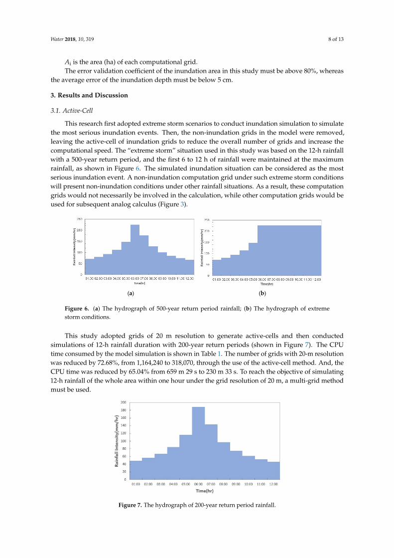
This research first adopted extreme storm scenarios to conduct inundation simulation to simulatethe most serious inundation events. Then, the non-inundation grids in the model were removed,leaving the active-cell of inundation grids to reduce the overall number of grids and increase thecomputational speed. The “extreme storm” situation used in this study was based on the 12-h rainfallwith a 500-year return period, and the first 6 to 12 h of rainfall were maintained at the maximumrainfall, as shown in Figure 6. The simulated inundation situation can be considered as the mostserious inundation event. A non-inundation computation grid under such extreme storm conditionswill present non-inundation conditions under other rainfall situations. As a result, these computationgrids would not necessarily be involved in the calculation, while other computation grids would beused for subsequent analog calculus (Figure 3).

Water 2018, 10, x FOR PEER REVIEW 8 of 13

3. Results and Discussion

3.1. Active-Cell

This research first adopted extreme storm scenarios to conduct inundation simulation to simulate the most serious inundation events. Then, the non-inundation grids in the model were removed, leaving the active-cell of inundation grids to reduce the overall number of grids and increase the computational speed. The “extreme storm” situation used in this study was based on the 12-h rainfall with a 500-year return period, and the first 6 to 12 h of rainfall were maintained at the maximum rainfall, as shown in Figure 6. The simulated inundation situation can be considered as the most serious inundation event. A non-inundation computation grid under such extreme storm conditions will present non-inundation conditions under other rainfall situations. As a result, these computation grids would not necessarily be involved in the calculation, while other computation grids would be used for subsequent analog calculus (Figure 3).

(a) (b)

Figure 6. (a) The hydrograph of 500-year return period rainfall; (b) The hydrograph of extreme storm conditions.

This study adopted grids of 20 m resolution to generate active-cells and then conducted simulations of 12-h rainfall duration with 200-year return periods (shown in Figure 7). The CPU time consumed by the model simulation is shown in Table 1. The number of grids with 20-m resolution was reduced by 72.68%, from 1,164,240 to 318,070, through the use of the active-cell method. And, the CPU time was reduced by 65.04% from 659 m 29 s to 230 m 33 s. To reach the objective of simulating 12-h rainfall of the whole area within one hour under the grid resolution of 20 m, a multi-grid method must be used.

Figure 7. The hydrograph of 200-year return period rainfall.

Figure 6. (a) The hydrograph of 500-year return period rainfall; (b) The hydrograph of extremestorm conditions.

This study adopted grids of 20 m resolution to generate active-cells and then conductedsimulations of 12-h rainfall duration with 200-year return periods (shown in Figure 7). The CPUtime consumed by the model simulation is shown in Table 1. The number of grids with 20-m resolutionwas reduced by 72.68%, from 1,164,240 to 318,070, through the use of the active-cell method. And, theCPU time was reduced by 65.04% from 659 m 29 s to 230 m 33 s. To reach the objective of simulating12-h rainfall of the whole area within one hour under the grid resolution of 20 m, a multi-grid methodmust be used.

Water 2018, 10, x FOR PEER REVIEW 8 of 13

3. Results and Discussion

3.1. Active-Cell

This research first adopted extreme storm scenarios to conduct inundation simulation to simulate the most serious inundation events. Then, the non-inundation grids in the model were removed, leaving the active-cell of inundation grids to reduce the overall number of grids and increase the computational speed. The “extreme storm” situation used in this study was based on the 12-h rainfall with a 500-year return period, and the first 6 to 12 h of rainfall were maintained at the maximum rainfall, as shown in Figure 6. The simulated inundation situation can be considered as the most serious inundation event. A non-inundation computation grid under such extreme storm conditions will present non-inundation conditions under other rainfall situations. As a result, these computation grids would not necessarily be involved in the calculation, while other computation grids would be used for subsequent analog calculus (Figure 3).

(a) (b)

Figure 6. (a) The hydrograph of 500-year return period rainfall; (b) The hydrograph of extreme storm conditions.

This study adopted grids of 20 m resolution to generate active-cells and then conducted simulations of 12-h rainfall duration with 200-year return periods (shown in Figure 7). The CPU time consumed by the model simulation is shown in Table 1. The number of grids with 20-m resolution was reduced by 72.68%, from 1,164,240 to 318,070, through the use of the active-cell method. And, the CPU time was reduced by 65.04% from 659 m 29 s to 230 m 33 s. To reach the objective of simulating 12-h rainfall of the whole area within one hour under the grid resolution of 20 m, a multi-grid method must be used.

Figure 7. The hydrograph of 200-year return period rainfall.

Figure 7. The hydrograph of 200-year return period rainfall.

Water 2018, 10, 319 9 of 13

Table 1. Comparison of models with and without the active-cell method.

Method Number of Grid CPU Time

Without active-cell method 1,164,240 659 m 29 sWith active-cell method 318,070 230 m 33 s

3.2. Multi-Grid

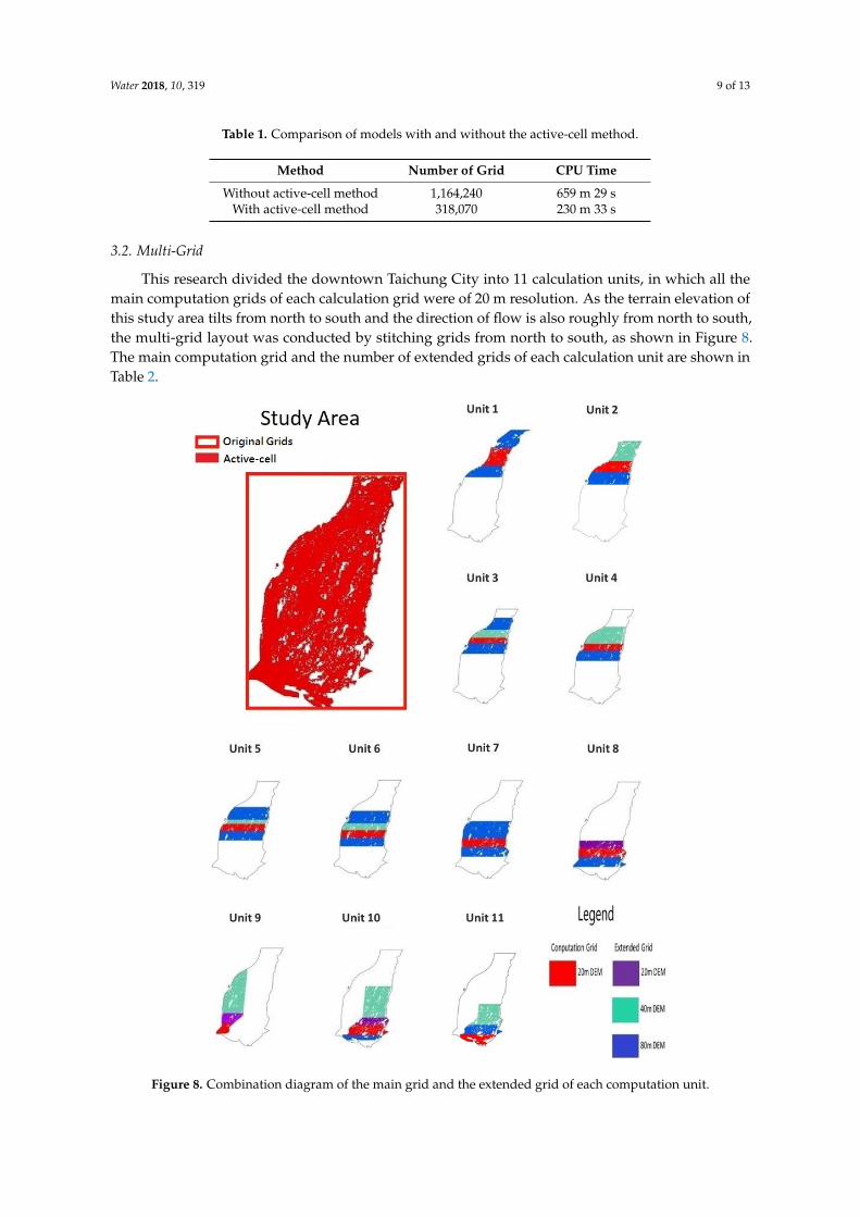
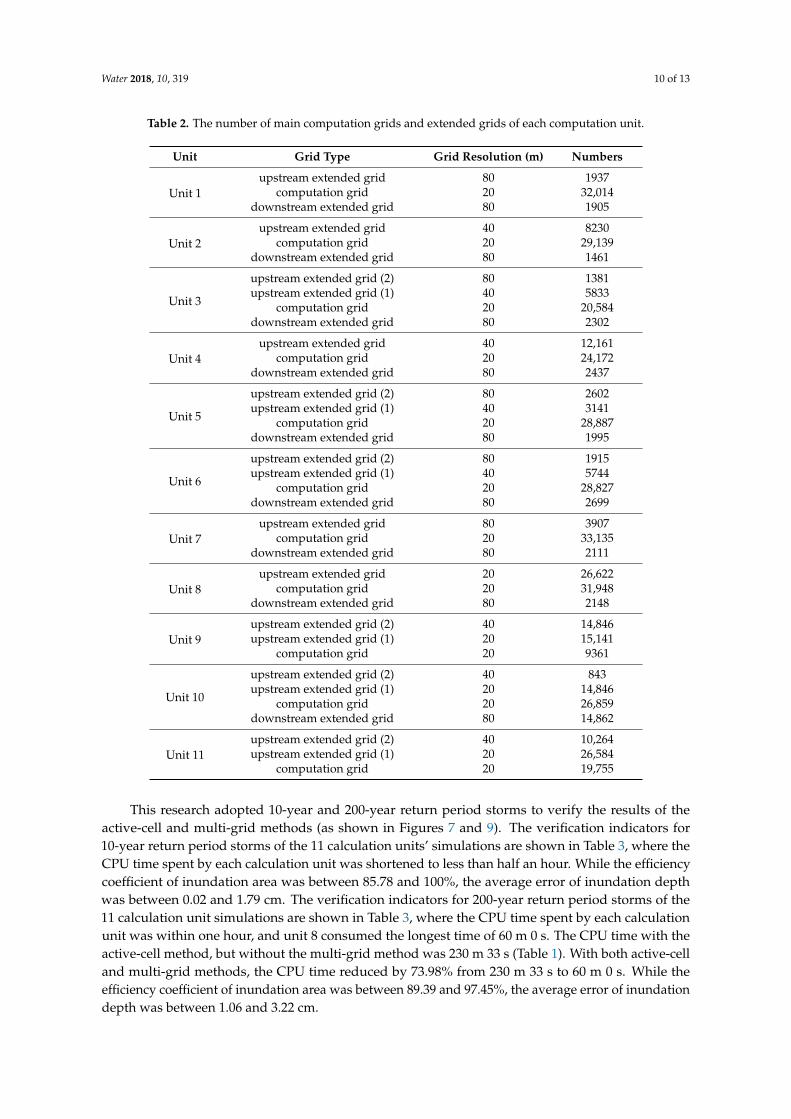
This research divided the downtown Taichung City into 11 calculation units, in which all themain computation grids of each calculation grid were of 20 m resolution. As the terrain elevation ofthis study area tilts from north to south and the direction of flow is also roughly from north to south,the multi-grid layout was conducted by stitching grids from north to south, as shown in Figure 8.The main computation grid and the number of extended grids of each calculation unit are shown inTable 2.

Water 2018, 10, x FOR PEER REVIEW 9 of 13

Table 1. Comparison of models with and without the active-cell method.

Method Number of Grid CPU Time Without active-cell method 1,164,240 659 m 29 s

With active-cell method 318,070 230 m 33 s

3.2. Multi-Grid

This research divided the downtown Taichung City into 11 calculation units, in which all the main computation grids of each calculation grid were of 20 m resolution. As the terrain elevation of this study area tilts from north to south and the direction of flow is also roughly from north to south, the multi-grid layout was conducted by stitching grids from north to south, as shown in Figure 8. The main computation grid and the number of extended grids of each calculation unit are shown in Table 2.

Figure 8. Combination diagram of the main grid and the extended grid of each computation unit. Figure 8. Combination diagram of the main grid and the extended grid of each computation unit.

Water 2018, 10, 319 10 of 13

Table 2. The number of main computation grids and extended grids of each computation unit.

Unit Grid Type Grid Resolution (m) Numbers

Unit 1upstream extended grid 80 1937

computation grid 20 32,014downstream extended grid 80 1905

Unit 2upstream extended grid 40 8230

computation grid 20 29,139downstream extended grid 80 1461

Unit 3

upstream extended grid (2) 80 1381upstream extended grid (1) 40 5833

computation grid 20 20,584downstream extended grid 80 2302

Unit 4upstream extended grid 40 12,161

computation grid 20 24,172downstream extended grid 80 2437

Unit 5

upstream extended grid (2) 80 2602upstream extended grid (1) 40 3141

computation grid 20 28,887downstream extended grid 80 1995

Unit 6

upstream extended grid (2) 80 1915upstream extended grid (1) 40 5744

computation grid 20 28,827downstream extended grid 80 2699

Unit 7upstream extended grid 80 3907

computation grid 20 33,135downstream extended grid 80 2111

Unit 8upstream extended grid 20 26,622

computation grid 20 31,948downstream extended grid 80 2148

Unit 9upstream extended grid (2) 40 14,846upstream extended grid (1) 20 15,141

computation grid 20 9361

Unit 10

upstream extended grid (2) 40 843upstream extended grid (1) 20 14,846

computation grid 20 26,859downstream extended grid 80 14,862

Unit 11upstream extended grid (2) 40 10,264upstream extended grid (1) 20 26,584

computation grid 20 19,755

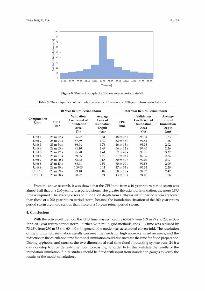
This research adopted 10-year and 200-year return period storms to verify the results of theactive-cell and multi-grid methods (as shown in Figures 7 and 9). The verification indicators for10-year return period storms of the 11 calculation units’ simulations are shown in Table 3, where theCPU time spent by each calculation unit was shortened to less than half an hour. While the efficiencycoefficient of inundation area was between 85.78 and 100%, the average error of inundation depthwas between 0.02 and 1.79 cm. The verification indicators for 200-year return period storms of the11 calculation unit simulations are shown in Table 3, where the CPU time spent by each calculationunit was within one hour, and unit 8 consumed the longest time of 60 m 0 s. The CPU time with theactive-cell method, but without the multi-grid method was 230 m 33 s (Table 1). With both active-celland multi-grid methods, the CPU time reduced by 73.98% from 230 m 33 s to 60 m 0 s. While theefficiency coefficient of inundation area was between 89.39 and 97.45%, the average error of inundationdepth was between 1.06 and 3.22 cm.

Water 2018, 10, 319 11 of 13

Water 2018, 10, x FOR PEER REVIEW 11 of 13

From the above research, it was shown that the CPU time from a 10-year return period storm was almost half that of a 200-year return period storm. The greater the extent of inundation, the more CPU time is required. The average errors of inundation depth from a 10-year return period storm are lower than those of a 200-year return period storm, because the inundation situation of the 200-year return period storm are more serious than those of a 10-year return period storm.

Figure 9. The hydrograph of a 10-year return period rainfall.

Table 3. The comparison of computation results of 10-year and 200-year return period storms.

Computation Unit

10-Year Return Period Storm 200-Year Return Period Storm

CPU Time

Validation Coefficient of

Inundation Area (%)

Average Error of Inundation

Depth (cm)

CPU Time

Validation Coefficient of

Inundation Area (%)

Average Error of Inundation

Depth (cm)

Unit 1 25 m 22 s 96.27 0.31 48 m 07 s 96.31 1.73 Unit 2 25 m 24 s 87.69 1.47 52 m 48 s 94.51 1.66 Unit 3 25 m 54 s 86.94 1.76 46 m 15 s 93.33 2.02 Unit 4 28 m 03 s 91.10 1.47 56 m 12 s 97.45 2.26 Unit 5 25 m 22 s 85.78 1.61 52 m 48 s 90.28 3.22 Unit 6 26 m 31 s 89.65 1.79 51 m 03 s 89.39 2.84 Unit 7 25 m 00 s 88.72 0.65 50 m 40 s 92.02 2.07 Unit 8 27 m 13 s 88.91 0.54 60 m 00 s 94.88 2.09 Unit 9 24 m 39 s 100.00 0.11 47 m 53 s 95.32 2.20 Unit 10 28 m 59 s 99.18 0.02 50 m 15 s 92.73 2.47 Unit 11 25 m 58 s 98.97 0.21 43 m 16 s 94.08 1.06

4. Conclusions

With the active-cell method, the CPU time was reduced by 65.04% from 659 m 29 s to 230 m 33 s for a 200-year return period storm. Further, with multi-grid methods, the CPU time was reduced by 73.98% from 230 m 33 s to 60 m 0 s. In general, the model was accelerated eleven-fold. The resolution of the inundation simulation results can meet the needs for high accuracy in urban areas, and the reduction in the calculation time for model simulation could also increase the time for flood preparation. During typhoons and storms, the two-dimensional real-time flood forecasting system runs 24 h a day non-stop to provide real-time flood forecasting. In order to further validate the results of the inundation simulation, future studies should be fitted with input from inundation gauges to verify the results of the model calculations.

Figure 9. The hydrograph of a 10-year return period rainfall.

Table 3. The comparison of computation results of 10-year and 200-year return period storms.

ComputationUnit

10-Year Return Period Storm 200-Year Return Period Storm

CPUTime

ValidationCoefficient of

InundationArea(%)

AverageError of

InundationDepth(cm)

CPUTime

ValidationCoefficient of

InundationArea(%)

AverageError of

InundationDepth(cm)

Unit 1 25 m 22 s 96.27 0.31 48 m 07 s 96.31 1.73Unit 2 25 m 24 s 87.69 1.47 52 m 48 s 94.51 1.66Unit 3 25 m 54 s 86.94 1.76 46 m 15 s 93.33 2.02Unit 4 28 m 03 s 91.10 1.47 56 m 12 s 97.45 2.26Unit 5 25 m 22 s 85.78 1.61 52 m 48 s 90.28 3.22Unit 6 26 m 31 s 89.65 1.79 51 m 03 s 89.39 2.84Unit 7 25 m 00 s 88.72 0.65 50 m 40 s 92.02 2.07Unit 8 27 m 13 s 88.91 0.54 60 m 00 s 94.88 2.09Unit 9 24 m 39 s 100.00 0.11 47 m 53 s 95.32 2.20

Unit 10 28 m 59 s 99.18 0.02 50 m 15 s 92.73 2.47Unit 11 25 m 58 s 98.97 0.21 43 m 16 s 94.08 1.06

From the above research, it was shown that the CPU time from a 10-year return period storm wasalmost half that of a 200-year return period storm. The greater the extent of inundation, the more CPUtime is required. The average errors of inundation depth from a 10-year return period storm are lowerthan those of a 200-year return period storm, because the inundation situation of the 200-year returnperiod storm are more serious than those of a 10-year return period storm.

4. Conclusions

With the active-cell method, the CPU time was reduced by 65.04% from 659 m 29 s to 230 m 33 sfor a 200-year return period storm. Further, with multi-grid methods, the CPU time was reduced by73.98% from 230 m 33 s to 60 m 0 s. In general, the model was accelerated eleven-fold. The resolutionof the inundation simulation results can meet the needs for high accuracy in urban areas, and thereduction in the calculation time for model simulation could also increase the time for flood preparation.During typhoons and storms, the two-dimensional real-time flood forecasting system runs 24 h aday non-stop to provide real-time flood forecasting. In order to further validate the results of theinundation simulation, future studies should be fitted with input from inundation gauges to verify theresults of the model calculations.

Water 2018, 10, 319 12 of 13

Acknowledgments: The authors thank the editors and anonymous referees for their thoughtful comments andsuggestions. This research project is funded by the Water Resources Agency, Ministry of Economic Affairs, Taiwan(grant numbers MOEAWRA1050132). The authors appreciate George Chih-Yu Chen for his assistance in theEnglish editing.

Author Contributions: Che-Hao Chang and Ming-Ko Chung performed the experiments; Song-Yue Yang wrotethe paper; Chih-Tsung Hsu and Shiang-Jen Wu built the model.

Conflicts of Interest: The authors declare no conflict of interest.

References

1. Werner, M.; Cranston, M.; Harrison, T.; Whitfield, D.; Schellekens, J. Recent developments in operationalflood forecasting in england, wales and scotland. Meteorol. Appl. 2009, 16, 13–22. [CrossRef]

2. Vehviläinen, B.; Huttunen, M. Hydrological Forecasting and Real Time Monitoring in Finland: The WatershedSimulation and Forecasting System (WSFS); Finnish Environment Institute: Helsinki, Finland, 2001.

3. Kirby, D. Flood integrated decision support system for melbourne (fidss). In Proceedings of the 2015Floodplain Management Association National Conference, Brisbane, Australia, 19–22 May 2015.

4. Johnell, A.; Lindström, G.; Olsson, J. Deterministic evaluation of ensemble streamflow predictions in sweden.Hydrol. Res. 2007, 38, 441–450. [CrossRef]

5. Krajewski, W.F.; Ceynar, D.; Demir, I.; Goska, R.; Kruger, A.; Langel, C.; Mantilla, R.; Niemeier, J.; Quintero, F.;Seo, B.-C. Real-time flood forecasting and information system for the state of iowa. Bull. Am. Meteorol. Soc.2017, 98, 539–554. [CrossRef]

6. Tospornsampan, M.J.; Malone, T.; Katry, P.; Pengel, B.; An, H.P. Fmmp component 1 short and medium-termflood forecasting at the regional flood management and mitigation centre. Mekong River Comm. 2009, 7,155–164.

7. Chang, C.-H. Establishment and Application of Radar Data and Hydrologic Models in an Integrated Platform ofHydrometeorology Observation; Water Resources Agency: Taichung, Taiwan, 2013.

8. Chang, C.-H. The Development of Value-Add Application for Rainfall Rader Data and Multiple Hydrology ModelsBased on Fews_Taiwan; Water Resources Agency: Taichung, Taiwan, 2014.

9. Syme, W.; Pinnell, M.; Wicks, J. Modelling flood inundation of urban areas in the uk using 2d/1d hydraulicmodels. In Proceedings of the 8th National Conference on Hydraulics in Water Engineering, Gold Coast,Australia, 13–16 July 2004; The Institution of Engineers: Gold Coast, Australia, 2004.

10. Chang, C.-H. Integrated Platform for Application of High-Performance 2D Inundation Simulation; Water ResourcesPlanning Institute: Taichung, Taiwan, 2016.

11. Moore, M.R. Development of a High-Resolution 1D/2D Coupled Flood Simulation of Charles City, Iowa; Universityof Iowa: Iowa City, ID, USA, 2011.

12. Sampson, C.C.; Fewtrell, T.J.; Duncan, A.; Shaad, K.; Horritt, M.S.; Bates, P.D. Use of terrestrial laser scanningdata to drive decimetric resolution urban inundation models. Adv. Water Resour. 2012, 41, 1–17. [CrossRef]

13. Meesuk, V.; Vojinovic, Z.; Mynett, A.E.; Abdullah, A.F. Urban flood modelling combining top-view lidardata with ground-view sfm observations. Adv. Water Resour. 2015, 75, 105–117. [CrossRef]

14. Marks, K.; Bates, P. Integration of high-resolution topographic data with floodplain flow models.Hydrol. Process. 2000, 14, 2109–2122. [CrossRef]

15. Haile, A.T.; Rientjes, T. Effects of lidar dem resolution in flood modelling: A model sensitivity study for thecity of Tegucigalpa, Honduras. In Proceedings of the ISPRS WG III/3, III/4, V/3 Workshop “Laser Scanning2005”, Enschede, The Netherlands, 12–14 September 2005; Volume 3, pp. 12–14.

16. Bates, P.D.; De Roo, A. A simple raster-based model for flood inundation simulation. J. Hydrol. 2000, 236,54–77. [CrossRef]

17. Liu, L.; Liu, Y.; Wang, X.; Yu, D.; Liu, K.; Huang, H.; Hu, G. Developing an effective 2-d urban floodinundation model for city emergency management based on cellular automata. Nat. Hazards Earth Syst. Sci.2015, 15, 381–391. [CrossRef]

18. Yu, D.; Lane, S.N. Urban fluvial flood modelling using a two-dimensional diffusion-wave treatment, part 1:Mesh resolution effects. Hydrol. Process. 2006, 20, 1541–1565. [CrossRef]

19. Chen, A.S.; Evans, B.; Djordjevic, S.; Savic, D.A. Multi-layered coarse grid modelling in 2d urban floodsimulations. J. Hydrol. 2012, 470, 1–11. [CrossRef]

Water 2018, 10, 319 13 of 13

20. Hunter, N.M.; Bates, P.D.; Horritt, M.S.; De Roo, A.; Werner, M.G. Utility of different data types for calibratingflood inundation models within a glue framework. Hydrol. Earth Syst. Sci. 2005, 9, 412–430. [CrossRef]

21. Wang, J.P.; Liang, Q. Testing a new adaptive grid-based shallow flow model for different types of floodsimulations. J. Flood Risk Manag. 2011, 4, 96–103. [CrossRef]

22. Wang, X.; Cao, Z.; Pender, G.; Neelz, S. Numerical modelling of flood flows over irregular topography.Proc. Inst. Civ. Eng. Water Manag. 2010, 163, 255–265. [CrossRef]

23. Sanders, B.F.; Schubert, J.E.; Detwiler, R.L. Parbrezo: A parallel, unstructured grid, godunov-type,shallow-water code for high-resolution flood inundation modeling at the regional scale. Adv. Water Resour.2010, 33, 1456–1467. [CrossRef]

24. Li, Z.; Wu, L.; Zhu, W.; Hou, M.; Yang, Y.; Zheng, J. A new method for urban storm flood inundationsimulation with fine cd-tin surface. Water 2014, 6, 1151–1171. [CrossRef]

25. Yu, D.; Lane, S.N. Urban fluvial flood modelling using a two-dimensional diffusion-wave treatment, part 2:Development of a sub-grid-scale treatment. Hydrol. Process. 2006, 20, 1567–1583. [CrossRef]

26. Yu, D. Parallelization of a two-dimensional flood inundation model based on domain decomposition.Environ. Model. Softw. 2010, 25, 935–945. [CrossRef]

27. Stelling, G.S. Quadtree flood simulations with sub-grid digital elevation models. Proc. Inst. Civ. Eng. 2012,165, 567. [CrossRef]

28. Dhondia, J.; Stelling, G. Application of one-dimensional-two-dimensional integrated hydraulic modelfor flood simulation and damage assessment. In Proceedings of the International Conference onHydroinformatics, Cardiff, UK, 1–5 July 2002; pp. 265–276.

29. Neal, J.C.; Fewtrell, T.J.; Bates, P.D.; Wright, N.G. A comparison of three parallelisation methods for 2d floodinundation models. Environ. Model. Softw. 2010, 25, 398–411. [CrossRef]

30. Kalyanapu, A.J.; Shankar, S.; Pardyjak, E.R.; Judi, D.R.; Burian, S.J. Assessment of GPU computationalenhancement to a 2D flood model. Environ. Model. Softw. 2011, 26, 1009–1016.

31. Teng, J.; Jakeman, A.J.; Vaze, J.; Croke, B.F.; Dutta, D.; Kim, S. Flood inundation modelling: A review ofmethods, recent advances and uncertainty analysis. Environ. Model. Softw. 2017, 90, 201–216.

32. Costabile, P.; Macchione, F. Enhancing river model set-up for 2-d dynamic flood modelling. Environ. Model.Softw. 2015, 67, 89–107. [CrossRef]

33. Werner, M.; van Dijk, M.; Schellekens, J. Delft-fews: An open shell flood forecasting system.In Hydroinformatics: (in 2 Volumes, with CD-ROM); World Scientific: Singapore, 2004; pp. 1205–1212.

34. Werner, M.; Heynert, K. Open model integration—A Review of practical examples in operational floodforecasting. In Proceedings of the Seventh International Conference on Hydroinformatics, Nice, France,4–8 September 2006; pp. 155–162.

35. Werner, M.; Schellekens, J.; Gijsbers, P.; van Dijk, M.; van den Akker, O.; Heynert, K. The delft-fews flowforecasting system. Environ. Model. Softw. 2013, 40, 65–77. [CrossRef]

36. Deltares. Sobek User Manual; Deltares: Delft, The Netherlands, 2017.

© 2018 by the authors. Licensee MDPI, Basel, Switzerland. This article is an open accessarticle distributed under the terms and conditions of the Creative Commons Attribution(CC BY) license (http://creativecommons.org/licenses/by/4.0/).