UNLV Theses, Dissertations, Professional Papers, and Capstones 5-1-2012 Improving Efficiency and Capacity of Hydro-Turbines in the Improving Efficiency and Capacity of Hydro-Turbines in the Western United States, Hoover Dam Western United States, Hoover Dam Jonathan Sanchez University of Nevada, Las Vegas Follow this and additional works at: https://digitalscholarship.unlv.edu/thesesdissertations Part of the Mechanical Engineering Commons, and the Oil, Gas, and Energy Commons Repository Citation Repository Citation Sanchez, Jonathan, "Improving Efficiency and Capacity of Hydro-Turbines in the Western United States, Hoover Dam" (2012). UNLV Theses, Dissertations, Professional Papers, and Capstones. 1622. http://dx.doi.org/10.34917/4332603 This Thesis is protected by copyright and/or related rights. It has been brought to you by Digital Scholarship@UNLV with permission from the rights-holder(s). You are free to use this Thesis in any way that is permitted by the copyright and related rights legislation that applies to your use. For other uses you need to obtain permission from the rights-holder(s) directly, unless additional rights are indicated by a Creative Commons license in the record and/ or on the work itself. This Thesis has been accepted for inclusion in UNLV Theses, Dissertations, Professional Papers, and Capstones by an authorized administrator of Digital Scholarship@UNLV. For more information, please contact [email protected].

Welcome message from author
This document is posted to help you gain knowledge. Please leave a comment to let me know what you think about it! Share it to your friends and learn new things together.
Transcript

UNLV Theses, Dissertations, Professional Papers, and Capstones
5-1-2012
Improving Efficiency and Capacity of Hydro-Turbines in the Improving Efficiency and Capacity of Hydro-Turbines in the
Western United States, Hoover Dam Western United States, Hoover Dam
Jonathan Sanchez University of Nevada, Las Vegas
Follow this and additional works at: https://digitalscholarship.unlv.edu/thesesdissertations
Part of the Mechanical Engineering Commons, and the Oil, Gas, and Energy Commons
Repository Citation Repository Citation Sanchez, Jonathan, "Improving Efficiency and Capacity of Hydro-Turbines in the Western United States, Hoover Dam" (2012). UNLV Theses, Dissertations, Professional Papers, and Capstones. 1622. http://dx.doi.org/10.34917/4332603
This Thesis is protected by copyright and/or related rights. It has been brought to you by Digital Scholarship@UNLV with permission from the rights-holder(s). You are free to use this Thesis in any way that is permitted by the copyright and related rights legislation that applies to your use. For other uses you need to obtain permission from the rights-holder(s) directly, unless additional rights are indicated by a Creative Commons license in the record and/or on the work itself. This Thesis has been accepted for inclusion in UNLV Theses, Dissertations, Professional Papers, and Capstones by an authorized administrator of Digital Scholarship@UNLV. For more information, please contact [email protected].

IMPROVING EFFICIENCY AND CAPACITY OF HYDRO-TURBINES
IN THE WESTERN UNITED STATES
- HOOVER DAM -
By
Jonathan Gamaliel Sanchez
A thesis submitted in partial fulfillment of the requirements for the
Master of Science in Mechanical Engineering
Mechanical Engineering Department Howard R. Hughes, College of Engineering
The Graduate College
University of Nevada, Las Vegas May 2012

Copyright by Jonathan G. Sanchez, 2012
All Rights Reserved
ii
THE GRADUATE COLLEGE We recommend the thesis prepared under our supervision by Jonathan Gamaliel Sanchez entitled Improving Efficiency and Capacity of Hydro-Turbines in the Western United States, Hoover Dam be accepted in partial fulfillment of the requirements for the degree of Masters of Science in Mechanical Engineering Department of Mechanical Engineering Yitung Chen, Ph.D., Committee Chair Robert Boehm, Ph.D., Committee Member Hui Zhao, Ph.D., Committee Member Yahia Baghzouz, Ph.D., Graduate College Representative Ronald Smith, Ph. D., Vice President for Research and Graduate Studies and Dean of the Graduate College May 2012

iii
ABSTRACT
Improving Efficiency and Capacity of Hydro-Turbines In the Western United States
- Hoover Dam –
by
Jonathan G. Sanchez
Dr. Yitung Chen, Examination Committee Chair Professor of Department of Mechanical Engineering
University of Nevada, Las Vegas
The goal for this thesis is to minimize clearances and tolerances, in order to
prevent water leakage. A proper seal on the seal rings does not let excess water flow
through the turbine runner, thus conserving more water and wasting less energy.
Moreover, water leakage past worn wear plates allows for an extra load for the turbine
when operating in condense mode. When the wicket gates are closed, water leakage past
worn plates wastes mechanical energy in the water; thus, decreasing the efficiency of the
Francis turbine, especially when operating at partial loads. Furthermore, the wicket gates
also known as guide vanes can increase the efficiency of the turbine in their relation to
their laminar profile and proper seal.
Water is a very vital resource in today’s society. This thesis illustrates how
existing hydro machinery can be improved to reduce the dependency on fossil fuels as an
electric energy source. This study provides actual examples of improvements using the
generating units located at Hoover Dam. Hoover Dam located in Boulder City, NV is part
of the Lower Colorado Region, of the U.S. Department of the Interior Bureau of
Reclamation.

iv
Overhauling a hydro unit to obtain better efficiency is very similar to overhauling
a vehicles engine to improve the vehicles fuel economy. Modifying and replacing three
major hydro-machinery components: seal rings, wear plates, and wicket gates, improves
the efficiency of Hoover Dam units by an average of 2 percent. This increase in capacity
equates to an additional 8,000 MW-hrs per year per unit. The wholesale market value of
this increase in energy and capacity, roughly equates to about $290,000 per unit per year
[1]. Engineering design, calculations, and performance test were conducted to improve
the parameters of the seal rings, wear plates, and wicket gates. MATLAB® and MS Excel
computer software was used to analyze testing results and provide data and calculation
results.
This study focuses mainly on the seal rings, wear plates, and wicket gates. In
order to achieve a 2% efficiency gain and about a 3% to 5% capacity gain per unit, the
dimensions of the wear plates and seal rings were changed to have tighter clearances, and
the wicket gate design and profile were changed by increasing the angle of attack by 2
degrees, and by increasing the trailing edge gap by 0.02 inches. Additionally, the servo
motors were stroke 2.5 feet more to achieve the 2 percent increase in efficiency.
As water levels keep on dropping in the Colorado River, future research and
analysis can be allocated in a new turbine runner design for low head operation ranges.
Additionally, there are a few other mechanical and electrical components that can be
modified or alternated to monitor and improve capacity efficiency.

v
ACKNOWLEDGEMENTS
I want to thank my committee members who were more than generous with their
expertise and precious time. A special thanks to Dr. Yitung Chen, my committee
chairman for his countless hours of reflecting, reading, encouraging, and most of all
patience throughout the entire process. I am forever grateful, thanks for all your support
Dr. Chen and may God bless you. Thank you Dr. Robert F. Boehm, Dr. Hui Zhao, and
Dr. Yahia Baghzouz for agreeing to serve on my committee, and for all your help and
support.
I would like to acknowledge and thank my school division and the US. Dept. of
the Interior, Bureau of Reclamation – Hoover Dam, for allowing me to conduct my
research and providing me with any assistance requested, especially the Hoover
Engineering Group. Special thanks go to the members of the UNLV Mechanical
Engineering department for their continued support, and the staff and employees at
Hoover Dam for supporting me throughout this process.
Special thanks go to Mr. Daniel A. Pellouchoud, PE, for believing in me since day
one. Not only are you a great engineer, a great mentor, but also a great friend. You helped
me throughout the process and established parameters that I could follow. Big thanks go
to you and also thank you for inspiring me, coaching me, training me, and supporting me
throughout the process. You once told me to “Never give up, never, never, never give
up”; and those words have surely paid-off.

vi
Last but not least, I wish to thank my family, friends, church member and
colleagues for their ongoing support and encouragement during my time at the University
of Nevada, Las Vegas and over the course of the research presented. Thank you all for
your prayers, your motivating and encouraging words, and for extending out a hand when
help was needed. You all made this possible and I am forever grateful.

vii
DEDICATION
To the four pillars of my life: God, my parents, my siblings, and my sweetheart.
Without your support, guidance, and encouraging words this will not have been possible.
Whenever I was down You lifted me up, whenever I was weak You gave me
strength, whenever I was lost and confused You provided me with guidance. Walking
with You, God, through this journey has given me right to say, “I can do all things
through Christ which strengthen me.”
Dad and Mom, thanks for your support, faith, and encouragement. Thanks for
always being there for me, in the good and in bad times. You are truly an inspiration to
me, and your great sacrifice and effort has paid off. You taught me how to become the
person that I am today, and I am proud to be your son.
Elias and Esther, you too have a big part on this accomplishment. You have
challenged me to achieve what I have until this day. My desire is that I can set a good
example for you both as an older brother, and to see you two achieve much more than
what I have accomplished.
Sara, my love; I love you with all my heart. Thanks for supporting and
encouraging me to keep on going. Thank you so much for your patience, caring,
commitment, and teaching me that I should never surrender. Without your love and
understanding I would not be able to make it.
To God be all the glory, all the honor, and all the praise.

viii
TABLE OF CONTENTS
Copyright ................................................................................................................. i
Approval Page ......................................................................................................... ii
Abstract .................................................................................................................. iii
Acknowledgements ..................................................................................................v
Dedication ............................................................................................................. vii
List of Tables ...........................................................................................................x
List of Figures ........................................................................................................ xi
Chapter 1: Introduction ............................................................................................1
1.1 Introduction ................................................................................................1
1.2 Background of Hydropower .......................................................................3
1.3 Background of Hoover Dam ...................................................................16
1.4 Research Objectives .................................................................................26
1.5 Literature Review .....................................................................................32
Chapter 2: Exergy Analysis ...................................................................................33
2.1 Laws of Thermodynamics ........................................................................33
2.2 Calculating the Thermodynamic Exergy ..................................................37
Chapter 3: Hydro-Machine Parameter Improvements ...........................................44
3.1 Correlated Variables .................................................................................44
3.2 Hydro-Machinery Components ................................................................45
3.2.1 Seal Rings .....................................................................................46
3.2.2 Wear Plates ...................................................................................49
3.2.3 Wicket Gates ................................................................................52
Chapter 4: Results and Discussion .........................................................................66
4.1 Results .....................................................................................................66
4.2 MATLAB® Coding .................................................................................68
4.2.1 Baseline Calculations MATLAB® Coding ..................................68
4.2.2 Parametric Analysis Calculations MATLAB® Coding ................71
4.2.3 Seal Ring Calculations MATLAB® Coding ...............................74

ix
4.2.4 Pre and Post-Overhaul Calculations MATLAB® Coding ..........78
4.3 Discussion ................................................................................................83
Chapter 5: Conclusion and Suggestions ................................................................85
5.1 Findings ....................................................................................................85
5.2 Suggestions ...............................................................................................86
Exhibits ..................................................................................................................87
Exhibit 1: Figures ...........................................................................................87
E-1: Cross-Section of a typical Hoover Dam Generator Unit ...............87
Appendices .............................................................................................................88
Appendix A: Glossary ....................................................................................88
A-1: Utility Definitions .........................................................................88
A-2: Electrical Definitions ....................................................................89
A-3: Mechanical Definitions .................................................................93
Appendix B: MATLAB® Coding ......................................................................95
B-1: Baseline Calculations MATLAB® Coding ...................................95
B-2: Exergy and Parametric Study MATLAB® Coding .......................97
B-3: Seal Ring Calculations MATLAB® Coding ..................................99
B-4: Pre-Overhaul and Post-Overhaul Calculations MATLAB®
Coding ........................................................................................102
References ............................................................................................................108
Curriculum Vitae (Vita) .......................................................................................111

x
LIST OF TABLES
Table 1: Hydropower Unit Variable Parameters ...................................................36
Table 2: Exergy Parametric Study Analysis Comparison ......................................41
Table 3: Hoover Power Plant Projected Capacity Increases Achieved .................67
Table 4: Seal Ring Clearances Parameter Values ..................................................74
Table 5: Stabilized Readings, Prior to Unit Overhaul ...........................................80
Table 6: Stabilized Readings, After Unit Overhaul ...............................................81
xi
LIST OF FIGURES
Figure 1: Major Producers of Hydropower, Hydroelectric Generation Capacity in
MWe ........................................................................................................5
Figure 2: Schematic of an Impoundment Dam ........................................................9
Figure 3: Hydropower Unit Components ..............................................................10
Figure 4: Schematic of a Pumped Storage Facility ................................................11
Figure 5: Hydropower Generating Unit Components ...........................................14
Figure 6: Inside a Hydropower Plant .....................................................................15
Figure 7: U.S. Dept. of the Interior, Bureau of Reclamation Jurisdiction .............16
Figure 8: Hoover Dam ...........................................................................................25
Figure 9: Hoover Power Plant ................................................................................26
Figure 10: Wear plate ready for bolting above and below wicket gates ................28
Figure 11: New wear plates bolted below wicket gates. ........................................28
Figure 12: HEM’s working on the wear plates on units head cover ......................29
Figure 13: New wear plates at top and bottom. .....................................................29
Figure 14: Restoration of Seal Rings and Wear Plates .........................................30
Figure 15: New Stainless Steel Wicket Gate vs. Old Cast Steel Wicket Gate ......30
Figure 16: New Wicket Gates being installed ......................................................31
Figure 17: Control Volume Parametric Analysis ..................................................38
Figure 18: Lower Seal Ring ...................................................................................48
Figure 19: Machining the Turbine Runner Seal Rings ..........................................48
Figure 20: Machining the Seal Rings on the Turbine Runner for Final
Clearances .............................................................................................49
Figure 21: Damaged and Corroded Wear Plates ....................................................50
Figure 22: Refurbished Nitronic 60 Wear Plates ...................................................51
Figure 23: Check Stress Analysis for Turbine Flanges and Gates ........................52
Figure 24: Hoover Dam Mussel Curve .................................................................54
Figure 25: New Optimized Wicket Gate – VA Tech Profile A
(Asymmetrical Shape) ..........................................................................55

xii
Figure 26 : New Optimized Wicket Gate – VA Tech Profile B
(Symmetrical Shape) ...........................................................................56
Figure 27: Wicket Gate Function Schematic .........................................................57
Figure 28: Wicket Gate and Turbine Arrangement ...............................................58
Figure 29: Existing Wicket Gate – 1930’s Profile .................................................59
Figure 30: New Wicket Gate – Modern Profile .....................................................60
Figure 31: Comparing Existing and New Wicket Gate Profile .............................60
Figure 32:Wicket Gate Servo Motor Arm and Wicket Gate Mechanism ..............61
Figure 33:Wicket Gate Servo Motor Arm and Shift Ring Mechanism .................62
Figure 34:Wicket Gate Linkage Mechanism .........................................................62
Figure 35:Turbine Pit Area, Without the Wicket Gate Shift Ring ........................63
Figure 36: Turbine Runner Being Staged for Modifications and Repairs .............64
Figure 37: Cavitation seen on the turbine runner bucket .......................................64
Figure 38: MATLAB® plot of Unit Capacity - Data Normalized to 490.36 ft.
of net head ...........................................................................................78
Figure 39: MATLAB® plot of Unit Efficiency - Data Normalized to 490.36 ft.
of net head ...........................................................................................79
Figure 40: MATLAB® plot of Unit Capacity Prior to Unit Overhaul - Data
Normalized to 490.36 ft. of net head ..................................................82
Figure 41: MATLAB® plot of Unit Capacity After Unit Overhaul - Data
Normalized to 490.36 ft. of net head ..................................................83

1
CHAPTER 1
INTRODUCTION
1.1 Introduction
The United States Department of the Interior, Bureau of Reclamation, with full
support from power customers, is completing major projects to improve plant generating
capacity and efficiency available from the existing renewable hydro generation resources
at Hoover Dam.
Hoover Dam, located in Boulder City, NV has seventeen commercial generators.
The nameplate capacity rating of all these generators combined is 2074 megawatts
(MWe). The current capacity of all the generators at Hoover Dam is 1885 MWe with a
Lake Mead elevation of 1134 ft on January 2012. Lower lake levels result in less capacity
available from these units. More flow and change in net head, allow for more capacity
and power to be produced at Hoover Dam.
Capacity improvements at Hoover Dam are focused on allowing an increase in the
maximum amount of water allowed to flow into the turbines at low lake levels.
Additional water flow translates into additional horsepower capability at the turbine and
it allows for additional electrical capacity for the overall plant.
Wicket gates or guide vanes are large steel gates which can be opened or closed to
control the flow of high pressure water to a hydro turbine. The wicket gate system
consists of 24 large steel gates arranged like a cylindrical venetian blinds around the
turbine. A method used to improve the flow capacity to the turbines, and the power

2
output capacity is to replace the old cast steel wicket gates with new stainless steel wicket
gates to allow more water to flow through the turbine. The new gates have a more
streamlined flow profile when compared to the old gates, and are designed with a larger
maximum opening.
The benefits from the increased capacity provide payback of project investments
within a few years. Using a conservative wholesale market price for capacity ($2660 per
MW-month), the value of 70 megawatts of new capacity added at Hoover Dam is $2.2
million per year.
Another strategic goal for Reclamation at Hoover Dam is to improve hydro unit
operating efficiencies. Major turbine overhauls have been underway since October 1999
for the purpose of restoring machinery to a more efficient operating condition.
Overhauling a hydro unit to obtain better efficiency is equivalent to overhauling an
automobile engine to improve fuel economy. Hoover unit efficiencies improve in an
average of 2 percent after a turbine overhaul. The improved efficiency results in more
energy production using the same amount of water. An additional 8,000 megawatt-hours
per year per unit for each unit overhauled has been gained. The wholesale market value
of this added energy is $290K per unit per year. If the 8,000 MW-hrs were produced at a
conventional power plant, more than 14,000 barrels of crude oil would be burned to
produce the amount of added electrical energy which results from one unit overhaul.
Major turbine overhauls include work such as modifying and replacing seal rings and
wear plates to reduce high-pressure leakage of water through the wicket gate system
which occurs when the hydro units are shut down. Preventing the leakage of water,
results in more water available in the future to produce valuable electrical energy. The

3
wholesale market value from reducing leakage through wicket gates at Hoover is $200K
per unit per year. If the energy produced by the saved water were produced by burning
oil at a conventional power plant, over 10,000 barrels of crude oil would be burned to
produce the amount of electrical energy produced by the “saved” water. [2]
1.2 Background of Hydropower
What is hydropower? Hydropower is a form of energy that is renewable, reliable,
and efficient. This form of energy does not directly emit greenhouse gases or other air
pollutants into the environment; therefore it greatly reduces our carbon foot print here on
planet Earth.
Water has always been one of mankind’s most vital resources. We use water for
cleaning, cooking, irrigation and for recreational activities. While the human body can go
weeks without food, it can only survive for a couple of days without water consumption
[3]. However, water can be used as an energy source, known as hydro-electric power or
simply hydropower.
Some of the first recorded mentions of hydropower go back over 2,000 years ago
to ancient Greece and Egypt, where water wheels were connected to grindstones to turn
wheat into flour. The invention of the electrical generator in the late 1800’s created a new
way to utilize hydropower for the growth of civilization. By combining water turbines to
generators with belts and gears, a reliable source of electricity was created that could be
used to power factories and businesses around the world.

4
Water development meant far more than irrigation. In the twentieth century, the
United States Department of the Interior, Bureau of Reclamation responded to the call for
multipurpose water development. Its vast network of irrigation projects, dams, reservoirs,
canals, and aqueducts supplied rural and urban water users, and, most of all, supplied an
industrializing society the many-faceted resources of hydropower [4].
The United States Department of the Interior, Bureau of Reclamation also known
as Reclamations is known as the largest water resource management in the West. It
accounts for 348 reservoirs that deliver 30 million acre feet of water annually. It serves
water to about one-third of the West’s irrigated agriculture that is roughly about 31
million people. Reclamation is responsible and in charge of 50 hydroelectric power
plants, that is 194 generating units that total an installed capacity of 14,778 megawatts
(MWe). The total installed capacity makes Reclamation the tenth largest power utility in
the United States; it provides electricity for roughly 9 million people.
Figure 1 shows the major producers of hydropower from largest to smallest. The
producers include: the U.S. Army Corps of Engineers producing roughly 21 thousands of
MWe , the U.S. Bureau of Reclamation producing roughly 15 thousands of MWe, the
Tennessee Valley Authority producing roughly 7 thousands of MWe, the Power
Authority of State of New York producing roughly 4.5 thousands of MWe, the Pacific
Gas and electric Co. producing roughly 4 thousands of MWe, the Duke Power Co.
producing roughly 2.5 thousands of MWe, the Virginia Electric & Power Co. producing
roughly 2.25 thousands of MWe, Consumers Energy Co. producing roughly 2 thousands
of MWe, PUD No.2 of Grant County producing roughly 1.97 thousands of MWe, PUD

5
No.1 of Chelan County producing roughly 1.97 thousands of MWe, the Seattle City Light
producing roughly 1.95 thousands of MWe, the Idaho Power Co. producing roughly 1.94
thousands of MWe, the California Dept. of Water Resources producing roughly 1.5
thousands of MWe, the Alabama Power Co. producing roughly 1.5 thousands of MWe,
the City of Los Angeles producing roughly 1.5 thousands of MWe, the PECO Energy Co.
producing roughly 1.25 thousands of MWe, the Southern California Edison producing
roughly 1 thousands of MWe, the PacifiCorp producing roughly 1 thousands of MWe, the
Northeast Generation Services producing roughly 0.75 thousands of MWe, and the
Georgia Power Co producing roughly 0.5 thousands of MWe.
Figure 1: Major Producers of Hydropower, Hydroelectric Generation Capacity in MWe [4].

6
There are several benefits of hydropower. Hydropower can be considered as a
renewable source of energy, as it relies on water, and water can be renewed through the
water cycle. Hydroelectricity’s ability to be dispatched quickly to meet peak electricity
demand have made it one of the most valuable renewable energy sources worldwide;
additionally, it is low-cost, and it produces near-zero emissions [5]. In the 1920’s
hydroelectric plants supplied as much as 40% of the electric energy produced, today
hydropower only accounts for about 7% of the nation’s total energy produced.
Hydropower is an essential contributor in the national power grid because of its ability to
respond quickly to rapidly varying loads or systems disturbances. Base load plants with
steam systems powered by combustion or nuclear processes cannot accommodate for
rapid varying loads. Hydropower has grown over the last century from 45 hydroelectric
facilities in 1886 to more than 2,000 facilities in 50 states and Puerto Rico. The
hydropower facilities throughout the United States contribute approximately 80,000 MWe
to our nation’s electrical capacity [6]. Reclamation’s fifty-eight hydro-electric power
plants throughout the Western United States produce an account for an average of 42
billion kWh per year. This amount of electricity is enough to meet the needs of more than
14 million people. Hydropower is also one of the most economic energy resources and it
is not affected by market fluctuations or embargos, which helps support our nation’s
energy independence. Hydropower has also non-power benefits than any other generation
sources. It provides flood control, water supply for irrigation districts, navigation and
recreational activities. The hydropower projects in the United States, accounts for more
than 47,000 miles of shoreline; 2,000 water access sites; 28,000 tent, trailer, and
recreational vehicle sites for camping; 1,100 miles of trails, and 1,200 picnic areas.

7
While there are many advantages to hydroelectric production, the industry faces
several unique environmental challenges. Potential environmental impacts include
changes in aquatic and stream side habitats; alteration of landscapes through the
formation of reservoirs; effects on water quality and quantity; interruption of migratory
patterns for fish; and injury or death of fish passing through the turbines. Hydropower is
mainly criticized for its negatively environmental impacts on local ecosystems and it
environments.
Hydropower alters the natural flow of a river, which in turn changes the aquatic
habitat. It converts a river ecosystem into a lake ecosystem overnight. Damming a river
creates a change and damages the river’s natural animal life and natural plant life.
Additionally, hydropower is not as cheap as we often think. While hydropower saves up
in the cost of fuel, as there is with coal and oil, there is a heavy cost for construction,
upkeep, and land rights.
Money is also invested in water delivery and usage between Mexico and the
United States. The United States Department of the Interior, under the Bureau of
Reclamation handles those water rights and water relations between both countries. An
estimated amount of 1.5 million acre feet of water is delivered to Mexico yearly. The
Colorado River Compact of 1922, also known as the “Law of the River” defines the
relationship between the upper basin states and lower basin states.

8
The Colorado River Compact of 1922 - The cornerstone of the "Law of the
River", this Compact was negotiated by the seven Colorado River Basin
states and the federal government in 1922. It defined the relationship
between the upper basin states, where most of the river's water supply
originates, and the lower basin states, where most of the water demands
were developing. At the time, the upper basin states were concerned that
plans for Hoover Dam and other water development projects in the lower
basin would, under the Western water law doctrine of prior appropriation,
deprive them of their ability to use the river's flows in the future.
The states could not agree on how the waters of the Colorado River Basin
should be allocated among them, so the Secretary of Commerce Herbert
Hoover suggested the basin be divided into an upper and lower half, with
each basin having the right to develop and use 7.5 million acre-feet (maf) of
river water annually. This approach reserved water for future upper basin
development and allowed planning and development in the lower basin to
proceed.
Hydropower and pumped-storage hydroelectricity is often used in combination
with dams to generate electricity. What is a dam? A dam is a barrier that is used to store
water. It is also known as a reservoir. In the United States, there are about 80,000 dams
of which only about 2,400 produce power. The other dams are used for recreation,
irrigation, farming, flood control, and water supply. Hydropower facilities or plants can

9
be categorized under the following distinctive categories: impoundment, diversion or run-
of-river, and pumped storage.
The most commonly seen and used type of dam is the impoundment facility.
Figure 2 demonstrates an impoundment plant which uses a dam to store water in the
reservoir. Water released from the reservoir is transported through pipes, also known as
penstocks, where the water flows through a turbine runner, which causes the runner to
spin a generator which in turn creates electricity. The water at an impoundment facility
may be released to meet changing electricity needs or to maintain a constant reservoir
level, flood control. Hoover Dam is considered to be an impoundment dam.
Figure 2: Schematic of an Impoundment Dam [6].

10
Figure 3 shows the major components found on hydro-unit. This demonstrates a
cut-view of the reservoir and how water enters the plan from the forebay (lake) traveling
through all the hydro-components, and finally exiting back into the tailrace (river).
Figure 3: Hydropower Unit Components [6].
A diversion plant channels a portion of a river through a canal or penstock. A
diversion facility is sometimes referred to as a run-of-river plant. A run-of-river plant
uses water within the natural flow range of the river, requiring little or no impoundment.
A run-of-river, facility channels a portion of a river through a canal or penstock.

11
These facilities are usually built on rivers with steady natural flows or regulated
flows discharged from upstream reservoirs. These units have little or close no storage
capacity, thus, hydropower is generated using the river flow and water head. Run-of-river
hydropower plants are less appropriate for rivers with large seasonal fluctuation. These
facilities may not always require the use of a dam.
Last but not least, Figure 4 shows how pumped storage hydropower plants store
water in a lower reservoir after it is released from an upper reservoir to drive the turbine
and generate power. The water is then pumped back to the upper reservoir for reuse.
Pumping the water back to the upper reservoir requires energy. Pumped storage systems
are considered flexible sources of electricity generation. Pumped storage plants are not
net energy producers; in contrast, pumped storage plants provide energy storage and
electricity at its peak demand times. The units generate electricity when demand and
price are higher, during peak hours, and pump water back to the upper reservoir when
electricity demand and price are lower.
Figure 4: Schematic of a Pumped Storage Facility [7].

12
Hydropower facilities range in size from large power plants that supply many
consumers with electricity to small plants that individuals operate for their own energy
needs or to sell power to utilities. Therefore, hydropower plant can also be categorized
based on their capacities.
Large hydropower plants typically have a capacity of more than 30 MWe, Hoover
Dam for example, has a nameplate capacity of 2,074 MWe. Small hydropower plants
have a generation capacity of 1 to 30 MWe, and micro hydropower plants have a
generation capacity of less than 100 kWe. A small micro hydropower plant can produce
enough electricity for a home, farm, ranch, or village [6].
How does hydropower work? First of all hydropower is obtained from water at
work, water in motion. Hydropower can be seen as a form of solar energy, as the sun
powers the hydrologic cycle which gives the planet Earth its water. Following the
hydrologic cycle, atmospheric water reaches the earth’s surface as precipitation, rain.
Some water from the rain evaporates, but a big percentage of the water from the rain
either penetrates into the soil or it becomes a surface runoff. Water from the rain and
snow pack eventually reaches ponds, rivers, oceans, reservoirs, and lakes where
evaporation occurs constantly. Water vapor passes into the atmosphere by evaporation
then circulates, condenses into clouds, and some returns to earth as precipitation. Thus,
completing the water cycle, and allowing hydropower to be called a form of sustainable
and reliable energy.

13
As the First Law of Thermodynamics states, energy cannot be created or
destroyed, it can only change forms. In hydropower when electricity is generated, no new
energy is created, but simply one form of energy is converted into another form. To
generate electricity, water must be in motion. This form of energy is called kinetic or
moving energy.
When the flowing water turns the blades in a turbine runner, the form of energy is
the changed to mechanical energy or machine energy. The turbine runner then turns a
vertical shaft which is connected to a big generator rotor. The turning of the runner
causes the generator rotor to turn, thus converting the mechanical energy into another
energy form, electricity.
Hydropower plants are located on rivers, streams, and canals, but for a reliable
water supply, the usage and maintenance of dams is necessary. Dams store water for later
release, for purposes such as irrigation, domestic and industrial use, and of course power
generation. The reservoir behind the dam acts much like a battery, storing water to be
released as needed in order to generate power.
Figure 5 shows the major hydro components found in a typical hydro-unit. The
generator that produces electricity when falling water is converted into mechanical
energy to drive the generator. The stator being a stationary component is composed of
copper coils. The rotor is connected to the turbine generator shaft that spins the entire unit
from the mechanical energy receive by the turbine runner. Additionally, the rotor is
composed of electromagnets also referred to as poles. The wicket gates act as guide veins
which control the flow of water from the scroll case into the turbine runner.

14
Figure 5: Hydropower Generating Unit Components [Web].
The differential altitude between the lake and the river creates the net head. The
greater the net head, the more pressure the reservoir can be accounted for. A pipe also
known as penstock carried the water from the reservoir to the turbine. The fast-flowing
water then pushes the turbine blades or buckets, which causes the turbine to rotate the
rotor, the moving part of the electric generator. When coils of wire on the rotor sweep
past the generator’s stationary coil (stator), electricity is produced [8]. This concept was

15
first discovered by scientist Michael Faraday in 1831 when he found that electricity could
be created by rotating magnets within copper coils.
Figure 6 shows a schematic inside a hydropower plant. It’s a cut-view section that
demonstrates how the water flows form the reservoir into the dam, and is finally
converted into electrical energy in where the electricity is transported through the power
lines.
Figure 6: Inside a Hydropower Plant [7].

16
1.3 Background of Hoover Dam
The United States Department of the Interior, Bureau of Reclamation main
purpose is to manage the water in the West, and utilize its structures and construction
projects for flood control, water irrigation, and for the production of hydro-electric
power. Reclamation’s consumers include: farmers, cities, tribes, power, recreation, fish
and wildlife, and foreign countries.
Figure 7 shows the United States Department of the Interior Bureau of
Reclamation’s jurisdiction. Reclamation’s jurisdiction includes the seventeen Western
States, which are: Arizona, California, Colorado, Idaho, Kansas, Montana, Nebraska,
Nevada, New Mexico, North Dakota, Oklahoma, Oregon, South Dakota, Texas, Utah,
Washington, and Wyoming. These seventeen states then make up five regions: Great
Plains, Lower Colorado, Mid Pacific, Pacific Northwest, and Upper Colorado.
Figure 7: U.S. Dept. of the Interior, Bureau of Reclamation Jurisdiction [9].

17
Hoover Dam pertains to the Lower Colorado Region. The Lower Colorado
Region encompasses southern Nevada, southern California, most of Arizona, a small
corner of southwest Utah and a small section of west-central New Mexico. The Lower
Colorado Regional office is located in Boulder City, Nevada. There are also other offices
within our region located in Phoenix, Arizona (Phoenix Area Office, PXAO); Yuma,
Arizona (Yuma Area Office, YAO); Temecula, California (Southern California Area
Office, SCAO); and at Hoover Dam (Lower Colorado Dams Office, LCDO).
The LCDO Area Office consists of Hoover Dam, Davis Dam, and Parker Dam,
and their associated power plants and other facilities on the Lower Colorado River.
Hoover Dam, Davis Dam, and Parker Dam were completed in 1935, 1953, and 1938,
respectively. These three facilities were essential to the economic growth of the
Southwest, and continue to sustain that growth today. The three dams annually deliver an
average of 7.5 million acre feet of Colorado River water to urban and agricultural water
users, including Indian Tribes, in Arizona, Nevada, and California, and 1.5 million acre
feet of water to Mexico. Hoover, Davis, and Parker, also protect downstream
communities from floods and together annually generate an average of more than 6.5
billion kilo-watt-hours (kWh) of electricity that it’s distributed to the three states [9]. A
kWh is a unit of work or energy equal to that done by one kilowatt of power acting for
one hour. A kilowatt is 1,000 watts or 1.34 horsepower.
The primary parts of a generating unit are: the exciter, the rotor, the stator, the
shaft, and the turbine. The exciter is itself a small generator that makes electricity, which
is sent to the rotor, charging it with a magnetic field. The rotor is a series of

18
electromagnets, also known as and called poles. The rotor is connected to the shaft, so
that the rotor rotates when the shaft rotates. The stator is a coil of copper wire. It is
stationary. The shaft connects the exciter and the rotor to the turbine.
Hoover Dam spelled security for southern California’s Imperial Valley, power
and water for Los Angeles, and even promised to make Nevada a viable state [4]. Hoover
Dam generates, on average, about 4 billion kWh of hydroelectric power each year for use
in Nevada, Arizona, and California - enough to serve 1.3 million people. From 1939 to
1949, Hoover power plant was the world's largest hydroelectric installation; today, it is
still one of the country's largest. Each power plant wing is 650 feet long (the length of
almost 2 football fields) and rise 299 feet (nearly 20 stories) above the power plant
foundation. In all of the galleries of the plant there are 10 acres of floor space. There are
seventeen main turbines in the Hoover Power plant -- nine on the Arizona wing and eight
on the Nevada wing. The original turbines were replaced through an uprating program
between 1986 and 1993. The plant has a nameplate capacity of about 2,080 MWe. This
includes the two station-service units (small generating units that provide power for plant
operations), which are rated at 2.4 MWe each. With the main units having a combined
rated capacity of 2,991,000 horsepower (hp), and two station-service units rated at 3,500
horsepower each, the plant has a rated capacity of 2,998,000 horsepower. The water
reaches the turbines through four penstocks, two on each side of the river. Wicket gates
control water delivery to the units. Maximum head (vertical distance the water travels), at
maximum lake level is around 590 feet; minimum net head, 420 feet; and average net
head, 510 to 530 feet.

19
The installation of the last generating units was completed in 1961. A plant
uprating was completed in 1993, so presently there are fifteen 178,000 horsepower, one
100,000 horsepower, and one 86,000 horsepower Francis-type vertical hydraulic turbines
in the Hoover power plant. There are also thirteen 130,000 kWe, two 127,000 kWe, one
61,500 kWe, and one 68,500 kWe generators.
All machines are operated at 60 cycles. The two 2,400 kWe station-service units
are driven by Pelton turbine runners. Pelton turbine runners are a form of impulse turbine
runners. An impulse turbine runner is a horizontal or vertical wheel that uses the kinetic
energy of water striking its buckets or blades to cause rotation. The wheel is covered by a
housing and the buckets or blades are shaped so they turn the flow of water about 170
degrees inside the housing. After turning the blades or buckets, the water falls to the
bottom of the wheel housing and flows out. These provide electrical energy for lights and
for operating cranes, pumps, motors, compressors, and other electrical equipment within
the dam and power plant.
The machinery was transported from the canyon to the power plant by an
electrically operated cableway of 150 tons rated capacity, with a 1,200-foot span across
the canyon. This cableway lowered all heavy and bulky equipment. The cableway is still
used when necessary. The average annual net generation for Hoover power plant for 1947
through 2008 was about 4.2 billion kilowatt-hours. The ten-year annual average for 1999
through 2008 was about 4.2 billion kilowatt-hours. The maximum annual net generation
at Hoover power plant was 10,348,020,500 kilowatt-hours in 1984, while the minimum
annual net generation since 1940 was 2,648,224,700 kilowatt-hours in 1956.

20
The power plant is operated and maintained by the Bureau of Reclamation. The
power customer for Hoover Dam include the States of Arizona and Nevada; City of Los
Angeles; Southern California Edison Co.; Metropolitan Water District of Southern
California; California cities of Glendale, Burbank, Pasadena, Riverside, Azusa, Anaheim,
Banning, Colton, and Vernon; and the city of Boulder City, Nevada.
The energy generated at Hoover dam is allocated as follow:
Arizona - 18.9527 %
Nevada - 23.3706 %
Metropolitan Water District of Southern California - 28.5393 %
Burbank, CA - 0.5876 %
Glendale, CA - 1.5874 %
Pasadena, CA - 1.3629 %
Los Angeles, CA - 15.4229 %
Southern California Edison Co. - 5.5377 %
Azusa, CA - 0.1104 %
Anaheim, CA - 1.1487 %
Banning, CA - 0.0442 %
Colton, CA - 0.0884 %
Riverside, CA - 0.8615 %
Vernon, CA - 0.6185 %
Boulder City, NV - 1.7672 %

21
To pay all operation, maintenance and replacement costs (including interest
expense and repayment of investments) to meet the requirements of the project. The cost
of construction completed and in service by 1937 was repaid from power revenues by
May 31, 1987, except for costs relating to flood control. Repayment of the $25 million
construction costs allocated to flood control will be repaid by 2037. Any features added
after May 31, 1987 will be repaid within 50 years of the date of installation or as
established by Congress. In addition, Arizona and Nevada each receive $300,000
annually in lieu of taxes.
Hoover Dam is not only a national landmark but it is also known as one of the
seven civil engineering wonders of the world. The project was authorized under the
Boulder Canyon Project Act of 1928. Its authorized cost was of $165,000,000 with the
first $25,000,000 being allocated for flood control as specified by the Boulder Canyon
Project Authorization.
Preparation for the construction site of Hoover Dam, required for four diversion
tunnels to be blasted and bored through the canyon walls, two on the Arizona side and
two on the Nevada side. Excavation began in June of 1931 and it was completed in
November of 1933. The construction site tunnels are 56 feet in diameter and they are
lined with three foot thickness of concrete, leaving the final diameter of the tunnel to be
50 ft. in diameter. The combined length of all four diversion tunnels is approximately
three miles in length.

22
The Colorado River was diverted into the fourth tunnel on November 14, 1932.
Additionally, two coffer dams were built. The first coffer dam was 100 feet high and was
located upstream between the construction site and the downstream exit of the diversion
tunnels. The excavation from the river bed, to the bed rock below, was approximately a
total of 135 ft.
The dam itself is a concrete arch-gravity type of dam. An arch-gravity dam is a
dam with the characteristics of both an arch dam and a gravity dam. Meaning that the
dam curves upstream in a narrowing curve, thus directing most of the water against the
canyon rock walls; therefore, the force of gravity seen by the dam, compresses the dam
downward. Registry of the first concrete pour at Hoover Dam dates back to June 6, 1933.
The construction project was continuous and did not stop until the dam was all complete
on May 29, 1935. The dam was completed, two years ahead of schedule. In order to
accelerate the curing process of the concrete, an ammonia 1,000 ton chilling plant was
constructed on the lower coffer dam to provide chilled brine that was pumped through
piping throughout each of the lifts. Each concrete lift was cured enough to be stripped of
its forms every 72 hours. The total amount of concrete in the dam itself equals
approximately 3.25 million cubic yards that is about 6,600,000 tons of concrete. There is
enough concrete in the dam to pave a 3 inch thick, 18 ft. wide highway from San
Francisco, California to New York City, New York. Believe it or not the concrete
continues to cure, until this day. The life span of the concrete is estimated to be around
2,000 years that is 1,925 years to go from the year 2012. Hoover Dam is 726.4 ft. in
height from bedrock to the roadway; 1,244 ft. between the canyon walls at its widest

23
point; 660 ft. at its base, and 45 ft. thick at its crest. The Nevada-Arizona State line is
located right at the center of the dam’s crest [1].
Hoover Dam’s powerhouse/power plant contains two power plant wings. One
located in Nevada with eight commercial generators and one station service generator
that provides the power for the power plant. Likewise, another wing is located on the
Arizona side. The Arizona wing contains nine commercial generators and one station
service generator. The approximate length of each wing is about 650 feet, and eight
stories high. As mentioned before there is a total of 17 commercial generators. Each
generator is water wheel driven by a stainless steel Francis turbine runner. The total
nameplate capacity for the plant is 2,074 MWe.
Hoover Dam is truly a unique power plant; each unit is unique from the others.
The rotors on units N1 through N8 and A1, A2, A5, and A7 rotate at 180 revolutions per
minute (rpm). These 12 units combined develop approximately 178,000 horsepower. The
rotors have 40 electromagnetic poles. The rotors on units A3 and A4 rotate at 200 rpm
and have 36 electromagnetic pole pieces. The two station service units differentiate in
that they have Pelton type turbine runners instead of Francis type turbine runners. These
two station service units, A0 and N0 rotate at 300 rpm and have 24 electromagnetic pole
pieces. Additionally, all generators except for N7, A5, A7, and A8 are rated at 133,333
kilo-volt ampere (KVA) and 16,500 volts. Units N7 and A5 are rated at 130,256 KVA
and 16,500 volts, and unit A9 is rated at 70, 256 KVA and 16,500 colts. The main
excitation voltage is 250 VDC. The main shaft that connects the turbine runner and the

24
generator rotor, is 38 inches in diameter, weighs approximately 114 tons, and is about 65
ft. in length.
The intake towers are the inlets for the water to flow through the dam and to the
power plant into the units. There is a total of four intake towers, one for each upper and
lower penstock on each wing of the power plant. Each intake tower is built on a rock
shelf, and is approximately 395 ft. tall. It has a diameter of 82 ft. and it tapers to the top
with a final diameter of 63 ft.
The four main penstocks located in the dam are 30 ft. in diameter, and constructed
from a 2.75 inch boiler steel plate. Each pipe section varies in length from 11 ft. to 30 ft..
Each section interlocks with adjacent sections, and is connected by the use of friction-fit
steel pins, which were inserted from inside the penstock and pressed into position with a
hydraulic ram. There is approximately 272 pins per each joint. The penstocks that branch
off from the big penstocks are also known as laterals. Each lateral is 13 ft. in diameter
and supply water into the scroll case and finally the generating unit.
The spillways are located at each side of the dam, one in Nevada and the other
one in Arizona. Each spillway connects to one of the original diversion tunnel. Each
spillway is approximately 650 ft. long, 750 ft. wide and 170 ft. deep. The spillways act as
a flood control passage in case the lake ever goes up high enough, as high as 1,232 ft. In
such event the spillways will diverge the water from the lake into the river, preventing the
water to top over the dam. Each spillway is regulated by four (16 ft. X 100 ft.) drum
gates. Each drum gate weighs approximately 500,000 pounds.

25
Figure 8 shows Hoover Dam at is whole. In the figure one can see the two wings
of the power house for Nevada and Arizona as well as the face of the dam, which holds
back Lake Mead. Additionally, the figure shows the Stoney Gates tunnel that allow the
water to flow back into the river once it has gone through the generating units and the
Spill Way tunnels that will allow the water to bypass the dam in the event of an overspill.
Figure 8: Hoover Dam [2].
Figure 9 shows the Hoover Power Plant. This photograph was taken in the
Nevada Wing of the Powerhouse. Nine hydro-generating units are shown. Eight
commercial units and one in-house unit that provides power for the power plant' electrical
needs and use.

26
Figure 9: Hoover Power Plant, Nevada Wing [2].
1.4 Research Objectives
Efficiency is the amount of electrical power generated over known water flow.
After studying, analyzing, and researching how valuable the water is for our daily use,
one comes to realize that we have to do our best and use water efficiently and effectively.
Hydro-turbine generating units are units that use the water flow and force to spin
a magnetic generator which in result produces electricity. This thermodynamic system
can be assumed to be an open system; however, there are some losses and factors that
must be accounted for in determining the complete and total output efficiency.

27
Every year or so there is a turbine overhaul in a certain unit at Hoover Dam.
Ideally, every unit should get overhaul every 10 to 15 years, depending on the inspection
results and wear and tear circumstances. Since there is 17 generating units at Hoover
Dam, a unit overhaul takes place every year. During a unit overhaul, many factors and
machine components are inspected, tested, and replaced.
Hoover Engineering believes that the efficiency of Hoover’s generating units can
be increased by having tighter clearances and tighter tolerances in the turbine runner seal
rings, turbine pit wear plates, and by modifying the design of the wicket gates, by
reducing the wicket gate camber profile. These factors will not only increase the overall
plant efficiency, but in the long run it will benefit Hoover Dam, and its customers. Better
efficiency means more power that can be produced utilizing the same water intake and
water flow.
In Figure 10 one can see a new set of wear plates ready to be installed in the
turbine pit. A Hoover hydro-unit is composed of 24 wicket gates; therefore, there is a
total of eight sets of three bore holes per unit. This makes it easier for the hydro-electric
mechanics to mobilize and install each set.

28
Figure 10: Wear plate ready for bolting above and below wicket gates [2].
Figure 11 shows two sets of wear plates being installed on the turbine pit and
below the stay vanes and wicket gates. Note the head cover has not been installed yet,
Figure 13 will show the installation of the top and bottom wear plates.
Figure 11: New wear plates bolted below wicket gates [2].

29
Figure 12 shows the head cover upside down while Hoover’s hydro-electric
mechanics install the wear plates.
Figure 12: Hydro-Electric Mechanics (HEM’s) working on the wear plates that are
attached to the units head cover [2].
Figure 13 demonstrates the top and bottom wear plates once installed inside the
turbine pit. The white walls shown are the stay vanes that allow the water to flow into the
turbine runner once the water has been guided by the wicket gates.
Figure 13: New wear plates installed at top and bottom of the turbine pit [2].

30
Figure 14 show both the stationary seal ring and the top portion of the wear plates
after restoration.
Figure 14: Restoration of Seal Rings (top left) and Wear Plates (top right) [2].
Figure 15 shows a comparison between a new stainless steel wicket gate and an
existing cast steel wicket gate. Note that the stainless steel wicket gate has a slimmer
profile.
Figure 15: New Stainless Steel Wicket Gate (left) vs. Old Cast Steel Wicket Gate (right)
[2].

31
Figure 16 shows the new stainless steel wicket gates being installed inside the
turbine pit.
Figure 16: New Wicket Gates being installed [2].
The Laws of Thermodynamics will be applied to analyze the tighter clearances
and design modifications, that will help improve the capacity and efficiency of a hydro-
turbine unit. Data from MATLAB® and MS Excel will be used to analyze the
dimensions, tolerances, and clearances for the seal rings, wear plates, and wicket gates.
Tighter dimension and clearances will be the main focus for the seal rings and wear
plates. A change in camber, possibly the chord, and the angle of attack will be parameters
taken into account for the wicket gate analysis.

32
1.5 Literature Review
Similar studies in analyzing and studying the wicket gates have been done by the
Unites States Army Corps of Engineers. A study done at Lower Granite Lock & Dam to
evaluate potential environmental and performance gains that can be achieved in Kaplan
turbine units, through non-structural modifications to stay vanes and wicket gate
assemblies [10], was done back in 2005.
The wicket analysis was done by VA Tech Hydro [11], similar to the design
modifications and studies done at Hoover Dam. The analysis report showed that in order
to achieve their efficiency gains, the minimal losses are reached by a rotation of
approximately 1.0 degrees; and that the stay vane trailing edge is extended to minimize
the gap between the stay vane and the wicket gate.

33
CHAPTER 2
EXERGY ANALYSIS
2.1 Laws of Thermodynamics
Thermodynamics plays an important role when analyzing and designing thermal
design systems. The first law of thermodynamics states the change in the amount of
energy contained within a system during some interval time is equal to the difference of
the net amount of energy transferred in across the system boundary by heat transfer
during the time interval and the net amount of energy transferred out across the system
boundary by work during the time interval. The first law of thermodynamics is expressed
in Eq. (2.1),
WQE (2.1)
In Eq. (2.1), ∆E, represents the change of energy found on the system (ft-lbs), Q,
represents the amount of heat done on or created by the system (Btu), and W, represents
the amount of work done on or created by the system (ft-lbf).
In analyzing the energy balance, one considers a process in where the system and
the environment come to equilibrium. The energy balance for the overall system as seen
in Eq. (2.1), includes the kinetic, potential, and internal energies of the system. Analyzing
how energy is lost throughout the system helps one understand the overall energy
balance. For example, when a diesel engine turns a generator, the engine's mechanical
energy is converted into electricity. The electricity is still concentrated, but not all of the
mechanical energy is converted to electricity. Some of the energy is lost through heat,

34
and friction that is lost through all the mechanical components. The generator wires are
heated up by internal friction as electrons flow through them. The generator cooling fan
heats up more air by blowing it over the generator to keep it cool. All of this heat expands
into the air around the generator. The energy is still there, however, it is no longer useful
to the system.
In average a generator converts about 90 to 98 percent of the mechanical energy
received into electrical energy, or electricity. The remaining 2 to 10 percent of the energy
that is lost becomes low grade energy, or a less effective form of energy.
As the electrical energy flows through the transmission lines into the power
generating substations and into our homes, the wires are heated by the flowing electrons.
This result in more energy lost. Finally the electrical energy reaches our homes, in where
the energy is converted into heat or mechanical energy.
The second law of thermodynamics states that the change in the amount of
entropy contained with the system during some interval is equal to the difference between
the net amount of entropy transferred in across the system boundary during the time
interval and the amount of entropy produced within the system during the time interval.
For simplicity, the second law of thermodynamics is expressed by Eq. (2.2),
QT
s
1 (2.2)
In Eq. (2.2), ∆s represents the change of entropy in the system (S.I. units are
[kJ/kg · K] and English are [Btu/lb·°R]), T is the absolute temperature at the part of the

35
boundary of the system (S.I. units are [°C] and English are [°F]), and δQ represents the
heat transfer at a part of the system boundary (S.I. units are [J] and British are [Btu]).
Looking at a hydropower generating unit, the first and second law of
thermodynamics can be applied in many distinctive ways. First and foremost, one must
account for all mass flow rate, energy balance, and mass balance. Certain assumptions are
made in this case study. Hoover Dam, is both a regulating and peak hydropower
generating plant, therefore, the units do not run at a constant mode. Hoover Dam is
frequently, changing its power output, by adjusting the amount of water intake. The
plants power output is regulated based on the power customer’s need and also based on
the water capacity and flow that the dams downstream desire. It is safe to assume
however, that a specific unit will operate constantly at full capacity, meaning that the
wicket gates will be 100% open, allowing for maximum flow and maximum power
output from the generating unit, based on the existing net head.
Another assumption that is accounted for is a constant head. Lake Mead has been
increasing lately, during the past year. Back on October 2010, the lake was at El. 1080 ft.,
and recently on January 2012, the lake is at El. 1133 ft.. The value of the net head is the
difference between the river (Tailbay) and lake (Forebay) elevations. For consistency and
comparison feasibility the net head used in this thesis is 490.36 ft. The baseline
calculations will reflect that net head parameter, unless noted otherwise; 490.36 ft was
the net head value obtained on November 2011.

36
Table 1, shows the distinctive parameters used for the thermodynamic analysis of
this case study. Some of these values where obtained from the Fundamentals of
Engineering Thermodynamics, 6th Ed. textbook written by Michael J. Moran and Howard
D. Shapiro [12], and others from Hoover Dam SCADA software.
Table 1: Hydropower Unit Variable Parameters.
Variable Value Units
Net Head, z 490.36 ft
Gravity Constant, g 32.2 ft/s2
Water Density, ρf 62.4 lb/ft3
Water Mass, m 62.4 lbs
Water Temperature, Tf 60 °F
Constant Volumetric Flowrate, Q 3100 cfs
Constant Mass Flow Rate, mdot 193440 lbm/s
Constant Pressure, p0 212 psi
For this case analysis MATLAB® and MS Excel were used for data gathering and
numerical analytical programming. MATLAB® coding and MS Excel data and results
will be referred to in later sections. By using the above parameters listed in Table 1, one
is able to obtain the distinctive energy balance, mass balance, entropy balance, and
exergy balance values that are applicable to this study.

37
2.2 Calculating the Thermodynamic Exergy
What is exergy? As defined by the textbook written by Moran and Shapiro,
exergy is the maximum theoretical work obtainable from an overall system consisting of
a system and the environment as the system comes into equilibrium with the
environment. In other words into the work passes the dead state. The work developed is
fully available for lifting a weight or, equivalently as mechanical work or electrical work.
The exergy of a system for control volumes at steady states is given by Eq. (2.3):
(2.3)
T0 = temperature on the environment (°R)
Tj = temperature on the boundary (°R)
= heat transfer rate (Btu/s)
= energy transfer by work of the control volume (Btu/s)
= mass flow rate (lbm/s)
ef = h-h0-T0(s-s0)+0.5(V2)+gz (ft-lb)
The control volume was treated as an incompressible fluid; therefore, the temperature and
pressure remained constant. Thus ef, represents only the kinetic and potential energy of
the system. Eq. (2.3) allows one to calculate for the exergy of the control volume, setting
the first term of the equation to zero. Figure 17 demonstrates the control volume that was
analyzed in the parametric study at steady state 1, and steady state 2. A single unit was
analyzed, therefore the volumetric flow rate was kept constant through both steady states.
i efeefii
j jdememcvT
T EWQ010
cvW
Q
m

38
Figure 17: Control Volume Used in Parametric Analysis
The distinctive parametric values analyzed in this study were the mass flow rate, the
velocity at the inlet and outlet, the pressure seen by the system, and the water temperature
of the system. As mentioned before, a constant T=60°F and mass flow rate of =193440
lbm/s, were obtained by using volumetric flow rate value of Q=3100 cfs and a net head of
z=490.36 ft. Additionally, the medium in the control volume was taken to be as an
incompressible fluid, meaning that the temperature and the pressure remained constant;
thus, allowing for the first term in Eq. (2.3) to be cancelled out.
As seen in Figure 17, steady state 1 accounts for the parameters as the water flows from
the lake and into the 30 ft. diameter penstock. Steady state 2 accounts for the water flow
from the turbine outlet and into the river.
m

39
Eq. (2.4) demonstrates Eq. (2.3) when simplified to account for an irreversible and
adiabatic system.
(2.4)
= energy transfer by work of the control volume, c.v. (Btu/s)
= mass flow rate (lbm/s)
V1 = velocity coming into system (ft/s)
V2 = velocity coming out of the system (ft/s)
z1 = forebay/lake elevation (ft)
z2 = tailbay/river elevation (ft)
= exergy destruction due to irreversibilities (Btu/s)
V1 and V2 were calculated by setting the volumetric flow rate coming in to the system to
be equal with the volumetric flow rate coming out of the system. Eq. (2.5) shows how to
calculate for velocity, using a volumetric flow rate of, Q=3100 cfs.
Additionally, an area of 706.86 ft2 was used for steady state 1, accounting for an entry
water flow into a 30 ft. diameter penstock, and an area of 113.10 ft2 was used for steady
state 2, accounting for an exit water flow from the turbine outlet.
(2.5)
Q = volumetric flow rate (cfs)
A = area for the flow passage (ft2)
V = velocity of the water flow (ft/s2)
dEmW zzg
VVcv
21
22
21
20
AVQ
cvW
m
dE

40
Eq. (2.4) allows one to solve for the system exergy destruction, . The exergy
destruction represents all the losses accounted for in the system, losses such as friction
losses, fluid losses, pressure losses etc. After solving for the exergy destruction, one is
able to solve for the entropy production, of the system. Eq. (2.6) demonstrates how to
solve for the entropy production, using the absolute temperature and the exergy
destruction due to irreversibilities.
cvd TE
0 (2.6)
= exergy destruction due to irreversibilities (Btu/s)
T0 = temperature on the environment (°R)
= entropy production (Btu/s-°R)
Solving for Eq. (2.4) and Eq. (2.6) allows one to obtain the exergetic turbine efficiency of
the system. This exergetic turbine efficiency value will be used to calculate the
parametric study analysis discussed in Chapter 4. Eq. (2.7) shows how to calculate for the
exergetic turbine efficiency value, using the results from steady state 1 and steady state 2.
(2.7)
= energy transfer by work of the control volume, c.v. (Btu/s)
= mass flow rate (lbm/s)
= exergy destruction due to irreversibilities (Btu/s)
dE
cv
dE
cv
m
E
m
W
m
W
dcv
cv
exergeticturbine
cvW
m
dE

41
Table 2 demonstrates the results of the exergy analysis before and after a unit’s
overhaul. The wicket gate guide vein opening and the seal ring and wear plate clearances
were modified to obtain a better efficiency and plant capacity. These parameters and
modifications will be discussed in Chapter 3.
Table 2: Exergy Parametric Study Analysis Comparison
Table 2 demonstrates that after a unit’s overhaul the same amount of power can be
produced with a smaller volumetric flow rate.
In calculating the thermodynamic exergy analysis of a hydropower unit, there are several
aspects of the thermodynamic exergy analysis that must be taken into account [12].
1. Exergy is a measure of the departure of the state of a system from that of the
environment. It is therefore, an attribute of the system and environment
together. However, once the environment is specified, a value can be assigned
to the exergy in terms of property values for the system only, so exergy can be
regarded as a property of the system. This classifies exergy as an extensive
property.
2. The value of exergy cannot be negative. If a system were at any state other
than the dead state, the system would be able to change its condition
spontaneously toward the dead state; this tendency would cease when the dead
Case Net Head
Study (ft.)
Pre‐Overhaul 490.36
Post‐Overhaul 490.362745 96.93 124.656 130 95.89
3100 96.93 124.656 130 95.89
(cfs) (%) (MWe) (MWe) (%)
Q Exergetic Efficiency Power Produced Power Max Capacity Unit Efficiency

42
state was reached. No work must be done to effect such a spontaneous change.
Accordingly, any change in state of the system to the dead state can be
accomplished with at least zero work being developed, and thus the maximum
work or exergy cannot be negative.
3. Exergy is not conserved but is destroyed by irreversibilities. A limiting case is
when exergy is completely destroyed, as would occur if a system were
permitted to undergo a spontaneous change to the dead state with no provision
to obtain work. The potential to develop work that existed originally would be
completely wasted in such a spontaneous process.
4. Exergy has been viewed thus far as the maximum theoretical work obtainable
from an overall system of system plus environment as the system passes from
a given state to the dead state. Alternatively, exergy can be regarded as the
magnitude of the minimum theoretical work input required to bring the system
from the dead state to the given state.
5. When a system is at the dead state, it is thermal and mechanical equilibrium
with the environment and the value of exergy is zero. The contents of a
system at the dead state are permitted to enter into chemical reaction with
environmental components and in so doing develop additional work. This
contribution to exergy is called chemical exergy.

43
As mentioned before exergy is the maximum theoretical value of the work
obtainable as the system comes into equilibrium with the environment that is when the
system passes to the dead state. The system plus the environment is referred to as the
overall system. The boundary of the overall system is located so there is no energy
transfer across it by heat transfer: Q = 0. Moreover, the boundary of the overall system is
located so that the volume remains constant, even though the volumes of the system and
environment can vary. The work is the only energy transfer across the boundary of the
overall system and is fully available for lifting a weight, turning a shaft, or producing
electricity in the surroundings. Next, the energy and entropy balances are applied to
determine the maximum theoretical value for the work.

44
CHAPTER 3
HYDRO-MACHINE PARAMETER IMPROVEMENTS
3.1 Correlated Variables
Generation of hydropower can be said that is driven by two factors. The water
levels in the reservoir and the efficiency in transforming the water energy’s into electrical
power. The relationship between the water levels in the lake and power generation is
divided into demand (energy conversion efficiency) and capacity (Hoover Dam capacity).
Mechanical factors that affect the efficiency of the Energy Conversion System (ECS) and
methods in how to increase the power plants efficiency reducing the Energy Conversion
Gap (ECG) were analyzed. The ECG is the difference between the designed efficiency
and the current efficiency.
Previous researches have studied distinctive methods in how to improve power
plant efficiency, but most of them are focused in alternating or modifying explicit
software programs. At Hoover Dam the operations and engineering group have a
computer system called SCADA (Supervisory Control And Data Acquisition). SCADA is
a computer system in an industrial plant that provides process control for machinery and
data for monitoring machinery operations. Additionally, SCADA systems are used in
power plants to start and stop units, and control MWe, voltage, and unit operating mode
(i.e. either in condense mode or generate mode). In condense mode the commercial units
act as a motor, in where it does not provide power, but it takes power from the system.
Since Hoover Dam it’s both a regulating and generating plant, the units are often put in-
line and off-line. Generating mode helps facilitate the process by keeping the units

45
spinning and in reserve ready to go for whenever more power is required. The units can
easily be put online in about 15 seconds, as oppose as to having to start up a unit from
complete stand-by mode which can take much longer than 15 seconds. When the units
are on-line then they act as a big generator that produces and supplies as much as 130
MWe of power.
Hoover turbines are generally 85% to 95% efficient when operated in the best
range for a given head. With three different groupings of unit efficiencies, the best
efficiency occurs from around 90 MWe to about 130 MWe for a majority of the units at
Hoover Dam. Very low turbine efficiency occurs at loads below 50 MWe. Hence, that is
the reason why the units are put in condense mode. It is more convenient to put the units
off-line, then risking the changes of seeing and experimenting rough zones and cavitation
problems when operating our units at low loads.
3.2 Hydro-Machinery Components
The machinery components for this study were seal rings, wear plates, and wicket
gates. A proper seal on the seal rings does not let excess water flow through, thus
conserving more water and wasting less energy. Water leakage past worn wear plates
puts an extra load on a turbine runner when operating in condense mode. Additionally,
water leakage past worn plates decreases the efficiency of the Francis turbine, especially
when operating at partial loads and the wicket gates are closed.

46
3.2.1 Seal Rings
Turbine runner seal rings have both stationary and rotating components. The
rotating components are attached to the turbine runner itself and the stationary
components are attached to the turbine pit itself. Additionally, there is upper and lower
rotating and stationary components. The seal rings main function is to reduce water
leakage around the shroud of the runner and between the crown plate of the runner and
the turbine cover plate. When the unit is operating as a synchronous condenser the runner
seal chamber is supplied with penstock water through two 4-inch pipes, which are
capable of delivering about 3 cfs of water to each seal chamber. The sealing water acts as
a cooling medium to prevent heating and seizing of the runner bands in case the
stationary and revolving metal components come in contact.
In the original design the use of two metals of different characteristics was
desirable in the event of accidental contact between the rotating and stationary rings. The
stationary seal rings were made out of stainless steel. These were made in segments of a
ring and bolted to the stationary seats. The runner seals were made of carbon steel forged
into a ring and shrunk on the runner bands [14].
The seal rings are now being manufactured and produced out of a Nitronic 60
material. Nitronic 60 is an all-purpose metal (austenitic stainless). This fully austenitic
alloy was originally designed as a temperature alloy, and subsequently has good high
temperature properties for temperatures around 1800 °F. The oxidation resistance of
Nitronic 60 is similar to Type 309 Stainless Steel, and far superior to Type 304 Stainless
Steel. This grade is best known for its wear and galling resistance.

47
The additions of Silicon and Manganese have given this alloy a matrix to inhibit
wear, galling, and fretting even in the annealed condition. Higher strengths are attainable
through cold working the material and are still fully austenitic after severe cold-working.
This working does not enhance the anti-galling properties as is normal for carbon steels
and some stainless steels. The benefit to the cold or hot work put into the material is
added strength and hardness, and the wear resistance does not decrease noticeably.
Chromium and Nickel additions give it comparable corrosion to 304 and 316 stainless
steels, while having approximately twice the yield strength. The high mechanical strength
in annealed parts permits use of reduced cross sections for weight, and cost reductions
through the use of thinner stock.
As mentioned before a proper seal and tight tolerances on the seal rings do not let
excess water flow through the system. A better seal conserves more water, and reduces
the energy wasted. Hoover Engineering’s goal is to try and keep tight tolerances, while
avoiding contact with the other metal components. Additionally, the goal is to replace the
seal rings with a Nitronic 60 material, machine new radial surfaces concentric, and
restore the design clearance to improve the unit efficiency.
Figure 18 shows the stationary seal ring inside the turbine pit. A turbine runner is
composed of a total of four seal rings. Two upper seal rings and two lower seal rings. The
upper seal rings are composed of a stationary seal ring that remains stationary and a
rotating seal ring that rotates with the turbine runner. The same applies for the lower seal
rings. The lower seal rings are composed of a stationary seal ring that remains stationary
and a rotating seal ring that rotates with the turbine runner.

48
Figure 18: Lower Seal Ring [2].
Figure 19 shows the seal ring being machined in the Big Cincinnati machine at
Hoover’s Machine Shop.
Figure 19: Machining the turbine runner seal rings on the Cincinnati [2].
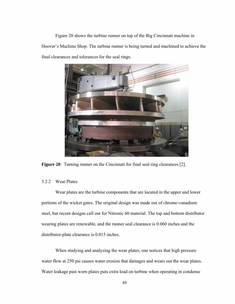
49
Figure 20 shows the turbine runner on top of the Big Cincinnati machine in
Hoover’s Machine Shop. The turbine runner is being turned and machined to achieve the
final clearances and tolerances for the seal rings.
Figure 20: Turning runner on the Cincinnati for final seal ring clearances [2].
3.2.2 Wear Plates
Wear plates are the turbine components that are located in the upper and lower
portions of the wicket gates. The original design was made out of chrome-vanadium
steel, but recent designs call out for Nitronic 60 material. The top and bottom distributor
wearing plates are renewable, and the runner seal clearance is 0.060 inches and the
distributor-plate clearance is 0.015 inches.
When studying and analyzing the wear plates, one notices that high pressure
water flow at 250 psi causes water erosion that damages and wears out the wear plates.
Water leakage past worn plates puts extra load on turbine when operating in condense

50
mode. Furthermore, once the wicket gates are closed the water leakage that passes
through the worn wear plates, wastes the energy in the water. The water leakage past
worn wear plates decreases the efficiency of turbine runner, especially when operating at
partial loads.
Figure 21 demonstrates a corroded section of a wear plate. Sever corrosion affects
the efficiency of the unit tremendously as it is more exposed to water leakage that might
lead to cavitation. Cavitation is the vaporization of fluids due to pressure loss which
forms vapor pockets, and upon collapse, produces vibrations, noise, and destruction of
the surrounding walls [13].
Figure 21: Damaged and Corroded wear plates [2].
Figure 22 is a series of photographs that show the wear plates once they have
been refurbished. If the wear plates are not replaced with new ones, then all the corrosion
is removed and the wear plates are restore to their original condition.
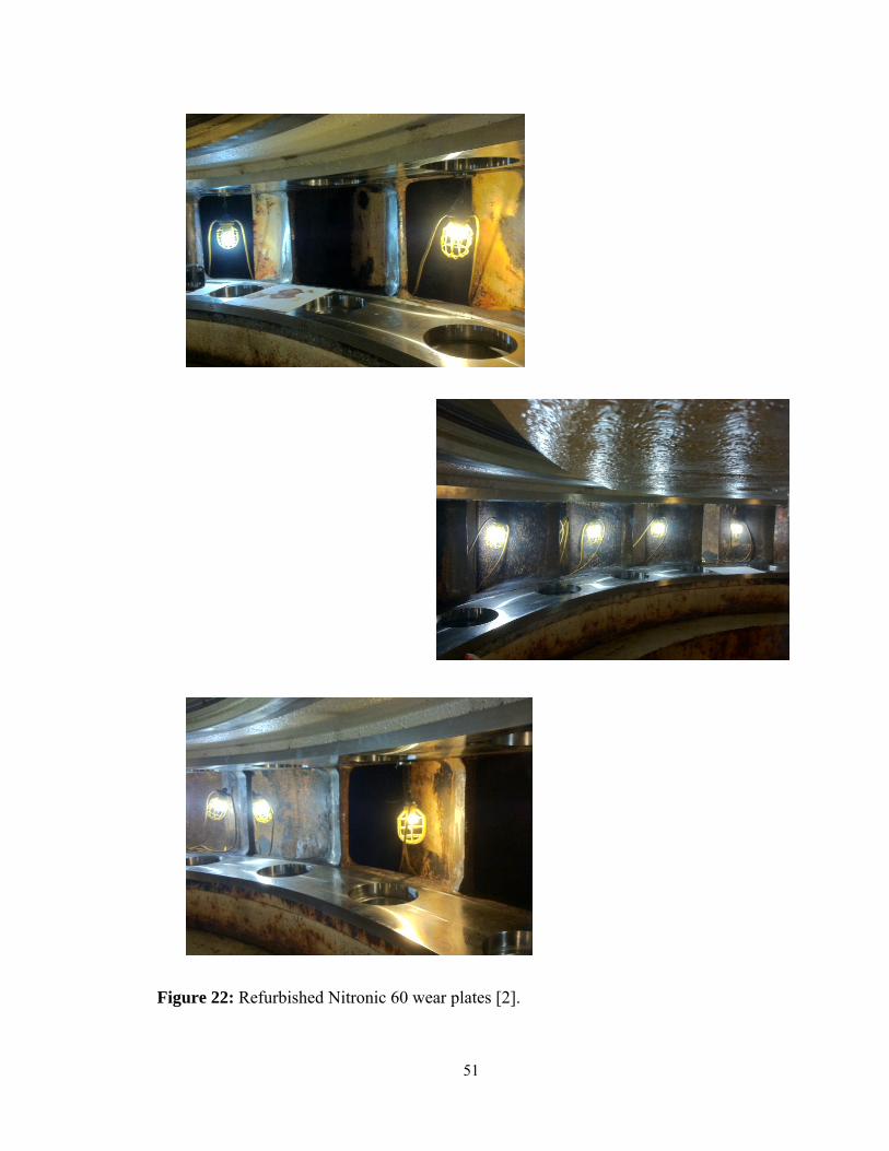
51
Figure 22: Refurbished Nitronic 60 wear plates [2].

52
3.2.3 Wicket Gates (Guide Vanes) Wicket gates control the flow of water from the input pipes, that is water from the
penstock and then into the scroll case to the turbine runner. Wicket gates are also referred
to as paddles or guide vanes. Modifying the existing wicket gate to have a slimmer
profile and tighter clearances reduces the water leakage between them. This was achieve
by analyzing the wicket gate as an airfoil, and taking into account the airfoil’s chord
length, camber, and the angle of attack.
The tighter clearances reduce water leakage, and store more water in the reservoir
for future use whenever the water is not required. Figure 23 shows that when the wicket
gates are pinched shut under normal operating conditions each gate is subject to a system
of forces. These forces cause bending about the horizontal and vertical axes.
Figure 23: Check Stress Analysis for Turbine Flanges and Gates [2].

53
As seen in Figure 23, the gate stem is subjected to torsion and shear as well as
bending about a horizontal axis. Each gate stem is provided with three bronze-bushed
grease-lubricated guide bearings, one located in the lower cover or curb plate and the
other two located in the top cover or crown plate. Additionally, one is located above the
stuffing box and the other one is located below the stuffing box. A shearing pin is
located between each gate stem and the gate shifting rings which is strong enough to
withstand the maximum operating forces that the system will see, but this shear pin will
break or yield and protect the rest of the mechanism from injury in case one or more of
the gates becomes locked. The shear pins are designed to fail under double shear and
have a vee-grooved configuration at the shear plane to reduce bending of the pin. This
facilitates the removal of the broken parts.
The design of the wicket gates itself is such that in case any individual gate
becomes disconnected from the gate-shifting mechanism, no part of the gate can come in
contact with the turbine runner. The mechanism and the connections that control the
wicket gates are mounted on the shift ring located inside the turbine pit.
When one modifies the wicket gate profile to make them squeeze tighter, it
prevents leakage but also it result in a bigger guide vane opening (GVO). This is
achieved by reducing the wicket gate airfoil camber profile. More flow results in more
power. Lately, Hoover’s goal has also been to replace the old cast-steel wicket gates with
new thinner profile wicket gates made out of a stainless steel material. The wicket gates
need a tighter squeeze to conserve energy and reduce water leakage. As Lake Mead goes
down, the plant’s output is reduced. According to a study done by VA Tech Hydro, the

54
new optimized wicket gate profile will increase peak efficiency by 1.00 to 1.25 %,
resulting in a 5 % unit capacity increase.
Figure 24 shows that with an optimal head of 490 ft. to get a 90.25% efficiency
the gates have to be open approximately 0.893” roughly 10% of gate opening, with a
water flow of 1.28 cfs. Additionally, the wicket gate operational opening is limited by
opening and closing time rate factors. The ranges used for this study are: 0%, 10%, 70%,
80%, 90%, and 100% of wicket gate opening.
Figure 24: Hoover Dam Mussel Curve, showing an operating range of 400 ft to 550 ft [2].

55
The standard operating rate of the wicket gates is limited to a 15 second opening
time frame that allows the wicket gates to open from 0% open to 100% open. The 15
second time frame is restricted to a certain interval to prevent vibration and water
hammer to occur in a 130 MWe unit. Water hammer is a pressure surge that results when
a fluid in motion is forced to come to a stop or change fluid flow direction.
VA Tech Hydro did a study for distinctive variations and profiles of a new and
optimized wicket gate design made with a stainless steel material. Figure 25 shows a
sleeker profile, with an asymmetrical shape and a thin trailing edge. The black outline is
the existing profile (d0), while the red outline is the proposed designed assymetrical
slimmer profile (d1). In this profile the parameters that were analyzed were the airfoil
camber and angle of attack.
Overall, in order to achieve the 2 percent average efficiency, the angle of attack
will need to be increased by 2 degrees, and the trailing edge gap by 0.02 inches.
Additionally, the servo motors will have to be stroke 2.5 feet more to achieve the
2 percent increase in efficiency.
Figure 25: New Optimized Wicket Gate – VA Tech Hydro Profile A (Asymmetrical Shape) [11].
d0 d1

56
Figure 26 shows another design similar to Figure 24, however, with a slight
difference in the wicket gate profile. Instead of having an asymmetrical shape the profile
has a symmetrical shape. The black outline is the existing profile (d0), while the green
outline is the proposed designed symmetrical slimmer profile (d2). In this profile the
parameters that were analyzed were the airfoil camber and angle of attack. The
asymmetrical is a little off center from the nose of the wicket gate profile. Studies showed
that a profile with a symmetrical shape is not as efficient as a profile with an
asymmetrical shape. In a symmetrical shape the flow of water tries to bypass a congruent
shape and flow around the wicket gates, thus increasing the possibility of eddy currents
and possible corrosion.
Figure 26: New Optimized Wicket Gate – VA Tech Hydro Profile B (Symmetrical Shape) [11].
Wicket gates act like Venetian blinds that let the sun shine go through a window.
The more one opens the blinds the more sun shine one allows for to enter the room.
Wicket gates are very similar alike in the concept of letting more water flow through. As
seen in the picture below the more the wicket gates are open, the more output power our
generating units can produce. However, in a perfect scenario in order to produce more
power the wicket gates will be 100 % open at all times, to allow for more water flow to
enter the turbine. This concept is hard to follow at Hoover Dam, since Hoover is a special
d0 d2

57
unique plant that generates and regulates power at the same time. Therefore, Hoover’s
power demand varies and fluctuates depending on the time of day and seasonal time of
the year.
Figure 27 shows the water energy coming into the scroll case and into the turbine
runner. The water flow is however control by the twenty-four (24) wicket gates around
the unit which control the flow of water. More water flow into the unit allows for more
power to be generated.
Figure 27: Wicket Gate Function Schematic [2].

58
Figure 28 below clearly demonstrates the importance of tight tolerances on the
turbine runner stationary and rotating seal rings in both the upper and lower portions of
the runner. Furthermore, the precise measurements of the wear plates are extremely
important to prevent excess water leakage through the wicket gate profile. The
photograph also demonstrates how the nose and tail of the wicket gate profile come in
contact with each other once the wicket gates are close. If there is an excessive gap
between the nose and tail of the wicket gate, then energy will be wasted. It is Hoover
Engineering’s goal for the new wicket gate profile to have a tighter squeeze on the gates
once they are closed.
Figure 28: Wicket Gate and Turbine Runner Arrangement [15].

59
A0
A large passage area, also known as the Guide Vane Opening (GVO), allows for
more water flow to pass through the wicket gates. In having a bigger GVO and a thinner
hydraulic profile, the new wicket gate made out of stainless steel will increase the
maximum flow rate to the turbine from 3,400 cfs to 3,600 cfs. The end results are a
capacity increase of 7 MW when the lake levels are below 1,180 ft. of elevation [1].
Figure 29 shows how the water passage area or the GVO (A0) affects the amount
of water flow (cfs) that goes into a unit. More water flow creates more power.
Figure 29: Existing Wicket Gate - 1930’s Mild Steel Castings with Stainless Steel Inlays [15]. Figure 30 reiterates the idea that a larger GVO (A1) creates more water flow
which in turn creates more power. That’s why having a slimmer wicket gate profile it’s
truly beneficial in increasing efficiency and capacity of Hoover Dam.

60
Figure 30: New Wicket Gate – Modern, Thinner Design all Stainless Steel [15].
Figure 31 comparison the old cast steel wicket gate design (d0 and A0) with the
new slimmer profile stainless steel wicket gate design (d1 and A1). Additionally, the GVO
with the new stainless steel wicket gate design increases by 12%.
Note how d0> d1, but A0<A1. As mentioned previously a larger GVO (A1) creates more
water flow which in turn creates more power.
Figure 31: Comparing Existing and New Wicket Gate Profile and Guide Vane Opening [15].
A1
0.02 inch gap increase
2° increase in
angle of attack

61
Another possible solution in increasing power capacity is to over stroke the
wicket gates. Over stroking the wicket gates involves modifying the existing wicket gate
mechanism, by extending the wicket gate servo motor linear travel by about 1 to 4 inches
of travel. This slight modification, involves machining or moving the wicket gate servo
motor stop nuts back further. By doing so, the servomotor arm is allowed to travel up to 4
more inches, allowing the wicket gates to have a bigger GVO when opened and a tighter
squeeze when closed. The modification of over stroking the wicket gates allows a larger
GVO, which allows for a flow rate increase from 2,900 cfs to 3,400 cfs, that is a 500 cfs
flow rate increase.
Figure 32 shows the green wicket gate linkage mechanism that operates the gates
to open and close. The orange rod is part of the servo motor components which
hydraulically operates the gates to open or close.
Figure 32: Wicket Gate Servo Motor Arm and Wicket Gate Mechanism [2].

62
Figure 33 shows the green shift ring and orange rod servo motors. The wicket
gate mechanism is linked to the shift ring in order to be hydraulically operated to open or
close.
Figure 33: Wicket Gate Servo Motor Arm and Shift Ring Mechanism [2].
Figure 34 shows the wicket gate mechanism that is linked to the shift ring, which
is hydraulically operated by the servo motors.
Figure 34: Wicket Gate Linkage Mechanism [2].
Shift Ring

63
In Figure 35, note the wicket gate level arms sticking out of the turbine pit. In this
figure the shift ring and turbine guide bearing have been removed. This figure also shows
the two orange servo motors that hydraulically operate the wicket gates.
Figure 35: Turbine Pit Area, without the Wicket Gate Shift Ring [2].
Other benefits of the new wicket gate profile and modifications, include less
turbine cavitation at the leading edges of the turbine runners, because of the uniform
velocities across the newly design wicket gates. The new wicket gates prevent the wear
plates to experience less damage from leakage in comparison to the old cast-steel wicket
gate design.
Figure 36 shows a typical Hoover Dam turbine runner. This runner is being stayed
in the power house wing, for future modifications and repairs in the runner’s buckets.
Servo Motor
Hydraulic Arm
Vertical Turbine
Shaft
Turbine Pit Area
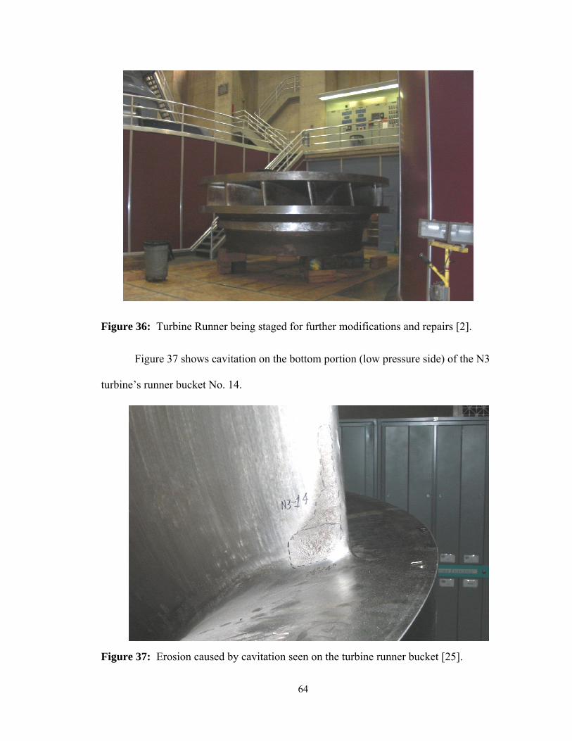
64
Figure 36: Turbine Runner being staged for further modifications and repairs [2].
Figure 37 shows cavitation on the bottom portion (low pressure side) of the N3
turbine’s runner bucket No. 14.
Figure 37: Erosion caused by cavitation seen on the turbine runner bucket [25].

65
Cavitation occurs when the pressure of water flow drops and forms vapor
bubbles. In cavitation the vaporization of fluids due to pressure loss forms vapor pockets,
and upon collapse, produces vibrations, noise, and destruction of the surrounding walls
[13].
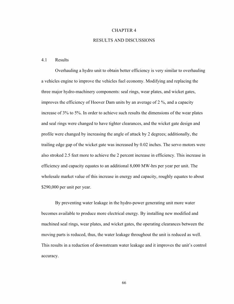
66
CHAPTER 4
RESULTS AND DISCUSSIONS
4.1 Results
Overhauling a hydro unit to obtain better efficiency is very similar to overhauling
a vehicles engine to improve the vehicles fuel economy. Modifying and replacing the
three major hydro-machinery components: seal rings, wear plates, and wicket gates,
improves the efficiency of Hoover Dam units by an average of 2 %, and a capacity
increase of 3% to 5%. In order to achieve such results the dimensions of the wear plates
and seal rings were changed to have tighter clearances, and the wicket gate design and
profile were changed by increasing the angle of attack by 2 degrees; additionally, the
trailing edge gap of the wicket gate was increased by 0.02 inches. The servo motors were
also stroked 2.5 feet more to achieve the 2 percent increase in efficiency. This increase in
efficiency and capacity equates to an additional 8,000 MW-hrs per year per unit. The
wholesale market value of this increase in energy and capacity, roughly equates to about
$290,000 per unit per year.
By preventing water leakage in the hydro-power generating unit more water
becomes available to produce more electrical energy. By installing new modified and
machined seal rings, wear plates, and wicket gates, the operating clearances between the
moving parts is reduced, thus, the water leakage throughout the unit is reduced as well.
This results in a reduction of downstream water leakage and it improves the unit’s control
accuracy.

67
The estimated wholesale market value at Hoover Dam from reducing water
leakage through the wicket gates is approximately $200,000 per unit per year. That is a
total savings of $3,400,000 a year for the 17 power-generating units at Hoover Dam.
Additionally, by preventing water leakage in the hydro-power generating unit
more water becomes available to produce more electrical energy. In installing new
modified and machined seal rings, new wear plates, and new wicket gates, the operating
clearances between the moving parts is reduced, thus, minimizing the water leakage
throughout the unit, and also minimizing energy losses. This results in a reduction of
downstream water leakage and it improves the unit control accuracy. Table 3
demonstrates how the power plant capacity increases by installing new wicket gates for
units that have been previously overhauled.
Table 3: Hoover Power Plant Projected Capacity Increases Achieved [2].
Unit Number
Date Modification Capacity Increase
when Lake Mead is below 1145 (MWe)
A6 July 21, 2010 New Stainless
Steel Wicket Gates 5
N3 May 26, 2011 New Stainless
Steel Wicket Gates 10

68
4.2 MATLAB® Coding
The computer software used was MATLAB® which is developed by MathWorks.
Some coding was programmed in MATLAB®, but some data collection and analysis was
done in Excel. The MATLAB® codes show analysis of hydro-unit variables necessary for
an efficiency study. The exergy process analysis was discussed in Chapter 2.
4.2.1 Baseline Calculations MATLAB® Coding
The baseline parameters were coded in MATLAB® using English units.
To account for the head of water elevation one must first take the difference between the
Forebay (Lake) elevation and the Tailbay (River) elevation.
Eq. (4.1) shows one how to calculate for the total net head, given FEl. = 1125.27 ft
and TEl. = 634.91 ft.
.. ElEl TFH (4.1)
H = net head of water elevation (ft)
FEl. = forebay (lake) elevation (ft)
TEl. = tailbay (river) elevation (ft)
Having obtained the net head of the system, H = 490.36 ft. one can substitute Eq. (4.1)
into Eq. (4.2) to obtain the pressure coming into the system.
Eq. (4.2) demonstrates the conversion from net head into psi.
Hz
307.2
1 (4.2)
H = net head of water elevation (ft); using a value of 490.36 ft. for net head.

69
z = pressure coming into the system (psi); the value obtained is 212.5531 psi.
The following parameters are values obtained from Hoover Dam SCADA software. For
study analysis these values will be kept constant, unless otherwise noted.
Eq. (4.3) denotes the gravity coefficient of the system.
2/2.32 sftg (4.3)
g = gravity constant (ft/s2)
Eq. (4.4) denotes the density of water of the system.
3/4.62
2ftlbOH (4.4)
ρH2O = density of water (lb/ft3)
Eq. (4.5) denotes the temperature of the water of the system.
FT OH60
2 (4.5)
TH2O = temperature of water (°F)
Eq. (4.6) denotes the volumetric flow rate coming in to the system, at the time
when the net head was 490.36 ft.
cfsQin 12042 (4.6)
Qin = volumetric flow rate coming in into the system (cfs)

70
The mass flow rate coming in into the system can be obtained by substituting
Eq. (4.4) and Eq. (4.6) into Eq. (4.7).
inOHin Qm2
(4.7)
mdot_in = mass flow rate coming in into the system (cfs)
ρH2O = density of water (lb/ft3)
Qin = volumetric flow rate coming in into the system (cfs)
Thus, the value obtained for the mass flow rate coming in, mdot_in=751421 lbm/s. The
same procedures were done to obtain the value for the mass flow rate coming out of the
system, with the only exception that Qout was used for the volumetric flow rate. The value
obtained from SCADA for Qout =9341 cfs, meaning that the value for,
mdot_out = 582878 lbm/s, see Eq. (4.9) for procedures.
Eq. (4.8) denotes the volumetric flow rate coming out of the system.
cfsQout 9341 (4.8)
Qout = volumetric flow rate coming out of the system (cfs)
The mass flow rate coming out of the system can be obtained by substituting Eq. (4.4)
and Eq. (4.8) into Eq. (4.9).
outOHout Qm2
(4.9)
mdot_out = mass flow rate coming out of the system (cfs)
ρH2O = density of water (lb/ft3)
Qout = volumetric flow rate coming out of the system (cfs)

71
In order to obtain the mass flow rate for the overall system Eq. (4.9) is subtracted
from Eq. (4.7), see Eq. (4.10) for mathematical procedure.
inoutbaseline mmm
(4.10)
mdot = mass flow rate of the system (cfs)
mdot_out = mass flow rate coming out of the system (cfs)
mdot_in = mass flow rate coming in into the system (cfs)
Thus, the value obtained for the mass flow rate, mdot_baseline = 168542 lbm/s.
4.2.2 Parametric Analysis Calculations MATLAB® Coding
A baseline value of Qbaseline=2701 cfs was used for the baseline calculations, when
there was a net head of 490.36 ft. However, in order to keep the parametric study
constant a volumetric flow rate of Qsystem=3100 cfs will be used in Eq. (4.13) for the
comparison parametric study.
Eq. (4.11) will be used to compare the turbine exergetic efficiency, with the actual
efficiency obtain from an actual unit. The Pproduced was obtained from the exergy study
analysis at H=490.36 ft., Q=3100 cfs, and ηturbine_exergetic_efficiency .
capacity
producedturbine P
P (4.11)
ηturbine = efficiency of turbine unit (%)
Pproduced = overall power produced by unit (MWe)
Pcapacity = capacity of power that a unit can produce, stator max capacity (MWe)
Eq. (4.12) shows the volumetric flow rate of the system that was used in the comparison
analysis for the distinctive power outputs.

72
cfsQsystem 3100 (4.12)
Qsystem = volumetric flow rate of the system (cfs)
Eq. (4.13) shows how to calculate for power in a hydro unit.
e
eOHsystemexergeticturbinesystem kW
MW
hp
kW
lbft
hpHQP
1000
1
1
747.0
sec/550
12_ (4.13)
ηturbine_exergetic = turbine exergetic efficiency (%)
Qsystem = volumetric flow rate of the system (cfs)
H = net head of water elevation (ft)
ρH2O = density of water (lb/ft3)
From Eq. (4.13), Psystem= 124 MW. This power produce is not the maximum
power that the unit is capable of producing, the stator is rated for a 130 MWe max power
output. This power output is lower than 130 MWe due to the low net head and low
volumetric flow rate into the system.
(Please refer to Appendix B (B-1) and (B-2) to reference the MATLAB® Coding)
Solving for the mass balance, energy balance, and exergy balance requires solving
for the unit’s kinetic energy, potential energy, internal energy, and the heat transferred.
Parameters from Table 1, were used to perform some of the required calculations.
Eq. (4.14) demonstrates how to calculate for the kinetic energy of the system.
2
2
1mvKE (4.14)

73
KE = kinetic energy of the system (ft-lb)
m = mass of water (lb) (*62.4 lbs in a cubic feet)
v = velocity of the fluid medium in the system (ft/s)
Eq. (4.15) demonstrates how to calculate for the kinetic energy of the system.
mgHPE (4.15)
PE = potential energy of the system (ft-lb)
m = mass of water (lb) (*62.4 lbs in a cubic feet)
g = gravity constant (ft/s2)
H = net head of water elevation (ft)
The system was taken to be an adiabatic process; therefore, there was no heat
transfer and internal energy is kept constant. Qheat = 0, adiabatic and U = 0, constant
internal energy.
Eq. (4.16) demonstrates how to calculate for the overall energy of the system.
UKEPEE (4.16)
E = overall energy of the system (ft-lb)
PE = overall potential energy of the system (ft-lb)
KE = overall kinetic energy of the system (ft-lb)
U = overall internal energy of the system (ft-lb)
Now, one can calculate for the mass balance, energy balance, and exergy balance
of the system. Eq. (4.17) demonstrates how to find the mass balance in the system.
systemOH Qm2
(4.17)
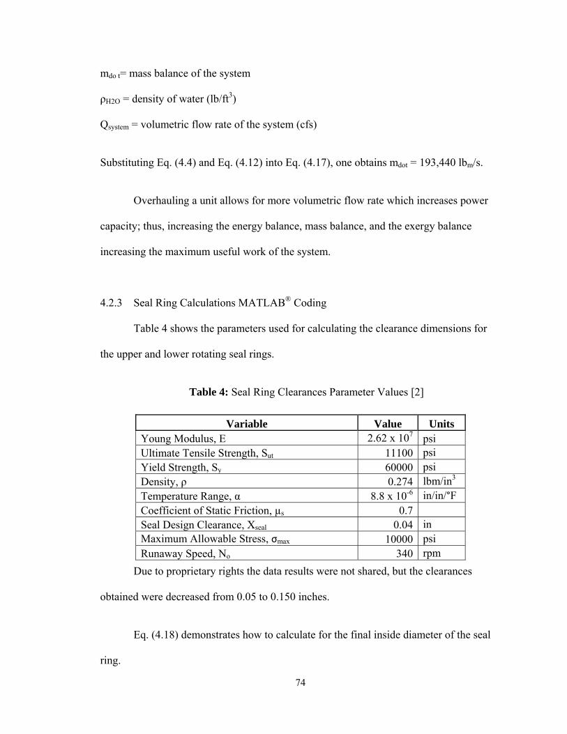
74
mdo t= mass balance of the system
ρH2O = density of water (lb/ft3)
Qsystem = volumetric flow rate of the system (cfs)
Substituting Eq. (4.4) and Eq. (4.12) into Eq. (4.17), one obtains mdot = 193,440 lbm/s.
Overhauling a unit allows for more volumetric flow rate which increases power
capacity; thus, increasing the energy balance, mass balance, and the exergy balance
increasing the maximum useful work of the system.
4.2.3 Seal Ring Calculations MATLAB® Coding
Table 4 shows the parameters used for calculating the clearance dimensions for
the upper and lower rotating seal rings.
Table 4: Seal Ring Clearances Parameter Values [2]
Due to proprietary rights the data results were not shared, but the clearances
obtained were decreased from 0.05 to 0.150 inches.
Eq. (4.18) demonstrates how to calculate for the final inside diameter of the seal
ring.
Variable Value Units Young Modulus, E 2.62 x 10⁷ psi Ultimate Tensile Strength, Sut 11100 psi Yield Strength, Sy 60000 psi Density, ρ 0.274 lbm/in3
Temperature Range, α 8.8 x 10⁻⁶ in/in/°F Coefficient of Static Friction, µs 0.7 Seal Design Clearance, Xseal 0.04 in Maximum Allowable Stress, σmax 10000 psi Runaway Speed, No 340 rpm

75
E
ODngIDofSealRi runnermax1
(4.18)
IDsealring = final inside diameter of rotating seal ring (in)
ODrunner = outside diameter of runner (in)
σmax = maximum allowable stress (psi)
E = Young Modulus (psi)
Eq. (4.19) demonstrates how to calculate for the final inside diameter of the seal
ring tongue.
tonguesealring XIDngTongueIDofSealRi 2 (4.19)
IDsealring_tongue = final inside diameter of rotating seal ring tongue (in)
IDsealring = final inside diameter of rotating seal ring (in)
Xtongue = thickness of rotating seal ring tongue (in)
Eq. (4.20) demonstrates how to calculate for the final outside diameter of the seal
ring.
sealstationary XIDngODofSealRi 2 (4.20)
ODsealring = final outside diameter of rotating seal ring (in)
IDstationary = inside diameter of stationary seal ring (in)
Xseal = rotating seal ring design clearance (in)
Eq. (4.21) demonstrates how to calculate for the inside diameter of the rotating
seal ring at the installation temperature.
ambientoninstallatisealringoninstallati TTIDID 1 (4.21)
IDinstallation = inside diameter of rotating seal ring at installation temperature (in)

76
IDsealring = final inside diameter of rotating seal ring (in)
α = temperature range @ 75 °F to 200 °F (in/in/°F)
Tinstallation = rotating seal ring installation temperature (°F)
Tambient = rotating seal ring ambient temperature (°F)
Eq. (4.22) demonstrates how to calculate for clearances between the inside
diameter of the rotating seal ring to the outer diameter of the turbine at the installation
temperature.
sealringoninstallaticlearances IDIDID (4.22)
IDclearances = inside diameter of rotating seal ring to the outside diameter of runner (in)
IDinstallation = inside diameter of rotating seal ring at installation temperature (in)
IDsealring = final inside diameter of rotating seal ring (in)
Eq. (4.23) demonstrates how to calculate for clearances between the inside
diameter of the rotating seal ring tongue to the outer diameter of the turbine at the
installation temperature.
runnertongueoninstallatitongueclearances ODXIDID 2 (4.23)
IDclearancestongue = inside diameter of rotating seal ring tongue to the outside diameter of runner (in) IDinstallation = inside diameter of rotating seal ring at installation temperature (in)
Xtongue = thickness of rotating seal ring tongue (in)
ODrunner = outside diameter of runner (in)
Eq. (4.24) demonstrates how to calculate for the average diameter of the rotating
seal ring at the cross section installed.

77
sealringrunneravg ODODD (4.24)
Davg = average diameter of rotating seal ring at the cross section installed (in) ODrunner = outside diameter of runner (in)
ODsealring = final outside diameter of rotating seal ring (in)
Eq. (4.25) demonstrates how to calculate for the centrifugal stress at the runaway
speed.
386
60
2
avgo
cf
DN
(4.25)
σcf = centrifugal stress at the runway speed (psi)
ρ = density of material (lbm/in3)
No = runaway speed (rpm)
Davg = average diameter of rotating seal ring at the cross section installed (in)
Eq. (4.26) demonstrates how to calculate for the factor of safety against a seal ring
separation at the runaway speed.
cf
sealringFS max (4.26)
FSsealring = factor of safety against a seal ring separation at the runaway speed σmax = maximum allowable stress (psi)
σcf = centrifugal stress at the runway speed (psi)
(Please refer to Appendix B (B-3) to reference the MATLAB® Coding)

78
4.2.4 Pre-Overhaul and Post-Overhaul Calculations MATLAB® Coding
Data values were obtained from the Hoover Dam SCADA software see Table 5
and Table 6 for results.
(Please refer to Appendix B (B-4) to reference the MATLAB® Coding)
Figure 38 shows a plot of unit capacity with the data normalized at 490.36 ft of
net head. Power (MWe) is plotted on the vertical axis, while the Volumetric Flow Rate
(cfs) is plotted on the horizontal axis. Figure 37 shows that in order for a unit to produce
130 MWe of power there must be a volumetric flow rate of at least 3300 cfs
Figure 38: MATLAB® plot of Unit Capacity - Data Normalized to 490.36 ft. of net head.

79
Figure 39 shows a plot of unit efficiency with the data normalized at 490.36 ft of
net head. Efficiency (%) is plotted on the vertical axis, while the Volumetric Flow Rate
(cfs) is plotted on the horizontal axis. Figure 38 shows that a unit is 78 % efficient when
it produces 130 MWe of power.
Figure 39: MATLAB® plot of Unit Efficiency - Data Normalized to 490.36 ft. of net head. Table 5 demonstrates the values obtained from the SCADA software at Hoover
Dam, prior to the unit overhaul. Certain values were analyzed and will be plotted in
Figures 40 and 41 to compare data results pre-overhaul and post-overhaul. The
parameters analyzed were: the stroke of the servo motors measured out in inches, the
percent of the servo motor in an open position, the volumetric flow rate of water flow

80
through the unit measured out in cfs, the power generated by the unit as a result of the
volumetric flow rate, the elevation of both the Forebay and Tailbay measured out in feet
at the time the data was recorded, the net head parameter equals the difference between
the Forebay elevation and Tailbay elevation, and lastly the units efficiency. Since the
SCADA software records data values in a certain time rate, the data used was recorded
when servo opening percent values were at 10, 70, 80, 90, and 100 percent. Additionally,
the volumetric flow rate values and the efficiency values have been normalized to
account for a net head of 490.36 ft. As mentioned previously, 490.36 ft of net head was
the net head available on November 2011, when the performance tests were analyzed.
Table 5: Stabilized Readings, Prior to Unit Overhaul
Note: (The values recorded represent the data without new seal rings, without new wear
plates and without any new wicket gates)
Servo Stroke Servo Opening Flow Power Forebay El. Tailbay El. Net Head El. Efficiency (inches) (percent) (cfs) (MWe) (ft.) (ft.) (ft.) (percent) 1.25 10 336.68 1.4629 1138.5 643.37 495.12 10.482
8.75 70 2385 85.406 1138.5 643.66 494.83 86.387
10 80 2713.6 99.458 1138.5 644.01 494.48 88.418
11.25 90 3054.4 111.94 1138.5 644.36 494.13 88.41
12.5 98.9 3299.2 119.62 1138.5 645.2 493.28 87.466
Table 6 demonstrates the values obtained from the SCADA software at Hoover
Dam, after the unit overhaul. Certain values were analyzed and were plotted in Figures 40
and 41 to compare results, pre-overhaul and post-overhaul. The parameters analyzed
were: the stroke of the servo motors measured out in inches, the percent of the servo

81
motor in an open position, the volumetric flow rate of water flow through the unit
measured out in cfs, the power generated by the unit as a result of the volumetric flow
rate, the elevation of both the Forebay and Tailbay measured out in feet at the time the
data was recorded, the net head parameter equals the difference between the Forebay
elevation and Tailbay elevation, and lastly the units efficiency. Since the SCADA
software records data values in a certain time rate, the data used was recorded when servo
opening percent values were at 10, 70, 80, 90, and 100 percent. Additionally, the
volumetric flow rate values and the efficiency values were normalized to account for a
net head of 490.36 ft.
Table 6: Stabilized Readings, After Unit Overhaul
Note: (The values recorded represent the data with new seal rings, with new wear plates and with new wicket gates)
Servo Stroke Servo Opening Flow Power Forebay El. Tailbay El. Net Head El. Efficiency (inches) (percent) (cfs) (MWe) (ft.) (ft.) (ft.) (percent) 1.25 10 277.38 1.1926 1126.5 643.37 488.26 10.372
8.75 70 2313.8 82.828 1126.5 643.66 487.71 86.355
10 80 2650.6 97.048 1126.5 644.01 487.41 88.327
11.25 90 2994 110.07 1126.5 644.36 487.23 88.684
12.5 100 3330.2 121.12 1126.5 645.2 487.01 87.738
Figure 40 shows the pre-overhaul and post-overhaul results. Figure 39 compares
the overall unit capacity data. Pre-Overhaul data is in blue and Post-Overhaul data is in
red. The Volumetric Flow Rate (cfs) of the unit is plotted in the x-axis and the amount of

82
Power (MWe) generated by the unit is plotted in the y-axis. In Figure 39 one can see that
at a flow of 3000 cfs, after a unit’s overhaul the capacity increases by around 4 MWe
Figure 40: MATLAB® plot of Unit Capacity – Pre-Overhaul vs. Post-Overhaul Data.
Figure 41 compares the overall unit efficiency data. Pre-Overhaul data is in blue
and Post-Overhaul data is in red. The Power (MWe) generated by the unit is plotted in the
x-axis and the unit recorded Efficiency (%) is recorded in the y-axis. In Figure 40 one can
see that at 80 MWe of power produced by the unit, after a unit’s overhaul the efficiency
increases by around 2%.
104

83
Figure 41: MATLAB® plot of Unit Efficiency – Pre-Overhaul vs. Post-Overhaul Data.
4.3 Discussion
Water is a vital resource to everyone, especially if you live out in the desert. It is
extremely important to use the water efficient. At Hoover Dam, one of the main goals is
to reduce water leakage in order to prevent energy from getting wasted. Capacity
improvements at Hoover Dam are focused on allowing an increase in the maximum
amount of water allowed to flow into the turbines at lower net heads.
As discussed in this study there are various mechanical components as well as
electrical components that can be modified or alternated to improve capacity efficiency,
88

84
however, the three major components that this study focuses on are the seal rings, wear
plates, and wicket gates. As water levels keep on dropping in the Colorado River, future
research and analysis can be allocated in a new turbine runner design for low head
operation ranges. Additionally, there are a few other mechanical and electrical
components that can be modified or alternated to monitor and improve capacity
efficiency.
The benefits from the increased capacity provide payback of project investments
within a few years. Using a conservative wholesale market price for capacity, the value
of 70 MWe of new capacity added at Hoover Dam is an increase of approximately $2.2
million per year in capital.
To reference back turbine overhauls include work such as modifying and
replacing seal rings and wear plates to reduce high-pressure leakage of water through the
wicket gate system which occurs when the hydro units are shut down. Preventing the
leakage of water, results in more water available in the future to produce valuable
electrical energy. The wholesale market value from reducing leakage through wicket
gates at Hoover is approximately $200,000 per unit per year.

85
CHAPTER 5
CONCLUSION
5.1 Findings
Modifying and replacing the three major hydro-machinery components: seal
rings, wear plates, and wicket gates, improves the efficiency of Hoover Dam units by an
average of 2 percent. This increases a unit’s capacity by 3 percent to about 5 percent. The
increase in capacity equates to an additional 8,000 MW-hrs per year per unit. The
wholesale market value of this increase in energy and capacity, roughly equates to about
$290,000 per unit per year.
Engineering design, calculations, and performance test were utilized to improve
the parameters of the seal rings, wear plates, and wicket gates. MATLAB® and MS Excel
computer software was used to analyze numerical analytically results and data plots.
The goal to minimize clearances, in order to prevent water leakage, create a
proper seal on the seal rings which do not let excess water flow through, thus, conserving
more water and wasting less energy. Furthermore, the new wicket gates design increases
the efficiency of the turbine unit due to their laminar profile and proper seal. By
increasing the angle of attack by 2 degrees, and increasing the trailing edge gap by 0.02
inches, as well as stroking the servo motor arms 2.5 feet further the 2 percent increase in
unit efficiency was achieved.

86
5.2 Suggestions
The seal rings, wear plates, and wicket gates were the three major hydro-
components analyzed in this thesis. Future system analysis should examine modifications
and new design of low-head turbine runners. As water levels keep on dropping in the
Colorado River, future research and analysis can be allocated in a new turbine runner
design for low head operation ranges. Additionally, there are a few other mechanical and
electrical components that can be modified or alternated to monitor and improve capacity
efficiency.
It is strongly recommended to continue with the overhaul procedures at Hoover
Dam. After all, it is a great investment that will pay back by itself, and it will maintain
the generating units running properly and stable for many more years of hydro power to
be produced.

87
EXHIBITS
Exhibit 1: Figures
Exhibit E-1 shows a cut section of a typical Hoover generator unit. It shows all
the different powerhouse elevations with all the major components. Exhibit E-1 shows
that the generating unit is approximately 100 ft. tall.
E-1: Cross-Section of a typical Hoover Dam Generator Unit [25].

88
APPENDICES
Appendix A: Glossary (Principles of Hydro-Electric Power)
A-1: Utility Definitions Base Load The minimum load over a given period of time. Capability "The maximum load which a machine, apparatus, station,
or system can carry under specified conditions for a given time interval.
Capacity The load from which a machine, apparatus, station, or system is rated.
Demand The load at the terminals of an installation or system averaged over a specified interval of time. Demand is expressed in kilowatts, kilovolt amperes or other suitable units.
Energy That which does or is capable of doing work. It is measured
in terms of the work it is capable of doing; electric energy is usually measured in kilowatt-hours.
Load Factor The ratio of the average load over a designated period to
the peak load occurring in that period. Off-Peak Energy Electric energy supplied during periods of relatively
low system demands as specified by the supplier. On-Peak Energy Electric energy supplied during periods of relatively
high system demands as specified by the supplier. Peaking Capacity Generating capacity available to assist in meeting that
portion of peak load which is above base load.

89
Plant Factor The ratio of the average load on the plant for the period of
time considered to the aggregate rating of all the generating equipment installed in the plant.
Rating Limits placed on operating conditions of a machine
apparatus, or device based on its design characteristics. Such limits as load, voltage and frequency may be given in the rating.
SCADA Supervisory Control and Data Acquisition (SCADA) is an industrial control computer system that monitors infrastructure, or facility-based processes.
Spinning Reserve That reserve generating capacity connected to the bus and
ready to take load. Station Service Auxiliary and other facilities for station use in a generating,
switching, converting, or transforming station. Variable Costs Costs associated with operation or utilization of plant. A-2: Electrical Definitions Ampere (Amp) The basic unit of current or electron flow. Base Load The minimum load over a given period of time. Battery A group of several cells connected together as a unit
for furnishing electric current. Boost Raise or attempt to raise voltage.

90
Bus A bus conductor, or group of conductors, is a switchgear assembly which serves as a common connection for three or more circuits. NOTE: The conductors of a bus are usually in the form of a bar.
Collector Rings Metal rings suitably mounted on the rotating member of an
electric machine, serving through stationary brushes bearing thereon, to conduct current into or out of the rotating member.
Current Transformer A small transformer for measuring heavy currents
in power leads. The primary is in series with the power lead and full rated current in the primary gives 5 amps in the secondary. (Never open the secondary circuit of a current transformer when the primary is energized.)
Efficiency The ratio of output to input power, generally expressed
as a percentage. Electric Generator A machine which transforms mechanical power
into electrical power. Electric Motor A machine which transforms electric energy into
mechanical energy. Exciter An auxiliary DC generator which supplies energy for the
field excitation of another electric machine.
Frequency (F) The number of complete cycles per second existing in any
form of wave motion; such as the number of cycles per second of an alternating current. See Hertz.
Generating Station A plant wherein electric energy is produced from some
form of energy (e.g. chemical, mechanical, or hydraulic) by means of suitable apparatus.

91
Generator A machine that converts mechanical energy into electrical energy.
Ground Bus A bus used to connect a number of grounding conductors
to one or more grounding electrodes. Ground Current Any current flowing in the earth. Grounding Switch A form of air switch by means of which a circuit or a piece
of apparatus may be connected to ground. Hertz Replaces cycle as the basic unit of frequency. High Voltage Above 600 volts. Hot Energized electrically referring to pieces of electrical
equipment, buses or lines. House Turbine A turbine installed to provide a source of auxiliary power. Kilowatt Hour (kW-hr) A unit of energy equal to 1000 watthours. Lag The amount one wave is behind another in time; expressed
in electrical degrees. Lead The opposite of lag. Also, a wire or connection. Load The impedance to which energy is being supplied. Megawatt (MW) One million watts. Pole One of the ends of a magnet where most of its magnetism
is concentrated.

92
Power The rate of doing work or the rate of expending energy.
The unit of electrical power is the watt. Rotor The rotating member of a machine. Solenoid An electric conductor wound as a helix with a small pitch,
or as two or more coaxial helices. Spinning Reserve That reserve generating capacity connected to the
system and ready to take load. Static A fixed nonvarying condition; without motion. Static Electricity A stationary charge of electricity. Stator The part of a machine which contains the stationary parts of
the magnetic circuit with their associated windings. Transformer An electric device which by electromagnetic induction
transforms electric energy from one or more circuits to one or more other circuits at the same frequency, usually with changed values of voltage and current.
Trip An accessory or the act of divorcing a piece of equipment
from its source of energy. Var Reactive volt-amperes. Volt The unit of electromotive force. Watt A unit of electric power produced by a current of one
ampere at one volt.
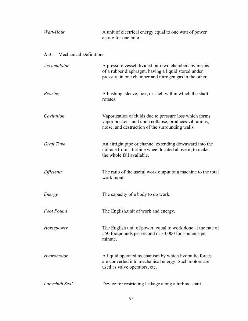
93
Watt-Hour A unit of electrical energy equal to one watt of power acting for one hour.
A-3: Mechanical Definitions Accumulator A pressure vessel divided into two chambers by means
of a rubber diaphragm, having a liquid stored under pressure in one chamber and nitrogen gas in the other.
Bearing A bushing, sleeve, box, or shell within which the shaft
rotates. Cavitation Vaporization of fluids due to pressure loss which forms
vapor pockets, and upon collapse, produces vibrations, noise, and destruction of the surrounding walls.
Draft Tube An airtight pipe or channel extending downward into the
tailrace from a turbine wheel located above it, to make the whole fall available.
Efficiency The ratio of the useful work output of a machine to the total
work input. Energy The capacity of a body to do work. Foot Pound The English.unit of work and energy. Horsepower The English unit of power, equal to work done at the rate of
550 footpounds per second or 33,000 foot-pounds per minute.
Hydromotor A liquid operated mechanism by which hydraulic forces
are converted into mechanical energy. Such motors are used as valve operators, etc.
Labyrinth Seal Device for restricting leakage along a turbine shaft.

94
Lantern Ring An open metal ring between rings of packing in a stuffing
box used to admit a sealing or lubricating fluid. Power The amount of work done in a given interval of time. Rotor The rotating member of a machine. Servomotor A mechanism controlled by governor oil to operate inlet
valves on a turbine. Stop Log One of a set of timber pieces, usually square, which serve
to form a dam to check the flow of water. Trip An accessory or the act of divorcing a piece of equipment
from its source of energy. Venturi A primary device used for establishing, pressure
differentials used in the measurement of flow through pipes.

95
Appendix B: MATLAB® Coding
B-1: Baseline Calculation MATLAB® Coding %% Variables for Baseline Calculations % Pressure River_Elevation=634.91; %Elevation of Mohave River (ft). As of 11/28/11 % OPS Daily Operating Report Lake_Elevation=1125.27; %Elevation of Lake Mead in (ft). As of 11/28/11 % OPS Daily Operating Report Head=Lake_Elevation-River_Elevation; %Head of Water Elevation (ft). % Head=490.3600 (ft). z=(1/2.307)*Head; %Pressure coming into the system (psi) % Note:(1/2.307) is conversion factor % from ft. to psi. % z=212.5531 (psi) % Gravity Constant gravity_EE=32.2; %(ft/s^2) % Water Parameters H20_density=62.4; %Density of Water (lb/ft^3) H20_temperature=60; %Temperature of water (deg. F) H20_mass=62.4; %Pounds in a cubic feet. H20_volume=1; %Volume is accounted for a ft^3. % Mass flow-in and Volumetric Flow Rate-in H20_volumetricflowrate_in=12042; %Hoover Dam Water Intake (cfs). % OPS Daily Operating Report. % Based on 5.4 Million gpm. % Multiply 5.4 Million gpm by 0.00223 % to get cfs. mdot_in=H20_density*H20_volumetricflowrate_in; %(lb/s) % Mass flow-out and Volumetric Flow Rate-in H20_volumetricflowrate_out=9341; %Hoover Dam Water Release (cfs). As of % 11/28/11, OPS Daily Operating Report mdot_out=H20_density*H20_volumetricflowrate_out; %(lb/s) % Change in Mass flow rate and Change in Volumetric Flow Rate mdot=mdot_in-mdot_out; %(lb/s) H20_volumetricflowrate_cfs=H20_volumetricflowrate_in-H20_volumetricflowrate_out; %(cfs)

96
% Unit Conversion Factors hp_ftlbsec=550; % Horsepower in (ft.-lbf)/sec) hp_kW=0.7457; % Horsepower in (kW) kW=0.001; % Megawatts (MW) MW=1000; % kilowatts (kW) % Hydro-Power Calculation % Power: MW = efficiency[(Q,cfs)*(Head, ft)*(H20 density,lbf/ft^2) % *(((1 hp)/(550 ft-lb/sec))*(((0.7457 kW)/(1 hp))) % *(((1 MW)/(1000 kW))) Power_Produced=124*MW; Power_Capacity=130*MW; efficiency=(Power_Produced)/(Power_Capacity) % efficiency=0.9538; Power_MW=(efficiency)*(H20_volumetricflowrate_in*Head*H20_density*(1/hp_ftlbsec)*(hp_kW)*(kW)); % Unit Capacity: Power(MW) vs. Flow (cfs)[Per unit] % z=212.5531 psi cfs_perunit=[100:25:3350]; Power_MW_perunit=[0:1:130]; cfstoMW=H20_volumetricflowrate_in*H20_density*Head*(1/hp_ftlbsec)*(hp_kW)*(kW); % Unit Efficiency: Efficiency (%) vs. Flow (cfs)[Per unit] % z=212.5531 psi cfstoMW_plot=cfs_perunit*(H20_volumetricflowrate_in*Head*H20_density*(1/hp_ftlbsec)*(hp_kW)*(kW))*(1/1000000); efficiency_plot=(Power_MW_perunit./cfstoMW_plot); %% Plots % Plot of Unit Capacity (Data Normalized to 490.3600 ft. Net Head) figure (1) plot(cfs_perunit,Power_MW_perunit); grid title('Unit Capacity: Data Normalized to 490.3600 ft. Net Head') xlabel('Volumetric Flow Rate (cfs)'); ylabel('Power (MWe)'); % Plot of Unit Efficiency (Data Normalized to 490.3600 ft. Net Head) figure (2) plot(Power_MW_perunit,efficiency_plot); grid title('Unit Efficiency: Data Normalized to 490.3600 ft. Net Head') xlabel('Power (MWe)'); ylabel('Efficiency(%)');

97
%% Balance Equations Variables % Gravity Constant g_EE=gravity_EE; %32.2 (ft/s^2) % Water Temperature T=H20_temperature; %T=60 deg. F % Kinetic Energy (ft-lb) KE_ftlb=(1/2)*H20_mass*velocity^2; %(ft-lb), Mass is accounted for a % ft^3 which is 62.4 lbs. % KE=455.5531 (ft-lb) % Potential Energy (ft-lb) PE_ftlb=H20_mass*gravity_EE*Head; %PE_ftlb=9.8527e+005 % Heat Transfer on System Q=0; %Adiabatic process, no heat transfer % Mass Balance, mdot(in)=mdot(out) mdot=mdot_in-mdot_out; %(lb/s) % mdot=1.6854e+005 %(lb/s) % Energy Balance, (d=DELTA) dKE+dPE+dU=Q-W (English) W_ftlb=KE_ftlb+PE_ftlb+U_ftlb; %(ft-lb) % W_ftlb=1.9715e+006 %(ft-lb) B-2: Exergy and Parametric Study MATLAB® Coding clear all clc format bank %% Baseline Power_MW_max=130; W_dotMW_max=Power_MW_max; %MW kW1=1000;% 1000 kW in 1 MW W_dotBTUsec=(W_dotMW_max*kW1)*(3413/1)*(1/3600) %BTU/sec W_dot=W_dotBTUsec; Q=3100; %cfs ro=62.4; %lb/ft^3 m_dot=ro*Q %lbm/s ft2s2_btusec=4e-5; %BTU/s g=32.2; %ft/s^2 To=60; % deg. F To_R=To+460; % deg. R lbmsec_btusec=(m_dot)*(1/32.714)*(1/1.285e-3)*g; %BTU/s d1=30; %30 ft pipe section at control volume inlet d2=12; %12 ft pipe section at control volume outlet A1=(pi*d1^2)/4; %Area of state 1 A2=(pi*d2^2)/4; %Area of state 2 V1=Q/A1; %ft/s V2=Q/A2; %ft/s

98
z1=1125.27; %ft z2=634.91; z=z1-z2; %ft hp_ftlbsec=550; % Horsepower in [(ft.-lbf)/(sec)] hp_kW=0.7457; % Horsepower in (kW) kW=0.001; % Megawatts (MW) MW=1000; % kilowatts (kW) %% Data Calculation % Solving for exergy destruction STATE 1 to STATE 3 % Ed_dot=W_dot-((m_dot)*((0.5*(V1^2-V2^2)*(1/25026.84158))-((m_dot*4e-5)*g*(z1-z3)*(1/25026.84158)))) Ed_dot=W_dot-(m_dot*(((((V1^2-V2^2)/(2))*ft2s2_btusec))+(((g)*(z))*ft2s2_btusec))) % (Btu/sec) % Solving for system irreversibilities sigma_cv=(Ed_dot/To_R) % (Btu/sec-deg. R) % Solving for exergetic turbine efficiency turbine_exergetic_efficiency=(((W_dot)/(m_dot))/(((W_dot)/(m_dot))+((Ed_dot)/(m_dot))))*100 % Solving for energy coming in to the system energyin=m_dot*(((((V1^2-V2^2)/(2))*ft2s2_btusec))+(((g)*(z))*ft2s2_btusec)) % Solving for power produced Power_MW_produced=(turbine_exergetic_efficiency/100)*(Q*z*ro*(1/hp_ftlbsec)*(hp_kW)*(kW)); W_dotMW_produced=Power_MW_produced; % Solving for unit efficiency taken into account max capacity and power produced unit_efficiency=((W_dotMW_produced)/(W_dotMW_max))*100; %% Post-Overhaul table=[Q,m_dot,V1,V2,z1,z2,z,turbine_exergetic_efficiency,Power_MW_produced,Power_MW_max,unit_efficiency]; %% Table disp(' Table 5: Exergy Analysis Parametric Study Results') fprintf('\n') fprintf('\n') disp('Volumetric Flow Rate Mass Flow Rate Velocity S1 Velocity S2 Forebay El. Tailbay El. Net Head El. Exergetic Efficiency Power Produced Power Max Capacity Unit Efficiency')

99
disp(' (cfs) (lbm/s) (ft/s) (ft/s) (ft.) (ft.) (ft.) (percent) (MWe) (MWe) (percent)') fprintf('\n') fprintf(' %4.2f %8.2f %4.2f %4.2f %4.2f %4.2f %3.2f %3.2f %2.3f %2.2f %2.2f %2.3f',table) fprintf('\n\n') B-3: Seal Ring Calculation MATLAB® Coding
%% UNIT CALCULATION FOR UPPER AND LOWER ROTATING SEAL RINGS %% UNIT CALCULATION GENERAL DATA VALUES E=2.62e+007; % Young's Modulus (psi) S_ut=111000; % Ultimate Tensile Strength (psi) S_y=60000; % Yield Strength (psi) rho=0.2754; % Density (lbm/in^3) alpha=8.80e-006; % Temperature Range @ 75 to 200 deg. F (in/in/deg. F) mu_s=0.7; % Co-efficient of Static friction (in/in/deg.F) X_seal=0.04; % Seal design clearance - Radial (in.) sigma_max=10000; % Maximum Allowable Stress (psi) N_o=340; % Runaway Speed (rpm) %% UNIT VARIABLES FOR UPPER ROTATING SEAL RING %Data OD_runner_upper=; % Outside Diameter of Runner (in) OD_runnertongue_upper=; % Outside Diameter of Runner Tongue % Grove (in) ID_stationary_upper=; % Inside Diameter of Stationary Ring (in) X_tongue_upper=; % Thickness of Seal Ring Tongue H_upper=; % Height of Seal Ring (in) T_ambient_upper=; % Ambient Ring Temperature in Machine Shop (deg. F) T_operation_upper=; % Average Ring Temperature in Operation (deg. F) T_installation_upper=; % Ring Temperature for Installation (deg. F

100
%Find % Inside Diameter of Ring (in) ID_final_upper=(OD_runner_upper).*((1-((sigma_max)./(E)))); % Inside Diamter of Ring Tongue (in) ID_tongue_upper=(ID_final_upper)-2*(X_tongue_upper); % Outside Diameter of Ring (in) OD_final_upper=(ID_stationary_upper)-2*X_seal; % Inside Diameter of Ring @ Installation Temperature (in) ID_installation_upper=(ID_final_upper)*(1+alpha*(T_installation_upper-T_ambient_upper)); % Clearance between the inside Diameter of RIng to the OD of Turbine @ Installation % Temperature Delta_ID_upper=ID_installation_upper-ID_final_upper; % Clearance between Inside Diameter of Ring Tongue to the OD of Turbine @ % Installation Temperature Clearance_ID_upper=(ID_installation_upper)-(2*X_tongue_upper)-OD_runner_upper; % Average Diameter of Ring Cross Section Installed (in) D_c_upper=(OD_runner_upper+OD_final_upper)/2; % Centrifugal Stress at the Runaway Speed (psi) sigma_cf_upper=(rho*((N_o*pi*D_c_upper)/60)^2)/386; % Factor of Safety Against Ring Seperation at the Runway Speed FS_cf_upper=(sigma_max/sigma_cf_upper); %% UNIT VARIABLES FOR LOWER ROTATING SEAL RING %Data OD_runner_lower=; % Outside Diameter of Runner (in) OD_runnertongue_lower=; % Outside Diameter of Runner Tongue % Grove (in) ID_stationary_lower=; % Inside Diameter of Stationary Ring % (in) X_tongue_lower=; % Thickness of Seal Ring Tongue H_lower=; % Height of Seal Ring (in) T_ambient_lower=; % Ambient Ring Temperature in Machine Shop (deg. F) T_operation_lower=; % Average Ring Temperature in Operation (deg. F) T_installation_lower=; % Ring Temperature for Installation (deg. F)

101
%Find % Inside Diameter of Ring (in) ID_final_lower=(OD_runner_lower).*((1-((sigma_max)./(E)))); % Inside Diamter of Ring Tongue (in) ID_tongue_lower=(ID_final_lower)-2*(X_tongue_lower); % Outside Diameter of Ring (in) OD_final_lower=(ID_stationary_lower)-2*X_seal; % Inside Diameter of Ring @ Installation Temperature (in) ID_installation_lower=(ID_final_lower)*(1+alpha*(T_installation_lower-T_ambient_lower)); % Clearance between the inside Diameter of RIng to the OD of Turbine @ Installation % Temperature Delta_ID_lower=ID_installation_lower-ID_final_lower % Clearance between Inside Diameter of Ring Tongue to the OD of Turbine @ % Installation Temperature Clearance_ID_lower=(ID_installation_lower)-(2*X_tongue_lower)-OD_runner_lower % Average Diameter of Ring Cross Section Installed (in) D_c_lower=(OD_runner_lower+OD_final_lower)/2 % Centrifugal Stress at the Runaway Speed (psi) sigma_cf_lower=(rho*((N_o*pi*D_c_lower)/60)^2)/386 % Factor of Safety Against Ring Seperation at the Runway Speed FS_cf_lower=(sigma_max/sigma_cf_lower)

102
B-4: Pre-Overhaul and Post-Overhaul Calculation MATLAB® Coding
%% DATA %% Pre-Overhaul Data Pre_Servo_Stroke=[1.25, 8.75, 10, 11.25, 12.5]; % Servo Stroke of wicket gates measured in inches. Pre_Servo_Percent_Open=[10, 70, 80, 90, 98.9]; % Percent of opening of Servo Stroke. Pre_CFS=[338.31, 2396.54, 2726.75, 3069.15, 3315.20]; % Recorded amount of Flow during testing analysis. Pre_MW=[1.47, 85.82, 99.94, 112.48, 120.20]; % Recorded amount of Power during testing analysis. Pre_Forebay=[1138.49, 1138.49, 1138.49, 1138.49, 1138.48]; % Recorded Forebay (lake) elevation during testing analysis. Pre_Tailbay=[643.37, 643.66, 644.01, 644.36, 645.20]; % Recorded Tailbay (river) elevation during testing analysis. Pre_NetHead=Pre_Forebay-Pre_Tailbay; % Recorded Net Head (lake-river) during testing analysis. Pre_NormalizedHead=490.36; % Data was taken prior to a Net Head elevation of 490.36 ft. therefore, % the data has been normalized. Pre_CFS_Normalized_Matrix=((Pre_CFS'))*sqrt(((490.36)/(Pre_NetHead'))); % Data for CFS was normalized and factored in to correct values. Pre_CFS_Normalized_Vector=Pre_CFS_Normalized_Matrix(:,1)'; % Zeroes were deleted from CFS matrix and left only with % desired values. Pre_MW_Normalized_Matrix=((Pre_MW'))*sqrt(((Pre_NormalizedHead)/(Pre_NetHead'))); % Data for MW was normalized and factored in to correct values. Pre_MW_Normalized_Vector=Pre_MW_Normalized_Matrix(:,1)'; % Zeroes were deleted from MW matrix and left only with % desired values. Pre_Efficiency_Factor_Matrix_11=(1/(0.00000135582.*Pre_CFS_Normalized_Vector(1,1)*62.35*Pre_NormalizedHead)); % Data for Efficiency was normalized and factored in to correct values. Pre_Overall_Efficiency_11=Pre_Efficiency_Factor_Matrix_11*Pre_MW_Normalized_Vector(1,1); % Efficiency of element (1,1) from Efficiency Matrix was evaluated.

103
Pre_Efficiency_Factor_Matrix_12=(1/(0.00000135582.*Pre_CFS_Normalized_Vector(1,2)*62.35*Pre_NormalizedHead)); % Data for Efficiency was normalized and factored in to correct values. Pre_Overall_Efficiency_12=Pre_Efficiency_Factor_Matrix_12*Pre_MW_Normalized_Vector(1,2); % Efficiency of element (1,2) from Efficiency Matrix was evaluated. Pre_Efficiency_Factor_Matrix_13=(1/(0.00000135582.*Pre_CFS_Normalized_Vector(1,3)*62.35*Pre_NormalizedHead)); % Data for Efficiency was normalized and factored in to correct values. Pre_Overall_Efficiency_13=Pre_Efficiency_Factor_Matrix_13*Pre_MW_Normalized_Vector(1,3); % Efficiency of element (1,3) from Efficiency Matrix was evaluated. Pre_Efficiency_Factor_Matrix_14=(1/(0.00000135582.*Pre_CFS_Normalized_Vector(1,4)*62.35*Pre_NormalizedHead)); % Data for Efficiency was normalized and factored in to correct values. Pre_Overall_Efficiency_14=Pre_Efficiency_Factor_Matrix_14*Pre_MW_Normalized_Vector(1,4); % Efficiency of element (1,4) from Efficiency Matrix was evaluated. Pre_Efficiency_Factor_Matrix_15=(1/(0.00000135582.*Pre_CFS_Normalized_Vector(1,5)*62.35*Pre_NormalizedHead)); % Data for Efficiency was normalized and factored in to correct values. Pre_Overall_Efficiency_15=Pre_Efficiency_Factor_Matrix_15*Pre_MW_Normalized_Vector(1,5); % Efficiency of element (1,5) from Efficiency Matrix was evaluated. Pre_Overall_Efficiency_Vector=[Pre_Overall_Efficiency_11, Pre_Overall_Efficiency_12, Pre_Overall_Efficiency_13, Pre_Overall_Efficiency_14, Pre_Overall_Efficiency_15]; % All the evaluated Efficiency values were put into a vector for % simplcity. Pre_Overall_Efficiency_Percent=100*Pre_Overall_Efficiency_Vector; % Efficiency is converted into percent.

104
%% Post-Overhaul Data Post_Servo_Stroke=[1.25, 8.75, 10, 11.25, 12.5]; % Servo Stroke of wicket gates measured in inches. Post_Servo_Percent_Open=[10, 70, 80, 90, 100]; % Percent of opening of Servo Stroke. Post_CFS=[276.79, 2308.89, 2644.88, 2987.60, 3323.10]; % Recorded amount of Flow during testing analysis. Post_MW=[1.19, 82.65, 96.84, 109.83, 120.86]; % Recorded amount of Power during testing analysis. Post_Forebay=[1126.48, 1126.48, 1126.46, 1126.47, 1126.47]; % Recorded Forebay (lake) elevation during testing analysis. Post_Tailbay=[638.22, 638.77, 639.05, 639.24, 639.46]; % Recorded Tailbay (river) elevation during testing analysis. Post_NetHead=Post_Forebay-Post_Tailbay; % Recorded Net Head (lake-river) during testing analysis. Post_NormalizedHead=490.36; % Data was taken prior to a Net Head elevation of 490.36 ft. therefore, % the data has been normalized. Post_CFS_Normalized_Matrix=((Post_CFS'))*sqrt(((490.36)/(Post_NetHead'))); % Data for CFS was normalized and factored in to correct values. Post_CFS_Normalized_Vector=Post_CFS_Normalized_Matrix(:,1)'; % Zeroes were deleted from CFS matrix and left only with % desired values. Post_MW_Normalized_Matrix=((Post_MW'))*sqrt(((Post_NormalizedHead)/(Post_NetHead'))); % Data for MW was normalized and factored in to correct values. Post_MW_Normalized_Vector=Post_MW_Normalized_Matrix(:,1)'; % Zeroes were deleted from MW matrix and left only with % desired values. Post_Efficiency_Factor_Matrix_11=(1/(0.00000135582.*Post_CFS_Normalized_Vector(1,1)*62.35*Post_NormalizedHead)); % Data for Efficiency was normalized and factored in to correct values. Post_Overall_Efficiency_11=Post_Efficiency_Factor_Matrix_11*Post_MW_Normalized_Vector(1,1); % Efficiency of element (1,1) from Efficiency Matrix was evaluated. Post_Efficiency_Factor_Matrix_12=(1/(0.00000135582.*Post_CFS_Normalized_Vector(1,2)*62.35*Post_NormalizedHead)); % Data for Efficiency was normalized and factored in to correct values.

105
Post_Overall_Efficiency_12=Post_Efficiency_Factor_Matrix_12*Post_MW_Normalized_Vector(1,2); % Efficiency of element (1,2) from Efficiency Matrix was evaluated. Post_Efficiency_Factor_Matrix_13=(1/(0.00000135582.*Post_CFS_Normalized_Vector(1,3)*62.35*Post_NormalizedHead)); % Data for Efficiency was normalized and factored in to correct values. Post_Overall_Efficiency_13=Post_Efficiency_Factor_Matrix_13*Post_MW_Normalized_Vector(1,3); % Efficiency of element (1,3) from Efficiency Matrix was evaluated. Post_Efficiency_Factor_Matrix_14=(1/(0.00000135582.*Post_CFS_Normalized_Vector(1,4)*62.35*Post_NormalizedHead)); % Data for Efficiency was normalized and factored in to correct values. Post_Overall_Efficiency_14=Post_Efficiency_Factor_Matrix_14*Post_MW_Normalized_Vector(1,4); % Efficiency of element (1,4) from Efficiency Matrix was evaluated. Post_Efficiency_Factor_Matrix_15=(1/(0.00000135582.*Post_CFS_Normalized_Vector(1,5)*62.35*Post_NormalizedHead)); % Data for Efficiency was normalized and factored in to correct values. Post_Overall_Efficiency_15=Post_Efficiency_Factor_Matrix_15*Post_MW_Normalized_Vector(1,5); % Efficiency of element (1,5) from Efficiency Matrix was evaluated. Post_Overall_Efficiency_Vector=[Post_Overall_Efficiency_11, Post_Overall_Efficiency_12, Post_Overall_Efficiency_13, Post_Overall_Efficiency_14, Post_Overall_Efficiency_15]; % All the evaluated Efficiency values were put into a vector for %simplcity. Post_Overall_Efficiency_Percent=100*Post_Overall_Efficiency_Vector; % Efficiency is converted into percent.

106
%% TABLES %% Pre-Overhaul Table disp('Table 3: Stabilized Readings, Prior to Unit Overhaul') disp(' Note: (The values recorded represent the data without new seal rings, without new wear plates') disp(' and without any new wicket gates)') fprintf('\n') disp('Servo Stroke Servo Opening Flow Power Forebay El. Tailbay El. Net Head El. Efficiency') disp(' (inches) (percent) (cfs) (MWe) (ft.) (ft.) (ft.) (percent)') fprintf('\n') tablePre=[Pre_Servo_Stroke; Pre_Servo_Percent_Open; Pre_CFS_Normalized_Vector; Pre_MW_Normalized_Vector; Pre_Forebay; Pre_Tailbay; Pre_NetHead; Pre_Overall_Efficiency_Percent]; disp(tablePre') %% Post-Overhaul Table disp('Table 4: Stabilized Readings, After Unit Overhaul') disp(' Note: (The values recorded represent the data with new seal rings, with new wear plates') disp(' and with any new wicket gates)') fprintf('\n') disp('Servo Stroke Servo Opening Flow Power Forebay El. Tailbay El. Net Head El. Efficiency') disp(' (inches) (percent) (cfs) (MWe) (ft.) (ft.) (ft.) (percent)') fprintf('\n') tablePost=[Post_Servo_Stroke; Post_Servo_Percent_Open; Post_CFS_Normalized_Vector; Post_MW_Normalized_Vector; Post_Forebay; Pre_Tailbay; Post_NetHead; Post_Overall_Efficiency_Percent]; disp(tablePost')

107
%% DATA FOR PLOTS (PRE-OVERHAUL vs. POST-OVERHAUL) prex_capacity=[293.5543869, 563.994155, 824.9794444, 1078.877906, 1342.327087, 1604.030412, 1870.696168, 2142.474334, 2431.724913, 2556.818498, 2670.594957, 2850.743578, 3037.321823]; prey_capacity=[0.5, 9.865, 20.0025, 29.884375, 40.08875, 50.396875, 59.755625, 70.19625, 80.13687375, 84.87749938, 89.59999938, 95.28249813, 101.159375]; postx_capacity=[272, 517, 777, 1043, 1291, 1558, 2090, 2362, 2483, 2636, 2767, 2912, 3074, 3341]; posty_capacity=[0.54, 9.66, 20.07, 30.26, 40.32, 50.41, 69.84, 79.85, 85.5, 90.41, 95.52, 100.24, 105.16, 112.6]; prex_efficiency=[9.865, 20.0025, 29.884375, 40.08875, 50.396875, 59.755625, 70.19625, 80.13687375, 84.87749938, 89.59999938, 95.28249813, 101.159375]; prey_efficiency=[46.68262709, 64.71496054, 73.95545156, 79.77233298, 83.9555221, 85.39943515, 87.64979257, 88.19142979, 88.87155098, 89.79701207, 89.40520469, 89.03212675]; postx_efficiency=[0.54, 9.66, 20.07, 30.26, 40.32, 50.41, 69.84, 79.85, 85.5, 90.41, 95.52, 100.24, 105.16, 112.60]; posty_efficiency=[5.263913101, 49.52164837, 68.44893436, 76.8699843, 82.72744976, 85.68740759, 88.49840352, 89.51676923, 91.12266174, 90.82384784, 91.35899871, 91.14437454, 90.5626378, 89.20243704]; %% PLOTS (PRE-OVERHAUL vs. POST-OVERHAUL) % Unit Capacity: Pre-Overhaul vs. Post-Overhaul Plot figure (3) plot(prex_capacity,prey_capacity,'-b',postx_capacity,posty_capacity,'-r'); grid legend('Pre-Overhaul','Post-Overhaul',0) title('Unit Capacity') xlabel('Volumetric Flow Rate (cfs)'); ylabel('Power (MWe)'); axis(0,3500,0,130) % Unit Efficiency: Pre-Overhaul vs. Post-Overhaul Plot figure (4) plot(prex_efficiency,prey_efficiency,'-b',postx_efficiency,posty_efficiency,'-r'); grid legend('Pre-Overhaul','Post-Overhaul',0) title('Unit Efficiency') xlabel('Power (MWe)'); ylabel('Efficiency (%)');

108
REFERENCES
1. William M. Bruninga, P.E. "EQUIPMENT: Turbine Improvements at Hoover Dam." HydroReview. Web.
<http://www.hydroworld.com/hrhrw/en-us/index/article-tools-template.articles.hydro-review.volume-28.issue-6.feautured-articles.cover-story.equipment_-turbine.htmlhtml>.
2. Hoover Dam Engineering Group
3. "Renewable Energy: Hydropower." ESA21 Environmental Science Activities for
the 21st Century.
4. Rowley, William D. The Bureau of Reclamation: Origins and Growth to 1945, Volume 1. Washington, D.C.: Government Printing Office, 2006. Print.
5. "Hydropower." Center for Climate and Energy Solutions. Web. <http://www.c2es.org/print/technology/factsheet/hydropower>.
6. National Renewable Energy Laboratory. "Setting a Course for Our Energy Future." Hydropower. U.S. Department of Energy: Energy Efficiency and Renewable Energy, July 2004.
7. "Hydroelectric Power." - Wikid Energy Funhouse. Web. 17 Mar. 2012. <http://wiki.uiowa.edu/display/greenergy/Hydroelectric Power>.
8. U.S. Department of the Interior. "Hydroelectric Power." Ed. Bureau of Reclamation - Power Resources Office. July 2005. Print.
9. U.S. Department of the Interior. "The Lower Colorado Region an Overview." (2009): 1-31. Print.
10. US Army Corps of Engineers. "Stay Vane and Wicket Gate Relationship Study."
Http://www1.eere.energy.gov/water/pdfs/doewater-wicket_gate_stay_vane_mods.pdf.
Web

109
11. VA Tech Hydro
12. Moran, Michael J., and Howard N. Shapiro. Fundamentals of Engineering Thermodynamics. Hoboken, NJ: Wiley, 2008. Print.
13. Lower Colorado Dams Project Division of River Operations Technical Support Branch. Principles of Hydro Electric Power. USBR. Print.
14. Winter, Ireal A. Turbines for Boulder Dam. Mechanical Features of the Largest Hydraulic Turbines in the World. Denver, Colorado: U.S. Bureau of Reclamation, 1934. Print.
15. William M. Bruninga, P.E. “Install New Stainless Steel Wicket Gates at Hoover Dam”. PowerPoint presentation. Spring 2010
16. "Bureau of Reclamation: Lower Colorado Region - Colorado River FAQs." Bureau of Reclamation Homepage. Web. <http://www.usbr.gov/lc/hooverdam/faqs/riverfaq.html>.
17. "Bureau of Reclamation: Lower Colorado Region - Hoover Dam Tunnel FAQs." Bureau of Reclamation Homepage. Web. <http://www.usbr.gov/lc/hooverdam/faqs/tunlfaqs.html>.
18. "Bureau of Reclamation: Lower Colorado Region - Hoover Dam FAQs." Bureau of Reclamation Homepage. Web. <http://www.usbr.gov/lc/hooverdam/faqs/damfaqs.html>.
19. "Bureau of Reclamation: Lower Colorado Region - Hoover Dam Power FAQs." Bureau of Reclamation Homepage. Web. <http://www.usbr.gov/lc/hooverdam/faqs/powerfaqs.html>.
20. "Boulder Dam Power." Print. Rpt. in A Pictorial History Electrical West. Print.
21. Life Extension of Hydro Turbines Provides 120 MW Capacity Increase. Rep. Print.

110
22. Patrick A. March, Charles W. Almquist, and Paul J. Wolff. "Best Practice" Guidelines for Hydro Performance Processes. Tech. Print.
23. Daniel A. Pellouchoud, P.E. Hoover Dam Improves Renewable Hydro Capacity and Efficiency. Rep. Print..
24. Jom E. O'Connor, Lisa L. Elly, Ellen E. Wohl, Lawrence E. Stevens, Theodore S. Melis, Vishwas S. Kale, and Victor R. Baker. "A 4500-Year Record of Large Flood on the Colorado River in the Grand Canyon, Arizona." Print.
25. Qian Zhong-dong, Yang Jian-dong, Huai Wen-xin. "Numerical Simulation and Analysis of Pressure Pulsation in Francis Hydraulic Turbine with Air Admission." ScienceDirect Journal of Hydrodynamics (2007). Web.
26. Pardeep Kumar, R.P. Saini. "Study of Cavitation in Hydro Turbines - A Review." Renewable and Sustainable Energy Reviews (2009). Web.

111
VITA
Graduate College
University of Nevada, Las Vegas
Jonathan G. Sanchez
Degree:
Bachelor of Science, Mechanical Engineering, 2010
University of Nevada, Las Vegas
Thesis Title:
Improving Efficiency and Capacity of Hydro-Turbines in the Western United States, Hoover Dam
Thesis Examination Committee:
Chairperson, Dr. Yitung Chen, Ph.D.
Committee Member, Dr. Robert Boehm, Ph.D.
Committee Member, Dr. Hui Zhao, Ph.D.
Graduate Faculty Representative, Dr. Yahia Baghzouz, Ph.D.
Related Documents