High-Throughput Legume Seed Phenotyping Using a ... - MDPI

Page 1

�����������������

Citation: Huang, X.; Zheng, S.; Zhu,

N. High-Throughput Legume Seed

Phenotyping Using a Handheld 3D

Laser Scanner. Remote Sens. 2022, 14,

431. https://doi.org/10.3390/

rs14020431

Academic Editors: Lorenzo Comba,

Jordi Llorens and Alessandro Biglia

Received: 20 December 2021

Accepted: 14 January 2022

Published: 17 January 2022

Publisher’s Note: MDPI stays neutral

with regard to jurisdictional claims in

published maps and institutional affil-

iations.

Copyright: © 2022 by the authors.

Licensee MDPI, Basel, Switzerland.

This article is an open access article

distributed under the terms and

conditions of the Creative Commons

Attribution (CC BY) license (https://

creativecommons.org/licenses/by/

4.0/).

remote sensing

Article

High-Throughput Legume Seed Phenotyping Using aHandheld 3D Laser ScannerXia Huang 1 , Shunyi Zheng 1,* and Ningning Zhu 2

1 School of Remote Sensing and Information Engineering, Wuhan University, Wuhan 430079, China;[email protected]

2 State Key Laboratory of Information Engineering in Surveying, Mapping and Remote Sensing,Wuhan University, Wuhan 430079, China; [email protected]

* Correspondence: [email protected]

Abstract: High-throughput phenotyping involves many samples and diverse trait types. For thegoal of automatic measurement and batch data processing, a novel method for high-throughputlegume seed phenotyping is proposed. A pipeline of automatic data acquisition and processing,including point cloud acquisition, single-seed extraction, pose normalization, three-dimensional (3D)reconstruction, and trait estimation, is proposed. First, a handheld laser scanner is used to obtain thelegume seed point clouds in batches. Second, a combined segmentation method using the RANSACmethod, the Euclidean segmentation method, and the dimensionality of the features is proposedto conduct single-seed extraction. Third, a coordinate rotation method based on PCA and the tablenormal is proposed to conduct pose normalization. Fourth, a fast symmetry-based 3D reconstructionmethod is built to reconstruct a 3D model of the single seed, and the Poisson surface reconstructionmethod is used for surface reconstruction. Finally, 34 traits, including 11 morphological traits, 11 scalefactors, and 12 shape factors, are automatically calculated. A total of 2500 samples of five kindsof legume seeds are measured. Experimental results show that the average accuracies of scanningand segmentation are 99.52% and 100%, respectively. The overall average reconstruction error is0.014 mm. The average morphological trait measurement accuracy is submillimeter, and the averagerelative percentage error is within 3%. The proposed method provides a feasible method of batchdata acquisition and processing, which will facilitate the automation in high-throughput legume seedphenotyping.

Keywords: high-throughput; automatic measurement; batch data processing; handheld laser scanner;3D reconstruction

1. Introduction

Legumes, such as soybeans, peas, black beans, red beans, and mung beans, haveconsiderable economic importance and value worldwide [1,2]. The volume, surface area,length, width, thickness, cross-sectional perimeter and area, scale factor, and shape factorof legume seeds are important in the research for legume seed quality evaluation [3,4],optimization breeding [5], and yield evaluation [6]. The consuming and costly conventionalmanual measurement method using vernier calipers can only measure the length, width,and thickness of the legume seeds. Automatic measurement has great significance inagricultural research [7–9]. High-throughput phenotyping is changing traditional plantmeasurement [10]. High-throughput legume seed phenotyping involves a wide varietyof trait types and massive measurement samples, which require automatic and batch-based data acquisition and processing [11]. For this reason, it is necessary to explore ahigh-throughput phenotyping method to automatically measure legume seeds.

Digital imaging technology is widely used in legume seed trait measurement andhas shown utility in high-throughput phenotyping [12]. The length, width, and projected

Remote Sens. 2022, 14, 431. https://doi.org/10.3390/rs14020431 https://www.mdpi.com/journal/remotesensing

Page 2

Remote Sens. 2022, 14, 431 2 of 21

perimeter and area can be acquired using 2D orthophotos [13–15]. ImageJ [16], CellPro-filer [17], WinSEEDLE [18], SmartGrain [19], and P-TRAP [20] are open-source programsthat can quickly estimate 2D traits of the seeds based on digital imaging technology. How-ever, it is difficult for digital imaging technology to obtain 3D traits, such as volume, surfacearea, and thickness.

Vision technology and 3D reconstruction technology are applied in various engineer-ing fields. Chen et al. [21] studied the 3D perception of orchard banana central stockenhanced by adaptive multivision technology. Lin et al. [22] detected the spherical orcylindrical fruits on plants in natural environments and guided harvesting robots to pickthem automatically using a color-, depth- and shape-based 3D fruit detection method.Measurement using three-dimensional (3D) technology is an active area of research inagriculture [23]. It can be applied in measurements of leaf area, leaf angle, stem and shoots,fruit, and seeds [24,25]. In addition to conventional 2D traits, such as length, width, and theprojected perimeter and area, 3D technology can obtain additional traits, such as volume,surface area, thickness, and other shape traits. Structure from motion (SFM) is a good wayto get a plant 3D point cloud [26]. The impact of camera viewing angles for estimatingagricultural parameters from 3D point clouds has been discussed in detail [27,28]. Wenet al. [29] took between 30 minutes to 1 hour to capture the point cloud of a single seedusing a SmartSCAN3D-5.0M color 3D scanner together with an S-030 camera. The processproduced a detailed 3D model of a single corn seed. Roussel et al. [30] reconstructed a3D seed shape from silhouettes and calculated the seed volume. Li et al. [31] used com-bined data from four viewpoints to obtain a complete 3D point cloud of a single rice seed.Length, width, thickness, and volume were automatically extracted. In the aforementionedresearch, it took a long time to get the 3D data of a single seed. Due to the large samplesizes involved in high-throughput phenotyping analysis, it is necessary to explore fasterand more automated batch data processing methods.

It is difficult to obtain complete point cloud data when scanning seeds in batches [32].Therefore, the current goal for high-throughput phenotyping of legume seeds using 3Dtechnology is the batch-based rapid 3D reconstruction of legume seeds with large samples.The key algorithm in batch data processing in seed measurement based on point clouds isthe point cloud completion approach. In addition to the existing 3D traits, it is meaningful toextract additional 3D traits and shape factors, especially traits of transverse and longitudinalprofiles that are hardly discussed in previous works in this area.

Soybeans, peas, black beans, red beans, and mung beans are typical legume seeds,which are important foods around the world. High-throughput legume seed phenotypingis very valuable and can facilitate easier evaluation of legume seed yield and quality.Legume seeds come in a variety of shapes and sizes. The common ones are approximatelyspherical or ellipsoidal [33]. Examples of spherical legume seeds are soybeans and peas [34].Examples of ellipsoidal legume seeds are black beans, red beans, and mung beans [35].Spherical or elliptical seeds are symmetrical, a property that can be taken advantage of forrapid batch 3D modeling.

In our previous work measuring the kernel traits of grains, the traits were measuredon an incomplete point cloud [36]. The point cloud completion problem was ignored. Theautomatic cloud completion problem will be handled in this work. A novel method forhigh-throughput legume seed phenotyping using a handheld 3D laser scanner is proposedin this paper. The objective of this method is to achieve automatic measurement and batchdata processing. A single 3D seed model and 34 traits will be obtained automatically. Ahandheld laser scanner (RigelScan Elite) will be used to obtain incomplete point clouds oflegume seeds in batches. An automatic data processing pipeline of single-seed extraction,pose normalization, 3D reconstruction, and trait estimation is proposed. A complete 3Dmodel of a single seed based on the incomplete point cloud of legume seeds obtained inbatches can be quickly acquired. A total of 34 traits can be automatically measured. Themain contribution of this paper is to propose an automatic batch measurement method

Page 3

Remote Sens. 2022, 14, 431 3 of 21

for high-throughput legume seed phenotyping. The proposed method is for seeds withsymmetrical shapes.

2. Materials and Methods

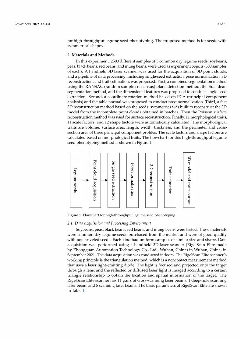
In this experiment, 2500 different samples of 5 common dry legume seeds, soybeans,peas, black beans, red beans, and mung beans, were used as experiment objects (500 samplesof each). A handheld 3D laser scanner was used for the acquisition of 3D point clouds,and a pipeline of data processing, including single-seed extraction, pose normalization, 3Dreconstruction, and trait estimation, was proposed. First, a combined segmentation methodusing the RANSAC (random sample consensus) plane detection method, the Euclideansegmentation method, and the dimensional features was proposed to conduct single-seedextraction. Second, a coordinate rotation method based on PCA (principal componentanalysis) and the table normal was proposed to conduct pose normalization. Third, a fast3D reconstruction method based on the seeds’ symmetries was built to reconstruct the 3Dmodel from the incomplete point clouds obtained in batches. Then the Poisson surfacereconstruction method was used for surface reconstruction. Finally, 11 morphological traits,11 scale factors, and 12 shape factors were automatically calculated. The morphologicaltraits are volume, surface area, length, width, thickness, and the perimeter and cross-section area of three principal component profiles. The scale factors and shape factors arecalculated based on morphological traits. The flowchart for this high-throughput legumeseed phenotyping method is shown in Figure 1.

Remote Sens. 2022, 14, x FOR PEER REVIEW 3 of 22

method for high-throughput legume seed phenotyping. The proposed method is for seeds

with symmetrical shapes.

2. Materials and Methods

In this experiment, 2500 different samples of 5 common dry legume seeds, soybeans,

peas, black beans, red beans, and mung beans, were used as experiment objects (500 sam-

ples of each). A handheld 3D laser scanner was used for the acquisition of 3D point clouds,

and a pipeline of data processing, including single-seed extraction, pose normalization,

3D reconstruction, and trait estimation, was proposed. First, a combined segmentation

method using the RANSAC (random sample consensus) plane detection method, the Eu-

clidean segmentation method, and the dimensional features was proposed to conduct sin-

gle-seed extraction. Second, a coordinate rotation method based on PCA (principal com-

ponent analysis) and the table normal was proposed to conduct pose normalization.

Third, a fast 3D reconstruction method based on the seeds’ symmetries was built to recon-

struct the 3D model from the incomplete point clouds obtained in batches. Then the Pois-

son surface reconstruction method was used for surface reconstruction. Finally, 11 mor-

phological traits, 11 scale factors, and 12 shape factors were automatically calculated. The

morphological traits are volume, surface area, length, width, thickness, and the perimeter

and cross-section area of three principal component profiles. The scale factors and shape

factors are calculated based on morphological traits. The flowchart for this high-through-

put legume seed phenotyping method is shown in Figure 1.

Figure 1. Flowchart for high-throughput legume seed phenotyping.

2.1. Data Acquisition and Processing Environment

Soybeans, peas, black beans, red beans, and mung beans were tested. These materials

were common dry legume seeds purchased from the market and were of good quality

without shriveled seeds. Each kind had uniform samples of similar size and shape. Data

acquisition was performed using a handheld 3D laser scanner (RigelScan Elite made by

Zhongguan Automation Technology Co., Ltd., Wuhan, China) in Wuhan, China, in Sep-

tember 2021. The data acquisition was conducted indoors. The RigelScan Elite scanner’s

working principle is the triangulation method, which is a noncontact measurement

method that uses a laser light-emitting diode. The light is focused and projected onto the

target through a lens, and the reflected or diffused laser light is imaged according to a

certain triangle relationship to obtain the location and spatial information of the target.

The RigelScan Elite scanner has 11 pairs of cross-scanning laser beams, 1 deep-hole scan-

ning laser beam, and 5 scanning laser beams. The basic parameters of RigelScan Elite are

shown in Table 1.

Each kind of legume seed was sorted into batches, and all the seeds in a batch were

scanned at once. There were no overlapped, pasted, and attached seeds. The seeds were

on the table and scanned using RigelScan Elite (Figure 2a). Some reflective marker points

for point cloud stitching between multiple frames were pasted on the table to assist in the

Leg

um

e seeds

Po

int clo

ud

acqu

isition

Sin

gle seed

extractio

n

Po

se no

rmalizatio

n

3D reco

nstru

ction

Trait estim

ation

3D m

od

el and

traits ou

tpu

t

Figure 1. Flowchart for high-throughput legume seed phenotyping.

2.1. Data Acquisition and Processing Environment

Soybeans, peas, black beans, red beans, and mung beans were tested. These materialswere common dry legume seeds purchased from the market and were of good qualitywithout shriveled seeds. Each kind had uniform samples of similar size and shape. Dataacquisition was performed using a handheld 3D laser scanner (RigelScan Elite madeby Zhongguan Automation Technology Co., Ltd., Wuhan, China) in Wuhan, China, inSeptember 2021. The data acquisition was conducted indoors. The RigelScan Elite scanner’sworking principle is the triangulation method, which is a noncontact measurement methodthat uses a laser light-emitting diode. The light is focused and projected onto the targetthrough a lens, and the reflected or diffused laser light is imaged according to a certaintriangle relationship to obtain the location and spatial information of the target. TheRigelScan Elite scanner has 11 pairs of cross-scanning laser beams, 1 deep-hole scanninglaser beam, and 5 scanning laser beams. The basic parameters of RigelScan Elite are shownin Table 1.

Page 4

Remote Sens. 2022, 14, 431 4 of 21

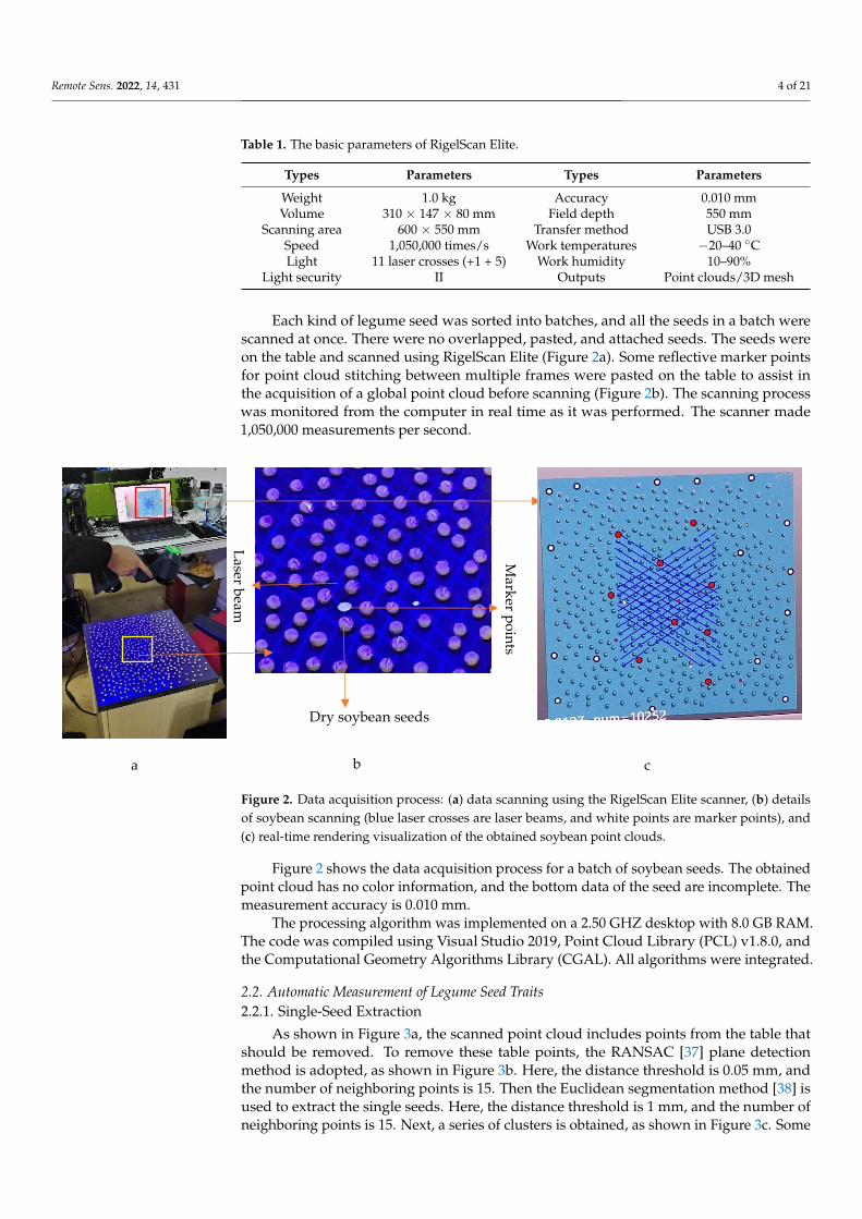
Table 1. The basic parameters of RigelScan Elite.

Types Parameters Types Parameters

Weight 1.0 kg Accuracy 0.010 mmVolume 310 × 147 × 80 mm Field depth 550 mm

Scanning area 600 × 550 mm Transfer method USB 3.0Speed 1,050,000 times/s Work temperatures −20–40 ◦CLight 11 laser crosses (+1 + 5) Work humidity 10–90%

Light security II Outputs Point clouds/3D mesh

Each kind of legume seed was sorted into batches, and all the seeds in a batch werescanned at once. There were no overlapped, pasted, and attached seeds. The seeds wereon the table and scanned using RigelScan Elite (Figure 2a). Some reflective marker pointsfor point cloud stitching between multiple frames were pasted on the table to assist inthe acquisition of a global point cloud before scanning (Figure 2b). The scanning processwas monitored from the computer in real time as it was performed. The scanner made1,050,000 measurements per second.

Remote Sens. 2022, 14, x FOR PEER REVIEW 4 of 24

acquisition of a global point cloud before scanning (Figure 2b). The scanning process was

monitored from the computer in real time as it was performed. The scanner made

1,050,000 measurements per second.

Figure 2 shows the data acquisition process for a batch of soybean seeds. The ob-

tained point cloud has no color information, and the bottom data of the seed are incom-

plete. The measurement accuracy is 0.010 mm.

Table 1. The basic parameters of RigelScan Elite.

Types Parameters Types Parameters

Weight 1.0 kg Accuracy 0.010 mm

Volume 310 × 147 × 80 mm Field depth 550 mm

Scanning area 600 × 550 mm Transfer method USB 3.0

Speed 1,050,000 times/s Work temperatures −20–40 °C

Light 11 laser crosses (+1 +

5) Work humidity 10–90%

Light security ΙΙ Outputs Point clouds/3D mesh

a b c

Laser b

eam

Mark

er po

ints

Dry soybean seeds

a b c

Laser b

eam

Mark

er po

ints

Dry soybean seeds

Figure 2. Data acquisition process: (a) data scanning using the RigelScan Elite scanner, (b) detailsof soybean scanning (blue laser crosses are laser beams, and white points are marker points), and(c) real-time rendering visualization of the obtained soybean point clouds.

Figure 2 shows the data acquisition process for a batch of soybean seeds. The obtainedpoint cloud has no color information, and the bottom data of the seed are incomplete. Themeasurement accuracy is 0.010 mm.

The processing algorithm was implemented on a 2.50 GHZ desktop with 8.0 GB RAM.The code was compiled using Visual Studio 2019, Point Cloud Library (PCL) v1.8.0, andthe Computational Geometry Algorithms Library (CGAL). All algorithms were integrated.

2.2. Automatic Measurement of Legume Seed Traits2.2.1. Single-Seed Extraction

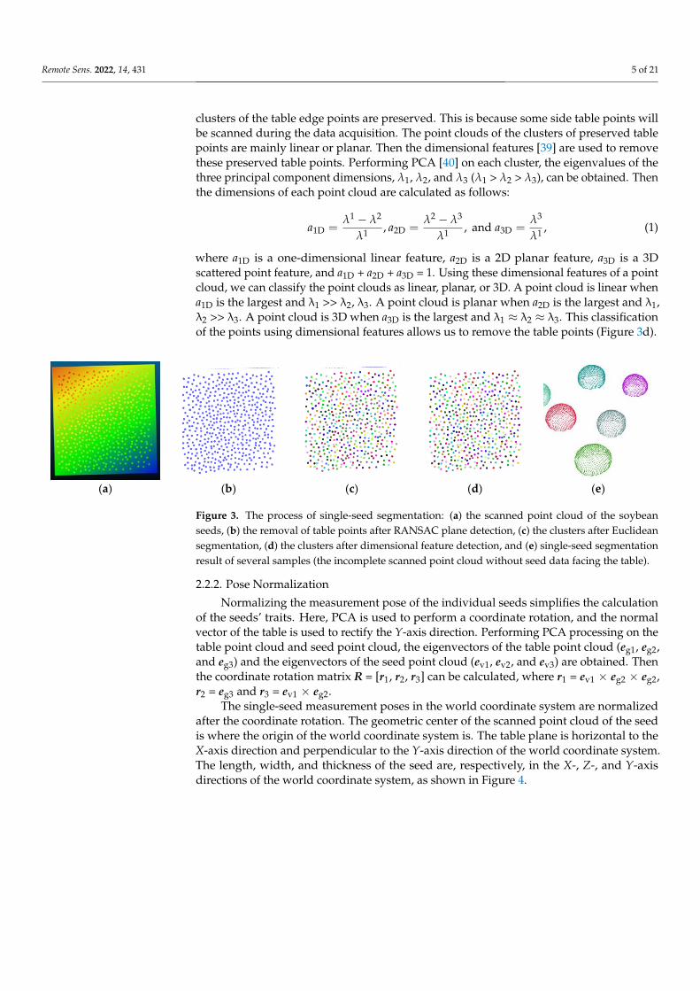
As shown in Figure 3a, the scanned point cloud includes points from the table thatshould be removed. To remove these table points, the RANSAC [37] plane detectionmethod is adopted, as shown in Figure 3b. Here, the distance threshold is 0.05 mm, andthe number of neighboring points is 15. Then the Euclidean segmentation method [38] isused to extract the single seeds. Here, the distance threshold is 1 mm, and the number ofneighboring points is 15. Next, a series of clusters is obtained, as shown in Figure 3c. Some

Page 5

Remote Sens. 2022, 14, 431 5 of 21

clusters of the table edge points are preserved. This is because some side table points willbe scanned during the data acquisition. The point clouds of the clusters of preserved tablepoints are mainly linear or planar. Then the dimensional features [39] are used to removethese preserved table points. Performing PCA [40] on each cluster, the eigenvalues of thethree principal component dimensions, λ1, λ2, and λ3 (λ1 > λ2 > λ3), can be obtained. Thenthe dimensions of each point cloud are calculated as follows:

a1D =λ1 − λ2

λ1 , a2D =λ2 − λ3

λ1 , and a3D =λ3

λ1 , (1)

where a1D is a one-dimensional linear feature, a2D is a 2D planar feature, a3D is a 3Dscattered point feature, and a1D + a2D + a3D = 1. Using these dimensional features of a pointcloud, we can classify the point clouds as linear, planar, or 3D. A point cloud is linear whena1D is the largest and λ1 >> λ2, λ3. A point cloud is planar when a2D is the largest and λ1,λ2 >> λ3. A point cloud is 3D when a3D is the largest and λ1 ≈ λ2 ≈ λ3. This classificationof the points using dimensional features allows us to remove the table points (Figure 3d).

Remote Sens. 2022, 14, x FOR PEER REVIEW 5 of 22

be scanned during the data acquisition. The point clouds of the clusters of preserved table

points are mainly linear or planar. Then the dimensional features [39] are used to remove

these preserved table points. Performing PCA [40] on each cluster, the eigenvalues of the

three principal component dimensions, λ1, λ2, and λ3 (λ1 > λ2 > λ3), can be obtained. Then

the dimensions of each point cloud are calculated as follows:

1 21D

1

a

−= , 2 3

2D

1

a

−= , and 3

3D

1

a

= , (1)

where a1D is a one-dimensional linear feature, a2D is a 2D planar feature, a3D is a 3D scat-

tered point feature, and a1D + a2D + a3D = 1. Using these dimensional features of a point

cloud, we can classify the point clouds as linear, planar, or 3D. A point cloud is linear

when a1D is the largest and λ1 >> λ2, λ3. A point cloud is planar when a2D is the largest and

λ1, λ2 >> λ3. A point cloud is 3D when a3D is the largest and λ1 ≈ λ2 ≈ λ3. This classification

of the points using dimensional features allows us to remove the table points (Figure 3d).

(a) (b) (c) (d) (e)

Figure 3. The process of single-seed segmentation: (a) the scanned point cloud of the soybean seeds,

(b) the removal of table points after RANSAC plane detection, (c) the clusters after Euclidean seg-

mentation, (d) the clusters after dimensional feature detection, and (e) single-seed segmentation re-

sult of several samples (the incomplete scanned point cloud without seed data facing the table).

2.2.2. Pose Normalization

Normalizing the measurement pose of the individual seeds simplifies the calculation

of the seeds’ traits. Here, PCA is used to perform a coordinate rotation, and the normal

vector of the table is used to rectify the Y-axis direction. Performing PCA processing on

the table point cloud and seed point cloud, the eigenvectors of the table point cloud (eg1,

eg2, and eg3) and the eigenvectors of the seed point cloud (ev1, ev2, and ev3) are obtained.

Then the coordinate rotation matrix R = [r1, r2, r3] can be calculated, where r1 = ev1 × eg2 ×

eg2, r2 = eg3 and r3 = ev1 × eg2.

The single-seed measurement poses in the world coordinate system are normalized

after the coordinate rotation. The geometric center of the scanned point cloud of the seed

is where the origin of the world coordinate system is. The table plane is horizontal to the

X-axis direction and perpendicular to the Y-axis direction of the world coordinate system.

The length, width, and thickness of the seed are, respectively, in the X-, Z-, and Y-axis

directions of the world coordinate system, as shown in Figure 4.

Figure 3. The process of single-seed segmentation: (a) the scanned point cloud of the soybeanseeds, (b) the removal of table points after RANSAC plane detection, (c) the clusters after Euclideansegmentation, (d) the clusters after dimensional feature detection, and (e) single-seed segmentationresult of several samples (the incomplete scanned point cloud without seed data facing the table).

2.2.2. Pose Normalization

Normalizing the measurement pose of the individual seeds simplifies the calculationof the seeds’ traits. Here, PCA is used to perform a coordinate rotation, and the normalvector of the table is used to rectify the Y-axis direction. Performing PCA processing on thetable point cloud and seed point cloud, the eigenvectors of the table point cloud (eg1, eg2,and eg3) and the eigenvectors of the seed point cloud (ev1, ev2, and ev3) are obtained. Thenthe coordinate rotation matrix R = [r1, r2, r3] can be calculated, where r1 = ev1 × eg2 × eg2,r2 = eg3 and r3 = ev1 × eg2.

The single-seed measurement poses in the world coordinate system are normalizedafter the coordinate rotation. The geometric center of the scanned point cloud of the seedis where the origin of the world coordinate system is. The table plane is horizontal to theX-axis direction and perpendicular to the Y-axis direction of the world coordinate system.The length, width, and thickness of the seed are, respectively, in the X-, Z-, and Y-axisdirections of the world coordinate system, as shown in Figure 4.

Page 6

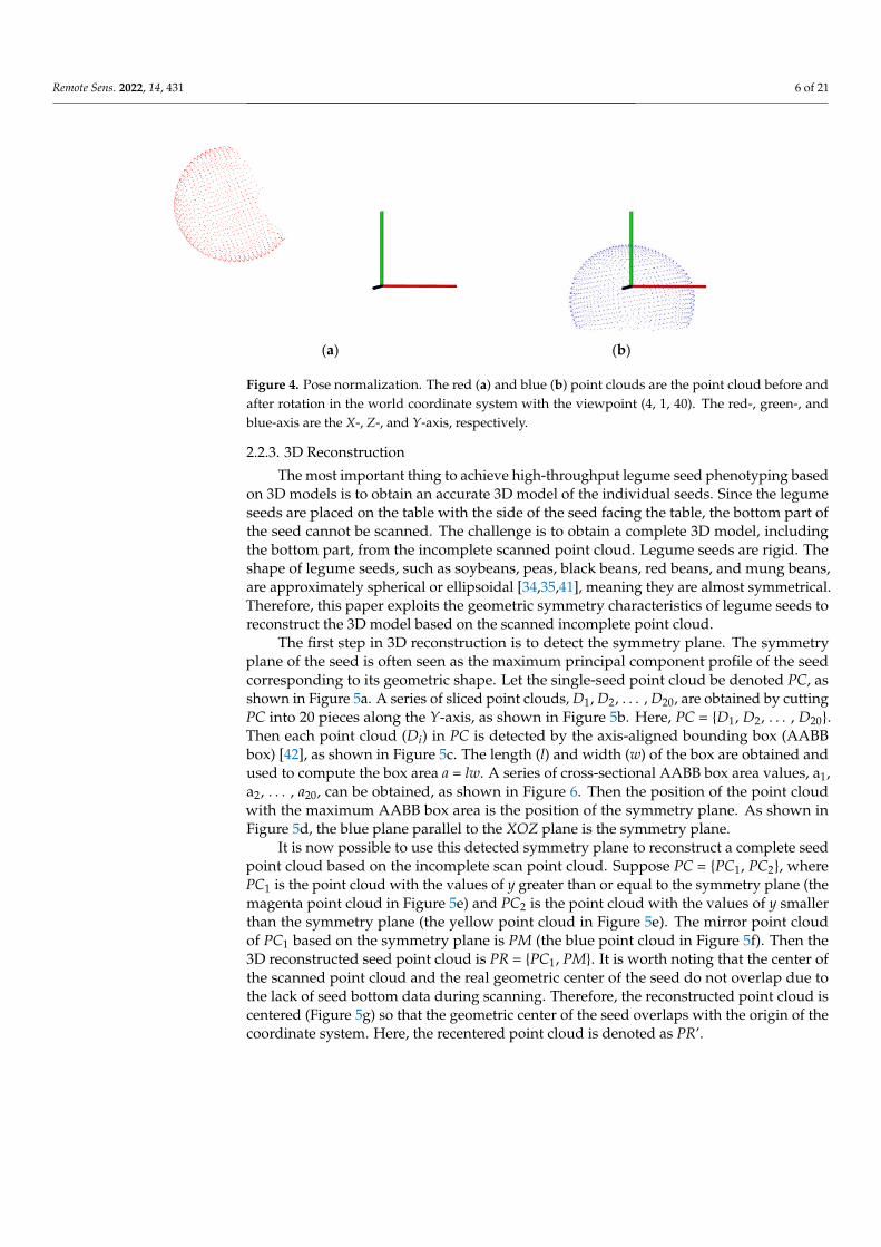
Remote Sens. 2022, 14, 431 6 of 21Remote Sens. 2022, 14, x FOR PEER REVIEW 6 of 22

(a) (b)

Figure 4. Pose normalization. The red (a) and blue (b) point clouds are the point cloud before and

after rotation in the world coordinate system with the viewpoint (4, 1, 40). The red-, green-, and

blue-axis are the X-, Z-, and Y-axis, respectively.

2.2.3. 3D Reconstruction

The most important thing to achieve high-throughput legume seed phenotyping

based on 3D models is to obtain an accurate 3D model of the individual seeds. Since the

legume seeds are placed on the table with the side of the seed facing the table, the bottom

part of the seed cannot be scanned. The challenge is to obtain a complete 3D model,

including the bottom part, from the incomplete scanned point cloud. Legume seeds are

rigid. The shape of legume seeds, such as soybeans, peas, black beans, red beans, and

mung beans, are approximately spherical or ellipsoidal [34,35,41], meaning they are

almost symmetrical. Therefore, this paper exploits the geometric symmetry characteristics

of legume seeds to reconstruct the 3D model based on the scanned incomplete point cloud.

The first step in 3D reconstruction is to detect the symmetry plane. The symmetry

plane of the seed is often seen as the maximum principal component profile of the seed

corresponding to its geometric shape. Let the single-seed point cloud be denoted PC, as

shown in Figure 5a. A series of sliced point clouds, D1, D2, …, D20, are obtained by cutting

PC into 20 pieces along the Y-axis, as shown in Figure 5b. Here, PC = {D1, D2, …, D20}. Then

each point cloud (Di) in PC is detected by the axis-aligned bounding box (AABB box) [42],

as shown in Figure 5c. The length (l) and width (w) of the box are obtained and used to

compute the box area a = lw. A series of cross-sectional AABB box area values, a1, a2, …,

a20, can be obtained, as shown in Figure 6. Then the position of the point cloud with the

maximum AABB box area is the position of the symmetry plane. As shown in Figure 5d,

the blue plane parallel to the XOZ plane is the symmetry plane.

It is now possible to use this detected symmetry plane to reconstruct a complete seed

point cloud based on the incomplete scan point cloud. Suppose PC = {PC1, PC2}, where PC1

is the point cloud with the values of y greater than or equal to the symmetry plane (the

magenta point cloud in Figure 5e) and PC2 is the point cloud with the values of y smaller

than the symmetry plane (the yellow point cloud in Figure 5e). The mirror point cloud of

PC1 based on the symmetry plane is PM (the blue point cloud in Figure 5f). Then the 3D

reconstructed seed point cloud is PR = {PC1, PM}. It is worth noting that the center of the

scanned point cloud and the real geometric center of the seed do not overlap due to the

lack of seed bottom data during scanning. Therefore, the reconstructed point cloud is

centered (Figure 5g) so that the geometric center of the seed overlaps with the origin of

the coordinate system. Here, the recentered point cloud is denoted as PR’.

Surface reconstruction is necessary to measure the volume and surface area. Here,

the Poisson surface reconstruction method [43] is adopted. Poisson surface reconstruction

is based on the Poisson equation, which is an implicit surface reconstruction and can be

calculated by:

Figure 4. Pose normalization. The red (a) and blue (b) point clouds are the point cloud before andafter rotation in the world coordinate system with the viewpoint (4, 1, 40). The red-, green-, andblue-axis are the X-, Z-, and Y-axis, respectively.

2.2.3. 3D Reconstruction

The most important thing to achieve high-throughput legume seed phenotyping basedon 3D models is to obtain an accurate 3D model of the individual seeds. Since the legumeseeds are placed on the table with the side of the seed facing the table, the bottom part ofthe seed cannot be scanned. The challenge is to obtain a complete 3D model, includingthe bottom part, from the incomplete scanned point cloud. Legume seeds are rigid. Theshape of legume seeds, such as soybeans, peas, black beans, red beans, and mung beans,are approximately spherical or ellipsoidal [34,35,41], meaning they are almost symmetrical.Therefore, this paper exploits the geometric symmetry characteristics of legume seeds toreconstruct the 3D model based on the scanned incomplete point cloud.

The first step in 3D reconstruction is to detect the symmetry plane. The symmetryplane of the seed is often seen as the maximum principal component profile of the seedcorresponding to its geometric shape. Let the single-seed point cloud be denoted PC, asshown in Figure 5a. A series of sliced point clouds, D1, D2, . . . , D20, are obtained by cuttingPC into 20 pieces along the Y-axis, as shown in Figure 5b. Here, PC = {D1, D2, . . . , D20}.Then each point cloud (Di) in PC is detected by the axis-aligned bounding box (AABBbox) [42], as shown in Figure 5c. The length (l) and width (w) of the box are obtained andused to compute the box area a = lw. A series of cross-sectional AABB box area values, a1,a2, . . . , a20, can be obtained, as shown in Figure 6. Then the position of the point cloudwith the maximum AABB box area is the position of the symmetry plane. As shown inFigure 5d, the blue plane parallel to the XOZ plane is the symmetry plane.

It is now possible to use this detected symmetry plane to reconstruct a complete seedpoint cloud based on the incomplete scan point cloud. Suppose PC = {PC1, PC2}, wherePC1 is the point cloud with the values of y greater than or equal to the symmetry plane (themagenta point cloud in Figure 5e) and PC2 is the point cloud with the values of y smallerthan the symmetry plane (the yellow point cloud in Figure 5e). The mirror point cloudof PC1 based on the symmetry plane is PM (the blue point cloud in Figure 5f). Then the3D reconstructed seed point cloud is PR = {PC1, PM}. It is worth noting that the center ofthe scanned point cloud and the real geometric center of the seed do not overlap due tothe lack of seed bottom data during scanning. Therefore, the reconstructed point cloud iscentered (Figure 5g) so that the geometric center of the seed overlaps with the origin of thecoordinate system. Here, the recentered point cloud is denoted as PR’.

Page 7

Remote Sens. 2022, 14, 431 7 of 21

Remote Sens. 2022, 14, x FOR PEER REVIEW 7 of 22

2 2 2

2 2 2f

x y z

=

+ +

, (2)

where x, y, and z are the coordinate values of the points, and φ is a real-valued function

that is twice differentiable in x, y, and z. Poisson surface reconstruction has the advantages

of both global fitting and local fitting. Figure 5h–j shows the wireframe, triangle mesh,

and surface visualization of the soybean seed’s 3D model constructed with the Poisson

surface reconstruction method.

(a) (b) (c) (d) (e)

(f) (g) (h) (i) (j)

Figure 5. The 3D model reconstruction process: (a) the scanned point cloud after pose normalization;

(b) the sliced point clouds; (c) the AABB box of one sliced point cloud; (d) the symmetry plane; (e)

the point clouds on both sides of the symmetry plane; (f) the reconstructed point cloud; (g) the cen-

tered reconstructed point cloud; and (h–j) the wireframe, triangle mesh, and surface visualization

of the soybean seed’s 3D model built by the Poisson surface reconstruction method.

Figure 6. The symmetry plane detection based on the box area of the sliced point clouds. The posi-

tion of the red point with the maximum box area is the position of the symmetry plane.

2.2.4. Trait Estimation

Morphological traits, scale factors, and shape factors are often used to describe seed

size and shape. According to the related research [44–47], 11 morphological traits, 11 scale

factors, and 12 shape factors are measured in this paper. These are listed in Tables 2 and

3.

As shown in Figure 7a, the 3D seed model is triangular meshed. The seed volume (V)

can be regarded as the volume of a closed space enclosed by this triangular mesh, which

is the sum of the projected volumes of all the triangular patches.

0

20

40

60

80

0 5 10 15 20

AA

BB

bo

x ar

ea (

mm

2 )

The sliced point cloud ID

Figure 5. The 3D model reconstruction process: (a) the scanned point cloud after pose normalization;(b) the sliced point clouds; (c) the AABB box of one sliced point cloud; (d) the symmetry plane; (e) thepoint clouds on both sides of the symmetry plane; (f) the reconstructed point cloud; (g) the centeredreconstructed point cloud; and (h–j) the wireframe, triangle mesh, and surface visualization of thesoybean seed’s 3D model built by the Poisson surface reconstruction method.

Remote Sens. 2022, 14, x FOR PEER REVIEW 7 of 22

2 2 2

2 2 2f

x y z

=

+ +

, (2)

where x, y, and z are the coordinate values of the points, and φ is a real-valued function

that is twice differentiable in x, y, and z. Poisson surface reconstruction has the advantages

of both global fitting and local fitting. Figure 5h–j shows the wireframe, triangle mesh,

and surface visualization of the soybean seed’s 3D model constructed with the Poisson

surface reconstruction method.

(a) (b) (c) (d) (e)

(f) (g) (h) (i) (j)

Figure 5. The 3D model reconstruction process: (a) the scanned point cloud after pose normalization;

(b) the sliced point clouds; (c) the AABB box of one sliced point cloud; (d) the symmetry plane; (e)

the point clouds on both sides of the symmetry plane; (f) the reconstructed point cloud; (g) the cen-

tered reconstructed point cloud; and (h–j) the wireframe, triangle mesh, and surface visualization

of the soybean seed’s 3D model built by the Poisson surface reconstruction method.

Figure 6. The symmetry plane detection based on the box area of the sliced point clouds. The posi-

tion of the red point with the maximum box area is the position of the symmetry plane.

2.2.4. Trait Estimation

Morphological traits, scale factors, and shape factors are often used to describe seed

size and shape. According to the related research [44–47], 11 morphological traits, 11 scale

factors, and 12 shape factors are measured in this paper. These are listed in Tables 2 and

3.

As shown in Figure 7a, the 3D seed model is triangular meshed. The seed volume (V)

can be regarded as the volume of a closed space enclosed by this triangular mesh, which

is the sum of the projected volumes of all the triangular patches.

0

20

40

60

80

0 5 10 15 20

AA

BB

bo

x ar

ea (

mm

2 )

The sliced point cloud ID

Figure 6. The symmetry plane detection based on the box area of the sliced point clouds. The positionof the red point with the maximum box area is the position of the symmetry plane.

Surface reconstruction is necessary to measure the volume and surface area. Here,the Poisson surface reconstruction method [43] is adopted. Poisson surface reconstructionis based on the Poisson equation, which is an implicit surface reconstruction and can becalculated by:

f =∂2 ϕ

∂x2 +∂2 ϕ

∂y2 +∂2 ϕ

∂z2 , (2)

where x, y, and z are the coordinate values of the points, and ϕ is a real-valued functionthat is twice differentiable in x, y, and z. Poisson surface reconstruction has the advantagesof both global fitting and local fitting. Figure 5h–j shows the wireframe, triangle mesh, andsurface visualization of the soybean seed’s 3D model constructed with the Poisson surfacereconstruction method.

2.2.4. Trait Estimation

Morphological traits, scale factors, and shape factors are often used to describe seedsize and shape. According to the related research [44–47], 11 morphological traits, 11 scalefactors, and 12 shape factors are measured in this paper. These are listed in Tables 2 and 3.

Page 8

Remote Sens. 2022, 14, 431 8 of 21

Table 2. Morphological traits. Sym.: symbols of the traits.

NO. Traits Sym.

1 Volume V2 Surface area S3 Length L4 Width W5 Thickness H6 Horizontal profile perimeter C17 Transverse profile perimeter C28 Longitudinal profile perimeter C39 Horizontal profile cross-section area A110 Transverse profile cross-section area A211 Longitudinal profile cross-section area A3

Table 3. Scale factors and shape factors.

NO. Scale Factors NO. Shape Factors

1 W/L 1 XZsf 1 = 4πA1/C12

2 H/L 2 XZsf 2 = A1/L3

3 H/W 3 XZsf 3 = 4A1/πL2

4 L/S 4 XZsf 4 = A1/LW5 L/V 5 XYsf 1 = 4πA2/C2

2

6 W/S 6 XYsf 2 = A2/L3

7 W/V 7 XYsf 3 = 4A2/πL2

8 H/S 8 XYsf 4 = A2/LW9 H/V 9 YZsf 1 = 4πA3/C3

2

10 A/V 10 YZsf 2 = A3/L3

11 V/LWH 11 YZsf 3 = 4A3/πW2

W/L 12 YZsf 4 = A3/WH

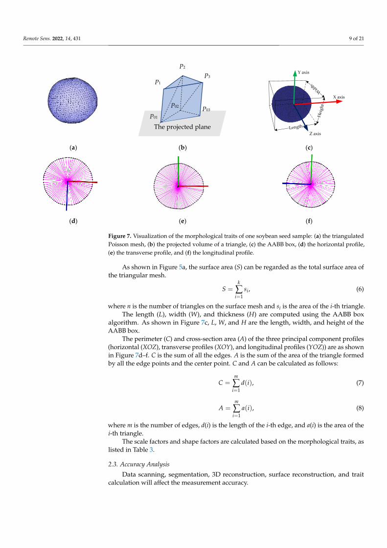
As shown in Figure 7a, the 3D seed model is triangular meshed. The seed volume (V)can be regarded as the volume of a closed space enclosed by this triangular mesh, which isthe sum of the projected volumes of all the triangular patches.

V =n

∑i=1

(−1)MV(∆i), (3)

where n is the number of triangles on the surface mesh, M is the direction of the trianglenormal vector, and V(∆i) is the projected volume of the i-th triangle. The projected volumeof a triangle can be seen as a convex pentahedron. Supposing a projection plane that doesnot intersect with all triangles in the mesh model, the projected volume is the volume ofthe convex pentahedron enclosed by the triangles and the projection plane. As shown inFigure 7b, a convex pentahedron, P1P2P3P01P02P03, can be divided into three tetrahedrons,and the volume of the convex pentahedron is:

V(∆i) = V(P01P1P3P2 + P01P2P3P03) ,+P01P2P03P02 (4)

where P1, P2, and P3 are the three vertices of the i-th triangle, and P01, P02, and P03 are theprojection vertices of P1, P2, and P3 on the projection plane. If (x1, y1, z1), (x2, y2, z2), (x3, y3,z3), and (x4, y4, z4) are four vertices of a tetrahedron, the volume of the tetrahedron can becalculated by:

V((x1, y1, z1), (x2, y2, z2), (x3, y3, z3), (x4, y4, z4))

= 16 |

x2 − x1 x3 − x1 x4 − x1y2 − y1 y3 − y1 y4 − y1z2 − z1 z3 − z1 z4 − z1

| . (5)

Page 9

Remote Sens. 2022, 14, 431 9 of 21

Remote Sens. 2022, 14, x FOR PEER REVIEW 9 of 22

Table 2. Morphological traits. Sym.: symbols of the traits.

NO. Traits Sym.

1 Volume V

2 Surface area S

3 Length L

4 Width W

5 Thickness H

6 Horizontal profile perimeter C1

7 Transverse profile perimeter C2

8 Longitudinal profile perimeter C3

9 Horizontal profile cross-section area A1

10 Transverse profile cross-section area A2

11 Longitudinal profile cross-section area A3

Table 3. Scale factors and shape factors.

NO. Scale Factors NO. Shape Factors

1 W/L 1 XZsf1 = 4πA1/C12

2 H/L 2 XZsf2 = A1/L3

3 H/W 3 XZsf3 = 4A1/πL2

4 L/S 4 XZsf4 = A1/LW

5 L/V 5 XYsf1 = 4πA2/C22

6 W/S 6 XYsf2 = A2/L3

7 W/V 7 XYsf3 = 4A2/πL2

8 H/S 8 XYsf4 = A2/LW

9 H/V 9 YZsf1 = 4πA3/C32

10 A/V 10 YZsf2 = A3/L3

11 V/LWH 11 YZsf3 = 4A3/πW2

W/L 12 YZsf4 = A3/WH

X axis

Y axis

Z axis

(a) (b) (c)

(d) (e) (f)

Figure 7. Visualization of the morphological traits of one soybean seed sample: (a) the triangulated

Poisson mesh, (b) the projected volume of a triangle, (c) the AABB box, (d) the horizontal profile,

(e) the transverse profile, and (f) the longitudinal profile.

The projected plane

P2

P1 P3

P01 P03

P02

Figure 7. Visualization of the morphological traits of one soybean seed sample: (a) the triangulatedPoisson mesh, (b) the projected volume of a triangle, (c) the AABB box, (d) the horizontal profile,(e) the transverse profile, and (f) the longitudinal profile.

As shown in Figure 5a, the surface area (S) can be regarded as the total surface area ofthe triangular mesh.

S =k

∑i=1

si, (6)

where n is the number of triangles on the surface mesh and si is the area of the i-th triangle.The length (L), width (W), and thickness (H) are computed using the AABB box

algorithm. As shown in Figure 7c, L, W, and H are the length, width, and height of theAABB box.

The perimeter (C) and cross-section area (A) of the three principal component profiles(horizontal (XOZ), transverse profiles (XOY), and longitudinal profiles (YOZ)) are as shownin Figure 7d–f. C is the sum of all the edges. A is the sum of the area of the triangle formedby all the edge points and the center point. C and A can be calculated as follows:

C =m

∑i=1

d(i), (7)

A =m

∑i=1

a(i), (8)

where m is the number of edges, d(i) is the length of the i-th edge, and a(i) is the area of thei-th triangle.

The scale factors and shape factors are calculated based on the morphological traits, aslisted in Table 3.

2.3. Accuracy Analysis

Data scanning, segmentation, 3D reconstruction, surface reconstruction, and traitcalculation will affect the measurement accuracy.

Page 10

Remote Sens. 2022, 14, 431 10 of 21

The scanning accuracy (R_scan) and segmentation accuracy (R_seg) are calculated asfollows:

R_scan =N2

N1× 100% and R_seg =

N3

N2× 100%, (9)

where N1, N2, and N3 are the numbers of total seeds, scanned seeds, and automaticallyextracted seeds, respectively.

Since the shape of the seed is not perfectly symmetrical, there will be a certain errorbetween the reconstructed point cloud and the true point cloud. The error is defined asfollows:

Er =1n

n

∑i=1

dcloset(Pi, Pmj), (10)

where n is the number of the true point cloud, and dclosest (Pi, Pmj) is the distance betweenthe true point Pi and the closest reconstructed point Pmj. The value of dclosest (Pi, Pmj) canreflect the deviation between the true point cloud and the reconstructed point cloud. If thepoint cloud is perfectly symmetrical, then Pi and Pmj are completely coincident, and dclosest(Pi, Pmj) = 0.

The mean absolute error (MAE), mean relative error (MRE), root mean square error(RMSE), and correlation coefficient (R) between the measured values and the true valuesare used to verify the accuracy of measurement traits.

MAE =1n

n

∑i=1|xai − xmi|, (11)

MRE =1n

n

∑i=1

|xai − xmi|xmi

× 100%, (12)

RMSE =

√1n

n

∑i=1

(xai − xmi)2, (13)

R(xai, xmi) =Cov(xai, xmi)√

Var[xai]Var[xmi], (14)

3. Results3.1. Visualization of Scanning and Segmentation Results

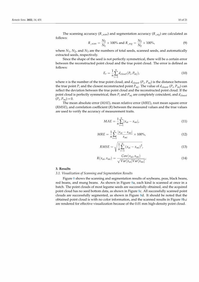
Figure 8 shows the scanning and segmentation results of soybeans, peas, black beans,red beans, and mung beans. As shown in Figure 8a, each kind is scanned at once in abatch. The point clouds of most legume seeds are successfully obtained, and the acquiredpoint cloud has no seed bottom data, as shown in Figure 8c. All successfully scanned pointclouds are successfully segmented, as shown in Figure 8d. It should be noted that theobtained point cloud is with no color information, and the scanned results in Figure 8b,care rendered for effective visualization because of the 0.01 mm high-density point cloud.

Page 11

Remote Sens. 2022, 14, 431 11 of 21Remote Sens. 2022, 14, x FOR PEER REVIEW 11 of 22

Figure 8. Visualization of scanning and segmentation results: (a) legume seeds on the table ready

for data scanning, (b) rendered visualization of the obtained point clouds, (c) detailed display of the

red box area in (b), (d) segmentation results, and (e) detailed display of the red box area in (d).

3.2. Visualization of 3D Reconstruction

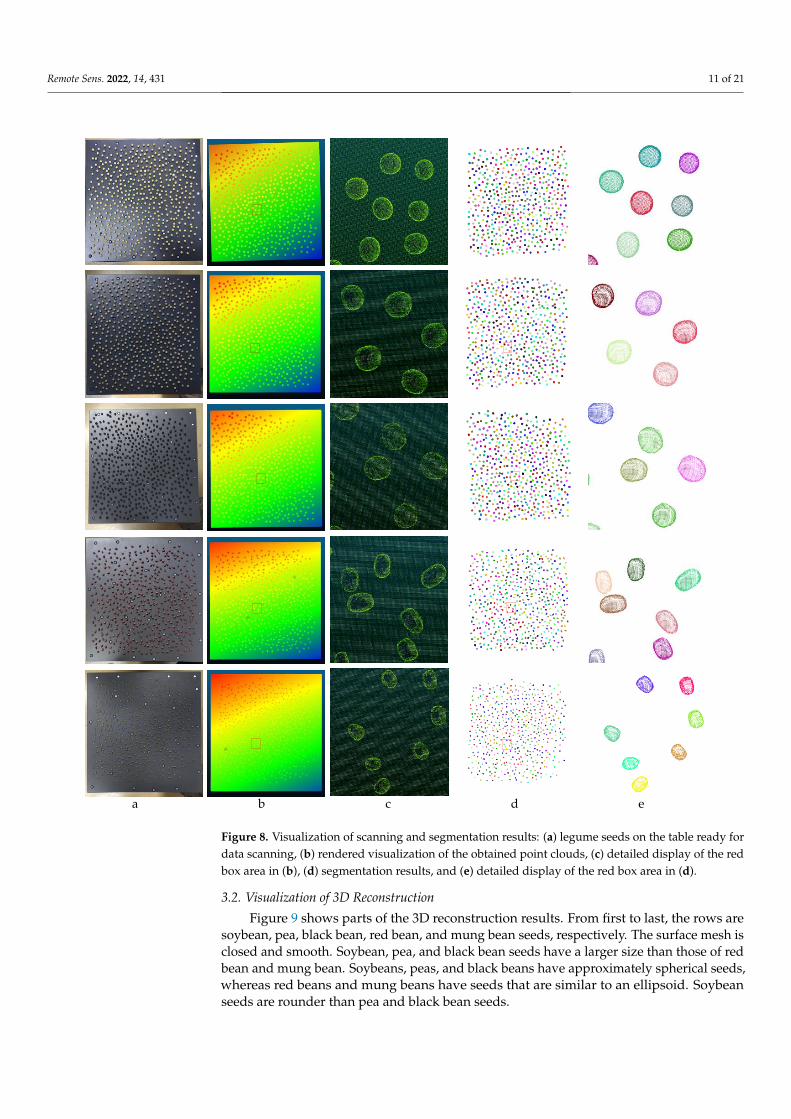
Figure 9 shows parts of the 3D reconstruction results. From first to last, the rows are

soybean, pea, black bean, red bean, and mung bean seeds, respectively. The surface mesh

is closed and smooth. Soybean, pea, and black bean seeds have a larger size than those of

red bean and mung bean. Soybeans, peas, and black beans have approximately spherical

b d c a e

Figure 8. Visualization of scanning and segmentation results: (a) legume seeds on the table ready fordata scanning, (b) rendered visualization of the obtained point clouds, (c) detailed display of the redbox area in (b), (d) segmentation results, and (e) detailed display of the red box area in (d).

3.2. Visualization of 3D Reconstruction

Figure 9 shows parts of the 3D reconstruction results. From first to last, the rows aresoybean, pea, black bean, red bean, and mung bean seeds, respectively. The surface mesh isclosed and smooth. Soybean, pea, and black bean seeds have a larger size than those of redbean and mung bean. Soybeans, peas, and black beans have approximately spherical seeds,whereas red beans and mung beans have seeds that are similar to an ellipsoid. Soybeanseeds are rounder than pea and black bean seeds.

Page 12

Remote Sens. 2022, 14, 431 12 of 21

Remote Sens. 2022, 14, x FOR PEER REVIEW 12 of 22

seeds, whereas red beans and mung beans have seeds that are similar to an ellipsoid.

Soybean seeds are rounder than pea and black bean seeds.

Figure 9. Partial visualization of 3D reconstruction results. From first to last, the rows are soybean,

pea, black bean, red bean, and mung bean seeds, respectively.

3.3. Results of Trait Estimation

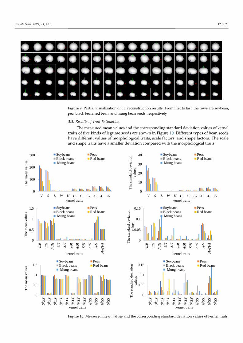
The measured mean values and the corresponding standard deviation values of ker-

nel traits of five kinds of legume seeds are shown in Figure 10. Different types of bean

seeds have different values of morphological traits, scale factors, and shape factors. The

scale and shape traits have a smaller deviation compared with the morphological traits.

0

100

200

300

V S L W H C₁ C₂ C₃ A₁ A₂ A₃

Th

e m

ean

val

ues

kernel traits

Soybeans PeasBlack beans Red beans Mung beans

0

10

20

30

40

V S L W H C₁ C₂ C₃ A₁ A₂ A₃

Th

e st

and

ard

dev

iati

on

val

ues

kernel traits

Soybeans PeasBlack beans Red beans Mung beans

0

0.5

1

1.5

W/L

H/L

H/W

L/S

L/V

W/S

W/V

H/S

H/V

A/V

V/L

WH

Th

em

ean

val

ues

kernel traits

Soybeans PeasBlack beans Red beans Mung beans

0

0.05

0.1

0.15

W/L

H/L

H/W

L/S

L/V

W/S

W/V

H/S

H/V

A/V

V/L

WH

Th

e st

and

ard

dev

iati

on

val

ues

kernel traits

Soybeans PeasBlack beans Red beans Mung beans

Figure 9. Partial visualization of 3D reconstruction results. From first to last, the rows are soybean,pea, black bean, red bean, and mung bean seeds, respectively.

3.3. Results of Trait Estimation

The measured mean values and the corresponding standard deviation values of kerneltraits of five kinds of legume seeds are shown in Figure 10. Different types of bean seedshave different values of morphological traits, scale factors, and shape factors. The scaleand shape traits have a smaller deviation compared with the morphological traits.

Remote Sens. 2022, 14, x FOR PEER REVIEW 12 of 22

seeds, whereas red beans and mung beans have seeds that are similar to an ellipsoid.

Soybean seeds are rounder than pea and black bean seeds.

Figure 9. Partial visualization of 3D reconstruction results. From first to last, the rows are soybean,

pea, black bean, red bean, and mung bean seeds, respectively.

3.3. Results of Trait Estimation

The measured mean values and the corresponding standard deviation values of ker-

nel traits of five kinds of legume seeds are shown in Figure 10. Different types of bean

seeds have different values of morphological traits, scale factors, and shape factors. The

scale and shape traits have a smaller deviation compared with the morphological traits.

0

100

200

300

V S L W H C₁ C₂ C₃ A₁ A₂ A₃

Th

e m

ean

val

ues

kernel traits

Soybeans PeasBlack beans Red beans Mung beans

0

10

20

30

40

V S L W H C₁ C₂ C₃ A₁ A₂ A₃

Th

e st

and

ard

dev

iati

on

val

ues

kernel traits

Soybeans PeasBlack beans Red beans Mung beans

0

0.5

1

1.5

W/L

H/L

H/W

L/S

L/V

W/S

W/V

H/S

H/V

A/V

V/L

WH

Th

em

ean

val

ues

kernel traits

Soybeans PeasBlack beans Red beans Mung beans

0

0.05

0.1

0.15

W/L

H/L

H/W

L/S

L/V

W/S

W/V

H/S

H/V

A/V

V/L

WH

Th

e st

and

ard

dev

iati

on

val

ues

kernel traits

Soybeans PeasBlack beans Red beans Mung beans

Remote Sens. 2022, 14, x FOR PEER REVIEW 13 of 22

Figure 10. Measured mean values and the corresponding standard deviation values of kernel traits.

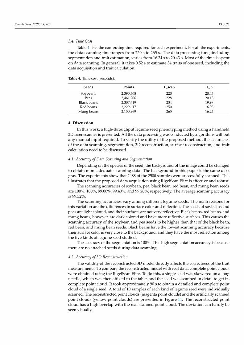
3.4. Time Cost

Table 4 lists the computing time required for each experiment. For all the experi-

ments, the data scanning time ranges from 220 s to 265 s. The data processing time, in-

cluding segmentation and trait estimation, varies from 16.24 s to 20.43 s. Most of the time

is spent on data scanning. In general, it takes 0.52 s to estimate 34 traits of one seed, in-

cluding the data acquisition and trait calculation.

Table 4. Time cost (seconds).

Seeds Points T_scan T_p

Soybeans 2,390,308 220 20.43

Peas 2,461,206 228 20.13

Black beans 2,307,619 234 19.98

Red beans 2,229,617 250 16.93

Mung beans 2,150,969 265 16.24

4. Discussion

In this work, a high-throughput legume seed phenotyping method using a handheld

3D laser scanner is presented. All the data processing was conducted by algorithms with-

out any manual input required. To verify the utility of the proposed method, the accura-

cies of the data scanning, segmentation, 3D reconstruction, surface reconstruction, and

trait calculation need to be discussed.

4.1. Accuracy of Data Scanning and Segmentation

Depending on the species of the seed, the background of the image could be changed

to obtain more adequate scanning data. The background in this paper is the same dark

gray. The experiments show that 2488 of the 2500 samples were successfully scanned. This

illustrates that the proposed data acquisition using RigelScan Elite is effective and robust.

The scanning accuracies of soybean, pea, black bean, red bean, and mung bean seeds

are 100%, 100%, 99.00%, 99.40%, and 99.20%, respectively. The average scanning accuracy

is 99.52%.

The scanning accuracies vary among different legume seeds. The main reasons for

this variation are the differences in surface color and reflection. The seeds of soybeans and

peas are light colored, and their surfaces are not very reflective. Black beans, red beans,

and mung beans, however, are dark colored and have more reflective surfaces. This causes

the scanning accuracy of the soybean and pea seeds to be higher than that of the black

bean, red bean, and mung bean seeds. Black beans have the lowest scanning accuracy

because their surface color is very close to the background, and they have the most reflec-

tion among the five kinds of legume seed studied.

The accuracy of the segmentation is 100%. This high segmentation accuracy is be-

cause there are no attached seeds during data scanning.

0

0.5

1

1.5

XZsf₁

XZsf₂

XZsf₃

XZsf₄

XYsf₁

XYsf₂

XYsf₃

XYsf₄

YZsf₁

YZsf₂

YZsf₃

YZsf₄

Th

e m

ean

val

ues

kernel traits

Soybeans PeasBlack beans Red beans Mung beans

0

0.05

0.1

0.15

XZsf₁

XZsf₂

XZsf₃

XZsf₄

XYsf₁

XYsf₂

XYsf₃

XYsf₄

YZsf₁

YZsf₂

YZsf₃

YZsf₄

Th

e st

and

ard

dev

iati

on

val

ues

kernel traits

Soybeans PeasBlack beans Red beans Mung beans

Figure 10. Measured mean values and the corresponding standard deviation values of kernel traits.

Page 13

Remote Sens. 2022, 14, 431 13 of 21

3.4. Time Cost

Table 4 lists the computing time required for each experiment. For all the experiments,the data scanning time ranges from 220 s to 265 s. The data processing time, includingsegmentation and trait estimation, varies from 16.24 s to 20.43 s. Most of the time is spenton data scanning. In general, it takes 0.52 s to estimate 34 traits of one seed, including thedata acquisition and trait calculation.

Table 4. Time cost (seconds).

Seeds Points T_scan T_p

Soybeans 2,390,308 220 20.43Peas 2,461,206 228 20.13

Black beans 2,307,619 234 19.98Red beans 2,229,617 250 16.93

Mung beans 2,150,969 265 16.24

4. Discussion

In this work, a high-throughput legume seed phenotyping method using a handheld3D laser scanner is presented. All the data processing was conducted by algorithms withoutany manual input required. To verify the utility of the proposed method, the accuraciesof the data scanning, segmentation, 3D reconstruction, surface reconstruction, and traitcalculation need to be discussed.

4.1. Accuracy of Data Scanning and Segmentation

Depending on the species of the seed, the background of the image could be changedto obtain more adequate scanning data. The background in this paper is the same darkgray. The experiments show that 2488 of the 2500 samples were successfully scanned. Thisillustrates that the proposed data acquisition using RigelScan Elite is effective and robust.

The scanning accuracies of soybean, pea, black bean, red bean, and mung bean seedsare 100%, 100%, 99.00%, 99.40%, and 99.20%, respectively. The average scanning accuracyis 99.52%.

The scanning accuracies vary among different legume seeds. The main reasons forthis variation are the differences in surface color and reflection. The seeds of soybeans andpeas are light colored, and their surfaces are not very reflective. Black beans, red beans, andmung beans, however, are dark colored and have more reflective surfaces. This causes thescanning accuracy of the soybean and pea seeds to be higher than that of the black bean,red bean, and mung bean seeds. Black beans have the lowest scanning accuracy becausetheir surface color is very close to the background, and they have the most reflection amongthe five kinds of legume seed studied.

The accuracy of the segmentation is 100%. This high segmentation accuracy is becausethere are no attached seeds during data scanning.

4.2. Accuracy of 3D Reconstruction

The validity of the reconstructed 3D model directly affects the correctness of the traitmeasurements. To compare the reconstructed model with real data, complete point cloudswere obtained using the RigelScan Elite. To do this, a single seed was skewered on a longneedle, which was then affixed to the table, and the seed was scanned in detail to get itscomplete point cloud. It took approximately 90 s to obtain a detailed and complete pointcloud of a single seed. A total of 10 samples of each kind of legume seed were individuallyscanned. The reconstructed point clouds (magenta point clouds) and the artificially scannedpoint clouds (yellow point clouds) are presented in Figure 11. The reconstructed pointcloud has a high overlap with the real scanned point cloud. The deviation can hardly beseen visually.

Page 14

Remote Sens. 2022, 14, 431 14 of 21

Remote Sens. 2022, 14, x FOR PEER REVIEW 14 of 22

4.2. Accuracy of 3D Reconstruction

The validity of the reconstructed 3D model directly affects the correctness of the trait

measurements. To compare the reconstructed model with real data, complete point clouds

were obtained using the RigelScan Elite. To do this, a single seed was skewered on a long

needle, which was then affixed to the table, and the seed was scanned in detail to get its

complete point cloud. It took approximately 90 s to obtain a detailed and complete point

cloud of a single seed. A total of 10 samples of each kind of legume seed were individually

scanned. The reconstructed point clouds (magenta point clouds) and the artificially

scanned point clouds (yellow point clouds) are presented in Figure 11. The reconstructed

point cloud has a high overlap with the real scanned point cloud. The deviation can hardly

be seen visually.

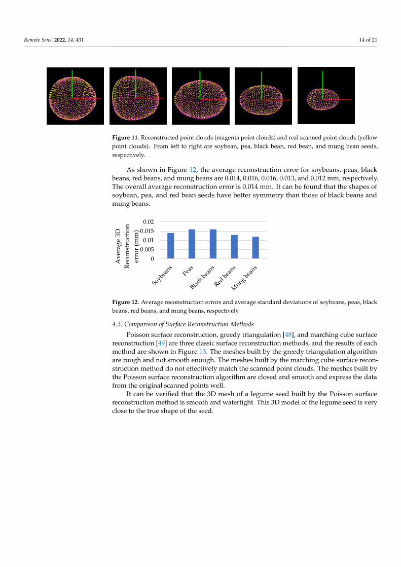
Figure 11. Reconstructed point clouds (magenta point clouds) and real scanned point clouds (yellow

point clouds). From left to right are soybean, pea, black bean, red bean, and mung bean seeds, re-

spectively.

As shown in Figure 12, the average reconstruction error for soybeans, peas, black

beans, red beans, and mung beans are 0.014, 0.016, 0.016, 0.013, and 0.012 mm, respec-

tively. The overall average reconstruction error is 0.014 mm. It can be found that the

shapes of soybean, pea, and red bean seeds have better symmetry than those of black

beans and mung beans.

Figure 12. Average reconstruction errors and average standard deviations of soybeans, peas, black

beans, red beans, and mung beans, respectively.

4.3. Comparison of Surface Reconstruction Methods

Poisson surface reconstruction, greedy triangulation [48], and marching cube surface

reconstruction [49] are three classic surface reconstruction methods, and the results of

each method are shown in Figure 13 (from top to bottom). The meshes built by the greedy

triangulation algorithm are rough and not smooth enough. The meshes built by the

marching cube surface reconstruction method do not effectively match the scanned point

clouds. The meshes built by the Poisson surface reconstruction algorithm are closed and

smooth and express the data from the original scanned points well.

It can be verified that the 3D mesh of a legume seed built by the Poisson surface

reconstruction method is smooth and watertight. This 3D model of the legume seed is

very close to the true shape of the seed.

0

0.005

0.01

0.015

0.02

Av

erag

e 3D

Rec

on

stru

ctio

n

erro

r (m

m)

Figure 11. Reconstructed point clouds (magenta point clouds) and real scanned point clouds (yellowpoint clouds). From left to right are soybean, pea, black bean, red bean, and mung bean seeds,respectively.

As shown in Figure 12, the average reconstruction error for soybeans, peas, blackbeans, red beans, and mung beans are 0.014, 0.016, 0.016, 0.013, and 0.012 mm, respectively.The overall average reconstruction error is 0.014 mm. It can be found that the shapes ofsoybean, pea, and red bean seeds have better symmetry than those of black beans andmung beans.

Remote Sens. 2022, 14, x FOR PEER REVIEW 14 of 22

4.2. Accuracy of 3D Reconstruction

The validity of the reconstructed 3D model directly affects the correctness of the trait

measurements. To compare the reconstructed model with real data, complete point clouds

were obtained using the RigelScan Elite. To do this, a single seed was skewered on a long

needle, which was then affixed to the table, and the seed was scanned in detail to get its

complete point cloud. It took approximately 90 s to obtain a detailed and complete point

cloud of a single seed. A total of 10 samples of each kind of legume seed were individually

scanned. The reconstructed point clouds (magenta point clouds) and the artificially

scanned point clouds (yellow point clouds) are presented in Figure 11. The reconstructed

point cloud has a high overlap with the real scanned point cloud. The deviation can hardly

be seen visually.

Figure 11. Reconstructed point clouds (magenta point clouds) and real scanned point clouds (yellow

point clouds). From left to right are soybean, pea, black bean, red bean, and mung bean seeds, re-

spectively.

As shown in Figure 12, the average reconstruction error for soybeans, peas, black

beans, red beans, and mung beans are 0.014, 0.016, 0.016, 0.013, and 0.012 mm, respec-

tively. The overall average reconstruction error is 0.014 mm. It can be found that the

shapes of soybean, pea, and red bean seeds have better symmetry than those of black

beans and mung beans.

Figure 12. Average reconstruction errors and average standard deviations of soybeans, peas, black

beans, red beans, and mung beans, respectively.

4.3. Comparison of Surface Reconstruction Methods

Poisson surface reconstruction, greedy triangulation [48], and marching cube surface

reconstruction [49] are three classic surface reconstruction methods, and the results of

each method are shown in Figure 13 (from top to bottom). The meshes built by the greedy

triangulation algorithm are rough and not smooth enough. The meshes built by the

marching cube surface reconstruction method do not effectively match the scanned point

clouds. The meshes built by the Poisson surface reconstruction algorithm are closed and

smooth and express the data from the original scanned points well.

It can be verified that the 3D mesh of a legume seed built by the Poisson surface

reconstruction method is smooth and watertight. This 3D model of the legume seed is

very close to the true shape of the seed.

0

0.005

0.01

0.015

0.02

Av

erag

e 3D

Rec

on

stru

ctio

n

erro

r (m

m)

Figure 12. Average reconstruction errors and average standard deviations of soybeans, peas, blackbeans, red beans, and mung beans, respectively.

4.3. Comparison of Surface Reconstruction Methods

Poisson surface reconstruction, greedy triangulation [48], and marching cube surfacereconstruction [49] are three classic surface reconstruction methods, and the results of eachmethod are shown in Figure 13. The meshes built by the greedy triangulation algorithmare rough and not smooth enough. The meshes built by the marching cube surface recon-struction method do not effectively match the scanned point clouds. The meshes built bythe Poisson surface reconstruction algorithm are closed and smooth and express the datafrom the original scanned points well.

It can be verified that the 3D mesh of a legume seed built by the Poisson surfacereconstruction method is smooth and watertight. This 3D model of the legume seed is veryclose to the true shape of the seed.

Page 15

Remote Sens. 2022, 14, 431 15 of 21Remote Sens. 2022, 14, x FOR PEER REVIEW 15 of 22

Figure 13. Surface reconstruction results. Each column shows a type of seed, from left to right: soy-

beans, peas, black beans, red beans, and mung beans. The rows show the mesh built by Poisson

surface reconstruction, greedy triangulation, and marching cube surface reconstruction from top to

bottom.

4.4. Accuracy of Trait Estimation

From the scanned 2500 samples, 50 seeds (the same seeds as in Section 4.2) were

measured manually to evaluate the algorithm performance. The ground truths of length,

width, and thickness were obtained using a vernier caliper. The other traits were

measured by the software Geomagic Studio based on the real 3D point cloud obtained in

Section 4.2. All the ground truths were manually measured three times by three people,

and the average was adopted.

The measurement accuracies of 11 morphological traits, 11 scale factors, and 12 shape

factors are shown in Figure 14, Appendix A, and Appendix B. The values of MAE, RMSE,

MRE, and R2 of these kernel traits are presented in detail. The average absolute

measurement accuracy and root mean square error are in submillimeter, the average

relative measurement accuracy is within 3%, and R2 is above 0.9983 for the 11

morphological traits. The average relative measurement accuracy is within 4%, and R2 for

the 11 morphological traits is above 0.8343 for 11 scale factors and 12 shape factors. The

experiments show that the measurement accuracy of the proposed method is comparable

to previous work in this area [6,44,50]. Moreover, the proposed method shows the

viability and effectiveness of automatic estimation and batch extraction of seeds’

geometric parameters, especially their 3D traits.

Figure 13. Surface reconstruction results. Each column shows a type of seed, from left to right:soybeans, peas, black beans, red beans, and mung beans. The rows show the mesh built by Poissonsurface reconstruction, greedy triangulation, and marching cube surface reconstruction from top tobottom.

4.4. Accuracy of Trait Estimation

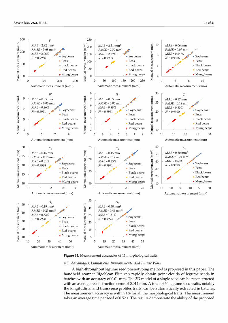
From the scanned 2500 samples, 50 seeds (the same seeds as in Section 4.2) weremeasured manually to evaluate the algorithm performance. The ground truths of length,width, and thickness were obtained using a vernier caliper. The other traits were measuredby the software Geomagic Studio based on the real 3D point cloud obtained in Section 4.2.All the ground truths were manually measured three times by three people, and the averagewas adopted.

The measurement accuracies of 11 morphological traits, 11 scale factors, and 12 shapefactors are shown in Figure 14, Appendix A, and Appendix B. The values of MAE, RMSE,MRE, and R2 of these kernel traits are presented in detail. The average absolute mea-surement accuracy and root mean square error are in submillimeter, the average relativemeasurement accuracy is within 3%, and R2 is above 0.9983 for the 11 morphological traits.The average relative measurement accuracy is within 4%, and R2 for the 11 morphologicaltraits is above 0.8343 for 11 scale factors and 12 shape factors. The experiments show thatthe measurement accuracy of the proposed method is comparable to previous work in thisarea [6,44,50]. Moreover, the proposed method shows the viability and effectiveness ofautomatic estimation and batch extraction of seeds’ geometric parameters, especially their3D traits.

Page 16

Remote Sens. 2022, 14, 431 16 of 21Remote Sens. 2022, 14, x FOR PEER REVIEW 16 of 22

Figure 14. Measurement accuracies of 11 morphological traits.

4.5. Advantages, Limitations, Improvements, and Future Work

A high-throughput legume seed phenotyping method is proposed in this paper. The

handheld scanner RigelScan Elite can rapidly obtain point clouds of legume seeds in

batches with an accuracy of 0.01 mm. The 3D model of a single seed can be reconstructed

with an average reconstruction error of 0.014 mm. A total of 34 legume seed traits, notably

the longitudinal and transverse profiles traits, can be automatically extracted in batches.

The measurement accuracy is within 4% for all the morphological traits. The measurement

0

100

200

300

0 100 200 300Man

ual

mea

sure

men

t (m

m3 )

Automatic measurement (mm3)

V

Soybeans

Peas

Black beans

Red beans

Mung beans

MAE = 2.82 mm3

RMSE = 3.68 mm3

MRE = 2.06%

R2 = 0.9986

0

50

100

150

200

250

0 50 100 150 200 250Man

ual

mea

sure

men

t (m

m2 )

Automatic measurement (mm2)

S

Soybeans

Peas

Black beans

Red beans

Mung beans

MAE = 2.31 mm2

RMSE = 2.72 mm2

MRE = 2.09%

R2 = 0.9983

4

6

8

10

4 6 8 10Man

ual

mea

sure

men

t (m

m)

Automatic measurement (mm)

L

Soybeans

Peas

Black beans

Red beans

Mung beans

MAE = 0.06 mm

RMSE = 0.07 mm

MRE = 0.84 %

R2 = 0.9986

3

5

7

9

3 5 7 9Man

ual

mea

sure

men

t (m

m)

Automatic measurement (mm)

W

Soybeans

Peas

Black beans

Red beans

Mung beans

MAE = 0.05 mm

RMSE = 0.06 mm

MRE = 0.86%

R2 = 0.9991

2

3

4

5

6

7

8

2 3 4 5 6 7 8Man

ual

mea

sure

men

t (m

m)

Automatic measurement (mm)

H

Soybeans

Peas

Black beans

Red beans

Mung beans

MAE = 0.05 mm

RMSE = 0.06 mm

MRE = 0.88%

R2 = 0.9991

10

15

20

25

30

10 15 20 25 30Man

ual

mea

sure

men

t (m

m)

Automatic measurement (mm)

C1

Soybeans

Peas

Black beans

Red beans

Mung beans

MAE = 0.17 mm

RMSE = 0.18 mm

MRE = 0.80%

R2 = 0.9990

10

15

20

25

30

10 15 20 25 30Man

ual

mea

sure

men

t (m

m)

Automatic measurement (mm)

C2

Soybeans

Peas

Black beans

Red beans

Mung beans

MAE = 0.16 mm

RMSE = 0.18 mm

MRE = 0.81%

R2 = 0.9988

10

15

20

25

10 15 20 25Man

ual

mea

sure

men

t (m

m)

Automatic measurement (mm)

C3

Soybeans

Peas

Black beans

Red beans

Mung beans

MAE = 0.15 mm

RMSE = 0.17 mm

MRE = 0.83%

R2 = 0.9991

10

20

30

40

50

60

10 20 30 40 50 60Man

ual

mea

sure

men

t (m

m2 )

Automatic measurement (mm2)

A1

Soybeans

Peas

Black beans

Red beans

Mung beans

MAE = 0.20 mm2

RMSE = 0.24 mm2

MRE = 0.60%

R2 = 0.9998

10

20

30

40

50

10 20 30 40 50Man

ual

mea

sure

men

t (m

m2 )

Automatic measurement (mm2)

A2

Soybeans

Peas

Black beans

Red beans

Mung beans

MAE = 0.19 mm2

RMSE = 0.23 mm2

MRE = 0.62%

R2 = 0.9998

5

15

25

35

45

55

5 15 25 35 45 55Man

ual

mea

sure

men

t (m

m2 )

Automatic measurement (mm2)

A3

Soybeans

Peas

Black beans

Red beans

Mung beans

MAE = 0.30 mm2

RMSE = 0.49 mm2

MRE = 1.81%

R2 = 0.9993

Figure 14. Measurement accuracies of 11 morphological traits.

4.5. Advantages, Limitations, Improvements, and Future Work

A high-throughput legume seed phenotyping method is proposed in this paper. Thehandheld scanner RigelScan Elite can rapidly obtain point clouds of legume seeds inbatches with an accuracy of 0.01 mm. The 3D model of a single seed can be reconstructedwith an average reconstruction error of 0.014 mm. A total of 34 legume seed traits, notablythe longitudinal and transverse profiles traits, can be automatically extracted in batches.The measurement accuracy is within 4% for all the morphological traits. The measurementtakes an average time per seed of 0.52 s. The results demonstrate the ability of the proposed

Page 17

Remote Sens. 2022, 14, 431 17 of 21

method to perform data batch processing and automatic measurement, which showspotential for real-time measurement and high-throughput phenotyping.

The extracted 34 trait indicators in this paper have prospects and research value inapplication in precision agriculture. The morphological traits, such as the volume, surfacearea, length, width, thickness, horizontal profile perimeter, transverse profile perimeter,longitudinal profile perimeter, horizontal profile cross-section area, transverse profile cross-section area, and longitudinal profile cross-section area, can directly quantitatively describethe seed size, which is important in quality evaluation, optimization breeding, and yieldevaluation. The scale traits and shape factors can quantitatively describe the seed shape,which can be helpful in species identification and classification and quantitative trait loci.

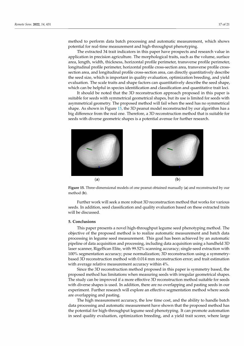
It should be noted that the 3D reconstruction approach proposed in this paper issuitable for seeds with symmetrical geometrical shapes, but its use is limited for seeds withasymmetrical geometry. The proposed method will fail when the seed has no symmetricalshape. As shown in Figure 15, the 3D peanut model reconstructed by our algorithm has abig difference from the real one. Therefore, a 3D reconstruction method that is suitable forseeds with diverse geometric shapes is a potential avenue for further research.

Remote Sens. 2022, 14, x FOR PEER REVIEW 17 of 22

takes an average time per seed of 0.52 s. The results demonstrate the ability of the pro-

posed method to perform data batch processing and automatic measurement, which

shows potential for real-time measurement and high-throughput phenotyping.

The extracted 34 trait indicators in this paper have prospects and research value in

application in precision agriculture. The morphological traits, such as the volume, surface

area, length, width, thickness, horizontal profile perimeter, transverse profile perimeter,

longitudinal profile perimeter, horizontal profile cross-section area, transverse profile

cross-section area, and longitudinal profile cross-section area, can directly quantitatively

describe the seed size, which is important in quality evaluation, optimization breeding,

and yield evaluation. The scale traits and shape factors can quantitatively describe the

seed shape, which can be helpful in species identification and classification and quantita-

tive trait loci.

It should be noted that the 3D reconstruction approach proposed in this paper is suit-

able for seeds with symmetrical geometrical shapes, but its use is limited for seeds with

asymmetrical geometry. The proposed method will fail when the seed has no symmetrical

shape. As shown in Figure 15, the 3D peanut model reconstructed by our algorithm has a

big difference from the real one. Therefore, a 3D reconstruction method that is suitable for

seeds with diverse geometric shapes is a potential avenue for further research.

Further work will seek a more robust 3D reconstruction method that works for vari-

ous seeds. In addition, seed classification and quality evaluation based on these extracted

traits will be discussed.

(a) (b)

Figure 15. Three-dimensional models of one peanut obtained manually (a) and reconstructed by

our method (b).

5. Conclusions

This paper presents a novel high-throughput legume seed phenotyping method. The

objective of the proposed method is to realize automatic measurement and batch data

processing in legume seed measurement. This goal has been achieved by an automatic

pipeline of data acquisition and processing, including data acquisition using a handheld

3D laser scanner, RigelScan Elite, with 99.52% scanning accuracy; single-seed extraction

with 100% segmentation accuracy; pose normalization; 3D reconstruction using a sym-

metry-based 3D reconstruction method with 0.014 mm reconstruction error; and trait es-

timation with average relative measurement accuracy within 4%.

Since the 3D reconstruction method proposed in this paper is symmetry based, the

proposed method has limitations when measuring seeds with irregular geometrical

shapes. The study can be improved if a more effective 3D reconstruction method suitable

for seeds with diverse shapes is used. In addition, there are no overlapping and pasting

seeds in our experiment. Further research will explore an effective segmentation method

where seeds are overlapping and pasting.

The high measurement accuracy, the low time cost, and the ability to handle batch

data processing and automatic measurement have shown that the proposed method has

the potential for high-throughput legume seed phenotyping. It can promote automation

Figure 15. Three-dimensional models of one peanut obtained manually (a) and reconstructed by ourmethod (b).

Further work will seek a more robust 3D reconstruction method that works for variousseeds. In addition, seed classification and quality evaluation based on these extracted traitswill be discussed.

5. Conclusions

This paper presents a novel high-throughput legume seed phenotyping method. Theobjective of the proposed method is to realize automatic measurement and batch dataprocessing in legume seed measurement. This goal has been achieved by an automaticpipeline of data acquisition and processing, including data acquisition using a handheld 3Dlaser scanner, RigelScan Elite, with 99.52% scanning accuracy; single-seed extraction with100% segmentation accuracy; pose normalization; 3D reconstruction using a symmetry-based 3D reconstruction method with 0.014 mm reconstruction error; and trait estimationwith average relative measurement accuracy within 4%.

Since the 3D reconstruction method proposed in this paper is symmetry based, theproposed method has limitations when measuring seeds with irregular geometrical shapes.The study can be improved if a more effective 3D reconstruction method suitable for seedswith diverse shapes is used. In addition, there are no overlapping and pasting seeds in ourexperiment. Further research will explore an effective segmentation method where seedsare overlapping and pasting.

The high measurement accuracy, the low time cost, and the ability to handle batchdata processing and automatic measurement have shown that the proposed method hasthe potential for high-throughput legume seed phenotyping. It can promote automationin seed quality evaluation, optimization breeding, and a yield trait scorer, where large

Page 18

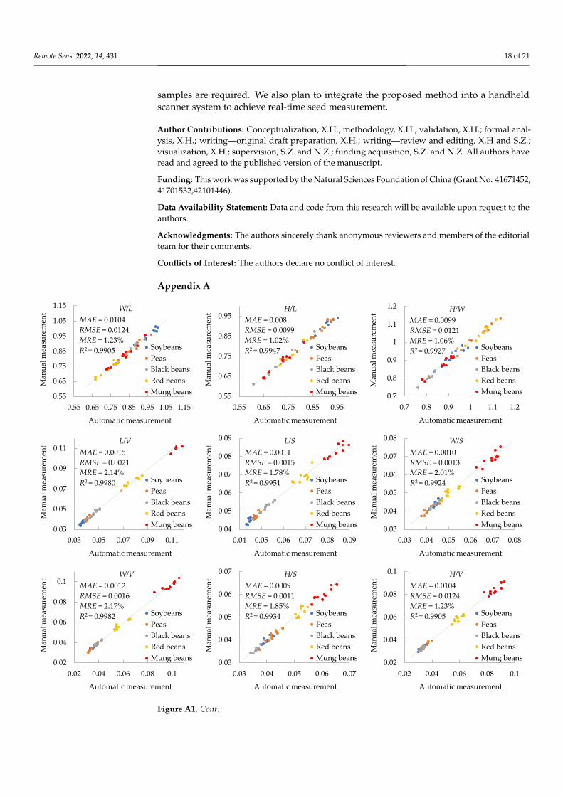
Remote Sens. 2022, 14, 431 18 of 21

samples are required. We also plan to integrate the proposed method into a handheldscanner system to achieve real-time seed measurement.

Author Contributions: Conceptualization, X.H.; methodology, X.H.; validation, X.H.; formal anal-ysis, X.H.; writing—original draft preparation, X.H.; writing—review and editing, X.H and S.Z.;visualization, X.H.; supervision, S.Z. and N.Z.; funding acquisition, S.Z. and N.Z. All authors haveread and agreed to the published version of the manuscript.

Funding: This work was supported by the Natural Sciences Foundation of China (Grant No. 41671452,41701532,42101446).

Data Availability Statement: Data and code from this research will be available upon request to theauthors.

Acknowledgments: The authors sincerely thank anonymous reviewers and members of the editorialteam for their comments.

Conflicts of Interest: The authors declare no conflict of interest.

Appendix A

Remote Sens. 2022, 14, x FOR PEER REVIEW 18 of 22

in seed quality evaluation, optimization breeding, and a yield trait scorer, where large

samples are required. We also plan to integrate the proposed method into a handheld

scanner system to achieve real-time seed measurement.

Author Contributions: Conceptualization, X.H.; methodology, X.H.; validation, X.H.; formal anal-

ysis, X.H.; writing—original draft preparation, X.H.; writing—review and editing, X.H and S.Z.;

visualization, X.H.; supervision, S.Z. and N.Z.; funding acquisition, S.Z. and N.Z. All authors have

read and agreed to the published version of the manuscript.

Funding: This work was supported by the Natural Sciences Foundation of China (Grant No.

41671452, 41701532,42101446).

Data Availability Statement: Data and code from this research will be available upon request to the

authors.

Acknowledgments: The authors sincerely thank anonymous reviewers and members of the edito-

rial team for their comments.

Conflicts of Interest: The authors declare no conflicts of interest.

Appendix A

0.55

0.65

0.75

0.85

0.95

1.05

1.15

0.55 0.65 0.75 0.85 0.95 1.05 1.15

Man

ual

mea

sure

men

t

Automatic measurement

W/L

Soybeans

Peas

Black beans

Red beans

Mung beans

MAE = 0.0104

RMSE = 0.0124

MRE = 1.23%

R2 = 0.9905

0.55

0.65

0.75

0.85

0.95

0.55 0.65 0.75 0.85 0.95

Man

ual

mea

sure

men

t

Automatic measurement

H/L

Soybeans

Peas

Black beans

Red beans

Mung beans

MAE = 0.008

RMSE = 0.0099

MRE = 1.02%

R2 = 0.9947

0.7

0.8

0.9

1

1.1

1.2

0.7 0.8 0.9 1 1.1 1.2

Man

ual

mea

sure

men

t

Automatic measurement

H/W

Soybeans

Peas

Black beans

Red beans

Mung beans

MAE = 0.0099

RMSE = 0.0121

MRE = 1.06%

R2 = 0.9927

0.03

0.05

0.07

0.09

0.11

0.03 0.05 0.07 0.09 0.11

Man

ual

mea

sure

men

t

Automatic measurement

L/V

Soybeans

Peas

Black beans

Red beans

Mung beans

MAE = 0.0015

RMSE = 0.0021

MRE = 2.14%

R2 = 0.9980

0.04

0.05

0.06

0.07

0.08

0.09

0.04 0.05 0.06 0.07 0.08 0.09

Man

ual

mea

sure

men

t

Automatic measurement

L/S

Soybeans

Peas

Black beans

Red beans

Mung beans

MAE = 0.0011

RMSE = 0.0015

MRE = 1.78%

R2 = 0.9951

0.03

0.04

0.05

0.06

0.07

0.08

0.03 0.04 0.05 0.06 0.07 0.08

Man

ual

mea

sure

men

t

Automatic measurement

W/S

Soybeans

Peas

Black beans

Red beans

Mung beans

MAE = 0.0010

RMSE = 0.0013

MRE = 2.01%

R2 = 0.9924

0.02

0.04

0.06

0.08

0.1

0.02 0.04 0.06 0.08 0.1

Man

ual

mea

sure

men

t

Automatic measurement

W/V

Soybeans

Peas

Black beans

Red beans

Mung beans

MAE = 0.0012

RMSE = 0.0016

MRE = 2.17%

R2 = 0.9982

0.03

0.04

0.05

0.06

0.07

0.03 0.04 0.05 0.06 0.07

Man

ual

mea

sure

men

t

Automatic measurement

H/S

Soybeans

Peas

Black beans

Red beans

Mung beans

MAE = 0.0009

RMSE = 0.0011

MRE = 1.85%

R2 = 0.9934

0.02

0.04

0.06

0.08

0.1

0.02 0.04 0.06 0.08 0.1

Man

ual

mea

sure

men

t

Automatic measurement

H/V

Soybeans

Peas

Black beans

Red beans

Mung beans

MAE = 0.0104

RMSE = 0.0124

MRE = 1.23%

R2 = 0.9905

Figure A1. Cont.

Page 19

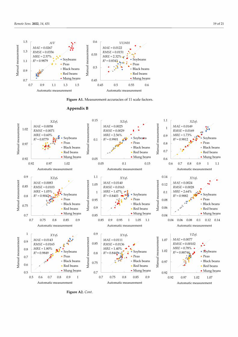
Remote Sens. 2022, 14, 431 19 of 21Remote Sens. 2022, 14, x FOR PEER REVIEW 19 of 22

Figure A1. Measurement Accuracies of 11 Scale Factors.

Appendix B

0.7

0.9

1.1

1.3

1.5

0.7 0.9 1.1 1.3 1.5

Man

ual

mea

sure

men

t

Automatic measurement

A/V

Soybeans

Peas

Black beans

Red beans

Mung beans

MAE = 0.0267

RMSE = 0.0356

MRE = 2.57%

R2 = 0.9879

0.45

0.5

0.55

0.6

0.45 0.5 0.55 0.6M

anu

al m

easu

rem

ent

Automatic measurement

V/LWH

Soybeans

Peas

Black beans

Red beans

Mung beans

MAE = 0.0122

RMSE = 0.0151

MRE = 2.32%

R2 = 0.8343

0.92

0.97

1.02

0.92 0.97 1.02

Man

ual

mea

sure

men

t

Automatic measurement

XZsf₁

Soybeans

Peas

Black beans

Red beans

Mung beans

MAE = 0.0058

RMSE = 0.0071

MRE = 0.60%

R2 = 0.8779

0.05

0.1

0.15

0.05 0.1 0.15

Man

ual

mea

sure

men

t

Automatic measurement

XZsf₂

Soybeans

Peas

Black beans

Red beans

Mung beans

MAE = 0.0025

RMSE = 0.0029

MRE = 2.56%

R2 = 0.9901

0.6

0.7

0.8

0.9

1

1.1

0.6 0.7 0.8 0.9 1 1.1

Man

ual

mea

sure

men

t

Automatic measurement

XZsf₃

Soybeans

Peas

Black beans

Red beans

Mung beans

MAE = 0.0149

RMSE = 0.0169

MRE = 1.73%

R2 = 0.9812

0.7

0.75

0.8

0.85

0.9

0.7 0.75 0.8 0.85 0.9

Man

ual

mea

sure

men

t

Automatic measurement

XZsf₄

Soybeans

Peas

Black beans

Red beans

Mung beans

MAE = 0.0083

RMSE = 0.0103

MRE = 1.05%

R2 = 0.9042

0.85

0.9

0.95

1

1.05

1.1

0.85 0.9 0.95 1 1.05 1.1

Man

ual

mea

sure

men

t

Automatic measurement

XYsf₁

Soybeans

Peas

Black beans

Red beans

Mung beans

MAE = 0.0140

RMSE = 0.0163

MRE = 1.47%

R2 = 0.8403

0.04

0.06

0.08

0.1

0.12

0.14

0.04 0.06 0.08 0.1 0.12 0.14

Man

ual

mea

sure

men

t

Automatic measurement

XYsf₂

Soybeans

Peas

Black beans

Red beans

Mung beans

MAE = 0.0024

RMSE = 0.0028

MRE = 2.64%

R2 = 0.9882

0.5

0.6

0.7

0.8

0.9

1

0.5 0.6 0.7 0.8 0.9 1

Man

ual

mea

sure

men

t

Automatic measurement

XYsf₃

Soybeans

Peas

Black beans

Red beans

Mung beans

MAE = 0.0143

RMSE = 0.0165

MRE = 1.80%

R2 = 0.9849

0.7

0.75

0.8

0.85

0.9

0.7 0.75 0.8 0.85 0.9

Man

ual

mea

sure

men

t

Automatic measurement

XYsf₄

Soybeans

Peas

Black beans

Red beans

Mung beans

MAE = 0.0111

RMSE = 0.0136

MRE = 1.40%

R2 = 0.8445

0.92

0.97

1.02

1.07

0.92 0.97 1.02 1.07

Man

ual

mea

sure

men

t

Automatic measurement

YZsf₁

Soybeans

Peas

Black beans

Red beans

Mung beans

MAE = 0.0077

RMSE = 0.00102

MRE = 0.78%

R2 = 0.88744

Figure A1. Measurement accuracies of 11 scale factors.

Appendix B

Remote Sens. 2022, 14, x FOR PEER REVIEW 19 of 22

Figure A1. Measurement Accuracies of 11 Scale Factors.

Appendix B

0.7

0.9

1.1

1.3

1.5

0.7 0.9 1.1 1.3 1.5

Man

ual

mea

sure

men

t

Automatic measurement

A/V

Soybeans

Peas

Black beans

Red beans

Mung beans

MAE = 0.0267

RMSE = 0.0356

MRE = 2.57%

R2 = 0.9879

0.45

0.5

0.55

0.6

0.45 0.5 0.55 0.6M

anu

al m

easu

rem

ent

Automatic measurement

V/LWH

Soybeans

Peas

Black beans

Red beans

Mung beans

MAE = 0.0122

RMSE = 0.0151

MRE = 2.32%

R2 = 0.8343

0.92

0.97

1.02

0.92 0.97 1.02

Man

ual

mea

sure

men

t

Automatic measurement

XZsf₁

Soybeans

Peas

Black beans

Red beans

Mung beans

MAE = 0.0058

RMSE = 0.0071

MRE = 0.60%

R2 = 0.8779

0.05

0.1

0.15

0.05 0.1 0.15

Man

ual

mea

sure

men

t

Automatic measurement

XZsf₂

Soybeans

Peas

Black beans

Red beans

Mung beans

MAE = 0.0025

RMSE = 0.0029

MRE = 2.56%

R2 = 0.9901

0.6

0.7

0.8

0.9

1

1.1

0.6 0.7 0.8 0.9 1 1.1

Man

ual

mea

sure

men

t

Automatic measurement

XZsf₃

Soybeans

Peas

Black beans

Red beans

Mung beans

MAE = 0.0149

RMSE = 0.0169

MRE = 1.73%

R2 = 0.9812

0.7

0.75

0.8

0.85

0.9

0.7 0.75 0.8 0.85 0.9

Man

ual

mea

sure

men

t

Automatic measurement

XZsf₄

Soybeans

Peas

Black beans

Red beans

Mung beans

MAE = 0.0083

RMSE = 0.0103

MRE = 1.05%

R2 = 0.9042

0.85

0.9

0.95

1

1.05

1.1

0.85 0.9 0.95 1 1.05 1.1

Man

ual

mea

sure

men

t

Automatic measurement

XYsf₁

Soybeans

Peas

Black beans

Red beans

Mung beans

MAE = 0.0140

RMSE = 0.0163

MRE = 1.47%

R2 = 0.8403

0.04

0.06

0.08

0.1

0.12

0.14

0.04 0.06 0.08 0.1 0.12 0.14

Man

ual

mea

sure

men

t

Automatic measurement

XYsf₂

Soybeans

Peas

Black beans

Red beans

Mung beans

MAE = 0.0024

RMSE = 0.0028

MRE = 2.64%

R2 = 0.9882

0.5

0.6

0.7

0.8

0.9

1

0.5 0.6 0.7 0.8 0.9 1

Man

ual

mea

sure

men

t

Automatic measurement

XYsf₃

Soybeans

Peas

Black beans

Red beans

Mung beans

MAE = 0.0143

RMSE = 0.0165

MRE = 1.80%

R2 = 0.9849

0.7

0.75

0.8

0.85

0.9

0.7 0.75 0.8 0.85 0.9

Man

ual

mea

sure

men

t

Automatic measurement

XYsf₄

Soybeans

Peas

Black beans

Red beans

Mung beans

MAE = 0.0111

RMSE = 0.0136

MRE = 1.40%

R2 = 0.8445

0.92

0.97

1.02

1.07

0.92 0.97 1.02 1.07

Man

ual

mea

sure

men

t

Automatic measurement

YZsf₁

Soybeans

Peas

Black beans

Red beans

Mung beans

MAE = 0.0077

RMSE = 0.00102

MRE = 0.78%

R2 = 0.88744

Figure A2. Cont.

Page 20

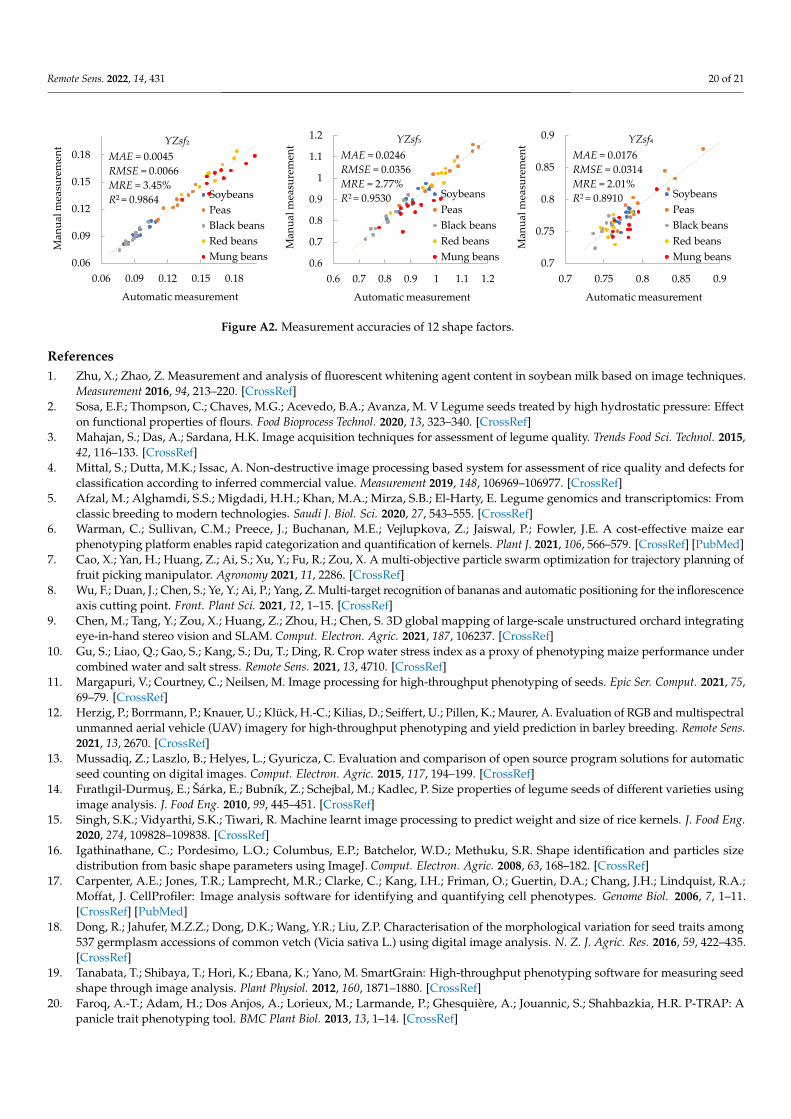
Remote Sens. 2022, 14, 431 20 of 21Remote Sens. 2022, 14, x FOR PEER REVIEW 20 of 22

Figure A2. Measurement Accuracies of 12 Shape Factors.

References

1. Zhu, X.; Zhao, Z. Measurement and analysis of fluorescent whitening agent content in soybean milk based on image techniques.

Measurement 2016, 94, 213–220. https://doi.org/10.1016/j.measurement.2016.07.068.

2. Sosa, E.F.; Thompson, C.; Chaves, M.G.; Acevedo, B.A.; Avanza, M. V Legume seeds treated by high hydrostatic pressure: Effect

on functional properties of flours. Food Bioprocess Technol. 2020, 13, 323–340. https://doi.org/10.1007/s11947-019-02386-9.

3. Mahajan, S.; Das, A.; Sardana, H.K. Image acquisition techniques for assessment of legume quality. Trends Food Sci. Technol.

2015, 42, 116–133. https://doi.org/10.1016/j.tifs.2015.01.001.

4. Mittal, S.; Dutta, M.K.; Issac, A. Non-destructive image processing based system for assessment of rice quality and defects for

classification according to inferred commercial value. Measurement 2019, 148, 106969–106977.

https://doi.org/10.1016/j.measurement.2019.106969.

5. Afzal, M.; Alghamdi, S.S.; Migdadi, H.H.; Khan, M.A.; Mirza, S.B.; El-Harty, E. Legume genomics and transcriptomics: From

classic breeding to modern technologies. Saudi J. Biol. Sci. 2020, 27, 543–555. https://doi.org/10.1016/j.sjbs.2019.11.018.

6. Warman, C.; Sullivan, C.M.; Preece, J.; Buchanan, M.E.; Vejlupkova, Z.; Jaiswal, P.; Fowler, J.E. A cost-effective maize ear

phenotyping platform enables rapid categorization and quantification of kernels. Plant J. 2021, 106, 566–579.

https://doi.org/10.1101/2020.07.12.199000.

7. Cao, X.; Yan, H.; Huang, Z.; Ai, S.; Xu, Y.; Fu, R.; Zou, X. A multi-objective particle swarm optimization for trajectory planning

of fruit picking manipulator. Agronomy 2021, 11, 2286. https://doi.org/10.3390/agronomy11112286.

8. Wu, F.; Duan, J.; Chen, S.; Ye, Y.; Ai, P.; Yang, Z. Multi-target recognition of bananas and automatic positioning for the

inflorescence axis cutting point. Front. Plant Sci. 2021, 12, 1-15. https://doi.org/10.3389/fpls.2021.705021.

9. Chen, M.; Tang, Y.; Zou, X.; Huang, Z.; Zhou, H.; Chen, S. 3D global mapping of large-scale unstructured orchard integrating

eye-in-hand stereo vision and SLAM. Comput. Electron. Agric. 2021, 187, 106237. https://doi.org/10.1016/j.compag.2021.106237.

10. Gu, S.; Liao, Q.; Gao, S.; Kang, S.; Du, T.; Ding, R. Crop water stress index as a proxy of phenotyping maize performance under

combined water and salt stress. Remote Sens. 2021, 13, 4710. https://doi.org/10.3390/rs13224710.

11. Margapuri, V.; Courtney, C.; Neilsen, M. Image processing for high-throughput phenotyping of seeds. Epic Ser. Comput. 2021,

75, 69–79. https://doi.org/10.29007/x4p4.

12. Herzig, P.; Borrmann, P.; Knauer, U.; Klück, H.-C.; Kilias, D.; Seiffert, U.; Pillen, K.; Maurer, A. Evaluation of RGB and

multispectral unmanned aerial vehicle (UAV) imagery for high-throughput phenotyping and yield prediction in barley

breeding. Remote Sens. 2021, 13, 2670. https://doi.org/10.3390/rs13142670.

13. Mussadiq, Z.; Laszlo, B.; Helyes, L.; Gyuricza, C. Evaluation and comparison of open source program solutions for automatic

seed counting on digital images. Comput. Electron. Agric. 2015, 117, 194–199. https://doi.org/10.1016/j.compag.2015.08.010.

14. Fıratlıgil-Durmuş, E.; Šárka, E.; Bubník, Z.; Schejbal, M.; Kadlec, P. Size properties of legume seeds of different varieties using

image analysis. J. Food Eng. 2010, 99, 445–451. https://doi.org/10.1016/j.jfoodeng.2009.08.005.

15. Singh, S.K.; Vidyarthi, S.K.; Tiwari, R. Machine learnt image processing to predict weight and size of rice kernels. J. Food Eng.

2020, 274, 109828–109838. https://doi.org/10.1101/743427.

16. Igathinathane, C.; Pordesimo, L.O.; Columbus, E.P.; Batchelor, W.D.; Methuku, S.R. Shape identification and particles size

distribution from basic shape parameters using ImageJ. Comput. Electron. Agric. 2008, 63, 168–182.

https://doi.org/10.1016/j.compag.2008.02.007.

17. Carpenter, A.E.; Jones, T.R.; Lamprecht, M.R.; Clarke, C.; Kang, I.H.; Friman, O.; Guertin, D.A.; Chang, J.H.; Lindquist, R.A.;

Moffat, J. CellProfiler: Image analysis software for identifying and quantifying cell phenotypes. Genome Biol. 2006, 7, 1–11.

https://doi.org/10.1186/gb-2006-7-10-r100.

18. Dong, R.; Jahufer, M.Z.Z.; Dong, D.K.; Wang, Y.R.; Liu, Z.P. Characterisation of the morphological variation for seed traits

among 537 germplasm accessions of common vetch (Vicia sativa L.) using digital image analysis. N. Z. J. Agric. Res. 2016, 59,

422–435. https://doi.org/10.1080/00288233.2016.1229682.

19. Tanabata, T.; Shibaya, T.; Hori, K.; Ebana, K.; Yano, M. SmartGrain: High-throughput phenotyping software for measuring seed

shape through image analysis. Plant Physiol. 2012, 160, 1871–1880. https://doi.org/10.2307/41812032.

0.06

0.09

0.12

0.15

0.18

0.06 0.09 0.12 0.15 0.18

Man

ual

mea

sure

men

t

Automatic measurement

YZsf₂

Soybeans

Peas

Black beans

Red beans

Mung beans

MAE = 0.0045

RMSE = 0.0066

MRE = 3.45%

R2 = 0.9864

0.6

0.7

0.8

0.9

1

1.1

1.2

0.6 0.7 0.8 0.9 1 1.1 1.2M

anu

al m

easu

rem

ent

Automatic measurement

YZsf₃

Soybeans

Peas

Black beans

Red beans

Mung beans

MAE = 0.0246

RMSE = 0.0356

MRE = 2.77%

R2 = 0.9530

0.7

0.75

0.8

0.85

0.9

0.7 0.75 0.8 0.85 0.9

Man

ual

mea

sure

men

t

Automatic measurement

YZsf₄

Soybeans

Peas

Black beans

Red beans

Mung beans

MAE = 0.0176

RMSE = 0.0314

MRE = 2.01%

R2 = 0.8910

Figure A2. Measurement accuracies of 12 shape factors.

References1. Zhu, X.; Zhao, Z. Measurement and analysis of fluorescent whitening agent content in soybean milk based on image techniques.

Measurement 2016, 94, 213–220. [CrossRef]2. Sosa, E.F.; Thompson, C.; Chaves, M.G.; Acevedo, B.A.; Avanza, M. V Legume seeds treated by high hydrostatic pressure: Effect

on functional properties of flours. Food Bioprocess Technol. 2020, 13, 323–340. [CrossRef]3. Mahajan, S.; Das, A.; Sardana, H.K. Image acquisition techniques for assessment of legume quality. Trends Food Sci. Technol. 2015,

42, 116–133. [CrossRef]4. Mittal, S.; Dutta, M.K.; Issac, A. Non-destructive image processing based system for assessment of rice quality and defects for

classification according to inferred commercial value. Measurement 2019, 148, 106969–106977. [CrossRef]5. Afzal, M.; Alghamdi, S.S.; Migdadi, H.H.; Khan, M.A.; Mirza, S.B.; El-Harty, E. Legume genomics and transcriptomics: From

classic breeding to modern technologies. Saudi J. Biol. Sci. 2020, 27, 543–555. [CrossRef]6. Warman, C.; Sullivan, C.M.; Preece, J.; Buchanan, M.E.; Vejlupkova, Z.; Jaiswal, P.; Fowler, J.E. A cost-effective maize ear

phenotyping platform enables rapid categorization and quantification of kernels. Plant J. 2021, 106, 566–579. [CrossRef] [PubMed]7. Cao, X.; Yan, H.; Huang, Z.; Ai, S.; Xu, Y.; Fu, R.; Zou, X. A multi-objective particle swarm optimization for trajectory planning of

fruit picking manipulator. Agronomy 2021, 11, 2286. [CrossRef]8. Wu, F.; Duan, J.; Chen, S.; Ye, Y.; Ai, P.; Yang, Z. Multi-target recognition of bananas and automatic positioning for the inflorescence

axis cutting point. Front. Plant Sci. 2021, 12, 1–15. [CrossRef]9. Chen, M.; Tang, Y.; Zou, X.; Huang, Z.; Zhou, H.; Chen, S. 3D global mapping of large-scale unstructured orchard integrating

eye-in-hand stereo vision and SLAM. Comput. Electron. Agric. 2021, 187, 106237. [CrossRef]10. Gu, S.; Liao, Q.; Gao, S.; Kang, S.; Du, T.; Ding, R. Crop water stress index as a proxy of phenotyping maize performance under

combined water and salt stress. Remote Sens. 2021, 13, 4710. [CrossRef]11. Margapuri, V.; Courtney, C.; Neilsen, M. Image processing for high-throughput phenotyping of seeds. Epic Ser. Comput. 2021, 75,

69–79. [CrossRef]12. Herzig, P.; Borrmann, P.; Knauer, U.; Klück, H.-C.; Kilias, D.; Seiffert, U.; Pillen, K.; Maurer, A. Evaluation of RGB and multispectral

unmanned aerial vehicle (UAV) imagery for high-throughput phenotyping and yield prediction in barley breeding. Remote Sens.2021, 13, 2670. [CrossRef]

13. Mussadiq, Z.; Laszlo, B.; Helyes, L.; Gyuricza, C. Evaluation and comparison of open source program solutions for automaticseed counting on digital images. Comput. Electron. Agric. 2015, 117, 194–199. [CrossRef]

14. Fıratlıgil-Durmus, E.; Šárka, E.; Bubník, Z.; Schejbal, M.; Kadlec, P. Size properties of legume seeds of different varieties usingimage analysis. J. Food Eng. 2010, 99, 445–451. [CrossRef]

15. Singh, S.K.; Vidyarthi, S.K.; Tiwari, R. Machine learnt image processing to predict weight and size of rice kernels. J. Food Eng.2020, 274, 109828–109838. [CrossRef]

16. Igathinathane, C.; Pordesimo, L.O.; Columbus, E.P.; Batchelor, W.D.; Methuku, S.R. Shape identification and particles sizedistribution from basic shape parameters using ImageJ. Comput. Electron. Agric. 2008, 63, 168–182. [CrossRef]

17. Carpenter, A.E.; Jones, T.R.; Lamprecht, M.R.; Clarke, C.; Kang, I.H.; Friman, O.; Guertin, D.A.; Chang, J.H.; Lindquist, R.A.;Moffat, J. CellProfiler: Image analysis software for identifying and quantifying cell phenotypes. Genome Biol. 2006, 7, 1–11.[CrossRef] [PubMed]

18. Dong, R.; Jahufer, M.Z.Z.; Dong, D.K.; Wang, Y.R.; Liu, Z.P. Characterisation of the morphological variation for seed traits among537 germplasm accessions of common vetch (Vicia sativa L.) using digital image analysis. N. Z. J. Agric. Res. 2016, 59, 422–435.[CrossRef]

19. Tanabata, T.; Shibaya, T.; Hori, K.; Ebana, K.; Yano, M. SmartGrain: High-throughput phenotyping software for measuring seedshape through image analysis. Plant Physiol. 2012, 160, 1871–1880. [CrossRef]

20. Faroq, A.-T.; Adam, H.; Dos Anjos, A.; Lorieux, M.; Larmande, P.; Ghesquière, A.; Jouannic, S.; Shahbazkia, H.R. P-TRAP: Apanicle trait phenotyping tool. BMC Plant Biol. 2013, 13, 1–14. [CrossRef]

Page 21

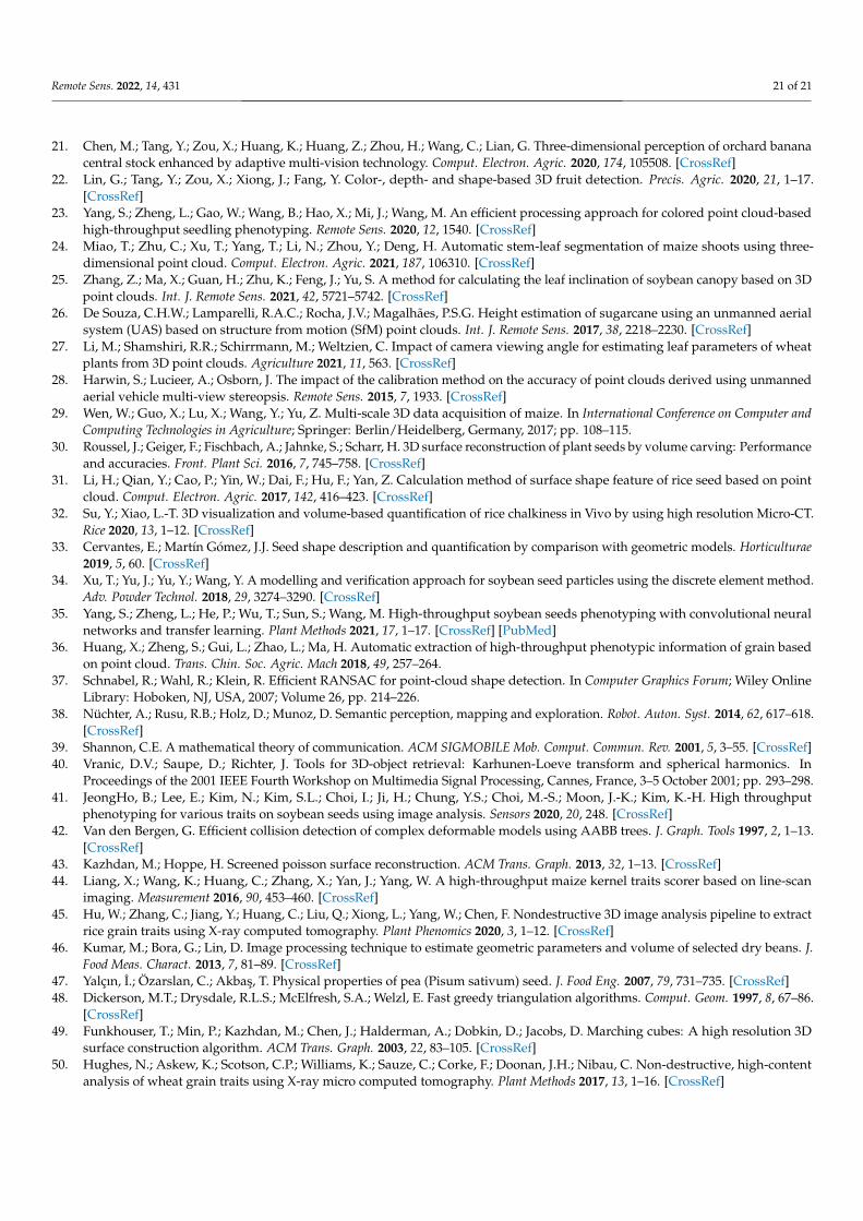
Remote Sens. 2022, 14, 431 21 of 21

21. Chen, M.; Tang, Y.; Zou, X.; Huang, K.; Huang, Z.; Zhou, H.; Wang, C.; Lian, G. Three-dimensional perception of orchard bananacentral stock enhanced by adaptive multi-vision technology. Comput. Electron. Agric. 2020, 174, 105508. [CrossRef]

22. Lin, G.; Tang, Y.; Zou, X.; Xiong, J.; Fang, Y. Color-, depth- and shape-based 3D fruit detection. Precis. Agric. 2020, 21, 1–17.[CrossRef]

23. Yang, S.; Zheng, L.; Gao, W.; Wang, B.; Hao, X.; Mi, J.; Wang, M. An efficient processing approach for colored point cloud-basedhigh-throughput seedling phenotyping. Remote Sens. 2020, 12, 1540. [CrossRef]

24. Miao, T.; Zhu, C.; Xu, T.; Yang, T.; Li, N.; Zhou, Y.; Deng, H. Automatic stem-leaf segmentation of maize shoots using three-dimensional point cloud. Comput. Electron. Agric. 2021, 187, 106310. [CrossRef]

25. Zhang, Z.; Ma, X.; Guan, H.; Zhu, K.; Feng, J.; Yu, S. A method for calculating the leaf inclination of soybean canopy based on 3Dpoint clouds. Int. J. Remote Sens. 2021, 42, 5721–5742. [CrossRef]

26. De Souza, C.H.W.; Lamparelli, R.A.C.; Rocha, J.V.; Magalhães, P.S.G. Height estimation of sugarcane using an unmanned aerialsystem (UAS) based on structure from motion (SfM) point clouds. Int. J. Remote Sens. 2017, 38, 2218–2230. [CrossRef]

27. Li, M.; Shamshiri, R.R.; Schirrmann, M.; Weltzien, C. Impact of camera viewing angle for estimating leaf parameters of wheatplants from 3D point clouds. Agriculture 2021, 11, 563. [CrossRef]

28. Harwin, S.; Lucieer, A.; Osborn, J. The impact of the calibration method on the accuracy of point clouds derived using unmannedaerial vehicle multi-view stereopsis. Remote Sens. 2015, 7, 1933. [CrossRef]

29. Wen, W.; Guo, X.; Lu, X.; Wang, Y.; Yu, Z. Multi-scale 3D data acquisition of maize. In International Conference on Computer andComputing Technologies in Agriculture; Springer: Berlin/Heidelberg, Germany, 2017; pp. 108–115.

30. Roussel, J.; Geiger, F.; Fischbach, A.; Jahnke, S.; Scharr, H. 3D surface reconstruction of plant seeds by volume carving: Performanceand accuracies. Front. Plant Sci. 2016, 7, 745–758. [CrossRef]

31. Li, H.; Qian, Y.; Cao, P.; Yin, W.; Dai, F.; Hu, F.; Yan, Z. Calculation method of surface shape feature of rice seed based on pointcloud. Comput. Electron. Agric. 2017, 142, 416–423. [CrossRef]

32. Su, Y.; Xiao, L.-T. 3D visualization and volume-based quantification of rice chalkiness in Vivo by using high resolution Micro-CT.Rice 2020, 13, 1–12. [CrossRef]

33. Cervantes, E.; Martín Gómez, J.J. Seed shape description and quantification by comparison with geometric models. Horticulturae2019, 5, 60. [CrossRef]

34. Xu, T.; Yu, J.; Yu, Y.; Wang, Y. A modelling and verification approach for soybean seed particles using the discrete element method.Adv. Powder Technol. 2018, 29, 3274–3290. [CrossRef]

35. Yang, S.; Zheng, L.; He, P.; Wu, T.; Sun, S.; Wang, M. High-throughput soybean seeds phenotyping with convolutional neuralnetworks and transfer learning. Plant Methods 2021, 17, 1–17. [CrossRef] [PubMed]

36. Huang, X.; Zheng, S.; Gui, L.; Zhao, L.; Ma, H. Automatic extraction of high-throughput phenotypic information of grain basedon point cloud. Trans. Chin. Soc. Agric. Mach 2018, 49, 257–264.

37. Schnabel, R.; Wahl, R.; Klein, R. Efficient RANSAC for point-cloud shape detection. In Computer Graphics Forum; Wiley OnlineLibrary: Hoboken, NJ, USA, 2007; Volume 26, pp. 214–226.

38. Nüchter, A.; Rusu, R.B.; Holz, D.; Munoz, D. Semantic perception, mapping and exploration. Robot. Auton. Syst. 2014, 62, 617–618.[CrossRef]

39. Shannon, C.E. A mathematical theory of communication. ACM SIGMOBILE Mob. Comput. Commun. Rev. 2001, 5, 3–55. [CrossRef]40. Vranic, D.V.; Saupe, D.; Richter, J. Tools for 3D-object retrieval: Karhunen-Loeve transform and spherical harmonics. In

Proceedings of the 2001 IEEE Fourth Workshop on Multimedia Signal Processing, Cannes, France, 3–5 October 2001; pp. 293–298.41. JeongHo, B.; Lee, E.; Kim, N.; Kim, S.L.; Choi, I.; Ji, H.; Chung, Y.S.; Choi, M.-S.; Moon, J.-K.; Kim, K.-H. High throughput

phenotyping for various traits on soybean seeds using image analysis. Sensors 2020, 20, 248. [CrossRef]42. Van den Bergen, G. Efficient collision detection of complex deformable models using AABB trees. J. Graph. Tools 1997, 2, 1–13.

[CrossRef]43. Kazhdan, M.; Hoppe, H. Screened poisson surface reconstruction. ACM Trans. Graph. 2013, 32, 1–13. [CrossRef]44. Liang, X.; Wang, K.; Huang, C.; Zhang, X.; Yan, J.; Yang, W. A high-throughput maize kernel traits scorer based on line-scan

imaging. Measurement 2016, 90, 453–460. [CrossRef]45. Hu, W.; Zhang, C.; Jiang, Y.; Huang, C.; Liu, Q.; Xiong, L.; Yang, W.; Chen, F. Nondestructive 3D image analysis pipeline to extract

rice grain traits using X-ray computed tomography. Plant Phenomics 2020, 3, 1–12. [CrossRef]46. Kumar, M.; Bora, G.; Lin, D. Image processing technique to estimate geometric parameters and volume of selected dry beans. J.

Food Meas. Charact. 2013, 7, 81–89. [CrossRef]47. Yalçın, I.; Özarslan, C.; Akbas, T. Physical properties of pea (Pisum sativum) seed. J. Food Eng. 2007, 79, 731–735. [CrossRef]48. Dickerson, M.T.; Drysdale, R.L.S.; McElfresh, S.A.; Welzl, E. Fast greedy triangulation algorithms. Comput. Geom. 1997, 8, 67–86.

[CrossRef]49. Funkhouser, T.; Min, P.; Kazhdan, M.; Chen, J.; Halderman, A.; Dobkin, D.; Jacobs, D. Marching cubes: A high resolution 3D

surface construction algorithm. ACM Trans. Graph. 2003, 22, 83–105. [CrossRef]50. Hughes, N.; Askew, K.; Scotson, C.P.; Williams, K.; Sauze, C.; Corke, F.; Doonan, J.H.; Nibau, C. Non-destructive, high-content

analysis of wheat grain traits using X-ray micro computed tomography. Plant Methods 2017, 13, 1–16. [CrossRef]