High-speed Decision-making in Archerfish (Hochgeschwindigkeits-Entscheidungsfindung bei Schützenfischen) Der Naturwissenschaftlichen Fakultät der Friedrich-Alexander-Universität Erlangen-Nürnberg zur Erlangung des Doktorgrades Dr. rer. nat. vorgelegt von Thomas Schlegel aus Nürnberg

Welcome message from author
This document is posted to help you gain knowledge. Please leave a comment to let me know what you think about it! Share it to your friends and learn new things together.
Transcript

High-speed Decision-making in Archerfish
(Hochgeschwindigkeits-Entscheidungsfindung bei
Schützenfischen)
Der Naturwissenschaftlichen Fakultät
der Friedrich-Alexander-Universität Erlangen-Nürnberg
zur
Erlangung des Doktorgrades Dr. rer. nat.
vorgelegt von
Thomas Schlegel
aus Nürnberg

Als Dissertation genehmigt von der
Naturwissenschaftlichen Fakultät der Friedrich-Alexander-
Universität Erlangen-Nürnberg
Tag der mündlichen Prüfung: 08. Juni 2010
Vorsitzender der
Promotionskommission: Prof. Dr. Eberhard Bänsch
Erstberichterstatter: Prof. Dr. Stefan Schuster
Zweitberichterstatter: Prof. Dr. Helmut Brandstätter

High-speed Decision-making in Archerfish

Abstract
4
1. Abstract Archerfish are famous for their ability to dislodge insects (such as flies) by
spitting precisely aimed jets of water at them. Once fish manage to dislodge a
prey of interest, they carefully monitor the initial movement of the prey item,
precisely extracting several critical parameters of movement (such as speed
and direction of prey movement, the distance to and height of prey), promptly
predicting its future impact position, reacting with a swift and accurate turn.
Finally fish accelerate towards that position, snatching their reward as it hits
the water surface. The experiments of this thesis extensively engaged in the
manipulation of the visual input cues, e.g. via changes in contrast levels,
displaying two prey objects simultaneously or depriving the available visual
input of moving prey spatially and temporally. The method of choice was the
study of archerfish behaviour subsequent to the onset of prey movement as
an amalgamation of the whole system!s signal extraction, information
processing, decision-making and overall performing abilities.
In the process, I discovered that the archerfish!s predictive turning behaviour
can be elicited via prey movement alone – no preceding shooting is
necessary (enabling all subsequent experimentation in the first place). The
predictive behaviour is all the more remarkable, since it features the ability to
instantly decide for one of two simultaneously appearing flies, applying a
spatial representation of the outside world in the process. Furthermore fish
keep up their turning accuracy even if prey motion will appear with a spatial
offset to the fish!s point of gaze. The latency of the fish!s responses depends
e.g. on the contrast levels between fly and background. The entire processing
in between the onset of prey movement and the triggering of the fish!s turn
can be delivered within a time frame of 40 milliseconds, severely restricting
the number of underlying neurons. Subsequent experiments revealed a visual
input of less than 300 activated photoreceptors (equivalent to a retinal area of
roughly 0.01 mm) completely suffices to elicit a precise predictive reaction.
The accumulated results prove Archerfish to be a vertebrate system, shaped
for top speed, in which a complex and plastic decision is performed by
surprisingly small circuitry.

Tables
5
2. Tables
2.1 Table of contents
1. Abstract .................................................................................................... 4
2. Tables ....................................................................................................... 5
2.1 Table of contents .................................................................................. 5
2.2 Table of figures ..................................................................................... 7
2.3 Table of supplemental tables ................................................................ 8
3.Introduction ............................................................................................... 9
4. General methods.................................................................................... 16
4.1 Animals and their keeping................................................................... 17
4.2 Recording and managing behavioural data......................................... 19
4.3 Statistics ............................................................................................. 20
4.4 Characterising the fish!s performance................................................. 21
4.4.1 Latency ........................................................................................ 21
4.4.2 Precision and Error....................................................................... 22
4.5 Seven criteria separating the analysable from the discarded reactions 24
5. The experiments .................................................................................... 25
5.1 Depriving the fish of shooting-related information ............................... 26
5.1.1 Objectives and Experimental Approach........................................ 26
5.1.2 Results ......................................................................................... 27
5.1.3 Discussion.................................................................................... 30
5.2 Spatial attention .................................................................................. 34
5.2.1 Objectives and Experimental Approach........................................ 34
5.2.2 Results ......................................................................................... 35
5.2.3 Discussion.................................................................................... 37
5.3 Deciding for one of two flies ................................................................ 38
5.3.1 Objectives and Experimental Approach........................................ 38
5.3.2 Results ......................................................................................... 39

Table of contents
6
5.3.3 Discussion.................................................................................... 42
5.4 Contrast dependency.......................................................................... 44
5.4.1 Objectives and Experimental Approach........................................ 44
5.4.2 Results ......................................................................................... 46
5.4.3 Discussion.................................................................................... 48
5.5 Do the fish need a priori information on target height .......................... 50
5.5.1 Objectives and Experimental Approach........................................ 50
5.5.2 Results ......................................................................................... 52
5.5.3 Discussion.................................................................................... 57
5.6 Finding the minimal integration interval ............................................... 59
5.6.1 Objectives and Experimental Approach........................................ 59
5.6.2 Results ......................................................................................... 64
5.6.3 Discussion.................................................................................... 78
5.7 Breeding Archerfish ............................................................................ 81
5.7.1 Objectives and Experimental Approach........................................ 81
5.7.2 Results ......................................................................................... 82
5.7.3 Discussion.................................................................................... 83
6. Discussion.............................................................................................. 87
6.1 A conception of archerfish: from visual input to motor output .............. 88
6.2 Some closing remarks on cognition .................................................... 94
7. References ............................................................................................. 96
9. Supplemental ....................................................................................... 107
10. Acknowledgements ........................................................................... 121
11. Zusammenfassung auf Deutsch ....................................................... 123

Table of figures
7
2.2 Table of figures
Figure 1: Distribution of participating fish species ......................................... 17
Figure 2: Exemplary experimental setup ...................................................... 20
Figure 3: Sequence, visualising latency determination ................................. 21
Figure 4: Sequence, visualising determination of precision .......................... 22
Figure 5: Sign conventions applied in error measurements .......................... 23
Figure 6: Experimental differences in deprived versus natural setup ............ 27
Figure 7: Reactions to natural and deprived conditions are alike .................. 29
Figure 8: Matching fly movement in natural and deprived conditions ............ 30
Figure 9: Using several platforms to test spatial attention............................. 35
Figure 10: Behavioural reactions to horizontal offsets .................................. 36
Figure 11: Two flies simultaneously.............................................................. 39
Figure 12: Providing two flies simultaneously ............................................... 40
Figure 13: Parameters of fly movement........................................................ 41
Figure 14: Experimental setups applied to test for several visual contrasts .. 45
Figure 15: No correlation between latency and the fly!s velocity ................... 46
Figure 16: Changing contrast conditions affects latency but not precision .... 47
Figure 17: Testing ten different contrast levels on two groups of fish............ 48
Figure 18: Experimental setup, testing behaviour to vertical offsets ............. 51
Figure 19: Applicability of method for fish of group B.................................... 52
Figure 20: Responses according to attentional presetting and height ........... 54
Figure 21: The fish do not need a priori information on object height............ 55
Figure 22: Comparability of the applied conditions ....................................... 56
Figure 23: Setup for temporally restricting the available visual input............. 62
Figure 24: Display of the black coating of the depriving pipes ...................... 63
Figure 25: Applied accuracy to measure the fly!s velocity............................. 65
Figure 26: In time reactions depend on input duration .................................. 67
Figure 27: Projecting the flies! movement onto the fish!s retina .................... 68
Figure 28: Control data for reactions to fully available visual input................ 69
Figure 29: Latency of the reactions .............................................................. 70
Figure 30: Bearing errors with respect to both of the fish!s turns .................. 71
Figure 31: Duration and size of the fish!s first and second turns ................... 73

Table of figures
8
Figure 32: First turns of reactions classified as too late ................................ 75
Figure 33: Combining two intervals leads to longer latencies ....................... 77
Figure 34: Injecting procedure ...................................................................... 82
Figure 35: Exemplary images of fertilised eggs and fish larvae .................... 83
Figure 36: Visualisation of processes that lead to a predictive turn............... 93
2.3 Table of supplemental tables
Table 1: Supporting data for figures 7, 8 and 10. ........................................ 107
Table 2: Supporting data for figures 12, 13 and 16. .................................... 108
Table 3: Supporting data for figure 17. ....................................................... 109
Table 4: Supporting data for figures 19, 20, 21 and 22. .............................. 110
Table 5: Supporting data for figures 25 and 26. .......................................... 111
Table 6: Supporting data for figures 26 and 27 A. ...................................... 112
Table 7: Supporting data for figures 27 B and 28. ...................................... 113
Table 8: Supporting data for figure 29. ....................................................... 114
Table 9: Supporting data for figure 30 A. .................................................... 115
Table 10: Supporting data for figure 30 B. .................................................. 116
Table 11: Supporting data for figure 31 A. .................................................. 117
Table 12: Supporting data for figure 31 B. .................................................. 118
Table 13: Supporting data for figure 32. ..................................................... 119
Table 14: Supporting data for figure 33. ..................................................... 120

9
3.Introduction

Introduction
10
During the last couple of years, archerfish proved to feature a diversity of
sophisticated behaviours in addition to their shooting ability. It became
increasingly conceivable that this species features astonishingly fast visual
processing and may provide more than understanding of its shooting
mechanism. However, completely and properly characterising the archerfish!s
behavioural repertoire in the first place is not just bearing an inherent
fascination by itself; it is also fundamentally necessary to provide a decent
basis for further neurobiological studies. Knowledge of as many constraints of
the natural behaviour as possible, will guide the dissection of its function.
This dissection could start with multi-electrode recordings [1, 2] for instance,
or a histological approach – or a combination of both [3]. Concepts about the
"where! and "when! of signal computation within the fish!s brain may be
generated, using functional magnetic resonance imaging [4-9]. The shape and
activity of single cells can be visualised with single-unit recordings with
subsequent cell staining [10-13], even using multi-photon laser scanning
nowadays [14-19]. With such an abundance of neurobiological methods
available, what is the benefit of behavioural studies?
The clear benefit of behavioural studies originates within the chance to study
animals as a whole and entirely intact system, flexibly moving in familiar
territory. In such a system, the single components are precisely co-operating
to perform the sound symphony of animal behaviour. Harmony within that
symphony is the ultimate verification that the system is operating properly, as
a whole. But at the same time – having to cope with a whole symphony can
become a tough challenge. Unless we have the possibility to identify the
functional role of each single unit ("how does a viola sound, compared to a
violin!), the whole issue can become fairly puzzling. But at the same time,
exactly distinguishing each single instrument will probably prevent us from
having a satisfactory musical enjoyment. The same applies for a certain
behavioural pattern – watching animals behave will not inevitably result in
better understanding of the underlying neuronal circuits. Such an
understanding requires plausible concepts about the number and nature of

Introduction
11
units involved, and the way these units are interacting. Finally, drawing
conclusions about the function of a particular unit involved in generating
certain behaviour, makes it necessary to trace that unit within the whole – a
delicate matter.
The archerfish, as the animal of choice in this thesis, features a hunting
strategy that depends on high-speed visual processing. The way that
archerfish behave during hunting is not just extraordinary in itself – it enables
to extract information about the units involved. I will first describe the
behaviour these fish are famous for, before describing which substrate may
underlie their behaviour.
Archerfish are famous for their ability to dislodge stationary as well as moving
insect prey by spitting precisely aimed jets of water [20-28]. These jets are
generated by a blast pipe within the fish!s mouth, formed between a slot in its
palatine and its brawny tongue and are powerful enough to carry water at
remarkable heights of up to twenty times the fish!s own body length [20, 25,
29-31]. Moreover these jets are aimed with top precision and fish are able to
fire them from apparently any viewing angle [26], revealing their superior skill
to accurately evaluate not only the visual offset produced by water refraction
[24, 32, 33], but also the distance to, and the absolute size of prey [34].
Evolutionary reasonable these fish also modify the amount of water spat,
always providing their shots with a "force security factor! of about ten times
more force, than prey animals of a certain size can maximally attain to attach
themselves to vegetation [31]. Typical forces that fish reach with ease suffice
to dislodge prey sizes of up to small lizards [20], but their usual diet consists
of tiny to medium sized insects – like flies – commonly enriched by aquatic
arthropods [20, 21].
Once fish manage to dislodge an aerial prey of interest, they are confronted
with another major challenge: Catching those fast-moving objects. Archerfish
are schooling fish and a dislodged insect will instantly gain attention within the
school. So in order to be rewarded for the shooting investment, the shooter

Introduction
12
has to be really fast to catch his reward. However, depending on its initial
height, the prey might just be in the air for a few 100 milliseconds until it
impacts onto the water surface. So waiting for the lateral line organ to provide
information about the correct impact position would drastically reduce the time
left, reducing the chance to snatch the reward just as much.
So in order to receive a worthwhile payback for the shooting investment, the
best strategy would be to arrive simultaneously with the prey at its impact
position, making the catch the very moment the prey touches the water
surface. According to former research in our lab, fish always reach that impact
position either at the same time with the prey, or slightly subsequent to prey
impact – never earlier than the prey [35, 36], which would be quite disastrous
by the way, for fish do not slow down when they get near the impact position
(for energetic reasons), but rather snatch the prey at full speed [35, 36]. So
when they arrived late, they couldn!t simply turn around and try again – they
would just miss that particular prey. Besides, fish cannot increase their
swimming speed infinitely [37], so the only chance to save time is to trigger
the start towards the prey as soon as possible. Now I will describe the kind of
behaviour directly following a successful dislodgement.
Fish carefully monitor the initial movement of the prey item, and then promptly
react with a swift and accurate turn towards its future impact position, before
they finally start to speed up in that direction [35, 36, 38]. In the process,
precisely monitoring the moving prey is a crucial requirement and former
research reported a very tight time frame of about 100 milliseconds as
sufficient for that [39]. This time frame contains several processes, most likely
happening in three spatially separable areas: (1) the retina, handling all visual
input, probably already extracting important movement parameters (2) the
brain, relaying and perhaps further processing that extracted information and
finally (3) the motor system, not only taking finished orders, but probably
further processing the information. According to published data, the duration
for retinal processing might very well be the most time consuming in this chain
of events [40-42], as it includes the absorption of light by the visual pigment,

Introduction
13
leading to a cascade of biochemical reactions within the photoreceptor cells
[43]. These processes precede downstream computational processes [44-47],
in higher brain areas like the optic tectum for instance. Although lacking
evidence about whether the extracted visual information is computed within
the brain at all, the optic tectum is most likely a candidate to be involved in
these processes, at least as a major input target for retinal ganglion cells [48].
Finally a well-defined and fine-grained order must be released, being
conducted via a pair of huge nerve cells well known as Mauthner cells (named
after the ophthalmologist Ludwig Mauthner), fine-tuning and mediating the
movement orders [49-53]. Although we are again lacking strict knowledge
about whether these cells are actually involved or not, former research in our
lab proves a striking similarity between the predictive turns fish use to aim at
their prey of interest and their C-shaped escape turns [38] evidentially evoked
and conducted by a pair of Mauthner cells, characteristic for all teleost fish –
and as recently discovered fish also feature voluntary control of the onset and
fine-tuning of these characteristic C-shaped body bends [54]. The giant
medullary Mauthner cells may readily distribute the appropriate activation
signal among the primary motorneurons, leading to well-dosed muscular
contraction and hence to accurate turning of the fish!s body. At last the
archerfish now aims towards the future impact position of its prey, ready to
speed up to make the catch.
We do know about the archerfish!s ability to identify the absolute size of prey
items [34], but what about height, direction and velocity? These parameters
are quite variable amongst different hunting situations. So assuming, that fish
are very well capable to instantly react to virtually any falling insect, plus the
assumption that these parameters have to be extracted within a fraction of
100 milliseconds, appoints the fish!s retina most likely as the unit to extract
the parameters named above. In recent years it has been shown that retinae
can extract parameters like relative velocity and direction – all within their cell
layers already [55-57]. The information is conducted through the optic nerve

Introduction
14
and into the brain where it will be transformed into a matching nerve activation
pattern, finally fine-tuning the activation of muscle.
To analyse the conditions that must be fulfilled for top performance two criteria
were used that are of main importance for the fish to successfully make a
catch: the time to trigger the turning (latency), and the turning precision
(accuracy). These criteria were analysed in all of the experiments covered by
this thesis, when appropriate, extended to turn duration and the angular size
of the fish!s turns. The flies! velocities and trajectory lengths were closely
analysed to ensure the comparability of setups, whenever required.
With these criteria at hand, I challenged the fish with various experimental
setups, altering the character of visual input available, checking the fish!s
resulting reactions. The type of input that triggers the predictive turn of fish is
a most important point to know: Is another fish!s shooting necessary, or does
the mere movement of a prey object suffice as a trigger? Since prey
movement suffices (as I will show subsequently), a whole world of
experiments come into reach that would otherwise be impossible to realise.
With prey items starting anytime on my command and from a starting position
defined by me and not by a shooting fish, I am in a position to check if the
fish!s turning behaviour can only be triggered if fish gazed at the point of
expected prey movement, or if and how they would react to a movement
event, starting in the periphery of their visual field, for instance. Starting the
fly!s movement with a vertical offset from the position expected by the fish
would also become possible, just as expanding or decreasing the length of
the flies! trajectory. How if at all, the fish!s reaction depended on certain
contrast levels would then be just as accessible, as testing the fish!s reaction
to more than one prey objects simultaneously starting and moving in contrary
directions. Altogether, defining the character of the parameters and the
duration of their availability, enabled me to challenge the fish with setups that
would never be possible in natural surroundings, thus enabling understanding
of the fish!s behavioural mechanisms via their modified reactions to
completely unexpected and novel visual input.

Introduction
15
When fish decide to react to a falling prey item, performing a predictive turn,
they should carefully decide for the most effective trade-off between the
accuracy of their turn and the speed with which to elicit that turn. This is
probably critical, because inaccurate performance either in extracting the
prey!s movement parameters, or in computing the proper motor reaction, will
most likely lead to the missing of that prey. This trade-off may be the basis for
making the archerfish a high-speed predator with unfailing aiming accuracy.
Although archerfish will perhaps not make it into the squad of model-systems,
lacking the availability of easily generated genetic mutants, research on this
species will certainly and significantly contribute to our understanding of the
mechanisms of visual processing and the essential transformation of the
generated information into proper behaviour, subsequent to computation. At
least these fish will remain a rich source for behavioural studies, since their
willingness to participate in novel and perfectly challenging setups equals their
appetite for just the next fly.

16
4. General methods

4.1. Animals and their keeping
17
4.1 Animals and their keeping
Archerfish belong to the family of Toxotidae (order Perciformes) consisting of
seven species all occurring in fresh, brackish and marine waters from India to
the Philippines, Australia and Polynesia [58, 59] (see figure 1). Toxotes
jaculatrix (PALLAS) and Toxotes chatareus (HAMILTON) are the most
widespread representatives of the genus and all experiments are conducted
on these two species. They commonly inhabit mangrove-lined estuaries
where they can be found hiding amongst the numerous roots or hunting for
insect prey resting on overhanging vegetation. In the laboratory fish were kept
and all experiments were done in large tanks filled with brackish water
(conductivity 3.5 mS/cm; temperature 28 °C; tank measurements either 1.6 m
x 0.6 m x 0.6 m for experiments 5.1 - 5.4; or 1.0 m x 1.0 m x 0.6 m for
experiments 5.5 - 5.6; each filled to a height of 30 cm). Animals were
subjected to a 12:12 light regime and all experiments started no earlier than
five hours after light onset.
Figure 1: Distribution of participating fish species
According to Allen (1978) the distribution of the two archerfish species Toxotes jaculatrix (B) and Toxotes chatareus (C) reaches from India to the Philippines, Australia and Polynesia, as displayed (A). Red dots on the globe (A) represent the distribution of Toxotes jaculatrix; black dots that of Toxotes chatareus.

4.1. Animals and their keeping
18
The behavioural studies were performed with a group of either five Toxotes
jaculatrix (standard length 12 cm (this is the length without the length of the
caudal fin); experiments 5.1 to 5.4, referred to as "group A!), or a mixed group
consisting of three Toxotes jaculatrix and seven Toxotes chatareus. These
are likely to have participated uniformly throughout these experiments, as they
did in similar experiments by my colleague Caro Reinel (personal
communication. The fish!s standard lengths was 12 cm; experiment 5.5 to 5.6,
referred to as "group B!). An additional third group, consisting of four adult and
“retired” Toxotes chatareus participated in the breeding experiment (standard
length 12 to 15 cm; experiment 5.7, "group C!). Fish were purchased from
tropical fish importer (“Stimex Corporation”, “Aquarium Glaser”), caught in the
wild (supposedly in Thailand) and trained in the laboratory for at least one
year previously to all described experiments. Performing precise shooting and
fast predictive reactions were all part of the training, as well as adapting to
being fed by an experimenter. During all behavioural experiments fish were
exclusively rewarded with flies (Calliphora spec. average body lengths of 11.0
mm and fresh weight of roughly 57.0 mg each), receiving an additional
handful of “Cichlid Sticks” (SERA, Heinsberg, Germany) at the end of each
week!s experiments, supplying the fish with vitamins and nutrients to maintain
their health at a standardized high level.

4.2. Recording and managing behavioural data
19
4.2 Recording and managing behavioural data
All behavioural data was obtained by imaging behaving fish at a frame rate of
500 frames per second (resulting in a temporal resolution of 2 ms; shutter
1/500), via digital high-speed video (HotShot 1280, NAC Image Technology,
California, USA). In all experiments the camera was positioned above the
tank, generating a top view of the scenery, using either 20 mm (Nikkor 1:2.8
or Sigma 1:1.8) or 35 mm lenses (Nikkor 1:1.4).
If necessary, a second camera of the same type recorded an additional side
view, using a MASTER-8 (A.M.P.I., Jerusalem, Israel) for synchronous
triggering of both of the cameras. The videos were obtained with HotShot
software (version 1.2.2.3), using *.avi file extensions (resolution 1280 x 1024
pixels), then converted to *.dv using iMovie (version 4.0.1, resolution 720 x
576 pixels) and finally analysed via Object-Image (version 2.12). Analyzing
the videos, generally means breaking down the images of behaving animals
into 2-D coordinates of distinctive fish and fly positions, as well as frame
numbers essentially necessary for further evaluation of data, like gaining
latencies and errors (for details see 4.4).
Although the camera system allowed recordings with regular room
illumination, the tank was diffusely illuminated from below with one or two
halogen lamps, as appropriate (500 W each) for increased contrast in the
recording. One or multiple additional halogen lamps illuminated a white cloth
(cotton), spanned above the tank to increase contrast between the moving fly
and its background, as seen by the fish. Contrast values were gained using a
luminance meter (luminance meter LS-110, Minolta camera, Japan),
averaging luminance values (measured as cd/m2) for background and fly
respectively and converting these values to Michelson contrast (
!
Imax
" Imin
Imax
+ Imin
). All
initial plotting of data was done using OriginPro (version 7.5) and all plots
were further refurbished using CorelDRAW (version 11.633 for Macintosh).
For a general illustration of the behavioural setup, see figure 2.

4.2. Recording and managing behavioural data
20
Figure 2: Exemplary experimental setup
This is an exemplary illustration, showing a typical experimental setup (in this case experiment 5.5), using two simultaneously triggered HotShot cameras. In the background, tank and fish are clearly visible with the two cameras and the testing setup mounted above the water surface. The computer screen in front shows a still image side view of the setup referring to the camera in the middle of the picture (left of the tank). Halogen lamps (not visible) diffusely illuminate the white cloth beyond the upper camera and the bottom of the tank. Several fish (group B) cruise along the tank!s front pane, curious about the things to come.
4.3 Statistics
All statistical evaluation was done using SigmaStat (version 3.11.0), utilizing
Mann-Whitney Rank Sum Tests (U-test), whenever a comparison of two
original datasets was necessary (like latencies of natural versus deprived
conditions, see figure 7 B). Checking for statistical relations of more than two
datasets (like latencies of ten different contrast conditions, see figure 17),
intending to detect differences or attest consistency, One-Way Analysis Of
Variance On Ranks (ANOVA) was utilized, with an additional Dunn!s test, if
appropriate. Regression analysis, as well as statistical comparison of a whole
dataset to a single value (like comparing a set of latencies to 40 ms, see
figure 32 B) was done via t-test, using OriginPro (version 7.5).

4.4 Characterising the fish!s performance
21
4.4 Characterising the fish!s performance
The fish!s central performance subsequent to successfully dislodging its prey
is a quick and immediate turn towards the prey!s future point of impact.
According to their anticipating nature, these turns are referred to as "predictive
turns!, "predictive reactions!, or simply as "predictions!, characterized primarily
by the elapsed time until they are initiated (latency) and the accuracy leading
the fish towards the target!s impact position (error).
4.4.1 Latency
The latency of the reaction is defined as the time-span beginning with the
onset of the prey!s movement and ending with the onset of the fish!s
predictive turn. Extracting this time span simply works via frame counting: At a
frame rate of 500 frames per second (resulting in a time interval of 2 ms
between each successive frame), the latency can simply be calculated by
subtracting the frame numbers of the related frames and multiplying these
figures by two (figure 3). All the other important time-spans, like turn
durations, input durations and such, are determined the same way.
Figure 3: Sequence, visualising latency determination
This sequence was extracted from a typical movie, showing the fish!s reaction to a falling fly that was dislodged from a transparent platform (greyish circle) above water level, as indicated by a red arrow (A). The onset of the fly!s movement (B), defined the starting point of latency measurement, whilst the onset of the fish!s predictive turn (C) defines the ending. In this particular example the latency of this reaction was 60 ms (72 ms minus 12 ms). Movies always end as fish grab their reward (D). A red line encircles the interesting spots.

4.4 Characterising the fish!s performance
22
4.4.2 Precision and Error
The accuracy of the fish!s turns (referred to as error) was assessed by the
angular deviation between the required direct course to the later point of prey
impact (or the point where a fish grabs the fly as this occasionally happened
briefly previous to the fly!s impact) and the orientation assumed at the end of
the fish!s predictive turn. The end of the predictive turn is defined as the frame
in which the fish completely finished bending (showing a straight-lined body),
just before accelerating towards the fly!s impact position. Extracting this angle
works via simple geometry using pixel coordinates (x and y values) of marked
positions such as the tip of the fish!s snout, its centre of mass (see [38] for a
definition of centre of mass) and starting as well as impact position of the
falling fly (see figures 4 and 5). As indicated in figure 5 the assessment of the
angular deviation of the two straight lines (direct course and fish!s orientation)
use the fish!s centre of mass as intersection. All the other important angles,
like turning angles, intersecting angles, are determined following the same
principles.
All of the fish!s actual bearings in each experimental condition (e.g. deprived,
see 5.1) were always compared to controls conducted and randomly
interspersed in the same experimental setup (e.g. natural, see 5.1).
Figure 4: Sequence, visualising determination of precision
This sequence was extracted from a typical movie, showing the fish!s reaction to a falling fly that was shot down from a transparent platform (greyish circle) mounted above water level, as indicated by a red arrow (A) with the onset of the fly!s movement encircled in B. Finishing its predictive turn, the fish accelerates towards the prey!s future point of impact, seeking to select a most effective trade-off between speed and accuracy, bearing as precise as possible. However there might still be an angular offset (as indicated by the angle between both red lines in C), which can then be calculated via simple geometry. In this particular example the fish!s error is 12,3°. Movies always end when fish grab their reward despite their initial offset (D).

4.4 Characterising the fish!s performance
23
Figure 5: Sign conventions applied in error measurements
These are two examples to illustrate the sign convention adopted to describe the aiming of fish after finishing their predictive turns. Although a predictive turn will always lead a fish towards the future impact position of its prey (red circle), a small angular offset may remain (red area). Two straight lines (the elongation of the fish!s orientation after finishing its turn, and the direct course needed for an exact aim towards the prey), intersecting at the fish!s centre of mass (CM), are utilised to assess the angular offset. According to the starting position of the fly!s movement this angular offset is defined either as negative (A), when the intersection of the fish!s course with the direction of fly movement lies between the fly!s starting and impact position, or as positive when the intersection lies beyond the fly!s impact position (B). This sign convention is applied, when it is helpful for understanding the aiming behaviour of fish and in those cases, the aiming offset is referred to as "error!. If knowing the sign will not contribute to understanding the aiming behaviour at hand, the offsets! absolute values are utilised, referred to as "precision!.

4.5 Criteria for analysable reactions
24
4.5 Seven criteria separating the analysable from the discarded reactions
1. Working with schools of fish bears a formidable problem when
accessing the fish!s predictive turns: In cases when a school member
is blocking the direct course towards the prey!s later point of impact,
fish tend to making the detour via the “edge” of the blocking fish [36]
and therefore bearing of fish will not lead to the fly!s impact position,
but to the “edge” of the blocker. These reactions had to be excluded
since they do not show the fish!s reaction to the falling fly alone.
2. Avoiding that fish could simply respond to performing school members,
generating their turns accordingly, reactions of all other than the first
reacting fish were strictly excluded. Assuring to only consider reactions
surely following the visual input of moving prey – and not that of
moving school members.
3. To exclude responses in which the fish could simply continue along
their initial direction, a minimal necessary turning angle to the later
point of impact of 10° was required.
4. Only those predictive turns were to be analysed, that were led by visual
input cues and not by input generated by their lateral organ, so fish had
to finish their predictive turns before the flies! impact on the water
surface. This criterion was not a problem at all, as reactions were
always initiated before the flies! impact.
5. Fish had to be attentive to the task at hand, so reactions of fish chasing
other fish, or being chased were excluded. Fish had to stand still and
nearby the surface of the water, before initiating their turn.
6. Obtaining the positions of fish and flies obviously requires their full
visibility, so reactions in which these positions were hidden also had to
be excluded.
7. Deflections of the fly!s trajectory through setup fittings or the tank!s
glass panel lead to exclusion of that particular movie, since sudden
changes in prey movement may misguide the fish and interfere with
their turning.

25
5. The experiments

5.1 Depriving the fish – Objectives and Approach
26
5.1 Depriving the fish of shooting-related information
5.1.1 Objectives and Experimental Approach
To check whether the shot that normally started prey motion would be a
necessary trigger for eliciting the fish!s predictive response, I confronted the
fish with either of two conditions in random order (figure 6): In the 'natural'
condition a wetted fly was manually centred to the bottom side of a
transparent disk (Plexiglas, 32 mm in diameter, mounted 30 cm above the
water surface) with fish dislodging it as soon as my hand cleared the view. In
the 'deprived' condition a non-transparent disk (Polyvinyl chloride, 30 mm in
diameter, same height above the water surface) was attached directly on top
of the first one allowing the option to place a fly on the upside, invisible from
the fish!s view. Centred to this top platform, a flexible tube (12 mm in
diameter), equipped with eight equally spaced air-valves (3 mm diameter
each), enables the direction of an air current directly at a fly placed above the
rim of that platform. Flies left the platform at random angle with respect to the
10 mm rim, depending on their controlled position before take-off. The tube
between my mouth, where activation of the air current took place (simply by
blowing into the tube) and the platform, where the fly was launched had a
length of 1 m. Comparing reactions to different setup conditions requires
equal levels of attention in the fish, so in both approaches identical hand
movements were adopted – actually sticking the fly to the platforms bottom in
the natural condition and mimicking this hand movement in the deprived
condition.

5.1 Depriving the fish – Objectives and Approach
27
Figure 6: Experimental differences in deprived versus natural setup
In the 'natural' condition (A), a wetted fly was manually centred to the bottom side of a transparent disk with fish dislodging it as soon as my hand cleared the view. In the 'deprived' condition (B), a non-transparent disk was attached directly on top of the first one with a fly placed on the upside, invisible from the fish!s view. Centred to this top platform, a flexible tube equipped with eight equally spaced air-valves (indicated as tiny grey dots) enables the direction of an air current (green arrow) straight at the fly placed above the rim. The colour convention with blue associated with natural and green with the deprived condition remains throughout the results section.
5.1.2 Results
The archerfish!s predictive reaction can be elicited, independently from a
shooting event – fish are able to react without a triggering input by their own
shot, or the shooting of a school member. Having seen the preceding shot
before the prey!s movement does not improve the fish!s performance, neither
in terms of accuracy, nor in terms of latency. Their precision does not change
significantly, comparing natural (with preceding shot) to deprived (without)
conditions (p = 0.212; see figure 7 C), but rather matches in both conditions.
Furthermore, depriving fish from shooting-related information does not
lengthen the latency as one could expect, but even reduces it slightly but
significantly (by 5.1 ms comparing the mean values; p = 0.034; see figure 7
B). These findings confirm that motion cues are necessary and sufficient to

5.1 Depriving the fish – Results
28
trigger the archerfish!s predictive reaction. The second key result is, that fish
occasionally perform their turns with latencies of 40 ms. Please note that
latency not only includes photo-transduction, but also processing of the visual
stimuli as well as selecting and eliciting the proper motor program. Analysing
three parameters of fish movement ensured otherwise comparable complexity
in the responses in both natural and deprived conditions. These parameters
were: the size of the fish!s turning angle (the angle between the course of the
fish before and after finishing its turn, see figure 7 D); the duration of the fish!s
turn (how long did it take the fish to perform the turn, see figure 7 F); and the
angle, spanned between the elongation of the fish!s orientation before its turn
and the course of the fly!s movement (intersecting angle, see figure 7 E). All
three characteristics had equal distributions, no significant differences were
found in any of them (p = 0.459; p = 0.502; p = 0.276 respectively).
Additionally it was assured, that the flies! movement parameters matched in
both conditions, verifying that neither its speed, nor – connected to speed – its
trajectory length bore any significant differences (p = 0.270 for speed and p =
0.914 for trajectory length, respectively; see figures 8 A and B). Due to
compliance with the previously defined seven separating criteria (see 4.5) of
the provided 426 flies only 185 (43.4 %) led to analysable data, composed of
N = 91 for natural and N = 94 for deprived conditions.

5.1 Depriving the fish – Results
29
Figure 7: Reactions to natural and deprived conditions are alike
Blue colour refers to the "natural! condition with a shot preceding prey motion, whereas green colour refers to the "deprived! condition, without preceding shot (A). The latency of reactions to deprived stimuli is not larger, but in contrast even slightly higher than those reactions to natural conditions (B). The fish!s accuracy of aiming stayed alike in both conditions (C) and neither the sizes of the fish!s turns (D), nor the turn durations (F) and the intersecting angle (i.e. the elongation of the fish!s orientation before its turn and the course of the fly!s movement) are significantly different (E). Respective bin sizes are 10 ms (A, F), 10 degrees (E) and 5 degrees (C, D) with blue and green bins sharing each interval. For information on total counts see supplemental table 1.

5.1 Depriving the fish – Results
30
Figure 8: Matching fly movement in natural and deprived conditions
Neither the lengths of the flies! trajectories (A), nor the flies! velocities (B) bear significant differences, ensuring full comparability of both visual cues, delivering a good prerequisite to compare the fish!s reactions. For colour conventions see figure 7 A. Respective bin sizes are 20 mm (A) and 0.2 m/s (B) with blue and green bins sharing each interval. For information on total counts see supplemental table 1.
5.1.3 Discussion
The very first observation of this thesis, and also one of its major results, is
the complete independence of the fish!s predictive reaction from a preceding
shot as a triggering stimulus. Fish are capable of utilising the mere stimulus of
moving prey, immediately predicting its future impact position onto the water
surface. Using this knowledge, they instantly turn towards that impact position
and speed up to make the catch, just as they would do subsequent to
successful dislodgement by shooting. Comparing "natural! and "deprived!
conditions does not reveal any differences in terms of turning precision.
Comparing latencies even reveals that reactions to shooting deprived input
are not a bit slower, than to the natural situation, i.e. if the trigger would have
been a preceding shot. Even the opposite is true, for fish reacted slightly
faster (about 5 ms). This may be because without a shot they don!t have to

5.1 Depriving the fish – Discussion
31
distinguish the moving fly amongst the expanding curtain of water droplets
that are usually reflected from the food-presenting platform subsequent to the
impact of the shot. It has been demonstrated that a mixture of moving stimuli
(containing relevant and non-relevant information calling to be classified as
such) can affect the spatial location extraction of a particularly interesting
moving stimulus [60].
This first observation is actually a very central one, enabling all subsequent
experiments described in this thesis, which on the other hand enables the
functional and anatomical fractionalisation of principles of visual input
processing and subsequent generation of motor output. My experiments
solely engaged in the manipulation of the visual input available for the fish to
judge the prey!s future impact position, subsequently studying the fish!s
behaviour as an amalgamation of the whole system!s processing and
performing abilities. But these results now enable to continue the
deconstruction of units involved in the performance. Decoding the cellular
mechanisms of the featured decision-making would be complicated, if the fish
still had to perform the shooting task as a trigger for its decision-making
machinery, and – although possible, as previously described [61] – single-unit
recordings within the fish!s motor system would be severely complicated in a
living, behaving fish without inducing unpredictable effects on the subsequent
swimming behaviour. Finally there is no such instrument as functional
magnetic resonance imaging (FMRI) of fish during unaffected swimming
behaviour and multi-photon microscopy would be difficult.
But now, as straight implication of the fish!s independence from shooting, it
seems no trouble at all to simply immobilise a living fish (e.g. via curare
injection), equipping all the neurons of interest with electrodes, and displaying
moving flies, or simplified visual stimuli (e.g. black dots) above the fish!s eyes.
This would as well result in an increased independence of the objects
displayed. In a behavioural setup for instance, it might be difficult, if not
impossible, to display red, yellow or blue flies of the same size, or to display
moving targets, that won!t impact onto the water surface, or that won!t be

5.1 Depriving the fish – Discussion
32
edible for the fish. Fact is, if fish aren!t instantly rewarded subsequent to the
performance of their predictive reactions, this will either result in a total loss of
willingness to perform, or – if fish still reacted – in an unpredictable impact on
the reaction (latency will certainly increase), therefore disabling promising
experimental setups. But multi-electrode preparations of archerfish retina,
investigating the retinal part of visual processing and computational processes
in separation from the other participating units (brain, motor system), will
enable to explore the retinal specialisations of archerfish retina. This could
reveal the limits or prospects of information extraction in the archerfish retina,
providing a more general contribution to the understanding of retinal
movement computation, since retinae of different vertebrate species feature a
fairly similar anatomy and neurophysiology [62].
Immobilized fish could easily be prepared for single-unit recordings of
Mauthner cells, revealing the timing and character of cell activation (Mauthner
cells are a key part of the motor system of any teleost fish and research on
them enormously contributed to our concept of neuronal function in the past).
The Mauthner cell system could also be part of the computational network
itself, since its various forms of plasticity [52, 63, 64] could account for the
fine-tuning of the motor response, building up an outside world induced
“decisional threshold” that finally triggers movement [65-67]. Knowledge about
the timing of Mauthner cell activation will allow a calculation of the time left for
computational tasks and by adding information about the retinal processing
time (e.g. via multi-electrode recordings, providing matching visual input), we
will gain information about the scale of computational processes within the
fish!s brain.
The fish!s ability to predict the impact position of falling food, without
preceding shot, would not be too much of a surprise by itself, being shared
amongst other surface feeding fishes (e.g. the central American species
Brycon guatemalensis [68], or the zebrafish Danio rerio, as recently
discovered in our lab).

5.1 Depriving the fish – Discussion
33
Compared to these species, archerfish performance is superior in terms of the
level of accuracy of their initial turns and in latency. The fastest though still
accurate predictive reactions were elicited already 40 milliseconds after onset
of the moving prey!s visual stimulus [69]. This incredibly short period
obviously includes everything crucially necessary to elicit a correct predictive
turn: The extraction of relevant movement parameters via the fish!s retinae,
their computation within the fish!s brain (or somewhere else in addition),
leading to the generation and release of a precisely matching motor pattern,
completed by activation of the appropriate muscles, most likely via the
Mauthner neurons as discussed above. Just to provide an idea about the
duration for a rudimentarily similar task in humans: For a comparable task of
motion detection, followed by a simple hand movement (in this case, pressing
a button) we need about 200 milliseconds [70].
Supposing the co-operation of retina, brain and motor system, the largest part
of the 40 ms described in archerfish may be, according to published data, due
to retinal processing (in humans it surely is the processing within the brain
[71]). Human cones for instance, react to a light pulse stimulation with first
changes in membrane current around 50 to 100 ms following light onset (with
latency increasing with photon density [41]). However, ganglion cells of cat
retinae generate flash light related responses 30 to 40 ms after stimulus onset
[42]. These ganglion cell responses are already filtered through the cell layers
of the cat!s retina, but it is unclear which information these responses carry.
Challenging turtle retinae with the moving stimulus of a bright bar in front of a
dark background, revealed response latencies of about 100 ms for ganglion
cell responses, including at least relevant information for motion processing
[72].

5.2 Spatial attention – Objectives and approach
34
5.2 Spatial attention
5.2.1 Objectives and Experimental Approach
After spotting a prey item fish usually direct their full attention towards the
spatial position of that prey by orienting their body in prey direction, focussing
the prey to aim for a shot. To check if fish were able to improve their reaction
by directing their full attention to the position of movement onset (for instance
by gazing at it), compared to movement onset outside their putative centre of
attention, I challenged them with a setup in which the fly!s movement could be
started from three platforms instead of just one. The platforms (for platform
description see 5.1.1, "deprived! condition) were installed set distances apart
from each other (10, 20 and 40 cm; figure 9), each being equipped with a blow
tube, enabling each one to be the starting platform for fly movement. As fish
focussed their attention to one of the platforms, supposedly expecting prey
movement onset from this position, I either initiated fly movement from this
platform or, randomly interspersed, from one of the other platforms,
comparing the fish!s reactions to both conditions.
The direction of moving flies was randomised disabling fish to guess the fly!s
trajectory. Each test started with fish being randomly cued to one of the
platforms (referred to as "the cueing platform!), by mimicking the hand
movement of sticking a fly to its bottom (without actually sticking a fly). Within
five seconds past this signal, a fly movement started either from the cueing
platform (providing a control-group dataset – the "0 cm! distance) or randomly
switching, from any of the other two platforms. To keep the cuing stimulus
effective, I interspersed trials, in which a fly was actually stuck to the bottom of
a platform and readily dislodged by the fish (at a frequency of 20 % of all
provided flies). I then analysed the fish!s precision and latency as they reacted
to a moving stimulus appearing with a certain offset between their putative
centre of attention and the movement of their prey.

5.2 Spatial attention – Objectives and approach
35
Figure 9: Using several platforms to test spatial attention In this setup the fly!s movement can be started from one of three platforms instead of one. The three platforms are installed set distances apart from each other (d could be 10, 20 or 40 cm), each being equipped with a blow tube, and each one of them being a possible starting point for a fly!s course towards the water surface. Each test started with fish being cued to one of the platforms (the cueing platform, indicated by the red arrow) and by blowing into the appropriate tube (green arrow) the fly!s movement started. Fly movements could either be started from the cueing platform or from any of the other two platforms.
5.2.2 Results
Substantial horizontal offsets of 10 cm and 20 cm (18.4° and 34° respectively,
seen from below the cueing platform) did not affect response latency,
compared to reactions to the cueing platform (p = 0.144 for 10 cm and p =
0.103 for 20 cm). Latency increased only at an offset between expected and
actual takeoff of 40 cm (or about 53° of visual angle; p < 0.001; see figure 10
A). Minimum latency, observed in the fastest responses, was also only
affected at this large offset (see supplemental table 1).
Furthermore the precision of the fish!s turns remained completely unaffected
by displacing the prey!s starting position (p > 0.3 in all cases; see figure 10 B).
The fish!s turning angles did not differ significantly throughout reactions to the
tested horizontal offsets from the cuing platform (p > 0.3 each, results not
shown). As these findings suggest, fish do not a priori limit the processing of
target motion to a special region of interest, they are very well able to elicit
precise turns in response to an object moving even from where they do not
direct their full attention to. Gazing at the moving object, therefore

5.2 Spatial attention – Results
36
representing it onto the fovea-like structure which archerfish feature
(according to Lüling [21]), does not bear an advantage in terms of speed or
accuracy of the fish!s reactions.
Due to compliance with the previously defined seven separating criteria (see
section 4.5), of the provided 769 flies only 556 (72.3 %) were to be analysed,
composed of N = 300 for 0 cm distance, N = 73 for 10 cm, N = 107 for 20 cm
and N = 76 for 40 cm distance.
Figure 10: Behavioural reactions to horizontal offsets
Horizontal offsets of 10 cm and 20 cm did not affect response latency, compared to 0 cm (fly movement starts from the cueing platform). Latency increased only at an offset between expected and actual takeoff of 40 cm (A). The precision of the fish!s turns remained completely unaffected by displacing the prey!s starting position (B). Hence, the fish did not a priori limit or enhance the processing of target motion to a region of interest. For information on total counts see supplemental table 1.

5.2 Spatial attention – Discussion
37
5.2.3 Discussion
Archerfish are able to react to moving stimuli with incredibly short latencies,
but besides that fact, they feature another striking ability: precisely predicting
a prey!s impact position, although the movement of that prey did not start,
where the fish expected it to start, but with substantial horizontal offsets to the
fish!s point of gaze. This ability reveals the retina!s capability to extract all the
necessary information throughout a huge visual field – not just within a small
and specialised retinal area (e.g. a fovea-like structure; a specialised retinal
area, which the fish feature demonstrably [21]). So fish are not just able to
react to movements within the periphery of their visual field, they instantly
employ this ability for their predictive reaction, without having to go through a
major learning process. In conclusion, it is not necessary for archerfish to
focus their prey!s movement within a specialised area of their retina – the
extraction of information necessary to elicit a precise predictive turn is
possible within a huge visual field. It also needs very large offsets of 53° of
visual angle to significantly increase the fish!s latency.

5.3 Deciding for one of two flies – Objectives and approach
38
5.3 Deciding for one of two flies
5.3.1 Objectives and Experimental Approach
To probe the fish!s capacity to decide between conflicting visual stimuli, I
confronted them with two moving flies, simultaneously released from the
same platform, moving into opposing directions. The flies started from an
inverted T-tube (internal diameter 8.0 mm), pivot-mounted onto the usual
platform (figure 11). Randomly rotating the shaft (length 40 mm) before each
run ensured that fish could not guess the course of the moving flies
beforehand, since the T-tube was not visible from within the tank. Equally to
the deprived condition setup (see 5.1.1), a stream of air into the inverted T-
tube started the motion of the flies. Fitting the T-ends with equally sized flies
ensured approximately matching speed levels and retinal object size of the
two flies. I checked if the flies left the two ends of the T-tube simultaneously
(applying 500 frames per second which results in a temporal resolution of 2
ms). Only those cases with confirmed synchronous appearance of both flies
were analysed (46% of total) and these reactions were compared to
interspersed tests with just one fly blown out of the T-tube, serving as control.
In the process, I analysed and compared three different angles, taking the
fish!s resulting aiming subsequent to its predictive turn as a reference: (1) The
angle to the impact of the centre of mass of the two flies (i.e. the centred point
between the two actual points of impact; referred to as CM), (2) the angle to
the later impact position of the fly the fish chooses to catch and (3) the angle
to the impact position of that of the two flies the fish rejects (see figure 11).

5.3 Deciding for one of two flies – Objectives and approach
39
Figure 11: Two flies simultaneously
A stream of air into an inverted T-tube (green arrow) simultaneously starts the motion of two flies and their ballistic path towards the water surface. Three angles that intersect the fish!s initial course were analysed: to the impact position of the chosen fly, to the impact position of the rejected fly and to the centre of mass (CM) of both fly movements, calculated as the centre between the two actual impact positions. These positions are indicated by the red semicircles.
5.3.2 Results
Challenging the fish with two flies starting simultaneously from the same
platform but in opposite directions, revealed the fish!s capacity to immediately
and highly selectively choose one of the two conflicting motion signals.
Predictive turns were directed not at the point predicted by averaging the two
motion signals (which would be the centre of mass, CM; see figure 11) or any
intermediate point, but right at the impact position of the chosen fly (figure 12
B). The error to the chosen fly!s impact position is not significantly different
comparing one-fly with two-flies conditions (p = 0.10), but there is a significant
difference comparing bearings to the centre of mass with bearings to the
chosen fly in one- and two-flies conditions (p < 0.001 each). Although there is
a significant difference in the fish!s turning angles towards the prey in both
conditions, (p = 0.004; see figure 12 D), their range is similar and very broad.
Surprisingly, the added decision which of the two targets to choose did not
increase latency (figure 12 A; p = 0.13), even though the decisions, which fly
to attend to, were not made at random. Although trajectory lengths and
associated fly velocities are significantly different comparing one-fly with two-
flies conditions (p < 0.001 each; see figures 13 A and B), the choices which
one of two simultaneously appearing flies the fish choose and which one they

5.3 Deciding for one of two flies – Discussion
40
reject, cannot be explained by such differences in trajectory lengths (p =
0.739) or speed of the two flies (p = 0.148; see figures 13 C and D). Fish
significantly preferred that of the two flies, featuring a landing position closer
to the fish!s own pre-start position. Chosen flies had an average distance of
266 mm, whereas rejected flies possessed significantly larger distances with
an average of 353 mm (p < 0.001; figure 12 C).
Figure 12: Providing two flies simultaneously
As fish are challenged with two simultaneously appearing flies, their latency is not increased compared to the usual challenge of predicting the future impact position of just one fly (A). With a precision that matches one-fly events, they choose one of the two flies and adjust their turn accordingly, completely ignoring the other fly or the centre of mass of both flies! movements (B). The fish will choose that of the two flies with significantly nearer impact position (C) and their turns feature the same variability of turning angles, comparing one-fly with two-flies events (D). Respective bin sizes are 10 ms (A), 10 degrees (B, D) and 50 mm (C) with blue and grey bins sharing each interval and the red bins are centred above them (B). For information on total counts see supplemental table 2.

5.3 Deciding for one of two flies – Discussion
41
Figure 13: Parameters of fly movement
Trajectory lengths (A) and associated velocities of fly movement (B) both significantly increase comparing events where two flies appeared simultaneously to events when only one fly appeared. But differences like these could not explain which of the two flies the fish chose to catch, since such differences lacked when trajectory lengths (C) and flies! velocities (D) were compared between chosen and rejected flies in the experiments in which the fish were confronted with two flies. Respective bin sizes are 20 mm (A), 0.1 m/s (B, D) and 40 mm (C) with blue and grey bins sharing each interval. For information on total counts see supplemental table 2.
Due to compliance with the previously defined seven separating criteria (see
section 4.5), of the provided 731 flies only 243 (33.2 %) could be analysed,
composed of 163 single fly events and a total of 174 double fly events, further
reduced to an analysable 80, because of the requirement of exactly
simultaneous starting fly movement (at 2 ms resolution).

5.3 Deciding for one of two flies – Discussion
42
5.3.3 Discussion
Surprisingly, fish can instantly decide which one of two simultaneously
appearing prey objects to attend to – while completely ignoring the other!s
movement. They are able to find a decision for one of the two flies, instead of
being misled by averaging of both movement signals and thus bearing to an
intermediate direction. Their decision for one of the flies is furthermore not
made at random: Fish take their estimations for both flies! future impact
positions into account, significantly selecting that of the two flies that will
impact nearer to the fish!s initial position, revealing that their decision is based
on knowledge of the two distances.
This astonishingly sophisticated behaviour comes in accompanied with
another surprise: Fish reach this decision completely without time delay,
comparing latencies with the apparently simpler situation, of just having to
attend to one moving fly. So the decision must be guided by surprisingly
sophisticated feedback through the extracted knowledge of the future impact
position of both prey objects. Since it is rather unlikely that the fish!s retina is
exclusively responsible for decision-making in addition to the already
demanding computational task of extracting meaningful parameters from the
moving stimuli, it makes involvement of other units very likely. These units
could either be the fish!s brain (which is highly probable), or the fish!s
Mauthner network, having the final say before the turn will be carried out.
Screening the literature about decision-making and its underlying circuitry, will
at first reveal a whole world of studies about economic decision-making in
humans, mostly linked to game theory and the value of social factors such as
reciprocity and equity [6, 7, 73, 74]. But the choices that participants have to
cope with, commonly feature a fixed number of possibilities: Will I take the
apple, or the pear – mostly within the context of social interaction. Whereas
studies with a continuous array of possibilities to choose from [75] are a better
parallel for the challenges an archerfish has to overcome when deciding for
one of two moving preys. Although this decision may look like a simple A or B

5.3 Deciding for one of two flies – Discussion
43
task at first glance, fish first have to go pass a world of processes, revealing
which fly will impact nearer to their actual position – and then they still have to
decide for the correct motor program to initiate the appropriate turn. This is the
real challenge for the fish!s decision-making network, since the computational
unit (wherever it may be located) very likely just gets the retinal information
about the prey!s movement parameters, having to pick a motor program that
exactly matches the requirements. Otherwise the fish will easily start with
considerable angular offset that will not lead to the aspired reward. Decisions
that have to be drawn amongst a continuous array of choices (which angle
should I use for my turn), emerging from parameters of apparently any value
(like direction, height and velocity of moving flies) may still be explainable
using a finite number of accumulators. The resolution of the fish!s visual
system and the controlled fine-tuning of the fish!s motor system may not
require its computational unit to represent an infinite array of possibilities [76].
Turning precision will very likely still suffice if fish used a two degrees turning
accuracy. This could be sufficiently reached with representing 180 different
motor programs (providing a 360 degree moving ability). On the other hand,
today!s image of brain function is considerably different from the accumulation
of inflexibly linked cogwheels, suggested by Descartes back in the 1630s. A
set of few flexibly co-operating neurons could be just enough to perform all
necessary computation and decision-making, superseding the need for a
large number of hard-wired neuronal circuits, each representing a different
motion pattern.
Even if fish featured such hard-wired circuits, they still were in need for a
structure to make the decision which one to activate. Their computational
network therefore must have been evolutionary prepared to situations in which
they instantly and flexibly had to decide which of two (and maybe even
several) stimuli to attend to, ignoring the other(s).

5.4 Contrast dependency – Objectives and approach
44
5.4 Contrast dependency
5.4.1 Objectives and Experimental Approach
The aim of this experimental setup was to analyse if precision and latency of
the fish!s predictive turns correlated with different levels of contrast. Assessing
accuracy however made top view monitoring necessary and it would also be
necessary to apply exchangeable backgrounds of different luminosities.
Mounting expanded backgrounds above the camera (as it was done in the
other projects) and changing them several times a day however would be
impractical and would moreover bear the problem of scaring the fish in the
process. On the other hand, mounting smaller backgrounds at manageable
height above the tank would considerably block the camera!s view. The
solution to this problem was to use just small rectangular plates (50 x 150
mm, Polyvinyl chloride) as backgrounds for the moving fly, blocking just a
small area from the camera!s view, but ensuring that fish would see the
moving fly in front of this background even for large speed and from all
viewing positions (placing the plate approximately 5 mm above the fly's initial
path). One fly at a time was blown out of a tube in a fixed direction, leading
flies straight towards the background plate (tube length 200 mm, internal
diameter 13 mm; due to an opaque cardboard mounted below the tube, fish
could not see the flies until they left the tube, passing the edge of the
cardboard, see figure 14 A). The scene was monitored from above and just
those reactions were analysed that were initiated while the fly was moving in
front of the background plate.
In a first run two backgrounds with largely differing luminosities were used,
accompanied by a second run in which I selected ten backgrounds (figure 14
B) of ascending luminosity to further analyse the interstages. In the first run
the darker background reflected 8.8 cd/m2 whereas the flies in front of this
background reflected 7.8 cd/m2; the respective figures were 65.0 cd/m2 and
21.1 cd/m2 for the lighter background, resulting in a Michelson contrast of C =
0.061 (dark) and C = 0.51 (light) respectively. The fly to background contrasts

5.4 Contrast dependency – Objectives and approach
45
for the backgrounds used in the second run ranged from C = 0.026 to C =
0.85 (for detailed values see supplemental table 3).
Figure 14: Experimental setups applied to test for several visual contrasts
To test the fish!s behaviour to variable contrasts between background and moving flies, two similar experimental setups were utilised, using either two (A), or ten background-plates (B). In these two setups, fish were monitored from above the plates, using a setup with flies closely moving underneath the background plates (A). The flies! movement was elicited via blowing into a tube (green arrow in A) in which a fly was previously placed.

5.4 Contrast dependency – Results
46
5.4.2 Results
Challenging the fish with two different backgrounds, changing the visual
contrast between the prey and its immediate background considerably, did not
significantly affect precision (p = 0.924; figure 16 B), though strongly affecting
latency (p < 0.001; figure 16 A). Trajectory lengths and associated velocities
of the flies! movements were significantly lower in the experiments with the
darker of the two backgrounds (p < 0.001; see figure 16 C and D), which
seems not to account for the significant increase in latency, since slower
velocities of flies should result in faster reactions if they had any impact at all.
However no correlations were found, that would be as required. Neither for
flies moving in front of light nor in front of dark backgrounds (R = -0.164; p =
0.162 for light background, see figure 15 A; and R = -0.376; p = 0.004 for dark
background, see figure 15 B. Although the p-value is significant for the dark
background, the respective R-value does not correspond to a linear
correlation and this significance may just arise because of few data points
with very low latency).
Due to compliance with the previously defined seven separating criteria (see
section 4.5), of the provided 287 flies only 131 (45.6 %) were to be analysed,
composed of 74 for high contrast and 57 for low contrast.
Figure 15: No correlation between latency and the fly!s velocity
Slower velocities of flies do not result in faster reactions. This is true for flies moving in front of the light background (A) as well as in front of the dark background (B). Each black dot represents one reaction (N = 74 for A and N = 57 for B). A linear fit is displayed as dotted, black line.

5.4 Contrast dependency – Results
47
Figure 16: Changing contrast conditions affects latency but not precision
Challenging the fish with two different backgrounds did significantly affect latency (A) but completely left the precision of the fish!s bearing unaffected (B). Trajectory lengths (C) and velocities of the flies! movements (D) are significantly decreased for the darker of the two backgrounds, which cannot account for the significant increase in latency, since slower velocities and hence shorter trajectory lengths should result in faster reactions if they had any impact at all. Respective bin sizes are 10 ms (A), 5 degrees (B), 50 mm (C) and 0.2 m/s (D) with light grey and dark grey bins sharing each interval. For information on total counts see supplemental table 2.
Challenging the fish with ten intermediate background luminosities resulted in
a better understanding of the correlation of latency with background contrast.
As contrast did not have significant impact on the fish!s turning precision in
the previous contrast setup (testing two different background luminosities), I

5.4 Contrast dependency – Results
48
passed the analysis of accuracy in this setup, conducting the experiments
with both of the used groups of fish for better validity. The results in both
groups match, showing excellent linear correlations across the whole
variability of contrasts tested (linear regression; Group A: R = -0.924 and p <
0.001; Group B: R = -0.856 and p = 0.002).
Due to compliance with the previously defined seven separating criteria (see
section 4.5), 177 (88.5 %) of the provided 200 flies were to be analysed in
group A and 218 (87.2 %) of the provided 250 flies in group B, both numbers
uniformly distributed among the ten contrasts tested. Please refer to the
supplemental table 3 for detailed composition of numbers.
Figure 17: Testing ten different contrast levels on two groups of fish
Two groups of fish (group A and B, see 4.1) were tested with ten intermediate background luminosities. Due to differences in the illumination levels of tanks, backgrounds and flies, different ranges of contrasts could be tested (see X-coordinate). In both groups of fish the latencies of the reactions decreased linearly as contrast increased. The linear regression is significant in both groups. Data points are mean values with the error bars showing +/- SEM. For information on total counts see supplemental table 3.
5.4.3 Discussion
As photons travel through the compartments of the archerfish eye, passing
the lens, vitreous and the cell layers of the retina, they finally arrive at the
membranes of the photoreceptors – the cones and rods. Retinaldehyde (or

5.4 Contrast dependency – Discussion
49
"retinal! in short) a photoactive molecule shared by all vertebrates, absorbs
them, leading to a specific change in conformation that ultimately triggers a
whole world of actions within the photoreceptor cells, called the “visual
phototransduction” [44]. A major part of these actions results in the opening or
closing of distinct ion-channels within cell membranes throughout the whole
retina, and the connected release (or holding back) of vesicles filled with
neurotransmitter. Ultimately these events will lead to the generation of action
potentials encoding the visual surroundings. Via ganglion cells, these spikes
will then be sent through the axons of the optic nerve into certain areas of the
fish!s brain [77].
As more photons hit the eye, more retinal molecules will change their
conformation per time unit, resulting in faster generation of action potentials
within the ganglion cells, which eventually leads to the earlier arrival of
selected information in the fish!s brain. In the experiments presented here,
better contrast always comes associated with brighter levels of luminance
(see page 42), since brighter backgrounds will reflect more photons. The
results of the behavioural experiments – substantial lengthening of the latency
under deteriorated levels of visual contrast between prey and background –
have their seeds in the delay of arrival of the visual information in the brain.
This assumption is confirmed by previous experiments e.g. in macaque
monkeys [78, 79], toads [80] and even humans [81-83], consolidating the idea
that the retina is bearing the main if not all of the responsibility for the
substantial difference in latency found in behavioural experiments with
different visual contrasts.
In slight contrast to recently published data [84] about the correlation between
grating contrasts and the optokinetic gain in zebrafish (visually evoked escape
C-starts), the archerfish!s latency correlates linearly with contrast between
background and moving fly, although logarithmic correlation just results in
minimally different values for correlation coefficients and probabilities.

5.5 A priori information on target height – Objectives and approach
50
5.5 Do the fish need a priori information on target height
5.5.1 Objectives and Experimental Approach
Archerfish need to gather information about the prey!s initial height above the
water surface, to accurately compute the later point of impact. The aim of this
experimental approach was to test if the fish!s predictive system used a
presetting of height information before the initiation of prey movement, or if
fish gathered this information instantly – right after prey gets visible.
Two platforms like the one described earlier (5.1.1, deprived condition), were
mounted on top of each other, resulting in platforms at 40 cm and 60 cm
above the water surface (figure 18). Both platforms were connected to the
same tube and simply by blowing into that tube, a fly that was previously
placed onto one of the platforms was blown off towards the water surface (fly
to background contrast of C = 0.56). Flies were either attached to the lower
platform and then shot down by the fish (45 % of all presentations), or blown
away from either the lower (control condition, 45 %) or the upper of the two
platforms (10 %) in random order. When flies were blown away, a hand
movement, mimicking the attachment of a fly to the bottom of the lower
platform, was always presetting the fish!s attention to a target height of 40 cm,
while fly movement could as well be started from 60 cm (in 10 % of all cases,
as mentioned). If fish were feeding their predictive network with the height
information of 40 cm as a preset, and then the flies! movement started at 60
cm, the trajectory length would be substantially longer than expected by the
fish. Hence, a comparison of the initial aiming of the fish in this condition
compared to the control condition in which actual and expected target height
are the same (40 cm) should lead to significantly different aiming errors.
Whereas a similar distribution of aiming errors would prove that fish do not
need a priori information of height.
In a control experiment I checked if the fish!s predictive reactions to both prey
heights (40 and 60 cm) were comparable, using just one of the previously
described platforms, mounted 60 cm above the water surface. In contrast to

5.5 A priori information on target height – Objectives and approach
51
the experimental setup previously described (using 40 cm and 60 cm,
randomly in the same experiment), the fish!s attention was now always
directed to the actual target height of 60 cm. Flies were either shot down by
the fish or blown away by a stream of air (50 % each) in random direction.
The results of both experiments were compared.
Figure 18: Experimental setup, testing behaviour to vertical offsets
Through hand movement, mimicking the sticking of a fly to the lower platform, fish were always cued to the lower height (red arrow). A stream of air (indicated by the green arrow) into a tube fitted to the platforms then started the motion of a fly either from an upper (60 cm, 10 %), or a lower platform (40 cm, 45 %), interspersing the actual sticking of flies (45 %) to keep the cueing gesture interesting for the fish. I always analysed the fish!s course with respect to the actual impact position of the fly (“A”) and in those cases, where flies started from 60 cm, additionally with respect to the position the flies would have impacted, had they been starting their movement at 40 cm (i.e. virtual impact position, “V”). Using 40 cm as initial height (instead of 60 cm) and calculating the fly!s “virtual trajectory length” led this position.

5.5 A priori information on target height – Results
52
5.5.2 Results
Since these experiments were done with a different group of fish (group B), I
first had to recheck, if this group of fish reacted to both the natural and the
deprived conditions in a similar way than group A (see 5.1). A comparison of
the fish!s reactions to naturally dislodged flies with those to flies blown away
from a platform (deprived condition), resulted in corresponding results. The
predictive starts to deprived conditions were again slightly faster (4.1 ms in
average) than those to the naturally dislodged flies at the same height (both
40 cm; p = 0.012; see figure 19 A). Comparing the aiming precision of
reactions to the natural and deprived conditions revealed no significant
differences (both 40 cm; p = 0.321; see figure 19 B). These results match
those found for the fish of group A, proving the applicability of the method to
group B.
Figure 19: Applicability of method for fish of group B
Comparing the fish!s reactions to naturally dislodged flies (blue bins) with those to flies blown away from a platform (green bins), resulted in results, corresponding to the fish of group A (see 5.1 on page 27). The predictive starts to deprived conditions were slightly faster (4.1 ms in average) than those to the naturally dislodged flies at the same height (both 40 cm, A) and the aiming precision remained constant for reactions to the natural and deprived conditions (both 40 cm, B). Respective bin sizes are 10 ms (A) and 5 degrees (B) with blue and green bins sharing each interval. For information on total counts see supplemental table 4.

5.5 A priori information on target height – Results
53
When presetting the fish!s attention to certain heights above the water surface
and comparing the behavioural results to flies starting from different heights, it
is important to know if a difference in height or preset will already change the
fish!s behaviour. In the following paragraph I will present data, showing that
such changes will not result in decreased aiming accuracy, but will lead to
clear changes in latency.
Presetting the fish!s attention to 40 cm height left them perfectly able to
predict the future impact position of flies that start their movement either from
40 cm, or from 60 cm above the water surface. The errors of initial aiming
towards impact position are similar in both conditions (figure 20 B; p = 0.378).
This suggests that fish are able to predict the prey!s future impact position
independent from attentional presetting or actual object height. According to
the hypothesis, this similarity of aiming error distribution suggests that fish do
not need a priori information of height.
However, the fish could react significantly faster if fly movement started from
preset height (40 cm), compared to if fly movement started from above preset
height (60 cm; see figure 20 A; p < 0.001; mean difference of 25.5 ms).
Presetting the fish!s attention to the respective height of actual fly movement
in a natural condition (where fish shot down the flies themselves) resulted in
significantly longer latencies for the bigger height of 60 cm (see figure 20 C; p
< 0.001; mean difference of 13.9 ms).
Reactions to flies that start their movement from 60 cm show slightly longer
latencies if the fish!s attention was preset to 40 cm compared to a presetting
to 60 cm height (see figure 20 D; p = 0.018). The mean difference of these
latencies is 2.7 ms (which is one tenth of the 25.5 ms difference in A) and it is
arguable if these 2.7 ms are the time the fish need to change an inner preset
of object height.

5.5 A priori information on target height – Results
54
Figure 20: Responses according to attentional presetting and height
Presetting the fish!s attention to 40 cm object height, while starting the fly!s movement from 60 cm, resulted in significantly longer latencies, compared to fly movement starting from 40 cm (A; mean differences in latencies of 25.5 ms). However, fish that are preset to 40 cm height, were perfectly able to predict the future impact positions of flies moving either from 40 cm, or from 60 cm height, showing the same range of errors in both conditions (B). Green bins show data for fly movement starting from 40 cm; grey bins refer to flies that were starting from 60 cm height. Presetting the fish!s attention to the respective height of actual fly movement in a natural condition (where fish shoot down the flies themselves) results in significantly longer latencies for the bigger height (C; blue bins refer to attentional preset to 40 cm, whereas green bins refer to such a preset to 60 cm). Reactions to flies that start their movement from 60 cm show slightly longer latencies if the fish!s attention was preset to 40 cm (D, grey bins) instead of 60 cm (green bins). Note that the mean difference in these latencies is just 2.7 ms, which is ten fold smaller compared to the 25.5 ms difference in A. Respective bin sizes are 10 ms (A, C and D) and 5 degrees (B) with green and grey bins as well as blue and green bins sharing each interval. For information on total counts see supplemental table 4.

5.5 A priori information on target height – Results
55
If fish were feeding their predictive network with the height information of 40
cm as a preset, and then the flies! movement started at 60 cm, their initial
aiming should lead towards the position where the fly would have impacted,
had it been starting its movement from 40 cm (referred to a virtual position
“V”). This is not the case, since the aiming with respect to “V” is significantly
different compared to the aiming to the actual impact position “A” of flies with
matching target height and height of attentional presetting (40 cm; see figure
21 B; p < 0.001). Comparing the fish!s initial aiming with respect to the two
impact positions “A” and “V” in the same set of data (e.g. deprived condition,
target height of 60 cm and attentional presetting to 40 cm) reveals the same
significant difference, as seen before (see figure 21 A; p < 0.001). The fish are
aiming towards the fly!s actual impact positions, not towards the position
where they would aim, if they fed their predictive system with the height of
attentional presetting. This result completes the proof that fish do not use a
priori information on object height.
Figure 21: The fish do not need a priori information on object height
This is a comparison of the fish!s initial aiming with respect to two possible impact positions (“A” is the actual impact position of the fly, whereas “V” is that position where the fly would have impacted, had it been starting its movement from 40 cm). The data was obtained from reactions to the deprived condition and an attentional presetting to 40 cm height. The aiming with respect to “V” (red bins) is significantly different compared to the aiming to “A” with the same target height (A, grey bins), as well as compared to the aiming to “A” to a target height of 40 cm (B, green bins), proving that fish do not need a priori information on object height. Respective bin sizes are 5 degrees (A and B) with red and grey bins as well as red and green bins sharing each interval. For information on total counts see supplemental table 4.

5.5 A priori information on target height – Results
56
The fish!s turning angles comparing the three conditions with attentional
presetting to an object height of 40 cm (natural 40 cm, deprived 40 cm and
deprived 60 cm) are not significantly different (p = 0.239, see figure 22 A),
proving that fish react with the same range of turning size to these conditions.
The trajectory lengths for the fly!s falling curve towards the water surface
however, are significantly different (p = 0.010; see figure 22 B). A detailed
analysis of the data shows a significant difference comparing the natural
condition (40 cm) with those for the deprived condition at 40 cm (p = 0.034),
but not at 60 cm (p = 0.859). The two deprived conditions (40 and 60 cm) are
significantly different as well (p = 0.002). The fish nonetheless had to react to
a comparable range and size of trajectory lengths in all conditions and could
not anticipate which condition will apply next (please refer to supplemental
table 4 for further information on data range).
Figure 22: Comparability of the applied conditions
The fish react with the same range of turning angles to the three conditions with attentional presetting to an object height of 40 cm (A; blue bins: natural 40 cm; green bins: deprived 40 cm and grey bins: deprived 60 cm). The trajectory lengths for the fly!s falling curve towards the water surface (B) reveal a significant difference among the three conditions with bigger lengths for flies dislodged at 60 cm, compared to those starting from 40 cm. Respective bin sizes are 18 degrees (A) and 50 mm (B) with blue, green and grey bins sharing each interval. For information on total counts see supplemental table 4.

5.5 A priori information on target height – Results
57
Due to compliance with the previously defined seven separating criteria (see
section 4.5), and due to the fact, that the deprived condition at 60 cm target
height was only interspersed at a 10 % frequency, and just the same amount
of 40 cm height dislodgements were analysed (natural and deprived, picked at
random), 245 (15.3 %) of the provided 1598 flies were analysed in the first
setup. In the second setup, 166 (75.5 %) of the provided 220 flies could be
analysed.
5.5.3 Discussion
The precision of the fish!s predictive turns does not deteriorate with increasing
offset between the start of prey movement and the fish!s putative point of
gaze, neither horizontally (see 5.2), nor vertically (see 5.5), but the latency of
the predictive reaction does so for substantial offsets in both cases. This could
simply be because of decreased retinal effectiveness in computing object
motion, when it is displayed distant to a fovea-like structure (described by
Lüling [21]). However, published theories about the effects of visual attention
would also provide an explanation for shorter latencies near the fish!s putative
point of gaze: Stimulus driven (or "bottom-up!) attentional cueing to a particular
feature (in this case the "cuing platform!) will lead to faster reactions [85-87],
or in general, will lead to enhanced responses to task-relevant features [88] –
whereas reactions driven by an abrupt visual onset within the periphery will
inevitably lead to lengthened latency. So another possible explanation for the
described effect of shorter latencies for objects moving near the fish!s putative
point of gaze, could be that the fish pay more attention to these, than to
movements within the surrounding visual field.
Remarkably, whenever I challenged the fish with an input that deteriorated the
quality of their predictive reaction (like for poor contrast, or spatial offset to the
putative point of gaze), they keep up turning precision, while deteriorating their
reactions! latencies instead. This is of course a wise decision, as a huge error
in the initial turning precision will not only instantly decrease the chance to

5.5 A priori information on target height – Discussion
58
snatch the prey, it will also – to prevent missing the prey in the end – require
correcting the swimming course later on. These corrections on the other hand,
require visual input of the moving prey – only this time fish have to cope with
the extended difficulty to extract the necessary information from a moving
background, since they already started to accelerate themselves. This should
make an accurate judgement of prey parameters more difficult, than from a
stationary point of view. So in order to keep up a good turning precision it is
best to observe a little longer, starting the reaction just when the appropriate
accuracy can be obtained. Interestingly, the ability to delay a response to
consider the incoming information is discussed as a hallmark of higher brain
function [76], therefore immediately being associated with cognitive abilities.
The big and remaining question is the kind of neuronal mechanism, that
causes the fish to monitor the prey object for exactly the necessary period of
time to reach a convincing level of accuracy, and more important: What kind
of mechanism decides if that level of accuracy will be satisfactory.
In this experiment I found a significant difference in the fish!s latencies
(reacting to 60 cm target height) comparing the cases of attentional cueing to
40 cm or to 60 cm height. The mean difference in latencies is 2.7 ms (see
figure 20 D) – though significant, it is doubtful that this small difference reveals
the time interval that the fish!s predictive network needed to change a false
presetting of object height, replacing it with the accurate value. It is more likely
that this difference originated in the difference of accommodation to the preset
target height. If movement started from another height, the picture of moving
prey will not be displayed with a sharp edge onto the retina (like the fish
planned to), but as a gradient of changing contrast. The extraction of
movement parameters from such a gradient will be more difficult and therefore
more time consuming, than from a sharp edge. In this particular case, it is
likely that displaying a sharp edge will lead to earlier activation of "motion
extraction units!, than a moving gradient will do.

5.6 Finding the minimal integration interval – Objectives and approach
59
5.6 Finding the minimal integration interval
5.6.1 Objectives and Experimental Approach
The latency of the fish!s predictive reactions is functionally composed of (1)
the visual monitoring of a moving object, (2) the extraction and processing of
required parameters (such as height, velocity and direction) and (3) the
activation of a precise and fine-tuned motor response, matching the demands.
The aim of this experimental setup is to find the minimal integration interval
that still provides the fish with all necessary information to elicit such a highly
elaborate and fast motor response as the predictive turn. This information
could be useful to understand the processing that takes place in the fish!s
retina.
A pivot-mounted, non-transparent platform was designed, holding nine equally
spaced transparent pipes (figure 23). Eight of these pipes, all equally sized
(110 mm in length and 10 mm in diameter) were specifically coated with black
adhesive tape, each pipe featuring one window of defined width, remaining
free and transparent (the eight widths are: 5, 10, 15, 20, 25, 30, 35 and 40
mm, see figure 24 A). The first 10 mm of each of these pipes was coated
black to leave the first part of fly movement invisible for the fish, since in that
part the fly!s velocity will change due to acceleration. Changing velocity
however would make it difficult to judge, if a given change in the fish!s
behaviour resulted due to the briefness of visual input, or due to a change in
velocity while processing is still in progress.
A tube was centred onto the platform and by blowing into that tube, a fly
previously positioned inside one of the pipes, invisible for the fish, moved
through its complete length (black part, as well as transparent part) before
finishing its flight by hitting the water surface. The different sized, transparent
windows enabled a specific cut-down of the time of visual input availability of
fly movement. Each of the eight specifically coated pipes had black coating on
its remaining length (behind the transparent windows, see figure 24) to give
the fish time to start a reaction before the fly will leave the pipe and fall

5.6 Finding the minimal integration interval – Objectives and approach
60
towards the water surface. The last of the nine tubes had a length of just 10
mm (black coated, like the others) and served as a control, gathering the
fish!s reactions to fly movement with full visual input being available. The
fish!s reactions to this control are then compared to those reactions with
previously constricted visual input through the differently sized transparent
windows.
Before a fly was blown through one of the pipes, the fish!s attention was
always cued to the platform by a hand movement mimicking the sticking of a
fly to the platform!s bottom, interspersed with the actual sticking of flies (10 %)
to keep the fish interested in the stimulus. The other 90 % of experimental
feeding events were equally distributed among the nine pipes (10 % each).
The pipes were mounted in random order, and before a fly was set into
motion, the platform was always turned randomly, reaching a novel position
each time, so that fish could not adjust to familiar directions. The decision
which of the pipes will be used was as well randomised.
A predictive reaction was classified as "in time! when fish launched their turns
while flies were still en route inside the pipe and classified as "late! when flies
already left the pipe as fish initiated their turn. In the fish!s late reactions it is
not exactly clear, which part of the flies! visible movement was processed
(visible part inside the pipe, outside the pipe, or both). Therefore parameters
concerning the movement of the fly were analysed in reactions of both
classifications, to get an idea of how novel input needs to be integrated to
elicit a predictive turn. Four parameters characterise the flies! movement: (1)
velocity, (2) the complete time of visibility within the transparent part of the
pipe, (3) direction of the fly!s movement relative to the direction of the fish!s
length axis and presumed "gazing! and (4) the distance covered on the fish!s
retina by the moving fly (according to the distance between reacting fish and
moving fly, the visible distance covered by the fly moving inside the
transparent window and the size of the fish!s eyes). The parameters
characterising the fish!s performance are (as described before) latency and

5.6 Finding the minimal integration interval – Objectives and approach
61
the angular accuracy of the predictive turns comparing reactions elicited by
temporally restricted input to those with fully available input.
Fish that react to temporally restricted input (input via the transparent
windows) in time, should adjust their aiming to a position where the fly would
have landed, had it left the pipe where it got visible initially: right behind the
transparent window. The corresponding landing point is referred to as “virtual
impact position” or simply as “V”. I calculated this position by using initial
parameters of fly movement, such as the fly!s velocity (which was assumed to
be constant) within the transparent windows, calculated via the time the fly
needed to pass the length of the window as well as the measured width of the
window. In addition to the fly!s velocity, its height above the water surface and
its direction of movement were used to calculate the virtual impact position.
The accuracy of this calculation depends nearly exclusively on the accuracy of
velocity-determination and to check my applied accuracy, I conducted a
control experiment in which a fly was blown through a completely transparent
pipe (all other parameters were equal), measuring the fly!s velocity every
interval of 5 mm. I will refer to that in the results section (figure 25).
If fish just processed that part of the visible fly movement, after the fly has left
the pipe (and therefore reacted too late), their aiming should lead them
towards a position near the fly!s “actual impact position”, referred to as “A”
(see figure 23). The fish!s initial aiming was analysed according to these two
positions. To see if the integration interval had an effect on the fish!s turns, I
analysed their duration. This duration is the complete time from the beginning
of bending until the fish reached a straight axis again, ready to accelerate
towards the future impact position.

5.6 Finding the minimal integration interval – Objectives and approach
62
Figure 23: Setup for temporally restricting the available visual input
Illustration of the general setup featuring the pivot-mounted platform 30 cm above the water surface, holding nine pipes variably coated with black adhesive tape (for coating and length information see text and figure 24). A stream of air (green arrow) into the platform elicits the movement of a previously inserted fly. The fly will travel past the pipe!s transparent window, travelling the whole length of the pipe and finally falling towards the water surface in a ballistic curve (black, continuous line). If the fish would just use that part of the fly movement that is visible through the window as input for their prediction, they ought to aim at a position near the red dot “V” – if they waited until flies leave the pipe, their aim should lead to a position near the red dot “A”. Flies, leaving the platform through the “control pipe” (the shortest pipe) were interspersed at a rate of 10 %, providing a set of data to compare the fish!s reactions elicited by temporally restricted input to those with fully available input.
In a second set of experiments I tested if fish were still able to react to flies
moving through window sizes smaller than the 5 mm already tested. The
same setup was used, except that applied window sizes were 4, 3, 2 and 1
mm. To gain a higher number of analysable reactions each window size was
represented by two pipes, instead of one. Since this experiment did not result
in an evaluable proportion of reactions (just three "in time! reactions out of 200
provided flies (1.5 %) with one reaction to 3 mm and two reactions to 4 mm) it
was not pursued any further. Of these three reactions classified as in time,
none was due to shorter input durations, than reported for 5 mm window width
(in these cases, flies moved slow enough to be sufficiently visible).

5.6 Finding the minimal integration interval – Objectives and approach
63
In a third set of experiments I adjusted the field sizes of the pipes! transparent
parts in such a way that each pipe always featured two equally sized windows
(5 mm each) but with different lengths of black adhesive tape in between them
(lengths of 5, 10, 15, 20, 25, 30, 35 and 40 mm, figure 24 B). This setup
enabled fragmenting the fly!s movement into separated intervals for
integrating movement-related information. The aim of this setup was to test
whether fish were able to connect these two separated intervals, enhancing
their performance accordingly. The fish!s performance to this setup (in terms
of latency and accuracy of turning) was compared to the performance of just
having one window with a width of 10 mm and to the performance with full
visual input available (control condition).
Figure 24: Display of the black coating of the depriving pipes
These graphs represent the different coatings of black adhesive tape of the pipes used. The first setup (A) tested if window sizes of 5 to 40 mm (at 5 mm steps) sufficed to elicit a fish!s predictive turn. The third setup (B) tested how or if reactions changed by providing two equally sized windows instead of one. Here, window size was always 5 mm, just the distance between those two varied from 5 to 40 mm (again at 5 mm steps).

5.6.2 Finding the minimal integration interval - Results
64
5.6.2 Results
The position where a fly would have impacted, had it left the pipe right behind
the transparent window, cannot be seen on the movies, since the flies do not
actually leave the pipes at this position, but at the end of the pipes. As a result
this position has to be calculated. A precise calculation however, needs
knowledge of the flies! initial velocity, height and direction of movement. The
fly!s initial velocity, as it gets visible within the transparent windows, is the
most inaccurate factor (that bears the biggest chance for inaccuracy), since it
has to be accurately measured from a very short sight of a fly!s movement.
The accuracy and the time course of the fly!s velocity (see figure 25 A) are
checked in a control experiment in which a fly was blown through a
completely transparent pipe enabling the measurement of the fly!s velocity
within. This pipe had black markings every 5 mm and the flies! velocities
(composed of the time they needed to pass thorough a certain length) were
measured within intervals equal to the ones that were used in the main
experiment (5 mm to 40 mm).
As shown in figure 25 A, the flies are accelerated within the pipes, visible in a
significant increase in the flies! velocities the bigger the window widths (R =
0.936; p < 0.001). This increase is an actual one and is not due to an
inaccuracy in measuring the length of the intervals (see figure 25 B). A
comparison of the measured length and the actual length of the intervals
shows no significant increase of error with shorter intervals (R = -0.401; p =
0.317), but an average error of length measurement of about 12.5 %. This
error will lead to a change of the fly!s virtual impact position by average 3.7
cm (calculated for an initial velocity of 1.2 m/s and an object height of 30 cm),
which is roughly one-third of the 10 cm distance between virtual and actual
impact position (due to the fact that each pipe lengthens the fly!s trajectory
length by 10 cm). The fish!s initial aiming with respect to these two positions
will still lead to distinguishable results.

5.6.2 Finding the minimal integration interval - Results
65
The second factor to calculate the fly!s velocity is time, which is measured by
simply counting the number of frames a fly needs to move through a certain
interval; a procedure which is assumed to be accurate.
Figure 25: Applied accuracy to measure the fly!s velocity
A control experiment in which a fly was blown through a completely transparent pipe enabled to estimate the fly!s velocity within the pipes. This pipe had a black marking every 5 mm and the flies! velocities were measured within intervals equal to the ones that were used in the experiment (5 mm to 40 mm). The results show a development from smaller velocities within the first part of the pipes, right after movement initiation (first 5 mm of window width), to about two fold bigger velocities, for flies that are visible for a longer period of time (40 mm window width, A). This increase in velocity however is not due to a corresponding increase in error of length measurement. A comparison of length measurements of the window widths with the actual widths of the windows does not show a significant trend, but an overall error of mean 12.5 % (B). Results are plotted as histograms of the mean values with error bars showing the SEM. For information on total counts see supplemental table 5.
In this experiment, moving flies are visible within a short transparent window
of a pipe, are then invisible again, before they will finally leave the pipe and
fall towards the water surface. Fish that are reacting while flies are still inside
the pipe (defined as reacting “in time”) use the flies! movement, seen within
the transparent window, to estimate the future impact position. However, it
remains unclear if fish reacting “too late” (as flies already left the pipe) applied

5.6.2 Finding the minimal integration interval - Results
66
the flies! movement within the pipe, outside the pipe, or a mixture of both. The
following analysis reveals the origins why some visual inputs suffice to elicit a
reaction, while others do not.
In this context, the angles intersecting the direction of fly movement and the
orientation of the fish!s body axis are no critical factor to determine if fish react
in time or too late, since they do not show significant changes in a comparison
of these two groups of reactions (p > 0.1 comparing in time with too late
reactions for each window width; figure 26 B is an exemplary plot for the
smallest of the windows (5 mm) and here p = 0.614).
The duration of the files! visibility within the transparent windows is a critical
factor and input durations have to be long enough to elicit a fish!s reaction in
time. Comparing the two groups of reactions (in time and too late) reveals
significant differences for all but the smallest window width (p < 0.004 for all
but 5 mm width – here p = 0.101; see figure 26 A).
A projection of the fly!s movement onto the fish!s retina leads to a clearer view
of the cause that some reactions are in time, while others are not. While the
distance that is covered by the image of the moving fly on the retina cannot
account for the difference in behaviour (see figure 27 A, no significant
difference comparing in time with too late reactions for each window width;
each p > 0.05), the velocity of the fly!s picture can. Significantly smaller retinal
velocities elicit in time reactions (p < 0.009 for all but 5 mm width – here p =
0.996). This means, that although a sufficient retinal distance was covered by
the image of a moving fly, the velocity of this image could nevertheless be too
high to elicit a predictive reaction.
The ability of fish to react in time vanishes, if the velocity of the flies!
projections onto the fish!s retina exceeds a certain value – fish then refuse to
react to an input of defined length. The same result applies for the actual
velocities of the flies, measured within the pipe!s transparent windows (p <
0.009 for all but 5 mm width – here p = 0.190; see figure 27 B) in a
comparison of reactions elicited in time or too late. But since the retinal
velocity comprises the distance of fish to the transparent window within the

5.6.2 Finding the minimal integration interval - Results
67
pipes and hence to moving flies, comparing retinal velocities leads to a more
meaningful conclusion.
These results are in good accordance to the findings for the input duration –
the important factor seems not to be the distance a moving picture covers on
the retina; it is its duration and thus the velocity of the moving stimulus (since
shorter duration links to higher velocity).
Figure 26: In time reactions depend on input duration
These plots are comparing reactions classified as in time (yellow dots and bins) with those classified as too late (grey). The duration of the flies! visibility (A) shows significant differences in all but the smallest window width, revealing this duration as a critical factor to determine if fish are able to react in time, or if not. The angles intersecting the direction of fly movement and the orientation of the fish!s body axis previous to its turn show no significant changes (B), which is exemplary shown for reactions within the smallest of the windows (5 mm width). Results for (A) are plotted as mean values with +/- error bars showing the SEM. Bin sizes for (B) are 20 degrees (B) with grey and yellow bins sharing each interval. For information on total counts see supplemental tables 5 and 6.

5.6.2 Finding the minimal integration interval - Results
68
Figure 27: Projecting the flies! movement onto the fish!s retina
The distance covered by the image of a moving fly onto the retina (A) cannot account for the difference in behaviour, while the velocity of the fly!s picture can. Smaller velocities of the flies! movement on the fish!s retina (B) enable fish to react in time, while bigger velocities lead to too late reactions. This effect is significant for all, but the 5 mm window width. Here it remains unclear why fish are sometimes reacting in time and sometimes too late. Results are plotted as mean values (grey dots for reactions defined as too late and yellow dots for reactions defined as in time) with +/- error bars showing the SEM. For information on total counts see supplemental table 6 and 7.
Figure 28 shows the fish!s reactions to fly movement with full visual input
available and serves as proof that fish are reacting comparable to previous
experiments (e.g. see 5.1.2), if the fly!s movement is fully visible on its whole
length towards the water surface. These data sets serve as control to
compare the fish!s natural reactions (i.e. to fully available visual input) to those
reactions with minimised integration interval and to see which impact such a
minimisation will have on the fish!s behaviour.
Mean values as well as the SEM of latency and error of the fish!s reactions
will build the foundation of the green line in the following graphs, referred to as
the “comparison line”, with a black line indicating the mean and a green area
indicating the +/- SEM.

5.6.2 Finding the minimal integration interval - Results
69
Figure 28: Control data for reactions to fully available visual input
These are frequency plots of latency (A) and error (B) of the fish!s reactions to flies falling from the shortest of the nine pipes. This pipe ends after the first 10 mm of black coating and flies blown through provide full visual information on their way towards the water surface. This data serves as control in the comparison with the fish!s reactions to restricted visual input. Mean values and the SEM of these data sets will build the foundation of the green line in the following graphs, referred to as the “comparison line”. Respective bin sizes are 10 ms (A) and 5 degrees (B). For information on total counts see supplemental table 7.
Smaller integration intervals lead to a significant increase in latency. This
applies for both groups of reactions, in time (R = -0.931; p < 0.001) as well as
too late (R = -0.990; p < 0.001; see figure 29). For small window widths, those
reactions elicited in time, had significantly bigger latencies compared to
reactions where fish had full visual input available (p < 0.02 for 5 mm to 30
mm window widths). For window widths of 35 mm and 40 mm, fish are able to
elicit their reactions with comparable latencies than if they had full visual input
available (p = 0.336 for 35 mm and p = 0.679 for 40 mm window width,
respectively). Reactions elicited too late, all had significantly bigger latencies
than the fish!s reactions to full visual input (p < 0.001 for all window widths).
The group of too late responses has significantly bigger latencies, than the
group with in time reactions (p < 0.001; for all window widths) as expected,
since latency is always measured beginning with the first sight of a moving fly
within a transparent window and ending with the start of a fish!s turn. In
conclusion the fish!s latency increases by a decrease in integration interval.

5.6.2 Finding the minimal integration interval - Results
70
Figure 29: Latency of the reactions
The fish!s latency significantly increases for smaller integration intervals, for both groups of reactions, in time and too late. Results are plotted as mean values (grey dots for reactions defined as too late and yellow dots for reactions defined as in time) with +/- error bars showing the SEM. The green line shows latency values for reactions with full visual input available (referred to as the comparison line, see figure 20-1 B) with the mean value as thin black line and +/- SEM as
green area. For information on total counts see supplemental table 8.
In an analysis of the accuracy of the fish!s initial turn (i.e. the fish!s initial
turning error, see 4.4.2 for a definition), it is important to know that fish
reacting in time, always reacted with two distinguishable turns to the moving
fly. The first turn is elicited, while the fly is still inside the pipe (hence leading
to the classification of “in time”), whereas the second turn is elicited while the
fly has left the pipe, moving on its trajectory towards the water surface. Figure
30 B compares errors of both turns with respect to the two possible impact
positions, virtual and actual, and reveals that the first of the fish!s turns aims
towards the virtual impact position (that position, where the fly would have
landed, had it left the pipe right at the transparent window), whereas the
second turn aims towards the fly!s actual impact position. The fish!s first turn
bearings towards the virtual impact position reach the level of accuracy of
bearings with full visual input available just for the biggest two of the window
widths (p = 0.087 for 35 mm and p = 0.083 for 40 mm). For smaller window
widths, the fish!s bearings are significantly worse than bearings with full visual
input available (p < 0.001 comparing each window width with the data of the
green comparison line). Nonetheless, the respective bearing errors towards
the virtual impact position are nearer to the fish!s natural level for the first turn
(comparing the green comparison line with the errors to the virtual position in
figure 30 A). Bearing errors towards the actual impact position are nearer to
the fish!s natural level for the second turn (see figure 30 B).

5.6.2 Finding the minimal integration interval - Results
71
However, the fish!s initial bearing towards the virtual impact position (first
turn), significantly improved for longer integration intervals (i.e. for bigger
window widths; R = 0.901; p = 0.002).
The fish!s bearings in the second turn led slightly better towards the fly!s
actual impact position, than the initial bearings would do in a situation in which
fish had full visual input available (p < 0.001 (t-test); see figure 30 B
comparing the green comparison line with zero degrees error, which would be
the correct aiming). Although a comparison of the errors for the different
window widths with a error of zero degrees does not allow a clear conclusion
(p > 0.05 for 5, 10 and 15 mm width and p < 0.05 for 20 to 40 mm width), the
errors are nearer to zero degrees of error and they also show a clear trend
towards zero for bigger window widths (R = 0.915; p = 0.001). This could be
due to the fact that fish in this situation are already on the move towards the
fly!s impact, being aware of the fly!s direction of movement and the range of
velocities that they are faced with. It is however clear, that the fish!s initial first
turn leads them towards the fly!s virtual impact position, while their second
turn leads them towards the fly!s actual impact position.
Figure 30: Bearing errors with respect to both of the fish!s turns
These plots show the fish!s initial turning errors with respect to the flies! actual and virtual impact positions (please refer to page 60 for a definition of these positions), for the fish!s first (A) and second turns (B). With their first turn, fish aim towards the fly!s virtual impact position, rather than its actual one (A), while their second turn will lead them towards the fly!s actual impact position (B). (text continues on next page)

5.6.2 Finding the minimal integration interval - Results
72
Results are plotted as mean values (grey dots for bearings towards the actual impact position and orange dots for bearings towards the actual position) with +/- error bars showing the SEM. The green line shows error values for reactions with full visual input available (referred to as the comparison line, see figure 20-1 B) with the mean value as thin black line and +/- SEM as green area. For information on total counts see supplemental tables 9 and 10.
For flies moving through the smallest of the transparent windows (5 mm
width) a minimal duration of visibility within the window of 12 milliseconds was
adequate for a fish to still react in time to a fly moving at a speed of 1.3 m/s.
22 more input durations between 14 and 18 milliseconds sufficed to elicit
predictive reactions. Although these reactions are not generally characterised
by the most accurate of all turns (with large variation (SD = -27.9 degrees)
and inaccuracy ranging up to 80 degrees off the target) there are also very
good turns among them (e.g. the best one features an inaccuracy of 1.3
degrees with an input duration of 18 ms and a velocity of fly movement of 1.2
m/s).
To see if there were differences between the first and the second turn, I
analysed the size and duration of both of the fish!s turns. The durations of
both turns increase with smaller integration intervals (see figure 31 A; R = -
0.862; p = 0.006 for the first turn and R = -0.893; p = 0.003 for the second
turn, respectively). The durations of the first turn are significantly bigger than
that of the control group with full visual information available (p < 0.04 for all
window widths). In the second turn the durations are significantly smaller for
bigger window widths of 30, 35 and 40 mm compared to the control condition
(p < 0.4 for the three widths) but they remain comparable for smaller window
widths (p > 0.08 for 5 mm to 25 mm).
The sizes of the fish!s first turns (see figure 31 B) are fully comparable to the
control condition (p > 0.2 for all window widths) and stay within the same
range of values (no gradient; R = 0.468; p = 0.242). The second turns
however, develop from comparable turn sizes (p > 0.05 for 5, 10 and 15 mm
window widths) to significantly smaller sizes with increasing integration
interval (p < 0.05 for 20 mm to 40 mm window width; data compared to control

5.6.2 Finding the minimal integration interval - Results
73
condition; R = -0.942; p < 0.001). This decrease in turn duration can be
explained with the smaller turning errors of the fish!s initial first turns. For
longer integration intervals (i.e. bigger window widths), fish are able to initiate
a more accurate turn (see figure 30), leading better towards the direction of
both impact positions, than for smaller ones. Hence the modification of their
bearing needs smaller turns and shorter time.
Compared to the fish!s first turns, it is no surprise that durations and sizes of
the second turns are smaller, since after the first turn, fish are already heading
towards the direction of the virtual impact position. This position though, lies
relatively close to the actual position – at least it lies within the same area of
the tank. It is remarkable however that the duration of the fish!s first turn is
significantly longer, compared to turns where fish had full visual information
available. Even more since the sizes of the first turns were comparable to the
control condition. Minimising the integration interval leads to longer turn
durations for the fish!s first turns. Their second turns benefit from full visual
input (after the flies had left the pipe), and they also benefit from the fact that
the fish!s bearing already leads towards the required direction.
Figure 31: Duration and size of the fish!s first and second turns
The duration of the fish!s first turns is significantly longer than the fish!s second turns and than the control condition with full visual input available (A). However, the size of first turns remains comparable to control condition, whereas the size of the second turns decreases with increasing window width

5.6.2 Finding the minimal integration interval - Results
74
(B). Results are plotted as mean values (brown dots for results of the first turn and teal dots for results of the second turn) with +/- error bars showing the SEM. The green line shows error values for control condition (reactions with full visual input available) with the mean value as thin black line and +/- SEM as green area. For information on total counts see supplemental tables 11 and 12.
Fish that reacted too late (i.e. when the fly already left the pipe) combined the
visual input of fly movement within the transparent windows with the visual
input of fly movement after it has left the pipe, travelling towards the water
surface. The processing of both visual inputs leads to an initial bearing
towards the actual impact position of the fly for all window widths (see figure
32 A; p > 0.1 for all window widths compared to control condition). In contrast
to the data seen before (see figure 30), fish do not aim their first turn towards
the virtual impact position, correcting that aiming with a second turn later on.
For window widths of 20 mm and more, the fish!s bearings towards the virtual
position are just as good as towards the actual position (p > 0.4, compared to
control condition and p > 0.2 compared to bearings to actual position), which
leads to the conclusion that in these cases fish initially aimed towards an
intermediate position, situated between actual and virtual position.
Analysing the time of the onset of the fish!s reaction after the fly has left the
pipe (referred to “time interval” to clarify the difference to latency), proves that
fish combine both visual inputs, not just using the visual input from fly
movement seen after it has left the pipe. Throughout all window widths this
time interval is significantly shorter than the fish!s latency in control condition
(p < 0.001 for all window widths, see figure 32 B) and for window widths
bigger than 10 mm this time interval is even significantly shorter than the 40
ms thought to be the fish!s minimum (p < 0.03 for a comparison of control
condition to data for 15 mm to 40 mm, applying t-test). If fish just used the
visual input of fly movement after flies have left the pipes, they could not have
initiated their reaction that fast – they included the visual integration of both
visible movements: inside the pipes (seen through the transparent windows)
and outside the pipes (seen after flies had left the pipes).

5.6.2 Finding the minimal integration interval - Results
75
Due to compliance with the previously defined seven separating criteria (see
section 4.5), of the provided 1662 flies, 771 (46.4 %) were to be analysed,
composed of 627 (37.7 %) events in which flies were blown out of one of the
nine pipes and 164 (9.9 %) naturally dislodged flies. Please refer to the
supplemental tables 5 - 13 for detailed composition of numbers for each pipe.
Figure 32: First turns of reactions classified as too late
A shows the fish!s initial turning errors with respect to the flies! actual and virtual impact positions (please refer to page 60 for a definition of these positions), for reactions that are initiated after flies had already left the pipe. In this case, fish aim towards the fly!s actual impact position with their first turn already, rather than its virtual one, like they would do in “in time” reactions (compare to figure 30). The time interval between the flies! ejection from the pipe and the beginning of the fish!s initial turn is plotted in B. Compared to control condition (which is the latency of reactions with full visual input available) these intervals are significantly shorter and for window widths of 15 mm and more, they are even significantly shorter than the 40 ms previously assumed to mark the possible minimum without a priori information. Results are plotted as mean values (grey dots for bearings towards the actual impact position and orange dots for bearings towards the actual position in A) with +/- error bars showing the SEM. The green line shows error values for reactions with full visual input available (referred to as the comparison line, see figure 28) with the mean value as thin black line and +/- SEM as green area. For information on total counts see supplemental table 13.

5.6.2 Finding the minimal integration interval - Results
76
To test whether fish were able to combine visual input sampled in two
separated intervals (like they did in the too late reactions), fish were allowed
to combine two separated intervals of visible fly movement via a setup in
which the pipes had two transparent windows of 5 mm width each with
defined distance to each other of 5, 10, 15, 20, 25, 30, 35 and 40 mm. In this
setup the fish!s performance (in terms of latency and accuracy of turning) was
compared to the performance of the fish with full visual input available (control
condition) and also with the data set of reactions to one window with a width
of 10 mm. Only in time reactions were analysed. This comparison was made
to see, if the fish!s reaction to two windows of 5 mm width matched their
reaction to one window of 10 mm width.
The latencies of these reactions were significantly longer compared to control
condition (p < 0.001 for each window distance, see figure 33 B) and most of
the window distances also led to significantly longer latencies compared to the
data set of one window with a width of 10 mm (p < 0.1 for distances of 5, 15,
25, 30, 35 and 40 mm and p > 0.2 for 10 and 20 mm). The errors were
comparable to the control condition (p > 0.05 for each distance except 35 mm,
here p = 0.037) and a comparison with the data set of one window with a
width of 10 mm showed significantly better initial bearings for 15, 20 and 25
mm window distance (p < 0.004 for each) whereas the other distances of 5,
10, 30, 35 and 40 mm did not lead to better bearings (p > 0.19 for each).
If fish are allowed to combine two visual inputs (5 mm width each; with a set
distance to each other) their accuracy significantly increases for distances of
15, 20 or 25 mm, but decreases for distances smaller as well as bigger
(compared to reactions elicited by just one window of visual input of 10 mm).
The latency of their reactions, however significantly deteriorates for all
distances tested.
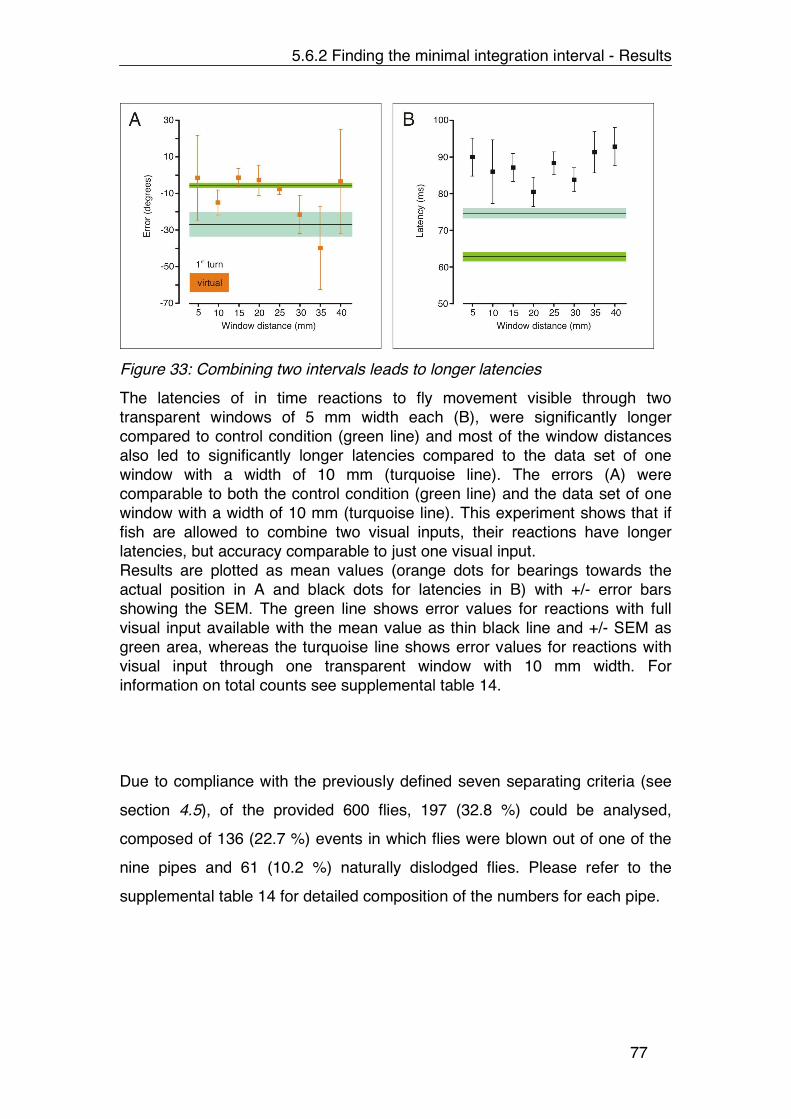
5.6.2 Finding the minimal integration interval - Results
77
Figure 33: Combining two intervals leads to longer latencies
The latencies of in time reactions to fly movement visible through two transparent windows of 5 mm width each (B), were significantly longer compared to control condition (green line) and most of the window distances also led to significantly longer latencies compared to the data set of one window with a width of 10 mm (turquoise line). The errors (A) were comparable to both the control condition (green line) and the data set of one window with a width of 10 mm (turquoise line). This experiment shows that if fish are allowed to combine two visual inputs, their reactions have longer latencies, but accuracy comparable to just one visual input. Results are plotted as mean values (orange dots for bearings towards the actual position in A and black dots for latencies in B) with +/- error bars showing the SEM. The green line shows error values for reactions with full visual input available with the mean value as thin black line and +/- SEM as green area, whereas the turquoise line shows error values for reactions with visual input through one transparent window with 10 mm width. For information on total counts see supplemental table 14.
Due to compliance with the previously defined seven separating criteria (see
section 4.5), of the provided 600 flies, 197 (32.8 %) could be analysed,
composed of 136 (22.7 %) events in which flies were blown out of one of the
nine pipes and 61 (10.2 %) naturally dislodged flies. Please refer to the
supplemental table 14 for detailed composition of the numbers for each pipe.

5.6.3 Finding the minimal integration interval - Discussion
78
5.6.3 Discussion
In conclusion, fish are able to react to spatially and temporally restricted visual
input. This makes sense, bearing in mind the conditions of the fish!s natural
habitat: The space above the water surface in a mangrove lined estuary –
where archerfish perform most of their hunting – is densely filled with
overhanging vegetation, featuring all sorts of leaves and branches. It is easily
imaginable that the moving path of a prey insect, once dislodged, bears a
considerable probability to cover behind leaves, therefore just providing
restricted visibility during its fall towards the water surface. Nonetheless, fish
have to decide quickly where to turn to, starting their movement even when
the prey object of choice is not visible during its whole trajectory towards the
water surface. Another fish could have a better viewpoint, being first at impact
position.
Making matters even worse, the amount of vegetation between the dislodged
flies and the water surface can also lead to the deflection of the prey insects
on one of the obstacles within the trajectory of the flies! falling paths. This will
redirect them to an impact position different from the position assumed
through initial movement parameters. As I could show, fish go on monitoring
the movement of a falling prey object after initiation of their predictive start.
This provides them with all the chance they need to redirect their own bearing,
if necessary. Fish routinely include this “second safety look” in every of their
turns, as illustrated by the fact that, when challenged with flies moving through
pipes (restricting the visibility of the flies temporally and spatially via
transparent windows of different length), fish always turned twice, aiming their
second turn according to the actual impact position; the position where the fly
will actually impact onto the water surface after completely leaving the
depriving pipe. Whereas their first turn always led them towards the position
where they assumed the fly!s landing to happen, according to its visible
movement within the transparent window of the depriving pipe.
The accuracy of the fish!s initial bearing not only gets significantly worse with
smaller window widths, error values turn considerably towards more negative

5.6.3 Finding the minimal integration interval - Discussion
79
offsets (please refer to 4.4.2 for sign convention). Fish systematically seem to
underestimate the fly!s velocity, when these are only visible for a short period
of time and within a small spatial window. Another problem is that flies in fact
are still accelerated within the transparent pipes (since flies! velocities for 40
mm pipe width are bigger, than for 5 mm width, see figure 25 A). So for small
window widths, fish might have a problem in estimating the velocity, since fly
movement is simply not visible long enough. For bigger window widths on the
other hand, it could be that the fish!s estimation will be incorrect, due to the
still ongoing change in the fly!s velocity while the fish already finished
monitoring and started computing.
In a considerable amount of cases (43.7 % of all flies blown through one of
the pipes), fish did not react to the visible movement of flies, while the flies
were still inside the pipes but reacted as flies already left the pipes instead
(classified as "too late!). Although fish did not react fast enough to respond
while the fly was still inside the pipe, they were very well able to use the
earlier, visual input to minimise their latency by simultaneously enhancing the
accuracy of their predictive turns. Their “refusal” to react "in time! could be a
delay due to a lack of threshold in the decision-making circuitry, being
reached with additional input. The reason could be that the area activated by
the display of moving prey on the retina did not include the passing of the
border between centre and surround of a connected unit, or border crossing
may just have provided inadequate input to generate a sufficient level of
activation to evoke critical changes in the spike frequency of retinal ganglion
cells. This could also be the reason for the overall decrease in the number of
"in time! reactions, as input durations abbreviate via smaller window widths
(please refer to supplemental table 8 for total counts).
The results of another, related experiment revealed a satisfactory match of
these findings: Challenging the fish with a situation in which they could add
two consecutive prey movements of short visibility, to one trajectory
(presenting two transparent windows with a small, defined distance in

5.6.3 Finding the minimal integration interval - Discussion
80
between), significantly improved the aiming precision of their first turns for 15,
20 and 25 mm distance between the transparent windows of 5 mm width (see
figure 33). This improvement comes at the cost of a significant increase in
latency (compared to control condition with full visual input available), which in
this case is actually a benefit, since watching longer enabled the fish to react
more accurate, a trade off that seems to be highly worthwhile.
This result can also be explained via the activation of centre-surround units,
since the extraction of values for direction and speed of a moving stimulus will
enable improved results, if a given number of activated units would be
situated distant to one another, covering an enlarged measuring section as a
result. This only applies if the participating units were functionally connected.
In this case the combination of the measurements of two activated units could
provide the fish with a better overall accuracy, than the measurements of just
one unit – even if the covered spatial section may be equal (seen in a
comparison of inputs through two windows of 5 mm width each, with one
window of 10 mm width). The fact that this improvement of accuracy can only
be detected at certain distances (15, 20 and 25 mm distance between the
transparent windows) could lead to the conclusion that these distances
represent retinal distances of functionally connected units. A translation of
these values onto the retina suggests distances of approximately 300 µm to
400 µm between two activated areas (of approximately 100 µm size each) as
an optimal distance for a combination of two inputs of that size. Although this
result still provides no explanation for the observed delay in latency, it
however may be interesting for a deeper analysis of retinal functionality.

5.7 Breeding Archerfish – Objectives and approach
81
5.7 Breeding Archerfish
5.7.1 Objectives and Experimental Approach
Naïve archerfish offspring would bear the possibility to study how the fish
learn such complex behaviours, like precise spitting of water, predicting a
prey!s future impact position and reacting with a precise turn. The problem is,
that we completely lack knowledge about the habitat, and environmental
conditions that these fish need to breed. Archerfish can be found in habitats
as diverse as freshwater rivers, mangrove lined estuaries filled with brackish
water and even in the open sea. According to rumours among fish owners
they breed in coral reefs – others guess that they are breeding in freshwater.
It seems rather difficult to find the perfect breeding habitat and it remains
doubtful if an extensive search will be worth the effort. I tried a simpler
method, used in fish farms, to see if breeding was possible.
Four adult Toxotes chatareus (sized 12 cm to 15 cm; weight 45 g to 63 g)
were kept in a tank (1.0 m x 0.5 m x 0.5 m), filled with brackish water at a
slightly lower-than-normal conductivity level of 2.0 mS/cm, at a temperature of
28 °C. All fish were injected with OVAPRIM (Syndel Labs, Vancouver,
Canada) at the required dosage of 0.5 ml per kg body weight using sterile
disposable syringes. OVAPRIM contains an efficient salmon GnRH analogue,
which stimulates the fish!s endocrine system to induce synchronous spawning
(and maturation) in both sexes. The remedy was injected into the body cavity
beneath the pectoral fin (figure 34). Prior to injecting, fish were anesthetized
with MS 222 (Sigma-Aldrich, Steinheim, Germany), dissolved in water (100
mg/l) to minimize the risk of injury.

5.7 Breeding Archerfish – Objectives and approach
82
Figure 34: Injecting procedure
This photograph shows an adult Toxotes jaculatrix during the process of injecting OVAPRIM into the body cavity beneath the pectoral fin. The syringes, the bottle of remedy and the anesthetized fish are clearly visible. Bruce Sambell graciously provided this picture (AUSYFISH, Queensland, Australia).
After spawning, the floating eggs were transferred into a smaller separate
tank (30 litre; equipped with an air pump to keep the water both oxygenated
and in motion) filled with water from the breeding tank (ensuring matching
quality). Adding the fungicide Fungol (JBL, Neuhofen, Germany) at a
concentration of 0.25 ml/l prevented mycosis during the eggs! maturation.
Immediately subsequent to hatching, the larvae were transferred to two
smaller tanks (0.5 litre each, stable temperature of 28°C) gaining improved
control of conditions. For best results the water of these small tanks was
completely exchanged each day, using water from the breeding tank. Larvae
were provided with freshly hatched Artemia salina (Linnaeus) twice a day.
5.7.2 Results
Two days past OVAPRIM injection the four Toxotes chatareus spawned some
estimated 5000 floating eggs, of which about 4000 were transferred into a
separate tank for hatching. Three days later, 40 larvae had hatched (1 %) and
were gently transferred into smaller tanks. Single larvae developed and
survived until 14 days after hatching, but due to decay during this period, none
of them survived. Much as in zebrafish, Danio rerio (Hamilton) (see e.g. [89],
the larvae were capable of escape reactions three days after spawning, and
began to show target-oriented swimming behaviour the day later. Due to fish
larvae!s usual initial transparency, their organs were clearly visible (like the
beating heart, skeleton and nervous system). In contrast to equally aged

5.7 Breeding Archerfish – Results
83
zebrafish [89] the eyes of archerfish larvae appeared to develop their full
pigmentation later after hatch. Subsequent stages of archerfish larvae
developed the typical densely pigmented epithelium and body pigmentation
(see figure 35).
Figure 35: Exemplary images of fertilised eggs and fish larvae
A shows a sample of fertilised eggs as seen in the tank two days past injection of OVAPRIM. Eggs are approximately 0.5 mm in diameter. The exemplary images of archerfish offspring illustrate three stages of larval development, three (B), seven (C) and eleven (D) days post fertilization, respectively. The eyes are initially well transparent (see B) but pigmentation soon develops. Scale bars 0.2 mm; images (B – D) show different individuals of the same clutch.
5.7.3 Discussion
This experiment clearly demonstrates the possibility to breed archerfish under
controlled conditions in the lab, generating the possibility to study naïve
archerfish offspring on their way to maturity. Of course this first approach is
far from being perfect – at least none of the larvae survived. However it also
demonstrates that it is after all possible to breed these fish in the lab.

5.7 Breeding Archerfish – Discussion
84
A possible next step would be to start experimenting with levels of salinity;
both after spawning and once larvae have hatched. It would also be nice to
see how the mating takes place as this might help to increase the number of
fertilised eggs in the future (e.g. I do not know the sex ratio within the breeding
group, since sexing of fish of that size is impossible without dissecting them).
Further experimentation with different food sources for the freshly hatched
larvae will also be advisable to provide a well-balanced diet.
As soon as a proper method will be found, studying archerfish will proceed to
a new level, since it will enable to study the learning behaviour of completely
naïve fish. Challenging them in experimental situations, which they are
definitely unfamiliar with, will reveal how fish will adapt to novel challenges.
Their predictive behaviour, for example is above all a complex one and
although in part hereditary [31], it is very likely that juveniles first have to learn
major aspects of the including repertoire (as shown [28]) before they reach
their accustomed level of ingenuity. It is of course this learning behaviour that
could play a key role in discovering the fundamental co-operation of
underlying networks. Achieved either with added developmental studies on
cellular level, or through thoroughly studying the juvenile archerfish!s
behaviour when exposed to unnatural situations to which they likely will
habituate during their adolescence. These situations could include prey
movements after dislodgement that would never occur in natural
surroundings, targets moving faster or slower, than the range a fish would
naturally expect. Or moving into an unexpected direction, like moving
backwards, when dislodged in forward direction by a fish. Artificial, or virtual
prey objects could change their size after dislodgement and therefore
hopefully fool the fish to think of a vertical aspect of prey movement when in
fact movement is only horizontally. With sophisticated optical methods (e.g.
through lenses) “changing” the prey!s size during movement could also be
reached, using real and therefore edible prey objects. These significantly
modified visual inputs should alter the fish!s predictive system to aim the turns
to positions, where the prey will not at all impact actually, for in fact it never

5.7 Breeding Archerfish – Discussion
85
moved on something else than a ballistic path, starting with horizontal speed
only. If fish grew up learning to compensate this for long enough and are then
challenged with normal moving flies, we will be able to see, if the neuronal
network is flexible enough to change back to “normal”, whereas fish never
experienced what “normal” is like.
The good thing with archerfish is, that they seem to habituate to a diversity of
situations without difficulty, for example they easily learn to shoot at prey sizes
bigger than they would be able to swallow [31, 34]. So as another promising
experiment, we could think of providing one of the fish!s eyes with a darkened
contact lens, filtering a substantial part of the incoming light. If fish needed
bifocal vision in their task, their prediction should get confused, for the input
through the filtered eye will provide the extracted information a little later, than
the non-filtered eye (this would also be an elegant way to find out if fish
utilised both eyes, e.g. for instantaneous distance measuring). This time delay
could have devastating (and hence very interesting) impacts on the fish!s
turning behaviour, as a comparable experiment in human vision reveals: The
so-called “Pulfrich stereo phenomenon”, named after physicist Carl Pulfrich, in
which a human observer tracks the lateral path of an oscillating object, placing
a dark filter over one eye. The resulting time delay of the visual information
from that eye causes the visual cortex to interpret the actually lateral
movement as an elliptical one, adding the illusion of a certain depth
component. This phenomenon strongly depends on target size, distance to
target, target velocity and the differences in intensity between both eyes [90-
93]. Therefore it seems an ideal experiment to challenge archerfish, since
exactly these components are essentially necessary for the fish!s evaluation
of a prey!s future impact position. Equipping adult fish with darkened lenses
would be a possibility.
In addition to an unnatural habituation of archerfish offspring, we could
observe their natural learning progress, being rewarded with knowledge of the
exact timing when they start their shooting and the extend to which they can
perform at first, the way they improve. Inevitably particular school members

5.7 Breeding Archerfish – Discussion
86
will perform better than others at first – what amount of impact will this have
on the social structure within the group? Who will dominate the others: The
best marksman, or the one that reacts fastest, gets the most food and
therefore will grow fastest. Is the ability to successfully shoot down prey
associated with intraspecific aggression, or is this an anthropomorphic
fallacy? Nonetheless, dominant and aggressive behaviour can already be
observed in juvenile archerfish [94], so it would be quite interesting to know
the cause.
Monitoring the fish!s improvement in their overall performance will provide
ideas about their computation and signal extraction, since the neuronal
correlates like the fish!s retinae and brain are still growing (lifelong in fish).
Maybe there is a critical mass of neurons necessary to perform the task,
either to extract the needed information within the fish!s retina, or to compute
that information into the matching motor program, or just to provide a
reasonable resolution. The motor system however, should instantly be able to
conduct the turns, for the Mauthner cell network seems to be instantly fully
functional after hatch. At least archerfish larvae were able to perform
reasonable escape reactions at that stage. So in combination with
developmental studies (neuronal development in general and retinal
development in particular) the observation of the improving of shooting and
predicting abilities of naïve fish could add significantly to our understanding of
the mechanisms of such a sophisticated behavioural repertoire, as the
archerfish!s predictive behaviour.

87
6. Discussion

6. Discussion
88
6.1 A conception of archerfish: from visual input to motor output
Archerfish habitually and effortless translate the visual input of moving prey
objects to accurately matching motor patterns, and they are able to do this
translation in remarkable short time. This paragraph will merge the data
gathered throughout the described experiments with a few published concepts
about visual input processing, input computation and its further transcription to
matching activation patterns. This merge will lead to a concept of the
properties that are necessary for the extraction of the required movement
parameters within the fish!s retina.
Challenging the fish with a spatially and temporally minimised integration
interval for visual processing, revealed that 18 milliseconds of visible prey
movement sufficed to elicit a precise predictive turn towards the future impact
position of that prey (error of 1.8°). During these 18 ms, the visual stimulus
covered a retinal length of 108 µm (an area of roughly 0.01 mm2). This is just
an example to convey a feeling for the scale of the observed data. There are
more reactions to input of 14 to 20 ms, but most of them are followed by less
accurate predictive turns. However input durations of this scale sufficed to
elicit predictive turns (please see supplemental table 8 for total counts).
According to published work on structure and composition of the archerfish
retina [95], the covered 108 µm length equates a line of about 18 cones in
length and an area of precisely 300 cones. According to the same source, the
radius of an archerfish receptive field is roughly 125 µm, so activation of a
retinal field considerable smaller than the radius of a receptive field still
suffices to elicit predictive turns. Since we defined direction, velocity and size
of the moving prey object as the kind of information a fish!s brain must
necessarily possess to be able to compute a matching activation pattern of
motor output, it is rather surprising, that these small fields of few darkened
photoreceptors sufficed for the task.
To understand how the retina can achieve this, it will be helpful to recall a few
key concepts of retinal processing:

6. Discussion
89
Already in the 1950s, groundbreaking work on cat retinae expanded the
existing knowledge of ganglion cell receptive fields by the concept of so called
“centre-surround receptive fields” [96] which provided a fundament for
numerous investigations [97-101]. About a decade later, extensive work on
rabbit retinae revealed retinal units (ganglion cells), responding highly
selectively (with an increase in firing rate) to stimuli moving in a certain
direction, falling completely silent when stimulated with the reverse direction
[102, 103]. Most interestingly, the so called “ON-centre unit” does not have to
be stimulated over its full length, but a stimulus beginning its movement from
within the surrounding periphery, will inevitably evoke a response (discharge
of retinal ganglion cell), as it proceeds into the centre of the unit. As soon as it
crosses the centre and starts moving towards the periphery again, the
discharge abruptly slows or stops (the opposite applies for “OFF-centre units”
[102]).
So if archerfish utilised something similar to those ON- or OFF-centre units
found in rabbits, activating a certain part of the receptive field instead of
activating the whole field, could as well suffice to evoke a response. Such a
response would not just provide information about the direction of movement,
but as found in turtle retinae, the exact same cell could simultaneously provide
information about the velocity of moving prey as well [104]. The achieved
accuracy might just be defined via the cell!s angular division of direction
selectivity, which if very small (as necessary in archerfish) needed huge
numbers of such fields throughout the retina in turn.
A particular type of retinal ganglion cells has recently been described (in mice)
that has its direction selectivity due to a certain and well-defined asymmetry of
its dendritic tree. The preferred direction corresponds to the direction in which
the dendrites point from the cell soma [105]. Such an asymmetry was also
found in rabbit retinae [106-108]. But of course direction selectivity does not
necessarily need such an asymmetry of the dendritic field, as proven by
several studies [47, 109, 110]. Speculating about the morphological
characteristics of units, of which we are lacking direct evidence about their
existence, is an idle business and may easily be misleading.

6. Discussion
90
But since direction selectivity in ganglion cells exists in various vertebrates
(e.g. in goldfish [48] and rainbow trout [111] – and are not unique to rabbits), it
seems very likely, that archerfish employ it as well. Finding the origins of the
direction selectivity of a retinal ganglion cell is obviously interesting and
profound ideas have as well been suggested earlier [103, 112]. Still
researchers – though employing an abundant variation of organisms and
methods – struggle to find the final solution to the subject of direction
selectivity of retinal ganglion cells [56, 57, 109, 110, 113, 114].
Simultaneous with movement parameter discrimination, the size of a visual
stimulus can be determined, employing the same field of photoreceptors. The
signal generated by those photoreceptors can simply be distributed to an
additional group of ganglion cells responsible for forwarding size information
to the brain [47, 115]. A much more formidable problem is the extraction of
information about the distance to the moving prey. Although distance
discrimination can of course be done binocularly [116], nothing is known
about the visual field provided by the two eyes of an archerfish (i.e. about the
existence and size of a binocular field). Testing the fish!s spatial attention (see
5.2, figure 10) showed, that fish were still able to react accurately to visual
stimuli within the periphery of their visual field (e.g. for a horizontal distance of
40 cm in figure 10), displaying the stimulus only on one of the eyes, providing
monocular input only. Being challenged like that, fish do need significantly
longer to react to that input, but the fact that they are able to do so at all,
applying the same accuracy, as if the input would have been binocular, is a
clear evidence that the whole necessary visual parameter extraction works
just as well with one eye, as it does with both eyes. Distance discrimination
via monitoring the accommodation level of one!s lens (as humans do) just
works fine if that eye is fixing the position of movement – but it will not work
when that one eye is fixing a position at a different distance (like in the set of
experiments described in 5.2 and 5.5) and apart from that, fish do not
accommodate like humans.
So how can archerfish in this experiment know the distance between a
moving fly and themselves – a distance they implicitly need to compute the

6. Discussion
91
fly!s future impact position and their own distance to this position? A possible
explanation could be that the whole extraction of motion parameters has to
generate qualitatively equal values of the movement parameters with diffusely
displayed objects as with perfectly edged ones (which is obvious according to
the results of the experiment mentioned above, see 5.2 – the accuracy of the
fish!s reaction stays high level for big offsets, just the latency deteriorates).
Fish are familiar with the size of prey objects they encounter in the lab, since
they were fed with the same species of flies everyday throughout more than
two years previous to the first experiments described here. Thus fish are, in
principle, able to estimate the distance to a prey object, moving outside of
focus, by comparing the actual size of that object that is diffusely displayed
onto the retina, with learned actual sizes of objects of that kind. This way, they
could reversely discriminate the distance via the assumed actual size of prey.
This would of course be much more difficult in a natural situation, since fish
are then faced with prey of very variable sizes, but it could in principle be very
well possible in the artificial situation of living in a tank for years, being fed
with the same food every day.
Interestingly fish do not use this reverse discrimination, since (as recently
shown in our lab [117]) they are able to accurately predict the impact position
of differently sized prey objects within the same experimental setup. If they
applied reverse size discrimination they should have judged the height of a
smaller prey object higher as that of a bigger one – their bearing towards one
of the prey objects should have been considerably different compared to the
other. However, this is not what Carmen Stöhr found. So far the archerfish!s
method of discriminating the size of its prey objects, will remain its secret.
Assuming the possibilities of retinal computational abilities, it is very likely that
the information coded as spike trains and forwarded through the thick pipeline
of the optical nerve already contains precise surveillance data of the most
important parameters of prey movement, such as speed and direction of
movement, as well as the size of and distance to the prey, plus of course the
prey!s aerial position, decoded via its retinal position. Since most of the prey!s

6. Discussion
92
movements are visible for both eyes (except of large offsets between the
fish!s direction of gaze and movement onset), these values are predominantly
incoming in duplicate. It is very likely that they are not just projected to the
same hemisphere of the optic tectum (via the optic chiasm as common among
vertebrates), but actually to the very same cells, as previously shown in the
visual system of cats [99, 118]. These cells (whatever their morphology,
number and wiring may be) are the first of probably several stations for the
final computation and decision-making, driving motorneurons and muscles to
fine-tune the turn.
Particularly the “ON directionally selective ganglion cells” of rabbits, projecting
to the accessory optic system [119], are renowned for driving fast motor
behaviour known as "optokinetic response! [120-122]. Recent findings in our
lab imply that archerfish diverted their fast escape network from its intended
use, by utilising it for their predictive turns as well, since their C-shaped body
bends show all the hallmarks of Mauthner cell involvement [38]. There is
indeed established evidence that fish are able to utilise their fast Mauthner
cell network voluntarily during prey capture [51, 54, 123], which is of course
completely reasonable avoiding to reinvent the wheel. Employing an already
fully evolved fast network in an additional task is much more reasonable in
evolutionary terms, than evolving a functional match for a second time –
especially since the existing network features all the necessities for the new
task at hand: enormous speed accompanied by adjusted directionality [124,
125]. Maintaining two systems with the same functional scope would be
inappropriate, since such networks will obviously never be needed
simultaneously – mixing escaping and chasing behaviour at the same time is
simply pointless.
The wish to decode the computational or modulating processes within the
fish!s hindbrain area, cannot concentrate on the Mauthner cell alone, since it
is just one of many reticulospinal neurons that normally participate in the
programming of C-start responses [63]. Especially the angle and duration of
the first stage of the C-start (the part that forms the C-shape) essentially
depends upon an entire array of neurons [50, 63, 126-129] and the

6. Discussion
93
composition of recruited neurons finally depends on the direction of the
startling stimulus relative to the orientation of the fish [124, 130-133]. But
since the Mauthner cell is probably the best-known neuron within the nervous
system of vertebrates, it is surely a particularly suitable starting point for a
most fruitful scientific venture.
Finally the involvement of a neuronal network, especially evolved for
generating precise and reliably fast reactions, would account for the
impressive brevity of latency of the archerfish!s predictive turn, a latency that
can be as short as 40 milliseconds.
Figure 36: Visualisation of processes that lead to a predictive turn
This drawing is a rough visualisation of the procedures activated during the monitoring of a falling fly. The retinal picture of the fly activates processes within photoreceptors, getting translated from simple changes in membrane potential to neurotransmitter release. This transformation of physical energy (light waves) into cellular mechanisms, culminates in the generation of concerted spike trains of action potentials of retinal ganglion cells, encoding some of the most important parameters of fly movement, like direction, velocity, size and aerial position. Via the thick optic nerve, this information is forwarded most likely to the optic tectum of the fish!s brain (according to the position of the visual input either to the left, the right or both sides of the tectal lobes). Here the information computation and decision-making is taking place and the generated neuronal output then controls the activation of the Mauthner cell network. One of these Mauthner cells activates primary motorneurons (inhibiting the second Mauthner neuron at the same time) activating muscle fibres, which results in the contraction of that of the fish!s

6. Discussion
94
sides, pointing towards the fly!s future impact position onto the water surface. In doing so the activated Mauthner neuron fine-tunes the muscular response allowing for precisely fractioned turning steps.
6.2 Some closing remarks on cognition
I don!t want to stress this point too much, since it is likely to achieve nothing
more than overall perplexity and in the worst case even resistance against the
archerfish!s unquestioned abilities, but let me share a current quote about the
concept of cognition: Cognition can be defined as the ability to use internal
representations of information acquired in separate events, and to combine
these to generate novel information and apply it in an adaptive manner [134].
The authors suggest the cognitive map as a classic example, where subjects
(in this case bees) integrate information from separately travelled paths to
calculate new routes [135, 136]. Cognitive abilities have also been described
in a variety of animals so far [137-142] even in fish [143-145], so a certain
level of abstraction may be admitted to animals by now.
Applying the above definition of cognition, the predictive reaction of archerfish
can in good conscience be defined as cognitive, since these fish feature
internal representations of information (e.g. the distance to impact positions of
one or more prey objects, judging their absolute size in the process [34]),
generating novel information (which one is nearer to my actual position) and
applying this information in an adaptive manner (turning to the nearer prey).
Moreover, archerfish can learn to cope with novel situations (e.g. rapidly
moving prey objects), flexibly changing their reacting strategy in the process.
Above all, these fish are able to learn new patterns of behaviour simply by
watching other fish performing them [28, 34].
Of course I am well aware that there are numerous other definitions of
cognition [146] and archerfish behaviour may not entirely fit within all of them,
but whether we tend to call the fish!s predictive response cognitive or not,
archerfish still feature a most remarkable hunting strategy, that comes linked
with a delightful collection of highly sophisticated skills, interesting within a

6. Discussion
95
variety of contexts and still most noteworthy by themselves. Archerfish will
certainly provide more surprises in the contexts of fields like neuronal
decision-making, cognition, retinal computation and computation along motor
systems – so let!s stay tuned.

References
96
7. References
1. Meister, M., Pine, J. and Baylor, D.A., Multi-neuronal signals from the retina: acquisition and analysis. J Neurosci Methods, 1994. 51(1): p. 95-106.
2. Fernandez, E., Ferrandez, J., Ammermuller, J. and Normann, R.A., Population coding in spike trains of simultaneously recorded retinal ganglion cells. Brain Res, 2000. 887(1): p. 222-229.
3. Kolb, H., The architecture of functional neural circuits in the vertebrate retina. The Proctor Lecture. Invest Ophthalmol Vis Sci, 1994. 35(5): p. 2385-2404.
4. Dehaene, S., Spelke, E., Pinel, P., Stanescu, R. and Tsivkin, S., Sources of mathematical thinking: behavioral and brain-imaging evidence. Science, 1999. 284(5416): p. 970-974.
5. Nelissen, K., Luppino, G., Vanduffel, W., Rizzolatti, G. and Orban, G.A., Observing others: multiple action representation in the frontal lobe. Science, 2005. 310(5746): p. 332-336.
6. Sanfey, A.G., Rilling, J.K., Aronson, J.A., Nystrom, L.E. and Cohen, J.D., The neural basis of economic decision-making in the Ultimatum Game. Science, 2003. 300(5626): p. 1755-1758.
7. Tom, S.M., Fox, C.R., Trepel, C. and Poldrack, R.A., The neural basis of loss aversion in decision-making under risk. Science, 2007. 315(5811): p. 515-518.
8. Jacob, S.N. and Nieder, A., Notation-independent representation of fractions in the human parietal cortex. J Neurosci, 2009. 29(14): p. 4652-4657.
9. Mobbs, D., Yu, R., Meyer, M., Passamonti, L., Seymour, B., Calder, A.J., Schweizer, S., Frith, C.D. and Dalgleish, T., A key role for similarity in vicarious reward. Science, 2009. 324(5929): p. 900.
10. Ammermuller, J. and Kolb, H., The organization of the turtle inner retina. I. ON- and OFF-center pathways. J Comp Neurol, 1995. 358(1): p. 1-34.
11. Ammermuller, J., Muller, J.F. and Kolb, H., The organization of the turtle inner retina. II. Analysis of color-coded and directionally selective cells. J Comp Neurol, 1995. 358(1): p. 35-62.

References
97
12. Cohen, L.B., Salzberg, B.M. and Grinvald, A., Optical methods for monitoring neuron activity. Annu Rev Neurosci, 1978. 1: p. 171-182.
13. Miesenbock, G. and Kevrekidis, I.G., Optical imaging and control of genetically designated neurons in functioning circuits. Annu Rev Neurosci, 2005. 28: p. 533-563.
14. Blow, N., Functional Neuroscience: How to get ahead in imaging. Nature, 2009. 458(7240): p. 925-928.
15. Fetcho, J.R. and O'Malley, D.M., Imaging neuronal networks in behaving animals. Curr Opin Neurobiol, 1997. 7(6): p. 832-838.
16. Helmchen, F. and Waters, J., Ca2+ imaging in the mammalian brain in vivo. Eur J Pharmacol, 2002. 447(2-3): p. 119-129.
17. Stutzmann, G.E. and Parker, I., Dynamic multiphoton imaging: a live view from cells to systems. Physiology (Bethesda), 2005. 20: p. 15-21.
18. Helmchen, F. and Denk, W., New developments in multiphoton microscopy. Curr Opin Neurobiol, 2002. 12(5): p. 593-601.
19. Helmchen, F., Fee, M.S., Tank, D.W. and Denk, W., A miniature head-mounted two-photon microscope. high-resolution brain imaging in freely moving animals. Neuron, 2001. 31(6): p. 903-912.
20. Smith, H., The archer fish. Natur. Hist., 1936. 38: p. 2-11.
21. Lüling, K., Morphologisch-Anatomische und histologische Untersuchungen am Auge des Schützenfisches Toxotes jaculatrix (PALLAS 1766) (Toxotidae), nebst Bemerkungen zum Spuckgehaben. Z. Morph. u. Ökol. Tiere, 1958.
22. Hediger, H. and Heusser, H., Zum “Schießen” des Schützenfisches, Toxotes jaculatrix. Natur und Volk, 1961.
23. Lüling, K., The archerfish. Sci. Am, 1963. 209: p. 100-108.
24. Dill, L., Refraction and the spitting behavior of the archerfish (Toxotes chatareus). Behavioral Ecology and Sociobiology, 1977. 2(2): p. 169-184.
25. Timmermans, P., Prey catching in the archer fish: marksmanship, endurance of squirting at an aerial target. Netherlands Journal of Zoology, 2000.
26. Timmermans, P.J., Prey catching in the archer fish: angles and probability of hitting an aerial target. Behav Processes, 2001. 55(2): p. 93-105.

References
98
27. Schuster, S., Archerfish. Curr Biol, 2007. 17(13): p. R494-495.
28. Schuster, S., Wohl, S., Griebsch, M. and Klostermeier, I., Animal cognition: how archer fish learn to down rapidly moving targets. Curr Biol, 2006. 16(4): p. 378-383.
29. Milburn, O. and Alexander, R., The performance of the muscles involved in spitting by the archerfish Toxotes. J. Zool. London, 1976. 180: p. 243-251.
30. Elshoud, G. and Koomen, P., A biomechanical analysis of spitting in archer fishes (Pisces, Perciformes, Toxidae). Zoomorphology, 1985. 105: p. 240-252.
31. Schlegel, T., Schmid, C.J. and Schuster, S., Archerfish shots are evolutionarily matched to prey adhesion. Curr Biol, 2006. 16(19): p. R836-837.
32. Timmermans, P.J. and Vossen, J.M., Prey catching in the archer fish: does the fish use a learned correction for refraction? Behav Processes, 2000. 52(1): p. 21-34.
33. Temple, S.E., Effect of salinity on the refractive index of water: considerations for archer fish aerial vision. Journal of Fish Biology, 2007. 70(5): p. 1626-1629.
34. Schuster, S., Rossel, S., Schmidtmann, A., Jager, I. and Poralla, J., Archer fish learn to compensate for complex optical distortions to determine the absolute size of their aerial prey. Curr Biol, 2004. 14(17): p. 1565-1568.
35. Wöhl, S. and Schuster, S., Hunting archer fish match their take-off speed to distance from the future point of catch. J Exp Biol, 2006. 209: p. 141-151.
36. Wöhl, S., Zielprädiktion beim Schützenfisch: eine komplexe kognitive Leistung mit extrem hoher Geschwindigkeit. PhD Thesis, 2008.
37. Wardle, C.S., Limit of fish swimming speed. Nature, 1975. 255(5511): p. 725-727.
38. Wöhl, S. and Schuster, S., The predictive start of hunting archer fish: a flexible and precise motor pattern performed with the kinematics of an escape C-start. J Exp Biol, 2007. 210: p. 311-324.
39. Rossel, S., Corlija, J. and Schuster, S., Predicting three-dimensional target motion: how archer fish determine where to catch their dislodged prey. J Exp Biol, 2002. 205(21): p. 3321-3326.

References
99
40. Lennie, P., The physiological basis of variations in visual latency. Vision Res, 1981. 21(6): p. 815-824.
41. Schnapf, J.L., Kraft, T.W. and Baylor, D.A., Spectral sensitivity of human cone photoreceptors. Nature, 1987. 325(6103): p. 439-441.
42. Levick, W.R., Variation in the response latency of cat retinal ganglion cells. Vision Res, 1973. 13(4): p. 837-853.
43. Rieke, F. and Baylor, D.A., Single-photon detection by rod cells of the retina. Reviews of Modern Physics, 1998. 70(3): p. 1027-1036.
44. Baylor, D.A., Photoreceptor signals and vision. Proctor lecture. Invest Ophthalmol Vis Sci, 1987. 28(1): p. 34-49.
45. Masland, R.H., The fundamental plan of the retina. Nat Neurosci, 2001. 4(9): p. 877-886.
46. Masland, R.H. and Martin, P.R., The unsolved mystery of vision. Curr Biol, 2007. 17(15): p. R577-582.
47. Wassle, H., Parallel processing in the mammalian retina. Nat Rev Neurosci, 2004. 5(10): p. 747-757.
48. Jacobson, M. and Gaze, R.M., Types of Visual Response from Single Units in the Optic Tectum and Optic Nerve of the Goldfish. Q J Exp Physiol Cogn Med Sci, 1964. 49: p. 199-209.
49. Eaton, R.C., Bombardieri, R.A. and Meyer, D.L., The Mauthner-initiated startle response in teleost fish. J Exp Biol, 1977. 66(1): p. 65-81.
50. Eaton, R.C., DiDomenico, R. and Nissanov, J., Role of the Mauthner cell in sensorimotor integration by the brain stem escape network. Brain Behav Evol, 1991. 37(5): p. 272-285.
51. Canfield, J.G. and Rose, G.J., Activation of Mauthner neurons during prey capture. J Comp Physiol [A], 1993. 172: p. 611-618.
52. Zottoli, S.J. and Faber, D.S., The Mauthner Cell: What Has It Taught Us? The Neuroscientist, 2000. 6: p. 25-37.
53. Kohashi, T. and Oda, Y., Initiation of Mauthner- or non-Mauthner-mediated fast escape evoked by different modes of sensory input. J Neurosci, 2008. 28(42): p. 10641-10653.
54. Canfield, J.G., Some voluntary C-bends may be Mauthner neuron initiated. J Comp Physiol A Neuroethol Sens Neural Behav Physiol, 2007. 193(10): p. 1055-1064.

References
100
55. Olveczky, B.P., Baccus, S.A. and Meister, M., Segregation of object and background motion in the retina. Nature, 2003. 423(6938): p. 401-408.
56. Hosoya, T., Baccus, S.A. and Meister, M., Dynamic predictive coding by the retina. Nature, 2005. 436(7047): p. 71-77.
57. Baccus, S.A., Olveczky, B.P., Manu, M. and Meister, M., A retinal circuit that computes object motion. J Neurosci, 2008. 28(27): p. 6807-6817.
58. Allen, G., A review of the archerfishes (family Toxotidae). Rec. West. Aust. Mus, 1978. 6(4): p. 355 - 378.
59. Allen, G., Toxotes kimberleyensis, a new species of archerfish (Pisces: Toxotidae) from fresh waters of Western Australia. Records of the Australian Museum, 2004.
60. Whitney, D. and Cavanagh, P., Surrounding motion affects the perceived location of moving stimuli. Visual Cognition, 2002. 9(1/2): p. 139-152.
61. Weiss, S.A., Zottoli, S.J., Do, S.C., Faber, D.S. and Preuss, T., Correlation of C-start behaviors with neural activity recorded from the hindbrain in free-swimming goldfish (Carassius auratus). J Exp Biol, 2006. 209: p. 4788-4801.
62. Dowling, J.E., The retina: an approachable part of the brain. Harvard University Press, Cambridge, Massachusetts, 1987.
63. Eaton, R.C., Lee, R.K. and Foreman, M.B., The Mauthner cell and other identified neurons of the brainstem escape network of fish. Prog Neurobiol, 2001. 63(4): p. 467-485.
64. Korn, H. and Faber, D.S., The Mauthner cell half a century later: a neurobiological model for decision-making? Neuron, 2005. 47(1): p. 13-28.
65. Oda, Y., Kawasaki, K., Morita, M., Korn, H. and Matsui, H., Inhibitory long-term potentiation underlies auditory conditioning of goldfish escape behaviour. Nature, 1998. 394(6689): p. 182-185.
66. Preuss, T. and Faber, D.S., Central cellular mechanisms underlying temperature-dependent changes in the goldfish startle-escape behavior. J Neurosci, 2003. 23(13): p. 5617-5626.
67. Schall, J.D. and Thompson, K.G., Neural selection and control of visually guided eye movements. Annu Rev Neurosci, 1999. 22: p. 241-259.

References
101
68. Krupczynski, P. and Schuster, S., Fruit-catching fish tune their fast starts to compensate for drift. Curr Biol, 2008. 18(24): p. 1961-1965.
69. Schlegel, T. and Schuster, S., Small circuits for large tasks: high-speed decision-making in archerfish. Science, 2008. 319(5859): p. 104-106.
70. Dzhafarov, E.N., Sekuler, R. and Allik, J., Detection of changes in speed and direction of motion: reaction time analysis. Percept Psychophys, 1993. 54(6): p. 733-750.
71. Rodieck, R.W., The first steps in seeing. Sinauer Associates, Sunderland, Massachusetts, 1998.
72. Wilke, S.D., Thiel, A., Eurich, C.W., Greschner, M., Bongard, M., Ammermuller, J. and Schwegler, H., Population coding of motion patterns in the early visual system. J Comp Physiol [A], 2001. 187(7): p. 549-558.
73. Sanfey, A.G., Social decision-making: insights from game theory and neuroscience. Science, 2007. 318(5850): p. 598-602.
74. Nienborg, H. and Cumming, B.G., Decision-related activity in sensory neurons reflects more than a neuron's causal effect. Nature, 2009. 459(7243): p. 89-92.
75. Nichols, M.J. and Newsome, W.T., Middle temporal visual area microstimulation influences veridical judgments of motion direction. J Neurosci, 2002. 22(21): p. 9530-9540.
76. Churchland, A.K., Kiani, R. and Shadlen, M.N., Decision-making with multiple alternatives. Nat Neurosci, 2008. 11(6): p. 693-702.
77. Springer, A.D. and Gaffney, J.S., Retinal projections in the goldfish: a study using cobaltous-lysine. J Comp Neurol, 1981. 203(3): p. 401-424.
78. Maunsell, J.H., Ghose, G.M., Assad, J.A., McAdams, C.J., Boudreau, C.E. and Noerager, B.D., Visual response latencies of magnocellular and parvocellular LGN neurons in macaque monkeys. Vis Neurosci, 1999. 16(1): p. 1-14.
79. Kaplan, E. and Shapley, R.M., The primate retina contains two types of ganglion cells, with high and low contrast sensitivity. Proc Natl Acad Sci U S A, 1986. 83(8): p. 2755-2757.
80. Aho, A.C., Donner, K., Helenius, S., Larsen, L.O. and Reuter, T., Visual performance of the toad (Bufo bufo) at low light levels: retinal ganglion cell responses and prey-catching accuracy. J Comp Physiol [A], 1993. 172(6): p. 671-682.

References
102
81. White, A.L., Linares, D. and Holcombe, A.O., Visuomotor timing compensates for changes in perceptual latency. Curr Biol, 2008. 18(20): p. R951-953.
82. Williams, J.M. and Lit, A., Luminance-dependent visual latency for the Hess effect, the Pulfrich effect, and simple reaction time. Vision Res, 1983. 23(2): p. 171-179.
83. Allik, J. and Kreegipuu, K., Multiple Visual Latency. Psychol Sci, 1998. 9(2): p. 135-138.
84. Rinner, O., Rick, J.M. and Neuhauss, S.C., Contrast sensitivity, spatial and temporal tuning of the larval zebrafish optokinetic response. Invest Ophthalmol Vis Sci, 2005. 46(1): p. 137-142.
85. Egeth, H.E. and Yantis, S., Visual attention: control, representation, and time course. Annu Rev Psychol, 1997. 48: p. 269-297.
86. Lamme, V.A.F., Neural Mechanisms of Visual Awareness: A Linking Proposition. Brain and Mind, 2000. 1: p. 385-406.
87. Knudsen, E.I., Fundamental components of attention. Annu Rev Neurosci, 2007. 30: p. 57-78.
88. Braun, J. and Schoenfeld, M.A., Vision: attention makes the cup flow over. Curr Biol, 2008. 18(16): p. R713-715.
89. Kimmel, C.B., Ballard, W.W., Kimmel, S.R., Ullmann, B. and Schilling, T.F., Stages of embryonic development of the zebrafish. Dev Dyn, 1995. 203(3): p. 253-310.
90. Lit, A., The magnitude of the Pulfrich stereophenomenon as a function of binocular differences of intensity at various levels of illumination. Am J Psychol, 1949. 62(2): p. 159-181.
91. Lit, A. and Hyman, A., The magnitude of the Pulfrich stereophenomenon as a function of distance of observation. Am J Optom Arch Am Acad Optom, 1951. 28(11): p. 564-580.
92. Lit, A., Magnitude of the Pulfrich stereophenomenon as a function of target thickness. J Opt Soc Am, 1960. 50: p. 321-327.
93. Lit, A., The magnitude of the Pulfrich stereophenomenon as a function of target velocity. J Exp Psychol, 1960. 59: p. 165-175.
94. Timmermans, P. and Maris, E., Does the bright spot on the back of young archer fishes serve group coherence? Netherlands Journal of Zoology, 2000. 50: p. 401-409.

References
103
95. Segev, R., Schneidman, E., Goodhouse, J. and Berry, M.J., 2nd, Role of eye movements in the retinal code for a size discrimination task. J Neurophysiol, 2007. 98(3): p. 1380-1391.
96. Kuffler, S.W., Discharge patterns and functional organization of mammalian retina. J Neurophysiol, 1953. 16(1): p. 37-68.
97. Wiesel, T.N., Receptive fields of ganglion cells in the cat's retina. J Physiol, 1960. 153: p. 583-594.
98. Barlow, H.B., Fitzhugh, R. and Kuffler, S.W., Change of organization in the receptive fields of the cat's retina during dark adaptation. J Physiol, 1957. 137(3): p. 338-354.
99. Hubel, D.H. and Wiesel, T.N., Receptive fields, binocular interaction and functional architecture in the cat's visual cortex. J Physiol, 1962. 160: p. 106-154.
100. Hubel, D.H. and Wiesel, T.N., Receptive Fields and Functional Architecture in Two Nonstriate Visual Areas (18 and 19) of the Cat. J Neurophysiol, 1965. 28: p. 229-289.
101. Hubel, D.H. and Wiesel, T.N., Receptive fields and functional architecture of monkey striate cortex. J Physiol, 1968. 195(1): p. 215-243.
102. Barlow, H.B., Hill, R.M. and Levick, W.R., Retinal Ganglion Cells Responding Selectively to Direction and Speed of Image Motion in the Rabbit. J Physiol, 1964. 173: p. 377-407.
103. Barlow, H.B. and Levick, W.R., The mechanism of directionally selective units in rabbit's retina. J Physiol, 1965. 178(3): p. 477-504.
104. Thiel, A., Greschner, M., Eurich, C.W., Ammermuller, J. and Kretzberg, J., Contribution of individual retinal ganglion cell responses to velocity and acceleration encoding. J Neurophysiol, 2007. 98(4): p. 2285-2296.
105. Kim, I.J., Zhang, Y., Yamagata, M., Meister, M. and Sanes, J.R., Molecular identification of a retinal cell type that responds to upward motion. Nature, 2008. 452(7186): p. 478-482.
106. Amthor, F.R., Takahashi, E.S. and Oyster, C.W., Morphologies of rabbit retinal ganglion cells with concentric receptive fields. J Comp Neurol, 1989. 280(1): p. 72-96.
107. Amthor, F.R., Takahashi, E.S. and Oyster, C.W., Morphologies of rabbit retinal ganglion cells with complex receptive fields. J Comp Neurol, 1989. 280(1): p. 97-121.

References
104
108. Oesch, N., Euler, T. and Taylor, W.R., Direction-selective dendritic action potentials in rabbit retina. Neuron, 2005. 47(5): p. 739-750.
109. Demb, J.B., Cellular mechanisms for direction selectivity in the retina. Neuron, 2007. 55(2): p. 179-186.
110. Taylor, W.R. and Vaney, D.I., New directions in retinal research. Trends Neurosci, 2003. 26(7): p. 379-385.
111. Klar, M. and Hoffmann, K.P., Visual direction-selective neurons in the pretectum of the rainbow trout. Brain Res Bull, 2002. 57(3-4): p. 431-433.
112. Euler, T., Detwiler, P.B. and Denk, W., Directionally selective calcium signals in dendrites of starburst amacrine cells. Nature, 2002. 418(6900): p. 845-852.
113. Gilbert, C., Visual neuroscience: revealing the motion-detecting circuitry. Curr Biol, 2008. 18(17): p. R745-R748.
114. Elyada, Y.M., Haag, J. and Borst, A., Different receptive fields in axons and dendrites underlie robust coding in motion-sensitive neurons. Nat Neurosci, 2009. 12(3): p. 327-332.
115. Schnitzer, M.J. and Meister, M., Multineuronal firing patterns in the signal from eye to brain. Neuron, 2003. 37(3): p. 499-511.
116. Barlow, H.B., Blakemore, C. and Pettigrew, J.D., The neural mechanism of binocular depth discrimination. J Physiol, 1967. 193(2): p. 327-342.
117. Stöhr, C., Plastizität des prädiktiven Starts der Schützenfische. Diploma Thesis, 2009.
118. Hubel, D.H. and Wiesel, T.N., Receptive fields of single neurones in the cat's striate cortex. J Physiol, 1959. 148: p. 574-591.
119. Simpson, J.I., The accessory optic system. Annu Rev Neurosci, 1984. 7: p. 13-41.
120. Buhl, E.H. and Peichl, L., Morphology of rabbit retinal ganglion cells projecting to the medial terminal nucleus of the accessory optic system. J Comp Neurol, 1986. 253(2): p. 163-174.
121. Oyster, C.W., Simpson, J.I., Takahashi, E.S. and Soodak, R.E., Retinal ganglion cells projecting to the rabbit accessory optic system. J Comp Neurol, 1980. 190(1): p. 49-61.

References
105
122. Soodak, R.E. and Simpson, J.I., The accessory optic system of rabbit. I. Basic visual response properties. J Neurophysiol, 1988. 60(6): p. 2037-2054.
123. Gahtan, E., Tanger, P. and Baier, H., Visual prey capture in larval zebrafish is controlled by identified reticulospinal neurons downstream of the tectum. J Neurosci, 2005. 25(40): p. 9294-9303.
124. Liu, K.S. and Fetcho, J.R., Laser ablations reveal functional relationships of segmental hindbrain neurons in zebrafish. Neuron, 1999. 23(2): p. 325-335.
125. Sillar, K.T., Mauthner cells. Curr Biol, 2009. 19(9): p. R353-355.
126. Bosch, T.J., Maslam, S. and Roberts, B.L., Fos-like immunohistochemical identification of neurons active during the startle response of the rainbow trout. J Comp Neurol, 2001. 439(3): p. 306-314.
127. Foreman, M.B. and Eaton, R.C., The direction change concept for reticulospinal control of goldfish escape. J Neurosci, 1993. 13(10): p. 4101-4113.
128. Gahtan, E., Sankrithi, N., Campos, J.B. and O'Malley, D.M., Evidence for a widespread brain stem escape network in larval zebrafish. J Neurophysiol, 2002. 87(1): p. 608-614.
129. Nakayama, H. and Oda, Y., Common sensory inputs and differential excitability of segmentally homologous reticulospinal neurons in the hindbrain. J Neurosci, 2004. 24(13): p. 3199-3209.
130. Canfield, J.G., Functional evidence for visuospatial coding in the Mauthner neuron. Brain Behav Evol, 2006. 67(4): p. 188-202.
131. O'Malley, D.M., Kao, Y.H. and Fetcho, J.R., Imaging the functional organization of zebrafish hindbrain segments during escape behaviors. Neuron, 1996. 17(6): p. 1145-1155.
132. Eaton, R.C. and Emberley, D.S., How stimulus direction determines the trajectory of the Mauthner-initiated escape response in a teleost fish. J Exp Biol, 1991. 161: p. 469-487.
133. Eaton, R.C., Nissanov, J. and Wieland, C.M., Differential activation of Mauthner and non-Mauthner startle circuits in the zebrafish: Implications for functional substitution. J Comp Physiol [A], 1984. 155: p. 813-820.
134. Chittka, L. and Osorio, D., Cognitive dimensions of predator responses to imperfect mimicry. PLoS Biol, 2007. 5(12): p. e339.

References
106
135. Menzel, R. and Giurfa, M., Cognitive architecture of a mini-brain: the honeybee. Trends Cogn Sci, 2001. 5(2): p. 62-71.
136. Menzel, R., Chittka, L., Eichmüller, S., Geiger, K., Pietsch, D. and Knoll, P., Dominance of Celestial Cues over Landmark Disproves Map-Like Orientation in Honey Bees. Z. Naturforsch., 1990. 45c: p. 723-726.
137. Gould, J.L., Animal cognition. Curr Biol, 2004. 14(10): p. R372-375.
138. Gould, J.L., Honey bee cognition. Cognition, 1990. 37(1-2): p. 83-103.
139. Marino, L., Dolphin cognition. Curr Biol, 2004. 14(21): p. R910-911.
140. Bates, L.A., Poole, J.H. and Byrne, R.W., Elephant cognition. Curr Biol, 2008. 18(13): p. R544-546.
141. Clayton, N. and Emery, N., Corvid cognition. Curr Biol, 2005. 15(3): p. R80-81.
142. Prior, H., Schwarz, A. and Gunturkun, O., Mirror-induced behavior in the magpie (Pica pica): evidence of self-recognition. PLoS Biol, 2008. 6(8): p. e202.
143. Rodriguez, F., Duran, E., Gomez, A., Ocana, F.M., Alvarez, E., Jimenez-Moya, F., Broglio, C. and Salas, C., Cognitive and emotional functions of the teleost fish cerebellum. Brain Res Bull, 2005. 66(4-6): p. 365-370.
144. Rodríguez, F., Durán, E., Vargas, J.P., Torres, B. and Salas, C., Performance of goldfish trained in allocentric and egocentric maze procedures suggests the presence of a cognitive mapping system in fishes. Animal learning and Behavior, 1994. 22: p. 409-420.
145. Broglio, C., Rodriguez, F. and Salas, C., Spatial cognition and its neural basis in teleost fishes. Fish and Fisheries, 2003. 4: p. 247-255.
146. Shettleworth, S.J., Animal cognition and animal behaviour. Animal Behaviour, 2001. 61: p. 277-286.

Supplemental
107
9. Supplemental
Table 1: Supporting data for figures 7, 8 and 10.
Background colour matches data display in the respective figures.

Supplemental
108
Table 2: Supporting data for figures 12, 13 and 16.
Background colour matches data display in the respective figures.

Supplemental
109
Table 3: Supporting data for figure 17.

Supplemental
110
Table 4: Supporting data for figures 19, 20, 21 and 22.
Background colour matches data display in the respective figures.

Supplemental
111
Table 5: Supporting data for figures 25 and 26.
Background colour matches data display in the respective figures.

Supplemental
112
Table 6: Supporting data for figures 26 and 27 A.
Background colour matches data display in the respective figures.

Supplemental
113
Table 7: Supporting data for figures 27 B and 28.
Background colour matches data display in the respective figures.

Supplemental
114
Table 8: Supporting data for figure 29.
Background colour matches data display in the respective figures.

Supplemental
115
Table 9: Supporting data for figure 30 A.
Background colour matches data display in the respective figures.

Supplemental
116
Table 10: Supporting data for figure 30 B.
Background colour matches data display in the respective figures.

Supplemental
117
Table 11: Supporting data for figure 31 A.
Background colour matches data display in the respective figures.

Supplemental
118
Table 12: Supporting data for figure 31 B.
Background colour matches data display in the respective figures.

Supplemental
119
Table 13: Supporting data for figure 32.
Background colour matches data display in the respective figures.

Supplemental
120
Table 14: Supporting data for figure 33.
Background colour matches data display in the respective figures.

Acknowledgements
121
10. Acknowledgements
My dear parents: Thank you for everything you have done for me, for all the
love, assistance and backup you provided during my entire life. Starting with
that lovely night in March 1978 your parental care is still going on and will
hopefully be going on for a lot longer.
Thank you Christine for everything you shared with me. My life would be
unimaginable dull without you at my side. You are the love of my life and I am
delighted by the prospect that we will share the whole rest of it.
Thank you Stefan for supervising me during the years of my thesis and for the
pleasure to publish parts of it in a decent Science paper. In close accordance
to the quote by Stanislaw Jerzy Lec, pinned next to your door, you somehow
managed to teach me a lot of things about science, the inner life of German
universities and last but not least – about archerfish.
Thank you Helmut for inspiring chats about future career-development, for
sharing the thoughts of Mother Teresa and for the trust you put in my abilities
to organise the annual “Berg” event. Last but not least, I like to thank you for
being my second referee.
Thank you Andreas for agreeing to be my third referee – I hope this thesis
was both interesting and entertaining for you.
Thanks to all participating archerfish – every time when experimental setups
suddenly collapsed after weeks of fiddling about, you have been the flame to
relight my motivational glow. Every time when I am playing squash, chasing a
ball not by running on a straight line towards its point of impact, but by running
on a curved line, crashing into the wall with my eyes still resting on the ball, I
am remaining in deep respect for your abilities (no, I!m not just sitting there,

Acknowledgements
122
holding my head). Abilities that come with an ease and speed I could only
dream of. Thank you for the wonder of your existence.
Thanks to all the colleagues in the lab – it was a pleasure to work with you
and I learned a lot from all of you! I hope you will all have the future you!re
dreaming of. Special thanks to Caro (the best "successor! I could imagine),
Philipp, Mario, Carmen, Amke, Micha, Sönke, Romy, Marc, Peggy, Bianca,
Carina, Claudi, Nicole, Rini, Doro and Saskia!
Thank you Peter for willingly constructing and advancing the setup
constructions, I came up with. Your first class constructions enabled the
"evolution! of my homemade setups from "sellotape-built! to "precision-built! by
the master of the workshop himself.
Thank you Dagmar for helping with all the small and big problems that arouse
during my years in Erlangen, starting with the issuance of keys to the delicate
matter of near-term extending my contract. Thank you for being the good-
hearted person you are.
All the good friends of the Brandstätter lab! Special Thanks to Freya, the most
warm-hearted person I met in Erlangen (except Christine, of course) and
Hanna and her husband Tobias, who grew to and who will hopefully remain
dear friends of us.
All the friends of the Ammermüller lab: Josef ("Beppi!) for graciously letting me
get my hands on his array, Malte for your patience in trying to demystify the
basics of spike sorting and Fritz and Viola for sharing exiting canoe tours on
the river “Hunte”, burning small lights to find our way through the darkness of
the night as well as through our afternoons in the darkened lab, tapping
monotone rhythms to the firing of ganglion cells (yes they did).

Zusammenfassung auf Deutsch
123
11. Zusammenfassung auf Deutsch
Schützenfische sind berühmte Meisterschützen die Beuteinsekten, wie zum
Beispiel Fliegen, mit präzise gezielten Wasserstrahlen abspucken. Sobald der
Abschuss geglückt ist, beobachten die Fische überaus sorgfältig die
Anfangsbewegung der Beute, extrahieren dabei wichtige Parameter (wie zum
Beispiel Geschwindigkeit und Richtung der Beutebewegung, sowie die
Entfernung zur Beute und die Höhe der Beute), reagieren blitzschnell mit
einer präzisen Drehung in Richtung des zukünftigen Fliegenaufschlags,
beschleunigen und schnappen ihre Beute gleichzeitig mit deren Aufprall.
In der vorliegenden Arbeit wurden die visuellen Informationen manipuliert, die
den Fischen für ihre Reaktion zur Verfügung stehen, zum Beispiel über eine
Änderungen der Kontrastverhältnisse zwischen Beute und Hintergrund, der
gleichzeitigen Bewegung zweier Beuteobjekte, oder durch das Vorenthalten
räumlicher und zeitlicher Informationen der Beutebewegung. Alle Versuche
resultierten in der Beeinflussung der dem Fisch für seine Einschätzung der
passenden Reaktion zur Verfügung stehenden Parameter.
Verhaltensbeobachtung war hierbei die durchgehend benutzte Methode,
stellvertretend als eine Fusion aus Signalextraktion, Entscheidungsfindung
und motorischer Umsetzung. Dabei wurde festgestellt, dass das prädiktive
Drehverhalten der Schützenfische bereits durch die bloße Bewegung eines
Beuteobjektes ausgelöst werden kann – kein vorausgehender Schuss ist
hierfür nötig (was alle nachfolgenden Experimente überhaupt erst ermöglicht).
Das Kontrastabhängige, prädiktive Verhalten ist gerade deshalb so
bemerkenswert, weil die Fische ohne Zeitverlust zwischen zwei gleichzeitig
auftauchenden Fliegen entscheiden können, wobei sie eine räumliche
Repräsentation ihrer Umwelt benutzen. Darüber hinaus benötigt die gesamte
Verarbeitung der für eine prädiktive Drehung benötigten Information gerade
einmal 40 Millisekunden, was die Anzahl der beteiligten Neurone empfindlich
reduziert. Weitere Experimente konnten zeigen, dass ein visueller Input, der
nicht mehr, als 300 Photorezeptoren überstreicht (was einer retinalen Fläche
von 0,01 mm entspricht), komplett ausreicht eine präzise prädiktive Drehung

Zusammenfassung auf Deutsch
124
auszulösen. Diese Ergebnisse zeigen den Schützenfisch als zur
Hochgeschwindigkeit getrimmtes Vertebraten, in dem eine komplexe und
flexible Entscheidung von einem überraschend kleinen Netzwerk getroffen
wird.
Related Documents