Growth and Chronic Poverty: Evidence from Rural Communities in Ethiopia

CSAE�Working�Paper�WPS/2011�18�

Growth and chronic poverty: Evidence from rural communities in Ethiopia

Stefan Dercon John Hoddinott

Tassew Woldehanna

May 2008 April 2009

December 2009 January 2011

This version June 2011 What keeps some people persistently poor, even in the context of relative high growth? In this paper, we explore this question using a 15-year longitudinal data set from Ethiopia. We compare the findings of an empirical growth model with those derived from a model of the determinants of chronic poverty. We ask whether the chronically poor are simply not benefiting in the same way from the same factors that allowed others to escape poverty, or whether there are latent factors that leave them behind? We find that this chronic poverty is associated with several initial characteristics: lack of physical assets, education, and ‘remoteness’ in terms of distance to towns or poor roads. The chronically poor appear to benefit from some of the drivers of growth, such as better roads or extension services in much the same way that the non-chronically poor benefit. However, they appear to have lower growth in this period, related to time-invariant characteristics, and this suggests that they face a considerable growth and standard of living handicap.

1

1. Introduction In recent years, many African countries have experienced faster growth. Have all, some or

few poor households benefited from this growth? We address this question using a unique 15

year household panel data set from Ethiopia. Several intertemporal measures all show

considerable ‘chronic’ poverty in this sample. Are the chronically poor simply not benefiting

from the same factors that allowed others to escape poverty, or are there other, latent effects

that make them stay behind? We find that chronic poverty is associated with several time-

invariant characteristics: lack of physical assets, education, and ‘remoteness’ in terms of

distance to towns or poor roads. The chronically poor appear to benefit from some of the

drivers of growth, such as better roads or extension services in much the same way that the

non-chronically poor benefit. However, their ‘initial’ endowments, as captured in the

estimated latent growth related to time-invariant characteristics suggest that they face a

considerable growth handicap, that would lead to a permanently lower ‘steady state’. This

‘fixed’ growth effect is correlated with the characteristics of the chronic poor during the

sample period. Chronic poverty, as reflected in poor initial assets and remoteness, appears to

be correlated with a divergence in living standards over the sample period.

Ethiopia is an appropriate country for such a study. In 1991, after decades of civil

war, the military Marxist-inspired regime of the Dergue came to an end with its defeat by a

coalition of opposition forces. It has few natural resources, is highly drought-prone and has

poor economic and political relations with most of its neighbours. Despite these handicaps,

however, considerable change has occurred. The economy has been significantly reformed

with the elimination of a number of the extensive but counterproductive control regimes

established during the Dergue. Bilateral and multilateral aid has increased dramatically, albeit

from extremely low levels, resulting in significant investment in health and education

infrastructure, and not least, in new roads. A series of initiatives to stimulate agricultural

productivity growth have been undertaken, including technology transfer based on extension,

fertilizer and HYV seeds. But serious instability remained. Political reform has been slow.

After granting Eritrea independence in 1993, relations broke down and by 1998, a bloody,

costly war broke out ending with a ceasefire in 2000. A serious drought hit the country in

2002, and large scale relief operations unseen since the 1984-85 famine took place. Free

elections in 2005 resulted in contested results, leading to violence and a temporary cooling of

donor aid relations. Macroeconomic imbalances, monetary and inflationary pressures

followed, fanned by rising international commodity prices for food and fuel. Despite these

2

adverse economic events, real per capita GDP grew by more than 3 percent per year between

1994 and 2009, albeit with high variability and analysis of nationally representative data,

covering the period up to 2004, indicates that consumption poverty fell, albeit slowly over

this period (Woldehanna et al, 2008).

In this paper we use longitudinal data on households in 15 Ethiopian villages between

1994 and 2009. Growth and poverty reduction in these communities was substantial in the

period up to 2004; headcount poverty fell from 48 to 35 percent. However, the

macroeconomic imbalances resulted in very high inflation in these communities – even

outpacing official inflation figures that showed a 125% increase between 2004 and 2009.

Although these vast price increases complicate welfare comparisons in monetary terms, the

data suggest that the high growth in the country in this period is not quite reflected in the

communities studied, and poverty did not decline further between 2004 and 2009, possibly to

the contrary.

Dercon et al. (2009) modeled the underlying growth process in these 15 villages,

finding that a number of key policy variables such as road infrastructure and agricultural

extension services contributed significantly to the growth in incomes and the poverty

reduction between 1994 and 2004. However, there was also movement in and out of poverty

over this period and a significant proportion of the sample was chronically poor. In this

paper, we extend this earlier analysis to explore what is behind this poverty persistence. Did

the chronic poor not benefit in the same way from the factors contributing to the fast growth

in this period? What is behind their apparent growth handicap?

Earlier work on poverty dynamics in poor contexts, such as the contributions in

Baulch and Hoddinott (2000), has tended to focus on poverty transitions: the frequency of

people moving in and out of poverty. This counting approach provides helpful insights in

describing the nature of poverty over a period of time, and is presented in this paper as well.

However, a weakness is that it does not take account of the depth and severity of poverty in

each period. Jalan and Ravallion (2000) address this by presenting an approach in which

chronic poverty over a particular period of time is defined as the Foster-Greer-Thorbecke

(FGT) index of poverty, defined using average consumption over this period of time. A

person is chronically poor if her average consumption is below the poverty line; the depth

and severity of chronic poverty is then defined using the gap with the poverty line based on

average consumption. A weakness of this approach is that allows for full compensation

between years of low consumption and high consumption. Calvo and Dercon (2009) present a

3

number of alternative approaches. An intuitively appealing approach is to use all information

on gaps between consumption and the poverty line, and the average value of the FGT index

can then be seen as an index of chronic poverty, or more precisely, an index of intertemporal

poverty. Foster (2007) offers a hybrid version of the counting approach and this approach, by

limiting those counted as chronically poor to those poor for more than a threshold number of

periods, and then offering the average FGT based on the gap between consumption and the

poverty line for these households only. These approaches can at least handle two of the key

characteristics put forward for a measure of chronic poverty: accounting for the severity of

poverty, as well as for its duration (Hulme (2004)).

The question whether poverty dynamics result in some households staying

persistently behind others is also addressed in the literature modeling the dynamic process of

poverty. More specifically, it focuses on identifying the presence of non-linear income and

consumption dynamics, and the presence of poverty traps. Poverty traps are defined here as

an equilibrium outcome with low income or welfare, in the presence of multiple equilibria

that could possibly have been attained. Empirical approaches to identifying these traps and

linking them to chronic poverty include Lybbert et al. (2004), Carter and Barrett (2006),

Adato, Carter and May (2006) and Baulch (2011). Our approach is methodologically

different and arguably less demanding from the data. Although we are still building on the

evidence from dynamic models of consumption dynamics to develop our argument, we are

not trying to identify multiple equilibria from our dynamic analysis. Instead, we focus first on

dynamic poverty measures, that summarize information across many years in the data, and

second, we focus on the underlying individual heterogeneity in growth, as captured by

estimating the ‘fixed effects’ in micro-level consumption growth regressions using long

panels. We derive an underlying, household-specific growth rate that here results in a

trajectory of poverty over time that leads to different long-term (steady-state) outcomes in the

standard of living across households.

In the next section, we describe the household level longitudinal data we use. In

section 3, we present the basic evidence on poverty and its dynamics. We focus on standard

period-by-period overall living standards, as well as measures that capture the persistence of

poverty. In section 4, we take up a discussion of likely causal factors in explaining this

evolution. We present a simple model and a regression analysis that nests a few of the key

likely factors that may have mattered, extending Dercon et al. (2009) by another round of the

survey data, and explore whether the chronic poor’s growth is affected by different time

4

varying factors. We use this dynamic model to retrieve a household-specific growth effect,

and compare and contrast it with the evidence generated from the intertemporal poverty

measures. We find that both methods give us very similar results, highlighting the role of

endowments and remoteness as a key factor determining consumption growth prospects of

households over time. Section 5 concludes.

2. Data and setting

Ethiopia is a federal country divided into 11 regions. Each region is sub-divided into zones

and the zones into woredas which are roughly equivalent to a county in the US or UK.

Woredas, in turn, are divided into Peasant Associations (PA), or kebeles, an administrative

unit consisting of a number of villages. Peasant Associations were set up in the aftermath of

the 1974 revolution. Our data are taken from the Ethiopia Rural Household Survey (ERHS), a

unique longitudinal household data set. The ERHS began in 1989, when a survey team visited

6 Peasant Associations in Central and Southern Ethiopia. The survey was expanded in 1994

to include an additional nine Peasant Associations, yielding a sample of 1477 households. As

part of the survey re-design and extension that took place in 1994, the samples in the original

six villages were adjusted so as to be representative at the village level. The nine additional

PAs were selected to better account for the diversity in the farming systems found in

Ethiopia. The sample was stratified within each village to ensure that a representative number

of landless households were also included. Similarly, an exact proportion of female

headed households were included via stratification, see Dercon and Hoddinott (2004) for

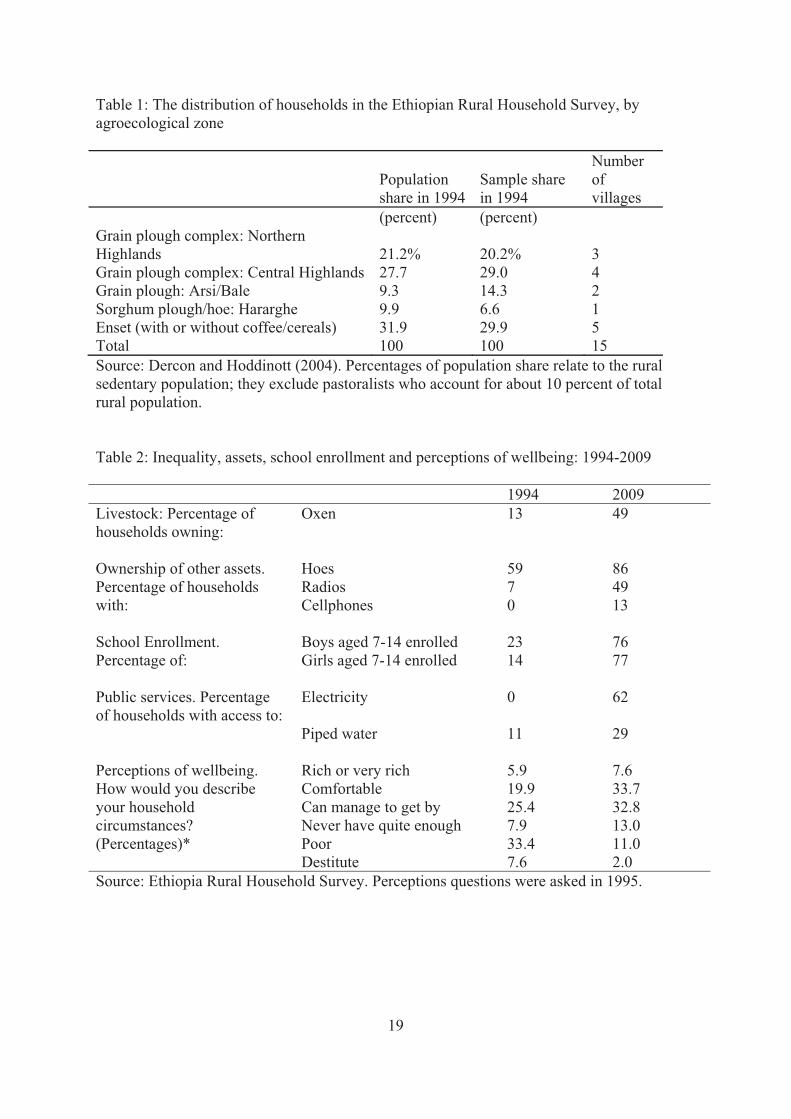
further details. Table 1 gives the details of the sampling frame and the actual proportions in

the total sample. Using the classifications found in Westphal (1976) and Getahun (1978),

Table 1 also shows that population shares within the sample are broadly consistent with the

population shares in the three main sedentary farming systems – the plough based cereals

farming systems of the Northern and Central Highlands, mixed plough/hoe cereals

farming systems, and farming systems based around enset (a root crop also called false

banana) that is grown in southern parts of the country. In fact, the sample sizes in each

village were chosen so as to approximate a self-weighting sample, when considered in terms

of farming system: each person (approximately) represents the same number of persons found

in the main farming systems as of 1994. However, results should not be regarded as

nationally representative. The sample does not include pastoral households or urban areas.

Also, the practical aspects associated with running a longitudinal household survey when the

sampled localities are as much as 1000km apart in a country where top speeds on the best

5

roads rarely exceed 50km/hour constrained sampling to only 15 communities in a country of

thousands of villages. Therefore, extrapolation from these results should be done with care.

An additional round was conducted in late 1994, with further rounds in 1995, 1997,

1999, 2004 and 2009. These surveys were conducted, either individually or collectively, by

the Economics Department at Addis Ababa University, the Centre for the Study of African

Economies, University of Oxford or the International Food Policy Research Institute. Sample

attrition between 1994 and 2009 is low, with a loss of only 16.1 percent (or 1.1 percent per

year) of the sample over this 15 year period, in part because of this institutional continuity.

This continuity also helped ensure that questions asked in each round were identical, or very

similar, to those asked in previous rounds and that the data were processed in comparable

ways. Attrition is linked closely to initial (1994) demographic characteristics and, to a much

lesser extent, near landlessness. Controlling for location, education, and initial livestock

holdings, a household headed by a female aged 70, with only one member and with less than

0.25 ha of land has a 39 percentage point higher probability of attriting than a household

headed by a male, aged 30, with three or more persons and more than one ha of land. Further,

most of the attrition observed in the ERHS occurs in the early years of the study; attrition

between 2004 and 2009 is less than 0.6 percent per year.

3. Poverty and welfare

Table 2 describes the evolution of household welfare in terms of selected data on assets,

human capital formation, access to public services and perceptions of wellbeing. There are

improvements in all of these measures, although certain outcomes remain low. In 2009, we

asked people to rank themselves (in a scale of seven steps) how poor or rich they were. We

asked the same question in 1995 and Table 2 also reports these findings. These self-reports

also speak to improvements in well-being, with the proportions of households reporting

themselves to be in the poorest two categories dropping markedly.

For the remainder of the paper, however, we focus on poverty defined in terms of

consumption. More than any other dimension of poverty, such as education or child

mortality, it tends to be most closely related to changing economic opportunities.

Consumption is defined as the sum of values of all food items, including purchased meals,

and non-investment non-food items. The latter are interpreted in a limited way, so that

contributions for durables and spending with some investment connotation, such as health

and education expenditures, are not included (Hentschel and Lanjouw, 1996). Although there

6

are good conceptual reasons for including use values for durables or housing (Deaton and

Zaidi, 2002), we do not do so here; the heterogeneity in terms of age and quality of durables

owned by our respondents, together with the near complete absence of a rental market for

housing would make the calculation of use values highly arbitrary. Because comparisons of

productive and consumer durable holdings between 1994 and 2009 show rising holdings of

these durables and comparisons of school enrollment data show significant increases

in enrollment (Table 2), ceteris paribus, our consumption estimates may understate the actual

increases in household welfare. Consumption is expressed in monthly per capita terms and

deflated using the food price index with base year 1994.

We also consider the evolution of poverty in these villages. Doing so requires first

setting a poverty line. We use a cost-of-basic-needs approach. Based on the 1994 data, a

food poverty line is constructed using a bundle of food items that would provide 2300Kcal

per adult per day. To this, we add a non-food bundle using the method set out in

Ravallion and Bidani (1994) and obtain a poverty line of 50 birr per capita per month in

1994 prices. Dercon and Krishnan (1996) provide further information on the construction

of the poverty line, including details of the food basket and its sensitivity to different sources

of data on prices used to value the food basket.

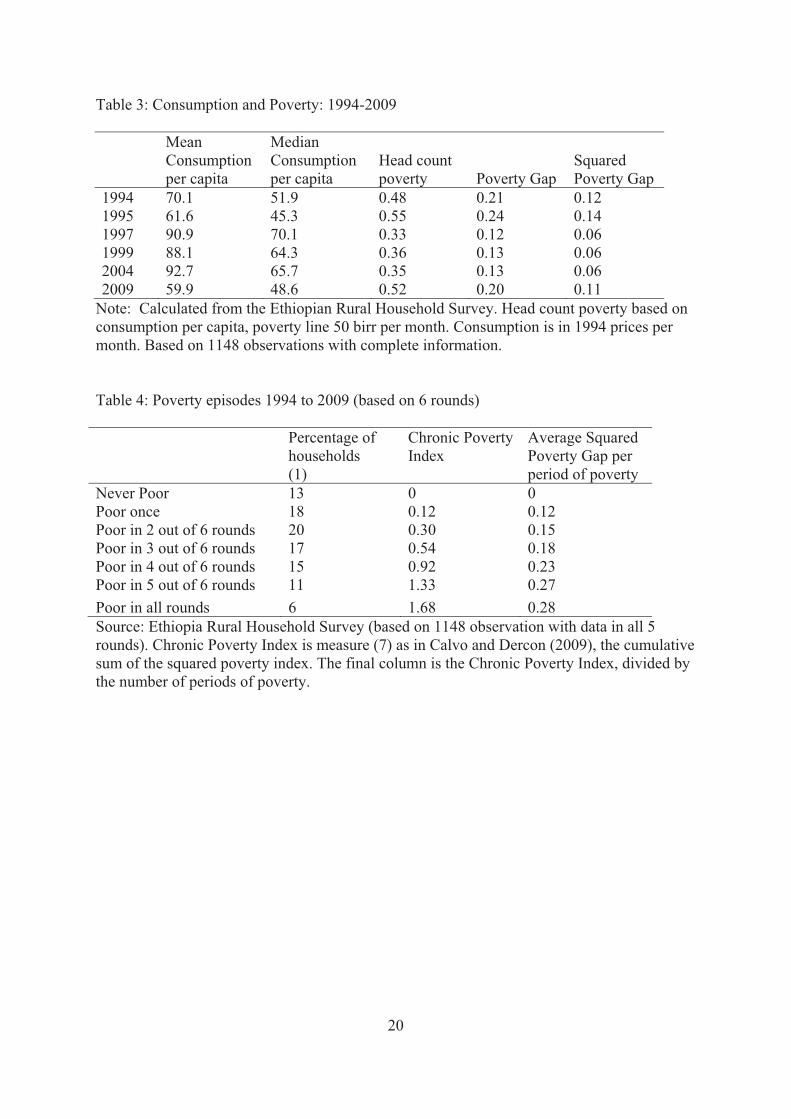
Table 3 provides data on mean and median consumption per month per capita, as well

as three poverty measures, the head count (P0), the poverty gap (P1) and the squared poverty

gap (P2) measure, all belonging to the Foster-Greer-Thorbecke family of poverty measures.

Data are presented from 1994, 1995, 1997, 1999, 2004 and 2009. We exclude findings from

the second round of data collection in 1994, which was mainly meant to provide data on

consumption from a different season than other rounds. As discussed in Dercon and Krishnan

(2000), the seasonality in consumption in Ethiopia as reflected in these data is high, and since

this is not the focus of the paper, the round was dropped from the rest of the analysis. Note

that the timing of the 1997 round was also not optimal for comparability – the immediate

post-harvest period – and this seasonal consideration together with the fact that 1997 was a

good year in terms of crop production has the effect of making the 1997 outcomes look

particularly high. Mean consumption per capita in 1994 was 71.1 birr per capita per month

(about 14 US $ per month per capita at the exchange rate of the time). By 2004, this had risen

to 91.5 birr per capita in real (1994) terms. Between 1994 and 2004, consumption growth of

the mean was on average 2.6 percent per year. This is broadly comparable to the

average annual rate of growth of real GDP per capita (2.1 per cent) and the increases

7

reported using nationally representative household consumption data found in Woldehanna et

al (2008).

Between 2004 and 2009, both mean and median consumption fall. Further, the Gini

coefficient for per capita consumption also falls, from 0.44 to 0.37, suggesting that the largest

reductions in consumption are occurring amongst better-off households. Unlike the 1994-

2004 period, mean consumption growth in the ERHS villages does not track real GDP per

capita growth which is positive over this period. This is surprising. We cannot attribute this to

changes in the way these data were collected. The questionnaire was identical to that used in

2004 as was the training of the enumerators and supervisors, and a significant number had

worked on the ERHS in earlier rounds. Further, the decline in consumption is not uniform

across all survey sites; several villages see a rise in consumption between 2004 and 2009. We

note, however, two factors that may have played a role in this decline. Several villages in

Tigray and SNNPR experienced severe localized droughts that caused considerable income

losses. Second, the 2009 round was fielded approximately six months after the 2008 harvest

and in the aftermath of the rapid rise in food prices in 2008. Since many households in the

ERHS are net food purchasers, the 2009 round may have occurred just at the point where

food stocks had run out and households were entering the market. With prices significantly

higher, they may have been reducing quantities consumed.

Mirroring the consumption data, there are significant reductions in poverty between

1994 and 2004. Headcount poverty fell from 48 to 35 per cent; proportionately, even larger

falls were recorded in the poverty gap and squared poverty gap indices. However, poverty

jumps sharply between 2004 and 2009. The headcount index rises to 0.52; the poverty gap

and the squared poverty gap also jump.

Table 4 provides further evidence on the persistence of poverty. Since food

consumption accounts for more than 75 per cent of total consumption, and since as is

customary, food consumption is measured using a short recall period, it should not come as a

surprise that many households were identified at least once above the poverty line. But about

17 percent remained poor throughout or had only once a consumption level above the poverty

line, while 13 percent were never poor and 28 percent poor once.

One definition of ‘chronic’ poverty is the head count of those poor at least half the

time, in this case, three or more times below the poverty line (Foster, 2007). Using

this definition, about 49 percent of our sample is chronically poor. Calvo and Dercon

(2009) describe an alternative set of measures of chronic or intertemporal poverty. One such

8

set is the sum across all time periods of the Foster-Greer-Thorbecke poverty measures for

each period of time.1 Its advantage is that it takes all poverty episodes into account, and does

not allow for compensation over time, in contrast to the ‘chronic’ measure of poverty as

in Ravallion and Jalan (2000) which is based on average consumption (and therefore

allows for perfect compensation).

Column (2) gives this based on the within period P2 (severity) of poverty, so the

measure is simply the sum of the P2 measures over six periods, giving a sense of how bad

this 15-year period (6 observations) has been. It offers a more comprehensive way

of quantifying poverty over time, taking into account the severity of poverty in each

period, which simple counting approaches ignore. The final column takes the average of

the Chronic Poverty Index, per period of poverty. In other words, it gives a sense of the

depth of poverty experienced in each poverty episode by particular groups. The results are

very suggestive. Unsurprisingly, those with more periods in poverty experience more

‘chronic’ poverty, as measured by the cumulative Chronic Poverty index in column (2).

However, the increase is not linear: more episodes do not add to chronic poverty to the same

extent. The last column, which gives the average FGT squared poverty gap index (which is

the same as the per period average of the chronic poverty index), shows that those

experiencing more periods of poverty also had the highest severity of poverty on average in

their periods of poverty. In other words, these people are not just poor more often over these

15 years, their poverty is more severe.

4. Conceptual framework and econometric results

The descriptive statistics provided above suggest that income growth, as proxied by changes

in consumption, is associated with reductions in poverty. To explore this hypothesis further,

we use a standard empirical growth model, allowing for transitional dynamics (Temple,

1999). We observe i households (i = 1, …, N) across periods t (t = 1, …, T).2 Growth rates

for household i (ln yit – ln yit-1) are negatively related to initial levels of income (ln yit-1). Let �

represent sources of growth common to all households and X reflect fixed characteristics of

the household, such as location, that also affect growth. Other sources of growth from t to t-1

are exogenous levels of capital stocks and access to technologies (kit-1) observed at t-1 both of

which are time varying. Lastly, while standard growth models do not allow for transitory

shocks such as changes in rainfall (ln Rt – ln Rt-1), we know from previous work with our data

(Dercon, 2004; Dercon, Hoddinott and Woldehanna, 2005) that such events do have growth

effects. Mindful of the numerous reasons why one should be careful in applying this

9

framework to any context, given the theoretical and empirical assumptions implied by this

model (Temple, 1999) and dropping the i subscripts, our basic model is:

ln yt – ln yt-1 = � + �ln yt-1 + �ln kt-1 + �(ln Rt – ln Rt-1) + �X (1)

We will use (1) first to explore the factors kt-1 that may have been behind the growth

in this period. As in Dercon et al. (2009), a detailed analysis was done on this and other

aspects of the overall growth process, we build on this paper for this part of our analysis, to

prepare us for in-depth analysis of the links between growth and chronic poverty. Secondly,

we will explore whether the chronic poor were similarly responsive to the same factors, or

whether they had different returns to these improving factors. This will first be done using

interaction terms in (1) to describe potentially differential effects between the chronic poor

and the rest of the sample. As will be seen, this is not enough to fully understand why there is

such a different growth experience between the chronic poor and the rest of the sample. To

dig deeper, and as we have access to longitudinal data, we can estimate these regressions

using household fixed effects, i.e. allowing for household-specific factors that did not change

over time but nevertheless affect growth in each period. Typically, in econometric work,

these household fixed effects are not explored further, even though they are a perfect measure

of differences between households in growth in the sample, and are of specific interest to us,

as they offer us an estimate of a constant growth effect, experienced in each period by each

household, and that has remained latent throughout the period. As in macro-growth

regressions, this latent growth effect also affects the steady state consumption, leading to

permanent differences in the standard of living, as in the literature on conditional

convergence. One specific hypothesis is that this latent effect is different for the chronically

poor, and its correlates could give us insight in what makes these chronically poor different

from other households. In practice, we will explore this by contrasting the results from

regressions linking chronic poverty to initial characteristics and the correlates of the fixed

effect in the growth regression (1).

All households in this sample have access to some sort of road or path. However, the

quality of this road varies significantly from all-weather roads suitable for vehicular traffic to

mud tracks that at best can support foot traffic. The benefits to roads are perceived to operate

through four channels: reducing the costs of acquiring inputs; reducing margins in output

prices between market town and the village; reducing the impact of shocks and permitting

10

entry into new, more profitable activities. Given this, and given the data available to us in the

survey, we define road access as a dummy variable equaling one if the household has access

to a road capable of supporting truck (and therefore trade) and bus (and therefore facilitating

the movement of people) traffic in both the rainy and dry seasons.

Capturing the role played by the agricultural productivity programme in existence

during this period is more complicated. The household survey instrument asked households

how many times they had been visited by an extension agent during the last main cropping

season. Using these data, we create a dummy variable equaling one if the household had

received one such visit, zero otherwise. Initial levels of access to all-weather roads were

around 40 per cent, with significant improvements recorded between 1997 and 1999 and

1999 and 2004. The percentage of households receiving at least one visit from an extension

agent more than triples over this 15 year period. This increase is widely distributed with 13 of

our 15 villages recording an increase in the number of households receiving at least one visit.

However, the starting level in 1994 – 5.6 per cent – was stunningly low.

Finally, in addition to changes in rainfall, we include other transitory events that

might affect consumption growth: input price shocks; changes in log food prices; and

whether since the last round a death or a serious illness was experienced.

The first column of Table 5A shows the results of estimating (1) using an instrumental

variables model with household fixed effects.3 This regression suggests that 10 percent more

rainfall increases consumption by 1.8 percent. Rainfall is therefore one crucial source of

variability. Of the other shocks, only death and illness shocks appear to be significant –

suggesting that they contribute to an 11 percentage point losses in growth. Roads appear to

have mattered a lot in terms of explaining differential growth. Those with access to a road

appear to have almost 9 percent higher growth per year than those without. Given the nature

of the overall growth (a few percent per year in per capita terms), this is clearly a crucial

factor explaining divergence between communities. Roads improved considerably in the

sample – access to a good quality road has increased from about 40 percent of the sample to

about 70 percent in this period. The regression results suggest that road improvement

contributed to a growth acceleration by about 5 percent in our sample. Finally, we find

positive growth from extension services.4

In column (2), we include time dummy variables in the place of time varying shocks

such as rainfall and food and input price shocks. This represents a more general estimable

version of equation (1). Our estimates of the impact of lagged consumption and household

11

specific death and illness shocks remain largely unchanged; the parameter on extension is

smaller, however, and less precisely measured, leading to some caution in interpreting the

growth effects from extension as implied by column (1).

Do the chronically poor obtain similar growth effects from these changes? We begin

with households that are chronically poor, defined in terms of experiencing at least 3 periods

of poverty. Did they experience a different growth trajectory because they could not benefit

from roads or extension services and other factors in the same way, or was their growth

trajectory different for example because they simply had fewer roads or extension services

(or more negative shocks)? To explore this, we interact these independent variables (and the

shocks) with whether the household was ‘chronic poor’ in this period. The results found in

columns (3) and (4) suggest that the chronically poor have not been following a different

growth trajectory in nature: the only significant effect that we could find when using the

interaction terms is that the ‘chronic’ poor had somewhat lower sensitivity to rainfall and

higher, though imprecisely measured, sensitivity to death and illness shocks.5 But for the core

variables used to capture the growth process – the role of infrastructure and extension – we

find no significant differences between the chronic poor and the rest. However, as the

interaction variable uses information that is the outcome of the growth process (consumption

levels at t+1, t+2, etc), the results need to be treated with caution.

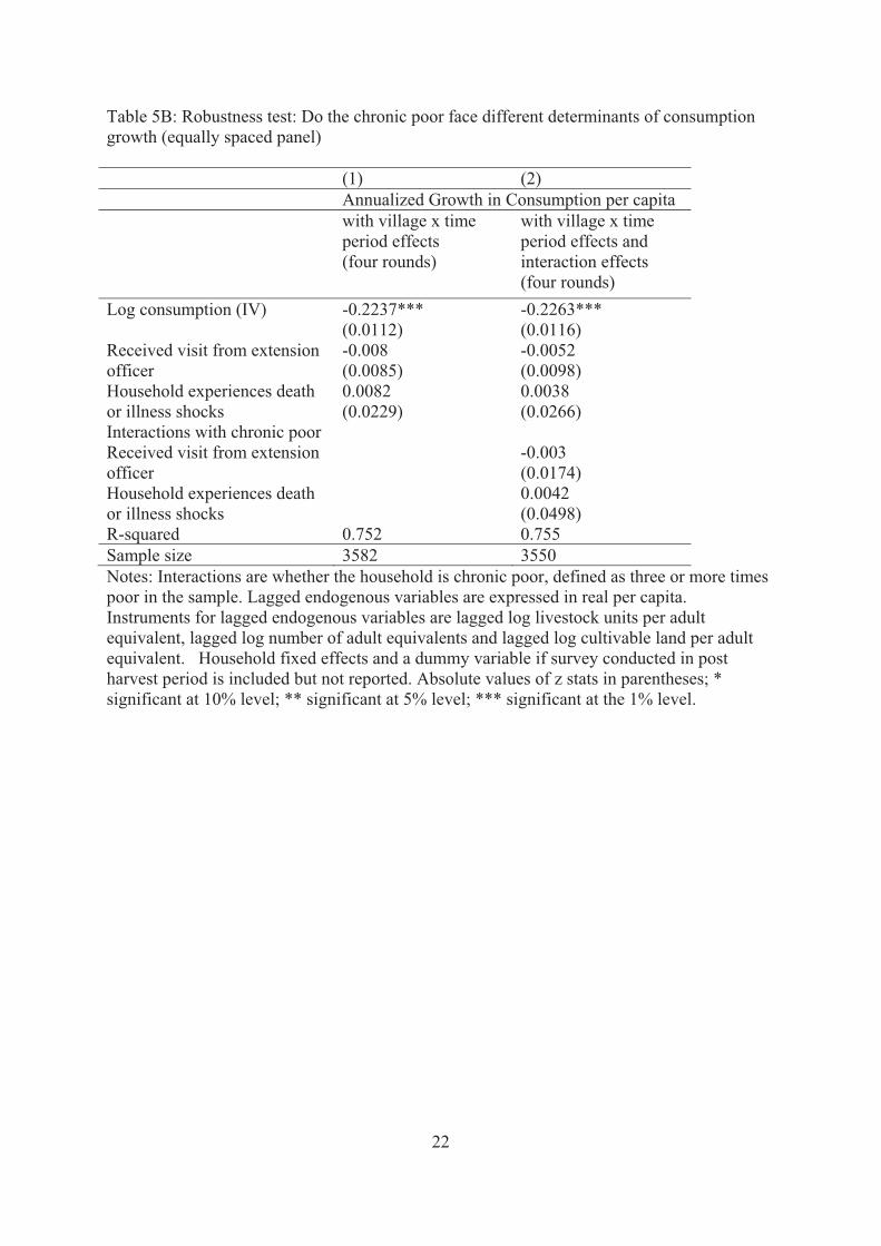
Before continuing, we note a potential econometric concern with the results of Table

5 resulting from the fact that the ERHS rounds are not evenly spaced. As noted by Andreou,

Ghysels and Kourtellos (2010), this can lead, under certain conditions, to biased and

inconsistent parameter estimates.6 However, if we restrict ourselves to using data collected in

1994, 1999, 2004 and 2009, we have four evenly spaced rounds which allows us to

circumvent this problem. Results using only these rounds, together with village-round

interaction terms (expressed as dummy variables) are reported in Table 5B. As seen by the R2

statistic, estimating the model with household fixed effects, village x round dummy variables

and lagged consumption soaks up a lot of the variation in consumption growth rates and so it

is not especially surprising that the household level shock variables, access to extension and

death and illness shocks, are no longer statistically significant, since the sample size is also

smaller due to dropping two rounds of data, making precise estimation harder. We note that

the coefficient on lagged consumption is smaller in Table 5B than 5A; this is consistent with

Andreou, Ghysels and Kourtellos’ (2010) findings on the impact of accounting for differing

lag lengths in cross-country growth regressions.7

12

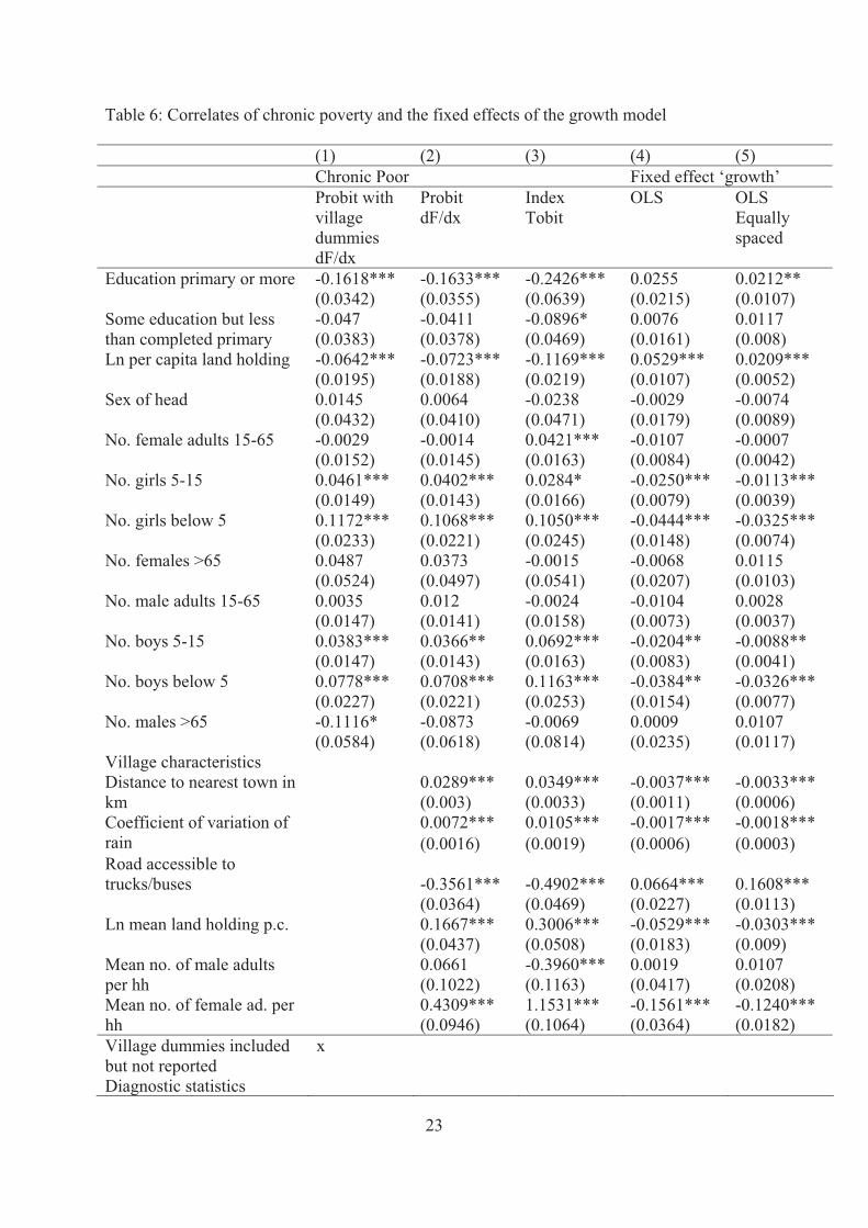
We next regress initial (1994) household and community characteristics on whether a

household was chronically poor. Household characteristics include levels of land per capita

(in natural logarithms of hectares per capita)8, education of the head (whether primary or

more had been completed, and whether at least some primary education had been

completed)9, household composition (the number of adults above 15 years of age, the number

of elderly above 65, children below 5 and children between 5 and 15, all disaggregated by

sex), and the sex of the head (male equals one).10 Table 6 reports the marginal effects of

probit regressions of being observed chronically poor in our villages, defined as three or more

episodes of poverty between 1994 and 2009. The first column controls for village dummies,

i.e. fixed effects, absorbing any factors contributing to village-wide chronic poverty.11 The

second column controls for these factors explicitly, thereby unpacking the community-wide

determinants of chronic poverty. As it is a cross-section regression based on 15 communities,

the degrees of freedom to identify the community-wide variables are limited. We

experimented with different possible characteristics, and the factors that were both stable

across specifications and left the household characteristics unaffected are included in table 6:

distance in kilometres to the nearest town, whether the road was capable of handling trucks

and buses, the coefficient of variation of yearly rainfall and number of village-wide averages

of endowments in terms of mean land holdings per capita, and mean number of male and

female adults per household in the village.12 As a cross-section regression, this does not

control for other unobserved heterogeneity, so the interpretation has to be done cautiously.

With or without village fixed effects, the marginal effects of the household

characteristics are similar. However, the village fixed effects (not reported) are suggestive in

themselves. Taking a striking example, a household residing in Gara Godo (an enset growing

village in the south) with household characteristics identical to a household in Sirbana Godeti

(not far from the large trading town Debre Zeit and the survey site closest to Addis Ababa) is

80 percent more likely to be chronically poor. Education matters: with primary education

complete in 1994, the probability to be found chronic poor in 1994-2009 was about 16

percent lower. Land matters as well, although in percentage terms not as much: doubling land

(which implies increasing land by just under one standard deviation in the land distribution)

would reduce the probability of being chronic poor by about 6 percent. There are surprisingly

strong effects from having children: they increase the likelihood of being found chronic poor

in this period, with children below 5 and especially girls adding most. We explored whether

this effect is due to the use of a poverty definition based on consumption per capita, which

13

would ‘penalize’ families with children relatively more by understating their likely

consumption, as children have lower basic food needs. However, even using consumption per

adult as the basis for poverty showed the same effect, even if all children and not just younger

children were similarly costly in terms of increasing the likelihood of being chronic poor. As

economies of scale are also possible, we have to be careful to attach too much importance to

this result, but the sheer size makes scale economies implausible: ceteris paribus, another

child appears to increase the probability of being found ‘chronic poor’ by up to 12 percent.

Turning to the community characteristics in column (2), the role of road access and

distance to towns is striking: having a good road reduces the likelihood of being found

chronic poor by 36 percent, while a reduced distance to the nearest small town by about 12

kilometres (which is moving from a distance as in the 75 percentile to the 25th percentile) also

brings down the probability of being chronic poor by about 35 percent. Rainfall variability,

the simplest measure of ‘risk’ faced by different communities, is also found to be highly

significant, but its impact is actually relatively small: moving from the 75th to 25th percentile

would reduce the probability of being chronic poor by about 1 percent. Finally, it should be

noted that the land result reported earlier is relative, as villages in the sample with more land

per capita (possibly a sign of poor land quality or agro-climatic conditions, sustaining low

population densities) are more likely to have high chronic poverty. Also, villages with

relatively speaking many female adults (in this sample a sign of high past involvement in

conflict resulting in a high male death rate, e.g. in the Tigrayan villages found in the northern

Highlands) are more likely to be chronically poor. As mentioned before, with only 15

communities, we have to be cautious with attaching to strong an interpretation to these

results. Column (3) reports an alternative way of exploring the correlates of chronic poverty,

using the chronic poverty index reported earlier, that takes into account the severity of

poverty in each period. In terms of the factors that matter, the results are similar adding

credence that these factors matter for different ways of looking at poverty persistence. In

short, we find that chronic poverty is correlated to a number of household and community

endowments (including education, productive assets such as land, as well as factors affecting

‘remoteness’ such as distance to towns and road access).

But this is not the whole story. The models in Table 5 are fixed effects models,

implying that they control for household heterogeneity. In other words, beyond the factors

modeled, each household has its own ‘unexplained’, latent part of growth, leading to its own

growth rate and a different steady state consumption level. Although this is a short sample,

14

we can still retrieve these fixed effects, essentially by averaging the residuals from the fixed

effects regression. Using model (1) in Table 5, we find that the average fixed effect for the

chronic poor is about -16 percent per year, while for the non-chronic poor it is +7 percent per

year; these means are significantly different from each other at 1 percent and less. In other

words, for the same values of shocks, or roads or extension visits, the growth difference

between these two groups is estimated to be about 23 percent. Further, the correlation

between the household fixed effect and whether one is chronic poor or not, or with the

chronic poverty index that allows for the severity of chronic poverty is very high

(respectively -0.51 and -0.56). In other words, the chronic poor face a serious growth deficit,

making catching up with the rest difficult – in terms of time-varying characteristics, they

need much ‘better’ values to obtain the same level of growth as the non-chronic poor.

This would seem an extremely large difference in yearly growth rates between the

chronic poor and the rest. Of course, this is not the entire story from the regression: as the

coefficient on the lagged dependent variable is negative, this is showing a relatively strong

convergence as well, with higher growth for those starting at t-1 with lower consumption.

The fixed effect offsets this convergence effect – and rather strongly for the chronic poor. It

has therefore also implications in terms of permanent differences in the long run, as measured

by the steady state: the 23 percent difference, with a coefficient on the lagged dependent

variable of about -0.33 implies a steady state difference of (0.23/0.33) or almost 70 percent

between these ‘chronic poor’ and the rest – a permanent difference. Given the small length of

the panel, we obviously have to be cautious with both the latent growth effect and its impact

on steady-state consumption; in any case, at least on the basis of this sample, very different

growth paths and a substantial difference in steady-states are implied.

What determines this fixed effect? By retrieving the fixed growth effect from the

regressions, it is possible to study its correlates. However, as this is a cross-section, one

should be careful not to overinterpret these regressions, reported in the fourth and fifth

columns in Table 6. Column (4) is based on extracting the fixed effect from Table 5A,

column (1). The most striking result is that the main correlates for lower chronic poverty are

the correlates for a higher fixed effect. For example, moving from the 25th to the 75th

percentile in terms of distance to town, would cost about 5 percent in latent growth (or about

15 percent in steady state difference, using the value of the lagged dependent variable of -

0.33 as before). Access to good roads also results in an additional 7 percent latent growth

effect (or 21 percent in steady-state difference). The source of the fixed effect – the

15

unevenly spaced or evenly spaced panel – does not affect these finding at least qualitatively:

column (5) is based on extracting the fixed effect from Table 5B, column (1). All these

results are similar to column (4) showing again the robustness of our core findings to this

methodological issue; one result that is strikingly different is an even higher latent growth

effect from the lack of good roads, at about 16 percent (and given a lagged dependent

variable in table 5B of -0.22, this would imply a steady state difference of more than 70

percent from road differences only).13

In sum, the evidence suggests that the chronic poor tend to have the same return from

growth stimulating factors, such as improved infrastructure or extension. Overall, however,

the chronic poor appear to start from a serious growth handicap, linked to physical assets,

education and remoteness, contributing to poverty persistence, leading to long-term outcomes

that are permanently lower..

5. Conclusion

This paper has explored chronic poverty and its link with consumption growth in 15

Ethiopian villages between 1994 and 2009. Ethiopia experienced considerable growth in this

period, and this is also reflected in growth in assets, education, access to services and roads,

and perceived growth in welfare. Between 1994 and 2004 consumption poverty declined,

although between 2004 and 2009, poverty reduction came to a halt, possibly linked to high

inflationary pressures and specific local factors; movements in and out of poverty remained

relatively large. In this paper, we focused on the persistence of poverty of some, and the

factors underlying this chronic poverty.

We use both a counting approach to identify the chronic poor and an index of chronic

poverty that takes into account not just the duration but also the depth of poverty. We find

that both indicators lead to broadly similar insights. Chronic poverty is associated with

several characteristics: lack of physical assets, education, and ‘remoteness’ in terms of

distance to towns or poor roads. Furthermore, we built on Dercon et al. (2009) to explore

some of the factors driving growth in a dynamic micro-level growth model. We find that

factors driving growth, such as extension or access to good roads, have similar impacts on

chronically poor and non-chronically poor households. However, their ‘fixed’ differences, as

reflected in the estimated latent growth related to time-invariant characteristics, suggest that

the chronic poor face a considerable growth handicap compared to the rest, leaving them

permanently behind. This ‘fixed’ growth effect correlates also well with the same

16

characteristics of the chronic poor during the sample period. Chronic poverty, as reflected in

poor initial assets and remoteness, appears to be correlated with a permanent gap in growth

and the living standards they tend to over the sample period.

17

References Adato, M., M. Carter and J. May, 2006. “Exploring poverty traps and social exclusion in South Africa using qualitative and quantitative data”, Journal of Development Studies 42(2): 226-247. Andreou, E., E. Ghysels and A. Kourtellos, 2010. “ Regression models with mixed sampling frequencies”, Journal of Econometrics 158: 246-261. Baulch, B. (ed), 2011. Why poverty persists: Poverty dynamics in Asia and Africa. Edward Elgar: Cheltenham. Baulch. B. and J. Hoddinott, 2000, “Economic Mobility and Poverty Dynamics in Developing Countries”, Journal of Development Studies 36: 1-24. Carter, M. and C.B. Barrett, 2006. “The economics of poverty traps and persistent poverty: An asset-based approach”, Journal of Development Studies 42(2): 178-199. Calvo, C. and S.Dercon (2007), “Chronic Poverty and All That: The Measurement of Poverty over Time” The Centre for the Study of African Economies Working Paper Series. Working Paper 263. Deaton, A. and S. Zaidi, 2002. Guidelines for constructing consumption aggregates for welfare analysis. Living Standards Measurement Study Working Paper: 135, Washington, D.C.: The World Bank. Dercon, S. 2004. Growth and shocks: Evidence from rural Ethiopia. Journal of Development Economics 74 (2): 309-329. Dercon, S., D.Gilligan, J.Hoddinott and T. Woldehanna. 2009, “The impact of roads and agricultural extension on consumption growth and poverty in fifteen Ethiopian villages,” American Journal of Agricultural Economics 91(4): 1007-1021. Dercon, S., and J. Hoddinott, 2004. The Ethiopian Rural Household Surveys: Introduction. International Food Policy Research Institute, mimeo. Dercon, S., J. Hoddinott and T. Woldehanna, 2005. Consumption and shocks in 15 Ethiopian Villages, 1999-2004. Journal of African Economies, 14: 559-585. Dercon, S., and P. Krishnan, 1996. A consumption based measure of poverty in Ethiopia: 1989-1994 in, M. Taddesse and B. Kebede, Poverty and economic reform in Ethiopia, Proceedings Annual Conference of the Ethiopian Economics Association. Dercon, S., and P. Krishnan. 2000. Vulnerability, poverty and seasonality in Ethiopia. Journal of Development Studies 36 (6): 25-53. Dercon S., and P. Krishnan. 2003. Changes in poverty in rural Ethiopia 1989-1995: in A.Booth and P.Mosley, (eds.) The New Poverty Strategies, Palgrave MacMillan, London.

18

Foster, J., 2007. A Class of Chronic Poverty Measures, mimeo. Getahun. 1978. Report on framing systems in Ethiopia. Ministry of Agriculture, Government of Ethiopia, Addis Ababa. Hentschel, J. and P. Lanjouw, 1996. Constructing an indicator of consumption for the analysis of poverty: Principles and illustrations with reference to Ecuador. Living Standards Measurement Study Working Paper: 124, Washington, D.C.: The World Bank. Hulme, D. (2004), “Chronic Poverty”, Special issue of the Journal of Human Development, vol 5, no. 2 Jalan, J. and M. Ravallion, 2000, ‘Is Transient Poverty Different? Evidence from Rural China’, Journal of Development Studies, Vol.36, No.6. Lybbert, T.J., C. B. Barrett, S. Desta, and D.L. Coppock, 2004. “Stochastic Wealth Dynamics and Risk Management Among A Poor Population,” Economic Journal, 114(October): 750�777. Temple, J., 1999. The new growth evidence. Journal of Economic Literature, 37(1): 112-156. Westphal, E. 1976. Farming Systems in Ethiopia. Food and Agriculture Organization of the United Nations. Woldehanna, T., J. Hoddinott, F. Ellis and S. Dercon, 2008. Dynamics of growth and poverty in Ethiopia: 1995/96-2004/05. Report submitted to Ministry of Finance and Economic Development, Addis Ababa.

19

Table 1: The distribution of households in the Ethiopian Rural Household Survey, by agroecological zone

Population share in 1994

Sample share in 1994

Number of villages

(percent) (percent) Grain plough complex: Northern Highlands 21.2% 20.2% 3 Grain plough complex: Central Highlands 27.7 29.0 4 Grain plough: Arsi/Bale 9.3 14.3 2 Sorghum plough/hoe: Hararghe 9.9 6.6 1 Enset (with or without coffee/cereals) 31.9 29.9 5 Total 100 100 15 Source: Dercon and Hoddinott (2004). Percentages of population share relate to the rural sedentary population; they exclude pastoralists who account for about 10 percent of total rural population. Table 2: Inequality, assets, school enrollment and perceptions of wellbeing: 1994-2009 1994 2009 Livestock: Percentage of households owning:

Oxen 13 49

Ownership of other assets. Percentage of households with:

Hoes 59 86 Radios 7 49 Cellphones 0 13

School Enrollment. Percentage of:

Boys aged 7-14 enrolled 23 76 Girls aged 7-14 enrolled 14 77

Public services. Percentage of households with access to:

Electricity 0 62

Piped water 11 29 Perceptions of wellbeing. How would you describe your household circumstances? (Percentages)*

Rich or very rich 5.9 7.6 Comfortable 19.9 33.7 Can manage to get by 25.4 32.8 Never have quite enough 7.9 13.0 Poor 33.4 11.0 Destitute 7.6 2.0

Source: Ethiopia Rural Household Survey. Perceptions questions were asked in 1995.

20

Table 3: Consumption and Poverty: 1994-2009

Mean Consumption per capita

Median Consumption per capita

Head count poverty Poverty Gap

Squared Poverty Gap

1994 70.1 51.9 0.48 0.21 0.12 1995 61.6 45.3 0.55 0.24 0.14 1997 90.9 70.1 0.33 0.12 0.06 1999 88.1 64.3 0.36 0.13 0.06 2004 92.7 65.7 0.35 0.13 0.06 2009 59.9 48.6 0.52 0.20 0.11

Note: Calculated from the Ethiopian Rural Household Survey. Head count poverty based on consumption per capita, poverty line 50 birr per month. Consumption is in 1994 prices per month. Based on 1148 observations with complete information. Table 4: Poverty episodes 1994 to 2009 (based on 6 rounds) Percentage of

households (1)

Chronic Poverty Index

Average Squared Poverty Gap per period of poverty

Never Poor 13 0 0 Poor once 18 0.12 0.12 Poor in 2 out of 6 rounds 20 0.30 0.15 Poor in 3 out of 6 rounds 17 0.54 0.18 Poor in 4 out of 6 rounds 15 0.92 0.23 Poor in 5 out of 6 rounds 11 1.33 0.27 Poor in all rounds 6 1.68 0.28 Source: Ethiopia Rural Household Survey (based on 1148 observation with data in all 5 rounds). Chronic Poverty Index is measure (7) as in Calvo and Dercon (2009), the cumulative sum of the squared poverty index. The final column is the Chronic Poverty Index, divided by the number of periods of poverty.

21

Table 5A: Do the chronic poor face different determinants of consumption growth 1994-2009?

(1) (2) (3) (4) Annualized Growth in Consumption per capita (six rounds)

with village x time period effects

with chronic poverty interaction effects

with chronic poverty interaction effects and village x time period effects

Log consumption (IV) -0.3336*** -0.3416*** -0.3164*** -0.3285*** (0.0270) (0.0294) (0.0279) (0.0305)

Access to all-weather road

0.0900*** 0.0908*** (0.0184) (0.0229)

Received visit from extension officer

0.0442* 0.0285 0.0568* 0.0384 (0.0230) (0.0244) (0.0291) (0.0276)

Rainfall shocks 0.1845*** 0.2882*** (0.0390) (0.0548)

Input price shocks -0.0548 -0.0521 (0.0840) (0.0713)

Change in log food prices

-0.0013 -0.0054 (0.0034) (0.0042)

Household experiences death or illness shocks

-0.1107* -0.1156** -0.0521 -0.0715 (0.0594) (0.0547) (0.0713) (0.0673)

Interaction terms with chronic poor

Access to all-weather road

0.003 (0.0419)

Received visit from extension officer

-0.0388 -0.0356 (0.0485) (0.0498)

Rainfall shocks -0.2387*** (0.0885)

Input price shocks -0.1416 (0.1342)

Change in log food prices

0.0115 (0.0082)

Household experiences death or illness shocks

-0.1416 -0.1316 (0.1342) (0.1169)

Sample size 5870 5870 5458 5458 Notes: Lagged endogenous variables are expressed in real per capita. Instruments for lagged endogenous variables are lagged log livestock units per adult equivalent, lagged log number of adult equivalents and lagged log cultivable land per adult equivalent. In column (1), Cragg-Donald Wald F statistic is 212, rejecting weak instruments. Hansen J test (overidentification) is 0.60 and not significant. Household fixed effects and a dummy variable if survey conducted in post harvest period is included but not reported. Interactions are whether the household is chronic poor in column (3) and (4), defined as three or more times poor in the sample. Absolute values of z stats in parentheses; * significant at 10% level; ** significant at 5% level; *** significant at the 1% level.

22

Table 5B: Robustness test: Do the chronic poor face different determinants of consumption growth (equally spaced panel) (1) (2) Annualized Growth in Consumption per capita with village x time

period effects (four rounds)

with village x time period effects and interaction effects (four rounds)

Log consumption (IV) -0.2237*** -0.2263*** (0.0112) (0.0116)

Received visit from extension officer

-0.008 -0.0052 (0.0085) (0.0098)

Household experiences death or illness shocks

0.0082 0.0038 (0.0229) (0.0266)

Interactions with chronic poor Received visit from extension officer

-0.003 (0.0174)

Household experiences death or illness shocks

0.0042 (0.0498)

R-squared 0.752 0.755 Sample size 3582 3550 Notes: Interactions are whether the household is chronic poor, defined as three or more times poor in the sample. Lagged endogenous variables are expressed in real per capita. Instruments for lagged endogenous variables are lagged log livestock units per adult equivalent, lagged log number of adult equivalents and lagged log cultivable land per adult equivalent. Household fixed effects and a dummy variable if survey conducted in post harvest period is included but not reported. Absolute values of z stats in parentheses; * significant at 10% level; ** significant at 5% level; *** significant at the 1% level.

23

Table 6: Correlates of chronic poverty and the fixed effects of the growth model (1) (2) (3) (4) (5) Chronic Poor Fixed effect ‘growth’ Probit with

village dummies dF/dx

Probit dF/dx

Index Tobit

OLS OLS Equally spaced

Education primary or more -0.1618*** -0.1633*** -0.2426*** 0.0255 0.0212** (0.0342) (0.0355) (0.0639) (0.0215) (0.0107) Some education but less than completed primary

-0.047 -0.0411 -0.0896* 0.0076 0.0117 (0.0383) (0.0378) (0.0469) (0.0161) (0.008)

Ln per capita land holding -0.0642*** -0.0723*** -0.1169*** 0.0529*** 0.0209*** (0.0195) (0.0188) (0.0219) (0.0107) (0.0052) Sex of head 0.0145 0.0064 -0.0238 -0.0029 -0.0074 (0.0432) (0.0410) (0.0471) (0.0179) (0.0089) No. female adults 15-65 -0.0029 -0.0014 0.0421*** -0.0107 -0.0007 (0.0152) (0.0145) (0.0163) (0.0084) (0.0042) No. girls 5-15 0.0461*** 0.0402*** 0.0284* -0.0250*** -0.0113*** (0.0149) (0.0143) (0.0166) (0.0079) (0.0039) No. girls below 5 0.1172*** 0.1068*** 0.1050*** -0.0444*** -0.0325*** (0.0233) (0.0221) (0.0245) (0.0148) (0.0074) No. females >65 0.0487 0.0373 -0.0015 -0.0068 0.0115 (0.0524) (0.0497) (0.0541) (0.0207) (0.0103) No. male adults 15-65 0.0035 0.012 -0.0024 -0.0104 0.0028 (0.0147) (0.0141) (0.0158) (0.0073) (0.0037) No. boys 5-15 0.0383*** 0.0366** 0.0692*** -0.0204** -0.0088** (0.0147) (0.0143) (0.0163) (0.0083) (0.0041) No. boys below 5 0.0778*** 0.0708*** 0.1163*** -0.0384** -0.0326*** (0.0227) (0.0221) (0.0253) (0.0154) (0.0077) No. males >65 -0.1116* -0.0873 -0.0069 0.0009 0.0107 (0.0584) (0.0618) (0.0814) (0.0235) (0.0117) Village characteristics Distance to nearest town in km

0.0289*** 0.0349*** -0.0037*** -0.0033*** (0.003) (0.0033) (0.0011) (0.0006)

Coefficient of variation of rain

0.0072*** 0.0105*** -0.0017*** -0.0018*** (0.0016) (0.0019) (0.0006) (0.0003)

Road accessible to trucks/buses -0.3561*** -0.4902*** 0.0664*** 0.1608*** (0.0364) (0.0469) (0.0227) (0.0113) Ln mean land holding p.c. 0.1667*** 0.3006*** -0.0529*** -0.0303*** (0.0437) (0.0508) (0.0183) (0.009) Mean no. of male adults per hh

0.0661 -0.3960*** 0.0019 0.0107 (0.1022) (0.1163) (0.0417) (0.0208)

Mean no. of female ad. per hh

0.4309*** 1.1531*** -0.1561*** -0.1240*** (0.0946) (0.1064) (0.0364) (0.0182)

Village dummies included but not reported

x

Diagnostic statistics

24

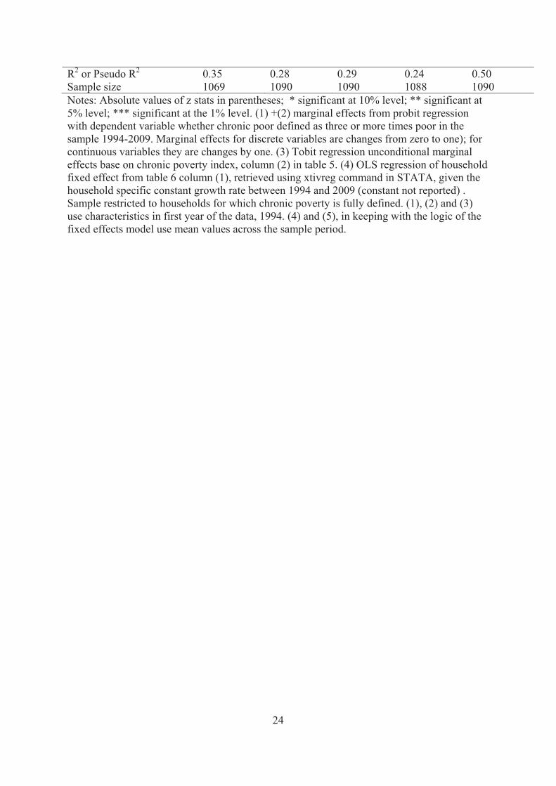
R2 or Pseudo R2 0.35 0.28 0.29 0.24 0.50 Sample size 1069 1090 1090 1088 1090 Notes: Absolute values of z stats in parentheses; * significant at 10% level; ** significant at 5% level; *** significant at the 1% level. (1) +(2) marginal effects from probit regression with dependent variable whether chronic poor defined as three or more times poor in the sample 1994-2009. Marginal effects for discrete variables are changes from zero to one); for continuous variables they are changes by one. (3) Tobit regression unconditional marginal effects base on chronic poverty index, column (2) in table 5. (4) OLS regression of household fixed effect from table 6 column (1), retrieved using xtivreg command in STATA, given the household specific constant growth rate between 1994 and 2009 (constant not reported) . Sample restricted to households for which chronic poverty is fully defined. (1), (2) and (3) use characteristics in first year of the data, 1994. (4) and (5), in keeping with the logic of the fixed effects model use mean values across the sample period.

25

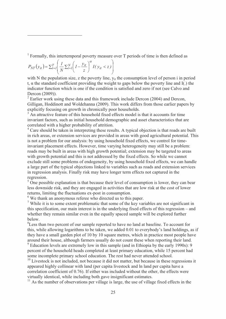
1 Formally, this intertemporal poverty measure over T periods of time is then defined as

� � � ��

�

�

��

� ��

��

� �

T1t

N1i it

ititNT )zy(I

zy

1N1yP

�

with N the population size, z the poverty line, yit the consumption level of person i in period t, � the standard coefficient providing the weight to gaps below the poverty line and I(.) the indicator function which is one if the condition is satisfied and zero if not (see Calvo and Dercon (2009)). 2 Earlier work using these data and this framework include Dercon (2004) and Dercon, Gilligan, Hoddinott and Woldehanna (2009). This work differs from those earlier papers by explicitly focusing on growth in chronically poor households. 3 An attractive feature of this household fixed effects model is that it accounts for time invariant factors, such as initial household demographic and asset characteristics that are correlated with a higher probability of attrition. 4 Care should be taken in interpreting these results. A typical objection is that roads are built in rich areas, or extension services are provided in areas with good agricultural potential. This is not a problem for our analysis: by using household fixed effects, we control for time-invariant placement effects. However, time varying heterogeneity may still be a problem: roads may be built in areas with high growth potential; extension may be targeted to areas with growth potential and this is not addressed by the fixed effects. So while we cannot exclude still some problems of endogeneity, by using household fixed effects, we can handle a large part of the typical objections linked to variables such as roads and extension services in regression analysis. Finally risk may have longer term effects not captured in the regression. 5 One possible explanation is that because their level of consumption is lower, they can bear less downside risk, and they are engaged in activities that are low risk at the cost of lower returns, limiting the fluctuations ex-post in consumption. 6 We thank an anonymous referee who directed us to this paper. 7 While it is to some extent problematic that some of the key variables are not significant in this specification, our main interest is in the underlying fixed effects of this regression – and whether they remain similar even in the equally spaced sample will be explored further below. 8Less than two percent of our sample reported to have no land at baseline. To account for this, while allowing logarithms to be taken, we added 0.01 to everybody’s land holdings, as if they have a small garden plot of 10 by 10 square metres, which in practice most people have around their house, although farmers usually do not count these when reporting their land. 9 Education levels are extremely low in this sample (and in Ethiopia by the early 1990s): 9 percent of the household heads completed at least primary education, while 15 percent had some incomplete primary school education. The rest had never attended school. 10 Livestock is not included, not because it did not matter, but because in these regressions it appeared highly collinear with land (per capita livestock and ln land per capita have a correlation coefficient of 0.76). If either was included without the other, the effects were virtually identical, while including both gave insignificant estimates. 11 As the number of observations per village is large, the use of village fixed effects in the

26

probit regression is unlikely to lead to serious problems related to the consistency of the estimator. 12 The village-wide mean values of land per capita and adults per household were relevant for the stability of the results on other village-wide variables, probably reflecting relative land and labour scarcity. 13 One reason for this difference may be that the regression in table 5B, column (1) did not find a direct effect from (changes) in access to good roads, leaving the effect of roads as a latent growth effect. As a result the interpretation – a high effect of access to roads – is still qualitatively similar between the two models, although the model in table 5B suggests that there are no specific returns to changing the quality of roads, but simply a result from having a good road to start with. Given the relatively small number of rounds in table 5B to identify changes in village level circumstances, this interpretation would have to be made with caution.