The Analysis of Rural Poverty in Ethiopia

Uppsala University

Department of Economics

Master thesis

Spring 2009

The Analysis of Rural Poverty in Ethiopia regarding the three measurements of poverty

Supervisor: Dr. Ranjula Bali Swain

Author: Mohammad Sepahvand

1

Acknowledgments

This paper is intended to be a master thesis in economics at Uppsala University.

The topic that is chosen, is something I find very interesting and significant to know more

about. However, I have just been able to scratch the surface, and it fulfills my initial

expectations of how exiting this area is.

While I have been solely responsible for writing this paper, I would like to extend my

gratitude to the following people for their valuable contributions to the process in general.

Ranjula Bali Swain from the Department of Economics at Uppsala University has been my

tutor during the whole period. I am grateful for all the important comments and advice that I

have received throughout the process of writing this thesis, which would not be possible to

write without Dr Swain.

My fellow students who during the preparation seminars for this thesis came with insightful

comments.

I would also want to thank my colleagues at Statistic Sweden for having the patience by

providing me the time to finalize this paper.

Last but definitely not least I would like to thank my family and friends for the motivational

support I have received during this time.

Mohammad Sepahvand

Uppsala, Sweden, 2009-05-07

The data used in this paper has been made available by the Economics Department, Addis Ababa

University, the Centre for the Study of African Economies, University of Oxford and the International

Food Policy Research Institute. Funding for data collection was provided by the Economic and Social

Research Council (ESRC), the Swedish International Development Agency (SIDA) and the United

States Agency for International Development (USAID); the preparation of the public release version

of these data was supported, in part, by the World Bank. AAU, CSAE, IFPRI, ESRC, SIDA, USAID

and the World Bank are not responsible for any errors in these data or for their use or interpretation.

2

Abstract

This paper analyses rural poverty in Ethiopia using the 1997 round of household survey data

from the Ethiopian Rural Household Survey. Poverty measurements are estimated using a

consumption based two-step procedure through the implementation of the Foster-Greer-

Thorbecke model. The results indicate that the incidence of rural poverty is high for villages

that have lower conditions for agriculture. These findings imply that poverty reduction can be

possible through effective policies toward improving the conditions for agriculture in the rural

areas. Moreover, examination of the connection between different socioeconomic

characteristics and poverty indicates that households consisting of household heads with a

higher age and availability of farmland are relatively less poor. However, households where

the household head has completed at least primary school suffer from most incidence of

poverty.

Furthermore, this study use three different definitions of poverty in connection to well-being

to determine poverty. It is possible to state that these measurements are different

modifications of each other with common variables and follow the same trend.

The results of the paper may increase our understanding of the nature of rural poverty in

Ethiopia and help in providing different poverty reducing policies, for the specific survey

round.

3

Table of Contents List of Abbreviations...........................................................................................5

1 Introduction......................................................................................................6

2 Country Profile.................................................................................................8

3 Literature survey............................................................................................103.1 Empirical work .......................................................................................................13

4 The Theoretical framework ..........................................................................144.1 Different poverty measurements.............................................................................15

5 The Econometric model.................................................................................18 5.1 Consumption based poverty measurement .............................................................18

5.2 Poverty simulations.................................................................................................21

6 Data section.....................................................................................................21 6.1 Database description................................................................................................23

6.1.1 Ethiopia Rural Household Survey.............................................................................23

6.1.2 Information that the Ethiopian dataset provides..............................................................25

6.2 Variable description.........................................................................................................25

6.3 Descriptive statistics................................................................................................26

7 Empirical result and Analysis.......................................................................27 7.1 The Consumption based model...............................................................................27

7.2 Poverty simulation...........................................................................................................30

7.2.1 Contribution to poverty by the sampled villages.............................................................31

7.2.2 Poverty incidence by different socio-economic characteristics.......................................35

8 Conclusion ......................................................................................................39

References..........................................................................................................41Literature.......................................................................................................................41 Internet sources..............................................................................................................43Appendix 1: The Agricultural sector....................................................................................44Appendix 2: Defining a poverty line......................................................................................45Appendix 3: The FGT measurement.....................................................................................47Appendix 4: Map and characteristics of sampled villages..................................................50Appendix 5: Variable description..........................................................................................52Appendix 6: Plot over residuals.............................................................................................55

4

List of Abbreviations ADLI Agricultural Development Led Industrialisation

Birr Ethiopian National Currency

CPI Consumer Price Index

CSD Coordination and Sustainable Development

ERHS Ethiopian Rural Household Survey

EUHS Ethiopian Urban Household Survey

GDP Gross Domestic Product

HDR Human Development Report

IFPRI International Food Policy Research Institution

NGO Non Governmental Organisation

PA Peasant Association

SDPRP Sustainable Development Poverty Reduction Program

SEPAR Southern Ethiopian Peoples Association Region

UNDP United Nations Development Program

UN United Nations

WB World Bank

WHO World Health Organisation

5

1 Introduction

According to the World Bank, the Ethiopian society is one of the poorest societies, with the

lowest GNP per capita in the world1. The Human Poverty Index puts Ethiopia as the country

with the largest extent of poverty among other developing countries.

Poverty and poverty analysis, is a complex multidimensional concept and there exist many

different definitions of poverty. This paper aims to investigate three different definitions of

poverty in connection to well-being, the headcount, the poverty gap and the squared poverty

gap index in relation to regional socioeconomic characteristic in rural Ethiopia. All of these

measurement are connected to the concept of well-being and poverty would be quantified and

measured by implementing the Foster-Greer-Thorbecke model. In the case of Ethiopia, the

poverty experienced by many Ethiopians can be detected in a range of well being measures. Such

as the fact that the majority of Ethiopians do not have access to drinkable water, on average die

almost 30 years earlier than Europeans and only around 12 percentage of the population live

under acceptable sanitation conditions (UNDP, 2003, pp. 237).

The study analyze poverty in Ethiopia using the 1997 household data survey provided from

the Ethiopian Rural Household Survey (ERHS). The database is a longitudinal household data

covering villages from north to south in the rural part of Ethiopia. The surveys of the ERHS

was conducted during four rounds, starting in 1989. The emphasis in this paper would be on

its latest round, the 1997 sample.

The modeling approach follows a two-step consumption-based procedure by first modeling a

consumption function and in the second step measuring poverty, which is defined in terms of

consumption at the household level. Thereafter, poverty simulations are conducted for each

sampled village and between different socioeconomic characteristics. Moreover, the

household poverty level is analyzed for these factors in the ERHS and estimates indicate the

areas in which policy instruments should be implemented.

The reason for the great extent of poverty in Ethiopia are several and no single factor can be

pointed out. Significant factors could be the devastated civil war with all its horrible effects

on human life and infrastructure. But also the outcomes from the not so optimal planed

1 www.worldbank.org/ethiopia , last accessed 14 of Januari 2009

6

economic structure that was in place for decades and contributed in a negative way to

affecting the Ethiopian society.

The situation in Ethiopia is becoming better, but there is a long way to go. Ever since the end

of the civil war and the change in the economic thinking, poverty reduction has been

implemented and growth has been visible. Nevertheless, many Ethiopians live in extreme

poverty. In todays Ethiopia the majority of the population live below the 1 USD a day

threshold2.

Literature concerning poverty analysis in Ethiopia concentrates either on rural (Dercon, 2001)

or the urban area (Tadesse, 1999). The reason for focusing on the rural area is because the

majority of the Ethiopian population lives in the rural area, and therefore any analysis

concerning poverty should concentrate on this area. However, due to the fact that effects such

as fluctuations in the weather may have an extreme impact on the rural life and thereby

poverty analysis, other studies have focused more on the urban side of Ethiopia.

The outline of the paper is organized as follows: In the next section, a country profile is given

for Ethiopia. Following this, in section three a literature survey is provided. In section four,

conceptual issues connected to the measurement of poverty are described in the theoretical

framework. The econometric model and the data used in the study are then described in

section five and six. The remaining sections will be dealing with the empirical result, analysis

and conclusion.

2 www.worldbank.org/ethiopia , last accessed 22 of April 2009. However, this threshold may overestimate the amount of poverty in Ethiopia because the minimum food and consumption required to survive is less than 1 USD, but this does not drastically affect the seriousness that is imposed by the extreme poverty in Ethiopia (Bigsten et al ,2003).

7

2 Country Profile

At the horn of Africa lies Ethiopia, with a population of over 80 million and an area of 1.13

million square kilometers (km). Ethiopia has been the place for one of the oldest and riches

dynasties through time, the Abyssinia dynasty which was also one of the last countries in

Africa to be colonized (HDR, 2008).

Of its 1.13 million square km of covered land, 7.444 square km is water3. This makes Ethiopia

one of the water-richest countries in the region. However, instead of creating or improving the

irrigation system, the agriculture is more dependent on rainfall (Country studies, 1991). This

creates a large lack in the economic performance of the country, especially when agriculture

is the predominantly biggest sector in the Ethiopian economy4. Furthermore, due to the fact

that the growth in productivity in agriculture during the last decades has not been able to

match the growth in population5. And, that of the 1.12 million square km total land (which

two-thirds can be used for arable agriculture land) only one-third of the arable land is used,

combined with a per capita income of 630 US$6, Ethiopia is one of the poorest countries in

the region and the world, with the lack of necessary institutions and infrastructure.

The country has a federal system and is divided into 11 regions, with each region being

divided into zones. Each zone is divided into woredas or counties, which in turn are divided

into Peasant Associations (PA) or kebeles. Each PA consists of a number of villages and is a

kind of administrative unit operating under the county.

The main export commodities in Ethiopia are coffee and t'chat (which are the largest two),

livestock and gold7.

From the 1930s until the middle of the 1970 the Ethiopian economy was market-oriented with

private credit institutions handling loans to farms. During this time a feudal system was in

place with a few that owned most of the land. After the 1970's, the country came under a

3 www.worldbank.org/ethiopia , last accessed 14 of Januari 20094 The agricultural sector constitutes 46 % of GDP and the majority of the export earnings and employment is

linked to the agriculture sector (www.worldbank.org/ethiopia, last accessed 14 of Januari 2009).5 www.ethioembassy.org, last accessed 2 of November 2008.6 www.unicef.org, last accessed 10 of december 20087 www.worldbank.org/ethiopia , last accessed 14 of Januari 2009

8

socialist control. Therefore, the feudal system and market orientation was abolished and farms

could use land without any ownership claims. However, the land was solely owned by the

state and distributed to the farmers. The state also subsidized credit to farms, who were

members of co-ops, during the socialist regime (Hussein, 2007, pp. 8).

With the fall of the Soviet Union, the fall of the Socialist regime in Ethiopia in 1991 was a

fact. Market orientation was reinstituted but state ownership and distribution policy with

subsidies to farms remained. The land ownership was still publicly owned but the created

Peasant Associations had the right to provide a specific amount of land to individual families.

Also, an informal market emerged with families being able to give away land or use other

land, given certain restraints (Ehui & Jabbar, 2002, p 16).

During the new, more market oriented-regime, the country created an anti-poverty program

with the main focus to reduce poverty through increasing productivity in the main economic

sector of Ethiopia, the agriculture sector8. One of the main development programs was the

Agricultural Development Led industrialisation (ADLI) that aimed to have agriculture as the

main focus point for development by increasing the productivity of smallholder farms. With

the creation of ADLI the regime launched a five year agricultural development program with

the objective to match the growth in population and productivity. Furthermore, the regime

also provided technical and institutional support to the farmers within the framework of the

ADLI such as: fertiliser, seed supply and distribution, price policy and improved irrigation

system (Hussein, 2007, p 8).

These anti-poverty government programs, that went under the umbrella of Structural

Adjustment Programs during the 1990's, have changed to become the Ethiopian Sustainable

Development and Poverty Reduction Program (SDPRP) after the millennium. The aim of

SDPRP is to follow the UN millennium goals9 by creating more market orientation and less

state dependent agriculture (Jema, 2008, p 16).

Despite the above mentioned efforts, issues such as limited use and knowledge of modern

inputs and technology for agriculture, lack of accessibility to infrastructure and disadvantages

in health statues puts hinders to reach the expected productivity gains. Therefore, Ethiopia is

still one of the poorest countries in the world (WHO, 2008).

8 For more information on this sector, see Appendix 1 concerning the agricultural sector.9 For a description of the UN millennium goals, see UN web page (www.un.org)

9

3 Literature survey

Measuring poverty on a scientific bases began in Britain at the end of the 19th century. The

approach was to determine the living standard for a sample of households by conducting

poverty analysis (Maxwell, 1999). This approach was in the beginning related to more

developed countries such as Britain, but has throughout time spread across the world as an

acceptable way of preforming poverty measurement. The empirical way of conducting this

approach was to directly model the household level of poverty against different set of

household characteristics such as: household size, education, consumption and / or income.

Thereafter, the poverty indicator from this regression was divided by a defined poverty line.

This procedure indicated which households that were above or below the poverty line,

meaning which households that are considered poor and not poor (Bardhan,1984).

The approach of measuring poverty came under strong critique, especially from Sen (1976)

who pointed out the inefficiency of analyzing poverty in this kind of headcount manners10.

Sen (1976) pointed out that this approach did not include the degree of poorness, only the

proportion.

This in turn gave rise to alternative measurements of poverty, such as Sen's own measurement

of poverty (Sen, 1976) and the more used Foster-Greer and Thorbeck measurement (Foster et

al, 1984).

Nowadays most countries, developed and developing, collect data on consumption and

income sources on the household level to conduct poverty analysis11. The empirical

differences of conduction poverty analysis nowadays has been to mainly chose consumption

as the monetary value for each household in the sample. Thereafter, this monetary poverty

indicator is modeled against different household characteristics, which is then divided by a

defined poverty line. However, the difference is that it shows the cost for the household to

escape poverty (Ravallion, 1996, p 2).

10 The headcount approach of analyzing poverty, which would be described further down, is the procedure of dividing the poverty indicator by the poverty line.

11 For example the World Bank's ”Living Standard Measurement Study”.

10

There are different ways of defining a poverty line (Ravallion, 1996). This paper has used an

already defined poverty line given by the WB. In Appendix 2 there is a description of the

process of defining a poverty line (Appendix 2: Defining a poverty line).

According to the WB, poverty is defined as a lost in well-being (World Bank, 2002). The

issue of identifying poverty is not about providing a straight forward definition of the concept

but rather to state what the concept stands for and how it should be measured. There has been

different ways in doing this but in broad terms two main approaches has been agreed on: the

welfarist and non-welfarist approach. According to Sen (1985) these approaches can be

regarded as two individuals, A and B. Individual A has low access to basic needs such as

food, housing and health care as compared to Individual B. Even though A has a lower

standard in material, she is more “happy” than B. The well-being is higher for individual A

according to the welfarist approach because A is more “happy” than B. However, due to the

fact that individual B has a higher standard in basic needs such as food and housing

compared to A, the non-welfarist approach considers B to have the highest well-being.

Later on, Ravallion (1994) re-defined the welfarist and non-welfarist approach. The non-

welfarist approach regards well-being based on what the individual has achieved in terms of

the amount of food, accessibility to housing and other fundamental achievements. However,

the welfarist approach defines well-being mainly based on what preferences the individual has

in terms of its given utility function.

The arguments for and against the approaches has been many, but no consensus has been

reached. According to those in favor of the welfarist approach, the notion of not including the

individual's “happiness” or preferences makes the non-welfarist approach less bounded to

economic utility based theory and thereby less legitimate. However, according to the pro non-

welfarist, it is essential to mainly regard well-being in terms of satisfiable fulfillment of basic

needs. (Ravallion, 1994, p 5)12.

12 Because, this approach is both possible to measure and also important for providing an acceptable way of living for the individual

11

However, there are other concepts of what well-being stands for and how it should be

measured, and thereby how poverty should be defined. For example, Sen (1985), in his

Commodities and Capabilities work on poverty, focuses on a totally different way of viewing

the concept of well-being. According to this concept, well-being is regarded as a result of the

functions the individual choses to do and what capabilities that are available for providing the

ability to reach these functions (Sen, 1985, p 28). Well-being can from this point of view be

regarded as what life the individual is living, such as if she has enough food, a high education

and a part in the society. And also, how this living is going in terms of what has been and will

be achieved, such as what opportunities the individual has in reaching the level of having

enough food, high education and being a part of the society. According to this concept of

well-being, an individual is regarded as having a low well-being if she does not have the

opportunity of reaching her functions.

However, despite the fact that there are two main approaches for stating the concept of well-

being, poverty has in most papers been defined in monetary and material terms. This

definition has been related to connecting the concept of poverty to a certain general region or

country specific group of material needed for the individual to attain an acceptable minimum

standard of living. Therefore, the welfarist and non-welfarist approach have been substituted

by a more pure monetary approach toward the concept of well-being which is either

consumption or income based (Ravallion, 1996, p 2).

12

3.1 Empirical work As in most developing countries, the availability of welfare measurements are limited (in

Ethiopia) due to lack of databases.

Tadesse (1996), used the Ethiopian Urban Household Survey (EUHS) for 1994 that consisted

of demographic and consumption behavior of around 1 500 randomly selected households

from different regions across urban Ethiopia. Due to the fact that in the beginning of the

1990's starvation was an major concern in Ethiopia, Tadesse's work concentrated on the

determination of a food poverty line, which was obtained from a regression of total food

expenditure on consumption. Thereafter, Tadesse (1996) derived the proportion of poor urban

households from the obtained poverty line13, which would be conducted in this study but for

rural households.

Furthermore, another round of poverty analysis by Tadesse came in 1999 (Tadesse, 1999)

through a panel data analysis with the EUHS for the years of 1994, 1995 and 1997. In this

analysis the poverty line was created by following the basic needs approach14. The study

showed that the poverty level increased between the first two years and thereafter decreased,

which indicates a volatile behavior. Due to this volatile nature the studies' main suggestion

was on price stabilization norms (mainly within the agricultural sector) as the main tool in

dealing with poverty. This notion can be relevant for the ERHS as almost all of the sampled

villages are involved in agriculture.

Regarding the rural area, Dercon and Krishnan (1998) used the Ethiopian Rural Household

Survey in analyzing poverty for a panel of 1989, 1994 and 1995. This is highly relevant for

this paper, due to the fact that the same database has been used. Here, consumption was put as

equal to a measurement of welfare and then a common food basket was used to construct a

poverty line. Thereafter, the different definitions of consumption was analyzed to be able to

detect any change in results regarding the panel15.

13 40 percentage of the EUHS sample lived below the determined food poverty line. 14 Tadesse's way of following the basic needs approach was to construct a consumption basket with a minimum

requirement of 2200 kcal of energy per adult per day. The cost of this basket was then calculated at region specific prices to be able to determine the food poverty line, which was then used to get the total poverty line. This was done by dividing the food poverty line by the average food budget share of households to obtain the poverty line.

15 Poverty declined between 1989 and 1995, but with no change between 1994 and 1995.

13

In 1999, Dercon and Tadesse wrote a joint paper comparing rural and urban poverty for the

year of 1994 (Dercon and Tadesse, 1999). To be able to conduct the comparison, they used

different food baskets to construct several poverty lines16. By using this approach they also

faced the critiques given to the earlier work of Dercon and Krishnan (1998) about using a

common food basket. The paper showed that the level of poverty was greater in the rural area,

even though the effect was not that significant. However, when they used a common food

basket for both the urban and rural area, the poverty was higher in the urban area.

4 The Theoretical framework

When individual or household consumption is compared with the poverty line, those with a

level of consumption below the poverty line, are considered to be in poverty. There are

several measurements that can provided information on poverty. This paper will use the most

commonly used measurements and other measurements are in general different modification

of them (Zheng, 1997, p 142). The chosen poverty measurements are the head count (H), the

poverty gap (PG) and the squared poverty gap (PG2) measurements.

A significant feature with these poverty measurements is the fact that they are additively

decomposable, meaning for example that a national poverty head count measurement for

Ethiopia will be equal to the weighted average of the head counts in rural and urban areas.

The different chosen poverty measurements will be following Zheng (1997) and the UN CSD

Methodology Sheet17, described in terms of consumption.

16 The poverty lines were constructed by using the basic needs approach. And several poverty lines were used because of the assumption that rural and urban households have different preferences.

17 http://esl.jrc.it/envind/un_meths/UN_ME013.htm , last accessed 27 of April 2009

14

4.1 Different poverty measurementsThe head count ratio is one of the most commonly know measurements in determining

poverty (Zheng, 1997, p 142). The measurement is defined as the ratio between the number

of poor and the population size, which gives the proportion of individuals or households that

are poor:

H = q / n , equation (a)

where q is the number of individuals or households identified as poor and n the population

size. The head count measurement can be turned into percentage, which will then be called

head count index. This index, describes the proportion of individuals or households whose

cost of consumption is below the poverty line. An increase in the index will mean that a larger

proportion of individuals or households will be below the poverty line, and considered to be

poor. However, the index does not provide information on those that are already below the

poverty line.

The poverty gap measurement is also a well-known measurement. It defines the shortfall of

the poor from the poverty line, which gives an indication of the aggregated gap between those

individuals or households that are poor and the determined line that is needed to reach out of

poverty:

q

PG = Σ(z – yi), for i=1,2,,,,q individuals or households equation (b) i=1

where z is the poverty line and yi is the consumption (income) for the ith individual or

household. This measurement can be normalized in terms of an index:

q

PGindex = (1 / N) * Σ[(z – yi / z)], for i=1,2,,,,q individuals or households equation (c) i=1

where N is the population size.

The poverty gap index is the average measurement of the gaps between the standard of living

for the poor individual or household and the poverty line. This index is defined in terms of the

values zero to one. The value of zero in this index means that consumption is above the

poverty line. This index measures the depth of poverty and would therefore provide

15

information on those that are already below the poverty line. If the gap between those

individuals and households in relation to the poverty line increases (and they become “more”

poor) then the index would become closer to 1, meaning increase.

The squared poverty gap measurement is another measurement of poverty. However, its

absolute value does not have any intuitive definition and should therefore be explained in

index form. The index is similar to the poverty gap index, with the difference that the “gaps”

are squared. This implies that the biggest poverty gaps for individuals or households receive

the highest weights, according to the following formula:

q

PG2index = (1 / N) * Σ[(z – yi / z)]2, for i=1,2,,,,q individuals or households

i=1

where N is the population size, z the poverty line and yi the consumption (income) for the ith

individual or household.

The reason for using the squared poverty gap is due to the fact that the poverty gap index does

not include the concept of consumption distribution within those that are below the poverty

line. However, what the squared poverty gap index measures is the intensity of poverty and by

being squared gives more weight to the poorest of the poor, which in turn can show the

inequality in terms of consumption distribution among the poor individuals or households.

This could be relevant in cases when transactions are made to the poorest of the poor from a

poor individual or household. However, what this index does not take into consideration is the

proportion of poor individuals.

The described poverty measurements are not free from critiques even thought they are the

most commonly used and legitimate measurements.

According to Sen (1976) a legitimate poverty measurement should follow the rules of

monotonicity and transfer18. The monotonicity rule implies that a decrease in the income of an

individual should increase the poverty and thereby the relevant poverty measurement. The

18 However, Sen was not the first to indicate these rules. Watts (1968) did also discuss similar matters as Sen's monotonicity and transfer rule.

16

transfer rule indicates that if a poor individual transfers income to a less poor, there should be

a increase in poverty and thereby poverty measurement.

Non of the above mentioned poverty measurements satisfies Sen's rules simultaneously. In the

case of the Head count index, neither rules are satisfied. Because, the index is only a

measurement of the amount of poor and does not take any consideration to the “gaps” of

poverty. Therefore it does not change if for example income or the ability to consume is

transferred from a poor to a less poor individual. However, if the transfer is in the other

direction, meaning from a less poor to a poor, the head count index may decrease if this

transfer results in the individual or household coming above the poverty line. But, because it

does not work both ways, the head count index does not satisfy the transfer rule.

Concerning the poverty gap measurements, the rule of monotonicity is satisfied. Because,

both of the indexes measures the gaps between the standard of living for the poor individual

or household and the poverty line, which by increasing the gap (for example by a decrease in

the income or consumption) in relation to the poverty line, increases the poverty.

Due to the fact that non of the poverty measurements satisfied the rules19, Sen (1976)

developed his own poverty measurement, Sen's index. This index can be considered to be a

more effective variant of the poverty gap index. However, Sen's index will not be used here,

even though it may satisfy Sen's own basic rules of a legitimate poverty measurement.

Because the need of a poverty measurement is related to the purpose of the measurement, as

Atkinson (1987) implied. In this paper the purpose of the poverty measurement is that it

should satisfy other legitimate poverty rules as well (Kakwani, 1980, pp. 438 and Foster &

Shorrocks 1991, p 691)20.

A measurement that does satisfy the above mentioned rules for legitimate poverty

measurement, is the Foster-Greer and Thorbeck (FGT) measurement (Foster et al, 1984). The

FGT, in modified form, is what the econometric model of this paper is based on and would be

described briefly in the Appendix (Appendix 3: The FGT measurement).

19 In fact the squared poverty gap index may satisfy the transfer rule, but it does not satisfy the other poverty measurement rules described by Kakwani (1980) and Foster & Shorrocks (1991).

20 The poverty measurement rules that are mentioned by Kakwani (1980) are the rules of Transfer-sensitivity I and II. The poverty measurement rule that is mentioned by Foster & Shorrocks (1991) is the rule of sub consistency.

17

5 The Econometric model

This paper will be using a monetary measurement for well-being and thereby poverty. Even

though, this way of measuring follows how poverty is measured in most countries nowadays,

it does not mean that this is the optimal measurement.

According to Sen (1999), a poverty measurement should not solely be based on a money

metric view, such as the consumption based approach of measuring poverty. Instead other

basic indicators on welfare, such as the level of education, health statues and other

socioeconomic variables should be incorporated in the poverty measurement (Ravallion,

1998, p 15).

However, even though Sen's critique against the monetary based poverty measurements is

fundamental, the inclusion of more socioeconomic indicators does not make the poverty

measurement resistance from critique (Deaton, 2003, p 141).

The framework for the econometric model of this paper, uses the standard two step

consumption based approach of measuring poverty. Similar models has been used in the WB's

Living Standard Measurement Study. The outline for the econometric model in this paper will

be following a paper by Datt & Jolliffe (2005).

5.1 Consumption based poverty measurement The usual approach concerning poverty measurements has historically been to model poverty

directly, as following:

Páj=âá*Xj + εj, for j individuals or households equation (1)

where Páj is individual or household j's poverty, Xj is a set of household characteristics and ε the error term.

The reason for not using this approach is that it gives rise to arbitrage results, because of the

difficulties in determining the exact level of an absolute poverty line for different areas.

18

However, by using a consumption based approach to measure poverty there will not be a

direct link to poverty. Instead the poverty line will come in the second stage of the model

estimation.

The poverty measurements in the consumption based approach will be estimated in a two-

stage procedure by first estimating the level of household consumption21 and then estimating

the level of poverty for the ERHS. In the simple form, the first step will be the following:

lnCj= a'*Xj + έj, for j households equation (2)

where Cj is household j's consumption per capita, Xj is a set of household characteristics and

έ the error term.

In the second step the poverty measurement of each household (in terms of its consumption)

in its simple form will be the following22:

Páj=[max((1-Cj/Z), 0]á, for j households with á≥0 equation (3)

where Páj is household j's poverty level (that will show the effects from á) with consumption

(Cj) as one of the determinate of poverty. Z is the poverty line and á a poverty aversion

parameter which when taking the values of 0, 1 and 2 denotes the household equivalents of

the headcount, poverty gap and squared poverty gap index23. Equation (3) is similar to the

Foster-Greer-Thorbecke measurement of poverty.

From the basic consumption based approach, consumption will be expressed in real terms and

there will not be a direct use of a predetermined poverty level as in equation (1). Instead the

poverty line, Z will be included as an explanatory variable having an effect on the households

poverty level, Páj .

21 As the ERHS sample used in this paper will be on the household level, the terminology will from now own only refer to households.

22 For the methodology behind deriving the poverty measurement from the consumption based approach see Datt & Jolliffe (2005, p 337 & 344).

23 The relevant formulas for deriving these poverty measurements from equation (3) are explained in detail by Datt & Jolliffe (2005, p 344)

19

The reasons for using the two step approach is related to the loss of information. As direct

modeling of poverty against certain explanatory characteristics, will only provide information

for the poor. However, by modeling consumption against explanatory variables, consumption

will not be affected by the poverty line. Therefore, consumption will not change according to

a determined poverty line, which would be the case in the direct approach by the poverty

indicator changing depending on the chosen poverty lines.

The two step approach would make it possible to gain higher information, in terms of

analyzing what affects consumption and poverty, which are interconnected due to

consumption being a welfare indicator.

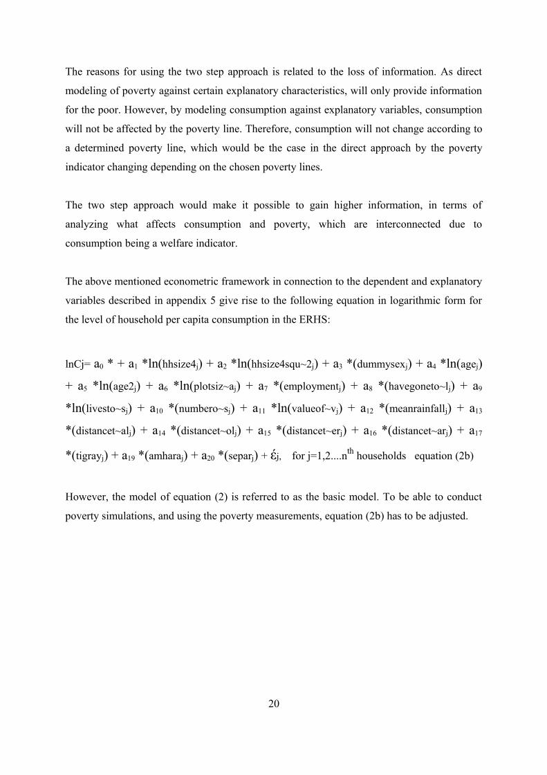
The above mentioned econometric framework in connection to the dependent and explanatory

variables described in appendix 5 give rise to the following equation in logarithmic form for

the level of household per capita consumption in the ERHS:

lnCj= a0 * + a1 *ln(hhsize4j) + a2 *ln(hhsize4squ~2j) + a3 *(dummysexj) + a4 *ln(agej)

+ a5 *ln(age2j) + a6 *ln(plotsiz~aj) + a7 *(employmentj) + a8 *(havegoneto~lj) + a9

*ln(livesto~sj) + a10 *(numbero~sj) + a11 *ln(valueof~vj) + a12 *(meanrainfallj) + a13

*(distancet~alj) + a14 *(distancet~olj) + a15 *(distancet~erj) + a16 *(distancet~arj) + a17

*(tigrayj) + a19 *(amharaj) + a20 *(separj) + έj, for j=1,2....nth households equation (2b)

However, the model of equation (2) is referred to as the basic model. To be able to conduct

poverty simulations, and using the poverty measurements, equation (2b) has to be adjusted.

20

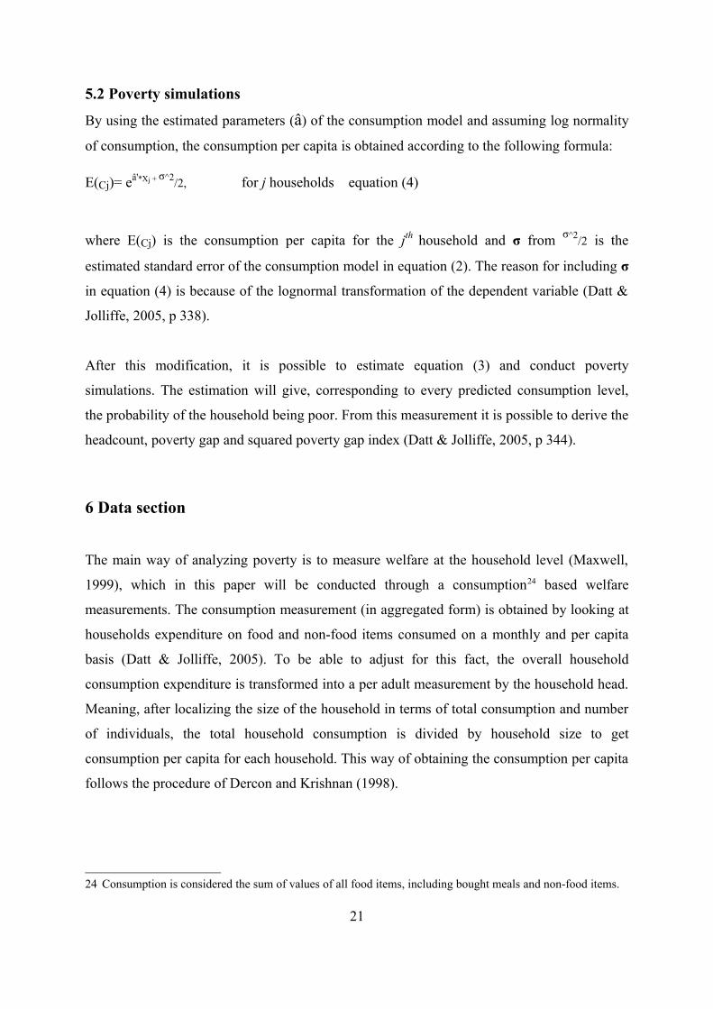
5.2 Poverty simulations

By using the estimated parameters (â) of the consumption model and assuming log normality

of consumption, the consumption per capita is obtained according to the following formula:

E(Cj)= eâ'*Xj + σ^2/2, for j households equation (4)

where E(Cj) is the consumption per capita for the jth household and σ from σ^2/2 is the

estimated standard error of the consumption model in equation (2). The reason for including σ

in equation (4) is because of the lognormal transformation of the dependent variable (Datt &

Jolliffe, 2005, p 338).

After this modification, it is possible to estimate equation (3) and conduct poverty

simulations. The estimation will give, corresponding to every predicted consumption level,

the probability of the household being poor. From this measurement it is possible to derive the

headcount, poverty gap and squared poverty gap index (Datt & Jolliffe, 2005, p 344).

6 Data section

The main way of analyzing poverty is to measure welfare at the household level (Maxwell,

1999), which in this paper will be conducted through a consumption24 based welfare

measurements. The consumption measurement (in aggregated form) is obtained by looking at

households expenditure on food and non-food items consumed on a monthly and per capita

basis (Datt & Jolliffe, 2005). To be able to adjust for this fact, the overall household

consumption expenditure is transformed into a per adult measurement by the household head.

Meaning, after localizing the size of the household in terms of total consumption and number

of individuals, the total household consumption is divided by household size to get

consumption per capita for each household. This way of obtaining the consumption per capita

follows the procedure of Dercon and Krishnan (1998).

24 Consumption is considered the sum of values of all food items, including bought meals and non-food items.

21

Furthermore, to obtain the poverty measurement through the consumption based poverty

analysis, a poverty line estimation is needed. This study will be using the estimation used by

the World bank for rural Ethiopia, which is given through the World Bank's poverty database

PovcalNet25. According to this estimation, the poverty line per adult would be 255 Birr per

month26. The underlying assumptions behind the estimation of this poverty line is the “cost of

basic need approach” (Tadesse, 1999). This approach starts with emphasizing a food poverty

line by constructing a food basket that is valued at market price. The food poverty line is then

divided by the average food share of households who are in the consumption boundaries of

this food basket, to obtain the poverty line.

To draw any conclusions regarding the reasons of poverty in Ethiopia, poverty simulations are

created by looking at significant socioeconomic characteristics. The computer package used

for deriving these statistics will be the software of Stata version 10.

The definition of consumption here does not include expenditure on durable goods and/or

services. From a welfare measurement concept, these goods should be included in the

definition (Deaton, 2003). The reason for not including durable goods in this study has to do

with the fact that the ERHS does not provide accurate information on the depreciation rate for

these kind of goods. This would not create a significant lack in the consumption

measurement, as consumption in durable goods are quite low compared to for example food

and has the largest impact on consumption expenditure (Tadesse, 1996).

In the ERHS, consumption data is available only at the household level. However, a structure

of a household differs depending on were in the world you are, especially in developing

countries. This paper will focus on the 1997 ERHS database and will therefore use the

corrections for household size and unit by the already given conversion codes in the data.

Furthermore, the paper will use given definitions of a household provided in the database,

which in broad terms assume that a household constitutes of those who share the same stock

of food, live under the same roof and are recognized as either heads or other members of the

house. Also, due to regional differences, the southern villages of Ethiopia are separated from

the rest and its effect is captured by region specified dummy variables.

25 http://econ.worldbank.org , last accessed 11 of April 200926 This poverty line was obtained for the first of January 1999 and was 38 US Dollars=254.524 Ethiopian Birr

~ 255 Birr. This is the default monthly poverty line in 2005 PPPs, which is the World Bank $1.25 per day poverty line

($38=$1.25*365/12).

22

6.1 Database descriptionThis paper will use a dataset provided by the International Food Policy Research Institute

(IFPRI) for Ethiopian households based on the 1989 to 1997 survey data obtained from the

Ethiopian Rural Household Survey (ERHS). The paper will be focusing on the 1997 survey

round of the ERHS and will therefore be a cross sectional study.

The ERHS has been supervised by the Economic Department in Addis Ababa University, the

Center for the Study of African Economies at University of Oxford and IFPRI.

6.1.1 Ethiopia Rural Household Survey

The surveys within the ERHS are based on qualitative and quantitative fieldwork, secondary

sources, interviews with key informants in each survey area and community level

questionnaires. The aim with the surveys is to locate each household and area in time and

space so that seasonal factors can affect the patterns of households. But also to show the most

significant economic activities and the role played by active institutions and organizations in

each sampled village. Furthermore, the surveys were in general conducted either in the

beginning of the summer (June or July) or around two months before the harvest time

(October or November). The length of each survey was in average one month27.

The ERHS is a longitudinal household data including villages in the rural part of Ethiopia.

Due to the Ethiopian-Eritrean conflict, this dataset has not been totally random but rather

focused on the villages that were not in the conflict zone. The aim of the survey is to reflect

the major socio-economic characteristics of the rural population in Ethiopia.

The survey started in 1989 and included a total sample size of 450 households (in seven

Peasant Associations28 which covered 6 villages). These households were selected in

proportion to the size of the population in the chosen villages. The sample included variables

on asset, consumption and income. The main purpose of the 1989 survey was to interpret the

response of households to food crises. The regions covered from north to south were: Tigray,

Amhara, Oromiya and SEPAR (Souther Ethiopian People's Association)29.

27 The reason for this time frame, was because the surveys were coordinated to be able to take consideration of the seasonal patterns and thereby receive a high outcome.

28 In Ethiopia, the smallest unit of aggregation is the Peasant Association, an administrative unit of one or a small number of villages.

29 These regions are according to the post 1991 era and differs from how the regions were during the communist period with the old empire provinces. The only region in this sample that is from the pre 1991 period is Tigray, which had its borders redrawn (http://www.angelfire.com/ny/ethiocrown/maps.html , last accessed 3 of Januari 2009).

23

In 1994 the survey was retaken, but now to include one less village due to the fact that one of

the villages was affected by the Ethiopian-Eritrean conflict. In addition nine new villages

were included which also covered other regions of the country. Within each village random

sampling has been used, which covers both landowned and landless households30.

In 1994, 1995 and 1997 the survey was expanded to cover 15 villages across the country and

accounted for diversity in the farming system. This expansion made the sample grew to 1477

households.

When concentrating on accounting for the farming system, the randomness of the sample may

be questionable. However, this concentration is due to practical constraints of conducting a

pure random sample in a country as Ethiopia with some of the villages having a large distance

between them and lacking accessibility in infrastructure. The stratification of the sample

according to the farming system was related to the main agricultural zones in rural Ethiopia,

with one to three villages selected per strata (Dercon & Hoddinott, 2004).

A brief description and geographical location of the villages in the ERHS is given in

Appendix 4. For a more detailed description of the sampled villages there is a comprehensive

study of each village linked to the IFPRI research project (Bevan & Pankhurst, 1996).

30 The reason is because it had been suggested that in some areas landlessness is increasing. Mainly with the absence of redistribution and a ban on land sales and rental against fixed payment, no legal mechanisms exist for young households to acquire land in land constrained areas. To make sure that these households were properly represented in the sample, this stratification was done (Dercon & Hoddinott, 2004).

24

6.1.2 Information that the Ethiopian dataset provides

The Household level of the survey provides data on: household characteristics, agriculture and

livestock information, food consumption, health information, women's activities and other

related household information.

The Community level of the survey provides data on: electricity and water information,

sewage and toilet facilities, health services, education, NGO activity, migration, wages,

production and marketing.

6.2 Variable descriptionIn selecting among the potential determinants of poverty, the main consideration has been to

select variables that have a legitimate use in poverty analysis and for Ethiopia. Therefore,

after considering the literature on poverty analysis for Ethiopia and the approach of finding

determinants for poverty in the paper by Datt & Jolliffe (2005), the following categories were

searched for in the ERHS: demographic, educational, health, employment and household asset

variables. Therefore, the composition of each category and construction of each variable,

depends on their availability in the ERHS.

From these categories, variables were constructed to be estimated in equation (2b). The

variables used in this paper are described in the Appendix (Appendix 5: Variable description).

As this paper will deal with monetary variables, it is essential to take consideration of the real

price, by letting the nominal price variables be deflated by the consumer price index (CPI).

The ERHS provides measurement of CPI values and conversion mechanism for each area that

is used to deflate the data.

25

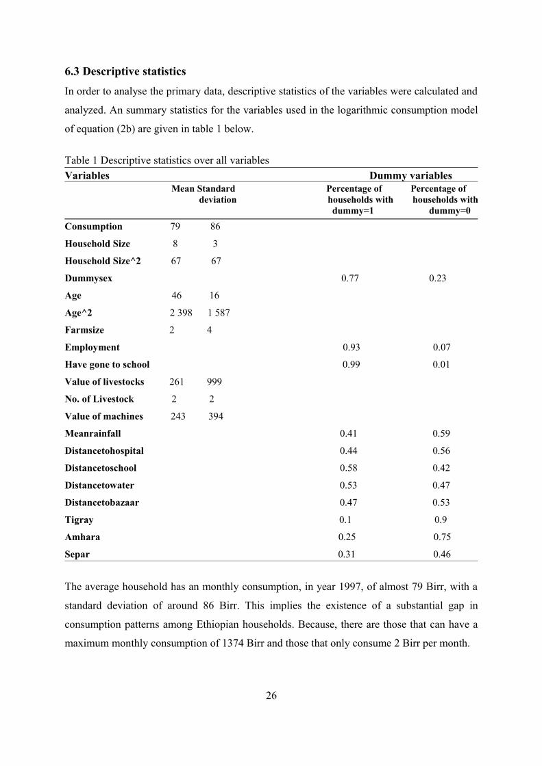
6.3 Descriptive statisticsIn order to analyse the primary data, descriptive statistics of the variables were calculated and

analyzed. An summary statistics for the variables used in the logarithmic consumption model

of equation (2b) are given in table 1 below.

Table 1 Descriptive statistics over all variables Variables Dummy variables Mean Standard Percentage of Percentage of

deviation households with households with dummy=1 dummy=0

Consumption 79 86

Household Size 8 3

Household Size^2 67 67

Dummysex 0.77 0.23

Age 46 16

Age^2 2 398 1 587

Farmsize 2 4

Employment 0.93 0.07

Have gone to school 0.99 0.01

Value of livestocks 261 999

No. of Livestock 2 2

Value of machines 243 394

Meanrainfall 0.41 0.59

Distancetohospital 0.44 0.56

Distancetoschool 0.58 0.42

Distancetowater 0.53 0.47

Distancetobazaar 0.47 0.53

Tigray 0.1 0.9

Amhara 0.25 0.75

Separ 0.31 0.46

The average household has an monthly consumption, in year 1997, of almost 79 Birr, with a

standard deviation of around 86 Birr. This implies the existence of a substantial gap in

consumption patterns among Ethiopian households. Because, there are those that can have a

maximum monthly consumption of 1374 Birr and those that only consume 2 Birr per month.

26

Furthermore the summary statistic of the indicator variables, shows that almost all of the 1367

household heads in the ERHS sample of 1997 have attended primary school, as is indicated

by the “Have gone to school” variable.

7 Empirical result and Analysis

The objective of this paper has been to estimate poverty measurements and determine whether

these measurements can be explained by regional and socioeconomic characteristics, in

Ethiopia. Thereafter, it would be possible to give a brief explanation for the underlying

determinants of poverty. This has been done for a sample of 1367 rural households in

Ethiopia through the use of a two step approach of consumption based modeling for poverty.

The following sections below provides description of the empirical work and the analysis of

the consumption based model, poverty simulations of the poorest and wealthiest villages, and

poverty incidence by different socioeconomic characteristics.

7.1 The Consumption based modelThrough the use of the mentioned methodology, logarithmic-ordinary least square-estimates

for the consumption based model of equation (2b) have been obtained. These parameter

estimates, along with t-ratios for the Ethiopian households in the ERHS sample are presented

in table 2. The signs for most of the estimated parameters in the logarithmic consumption

based estimations are as expected. The estimated coefficients for all variables in the

consumption model confirm the expected relationship between Age, Household size, Distance

to hospital, school and water with per capita consumption. All of the coefficients are also

significant except for the variables Employment, Value and Number of livestock and Distance

to bazaar.

27

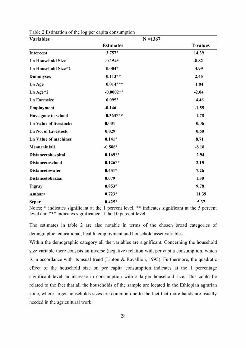
Table 2 Estimation of the log per capita consumption Variables N =1367 Estimates T-valuesIntercept 3.757* 14.39

Ln Household Size -0.154* -8.82

Ln Household Size^2 0.004* 4.99

Dummysex 0.113** 2.45

Ln Age 0.014*** 1.84

Ln Age^2 -0.0002** -2.04

Ln Farmsize 0.095* 4.46

Employment -0.146 -1.55

Have gone to school -0.363*** -1.78

Ln Value of livestocks 0.001 0.06

Ln No. of Livestock 0.029 0.60

Ln Value of machines 0.141* 8.71

Meanrainfall -0.586* -8.18

Distancetohospital 0.169** 2.94

Distancetoschool 0.126** 2.15

Distancetowater 0.451* 7.26

Distancetobazaar 0.079 1.30

Tigray 0.853* 9.78

Amhara 0.723* 11.39

Separ 0.425* 5.37 Notes: * indicates significant at the 1 percent level, ** indicates significant at the 5 percent level and *** indicates significance at the 10 percent level

The estimates in table 2 are also notable in terms of the chosen broad categories of

demographic, educational, health, employment and household asset variables.

Within the demographic category all the variables are significant. Concerning the household

size variable there consists an inverse (negative) relation with per capita consumption, which

is in accordance with its usual trend (Lipton & Ravallion, 1995). Furthermore, the quadratic

effect of the household size on per capita consumption indicates at the 1 percentage

significant level an increase in consumption with a larger household size. This could be

related to the fact that all the households of the sample are located in the Ethiopian agrarian

zone, where larger households sizes are common due to the fact that more hands are usually

needed in the agricultural work.

28

The variables age and age2 have the expected signs. This is an indication that the results for

the ERHS sample are in accordance with the life cycle phenomena, meaning a greater

experience (larger age) gives an increase in earning capacities which thereby has a smoothing

effect on consumption over time.

Both of the variables within the educational category are significant. The variable ”Have gone

to school” has a inverse (negative) relationship with per capita consumption. A reason could

be that only a few of those who have continued with higher education have received a better

paid job than the farming activities in their home villages. Therefore, the majority of the

sample that have finished their education have returned back to the home village, which in

most cases have meant back to unemployment due to the already poor conditions of the

village (Bevan & Pankhurst, 1996). However, education do not necessarily have a negative

impact on consumption. On the contrary, it seems that at the five percentage level, the

“Distance to school” variable has a positive significant relationship with consumption. This

indicates a higher consumption for those households that have a functioning primary school in

their villages as compared to not.

Concerning the health category, both the closeness to a drinkable water source and a basic

functional health clinic have significant positive effects on consumption as compared to not.

This is a reasonable assumption because higher sanitation leads to an increase in life

expectancy and living standard, which thereby can affect factors such as age and household

size.

The Household asset variables: “Values of machines related to cultivation” and the

“Farmsize” of the household, have a significant relationship with consumption. These

variables are also connected in terms that a higher value of machines (more machines in

amount and technology) can cultivate the farmsize in a more effective manner. The positive

effect between “Farmsize” and consumption is an indication that the sample is located in the

agrarian zone of Ethiopia where the majority of the population are highly dependent on the

most important sector at place, namely the agricultural sector.

29

7.2 Poverty simulationTo be able to conduct poverty measurements according to the two step procedure described in

the theoretical framework, equation (3) has to be estimated31. This estimation will give the

probability of the household being poor according to the predicted consumption level from the

consumption based model. From this measurement it is possible to derive the headcount,

poverty gap and squared poverty gap index (Datt & Jolliffe, 2005, p 344).

Table 3 and 4 present estimates for the poverty measurements (Po, P1 and P2)32 in terms of the

sampled villages and the socioeconomic characteristics.

31 However, before equation (3) is estimated the log normal transformation of the consumption based model of equation (2b) has to have normality in its disturbance terms. This is indicated by the “belly” shaped histogram in Appendix 6.

32 Po, is the Headcount index, P1 and P2 are the poverty and squared poverty gap indexes.

30

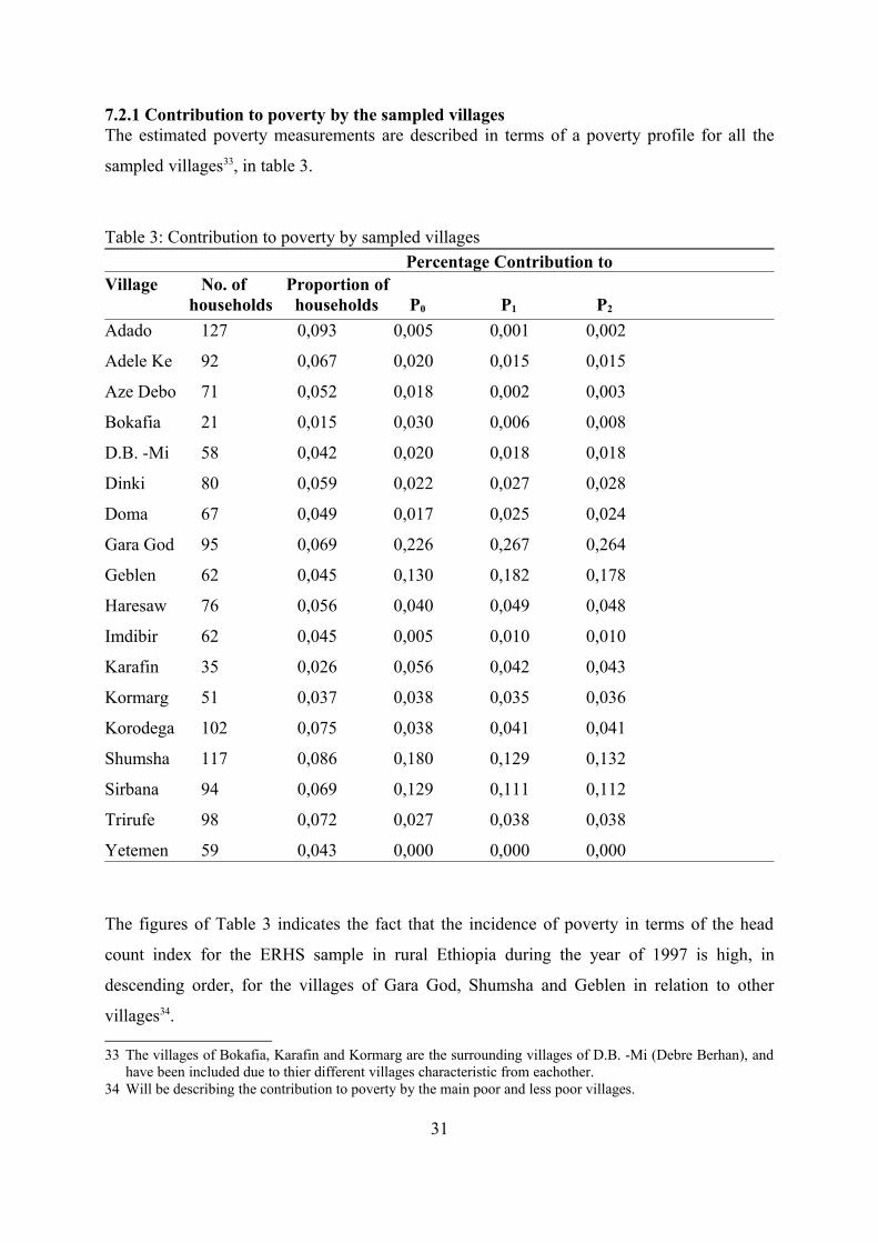
7.2.1 Contribution to poverty by the sampled villagesThe estimated poverty measurements are described in terms of a poverty profile for all the

sampled villages33, in table 3.

Table 3: Contribution to poverty by sampled villages Percentage Contribution to Village No. of Proportion of households households P0 P1 P2 Adado 127 0,093 0,005 0,001 0,002

Adele Ke 92 0,067 0,020 0,015 0,015

Aze Debo 71 0,052 0,018 0,002 0,003

Bokafia 21 0,015 0,030 0,006 0,008

D.B. -Mi 58 0,042 0,020 0,018 0,018

Dinki 80 0,059 0,022 0,027 0,028

Doma 67 0,049 0,017 0,025 0,024

Gara God 95 0,069 0,226 0,267 0,264

Geblen 62 0,045 0,130 0,182 0,178

Haresaw 76 0,056 0,040 0,049 0,048

Imdibir 62 0,045 0,005 0,010 0,010

Karafin 35 0,026 0,056 0,042 0,043

Kormarg 51 0,037 0,038 0,035 0,036

Korodega 102 0,075 0,038 0,041 0,041

Shumsha 117 0,086 0,180 0,129 0,132

Sirbana 94 0,069 0,129 0,111 0,112

Trirufe 98 0,072 0,027 0,038 0,038

Yetemen 59 0,043 0,000 0,000 0,000

The figures of Table 3 indicates the fact that the incidence of poverty in terms of the head

count index for the ERHS sample in rural Ethiopia during the year of 1997 is high, in

descending order, for the villages of Gara God, Shumsha and Geblen in relation to other

villages34.

33 The villages of Bokafia, Karafin and Kormarg are the surrounding villages of D.B. -Mi (Debre Berhan), and have been included due to thier different villages characteristic from eachother.

34 Will be describing the contribution to poverty by the main poor and less poor villages.

31

The highest proportion of poor households comes from the village of Gara God, which is

densely populated and located in the “malaria area”. This affects the village productivity and

thereby puts its marks on consumption and poverty. During the 1980s some Ethiopian

villages, including Gara God, had its population and the surrounding area affected by famine

(1983/84) and malaria in 1988 (Dercon & Hoddinott, 2004, p 9). This could be an explanation

of why the depth of poverty is quite high in the village and community surrounding Gara

God, which is indicated by the “gap” indexes. Furthermore, in Gara God the average

wealthiest are those that have one or two pairs of oxen, 10 or more heads of cattle, farmsize

of two hectares or more and liquidity in terms of 400-500 birr. However, the poor are in

average those that have no oxen, perhaps one or 2 sheep and/or goats, minimum farmsize and

no liquidity (Bevan & Pankhurst, 1996, p 24).

The village of Shumsha's high proportion of poor can be related to the fact that only 10

percentage of the area the village is located in is considered cultivated. Because, the area

surrounding Shumsha is highly affected by drought compared to rest of Ethiopia35, due to its

position in the north. The village is also almost solely dependent on farming and therefore

every effect on agriculture has a high impact on the living conditions. The harsh agricultural

condition and the high dependence on it has contributed to large degree of famine in the

community of Shumsha. Especially during the drought months of February to June36 (Bevan

& Pankhurst, 1996, p 2). Furthermore, the depth of poverty in the village is less than Gara

God but still relatively more than the other villages, which can be shown by the “gap”

indexes. In Shumsha the average wealthiest are those that can produce enough to eat three

meals a day during a year. However, the poor are in average those that have no oxen,

minimum farmsize and can only produce to eat one or sometimes two meals a day during a

year.

The reason the village of Geblen has a high contribution to the proportion of poor could be

that the area surrounding Geblen is affected by drought compared to the rest of Ethiopia due

to its geographical position in the north and closeness to the dry Red Sea. However, the

drought and lack of arable agricultural land is not as severe as Shumsha, which can also

explain its lower contribution to the proportion of the poor.

35 This area is called the “kolla to weyna dega” (Bevan & Pankhurst, 1996, p 2). 36 Sometimes there is no rain thoughtout the year.

32

Geblen, as Shumsha, is also mainly dependent on farming and therefore highly sensitive to

the volatility of the agricultural production. This is apparent by how famine has affected the

community of Geblen, mainly as a result of drought due to shortage of rain during the last

years (Bevan & Pankhurst, 1996, p 2). Moreover, the depth of poverty in the village is less

than Gara God but more than Shumsha, as the “gap” indexes indicate. The wealthiest

households in the village are in average those with any number of livestocks. The amount of

people with a consumption level above the poverty line is marginal from the 62 sampled

households. A possible explanation for Geblen having a higher depth of poverty than

Shumsha could be the forced evacuation of the village area due to the drought of 1984, which

made most of the households lose the majority of their assets (Bevan & Pankhurst, 1996, p

34). This could be an indication that even though there will be less poor households, the

households that are poor have a larger path to go before reaching above the poverty line.

Furthermore, the figures of Table 3 indicate that the smallest proportion of the poor for the

ERHS sample in rural Ethiopian during the year of 1997, are in the villages of Adado, Imdibir

and Yetemen.

The reason the lowest contribution to the proportion of poor households comes from the

village of Yetemen could be that the villages due to its location, by it being surrounded by

two rivers37, has good conditions for agriculture. Therefore, the households of Yetemen can

produce enough to consume, mainly because around 90 percentage of the area the village is

located in is considered cultivated (Bevan & Pankhurst, 1996, p 2). Furthermore, the depth of

poverty is relatively low in the community surrounding Yetemen, which is indicated by the

“gap” indexes. In Yetemen the average wealthiest are those that own the capital, livestock and

farmland. However, the poor are in average those that work for the wealthiest on a daily wage

basis and have limited capital, farmland and no livestock (Bevan & Pankhurst, 1996, p 27).

But the conditions of the poor is different from the other villages in the sample. Because the

poor in Yetemen can work on a daily basis and therefore also bring themselves out of poverty

through working from a young age and saving. This opportunity is not possible in for example

the village of Gara God, where the wealthiest are not able to employ the poor on a daily basis,

which can be shown by the relatively large distance between the “gap” indexes of Yetemen

and Gara God.

37 Muga, that is a perennial (all-year-wet) river and Yegudfin which has only water during the wet season (Bevan & Pankhurst, 1996, p 1).

33

The village of Imdibir's relatively low proportion of poor can be related to the fact that the

surrounding area of the village have water resources and a preferable climate for agriculture,

as Yetemen. However, Imdibir has more mountainous terrain and heavy rains38 than Yetemen

and therefore has not been the optimal place for cultivation (Bevan & Pankhurst, 1996, p 1).

This could be a reason of why Imdibir has a higher proportion of poor households than

Yetemen. Furthermore, the low depth of poverty in the village is less than villages such as

Shumsha but still relatively more than Yetemen, which can be shown by the “gap” indexes. In

Imdibir the average wealthiest are those that own large amount of land, livestock and capital.

In contrast to the poor that on average have very small amounts of these assets. As in

Yetemen, the poor can work on a daily basis for those that own more land and capital.

However, the difference to Yetemen is the size of the average household, which is large

(Bevan & Pankhurst, 1996, p 24). This can explain why the “gap” indexes are bigger for

Imdibir than Yetemen.

Adado's low contribution to the proportion of poor has similar characteristic as the village of

Imdibir. The Adado village area have a favorable climate for agriculture and same

mountainous terrain and rainfall as in Imdibir (Bevan & Pankhurst, 1996, p 1). Therefore,

Adado, as Imdibir, have less advantage in terms of cultivation compared to Yetemen.

Moreover, the low depth of poverty in the village is less than Imdibir, as the “gap” indexes

indicate. The average wealthiest are those that own large amount of land, livestock and capital

compared to the poor that do not have these factors. As in Imdibir, the poor can work on a

daily basis for the wealthiest. However, the size of the average household is less in Adado

than Imdibir (Bevan & Pankhurst, 1996, pp. 22), which can explain the larger “gap” indexes

for Imdibir than Adado.

38 The average mean rainfall is higher in Imdibir than Yetemen, which tends to overflow the farmland in the area.

34

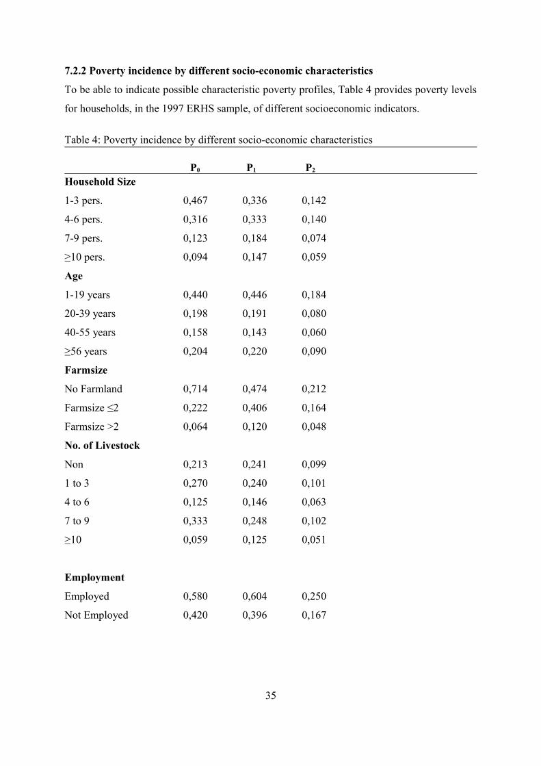
7.2.2 Poverty incidence by different socio-economic characteristics

To be able to indicate possible characteristic poverty profiles, Table 4 provides poverty levels

for households, in the 1997 ERHS sample, of different socioeconomic indicators.

Table 4: Poverty incidence by different socio-economic characteristics P0 P1 P2 Household Size

1-3 pers. 0,467 0,336 0,142

4-6 pers. 0,316 0,333 0,140

7-9 pers. 0,123 0,184 0,074

≥10 pers. 0,094 0,147 0,059

Age

1-19 years 0,440 0,446 0,184

20-39 years 0,198 0,191 0,080

40-55 years 0,158 0,143 0,060

≥56 years 0,204 0,220 0,090

Farmsize

No Farmland 0,714 0,474 0,212

Farmsize ≤2 0,222 0,406 0,164

Farmsize >2 0,064 0,120 0,048

No. of Livestock

Non 0,213 0,241 0,099

1 to 3 0,270 0,240 0,101

4 to 6 0,125 0,146 0,063

7 to 9 0,333 0,248 0,102

≥10 0,059 0,125 0,051

Employment

Employed 0,580 0,604 0,250

Not Employed 0,420 0,396 0,167

35

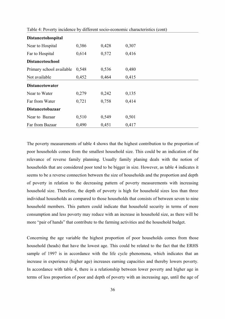
Table 4: Poverty incidence by different socio-economic characteristics (cont)

Distancetohospital

Near to Hospital 0,386 0,428 0,307

Far to Hospital 0,614 0,572 0,416

Distancetoschool

Primary school available 0,548 0,536 0,480

Not available 0,452 0,464 0,415

Distancetowater

Near to Water 0,279 0,242 0,135

Far from Water 0,721 0,758 0,414

Distancetobazaar

Near to Bazaar 0,510 0,549 0,501

Far from Bazaar 0,490 0,451 0,417

The poverty measurements of table 4 shows that the highest contribution to the proportion of

poor households comes from the smallest household size. This could be an indication of the

relevance of reverse family planning. Usually family planing deals with the notion of

households that are considered poor tend to be bigger in size. However, as table 4 indicates it

seems to be a reverse connection between the size of households and the proportion and depth

of poverty in relation to the decreasing pattern of poverty measurements with increasing

household size. Therefore, the depth of poverty is high for household sizes less than three

individual households as compared to those households that consists of between seven to nine

household members. This pattern could indicate that household security in terms of more

consumption and less poverty may reduce with an increase in household size, as there will be

more “pair of hands” that contribute to the farming activities and the household budget.

Concerning the age variable the highest proportion of poor households comes from those

household (heads) that have the lowest age. This could be related to the fact that the ERHS

sample of 1997 is in accordance with the life cycle phenomena, which indicates that an

increase in experience (higher age) increases earning capacities and thereby lowers poverty.

In accordance with table 4, there is a relationship between lower poverty and higher age in

terms of less proportion of poor and depth of poverty with an increasing age, until the age of

36

56 years. The possible exception from the life cycle phenomena for those households higher

than or equal to 56 years, can be related to the notion of a smaller household size for

household heads that reach the age of 56 or more39. As described earlier, concerning the

household size effect, it seems that the incidence of poverty is more apparent in small size

household. This could be related in explaining the sudden shift in pattern of decreasing

poverty level with a higher age.

The reason the highest proportion of poor households comes from those household that have

non or low amounts of farmland can be related to the ERHS geographical location. Because,

as the sample is located in the agrarian zone, the main-farmland-intensive sector (agriculture)

dominates the area. Therefore, the households of the sample have a significant dependence to

farmland for their survival. This may also be what the estimations of table 4 indicates: a larger

proportion of poor and relatively high depth of poverty for households that have less farmland

compared to those with more than two hectares of farmland.

Within the number-of-livestocks, the highest contribution to the proportion of poor

households comes from those households that have less livestocks. However, as indicated in

table 4, there is not a clear proportional pattern of less contribution to poverty by a larger

amount of livestocks. The poverty level seems to be increasing for households with up to

three and seven to nine livestocks. A possible reason for why the contribution to poverty is

higher for households owning livestocks of either one to three and seven to nine, can be

related to the fact that the amount may not be sufficient. Because the trend in some villages of

the ERHS was that the households were faced with more harsh conditions for their livestocks,

such as famine, diseases, forced sale at cheaper price for providing food and other factors that

have made it difficult for households (farming or not) to keep very large amounts of

livestocks (Bevan & Pankhurst, 1996, pp. 7). With this in mind, those households that have

between one to three livestocks have not necessarily less farming land but less consumption,

which can be an indication that they belong to the group that have been forced to reduce or

can not sustain larger amount of livestocks due to the harsh conditions.

Furthermore, those households that have more than or equal to 10 livestocks, have also more

than two hectares of farmland in average, which is an indication that they provide less to

39 The age of 56 is considered to be high in Ethiopia as the average life expectancy is around 47 years old.

37

poverty. This is in accordance with the fact that the ERHS is taken from the Ethiopian

agrarian zone, were concepts such as more farmland (and thereby more livestocks) are

preferable in terms of less contribution to poverty.

Concerning the employment variable the pattern should be that the proportion of poor and

depth of poverty be high among those households (heads) that are not employed, in contrast to

the findings shown in table 4. One possible reason is that the employment variable does not

capture all the different forms of employment. However, this pattern could also be related to

the group of households heads which are retired and therefore not considered as employed.

They will be considered as not employed and retired, even though their plot is being used by

younger farmers that pay rent to them. This rent can be considered as a kind of pension, which

provides an acceptable living standard that in many cases is higher than those being

employed. Therefore, the “reverse” effect of poverty on the employment variable is not

without a possible explanation40.

Households that have a far distance to a functional hospital or a drinkable water source,

contribute to the proportion of poor. A possible explanation can be that the opposite leads to

creating consumption enhancing effects for the households, due to the fact that they would

survive for a longer period of time. This enhancing effect provides a lower depth of poverty,

which is a legitimate assumption because the accessibility to these categories leads to

improving the living standard.

Household that have a far distance to a bazaar and not a functional school in the village,

contribute to the proportion of poor. Concerning the pattern of the distance to bazaar variable,

the variable is not significant in the consumption based estimations of table 2. A possible

explanation of why the contribution to poverty is higher for households that are located in

villages with a functional school could be related to the poverty those households that have

chosen to educate themselves experience. Because by being less available for farming and

more for education, the households tend to lose a “pair of hands”.

The above mentioned connections between poverty and the different socioeconomic

characteristic should be interpreted with causation as these connections are more complex.

40 The employement variable was still not significant during other model specifications, even though it had the ”right” (positive) sign.

38

8 Conclusion

This aim of this paper was to analyze three different definitions of poverty in connection to

well-being in rural Ethiopia using the 1997 household data survey provided from the ERHS.

The poverty estimates provided emphasize the harsh conditions for households in the rural

areas of Ethiopia.

Poverty measurements were given for households in terms of each sampled village and their

socioeconomic characteristics. This makes the poverty profile multidimensional and point out

what characterize poor households. The outcome from this paper may contribute to

understanding poverty in rural Ethiopia by considering the used poverty measurements.

The poverty measurements indicate that the proportion of poor are lower in areas with good

farming conditions than not. Therefore, typical agricultural villages such as Adado, Imdibir

and Yetemen have a less proportion of households that are poor. These findings indicate a

correlation between better farming conditions and lower poverty, which is something that can

be useful to emphasize as an initial step in poverty reduction for the rural areas. This in turn

can reduce the inefficiency in the rural agricultural sector through for example infrastructural

improvements, such as higher accessibility to water.

However, the correlation between farming conditions and poverty does not necessarily give us

much information about the causal effect. Because, a farmer that has more wealth can also

have better farming conditions and thereby lower poverty.

Furthermore, the poverty profile by different socioeconomic characteristics shows that larger

households are not necessarily poorer in the rural areas, in fact the reverse effect is apparent.

However, this does not imply that a larger household size reduces poverty, as there is a cost

related to supporting more household members than less.

The results also indicate the importance of experience and availability of farmland in having a

lower effect on poverty. Moreover, the increase of experience with age, is connected to the

health categories. Because, a functional hospital and acceptable sanitation would not only

have a reducing effect on poverty but also indirectly affect factors such as experience, by

39

contributing to a higher living standard41. The impact of education seems to not have a

reducing effect on the poverty level. This could be related to the fact that policy instruments

should initially aim at providing arable farmland that satisfies the basic needs. Otherwise the

effect of education can not be fully achieved, in terms of higher education and lower poverty.

Further, the results establish that households with a overall higher amount of livestock tend to

be less poor. This should not be surprising since it is related to the size of farmland and

agricultural conditions. Since social security is almost not available in Ethiopia, the size of the

farm and the amount of livestock are factors that can be regarded as deposits and pensions.

Therefore, government transfers of improving agricultural conditions, does not only

contribute to reducing poverty at the present stage but also in the future.

This study aimed to investigate three different definitions of poverty in connection to well-

being: the headcount, the poverty gap and the squared poverty gap index. It is possible to state

that these measurements are different modifications of each other with common variables.

The empirical results for the ERHS database strengthens this statement by indicating the fact

that these measurements follow the same trend. Such as, if the proportion of poor households

are large for a certain village, so is the depth of poverty. Or if the headcount index decreases

for specific characteristic, such as household size, the poverty gap indexes follows the same

pattern. There were exceptions to this trend, as in the case of number of livestocks owned by

the household. Otherwise, it seems that the three different poverty measurements follow each

other.

41 Because if households can live more due to better health, they will also gain higher experience.

40

References

Literature

Atkinson A B (1987), On the Measurement of Poverty, Econometrica, Vol. 55, No. 4, pp. 749-764

Bardhan K P (1984), Land, Labour and Rural Poverty: Essays in Development Economics, Colombia University Press, New York

Bevan P & Pankhurst A (1996), Ethiopian Village Studies, ed., IFPRI

Bigsten A, Bereket K, Abebe S and Mekonnen T (2003), Growth and Poverty Reduction in Ethiopia: Evidence from Household Panel Surveys. World Development, Vol. 31, No. 1, pp. 87-106

Coudouel A, Hentschel S J and Wodon T Q (2002),Poverty Measurement and Analysis, In the PRSP Sourcebook, World Bank, Washington D.C

Datt G & Jolliffe D (2005), Poverty in Egypt: Modeling and Policy Simulations, Economic Development and Cultural Change, Vol. 53, pp. 327–346, January 2005

Deaton A (2003), Household Surveys, Consumption, and the Measurement of Poverty, Economic Systems Research, Vol. 15, No. 2, June 2003

Dercon S & P Krishnan. (1998), Changes in Poverty in Rural Ethiopia 1989-1995: Measurement, Robustness Tests and Decomposition, Working paper, Centre for the study of African Economies, University of Oxford.

Dercon S & M Tadesse (1999), A Comparison of Poverty in Rural and Urban Ethiopia, Ethiopian Journal of Economics, Vol. 8, No. 1, pp. 83-98.

Dercon S & Hoddinott J (2004), The Ethiopian Rural Household Surveys: Introduction, IFPRI

Dercon S (2001), Economic Reform, Growth and the Poor: Evidence from Rural Ethiopia, Working paper, Centre for the Study of African Economies, University of Oxford

Ehui, S K and Jabbar M A (2002), Measuring Productivity in African Agriculture: A Survey of Applications of the Superlative Index Numbers Approach, Socio-economics and Policy Research working paper 38, ILRI (International Livestock Research Institute), Nairobi, Kenya, pp. 1-27

Foster J, Greer J and Thorbecke E (1984), A Class of Decompostable Poverty Measures, Econometrica, Vol 52, No. 3 (May), pp 761-766

Foster J & Shorrocks A F (1991), Subgroup Consistent Poverty Indices, Econometrica, Vol. 59, No. 3, pp. 687-709

41

HDR (HUMAN DEVELOPMENT REPORTS) (2007/08), UNDP Report, available at http://hdr.undp.org/en/countries/

Hussein H K (2007), Farm Household Economic Behaviour in Imperfect Financial Markets, Faculty of Natural Resources and Agricultural Sciences, Department of Economics, Doctoracl Thesis Swedish University of Agriculture Science, Uppsala

Jema H (2008), Economic Efficiency and Marketing performance of Vegetable Production in the Eastern and Central Parts of Ethiopia, Faculty of Natural Resources and Agricultural Sciences, Department of Economics, Doctoral Thesis, Swedish University of Agriculture Science, Uppsala

Kakwani N C (1977), Measurement of Poverty and the Negative Income Tax, Australian Economic Papers, Vol 16, pp. 237-248

Kakwani N (1980), On a Class of Poverty Measures, Econometrica, Vol. 48, No. 2, pp. 437-447

Kassa H (2003), Livestock and livelihood security in the Harar Highlands of Ethiopia:Implications for Research and Development, Faculty of Natural Resources and Agricultural Sciences, Department of Economics, Doctoral Thesis, Swedish University of Agriculture Science, Uppsala

Legesse B (2003), Risk Management Strategies of Smallholder Farmers in the EasternHighlands of Ethiopia, Department of Rural Development Studies, Doctoral Thesis, Swedish University of Agriculture Science, Uppsala

Lipton M & Ravallion M (1995), Handbook of Development Economics 3B, ed. Behrman JR & Srinivasan TN, Amsterdam, Elsevier

Maxwell S (1999), Overseas Development Institute Poverty Briefing, available at http://www.odi.org.uk/publications/briefing/pov3.html , 3 of February

Ravallion M, Datt G and Walle D (1991), Quantifying Absolute Poverty in The Developing World, Review of Income and Wealth, Series 37, No.4, December 1991

Ravallion M (1994), Poverty Comparisons, Chur: Harwood academic publishers.

Ravallion M and Bidani B (1994), How Robust Is A Poverty Profile, World Bank Economic Review, Vol 8, No 1(Jan), pp 75-102

Ravallion M (1996), Issues in Measuring and Modeling Poverty, Policy Research Working Paper WPS1615, The World Bank, June 1996, p 1-29

Ravallion M (1998), Poverty lines in theory and practice, LSMS Working Paper 133, Washington DC, The World Bank

42

Sen A (1976), Poverty: An Ordinal Approach to Measurement, Econometrica, Vol 46, No 2 (Mar), pp. 437-446

Sen A (1985), Commodities and capabilities, Amsterdam, North Holland

Sen A (1999), Poverty and Famines: An Essay on Entitlements and Deprivation, In The Sen A & Omnibus J D, ed. Sen A. New Delhi, Oxford University Press

Tadesse, M (1996), Food Consumption and Poverty in Urban Ethiopia: A Preliminary Assessment, In Proceedings of the Fifth Annual Conference on the Ethiopian Economy, ed Kebede, B., and M. Tadesse. Addis Ababa

Tadesse, M (1999), Determinants and Dynamics of Urban Poverty in Ethiopia, Ethiopian Journal of Economics, Vol 8, No. 1, pp. 61-82

UNDP (2003) Human Development Report, New York, Oxford University Press

UN Millenimum develpment goals 2015, available at http://www.un.org/millenniumgoals/

U.S. Library of Congress (1991), Country studies, available at http://countrystudies.us/ethiopia/87.htm

Watts H (1968), An Economic Definition of Poverty, in Moynihan D P, ed., On Understanding Poverty, Basic Books, New York

WHO (2008). World Health Organizations Report. Health action in crises, issue 3 of October 2008, available athttp://www.who.int/hac/en/

Webb, P., J. Von Braun and Y. Yohannes (1992), “Famine in Ethiopia: Policy Implication of Coping Failure at National and Household Levels”, Research Report no. 92, International Food Policy Research Institute, Washington D.C

Zheng B (1997), Aggregate Poverty Measures, Journal of Economic Surveys, Vol. 11, No.2, pp. 123-162

Internet sourcesA: (www.worldbank.org/ethiopia )

B: (www.ethioembassy.org)

C: (www.unicef.org)

D: (http://esl.jrc.it/envind/un_meths/UN_ME013.htm)

E: (www.angelfire.com/ny/ethiocrown/maps.html)

43

Appendix 1: The Agricultural sector The majority of the Ethiopian population live on the country side. This constitutes almost 85

percentage of the Ethiopians farmers that are engaged in crop and livestock mixed farming42.

However, due to the fact that the Ethiopian population is quite poor, most farmers are also engage in

other cash bringing activities beside their agricultural activities (Kassa, 2003). For the last decades the

crop production has been volatile, which has created a state of crises in Ethiopia (Legesse, 2003, p 11).

Most of the farmers in Ethiopia are smallholder farmers, which is also reflected on the main

agricultural production that has been created by smallholder farmers43. However, due to the low level

of technical efficiency in the agricultural sector the agricultural production is not sufficient in clearing

the market, despite the efforts of the SDPRP's. Furthermore, the economic and social foundation for

the countryside is not optimal in the sense to promote a huge agricultural production, which has

created a lagged production behind population growth and has made more than 5 million people in

constant need of food assistance. The Ethiopian countryside is characterized by inaccessibility in its

infrastructure, financial and social institutions and water and electricity. This makes the agricultural

production inefficient. Furthermore, the societies in the Ethiopian countryside are quite poor: a farm

household do not only purchase agricultural products but also labor44, which by being inefficient

creates a large lack of consumption power within the population. Even the presents of lending

institutions has not been able to reduce the lack of consumption, because they are more for production

purposes. Despite these facts, the agricultural sector is considered as the main economic sector for

growth in Ethiopia with a contribution to GDP that averages over 50 percentage (Bigsten et al, 2003, p

89) and would give fuel to a sustainable development in the future. Because Ethiopians still have the

largest share of livestock per capita in whole Africa, which even though the risk with holding livestock

gives them the opportunity to have a sufficient food supply (Legesse, 2003, p14). However, the

inefficiency is large and this is reflected on the amount of production, even though the Ethiopian

farmers adapt by implementing mixed crop and livestock farming.

42 The reason for the Ethiopian farmers being involved in mixed farming is to be able to reduce the risk related to the farm-problem of prices and weather fluctuations but also diseases.

43 www.ethioembassy.org , l ast accessed 10 of November 200844 The agricultural sector accounts for almost 80 percentage of the employment (World Factbook, 2008).

44

Appendix 2: Defining a poverty lineWhen conducting poverty analysis and defining the concept of poverty, the poverty line is essential in

the analytical framework. What the poverty line defines is who should be considered poor45.

As with the concept of poverty, there has not been a clear consensus for defining the poverty line.

There are different terminologies used when discussing the concept. The most commonly used

terminology in defining the poverty line is to estimate the cost of a consumption basket. This basket

will consist of the necessities that the individual or household needs to be able to have an acceptable

minimum living standard46. In general the empirical way of conducting this approach is to initially

define a food poverty line. The food poverty line is an estimation of the cost for the minimum

acceptable food or caloric requirements needed on for example a daily basis (World Health

Organization 2008)47.

Thereafter, due to the fact that the poverty line is constructed as the sum of a food and non-food

poverty line, the non-food poverty line is defined. The non-food poverty line is an estimation of the

minimum acceptable weighted average of goods or services that are not considered food. The reason

for using this approach when defining the poverty line is the view that households that can consume

the minimum acceptable food requirements can also consume the minimum required goods or services

that are non-food (Lipton & Ravallion, 1995).

Another method for defining the poverty line is close to the above mentioned approach but with the

difference when it comes to estimating the cost of the consumption basket. The food poverty line is

estimated by first deriving the food “Engle curve”, which determines an average food share that is the

basic minimum food requirements needed for the individual or household at the market price48.

Thereafter, the food and non-food poverty lines are summed together to obtain the poverty line

(Ravallion & Bidani, 1994).

The above mentioned methods, are also the two main approaches when deriving the poverty line

(Ravallion, 1994).

The first approach, that uses the minimum acceptable food or caloric requirements needed for an

individual or household on for example a daily basis, uses this requirement in connection to identify

45 “Who” can in this context be either individuals or households. 46 This way of estimating the poverty line, is sometimes called the cost of basic needs approach.47 This is a minimum energy requirement for a typical person to keep up normal activities, such as the 2,200

Kcal per day threshold.48 Usual this method of obtaining the poverty line, is derived for each household. However, it is possible to

derive it on a individual basis too.

45

the total cost of consumption needed for obtaining it. By obtaining the total cost of consumption

through modeling food requirement on cost of consumption, the poverty line that is derived would

define were the total cost of minimum acceptable caloric requirement needed is put. However, what

this approach does not take into consideration is the fact that the poverty line is not the same for all

regions and throughout time. Because, individuals or households would not have the same total cost of

consumption for a minimum acceptable food basket in different areas and over time (Liption &

Ravallion, 1995, p 2576).

The second approach uses the minimum acceptable food share needed for an individual or household

and identifies the cost of consumption for a minimum required food share or basket. By this approach,

the food poverty lines are obtained for each sub-group within the relevant population for the purpose

of the study. The poverty line is derived by dividing the obtained food poverty lines by the minimum

acceptable food share of the poorest individuals or households. However, the same obvious

measurement error as above is present in terms of not taking changes in minimum acceptable food

share cost over time into consideration (Ravallion, 1994).

In this paper, the poverty line was not empirically derived but instead the poverty line provided by the

WB was used. This poverty line is given through the WB's poverty database PovcalNet and follows

the first approach of deriving poverty lines by using the minimum acceptable food or caloric

requirements needed for an individual or household49.

The reason for not deriving the poverty line empirically in this paper was not only due to the fact that

there was a lack of all necessarily information but also that the derivation of poverty lines in general

presents some hinders in providing a legitimate estimation.

The poverty lines described above, all have the main assumption of a basket that consist of the

necessities that the individual or household needs to be able to have an acceptable minimum living

standard. However, depending on which approach that will be used, difficulties arise. Both approach

uses a minimum acceptable food or caloric requirements, which tends to regard all individuals and

households as equal with no variation in between over time. But, due to the fact that individuals ability

to consume and preferences for how much to consume differs, there consist no method of setting a

minimum acceptable food requirement within the chosen consumption basket for all these individuals

or households, over time. The empirical task of solving the issue is dependent on measuring for

example the eating habits of the sample (Sen, 1981, p 12), which is not possible to solve for countries

with limited recourses. Furthermore, in connection to the minimum consumption basket is the concept

of the non-food poverty line. Because, according to the construction of the poverty line, the non-food

poverty line is highly related to the food poverty line and its minimum consumption basket. Therefore,

49 http://econ.worldbank.org , last accessed 11 of April 2009

46

the usage of the non-food poverty line has so far not been related to other concepts than the food

poverty line, when deriving the poverty line (Ravallion, 1994).

The issue of difficulties in deriving the poverty line can also be related to the ERHS that is used in this

paper. Concerning the concept of a basket that consists of a bundle of consumption goods which

provides an acceptable minimum living standard, the underlying assumption of the availability of all

these goods have to be meet. This information is not possible to obtain for all the regions and goods in

the ERHS (Dercon & Hoddinott, 2004).

Furthermore, due to the fact of regional differences in farming50, the eating habits of each region

differs, which means that the bundle of consumption goods differs. Therefore, different consumption

baskets have to be derived for each specific region, which would imply that comparisons between

regions would not be as straightforward as if a general consumption basket is derived (Dercon &

Hoddinott, 2004). However, with the concept of a general consumption basket comes the issues

mentioned above.

The above mentioned difficulties in obtaining a legitimate poverty line are of course also relevant for

the poverty line used in this paper that is given by the WB, as it follows the same approach of using a

consumption basket that consist of the necessities that the individual or household needs to be able to

have an acceptable minimum living standard. However, the WB poverty line can be regarded as more

common from an empirical point of view and therefore having more legitimacy. Also, the WB poverty

line is using the concept of a common consumption basket for all regions in the ERHS. Because, this

paper is not dealing with changes over time, it is possible to settle down with a simple common

poverty line, due to the fact that there are no seasonal effects or patterns over time to adjust for

(Dercon & Krishnan, 1994).

Appendix 3: The FGT measurementIn the following part a brief description of the FGT model will be given as a decomposable

poverty measurement. However, where the FGT measurement use income this paper will use

consumption due to the benefits of using consumption rather than income.

Sen's (1976) approach towards the inefficiency of the poverty measurements, especially the

headcount index, created the urge for more solid poverty measurements. FGT (1984) came

with an approach that not only satisfied Sen's critique but also provided a way to conduct

poverty measurements and analysis for the total population by only looking at a subgroup.

50 For example that some areas cultivate enset while others are more cereal dependent.

47

By not using the headcount-total population-index approach of measuring poverty, the FGT

measurement indicated that a change in the sample, ceteris paribus, leads to the same change

for the population. The way to do this was to use a decomposable approach by deriving total

poverty as a weighted average of the poverty level for the subgroup (Foster et al, 1984, p

761). However, FGT's usage of a decomposable poverty measurement approach was not

something new, as a matter of fact the decomposable poverty approach had been used earlier,

such as in Kakwani (1977). But, these studies did not address Sen's transfer rule, except for

the FGT measurement.

The FGT poverty measurement is defined as the following (Foster et al, 1984, p 762):

q

P(y;z) = 1/nz2 * Σ gi2, i=1,2,,,,q individuals or households equation (a)

i=1

where n is the number of total individuals or households, y is a vector of household income in

increasing order, z the poverty line, gi= (y-z) the income poverty gap (or consumption

shortfall) of the ith individual or household and q the number of poor household with g≤0.

Equation (a) not only satisfies Sen's transfer rule of legitimate poverty measurements, but also

other rules, which justified the usage of it as a measurement of poverty51.

Equation (a) can be written in a more general way, which is also how the measurement is

most commonly know. This gives the following generalized and empirically convenient form

of the FGT measurement for any distribution of consumption or income (Foster et al, 1984, p

763):

q

Pα = Σ [(z-yi)/z]α /n, i=1,2,,,,q individuals or households with yi<z equation (b)

i=1

where all the variables follow the same definition as in equation (a) with the exception of the

new symbol, α, which is a poverty aversion parameter that takes the mentioned poverty

measurements into consideration. When α takes the value of zero, the FGT measurement in

equation (b) is equal to the head count index. Furthermore, when α takes the value of unity,

51 Such as the critiques delivered by Kakwani (1980) and Foster & Shorrocks (1991).

48

the FGT measurement in equation (b) corresponds to the poverty gap index. The FGT

measurement of equation (b) is equal to the squared poverty gap index, when α takes values

bigger than unity. The empirical approach of using the FGT measurement is to give α the

values of zero, one and two. Moreover, the feature of decomposability with the FGT

measurement, is empirically useful, due to the fact that it is possible to derive the percentage

contribution of a certain subgroup poverty to total poverty52. A modification of Equation (b)

will be used in this paper.

The FGT measurement does thereby satisfy the different rules of poverty measurement

through the values taken by the poverty aversion parameter, α. When α takes values bigger

than zero and one, the monotonicity and transfer rule are satisfied. For α values bigger than

two and all other alpha values, the poverty rules of Kakwani (1980) and Foster & Shorrocks

(1991) are satisfied.

However, FGT is not free from errors, one obvious problem with the model is related to the

amount of available data for the poor. If this availability is low, the poverty measurement will

be biased. Another issue with the FGT measurement is comparisons across countries. When

the measurement look at individual or household consumption (or income) at one point of

time and use aggregate household data for a sample, it is more difficult to find a common

indicator between countries due to demographic and consumption (income) differences

between countries (Ravallion et al, 1991, pp. 351).

Despite its errors, the FGT measurement is consider to be a legitimate measurement and will

therefore, in modified form, be what the econometric model of this paper is based on.

Because, this paper will use consumption rather that income as the monetary measurement for

poverty, the derivation of the FGT poverty measurement will be conducted in a two step

manners. This is described in the section about the econometric model.

52 Which will satisfy the sub group monotonicity rule (Foster et al, 1984, p 764).

49

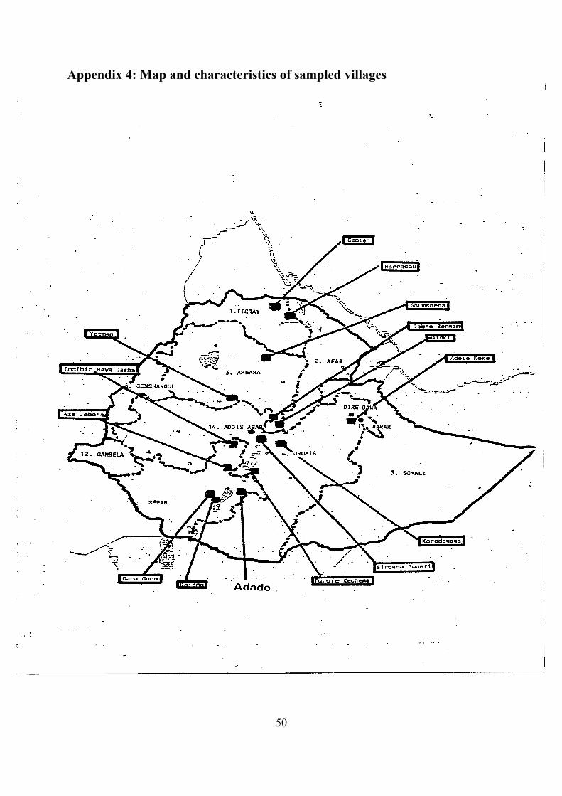
Appendix 4: Map and characteristics of sampled villages

50

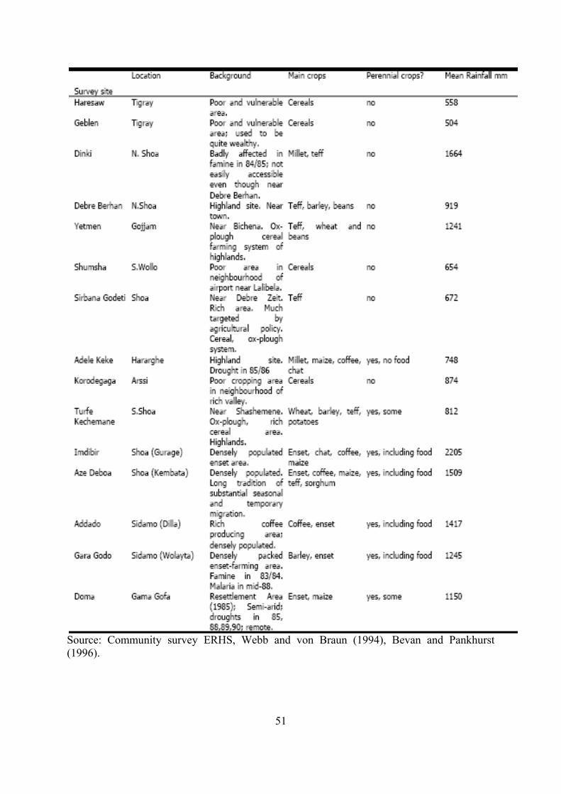
Source: Community survey ERHS, Webb and von Braun (1994), Bevan and Pankhurst (1996).

51

Appendix 5: Variable description

The dependent variableThe dependent variable for equation (2) is consumption per capita. In the ERHS this variable became

“Cons4”. “Cons4” indicates monthly consumption for the household in Birr (Ethiopian Currency). The

Consumption variable includes both food and non food consumption during the measured period. Gifts

are excluded.

The explanatory variablesThe composition of the explanatory variables are within the categories of demographic, education,

health, employment, household asset and other variables.

Within the demographic category the following variables were created:

● hhsize4: indicates the size of the household for the sampled period in number of persons

(where 4=1997, due to the fact that there are 4 sample periods).

● hhsize4squ~2: The square of the hhsize4 variable. Is included to indicate the notion of any

marginal effect on consumption and poverty with an increasing size of the household.

● dummysex: is a dummy variable to indicate the gender of the household head, where 1=Man

and 0=Female.

● age: indicates the age of the head of the household (in years). In the construction of the Age

variable there were some observations that had decimals, such as 62.92 years, these were

rounded up to nearest number, in this case 63.

● age2: The square of the age variable. Is included to indicate the notion of any marginal effect

on consumption and poverty with an increasing age

Within the educational category the following variables are created:

● havegoneto~l: is the Have gone to school variable. The variable is a dummy variable that

states if the household head has attended at least primary school or not, 1=Have gone to

school and 0=never attended school. From the village studies most of the older (above the age

of 40 in Ethiopia) have gone to some sort of school but never continued with higher education.

The young generation (under 18) of 1997 have at least gone to primary school but not higher

education.

52

● distancet~ol: is the Distance to School variable. The variable is a dummy variable that

indicates if there is any primary school available in the village that has the standard to teach

students (because in some cases there are schools available but they are so poorly equipped

that it is not possible to teach at the school). The dummy is constructed as 1=a functioning

primary school is available and 0=Not.

The health category consists of the following created variables:

● distancet~al: is the Distance to Hospital variable. The variable is a dummy variable that

indicates if the household is located in a village that have accessibility to a health clinic

(1=Close and 0=Not, i.e far distance to health) . Category 1 means that there is a health clinic

in the village that has reasonable opening hours and also have the necessities in term of

medicine and walking distance (20 min). Even though almost all the surveyed villages believe

in self-medication, the medicines against deadly decease in Ethiopian such as malaria, polio

and cholera is not something that in the first hand can be helped through self-medication on a

large scale.

● distancet~er: is the Distance to Water variable. The variable is a dummy variable that indicates

if there is available water within 15-20 min walking distance all year and if the water is

drinkable. The variable takes the form of 1=Close and 0=Not, i.e far distance to water.

Within the asset category the following variables are created:

● plotsiz~a: is the plotsize variable. This variable is owned cultivated land in hectare for each

household.

● livesto~s: is the Livestockvalue variable. The variable indicates livestock value in monetary

terms (Birr). The value is in 97 prices and corrected according to CPI in Ethiopia.

● numbero~s: is the Number-of-livestock-variable. The variable indicates the amount of

livestock owned per household. A livestock is everything from Cow and young bulls to

Camel, Hiefer, Sheep, Goat, Donkey and Mule.

● valueof~v: is the Value-of-machines-related-to-cultivation-variable. The variable indicates the

value of machines per household (in Birr) that are used to cultivate the land.

The employment category consist of the following created variable:

● employment: is a dummy variable to indicate whether or not the household head is employed,

were 1=Employed and 0=Not. All the people that have some kind of employment will be

considered in category 1. There are some exceptions: Women that are working as domestic

workers will be considered in category 1 (because in the village studies there are descriptions

of women working 12 hours a day, with all from childcare and cooking to cutting grass,

53

searching wood and water to helping with light farming activities. In amount of hours, women

work more than men in general according to the anthropological village studies). Another

exceptions are men that have stated that they are not employed and not looking for job but are

over the age of 60. They will be considered as not employed and retired, even though their

plot is being used by younger farmers that pay rent to them (this rent can be considered as a

pension). Other categories that will be considered as unemployed are Students, Disables,

Others (those that have stated “Other” as an activity in the ERHS sample) and Children under

the age of 15.

Other variables that are not within the above categories but included in the variables to be estimated

for equation (2b) are the following:

● meanrainfall: is a dummy variable that indicates if the village of the household is located

above or below the annual mean rainfall average for the 1997 ERHS sample (1=above mean

average and 0=Not, i.e below average variable).

● distancet~ar: is the Distance to Bazaar variable. The variable is a dummy variable that

indicates if there is a significant bazaar in the village that people go to within 2 hours of

walking distance. The variable takes the form of 1=Close and 0=far distance.

● Region: The region variables are constructed as dummy variables for the different regions in

Ethiopia that are included in the sampled villages. The regions are constructed according to

the post 1991 map of Ethiopia. The Four regions in (bold letters) and the corresponding

villages (in brackets) are: Tigray (Geblen, Harresaw), Amhara (Shumsnena, Yetmen, Dinki,

Debre Berhan, Bokafya, Karafino and Koremargefia), Oromia (Turufe, Sirbana, Korodegaga,

Adele Keke) and Separ (Gara Godo, Do'oma, Adado, Aze Debo'a , Imdibir).

54

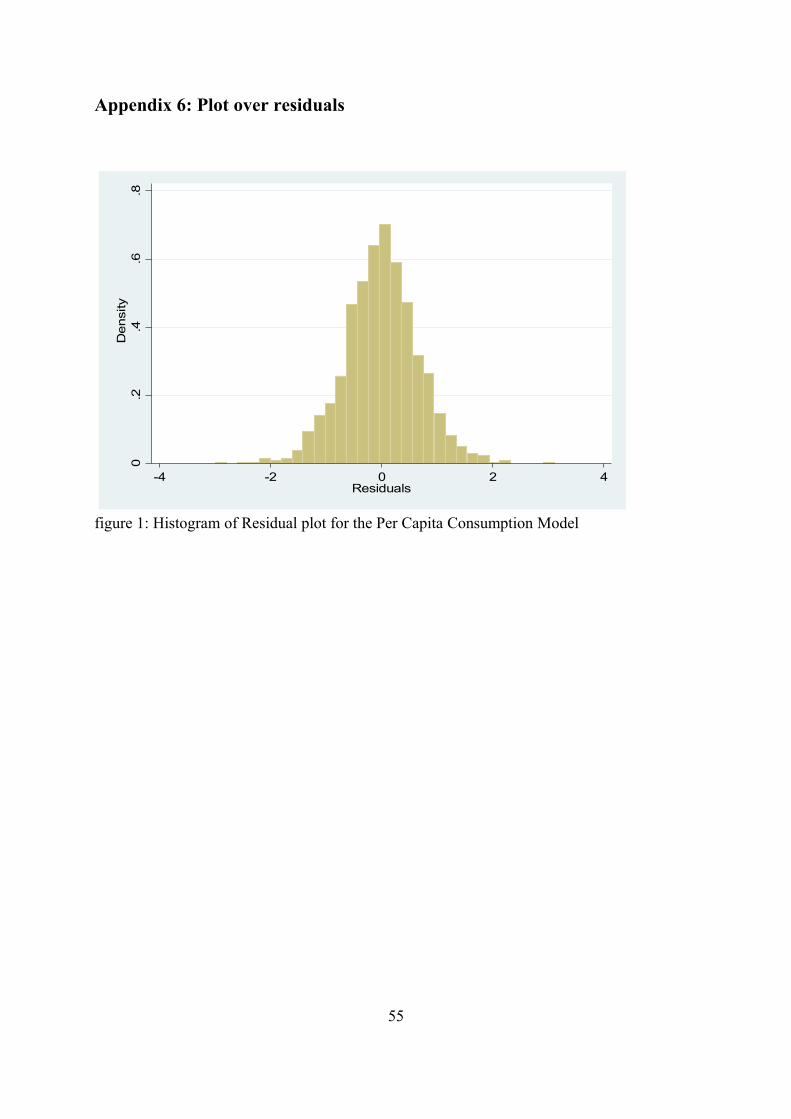
Appendix 6: Plot over residuals0

.2.4

.6.8

Density

-4 -2 0 2 4Residuals

figure 1: Histogram of Residual plot for the Per Capita Consumption Model

55