General Conclusion and Perspectives - Springer978-3-319-45355-2/1.pdf · General Conclusion and Perspectives ... at sea and on land, has relied very readily on geological

General Conclusion and Perspectives

Though seabed logging techniques have their origin in the early days of applied

geophysics, relayed then in earth physics, they have especially developed over a

decade with a priori undeniable success in the search for hydrocarbons. This

therefore justifies an introductory book on these new methods and prospecting

technologies, then answering questions that any innovative technology awakens

as soon as its appears, and especially when it seems to question established

industrial processes.

Petroleum geophysics, at sea and on land, has relied very readily on geological

knowledge and more particularly on that concerning the structure of the subsoil,

qualifying these indirect geophysics as structural or even stratigraphic today,

intimately connected with the tectonics of sedimentary basins, which gives rise to

the trap and then eventually to the reservoir of hydrocarbons.

On the other hand, petroleum geophysics fitted in early and almost exclusively with

seismic methods, refraction and reflection especially, which have continued to evolve

with advances in digital electronics, computer science and especially signal processing.

In contrast, the probability of finding a productive trap, despite continuing efforts in

research and development, has so far remained relatively low (25% chance of success

on average), with no hope of immediate improvement, leading to very important

investments in terms of well logging and especially exploration drilling which, let us

remember, are the heaviest budget items in a marine exploration campaign and more

particularly in the deep sea.

Although indirect geophysics has thus so far dominated oil exploration for

nearly 70 years, direct prospecting has always been of very understandable interest,

which has often led over time and events to stormy and passionate debates that have

not always been objective. Ironically, the common point of these techniques was the

systematic use, more or less wisely, of radio or high frequency electromagnetic

waves, whose interpretation for the detection and localization of oil fields was very

often outside the scope of the demonstrated physics.

Currently announced with great fanfare as a method for direct detection of

hydrocarbons, seabed logging in its commercial versions (mCSEM and mMT)

© Springer International Publishing Switzerland 2017

S. Sainson, Electromagnetic Seabed Logging, DOI 10.1007/978-3-319-45355-2403

can be understood as such, if we only look at first the rate of discovery, which

currently approximates about 90 %.

However, looking at it closer, we firstly see that electromagnetic investigation

can only be considered and carried out on geologically recognized traps and

secondly that these techniques are all the more effective when the external data

used to run the interpretation models (inversion data) are numerous and varied.

In these particular circumstances, which are virtually unique in the field of

applied geophysics, EM seabed logging, without the contribution of this additional

and complementary information, cannot be considered in the current state of

knowledge, and objectively, as a full direct method. However, coupled with a

structural geophysics technique, such as reflection seismics, which has in addition

much superior resolution, seabed logging can be seen and then accepted as one of

the key elements of a direct method provided that:

– The electrical conductivity of the hydrocarbon reservoir contrasts very strongly

with that of the surrounding sedimentary environment.

– The dimensions of the target are large enough so that at a distance the disturbing

action is meaningful or more accurately measurable.

In these favorable conditions, where:

– A priori reflection seismics gives information precisely on the form and structure

of the terrains, in this case on the presence of potential traps

– A posteriori seabed EM logging provides information on the horizontal and

lateral evolution of the properties of the various geological strata, i.e., facies

we can then assume that the coupling of the two techniques forms a full direct

prospecting method, or at least that EM seabed logging for its part provides a good

indicator of the presence of hydrocarbons (direct hydrocarbon indicator or DHI)

when the existence of traps has been previously proven.

On the other hand, one can imagine, with the progress of seismic analysis with

offset (AVO), that electromagnetic and seismic techniques jointly applied (joint

acquisition) will provide in the future a better DHI, thus reducing economic risks.

Similarly, we can also hope that research on the seismo-electric effect (creation of

an electric field concomitant to important mechanical stimulation) may be included

this time with offshore equipment. In a marine environment (incompressible),

saturated with water (sediments), the method should a priori lead to much better

results than that initiated in the 1930s–1960s on land in an undoubtedly more complex

geological context (presence of overburden).

Field monitoring will also be greatly improved by permanently placed instru-

mentation, allowing us to monitor virtually and in real time the evolution of the

reserve, in addition to well data (pressure, temperature, flow, etc.), production logs

and 4D seismics for example. This time-lapse control will be all the more accurate

when by measures are propped up once and for all in time and space.

In addition, mMT may also play a key role in cases of the presence of seismic

masks that prevent sound waves to penetrate deeper. In this case we would then turn

to the EM methods only, or then in support of the gravimetric method.

404 General Conclusion and Perspectives

In an increasingly tense energy context, where one barrel of oil is discovered as

three are consumed, where production techniques reach their limits (considerable

water depths), it seems well established that seabed logging is at the point of

becoming a truly disruptive technology (breakthrough) now impacting the entire

exploration sector and can be regarded as a promising technology just as much as

4D coverage and multiple-azimuth seismic surveys a few years ago (Saniere

et al. 2010).

Does this represent a revolution in the world of exploration?Probably yes, because if in the future the success is confirmed, this highly

innovative advance will likely have immediate repercussions for drilling and

logging activities and a significant impact on offshore exploration in general,

undoubtedly completely changing the situation in the oil service companies of the

sector (Anonymous 2011; Ridward and Hesthammer 2011).

The future of seabed loggingwill inevitably be in theminiaturization of the sensors,

and in the increase of their performance (sensitivity, accuracy, etc.), allowing us in

particular to increase the depth of investigation and resolution. The immediate future

is already in sensors with very low dimensions (EM streamers being commercialized),

which may for example be integrated later on seismic acquisition streamers or OBC

cables, giving then, thanks to this combined technology (seismics/EM), direct and

immediate access (in real time) to geological, and why not economical, information.

The flexibility of use of this unique technology can also be a sign of many more

geological applications with the search for various types of mineral wealth such as:

– Reserves of gas hydrates as economically viable methane resources (Edwards

1997; Hyndman et al. 1999; Yuan and Edwards 2000; Schwalenberg et al. 2005,

2009; Thakur and Rajput 2011)

– Ore deposits (Mero 1965; Gibbons 1987; Fouquet and Lacroix 2012), sulfur

cluster type (Wolfgram 1986), polymetallic or hydrothermal nodules, for exam-

ple related to submarine volcanism (the Kulolasi volcano off the Wallis and

Futuna Islands)1

– Rare-earths deposits,2 recently found in the Pacific (Wallis and Futuna), the

need for which in the electronic industry has become urgent (strategic minerals)

– Freshwater aquifers present in coastal areas allowing some countries to have

resources that they previously lacked

1These rare-earth reserves are among the largest in the world (Planchais, 2011). With its marine

areas, the French territory is larger than Europe (11.1 million km2 against 9 million km2) and is

second behind the US (11.3 million km2). China, which now has a virtual monopoly on lanthanides

(La, Ce, Pr, Nd, Pm, Sm, Eu, Gd, Tb, Dy, Ho, Er, Tm, Yb, Lu), with 97% of the world production,

regularly files license applications for prospecting and exploitation of these deposits with the ISA

(International Seabed Authority).2Rare earths are not found in nature, but are combined with other elements (minerals and ores such

as monazite and bastnaesite). On land, their geophysical exploration is done by magnetic and

gravimetric methods, or even in some cases by radiometric methods. At sea no method has yet

been proposed.

General Conclusion and Perspectives 405

or why not, in the longer term, in addition to other techniques such as:

– “Forecasting” of seismic hazards (earthquakes and especially tsunamis and tidal

waves, underwater landslides due to hydrates and shallow gas, etc.), taking into

account submarine warning signals (Rikitake 1976; Kornprobst and Laverne

2011; Surkov and Hayakawa 2014)

– Or monitoring of CO2 storage sites

We can hope that with this newmethod, the number of production wells, for better

resource management, will decrease, relatively speaking, thus reversing the exponen-

tial trend that began in the year 1990 (Hesthammer et al. 2010). This will also allow us

to reduce the ecological footprint in sensitive areas that already suffer enough con-

straints due to noise pollution (Lurton andAntoine 2007), risks of oil spills, etc., and to

support, if necessary, moratoria on certain areas such as, for example, the Gulf of

Mexico or the Arctic territories, and the prospect of new frontiers.

Finally, we hope that this introduction to EM seabed logging techniques, where

many pages remain to be written, will have aroused interest. We also hope not to

have failed Paul Valery’s maxim, “what is simple is false, what is complicated isunusable” by more or less skillfully transcribing through our words the ideas and

concepts of the promoters of this original technique for marine exploration.

References

Anonymous (2011) The future of marine CSEM. First Break, vol. 29, April

Edwards RN (1997) On the resource evaluation of marine gas hydrate deposits using a seafloor

transient electric dipole–dipole method. Geophysics, 62:63–74

Fouquet Y, Lacroix D (2012) Les ressources minerales marines profondes: Etude prospective �al’horizon 2030

Gibbons et al (1987) Marine minerals: exploring our new ocean frontier. Ed. US Congress,

Washington, DC, 349 p

Hesthammer et al (2010) CSEM performance in light of well results. Lead Edge 29(34):258–264

Hyndman RD, Yuan T, Moran K (1999) The concentration of deep sea gas hydrates from

downhole electrical resistivity measurements. Earth Planet Sci Lett 172:167–177

Kornprobst J, Laverne C (2011) A la conquete des grands fonds. Ed. Quae. p 172

Lurton X, Antoine L (2007) Analyse des risques pour les mammiferes marins lies �a l’emploi des

methodes acoustiques en oceanographie. Rapport Ifremer. DOP/CB/NSE/AS/07-07. 88 p

Mero JL (1965) The mineral ressources of the sea. Ed. Elsevier, Amsterdam, 312 p

Planchais B (2011) Les ruptures strategiques dans l’espace maritime. Centre d’etude de

prospection strategique

Ridward DR, Hesthammer J (2011) Value creation using electromagnetic imaging. World Oil 234

(3):51–54.

Rikitake T (1976) Earthquake predictions. Ed. Elsevier, Amsterdam, 337 p

Saniere A et al (2010) Les investissements en exploration-production et en raffinage. IFP Energie

nouvelle, p 15

Schwalenberg K, Willoughby E, Mir R, Edwards N (2005) Marine gas hydrate electromagnetic

signatures in Cascadia and their correlation with seismic blank zones. First Break 23:57–64

406 General Conclusion and Perspectives

Schwalenberg K, Haeckel M, Poort J, Jegen M (2009) Evaluation of gas hydrate deposits in an

active seep area using marine controlled source electromagnetics: results from Opouawe Bank,

Hikurangi Margin, New Zealand. Mar Geol doi:10.1016/j.margeo/2009.07.006

Surkov V, Hayakawa M (2014) Ultra and extremely low frequency electromagnetic fields.

Ed. Springer, Tokyo, 300 p

Thakur NK, Rajput S (2011) Exploration of gas hydrates. Ed. Springer, Berlin, 281 p

Wolfgram PA (1986) Stanford exploration project report polymetallic sulfide exploration on the

deep seafloor. The feasibility of the MINI-MOSES experiment. Geophysics 51(9):1808–1818

Yuan J, Edwards RN (2000) The assessment of marine hydrates through electrical remote

sounding: hydrate without a BSR? Geophys Res Lett 27(16):2397–2400

General Conclusion and Perspectives 407

Postface

Our friends, the readers, may have noticed the fierce and bitter struggle, barely

concealed, between the oil majors and, in particular, oil services companies

regarding innovation (technological watch, war of patents, trials concerning

forgery, etc.). The stakes are huge. We can then wonder what means the authors

of university works, small businesses, independent engineers and many other

inventors can have to assert their rights over intellectual property. Of course, the

filing of a patent is a guarantee if indeed one is then able to carry out an action in

terms of justice and if a circumvention of claims (now a rule) has not yet been made.

All that remains to us unfortunate innovators is the publication of an article or, if we

are brave, the writing of a book.

A priori, this fact is not new. Here is what was written in the 1930s by RobertEsnault-Pelterie, a French industrialist and metrologist, but especially a pioneer in

aviation and astronautics, as a preamble to a note on his scientific work, particularly

in a paragraph on the spoliation of his ideas, titled:

Why and how others have used my inventions more than myself.

The introduction of this chapter in the history of my work caused me some perplexity.

Having written it a first time, I thought to suppress it, not to risk giving me the air of a

righter of wrongs or a martyr, states for which I really have no taste. Then I thought that in

our time of reversal of the values, where scholars and professors are treated as pariahs while

entertainers of crowds earn millions, too many people are inclined to judge on what they

call the results, without worry about the means leading to it, not even their real value. . .(E. P. November 21, 1931)

The author then mentions some of the plagiarism of which he was the victim.

The reader may well find that, despite the enormous scientific progress, and the

more and more important involvement of people of science in our modern world,

our society, however, has not fundamentally changed. . . (Stephane Sainson,

September 8, 2011)



Complementary Bibliography

This nonexhaustive list, not taken into account in the writing of this book, contains references(articles, theses, dissertations, reports, patents, etc.) that complement those that helped topartly develop each chapter.

The publications prior to 2000 mainly concern works in earth physics and many of them are resultsfrom US teams who have worked on international oceanic geophysics programs. Since then,the number of items, especially those relating to offshore exploration, has significantlyincreased each year (more than 50 in 2011).

Alcocer JA, Garcia MV, Soto HS, Baltar D, Paramo VR, Gabrielson P, Roth F (2013) Reducing

uncertainty by integrating 3D CSEM in the Mexican deepwater workflow. First Break

31:75–79

Alekseev DA, Palshin NA, Varentsov IM (2009) Magnetotelluric dispersion relations in a

two-dimensional model of the coastal effect. Izv Phys Solid Earth 45(2):167–170

Andreis D, MacGregor L (2011) Using CSEM to monitor production from a complex 3D gas

reservoir: a synthetic case study. Lead Edge 30:1070–1079

Ashour AA (1965) The coast line effect on rapid geomagnetic variations. Geophys J RAS 10

(2):147–161

Baba K, Chave AD, Evans RL, Hirth G, Mackie RL (2003) Melt generating processes at the

southern East Pacific Rise revealed by the electrical conductivity structure. In: Proceedings

23nd general assembly of the international union of Geodesy and Geophysics, Sapporo, Japan,

30 June–11 July, paper SS03/07A/A02-011, B.460

Baba K, Tarits P, Chave AD, Evans RL, Hirth G, Mackie RL (2006) Electrical structure beneath a

magma-poor segment of the East Pacific Rise at 15�450S. Geophys Res Lett 33, L22301,

doi:10.1029/2006GL027538

Bachrach R (2011) Elastic and resistivity anisotropy of shale during compaction and diagenesis:

joint effective medium modeling and field observations. Geophysics 76(6):E175–E186

Bakr SA, Mannseth T (2009) Feasibility of simplied integral equation modelling of low frequency

marine CSEM with a resistive target. Geophysics 74(5):F107–F117

Bannister PR (1984) ELF propagation update. IEEE J Ocean Eng OE-9:179–188

Barker ND, Morten JP, Shantsev DV (2012) Optimizing EM data acquisition for continental shelf

exploration. Lead Edge 31:1276–1284

Belash VA (1981) Characteristic features of undersea electromagnetic sounding. Geophys J 3

(6):860–875

Berre I, Lien M, Mannseth T (2011) Identification of three-dimensional electric conductivity

changes from time-lapse electromagnetic observations. J Comput Phys 230(10):3915–3928

Bhuiyan AH (2009) Three-dimensional modelling and interpretation of CSEM data from offshore

Angola. Petrol Geosci 15(2):175–189

Bhuyian AH, Thrane BP, Landro M, Johansen SE (2010) Controlled source electromagnetic three-

dimensional grid-modelling based on a complex resistivity structure of the seafloor effects of

acquisition parameters and geometry of multi-layered resistors. Geophys Prospect 58

(3):505–533

Bindoff NL, Filloux JH, Mulhearn PJ, Lilley FE, Ferguson IJ (1986) Vertical electric field

fluctuations at the floor of the Tasman abyssal plain. Deep Sea Res Part A Oceanogr Res Pap

33(5):587–600

Bindoff NL, Lilley F, Filloux JH (1988) A separation of ionospheric and oceanic tidal components

in magnetic fluctuation data. J Geomag Geoelec 40:1445–1467

Bostick FX, Cox CS, Field EC (1978) Land-to-seafloor electromagnetic transmissions in 0.1 to

15 Hz band. Radio Sci 13(4):701–708

410 Postface

Brown V, Hoversten M, Key K, Chen J (2012) Resolution of reservoir scale electrical anisotropy

from marine CSEM data. Geophysics 77(2):E147–E158

Brock-Nannestad L (1965a) EM phenomena in the ELF range. EM fields of submerged dipoles

and finite antennas. Technical report

Brock-Nannestad L (1965b) Determination of the electric conductivity of the seabed in shallow

waters with varying conductivity profile. Electron Lett 1:274–276

Bhuiyan A, Sakariassen R, Hallanger ~A, McKay A (2013) Modelling and interpretation of CSEM

data from Bressay, Bentley and Kraken area East Shetland platform, North Sea: 83rd Annual

International Meeting, SEG, Expanded Abstracts.

Cagniard L (1953) Basic theory of the magneto-telluric method of geophysical prospecting.

Geophysics 37:605–635

Cairns G (1997) Development of a short-baseline transient EM marine system and its application

in the study of the TAG hydrothermal mound. PhD thesis, University of Toronto

Chan GH, Dosso HW, Law LK (1981) Electromagnetic induction in the San-Juan Bay region of

Vancouver-Island. Phys Earth Planet Inter 27(2):114–121

Chan E, Dosso HW, Law LK, Auld DR, Nienaber W (1983) Electromagnetic induction in the

Queen Charlotte Islands Region—analog model and field station results. J Geomag Geoelec 35

(11–1):501–516

Chang-Sheng L, Jun L (2006) Transient electromagnetic response modelling of magnetic source

on seafloor and the analysis of seawater effect. Chin J Geophys 49(6):1891–1898

Chang-Sheng L, Everett, ME, Jun L, Feng-Dao Z (2010) Modelling of seafloor exploration using

electric-source frequency-domain CSEM and the analysis of water depth effect. Chin J Geophy

53(8):1940–1952

Chave AD, Tarits P, Evans RL, Booker JR (2000a) Asymmetric electrical structure beneath the

southern East Pacific Rise, EOS, 81 (48), Fall Meet. Suppl., Abstract V12B-03

Chave AD, Evans R L, Tarits P (2000b) Asymmetric mantle electrical structure beneath the East

Pacific Rise at 17S. In: Proceedings of 15th Workshop on Electromagnetic Induction in the

Earth, Cabo Frio, Brazil, 19–26 August

Chave AD (1983a) On the theory of electromagnetic induction in the earth by ocean currents. J

Geophys Res 88(B4):3531–3542

Chave AD (1983b) Numeric evaluation of related Hankel transforms by quadrature and continued

fraction expension. Geophysics 48(12):1671–1686

Chave AD (1984) On the electromagnetic fields induced by oceanic internal waves. J Geophys Res

89(C6):10.519–10.528

Chave AD, Cox CS (1983) Electromagnetic induction by ocean currents and the conductivity of

the oceanic lithosphere. J Geomag Geoelectr 35:491–499

Chave AD, Filloux JH (1984) Electromagnetic induction field in the deep ocean of California:

oceanic and ionospheric sources. Geophys J R Astr Soc 77:143–171

Chave AD, Filloux JH (1985) Observation and interpretation of the sea floor vertical electric field

in the eastern north Pacific. Geophys Res Lett 12(12):793–796

Chave AD, Constable SC, Edwards RN (1986) Electrical exploration methods for the sea floor. In:

Nabighian MN (ed) Electromagnetic methods vol 2: applications. Ed. Society of Exploration

Geophysicists, Tulsa

Chave AD et al (1989a) Observations of motional electromagnetic fields during EMSLAB. J

Geophys Res 94(B10):14.153–14.166

Chave AD, Thomson DJ (1989b) Some comments on magnetotelluric response function estima-

tion. J Geophys Res 94(B10):14.215–14.225

Chave AD, Luther DS (1990) Low-frequency, notionally induced electromagnetic field in the

ocean. J Geophys Res 95(C5):7185–7200

Postface 411

Chave AD, Tarits P (1992) Passive electromagnetic methods in the ocean. Ridge Events 3:5–6

Chave AD et al (1990a) Report of a workshop on the geoelectric and geomagnetic environment

of continental margins; NTIS AD-A223 743, Scripps Institution of Oceanography report

90–20, University of Califomia, San Diego

Chave AD et al (1990b) Some comments on seabed propagation of ULF/BLF electromagnetic

fields. Radio Sci 25(5):825–836

Chave AD, Evans RL, Hirth JG, Tarits P, Mackie RL, Booker JR (2001) Anisotropic electrical

structure beneath the East Pacific Rise at 17S. In: Proceedings of Ocean Hemisphere Program/

International Ocean Network Joint Symposium, Mt. Fuji, Japan, 21–27, 4 pp

Cheesman SJ, Edwards RN, Law LK (1990) A short baseline transient electromagnetic method for

use on the sea floor. Geophy J Int 103:431–437

Cheesman SJ, Law LK, Edwards RN (1991) Porosity determinations of sediments in Knight Inlet

using a transient electromagnetic system. Geomar Lett 11:84–89

Chen J, Hoversten GM (2012) Joint inversion of marine seismic AVA and CSEM data using

statistical rock physics and Markov random fields. Geophysics 77(1):R65–R80

Chen JP, Alumbaugh DL (2001) Three methods for mitigating air waves in shallow water marine

controlled-source electromagnetic data. Geophysics 76(2):F89–F99

Chen JP, Dickens TA (2009) Effects of uncertainty in rock-physics models on reservoir parameter

estimation using seismic amplitude variation with angle and controlled-source electromag-

netics data. Geophys Prospect 57(1):61–74

Chen JP, Oldenburg DW (2006) A new formula to compute apparent resistivities from marine

magnetometric resistivity data. Geophysics 71(3):G73–G81

Chen J, Haber E, Oldenburg DW (2002) Three-dimensional numerical modelling and inversion of

magnetometric resistivity data. Geophys J Int 149:679–697

Chen JP, Oldenburg DW, Haber E (2005). Reciprocity in electromagnetics: application to model-

ling marine magnetometric resistivity data. Phys Earth Planet Inter 150(1–3):45–61

Chen JP, Hoversten GM, Vasco D, Rubin Y, Hou, Z (2007) A Bayesian model for gas saturation

estimation using marine seismic AVA and CSEM data. Geophysics 72(2):WA85–WA95

Christensen NB, Dodds K (2007) 1D inversion and resolution analysis of marine CSEM data.

Geophysics 72(2):WA27–WA38

Coggon JH, Morrison HF (1970) Electromagnetic investigation of sea floor. Geophysics 35

(3):476–489

Colombo D, MacNiece G, Curiel ES, Fox A (2013) Full tensor CSEM and MT for subsalt

structural imaging in the Red Sea: implications for seismic and electromagnetic integration.

Lead Edge 32:436–449

Commer M, Newman GA (2008) New advances in three-dimensional controlled-source electro-

magnetic inversion. Geophys J Int 172(2):513–535

Commer M, Newman GA (2009) Three-dimensional controlled-source electromagnetic and

magnetotelluric joint inversion. Geophys J Int 178(3):1305–1316

Commer M, Newman GA, Caraone JJ, Dickens TA, Green KE, Wahrmund LA, Willen DE, Shiu J

(2008) Massively parallel electrical conductivity imaging of hydrocarbons using the IBM Blue

Gene/L supercomputer. IBM J Res Dev 52:93–103

Connell D (2011) A comparison of marine time-domain and frequency-domain controlled source

electromagnetic methods. Master’s thesis, University of California, San Diego

Constable S (2006) Marine EM methods—a new tool for offshore exploration. Lead Edge, April,

pp 438–444

Constable S, Cox C (1996) Marine controlled source electromagnetic sounding—II: the PEGA-

SUS experiment. J Geophys Res 97:5519–5530

412 Postface

Constable S, Weiss CJ (2006) Mapping thin resistors and hydrocarbons with marine EM methods:

insights from 1D modelling. Geophysics 71:G43–G51

Constable SC, Parker RL, Constable CG (1987) Ocean’s inversion: a practical algorithm for

generating smooth models from EM sounding data. Geophysics 52:289–300

Constable S, Orange AS, Hoverston GM, Morrison M (1998) Marine magnetotellurics for

petroleum exploration part I: a sea-floor equipment system. Geophysics 63:816–825

Constable S, Kannberg P, Callaway K, Ramirez Mejia D (2012) Mapping shallow geological

structure with towed marine CSEM: 82nd Annual International Meeting, SEG, Expanded

Abstracts

Cox CS (1980) Electromagnetic induction in the ocean and interference on the constitution of the

Earth. Geophys Surv 4:137–156

Cox CS, Filloux JH (1974) Two dimensional numerical models of the califomia electromagnetic

coastal anomaly. J Geomag Geoelectr 26:257–267

Cox CS, Filloux JH, Larsen JC (1971) Electromagnetic studies of ocean currents and electrical

conductivity below the ocean floor. The Sea, vo1. 4, part 1. Ed. Willey Interscience, New York,

pp 637–693

Darnet M, Choo MC, Plessix RE, Rosenquist ML, Yip-Cheong K, Sims E, Voon JW (2007)

Detecting hydrocarbon reservoirs from CSEM data in complex settings. Application to Deep-

water Sabah, Malaysia. Geophysics 72(2):WA97–WA103

Daud H, Yahya N, Asirvadam V (2011) Development of EM simulator for sea bed logging

applications using MATLAB. Indian J Geo-Mar Sci 40(2):267–274

Davydycheva S, Rykhlinski N (2011) Focused-source electromagnetic survey versus standard

CSEM: 3D modelling in complex geometries. Geophysics 76(1):F27–F41

de Groot-Hedlin C, Constable S (2004) Inversion of magnetotelluric data for 2D structure with

sharp resistivity contrasts. Geophysics 69(1):78–86

DeLaurier JM (1985) First results of the MOSES experiment: sea sediment conductivity and

thickness determination, Bute Inlet, British Columbia, by magnetometric offshore electrical

sounding. Geophysics 50:153–160

DeLaurier JM, Auld DR, Law LK (1983) The geomagnetic response across the continental-margin

off Vancouver Island—comparison of results from numerical modelling and field data. J

Geomag Geoelec 35(11–1):517–528

Dell’Aversana P, Vivier M (2009) Expanding the frequency spectrum in marine CSEM applica-

tions. Geophys Prospect 57:573–590

Dmitriev VI, Mershchikova NA (2010) Mathematical modelling of the influence of the coastal

effect on marine magnetotelluric soundings. Izv Phys Solid Earth 46(8):717–721

Du Frane WL, Stern LA, Weitemeyer KA, Constable S, Pinkston JC, Roberts JJ (2011) Electrical

properties of polycrystalline methane hydrate. Geophys Res Lett 38

Duran PB (1987) The use of marine electromagnetic conductivity as a tool in hydrogeologic

investigations. Ground Water 25(2):160–166

Edwards RN (1988) Two-dimensional modelling of a towed electric dipole–dipole EM system: the

optimum time delay for target resolution. Geophysics 53:846–853

Edwards RN (1997) On the resource evaluation of marine gas hydrate deposits using a sea floor

transient electric dipole–dipole method. Geophysics 62:63–74

Edwards RN, Law LK, DeLaurier JM (1981) On measuring the electrical conductivity of the

oceanic crust by a modified magnetometric resistivity Method. J Geophys Res

86:11609–11615

Edwards RN, Wolfgram PA, Judge AS (1988) The ICE-MOSES experiment: mapping permafrost

zones electrically beneath the Beaufort Sea. Mar Geophys Res 9:265–290

Postface 413

Eidesmo T, Ellingsrud S, Kong FN, Westerdahl H, Johansen S (2000) Method and apparatus for

determining the nature of subterranean reservoirs, Patent application number WO 00/13046

Eidesmo T et al (2002) Seabed logging (SBL) a new method for remote and direct identification of

hydrocarbon filled layers in deepwater areas, First Break

Eidesmo T, Ellinsrud S, Kong FN, Westerdahl H, Johansen S (2003) Method and apparatus for

determining the content of subterranean reservoirs. US Patent no. 6628119B1. Den Norske

Stats Oljeselskap

Eidsvik J, Bhattacharjya D, Mukerji T (2008) Value of information of seismic amplitude and

CSEM resistivity. Geophysics 73(4):R59–R69

Ellingsrud S, Eidesmo T, Johansen S, Sinha MC, MacGregor LM, Constable SC (2002a) Remote

sensing of hydrocarbon layers by seabed imaging (SBL): results from a cruise offshore Angola.


Ellingsrud S, Eidesmo T, Johansen S, Sinha MC, MacGregor LM, Constable S (2002b) Remote

sensing of hydrocarbon layers by seabed logging (SBL): results from a cruise offshore Angola.

Lead Edge 21:972

Ellingsrud S, Eidesmo T, Westerdahl, H, Kong FN (2003) Method and apparatus for determining

the nature of subterranean reservoirs. U. S. Patent no. 2003/0052685

Ellis M, Evans RL, Hutchinson D, Hart P, Gardner J, Hagen R (2008) Electromagnetic surveying

of seafloor mounds in the northern Gulf of Mexico. Mar Pet Geol 25(9):960–968

Ellis MH, Sinha MC, Minshull TA, Sothcott J, Best AI (2010) An anisotropic model for the

electrical resistivity of two-phase geologic materials. Geophysics 75(6):E161–E170

Endo M, Cuma M, Zhdanov MS (2009) Large-scale electromagnetic modelling for multiple

inhomogeneous domains. Commun Comput Phys 6(2):269–289

Ershov S, Mikhaylovskaya I, Novik O (2006) Theory of EM monitoring of sea bottom geothermal

areas. J Appl Geophys 58(4):330–350

Evans RL, Webb SC, Jegen M, Sananikone K (1998) Hydrothermal circulation at the Cleft-Vance

overlapping spreading center: results of a magnetometric resistivity survey. J Geophys Res

103:12321–12338

Evans RL, Tarits P, Chave AD, White A, Heinson G, Filloux JH, Toh H, Seama N, Utada H,

Booker JR, Unsworth M (1999) Asymmetric mantle electrical structure beneath the East

Pacific Rise at 17S. Sci, 286:752–756

Everett M (1991) Active electromagnetics at the mid-ocean ridge. PhD thesis, University of

Toronto

Everett ME, Constable S (1999) Electric dipole fields over an anisotropic seafloor: theory and

application to the structure of 40 Ma Pacific ocean lithosphere. Geophys J Int 136(1):41–56

Everett ME, Edwards RN (1989) Electromagnetic expression of axial magma chambers. Geophys

Res Lett 16(9):1003–1006

Everett ME, Edwards RN (1991) Theoretical controlled-source electromagnetic responses of fast-

spreading mid-ocean ridge models. Geophys J Int 105(2):313–323

Fan Y, Snieder R, Slob E, Hunziker J, Singer J, Sheiman J, Rosenquist M (2010) Synthetic

aperture controlled source electromagnetics. Geophys Res Lett 37

Fanavoll S, Ellingsrud S, Gabrielsen PT, Tharimela R, Ridyard D (2012) Exploration with the use

of EM data in the Barents Sea: the potential and the challenges. First Break 30:89–96

Farrelly BC, Ringstad SE, Johnstad, Ellingsrud S (2004) Remote characterization of hydrocarbon

filled reservoirs at the Troll field by sea bed logging, EAGE Fall Research Workshop Rhodes,

Greece, 19th�23rd September

Ferguson IJ (1988) The Tasman project of seafloor magnetotelluric exploration. PhD thesis,

Australian National University

414 Postface

Ferguson IJ, Edwards RN (1994) Electromagnetic mode conversion by surface-conductivity

anomalies—applications for conductivity soundings. Geophys J Int 117(1):48–68

Ferguson I, Filloux JH, Lilley F (1985) A seafloor magnetotelluric sounding in the Tasman Sea.

Geophys Res Lett 12:545–548

Ferguson I, Lilley F, Filloux JH (1990) Geomagnetic induction in the Tasman Sea and electrical

conductivity structure beneath the Tasman seafloor. Geophys J Int 102:299–312

Filloux JH (1967) Oceanic electric currents, geomagnetic variations and the deep electrical

conductive structure of the ocean-continent transition of central California. PhD thesis, Uni-

versity of California, San Diego

Filloux JH (1978) Observation of VLF electromagnetic signals in the ocean in U. Schmuker. Adv

Earth Planet Sci 9:1–12

Filloux JH (1980) Observation of very low frequency electromagnetic signals in the ocean. J

Geomag Geoelec 32:SIl–SI12

Filloux JH, Tarits P, Chave AD (1988) EM sounding of oceanic upper mantle in BEMPEX area

(42N, 162W). In: Proceedings of Ninth Workshop on EM Induction in the Earth and Moon,

Sochi, USSR, 24–31 October

Filloux JH, Chave AD, Tarits P, Petitt RA, Bailey J, Moeller HH, Debreule A, Petiau G, Banteaux

L (1994) Southeast Appalachians experiment: offshore component. In: Proceedings of 12th

Workshop on Electromagnetic Induction, Brest, France, 7–14 August 1

Flosadottir AH, Constable S (1996)Marine controlled-source electromagnetic sounding, 1. Model-

ling and experimental design. J Geophys Res Solid Earth 101:5507–5517

Fonarev G (1982) Electromagnetic research in the ocean. Geophys Surv 4(4):501–508

Franke A, Borner RU, Spitzer K (2007) Adaptive unstructured grid finite element simulation of

two-dimensional magnetotelluric fields for arbitrary surface and seafloor topography. Geophys

J Int 171(1):71–86

Fujii I, Chave AD (1999) Motional induction effect on the planetary scale geoelectric potential in

the eastern North Pacific. J Geophys Res Oceans 104(C1):1343–1359

Gaillard F, Malki M, Iacono-Marziano G, Pichavant M, Scaillet B (2008) Carbonatite melts and

electrical conductivity in the asthenosphere. Sci 322(5906):1363–1365

Giannini JA, Thayer DL (1982) Extremely low-frequency quasi-static propagation measurements

from a calibrated electric-field source in the ocean. IEEE Trans Antennas Propag 30

(5):825–831

Goldman M (1987) Forward modelling for frequency domain marine electromagnetic systems.

Geophys Prospect 35:1042–1064

Goldman M, Levi E, Tezkan B, Yogeshwar P (2011) The 2D coastal effect on marine time domain

electromagnetic measurements using broadside dBz/dt of an electrical transmitter dipole.

Geophysics 76(2):F101–F109

Greenhouse JP (1972) Geomagnetic time variations on the sea floor of Southern California. PhD

thesis, University of California, San Diego

Greenhouse JP, Parker R, White A (1973) Modelling geomagnetic variations in or near an ocean

using a generalized image technique. Geophys J Royal Astron Soc 32:325–338

Gribenko A, Zhdanov M (2007) Rigorous 3D inversion of marine CSEM data based on the integral

equation method. Geophysics 72(2):WA73–WA84

Groom RW, Bailey RC (1988) A decomposition of the magnetotelluric impedance tensor which is

useful in the presence of channelling, J Geophys Res 94b:1913–1925

Gui-Bo C, Hong-Nian W, Jing-Jin Y, Zi-Ye H (2009) Three-dimensional numerical modelling of

marine controlled-source electromagnetic responses in a layered anisotropic seabed using

integral equation method. Acta Physica Sinica 58(6):3848–3857

Postface 415

Gunning J, Glinsky ME, Hedditch, J (2010) Resolution and uncertainty in 1D CSEM inversion: a

Bayesian approach and open-source implementation. Geophysics 75(6):151–F171

Harvey RR (1972) Oceanic water motion derived from the measurement of the vertical electric

field report. Hawaii Institute of Geophysics, HIG-72-7, Honolulu, Hawaii

Harvey RR (1974) Derivation of oceanic water motions from measurement of the vertical electric

field. J Geophys Res 79(30):4512–4516

Harvey RR, Larsen JC, Montaner R (1977) Electric field recording of tidal currents in the strait of

Magellan. J Geophys Res 82(24):3472–3476

Heinson G (1999) Electromagnetic studies of the lithosphere and asthenosphere. Surv Geophy

20:229–255

Heinson G, Constable S (1992) The electrical conductivity of the oceanic upper mantle. Geophys J

Int 110:159–179

Heinson G, Lilley F (1993) An application of thin-sheet electromagnetic modelling to the Tasman

Sea. Phys Earth Planet Inter 81:231–251

Heinson G, Segawa J (1997) Electrokinetic signature of the Nankai Trough accretionary complex:

preliminary modelling for the Kaiko-Tokai program. Phys Earth Planet Inter 99:33–54

Heinson G, White A (2005) Electrical resistivity of the Northern Australian lithosphere. Crustal

anisotropy or mantle heterogeneity. Earth and Planet Sci Lett 232(1–2):157–170

Heinson G, Constable S, White A (1993a) The electrical conductivity of the lithosphere and

asthenosphere beneath the coastline of Southern California. Explor Geophys 24:195–200

Heinson G, Constable S, White A (1993b) EMRIDGE: the electromagnetic investigation of the

Juan de Fuca Ridge. Mar Geophys Res 15:77–100

Heinson G, Constable S, White A (1996a) Seafloor magnetotelluric sounding above axial sea

mount. Geophys Res Lett 23:2275–2278

Heinson G, Constable S, White A (1996b) Seafloor magnetotelluric sounding above axial sea-

mount. Geophys Res Lett 23(17):2275–2278

Heinson G, White A, Constable S, Key K (1999) Marine self potential exploration. Expl Geophys

30(1/2):1–4

Heinson G, Constable S, White A (2000) Episodic melt transport at mid-ocean ridges inferred

from magnetotelluric sounding. Geophys Res Lett 27(15):2317–2320

Heinson G, White A, Lilley FEM (2005a) Rifting of a passive margin and development of a lower-

crustal detachment zone: evidence from marine magnetotellurics. Geophys Res Lett 32(12):

L12305

Heinson G, White A, Lilley FEM (2005b) Marine self-potential gradient exploration of the

continental margin. Geophysics 70:G109–G118

Hesthammer J, Stefatos A, Boulaenko M, Vereshagin A, Gelting P, Wedberg T, Maxwell G (2010)

CSEM technology as a value driver for hydrocarbon exploration. Mar Pet Geol 27

(9):1872–1884

Hoefel FG, Evans RL (2001) Impact of low salinity porewater on seafloor electromagnetic data: a

means of detecting submarine groundwater discharge. Estuar Coast Shelf Sci 52(2):179–189

Hoehn GL, Warner BN (1983) Magnetotelluric measurements in the Gulf of Mexico at 20 m ocean

depths. In: Geryer RA, Moore JR (eds) CRC handbook of geophysical exploration at sea. CRC

Press, Boca Raton, pp 397–416

Hou Z, Rubin Y, Hoversten GM, Vasco D, Chen J (2006) Reservoir parameter identification using

minimum relative entropy-based Bayesian inversion of seismic AVA and marine CSEM data.

Geophysics 71(6):O77–O88

Hoversten GM, Cassassuce F, Gasperikova E, Newman GA, Chen JS, Rubin Y, Hou ZS, Vasco D

(2006a) Direct reservoir parameter estimation using joint inversion of marine seismic AVA

and CSEM data. Geophysics 71(3):C1–C13

416 Postface

Hoversten GM et al (2006b) 3D modelling of a deepwater EM exploration survey. Geophysics 71

(5):G239–G248

Hoversten GM, Morrison HF, Constable SC (1998) Marine magnetotellurics for petroleum

exploration, part II: numerical analysis of subsalt resolution. Geophysics 63(03):826–840

Hoversten GM, Constable SC, Morrison HF (2000) Marine magnetotellurics for base-of-salt

mapping: Gulf of Mexico field test at the Gemini structure. Geophysics 65(5):1476–1488

Hu W, Abubakar A, Habashy TM (2009) Joint electromagnetic and seismic inversion using

structural constraints. Geophysics 74(6):R99–R109

Hunziker J, Slob E, Mulder W (2011) Effects of the airwave in time-domain marine controlled-

source electromagnetics. Geophysics 76(4):F251–F261

Hyndman RD, Yuan T, Moran K (1999) The concentration of deep sea gas hydrates from

downhole electrical resistivity logs and laboratory data. Earth Planet Sci Lett 172:167–177

Ichiki M, Baba K, Obayashi M, Utada H (2006) Water content and geotherm in the upper mantle

above the stagnant slab: interpretation of electrical conductivity and seismic P-wave velocity

models. Phys Earth Planet Inter 155(1–2):1–15

Ichiki M, Baba K, Toh H, Fuji-ta K (2009) An overview of electrical conductivity structures of the

crust and upper mantle beneath the northwestern Pacific, the Japanese Islands, and continental

East Asia. Gondwana Res 16(3–4):545–562

Inan AC, Fraser OC, Villard J (1986) ULF/ELF electromagnetic fields generated along the seafloor

interface by a straight current source on infinite length. Radio Sci 21(3):409–420

Jegen M, Edwards RN (1998) The electrical properties of a two-dimensional conductive zone

under the Juan de Fuca Ridge. Geophys Res Lett 19:3647–3651

Johansen SE, Amundsen HE, Rosten T, Ellingsrud S, Eidesmo T, Bhuyian AH (2005) Subsurface

hydrocarbons detected by electromagnetic sounding. First Break 23:31–36

Joseph EJ, Toh H, Fujimoto H, Iyengar RV, Singh BP, Utada H, Segawa J (2000) Seafloor

electromagnetic induction studies in the Bay of Bengal. Mar Geophys Res 21(1–2):1–21

Kasaya T, Goto TN (2009) A small ocean bottom electromagnetometer and ocean bottom

electrometer system with an arm-folding mechanism. Explor Geophys 40(1):41–48

Kasaya T, Goto TN, Mikada H, Baba K, Suyehiro K, Utada H (2005) Resistivity image of the

Philippine Sea Plate around the 1944 Tonankai earthquake zone deduced by marine and land

MT surveys. Earth Planet Space 57(3):209–213

Kasaya T, Mitsuzawa K, Goto TN, Iwase R, Sayanagi K, Araki E, Asakawa K, Mikada H,

Watanabe T, Takahashi I, Nagao T (2009) Trial of multidisciplinary observation at an

expandable sub-marine cabled station “Off-Hatsushima Island Observatory” in Sagami Bay,

Japan, Sens 9(11):9241–9254

Kaufman et al (1981) Ocean floor electrical surveys. 51st annual international meeting of the

Society of exploration geophysicists

Kellett R, Lilley F, White A (1991) A 2-Dimensional interpretation of the geomagnetic coast effect

of southeast Australia, observed on land and sea floor. Tectonophysics 192(3–4):367–382

Key K, Weiss C (2006) Adaptive finite element modelling using unstructured grids: the 2D

magnetotelluric example. Geophysics 71(6):G291–G299

Key K, Constable S, Behrens J, Heinson G, Weiss C (2005) Mapping the northern EPR magmatic

system using marine EM. Ridge 2000 Events 3:35–37

Key KW, Constable SC, Weiss CJ (2006) Mapping 3D salt using the 2D marine magnetotelluric

method: case study from Gemini Prospect, Gulf of Mexico. Geophysics 71(1):B17–B27

King J (2004) Using a 3D finite element forward modelling code to analyze resistive structures

with controlled-source electromagnetics in a marine environment. Master’s thesis, Texas

A&M University

Postface 417

Kong FN (2007) Hankel transform filters for dipole antenna radiation in a conductive medium:

Geophys Prospect 55(1):83–89

Kong FN, Johnstad SE, Rosten T,Westerdahl H (2008) A 2.5D finite element modelling difference

method for marine CSEM modelling in stratified anisotropic media. Geophysics 73(1):F9–F19

Kong FN, Roth F, Olsen PA, Stalheim SO (2009) Casing effects in the sea-to-borehole electro-

magnetic method. Geophysics 74(5):F77–F87

Kong FN, Johnstad SE, Park J (2010) Wavenumber of the guided wave supported by a thin

resistive layer in marine controlled-source electromagnetics. Geophys Prospect 58(4):711–723

Korotaev SM, Trofimov IL, Shneyer VS (1981) Integral conductivity determination of sea

sediments in some world ocean areas by the sea currents electric field. Ann Geophys t. 37,

fasc. 2:321–325

Korneva LA (1951) The anomalous geomagnetic field and the equivalent system of currents in the

worlds ocean. Dok Akad Nauk 76(1):49–52

Kwon MJ, Snieder R (2011) Uncertainty analysis for the integration of seismic and controlled

source electro-magnetic data. Geophys Prospect 59(4):609–626

Lanzerotti LJ, Chave AD, Sayres CH, Medford LV, Maclennan CG (1993) Large-scale electric-

field measurements on the Earths surface—a review. J Geophys Res Planet 98

(E12):23525–23534

Larsen JC (1968) Electric and magnetic field induced by deep sea tides. Geophys J R Astr Soc

16:47–70

Larsen JC (1971) The electromagnetic field of long and intermediate water waves. J Mar Res 69

(20):28–45

Larsen JC (1975) Low frequency (0.1–6.0 cpd) electromagnetic study of deep mantle electrical

conductivity beneath the Hawaiian Islands. Geophys J R Astr Soc 43:17–46

Larsen JC (1991) Transport measurements from in-service undersea telephone cables. IEEE J

Ocean Eng 16:313–318

Larsen J, Cox C (1966) Lunar and solar daily variation in magnetotelluric field beneath ocean. J

Geophys Res Solid Earth 71(18):4441–4445

Larsen JC, Sanford TB (1985) Florida curent volume transports from voltage measurements.

Science 227:302–304

Launay L (1974) Conductivity under the oceans: interpretation of a magnetotelluric sounding

630 km off the Californian coast. Phys Earth Planet Inter 8:83–86

Law L (1983) Marine electromagnetic research. Surv Geophys 6:123–135

Law LK, Greenhouse JP (1981) Geomagnetic variation sounding of the asthenosphere beneath the

Juan de Fuca Ridge. J Geophys Res 86:967–978

Law LK, Edwards RN (1986) The determination of resistivity and porosity of the sediment and

fractured Basalt layers near the Juan de Fuca Ridge. Geophys J R Astr Soc 86:289–318

Lei H, Nobes DC (1994) Resistivity structure of the under consolidated sediments of the Cascadia

Basin. Geophys J Int 118(3):717–729

Lewis L (2005) A marine magnetotelluric study of the San Diego Trough, Pacific Ocean, USA.

Master’s thesis, San Diego State University, San Diego State University

Lezaeta PF, Chave AD, Evans RL (2005) Correction of shallow-water electromagnetic data for

noise induced by instrument motion. Geophysics 70(5):G127–G133

Li Y, Constable S (2007) 2D marine controlled-source electromagnetic modelling. Part 2: the

effect of bathymetry. Geophysics 72(2):WA63–WA71

Li Y, Constable S (2010) Transient electromagnetic in shallow water. Insights from 1d modelling.

Chin J Geophys 53(3):737–742

418 Postface

Li Y, Dai S (2011) Finite element modelling of marine controlled-source electromagnetic

responses in two-dimensional dipping anisotropic conductivity structures. Geophys J Int

185:622–636

Li Y, Key K (2007) 2D marine controlled-source electromagnetic modelling: part 1—an adaptive

nite element algorithm. Geophysics 72(2):WA51–WA62

Li Y, Pek J (2008) Adaptive finite element modelling of two-dimensional magnetotelluric fields in

general anisotropic media. Geophys J Int 175(3):942–954

Li S, Booker JR, Aprea C (2008) Inversion of magnetotelluric data in the presence of strong

bathymetry/topography. Geophys Prospect 56(2):259–268

Li M, Abubakar A, Habashy TM, Zhang Y (2010) Inversion of controlled-source electromagnetic

data using a model-based approach. Geophysi Prospect 58(3):455–467

Lilley FE, Hitchman A (2004) Sea-surface observations of the magnetic signals of ocean swells.

Geophys J Int 159:565–572

Lilley FE, Filloux JH, Bindoff N, Ferguson IJ (1986) Barotropic flow of a warm-core ring from

seaoor electric measurements. J Geophys Res Solid Earth 91:979–984

Lilley FE, Filloux JH, Ferguson IJ, Bindoff NL, Mulhearn PJ (1989) The Tasman project of seaoor

magnetotelluric exploration—experiment and observations. Phys Earth Planet Inter 53

(3–4):405–421

Lilley FE, Filloux JH, Mulhearn PJ, Ferguson IJ (1993) Magnetic signals from an ocean eddy. J

Geomag Geoelec 45(5):403–422

Lilley F, White A, Heinson G (2000) The total field geomagnetic coast effect. The CICADA97 line

from deep Tasman Sea to inland New South Wales. Explor Geophys 31:52–57

Lilley F, White A, Heinson G (2001) Earth’s magnetic field: ocean current contributions to vertical

profiles in deep oceans. Geophys J Int 147:163–175

Lilley F, White A, Heinson G (2004) Seeking a seafloor magnetic signal from the Antarctic

Circumpolar Current. Geophys J Int 157:175–186.

Lizarralde D, Chave A, Hirth G, Schultz A (1995) Northeastern Pacific mantle conductivity profile

from long-period magnetotelluric sounding using Hawaii-to-California submarine cable data. J

Geophys Res Solid Earth 100(B9):17837–17854

Loseth LO (2011) Insight into the marine controlled-source electromagnetic signal propagation.


Loseth LO, Ursin B (2007) Electromagnetic fields in plenary layered anisotropic media. Geophys J

Int 170(1):44–80

Loseth L, Pedersen HM, Schaug-Pettersen T, Ellingsrud S, Eidesmo T (2008) A scaled experiment

for the verification of the sea bed logging method. J Appl Geophys 64(3–4):47–55

Loseth LO, Amundsen L, Jenseen AJ (2010) A solution to the airwave-removal problem in

shallow-water marine EM. Geophysics 75(5):A37–A42

Loseth LO, Wiik T, Olsen PA, Becht A, Hansen JO (2013) CSEM exploration in the Barents Sea,

part 1: detecting Skrugard from CSEM: 75th Annual Conference and Exhibition, EAGE,

Extended Abstracts

Luanxiao Z, Jianhua G, Shengye Z, Dikun Y (2008) 1-D controlled sourceelectromagnetic forward

modelling for marine gas hydrates studies. Appl Geophys 5(2):121–126

Luther DS, Filloux JH, Chave AD (1998) Low-frequency, motionally induced electromagnetic

fields in the ocean. 2. Electric field and eulerian current comparison. J Geophys Res Solid Earth

96(12):79712

Maao FA and Nguyen AK (2010) Enhanced subsurface response for marine CSEM surveying.

Geophysics 75(3):A7–A10

MacBarnet A (2004) All at sea with EM. Offshore Eng 29:20–22

Postface 419

MacGregor LM (2012) Integrating seismic, CSEM and well log data for reservoir characterisation.


Matsuno T, Seama N, Baba K, Goto T, Chave A, Evans R, White A, Boren G, Yio Yoneda A,

Iwamoto H, Tsujino R, Baba Y, Utada H, Suyehiro K (2007a) Preliminary results of

magnetotelluric analysis across the central Mariana transect. In: Proceedings of Japanese

Geoscience Union, Chiba, Japan, May 19–24

Matsuno T, Seama N, Baba K (2007b) A study on correction equations for the effect of seafloor

topography on ocean bottom magnetotelluric data. Earth Planet Space 59(8):981–986

Matsuno T, Seama N, Evans R, Chave A, Baba K, White A, Goto TN, Heinson G, Boren G,

Yoneda A, Utada H (2010) Stanford exploration project report upper mantle electrical resis-

tivity structure beneath the central Mariana subduction system. Geochem Geophys Geosyst 11

(9):Q09003

Mattsson J, Lund L, Lima J, Engelmark F, McKay A (2010) Case study: a towed EM test at the

Peon discovery in the North Sea. EAGE Meeting, pp 1–5

Mattsson J, Lindqvist P, Juhasz R, Bjornemo E (2012) Noise reduction and error analysis for a

towed EM system: 72nd Annual International Meeting, SEG, Expanded Abstracts, pp 1–5

Mattsson J, Englemark F, Anderson C (2013) Towed streamer EM: the challenges of sensitivity

and anisotropy. First Break 31:155–159

Menvielle M, Tarits P (1994) Adjustment of the electromagnetic-field distorted by 3-D heteroge-

neities. Geophys J Int 116(3):562–570

Meunier J (1965) Enregistrements telluriques en mer. Bull Inst Oceano de Monaco 65, no. 1339,

28 p

Mittet R (2010) High-order finite-difference simulations of marine CSEM surveys using a

correspondence principle for wave and diffusion fields. Geophysics 75(1):F33–F50

Mittet R, Schaug-Pettersen T (2008) Shaping optimal transmitter waveforms for marine CSEM

surveys. Geophysics 73(3):F97–F104

Mittet R, Aakervik OM, Jensen HR, Ellingsrud S, Stovas A (2007) On the orientation and absolute

phase of marine CSEM receivers. Geophysics 72(4):F145–F155

Morten JP, Roth F, Karlsen SA, Tampko D, Pacurar C, Olsen PA, Nguyen AK, Gjengedal J (2012)

Field appraisal and accurate resource estimation from 3D quantitative interpretation of seismic

and CSEM data. Lead Edge 31:448–456.

Mosnier J (1982) Induction in the Earth’s crust. Observational methods on land and sea. Geophys

Surv 4(4):353–371

Mulder WA (2006) A multigrid solver for 3D electromagnetic diffusion: Geophys Prospect 54

(5):633–649

Mulder WA, Wirianto M, Slob EC (2008) Time-domain modelling of electromagnetic diffusion

with a frequency-domain code. Geophysics 73(1):F1–F8

Muller H, Dobeneck T, NehmizW, Hamer K (2010) Near-surface electromagnetic, rock magnetic,

and geochemical finger printing of submarine freshwater seepage at Eckernforde Bay

(SW Baltic Sea). Geo-Mar Lett 31:1–18

Myer D, Constable S, Key K (2010) A marine EM survey of the Scarborough gas field, Northwest

Shelf of Australia. First Break 28:77–82

Myer D, Constable S, Key K (2011) Broad-band waveforms and robust processing for marine

CSEM surveys. Geophys J Int 184:689–698

Myer D, Constable S, Key K (2012) Marine CSEM survey of the Scarborough gas field, part 1:

experimental design and data uncertainty. Geophysics 77:E281–E299

Newman GA, Commer M, Carazzone JJ (2010) Imaging CSEM data in the presence of electrical

anisotropy. Geophysics 75(2):F51–F61

420 Postface

Nobes DC, Law LK, Edwards RN (1986a) The determination of resistivity and porosity of the

sediment and fractured basalt layers near the Juan-De-Fuca Ridge. Geophys J R Astron Soc 86

(2):289–317

Nobes DC, Law LK, Edwards RN (1986b) Estimation of marine sediment bulk physical-properties

at depth from sea-floor geophysical measurements. J Geophys Res Solid Earth Planet 91

(B14):14033–14043

Nobes DC, Law LK, Edwards RN (1992) Results of a sea-floor electromagnetic survey over a

sedimented hydrothermal area on the Juan-De-Fuca Ridge. Geophys J Int 110(2):333–346

Nolasco R, Tarits P, Filloux, JH, Chave A (1998) Magnetotelluric. Imaging of the Society Island

hotspot, J Geophys Res 103(B12):30287–30309

Nordskag JI, Amundsen L (2007) Asymptotic airwave modelling for marine control led-source

electromagnetic surveying. Geophysics 72(6):F249–F255

Nordskag JI, Amundsen L, Loseth L, Holvik E (2009) Elimination of the water-layer response

from multi-component source and receiver marine electromagnetic data. Geophys Prospect 57

(5):897–918

Palshin NA (1996) Oceanic electromagnetic studies. A review. Surv Geophys 17(4):455–491

Pardo D, Nam MJ, Torres-Verdin C, Hoversten MG, Garay I (2011) Simulation of marine

controlled source electromagnetic measurements using a parallel fourier hp-finite element

method. Comput Geosci 15:53–67

Peter W (2007) Guided waves in marine CSEM. Geophys J Int 171(1):153–176

Petitt RA, Chave AD, Filloux JH, Moeller HH (1994) Electromagnetic field instrument for the

continental-shelf. Sea Technol 35(9):10–13

Pirjola R, Viljanen A (2000) Electric field at the seafloor due to a two dimensional ionospheric

current. Geophys J Int 140:286–294

Pistek P (1977) Conductivity of the ocean crust. PhD thesis, University of California, San Diego

Plessix RE, Mulder WA (2008) Resistivity imaging with controlled-source electromagnetic data

depth and data weighting. Inverse Prob 24(3):1–21

Plessix RE, Darnet M, Mulder WA (2007) An approach for 3D multisource, multifrequency

CSEM modelling. Geophysics 72(5):SM177–SM184

Popkov I, White A, Heinson G, Constable S, Milligan P, Lilley FEM (2000) Electromagnetic

investigation of the Eyre Peninsula conductivity anomaly. Expl Geophys 31:187–191

Price AT (1962) The theory of magnetotelluric methods when the source field is considered.


Ramananjaona C, MacGregor L, Andreis D (2011) Sensitivity and inversion of marine electro-

magnetic data in a vertically anisotropic stratified earth. Geophys Prospect 59(2):341–360

Ramaswamy V, Nienaber W, Dosso HW, Jones FW, Law LK (1975) Numerical and analog model

results for electromagnetic induction for an island situated near a coastline. Phys Earth Planet

Inter 11(2):81–90

Rossignol JC (1966) Sur les variations transitoires du champ magnetiques terrestre en bordure de

la manche. Dess universite de Paris. 101 p

Sampaio EE (2009) A moving magnetic dipole in a conductive medium. Geophys Prospect 57

(4):591–600

Sanford TB (1986) Recent improvements in ocean currents measurement from motional electric

fields and currents. In: Proceedings of IEEE third conference on current measurement. pp 1–12

Sasaki Y, Meju MA (2009) Useful characteristics of shallow and deep marine CSEM responses

inferred from 3D finite difference modelling. Geophysics 74(5):F67–F76

Schmucker U (1970). Anomalies of geomagnetic variations in the south western United States:

Bull. Scripps Inst. Oceanogr., 13, pp.1–170.

Postface 421

Scholl C, Edwards RN (2007) Marine down hole to seafloor dipole–dipole electromagnetic

methods and the resolution of resistive targets. Geophysics 72(2):WA39–WA49

Schuleikin VV (1958) Telluric currents in an ocean and magnetic declination. Dokl AN URSS 119

(2):257–260

Schwalenberg K, Edwards RN (2004) The effect of seafloor topography on magnetotelluric fields.

An analytic formulation confirmed with numerical results. Geophys J Int 159:607–621

Schwalenberg K, Willoughby EC, Mir R, Edwards RN (2005) Marine gas hydrate electromagnetic

signatures in Cascadia and their correlation with seismic blank zones. First Break 23:57–63

Schwalenberg K, Haeckel M, Poort J, Jegen M (2010a) Evaluation of gas hydrate deposits in an

active seep area using marine controlled source electromagnetics. Results from Opouawe

Bank, Hikurangi Margin, New Zealand. Mar Geol 272:79–88

Schwalenberg K, Haeckel M, Poort J, Jegen M (2010b) Preliminary interpretation of electromag-

netic, heat flow, seismic, and geochemical data for gas hydrate distribution across the

Porangahau Ridge, New Zealand. Mar Geol 272:89–98

Seama N, Yamazaki T, Evans R, Goto T, Utada H, Chave A, Suyehiro K (2002) Tectonics of the

Mariana Trough and magnetotelluric transects across the central Mariana subduction system.

In: Proceeding of NSF/IFREE MARGINS workshop on the Izu-Bonin-Mariana-Subduction

system, Honolulu, HI, September 8–12

Seama N, Baba K, Utada H, Toh H, Tada N, Ichiki M, Matsuno T (2007) 1-D electrical

conductivity structure beneath the Philippine Sea. Results from an ocean bottom

magnetotelluric survey. Phys Earth Planet Inter 162:2–12

Segawa J, Koizumi K (1994) An attempt to detect a long-term change of geomagnetic total force at

fixed observation stations on the sea-floor. J Geomag Geoelec 46(5):381–391

Segawa J, Toh H (1990) Electromagnetometry at the seafloor. Proc Indian Acad Sci Earth Planet

Sci 99(4):639–656

Segawa J, Toh H (1992) Detecting fluid circulation by electric-field variations at the Nankai

Trough. Earth Planet Sci Lett 109(3–4):469–476

Sheard SN, Ritchie TJ, Christopherson KR, Brand E (2005) Mining, environmental, petroleum,

and engineering industry applications of electromagnetic techniques in geophysics. Surv

Geophys 26(5):653–669

Shimizu H, Koyama T, Baba K, Utada H (2010) Revised 1-D mantle electrical conductivity

structure beneath the North Pacific. Geophys J Int 180(3):1030–1048

Shneyer VS, Trofimov I, Abramov YM, Zhdanov MS, Machinin VA, Shabelyansky SV (1991)

Some results of gradient electromagnetic sounding in Doldrums Mid-Atlantic Ridge fracture.

Phys Earth Planet Inter 66:259–264

Singer BS (2008) Electromagnetic integral equation approach based on contraction operator and

solution optimisation in Krylov subspace. Geophys J Int 175(3):857–884

Sinha MC, Navin DA, MacGregor LM, Constable S, Peirce C, White A, Heinson G, Inglis MA

(1997) Evidence for accumulated melt beneath the slow spreading Mid-Atlantic Ridge. Philos

Trans R Soc Lond Series Math Phys Eng Sci 355(1723):233–253

Sinha MC, Constable SC, Peirce C, White A, Heinson G, MacGregor LM, Navin DA (1998)

Magmatic processes at slow spreading ridges: implications of the RAMESSES experiment at

57450N on the Mid-Atlantic Ridge. Geophys J Int 135(3):731–745

Slob E, Hunziker J, Mulder WA (2010) Green’s tensors for the diffusive electric field in a VTI halfspace. Prog Electromagnetics Res-Pier 107:1–20

Spence GD, Hyndman RD, Chapman NR,Walia R, Gettrust J, Edwards RN (2000) North Cascadia

deep sea gas hydrates. Gas hydrates. Challenges future 912:65–75

Streich R, Becken M (2011) Electromagnetic fields generated by finite length wire sources:

comparison with point dipole solutions. Geophys Prospect 59(2):361–374

422 Postface

Snrka LJ (1986) Method and apparatus for offshore electromagnetic sounding utilizing wave-

length effects to determine optimum source and detector position. US patent no. 4617518. Oct

14

Srnka L (2003). Remote reservoir resistivity mapping. US. Patent no. 6603313

Srnka LJ, Carazzone JJ, Ephron MS, Eriksen EA (2006) Remote reservoir resistivity mapping.

Lead Edge August, pp 972–975

Streich R (2009) 3D finite difference frequency-domain modelling of controlled source electro-

magnetic data: direct solution and optimisation for high accuracy. Geophysics 74(5):F95–F105

Swidinsky A, Edwards RN (2009) The transient electromagnetic response of a resistive sheet:

straightforward but not trivial. Geophys J Int 179(3):1488–1498

Swidinsky A, Edwards RN (2010) The transient electromagnetic response of a resistive sheet: an

extension to three dimensions. Geophys J Int 182(2):663–674

Swidinsky A, Edwards RN (2011) Joint inversion of navigation and resistivity using a fixed

transmitter and a towed receiver array: a transient marine CSEM model study. Geophys J Int

186:987–996

Tada N, Seama N, Goto TN, Kido M (2005) 1-D resistivity structures of the oceanic crust around

the hydrothermal circulation system in the central Mariana Trough using magnetometric

resistivity method. Earth Planet Space 57(7):673–677

Tarits P (1984) Algorithme de modelisation magneto-tellurique en deux dimension: rapport

interne, Beicip

Tarits P, Chave AD, Evans R (2000) Along ridge changes in the mantle electrical conductivity

structure beneath the EPR between 17 and 15S. In: Proceeding of 15th workshop on electro-

magnetic induction in the earth, Cabo Frio, Brazil, 19–26 August

Tarits P, Mandea M, Chave AD, Garcia X, Calzas M, Drezen C, Dubreule A, Bailey J, Filloux JH

(2003) The French-US program of seafloor geomagnetic observatories. In: Proceeding of 23nd

general assembly of the international union of Geodesy and Geophysics, Sapporo, Japan,

30 June-11 July, paper JSS03/03P/A13-005, A-169

Tarits P, Filloux JH, Chave AD (1986a) Constraints on conductivity structure of Juan de Fuca plate

deduced from EM fields tidally induced over offshore EMSLAB area. In: Proceedings of eigth

workshop on electromagnetic induction in the earth and moon, Neuchatel, Switzerland,

24–31 August

Tarits P, Filloux JH, Chave AD (1986b) EM induction by tides in EMSLAB experiment: tidal

modes separation and electrical conductivity of the seafloor, EOS, 67, 919, AGU meeting

Tarits P, Filloux JH, Chave AD, Menvielle M, Sichler B (1990a) Seafloor electromagnetic

sounding of the Tahiti hot spot. In: Proceeding of tenth workshop on electromagnetic induction

in the earth, Ensenada, B.C., Mexico, 22–29 August

Tarits P, Filloux JH, Chave AD, Menvielle M, Sichler B (1990b) Sondages electromagnetiques

sous-marins sur le point chaud de Teahitia. In: Proceeding of Symposium on Intraplate

Volcanism of the Reunion Hot Spot, Reunion Island, 12–17 November

Tarits P, Filloux JH, Chave AD, Menvielle M (1991) Structure of the Tahiti hot spot inferred from

sea floor electromagnetic soundings In: Proceeding of 20th general assembly of the interna-

tional union of Geodesy and Geophysics, Vienna, Austria, 11–24 August

Tarits P, Chave AD, Schultz A (1993) Comment on “the electrical conductivity of the oceanic

upper mantle” by G. Heinson and S. Constable. Geophys J Int 114:711–716

Tehrani AM, Slob E (2010) Fast and accurate three-dimensional controlled source electromagnetic

modelling. Geophys Prospect 58(6):1133–1146

Thayer DL, Scheer L, Tossman BE (1982) A triaxial coil receiver system for the study of

subsurface electromagnetic propagation. IEEE J Ocean Eng 7(2):75–82

Postface 423

Toh H, Baba K, Ichiki M, Motobayashi T, Ogawa Y, Mishina M, Takahashi I (2006) Two

dimensional electrical section beneath the eastern margin of Japan Sea. Geophys Res Lett 33

(22):L22309

Toh H, Hamano Y, Goto T, Utada H (2010) Long term seafloor electromagnetic observation in the

Northwest Pacific may detect the vector geomagnetic secular variation. Data Sci J 9 IS -:

IGY100–IGY109

Tompkins MJ, Srnka LJ (2007) Marine controlled-source electromagnetic methods—introduction.

Geophysics 72(2):WA1–WA2

Ueda T, Zhdanov MS (2008) Fast numerical methods for marine controlled source electromag-

netic (EM) survey data based on multigrid quasi-linear approximation and iterative EM

migration. Explor Geophys 39(1):60–67

Um ES (2005) On the physics of galvanic source electromagnetic geophysical methods for

terrestrial and marine exploration. Master’s thesis, University of Wisconsin-Madison

Um ES, Alumbaugh DL (2007) On the physics of the marine controlled source electromagnetic

method. Geophysics 72(2):WA13–WA26

Unsworth M, Oldenburg D (1995) Subspace inversion of electromagnetic data: application to mid-

ocean-ridge exploration. Geophys J Int 123(1):161–168

Unsworth MJ (1991) Electromagnetic exploration of the oceanic crust with controlled sources,

PhD thesis, University of Cambridge

Unsworth MJ (1994) Exploration of mid-ocean ridges with a frequency domain electromagnetic

system. Geophys J Int 116:447–467

Utada H, Booker, JR, Unsworth MJ (1999) Asymmetric electrical structure in the mantle beneath

the East Pacific Rise at 17 deg. S. Sci 286:752–756

Vanyan LL, Cox CS (1983) Comparison of deep conductivities beneath continents and oceans. J

Geomag Geoelec 35(11–1):805–809

Vanyan L, Kharin EP, Osipova IL, Spivak VA (1976) Interpretation of a deep electromagnetic

sounding of the ocean floor near the Californian coast. Phys Earth Planet Inter 13(2):119–122

Vitale S, de Santis A, Di Mauro D, Cafarella L, Palangio P, Beranzoli L, Favali P (2009)

GEOSTAR deep seafloor missions: magnetic data analysis and 1D geoelectric structure

underneath the Southern Tyrrhenian Sea. Ann Geophys 52(1):57–63

Vozoff K (1988) The magnetotelluric method, in Electromagnetic methods in applied geophys-

ics—Application, Part B, Ed. M.N. Nabighian, SEG, Tulsa, pp 641–712

Wang Z, Gelius LJ, Kong FN (2009) Simultaneous core sample measurements of elastic properties

and resistivity at reservoir conditions employing a modified tri-axial cell: a feasibility study.


Wang Z, Deng M, Chen K, Wang M (2013) An ultralow-noise Ag/AgCl electric field sensor with

good stability for marine EM applications. In: Seventh International Conference on Sensing

Technology (ICST), pp 747–750

Wannamaker PE, Booker JR, Filloux JH, Jones AG, Jiracek GR, Chave AD, Tarits P, Waff HS,

Egbert GD, Young CT, Stodt JA, Martinez M, Law LK, Yukutake T, Segawa JS, White A,

Green AW (1989a) Magnetotelluric observations across the Juan de Fuca subduction system in

the EMSLAB project. J Geophys Res Solid Earth 94(B10):14111–14125

Wannamaker PE, Booker JR, Filloux JH, Jones AG, Jiracek GR, Chave AD, Tarits P, Waff HS,

Egbert GD, Young CT, Stodt JA, Martinez M, Law LK, Yukutake T, Segawa JS, White A,

Green AW (1989b) Resistivity cross section through the Juan de Fuca subduction system and

its tectonic implications. J Geophys Res Solid Earth 94(B10):14127–14144

Wapenaar K, Slob E, Snieder R (2008) Seismic and electromagnetic controlled-source interfer-

ometry in dissipative media. Geophys Prospect 56:419–434

Webb SC, Cox C (1982) Electromagnetic fields induced at the seafloor by Rayleigh Stoneley

waves. J Geophys Res Solid Earth 87:4093–4102

424 Postface

Webb SC, Edwards RN (1995) On the correlation of electrical conductivity and heat flow in

Middle Valley, Juan-De-Fuca Ridge. J Geophys Res Solid Earth 100(B11):22523–22532

Webb SC, Constable SC, Cox CS, Deaton T (1985) A seafloor electric field instrument. J Geomag

Geoelec 37:1115–1130

Webb S, Edwards RN, Yu LM (1993) 1st measurements from a deep-tow transient electromag-

netic sounding system. Mar Geophys Res 15(1):13–26

Weiss C (2007) The fallacy of the shallow-water problem in marine CSEM exploration. Geo-

physics 72(6):A93–A97

Weiss CJ, Constable S (2006) Mapping thin resistors in the marine environment, part II: modelling

and analysis in 3D. Geophysics 71(6):G321–G332

Weitemeyer K (2008) Marine electromagnetic methods for gas hydrate characterization. PhD

thesis, University of California, San Diego

Weitemeyer KA, Constable SC, Key KW, Behrens JP (2006a) First results from a marine

controlled-source electromagnetic survey to detect gas hydrates offshore Oregon. Geophys

Res Lett 33(3):L03304

Weitemeyer KA, Constable SC, Key KW, Behrens JP (2006b) Marine EM techniques for

gas-hydrate detection and hazard mitigation. The Leading Edge, 25, no. 5, pp. 629–632.

Weitemeyer K, Gao G, Constable S, Alumbaugh D (2010) The practical application of 2D

inversion to marine controlled-source electromagnetic data. Geophysics 75(6):F199–F211

Wen-BoW, Ming D, Zhen-HeW, Zi-Li Z, Gao-Feng Y, Sheng J, Qi-Sheng Z, Jian-En J, Meng W,

Kai C (2009) Experimental study of marine magnetotellurics in southern Huanghai. Chin J

Geophys 52(3):740–749

Wertheim G (1953) Studies of the electric potential between Key West, Florida, Havana, Cuba.

Technical report

White A (1979) A sea floor magnetometer for the continental shelf. Mar Geophys Res 4:105–114

White SN, Chave AD, Filloux JH (1997) A look at galvanic distortion in the Tasman Sea and the

Juan de Fuca plate. J Geomag Geoelec 49(11–12):1373–1386

Wiik T, Loseth LO, Ursin B, Hokstad K (2011) TIV contrast source inversion of mCSEM data.


Wirianto M, Mulder WA, Slob EC (2011) Applying essentially nonoscillatory interpolation to

controlled-source electromagnetic modelling. Geophys Prospect 59(1):161–175

Wolfgram PA (1985) Development and application of a short-baseline electromagnetic technique

for the ocean floor. PhD thesis, University of Toronto, Toronto

Worzewski T, Jegen M, Kopp H, Brasse H, Castillo WT (2010) Magnetotelluric image of the fluid

cycle in the Costa Rican subduction zone. Nat Geosci 3(12):1–4

Wu X, Sandberg S, Roper T (2008) Three-dimensional marine magnetotelluric resolution for

subsalt imaging and case study in the Gulf of Mexico. SEG Technical Program Expanded

Abstracts, 27, no. 1, pp 574–578

Yang JW, Edwards RN (2000) Controlled source time-domain electromagnetic methods for

seafloor electric conductivity mapping. Transactions of nonferrous metals. Society of China,

10, no. 2, pp 270–274

Yin C (2006) MMT forward modelling for a layered earth with arbitrary anisotropy. Geophysics

71(3):G115–G128

Young PD, Cox CS (1981) Electromagnetic active source sounding near the East Pacific Rise.


Yu LM, Edwards RN (1992a) Algorithms for the computation of the electromagnetic response of a

multi layered, laterally anisotropic sea floor to arbitrary finite sources. Geophys J Int 111

(1):185–189

Postface 425

Yu LM, Edwards RN (1992b) The detection of lateral anisotropy of the ocean floor by electro-

magnetic methods. Geophys J Int 108(2):433–441

Yu LM, Edwards RN (1996) Imaging axi-symmetric TAG-like structures by transient electric

dipole sea floor electromagnetics. Geophys Res Lett 23(23):3459–3462

Yuan J, Edwards RN (2000) The assessment of marine gas hydrate through electrical remote

sounding: hydrate without a BSR. Geophys Res Lett 27:2397–2400

Yukutake T, Filloux JH, Segawa J, Hamano Y, Utada H (1983) Preliminary report on a

magnetotelluric array study in the Northwest Pacific. J Geomag Geoelec 35(11–1):575–587

Zach JJ, Brauti K (2009) Methane hydrates in controlled-source electromagnetic surveys—

analysis of a recent data example. Geophys Prospect 57(4):601–614

Zaslavsky M, Druskin V, Davydycheva S, Knizhnerman L, Abubakar A, Habashy T (2011) Hybrid

finite difference integral equation solver for 3D frequency domain anisotropic electromagnetic

problems. Geophysics 76(2):F123–F137

Zhanxiang H, Strack K, Gang Y, Zhigang W (2008) On reservoir boundary detection with marine

CSEM. Appl Geophys 5(3):181–188

Zhan-Xiang H, Zhi-Gang W, Cui-Xian M, Xi-Ming S, Xiao-Ying H, Jian-Hua X (2009) Data

processing of marine CSEM based on 3D modelling. Chin J Geophys 52(8):2165–2173

Zhao G, Yukutake T, Filloux JH, Law LK, Segawa J, Hamano Y, Utada H, White T, Chave AD,

Tarits P (1989) Two-dimensional modelling of the electrical resistivity structure of the Juan de

Fuca plate. In: Proceedings of Sixth Scientific Assembly of the International Association of

Geomagnetism and Aeronomy, Exeter, UK, 24 July – 4 August

Zhao GZ, Yukutake T, Hamano Y, Utada H, Segawa J, Filloux JH, Law LK, White T, Chave AD,

Tarits P (1990) Investigation on magneto-variational data of the Defuca Juan Plate in Eastern

Pacific ocean. Acta Geophys Sin 33(5):521–529

Zhdanov MS, Lee SK, Yoshioka K (2006) Integral equation method for 3D modelling of

electromagnetic fields in complex structures with inhomogeneous background conductivity.

Geophysics 71(6):G333–G345

Zhdanov MS, Wan L, Gribenko A, Cuma M, Key K, Constable S (2009) Rigorous 3D inversion of

marine magnetotelluric data in the area with complex bathymetry. SEG Technical Program

Expanded Abstracts, 28, no. 1, pp 729–733

Zhdanov MS, Wan L, Gribenko A, Cuma M, Key K, Constable S (2011) Large-scale 3D inversion

of marine magnetotelluric data: case study from the Gemini Prospect, Gulf of Mexico.


Zhdanov MS, Endo M, Cuma M, Linfoot J, Cox L, Wilson G (2012). The first practical 3D

inversion of towed streamer EM data from the Troll field trial: 82nd Annual International

Meeting, SEG, Expanded Abstracts

Ziolkowski A, Hobbs BA (2003) Detection of subsurface resistivity contrasts with application to

location of fluids. International patent WO 03/023452 A1. Edinburgh University

Ziolkowski A, Parr R, Wright D, Nockles V, Limond C, Morris E, Linfoot J (2010) Multi-transient

electromagnetic repeatability experiment over the North Sea Harding field. Geophys Prospect

58(6):1159–1176

Ziolkowski A, Wright D, Mattsson J (2011) Comparison of pseudo random binary sequence and

square wave transient controlled source electromagnetic data over the Peon gas discovery,

Norway. Geophys Prospect 59:1114–1131

426 Postface

To follow technical information about this technology, particularly that relating

to prospecting, the reader may consult the following monthly and bimonthly

journals:

– Geophysical Prospecting. Ed. Wiley

– Journal of Applied Geophysics. Ed. Elsevier– Marine and Petroleum Geology. Ed. Elsevier– Applied Geophysics. Ed. Springer– Surveys in Geophysics. Ed. Springer– First Break. Ed. EAGE– Petroleum Geoscience. Ed. EAGE– Geophysics. Ed. SEG– The Leading Edge. Ed. SEG– Journal of Exploration Geophysics. Ed. CSEG– Hydrographic and Seismic. Ed. Engineer Live– Oil & Gas Engineer. Ed. Engineer Live– Offshore. Ed. PennWell

– World Oil. Ed. Gulf Publishing– Pipeline and Gas Journal. Ed. Oildom Publishing

available in print (magazine) or digital (Internet) versions.

For the aspects concerning earth physics, the reader can also read more funda-

mental articles in the leading journals:

– Geophysical Research Letters– Annals of Geophysics– Izvestiya (in Russian)– Journal of Geomagnetism and Geoelectricity– Geophysical Journal International– Chinese Journal of Geophysics– Physics of the Earth and Planetary Interiors– Journal of Geophysical Research Solid Earth– Geophysical Journal of the Royal Astronomical Society– Oceanographic Research– Earth Planets and Space– Nature Geoscience– Marine Geology– Marine Geophysical Research– Journal of Geophysical Research Planets– Earth and Planetary Science Letters– Journal of Oceanic Engineering– Oceanographic Research. Papers

Postface 427

Appendices

Chapter 1

Appendix A1.1

Chapter 2

Appendix A2.1

Appendix A2.2

Appendix A2.3

Appendix A2.4

Appendix A2.5

Chapter 3

Appendix A3.1

Appendix A3.2

Chapter 4

Appendix A4.1

Chapter 5

Appendix A5.1

Appendix A5.2

Appendix A5.3

Appendix A5.4

Appendix A5.5

Appendix A5.6

Appendix A5.7

Program P5.1

Program P5.2

Chapter 6

Appendix A6.1



Appendix A1.1

Book References (in Order of Publication)

To deepen this very informative aspect of the industrial history of applied geo-physics in general, as well as that of the techniques and practices related to general

electrical and electromagnetic prospecting, the reader may refer to the chrono-

logical list of a few books:

– Etude sur la prospection electrique du sous-sol (Schlumberger 1920)

– Electrical prospecting in Sweden (Sundberg et al. 1925)

– Methoden der angewandten Geophysik (Ambronn 1926)

– Geologische Einf€uhrung in die Geophysik (Sieberg 1927)

– Conferences sur la prospection geophysique (Charrin 1927)

– Los metodos geofisicos de prospection (Sineriz 1928)

– Elektrische Bodenforschung (Heime 1928)

– Les methodes geophysiques de prospection appliques �a la recherche du petrole(Boutry 1929)

– Geophysical prospecting (AIME 1929)

– Applied geophysics (Eve and Key 1929)

– Geophysical methods of prospecting (Heiland 1929)

– Les methodes de prospection du sous-sol (Rothe 1930)– Angewandte Geophysik (Angenheister et al. 1930)– Principle and practice of geophysical prospecting (Broughton Edge and Laby

1931)

– Applied geophysics (Shaw et al. 1931)


– Traite pratique de prospection geophysique (Alexanian 1932)


– Lehrbuch der angewandten Geophysik (Haalck 1934)

– Angewandte Geophysik f€ur Bergleute und Geologen (Reich 1934)

– Geophysics (AIME 1940)

– Geophysical exploration (Heiland 1940)

– Exploration geophysics (Jakovky 1940)

– Taschenbuch der angewandten Geophysik (Reich and Zwenger 1943)

– Praktische Geophysik (Messer 1943)

– Geophysics (AIME 1945)

– La prospection electrique du sous-sol (Poldini 1947)– Grundzuge der angewandte Geoelektrik (Fritsch 1949)

– Introduction to geophysical prospecting (Dobrin 1952)

– Die physikalisch technischen Fortschritte der Geoelektrik (Muller 1952)

– Prospection geophysique (Rothe 1952)– Tellurik, Grundlagen und Anwendungen (Porstendorfer 1954)

– Grundlagen der Geoelektrik (Krajew 1957)

– Lehrbuch der allgemeinen Geophysik (Toperczer 1960)

430 Appendices

– Principles of applied geophysics (Parasnis 1962)– Applied geophysics USSR (Rast 1962)

– Essai d’un historique des connaissances magneto-telluriques (Fournier 1966)– Interpretation of resistivity data (Van Nostrand and Cook 1966)

– The history of geophysical prospecting (Sweet 1969)

– Zur Geschichte der Geophysik (Birett et al. 1974)– Schlumberger : histoire d’une technique (Allaud and Martin 1976)

– Schlumberger: the history of a technique (Allaud and Martin 1977)

– La boite magique (Gruner 1977)– The Schlumberger adventure (Gruner 1982)– Geophysics in the affairs of man (Bates et al. 1982)

– A short history of electrical techniques in petroleum exploration (Hughes 1983)

– 60 ans de geophysique en URSS (Itenberg 1994)

– Science of the run (Bowker 1994)

– Les aventuriers de la terre CGG: 1931–1990. . . (Castel et al. 1995)– Geschichte der Geophysik (Kerz and Glassmeier 1999)

– CGG 1931–2006, 75 ans de passion (Chambovet et al. 2006)

– Le sens du courant, la vie d’Henri Georges Doll (Dorozynski and Oristaglio 2007)– A sixth sense, the life and science of Henri Georges Doll (Dorozynski and

Oristaglio 2009)

The reader will also find short histories in the many monographs devoted to

specific electrical and electromagnetic prospecting.

Appendix A2.1

References to authors in the following texts can be found in Chapter 2references

Theoretical electromagnetism recollections3

Continuous Currents

For continuous currents (DC), in an heterogeneous but isotropic medium,

considering the conservation of charges in the medium (charge density q) expressed

by the conservation equation:

3The reader will find more detailed presentations in the literature on theoretical electromagnetism

(Stratton 1961; Gardiol 1979) and more specifically on the Maxwell equations (Hulin et al. 1993;

De Becherrawy 2012). The latter are also contained in more or less specialized books about

applied geophysics (Keller and Fischknecht 1966; Nabigian 1987).

Appendices 431

2

~∇:~Jþ ∂q∂t¼ 0 ðA2.1.1Þ

the electric field, the current density and the electric conductivity then obey the

following three laws.

The electric field ~E drifts from a scalar potential V such that:

~E ¼ �~∇V ðA2.1.2aÞThe current is said to be continuous or stationary when there is no accumulation of

charges, that is, when the flow of~J (current density) through a closed surface is zero:

~∇:~J ¼ 0 ðA2.1.2bÞIn the local conditions, the current density ~J is proportionately related to the

electric field ~E by the constant of the medium, i.e., in this case its conductivity σsuch that:

~J ¼ σ~E ðA2.1.2cÞa generic term that formalizes then Ohm’s law.

From these three Eqs. (A2.1.2a, A2.1.2b, A2.1.2c) is thus easily deduced

∇2~E ¼ 0, which then means the Laplace equation whose solution will give, after

taking into account the limit conditions on the electrical discontinuities, the field

values (solutions).

Alternative and Variable Currents

In what follows, for alternative or periodic currents (AC), we consider a plane wave

(far field criterion) with a sinusoidal time variation (e�iωt) moving in the direction

of propagation z (see Fig. A2.1). This signal S is characterized by its amplitude A,its frequency or its pulsation ω and phase φ such that S¼A e�iωt+φ.

This description can be generalized to any waveform, thanks to Fourier analysis,

which allows us to decompose signals of any form in a sum of elementary sinusoids

(cf. Chap. 4, Sect. 4.3).

We would like to recall that solving the problem of wave propagation can often

only be done in the time domain. Indeed, in many cases, it is necessary to introduce

the concept of time and especially to concretely define its direction (� t). We then

set additional or initial conditions to get the uniqueness of the solution. Then the

transition from the time domain to the frequency domain is carried out by a Fourier

transform (the variable t then disappears).

We can recall that the electromagnetic wave is defined by its pulsation:

432 Appendices

http://dx.doi.org/10.1007/978-3-319-45355-2_5

http://dx.doi.org/10.1007/978-3-319-45355-2_5

ω rad=s½ � ¼ 2πf ðA.2.1.3aÞ

It is related to the propagation velocity c (m.s�1) in the medium by the wave

number4:

k ¼ ω=c ¼ 2π=λ ðA.2.1.3bÞ

The intervals T (defining the period) or the frequency f (number of beats or cycles

per second equivalent to 1/T) are characterized by the wavelength λ (m) and the

propagation velocity as:

T s½ � ¼ λ=c or f Hz½ � ¼ c=λ ðA.2.1.3cÞ

The wavelength reflects the spatial interval between two points of the medium

animated by the same vibratory state (with a phase shift of 2π) or the distance

Far field(plane waves) Polarization plane of E Direction of

propagation

Wave front

TEM mode

time

Fig. A2.1 In a continuous isotropic medium, for a sinusoidal plane wave (a) the electric field andmagnetic field vectors are orthogonal to each other and oscillate in phase everywhere. They find

themselves in a plan perpendicular to the direction of propagation (b). The wave has its electric

field vector invariably headed in the direction of Ox. This direction remains constant throughout

the propagation (Oz axis). The wave is said to be plane polarized and its plan of polarization is xOz.In this case the components Ez and Bz are zero and the wave propagates in a TEM mode

4Physically the wave number counts the number of “peaks” over a given distance and is calculated

by dividing the latter by the length of the wave.

Appendices 433

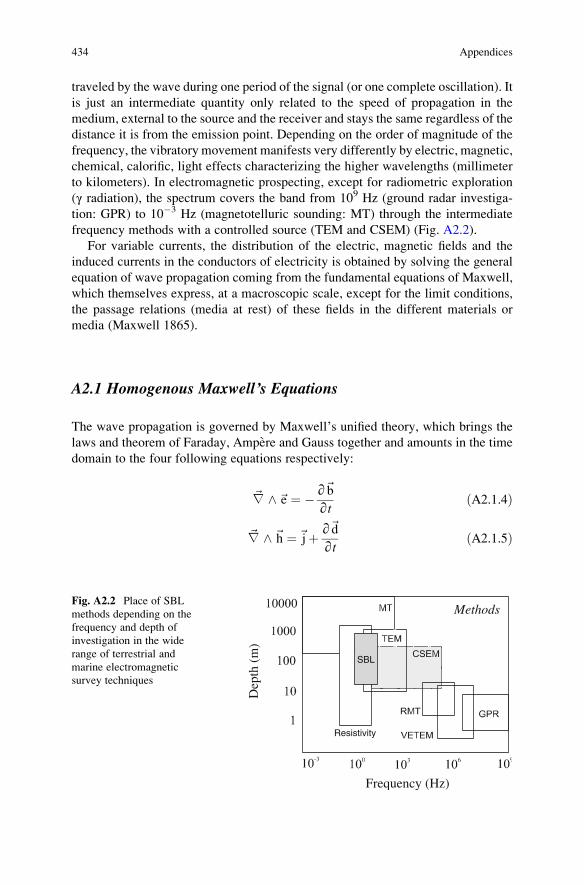
traveled by the wave during one period of the signal (or one complete oscillation). It

is just an intermediate quantity only related to the speed of propagation in the

medium, external to the source and the receiver and stays the same regardless of the

distance it is from the emission point. Depending on the order of magnitude of the

frequency, the vibratory movement manifests very differently by electric, magnetic,

chemical, calorific, light effects characterizing the higher wavelengths (millimeter

to kilometers). In electromagnetic prospecting, except for radiometric exploration

(γ radiation), the spectrum covers the band from 109 Hz (ground radar investiga-

tion: GPR) to 10�3 Hz (magnetotelluric sounding: MT) through the intermediate

frequency methods with a controlled source (TEM and CSEM) (Fig. A2.2).

For variable currents, the distribution of the electric, magnetic fields and the

induced currents in the conductors of electricity is obtained by solving the general

equation of wave propagation coming from the fundamental equations of Maxwell,

which themselves express, at a macroscopic scale, except for the limit conditions,

the passage relations (media at rest) of these fields in the different materials or

media (Maxwell 1865).

A2.1 Homogenous Maxwell’s Equations

The wave propagation is governed by Maxwell’s unified theory, which brings the

laws and theorem of Faraday, Ampere and Gauss together and amounts in the time

domain to the four following equations respectively:

~∇ ^~e ¼ �∂~b∂t

ðA2.1.4Þ

~∇ ^ ~h ¼~jþ ∂~d∂t

ðA2.1.5Þ

Methods

Dep

th (

m)

Resistivity

SBL

Frequency (Hz)

Fig. A2.2 Place of SBL

methods depending on the

frequency and depth of

investigation in the wide

range of terrestrial and

marine electromagnetic

survey techniques

434 Appendices

~∇ � ~b ¼ 0 ðA2.1.6Þ~∇ � ~d ¼ p ðA2.1.7Þ

where, in standardized SI units,~e is the electric field (V/m),~b the magnetic induction

(Tesla), ~h the magnetic field (A/m), ~d the dielectric displacement (C/m2), ~j thecurrent density (A/m2) and finally p the density of electric charge (C/m3).

These equations state that any spatial variation of a field (electric or magnetic) at

any point of the space leads to the existence of a time variation of another field at

the same point and vice versa. These equations are presented here in their local

form, i.e., a differential form (Fig. A2.3).

Maxwell’s equations can also be made in the integral form, where they express

then the relations between the electromagnetic fields in an area, rather than at a

point (local form). Under these conditions the relations with rotationals are inte-

grated on a surface using Stokes’ theorem to obtain the flow of the vectors~e and ~h.

A2.2 Constitutive Relations

As Maxwell’s equations are not coupled together, it is then necessary to connect theexpressions of the fields, the charges and the currents by relations expressing

behavioral laws depending this time on the frequency such that:

~D ¼ ε ω, ~e, ~r, t, T, P, . . .ð Þ � ~E ðA2.1.8Þ~B ¼ μ ω, ~e, ~r, t, T, P, . . .ð Þ � ~H ðA2.1.9Þ~J ¼ σ ω, ~e, ~r, t, T, P, . . .ð Þ � ~E ðA2.1.10Þ

where ε, μ and σ are respectively the dielectric permittivity, magnetic permeability

and electrical conductivity tensors, and t, T and P the parameters of time,

Fig. A2.3 Illustration of

the nature of the magnetic

and electric fields: vector ~bpassing through a surface S

(a) and vector ~e circulatingon an MN curve (b)

Appendices 435

temperature and pressure. Theoretically these tensors are complex, involving phase

shifts between the fields ~D and ~E and also between and ~H, ~J and ~E.Practically, except in special cases, these tensors may be replaced by scalars,

under the cover of simplifying assumptions:

– Linear propagation media, homogeneous and isotropic

– Electrical process no more dependent on time, temperature and pressure

– Nonmagnetic media where the permeability of the media is equivalent to the

permeability of the vacuum (μ ¼ μrock ¼ μwater ¼ μ0 ¼ 4π� 10�7H:m�1).

Under these conditions, the above constitutive equations reduce to:

~D ¼ ε0 ωð Þ � iε00ωð Þ

h i~E ¼ ε~E ðA2.1.11Þ

~J ¼ σ0 ωð Þ þ iσ00ωð Þ

h i~E ¼ σ~E ðA2.1.12Þ

and:

~B ¼ μ~H ðA2.1.13Þ

where the permittivity and conductivity are complex functions of frequency, when

the permeability, which no longer depends on the frequency, is real (Fig. A2.4).

A2.3 Formation and Formulation of the Wave Equation

Taking the rotational�~∇ ^ � of the first two equations of Maxwell, i.e.:

~∇ ^ �~∇ ^~e�þ ~∇ ^ ∂~b∂t¼ 0 ðA2.1.14Þ

and:

Fig. A2.4 In Maxwell’sterminology, the lines of

force (a) between two

magnetic charges (+/�m)

can be interpreted as tubes

(b) formed from the

current loops (see Fig. 2.3)

(Maxwell 1861, 1862)

436 Appendices

2.3

~∇ ^ �~∇ ^ ~h�� ~∇ ^ ∂~d

∂t¼ ~∇ ^~j ðA2.1.15Þ

using by another way the constitutive relations in the time domain, where the

constants ε, μ, et σ are then independent on time such that:

~d ¼ ε~e ðA2.1.16Þ

and:

~b ¼ μ~h ðA2.1.17Þ

and:

~j ¼ σ~e ðA2.1.18Þ

and replacing the latter in the former, we finally obtain:

~∇ ^ ~∇ ^~eþ μ~∇ ^ ∂~h∂t¼ 0 ðA2.1.19Þ

and:

~∇ ^ ~∇ ^ ~h� ε~∇ ^ ∂~e∂t¼ σ~∇ ^~e ðA2.1.20Þ

By interchanging the derivative operators (as vector functions~h and~e and their firstand second derivatives are continuous throughout the domain), we arrive at:

~∇ ^ ~∇ ^~eþ μ∂∂t

�~∇ ^ ~h

� ¼ 0 ðA2.1.21Þ

and:

~∇ ^ ~∇ ^ ~h� ε∂∂t

�~∇ ^~e� ¼ σ~∇ ^~e ðA2.1.22Þ

and then replacing ~∇ ^ ~h and ~∇ ^~e given by Maxwell’s equations it remains that:

~∇ ^ ~∇ ^~eþ με∂2~e

∂t2þ μσ

∂~e∂t¼ 0 ðA2.1.23Þ

and:

Appendices 437

~∇ ^ ~∇ ^ ~hþ με∂2~h

∂t2þ μσ

∂~h∂t¼ 0 ðA2.1.24Þ

Considering the remarkable vector identity ~∇ ^ ~∇ ^~a�~∇ ~∇ �~a ¼ ∇2~a (given

for any vector ~a) with ~∇:~h ¼ 0 and ~∇:~e ¼ 0 for homogeneous media,5 we can

write then (Reitz and Milford 1962):

∇2~e� με∂2~e

∂t2� μσ

∂~e∂t¼ 0 ðA2.1.25Þ

and:

∇2~h� με∂2~h

∂t2� μσ

∂~h∂t¼ 0 ðA2.1.26Þ

Turning now to the Fourier domain, such that the field excitation varies over time in

a sinusoidal manner, it eventually comes for the electric field6 and for a monochro-

matic plane wave to the propagation/diffusion equation, which in the field fre-

quency (ω) is written (Reitz and Milford 1962)7:

∇2~Eþ ω2με� iωμσ� �

~E ¼ 0 ðA2.1.27Þ

more commonly called the Helmholtz equation, which also reflects an irreversible

phenomenon.

A2.4 Helmholtz Equation: Discussion

By grouping the variational terms (μ, σ, ε) affecting the propagation medium and

the frequency ω, the above equation in the frequency domain (cf. Eq. A2.1.27) can

be reduced to:

∇2~Eþ k2~E ¼ 0 ðA2.1.28Þ

with:

5In reality the rocks cannot be considered as homogeneous media and we have ∇~e 6¼ 0. The

resistivity contrasts then act as secondary sources.6For convenience, we introduce here the complex notation that can express derivations such as

∂/∂t! iω or ∇2! – k2.7To form the wave equation we can also rely on Maxwell’s equations set out in the frequency

domain. They can be found in all books of mathematical physics.

438 Appendices

k2 ¼ ω2με� iωμσ ðA2.1.29Þ

where k represents the wave number or spreading factor.

This complex number consisting of a real part and an imaginary part, depending

on the electromagnetic properties of the crossed media, will not have the same

impact on the propagation/diffusion phenomena depending on the balance of its

parts whether they are real or imaginary.

Discussion

The previous expression (cf. Eq. A2.1.29) therefore shows two scenarios:

• First case: ω2με >> ωμσ or ωε/σ >>1. In this case we have:

k2 ωμε ðA2.1.30Þ

which is real as k is. By replacing k2 with its value (με), the equation

(cf. Eq. A2.1.25) in the time domain becomes then:

∇2~e� με∂2~e

∂t2¼ 0 ðA2.1.31Þ

and describes, because of the presence of the second derivative, the wave propa-

gation (propagation equation) moving at the speed 1=ffiffiffiffiffiμεp and dependent on the

magnetic permeability μ and especially on the dielectric permittivity ε of the

medium. In these circumstances, the displacement currents are dominant (!insulating media).

• Second case: ω2με << ωμσ or ωε/σ << 1. In this case we have then:

k2 �iωμσ ðA2.1.32Þ

which is a pure imaginary and k a complex. By replacing k2 with its value (μσ), theEq. (A2.1.25) in the time domain becomes:

∇2e* � μσ

∂e*

∂t¼ 0 ðA2.1.33Þ

and describes the diffusion of a field (diffusion equation) whose amplitude, depen-

dent on the electrical conductivity σ of the medium, decreases with the distance. In

these circumstances the conduction currents dominate (! conductive media). This

equation, which neglects the second derivatives, is then applied to the phenomena

slowly varying over time.

Appendices 439

Solution for the diffusion equation: considering a single dimension (z) in the

direction of propagation, the equation becomes:

∂2~e

∂z2� μσ

∂~e∂t¼ 0 ðA2.1.34Þ

The solution for the electric field is now of the form:

~e ¼ ~eþ0 e�i kz�ωtð Þ þ~e�0 e

�i -kz�ωtð Þ ðA2.1.35Þ

where ~eþ0 and ~e�0 respectively correspond to the upward and downward field.

If we now only consider the downward wave, there is in these circumstances:

~e ¼ ~eþ0 e�iαze�βzeiωt ðA2.1.36Þ

which shows the weakening of an alternating field (e�iαz, eiωt ) with depth (e�βz )(Fig. A2.5).

A2.5 Laplace Equations

Solving the Laplace equation allows us, whenever possible (quasistatic approxima-

tion), to overcome the effects of frequency as is the case at very low frequencies.8

We can then solve complex problems of potential or field distribution as in DC

stimulation with a minimum of calculations and good estimation.

The Laplace equation is obtained by taking the first Maxwell equation:

Diffusive field

Dep

th

Direction of propagation

Fig. A2.5 Allure of a

diffusive field marking an

exponential diminution of

energy (amplitude) with

depth

8At sufficiently low frequencies, the AC behaves in the subsoil and especially in conducting media

as DC.

440 Appendices

~∇ ^~eþ ∂~b∂t¼ 0 ðA2.1.37Þ

and considering a quasistatic or steady regime with:

∂~b∂t¼ 0 ðA2.1.38Þ

where:

~∇ ^~e ¼ 0 ðA2.1.39Þ

This expression shows that the electric field is conservative, a necessary and

sufficient condition to demonstrate that it do derive of a scalar potential (gradient)

such that:

~E ¼ �~∇V ðA2.1.40ÞFrom the fourth law of Maxwell (ε does not vary with position) we then show that:

~∇: ~E ¼ q=ε ðA2.1.41Þ

or that:

~∇ : ~∇V�∇2V ¼ q=ε ðA2.1.42Þ

In each point free of charge (q¼ 0), we finally obtain the Laplace equation valid in

an environment without a power source:

∇2V ¼ 0 ðA2.1.43Þ

which can be solved in different types of coordinates, Cartesian, cylindrical or

spherical, according to the desired geophysical applications.

However, this partial derivative equation is not sufficient in itself to determine

the function V to which it relates. This uncertainty reflects the fact that at a given

electric field corresponds to not a potential but a group of potentials. To remove the

indeterminacy, we then fix limit conditions that define the boundary elements on

which restrictions may be imposed.

A2.6 Poisson Equation

The Poisson equation or equation of the potential vector is an equation of the same

type as the Laplace equation (see Eq. A2.1.43) but whose second member this time

is not zero:

Appendices 441

∇2V ¼ q=ε ðA2.1.44Þ

The general solution of this equation is obtained by adding to the solution of the

equation without a second member (Laplace equation) a particular solution of the

equation with a second member.

A2.7 Solution Unicity

If we consider, for distinct potentials V1 and V2, the equations:

∇2V1 ¼ q=ε and ∇2V2 ¼ q=ε ðA2.1.45Þ

the unicity theorem proved for the Laplace equation is then transposable to the

Poisson equation, such that by taking the difference we obtain again:

∇2 V1 � V2ð Þ ¼ 0 ðA2.1.46Þ

A2.8 Passage Relations at the Interfaces

At the interfaces separating two different propagation media (1 and 2 for example),

the components of the electric fields ~E, ~D and magnetic fields ~H, ~B must satisfy

certain conditions of passage. These data are then given by integrating, on an

elementary volume, the fundamental equations, such that we have:

~n12 ^ ~E2 þ ~n21 ^ ~E1 ¼ ~n12 ^ ~E2 � ~E1

� � ¼ 0 ðA2.1.47Þ~n12 ^ ~D2 þ ~n21 ^ ~D1 ¼ ~n12 ^ ~D2 � ~D1

� � ¼ ~qs ðA2.1.48Þ

~n12 ^ ~H2 þ ~n21 ^ H

1 ¼ ~n12 ^ ~H2 � ~H1

� � ¼ ~Js ðA2.1.49Þ~n12 ^ ~B2 þ ~n21 ^ ~B1 ¼ ~n12 ^ ~B2 � ~B1

� � ¼ 0 ðA2.1.50Þ

where ~n12 and ~n21 are normal at the considered interfaces (respectively from 1 to

2 and from 2 to 1),~qs the surface charge density and~Js the actual density of surfacecurrent (Fig. A2.6).

More simply for a stationary current or equivalent, at a point P located at the

interface of two media of different resistivities ρ1 and ρ2, the relations of passage

through a plan (n, x) correspond, for some fields ~E such as ~E1,2 ¼ �~∇V1,2 to:

442 Appendices

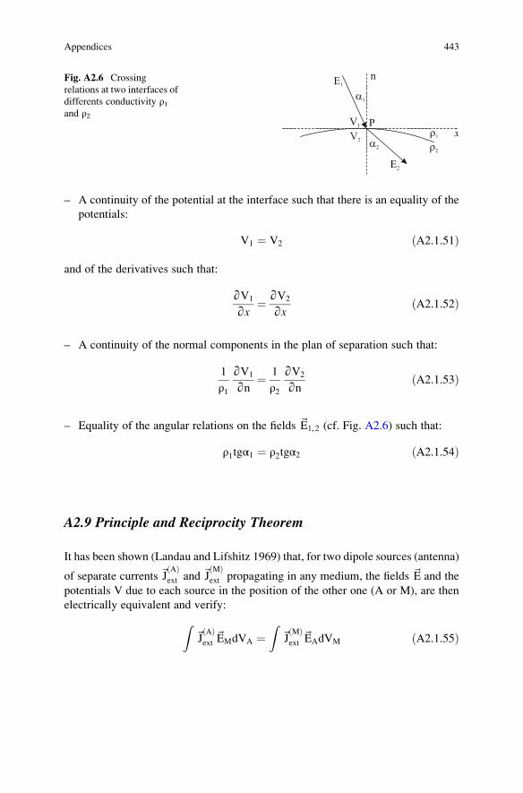
– A continuity of the potential at the interface such that there is an equality of the

potentials:

V1 ¼ V2 ðA2.1.51Þ

and of the derivatives such that:

∂V1

∂x¼ ∂V2

∂xðA2.1.52Þ

– A continuity of the normal components in the plan of separation such that:

1

ρ1∂V1

∂n¼ 1

ρ2∂V2

∂nðA2.1.53Þ

– Equality of the angular relations on the fields ~E1,2 (cf. Fig. A2.6) such that:

ρ1tgα1 ¼ ρ2tgα2 ðA2.1.54Þ

A2.9 Principle and Reciprocity Theorem

It has been shown (Landau and Lifshitz 1969) that, for two dipole sources (antenna)

of separate currents ~JAð Þext and

~JMð Þext propagating in any medium, the fields ~E and the

potentials V due to each source in the position of the other one (A or M), are then

electrically equivalent and verify:Z~J

Að Þext

~EMdVA ¼Z

~JMð Þext

~EAdVM ðA2.1.55Þ

Fig. A2.6 Crossing

relations at two interfaces of

differents conductivity ρ1and ρ2

Appendices 443

This formulation, which corresponds to the reciprocity theorem,9 where the

Maxwell’s equations satisfy these properties, is particularly important in electrical

prospecting, especially in the interpretation algorithms using migration techniques

(3D imaging) and the control of the quality of the acquisition.

A2.10 Static and Quasistatic Approximations

To simplify the calculations, it is possible in certain situations to establish some

approximations. This is the case for instance:

– In DC prospecting where we practice static approximation, which consists of

considering the potential differences or gradient as differences of electrostatic

potentials10 where electrical and magnetic phenomena are then independent.11

– In the investigations in low frequency alternating current when we practice

the quasistatic approximation which consists of neglecting the induced effect12

( ~∇ ^~e ¼ 0 ) ~E ¼ �~∇V) in the limit of the skin depth (cf. Sect. 3.3.1

Chap. 3) where only the conduction currents are considered. In the case where

the field change is sufficiently slow (T >> ς/c where ς is the size of the circuit)or in other words where this variability occurs on long time scales relative to the

time characteristic of field adjustment, their distribution throughout space at

any instant looks like that of a static field. The propagation velocity and time

delay can be neglected. The field equations, also called pre-Maxwell equations

(since they were discovered before Maxwell’s equations were introduced), are

invariant under the Galilean transformation. It follows that for quasistatic fields

the differential equation is given by Eq. A2.1.33.

In those situations where we consider a uniform field, then we can use the results

of the mathematical analysis (analytical or numerical) on the distributions

established in the electrostatic field (Fig. A2.7).

9For the whole vector field see also (Kraichman, 1976) and for a detailed demonstration see the

following Appendix.10The electrical potential V(r) is defined (Ellis and Singer, 2007) as the electrostatic potential υ(r)coming from the electrostatic field E (Coulomb’s law), itself attributed to the electrostatic force

field (q) such that: ~E ¼ 14πε0

qr2 r ! ϑ rð Þ ¼ q

4πε01r ¼ V rð Þ

It is assumed in this case that the electrostatic laws still apply when electricity moves, i.e., when

electrical currents appear as long as we are dealing with a steady state.11Unlike electric masses at rest which do not engage any action on magnetic masses, electrical

masses in motion engage one.12See Chap. 5, Sect. 3.1.2

444 Appendices

http://dx.doi.org/10.1007/978-3-319-45355-2_3

http://dx.doi.org/10.1007/978-3-319-45355-2_3

http://dx.doi.org/10.1007/978-3-319-45355-2_5

http://dx.doi.org/10.1007/978-3-319-45355-2_5

Appendix A2.2

Demonstration of the reciprocity theorem

Preamble

In physics, the reciprocity theorem allocated to the principle of the same name takes

on an important general character.13 It can be applied both in the field of elastic

wave propagation and in that of the diffusion and potential of electric currents.

Specifically, in acoustics for example (Landau and Lifchitz 1971), it governs the

operation of piezoelectric sensors by using them both together or separately as a

transmitter and a receiver (transducers or reciprocal sensors). It greatly also

improves seismic data processing (Claerbout 1976).

In on-land or seabed electromagnetic prospecting, it allows us to diversify easily

the geometric patterns as the arrays and instrumental arrangements according to the

experimental stresses, and is of the greatest importance in the field of downhole

well logging. The first one in 1915 to seize on the problem and use the reciprocity

theorem (a priori without demonstrating this) was Frank Wenner from the US

Bureau of Standards (Van Nostrand and Cook 1966).

In what follows, we take into account for the calculations the quasistatic

approximation as DC computing.

A2.1. Principle

We prove for two fixed points A and M (electrodes) immersed in any homogeneous

or heterogeneous medium, isotropic or anisotropic, that the potential V in M

Fig. A2.7 Static and quasistatic approximations performed under exploration DC and under low

frequency variable currents (LF)

13First formulated by Lord Rayleigh in his famous book Theory of Sound. It was H. A. Lorentzwho enunciated in 1895 a reciprocity theorem for electromagnetic fields, which was completed in

1923 by J. R. Carson of Bell Laboratories for radio wave communication (Carson, 1923). See also

P. Poincelot (Poincelot, 1961) and M. L. Burrows (Burrows 1978).

Appendices 445

resulting from a given current I sent to A is equal to what would be the potential in

A if the current was sent to M (cf. Fig. A2.8).

A2.2. Preliminary Formula Demonstration

In the proof of the theorem that follows, to avoid writing at great length, we use

symbolic notations, which will be explained as and when they are introduced in

the text.

A2.2.1. Partial Derivative Equation

The partial derivative equation, which satisfies the electric potential in a heteroge-

neous and anisotropic medium, and allows us to solve the problem, is built from

three basic assumptions that:

– The electric field ~E is derived from a scalar potential V:

~E ¼ �~∇V ðA2.2.1Þ

also given for its components in rectangular coordinates (x1, x2, x3):

E1 ¼ � ∂V∂x1

, E2 ¼ � ∂V∂x2

, E1 ¼ � ∂V∂x3

ðA2.2.2Þ

– Ohm’s law, which states that the current density vector ~J is deduced from the

electric field vector ~E and the electrical conductivity σ by a symmetrical

determinant linear transformation such that:

~J ¼ σ~E ðA2.2.3Þ

or by considering the anisotropy of conductivity:

Fig. A2.8 Principle of

reciprocity: an equivalence

of potentials and currents

446 Appendices

J1 ¼ σ11E1 þ σ12E2 þ σ13E3

J2 ¼ σ21E1 þ σ22E2 þ σ23E3

J3 ¼ σ31E1 þ σ32E2 þ σ33E3

8<: ðA2.2.4Þ

with σ21 ¼ σ12, σ31 ¼ σ13 and σ23 ¼ σ32equations that can be symbolically written as:

Jk ¼ σklEl with σkl ¼ σlk ðA2.2.5Þ

– Kirchhoff’s law, according to which the flow of the current density vector

through a closed surface containing no power source is zero, results in:

~∇:~J ¼ 0 ðA2.2.6Þ

or in rectangular coordinates:

∂J1∂x1þ ∂J2∂x2þ ∂J3∂x3

¼ 0 ðA2.2.7Þ

By transferring this time (A2.2.2) and (A2.2.4) into (A2.2.7) we obtain then:

σ11∂2

V

∂x12þ σ12

∂2V

∂x1∂x2þ σ13

∂2V

∂x1∂x3þ ∂σ11

∂x1

∂V∂x1þ ∂σ12

∂x1

∂V∂x2þ ∂σ13

∂x1

∂V∂x3

þσ21 ∂2V

∂x1∂x2þ σ22

∂2V

∂x22þ σ23

∂2V

∂x2∂x3þ ∂σ21

∂x2

∂V∂x1þ ∂σ21

∂x2

∂V∂x2þ ∂σ23

∂x2

∂V∂x3

þσ31 ∂2V

∂x1∂x3þ σ32

∂2V

∂x2∂x3þ σ33

∂2V

∂x32þ ∂σ31

∂x3

∂V∂x1þ ∂σ32

∂x3

∂V∂x2þ ∂σ33

∂x3

∂V∂x3¼ 0

ðA2.2.8Þ

an equation which is symbolically written:

σkl∂2

V

∂xk∂xlþ ∂σkl

∂xk

∂V∂xkl¼ 0 ðA2.2.9Þ

This is the basic equation which the electrical potential satisfies at any point where

it is regular.

A2.2.2. Green Formula

From the preceding equation we can deduce another relation that satisfies the

electrical potential.

Appendices 447

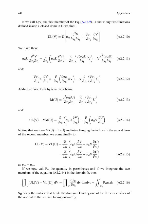
If we call L(V) the first member of the Eq. (A2.2.9), U and V any two functions

defined inside a closed domain D we find:

UL Vð Þ ¼ U σkl∂2

V

∂xk∂xlþ ∂σkl

∂xk

∂V∂xkl

" #ðA2.2.10Þ

We have then:

σklU∂2

V

∂xk∂xl¼ ∂

∂xkσklU

∂V∂xl

� �� ∂∂xl

∂ σklUð Þ∂xk

V

� �þ V

∂2 σklUð Þ∂xk∂xl

ðA2.2.11Þ

and:

∂σkl∂xk

U∂V∂xl¼ ∂

∂xl

∂σkl∂xk

UV

� �� V

∂∂xl

∂σkl∂xk

U

� �ðA2.2.12Þ

Adding at once term by term we obtain:

M Uð Þ ¼ ∂2 σklUð Þ∂xk∂xl

� ∂∂xl

∂σkl∂xk

U

� �ðA2.2.13Þ

and:

UL Vð Þ � VM Uð Þ ¼ ∂∂xk

σklU∂V∂xl

� �� ∂∂xl

σklV∂U∂xk

� �ðA2.2.14Þ

Noting that we have M (U)¼L (U) and interchanging the indices in the second term

of the second member, we come finally to:

UL Vð Þ � VL Uð Þ ¼ ∂∂xk

σklU∂V∂xl� σlkV

∂U∂xl

� �¼ ∂

∂xkσklU

∂V∂xl� σklV

∂U∂xl

� �ðA2.2.15Þ

as σkl ¼ σlk.If we now call Pkl the quantity in parentheses and if we integrate the two

members of the equation (A2.2.14) in the domain D, then:ðððD

UL Vð Þ � VL Uð Þ½ � dV ¼ððð

D

∂Pkl∂xk

dx1dx2dx3 ¼ZZ

SD

Pklnkds ðA2.2.16Þ

SD being the surface that limits the domain D and nk one of the director cosines of

the normal to the surface facing outwardly.

448 Appendices

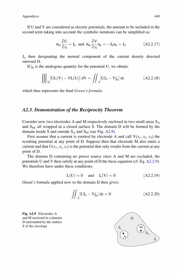
If U and V are considered as electric potentials, the amount to be included in the

second term taking into account the symbolic notations can be simplified as:

σkl∂U∂xl¼ Jk and σkl

∂V∂xl

nk ¼ �Jknk ¼ Jn ðA2.2.17Þ

Jn then designating the normal component of the current density directed

outward D.

If jn is the analogous quantity for the potential U, we obtain:ðððD

UL Vð Þ � VL Uð Þ½ � dV ¼ZZ

S

UJn � Vjn½ � ds ðA2.2.18Þ

which thus represents the final Green’s formula.

A2.3. Demonstration of the Reciprocity Theorem

Consider now two electrodes A and M respectively enclosed in two small areas SAand SM, all wrapped in a closed surface S. The domain D will be formed by the

domain inside S and outside SA and SM (see Fig. A2.9).

First assume that a current is emitted by electrode A and call V(x1, x2, x3) theresulting potential at any point of D. Suppose then that electrode M also emits a

current and that U(x1, x2, x3) is the potential that only results from the current at any

point of D.

The domain D containing no power source since A and M are excluded, the

potentials U and V then satisfy at any point of D the basic equation (cf. Eq. A2.2.9).

We therefore have under these conditions:

L Uð Þ ¼ 0 and L Vð Þ ¼ 0 ðA2.2.19ÞGreen’s formula applied now to the domain D then gives:ZZ

S

UJn � Vjn½ � ds ¼ 0 ðA2.2.20Þ

Fig. A2.9 Electrodes A

and M enclosed in a domain

D surrounded by the surface

S of the envelope

Appendices 449

where S denotes the set of the surfaces SD, SA, SM and Jn, jn are the normal

components of the current crossing these surfaces to the interior of the domain D.

If we call i the first member of the above equation, i consists of three terms iA, iMand iD related to the integrals extended respectively to the corresponding surfaces

SA, SM, SD.

First considering the term:

iA ¼ZZ

SA

UJn-Vjn½ � ds ðA2.2.21Þ

the surface SA then tends to the point A.

As the potential U (potential due to the electrode M) has no singularity at the A

its value will tend to the value it has in A.

As on the other hand: ZZS

Jnds ¼ J ðA2.2.22Þ

current emitted by A, we can easily recognize (see below) that the first part of iAtends to JU(A) such that:

limS ! SA

ZZUJnds ¼ JU Að Þ ðA2.2.23Þ

As for the second part of iA: ZZSA

Vjnds ðA2.2.24Þ

it can be assumed that it tends to zero.

Indeed, the current from M remains naturally finite and as the area SA also tends

to zero as r2 (r is the distance of any of its points to A) one need only assume that V

tends to infinity as 1/r to see that the integral tends to zero as r.For the demonstration to be complete it would still have to be proved that V is

actually of the order of 1/r. However, we can in a first step overcome this condition

(cf. Sect. A2.4).

Ultimately we have for A:

limSA ! 0

iA ¼ JU Að Þ ðA2.2.25Þ

and for M:

limSM ! 0

iM ¼ �jV Mð Þ ðA2.2.26Þ

It now remains to evaluate the integral on S. Assuming that S is the surface of the

subsoil, and as no current flows through this area, we have in fact:

450 Appendices

Jn ¼ 0 jn ¼ 0 so iSD ¼ 0 ðA2.2.27Þ

The equation:

i ¼ iA þ iM þ iSD ¼ 0 ðA2.2.28Þ

therefore ultimately reduces to:

JU Að Þ � jV Mð Þ ¼ 0 ðA2.2.29Þ

If in addition the currents sent by A and M are equal, that is J¼ j, one will finally

have:

U Að Þ ¼ V Mð Þ ðA2.2.30Þ

The potential in A which results from a certain current supplied by M and the

potential in M which results from an equal current supplied by A are finally equal.

A2.4. Condition on the Potential

In the first part of this Appendix, to avoid overloading the scriptures, certain

assumptions have been accepted and in particular those concerning the potential.

Thus, it can be shown:

– Firstly that:

limSA ! 0

ZZSA

UJnds ¼ JU Að Þ ðA2.2.31Þ

Let P be any point in SA. The potential U from M being continuous next to A we

have:

U Pð Þ � U Að Þ ξh ðA2.2.32Þ

ξ being very small.

If P – A is small enough, that is P� Að Þ ηh , and on the other hand if we have

whatever SA: ZZSA


we must show that:

Appendices 451

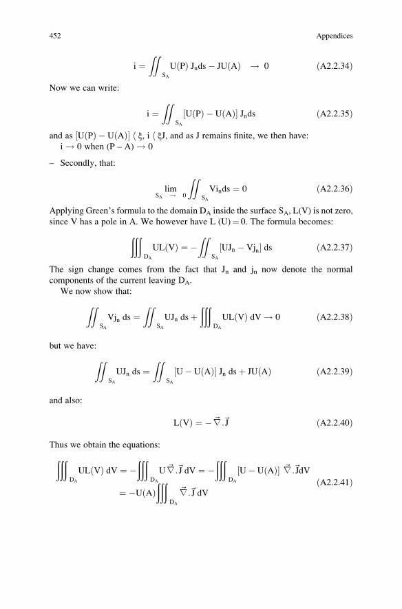
i ¼ZZ

SA

U Pð Þ Jnds� JU Að Þ ! 0 ðA2.2.34Þ

Now we can write:

i ¼ZZ

SA

U Pð Þ � U Að Þ½ � Jnds ðA2.2.35Þ

and as U Pð Þ � U Að Þ½ � ξh , i ξJh , and as J remains finite, we then have:

i! 0 when (P – A)! 0

– Secondly, that:

limSA ! 0

ZZSA

Vinds ¼ 0 ðA2.2.36Þ

Applying Green’s formula to the domain DA inside the surface SA, L(V) is not zero,

since V has a pole in A. We however have L (U)¼ 0. The formula becomes:ðððDA

UL Vð Þ ¼ �ZZ

SA

UJn � Vjn½ � ds ðA2.2.37Þ

The sign change comes from the fact that Jn and jn now denote the normal

components of the current leaving DA.

We now show that:ZZSA

Vjn ds ¼ZZ

SA

UJn dsþððð

DA

UL Vð Þ dV! 0 ðA2.2.38Þ

but we have:ZZSA

UJn ds ¼ZZ

SA

U� U Að Þ½ � Jn dsþ JU Að Þ ðA2.2.39Þ

and also:

L Vð Þ ¼ �~∇:~J ðA2.2.40Þ

Thus we obtain the equations:ðððDA

UL Vð Þ dV ¼ �ððð

DA

U~∇:~J dV ¼ �ððð

DA

U� U Að Þ½ � ~∇:~JdV

¼ �U Að Þððð

DA

~∇:~J dVðA2.2.41Þ

452 Appendices

As: ðððDA

~∇:~J dV ¼ZZ

SA


then:ZZSA

Vjn ds ¼ZZ

SA

U� U Að Þ½ � Jn ds�ððð

DA

U� U Að Þ½ � ~∇:~J dV ðA2.2.43Þ

and therefore: ZZSA

Vjn ds

� � 2ξJ! 0 ðA2.2.44Þ

Appendix A2.3

Magnetic field produced by telluric currents

Preamble

To evaluate the magnetic field from the telluric currents flowing through the

earth, we consider here a subsoil consisting of a stack of substantially horizontal

geological strata.

A3.1. Magnetic Field Calculation

It is assumed here that the telluric field is uniform. We then consider a horizontal

layer of thickness dz, where ρ is the electrical resistivity and the value of the currentdensity flowing through the element is j (see Fig. A2.10).

In the x direction, a current tube lying in this layer with vertical (z, z + dz) andhorizontal (x, x + dx) dimensions pierces the plan xOz at a point M. The horizontal

magnetic field at a point P located at the ground surface, perpendicular to the

current direction, is of the form:

dH ¼ 2j

PMdx dz cos α ðA2.3.1Þ

where α is the angle between the line joining the points P and M, and the z-axis.Considering that:

Appendices 453

PM ¼ z

cos αand x ¼ z tgα

! dx ¼ zdα

cos 2α

ðA2.3.2Þ

we draw:

dH ¼ 2j dz dα ðA2.3.3Þand then integrating from �π/2 to +π/2 we finally obtain:

dH ¼ 2πj dz ðA2.3.4ÞAs:

j ¼ 1

ρdV

dyðA2.3.5Þ

where dV/dy is the potential gradient in the y direction,thus we arrive at:

H ¼Z z

0

2πρdV

dydz ðA2.3.6Þ

As the field is uniform, the potential gradient dV/dy is then constant everywhere.

We can therefore write:

H ¼ 2πdV

dy

Z z

0

dz

ρðA2.3.7Þ

which is representative of the total conductance of the field.

A3.2. Order of Magnitude of the Magnetic Field

If now V is expressed in volts, y, z and r in meters and ρ inΩ.m, we obtain the value

of H (by dividing by 103) in Gauss:

Earth surfaceFig. A2.10 Geometric

model for the establishment

of the calculation of the

magnetic field associated

with the flow of telluric

currents

454 Appendices

H G½ � ¼2π103

dV

dy

Z z

0

dz

ρðA2.3.8Þ

To assess and establish an order of magnitude, the following is assumed in

substance:

– A telluric field of 1 mV/km, i.e., a gradient dV/dy corresponding to 10�6 V/m– A layer of conductive ground of 10 Ω.m and 1 km thick resting on insulating

grounds (z/ρ¼102)In these local conditions we find after integration of (A2.3.8):

H G½ � ¼ 2π103

dV

dy

� �z

ρðA2.3.9Þ

or finally by substituting by the above values:

H ¼ 2π10�7G or H ¼ 2π10�2γ ðA2.3.10Þ

a very low value14 compared to the natural allochthonous variations present in the

subsoil, but still measurable over a long period with sensitive variometers (see

Chap. 4, Sect. 5.7.2).

However, if we admit that the telluric field varies with an angular velocity of

about 1/5 rad for a period of 30 s, the maximum dH/dt will be then:

2π510�2γ=s ðA2.3.11Þ

This variation is actually of the same order of magnitude as that which corresponds

to the diurnal variation of the earth’s magnetic field and far greater than that which

corresponds to the secular variation (see Chap. 4, Sect. 4.5.1).

However it can on one hand be measured with sufficient accuracy in the range of

considered frequencies, and on the other hand be relatively easily separated from

the natural variations as it precisely follows the variations of the telluric field and

remains proportional to it.

14I hope that the younger generation of geophysicists will not be cross with our use of the old

notation (CGS), i.e., the Gauss (G) and gamma (γ), which I think are more appropriate than the

Tesla (T) at the magnitude orders of the measurements in geophysics (1 γ is equal to 10�9 T or to

10�5 G).

Appendices 455

http://dx.doi.org/10.1007/978-3-319-45355-2_4

http://dx.doi.org/10.1007/978-3-319-45355-2_4

http://dx.doi.org/10.1007/978-3-319-45355-2_4

http://dx.doi.org/10.1007/978-3-319-45355-2_4

Appendix A2.4

Brief history of onshore electrotelluric or telluric prospecting

Preamble

The experience of Vitre15 (Schlumberger 1930) demonstrated the efficiency of the

electrical method for deep geological layer investigations, but also the inadequacy

of the means implemented for a truly industrial application. The idea was then to

use not an artificial current but the natural currents flowing through the earth’s crustand well known by the earth scientists and telegraphists at this time.

This principle has the merit of significantly limiting the length of lines and

consequently the emitted power. Considering the local variations in the density and

azimuth of the telluric current sheets, all the emission devices disappear and the

exploration equipment becomes much lighter. However, it no longer reaches

vertical scaling as in conventional electric sounding, but there are structural variations

in the horizontal direction with an ad hoc device (base and mobile station).

However, the major difficulty is that these fields are highly variable, depending

on the time, direction and intensity. The comparisons of the fields at two distinct

points on the surface earth’s, to be valid, must be made between fields at the same

time. We then observe, as the theory predicts, that the relation between the fields at

two points is projective. This projection can be represented by two linear relations

between the horizontal components of the two fields whose determinant is a number

that only depends on the two points of measurement. This number, known as the

area, corresponds to the ratio of the areas constructed from the two field vectors and

is the basis of the interpretation of the telluric maps; the area map represents the

map of the interferences caused by the geological structure.

By 1921, unidirectional observations in France were realized on each side of the

Rhine fault (Leonardon 1928), followed in June 1922 by others executed in the

French district of the Haute Marne with two identical measuring devices 2 km apart,

each of them this time made with two perpendicular lines 100 long, leading to

remarkable conclusions about possible correlations at a distance. At Val Richer in

March 1934 (the Norman property of the Schlumberger family), it was found that

15The electrical sounding used at Vitre (the Ile et Vilaine French district) foreshadowed deep oil

exploration. Before all experience of earth physics, this survey realized in 1928 in Normandy

(France) aimed to establish the structure of the subsoil at depths allowing the researchers to reach

the base of the Armorican block. The difficulty here lay in the fact that to achieve a sufficient depth

of investigation it was necessary to have long lengths of line. For that, Conrad and Marcel

Schlumberger and their collaborators used the telegraph line along the Rennes–Laval railway,

available to them for the occasion from the local post and telecommunications. The sending power

line (2 A at 200 V) was then a little over 200 km long. The DC was periodically reversed after

a varying time of a few seconds. The expected depth of investigation was approximately

50 kilometers and the measured resistivities varied from 500 to 1800 Ω.m2/m. This unique

experiment would be published a few months later in the renowned journal of the American

Institute of Mining and Metallurgical Engineers (AIME).

456 Appendices

with 500 m bases, correlations were possible between stations spaced by several

tens of kilometers. At this time, it was suggested to apply the method to the

exploration of the salt domes of the Oural–Emba region in the Soviet Union (now

in Kazakhstan). To reinforce this idea some tests took place near the Colmar city in

June 1934 and in July 1936 in the plain of Alsace near Hettenschlag on the very site

where a diapir had been recognized. The map of tellurics as it was called later by the

prospectors perfectly overlapped with that of the resistivities obtained by previous

electrical soundings, marking then the first success of this method. On the eve of the

Second World War a specific and compact device (the UR for Universal Recorder)

was designed and manufactured clandestinely in France, collecting in the same

“box”, of some 20 kg weight, the entire measuring device: antivibration galvanom-

eters of the Piccard type and two canals photographic recorder (argentic film).

Then experimented with in Morocco and Sumatra, the method mainly developed

in occupied France. From 1941 to 1945, several teams from CGG covered the

Aquitaine region totaling over 20,000 km2, highlighting the major tectonic axes of

the southern part of the sedimentary basin. After 1945, the technique spread in the

French colonies and especially in the Sahara Desert, Equatorial Africa, Madagas-

car, Italy, and Sicily, but also in the USSR and Austria (Porstendorfer 1960),

generally prior to detailed seismic operations or replacing them for some reasons

of difficult topography or complex tectonics (Migaux 1948). For lack of market

outlets, especially in the USA—a major consumer of geophysics, where seismic

reflection was largely dominant in the market—the telluric method dwindled in the

late 1950s (Allaud and Martin 1976).

Bibliographic References

Allaud L, Martin M (1976) Schlumberger: histoire d’une technique. Ed. Berger-Levrault. 348 p

Leonardon EG (1928) Some observations upon telluric currents and their application to electrical

prospecting. Terr Magn Atmos Electr 33(2):91–94

Migaux L (1948) Une methode nouvelle de geophysique appliquee: la prospection par courants

telluriques. Tire �a part de la Compagnie generale de geophysique, 31 p

Porstendorfer G (1960) Tellurik. Grundlagen Messtechnik und neue Einsatzm€oglichkeit.Ed. Akadenie Verlag, 186 p

Schlumberger C et M (1930) Electrical studies of the earth’s crust at great depth. New York

meeting. Geophysical prospecting AIME 1932, pp 134–140

Appendix A2.5

Definitions

As long as it is to make measurements, geophysics can be regarded as an exactscience. It is no more true when it comes to interpreting the geological results of

Appendices 457

these measurements, since it involves so many simplifying assumptions that areestablished a priori from the knowledge of the regional or local geology. This mayseem paradoxical if we also think of the extremely sophisticated mathematicalmodels that are used.

In this context of uncertainty, it is necessary to precisely define some concepts onnatural environments. They allow us to fix once and for all the limitations of thegeological interpretation that varies as we think from one prospect to another.

Homogeneous Medium. The geophysical definition of homogeneity has not the

rigor of that used in physics or chemistry. A rock formation is considered electri-

cally homogeneous if its resistivity does not substantially vary over the whole or a

part of its extent (of the order of 1/20). It is enough that the layer is geologically

monotonous and regular over the considered extent, i.e., its physical and chemical

structure remains substantially constant in this space.

Isotropic Medium. A medium is said to be isotropic when its electrical properties

are the same in all directions. In reality, however, the grounds are very often

anisotropic. This anisotropy in the sedimentary layers of the same age, for example,

is often linked to the stratification (due in particular to the conditions of sedimen-

tation and tectonics). In this case, the electric current tends to flow along a preferred

direction, in this case that of the strata whose conductivity is generally maximum.

Anomaly. We can affirm the existence of an anomaly when, after the use of a

suitable investigation depth and a choice of suitable scale, the amplitude of the

detected anomaly is on one hand consistent with what can be expected in a given

geological environment (size, depth, electromagnetic characteristics, etc.), and on

the other hand greater than the possible or probable error made in the acquisition

measures.

458 Appendices

Appendix A3.1

Abacus giving the resistivities (Ω.m) of different waters, depending on the

concentration in G/G (grains per gallon) or in PPM of sodium chloride

(NaCl) and temperature (�F)

According to Ellis and Singer (2007).

Appendix A3.2

Calculation of the magnetic field of an electric current from one or two point

electrodes and topological shape of this field in a electrically conductive

environment

In low frequency approximation (quasistatic approximation), we usually consider

the distribution of the electric current from a point electrode placed in O in an

indefinite homogeneous medium as having a spherical symmetry, the current then

regularly escaping in all directions of space.

Appendices 459

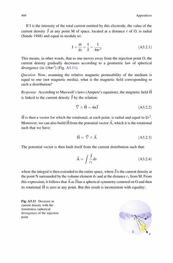
If I is the intensity of the total current emitted by this electrode, the value of the

current density ~J at any point M of space, located at a distance r of O, is radial(Sunde 1948) and equal in module to:

J ¼ di

ds¼ I

S¼ I

4πr2ðA3.2.1Þ

This means, in other words, that as one moves away from the injection point O, the

current density gradually decreases according to a geometric law of spherical

divergence (in 1/4πr2) (Fig. A3.11).

Question Now, assuming the relative magnetic permeability of the medium is

equal to one (not magnetic media), what is the magnetic field corresponding to

such a distribution?

Response According to Maxwell’s laws (Ampere’s equation), the magnetic field ~H

is linked to the current density ~J by the relation:

~∇ ^ ~H ¼ 4π~J ðA3.2.2Þ

~H is then a vector for which the rotational, at each point, is radial and equal to I/r2.

Moreover, we can also build ~Hfrom the potential vector ~A, which it is the rotationalsuch that we have:

~H ¼ ~∇ ^ ~A ðA3.2.3Þ

The potential vector is then built itself from the current distribution such that:

~A ¼Z ~J

r1dv ðA3.2.4Þ

where the integral is then extended to the entire space, where~J is the current density atthe point N surrounded by the volume element dv and at the distance r1 fromM. From

this expression, it follows that ~Aas~J has a spherical symmetry centered on O and then

its rotational ~H is zero at any point. But this result is inconsistent with equality:

Fig. A3.11 Decrease in

current density with the

remoteness (spherical

divergence) of the injection

point

460 Appendices

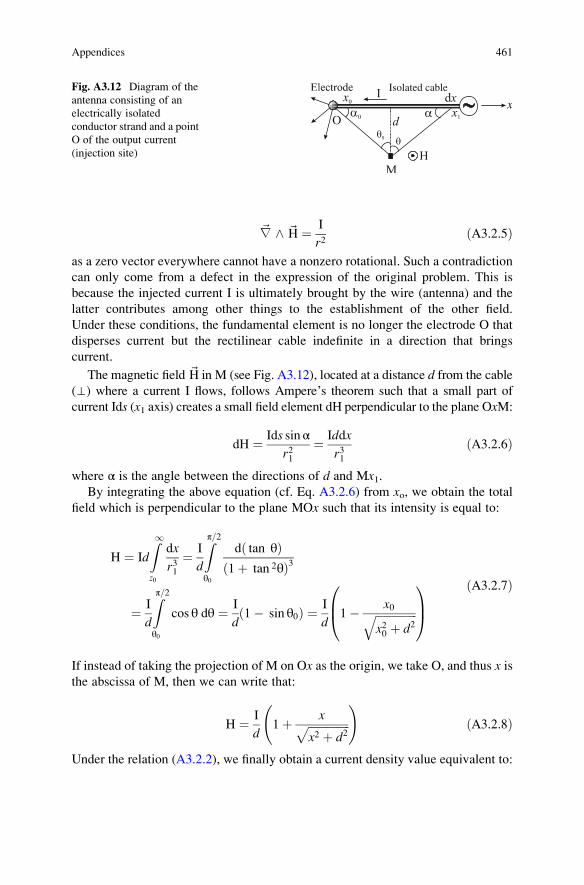
~∇ ^ ~H ¼ I

r2ðA3.2.5Þ

as a zero vector everywhere cannot have a nonzero rotational. Such a contradiction

can only come from a defect in the expression of the original problem. This is

because the injected current I is ultimately brought by the wire (antenna) and the

latter contributes among other things to the establishment of the other field.

Under these conditions, the fundamental element is no longer the electrode O that

disperses current but the rectilinear cable indefinite in a direction that brings

current.

The magnetic field ~H in M (see Fig. A3.12), located at a distance d from the cable

(⊥) where a current I flows, follows Ampere’s theorem such that a small part of

current Ids (x1 axis) creates a small field element dH perpendicular to the plane OxM:

dH ¼ Ids sin αr21

¼ Iddx

r31ðA3.2.6Þ

where α is the angle between the directions of d and Mx1.By integrating the above equation (cf. Eq. A3.2.6) from xo, we obtain the total

field which is perpendicular to the plane MOx such that its intensity is equal to:

H ¼ Id

Z1z0

dx

r31¼ I

d

Zπ=2θ0

d tan θð Þ1þ tan 2θð Þ3

¼ I

d

Zπ=2θ0

cos θ dθ ¼ I

d1� sin θ0ð Þ ¼ I

d1� x0ffiffiffiffiffiffiffiffiffiffiffiffiffiffiffi

x20 þ d2q

0B@1CA

ðA3.2.7Þ

If instead of taking the projection of M on Ox as the origin, we take O, and thus x isthe abscissa of M, then we can write that:

H ¼ I

d1þ xffiffiffiffiffiffiffiffiffiffiffiffiffiffiffi

x2 þ d2p !

ðA3.2.8Þ

Under the relation (A3.2.2), we finally obtain a current density value equivalent to:

Isolated cableFig. A3.12 Diagram of the

antenna consisting of an

electrically isolated

conductor strand and a point

O of the output current

(injection site)

Appendices 461

J ¼ I

4πr2¼ I

4π x2 þ d2� � ðA3.2.9Þ

The magnetic field resulting from the current threads flowing in the medium is zero

because of their spherical symmetry. The radial current can only exist because the

total magnetic field has a nonzero rotational. This circumstance only occurs

because the cable of the antenna Ox is interrupted in O. In other words, the current

is spread in the environment only because the cable is interrupted. Conversely, the

spherical distribution of the current from O cannot be conceivable without the Oxcable.

When the cable is interrupted at another point O0 serving for example as a return

electrode, we then obtain in such circumstances the corresponding magnetic and

electric fields, by superposing on the Ox cable (conducting I, interrupted in O), a

cable O0x (conducting I, interrupted in O0) (Fig. A3.13).16

The value of the magnetic field, perpendicular in M to the plane MOO0, is thenequal in these circumstances to:

H ¼ I

dsin θ00 � sin θ0� � ¼ I

d

x00ffiffiffiffiffiffiffiffiffiffiffiffiffiffiffi

x00 þ d2

q � x0ffiffiffiffiffiffiffiffiffiffiffiffiffiffiffix0 þ d2p

0B@1CA ðA3.2.10Þ

In the case of a dipole, the field is reduced to:

H ¼ I

dcos θ dθ ¼ Id

dx

x2 þ d2� � 3=2

ðA3.2.11Þ

If instead of being rectilinear the cable OO0 is of any form, the electric field and the

current density in the medium remain unchanged. In contrast, all magnetic fields

corresponding to the various forms of the cable have the same rotational and thus

correspond to the same current distribution in the medium.

Isolated cableFig. A3.13 Diagram of the

antenna with two injection

points OO0 (input and returncurrent)

16In AC, this condition can be made possible, for example, when the current flowing out of the first

electrode is in phase opposition with the current entering the second electrode (! polarized

electric dipole �).

462 Appendices

The magnetic field of the rectilinear cable Ox interrupted in O has, as a rotational,

a distribution of spherical current around O, with an own magnetic field equal to zero.

We have just seen that the antenna consisting of the Ox cable with spherical emission

through O is a solution of the equations of electricity. Is this the only one?

There may exist a current distribution with nonspherical symmetry around O that

would not have a zero magnetic field, such that this magnetic field had then

precisely as a rotational the difference between the real distribution and the

spherical distribution of the current. We may think that such distributions exist,

and that they even are the only real ones for the following reason.

A thread of current in the environment in reality consists of a discrete sequence

of charged particles (electrons, ions, etc.) moving at a speed~v. Each particle with a

charge q is subjected because of the electric field ~E to an electrostatic force q~E. But

as this one moves in a magnetic field ~H, it is also subjected to a Lorentz force as

~v ^ ~H� �

q. The total electromotive force is then ~Eþ ~v ^ ~H� �

. Ohm’s law in these

circumstances is no longer written in the standard form ~J ¼ σ~E but in the form:

~J ¼ σ ~Eþ ~v ^ ~H� � ðA3.2.12Þ

where σ is the electrical conductivity of the medium.

The total force and the current density do have a cylindrical symmetry around the axis

Ox. The transmitting device then has a priori no reason to have a spherical symmetry.

In fact, the Lorentz force is at each point perpendicular to the current thread and

the magnetic field. It is contained in the meridian plane of the thread and gives it a

curvature which deviates it from Ox. It performs no work and therefore does not

alter the potential distribution. The potential, which E continues to be, except for

the sign, the gradient ð~E ¼ �~∇VÞ, results from the condition of conservation of

electricity ð~∇: ~J ¼ 0Þ which is then written:

~∇: ~Eþ ~∇: ~v ^ ~H� � ¼ 0 ðA3.2.13Þ

It goes without saying that ~v, in a homogeneous and isotropic medium, is propor-

tional to ~J : ~v ¼ ξ~J where ξ is a factor dependent on the density of the working

charges in the conductor (number of free electrons or ions per cm3). The spherical

symmetry current then corresponds to ξ ¼ 0.

However, the experiments on ion mobility showed that ~v was still very small in

electrolytes.17 As a result, as long as ~H is low (a few Gauss), then the product~v ^ ~H

is very small in front of ~E. The weakness of~v ^ ~H compared to ~E18 thus enables us

17Depending on the nature of the ions, the speed varies from 4 to 33 μm.s�1 in a total electric fieldof 1 V/cm (Lodge, 1892).18Indeed if E¼ 100 V.m�1, v on average is about 10 μm.s�1 and for H¼ 1G, (v.H) is at a

maximum of 10�3. Then E is 1011 times larger than (v.H). The total electric force only differs

from E by 10�22.

Appendices 463

to treat the spherical symmetry field in a first approximation and then the effect of

the magnetic field ~H as an additional disturbance (Fig. A3.14).

At any point M, ~v : ~H� �

must be perpendicular to ~v, then to ~J, i.e., to the total

electrical force. The latter therefore makes with ~E an angle a φ such that:

sinφ ¼ ~v: ~H� �

~EðA3.2.14Þ

But as a first approximation we have:

~H ¼ I

l1þ x

r

with ~v ¼ 10�11~E ðA3.2.15Þ

so finally:

sinφ ¼ 10�11I

l1þ x

r

ðA3.2.16Þ

As the inside of the parentheses is between 0 and 2, we see that for low values of I

(1 A for example), sin φ remains extremely small (of the order of 10�12).In conclusion we can neglect the difference between~Eand the total field. It could

be said that the actual current distribution from a point electrode remains almost

spherical in electrolytes (seawater) and grounds with a conductivity of electrolytic

type (marine sediments).19

We can note that near the seafloor, above a conductor ground of thickness h

overcoming a resistant horizon, the current threads from a source O (cf. Fig. A3.15)

do not spread in a sphericalmanner as in an isotropicmedium (cf. Eq. A3.2.1), but then

follow a cylindrical symmetry such that the value of the current density is of the form:

J ¼ I

4πrhðA3.2.17Þ

In this particular condition, density will be r/h times larger than that present in an

homogeneous undefined medium.

Isolated cableFig. A3.14 Effect of the

magnetic field H at a point

M remote from the source

19Calculation of the electromagnetic field caused by an endless cable submerged in the sea is

disclosed in the article by Von Aulock (Von Aulock, 1953).

464 Appendices

Appendix A4.1

Impedance and ResistanceThis digression is only intended to show, as an exercise, at which frequency, in themarine environment, we must consider losses by capacity and if so, what formshould then take the expression of the electrical conductivity.

When a pair of metallic electrodes is immersed in an electrically conductive

environment and when we inject a DC, it is known that the resistance offered by

the medium, that is its the reaction, only depends on the geometric shape of the

electrode system and on the resistivity ρ of the immersion medium.

Nevertheless, when using an alternating current, the dielectric constant ε inter-venes.20 Resistance and capacitance then combine into one identity: the impedance.

This corresponds to the apparent resistance to the passage of the alternating current

but also takes into account the reactance, i.e., further opposition to the movements

of the electric charges caused by changes in the electromagnetic fields.

Question

At what frequency f does the current leakage by capacity start to become significant

compared to the current flowing directly by conduction between the two electrodes?

Answer

If it is considered that this system is equivalent to an electrical circuit (analog

model) comprising in parallel a resistance R and a capacity C, then we know that for

a sinusoidal current, with angular frequency ω (ω ¼ 2πf ) passing through it, the

impedance is equivalent to:

Z ¼ 1þ R

1þ ω2R2C2ðA4.1.1Þ

So this impedance differs from the resistance in so far as the denominator differs

from 1. If we are able to measure R within 5%, the influence of C will be effective

only when, in the denominator, ω2R2C2 is greater than 0.05, that is to say when:

Sea water

Sediments

Dielectric bedrock or thick reservoir

Fig. A3.15 Near an

insulating horizon, the

current density then

assumes a cylindrical

distribution

20In a nonmagnetic medium, the magnetic permeability is not considered.

Appendices 465

ω iffiffiffiffiffiffiffiffiffi0:05p

RC! f i 0:224

2πRCðA4.1.2Þ

As far as f does not reach this value, resistance and impedance are then equivalent.

For example, to simplify the discussion, if it is assumed that the electrode system

is reduced to a single electrode, with a spherical shape, having a radius r, the otherone being discharged to a very large distance (infinite), we know that in this case R

is equal to ρ/4πr while C is equal to εr. The amount 2πRC is then equal to ρε/2. Thelimit frequency below which the influence of the capacitance is negligible is then:

f l ¼2ffiffiffiffiffiffiffiffiffi0:05p

ρεðA4.1.3Þ

Using the average electrical characteristics of seawater (ρw¼ 0,2 Ω.m and εw¼ 80

� 8,8.10�12 F/m) we then obtain, under these conditions, a limit frequency fl of theorder of 1 GHz which happens to be well beyond the frequencies used.

So it can be shown that regardless of the shape of the electrodes and their

arrangement in the medium, there is always between C and R a relation of the form:

2πRC ¼ ρε2

ðA4.1.4Þ

For the Eq. (A4.1.4) to be a generic law, we must remember that the leakage by

capacity is not anything other than the one that governs the Maxwell displacementcurrent. If e is the value of the electric field that exists in the environment, the

displacement current density has for general expression in the time domain:

ε4π

∂e∂t

ðA4.1.5Þ

If the field is sinusoidal E ¼ E0eiωt� �

, this is equivalent in the frequency domain to:

∂e∂t¼ iω0E0e

iωt ¼ iωE ðA4.1.6Þ

Hence, if the values of the density of the displacement current Jd and of the

conduction current Jc are respectively equal to:

Jd ¼ iωε4π

E and Jc ¼ 1

ρE ðA4.1.7Þ

and are phase shifted by 90�, the ratio of their absolute value is equivalent to:

ωερ4π¼ ερ

2f ðA4.1.8Þ

a ratio that remains constant regardless of E for a frequency f.Thus at any point in space, once f is determined, there is a unique and defined

ratio between the displacement current and the conduction current. The ratio of the

466 Appendices

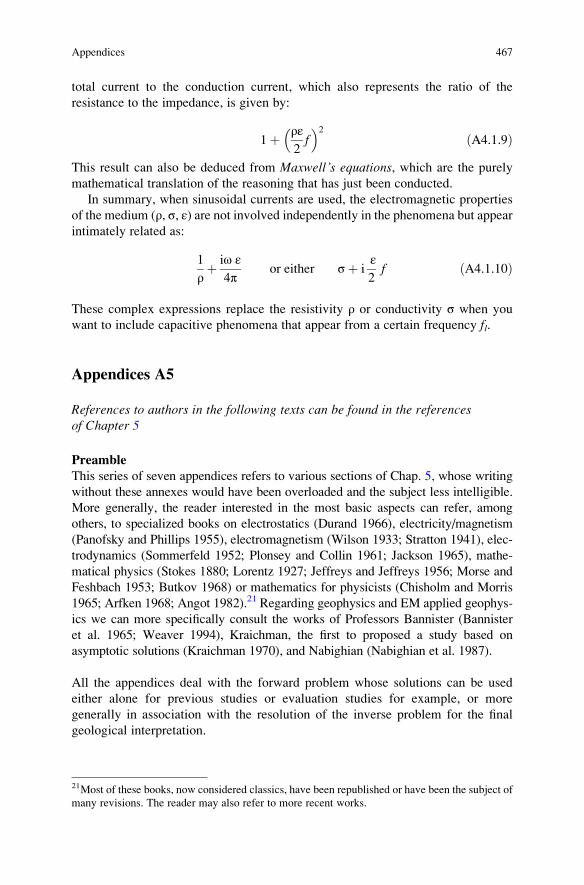
total current to the conduction current, which also represents the ratio of the

resistance to the impedance, is given by:

1þ ρε2f

2ðA4.1.9Þ

This result can also be deduced from Maxwell’s equations, which are the purely

mathematical translation of the reasoning that has just been conducted.

In summary, when sinusoidal currents are used, the electromagnetic properties

of the medium (ρ, σ, ε) are not involved independently in the phenomena but appear

intimately related as:

1

ρþ iω ε

4πor either σþ i

ε2

f ðA4.1.10Þ

These complex expressions replace the resistivity ρ or conductivity σ when you

want to include capacitive phenomena that appear from a certain frequency fl.

Appendices A5

References to authors in the following texts can be found in the referencesof Chapter 5

Preamble

This series of seven appendices refers to various sections of Chap. 5, whose writing

without these annexes would have been overloaded and the subject less intelligible.

More generally, the reader interested in the most basic aspects can refer, among

others, to specialized books on electrostatics (Durand 1966), electricity/magnetism

(Panofsky and Phillips 1955), electromagnetism (Wilson 1933; Stratton 1941), elec-

trodynamics (Sommerfeld 1952; Plonsey and Collin 1961; Jackson 1965), mathe-

matical physics (Stokes 1880; Lorentz 1927; Jeffreys and Jeffreys 1956; Morse and

Feshbach 1953; Butkov 1968) or mathematics for physicists (Chisholm and Morris

1965; Arfken 1968; Angot 1982).21 Regarding geophysics and EM applied geophys-

ics we can more specifically consult the works of Professors Bannister (Bannister

et al. 1965; Weaver 1994), Kraichman, the first to proposed a study based on

asymptotic solutions (Kraichman 1970), and Nabighian (Nabighian et al. 1987).

All the appendices deal with the forward problem whose solutions can be used

either alone for previous studies or evaluation studies for example, or more

generally in association with the resolution of the inverse problem for the final

geological interpretation.

21Most of these books, now considered classics, have been republished or have been the subject of

many revisions. The reader may also refer to more recent works.

Appendices 467

5

http://dx.doi.org/10.1007/978-3-319-45355-2_5

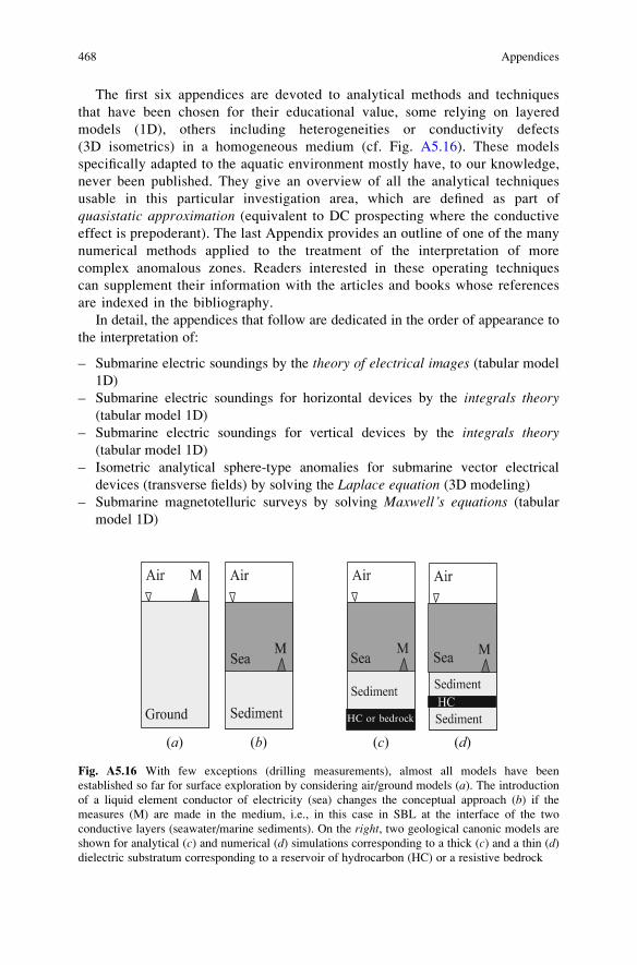
The first six appendices are devoted to analytical methods and techniques

that have been chosen for their educational value, some relying on layered

models (1D), others including heterogeneities or conductivity defects

(3D isometrics) in a homogeneous medium (cf. Fig. A5.16). These models

specifically adapted to the aquatic environment mostly have, to our knowledge,

never been published. They give an overview of all the analytical techniques

usable in this particular investigation area, which are defined as part of

quasistatic approximation (equivalent to DC prospecting where the conductive

effect is prepoderant). The last Appendix provides an outline of one of the many

numerical methods applied to the treatment of the interpretation of more

complex anomalous zones. Readers interested in these operating techniques

can supplement their information with the articles and books whose references

are indexed in the bibliography.

In detail, the appendices that follow are dedicated in the order of appearance to

the interpretation of:

– Submarine electric soundings by the theory of electrical images (tabular model

1D)

– Submarine electric soundings for horizontal devices by the integrals theory(tabular model 1D)

– Submarine electric soundings for vertical devices by the integrals theory(tabular model 1D)

– Isometric analytical sphere-type anomalies for submarine vector electrical

devices (transverse fields) by solving the Laplace equation (3D modeling)

– Submarine magnetotelluric surveys by solving Maxwell’s equations (tabular

model 1D)

HC or bedrock

(a) (b) (c) (d)

Fig. A5.16 With few exceptions (drilling measurements), almost all models have been

established so far for surface exploration by considering air/ground models (a). The introductionof a liquid element conductor of electricity (sea) changes the conceptual approach (b) if the

measures (M) are made in the medium, i.e., in this case in SBL at the interface of the two

conductive layers (seawater/marine sediments). On the right, two geological canonic models are

shown for analytical (c) and numerical (d) simulations corresponding to a thick (c) and a thin (d)dielectric substratum corresponding to a reservoir of hydrocarbon (HC) or a resistive bedrock

468 Appendices

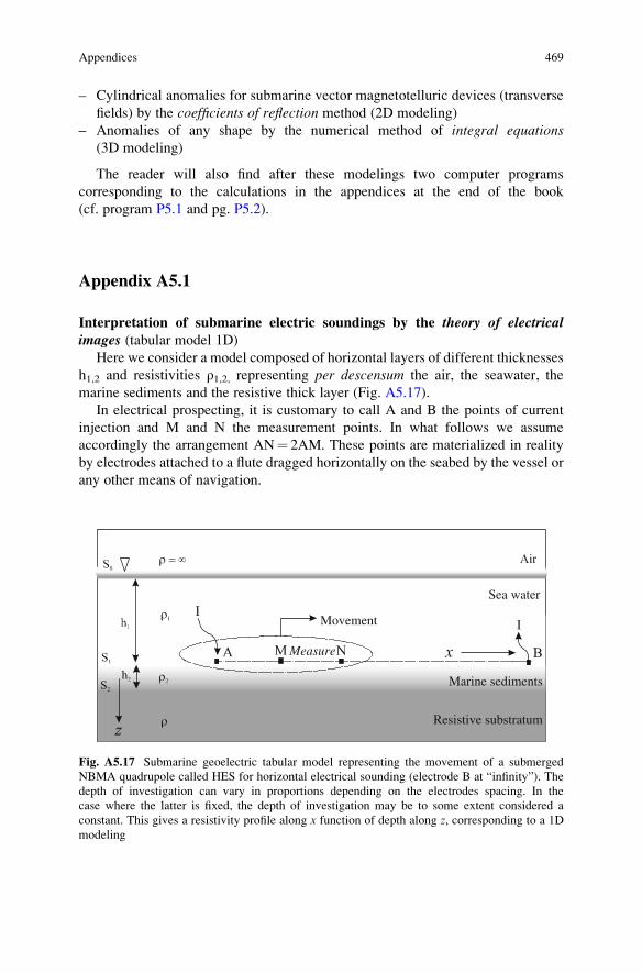
– Cylindrical anomalies for submarine vector magnetotelluric devices (transverse

fields) by the coefficients of reflection method (2D modeling)

– Anomalies of any shape by the numerical method of integral equations(3D modeling)

The reader will also find after these modelings two computer programs

corresponding to the calculations in the appendices at the end of the book

(cf. program P5.1 and pg. P5.2).

Appendix A5.1

Interpretation of submarine electric soundings by the theory of electricalimages (tabular model 1D)

Here we consider a model composed of horizontal layers of different thicknesses

h1,2 and resistivities ρ1,2, representing per descensum the air, the seawater, the

marine sediments and the resistive thick layer (Fig. A5.17).

In electrical prospecting, it is customary to call A and B the points of current

injection and M and N the measurement points. In what follows we assume

accordingly the arrangement AN¼ 2AM. These points are materialized in reality

by electrodes attached to a flute dragged horizontally on the seabed by the vessel or

any other means of navigation.

Sea water

Movement

Measure

Marine sediments

Resistive substratum

Fig. A5.17 Submarine geoelectric tabular model representing the movement of a submerged

NBMA quadrupole called HES for horizontal electrical sounding (electrode B at “infinity”). The

depth of investigation can vary in proportions depending on the electrodes spacing. In the

case where the latter is fixed, the depth of investigation may be to some extent considered a

constant. This gives a resistivity profile along x function of depth along z, corresponding to a 1D

modeling

Appendices 469

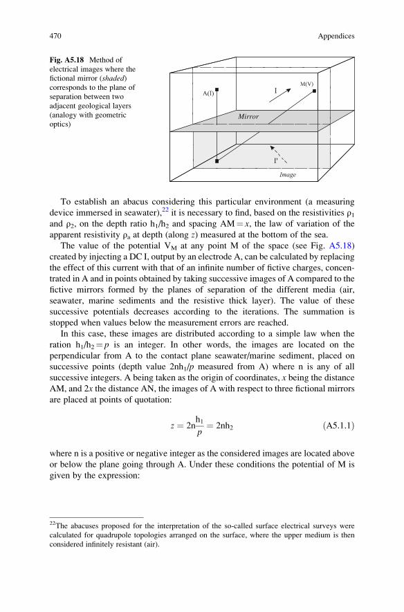
To establish an abacus considering this particular environment (a measuring

device immersed in seawater),22 it is necessary to find, based on the resistivities ρ1and ρ2, on the depth ratio h1/h2 and spacing AM¼ x, the law of variation of the

apparent resistivity ρa at depth (along z) measured at the bottom of the sea.

The value of the potential VM at any point M of the space (see Fig. A5.18)

created by injecting a DC I, output by an electrode A, can be calculated by replacing

the effect of this current with that of an infinite number of fictive charges, concen-

trated in A and in points obtained by taking successive images of A compared to the

fictive mirrors formed by the planes of separation of the different media (air,

seawater, marine sediments and the resistive thick layer). The value of these

successive potentials decreases according to the iterations. The summation is

stopped when values below the measurement errors are reached.

In this case, these images are distributed according to a simple law when the

ration h1/h2¼ p is an integer. In other words, the images are located on the

perpendicular from A to the contact plane seawater/marine sediment, placed on

successive points (depth value 2nh1/p measured from A) where n is any of all

successive integers. A being taken as the origin of coordinates, x being the distanceAM, and 2x the distance AN, the images of A with respect to three fictional mirrors

are placed at points of quotation:

z ¼ 2nh1

p¼ 2nh2 ðA5.1.1Þ

where n is a positive or negative integer as the considered images are located above

or below the plane going through A. Under these conditions the potential of M is

given by the expression:

Mirror

Fig. A5.18 Method of

electrical images where the

fictional mirror (shaded)corresponds to the plane of

separation between two

adjacent geological layers

(analogy with geometric

optics)

22The abacuses proposed for the interpretation of the so-called surface electrical surveys were

calculated for quadrupole topologies arranged on the surface, where the upper medium is then

considered infinitely resistant (air).

470 Appendices

1

ρ1VM ¼ S0

xþXn¼1n¼1

Snffiffiffiffiffiffiffiffiffiffiffiffiffiffiffiffiffiffiffiffiffiffiffiffiffiffiffix2 þ n2 2h2ð Þ2

q ðA5.1.2Þ

where S0 is the emissivity (or I/4π) of the electrode A and Sn the sum of the

emissivities of the pair of images of quotations +2nh1 and –2nh1.

If now we pose:

u ¼ 2h2

xðA5.1.3Þ

it comes at the point M:

1

ρ1VM ¼ 1

xS0 þ

Xn¼1n¼1

Snffiffiffiffiffiffiffiffiffiffiffiffiffiffiffiffiffi1þ n2h22

q0B@

1CA ðA5.1.4Þ

as well as at the point N:

1

ρ1VN ¼ 1

x

S0

2þXn¼1n¼1

Snffiffiffiffiffiffiffiffiffiffiffiffiffiffiffiffiffi4þ n2h22

q0B@

1CA ðA5.1.5Þ

from which we have for the potential difference ΔVMN:

1

ρ1ΔVMN ¼ 1

x

S0

2þXn¼1n¼1

Sn1ffiffiffiffiffiffiffiffiffiffiffiffiffiffiffiffiffi

1þ n2h22

q � 1ffiffiffiffiffiffiffiffiffiffiffiffiffiffiffiffiffi4þ n2h22

q0B@

1CA0B@

1CA ðA5.1.6Þ

But to define the apparent resistivity, it is necessary to consider a fictitious homo-

geneous ground23 giving the same ΔVMN for the same values of x. In such a groundwhere Sn¼ 0, we can write to define ρa that:

1

ρaΔVMN ¼ 1

x

S0

2ðA5.1.7Þ

when setting:

23Here we form (the method of Hummel) a fictional ground developed from the first layers, so that

this one, electrically equivalent, forms with the underlying grounds a new interpretable set (new

curve). This principle of sequential development of “auxiliary curves” called the principle ofreduction can be repeated interactively until the desired number of layers (Hummel 1929) is

obtained.

Appendices 471

Kn ¼ 1ffiffiffiffiffiffiffiffiffiffiffiffiffiffiffiffiffi1þ n2h22

q � 1ffiffiffiffiffiffiffiffiffiffiffiffiffiffiffiffiffi4þ n2h22

q ðA5.1.8Þ

we finally obtain the expression of the apparent resistivity:

ρa ¼ ρ1 1þ 2Xn¼1n¼1

Sn

S0Kn

!ðA5.1.9Þ

From this simple formulation, we can then construct abacuses. These are developed

by successive approximations by summing a number of terms of the series ∑(Sn/S0)Kn after determining S0, Sn and Kn.

The values of the Kn terms were calculated by the physicist Hummel

(Hummel 1929).

The emissivity values S0, Sn are then determined from the recurrence relations

between the emissivities of the images n, n�1, n�2, etc. For this we express the

values of the potential V1,2 at any point of space (defined by its coordinates x and z)by considering the four media of resistivity ρ0 for the air, ρ1 for seawater, ρ2 for themarine sediments and ρ3 for the resistive thick layer. This potential is thus

expressed according to the image emissivities.

Taking into account the conditions that must be met in the different environ-

ments, we obtain a number of equations from which can be derived a recurrence

formula.

If we agree then to indicate by:

– a0n and b

0n the emissivities of the images contributing to give the potential V1

– a00 and a

000 the emissivities of the images located respectively below and above the

contact between 1 and 2

– a00n and b

00n the emissivities of the images used to calculate the potential V2

thus we obtain:

1

ρ1V1 ¼ a00ffiffiffiffiffiffiffiffiffiffiffiffiffiffi

x2 þ z2p þ

Xn¼1n¼1

a0nffiffiffiffiffiffiffiffiffiffiffiffiffiffiffiffiffiffiffiffiffiffiffiffiffiffiffiffiffix2 þ zþ 2n

p

2r þXn¼1n¼1

b0nffiffiffiffiffiffiffiffiffiffiffiffiffiffiffiffiffiffiffiffiffiffiffiffiffiffiffiffiffix2 þ zþ 2n

p

2r ðA5.1.10Þ

and:

1

ρ2V2 ¼ a

000ffiffiffiffiffiffiffiffiffiffiffiffiffiffi

x2 þ z2p þ

Xn¼1n¼1

a00nffiffiffiffiffiffiffiffiffiffiffiffiffiffiffiffiffiffiffiffiffiffiffiffiffiffiffiffiffi

x2 þ zþ 2np

2r þXn¼1n¼1

b00nffiffiffiffiffiffiffiffiffiffiffiffiffiffiffiffiffiffiffiffiffiffiffiffiffiffiffiffiffi

x2 þ zþ 2np

2r þ � � �

ðA5.1.11Þ

472 Appendices

Using the four classical boundary conditions adopted in the definition of the model

with four layers, namely:

∂V1

∂z¼ 0 for z ¼ h1 þ ph2 ¼ 1

∂V2

∂z¼ 0 for z ¼ �h2 ¼ 1

p

1

ρ1∂V1

∂z¼ 1

ρ2∂V2

∂zfor z ¼ 0

V1 ¼ V2 for z ¼ 0

8>>>>>>>>>>><>>>>>>>>>>>:ðA5.1.12Þ

thus we obtain in those situations:

a00ffiffiffiffiffiffiffiffiffiffiffiffiffix2 þ 13p þ

Xn¼1n¼1

1þ 2np

a0nffiffiffiffiffiffiffiffiffiffiffiffiffiffiffiffiffiffiffiffiffiffiffiffiffiffiffiffiffiffi

x2 þ 1þ 2np

23

r þXn¼1n¼1

1� 2np

b0nffiffiffiffiffiffiffiffiffiffiffiffiffiffiffiffiffiffiffiffiffiffiffiffiffiffiffiffiffiffi

x2 þ 1� 2np

23

r ¼ 0 ðA5.1.13Þ

and:

1p a000ffiffiffiffiffiffiffiffiffiffiffiffiffiffi

x2 þ 1p2

3

q þXn¼1n¼1

2n�1p

a00nffiffiffiffiffiffiffiffiffiffiffiffiffiffiffiffiffiffiffiffiffiffiffiffiffiffi

x2 þ 2n�1p

23

r þXn¼1n¼1

2n�1p

b00nffiffiffiffiffiffiffiffiffiffiffiffiffiffiffiffiffiffiffiffiffiffiffiffiffiffi

x2 þ 2n�1p

23

r ¼ 0 ðA5.1.14Þ

and:

ρ1a00xþXn¼1n¼1

a0n þ b0nffiffiffiffiffiffiffiffiffiffiffiffiffiffiffiffiffiffiffiffiffix2 þ 2n

p

2r2664

3775 ¼ ρ2a000

xþXn¼1n¼1

a00n þ b

00nffiffiffiffiffiffiffiffiffiffiffiffiffiffiffiffiffiffiffiffiffi

x2 þ 2np

2r2664

3775 ðA5.1.15Þ

and:

a0n � b0n� �

2npffiffiffiffiffiffiffiffiffiffiffiffiffiffiffiffiffiffiffiffiffi

x2 þ 2np

23

r ¼a00n � b

00n

� �2npffiffiffiffiffiffiffiffiffiffiffiffiffiffiffiffiffiffiffiffiffi

x2 þ 2np

23

r ðA5.1.16Þ

On the other hand, the fact that the potential distribution near the injection electrode

A is spherical (cf. Chap. 3 Appendix A3.2) now implies that:

ρ1a00 ¼ ρ2a

000 ðA5.1.17Þ

thereby allowing us to alleviate the above equations, by setting:

Appendices 473

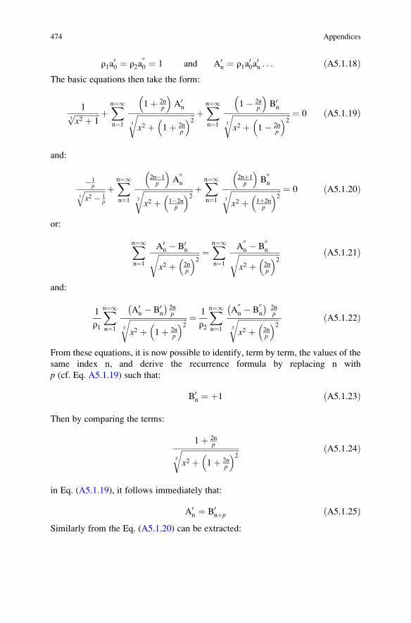
http://dx.doi.org/10.1007/978-3-319-45355-2_3

ρ1a00 ¼ ρ2a

000 ¼ 1 and A0n ¼ ρ1a

00a0n . . . ðA5.1.18Þ

The basic equations then take the form:

1ffiffiffiffiffiffiffiffiffiffiffiffiffix2 þ 13p þ

Xn¼1n¼1

1þ 2np

A0nffiffiffiffiffiffiffiffiffiffiffiffiffiffiffiffiffiffiffiffiffiffiffiffiffiffiffiffiffiffi

x2 þ 1þ 2np

23

r þXn¼1n¼1

1� 2np

B0nffiffiffiffiffiffiffiffiffiffiffiffiffiffiffiffiffiffiffiffiffiffiffiffiffiffiffiffiffiffi

x2 þ 1� 2np

23

r ¼ 0 ðA5.1.19Þ

and:

�1pffiffiffiffiffiffiffiffiffiffiffiffi

x2 � 1p

3

q þXn¼1n¼1

2n�1p

A00nffiffiffiffiffiffiffiffiffiffiffiffiffiffiffiffiffiffiffiffiffiffiffiffiffiffi

x2 þ 1�2np

23

r þXn¼1n¼1

2nþ1p

B00nffiffiffiffiffiffiffiffiffiffiffiffiffiffiffiffiffiffiffiffiffiffiffiffiffiffi

x2 þ 1þ2np

23

r ¼ 0 ðA5.1.20Þ

or:

Xn¼1n¼1

A0n � B0nffiffiffiffiffiffiffiffiffiffiffiffiffiffiffiffiffiffiffiffiffix2 þ 2n

p

2r ¼Xn¼1n¼1

A00n � B

00nffiffiffiffiffiffiffiffiffiffiffiffiffiffiffiffiffiffiffiffiffi

x2 þ 2np

2r ðA5.1.21Þ

and:

1

ρ1

Xn¼1n¼1

A0n � B0n� �

2npffiffiffiffiffiffiffiffiffiffiffiffiffiffiffiffiffiffiffiffiffiffiffiffiffiffiffiffiffiffi

x2 þ 1þ 2np

23

r ¼ 1

ρ2

Xn¼1n¼1

A00n � B

00n

� �2npffiffiffiffiffiffiffiffiffiffiffiffiffiffiffiffiffiffiffiffiffi

x2 þ 2np

23

r ðA5.1.22Þ

From these equations, it is now possible to identify, term by term, the values of the

same index n, and derive the recurrence formula by replacing n with

p (cf. Eq. A5.1.19) such that:

B0n ¼ þ1 ðA5.1.23Þ

Then by comparing the terms:

1þ 2npffiffiffiffiffiffiffiffiffiffiffiffiffiffiffiffiffiffiffiffiffiffiffiffiffiffiffiffiffiffi

x2 þ 1þ 2np

23

r ðA5.1.24Þ

in Eq. (A5.1.19), it follows immediately that:

A0n ¼ B0nþp ðA5.1.25ÞSimilarly from the Eq. (A5.1.20) can be extracted:

474 Appendices

A00nþ1 ¼

1

2p� 1ðA5.1.26Þ

and:

A00nþ1 ¼ B

00n ðA5.1.27Þ

as well as for Eqs. (A5.1.21) and (A5.1.22):

A0n þ B0n ¼ A00n þ B

00n ðA5.1.28Þ

and:

1

ρ1A0n þ B0n� � ¼ 1

ρ2A00n þ B

00n

ðA5.1.29Þ

From the last two relations, it expressly emerges that:

2A00n ¼ A0n 1þ ρ2

ρ1

� �þ B0n 1� ρ2

ρ1

� �ðA5.1.30Þ

and:

2B00n ¼ A0n 1� ρ2

ρ1

� �þ B0n 1þ ρ2

ρ1

� �ðA5.1.31Þ

which from Eqs. (A5.1.25) and (A5.1.27) gives:

2A00n ¼ A0n 1þ ρ2

ρ1

� �þ A0n�p 1� ρ2

ρ1

� �ðA5.1.32Þ

and:

2B00n ¼ A0n 1� ρ2

ρ1

� �þ A0n�p 1þ ρ2

ρ1

� �ðA5.1.33Þ

Yet:

2B00n�1 ¼ A0n 1þ ρ2

ρ1

� �þ A0n�p 1� ρ2

ρ1

� �ðA5.1.34Þ

and from Eq. (A5.1.33) we have:

Appendices 475

A0n 1þ ρ2ρ1

� �þ A0n�p 1� ρ2

ρ1

� �¼ A0n�1 1� ρ2

ρ1

� �þ A0n�p�1 1� ρ2

ρ1

� �ðA5.1.35Þ

Using conventional notation:

ρ1 � ρ2ρ1 þ ρ2

¼ k ðA5.1.36Þ

thus we can write:

A0n ¼ kA0n�p ¼ �kA0n�1 þ A0n�p�1 ðA5.1.37Þ

We then obtain the first recurrence formula:

A0n ¼ �kA0n�1 þ kA0n�p þ A0n�p�1 ðA5.1.38Þ

The same identity would be found for the terms in B0 by setting:

S0n ¼ A0n þ B0n ðA5.1.39Þ

i.e.:

S0n ¼ �kS0n�1 þ kS0n�p þ S0n�p�1 ðA5.1.40Þ

and also from Eq. (A5.1.28):

S00n ¼ �kS

00n�1 þ kS

00n�p þ S

00n�p�1 ðA5.1.41Þ

This recurrence formula can be written more generally as:

Sn ¼ �kSn�1 þ kSn�p þ Sn�p�1 ðA5.1.42Þ

However, it does not apply to the rank lower to p. For the first terms of the series,

then it is necessary to directly calculate them step by step. Thus we find:

S0 ¼ 1þ k

S1 ¼ 2 1þ kð Þ 1� kð Þ

S2 ¼ 2 1þ kð Þ 1þ k2� �

etc:

8>>>>>>>><>>>>>>>>:ðA5.1.43Þ

Ultimately, if we refer to the general formula for the apparent resistivity

(cf. Eq. A5.1.9) and using either the Hummel values Kn or the recurrence relations

476 Appendices

that allow to calculate the emissivities, then it is possible to determine the values of

h2 (marine sediments) corresponding to some given values of the ratios h1/h2 and

ρ1/ρ2.The application of the theory of electrical images is relatively well suited to

unstructured acquisition streamer-type devices (and also to Wenner or

Schlumberger-type arrangements, etc.) where lateral variations in resistivity can

be considered negligible. This type of interpretation only allows us to approach

problems in one dimension (1D) as vertical profiles.

With relatively simple programming, the technique allows with few acquisition

data a rapid interpretation by abacuses (see Fig. A5.19) or any other automatic

approach to successive approximations.

This technique can be effective to affirm, confirm or clarify, with relatively good

accuracy, features of geological objects (lithology and sedimentary cover in par-

ticular), in a specific structural context (a tabular model on a resistive layer).

However, this type of investigation is not suitable for multidimensional interpreta-

tion in two dimensions where other methods, coupled with more sophisticated

technologies and acquisition systems, are then more efficient.24

seawater

Fig. A5.19 Abacus to interpret submarine vertical electrical soundings (sediment/resistive thick

layer). The use of this type of abacus has long been the cornerstone of data interpretation of

electrical soundings in general. The logarithmic scale here is perfectly suited to the conductive

nature of marine sediments

24In surface prospecting, 2D and 3D models were proposed for arrangements of the dipole–dipole

type (Medkour 1984).

Appendices 477

Appendix A5.2

Interpretation of submarine electric soundings for horizontal devices by the

integrals theory (1D modeling)

In what follows we consider a model composed of horizontal layers of thickness

h1,2 of different conductivities σ1,2,3 representing, per descensum, the air, the

seawater, the marine sediments and the bedrock or thick resistive substratum.

In the above pattern (see Fig. A5.20), where the different points in the vertical

plane are expressed by their cylindrical coordinates (r, z), we solve the equation of

electrical prospecting.25

In the preamble, to lighten the mathematical apparatus, theoretically poles N

(measurement) and B (injection) are rejected to infinity. Then we shall easily pass

on to the case of the quadrupole ABMN by applying the law of superimposing of

the states of balance (called also superposition theorem).

If the layers 1 (seawater) and 2 (sediments) respectively fill two half-spaces (z<0) and (z> 0), the electrode A supplying a current I thus produces at any point M on

the line a primary potential of the form:

V0 ¼ I

4π2

σ1 þ σ2ð Þ1ffiffiffiffiffiffiffiffiffiffiffiffiffiffi

z2 þ r2p ðA5.2.1Þ

To solve the equation we can first of all:

Sea water

Movement

Marine sediments


Fig. A5.20 Tabular submarine geoelectric model (three layers) corresponding to a horizontal

investigation device that can be dragged at the bottom of the sea

25The fundamental equations of electrical prospecting were defined by the French school of

geophysics (Schlumberger, Stefanescu, Kostitzine, etc.). The results of these works (prospecting

equation, resolutions and solutions) which apply only to surface prospecting are summarized in

Raymond Maillet’s article (Maillet 1947).

478 Appendices

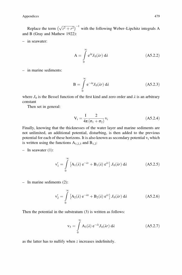
Replace the termffiffiffiffiffiffiffiffiffiffiffiffiffiffiz2 þ r2p� ��1

with the following Weber–Lipchitz integrals A

and B (Gray and Mathew 1922):

– in seawater:

A ¼Z10

eλzJ0 λrð Þ dλ ðA5.2.2Þ

– in marine sediments:

B ¼Z10

e�λzJ0 λrð Þ dλ ðA5.2.3Þ

where J0 is the Bessel function of the first kind and zero order and λ is an arbitrary

constant

Then set in general:

Vi ¼ I

4π2

σ1 þ σ2ð Þ vi ðA5.2.4Þ

Finally, knowing that the thicknesses of the water layer and marine sediments are

not unlimited, an additional potential, disturbing, is then added to the previous

potential for each of these horizons. It is also known as secondary potential vi which

is written using the functions A1,2,3 and B1,2:

– In seawater (1):

v01 ¼Z10

A1 λð Þ e�λz þ B1 λð Þ eλz� �J0 λrð Þ dλ ðA5.2.5Þ

– In marine sediments (2):

v02 ¼Z10

A2 λð Þ e�λz þ B2 λð Þ eλz� �J0 λrð Þ dλ ðA5.2.6Þ

Then the potential in the substratum (3) is written as follows:

v3 ¼Z10

A3 λð Þ e�λzJ0 λrð Þ dλ ðA5.2.7Þ

as the latter has to nullify when z increases indefinitely.

Appendices 479

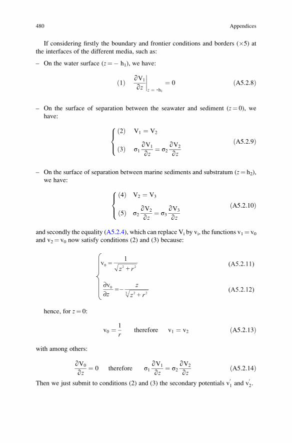
If considering firstly the boundary and frontier conditions and borders (�5) atthe interfaces of the different media, such as:

– On the water surface (z¼� h1), we have:

1ð Þ ∂V1

∂z

z ¼ -h1

¼ 0 ðA5.2.8Þ

– On the surface of separation between the seawater and sediment (z¼ 0), we

have:

2ð Þ V1 ¼ V2

3ð Þ σ1∂V1

∂z¼ σ2

∂V2

∂z

8><>: ðA5.2.9Þ

– On the surface of separation between marine sediments and substratum (z¼ h2),

we have:

4ð Þ V2 ¼ V3

5ð Þ σ2∂V2

∂z¼ σ3

∂V3

∂z

8><>: ðA5.2.10Þ

and secondly the equality (A5.2.4), which can replace Vi by vi, the functions v1¼ v0and v2¼ v0 now satisfy conditions (2) and (3) because:

22

1

∂v0

v0 rz +=

= –3 22 rz

z∂z +

(A5.2.11)

(A5.2.12)

hence, for z¼ 0:

v0 ¼ 1

rtherefore v1 ¼ v2 ðA5.2.13Þ

with among others:

∂V0

∂z¼ 0 therefore σ1

∂V1

∂z¼ σ2

∂V2

∂zðA5.2.14Þ

Then we just submit to conditions (2) and (3) the secondary potentials v01 and v

02.

480 Appendices

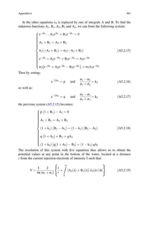
In the other equations v0 is replaced by one of integrals A and B. To find the

unknown functions A1, B1, A2, B2 and A3, we can form the following system:

e�λh1 � A1eλh1 þ B1e

�λh1 ¼ 0

A1 þ B1 ¼ A2 þ B2

σ1 �A1 þ B1ð Þ ¼ σ2 �A2 þ B2ð Þ

e�λh2 þ A2e�λh2 þ B2e

�λh2 ¼ A3e�λh2

σ2 e�λh2 þ A2e�λh2 � B2e

�λh2� � ¼ σ3A3e�λh2

8>>>>>>>>>>>><>>>>>>>>>>>>:ðA5.2.15Þ

Then by setting:

e�2λh1 ¼ p andσ1 � σ2σ1 þ σ2

¼ k1 ðA5.2.16Þas well as:

e�2λh2 ¼ q andσ2 � σ3σ2 þ σ3

¼ k2 ðA5.2.17Þ

the previous system (A5.2.15) becomes:

p 1þ B1ð Þ � A1 ¼ 0

A1 þ B1 ¼ A2 þ B2

1þ k1ð Þ B1 � A1ð Þ ¼ 1� k1ð Þ B2 � A2ð Þ

q 1þ A2ð Þ þ B2 ¼ qA3

1þ k2ð Þ q 1þ A2ð Þ � B2½ � ¼ 1� k2ð Þ qA3

8>>>>>>>>>>>><>>>>>>>>>>>>:ðA5.2.18Þ

The resolution of this system with five equations thus allows us to obtain the

potential values at any point in the bottom of the water, located at a distance

r from the current injection electrode of intensity I such that:

V ¼ I

4π2

σ1 þ σ2ð Þ1

rþZ10

A1 λð Þ þ B1 λð Þ½ � J0 λrð Þ dλ8<:

9=; ðA5.2.19Þ

Appendices 481

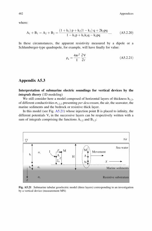
where:

A1 þ B1 ¼ A2 þ B2 ¼ 1þ k1ð Þ pþ k2 1� k1ð Þ qþ 2k2pq

1� k1pþ k1k2q� k2pq:::: ðA5.2.20Þ

In these circumstances, the apparent resistivity measured by a dipole or a

Schlumberger-type quadrupole, for example, will have finally for value:

ρa ¼4πr2

I

∂V∂r

ðA5.2.21Þ

Appendix A5.3

Interpretation of submarine electric soundings for vertical devices by the

integrals theory (1D modeling)

We still consider here a model composed of horizontal layers of thickness h1,2,

of different conductivities σ1,2,3 presenting per descensum, the air, the seawater, themarine sediments and the bedrock or resistive thick layer.

In this model (see Fig. A5.21) whose injection point B is placed to infinity, the

different potentials Vi in the successive layers can be respectively written with a

sum of integrals comprising the functions A1,2 and B1,2:

Sea waterMovement

Marine sediments


Fig. A5.21 Submarine tabular geoelectric model (three layers) corresponding to an investigation

by a vertical device (measurement MN)

482 Appendices

– In seawater (1):

V1 ¼ I

4πσ1

Z10

e�λ z�z0j jJ0 λpð Þ dλþZ10

A1e�λz þ B1e

þλz� �J0 λpð Þ dλ

8<:9=; ðA5.3.1Þ

– In the marine sediments (2):

V2 ¼ I

4πσ1

Z10

A2eþλz þ B2e

�λz� �J0 λpð Þ dλ ðA5.3.2Þ

where J0 is the Bessel function of the first kind and zero order (see Special functionsat the end of the volume) and λ is an arbitrary constant.

Considering now the following boundary conditions:

– At the surface of separation seawater/sediment (σ1! σ2):

e�λz0 þ A1 þ B1 ¼ A2 þ B2

σ1 e�λz0 � A1 þ B1

� � ¼ σ2 A2 � B2ð Þ

8<: ðA5.3.3Þ

– At the surface of separation sediments/Resistive sediment (σ2!1):

A2e�λh2 þ B2e

λh2 ¼ 0 ðA5.3.4Þ

– At the surface of separation water/air (σ1!1):

�e�λ h1�z0ð Þ � A1e�λh1 þ B1e

λh1 ¼ 0 ðA5.3.5Þ

and setting now:

B1 þ e�λz0 ¼ B01 ðA5.3.6Þ

we have the following system:

A1 þ B01 � A2 � B2 ¼ 0

σ1A1 � σ1B01 þ σ2A2 � σ2B2 ¼ 0

e�λh2A2 � eλh2B2 ¼ 0

e�λh1A1 � eλh1B01 ¼ �e�λ h1�z0ð Þ � eλ h1�z0ð Þ ¼ �2 coshλ h1 � z0ð Þ

8>>>>>>>><>>>>>>>>:ðA5.3.7Þ

which is solved by achieving the ratio σ1�σ2σ1þσ2 ¼ k:

Appendices 483

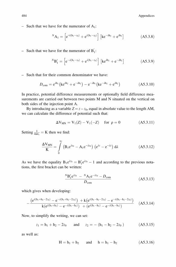
– Such that we have for the numerator of A1:

NA1 ¼ e-λ h1�z0ð Þ þ eλ h1�z0ð Þh i

ke�λh2 þ eλh2� � ðA5.3.8Þ

– Such that we have for the numerator of B01:

NB01 ¼ e�λ h1�z0ð Þ þ eλ h1�z0ð Þh i

keλh2 þ e�λh2� � ðA5.3.9Þ

– Such that for their common denominator we have:

Dcom ¼ eλh1 keλh2 þ e�λh2� �� e�λh1 ke�λh2 þ eλh2

� � ðA5.3.10Þ

In practice, potential difference measurements or optionally field difference mea-

surements are carried out between two points M and N situated on the vertical on

both sides of the injection point A.

By introducing as a variable Z¼ z – z0, equal in absolute value to the length AM,

we can calculate the difference of potential such that:

ΔVMN ¼ V1 Zð Þ � V1 �Zð Þ for ρ ¼ 0 ðA5.3.11Þ

Setting I4πσ1 ¼ K then we find:

ΔVMN

K¼Z10

B1eλz0 � A1e

�λz0� �eλz � e�λz� �

dλ ðA5.3.12Þ

As we have the equality B1eλz0 ¼ B01e

λz0 � 1 and according to the previous nota-

tions, the first bracket can be written:

NB01eλz0 � NA1e

�λz0 � Dcom

Dcom

ðA5.3.13Þ

which gives when developing:

� eλ h1þh2�2z0ð Þ � e�λ h1þh2�2z0ð Þ� � þ k eλ h1�h2�2z0ð Þ � e�λ h1�h2�2z0ð Þ� �k eλ h1þh2ð Þ � e�λ h1�h2ð Þð Þ þ eλ h1�h2ð Þ � e�λ h1�h2ð Þð Þ ðA5.3.14Þ

Now, to simplify the writing, we can set:

z1 ¼ h1 þ h2 � 2z0 and z2 ¼ � h1 � h2 � 2z0ð Þ ðA5.3.15Þ

as well as:

H ¼ h1 þ h2 and h ¼ h1 � h2 ðA5.3.16Þ

484 Appendices

we finally obtain:

ΔVMN

2K¼Z10

k sinhλ z2 � sinhλ z1k sinhλ H� sinhλ h

sinhλ Z dλ ðA5.3.17Þ

a formula that is suitable for numerical calculation by approached integration, the

integral rapidly converging, since H is always greater than z1 + Z and than z2 + Z.Assuming now that z1 > z2 and reintroducing the exponential functions, we can

literally write:

ΔVMN

K¼ 1

k

Z10

e�λ H�z1�Zð Þ�

1� e�2λZ � k e�λ z1�z2ð Þ � e�λ z1�z2þ2Zð Þ � e�λ z1þz2ð Þ � e�λ z1þz2þ2Zð Þ� �� e�2λz1 þ e�2λ z1þZð Þ

1þ k�1e�λ H�hð Þ � e�2λH � e�2λ H�hð Þ dλ

ðA5.3.18Þ

For more convenience, we can choose the parameters an so that the powers of

exponential function e admit a common divisor α as large as possible such that we

have e� αλ. We obtain then:

1

k

Z10

e�λ H�z1�Zð ÞX1n¼0

ane�nλαdλ ðA5.3.19Þ

whose value is:

1

k

an

H� z0 � Zð Þ þ nαðA5.3.20Þ

We just have then to multiply an by an inverse series to find the researched values

(Fig. A5.22).

Appendix A5.4

Interpretation of isometric anomalies (sphere type) for submarine vector

electrical devices (transverse fields) by solving the Laplace equation

(3D modeling)

This type of model in low frequency approximation can only describe the

galvanic effects of a sphere on the currents (distribution of potentials and electric

fields around it). However, it is possible to get in some way a phase term compa-

rable to a periodic investigation () in opposition phase for injection, by choosing

an arrangement such that the points of the entrance and exit of current are then

Appendices 485

alternately at opposite potentials (+/�). This modeling can have theoretical interest

for the study of the mechanisms of electromagnetic detection (respective contribu-

tions of galvanic phenomena and vortex), and applications in:

– Interpretation of data acquisition

– Development of in situ correction devices

– Calibration of acquisition systems

– Development of field sensors

– Confrontation with measures made by means of analog models (rheostatic tanks

for example), etc (Fig. A5.23).

The analytical expression of anomalous fields caused by the presence of a body

with sufficient resistivity contrast with the surrounding grounds is given by solving

the wave equation. For its resolution, this expression can be put in the form of a

partial differential equation that takes into account, for its simplification, the

Fig. A5.22 Abacus for the interpretation of submarine soundings (marine sediment/resistive thick

layer) for a vertical acquisition device

486 Appendices

geometry of the problem.26 For example, for a spherical anomaly, the potential V at

a distance r from the center of the sphere is obtained by solving the equation in

spherical coordinates as described in Fig. A5.24:

1

r2∂∂r

r2∂∂r

� �þ 1

r2 sin θ∂∂θ

sin θ∂∂θ

� �þ 1

r2 sin θ∂2

∂φ2þ k2r2

" #V r; θ;φ;ωð Þ ¼ 0

ðA5.4.1Þ

A4.1. Laplace Equation

Using low frequencies also authorizes the use of the Laplace equation (∇2V ¼ 0) so

that the frequency ω (k2r2¼ 0) is not required. Then we resolve, as for a direct

current (quasistatic approximation), the equation in three dimensions:

Quasisatatic approximation

Model Model

Galvanic effect

Vortex effect

Fig. A5.23 Interest of stationary models for differentiation of vortex and galvanic effects by

extraction by calculating the galvanic effect (quasistatic approximation)

26The theory of electrical images can also be used (Grant and West, 1965). The problem of the

influence of a sphere on the potential distribution by this theory was discussed for the first time

(sphere in a uniform current field) by Hummel (Hummel 1928). The use of spherical functions for

solving the Laplace equation was proposed a few years later (Boursian 1933). The distribution of

potential caused by a punctual current injection was then calculated by Zaborovsky (Zaborovsky,

1936). Finally, the anomalous field, on its transverse components caused by a symmetrical dipolar

injection, was determined in the 1980s (Sainson, 1984). These theoretical investigations had

mining goals at that time (detection and location of massive sulphides around a drill hole).

The study of the potential distribution around a sphere, for example, reduced to that of a

curvilinear coordinate system (spherical coordinates) returns to characterize this system by

differential invariants of the functions, i.e., by calculating the Laplacian (denoted Δ or ∇2). It

then remains to find the separated variable solutions of equations associated with ∇2 on the

surfaces of coordinates and finally to solve the problem by series of such solutions.

Appendices 487

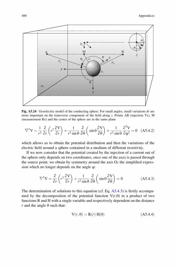
∇2V ¼ 1

r2∂∂r

r2∂V∂r

� �þ 1

r2 sin θ∂∂θ

sin θ∂V∂θ

� �þ 1

r2 sin θ∂2

V

∂φ2¼ 0 ðA5.4.2Þ

which allows us to obtain the potential distribution and then the variations of the

electric field around a sphere contained in a medium of different resistivity.

If we now consider that the potential created by the injection of a current out of

the sphere only depends on two coordinates, once one of the axes is passed through

the source point, we obtain by symmetry around the axis Oz the simplified expres-

sion which no longer depends on the angle φ:

∇2V ¼ ∂∂r

r2∂V∂r

� �þ 1

r2 sin θ∂∂θ

sin θ∂V∂θ

� �¼ 0 ðA5.4.3Þ

The determination of solutions to this equation (cf. Eq. A5.4.3) is firstly accompa-

nied by the decomposition of the potential function V(r,θ) in a product of two

functions R and H with a single variable and respectively dependent on the distance

r and the angle θ such that:

V r; θð Þ ¼ R rð Þ H θð Þ ðA5.4.4Þ

Fig. A5.24 Geoelectric model of the conducting sphere. For small angles, small variations dr aremore important on the transverse component of the field along z. Points AB (injection Tx), M

(measurement Rz) and the center of the sphere are in the same plane

488 Appendices

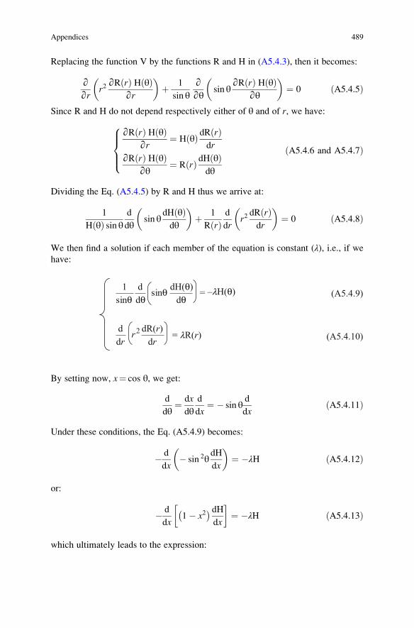
Replacing the function V by the functions R and H in (A5.4.3), then it becomes:

∂∂r

r2∂R rð Þ H θð Þ

∂r

� �þ 1

sin θ∂∂θ

sin θ∂R rð Þ H θð Þ

∂θ

� �¼ 0 ðA5.4.5Þ

Since R and H do not depend respectively either of θ and of r, we have:

∂R rð Þ H θð Þ∂r

¼ H θð Þ dR rð Þdr

∂R rð Þ H θð Þ∂θ

¼ R rð Þ dH θð Þdθ

8>><>>: ðA5.4.6 and A5.4.7Þ

Dividing the Eq. (A5.4.5) by R and H thus we arrive at:

1

H θð Þ sin θd

dθsin θ

dH θð Þdθ

� �þ 1

R rð Þd

drr2dR rð Þdr

� �¼ 0 ðA5.4.8Þ

We then find a solution if each member of the equation is constant (λ), i.e., if wehave:

rr

r ddR(r)

dd

dθdH(θ)sinθ

dθd

sinθ1

2

–lH(θ)

= lR(r)

= (A5.4.9)

(A5.4.10)

By setting now, x¼ cos θ, we get:

d

dθ¼ dx

dθd

dx¼ � sin θ

d

dxðA5.4.11Þ

Under these conditions, the Eq. (A5.4.9) becomes:

� d

dx� sin 2θ

dH

dx

� �¼ �λH ðA5.4.12Þ

or:

� d

dx1� x2� � dH

dx

� �¼ �λH ðA5.4.13Þ

which ultimately leads to the expression:

Appendices 489

1� x2� � d2H

dx2� 2x

dH

dx� λH ¼ 0 ðA5.4.14Þ

Furthermore, by setting λ ¼ n(n + 1), we find:

1� x2� � d2H

dx2þ 2x

dH

dx� n nþ 1ð Þ H ¼ 0 ðA5.4.15Þ

a differential equation whose solutions can be expressed using Legendre poly-

nomials27 Pn such that:

H θð Þ ¼ Pn cos θð Þ ðA5.4.16Þ

The Eq. (A5.4.10) becomes now:

2rdR rð Þdrþ r2

d2R rð Þdr2

¼ λR rð Þ ðA5.4.17ÞSetting r R(r)¼U(r), we obtain:

2rd

U rð Þr

h idr

þ r2d2

U rð Þr

h idr2

¼ λU rð Þr

ðA5.4.18Þwhich gives, neglecting the terms in 1/r2 and 1/r3:

rd2U rð Þdr

¼ λU rð Þr

ðA5.4.19Þor alternatively:

d2U rð Þdr2

� λ

r2U rð Þ ¼ 0 ðA5.4.20Þ

Considering always λ ¼ n(n + 1), the general solution of (A5.4.20) is of the form:

U rð Þ ¼ Ar�n þ Brnþ1 ðA5.4.21Þwhich also gives:

R rð Þ ¼ Ar�n�1 þ Brn ðA5.4.22Þ

The general solution of the Laplace equation with two separate variables r and θ is

therefore a linear combination of the solutions corresponding to the different values

of n such that:

27See the definition at the end of the Appendix (formulas and curves).

490 Appendices

V r; θð Þ ¼X1n¼0

Anr�n�1 þ Bnr

n� �

Pn cos θð Þ ðA5.4.23Þ

The constants A, B, C andD can be determined by the boundary conditions imposed

by the model, i.e.:

– In the sphere:

VS ¼X1n¼0

Anr�n�1 þ Bnr

n� �


– Out of the sphere:

VM ¼X1n¼0

Cnr�n�1 þ Dnr

n� �


As the potential VM must be zero to infinity, this means that:

Dn ¼ 0 ðA5.4.26ÞSimilarly VS cannot tend to infinity if we make r tend to 0. We have then:

An ¼ 0 ðA5.4.27Þ

Consequently, this leads to:

– In the sphere:

VS ¼X1n¼0

BnrnPn cos θð Þ ðA5.4.28Þ

– Out of the sphere:

VM ¼X1n¼0

Cnr�n�1Pn cos θð Þ ðA5.4.29Þ

The potential near the source A must be in 1/r, that is, more exactly in 1= ~r0 �~rj jwhich, considering the resistivity ρm of the medium, leads to (Fig. A5.4.25):

VM ¼ ρmI4π

1

~r0 �~rj j þX1n¼0

Cnr�n�1Pn cos θð Þ ðA5.4.30Þ

This equation is coherent if 1= ~r0 �~rj j is turned into Legendre polynomials.

Appendices 491

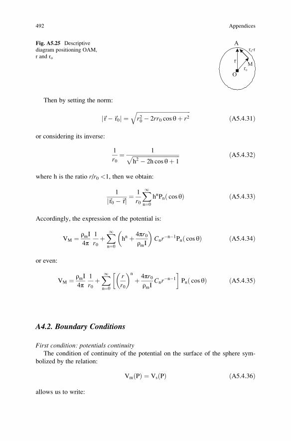
Then by setting the norm:

~r�~r0j j ¼ffiffiffiffiffiffiffiffiffiffiffiffiffiffiffiffiffiffiffiffiffiffiffiffiffiffiffiffiffiffiffiffiffiffiffiffiffiffiffir20 � 2rr0 cos θþ r2

qðA5.4.31Þ

or considering its inverse:

1

r0¼ 1ffiffiffiffiffiffiffiffiffiffiffiffiffiffiffiffiffiffiffiffiffiffiffiffiffiffiffiffiffiffiffiffiffiffi

h2 � 2h cos θþ 1p ðA5.4.32Þ

where h is the ratio r/r0 <1, then we obtain:

1

~r0 �~rj j ¼1

r0

X1n¼0

hnPn cos θð Þ ðA5.4.33Þ

Accordingly, the expression of the potential is:

VM ¼ ρmI4π

1

r0þX1n¼0

hn þ 4πr0ρmI

� �Cnr

�n�1Pn cos θð Þ ðA5.4.34Þ

or even:

VM ¼ ρmI4π

1

r0þX1n¼0

r

r0

� �n

þ 4πr0ρmI

Cnr�n�1

� �Pn cos θð Þ ðA5.4.35Þ

A4.2. Boundary Conditions

First condition: potentials continuityThe condition of continuity of the potential on the surface of the sphere sym-

bolized by the relation:

Vm Pð Þ ¼ Vs Pð Þ ðA5.4.36Þ

allows us to write:

Fig. A5.25 Descriptive

diagram positioning OAM,

r and ro

492 Appendices

ρmI4π

1

r0þX1n¼0

r

r0

� �n

þ 4πr0ρmI

Cnr�n�1

� �Pn cos θð Þ ¼

X1n¼0

BnrnPn cos θð Þ

ðA5.4.37Þ

with the radius of the sphere being R (r¼R), this means:

ρmI4π

1

r0

Rn

r n0þ 4πr0

ρmICnR

�n�1� �

¼ BnRn ðA5.4.38Þ

and thus after calculations:

Bn ¼ ρmI4πrnþ10

þ CnR�2n�1 ðA5.4.39Þ

Second condition: continuity of the normal component of the current densityNow, taking into account the resistivity ρs of the sphere, the condition of

continuity of the normal component of the current density vector required at the

interface by the relation28:

1

ρm∂VM

∂r¼ 1

ρs∂VS

∂rðA5.4.40Þ

leads to:

1

ρmρmI4πr0

nrn�1

r n0þ 1

ρm�n� 1ð Þ Cnr

�n�2 ¼ 1

ρsnBnr

n�1 ðA5.4.41Þ

and to:

Bn ¼ ρsρm

ρmI4πrnþ10

þ �n� 1ð Þn

Cnr�2n�1

� �ðA5.4.42Þ

and, according to the relations (A5.4.39) and (A5.4.40), to:

Cn ¼ ρmI4πrnþ10

n ρs � ρmð Þ r2nþ1n ρm þ ρsð Þ þ ρs½ � ðA5.4.43Þ

28The potential V varies continuously when the current lines cross the parting surface of the two

media. Due to the current conservation law it is the same for 1/ρ ∂V/∂r when r denotes the normal

to the separation surface. These conditions govern the refraction of the current lines and equipo-

tential surfaces (thus the fields) at the crossing of resistivity discontinuity surfaces.

Appendices 493

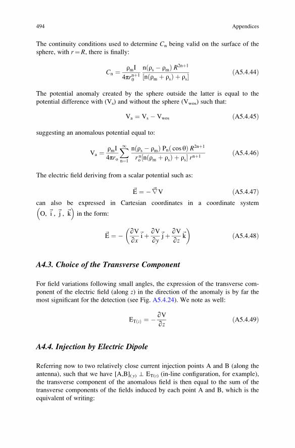
The continuity conditions used to determine Cn being valid on the surface of the

sphere, with r¼R, there is finally:

Cn ¼ ρmI4πrnþ10

n ρs � ρmð Þ R2nþ1

n ρm þ ρsð Þ þ ρs½ � ðA5.4.44Þ

The potential anomaly created by the sphere outside the latter is equal to the

potential difference with (Vs) and without the sphere (Vwos) such that:

Va ¼ Vs � Vwos ðA5.4.45Þ

suggesting an anomalous potential equal to:

Va ¼ ρmI4πro

X1n¼1

n ρs � ρmð Þ Pn cos θð Þ R2nþ1

r no n ρm þ ρsð Þ þ ρs½ � rnþ1 ðA5.4.46Þ

The electric field deriving from a scalar potential such as:

~E ¼ �~∇V ðA5.4.47Þcan also be expressed in Cartesian coordinates in a coordinate system

O, ~i , ~j , ~k

in the form:

~E ¼ � ∂V∂x

~iþ ∂V∂y

~jþ ∂V∂z

~k

� �ðA5.4.48Þ

A4.3. Choice of the Transverse Component

For field variations following small angles, the expression of the transverse com-

ponent of the electric field (along z) in the direction of the anomaly is by far the

most significant for the detection (see Fig. A5.4.24). We note as well:

ET zð Þ ¼ �∂V∂z

ðA5.4.49Þ

A4.4. Injection by Electric Dipole

Referring now to two relatively close current injection points A and B (along the

antenna), such that we have [A,B]( y) ⊥ ET(z) (in-line configuration, for example),

the transverse component of the anomalous field is then equal to the sum of the

transverse components of the fields induced by each point A and B, which is the

equivalent of writing:

494 Appendices

ET zð Þ ¼ EAT zð Þ þ EB

T zð Þ ðA5.4.50Þor literally:

ET zð Þ

¼ �ρmI4πr0A

X1n¼1

n ρs � ρmð Þ R2nþ1

r n0A n ρm � ρsð Þ þ ρs½ �∂Pn cos θð ÞA∂ cos θð ÞA

∂ cos θð ÞA∂z

1

rnþ1þ Pn cos θð ÞA

∂∂z

1

rnþ1

� �zfflfflfflfflfflfflfflfflfflfflfflfflfflfflfflfflfflfflfflfflfflfflfflfflfflfflfflfflfflfflfflfflfflfflfflfflfflfflfflfflfflfflfflfflfflfflfflfflfflfflfflfflfflfflfflfflfflfflfflfflfflfflfflfflfflfflfflfflfflfflffl}|fflfflfflfflfflfflfflfflfflfflfflfflfflfflfflfflfflfflfflfflfflfflfflfflfflfflfflfflfflfflfflfflfflfflfflfflfflfflfflfflfflfflfflfflfflfflfflfflfflfflfflfflfflfflfflfflfflfflfflfflfflfflfflfflfflfflfflfflfflfflffl{EAT zð Þ

þ EBT zð Þ ðA5.4.51Þ

This expression gives, after calculations of the derivatives (∂), the values of

variations of the anomalous transverse field (�∂V/∂z), directly usable for the

comparative interpretation of field or experimental data available from the elec-

trometers after correction and calibration.

When there is no anomaly (angle 0), the transverse component is zero.

ET zð Þ ¼ 0 ðA5.4.52Þ

However, these models have limitations. If we consider, for example, a sphere of

infinite radius, i.e., a flat surface seen from the top, it could then be detected at an

infinite depth, which of course is not true. At this level then we join the problems

relative to horizontal strata mentioned in the previous appendices (tabular model).

This type of modeling is all the more effective when the resistivity contrast is

important. In absolute terms, the resolution is at maximum when the contrast is

Fig. A5.26 Synthetic responses (mathematical model) for a conducting sphere, confronted with

experimental responses in a rheostatic tank (see Chap. 5, Sect. 6.2) showing dispersive curves. For

a resistive sphere we have absorption curves (not represented). The current injection electrodes A

and B (at low frequency) placed on either side of the measuring device (in line) allow us to

measure with the phase change the variations of the transverse electric field component. The

electrokinetic equivalence is obtained by an LF current injection symmetrical system, whose

injection points provide an antiphase signal, similar to a current dipole +/� (Sainson, 1984)

Appendices 495

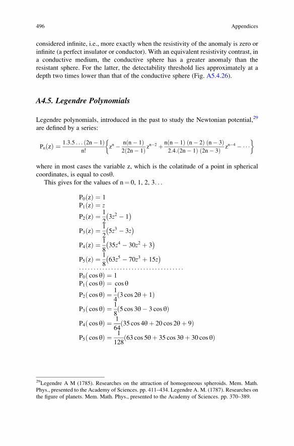
http://dx.doi.org/10.1007/978-3-319-45355-2_5

http://dx.doi.org/10.1007/978-3-319-45355-2_5

considered infinite, i.e., more exactly when the resistivity of the anomaly is zero or

infinite (a perfect insulator or conductor). With an equivalent resistivity contrast, in

a conductive medium, the conductive sphere has a greater anomaly than the

resistant sphere. For the latter, the detectability threshold lies approximately at a

depth two times lower than that of the conductive sphere (Fig. A5.4.26).

A4.5. Legendre Polynomials

Legendre polynomials, introduced in the past to study the Newtonian potential,29

are defined by a series:

Pn zð Þ ¼ 1:3:5 . . . 2n� 1ð Þn!

zn � n n� 1ð Þ2 2n� 1ð Þ z

n�2 þ n n� 1ð Þ n� 2ð Þ n� 3ð Þ2:4: 2n� 1ð Þ 2n� 3ð Þ zn�4 � � � �

� �

where in most cases the variable z, which is the colatitude of a point in spherical

coordinates, is equal to cosθ.This gives for the values of n¼ 0, 1, 2, 3. . .

P0 zð Þ ¼ 1

P1 zð Þ ¼ z

P2 zð Þ ¼ 1

23z2 � 1� �

P3 zð Þ ¼ 1

25z3 � 3z� �

P4 zð Þ ¼ 1

835z4 � 30z2 þ 3� �

P5 zð Þ ¼ 1

863z5 � 70z3 þ 15z� �

. . . . . . . . . . . . . . . . . . . . . . . . . . . . . . . . . . . .P0 cos θð Þ ¼ 1

P1 cos θð Þ ¼ cos θ

P2 cos θð Þ ¼ 1

43 cos 2θþ 1ð Þ

P3 cos θð Þ ¼ 1

85 cos 3θ� 3 cos θð Þ

P4 cos θð Þ ¼ 1

6435 cos 4θþ 20 cos 2θþ 9ð Þ

P5 cos θð Þ ¼ 1

12863 cos 5θþ 35 cos 3θþ 30 cos θð Þ

29Legendre A M (1785). Researches on the attraction of homogeneous spheroids. Mem. Math.

Phys., presented to the Academy of Sciences. pp. 411–434. Legendre A. M. (1787). Researches on

the figure of planets. Mem. Math. Phys., presented to the Academy of Sciences. pp. 370–389.

496 Appendices

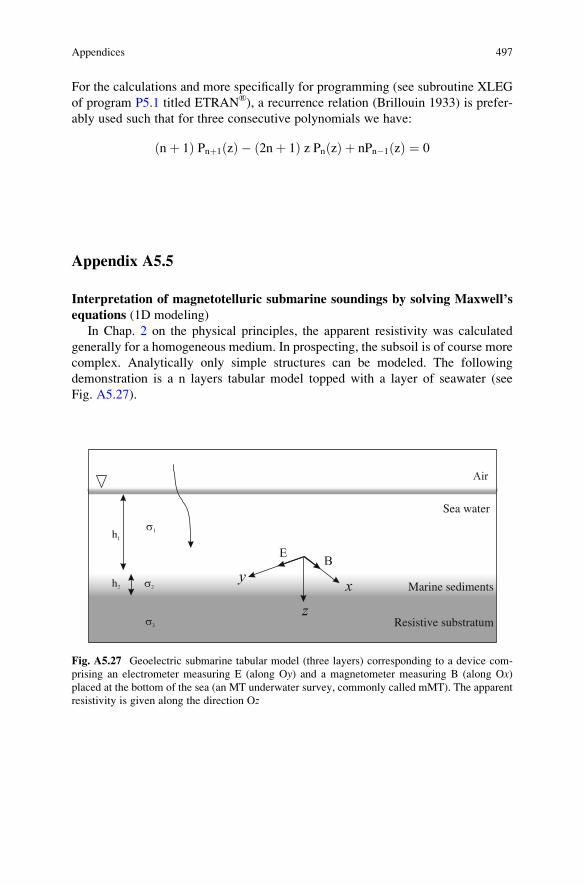
For the calculations and more specifically for programming (see subroutine XLEG

of program P5.1 titled ETRAN®), a recurrence relation (Brillouin 1933) is prefer-

ably used such that for three consecutive polynomials we have:

nþ 1ð Þ Pnþ1 zð Þ � 2nþ 1ð Þ z Pn zð Þ þ nPn�1 zð Þ ¼ 0

Appendix A5.5

Interpretation of magnetotelluric submarine soundings by solving Maxwell’sequations (1D modeling)

In Chap. 2 on the physical principles, the apparent resistivity was calculated

generally for a homogeneous medium. In prospecting, the subsoil is of course more

complex. Analytically only simple structures can be modeled. The following

demonstration is a n layers tabular model topped with a layer of seawater (see

Fig. A5.27).

Sea water

Marine sediments


Fig. A5.27 Geoelectric submarine tabular model (three layers) corresponding to a device com-

prising an electrometer measuring E (along Oy) and a magnetometer measuring B (along Ox)placed at the bottom of the sea (an MT underwater survey, commonly called mMT). The apparent

resistivity is given along the direction Oz

Appendices 497

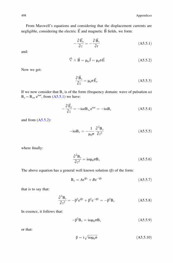
http://dx.doi.org/10.1007/978-3-319-45355-2_2

From Maxwell’s equations and considering that the displacement currents are

negligible, considering the electric ~E and magnetic ~B fields, we form:

�∂~Ey

∂z¼ �∂~Bx

∂tðA5.5.1Þ

and:

~∇ ^ ~B ¼ μ0~J ¼ μ0σ~E ðA5.5.2Þ

Now we get:

∂~Bx

∂z¼ μ0σ~Ey ðA5.5.3Þ

If we now consider that Bx is of the form (frequency domain: wave of pulsation ω)Bx¼Bxo e

iωt, from (A5.5.1) we have:

�∂~Ey

∂z¼ �iωtBxoe

iωt ¼ �iωBx ðA5.5.4Þ

and from (A5.5.2):

�iωBx ¼ � 1

μ0σ∂2

Bx

∂z2ðA5.5.5Þ

where finally:

∂2Bx

∂z2¼ iωμ0σBx ðA5.5.6Þ

The above equation has a general well known solution (β) of the form:

Bx ¼ Aeiβz þ Be�iβz ðA5.5.7Þ

that is to say that:

∂2Bx

∂z2¼ �β2eiβz þ β2e�iβz ¼ �β2Bx ðA5.5.8Þ

In essence, it follows that:

�β2Bx ¼ iωμ0σBx ðA5.5.9Þ

or that:

β ¼ iffiffiffiffiffiffiffiffiffiffiffiffiiωμ0σ

pðA5.5.10Þ

498 Appendices

By replacing β by its value, the expression (A5.5.7) is written:

Bx ¼ Ae�ffiffiffiffiffiffiffiffiffiiωμoσp

z þ Beffiffiffiffiffiffiffiffiffiiωμoσp

z ðA5.5.11ÞBy setting k ¼ ffiffiffiffiffiffiffiffiffiffiffiffi

iωμ0σp

, it immediately becomes at layer i:

Bx ¼ Aie�kiz þ Bie

kiz ðA5.5.12Þ

and from (A5.5.3):

Ey ¼ 1

μ0σ∂~Bx

∂z

¼ 1

μ0σ�kiAie

�kiz þ kiBiekiz

� �¼ ki

μ0σ�Aie

�kiz þ Biekiz

� �ðA5.5.13Þ

Now considering the boundary conditions:

– When z tends to infinity: Ey¼ 0 and By¼ 0, it imposes for layer n, Bn¼ 0

– at the interface of layers (n�1) and (n�1)�n, we obtain the equations for the

horizontal fields Ey and Bx at:

– the layer (n�1) at the depth zn-1:

B(A )z–kx

n–1 n–1 zkn–1 n–1ee +B = n–1n–1

(–A )z–kn–1 n–1 zkn–1 n–1+= eeEμ n–1

n–1 n–1n–1

0

ny Bk

σ

(A5.5.14)

(A5.5.15)

– the layer (n�1)-n:

A z–kx

n–1n

z–k n–1n

eB =

= –

n

eEμ σ n

n0

ny Ak

(A5.5.16)

(A5.5.17)

Setting An¼ 1 for the layer n, thus we normalize the ratio Ey/Bx. The expressions

(A5.5.14) and (A5.5.16) as well as (A5.5.15) and (A5.5.17) then form a system of

equations with two unknown variables which are the coefficients An and Bn. Solving

this system for n layers is done going back to the upper layers, each time setting the

Eqs. (A5.5.14, A5.5.15, A5.5.16 and A5.5.17), and can be calculated numerically

(see program P5.2) (Fig. A5.28).

Appendices 499

Appendix A5.6

Interpretation of isometric anomalies (cylinder) for vector magnetotelluric

devices (transverse fields) by the method of the coefficients of reflection(2D modeling).

The distribution of an anomalous field caused by the presence of an isometric

anomaly can be calculated analytically (cf. Appendix A5.4). For more complex

structures with multiple axes of radial symmetry such as disks or cylinders, special

techniques are proposed. This is the case, for example, of the following one

(a cylinder) which takes into account the reflections of waves on the different

interfaces (Jegen and Edwards 2000). We shall also find in the scientific literature

the technique for example concerning the distribution of fields around an insulating

disk (Bailey 2008).

T in seconds

Fig. A5.28 Abacus for interpreting mMT underwater soundings to obtain the characteristics of

the layer thickness h2 corresponding to marine sediments (1–10 m) resting on a resistive thick layer

(see Fig. A5.27)

500 Appendices

The transverse component, along y, of the electric field (TE mode), at the bottom

of the sea, directly above an anomaly of conductivity σ1+δσ1, buried at a depth h ina medium of conductivity σ1 (see Fig. A5.29), as a function along y of the initial

field (sea surface), is equal to:

E1y x; hð Þ ¼ E1

y x; 0ð Þ e�k1h ðA5.6.1Þ

where the wave number k1 is equal toffiffiffiffiffiffiffiffiffiffiffiffiffiffiiωμ0σ1

pand ω the wave pulsation.

In this case, the current in the anomaly of radius a can be put in the form:

Iay ¼ δσ1E1y x; hð Þ πa2 ðA5.6.2Þ

The electric and magnetic field intensities are respectively equal to:

Eay x; 0ð Þ ¼ I ayμ0

2

Z1�1� iωe�θ1h

θ11� RTEð Þ e�ipxdp ðA5.6.3Þ

Bay x; 0ð Þ ¼ I ayμ0

2

Z1�1

e�θ1h 1þ RTEð Þe�ipx dp ðA5.6.4Þ

where the incident angle θ1 is defined as θ21 ¼ iωμ0σ1 þ p2θ iωμ0σ1 þ p2 with

p the wave number of the anomalous field in the x direction.The anomalous signal comes from the superposition of the upgoing field (from

the anomaly) and the downgoing field, from the reflections with the water/air

Sea water

Marine sediments


Fig. A5.29 Geoelectric model mMT used in this section (sectional cylinder)

Appendices 501

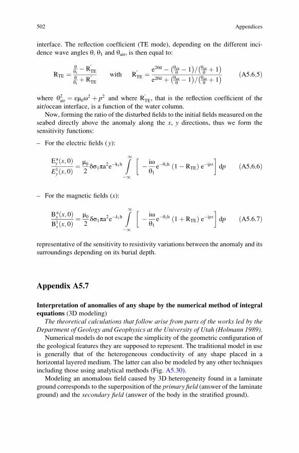
interface. The reflection coefficient (TE mode), depending on the different inci-

dence wave angles θ, θ1 and θair, is then equal to:

RTE ¼θθ1 � R

0TE

θθ1 þ R

0TE

with R0TE ¼

e2θd � θairθ � 1� �

= θairθ þ 1� �

e2θd þ θairθ � 1� �

= θairθ þ 1� � ðA5.6.5Þ

where θ2air ¼ εμ0ω2 þ p2 and where R0TE, that is the reflection coefficient of the

air/ocean interface, is a function of the water column.

Now, forming the ratio of the disturbed fields to the initial fields measured on the

seabed directly above the anomaly along the x, y directions, thus we form the

sensitivity functions:

– For the electric fields (y):

Eay x; 0ð Þ

E1y x; 0ð Þ ¼

μ02δσ1πa2e�k1h

Z1�1

� iωθ1

e�θ1h 1� RTEð Þ e�ipx� �

dp ðA5.6.6Þ

– For the magnetic fields (x):

Bax x; 0ð Þ

B1x x; 0ð Þ ¼

μ02δσ1πa2e�k1h

Z1�1

� iωθ1

e�θ1h 1þ RTEð Þ e�ipx� �

dp ðA5.6.7Þ

representative of the sensitivity to resistivity variations between the anomaly and its

surroundings depending on its burial depth.

Appendix A5.7

Interpretation of anomalies of any shape by the numerical method of integralequations (3D modeling)

The theoretical calculations that follow arise from parts of the works led by theDepartment of Geology and Geophysics at the University of Utah (Holmann 1989).

Numerical models do not escape the simplicity of the geometric configuration of

the geological features they are supposed to represent. The traditional model in use

is generally that of the heterogeneous conductivity of any shape placed in a

horizontal layered medium. The latter can also be modeled by any other techniques

including those using analytical methods (Fig. A5.30).

Modeling an anomalous field caused by 3D heterogeneity found in a laminate

ground corresponds to the superposition of the primary field (answer of the laminate

ground) and the secondary field (answer of the body in the stratified ground).

502 Appendices

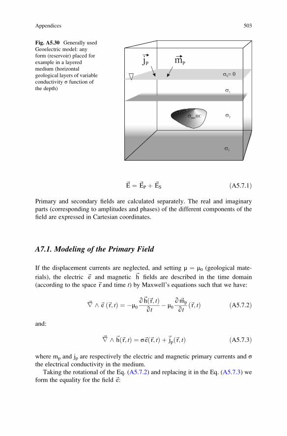
~E ¼ ~EP þ ~ES ðA5.7.1Þ

Primary and secondary fields are calculated separately. The real and imaginary

parts (corresponding to amplitudes and phases) of the different components of the

field are expressed in Cartesian coordinates.

A7.1. Modeling of the Primary Field

If the displacement currents are neglected, and setting μ ¼ μ0 (geological mate-

rials), the electric ~e and magnetic ~h fields are described in the time domain

(according to the space~r and time t) by Maxwell’s equations such that we have:

~∇ ^~e ~r; tð Þ ¼ �μ0∂~h ~r; tð Þ

∂t� μ0

∂~mp

∂t~r; tð Þ ðA5.7.2Þ

and:

~∇ ^ ~h ~r; tð Þ ¼ σ~e ~r; tð Þ þ~jp ~r; tð Þ ðA5.7.3Þ

where mp and jp are respectively the electric and magnetic primary currents and σthe electrical conductivity in the medium.

Taking the rotational of the Eq. (A5.7.2) and replacing it in the Eq. (A5.7.3) we

form the equality for the field ~e:

HC

Fig. A5.30 Generally used

Geoelectric model: any

form (reservoir) placed for

example in a layered

medium (horizontal

geological layers of variable

conductivity σ function of

the depth)

Appendices 503

~∇ ^ ~∇ ^~eþ μ0σ∂~e∂t¼ �μ0

∂~jp∂t� μ0 ~∇ ^

∂~mp

∂tðA5.7.4Þ

Also using the rotational of the Eq. (A5.7.3) and replacing it in the Eq. (A5.7.2) we

get the diffusion equation for the field ~h:

~∇ ^~∇ ^ ~h

σ

!þ μ0

∂~h∂t¼ ~∇ ^

~jpσ

!� μ0

∂~mp

∂t

ðA5.7.5Þ

Using the vector identity ~∇ ^ ~∇ ^ ~A ¼ �∇2~Aþ ~∇ð~∇: ~A�the Eq. (A5.7.4)

becomes:

�∇2~eþ ~∇�~∇ � ~e

�þ μ0σ

∂~e∂t¼ �μ0

∂~jp∂t� μ0 ~∇ ^

∂~mp

∂tðA5.7.6Þ

Expressly using the divergence of the Eq. (A5.7.3),~∇: σ~eð Þ ¼ σ~∇:~eþ ~∇σ:~e ¼ �~∇:~jp, and substituting ~∇:~e in the Eq. (A5.7.6),

we arrive at:

∇2~eþ ~∇ ~e �~∇σσ

!� μ0σ

∂~e∂t

¼ μ0∂~jp∂t� 1

σ~∇�~∇ �~jp

�þ μ0 ~∇ ^

∂~mp

∂tðA5.7.7Þ

considering that the source is in a medium with a homogeneous conductivity.

Now assigning the following identity, ~∇ ^ φ~A ¼ φ~∇ ^ ~A� ~A ^ ~∇φ, theEq. (A5.7.5) can be written now as:

1

σ~∇ ^ ~∇ ^ ~h�

�~∇ ^ ~h

�^ ~∇

�1

σ

�þ μ0

∂~h∂t¼ 1

σ~∇ ^~jp � μ0

∂~mp

∂tðA5.7.8Þ

or:

�∇2~hþ ~∇�~∇ � ~h

�� σ�~∇ ^ ~h

�^ ~∇

1

σ

� �þ μ0σ

∂~h∂t

¼ ~∇ ^~jp � μ0σ∂~mp

∂tðA5.7.9Þ

Knowing besides that the divergence of the magnetic field is nonzero at the source,

the divergence of the expression (A5.7.2) shows that ~∇:~h ¼ �~∇:~mp and that:

504 Appendices

∇2~hþ σ�~∇ ^ ~h

�^ ~∇

1

σ

� �� μ0σ

∂~h∂t

¼ μ0σ∂~mp

∂t� ~∇

�~∇ � ~mp

��∇ ^~jp ðA5.7.10Þ

The above Eqs. (A5.7.7) and (A5.7.10) are the general equations of the total electric

and magnetic fields at any point in the propagation medium. The primary electric

~eP and magnetic~hp fields that correspond to the fields in a stratified medium without

anomaly can be calculated from the equations:

~∇ ^~eP ¼ �μ0∂~hp∂t� μ0

∂~mp

∂tðA5.7.11Þ

and:

~∇ ^ ~hp ¼ σwob~ep þ~jp ðA5.7.12Þwhere σwob is the electrical conductivity in the absence of any foreign body

(or without body).

These equations, in integral form, can then be calculated numerically. By

application, for example, for each function of time eiωt, the Fourier transforms

(Papoulis 1962; Bracewell 1986; Wijewardena 2007) such that:

F ~r;ωð Þ ¼Z 1�1

f ~r; tð Þ e�iωtdtand

f ~r; tð Þ ¼ 1

2π

Z 1�1

F ~r;ωð Þ eiωtdωðA5.7.13Þ

whose representations are equivalent, f ~r; tð Þ , F ~r;ωð Þ, we get the Eqs. (A5.7.7)

and (A5.7.10) in the frequency domain ~e, ~h! ~E, ~H

:

∇2~Eþ ~∇�~E �

~∇σσ

�þ k2~E

¼ iωμ0~jp �1

σ~∇�~∇ �~Jp

�þ iωμ0 ~∇ ^ ~Mp ðA5.7.14Þand:

∇2~Hþ σ�~∇ ^ ~H

� ^ ~∇1

σ

� �þ k2~H

¼ iωμ0 ~Mp �∇ �

~∇ � ~Mp

�� ~∇ ^~Jp ðA5.7.15Þ

with k2 ¼ �iωμ0σ

Appendices 505

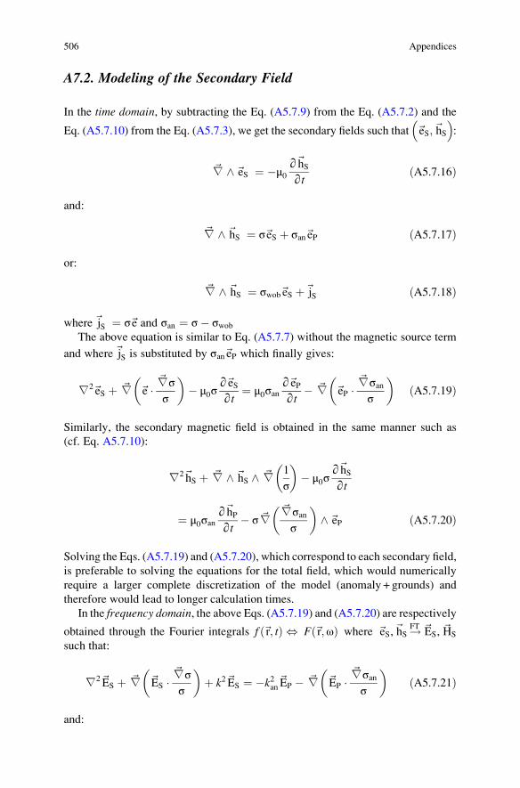
A7.2. Modeling of the Secondary Field

In the time domain, by subtracting the Eq. (A5.7.9) from the Eq. (A5.7.2) and the

Eq. (A5.7.10) from the Eq. (A5.7.3), we get the secondary fields such that ~eS; ~hS

:

~∇ ^~eS ¼ �μ0∂~hS∂t

ðA5.7.16Þ

and:

~∇ ^ ~hS ¼ σ~eS þ σan~eP ðA5.7.17Þ

or:

~∇ ^ ~hS ¼ σwob~eS þ~jS ðA5.7.18Þ

where~jS ¼ σ~e and σan ¼ σ� σwobThe above equation is similar to Eq. (A5.7.7) without the magnetic source term

and where~jS is substituted by σan~eP which finally gives:

∇2~eS þ ~∇�~e �

~∇σσ

�� μ0σ

∂~eS∂t¼ μ0σan

∂~eP∂t� ~∇

�~eP �

~∇σanσ

�ðA5.7.19Þ

Similarly, the secondary magnetic field is obtained in the same manner such as

(cf. Eq. A5.7.10):

∇2~hS þ ~∇ ^ ~hS ^ ~∇1

σ

� �� μ0σ

∂~hS∂t

¼ μ0σan∂~hP∂t� σ~∇

�~∇σanσ

�^~eP ðA5.7.20Þ

Solving the Eqs. (A5.7.19) and (A5.7.20), which correspond to each secondary field,

is preferable to solving the equations for the total field, which would numerically

require a larger complete discretization of the model (anomaly + grounds) and

therefore would lead to longer calculation times.

In the frequency domain, the above Eqs. (A5.7.19) and (A5.7.20) are respectively

obtained through the Fourier integrals f ~r; tð Þ , F ~r;ωð Þ where ~eS,~hS!FT ~ES, ~HS

such that:

∇2~ES þ ~∇�~ES �

~∇σσ

�þ k2~ES ¼ �k2an~EP � ~∇

�~EP �

~∇σanσ

�ðA5.7.21Þ

and:

506 Appendices

∇2~HS þ σ�~∇ ^ ~HS

�^ ~∇

1

σ

� �þ k2~HS ¼ �k2an~HP � σ~∇

�~∇σanσ

�ðA5.7.22Þ

with k2 ¼ �iωμ0σ and k2an ¼ �iωμ0σanSolutions for secondary fields are finally calculated from Eqs. (A5.7.16) and

(A5.7.18) in the frequency domain, such that:

~∇ ^ ~ES ¼ �iωμ0~HS ðA5.7.23Þ

and:

~∇ ^ ~HS ¼ σwob~ES þ~JS ðA5.7.24Þ

To formulate then the integral equation, we consider~JS as a current source. In this

empty space, the secondary electric field is then given by the expression:

~ES ¼ �iωμ0~AS � ~∇VS ðA5.7.25Þ

where ~AS and VS are respectively the vector and the scalar potential for the Lorentz

gauge.

The integral equations on the volume v for ~AS and VS as a function of~r are thenformulated by the following integrals:

~AS ~rð Þ ¼Zv

~JS ~r0� �

G ~r,~r0� �

dv0 ðA5.7.26Þ

and:

VS ~rð Þ ¼ � 1

σwob

Zv

∇ �~JS ~r0� �

G ~r,~r0� �

dv0 ðA5.7.27Þ

where G is the scalar Green’s function such that:

G ~r,~r0� � ¼ e�ikwob r�r

0j j

4π ~r�~r0 ðA5.7.28Þ

with kwob ¼ffiffiffiffiffiffiffiffiffiffiffiffiffiffiffiffiffiffiffiffiffiffi�iωμ0σwob

pFor a conductivity anomaly present in a homogeneous (Holmann 1975) or

stratified half-space (Vannamaker et al. 1984), an additional term is added to

Eq. (A5.7.25).

Appendices 507

A7.3. The Total Field

Finally, by adding the primary and secondary fields (cf. Eq. A5.7.1), we obtain the

integral equation of the total field so that:

~E ~rð Þ ¼ ~EP ~rð Þ þZv

G ~r,~r0� � � σan ~r0

� �~E ~r0� �

dv0 ðA5.7.29Þ

where G is the tensor of Green’s function.This integral equation is limited to a 3D anomaly in a 1D environment, stratified

or not. This corresponds to the majority of cases encountered in petroleum geology

where the sedimentary layers remain relatively monotonous laterally.

Today, one of the main purpose of 3D modeling is also to include the broadside

EM field data taking into account TE and TM modes, the amplitude and the phase

measurements.

Program P5.1

ETRAN Fortran program for the evaluation of TE transverse field. (Model of

the sphere/Laplace, cf. Appendix A5.4).

Preamble

The f2c software available for free at AT&T Bell Labs is used to transcribe the

FORTRAN 77 programs in C. The following program was written in FORTRAN

4, whose syntax is almost identical to that of Fortran 77 or 90.

C*********************** PROGRAM ETRAN ***************************

C THIS PROGRAMM CALCULATES THE TRANSVERSE ELECTRIC FIELD

MODIFIED BY AN

C IMMERGED SPHERE PLACED AT A DISTANCE ALONG THE MEASUREMENT

DETECTION

C DEVICE COMPOSED BY A DIPOLE PLACED IN THE CENTER OF AN

TRANSMITTING DIPOLE

C LINE WHERE THE TWO INJECTION ELECTRODES ARE IN PHASE

OPPOSITION ( +/-).

C***************************************************************

0001 FTN4,L

0002 PROGRAM ETRAN. AUTHOR: STEPHANE SAINSON

0003 DOUBlE PRECISION XLEG, ZA, ZB, EA, EB, ET, XPA, XPAP,

XPB, XPBP

0004 DIMEMSION IPAR(5)

0005 CAll RNPAR(IPAR)

508 Appendices

0006 IN¼IPAR(l)0007 NOUT¼IPAR(2)0008 IF(IH.EQ.O) IN¼l0009 IF(NOUT.EQ.O) HOUT¼10010 WRITE (NOUT.100)

0011 100 FORMAT(“ENTER THE RESISTIVITY OF THE GROUND, OF THE

SPHERE”)

0012 READ(IN,*)ROM.ROS

0013 WRITE(NOUT 200)

0014 200 FORMAT(“ENTER THE RADIUS OF THE SPHERE, THE LENGTH OF THE

DEVICE”)

0015 READ(IN,*) RS.ZL

0016 WRITE(NOUT 300)

0017 300 FORMAT(“ENTER THE CURRENT INTENSITY,/

0018 2 “THE HORIZONTAL DISTANCE FROM THE SPHERE TO THE DEVICE”)

0019 READ(IN,*) XI.YDS

0020 WRITE(NOUT,400)

0021 400 FORMAT(“ENTER THE RANGE N”)

0022 READ(IN,*) NW

0023 WRITE(NOUT,900)

0024 900 FORMAT(“ENTER THE VERTICAL DISTANCES MINI AND MAXI OF THE

0025 1 SPHERE TO THE DEVICE“,/,” AND THE STEP DZ”)

0026 READ(IN,*) ZMS1, ZMS2 ZMS0

0027 INBS¼IFIX((S2-ZKS1)/ZKSO)0028 DO 20 IMZS ¼l,INBMS+10029 IZKSP¼IZMS-l0030 ZMS¼ZMS1+IZMSP*ZMS00031 ZAS¼ZMS-ZL0032 ZBS¼ZMS+ZL0033 DMS¼SQRT(YDS**2+ZMS**2)0034 DAS¼SQRT(YDS**2+ZAS**2)0035 DBS¼SQRT(YDS**2+ZBS**2)0036 ZA¼ (YDS**2+ZAS*ZMS)/(SQRT(YDS**2+ZAS**2)*SQRT(YD5**2

+ZMS**2)

0037 ZB¼(YDS**2+ZBS*ZMS)/(SQRT(YDS**2+ZBS**2)*SQRT(YDS**2+ZMS**2)

0038 WK¼-ROM*XI*(ROS-ROM).YDS/(4.3.14159)0039 ET¼O0040 XPAP¼XLEG(0,ZA,IN,NOUT)0041 XPBP¼XLEG(0,ZB,IN,NOUT)0042 DO l0 N¼1, NN

0043 XPA¼XLEG(N,ZA,IN,NOUT)0044 XPB¼XLEG(N,ZB,IN,NOUT)0045 C WRITE(NOUT,800) ZA,ZB,XPA,XPB,XPAP,XPBP

0046 800 FORMAT(“COS TETA FOR A , B “F5,2,3X,F5,2,/,

Appendices 509

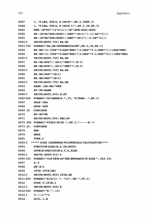
0047 1, “P LEG, FOR A, B (RG N)”,E8.3,3XE8.3)

0048 1, “P LEG, FOR A, B (RG N-1)”,E8.3,3X,E8.3)

0049 WKN¼(N*RS**(2*n+1))/(N*(ROM-ROS)+ROS)0050 EA¼(N*ZA*XPA+XPAP)/(DMS**(N+1)*(-(1-ZA**2)))0051 EB¼(N*ZB*XPB+XPBP)/(DMS**(N+1*(-(1-ZB**2)))0052 C WRITE(NOUT,700) EA,ED

0053 700 FORMAT(“EA,EB INTERMEDIAIRE”,E8.3,3X,E8.3)

0054 EA¼EA*(2-(YDS**2+ZAS*ZMS)*(1/DAS**2-1/DMS**))/(DAS*DMS)0055 EB¼EB*(2-(YDS**2+ZBS*ZMS)*(1/DBS**2-1/DHS**2))/(DBS*DMS)0056 C WRITE(NOUT,700) EA,EB

0057 EA¼EA+XPA*(-(N+1)*DMS**(-N-3)0058 EB¼EB+XPB*(-(N+1)*DMS**(-N-3)0059 C WRITE(NOUT,700) EA,EB

0060 EA¼EA/DAS**(N+l)0061 EB¼EB/DBS**(N+l)0062 C WRITE(NOUT,700) EA,EB

0063 EABN¼(EA-EB)*WKN0064 ET¼ET+EABN0065 C WRITE(NOUT,600) N,ET

0066 600 FORMAT(“AT RANGE N¼”,I3, “E TRAN¼ ”,E8.3)

0067 XPAP¼XPA0068 XPBP¼XPB0069 10 CONTINUE

0070 ET¼ET*WK0071 WRITE(NOUT,500) ZMS,ET

0072 500 FORMAT(“FIELD IN DZ¼”,E8.3,“-----E¼”)0073 20 CONTINUE

0074 END

0075 END$

0001 FTN4,L

0002 C ***** XlEG (LEGENDRE POLYNOMIALS CALCULATION)***

0003 FUNCTION XLEG(N,Z,IN,NOUT)

0004 DOUBlE PRECISION X,Y,Z,XLEG

0005 C WRITE (NOUT 333) Z

0006 333 FORMAT(“COS TETA AT THE ENTRANCE OF XLEG ”, D20.15)

0007 X¼00008 XN¼H/20009 IFIN¼IFIX(XN)0010 C WRITE(MOUT,800) IFIN,XN

0011 800 FORMAT(“E(N/2)¼”, “13”, XN¼”,F5.2)0012 DO4K¼0,IFIN,10013 C WRITE(MOUT,500) K

0014 500 FORMAT(“K¼”, 13)

0015 1 Y¼(-l)**I0016 DO3L¼1,N

510 Appendices

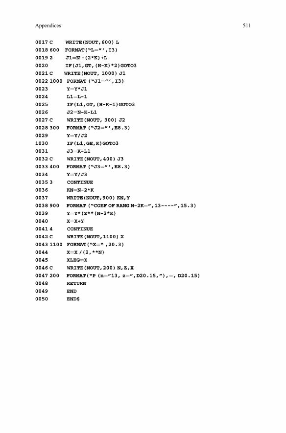
0017 C WRITE(NOUT,600) L

0018 600 FORMAT(“L¼”’,I3)0019 2 J1¼N -(2*K)+L

0020 IF(J1,GT,(H-K)*2)GOTO3

0021 C WRITE(NOUT, 1000) J1

0022 1000 FORMAT (“J1¼”’,I3)0023 Y¼Y*J10024 L1¼L-10025 IF(L1,GT,(H-K-1)GOTO3

0026 J2¼N-K-L10027 C WRITE(NOUT, 300) J2

0028 300 FORMAT (“J2¼”’,E8.3)0029 Y¼Y/J21030 IF(L1,GE,K)GOTO3

0031 J3¼K-L10032 C WRITE(NOUT,400) J3

0033 400 FORMAT (“J3¼”’,E8.3)0034 Y¼Y/J30035 3 CONTINUE

0036 KN¼N-2*K0037 WRITE(NOUT,900) KN,Y

0038 900 FORMAT (“COEF OF RANG N-2K¼”,13----”,15.3)0039 Y¼Y*(Z**(N-2*K)0040 X¼X+Y0041 4 CONTINUE

0042 C WRITE(NOUT,1100) X

0043 1100 FORMAT(“X¼“ ,20.3)

0044 X¼X /(2,**N)

0045 XLEG¼X0046 C WRITE(NOUT,200) N,Z,X

0047 200 FORMAT(“P (n¼”13, z¼”,D20.15,”),¼, D20.15)

0048 RETURN

0049 END

0050 END$

Appendices 511

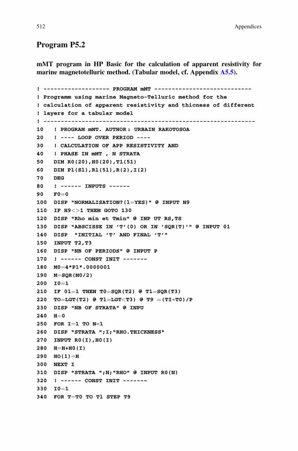
Program P5.2

mMT program in HP Basic for the calculation of apparent resistivity for

marine magnetotelluric method. (Tabular model, cf. Appendix A5.5).

! ------------------– PROGRAM mMT ----------------------------

! Programm using marine Magneto-Telluric method for the

! calculation of apparent resistivity and thicness of different

! layers for a tabular model

! -------------------------------------------------------------

10 ! PROGRAM mMT. AUTHOR: URBAIN RAKOTOSOA

20 ! ---- LOOP OVER PERIOD ----

30 ! CALCULATION OF APP RESISTIVITY AND

40 ! PHASE IN mMT , N STRATA

50 DIM R0(20),H0(20),T1(51)

60 DIM Pl(Sl),Rl(5l),R(2),I(2)

70 DEG

80 ! ------ INPUTS ------

90 F0¼0100 DISP "NORMALISATION?(l¼YES)" @ INPUT N9

110 IF H9<>1 THEM GOTO 130

120 DISP "Rho min et Tmin" @ INP UT RS,TS

130 DISP "ABSCISSE IN ’T’(0) OR IN ’SQR(T)’" @ INPUT 01

140 DISP "INITIAL ’T’ AND FINAL ’T’"

150 INPUT T2,T3

160 DISP "NB OF PERIODS" @ INPUT P

170 ! ------ CONST INIT ------–

180 M0¼4*Pl*.0000001190 M¼SQR(M0/2)200 I0¼1210 IF 01¼1 THEN T0¼SQR(T2) @ T1¼SQR(T3)220 TO¼LGT(T2) @ Tl¼LGT<T3) @ T9 ¼(TI-T0)/P230 DISP "NB OF STRATA" @ INPU

240 H¼0250 FOR I¼1 TO N-1

260 DISP "STRATA ";I;"RHO.THICKNESS"

270 INPUT R0(I),H0(I)

280 H¼H+H0(I)290 HO(1)¼H300 NEXT I

310 DISP "STRATA ";N;"RHO" @ INPUT R0(N)

320 ! ------ CONST INIT ------–

330 I0¼1340 FOR T¼T0 TO Tl STEP T9

512 Appendices

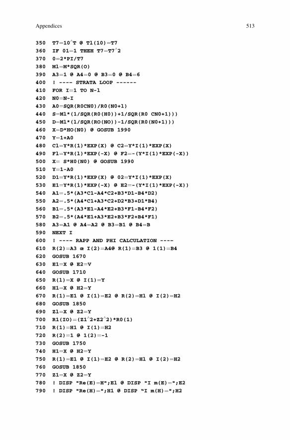
350 T7¼10^T @ Tl(10)¼T7360 IF 01¼1 THEH T7¼T7^2370 0¼2*PI/T7380 Ml¼M*SQR(O)390 A3¼1 @ A4¼0 @ B3¼0 @ B4¼6400 ! ---– STRATA LOOP ------

410 FOR I¼1 TO N-l

420 N0¼N-I430 A0¼SQR(R0CN0)/R0(N0+l)440 S¼Ml*(1/SQR(R0(H0))+1/SQR(R0 CN0+1)))

450 D¼Ml*(l/SQR(RO(NO))-1/SQR(R0(N0+1)))460 X¼D*HO(N0) @ GOSUB 1990

470 Y¼1+A0480 Cl¼Y*R(1)*EXP(X) @ C2¼Y*I(1)*EXP(X)490 Fl¼Y*R(l)*EXP(-X) @ F2¼-(Y*I(1)*EXP(-X))500 X¼ S*H0(N0) @ GOSUB 1990

510 Y¼1-A0520 D1¼Y*R(1)*EXP(X) @ 02¼Y*I(1)*EXP(X)530 E1¼Y*R(1)*EXP(-X) @ E2¼-(Y*I(1)*EXP(-X))540 A1¼.5*(A3*C1-A4*C2+B3*D1-B4*D2)550 A2¼.5*(A4*C1+A3*C2+D2*B3+D1*B4)560 B1¼.5*(A3*E1-A4*E2+B3*F1-B4*F2)570 B2¼.5*(A4*E1+A3*E2+B3*F2+B4*F1)580 A3¼A1 @ A4¼A2 @ B3¼B1 @ B4¼B590 NEXT I

600 ! ---– RAPP AND PHI CALCULATION ---–

610 R(2)¼A3 œ I(2)¼A4@ R(1)¼B3 @ 1(1)¼B4620 GOSUB 1670

630 E1¼X @ E2¼V640 GOSUB 1710

650 R(l)¼X @ I(1)¼Y660 H1¼X @ H2¼Y670 R(1)¼E1 @ I(1)¼E2 @ R(2)¼Hl @ I(2)¼H2680 GOSUB 1850

690 Zl¼X @ Z2¼Y700 R1(IO)¼(Z1^2+Z2^2)*R0(1)710 R(1)¼H1 @ I(1)¼H2720 R(2)¼1 @ 1(2)¼-1730 GOSUB 1750

740 H1¼X @ H2¼Y750 R(1)¼E1 @ I(1)¼E2 @ R(2)¼Hl @ I(2)¼H2760 GOSUB 1850

770 Z1¼X @ Z2¼Y780 ! DISP "Re(E)¼H";El @ DISP "I m(E)¼";E2790 ! DISP "Re(H)¼";H1 @ DISP “I m(H)¼";H2

Appendices 513

800 Pl(I0)¼ATN(Z2/Z1)810 ! DISP "Re(E/H)¼";Z1820 ! DISP "Im(E/H)¼”;Z2830 I0¼ I0+1

840 IF 01#1 THEH D1SP “T¼";Tl(IO-1) @ GOTO 860

850 DISP "rac(T)¼";Tl(I0-l)860 DISP "RAPP¼ ";Rl(I0-1)

870 DISP "PHI¼";Pl(IO-l)880 DISP

890 NEXT T

900 ! ---– TRACES ------

910 IF N9¼1 THEN GOTO 990

920 T0¼100000000000930 R0¼100000000000940 FOR 1¼1 TO P

950 IF Tl(I)<¼T0 THEN T0¼Tl(l)960 IF Rl(I)<¼R0 THEN R0¼Rl(I)970 NEXT 1

980 GOlO 1010

990 T0¼T51000 R9¼R51010 T0¼10ÎNT(LGT(T0))1020 R0¼10ÎNT(LGT(R0))1030 ! ---– AXES ------

1040 PLOTTER 1S 705

1050 CSIZE 4

1060 MSCALE 220,20

1070 IF F0<>0 THEM GOTO 1560

1080 XAXIS 0,0,-195,0

1090 YAXIS O,0,0,180

1100 PLOT -210,-10,-2

1110 LDIR 90 @ LABEL "Ra( .m)"

1120 FOR E¼0 TO 1

1130 K0¼10Ê1140 FOR K¼K0 TO 10*K0 STEP K0

1150 PLOT 0,LGT(K)*75,-2

1160 LORG 5 @ LDIR 0

1170 LABEL “-"

1180 IF K#K0 THEN 1210

1190 PLOT 10,LGT(K)*75.-2

1200 LDIR 180 @ LABEL K0*T0

1210 HEXT K

1212 HEXT E

1214 FOR J¼0 TO 2

1216 K0¼10^J

514 Appendices

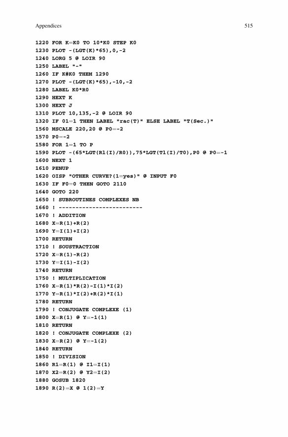
1220 FOR K¼K0 TO 10*K0 STEP K0

1230 PLOT -(LGT(K)*65),0,-2

1240 LORG 5 @ LOIR 90

1250 LABEL "-"

1260 IF K#K0 THEM 1290

l270 PLOT -(LGT(K)*65),-10,-2

1280 LABEL K0*R0

1290 HEXT K

1300 HEXT J

1310 PLOT 10,135,-2 @ LOIR 90

1320 IF 01¼1 THEN LABEL "rac(T)" ELSE LABEL "T(Sec.)"

1560 MSCALE 220,20 @ P0¼-21570 P0¼-21580 FOR 1¼1 TO P

1590 PLOT -(65*LGT(Rl(I)/R0)),75*LGT(Tl(I)/T0),P0 @ P0¼-11600 NEXT 1

1610 PENUP

1620 OISP "OTHER CURVE?(1¼yes)" @ INPUT F0

1630 IF F0¼0 THEN GOTO 2110

1640 GOTO 220

1650 ! SUBROUTINES COMPLEXES NB

1660 ! -------------------------

1670 ! ADDITION

1680 X¼R(1)+R(2)1690 Y¼I(1)+I(2)1700 RETURN

1710 ! SOUSTRACTION

1720 X¼R(1)-R(2)1730 Y¼I(1)-I(2)1740 RETURN

1750 ! MULTIPLICATION

1760 X¼R(1)*R(2)-I(1)*I(2)1770 Y¼R(1)*I(2)+R(2)*I(1)1780 RETURN

1790 ! CONJUGATE COMPLEXE (1)

1800 X¼R(1) @ Y¼-1(1)1810 RETURN

1820 ! CONJUGATE COMPLEXE (2)

1830 X¼R(2) @ Y¼-1(2)1840 RETURN

1850 ! DIVISION

1860 R1¼R(1) @ I1¼I(1)1870 X2¼R(2) @ Y2¼I(2)1880 GOSUB 1820

1890 R(2)¼X @ 1(2)¼Y

Appendices 515

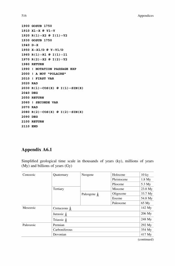
1900 GOSUB 1750

1910 Xl¼X @ Y1¼Y1920 R(1)¼X2 @ I(1)¼Y21930 GOSUB 1750

1940 D¼X1950 X¼X1/D @ Y¼Y1/D1960 R(1)¼Rl @ I(1)¼I11970 R(2)¼X2 @ I(2)¼Y21980 RETURN

1990 ! NOTATION PASSAGE EXP

2000 ! A NOT “POLAIRE"

2010 ! FIRST VAR

2020 RAD

2030 R(l)¼COS(X) @ I(1)¼SIN(X)2040 DEG

2050 RETURN

2060 ! SECONDE VAR

2070 RAD

2080 R(2)¼COS(X) @ I(2)¼SIN(X)2090 DEG

2100 RETURN

2110 END

Appendix A6.1

Simplified geological time scale in thousands of years (ky), millions of years

(My) and billions of years (Gy)

Cenozoic Quaternary Neogene Holocene 10 ky

Pleistocene 1.8 My

Pliocene 5.3 My

Tertiary Miocene 23.8 My

Paleogene Oligocene 33.7 My

Eocene 54.8 My

Paleocene 65 My

Mesozoic Cretaceous 142 My

Jurassic 206 My

Triassic 248 My

Paleozoic Permian 292 My

Carboniferous 354 My

Devonian 417 My

(continued)

516 Appendices

Silurian 443 My

Ordovician 495 My

Cambrian 545 My

Precambrian Proteozoic 2.5 Gy

Archean 4.5 Gy

Appendices 517

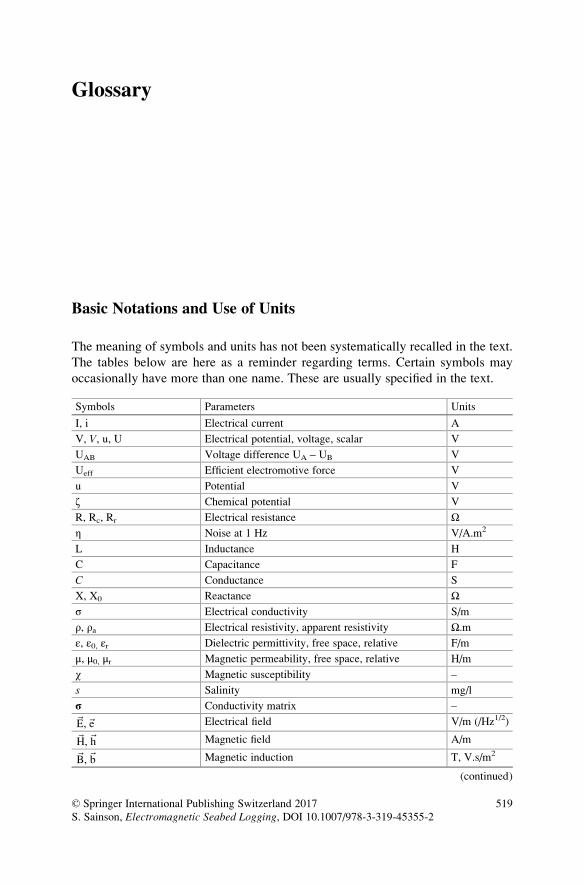
Glossary

Basic Notations and Use of Units

The meaning of symbols and units has not been systematically recalled in the text.

The tables below are here as a reminder regarding terms. Certain symbols may

occasionally have more than one name. These are usually specified in the text.

Symbols Parameters Units

I, i Electrical current A

V, V, u, U Electrical potential, voltage, scalar V

UAB Voltage difference UA – UB V

Ueff Efficient electromotive force V

u Potential V

ζ Chemical potential V

R, Rc, Rr Electrical resistance Ωη Noise at 1 Hz V/A.m2

L Inductance H

C Capacitance F

C Conductance S

X, X0 Reactance Ωσ Electrical conductivity S/m

ρ, ρa Electrical resistivity, apparent resistivity Ω.mε, ε0, εr Dielectric permittivity, free space, relative F/m

μ, μ0, μr Magnetic permeability, free space, relative H/m

χ Magnetic susceptibility –

s Salinity mg/l

σ Conductivity matrix –

~E,~e Electrical field V/m (/Hz1/2)

~H,~h Magnetic field A/m

~B,~b Magnetic induction T, V.s/m2

(continued)




~D, d* Electric displacement A.s/m2

~F Varying magnetic field force A/m

~J,~JS Current density A/m2

~n Normal vector, or Poynting vector V.A/m2

r* Directional vector –

~A Potential vector V.s/m

TEx, TEy Transverse component V/m, A/m

q Charge or charge density C or C/m3

Φ Magnetic flux Wb

Z Impedance Ωeζ Complex impedance Ωeε Complex permittivity F/mec Complex speed m/s

f, Δf Frequency and frequency bandwidth Hz

T Period s

ω Angular frequency or pulsation rad/s

k, kz, Wave number, in z direction –

p, pmin, pmax Sample, extreme axes –

~k Wave vector –

K Geometric factor –

k,ε, Factor, scale factor –

kB Boltzmann’s constant (¼1.38∙10�23) Joule/�KhP Planck’s constant (¼663∙10�34) J.s

π Number Pi (3.14159) –

δ Skin depth m

λ Wave length m

RTE Reflection coefficient –

RTEL RTM

LInteractions coefficient –

p Pressure, hydrostatic pressure Pa

T Temperature �C or �Kl, L Length, offset m or km

α, β, γ Attenuation dB

n, m Index, mode, number or parameter –

α, β, θ, ϕ, φ Angles � or radF, Π Plan –

ϕ0, ϕa, Δϕ Phase and phase shift � or radϕ, dϕ Flux, flux variation –

(x, y, z) Cartesian or rectangular coordinates –

(r, θ) Spherical or polar coordinates –

(r, θ, z) Cylindrical coordinates –

t, τ, Δt, Δτ Times, time shift and delay time s

a, R, r, d Radius or distance, diameter m or km

h, h, pR, th Water, depth and layer thickness m

(continued)

520 Glossary


S, s, a, V, v, βv Surface, volume m2, m3

ha Altitude m or km

g Gravity acceleration (earth: 9.81) m/s2

A, B, M, N, O, P Points (measurement, observation, etc.) –

(C) Curve –

A, Sn, D Area, plan, surface, domain or travel –

v, v, c Velocity, celerity, speed m/s

P Dipole moment A.m

W Power W

PD Spectral density power –

ϕ m Porosity %

RN Digital resolution %

D Dynamic range dB

Principal Unit Denominations

Unit abbreviation Unit name

A Ampere

V Volt

Ω Ohm

W Watt

dB Decibel

Hz Hertz

S Siemens

T, γ, G Tesla, gamma, Gauss

F Farad

H Henry

C Coulomb

Wb Weber

Pa Pascal

J Joule�C, �K �Celsius, �Kelvin�, rd Degree, radian

m Meter

s Second

l Liter

g Gram

% Percent

Glossary 521

Prefixes in the International System of Unitsand Corresponding Values

Prefix (SI) Value

Tera T 1012

Giga G 109

Mega M 106

Kilo K 103

Milli m 10�3

Micro μ 10�6

Nano n 10�9

Pico p 10�12

Mathematical Symbolism

Notations and mathematical operatorsec, c Complex

a, G Tensor, Green tensor

m, M, χ Matrix

CX Covariance matrix

JT Jacobian matrix

I Identity matrix

D, W Regularization matrix

C Covariance matrix

ϑ, G E,H,D,S Operator, integration operator

s, n, n Scalar, number

λ, An, Bn, Cn Constant, coefficient

D, S Domain, surface

~a, ~A, 0 Vectors (temporal and frequency domain)

Re, Re{} Real part

i, Im Imaginary part

z Director vector

~Π Poynting vector

+, �, � Addition, subtraction, more or less

�, �, / Multiplication, division

¼, , � Equal, approximately equal to, equivalent

< > Average or distribution

(continued)

522 Glossary

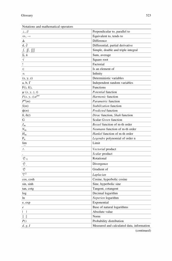
Notations and mathematical operators

⊥, // Perpendicular to, parallel to

,,! Equivalent to, tends to

Δ Difference

d, ∂ Differential, partial derivativeR,RR,ÐÐÐ

Simple, double and triple integral

Σ, a Sum, average

√ Square root

! Factorial

2 Is an element of

/ Infinity

(x, y, z) Deterministic variables

a, b, Γ Independent random variables

F(), f(), Functions

ψ (x, y, z, t) Potential function

F(x, y, z).ejωt Harmonic function

Pα(m) Parametric function

S(m) Stabilization function

ϕ(m) Predicted function

δ, δ(t) Dirac function, Shah function

G Scalar Green function

Jm Bessel function of m-th order

Nm Neumann function of m-th order

Hm Hankel function of m-th order

Pn Legendre polynomial of order n

lim! Limit

^ Vectorial product

. Scalar product

~∇^ Rotational

~∇: Divergence

~∇ Gradient of

∇2 Laplacian

cos, cosh Cosine, hyperbolic cosine

sin, sinh Sine, hyperbolic sine

tan, cotg Tangent, cotangent

log Decimal logarithm

ln Neperien logarithm

e, exp Exponential

e Base of natural logarithms

| | Absolute value

k k Norm

P() Probability distribution

d, g, I Measured and calculated data, information

(continued)

Glossary 523

Notations and mathematical operators

e, ~e Error, parameter, error vector

P{} Probability

f(m|I ), P(X) Probability distribution

* Convolution product

Definition of the Vector Operators (Gradient, Divergence,Rotational, Laplacian)

– The gradient operator transforms a scalar function into a vector function. The

gradient vector ~∇ψ of a scalar field ψ in a given direction corresponds to the

partial derivative of ψ in this direction.

In a system of rectangular coordinates (x, y, z), axes of unit vectors ~i;~j; ~k

, it is

defined by its projections such that:

~∇ψ ¼ ∂ψ∂x

~iþ ∂ψ∂y

~jþ ∂ψ∂z

~k

This vector is then the variations of a scalar quantity in a given direction.

– The divergence operator ~∇:~a of a vector~a at any point in the space correspondsto the flux variation dϕ of this vector relative to an elementary volume dv

containing the point. This flux passes through the closed surface which delimits

this volume such that:

~∇:~a ¼ limdv!0

dϕdv

In a system with rectangular coordinates (x, y, z), its expression as a function of thevector projections ~a becomes:

~∇:~a ¼ ∂ ~ax∂xþ ∂ ~ay

∂yþ ∂ ~az

∂z

524 Glossary

– The rotational operator ~∇ ^~a of a vector~a in a given direction d~l corresponds tothe limit of the movement ~a (c) around the surface d~s normal at d~l when d~sapproaches zero, such that:

~∇ ^~a ¼ limds!0

Icð Þ~a:d~l

In a system with rectangular coordinates (x, y, z), axes of unit vectors ~i;~j; ~k

, its

expression is equivalent to:

~∇ ^~a ¼ ∂ ~az∂y� ∂ ~ay

∂z

� �~iþ ∂ ~ax

∂z� ∂ ~az

∂x

� �~jþ ∂ ~ay

∂x� ∂ ~ax

∂y

� �~k

– The Laplacian operator∇2 is applied to scalar and vectorial fields and is equal to

∇:∇. It is used to resolve the Laplace equation (∇2 ¼ 0), the Poisson equation

or the wave equation. It is given in Cartesian or rectangular coordinates (x, y, z)by the expression:

∇2 ¼ ∂2

∂x2þ ∂2

∂y2þ ∂2

∂z2

Depending on the case to solve, it can be also expressed in polar, cylindrical or

spherical coordinates.

For vectorial analysis, see, for example, the work of Professor H. Skilling

(1942): Fundamentals of Electric Waves, Ed Wiley (pp. 10–36) or that of Professor

E. Durand (1964): Electrostatique. Volume 1. Distributions. Masson Ed. Chap. 2, or

that of G. Goudet (1956): Electricity. Masson Ed.

Glossary 525

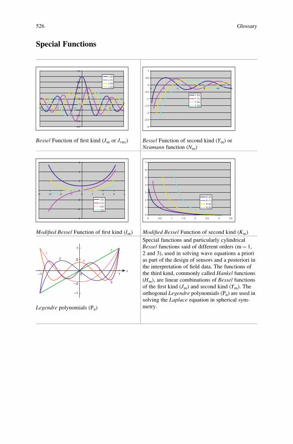
http://dx.doi.org/10.1007/978-3-319-45355-2_2

Special Functions

1.2

1

0.8

0.6

0.4

0.2

0

–0.2–2–7–12 3

–0.4

–0.6

–0.8

J (0)

J (1)

J (2)

J (3)

8

Bessel Function of first kind (Jm or J(m))

0 2 4

1

0.5

0

–0.5

–1

–1.5

–2

–2.5

–3

Y (0)

Y (1)

Y (2)

Y (3)

6 8 10 12

Bessel Function of second kind (Ym) orNeumann function (Nm)

–2 I (0)

I (1)

I (2)

I (3)

–4 –3 –2 –1 0

0

–4

–6

2

4

6

1 2 3 4

Modified Bessel Function of first kind (Im)

K (0)

K (1)

K (2)

K (3)

7

6

5

4

3

2

1

0

0 0.5 1 1.5 2 2.5 3 3.5

Modified Bessel Function of second kind (Km)

2

34

5

1

–1

–.5

.5

1

0–1 1x

Legendre polynomials (Pn)

Special functions and particularly cylindrical

Bessel functions said of different orders (m¼ 1,

2 and 3), used in solving wave equations a priori

as part of the design of sensors and a posteriori in

the interpretation of field data. The functions of

the third kind, commonly called Hankel functions(Hm), are linear combinations of Bessel functionsof the first kind (Jm) and second kind (Ym). Theorthogonal Legendre polynomials (Pn) are used in

solving the Laplace equation in spherical sym-

metry.

526 Glossary

Index

AAbacus(es), 316, 500

Absence of errors, 194

Absolute error, 194

Absolute measure magnetometers, 62

Accuracy, 195, 216

Acoustic survey, 60

Acoustic waves, 6

Acquisition frequency, 287

Active detection, 255

A/D converter, 288

Ag/AgCl electrodes, 245

Against-electromotive force, 269

Air guns, 120

Airspace, 237

Air waves, 158, 171, 172, 179, 270

Alternating current methods, 54, 55, 152,

444, 465

Amagnetic, 284

Ambient noise, 100, 188

Ampere’s theorem, 57

Amplifier(s), 34

Amplifier(s) chains, 246

Amplitude offset, 260

Analog models, 363

Analog multiplier, 266

Analytical methods, 44, 66, 326

Analytical resolutions, 184

Angular frequency, 84, 153

Anhydrites, 8, 111

Anisotropic magnetoresistance (AMR), 284

Anisotropy, 118, 142, 343, 446, 458

Anisotropy effect, 118

Anisotropy matrix, 117

Anodes, 200

Antenna, 164, 186

Anthropogenic factors, 187

Anti-aliasing filter, 287

Anticline, 8

Apparent conductivity, 109, 311

Apparent resistivity, 63, 65, 88, 90,

324, 497

Aquifer rocks, 11

Arctic, 6

Arctic Ocean, 3, 28

Arctic regions, 137, 396

Arctic seas, 3

Arctic territories, 406

Arctic zones, 298

Artificial current, 456

Artificial fields, 17

ASIC electronic conditioner, 298

Asthenosphere, 32

Atmosphere, 105

Atmospheric storms, 236

Attenuation, 77

Autocorrelation, 291

Autonomous underwater vehicle, 299

Azimuthal electric field, 97

BBackground noise, 34, 180, 187, 244,

262, 295

Basalt plateaus, 111

Bathymetry, 195, 222

Bathyscaphe, 28, 237

Bayesian inverse problem, 354

Bayesian method, 353

Bayes’ theorem, 353, 360



Bedrock, 89, 98

Bessel functions, 327

Biases, 116

Biaxial inclinometer, 285

Biaxial measurements, 193

Boltzmann’s constant, 267Boreholes, 18

Boundary conditions, 80, 341, 483, 491, 499

Boundary elements method (BEm), 323

Broadband amplifier, 263, 264

Broadside array, 77

Broadside configuration, 97

CCagniard impedances, 109, 285

Calcareous sandstone, 7

Calibration, 194, 339

Canonic models, 468

Capacitance, 465

Capacity, 465

Capture effect, 258

Carbonates, 111

Carrots, 60

Catagenesis, 9

Cathodic protection, 203, 388

Cementation factor, 140, 142

Cemented detritus rock, 141

Channeling effect, 164

Charge distributions, 63

Chemical potential gradient, 68

Chopper amplifier, 249

Circular polarizer, 277

Clays, 8

Coastal, 188

Coastal areas, 395, 405

Coastal auscultation, 64

Coastal effect, 204

Coastal geology, 113

Coastal plain, 14

Coherent noise, 194

Cohesion factors, 393

Combined effects, 54

Compute Unified Device Architecture

(CUDA), 362

Computing method, 258

Conduction currents, 56, 71, 439, 444, 446, 467

Conduction phenomena, 59

Conductive anomaly, 65

Conductivity, 56, 67, 134

Conductivity of seawater, 136

Continuity conditions, 494

Continuity factors, 394

Continuous current, 53, 55, 431

Continuous current methods, 60

Continuous domain, 98

Continuous electronic voltmeter, 112

Continuous spectrum, 265

Conventional electrometers, 260

Convolution, 291, 292

Convolution filters, 169

Convolution product, 292

Correction algorithms, 116

Corrosion, 71, 267, 388

Corrosion currents, 203

Coulomb force, 256

Coulomb’s law, 66, 444Cover rocks, 8, 9

Cracked dolomite, 7

Cross-well, 277

Crystalline rock, 147

Current density, 56, 67, 116, 154, 193, 201,

388, 464

Current density electrometer (CDE), 221, 257,

270, 298

Current density vector

electrometers, 255

Current dipole, 495

Current distribution, 462, 463

Current loop, 189

Cutoff frequency, 165, 265, 274

Cuttings, 60

Cylindrical coordinates, 478

DData inversion processing, 99

DC potential, 245

Declination, 284

Declinometers, 63

Decomposition methods, 291

Deep geomagnetic survey, 104

Deep structures, 111

Demodulator, 188

Density, 18, 144

Density logs, 379

Depolarization current, 65

Depth of investigation, 149

Depth of penetration, 150

Detection accuracy, 173, 261

Detection sensitivity, 155

Detection strategy, 189

Detection windows, 175

Deterministic, 102

Deterministic approaches, 352

Deterministic physical laws, 311

Detrital rock, 89

Diagenesis, 7, 9

528 Index

Diapirs, 13

Dielectric constant, 57, 465

Dielectric displacement, 435

Dielectric permittivity, 80, 133, 145, 169,

177, 435

Differential aeration, 112

Differential amplifier, 247, 261, 264

Differential invariants, 487

Differential pressure, 112

Diffusion equation, 83, 439

Diffusion equation in the frequency domain, 99

Diffusion physics, 81

Diffusion term, 81

Digital/analog converter, 265

Digital signal processing, 100

Dipole–dipole, 477, 482

Dipole moment, 97, 186, 229

Dipole sources, 417

Dirac comb, 287

Dirac function, 69

Direct current (DC), 52

Direct hydrocarbon indicator (DHI), 404

Direction, 160

Direct methods, 38

Direct prospecting, 13, 14

Direct prospecting methods, 5

Direct waves, 115, 166

Dirichlet boundary conditions, 259

Dirichlet limit conditions, 117

Dirichlet problem, 315

Discretization, 506

Displacement current, 58, 59, 71, 439, 466, 467

Displacement current density, 466

Displacement of electrons, 134

Dissipative effects, 15

Distortion, 276

Distribution, 59

Diving saucer, 237

Dosage method, 136

Downhole logging, 112

Down waves, 167

Dyadic Green’s function, 343Dynamic data, 267

Dynamic error, 194

EEarth physics, 34

Earthquakes, 188

Earth’s crust, 456Earth’s magnetic field, 24, 27, 188

Echo sounder, 293

Eddy current, 60, 73, 147, 254

Effective power, 224

Effects of bathymetry, 157, 204

Effects of errors, 194

Efficiency, 102, 235

Einstein convention, 344

Elastic properties, 11

Elastic constants, 138

Elasticity, 18, 144

Electrical charges, 56

Electrical conduction, 72

Electrical conductivity, 11, 57, 84

Electrical discontinuities, 65

Electrical energy, 51

Electrical methods, 11, 15, 17

Electrical panels, 99

Electrical resistivity, 18, 177

Electric charge, 435

Electric current, 381, 458

Electric dipole, 462

Electric field, 28, 42, 56, 58, 67

Electric soundings, 103

Electrochemical couples, 24

Electrochemical noise, 245

Electrochemical reactions, 269

Electrodynamic noise, 296

Electrofacies, 142

Electrokinetic current, 203

Electrokinetic energy, 56

Electrokinetic potential, 69

Electrolyte, 53, 112

Electrolytic conduction, 139

Electromagnetic energy, 82

Electromagnetic fields, 24

Electromagnetic induction, 71, 72

Electromagnetic loops, 62

Electromagnetic methods, 9

Electromagnetic noise, 85, 122, 158, 197, 207,

221, 381

Electromagnetic propagation, 71

Electromagnetic waves, 30, 152, 432

Electrometer calibration, 194

Electrometers, 22, 34, 63, 103, 221, 241, 301

Electromotive forces, 66, 253, 463

Electronic conduction, 53, 134, 227

Electronic inverter, 274

Electronic methods, 258

Electronic multiplier, 274

Electronic noise, 34, 219

Electrons, 56, 70

Electrostatic fields, 56, 253, 338, 444

Electrotelluric, 38

Electrotelluric method, 38, 103, 104, 107, 324

Ellipses of polarization, 251

Index 529

Energy absorption, 100

Energy dissipation, 83

Energy transfer, 64, 71, 131

Entropy, 290

Equation of Helmholtz, 239

Equation of Lippmann–Schwinger type, 343

Equations of Maxwell, 58

Ergodic noise, 187

Error minimization, 118

Errors, 194

Evaporites, 8, 111

FFacies, 7, 19, 139

Facies variations, 11

Faraday’s constant, 245Faraday’s law, 57Far field, 154

Far field criterion, 153, 230, 432

Fast Fourier transform, 204

Fault, 8

Fault tree, 216

Feasibility index, 198

Feedback field, 283

Feedback loop, 264

Ferromagnetic materials, 133

Fiber cables, 398

Field of force, 14, 241

Field vector, 75

Finite differences code, 118

Finite differences method (FDm), 323

Finite elements method (FEm), 323

Finite surface/volume integration

technique (FIt), 323

Floating anchor, 222

Floating input amplifier, 247

Formation factors, 139

Forward modeling, 297

Forward problem, 99, 118, 184, 317, 338, 467

Fourier analysis, 432

Fourier integrals, 506

Fourier series, 327

Fourier transform, 99, 226, 291, 292, 432, 505

Fractured rocks, 53, 140

Frechet derivative, 157

Frequency, 99

Frequency approximation, 459

Frequency band, 267

Frequency bandwidth, 100, 192

Frequency domain, 94, 155, 432, 466, 498,

505, 506

Frequency effect, 165

Frequency reference, 265

Frequency spectra, 107

Freshwater aquifers, 405

Fundamental frequency, 236

GGalilean transformation, 444

Galvanic cell, 112

Galvanic contribution, 334

Galvanic current, 58, 189

Galvanic effect, 54, 65, 67, 73,

122, 381

Galvanic field, 190

Galvanic methods, 52

Galvanic sources, 75

Galvanometers, 457

Gaps, 115

Gas-cap system, 393

Gas hydrates, 190, 405

Gas reservoir, 141

Gaussian distribution, 350

Gaussian function, 291

Gauss law, 187

Gauss/Newton-type optimization, 350

Gauss separation, 104

General wave equation, 83

Geodynamic processes, 7

Geoelectric model, 482

Geographically invariant, 105

Geological canonic model, 314

Geological techniques, 4

Geomagnetic deep sounding (GDS), 104

Geomagnetic equator, 234

Geomagnetic field, 203, 237

Geomagnetic usual unit, 234

Geometric divergence, 166

Geometric model, 396

Geophysical prospecting, 5

Geophysical techniques, 4

Giant magnetoimpedance (GMI), 284

Giant magnetoresistance (GMR), 284

Gitological context, 14

Global geodynamics, 34

Global positioning system (GPS), 222

Gradient, 184

Graphic processor unit (GPU), 362

Graphite, 14

Gravimetry, 119

Ground-penetrating radar (GPR), 152, 434

Group speed, 100, 177

Guard electrodes, 86

Guided waves, 164

530 Index

HHankel transforms, 315

Hard rock, 89

Harmonic current, 230

Harmonic regime, 153, 176

Harmonic variation, 79

Hazard, 3

Helmholtz coils, 282

Helmholtz’s equation, 81, 148, 170, 320Hertz potential vector, 314

Heuristic approaches, 352

High closure, 8

High frequency methods, 38

High pass filter, 266

Homodyne detection, 216, 273

Horizontal anisotropy, 379

Horizontal contrasts, 54, 73

Horizontal electric dipole (HED), 97, 223

Horizontal field, 105, 186, 499

Horizontal resistivity, 91

HSE standards, 120

Hummel values, 476

Hydraulic permeability, 139

Hydrocarbon detection, 91

Hydromechanical conditions, 138

Hydro static level, 112

Hydrostatic pressure, 139

Hydrothermal ore deposits, 396

Hypsometric quotation, 379

Hypsometric ratings, 393

IIgneous rocks, 78

Images method, 327

Impedance, 228, 465

Imperfect dielectrics, 52

Impermeable rock, 8

Impregnation fluid, 60

Indirect methods, 5, 38

Indirect prospecting, 11

Induced currents, 189, 434

Induced effect, 14, 59

Induced electric currents, 28

Induced fields, 35

Inductance, 228

Induction vectors, 78

Inductive effect, 52, 54, 58, 71, 77, 155

Inductive methods, 38

Inductive shift, 73

Inductive sources, 75

Initial conditions, 79, 319, 322, 341, 432

Injected current, 461

In-line acquisition, 310

In-line inspection, 388

In-line and broadside measurements, 93

In-line array, 77

In-line configuration, 97, 334

Input impedance, 112

Instrumental method, 258

Instrumentation amplifier, 244, 245

Instrumented pig, 388

Insulated gate bipolar transistor (IGBT), 224

Integration method, 233

Interface waves, 166

Interfacial polarization, 148

Interpretation model, 363, 381

Interpretive model, 379

Interstitial water, 139, 141

Invariants, 5, 59

Inverse problem, 316, 324, 467

Inversion data methods, 102

Inversion method, 20, 44, 347

Ionosphere, 105, 233, 236

Ions, 70

Isometric anomaly, 500

Isometric models, 321

Isotropic conductors, 56

Iterations, 340

Iterative methods, 354

JJohnson noise, 245, 266

Joule effect, 56, 83, 147, 190, 227, 233

KKarsts, 111

Kelvin effect, 73, 149

LLaplace equation, 56, 69, 321, 334,

338, 487

Laplace force, 254

Large scale, 20

Lateral anisotropy, 93

Lateral conductivity, 105, 117

Lateral exploration, 60

Lateral resistivity contrasts, 100

Layered models, 468

Leak detection, 90

Least squares method, 334, 350, 354

Lightning, 236

Light spectrum, 267

Index 531

Limit conditions, 56, 117, 170, 315, 322, 432,

434, 441

Linear detector, 290

Linearity, 216

Linear sensor, 188

Lithological discontinuities, 9

Lithology, 19, 139, 143

Lithosphere, 107, 134

Littoral, 188

Local conditions, 68

Lock-in detection, 273

Logging tools, 242, 276

Long base horizontal, 218

Longitudinal conductance, 88

Longitudinal resolution, 251

Lorentz force, 253

Low closure, 8

Low frequency, 217

Low frequency approximation, 153, 485

Low noise electronic, 34

Low noise preamplifiers, 247

Low pass amplifiers, 247

Low pass filter, 274

Low pass passive filters, 265

MMagnetic field, 28, 36, 78

Magnetic induction, 58, 435

Magnetic methods, 106

Magnetic permeability, 11, 57, 84, 145, 435

Magnetic resonance

magnetometers, 277

Magnetic rocks, 14

Magnetic storms, 103, 233

Magnetic toroidal type, 93

Magnetic waves, 105

Magnetometers, 63

Magnetometric resistivity, 30

Magnetosphere, 233

Magnetotelluric, 38

Magnetotelluric method, 15, 28, 103, 104, 106

Mantle conductivity, 32

Marine biology, 121

Marine controlled source electromagnetic

sounding (mCSEM), 22

Marine differential magnetic sounding (mDM),

22

Marine direct current sounding (mDC), 22

Marine fauna, 121

Marine magnetotelluric sounding (mMT), 22

Marine spontaneous polarization (mSP), 22

Markov chain, 354

Marls, 8

Mathematical algorithms, 317

Mathematical model, 458, 495

Maxwell displacement current, 466

Maxwell’s equations, 78, 80, 94, 105, 108, 170,180, 343, 435, 498, 503

Maxwell terminology, 70

Maxwell–Wagner effect, 148

Measure correction, 339

Measurements, 299

Measure of entropy, 290

Metal electrodes, 56

Metallic sulfide deposits, 381

Metallogenic context, 14

Metamorphism, 14

Methods of errors assessment, 174

Microprocessors, 226, 287

Microseismic monitoring, 394

Microvoltmeter, 219

Migration, 9

Mining exploration, 35

Modeling methods, 315

Monitoring, 4, 277, 378, 379, 394

Monotonous layers, 14

Monte Carlo method, 226, 352

Moore’s law, 362MOSES method, 29

Motion reference unit (MRU), 293, 294

Movement of ions, 134

Moving magnet variometers, 105

MT audio, 107

MTBF, 216

Mud logs, 60

Multifrequency acquisition, 389

Multiple-azimuth seismics, 39

Multipole panels, 398

Multitransient currents (mMTEM), 102

NNarrow band amplifier, 265, 266

Natural currents, 456

Nernst equation, 245

Nernst potential, 269

Neumann boundary conditions, 259

Newton/Gauss method, 356

Newtonian potential, 496

Noise, 299

Noise level, 187, 188, 192

Nonlinear medium, 259

Nonpolarizing electrode, 244

Normalized amplitude, 198

Nuclear resonance magnetometers, 277

532 Index

Numerical algorithms, 328

Numerical analysis, 341

Numerical calculation, 316

Numerical codes, 323

Numerical form, 329

Numerical integrations, 315

Numerical methods, 67, 102, 315

Numerical models, 233, 363, 379

Numerical packs, 334

Numerical resolution, 317

Numerical resolution methods, 259

Numerical simulations, 312

Numerical software, 340

Nyquist noise, 266

Nyquist frequency, 287

Nyquist-Shannon sampling criterion, 287

OOccam algorithm, 381

Occam’s razor, 360Ocean Bottom Magnetometer, 90

Oceanic crust, 34

Oceanic current, 28

Oceanic phenomena, 218

Offset, 115, 179

Offset compensators, 101

Ohmic resistive force, 254

Ohm-meter, 135

Ohm’s law, 60, 79, 202, 329Oil rocks, 11, 52

Operational amplifier, 246

Optical coupler, 274

Optical pumping magnetometers, 277

Optimization, 325

Opto-isolator, 274

Ore bodies, 54

Ore deposits, 405

Organicmatter, 9

PParsimony principle, 360

Passive methods, 104

Perfect gas constant, 245

Periodic currents (AC), 432

Permeability, 7, 19

Permeable rock, 8, 134

Permittivity, 59

Petromechanical models, 398

Petrophysics, 4, 8, 144

Phase comparator, 280

Phased array, 398

Phase detector, 261

Phase difference, 115, 154

Phase locking loop, 280

Phasemeter, 280

Phase shift, 77, 109, 116, 168, 274, 330, 433

Pipelines, 234, 388

Planck’s constant, 267Planck’s law, 267Plane wave, 154, 160, 176, 239

Plan of polarization, 433

Plate tectonics, 28

Plurivocal problem, 60

Poisson equation, 56, 95, 321

Polarization, 14, 27, 83, 160

Polarization cells, 203

Polarization currents, 64

Polarization effects, 98

Polarization ellipse, 60, 185, 186

Polarization mechanisms, 66

Polarization of the electrodes, 64

Polarization phenomena, 59, 244

Polarization potential difference, 245

Polarization transverse modes, 163

Porosity, 7, 19, 60, 138, 379

Porous layer, 112

Porous matrix, 53, 142

Porous rocks, 142

Potential difference, 75, 193

Potential difference electrometers,

221, 242

Potential fields, 56

Potential function, 488

Potential gradient, 454

Potentials continuity, 492

Potentiometric method, 34

Power amplifier, 225

Power factor, 224

Power thyristors, 224

Power transistors, 224

Precision, 195

Precision Time Protocol, 225

Precison instrumentation amplifier, 247

Predefined model, 381

Predicted field, 359

Predictive techniques, 360

Pressure, 137

Primary field, 65, 502

Principle of reduction, 471

Priori model, 360

Prismatic model, 360

Probability of detection, 290

Productive trap, 403

Propagation, 59

Index 533

Propagation equation, 439

Propagation factor, 82, 164, 166

Propagation physics, 81

Propagation speed, 100

Propagation term, 81

Pulsation, 153

Pulse, 180

Pulse sampling, 100

QQuadratic detector, 188

Quadratic norm, 350

Quadrupole type Wenner/Schlumberger

arrays, 86

Quality assurance, 205

Quality control, 205

Quantitative calibration, 60

Quasistatic approximation, 30, 79, 90, 315,

329, 459, 468

Quick look interpretation, 296

Quotient-meter, 135

RRadioactive properties, 11

Radial current, 462

Radiation pattern, 231–232

Radioelectric waves, 82

Radiofrequency range, 267

Radio waves, 15

Random errors, 194

Random processes, 352

Rapid run variometers, 278

Rare-earths deposits, 405

Raw data, 296

Reactance, 465

Read-only memory (ROM), 251, 378

Realistic model, 381

Reciprocity theorem, 97, 327, 359

Record factor, 134

Recurrence relation, 476, 497

Redox potentials, 112

Reference frequency, 100

Reference signal, 274

Reflected waves, 15, 101, 166

Reflection coefficient, 502

Refracted waves, 164, 166

Refraction methods, 119

Refraction seismic, 164

Rejection filter, 112, 187

Relaxation, 83, 148

Relief of the seabed, 89

Repeatability, 195

Reservoir acidification, 393

Reservoir rock, 7, 379

Residual field, 359

Resistance, 465

Resistance noise, 259

Resistant rocks, 309

Resistive anomaly, 65

Resistivity, 60, 66, 68, 134

Resistivity contrast, 11, 63

Resistivity method, 64, 87

Resolution, 152

Resonance frequency, 165, 236

Resonator, 165

Rheographic basin, 363

Rheostatic tank, 319, 363, 486

RISE project, 29

Rubidium vapor, 277

SSacrificial anode, 388

Salinity, 137

Salt dome, 8, 111, 119

Sampling electrodes, 276

Sampling frequency, 251, 287

Saturation factor, 142

Saturation index, 120

Scalar magnetometer, 278

Scalar potential, 184

Scale factor, 185, 317

Schlumberger methods, 13

Schlumberger-type

arrangements, 477

Schumann resonance, 218, 233

Seabed electrometers, 270

Seabed ocean currents, 202

Seaboard effect, 26

Seaside effect, 218, 235

Seawater conductivity, 259

Secondary field, 65, 502

Sedimentary basins, 5

Sedimentary rocks, 7, 53, 138

Sedimentary sequences, 19

Sedimentation, 9

Sediment porosity, 140

Seismic analysis with offset (AVO), 404

Seismic method, 15, 17

Seismic reflection, 5, 13, 14, 101

Seismic reflection method, 14

Seismic sections, 378

Seismo-electric effect, 404

Self-potential mechanism, 112

Sensitivity, 192, 216, 219, 259

Sensitivity matrix, 350

534 Index

Separate currents, 443

Shah function, 287

Short base devices, 218

Side-scan sonar, 293

Signal-to-noise (S/N) ratio, 85, 180, 216

Sine waves, 226

Sinusoidal current, 465

Sinusoidal wave, 225

Sinusoidal waveforms, 100

Skin depth, 77, 149, 150

Skin effect, 15, 30, 32, 60, 73, 147

Smaller scale, 20

Snell-Descartes law, 161

SOFAR, 120

Solar flares, 103

Solid matrix, 138

Sommerfeld integrals, 315

Sommerfeld radiation condition, 344

Sounding, 99

Sound waves, 404

Source rock, 7

Sparkers, 120

Special functions, 483

Specific conductivities, 311

Specific polarization, 168

Specific resistivities, 63

Spectral analysis, 264

Spectrum analyzer, 269, 364

Speed, 100

Speed of propagation, 177

Spherical coordinates, 231

Spherical current, 463

Spherical divergence, 83

Spherical wave guide, 236

Spontaneous polarization (SP), 14, 112, 327

Spreading factor, 439

Square-shaped waves, 225

Stacking, 101

Standardization, 194

Static approximation, 56, 69, 444

Static shift, 65, 73

Stationary currents, 442

Stationary models, 487

Statistical dependence, 291

Statistical methods, 194

Statistical treatment, 187

Stochastic approaches, 352

Stochastic analysis, 367

Stochastic methods, 351

Stochastic optimization processes, 102

Stokes’ theorem, 254

Stratigraphic correlations, 5

Stratigraphic transitions, 9

Stray currents, 203

Streamer, 6, 116, 120, 255, 298–299

Streamer cables, 242

Structural geophysics, 5

Structural model, 387

Structural traps, 8

Submarine detection, 221

Submersible fish, 221

Sub-outcropping limestone slabs, 111

Subsidence, 394

Subsurface exploration, 38

Subsurface rocks, 146

Surface currents, 442

Surface waves, 91, 158, 171, 175, 290

Sweep, 180, 225

Symmetry current, 463

Synchronous demodulation, 247

Synchronous detector, 185, 247, 273, 282

Synthetic aperture antennas, 398

Synthetic aperture sonar (SAS), 293

Synthetic responses, 324

TTabular model, 321, 468

Tectonics, 5

Tectonophysics, 111

Telluric currents, 28, 453, 456

Telluric fields, 28

Telluric method, 38, 121, 152

TEM mode, 93

Temperature, 137

Theoretical models, 367

Thermal noise, 249, 266

Thermodynamic process, 7

Tidal waves, 406

Time domain, 99, 171, 175, 180, 293, 311, 320,

328, 330, 341, 343, 432, 466

Time effect, 165

Time-lapse technique, 277

Time of flight (ToF), 100

Topography, 89

Tortuosity factor, 140, 142

Total conductance, 110

Total current, 460

Total field, 34, 59, 63, 167, 241, 278, 464,

506, 508

Tow-fish, 222

Transient currents (t-mEM or mTEM), 102

Transient domain, 99

Transient electromagnetic technics, 161

Transient fields, 105

Transient methods, 311

Index 535

Transistors, 34

Transit time, 100

Transmitted power, 229

Transmitted waves, 96

Transverse anisotropy, 117

Transverse electric field (TE mode), 94, 96, 97,

221, 243, 501–502

Transverse magnetic field (TM mode), 94, 96,

97, 314

Transverse resistance, 74

Trapping, 9

Traps, 7, 13

Triaxial magnetometer, 193, 277

Triaxial measurements, 193

UUltra Low Frequencies (ULF), 39

Underground storage, 221

Underwater detection, 35, 218

Underwater sonar, 388

Uniform field, 153, 337, 444

Unpolarizable electrode, 112, 244–245

Up fields, 168

Up waves, 167

VVariable currents, 55, 365, 434

Variable depth investigation, 88

Variable gain amplification, 266

Variometers, 63

Vector electrometer, 260

Vectorial electrometer, 272

Vectorial magnetometer, 22, 286

Vector sensors, 115

Vertical currents, 73

Vertical dipoles (VED), 97, 102

Vertical electric field, 97

Vertical exploration, 38, 59

Vertical field, 243, 335

Vertical gradients, 118

Vertical investigation, 18

Vertical magnetic dipole, 221

Vertical resistivity, 91

Very low frequencies (VLF), 39

VLF currents, 83

Volcanic rocks, 145

Volume waves, 166

Vortex effect, 75, 91, 97, 122, 144,

155, 337

WWalk-away, 277

Walkaway vertical seismic profile, 390

Water-drive system, 393

Water-saturated rocks, 139

Wave guide, 164

Wavelength, 160

Waves gravity, 188

Well logging, 112, 349

Well-logging techniques, 4

Well stimulations, 393

Wenner, 477

Wheatstone bridge, 135

Wildcat, 3, 276

Work frequency, 164, 259

ZZeeman states, 277

Zinc anodes, 388

536 Index

General Conclusion and Perspectives - Springer978-3-319-45355-2/1.pdf · General Conclusion and Perspectives ... at sea and on land, has relied very readily on geological

Documents