Free vibrations of an uncertain energy pumping system

Contents lists available at ScienceDirect

Journal of Sound and Vibration

Journal of Sound and Vibration 332 (2013) 6815–6828

0022-46http://d

n CorrE-m

journal homepage: www.elsevier.com/locate/jsvi

Free vibrations of an uncertain energy pumping system

Edson Cataldo a,n, Sergio Bellizzi b, Rubens Sampaio c

a Universidade Federal Fluminense, Applied Mathematics Department and Graduate program in Telecommunications Engineering,Rua Mário Santos Braga, S/N, Centro, Niteroi, RJ, CEP: 24020-140, Brazilb LMA, CNRS, UPR 7051, Centrale Marseille, Aix-Marseille Univ, F-13402 Marseille Cedex 20 Francec PUC-Rio, Mechanical Engineering Department, Rua Marquês de São Vicente, 225, Gavea, Rio de Janeiro, RJ, CEP: 22453-900, Brazil

a r t i c l e i n f o

Article history:Received 22 January 2013Received in revised form5 July 2013Accepted 17 August 2013

one nonlinear subsystem, the so-called NES (nonlinear energy sink). Three parameters of

Available online 12 September 2013

0X/$ - see front matter & 2013 Elsevier Ltd.x.doi.org/10.1016/j.jsv.2013.08.022

esponding author. Tel.: þ55 2196318344.ail addresses: [email protected] (E. Cataldo)

a b s t r a c t

The aim of this paper is to study the energy pumping (the irreversible energy transferfrom one structure, linear, to another structure, nonlinear) robustness considering theuncertainties of the parameters of a two DOF mass-spring-damper, composed of twosubsystems, coupled by a linear spring: one linear subsystem, the primary structure, and

the system will be considered as uncertain: the nonlinear stiffness and the two dampers.Random variables are associated to the uncertain parameters and probability density func-tions are constructed for the random variables applying the Maximum Entropy Principle.A sensitivity analysis is then performed, considering different levels of dispersion,and conclusions are obtained about the influence of the uncertain parameters in therobustness of the system.

& 2013 Elsevier Ltd. All rights reserved.

1. Introduction

Energy pumping (EP) refers to a mechanism in which energy is transferred in an one-way irreversible fashion from asource to a receiver. In the context of passive vibration control of mechanical systems, it can be used to develop a nonlineardynamic absorber. In this case, the energy pumping occurs from the main, or primary, structure, which needs to beprotected, to the nonlinear absorber coupled with it. The nonlinear absorber, also named Nonlinear Energy Sink (NES),consists of a mass with an essential nonlinear spring. This concept involves nonlinear energy interactions which occur dueto internal resonances making possible irreversible nonlinear energy transfers from the primary system to the attachment.The nonlinear energy pumping in nonlinear mechanical systems was first described in [3,17]. An important characteristicof the nonlinear dynamic absorber should be highlighted: since the NES is essential nonlinear, this system has no (or verysmall) natural frequency and it is effective for a large range of frequencies, while the linear absorbers attenuate well onlyone frequency. The linear system to which the NES is attached has, of course, a natural frequency. A complete description ofthe energy pumping phenomenon can be found in [18].

The energy pumping phenomenon has been studied extensively in deterministic frameworks including theoretical,numerical and experimental investigations. Very few studies have been devoted to analyze it in stochastic cases. Stochasticitywas taken into account to discuss the robustness of energy pumping. In [7], the robustness of a nonlinear energy sink duringtransient regime was analyzed assuming various parameters as Gaussian random variables and using polynomial chaosexpansion. In [14], the robustness was considered with respect to the initial condition and external excitation forces. Assuming

All rights reserved.

, [email protected] (S. Bellizzi), [email protected] (R. Sampaio).

E. Cataldo et al. / Journal of Sound and Vibration 332 (2013) 6815–68286816

Gaussian initial condition and white-noise excitation forces, the problem was analyzed solving the associated Fokker–Planckequation. In [13], a general linear system connected with an essentially nonlinear attachment in the presence of stochasticexcitation to both the linear system and the nonlinear attachment and with random initial conditions was considered. Theproblem was analyzed combining the complexification-averaging technique and solving the Fokker–Planck–Kolmogorovequation associated to the slow dynamics of the system.

In this paper, uncertain parameters are considered and random variables are associated to them as in [7]. However, thecorresponding probability density functions are constructed using the Maximum Entropy Principle [9]. This principle statesthat out of all probability density distributions consistent with the given set of available information, the one with themaximum uncertainty (entropy) must be chosen. Next, the robustness is investigated from the probabilistic properties ofsome quantities that measure the transfer of energy between the primary system to the NES. We focus on the ratio of thesum of the energy stored and energy dissipated in the primary system and sum of the energy stored and energy dissipatedin the NES. This ratio can be related to the percentage of energy dissipated by the NES.

This paper is organized as follows: in Section 2, the deterministic model used to study the energy pumping phenomenonis introduced and the energy quantity used to analyze the transfer of energy is described. The stochastic approach used isdescribed in Section 3. In Section 4, the robustness of the system is discussed taking into account the uncertainties of theparameters. A special case, considering the situation where the maximum of the energy pumping is obtained, is showed inSection 5. Finally, in Section 6 conclusions are outlined.

2. The deterministic model used

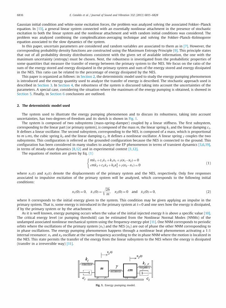
The system used to illustrate the energy pumping phenomenon and to discuss its robustness, taking into accountuncertainties, has two-degrees-of-freedom and its sketch is shown in Fig. 1.

The system is composed of two subsystems (mass-spring-damper) coupled by a linear stiffness. The first subsystem,corresponding to the linear part (or primary system), is composed of the massm, the linear spring k1 and the linear damping c1.It defines a linear oscillator. The second subsystem, corresponding to the NES, is composed of a mass, which is proportionalto m ðϵmÞ, the cubic spring k2 and the linear damping c2. It defines a nonlinear oscillator. A linear spring γ couples the twosubsystems. This configuration is referred as the grounded configuration because the NES is connected to the ground. Thisconfiguration has been considered in many studies to analyze the EP phenomenon in terms of transient dynamics [3,6,19],in terms of steady-state dynamics [8,12] and in experimental context [1,12].

The equations of motion are given by Eq. (1)

m €x1þc1 _x1þk1x1þγðx1�x2Þ ¼ 0ϵm €x2þc2 _x2þk2x32þγðx2�x1Þ ¼ 0

((1)

where x1ðtÞ and x2ðtÞ denote the displacements of the primary system and the NES, respectively. Only free responsesassociated to impulsive excitation of the primary system will be analyzed, which corresponds to the following initialconditions:

x1ð0Þ ¼ 0; _x1ð0Þ ¼ffiffiffiffiffiffi2hm

r; x2ð0Þ ¼ 0 and _x2ð0Þ ¼ 0; (2)

where h corresponds to the initial energy given to the system. This condition may be given applying an impulse in theprimary system. That is, some energy is introduced in the primary system at t¼0 and one sees how the energy is dissipated,if by the primary system or by the attachment.

As it is well known, energy pumping occurs when the value of the initial injected energy h is above a specific value [10].The critical energy level (or pumping threshold) can be estimated from the Nonlinear Normal Modes (NNMs) of theundamped associated nonlinear mechanical system using the frequency-energy-plot [11]. One NNM corresponds to periodicorbits where the oscillations of the primary system (x1) and the NES (x2) are out of phase the other NNM corresponding toin phase oscillations. The energy pumping phenomenon happens through a nonlinear beat phenomenon activating a 1:1internal resonance: x1 and x2 oscillate at the same frequency according to the in phase NNMwhere the motion is localized inthe NES. This state permits the transfer of the energy from the linear subsystem to the NES where the energy is dissipated(transfer in a irreversible way) [11].

Fig. 1. Energy pumping model.

E. Cataldo et al. / Journal of Sound and Vibration 332 (2013) 6815–6828 6817

The transfer of energy can be analyzed observing the energy exchanged between the two subsystems and/or comparingthe energy dissipated by the two subsystems. This approach will be considered here.

As in [6], the following energy quantities are introduced:

E1ðtÞ ¼12m _x21ðtÞþ

12k1x21ðtÞþc1

Z t

0_x21ðsÞ ds (3)

E2ðtÞ ¼12ϵm _x22ðtÞþ

14k2x42ðtÞþc2

Z t

0_x22ðsÞ ds (4)

where Ei(t) denotes the sum of the mechanical energy present in the subsystem i at time t and the energy dissipated in thesubsystem i over ½0; t�. At t¼0, Eið0Þ corresponds to the energy introduced in the subsystem i and at t ¼ þ1, Eiðþ1Þcorresponds to the energy dissipated in the subsystem i. Note that with the imposed initial conditions (2), E1ð0Þ ¼ h andE2ð0Þ ¼ 0.

Starting from the equations of motion (1) and using the initial conditions (2), it can be shown that the nondimensionalratio rEðtÞ ¼ E2ðtÞ=E1ðtÞ (also named energy ratio) reduces to

rEðtÞ ¼� R t0 _x1ðsÞx2ðsÞ ds�1

2x22ðtÞ

hγ þ

R t0_x1ðsÞx2ðsÞ ds�1

2x21ðtÞ

(5)

giving

rEð0Þ ¼ 0 and rEðþ1Þ¼ � R þ10

_x1ðsÞx2ðsÞ dshγþR þ10

_x1ðsÞx2ðsÞ ds: (6)

The nondimensional ratio rEðþ1Þ is also related to the percentage of energy dissipated by the subsystem 2 (the NES) over½0; þ1� as

Edis2

Edis1 þEdis2

¼ rEðþ1Þ1þrEðþ1Þ (7)

where Edisi denotes the energy dissipated in the subsystem i over ½0; þ1�.When energy is transferred from the primary system to the NES, E2ðtÞ can become greater than E1ðtÞ giving rEðtÞ41.

Hence, energy pumping occurs if there exists Tp such that rEðtÞZ1 for all t, tZTp. Note that rEðtÞZ1 can also occur for toTp.Energy pumping will be efficient if Tp is small and rEðþ1Þ is large (always greater than 1). The last condition will

be satisfied if the denominator of (6) is near zero corresponding to a negative value for the integralR þ10

_x1ðsÞx2ðsÞ ds. Thiscondition will mainly occur during the activation of a 1:1 internal resonance (the energy pumping phase) where thecomponents x1ðtÞ and x2ðtÞ are in-phase (see previous comment and [1]). In this paper, the free vibration problem is beingdiscussed and the conditions that assure the energy pumping are being studied, but not its effectiveness. In a follow-upproblem dealing with forced vibrations, where a primary system is to be protected using a NES, it would be more interestingto study also the effectiveness of the energy pumping, connected with the value of Tp .

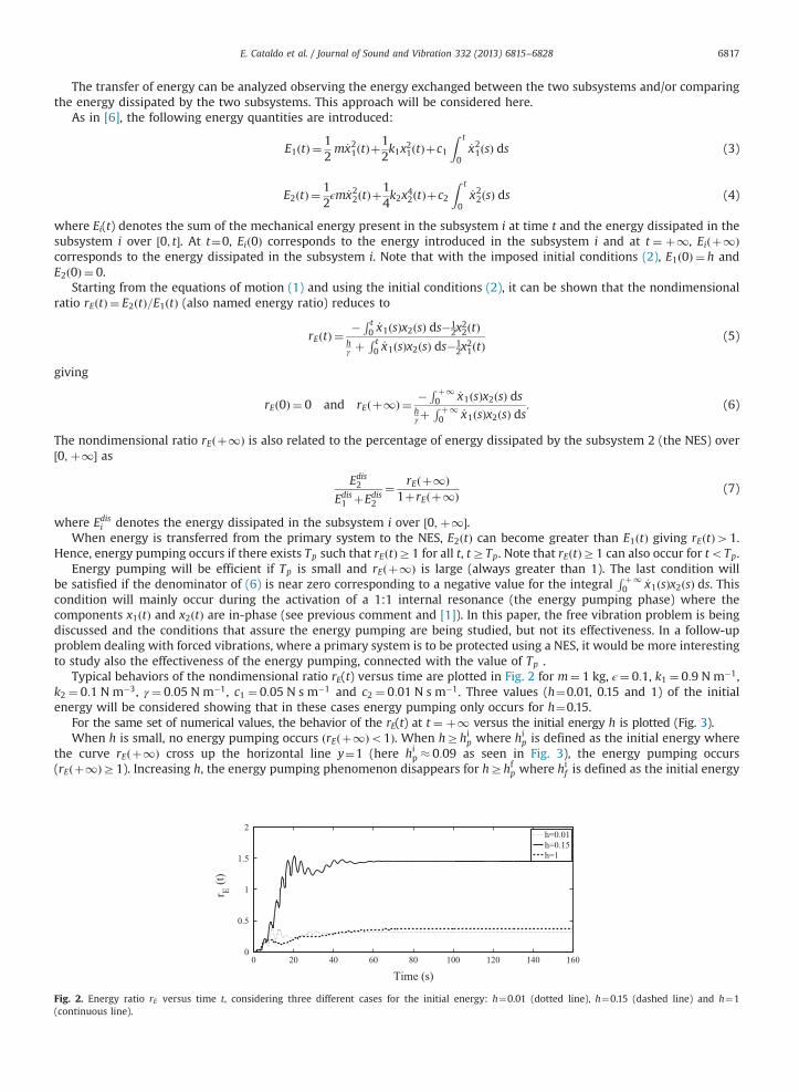
Typical behaviors of the nondimensional ratio rE(t) versus time are plotted in Fig. 2 for m¼ 1 kg, ϵ¼ 0:1, k1 ¼ 0:9 N m�1,k2 ¼ 0:1 N m�3, γ ¼ 0:05 N m�1, c1 ¼ 0:05 N s m�1 and c2 ¼ 0:01 N s m�1. Three values (h¼0.01, 0.15 and 1) of the initialenergy will be considered showing that in these cases energy pumping only occurs for h¼0.15.

For the same set of numerical values, the behavior of the rE(t) at t ¼ þ1 versus the initial energy h is plotted (Fig. 3).When h is small, no energy pumping occurs ðrEðþ1Þo1Þ. When hZhip where hip is defined as the initial energy where

the curve rEðþ1Þ cross up the horizontal line y¼1 (here hip � 0:09 as seen in Fig. 3), the energy pumping occurs(rEðþ1ÞZ1). Increasing h, the energy pumping phenomenon disappears for hZhf

p where hif is defined as the initial energy

0 20 40 60 80 100 120 140 1600

0.5

1

1.5

2

Time (s)

r E (t)

h=0.01h=0.15h=1

Fig. 2. Energy ratio rE versus time t, considering three different cases for the initial energy: h¼0.01 (dotted line), h¼0.15 (dashed line) and h¼1(continuous line).

0 0.1 0.2 0.3 0.4 0.5 0.6 0.7 0.80

0.5

1

1.5

Initial energy (h)r E (+

∞)

Fig. 3. Energy ratio rE(t) at t ¼ þ1 versus initial energy h.

0.6 0.7 0.8 0.9 1 1.1 1.2 1.3 1.4 1.50

0.1

0.2

0.3

0.4

0.5

0.6

0.7

0.8

Frequency

Ener

gy ( h

)

0.6 0.7 0.8 0.9 1 1.1 1.2 1.3 1.4 1.50.4

0.2

0

0.2

0.4

0.6

0.8

Frequency

x 1, x2

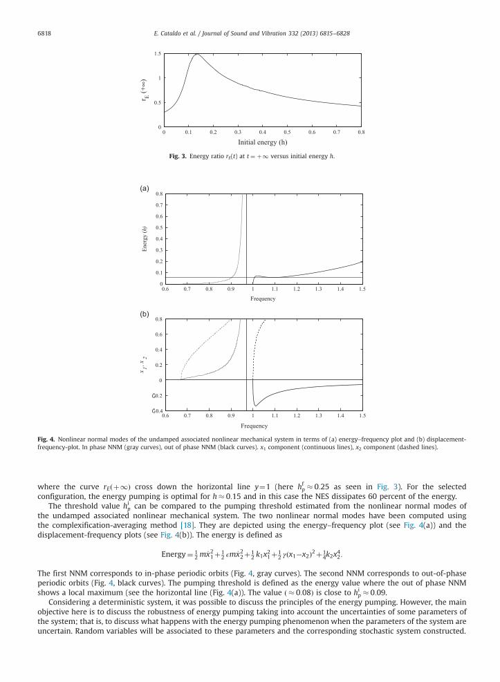
Fig. 4. Nonlinear normal modes of the undamped associated nonlinear mechanical system in terms of (a) energy–frequency plot and (b) displacement-frequency-plot. In phase NNM (gray curves), out of phase NNM (black curves). x1 component (continuous lines), x2 component (dashed lines).

E. Cataldo et al. / Journal of Sound and Vibration 332 (2013) 6815–68286818

where the curve rEðþ1Þ cross down the horizontal line y¼1 (here hfp � 0:25 as seen in Fig. 3). For the selectedconfiguration, the energy pumping is optimal for h� 0:15 and in this case the NES dissipates 60 percent of the energy.

The threshold value hip can be compared to the pumping threshold estimated from the nonlinear normal modes ofthe undamped associated nonlinear mechanical system. The two nonlinear normal modes have been computed usingthe complexification-averaging method [18]. They are depicted using the energy–frequency plot (see Fig. 4(a)) and thedisplacement-frequency plots (see Fig. 4(b)). The energy is defined as

Energy¼ 12 m _x21þ1

2 ϵm _x22þ12 k1x

21þ1

2 γðx1�x2Þ2þ14k2x

42:

The first NNM corresponds to in-phase periodic orbits (Fig. 4, gray curves). The second NNM corresponds to out-of-phaseperiodic orbits (Fig. 4, black curves). The pumping threshold is defined as the energy value where the out of phase NNMshows a local maximum (see the horizontal line (Fig. 4(a)). The value ð � 0:08Þ is close to hip � 0:09.

Considering a deterministic system, it was possible to discuss the principles of the energy pumping. However, the mainobjective here is to discuss the robustness of energy pumping taking into account the uncertainties of some parameters ofthe system; that is, to discuss what happens with the energy pumping phenomenon when the parameters of the system areuncertain. Random variables will be associated to these parameters and the corresponding stochastic system constructed.

E. Cataldo et al. / Journal of Sound and Vibration 332 (2013) 6815–6828 6819

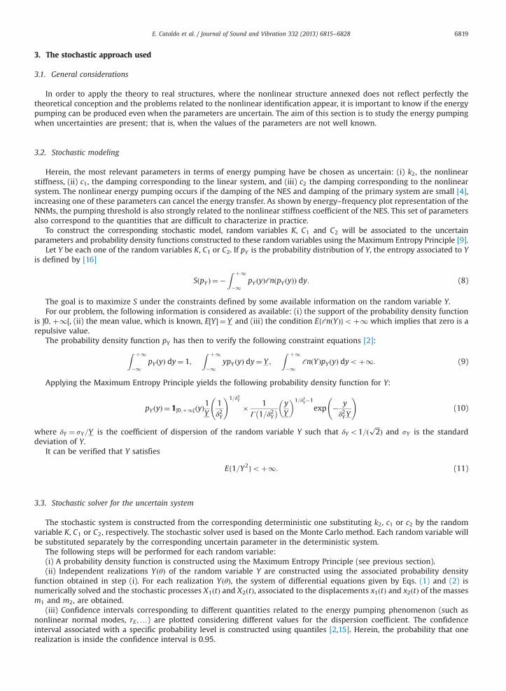
3. The stochastic approach used

3.1. General considerations

In order to apply the theory to real structures, where the nonlinear structure annexed does not reflect perfectly thetheoretical conception and the problems related to the nonlinear identification appear, it is important to know if the energypumping can be produced even when the parameters are uncertain. The aim of this section is to study the energy pumpingwhen uncertainties are present; that is, when the values of the parameters are not well known.

3.2. Stochastic modeling

Herein, the most relevant parameters in terms of energy pumping have be chosen as uncertain: (i) k2, the nonlinearstiffness, (ii) c1, the damping corresponding to the linear system, and (iii) c2 the damping corresponding to the nonlinearsystem. The nonlinear energy pumping occurs if the damping of the NES and damping of the primary system are small [4],increasing one of these parameters can cancel the energy transfer. As shown by energy–frequency plot representation of theNNMs, the pumping threshold is also strongly related to the nonlinear stiffness coefficient of the NES. This set of parametersalso correspond to the quantities that are difficult to characterize in practice.

To construct the corresponding stochastic model, random variables K, C1 and C2 will be associated to the uncertainparameters and probability density functions constructed to these random variables using the Maximum Entropy Principle [9].

Let Y be each one of the random variables K, C1 or C2. If pY is the probability distribution of Y, the entropy associated to Yis defined by [16]

SðpY Þ ¼ �Z þ1

�1pY ðyÞℓnðpY ðyÞÞ dy: (8)

The goal is to maximize S under the constraints defined by some available information on the random variable Y.For our problem, the following information is considered as available: (i) the support of the probability density function

is �0; þ1½, (ii) the mean value, which is known, E½Y� ¼ Y and (iii) the condition EfℓnðYÞgoþ1 which implies that zero is arepulsive value.

The probability density function pY has then to verify the following constraint equations [2]:Z þ1

�1pY ðyÞ dy¼ 1;

Z þ1

�1ypY ðyÞ dy¼ Y ;

Z þ1

�1ℓnðYÞpY ðyÞ dyoþ1: (9)

Applying the Maximum Entropy Principle yields the following probability density function for Y:

pY ðyÞ ¼ 1�0;þ1½ðyÞ1Y

1δ2Y

!1=δ2Y

� 1Γ 1=δ2Y� � y

Y

� �1=δ2Y�1

exp � yδ2YY

!(10)

where δY ¼ sY=Y is the coefficient of dispersion of the random variable Y such that δY o1=ðffiffiffi2

pÞ and sY is the standard

deviation of Y.It can be verified that Y satisfies

Ef1=Y2goþ1: (11)

3.3. Stochastic solver for the uncertain system

The stochastic system is constructed from the corresponding deterministic one substituting k2, c1 or c2 by the randomvariable K, C1 or C2, respectively. The stochastic solver used is based on the Monte Carlo method. Each random variable willbe substituted separately by the corresponding uncertain parameter in the deterministic system.

The following steps will be performed for each random variable:(i) A probability density function is constructed using the Maximum Entropy Principle (see previous section).(ii) Independent realizations YðθÞ of the random variable Y are constructed using the associated probability density

function obtained in step (i). For each realization YðθÞ, the system of differential equations given by Eqs. (1) and (2) isnumerically solved and the stochastic processes X1ðtÞ and X2ðtÞ, associated to the displacements x1ðtÞ and x2ðtÞ of the massesm1 and m2, are obtained.

(iii) Confidence intervals corresponding to different quantities related to the energy pumping phenomenon (such asnonlinear normal modes, rE;…) are plotted considering different values for the dispersion coefficient. The confidenceinterval associated with a specific probability level is constructed using quantiles [2,15]. Herein, the probability that onerealization is inside the confidence interval is 0.95.

E. Cataldo et al. / Journal of Sound and Vibration 332 (2013) 6815–68286820

4. Energy pumping robustness

The following numerical values have been used to define the nominal system: m¼ 1 kg, ϵ¼ 0:1, k1 ¼ 0:9 N m�1,k2 ¼ 0:1 N m�3, γ ¼ 0:05 N m�1, c1 ¼ 0:05 N s m�1 and c2 ¼ 0:01 N s m�1. The equations of motion Eqs. (1) and (2) havebeen approximated over ½0; T � with T ¼ 160 s using Runge–Kutta method. The confidence intervals have been estimatedsimulating 200 realizations.

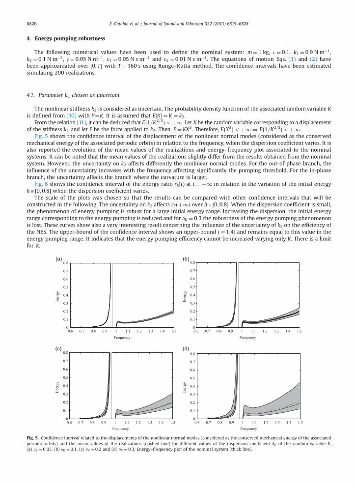
4.1. Parameter k2 chosen as uncertain

The nonlinear stiffness k2 is considered as uncertain. The probability density function of the associated random variable Kis defined from (10) with Y¼K. It is assumed that E½K� ¼ K ¼ k2.

From the relation (11), it can be deduced that Ef1=K2=3goþ1. Let X be the randomvariable corresponding to a displacementof the stiffness k2 and let F be the force applied to k2. Then, F ¼ KX3. Therefore, EfX2goþ1 ) Ef1=K2=3goþ1.

Fig. 5 shows the confidence interval of the displacement of the nonlinear normal modes (considered as the conservedmechanical energy of the associated periodic orbits) in relation to the frequency, when the dispersion coefficient varies. It isalso reported the evolution of the mean values of the realizations and energy–frequency plot associated to the nominalsystems. It can be noted that the mean values of the realizations slightly differ from the results obtained from the nominalsystem. However, the uncertainty on k2 affects differently the nonlinear normal modes. For the out-of-phase branch, theinfluence of the uncertainty increases with the frequency affecting significantly the pumping threshold. For the in-phasebranch, the uncertainty affects the branch where the curvature is larger.

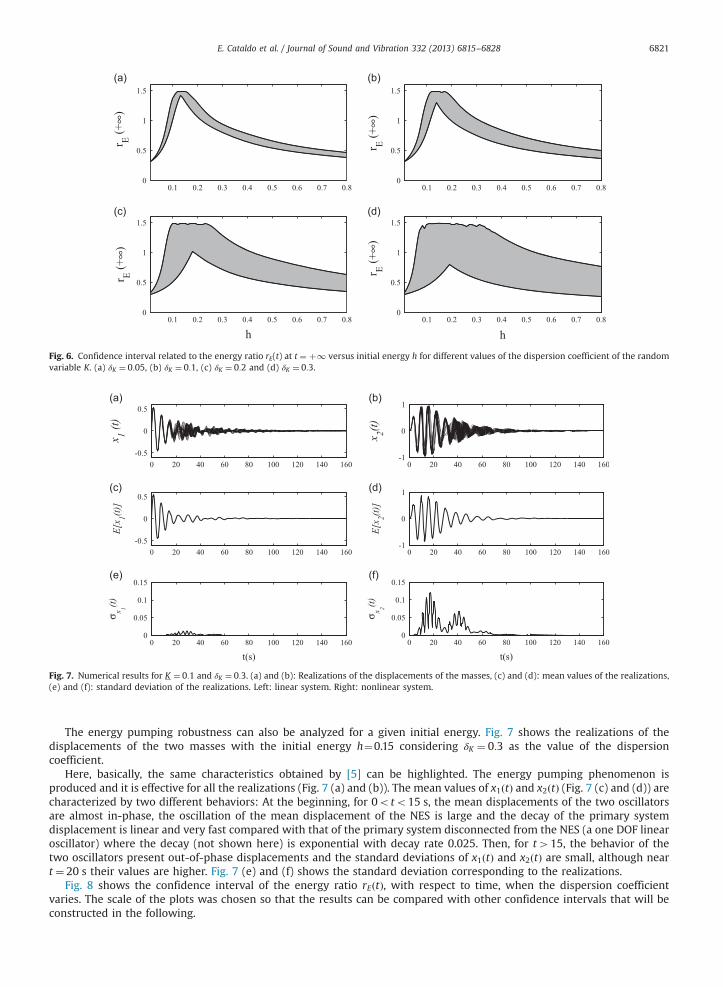
Fig. 6 shows the confidence interval of the energy ratio rE(t) at t ¼ þ1 in relation to the variation of the initial energyhA ½0;0:8� when the dispersion coefficient varies.

The scale of the plots was chosen so that the results can be compared with other confidence intervals that will beconstructed in the following. The uncertainty on k2 affects rEðþ1Þ over hA ½0;0:8�. When the dispersion coefficient is small,the phenomenon of energy pumping is robust for a large initial energy range. Increasing the dispersion, the initial energyrange corresponding to the energy pumping is reduced and for δK ¼ 0:3 the robustness of the energy pumping phenomenonis lost. These curves show also a very interesting result concerning the influence of the uncertainty of k2 on the efficiency ofthe NES. The upper-bound of the confidence interval shows an upper-bound ð � 1:4Þ and remains equal to this value in theenergy pumping range. It indicates that the energy pumping efficiency cannot be increased varying only K. There is a limitfor it.

0.6 0.7 0.8 0.9 1 1.1 1.2 1.3 1.4 1.50

0.1

0.2

0.3

0.4

0.5

0.6

0.7

0.8

Frequency

Ener

gy

0.6 0.7 0.8 0.9 1 1.1 1.2 1.3 1.4 1.50

0.1

0.2

0.3

0.4

0.5

0.6

0.7

0.8

Frequency

Ener

gy

0.6 0.7 0.8 0.9 1 1.1 1.2 1.3 1.4 1.50

0.1

0.2

0.3

0.4

0.5

0.6

0.7

0.8

Frequency

Ener

gy

0.6 0.7 0.8 0.9 1 1.1 1.2 1.3 1.4 1.50

0.1

0.2

0.3

0.4

0.5

0.6

0.7

0.8

Frequency

Ener

gy

Fig. 5. Confidence interval related to the displacements of the nonlinear normal modes (considered as the conserved mechanical energy of the associatedperiodic orbits) and the mean values of the realizations (dashed line) for different values of the dispersion coefficient δK of the random variable K.(a) δK ¼ 0:05, (b) δK ¼ 0:1, (c) δK ¼ 0:2 and (d) δK ¼ 0:3. Energy–frequency plot of the nominal system (thick line).

0.1 0.2 0.3 0.4 0.5 0.6 0.7 0.80

0.5

1

1.5

r E (+∞

)

0.1 0.2 0.3 0.4 0.5 0.6 0.7 0.80

0.5

1

1.5

r E (+∞

)

0.1 0.2 0.3 0.4 0.5 0.6 0.7 0.80

0.5

1

1.5

r E (+∞

)

h0.1 0.2 0.3 0.4 0.5 0.6 0.7 0.8

0

0.5

1

1.5

r E (+∞

)

h

Fig. 6. Confidence interval related to the energy ratio rE(t) at t ¼ þ1 versus initial energy h for different values of the dispersion coefficient of the randomvariable K. (a) δK ¼ 0:05, (b) δK ¼ 0:1, (c) δK ¼ 0:2 and (d) δK ¼ 0:3.

Fig. 7. Numerical results for K ¼ 0:1 and δK ¼ 0:3. (a) and (b): Realizations of the displacements of the masses, (c) and (d): mean values of the realizations,(e) and (f): standard deviation of the realizations. Left: linear system. Right: nonlinear system.

E. Cataldo et al. / Journal of Sound and Vibration 332 (2013) 6815–6828 6821

The energy pumping robustness can also be analyzed for a given initial energy. Fig. 7 shows the realizations of thedisplacements of the two masses with the initial energy h¼0.15 considering δK ¼ 0:3 as the value of the dispersioncoefficient.

Here, basically, the same characteristics obtained by [5] can be highlighted. The energy pumping phenomenon isproduced and it is effective for all the realizations (Fig. 7 (a) and (b)). The mean values of x1ðtÞ and x2ðtÞ (Fig. 7 (c) and (d)) arecharacterized by two different behaviors: At the beginning, for 0oto15 s, the mean displacements of the two oscillatorsare almost in-phase, the oscillation of the mean displacement of the NES is large and the decay of the primary systemdisplacement is linear and very fast compared with that of the primary system disconnected from the NES (a one DOF linearoscillator) where the decay (not shown here) is exponential with decay rate 0.025. Then, for t415, the behavior of thetwo oscillators present out-of-phase displacements and the standard deviations of x1ðtÞ and x2ðtÞ are small, although neart ¼ 20 s their values are higher. Fig. 7 (e) and (f) shows the standard deviation corresponding to the realizations.

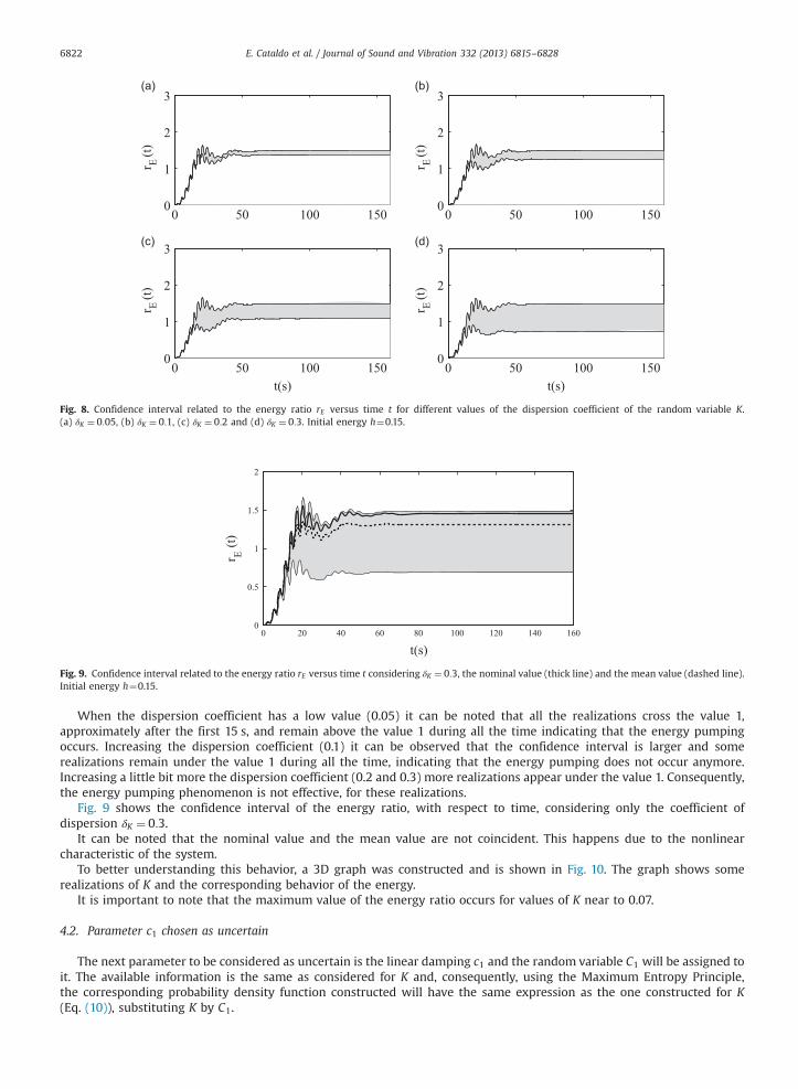
Fig. 8 shows the confidence interval of the energy ratio rEðtÞ, with respect to time, when the dispersion coefficientvaries. The scale of the plots was chosen so that the results can be compared with other confidence intervals that will beconstructed in the following.

0 50 100 1500

1

2

3

r E (t)

0 50 100 1500

1

2

3

0 50 100 1500

1

2

3

t(s)

r E (t)

r E (t)

r E (t)

0 50 100 1500

1

2

3

t(s)

Fig. 8. Confidence interval related to the energy ratio rE versus time t for different values of the dispersion coefficient of the random variable K.(a) δK ¼ 0:05, (b) δK ¼ 0:1, (c) δK ¼ 0:2 and (d) δK ¼ 0:3. Initial energy h¼0.15.

0 20 40 60 80 100 120 140 1600

0.5

1

1.5

2

t(s)

r E (t)

Fig. 9. Confidence interval related to the energy ratio rE versus time t considering δK ¼ 0:3, the nominal value (thick line) and the mean value (dashed line).Initial energy h¼0.15.

E. Cataldo et al. / Journal of Sound and Vibration 332 (2013) 6815–68286822

When the dispersion coefficient has a low value (0.05) it can be noted that all the realizations cross the value 1,approximately after the first 15 s, and remain above the value 1 during all the time indicating that the energy pumpingoccurs. Increasing the dispersion coefficient (0.1) it can be observed that the confidence interval is larger and somerealizations remain under the value 1 during all the time, indicating that the energy pumping does not occur anymore.Increasing a little bit more the dispersion coefficient (0.2 and 0.3) more realizations appear under the value 1. Consequently,the energy pumping phenomenon is not effective, for these realizations.

Fig. 9 shows the confidence interval of the energy ratio, with respect to time, considering only the coefficient ofdispersion δK ¼ 0:3.

It can be noted that the nominal value and the mean value are not coincident. This happens due to the nonlinearcharacteristic of the system.

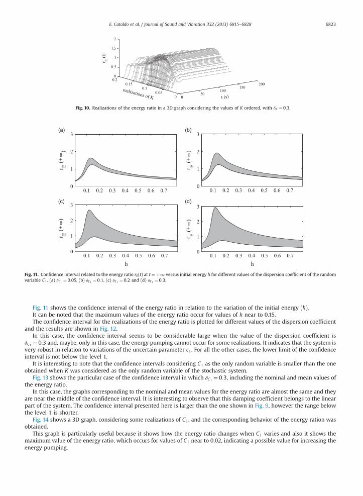
To better understanding this behavior, a 3D graph was constructed and is shown in Fig. 10. The graph shows somerealizations of K and the corresponding behavior of the energy.

It is important to note that the maximum value of the energy ratio occurs for values of K near to 0.07.

4.2. Parameter c1 chosen as uncertain

The next parameter to be considered as uncertain is the linear damping c1 and the random variable C1 will be assigned toit. The available information is the same as considered for K and, consequently, using the Maximum Entropy Principle,the corresponding probability density function constructed will have the same expression as the one constructed for K(Eq. (10)), substituting K by C1.

050

100150

200

00.05

0.10.15

0.20

0.5

1

1.5

2

t (s)realizations of K

r E (t

)Fig. 10. Realizations of the energy ratio in a 3D graph considering the values of K ordered, with δK ¼ 0:3.

0.1 0.2 0.3 0.4 0.5 0.6 0.70

1

2

3

r E (+

∞)

0.1 0.2 0.3 0.4 0.5 0.6 0.70

1

2

3

r E (+

∞)

0.1 0.2 0.3 0.4 0.5 0.6 0.70

1

2

3

h

r E (+

∞)

0.1 0.2 0.3 0.4 0.5 0.6 0.70

1

2

3

h

r E (+

∞)

Fig. 11. Confidence interval related to the energy ratio rE(t) at t ¼ þ1 versus initial energy h for different values of the dispersion coefficient of the randomvariable C1. (a) δC1 ¼ 0:05, (b) δC1 ¼ 0:1, (c) δC1 ¼ 0:2 and (d) δC1 ¼ 0:3.

E. Cataldo et al. / Journal of Sound and Vibration 332 (2013) 6815–6828 6823

Fig. 11 shows the confidence interval of the energy ratio in relation to the variation of the initial energy (h).It can be noted that the maximum values of the energy ratio occur for values of h near to 0.15.The confidence interval for the realizations of the energy ratio is plotted for different values of the dispersion coefficient

and the results are shown in Fig. 12.In this case, the confidence interval seems to be considerable large when the value of the dispersion coefficient is

δC1 ¼ 0:3 and, maybe, only in this case, the energy pumping cannot occur for some realizations. It indicates that the system isvery robust in relation to variations of the uncertain parameter c1. For all the other cases, the lower limit of the confidenceinterval is not below the level 1.

It is interesting to note that the confidence intervals considering C1 as the only random variable is smaller than the oneobtained when K was considered as the only random variable of the stochastic system.

Fig. 13 shows the particular case of the confidence interval in which δC1 ¼ 0:3, including the nominal and mean values ofthe energy ratio.

In this case, the graphs corresponding to the nominal and mean values for the energy ratio are almost the same and theyare near the middle of the confidence interval. It is interesting to observe that this damping coefficient belongs to the linearpart of the system. The confidence interval presented here is larger than the one shown in Fig. 9, however the range belowthe level 1 is shorter.

Fig. 14 shows a 3D graph, considering some realizations of C1, and the corresponding behavior of the energy ration wasobtained.

This graph is particularly useful because it shows how the energy ratio changes when C1 varies and also it shows themaximum value of the energy ratio, which occurs for values of C1 near to 0.02, indicating a possible value for increasing theenergy pumping.

0 20 40 60 80 100 120 140 1600

1

2

3

r E (t)

0 20 40 60 80 100 120 140 1600

1

2

3

r E (t)

0 20 40 60 80 100 120 140 1600

0.5

1

1.5

2

2.5

t(s)

r E (t)

0 20 40 60 80 100 120 140 1600

1

2

3

t(s)

r E (t)

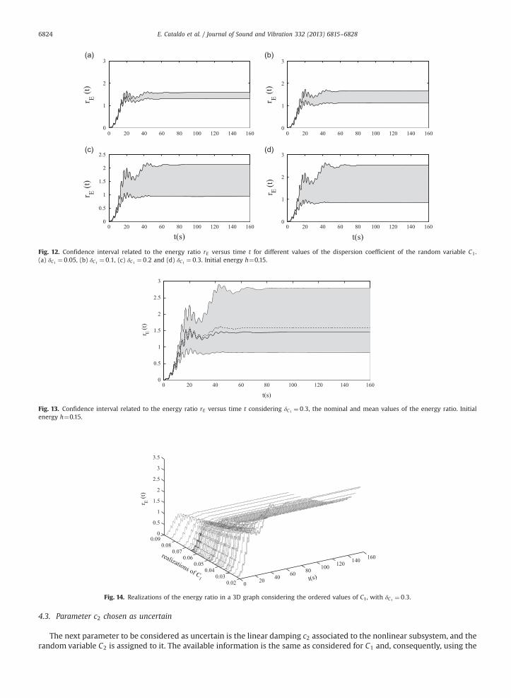
Fig. 12. Confidence interval related to the energy ratio rE versus time t for different values of the dispersion coefficient of the random variable C1.(a) δC1 ¼ 0:05, (b) δC1 ¼ 0:1, (c) δC1 ¼ 0:2 and (d) δC1 ¼ 0:3. Initial energy h¼0.15.

0 20 40 60 80 100 120 140 1600

0.5

1

1.5

2

2.5

3

t(s)

r E (t)

Fig. 13. Confidence interval related to the energy ratio rE versus time t considering δC1 ¼ 0:3, the nominal and mean values of the energy ratio. Initialenergy h¼0.15.

0 20 40 60 80 100 120 140 160

0.020.03

0.040.05

0.060.07

0.080.09

0

0.5

1

1.5

2

2.5

3

3.5

t(s)

realizations of C1

r E (t)

Fig. 14. Realizations of the energy ratio in a 3D graph considering the ordered values of C1, with δC1 ¼ 0:3.

E. Cataldo et al. / Journal of Sound and Vibration 332 (2013) 6815–68286824

4.3. Parameter c2 chosen as uncertain

The next parameter to be considered as uncertain is the linear damping c2 associated to the nonlinear subsystem, and therandom variable C2 is assigned to it. The available information is the same as considered for C1 and, consequently, using the

0.1 0.2 0.3 0.4 0.5 0.6 0.70

0.5

1

1.5

2

r E (+∞

)

0.1 0.2 0.3 0.4 0.5 0.6 0.70

0.5

1

1.5

2

r E (+∞

)

0.1 0.2 0.3 0.4 0.5 0.6 0.70

0.5

1

1.5

2

h

r E (+∞

)

0.1 0.2 0.3 0.4 0.5 0.6 0.70

0.5

1

1.5

2

h

r E (+∞

)

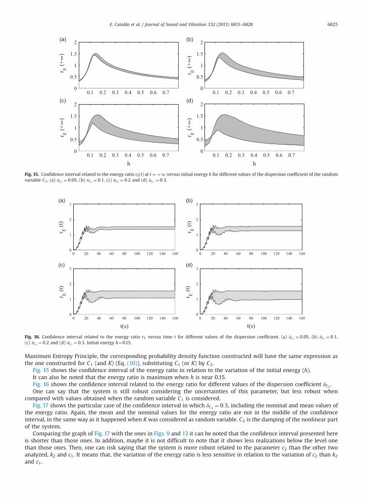
Fig. 15. Confidence interval related to the energy ratio rE(t) at t ¼ þ1 versus initial energy h for different values of the dispersion coefficient of the randomvariable C2. (a) δC2 ¼ 0:05, (b) δC2 ¼ 0:1, (c) δC2 ¼ 0:2 and (d) δC2 ¼ 0:3.

0 20 40 60 80 100 120 140 1600

1

2

3

r E (t)

0 20 40 60 80 100 120 140 1600

1

2

3

r E (t)

0 20 40 60 80 100 120 140 1600

1

2

3

t(s)

r E (t)

0 20 40 60 80 100 120 140 1600

1

2

3

t(s)

r E (t)

Fig. 16. Confidence interval related to the energy ratio rE versus time t for different values of the dispersion coefficient. (a) δC2 ¼ 0:05, (b) δC2 ¼ 0:1,(c) δC2 ¼ 0:2 and (d) δC2 ¼ 0:3. Initial energy h¼0.15.

E. Cataldo et al. / Journal of Sound and Vibration 332 (2013) 6815–6828 6825

Maximum Entropy Principle, the corresponding probability density function constructed will have the same expression asthe one constructed for C1 (and K) (Eq. (10)), substituting C1 (or K) by C2.

Fig. 15 shows the confidence interval of the energy ratio in relation to the variation of the initial energy (h).It can also be noted that the energy ratio is maximum when h is near 0.15.Fig. 16 shows the confidence interval related to the energy ratio for different values of the dispersion coefficient δC2 .One can say that the system is still robust considering the uncertainties of this parameter, but less robust when

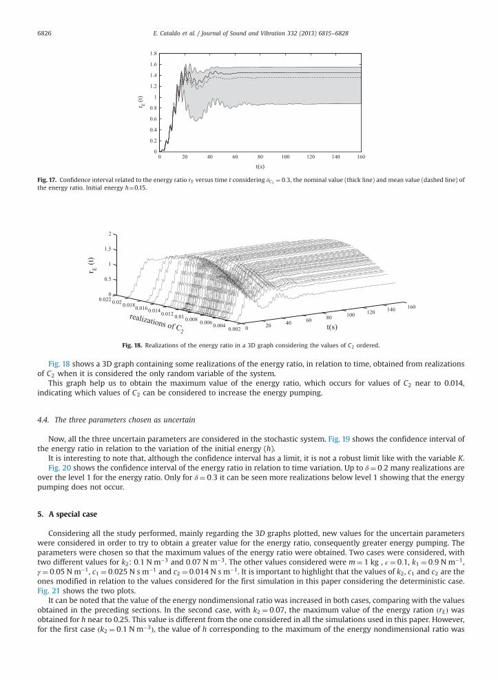
compared with values obtained when the random variable C1 is considered.Fig. 17 shows the particular case of the confidence interval in which δC2 ¼ 0:3, including the nominal and mean values of

the energy ratio. Again, the mean and the nominal values for the energy ratio are not in the middle of the confidenceinterval, in the same way as it happened when Kwas considered as random variable. C2 is the damping of the nonlinear partof the system.

Comparing the graph of Fig. 17 with the ones in Figs. 9 and 13 it can be noted that the confidence interval presented hereis shorter than those ones. In addition, maybe it is not difficult to note that it shows less realizations below the level onethan those ones. Then, one can risk saying that the system is more robust related to the parameter c2 than the other twoanalyzed, k2 and c1. It means that, the variation of the energy ratio is less sensitive in relation to the variation of c2 than k2and c1.

0 20 40 60 80 100 120 140 1600

0.2

0.4

0.6

0.8

1

1.2

1.4

1.6

1.8

t(s)

r E (t)

Fig. 17. Confidence interval related to the energy ratio rE versus time t considering δC2 ¼ 0:3, the nominal value (thick line) and mean value (dashed line) ofthe energy ratio. Initial energy h¼0.15.

0 20 40 60 80 100 120 140 160

0.0020.0040.0060.0080.010.0120.0140.0160.0180.020.0220

0.5

1

1.5

2

t(s)realizations of C2

r E (t

)

Fig. 18. Realizations of the energy ratio in a 3D graph considering the values of C2 ordered.

E. Cataldo et al. / Journal of Sound and Vibration 332 (2013) 6815–68286826

Fig. 18 shows a 3D graph containing some realizations of the energy ratio, in relation to time, obtained from realizationsof C2 when it is considered the only random variable of the system.

This graph help us to obtain the maximum value of the energy ratio, which occurs for values of C2 near to 0.014,indicating which values of C2 can be considered to increase the energy pumping.

4.4. The three parameters chosen as uncertain

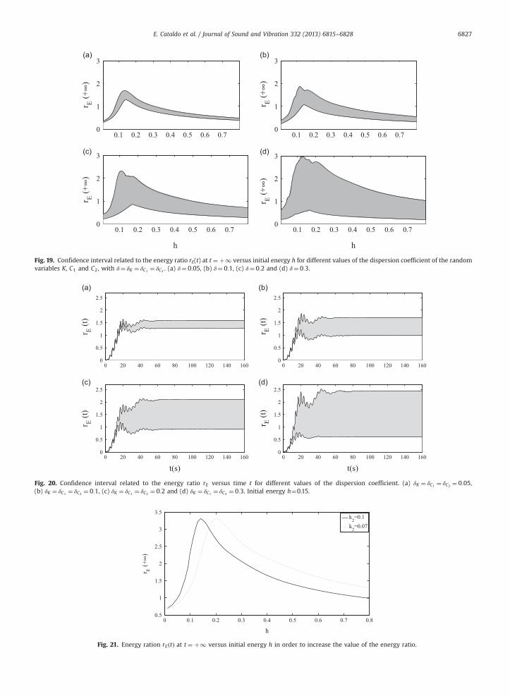
Now, all the three uncertain parameters are considered in the stochastic system. Fig. 19 shows the confidence interval ofthe energy ratio in relation to the variation of the initial energy (h).

It is interesting to note that, although the confidence interval has a limit, it is not a robust limit like with the variable K.Fig. 20 shows the confidence interval of the energy ratio in relation to time variation. Up to δ¼ 0:2 many realizations are

over the level 1 for the energy ratio. Only for δ¼ 0:3 it can be seen more realizations below level 1 showing that the energypumping does not occur.

5. A special case

Considering all the study performed, mainly regarding the 3D graphs plotted, new values for the uncertain parameterswere considered in order to try to obtain a greater value for the energy ratio, consequently greater energy pumping. Theparameters were chosen so that the maximum values of the energy ratio were obtained. Two cases were considered, withtwo different values for k2: 0:1 N m�3 and 0:07 N m�3. The other values considered were m¼ 1 kg , ϵ¼ 0:1, k1 ¼ 0:9 N m�1,γ ¼ 0:05 N m�1, c1 ¼ 0:025 N s m�1 and c2 ¼ 0:014 N s m�1. It is important to highlight that the values of k2, c1 and c2 are theones modified in relation to the values considered for the first simulation in this paper considering the deterministic case.Fig. 21 shows the two plots.

It can be noted that the value of the energy nondimensional ratio was increased in both cases, comparing with the valuesobtained in the preceding sections. In the second case, with k2 ¼ 0:07, the maximum value of the energy ration ðrEÞ wasobtained for h near to 0.25. This value is different from the one considered in all the simulations used in this paper. However,for the first case ðk2 ¼ 0:1 N m�3Þ, the value of h corresponding to the maximum of the energy nondimensional ratio was

0.1 0.2 0.3 0.4 0.5 0.6 0.70

1

2

3

r E (+∞

)

0.1 0.2 0.3 0.4 0.5 0.6 0.70

1

2

3

r E (+∞

)

0.1 0.2 0.3 0.4 0.5 0.6 0.70

1

2

3

h

r E (+∞

)

0.1 0.2 0.3 0.4 0.5 0.6 0.70

1

2

3

h

r E (+∞

)Fig. 19. Confidence interval related to the energy ratio rE(t) at t ¼ þ1 versus initial energy h for different values of the dispersion coefficient of the randomvariables K, C1 and C2, with δ¼ δK ¼ δC1 ¼ δC2 . (a) δ¼ 0:05, (b) δ¼ 0:1, (c) δ¼ 0:2 and (d) δ¼ 0:3.

0 20 40 60 80 100 120 140 1600

0.5

1

1.5

2

2.5

r E (t)

0 20 40 60 80 100 120 140 1600

0.5

1

1.5

2

2.5

r E (t)

0 20 40 60 80 100 120 140 1600

0.5

1

1.5

2

2.5

t(s)

r E (t)

0 20 40 60 80 100 120 140 1600

0.5

1

1.5

2

2.5

t(s)

r E (t)

Fig. 20. Confidence interval related to the energy ratio rE versus time t for different values of the dispersion coefficient. (a) δK ¼ δC1 ¼ δC2 ¼ 0:05,(b) δK ¼ δC1 ¼ δC2 ¼ 0:1, (c) δK ¼ δC1 ¼ δC2 ¼ 0:2 and (d) δK ¼ δC1 ¼ δC2 ¼ 0:3. Initial energy h¼0.15.

0 0.1 0.2 0.3 0.4 0.5 0.6 0.7 0.80.5

1

1.5

2

2.5

3

3.5

h

r E (+

∞)

k2=0.1k2=0.07

Fig. 21. Energy ration rEðtÞ at t ¼ þ1 versus initial energy h in order to increase the value of the energy ratio.

E. Cataldo et al. / Journal of Sound and Vibration 332 (2013) 6815–6828 6827

E. Cataldo et al. / Journal of Sound and Vibration 332 (2013) 6815–68286828

near to 0.15. Then, it was possible to obtain a greater value for the energy ratio; that is, it was possible to increase the energypumping, changing the values of the parameters and using all the study described in this paper.

6. Conclusions

This paper analyzes energy pumping using a system composed of two subsystems, one linear and another nonlinear, totake into account the uncertainties in some parameters. The main objective was to analyze the robustness of the energypumping. So, three parameters were considered as uncertain: the nonlinear stiffness and the two damping, one of the linearsubsystem and the other of the nonlinear subsystems. Probability density functions (pdfs) were assigned to the randomvariables related to these parameters.

The main conclusions obtained were that the system is more robust when uncertainties related to the dampers are takeninto account, because with a greater level of dispersion in this parameter, the energy pumping phenomenon could still beobserved. For the same level of dispersion, the effects of the three random variables were compared and the system resultswere more sensitive to variations of the random variable associated to the stiffness associated to the nonlinear system. Inaddition, the displacements of the linear subsystem are less sensitive to the variations of the uncertain parameter than thedisplacements of the nonlinear subsystem.

It was also possible to verify that, in some cases, there are limitation for the energy pumping. As an example, when onlythe stiffness associated to the nonlinear system was considered, it was not possible to increase the energy pumping varyingthe value of the random variable associated to the corresponding stiffness. However, it was possible to increase the energypumping modifying the parameters of the system, according to all the study performed in the paper, considering theuncertain parameters, the random variables associated to them and the corresponding stochastic system.

An idea for a future study is to consider other parameters as uncertain and employ other methodologies to take it intoaccount. The sensitive analysis can be performed considering Other quantities, for example, the energy variation of the system.

Acknowledgments

This work was supported by FAPERJ (Fundação de Amparo à Pesquisa no Rio de Janeiro), by CAPES (CAPES/COFECUBproject N. 672/10) and by CNPq (Brazilian Agency Conselho Nacional de Desenvolvimento Científico e Tecnológico).

References

[1] R. Bellet, B. Cochelin, P. Herzog, P.-O. Mattei, Experimental study of targeted energy transfer from an acoustic system to a nonlinear membraneabsorber, Journal of Sound and Vibration 329 (2010) 2768–2791.

[2] E. Cataldo, C. Soize, R. Sampaio, C. Desceliers, Probabilistic modeling of a nonlinear dynamical system used for producing voice, ComputationalMechanics 43 (2009) 265–275.

[3] O.V. Gendelman, L.I. Manevitch, A.F. Vakakis, R. M’Closkey, Energy pumping in nonlinear mechanical oscillators: part I - dynamics of the underlyinghamiltonian systems, Journal of Applied Mechanics 68 (2001) 34–41.

[4] E. Gourdon, Controle passif de vibrations par pompage énergétique, PhD Thesis, Ecole Centrale de Lyon, 2006.[5] E. Gourdon, C.H. Lamarque, Energy pumping for a larger span of energy, Journal of Sound and Vibration 285 (2005) 711–720.[6] E. Gourdon, C.H. Lamarque, Energy pumping with various nonlinear structures: numerical evidences, Nonlinear Dynamics 40 (2005) 281–307.[7] E. Gourdon, C.H. Lamarque, Nonlinear energy sink with uncertain parameters, Journal of Computational and Nonlinear Dynamics 1 (2006) 187–195.[8] X. Jang, D.M. McFarland, L.A. Bergman, A.F. Vakakis, Steady state passive nonlinear energy pumping in coupled oscillators: theoretical and experimental

results, Nonlinear Dynamics 33 (2003) 87–102.[9] J.N. Kapur, H.K. Kesavan, Entropy Optimization Principles with Applications, Academic Press, San Diego, 1992.

[10] G. Kerschen, Y.S. Lee, A.F. Vakakis, D.M. McFarland, L.A. Bergman, Irreversible passive energy transfer in coupled oscillators with essential nonlinearity,Journal of Applied Mathematics 66 (2006) 648–679.

[11] G. Kerschen, A.F. Vakakis, Y.S. Lee, D.M. McFarland, J.J. Kowtko, L.A. Bergman, Energy transfers in a system of two coupled oscillators with essentialnonlinearity: 1:1 resonance manifold and transient bridging orbits, Nonlinear Dynamics 42 (2005) 283–303.

[12] D.M. McFarland, L.A. Bergman, A.F. Vakakis, Experimental study of non-linear energy pumping occurring at a single fast frequency, InternationalJournal of Non-Linear Mechanics 40 (2005) 891–899.

[13] T.P. Sapsis, A.F. Vakakis, L.A. Bergman, Effect of stochasticity on targeted energy transfer from a linear medium to a strongly nonlinear attachment,Probabilistic Engineering Mechanics (2010).

[14] F. Schmidt, C.-H. Lamarque, Computation of the solutions of the Fokker Planck equation for one and two dof systems, Communications in NonlinearScience and Numerical Simulation 14 (2009) 529.

[15] R. Serfling, Approximation Theorems of Mathematical Statistics, Wiley, 1980.[16] C.E. Shannon, A mathematical theory of communication, Bell System Technical Journal 27 (1948) 379–423. 623–659.[17] A.F. Vakakis, O.V. Gendelman, Energy pumping in nonlinear mechanical oscillators: part II – resonance capture, Journal of Applied Mechanics 68 (2001)

42–48.[18] A.F. Vakakis, O.V. Gendelman, L.A. Bergman, D.M. McFarland, G. Kerschen, Y.S. Lee, Nonlinear Targeted Energy Transfer in Mechanical and Structural

Systems, Solid Mechanics and its Applications, vol. 156, Springer, 2008.[19] A.F. Vakakis, L.I. Manevitch, O.V. Gendelman, L.A. Bergman, Dynamics of linear discrete systems connected to local, essentially non-linear attachments,

Journal of Sound and Vibration 264 (2003) 559–577.