AA242B: MECHANICAL VIBRATIONS 1 / 50 AA242B: MECHANICAL VIBRATIONS Undamped Vibrations of n-DOF Systems These slides are based on the recommended textbook: M. G´ eradin and D. Rixen, “Mechanical Vibrations: Theory and Applications to Structural Dynamics,” Second Edition, Wiley, John & Sons, Incorporated, ISBN-13:9780471975465 1 / 50

Welcome message from author
This document is posted to help you gain knowledge. Please leave a comment to let me know what you think about it! Share it to your friends and learn new things together.
Transcript

AA242B: MECHANICAL VIBRATIONS 1 / 50
AA242B: MECHANICAL VIBRATIONSUndamped Vibrations of n-DOF Systems
These slides are based on the recommended textbook: M. Geradin and D. Rixen, “MechanicalVibrations: Theory and Applications to Structural Dynamics,” Second Edition, Wiley, John &
Sons, Incorporated, ISBN-13:9780471975465
1 / 50

AA242B: MECHANICAL VIBRATIONS 2 / 50
Outline
1 Linear Vibrations
2 Natural Vibration Modes
3 Orthogonality of Natural Vibration Modes
4 Modal Superposition Analysis
5 Spectral Expansions
6 Forced Harmonic Response
7 Response to External Loading
8 Mechanical Systems Excited Through Support Motion
2 / 50

AA242B: MECHANICAL VIBRATIONS 3 / 50
Linear Vibrations
Equilibrium configuration
qs(t) = qs(0)qs(t) = 0
s = 1, · · · , n (1)
Recall the Lagrange equations of motion
− d
dt
(∂T∂qs
)+∂T∂qs− ∂V∂qs− ∂D
∂qs+ Qs(t) = 0
where T = T0 + T1 + T2
Recall the generalized gyroscopic forces
Fs = −n∑
r=1
∂2T1
∂qs∂qrqr +
∂T1
∂qs=
n∑r=1
(∂2T1
∂qs∂qr−
∂2T1
∂qr∂qs
)qr , s = 1, · · · , n
Definition: the effective potential energy is defined as V? = V − T0
The Lagrange equations of motion can be re-written as
d
dt
(∂T2
∂qs
)− ∂T2
∂qs= Qs(t)− ∂V?
∂qs− ∂D
∂qs+ Fs −
∂
∂t
(∂T1
∂qs
)3 / 50
AA242B: MECHANICAL VIBRATIONS 4 / 50
Linear Vibrations
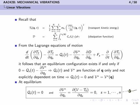
Recall that
T0(q, t) =1
2
N∑k=1
3∑i=1
mk
(∂Uik
∂t(q, t)
)2
(transport kinetic energy)
D =N∑
k=1
∫ vk (q)
0
Ck fk (γ)dγ (dissipation function)
From the Lagrange equations of motion
d
dt
(∂T2
∂qs
)− ∂T2
∂qs= Qs(t)− ∂V?
∂qs− ∂D
∂qs+ Fs −
∂
∂t
(∂T1
∂qs
)it follows that an equilibrium configuration exists if and only if
0 = Qs(t)− ∂V?
∂qs⇒ Qs(t) and V? are function of q only and not
explicitly dependent on time ⇒ Qs(t) = 0 and V? = V?(q)
At equilibrium
Qs(t) = 0 and∂V?
∂qs=∂(V − T0)
∂qs= 0, s = 1, · · · , n
4 / 50
AA242B: MECHANICAL VIBRATIONS 5 / 50
Linear Vibrations
Free-Vibrations About a Stable Equilibrium Position
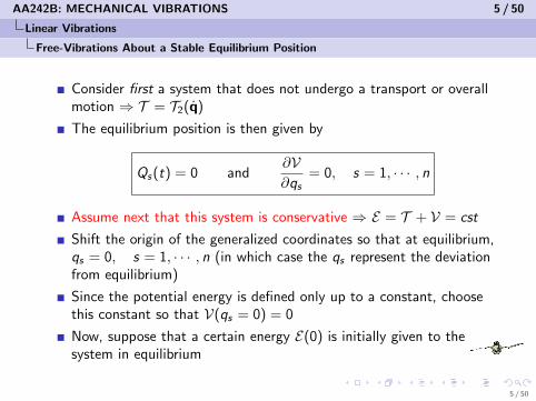
Consider first a system that does not undergo a transport or overallmotion ⇒ T = T2(q)
The equilibrium position is then given by
Qs(t) = 0 and∂V∂qs
= 0, s = 1, · · · , n
Assume next that this system is conservative ⇒ E = T + V = cst
Shift the origin of the generalized coordinates so that at equilibrium,qs = 0, s = 1, · · · , n (in which case the qs represent the deviationfrom equilibrium)
Since the potential energy is defined only up to a constant, choosethis constant so that V(qs = 0) = 0
Now, suppose that a certain energy E(0) is initially given to thesystem in equilibrium
5 / 50
AA242B: MECHANICAL VIBRATIONS 6 / 50
Linear Vibrations
Free-Vibrations About a Stable Equilibrium Position
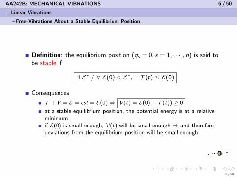
Definition: the equilibrium position (qs = 0, s = 1, · · · , n) is said tobe stable if
∃ E? / ∀ E(0) < E?, T (t) ≤ E(0)
Consequences
T + V = E = cst = E(0)⇒ V(t) = E(0)− T (t)) ≥ 0
at a stable equilibrium position, the potential energy is at a relativeminimumif E(0) is small enough, V(t) will be small enough ⇒ and thereforedeviations from the equilibrium position will be small enough
6 / 50

AA242B: MECHANICAL VIBRATIONS 7 / 50
Linear Vibrations
Free-Vibrations About a Stable Equilibrium Position
Linearization of T and V around an equilibrium position
(qs = 0,∂V∂qs
= 0)
actually, this means obtaining a quadratic form of T and V in q andq so that the corresponding generalized forces are linearsince qs (t) represent deviations from equilibrium, V can be expandedas follows
V(q) = V(0) +n∑
s=1
∂V∂qs|q=0 qs +
1
2
n∑s=1
n∑r=1
∂2V∂qs∂qr
|q=0 qsqr +O(q3)
= V(0) +1
2
n∑s=1
n∑r=1
∂2V∂qs∂qr
|q=0 qsqr +O(q3)
since the potential energy is defined only up to a constant, if thisconstant is chosen so that V(0) = 0, then a second-orderapproximation of V(q) is given by
V(q) =1
2
n∑s=1
n∑r=1
∂2V∂qs∂qr
|q=0 qsqr , for q 6= 0
7 / 50

AA242B: MECHANICAL VIBRATIONS 8 / 50
Linear Vibrations
Free-Vibrations About a Stable Equilibrium Position
Stiffness matrix
let K = [ksr ] where ksr = krs =∂2V∂qs∂qr
|q=0
=⇒ V(q) =1
2qT Kq > 0, for q 6= 0
K is symmetric positive (semi-) definite
8 / 50

AA242B: MECHANICAL VIBRATIONS 9 / 50
Linear Vibrations
Free-Vibrations About a Stable Equilibrium Position
Recall that
T2 =1
2
n∑s=1
n∑r=1
N∑k=1
3∑i=1
mk∂Uik
∂qs
∂Uik
∂qrqs qr (relative kinetic energy)
T2(q, q) = T2(0, 0) +n∑
s=1
∂T2
∂qs|q=0,q=0 qs +
n∑s=1
∂T2
∂qs|q=0,q=0 qs
+1
2
n∑s=1
n∑r=1
∂2T2
∂qs∂qr|q=0,q=0 qs qr +
n∑s=1
n∑r=1
∂2T2
∂qs∂qr|q=0,q=0 qs qr
+1
2
n∑s=1
n∑r=1
∂2T2
∂qs∂qr|q=0,q=0 qs qr +O(q3
, q3)
=1
2
n∑s=1
n∑r=1
∂2T2
∂qs∂qr|q=0,q=0 qs qr +O(q3
, q3)
9 / 50

AA242B: MECHANICAL VIBRATIONS 10 / 50
Linear Vibrations
Free-Vibrations About a Stable Equilibrium Position
Hence, a second-order approximation of T2(q) is given by
T2(q) =1
2qT Mq > 0, for q 6= 0
where
M =
[msr = mrs =
∂2T2
∂qs∂qr|q=0 =
N∑k=1
mk
3∑i=1
∂Uik
∂qs|q=0
∂Uik
∂qr|q=0
]is the mass matrix and is symmetric positive definite
10 / 50

AA242B: MECHANICAL VIBRATIONS 11 / 50
Linear Vibrations
Free-Vibrations About a Stable Equilibrium Position
Free-vibrations about a stable equilibrium position of a conservativesystem that does not undergo a transport or overall motion(T0 = T1 = 0)
d
dt
(∂T2
∂qs
)− ∂T2
∂qs= − ∂V
∂qs
=⇒ d
dt(Mq)− 0 = −Kq
=⇒ Mq + Kq = 0
11 / 50

AA242B: MECHANICAL VIBRATIONS 12 / 50
Linear Vibrations
Free-Vibrations About an Equilibrium Configuration
Consider next the more general case of a system in steady motion (atransported system) whose equilibrium configuration defined by
∂V?
∂qs=∂(V − T0)
∂qs= 0, s = 1, · · · , n
corresponds to the balance of forces deriving from a potential(∂V∂qs
)and centrifugal forces
(∂T0
∂qs
)It is an equilibrium configuration in the sense that qs — whichrepresent here the generalized velocities relative to a steady motion— are zero but the system is not idle
12 / 50
AA242B: MECHANICAL VIBRATIONS 13 / 50
Linear Vibrations
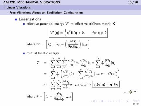
Free-Vibrations About an Equilibrium Configuration
Linearizationseffective potential energy V? ⇒ effective stiffness matrix K?
V?(q) =1
2qT K?q > 0, for q 6= 0
where K? =
[k?sr = ksr −
(∂2T0
∂qs∂qr
)|q=0
]mutual kinetic energy
T1 =n∑
s=1
N∑k=1
3∑i=1
∂Uik
∂tmk
∂Uik
∂qsqs =
n∑s=1
qs∂T1
∂qs(q)
=n∑
s=1
qs
(∂T1
∂qs(0) +
n∑r=1
∂2T1
∂qsqr|q=0 qr +O(q2)
)
≈n∑
s=1
n∑r=1
∂2T1
∂qsqr |q=0 qsqr ⇒ T1(q, q) = qT Fq
where F =
[fsr =
∂2T1
∂qs∂qr|q=0
]13 / 50

AA242B: MECHANICAL VIBRATIONS 14 / 50
Linear Vibrations
Free-Vibrations About an Equilibrium Configuration
Equations of free-vibration around an equilibrium configuration
the equilibrium configuration generated by a steady motion remainsstable as long as V? = V − T0 ≥ 0this corresponds to the fact that K? remains positive definitein the neighborhood of such a configuration, the equations of motion(for a conservative system undergoing transport or overall motion)are
d
dt
(∂T2
∂qs
)− ∂T2
∂qs︸︷︷︸0
= Qs (t)︸ ︷︷ ︸0
−∂V?
∂qs− ∂D
∂qs︸︷︷︸0
+Fs −∂
∂t
(∂T1
∂qs
)︸ ︷︷ ︸
0
where Fs =n∑
r=1
(∂2T1
∂qs∂qr− ∂2T1
∂qr∂qs
)qr = (FT − F)q
Mq + Gq + K?q = 0
where G = F− FT = −GT is the gyroscopic coupling matrix
14 / 50

AA242B: MECHANICAL VIBRATIONS 15 / 50
Linear Vibrations
Free-Vibrations About an Equilibrium Configuration
Example
X = (a + x) cos Ωt Y = (a + x) sin Ωt v 2 = X 2 + Y 2 = (a + x)2Ω2 + x2
V =1
2kx2 T0 =
1
2Ω2m(a + x)2 T1 = 0 T2 =
1
2mx2 V? =
1
2kx2 −
1
2Ω2m(a + x)2
equilibrium configuration
∂V?
∂x= 0 =⇒ kx − Ω2m(a + x) = 0 =⇒ xeq =
Ω2ma
k − Ω2m
the system becomes unstable for Ω2 =k
m
k? =∂2V?
∂x2= k − Ω2m⇒ system is unstable for Ω2 ≥ k
m
15 / 50

AA242B: MECHANICAL VIBRATIONS 16 / 50
Natural Vibration Modes
Free-vibration equations: Mq + Kq = 0
q(t) = qaeiωt ⇒ (K− ω2M)qa = 0⇒ det (K− ω2M) = 0
If the system has n degrees of freedom (dofs), M and K are n × nmatrices ⇒ n eigenpairs (ω2
i ,qai )
Rigid body mode(s): ω2j = 0⇒ Kqaj = 0
For a rigid body mode, V(qaj ) =1
2qT
ajKqaj = 0
16 / 50

AA242B: MECHANICAL VIBRATIONS 17 / 50
Orthogonality of Natural Vibration Modes
Distinct Frequencies
Consider two distinct eigenpairs (ω2i ,qai ) and (ω2
j ,qaj )
qTaj
Kqai = qTajω2
i Mqai (2)
qTai
Kqaj = qTaiω2
j Mqaj (3)
Because M and K are symmetric
(2)− (3)T ⇒ 0 = (ω2i − ω2
j )qaj
T Mqai
since ω2i 6= ω2
j ⇒ qaj
T Mqai = 0 and qaj
T Kqai = 0
17 / 50

AA242B: MECHANICAL VIBRATIONS 18 / 50
Orthogonality of Natural Vibration Modes
Distinct Frequencies
Physical interpretation of the orthogonality conditions
qaj
T Mqai = 0⇒ qaj
T(ω2
i Mqai
)= (ω2
i Mqai )T qaj = 0
which implies that the virtual work produced by the inertia forces ofmode i during a virtual displacement prescribed by mode j is zero
qaj
T Kqai = 0⇒ (Kqai )T qaj = 0
which implies that the virtual work produced by the elastic forces ofmode i during a virtual displacement prescribed by mode j is zero
18 / 50

AA242B: MECHANICAL VIBRATIONS 19 / 50
Orthogonality of Natural Vibration Modes
Distinct Frequencies
Rayleigh quotient
Kqai = ω2i Mqai ⇒ qai
T Kqai = ω2i qai
T Mqai ⇒ ω2i =
qaiT Kqai
qaiT Mqai
=γi
µi
γi = generalized stiffness coefficient of mode i (measures thecontribution of mode i to the elastic deformation energy)
µi = generalized mass coefficient of mode i (measures thecontribution of mode i to the kinetic energy)
Since the amplitude of qai is determined up to a factor only ⇒ γi
and µi are determined up to a constant factor only
Mass normalization
qaj
T Mqai = δij
qaj
T Kqai = ω2i δij
19 / 50

AA242B: MECHANICAL VIBRATIONS 20 / 50
Orthogonality of Natural Vibration Modes
Degeneracy Theorem
What happens if a multiple circular frequency is encountered?
Theorem: to a multiple root ω2p of the system
Kx = ω2Mx
corresponds a number of linearly independent eigenvectors qaiequal to the root multiplicity
20 / 50
AA242B: MECHANICAL VIBRATIONS 21 / 50
Modal Superposition Analysis
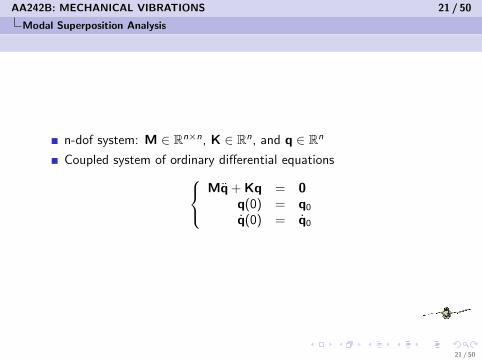
n-dof system: M ∈ Rn×n, K ∈ Rn, and q ∈ Rn
Coupled system of ordinary differential equations Mq + Kq = 0q(0) = q0
q(0) = q0
21 / 50

AA242B: MECHANICAL VIBRATIONS 22 / 50
Modal Superposition Analysis
Natural vibration modes (eigenmodes)
Kqai = ω2i Mqai , i = 1, · · · , n
Q = [qa1 qa2 · · · qan ]⇒
QT KQ = Ω2
QT MQ = I
Ω2 =
ω21
. . .
ω2n
Truncated eigenbasis
Qr =[qa1
qa2· · · qar
], r << n ⇒
QT
r KQr = Ω2r (reduced stiffness matrix)
QTr MQr = Ir (reduced mass matrix)
Ω2r =
ω2
1
. . .
ω2r
22 / 50

AA242B: MECHANICAL VIBRATIONS 23 / 50
Modal Superposition Analysis
Modal superposition: q = Qr y =r∑
i=1
yi qai where
y = [y1 y2 · · · yr ]T and yi is called the modal displacement
Substitute in Mq + Kq = 0
=⇒MQr y + KQr y = 0
=⇒ QTr MQr y + QT
r KQr y = 0
=⇒ Ir y + Ω2r y = 0
Uncoupled differential equations (modal equations)
yi + ω2i yi = 0, i = 1, · · · r
23 / 50

AA242B: MECHANICAL VIBRATIONS 24 / 50
Modal Superposition Analysis
yi + ω2i yi = 0, i = 1, · · · r
Case 1: ω2i = 0 (rigid body mode)
yi = ai t + bi
Case 2: ω2j 6= 0
yj = cj cosωj t + dj sinωj t
General case: rb rigid body modes
q =
rb∑i=1
(ai t + bi )qai +
r−rb∑j=1
(cj cosωj t + dj sinωj t)qaj
Initial conditions
q(0) = q0 = Qy(0) and q(0) = q0 = Qy(0)
24 / 50

AA242B: MECHANICAL VIBRATIONS 25 / 50
Modal Superposition Analysis
q0 = Qy(0) and q0 = Qy(0)
=⇒ qTai
Mq0 = qTai
MQy(0)
From the orthogonality properties of the natural mode shapes (eigenvectors) it follows that
qTai
Mq0 = qTai
MQy(0) = qTai
Mqaiyi (0) = yi (0)⇒ yi (0) = qT
aiMq(0)
Case 1: ω2i = 0 (rigid body mode) ⇒ ai × 0 + bi = qT
aiMq(0)⇒ bi = qT
aiMq(0)
Case 2: ω2j 6= 0 ⇒ cj × 1 + dj × 0 = qT
ajMq(0)⇒ cj = qT
ajMq(0)
Case 1: ω2i = 0 (rigid body mode) ⇒ ai = qT
aiMq(0)
Case 2: ω2j 6= 0 ⇒ dj = qT
ajMq(0)
Thus, the general solution is
q(t) =
rb∑i=1
([qT
aiMq(0)
]t + qT
aiMq(0)
)qai
+
r−rb∑j=1
(qT
ajMq(0) cosωj t + qT
ajMq(0)
sinωj t
ωj
)qaj
25 / 50

AA242B: MECHANICAL VIBRATIONS 26 / 50
Spectral Expansions
∀x ∈ Rn, x =
n∑s=1
αs qas ⇒ qTaj
Mx =n∑
s=1
αs qTaj
Mqas = αj
=⇒ ∀x ∈ Rn, x =
n∑s=1
(qT
asMx)
qas =n∑
s=1
qas
(qT
asMx)
=n∑
s=1
(qas qT
as
)Mx =
(n∑
s=1
(qas qTas
)M
)x
⇒n∑
s=1
(qas qT
as
)M = I
This is the same result as QT MQ = I
A given load p can be expanded in terms of the inertia forcesgenerated by the eigenmodes, Mqaj as follows
p =n∑
j=1
βj Mqaj ⇒ qTai
p =n∑
j=1
βj qTai
Mqaj = βi
=⇒ βi = qTai
p = modal participation factor→ p =n∑
j=1
(qT
ajp)
Mqaj
26 / 50

AA242B: MECHANICAL VIBRATIONS 27 / 50
Spectral Expansions
Recall thatn∑
s=1
(qas qT
as
)M = I
Hence, ∀A ∈ Rn, A =n∑
s=1Aqas qT
asM and A =
n∑s=1
qas qTas
MA
A = M⇒ M =n∑
s=1Mqas qT
asM =
n∑s=1
Mqas (Mqas )T (because M is symmetric)
A = K⇒ K =n∑
s=1Kqas qT
asM =
n∑s=1ω2
s Mqas qTas
M =n∑
s=1ω2
s Mqas (Mqas )T
A = M−1 ⇒ M−1 =n∑
s=1qas qT
asMM−1 ⇒ M−1 =
n∑s=1
qas qTas
A = K−1 ⇒ K−1 =n∑
s=1qas qT
asMK−1 =
n∑s=1
qas (Mqas )T K−1 ⇒ K−1 =n∑
s=1
qas qTas
ω2s
27 / 50

AA242B: MECHANICAL VIBRATIONS 28 / 50
Forced Harmonic Response
Mq + Kq = sa cosωtq(0) = q0
q(0) = q0
Solution can be decomposed asq = qH (homogeneous) + qP (particular)
qp = qa cosωt ⇒ qa = (K− ω2M)−1sa where (K− ω2M)−1 iscalled the admittance or dynamic influence matrix
The forced response is the part of the response that is synchronousto the excitation — that is, qp
28 / 50
AA242B: MECHANICAL VIBRATIONS 29 / 50
Forced Harmonic Response
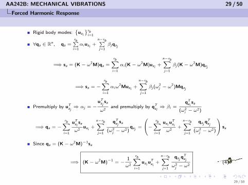
Rigid body modes:
uai
rbi=1
∀qa ∈ Rn, qa =rb∑
i=1
αi uai+
n−rb∑j=1
βj qaj
=⇒ sa = (K− ω2M)qa =
rb∑i=1
αi (K− ω2M)uai+
n−rb∑j=1
βj (K− ω2M)qaj
=⇒ sa = −rb∑
i=1
αiω2Muai
+
n−rb∑j=1
βj (ω2j − ω
2)Mqaj
Premultiply by uTaj⇒ αj = −
uTaj
sa
ω2and premultiply by qT
ai⇒ βi =
qTai
sa
(ω2i − ω2)
=⇒ qa = −rb∑
i=1
uTai
sa
ω2uai
+
n−rb∑j=1
qTaj
sa
(ω2j − ω2)
qaj=
− rb∑i=1
uaiuT
ai
ω2+
n−rb∑j=1
qajqT
aj
(ω2j − ω2)
sa
Since qa = (K− ω2M)−1sa
=⇒ (K− ω2M)−1 = −1
ω2
rb∑i=1
uaiuT
ai+
n−rb∑j=1
qajqT
aj
ω2j − ω2
(4)
29 / 50
AA242B: MECHANICAL VIBRATIONS 30 / 50
Forced Harmonic Response
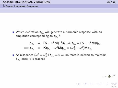
Which excitation sam will generate a harmonic response with anamplitude corresponding to qam ?
qam = (K− ω2M)−1sam ⇒ sam = (K− ω2M)qam
=⇒ sam = Kqam − ω2Mqam = (ω2m − ω2)Mqam
At resonance (ω2 = ω2m) sam = 0⇒ no force is needed to maintain
qam once it is reached
30 / 50
AA242B: MECHANICAL VIBRATIONS 31 / 50
Forced Harmonic Response
The inverse of an admittance is an impedance
Z(ω2) = (K− ω2M)
31 / 50

AA242B: MECHANICAL VIBRATIONS 32 / 50
Forced Harmonic Response
Application: substructuring (or domain decomposition)
the dynamical behavior of a substructure is described by its harmonicresponse when forces are applied onto its interface boundariesa subsystem is typically described by K and M, has n1 free dofs q1,and is connected to the rest of the system by n2 = n − n1 boundarydofs q2 where the reaction forces are denoted here by g2(
Z11 Z12
Z21 Z22
)(q1
q2
)=
(0g2
)=⇒ Z11q1 + Z12q2 = 0⇒ q1 = −Z−1
11 Z12q2
=⇒ (Z22 − Z21Z−111 Z12)q2 = Z?22q2 = g2
Z?22 is the “reduced” impedance (reduced to the boundary)
32 / 50
AA242B: MECHANICAL VIBRATIONS 33 / 50
Forced Harmonic Response
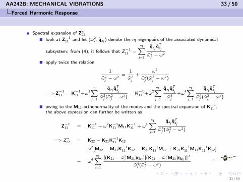
Spectral expansion of Z?22
look at Z−111 and let (ω2
i , qai) denote the n1 eigenpairs of the associated dynamical
subsystem: from (4), it follows that Z−111 =
n1∑j=1
qajqT
aj
ω2j − ω2
apply twice the relation
1
ω2j − ω2
=1
ω2j
+ω2
ω2j (ω2
j − ω2)
=⇒ Z−111 = K−1
11 +ω2n1∑
j=1
qajqT
aj
ω2j (ω2
j − ω2)= K−1
11 +ω2n1∑
j=1
qajqT
aj
ω4j
+ω4n1∑
j=1
qajqT
aj
ω4j (ω2
j − ω2)
owing to the M11-orthonormality of the modes and the spectral expansion of K−111 ,
the above expression can further be written as
Z−111 = K−1
11 + ω2K−1
11 M11K−111 + ω
4n1∑
j=1
qajqT
aj
ω4j (ω2
j − ω2)
=⇒ Z?22 = K22 − K21K−111 K12
− ω2[M22 −M21K−1
11 K12 − K21K−111 M12 + K21K−1
11 M11K−111 K12]
− ω4
n1∑i=1
[(K21 − ω2i M21)qai
][(K21 − ω2i M21)qai
)]T
ω4i (ω2
i − ω2)
33 / 50

AA242B: MECHANICAL VIBRATIONS 34 / 50
Forced Harmonic Response
Z?22 = K22 −K21K−111 K12
−ω2[M22 −M21K−111 K12 −K21K−1
11 M12 + K21K−111 M11K−1
11 K12]
−ω4n1∑
i=1
[(K21 − ω2i M21)qai ][(K21 − ω2
i M21)qai )]T
ω4i (ω2
i − ω2)
The first term K22 −K21K−111 K12 represents the stiffness of the
statically condensed system
The second termM22 −M21K−1
11 K12 −K21K−111 M12 + K21K−1
11 M11K−111 K12 represents
the mass of the subsystem statically condensed on the boundary
The last term represents the contribution of the subsystemeigenmodes since it is generated by qai q
Tai
(K21 − ω2i M21)qai is the dynamic reaction on the boundary
34 / 50

AA242B: MECHANICAL VIBRATIONS 35 / 50
Response to External Loading
Mq + Kq = p(t)q(0) = q0
q(0) = q0
General approach
consider the simpler case where there is no rigid body mode ⇒eigenmodes (qai , ω
2i ), ω2
i 6= 0, i = 1, · · · , n
modal superposition: q = Qy =n∑
i=1
yi qai
substitute in equations of dynamic equilibrium
=⇒MQy + KQy = p(t)⇒ QT MQy + QT KQy = QT p(t)
modal equations yi + ω2i yi = qT
aip(t), i = 1, · · · , n
yi (t) depend on two constants that can be obtained from the initialconditionsq(0) = Qy(0), q(0) = Qy(0) ⇒
orthogonality conditionsyi (0), yi (0)
35 / 50

AA242B: MECHANICAL VIBRATIONS 36 / 50
Response to External Loading
Response to an impulsive force
spring-mass system: m, k, ω2 =k
mimpulsive force f (t): force whose amplitude could be infinitely largebut which acts for a very short duration of time
magnitude of impulse: I =
∫ τ+ε
τ
f (t)dt
impulsive force = Iδ(t) where δ is the “delta” function
centered at t = 0 and satisfying
∫ ε
0
δ(t)dt = 1
36 / 50

AA242B: MECHANICAL VIBRATIONS 37 / 50
Response to External Loading
Response to an impulsive force (continue)
dynamic equilibrium
m
∫ τ+ε
τ
du
dtdt + k
∫ τ+ε
τ
udt =
∫ τ+ε
τ
f (t)dt = I
assume that at t = τ , the system is at rest (u(τ) = 0 and u(τ) = 0)
u = A/ε⇒∫ τ+ε
τ
udt = A and
∫ τ+ε
τ
udt = Aε2/6
hence
m
∫ τ+ε
τ
du
dtdt = I ⇒ m∆u = I ⇒ ∆u = u(τ + ε)− u(τ) =
I
m⇒ u(τ + ε) =
I
m∫ τ+ε
τ
udt = 0⇒ ∆u = 0⇒ u(τ + ε)− u(τ) = 0⇒ u(τ + ε) = 0
the above equations provide initial conditions for the free-vibrationsthat start at the end of the impulsive load
=⇒ u(t) =I
mωsinωt
37 / 50

AA242B: MECHANICAL VIBRATIONS 38 / 50
Response to External Loading
Response to an impulsive force (continue)
linear system ⇒ superposition principle
du =f (τ)dτ
mωsinω(t − τ)⇒ u(t) =
1
mω
∫ t
0
f (τ) sinω(t − τ)dτ
38 / 50

AA242B: MECHANICAL VIBRATIONS 39 / 50
Response to External Loading
Time-integration of the normal equations
let pi (t) = qTai
p(t) = i-th modal participation factormodal or normal equation: yi + ω2
i yi = pi (t)yi (t) = yH
i (t) + yPi (t), yH
i = Ai cosωi t + Bi sinωi tthe particular solution yP
i (t) depends on the form of pi (t)however, the general form of a particular solution that satisfies therest initial conditions is given by the Duhamel’s integral
yPi (t) =
1
ωi
∫ t
0
pi (τ) sinωi (t − τ)dτ
complete solution
yi (t) = Ai cosωi t + Bi sinωi t +1
ωi
∫ t
0
pi (t) sinωi (t − τ)dτ
Ai = yi (0),Bi =yi (0)
ωiand yi (0) and yi (0) can be determined from
the initial conditions q(0) and q(0) and the orthogonality conditions
39 / 50

AA242B: MECHANICAL VIBRATIONS 40 / 50
Response to External Loading
Response truncation and mode displacement method
computational efficiency ⇒ q = Qr y =r∑
i=1
yi qai , r n
what is the effect of modal truncation?consider the case where p(t) = g
static loaddistribution
× φ(t)amplification
factor
for a system initially at rest (q(0) = 0 and q(0) = 0)yi (0) = qT
aiMq(0) = 0 and yi (0) = qT
aiMq(0) = 0 ⇒ Ai = Bi = 0
=⇒ yi (t) =1
ωi
∫ t
0
pi (τ) sinωi (t−τ)dτ =qT
aig
ωi
∫ t
0
φ(τ) sinωi (t − τ)dτ
=⇒ q(t) =r∑
i=1
[qai q
Tai
gspatial factor
] 1
ωi
∫ t
0
φ(τ) sinωi (t − τ)dτ
temporal factor
40 / 50

AA242B: MECHANICAL VIBRATIONS 41 / 50
Response to External Loading
Response truncation and mode displacement method (continue)
general solution for restrained structure initially at rest
=⇒ q(t) =r∑
i=1
[qai q
Tai
gspatial factor
] 1
ωi
∫ t
0
φ(τ) sinωi (t − τ)dτ
temporal factor θi (t)
truncated response is accurate if neglected terms are small, which istrue if:
qTai
g is small for i = r + 1, · · · , n ⇒ g is well approximated in therange of Qr
1
ωj
∫ t
0φ(τ) sinωj (t − τ)dτ is small for j > r , which depends on the
frequency content of φ(t)
φ(t) = 1 ⇒ θi (t) =1− cosωi t
ωi→ 0 for large circular frequencies
φ(t) = sinωt ⇒ θi (t) =ωi sinωt − ω sinωi t
ωi (ω2i − ω2)
41 / 50

AA242B: MECHANICAL VIBRATIONS 42 / 50
Response to External Loading
Mode acceleration method
Mq + Kq = p(t)⇒ Kq = p(t)−Mq
apply truncated modal representation to the acceleration
q(t) = Qr y(t)⇒ q(t) = Qr y(t)
=⇒ Kq = p(t)−r∑
i=1
Mqai yi =⇒ q = K−1p(t)−r∑
i=1
qai
ω2i
yi
recall thatyi + ω2
i yi = qTai
p(t) (5)
and that for a system initially at rest
yi (t) =1
ωi
∫ t
0
qTai
p(τ) sinωi (t − τ)dτ (6)
(5) and (6) ⇒ yi (t) = qTai
(p(t)− ωi
∫ t
0p(τ) sinωi (t − τ)dτ
)42 / 50

AA242B: MECHANICAL VIBRATIONS 43 / 50
Response to External Loading
Mode acceleration method (continue)
substitute in q(t) = K−1p(t)−r∑
i=1
qai
ω2i
yi
=⇒ q(t) =r∑
i=1
qai qTai
ωi
∫ t
0
p(τ) sinωi (t−τ)dτ+
(K−1 −
r∑i=1
qai qTai
ω2i
)p(t)
recall the spectral expansion K−1 =n∑
i=1
qai qTai
ω2i
=⇒ q(t) =r∑
i=1
qai qTai
ωi
∫ t
0
p(τ) sinωi (t − τ)dτ +
(n∑
i=r+1
qai qTai
ω2i
)p(t)
which shows that the mode acceleration method complements thetruncated mode displacement solution with the missing terms usingthe modal expansion of the static response
43 / 50

AA242B: MECHANICAL VIBRATIONS 44 / 50
Response to External Loading
Direct time-integration methods for solving Mq + Kq = p(t)q(0) = q0
q(0) = q0
will be covered towards the end of this course
44 / 50
AA242B: MECHANICAL VIBRATIONS 45 / 50
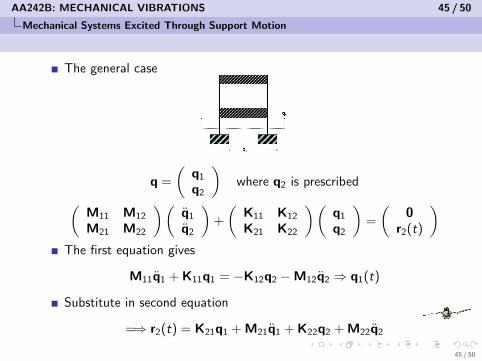
Mechanical Systems Excited Through Support Motion
The general case
q =
(q1
q2
)where q2 is prescribed(
M11 M12
M21 M22
)(q1
q2
)+
(K11 K12
K21 K22
)(q1
q2
)=
(0
r2(t)
)The first equation gives
M11q1 + K11q1 = −K12q2 −M12q2 ⇒ q1(t)
Substitute in second equation
=⇒ r2(t) = K21q1 + M21q1 + K22q2 + M22q2
45 / 50

AA242B: MECHANICAL VIBRATIONS 46 / 50
Mechanical Systems Excited Through Support Motion
Quasi-static response of q1
0 + K11q1 = −K12q2 − 0
=⇒ qqs1 = −K−1
11 K12q2 = Sq2
Decompose q1 = qqs1 + z1 = Sq2 + z1
=⇒ q(t) =
(q1
q2
)=
(I S0 I
)(z1
q2
)where z1 represents the sole dynamics part of the response
Substitute in the first dynamic equation and exploit above results
=⇒M11Sq2 + M11z1 + K11qqs1 + K11z1 = −K12q2 −M12q2
=⇒
M11z1 + K11z1 = g1(t)g1(t) = −M11qqs
1 −M12q2 = −(M11S + M12)q2
46 / 50

AA242B: MECHANICAL VIBRATIONS 47 / 50
Mechanical Systems Excited Through Support Motion
Consider next the system fixed to the ground and solve thecorresponding EVP
K11x = ω2M11x⇒ Q = [· · · qai · · · ]
=⇒ z1(t) = Qη(t)
Solve M11z1 + K11z1 = g1(t) for z1(t) using the modalsuperposition technique
47 / 50

AA242B: MECHANICAL VIBRATIONS 48 / 50
Mechanical Systems Excited Through Support Motion
Case of a global support acceleration q2(t) = u2φ(t), whereu = [u1 u2]T denotes a rigid body mode
decomposition of the solution into a rigid body motion and a relativedisplacement y
q = qrb + y⇒[
q1
q2
]=
[u1
u2
]φ(t) +
[y1
0
]u1 = Su2 ⇒ g1(t) = −(M11Su2 + M12u2)φ(t)
=⇒ g1(t) = −(M11u1 + M12u2)φ(t)
48 / 50

AA242B: MECHANICAL VIBRATIONS 49 / 50
Mechanical Systems Excited Through Support Motion
Method of additional masses (approximate method)
suppose the system is subjected not to a specified q2(t) but to animposed (
0f(t)
)suppose that masses associated with q2 are increased to M22 + M?
22
then(M11 M12
M21 M22 + M?22
)(q1
q2
)+
(K11 K12
K21 K22
)(q1
q2
)=
(0
f(t)
)by elimination one obtainsq2 = (M22 + M?
22)−1 (f(t)−K22q2 −K21q1 −M21q1) and
M11q1 + K11q1 = −K12q2 −M12(M22 + M?22)−1 (f(t)− K22q2 − K21q1 −M21q1)
49 / 50

AA242B: MECHANICAL VIBRATIONS 50 / 50
Mechanical Systems Excited Through Support Motion
Method of additional masses (continue)therefore
M11 − M12(M22 + M?22)−1M21 q1 +
K11 −M12(M22 + M?
22)−1K21
q1
= −K12q2 −M12(M22 + M?22)−1 (f(t)− K22q2)
now if (M22 + M?22)−1 → 0 and if f(t) = (M22 + M?
22)q2, one obtains
M11q1+K11q1 = −K12q2−M12q2 =⇒M11q1+M12q2+K11q1+K12q2 = 0
which is the same equation as in the general case of excitationthrough support motion⇒ for M?
22 very large, the response of the system with groundmotion is the same as the response of the system with added lumpedmass M?
22 and the forcing function(0
(M22 + M?22)q2
)≈(
0M?
22q2
)where q2 is given ⇒ apply same solution method as for problems ofresponse to external loading
50 / 50
Related Documents